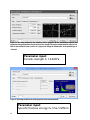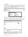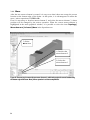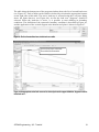
1
Červenka Consulting s.ro. Na Hrebenkach 55 150 00 Prague Czech Republic Phone: +420 220 610 018 E-mail: [email protected] Web: http://www.cervenka.cz ATENA Program Documentation Part 4-2 Tutorial for Program ATENA 3D Written by: Jan Červenka, Zdenka Procházková Prague, August 19, 2015 Trademarks: ATENA is registered trademark of Vladimir Cervenka. Microsoft and Microsoft Windows are registered trademarks of Microsoft Corporation. Other names may be trademarks of their respective owners. Copyright © 2000-2015 by Červenka Consulting s.r.o. CONTENTS 1. INTRODUCTION 1 2. STARTING PROGRAM 3 3. PRE-PROCESSING 5 Introduction 5 3.1 3.1.1 3.1.2 3.1.3 3.2 Introduction of The Graphical User Interface Definition of the Geometrical Model Saving of Data Material Parameters 3.2.1 3.2.2 3.2.3 3.3 3.3.1 3.3.2 3.4 10 Steel Plates Reinforcement Concrete Beam 11 12 13 Concrete Beam 16 Geometry Definition Material Definition Steel Plates 3.4.1 3.4.2 3.4.3 3.4.4 3.4.5 3.4.6 3.4.7 3.4.8 6 9 10 18 20 22 Grid Setting Joints Definition Lines Definition Surface Definition Extrusion Material Definition Copy Move 23 24 25 27 29 31 32 34 3.5 Mesh Generation 38 3.6 Bar-reinforcement 42 3.6.1 3.6.2 First Bar Second Bar 42 46 3.7 Supports and Actions 49 3.8 Loading History and Solution Parameters 56 3.9 Monitoring Points 62 4. FE NON-LINEAR ANALYSIS 67 4.1 Introduction 67 4.2 Interactive Window 67 ATENA Engineering - 3D - Tutorial i 5. POST-PROCESSING 73 5.1 Introduction 73 5.2 Post-processing Window 73 5.3 Load-displacement Diagrams 82 5.4 Text Output 84 5.5 Analysis Log Files 85 6. CONCLUSIONS 87 7. PROGRAM DISTRIBUTORS AND DEVELOPERS 89 8. LITERATURE 90 ii 1. INTRODUCTION This tutorial provides a basic introduction to the usage of the program ATENA 3D, and it is specifically targeted for ATENA 3D beginners. This tutorial contains a step by step explanation how to perform a non-linear analysis on an example problem of a reinforced beam without smeared reinforcement. The geometrical and material properties correspond to the experimental setup by Leonhard in 1962. More details about the problem or experiment can be also obtained from the original report [5] or from the program developer or distributor. The step by step demonstration is performed on an example of simply supported beam, which is loaded by two loads as it is shown in Figure 1. The problem is symmetric around its vertical axis; therefore, only one symmetric half of the beam will be analyzed. The steps necessary for the data preparation, non-linear analysis and post-processing are depicted on subsequent figures, which show the computer screen for each step and user action. There is always also a short description for each figure. In the post-processing stage only some basic post-processing methods are described. ATENA offers many options for viewing results from FE non-linear analysis. These options can be easily accessed from the post-processing window by self-explanatory buttons and toolbars. For more details, it is recommended to consult the ATENA 3D user's manual or the hotline desk at the program distributor or developer. Figure 1: Geometry of the structure. ATENA Engineering - 3D - Tutorial 1 2 2. STARTING PROGRAM The simulation system ATENA 3D can be started by executing the program ATENA3D_1_EN.EXE from the directory where the ATENA system is installed. It is however more convenient to started the program from Start | Programs menu on your computer desktop. ATENA Engineering - 3D - Tutorial 3 4 3. PRE-PROCESSING 3.1 Introduction This chapter explains the basic steps, which are to be performed in order to define a complete geometrical, and then a finite element model for non-linear FE analysis by ATENA 3D. The purpose of the geometrical model is to describe the geometry of the structure, its material properties and boundary conditions. The analytical model for the finite element analysis will be created during the pre-processing with the help of the fully automated mesh generator. The geometrical model is composed of three-dimensional solid regions called “macro-elements”. Each macro-element is defined separately, and it is composed of joints, lines and surfaces. In ATENA 3D each macro-element has its own joints, lines and surfaces. This means that no joint, line or surface can be shared by two macro-elements. It is possible to use previously defined entities, i.e. joints, lines or surfaces, for the definition of a new macro-element, but every time this is done, a new copy of the entity is created with identical geometry but different id. Macro-element definition starts with the creation of geometrical joints. These joints are later connected into boundary lines. The current version of the program supports only straight lines. Curved lines can be approximated by several linear segments. The program includes tools for automatic generation of such piecewise linear segments for arcs and circles. The subsequent step in the macro-element definition is the creation of surfaces. The current version is limited to planar surfaces. Curved surfaces must be approximated by several planar surfaces. Alternatively the program supports also the import of existing finite element meshes. Such a mesh can be created by an external program and imported into ATENA for definition of ATENA specific features. The surfaces are composed of the previously defined lines. The program contains also tools for direct generation of simple geometrical objects such as: prisms, multi-sided prisms or pyramids. When two macro-elements touch each other, program automatically detects this condition and creates contacts at the appropriate locations. These contacts can be later modified to simulate perfect connection, gaps or other interface types. ATENA Engineering - 3D - Tutorial 5 3.1.1 Introduction of The Graphical User Interface Before starting the definition of the geometrical model it is a good idea to introduce the graphical user interface of ATENA 3D pre-processor. The pre-processing window is shown in the subsequent Figure 2. Main Menu Selection of active loadcase Miscellaneous Toolbars Switch to solution/postprocessing Selection of active part of structure. Main view window containing the created geometrical and FE model. Input data tree for data definition Selection of entities/items visible Tables for data input and modification. Table for the active item in the data access tree is shown. Figure 2: Graphical user interface of ATENA 2D pre-processor. ATENA 3D contains seven main toolbars: File toolbar: New problem 6 Open file Save file Text output Graphical output Free rotation Translation and rotation Zoom out at mouse location Zoom window Zoom extend to view and Scale toolbars: Previous zoom Move Zoom in/out Zoom in at mouse location Select by crossing Selection toolbar: Select by skewed rectangle Select by clicking Partial selection on/off Select by rectangle ATENA Engineering - 3D - Tutorial Zoom in around center Zoom out around center Invert selection allmode objects of the Selection selected type add, remove, invert Deselect all items of selected type Select all objects of selected type 7 Pictures toolbar: Save the current picture Selection of saved pictures Listing in pictures Picture manager Handling 3D view toolbar: Axonometric view Perspective view View in the direction of the X-axis Predefined default 3D view View in the direction of the -X-axis View in the direction of the Z-axis View in the direction of the Y-axis Viewing parameters toolbar: View the grid model 8 View the full model Set the direction of illumination View in the direction of the -Z-axis View in the direction of the -Y-axis 3.1.2 Definition of the Geometrical Model After examination of the user interface layout, it is possible to start with the definition of the geometrical model of the analyzed structure. It is a good practice to provide a short description of the problem to be analyzed. In ATENA 3D this can be done by selecting the General data | Analysis information item in the Input data tree. Select this item to define global problem attributes. Figure 3: Definition of global analysis attributes. In this tutorial problem, the Input for global structural parameters as well as solution parameters is shown in Figure 4 and Figure 5. Figure 4: Input of global structural parameters. ATENA Engineering - 3D - Tutorial 9 Figure 5: Input of global solution parameters. 3.1.3 Saving of Data At this point it is also recommended to save the new data under a new file into the working directory. Use the menu item File | Save as .. to locate an appropriate directory and save the new data for instance under the name “Shear beam 3D”. Figure 6: Saving data using the File | Save as .. menu item. 3.2 Material Parameters Next step should be the definition of material groups and material properties. Selecting the item Materials from the Input data tree opens the General data | Materials table in the bottom right part of the program screen. Figure 7: The Materials table, from which new materials can be added or existing materials can be modified or removed. Clicking the Add button on the material table window creates a new material. For the current problem, it is necessary to define three material types: one elastic material for the steel plates at support and loading points, concrete material for the beam and reinforcement material. There exist three methods for creating new materials (see Figure 8). A new material can be defined directly using various ATENA material models, or a previously saved material definition can be used. The third method is to use a material definition from the available catalogue of materials. The catalogue contains various material definitions based on the various national or international standards. For the purpose of this tutorial let’s use the direct definition. 10 3.2.1 Steel Plates Figure 8: After selecting the Add button it is possible to specify how the new material will be created. Figure 9: Selection of elastic isotropic material for the steel plates. Figure 10: The dialog for the definition of material properties for the steel plates. ATENA Engineering - 3D - Tutorial 11 3.2.2 Reinforcement Figure 11: Selection of material model for the bar reinforcement. Figure 12: The dialog for the definition of reinforcement material parameters. The bi-linear elastic-perfectly plastic stress-strain diagram is selected for this problem. Parameter input: Type: Bilinear Elastic modulus: 208 000 MPa σy : 560 MPa 12 3.2.3 Concrete Beam Figure 13: Selection of 3D Nonlinear Cementitious 2 material model for the concrete beam. Parameter input: Cubic fcu: 33.5 MPa Figure 14: Default values of material parameters are generated based on the cube strength of concrete. For this case, the cube strength should be 33.5 MPa. NOTE: There are predefined parameters in dialog windows for the definitions of parameters. The table named “Parameter input:” shows the parameters which should be changed. ATENA Engineering - 3D - Tutorial 13 Figure 15: The dialog window for the definition of basic properties for the cementitious material. The parameters were generated based on the concrete cube strength. The tensile strength should be edited to 1.64 MPa for the Leonhard's beam as well as it is proposed to change the default name of the material type to “Concrete”. Parameter input: Tensile strength ft: 1.64 MPa Figure 16: The dialog window for the tensile properties for the concrete material. Parameter input: Specific fracture energy Gf: 5.5e-5 MN/m 14 Figure 17: The dialog window for the compressive properties of concrete material. Figure 18: The dialog window for the miscellaneous properties of concrete material. In this window it is recommended to verify that the fixed crack model coefficient is set to 1.0. Figure 19: The three materials, which were defined previously, can be viewed or modified from the Materials table window at the bottom part of the ATENA 3D window. ATENA Engineering - 3D - Tutorial 15 3.3 Concrete Beam Next step in the Input data preparation should be the definition of problem geometry. The geometry is created by defining individual solid regions. In ATENA 3D these regions are called Macro-elements. The macro-element definition is activated by selecting Topology | Macroelements | Add in the Input data tree on the left side of ATENA 3D window. This action opens a new window that is to be used for the definition of joints, lines and surfaces composing the new macro-element. Each macroelement has its own set of joints, lines and surfaces. The window layout is shown in Figure 20. A new macro-element can be created by several approaches. The simplest one but the most time consuming method is to define individual joints. Then connect them to lines, which are later connected to form surfaces. Surfaces can be used directly to define a solid or the extrusion feature can be used to create a new solid by extruding a surface along a predefined vector. The easiest method is to create a solid using the parametric definition from simple entities such as columns, beams or pyramids. Some of these approaches will be used in this tutorial example. The user is encouraged to explore the various items in the Input data tree in the window that is shown in Figure 20. This can provide the user with an overview of the various features available in ATENA for three-dimensional solid modeling. The current version of the program supports only straight lines. Curved lines can be approximated by several linear segments. The program includes tools for automatic generation of such piecewise linear segments for arcs and circles. 16 Buttons to switch between geometry view and macroelement properties dialog. Grid toolbar can be used to modify the work-plane and grid settings. Input data access tree activates the definition of various entities. Selection of visible entities. This toolbar is used for selection of perspective/ isoparametric projection or quick view changes. Here it is possible to switch between standard solid macroelements and special shell/plate macroelements. Window for entities tables, generation of simple objects and copy/move Figure 20: Layout of the ATENA window for macro-element definition. ATENA Engineering - 3D - Tutorial 17 3.3.1 Geometry Definition The analyzed structure is symmetrical so it is possible to analyze only the symmetrical half. The first task would be to define the concrete beam. Subsequently the steel plates for loading and supports will be created. The concrete beam is a prism, and therefore, it is advantageous to generate its geometry using the parametric definition of simple entities. This can be accomplished by selecting the item Generation | Simple objects in the Input data tree. This activates the generation window along the bottom edge of the macro-element window. In this window the following data should be specified (see Figure 21): The input of numerical quantities such as coordinates or beam sizes must be completed by clicking the check box or by pressing the Enter key on your keyboard. Otherwise the numerical value is not accepted. Figure 21: The parameters for the entity generation can be modified by clicking the highlighted items. The numerical input is finalized by clicking the checkbox button. Parameter input: entity type: column/beam, Entity type: column/beam coordinate system: Coordinate system: global, global reference point: (0,0,0) Reference point: (V (0,0,0) size =1.275,V =0.190,V =0.320) Size: (Vx=1.275, Vy=0.190, Vz=0.320) x 18 y z Immediately after all parameters for the beam are specified, the preview of the beam geometry is visible in the main window. In some cases it is necessary to zoom in to see clearly the beam geometry. This can be accomplished by selecting the Zoom extend button . Zoom extend button to fit the structure into the window Figure 22: Preview of the specified parametric entity before it is created. In some cases the previewed structure may be very small in the middle of the screen. The display can be fitted to the whole window by selecting the Zoom extend button . The preview in this case shows that the beam geometry is correct so it is possible to finalize the beam definition by clicking the Generate button in the right part of the generation window. The resulting display is shown in Figure 23. Figure 23: Program display after the generation of the parameterized beam element. ATENA Engineering - 3D - Tutorial 19 3.3.2 Material Definition The next step is to specify an appropriate material for the generated beam. The property window appears if the Properties tab is selected. The resulting window is shown in Figure 24. In this window, an appropriate material type can be assigned to the macro-element. Select this tab to switch to the definition of macroelement properties such as material or smeared reinforcement. Figure 24: The material type for the generated beam is specified by clicking the Properties button in top left corner of the macro-element definition window. In this case “Concrete” is the correct material for the created beam. In this window, it is also possible to specify smeared reinforcement. This is one of the two possible methods for reinforcement modeling that are implemented in ATENA. Reinforcement can be modeled either by modeling each individual bar or in an average sense by reinforcing a macro-element in certain directions by specifying an appropriate reinforcement ratio [%]. This type of reinforcement model is called “smeared reinforcement” in ATENA, and it can be inserted into each macro/element by selecting the button in the smeared reinforcement section of this window. The smeared reinforcement feature is useful especially for modeling reinforcement mats or stirrups. The analyzed beam, however, is without stirrups so the smeared reinforcement feature will not be used, and therefore, the smeared reinforcement list should be left empty. 20 After the definition of material model for the created beam it is possible to finalize the macro-element definition by returning back to the Topology tab and by selecting the button in the most bottom-right corner of the macro-element definition window. Please note that this is a different button than the one used for the definition of smeared reinforcement that was discussed before. At this point the created beam is added to the model, and it is possible to start defining other macro-elements. It is possible to look at the so far created model by selecting the button at the most bottom-right part of the macro-element definition window to return to the main program view (Figure 25). Figure 25: The program display after the definition of the first macro-element. ATENA Engineering - 3D - Tutorial 21 3.4 Steel Plates The next steps will be to define macro-elements for modeling the loading and supporting steel plates. In nonlinear analysis it is often necessary to avoid any unrealistic stress concentration, as this may cause premature failure or cracking in these locations. If the support conditions or loads are applied at single nodes, this may create strong stress concentrations affecting the analysis results. It should be considered that in most cases such a stress concentration very seldom exists in reality as the supports or loads are usually applied over a certain area and never at single points. This is also the case in our example, which corresponds to an experimental setup, where loading and supports were realized using small steel plates. A different modeling approach will be used to define the support plates to demonstrate the other modeling methods in ATENA 3D. First a plate cross-section will be created, which will be later extruded to create a three-dimensional model. To start the definition of new macro-elements, again select the button Topology | Macroelements | Add in the Input data tree on left side of the program window. This action opens the macro-element definition window (see Figure 26), in which the previously defined macro-elements are shown in a very schematic way. Figure 26: The beginning of support plate definition. 22 3.4.1 Grid Setting When defining two-dimensional macro-element cross-section it is advantageous to utilize the working plane grid. The grid settings are controlled by the toolbar shown in Figure 27. Figure 27: The toolbar controlling the grid settings. Select the button for the manual specification of grid properties, and set the grid specifications according to Figure 28. The plate cross-section should be defined in the plane XZ and since the plate dimensions are 0.03x0.10, the following values for dx = 0.05 and dz = 0.03 should be used (see Figure 28). Parameter input: Origin: Step: X: 0.165 X: 0.050 Y: 0.000 Y: 0.500 Z: 0.320 Z: 0.030 Working plane: XZ Figure 28: Grid settings for the support plate definition. The grid origin should be moved to (0.165, 0, 0.32) in order to place the grid origin into the center of bottom part of the loading steel plate. At this point it is more convenient to modify the view of the structure in order to start defining the support plate geometry. First let’s change the view such that the structure is viewed from the negative Y axis by selecting the button . This view is perpendicular to the beam geometry as well as the grid plane. By selecting the zoom extend button , the display of the whole beam appears. It is also more convenient to switch to parallel view by clicking the button . If the parallel projection is selected the exact projection of the beam geometry into the X-Z plane is obtained. ATENA Engineering - 3D - Tutorial 23 3.4.2 Joints Definition Now it is time to define the support plate cross-section by creating joints and by directly clicking into the appropriate grid locations. The joint definition starts in the Input data tree Entities | Joints | Add. As you can see in Figure 30 it is necessary to create 5 joints. The middle joint will be used for application of load. The middle point will be used later for load application. Figure 29: Definition of geometrical joints for support plate cross-section. Figure 30: The table of joint’s coordinates which can be used in the case the grid is not displayed correctly. 24 3.4.3 Lines Definition The next step is to connect these joints via lines. The line input is activated by the item in the Input data tree Entities | Lines | Add in the Input data tree on left side of the program window. Each boundary line is defined by first selecting the beginning joint and then the end joint. It does not matter in which order are the joints selected, however, for subsequent definition of surfaces, it is important that the created lines form a closed surface. The process of line definition is shown in Figure 31, and the Figure 32 depicts the program display after all boundary lines are created. Altogether 5 lines need to be created to form a closed surface. Naturally, the next step is to create the surface that will represent the crosssection of the loading plate. First select the beginning joint and then select the end joint. Figure 31: Definition of boundary lines ATENA Engineering - 3D - Tutorial 25 . Figure 32: Program display after the definition of boundary lines for the loading plate cross-section. 26 3.4.4 Surface Definition The surface definition starts in a similar manner by selecting the item Entities | Surfaces | Add in the Input data tree. This activates the interactive surface definition. The surface is defined by selecting the lines that form its boundary (see Figure 33). In this case, it is not necessary to select all the boundary lines forming the surface, since the program immediately recognizes that in this special case only one solution is possible to create a closed surface, and automatically includes the other lines into the surface definition. Figure 33: Surface definition. ATENA Engineering - 3D - Tutorial 27 Table for the manual surface definition. Use the Add button to manually specify the surface boundary. Figure 34: The final display after the first surface definition. At this point it should be also noted that a surface could be also defined manually by specifying the ID numbers of each line forming the surface. The manual input is always activated from the table in the bottom of the macro-element definition window. 28 3.4.5 Extrusion The macro-element for the loading plate can be now created by extruding this surface in the Y direction over the beam thickness (i.e. 0.19 m). The extrusion process can be started from the Input data tree item Generation | Extrusion. When this item is selected a window appears along the bottom part of the macro-element definition window, in which the extrusion parameters can be specified (see Figure 35). Figure 35: Extrusion parameters. Parameter input: Surface: number1 Direction: global Y axis Size: 0.190 m Each extrusion parameter can be modified by clicking the highlighted fields. The modifications are saved by hitting the Enter key or by clicking the button . Immediately after a meaningful set of extrusion parameters is specified a preview of the generated region can be seen in the main window. If needed, the rotation button can be used to rotate the structure slightly to get a better view of the new entity. Figure 36: Preview of the new entity for the modeling of the loading plate. ATENA Engineering - 3D - Tutorial 29 If the preview indicates that the new entity has a correct shape, the Generate button has to be selected in order to actually create this entity. It is important not to forget to click the Generate button; otherwise this new entity could be lost. After the Generate button is selected, it is possible to note that the entity display has also changed in the main window (see Figure 37). Figure 37: Program display after generating the extruded entity. 30 3.4.6 Material Definition The next step is to assign material properties to the newly created entity. This is accomplished by switching to the Properties tab of the macro-element definition (see Figure 38). Here the previously created material “Steel plates” is to be selected. Figure 38: Material definition for the loading plate macro-element. Now, the macro-element for the modeling of the loading plate is fully defined, and it is possible to include it into the global model by clicking the button in the most bottom-right corner of the macro-element definition window. At this time, it is possible to exit the macro-element definition window, and return to the main program window by selecting the button. This button is also located at the bottom right corner. Figure 39: Main window after the definition of the loading plate. Then it remains to create the support plate on the left side of the beam. Since the geometry of this plate is identical to the loading plate that we have just created, it should be advantageous to exploit the copy and rotate options of ATENA 3D. ATENA Engineering - 3D - Tutorial 31 3.4.7 Copy This operation is started by selecting the macro-element to be copied. This can be accomplished by selecting the item Macroelements in the Input data tree on the left side of the program main window. This opens a table listing the existing macro-elements in the model. This table appears along the bottom part of the program window (see Figure 40). In this table, the macro-element 2 is to be selected. This macro-element represents the loading plate, and the correct selection is highlighted by green color of the selected macro-element. Also the corresponding line in the macroelement list changes to blue color. If the correct macro-element is selected as indicated in Figure 40, it is possible to proceed to the actual copy operation. The copy operation starts by selecting the Topology | Macroelements | Selected | Copy item in the Input data tree. This action changes the content of the bottom window as shown in Figure 41, where the parameters of this operation are to be specified. Each parameter can be modified by clicking the highlighted items. The selected macro-element is to be copied and shifted along the x-axis by the distance of 0.810 m. Only one copy is necessary, and since there are no forces or springs attached to the source macro-element, it does not matter what is selected for the last two parameters. 1) First select the item Macroelements 3) Then select the item Macroelements | Selected | Copy. 2) Then highlight the macroelement 2. Figure 40: Selection of loading plate macroelement for copy operation to create a similar macroelement for support plate. 32 The Figure 41 shows the recommended set of parameters. Once a valid set of parameters is selected a preview of the new macro-element appears in the main graphical window. If the preview shows that the new macro-element has been created at the correct position (see Figure 41), it is possible to click the button Copy at the right bottom corner of the program window. This action will actually create the new macro-element at the specified location. It should be noted that no new macro-element is created if the Copy button is not selected. In order to better see the coordinate axis along which the shift is to be performed, it is useful to deactivate the surface Copy parameters are specified by clicking the highlighted items. Figure 41: Shifting the copy of the loading plate along the x axis by the distance of 0.810 m. Parameter input: shift value: 0.810 m ATENA Engineering - 3D - Tutorial 33 3.4.8 Move After the new macro-element is created, it is easy to see that it does not occupy the correct location at the bottom edge of the beam. At this point, it is advantageous to utilize the move | mirror operation of ATENA 3D. First it is necessary to deselect macro-element 2, and select the macro-element 3, whose position will be changed by the mirror operation. When the correct macro-element is highlighted in the main graphical window, it is possible to select the item Topology | Macroelements | Selected | Move in the Input data tree. 3) Select Move item 1) Deselect the macroelement 2 2) Select the macroelement 3 Figure 42: The next step is to move the new macro-element 3, such that it occupies the correct location along the bottom edge of the beam. Move | Mirror operation is used to accomplish that. 34 This action again changes the content of the bottom window, which now contains the parameters for the move operation. There are several possible move methods: shift, rotation and mirror. In this case, it is advantageous to use the mirror method. The mirroring should occur with respect to the XY plane that should be shifted by 0.16 m along the Z axis from the origin. The correct definition of the move parameters is shown in Figure 43, which also shows the display of the main graphical window after the above set of parameters is used. The graphical window also shows the preview of the new location of the macro-element 3. If the correct position is verified it is possible to press the Move button to actually perform the mirror operation. Figure 43: Mirror operation for moving the support plate macro-element into the correct position. Parameter input: mirror Operation: Shifted to (Z): 0.16 m ATENA Engineering - 3D - Tutorial 35 Now the geometry of the whole structure is created. It is possible to rotate and zoom the structure using the buttons and respectively in order to verify that the support plate is positioned correctly at the bottom part of the beam (see Figure 44). Figure 44: The bottom view of the beam with the support plate. 36 At this point, all geometry is defined. The program automatically recognizes all possible contacts among the existing macro-elements. It is possible to visualize the recognized contacts by selecting the item Topology | Contacts in the Input data tree. In order to properly see the generated contacts it is recommended to deactivate the display of surfaces in the View window at the bottom left corner of the program screen (see Figure 45). By editing the contacts it is possible to specify special contact conditions such as for instance nonlinear interface behavior. In this problem, perfect connection is assumed, which is the default contact setting, so no editing is necessary. Automatically recognized two contacts between the beam and two steel plates. In order to see the contacts, it is recommended to turn off the display of surfaces. Figure 45: The program automatically recognizes existing contacts among the created macro-elements. ATENA Engineering - 3D - Tutorial 37 3.5 Mesh Generation After the definition of macro-elements is completed it is possible to proceed to the next step in the definition of the numerical model that is the automatic mesh generation. In ATENA 3D, each macro-element can be meshed independently. Three main options exist for the macro-element mesh generation. It is possible to create a structured mesh that consists of only brick elements. Such a method is possible only for macro-elements that have six boundary surfaces. For other macro-elements that do not fulfill this requirement tetrahedral or mixed meshes can be created. In the case of mixed meshes, the program attempts to create a uniform brick mesh in the interior or the model. The remaining regions close to the boundary are then meshed with pyramid and tetrahedral elements. This method works satisfactory only if the selected mesh size is sufficiently small. If the specified elements are too big the program fails to create the uniform brick mesh in the interior of the macro-element, and only tetrahedral elements are created. The mesh generation parameters can be specified by accessing the FE Mesh | Generation item in the Input data tree. When this button is selected, the window along the bottom part of the program window changes its content as shown in Figure 46. It shows the main mesh generation parameters. In the top part of this window, there is a global default mesh size that can be modified by clicking the Edit button next to it. For this case, the value of 0.05 m should be used (see Figure 46). Parameter input: Global element size: Figure 46: The main mesh generation parameters. 38 0.05m The table in this window shows three items, one for each macro-element (Figure 46). There it is possible to select for which macro-elements the automated mesh generator is to be started, which generator is to be used (currently only one generator T3D is available), and what kind of elements are to be generated: linear or quadratic. Linear elements are low order elements with nodes at each element corner. Quadratic elements usually have additional nodes on each element edge. Some quadratic elements may have even nodes in the middle of element sides or inside the element. In this case, linear elements will be used, and it is recommended to use only brick elements whenever possible. The close examination of the existing macro-elements clearly shows that only the first macro-element (i.e. the beam) can be meshed with brick elements. For the steel plates the tetrahedral elements will have to be used. Even though the linear tetrahedral elements are generally not recommended for stress analysis, they can be used in this case for modeling the steel plates, since an accurate modeling of stresses and deformations in these areas is not as important as the modeling of the concrete beam itself. The meshing parameters for the beam macro-element are modified by selecting the item FE Mesh | Macroelements | Add in the Input data tree. This again changes the bottom table window and opens the dialog that is shown in Figure 47 for defining a prototype of macro-element mesh properties. Here the “brick” mesh type should be selected. After clicking OK button, this prototype can be assigned to the macro-element 1 representing the concrete beam (see Figure 48). Figure 47: The prototype of macro-element mesh parameters. Notes on meshing The finite element mesh quality has a very important influence on the quality of the analysis results, the speed, and memory requirements. Refining only the important parts can save a lot of processor time and disk space. A bad mesh, like a single layer of volume elements in a region where bending plays a significant role, can produce very wrong results – see the "Mesh Study" example in the ATENA Engineering Example Manual. A minimum of 4-6 elements per thickness is recommended for at least qualitative results in bending. Alternatively, shell elements may be used (see section Shell Macroelements in the User’s Manual for ATENA 3D). ATENA Engineering - 3D - Tutorial 39 Figure 48: Specification of mesh properties for macro-element 1. Other items in the FE Mesh section of the Input data tree allow the user to define similar mesh parameters for joints, lines, surfaces or contacts. They can be used to specify certain areas with mesh refinement. However, if areas with mesh refinement are selected, it is often impossible to mesh the adjacent regions with hexahedral elements (i.e. brick elements), and tetrahedral finite elements must be used instead. In the case of contacts, it is possible to enforce compatible meshes on both side of the contact. In general case, ATENA supports contacts with incompatible meshes, but this feature should not be used if it is important to properly model stresses and deformation in the contact area. In the analyzed case, the contact regions between concrete beam and steel plates should not have a great influence on the beam behavior, so it is not necessary to enforce the full mesh compatibility on the two contacts. Due to this assumption, it is also possible to mesh the beam with brick elements and the plates with tetras. This greatly simplifies the model definition, but it is necessary to understand that this will result in certain incompatibilities in the displacement field on these contacts. In this case, it is not a big problem, since in reality the connection among the steel plates and concrete would not be perfect as well. 40 At this point, it is possible to generate the finite element mesh by selection the button Generate. This button is visible from the main mesh generation window that is accessible by selecting the FE Mesh | Generation in the Input data tree. Note on ATENA Demo version limitations If you are working on this tutorial example using ATENA Engineering 3D Demo license only, please take the following steps not to exceed the limited number of finite elements: 1. set the global mesh size to 0.2m (instead of 0.05m) 2. add absolute mesh refinement to 0.05m on all 4 vertical edges and the 4 long edges, i.e., all edges of the concrete macroelement except those in Y direction (beam width). 3. generate the mesh Activate the main mesh generation window below by selection the item FE Mesh | Generation Mesh incompatibilities Start automatic mesh generation by clicking the Generate button. Figure 49: FE mesh generation. The close examination of the mesh that was created at the contacts of the steel plates with the concrete beam clearly shows that the meshes in the neighboring regions are not compatible. This is due to the fact that we have not enforced this compatibility as it was discussed in the previous paragraphs. The incompatible meshes should be used with great care since the results close to these regions have lower level of accuracy. The program internally applies certain special constraint conditions to enforce a proper connection of these regions, but such a connection is less accurate than in the case of compatible meshes. ATENA Engineering - 3D - Tutorial 41 3.6 Bar-reinforcement In the next step reinforcing bars will be defined. It should be noted that reinforcement bars can be defined any time during the input data preparation. It is not necessary to wait till the macro-elements are defined and mesh is generated. 3.6.1 First Bar The reinforcement bar definition starts by highlighting the Topology | Reinforcement bars | Add item in the Input data tree. This opens a new program window, which is similar to the one that was used to define macro-elements (Figure 51). In this window, it is again possible to define the bar geometry by mouse or by numerical values. There are several methods for the bar definition. Either it is possible to start by defining individual bar joints, which will be later used to define the individual segments, i.e. parts of the reinforcement. The item Polyline can be used to directly define the reinforcement by clicking in the graphical window. When the entities are defined in an interactive manner using the mouse, it is advantageous to utilize the grid option analogically to the description in Section 0 during macro-element 2 definition. The item Arcs & circles can be used to define reinforcement bars, whose parts or formed by arcs or circles. Use these buttons for graphical input and editing. This button starts the numerical input of reinforcing bars. This button will be used for the definition of the two joints of the first bar. Figure 50: The program window at the beginning of the reinforcement bar definition. 42 In this example, there are two reinforcing bars along the bottom side of the beam with diameter 26 mm. The bar distance from the beam bottom surface is 0.05 m. In this case, the bar definition will start by defining the first bar, which will be then copied to create the second one. The definition of the first bar will start by direct numerical definition of the coordinates for the bar beginning and end. The numerical definition is activated by selecting the Add button on the right from the Table of joints along the bottom part of the screen. This opens a dialog that is shown in Figure 51, into which the coordinates of the two joints should be specified. The first joint should have the coordinates: (0.0; 0.05; 0.05) and the second one: (1.225; 0.05; 0.05). Figure 51: The coordinates of the first and second joint. The Add button should be selected after the definition of each joint. Parameter input: 2 Number: 1 Number: 0.000 X: 1.225 X: Y: 0.050 Y: 0.050 Z: 0.050 Z: 0.050 Figure 52: The program view after the definition of the two reinforcement joints. ATENA Engineering - 3D - Tutorial 43 After the two joints are defined, it is possible to proceed, and connect these points using the item Entities | Segments | Add in the Input data tree on the left. Then the first point and the second bar point should be selected as shown Figure 53. After the definition of the bar geometry, the next step is define the other bar properties such as material and cross-sectional area. This information is accessible from the Properties tab as described in Figure 54. The Properties window is shown in Figure 55. Figure 53: The creation of the first reinforcement bar by selection of the first and second bar joint. 44 When the geometry of the first bar is defined, the Properties tab should be selected to specify the remaining properties. Figure 54: The first reinforcement bar. Figure 55: The reinforcement bar properties. The cross-sectional area can be comfortably calculated by using the available area calculator. Parameter input: Material: (2) Reinforcement 0.026 m Bar diameter: Number of bars: 1 ATENA Engineering - 3D - Tutorial 45 3.6.2 Second Bar The second bar will be created by exploiting the copy feature of ATENA. This feature is accessible only from the main ATENA window. However, before exiting the reinforcement bar definition window it is important to add the created bar into the model. This is accomplished by selecting the Add button in the most right-bottom corner of this program window (see Figure 56). Then the neighboring Quit button could be used to return to the main program window. This button must be selected to include the created bar into the global model. Figure 56: Before exiting the bar definition window it is important to add the created bar into the global model. After the return into the main program window, it is recommended to deactivate the display of surfaces and the FE mesh in order to see the reinforcement in the interior (see Figure 57). The next step is to select the reinforcement bar for copying. This process is described step by step in Figure 58. If the three steps that are described in this figure are performed, the appearance of the bottom window changes and it can be used now to define the parameters necessary for the copy operation. This process as well as the copy parameters to be used are shown in Figure 59. 46 The new reinforcement bar is here. In order to see the reinforcement in the interior of the model the display of surfaces and FE mesh should be deactivated here. Figure 57: The global view of the model with the new reinforcing bar. 1) Select the item Topology | Reinforcements. This brings up the list of currently defined reinforcement in the table below. 2) Select the reinforcement 1. The selected reinforcement will be highlighted in green color. 3) Select the item Topology Reinforcement | Selected | Copy. | Figure 58: The selection of the reinforcement bar 1 for copying. ATENA Engineering - 3D - Tutorial 47 Immediately after a meaningful set of copy parameters is defined a preview of the copied bar appears in the main graphical window. This preview is denoted by dashed line (see Figure 59). The new bar is created by pressing the Copy button on the right side of the program window. Figure 59: The copying of the reinforcement bar. Parameter input: shift Operation: Y axis Dir.: Shift value: 0.09 m Now all the reinforcement is generated. Later on when the analysis is started, the program will decompose each reinforcement bar into individual truss finite elements, which will be embedded into the solid elements. In this way the bar stiffness will be included into the numerical analysis. This process is however fully automatic and the user does not have to deal with it. The automatically created individual truss elements will be visible in the postprocessing phase of the analysis. 48 3.7 Supports and Actions This section describes the definition of supports and loads for this example problem. The analyzed beam is supported at the bottom steel plate in the vertical direction. Since we are analyzing only a symmetric half of the beam, it is necessary to enforce the axis of symmetry along the right side of the beam. This means that the horizontal x-displacements along this side should be equal to zero. The beam is loaded at the top steel plate. We are interested in determining the maximal load-carrying capacity of the beam, which means we want to be able to trace the structural response also in the post-peak regime. The easiest method to accomplish this is by loading the beam by prescribed displacements at the top steel plate. It is also possible to apply the loading by vertical forces, which will be increased in each load step. In order to be able to go into post-peak, advanced non-linear solution strategies such as Arc-length method would be necessary. Such techniques are available in ATENA 3D, but they will not be used in this example, where Newton-Raphson method and displacement load control is sufficient and will provide more robust results. A loading history in ATENA 3D is defined in analogy to previous versions ATENA 2D and SBETA. This means that first load cases are defined, and then they are combined together to form a loading history for an analyzed structure. In ATENA each loading step then represents a loading increment, which is added to the previous loading history. The load-case definition starts by highlighting the Loading | Load cases item in the Input data tree and clicking the Add button in the Load cases tables (Figure 60). Figure 60: The load case definition ATENA Engineering - 3D - Tutorial 49 For this example, two load cases are needed: one containing the vertical and horizontal supports, and second with the prescribed deformations at the top steel plate (see Figure 61 and Figure 62). Figure 61: The first load case will contain the horizontal and vertical supports. Figure 62: The second load/case will contain the prescribed deformation at the top steel plate. 50 The table along the bottom part of the program window shows the list of created load-cases (see Figure 63). Each of them can be edited or deleted by selection the appropriate buttons on the right side of this table. The active load-case is selected using the Load case dialog above the Input data tree (see Figure 64). At first the load case “Supports” should be selected. When the load-case is active, it is possible to start defining its boundary conditions. The definition of the symmetric boundary condition is described in Figure 65, and the application of the vertical support at the bottom steel plate is shown in Figure 67. Figure 63: The list of created load-cases in the Load cases table. Active load case selection: Prescribed deformation Figure 64: An appropriate active load case must be selected prior to the support definition. Supports should be in the load case 1. ATENA Engineering - 3D - Tutorial 51 1) Select Loading|Surfaces|Add item in the input data tree 3) Select this surface to apply the boundary condition. 2) Define the correct condition attributes: support in x and click OK button (see Figure 66). Figure 65: The definition of the horizontal support at the right side of the beam. Figure 66: The definition of the symmetric boundary condition 52 1) Select Loading|Lines|Add item in the Input data tree. 2) In this dialog the attributes for the required boundary condition are to be specified: support in y and z directions. Then click OK (see Figure 68). Figure 67: The definition of vertical support along the bottom steel plate. If necessary the button used to rotate the structure. can be Figure 68: The definition of the vertical support condition It should be noted that the support steel plate is fixed also in the y direction in order to prevent any rigid body displacements. Next, the second load case should be activated in a similar manner to the first one as it was shown in Figure 64. Now it would be advantageous to apply the prescribed displacement to ATENA Engineering - 3D - Tutorial 53 a single node rather than to a line as it was done in the case of the bottom support plate (see Figure 67). If the prescribed displacement is applied to a single node it is possible to monitor the reaction forces at this node. They will be directly equivalent to the half of the loading forces necessary to break the beam. If the prescribed displacement is applied to a line, it will be necessary to sum all the reactions at these nodes in order to obtain the total loading force. This is of course also possible, but in this example for demonstration purposes the prescribed deformation will be applied to a single node to simplify the monitoring of the results. ATENA supports the application of load or boundary conditions only for geometrical entities. The close examination of the top loading steel plate shows that there are no geometrical joints in the middle of the plate that could be used for the application of the prescribed deformation. It is not possible to apply the prescribed deformation to the joints at the steel plate corners since this would result in un-symmetric deformations with respect to the XZ plane. Therefore it is necessary to include one more geometrical joint on the top of the loading steel plate. Old Method - NOT recommended in general This is accomplished by selection the item Topology | Macroelements | Edit in the Input data tree. Then the macro-element 2 should be selected. This brings up the window for macro-element editing that is shown in Figure 69. In this window the new joint can be added by manually defining its coordinates (0.165; 0.095; 0.35). The new joint is added to the geometry of the macro-element 2. The program automatically recognizes that the joint lies on one of its lines. During the mesh generation a finite element model will be created in such a manner that a finite element node will be created at the same location. Any loading or boundary conditions attached to the new geometrical joint will automatically propagate to the associated finite element node. The OK button should be selected to accept the changes to the macro-element 2. The operation erased the finite element mesh in the macro-element 2. It is necessary to generate it again (see the Section 3.5). 54 The button Add allows the manual specification of the coordinates for the new joint in the middle-top of the loading steel plate. Figure 69: Addition of a new joint to the macro-element 2. Parameter input: Coordinate: X: 0.165 m Y: 0.095 m Z: 0.350 m Recommended Method ALTERNATIVE METHOD: Sometimes in the case of too coarse grid, the program cannot automatically recognize that the joint lies on the line. The joint has to be part of the all contour lines of the macroelement. Therefore it is necessary to add joint in a different way. It is done by removing the line (surfaces will be automatically removed with the line) lying on the top loading plate and then add the new joint, lines and surfaces again. This is accomplished by selection the item Topology | Macroelements | Edit in the Input data tree. Then the macro-element 2 should be selected and press button Edit. This brings up the window for macro-element editing that is shown in Figure 69. In this window the line is removed by selection the item Entities | Line | Remove in the input data tree and then by selected line. Neighboring surfaces will be removed automatically with the removed line. ATENA Engineering - 3D - Tutorial 55 At this point, it is possible to proceed with the definition of the prescribed deformation in the load-case 2. This process is schematically depicted in Figure 70. 1) The load-case 2 should be selected here. 2) Select the item Loading|Joints|Add 4) Select the joint for load application. 3) Specify condition attributes: support in z, w = -0.0001 and click OK button. Figure 70: The definition of the prescribed displacement at the top steel plate in load case 2. Parameter input: Support in Zg: fixed WZg: -0.0001 m 3.8 Loading History and Solution Parameters This section describes the definition of loading history for the analysis of Leonhardt's shear beam. The loading history consists of load steps. Each load step is defined as a combination of load cases, which had been defined previously. Each load step contains also a definition of solution parameters, which define solution methods that are to be used during the load steps. ATENA 3D contains a standard set of solution parameters. The standard solution parameters can be examined in the table of Solution parameters. This table appears in the table window after highlighting the Run | Solution Parameters item in the Input data tree. 56 The new set of solution parameters can be defined by selecting the button Add on the right side of this table. In this example, a new set of solution parameters called “My N-R parameters” will be created as depicted in Figure 71, Figure 72, Figure 74 and Figure 75. Figure 71: The first property sheet for the new set of solution parameters for Leonhardt's beam analysis. Parameter input: Title: Solution Method: ATENA Engineering - 3D - Tutorial My N-R parameters Newton-Raphson 57 Figure 72: The second property sheet for the new set of solution parameters for Leonhardt's beam analysis. Parameter input: Break after step Displacement error multiple: 10 Residual error multiple: 10 Abs. residual error multiple: 10 Energy error multiple: 1000 Figure 73: The third property sheet Conditional break criteria can be set to stop the computation if an error exceeds the prescribed tolerance multiplied by the prescribed factor during the iterations or at the end of an analysis step. 58 After the required solution properties are prescribed, the Add button will include the new solution properties into the list of all solution properties of this problem as is shown in Figure 74. Figure 74: The table with the newly created solution parameters. ATENA Engineering - 3D - Tutorial 59 Now, it is possible to prescribe the loading history for the given problem. The objective is to keep increasing the load up to failure. Very often before an analysis is started it is difficult to estimate the required loading level that would lead to failure. The maximal load level however, can be often estimated either by simple hand calculation or by performing an initial analysis with a very small load level. Then from the resulting stresses it is possible to estimate how much the load must be increased to fail the structure. In this example, it is known from the experimental results that the beam should fail at the deflection of about 0.003 m. In load case 2 we have defined a prescribed displacement of 0.0001 m. This means that approximately 30 load steps would be needed to reach the failure. Base on this assumption, 40 load steps will be specified in this demonstration example. The loading history is prescribed by selecting the item Run | Analysis steps in the Input data tree. This changes the content of the bottom part of the program window (see Figure 75). It shows the table of the prescribed loading history. No history is currently defined, so the table is empty. Individual load steps can be now added to the table by pressing the button Add on the right side of this table. 3) In this dialog the step parameters are specified. 1) Select the item Run | Analysis steps. 2) Click the Add button to start load step definition. Figure 75: Load steps are specified using the button Add from the table of Analysis steps. This table appears in the table window after highlighting the Run | Analysis steps item in the Input data tree. 60 Parameter input: Load cases: Number of added load steps: 1-2 40 Figure 76: The Analysis steps table after the definition of 40 load steps with the above parameters. It is possible to add more load steps later during the analysis. For each analysis step, it is necessary to select the load cases, which should be applied, solution parameters and a multiplier that is used to scale all forces or prescribed displacements for the given step. Load case numbers should be separated by comas or dashes. A dash means that all load cases between the given numbers are to be applied in this step. It is always possible to add, insert or remove steps from this table. However, once a step is inserted before a step that had been already analyzed, the results for analysis steps after the inserted step will be lost. If an analysis shows that a required load level or failure had not been reached, it is possible to add more load steps and continue with the analysis up to failure. ATENA Engineering - 3D - Tutorial 61 3.9 Monitoring Points During non-linear analysis it is useful to monitor forces, displacements or stresses in the model. The monitored data can provide important information about the state of the structure. For instance from monitoring of applied forces or reactions, it is possible to determine if the maximal load was reached or not. Monitoring points can be defined by highlighting the Run | Monitoring points item in the Input data tree. This action again changes the content of the bottom window that now shows the list of currently defined monitoring points. This list is currently empty, and monitoring points can be added by selecting the Add button on the right side of this table. For this example, the first monitoring should be located at the middle of the beam near its bottom surface, where the largest vertical displacements can be expected. The deflections will be monitored at this location. The beam deflection corresponds to displacement in the z-direction, i.e. the third displacement component. The monitor definition is shown in Figure 77, and the detailed description of the selected parameters is depicted in the subsequent Figure 78. During the analysis, the program will find the closest location to the prescribed monitoring coordinates where the specified data are available, and the results from this location will be monitored throughout the analysis. 1) Select Run | Monitoring points 3) Define parameters for this monitor according to this dialog (see Figure 78). 4) Press Add and a new monitoring point will appear. 2) Press Add button to define a monitor. Figure 77: The definition of the first monitoring point. 62 Monitor’s name for easy identification. Monitor type. In this case, a nodal displacement will be monitored that is closest to the coordinates that are provided below. Here it is possible to select a data type available for the given monitoring type. Here the item that is to be monitored has to be selected. For z-displacement, the “Component 3” is to be selected. The program will search for the closes node in this macro-element, whose displacements will be monitored. Here the entity for the monitoring is defined, such as macro-element, reinforcement etc. Figure 78: The explanation of individual monitoring parameters. It is important to specify in which macroelement the monitor is located. In this case the first monitor is located in macroelement 1. Parameter input: Title: Deflection Type: Value at node Value: Displacement Item: Component 3 Macroelement: 1 Closest to the point: X: 0.0000 m Y: 0.0950 m Z: 0.0000 m ATENA Engineering - 3D - Tutorial 63 The second monitoring point should be added near the joint where the prescribed displacements are applied. The third component (i.e. z direction) of nodal reactions should be monitored at this point (see Figure 79). Figure 79: The definition of the second monitoring point for modeling reactions, i.e. loads. It is important to specify in which macroelement the monitor is located. In this case the first monitor is located in macroelement 2. Parameter input: Title: Load Type: Value at node Value: Reactions Item: Component 3 Macroelement: 2 Closest to the point: X: 0.1650 m Y: 0.0950 m Z: 0.3500 m 64 These two monitoring points will allow us to monitor the load-displacement curve during the non-linear finite element analysis. It makes it possible to see the changes of actions and displacement at each load step and even at each iteration. The program display after the definition of the monitoring points is shown in Figure 80. Figure 80: The program display after the definition of monitoring points. ATENA Engineering - 3D - Tutorial 65 66 4. FE NON-LINEAR ANALYSIS 4.1 Introduction This section describes the process of running a non-linear finite element analysis of the Leonhardt beam using the data that have been prepared in the previous sections of this tutorial. Before finite element analysis it may be useful to save the data. This is done by selecting the menu item File | Save at top part of the main program window. The finite element analysis is started using the button in the top right part. After clicking this button, the program will start to generate the input files for each step of the non-linear analysis. This process is indicated by a progress bar showing the status of this operation. These input files are stored only the program memory and will not appear in the current working directory. 4.2 Interactive Window After the button is selected and all input files for all steps are created, the program enters the interactive mode for monitoring the analysis progress. The content of this window is shown in Figure 81. The analysis can be started now by pressing the Calculate button in the top-right part of this window. Once this button is selected, the analysis starts, and the progress of various tasks is shown by a progress bar in the top-right part of the run-time window (see Figure 81). ATENA Engineering - 3D - Tutorial 67 This window shows the predefined load steps. Results saving can be selected here. The monitoring data can be graphically displayed here, and their numerical values are listed in the t bl b l Calculate buton starts the analysis. These buttons are used to switch to pre-processing or post-processing modes. This windows shows the analyzed model. Visualization of results during the analysis can be selected here. Various messages about progress are shown here. the analysis Figure 81: The interactive window for monitoring the progress of non-linear analysis. The graph window on left part of the screen shows the development of monitoring point values. By default this window shows the evolution of convergence criteria of the nonlinear solution algorithm. In most cases, it is desirable to modify this window such that it can also show the graphical evolution of a load-displacement diagram. Such a diagram usually plots deflection on the horizontal axis and loads on the vertical axis. In the pre-processing stage, two additional monitors had been defined: one for monitoring deflections and the other one for monitoring reactions. It is useful to modify the graph on the left side of the run-time window such that it shows the development of these monitoring points during the analysis. 68 The contents of the graph window can be modified by pressing the button above the graph window. This action opens a dialog window that is shown in Figure 82. Here it is possible to select the monitoring data that are to be displayed on the horizontal and vertical axis. The “deflection” monitor should be selected for the horizontal axis. Then for the vertical axis, it is necessary to first select the units. The reactions have the units of force, i.e. MN. When a proper unit is selected the contents of the bottom part of this dialog changes, and it is possible to select the monitor “Load”. Here the label can be specified for the horizontal axis. Here the monitor „Deflection“ should be selected. Label for the vertical axis. Here the units for the vertical axis can be selected. Monitor selection from the list of available monitors. Figure 82: The dialog for modifying the graph display in the left part of the run-time window. Parameter input: X axis Axis label: Displacement Value: Deflection Switch axis orientation Y axis Axis label: Load Value: [MN] Switch axis orientation ATENA Engineering - 3D - Tutorial 69 Since the prescribed beam deformation is negative, it can be expected that the monitored values of deflection and load will also be negative. Therefore, it is useful to switch the orientation of both horizontal and vertical axis by selecting the appropriate check boxes. At the bottom of this dialog, a list box exists, where it is possible to select how the graph is assembled. It is possible to display all iterative changes, i.e. see how the monitoring values change during iterations, or to specify a display based on values at the end of each increment. The effect of this parameter can be easily seen by close examination of Figure 83 and Figure 86. When the OK or Apply button is selected the content of the graph window changes as is shown in Figure 83. above the graph It is useful to save these graphs settings, by clicking the button window and name it “LD”. This enables the saving of the current graph settings under a user defined name. The saved graph settings are accessible from the list box above the graph window, and they become available every time the same input file is opened. In this toolbar, it is possible to modify the run-time display. In this dialog, a quantity can be selected for contour area display. Here quantities can be selected, for which the run-time display is available. If too many quantities are selected, considerable increase in the analysis time can be expected. Figure 83: The run-time window showing the iterative changes of the load-displacement diagram and the contour plot of xx stresses. 70 When the specified load steps are completed the content of the run-time window (Figure 84) shows the deformed shape of the structure along with the current level or cracking. The graph window clearly indicates that the structure is failing by a diagonal shear crack that is shown in the run-time window. Figure 84: The run-time window after the completion of all 40 steps and selecting a crack filter of 0.1 mm. Normally the program displays all cracks, even very small cracks that are normally no visible. A somewhat cleaner display of the main crack can be obtained by introducing a in the proper crack filter. A crack filter can be introduced by selecting the button toolbar to the left of the main run-time window (see Figure 85). Often an appropriate minimal crack width to be displayed is 0.0001 m, i.e. 0.1 mm. Figure 85: Crack filter toolbar. ATENA Engineering - 3D - Tutorial 71 Figure 86: The graph display when monitoring after steps is selected. After the analysis is completed it is possible to return to the pre-processor for making any necessary changes, such as for instance adding more load steps, or proceed to the postprocessing stage of the analysis by clicking the post-processing button in the top-right corner. NOTE: In order to eliminate a loss of data in case of computer crash it is useful to automatically safe data by each step. It can be done by selecting the checkbox – Save all data after completing each step. This checkbox is located in the top right corner below the Calculate button. 72 5. POST-PROCESSING 5.1 Introduction After the finite element analysis is completed or terminated it is possible to click the postprocessing button . The selection of this button is meaningful only after the analysis has been performed, otherwise there would be no results to visualize. 5.2 Post-processing Window The layout of the post-processing window is shown in Figure 87. The menu and the toolbar along the top part of the window can be used for typical operations such as saving or opening data files or various rotation or shift operations. The user is encouraged to consult the ATENA User’s Manual for detailed understanding of the available options. At this point it may be important to mention the rotation button . If this button is selected, it is possible to rotate the structure by placing the cursor inside the main graphical window, holding down the left mouse button and moving the cursor. This action will start to rotate the structure inside the graphical window. Other important button is the move button . If this button is selected and the cursor is inside the main graphical window and the left mouse button is pressed, the structure follows the mouse movements. The button activates the zoom. The zoom area is selected by pressing the left mouse button once; selecting the desired area and the zooming operation is performed by again pressing the left mouse button. Any zoom operation can be cancelled by selecting the zoom extent button , which changes the view such that the whole structure fits into the main window. The first step in post-processing is to select the analysis step (i.e. load step), from which the results are requested. The program loads the data for the requested load step into the computer memory, and fills in appropriately the lists of available output quantities. The type of analysis and used material models determine the available output data. The process of selecting a display showing the deformed shape with contour areas of maximal principal strain is depicted in Figure 87. In the case of reinforced concrete structures, it is often important to display result quantities along the reinforcement bars. Reinforcement data can be visualized by deselecting 3D results as it is described in Figure 89 and Figure 90. There it is possible to see the two available methods for visualizing reinforcement data: either by using different colors or 2D diagrams. ATENA Engineering - 3D - Tutorial 73 1) Select load step, which results are to be visualized. 2) The deformed shape can be activated here and scaling factor can be specified. 3) Before any results can be displayed, 3D results must be selected. 4) Select scalar data for rendering, contour areas or iso-lines Figure 87: The post-processing window containing contour areas of maximal principal strain, cracks and deformed shape for the last load step 40. The best crack visualization is obtained by turning of the deformed shape. The crack display can be selected here. It is recommended to filter out the smallest cracks < 0.1 mm. Cracks can be displayed on the element level or integration point level. The recommended method for solid elements is the element level, for plate/shell elements it is the integration point level. Figure 88: Filtered crack display along with the contour areas of maximal principal strains. 74 In order to visualize reinforcement 3D layer is to be deactivated. The distribution of scalar quantities can be displayed using different colors. The evolution of 1D quantity can be also displayed as 2D graphs along the reinforcement. Figure 89: The display of reinforcement bar stresses activated by clicking an appropriate labels and check boxes in the toolbar along the left side of the program window. Figure 90: The post-processing window with color rendering and evolution of stresses along the reinforcement bars. ATENA Engineering - 3D - Tutorial 75 Another important feature is the possibility to cut the analyzed structure by an arbitrary plane and display results on this plane. The option is activated by selecting the button below in the Section toolbar. This opens a window showing a list of currently defined cuts (see Figure 91). There are no cuts now, but a new one can be created by selecting the Add button. This opens another window that is shown in Figure 92, for cut definition. Cut definition is started by clicking this button in the Section toolbar. This opens a window listing the current cut definitions. The Add button is used for defining new cuts. Figure 91: The beginning of cut definition. It is possible to name each cut for future usage and identification. The highlighted items are clickable and can be used to specify the desired cut Press Add button to add the cut definition to the list. Figure 92: Cut definition window. A cut parallel to YZ plane is selected with origin at 0.5 m and named “Cut 1”. 76 In this window (see Figure 92), it is possible to see the cut plane as it is intersecting the structure. After the cut is created and saved using the Add button, it is possible to select it in the list box in the Section toolbar. This hides the whole structure, and shows the selected output quantity only on the predefined cut plane as it is shown in Figure 93. After the cut definition, it is possible to activate its display by selecting the appropriate cut name in the list box in the Section toolbar. Figure 93: The display of maximal principal strains on the predefined cut. There are many possible displays of results in ATENA, the user is encouraged to explore the available menus in ATENA post-processor or to consult the ATENA User’s Manual for more details. The subsequent figures summarize some of the possible methods for displaying the results from ATENA analysis. ATENA Engineering - 3D - Tutorial 77 Figure 94: The display of un-deformed mesh outline and element cracks in the interior of the structure. The crack filter of 0.3 mm is used. Figure 95: Un-deformed mesh outline with displacement vectors at finite element nodes. 78 Figure 96: Principal stress tensors at integration points. Figure 97: Iso-areas of xx-component of stresses. ATENA Engineering - 3D - Tutorial 79 The Figure 96 and Figure 97 show that there exist a large stress concentration at the loading and support steel plates. It is understandable, but this affects the color scale that is automatically selected such that it covers the whole stress range in the current figure. Very often this is not desirable, since it would be more interesting to learn about the stress distribution in the beam. With this scale setting, it is not possible since almost the whole beam is covered by a single color. There are two ways how to resolve this problem and obtain a better color distribution. One method is to deactivate the automatic color scale and define a new color scale (see Figure 98) that can be for instance saved for future use. 1) This button overrides the automatic color scale. 2) When automatic scale is deactivated, this button opens a dialog for manual definition of a user-scale. 3) These buttons and boxes can be used to save the created color scale for future use. Figure 98: The boxes at the bottom of the Result toolbar can be used to create a user-defined color scale. Another method for changing the color scale is to activate the display of only certain parts of the structure. Then the automatic color scale is adjusted based on the maximal and minimal values of the active part of the analyzed structure. In this case, for instance, it would be desirable to display only the concrete beam without the steel plates. This feature is called “activity” in ATENA 3D and an activity can be selected in the Activity toolbar in the toolbar window on the left. The activity list is currently empty since no activities have been defined so far. New activities can be selected only in the pre-processor. List box for activity selection. Manager for activity list modifications. Figure 99: Activity toolbar. It is possible to return to the pre-processing part of the program by selecting the button in the top right corner of the post-processing window. This operation does not delete any of the calculated results. The results can be however deleted automatically by the program, if certain editing operations are performed in the post-processor. However, the user is always notified and warned if certain operation can result in the loss of calculated results. At any time it is possible to return to the post-processor and continue with the post-processing of the analysis results. Once the pre-processor is selected, and ATENA changes to the pre-processing mode, a new activity can be defined by selecting the Activity item in the Input data tree on the left (see Figure 100). 80 1) Select the item Activity. 3) In this input field an activity name can be specified. 4) Appropriate check boxes should be deselected to define the activity contents. 2) Select Add button to create a new activity. Figure 100: Activity definition in the ATENA 3D pre-processor. Figure 101: Display of minimal principal stresses on the activity “Concrete beam”. ATENA Engineering - 3D - Tutorial 81 After the activity definition, it is possible to return to the post-processor by selecting the button . The Figure 101 shows the program display if the previously defined activity “Concrete beam” is selected as well as the display of minimal principal stresses. It can be clearly seen that the new display is much more representative and gives a better understanding about stress distribution in the structure. The active post-processing window can be printed from the menu item File | Print graphic… or copied to the clipboard from Edit | Copy. The copied picture can be for instance pasted to a Microsoft Word document. It is possible to modify some parameters controlling the display on the screen or on paper with the help of the dialog Options | Display and Options | Settings. 5.3 Load-displacement Diagrams The important information about the structural behavior can be obtained from the data collected during the analysis at the monitoring points. In this case, the force at the point of load application and the maximal vertical displacement were monitored. The loaddisplacement diagram can be displayed as another post-processing window from the menu item Graphs. By default, convergence characteristics are displayed in the graph window. Select the previously created „LD“ diagram. This button can be used to modify the graph content. New graph definitions can be saved for future use by selecting this buton. Figure 102: Load-displacement graph in the post-processing. Previously during the analysis execution a new graph had been created. This graph was named “LD” and it is possible to select it in the list box at the top part of this window. The 82 properties of the graph display can be modified by selecting the button in Figure 103. as can be seen This button switches the positive and negative orientation of each axis. In this box, it is possible to select if the graph will show also iterative changes or only the final converged results at the end of the steps. Figure 103: The window for editing graph parameters with the description of some of its important features. The selected diagram can be printed in the same manner as it was described on page 82. The numerical values of the monitored quantities can be obtained from the text output that is described in Section 5.4. ATENA Engineering - 3D - Tutorial 83 5.4 Text Output This section describes another form of output from the program ATENA 3D. The text output can be used to obtain numerical data at finite element nodes, elements, integration points or monitoring points. The text output is selected from the menu item Files | Print text…. This selection opens the window that is shown in Figure 104. The window is composed of two main subwindows. The left-hand window contains a tree structure of the available data types and load steps. The requested data should be checked in this tree, and then by selecting those data an alpha-numerical output will be automatically created in the right-hand window. The contents of this window can be printed, saved to a file or copied to another program using the system clipboard. Figure 104: The program window for the definition of alpha-numerical output. 84 5.5 Analysis Log Files The program ATENA 3D consists of several modules. The two main modules are the graphical user interface (GUI) and the analysis module. These two modules communicate with each other through the Microsoft component object model (COM) interfaces and also through four file streams. The contents of these streams for each analysis step can be examined using the menu item Data | Analysis progress information. This action opens the following window on your computer screen: Figure 105: The step information window contains the input and output files from the finite element analysis. It is possible to view the contents of the various data streams for each analysis step, which can be selected from the pull-down list at the top of the window. The content of each data stream can be examined by selecting an appropriate tab at the top part of the window. The input stream contains the commands that were passed from the pre-processor to the analysis module. In the first step, it contains the definition of the numerical model. In the subsequent load steps it contains the definition of supports, loads and solution parameters. The format of this file is described in the ATENA Input File Format manual [4]. The advanced users can modify the contents of this file by copying and pasting it into an external editor. Then such an input file (it is recommended to use the extension *.inp for these files) can be loaded into the ATENA 3D pre-processor using the command File | Open other | Analysis control file. Only users experienced with the program ATENA and the format of this file should modify the input file, otherwise they can damage their data, which may then become unusable. The output stream contains the output from the analysis module. Normally this stream is empty since it is used later when text output is requested. The message stream contains the information about the analysis progress as they appeared also in the interactive window during the non-linear analysis. The error stream contains error and warning messages from the analysis modules. This stream should be examined for errors that might have occurred during the numerical calculations. ATENA Engineering - 3D - Tutorial 85 86 6. CONCLUSIONS This tutorial provided a step by step introduction to the usage of ATENA 3D on an example of a reinforced concrete beam without shear reinforcement. Although this example is relatively simple from geometrical and topological point of view, it is not a simple problem from the numerical point of view. Due to the missing shear reinforcement the beam fails by a diagonal shear crack, which is very difficult to capture using smeared crack approach. This example demonstrates the powerful simulation capabilities of ATENA for modeling the brittle failure of concrete structures. Even with a rather coarse mesh, which was used in this demonstration example, the diagonal shear crack was successfully captured. Further improvement of the results can be achieved by decreasing the finite element size to for instance 8 elements over the beam height. The objective of this tutorial is to provide the user with basic understanding of the program behavior and usage. For more information the user should consult the user’s manual [2] or contact the program distributor or developer. Our team is ready to answer your questions and help you to resolve your problems. The theoretical derivations and formulations that are used in the program are described in the theory manual [1]. The experienced users can also find useful information in the manual for the analysis module only [4]. ATENA Engineering - 3D - Tutorial 87 88 7. PROGRAM DISTRIBUTORS AND DEVELOPERS Program developer: Červenka Consulting s.r.o. Na Hrebenkach 55, 150 00 Prague 5, Czech Republic phone: +420 220 610 018 fax: +420 220 612 227 www.cervenka.cz email: [email protected] The current list of our distributors can be found on our website: http://www.cervenka.cz/company/distributors/ ATENA Engineering - 3D - Tutorial 89 8. LITERATURE [1] ATENA Program Documentation, Part 1, ATENA Theory Manual, CERVENKA CONSULTING, 2000-2014 [2] ATENA Program Documentation, Part 2, ATENA 2D User’s Manual, CERVENKA CONSULTING, 2000-2014 [3] ATENA Program Documentation, Part 3-1, ATENA Engineering Example Manual, CERVENKA CONSULTING, 2000-2010 [4] ATENA Program Documentation, Part 6, ATENA Input File Format, CERVENKA CONSULTING, 2000-2014 [5] Leonhardt and Walther, Schubversuche an einfeldringen Stahlbetonbalken mit und Ohne Schubbewehrung, Deutscher Ausschuss fuer Stahlbeton, Heft 51, Berlin 1962, Ernst&Sohn. 90