Download ATENA Example Manual

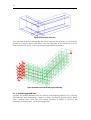
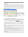
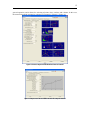
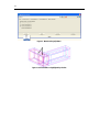
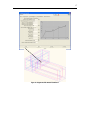
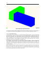
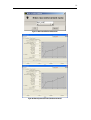
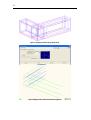
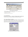
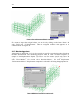
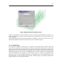
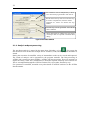
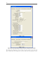
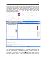
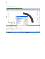
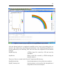
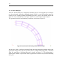
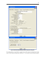
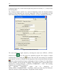
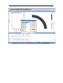
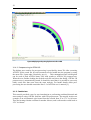
Cervenka Consulting Ltd.
Na Hrebenkach 55
150 00 Prague
Czech Republic
Phone: +420 220 610 018
E-mail: [email protected]
Web: http://www.cervenka.cz
ATENA Program Documentation
Part 3-2
Example Manual
ATENA Science
Written by
Vladimír Červenka, Jan Červenka,
and Zdeněk Janda
Prague, January 6, 2010
ii
Trademarks:
ATENA is registered trademark of Vladimir Cervenka.
GiD is registered trademark of CIMNE of Barcelona, Spain.
Microsoft and Microsoft Windows are registered trademarks of Microsoft Corporation.
Other names may be trademarks of their respective owners.
Copyright © 2000-2010 Cervenka Consulting Ltd.
iii
CONTENTS
1.
CREEP ANALYSIS
1.1
Long term deflection of a reinforced concrete beam.
1.1.1
Introduction
1.1.2
Comments on FE model preparation
1.1.3
Results
1.1.4
References
2.
STATIC ANALYSIS
5
5
5
5
7
7
10
2.1
Example of a static analysis with reinforcement
2.1.1
Reinforcement modelling
2.1.2
Problem type and data
2.1.3
Geometry
2.1.4
Materials
2.1.5
Supports and loading
2.1.6
Meshing
2.1.7
Monitoring points
2.1.8
Load history
2.1.9
Analysis and post-processing
10
10
12
13
14
21
24
26
27
28
2.2
Tutorial for Construction Process
2.2.1
Introduction
2.2.2
Geometry, boundary conditions and load
2.2.3
Running analysis
29
29
30
33
TRANSPORT ANALYSIS
34
3.1
Tutorial for Thermal Analysis
3.1.1
Introduction
3.1.2
Thermal Analysis
3.1.3
Stress Analysis
3.1.4
Postprocessing
3.1.5
Conclusions
3.1.6
Literature
34
34
34
42
46
50
52
3.
5
1. CREEP ANALYSIS
This chapter contains examples of creep analysis using the program ATENA. Currently the
commands required for creep analysis are not supported by the native ATENA graphical
environment, and therefore the necessary commands must be entered manually or by using the
ATENA-GID interface. GID (see the Internet address http://gid.cimne.upc.es/) is a general
purpose finite element pre and post-processor that can be used for data preparation for ATENA.
See the README.TXT file in the ATENA installation for the instructions how to install the
ATENA interface to GID.
In order to activate the creep analysis option an appropriate problem type must be selected: Data |
Problem type | AtenaV4 | Creep.
1.1 Long term deflection of a reinforced concrete beam.
Keywords:
reinforced concrete, discrete reinforcement, creep
Input files:
EXAMPLES\GID\CREEP2D\VITEK2D.GID,
EXAMPLES\GID\CREEP3D\VITEK3D.GID
1.1.1 Introduction
This example demonstrates the application of ATENA system to the creep analysis of a
reinforced concrete beam. The analyzed beam was tested by Dr. Jan Vitek from
Metrostav corp., Czech Republic.
1.1.2 Comments on FE model preparation
General data
The problem is modeled by two models: two-dimensional one and threedimensional. In both cases the geometrical model (Figure 2 and Figure 4) is created in
such a way to facilitate the generation of purely structural meshes, i.e. meshes that are
composed of only quadrilateral and hexahedral elements in 2D and 3D respectively.
1.1.2.1 Reinforcement
If program GID is used for pre-processing, the reinforcement can be modeled in two ways:
smeared reinforcement can be modeled by Reinforced Concrete material or by discrete bars.
Discrete reinforcement bars are modeled as line curves. These lines should be meshed by as few
elements as possible. Typically one truss element per line is sufficient. ATENA then automatically
determines the intersection of these lines with the 3D model and places reinforcement embedded
elements into each segment that is created by this process.
6
1.1.2.2 Materials
When creep analysis is requested, the material for which creep should be taken into account
must be modeled by one of the creep materials (see the Atena Theory Manual [1] or Atena Input
File Format [2]). Within the creep material a base concrete material is defined, which is one of
the standart ATENA materials. Currently only following materials are supported as creep base
materials:
“CC3DNonLinCementitious2”,
“CC3DbiLinearSteelVonMises”
or
“CC3DDruckerPragerPlasticity”.
Material properties used in this example are listed in Table 1.1-1 and Table 1.1-2.
1.1.2.3 Topology and loading
The loading history is defined in terms of intervals in GID. In the first interval the supports are
defined as well as the two vertical forces. The first interval should represent the application of the
permanent load. In the subsequent interval this load will be kept constant and the material will creep
causing the deflections as well as cracking increase. The application of the permanent load is expected
to cause some cracking, therefore it is subdivided in 20 steps. The application of the permanent load
will start at the time of 63 days and it will be completed at 63.02 days.
In the second interval, no additional forces are applied, therefore only supports are defined for this
interval. The interval starts at 63.02 days and continues up to the stop time (i.e. 365 days) defined in
Data | Problem Data. This interval is represented in ATENA by only a single step. ATENA
automatically inserts substeps, if it determines that one load step would not be sufficient for such a
long time period.
Monitoring points
Monitoring points are chosen in order to describe a load-displacement response as well as the long
term behavior. In ATENA-GID interface the monitoring is defined as conditions (Data |
Conditions). The monitoring defined in this way is considered only if specified in the first interval.
The definition of monitoring points in subsequent intervals is ignored. In this example always the
applied force is monitored as well as the mid-span deflection.
Run
Analysis can be started either directly from GID or by typing the following command:
%AtenaWin% /M CCStructuresCreep
It is important to specify the /M option in the command line when invoking the AtenaWin program.
This activates the creep module and various creep commands. If the /M option is not used various
syntax messages are obtained.
7
1.1.3 Results
The results from the analysis are documented in Figure 6, where the calculated long term midspan deflection is compared with the experimental data obtained by Dr. Vitek. It shows that
without any specific calibration, the model predicts well the long term deflections.
1.1.4 References
[1] Atena Documentation, Part 1, Atena Theory Manual, Cervenka Consulting 2003.
[2] Atena Documentation, Part 6, Atena Input File Format, Cervenka Consulting 2003.
[3] Atena Documentation, Part 8, User’s Manual for ATENA-GID Interface, Cervenka Consulting
2003.
Table 1.1-1 Material properties of concrete
Creep material: CCModelB3
Material type
1
Concrete type
Thickness, i.e. ratio of volume [m3] to
surface area [m2] of cross section
Cylindrical compressive
after 28 days [MPa]
strength
Elastic modulus after 28 days [GPa]
0.05138
f c´28
46.75
E 28
34,2
0.6
Humidity [-]
ρ
Density [kg/m3]
2 370 kg
Aggregate/cement ratio [-]
AC
4.44
Water/cement ratio [-]
WC
0.5
Shape factor [-]
1.0
Curing [-]
Air
7
End of curing [days]
Elastic modulus
[GPa]
Poisson’s ratio Compressive strength [MPa]
Tensile strength
[MPa]
Ec
Base material:
CC3DNonLinCementitious2
34 200 MPa
ν
fc
ft
0.2
46.75
3.257
8
Fracture energy
[N/m]
Compressive plast. def. [m]
Gf
wd
Table 1.1-2
127
-0,0005
Material properties of reinforcement
Reinforcement
Material type
bilinear
Elastic modulus
E
210 GPa
Yield strength
Hardening
σy
400 MPa
perfectly plastic
Table 1.1-3
Finite element mesh
Finite element type
CCIsoQuad
– Quadrilateral,
isoparametric
N/A
Gibbs-Poole
Element shape smoothing
Optimization
Table 1.1-4
Solution parameters
Solution method
Stiffness/update
Number of iterations
Error tolerance
Line search
Newton-Raphson
Tangent/each iteration
60
0.01/0.0001/0.01/0.01
off
Prostý nosník A a B
Pohled
CCIsoBrick
- Hexahedral
isoparametric
N/A
Gibbs-Poole
1.35
1.35
0.8
F
F
3.5
0.2
0.2
3.9
Příčný řez
0.14
Výztuž
Krytí
4 x φ 10 mm 10505 R
30 mm
Zatížení -
F = 6.9 kN
0.3
Figure 1: Geometry of the reinforced concrete beam.
9
Figure 2: Two dimensional geometrical model with reinforcement, loading and boundary conditions in GID.
Figure 3: Two-dimensional finite element model.
Figure 4: Three-dimensional geometrical model with reinforcement, loading and boundary conditions in GID.
Figure 5: Three-dimensional finite element model.
10
Total middle deflection [mm]
30
25
20
15
10
Vitek2D
Vitek3D
Experiment A
Experiment B
5
0
60
90
120
150
180
210
240
270
300
330
360
Time [days]
Figure 6: Long-term mid-span deflection. Comparison of two- and three-dimensional analysis with experimental data.
2. STATIC ANALYSIS
This chapter contains examples of static analysis using the program ATENA. Currently some
commands required for static analysis are not supported by the native ATENA graphical
environment, and therefore the necessary commands must be entered manually or by using the
ATENA-GID interface. GID (see the Internet address http://gid.cimne.upc.es/) is a general
purpose finite element pre and post-processor that can be used for data preparation for ATENA.
See the README.TXT file in the ATENA installation for the instructions how to install the
ATENA interface to GID.
In order to activate the creep analysis option an appropriate problem type must be selected: Data |
Problem type | AtenaV4 | Static.
2.1 Example of a static analysis with reinforcement
In this example we demonstrate the usage of GiD for data generation of a simple structure. The
structure is a reinforced concrete L-shaped cantilever. It has fixed supports on one end and is
loaded by vertical force near the free end. See Figure 7. The first beam adjacent to the fixed end
is subjected to a simultaneous action of bending and torsion while the second beam, is only
under bending. A complex three-dimensional behaviour can be well analysed by ATENA, and
for this purpose, the input data can be prepared in GiD.
2.1.1 Reinforcement modelling
The longitudinal reinforcement is by bars 4Ø28 that are located long the edges, and by stirrups
Ø12 with spacing 100mm in the first beam, (section A) and with spacing 200mm in the second
beam (section B).
11
Since there are different possibilities to model reinforced concrete we make first a decision
about the modelling approach. Concrete shall be modelled by 3D brick elements. For this we
chose the hexahedra elements. The longitudinal reinforcement shall be modelled by discrete
bars. The stirrups shall be modelled as a smeared reinforcement within the reinforced concrete
composite material. This is a simplified method, by which we avoid an input of detail geometry
of stirrups. In smeared model the exact position of individual stirrups is not captured, and only
their average effect is taken into account.
The resulting model is shown in Figure 8. The colours of elements show two types of materials
used: the composite material named Cantilever1 in the short beam and Cantilever2 in the longer
beam. The discrete bars are modelled by linear elements as shown in Figure 9. In the following,
we shall treat the generation of the model in more details. A data file with this example can be
found
in
the
ATENA
installation
under
the
name
SmallCantileverWithTorsion_DiscreteBars.gidTutorial.Static3D in the subdirectory \Atena
Examples\ Tutorial.Static3D\.
Figure 7: L-shaped cantilever beam. Dimensions in mm.
Figure 8: The model with two composite materials: Cantilever 1 and Cantilever 2.
12
Figure 9: The model of the discrete bars.
Since the smeared model of stirrups does not exactly represent their geometry it is alternatively
possible to use discrete bars as well. This is case is not described in this manual, but it can be
found in the data file Demo_L_Bars.gid enclosed in the ATENA installation.
Figure 10: Final finite element model with supports and loading.
2.1.2 Problem type and data
Typically, the problem definition starts by choosing an appropriate problem type by selecting
the menu item ‘Data | Problem type | Atena V4 | Static’ and then the general solution data in
‘Data | Problem Data’. Both steps were already described in Chapter 4. However, the
parameters of ‘Problem Data’ can be also changed later.
13
2.1.3 Geometry
The geometry is created by using the GiD graphical tools from elementary objects
sequentially, starting from points, lines and finally surfaces and volumes. We start
with the definition of points. Points are connected to lines. From lines we can form
surfaces and from surfaces we can form volumes (solid objects). Details of this
input shall be skipped, since it belongs to standard GiD functions. The final
geometrical model is shown in Figure 11. Note that it contains two types of
objects: volumes for concrete (and reinforced concrete) and lines for the discrete
reinforcement.
In GiD, it is also possible to create volumes directly from predefined primitives as
shown in the figure on the right, which indicates the available list of predefined
primitives such as rectangle, circle, sphere, etc. The volumes can be also created by
extrusion, which is activated from the GiD menu Utilities | Move or Copy. In this
dialog various copy operations can be selected such as: rotation, translation, sweep.
There is also a check box, which activates the extrusion.
Figure 11: Geometrical model.
14
2.1.4 Materials
The materials can be defined and assigned to the geometry using the menu item ‘Data |
Materials‘. Recommended procedure is to keep the default material unchanged for later
reference and create any number of user-defined materials. Since we intend to model the
vertical stirrups by smeared reinforcement we shall use the material type ‘Reinforced concrete’.
CCCombinedMaterial is a default material and Cantilever1, Cantilever2 are user-defined
composite materials that are created from the default material by pressing the button
. This
command creates a new material of the same type, which can be assigned a suitable userdefined name (see Figure 12).
The smeared reinforcement
components are activated using
these
checkboxes.
When
selected, new property sheets
appear in the dialog
Figure 12: Reinforced concrete material. Two composite materials created.
2.1.4.1 Reinforced concrete as composite material
First we define parameters of concrete component. This can be done by selecting the tab
‘Concrete Component(0)’ and modifying its parameters. There are several choices available for
the basic material. It is recommended to select the material CC3DNonLinCementitious2, which
is identical to the same material from the group ‘Concrete’. The dialog window is extended to
allow additional reinforcement components. The buttons
allow changing, adding
the default
new and deleting of materials. When adding a new material with the button
material is first copied, then re-named and edited.
The stirrups are modelled by smeared reinforcement as Component(1) of the composite
material. The first 5 parameters describe the initial elastic modulus, reinforcing ratio and
direction.
The reinforcing ratio of smeared reinforcement is calculated as p=As/Ac, where As , Ac are the
section areas of bars and concrete, respectively, in the considered volume. This ratio is different
in each part of cantilever due to different stirrup spacing. The direction of the smeared
reinforcement is defined as a unit vector.
The constitutive law of the reinforcement is defined as multi-linear by a sequence of points
(stress-strain pairs). The first point is defined by yield strength (and elastic modulus). This gives
a bi-linear, elastic-plastic law, with unlimited ductility. A general multi-linear function can be
defined by additional points. Maximum 4 additional points can by given.
Up to three smeared reinforcements can be defined in one composite material. This limit exists
only in the GiD interface. (ATENA can define unlimited number of components for a single
composite material, in this case it is necessary to manually edit the ATENA input, which is
generated by GiD.)
After the parameter definition, the material can be assigned to the structure. This is done by the
button ‘Assign’ and following the appropriate selection by mouse. The process of selection is a
15
general operation, and it allows for selecting of points, lines, surfaces and volumes. In this case,
the material should be assigned to volumes (of geometry), Figure 15, Figure 16.
Figure 13: Concrete component in the ‘Reinforced concrete’ material
Figure 14: Components of smeared reinforcement in the composite material
16
Figure 15: Menu item ‘Assign | Volumes’.
Figure 16: Selected volumes are highlighted by red colour.
17
Figure 17: Assignment of the material ‘Cantilever2’
18
Figure 18: Display of the assigned material groups
A composite material for the second part of the structure (named as Cantilever2) can be defined
in a similar way, where the only difference is in the value of reinforcement ratio, Figure 17.
2.1.4.2 Bar reinforcement
From the menu ‘Data | Materials‘ we select the material ‘Reinforcement’, which is designated
for discrete bars. There we choose from the list the ATENA-model ‘CCReinforcement’ and
then click on the button ‘New reinforcement’ and enter the name for the reinforcement material.
After confirmation by OK a dialog for material parameters appears. The parameters include
initial elastic modulus, yield strength and optionally points on the stress-strain curve. The last
parameter is the bar cross-sectional area (see Figure 20).
The material is then assigned to the geometry by pressing the button ‘Assign‘ and selecting
‘line‘ geometric entities by the mouse. The selected bars are marked by red color, Figure 21.
Applying the command ‘Draw’ at the bottom of reinforcement material dialog (see Figure 22)
can check a correct assignment, which shows the geometry (in this case lines) with the currently
assigned material.
In case of pre-stressed bars each bar (cable) must have a distinct material (even if its values are
identical with other bars). The reason for this is to distinguish among groups of elements for
pre-stressing. The pre-stressing is defined in ‘Conditions | Lines | Initial strains’ and is assigned
to the lines that model the pre-stressing reinforcement.
19
Figure 19: New material for bar reinforcement.
Figure 20: Material parameters for the ‚Reinforcement‘ model
20
Figure 21: Assigning material to the geometry of bars.
Figure 22: Display of the reinforcement material assignment
21
2.1.5 Supports and loading
The supports and loading can be a specified using the menu ‘Data | Conditions’. We define the
fixed nodes by checking X-, Y-, Z-Constrains and the type of geometry ‘Surface’. Using the
command ‘Assign’ we selects the end face of the cantilever and finish the assignment of support
conditions.
In a similar way we assign the Point-displacement at the node of load application. The load is
applied as a vertical imposed displacement. Consequently the force value is a reaction at this
node.
Figure 23: Definition of the surface support in all directions
Figure 24: Definition of prescribed displacement in vertical direction
The conditions dialog of GiD can be also used to define ATENA monitors. These are special
type of conditions that does not affect the analysis results. They are merely used to monitor
certain quantities during the analysis. In this example, the following monitors will be specified:
•
Maximal crack width
•
Displacement at the point of load application
• Reaction at the point of load application
The definition process of the above conditions and monitors is described in Figure 26. The
resulting assignment of the boundary conditions can be checked using the command Draw | All
Conditions | Exclude local axis, which can be located at the bottom of the Conditions dialog. It
should be noted that it is also possible to apply these conditions directly on the generated finite
element model, but then the applied conditions are lost every time the mesh is regenerated.
22
Assign the crack width monitor to all
volumes
Assign the displacement
monitor to this point
Assign the reaction
monitor to this point
Figure 25: Definition of the ATENA monitors
23
Fixed surface in all three global directions
Volume monitors to extract maximal crack
width
Applied
displacement and
two monitors for
deflection and
reaction
monitoring
Use Draw | All Conditions | Exclude local axis to display conditions
Figure 26: Display of assigned conditions
In certain cases it may be advisable to manually identify which line entities represent
reinforcement. By default the GiD-ATENA interface attempts to treat all lines that are not
connected to any surface or volume as reinforcement. This default behavior is activated by the
corresponding check box in the Problem Data dialog. In certain cases the automatic
identification does not work properly. In this case it is advisable to deactivate this default
behavior, un-assign all reinforcement node and element identification and then assign it again
manually.
These two conditions should be
manually assigned to all
reinforcement line entities, if
error messages about
reinforcement identification
appear during mesh generation
or during the generation of the
ATENA input file.
Prior to that the automatic
reinforcement identification
check box should be
deselected and all
reinforcement identif.
Conditions unassigned
Figure 27: Manual identification of reinforcement nodes and elements
24
2.1.6 Meshing
In the preceding description the geometry was defined and all properties (material, supports,
loading) were assigned to geometry. Now we shall generate a finite element mesh.
For this we must set up appropriate parameters in the menu ‘Meshing’,
Figure 28: Meshing menu.
2.1.6.1 Mesh definition for volumes (concrete)
First we shall deal with the meshing of volumes (concrete). There are many ways how to define
mesh. In this case, we use a simple method, in which divisions on all lines are defined. If
opposite lines have the same division we can create a regular mesh.
•
In the item ‘Quadratic elements’ we define low order elements by checking ‘Normal’.
•
In ‘Structured’ we define division on all lines. It is always sufficient to select one line.
GiD automatically assigns the same division to all opposite edges.
•
In ‘Mesh criteria’ we select lines.
•
In ‘Element types’ select ‘Hexahedra’.
2.1.6.2 Mesh definition for lines (reinforcement)
It is important to realize, that lines of reinforcement in GiD serve only to export geometry to
ATENA. The embedded reinforcement will be generated in ATENA. This means that we should
make the line elements of reinforcement as large as possible. If we use division into a single
element then this single element is then passed to ATENA for the generation of the individual
bar segments. Finding the intersections of the reinforcement bar with the solid elements
generates the segments. In case, the reinforcement in GiD is modelled using curved lines, then it
is recommended to prescribe a certain division to finite elements such that the curved geometry
of the bar is properly represented.
25
Figure 29: One division in lines of reinforcement.
- In the item ‘Quadratic elements’ we define low order elements by checking ‘Normal’.
- In ‘Structured’ define 1 division on lines, Figure 29
- In ‘Mesh criteria’ select lines.
- In ‘Element types’ select ‘Linear | Lines ’.
2.1.6.3 Mesh generation
By selecting the item ‘Generate...’ the mesh is automatically generated. The mesh can be
inspected in the items ‘Mesh view’, ‘Mesh quality’. To change the mesh the whole process can
be repeated. GiD allows also changes by editing the mesh dimensions and properties.
2.1.6.4 Assign conditions to mesh nodes
Now, if needed it is possible to assign additional conditions or materials directly to finite
elements of nodes. Select ‘Data | Conditions’ as shown in Figure 30. For this we must select by
mouse the node, where condition should be applied. It is however, recommended to assign the
material properties and boundary conditions on the geometric entities rather then on the mesh,
otherwise it is necessary to reassign such properties every time the mesh is regenerated.
Figure 30: Assigning condition of point-displacement to a mesh node.
26
Figure 31: View and inspect a condition in a mesh node.
If we want to inspect the assigned values, we can do it by clicking on the button ‘Draw’ and
select ‘Field value | Z-Displacement’. Then the assigned condition value appears at the
concerned node. See Figure 31.
2.1.7 Monitoring points
Analogically to the Section 2.1.5 it is also possible to specify the monitoring points directly on
the finite element mesh. The monitoring points are tools to record a structural response, for
example a load-displacement diagram. In GiD we can for instance specify only force and
displacement monitoring at a mesh node. This is done also in ‘Conditions’. For applied force we
select ‘Force-Monitor’, for reaction force ‘Reaction-Monitor’, for nodal displacement
‘Displacement-Monitor’. Displacement component is selected by checking the appropriate box.
Figure 32: Definition of a monitor for reaction at node.
27
Figure 33: Definition of monitor for displacement at node.
Figure 32 and Figure 33 show definition of force (reaction) and displacement monitors at a
node. An inspection of monitors can be done by the command ‘Draw’ in the same manner as in
other conditions.
The monitoring points must be included within ‘Conditions’ of the first load interval in GiD.
Monitors included in other intervals will not be active in ATENA analysis.
2.1.8 Load history
For analysis in ATENA a load history as a sequence of load steps must be defined. The load
steps can be proportional or non-proportional. In this example the load history is simple. We
define first interval, which includes a set of conditions for supports at the fixed end and pointdisplacement. This can be checked and changed in the menu item ‘Data | Interval Data’. Next
load steps can be done in two ways. The simplest way is to enter the number of repeated load
steps and multipliers in the window of ‘Interval Data’, Figure 34, which is a proportional load
history. In case of a non-proportional history, for example, first a vertical load followed by a
horizontal load, we can use ‘Data | Interval Data’. Default settings of calculation method and
global settings are in ‘Data | Problem Data’.
28
All conditions will be multiplied by a factor
1.0 in all load steps generated in this interval
Results from all steps will be saved. Each step
is saved in a separate file, which is named
TaskName.xxx, where xxx denotes the step
number
50 load steps will be generated. All with the
same conditions
These data fields are editable only the import
of transport data is requested in Problem Data
dialog
Figure 34: Interval data definition
2.1.9 Analysis and post-processing
The non-linear analysis is started by the menu item ‘Calculate‘ or icon
. This causes the
data from GiD to be written into an input file for ATENA (*.INP) and the program AtenaWin is
started.
During the execution of AtenaWin variety of intermediate results can be viewed and inspected.
The results of analysis can be presented in the program Atena3D. The Post-processing in
ATENA 3D is started via menu ATENA | ATENA 3D post-processing. Then it is necessary to
import the binary result files (TaskName.xxx) from the required load steps into ATENA 3D.
This is accomplished through the ATENA 3D menu File | Open other | Results by step.
For operation of AtenaWin, Atena3D or any other details of ATENA software see the ATENA
Documentation.
29
2.2 Tutorial for Construction Process
2.2.1 Introduction
The objective of this tutorial is to show how the graphical environment of GID can be
used to model the construction process. The finite element solution core of ATENA
supports the possibility to add or remove groups of finite elements. This feature can be
used to model the construction process in GID. The ATENA-GiD extension of the GID
graphical environment includes direct support for this feature. This feature can be
modeled using the conditions for surface and it will be demonstrated in this manual on
the example of a tunnel (see Figure 35:).
Soil
Soil / Lining
Soil / Air
Figure 35: Model with three macro-elements.
The basic idea of the construction process modeling in ATENA is the following. It is possible to
add or remove finite element groups at any time.
30
2.2.2 Geometry, boundary conditions and load
We need to analyze a structure of a tunnel. Around the tunnel there is concrete lining. Boundary
conditions are seen in Figure 36.
Monitor points
Dead Load
Constraint
Figure 36: Draw all conditons on model
The construction should proceed as follows:
1. excavation of a circular hole in the soil
2. adding lining (ring)
3. adding load
First, it is necessary to construct the model of the whole structure. Three separate
macro-elements will be created for all four intervals.
Interval 1: this interval is used to define the basic boundary conditions to support the model
from the bottom and both sides.
Interval 2: this interval is used for excavation of a circular hole in the soil by deleting
two centered macroelements.
Interval 3: this interval is used to add lininig (ring shape) with concrete material characteric
around the hole.
Interval 4: this interval is used to add load to top face of the model.
At the beginning, the whole area consists of soil, however, we must define separate
macroelements for future changes (soil, lining, air). We assign the soil material to all these
macroelements for the first interval (Figure 37:). The additional intervals will be needed for the
subsequent phases of the construction process.
31
Figure 37: Material for interval 1
In next step (excavation) we need to remove both circles from the center. It can be made using
conditions for surface. In menu “Data > Interval > Current” we switch to interval No.2 which
we want to edit (Figure 38: ). In menu “Data > Conditions > Conditions for surface” we
choose “Elements Activity for Surface“ and select „Construction (Elements Activity) :
DELETE” (Figure 39). Next we can “Assign” areas which we want to excavate (Figure 40).
We can draw all macroelements which have assigned some conditions by choosing “Draw >
Colors” (Figure 40).
Figure 38: Switching current interval.
32
Figure 39: Conditions for surfaces
Figure 40: Deleting materials in interval 2
In the next step, we need to create the lining with non-linear concrete material. We switch the
current interval to No.3. In menu “Data > Conditions > Conditions for surface” we choose
“Elements Activity for Surface“ and select „Construction (Elements Activity): CREATE
WITH NEW MAT” (Figure 41), and choose the CC3DNonLinCementitious2 material. We can
create specific material for this case and assign to surfaces, which we want to create (Figure 42).
33
Figure 41: Condition for surface, create new material
Figure 42: Creating concerete lining.
In the last step (Interval No.4), we will only add load to top of the model
(“Data > Conditions > Conditions for line”, “Load for line”).
2.2.3 Running analysis
Analysis can be run by selecting button in menu “Calculate > Calculate” or clicking on the
button
“Atena Calculate” and in Atena Win by clicking on button
“Execute“.
34
3. TRANSPORT ANALYSIS
3.1 Tutorial for Thermal Analysis
An example demonstrating the coupling of thermal and stress analyses.
3.1.1 Introduction
This document describes an example of rotationally symmetrical vessel subjected to
thermal loading. The analysis is performed using the programs ATENA and GiD.
ATENA is used for thermal and static analysis and the program GiD is used for data
preparation and mesh generation.
The programs GiD and ATENA can be installed using the standard ATENA
installation. At the end of the installation the user must select the installation of GiD and
ATENA-GiD interface. After that your computer should be ready to run the example
problem described in this document.
3.1.2 Thermal Analysis
First the program GiD is started. The recommended version is 9.0.4 or newer (the oldest
supported version is 7.7.2b). After starting GiD, the user should open the example
analysis
"ATENA Science\ATENA-GiD\Tutorial.Temperature2D\PipeBTemp.gid".
This is an existing model demonstrating the combination of thermal and stress analysis.
This problem is using the problem type: AtenaV4 | Transport. It represents a section of a
pipe wall with thickness of 0.23 m and internal diameter of 1 m. Taking advantage of
the symmetry, only a quarter of the whole crossection is modeled. The geometry of the
model is shown Figure 43 and the numerical model is shown in Figure 44. Details about
ATENA-GiD interface and associated problem types for ATENA can be found in the
manual [6]. The same mesh size is used for thermal and static analysis. This is however
not a strong requirement. The thermal loading can be exchanged also between models
with totally different meshes.
35
Figure 43: Geometry and material properties of the axisymmetrical pipe model.
Figure 44: Numerical model, finite element mesh.
The loading is subdivided in 3 intervals. In the first interval 12 load steps are defined
with boundary conditions as described in Figure 45. In each step the temperature on the
outer surface is increased by 1 °C (see Figure 45). The temperature in the exterior is
36
increased up to 37 °C, starting from the initial uniform 25 °C. Each step in this interval
represents 3000 seconds, thus the whole interval covers the period 0-36000 seconds (010 hours).
Figure 45: Boundary conditions for the interval 1.
In the subsequent interval 2, the temperature at the outer surface is kept constant. This
interval contains 10 steps 2880 seconds long. This means the whole interval spans the
time period from 36000-64800 seconds (10 hours-18 hours).
Figure 46: Boundary conditions for the interval 2.
37
In the last interval 3, the outer surface is cooled back to 25 degrees. This interval
contains 12 steps 1800 seconds long. This means the whole interval spans the time
period from 64800-86400 seconds (18 hours-24 hours).
Figure 47: Boundary conditions for the interval 3.
38
Figure 48: Problem data dialog including the definition of temperature exchange files with stress analysis.
The problem data dialog that is shown in Figure 48 can be opened via the menu item
Data | Problem data. This dialog can be used to define the basic parameters for the
39
thermal analysis. The most important fields can be found at the bottom of the Time and
Transport tab, where the names of two files are to be specified. These files are used for
exchanging the temperature fields with the subsequent stress analysis. By default, the
files would be stored in the AtenaTransportCalculation subdirectory of the main
problem directory, inserting “../../” before the names writes them into the
Tutorial.Temperature2D directory.
The ATENA calculation is started from the menu ATENA | ATENA analysis or by
clicking the calculator icon
. This will start AtenaWin program which is a
graphical interactive environment for the execution control of ATENA finite element
core module. More details about the usage of this program can be found in the
corresponding ATENA manual [5].
After executing ATENA analysis the following window appears on the user’s computer
(see Figure 49).
Figure 49: The main AtenaWin window after its activation from GiD.
The ATENA analysis is started automatically (or by clicking the
button). This
starts the thermal analysis in AtenaWin environment. In order to visualize the
development of the temperature field the button
can be selected and this will open a
dialog that is shown in Figure 50. In this dialog various variables can be selected for
40
display.
The
temperature
fields
“CURRENT_PSI_VALUES” | Temper.
can
be
displayed
Figure 50: The selection of temperature display in AtenaWin.
by
selecting
41
Figure 51: The runtime display of temperature field during the thermal analysis in ATENA.
After the thermal analysis is completed AtenaWin can be closed. All resulting files are
stored in the subdirectory AtenaTransportCalculation of the PipeBTemp.gid directory.
In this subdirectory the following files will exist after the completion of the thermal
analysis:
PipeBTemp.inp
ATENA input file created by GiD and used by
AtenaWin
PipeB.00xx
Binary result files created by ATENA during the
thermal analysis.
These two files are created in the Tutorial.Temperature2D directory:
PipeB_Results.thw
Saved temperatures to be used by stress analysis.
PipeB_Geometry.bin
Saved geometry to be used for the interpolation of
temperatures in the stress analysis.
42
3.1.3 Stress Analysis
After the thermal analysis is completed AtenaWin can be closed and the stress analysis
can be performed using the calculated thermal fields. A new GiD problem must be
created or the existing problem PipeBStatic.gid can be used. This model defines the
input for stress analysis of the same pipe wall as was used in the thermal analysis.
The geometrical model and boundary conditions are shown in Figure 52.
Figure 52: Geometrical model and boundary conditions for stress analysis.
In order to be able to utilize the thermal fields calculated during the thermal analysis the
appropriate import files must be specified in the problem data dialog that is activated
from the menu Data | Problem data and is shown in Figure 53. This information is
located in the bottom 2 input fields where appropriate file names are specified including
their path.
43
Figure 53: Problem data dialog including the definition of temperature exchange files.
The loading history is specified in a single interval. The interval is divided into 50 load
steps. In each step the temperature difference of 720 seconds from the thermal analysis
44
is applied (Figure 54). So the interval spans the period of 10 hours, i.e., it only covers
the heating phase.
The Transport Import switch set to Interval Beginning means the thermal analysis
results are only imported once and the temperature values are interpolated for each
static analysis step. For complex temperature histories, it can be changed to Each Step.
Figure 54: Interval data for the interval 1.
The stress analysis is again started by selecting the menu item ATENA | ATENA
analysis or the
icon. This starts the AtenaWin program. The analysis is started
automatically or by clicking the
button. This starts the stress analysis in AtenaWin
environment. In order to visualize the development of the various data fields, the button
can be selected and this will open a dialog that is shown in Figure 55. In this dialog,
various variables can be selected for display. The contour areas of crack width can be
displayed by selecting Elements | “CRACK_ATTRIBUTES” | COD1. The resulting
computer screen in shown in Figure 56.
The
imported
temperature
values
can
be
displayed
as
ELEM_TOTAL_TEMPERATURE | TotalTemp. Please note that only the difference
from the reference (initial) temperature is displayed in static analysis.
45
Figure 55: Execution of static analysis in AtenaWin and the selection of crack opening display.
46
Figure 56: Execution process of stress analysis in AtenaWin showing the crack opening displacements.
After the completion of the analysis the AtenaCalculation subdirectory of
PipeBStatic.gid contains the following files:
PipeBStatic.inp
ATENA input file created by GiD and used by
AtenaWin
PipeBStatic.00xx
Binary result files created by ATENA during the
stress analysis.
3.1.4 Postprocessing
Postprocessing can be done either in AtenaWin, GiD, or Atena 3D. Normally,
AtenaWin displays the current step that is analysed. After the analysis is finished, the
last step remains in AtenaWin memory and can be visualized and further postprocessed. In case the user wants to post-process results from other load step, the
corresponding step results file is to be opened using the command Application | Restore
FE Model From. The step data file name is “task_name.00xx”, where task name is the
name of the current task as given in the problem data dialog (see Figure 53) and 00xx
represents the load step number which is to be post-processed.
47
(Alternatively, the new text window is to be opened using the menu item File | New.
Please note that a text window must be highlighted in order to another text window. If
graphical window is the active one, a new graphical window will be opened. Into the
new text window the following command shall be written:
RESTORE FROM “task_name.00xx”)
3.1.4.1 Postprocessing in GiD
To be able to postprocess the results in GiD, the result quantities must first be made
available by selecting them in the Data | Problem Data | Post Data dialog, see Figure 57.
Figure 57: Selecting results for postprocessing in GiD.
48
The menu command ATENA | GiD Post-processing or the
icon toggles GiD
between pre- and postprocessing. A warning about non-existent .res file may appear,
then a console windows is started and the results are converted into a format readable by
GiD, see Figure 58. The conversion can take a few minutes depending on model size,
number of load steps, and the number of quantities selected for postprocessing. The
results are stored into the AtenaResults.flavia.res file in the AtenaCalculation
respectively AtenaTransportCalculation directory for static analysis respectively
transport analysis. This file can be opened in GiD by the File | Open command (see
Figure 59).
Figure 58: Importing results for postprocessing in GiD.
49
Figure 59: Opening results for postprocessing in GiD.
The results can be then postprocessed. Figure 60 shows crack width as contour lines,
which can be selected by the menu command View results | Contour lines | CRACK
WIDTH | COD1. The command can also be accessed from the
icon.
50
Figure 60: Displaying crack opening displacement isolines in GiD.
3.1.4.2 Postprocessing in ATENA 3D
The highest user comfort for post-processing is provided by Atena 3D. After executing
ATENA 3D the result file for each increment can be loaded into the program by using
the menu File | Open other | Results by step (*) … This command activates a dialog that
can be used to load ATENA binary files with results to ATENA 3D postprocessor.
When the user finishes loading the needed result file and closes the dialog, ATENA 3D
postprocessor is automatically started. It should be noted that it is possible to open only
binary result files that come from the same analysis. For further details about postprocessing the user should consult the Part 2-2 of ATENA user’s manual [2].
3.1.5 Conclusions
This tutorial provided a step by step introduction to performing combined thermal and
stress analysis using ATENA software with GiD preprocessor. The tutorial involves an
example of an axisymmetric pipe heated from the outside from 25 to 37°C in 10 hours.
Then the heating remains constant for another 8 hours, and is afterwards cooled back to
25°C in 6 hours.
51
The objective of this tutorial is to provide the user with basic understanding of the
program behavior and usage. For more information the user should consult the user’s
manual [2] or contact the program distributor or developer. Our team is ready to answer
your questions and help you to solve your problems.
The theoretical derivations and formulations that are used in the program are described
in the theory manual [1].
Experienced users can also find useful information in the manual for the analysis
module only [4].
52
3.1.6 Literature
[1] ATENA Program Documentation, Part 1, ATENA Theory Manual, CERVENKA
CONSULTING, 2009
[2] ATENA Program Documentation, Part 2-1 and 2-2, ATENA 2D and 3D User’s
Manual, CERVENKA CONSULTING, 2008
[3] ATENA Program Documentation, Part 3, ATENA 2D Examples of Application,
CERVENKA CONSULTING, 2005
[4] ATENA Program Documentation, Part 6, ATENA Input File Format, CERVENKA
CONSULTING, 2009
[5] ATENA Program Documentation, Part 7, AtenaWin Manual, CERVENKA
CONSULTING, 2008
[6] ATENA Program Documentation, Part 8, User’s Manual for ATENA-GiD Interface,
CERVENKA CONSULTING, 2008