Download Particle system based visual effects editor

2IV05 Final report
Radim Čebiš and Pavel Černohorský
Particle system based visual effects editor
Final report
Additional component computer graphics
course at Technische Universiteit Eindhoven
2008
1/14
2IV05 Final report
Radim Čebiš and Pavel Černohorský
1. Introduction
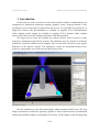
In this work we want to present our visual effects editor, which we implemented as an
assignment for Additional component computer graphics course. Program manual is also
provided as a part of this report in paper form and for user it is accessible by pressing F1 in
application. Source code documentation is available on supplied CD in Documentation
folder. Sample render outputs are available on supplied CD in Samples folder (sample
source project files are in the Samples sub-folder of the Binary folder).
Our target was to create user friendly tool which could be used by artists to create
impressive animations using particle systems. The animation uses key frames in which the
parameters of particle emitters can be changed. This way the artist can achieve non regular
behaviour of the particle systems. The parameter's values are interpolated between key
frames by interpolation curve which can be edited by the artist.
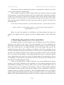
We also wanted to give the artist other things, which could be useful for him. The first
thing is placement of some basic geometry (spheres or boxes) which can help to understand
dimensions and which improves orientation in 3D space. As the output is only 2D image and
2/14
2IV05 Final report
Radim Čebiš and Pavel Černohorský
particles are 2D textures, the geometry can improve depth recognition. Second, the artist can
create forces which will affect the particles. The force is only changing acceleration of the
particles, but even using such a simple principle, the desired effects as wind or gravity are
achievable.
The usability was one of the most important aspects of the editor. We designed user
interface in a way that it should be understandable even without manual. It obeys few
principles in all the controls. This fact improved unification and thus it is faster to learn the
controls. Of course for more advanced actions as for example animating, the user manual is
included. We have left some options mainly about rendering in the menu which are not
much useful for user, because we selected the best option as default, but they are there to
show that we have tried several ways to achieve better performance of the application.
Application requirements were specified in the proposal, but we have made some
changes in them, because they were not always smart enough.
The targeted platform is Windows XP operating system and it is useful to have graphic
card with hardware T&L. The performance depends heavily on the complexity of the scene.
The application is still usable on two year old notebook (Pentium M 1.73GHz, 1.5 GB
RAM, ATI Radeon X700 with 64MB VRAM) with about 30 000 particles in scene.
2. Application design and implementation
At first we created graphical user interface with use of wxWidgets library and
wxFormBuilder tool. We have implemented OpenGL view port there for interactive view of
the scene. We decided that the whole GUI will be kept editable in wxFormBuilder, because
our GUI design had not been finished yet. For editing of parameters we used
wxPropertyGrid which is not supported in wxFormBuilder, so the handling of this had to be
done in source code.
Then we made the decision that the whole user created project will be kept in one
instance of class visual effect (CVisEff) which will be owned by the Main Frame of the
application. This way we could keep the design of the CVisEff separated from GUI.
3/14
2IV05 Final report
Radim Čebiš and Pavel Černohorský
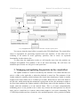
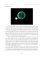
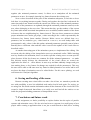
Very simplified class diagram to show the basic structure of the system
You can see, that the visual effect is owned by the GUI's MainFrame. The visual effect
object is responsible for processing requests from user interface. It also takes care of
rendering of all entities in scene (geometry, particles). But of course we separated
functionality in other classes also.
To show how the application works we will describe next, how the particles are
managed and updated. This method is one of the most interesting. We will leave out
animation part, because we will give it some space later.
3. Managing and updating the particles in the visual effect
The Update method of CvisEff is invoked by user interface. It is called when the user
moves a slider to the right side or when the playback is turned on. The parameter of the
Update method is timeStep which indicates how much time should pass, which is usually
length of one frame (frame rate is 30 frames per second). When the user moves the slider to
the left side, which means that the animation is going back in time, the animation rewinds to
the first frame and then the Update method is called many times with the timeStep of frame
length, until the animation is in the desired frame. This is of course computationally
demanding, but it is not possible to do it other way, because the dead particles are thrown
away and we would have to resurrect them which might be even more demanding. The
CVisEff object holds two lists of particles: alive and dead particles. Alive particles list holds
4/14
2IV05 Final report
Radim Čebiš and Pavel Černohorský
particles which are still alive and should be counted with. Dead particles list holds particles
which died. This is good for performance and we will mention it later.
For every living particles few steps are done. First we decrease time to live of the
particle, when it is lower than zero, the particle dies and it is moved to the list of dead
particles and we do not count with it any more while updating or rendering. If the particle is
still alive, we proceed with other computations with it. We try if it is inside a geometry
(IsInsideGeom method is used) which has interaction setting set to Kill and if it does the
particle is killed and moved to the list of dead particles. If it is still alive we continue with
computation of influencing forces. For each force we test if the particle is inside geometry
assigned to the force (IsInsideGeom method is used) and if it is, it is influenced by the force.
The last step done with particle is to call its Update method which will update its state.
The particle has many parameters, but for Update method the most essential are
position in space, velocity vector and acceleration vector. When the Update method of the
particle is called the velocity is changed like this: velocity += acceleration * timeStep and
then the position is changed like this: position += velocity * timeStep. By multiplication
with timeStep we are scaling the vector according to elapsed time.
5/14
2IV05 Final report
Radim Čebiš and Pavel Černohorský
The forces are influencing only particle acceleration. The force has its direction and
strength. When the particle is influenced, its acceleration is changed like this: acceleration
+= direction * strength * timeStep.
When all the particles were updated, we can proceed with emitting the new ones. For
each emitter the Emit method is called, its parameters are timeStep, list of alive particles and
list of dead particles. First, the emit method computes how many particles it should emit.
The emitter remembers what “part of the particle” it did not emitted in previous frame when
there was only the fraction of one. To this saved fraction the timeStep * number of particles
per second value is added. Then we use the integral part as a number of particles to create.
The non integral part of the number is saved for use in another frame. Then we continue with
creation of particles. First, we check if there are any particles in the list of dead particles. If
there are not any, we allocate thousand of new particles and put them into the list. Then we
take the tail particle saved in the list.
We set new particle's parameters and move it to list of alive particles. Emitter
remembers how the parameters of the particles were set by the user. These parameters are
usually randomized somehow. Most of them are described as value and variation of the
value. The value determines the central value of the parameter. The variation specifies in
percentage deviation from the value – tells us how the parameter can change for every
particle. For example the value is set to 300, if the variation is 0%, then the value is used. If
the variation would be 10% then the value would be somewhere between 270 and 330
randomly. This pseudo random value is then set as a parameter to the particle.
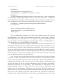
Also some other pseudo random parameters are counted. For example the position of
the particle on the limited plane (plane emitter) is counted like this:
position = position of the emitter + VectorX * (random number in <-1,1>) + VectorZ
* (random number in <-1,1>)
Vectors VectorX and VectorZ look like on this sketch:
Vectors are orthogonal. Their length is size of the plane in the specific dimension. And
the vectors are in the plane.
6/14
2IV05 Final report
Radim Čebiš and Pavel Černohorský
The direction of the acceleration and velocity is counted that we rotate the up vector
(0,1,0) pseudo randomly in defined range.
There would be an undesired effect, which would occur when the emitter is moving
fast in the space. It would create particles only in its actual position in that frame, but there
would not be any particles in between the position in the current and the position in the
previous frame. To overcome this, we always find out the previous position of the emitter
and we put the particles randomly in between the previous and new position. In pseudo code
it looks like this:
vector between emitter positions = previous emitter position – current emitter position
particle position = actual emitter position + (vector between emitter positions *
random number in <0,1>)
When we emit all the particles we should have the Emit method ends, some new
particles were added to the alive particles list and the Update method of the CVisEff ends
too.
4. Rendering the particles of the visual effect
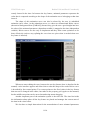
The Render method of CvisEff method is used to display the scene. The rendering is
present in two forms in the system. The first rendering is used for displaying the
intermediate results and previews while editing the particle system. It is done in real-time
and so the results may be a bit different thanks to the non-constant time steps in the
animation that may appear. The second form of rendering is the off-line rendering. It uses
the same rendering sub-system but in different way. Time steps are constant and the results
may have user defined resolution. These results are also frame by frame saved to the hard
drive. To measure the performance of the rendering subsystem, there is a button in Render
menu, Render batch test, which can execute the measurement of the performance. That is
accomplished as rendering of the current frame 100 times. The time spent is then shown. So
how does the rendering subsystem works?
Firstly we will explain how it works in interactive view. Later the differences between
interactive and off-line rendering will be mentioned. At first rendering subsystem sets the
transformation according to our camera setting. Then it sets the directional light vector. If
the grid is turned on, it is rendered as line primitives. Then we render emitters' graphical
representations. In other step the geometries are rendered. The ones which have some forces
assigned to them are rendered as wireframe. Then the blending function is set according to
project settings which include check box where it is possible to select, if we want normal or
additive alpha. Then the RenderParticles method is invoked to continue with rendering of the
7/14
2IV05 Final report
Radim Čebiš and Pavel Černohorský
alive particles.
First step of the RenderParticles method is to compute the destination of every particle
from the view plane which is defined as a plane whose normal vector is equal to the look at
vector of the camera and the camera position is in the plane. Then we sort the particles
according the setting in Render menu and Sorting techniques sub-menu. One of the options
is to sort with standard STL list.sort() method which is by our measurement the fastest one.
The other implemented option was to use Shell sort, but it proved to be slower. The last
option is that the particles will not be sorted. This is not useful when the transparency is used
in textures or when the alpha falloff parameter of the emitter is set to something else than
zero. Because it would lead to badly counted transparency.
The next and the last step is to render almost every alive particle. Just the particles
with negative distance from the view plane, meaning that the particle is behind the view
plane, are not rendered. We partly implemented four techniques to render them. Then we
selected the fastest one and implemented whole functionality of the rendering (for example
texturing support). There are many ways to render the particles. One of the main objectives
of rendering is to rotate the particles so they face the view plane. This is called billboarding.
The description of the techniques is always written for one particle, because the technique is
then executed on all appropriate particles.
Our first partly implemented technique is very simple and slow. It creates new
transformation matrix on the matrices stack of OpenGL and rotates and translates the space
so the particle is in the right position and right orientation. Then the particle is rendered in its
origin and the matrix is removed from the matrices stack. In pseudo code it works like this:
8/14
2IV05 Final report
Radim Čebiš and Pavel Černohorský
PushMatrix();
TransformateSpaceAccordingToCamera();
RenderQuad(size = sizeOfTheParticle, position = (0,0,0));
PopMatrix();
The other implemented technique proved to be the fastest one, so now it supports all
the functionality including alpha falloff and textures. At first it computes the 4 coordinates
of the quad placed in the origin, which is facing the camera. Then for every particle it uses
these coordinates but moves them to the right position. In pseudo code it works like this:
rotatedQuad = rotateBasicQuadAccordingToCameraRotationMatrix;
Foreach particle
{
quad = scaleBasicQuadTo(sizeOfTheParticle);
quad.allCoordinates += positionOfTheParticle;
Render(quad);
}
The “non billboarding” technique is not much of the technique because it does not do
any billboarding. It was only used to evaluate how much time is spent with or without a
billboarding. Because we had other ideas – for example to compute the billboarding inside
the vertex shader - but while comparing our fastest method and the “non billboarding”, we
found out that there is very small difference in performance.
The last partly implemented technique is point sprites extension. We hoped that it will
bring higher performance because with this extension only the position of the quad is sent to
the card and the card should compute billboarding and position of all 4 points of the quads.
So the bus should transfer only one point instead of 4 points. But this extension is poorly
supported by the graphic card drivers and most importantly it was not any faster than the our
fastest technique. So in the end our technique with one quad rotated to face the camera and
move to appropriate positions was used as default.
Now we know how does the rendering of the visual effects works for the previewing
so let's take a look on the differences in the off-line renderer. As stated before, off-line
renderer uses normal rendering, but with some special features. The most important feature –
rendering into the frame of any size that user enters in the renderer control window and
saving such a frame into the file is achieved through the OpenGL p-buffers (pixel buffers)
(theoretical background from [WYNN05]). This functionality is implemented by the
graphics hardware vendors for longer time but we have even now experienced some
problems with the combination of Windows Vista and Intel 950 GMA graphic card.
Whenever there are some problems using this functionality for the rendering, user is warned.
The process of the rendering itself works in the way that each single frame is rendered as
described earlier (with the only difference that emitter representation, geometry with some
9/14
2IV05 Final report
Radim Čebiš and Pavel Černohorský
force assigned and the grid are not rendered) and result of the rendering is saved to the file
with user given prefix and the frame number. Than time is advanced exactly by the length of
one frame and another frame is rendered. This way the whole visual effect is rendered so
user gets exactly all the pictures of each frame.
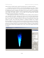
5. Animation subsystem of the application
Very important part of the application is the ability to animate all the relevant
parameters of the particle emitters. User can animate not only the parameters of the emitters
themselves (such as their position), but also the parameters of the emitted particles (such as
their acceleration or it's variation). For this to be achieved we created a animation subsystem
that automatically handles all the parameter changes in time and that is easily controllable by
the user (using animation curves as usual in animation software systems).
As a basis for this system, we created an animated parameter abstraction. Because all
the animated parameters we need to animate are either of floating-point type or can be
simulated by floating-point type, we chose to create this animated parameter abstraction to
be float. This animated parameter abstraction consists of one or more pieces of animation
curves that touch each other in significant points called the key frames. Values of the
animated parameters are set exactly at these points by the user. Each of these key frames is
10/14
2IV05 Final report
Radim Čebiš and Pavel Černohorský
exactly located in the time. In between the key frames, animated parameter represents the
value that is computed according to the shape of the animation curve belonging to that time
interval.
The shape of this animation curve can also be altered by the user in embedded
animation curve editor. As the animation curves, we chose two dimensional Bézier curves
(theoretical background from [ZARA05]) because they give the user a good insight into how
the value of the animated parameter (dependent variable) is mapped to the time (independent
variable). Bézier curves are also easy to implement and they allow some operations to be
done effectively (such as easy splitting the curve into two pieces that is needed when new
key frame is inserted).
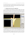
When user starts editing the curve between the two key frames (how is described in the
manual) a nice interface appears and allows him to alter the shape as he needs. Bézier curve
is described by four control points. Two corner points are the fixed values in the key frames
that can not be changed in the editor, but rather in the property grid (again see the manual)
but the middle two points can be moved around using mouse dragging.
Another important part of the animation system is the time line. The time line holds
the information about where all the key frames are placed and manages the current state of
the time in the visual effect.
We also have a simple abstraction for the accumulation of more animated parameters
11/14
2IV05 Final report
Radim Čebiš and Pavel Černohorský
together (the animated parameter owner). It allows us to manipulate all the animated
parameters at once, for example inserting key frames between the existing ones.
Now we have described all the parts of the animation subsystem, so let's take a closer
look how it everything interacts together. During each update, the time line is advanced for
some time and so new frame becomes the current one. Before any of the animated parameter
is used, all of the parameters are updated (through the animated parameters owners) to the
new values belonging to the new time. This means that they get the number of the current
key frame (this means associated interpolation curve to address) and the number of the frame
in between the two neighbouring key frames interval. They use these parameters to obtain
proper animation curve and to get proper y value according to the x value represented by the
in-between key frames frame number. Because Bézier curves are defined base on t
parameter, but we needed to get y value based on x not on t, we used lookup table with
precomputed x and y values. After this update, animated parameters generally start to behave
that they have a different value and this value is used in the update of the visual effect as
described earlier.
As another interesting part of the animation system, we implemented the editing. I do
not mean only the editing of the interpolation curves as mentioned earlier. While inserting
new key frames to the animation, there is a need to split the existing curve on some specific
place (because all the key frames are common for all the animated parameters – we made
this decision mostly because the characteristic of the visual effects we created our
application for allows it – effect behave in some way and than suddenly changes and goes
into another phase, so key frames for changes are needed for all the parameters). This way
the user will be able to add some new key frame he didn't planned to use earlier and he will
not loose the shape of animation curves he edited before. For this curve splitting, we used
well known de Casteljau's algorithm.
6. Saving and loading of the scene
Because creating some visual effect can take a lot of time, we wanted to provide the
user with possibility to save his unfinished work and to load it back again. For saving, we
are using text file which contains information about all the elements of the visual effect. We
created a simple framework that allows us to easily save and load all the entities we use
inside the program including parameters of interpolation curves.
7. Conclusion and future work
In this assignment, we had a possibility to explore further into the topics of particle
systems and animation curves. We also tried out how to cooperate in a small group of two
people while creating a application that is not just a small sketch or draft, but a working
12/14
2IV05 Final report
Radim Čebiš and Pavel Černohorský
system with user friendly interface usable by normal people (no computer specialists).
Compared to the proposal which we created at the beginning of our work, we had to
left out some of the features we were expecting to implement. Finally, although the system is
not implemented exactly according to the proposal, we were able to preserve it's usefulness
even with the smaller range of features. It can be verified that the system is useful by looking
at the samples and sample outputs or even by trying to use the system itself. With the
supplied user manual it should not be a big problem.
While designing the application, we were also focused on writing it in the way that it is
easily extendible in the future. Although some features were left out, their implementation
may not be a problem thanks to the application design. The most valuable directions for the
future work would be to implement selection of the entities and altering their position and
rotation by mouse. This would shift usability to completely different level. Another
directions might be the features described in the proposal such as bouncing of the particles
from solid obstacles, importing geometry from some popular graphical format and animating
parameters of geometry and forces, not only particle emitters. Another nice feature might be
the possibility to edit the whole animation curve at once, not just the segments between the
key frames.
13/14
2IV05 Final report
Radim Čebiš and Pavel Černohorský
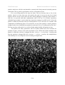
We believe that our application is useful and great outputs can be achieved by skilled
artist. Provided samples were created by us and we have absolutely no aesthetic sense.
8. Literature
1. Žára, J.; Beneš, B.; Sochor, J.; Felkel, P. (2005): Moderní počítačová grafika
(Modern Computer Graphics), ISBN 80-251-0454-0
2. Wynn, C. (2001): Using P-Buffers for Off-Screen Rendering,
http://developer.nvidia.com/attach/6483
14/14