Download Visual ModelQ User`s Manual Version 6.0

Visual ModelQ User’s Manual
Visual ModelQ User’s Manual
Version 6.0
Page 1
Visual ModelQ User’s Manual
Page 2
Table of Contents
1
Installation of Visual ModelQ............................................................................................... 3
1.1 Registration......................................................................................................................... 3
2
Introduction to Visual ModelQ ............................................................................................. 3
2.1 Drawing Models .................................................................................................................. 3
2.1.1
2.1.2
2.1.3
Blocks...................................................................................................................................................................... 4
Nodes ...................................................................................................................................................................... 4
Wires ....................................................................................................................................................................... 4
2.2 Types of Blocks .................................................................................................................... 5
2.2.1
2.2.2
2.2.3
2.2.4
2.2.5
2.2.6
3
Instruments and Meters........................................................................................................................................ 5
Constants ................................................................................................................................................................ 5
Standard blocks ..................................................................................................................................................... 6
Programs ................................................................................................................................................................. 6
Custom Modules ................................................................................................................................................... 7
Extenders and Anchors ........................................................................................................................................ 7
Running Models..................................................................................................................... 8
3.1 Compiling ............................................................................................................................ 8
3.2 Instability in the Solver........................................................................................................ 9
4
Visual ModelQ Design (.mqd) Files.................................................................................... 10
5
Program blocks..................................................................................................................... 11
5.1 Supported language constructs .......................................................................................... 12
6
Example Models................................................................................................................... 14
6.1 Default model.................................................................................................................... 14
6.1.1
6.1.2
6.1.3
6.1.4
Viewing and modifying node values ............................................................................................................... 16
The WaveGen block............................................................................................................................................ 17
The Scope Block.................................................................................................................................................. 20
The Live Scope block......................................................................................................................................... 21
6.2 Experiment A: Simple control system................................................................................ 22
6.2.1
6.2.2
6.2.3
6.2.4
6.2.5
6.2.6
6.2.7
6.2.8
6.2.9
6.2.10
6.2.11
6.2.12
6.2.13
Visual ModelQ constants: many ways to change parameters ...................................................................... 24
Inverse Live Constants ....................................................................................................................................... 25
Scale-by Live Constants .................................................................................................................................... 26
String Live Constants ......................................................................................................................................... 26
Simple constants ................................................................................................................................................. 28
Hot connections on a Live Scope...................................................................................................................... 28
Command response and control-law gains..................................................................................................... 30
Frequency domain analysis of a control system............................................................................................ 31
The Visual ModelQ DSA ................................................................................................................................... 31
DSA Nodes .......................................................................................................................................................... 32
The DSA display ................................................................................................................................................. 32
DSA controls ........................................................................................................................................................ 33
The DSA excitation signal................................................................................................................................. 34
6.3 Modeling digital control systems ....................................................................................... 34
Visual ModelQ User’s Manual
Page 3
This describes how to use Visual ModelQ. It provides overviews of how the modeling
environment works and how to enter models.
Details of operation of individual blocks can be found in the Visual ModelQ Reference Manual,
which installs with Visual ModelQ. Clicking F1 will bring up a copy of the Visual ModelQ
Reference Manual; clicking F1 with the cursor over a block will page down to the section where
that block is discussed in the manual.
1 Installation of Visual ModelQ
Visual ModelQ is available at http://www.qxdesign.com/. Visual ModelQ runs on PCs using
Windows 95, Windows 98, Windows 2000, or Windows NT. Download and run the executable
file setup.exe for Visual ModelQ V6.0 or later.
1.1
Registration
The unregistered version of Visual ModelQ is available free of charge, but lacks several features.
Users may elect to register copies of Visual ModelQ at any time; visit http://www.qxdesign.com/
for details.
2 Introduction to Visual ModelQ
Visual ModelQ is written to teach control theory and so makes convenient many activities that
are advantageous for studying controls. Visual ModelQ models run continuously and without a
specific end time, similar to the way real-time controllers run. The measurement-equipment
models runs independently of the modeled elements, similar to instrumentation in a physical
laboratory. Control-law gains and model parameters are easily changed and results are displayed
immediately; plots of frequency-domain response (Bode plots) are run with the press of a button.
2.1
Drawing Models
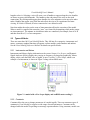
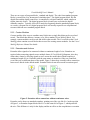
Visual ModelQ models are drawn on a canvas. Blocks are selected from a palette of over 100
choices. Blocks are interconnected by wiring nodes together. Figure 1 shows the Visual ModelQ
default model, the model that is automatically drawn each time the program is launched. It has
four blocks: a solver, a scope, a waveform generator, and a Live Scope labeled Variable1. Each
block has multiple nodes; nodes are shaped like triangles, diamonds, and squares, and are shown
inside the perimeter of the blocks. One wire is present in Figure 1; it connects the output node of
Wave Gen to the input node of Variable1.
Visual ModelQ User’s Manual
Page 4
Figure 1. The Visual ModelQ default model
2.1.1 Blocks
Visual ModelQ blocks provide numerous functions. Most functions modify signals from input to
output. For example, control laws, filters, and math functions produce outputs by operating on
inputs. Instruments, such as Variable1 in Figure 1, and meters are specialized blocks that display
output on the model diagram so the user can monitor operation.
2.1.2 Nodes
Nodes provide access to model signals and parameters. There are several types of nodes. Input
and output nodes, shaped like triangles, provide access to signals that normally change during
model operation. In Figure 1, an output node in Wave Gen connects to an input node in
Variable1. Configuration nodes, which are shaped like diamonds, provide access to parameters
that do not change during operation. Configuration nodes cannot be changed while the model is
operating; changing a configuration node while the model is stopped forces the model to
recompile and restart simulation from zero time.
2.1.3 Wires
Wires interconnect input and output nodes. Any number of input nodes can be connected
together; however, one and only one output node should be connected in a single network of
wires. If multiple outputs are interconnected, an error will result and the model will not run. If no
outputs are connected in a group of wires, a warning will be displayed because the network has
no effect on model operation; however, this does not prevent the model from running.
Wires are entered by first clicking the wiring tool, which is shown as spool of wire near the left
side of the palette. Then move the cursor over an input or output (triangle shaped) node and
click to start the wire. Finally, move the cursor over another input or output node and click a
second time. At this point, the completed wire will be automatically drawn between those two
nodes.
After a wire is drawn, it can be moved and stretched. First click anywhere along the wire’s
Visual ModelQ User’s Manual
Page 5
length to select it. Selecting a wire will cause a set of handles to appear along the wire; handles
are drawn as green solid diamonds. The handles at the end points of the wire are the node
connections. By clicking and dragging these handles, the wire endpoints can be moved to other
nodes. Handles that appear away from the ends allow the wire to be repositioned for better
viewing. If a block is deleted, all wires connected to it are deleted as well.
Note that neither the order nor the route of interconnection affects the execution of the model.
When a model is compiled, the networks (“nets”) are formed by determining which nodes groups
are interconnected. The manner in which those nodes are connected (for example, from A to B
and then from B to C) is of no consequence.
2.2
Types of Blocks
There are more than 100 Visual ModelQ blocks. They fall into five categories: instruments and
meters, constants, standard functions, programs, custom modules, and extenders and anchors.
See the Visual ModelQ Reference Manual for details on specific blocks.
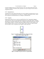
2.2.1 Instruments and Meters
Instruments and Meters display information to the screen. Scopes, Live Scopes, and Dynamic
Signal Analyzers (DSAs) display time-varying or frequency-varying plots graphically. Meters
display values, such the RMS value of signal, as text. Variable1, a Live Scope, which is an
example of an instrument, is shown in Figure 2 along with an RMS meter.
Figure 2. A model with a Live Scope display and an RMS meter reading 1.
2.2.2 Constants
Constants allow the user to change parameters of a model rapidly. There are numerous types of
constants in Visual ModelQ to support a wide range of model parameters. Constants can be
changed while the model is operating to encourage experimentation. Using constants, models can
Visual ModelQ User’s Manual
Page 6
be adjusted multiple times per second and on-the-fly; this is more efficient than the structure
common to modeling environments where parameters can only be changed when the model is
stopped and restarted.
2.2.3 Standard blocks
Standard blocks are those blocks that produce one or more outputs by operating on one or more
inputs. Most Visual ModelQ blocks are of this type. Comparison, Boolean logic, filters, control
laws, integration, and math functions are all examples of standard blocks.
2.2.4 Programs
Program blocks allow the user to write in a simplified form of the C programming language.
These blocks have between two and eight inputs and between two and eight outputs. The inputs
and outputs act as program variables that can be combined in mathematical expressions. Program
blocks support a subset of C: Boolean comparisons, algebraic operators, if/then structures, and
numerous function calls (see Section 5 for more detail). Figure 3 shows an example Program
block and Figure 4 shows a program such as might be stored in that block.
Figure 3. An 8x8 Program block takes 8 Inputs (left side)
and provides 8 outputs (right side)
Figure 4. Example Program stored in a Program Block.
Visual ModelQ User’s Manual
Page 7
There are two types of program blocks: standard and digital. The code from standard program
blocks is executed at every increment of simulation time. The digital program block, like the
digital filter and the digital control law, is controlled by a digital controller, which samples at
regular intervals of time. The digital program block executes once each time the digital
controller samples. Typically, this will be much less frequently than the standard program block;
as a result, a program run in a digital program block will usually expend fewer computational
resources than one run a standard program block.
2.2.5 Custom Modules
Custom modules allow users to combine many blocks into a single block that can be saved and
reused. That block then behaves, in many ways, like a standard Visual ModelQ block. For
example, custom modules can be saved and used in other models. The Custom tab on the Visual
ModelQ palette contains several blocks that are used for creating custom modules. See the Visual
ModelQ Reference Manual for details.
2.2.6 Extenders and Anchors
Extenders allow signals to be connected without a continuous length of wire. Extenders are
required when connecting signals across multiple sheets of Visual ModelQ diagrams; also, they
often reduce clutter by allowing signals to move across the model sheet without requiring a
continuous length of wire. Extenders with the same name are treated as if they are connected,
even if they are on different sheets of the model. Figure 5 shows how extenders allow connection
between two blocks in the default model. Extender blocks do not affect model execution speed.
Figure 5. Extenders allow connections without continuous wires.
Extenders can be shown as standard extenders, pointing out of the wire like Ext1 at the top right
of Figure 5, or Extender Output blocks like Ext1 at the center left of Figure 5, which point into
the wire. This difference is only for the display and has no effect on the compilation or execution
Visual ModelQ User’s Manual
Page 8
of the model. Extenders can be exchanged to and from Extender Outputs by right clicking on the
block and choosing "Reverse Extender."
Visual ModelQ attempts to route a wire along the most direct route between two blocks. Anchors
provide a means for users to specify other routes. The function of an Anchor is to force the wire
out of the standard Visual ModelQ route, usually to increase the clarity of the model. For
example, Figure 6 shows how an Anchor block provides means to avoid blocks between two
interconnected blocks. Anchor blocks do not affect model execution speed.
Figure 6. Using anchors to direct a wire outside the standard Visual ModelQ routing to
increase clarity.
3 Running Models
After a model is drawn, it can be compiled and then run. If errors are located during the
compilation, the process is aborted and the model does not run.
3.1
Compiling
A model is compiled by clicking on the Compile button, the red or green circle at the left of the
modeling environment (see Figure 9). Also, clicking the Run button, the black triangle right of
the compile button, for a model that is not compiled will automatically force the model to
compile before running. A program that is compiled will have a green Compile button; one that
is not will have a red Compile button.
A model can be stopped by clicking on the Stop button, the black square right of the Run button.
Stopping and starting a model will not force a model to recompile. However, if a model block or
wire is removed or added while the model is stopped, or if the value of a configuration node is
changed, the model will need to be recompiled and the Compile button will change from green to
red. Model execution must restart at zero time.
Visual ModelQ User’s Manual
3.2
Page 9
Instability in the Solver
Time-based models are systems of differential equations that are solved in small increments of
time. For example, the solver may take the results of the last solution and then project 5 µsec
forward for the next solution. That solution may be used to project another 5 µsec, and then
another. This process is repeated many times; after the equations have been solved enough
times, the small time increments add to significant intervals. The model user is presented with
solutions that appear to move continuously not unlike the way individual frames of a cinema film
give the perception of continuous motion. This is the desired operation of a model, but it is by
no means guaranteed. The solver can become unstable, a condition where the output of the
differential equation solver can grow without bound independent of whether the system being
modeled is stable.
The causes of instability in time-based models are complex. The differential equation solver
used by Visual ModelQ is the 4th order Runge-Kutta equation solver. This method is well known
to be stable in a broad range of conditions. The most common cause of solver instability is
setting the solver time increment to be too large for the dynamics of the system being modeled.
When selecting the solver increment of time, set it to be much faster than the dynamics of the
system. When unsure of system dynamics, set the time increment to a small value. If the system
is stable, the time increment can be increased to reduce execution time later.
In Visual ModelQ, the solver time increment is set in the Solver block (reference the bottom left
of Figure 6). Every Visual ModelQ must have one and only one Solver block.
Note that the instability discussed here is unrelated to instability that may occur in the control
system being modeled. Instability of the solver is an artifact of the simulation tool; the system
being modeled may be stable while the solver shows instability. On the other hand, instability in
the system can be accurately reflected by the solver when the solver is stable. Unfortunately, the
results of both problems can appear similar. One way to test which type of instability is present
is to look at the frequency of oscillation: instability from the solver will generate frequencies on
the order of the solver time increment. Oscillations in lower frequencies normally indicate the
solver is stable and the modeled system is unstable. However, oscillations at high frequency can
come from either problem.
A second way to determine the source of instability (that is, in the solver or in the modeled
system) is to lower control system gains; normally, lower gains will stabilize a system. If
systems with very low control-loop gains are unstable, it becomes more likely that the solver is
unstable. Another way to test instability is to reduce the solver sample time. In many cases, if
instability results from the solver, lowering the solver time will correct the problem.
Another path to find instability is to simplify the model block by block to see when the
instability is removed. Knowing which block causes instability in the system can help solve the
problem. Stability problems in systems of differential equations can result from complex
problems that are difficult to identify or correct. You may need to refer to a text on differential
equations.
When attempting to locate stability problems, note that Visual ModelQ provides the function
Visual ModelQ User’s Manual
Page 10
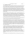
“Zero All Stored Outputs” in the Edit menu as shown at the bottom of Figure 7. This function
attempts to reset all values in the model that store values, for example, the integration that results
from solving systems of differential equations. This does not cure the stability problem, but
usually resets the model, allowing further experimentation more quickly than resetting the
model.
Figure 7. Visual ModelQ provides “Zero All Stored Outputs” at the bottom of the Edit
menu.
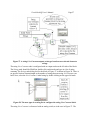
4 Visual ModelQ Design (.mqd) Files
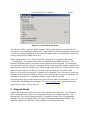
Visual ModelQ design files hold information describing models. Create new models by selecting
File, New Design…as shown in Figure 8. Open existing models by clicking File, Open Design,
… or by clicking the file open icon at the top left of the screen. Save models to their current mqd
file by clicking File, Save, … or by clicking the file save icon. Save models into new files by
clicking File, Save as….
Visual ModelQ User’s Manual
Page 11
Figure 8. Visual ModelQ File menu
The File menu offers “Auto save before compile” which, when checked, causes the file to be
saved before every compilation of the model. In the unlikely event that the program experienced
a serious error during compilation or execution, this option makes it less likely that information
recently entered into the model will be lost.
Before saving models, Visual ModelQ copies the existing file to a temporary file named
__VisualModelQ__nnnnn.tmp where nnnnn is a number between 00000 and 99999. This
method is designed to make it less likely for the original file to be corrupted. If a catastrophic
error causes the mqd file to be lost or corrupted, search for the temp file (normally located in the
same directory as the file is being saved). Make another copy of this file with the extension mqd
and try to open it with Visual ModelQ. In many cases, the temporary file will be usable.
However, no system of copying files is immune to file corruption. Save files often to reduce the
harm the can be caused by corruption. Finally, Visual ModelQ files are text files and if they are
corrupted in a minor way it is sometimes possible to restore the file by hand.
Unregistered users are prevented from saving files with more than a fixed number of wires (12
as of the time of publishing this document). Visit www.qxdesign.com to get information on
registering your copy of Visual ModelQ.
5 Program blocks
Program blocks provide for the use of text code to describe block functions. Text blocks are
more versatile and can be easier to use than graphical blocks for complex functions. The
language for Visual ModelQ program blocks is a simplified version of the C programming
language. The goal of program blocks is to support text-based mathematical equations; the
functions supported as of the time of this printing are focused on those areas.
Visual ModelQ User’s Manual
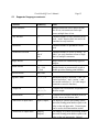
5.1
Page 12
Supported language constructs
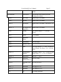
Construct
Symbol(s)
Notes
End of statement
;
Multiple statements can be placed on one
line of text; one statement can be split
across multiple lines of text.
Curly brackets
{}
Unlimited number of curly brackets can be
used; “main” function does not need to be
contained in curly brackets.
Parentheses
()
Unlimited number of parenthesis can be
used.
Conditional execution
if
else if
else
Unlimited number of levels of nesting. As
with C, use curly brackets to form a single
block of multiple statements.
Integer literals
1, -2
Integer literals are automatically typed as
integers.
Double literals
1.0, -2.44,
-7.4e-8
Double literals are automatically typed as
double-precision floating point numbers.
Boolean literals
true, false
Algebraic math
*, /, +, -, %
Standard hierarchy is observed; * and / are
carried out before + and -; in turn, + and –
are carried out before %. (% is the integer
remainder or modulo function.)
Comparison
>, >=, <,
<=, = =, !=
Compares any two numbers and produces a
Boolean output.
Boolean math
&&, ||, !
Combine two Booleans with && (AND) or
|| (OR). Invert one Boolean with !.
Connections to input nodes
Input1, Input2,
…
Use Inputn as symbol representing doubleprecision floating-point number equal to the
value on the nth input node. Unused inputs
can be used to hold intermediate results.
Connections to output nodes
Output1,
Output2, …
Use Outputn as symbol representing doubleprecision floating-point number equal to the
value on the nth output node. Unused
Visual ModelQ User’s Manual
Page 13
outputs can be used to hold intermediate
results.
Fixed functions
Description
All functions return double-precision
floating-point number.
acos(x)
arc-cosine
Return value is in radians.
asin(x)
arc-sine
Return value is in radians.
atan(x/y)
arc-tangent
Return value is in radians. Must add π/2 if y
< 0.
atan2(x, y)
arc-tangent (two
argument)
Return value is in radians.
ceil(x)
ceiling
The smallest integer >= x. See also,
floor(x).
cos(x)
cosine
x is in radians.
cosh(x)
hyperbolic
cosine
exp(x)
exponential
fabs(x)
absolute value
floor(x)
floor
The largest integer <= x. Note: to round to
nearest integer, use floor(x + 0.5). See also,
ceil(x).
fmod(x, y)
floating-point
modulo
Remainder f where x = ay + f, where a is an
integer and 0 <= f < y. If y = 0, returns 0.
hypot(x, y)
hypotenuse
sqrt(x x x + y x y).
log(x)
logarithm
(natural, base-e)
See also, exp(x).
log10(x)
logarithm (base10)
See also, pow10(x).
max(x, y)
maximum
The larger of x or y.
min(x, y)
minimum
The smaller of x or y.
PI( )
PI
No calling arguments.
See also, log(x).
Visual ModelQ User’s Manual
Page 14
pow(x, y)
power of y
x raised to the power of y
pow10(x)
power of 10
10 raised to the power of x. See also
log10(x).
sin(x)
sine
x is in radians.
sinh(x)
hyperbolic sine
sqrt(x)
square root
stop( )
stop model
execution
Stop program execution. For example, the
following program stops model execution
after each second of simulation time:
if(t( ) > Input2 + 1){
Input2 = t( );
stop( );
}
Note: this program requires Input2 is an
unused input. In this case, Input2 will be set
to zero at each compile, and the program
can change the value.
t( )
time (of
simulation)
No calling arguments. See “stop( )” for
example program using t( ).
tan(x)
tangent
x is in radians.
tanh(x)
hyperbolic
tangent
6 Example Models
The following section will review a few example models.
6.1
Default model
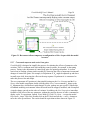
When Visual ModelQ is launched, the default model is automatically loaded. The purpose of this
model is to provide a simple system and to demonstrate a few functions. The default model and
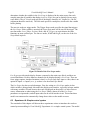
the control portion of the Visual ModelQ environment are shown in Figure 9.
Visual ModelQ User’s Manual
Page 15
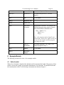
Figure 9. Screen capture of Visual ModelQ environment showing the default model.
The model compilation and execution are controlled with the block of three buttons at the upper
left of the screen: a compile (green circle), stop execution (black square), and start execution
(black triangle). These blocks, with the current execution time (here, 9.16051 seconds) are
shown in Figure 10. If a model must be compiled before it can be run, the green circle will turn
red. The circle will turn red in three cases: at launch, anytime either a block or a wire is added or
taken away from the model, and when the value of a configuration node is changed. Any time a
model is recompiled, the model timer will return to 0 seconds and all default values of model
blocks will be reloaded.
Figure 10. Compile and run controls.
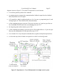
The default model is detailed in Figure 11. There are four blocks, two of which are connected
with a wire:
•
Solver: The solver configures the differential-equation solver used to simulate system
components. One and only one solver is required in every model.
•
Scope: The main scope provides a display for up to eight channels of input. The workings of
the scope and its trigger mechanism are similar to those of a physical oscilloscope. At least
one scope is required for every model.
•
Waveform Generator: The waveform generator can be used to generate standard waveforms
Visual ModelQ User’s Manual
Page 16
such as sine waves and triangle waves. Frequency, amplitude, and phase are all adjustable
while the model is running. The generator here is set to produce a square wave at 10 Hz with
an amplitude of ±1.
•
Live Scope: The Live Scope displays its output on the block diagram. Live Scope variables
automatically display on all main scope blocks as well. Notice in Figure 11 that a short wire
connects the output of the waveform generator to the input of the scope; this connection
specifies that the Live Scope should plot the output of the waveform generator.
Figure 11. Detail of default model.
6.1.1 Viewing and modifying node values
Blocks have nodes, which are used to configure and wire the elements into the model. For
example, the solver block, shown in Figure 12, has two nodes. There is a configuration node (a
green diamond) at the left named h. This node sets the sample time of the differential equation
solver. The sample time is set to 5 µsec by default.
Figure 12. Detail of Solver node.
The solver block includes a documentation node (a rectangle) at the right. The documentation
node, which is provided on almost all Visual ModelQ blocks, allows the user to enter notes about
the block for reference. The name of the block, Solver in this case, is shown immediately below
the block. The user can change the name of any Visual ModelQ block by positioning the cursor
within the name and double-clicking.
Visual ModelQ User’s Manual
Page 17
There are several ways to read the values of nodes such as the h node of the sample block. The
easiest is to use fly-over help. After the model is compiled, position the cursor over the node and
the value will be displayed in fly-over help for about one second, as shown in Figure 13.
Figure 13. Visual ModelQ provides fly-over help for nodes.
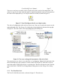
The value of configuration nodes can be set in two ways. One way is to place the cursor over the
node and double-click. The Change/View dialog box is then displayed as shown at the top right
of Figure 14. The value can be viewed and changed from this dialog box.
Figure 14. Two ways to change the h parameter of the solver block.
The second way to set values is to use the Block set-up dialog box. Right-click in the body of the
block; this brings up a pop-up menu as is shown center left of Figure 14. Select the Properties
item in that menu to bring up the Block set-up dialog box. This box will show the value of all the
nodes in the block. Click the View/Change button to bring into view the Change/View dialog
box.
6.1.2 The WaveGen block
The WaveGen block has ten nodes, as shown in Figure 15. The nodes are:
Visual ModelQ User’s Manual
Page 18
•
Waveform: Select initial value from several available waveforms such as sine or square
waves.
•
Frequency: Set initial frequency in Hertz.
•
Amplitude: Set initial value of peak amplitude. For example, setting the amplitude to 1
produces an output of ± 1.
•
Enable: Allows automatic disabling of the waveform generator. When the value is 1, the
generator is enabled. When 0, the generator is disabled. For digital inputs such as this node,
Visual ModelQ considers any value greater than or equal to 0.5 to be equivalent to 1 (true);
all values less than .5 are considered equivalent to 0 (false). This function will be especially
useful when taking Bode plots since all waveform generators should be disabled in this case.
•
Offset: Initial value by which the waveform generator output should be offset.
•
Phase: Initial value of waveform phase, in degrees, of the waveform generator. For example,
if the output is a sine wave, the output will be:
Output = Amplitude * sin(Frequency x 2π x t + Phase x π / 180) + Offset.
•
Duty cycle: Initial value of duty cycle for pulse waveforms.
•
Multiplier: value by which to multiply waveform generator output. This is normally used for
unit conversion. For example, most models are coded in system international (SI) units. If the
user finds RPM more convenient for viewing than the SI rad/sec, the multiplier can be set to
0.105 to convert RPM (the user units) to radians/second (SI units). The multiplier node is
present in most instruments such as scopes and waveform generators to simplify conversion
of user units to and from SI units.
Figure 15. The waveform generator has 10 nodes.
The Enable node of the WaveGen block is an input node, as the inward-pointing triangle
indicates. Input nodes can be changed while the model is running and they can be wired in the
model. Neither of these characteristics are true of configuration nodes (those shaped like green
diamonds).
Visual ModelQ User’s Manual
Page 19
Using the block set-up dialog box can speed the set up of more complicated blocks such as the
WaveGen. The WaveGen block setup dialog is shown in Figure 16. The benefit of the block setup dialog is that all of the parameters are identified by name and can be set one after the other.
Notice that the fifth node in the dialog, Output, cannot be changed, as indicated by the gray text
in the nodes “Present Value” edit box. This is necessary because some nodes, such as output
nodes, cannot be configured manually.
Figure 16. Block set-up dialog box for the waveform generator.
The parameters of the waveform generator set in the nodes are only initial (precompiled) values.
To change the configuration of the waveform generator when the model is running, double click
anywhere inside the block and bring up the waveform generator control panel. This panel, shown
in Figure 17, allows six key parameters of the waveform to be changed while the model is
running. The buttons marked "<" and ">" move the value up and down by about 20% for each
click. Changing these values has no permanent affect on the model; when the model is
recompiled, all these values will be returned to their initial values as specified by the
corresponding configuration nodes.
Visual ModelQ User’s Manual
Page 20
Figure 17. Waveform generator control panel, which is displayed by double-clicking on the
WaveGen block after the model has been compiled.
6.1.3 The Scope Block
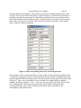
The Scope block with a list of its nodes is shown in Figure 18. Most of the nodes set functions
that are consistent with laboratory oscilloscopes, and thus will be familiar to most readers. One
node that should be discussed is the Trigger Source node. This node sets the initial variable that
will trigger the scope when the scope mode is set to Auto or Normal. If this variable is not set
prior to compiling the model, a warning will be generated. To eliminate this warning, doubleclick on the node and select a variable from a drop-down list to trigger the scope. Choose from
any Variable or Live Scope, as shown in Figure 18.
Figure 18. The Trigger Source of a Scope can be set to any variable (such as Variable6) or
any Live Scope (such as Variable1).
The scope display is normally not visible. However, it can be made visible by double clicking
inside the scope block after the model has been compiled. The block can be hidden from view by
clicking the "X" icon at the top right of the scope window.
Visual ModelQ User’s Manual
Page 21
Figure 19. Output of main scope in default model.
The scope display provides two tabs: Scale and Trigger. The Scale tab (showing in Figure 19)
provides control of the horizontal and vertical scaling. The Trigger tab provides various trigger
settings. At the bottom of the scope there are a few controls. Starting at the bottom left of Figure
19:
•
the Trig button flashes green for each trigger event;
•
the sun glasses button hides the control panel at left, maximizing the display area of the plot;
•
the single-shot check box enables single-shot mode;
•
the scale-legend control button turns the scale legend (immediately below the plot) on and
off;
•
the three cursor buttons select 0, 1, or 2 cursors.
Note that single-shot mode stops the model from running after the scope screen has filled up.
Restart the model using the Run (black triangle) button after each single shot event.
6.1.4 The Live Scope block
The default model also includes a Live Scope block, as shown in Figure 20. The input comes in
at top left, with the scale, offset, and time scale set in the nodes just below that. The Show node
Visual ModelQ User’s Manual
Page 22
determines whether the variable in the Live Scope is displayed in the main scopes after each
compile (note that all variables that display in a Live Scope also can be displayed in any main
scope block). The AC Couple node specifies if the display should be AC coupled (i.e., the DC
component should be removed.) The Mult node specifies a multiplier, which scales the variable
before plotting.
The next six nodes are trigger nodes. The Trigger Source node specifies the signal that triggers
the Live Scope. If this variable is unwired, the Input (first) node will be used as the trigger. The
next four nodes: Level, Slope, Position, Mode, and AC Trigger, are equivalent to the same
functions on most oscilloscopes. The last two nodes, Width and Height, set the size of the Live
Scope block in pixels.
Figure 20. Detail of the Live Scope nodes.
Live Scopes provide simple display features compared to the main scope block, and there are
several limitations. No more than two channels can be displayed using a Live Scope. There are
fewer trigger options. Another limitation is that Live Scopes only show input vs. time; there is no
option for Input1 vs. Input2 (x vs. y) as there is for the main Scope blocks.
The Live Scope also has several advantages. First, the wiring to a Live Scope makes it clear
which variable is being plotted; this makes the display more intuitive, especially in larger models
with many variables. Second, because the result is displayed on the model, it is often easier to
convey information to others using the Live Scope. Finally, almost all of the Live Scope
parameters are input nodes, and all input nodes can be wired into the circuit. This means that a
model can constructed to automatically change those values as the model executes.
6.2
Experiment A: Simple control system
The remainder of this chapter will discuss three experiments written to introduce the reader to
control-system modeling in Visual ModelQ. Experiment A is a simple control system. The model
Visual ModelQ User’s Manual
Page 23
diagram is shown in Figure 21. The model is comprised of several elements:
•
A waveform generator produces the command.
•
A summing junction compares the command and the feedback (output from the feedback
filter) and produces an error signal.
•
A PI control law, which is configured with two Live Constants, a proportional gain, KP, and
an integral gain, KI. These blocks will be discussed shortly.
•
A filter simulating the power converter. The power converter is a 2-pole low-pass filter set
for a bandwidth of 800 Hz and with a zeta (damping ratio) of 0.707.
•
An integrating plant with an intrinsic gain of 500.
•
A filter simulating the feedback conversion process. The feedback filter is a 2-pole low-pass
filter set with a bandwidth of 350 Hz and with a zeta of 0.707.
•
A two-channel Live Scope that plots command (above) against actual plant output (below).
•
A solver and scope, both of which are required for a valid Visual ModelQ model.
Figure 21. Experiment A: Visual ModelQ model of a simple control system.
Visual ModelQ User’s Manual
Page 24
6.2.1 Visual ModelQ constants: many ways to change parameters
Visual ModelQ provides numerous ways to change model parameters. Of course, any unwired
node can be changed by double clicking on a node, or right clicking and bringing up the Block
set-up dialog box (see Figure 22). However, numerous blocks are provided to simplify the task
of changing node values.
The Constants tab in the Visual ModelQ environment provides seven constant types: simple
constants, Live Constants, Inverse Live Constants, Scale-by simple constants, Scale-by Live
Constants, Scale-by inverse Live Constants, and String Live Constants. The selection buttons for
each of these constants are shown in Figure 22, which is a screen capture of the top portion of the
Visual ModelQ environment.
Figure 22. Selecting from among the many constants available in Visual ModelQ.
Live Constants, such as KP and KI in the PI controller of Figure 21, provide the most control. The
icons of blocks have a "<< >>" symbol. After the model has compiled, double click anywhere
inside the block and the adjustment box of Figure 23 will appear. Using the adjustment box, the
value of the parameter can be changed while the model runs. A new value can be typed in with
the keyboard by clicking the cursor in the value edit box. (Note that when using the keyboard,
the new value does not take effect until the return key is hit.) In addition, there are six
logarithmic adjustment buttons in the adjustment box. The double less-than block (<<) reduces
the value to the next lowest value with the first digit 1, 2, or 5. For example, if the value of the
variable is 1.75, clicking "<<" will change the value to 1; clicking again will reduce it to 0.5;
clicking again will reduce it to 0.2, and so on. Each click reduces the value approximately by
half. The double greater-than (>>) performs a similar function except it moves to the next higher
value: 1, 2, 5, 10, 20, and so on.
Visual ModelQ User’s Manual
Page 25
Figure 23. Adjustment box appears when double-clicking a Live Constant any time after
the model has been compiled.
The remaining adjust buttons are straightforward. The bold single-less-than button reduces the
value of the constant by about 20% for each click; the non-bold single-less-than reduces the
value by about 4%. The bold and non-bold single-greater-than blocks perform a similar function,
only raising the value. If the parameter can take on values of both signs, the +/- button will be
enabled, allowing a change in sign at the click of a button.
The Live Constant model block and its nodes are shown in Figure 24. The initial value node
specifies the value that the constant is reset to after each compile. The minimum and maximum
nodes specify the range that the input can take on. The multiplier and documentation nodes are
standard Visual ModelQ nodes. The output makes available the value of the Live Constant so it
can be wired in the model. The value displayed in text inside the block is not scaled by the Mult
node; the value in the output node is.
Figure 24. Detail of a Live Constant.
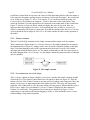
6.2.2 Inverse Live Constants
The inverse Live Constant works like the standard Live Constant except the output is one divided
by the parameter value and then multiplied by the value of the Mult node. This constant is used
when the model needs to scale by the inverse (1/x) of the parameter value such as is usually the
case for mass, moment of inertia, thermal mass, capacitance, inductance, and many other
physical parameters. The inverse Live Constant is a space-saving alternative to combining a
standard Live Constant and a 1/x block.
Visual ModelQ User’s Manual
Page 26
Figure 25. Inverse Live Constant generates output inversely proportional to constant value.
6.2.3 Scale-by Live Constants
Scale-by Live Constants are similar to Live Constants except that the output node is the product
of an input node and the value of the constant. In fact, if the input node is set to one, Scale-by
Live Constants behave identically to standard Live Constants. The two Scale-by Live Constants
(standard and inverse) are shown in Figure 26
Figure 26. Standard and inverting scale-by Live Constants.
6.2.4 String Live Constants
String Live Constants allow the model constants to be adjusted as strings. The user selects a
string from a list and the string Live Constant block outputs an integer value according to
position in the list occupied by the selected string. For example, the string Live Constant named
Select XN in Figure 27 is configured to allow the user to select one of four strings: X0, X1, X2,
and X3. Depending on which constant the user selects, the output node will be 0, 1, 2, or 3,
according to the position of the string within the list.
Visual ModelQ User’s Manual
Page 27
Figure 27. A string Live Constant outputs an integer based on user-selected character
strings.
The string Live Constant node is configured with two input nodes on the left side of the block.
The Strings node should be filled first; double click on this node and type in a list of string
constants. The Strings node dialog box for the block of Figure 27 is shown in Figure 28. There is
no specific limit on constant length or the number of strings that one string Live Constant can
hold. Next, select the Live Constant’s initial string by double clicking on the upper left node.
Figure 28. The user types in a string list to configure the string Live Constant block.
The string Live Constant is often used with an analog switch, as is the case in Figure 27. The
Visual ModelQ User’s Manual
Page 28
switch has a control node at top center, the value of which determines which of the four inputs at
left is routed to the output: moving from top to bottom, 0 selects the first input, 1 the second, and
so on. In the case of Figure 27, Select XN is equal to X1, as is indicated inside the string Live
Constant block. This produces an output of 1, which is fed to the switch control node. That
causes the Position-1 (second) input node to be connected to the output node of the switch block.
Figure 27 also has an Inspector block, which can display the value of any node. Here, the
inspector shows that output of Switch4 is 10.01 matching the value of the Live Constant X1,
which is connected to the Position-1 input node. Note that the naming of the four Live Constants
at left to match the list of strings in Select XN is for clarity and has no effect on the operation of
the model.
6.2.5 Simple constants
The last Visual ModelQ constants are the simple constant and the simple scale-by constant.
These constants are similar to the Live Constant. However, the simple constants do not support
the adjustment box of Figure 23; changes to the value are made via double-clicking on the input
node. (Note that changing a node value is permanent after the model is saved.) Also, neither
maximum nor minimum limits can be set. The simple constant takes a little less screen space in
the model diagram than a Live Constant. Use the simple constant for parameters that are changed
only occasionally.
Figure 29. The simple constant.
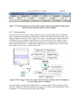
6.2.6 Hot connections on a Live Scope
The Live Scope supports a feature called hot connections. Anytime the model is running, double
click on the Live Scope and its Control Panel box will appear as shown in Figure 30. Near the
bottom, click the “Hot Connect” button to start the process of making a hot connection. Move the
mouse over any wire or input/output node in the model and click. The scope will temporarily
graph the value of that node or wire; the scope outline will turn green to indicate that the scope is
in hot connect mode. (For two-channel Live Scopes, Channel 1 displays the hot connection;
Channel 2 is unaffected.) The operation of hot connection is displayed in Figure 31. Hot
connections are especially useful when debugging a model, as wires and nodes can be viewed
without adding a scope and recompiling.
Visual ModelQ User’s Manual
Page 29
Figure 30. Control Panel for Live Scopes.
After making a hot connection, the Hot Connect button will change to “Restore Scope.” Click
this button or recompile the model to restore the scope to its original display. Note that the scope
scale and offset nodes may need to be adjusted to view the signal. Most parameters in a Live
Scope will be restored to their pre-hot-connect values; consult the Visual ModelQ Reference
Manual for details.
Visual ModelQ User’s Manual
Page 30
Figure 31. Hot connect allows temporary reconfiguration of Live Scopes while the model
executes.
6.2.7 Command response and control-law gains
Visual ModelQ is designed to simplify the process of evaluating the effects of parameter value
variation. This is a common need when modeling control systems, for example, in the tuning
process. Tuning is the adjustment of control-loop gains for optimal performance. It is often
carried out in working systems (and in models) by observing the effect of numerous incremental
changes of control-law gains. For example, in Experiment A, KP might be adjusted up and down
in small steps while observing the effect on the step response. Experiment A is constructed to
make this process fast and simple.
The two components of Experiment A that simplify tuning are the Live Constant and the Live
Scope. After model compilation, double clicking on the Live Constant named KP brings up the
KP adjustment box, which allows rapid changes of value, perhaps one per second. Compare this
to standard modeling environments where the model must be stopped, modified, and recompiled.
A simple change can take on the order of a minute. In addition, the Live Scope gives immediate
feedback of the effect of the new parameter, without the need for the user to issue a command to
display a plot. To experiment, Launch Visual ModelQ. Click File, Open… to open the model
Experiment_A.mqd. Click Run. Double-click on the KP block and use the << and >> buttons to
move the value up and down. The results should be equivalent to those shown in Figure 32.
Visual ModelQ User’s Manual
Page 31
Figure 32. Results of varying with KP in Experiment A.
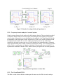
6.2.8 Frequency domain analysis of a control system
Control systems often need to be analyzed in the frequency domain. The most intuitive method
of frequency-domain analysis for most people is the Bode plot, which graphs gain and phase
across a range of frequencies. A gain plot displays the amplitude of an output signal divided by
the amplitude of the input signal at many frequencies as if sine waves at many frequencies had
been applied to the model, one at a time. A phase plot displays the time lag of the output
compared to the input for many sine waves. In the laboratory, the instrument that is commonly
used to generate Bode plots is called a dynamic signal analyzer (DSA). Visual ModelQ provides
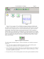
a DSA, which is used regularly in Chapters 4 through 8. Experiment B, shown in Figure 33, is
Experiment A modified to include a DSA, which is shown just right of the waveform generator.
Figure 33. Experiment B: Experiment A with a DSA.
6.2.9 The Visual ModelQ DSA
The DSA is wired in line with the excitation path. In most cases, the DSA is used to analyze
Visual ModelQ User’s Manual
Page 32
command response and so will normally be inserted in line with the command as it is in Figure
33. All DSAs read all model variables, no matter how they are wired. In Visual ModelQ, the term
variables includes three types of signals:
•
The input to 1-Channel Live Scopes,
•
The input to Channel 1 of 2-Channel Live Scopes, such as Command in Figure 33, and
•
Visual ModelQ variables blocks such as Feedback in Figure 33.
The DSA here will be used to show the relationship between command and feedback. Notice that
Experiment B required the addition of the variable block Feedback at top right. In Experiment B
that node was not connected to a variable block as it was only needed for display as Channel 2 of
a Live Scope. In Experiment C, an explicit variable block named Feedback is required to grant
access of the signal to the DSA.
6.2.10 DSA Nodes
The complete details on configuring a DSA go beyond the scope of this chapter. However, a few
details should be mentioned. For a complete discussion of DSA configuration, refer to the Visual
ModelQ User’s Manual.
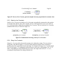
The four most important nodes of a DSA block are shown in Figure 34. At left is the input node.
Normally, the DSA is inactive and the input node passes directly to the output node. However,
when the user wants a new Bode plot, the DSA is commanded to excite the model. This
temporarily disconnects the input node and replaces it with a random signal excitation. The
Excitation Amplitude and DSA Inactive Nodes will be discussed later in Section 2.3.4.5.
Figure 34. Detail of DSA Nodes.
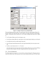
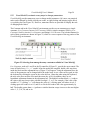
6.2.11 The DSA display
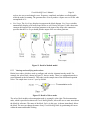
A Bode plot from a DSA is shown in Figure 35. This shows the relationship between command
and feedback, commonly called the closed-loop response, for Experiment B where KP = 1 and KP
= 2; the gain plots are above and the phase plots below. Most of the time, the closed-loop gain
plot will be of primary interest. The two cases here behave similarly at low frequency (shown at
left) and the plots below about 100 Hz are nearly indistinguishable. However, above 100 Hz,
there are significant differences, especially that the gain of the KP = 2 case sharply rises before
falling, displaying an undesirable characteristic called peaking. The purpose of this section is to
Visual ModelQ User’s Manual
Page 33
introduce Visual ModelQ, so a detailed discussion of resulting waveforms is outside the scope of
this discussion. However, it may be interesting to readers to notice that the two cases plotted in
Figure 35 match the time domain plots for Figure 32a and b, where the less stable Figure 32b
corresponds to the plot in Figure 26 with peaking. Peaking and ringing are both reliable
indicators of inadequate margins of stability. Stability issues will be discussed in Chapter 3.
Figure 35. Output of DSA for KP = 1 and KP= 2
Like the Scope display, the DSA display is normally not visible when a model starts to run. The
DSA display can be made visible by double clicking inside the DSA block after the model has
been compiled. Clicking on the model will move the model diagram in front of the DSA; to
prevent this, right click anywhere in the DSA display to bring up the DSA pop-up menu; then,
select "Stay on Top."
6.2.12 DSA controls
The user can request a new Bode plot when the model is running by clicking on the GO button at
bottom left of the DSA. This starts a new excitation period. After that, a new Bode plot will be
displayed. Up to four plots can be saved. Right-click in the graph area of the DSA to bring up a
pop-up menu and select Save as to save the most recent plot. Pressing the GO button a second
time during the excitation period cancels the command for a new Bode plot.
To the right of the GO button, the sunglasses button hides the control panel. The gear button
brings to view a dialog box for setting up the DSA excitation signal. The autofind button places a
cursor according to the criteria in the adjoining combo box, which is set to 3 dB in Figure 35.
Visual ModelQ User’s Manual
Page 34
The last three buttons control the number of cursors visible, allowing no cursors, one cursor, or
two cursors.
6.2.13 The DSA excitation signal
The DSA works by generating a random command for a short period of time. The random signal
is rich—it contains all the frequencies of the Bode plot. During the period of excitation, the DSA
monitors all variables in the model. After the excitation, the DSA executes a fast Fourier
transform (FFT) to convert the recorded data to a frequency-domain plot. When the random
signal is applied to the model, the richness of the signal allows it to excite all frequencies at once.
This is ideal for a modeling environment because it minimizes the time the DSA must excite the
system. However, it also it presents problems. First, the system must remain out of saturation—
the power converter must not be driven beyond its maximum during the excitation. If a system is
driven into saturation, the excitation amplitude can be reduced using the Excitation Amplitude
Node at top left of the DSA (see Figure 34). However, if the amplitude is set too low, the signalto-noise ratio of the system will be insufficient and the Bode plot will be distorted at high
frequencies. Setting the amplitude of the excitation is sometimes a matter of experimentation.
When doing so, always monitor the power converter output to ensure the system remains out of
saturation for the entire excitation period.
All commands except the DSA excitation must be shut off during the excitation period. The DSA
will automatically disconnect the input node so that any signals connected to the input are
disabled during DSA excitation; this is the case with the waveform generator in Figure 33. If
there are waveform generators connected to other parts of the model, the DSA Inactive node at
lower right of Figure 34 can be wired to disable those generators. The DSA Inactive node falls to
zero during the excitation period; when wired to a waveform generator Enable node, the desired
behavior is realized.
6.3
Modeling digital control systems
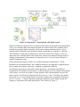
Experiment C, the final model of this chapter, will demonstrate how to model a simple digital
control system in Visual ModelQ. This model, shown in Figure 36, is similar to Experiment B
except that three blocks have been added. First, the PI controller, just below KP and KI, is now
digital. The border area of this block is yellow in the Visual ModelQ environment.
Visual ModelQ User’s Manual
Page 35
Figure 36. Experiment C, Experiment B with digital control.
Digital PI controllers sample the error at regular periods of time. The period for any digital block
is set via its controller node, the diamond at bottom left of the PI block. The controller can be
selected from multiple digital controllers, which can be running simultaneously in a Visual
ModelQ model. Fortunately, most models are simple enough that one controller is sufficient.
That controller is called Main in Experiment C and is near center-left of Figure 36. The sole
input node of the controller block is the sample time, which can be changed while the model is
running. In Experiment C, that parameter is connected to a Live Constant named TSample to
simplify changing the value.
Notice that the step response in Figure 36 overshoots and rings in Experiment C. All the
parameters of Experiments B and C have identical defaults so one might have expected them to
have a similar step response. Obviously, something is significantly different.
The difference between the two models is that Experiment C is the digital equivalent of
Experiment B. The problem in Experiment C is that the sample time is too long for the dynamics
of the system. As a result, the system is nearly unstable. Some experimentation can prove the
point. Launch Visual ModelQ and load the file "Experiment_C.mqd." Click Run. Now, double
click on the Live Constant named TSample. Reduce the sample time by repeatedly clicking on
the Live Constant "<<" button. When the sample time falls below about 0.0002 seconds, the
response is equivalent to the analog performance. This is shown in Figure 37.
Visual ModelQ User’s Manual
Page 36
Figure 37. From Experiment C: Reducing sample time can stabilize a system.
Visual ModelQ User’s Manual
Page 37
Index
analog switch.................................................................. 27
anchors ............................................................................... 7
auto save before compile .............................................. 11
blocks ................................................................................. 4
Bode pl............................................................................. 31
Boolean............................................................................ 12
c programming language.............................................. 11
compiling.....................................................................8, 15
configuration node...................................................16, 17
constants............................................................................ 5
Visual ModelQ types ............................................... 24
controls
compile and run......................................................... 15
custom modules................................................................ 7
default model..............................................................3, 14
design files ...................................................................... 10
differential equation solver............................................ 9
digital PI control law..................................................... 35
documentation node................................................16, 25
drawing .............................................................................. 3
dynamic signal analyzer (DSA)................................... 31
fast Fourier transform (FFT) ........................................ 34
files ................................................................................... 10
temporary ................................................................... 11
fly-over help .................................................................... 17
frequency analysis ......................................................... 31
hot connection................................................................ 28
instability
in the solver................................................................. 9
installation......................................................................... 3
inverse Live Constant ................................................... 25
literals ............................................................................... 12
Live Constant ................................................................. 23
adjustment box.......................................................... 25
Live Scope............................................................3, 16, 21
control panel............................................................. 29
hot connection........................................................... 28
two channel................................................................ 23
meters ................................................................................. 5
mqd files .......................................................................... 10
multiplier............................................................18, 22, 25
nets ..................................................................................... 5
nodes ..............................................................................3, 4
changing value.......................................................... 16
configuration ............................................................... 4
input.............................................................................. 4
output............................................................................ 4
PI control law............................................................23, 35
program blocks ...........................................................6, 11
digital............................................................................ 7
Reference Manual............................................................ 3
registration ........................................................................ 3
running models ................................................................. 8
scale-by Live Constants ................................................ 26
scope ...................................................................15, 20, 23
simple constant............................................................... 28
simulation time ............................................................... 15
solver..........................................................................15, 23
Solver block...................................................................... 9
string Live Constants .................................................... 26
switch block.................................................................... 27
system international (SI) units ..................................... 18
unregistered copies
limitations.................................................................. 11
waveform generator.................................................15, 17
wires ................................................................................... 4
wiring tool......................................................................... 4
zero all stored outputs ................................................... 10