1
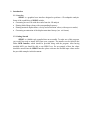
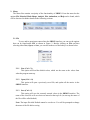
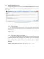
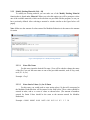
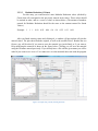
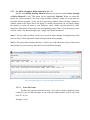
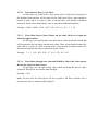
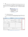
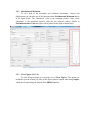
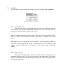
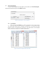
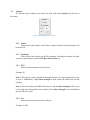
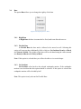
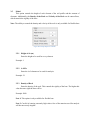
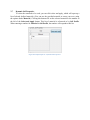
2013 UCSD [USER MANUAL FOR SB2013] A computer program for conducting seismic analysis of soil. John Li Contents 1. Introduction ............................................................................................................................. 4 2. 1.1. Overview .......................................................................................................................... 4 1.2. Getting Started.................................................................................................................. 4 Menu ........................................................................................................................................ 5 2.1. 2.1.1 New (Ctrl + N) .......................................................................................................... 5 2.1.2 Open (Ctrl + O) ......................................................................................................... 5 2.1.3 Save (Ctrl + S) .......................................................................................................... 5 2.2 Material Properties ........................................................................................................... 6 2.2.1 Define New Material (Ctrl + D)................................................................................ 7 2.2.2 Modify Existing Material (Ctrl + M) ........................................................................ 9 2.2.3 Use Shear Strength to Define Material (Ctrl + U) .................................................. 11 2.2.4 View Existing Material (Ctrl + I) ........................................................................... 14 2.3 Mode Shape .................................................................................................................... 15 2.4 Analysis .......................................................................................................................... 16 2.4.1 Run (Ctrl + R) ......................................................................................................... 16 2.4.2 Save Output (Ctrl + E) ............................................................................................ 16 2.5 Plot ................................................................................................................................. 17 2.5.1 Maximum Absolute Value ...................................................................................... 17 2.5.2 Maximum and Minimum ........................................................................................ 18 2.5.3 Close Figures (Ctrl + F) .......................................................................................... 18 2.6 Animation ....................................................................................................................... 19 2.6.1 Create (Ctrl + A) ..................................................................................................... 19 2.6.2 Play (Ctrl + P) ......................................................................................................... 19 2.7 3. File.................................................................................................................................... 5 Help ................................................................................................................................ 21 Entering Values into SB2013 ................................................................................................ 22 3.1 File Name ....................................................................................................................... 22 3.2 Selecting Earthquake ...................................................................................................... 23 3.2.1 User Defined ........................................................................................................... 23 3.2.2 Unit of Acc .............................................................................................................. 24 3.2.3 dt (of EQ data in sec) .............................................................................................. 24 3.2.4 Scale EQ Data by .................................................................................................... 24 3.3 Analysis .......................................................................................................................... 25 3.3.1 Linear ...................................................................................................................... 25 3.3.2 Nonlinear................................................................................................................. 25 3.3.3 NYS......................................................................................................................... 25 3.3.4 Tol ........................................................................................................................... 25 3.4 Base ................................................................................................................................ 26 3.4.1 Rigid Base ............................................................................................................... 26 3.4.2 Flexible Base ........................................................................................................... 26 3.4.3 Not Incident ............................................................................................................ 26 3.5 Model ............................................................................................................................. 27 3.5.1 Height of ele (m) ..................................................................................................... 27 3.5.2 # of Ele .................................................................................................................... 27 3.5.3 Density of Rock ...................................................................................................... 27 3.5.4 Velocity of Rock ..................................................................................................... 28 3.6 Damping ......................................................................................................................... 29 3.6.1 Rayleigh Damping .................................................................................................. 29 3.6.2 Luco Damping ........................................................................................................ 30 3.7 Dynamic Soil Properties................................................................................................. 31 3.8 Soil Profile...................................................................................................................... 32 3.8.1 Elements .................................................................................................................. 32 3.8.2 Shear Velocity......................................................................................................... 32 3.8.3 Shear Strength ......................................................................................................... 32 3.8.4 Max Shear Strain (%).............................................................................................. 33 3.8.5 Mass Density........................................................................................................... 33 3.9 Output ............................................................................................................................. 35 1. Introduction 1.1. Overview SB2013 is a graphical user interface designed to perform a 1D earthquake analysis. Some of the capabilities of SB2013 include: Generating an excel file with the results from the 1D analysis Plotting Mode Shapes along with corresponding frequency Plotting maximal displacement, velocity and acceleration values (with respect to nodes) Generating an animation of the displacement time history (in a .avi format) 1.2. Getting Started SB2013 is a Matlab code complied into an executable. To make use of this program, you would first need to install MCR onto your computer. The installer can be found in the folder MCR Installer, which should be provided along with the program. After having installed MCR you should be able to run SB2013.exe. For an example of how the values should be entered into the SB2013 Interface please reference the Default input values and/or the provided examples in this document. 2. Menu The Menu Bar contains a majority of the functionality of SB2013. From the menu bar the options File, Material, Mode Shape, Analysis, Plot, Animation, and Help can be found, which will be discussed in further details in the following sections. Figure 1 Menu Bar 2.1. File To save and/or open inputs entered into the SB2013 interface you can use the options that can be found under File as shown in Figure 2. Besides clicking on File and then selecting either New, Open, or Save, you can also make use of the hotkeys as shown below. Figure 2 Submenu for "File" 2.1.1 New (Ctrl + N) This option will load the default values, which are the same as the values from when the program starts up. 2.1.2 Open (Ctrl + O) This option will open a previously saved file, and update all the entries in the SB2013 interface. 2.1.3 Save (Ctrl + S) This option will save the currently entered values in the SB2013 interface. The name of the saved file will use what was entered at the top left. (At start up, the name of the file will be called default.) Note: The input file titled Default cannot be saved over. You will be prompted to change the name of the file before saving. 2.2 Material Properties To generate, modify, or view materials that can be used to define the Stress Strain Curve for nonlinear analysis, you can make use of the options found under Material. Note 1: The created Material files are stored in a folder called Material. In the folder there should already be several materials provided which are Clay, Rock, Sand, PI – 0, PI – 15, PI– 30, PI – 50, PI – 100, and PI – 200. These materials cannot be saved over, and when modifying these materials you will be prompted to change the name before saving. Note 2: The material files for SB2013 and Shake91_Input are in the same format. If you want to reuse the material files created in SB2013 for Shake91_Input, you can. There is however, a limit for how many values can be used for Shake91, which is 20. Additionally, the data from the damping is not used for SB2013, but are kept in the file for compatibility. Figure 3 Submenu for "Material" 2.2.1 Define New Material (Ctrl + D) To define a new material you can make use of the Define New Material function that is found under Material. When you select this option a window similar to the one shown below should appear. Figure 4 Example inputs for "Define New Material" 2.2.1.1 Enter File Name For this entry input the desired file name. (You will be asked to change the name of the file, if you use the same name as one of the provided materials, such as clay, sand, rock, PI – 0, etc.) Example: Clay2 2.2.1.2 Enter Strain Values (%) for G/Gmax For this entry you would need to enter strain values (%) that will correspond to the Modulus Reduction that are entered in the field below. These values should be entered in order, and as a vector of values as shown below. (The amount of numbers entered for Strain Values should be the same as the amount entered for Modulus Reduction.) Example: 0.0001 0.0003 0.001 0.003 0.01 0.03 0.1 0.3 1 3 10 2.2.1.3 Modulus Reduction (G/Gmax) For this entry you would need to enter Modulus Reduction values (divided by Gmax) that will correspond to the previously entered strain values. These values should be entered in order, and as a vector of values as shown below. (The amount of numbers entered for Modulus Reduction should be the same as the amount entered for Strain Values.) Example: 1 1 1 0.97 0.94 0.8 0.65 0.43 0.23 0.14 0.1 After you finish entering values and clicking ok, a window will pop up that will plot the entered values. The plot shows both the original, as well as the modified curve. Besides the two figures, you will be asked if you want to save the material you just defined, or if you want to keep modifying the material as shown in the figure below. Clicking yes will save the material using the file name entered previously. If you already have a file with the given name you will be asked if you want to save over it. You cannot save over the materials that came with the program. Figure 5 Example using "Define New Material" 2.2.2 Modify Existing Material (Ctrl + M) To modify an existing material you can make use of the Modify Existing Material function that is found under Material. When you select this option you will be prompt to select one of the available materials, which can be one that was provided with the program, or one you have previously defined. After selecting a material a window similar to the figure below will popup. Note: Make sure the amount of values entered for Modulus Reduction is the same as the amount for strain. Figure 6 Example inputs for "Modify Existing Material" 2.2.2.1 Enter File Name For this entry input the desired file name. (You will be asked to change the name of the file if you use the same name as one of the provided materials, such as clay, sand, rock, PI – 0, etc.) Example: Clay2 2.2.2.2 Enter Strain Values (%) for G/Gmax For this entry you would need to enter strain values (%) that will correspond to the Modulus Reduction that will be entered in the field below. These values should be entered in order, and as a vector of values as shown below. (The amount of numbers entered for Strain Values should be the same as the amount entered for Modulus Reduction.) Example: 0.0001 0.0003 0.001 0.003 0.01 0.03 0.1 0.3 1 3 10 2.2.2.3 Modulus Reduction (G/Gmax) For this entry you would need to enter Modulus Reduction values (divided by Gmax) that will correspond to the previously entered strain values. These values should be entered in order, and as a vector of values as shown below. (The amount of numbers entered for Modulus Reduction should be the same as the amount entered for Strain Values.) Example: 1 1 1 0.99 0.95 0.86 0.6 0.4 0.22 0.13 0.09 After you finish entering values and clicking ok, a window will pop up that will plot the entered values. The plot shows both the original, as well as the modified curve. Besides the two figures, you will be asked if you want to save the material you just defined, or if you want to keep modifying the material as shown in the figure below. Clicking yes will save the material using the file name entered previously. If you already have a file with the given name you will be asked if you want to save over it. You cannot save over the materials that came with the program. Figure 7 Example using "Modify Existing Material" 2.2.3 Use Shear Strength to Define Material (Ctrl + U) Besides using Modify Existing Material function, you can also use Use Shear Strength to Define Material as well. This option can be found under Material. When you select this option you will be prompt to select one of the available materials, which can be one that was provided with the program, or one you have previously defined. After selecting a material a window similar to the figure below will popup. To modify the material you can simply change the numbers to what you want, or even add more values. (Make sure the amount of values entered for Shear Stress is the same as the corresponding Strain Values, if you are going to enter or delete values.) For Shear Strength, only a single value should be entered. Note 1: The last value for Shear will be set to equal the shear strength, and adjustments to the last few values will be adjusted if needed to help reach the shear strength. Note 2: This option only considers the Stress – Strain curve, and adjusts the values of Stress such that the slopes is not increasing, and is able to reach the Shear Strength. . Figure 8 Example inputs for “Use Shear Strength to Modify Material” 2.2.3.1 Enter File Name For this entry input the desired file name. (You will be asked to change the name of the file if you use the same name as one of the provided materials, such as clay, sand, rock, PI – 0, etc.) Example: Clay2 2.2.3.2 Enter Strain Values (%) for Shear For this entry you would need to enter strain values (%) that will correspond to the Modulus Reduction that will be entered in the field below. These values should be entered in order, and as a vector of values as shown below. (The amount of numbers entered for Strain Values should be the same as entered for Modulus Reduction.) Example: 0.0001 0.0003 0.001 0.003 0.01 0.03 0.1 0.3 1 3 10 2.2.3.3 Enter Shear Stress Values (/Gmax, the last value will be set to equal the Shear Strength set below) For this entry you would need to enter Shear Stress values (divided by Gmax) that will correspond to the previously entered strain values. These values should be entered in order, and as a vector of values as shown below. (The amount of numbers entered for Shear Stress should be the same as entered for Strain Values.) Example: 1 1 1 0.99 0.95 0.86 0.7 0.45 0.25 0.2 0.12 2.2.3.4 Enter Shear Strength (one value and divided by Gmax, this value controls the last few values for Shear Stress) For this entry you can enter a single value, which will adjust the last few values entered for Shear Stress to reach the Shear Strength. Example: 0.014 Note: The last value for Shear Stress will be set equal to the Shear Strength, and if necessary the last few numbers will be adjusted. After you finish entering values and clicking ok, a window will pop up that will plot the entered values. The plot shows both the original, as well as the modified curve. Besides the two figures, you will be asked if you want to save the material you just defined, or if you want to keep modifying the material as shown in the figure below. Clicking yes will save the material using the file name entered previously. If you already have a file with the given name you will be asked if you want to save over it. You cannot save over the materials that came with the program. Figure 9 Example using “Use Shear Strength to Define Material” 2.2.4 View Existing Material (Ctrl + I) To view an existing material you can use the View Existing Material function, which will open three figures. Two of the figures plot Strain vs. Modulus, and Strain vs. Stress, while the last figure lists the values for Strain, Modulus Reduction, and Shear Stress as shown in the figure below. Figure 10 Example using "View Existing Material" 2.3 Mode Shape To view the mode shape for the soil profile you can make use of the Mode Shape option that is shown in the figure below. Note: Mode Shape is currently only available for Rigid Base. If you have Flexible Base selected you will be prompted to change it to Rigid Base. Figure 11 Highlighting location of "Mode Shape" When you select the option Mode Shape you will be asked to enter a number. The number of allowable of Mode Shape is equal to how many elements are defined. Note: The mode shape shown is generated using the Mass Matrix and Stiffness Matrix, which utilize only the Shear Wave Velocity, Mass Density, and Height of the element to calculate. (The Material selected is not taken into account when determining the mode shape.) Figure 12 Example using "Mode Shape" When you enter a valid number for the Mode Shape you wish to see, it will be plotted on the right of the SB2013 Interface as shown in the figure below. Figure 13 Highlighting location of where the Mode Shape plotted 2.4 Analysis To run and/or save the outputs for an analysis you can make use of the functions under Analysis as shown in the figure below. Figure 14 Submenu for "Analysis" 2.4.1 Run (Ctrl + R) This option will run an analysis using the values entered into the SB2013 Interface. When the run is complete, a message box will appear that says “Complete”. 2.4.2 Save Output (Ctrl + E) This option will create an excel file using the results of the analysis. (To run an analysis use the Run option mentioned above. The excel file will contain the input motion, and the displacement, velocity, acceleration, strain, and stress for every node.) 2.5 Plot After running the analysis using the Run option mentioned on the previous page, you can plot the results using either the options under Plot or options under Output, which is located along the bottom of the Interface. From Plot there are two primary methods to plot the results for the analysis. You can view the Maximum Absolute Value or the Maximum and Minimum value. Figure 15 Submenu for "Plot" 2.5.1 Maximum Absolute Value To view maximum absolute value for acceleration, velocity and displacement you can make use of the functions under Maximum Absolute Value shown in the figure below. Figure 16 Highlighting location of "Maximum Absolute Value" 2.5.2 Maximum and Minimum To view both of the maximum and minimum acceleration, velocity and displacement you can make use of the functions under Maximum and Minimum shown in the figure below. The “Maximum” value is the maximum positive value, while “Minimum” is the maximum negative value (for the respective nodes). Similar to Maximum Absolute Value the figure will be plotted on the right as shown below. Figure 17 Highlighting location of where Maximum and Minimum is plotted 2.5.3 Close Figures (Ctrl + F) To close all open figures you can make use of Close Figures. This option was included to provide a hotkey to close all the figures that are opened when using Output, which can be found along the bottom of the SB2013 Interface. 2.6 Animation To create and/or play animations you can make use of the functions under Animation. Figure 18 Submenu for "Animation" 2.6.1 Create (Ctrl + A) This option will create an animation using the results of the earthquake analysis. The animation will show the displacement time history of every node, along with the input motion. The animation is created as an .avi file. Note 1: Creating an animation will take awhile. When you select this option you will be unable to interact with the SB2013 interface until SB2013 is finished with creating the .avi. Note 2: Before you use this option, you are required to first install ffdshow, which is a codec that is used to compress the .avi file. To install this codec you can make use of the installer “windows.7.codec.pack.v4.0.7.setup.exe”, which can be found in the folder Codec. 2.6.2 Play (Ctrl + P) This option will open a figure similar to the figure on the following page. The animation shows two plots. The first of the plot shows the displacement of each node, while the second plot shows displays the input motion with a red dot showing where how far along the animation is. Figure 19 Example using "Play" 2.7 Help If you have questions about SB2013 you can reference this user manual, which can be opened by using the functions under Help. Figure 20 Submenu for "Help" 2.7.1 Open User Manual (Ctrl + H) To open up the user manual you can use ctrl + H, or look in the folder called User Manual. 2.7.2 About SB2013 This will opens up a message box, with brief message with a little bit of info about what SB2013 is. 3. Entering Values into SB2013 3.1 File Name To enter the file name that will be used when saving the input, change the entry at the top left of the SB2013 interface as shown in the figure below. Example: Example Note: Do not include the extension of the file. Figure 21 Highlighting location of where to change “File Name” 3.2 Selecting Earthquake To select which earthquake to use for analysis, you can make use of Select Earthquake, which can be found to the top left of the SB2013 interface. Figure 22 Example inputs for "Select Earthquake" 3.2.1 User Defined When selecting User Defined, you will be prompted to select an input motion. The selected input motion must be formatted such that there is no header line (which means the values of acceleration start right away.) The input motion can be formatted with or without time, but must in a column as shown below. Figure 23 Format for Earthquake Motion (either is fine) 3.2.2 Unit of Acc For Unit of Acc if the option g is selected then it signifies that the selected Input Motion is in units of g. If g is selected then the Input Motion will be multiplied by the selected acceleration of gravity, which can either be m/s^2 or in/s^2. If g is not selected then the Input motion will not be multiplied, and depending on if m/s^2 or in/s^2 is selected then the outputs will be formatted as such. Note: If the selected earthquake motion is not in m/s^2 or in/s^2 then you can make use of Scale EQ Data by to adjust the earthquake data. Be careful to note that if g is selected then the Input Motion will be multiplied by the unit of acceleration selected. (This option is to the right of Unit of Acc.) 3.2.3 dt (of EQ data in sec) This option will automatically be filled in if there are two columns in the selected input motion. Otherwise enter the appropriate time step that will be used for analysis. 3.2.4 Scale EQ Data by You can use this option to scale the Input Motion. The Input Motion will be multiplied by the entered value. By default this will be set to 1, which will essentially have no effect. 3.3 Analysis To select the type of analysis you wish to be done, look under Analysis (not the one on the menu.) Figure 24 Example inputs for "Analysis" 3.3.1 Linear When selected the analysis will be linear, options unrelated to linear analysis will be turned off. 3.3.2 Nonlinear When selected the analysis run will be nonlinear. Selecting this option will open up more required inputs, such as NYS, Max Shear Strain, etc. 3.3.3 NYS Enter the desired number of yield surface. Example: 20 Note 1: This option is only available for nonlinear analysis. For linear analysis this value is set to 1. Additionally, a high Shear Strength is used, which will result in the soil not yielding. Note 2: For linear analysis the NYS will be set to 1 and the Shear Strength will be set to a very high value (that should not be reached). If the Shear Strength is not reached then the soil will never yield. 3.3.4 Tol Enter the desired tolerance for the analysis. Example: 1e-005 3.4 Base The option Base allows you to change the rigidity of the base. Figure 25 Example inputs for "Base" 3.4.1 Rigid Base In Rigid Base the base is assumed to be fixed, and is not allowed to move. 3.4.2 Flexible Base In Flexible Base the base node is allowed to be moved as well. Selecting this option will open up three additionally fields, which are Not Incident, Density of Rock, and Velocity of Rock. The rigidity of the base will be calculated using the values entered into Density of Rock and Velocity of Rock. Note: If this option is selected then you will not be able to view mode shapes. 3.4.3 Not Incident Not Incident refers back to the selected earthquake motion. If the earthquake motion is not incident then this option should be selected. If this option is selected the earthquake motion will be divided by half. Note: This option is only relevant for Flexible Base 3.5 Model This option controls the height of each element of the soil profile and the amount of elements. Additionally, the Density of the Rock and Velocity of the Rock can be entered here, which controls the rigidity of the base. Note: The ability to control the density and velocity of the rock is only available for flexible base. Figure 26 Example inputs for "Model" 3.5.1 Height of ele (m) Enter the height to be used for every element. Example: 1 3.5.2 # of Ele Enter the # of elements to be used for analysis. Example: 21 3.5.3 Density of Rock Enter the density of the rock. This controls the rigidity of the base. The higher this value the more rigid the base will be. Example: 2000 Note 1: This option is only available for flexible base. Note 2: Careful of entering extremely high values. One of the matrixes used for analysis will become nearly singular. 3.5.4 Velocity of Rock Enter the shear wave velocity of the rock. This controls the rigidity of the base. The higher this value the more rigid the base will be. Example: 1000 Note 1: This option is only available for flexible base. Note 2: Careful of entering extremely high values. One of the matrixes used for analysis will become nearly singular. 3.6 Damping This option controls the amount of damping and what type of damping to be used for the analysis. Figure 27 Example inputs for "Damping" 3.6.1 Rayleigh Damping Figure 28 Example inputs for "Rayleigh Damping" 3.6.1.1 Freq. 1 (Hz.) Enter the frequency in Hz. to be used for the first damping value. Example: 1 3.6.1.2 Freq. 2 (Hz.) Enter the frequency in Hz. to be used for the second damping value. Example: 6 3.6.1.3 Damping @ Freq. 1 (%) Enter the value of damping in % that will correspond to Freq. 1. Example: 5 3.6.1.4 Damping @ Freq. 2 (%) Enter the value of damping in % that will correspond to Freq. 2. Example: 5 3.6.2 Luco Damping Note: Currently Luco Damping is only available for Rigid Base. 3.6.2.1 Damping (%) Enter the value of damping that will be used to form the Luco Damping Matrix. Figure 29 Example inputs for "Luco Damping" 3.7 Dynamic Soil Properties To select the materials to be used, you can click select and apply, which will open up a list of already defined materials. (You can use the provided material or create your own, using the options under Material). Clicking this button will set the selected material to the number to the left of the Select and Apply button. This list of material is referenced to by Soil Profile. When entering a number for Material in Soil Profile, the number will respond to this list. Figure 30 Example inputs for "Dynamic Soil Properties" 3.8 Soil Profile To define the properties of the soil, look under Soil Profile. Note: To the right of each field under Soil Profile is a small box where you can enter a number. This will multiply the corresponding values by a power of 10. If 0 is entered then it will multiply the corresponding value by 1. If 1 is entered then the corresponding values are multiplied by 10, and so on and so forth. 3.8.1 Elements This entry defines what properties are used for which layer. For the example shown, layers 1:10 will have a Shear Wave Velocity of 100, while layer 11:20 will have a Shear Wave Velocity of 120, and layers 21 will have a Shear Wave Velocity of 150. (This example refers to the Shear Velocity shown below.) Example 1: 1:10 11:20 21 Example 2: 1 2 3 4 5 6:10 Note: Example 1 counts as having 3 entries, which requires that 3 entries are entered for Shear Velocity, Shear Strength, Max Shear Strain, Mass Density and Material. Example 2 on the other hand will require 6 entries each. 3.8.2 Shear Velocity This entry defines the Shear Wave Velocity of the Soil Profile. The first entry of Shear Velocity will correspond to the first entry in Layers. For this example the first entry of Layers is 1:10, and has a Shear Velocity of 100. Example: 100 120 150 3.8.3 Shear Strength This entry defines the shear strength of the Soil Profile. The first entry of Shear Strength will correspond to the first entry in Layers. For this example the first entry of Layers is 1:10, and has a Shear Strength of 75. Example: 75 80 85 Note: This option is only available for nonlinear analysis. 3.8.4 Max Shear Strain (%) This entry defines the Max Shear Strain for the Soil Profile. The first entry of Max Shear Strain will correspond to the first entry in Layers. For this example the first entry of Layers is 1:10, and has a Max Shear Strain of 3. Example: 3 3 3 Note: This option is only available for nonlinear analysis. 3.8.5 Mass Density This entry defines the Mass Density of the Soil Profile. The first entry of Mass Density will correspond to the first entry in Layers. For this example the first entry of Layers is 1:10, and has a Mass Density of 2000. Example: 2 2.2 4 Note: The reason why the density is 2000 instead of 2 is because to the right of Mass Density the number in the small box is 3 instead of 0. This would mean the entries in Mass Density is multiplied by 10^3. 3.8.6 Material This entry defines the stress-strain curve to be used for plastic analysis. The first entry of Material will correspond to the first entry in Layers. For this example the first entry of Layers is 1:10 will use material 0. (To define what material is what, look under Dynamic Soil Properties. In the figure below, Material 1 is “Clay”, which can be seen on the figure for Dynamic Soil Properties. Example: 0 1 0 Note 1: This option is only available for nonlinear analysis. Note 2: Material 0 will use the built in stress-strain curve. 3.8.7 View This option allows you to view the stress strain curves that would be used. The curves are all adjusted to be able to reach the Shear Strength. You can use this option to judge if you should adjust the soil properties, or select a different material. Figure 31Example inputs for "Soil Profile" 3.9 Output To plot the results of the analysis you can make use of Output, located at the bottom of the Interface as shown in the figure below. This option only becomes available after you run an analysis. To output the desired figures click the available options Displacement, Velocity, Acceleration, Strain, Stress, and Stress vs. Strain. After selecting what you want you can enter the number you want the plot for. For example if you want Acceleration for Layers 1, 2, 3, and 5 you can enter 1:3 5. (You are not limited to only output acceleration you can output all the figures.) After entering the numbers you can click “Output Figures”. Additionally, if you have Separated clicked it will separate all the figures otherwise they will be grouped by nodes. Furthermore checking Input Motion will output the input motion multiplied by the acceleration of gravity and scale). Figure 32 Example inputs for "Output"