1
Project Report
Automatic Detection and Analysis of Tumor
Tissue in Prostate Punch Biopsies
Implementation of an Image Processing Pipeline
Master of Science in Engineering
P8, Fall Semester 2015
Dario Vischi
Advisor:
Prof. Dr. Christoph Stamm, FHNW
Customer:
Prof. Dr. Peter Wild, USZ
Dr. Qing Zhong, USZ
Norbert Wey, USZ
Institute: Institute of Mobile and Distributed Systems (IMVS)
I like to thank Prof. Dr. Christoph Stamm and Mr. Norbert Wey for there valuable
advisory support in the field of modern C++ programming and image processing. Also,
I like to thank Prof. Dr. Peter Wild and Dr. Qing Zhong for their great encouragement
and their help in medical questions. My sincere thanks also goes to Mr. Roman Bolzern
who supported me with conceptual ideas and feedback during many discussions.
Abstract
The prostate cancer is the most common type of cancer we have in Switzerland. Every
year about 5300 people develop cancer and around 1300 men die from it. The research
for unambiguous indicators for an early detection of the cancer is nowadays an active
field in the area of medication. In this context, the aim of a current project at the University Hospital of Zurich is the automatic detection of tumor tissues in prostate punch
biopsies. We would like to perform the detection on a cohort from Aarau with samples
from about 9900 men to build up a model to describe the cancer’s progress.
The current documentation at hand describes the second out of three sub-projects for
the automatic detection of the tumor tissues. In the first sub-project we made the acquisition of about 260 images by scanning prostate punch biopsies from the cohort of
Aarau. In the current sub-project we implement an image processing pipeline for processing this image data and prepare the pipeline for the upcoming sub-project, which
has the aim to find cancerous tissues. The pipeline is based on Microsoft’s DirectShow
framework and implemented in C++. We offer several base classes which can be used for
implementing further steps, so called filters, within the pipeline in a most simple way.
As a first example for our pipeline framework we implement a cell nucleus detection
algorithm which results can be stored locally or uploaded to a web server. Additionally,
we present an evaluation filter which can measure the quality of our detection algorithm.
In the last sub-project we will extend our image processing pipeline with an algorithm
for detecting tumor tissues. The algorithm will be optimized using the evaluation filter
approach from the current project and the training data from the previous project made
by Prof. Dr. Peter Wild.
Table of Content
Table of Content
Abstract
Abbreviations
1
1 About the Document
2
2 Project Definition
2.1 Background . . . . . . . . . . . . . . . . . . . . . . . . . . . . . . . . . .
2.2 Identification of requirements . . . . . . . . . . . . . . . . . . . . . . . .
3
4
6
3 Image Processing Pipeline
3.1 Pipeline System . . . . . . . . . . . . . .
3.1.1 Platform Independence . . . . . .
3.2 Plugin Framework . . . . . . . . . . . .
3.2.1 System Calls . . . . . . . . . . .
3.2.2 Binary Compatibility . . . . . . .
3.2.3 Plugin Manager . . . . . . . . . .
3.3 Performance Optimization . . . . . . . .
3.3.1 Memory Management . . . . . . .
3.3.2 Compilation . . . . . . . . . . . .
3.3.3 Concurrent & Parallel Computing
3.4 Reproduceable Execution Plans . . . . .
3.5 Bring It All Together . . . . . . . . . . .
4 System Integration
4.1 Overview . . . . . . . . .
4.2 Graphical User Interface
4.3 Data Transfer . . . . . .
4.4 Training Data Sets . . .
4.5 Data Evaluation . . . . .
.
.
.
.
.
.
.
.
.
.
.
.
.
.
.
.
.
.
.
.
.
.
.
.
.
.
.
.
.
.
.
.
.
.
.
5 Image Analysis Tool
5.1 Overview . . . . . . . . . . . . . . . .
5.1.1 Build Up A Filter Graph . . .
5.1.2 Source Filter . . . . . . . . .
5.1.3 Transform Filter . . . . . . .
5.1.4 Sink Filter . . . . . . . . . . .
5.1.5 Filter Connection . . . . . . .
5.1.6 Passing Data Between Filters
5.1.7 Filter Registration . . . . . .
i
.
.
.
.
.
.
.
.
.
.
.
.
.
.
.
.
.
.
.
.
.
.
.
.
.
.
.
.
.
.
.
.
.
.
.
.
.
.
.
.
.
.
.
.
.
.
.
.
.
.
.
.
.
.
.
.
.
.
.
.
.
.
.
.
.
.
.
.
.
.
.
.
.
.
.
.
.
.
.
.
.
.
.
.
.
.
.
.
.
.
.
.
.
.
.
.
.
.
.
.
.
.
.
.
.
.
.
.
.
.
.
.
.
.
.
.
.
.
.
.
.
.
.
.
.
.
.
.
.
.
.
.
.
.
.
.
.
.
.
.
.
.
.
.
.
.
.
.
.
.
.
.
.
.
.
.
.
.
.
.
.
.
.
.
.
.
.
.
.
.
.
.
.
.
.
.
.
.
.
.
.
.
.
.
.
.
.
.
.
.
.
.
.
.
.
.
.
.
.
.
.
.
.
.
.
.
.
.
.
.
.
.
.
.
.
.
.
.
.
.
.
.
.
.
.
.
.
.
.
.
.
.
.
.
.
.
.
.
.
.
.
.
.
.
.
.
.
.
.
.
.
.
.
.
.
.
.
.
.
.
.
.
.
.
.
.
.
.
.
.
.
.
.
.
.
.
.
.
.
.
.
.
.
.
.
.
.
.
.
.
.
.
.
.
.
.
.
.
.
.
.
.
.
.
.
.
.
.
.
.
.
.
.
.
.
.
.
.
.
.
.
.
.
.
.
.
.
.
.
.
.
.
.
.
.
.
.
.
.
.
.
.
.
.
.
.
.
.
.
.
.
.
.
.
.
.
.
.
.
.
.
.
.
.
.
.
.
.
.
.
.
.
.
.
.
.
.
.
.
.
.
.
.
.
.
.
.
.
.
.
.
.
.
.
.
.
.
.
.
.
.
.
.
.
.
.
.
.
.
.
.
.
.
.
.
.
.
.
.
.
.
.
.
.
.
.
.
.
.
.
.
.
.
.
.
.
.
.
.
.
.
.
.
.
.
.
.
.
.
.
.
.
.
.
.
.
.
.
.
.
.
.
.
7
7
8
8
9
9
9
10
10
10
10
11
11
.
.
.
.
.
14
14
17
19
19
19
.
.
.
.
.
.
.
.
21
21
24
28
28
29
29
30
34
Table of Content
5.2
5.3
5.4
Image Analysis Filters . . . . . . . . .
5.2.1 IA Base Filters . . . . . . . . .
5.2.2 User Defined Media Types . . .
5.2.3 Media Type Conversion . . . .
5.2.4 Sample’s Memory Management
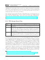
Cell Nucleus Detection . . . . . . . . .
5.3.1 TIFF Ventana Source Filter . .
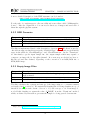
5.3.2 RGB Converter . . . . . . . . .
5.3.3 Empty Image Filter . . . . . . .
5.3.4 Grayscale Converter . . . . . .
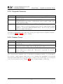
5.3.5 Contour Tracer . . . . . . . . .
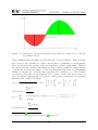
5.3.6 Non-Overlapping Contour Filter
5.3.7 Concave Contour Separator . .
5.3.8 Color Deconvolution Classifier .
5.3.9 Contour Plotter . . . . . . . . .
5.3.10 Bitmap Set Sink Filter . . . . .
5.3.11 Contour Sink Filter . . . . . . .
Algorithm Evaluation . . . . . . . . . .
.
.
.
.
.
.
.
.
.
.
.
.
.
.
.
.
.
.
.
.
.
.
.
.
.
.
.
.
.
.
.
.
.
.
.
.
.
.
.
.
.
.
.
.
.
.
.
.
.
.
.
.
.
.
.
.
.
.
.
.
.
.
.
.
.
.
.
.
.
.
.
.
.
.
.
.
.
.
.
.
.
.
.
.
.
.
.
.
.
.
.
.
.
.
.
.
.
.
.
.
.
.
.
.
.
.
.
.
.
.
.
.
.
.
.
.
.
.
.
.
.
.
.
.
.
.
.
.
.
.
.
.
.
.
.
.
.
.
.
.
.
.
.
.
.
.
.
.
.
.
.
.
.
.
.
.
.
.
.
.
.
.
.
.
.
.
.
.
.
.
.
.
.
.
.
.
.
.
.
.
.
.
.
.
.
.
.
.
.
.
.
.
.
.
.
.
.
.
.
.
.
.
.
.
.
.
.
.
.
.
.
.
.
.
.
.
.
.
.
.
.
.
.
.
.
.
.
.
.
.
.
.
.
.
.
.
.
.
.
.
.
.
.
.
.
.
.
.
.
.
.
.
.
.
.
.
.
.
.
.
.
.
.
.
.
.
.
.
.
.
.
.
.
.
.
.
.
.
.
.
.
.
.
.
.
.
.
.
.
.
.
.
.
.
.
.
.
.
.
.
.
.
.
.
.
.
.
.
.
.
.
.
.
.
.
.
.
.
.
.
.
.
.
.
.
.
.
.
.
.
.
.
.
.
.
.
.
.
.
.
.
.
36
36
38
40
43
46
50
52
52
53
53
55
57
58
58
58
59
59
6 Software Testing
62
6.1 Function Tests . . . . . . . . . . . . . . . . . . . . . . . . . . . . . . . . . 62
6.2 System Test . . . . . . . . . . . . . . . . . . . . . . . . . . . . . . . . . . 65
7 Evolution
7.1 IA Filter Extension . . . . . .
7.2 GPGPU . . . . . . . . . . . .
7.3 Distributed Pipeline Systems .
7.4 Windows Media Foundation .
.
.
.
.
.
.
.
.
.
.
.
.
.
.
.
.
.
.
.
.
.
.
.
.
.
.
.
.
.
.
.
.
.
.
.
.
.
.
.
.
.
.
.
.
.
.
.
.
.
.
.
.
.
.
.
.
.
.
.
.
.
.
.
.
.
.
.
.
.
.
.
.
.
.
.
.
.
.
.
.
.
.
.
.
.
.
.
.
.
.
.
.
.
.
.
.
66
66
66
67
67
8 Results
69
9 Reflection
72
10 Bibliography
74
11 Declaration of Originality
76
12 Appendix
12.1 A Cross-Platform Plugin Framework For C/C++ . . . .
12.2 Doxygen Documentation . . . . . . . . . . . . . . . . . .
12.3 Using DirectShow Filters Inside Microsoft’s MediaPlayer
12.4 IA Base Class Diagrams . . . . . . . . . . . . . . . . . .
12.5 XMLLite . . . . . . . . . . . . . . . . . . . . . . . . . . .
12.6 C++/CX Analogies . . . . . . . . . . . . . . . . . . . . .
12.7 Selenium Test Cases . . . . . . . . . . . . . . . . . . . .
12.8 Image Results . . . . . . . . . . . . . . . . . . . . . . . .
12.9 Attached Materials . . . . . . . . . . . . . . . . . . . . .
ii
.
.
.
.
.
.
.
.
.
.
.
.
.
.
.
.
.
.
.
.
.
.
.
.
.
.
.
.
.
.
.
.
.
.
.
.
.
.
.
.
.
.
.
.
.
.
.
.
.
.
.
.
.
.
.
.
.
.
.
.
.
.
.
.
.
.
.
.
.
.
.
.
.
.
.
.
.
.
.
.
.
77
77
79
81
82
86
88
91
92
94
Table of Content
Abbreviations
ABI
AMP
API
BNF
BPP
C#
CHM
CLI
CLSID
COM
DB
DBMS
DLL
FHNW
GIT
GUID
PSR
TIF
UML
URL
USZ
XML
Application Binary Interface
Accelerated Massive Parallelism
Application Prog. Interface
Backus-Naur Form
Bits Per Pixel
C Sharp
Microsoft Compiled HTML Help
Common Language Infrastruct.
Class Identifier
Component Object Model
Database
Database Management Systems
Dynamic-Link Library
Fachhochschule Nordwestschweiz
Global Information Tracker
Globally Unique Identifier
“Pathology-Study & Research”
Tagged Image File
Unified Modeling Language
Uniform Resource Locator
Universitaetsspital Zuerich
Extensible Markup Language
1
Interface between program components
C++ library supporting data parallelism
Interface for interacting with a system
Notation for context-free-grammars
The color depth
Programming language for the CLI
Help file containing HTML files
System spec. for platform independency
GUID for COM classes
Software com. standard by Microsoft
Data collection
System for managing databases
Shared application library for Windows
Univ. of Appl. Sc. NW Switzerland
Revision control system
Unique reference no. within a software
Inventory system for study data
Image format for raster graphics
Modeling language used in software eng.
Reference to a resource
University Hospital of Zurich
Data representation of hierarchical data
CHAPTER 1. ABOUT THE DOCUMENT
1 About the Document
The documentation at hand refers to the implementation of an image processing pipeline
for analysis oversized tissue images, by using Microsoft’s DirectShow. The documentation starts with the project definition, background and the origin problem to solve in
Chapter 2. Before we go into any technical details Chapter 3 refers to a summary of
general issues to consider regarding implementing a pipeline system for image data. Following the introduction of the pipeline system, Chapter 4 discusses about its integration
in the already existing IT infrastructure and how to evaluate data received from its
output. Chapter 5 finally presents the concrete implementation of the pipeline system
which was started with a conceptual overview followed by a concrete example of the
implementation of an algorithm for cell nucleus detection. To ensure a certain level of
quality, the system was tested through several steps as described in Chapter 6 which is
important for the current system as well as further evolution mentioned in Chapter 7.
The last two chapters 8 and 9 summarize the results of the image processing pipeline
and reflect the overall project’s achievement.
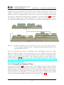
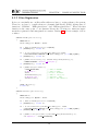
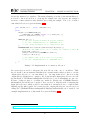
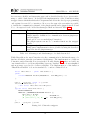
The documentation excludes UML sequence diagrams as they are hard to read and
therefore less beneficial. Instead, we use a simplified version which can be read from the
left bottom to the right top. A simple example is shown in Figure 1.1.
i n t main ( ) {
int a = 0;
a = inc (a) ;
print (a) ;
};
int inc ( int i )
{ i ++; }
v o i d p r i n t ( i n t i ) { c o u t << i << e n d l ; }
a ß inc(a)
print(a)
a ß main [initialize a with 0]
Figure 1.1: Sequence diagram from a short demonstration code.
2
CHAPTER 2. PROJECT DEFINITION
2 Project Definition
In the previous project called “Implementation of an Inventory System to Acquire Digital Image Data” we built up a process to inventorize patient data and the related punch
biopsies from medical studies. Using the system we digitized more than 260 glass slides
and annotated around 50 images with cancerous tissue from a cohort of Aarau.
In a next step we would like to analyze this data using a flexible and extendable pipeline
system. While the analysis of the image data is mainly part of the upcoming project we
focus in the current project on the implementation of the pipeline system. The pipeline
supports the ability to analyze image data by using a wide range of algorithms from different domains such as image processing, computer vision and machine learning. Given
the new pipeline system we implement a cell detection algorithm as a proof of concept.
The algorithm results in several filters which include basic functionalities such as loading
and saving an image file or simple transformations such as blur effect or edge detection.
Next to the filters required by the analysis task it is also important to measure the performance of the analysis result to benchmark an algorithm. Therefore a precision and
recall filter is implemented which can evaluate an extracted feature with the annotations
made in the previous project.
The final outcome of the pipeline is again an image file with plotted features, if desired,
and an XML file containing analysis information, e.g. about the extracted object features. The XML file structure is based on established applications at the University
Hospital of Zurich and therefore can be used in further post processing steps. In this
case we also support a point of particular importance: the integration of the pipeline in
the already given IT infrastructure.
In the upcoming and last project we will use this pipeline system for detecting tumor tissues and extracting corresponding feature data which represents the final goal of
the overall project.
Further details can be found in the attached document “Project definition” which is
also enlisted in the appendix 12.9.
3
CHAPTER 2. PROJECT DEFINITION
2.1 Background
The prostate cancer is the most common type of cancer we have in Switzerland. Every
year about 5300 people develop cancer and around 1300 men die from it. A diseased
person can be actively medicated, but only with the risk of complications and adverse
reactions. The medication is not only restrictively recommended because of the possible
risks but also because only 3 out of 40 people die as can be proved by prostate cancer.
A major problem presents the early detection of the cancer. All known methods such
as the digital rectal examination, the PSA-Test1 or the biopsy of the prostate do not
present unambiguous indicators. It is part of the nowadays ongoing research to find
better indicators, e.g. the European Randomized Study of Screening for Prostate Cancer (ERSPC) [1, p.17] [2, p.2]. A current study at the University Hospital of Zurich
researches a regression analysis of historical data from patients and extracted features
from DNA, RNA and Protein analyses. One sub-project of this regression analysis deals
with the extraction of features from prostate images which will be combined with the
features from the other areas.
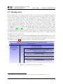
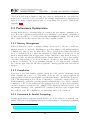
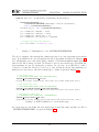
For this purpose an inventory system was implemented where patient data from a cohort
of Aarau was put into. Before we can start with the extraction of the feature data we
firstly need a robust and flexible data processing pipeline upon which we can base our
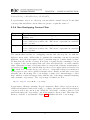
algorithms. Figure 2.1 shows an overview of the whole project stack.
GregressionGanalysisGofGDNA,GRNA,GandGproteinGmeasurementGdata
(domain:Gbiology)
extractionGof
featuresGfrom
theGDNAGandGRNA
analysis
extractionGofGfeatures
fromGtheGproteinGanalysis
automaticGclassificationGofGtumourGtissuesGin
prostateGpunchGbiopsiesGinGtheGareaGofGtheGproteinGanalysis.
(domain:GcomputerGscience)
informaticsGprojectG9
(calculatingGtheGGleasonGScoreGofGindividualGimageGregions)
informaticsGprojectG8
(implementationGofGtheGprocessingGpipelineGforGextractingGfeatures)
informaticsGprojectG7
(mappingGtheGorderGprocessG8GacquisitionGofGimageGdata)
Figure 2.1: Overview of the project stack.
1
Test method for measure the amount of prostate-specific antigen (PSA) inside the blood.
4
CHAPTER 2. PROJECT DEFINITION
The main objectives of the roadmap concerning the informatics project (IP) 7 to 9,
which are part of the Master education, can be summarized as follows:
Project Short description
IP7
Acquisition of digital image data with the Ventana iScan HT and semiautomation of the inventory process. Additionally, annotation of the image
data with areas of healthy and cancerous tissue.
IP8
Implementation of an image processing pipeline. The pipeline’s components
such as filters or transformations are implemented as plugins which then
can be combination in a flexible and extendable way. Based on the new
system a cell core segmentation algorithm is developed. To give a qualitative
statement about the algorithm we express the performance by its precision
and recall.
IP9
Developing an image-based computational score to correlate with the existing Gleason score from the acquired image data for patient stratification
and survival analysis. The used algorithms will be evaluated with the annotations from IP7 as a test set and the process from IP8 to measure its
performance.
Table 2.1: Overview of the informatics projects.
5
CHAPTER 2. PROJECT DEFINITION
2.2 Identification of requirements
The University Hospital of Zurich has a developed IT infrastructure which includes an
image analysis tool implemented by Norbert Wey. The tool is already in use and connected with other applications. However, the tool was sequentially implemented and is
limited in its flexibility and further development. A new system would offer the desired
flexibility in an extendable way. Therefore, such a new system was requested, being
compatible with the existing infrastructure and following the principal ideas of a modular structure. The current analysis tool is written in C++, which is well established in
Norbert Wey’s team and runs on a single Windows Server. Based on the given image
data from the previous project, the pipeline system has to be able to read BigTIFF files2
which represent TIFF containers with 64bit offsets.
As a proof of concept a first algorithm should be realized through the new pipeline
system to extract cell nucleus. Furthermore, it should be possible to benchmark the algorithm by evaluating the resulting features with the annotations made in the previous
project. Based on the given initial situation, the requirements of a processing pipeline
are defined as below:
Implementing a processing pipeline...
1. allowing the flexible combination of processing steps without restrictions on
data types, such as image data
2. holding an integrated plugin system for further extensibility
3. being lightweight and supporting performance optimization
4. being compatible with the existing infrastructure
Supporting restorable execution plans of pipeline algorithms.
Enable to evaluate a given algorithm inside the image processing pipeline.
Implementing a cell nucleus detection algorithm as proof of concept.
2
http://www.awaresystems.be/imaging/tiff/bigtiff.html
6
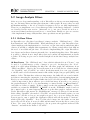
CHAPTER 3. IMAGE PROCESSING PIPELINE
3 Image Processing Pipeline
Before we go into technical details about the implementation of the pipeline in the
existing IT infrastructure as described in Chapter 4 or how to implement the cell nucleus algorithm as described in Chapter 5 we firstly would like to discuss general issues
concerning an image processing pipeline. We discuss advantages and disadvantages for
different approaches and give a conclusion which framework fits best for the current
project.
3.1 Pipeline System
Talking about a pipeline system in software engineering means a chain of processing
steps, so called functions or filters, linked with each other. The pipeline can be filled
with data which then traverse through the pipeline being processed by each passing
filter. The processed data may or may not result in an output of the pipeline; defined
by its behavior.
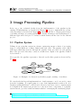
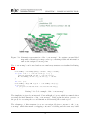
More specific, the pipeline represents a directed acyclic filter graph as shown in Figure 3.1.
3
Sink1
6
Source1
4
9
Sink2
Source2
5
7
Figure 3.1: Example of a directed acyclic filter graph consisting of ten filters.
We can already find several implementations of such systems so we do not need to start
from the beginning. For study purpose a very basic implementation such as Boost’s
Dataflow and Graph library1 could be used. However, if we have a more complex system
it is helpful if the framework provides not only most basic components of a pipeline
system but also provides additional functionalities for managing the underlying graph.
1
http://www.boost.org/doc/libs/1_57_0/libs/graph/doc/index.html
https://svn.boost.org/trac/boost/wiki/LibrariesUnderConstruction#Boost.Dataflow
7
CHAPTER 3. IMAGE PROCESSING PIPELINE
Examples for such functionalities are manipulating the graph’s state, e.g. running or
pausing the graph, or validating the compatibility while connecting two filters with each
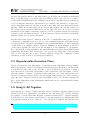
other. Such a framework could be the CellProfiler2 which brings us to a next issue to
discuss. The design of the CellProfile prescribes a sequence of consecutively connected
steps rather than an acyclic graph which brings strong limitations for the system. We
could not implement two execution threads as presented in figure 3.2.
Image Filter1
Image Filter2
Image Source
Feature Plotting
Feature Detection
Feature Manipulation
Figure 3.2: Example of two execution threads.
We could simply sequencing the above graph as for example by merging the feature
detection, the feature manipulation as well as the two image filter operations into a single
filter. However, if we need the first image filter later on in another pipeline combination
we could not reuse the merged filter. An example for a more flexible framework fully
supporting acyclic filter graphs is Microsoft’s DirectShow3 .
3.1.1 Platform Independence
A first and important question to answer before going into any more details is the
platform independence. Should our pipeline system run on a single platform or should
we support cross-platform compatibility? If we use Java or Python we directly support
platform independence where we have to be more careful using programming languages
such as C/C++. This especially affects libraries we are able to use for our pipeline
system or possible subsystems. Namely the graphical user interface is a key point to
mention. Still, we have several options to solve our problem using Qt4 , GTK5 or Swing6 .
3.2 Plugin Framework
When we talk about a pipeline system we may directly think about a plugin system
where each filter represents a single plugin. Indeed, almost all pipeline systems integrate a plugin framework. However, not only the design of a pipeline system which fits
perfectly for a plugin integration is the determining factor. If we take an image processing pipeline we could easily think about several dozens base filters, such as a Sobel
or Gaussian filter, which one could implement. If such a system supports plugins and
2
3
4
5
6
http://www.cellprofiler.org/
https://msdn.microsoft.com/en-us/library/windows/desktop/dd375454(v=vs.85).aspx
https://www.qt.io/
http://www.gtk.org/
http://docs.oracle.com/javase/tutorial/uiswing/
8
CHAPTER 3. IMAGE PROCESSING PIPELINE
provides a community the software architect only needs to provide the pipeline system
whereas the community can implements the corresponding filters. In our case a plugin
framework is crucial so later development also from outside the University Hospital of
Zurich is possible.
Providing a plugin framework, however, holds some pitfalls we have to discuss in the
following sections.
3.2.1 System Calls
Supporting plugins also involves the need of loading them into our system. The plugin,
independent it’s representation, somehow lays on our file system we need to get access
to. If we use Java we have an unified function set for doing so. Under C/C++ and other
programming languages we have to care as we can not only use our native functionalities.
In C++ for example we could use Apache’s Portable Runtime7 or the libuv8 library which
both supports platform independent system calls.
3.2.2 Binary Compatibility
A more technical problem is the binary compatibility between plugins and the pipeline
system. We can distinguish between the application programming interface (API) and
the application binary interface (ABI). In a typed programming language the API has
to be met during compile time. It specifies e.g. the parameters and abstract methods
we have to correctly implement for our plugin. The ABI, however, defines e.g. the order
how parameters are pushed onto the stack while initializing a function call. Moreover,
it defines the order of virtual functions in an interface or abstract class. This means, as
if we use a plugin compiled with an ABI incompatible compiler it might be possible as
our pipeline system calls an unexpected method due a wrong virtual function pointer.
Again, we do not need to think about this issue using programming languages which
do not providing binary compilations such as Java or Python. Nevertheless, if we use
e.g. C++ we have to care about it by ourselves, especially if we implement our own
plugin framework from the scratch. A corresponding approach using a C communication channel is provided in the appendix 12.1. A great benefit to this subject offer
already established pipeline systems or plugin frameworks which provide corresponding
functionalities in there base classes.
3.2.3 Plugin Manager
Another issue to discuss is the way we handle our plugins while starting our system and
during its runtime. The simplest approach is to load all plugins in binary representation
during the system start and do not any further management. More advanced systems
provide a plugin manager which can search new plugins also during runtime. If a new
7
8
https://apr.apache.org/
https://github.com/libuv/libuv
9
CHAPTER 3. IMAGE PROCESSING PIPELINE
object is needed from a plugin we may use a factory which then also can deallocate
memory as soon as the object is released. An example implementing a plugin system
under C++ using a plugin manager and a corresponding factory can be found in the
appendix 12.1.
3.3 Performance Optimization
An important subject concerning image processing is the performance optimization aspect. If we use a pipeline system without any possibilities of performance optimization
we may end up with a good overall architecture but insufficient runtime. We only would
like to mention a few key aspects when choosing a pipeline system.
3.3.1 Memory Management
When creating new objects or deleting existing ones we need to allocate or deallocate
physical memory on our device. Furthermore, if we have function calls with parameters
committed by value we face the same effect. Those operations need time especially if
we do so excessively. If we consider the internals of a single filter we should care about
memory management with an appropriate design. Much more important, however, is
the way we pass our data through the pipeline system. Instead of copy a data package
each time when passing it over from one filter to another we may think about to use
pointers or references. If our programming language do not support such constructs
we could use approaches like the factory pattern to manage pipeline-wide data and its
memory.
3.3.2 Compilation
If we have a very time sensitive pipeline system we could consider optimization flags
while compiling the source code. Depending on the use case one says as applications
with repetitive execution sequences may even run faster using a “Just In Time Compiler”
(JIT). The substantiation is as follows: Comparing to a generally compiled 32bit code,
which is runnable on all 32bit operating systems, an intermediate code could be optimally
compiled by a JIT for the architecture the application is used on. If we have repetitive
execution sequences we can store the optimized JIT compilation and reuse it later on. If
the runtime advantage of the optimized JIT compilation and there reuse is higher than
the overhead of the JIT compiling we are faster than native code - in theory9 .
3.3.3 Concurrent & Parallel Computing
An important subject a pipeline system should cover is the ability for concurrent computing. While more programming languages nowadays support concurrent programming
9
For more details please refer to
http://stackoverflow.com/questions/5326269/is-c-sharp-really-slower-than-say-c
10
CHAPTER 3. IMAGE PROCESSING PIPELINE
we may ask ourselves where to use this technology. Would we use it inside an individual
filter or pipeline-wider? A possible approach which is called “Actor Model”10 could be
a single thread handling the whole pipeline system where each filter has its own thread
for proceeding incoming data. Alternatively, we could also use a thread pool approach11
where each idling thread loads data from the source filter and pass them through the
pipeline. While in the first approach the largest filter defines the execution time it is
the overall longest execution chain in the second approach. We can not give a general
statement about which concurrency pattern to use in a pipeline system as it strongly
depends on the algorithm used later on. If we discuss about an extendable and flexible
pipeline system it is even more uncertain.
Another important aspect to mention is the use of parallelism technologies. Like in
concurrency computing we need to choose a programming language with supports appropriate libraries. We then could think about to parallelism filters on other computers
or run them on a graphics adapter. However, thinking about parallelism on the level
of the whole pipeline also has an enormous impact on the simplicity of our pipeline.
We could pass those responsibility to the individual filters and keep the pipeline system
lightweight. Each filter then can decide to proceed the incoming data on the graphics
card or even outsource the work to another computer. Again, the complexity of such
systems grow and we have to weigh up its advantages.
3.4 Reproduceable Execution Plans
Most forgotten is the reproduceability of a pipeline system. Like using an image manipulation program we can process an image in many ways and save them to the hard disk.
A year later we still could see the outcome of our work but most probably we could not
reproduce the process chain. Depending on the domain the reproduceability could be
very important to compare old pipeline results with new ones. Most systems therefore
allows to set filter properties and to save the designed filter graph, also called execution
plan. In a more advanced system we may even think about to save the filter settings and
the corresponding filter graph individually which then can be combined flexible during
its initialization.
3.5 Bring It All Together
After having an overview of issues and approaches concerning a pipeline system we can
discuss about how to implement our system for the current project. As the old image
processing tool at the University Hospital of Zurich is written in C++ and the language
is well known by the client it seems likely to use this language for implementing the
new pipeline system as well. Using C++ also allows us to migrate the already given
10
11
http://web.fhnw.ch/plattformen/conpr/materialien/scala-actors/11_sl_scala_actors
https://msdn.microsoft.com/en-us/library/0ka9477y(v=vs.110).aspx
11
CHAPTER 3. IMAGE PROCESSING PIPELINE
algorithms without rewriting the whole code. Furthermore, C++ is a preferred language for high performance applications and also well established in the field of image
processing12 . As the current image analysis tool runs on a Microsoft Server and it is
not intended to change the platform we could use a platform-dependent approach which
makes the design more simple and understandable.
Based on those pre-definitions we would like to compare three kind of approaches to
choose from. The first approach is a self-developed pipeline system starting from the
scratch. An intermediate approach is DirectShow which supports us with a pipeline
system but is not yet adapted for image data whereas the CellProfiler13 is an already
established image processing pipeline we could use. Table 3.1 compares the three approaches and there advantages.
Issue
Filter
Graph
Platform
Independence
Plugin
Framework
Self-Dev. Pipeline
(+) At free choice
(−) Time consuming
(+) At free choice
(−) Time consuming
Performance
Optimization
(+) At free choice
(+) Supports concurrent programming
(+) Supports parallel
programming
Reproduceable
Execution
Plans
(+) At free choice
(−) Time consuming
(−) ABI issues
(−) No default plugin
manager
DirectShow
(+) Supports acyclic
graphs
(−) Only available
under Microsoft
Windows
(+) Already included
(+) ABI compatibility
by base classes
(+) Uses system-wide
COM-objects
(+) Is geared toward
performance
(+) Supports concurrent programming
(+) Supports parallel
programming
( o ) Possible to implement
CellProfiler
(−) Only supports
sequential chains
(+) Supported
(+) Already included
(+) No ABI
incompatibility
(+) Supports concurrent programming
(+) Supports parallel
programming
( o ) Possible to implement
Table 3.1: Overview of the informatics projects.
Implementing a new pipeline system would offer a maximum flexibility. Unfortunately,
writing all functionalities by ourselves would be very time consuming and exceeding the
given budget. Comparing the remaining two approaches we see as DirectShow is platform
dependent and the CellProfiler can not proceed acyclic graphs. As platform independency is not a requirement DirectShow is our proffered choice. Another aspect not yet
12
13
Some well known tools/libraries written in C++: ITK, OpenCV, Adobe’s Photoshop, etc.
The tool was mentioned by the client as possible pipeline solution.
12
CHAPTER 3. IMAGE PROCESSING PIPELINE
mentioned is the documentation of the frameworks which do not affect the functionality
but the development time. Here, DirectShow has an outstanding documentation within
the Microsoft Developer Network (MSDN) whereas the CellProfiler has a weak documentation. A last point to mention: the CellProfiler already comes with a ready-to-use set
of filters which saves a lot of initial time we have with DirectShow. However, comparing
the additional filters of the CellProfiler with DirectShow which supports acyclic graphs
and allows its integration into user defined applications (which supports customizable
GUIs or security restrictions) do not cover its disadvantages.
13
CHAPTER 4. SYSTEM INTEGRATION
4 System Integration
In the last chapter we discussed about general issues concerning an image processing
pipeline and compared different approaches with each other. In the current chapter we
would like to discuss how to integrate our chosen pipeline framework, namely Direct
Show, into the infrastructure of the University Hospital of Zurich and thereby give an
overview of our overall system. The next Chapter 5 then goes into technical details
about how we can implement the image processing pipeline into an image analysis tool
and how we can realize specialized filters for detecting cell nucleus.
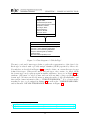
4.1 Overview
As mentioned in Chapter 2.2 an important requirement is the integration of the new
image analysis tool inside the existing IT infrastructure. The current tool in use expects
a folder with images and corresponding XML files of the same name. The XML file
contains information about the image, its origin and how it has to be analyzed within
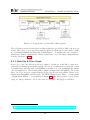
the “ImageFile/Processing” node. A more formal definition is given in Table 4.1.
ImageFile
Processing
Order
[System]
[ID]
[PatientID]
[ImageID]
Analysis
[Graph]
[ID]
Source
[OriginalUri]
[Width]
[Height]
[Zoom]
[Stain]
[Block]
[Schnitt]
The file to proceed
Processing information
[opt] Order information
[opt] System used for the order
[opt] ID of the order
[opt] Patient ID of the order
[opt] Image ID of the order
Analysis information
Filter graph file containing the analysis pipeline
Configuration to choose for the analysis
Source information
Name of the source file
Width of the source file
Height of the source file
[opt] Zoom level of the tissue scanned as source file
[opt] Staining of the tissue scanned as source file
[opt] Block ID of the tissue scanned as source file
[opt] Slice number of the tissue scanned as source file
14
CHAPTER 4. SYSTEM INTEGRATION
Target
[ImageName]
[X]
[Y]
[Width]
[Height]
[Xres]
[Yres]
[Zstack]
[Field]
[OverviewName]
Classification
ObjectClass
[ID]
[Color]
[Name]
Properties
...
ImageObject
[ID]
[ObjectClass]
Properties
...
Contour
[ContourWidth]
[ContourHeight]
[ContourArea]
[ContourCenterX]
[ContourCenterY]
Point
[X]
[Y]
Target information
Name of the target file
X origin on the source file
Y origin on the source file
Width of the target file
Height of the target file
X resolution of the target file (in mm/pixel)
Y resolution of the target file (in mm/pixel)
[opt] Z position where to take the target file from
[opt] Area identifier where to take the target file from
[opt] Name for a target thumbnail
Classification information
Object’s classification definition
ID of the object classification
Color of the object classification
Name of the object classification
[opt] General property information of the processed file
[opt] Specific file property, e.g. <P1>1</P1>
[opt] Extracted object information
[opt] ID of the extracted object
[opt] Classification of the extracted object
[opt] Object’s property information
[opt] Specific object property, e.g. <P1>1</P1>
[opt] Object’s contour information
[opt] Width of the object’s contour
[opt] Height of the object’s contour
[opt] Area of the object’s contour
[opt] X coordinate of the object’s contour center
[opt] Y coordinate of the object’s contour center
[opt] Specific point on the object’s contour boundary
[opt] X coordinate of the object’s contour point
[opt] Y coordinate of the object’s contour point
Table 4.1: XML definition for image metadata.
After proceeding such an image the analysis tool writes its results into the “ImageFile/Properties” and “ImageFile/ImageObject” nodes of the same XML file which later
on can be visualized and post processed by a web viewer. If our new image analysis tool
would like to be compatible with the old one we have to be able to read a set of images
from a specific folder, analyze them and save the result in a new XML file readable
by the web viewer. The ability to read a set of images by our processing pipeline is
described in Subsection 5.2.1.
15
CHAPTER 4. SYSTEM INTEGRATION
Our system is not yet ready to integrate with the given infrastructure. Still, there
are several more interfaces to define. Firstly, how does the user interact with the analysis tool? As most of the time we have sets of data to process, the tools at the hospital are
intended to be used in batch process. We can easily do so by implementing the analysis
tool as a command line application. However, we then face the problems as we need
direct access to the tool, we need a Microsoft Windows computer to run an analysis on
and most users prefer graphical user interfaces instead of command prompts. We could
offer a command line application with a graphical user interface and an intermediate
application server which makes our tool accessible also for users at the hospital who do
not have direct access. However, this would result in a lot of complexity and additional
tools to maintain.
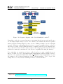
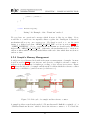
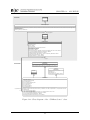
Regarding to the previous project we implemented the tool “Patho Study & Research”
(PSR), a web based inventory system with a dedicated Microsoft SQL database. Instead of implementing a complex application server we could easily extend the already
given PSR system which then is also available to everybody and independently of its
operating system. Furthermore, our analysis tool do not need an additional graphical
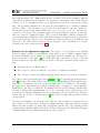
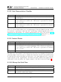
user interface which reduce complexity and supports maintenance. Figure 4.1 visualize
the interaction of both tools.
<<PHP / Zend>>
Patho Study & Research
Command Line
Prompt
Input
Annotation Import
..
<<Image>>
Cell Nucleus
Annotation
Feature Import
<<Annotations>>
.tif
Output Validation
.xml
<<C++ / DirectShow>>
Image Analysis
Export
x
xxx x xx
xxxxxx
..
..
<<Subimage + <<Features>> <<Subimage>>
Features>>
.jpg
.xml
.jpg
Figure 4.1: Overview of the image analysis pipeline integration.
16
CHAPTER 4. SYSTEM INTEGRATION
As we can see, the PSR system calls the image analysis tool with parameters which
define the path to an image and the properties how to analyze this image. The output,
as described, has to be an XML file e.g. with resulting features. Next to the XML
file we may provide additional data as e.g. image files. One could be the origin image
tile which can be visualized in combination with the XML features by the existing web
viewer. Another image tile could directly visualize the features found during the analysis.
A requirement we put aside until now is the ability to evaluate an algorithm from
our analysis tool. To do so we firstly need labeled data which we can compare with
the outcome of our analysis process. The so obtained evaluation measurements could
be saved additionally within the resulting XML file. The labeled data could be load
from a simple XML file containing annotations or downloaded from the PSR system
which already provides the required functinoalities. The same way we could upload our
resulting XML file directly to the PSR tool instead of saving the file locally.
More details about the overall process are provided by the following sections.
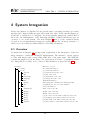
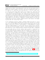
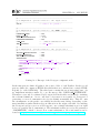
4.2 Graphical User Interface
The graphical user interface is implemented in the already given PSR system. Therefore,
we extend the system with a new routine as visualized in Figure 4.2 which allows the user
to define settings, to run the analysis process and to acquire feedback about the actual
results. The settings page is a simple web form which values are used as parameters
while calling the image analysis tool by command prompt. The user will see the status of
the image analysis tool by an automatically refreshing status page where the underlying
web application grab the output of the IA tool, written in the standard output stream
(stdout), and prepare it as web content. After the IA tool finished the user is redirected
to an overview page containing statistic information and the results from the analysis.
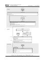
(a) Preparation form
17
CHAPTER 4. SYSTEM INTEGRATION
(b) Status page
(c) Process summary
Figure 4.2: Graphical user interfaces of the image analysis process.
When the PSR system calls the IA console tool by command prompt using the function
“$handle = popen($cmdCommand)” it holds a handle to the executing program. Using
this handle with the function “$buf f er = f gets($handle)” we can access the stdout
stream and receive all status reports from the IA tool. The PSR system redirect all
those information to the status page which is continuously updated for the user.
18
CHAPTER 4. SYSTEM INTEGRATION
4.3 Data Transfer
The data transfer between the image analysis tool and the PSR system is web based and
described in [3, p.48–50]. To upload a result file from the analysis the PSR tool expects
a POST request with XML data. More details about creating and parsing XML files
under C++ is given in Chapter 12.5. Depending on the library used the POST header is
generated automatically or need to be defined manually. An implementation example is
given by the “Contour Sink” filter described in Section 5.3.11. After sending the header
information we can start uploading the XML file which structure is given by Table 4.1.
4.4 Training Data Sets
The training data set for the cancerous tissue areas is given by the previous project.
However, for our nucleus detection algorithm an additional training set is required containing the annotated cell cores. The annotations were made with the Ventana image
viewer and saved as XML files. A detailed description about the XML structure can be
found in [3, p.49–50].
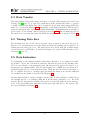
4.5 Data Evaluation
For evaluating an algorithm’s result from the image analysis tool we compare its resulting feature objects, the cell nucleus, with the annotations given by the training data.
We now can calculate a measurement value like the precision and recall values for expressing the algorithms quality. Like the mean square error (MSE) there are many more
statistical approaches for a measurement value. With the precision and recall values we
choose a simple and easy to calculate approach which information are already sufficient
for tweaking an algorithm as described in Chapter 5.4.
Another functionality to mention in this context is the “feature validation” which allows
the manual upload of a resulting XML file from the image analysis tool to the PSR
system. Hereby, the system calculates the precision and recall values from the intersections of the given XML data with annotations previously uploaded to the system. The
process is visualized in Figure 4.3.
19
CHAPTER 4. SYSTEM INTEGRATION
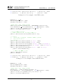
(a) Preparation form
(b) Validation report
Figure 4.3: Graphical user interfaces of the feature validation process.
The intersection itself is calculated on the Microsoft SQL Server which also holds the
annotation data. Since SQL Server 2008 spatial data are natively supported which
provides useful functions for handling geometry data. For more information we refer to
the official documentation at https://msdn.microsoft.com/en-us/bb933790.aspx.
20
CHAPTER 5. IMAGE ANALYSIS TOOL
5 Image Analysis Tool
The current chapter describes the technical details about the implementation of the Image Analysis tool (IA) using DirectSow as internal image processing pipeline. We start
with an overview of DirectShow and discuss specialized filters later on. Software tests
and evaluation scenarios can be found in Chapters 6 and 7. The results obtained by the
IA tool are described in Chapter 8.
The source code itself is listed in the appendix 12.9 and available as attached material, documented by appropriate comments.
5.1 Overview
The IA tool can be considered as a wrapper for the DirectShow pipeline. The command
line tool expects three parameters to initialize and to run the analysis process. The
parameters are enlisted in Table 5.1.
Parameter Description
image file
The image file to analyze.
graph file
A GRF file contains the filter graph to execute. The filter graph defines
the filter in use, how they are connected with each other and defines the
standard settings. It is also called execution plan.
config id
The configuration ID defines the set of filter configurations to load.
Table 5.1: Parameters of the IA tool.
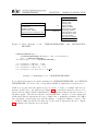
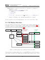
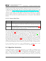
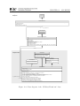
The internal data flow is visualized in Figure 5.1. We first load the filter graph, set up the
participating filters with properties defined by the configuration ID and run the graph
with the specified image file. Hereby, the image file parameter is treated like a normal
filter property, e.g. the logging level of a filter, and set during the filter configurations.
get filter
from graph
graph ß LoadGraphFile
config ß LoadConfigFile
set filter properties
from config
for each filter in config
main
Figure 5.1: Main sequence of the IA tool.
21
run image
processing pipeline
CHAPTER 5. IMAGE ANALYSIS TOOL
The requirement, enlisted in Chapter 2.2, is the support of a restorable execution plan.
Therefore, the tool distinguishes between a graph file and a configuration file for more
flexibility. While the graph file containing the graph in a modified Backus-Naur Form
(BNF) is specified by Microsoft1 , the configuration file is newly defined in XML notation
as given in Table 5.2. All attributes are written in brackets and the XML definition is
omitted. XML is the preferable format and widely used in the hospital’s environment.
Graph
[Name]
[Configurations]
Configuration
[ID]
Filters
Filter
[Name]
Settings
Setting
Key
Value
The root node containing all related configurations
Name of the graph
Number of available configurations
A specific configuration
ID of the configuration
All filters specified by the configuration
A specific filter
Name of the filter
All settings of the filter
A specific setting
Key of the setting
Value of the setting
Table 5.2: XML definition of a graph configuration.
A possible configuration file may show as follow:
<? xml v e r s i o n=” 1 . 0 ” s t a n d a l o n e=” y e s ” ?>
<Graph Name=” Graph001 ” C o n f i g u r a t i o n s=” 1 ”>
<C o n f i g u r a t i o n ID=” 1 ”>
< F i l t e r s>
< F i l t e r Name=”IA ( Pre ) Simple Transform F i l t e r ” />
<S e t t i n g s>
<S e t t i n g Key=” LogLevel ” v a l u e=”INFO” />
<S e t t i n g Key=” e f f e c t ” Value=” 1005 ” />
</ S e t t i n g s>
</ F i l t e r>
</ F i l t e r s>
</ C o n f i g u r a t i o n>
</ Segmentation>
We now have a configured filter graph which we can run. Regarding how is this filter
graph is build up and how we can control it, we start our explanation with a short
introduction to DirectShow. However, the concept behind can be found not only in DirectShow but also in many other filter graph pipelines. The graph consists of three filter
1
The format specification is given at
https://msdn.microsoft.com/en-us/library/windows/desktop/dd388788(v=vs.85).aspx
22
CHAPTER 5. IMAGE ANALYSIS TOOL
types: a source, a transformation and a sink filter. As the names suggest, the source
filter loads a file, the transform filter manipulates them and the sink filter saves them
again. The graph can be composed by any number of those filters which then are linked
with each other by pins. While the source and sink filter most of the time only provide
a single pin and the transformation filter provides two pins there are no hard limitations.
While connecting pins or starting and stopping the graph a single thread is involved:
the application thread. This thread validates filter connections for compatibility and,
in its very basic form, starts a new thread in each source filter, the so called streaming
threads. Such a thread load data from a given source, traverse through the graph and
save the data due a sink filter. After handling the data it returns back to the source
filter and delete the before allocated memory. Using this approach limits us to a sequential execution of the pipeline without possibility of concurrency. This contradict
the requirement of a performance pipeline as described in Chapter 2.2. We could think
about to initialize new threads by ourselves and let them run over a defined number of
filters or somehow initialize several filter graphs in parallel. A much simpler solution is
described in terms of DirectShow filters under Windows Embedded Compact 72 . Here,
we use the COutputQueue class on each output pin which is managed by a dedicated
and individual thread. After loading a data sample in the source filter the first streaming
thread hand over his data into a COutputQueue and returns immediately to load a next
data sample. The sample is then taken by a second streaming thread which proceed the
sample in the down-streaming filter and, again, hand it over to the next COutputQueue.
Like before, the second streaming thread returns to his origin queue and take the next
sample to proceed. This way, each filter can run concurrently whenever work is available.
However, the approach has one pitfall to care about. The more filters we integrate in
our graph the more queues we have and the more potential data we could store there.
Not to exceed our memory limitations we have to care about this issue by ourselves.
Generally we should proceed non-oversized images and reduce there size as the number
of filters inside the pipeline increases. Figure 5.2 summarize the described components
of a DirectShow filter graph.
2
https://msdn.microsoft.com/en-us/library/jj659790(v=winembedded.70).aspx
23
CHAPTER 5. IMAGE ANALYSIS TOOL
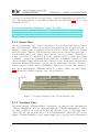
Figure 5.2: Components of a DirectShow filter graph1 .
The following sections describe the base filters which are provided by Microsoft more in
detail. The source code is provided with the Windows SDK and located under “[SDK
Root]/Samples/Multimedia/DirectShow/BaseClasses”. Compiling the base classes results in the library “strmbase.lib” which is used later on for the image analysis filters
described in Section 5.2.1.
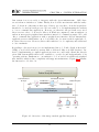
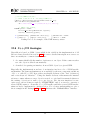
5.1.1 Build Up A Filter Graph
Before we go into any details about how a filter looks like we would like to start more
generally by building up a first filter graph. We can do so either using a graph editor with
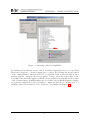
a graphical user interface such as GraphEdit from Microsoft or programmatically within
our own application. We starting with a simple example using GraphEdit. We would
like to proceed our before acquired images by an edge detection algorithm. Therefor, we
simply start GraphEdit and insert the “IA TIFF Ventana Source Filter” over the menu
“Graph/Insert Filters...” as visualized in Figure 5.3. The filter is then located in the
category “Image Analysis”. We do the same for the filter “IA (Rep) Sobel Filter”.
1
Adapted from
https://msdn.microsoft.com/en-us/library/windows/desktop/dd390948(v=vs.85).aspx
24
CHAPTER 5. IMAGE ANALYSIS TOOL
Figure 5.3: Inserting a filter in GraphEdit.
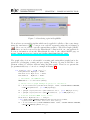
By clicking and holding the mouse button on a filter’s input pin an arrow occur which
than can be dragged to a desired output pin to connect. By releasing the mouse button
on the output pin the connection is tried to be establish. If the connection fails an error
message appears, otherwise the arrow remains. Doing so from the source filter to the
Sobel filter automatically implies an RGB converter which is necessarily as the format
of the Ventana images is RGB24 while the Sobel filter expects RGB32 images. Finally,
we perform a right click on the Sobel filter’s output pin and choose “Render Pin” for
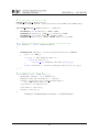
including Microsoft’s standard “Video Renderer” as visualized in Figure 5.4.
25
CHAPTER 5. IMAGE ANALYSIS TOOL
Figure 5.4: Rendering a pin in GraphEdit.
We now have an executable pipeline which can be applied for all tiles of the source image
using the run button ( ) or can process each tile separately using the seek function
( ). Moreover, we can also save the current filter graph by “File/Save Graph (.GRF)”
which later on can be restored by the FilterGraph or imported in our own application.
For more information about the FilterGraph we refer to the official MSDN page at
https://msdn.microsoft.com/en-us/library/dd377601(VS.85).aspx.
The graph editor is is not only useful for creating and saving filter graphs but is also
practical for debugging, testing and prototyping. However, we may would like to implement a filter by ourselves without using any filter graph. Therefore we present the
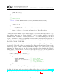
programmatically way of our above example in Listing 5.1.
v o i d main ( i n t argc , c h a r * argv [ ] ) {
I G r a p h B u i l d e r * pGraph = NULL;
I M e d i a C o n t r o l * p C o n t r o l = NULL;
IMediaEvent
* pEvent = NULL;
// I n i t i a l i z e t h e COM l i b r a r y .
HRESULT hr = C o I n i t i a l i z e (NULL) ;
// C r e a t e f i l t e r graph manager & query f o r i n t e r f a c e s .
hr = C o C r e a t e I n s t a n c e ( CLSID FilterGraph , NULL, CLSCTX INPROC SERVER,
,→ I I D I G r a p h B u i l d e r , ( v o i d * * )&pGraph ) ;
hr = pGraph−>Q u e r y I n t e r f a c e ( I I D I M e d i a C o n t r o l , ( v o i d * * )&p C o n t r o l ) ;
hr = pGraph−>Q u e r y I n t e r f a c e ( IID IMediaEvent , ( v o i d * * )&pEvent ) ;
// Load t h e Ventana TIFF s o u r c e f i l t e r
IBaseFilter * pTiffSource = nullptr ;
c o n s t GUID CLSID IATIFFSOURCE{0 x30f6349d , 0 xb832 0 x4f09 ,
,→{0 xa9 , 0 x16 , 0 xb7 , 0 xd5 , 0 x c f , 0 x c f , 0 xeb , 0 x6c } } ;
hr = C o C r e a t e I n s t a n c e (CLSID IATIFFSOURCE , NULL, CLSCTX INPROC SERVER,
,→IID PPV ARGS(& p T i f f S o u r c e ) ) ;
26
CHAPTER 5. IMAGE ANALYSIS TOOL
// S e t t h e image t o p r o c e e d
IFileSourceFilter * fileSourceFilter = nullptr ;
p T i f f S o u r c e −>Q u e r y I n t e r f a c e ( I I D I F i l e S o u r c e F i l t e r ,
,→ ( v o i d * * )&f i l e S o u r c e F i l t e r ) ;
f i l e S o u r c e F i l t e r −>Load (L”C: \ \ tmp\\myImage . t i f ” , NULL) ;
hr = pGraph−>A d d F i l t e r ( p T i f f S o u r c e , L” IATIFFSource ” ) ;
// Load t h e S o b e l f i l t e r
IBaseFilter * pSobelFilter = nullptr ;
c o n s t GUID CLSID IASOBELFILTER{0 x71ac9203 , 0 x 4 a f c , 0 x42a9 ,
,→{0 xae , 0 x17 , 0 x12 , 0 x69 , 0 x9f , 0 x55 , 0 xaa , 0 x3 } } ;
hr = C o C r e a t e I n s t a n c e (CLSID IASOBELFILTER , NULL,
,→CLSCTX INPROC SERVER, IID PPV ARGS(& p S o b e l F i l t e r ) ) ;
hr = pGraph−>A d d F i l t e r ( p S o b e l F i l t e r , L” I A S o b e l F i l t e r ” ) ;
// E s t a b l i s h c o n n e c t i o n s
I P i n * pOut = NULL;
hr = FindUnconnectedPin ( p T i f f S o u r c e , PINDIR OUTPUT, &pOut ) ;
hr = C o n n e c t F i l t e r s ( pGraph , pOut , p S o b e l F i l t e r ) ;
pOut−>R e l e a s e ( ) ;
hr = FindUnconnectedPin ( p S o b e l F i l t e r , PINDIR OUTPUT, &pOut ) ;
pGraph−>Render ( pOut ) ;
pOut−>R e l e a s e ( ) ;
// O p t i o n a l l y s a v e f i l t e r graph
// SaveGraphFile ( pGraph , L”C: \ \ tmp\\myGraph . g r f ” ) ;
i f (SUCCEEDED( hr ) ) {
// Run t h e graph .
hr = pControl−>Run ( ) ;
i f (SUCCEEDED( hr ) ) {
l o n g evCode ;
pEvent−>WaitForCompletion ( 2 0 0 0 0 / * ms * / ,&evCode ) ;
}
}
S a f e R e l e a s e (& p T i f f S o u r c e ) ;
S a f e R e l e a s e (& p S o b e l F i l t e r ) ;
pControl−>R e l e a s e ( ) ;
pEvent−>R e l e a s e ( ) ;
pGraph−>R e l e a s e ( ) ;
CoUninitialize () ;
}
Listing 5.1: Programmatically implementation of a filter graph.
The programmatically implementation is quite similar to the filter graph buildup with
GraphEdit. We create the filter graph itself and the participating filters, connect the
pins with each other, add the video renderer and run the graph. As before, the RGB
27
CHAPTER 5. IMAGE ANALYSIS TOOL
converter is automatically involved due image format incompatibility as described before. The implementation of all additional functions given in Listing 5.1 can be found
at MSDN as follow:
General Graph-Building Techniques - Connect Two Filters
https://msdn.microsoft.com/en-us/library/windows/desktop/dd387915(v=vs.85).aspx
General Graph-Building Techniques - Find an Unconnected Pin on a Filter
https://msdn.microsoft.com/en-us/library/windows/desktop/dd375792(v=vs.85).aspx
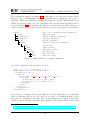
5.1.2 Source Filter
The most interesting part on the source filter is not the filter itself but its related
pin “CSourceStream”. Whenever the filter graph changes from a stopped state into a
running or paused state its application thread calls the “Active” method on all pins
inside the graph. Thereby, “CSourceStream” pins react in a special way and create a
new streaming thread each. Such a thread has his own, never ending, “ThreadProc”
routine and reacts on commands sent by the application thread. If the filter graph
is running or paused the streaming thread enters the “DoBufferProcessingLoop” and
creates an empty sample, fills it with data, delivers it to the output queue and releases it
afterward. During all this steps we only call once the underlying source filter “CSource”.
This is, when we call the method “FillBuffer”. Inherit from a source filter means we
have only to implement the “FillBuffer” method to compile a valid source filter. Figure
5.5 visualizes the sequence diagram of the “CSourceStream”.
called by
application thread
sample ß GetDeliveryBuffer
<<pure virtual>>
FillBuffer(sample)
Deliver(sample)
Release(sample)
DoBufferProcessingLoop [proceeding a sample]
cmd ß GetRequest
If cmd == CMD_RUN || cmd == CMP_PAUSE
ThreadProc [handle incomming commands from the application thread]
Active [create streaming thread]
Figure 5.5: Sequence diagram of the “CSourceStream” pin.
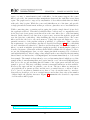
5.1.3 Transform Filter
The transform filter “CTransformFilter” is prepared for holding two pins. One input pin
“CTransformInputPin” and one output pin input pin “CTransformOutputPin”. When
receiving a sample from an up-stream filter the “Receive” method of the input pin is
called. The pin calls the same method on “CTransformFilter” which then process the
sample. It firstly initializes a new output sample and copies the header information
28
CHAPTER 5. IMAGE ANALYSIS TOOL
from the input to the output sample. It then transform the input sample into the
output sample and delivers the output sample to the down-stream’s input pin. At the
end it releases the output sample again (the input sample will be released by the caller of
“CTransformInputPin::Receive”). Inherit from the transform filter means we have only
to implement the “Transform” method to compile a valid transformation filter. Figure
5.6 visualizes the sequence diagram of the “CTransformFilter”.
called by previous
streaming thread
outSample ß InitializeOutputSample(inSample)
[get buffer from allocator & copy sample header]
<<virtual>>
Transform(inSample, outSample)
Deliver(sample)
Release(sample)
inSample ß Receive
Figure 5.6: Sequence diagram of the “CTransformFilter”.
An inconsistency is highlighted in Figure 5.6. When delivering a sample to the input pin
of the down-stream filter the base implementation directly calls the “Receive” method
of this pin. In this situation the “CTransformOutputPin” has no functionality but only
links the transform filter with the input pin from a down-stream filter. Instead, we should
call the “Deliver” method of the output pin so we could invoke additional functionality
before sending the sample. This behavior is corrected in the “CIABaseTransform” filter
as described later on.
5.1.4 Sink Filter
The simplest of all base filters is the sink filter. When receiving a sample from an
up-stream filter the “Receive” method of the “CRenderInputPin” is called which only
validates the sample. For a meaningful action we should call a method like “SaveSample”
on the underlying sink filter. As there is no explicit base sink filter available we have to
implement one by ourselves; inheriting from “CBaseFilter.
5.1.5 Filter Connection
DirectShow has an intelligent system for validating pin connections. Generally, each
output pin has to proved one or more so called media types. The media type defines
the content of a sample by its type (e.g. Video), subtype (e.g. RGB24) and format
(providing additional information like bits per pixel). When connecting an output pin
with an input pin all provided media types by the output pin are tried until either the
input pin accepts or the connection is rejected. The base transform filters provide an
additional check when connecting the output pin with a down-stream input pin. We still
29
CHAPTER 5. IMAGE ANALYSIS TOOL
enumerate through all media types provided by the output pin and try to find a compatible one. However, as soon as we found one we do not yet connect the two pins. An
additional method “CheckTransform” is invoked to verify as we can transform the input
type into the output type. This method is essential for converters. Figure 5.7 visualizes
the validation sequence (also called “Media Type Negotiation”) when trying to connect
an output pin with an input pin. The validation is performed by the application thread.
<<pure virtual>>
CheckInputType
<<pure virtual>>
CheckTransform
<<pure virtual>>
CheckInputType
<<virtual>>
SetMediaType
<<virtual>>
CheckConnect
CheckMediaType
SetMediaType
<<virtual>>
CompleteConnection
CheckConnect
CheckMediaType
SetMediaType
CompleteConnection
(outputPin, mediaType) ß ReceiveConnection
CheckTransform
called by
application thread
<<virtual>>
CheckConnection
CheckMediaType
CheckTransform
<<virtual>>
CheckConnection
CheckMediaType
<<virtual>>
SetMediaType
<<virtual>>
CompleteConnect
AttemptConnection
<<virtual>>
SetMediaType
<<virtual>>
CompleteConnect
mediaType ß TryMediaTypes
AttemptConnection
Enumerate through all provided media types
If IsPartialSpecified(mediaType)
else
AgreeMediaType
(inputPin, mediaType) ß Connect [mediaType is initialized with the preferred type]
Figure 5.7: Sequence diagram from the connection process of two pins. The solid green
boxes represents input respective output pins while the shaded blue boxes
represents filter methods.
Moreover, DirectShow provides a mechanisms called “Intelligent Connection” which
makes connection possible even two media types are not compatible with each other.
Therefore, additional filters are systematically tried between the two incompatible pins,
hoping to find a valid conversion filter. An example for such a conversion filter is described in Section 5.2.3. We do not go into more details which can be found at the
following website: https://msdn.microsoft.com/en-us/library/windows/desktop/
dd390342(v=vs.85).aspx
5.1.6 Passing Data Between Filters
As described in Chapter 5.1 DirectShow uses so called sample packages as data containers
which then are passed from one filter to another. A sample contains a header and an
arbitrary data body whereas the header describes the data representation more in detail.
The header mainly contains the media type of the data, its size and time, if the sample
is part of a time ordered sequence, e.g. an image from a video. The media type itself
can be split up again in smaller attributes as presented in Figure 5.8.
30
CHAPTER 5. IMAGE ANALYSIS TOOL
_AMMediaType
jmajortype:IGUID
jsubtype:IGUID
jbFixedSizeSamples:IBOOL
jbTemporalCompression:IBOOL
jlSampleSize:IULONG
jformattype:IGUID
jpUnk:IIUnknownY
jcbFormat:IULONG
jpbFormat:IBYTEY
CMediaType
joperator=INconstICMediaTypeuG:ICMediaTypeu
joperator==INconstICMediaTypeuG:IBOOL
joperatorV=INconstICMediaTypeuG:IBOOL
jSetNconstICMediaTypeuIrtG:IHRESULT
jIsValidNG:IBOOL
jAllocFormatBufferNULONGG:IBYTE
Figure 5.8: Class diagram of “CMediaType”.
The major, sub and format types define together the representation of the data body.
Each type is related with a globally unique identifier (GUID) specified by Microsoft3 .
Nevertheless, as described in Chapter 5.2 we can also define our own media types for user
defined data types. Whereas the major and sub types only consists of a single GUID
the format type can be split up again in smaller attributes. As we see in Figure 5.8 the
attribute “pbFormat” is only a pointer and can hold any kind of data, specified by the
format type. We first can allocate memory using the method “AllocFormatBuffer” and
then assign format information like a “VIDEOINFOHEADER”4 . For a better understanding we give a code snipped in Listing 5.2 as well as the “VIDEOINFOHEADER”
and its internal “BITMAPINFOHEADER” structure in Figure 5.9.
3
4
The type descriptions are given at
https://msdn.microsoft.com/en-us/library/windows/desktop/dd390670(v=vs.85).aspx
https://msdn.microsoft.com/en-us/library/windows/desktop/dd407325(v=vs.85).aspx
31
CHAPTER 5. IMAGE ANALYSIS TOOL
BITMAPINFOHEADER
VIDEOINFOHEADER
XrcSource:MRECT
XrcTarget:MRECT
XdwBitRate:MDWORD
XdwBitErrorRate:MDWORD
XAvgTimePerFrame:MREFERENCE_TIME
1111
XbmiHeader
XbiSize:MDWORD
XbiWidth:MLONG
XbiHeight:MLONG
XbiPlanes:MWORD
XbiBitCount:MWORD
XbiCompression:MDWORD
XbiSizeImage:MDOWRD
XbiXPelsPerMeter:MLONG
XbiYPelsPerMeter:MLONG
XbiClrUsed:MDWORD
XbiClrImportant:MDWORD
Figure 5.9: Class diagram of the “VIDEOINFOHEADER” and “BITMAPINFOHEADER”.
VIDEOINFOHEADER * p v i =
,→ (VIDEOINFOHEADER* ) pMediaType−>A l l o c F o r m a t B u f f e r (
,→ s i z e o f (VIDEOINFOHEADER) ) ;
ZeroMemory ( pvi , s i z e o f (VIDEOINFOHEADER) ) ;
pvi−>bmiHeader . biWidth = 1 0 2 4 ;
pvi−>bmiHeader . b i H e i g h t = 1 0 2 4 ;
pvi−>bmiHeader . biBitCount = 2 4 ;
pvi−>bmiHeader . bi C o m pr e s s io n = BI RGB ;
...
Listing 5.2: Initialization of a “VIDEOINFOHEADER”.
For a detailed description about the attributes in “VIDEOINFOHEADER” and “BITMAPINFOHEADER” we refer to the corresponding MSDN documentation as given above.
Until now we put back the question how we create or destroy a sample and how we
manage its life-cycle. As addressed in Figure 5.2 we can find a memory allocator between each two filters which is initialized by the application thread due the creation of
the filter graph. The thread calls the “DecideBufferSize” method on each output pin
which then asks its up-stream allocator’s buffer size or manually calculates the buffer
size depending on the media type and the number of requested buffers to reserve. The
so obtained buffer specification is then set for the next down-stream allocator. Figure
5.10 visualizes the sequence more in detail.
32
CHAPTER 5. IMAGE ANALYSIS TOOL
Figure 5.10: Sequence diagram of the “DecideBufferSize” method1 .
Depending on the above reserved memory a streaming thread can now ask an allocator
for an empty sample and proceed it. If no memory is available the thread is paused
until a currently existing sample becomes obsolete. Making a sample obsolete is straight
forward. Whenever a streaming thread receives or creates a sample it has to release it
after its proceeding. When calling the method “sample->Release()” the internal reference count is decreased. If this counter reaches 0 the sample get automatically deleted
and the free memory is announced to the allocator originally allocating the memory.
For completing our excursion we have to talk about how to pass a sample from one
filter to another one. If no other functionality is implemented a filter calls the “Deliver”
method of its output pin which then calls “m pInputPin->Receive(pSample)” to pass
the sample to the connected input pin of the down-stream filter. Not to forget: the
sample has to be released after returning from the down-stream filter.
1
Adapted from https://msdn.microsoft.com/en-us/magazine/cc301631.aspx
33
CHAPTER 5. IMAGE ANALYSIS TOOL
5.1.7 Filter Registration
Before we can finally use our DirectShow filters we have to register them to the system.
Therefore, we have to compile them as a dynamic link library (DLL) offering three C
functions: “DllMain”, “DllRegisterServer” and “DllUnregisterServer”. Where the first
function is the entry point of our dynamic library the following two functions implement the registration and unregistration routines. Listing 5.3 gives an example of those
routines.
STDAPI D l l R e g i s t e r S e r v e r ( )
{
HRESULT hr ;
I F i l t e r M a p p e r 2 *pFM2 = NULL;
hr = A M o v i e D l l R e g i s t e r S e r v e r 2 (TRUE) ;
i f (FAILED( hr ) ) r e t u r n hr ;
hr = C o C r e a t e I n s t a n c e ( CLSID FilterMapper2 , NULL,
,→CLSCTX INPROC SERVER, I I D I F i l t e r M a p p e r 2 , ( v o i d * * )&pFM2) ;
i f (FAILED( hr ) ) r e t u r n hr ;
hr = pFM2−>C r e a t e C a t e g o r y ( CLSID ImageAnalysisCategory ,
,→MERIT NORMAL, L” Image A n a l y s i s ” ) ;
i f (FAILED( hr ) ) r e t u r n hr ;
hr = pFM2−>R e g i s t e r F i l t e r (
CLSID MYFILTER ,
L” M y F i l t e r ” ,
NULL,
&CLSID IACategory ,
L” M y F i l t e r 0 1 ” ,
&r f 2 F i l t e r R e g
);
//
//
//
//
//
//
F i l t e r CLSID .
F i l t e r name .
D e vi ce moniker .
F i l t e r category .
I n s t a n c e data .
F i l t e r information .
pFM2−>R e l e a s e ( ) ;
r e t u r n hr ;
}
STDAPI D l l U n r e g i s t e r S e r v e r ( )
{
HRESULT hr ;
I F i l t e r M a p p e r 2 *pFM2 = NULL;
hr = A M o v i e D l l R e g i s t e r S e r v e r 2 (FALSE) ;
i f (FAILED( hr ) ) r e t u r n hr ;
hr = C o C r e a t e I n s t a n c e ( CLSID FilterMapper2 , NULL,
,→CLSCTX INPROC SERVER, I I D I F i l t e r M a p p e r 2 , ( v o i d * * )&pFM2) ;
i f (FAILED( hr ) ) r e t u r n hr ;
hr = pFM2−>U n r e g i s t e r F i l t e r ( &CLSID ImageAnalysisCategory ,
,→L” M y F i l t e r ” , CLSID MYFILTER) ;
34
CHAPTER 5. IMAGE ANALYSIS TOOL
pFM2−>R e l e a s e ( ) ;
r e t u r n hr ;
}
//
// D l l E n t r y P o i n t
//
e x t e r n ”C” BOOL WINAPI D l l E n t r y P o i n t (HINSTANCE,ULONG, LPVOID) ;
BOOL APIENTRY DllMain (HANDLE hModule , DWORD dwReason , LPVOID
,→ l p R e s e r v e d )
{
r e t u r n D l l E n t r y P o i n t ( (HINSTANCE) ( hModule ) , dwReason ,
,→ l p R e s e r v e d ) ;
}
Listing 5.3: Methods for register and unregister a DirectShow filter.
“DllRegisterServer” firstly creates a filter mapper object witch then can be used to register the new filter category “Image Analysis”, if not yet existing, and then to register
the filter itself. The function “DllUnregisterServer” do the same but unregister the filter
again. Each filter is defined by an unique class identifier (CLSID), which represents a
global unique identifier (GUID). This means as the class to register is only identified by
its GUID “CLSID MYFILTER”.
A last important fragment of the registration process is the “CFactoryTemplate”. When
registering a DirectShow filter the template gives all necessarily information such as the
function pointer to a method which can instantiate a filter object or the pointer to setup
information. If last one is set the filter is automatically registered within the “DirectShow Filters” category. As we would like to use our own category we set the parameter
to “NULL”. Listing 5.4 gives an example of the “CFactoryTemplate”.
CFactoryTemplate g Templates [ 1 ] =
{
{
L” M y F i l t e r ” ,
&CLSID MYFILTER ,
MyFilter : : CreateInstance ,
NULL,
NULL
},
};
//
//
//
//
//
F i l t e r name
F i l t e r CLSID
I n s t a n t i a t i o n func .
Init . function
Set−up i n f o r m a t i o n
Listing 5.4: Example of a template factory.
Additional information about registering a DirectShow filter can be found at https://
msdn.microsoft.com/en-us/library/windows/desktop/dd389099(v=vs.85).aspx or
in the Doxygen documentation of the source code as listed in 12.9.
35
CHAPTER 5. IMAGE ANALYSIS TOOL
5.2 Image Analysis Filters
After we get a deeper understanding on how DirectShow works we can start implementing our own image filters and integrate them into a filter graph. However, there are still
mechanisms missing or the above described sequences are not yet fully implemented.
Therefore, we implement a set of base filters specially for the Image Analysis tool which
are described in the next section. Afterward, we go into more details about how to
create used defined media types and how to convert them. Finally, we give an overview
of the implemented image analysis filter, there specifications and specialties.
5.2.1 IA Base Filters
As DirectShow we offer three base filters for image analysis: “CIABaseSource”, “CIABaseTransform” and “CIABaseSink”. While inheriting from one of the DirectShow base
classes implicates the implementation of at least one pin class and its underlying filter
class we would like to simplify this circumstance by offering a single filter class without
the need of an additional pin class. We therefor implementing the origin DirectShow
base classes and redirect abstract pin methods to its underlying filter class. This makes
it possible to inherit from a single filter class and combine all implementation details
together. Following we give a more detailed insight about the three image analysis base
classes.
IA Base Source The “CIABaseSource” class, which is inherited from “CSource”, can
be used to load full images or tiles of images to proceed. At first place, the “Load”
method is called when including the filter into the filter graph due inheritance from
“IFileSourceFilter”. Hereby, the chosen file name is stored and the two abstract methods “OpenFile” and “CloseFile” are called. In the first method we can open a handle
to the file and load all relevant information like width, height, bits per pixel (BPP) and
number of tiles. The first three values are important so the buffer allocator can be initialized when connecting the output pin of our source filter with a down-streaming input pin.
Hereby, we can calculate the required buffer size by W idth∗Height∗BP P . The number
of tiles is important to know when we proceed the last image from a file so we can stop
the graph afterward. We do so by incrementing a counter variable “m iFrameNumber”
each time we deliver a sample. If this counter reaches the maximum number of tiles
available we return the HRESULT “S FALSE” from the “FillBuffer” method and set
the counter back to 0; same happens when we stop the filter graph to indicate a reset.
Under DirectShow this means an “EndOfStream” message is delivered down-stream.
After calling “OpenFile” the method “CloseFile” releases the file handle again so we can
get access to the file as long as our graph is stopped. As soon as we change the state
from stopped to run or paused the application thread will call the method “Activate”
which again calls “OpenFile”. If we load the whole image into the buffer we can just
ignore the call. However, if we need additional information from the file we can reopen
it here. Vice versa, if the graph changes to the stop state the application thread calls
“Inactive” and with it the method “CloseFile”.
36
CHAPTER 5. IMAGE ANALYSIS TOOL
Now as we know how the file is accessed we need to read its data and pack it into
a sample to deliver. We do so by extending the data flow from 5.5. Within the method
“FillBuffer” we call the abstract method “GetImageDataPointer” with the actual frame
number as parameter. Depending on this parameter we can now either giving back a
pointer to the corresponding tile or a pointer to the whole image if we do not support
tiles.
As mentioned in Chapter 5.1 we would like to use a “COutputQueue” within our “CIABaseSourcePin” for the parallel execution of filter procedures. Hereby, we adapt the
same mechanism as we do for opening and closing the image handle. When calling the
“Active” method we initialize the “COutputQueue” and when calling the “Inactive”
method we destroy it again. Destroying the queues including all so far proceeded samples is possible as a stop command means we reset the whole filter graph. So our frame
counter is also reset to 0 and we have to start all over again with our analysis.
This is a base implementation and the behavior can freely be adapter. One example
is the “CIABaseSetSource” class which inherits directly from “CIABaseSource”. The
above described approach to read data works just fine for a single file. If we have a set
of images e.g. in a specify directory we have to call the “OpenFile” method not only
when we run the filter graph but each time we increment the frame counter. This is
exactly what happens in the “FillBuffer” method of the “CIABaseSetSource” class. We
first call “OpenFile” with the current frame number as parameter, get the pointer to the
image data by “GetImageDataPointer” amd close the file handle again by “CloseFile”.
A class diagram of the relation between “CIABaseSource” and “CIABaseSourcePin”
can be found in the appendix 12.4. Additional information can also be found in the
Doxygen documentation of the source code as listed in 12.9.
IA Base Transform The “CIABaseTransform” class, which is inherited from “CTransform”, can be used to manipulate our image data, packed inside a sample, while heading
down the filter stream. When receiving a sample through the “CTransformInputPin” it
is forwarded to our “Transform(inSample, outSample)” method inside “CIABaseTransform”. We expect most of the time as we only manipulate the input data. This means
we do not need the input as well as the output sample separately. Because of that,
we simply copy the input data into the new output sample and forward it the abstract
method “Transform(pMediaSample)”. In this way a programmer do not even need to
think about how to handle input and output samples but can directly work on the output sample which is then directly forwarded to the next filter. This behavior however
may not be intended all the time. If we think about a media type converter we need
both, the input as well as the output sample. Because there is not guarantee as both
samples have the same size we can not simply copy data from the input to the output
sample. For this reason the “Transform(inSample, outSample)” method is declared as
virtual so we can override it if needed.
37
CHAPTER 5. IMAGE ANALYSIS TOOL
As mentioned in Figure 5.6 there is an inconsistency in delivering a sample by the
“CTransform” filter. Because of that the method “Receive” was slightly adapted so the
“Deliver” method of the output pin is called.
Like the “CIABaseSourcePin” also the transform output pin is extended by a “COutputQueue”. The mechanisms and behaviors are thereby the same as described for the
“CIABaseSource” class.
A class diagram of the relation between “CIABaseTransform” and “CTransformInputPin” can be found in the appendix 12.4. Additional information can also be found in
the Doxygen documentation of the source code as listed in 12.9.
IA Base Sink The “CIABaseSink” class, which is inherited from “CBaseFilter”, can
be used to save image data traversed the processing pipeline. When a sink filter receives
data its input pin “CIABaseSinkInputPin” is called by the method “Receive”. Hereby,
we call the methods “OpenFile”, “SaveFrame” and “CloseFile” from the underlying
“CIABaseSink”.
As we only save data when we receive it we do not need to care if we read from a
single source of from a set of images. We only save sequentially our data and release the
handle as soon as work is done. For that, we do not need a class like “CIABaseSetSink”.
A class diagram of the relation between “CIABaseSink” and “CIABaseSinkInputPin”
can be found in the appendix 12.4. Additional information can also be found in the
Doxygen documentation of the source code as listed in 12.9.
5.2.2 User Defined Media Types
As previously described, based on the “VIDEOINFOHEADER”, we can change the format type of the media type with a user defined one of our choice. With our image
processing pipeline we would like to establish an own information header to store additional meta data. If e.g. we send an input image through the pipeline we would like
to save the resulting images at the same directory into a new results folder. However,
until now we can not pass this information through the pipeline so we have to extend
the given “VIDEOINFOHEADER”. The following Listing 5.5 shows the relevant code
fragments.
t y p e d e f s t r u c t tagIAVIDEOINFOHEADER : p u b l i c tagVIDEOINFOHEADER
{
w c h a r t * sourceName ;
wchar t * sourcePath ;
...
} IAVIDEOINFOHEADER;
38
CHAPTER 5. IMAGE ANALYSIS TOOL
HRESULT MySource : : GetMediaType ( CMediaType * pMediaType )
{
IAVIDEOINFOHEADER * p v i =
,→ (IAVIDEOINFOHEADER * ) pMediaType−>A l l o c F o r m a t B u f f e r (
,→ s i z e o f (IAVIDEOINFOHEADER) ) ;
ZeroMemory ( pvi , s i z e o f (IAVIDEOINFOHEADER) ) ;
pvi−>bmiHeader . biWidth = 1 0 2 4 ;
pvi−>bmiHeader . b i H e i g h t = 1 0 2 4 ;
pvi−>bmiHeader . biBitCount = 2 4 ;
pvi−>bmiHeader . bi C o m pr e s s io n = BI RGB ;
// A d d i t i o n a l meta i n f o r m a t i o n
pvi−>sourceName = L” MySource . png” ;
...
}
Listing 5.5: Initialization of an “IAVIDEOINFOHEADER”.
The above example only extends the format type but do not yet represents a new media
type. If we think about our cell nucleus detection algorithm, described in Chapter 5.3,
we could imagine as we only send found geometries of cell nucleus within sample packages
and not the whole image as such. We therefore need a new media type describing the
data structure we use for saving the geometry. In our case, we would like to send a
collection of centroids. However, before we go into details about the data structure we
firstly need a new major, sub and format type to define as given in Listing 5.6.
// new media type
// {05797 C20−D86F−44D7−82A3−FAC3991048AC}
DEFINE GUID( MEDIATYPE Metadata ,
0 x5797c20 , 0 xd86f , 0 x44d7 , 0 x82 , 0 xa3 , 0 xfa , 0 xc3 , 0 x99 , 0 x10 , 0 x48 , 0 xac ) ;
// new media sub−type
// {B836F1E4−BDB4−4D3A−87CB−28073BC72AB6}
DEFINE GUID(MEDIASUBTYPE CONTOURCOLLECTION,
0 xb836f1e4 , 0 xbdb4 , 0 x4d3a , 0 x87 , 0 xcb , 0 x28 , 0 x7 , 0 x3b , 0 xc7 , 0 x2a , 0 xb6 ) ;
// new media format type
// {96ABD28C−C961−4AB1−A281−3997B8FDFC3C}
DEFINE GUID( FORMAT IAMetaInfo ,
0 x96abd28c , 0 xc961 , 0 x4ab1 , 0 xa2 , 0 x81 , 0 x39 , 0 x97 , 0 xb8 , 0 xfd , 0 x f c , 0 x3c ) ;
Listing 5.6: GUID definitions of a new media type.
In a next step we can define the new media type format the same way like we did for
“IAVIDEOINFOHEADER” as given in Listing 5.7.
39
CHAPTER 5. IMAGE ANALYSIS TOOL
t y p e d e f s t r u c t tagIAMETAINFOHEADER {
...
i n t surfaceWidth ;
int surfaceHeight ;
IACONTOURINFOHEADER c i H e a d e r ;
} IAMETAINFOHEADER;
t y p e d e f s t r u c t tagIACONTOURINFOHEADER {
IADataStruct d a t a S t r u c t ;
IAElementType elementTypes ;
int containerSize ;
} IACONTOURINFOHEADER;
enum IADataStruct { dARRAY, dVECTOR, dLIST , dSTACK } ;
enum IAElementType { eBYTE, eINT , eFLOAT, eDOUBLE,
eBYTE PTR, eINT PTR ,
eFLOAT PTR, eDOUBLE PTR,
eCOORDINATE,
eCOORDINATE PTR} ;
Listing 5.7: Definition of the new media type format “IAMETAINFO”.
With the above structures we can now chose which data structure and which data types
we would like to implement. For our above centroid example we may use an integer
array. We then set the IACON T OU RIN F OHEADER :: dataStruct = dARRAY
and IACON T OU RIN F OHEADER :: elementT ypes = eIN T . The sample we would
like to fulfill with our data only expects a byte array so we can assign any arbitrary data
we like.
5.2.3 Media Type Conversion
A more complex example of a transform filter is a conversion filter. Again, we would
like to give an example from the given implementation. As described in Chapter 2.2 we
work with a BigTIFF file format containing BGR24 images. This means as each pixel
consists of 24 bits which are equally used for the blue, green and red channel. This
format should not be confused with RGB24 which stores the channels in inverted order.
The BGR24 format however can not be visualized by the given renderer from Microsoft.
We therefore need a converter. Again, the new BGR24 format can easily be established
by defining a new media sub-type as described in the previous chapter. Firstly, we need
to define the supported media types which includes two methods, the “CheckInputType”
and “GetMediaType”. The first method is called when a down-streaming input filter
tries a connection with our filter. Within “CheckInputType” we can decide to accept or
refuse the proposed media type. Listing 5.8 gives an example.
40
CHAPTER 5. IMAGE ANALYSIS TOOL
HRESULT MyConv : : CheckInputType ( c o n s t CMediaType * mtIn )
{
i f ( IsEqualGUID ( * mtIn−>Type ( ) , MEDIATYPE Video) )
{
i f ( IsEqualGUID ( * mtIn−>Subtype ( ) , MEDIASUBTYPE BGR24) )
{
VIDEOINFOHEADER * p v i =
(VIDEOINFOHEADER * ) mtIn−>Format ( ) ;
i f ( pvi−>bmiHeader . biBitCount == 2 4 )
r e t u r n NOERROR;
}
}
r e t u r n E FAIL ;
}
Listing 5.8: Example of the “CheckInputType” method.
In a next step our converter will try to connect to a down-stream filter’s input pin. We
therefore can offer supported media types by the “GetMediaType” method. When we
try to open a connection the application thread will ask this method for our supported
media types, each time with another position pointer. This process stops as soon as
an accepted media type is found or we return the value “VFW S NO MORE ITEMS”.
Listing 5.9 gives an example.
HRESULT MyConv : : GetMediaType ( i n t iPos , CMediaType * mtOut )
{
// Read i n p u t media type
HRESULT hr = m pInput−>ConnectionMediaType ( mtOut ) ;
VIDEOINFOHEADER * p v i = (VIDEOINFOHEADER* ) mtOut−>pbFormat ;
i f (FAILED( hr ) ) { r e t u r n hr ; }
switch ( iPos ) {
case 0:
// Convert h e a d e r i n f o r m a t i o n
mtOut−>SetSubtype (&MEDIASUBTYPE RGB32) ;
pvi−>bmiHeader . biBitCount = 3 2 ;
mtOut−>S e t S a m p l e S i z e (
,→pvi−>bmiHeader . biWidth * pvi−>bmiHeader . b i H e i g h t * 4 ) ;
pvi−>bmiHeader . b i S i z e I m a g e =
,→pvi−>bmiHeader . biWidth * pvi−>bmiHeader . b i H e i g h t * 4 ;
break ;
case 1:
...
default :
r e t u r n VFW S NO MORE ITEMS ;
}
r e t u r n S OK ;
}
Listing 5.9: Example of the “GetMediaType” method.
41
CHAPTER 5. IMAGE ANALYSIS TOOL
As mentioned in paragraph 5.2.1 after we found a valid media type we can still refuse
the connection due the “CheckTransform” method. Here, we can finally decide if a conversion is possible or not.
The transformation takes place in the method “Transform(inSample, outSample)” where
we get an input sample with the before set input media type and the output sample
with enough allocated memory to store the converted data in. In a first step we copy
the media header from the input to the output sample and adapt its header information
for the converted output media type. We then start converting the data. Listing 5.10
gives a simplified example.
HRESULT MyConv : : Transform ( IMediaSample * pIn , IMediaSample * pOut )
{
// Copy t h e h e a d e r i n f o r m a t i o n
HRESULT hr = Copy ( pIn , pOut ) ;
i f (FAILED( hr ) ) { r e t u r n hr ; }
// Adapt output media type
CMediaType pmtOut ;
m pOutput−>ConnectionMediaType(&pmtOut ) ;
pOut−>SetMediaType(&pmtOut ) ;
FreeMediaType ( pmtOut ) ;
// S t a r t c o n v e r t i o n
CMediaType mtIn = m pInput−>CurrentMediaType ( ) ;
VIDEOINFOHEADER * p v i I n =
(VIDEOINFOHEADER * ) mtIn . pbFormat ;
CMediaType mtOut = m pOutput−>CurrentMediaType ( ) ;
VIDEOINFOHEADER * pviOut =
(VIDEOINFOHEADER * ) mtOut . pbFormat ;
PBYTE pbInData , pbOutData ;
hr = pIn−>G e t P o i n t e r (&pbInData ) ;
i f (FAILED( hr ) ) { r e t u r n S FALSE ; }
hr = pOut−>G e t P o i n t e r (&pbOutData ) ;
i f (FAILED( hr ) ) { r e t u r n S FALSE ; }
i f ( IsEqualGUID ( mtIn . subtype , MEDIASUBTYPE BGR24) &&
IsEqualGUID ( mtOut . subtype , MEDIASUBTYPE RGB32) )
{
RGB24* p x l I n = (RGB24 * ) &pbInData [ 0 ] ;
RGB32* pxlOut = (RGB32 * ) &pbOutData [ 0 ] ;
f o r ( i n t y=0; y<p v i I n −>bmiHeader . b i H e i g h t ; y++) {
f o r ( i n t x=0; x<p v i I n −>bmiHeader . biWidth ; x++) {
pxlOut−>byte0 = p x l I n −>byte0 ;
pxlOut−>byte1 = p x l I n −>byte1 ;
pxlOut−>byte2 = p x l I n −>byte2 ;
pxlOut−>byte3 = 0 ;
42
CHAPTER 5. IMAGE ANALYSIS TOOL
p x l I n ++; pxlOut++;
}
}
}
...
r e t u r n Transform ( pOut ) ;
}
Listing 5.10: Example of the “Transform” method.
We now have an operational converter which however is lake in one thing. If we
would like to connect two incompatible filters together the “Intelligent Connection”
mechanism will not try our converter yet. We therefore need to to set the merit
during to a higher level than “MERIT DO NOT USE” as done in section 5.1.7, e.g.
“MERIT UNLIKELY”. Not to overstrain the mechanism we should rarely use merits
higher than “MERIT DO NOT USE”. Otherwise, the mechanism need to check more
and more filters while connecting invalid filters with each other which then needs more
and more time.
5.2.4 Sample’s Memory Management
A subject not yet discussed in details is the memory management of samples. As mentioned in section 5.1.6 we can increase and decrease a sample’s reference counter to
indicate if we need its data for further proceeding or if we release its resources. Figure
5.11 shows the life cycle of a sample and the method calls in which the reference counter
increases (<<AddRef>>) and decreases (<<Release>>).
<<AddRef>>
CIABaseSourcePin::
<<AddRef>>
Deliver
CSourceStream::
DoBufferProcessingLoop
Source
<<Release>>
CSourceStream::
DoBufferProcessingLoop
Output
Pin
Output
Queue
<<Release>>
CIABufferOutputQueue::
ThreadProc
<<AddRef>>
CIABufferTransformOutputPin::
<<AddRef>>
Deliver
CIABaseTransform::
Receive
Input
Pin
Transform
<<Release>>
CIABaseTransform::
Receive
Output
Pin
Output
Queue
Input
Pin
Sink
<<Release>>
CIABufferOutputQueue::
ThreadProc
Figure 5.11: Life cycle of a sample and its reference counter.
A sample is either created in the method “CSourceStream::DoBufferProcessingLoop” or
“CIABaseTransform::Receive” which both set the reference counter to 1. To release the
43
CHAPTER 5. IMAGE ANALYSIS TOOL
sample again we call the corresponding method at the end of the same method after we
finished proceeding the sample. A problem occurs as the streaming thread hand over
the sample into an output queue and return right after to release the sample again,
proceeding the next incoming sample. In this case the sample in the output queue will
not be valid anymore for further proceeding. Because of that we increase the reference
counter whenever delivering the sample to the output queue and decrease the reference
count whenever a queue thread returns from a down-stream filter. This approach works
with with both an output queue with and without running an independent streaming
thread. Furthermore, the behavior is implemented already into the image analysis base
classes which do not need any more consideration. For filters which do not follow the
standard approach we have to handle a sample’s reference count ourselves. An example
is given by the “IA - Contour Tracer” filter.
A more challenging problem are samples containing dynamic data such as a contour
vector. The standard samples which hold image data provide a fix memory block which
size can be previously defined by the images width, its height and the bits per pixel
(BPP). A contour vector, however, could contains zero or several hundreds or contours
each with a different number of contour points. Because of that we can not take the
same approach as used for the RGB or grayscale converters which takes the down-stream
filter’s media type, again containing the image’s dimensions and the BPP, to distinguish
the actual require memory to allocate. Another solution would be to calculate the contour array and its size while running the filter and establish a new media type to the
down-stream filter5 . This process however has a lot of disadvantages. Firstly, the data
stream has to be blocked while reconnecting the pin to the down-stream filter with a new
media type. The approach needs a lot of additional resources as all the down-stream
filters might need a reconnection due the media type change. Moreover, the new media type might not be accepted by a down-stream filter which will interrupt the whole
graph’s execution. In this situation we will lose all proceeding samples currently inside
the pipeline. A more robust solution is therefore preferred. As mentioned, if we could
keep the sample size constant, we do not need a reconnection during the filter graph’s
execution. We can do so by saving only a pointer to a contour structure inside the
sample which then has always the same size. We now face a new problem: who cleans
the contour structure’s memory when a sample is released? The simplest solution would
be to do so in a down-stream filter. But, this is not a valid solution as we can not assure
a secure cleaning. A third party filter might not even know as it needs to clean the sample. Another problem comes when we split up the filter graph into two branches. Which
branch has to clean the contour structure and how can we manage the circumstance as
a filter from one branch could clean up the contour structure while another filter from
the other branch still needs the data? There is only one proper solution left: we have
to implement a customized memory allocator. As described in section 5.1.3 each sample
has it’s own reference counter. As soon as this counter falls to zero it calls its allocator
for releasing the memory. With a customized allocator we could invoke this process and
5
For more details please refer to
https://msdn.microsoft.com/en-us/library/windows/desktop/dd388731(v=vs.85).aspx
44
CHAPTER 5. IMAGE ANALYSIS TOOL
release the memory by ourselves. The main advantage is as the down-stream filters do
not need to know about how to clean up the sample but only decrease the sample’s
reference counter whenever they finished proceeding the sample. The code of such a
customized allocator is given in Listing 5.11.
c l a s s MyAllocator : p u b l i c CMemAllocator
{
public :
MyAllocator (HRESULT * phr ) :
,→CMemAllocator (TEXT( ” MyAlloc \0 ” ) ,NULL, phr ) { } ;
˜ CIAContourMemAllocator ( ) { } ;
HRESULT A l l o c ( ) {
// a l l o c a t e r e q u e s t e d memory & p r e p a r e s a m p l e s
// s e e a l s o i m p l e m e n t a t i o n o f ” CMemAllocator ”
// u s e r d e f i n e d s a m pl e s can be i n i t i a l i z e d h e r e
};
STDMETHODIMP R e l e a s e B u f f e r ( IMediaSample * pSample ) {
/ * R e l e a s e t h e COM o b j e c t b e f o r e r e u s i n g i t s a d d r e s s p o i n t e r * /
IUnknown * comObject ;
pSample−>G e t P o i n t e r ( (BYTE* * )&comObject ) ;
comObject−>R e l e a s e ( ) ;
// put sample back on f r e e l i s t f o r r e c y c l i n g
// s e e a l s o i m p l e m e n t a t i o n o f ” CMemAllocator ”
};
};
Listing 5.11: Implementation of a memory allocator.
In a next step we need to integrate the new allocator into one of our filters. Talking about the contour structure initialized in a transformation filter we have to set the
output pin’s allocator to our customized one. An important fact to know is as the
output pin by default tries to assign to the down-stream’s input pin’s allocator by calling the method “CIATransformInputPin::GetAllocator” before initializing an own one6 .
Because of that we have to overwrite two methods. Firstly, the “CIABufferTransformOutputPin::DecideAllocator” method: here, we need to skip the trial of assigning the
input pin’s allocator which would be successful if no unexpected error occurred while
building up the filter graph. In a next step the output pin tries its own allocator by
calling the “CIABufferTransformOutputPin::InitCustomOutPinAllocator” method. An
example implementation of this method is given in Listing 5.12.
6
For more details please refer to
https://msdn.microsoft.com/en-us/library/windows/desktop/dd377477(v=vs.85).aspx
45
CHAPTER 5. IMAGE ANALYSIS TOOL
HRESULT M y F i l t e r : : I n i t C u s t o m O u t P i n A l l o c a t o r ( IMemAllocator ** p p A l l o c ) {
HRESULT hr = S OK ;
MyAllocator * p A l l o c = new MyAllocator (&hr ) ;
i f ( ! p A l l o c ) r e t u r n E OUTOFMEMORY;
i f (FAILED( hr ) )
{ d e l e t e pAlloc ;
r e t u r n hr ;
}
r e t u r n pAl loc −>Q u e r y I n t e r f a c e ( IID IMemAllocator , ( v o i d * * ) p p A l l o c ) ;
}
Listing 5.12: Example of the “InitCustomOutPinAllocator” method.
For more details we refer to the implementation of the “IA - Contour Tracer” filter.
5.3 Cell Nucleus Detection
After the discussion about the basics of DirectShow and our image analysis filter, we
would like to provide a concrete example of a filter graph, as shown in Figure 5.12. for
detecting cell nucleus. We will use this pipeline later to analysis our given images from
the previous project as described in Chapter 2.2.
IAfTIFFfVentanafSourcef
Filter
IAf(Pre)fRGBfConverter
IAf(Pre)fEmptyfImagef
Filter
Nucleus Detection
Algorithm
IAf(Pre)fRGBfConverter
InfinitefPinfTeef
Filter
IAf(Pre)fGrayscalef
Converter
Analysis Data
Output
IAf(Post)fContourf
Plotter
IAfBitmapfSetfSinkf
Filter
InfinitefPinfTeefFilter
IAfContourfSinkfFilter
IAf(Pre)fConturfTracer
IAf(Seg)fNonOverlappingfContourf
Filter
IAf(Seg)fConcavef
ContourfSeparator
IAf(Rec)fColorf
Deconvolutionf
Classifier
IAf(Pre)fRGBfConverter
VideofRenderer
IAfBitmapfSetfSinkf
Filter
Figure 5.12: Filter graph of the cell nucleus detection algorithm.
We start with a source filter which is able to read a BigTIFF image created by Ventana’s
slide scanner, iScan HT. The resulting tiles are BGR24 images which we then convert
46
CHAPTER 5. IMAGE ANALYSIS TOOL
into RGB32 images. The “Empty Image Filter” search for homogeneous images without
edges and drop them from the pipeline. As our images contain up to 80% background we
can save a lot of computation power by dropping those tiles in an early pre-processing
step. Those sample which are not dropped are then duplicate by a standard “Infinite
Pin Tree Filter”. On the first copy we draw all found nucleus contours obtained by
the nucleus detection algorithm which needs a second copy to work on. The last two
copies are once rendered in a separate window as visual feedback for the proceeding tile
and once saved as original tile image. The “Contour Sink Filter” finally evaluates the
contour information with the trainee data and calculates its precision and recall values.
Those values and the related contour information are then locally saved as XML file and
uploaded to the PSR system and saved in its database. More information about the
evaluation process is given in section 5.4.
Research Of An Appropriate Algorithm The heart of our pipeline is the nucleus
detection which consists of several filters. It should be a more complex example which
proves the flexibility and potential of our pipeline system for further use. We therefore
make a research on the paper [4, p.97–114] which gives an actual overview of nucleus
detection methods. Our filter criteria are based on the given prostate tissue images we
have.
The tissue has to be H&E stained.
The objects to detect are nucleus of prostate; no lymphocyte nucleus.
The objects to detect are healthy nucleus; neither mitotic nor cancerous nucleus.
We compose three presented approaches: [5], [6] and [7]. Comparing the metrics that we
find [7] gets the best result. It discovers 91% of all existing nucleus (TPR) which represents 86% of all nucleus, detected by the algorithm (PPV). In addition to the metrics,
the approach of using image processing algorithms fits to our purpose of an IA pipeline.
Furthermore, the theory behind the algorithms is known by the student, which reduce
the risk of failing while implementing one of the other approaches. Namely the active
contour model and the multiphase level set segmentation are not well known. Unfortunately, this also holds for another article [8] introduced by Qing Zhong which is based
on superpixels.
We may over-simplify our research and could get better results by relaxing the criteria. Still, we did the trade off between quality insurance and risk reduction which
affects the time available for improving our pipeline system. Also, the pipeline system
is important for further studies and can be used productively at the University Hospital
of Zurich while the algorithm has currently no major purpose.
47
CHAPTER 5. IMAGE ANALYSIS TOOL
The Processing Steps Paper [7] describes six major processing steps we have to discuss
and implement later on.
(a) Detection of all possible closed contours
(b) Contour evaluation
(c) Generation of a non-overlapping segmentation
(d) Contour optimization
(e) Concave object separation
(f) Classification into cell nuclei and other objects
The detection of all possible contours (a), as described in the paper, uses a scan line
algorithm. We iterate over each pixel in an image row and search for a local minimum, a
local maximum as well as the pixel in-between with a maximum local gradient P. Starting
from this point P we use the simple contour tracing algorithm “8M” as described by
the paper in method S6 for tracing an objects contour. The object’s foreground pixels
are thereby given by the range [local minimum value, local maximum value]. The so
found contours are then evaluated (b) by there so called contour value which measures
the sharpness of the contour against the background. In case of overlapping contours we
only keep the contour with the highest contour value (c). We now have a set of contours
which may have ripped edges we would like to smooth (d). We do so by using a distance
transformation and remove pixels with a large distance to the object’s centroid which
results in a compact object shape. In a last transformation step we separate multiple
cell nucleus which are detected as one single object by clustering the contour points into
groups. The last step uses color deconvolution for classifying objects as nucleus or other
objects by there nucleus-specific color information. We do not go into more details which
are well described in the paper but give a simple example for a better understanding as
visualized in Figure 5.13.
48
CHAPTER 5. IMAGE ANALYSIS TOOL
Figure 5.13: Contour extraction steps on an example. Steps (b) and (f) are not listed.
(a) Contour detection; (c) To be removed overlapping contour; (d) Optimized contour; (e) Separated objects.
If we implement the algorithm as described we can think about six filters, each proceeding one of the above steps. However, this will be inefficient as we could combine several
steps in order to prevent us from looping over the entire image in each step. While
detecting the contour we can easily calculate its contour value which combines steps
(a) and (b); see filter “Contour Tracer”. Steps (c) and (d) both works with a label or
distance map which again could be combined; see filter “Non-Overlapping Contour Filter”. While implementing each filter separately we need around 0.55seconds for a 1024
x 1024 tile on a nowadays standard laptop7 which means around 2.5hours for an entire
image. By combining the filters we still need 0.35seconds which means 1.5hours for an
entire image. While analyzing the pipeline, it appears that the contour detection and
the later remove of overlapping contours need most of the time. If we could omit already
invalid contours we should be able to improve our performance significantly. We could
do so by setting an empirically determined threshold while following the contour and
7
Intel Core i7 (2.4 GHz); 16GB RAM; Windows 7
49
CHAPTER 5. IMAGE ANALYSIS TOOL
calculating its contour value. If the contour do not satisfy an expected contour value,
after a few contour points are proceeded we declare the whole contour as invalid and
stop the tracing algorithm. We may lose some nucleus using this approach but expect a
dramatically improvement in the performance.
The following sections describe the image analysis filters more in detail and give possible alternative implementations. For more details about Microsoft’s “Infinite Pin Tee
Filter” and “Video Renderer Filter” please refer to the corresponding documentation:
https://msdn.microsoft.com/en-us/library/windows/desktop/dd390336(v=vs.85).aspx
https://msdn.microsoft.com/en-us/library/windows/desktop/dd407349(v=vs.85).aspx
5.3.1 TIFF Ventana Source Filter
Properties Description
Filter
Source filter for loading Ventana TIFF files and pass its subfiles through
the pipeline.
Input
TIFF files with a 64bit offsets, also called BigTIFF. The difference to a
normal 32bit offset TIFF file is also pointed out by the version number
which is 0x2B and not 0x2A as defined by the TIFF 6.0 specification6 .
By agreement a normal TIFF reader will refuse such a file due the wrong
version number.
Output
A BGR24 subfile of the TIFF container. This means, a 24 byte array
storing the red channel in byte 0, the green channel in byte 1 and the
blue channel in byte 2. Therefore, each channel can hold a value from 0
to 2557 .
As mentioned in the previous section we deal with BigTIFF files which contains images
up to 60 gigabyte in an uncompressed form. As most computers nowadays do not have
enough sufficient memory for handling the image at once we need to find an alternative
strategy. One would be to split up the image in a pre-processing step. This is possible
e.g. using the tool “TiffMakeMosaic” from the Large TIFF Tools collection8 . This
strategy would also be compatible with the existing IA tool which expects a directory
with JPEG files as input. Using the tool, however, will result in a large set of images
which represents only duplicates but do not contain any additional information than the
original source. Therefore, we have to create and delete the images each time we analyze
them. A more elegant solution would be to read the subfiles directly from the BigTiff
file instead of saving them onto the harddisk in a first place. We can do so adapting the
original source already given by the “TiffMakeMosaic” which represents an open source
6
7
8
https://partners.adobe.com/public/developer/en/tiff/TIFF6.pdf
https://msdn.microsoft.com/en-us/library/windows/desktop/dd407253(v=vs.85).aspx
http://www.imnc.in2p3.fr/pagesperso/deroulers/software/largetifftools/
50
CHAPTER 5. IMAGE ANALYSIS TOOL
tool. This code simply jump to a specific image file directory and read its data. As we
know, our BigTIFF files contains 13 subfiles where the first contains a thumbnail of the
overall image, the second contains the region of interests and the follow-up files store
the actual image in different resolutions, starting from the largest to the smallest one.
In this case, reading from the pointer of the third image, or with a zero-based index the
second one, gives us access to the largest image which is given in tiles of the size 1024 x
1024 pixel. Figure 5.14 visualize the data representation.
Figure 5.14: Ventana’s TIFF structure9 . (a) The image file header, (b) the image file
directory and (c) the tiled image data.
51
CHAPTER 5. IMAGE ANALYSIS TOOL
A more detailed description of the TIFF structure can be found at
http://www.fileformat.info/format/tiff/egff.htm.
For the sake of completeness we offer an additional source filter called “IABitmapSetSource”. Like the original IA tool it can read a directory of images and send each of
them through the pipeline system.
5.3.2 RGB Converter
Properties
Filter
Input
Output
Description
Pre-processing transformation filter for converting an RGB/BGR image.
RGB24/BGR24/RGB32/BGR32 image.
RGB24/BGR24/RGB32/BGR32 image.
The filter is implemented based on the description of section 5.2.3. We therefore need to
offer all four supported media types in the “GetMediaType” method and accept all media
types in the methods “CheckInputType” and “CheckTransform”. In the “Transform”
we then firstly copy the input sample into the output sample which may expand or
compress our image file by the alpha channel. In a next step we check if we have to
flip the red and blue channel, depending on the conversion of an RGB/BGR into a
BGR/RGB image.
5.3.3 Empty Image Filter
Properties Description
Filter
Pre-processing transformation filter for dropping images without content
such as tissues.
Input
RGB32 image.
Output
An RGB32 image if the image has content, nothing otherwise.
The filter calculates the contrast and entropy of the image using a co-occurrence matrix
as described in [9, p.849–859]. We empirically identified the following classifier as a good
threshold for images with content: contrast > 1.5f OR entropy > 3.0. If an image do
not hold this classifier we return the value “S FALSE” from the “Transform” method
which, as defined by DirectShow, prevents the sample for being passed down-stream.
9
Adapted from http://www.fileformat.info/format/tiff/egff.htm.
52
CHAPTER 5. IMAGE ANALYSIS TOOL
5.3.4 Grayscale Converter
Properties Description
Filter
Pre-processing transformation filter for converting an RGB image into a
grayscale image.
Input
RGB24/BGR24/RGB32/BGR32/GRAYSCALE32 image.
Where
GRAYSCALE32 represents a 32bit integer array storing a single value
for the grayscale value.
Output
RGB32/GRAYSCALE32 image. Where the RGB32 image stores the
grayscale value in each 8bit channel (expecting the alpha channel which
remains to 0) and the GRAYSCALE32 image only stores the grayscale
value as a single 32bit integer.
The filter is implemented the same way as the previously described “RGB Converter”.
See sections 5.2.3 and 5.3.2 for more details.
5.3.5 Contour Tracer
Properties Description
Filter
Pre-processing transformation filter for extracting contour signatures of
cell nucleus.
Input
GRAYSCALE32 image. Where GRAYSCALE32 represents a 32bit integer array storing a single value for the grayscale value.
Output
Collection of contour signatures. The collection is implemented as
vector<IAContour∗>where the “IAContour” represents an extended
vector of points.
The contour tracer extracts a set of contours by scanning each line of a given image.
For each two found extreme values in a row we calculate the maximum local gradient
in-between and define the foreground of the so found object by the range [local minimum
value, local maximum value]. Figure 5.15 gives a visual example of this step.
53
CHAPTER 5. IMAGE ANALYSIS TOOL
Figure 5.15: Derivation of an objects intensity range while proceeding a row of the image’s function I(x)8 .
Using a simple tracing algorithm9 we can extract the contour’s signature. While following
the contour we also calculate a so called contour value for evaluating a contours quality.
The contour value is the product of the “mean gradient” and the “gradient fit”. Whereas
the “mean gradient” describes the sharpness of the contour against the background the
“gradient fit” describes the number of contour pixels which represents a local maximum
within a 3x3 neighborhood, which center is given by the coordinate (xi , yi ). The formulas
are given as follow where S represents the Sobel operator, Ci the i th contour and pij its
j th contour pixel. Applying the Sobel operator on the point pij returns the corresponding
intensity value on the Sobel image:
−1
0
1
−1
−2
−1
p
0
0
Gx = −2 0 2 Gy = 0
|S| = (I ∗ Gx )2 + (I ∗ Gy )2
−1 0 1
1
2
1
X
max
pij
j
,
GradientF iti =
|Ci |
x − 1 ≤ n ≤ xi + 1 ∩
1
if max|S(pnm )| = |S(pij )| ∀ n, m i
max
yi − 1 ≤ m ≤ yi + 1
pij :=
0
otherwise
X
M eanGradienti =
8
9
|S(pij )|
j
|Ci |
Adapted from [7].
We used the “8M” algorithm as described by [7] in method S6
54
CHAPTER 5. IMAGE ANALYSIS TOOL
ContourV aluei = M eanGradienti · GradientF iti
For performance reason we only keep contours which contains between 70 and 1000
contour points and which contour values are greater or equal the value 2.5.
5.3.6 Non-Overlapping Contour Filter
Properties Description
Filter
Segmentation filter for discard overlapping contours and optimizing remaining ones.
Input
Collection of contour signatures. The collection is implemented as
vector<IAContour∗>where the “IAContour” represents an extended
vector of points.
Output
Collection of contour signatures. The collection is implemented as
vector<IAContour∗>where the “IAContour” represents an extended
vector of points.
The current filter searches for overlapping contours and only keep the one with the
highest contour value. Additionally, it optimizes the remaining contours by removing
filaments. As both steps require a label or intensity map we combine them together.
We first draw all contours on a map. If we draw on a pixel already containing a contour
we compare both contour values with each other and discard the one with a smaller
value. Afterward, we have a label map where we can perform a distance transformation
as described in [10, p.444]. On this map we remove non-compact pixels as described in
[7] by method S7. Because the process on how to obtain such a map is not mentioned
by the paper we give a more detailed description here. Firstly, we introduce a new data
structure, the contour map. The “contour map” consists of two internal maps, a “label
map” which is a static 2D integer array with the size of the image currently analyzing
and a dynamic “region map”. The “region map” is defined as follow:
map<i n t , map<i n t , Region *>*> regionMap ;
It represents a 2D map containing “Region” structures. Each of those regions can store
additional information such as its x and y coordinate, the pixel’s value and an assigned
contour as well as its contour point. While the “label map” contains a value for each
pixel in the image the “region map” only holds assigned contour points. This reduce the
memory overhead of our structure. Figure 5.16 visualizes the new “contour map”.
55
CHAPTER 5. IMAGE ANALYSIS TOOL
Figure 5.16: Schematic representation of the “contour map”. It contains a normal label
map with a virtual region map on its top containing additional information
such as the assigned contour point.
The “contour map” can be used such as a normal array structure as visualized in Listing
5.13.
ContourMap contourMap ( image−>width , image−>width ) ;
f o r ( i n t i =0; i < contour −>s i z e ( ) ; i ++) {
IAContourPoint * c P o i n t = contour −>a t ( i ) ;
* contourMap [ cPoint−>x ] [ cPoint−>y ] = c P o i n t ;
}
i n t x=5, y=7;
ContourMap : : Region * r e g i o n = contourMap−>a t ( x , y ) ;
i f ( region )
i f ( r e g i o n −>relatedContCoord −>i s C o n v e x P o i n t ( ) )
...
Listing 5.13: Code example of the “contour map”.
The simplicity is given by an internal “ContourMapRow” proxy which is returned when
accessing the first dimension of the “contour map”. Using again the index operator on
the proxy for accessing the second dimension dereferencing the actual region.
The advantage of this structure is as we can assign all given contours to the “contour map” which then mark overlapping contours for deleting and the same way build
56
CHAPTER 5. IMAGE ANALYSIS TOOL
up the label map. After removing the marked contours we can directly apply the distance transformation on the label map for optimizing the remaining contours. We can
so combine two steps instead of using two separate map structures.
5.3.7 Concave Contour Separator
Properties Description
Filter
Segmentation filter which splits contours containing more than one nucleus.
Input
Collection of contour signatures. The collection is implemented as
vector<IAContour∗>where the “IAContour” represents an extended
vector of points.
Output
Collection of contour signatures. The collection is implemented as
vector<IAContour∗>where the “IAContour” represents an extended
vector of points.
The concave contour separation filter iterates through each pair of concave points (C1 ,
C2 ) on a contour and calculates a “separation score” for them. The score consists of two
terms. Firstly, the “length score” which settles the distance of both concave points from
the convex hull (depth1 , depth2 ) of the contour and the there distance (r). Secondly, the
“angle score” take account of the angle between the new cutting line (C1 C2 ) and the
convex hull. Therefore, we follow each concave point forward and backward ,searching
for there next convex neighbor points and form a line between those two convex points
(A1 B1 , A2 B2 ). We then settles the angle (α1 ) between the lines A1 B1 and C1 C2 and the
angle (α2 ) between the lines A2 B2 and C1 C2 . The best pair of concave points is given by
a minimum “separation score” which decrease the closer both points are to each other,
the farther both points lay from the convex hull and the perpendicular α1 and α2 stands
on the cutting line C1 C2 . The formulas are given as follow:
r
r + depth1 + depth2
+ α2
AngleScore = α1 2π
LengthScore + AngleScore
SeparationScore =
2
LengthScore =
The algorithm is partly described in [7] by method S8.
57
CHAPTER 5. IMAGE ANALYSIS TOOL
5.3.8 Color Deconvolution Classifier
Properties Description
Filter
Recognition filter for classifying extracted contours as nucleus by color
deconvolution.
Input
Collection of contour signatures. The collection is implemented as
vector<IAContour∗>where the “IAContour” represents an extended
vector of points.
Output
Collection of contour signatures. The collection is implemented as
vector<IAContour∗>where the “IAContour” represents an extended
vector of points.
The color deconvolution filter is not yet implemented. Due the limited amount of time
we decided to spend more effort into the overall image analysis pipeline and do not
implement the current filter. For a future implementation we refer to the website http:
//web.hku.hk/~ccsigma/color-deconv/color-deconv.html which gives a good and
understandable introduction including a Matlab code for cell extraction.
5.3.9 Contour Plotter
Properties Description
Filter
Post-processing filter for plotting contour signatures on an image.
Input
Pin 1: RGB32 image.
Pin 2: Collection of contour signatures. The collection is expected as
vector<IAContour∗>where the “IAContour” represents an extended
vector of points.
Output
RGB32 image.
The filter is not necessarily for the nucleus detection but very helpful in debugging the
given algorithm. As it is not easy to evaluate the extracted contours only by there points
nor the precision and recall values an easy way to get a first impression is to draw the
found contours on the original image. We then can easily evaluate the results and see
faults made by the algorithm. An output example of the filter is given in Chapter 8.
5.3.10 Bitmap Set Sink Filter
Properties
Filter
Input
Output
Description
Sink filter for saving a set of images into a file directory.
RGB24/RGB32 image.
Each image is saved as JPG image with an individual filename containing
its position on the source image.
58
CHAPTER 5. IMAGE ANALYSIS TOOL
The filter uses the ATL component “CImage” which gives provides an easy interface for
loading and saving JPEG, GIF, BMP and PNG images. Further details can be found
at MSDN under https://msdn.microsoft.com/en-us/library/bwea7by5.aspx. The
“Bitmap Set Sink Filter” and the “Bitmap Sink Filter” are identically. The only difference is, as the “Bitmap Set Sink Filter” reads the additional meta data, if available,
from the sample’s header and concatenate its position on the source image within the
filename. If no meta data are available the filter uses its own internal counter within the
filename.
5.3.11 Contour Sink Filter
Properties Description
Filter
Sink filter for evaluating cell nucleus detection algorithm.
Input
Collection of contour signatures.
The collection is expected as
vector<IAContour∗>where the “IAContour” represents an extended
vector of points.
Output
An XML file on the file system which follows the definition of Table 4.1.
Optionally, this file can also be send to the PSR system for storing its
information inside the patient database.
The contour sink filter contains the actual algorithm evaluation which is described more
in detail in Chapter 5.4. The given contour vector is compared with the source image’s annotation file generated by Ventana’s image viewer. The XML structure of the
annotation file, which has to be named like its source file, can be found in [3, p.49].
The algorithm takes all annotations from the XML file contained within the tile’s dimensions and compare them with the extracted contour information. The so obtained
precision and recall values are then saved as property attributes into the resulting XML
file which structure is given in Table 4.1. The file is also filled with all extracted contours
and additional meta information about the source file and the proceeded tile image for
further traceability and post-processing. Optionally, this XML file can also be send to
the PSR system which parse the file and save its content into its Microsoft SQL database.
For more information about how to write an XML structure or sending data to a web
server we refer to the source code documentation and the appendix 12.5.
5.4 Algorithm Evaluation
An important feature of our pipeline system has to be the ability of evaluating a given
algorithm as enlisted in Chapter 2.2. With the flexibility of DirectShow we have many
ways to achieve such an evaluation. We could implement it fundamentally into our base
filters or somehow in the framework’s process. This, however, would limit our flexibility.
We have to define the place where our evaluation takes place in the process flow and
59
CHAPTER 5. IMAGE ANALYSIS TOOL
define interfaces. Another approach would be to expect a result file from the pipeline
system which then is post-processed and evaluated outside the DirectShow environment.
It might not be intuitive to find the evaluation algorithm outside the DirectShow graph
or inside the IA console tool which previously executes the filter graph. Also, we have to
define specific interfaces so our evaluation algorithms can read the outputs of the filter
graph and, most disadvantageous, the evaluation algorithm is not easily exchangeable or
extendable if we do not offer another plugin system there. However, an advantage would
be as we can independently execute the evaluation whenever needed without starting
the whole processing pipeline.
We finally followed the approach of DirectShow and do not give any restriction for
evaluation algorithms. We expect them to be implemented such as every other DirectShow filter. We then can integrate the new filter wherever we like inside our filter graph.
The evaluation filter most probably is a sink filter which stores its evaluation information
into a file on the file system or send it to a web server. However, we can also combine a
separate filter graph which source filter reads the output of the image analysis pipeline
and evaluate it by another evaluation filter. We than can also execute the evaluation
independently from the image analysis pipeline.
Following, we give a concrete example of our “Contour Sink Filter” which represents
such an evaluation filter. It reads the contour data given, our features to evaluate, and
compare them with the annotations within a test data set. The test data set in our case
is the XML file generated by Ventana’s image viewer which contains manually delineated
annotations. In our case, for each tile we set a window, with the dimensions and source
of our tile, on the annotation data and evaluate only the annotations within this window
with the extracted contours from the nucleus algorithm. We then calculate the precision
and recall values which then are saved as XML file on the file system or send to the PSR
system.
The results, evaluating our before presented nucleus algorithm on the image 169S1.tif
(imageID = 1, patientID = 169) are given in Figure 5.17. Hereby, we changed the contour value threshold defining a valid contour and calculate the precision and recall for
each run. As visualized the algorithm in its current state only discovers around 10% of
all cell nucleus where only 20% are true positives (contour value = 2.5). The approach
is adapted from [11] and will be very useful for the follow-up project when tuning the
tumor detection algorithm.
60
CHAPTER 5. IMAGE ANALYSIS TOOL
Figure 5.17: Precision and Recall graph of the implemented nucleus detection algorithm
with variable contour value thresholds.
The given graph states a poor performance for our nucleus algorithm. This, however,
is not surprisingly as we did not yet implement the “Color Deconvolution Classifier”
nor extensively tweak the detection algorithm. As mentioned, we therefore put more
effort in the pipeline system itself. However, as the graph shows we are able to evaluate
an algorithm within the filter graph which is the actual requirement we have to met.
Nevertheless, with the given evaluation algorithm and the nucleus detection filters it will
be easy to finish the implementation in one or two weeks including testing and deploying.
61
CHAPTER 6. SOFTWARE TESTING
6 Software Testing
To ensure as the PSR system as well as the IA tool work correctly the software were tested
continuously by function and system tests. During the function tests the individual
workflows of the PSR system as well as the one of the IA tool were evaluated while the
system test combines all workflows together.
6.1 Function Tests
During the implementation phase the individual workflows of the PSR system were
tested as done in the previous project. We therefore used the following test cases:
Use Case
Description
Precondition
Postcondition
Process
Pass
Fail
[UC001] Import image feature data
The user uploads an XML file, containing feature data, to the PSR
system.
- The user already face the start page of the PSR system
- The user has an XML file containing feature data to upload
- Image data related to the uploading features are already imported
[given by previous project]
All feature data are stored inside the PSR database.
- Go to: Update/Update features of scanned images
- Choose the XML file to upload and process
- Verify the import report
- All data are imported correctly into the database
- An error occur during the importing process
- Not all data are imported correctly into the database
62
CHAPTER 6. SOFTWARE TESTING
Use Case
Description
Precondition
Postcondition
Process
Pass
Fail
Use Case
Description
Precondition
Postcondition
Process
Pass
Fail
[UC002] Export image feature data
The user exports feature data from a specific image entry for further
analysis.
- The user already face the start page of the PSR system
- Image features are already imported [UC001]
The feature data are exported into an XML representation readable
by the Ventana image viewer.
- Go to: Export/Export features from database
- Choose a study containing the image which features to export
- Choose an image which features to export
- Start the export procedure
- Verify the export report and the created XML file
- The exported XML file contains all data chosen
- The exported XML file is readable by the Ventana image viewer
- The exported XML file do not contains all data chosen
- The exported XML file is not readable by the Ventana image
viewer
[UC003] Intersect image features with annotations
The user uploads a file with image features and intersects them
with the given annotations.
- The user already face the start page of the PSR system
- Image annotations are already imported [given by previous
project]
The user get the precision and recall values of the intersection.
- Go to: Analysis/Validate image feature intersection
- Choose the XML file to upload and process
- Verify the analysis report
- The analysis report do not provide any errors
- The analysis report do provide errors
63
CHAPTER 6. SOFTWARE TESTING
Use Case
Description
Precondition
Postcondition
Process
Pass
Fail
[UC004] Analyze an image using the IA tool
The user configure the image processing pipeline and run an analysis.
- The user already face the start page of the PSR system
- Data of the image to analyze are already imported [given by previous project]
- The filter graph file to use is available
- The configurations for the graph are defined
The user get feedback about the analysis results.
- Go to: Analysis/Analysis image with the IA tool
- Choose the image file to process
- Choose the filter graph to use
- Choose the graph configurations to use
- Start the analysis process
- Verify the status output
- Proceed when analysis is finished
- Verify the analysis summary
- Verify the analysis results
- The analysis ends without any error
- The analysis results are as expected; depending on the pipeline
chosen
- The analysis ends with an error
- The analysis results are not as expected (invalid or missing data).
In the same way as for the PSR system we can also define a use case concerning the IA
tool.
Use Case
Description
Precondition
Postcondition
Process
Pass
Fail
[UC005] Analyze an image from the command prompt
The user analysis an image by manually using the IA tool.
- The image to analyze is available
- The filter graph file to use is available
- The configurations of the graph are defined
The user get feedback about the analysis results.
- Start the IA tool from the command prompt with all necessarily
parameters
- Verify the status output
- Verify the analysis results
- The analysis ends without any error
- The analysis results are as expected; depending on the pipeline
chosen
- The analysis ends with an error
- The analysis results are not as expected (invalid or missing data).
64
CHAPTER 6. SOFTWARE TESTING
Beside the use cases, visible by the end user, we also tested the internal filters of the
IA tool separately. We do so by defining specific test data and validated the expected
outcome. Some filters still contains test blocks with test data to validate single functions or workflows within a filter. The test data mainly has there origin in examples
from the corresponding scripts. There, we also have the expected results to validate with.
Furthermore, also Norbert Wey was working with the IA tool and tested the filters using
different filter graphs and test data. His valuable feedback was continuously integrated
into the internally published GIT repository.
6.2 System Test
The system test is a combination of all function tests. As in the previous project the
Selenium tests were extended by the new use cases given in the previous section. The
Selenium tests can be found in the appendix 12.7. As the IA tool only has a single
purpose we do currently not offer any system tests.
65
CHAPTER 7. EVOLUTION
7 Evolution
Before we discuss the obtained results from the IA tool in Chapter 8 and reflect about
the overall project in Chapter 9 we would like to have a look into the future. The IA tool
is meant to be extended in the future so we have to discuss about potential evolution
scenarios in the following sections.
7.1 IA Filter Extension
An important requirement as described in Chapter 2.2 says as the pipeline system has to
be extendable in the future. This circumstance is already met by the DirectShow framework which supports any new filters with a COM interface. This however is not enough
to ensure a robust life cycle of further filter pipelines. We support this circumstance by
implementing a default life cycle into our base IA filters. When inherit from such a filter
we do not need to care about memory allocation and cleaning, initializing and assigning filter pins or proceeding samples with individual streaming threads for supporting
parallelization. This makes the implementation of an image processing filter very easy
as long as we do not extend the given workflow. If we do so we need to understand
the given approach as described in Chapter 5.2 which gives several examples extending
the default behavior. Without respecting the architecture we will struggle with memory
leaks and unwanted behaviors. We now have a maximized flexibility in extending and
adapting the given image analysis pipeline in the future. An important recommendation
is to implement each filter independently from any other. We strongly advice e.g. not
to allocating memory in one filter and release it in another one. Other users than the
creator of this two filters might not combine them and run into memory problems. To
solve this problem we can use a customized allocator as described in Section 5.2.4.
7.2 GPGPU
Another important aspect is the migration of existing or new code onto the graphics
adapter - also called “general-purpose computing on graphics processing units”. An
easy example would be the “Gaussian” or “Sobel” convolution filters. As already contemplate we implemented those filters using the AMP programming model1 from Microsoft which makes the migration easily possible by changing the restriction specifier
to “restrict(amp)”. However, we are not depended on those technology but could use
1
For more details please refer to
https://msdn.microsoft.com/en-us/library/hh265137.aspx
66
CHAPTER 7. EVOLUTION
any parallelization technique provided for C++. Please keep in mind the following
recommendations which cased problems while implementing AMP code into IA filters:
Only parallelize code with less conditional statements.
A parallelized code should not run longer than 2 seconds. Otherwise, the TDR
(Timeout Detection and Recovery) takes place and stops the execution of the GPU
code.
The required memory on the GPU has to be known a priori. An example for such
a problem is to trace a contour on the GPU as we do not know how long this
contour is and how much memory we need to reserve for the contour points to
store. While allocating a large memory block results in a performance issue when
copying memory blocks between CPU and GPU, proceeding only a small set of
contours implies a lot of content switches between GPU and CPU which again
prevents the GPU from using its potential.
7.3 Distributed Pipeline Systems
A requirement which could appear in the future is to distribute work packages onto other
computers. This is theoretically possible e.g. by implementing a filter for dividing a
problem into smaller problems and a second filter for retrieving and merging the results.
A possible approach could be “Map Reduced” as described in [12, p.107–113] using
MPICH2 . While waiting for the distributed work packages we could include additional
filters into the filter graph. This approach however contradict the idea as each filter
should be independent as described in section 7.1.
7.4 Windows Media Foundation
The current implementation is based on DirectShow which should be replaced by the
Windows Media Foundation in the future. Several functions are already ported from
DirectShow to the Media Foundation. However, yet not all functionalities are available
and especially the provided samples are very limited. Examples for the Media Foundation currently only covers video or audio pipelines which makes the adaption more
difficult - especially without previous knowledge of the technology. We therefore decided to use DirectShow which already gives insights of extending the pipeline system
for non-video pipelines. However, with the hereby given approaches and the further development of the Media Foundation and its demo samples we would recommend to adapt
the DirectShow code onto the new standard. Also Microsoft announced not to continue
with DirectShow it is unlikely as the support of DirectShow will be suspend in the next
years. DirectShow, previously ActiveMovie, already exists since about 20 years and is
2
For more details please refer to
http://www.mpich.org/
67
CHAPTER 7. EVOLUTION
widely-used in video and audio processing which will not change in the near future. A
comment on stackoverflow says: “Whatever marketers from MS say, DirectShow is here
to stay. Too many applications use it, so MS will support it forever, just as all other
COM-based technologies. And since DirectShow has much more features and is native
for C++ programming, I suggest sticking with it.”3 .
3
http://stackoverflow.com/questions/4407446/
directshow-vs-media-foundation-for-video-capture
68
CHAPTER 8. RESULTS
8 Results
After the implementation of our image processing pipeline and the nucleus detection
algorithm we would like to summarize and reflect about its most important results
which also include the given requirements in Chapter 2.2.
Benefits The image processing pipeline itself offers many advantages when implementing a new filter or creating a filter graph. The key points are given as follow:
1. Very good performance due the design of DirectShow and the implementation of
C++.
2. The plugin system of DirectShow allows third party contribution for new filters.
3. Offers a set of base classes already implementing the process workflow.
4. The base classes hide most of the COM interfaces for a better usability.
5. The memory management for samples is already done by the memory allocators
of the base classes.
6. All base classes support a buffered output pin which allows the parallel execution
of all filters within a filter graph.
7. The base classes inherits from the “CPersistStream” which allows to set filter
properties from outside the pipeline and to set a logging level.
8. A minimum IA filter, inheriting from an IA base filter, can be realized by only
implementing two methods.
9. A filter can take advantage of an arbitrary C/C++ library such as OpenCV1 , e.g.
for computer vision.
10. Due to new media types common media samples can now be extended by additional
meta data.
11. Due to the new COM memory allocator it is possible to deliver samples between
two filters without copying its media data.
12. The IA filters are compatible with the standard filters of Microsoft.
1
http://opencv.org/
69
CHAPTER 8. RESULTS
13. All IA converters support the “Intelligent Connection” mechanism which allows
the connection of two incompatible filters using a converter filter in-between.
14. Solutions for a wide range of problems are already given due a set of example
filters, e.g. the “Contour Plotter” filter which implements more than one input
pin.
Furthermore, the IA console tool which internally holds the image processing pipeline is
fully integrable into the existing IT infrastructure at the hospital and offers the following
advantages:
1. Loading of configuration files for reproduceable execution plans.
2. Support of batch jobs.
3. Dynamically composition of filter graphs.
4. Dynamically setting filter properties.
In this project a lot of effort was made in the extendability and user-friendliness of the IA
base filters. It should be easy to extend the set of filters and also support complex filters
using e.g. machine learning algorithms. Next to our work, DirectShow comes along
with many more conveniences such as a graph editor and the system wide registration of
our filters which could be very useful for further projects. Especially the Graph Editor
invites for playing with new filter combinations and the respective results.
Disadvantages During the implementation we faced certain trade-offs which yield the
following disadvantages:
1. As we use the DirectShow framework we only support Microsoft operating systems.
2. Future filters have to be implemented in C++, C# or Visual Basic.
3. As DirectShow mainly is an audio and video framework few image filters are available2 .
4. The memory management is not trivial and needs a better understanding of DirectShow if one would like to extend the IA base filters (otherwise the memory
handling is already given).
5. No support for Microsoft’s Media Foundation, which is the successor of DirectShow.
2
An example is the MontiVision Workbench at www.montivision.com.
70
CHAPTER 8. RESULTS
Cell Nucleus Detection The cell nucleus detection algorithm could not be totally
implemented. The “Color Deconvolution Classifier” is missing for classifying the found
contour signatures. Furthermore, the parameters of the already given filters are not yet
optimized and offer space for improvements. However, the implementation represents a
complex algorithm which answers many important questions relevant for future filters:
1. Passing dynamic data structures down the filter graph.
2. Reading Ventana’s TIFF image files.
3. Offering filter properties changeable from outside the filter graph.
4. Offering the ability of logging events.
5. Sending data to a web server.
6. Parsing XML data and writing XML files.
7. Evaluating the implemented algorithm by calculating its measurement values.
The obtained knowledge can now be transferred into the IP9 where we will implement
an algorithm for detecting cancerous tissues.
71
CHAPTER 9. REFLECTION
9 Reflection
After the detailed discussion about the image processing pipeline, we would like to take
a step back and reflect the overall process. Compared with the previous project, the
documentation process has been improved significantly. The writing plan evolved easily
as the report did. The close cooperation with the stakeholders was established during
the whole project which supported the better understanding of their requirements and
resulted in a fast reaction time on requests. In additions, the extension and migration of
the PSR tool was not an issue anymore which is explained by the better understanding
of the client’s environment. Apart of time schedule, the project management was very
successful.
The extendability of the PSR tool was a great help to implement new image feature
functions. Unfortunately, we did not have enough time for re-factoring the data access
layer of the tool. As mentioned by Prof. Stamm, we should not access data from the
database by specific query statements within the access layer but query database views
which provide the already prepared data. Nevertheless, the implementation was prompt
and we did not need to modify any core functionalities.
One of the best decisions was the use of DirectShow as our basic framework to process image data. It provided a great insight in DirectShow and improved the knowledge
in C++ significantly. Especially the introduction to C++/CX, the fundamentals of implementing a plugin system under C++, the use of Doxygen and the implementation of
the decoding filter for Ventana’s TIFF images resulted in a deeper understanding on the
issue. Thanks to the flexible design of DirectShow and the image analysis components
we strongly recommend the use of the pipeline in further projects. If compatibility is an
issue with DirectShow, a migration of the current image analysis filters to Microsoft’s
Media Foundation or the open source multimedia framework “GStreamer”1 is possible.
In [3, p.63] we gave general recommendations which we expand here in terms of C++
and the image processing pipeline as listed below:
1
Official website at http://gstreamer.freedesktop.org/
72
CHAPTER 9. REFLECTION
A key point in C++ is a good designed memory management. During processing
several gigabytes of data, an unresolved memory leak will not be unnoticed. In
our case, memory of media samples should always be managed by its allocator
while local allocated memory should be released whenever possible within the same
method. Memory should never be allocated in one filter and released in another
as we can not define any restrictions in filter combinations. In this situation, one
may not know or forget the second filter and end up with a memory leak.
Methods should be implemented in a general way for a better re-usability in later
applications or filters. In terms of DirectShow filters, it makes it possible to combine them in various ways with other filters. However, if an algorithm lakes on
performance, it might be necessary to implement specific methods or combine two
filters so that internal structures do not need to be initialized twice. The decision of such a trade-off depends on the situation and should be discussed with the
stakeholders.
A simple and understandable class responsibility significantly reduce the overall
complexity. In terms of DirectShow, there are many functions involving the data
flow from a source to a sink filter. It is recommended to handle functinalities to
deliver and receive samples within the corresponding input or output pins. The
transformation of a sample, however, should be implemented into the filter class
itself which provides a clear division of responsibilities. Furthermore, the data flow
becomes more understandable as no filter code is involved while passing samples
from one filter to another.
C++ has evolved during the last years and offers new keywords and operators.
Using such extensions can both improve productivity and avoid errors. In our
case, C++/CX for example offers the same reference counter mechanism as provided by COM without the need of implementing the query method for supported
interfaces. A total restructuring within DirectShow using C++/CX is, however,
not easily possible because the basic interfaces expect COM structures to handle
which requires to adapt all the DirectShow base classes.
73
CHAPTER 10. BIBLIOGRAPHY
10 Bibliography
[1] E. Ebnöther and J. Hablützel, “Früherkennung von prostatakrebs,” http://www.
krebsliga.ch/de/shop /prostatakrebs d2.cfm, Krebsliga Schweiz, Effingerstrasse 40,
Postfach 8219, 3001 Bern, 2010, p. 7.
[2] D. Ilic, M. M. Neuberger, M. Djulbegovic, and P. Dahm, “Screening for prostata
cancer,” The Cochrane Collaboration, Review CD004720, 2013, cochrane Database
of Systematic Reviews 2013, Issue 1, p. 2.
[3] D. Vischi, “Automatic detection and analysis of tumor tissue in prostate punch
biopsies, implementation of an inventory system to acquire digital image data,” University of Applied Sciences and Arts Northwestern Switzerland (FHNW) - School
of Engineering, Tech. Rep., January 2014, p. 3-4.
[4] H. Irshad, A. Veillard, L. Roux, and D. Racoceanu, “Methods for nuclei detection,
segmentation, and classification in digital histopathology: A review - current
status and future potential,” Biomedical Engineering, IEEE Reviews in, vol. 7, pp.
97–114, 2014. [Online]. Available: http://dx.doi.org/10.1109/RBME.2013.2295804
[5] A. Hafiane, F. Bunyak, and K. Palaniappan, “Clustering initiated multiphase active
contours and robust separation of nuclei groups for tissue segmentation,” in Pattern
Recognition, 2008. ICPR 2008. 19th International Conference on. IEEE, Dec
2008, pp. 1–4. [Online]. Available: http://dx.doi.org/10.1109/ICPR.2008.4761744
[6] S. Ali and A. Madabhushi, “An integrated region-, boundary-, shape-based active
contour for multiple object overlap resolution in histological imagery,” Medical
Imaging, IEEE Transactions on, vol. 31, no. 7, pp. 448–1460, July 2012. [Online].
Available: http://dx.doi.org/10.1109/TMI.2012.2190089
[7] S. Wienert et al., “Detection and segmentation of cell nuclei in virtual microscopy
images, a minimum-model approach,” Scientific Reports 2, Tech. Rep. 503, July
2012. [Online]. Available: http://dx.doi.org/10.1038/srep00503
[8] A. Beck et al., “Systematic analysis of breast cancer morphology uncovers
stromal features associated with survival,” Science Translational Medicine,
vol. 3, no. 108, pp. 108–113, November 2011. [Online]. Available: http:
//dx.doi.org/10.1126/scitranslmed.3002564
[9] R. C. Gonzalez and R. E. Woods, Digital Image Processing, 3rd ed.
Hall/Pearson Education, 2007.
74
Prentice
CHAPTER 10. BIBLIOGRAPHY
[10] W. Burger and M. J. Burge, Digital Image Processing: An Algorithmic
Introduction Using Java, ser. Oreilly and Associate Series. Springer Publishing
London, 2008, p. 4444, ISBN: 9781846283796. [Online]. Available: http:
//www.springer.com/us/book/9781846283796
[11] F. J. Estrada and A. D. Jepson, “Benchmarking image segmentation algorithms,”
International Journal of Computer Vision, vol. 85, no. 2, pp. 167–181, 2009.
[Online]. Available: http://dx.doi.org/10.1007/s11263-009-0251-z
[12] J. Dean and S. Ghemawat, “Mapreduce: Simplified data processing on large
clusters,” Commun. ACM, vol. 51, no. 1, pp. 107–113, January 2008. [Online].
Available: http://doi.acm.org/10.1145/1327452.1327492
75
CHAPTER 11. DECLARATION OF ORIGINALITY
11 Declaration of Originality
I hereby confirm that I am the sole author of the written work here enclosed and that I
have compiled it in my own words. Parts excepted are corrections of form and content
by the supervisor.
Date
Signature
76
CHAPTER 12. APPENDIX
12 Appendix
12.1 A Cross-Platform Plugin Framework For C/C++
As we used a DirectShow we did not need to take care about the underlying plugin
framework ourselves. However, this is an interesting subject we would like to pick up
here in a few words.
The following section is based on the article “Building Your Own Plugin Framework”
at http://www.drdobbs.com/cpp/building-your-own-plugin-framework-part/
204202899 and discuss about the implementation of a plugin framework under C++.
As mentioned in section 3.2 a main issue is the binary compatibility between the plugin
system and its plugins which might be violated using C++ interfaces. This is due the
virtual table (vtable) representation which can vary between different compilers such as
GCC or Microsoft’s C++ compiler. To solve this problem we could restrict the plugin
development for only vtable compatible compilers or, a more elegant solution, we use
C interfaces instead of C++ ones. As C only supports a subset of the C++ features,
holds a cumbersome API and is much more difficult to debug we put aside the idea of
implementing the whole application in C. However, if we only use C for the interfaces but
program the plugin system as well as its plugins in C++ we can combine the advantages
of both languages; and we are ABI compatible and do not need to worry about name
mangling1 . Figure 12.1 visualize this C/C++ approach.
Figure 12.1: Approach of implementing a C++ plugin system with C interfaces.
1
An overview of calling conventions can be found at
https://msdn.microsoft.com/en-us/library/deaxefa7.aspx
77
CHAPTER 12. APPENDIX
An even more flexible and interesting approach is described in the above given article;
using so called “dual classes”. It describes the implementation of the C interfaces using
wrapper classes which then hides the C fragments and allows the developer programming
only against decorated C++ interfaces. Moreover, the approach even makes it possible
to switch the communication channel of the plugin system and a plugin between C and
C++. As expected it also holds disadvantages which are listen in Table 12.1.
Advantages
Disadvantages
Dual class model
Plugin development possible in C or C++
Simple interface definition for communication between plugin system and plugin
Developer do not see underlying C interfaces
The plugin system can use C++ member functions due wrapper
classes
Wrapper and adapter mechanisms impacts the performance
Using pure C implementation is not possible by using the described
approach due the plugin manager
Table 12.1: Advantages and disadvantages of a dual class model.
While DirectShow also uses C interfaces for the communication it disclaim the usage of a
dual model which omits the performance disadvantage. The implementation of such an
C interface under DirectShow is given in the following Listing 12.1 where we build our
own virtual tables to avoid incompatibility between compilers. The code was simplified
and most macros resolved for better readability. The implementation of the function
“IBaseFilter::FindPin” is done in standard C++ and not enlisted below.
struct IBaseFilter : public IMediaFilter {
public :
v i r t u a l HRESULT FindPin (LPCWSTR Id , I P i n ** ppPin ) = 0 ;
...
};
#i f d e f
c p l u s p l u s e x t e r n ”C”{ #e n d i f
interface IBaseFilter {
const s t r u c t IBaseFilterVtbl * lpVtbl ;
};
typedef struct IBaseFilterVtbl {
BEGIN INTERFACE
HRESULT ( STDMETHODCALLTYPE * FindPin ) (
I B a s e F i l t e r * This ,
/* [ s t r i n g ] [ i n ] */
LPCWSTR Id ,
/ * [ a n n o t a t i o n ] [ out ] * /
o u t I P i n ** ppPin ) ;
...
};
#i f d e f
c p l u s p l u s } #e n d i f
Listing 12.1: C-interface snippets
78
CHAPTER 12. APPENDIX
#i f d e f
c p l u s p l u s e x t e r n ”C”{ #e n d i f
HRESULT B a s e F i l t e r F i n d P i n ( I B a s e F i l t e r * i f a c e ,
LPCWSTR Id , I P i n ** ppPin )
{
r e t u r n i f a c e −>FindPin ( Id , ppPin ) ;
}
#i f d e f
c p l u s p l u s } #e n d i f
Listing 12.2: C-wrapper code snippets
Another important part of a plugin system is the plugin manager which searches and
manages plugins. As described in the above article it could initialize a plugins object,e.g.
a DirectShow filter, and offers services, e.g. stopping the filter graph, for the plugins
due function pointers. A functionality not given in DirectShow is the plugin factory for
the dual class model. Whenever needed, it creates new objects from the plugins using
the plugin manager. The resulting objects offer C interfaces which then optionally are
decorated by a C++ adapter. Again, we obtain the possibility of switching between
C/C++ interfaces whereas we lose performance.
As can be read in the above given article there is much more to consider while implementing a plugin system. Additional information can easily be found as e.g. at
MSDN https://msdn.microsoft.com/en-us/library/ms972962.aspx.
12.2 Doxygen Documentation
The documentation enlisted in section 12.9 was generated using Doxygen. Doxygen can
easily be run by the following command:
doxygen D o x y f i l e > l a s t b u i l d . l o g
Hereby, the the “Doxyfile” contains all configurations used while generating the documentation whereas logging information are written into the “last build.log” file. The
interesting fragments of the Doxyfile are given in Listing 12.3.
79
CHAPTER 12. APPENDIX
#−−−−−−−−−−−−−−−−−−−−−−−−−−−−−−−−−−−−−−−−−−−−−−−−−−−−−−−
# Configuration options r e l a t e d to the input f i l e s
#−−−−−−−−−−−−−−−−−−−−−−−−−−−−−−−−−−−−−−−−−−−−−−−−−−−−−−−
INPUT
= ”< f i l t e r s r c p a t h s >”
#−−−−−−−−−−−−−−−−−−−−−−−−−−−−−−−−−−−−−−−−−−−−−−−−−−−−−−−
# C o n f i g u r a t i o n o p t i o n s r e l a t e d t o t h e HTML output
#−−−−−−−−−−−−−−−−−−−−−−−−−−−−−−−−−−−−−−−−−−−−−−−−−−−−−−−
GENERATE HTML
= YES
HTML OUTPUT
= html
HTML FILE EXTENSION
= . html
GENERATE HTMLHELP
= YES
CHM FILE
= . . / chm/ documentation . chm
HHC LOCATION
= ”<hhc path>”
#−−−−−−−−−−−−−−−−−−−−−−−−−−−−−−−−−−−−−−−−−−−−−−−−−−−−−−−
# Configuration options r e l a t e d to the p r e p r o c e s s o r
#−−−−−−−−−−−−−−−−−−−−−−−−−−−−−−−−−−−−−−−−−−−−−−−−−−−−−−−
ENABLE PREPROCESSING
= YES
MACRO EXPANSION
= YES
EXPAND ONLY PREDEF
= YES
PREDEFINED
= \
”DECLARE INTERFACE( name )=c l a s s name” \
”DECLARE INTERFACE ( name , b a s e )=c l a s s name : p u b l i c b a s e ” \
”STDMETHOD ( r e s u l t , name )=v i r t u a l r e s u l t name” \
THIS= \
”STDMETHOD( name )=v i r t u a l HRESULT name” \
THIS = \
”PURE= = 0 ” \
cplusplus
...
Listing 12.3: Excerpt of the Doxygen configuration file.
In the first part we define all paths to the source folder of each IA filter. In the second
part we define the output as HTML files which then are combined into a single HTML
help file (so called CHM file). The third part contains the most interesting part. As
we implement interfaces under C++ we use macros like “DECLARE INTERFACE”.
This macros can only be evaluated by Doxygen if all header files are included containing
the relevant definitions. As we only have a few macros neccesarily for Doxygen for
generating a correct documentation we give its definition manually here. This also omit
the circumstance as the path to necessarily header files may change depending on the
users installation paths which needs a modification in the script each time. By enabling
the Doxygen’s pre-processor we tell Doxygen to use a simple substitution process right
before we generate the documentation. The substitution rules are set by the parameter
“PREDEFINED” which looks as follow: term=substitution. More information can be
found at http://www.stack.nl/~dimitri/doxygen/manual/preprocessing.html.
80
CHAPTER 12. APPENDIX
12.3 Using DirectShow Filters Inside Microsoft’s
MediaPlayer
DirectShow filters are COM objects, registered on the operating system and therefore
accessible from everywhere. The following chapter gives such an example by using the
“TIFF Ventana Source Filter”2 within Microsoft’s MediaPlayer. We already know as
the filter can process Ventana’s image files and provides its tiles as RGB24 images.
Also the RGB24 images are not directly supported by the MediaPlayer it can use the
“Intelligent Connection” mechanism for searching conversion filters. Doing so he will
find the image analysis’ “RGB Converter” which can convert an RGB24 image into an
RGB32 image, readable by the MediaPlayer. The “RGB Converter” therefore needs a
merit higher than “MERIT DO NOT USE”, in our case “MERIT UNLIKELY”. When
trying to render the output pin of our “TIFF Ventana Source Filter” e.g. by the Filter
Graph Editor of Microsoft we can see as the standard “Video Render” is used which
will not fail but use the “RGB Converter” due intelligent connection. Before we can use
this mechanism with the MediaPlayer we need two more steps to perform. Firstly, we
need to link Ventana’s TIFF file format with our DirectShow filter. Doing so makes it
possible to open the image file format with all DirectShow based applications. We do so
by adding the following registry entry:
[ HKEY CLASSES ROOT\ Media Type\ E x t e n s i o n s \ . t i f v ]
” S o u r c e F i l t e r ”=” {30F6349D−B832−4F09−A916−B7D5CFCFEB6C} ”
” D e s c r i p t i o n ”=”Format o f Ventana ’ s TIFF f i l e s ”
We now can drag and drop our Ventana images (with the file extension “TIFV”) e.g.
into the Filter Graph Editor of Microsoft which then automatically build up the render
pipeline for the image file. In a last step we only need to tell the Microsoft MediaPlayer
to use DirectShow with our “TIFV” files for rendering them. Again, we do so by a
registry entry:
[HKEY LOCAL MACHINE\SOFTWARE\ M i c r o s o f t \ Multimedia \WMPlayer
,→\ E x t e n s i o n s \ . t i f v ]
” P e r m i s s i o n s ”=dword : 0 0 0 0 0 0 0 1
” ReplaceApps ”=” * . * ”
” Runtime ”=dword : 0 0 0 0 0 0 0 7
Hereby, the “Runtime” defines to use DirectShow for the render process.
If we use a 64bit Windows operating system we may have to set up the registry entries also for the following entries, depending if we use the 32bit or 64bit version of the
MediaPlayer:
2
see also Section 5.3.1
81
CHAPTER 12. APPENDIX
[ HKEY CLASSES ROOT\Wow6432Node\ Media Type\ E x t e n s i o n s \ . t i f v ]
...
[HKEY LOCAL MACHINE\SOFTWARE\Wow6432Node\ M i c r o s o f t
,→\ Multimedia \WMPlayer\ E x t e n s i o n s \ . t i f v ]
Moreover, if we do not want to link a file directly by its extension but its binary representation with a DirectShow filter we can also doing so by corresponding registry entries.
A detailed description is given at the MSDN https://msdn.microsoft.com/en-us/
library/windows/desktop/dd377513(v=vs.85).aspx.
12.4 IA Base Class Diagrams
This sections visualizes the class diagrams of the three base image analysis base classes
and there related pins.
82
CHAPTER 12. APPENDIX
COutputQueue
Source Pin
CIABufferOutputQueue
bCIABufferOutputQueue)pInputPin»EIPinW~Ephr»EHRESULTW~EdwPriority»EDWORD~EbAuto»EBOOL~EbQueue»BOOL~ElBatchSize»ELONG~EbBatchExact»EBOOL~ElListSize»ELONG~EbFlushingOpt»EboolQ
b~CIABufferOutputQueue)Q
bGetQueueCount)Q»Eint
bSetPriority)dwPriority»EDWORDQ»Ebool
FvvF
dm_pOutputQueue
CSourceStream
CIABaseSourcePin
bCIABaseSourcePin)phr»EHRESULTW~EpFilter»ECIABaseSourceWQ
b~CIABaseSourcePin)Q
bActive)Q»EHRESULT
bInactive)Q»EHRESULT
bDeliver)pMediaSample»EIMediaSampleWQ»EHRESULT
bDeliverEndOfStream)Q»EHRESULT
bDeliverBeginFlush)Q»EHRESULT
bDeliverEndFlush)Q»EHRESULT
bDeliverNewSegment)tStart»EREFERENCE_TIME~EtStop»EREFERENCE_TIME~EdRate»EdoubleQ»EHRESULT
bqqvirtual..CheckMediaType)pMediaType»ECMediaTypeWQ»EHRESULT
bGetMediaType)pMediaType»ECMediaTypeWQ»EHRESULT
bDecideBufferSize)pAlloc»EIMemAllocatorW~EpRequest»EALLOCATOR_PROPERTIESWQ»EHRESULT
bFillBuffer)pSample»EIMediaSampleWQ»EHRESULT
bNotify)pSelf»EIBaseFilterW~Eq»EQualityQ»EHRESULT
FvvF
Source Filter
dm_pPin
«interface»
IFileSourceFilter
yLoadBpszFileName:YLPCOLESTRwYpmt:YAM_MEDIA_TYPEnf:YHRESULT
yGetCurFileBppszFileName:YLPOLESTRnwYpmt:YAM_MEDIA_TYPEnf:YHRESULT
«interface»
IIABufferFilter
ySetBuffersBnBuffers:Yintf:YHRESULT
yGetBuffersBf:Yint
yGetFreeBuffersBf:Yint
ySetPriorityBdwPriority:YDWORDf:YHRESULT
CSource
CIABaseSource
dm_pIABaseSource
FvvF
<m_cQueueLock»ECCritSec
<m_cReadLock»ECCritSec
<m_bRunQueueWithThread»EBOOL
dm_iFramesDelivered»Eint
dm_rtFrameLength»EREFERENCE_TIME
dm_iTotalFrameNumber»Eint
dm_iFrameNumber»Eint
dm_pFileName»ELPOLESTR
dm_nSamplesToBuffer»Eint
bCIABaseSource)pName»ELPCTSTR~EpUnk»EIUnknownW~Ephr»EHRESULTW~Eclsid»EGUID~EsamplesToBuffer»EintQ
bCIABaseSource)pName»ELPCTSTR~EpUnk»EIUnknownW~Ephr»EHRESULTW~Eclsid»EGUID~EsamplesToBuffer»Eint~ErunQueueWithThread»EboolQ
b~CIABaseSource)Q
bqqpureEvirtual..OpenFile)Q»EHRESULT
bqqpureEvirtual..CloseFile)Q»EHRESULT
bqqpureEvirtual..GetImageDataPointer)frameNumber»Eint~EnewMemoryAllocated»EboolWQ»EBYTEW
<qqpureEvirtual..GetMediaType)pMediaType»ECMediaTypeWQ»EHRESULT
<qqvirtual..FillBuffer)pSample»EIMediaSampleWQ»EHRESULT
<NonDelegatingQueryInterface)riid»EREFIID~Eppv»EvoidWWQ»EHRESULT
Figure 12.2: Class diagram of the “CIABaseSource” class.
83
CHAPTER 12. APPENDIX
Transform
Output Pin
COutputQueue
CIABufferOutputQueue
bCIABufferOutputQueueupInputPin»EIPinQ)Ephr»EHRESULTQ)EdwPriority»EDWORD)EbAuto»EBOOL)EbQueue»BOOL)ElBatchSize»ELONG)EbBatchExact»EBOOL)ElListSize»ELONG)EbFlushingOpt»Eboolt
b~CIABufferOutputQueueut
bGetQueueCountut»Eint
bSetPriorityudwPriority»EDWORDt»Ebool
M<<M
lm_pOutputQueue
CTransformOutputPin
CIABufferTransformOutputPin
bCIABufferTransformOutputPinuphr»EHRESULTQ)EpFilter»ECIABaseTransformQt
bActiveut»EHRESULT
bInactiveut»EHRESULT
bDeliverupMediaSample»EIMediaSampleQt»EHRESULT
bDeliverEndOfStreamut»EHRESULT
bDeliverBeginFlushut»EHRESULT
bDeliverEndFlushut»EHRESULT
bDeliverNewSegmentutStart»EREFERENCE_TIME)EtStop»EREFERENCE_TIME)EdRate»Edoublet»EHRESULT
11usexx
Transform Filter
CPersistStream
bSizeMaxut»Eint
bWriteToStreamuQpStream»EIStreamt»EHRESULT
bReadFromStreamupStream»EIStreamQt»EHRESULT
bGetClassIDupClsid»ECLSIDQt»EHRESULT
«interface»
IIABufferFilter
+SetBuffers(nBuffers: int): HRESULT
+GetBuffers(): int
+GetFreeBuffers(): int
+SetPriority(dwPriority: DWORD): HRESULT
CTransformFilter
lm_pInput»ECTransformInputPinQ
lm_pOutput»ECTransformOutputPinQ
CIABaseTransform
lm_pIABaseTransform
M<<M
~m_cQueueLock»ECCritSec
~m_cLock»ECCritSec
~m_bRunQueueWithThread»EBOOL
lm_nSamplesToBuffer»Eint
bCIABaseTransformupName»ELPCTSTR)EpUnk»ELPUNKNOWN)Ephr»EHRESULTQ)Eclsid»EGUID)EsamplesToBuffer»Eint)ErunQueueWithThread»Eboolt
b~CIABaseTransformut
b11virtualxxTransformupIn»EIMediaSampleQ)EpOut»EIMediaSampleQt»EHRESULT
b11virtualxxCheckInputTypeumtIn»ECMediaTypeQt»EHRESULT
b11virtualxxCheckTransformumtIn»ECMediaTypeQ)EmtOut»ECMediaTypeQt»EHRESULT
b11virtualxxDecideBufferSizeupAlloc»EIMemAllocatorQ)EpProperties»EALLOCATOR_PROPERTIESQt»EHRESULT
b11virtualxxGetMediaTypeuiPosition»Eint)EpMediaType»ECMediaTypeQt»EHRESULT
bStopStreamingut»EHRESULT
b11virtualxxReceiveupSample»EIMediaSampleQt»EHRESULT
bNonDelegatingQueryInterfaceuriid»EREFIID)Eppv»EvoidQQt»EHRESULT
lCopyupSource»EIMediaSampleQ)EpDest»EIMediaSampleQt»EHRESULT
~CanPerformTransformationupMediaType»ECMediaTypeEQt»EBOOL
~11pureEvirtualxxTransformupMediaSample»EIMediaSampleQt»EHRESULT
Figure 12.3: Class diagram of the “CIABaseTransform” class.
84
CHAPTER 12. APPENDIX
COutputQueue
Source Pin
CIABufferOutputQueue
>CIABufferOutputQueueupInputPin»cIPintFcphr»cHRESULTtFcdwPriority»cDWORDFcbAuto»cBOOLFcbQueue»BOOLFclBatchSize»cLONGFcbBatchExact»cBOOLFclListSize»cLONGFcbFlushingOpt»cboolv
>~CIABufferOutputQueueuv
>GetQueueCountuv»cint
>SetPriorityudwPriority»cDWORDv»cbool
YmmY
Gm_pOutputQueue
CRenderedInputPin
CIABaseSinkInputPin
fm_pReceiveLock»cCCritSect
>CIABaseSinkInputPinupIABaseSink»cCIABaseSinktFcpUnk»cLPUNKNOWNFcpFilter»cCBaseFiltertFcpLock»cCCritSectFcpReceiveLock»cCCritSectFcphr»cHRESULTtv
>ReceiveupSample»cIMediaSampletv»cHRESULT
>EndOfStreamuv»cHRESULT
>ReceiveCanBlockuv»cHRESULT
>11virtualzzCheckMediaTypeupmt»cCMediaTypetv»cHRESULT
>BreakConnectuv»cHRESULT
>NewSegmentutStart»cREFERENCE_TIMEFctStop»cREFERENCE_TIMEFcdRate»cdoublev»cHRESULT
YmmY
Gm_pPin
«interface»
IFileSinkFilter
dSetFileNamenpszFileName:)LPCOLESTRw)pmt:)AM_MEDIA_TYPEyo:)HRESULT
dGetCurFilenppszFileName:)LPOLESTRyw)pmt:)AM_MEDIA_TYPEyo:)HRESULT
Sink Filter
CUnknown
fm_pIABaseSink
YmmY
fm_pIABaseSink
YmmY
«interface»
IIABufferFilter
dSetBuffersnnBuffers:)into:)HRESULT
dGetBuffersno:)int
dGetFreeBuffersno:)int
dSetPriorityndwPriority:)DWORDo:)HRESULT
CIABaseSink
Gm_Lock»cCCritSec
Gm_ReceiveLock»cCCritSec
Gm_pPosition»cCPosPassThru
Gm_pFileName»cLPOLESTR
>CIABaseSinkupUnk»cLPUNKNOWNFcphr»cHRESULTtFcclsid»cGUIDv
>~CIABaseSinkuv
>11purecvirtualzzOpenFileuintcframeNumberv»cHRESULT
>11purecvirtualzzCloseFileuintcframeNumberv»cHRESULT
>11purecvirtualzzSaveFrameupbDatacPBYTEFcpbMediaType»cAM_MEDIA_TYPEtFcframeNumber»cintv»cHRESULT
GHandleWriteFailureuv»cHRESULT
fNonDelegatingQueryInterfaceuriid»cREFIIDFcppv»cvoidttv»cHRESULT
Core Sink Filter
CBaseFilter
Gm_pIABaseSinkFilter
YmmY
CIABaseSinkFilter
>CIABaseSinkFilterupIABaseSink»cCIABaseSinktFcpUnk»cLPUNKNOWNFcpLock»cCCritSectFcphr»cHRESULTtFcclsid»cGUIDv
>~CIABaseSinkFilteruv
>GetPinun»cintv»cCBasePint
>GetPinCountuv»cint
>RunutStart»cREFERENCE_TIMEv»cHRESULT
>Pauseuv»cHRESULT
>Stopuv»cHRESULT
Figure 12.4: Class diagram of the “CIABaseSink” class.
85
CHAPTER 12. APPENDIX
12.5 XMLLite
The following section introduce XMLLite, an easy to use, performance and standard
compliance XML parser from Microsoft for C++. Before using XMLLite the only required header file is < xmllite.h >. Following, we present three simple example on how
to use the library. Listing 12.4 shows how to read an XML file while Listings 12.5 and
12.6 show how to write data into an XML file or temporarily into a memory stream. The
code samples and detailed information can be found at MSDN and the MSDN magazine:
https://msdn.microsoft.com/en-us/library/windows/desktop/ms752872(v=vs.85).aspx
https://msdn.microsoft.com/en-us/magazine/cc163436.aspx
IStream * p F i l e S t r e a m = NULL;
IXmlReader * pReader = NULL;
XmlNodeType nodeType ;
//Open read−o n l y i n p u t stream
SHCreateStreamOnFile (L”C: \ \ tmp\\ t e s t . xml” , STGM READ, &p F i l e S t r e a m ) ;
CreateXmlReader ( u u i d o f ( IXmlReader ) , ( v o i d * * )&pReader , NULL) ;
pReader−>S e t P r o p e r t y ( XmlReaderProperty DtdProcessing ,
,→ D t d P r o c e s s i n g P r o h i b i t ) ;
pReader−>S e t I n p u t ( p F i l e S t r e a m ) ;
// Reading XML f i l e
v e c t o r <v e c t o r <cv : : Point >*> a n n o t a t i o n s ;
v e c t o r <cv : : Point >* c u r r A n n o t a t i o n = NULL;
c o n s t WCHAR* p w s z P r e f i x ;
c o n s t WCHAR* pwszLocalName ;
c o n s t WCHAR* pwszValue ;
w h i l e (S OK == ( hr = pReader−>Read(&nodeType ) ) ) {
i f ( nodeType == XmlNodeType Element ) {
pReader−>GetLocalName(&pwszLocalName , NULL) ;
// we found an e l e m e n t node , e . g . <Element>
i f ( wcscmp ( pwszLocalName , L”ElementName” ) == 0 ) {
// Read e l e m e n t a t t r i b u t e s
pReader−>M o v e T o F i r s t A t t r i b u t e ( ) ;
pReader−>GetValue(&pwszValue , NULL) ;
i n t v a l = w t o i ( pwszValue ) ;
pReader−>MoveToNextAttribute ( ) ;
pReader−>GetValue(&pwszValue , NULL) ;
// . . .
}
}
// we found an e l e m e n t end−node , e . g . </Element>
i f ( nodeType == XmlNodeType EndElement ) {
// . . .
}
}
86
CHAPTER 12. APPENDIX
i f ( p F i l e S t r e a m ) { pFileStream −>R e l e a s e ( ) ; } p F i l e S t r e a m = NULL;
i f ( pReader )
{ pReader−>R e l e a s e ( ) ;
} pReader = NULL;
Listing 12.4: Code example of the XML reader.
HRESULT hr = S OK ;
IStream * p F i l e S t r e a m = NULL;
IXmlWriter * pWriter = NULL;
//Open w r i t e −o n l y output stream
SHCreateStreamOnFile ( xmlFilename , STGM WRITE, &p F i l e S t r e a m ) ;
CreateXmlWriter ( u u i d o f ( IXmlWriter ) , ( v o i d * * )&pWriter , NULL) ;
pWriter−>S e t P r o p e r t y ( XmlWriterProperty Indent , 4 ) ;
pWriter−>SetOutput ( p F i l e S t r e a m ) ;
// C r e a t e XML s t r u c t u r e
// <?xml v e r s i o n =”1.0” e n c o d i n g=”UTF−8”?>
pWriter−>WriteStartDocument ( XmlStandalone Yes ) ;
// <o r d e r >
//
<item d a t e =”2/19/01” orderID =”136A5”></item>
//
<note>t e x t </note>
// </o r d e r >
pWriter−>W r i t e S t a r t E l e m e n t (NULL, L” o r d e r ” , NULL) ;
pWriter−>W r i t e S t a r t E l e m e n t (NULL, L” item ” , NULL) ;
pWriter−>W r i t e A t t r i b u t e S t r i n g (NULL, L” d a t e ” , NULL, L” 2/19/01 ” ) ;
pWriter−>W r i t e A t t r i b u t e S t r i n g (NULL, L” orderID ” , NULL, L” 136A5” ) ;
pWriter−>WriteFullEndElement ( ) ;
pWriter−>W r i t e E l e m e n t S t r i n g (NULL, L” n o t e ” , NULL, L” t e x t ” ) ;
pWriter−>WriteEndElement ( ) ;
// Write t h e XML t o f i l e
pWriter−>WriteEndDocument ( ) ;
pWriter−>Flush ( ) ;
i f ( p F i l e S t r e a m ) { pFileStream −>R e l e a s e ( ) ; } p F i l e S t r e a m = NULL;
i f ( pWriter )
{ pWriter−>R e l e a s e ( ) ;
} pWriter = NULL;
Listing 12.5: Code example of the XML file writer.
HRESULT hr = S OK ;
IStream * pMemStream = NULL;
IXmlWriter * pWriter = NULL;
//Open w r i t e −o n l y output stream
pMemStream = : : SHCreateMemStream (NULL, 0 ) ;
CreateXmlWriter ( u u i d o f ( IXmlWriter ) , ( v o i d * * )&pWriter , NULL) ;
pWriter−>S e t P r o p e r t y ( XmlWriterProperty Indent , 4 ) ;
pWriter−>SetOutput ( pMemStream ) ;
87
CHAPTER 12. APPENDIX
// C r e a t e XML s t r u c t u r e
// <?xml v e r s i o n =”1.0” e n c o d i n g=”UTF−8”?>
pWriter−>WriteStartDocument ( XmlStandalone Yes ) ;
I S t r e a m W r i t e S t r ( pMemStream ,
,→L”<o r d e r ><item ... > </ item><n o t e/></o r d e r >” ) ;
// Write t h e s t r i n g
PWSTR pwStr = NULL;
I St re am R ea dS tr ( pMemStream , &pwStr ) ;
w s t r i n g x m l S t r i n g ( pwStr ) ;
i f ( pMemStream ) { pMemStream−>R e l e a s e ( ) ; } pMemStream = NULL;
i f ( pWriter )
{ pWriter−>R e l e a s e ( ) ;
} pWriter = NULL;
Listing 12.6: Code example of the XML memory writer.
12.6 C++/CX Analogies
DirectShow is based on COM objects which is also visible in the implementation of all
IA base classes described in section 5.2.1. In a more detailed investigation we can see as
there are mainly two common features in use:
1. A counter which holds the number of references to an object. If the counter reaches
zero the object is deleted automatically.
2. A method for queuing an interface from a COM object by a given GUID.
Especially the implementation and use of an interface involves a lot of COM specific
mechanisms. The same mechanisms are now available by the new component extensions
of C++, so called C++/CX. It provides a new handle declarator ˆ(also “hat” declarator)
and a new keyword “interface”. Using the handle declarator increments the internal
reference counter whenever a new object is created or copied and decremented whenever
the existing object is set to null or goes out of scope. Also the new interfaces become
easier as we can avoid macros such as “STDMETHOD” and do not need to generate a
related GUID anymore. Generally, C++/CX handles and hides several COM mechanisms we had to implement by ourselves before. For a better understanding we give a
short example in the Listings 12.7 and 12.8 which use the “IIABufferFilter” interface.
88
CHAPTER 12. APPENDIX
/* 1 ) I n t e r f a c e d e c l a r a t i o n */
DEFINE GUID( I I D I I A B u f f e r F i l t e r ,
0x63EF0035 , 0 x3FFE , 0 x4C41 , 0 x92 , 0 x30 , 0 x43 , 0 x46 , 0 xE0 , 0 x28 , 0 xBE, 0 x20 ) ;
DECLARE INTERFACE ( I I A B u f f e r F i l t e r , IUnknown )
{
STDMETHOD ( i n t , G e t B u f f e r s ) ( THIS ) PURE;
STDMETHOD( S e t B u f f e r s ) ( THIS i n t n B u f f e r s ) PURE;
STDMETHOD ( i n t , G e t F r e e B u f f e r s ) ( THIS ) PURE;
STDMETHOD( S e t P r i o r i t y ) ( THIS DWORD d w P r i o r i t y ) PURE;
};
/ * 2 ) Method i m p l e m e n t a t i o n f o r queuing an i n t e r f a c e * /
c l a s s MyFilter : p u b l i c I I A B u f f e r F i l t e r
{
...
STDMETHODIMP M y F i l t e r : : N o n D e l e g a t i n g Q u e r y I n t e r f a c e ( REFIID
,→ r i i d , v o i d ** ppv )
{
i f ( r i i d == I I D I I A B u f f e r F i l t e r ) {
return GetInterface (
,→ s t a t i c c a s t <I I A B u f f e r F i l t e r * >( t h i s ) , ppv ) ;
}
r e t u r n C B a s e F i l t e r : : N o n D e l e g a t i n g Q u e r y I n t e r f a c e ( r i i d , ppv ) ;
}
}
/ * 3 ) Using t h e i n t e r f a c e * /
v o i d main ( i n t argc , c h a r * argv [ ] ) {
M y F i l t e r * m y F i l t e r = new M y F i l t e r ( ) ;
IIABufferFilter * bufferFilter = nullptr ;
m y F i l t e r −>Q u e r y I n t e r f a c e ( I I D I I A B u f f e r F i l t e r ,
,→ ( v o i d * * )&b u f f e r F i l t e r ) ;
b u f f e r F i l t e r −>S e t B u f f e r s ( 2 ) ;
...
b u f f e r F i l t e r −>R e l e a s e ( ) ;
m y F i l t e r −>R e l e a s e ( ) ;
}
Listing 12.7: Implementation and use of a COM interface.
89
CHAPTER 12. APPENDIX
/* 1 ) I n t e r f a c e d e c l a r a t i o n */
public interface struct IIABufferFilter
{
int GetBuffers () = 0;
void SetBuffers ( i n t nBuffers ) = 0 ;
int GetFreeBuffers () = 0;
v o i d S e t P r i o r i t y (DWORD d w P r i o r i t y ) = 0 ;
};
/ * 2 ) Method i m p l e m e n t a t i o n f o r queuing an i n t e r f a c e * /
r e f c l a s s MyFilter s e a l e d : p u b l i c I I A B u f f e r F i l t e r {
...
}
/ * 3 ) Using t h e i n t e r f a c e * /
v o i d main ( i n t argc , c h a r * argv [ ] ) {
M y F i l t e r ˆ m y F i l t e r = r e f new M y F i l t e r ( ) ;
I I A B u f f e r F i l t e r ˆ b u f f e r F i l t e r = myFilter ;
b u f f e r F i l t e r −>S e t B u f f e r s ( 2 ) ;
...
// We do not need t o r e l e a s e any o b j e c t .
// Both a r e g o i n g out o f s c o p e when
// r e a c h i n g t h e f u n c t i o n body ’ s end .
// A l t e r n a t i v e : We can a l s o s e t t h e o b j e c t s t o n u l l
myFilter = n u l l p t r ;
bufferFilter = nullptr ;
}
Listing 12.8: Implementation and use of a CX interface.
We may ask if we could not replace the COM mechanism with purely CX interfaces. As
the DirectShow framework expects our filters to implement the “IUnknown” interface
which then is used to queue interfaces by the “NonDelegatingQueryInterface(REFIID
riid,void **ppv)” method we have to provide a COM compatible interface anyway. We
may provide ref objects within the “NonDelegatingQueryInterface” method but this
would bring compatibility problems between COM and CX. As CX do not support
native types such as “GUID” or “void**” (see parameter of the “NonDelegatingQueryInterface” method) we have to provide a wrapper class. We do not provide such wrappers
at the current moment.
More information about C++/CX can be found at MSDN under the following links:
90
CHAPTER 12. APPENDIX
Overview of CX
Handle declarator
Ref classes
Ref new & gcnew
Castings
https://msdn.microsoft.com/en-us/library/xey702bw.aspx
https://msdn.microsoft.com/en-us/library/yk97tc08.aspx
https://msdn.microsoft.com/en-us/library/hh699870.aspx
https://msdn.microsoft.com/en-us/library/te3ecsc8.aspx
https://msdn.microsoft.com/en-us/library/hh755802.aspx
For starting with C++/CX we strongly recommend the following two websites. On the
MSDN blog of the Visual C++ Team you can find a great introduction on CX and
the relation to COM objects: http://blogs.msdn.com/b/vcblog/archive/2012/08/
29/cxxcxpart00anintroduction.aspx. The second link on Pavel’s blog explains how
to set up Visual Studio to use the new component extensions (CX): http://blogs.
microsoft.co.il/pavely/2012/09/29/using-ccx-in-desktop-apps/.
12.7 Selenium Test Cases
The following tables describe the new Selenium test cases relevant for the IP8 which
were successfully performed. The old test cases can be found in [3, p.68–71]. For
further information about the syntax please visit http://docs.seleniumhq.org/docs/
02_selenium_ide.jsp#script-syntax.
Update Test (2)
open
click
clickAndWait
type
click
waitForText
verifyText
click
dbimport/main
xpath=(//button[@type=’button’])[4]
link=Update features of scanned images
name=input file
id=submitbutton
class=information
class=information
css=div.modal-footer > button.btn.btn-default
C:\tmp\Features 169.xml
2 feature(s) updated.
2 feature(s) updated.
Table 12.2: Update test case.
Analysis Test
open
click
clickAndWait
select
type
type
click
pause
selectFrame
waitForNotText
waitForNotText
selectWindow
click
waitForText
verifyText
analysis/main
xpath=(//button[@type=’button’])[6]
link=Analysis image with the IA tool
name=db file
name=graph file
name=configuration id
id=submitbutton
1000
id=cmd
body
body
label=[study #1/image #1] C:\PSR\169\1.tif
C:\IA Tool\grf\nucleus detection 1.0.grf
1
*The IA pipeline terminated with an unexpected error*
*Unexpected error*
//input[@value=’Next >’ and @name=’submit’]
//tr[8]/td[2]
//tr[8]/td[2]
None
None
Table 12.3: Analysis test case.
91
CHAPTER 12. APPENDIX
Export Test
open
click
clickAndWait
select
select
click
waitForText
waitForText
assertText
dbexport/main
xpath=(//button[@type=’button’])[5]
link=Export image features from database
name=study
name=image
id=submitbutton
css=span.progress-value
css=h1
css=h1
label=1
label=[1] 169S1.tif
regexp:ˆExport complete!$
Export completed without errors.
Export completed without errors.
Table 12.4: Export test case.
12.8 Image Results
In the following section we present selective extracted tiles resulting form the nucleus
detection algorithm.
Figure 12.5: (a) Overview of the processed source image. (b) Selective extracted tiles.
92
CHAPTER 12. APPENDIX
Figure 12.6: Selective extracted tiles from the nucleus detection algorithm.
93
CHAPTER 12. APPENDIX
12.9 Attached Materials
This report is related to the following materials which are deployed together:
Project definition
User-manual for the PSR system
Source code of the PSR system
Source code of the File Organizer
Source code of all DirectShow IA filters
Source code of the Image Analysis console tool
Source code documentation of the PSR system
Source code documentation of the File Organizer
Source code documentation of the DirectShow IA filters
DirectShow IA filters & dependencies
Batch file for installing/uninstalling the DirectShow filters
SQL script for creating the inventory database
(includes data of all currently scanned images)
Tools: GraphStudio, GraphStudioNext, DSFMgr
Selenium test cases
Excel report about the scanned tissue slides
Excel sheet containing the precision & recall graph
94