Download Mayavi User Guide - Enthought Tool Suite

Mayavi User Guide
Release 3.3.1
Prabhu Ramachandran, Gael Varoquaux
December 02, 2009
CONTENTS
i
ii
Mayavi User Guide, Release 3.3.1
Welcome. This is the User Guide for Mayavi (version 3.3.1), the scientific data visualization and 3D plotting tool in
Python.
Getting started
• To quick tour the functionalities of Mayavi, read the Tutorial examples to learn Mayavi section as a start.
• To learn how to use the interactive Mayavi2 application, see the Using the Mayavi application section,
although Tutorial examples to learn Mayavi is also an excellent introduction.
• To use Mayavi as a Matlab or pylab replacement for scripting 3D plots with numpy, get started with the
mlab: Python scripting for 3D plotting.
• Sources of inspiration may be found in the Example gallery, with example code.
CONTENTS
1
Mayavi User Guide, Release 3.3.1
2
CONTENTS
CHAPTER
ONE
AN OVERVIEW OF MAYAVI
Section summary
This section gives a quick summary of what is Mayavi, and should help you understand where, in this manual,
find relevent information to your use case.
1.1 Introduction
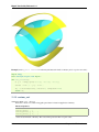
Mayavi2 seeks to provide easy and interactive visualization of 3D data, or 3D plotting. It does this by the following:
• an (optional) rich user interface with dialogs to interact with all data and objects in the visualization.
• a simple and clean scripting interface in Python, including ready to use 3D visualization functionality similar to
matlab or matplotlib (using mlab), or an object-oriented programming interface.
• harnesses the power of VTK without forcing you to learn it.
Additionally, Mayavi2 strives to be a reusable tool that can be embedded in your libraries and applications in different
ways or be combined with the Envisage application-building framework to assemble domain-specific tools.
1.1.1 What is Mayavi2?
Mayavi2 is a general purpose, cross-platform tool for 3-D scientific data visualization. Its features include:
• Visualization of scalar, vector and tensor data in 2 and 3 dimensions.
• Easy scriptability using Python.
• Easy extendability via custom sources, modules, and data filters.
• Reading several file formats: VTK (legacy and XML), PLOT3D, etc.
• Saving of visualizations.
• Saving rendered visualization in a variety of image formats.
• Convenient functionality for rapid scientific plotting via mlab (see mlab: Python scripting for 3D plotting).
Unlike its predecessor Mayavi1, Mayavi2 has been designed with scriptability and extensibility in mind from the
ground up. Mayavi2 provides a mayavi2 application which is usable by itself. However, Mayavi2 may also be used
as a plotting engine, in scripts, like with matplotlib or gnuplot, as well as a library for interactive visualizations in any
other application. It may also be used as an Envisage plugin which allows it to be embedded in other Envisage based
applications natively.
3
Mayavi User Guide, Release 3.3.1
1.1.2 Technical details
Mayavi2 provides a general purpose visualization engine based on a pipeline architecture similar to that used in VTK.
Mayavi2 also provides an Envisage plug-in for 2D/3D scientific data visualization. Mayavi2 uses the Enthought Tool
Suite (ETS) in the form of Traits, TVTK and Envisage. Here are some of its features:
• Pythonic API which takes full advantage of Traits.
• Mayavi can work natively and transparently with numpy arrays (this is thanks to its use of TVTK).
• Easier to script than Mayavi-1 due to a much cleaner MVC design.
• Easy to extend with added sources, components, modules and data filters.
• Provides an Envisage plugin. This implies that it is:
– easy to use other Envisage plugins in Mayavi. For example, Mayavi provides an embedded Python shell.
This is an Envisage plugin and requires one line of code to include in Mayavi.
– easy to use Mayavi inside Envisage based applications. Thus, any envisage based application can readily
use the mayavi plugin and script it to visualize data.
• wxPython/Qt4 based GUI (thanks entirely to Traits, PyFace and Envisage). It is important to note that there is
no wxPython or Qt4 code used directly in the Mayavi source.
• A non-intrusive reusable design. It is possible to use Mayavi without a wxPython or Qt4 based UI.
Note: All the following sections assume you have a working Mayavi, for information on downloading and installing
Mayavi, see the next section, Installation.
1.2 Using Mayavi as an application, or a library?
As a user there are three primary ways to use Mayavi:
1. Use the mayavi2 application completely graphically. More information on this is in the Using the Mayavi
application section.
2. Use Mayavi as a plotting engine from simple Python scripts, for example from Ipython, in combination with
numpy. The mlab scripting API provides a simple way of using Mayavi in batch-processing scripts, see mlab:
Python scripting for 3D plotting for more information on this.
3. Script the Mayavi application from Python. The Mayavi application itself features a powerful and general
purpose scripting API that can be used to adapt it to your needs.
(a) You can script Mayavi while using the mayavi2 application in order to automate tasks and extend
Mayavi’s behavior.
(b) You can script Mayavi from your own Python based application.
(c) You can embed Mayavi into your application in a variety of ways either using Envisage or otherwise.
More details on this are available in the Advanced Scripting with Mayavi chapter.
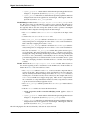
1.3 Scenes, data sources, and visualization modules: the pipeline
model
Mayavi uses a pipeline architecture like VTK. As far as a user is concerned this basically boils down to a simple
hierarchy.
4
Chapter 1. An overview of Mayavi
Mayavi User Guide, Release 3.3.1
• Data is loaded into Mayavi and stored in a data source (either using a file or created from a script). Any number
of data files or data objects may be opened. Data sources are rich objects that describe the data, but not how to
visualize it.
• This data is optionally processed using Filters that operate on the data and visualized using visualization Modules. The filters and modules are accessible in the application via the Visualize menu on the UI or context menus
on the pipeline. They may also be instantiated as Python objects when scripting Mayavi.
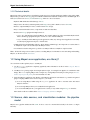
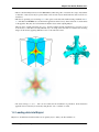
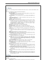
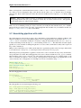
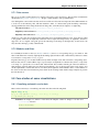
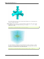
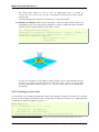
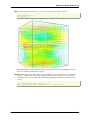
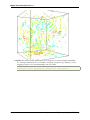
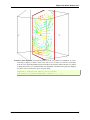
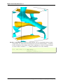
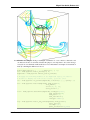
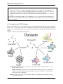
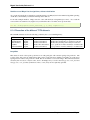
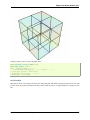
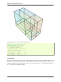
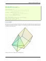
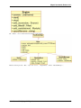
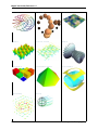
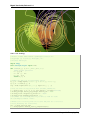
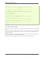
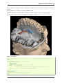
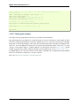
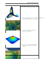
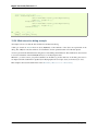
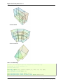
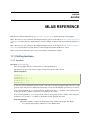
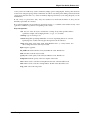
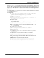
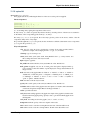
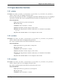
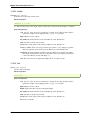
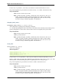
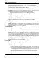
The reasons for separation between data source, the data container, and the visualizations tools used to look at
it, the modules, is that there are many different ways of looking at the same data. For instance the following
images are all made by applying different modules to the same data source:
• All objects belong to a Scene – this is an area where the 3D visualization is performed. In the interactive
application, new scenes may be created by using the File->New->VTK Scene menu.
1.4 Loading data into Mayavi
Mayavi is a scientific data visualizer. There are two primary ways to make your data available to it:
1.4. Loading data into Mayavi
5
Mayavi User Guide, Release 3.3.1
1. Store your data in a supported file format like VTK legacy or VTK XML files etc. See VTK file formats for
more information on the VTK formats. These files can be loaded in the interactive application using the menus.
2. Generate a TVTK dataset via numpy arrays or any other sequence. This is easiest done by using the scripting
APIs, for instance mlab (see the paragraph on creating data sources with mlab, or simply the 3D plotting
functions: 3D Plotting functions for numpy arrays).
Aternatively, if you whish to gain a deeper understanding by creating VTK data structures or files, more information
on datasets in general is available in the Data representation in Mayavi section.
6
Chapter 1. An overview of Mayavi
CHAPTER
TWO
INSTALLATION
Section summary
This section detais the various ways of installing and compiling Mayavi.
If you already have Mayavi up and running, you can skip this section.
2.1 Installing ready-made distributions
Windows Under Window the best way to install Mayavi is to install a full Python distribution, such
as EPD or Pythonxy. Note that for Pythonxy, you need to check in ‘ETS’ in the installer, when
selecting components. If you want to reduce the disk used by the Pythonxy, you can uncheck other
components.
MacOSX The full Python distribution EPD (that includes Mayavi) is also available for MacOSX. Unless
you really enjoy the intricacies of compilation, this is the best solution to install Mayavi.
Ubuntu or Debian Mayavi is packaged in Debian and Ubuntu.
In addition, more up
to date packages of Mayavi releases for old versions of Ubuntu are available at
https://launchpad.net/~gael-varoquaux/+archive . Experimental Debian packages are also available
at http://people.debian.org/~varun/ .
RedHat EL3 and EL4 The full Python distribution EPD (that includes Mayavi) is also available for
RHEL3 and 4.
2.2 Requirements for manual installs
If you are not using full, ready-made, scientific Python distribution, you need to satistify Mayavi’s requirements (for a
step-by-step guide on installing all these under windows, see below).
Mayavi requires at the very minimum the following packages:
• VTK >= 4.4 (5.x is ideal)
• numpy >= 1.0.1
• setuptools (for installation and egg builds)
• Traits >= 3.0 (Traits, TraitsGUI and TraitsBackendWX or TraitsBackendQt, EnthoughtBase, AppTools) Note
Depending on your installation procedure, you might not need to instal manually these requirements.
The following requirements are really optional but strongly recommended, especially if you are new to Mayavi:
7
Mayavi User Guide, Release 3.3.1
• wxPython 2.8.x
• configobj
• Envisage == 3.x (EnvisageCore and EnvisagePlugins) Note These last requirements can be automatically installed, see below.
One can install the requirements in several ways.
• Windows and MacOSX: even if you want to build from source, a good way to install the requirements is to
install one of the distributions indicated above. Note that under Windows, EPD comes with a compiler (mingw)
and facilitates building Mayavi.
• Linux: Most Linux distributions will have installable binaries available for the some of the above. For example,
under Debian or Ubuntu you would need python-vtk, python-wxgtk2.6, python-setuptools,
python-numpy, python-configobj. More information on specific distributions and how you can get the
requirements for each of these should be available from the list of distributions here:
https://svn.enthought.com/enthought/wiki/Install
• Mac OS X: The best available instructions for this platform are available on the IntelMacPython25 page.
There are several ways to install TVTK, Traits and Mayavi. These are described in the following.
2.3 Doing it yourself: Python packages: Eggs
2.3.1 Installing with easy_install
First make sure you have the prerequisites for Mayavi installed, as indicated in the previous section, i.e. the following
packages:
• VTK >= 4.4 (5.x is ideal)
• numpy >= 1.0.1
• wxPython >= 2.8.0
• configobj
• setuptools (for installation and egg builds; later the better)
Mayavi_ is part of the Enthought Tool Suite (ETS). As such, it is distributed as part of ETS and therefore binary
packages and source packages of ETS will contain Mayavi. Mayavi releases are almost always made along with an
ETS release. You may choose to install all of ETS or just Mayavi alone from a release.
ETS has been organized into several different Python packages. These packages are distributed as Python Eggs.
Python eggs are fairly sophisticated and carry information on dependencies with other eggs. As such they are rapidly
becoming the standard for distributing Python packages.
The easiest way to install Mayavi with eggs is to use pre-built eggs built for your particular platform and downloaded
by easy_install. Alternatively easy_install can build the eggs from the source tarballs. This is also fairly easy to do if
you have a proper build environment.
To install eggs, first make sure the essential requirements are installed, and then build and install the eggs like so:
$ easy_install "Mayavi[app]"
This one command will download, build and install all the required ETS related modules that Mayavi needs for the latest ETS release, this means that the Traits dependencies and the Envisage dependencies will be installed automatically.
If you run into trouble please check the Enthought Install pages.
8
Chapter 2. Installation
Mayavi User Guide, Release 3.3.1
One common sources of problems during an install, is the presence of older versions of packages such as Traits,
Mayavi, Envisage or TVTK. Make sure that you clean your site-packages before installing a new version of
Mayavi. Another problem often encountered is running into what is probably a bug of the build system that appears
as a “sandbox violation”. In this case, it can be useful to try the download and install command a few times.
If you still have problems, given this background, please see the following Enthought Install describes how ETS can
be installed with eggs. Check this page first. It contains information on how to install the prebuilt binary eggs for
various platforms along with any dependencies.
Note: Automatic downloading of required eggs
If you whish to download all the eggs fetched by easy_install, for instance to propagate to an offline PC, you can use
virtualenv to create an empty site-packages, and install to it:
virtualenv --no-site-packages temp
cd temp
source bin/activate
mkdir temp_subdir
easy_install -zmaxd temp_subdir "Mayavi[app,nonets]"
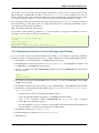
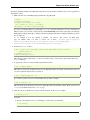
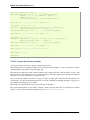
2.3.2 Step-by-step instructions to install with eggs under Windows
If you do not wish to install a ready-made distribution under Windows, these instructions (provided by Guillaume
Duclaux) will guide you through the necessary steps to configure a Windows environment in which Mayavi will run.
1. Install Python 2.5. Add ‘C:\Python25;‘ to the PATH environment variables.
2. Install Mingw32, from the Download section of http://www.mingw.org/ , use the MinGW5.1.4 installer. Add
‘C:\MinGW\bin;’ to the PATH environment variables.
3. Create a ‘c:\documents and settings\USERNAME\pydistutils.cfg’ file(where USERNAME is the login) with the
following contents:
[build]
compiler=mingw32
4. Create the new environment variable HOME and set it to the value: ‘c:\docume~1\USERNAME;’ (where USERNAME is the login name)
5. Install Setuptools (0.6c9 binary) from its webpage, and ‘C:Python25Scripts;’ to the PATH environment variables
6. Install VTK 5.2 (using Dr Charl P. Botha Windows binary http://cpbotha.net/2008/09/23/python-25-enabledvtk-52-windows-binaries/ )
• Unzip the folder content in ‘C:\Program Files\VTK5.2_cpbotha’
• add ‘C:\Program Files\VTK5.2_cpbotha\bin;’ to the PATH environment variables
• create a new environment variable PYTHONPATH and set it to the value ‘C:\Program
Files\VTK5.2_cpbotha\lib\site-packages;’
• If you are running an old version of windows (older than XP) download msvcr80.dll and msvcp80.dll from
the www.dll-files.com website and copy them into C:\winnt\system32.
7. Install Numpy (binary from http://numpy.scipy.org/ )
8. Installing wxPython (2.8 binary from http://www.wxpython.org/ )
9. Run in cmd.exe:
2.3. Doing it yourself: Python packages: Eggs
9
Mayavi User Guide, Release 3.3.1
easy_install Sphinx EnvisageCore EnvisagePlugins configobj
10. Finally, run in cmd.exe:
easy_install Mayavi[app]
2.4 Under Mac OSX Snow Leopard
Under Mac OSX Snow Leopard, you may need to build VTK yourself. Here are instructions specific to Snow Leopard
(thanks to Darren Dale for providing the instructions):
1. Download the VTK tarball, unzip it, and make a build directory (vtkbuild) next to the resulting VTK directory
2. Then cd into vtkbuild and run “cmake ../VTK”. Next, edit CMakeCache.txt (in vtkbuild) and set:
//Build Verdict with shared libraries.
BUILD_SHARED_LIBS:BOOL=ON
//Build architectures for OSX
CMAKE_OSX_ARCHITECTURES:STRING=x86_64
//Minimum OS X version to target for deployment (at runtime); newer
// APIs weak linked. Set to empty string for default value.
CMAKE_OSX_DEPLOYMENT_TARGET:STRING=10.6
//Wrap VTK classes into the Python language.
VTK_WRAP_PYTHON:BOOL=ON
//Arguments passed to "python setup.py install ..." during installation.
VTK_PYTHON_SETUP_ARGS:STRING=
3. Run “cmake ../VTK” again.
4. Run “make -j 2” for a single cpu system. “make -j 9” will compile faster on an 8-core system.
5. Run “sudo make install”
6. Edit your ~/.profile and add the following line:
export DYLD_LIBRARY_PATH=${DYLD_LIBRARY_PATH}:/usr/local/lib/vtk-5.4
7. Run “source ~/.profile” or open a new terminal so the DYLD_LIBRARY_PATH environment variable is available.
8. After that, install Mayavi in the usual way.
2.5 The bleeding edge: SVN
If you want to get the latest development version of Mayavi (e.g. for developing Mayavi or contributing to the
documentation), we recommend that you check it out from SVN. Mayavi depends on several packages that are part of
ETS. It is highly likely that the in-development mayavi version may depend on some feature of an as yet unreleased
component. Therefore, it is very convenient to get all the relevant ETS projects that mayavi recursively depends on
in one single checkout. In order to do this easily, Dave Peterson has created a package called ETSProjectTools. This
10
Chapter 2. Installation
Mayavi User Guide, Release 3.3.1
must first be installed and then any of ETS related repositories may be checked out. Here is how you can get the latest
development sources.
1. Make sure there is no other ETS package installed in your pythonpath:
$ python
>>> import enthought
Traceback (most recent call last):
File "<stdin>", line 1, in <module>
ImportError: No module named enthought
If you don’t get the ImportError (e.g. importing enthought succeeds), then there is no way to install the svn
Mayavi version over it (even if you put it first in your PYTHONPATH), because the older (setuptools managed)
ETS packages will get picked up too and they will mess up things. This behavior might be surprising if you are
new to setuptools.
So for example if you use Ubuntu or Debian, you need to first remove all ETS packages (in Ubuntu 9.04, you need to remove all of these:
mayavi2 python-apptools
python-enthoughtbase python-envisagecore python-envisageplugins
python-traits python-traitsbackendwx python-traitsgui).
2. Install ETSProjectTools like so:
$ svn co https://svn.enthought.com/svn/enthought/ETSProjectTools/trunk \
ETSProjectTools
$ cd ETSProjectTools
$ python setup.py install
This will give you the useful scripts ets. For more details on the tool and various options check the ETSProjectTools wiki page.
3. To get just the sources for mayavi and all its dependencies do this:
$ ets co "Mayavi[app]"
This will look at the latest available mayavi, parse its ETS dependencies and check out the relevant sources. If
you want a particular mayavi release you may do:
$ ets co "Mayavi[app]==3.0.1"
If you’d like to get the sources for an entire ETS release do this for example:
$ ets co "ets==3.0.2"
This will checkout all the relevant sources from SVN. Be patient, this will take a while. More options for the
ets tool are available in the ETSProjectTools page.
4. Once the sources are checked out you may enter the checked-out directory, for example:
$ cd Mayavi_3.3.1/
and either:
(a) Install a development version, to track changes to SVN easily (recommended):
$ ets develop
2.5. The bleeding edge: SVN
11
Mayavi User Guide, Release 3.3.1
This will install all the checked out sources via a setup.py develop applied to each package.
Note: To install of the packages in a different location than the default one, eg ‘~/usr/’, use the following
syntax:
ets develop -c"--prefix ~/usr"
make sure that the corresponding site-packages folder is in your PYTHONPATH environment variable (for
the above example it would be: ‘~/usr/lib/python2.x/site-packages/’
(b) Or build binary eggs of the sources to install localy:
$ cd Mayavi_3.3.1
$ ets bdist
This will build all the eggs and put them inside a dist subdirectory. Run ets bdist -h for more
bdist related options. The mayavi development egg and its dependencies may be installed via:
$ easy_install -f dist "Mayavi[app]"
(c) Alternatively, if you’d like just Mayavi installed via setup.py develop with the rest as binary eggs
you may do:
$ cd Mayavi_x.y.z
$ python setup.py develop -f ../dist
This will pull in any dependencies from the built eggs.
You should now have the latest version of Mayavi installed and usable.
2.6 Testing your installation
The easiest way to test if your installation is OK is to run the mayavi2 application like so:
mayavi2
To get more help on the command try this:
mayavi2 -h
mayavi2 is the mayavi application. On some platforms like win32 you will need to double click on the
mayavi2.exe program found in your Python2X\Scripts folder. Make sure this directory is in your path.
Note: Mayavi can be used in a variety of other ways but the mayavi2 application is the easiest to start with.
If you have the source tarball of mayavi or have checked out the sources from the SVN repository, you can run the
examples in enthought.mayavi*/examples. There are plenty of example scripts illustrating various features.
Tests are available in the enthought.mayavi*/tests sub-directory.
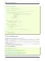
2.7 Troubleshooting
If you are having trouble with the installation you may want to check the Getting help page for more details on how
you can search for information or email the mailing list.
12
Chapter 2. Installation
CHAPTER
THREE
TUTORIAL EXAMPLES TO LEARN
MAYAVI
Section summary
In this section, we give a few detailed examples of how you can use the Mayavi application to tour some of its
features.
This section is mainly interested with the Mayavi application, but it is a good introduction to the ideas behind
using Mayavi as a library. However, if you are only interested in a quick start to use Mayavi as a simple, Matlablike, plotting library, you can jump directly to the mlab: Python scripting for 3D plotting section, and come back
later for a deeper understanding.
To get acquainted with mayavi you may start up the Mayavi2 application, mayavi2 in the command line, like so:
$ mayavi2
On Windows you can double click on the installed mayavi2.exe executable (usually in the Python2X\Scripts
directory), or use the start menu entry, if you installed python(x,y) or EPD.
Once Mayavi starts, you may resize the various panes of the user interface to get a comfortable layout. These settings
will become the default “perspective” of the mayavi application. More details on the UI are available in the General
layout of UI section.
Before proceeding on the quick tour, it can be useful to locate some data to experiment with. Two of the examples
below make use of data shipped with the mayavi sources ship. These may be found in the examples/data directory
inside the root of the mayavi source tree. If these are not installed, the sources may be downloaded from here:
http://code.enthought.com/enstaller/eggs/source/
13
Mayavi User Guide, Release 3.3.1
Examples:
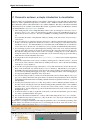
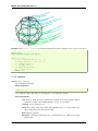
3.1 Parametric surfaces: a simple introduction to visualization
Parametric surfaces are particularly handy if you are unable to find any data to play with right away. Parametric
surfaces are surfaces parametrized typically by 2 variables, u and v. VTK has a bunch of classes that let users
explore Parametric surfaces. This functionality is also available in Mayavi. The data is a 2D surface embedded
in 3D. Scalar data is also available on the surface. More details on parametric surfaces in VTK may be obtained
from Andrew Maclean’s Parametric Surfaces document.
1. After starting mayavi2, create a simple Parametric surface source by selecting File->Load data->Create
Parametric Surface source. Once you create the data, you will see a new node on the Mayavi tree view on
the left that says ParametricSurface. Note that you will not see anything visualized on the TVTK scene
yet.
You can modify the nature of the parametric surface by clicking on the node for the ParametricSurface
source object.
2. To see an outline (a box) of the data, navigate to the Visualize->Modules menu item and select the Outline
module. You can also right-click on the ParametricSurface node to bring up a context menu and select
Add Module->Surface. You will immediately see a wireframe cube on the TVTK scene. You should also
see two new nodes on the tree view, one called Colors and legends and one underneath that called Outline.
3. You can change properties of the outline displayed by clicking on the Outline node on the left. This will
create an object editor window on left bottom of the window (the object editor tab) below the tree view.
Play with the settings here and look at the results. For example, to change the color of the outline box
modify the value in the color field. If you double-click a node on the left it will pop up an editor dialog
rather than show it in the embedded object editor.
4. To navigate the scene look at the section on Interaction with the scene section for more details. Experiment
with these.
5. To view the actual surface create a Surface module by selecting Visualize->Modules->Surface. You can
show contours of the scalar data on this surface by clicking on the Surface node on the left and switching
on the Enable contours check-box.
6. To view the color legend (used to map scalar values to colors), click on the Modules node on the tree view.
Then, on the ‘Scalar LUT’ tab, activate the Show scalar bar check-box. This will show you a legend on
the TVTK scene. The legend can be moved around on the scene by clicking on it and dragging it. It can
also be resized by clicking and dragging on its edges. You can change the nature of the color-mapping by
choosing among different lookup tables on the object editor.
7. You can add as many modules as you like. Not all modules make sense for all data. Mayavi does not yet
grey out (or disable) menu items and options if they are invalid for the particular data chosen. This will
be implemented in the future. However making a mistake should not in general be disastrous, so go ahead
and experiment.
8. You may add as many data sources as you like. It is possible to view two different parametric surfaces on
the same scene by selecting the scene node and then loading another parametric surface source. Whether
this makes sense or not is up to the user. You may also create as many scenes you want to and view
anything in those. You can cut/paste/copy sources and modules between any nodes on the tree view using
the right click options.
9. To delete the Outline module say, right click on the Outline node and select the Delete option. You may
also want to experiment with the other options.
10. You can save the rendered visualization to a variety of file formats using the File->Save Scene As menu.
11. The visualization may itself be saved out to a file via the File->Save Visualization menu and reloaded
using the Load visualization menu.
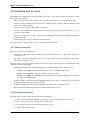
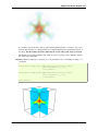
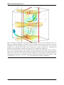
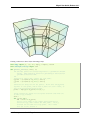
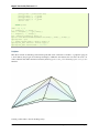
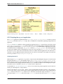
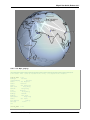
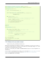
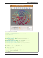
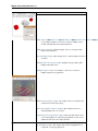
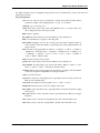
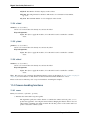
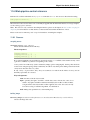
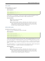
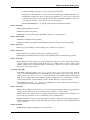
Shown below is an example visualization made using the parametric source. Note that the positioning of the
different surfaces was effected by moving the actors on screen using the actor mode of the scene via the ‘a’ key.
For more details on this see the section on Interaction with the scene.
14
Chapter 3. Tutorial examples to learn Mayavi
CHAPTER
FOUR
USING THE MAYAVI APPLICATION
Section summary
This section primarily concerns using the mayavi2 application. Some of the things mentioned here also apply
when Mayavi is scripted. We recommend that new users read this chapter to get a better knowledge of the
interactive use of the library.
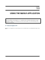
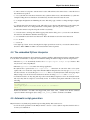
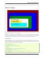
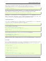
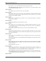
4.1 General layout of UI
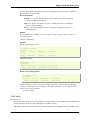
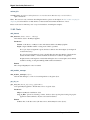
When the mayavi2 application is started it will provide a user interface that looks something like the figure shown
below.
15
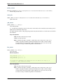
Mayavi User Guide, Release 3.3.1
Figure of Mayavi’s initial UI window.
The UI features several sections described below.
Menus The menus let you open files, load modules, set preferences etc.
The Mayavi engine tree view
This is a tree view of the Mayavi pipeline.
• Right click a tree node to rename, delete, copy the objects.
• Left click on a node to edit its properties on the object editor below the tree.
• It is possible to drag the nodes around on the tree. For example it is possible to drag and
move a module from one set of Modules to another, or to move a visualization from one
scene to another.
The object editor This is where the properties of Mayavi pipeline objects can be changed when an object
on the engine’s pipeline is clicked.
TVTK scenes This is where the visualization of the data happens. One can interact with this scene via
the mouse and the keyboard. More details are in the following sections.
Python interpreter The built-in Python interpreter that can be used to script Mayavi and do other things.
You can drag nodes from the Mayavi tree and drop them on the interpreter and then script the object
16
Chapter 4. Using the Mayavi application
Mayavi User Guide, Release 3.3.1
represented by the node!
If you have version of IPython above 0.9.1 installed, this Python interpreter will use IPython.
Logger Application log messages may be seen here.
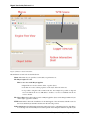
Mayavi’s UI layout is highly configurable:
• the line in-between the sections can be dragged to resize particular views.
• most of the “tabs” on the widgets can be dragged around to move them anywhere in the application.
• Each view area (the Mayavi engine view, object editor, python shell and logger) can be enabled and disabled in
the ‘View’ menu.
Each time you change the appearance of Mayavi it is saved and the next time you start up the application it will
have the same configuration. In addition, you can save different layouts into different “perspectives” using the View>Perspectives menu item.
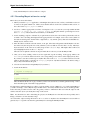
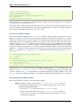
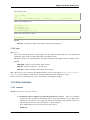
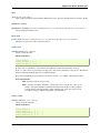
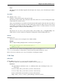
Shown below is a specifically configured Mayavi user interface view. In this view the size of the various parts are
changed.
Figure of Mayavi’s UI after being configured by a user.
4.1. General layout of UI
17
Mayavi User Guide, Release 3.3.1
4.2 Visualizing data
Visualization data in Mayavi is performed by loading some data as data sources, and applying visualization modules
to these sources to visualize the data as described in the An overview of Mayavi section and the Tutorial examples to
learn Mayavi section.
One needs to have some data or the other loaded before a Module or Filter may be used. Mayavi supports several data
file formats most notably VTK data file formats. Alternatively, mlab can be used to load data from numpy arrays. For
advanced information on data structures, refer to the Data representation in Mayavi section.
Once data is loaded one can optionally use a variety of Filters to filter or modify the data in some way or the other and
then visualize the data using several Modules.
Here we list all the Mayavi modules and filters. This list is useful as a reference:
18
Chapter 4. Using the Mayavi application
Mayavi User Guide, Release 3.3.1
List of modules and filters
4.2.1 Modules
Modules are the objects that perform the visualization itself: they use data to create the visual elements on the
scene.
Here is a list of the Mayavi modules along with a brief description.
Axes Draws simple axes.
ContourGridPlane A contour grid plane module. This module lets one take a slice of
input grid data and view contours of the data.
CustomGridPlane A custom grid plane with a lot more flexibility than GridPlane module.
Glyph Displays different types of glyphs oriented and colored as per scalar or vector
data at the input points.
GridPlane A simple grid plane module.
HyperStreamline A module that integrates through a tensor field to generate a hyperstreamline. The integration is along the maximum eigenvector and the cross section
of the hyperstreamline is defined by the two other eigenvectors. Thus the shape of
the hyperstreamline is “tube-like”, with the cross section being elliptical. Hyperstreamlines are used to visualize tensor fields.
ImageActor A simple module to view image data efficiently.
ImagePlaneWidget A simple module to view image data along a cut.
IsoSurface A module that allows the user to make contours of input volumetric data.
Labels Allows a user to label the current dataset or the current actor of the active module.
OrientationAxes Creates a small axes on the side that indicates the position of the coordinate axes and thereby marks the orientation of the scene. Requires VTK-4.5 and
above.
Outline A module that draws an outline for the given data.
ScalarCutPlane Takes a cut plane of any input data set along an implicit plane and plots
the data with optional contouring and scalar warping.
SliceUnstructuredGrid This module takes a slice of the unstructured grid data and
shows the cells that intersect or touch the slice.
Streamline Allows the user to draw streamlines for given vector data. This supports
various types of seed objects (line, sphere, plane and point seeds). It also allows
the user to draw ribbons or tubes and further supports different types of interactive
modes of calculating the streamlines.
StructuredGridOutline Draws a grid-conforming outline for structured grids.
Surface Draws a surface for any input dataset with optional contouring.
TensorGlyph Displays tensor glyphs oriented and colored as per scalar or vector data
at the input points.
Text This module allows the user to place text on the screen.
VectorCutPlane Takes an arbitrary slice of the input data along an implicit cut plane
and places glyphs according to the vector field data. The glyphs may be colored
using either the vector magnitude or the scalar attributes.
Vectors Displays different types of glyphs oriented and colored as per vector data at
the input points. This is merely a convenience module that is entirely based on the
Glyph module.
Volume The Volume module visualizes scalar fields using volumetric visualization techniques.
WarpVectorCutPlane Takes an arbitrary slice of the input data using an implicit cut
plane and warps it according to the vector field data. The scalars are displayed on
the warped surface as colors.
4.2.2 Filters
4.2. Visualizing data
19
Filters transform the data, but do not display it. They are used as an intermediate between the data sources and
the modules.
Here is a list of the Mayavi Filters.
Mayavi User Guide, Release 3.3.1
4.3 Interaction with the scene
The TVTK scenes on the UI can be closed by clicking on the little ‘x’ icon on the tab. Each scene features a toolbar
that supports various features:
• Buttons to set the view to view along the positive or negative X, Y and Z axes or obtain an isometric view.
• A button to turn on parallel projection instead of the default perspective projection. This is particularly useful
when one is looking at 2D plots.
• A button to turn on an axes to indicate the x, y and z axes.
• A button to turn on full-screen viewing. Note that once full-screen mode is entered one must press ‘q’ or ‘e’ to
get back a normal window.
• A button to save the scene to a variety of image formats. The image format to use is determined by the extension
provided for the file.
• A button that provides a UI to configure the scene properties.
The primary means to interact with the scene is to use the mouse and keyboard.
4.3.1 Mouse interaction
There are two modes of mouse interaction:
• Camera mode: the default, where the camera is operated on with mouse moves. This mode is activated by
pressing the ‘c’ key.
• Actor mode: in this mode the mouse actions operate on the actor the mouse is currently above. This mode is
activated by pressing the ‘a’ key.
The view on the scene can be changed by using various mouse actions. Usually these are accomplished by holding
down a mouse button and dragging.
• holding the left mouse button down and dragging will rotate the camera/actor in the direction moved.
– Holding down “SHIFT” when doing this will pan the scene – just like the middle button.
– Holding down “CONTROL” will rotate around the camera’s axis (roll).
– Holding down “SHIFT” and “CONTROL” and dragging up will zoom in and dragging down will zoom
out. This is like the right button.
• holding the right mouse button down and dragging upwards will zoom in (or increase the actors scale) and
dragging downwards will zoom out (or reduce scale).
• holding the middle mouse button down and dragging will pan the scene or translate the object.
• Rotating the mouse wheel upwards will zoom in and downwards will zoom out.
4.3.2 Keyboard interaction
The scene supports several features activated via keystrokes. These are:
• ‘3’: Turn on/off stereo rendering. This may not work if the ‘stereo’ preference item is not set to True.
• ‘a’: Use actor mode for mouse interaction instead of camera mode.
• ‘c’: Use camera mode for mouse interaction instead of actor mode.
• ‘e’/’q’/’Esc’: Exit full-screen mode.
20
Chapter 4. Using the Mayavi application
Mayavi User Guide, Release 3.3.1
• ‘f’: Move camera’s focal point to current mouse location. This will move the camera focus to center the view at
the current mouse position.
• ‘j’: Use joystick mode for the mouse interaction. In joystick mode the mouse somewhat mimics a joystick. For
example, holding the mouse left button down when away from the center will rotate the scene.
• ‘l’: Configure the lights that are illumining the scene. This will pop-up a window to change the light configuration.
• ‘p’: Pick the data at the current mouse point. This will pop-up a window with information on the current pick.
The UI will also allow one to change the behavior of the picker to pick cells, points or arbitrary points.
• ‘r’: Reset the camera focal point and position. This is very handy.
• ‘s’: Save the scene to an image, this will first popup a file selection dialog box so you can choose the filename,
the extension of the filename determines the image type.
• ‘t’: Use trackball mode for the mouse interaction. This is the default mode for the mouse interaction.
• ‘=’/’+’: Zoom in.
• ‘-‘: Zoom out.
• ‘left’/’right’/’up’/’down’ arrows: Pressing the left, right, up and down arrow let you rotate the camera in those
directions. When “SHIFT” modifier is also held down the camera is panned.
4.4 The embedded Python interpreter
The embedded Python interpreter offers extremely powerful possibilities. The interpreter features command completion, automatic documentation, tooltips and some multi-line editing. In addition it supports the following features:
• The name mayavi is automatically bound to the enthought.mayavi.script.Script instance. This
may be used to easily script Mayavi.
• The name application is bound to the envisage application.
• If a Python file is opened via the File->Open File... menu item one can edit it with a color syntax
capable editor. To execute this script in the embedded Python interpreter, the user may type Control-r on
the editor window. To save the file press Control-s. This is a very handy feature when developing simple
Mayavi scripts. You can also increase and decrease the font size using Control-n and Control-s.
• As mentioned earlier, one may drag and drop nodes from the Mayavi engine tree view onto the Python shell.
The object may then be scripted as one normally would. A commonly used pattern when this is done is the
following:
>>> tvtk_scene_1
<enthought.mayavi.core.scene.Scene object at 0x9f4cbe3c>
>>> s = _
In this case the name s is bound to the dropped tvtk_scene object. The _ variable stores the last evaluated
expression which is the dropped object. Using tvtk_scene_1 will also work but is a mouthful.
4.5 Automatic script generation
Mayavi features a very handy and powerful script recording facility. This can be used to:
• record all actions performed on the Mayavi UI into a human readable, Python script that should be able to
recreate your visualization.
4.4. The embedded Python interpreter
21
Mayavi User Guide, Release 3.3.1
• easily learn the Mayavi code base and how to script it.
4.5.1 Recording Mayavi actions to a script
Here is how you can use this feature:
1. When you start the mayavi2 application, on the Engine View (the tree view) toolbar you will find a red record
icon next to the question mark icon. Click it. Note that this will also work from a standalone mlab session, on
the toolbar of the Mayavi pipeline window.
2. You’ll see a window popup with a few lines of boilerplate code so you can run your script standalone/with
mayavi2 -x script.py ‘‘or ‘‘python script.py. Keep this window open and ignore for now
the Save script button, that will be used when you are finished.
3. Now do anything you please on the UI. As you perform those actions, the code needed to perform those actions
is added to the code listing and displayed in the popup window. For example, create a new source (either via
the adder node dialog/view, the file menu or right click, i.e. any normal option), then add a module/filter etc.
Modify objects on the tree view.
4. Move the camera on the UI, rotate the camera, zoom, pan. All of these will generate suitable Python code. For
the camera only the end position is stored (otherwise you’ll see millions of useless lines of code). The major
keyboard actions on the scene are recorded (except for the ‘c’/’t’/’j’/’a’ keys). This implies that it will record
any left/right/up/down arrows the ‘+’/’-‘ keys etc.
Since the code is updated as the actions are performed, this is a nice way to learn the Mayavi API.
5. Once you are done, clicking on the record icon again will stop the recording: in the pop-up window, the
Recording box will be ticked off and no code corresponding to new actions will be displayed any more.
If you want to save the recorded script to a Python file, click on the Save script button at the bottom of the
window. Save the script to some file, say script.py. If you are only interested in the code and not saving a
file you may click cancel at this point.
6. Close the recorder window and quit Mayavi (if you want to).
7. Now from the shell do:
$
mayavi2 -x script.py
or even:
$ python script.py
These should run all the code to get you where you left. You can feel free to edit this generated script – in fact
that is the whole point of automatic script generation!
It is important to understand that it is possible to script an existing session of Mayavi too. So, if after starting Mayavi
you did a few things or ran a Mayavi script and then want to record any further actions, that is certainly possible.
Follow the same procedure as before. The only gotcha you have to remember in this case is that the script recorder
will not create the objects you already have setup on the session.
Note: You should also be able to delete/drag drop objects on the Mayavi tree view. However, these probably aren’t
things you’d want to do in an automatic script.
As noted earlier, script recording will work for an mlab session or anywhere else where Mayavi is used. It will not
generate any mlab specific code but write generic Mayavi code using the OO Mayavi API.
22
Chapter 4. Using the Mayavi application
Mayavi User Guide, Release 3.3.1
4.5.2 Limitations
The script recorder works for most important actions. At this point it does not support the following actions:
• On the scene, the ‘c’/’t’/’j’/’a’/’p’ keys are not recorded correctly since this is much more complicated to implement and typically not necessary for basic scripting.
• Arbitrary scripting of the interface is obviously not going to work as you may expect.
• Only trait changes and specific calls are recorded explicitly in the code. So calling arbitrary methods on arbitrary
Mayavi objects will not record anything typically. Only the Mayavi engine is specially wired up to record
specific methods.
4.6 Command line arguments
The mayavi2 application features several useful command line arguments that are described in the following section.
These options are described in the mayavi2 man page as well.
A complete pipeline may be built from the command line, so that Mayavi can be integrated in shell scripts to provide
useful visualizations.
Mayavi can be run like so:
mayavi2 [options] [args]
Where arg1, arg2 etc. are optional file names that correspond to saved Mayavi2 visualizations (filename.mv2),
Mayavi2 scripts (filename.py) or any datafile supported by Mayavi. If no options or arguments are provided
Mayavi will start up with a default blank scene.
The options are:
-h
This prints all the available command line options and exits. Also available
through --help.
-V
This prints the Mayavi version on the command line and exits. Also available
through --version.
-z file_name
This loads a previously saved Mayavi2 visualization. Also available through
--viz file_name or --visualization file_name.
-d data_file
Opens any of the supported data file formats or non-file associated data source objects. This includes VTK file formats (*.vtk, *.xml, *.vt[i,p,r,s,u],
*.pvt[i,p,r,s,u]), VRML2 (*.wrl), 3D Studio (*.3ds), PLOT3D
(*.xyz), STL, BYU, RAW, PLY, PDB, SLC, FACET, OBJ, AVSUCD (*.inp),
GAMBIT (*.neu), Exodus (*.exii), PNG, JPEG, BMP, PNM, DCM, DEM,
MHA, MHD, MINC, XIMG, TIFF, and various others that are supported.
Note that data_file can also be a source object not associated with a file, for
example ParametricSurface or PointLoad will load the corresponding
data sources into Mayavi. Also available through --data.
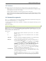
-m module-name
A module is an object that actually visualizes the data. The given module-name
is loaded in the current ModuleManager. The module name must be a valid
one if not you will get an error message.
If a module is specified as package.sub.module.SomeModule then the
module (SomeModule) is imported from package.sub.module. Standard
modules provided with mayavi2 do not need the full path specification. For
example:
4.6. Command line arguments
23
Mayavi User Guide, Release 3.3.1
mayavi2 -d data.vtk -m Outline -m user_modules.AModule
In
this
example
Outline
is
a
standard
module
and
user_modules.AModule is some user defined module. Also available
through --module.
-f filter-name
A filter is an object that filters out the data in some way or the other. The given
filter-name is loaded with respect to the current source/filter object. The
filter name must be a valid one if not you will get an error message.
If the filter is specified as package.sub.filter.SomeFilter then the
filter (SomeFilter) is imported from package.sub.filter. Standard
modules provided with mayavi2 do not need the full path specification. For
example:
mayavi2 -d data.vtk -f ExtractVectorNorm -f user_filters.AFilter
In this example ExtractVectorNorm is a standard filter and
user_filters.AFilter is some user defined filter. Also available
through --filter.
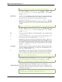
-M
Starts up a new module manager on the Mayavi pipeline. Also available through
--module-mgr.
-n
Creates a new window/scene. Any options passed after this will apply to this
newly created scene. Also available through --new-window.
-o
Run Mayavi in offscreen mode without any graphical user interface. This is most
useful for scripts that need to render images offscreen (for an animation say) in
the background without an intrusive user interface popping up. Mayavi scripts
(run via the -x argument) should typically work fine in this mode. Also available
through, --offscreen.
-x script-file
This executes the given script in a namespace where we guarantee that the name
‘mayavi’ is Mayavi’s script instance – just like in the embedded Python interpreter. Also available through --exec.
-t
Runs the Mayavi test suite and exits. If run as such, this runs both the TVTK and
Mayavi2 unittests. If any additional arguments are passed they are passed along
to the test runner. So this may be used to run other tests as well. For example:
mayavi2 -t enthought.persistence
This will run just the tests inside the enthought.persistence package.
You can also specify a directory with test files to run with this, for example:
mayavi2 -t relative_path_to/integrationtests/mayavi
will run the integration tests from the Mayavi sources. Also available as --test.
-s python-expression Execute the python-expression on the last created object. For example, lets say
the previous object was a module. If you want to set the color of that object and
save the scene, you may do:
$ mayavi2 [...] -m Outline -s"actor.property.color = (1,0,0)" \
-s "scene.save(’test.png’, size=(800, 800))"
24
Chapter 4. Using the Mayavi application
Mayavi User Guide, Release 3.3.1
You should use quotes for the expression. This is also available through --set.
Warning: Note that -x or --exec uses execfile, so this can be dangerous if the script does something nasty!
Similarly, -s or --set uses exec, which can also be dangerous if abused.
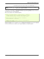
It is important to note that Mayavi’s command line arguments are processed sequentially in the same order they are
given. This allows users to do interesting things.
Here are a few examples of the command line arguments:
$ mayavi2 -d ParametricSurface -s "function=’dini’" -m Surface \
-s "module_manager.scalar_lut_manager.show_scalar_bar = True" \
-s "scene.isometric_view()" -s "scene.save(’snapshot.png’)"
$ mayavi2 -d heart.vtk -m Axes -m Outline -m GridPlane \
-m ContourGridPlane -m IsoSurface
$ mayavi2 -d fire_ug.vtu -m Axes -m Outline -m VectorCutPlane \
-f MaskPoints -m Glyph
In the above examples, heart.vtk and fire_ug.vtu VTK files can be found in the examples/data directory
in the source. They may also be installed on your computer depending on your particular platform.
4.6. Command line arguments
25
Mayavi User Guide, Release 3.3.1
26
Chapter 4. Using the Mayavi application
CHAPTER
FIVE
MLAB: PYTHON SCRIPTING FOR 3D
PLOTTING
Section summary
This section describes the mab API, for use of Mayavi as a simple plotting in scripts or interactive sessions.
This is the main entry point for people interested in doing 3D plotting à la Matlab or IDL in Python. If you are
interested in a list of all the functions exposed in mlab, see the MLab reference.
The enthought.mayavi.mlab module, that we call mlab, provides an easy way to visualize data in a script or
from an interactive prompt with one-liners as done in the matplotlib pylab interface but with an emphasis on 3D
visualization using Mayavi2. This allows users to perform quick 3D visualization while being able to use Mayavi’s
powerful features.
Mayavi’s mlab is designed to be used in a manner well-suited to scripting and does not present a fully object-oriented
API. It is can be used interactively with IPython.
Warning: When using IPython with mlab, as in the following examples, IPython must be invoked with the
-wthread command line option like so:
$ ipython -wthread
If you are using the Enthought Python Distribution, or the latest Python(x,y) distribution, the Pylab menu entry
will start ipython with the right switch. In older release of Python(x,y) you need to start “Interactive Console
(wxPython)”.
For more details on using mlab and running scripts, read the section Running mlab scripts
In this section, we first introduce simple plotting functions, to create 3D objects as representations of numpy arrays.
Then we explain how properties such as color or glyph size can be modified or used to represent data, we show how the
visualization created throught mlab can be modified interactively with dialogs, we show how scripts and animations
can be ran. Finally, we expose a more advanced use of mlab in which full visualization pipeline are built in scripts,
and we give some detailled examples of applying these tools to visualizing volumetric scalar and vector data.
27
Mayavi User Guide, Release 3.3.1
Section contents
•
•
•
•
•
•
•
•
A demo
3D Plotting functions for numpy arrays
Changing the looks of the visual objects created
Figures, legends, camera and decorations
Running mlab scripts
Animating the data
Assembling pipelines with mlab
Case studies of some visualizations
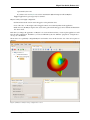
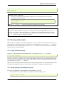
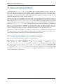
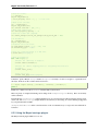
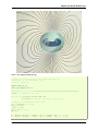
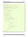
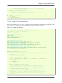
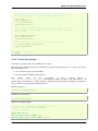
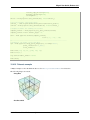
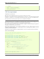
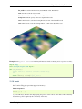
5.1 A demo
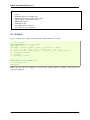
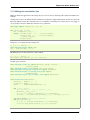
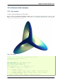
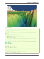
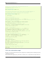
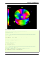
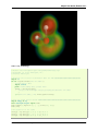
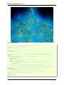
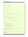
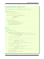
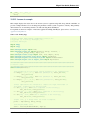
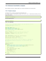
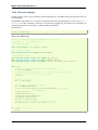
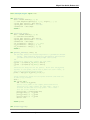
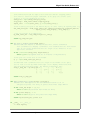
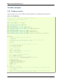
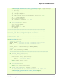
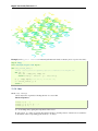
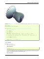
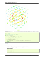
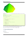
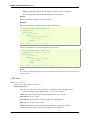
To get you started, here is a pretty example showing a spherical harmonic as a surface:
# Create the data.
from numpy import pi, sin, cos, mgrid
dphi, dtheta = pi/250.0, pi/250.0
[phi,theta] = mgrid[0:pi+dphi*1.5:dphi,0:2*pi+dtheta*1.5:dtheta]
m0 = 4; m1 = 3; m2 = 2; m3 = 3; m4 = 6; m5 = 2; m6 = 6; m7 = 4;
r = sin(m0*phi)**m1 + cos(m2*phi)**m3 + sin(m4*theta)**m5 + cos(m6*theta)**m7
x = r*sin(phi)*cos(theta)
y = r*cos(phi)
z = r*sin(phi)*sin(theta)
# View it.
from enthought.mayavi import mlab
s = mlab.mesh(x, y, z)
mlab.show()
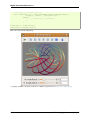
Bulk of the code in the above example is to create the data. One line suffices to visualize it. This produces the
following visualization:
28
Chapter 5. mlab: Python scripting for 3D plotting
Mayavi User Guide, Release 3.3.1
The visualization is created by the single function mesh() in the above.
Several examples of this kind are provided with mlab (see test_contour3d, test_points3d, test_plot3d_anim etc.). The
above demo is available as test_mesh. Under IPython these may be found by tab completing on mlab.test. You can
also inspect the source in IPython via the handy mlab.test_contour3d??.
5.2 3D Plotting functions for numpy arrays
Visualization can be created in mlab by a set of functions operating on numpy arrays.
The mlab plotting functions take numpy arrays as input, describing the x, y, and z coordinates of the data. They
build full-blown visualizations: they create the data source, filters if necessary, and add the visualization modules.
Their behavior, and thus the visualization created, can be fine-tuned through keyword arguments, similarly to pylab.
In addition, they all return the visualization module created, thus visualization can also be modified by changing the
attributes of this module.
Note: In this section, we only list the different functions. Each function is described in details in the MLab reference,
at the end of the user guide, with figures and examples. Please follow the links.
5.2. 3D Plotting functions for numpy arrays
29
Mayavi User Guide, Release 3.3.1
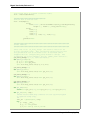
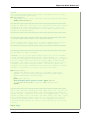
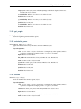
5.2.1 0D and 1D data
points3d()
Plots glyphs (like points) at the position of the supplied data, described by x, y, z
numpy arrays of the same shape.
plot3d()
Plots line between the supplied data, described by x, y, z 1D numpy arrays of the
same length.
30
Chapter 5. mlab: Python scripting for 3D plotting
Mayavi User Guide, Release 3.3.1
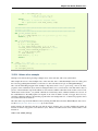
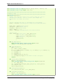
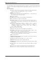
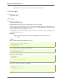
5.2.2 2D data
imshow()
View a 2D array as an image.
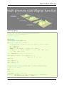
surf()
View a 2D array as a carpet plot, with the z axis representation through elevation the
value of the array points.
contour_surf()
View a 2D array as line contours, elevated according to the value of the array points.
mesh()
Plot a surface described by three 2D arrays, x, y, z giving the coordinnates of the
data points as a grid.
Unlike surf(), the surface is defined by its x, y and z coordinates with no
privileged direction. More complex surfaces can be created.
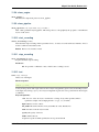
barchart()
Plot an array s, or a set of points with explicite coordinnates arrays, x, y and z, as a
bar chart, eg for histograms.
This function is very versatile and will accept 2D or 3D arrays, but also clouds of
points, to position the bars.
triangular_mesh()
Plot a triangular mesh, fully specified by x, y and z coordinnates of its vertices, and
the (n, 3) array of the indices of the triangles.
Vertical scale of surf() and contour_surf()
surf() and contour_surf() can be used as 3D representation of 2D data. By default the z-axis is supposed
to be in the same units as the x and y axis, but it can be auto-scaled to give a 2/3 aspect ratio. This behavior can
be controlled by specifying the “warp_scale=’auto”’.
5.2. 3D Plotting functions for numpy arrays
31
Mayavi User Guide, Release 3.3.1
From data points to surfaces.
Knowing the positions of data points is not enough to define a surface, connectivity information is also required.
With the functions surf() and mesh(), this connectivity information is implicitely extracted from the shape
of the input arrays: neighbooring data points in the 2D input arrays are connected, and the data lies on a grid.
With the function triangular_mesh(), connectivity is explicitely specified. Quite often, the connectivity is
not regular, but is not known in advance either. The data points lie on a surface, and we want to plot the surface
implicitely defined. The delaunay2d filter does the required nearest-neighboor matching, and interpolation, as
shown in the (Surface from irregular data example).
5.2.3 3D data
contour3d()
Plot isosurfaces of volumetric data defined as a 3D array.
quiver3d()
Plot arrows to represent vectors at data points. The x, y, z position are specified by
numpy arrays, as well as the u, v, w components of the vectors.
flow()
Plot trajectories of particles along a vector field described by three 3D arrays giving the
u, v, w components on a grid.
Structured or unstructured data
contour3d() and flow() require ordered data (to be able to interpolate between the points), whereas
quiver3d() works with any set of points. The required structure is detailed in the functions’ documentation.
Note: Many richer visualisations can be created by assembling data sources filters and modules. See the Assembling
pipelines with mlab and the Case studies of some visualizations sections.
5.3 Changing the looks of the visual objects created
5.3.1 Adding color or size variations
Color The color of the objects created by a plotting function can be specified explicitly using the ‘color’
keyword argument of the function. This color is than applied uniformly to all the objects created.
If you want to vary the color across your visualization, you need to specify scalar information for
each data point. Some functions try to guess this information: these scalars default to the norm of
the vectors, for functions with vectors, or to the z elevation for functions where is meaningful, such
as surf() or barchart().
32
Chapter 5. mlab: Python scripting for 3D plotting
Mayavi User Guide, Release 3.3.1
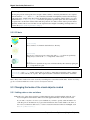
This scalar information is converted into colors using the colormap, or also called LUT, for Look
Up Table. The list of possible colormaps is:
accent
autumn
black-white
blue-red
blues
bone
brbg
bugn
bupu
cool
copper
dark2
flag
gist_earth
gist_gray
gist_heat
gist_ncar
gist_rainbow
gist_stern
gist_yarg
gnbu
gray
greens
greys
hot
hsv
jet
oranges
orrd
paired
pastel1
pastel2
pink
piyg
prgn
prism
pubu
pubugn
puor
purd
purples
rdbu
rdgy
rdpu
rdylbu
rdylgn
reds
set1
set2
set3
spectral
spring
summer
winter
ylgnbu
ylgn
ylorbr
ylorrd
The easiest way to choose the colormap most adapted to your visualization is to use the GUI (as
described in the next paragraph). The dialog to set the colormap can be found in the Colors and
legends node.
Size of the glyph The scalar information can also be displayed in many different ways. For instance it
can be used to adjust the size of glyphs positioned at the data points.
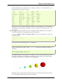
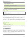
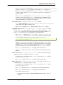
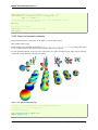
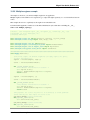
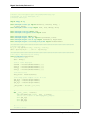
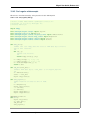
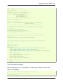
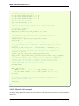
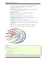
A caveat: Clamping: relative or absolute scaling Given six points positionned on a line with
interpoint spacing 1:
x = [1, 2, 3, 4, 5, 6]
y = [0, 0, 0, 0, 0, 0]
z = y
If we represent a scalar varying from 0.5 to 1 on this dataset:
s = [.5, .6, .7, .8, .9, 1]
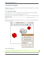
We represent the dataset as spheres, using points3d(), and the scalar is mapped to diameter of
the spheres:
from enthought.mayavi import mlab
pts = mlab.points3d(x, y, z, s)
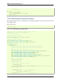
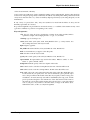
By default the diameter of the spheres is not ‘clamped’, in other words, the smallest value of the
scalar data is represented as a null diameter, and the largest is proportional to inter-point distance.
The scaling is only relative, as can be seen on the resulting figure:
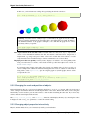
This behavior gives visible points for all datasets, but may not be desired if the scalar represents the
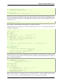
size of the glyphs in the same unit as the positions specified.
5.3. Changing the looks of the visual objects created
33
Mayavi User Guide, Release 3.3.1
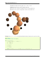
In this case, you shoud turn auto-scaling off by specifying the desired scale factor:
pts = mlab.points3d(x, y, z, s, scale_factor=1)
Warning: In earlier versions of Mayavi (up to 3.1.0 included), the glyphs are not auto-scaled,
and as a result the visualization can seem empty due to the glyphs being very small. In addition
the minimum diameter of the glyphs is clamped to zero, and thus the glyph are not scaled
absolutely, unless you specifie:
pts.glyph.glyph.clamping = False
More representations of the attached scalars or vectors There are many more ways to represent the
scalar or vector information attached to the data. For instance, scalar data can be ‘warped’ into a
displacement, e.g. using a WarpScalar filter, or the norm of scalar data can be extract to a scalar
component that can be visualized using iso-surfaces with the ExtractVectorNorm filter.
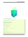
Displaying more than one quantity You may want to display color related to one scalar quantity while
using a second for the iso-contours, or the elevation. This is possible but requires a bit of work: see
Atomic orbital example.
If you simply want to display points with a size given by one quantity, and a color by a second, you
can use a simple trick: add the size information using the norm of vectors, add the color information
using scalars, create a quiver3d() plot choosing the glyphs to symetrix glyphs, and use scalars
to represent the color:
x, y, z, s, c = np.random.random((5, 10))
pts = mlab.quiver3d(x, y, z, s, s, s, scalars=c, mode=’sphere’)
pts.glyph.color_mode = ’color_by_scalar’
5.3.2 Changing the scale and position of objects
Each mlab function takes an extent keyword argument, that allows to set its (x, y, z) extents. This give both control
on the scaling in the different directions and the displacement of the center. Beware that when you are using this
functionality, it can be useful to pass the same extents to other modules visualizing the same data. If you don’t, they
will not share the same displacement and scale.
The surf(), contour_surf(), and barchart() functions, which display 2D arrays by converting the values
in height, also take a warp_scale parameter, to control the vertical scaling.
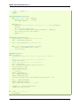
5.3.3 Changing object properties interactively
Mayavi, and thus mlab, allows you to interactively modify your visualization.
34
Chapter 5. mlab: Python scripting for 3D plotting
Mayavi User Guide, Release 3.3.1
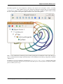
The Mayavi pipeline tree can be displayed by clicking on the mayavi icon in the figure’s toolbar, or by using
show_pipeline() mlab command. One can now change the visualization using this dialog by double-clicking
on each object to edit its properties, as described in other parts of this manual, or add new modules or filters by using
this icons on the pipeline, or through the right-click menus on the objects in the pipeline.
Note: A very useful feature of this dialog can be found by pressing the red round button of the toolbar. This opens
up a recorder that tracks the changes made interactively to the visualization via the dialogs, and generates valid lines
of Python code.
In addition, for every object returned by a mlab function, this_object.edit_traits() brings up a dialog that
can be used to interactively edit the object’s properties. If the dialog doesn’t show up when you enter this command,
please see Running mlab scripts.
5.3. Changing the looks of the visual objects created
35
Mayavi User Guide, Release 3.3.1
Using mlab with the full Envisage UI
Sometimes it is convenient to write an mlab script but still use the full envisage application so you can click on
the menus and use other modules etc. To do this you may do the following before you create an mlab figure:
from enthought.mayavi import mlab
mlab.options.backend = ’envisage’
f = mlab.figure()
# ...
This will give you the full-fledged UI instead of the default simple window.
5.4 Figures, legends, camera and decorations
5.4.1 Handling several figures
All mlab functions operate on the current scene, that we also call figure(), for compatibility with matlab and pylab.
The different figures are indexed by key that can be an integer or a string. A call to the figure() function giving
a key will either return the corresponding figure, if it exists, or create a new one. The current figure can be retrieved
with the gcf() function. It can be refreshed using the draw() function, saved to a picture file using savefig()
and cleared using clf().
5.4.2 Figure decorations
Axes can be added around a visualization object with the axes() function, and the labels can be set using the
xlabel(), ylabel() and zlabel() functions. Similarly, outline() creates an outline around an object.
title() adds a title to the figure.
Color bars can be used to reflect the color maps used to display values (LUT, or lookup tables, in VTK parlance).
colorbar() creates a color bar for the last object created, trying to guess whether to use the vector data or the scalar
data color maps. The scalarbar() and vectorbar() function scan be used to create color bars specifically for
scalar or vector data.
A small xyz triad can be added to the figure using orientation_axes().
Warning: The orientation_axes() was named orientationaxes before release 3.2.
5.4.3 Moving the camera
The position and direction of the camera can be set using the view() function. They are described in terms of Euler
angles and distance to a focal point. The view() function tries to guess the right roll angle of the camera for a
pleasing view, but it sometimes fails. The roll() explicitly sets the roll angle of the camera (this can be achieve
intercactively in the scene by pressing down the control key, while dragging the mouse, see Interaction with the scene).
The view() and roll() functions return the current values of the different angles and distances they take as
arguments. As a result, the view point obtained interactively can be stored an reset using:
# Store the information
view = mlab.view()
roll = mlab.roll()
36
Chapter 5. mlab: Python scripting for 3D plotting
Mayavi User Guide, Release 3.3.1
# Reposition the camera
mlab.view(*view)
mlab.roll(roll)
Rotating the camera around itself
You can also rotate the camera around itself using the roll, yaw and pitch methods of the camera
object. This moves the focal point:
f = mlab.gcf()
camera = f.scene.camera
camera.yaw(45)
Unlike the view() and roll() function, the angles are incremental, and not absolute.
Modifying zoom and view angle
The camera is entirely defined by its position, its focal point, and its view angle (attributes ‘position’, ‘focal_point’, ‘view_angle’). The camera method ‘zoom’ changes the view angle incrementally by the specify
ratio, where as the method ‘dolly’ translates the camera along its axis while keeping the focal point constant.
The move() function can also be useful in these regards.
5.5 Running mlab scripts
Mlab, like the rest of Mayavi, is an interactive application. If you are not already in an interactive environment (see
next paragraph), to interact with the figures or the rest of the drawing elements, you need to use the show() function.
For instance, if you are writing a script, you need to call show() each time you want to display one or more figures
and allow the user to interact with them.
5.5.1 Using mlab interactively
Using IPython, mlab instructions can be run interactively, or in scripts using IPython‘s %run command:
In [1]: %run my_script
You need to start IPython with the -wthread option (when installed with EPD, the pylab start-menu link does this
for you). In this environment, the plotting commands are interactive: they have an immediate effect on the figure,
alleviating the need to use the show() function.
Mlab can also be used interactively in the Python shell of the mayavi2 application, or in any interactive Python shell
of wxPython-based application (such as other Envisage-based applications, or SPE, Stani’s Python Editor).
5.5.2 Using together with Matplotlib’s pylab
If you want to use Matplotlib’s pylab with Mayavi’s mlab in IPython you should:
• if your IPython version is greater than 0.8.4: start IPython with the following options:
$ ipython -pylab -wthread
5.5. Running mlab scripts
37
Mayavi User Guide, Release 3.3.1
• elsewhere, start IPython with the -wthread option:
$ ipython -wthread
and before importing pylab, enter the following Python commands:
>>> import matplotlib
>>> matplotlib.use(’WxAgg’)
>>> matplotlib.interactive(True)
If you want matplotlib and mlab to work together by default in IPython, you can change you default matplotlib
backend, by editing the ~/.matplotlib/matplotlibrc to add the following line:
backend
: WXAgg
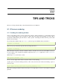
Capturing mlab plots to integrate in pylab
Starting from Mayavi version 3.4.0, the mlab screenshot() can be used to take a screenshot of the current
figure, to integrate in a matplotlib plot.
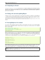
5.5.3 In scripts
Mlab commands can be written to a file, to form a script. This script can be loaded in the Mayavi application using
the File->Open file menu entry, and executed using the File->Refresh code menu entry or by pressing Control-r.
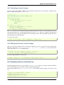
It can also be executed during the start of the Mayavi application using the -x command line switch.
As mentioned above, when running outside of an interactive environment, for instance with python myscript.py, you
need to call the show() function (as shown in the demo above) to pause your script and have the user interact with
the figure.
You can also use show() to decorate a function, and have it run in the event-loop, which gives you more flexibility:
from enthought.mayavi import mlab
from numpy import random
@mlab.show
def image():
mlab.imshow(random.random((10, 10)))
With this decorator, each time the image function is called, mlab makes sure an interactive environment is running
before executing the image function. If an interactive environment is not running, mlab will start one and the image
function will not return until it is closed.
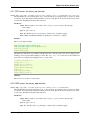
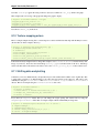
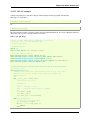
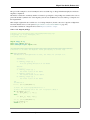
5.6 Animating the data
Often it isn’t sufficient to just plot the data. You may also want to change the data of the plot and update the plot
without having to recreate the entire visualization, for instance to do animations, or in an interactive application.
Indeed, recreating the entire visualization is very inefficient and leads to very jerky looking animations. To do this,
mlab provides a very convenient way to change the data of an existing mlab visualization. Consider a very simple
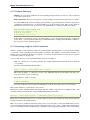
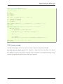
example. The mlab.test_simple_surf_anim function has this code:
38
Chapter 5. mlab: Python scripting for 3D plotting
Mayavi User Guide, Release 3.3.1
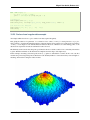
x, y = numpy.mgrid[0:3:1,0:3:1]
s = mlab.surf(x, y, numpy.asarray(x*0.1, ’d’))
for i in range(10):
s.mlab_source.scalars = numpy.asarray(x*0.1*(i+1), ’d’)
The first two lines define a simple plane and view that. The next three lines animate that data by changing the scalars
producing a plane that rotates about the origin. The key here is that the s object above has a special attribute called
mlab_source. This sub-object allows us to manipulate the points and scalars. If we wanted to change the x values we
could set that too by:
s.mlab_source.x = new_x
The only thing to keep in mind here is that the shape of x should not be changed.
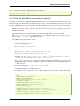
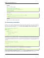
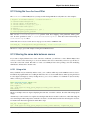
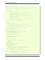
If multiple values have to be changed, you can use the set method of the mlab_source to set them as shown in the more
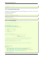
complicated example below:
# Produce some nice data.
n_mer, n_long = 6, 11
pi = numpy.pi
dphi = pi/1000.0
phi = numpy.arange(0.0, 2*pi + 0.5*dphi, dphi, ’d’)
mu = phi*n_mer
x = numpy.cos(mu)*(1+numpy.cos(n_long*mu/n_mer)*0.5)
y = numpy.sin(mu)*(1+numpy.cos(n_long*mu/n_mer)*0.5)
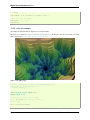
z = numpy.sin(n_long*mu/n_mer)*0.5
# View it.
l = plot3d(x, y, z, numpy.sin(mu), tube_radius=0.025, colormap=’Spectral’)
# Now animate the data.
ms = l.mlab_source
for i in range(10):
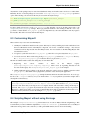
x = numpy.cos(mu)*(1+numpy.cos(n_long*mu/n_mer +
numpy.pi*(i+1)/5.)*0.5)
scalars = numpy.sin(mu + numpy.pi*(i+1)/5)
ms.set(x=x, scalars=scalars)
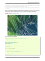
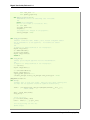
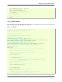
Notice the use of the set method above. With this method, the visualization is recomputed only once. In this case, the
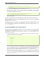
shape of the new arrays has not changed, only their values have. If the shape of the array changes then one should use
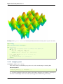
the reset method as shown below:
x, y = numpy.mgrid[0:3:1,0:3:1]
s = mlab.surf(x, y, numpy.asarray(x*0.1, ’d’),
representation=’wireframe’)
# Animate the data.
fig = mlab.gcf()
ms = s.mlab_source
for i in range(5):
x, y = numpy.mgrid[0:3:1.0/(i+2),0:3:1.0/(i+2)]
sc = numpy.asarray(x*x*0.05*(i+1), ’d’)
ms.reset(x=x, y=y, scalars=sc)
fig.scene.reset_zoom()
Many standard examples for animating data are provided with mlab. Try the examples with the name
mlab.test_<name>_anim, i.e. where the name ends with an _anim to see how these work and run.
5.6. Animating the data
39
Mayavi User Guide, Release 3.3.1
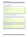
Note: It is important to remember distinction between set and reset. Use set or directly set the attributes (x, y, scalars
etc.) when you are not changing the shape of the data but only the values. Use reset when the arrays are changing
shape and size. Reset usually regenerates all the data and can be inefficient when compared to set or directly setting
the traits.
Warning: When creating a Mayavi pipeline, as explained in the following subsection, instead of using readymade plotting function, the mlab_source attribute is created only on sources created via mlab. Only pipeline
created entirely using mlab will present this attribute.
Note: If you are animating several plot objects, each time you modify the data with there mlab_source attribute,
Mayavi will trigger a refresh of the scene. This operation might take time, and thus slow your animation. In this case,
the tip Accelerating a Mayavi script may come in handy.
5.7 Assembling pipelines with mlab
The plotting functions reviewed above explore only a small fraction of the visualization possibilities of Mayavi. The
full power of Mayavi can only be unleashed through the control of the pipeline itself. As described in the An overview
of Mayavi section, a visualization in Mayavi is created by loading the data in Mayavi with data source object, optionally transforming the data through Filters, and visualizing it with Modules. The mlab functions build complex
pipelines for you in one function, making the right choice of sources, filters, and modules, but they cannot explore all
the possible combinations.
Mlab provides a submodule pipeline which contains functions to populate the pipeline easily from scripts. This module
is accessible in mlab: mlab.pipeline, or can be imported from enthought.mayavi.tools.pipeline.
When using an mlab plotting function, a pipeline is created: first a source is created from numpy arrays, then modules,
and possibly filters, are added. The resulting pipeline can be seen for instance with the mlab.show_pipeline command.
This information can be used to create the very same pipeline using directly the pipeline scripting module, as the
names of the functions required to create each step of the pipeline are directly linked to the default names of the
objects created by mlab on the pipeline. As an example, let us create a visualization using surf():
import numpy as np
a = np.random.random((4, 4))
from enthought.mayavi import mlab
mlab.surf(a)
mlab.show_pipeline()
The following pipeline is created:
Array2DSource
\__ WarpScalar
\__ PolyDataNormals
\__ Colors and legends
\__ Surface
The same pipeline can be created using the following code:
src = mlab.pipeline.array2d_source(a)
warp = mlab.pipeline.warp_scalar(src)
normals = mlab.pipeline.poly_data_normals(warp)
surf = mlab.pipeline.surface(normals)
40
Chapter 5. mlab: Python scripting for 3D plotting
Mayavi User Guide, Release 3.3.1
5.7.1 Data sources
The pipeline module contains functions for creating various data sources from arrays. They are fully documented in
details in the Mlab pipeline-control reference. We give a small summary of the possibilities here.
mlab distinguishes sources with scalar data, and sources with vector data, but more important, it has different functions
to create sets of unconnected points, with data attached to them, or connected data points describing continuously
varying quantities that can be interpolated between data points, often called fields in physics or engineering.
Unconnected sources scalar_scatter(), vector_scatter()
Implicitely-connected sources scalar_field(), vector_field(), array2d_source()
Explicitly-connected sources line_source(), triangular_mesh_source()
All the mab source factories are functions that take numpy arrays and return the Mayavi source object that was added
to the pipeline. However, the implicitely-connected sources require well-shaped arrays as arguments: the data is
supposed to lie on a regular, orthogonal, grid of the same shape as the shape of the input array, in other words, the
array describes an image, possibly 3 dimensional.
5.7.2 Modules and filters
For each Mayavi module or filter (see Modules and Filters), there is a corresponding mlab.pipeline function. The
name of this function is created by replacing the alternating capitals in the module or filter name by underscores. Thus
ScalarCutPlane corresponds to scalar_cut_plane.
In general, the mlab.pipeline module and filter factory functions simply create and connect the corresponding object.
However they can also contain addition logic, exposed as keyword arguments. For instance they allow to set up easily
a colormap, or to specify the color of the module, when relevant. In accordance with the goal of the mlab interface to
make frequent operations simple, they use the keyword arguments to choose the properties of the create object to best
suit the requirements. It can be thus easier to use the keyword arguments, when available, than to set the attributes of
the objects created. For more information, please check out the docstrings. Full, detailed, usage examples are given in
the next subsection.
5.8 Case studies of some visualizations
5.8.1 Visualizing volumetric scalar data
There are three main ways of visualizing a 3D scalar field. Given the following field:
import numpy as np
x, y, z = np.ogrid[-10:10:20j, -10:10:20j, -10:10:20j]
s = np.sin(x*y*z)/(x*y*z)
IsoSurfaces To display iso surfaces of the field, the simplest solution is simply to use the mlab
contour3d() function:
mlab.contour3d(s)
5.8. Case studies of some visualizations
41
Mayavi User Guide, Release 3.3.1
The problem with this method that outer iso-surfaces tend to hide inner ones. As a result, quite often
only one iso-surface can be visible.
Volume rendering Volume rendering is an advanced technique in which each voxel is given a partly
transparent color. This can be achieved with mlab.pipeline using the scalar_field() source,
and the volume module:
mlab.pipeline.volume(mlab.pipeline.scalar_field(s))
For such a visualization, tweaking the opacity transfer function is critical to achieving a good effect.
Typically, it can be useful to limit the lower and upper values to the 20 and 80 percentiles of the data,
in order to have a reasonnable fraction of the volume transparent:
mlab.pipeline.volume(mlab.pipeline.scalar_field(s), vmin=0, vmax=0.8)
42
Chapter 5. mlab: Python scripting for 3D plotting
Mayavi User Guide, Release 3.3.1
It is useful to open the module’s dialog (eg through the pipeline interface, or using it’s edit_traits()
method) and tweak the color transfert function to render transparent the low-intensities regions of
the image. For this module, the LUT as defined in the ‘Colors and legends‘ node are not used
The limitations of volume rendering is that, while it is often very pretty, it can be difficult to analysis
the details of the field with it.
Cut planes While less impressive, cut planes are a very informative way of visualising the details of a
scalar field:
mlab.pipeline.image_plane_widget(mlab.pipeline.scalar_field(s),
plane_orientation=’x_axes’,
slice_index=10,
)
mlab.pipeline.image_plane_widget(mlab.pipeline.scalar_field(s),
plane_orientation=’y_axes’,
slice_index=10,
)
mlab.outline()
5.8. Case studies of some visualizations
43
Mayavi User Guide, Release 3.3.1
The image plane widget can only be used on regular-spaced data, as created by
mlab.pipeline.scalar_field, but it is very fast. It should thus be prefered to the scalar cut plane,
when possible.
Clicking and dragging the cut plane is an excellent way of exploring the field.
A combination of techniques Finally, it can be interesting to combine cut planes with iso-surfaces and
thresholding to give a view of the peak areas using the iso-surfaces, visualize the details of the field
with the cut plane, and the global mass with a large iso-surface:
src = mlab.pipeline.scalar_field(s)
mlab.pipeline.iso_surface(src, contours=[s.min()+0.1*s.ptp(), ], opacity=0.1)
mlab.pipeline.iso_surface(src, contours=[s.max()-0.1*s.ptp(), ],)
mlab.pipeline.image_plane_widget(src,
plane_orientation=’z_axes’,
slice_index=10,
)
In some cases, thought not in our example, it might be usable to insert a threshold filter before the
cut plane, eg to remove area with values below ‘s.min()+0.1*s.ptp()’. In this case, the cut plane
needs to be implemented with mlab.pipeline.scalar_cut_plane as the data looses its structure after
thresholding.
5.8.2 Visualizing a vector field
A vector field, ie vectors continuously defined in a volume, can be difficult to visualize, as it contains a lot of information. Let us explore different visualizations for the velocity field of a multi-axis convection cell 1 , in hydrodynamics,
as defined by its components sampled on a grid, u, v, w:
import numpy as np
x, y, z = np.mgrid[0:1:20j, 0:1:20j, 0:1:20j]
u =
np.sin(np.pi*x) * np.cos(np.pi*z)
v = -2*np.sin(np.pi*y) * np.cos(2*np.pi*z)
w = np.cos(np.pi*x)*np.sin(np.pi*z) + np.cos(np.pi*y)*np.sin(2*np.pi*z)
1
44
Toussaint, V.; Carriere, P. & Raynal, F. A numerical Eulerian approach to mixing by chaotic advection Phys. Fluids, 1995, 7, 2587
Chapter 5. mlab: Python scripting for 3D plotting
Mayavi User Guide, Release 3.3.1
Quiver The simplest visualization of a set of vectors, is using the mlab function quiver3d:
mlab.quiver3d(u, v, w)
mlab.outline()
The main limitation of this visualization is that it positions an arrow for each sampling point on the
grid. As a result the visualization is very busy.
Masking vectors We can use the fact that we are visualizing a vector field, and not just a bunch of
vectors, to reduce the amount of arrows displayed. For this we need to build a vector_field source,
and apply to it the vectors module, with some masking parameters (here we keep only one point out
of 20):
src = mlab.pipeline.vector_field(u, v, w)
mlab.pipeline.vectors(src, mask_points=20, scale_factor=3.)
5.8. Case studies of some visualizations
45
Mayavi User Guide, Release 3.3.1
A cut plane If we are interested in displaying the vectors along a cut, we can use a cut plane. In particular,
we can inspect interactively the vector field by moving the cut plane along: clicking on it and
dragging it can give a very clear understanding of the vector field:
mlab.pipeline.vector_cut_plane(src, mask_points=2, scale_factor=3)
46
Chapter 5. mlab: Python scripting for 3D plotting
Mayavi User Guide, Release 3.3.1
IsoSurfaces of the magnitude An important parameter of the vector field is its magnitude. It can be
interesting to display iso-surfaces of the norm of the vectors. For this we can create a scalar field
from the vector field using the ExtractVectorNorm filter, and use the IsoSurface module on it. When
working interactively, a good understanding of the magnitude of the field can be gained by changing
the values of the contours in the object’s property dialog.
magnitude = mlab.pipeline.extract_vector_norm(src)
mlab.pipeline.iso_surface(magnitude, contours=[1.9, 0.5])
5.8. Case studies of some visualizations
47
Mayavi User Guide, Release 3.3.1
The Flow, or the field lines For certain vector fields, the line of flow of along the field can have an interesting meaning. For instance the can be interpreted as trajectories in hydrodynamics, or field lines
in electro-magnetism. We can display the flow lines originating for a certain seed surface using the
streamline module, or the mlab flow() function, which relies on streamline internally:
flow = mlab.flow(u, v, w, seed_scale=1,
seed_resolution=5,
integration_direction=’both’)
48
Chapter 5. mlab: Python scripting for 3D plotting
Mayavi User Guide, Release 3.3.1
A combination of techniques Giving a meaningful visualization of a vector field is a hard task, and
one must use all the tools at hand to illustrate his purposes. It is important to choose the message
conveyed. No one visualization will tell all about a vector field. Here is an example of a visualization
made by combining the different tools above:
mlab.figure(fgcolor=(0., 0., 0.), bgcolor=(1, 1, 1))
src = mlab.pipeline.vector_field(u, v, w)
magnitude = mlab.pipeline.extract_vector_norm(src)
# We apply the following modules on the magnitude object, in order to
# be able to display the norm of the vectors, eg as the color.
iso = mlab.pipeline.iso_surface(magnitude, contours=[1.9, ], opacity=0.3)
vec = mlab.pipeline.vectors(magnitude, mask_points=40,
line_width=1,
color=(.8, .8, .8),
scale_factor=4.)
flow = mlab.pipeline.streamline(magnitude, seedtype=’plane’,
seed_visible=False,
seed_scale=0.5,
seed_resolution=1,
linetype=’ribbon’,)
vcp = mlab.pipeline.vector_cut_plane(magnitude, mask_points=2,
scale_factor=4,
colormap=’jet’,
plane_orientation=’x_axes’)
5.8. Case studies of some visualizations
49
Mayavi User Guide, Release 3.3.1
Note: Although most of this section has been centered on snippets of code to create visualization objects, it is
important to remember that Mayavi is an interactive program, and that the properties of these objects can be modified interactively, as described in Changing object properties interactively. It is often impossible to choose the best
parameters for a visualization before hand. Colors, contour values, colormap, view angle, etc... should be chosen
interactively. If reproducibility is required, the chosen values can be added in the original script.
Moreover, the mlab functions expose only a small fraction of the possibilities of the visualization objects. The dialogs
expose more of these functionalities, that are entirely controlled by the attributes of the objects returned by the mlab
functions. These objects are very rich, as they are built from VTK objects. It can be hard to find the right attribute to
modify when exploring them, or in the VTK documentation, thus using the interactive dialog and recording to a script,
as described in Recording Mayavi actions to a script is the prefered way of tweaking a visualization.
50
Chapter 5. mlab: Python scripting for 3D plotting
CHAPTER
SIX
ADVANCED USE OF MAYAVI
Section summary
This section give details on the working principles Mayavi. Read it to gain a better understanding, in order to
use Mayavi’s full power.
• First we describe data structures, how they are defined and how you can build them. This information is
useful for a better understanding of how to build efficient pipelines.
• Second we describe the object-oriented structure behind Mayavi and the pipeline. This information opens
the door to advanced scripting of the Mayavi application, and is especially useful if you whish to develop
custom tools with Mayavi.
6.1 Data representation in Mayavi
Describing data in three dimension in the general case is a complex problem. Mayavi helps you focus on your
visualization work and not worry too much about the underlying data structures, for instance using mlab (see mlab:
Python scripting for 3D plotting). We suggest you create sources for Mayavi using mlab or Mayavi sources when
possible. However, it helps to understand the VTK data structures that Mayavi uses if you want to create data with a
specific structure for a more efficient visualization, or if you want to extract the data from the Mayavi pipeline.
Outline
•
•
•
•
•
Introduction to TVTK datasets
The flow of data
Retrieving the data from Mayavi pipelines
Dissection of the different TVTK datasets
Inserting TVTK datasets in the Mayavi pipeline.
51
Mayavi User Guide, Release 3.3.1
Mayavi data sources and VTK datasets
• When you load a file, or you expose data in Mayavi using one of the mlab.pipeline source functions (see
Data sources), you create an object in the Mayavi pipeline that is attached to a scene. This object is a
Mayavi source, and serves to describe the data and its properties to the Mayavi pipeline.
• The internal structures use to represent to data in 3D all across Mayavi are VTK datasets, as described
below.
One should not confuse VTK (or TVTK) datasets and Mayavi data sources. There is a finite and small number of
datasets. However, many pipeline objects could be constructed to fit in the pipeline below a scene and providing
datasets to the pipeline.
6.1.1 Introduction to TVTK datasets
Mayavi uses the VTK library for all its visualization needs, via TVTK (Traited VTK). The data is exposed internally,
by the sources, or at the output of the filters, as VTK datasets, described below. Understanding these structures is
useful not only to manipulate them, but also to understand what happens when using filters to transform the data in the
pipeline.
A dataset is defined by many different characteristics:
Connectivity Connectivity is not only necessary to draw lines between the different points, it is also
needed to define a volume.
Implicit connectivity: connectivity or positioning is implicit. In this case the data is considered as
arranged on a lattice-like structure, with equal number of layers in each direction, x increasing first
along the array, then y and finally z.
Data Dataset are made of points positioned in 3D, with the corresponding data. Each dataset can carry
several data components.
52
Chapter 6. Advanced use of Mayavi
Mayavi User Guide, Release 3.3.1
Scalar or Vectors data: The data can be scalar, in which case VTK can perform operations such as
taking the gradient and display the data with a colormap, or vector, in which case VTK can perform
an integration to display streamlines, display the vectors, or extract the norm of the vectors, to create
a scalar dataset.
Cell data and point data: Each VTK dataset is defined by vertices and cells, explicitly or implicitly. The data, scalar or vector, can be positioned either on the vertices, in which case it is called
point data, or associated with a cell, in which case it is called cell data. Point data is stored in the
.point_data attribute of the dataset, and the cell data is stored in the .cell_data attribute.
In addition the data arrays have an associated name, which is used in Mayavi to specify on which
data component module or filter apply (eg using the‘SetActiveAttribute‘ filter.
All VTK arrays, whether it be for data or position, are exposed as (n, 3) numpy arrays for 3D components, and flat (n,
) array for 1D components. The index vary in the opposite order as numpy: z first, y and then x. Thus to go from a 3D
numpy array to the corresponding flatten VTK array, the operation is:
vtk_array = numpy_array.T.ravel()
An complete list of the VTK datasets used by Mayavi is given below, after a tour of the Mayavi pipeline.
6.1.2 The flow of data
As described earlier, Mayavi builds visualization by assembling pipelines, where the data is loaded in Mayavi by a
data source, and it can be transformed by filters and visualized by modules.
To retrieve the data displayed by Mayavi, to modify it via Python code, or to benefit from the data processing steps
performed by the Mayavi filters, it can be useful to “open up” the Mayavi pipeline and understand how the data flows
in it.
Inside the Mayavi pipeline, the 3D data flowing between sources filters and modules is stored in VTK datasets. Each
source or filter has an outputs attribute, which is a list of VTK datasets describing the data output by the object.
For example:
>>>
>>>
>>>
>>>
import numpy as np
from enthought.mayavi import mlab
data = np.random.random((10, 10, 10))
iso = mlab.contour3d(data)
The parent of iso is its ‘Colors and legend’ node, the parent of which is the source feeding into iso:
>>> iso.parent.parent.outputs
[<tvtk_classes.image_data.ImageData object at 0xf08220c>]
Thus we can see that the Mayavi source created by mlab.surf exposes an ImageData VTK dataset.
Note: To retrieve the VTK datasets feeding in an arbitrary object, the mlab function pipeline.get_vtk_src()
may be useful. In the above example:
>>> mlab.pipeline.get_vtk_src(iso)
[<tvtk_classes.image_data.ImageData object at 0xf08220c>]
6.1. Data representation in Mayavi
53
Mayavi User Guide, Release 3.3.1
6.1.3 Retrieving the data from Mayavi pipelines
Probing data at given positions
If you simply want to retrieve the data values described by a Mayavi object a given position in space, you can use the
pipeline.probe_data() function (warning the probe_data function is new in Mayavi 3.4.0)
For example, if you have a set of irregularly spaced data points with no connectivity information:
>>> x, y, z = np.random.random((3, 100))
>>> data = x**2 + y**2 + z**2
You can expose them as a Mayavi source of unconnected points:
>>> src = mlab.pipeline.scalar_scatter(x, y, z, data)
and visualize these points for debugging:
>>> pts = mlab.pipeline.glyph(src, scale_mode=’none’,
...
scale_factor=.1)
The resulting data is not defined in the volume, but only at the given position: as there is no connectivity information,
Mayavi cannot interpolate between the points:
>>> mlab.pipeline.probe_data(pts, .5, .5, .5)
array([ 0. ])
To define volumetric data, you can use a Delaunay3D filter:
>>> field = mlab.pipeline.delaunay3d(src)
Now you can probe the value of the volumetric data anywhere. It will be non zero in the convex hull of the points:
>>> # Probe in the center of the cloud of points
>>> mlab.pipeline.probe_data(field, .5, .5, .5)
array([ 0.78386768])
>>> # Probe on the initial points
>>> data_probed = mlab.pipeline.probe_data(field, x, y, z)
>>> np.allclose(data, data_probed)
True
>>> # Probe outside the cloud
>>> mlab.pipeline.probe_data(field, -.5, -.5, -.5)
array([ 0.])
Inspecting the internals of the data structures
You may be interested in the data carried by the TVTK datasets themselves, rather than the values they represent, for
instance to replicate them. For this, you can retrieve the TVTK datasets, and inspect them.
54
Chapter 6. Advanced use of Mayavi
Mayavi User Guide, Release 3.3.1
Extracting data points and values
The positions of all the points of a TVTK dataset can be accessed via its points attribute. Retrieving the
dataset from the field object of the previous example, we can view the data points:
>>> dataset = field.outputs[0]
>>> dataset.points
[(0.72227946564137335, 0.23729151639368518, 0.24443798107195291), ...,
(0.13398528550831601, 0.80368395047618579, 0.31098842991116804)], length = 100
This is a TVTK array. For us, it is more useful to convert it to a numpy array:
>>> points = dataset.points.to_array()
>>> points.shape
(100, 3)
To retrieve the original x, y, z positions of the data points specified, we can transpose the array:
>>> x, y, z = points.T
The corresponding data values can be found in the point_data.scalars attribute of the dataset, as the data
is located on the points, and not in the cells, and it is scalar data:
>>> dataset.point_data.scalars.to_array().shape
>>> (100,)
Extracting lines
If we want to extract the edges of the Delaunay tessellation, we can apply the ExtractEdges filter to the
field from the previous example and inspect its output:
>>> edges = mlab.pipeline.extract_edges(field)
>>> edges.outputs
[<tvtk_classes.poly_data.PolyData object at 0xf34e5fc>]
We can see that the output is a PolyData dataset. Looking at how these are build (see PolyData), we see
that the connectivity information is help in the lines attribute (that we convert to a numpy array using its
.to_array() method):
>>> pd = edges.outputs[0]
>>> pd.lines.to_array()
array([ 2, 0, 1, ..., 2, 97, 18])
The way this array is build is a sequence of a length descriptor, followed by the indices of the data points
connected together in the points array retrieved earlier. Here we have only sets of pairs of points connected
together: the array is an alternation of 2 followed by a pair of indices.
A full example illustrating how to use the VTK Delaunay filter to extract a graph is given in Delaunay
graph example.
6.1. Data representation in Mayavi
55
Mayavi User Guide, Release 3.3.1
Headless use of Mayavi for the algorithms, without visualization
As you can see from the above example, it can be interesting to use Mayavi just for the numerical algorithm operating
on 3D data, as the Delaunay tessellation and interpolation demoed.
To run such examples headless, simply create the source with the keyword argument figure=False. As a result the
sources will not be attached to any engine, but you will still be able to use filters, and to probe the data:
>>> src = mlab.pipeline.scalar_scatter(x, y, z, data, figure=False)
6.1.4 Dissection of the different TVTK datasets
The 5 TVTK structures used are the following (ordered by the cost of visualizing them).:
VTK name
ImageData
RectilinearGrid
StructuredGrid
PolyData
UnstructuredGrid
Connectivity
Implicit
Implicit
Implicit
Explicit
Explicit
Suitable for
Volumes and surfaces
Volumes and surfaces
Volumes and surfaces
Points, lines and surfaces
Volumes and surfaces
Required information
3D data array and spacing along each axis
3D data array and 1D array of spacing for each axis
3D data array and 3D position arrays for each axis
x, y, z, positions of vertices and arrays of surface Cells
x, y, z positions of vertices and arrays of volume Cells
ImageData
This dataset is made of data points positioned on an orthogonal grid, with constant spacing along each axis. The
position of the data points are inferred from their position on the data array (implicit positioning), an origin and a
spacing between 2 slices along each axis. In 2D, this can be understood as a raster image. This is the data structure
created by the ArraySource mayavi source, from a 3D numpy array, as well as the mlab.pipeline.scalar_field and
mlab.pipeline.vector_field factory functions, if the x, y and z arrays are not explicitely specified.
56
Chapter 6. Advanced use of Mayavi
Mayavi User Guide, Release 3.3.1
Creating a tvtk.ImageData object from numpy arrays:
from enthought.tvtk.api import tvtk
from numpy import random
data = random.random((3, 3, 3))
i = tvtk.ImageData(spacing=(1, 1, 1), origin=(0, 0, 0))
i.point_data.scalars = data.ravel()
i.point_data.scalars.name = ’scalars’
i.dimensions = data.shape
RectilinearGrid
This dataset is made of data points positioned on an orthogonal grid, with arbitrary spacing along the various axis. The
position of the data points are inferred from their position on the data array, an origin and the list of spacings of each
axis.
6.1. Data representation in Mayavi
57
Mayavi User Guide, Release 3.3.1
Creating a tvtk.RectilinearGrid object from numpy arrays:
from enthought.tvtk.api import tvtk
from numpy import random, array
data = random.random((3, 3, 3))
r = tvtk.RectilinearGrid()
r.point_data.scalars = data.ravel()
r.point_data.scalars.name = ’scalars’
r.dimensions = data.shape
r.x_coordinates = array((0, 0.7, 1.4))
r.y_coordinates = array((0, 1, 3))
r.z_coordinates = array((0, .5, 2))
StructuredGrid
This dataset is made of data points positioned on arbitrary grid: each point is connected to its nearest neighbors on the
data array. The position of the data points are fully described by 1 coordinate arrays, specifying x, y and z for each
point. This is the dataset created by the mlab.pipeline.scalar_field and mlab.pipeline.vector_field factory functions, if
the x, y and z arrays are explicitely specified.
58
Chapter 6. Advanced use of Mayavi
Mayavi User Guide, Release 3.3.1
Creating a tvtk.StructuredGrid object from numpy arrays:
from numpy import pi, cos, sin, empty, linspace, random
from enthought.tvtk.api import tvtk
def generate_annulus(r, theta, z):
""" Generate points for structured grid for a cylindrical annular
volume. This method is useful for generating a unstructured
cylindrical mesh for VTK.
"""
# Find the x values and y values for each plane.
x_plane = (cos(theta)*r[:,None]).ravel()
y_plane = (sin(theta)*r[:,None]).ravel()
# Allocate an array for all the points. We’ll have len(x_plane)
# points on each plane, and we have a plane for each z value, so
# we need len(x_plane)*len(z) points.
points = empty([len(x_plane)*len(z),3])
# Loop through the points for each plane and fill them with the
# correct x,y,z values.
start = 0
for z_plane in z:
end = start+len(x_plane)
# slice out a plane of the output points and fill it
# with the x,y, and z values for this plane. The x,y
# values are the same for every plane. The z value
# is set to the current z
6.1. Data representation in Mayavi
59
Mayavi User Guide, Release 3.3.1
plane_points = points[start:end]
plane_points[:,0] = x_plane
plane_points[:,1] = y_plane
plane_points[:,2] = z_plane
start = end
return points
dims = (3, 4, 3)
r = linspace(5, 15, dims[0])
theta = linspace(0, 0.5*pi, dims[1])
z = linspace(0, 10, dims[2])
pts = generate_annulus(r, theta, z)
sgrid = tvtk.StructuredGrid(dimensions=(dims[1], dims[0], dims[2]))
sgrid.points = pts
s = random.random((dims[0]*dims[1]*dims[2]))
sgrid.point_data.scalars = ravel(s.copy())
sgrid.point_data.scalars.name = ’scalars’
PolyData
This dataset is made of arbitrarily positioned data points that can be connected to form lines, or grouped in polygons
to from surfaces (the polygons are broken up in triangles). Unlike the other datasets, this one cannot be used to describe volumetric data. The is the dataset created by the mlab.pipeline.scalar_scatter and mlab.pipeline.vector_scatter
functions.
Creating a tvtk.PolyData object from numpy arrays:
60
Chapter 6. Advanced use of Mayavi
Mayavi User Guide, Release 3.3.1
from numpy import array, random
from enthought.tvtk.api import tvtk
# The numpy array data.
points = array([[0,-0.5,0], [1.5,0,0], [0,1,0], [0,0,0.5],
[-1,-1.5,0.1], [0,-1, 0.5], [-1, -0.5, 0],
[1,0.8,0]], ’f’)
triangles = array([[0,1,3], [1,2,3], [1,0,5],
[2,3,4], [3,0,4], [0,5,4], [2, 4, 6],
[2, 1, 7]])
scalars = random.random(points.shape)
# The TVTK dataset.
mesh = tvtk.PolyData(points=points, polys=triangles)
mesh.point_data.scalars = scalars
mesh.point_data.scalars.name = ’scalars’
UnstructuredGrid
This dataset is the most general dataset of all. It is made of data points positioned arbitrarily. The connectivity between
data points can be arbitrary (any number of neighbors). It is described by specifying connectivity, defining volumetric
cells made of adjacent data points.
Creating a tvtk.UnstructuredGrid object from numpy arrays:
6.1. Data representation in Mayavi
61
Mayavi User Guide, Release 3.3.1
from numpy import array, random
from enthought.tvtk.api import tvtk
points = array([[0,1.2,0.6], [1,0,0], [0,1,0], [1,1,1], # tetra
[1,0,-0.5], [2,0,0], [2,1.5,0], [0,1,0],
[1,0,0], [1.5,-0.2,1], [1.6,1,1.5], [1,1,1], # Hex
], ’f’)
# The cells
cells = array([4, 0, 1, 2, 3, # tetra
8, 4, 5, 6, 7, 8, 9, 10, 11 # hex
])
# The offsets for the cells, i.e. the indices where the cells
# start.
offset = array([0, 5])
tetra_type = tvtk.Tetra().cell_type # VTK_TETRA == 10
hex_type = tvtk.Hexahedron().cell_type # VTK_HEXAHEDRON == 12
cell_types = array([tetra_type, hex_type])
# Create the array of cells unambiguously.
cell_array = tvtk.CellArray()
cell_array.set_cells(2, cells)
# Now create the UG.
ug = tvtk.UnstructuredGrid(points=points)
# Now just set the cell types and reuse the ug locations and cells.
ug.set_cells(cell_types, offset, cell_array)
scalars = random.random(points.shape[0])
ug.point_data.scalars = scalars
ug.point_data.scalars.name = ’scalars’
External references
This section of the user guide will be improved later. For now, the following two presentations best describe how one
can create data objects or data files for Mayavi and TVTK.
• Presentation on TVTK and Mayavi2 for course at IIT Bombay
https://svn.enthought.com/enthought/attachment/wiki/MayaVi/tvtk_mayavi2.pdf
This presentation provides information on graphics in general, 3D data representation, creating VTK data files,
creating datasets from numpy in Python, and also about mayavi.
• Presentation on making TVTK datasets using numpy arrays made for SciPy07.
https://svn.enthought.com/enthought/attachment/wiki/MayaVi/tvtk_datasets.pdf
This presentation focuses on creating TVTK datasets using numpy arrays.
Datasets creation examples
There are several examples in the mayavi sources that highlight the creation of the most important datasets from numpy
arrays. Specifically they are:
• Datasets example: Generate a simple example for each type of VTK dataset.
• Polydata example: Demonstrates how to create Polydata datasets from numpy arrays and visualize them in
mayavi.
• Structured points2d example: Demonstrates how to create a 2D structured points (an ImageData) dataset from
numpy arrays and visualize them in mayavi. This is basically a square of equispaced points.
62
Chapter 6. Advanced use of Mayavi
Mayavi User Guide, Release 3.3.1
• Structured points3d example: Demonstrates how to create a 3D structured points (an ImageData) dataset from
numpy arrays and visualize them in Mayavi. This is a cube of points that are regularly spaced.
• Structured grid example: Demonstrates the creation and visualization of a 3D structured grid.
• Unstructured grid example: Demonstrates the creation and visualization of an unstructured grid.
These scripts may be run like so:
$ mayavi2 -x structured_grid.py
or better yet, all in one go like so:
$ mayavi2 -x polydata.py -x structured_points2d.py \
> -x structured_points3d.py -x structured_grid.py -x unstructured_grid.py
6.1.5 Inserting TVTK datasets in the Mayavi pipeline.
TVTK datasets can be created using directly TVTK, as illustrated in the examples above. A VTK data source can be
inserted in the Mayavi pipeline using the VTKDataSource. For instance we can create an ImageData dataset:
from enthought.tvtk.api import tvtk
import numpy as np
a = np.random.random((10, 10, 10))
i = tvtk.ImageData(spacing=(1, 1, 1), origin=(0, 0, 0))
i.point_data.scalars = a.ravel()
i.point_data.scalars.name = ’scalars’
i.dimensions = a.shape
Inserting this dataset on the pipeline with VTKDataSource is done as such:
from enthought.mayavi.sources.api import VTKDataSource
src = VTKDataSource(data=i)
from enthought.mayavi.api import Engine
e = Engine()
e.start()
s = e.new_scene()
e.add_source(src)
In addition, if you are scripting using mlab, the mlab.pipeline factory functions creating filters and modules accept
VTK datasets, in which case they are automatically inserted on the pipeline. A surface module could have been used
to visualize the ImageData dataset as such:
from enthgouth.mayavi import mlab
mlab.pipeline.surface(i)
Of course, unless you want specific control on the attributes of the VTK dataset, or you are using Mayavi in the context
of existing code manipulating TVTK objects, creating an ImageData TVTK object is not advised. The ArraySource
Mayavi will actually create an ImageData, but make sure you don’t get the shape wrong, which can lead to a segmentation fault. An even easier way to create a data source for an ImageData is to use the mlab.pipeline.scalar_field
function.
6.1. Data representation in Mayavi
63
Mayavi User Guide, Release 3.3.1
6.2 Advanced Scripting with Mayavi
As elaborated in the An overview of Mayavi section, Mayavi can be scripted from Python in order to visualize data.
Mayavi was designed from the ground up to be highly scriptable. Everything that can be done from the user interface can be achieved using Python scripts. Scripting the Mayavi2 application is a great way to add domain-specific
functionality to the existing framework. In addition, understanding this application can help you design your own
applications using Mayavi as powerful visualization library.
If you are not looking to script the Mayavi2 application itself or to build an application, but looking for quick ways
to get your visualization done with simple code you may want to check out Mayavi’s mlab module. This is described
in more detail in the mlab: Python scripting for 3D plotting section. In addition to this Mayavi features an automatic
script recording feature that automatically writes Python scripts for you as you use the GUI. This is described in more
detail in the Automatic script generation chapter. This is probably the easiest and most powerful way to script Mayavi.
However, to best understand how to script Mayavi, a reasonable understanding of the Mayavi internals is necessary.
The following sections provides an overview of the basic design and objects in the Mayavi pipeline. Subsequent
sections consider specific example scripts that are included with the Mayavi sources that illustrate the ideas.
Mayavi uses Traits and TVTK internally. Traits in many ways changes the way we program. So it is important to have
a good idea of Traits in order to understand Mayavi’s internals. If you are unsure of Traits it is a good idea to get a
general idea about Traits now. Trust me, your efforts learning Traits will not be wasted!
6.2.1 Design Overview: Mayavi as a visualization framework
This section provides a brief introduction to Mayavi’s internal architecture.
The “big picture” of a visualization in Mayavi is that an Engine (enthought.mayavi.engine.Engine)
object manages the entire visualization.
The Engine manages a collection of Scene
(enthought.mayavi.core.scene.Scene) objects. In each Scene, a user may have created any number of Source (enthought.mayavi.core.source.Source) objects. A Source object can further
contain any number of Filters (enthought.mayavi.core.filter.Filter) or ModuleManager
(enthought.mayavi.core.module_manager.ModuleManager) objects. A Filter may contain either
other filters or ModuleManagers. A ModuleManager manages any number of Modules. The figure below
shows this hierarchy in a graphical form.
64
Chapter 6. Advanced use of Mayavi
Mayavi User Guide, Release 3.3.1
Illustration of the various objects in the Mayavi pipeline.
This hierarchy is precisely what is seen in the Mayavi tree view on the UI. The UI is therefore merely a graphical
representation of this internal world-view. A little more detail on these objects is given below. For even more details
please refer to the source code (hint: the source code of a class can be view in IPython by entering Class??).
A quick example
When scripting Mayavi to create or modify a visualization, one mainly deals with adding or removing objects to the
engine, or modifying their properties. We can thus rewrite the example of building a pipeline with mlab visited in
Assembling pipelines with mlab by explicit calls to the engine:
import numpy as np
a = np.random.random((4, 4))
from enthought.mayavi.api import Engine
e = Engine()
e.start()
s = e.new_scene()
from enthought.mayavi.sources.api import ArraySource
src = ArraySource(scalar_data=a)
e.add_source(src)
from enthought.mayavi.filters.api import WarpScalar, PolyDataNormals
warp = WarpScalar()
6.2. Advanced Scripting with Mayavi
65
Mayavi User Guide, Release 3.3.1
e.add_filter(warp, obj=src)
normals = PolyDataNormals()
e.add_filter(normals, obj=warp)
from enthought.mayavi.modules.api import Surface
surf = Surface()
e.add_module(surf, obj=normals)
As with all Mayavi code, you need to have the GUI mainloop running to have the visualization go live. Typing this
code in ipython -wthread will do this for you.
This explicit, object-oriented, code thus mirrors the mlab.pipeline code. It is more fine-grained, and gives you more
control. For instance it separate initialization of the objects, and their addition or removal to an engine. In general, it
is more suited to developing an application, as opposed to a script.
Life-cycle of the different objects
All objects in the Mayavi pipeline feature start and stop methods. The reasoning for this is that any object in
Mayavi is not usable (i.e. it may not provide any outputs) unless it has been started. Similarly the stop method
“deactivates” the object. This is done because Mayavi is essentially driving VTK objects underneath. These objects
require inputs in order to do anything useful. Thus, an object that is not connected to the pipeline cannot be used. For
example, consider an IsoSurface module. It requires some data in order to contour anything. Thus, the module in
isolation is completely useless. It is usable only when it is added to the Mayavi pipeline. When an object is added to
the pipeline, its inputs are setup and its start method is called automatically. When the object is removed from the
pipeline its stop method is called automatically. Note that if you are looking to remove an object from the mayavi
pipeline, you can use the remove method to do so. For example (the following will require that you use ipython
-wthread):
>>>
>>>
>>>
>>>
>>>
>>>
>>>
>>>
from enthought.mayavi.api import Engine
e = Engine()
e.start()
s = e.new_scene()
from enthought.mayavi.sources.api import ParametricSurface
p = ParametricSurface()
e.add_source(p) # calls p.start internally.
p.remove() # Removes p from the engine.
Apart from the Engine object, all other objects in the Mayavi pipeline feature a scene trait which refers to the
current enthought.tvtk.pyface.tvtk_scene.TVTKScene instance that the object is associated with. The
objects also feature an add_child method that lets one build up the pipeline by adding “children” objects. The
add_child method is “intelligent” and will try to appropriately add the child in the right place based on the context.
Objects populating the Mayavi pipeline
Here is a brief description of the key objects in the Mayavi pipeline.
Engine The Mayavi engine is defined in the enthought.mayavi.engine module. It
is the central object dealing with life-cycle of visualization objects and scene, as well as
connecting and updating the pipeline.
• It possesses a scenes trait which is a Trait List of Scene objects.
• Features several methods that let one add a Filter/Source/Module instance to
it. It allows one to create new scenes and delete them. Also has methods to load and
save the entire visualization.
66
Chapter 6. Advanced use of Mayavi
Mayavi User Guide, Release 3.3.1
• The EnvisageEngine, defined in the enthought.mayavi.plugins.envisage_engine
module, is a subclass of Engine and is the one used in the mayavi2 application.
• The OffScreenEngine, defined in the enthought.mayavi.core.off_screen_engine
module, is another subclass of Engine. It creates scenes that are not displayed on
screen by default.
• The NullEngine, defined in the enthought.mayavi.core.null_engine
module, is yet another subclass of Engine. With this engine, visualization objects
are not added to a scene, and thus cannot be rendered. This engine is useful for testing
and pure-data handling use of Mayavi’s data structures.
Scene Defined in the enthought.mayavi.core.scene module.
• scene attribute: manages a TVTKScene (enthought.tvtk.pyface.tvtk_scene)
object which is where all the rendering occurs.
• The children attribute is a List trait that manages a list of Source objects.
PipelineBase Defined in the enthought.mayavi.core.pipeline_base module.
Derives from Base which merely abstracts out common functionality.
The
PipelineBase is the base class for all objects in the mayavi pipeline except the Scene
and Engine (which really isn’t in the pipeline but contains the pipeline).
• This class is characterized by two events, pipeline_changed and
data_changed. These are Event traits. They determine when the pipeline
has been changed and when the data has changed. Therefore, if one does:
object.pipeline_changed = True
then the pipeline_changed event is fired. Objects downstream of object in the
pipeline are automatically setup to listen to events from an upstream object and will
call their update_pipeline method. Similarly, if the data_changed event is
fired then downstream objects will automatically call their update_data methods.
• The outputs attribute is a trait List of outputs produced by the object.
• The remove method can be used to remove the object (if added) from the mayavi
pipeline.
Source Defined in the enthought.mayavi.core.source module. All the file readers,
Parametric surface etc. are subclasses of the Source class.
• Contains the rest of the pipeline via its children trait. This is a List of either
Modules or other Filters.
• The outputs attribute is a trait List of outputs produced by the source.
Filter Defined in the enthought.mayavi.core.filter module. All the Filters
described in the Filters section are subclasses of this.
• Contains the rest of the pipeline via its children trait. This is a List of either
Modules or other Filters.
• The inputs attribute is a trait List of input data objects that feed into the filter.
• The outputs attribute is a trait List of outputs produced by the filter.
• Also features the three methods:
– setup_pipeline: used to create the underlying TVTK pipeline objects if
needed.
6.2. Advanced Scripting with Mayavi
67
Mayavi User Guide, Release 3.3.1
– update_pipeline: a method that is called when the upstream pipeline has been
changed, i.e. an upstream object fires a pipeline_changed event.
– update_data: a method that is called when the upstream pipeline has not been
changed but the data in the pipeline has been changed. This happens when the
upstream object fires a data_changed event.
ModuleManager Defined in the enthought.mayavi.core.module_manager module. This object is the one called Modules in the tree view on the UI. The main purpose
of this object is to manage Modules and share common data between them. All modules typically will use the same lookup table (LUT) in order to produce a meaningful
visualization. This lookup table is managed by the module manager.
• The source attribute is the Source or Filter object that is the input of this
object.
• Contains a list of Modules in its children trait.
• The scalar_lut_manager attribute is an instance of a LUTManager which basically manages the color mapping from scalar values to colors on the visualizations.
This is basically a mapping from scalars to colors.
• The vector_lut_manager attribute is an instance of a LUTManager which basically manages the color mapping from vector values to colors on the visualizations.
• The class also features a lut_data_mode attribute that specifies the data type to
use for the LUTs. This can be changed between ‘auto’, ‘point data’ and ‘cell data’.
Changing this setting will change the data range and name of the lookup table/legend
bar. If set to ‘auto’ (the default), it automatically looks for cell and point data with
point data being preferred over cell data and chooses the one available. If set to ‘point
data’ it uses the input point data for the LUT and if set to ‘cell data’ it uses the input
cell data.
Module Defined in the enthought.mayavi.core.module module. These objects are
the ones that typically produce a visualization on the TVTK scene. All the modules defined in the Modules section are subclasses of this.
• The components attribute is a trait List of various reusable components that are
used by the module. These usually are never used directly by the user. However,
they are extremely useful when creating new modules. A Component is basically a
reusable piece of code that is used by various other objects. For example, almost every
Module uses a TVTK actor, mapper and property. These are all “componentized”
into a reusable Actor component that the modules use. Thus, components are a means
to promote reuse between mayavi pipeline objects.
• The module_manager attribute specifies the ModuleManager instance that it is
attached to.
• Like the Filter modules also feature the three methods:
– setup_pipeline: used to create the underlying TVTK pipeline objects if
needed.
– update_pipeline: a method that is called when the upstream pipeline has been
changed, i.e. an upstream object fires a pipeline_changed event.
– update_data: a method that is called when the upstream pipeline has not been
changed but the data in the pipeline has been changed. This happens when the
upstream object fires a data_changed event.
The following figures show the class hierarchy of the various objects involved.
68
Chapter 6. Advanced use of Mayavi
Mayavi User Guide, Release 3.3.1
The ‘‘Engine‘‘ object and its important attributes and methods.
This hierarchy depicts the ‘‘Base‘‘ object, the ‘‘Scene‘‘, ‘‘PipelineBase‘‘ and the ‘‘ModuleManager‘‘.
6.2. Advanced Scripting with Mayavi
69
Mayavi User Guide, Release 3.3.1
This hierarchy depicts the ‘‘PipelineBase‘‘ object, the ‘‘Source‘‘, ‘‘Filter‘‘, ‘‘Module‘‘ and the ‘‘Component‘‘.
6.2.2 Scripting the mayavi2 application
The mayavi2 application is implemented in the enthought.mayavi.scripts.mayavi2 module (look at the
mayavi2.py file and not the mayavi2 script). This code handles the command line argument parsing and runs the
application.
mayavi2 is an Envisage application. It starts the Envisage application in its main method. The code for this is in the
enthought.mayavi.plugins.app module. Mayavi uses several envisage plugins to build up its functionality.
These plugins are defined in the enthought.mayavi.plugins.app module. In this module there are two functions that return a list of default plugins, get_plugins and the get_non_gui_plugins. The default application
uses the former which produces a GUI that the user can use. If one uses the latter (get_non_gui_plugins) then
the mayavi tree view, object editor and menu items will not be available when the application is run. This allows a
developer to create an application that uses mayavi but does not show its user interface. An example of how this may
be done is provided in examples/mayavi/nongui.py.
Scripting from the UI
When using the mayavi2 application, it is possible to script from the embedded Python interpreter on the UI. On the
interpreter the name mayavi is automatically bound to an enthought.mayavi.plugins.script.Script
instance that may be used to easily script mayavi. This instance is a simple wrapper object that merely provides some
nice conveniences while scripting from the UI. It has an engine trait that is a reference to the running mayavi engine.
Note that it is just as convenient to use an Engine instance itself to script mayavi.
As described in The embedded Python interpreter section, one can always drag a mayavi pipeline object from the tree
and drop it on the interpreter to script it directly.
One may select the File->Open Text File... menu to open an existing Python file in the text editor, or choose the File>New Text File menu to create a new file. The text editor is Python-aware and one may write a script assuming that the
mayavi name is bound to the Script instance as it is on the shell. To execute this script one can press Control-r
as described earlier. Control-s will save the script. Control-b increases the font size and Control-n reduces
it.
70
Chapter 6. Advanced use of Mayavi
Mayavi User Guide, Release 3.3.1
The nice thing about this kind of scripting is that if one scripts something on the interpreter or on the editor, one may
save the contents to a file, say script.py and then the next time this script can be run like so:
$ mayavi2 -x script.py
This will execute the script for automatically. The name mayavi is available to the script and is bound to the Script
instance. This is very convenient. It is possible to have mayavi execute multiple scripts. For example:
$ mayavi2 -d foo.vtk -m IsoSurface -x setup_iso.py -x script2.py
will load the foo.vtk file, create an IsoSurface module, then run setup_iso.py and then run script2.py.
There are several scripts in the mayavi examples directory that should show how this can be done.
examples/README.txt contains some information on the recommended ways to script.
The
Scripting from IPython
It is possible to script Mayavi using IPython. IPython will have to be invoked with the -wthread command line
option in order to allow one to interactively script the mayavi application:
$ ipython -wthread
To start a visualization do the following:
from enthought.mayavi.plugins.app import main
# Note, this does not process any command line arguments.
mayavi = main()
# ’mayavi’ is the mayavi Script instance.
It is also possible to use mlab (see mlab: Python scripting for 3D plotting) for this purpose:
from enthought.mayavi import mlab
f = mlab.figure() # Returns the current scene.
engine = mlab.get_engine() # Returns the running mayavi engine.
With this it should be possible to script Mayavi just the way it is done on the embedded interpreter or on the text editor.
An example
Here is an example script that illustrates various features of scripting Mayavi (note that this will work if you execute
the following from the embedded Python shell inside Mayavi or if you run it as mayavi2 -x script.py):
# Create a new mayavi scene.
mayavi.new_scene()
# Get the current active scene.
s = mayavi.engine.current_scene
# Read a data file.
d = mayavi.open(’fire_ug.vtu’)
# Import a few modules.
from enthought.mayavi.modules.api import Outline, IsoSurface, Streamline
6.2. Advanced Scripting with Mayavi
71
Mayavi User Guide, Release 3.3.1
# Show an outline.
o = Outline()
mayavi.add_module(o)
o.actor.property.color = 1, 0, 0 # red color.
# Make a few contours.
iso = IsoSurface()
mayavi.add_module(iso)
iso.contour.contours = [450, 570]
# Make them translucent.
iso.actor.property.opacity = 0.4
# Show the scalar bar (legend).
iso.module_manager.scalar_lut_manager.show_scalar_bar = True
# A streamline.
st = Streamline()
mayavi.add_module(st)
# Position the seed center.
st.seed.widget.center = 3.5, 0.625, 1.25
st.streamline_type = ’tube’
# Save the resulting image to a PNG file.
s.scene.save(’test.png’)
# Make an animation:
for i in range(36):
# Rotate the camera by 10 degrees.
s.scene.camera.azimuth(10)
# Resets the camera clipping plane so everything fits and then
# renders.
s.scene.reset_zoom()
# Save the scene.
s.scene.save_png(’anim%d.png’%i)
Sometimes, given a Mayavi Script instance or Engine, it is handy to be able to navigate to a particular module/object. In the above this could be achieved as follows:
x = mayavi.engine.scenes[0].children[0].children[0].children[-1]
print x
In this case x will be set to the Streamline instance that we just created.
There are plenty of examples illustrating various things in the examples/mayavi directory. These are all fairly
well documented.
In particular, the standalone.py example illustrates how one can script mayavi without using the envisage application at all. The offscreen.py example illustrates how this may be done using off screen rendering (if supported
by your particular build of VTK).
examples/README.txt contains some information on the recommended ways to script and some additional information.
6.2.3 Using the Mayavi envisage plugins
The Mayavi-related plugin definitions to use are:
72
Chapter 6. Advanced use of Mayavi
Mayavi User Guide, Release 3.3.1
• mayavi_plugin.py
• mayavi_ui_plugin.py
These are in the enthought.mayavi.plugins package. To see an example of how to use this see the
enthought.mayavi.plugins.app module. The explorer3D example in examples/mayavi/explorer
also demonstrates how to use Mayavi as an envisage plugin.
If you are writing Envisage plugins for an application and desire to use the Mayavi plugins from your plugins/applications then it is important to note that Mayavi creates three workbench service offers for your convenience.
These are:
• enthought.mayavi.plugins.script.Script: This is an enthought.mayavi.plugins.script.Script
instance that may be used to easily script mayavi. It is a simple wrapper object that merely provides some nice
conveniences while scripting from the UI. It has an engine trait that is a reference to the running Mayavi
engine.
• enthought.mayavi.core.engine.Engine: This is the running Mayavi engine instance.
A simple example that demonstrates the use of the Mayavi plugin in an envisage application is included in the
examples/mayavi/explorer directory. This may be studied to understand how you may do the same in your
envisage applications.
6.2. Advanced Scripting with Mayavi
73
Mayavi User Guide, Release 3.3.1
74
Chapter 6. Advanced use of Mayavi
CHAPTER
SEVEN
BUILDING APPLICATIONS USING
MAYAVI
Section summary
This section describes how Mayavi can be used as a scientific data visualization and 3D plotting tool in interactive
application.
Mayavi can be used as a fully integrated and interactive 3D plotting tool in a GUI application. Using the event model
behind Traits and TVTK, all the different properties of a visualization can be changed dynamically, including the data
visualized itself.
In this section, we first show how an interactive dialog embedding a Mayavi scene can be built, using Traits. Then we
show how to integrate this dialog in a WxPython or a PyQt application.
7.1 Custom interactive dialogs
Mayavi and TVTK are entirely built using the Traits library which provide easy callbacks and visualization for objects
attribute. All the different properties of the pipeline and pipeline objects are expressed as Traits, ie special attributes
that can be visualized in dialogs, and that fire callbacks when they are modified. In particuler this means that when a
visualization object is modified, the scene can update automatically.
We strongly suggest that you refer to the Traits documentation for more details, and to the tutorial for a quick introduction.
7.1.1 Embedding a Mayavi scene in a Traits dialog
To build a custom dialog with a Mayavi scene, the best option is to create a class deriving from the base Traits class.
A special attribute, called SceneModel can be used as an attribute to represent a Mayavi scene that can accept objects.
This defines the model, ie the main HasTraits object in which the application logics is contained.
A view of this object, as a dialog, can be created using the .configure_traits method of this object. If a view is
explicitely specified the embedded Mayavi scene can be represented with the usual widget for scene by specifying for
it the SceneEditor:
from
from
from
from
enthought.traits.api import HasTraits, Instance
enthought.traits.ui.api import View, Item
enthought.tvtk.pyface.scene_model import SceneModel
enthought.tvtk.pyface.scene_editor import SceneEditor
75
Mayavi User Guide, Release 3.3.1
class MyModel(HasTraits):
scene = Instance(SceneModel, ())
view = View(Item(’scene’, height=400, show_label=False,
editor=SceneEditor()))
MyModel().configure_traits()
A Mayavi button to pop up the pipeline dialog can be added on the toolbar by specifying a different scene view to the
SceneEditor:
from enthought.mayavi.core.ui.mayavi_scene import MayaviScene
#...
editor=SceneEditor(scene_class=MayaviScene)
#...
If, on the contrary, you want a view with no toolbar, you can replace the MayaviView by a raw tvtk view:
from enthought.tvtk.pyface.api import Scene
#...
editor=SceneEditor(scene_class=Scene)
#...
The Mayavi traits ui example is a fairly comprehensive example that demonstrates how you can embed almost the
entire Mayavi UI into your traits based UI.
7.1.2 A scene, with mlab embedded
An object representing a scene is interesting only if you can visualize data with the scene. For this we can instanciate
an Engine and assign it to the scene. Having an Engine only for one scene allows us to confine action and visualization
objects only to this scene.
We can also use an MlabSceneModel instance, rather than a SceneModel, imported from enthought.mayavi.tools.mlab_scene_model. This scene model registers the figure in mlab (mlab: Python scripting for
3D plotting). It has an embedded mlab attribute, that exposes the mlab commands (see 3D Plotting functions for
numpy arrays). For instance plotting 3D points can be achieved with self.scene.mlab.points3d(x, y, z, s).
Warning: Embedding several scenes in an application
When using several ‘MlabSceneModel’ in an application, there is an ambiguity regarding which scene mlab should
use to plot to. This is why relying on using the current figure, as mlab most often does, is dangerous.
The solution to this, is explicitely pass in the Mayavi figure to mlab’s figure keyword argument:
mlab.points3d(x, y, z, s, figure=self.scene.mayavi_scene)
However, this functionnality is new in Mayavi 3.2.1.
A full example with two embedded scenes is given on Multiple mlab scene models example.
Another way of creating isolation between scene is to explicitely insert them in different engines. This is demonstrated in Multiple engines example
76
Chapter 7. Building applications using Mayavi
Mayavi User Guide, Release 3.3.1
7.1.3 Making the visualization live
Having an interactive application is interesting only if you can do custom, domain-specific, interaction with the visualization.
An important use case is modifying the data visualized as a parameter is changed interactively. For this we can use the
inplace modification of the data of an mlab object, as for animation of an mlab plot (see Animating the data). Suppose
we are plotting a line curve defined by a function of two parameters:
from numpy import linspace, pi, cos, sin
def curve(n_mer, n_long):
phi = linspace(0, 2*pi, 2000)
return [ cos(phi*n_mer) * (1 + 0.5*cos(n_long*phi)),
sin(phi*n_mer) * (1 + 0.5*cos(n_long*phi)),
0.5*sin(n_long*phi),
sin(phi*n_mer)]
Using mlab, we could plot the curve with plot3d:
x, y, z, s = curve(4, 6)
from enthought.mayavi import mlab
plot = mlab.plot3d(x, y, z, s)
Modifying the plot for new parameters could be written:
x, y, z, t = curve(4, 8)
plot.mlab_source.set(x=x, y=y, z=z, scalars=t)
In a dialog, this would be:
from enthought.traits.api import HasTraits, Range, Instance, \
on_trait_change
from enthought.traits.ui.api import View, Item, HGroup
from enthought.tvtk.pyface.scene_editor import SceneEditor
from enthought.mayavi.tools.mlab_scene_model import \
MlabSceneModel
from enthought.mayavi.core.ui.mayavi_scene import MayaviScene
class Visualization(HasTraits):
meridional = Range(1, 30, 6)
transverse = Range(0, 30, 11)
scene
= Instance(MlabSceneModel, ())
def __init__(self):
# Do not forget to call the parent’s __init__
HasTraits.__init__(self)
x, y, z, t = curve(self.meridional, self.transverse)
self.plot = self.scene.mlab.plot3d(x, y, z, t, colormap=’Spectral’)
@on_trait_change(’meridional,transverse’)
def update_plot(self):
x, y, z, t = curve(self.meridional, self.transverse)
self.plot.mlab_source.set(x=x, y=y, z=z, scalars=t)
7.1. Custom interactive dialogs
77
Mayavi User Guide, Release 3.3.1
# the layout of the dialog created
view = View(Item(’scene’, editor=SceneEditor(scene_class=MayaviScene),
height=250, width=300, show_label=False),
HGroup(
’_’, ’meridional’, ’transverse’,
),
)
visualization = Visualization()
visualization.configure_traits()
This code creates the following dialog:
A complete, runnable, code based on the above comments is given in the Mlab interactive dialog example.
78
Chapter 7. Building applications using Mayavi
Mayavi User Guide, Release 3.3.1
Warning: Visualization objects and properties created before a scene is available
When creating a traited object with an embedded scene, the scene can be created and populated before a view on
it is actually open. However, some VTK objects or properties require a scene with a camera and interaction to be
open to work properly, mainly because either they orient themselves to the camera, or deal with interaction with
keyboard or mouse (such as interactors, eg an implicit plane). As a result some property changes on VTK objects
will raise warnings or simply not work when applied without a dialog opened. When embedding a scene in a
Traits object, the best option is to create and modify these objects only when the scene is activated, by listening to
changes on the ‘scene.activated’ traits:
@on_trait_change(’scene.activated’)
def create_plot(self):
# Do the plotting here
# ...
The Lorenz ui example shows a good example of this situation.
Learning by examples
Several full-featured examples can be used to learn more about how to develop an application with visualization
and data processing with Traits and Mayavi:
• Lorenz ui example: A didactic and simple example that shows how the Lorentz model can be integrated
and visualized interactively while changing the model parameters.
• Mayavi traits ui example: An example showing how you can mimic the UI of the Mayavi application with
simple code using Traits.
• Multiple engines example: An example showing how you can isolate different scenes by affecting them to
different engines.
• Coil design application example: A full-blown and elaborate application enabling specification of a
current-loop description for a coil, and integration of the resulting magnetic field with real-time visualization of the field and the coil structure.
7.2 Integrating in a WxPython application
Using the Visualization class defined above:
import wx
class MainWindow(wx.Frame):
def __init__(self, parent, id):
wx.Frame.__init__(self, parent, id, ’Mayavi in Wx’)
self.visualization = Visualization()
self.control = self.visualization.edit_traits(parent=self,
kind=’subpanel’).control
self.Show()
app = wx.PySimpleApp()
frame = MainWindow(None, wx.ID_ANY)
app.MainLoop()
Two examples of integrating Mayavi visualization with Wx applications are given:
• Wx embedding example: a simple example, as above.
7.2. Integrating in a WxPython application
79
Mayavi User Guide, Release 3.3.1
• Wx mayavi embed in notebook example: a more complexe example, showing 2 different Mayavi views embedded in a Wx notebook.
7.3 Integrating in a PyQt application
Before defining the Visualization class:
import os
os.environ[’ETS_TOOLKIT’] = ’qt4’
And using this class:
from PyQt4 import QtGui
class MainWindow(QtGui.QMainWindow):
def __init__(self, parent=None):
QtGui.QWidget.__init__(self, parent)
self.visualization = Visualization()
self.ui = self.visualization.edit_traits().control
self.setCentralWidget(self.ui)
window = MainWindow()
window.show()
QtGui.qApp.exec_()
For a full-blown example of embedding in Qt, see Qt embedding example.
Warning: On definition of the model (and thus previous to the start of the event loop), Traits sets up some hooks
on the main QApplication. As a result if you instanciate a new one, using for instance:
app = QtGui.QApplication()
Your Traits application will not work.
80
Chapter 7. Building applications using Mayavi
CHAPTER
EIGHT
TIPS AND TRICKS
Below are a few tips and tricks that you may find useful when you use Mayavi2.
8.1 Off screen rendering
8.1.1 Avoiding the rendering window
Often you write Mayavi scripts to render a whole batch of images to make an animation or so and find that each time
you save an image, Mayavi “raises” the window to make it the active window thus disrupting your work. This is
needed since VTK internally grabs the window to make a picture. Occluding the window will also produce either
blank or incorrect images.
If you already have a Python script, say script.py that sets up your visualization that you run like so:
$ mayavi2 -x script.py
Then it is very easy to have this script run offscreen. Simply run it like so:
$ mayavi2 -x script.py -o
This will run the script in an offscreen, standalone window. On Linux, this works best with VTK-5.2 and above.
For more details on the command line arguments supported by the mayavi2 application, see the Command line
arguments section.
When using mlab you will want to do this:
mlab.options.offscreen = True
before you create a figure and it will use an offscreen window for the rendering.
Another option for offscreen rendering would be to click on the scene and set the “Off screen rendering” option on.
Or from a script:
mayavi.engine.current_scene.scene.off_screen_rendering = True
This will stop raising the window. However, this may not be enough. Please see below on the situation on different
platforms.
81
Mayavi User Guide, Release 3.3.1
8.1.2 Platform Summary
• Windows: If you are using win32 then off screen rendering should work well out of the box. All you will need
to do is what is given above.
• Linux and the Mac: there are several options to get this working correctly and some major issues to consider:
If you have VTK-5.2 the offscreen rendering option should let you generate the pictures without worrying about
occluding the window. However, you will need VTK-5.2 to get this working properly. There are also situations
when this does not always work – try it and if you get blank windows, you have a problem. For example:
from enthought.mayavi import mlab
mlab.options.offscreen = True
mlab.test_contour3d()
mlab.savefig(’example.png’)
If this produces a clean image (even if you switch desktops or cover any windows produced), you should be
golden. If not you should consider either using a virtual framebuffer or building VTK with Mesa + OSMesa to
give you a pure software rendering approach.
8.1.3 Rendering using the virtual framebuffer
VTK uses openGL for all its rendering. Under any conventional Unix (including Linux), you need an Xserver running
to open a GL context (especially if you want hardware acceleration). This might be a problem when rendering on a
headless server. As mentioned in the above paragraph, on a desktop, using the default server may also be a problem
as it interferes with your ongoing work.
A good workaround is to use the virtual framebuffer X server for X11 like so:
• Make sure you have the Xvfb package installed. For example under Debian and derivatives this is called the
xvfb package.
• Create the virtual framebuffer X server like so:
Xvfb :1 -screen 0 1280x1024x24 -auth localhost
This creates the display “:1” and creates a screen of size 1280x1024 with 24 bpp (the 24bpp is important). For
more options check your Xvfb man page.
• Export display to :1 like so (on bash):
$ export DISPLAY=:1
• Now run your Mayavi script. It should run uninterrupted on this X server and produce your saved images.
This probably will have to be fine tuned to suit your taste.
Many Linux systems (including Ubuntu and Debian) ship with a helper script xvfb-run for running headless. The
following command can run a Python script with Mayavi2 visualizations headless:
xvfb-run --server-args="-screen 0 1024x768x24" python my_script.py
Beware that you shouldn’t call mlab.show or start the mainloop in the script, elsewhere the script will run endlessly,
waiting for interaction in a hidden window.
Note: If you want to use Mayavi without the envisage UI or even a traits UI (i.e. with a pure TVTK window) and do
off screen rendering with Python scripts you may be interested in the examples_offscreen. This simple example shows
how you can use Mayavi without using Envisage or the Mayavi envisage application and still do off screen rendering.
82
Chapter 8. Tips and Tricks
Mayavi User Guide, Release 3.3.1
If you are using mlab, outside of the Mayavi2 application, simply set:
mlab.options.offscreen = True
8.1.4 Using VTK with Mesa for pure software rendering
Sometimes you might want to run Mayavi/VTK completely headless on a machine with no X server at all and are
interested in pure offscreen rendering (for example for usage on the Sage notebook interface). In these cases one could
use Mesa’s OSMesa library to render offscreen. The downside is that you will not get any hardware acceleration in
this case. Here are brief instructions on how to build VTK to do this.
• Build a recent version of mesa. 7.0.4 (as of this time) should work as would 7.2. We assume you download
MesaLib-7.0.4.tar.bz2.
• Untar, and change directory to the new directory created. We call this directory $MESA henceforth.
• Run make configs/linux-x86, change file as per your configuration. Run make to see list of options.
Note: 7.2 has a ./configure script that you can run.
• Get VTK-5.2 or later (CVS will also work)..
• Run ccmake path/to/VTK.
– Now select advanced options ‘t’.
– Set VTK_OPENGL_HAS_OSMESA ON
– Configure: press ‘c’
– Set the OSMESA_INCLUDE_DIR to the $MESA/include dir
– Set OSMESA_LIBRARY to $MESA/lib/libOSMesa.so
– Similarly set the OPENGL_INCLUDE_DIR, OPENGL_gl_LIBRARY=$MESA/lib/libGL.so,
OPENGL_glu_LIBRARY, and OPENGL_xmesa_INCLUDE_DIR.
– Set VTK_USE_OFFSCREEN to ON if you want offscreen all the time, this will never produce an actual
mapped VTK window since the default value of the render window’s offscreen rendering ivar will be set
to True in this case.
– Any other settings like VTK_USE_GL2PS, USE_RPATH etc.
– Configure again (press ‘c’) and then generate ‘g’.
– Note that if you do not want to use ccmake and would like to do this from the command line you may
also do (for example):
cmake \
-DVTK_OPENGL_HAS_OSMESA=ON \
-DVTK_USE_OFFSCREEN=ON \
-DCMAKE_INSTALL_PREFIX=/path/to/vtk-offscreen \
-DVTK_WRAP_PYTHON=ON \
-DPYTHON_EXECUTABLE=/usr/bin/python2.5 \
-DPYTHON_LIBRARY=/usr/lib/libpython2.5.so \
-DBUILD_SHARED_LIBS=ON \
-DVTK_USE_GL2PS=ON \
-DOSMESA_INCLUDE_DIR=/path/to/Mesa-7.2/include/ \
-DOSMESA_LIBRARY=/home/path/to/Mesa-7.2/lib64/libOSMesa.so \
-DOPENGL_INCLUDE_DIR=/path/to/Mesa-7.2/include \
-DOPENGL_gl_LIBRARY=/path/to/Mesa-7.2/lib64/libGL.so \
8.1. Off screen rendering
83
Mayavi User Guide, Release 3.3.1
-DOPENGL_glu_LIBRARY=/path/to/Mesa-7.2/lib64/libGLU.so \
path/to/VTK/
• Run make and wait till VTK has built. Let us say the build is in $VTK_BUILD.
• Now install VTK or set the PYTHONPATH and LD_LIBRARY_PATH suitably.
Also ensure that
LD_LIBRARY_PATH points to $MESA/lib (if the mesa libs are not installed on the system) this ensures
that VTK links to the right GL libs. For example:
$ export PYTHONPATH=$VTK_BUILD/bin:$VTK_BUILD/Wrapping/Python‘‘
$ export LD_LIBRARY_PATH=$VTK_BUILD/bin:$MESA/lib
Now, you should be all set.
Once this is done you should be able to run mlab examples offscreen. This will work without an X display even.
With such a VTK built and running, one could simply build and install mayavi2. To use it in a Sage notebook for
example you’d want to set ETS_TOOLKIT=’null’ and set mlab.options.offscreen = True. Thats it.
Everything should now work offscreen.
Note that if you set VTK_USE_OFFSCREEN to ON then you’ll by default only get offscreen contexts. If you
do want a UI you will want to explicitly set the render window’s off_screen_rendering ivar to False
to force a mapped window. For this reason if you might need to popup a full UI, it might be better to not set
VTK_USE_OFFSCREEN=ON.
8.2 Extending Mayavi with customizations
A developer may wish to customize Mayavi by adding new sources, filters or modules. These can be done by writing
the respective filters and exposing them via a user_mayavi.py or a site_mayavi.py as described in Customizing Mayavi2. A more flexible and reusable mechanism for doing this is to create a full fledged Mayavi contrib
package in the following manner.
1. Create a Python package, lets call it mv_iitb (for IIT Bombay specific extensions/customizations). The directory structure of this package can be something like so:
mv_iitb/
__init__.py
user_mayavi.py
sources/
...
filters/
...
modules/
...
docs/
...
The two key points to note in the above are the fact that mv_iitb is a proper Python package (notice the
__init__.py) and the user_mayavi.py is the file that adds whatever new sources/filters/modules etc. to
Mayavi. The other part of the structure is really up to the developer. At the moment these packages can add new
sources, filters, modules and contribute any Envisage plugins that the mayavi2 application will load.
2. This package should then be installed somewhere on sys.path. Once this is done, users can find these
packages and enable them from the Tools->Preferences (the UI will automatically detect the package). The
user_mayavi.py of each selected package will then be imported next time Mayavi is started, note that this
will be usable even from mlab.
84
Chapter 8. Tips and Tricks
Mayavi User Guide, Release 3.3.1
Any number of such packages may be created and distributed. If they are installed, users can choose to enable them.
Internally, the list of selected packages is stored as the enthought.mayavi.contrib_packages preference
option. The following code shows how this may be accessed from a Python script:
>>> from enthought.mayavi.preferences.api import preference_manager
>>> print preference_manager.root.contrib_packages
[]
>>> preference_manager.configure_traits() # Pop up a UI.
For more details on how best to write user_mayavi.py files and what you can do in them, please refer to the
examples/mayavi/user_mayavi.py example. Please pay particular attention to the warnings in that file. It is a very
good idea to ensure that the user_mayavi.py does not implement any sources/modules/filters and only registers
the metadata. This will avoid issues with circular imports.
8.3 Customizing Mayavi2
There are three ways a user can customize Mayavi:
1. Via Mayavi contributions installed on the system. This may be done by enabling any found contributions from
the Tools->Preferences menu on the Mayavi component, look for the “contribution settings”. Any selected
contributions will be imported the next time Mayavi starts. For more details see the Extending Mayavi with
customizations section.
2. At a global, system wide level via a site_mayavi.py. This file is to be placed anywhere on sys.path.
3. At a local, user level. This is achieved by placing a user_mayavi.py in the users ~/.mayavi2/ directory.
If a ~/.mayavi2/user_mayavi.py is found, the directory is placed in sys.path.
The files are similar in their content. Two things may be done in this file:
1. Registering
new
sources,
modules
or
filters
in
the
Mayavi
registry
(enthought.mayavi.core.registry.registry). This is done by registering metadata for the
new class in the registry. See examples/mayavi/user_mayavi.py to see an example.
2. Adding additional envisage plugins to the mayavi2 application. This is done by defining a function called
get_plugins() that returns a list of plugins that you wish to add to the mayavi2 application.
The examples/mayavi/user_mayavi.py example documents and shows how this can be done. To see it, copy
the file to the ~/.mayavi2 directory. If you are unsure where ~ is on your platform, just run the example and it
should print out the directory.
Warning:
In the user_mayavi.py or site_mayavi.py, avoid Mayavi imports like from
enthought.mayavi.modules.outline import Outline etc. This is because user_mayavi is imported at a time when many of the imports are not complete and this will cause hard-to-debug circular import
problems. The registry is given only metadata mostly in the form of strings and this will cause no problem.
Therefore to define new modules, we strongly recommend that the modules be defined in another module or be
defined in a factory function as done in the example user_mayavi.py provided.
8.4 Scripting Mayavi without using Envisage
The example examples/standalone.py demonstrates how one can use Mayavi without using Envisage. This
is useful when you want to minimize dependencies. examples/offscreen.py demonstrates how to use Mayavi
without the envisage UI or even a traits UI (i.e. with a pure TVTK window) and do off screen rendering.
8.3. Customizing Mayavi2
85
Mayavi User Guide, Release 3.3.1
8.5 Computing in a thread
examples/compute_in_thread.py demonstrates how to visualize a 2D numpy array and visualize it as image
data using a few modules. It also shows how one can do a computation in another thread and update the Mayavi
pipeline once the computation is done. This allows a user to interact with the user interface when the computation is
performed in another thread.
8.6 Polling a file and auto-updating Mayavi
Sometimes you have a separate computational process that generates data suitable for visualization. You’d like Mayavi
to visualize the data but automatically update the data when the data file is updated by the computation. This is
easily achieved by polling the data file and checking if it has been modified. The examples/poll_file.py
demonstrates this. To see it in action will require that you edit the scalar data in the examples/data/heart.vtk
data file.
8.7 Serving Mayavi on the network
Say you have a little visualization script and you’d like to run some kind of server where you can script the running
Mayavi UI from a TCP/UDP connection. It turns out there is a simple way to do this if you have Twisted installed.
Here is a trivial example:
from enthought.mayavi import mlab
from enthought.mayavi.tools import server
mlab.test_plot3d()
server.serve_tcp()
There is no need to call mlab.show() in the above. The TCP server will listen on port 8007 by default in the
above (this can be changed with suitable arguments to serve_tcp()). Any data sent to the server is simply exec’d,
meaning you can do pretty much anything you want. The names engine, scene, camera and mlab are all
available and can be scripted with Python code. For example after running the above you can do this:
$ telnet localhost 8007
Trying 127.0.0.1...
Connected to localhost.
Escape character is ’^]’.
scene.camera.azimuth(45)
mlab.clf()
mlab.test_contour3d()
scene.camera.zoom(1.5)
The nice thing about this is that you do not loose any interactivity of the application and can continue to use its UI as
before, any network commands will be simply run on top of this. To serve on a UDP port use the serve_udp()
function. For more details on the server module please look at the source code – it is thoroughly documented.
Warning: While this is very powerful it is also a huge security hole since the remote user can do pretty much
anything they want once connected to the server.
86
Chapter 8. Tips and Tricks
Mayavi User Guide, Release 3.3.1
8.7.1 TCP server: the serve_tcp function
serve_tcp(engine=None, port=8007, logto=<open file ’<stdout>’, mode ’w’ at 0xb7779070>, max_connect=1)
Serve the M2TCP protocol using the given engine on the specified port logging messages to given logto which
is a file-like object. This function will block till the service is closed. There is no need to call mlab.show() after
or before this. The Mayavi UI will be fully responsive.
Parameters
engine Mayavi engine to use. If this is None, mlab.get_engine() is used to find an appropriate engine.
port int: port to serve on.
logto file: File like object to log messages to. If this is None it disables logging.
max_connect int: Maximum number of simulataneous connections to support.
Examples
Here is a very simple example:
from enthought.mayavi import mlab
from enthought.mayavi.tools import server
mlab.test_plot3d()
server.serve_tcp()
The TCP server will listen on port 8007 by default in the above. Any data sent to the server is simply exec’d,
meaning you can do pretty much anything you want. The engine, scene, camera and mlab are all available and
can be used. For example after running the above you can do this:
$ telnet localhost 8007
Trying 127.0.0.1...
Connected to localhost.
Escape character is ’^]’.
scene.camera.azimuth(45)
mlab.clf()
mlab.test_contour3d()
scene.camera.zoom(1.5)
Warning
Data sent is exec’d so this is a security hole.
8.7.2 UDP server: the serve_udp function
serve_udp(engine=None, port=9007, logto=<open file ’<stdout>’, mode ’w’ at 0xb7779070>)
Serve the M2UDP protocol using the given engine on the specified port logging messages to given logto which
is a file-like object. This function will block till the service is closed. There is no need to call mlab.show() after
or before this. The Mayavi UI will be fully responsive.
Parameters
engine Mayavi engine to use. If this is None, mlab.get_engine() is used to find an appropriate engine.
port int: port to serve on.
logto file : File like object to log messages to. If this is None it disables logging.
8.7. Serving Mayavi on the network
87
Mayavi User Guide, Release 3.3.1
Examples
Here is a very simple example:
from enthought.mayavi import mlab
from enthought.mayavi.tools import server
mlab.test_plot3d()
server.serve_udp()
Test it like so:
import socket
s = socket.socket(socket.AF_INET, socket.SOCK_DGRAM)
s.bind((’’, 9008))
s.sendto(’camera.azimuth(10)’, (’’, 9007))
Warning
Data sent is exec’d so this is a security hole.
8.8 Animating a visualization
Often users like to animate a visualization without affecting the interactive capabilities of the view. For example you
may want to rotate the camera continuously, take a snapshot while continuing to interact with the Mayavi UI. To do
this one can use the very convenient animate() decorator provided with Mayavi. Here is a simple example:
from enthought.mayavi import mlab
@mlab.animate
def anim():
f = mlab.gcf()
while 1:
f.scene.camera.azimuth(10)
f.scene.render()
yield
a = anim() # Starts the animation.
Notice the use of yield in the above, this is very crucial to this working. This example will continuously rotate the
camera without affecting the UI’s interactivity. It also pops up a little UI that lets you start and stop the animation
and change the time interval between calls to your function. For more specialized use you can pass arguments to the
decorator:
from enthought.mayavi import mlab
@mlab.animate(delay=500, ui=False)
def anim():
# ...
a = anim() # Starts the animation without a UI.
Note that if you don’t want to import all of mlab, the animate decorator is available from:
from enthought.mayavi.tools.animator import animate
For more details check the documentation of the animate() decorator available in the MLab reference. For an
example using it, alongside with the visual handy for object-movement animation, see Mlab visual example.
88
Chapter 8. Tips and Tricks
Mayavi User Guide, Release 3.3.1
8.8.1 Animating a series of images
Lets say you have a stack of PNG or JPEG files that are numbered serially that you want to animate on a Mayavi scene.
Here is a simple script (called img_movie.py):
# img_movie.py
from enthought.pyface.timer.api import Timer
def animate(src, N=10):
for j in range(N):
for i in range(len(src.file_list)):
src.timestep = i
yield
if __name__ == ’__main__’:
src = mayavi.engine.scenes[0].children[0]
animator = animate(src)
t = Timer(250, animator.next)
The Timer class lets you call a function without blocking the running user interface. The first argument is the time
after which the function is to be called again in milliseconds. The animate function is a generator and changes the
timestep of the source. This script will animate the stack of images 10 times. The script animates the first data source
by default. This may be changed easily.
To use this script do this:
$ mayavi2 -d your_image000.png -m ImageActor -x img_movie.py
8.8.2 Making movies from a stack of images
This isn’t really related to Mayavi but is a useful trick nonetheless. Lets say you generate a stack of images using
Mayavi say of the form anim%03d.png (i.e. anim000.png, anim001.png and so on), you can make this into
a movie. If you have mencoder installed try this:
$ mencoder "mf://anim%03d.png" -mf fps=10 -o anim.avi \
-ovc lavc -lavcopts vcodec=msmpeg4v2:vbitrate=500
If you have ffmpeg installed you may try this:
$ ffmpeg -f image2 -r 10 -i anim%03d.png -sameq anim.mov -pass 2
8.9 Scripting from the command line
The Mayavi application allows for very powerful Command line arguments that lets you build a complex visualization
from your shell. What follow is a bunch of simple examples illustrating these.
The following example creates a ParametricSurface source and then visualizes glyphs on its surface colored
red:
$ mayavi2 -d ParametricSurface -m Glyph \
-s"glyph.glyph.scale_factor=0.1" \
-s"glyph.color_mode=’no_coloring’" \
-s"actor.property.color = (1,0,0)"
8.9. Scripting from the command line
89
Mayavi User Guide, Release 3.3.1
Note that -s"string" applies the string on the last object (also available as last_obj), which is the glyph.
This example turns off coloring of the glyph and changes the glyph to display:
$ mayavi2 -d ParametricSurface -m Glyph\
-s"glyph.glyph.scale_factor=0.1" \
-s"glyph.color_mode=’no_coloring’" \
-s"glyph.glyph_source.glyph_source = last_obj.glyph.glyph_source.glyph_list[-1]"
Note the use of last_obj in the above.
8.10 Texture mapping actors
Here is a simple example showing how to texture map an iso-surface with the data that ships with the Mayavi sources
(the data files are in the examples directory):
$ mayavi2 -d examples/tvtk/images/masonry.jpg \
-d examples/mayavi/data/heart.vti \
-m IsoSurface \
-s"actor.mapper.scalar_visibility=False" \
-s"actor.enable_texture=True"\
-s"actor.tcoord_generator_mode=’cylinder’"\
-s"actor.texture_source_object=script.engine.current_scene.children[0]"
It should be relatively straightforward to change this example to use a ParametricSurface instead and any other
image of your choice. Notice how the texture image (masonry.jpg) is set in the last line of the above. The image
reader is the first child of the current scene and we set it as the texture_source_object of the isosurface actor.
8.11 Shifting data and plotting
Sometimes you need to shift/transform your input data in space and visualize that in addition to the original data. This
is useful when you’d like to do different things to the same data and see them on the same plot. This can be done
with Mayavi using the TransformData filter for StructuredGrid, PolyData and UnstructuredGrid
datasets. Here is an example using the ParametricSurface data source:
$ mayavi2 -d ParametricSurface \
-m Outline -m Surface \
-f TransformData -s "transform.translate(1,1,1)" \
-s "widget.set_transform(last_obj.transform)" \
-m Outline -m Surface
If you have an ImageData dataset then you can change the origin, spacing and extents alone by using the
ImageChangeInformation filter. Here is a simple example with the standard Mayavi image data:
$ mayavi2 -d examples/mayavi/data/heart.vti -m Outline \
-m ImagePlaneWidget \
-f ImageChangeInformation \
-s "filter.origin_translation=(20,20,20)" \
-m Outline -m ImagePlaneWidget
90
Chapter 8. Tips and Tricks
Mayavi User Guide, Release 3.3.1
8.12 Using the UserDefined filter
The UserDefined filter in Mayavi lets you wrap around existing VTK filters easily. Here are a few examples:
$ mayavi2 -d ParametricSurface -s "function=’dini’" \
-f UserDefined:GeometryFilter \
-s "filter.extent_clipping=True" \
-s "filter.extent = [-1,1,-1,1,0,5]" \
-f UserDefined:CleanPolyData \
-m Surface \
-s "actor.property.representation = ’p’" \
-s "actor.property.point_size=2"
This one uses a tvtk.GeometryFilter to perform extent based clipping of the parametric surface generated. Note the specification of the -f UserDefined:GeometryFilter. This data is then cleaned using the
tvtk.CleanPolyData filter.
Under mlab, the Userdefined can be used to wrap eg a GeometryFilter VTK filter with:
filtered_obj = mlab.pipeline.user_defined(obj, filter=’GeometryFilter’)
The Cursor example gives a full example of using the UserDefined curser.
8.13 Sharing the same data between scenes
If you want to display different views of the same data on different, you will have to create different Mayavi data
sources, as a data source can belong on to one scene. However, this does not mean that you need to copy the data, or
recreat the source from scratch. The trick is to create a second Mayavi data source pointing to the same underlying
VTK dataset, and attach it to another scene.
8.13.1 Using mlab
Every visualization object returned by mlab as a mlab_source attribute, which exposes the VTK data source as dataset.
In addition, the pipeline functions for adding modules know how to use raw VTK datasets. Thus exposing the dataset
in a new figure can simply by done by feeding the mlab_source.dataset attribute of a visualization object created by
mlab to an mlab.pipeline function:
from enthought.mayavi import mlab
ctr = mlab.test_contour3d()
mlab.figure()
ipw = mlab.pipeline.image_plane_widget(ctr.mlab_source.dataset)
mlab.show()
The above example creates two figures displaying the same data, one with iso-surfaces, the other with an image plane
widget.
Alternatively, it can be useful to be explicit about the figure that the new module is added onto, rather than using the
mlab current figure. This is important to make the code easier to read in situations where the current figure is not clear,
for instance in an interactive application, rather than a script:
new_fig = mlab.figure()
ipw = mlab.pipeline.image_plane_widget(ctr.mlab_source.dataset, figure=new_fig)
8.12. Using the UserDefined filter
91
Mayavi User Guide, Release 3.3.1
The Volume slicer example shows a complex dialog exposing the same data through different views via mlab.pipeline.
8.13.2 Using the core Mayavi API
You can also do this fully explicitly by creating the objects yourself through the Mayavi core api, and adding them to
the pipeline, rather than using factories:
import numpy as np
a = np.random.random((3, 3, 3))
from enthought.mayavi.sources.api import ArraySource, VTKDataSource
src1 = ArraySource(scalar_data=a)
engine.add_source(src1)
engine.new_scene()
scene2 = engine.current_scene
# Now create a second data source viewing the same data:
src2 = VTKDataSource(data=src1.image_data)
scene2.add_child(src2)
8.14 Changing the interaction with a scene
The default 3D interaction with the scene (left click on the background rotates the scene, right click scales, middle
click pans) is not suited for every visualization. For instance, in can be interesting to restrict the movement to 2D,
e.g. when viewing an object in the ‘x’ direction. This is done by changing the interactor_style of a scene. Here is an
example to use Mayavi as a 2D image viewer:
from enthought.mayavi import mlab
mlab.test_imshow()
mlab.view(0, 0)
fig = mlab.gcf()
from enthought.tvtk.api import tvtk
fig.scene.interactor.interactor_style = tvtk.InteractorStyleImage()
mlab.show()
Another useful interactor is the ‘terrain’ interactor, handy to have natural movement in scenes where you want the ‘up’
vector to be always pointing in the ‘z’ direction:
from enthought.mayavi import mlab
mlab.test_surf()
fig = mlab.gcf()
from enthought.tvtk.api import tvtk
fig.scene.interactor.interactor_style = tvtk.InteractorStyleTerrain()
mlab.show()
VTK has many different interactors. An easy way to list them is to display the VTK class browser (via the help
menu, in the mayavi2 application) and to search for “Interactor”. Another option is to tab complete on Ipython, on
tvtk.InteractorStyle.
92
Chapter 8. Tips and Tricks
Mayavi User Guide, Release 3.3.1
8.15 Accelerating a Mayavi script
You’ve just created a nice Mayavi/mlab script and now want to generate an animation or a series of images. You
realize that it is way too slow rendering the images and takes ages to finish. There are two simple ways to speed up
the rendering. Lets assume that obj is any Mayavi pipeline object that has a scene attribute:
obj.scene.disable_render = True
# Do all your scripting that takes ages.
# ...
# Once done, do the following:
obj.scene.disable_render = False
This will speed things up for complex visualizations sometimes by an order of magnitude.
While saving the visualization to an image you can speed up the image generation at the cost of loosing out on antialiasing by doing the following:
obj.scene.anti_aliasing_frames = 0
The default value is typically 8 and the rendered image will be nicely anti-aliased. Setting it to zero will not produce too
much difference in the rendered image but any smooth lines will now appear slightly jagged. However, the rendering
will be much faster. So if this is acceptable (try it) this is a mechanism to speed up the generation of images.
8.15. Accelerating a Mayavi script
93
Mayavi User Guide, Release 3.3.1
94
Chapter 8. Tips and Tricks
CHAPTER
NINE
MISCELLANEOUS
9.1 Getting help
Most of the user and developer discussion for Mayavi occurs on the Enthought OSS developers
mailing list ([email protected]).
This list is also available via gmane from here:
http://dir.gmane.org/gmane.comp.python.enthought.devel
Discussion and bug reports are also sometimes sent to the mayavi-users mailing list ([email protected]). We recommend sending messages to the enthought-dev list though.
The Mayavi wiki page: https://svn.enthought.com/enthought/wiki/MayaVi
is a trac page where one can also enter bug reports and feature requests.
If this manual, the Mayavi web page, the wiki page and google are of no help feel free to post on the enthought-dev
mailing list for help.
9.2 Tests for Mayavi
You can easily run the Mayavi test suite using mayavi2 -t from the command line. Running tests is useful to find out
if Mayavi works well on your particular system. Indeed, the systems can vary from one to another: in addition to the
variety of existing operative system, different versions of the libraries can be installed. The Mayavi developers do their
best to support many different configuration, but you can help them by running the test suite and reporting any errors.
ETS uses nose to gather and run tests. You can also run the unit tests of both packages by doing the following from
the root of the Mayavi source directory:
$ nosetests
---------------------------------------------------------------------Ran 170 tests in 39.254s
OK (SKIP=1)
If you get an “ERROR” regarding the unavailability of coverage you may safely ignore it. If for some reason nose is having difficulty running the tests, the tests may be found inside enthought/tvtk/tests and
enthought/mayavi/tests. You can run each of the test_*.py files in these directories manually, or change
your current directory to these directories and run nosetests there.
In addition to these unittests mayavi also has several integration tests.
These are
integrationtests/mayavi directory of the source distribution. You may run the tests there like so:
in
the
95
Mayavi User Guide, Release 3.3.1
$ ./run.py
These tests are intrusive and will create several mayavi windows and also take a while to complete. Some of them may
fail on your machine for various reasons.
9.3 Helping out
We are always on the lookout for people to help this project grow. If you need a functionnality added to Mayavi, just
pitch in on the enthought-dev mailing and we’ll help you code it.
9.3.1 Development quick start
To help improve Mayavi, you first need to install the development version (see Under Mac OSX Snow Leopard). You
can then modify your local installation of Mayavi to add the functionality you are interested in (make sure the tests
still run after your modifications). To keep track of your changes, you need to use subversion, if you have never used
it, see http://svnbook.red-bean.com/en/1.1/ch01s07.html. Once you are done, you can generate a path that sums up
your changes via by executing the following command in the root of the Mayavi source:
svn diff > my_patch.patch
Feel free to send us patches via the mailing list. Thanks!
9.3.2 Improving the documentation
Documentation of a project is incredibly important. It also takes a lot of time to write and improve. You can easily
help us with documentation.
For that, you can check out only the subversion tree of Mayavi, using:
svn co http://svn.enthought.com/svn/enthought/Mayavi/trunk/ mayavi
You will find the documentation sources in docs/sources/mayavi. The documentation is writen in sphinx. It is easy to
edit the .rst files to modify or extend the text. Once you have done your modifications, you can build the documentation
using by running:
python setup.py build_docs
in the base directory of your checkout. You will need sphinx installed for that. The documentation is then built as an
HTML documentation that you can find in the sub directory build/docs/html/mayavi. Once you are confortable with
the modifications, just generate an SVN patch using:
svn diff > my_patch.patch
And send us the patch via the mailing list. Thanks!
96
Chapter 9. Miscellaneous
CHAPTER
TEN
EXAMPLE GALLERY
10.1 Mlab functions gallery
These are the examples of the mlab plotting functions. They are copied out here for convenience. Please refer to the
corresponding section of the user guide for more information ( 3D Plotting functions for numpy arrays).
97
Mayavi User Guide, Release 3.3.1
plot3d()
points3d()
imshow()
surf()
contour_surf()
mesh()
barchart()
triangular_mesh()
contour3d()
quiver3d()
flow()
98
Chapter 10. Example gallery
Mayavi User Guide, Release 3.3.1
10.2 Advanced mlab examples
10.2.1 Boy example
A script to generate the Mayavi logo: a Boy surface.
The boy surface is a mathematical parametric surface, see http://en.wikipedia.org/wiki/Boy%27s_surface . We
display it by sampling the two parameters of the surface on a grid and using the mlab’s mesh function:
enthought.mayavi.mlab.mesh().
Source code: boy.py
# Author: Gael Varoquaux <[email protected]>
# Copyright (c) 2007, Enthought, Inc.
# License: BSD Style.
from numpy import sin, cos, mgrid, pi, sqrt
from enthought.mayavi import mlab
mlab.figure(fgcolor=(0, 0, 0), bgcolor=(1, 1, 1))
u, v = mgrid[-0.035:pi:0.01, -0.035:pi:0.01]
X = 2/3.* (cos(u)* cos(2*v)
+ sqrt(2)* sin(u)* cos(v))* cos(u) / (sqrt(2) - sin(2*u)* sin(3*v))
Y = 2/3.* (cos(u)* sin(2*v) - sqrt(2)* sin(u)* sin(v))* cos(u) / (sqrt(2)
- sin(2*u)* sin(3*v))
Z = -sqrt(2)* cos(u)* cos(u) / (sqrt(2) - sin(2*u)* sin(3*v))
10.2. Advanced mlab examples
99
Mayavi User Guide, Release 3.3.1
S = sin(u)
mlab.mesh(X, Y, Z, scalars=S, colormap=’YlGnBu’, )
# Nice view from the front
mlab.view(.0, -5.0, 4)
mlab.show()
10.2.2 Julia set example
An example showing the Julia set displayed as a z-warped surface.
The Julia set is a fractal (see http://en.wikipedia.org/wiki/Julia_set ). We display it here in a canyon-like view using
mlab’s surf function: enthought.mayavi.mlab.surf().
Source code: julia_set.py
# Author: Gael Varoquaux <[email protected]>
# Copyright (c) 2008, Enthought, Inc.
# License: BSD Style.
from enthought.mayavi import mlab
import numpy as np
# Calculate the Julia set on a grid
x, y = np.ogrid[-1.5:0.5:500j, -1:1:500j]
z = x + 1j*y
julia = np.zeros(z.shape)
100
Chapter 10. Example gallery
Mayavi User Guide, Release 3.3.1
for i in range(50):
z = z**2 -0.70176 -0.3842j
julia += 1/float(2+i)*(z*np.conj(z) > 4)
# Display it
mlab.figure(size=(400, 300))
mlab.surf(julia, colormap=’gist_earth’, warp_scale=’auto’, vmax=1.5)
# A view into the "Canyon"
mlab.view(65, 27, 390, [ 6.,
mlab.show()
-47,
169])
10.2.3 Surface from irregular data example
An example which shows how to plot a surface from data acquired irregularly.
Data giving the variation of a parameter ‘z’ as a function of two others (‘x’ and ‘y’) is often plotted as a carpet plot,
using a surface to visualize the underlying function. when the data has been acquired on a regular grid for parameters
‘x’ and ‘y’, it can simply be view with the mlab.surf function. However, when there are some missing points, or the
data has been acquired at random, the surf function cannot be used.
The difficulty stems from the fact that points positionned in 3D do not define a surface if no connectivity information
is given. With the surf function, this information is implicite from the shape of the input arrays.
In this example, randomly-positionned points in the (x, y) plane are embedded in a surface in the z axis. We first
visualize the points using mlab.points3d. We then use the delaunay2d filter to extract the mesh by nearest-neighboor
matching, and visualize it using the surface module.
10.2. Advanced mlab examples
101
Mayavi User Guide, Release 3.3.1
Source code: surface_from_irregular_data.py
# Author: Gael Varoquaux <[email protected]>
# Copyright (c) 2009, Enthought, Inc.
# License: BSD Style.
import numpy as np
# Create data with x and y random in the [-2, 2] segment, and z a
# Gaussian function of x and y.
np.random.seed(12345)
x = 4*(np.random.random(500) - 0.5)
y = 4*(np.random.random(500) - 0.5)
def f(x, y):
return np.exp(-(x**2 + y**2))
z = f(x, y)
from enthought.mayavi import mlab
mlab.figure(1, fgcolor=(0, 0, 0), bgcolor=(1, 1, 1))
# Visualize the points
pts = mlab.points3d(x, y, z, z, scale_mode=’none’, scale_factor=0.2)
# Create and visualize the mesh
mesh = mlab.pipeline.delaunay2d(pts)
surf = mlab.pipeline.surface(mesh)
mlab.view(47, 57, 8.2, (0.1, 0.15, 0.14))
mlab.show()
10.2.4 Canyon example
Retrieve radar data from the NASA and plot a view of the Grand Canyon landscape.
We cannot display the whole data, as it would be too big. To display more, see the canyon decimation example.
This example is interesting as it shows how numpy can be used to load and crop data completly foreign to Mayavi.
102
Chapter 10. Example gallery
Mayavi User Guide, Release 3.3.1
Source code: canyon.py
# Author: Gael Varoquaux <[email protected]>
# Copyright (c) 2008, Enthought, Inc.
# License: BSD Style.
# Retrieve the grand Canyon topological data ###################################
import os
if not os.path.exists(’N36W113.hgt.zip’):
# Download the data
import urllib
print ’Downloading data, please wait (10M)’
opener = urllib.urlopen(
’ftp://e0srp01u.ecs.nasa.gov/srtm/version2/SRTM1/Region_04/N36W113.hgt.zip’
)
open(’N36W113.hgt.zip’, ’w’).write(opener.read())
# Load the data (signed 2 byte integers, big endian) ###########################
import zipfile
import numpy as np
data = np.fromstring(zipfile.ZipFile(’N36W113.hgt.zip’).read(’N36W113.hgt’),
’>i2’)
data.shape = (3601, 3601)
data = data.astype(np.float32)
# Plot an interesting section ##################################################
from enthought.mayavi import mlab
data = data[:1000, 900:1900]
# Convert missing values into something more sensible.
data[data==-32768] = data[data>0].min()
10.2. Advanced mlab examples
103
Mayavi User Guide, Release 3.3.1
mlab.figure(size=(400, 320), bgcolor=(0.16, 0.28, 0.46))
mlab.surf(data, colormap=’gist_earth’, warp_scale=0.2,
vmin=1200, vmax=1610)
# The data takes a lot of memory, and the surf command has created a
# copy. We free the inital memory.
del data
# A view of the canyon
mlab.view(-5.9, 83, 570, [5.3, 20, 238])
mlab.show()
10.2.5 Spherical harmonics example
Plot spherical harmonics on the surface of the sphere, as well as a 3D polar plot.
This example requires scipy.
In this example we use the mlab’s mesh function: enthought.mayavi.mlab.mesh(). For plotting surfaces this
is a very versatile function. The surfaces can be defined as functions of a 2D grid.
For each spherical harmonic, we plot its value on the surface of a sphere, and then in polar. The polar plot is simply
obtained by varying the radius of the previous sphere.
Source code: spherical_harmonics.py
# Author: Gael Varoquaux <[email protected]>
# Copyright (c) 2008, Enthought, Inc.
# License: BSD Style.
from enthought.mayavi import mlab
import numpy as np
104
Chapter 10. Example gallery
Mayavi User Guide, Release 3.3.1
from scipy.special import sph_harm
# Create a sphere
r = 0.3
pi = np.pi
cos = np.cos
sin = np.sin
phi, theta = np.mgrid[0:pi:101j, 0:2*pi:101j]
x = r*sin(phi)*cos(theta)
y = r*sin(phi)*sin(theta)
z = r*cos(phi)
mlab.figure(1, bgcolor=(1, 1, 1), fgcolor=(0, 0, 0), size=(400, 300))
mlab.clf()
# Represent spherical harmonics on the surface of the sphere
for n in range(1, 6):
for m in range(n):
s = sph_harm(m, n, theta, phi).real
mlab.mesh(x-m, y-n, z, scalars=s, colormap=’jet’)
s[s<0] *= 0.97
s /= s.max()
mlab.mesh(s*x-m, s*y-n, s*z+1.3, scalars=s, colormap=’Spectral’)
mlab.view(90, 70, 6.2, (-1.3, -2.9, 0.25))
mlab.show()
10.2.6 Lorenz example
An example displaying the trajectories for the Lorenz system of equations along with the z-nullcline.
The vector field of the Lorenz system flow is integrated to display trajectories using mlab’s flow function:
enthought.mayavi.mlab.flow().
The z-nullcline is plotted by extracting the z component of the vector field data source with the ExtractVectorComponent filter, and applying an IsoSurface module on this scalar component.
10.2. Advanced mlab examples
105
Mayavi User Guide, Release 3.3.1
Source code: lorenz.py
# Author: Prabhu Ramachandran <[email protected]>
# Copyright (c) 2008-2009, Enthought, Inc.
# License: BSD Style.
import numpy
from enthought.mayavi import mlab
def lorenz(x, y, z, s=10.,r=28., b=8./3.):
"""The Lorenz system."""
u = s*(y-x)
v = r*x -y - x*z
w = x*y - b*z
return u, v, w
# Sample the space in an interesting region.
x, y, z = numpy.mgrid[-50:50:100j,-50:50:100j,-10:60:70j]
u, v, w = lorenz(x, y, z)
fig = mlab.figure(size=(400, 300), bgcolor=(0, 0, 0))
# Plot the flow of trajectories with suitable parameters.
f = mlab.flow(x, y, z, u, v, w, line_width=3, colormap=’Paired’)
f.module_manager.scalar_lut_manager.reverse_lut = True
f.stream_tracer.integration_direction = ’both’
f.stream_tracer.maximum_propagation = 200
# Uncomment the following line if you want to hide the seed:
#f.seed.widget.enabled = False
# Extract the z-velocity from the vectors and plot the 0 level set
# hence producing the z-nullcline.
src = f.mlab_source.m_data
e = mlab.pipeline.extract_vector_components(src)
106
Chapter 10. Example gallery
Mayavi User Guide, Release 3.3.1
e.component = ’z-component’
zc = mlab.pipeline.iso_surface(e, opacity=0.5, contours=[0,],
color=(0.6, 1, 0.2))
# When using transparency, hiding ’backface’ triangles often gives better
# results
zc.actor.property.backface_culling = True
# A nice view of the plot.
mlab.view(140, 120, 113, [0.65, 1.5, 27])
mlab.show()
10.2.7 Tvtk in mayavi example
An example of pure TVTK programming to build TVTK objects, which are then added to a Mayavi scene.
This example show how pure TVTK objects can be added to a Mayavi scene.
This programming style does not allow to benefit from the data-management facilities of Mayavi (the pipeline, the
data-oriented mlab functions), but it allows to easily reuse VTK code together with Mayavi or mlab code.
If you want to use arbritrary VTK filters with Mayavi, it is best to use the UserDefined Mayavi filter, which enables the
user to insert any VTK filter in the Mayavi pipeline. See, for instance, the Mri example for example of the UserDefined
filter. For a full-blown example of a complex VTK pipeline built with Mayavi, see Tvtk segmentation example.
Source code: tvtk_in_mayavi.py
10.2. Advanced mlab examples
107
Mayavi User Guide, Release 3.3.1
# Author: Gael Varoquaux <[email protected]>
# Copyright (c) 2008, Enthought, Inc.
# License: BSD Style.
from enthought.mayavi import mlab
# To access any VTK object, we use ’tvtk’, which is a Python wrapping of
# VTK replacing C++ setters and getters by Python properties and
# converting numpy arrays to VTK arrays when setting data.
from enthought.tvtk.api import tvtk
v = mlab.figure()
# Create a first sphere
# The source generates data points
sphere = tvtk.SphereSource(center=(0, 0, 0), radius=0.5)
# The mapper converts them into position in, 3D with optionally color (if
# scalar information is available).
sphere_mapper = tvtk.PolyDataMapper(input=sphere.output)
# The Property will give the parameters of the material.
p = tvtk.Property(opacity=0.2, color=(1, 0, 0))
# The actor is the actually object in the scene.
sphere_actor = tvtk.Actor(mapper=sphere_mapper, property=p)
v.scene.add_actor(sphere_actor)
# Create a second sphere
sphere2 = tvtk.SphereSource(center=(7, 0, 1), radius=0.2)
sphere_mapper2 = tvtk.PolyDataMapper(input=sphere2.output)
p = tvtk.Property(opacity=0.3, color=(1, 0, 0))
sphere_actor2 = tvtk.Actor(mapper=sphere_mapper2, property=p)
v.scene.add_actor(sphere_actor2)
# Create a line between the two spheres
line = tvtk.LineSource(point1=(0, 0, 0), point2=(7, 0, 1))
line_mapper = tvtk.PolyDataMapper(input=line.output)
line_actor = tvtk.Actor(mapper=line_mapper)
v.scene.add_actor(line_actor)
# And display text
vtext = tvtk.VectorText()
vtext.text = ’Mayavi’
text_mapper = tvtk.PolyDataMapper(input=vtext.get_output())
p2 = tvtk.Property(color=(0, 0.3, 0.3))
text_actor = tvtk.Follower(mapper=text_mapper, property=p2)
text_actor.position = (0, 0, 0)
v.scene.add_actor(text_actor)
# Choose a view angle, and display the figure
mlab.view(85, -17, 15, [ 3.5, -0.3, -0.8])
mlab.show()
10.2.8 Julia set decimation example
The Julia set, but with a decimated mesh: unecessary triangles due to the initial grid and not matching the geometry
of the Julia set are removed.
We first build the mesh, applying a warp_scalar filter to a array2d_source, to warp the Julia set along the z direction.
108
Chapter 10. Example gallery
Mayavi User Guide, Release 3.3.1
Then when have to convert the rectangles in the mesh to triangles, in order to apply the decimate_pro filter. This filter
does the decimation, and we can represent the result using surface modules.
The triangle-generation filter generates warnings: some polygons are degenerate, as the grid has subdivided flat parts
of the Julia set.
We have shown in white the decimated mesh, and in black the non-decimated one. The view is zoom to the center of
the Julia set. If you turn of the wireframes and zoom out, you can appreciate the quality of the decimation.
In the specific case of decimating a surface warped from 2D data, it is more efficient to use the greedy-terraindecimator, see the Canyon decimation example.
Source code: julia_set_decimation.py
# Author: Gael Varoquaux <[email protected]>
# Copyright (c) 2008, Enthought, Inc.
# License: BSD Style.
from enthought.mayavi import mlab
import numpy as np
# Calculate the Julia set on a grid
x, y = np.ogrid[-1.5:0.5:500j, -1:1:500j]
z = x + 1j*y
julia = np.zeros(z.shape)
for i in range(50):
z = z**2 -0.70176 -0.3842j
julia += 1/float(2+i)*(z*np.conj(z) > 4)
mlab.figure(size=(400, 300))
10.2. Advanced mlab examples
109
Mayavi User Guide, Release 3.3.1
# Create the mesh
mesh = mlab.pipeline.warp_scalar(mlab.pipeline.array2d_source(julia),
warp_scale=100)
# The decimate_pro filter works only on triangles. We need to apply the
# triangle_filter before applying decimate_pro.
dec = mlab.pipeline.decimate_pro(mlab.pipeline.triangle_filter(mesh))
# Set a very low feature_angle, so that the decimate_pro detects
dec.filter.feature_angle = 1
dec.filter.target_reduction = 0.5
# We display the lines of decimated mesh in white
mlab.pipeline.surface(dec, representation=’wireframe’, line_width=3,
color=(1, 1, 1))
# The decimated mesh itself.
mlab.pipeline.surface(dec, colormap=’gist_earth’, vmin=-0.1, vmax=0.4)
# The lines of the non-decimated mesh, in black, for comparisation.
mlab.pipeline.surface(mesh, representation=’wireframe’, color=(0, 0, 0))
mlab.view(-66, 25, 9.7, [-5.8, -54.5,
18.4])
mlab.show()
10.2.9 Atomic orbital example
An example showing the norm and phase of an atomic orbital: isosurfaces of the norm, with colors displaying the
phase.
This example shows how you can apply a filter on one data set, and dislay a second data set on the output of the filter.
Here we use the contour filter to extract isosurfaces of the norm of a complex field, and we display the phase of the
field with the colormap.
The first step is to create a data source with two scalar datasets. The second step is to apply filters and modules, using
the ‘set_active_attribute’ filter to select on which data these apply.
The field we choose to plot is a simplified version of the 3P_y atomic orbital for hydrogen-like atoms.
110
Chapter 10. Example gallery
Mayavi User Guide, Release 3.3.1
Source code: atomic_orbital.py
# Author: Gael Varoquaux <[email protected]>
# Copyright (c) 2008, Enthought, Inc.
# License: BSD Style.
# Create the data ############################################################
import numpy as np
x, y, z = np.ogrid[-.5:.5:200j, -.5:.5:200j, -.5:.5:200j]
r = np.sqrt(x**2 + y**2 + z**2)
# Generalized Laguerre polynomial (3, 2)
L = -r**3/6 + 5./2*r**2 - 10*r + 6
# Spherical harmonic (3, 2)
Y = (x+y*1j)**2*z/r**3
Phi = L*Y*np.exp(-r)*r**2
# Plot it ####################################################################
from enthought.mayavi import mlab
mlab.figure(1, fgcolor=(1, 1, 1), bgcolor=(0, 0, 0))
# We create a scalar field with the module of Phi as the scalar
src = mlab.pipeline.scalar_field(np.abs(Phi))
# And we add the phase of Phi as an additional array
10.2. Advanced mlab examples
111
Mayavi User Guide, Release 3.3.1
# This is a tricky part: the layout of the new array needs to be the same
# as the existing dataset, and no checks are performed. The shape needs
# to be the same, and so should the data. Failure to do so can result in
# segfaults.
src.image_data.point_data.add_array(np.angle(Phi).T.ravel())
# We need to give a name to our new dataset.
src.image_data.point_data.get_array(1).name = ’angle’
# Make sure that the dataset is up to date with the different arrays:
src.image_data.point_data.update()
# We select the ’scalar’ attribute, ie the norm of Phi
src2 = mlab.pipeline.set_active_attribute(src,
point_scalars=’scalar’)
# Cut isosurfaces of the norm
contour = mlab.pipeline.contour(src2)
# Now we select the ’angle’ attribute, ie the phase of Phi
contour2 = mlab.pipeline.set_active_attribute(contour,
point_scalars=’angle’)
# And we display the surface. The colormap is the current attribute: the phase.
mlab.pipeline.surface(contour2, colormap=’hsv’)
mlab.colorbar(title=’Phase’, orientation=’vertical’, nb_labels=3)
mlab.show()
10.2.10 Simple structured grid example
An example creating a structured grid data set from numpy arrays using TVTK and visualizing it using mlab.
In this example, we create a structured-grid data set: we describe data, both scalar and vector, lying on a structuredgrid, ie a grid where each vertex has 6 neighboors. For this we directly create a StructuredGrid tvtk object, rather than
using the mlab.pipeline source functions, as it gives us more control.
To visualize the resulting dataset, we apply several modules, using the mlab.pipeline interface (see Assembling
pipelines with mlab)
112
Chapter 10. Example gallery
Mayavi User Guide, Release 3.3.1
Source code: simple_structured_grid.py
# Author: Prabhu Ramachandran <[email protected]>
# Copyright (c) 2008, Prabhu Ramachandran.
# License: BSD Style.
from numpy import mgrid, empty, sin, pi
from enthought.tvtk.api import tvtk
from enthought.mayavi import mlab
# Generate some points.
x, y, z = mgrid[1:6:11j,0:4:13j,0:3:6j]
base = x[...,0] + y[...,0]
# Some interesting z values.
for i in range(z.shape[2]):
z[...,i] = base*0.25*i
# The actual points.
pts = empty(z.shape + (3,), dtype=float)
pts[...,0] = x
pts[...,1] = y
pts[...,2] = z
# Simple scalars.
scalars = x*x + y*y + z*z
# Some vectors
vectors = empty(z.shape + (3,), dtype=float)
vectors[...,0] = (4 - y*2)
10.2. Advanced mlab examples
113
Mayavi User Guide, Release 3.3.1
vectors[...,1] = (x*3 - 12)
vectors[...,2] = sin(z*pi)
# We reorder the points, scalars and vectors so this is as per VTK’s
# requirement of x first, y next and z last.
pts = pts.transpose(2, 1, 0, 3).copy()
pts.shape = pts.size/3, 3
scalars = scalars.T.copy()
vectors = vectors.transpose(2, 1, 0, 3).copy()
vectors.shape = vectors.size/3, 3
# Create the dataset.
sg = tvtk.StructuredGrid(dimensions=x.shape, points=pts)
sg.point_data.scalars = scalars.ravel()
sg.point_data.scalars.name = ’temperature’
sg.point_data.vectors = vectors
sg.point_data.vectors.name = ’velocity’
# Thats it!
# Now visualize the data.
d = mlab.pipeline.add_dataset(sg)
gx = mlab.pipeline.grid_plane(d)
gy = mlab.pipeline.grid_plane(d)
gy.grid_plane.axis = ’y’
gz = mlab.pipeline.grid_plane(d)
gz.grid_plane.axis = ’z’
iso = mlab.pipeline.iso_surface(d)
iso.contour.maximum_contour = 75.0
vec = mlab.pipeline.vectors(d)
vec.glyph.mask_input_points = True
vec.glyph.glyph.scale_factor = 1.5
mlab.show()
10.2.11 Chemistry example
In this example, we display the H2O molecule, and use volume rendering to display the electron localization function.
The atoms and the bounds are displayed using mlab.points3d and mlab.plot3d, with scalar information to control the
color.
The electron localization function is displayed using volume rendering. Good use of the vmin and vmax argument
to mlab.pipeline.volume is critical to achieve a good visualization: the vmin threshold should placed high-enough for
features to stand out.
The original is an electron localization function from Axel Kohlmeyer.
114
Chapter 10. Example gallery
Mayavi User Guide, Release 3.3.1
Source code: chemistry.py
# Author: Gael Varoquaux <[email protected]>
# Copyright (c) 2008, Enthought, Inc.
# License: BSD Style.
# Retrieve the electron localization data for H2O ##############################
import os
if not os.path.exists(’h2o-elf.cube’):
# Download the data
import urllib
print ’Downloading data, please wait’
opener = urllib.urlopen(
’http://code.enthought.com/projects/mayavi/data/h2o-elf.cube’
)
open(’h2o-elf.cube’, ’w’).write(opener.read())
# Plot the atoms and the bonds #################################################
import numpy as np
from enthought.mayavi import mlab
mlab.figure(1, bgcolor=(0, 0, 0), size=(350, 350))
mlab.clf()
# The position of the atoms
atoms_x = np.array([2.9, 2.9, 3.8])*40/5.5
atoms_y = np.array([3.0, 3.0, 3.0])*40/5.5
atoms_z = np.array([3.8, 2.9, 2.7])*40/5.5
10.2. Advanced mlab examples
115
Mayavi User Guide, Release 3.3.1
O = mlab.points3d(atoms_x[1:-1], atoms_y[1:-1], atoms_z[1:-1],
scale_factor=3,
resolution=20,
color=(1, 0, 0),
scale_mode=’none’)
H1 = mlab.points3d(atoms_x[:1], atoms_y[:1], atoms_z[:1],
scale_factor=2,
resolution=20,
color=(1, 1, 1),
scale_mode=’none’)
H2 = mlab.points3d(atoms_x[-1:], atoms_y[-1:], atoms_z[-1:],
scale_factor=2,
resolution=20,
color=(1, 1, 1),
scale_mode=’none’)
# The bounds between the atoms, we use the scalar information to give
# color
mlab.plot3d(atoms_x, atoms_y, atoms_z, [1, 2, 1],
tube_radius=0.4, colormap=’Reds’)
# Display the electron localization function ###################################
# Load the data, we need to remove the first 8 lines and the ’\n’
str = ’ ’.join(file(’h2o-elf.cube’).readlines()[9:])
data = np.fromstring(str, sep=’ ’)
data.shape = (40, 40, 40)
source = mlab.pipeline.scalar_field(data)
min = data.min()
max = data.max()
vol = mlab.pipeline.volume(source, vmin=min+0.65*(max-min),
vmax=min+0.9*(max-min))
mlab.view(132, 54, 45, [21, 20, 21.5])
mlab.show()
10.2.12 Wigner example
An example in which 3 functions of x and y are displayed with a surf plot, while the z scaling is kept constant, to allow
comparison between them.
The important aspect of this example is that the 3 functions should not be displayed on top of each other, but side by
side. For this we use the extent keyword argument.
In addition, the relative scale between the different plots is important. This is why we also use the warp_scale keyword
argument, to have the same scale on all plots.
Finally, we have to adjust the data bounds: as we want the “horizon” of the wigner function in the middle of our
extents, we put this to zero.
We add a set of axes and outlines to the plot. We have to play we extents and ranges in order to make them fit with the
data.
116
Chapter 10. Example gallery
Mayavi User Guide, Release 3.3.1
Source code: wigner.py
# Author: Gael Varoquaux <[email protected]>
# Copyright (c) 2007, Enthought, Inc.
# License: BSD Style.
import numpy
from enthought.mayavi import mlab
def cat(x, y, alpha, eta=1, purity=1):
""" Multiphoton shrodinger cat. eta is the fidelity, alpha the number
of photons"""
cos = numpy.cos
exp = numpy.exp
return (1 + eta*(exp(-x**2 -(y-alpha)**2) + exp(-x**2 (y+alpha)**2) + 2 * purity * exp(-x**2 - y**2) * cos(2* alpha * x))/(2
* (1 + exp(- alpha**2))))/2
x, y = numpy.mgrid[-4:4.15:0.1, -4:4.15:0.1]
mlab.figure(1, size=(500, 250), fgcolor=(1, 1, 1),
bgcolor=(0.5, 0.5, 0.5))
mlab.clf()
cat1 = cat(x, y, 1)
cat2 = cat(x, y, 2)
cat3 = cat(x, y, 3)
# The cats lie in a [0, 1] interval, with .5 being the assymptotique
# value. We want to reposition this value to 0, so as to put it in the
# center of our extents.
cat1 -= 0.5
cat2 -= 0.5
cat3 -= 0.5
cat1_extent = (-14,-6, -4,4, 0,5)
surf_cat1 = mlab.surf(x-10, y, cat1, colormap=’Spectral’, warp_scale=5,
extent=cat1_extent, vmin=-0.5, vmax=0.5)
10.2. Advanced mlab examples
117
Mayavi User Guide, Release 3.3.1
mlab.outline(surf_cat1, color=(.7, .7, .7))
mlab.axes(surf_cat1, color=(.7, .7, .7), extent=cat1_extent,
ranges=(0,1, 0,1, 0,1), xlabel=’’, ylabel=’’,
zlabel=’Probability’,
x_axis_visibility=False, z_axis_visibility=False)
mlab.text(-18, -4, ’1 photon’, z=-4, width=0.13)
cat2_extent = (-4,4, -4,4, 0,5)
surf_cat2 = mlab.surf(x, y, cat2, colormap=’Spectral’, warp_scale=5,
extent=cat2_extent, vmin=-0.5, vmax=0.5)
mlab.outline(surf_cat2, color=(0.7, .7, .7), extent=cat2_extent)
mlab.text(-4, -3, ’2 photons’, z=-4, width=0.14)
cat3_extent = (6,14, -4,4, 0,5)
surf_cat3 = mlab.surf(x+10, y, cat3, colormap=’Spectral’, warp_scale=5,
extent=cat3_extent, vmin=-0.5, vmax=0.5)
mlab.outline(surf_cat3, color=(.7, .7, .7), extent=cat3_extent)
mlab.text(6, -2.5, ’3 photons’, z=-4, width=0.14)
mlab.title(’Multi-photons cats Wigner function’)
mlab.view(142, -72, 32)
mlab.show()
10.2.13 Canyon decimation example
Use the greedy-terrain-decimator to display a decimated terrain view.
This example illustrates decimating a terrain. We use the greedy-terrain-decimator to create a reduced mesh with an
optimized grid that approximates the initial regular grid.
The initial grid is displayed in white, and the optimized grid is displayed in black, with the surface it creates. The
initial grid can be seen disappearing as it goes under the surface of the approximated grid: although the decimated
mesh follows closely the orginal, it is not exactly the same.
One can see that the reduction in number of polygons is huge: the white grid is much finer than the black grid. It
is interesting to note that the decimated mesh follows closely the original mesh, including in number of polygons, in
spots where the terrain changes most quickly.
This example uses the Grand Canyon topological radar data, from NASA.
The greedy-terrain-decimator is only useful to decimate a surface warped from 2D data. To decimated more general
meshes, you can use the less-efficient decimate-pro filter (see Julia set decimation example).
118
Chapter 10. Example gallery
Mayavi User Guide, Release 3.3.1
Source code: canyon_decimation.py
# Author: Gael Varoquaux <[email protected]>
# Copyright (c) 2008, Enthought, Inc.
# License: BSD Style.
# Retrieve the grand Canyon topological data ###################################
import os
if not os.path.exists(’N36W113.hgt.zip’):
# Download the data
import urllib
print ’Downloading data, please wait (10M)’
opener = urllib.urlopen(
’ftp://e0srp01u.ecs.nasa.gov/srtm/version2/SRTM1/Region_04/N36W113.hgt.zip’
)
open(’N36W113.hgt.zip’, ’w’).write(opener.read())
# Load the data (signed 2 byte integers, big endian) ###########################
import zipfile
import numpy as np
data = np.fromstring(zipfile.ZipFile(’N36W113.hgt.zip’).read(’N36W113.hgt’),
’>i2’)
data.shape = (3601, 3601)
data = data[200:400, 1200:1400]
10.2. Advanced mlab examples
119
Mayavi User Guide, Release 3.3.1
data = data.astype(np.float32)
# Plot an interecting section ##################################################
from enthought.mayavi import mlab
mlab.figure(1, size=(450, 390))
mlab.clf()
data = mlab.pipeline.array2d_source(data)
# Use a greedy_terrain_decimation to created a decimated mesh
terrain = mlab.pipeline.greedy_terrain_decimation(data)
terrain.filter.error_measure = ’number_of_triangles’
terrain.filter.number_of_triangles = 5000
terrain.filter.compute_normals = True
# Plot it black the lines of the mesh
lines = mlab.pipeline.surface(terrain, color=(0, 0, 0),
representation=’wireframe’)
# The terrain decimator has done the warping. We control the warping
# scale via the actor’s scale.
lines.actor.actor.scale = [1, 1, 0.2]
# Display the surface itself.
surf = mlab.pipeline.surface(terrain, colormap=’gist_earth’,
vmin=1450, vmax=1650)
surf.actor.actor.scale = [1, 1, 0.2]
# Display the original regular grid. This time we have to use a
# warp_scalar filter.
warp = mlab.pipeline.warp_scalar(data, warp_scale=0.2)
grid = mlab.pipeline.surface(warp, color=(1, 1, 1),
representation=’wireframe’)
mlab.view(-17, 46, 143, [1.46, 8.46, 269.4])
mlab.show()
10.2.14 Magnetic field lines example
This example uses the streamline module to display field lines of a magnetic dipole (a current loop).
This example requires scipy.
The magnetic field from an arbitrary current loop is calculated from eqns (1) and (2) in Phys Rev A Vol. 35, N 4, pp.
1535-1546; 1987.
To get a prettier result, we use a fairly large grid to sample the field. As a consequence, we need to clear temporary
arrays as soon as possible.
For a more thorough example of magnetic field calculation and visualization with Mayavi and scipy, see Magnetic
field example.
120
Chapter 10. Example gallery
Mayavi User Guide, Release 3.3.1
Source code: magnetic_field_lines.py
# Author: Gael Varoquaux <[email protected]>
# Copyright (c) 2007, Enthought, Inc.
# License: BSD Style.
import numpy as np
from scipy import special
#### Calculate the field #####################################################
radius = 1 # Radius of the coils
x, y, z = [e.astype(np.float32) for e in
np.ogrid[-10:10:150j, -10:10:150j, -10:10:150j] ]
# express the coordinates in polar form
rho = np.sqrt(x**2 + y**2)
x_proj = x/rho
y_proj = y/rho
# Free memory early
del x, y
E = special.ellipe((4 * radius * rho)/( (radius + rho)**2 + z**2))
K = special.ellipk((4 * radius * rho)/( (radius + rho)**2 + z**2))
10.2. Advanced mlab examples
121
Mayavi User Guide, Release 3.3.1
Bz =
1/np.sqrt((radius + rho)**2 + z**2) * (
K
+ E * (radius**2 - rho**2 - z**2)/((radius - rho)**2 + z**2)
)
Brho = z/(rho*np.sqrt((radius + rho)**2 + z**2)) * (
-K
+ E * (radius**2 + rho**2 + z**2)/((radius - rho)**2 + z**2)
)
del E, K, z, rho
# On the axis of the coil we get a divided by zero. This returns a
# NaN, where the field is actually zero :
Brho[np.isnan(Brho)] = 0
Bx, By = x_proj*Brho, y_proj*Brho
del x_proj, y_proj, Brho
#### Visualize the field #####################################################
from enthought.mayavi import mlab
fig = mlab.figure(1, size=(400, 400), bgcolor=(1, 1, 1), fgcolor=(0, 0, 0))
field = mlab.pipeline.vector_field(Bx, By, Bz)
# Unfortunately, the above call makes a copy of the arrays, so we delete
# this copy to free memory.
del Bx, By, Bz
magnitude = mlab.pipeline.extract_vector_norm(field)
contours = mlab.pipeline.iso_surface(magnitude,
contours=[0.01, 0.8, 3.8, ],
transparent=True,
opacity=0.4,
colormap=’YlGnBu’,
vmin=0, vmax=2)
field_lines = mlab.pipeline.streamline(magnitude, seedtype=’line’,
integration_direction=’both’,
colormap=’bone’,
vmin=0, vmax=1)
# Tweak a bit the streamline.
field_lines.stream_tracer.maximum_propagation = 100.
field_lines.seed.widget.point1 = [69, 75.5, 75.5]
field_lines.seed.widget.point2 = [82, 75.5, 75.5]
field_lines.seed.widget.resolution = 50
field_lines.seed.widget.enabled = False
mlab.view(42, 73, 104, [ 79,
75,
76])
mlab.show()
10.2.15 Mri example
Viewing MRI data with cut plane and iso surface.
This example downloads an MRI scan, turns it into a 3D numpy array and visualizes it.
122
Chapter 10. Example gallery
Mayavi User Guide, Release 3.3.1
First we extract some internal structures of the brain by defining a volume of interest around them, and using iso
surfaces.
Then we display two cut planes to show the raw MRI data itself.
Finally we display the outer surface, but we restrict it to volume of interest to leave a cut for the cut planes.
For an example of feature extraction from MRI data using Mayavi and vtk, see Tvtk segmentation example.
Source code: mri.py
### Download the data, if not already on disk ##################################
import os
if not os.path.exists(’mri_data.tar.gz’):
# Download the data
import urllib
print "Downloading data, Please Wait (7.8MB)"
opener = urllib.urlopen(
’http://www-graphics.stanford.edu/data/voldata/MRbrain.tar.gz’)
open(’mri_data.tar.gz’, ’wb’).write(opener.read())
# Extract the data
import tarfile
tar_file = tarfile.open(’mri_data.tar.gz’)
try:
10.2. Advanced mlab examples
123
Mayavi User Guide, Release 3.3.1
os.mkdir(’mri_data’)
except:
pass
tar_file.extractall(’mri_data’)
tar_file.close()
### Read the data in a numpy 3D array ##########################################
import numpy as np
data = np.array([np.fromfile(os.path.join(’mri_data’, ’MRbrain.%i’ % i),
dtype=’>u2’) for i in range(1, 110)])
data.shape = (109, 256, 256)
data = data.T
# Display the data #############################################################
from enthought.mayavi import mlab
mlab.figure(bgcolor=(0, 0, 0), size=(400, 400))
src = mlab.pipeline.scalar_field(data)
# Our data is not equally spaced in all directions:
src.spacing = [1, 1, 1.5]
src.update_image_data = True
# Extract some inner structures: the ventricles and the inter-hemisphere
# fibers. We define a volume of interest (VOI) that restricts the
# iso-surfaces to the inner of the brain. We do this with the ExtractGrid
# filter.
blur = mlab.pipeline.user_defined(src, filter=’ImageGaussianSmooth’)
voi = mlab.pipeline.extract_grid(blur)
voi.set(x_min=125, x_max=193, y_min=92, y_max=125, z_min=34, z_max=75)
mlab.pipeline.iso_surface(voi, contours=[1610, 2480], colormap=’Spectral’)
# Add two cut planes to show the raw MRI data. We use a threshold filter
# to remove cut the planes outside the brain.
thr = mlab.pipeline.threshold(src, low=1120)
cut_plane = mlab.pipeline.scalar_cut_plane(thr,
plane_orientation=’y_axes’,
colormap=’black-white’,
vmin=1400,
vmax=2600)
cut_plane.implicit_plane.origin = (136, 111.5, 82)
cut_plane.implicit_plane.widget.enabled = False
cut_plane2 = mlab.pipeline.scalar_cut_plane(thr,
plane_orientation=’z_axes’,
colormap=’black-white’,
vmin=1400,
vmax=2600)
cut_plane2.implicit_plane.origin = (136, 111.5, 82)
cut_plane2.implicit_plane.widget.enabled = False
# Extract two views of the outside surface. We need to define VOIs in
# order to leave out a cut in the head.
voi2 = mlab.pipeline.extract_grid(src)
voi2.set(y_min=112)
124
Chapter 10. Example gallery
Mayavi User Guide, Release 3.3.1
outer = mlab.pipeline.iso_surface(voi2, contours=[1776, ],
color=(0.8, 0.7, 0.6))
voi3 = mlab.pipeline.extract_grid(src)
voi3.set(y_max=112, z_max=53)
outer3 = mlab.pipeline.iso_surface(voi3, contours=[1776, ],
color=(0.8, 0.7, 0.6))
mlab.view(-125, 54, 326, (145.5, 138, 66.5))
mlab.roll(-175)
mlab.show()
import shutil
shutil.rmtree(’mri_data’)
10.2.16 Protein example
Visualize a protein graph structure downloaded from the protein database in standard pdb format.
We parse the pdb file, but extract only a very small amount of information: the type of atoms, their positions, and the
links between them.
Most of the complexity of this example comes from the code turning the PDB information into a list of 3D positions,
with associated scalar and connection information.
We assign a scalar value for the atoms to differenciate the different types of atoms, but it does not correspond to the
atomic mass. The size and the color of the atom on the visualization is therefore not chemicaly-significant.
The atoms are plotted using mlab.points3d, and connections between atoms are added to the dataset, and visualized
using a surface module.
The graph is created by adding connection information to points. For this, each point is designated by its number (in the
order of the array passed to mlab.points3d), and the connection array, made of pairs of these numbers, is constructed.
There is some slightly tedious data manipulation to go from the named-node graph representation as stored in the pdb
file, to the index-based connection pairs. A similar technique to plot the graph is done in the Flight graph example.
Another example of graph plotting, showing a different technique to plot the graph, can be seen on Delaunay graph
example.
To visualize the local atomic density, we use a gaussian splatter filter that builds a kernel density estimation of the
continuous density field: each point is convoluted by a Gaussian kernel, and the sum of these Gaussians form the
resulting density field. We visualize this field using volume rendering.
Reference for the pdb file standard: http://mmcif.pdb.org/dictionaries/pdb-correspondence/pdb2mmcif.html
10.2. Advanced mlab examples
125
Mayavi User Guide, Release 3.3.1
Source code: protein.py
# Author: Gael Varoquaux <[email protected]>
# Copyright (c) 2008, Enthought, Inc.
# License: BSD Style.
# The pdb code for the protein.
protein_code = ’2q09’
# Retrieve the file from the protein database ##################################
import os
if not os.path.exists(’pdb%s.ent.gz’ % protein_code):
# Download the data
import urllib
print ’Downloading protein data, please wait’
opener = urllib.urlopen(
’ftp://ftp.wwpdb.org/pub/pdb/data/structures/divided/pdb/q0/pdb%s.ent.gz’
% protein_code)
open(’pdb%s.ent.gz’ % protein_code, ’w’).write(opener.read())
# Parse the pdb file ###########################################################
import gzip
infile = gzip.GzipFile(’pdb%s.ent.gz’ % protein_code, ’rb’)
# A graph represented by a dictionary associating nodes with keys
# (numbers), and edges (pairs of node keys).
nodes = dict()
edges = list()
126
Chapter 10. Example gallery
Mayavi User Guide, Release 3.3.1
atoms = set()
# Build the graph from the PDB information
last_atom_label = None
last_chain_label = None
for line in infile:
line = line.split()
if line[0] in (’ATOM’, ’HETATM’):
nodes[line[1]] = (line[2], line[6], line[7], line[8])
atoms.add(line[2])
chain_label = line[5]
if chain_label == last_chain_label:
edges.append((line[1], last_atom_label))
last_atom_label = line[1]
last_chain_label = chain_label
elif line[0] == ’CONECT’:
for start, stop in zip(line[1:-1], line[2:]):
edges.append((start, stop))
atoms = list(atoms)
atoms.sort()
atoms = dict(zip(atoms, range(len(atoms))))
# Turn the graph into 3D positions, and a connection list.
labels = dict()
x
y
z
scalars
=
=
=
=
list()
list()
list()
list()
for index, label in enumerate(nodes):
labels[label] = index
this_scalar, this_x, this_y, this_z= nodes[label]
scalars.append(atoms[this_scalar])
x.append(float(this_x))
y.append(float(this_y))
z.append(float(this_z))
connections = list()
for start, stop in edges:
connections.append((labels[start], labels[stop]))
import numpy as np
x
= np.array(x)
y
= np.array(y)
z
= np.array(z)
scalars = np.array(scalars)
# Visualize the data ###########################################################
from enthought.mayavi import mlab
mlab.figure(1, bgcolor=(0, 0, 0))
mlab.clf()
pts = mlab.points3d(x, y, z, 1.5*scalars.max() - scalars,
scale_factor=0.015, resolution=10)
pts.mlab_source.dataset.lines = np.array(connections)
10.2. Advanced mlab examples
127
Mayavi User Guide, Release 3.3.1
# Use a tube fiter to plot tubes on the link, varying the radius with the
# scalar value
tube = mlab.pipeline.tube(pts, tube_radius=0.15)
tube.filter.radius_factor = 1.
tube.filter.vary_radius = ’vary_radius_by_scalar’
mlab.pipeline.surface(tube, color=(0.8, 0.8, 0))
# Visualize the local atomic density
mlab.pipeline.volume(mlab.pipeline.gaussian_splatter(pts))
mlab.view(49, 31.5, 52.8, (4.2, 37.3, 20.6))
mlab.show()
10.2.17 Flight graph example
An example showing a graph display between cities positionned on the Earth surface.
This graph displays the longest fligh routes operated by Boing 777. The two main interests of this example are that it
shows how to build a graph of arbitrary connectivity, and that it shows how to position data on the surface of the Earth.
The graph is created by first building a scalar scatter dataset with the mlab.points3d command, and adding line information to it. One of the difficulties is that the lines are specified using the indexing number of the points, so we must
‘massage’ our data when loading it. A similar technique to plot the graph is done in the Protein example. Another
example of graph plotting, showing a different technique to plot the graph, can be seen on Delaunay graph example.
To simplify things we do not plot the connection on the surface of the Earth, but as straight lines going throught the
Earth. As a result must use transparency to show the connection.
Data source: http://www.777fleetpage.com/777fleetpage3.htm
128
Chapter 10. Example gallery
Mayavi User Guide, Release 3.3.1
Source code: flight_graph.py
###############################################################################
# The data. This could be loaded from a file, or scraped from a website
routes_data = """
Bombay
Atlanta
Johannesburg
Atlanta
Dubai
Los Angeles
Dubai
Houston
Dubai
San Francisco
New York
Hong Kong
Newark
Hong Kong
Doha
Houston
Toronto
Hong Kong
Bombay
Newark
Bombay
New York
Vancouver
Hong Kong
Dubai
Sao Paulo
Los Angeles
Sydney
Chicago
Delhi
"""
cities_data = """
10.2. Advanced mlab examples
129
Mayavi User Guide, Release 3.3.1
Toronto
-79.38
43.65
Chicago
-87.68
41.84
Houston
-95.39
29.77
New York
-73.94
40.67
Vancouver
-123.13
49.28
Los Angeles
-118.41
34.11
San Francisco
-122.45
37.77
Atlanta
-84.42
33.76
Dubai
55.33
25.27
Sydney
151.21
-33.87
Hong Kong
114.19
22.38
Bombay
72.82
18.96
Delhi
77.21
28.67
Newark
-82.43
40.04
Johannesburg
28.04
-26.19
Doha
51.53
25.29
Sao Paulo
-46.63
-23.53
"""
###############################################################################
# Load the data, and put it in data structures we can use
import csv
routes_table = list(csv.reader(routes_data.split(’\n’), dialect=’excel-tab’))
# Build a dictionnary returning GPS coordinates for each city
cities_coord = dict()
for line in list(csv.reader(cities_data.split(’\n’),
dialect=’excel-tab’))[1:-1]:
name, long, lat = line
cities_coord[name] = (float(long), float(lat))
# Store all the coordinates of connected cities in a list also keep
# track of which city corresponds to a given index in the list. The
# connectivity information is specified as connecting the i-th point
# with the j-th.
cities = dict()
coords = list()
connections = list()
for city1, city2 in routes_table[1:-1]:
if not city1 in cities:
cities[city1] = len(coords)
coords.append(cities_coord[city1])
if not city2 in cities:
cities[city2] = len(coords)
coords.append(cities_coord[city2])
connections.append((cities[city1], cities[city2]))
###############################################################################
from enthought.mayavi import mlab
mlab.figure(1, bgcolor=(0.48, 0.48, 0.48), fgcolor=(0, 0, 0),
size=(400, 400))
mlab.clf()
###############################################################################
# Display points at city positions
import numpy as np
coords = np.array(coords)
130
Chapter 10. Example gallery
Mayavi User Guide, Release 3.3.1
# First we have to convert latitude/longitude information to 3D
# positioning.
lat, long = coords.T * np.pi/180
x = np.cos(long) * np.cos(lat)
y = np.cos(long) * np.sin(lat)
z = np.sin(long)
points = mlab.points3d(x, y, z,
scale_mode=’none’,
scale_factor=0.03,
color=(0, 0, 1))
###############################################################################
# Display connections between cities
connections = np.array(connections)
# We add lines between the points that we have previously created by
# directly modifying the VTK dataset.
points.mlab_source.dataset.lines = connections
points.mlab_source.update()
# To represent the lines, we use the surface module. Using a wireframe
# representation allows to control the line-width.
mlab.pipeline.surface(points, color=(1, 1, 1),
representation=’wireframe’,
line_width=4,
name=’Connections’)
###############################################################################
# Display city names
for city, index in cities.iteritems():
label = mlab.text(x[index], y[index], city, z=z[index],
width=0.016*len(city), name=city)
label.property.shadow = True
###############################################################################
# Display continents outline, using the VTK Builtin surface ’Earth’
from enthought.mayavi.sources.builtin_surface import BuiltinSurface
continents_src = BuiltinSurface(source=’earth’, name=’Continents’)
# The on_ratio of the Earth source controls the level of detail of the
# continents outline.
continents_src.data_source.on_ratio = 2
continents = mlab.pipeline.surface(continents_src, color=(0, 0, 0))
###############################################################################
# Display a semi-transparent sphere, for the surface of the Earth
# We use a sphere Glyph, throught the points3d mlab function, rather than
# building the mesh ourselves, because it gives a better transparent
# rendering.
sphere = mlab.points3d(0, 0, 0, scale_mode=’none’,
scale_factor=2,
color=(0.67, 0.77, 0.93),
resolution=50,
opacity=0.7,
name=’Earth’)
# These parameters, as well as the color, where tweaked through the GUI,
# with the record mode to produce lines of code usable in a script.
sphere.actor.property.specular = 0.45
10.2. Advanced mlab examples
131
Mayavi User Guide, Release 3.3.1
sphere.actor.property.specular_power = 5
# Backface culling is necessary for more a beautiful transparent
# rendering.
sphere.actor.property.backface_culling = True
###############################################################################
# Plot the equator and the tropiques
theta = np.linspace(0, 2*np.pi, 100)
for angle in (-np.pi/6, 0, np.pi/6):
x = np.cos(theta)*np.cos(angle)
y = np.sin(theta)*np.cos(angle)
z = np.ones_like(theta)*np.sin(angle)
mlab.plot3d(x, y, z, color=(1, 1, 1),
opacity=0.2, tube_radius=None)
mlab.view(63.4, 73.8, 4, [-0.05, 0, 0])
mlab.show()
132
Chapter 10. Example gallery
Mayavi User Guide, Release 3.3.1
Boy example
Julia set example
Surface from irregular data example
Canyon example
Spherical harm
A script to generate the Mayavi logo: a Boy surface.
Julia set example An example showing the Julia set
displayed as a z-warped surface.
Surface from irregular data example An example which
shows how to plot a surface from data acquired
irregularly.
10.2. Advanced mlab examples
133
Mayavi User Guide, Release 3.3.1
10.3 Interactive examples
Examples showing how to use the interactive features of Mayavi, either via the mayavi2 application, or via speciallycrafted dialogs and applications.
10.3.1 Mlab visual example
A very simple example to show how you can use TVTK’s visual module with mlab and create simple animations.
In the example, the grey box bounces back and forth between the two red ones.
The enthought.tvtk.tools.visual module exposes an API similar to VPython and is useful to create animation based on
rigid object movement.
The @animate decorator ( enthought.mayavi.mlab.animate() ) is detailed on section Animating a visualization.
If you want to modify the data plotted by the mlab (as in the mlab.test_plot3d() call) to create an animation, please see
section Animating the data.
Source code: mlab_visual.py
# Author: Prabhu Ramachandran <prabhu [at] aero.iitb.ac.in>
# Copyright (c) 2009, Enthought, Inc.
134
Chapter 10. Example gallery
Mayavi User Guide, Release 3.3.1
# License: BSD Style.
from enthought.mayavi import mlab
from enthought.tvtk.tools import visual
# Create a figure
f = mlab.figure(size=(500,500))
# Tell visual to use this as the viewer.
visual.set_viewer(f)
# A silly visualization.
mlab.test_plot3d()
# Even sillier animation.
b1 = visual.box()
b2 = visual.box(x=4., color=visual.color.red)
b3 = visual.box(x=-4, color=visual.color.red)
b1.v = 5.0
@mlab.show
@mlab.animate(delay=250)
def anim():
"""Animate the b1 box."""
while 1:
b1.x = b1.x + b1.v*0.1
if b1.x > 2.5 or b1.x < -2.5:
b1.v = -b1.v
yield
# Run the animation.
anim()
10.3.2 Mlab traits ui example
A simple example of how to use mayavi.mlab inside a traits UI dialog.
This example uses traitsUI ( traitsUI ) to create a the simplest possible dialog: a single Mayavi scene in a window.
Source code: mlab_traits_ui.py
# Authors: Prabhu Ramachandran <prabhu [at] aero.iitb.ac.in>
#
Gael Varoquaux
# Copyright (c) 2007, Enthought, Inc.
# License: BSD Style.
# Standard imports.
from numpy import sqrt, sin, mgrid
# Enthought imports.
from enthought.traits.api import HasTraits, Instance
from enthought.traits.ui.api import View, Item
from enthought.tvtk.pyface.scene_editor import SceneEditor
from enthought.mayavi.tools.mlab_scene_model import MlabSceneModel
from enthought.mayavi.core.ui.mayavi_scene import MayaviScene
######################################################################
10.3. Interactive examples
135
Mayavi User Guide, Release 3.3.1
class ActorViewer(HasTraits):
# The scene model.
scene = Instance(MlabSceneModel, ())
######################
# Using ’scene_class=MayaviScene’ adds a Mayavi icon to the toolbar,
# to pop up a dialog editing the pipeline.
view = View(Item(name=’scene’,
editor=SceneEditor(scene_class=MayaviScene),
show_label=False,
resizable=True,
height=500,
width=500),
resizable=True
)
def __init__(self, **traits):
HasTraits.__init__(self, **traits)
self.generate_data()
def generate_data(self):
# Create some data
X, Y = mgrid[-2:2:100j, -2:2:100j]
R = 10*sqrt(X**2 + Y**2)
Z = sin(R)/R
self.scene.mlab.surf(X, Y, Z, colormap=’gist_earth’)
if __name__ == ’__main__’:
a = ActorViewer()
a.configure_traits()
10.3.3 Wx embedding example
This example shows to embed a Mayavi view in a wx frame.
The trick is to create a HasTraits object, as in the mlab_traits_ui.py, mayavi_traits_ui.py, or the modifying_mlab_source.py examples (Mlab traits ui example, Mayavi traits ui example, Mlab interactive dialog example).
Calling the edit_traits method returns a ui object whose control attribute is the wx widget. It can thus be embedded in
a standard wx application.
In this example, the wx part is very simple. See Wx mayavi embed in notebook example for an example of more
complex embedding of Mayavi scenes in Wx applications.
Source code: wx_embedding.py
from numpy import ogrid, sin
from enthought.traits.api import HasTraits, Instance
from enthought.traits.ui.api import View, Item
from enthought.mayavi.sources.api import ArraySource
from enthought.mayavi.modules.api import IsoSurface
136
Chapter 10. Example gallery
Mayavi User Guide, Release 3.3.1
from enthought.tvtk.pyface.scene_editor import SceneEditor
from enthought.mayavi.tools.mlab_scene_model import MlabSceneModel
class MayaviView(HasTraits):
scene = Instance(MlabSceneModel, ())
# The layout of the panel created by Traits
view = View(Item(’scene’, editor=SceneEditor(), resizable=True,
show_label=False),
resizable=True)
def __init__(self):
HasTraits.__init__(self)
# Create some data, and plot it using the embedded scene’s engine
x, y, z = ogrid[-10:10:100j, -10:10:100j, -10:10:100j]
scalars = sin(x*y*z)/(x*y*z)
src = ArraySource(scalar_data=scalars)
self.scene.engine.add_source(src)
src.add_module(IsoSurface())
#----------------------------------------------------------------------------# Wx Code
import wx
class MainWindow(wx.Frame):
def __init__(self, parent, id):
wx.Frame.__init__(self, parent, id, ’Mayavi in Wx’)
self.mayavi_view = MayaviView()
# Use traits to create a panel, and use it as the content of this
# wx frame.
self.control = self.mayavi_view.edit_traits(
parent=self,
kind=’subpanel’).control
self.Show(True)
app = wx.PySimpleApp()
frame = MainWindow(None, wx.ID_ANY)
app.MainLoop()
10.3.4 Multiple mlab scene models example
Example showing a dialog with multiple embedded scenes.
When using several embedded scenes with mlab, you should be very careful always to pass the scene you want to use
for plotting to the mlab function used, elsewhere it uses the current scene. In this example, failing to do so would
result in only one scene being used, the last one created.
The trick is to use the ‘mayavi_scene’ attribute of the MlabSceneModel, and pass it as a keyword argument to the
mlab functions.
For more examples on embedding mlab scenes in dialog, see also: the examples Mlab interactive dialog example, and
Lorenz ui example, as well as the section of the user manual Embedding a Mayavi scene in a Traits dialog.
Source code: multiple_mlab_scene_models.py
10.3. Interactive examples
137
Mayavi User Guide, Release 3.3.1
import numpy as np
from enthought.traits.api import HasTraits, Instance, Button, \
on_trait_change
from enthought.traits.ui.api import View, Item, HSplit, Group
from enthought.mayavi import mlab
from enthought.mayavi.tools.mlab_scene_model import MlabSceneModel
from enthought.tvtk.pyface.scene_editor import SceneEditor
class MyDialog(HasTraits):
scene1 = Instance(MlabSceneModel, ())
scene2 = Instance(MlabSceneModel, ())
button1 = Button(’Redraw’)
button2 = Button(’Redraw’)
@on_trait_change(’button1’)
def redraw_scene1(self):
self.redraw_scene(self.scene1)
@on_trait_change(’button2’)
def redraw_scene2(self):
self.redraw_scene(self.scene2)
def redraw_scene(self, scene):
# Notice how each mlab
mlab.clf(figure=scene.mayavi_scene)
x, y, z, s = np.random.random((4, 100))
mlab.points3d(x, y, z, s, figure=scene.mayavi_scene)
# The layout of the dialog created
view = View(HSplit(
Group(
Item(’scene1’,
editor=SceneEditor(), height=250,
width=300),
’button1’,
show_labels=False,
),
Group(
Item(’scene2’,
editor=SceneEditor(), height=250,
width=300, show_label=False),
’button2’,
show_labels=False,
),
),
resizable=True,
)
m = MyDialog()
m.configure_traits()
138
Chapter 10. Example gallery
Mayavi User Guide, Release 3.3.1
10.3.5 Multiple engines example
An example to show how you can have multiple engines in one application.
Mutliple engines can be useful for more separation, eg to script each engine separately, or to avoid side effects between
scenes.
This example shows how to explicitely set the engine for an embedded scene.
To define default arguments, it makes use of the Traits initialization style, rather than overridding the __init__.
Source code: multiple_engines.py
# Author: Gael Varoquaux <gael _dot_ varoquaux _at_ normalesup _dot_ org>
# Copyright (c) 2009, Enthought, Inc.
# License: BSD Style.
from enthought.traits.api import HasTraits, Instance, on_trait_change
from enthought.traits.ui.api import View, Group, Item
from
from
from
from
enthought.mayavi.core.api import Engine
enthought.mayavi.tools.mlab_scene_model import MlabSceneModel
enthought.mayavi.core.ui.mayavi_scene import MayaviScene
enthought.tvtk.pyface.scene_editor import SceneEditor
################################################################################
class MyApp(HasTraits):
# The first engine. As default arguments (an empty tuple) are given,
# traits initializes it.
engine1 = Instance(Engine, args=())
scene1 = Instance(MlabSceneModel)
def _scene1_default(self):
" The default initializer for ’scene1’ "
self.engine1.start()
scene1 = MlabSceneModel(engine=self.engine1)
return scene1
engine2 = Instance(Engine, ())
scene2 = Instance(MlabSceneModel)
def _scene2_default(self):
" The default initializer for ’scene2’ "
self.engine2.start()
scene2 = MlabSceneModel(engine=self.engine2)
return scene2
# We populate the scenes only when it is activated, to avoid problems
# with VTK objects that expect an active scene
@on_trait_change(’scene1.activated’)
def populate_scene1(self):
self.scene1.mlab.test_surf()
@on_trait_change(’scene2.activated’)
def populate_scene2(self):
self.scene2.mlab.test_mesh()
10.3. Interactive examples
139
Mayavi User Guide, Release 3.3.1
# The layout of the view
view = View(Group(Item(’scene1’,
editor=SceneEditor(scene_class=MayaviScene),
width=480, height=480)),
Group(Item(’scene2’,
editor=SceneEditor(scene_class=MayaviScene),
width=480, height=480)),
resizable=True)
if __name__ == ’__main__’:
MyApp().configure_traits()
10.3.6 Mlab interactive dialog example
An example of how to modify the data visualized via an interactive dialog.
A dialog is created via TraitsUI from an object (MyModel). Some attributes of the objects are represented on the
dialog: first a Mayavi scene, that will host our visualization, and two parameters that control the data plotted.
A curve is plotted in the embedded scene using the associated mlab.points3d function. The visualization object created
is stored as an attribute on the main MyModel object, to modify it inplace later.
When the n_meridional and n_longitudinal attributes are modified, eg via the slide bars on the dialog, the curve is
recomputed, and the visualization is updated by modifying inplace the stored plot object (see Animating the data).
This example is discussed in details in the section Embedding a Mayavi scene in a Traits dialog.
140
Chapter 10. Example gallery
Mayavi User Guide, Release 3.3.1
Source code: mlab_interactive_dialog.py
# Author: Gael Varoquaux <[email protected]>
# Copyright (c) 2008, Enthought, Inc.
# License: BSD Style.
from numpy import arange, pi, cos, sin
from enthought.traits.api import HasTraits, Range, Instance, \
on_trait_change
from enthought.traits.ui.api import View, Item, Group
from enthought.mayavi.tools.mlab_scene_model import MlabSceneModel
from enthought.mayavi.core.api import PipelineBase
from enthought.mayavi.core.ui.api import MayaviScene, SceneEditor
dphi = pi/1000.
phi = arange(0.0, 2*pi + 0.5*dphi, dphi, ’d’)
def curve(n_mer, n_long):
mu = phi*n_mer
x = cos(mu) * (1 + cos(n_long * mu/n_mer)*0.5)
y = sin(mu) * (1 + cos(n_long * mu/n_mer)*0.5)
z = 0.5 * sin(n_long*mu/n_mer)
t = sin(mu)
10.3. Interactive examples
141
Mayavi User Guide, Release 3.3.1
return x, y, z, t
class MyModel(HasTraits):
n_meridional
= Range(0, 30, 6, )#mode=’spinner’)
n_longitudinal = Range(0, 30, 11, )#mode=’spinner’)
scene = Instance(MlabSceneModel, ())
plot = Instance(PipelineBase)
# When the scene is activated, or when the parameters are changed, we
# update the plot.
@on_trait_change(’n_meridional,n_longitudinal,scene.activated’)
def update_plot(self):
x, y, z, t = curve(self.n_meridional, self.n_longitudinal)
if self.plot is None:
self.plot = self.scene.mlab.plot3d(x, y, z, t,
tube_radius=0.025, colormap=’Spectral’)
else:
self.plot.mlab_source.set(x=x, y=y, z=z, scalars=t)
# The layout of the dialog created
view = View(Item(’scene’, editor=SceneEditor(scene_class=MayaviScene),
height=250, width=300, show_label=False),
Group(
’_’, ’n_meridional’, ’n_longitudinal’,
),
resizable=True,
)
my_model = MyModel()
my_model.configure_traits()
10.3.7 Wx mayavi embed in notebook example
This example show how to embedded Mayavi in a wx notebook.
This is a slightly more complex example than the wx_embedding example ( Wx embedding example), and can be used
to see how a large wx application can use different Mayavi views.
In this example, we embed one single Mayavi scene in a Wx notebook, with 2 tabs, each one of them hosting a
different view of the scene.
Source code: wx_mayavi_embed_in_notebook.py
# First thing, we need to make sure that we are importing a
# recent-enough version of wx
import wxversion
wxversion.ensureMinimal(’2.8’)
from numpy import ogrid, sin
from enthought.traits.api import HasTraits, Instance
from enthought.traits.ui.api import View, Item
142
Chapter 10. Example gallery
Mayavi User Guide, Release 3.3.1
from enthought.mayavi.sources.api import ArraySource
from enthought.mayavi.modules.api import IsoSurface
from enthought.mayavi.core.ui.api import MlabSceneModel, SceneEditor
#------------------------------------------------------------------------------class MayaviView(HasTraits):
scene = Instance(MlabSceneModel, ())
# The layout of the panel created by traits.
view = View(Item(’scene’, editor=SceneEditor(),
resizable=True,
show_label=False),
resizable=True)
def __init__(self):
HasTraits.__init__(self)
x, y, z = ogrid[-10:10:100j, -10:10:100j, -10:10:100j]
scalars = sin(x*y*z)/(x*y*z)
src = ArraySource(scalar_data=scalars)
self.scene.mayavi_scene.add_child(src)
src.add_module(IsoSurface())
#------------------------------------------------------------------------------# Wx Code
import wx
class MainWindow(wx.Frame):
def __init__(self, parent, id):
wx.Frame.__init__(self, parent, id, ’Mayavi in a Wx notebook’)
self.notebook = wx.aui.AuiNotebook(self, id=-1,
style=wx.aui.AUI_NB_TAB_SPLIT | wx.aui.AUI_NB_CLOSE_ON_ALL_TABS
| wx.aui.AUI_NB_LEFT)
self.mayavi_view = MayaviView()
# The edit_traits method opens a first view of our ’MayaviView’
# object
self.control = self.mayavi_view.edit_traits(
parent=self,
kind=’subpanel’).control
self.notebook.AddPage(page=self.control, caption=’Display 1’)
self.mayavi_view2 = MayaviView()
# The second call to edit_traits opens a second view
self.control2 = self.mayavi_view2.edit_traits(
parent=self,
kind=’subpanel’).control
self.notebook.AddPage(page=self.control2, caption=’Display 2’)
sizer = wx.BoxSizer()
sizer.Add(self.notebook,1, wx.EXPAND)
self.SetSizer(sizer)
10.3. Interactive examples
143
Mayavi User Guide, Release 3.3.1
self.Show(True)
if __name__ == ’__main__’:
app = wx.PySimpleApp()
frame = MainWindow(None, wx.ID_ANY)
app.MainLoop()
10.3.8 Subclassing mayavi application example
This script demonstrates how one can script Mayavi by subclassing the application, create a new VTK scene and create
a few simple modules.
This should be run as:
$ python test.py
Source code: subclassing_mayavi_application.py
# Author: Prabhu Ramachandran <[email protected]>
# Copyright (c) 2005-2007, Enthought, Inc.
# License: BSD Style.
# Standard library imports
from os.path import join, abspath, dirname
# Enthought library imports
from enthought.mayavi.plugins.app import Mayavi
from enthought.mayavi.scripts.util import get_data_dir
class MyApp(Mayavi):
def run(self):
"""This is executed once the application GUI has started.
*Make sure all other MayaVi specific imports are made here!*
"""
# Various imports to do different things.
from enthought.mayavi.sources.vtk_file_reader import VTKFileReader
from enthought.mayavi.modules.outline import Outline
from enthought.mayavi.modules.axes import Axes
from enthought.mayavi.modules.grid_plane import GridPlane
from enthought.mayavi.modules.image_plane_widget import ImagePlaneWidget
from enthought.mayavi.modules.text import Text
script = self.script
# Create a new scene.
script.new_scene()
# Read a VTK (old style) data file.
r = VTKFileReader()
r.initialize(join(get_data_dir(dirname(abspath(__file__))), ’heart.vtk’))
script.add_source(r)
# Put up some text.
t = Text(text=’MayaVi rules!’, x_position=0.2,
y_position=0.9, width=0.8)
t.property.color = 1, 1, 0 # Bright yellow, yeah!
144
Chapter 10. Example gallery
Mayavi User Guide, Release 3.3.1
script.add_module(t)
# Create an outline for the data.
o = Outline()
script.add_module(o)
# Create an axes for the data.
a = Axes()
script.add_module(a)
# Create an orientation axes for the scene. This only works with
# VTK-4.5 and above which is why we have the try block.
try:
from enthought.mayavi.modules.orientation_axes import OrientationAxes
except ImportError:
pass
else:
a = OrientationAxes()
a.marker.set_viewport(0.0, 0.8, 0.2, 1.0)
script.add_module(a)
# Create three simple grid plane modules.
# First normal to ’x’ axis.
gp = GridPlane()
script.add_module(gp)
# Second normal to ’y’ axis.
gp = GridPlane()
gp.grid_plane.axis = ’y’
script.add_module(gp)
# Third normal to ’z’ axis.
gp = GridPlane()
script.add_module(gp)
gp.grid_plane.axis = ’z’
# Create one ImagePlaneWidget.
ipw = ImagePlaneWidget()
script.add_module(ipw)
# Set the position to the middle of the data.
ipw.ipw.slice_position = 16
if __name__ == ’__main__’:
a = MyApp()
a.main()
10.3.9 Qt embedding example
This example demonstrates using Mayavi as a component of a large Qt application.
For this use, Mayavi is embedded in a QWidget. To understand this example, please read section :ref‘builingapplications‘.
Source code: qt_embedding.py
# First, and before importing any Enthought packages, set the ETS_TOOLKIT
# environment variable to qt4, to tell Traits that we will use Qt.
10.3. Interactive examples
145
Mayavi User Guide, Release 3.3.1
import os
os.environ[’ETS_TOOLKIT’] = ’qt4’
from PyQt4 import QtGui, QtCore
from enthought.traits.api import HasTraits, Instance, on_trait_change, \
Int, Dict
from enthought.traits.ui.api import View, Item
from enthought.mayavi.core.ui.api import MayaviScene, MlabSceneModel, \
SceneEditor
################################################################################
#The actual visualization
class Visualization(HasTraits):
scene = Instance(MlabSceneModel, ())
@on_trait_change(’scene.activated’)
def update_plot(self):
# This function is called when the view is opened. We don’t
# populate the scene when the view is not yet open, as some
# VTK features require a GLContext.
# We can do normal mlab calls on the embedded scene.
self.scene.mlab.test_points3d()
# the layout of the dialog screated
view = View(Item(’scene’, editor=SceneEditor(scene_class=MayaviScene),
height=250, width=300, show_label=False),
resizable=True # We need this to resize with the parent widget
)
################################################################################
# The QWidget containing the visualization, this is pure PyQt4 code.
class MayaviQWidget(QtGui.QWidget):
def __init__(self, parent=None):
QtGui.QWidget.__init__(self, parent)
layout = QtGui.QVBoxLayout(self)
layout.setMargin(0)
layout.setSpacing(0)
self.visualization = Visualization()
# If you want to debug, beware that you need to remove the Qt
# input hook.
#QtCore.pyqtRemoveInputHook()
#import pdb ; pdb.set_trace()
#QtCore.pyqtRestoreInputHook()
# The edit_traits call will generate the widget to embed.
self.ui = self.visualization.edit_traits(parent=self,
kind=’subpanel’).control
layout.addWidget(self.ui)
self.ui.setParent(self)
if __name__ == "__main__":
# Don’t create a new QApplication, it would unhook the Events
146
Chapter 10. Example gallery
Mayavi User Guide, Release 3.3.1
# set by Traits on the existing QApplication. Simply use the
# ’.instance()’ method to retrieve the existing one.
app = QtGui.QApplication.instance()
container = QtGui.QWidget()
container.setWindowTitle("Embedding Mayavi in a PyQt4 Application")
# define a "complex" layout to test the behaviour
layout = QtGui.QGridLayout(container)
# put some stuff around mayavi
label_list = []
for i in range(3):
for j in range(3):
if (i==1) and (j==1):continue
label = QtGui.QLabel(container)
label.setText("Your QWidget at (%d, %d)" % (i,j))
label.setAlignment(QtCore.Qt.AlignHCenter|QtCore.Qt.AlignVCenter)
layout.addWidget(label, i, j)
label_list.append(label)
mayavi_widget = MayaviQWidget(container)
layout.addWidget(mayavi_widget, 1, 1)
container.show()
window = QtGui.QMainWindow()
window.setCentralWidget(container)
window.show()
# Start the main event loop.
app.exec_()
10.3.10 Mayavi traits ui example
An example of how to create an almost complete Mayavi UI inside a Traits UI view.
This does not use Envisage and provides a similar UI as seen in the full Mayavi application.
This example uses traitsUI to create a dialog mimicking the mayavi2 application: a scene on the right, and on the left
a pipeline tree view, and below it a panel to edit the currently-selected object.
Source code: mayavi_traits_ui.py
# Authors: Prabhu Ramachandran <prabhu [at] aero.iitb.ac.in>
# Copyright (c) 2007, Enthought, Inc.
# License: BSD Style.
# Standard imports.
from numpy import sqrt, sin, mgrid
# Enthought imports.
from enthought.traits.api import HasTraits, Instance, Property, Enum
from enthought.traits.ui.api import View, Item, HSplit, VSplit, InstanceEditor
from enthought.tvtk.pyface.scene_editor import SceneEditor
from enthought.mayavi.core.ui.engine_view import EngineView
from enthought.mayavi.tools.mlab_scene_model import MlabSceneModel
######################################################################
class Mayavi(HasTraits):
10.3. Interactive examples
147
Mayavi User Guide, Release 3.3.1
# The scene model.
scene = Instance(MlabSceneModel, ())
# The mayavi engine view.
engine_view = Instance(EngineView)
# The current selection in the engine tree view.
current_selection = Property
######################
view = View(HSplit(VSplit(Item(name=’engine_view’,
style=’custom’,
resizable=True,
show_label=False
),
Item(name=’current_selection’,
editor=InstanceEditor(),
enabled_when=’current_selection is not None’,
style=’custom’,
springy=True,
show_label=False),
),
Item(name=’scene’,
editor=SceneEditor(),
show_label=False,
resizable=True,
height=500,
width=500),
),
resizable=True,
scrollable=True
)
def __init__(self, **traits):
HasTraits.__init__(self, **traits)
self.engine_view = EngineView(engine=self.scene.engine)
# Hook up the current_selection to change when the one in the engine
# changes. This is probably unnecessary in Traits3 since you can show
# the UI of a sub-object in T3.
self.scene.engine.on_trait_change(self._selection_change,
’current_selection’)
self.generate_data_mayavi()
def generate_data_mayavi(self):
"""Shows how you can generate data using mayavi instead of mlab."""
from enthought.mayavi.sources.api import ParametricSurface
from enthought.mayavi.modules.api import Outline, Surface
e = self.scene.engine
s = ParametricSurface()
e.add_source(s)
e.add_module(Outline())
e.add_module(Surface())
def _selection_change(self, old, new):
148
Chapter 10. Example gallery
Mayavi User Guide, Release 3.3.1
self.trait_property_changed(’current_selection’, old, new)
def _get_current_selection(self):
return self.scene.engine.current_selection
if __name__ == ’__main__’:
m = Mayavi()
m.configure_traits()
10.3.11 Compute in thread example
This script demonstrates how one can do a computation in another thread and update the mayavi pipeline. It also
shows how to create a numpy array data and visualize it as image data using a few modules.
Source code: compute_in_thread.py
# Author: Prabhu Ramachandran <[email protected]>
# Copyright (c) 2007-2008, Enthought, Inc.
# License: BSD Style.
# Standard library imports
import numpy
from threading import Thread
from time import sleep
# Enthought library imports
from enthought.mayavi.scripts import mayavi2
from enthought.traits.api import HasTraits, Button, Instance
from enthought.traits.ui.api import View, Item
from enthought.mayavi.sources.array_source import ArraySource
from enthought.mayavi.modules.outline import Outline
from enthought.mayavi.modules.image_plane_widget import ImagePlaneWidget
from enthought.pyface.api import GUI
def make_data(dims=(128, 128, 128)):
"""Creates some simple array data of the given dimensions to test
with."""
np = dims[0]*dims[1]*dims[2]
# Create some scalars to render.
x, y, z = numpy.ogrid[-5:5:dims[0]*1j,-5:5:dims[1]*1j,-5:5:dims[2]*1j]
x = x.astype(’f’)
y = y.astype(’f’)
z = z.astype(’f’)
scalars = (numpy.sin(x*y*z)/(x*y*z))
# The copy makes the data contiguous and the transpose makes it
# suitable for display via tvtk. Please note that we assume here
# that the ArraySource is configured to not transpose the data.
s = numpy.transpose(scalars).copy()
# Reshaping the array is needed since the transpose messes up the
# dimensions of the data. The scalars themselves are ravel’d and
# used internally by VTK so the dimension does not matter for the
# scalars.
10.3. Interactive examples
149
Mayavi User Guide, Release 3.3.1
s.shape = s.shape[::-1]
return s
class ThreadedAction(Thread):
def __init__(self, data, **kwargs):
Thread.__init__(self, **kwargs)
self.data = data
def run(self):
print "Performing expensive calculation in %s..."%self.getName(),
sleep(3)
sd = self.data.scalar_data
sd += numpy.sin(numpy.random.rand(*sd.shape)*2.0*numpy.pi)
GUI.invoke_later(self.data.update)
print ’done.’
class Controller(HasTraits):
run_calculation = Button(’Run calculation’)
data = Instance(ArraySource)
view = View(Item(name=’run_calculation’))
def _run_calculation_changed(self, value):
action = ThreadedAction(self.data)
action.start()
@mayavi2.standalone
def view_numpy():
"""Example showing how to view a 3D numpy array in mayavi2.
"""
# ’mayavi’ is always defined on the interpreter.
mayavi.new_scene()
# Make the data and add it to the pipeline.
data = make_data()
src = ArraySource(transpose_input_array=False)
src.scalar_data = data
mayavi.add_source(src)
# Visualize the data.
o = Outline()
mayavi.add_module(o)
ipw = ImagePlaneWidget()
mayavi.add_module(ipw)
ipw.module_manager.scalar_lut_manager.show_scalar_bar = True
ipw_y = ImagePlaneWidget()
mayavi.add_module(ipw_y)
ipw_y.ipw.plane_orientation = ’y_axes’
computation = Controller(data=src)
computation.edit_traits()
if __name__ == ’__main__’:
view_numpy()
150
Chapter 10. Example gallery
Mayavi User Guide, Release 3.3.1
10.3.12 Poll file example
A simple script that polls a data file for changes and then updates the mayavi pipeline automatically.
This script is to be run like so:
$ mayavi2 -x poll_file.py
Or:
$ python poll_file.py
The script currently defaults to using the example data in examples/data/heart.vtk. You can try editing that data file or
change this script to point to other data which you can edit.
Source code: poll_file.py
# Author: Prabhu Ramachandran <[email protected]>
# Copyright (c) 2006-2007, Enthought Inc.
# License: BSD Style.
# Standard imports.
import os
from os.path import join, abspath, dirname
# Enthought library imports
from enthought.mayavi.scripts import mayavi2
from enthought.mayavi.sources.vtk_file_reader import VTKFileReader
from enthought.mayavi.modules.outline import Outline
from enthought.mayavi.modules.contour_grid_plane import ContourGridPlane
from enthought.pyface.timer.api import Timer
######################################################################
# ‘Pollster‘ class.
class Pollster(object):
"""Given a file name and a mayavi2 data reader object, this class
polls the file for any changes and automatically updates the
mayavi pipeline.
"""
def __init__(self, fname, data):
"""Initialize the object.
Parameters:
----------fname -- filename to poll.
data -- the MayaVi source object to update.
"""
self.fname = fname
self.data = data
self.last_stat = os.stat(fname)
def poll_file(self):
# Check the file’s time stamp.
s = os.stat(self.fname)
if s[-2] == self.last_stat[-2]:
return
else:
10.3. Interactive examples
151
Mayavi User Guide, Release 3.3.1
self.last_stat = s
self.update_pipeline()
def update_pipeline(self):
"""Override this to do something else if needed.
"""
print "file changed"
# Force the reader to re-read the file.
d = self.data
d.reader.modified()
d.update()
# Propagate the changes in the pipeline.
d.data_changed = True
def setup_data(fname):
"""Given a VTK file name ‘fname‘, this creates a mayavi2 reader
for it and adds it to the pipeline. It returns the reader
created.
"""
# ’mayavi’ is always defined on the interpreter.
mayavi.new_scene()
d = VTKFileReader()
d.initialize(fname)
mayavi.add_source(d)
return d
def view_data():
"""Sets up the mayavi pipeline for the visualization.
"""
# ’mayavi’ is always defined on the interpreter.
o = Outline()
mayavi.add_module(o)
c = ContourGridPlane()
mayavi.add_module(c)
c.grid_plane.position = 16
c.module_manager.scalar_lut_manager.show_scalar_bar = True
@mayavi2.standalone
def main():
# Change this to suit your needs. Edit the file after running this
# script and the pipeline should be updated automatically.
fname = join(mayavi2.get_data_dir(abspath(dirname(__file__))),
’heart.vtk’)
data = setup_data(fname)
view_data()
# Poll the file.
p = Pollster(fname, data)
timer = Timer(1000, p.poll_file)
# To stop polling the file do:
#timer.Stop()
152
Chapter 10. Example gallery
Mayavi User Guide, Release 3.3.1
if __name__ == ’__main__’:
main()
10.3.13 Lorenz ui example
This example displays the trajectories for the Lorenz system of equations using mlab along with the z-nullcline. It
provides a simple UI where a user can change the parameters and the system of equations on the fly. This primarily
demonstrates how one can build powerful tools with a UI using Traits and Mayavi.
For explanations and more examples of interactive application building with Mayavi, please refer to section Building
applications using Mayavi.
Source code: lorenz_ui.py
# Author: Prabhu Ramachandran <[email protected]>
# Copyright (c) 2008-2009, Enthought, Inc.
# License: BSD Style.
import numpy
import scipy
from enthought.mayavi import mlab
from enthought.traits.api import HasTraits, Range, Instance, \
on_trait_change, Array, Tuple, Str
from enthought.traits.ui.api import View, Item, HSplit, Group
from enthought.tvtk.pyface.scene_editor import SceneEditor
from enthought.mayavi.tools.mlab_scene_model import MlabSceneModel
from enthought.mayavi.core.ui.mayavi_scene import MayaviScene
################################################################################
# ‘Lorenz‘ class.
################################################################################
class Lorenz(HasTraits):
# The parameters for the Lorenz system, defaults to the standard ones.
s = Range(0.0, 20.0, 10.0, desc=’the parameter s’, enter_set=True,
auto_set=False)
r = Range(0.0, 50.0, 28.0, desc=’the parameter r’, enter_set=True,
auto_set=False)
b = Range(0.0, 10.0, 8./3., desc=’the parameter b’, enter_set=True,
auto_set=False)
# These expressions are evaluated to compute the right hand sides of
# the ODE. Defaults to the Lorenz system.
u = Str(’s*(y-x)’, desc=’the x component of the velocity’,
auto_set=False, enter_set=True)
v = Str(’r*x - y - x*z’, desc=’the y component of the velocity’,
auto_set=False, enter_set=True)
w = Str(’x*y - b*z’, desc=’the z component of the velocity’,
auto_set=False, enter_set=True)
# Tuple of x, y, z arrays where the field is sampled.
points = Tuple(Array, Array, Array)
# The mayavi(mlab) scene.
scene = Instance(MlabSceneModel, args=())
10.3. Interactive examples
153
Mayavi User Guide, Release 3.3.1
# The "flow" which is a Mayavi streamline module.
flow = Instance(HasTraits)
########################################
# The UI view to show the user.
view = View(HSplit(
Group(
Item(’scene’, editor=SceneEditor(scene_class=MayaviScene),
height=500, width=500, show_label=False)),
Group(
Item(’s’),
Item(’r’),
Item(’b’),
Item(’u’), Item(’v’), Item(’w’)),
),
resizable=True
)
######################################################################
# Trait handlers.
######################################################################
# Note that in the ‘on_trait_change‘ call below we listen for the
# ‘scene.activated‘ trait. This conveniently ensures that the flow
# is generated as soon as the mlab ‘scene‘ is activated (which
# happens when the configure/edit_traits method is called). This
# eliminates the need to manually call the ‘update_flow‘ method etc.
@on_trait_change(’s, r, b, scene.activated’)
def update_flow(self):
x, y, z = self.points
u, v, w = self.get_uvw()
self.flow.mlab_source.set(u=u, v=v, w=w)
@on_trait_change(’u’)
def update_u(self):
self.flow.mlab_source.set(u=self.get_vel(’u’))
@on_trait_change(’v’)
def update_v(self):
self.flow.mlab_source.set(v=self.get_vel(’v’))
@on_trait_change(’w’)
def update_w(self):
self.flow.mlab_source.set(w=self.get_vel(’w’))
def get_uvw(self):
return self.get_vel(’u’), self.get_vel(’v’), self.get_vel(’w’)
def get_vel(self, comp):
"""This function basically evaluates the user specified system
of equations using scipy.
"""
func_str = getattr(self, comp)
try:
g = scipy.__dict__
x, y, z = self.points
s, r, b = self.s, self.r, self.b
154
Chapter 10. Example gallery
Mayavi User Guide, Release 3.3.1
val = eval(func_str, g,
{’x’: x, ’y’: y, ’z’: z,
’s’:s, ’r’:r, ’b’: b})
except:
# Mistake, so return the original value.
val = getattr(self.flow.mlab_source, comp)
return val
######################################################################
# Private interface.
######################################################################
def _points_default(self):
x, y, z = numpy.mgrid[-50:50:100j,-50:50:100j,-10:60:70j]
return x, y, z
def _flow_default(self):
x, y, z = self.points
u, v, w = self.get_uvw()
f = self.scene.mlab.flow(x, y, z, u, v, w)
f.stream_tracer.integration_direction = ’both’
f.stream_tracer.maximum_propagation = 200
src = f.mlab_source.m_data
o = mlab.outline()
mlab.view(120, 60, 150)
return f
if __name__ == ’__main__’:
# Instantiate the class and configure its traits.
lor = Lorenz()
lor.configure_traits()
10.3.14 Volume slicer example
Example of an elaborate dialog showing a multiple views on the same data, with 3 cuts synchronized.
This example shows how to have multiple views on the same data, how to embedded multiple scenes in a dialog, and
the caveat in populating them with data, as well as how to add some interaction logic on an ImagePlaneWidget.
The order in which things happen in this example is important, and it is easy to get it wrong. First of all, many
properties of the visualization objects cannot be changed if there is not a scene created to view them. This is why we
put a lot of the visualization logic in the callback of scene.activated, which is called after creation of the scene. Second,
default values created via the ‘_xxx_default’ callback are created lazyly, that is, when the attributes are accessed. As
the establishement of the VTK pipeline can depend on the order in which it is built, we trigger these access by
explicitely calling the attributes. In particular, properties like scene background color, or interaction properties cannot
be set before the scene is activated.
The same data is exposed in the different scenes by sharing the VTK dataset between different Mayavi data sources.
See the Sharing the same data between scenes tip for more details.
In this example, the interaction with the scene and the various elements on it is strongly simplified by turning off
interaction, and choosing specific scene interactor styles. Indeed, non-technical users can be confused with too rich
interaction.
Source code: volume_slicer.py
10.3. Interactive examples
155
Mayavi User Guide, Release 3.3.1
# Author: Gael Varoquaux <[email protected]>
# Copyright (c) 2009, Enthought, Inc.
# License: BSD Style.
import numpy as np
from enthought.traits.api import HasTraits, Instance, Array, \
on_trait_change
from enthought.traits.ui.api import View, Item, HGroup, Group
from enthought.tvtk.api import tvtk
from enthought.tvtk.pyface.scene import Scene
from
from
from
from
enthought.mayavi import mlab
enthought.mayavi.core.api import PipelineBase, Source
enthought.mayavi.core.ui.api import SceneEditor, MayaviScene
enthought.mayavi.tools.mlab_scene_model import MlabSceneModel
################################################################################
# Create some data
x, y, z = np.ogrid[-5:5:64j, -5:5:64j, -5:5:64j]
data = np.sin(3*x)/x + 0.05*z**2 + np.cos(3*y)
################################################################################
# The object implementing the dialog
class VolumeSlicer(HasTraits):
# The data to plot
data = Array()
# The 4
scene3d
scene_x
scene_y
scene_z
views displayed
= Instance(MlabSceneModel,
= Instance(MlabSceneModel,
= Instance(MlabSceneModel,
= Instance(MlabSceneModel,
())
())
())
())
# The data source
data_src3d = Instance(Source)
# The image plane widgets of the 3D scene
ipw_3d_x = Instance(PipelineBase)
ipw_3d_y = Instance(PipelineBase)
ipw_3d_z = Instance(PipelineBase)
_axis_names = dict(x=0, y=1, z=2)
#--------------------------------------------------------------------------def __init__(self, **traits):
super(VolumeSlicer, self).__init__(**traits)
# Force the creation of the image_plane_widgets:
self.ipw_3d_x
self.ipw_3d_y
self.ipw_3d_z
#--------------------------------------------------------------------------# Default values
156
Chapter 10. Example gallery
Mayavi User Guide, Release 3.3.1
#--------------------------------------------------------------------------def _data_src3d_default(self):
return mlab.pipeline.scalar_field(self.data,
figure=self.scene3d.mayavi_scene)
def make_ipw_3d(self, axis_name):
ipw = mlab.pipeline.image_plane_widget(self.data_src3d,
figure=self.scene3d.mayavi_scene,
plane_orientation=’%s_axes’ % axis_name)
return ipw
def _ipw_3d_x_default(self):
return self.make_ipw_3d(’x’)
def _ipw_3d_y_default(self):
return self.make_ipw_3d(’y’)
def _ipw_3d_z_default(self):
return self.make_ipw_3d(’z’)
#--------------------------------------------------------------------------# Scene activation callbaks
#--------------------------------------------------------------------------@on_trait_change(’scene3d.activated’)
def display_scene3d(self):
outline = mlab.pipeline.outline(self.data_src3d,
figure=self.scene3d.mayavi_scene,
)
self.scene3d.mlab.view(40, 50)
# Interaction properties can only be changed after the scene
# has been created, and thus the interactor exists
for ipw in (self.ipw_3d_x, self.ipw_3d_y, self.ipw_3d_z):
# Turn the interaction off
ipw.ipw.interaction = 0
self.scene3d.scene.background = (0, 0, 0)
# Keep the view always pointing up
self.scene3d.scene.interactor.interactor_style = \
tvtk.InteractorStyleTerrain()
def make_side_view(self, axis_name):
scene = getattr(self, ’scene_%s’ % axis_name)
# To avoid copying the data, we take a reference to the
# raw VTK dataset, and pass it on to mlab. Mlab will create
# a Mayavi source from the VTK without copying it.
# We have to specify the figure so that the data gets
# added on the figure we are interested in.
outline = mlab.pipeline.outline(
self.data_src3d.mlab_source.dataset,
figure=scene.mayavi_scene,
)
ipw = mlab.pipeline.image_plane_widget(
outline,
plane_orientation=’%s_axes’ % axis_name)
setattr(self, ’ipw_%s’ % axis_name, ipw)
10.3. Interactive examples
157
Mayavi User Guide, Release 3.3.1
# Synchronize positions between the corresponding image plane
# widgets on different views.
ipw.ipw.sync_trait(’slice_position’,
getattr(self, ’ipw_3d_%s’% axis_name).ipw)
# Make left-clicking create a crosshair
ipw.ipw.left_button_action = 0
# Add a callback on the image plane widget interaction to
# move the others
def move_view(obj, evt):
position = obj.GetCurrentCursorPosition()
for other_axis, axis_number in self._axis_names.iteritems():
if other_axis == axis_name:
continue
ipw3d = getattr(self, ’ipw_3d_%s’ % other_axis)
ipw3d.ipw.slice_position = position[axis_number]
ipw.ipw.add_observer(’InteractionEvent’, move_view)
ipw.ipw.add_observer(’StartInteractionEvent’, move_view)
# Center the image plane widget
ipw.ipw.slice_position = 0.5*self.data.shape[
self._axis_names[axis_name]]
# Position the view for the scene
views = dict(x=( 0, 90),
y=(90, 90),
z=( 0, 0),
)
scene.mlab.view(*views[axis_name])
# 2D interaction: only pan and zoom
scene.scene.interactor.interactor_style = \
tvtk.InteractorStyleImage()
scene.scene.background = (0, 0, 0)
@on_trait_change(’scene_x.activated’)
def display_scene_x(self):
return self.make_side_view(’x’)
@on_trait_change(’scene_y.activated’)
def display_scene_y(self):
return self.make_side_view(’y’)
@on_trait_change(’scene_z.activated’)
def display_scene_z(self):
return self.make_side_view(’z’)
#--------------------------------------------------------------------------# The layout of the dialog created
#--------------------------------------------------------------------------view = View(HGroup(
Group(
Item(’scene_y’,
editor=SceneEditor(scene_class=Scene),
height=250, width=300),
Item(’scene_z’,
158
Chapter 10. Example gallery
Mayavi User Guide, Release 3.3.1
editor=SceneEditor(scene_class=Scene),
height=250, width=300),
show_labels=False,
),
Group(
Item(’scene_x’,
editor=SceneEditor(scene_class=Scene),
height=250, width=300),
Item(’scene3d’,
editor=SceneEditor(scene_class=MayaviScene),
height=250, width=300),
show_labels=False,
),
),
resizable=True,
title=’Volume Slicer’,
)
m = VolumeSlicer(data=data)
m.configure_traits()
10.3.15 Volume slicer advanced example
An efficient implementation of the triple-plane view showing 3 cut planes on volumetric data, and side views showing
each cut, with a cursor to move the other cuts.
This is an example of complex callback interaction. It builds on the Volume slicer example but has more complex
logic. You should try to understand the Volume slicer example first.
In this example, the VolumeSlicer object displays a position attribute giving the position of the cut in data coordinates.
Traits callbacks are used to move the cut planes when this position attribute is modifed.
In the 3D window, the 3D cuts are displayed using ImagePlaneWidgets cutting the 3D volumetric data. The data
extracted by the ImagePlaneWidgets for plotting is captured using the TVTK ImagePlaneWidget’s _get_reslice_output
method. The resulting dataset is plotted in each side view using another ImagePlaneWidget. As a result the data is
not copied (at the VTK level, there is only one pipeline), and modifications of the data plotted on the planes in the 3D
view (for instance when these planes are moved) are propagated to the 2D side views by the VTK pipeline.
A cursor is displayed in each side view using a glyph. The cursor indicates the position of the cut.
In the side view, when the mouse button is pressed on the planes, it creates a VTK InteractionEvent. When this
happens, VTK calls an callback (observer, it VTK terms), that we use to move the position of the cut. The Traits
callbacks do the rest for the updating.
Source code: volume_slicer_advanced.py
import numpy as np
from enthought.traits.api import HasTraits, Instance, Array, \
Bool, Dict, on_trait_change
from enthought.traits.ui.api import View, Item, HGroup, Group
from enthought.tvtk.api import tvtk
from enthought.tvtk.pyface.scene import Scene
from enthought.mayavi import mlab
10.3. Interactive examples
159
Mayavi User Guide, Release 3.3.1
from enthought.mayavi.core.api import PipelineBase, Source
from enthought.mayavi.core.ui.api import SceneEditor
from enthought.mayavi.tools.mlab_scene_model import MlabSceneModel
################################################################################
# The object implementing the dialog
class VolumeSlicer(HasTraits):
# The data to plot
data = Array
# The position of the view
position = Array(shape=(3,))
# The 4
scene3d
scene_x
scene_y
scene_z
views displayed
= Instance(MlabSceneModel,
= Instance(MlabSceneModel,
= Instance(MlabSceneModel,
= Instance(MlabSceneModel,
())
())
())
())
# The data source
data_src = Instance(Source)
# The image plane widgets of the 3D scene
ipw_3d_x = Instance(PipelineBase)
ipw_3d_y = Instance(PipelineBase)
ipw_3d_z = Instance(PipelineBase)
# The cursors on each view:
cursors = Dict()
disable_render = Bool
_axis_names = dict(x=0, y=1, z=2)
#--------------------------------------------------------------------------# Object interface
#--------------------------------------------------------------------------def __init__(self, **traits):
super(VolumeSlicer, self).__init__(**traits)
# Force the creation of the image_plane_widgets:
self.ipw_3d_x
self.ipw_3d_y
self.ipw_3d_z
#--------------------------------------------------------------------------# Default values
#--------------------------------------------------------------------------def _position_default(self):
return 0.5*np.array(self.data.shape)
def _data_src_default(self):
return mlab.pipeline.scalar_field(self.data,
figure=self.scene3d.mayavi_scene,
name=’Data’,)
def make_ipw_3d(self, axis_name):
160
Chapter 10. Example gallery
Mayavi User Guide, Release 3.3.1
ipw = mlab.pipeline.image_plane_widget(self.data_src,
figure=self.scene3d.mayavi_scene,
plane_orientation=’%s_axes’ % axis_name,
name=’Cut %s’ % axis_name)
return ipw
def _ipw_3d_x_default(self):
return self.make_ipw_3d(’x’)
def _ipw_3d_y_default(self):
return self.make_ipw_3d(’y’)
def _ipw_3d_z_default(self):
return self.make_ipw_3d(’z’)
#--------------------------------------------------------------------------# Scene activation callbacks
#--------------------------------------------------------------------------@on_trait_change(’scene3d.activated’)
def display_scene3d(self):
outline = mlab.pipeline.outline(self.data_src,
figure=self.scene3d.mayavi_scene,
)
self.scene3d.mlab.view(40, 50)
# Interaction properties can only be changed after the scene
# has been created, and thus the interactor exists
for ipw in (self.ipw_3d_x, self.ipw_3d_y, self.ipw_3d_z):
ipw.ipw.interaction = 0
self.scene3d.scene.background = (0, 0, 0)
# Keep the view always pointing up
self.scene3d.scene.interactor.interactor_style = \
tvtk.InteractorStyleTerrain()
self.update_position()
def make_side_view(self, axis_name):
scene = getattr(self, ’scene_%s’ % axis_name)
scene.scene.parallel_projection = True
ipw_3d
= getattr(self, ’ipw_3d_%s’ % axis_name)
# We create the image_plane_widgets in the side view using a
# VTK dataset pointing to the data on the corresponding
# image_plane_widget in the 3D view (it is returned by
# ipw_3d._get_reslice_output())
ipw = mlab.pipeline.image_plane_widget(
ipw_3d.ipw._get_reslice_output(),
plane_orientation=’z_axes’,
vmin=self.data.min(),
vmax=self.data.max(),
figure=scene.mayavi_scene,
name=’Cut view %s’ % axis_name,
)
setattr(self, ’ipw_%s’ % axis_name, ipw)
# Make left-clicking create a crosshair
ipw.ipw.left_button_action = 0
10.3. Interactive examples
161
Mayavi User Guide, Release 3.3.1
x, y, z = self.position
cursor = mlab.points3d(x, y, z,
mode=’axes’,
color=(0, 0, 0),
scale_factor=2*max(self.data.shape),
figure=scene.mayavi_scene,
name=’Cursor view %s’ % axis_name,
)
self.cursors[axis_name] = cursor
# Add a callback on the image plane widget interaction to
# move the others
this_axis_number = self._axis_names[axis_name]
def move_view(obj, evt):
# Disable rendering on all scene
position = list(obj.GetCurrentCursorPosition())[:2]
position.insert(this_axis_number, self.position[this_axis_number])
# We need to special case y, as the view has been rotated.
if axis_name is ’y’:
position = position[::-1]
self.position = position
ipw.ipw.add_observer(’InteractionEvent’, move_view)
ipw.ipw.add_observer(’StartInteractionEvent’, move_view)
# Center the image plane widget
ipw.ipw.slice_position = 0.5*self.data.shape[
self._axis_names[axis_name]]
# 2D interaction: only pan and zoom
scene.scene.interactor.interactor_style = \
tvtk.InteractorStyleImage()
scene.scene.background = (0, 0, 0)
# Some text:
mlab.text(0.01, 0.8, axis_name, width=0.08)
# Choose a view that makes sens
views = dict(x=(0, 0), y=(90, 180), z=(0, 0))
mlab.view(*views[axis_name],
focalpoint=0.5*np.array(self.data.shape),
figure=scene.mayavi_scene)
scene.scene.camera.parallel_scale = 0.52*np.mean(self.data.shape)
@on_trait_change(’scene_x.activated’)
def display_scene_x(self):
return self.make_side_view(’x’)
@on_trait_change(’scene_y.activated’)
def display_scene_y(self):
return self.make_side_view(’y’)
@on_trait_change(’scene_z.activated’)
def display_scene_z(self):
return self.make_side_view(’z’)
#---------------------------------------------------------------------------
162
Chapter 10. Example gallery
Mayavi User Guide, Release 3.3.1
# Traits callback
#--------------------------------------------------------------------------@on_trait_change(’position’)
def update_position(self):
""" Update the position of the cursors on each side view, as well
as the image_plane_widgets in the 3D view.
"""
# First disable rendering in all scenes to avoid unecessary
# renderings
self.disable_render = True
# For each axis, move image_plane_widget and the cursor in the
# side view
for axis_name, axis_number in self._axis_names.iteritems():
ipw3d = getattr(self, ’ipw_3d_%s’ % axis_name)
ipw3d.ipw.slice_position = self.position[axis_number]
# Go from the 3D position, to the 2D coordinates in the
# side view
position2d = list(self.position)
position2d.pop(axis_number)
if axis_name is ’y’:
position2d = position2d[::-1]
# Move the cursor
self.cursors[axis_name].mlab_source.set(
x=[position2d[0]],
y=[position2d[1]],
z=[0])
# Finally re-enable rendering
self.disable_render = False
@on_trait_change(’disable_render’)
def _render_enable(self):
for scene in (self.scene3d, self.scene_x, self.scene_y,
self.scene_z):
scene.scene.disable_render = self.disable_render
#--------------------------------------------------------------------------# The layout of the dialog created
#--------------------------------------------------------------------------view = View(HGroup(
Group(
Item(’scene_y’,
editor=SceneEditor(scene_class=Scene),
height=250, width=300),
Item(’scene_z’,
editor=SceneEditor(scene_class=Scene),
height=250, width=300),
show_labels=False,
),
Group(
Item(’scene_x’,
editor=SceneEditor(scene_class=Scene),
height=250, width=300),
Item(’scene3d’,
editor=SceneEditor(scene_class=Scene),
10.3. Interactive examples
163
Mayavi User Guide, Release 3.3.1
height=250, width=300),
show_labels=False,
),
),
resizable=True,
title=’Volume Slicer’,
)
################################################################################
if __name__ == ’__main__’:
# Create some data
x, y, z = np.ogrid[-5:5:64j, -5:5:64j, -5:5:64j]
data = np.sin(3*x)/x + 0.05*z**2 + np.cos(3*y)
m = VolumeSlicer(data=data)
m.configure_traits()
10.3.16 Coil design application example
An full-blown application demoing a domain-specific usecase with Mayavi: interactive design of coils.
This is example of electromagnetic coils design, an application is built to enable a user to interactively position current
loops while visualizing the resulting magnetic field. For this purpose, it is best to use object-oriented programming.
Each current loop is written as an object (the Loop class), with position, radius and direction attributes, and that knows
how to calculate the magnetic field it generates: its Bnorm is a property, that is recomputed when the loop characteristic
changes. These loop objects are available to the main application class as a list. The total magnetic field created is
the sum of each individual magnetic field. It can be visualized via a Mayavi scene embedded in the application class.
As we use Traited objects for the current loops, a dialog enabling modification of their attributes can be generated by
Traits and embedded in our application.
The full power of Mayavi is available to the application. Via the pipeline tree view, the user can modify the visualization. Familiar interaction and movements are possible in the figure. So is saving the visualization, or loading data. In
addition, as the visualization model, described by the pipeline, is separated from the data that is visualized, contained
in the data source, any visualization module added by the user will update when coils are added or changed.
Simpler examples of magnetic field visualization can be found on Magnetic field lines example and Magnetic field
example. The material required to understand this example is covered in section Building applications using Mayavi.
Source code: coil_design_application.py
# Author: Gael Varoquaux <[email protected]>
# Copyright (c) 2009, Enthought, Inc.
# License: BSD Style.
# Major scientific library imports
import numpy as np
from scipy import linalg, special
# Enthought library imports:
from enthought.traits.api import HasTraits, Array, CFloat, List, \
Instance, on_trait_change, Property
from enthought.traits.ui.api import Item, View, ListEditor, \
HSplit, VSplit
from enthought.mayavi.core.ui.api import EngineView, MlabSceneModel, \
SceneEditor
164
Chapter 10. Example gallery
Mayavi User Guide, Release 3.3.1
##############################################################################
# Module-level variables
# The grid of points on which we want to evaluate the field
X, Y, Z = np.mgrid[-0.15:0.15:20j, -0.15:0.15:20j, -0.15:0.15:20j]
# Avoid rounding issues :
f = 1e4 # this gives the precision we are interested by :
X = np.round(X * f) / f
Y = np.round(Y * f) / f
Z = np.round(Z * f) / f
##############################################################################
# A current loop class
class Loop(HasTraits):
""" A current loop class.
"""
#------------------------------------------------------------------------# Public traits
#------------------------------------------------------------------------direction = Array(float, value=(0, 0, 1), cols=3,
shape=(3,), desc=’directing vector of the loop’,
enter_set=True, auto_set=False)
radius
= CFloat(0.1, desc=’radius of the loop’,
enter_set=True, auto_set=False)
position
= Array(float, value=(0, 0, 0), cols=3,
shape=(3,), desc=’position of the center of the loop’,
enter_set=True, auto_set=False)
_plot
Bnorm
= None
= Property(depends_on=’direction,position,radius’)
view = View(’position’, ’direction’, ’radius’, ’_’)
#------------------------------------------------------------------------# Loop interface
#------------------------------------------------------------------------def base_vectors(self):
""" Returns 3 orthognal base vectors, the first one colinear to
the axis of the loop.
"""
# normalize n
n = self.direction / (self.direction**2).sum(axis=-1)
# choose two vectors perpendicular to n
# choice is arbitrary since the coil is symetric about n
if np.abs(n[0])==1 :
l = np.r_[n[2], 0, -n[0]]
else:
l = np.r_[0, n[2], -n[1]]
l /= (l**2).sum(axis=-1)
m = np.cross(n, l)
10.3. Interactive examples
165
Mayavi User Guide, Release 3.3.1
return n, l, m
@on_trait_change(’Bnorm’)
def redraw(self):
if hasattr(self, ’app’) and self.app.scene._renderer is not None:
self.display()
self.app.visualize_field()
def display(self):
"""
Display the coil in the 3D view.
"""
n, l, m = self.base_vectors()
theta = np.linspace(0, 2*np.pi, 30)[..., np.newaxis]
coil = self.radius*(np.sin(theta)*l + np.cos(theta)*m)
coil += self.position
coil_x, coil_y, coil_z = coil.T
if self._plot is None:
self._plot = self.app.scene.mlab.plot3d(coil_x, coil_y, coil_z,
tube_radius=0.007, color=(0, 0, 1),
name=’Coil’)
else:
self._plot.mlab_source.set(x=coil_x, y=coil_y, z=coil_z)
def _get_Bnorm(self):
"""
returns the magnetic field for the current loop calculated
from eqns (1) and (2) in Phys Rev A Vol. 35, N 4, pp. 1535-1546; 1987.
"""
### Translate the coordinates in the coil’s frame
n, l, m = self.base_vectors()
R
= self.radius
r0
= self.position
r
= np.c_[np.ravel(X), np.ravel(Y), np.ravel(Z)]
# transformation matrix coil frame to lab frame
trans = np.vstack((l, m, n))
r -= r0
#point location from center of coil
r = np.dot(r, linalg.inv(trans) )
#transform vector to coil frame
#### calculate field
# express the coordinates in polar form
x = r[:, 0]
y = r[:, 1]
z = r[:, 2]
rho = np.sqrt(x**2 + y**2)
theta = np.arctan(x/y)
E = special.ellipe((4 * R * rho)/( (R + rho)**2 + z**2))
K = special.ellipk((4 * R * rho)/( (R + rho)**2 + z**2))
Bz = 1/np.sqrt((R + rho)**2 + z**2) * (
K
+ E * (R**2 - rho**2 - z**2)/((R - rho)**2 + z**2)
166
Chapter 10. Example gallery
Mayavi User Guide, Release 3.3.1
)
Brho = z/(rho*np.sqrt((R + rho)**2 + z**2)) * (
-K
+ E * (R**2 + rho**2 + z**2)/((R - rho)**2 + z**2)
)
# On the axis of the coil we get a divided by zero here. This returns a
# NaN, where the field is actually zero :
Brho[np.isnan(Brho)] = 0
B = np.c_[np.cos(theta)*Brho, np.sin(theta)*Brho, Bz ]
# Rotate the field back in the lab’s frame
B = np.dot(B, trans)
Bx, By, Bz = B.T
Bx = np.reshape(Bx, X.shape)
By = np.reshape(By, X.shape)
Bz = np.reshape(Bz, X.shape)
Bnorm = np.sqrt(Bx**2 + By**2 + Bz**2)
# We need to threshold ourselves, rather than with VTK, to be able
# to use an ImageData
Bmax = 10 * np.median(Bnorm)
Bx[Bnorm > Bmax] = np.NAN
By[Bnorm > Bmax] = np.NAN
Bz[Bnorm > Bmax] = np.NAN
Bnorm[Bnorm > Bmax] = np.NAN
self.Bx = Bx
self.By = By
self.Bz = Bz
return Bnorm
##############################################################################
# The application object
class Application(HasTraits):
scene = Instance(MlabSceneModel, (), editor=SceneEditor())
# The mayavi engine view.
engine_view = Instance(EngineView)
coils = List(Instance(Loop, (), allow_none=False),
editor=ListEditor(style=’custom’),
value=[ Loop(position=(0, 0, -0.05), ),
Loop(position=(0, 0, 0.05), ), ])
Bx
By
Bz
Bnorm
=
=
=
=
Array(value=np.zeros_like(X))
Array(value=np.zeros_like(X))
Array(value=np.zeros_like(X))
Array(value=np.zeros_like(X))
vector_field = None
10.3. Interactive examples
167
Mayavi User Guide, Release 3.3.1
def __init__(self, **traits):
HasTraits.__init__(self, **traits)
self.engine_view = EngineView(engine=self.scene.engine)
@on_trait_change(’scene.activated,coils’)
def init_view(self):
if self.scene._renderer is not None:
self.scene.scene_editor.background = (0, 0, 0)
for coil in self.coils:
coil.app = self
coil.display()
self.visualize_field()
def visualize_field(self):
self.Bx
= np.zeros_like(X)
self.By
= np.zeros_like(X)
self.Bz
= np.zeros_like(X)
self.Bnorm = np.zeros_like(X)
self.scene.scene.disable_render = True
for coil in self.coils:
self.Bnorm += coil.Bnorm
self.Bx += coil.Bx
self.By += coil.By
self.Bz += coil.Bz
if self.vector_field is None:
self.vector_field = self.scene.mlab.pipeline.vector_field(
X, Y, Z, self.Bx, self.By, self.Bz,
scalars=self.Bnorm,
name=’B field’)
vectors = self.scene.mlab.pipeline.vectors(self.vector_field,
mode=’arrow’, resolution=10,
mask_points=6, colormap=’YlOrRd’,
scale_factor=2*np.abs(X[0,0,0]
-X[1,1,1]) )
vectors.module_manager.vector_lut_manager.reverse_lut = True
vectors.glyph.mask_points.random_mode = False
self.scene.mlab.axes()
self.scp = self.scene.mlab.pipeline.scalar_cut_plane(
self.vector_field,
colormap=’hot’)
else:
# Modify in place the data source. The visualization will
# update automaticaly
self.vector_field.mlab_source.set(u=self.Bx, v=self.By, w=self.Bz,
scalars=self.Bnorm)
self.scene.scene.disable_render = False
view = View(HSplit(
VSplit(Item(name=’engine_view’,
style=’custom’,
resizable=True),
Item(’coils’, springy=True),
show_labels=False),
’scene’,
168
Chapter 10. Example gallery
Mayavi User Guide, Release 3.3.1
show_labels=False),
resizable=True,
title=’Coils...’,
height=0.8,
width=0.8,
)
##############################################################################
if __name__ == ’__main__’:
app = Application()
app.configure_traits()
10.3. Interactive examples
169
Mayavi User Guide, Release 3.3.1
Mlab visual example
Mlab traits ui example
Wx embedding example
Multiple mlab scene models example
Multiple
A very simple example to show how you can use TVTK’s visual
module with mlab and create simple animations.
Mlab traits ui example A simple example of how to use mayavi.mlab
inside a traits UI dialog.
Wx embedding example This example shows to embed a Mayavi view in a
wx frame.
Multiple mlab scene models example Example showing a dialog with
multiple embedded scenes.
Multiple engines example An example to show how you can have
multiple engines in one application.
Mlab interactive dialog example An example of how to modify the data
visualized via an interactive dialog.
Wx mayavi embed in notebook example This example show how to
embedded Mayavi in a wx notebook.
Subclassing mayavi application example This script demonstrates how
one can script Mayavi by subclassing the application, create a new
VTK scene and create a few simple modules.
170
Chapter 10. Example gallery
Qt embedding example This example demonstrates using Mayavi as a
component of a large Qt application.
Mayavi User Guide, Release 3.3.1
10.4 Advanced visualization examples
Data visualization using the core Mayavi API, object-oriented, and with more fine control than mlab.
10.4.1 Polydata example
An example of how to generate a polydata dataset using numpy arrays.
The example is similar to tvtk/examples/tiny_mesh.py. Also shown is a way to visualize this data with mayavi2. The
script can be run like so:
$ mayavi2 -x polydata.py
It can be alternatively run as:
$ python polydata.py
Source code: polydata.py
# Author: Prabhu Ramachandran <prabhu at aero dot iitb dot ac dot in>
# Copyright (c) 2007, Enthought, Inc.
# License: BSD style.
from numpy import array
from enthought.tvtk.api import tvtk
from enthought.mayavi.scripts import mayavi2
# The numpy array data.
points = array([[0,0,0], [1,0,0], [0,1,0], [0,0,1]], ’f’)
triangles = array([[0,1,3], [0,3,2], [1,2,3], [0,2,1]])
temperature = array([10., 20., 30., 40.])
# The TVTK dataset.
mesh = tvtk.PolyData(points=points, polys=triangles)
mesh.point_data.scalars = temperature
mesh.point_data.scalars.name = ’Temperature’
# Uncomment the next two lines to save the dataset to a VTK XML file.
#w = tvtk.XMLPolyDataWriter(input=mesh, file_name=’polydata.vtp’)
#w.write()
# Now view the data.
@mayavi2.standalone
def view():
from enthought.mayavi.sources.vtk_data_source import VTKDataSource
from enthought.mayavi.modules.surface import Surface
mayavi.new_scene()
src = VTKDataSource(data = mesh)
mayavi.add_source(src)
s = Surface()
mayavi.add_module(s)
if __name__ == ’__main__’:
view()
10.4. Advanced visualization examples
171
Mayavi User Guide, Release 3.3.1
10.4.2 Offscreen example
A simple example of how you can use Mayavi without using Envisage or the Mayavi Envisage application and do off
screen rendering.
On Linux/Mac, with VTK < 5.2, you should see a small black window popup and disappear, see the section Off screen
rendering to avoid this. On Win32 you will not see any windows popping up at all. In the end you should have an
offscreen.png image in the same directory with the rendered visualization.
It can be run as:
$ python offscreen.py
Source code: offscreen.py
# Author: Prabhu Ramachandran <[email protected]>
# Copyright (c) 2007, Enthought, Inc.
# License: BSD Style.
from os.path import join, abspath, dirname
# The offscreen Engine.
from enthought.mayavi.api import OffScreenEngine
# Usual MayaVi imports
from enthought.mayavi.scripts.util import get_data_dir
from enthought.mayavi.sources.api import VTKXMLFileReader
from enthought.mayavi.modules.api import Outline, ScalarCutPlane, Streamline
def main():
# Create the MayaVi offscreen engine and start it.
e = OffScreenEngine()
# Starting the engine registers the engine with the registry and
# notifies others that the engine is ready.
e.start()
# Create a new scene.
win = e.new_scene()
# Now setup a normal MayaVi pipeline.
src = VTKXMLFileReader()
src.initialize(join(get_data_dir(dirname(abspath(__file__))),
’fire_ug.vtu’))
e.add_source(src)
e.add_module(Outline())
e.add_module(ScalarCutPlane())
e.add_module(Streamline())
win.scene.isometric_view()
# Change the size argument to anything you want.
win.scene.save(’offscreen.png’, size=(800, 800))
if __name__ == ’__main__’:
main()
172
Chapter 10. Example gallery
Mayavi User Guide, Release 3.3.1
10.4.3 Surf regular mlab example
Shows how to view data created by enthought.tvtk.tools.mlab with mayavi2.
Source code: surf_regular_mlab.py
# Author: Prabhu Ramachandran <[email protected]>
# Copyright (c) 2006-2007, Enthought Inc.
# License: BSD Style.
import numpy
from
from
from
from
from
from
enthought.mayavi.scripts import mayavi2
enthought.tvtk.tools import mlab
enthought.mayavi.sources.vtk_data_source import VTKDataSource
enthought.mayavi.filters.warp_scalar import WarpScalar
enthought.mayavi.modules.outline import Outline
enthought.mayavi.modules.surface import Surface
def make_data():
"""Make some test numpy data and create a TVTK data object from it
that we will visualize.
"""
def f(x, y):
"""Some test function.
"""
return numpy.sin(x*y)/(x*y)
x = numpy.arange(-7., 7.05, 0.1)
y = numpy.arange(-5., 5.05, 0.05)
s = mlab.SurfRegular(x, y, f)
return s.data
def add_data(tvtk_data):
"""Add a TVTK data object ‘tvtk_data‘ to the mayavi pipleine.
"""
d = VTKDataSource()
d.data = tvtk_data
mayavi.add_source(d)
def surf_regular():
"""Now visualize the data as done in mlab.
"""
w = WarpScalar()
mayavi.add_filter(w)
o = Outline()
s = Surface()
mayavi.add_module(o)
mayavi.add_module(s)
@mayavi2.standalone
def main():
mayavi.new_scene()
d = make_data()
add_data(d)
surf_regular()
10.4. Advanced visualization examples
173
Mayavi User Guide, Release 3.3.1
if __name__ == ’__main__’:
main()
10.4.4 Structured points2d example
An example of how to generate a 2D structured points dataset using numpy arrays. Also shown is a way to visualize
this data with the mayavi2 application.
The script can be run like so:
$ mayavi2 -x structured_points2d.py
Alternatively, it can be run as:
$ python structured_points2d.py
Source code: structured_points2d.py
# Author: Prabhu Ramachandran <prabhu at aero dot iitb dot ac dot in>
# Copyright (c) 2007, Enthought, Inc.
# License: BSD style.
from numpy import arange, sqrt, sin
from enthought.tvtk.api import tvtk
from enthought.mayavi.scripts import mayavi2
#
x
y
r
z
Generate the scalar values.
= (arange(0.1, 50.0)-25)/2.0
= (arange(0.1, 50.0)-25)/2.0
= sqrt(x[:,None]**2+y**2)
= 5.0*sin(r)/r #
# Make the tvtk dataset.
# tvtk.ImageData is identical and could also be used here.
spoints = tvtk.StructuredPoints(origin=(-12.5,-12.5,0),
spacing=(0.5,0.5,1),
dimensions=(50,50,1))
# Transpose the array data due to VTK’s implicit ordering. VTK assumes
# an implicit ordering of the points: X co-ordinate increases first, Y
# next and Z last. We flatten it so the number of components is 1.
spoints.point_data.scalars = z.T.flatten()
spoints.point_data.scalars.name = ’scalar’
# Uncomment the next two lines to save the dataset to a VTK XML file.
#w = tvtk.XMLImageDataWriter(input=spoints, file_name=’spoints2d.vti’)
#w.write()
# Now view the data.
@mayavi2.standalone
def view():
from enthought.mayavi.sources.vtk_data_source import VTKDataSource
from enthought.mayavi.filters.warp_scalar import WarpScalar
from enthought.mayavi.filters.poly_data_normals import PolyDataNormals
from enthought.mayavi.modules.surface import Surface
mayavi.new_scene()
174
Chapter 10. Example gallery
Mayavi User Guide, Release 3.3.1
src = VTKDataSource(data = spoints)
mayavi.add_source(src)
mayavi.add_filter(WarpScalar())
mayavi.add_filter(PolyDataNormals())
s = Surface()
mayavi.add_module(s)
if __name__ == ’__main__’:
view()
10.4.5 Glyph example
This script demonstrates using the Mayavi core API to add a VectorCutPlane, split the pipeline using a MaskPoints
filter and then view the filtered data with the Glyph module.
Source code: glyph.py
# Author: Prabhu Ramachandran <[email protected]>
# Copyright (c) 2005-2008, Enthought, Inc.
# License: BSD Style.
# Standard library imports
from os.path import join, abspath, dirname
# Enthought library imports
from enthought.mayavi.scripts import mayavi2
from enthought.mayavi.sources.vtk_xml_file_reader import VTKXMLFileReader
from enthought.mayavi.modules.outline import Outline
from enthought.mayavi.modules.glyph import Glyph
from enthought.mayavi.modules.vector_cut_plane import VectorCutPlane
from enthought.mayavi.filters.mask_points import MaskPoints
@mayavi2.standalone
def glyph():
"""The script itself. We needn’t have defined a function but
having a function makes this more reusable.
"""
# ’mayavi’ is always defined on the interpreter.
# Create a new VTK scene.
mayavi.new_scene()
# Read a VTK (old style) data file.
r = VTKXMLFileReader()
r.initialize(join(mayavi2.get_data_dir(dirname(abspath(__file__))),
’fire_ug.vtu’))
mayavi.add_source(r)
# Create an outline and a vector cut plane.
mayavi.add_module(Outline())
v = VectorCutPlane()
mayavi.add_module(v)
v.glyph.color_mode = ’color_by_scalar’
# Now mask the points and show glyphs (we could also use
# Vectors but glyphs are a bit more generic)
10.4. Advanced visualization examples
175
Mayavi User Guide, Release 3.3.1
m = MaskPoints()
m.filter.set(on_ratio=10, random_mode=True)
mayavi.add_filter(m)
g = Glyph()
mayavi.add_module(g)
# Note that this adds the module to the filtered output.
g.glyph.scale_mode = ’scale_by_vector’
# Use arrows to view the scalars.
gs = g.glyph.glyph_source
gs.glyph_source = gs.glyph_dict[’arrow_source’]
if __name__ == ’__main__’:
glyph()
10.4.6 Contour contour example
This example shows how you can produce contours on an IsoSurface.
Source code: contour_contour.py
# Author: Prabhu Ramachandran <prabhu [at] aero . iitb . ac . in>
# Copyright (c) 2008, Enthought, Inc.
# License: BSD Style.
# Standard library imports
from os.path import join, abspath, dirname
# Mayavi imports.
from enthought.mayavi.scripts import mayavi2
from enthought.mayavi.sources.api import VTKXMLFileReader
from enthought.mayavi.filters.contour import Contour
from enthought.mayavi.filters.api import PolyDataNormals
from enthought.mayavi.filters.set_active_attribute import SetActiveAttribute
from enthought.mayavi.modules.api import Surface, Outline
@mayavi2.standalone
def main():
mayavi.new_scene()
# Read the example data: fire_ug.vtu.
r = VTKXMLFileReader()
filename = join(mayavi2.get_data_dir(dirname(abspath(__file__))),
’fire_ug.vtu’)
r.initialize(filename)
mayavi.add_source(r)
# Set the active point scalars to ’u’.
r.point_scalars_name = ’u’
# Simple outline for the data.
o = Outline()
mayavi.add_module(o)
# Branch the pipeline with a contour -- the outline above is
# directly attached to the source whereas the contour below is a
176
Chapter 10. Example gallery
Mayavi User Guide, Release 3.3.1
# filter and will branch the flow of data.
An isosurface in the
# ’u’ data attribute is generated and normals generated for it.
c = Contour()
mayavi.add_filter(c)
n = PolyDataNormals()
mayavi.add_filter(n)
# Now we want to show the temperature ’t’ on the surface of the ’u’
# iso-contour. This is easily done by using the SetActiveAttribute
# filter below.
aa = SetActiveAttribute()
mayavi.add_filter(aa)
aa.point_scalars_name = ’t’
# Now view the iso-contours of ’t’ with a Surface filter.
s = Surface(enable_contours=True)
mayavi.add_module(s)
if __name__ == "__main__":
main()
10.4.7 Scatter plot example
An example of plotting scatter points with Mayavi’s core API.
This script creates a bunch of random points with random scalar data and then shows these as a “scatter” plot of points.
The script illustrates how to
1. create a dataset easily using tvtk and numpy,
2. use a created dataset in Mayavi and visualize it.
This
example
achieve
the
same
functionnality
as
mlab’s
points3d
function
(
enthought.mayavi.mlab.points3d()), but explicitely creating the objects and adding them to the
pipeline engine via the Mayavi core API. Compared to using mlab, this method has the advantage of giving more
control on which objects are created, and there life cycle.
Run this script like so:
$ mayavi2 -x scatter_plot.py
Alternatively it can be run as:
$ python scatter_plot.py
Source code: scatter_plot.py
# Author: Prabhu Ramachandran <[email protected]>
# Copyright (c) 2007 Prabhu Ramachandran.
# License: BSD Style.
import numpy as np
from enthought.tvtk.api import tvtk
from enthought.mayavi.scripts import mayavi2
10.4. Advanced visualization examples
177
Mayavi User Guide, Release 3.3.1
@mayavi2.standalone
def main():
# Create some random points to view.
pd = tvtk.PolyData()
pd.points = np.random.random((1000, 3))
verts = np.arange(0, 1000, 1)
verts.shape = (1000, 1)
pd.verts = verts
pd.point_data.scalars = np.random.random(1000)
pd.point_data.scalars.name = ’scalars’
# Now visualize it using mayavi2.
from enthought.mayavi.sources.vtk_data_source import VTKDataSource
from enthought.mayavi.modules.outline import Outline
from enthought.mayavi.modules.surface import Surface
mayavi.new_scene()
d = VTKDataSource()
d.data = pd
mayavi.add_source(d)
mayavi.add_module(Outline())
s = Surface()
mayavi.add_module(s)
s.actor.property.set(representation=’p’, point_size=2)
# You could also use glyphs to render the points via the Glyph module.
if __name__ == ’__main__’:
main()
10.4.8 Structured points3d example
An example of how to generate a 3D structured points dataset using numpy arrays. Also shown is a way to visualize
this data with the mayavi2 application.
The script can be run like so:
$ mayavi2 -x structured_points3d.py
Alternatively, it can be run as:
$ python structured_points3d.py
Source code: structured_points3d.py
# Author: Prabhu Ramachandran <prabhu at aero dot iitb dot ac dot in>
# Copyright (c) 2007, Enthought, Inc.
# License: BSD style.
from
from
from
from
enthought.tvtk.api import tvtk
enthought.tvtk.array_handler import get_vtk_array_type
numpy import array, ogrid, sin, ravel
enthought.mayavi.scripts import mayavi2
# Make the data.
178
Chapter 10. Example gallery
Mayavi User Guide, Release 3.3.1
dims = array((128, 128, 128))
vol = array((-5., 5, -5, 5, -5, 5))
origin = vol[::2]
spacing = (vol[1::2] - origin)/(dims -1)
xmin, xmax, ymin, ymax, zmin, zmax = vol
x, y, z = ogrid[xmin:xmax:dims[0]*1j,
ymin:ymax:dims[1]*1j,
zmin:zmax:dims[2]*1j]
x, y, z = [t.astype(’f’) for t in (x, y, z)]
scalars = sin(x*y*z)/(x*y*z)
# Make the tvtk dataset.
spoints = tvtk.StructuredPoints(origin=origin, spacing=spacing,
dimensions=dims)
# The copy makes the data contiguous and the transpose makes it
# suitable for display via tvtk. Note that it is not necessary to
# make the data contiguous since in that case the array is copied
# internally.
s = scalars.transpose().copy()
spoints.point_data.scalars = ravel(s)
spoints.point_data.scalars.name = ’scalars’
# This is needed in slightly older versions of VTK (like the 5.0.2
# release) to prevent a segfault. VTK does not detect the correct
# data type.
spoints.scalar_type = get_vtk_array_type(s.dtype)
# Uncomment the next two lines to save the dataset to a VTK XML file.
#w = tvtk.XMLImageDataWriter(input=spoints, file_name=’spoints3d.vti’)
#w.write()
# Now view the data.
@mayavi2.standalone
def view():
from enthought.mayavi.sources.vtk_data_source import VTKDataSource
from enthought.mayavi.modules.outline import Outline
from enthought.mayavi.modules.image_plane_widget import ImagePlaneWidget
mayavi.new_scene()
src = VTKDataSource(data = spoints)
mayavi.add_source(src)
mayavi.add_module(Outline())
mayavi.add_module(ImagePlaneWidget())
if __name__ == ’__main__’:
view()
10.4.9 Streamline example
This script demonstrates how one can script Mayavi’s core API to display streamlines and an iso surface.
Source code: streamline.py
# Author: Prabhu Ramachandran <[email protected]>
# Copyright (c) 2005-2007, Enthought, Inc.
# License: BSD Style.
10.4. Advanced visualization examples
179
Mayavi User Guide, Release 3.3.1
# Standard library imports
from os.path import join, abspath, dirname
# Enthought library imports
from enthought.mayavi.scripts import mayavi2
from enthought.mayavi.sources.vtk_xml_file_reader import VTKXMLFileReader
from enthought.mayavi.sources.vrml_importer import VRMLImporter
from enthought.mayavi.modules.outline import Outline
from enthought.mayavi.modules.streamline import Streamline
from enthought.mayavi.modules.iso_surface import IsoSurface
def setup_data(fname):
"""Given a VTK XML file name ‘fname‘, this creates a mayavi2
reader for it and adds it to the pipeline. It returns the reader
created.
"""
r = VTKXMLFileReader()
r.initialize(fname)
mayavi.add_source(r)
return r
def show_vrml(fname):
"""Given a VRML file name it imports it into the scene.
"""
r = VRMLImporter()
r.initialize(fname)
mayavi.add_source(r)
return r
def streamline():
"""Sets up the mayavi pipeline for the visualization.
"""
# Create an outline for the data.
o = Outline()
mayavi.add_module(o)
s = Streamline(streamline_type=’tube’)
mayavi.add_module(s)
s.stream_tracer.integration_direction = ’both’
s.seed.widget.center = 3.5, 0.625, 1.25
s.module_manager.scalar_lut_manager.show_scalar_bar = True
i = IsoSurface()
mayavi.add_module(i)
i.contour.contours[0] = 550
i.actor.property.opacity = 0.5
@mayavi2.standalone
def main():
mayavi.new_scene()
data_dir = mayavi2.get_data_dir(dirname(abspath(__file__)))
vrml_fname = join(data_dir, ’room_vis.wrl’)
r = show_vrml(vrml_fname)
fname = join(data_dir, ’fire_ug.vtu’)
r = setup_data(fname)
180
Chapter 10. Example gallery
Mayavi User Guide, Release 3.3.1
streamline()
if __name__ == ’__main__’:
main()
10.4.10 Numeric source example
This script demonstrates how to create a numpy array data and visualize it as image data using a few modules.
Source code: numeric_source.py
# Author: Prabhu Ramachandran <[email protected]>
# Copyright (c) 2005-2008, Enthought, Inc.
# License: BSD Style.
# Standard library imports
import numpy
# Enthought library imports
from enthought.mayavi.scripts import mayavi2
from enthought.mayavi.sources.array_source import ArraySource
from enthought.mayavi.modules.outline import Outline
from enthought.mayavi.modules.image_plane_widget import ImagePlaneWidget
def make_data(dims=(128, 128, 128)):
"""Creates some simple array data of the given dimensions to test
with."""
np = dims[0]*dims[1]*dims[2]
# Create some scalars to render.
x, y, z = numpy.ogrid[-5:5:dims[0]*1j,-5:5:dims[1]*1j,-5:5:dims[2]*1j]
x = x.astype(’f’)
y = y.astype(’f’)
z = z.astype(’f’)
scalars = (numpy.sin(x*y*z)/(x*y*z))
# The copy makes the data contiguous and the transpose makes it
# suitable for display via tvtk. Please note that we assume here
# that the ArraySource is configured to not transpose the data.
s = numpy.transpose(scalars).copy()
# Reshaping the array is needed since the transpose messes up the
# dimensions of the data. The scalars themselves are ravel’d and
# used internally by VTK so the dimension does not matter for the
# scalars.
s.shape = s.shape[::-1]
return s
@mayavi2.standalone
def view_numpy():
"""Example showing how to view a 3D numpy array in mayavi2.
"""
# ’mayavi’ is always defined on the interpreter.
10.4. Advanced visualization examples
181
Mayavi User Guide, Release 3.3.1
mayavi.new_scene()
# Make the data and add it to the pipeline.
data = make_data()
src = ArraySource(transpose_input_array=False)
src.scalar_data = data
mayavi.add_source(src)
# Visualize the data.
o = Outline()
mayavi.add_module(o)
ipw = ImagePlaneWidget()
mayavi.add_module(ipw)
ipw.module_manager.scalar_lut_manager.show_scalar_bar = True
ipw_y = ImagePlaneWidget()
mayavi.add_module(ipw_y)
ipw_y.ipw.plane_orientation = ’y_axes’
if __name__ == ’__main__’:
view_numpy()
10.4.11 Image cursor filter example
Excample using the UserDefined filter to paint a cross-shaped cursor on data, in order to point out a special position.
We use the UserDefined filter ImageCursor3D to create the cursor. A Gaussian data field is painted with the cursor,
and then visualized using the ImagePlaneWIdget module.
ImageCursor3D is one example among many of the use of the UserDefined, which allows to use TVTK filters that are
not. See Using the UserDefined filter for more details. Also, another example using the UserDefined filter is provided
in Mri example.
Selecting the UserDefined filter in the Mayavi pipeline is a convenient way to look for additional filters. This pops
up a dialog called TVTK class chooser, with a Search field that allows to search for desired actions or properties.
For example, searching for cursor returns several filters, among which Cursor3D and ImageCursor3D. As a rule of
thumb, the name of TVTK filters acting on TVTK ImageData dataset starts with Image (ImageData is the type of VTK
data set created by e.g. mlab.pipeline.scalar_field. See Data representation in Mayavi for more details about VTK
datasets). In the dialog used to interactively add the UserDefined filet, we can therefore select ImageCursor3D. The
documentation of the filter is displayed when selecting its name within the Class name field of the dialog.
Source code: image_cursor_filter.py
#
#
#
#
Authors: Emmanuelle Gouillart <[email protected]>
and Gael Varoquaux <[email protected]>
Copyright (c) 2009, Enthought, Inc.
License: BSD Style.
from enthought.mayavi import mlab
import numpy as np
# Define Gaussian data field
x, y, z = np.ogrid[0:1:40j, 0:1:40j, 0:1:40j]
sig = 0.5
center = 0.5
g = np.exp(-((x-center)**2 + (y-center)**2 + (z-center)**2)/(2*sig**2))
182
Chapter 10. Example gallery
Mayavi User Guide, Release 3.3.1
################################################################################
mlab.figure(fgcolor=(0, 0, 0), bgcolor=(1, 1, 1))
# Define the cursor
s = mlab.pipeline.scalar_field(g)
cursor = mlab.pipeline.user_defined(s, filter=’ImageCursor3D’)
#
#
#
#
#
#
The TVTK filter used by Mayavi is accessible as the ’.filter’
attribute of the Mayavi filtered returned by user_defined.
We can set the graphical properties of the cross via attributes of
cursor.filter, and not of cursor itself. Here cursor is a Mayavi filter,
that is an object that inserts in the Mayavi pipeline, whereas
cursor.filter is the TVTK filter that actually does the work.
# Put the cursor at the center of the field volume (default is (0, 0, 0))
cursor.filter.cursor_position = np.array([20, 20, 20])
# Define the value of the cursor (default is 255) so that there is
# enough contrast between the cursor and the data values in the neighbourhood
# of the cursor. The cursor value is within the data value range so that
# the contrast of the data is not altered.
cursor.filter.cursor_value = 0
# Define the radius of the cross (the extent of the cross is 2xcursor_radius)
cursor.filter.cursor_radius = 10
# Display data and cursor using an image_plane_widget that intersects the
# cursor.
ipw = mlab.pipeline.image_plane_widget(cursor, plane_orientation=’x_axes’,
slice_index=20)
# View
mlab.colorbar()
mlab.view(15, 70, 100, [20, 20, 20])
mlab.show()
10.4.12 Contour example
This script demonstrates how one can script Mayavi and use its contour related modules.
Source code: contour.py
# Author: Prabhu Ramachandran <[email protected]>
# Copyright (c) 2005-2008, Enthought, Inc.
# License: BSD Style.
# Standard library imports
from os.path import join, abspath, dirname
# Enthought library imports
from enthought.mayavi.scripts import mayavi2
from enthought.mayavi.sources.vtk_file_reader import VTKFileReader
from enthought.mayavi.modules.outline import Outline
from enthought.mayavi.modules.grid_plane import GridPlane
from enthought.mayavi.modules.contour_grid_plane import ContourGridPlane
from enthought.mayavi.modules.iso_surface import IsoSurface
10.4. Advanced visualization examples
183
Mayavi User Guide, Release 3.3.1
from enthought.mayavi.modules.scalar_cut_plane import ScalarCutPlane
@mayavi2.standalone
def contour():
"""The script itself. We needn’t have defined a function but
having a function makes this more reusable.
"""
# ’mayavi’ is always defined on the interpreter.
# Create a new scene.
mayavi.new_scene()
# Read a VTK (old style) data file.
r = VTKFileReader()
filename = join(mayavi2.get_data_dir(dirname(abspath(__file__))),
’heart.vtk’)
r.initialize(filename)
mayavi.add_source(r)
# Create an outline for the data.
o = Outline()
mayavi.add_module(o)
# Create three simple grid plane modules.
# First normal to ’x’ axis.
gp = GridPlane()
mayavi.add_module(gp)
# Second normal to ’y’ axis.
gp = GridPlane()
mayavi.add_module(gp)
gp.grid_plane.axis = ’y’
# Third normal to ’z’ axis.
gp = GridPlane()
mayavi.add_module(gp)
gp.grid_plane.axis = ’z’
# Create one ContourGridPlane normal to the ’x’ axis.
cgp = ContourGridPlane()
mayavi.add_module(cgp)
# Set the position to the middle of the data.
cgp.grid_plane.position = 15
# Another with filled contours normal to ’y’ axis.
cgp = ContourGridPlane()
mayavi.add_module(cgp)
# Set the axis and position to the middle of the data.
cgp.grid_plane.axis = ’y’
cgp.grid_plane.position = 15
cgp.contour.filled_contours = True
# An isosurface module.
iso = IsoSurface(compute_normals=True)
mayavi.add_module(iso)
iso.contour.contours = [220.0]
# An interactive scalar cut plane.
cp = ScalarCutPlane()
mayavi.add_module(cp)
cp.implicit_plane.normal = 0,0,1
184
Chapter 10. Example gallery
Mayavi User Guide, Release 3.3.1
if __name__ == ’__main__’:
contour()
10.4.13 Unstructured grid example
A MayaVi example of how to generate an unstructured grid dataset using numpy arrays. Also shown is a way to
visualize this data with mayavi2. The script can be run like so:
$ mayavi2 -x unstructured_grid.py
Alternatively, it can be run as:
$ python unstructured_grid.py
Author: Prabhu Ramachandran <prabhu at aero dot iitb dot ac dot in>
Copyright (c) 2007, Enthought, Inc. License: BSD style.
Source code: unstructured_grid.py
from numpy import array, arange, random
from enthought.tvtk.api import tvtk
from enthought.mayavi.scripts import mayavi2
def single_type_ug():
"""Simple example showing how to create an unstructured grid
consisting of cells of a single type.
"""
points = array([[0,0,0], [1,0,0], [0,1,0], [0,0,1], # tets
[1,0,0], [2,0,0], [1,1,0], [1,0,1],
[2,0,0], [3,0,0], [2,1,0], [2,0,1],
], ’f’)
tets = array([[0, 1, 2, 3], [4, 5, 6, 7], [8, 9, 10, 11]])
tet_type = tvtk.Tetra().cell_type
ug = tvtk.UnstructuredGrid(points=points)
ug.set_cells(tet_type, tets)
return ug
def mixed_type_ug():
"""A slightly more complex example of how to generate an
unstructured grid with different cell types. Returns a created
unstructured grid.
"""
points = array([[0,0,0], [1,0,0], [0,1,0], [0,0,1], # tetra
[2,0,0], [3,0,0], [3,1,0], [2,1,0],
[2,0,1], [3,0,1], [3,1,1], [2,1,1], # Hex
], ’f’)
# shift the points so we can show both.
points[:,1] += 2.0
# The cells
cells = array([4, 0, 1, 2, 3, # tetra
8, 4, 5, 6, 7, 8, 9, 10, 11 # hex
])
# The offsets for the cells, i.e. the indices where the cells
# start.
offset = array([0, 5])
tetra_type = tvtk.Tetra().cell_type # VTK_TETRA == 10
10.4. Advanced visualization examples
185
Mayavi User Guide, Release 3.3.1
hex_type = tvtk.Hexahedron().cell_type # VTK_HEXAHEDRON == 12
cell_types = array([tetra_type, hex_type])
# Create the array of cells unambiguously.
cell_array = tvtk.CellArray()
cell_array.set_cells(2, cells)
# Now create the UG.
ug = tvtk.UnstructuredGrid(points=points)
# Now just set the cell types and reuse the ug locations and cells.
ug.set_cells(cell_types, offset, cell_array)
return ug
def save_xml(ug, file_name):
"""Shows how you can save the unstructured grid dataset to a VTK
XML file."""
w = tvtk.XMLUnstructuredGridWriter(input=ug, file_name=file_name)
w.write()
# ---------------------------------------------------------------------# Create the unstructured grids and assign scalars and vectors.
ug1 = single_type_ug()
ug2 = mixed_type_ug()
temperature = arange(0, 120, 10, ’d’)
velocity = random.randn(12, 3)
for ug in ug1, ug2:
ug.point_data.scalars = temperature
ug.point_data.scalars.name = ’temperature’
# Some vectors.
ug.point_data.vectors = velocity
ug.point_data.vectors.name = ’velocity’
# Uncomment this to save the file to a VTK XML file.
#save_xml(ug2, ’file.vtu’)
# Now view the data.
@mayavi2.standalone
def view():
from enthought.mayavi.sources.vtk_data_source import VTKDataSource
from enthought.mayavi.modules.outline import Outline
from enthought.mayavi.modules.surface import Surface
from enthought.mayavi.modules.vectors import Vectors
mayavi.new_scene()
# The single type one
src = VTKDataSource(data = ug1)
mayavi.add_source(src)
mayavi.add_module(Outline())
mayavi.add_module(Surface())
mayavi.add_module(Vectors())
# Mixed types.
src = VTKDataSource(data = ug2)
mayavi.add_source(src)
mayavi.add_module(Outline())
mayavi.add_module(Surface())
mayavi.add_module(Vectors())
if __name__ == ’__main__’:
view()
186
Chapter 10. Example gallery
Mayavi User Guide, Release 3.3.1
10.4.14 Structured grid example
An example of how to generate a structured grid dataset using numpy arrays. Also shown is a way to visualize this
data with the mayavi2 application.
The script can be run like so:
$ mayavi2 -x structured_grid.py
Alternatively, it can be run as:
$ python structured_grid.py
Source code: structured_grid.py
# Authors: Eric Jones <eric at enthought dot com>
#
Prabhu Ramachandran <prabhu at aero dot iitb dot ac dot in>
# Copyright (c) 2007, Enthought, Inc.
# License: BSD style.
import numpy as np
from numpy import cos, sin, pi
from enthought.tvtk.api import tvtk
from enthought.mayavi.scripts import mayavi2
def generate_annulus(r=None, theta=None, z=None):
""" Generate points for structured grid for a cylindrical annular
volume. This method is useful for generating a structured
cylindrical mesh for VTK (and perhaps other tools).
Parameters
---------r : array : The radial values of the grid points.
It defaults to linspace(1.0, 2.0, 11).
theta : array : The angular values of the x axis for the grid
points. It defaults to linspace(0,2*pi,11).
z: array : The values along the z axis of the grid points.
It defaults to linspace(0,0,1.0, 11).
Return
-----points : array
Nx3 array of points that make up the volume of the annulus.
They are organized in planes starting with the first value
of z and with the inside "ring" of the plane as the first
set of points. The default point array will be 1331x3.
"""
# Default values for the annular grid.
if r is None: r = np.linspace(1.0, 2.0, 11)
if theta is None: theta = np.linspace(0, 2*pi, 11)
if z is None: z = np.linspace(0.0, 1.0, 11)
# Find the x values and y values for each plane.
x_plane = (cos(theta)*r[:,None]).ravel()
y_plane = (sin(theta)*r[:,None]).ravel()
10.4. Advanced visualization examples
187
Mayavi User Guide, Release 3.3.1
# Allocate an array for all the points. We’ll have len(x_plane)
# points on each plane, and we have a plane for each z value, so
# we need len(x_plane)*len(z) points.
points = np.empty([len(x_plane)*len(z),3])
# Loop through the points for each plane and fill them with the
# correct x,y,z values.
start = 0
for z_plane in z:
end = start + len(x_plane)
# slice out a plane of the output points and fill it
# with the x,y, and z values for this plane. The x,y
# values are the same for every plane. The z value
# is set to the current z
plane_points = points[start:end]
plane_points[:,0] = x_plane
plane_points[:,1] = y_plane
plane_points[:,2] = z_plane
start = end
return points
# Make the data.
dims = (51, 25, 25)
# Note here that the ’x’ axis corresponds to ’theta’
theta = np.linspace(0, 2*np.pi, dims[0])
# ’y’ corresponds to varying ’r’
r = np.linspace(1, 10, dims[1])
z = np.linspace(0, 5, dims[2])
pts = generate_annulus(r, theta, z)
# Uncomment the following if you want to add some noise to the data.
#pts += np.random.randn(dims[0]*dims[1]*dims[2], 3)*0.04
sgrid = tvtk.StructuredGrid(dimensions=dims)
sgrid.points = pts
s = np.sqrt(pts[:,0]**2 + pts[:,1]**2 + pts[:,2]**2)
sgrid.point_data.scalars = np.ravel(s.copy())
sgrid.point_data.scalars.name = ’scalars’
# Uncomment the next two lines to save the dataset to a VTK XML file.
#w = tvtk.XMLStructuredGridWriter(input=sgrid, file_name=’sgrid.vts’)
#w.write()
# View the data.
@mayavi2.standalone
def view():
from enthought.mayavi.sources.vtk_data_source import VTKDataSource
from enthought.mayavi.modules.api import Outline, GridPlane
mayavi.new_scene()
src = VTKDataSource(data=sgrid)
mayavi.add_source(src)
mayavi.add_module(Outline())
g = GridPlane()
g.grid_plane.axis = ’x’
mayavi.add_module(g)
g = GridPlane()
g.grid_plane.axis = ’y’
mayavi.add_module(g)
188
Chapter 10. Example gallery
Mayavi User Guide, Release 3.3.1
g = GridPlane()
g.grid_plane.axis = ’z’
mayavi.add_module(g)
if __name__ == ’__main__’:
view()
10.4.15 Tvtk segmentation example
Using VTK to assemble a pipeline for segmenting MRI images. This example shows how to insert well-controled
custom VTK filters in Mayavi.
This example downloads an MRI scan, turns it into a 3D numpy array, applies a segmentation procedure made of VTK
filters to extract the gray-matter/white-matter boundary.
The segmentation algorithm used here is very naive and should, of course, not be used as an example of segmentation.
Source code: tvtk_segmentation.py
### Download the data, if not already on disk ##################################
import os
if not os.path.exists(’mri_data.tar.gz’):
# Download the data
import urllib
print "Downloading data, Please Wait (7.8MB)"
opener = urllib.urlopen(
’http://www-graphics.stanford.edu/data/voldata/MRbrain.tar.gz’)
open(’mri_data.tar.gz’, ’wb’).write(opener.read())
# Extract the data
import tarfile
tar_file = tarfile.open(’mri_data.tar.gz’)
try:
os.mkdir(’mri_data’)
except:
pass
tar_file.extractall(’mri_data’)
tar_file.close()
### Read the data in a numpy 3D array ##########################################
import numpy as np
data = np.array([np.fromfile(os.path.join(’mri_data’, ’MRbrain.%i’ % i),
dtype=’>u2’) for i in range(1, 110)])
data.shape = (109, 256, 256)
data = data.T
################################################################################
# Heuristic for finding the threshold for the brain
# Exctract the percentile 20 and 80 (without using
# scipy.stats.scoreatpercentile)
sorted_data = np.sort(data.ravel())
l = len(sorted_data)
lower_thr = sorted_data[0.2*l]
upper_thr = sorted_data[0.8*l]
10.4. Advanced visualization examples
189
Mayavi User Guide, Release 3.3.1
# The white matter boundary: find the densest part of the upper half
# of histogram, and take a value 10% higher, to cut _in_ the white matter
hist, bins = np.histogram(data[data > np.mean(data)], bins=50)
brain_thr_idx = np.argmax(hist)
brain_thr = bins[brain_thr_idx + 4]
del hist, bins, brain_thr_idx
# Display the data #############################################################
from enthought.mayavi import mlab
from enthought.tvtk.api import tvtk
fig = mlab.figure(bgcolor=(0, 0, 0), size=(400, 500))
# to speed things up
fig.scene.disable_render = True
src = mlab.pipeline.scalar_field(data)
# Our data is not equally spaced in all directions:
src.spacing = [1, 1, 1.5]
src.update_image_data = True
#---------------------------------------------------------------------# Brain extraction pipeline
#
#
#
#
In the following, we create a Mayavi pipeline that strongly
relies on VTK filters. For this, we make heavy use of the
mlab.pipeline.user_defined function, to include VTK filters in
the Mayavi pipeline.
# Apply image-based filters to clean up noise
thresh_filter = tvtk.ImageThreshold()
thresh_filter.threshold_between(lower_thr, upper_thr)
thresh = mlab.pipeline.user_defined(src, filter=thresh_filter)
median_filter = tvtk.ImageMedian3D()
median_filter.set_kernel_size(3, 3, 3)
median = mlab.pipeline.user_defined(thresh, filter=median_filter)
diffuse_filter = tvtk.ImageAnisotropicDiffusion3D(
diffusion_factor=1.0,
diffusion_threshold=100.0,
number_of_iterations=5, )
diffuse = mlab.pipeline.user_defined(median, filter=diffuse_filter)
# Extract brain surface
contour = mlab.pipeline.contour(diffuse, )
contour.filter.contours = [brain_thr, ]
# Apply mesh filter to clean up the mesh (decimation and smoothing)
dec = mlab.pipeline.decimate_pro(contour)
dec.filter.feature_angle = 60.
dec.filter.target_reduction = 0.7
smooth_ = tvtk.SmoothPolyDataFilter(
number_of_iterations=10,
relaxation_factor=0.1,
feature_angle=60,
190
Chapter 10. Example gallery
Mayavi User Guide, Release 3.3.1
feature_edge_smoothing=False,
boundary_smoothing=False,
convergence=0.,
)
smooth = mlab.pipeline.user_defined(dec, filter=smooth_)
# Get the largest connected region
connect_ = tvtk.PolyDataConnectivityFilter(extraction_mode=4)
connect = mlab.pipeline.user_defined(smooth, filter=connect_)
# Compute normals for shading the surface
compute_normals = mlab.pipeline.poly_data_normals(connect)
compute_normals.filter.feature_angle = 80
surf = mlab.pipeline.surface(compute_normals,
color=(0.9, 0.72, 0.62))
#---------------------------------------------------------------------# Display a cut plane of the raw data
ipw = mlab.pipeline.image_plane_widget(src, colormap=’bone’,
plane_orientation=’z_axes’,
slice_index=55)
mlab.view(-165, 32, 350, [143, 133, 73])
mlab.roll(180)
fig.scene.disable_render = False
mlab.show()
10.4.16 Datasets example
A Mayavi example to show the different data sets. See Data representation in Mayavi for a discussion.
The following images are created:
• ImageData
• RectilinearGrid
10.4. Advanced visualization examples
191
Mayavi User Guide, Release 3.3.1
• StructuredGrid
• UnstructuredGrid
Source code: datasets.py
# Author: Gael Varoquaux <gael dot varoquaux at normalesup.org>
# Copyright (c) 2008, Enthought, Inc.
# License: BSD style.
from numpy import array, random, linspace, pi, ravel, cos, sin, empty
from enthought.tvtk.api import tvtk
from enthought.mayavi.scripts import mayavi2
from enthought.mayavi.sources.vtk_data_source import VTKDataSource
192
Chapter 10. Example gallery
Mayavi User Guide, Release 3.3.1
from enthought.mayavi import mlab
def image_data():
data = random.random((3, 3, 3))
i = tvtk.ImageData(spacing=(1, 1, 1), origin=(0, 0, 0))
i.point_data.scalars = data.ravel()
i.point_data.scalars.name = ’scalars’
i.dimensions = data.shape
return i
def rectilinear_grid():
data = random.random((3, 3, 3))
r = tvtk.RectilinearGrid()
r.point_data.scalars = data.ravel()
r.point_data.scalars.name = ’scalars’
r.dimensions = data.shape
r.x_coordinates = array((0, 0.7, 1.4))
r.y_coordinates = array((0, 1, 3))
r.z_coordinates = array((0, .5, 2))
return r
def generate_annulus(r, theta, z):
""" Generate points for structured grid for a cylindrical annular
volume. This method is useful for generating a unstructured
cylindrical mesh for VTK (and perhaps other tools).
"""
# Find the x values and y values for each plane.
x_plane = (cos(theta)*r[:,None]).ravel()
y_plane = (sin(theta)*r[:,None]).ravel()
# Allocate an array for all the points. We’ll have len(x_plane)
# points on each plane, and we have a plane for each z value, so
# we need len(x_plane)*len(z) points.
points = empty([len(x_plane)*len(z),3])
# Loop through the points for each plane and fill them with the
# correct x,y,z values.
start = 0
for z_plane in z:
end = start+len(x_plane)
# slice out a plane of the output points and fill it
# with the x,y, and z values for this plane. The x,y
# values are the same for every plane. The z value
# is set to the current z
plane_points = points[start:end]
plane_points[:,0] = x_plane
plane_points[:,1] = y_plane
plane_points[:,2] = z_plane
start = end
return points
def structured_grid():
10.4. Advanced visualization examples
193
Mayavi User Guide, Release 3.3.1
# Make the data.
dims = (3, 4, 3)
r = linspace(5, 15, dims[0])
theta = linspace(0, 0.5*pi, dims[1])
z = linspace(0, 10, dims[2])
pts = generate_annulus(r, theta, z)
sgrid = tvtk.StructuredGrid(dimensions=(dims[1], dims[0], dims[2]))
sgrid.points = pts
s = random.random((dims[0]*dims[1]*dims[2]))
sgrid.point_data.scalars = ravel(s.copy())
sgrid.point_data.scalars.name = ’scalars’
return sgrid
def unstructured_grid():
points = array([[0,1.2,0.6], [1,0,0], [0,1,0], [1,1,1], # tetra
[1,0,-0.5], [2,0,0], [2,1.5,0], [0,1,0],
[1,0,0], [1.5,-0.2,1], [1.6,1,1.5], [1,1,1], # Hex
], ’f’)
# The cells
cells = array([4, 0, 1, 2, 3, # tetra
8, 4, 5, 6, 7, 8, 9, 10, 11 # hex
])
# The offsets for the cells, i.e. the indices where the cells
# start.
offset = array([0, 5])
tetra_type = tvtk.Tetra().cell_type # VTK_TETRA == 10
hex_type = tvtk.Hexahedron().cell_type # VTK_HEXAHEDRON == 12
cell_types = array([tetra_type, hex_type])
# Create the array of cells unambiguously.
cell_array = tvtk.CellArray()
cell_array.set_cells(2, cells)
# Now create the UG.
ug = tvtk.UnstructuredGrid(points=points)
# Now just set the cell types and reuse the ug locations and cells.
ug.set_cells(cell_types, offset, cell_array)
scalars = random.random(points.shape[0])
ug.point_data.scalars = scalars
ug.point_data.scalars.name = ’scalars’
return ug
def polydata():
# The numpy array data.
points = array([[0,-0.5,0], [1.5,0,0], [0,1,0], [0,0,0.5],
[-1,-1.5,0.1], [0,-1, 0.5], [-1, -0.5, 0],
[1,0.8,0]], ’f’)
triangles = array([[0,1,3], [1,2,3], [1,0,5],
[2,3,4], [3,0,4], [0,5,4], [2, 4, 6],
[2, 1, 7]])
scalars = random.random(points.shape)
# The TVTK dataset.
mesh = tvtk.PolyData(points=points, polys=triangles)
mesh.point_data.scalars = scalars
mesh.point_data.scalars.name = ’scalars’
return mesh
194
Chapter 10. Example gallery
Mayavi User Guide, Release 3.3.1
def view(dataset):
""" Open up a mayavi scene and display the dataset in it.
"""
engine = mlab.get_engine()
fig = mlab.figure(bgcolor=(1, 1, 1), fgcolor=(0, 0, 0),
figure=dataset.class_name[3:])
src = VTKDataSource(data=dataset)
engine.add_source(src)
mlab.pipeline.surface(src, opacity=0.1)
mlab.pipeline.surface(mlab.pipeline.extract_edges(src),
color=(0, 0, 0), )
@mlab.show
def main():
view(image_data())
view(rectilinear_grid())
view(structured_grid())
view(unstructured_grid())
view(polydata())
if __name__ == ’__main__’:
main()
10.4.17 Delaunay graph example
An example illustrating graph manipulation and display with Mayavi and NetworkX.
This example shows how to use Mayavi in a purely algorithmic way, to compute a Delaunay from data points, extract
it and pass it to networkx. It also shows how to plot a graph using quiver.
Starting from points positioned regularly on a sphere, we first use VTK to create the Delaunay graph, and also to plot
it. We then create a matching NetworkX graph, calling it’s minimum spanning tree function. We display it using
Mayavi.
The visualization clearly shows that the minimum spanning tree of the points, considering all possible connections, is
included in the Delaunay graph.
The function compute_delaunay_edges uses VTK to retrieve the Delaunay graph of a set of points. First a structure of
unconnected points is created using mlab.points3d. The Delaunay filter applied to it builds an unstructured grid (see
Data representation in Mayavi). We apply an ExtractEdges filter to it, which returns a structure of points connected
by edges: the PolyData structure. The dataset structure can be retrieved as the first item of the outputs list of the
ExtractEdges filter object, returned by the mlab.pipeline.extract_edges factory function. Once we have this object, we
extract the points and edge list from it. This graph-plotting technique differs from the technique used in the examples
Protein example and Flight graph example where points are created and connected by lines. Unlike these techniques,
it enables storing scalar data on each line.
To visualize the graph (function graph_plot), we build a list of vectors giving the edges, and use mlab.quiver3d to
display them. To display an unoriented graph, it is best to use the 2ddash mode of quiver3d.
Source code: delaunay_graph.py
10.4. Advanced visualization examples
195
Mayavi User Guide, Release 3.3.1
# Author: Gary Ruben
#
Gael Varoquaux <gael dot varoquaux at normalesup dot org>
# Copyright (c) 2009, Enthought, Inc.
# License: BSD style.
from enthought.mayavi import mlab
import numpy as np
import networkx as nx
def compute_delaunay_edges(x, y, z, visualize=False):
""" Given 3-D points, returns the edges of their
Delaunay triangulation.
Parameters
----------x: ndarray
x coordinates of the points
y: ndarray
y coordinates of the points
z: ndarray
z coordinates of the points
Returns
--------new_x: ndarray
new x coordinates of the points (same coords but different
assignment of points)
new_y: ndarray
new y coordinates of the points (same coords but different
assignment of points)
new_z: ndarray
new z coordinates of the points (same coords but different
assignment of points)
edges: 2D ndarray.
The indices of the edges of the Delaunay triangulation as a
(N, 2) array [[pair1_index1, pair1_index2],
[pair2_index1, pair2_index2],
...
]
"""
if visualize:
vtk_source = mlab.points3d(x, y, z, opacity=0.3, mode=’2dvertex’)
vtk_source.actor.property.point_size = 3
else:
vtk_source = mlab.points3d(x, y, z, figure=False)
delaunay = mlab.pipeline.delaunay3d(vtk_source)
delaunay.filter.offset = 999
# seems more reliable than the default
edges = mlab.pipeline.extract_edges(delaunay)
if visualize:
mlab.pipeline.surface(edges, opacity=0.3, line_width=3)
# We extract the output array. the ’points’ attribute itself
# is a TVTK array, that we convert to a numpy array using
# its ’to_array’ method.
new_x, new_y, new_z = edges.outputs[0].points.to_array().T
lines = edges.outputs[0].lines.to_array()
return new_x, new_y, new_z, np.array([lines[1::3], lines[2::3]]).T
196
Chapter 10. Example gallery
Mayavi User Guide, Release 3.3.1
def graph_plot(x, y, z, start_idx, end_idx, edge_scalars=None, **kwargs):
""" Show the graph edges using Mayavi
Parameters
----------x: ndarray
x coordinates of the points
y: ndarray
y coordinates of the points
z: ndarray
z coordinates of the points
edge_scalars: ndarray, optional
optional data to give the color of the edges.
kwargs:
extra keyword arguments are passed to quiver3d.
"""
vec = mlab.quiver3d(x[start_idx],
y[start_idx],
z[start_idx],
x[end_idx] - x[start_idx],
y[end_idx] - y[start_idx],
z[end_idx] - z[start_idx],
scalars=edge_scalars,
mode=’2ddash’,
scale_factor=1,
**kwargs)
if edge_scalars is not None:
vec.glyph.color_mode = ’color_by_scalar’
return vec
def build_geometric_graph(x, y, z, edges):
""" Build a NetworkX graph with xyz node coordinates and the node indices
of the end nodes.
Parameters
----------x: ndarray
x coordinates of the points
y: ndarray
y coordinates of the points
z: ndarray
z coordinates of the points
edges: the (2, N) array returned by compute_delaunay_edges()
containing node indices of the end nodes. Weights are applied to
the edges based on their euclidean length for use by the MST
algorithm.
Returns
--------g: A NetworkX undirected graph
Notes
-----We don’t bother putting the coordinates into the NX graph.
Instead the graph node is an index to the column.
"""
10.4. Advanced visualization examples
197
Mayavi User Guide, Release 3.3.1
xyz = np.array((x, y, z))
def euclidean_dist(i, j):
d = xyz[:,i] - xyz[:,j]
return np.sqrt(np.dot(d, d))
g = nx.Graph()
for i, j in edges:
if nx.__version__.split(’.’)[0] > ’0’:
g.add_edge(i, j, weight=euclidean_dist(i, j))
else:
g.add_edge(i, j, euclidean_dist(i, j))
return g
def points_on_sphere(N):
""" Generate N evenly distributed points on the unit sphere centered at
the origin. Uses the ’Golden Spiral’.
Code by Chris Colbert from the numpy-discussion list.
"""
phi = (1 + np.sqrt(5)) / 2 # the golden ratio
long_incr = 2*np.pi / phi
# how much to increment the longitude
dz = 2.0 / float(N)
bands = np.arange(N)
z = bands * dz - 1 + (dz/2)
r = np.sqrt(1 - z*z)
az = bands * long_incr
x = r * np.cos(az)
y = r * np.sin(az)
return x, y, z
#
#
#
#
#
a unit sphere has diameter 2
each band will have one point placed on it
the height z of each band/point
project onto xy-plane
azimuthal angle of point modulo 2 pi
################################################################################
if __name__ == ’__main__’:
# generate some points
x, y, z = points_on_sphere(50)
# Avoid triangulation problems on the sphere
z *= 1.01
mlab.figure(1, bgcolor=(0,0,0))
mlab.clf()
# Now get the Delaunay Triangulation from vtk via mayavi mlab. Vtk stores
# its points in a different order so overwrite ours to match the edges
new_x, new_y, new_z, edges = compute_delaunay_edges(x, y, z, visualize=True)
assert(x.shape == new_x.shape)
# check triangulation got everything
x, y, z = new_x, new_y, new_z
if nx.__version__ < ’0.99’:
raise ImportError(’The version of NetworkX must be at least ’
’0.99 to run this example’)
# Make a NetworkX graph out of our point and edge data
g = build_geometric_graph(x, y, z, edges)
# Compute minimum spanning tree using networkx
# nx.mst returns an edge generator
start_idx, end_idx, _ = np.array(list(nx.mst(g))).T
198
Chapter 10. Example gallery
Mayavi User Guide, Release 3.3.1
start_idx = start_idx.astype(np.int)
end_idx
= end_idx.astype(np.int)
# Plot this with Mayavi
graph_plot(x, y, z, start_idx, end_idx,
edge_scalars=z[start_idx],
opacity=0.8,
colormap=’summer’,
line_width=4,
)
mlab.view(60, 46, 4)
mlab.show()
10.4.18 Mlab 3D to 2D example
A script to calculate the projection of 3D world coordinates to 2D display coordinates (pixel coordinates) for a given
scene.
The 2D pixel locations of objects in the image plane are related to their 3D world coordinates by a series of linear
transformations. The specific transformations fall under the group known as projective transformations. This set
includes pure projectivities, affine transformations, perspective transformations, and euclidean transformations. In the
case of mlab (and most other computer visualization software), we deal with only the perspective and euclidean cases.
An overview of Projective space can be found here: http://en.wikipedia.org/wiki/Projective_space and a thorough
treatment of projective geometry can be had in the book “Multiple View Geometry in Computer Vision” by Richard
Hartley.
The essential thing to know for this example is that points in 3-space are related to points in 2-space through a series of
multiplications of 4x4 matrices which are the perspective and euclidean transformations. The 4x4 matrices predicate
the use of length 4 vectors to represent points. This representation is known as homogeneous coordinates, and while
they appear foriegn at first, they truly simplify all the mathematics involved. In short, homogeneous coordinates are
your friend, and you should read about them here: http://en.wikipedia.org/wiki/Homogeneous_coordinates
In the normal pinhole camera model (the ideal real world model), 3D world points are related to 2D image points
by the matrix termed the ‘essential’ matrix which is a combination of a perspective transformation and a euclidean
transformation. The perspective transformation is defined by the camera intrinsics (focal length, imaging sensor offset,
etc...) and the euclidean transformation is defined by the cameras position and orientation. In computer graphics, things
are not so simple. This is because computer graphics have the benefit of being able to do things which are not possible
in the real world: adding clipping planes, offset projection centers, arbitrary distortions, etc... Thus, a slightly different
model is used.
What follows is the camera/view model for OpenGL and thus, VTK. I can not guarantee that other packages follow
this model.
There are 4 different transformations that are applied 3D world coordinates to map them to 2D pixel coordinates. They
are: the model transform, the view transform, the perspective transform, and the viewport or display transform.
In OpenGL the first two transformations are concatenated to yield the modelview transform (called simply the view
transform in VTK). The modelview transformation applies arbitrary scaling and distortions to the model (if they are
specified) and transforms them so that the orientation is the equivalent of looking down the negative Z axis. Imagine
its as if you relocate your camera to look down the negative Z axis, and then move everything in the world so that
you see it now as you did before you moved the camera. The resulting coordinates are termed “eye” coordinates in
OpenGL (I don’t know that they have a name in VTK).
The perspective transformation applies the camera perspective to the eye coordinates. This transform is what makes
objects in the foreground look bigger than equivalent objects in the background. In the pinhole camera model, this
transform is determined uniquely by the focal length of the camera and its position in 3-space. In Vtk/OpenGL it
10.4. Advanced visualization examples
199
Mayavi User Guide, Release 3.3.1
is determined by the frustum. A frustum is simply a pyramid with the top lopped off. The top of the pyramid (a
point) is the camera location, the base of the pyramid is a plane (the far clipping plane) defined as normal to principle
camera ray at distance termed the far clipping distance, the top of the frustum (where it’s lopped off) is the near
clipping plane, with a definition similar to that of the far clipping plane. The sides of the frustum are determined by
the aspect ratio of the camera (width/height) and its field-of-view. Any points not lying within the frustum are not
mapped to the screen (as they would lie outside the viewable area). The perpspective transformation has the effect
of scaling everything within the frustum to fit within a cube defined in the range (-1,1)(-1,1)(-1,1) as represented by
homogeneous coordinates. The last phrase there is important, the first 3 coordinates will not, in general, be within the
unity range until we divide through by the last coordinate (See the wikipedia on homogeneous coordinates if this is
confusing). The resulting coordinates are termed (appropriately enough) normalized view coordinates.
The last transformation (the viewport transformation) takes us from normalized view coordinates to display coordinates. At this point, you may be asking yourself ‘why not just go directly to display coordinates, why need normalized
view coordinates at all?’, the answer is that we may want to embed more than one view in a particular window, there
will therefore be different transformations to take each view to an appropriate position an size in the window. The normalized view coordinates provide a nice common ground so-to-speak. At any rate, the viewport transformation simply
scales and translates the X and Y coordinates of the normalized view coordinates to the appropriate pixel coordinates.
We don’t use the Z value in our example because we don’t care about it. It is used for other various things however.
That’s all there is to it, pretty simple right? Right. Here is an overview:
Given a set of 3D world coordinates:
• Apply the modelview transformation (view transform in VTK) to get eye coordinates
• Apply the perspective transformation to get normalized view coordinates
• Apply the viewport transformation to get display coordinates
VTK provides a nice method to retrieve a 4x4 matrix that combines the first two operations. As far as I can tell, VTK
does not export a method to retrieve the 4x4 matrix representing the viewport transformation, so we are on our there
to create one (no worries though, its not hard, as you will see).
Now that the prelimenaries are out of the way, lets get started.
Source code: mlab_3D_to_2D.py
# Author: S. Chris Colbert <[email protected]>
# Copyright (c) 2009, S. Chris Colbert
# License: BSD Style
# this import is here because we need to ensure that matplotlib uses the
# wx backend and having regular code outside the main block is PyTaboo.
# It needs to be imported first, so that matplotlib can impose the
# version of Wx it requires.
import matplotlib
matplotlib.use(’WXAgg’)
import pylab as pl
import numpy as np
from enthought.mayavi import mlab
from enthought.mayavi.core.ui.mayavi_scene import MayaviScene
def get_world_to_view_matrix(mlab_scene):
"""returns the 4x4 matrix that is a concatenation of the modelview transform and
perspective transform. Takes as input an mlab scene object."""
if not isinstance(mlab_scene, MayaviScene):
raise TypeError(’argument must be an instance of MayaviScene’)
200
Chapter 10. Example gallery
Mayavi User Guide, Release 3.3.1
# The VTK method needs the aspect ratio and near and far clipping planes
# in order to return the proper transform. So we query the current scene
# object to get the parameters we need.
scene_size = tuple(mlab_scene.get_size())
clip_range = mlab_scene.camera.clipping_range
aspect_ratio = float(scene_size[0])/float(scene_size[1])
# this actually just gets a vtk matrix object, we can’t really do anything with it yet
vtk_comb_trans_mat = mlab_scene.camera.get_composite_perspective_transform_matrix(
aspect_ratio, clip_range[0], clip_range[1])
# get the vtk mat as a numpy array
np_comb_trans_mat = vtk_comb_trans_mat.to_array()
return np_comb_trans_mat
def get_view_to_display_matrix(mlab_scene):
""" this function returns a 4x4 matrix that will convert normalized
view coordinates to display coordinates. It’s assumed that the view should
take up the entire window and that the origin of the window is in the
upper left corner"""
if not (isinstance(mlab_scene, MayaviScene)):
raise TypeError(’argument must be an instance of MayaviScene’)
# this gets the client size of the window
x, y = tuple(mlab_scene.get_size())
# normalized view coordinates have the origin in the middle of the space
# so we need to scale by width and height of the display window and shift
# by half width and half height. The matrix accomplishes that.
view_to_disp_mat = np.array([[x/2.0,
0.,
0.,
x/2.0],
[
0., -y/2.0,
0.,
y/2.0],
[
0.,
0.,
1.,
0.],
[
0.,
0.,
0.,
1.]])
return view_to_disp_mat
def apply_transform_to_points(points, trans_mat):
"""a function that applies a 4x4 transformation matrix to an of
homogeneous points. The array of points should have shape Nx4"""
if not trans_mat.shape == (4, 4):
raise ValueError(’transform matrix must be 4x4’)
if not points.shape[1] == 4:
raise ValueError(’point array must have shape Nx4’)
return np.dot(trans_mat, points.T).T
if __name__ == ’__main__’:
f = mlab.figure()
10.4. Advanced visualization examples
201
Mayavi User Guide, Release 3.3.1
N = 4
#
X
Y
Z
create a few points in 3-space
= np.random.random_integers(-3, 3, N)
= np.random.random_integers(-3, 3, N)
= np.random.random_integers(-3, 3, N)
# plot the points with mlab
pts = mlab.points3d(X, Y, Z)
# now were going to create a single N x 4 array of our points
# adding a fourth column of ones expresses the world points in
# homogenous coordinates
W = np.ones(X.shape)
hmgns_world_coords = np.column_stack((X, Y, Z, W))
# applying the first transform will give us ’unnormalized’ view
# coordinates we also have to get the transform matrix for the
# current scene view
comb_trans_mat = get_world_to_view_matrix(f.scene)
view_coords = \
apply_transform_to_points(hmgns_world_coords, comb_trans_mat)
# to get normalized view coordinates, we divide through by the fourth
# element
norm_view_coords = view_coords / (view_coords[:, 3].reshape(-1, 1))
# the last step is to transform from normalized view coordinates to
# display coordinates.
view_to_disp_mat = get_view_to_display_matrix(f.scene)
disp_coords = apply_transform_to_points(norm_view_coords, view_to_disp_mat)
# at this point disp_coords is an Nx4 array of homogenous coordinates
# where X and Y are the pixel coordinates of the X and Y 3D world
# coordinates, so lets take a screenshot of mlab view and open it
# with matplotlib so we can check the accuracy
img = mlab.screenshot()
pl.imshow(img)
for i in range(N):
print ’Point %d: (x, y) ’ % i, disp_coords[:, 0:2][i]
pl.plot([disp_coords[:, 0][i]], [disp_coords[:, 1][i]], ’ro’)
pl.show()
# you should check that the printed coordinates correspond to the
# proper points on the screen
mlab.show()
#EOF
10.4.19 Magnetic field example
An example mixing numerical caculation and 3D visualization of the magnetic field created by an arbitrary number of
current loops.
202
Chapter 10. Example gallery
Mayavi User Guide, Release 3.3.1
The goal of this example is to show how Mayavi can be used with scipy to debug and understand physics and electromagnetics computation.
The field is caculated for an arbitrary number of current loops using the corresponding exact formula. The coils are
plotted in 3D with a synthetic view of the magnetic_field. A VectorCutPlane is used as it enables good inspection of
the magnetic field.
This example originated from a real-life case of coil design in Python ( Atomic sources for long-time-of-flight interferometric inertial sensors, G. Varoquaux, http://tel.archives-ouvertes.fr/tel-00265714/, page 148).
For another visualization of magnetic field, see the Magnetic field lines example.
Source code: magnetic_field.py
# Author: Gael Varoquaux <[email protected]>
# Copyright (c) 2009, Enthought, Inc.
# License: BSD Style.
import numpy as np
from scipy import special
from enthought.mayavi import mlab
##############################################################################
# Function to caculate the Magnetic field generated by a current loop
def base_vectors(n):
""" Returns 3 orthognal base vectors, the first one colinear to n.
Parameters
----------n: ndarray, shape (3, )
A vector giving direction of the basis
Returns
----------n: ndarray, shape (3, )
The first vector of the basis
l: ndarray, shape (3, )
The second vector of the basis
m: ndarray, shape (3, )
The first vector of the basis
"""
# normalize n
n = n / (n**2).sum(axis=-1)
# choose two vectors perpendicular to n
# choice is arbitrary since the coil is symetric about n
if np.abs(n[0])==1 :
l = np.r_[n[2], 0, -n[0]]
else:
l = np.r_[0, n[2], -n[1]]
l = l / (l**2).sum(axis=-1)
m = np.cross(n, l)
return n, l, m
10.4. Advanced visualization examples
203
Mayavi User Guide, Release 3.3.1
def magnetic_field(r, n, r0, R):
"""
Returns the magnetic field from an arbitrary current loop calculated from
eqns (1) and (2) in Phys Rev A Vol. 35, N 4, pp. 1535-1546; 1987.
Arguments
---------n: ndarray, shape (3, )
The normal vector to the plane of the loop at the center,
current is oriented by the right-hand-rule.
r: ndarray, shape (m, 3)
A position vector where the magnetic field is evaluated:
[x1 y2 z3 ; x2 y2 z2 ; ... ]
r is in units of d
r0: ndarray, shape (3, )
The location of the center of the loop in units of d: [x y z]
R: float
The radius of the current loop
Returns
-------B: ndarray, shape (m, 3)
a vector for the B field at each position specified in r
in inverse units of (mu I) / (2 pi d)
for I in amps and d in meters and mu = 4 pi * 10^-7 we get Tesla
"""
### Translate the coordinates in the coil’s frame
n, l, m = base_vectors(n)
# transformation matrix coil frame to lab frame
trans = np.vstack((l, m, n))
# transformation matrix to lab frame to coil frame
inv_trans = np.linalg.inv(trans)
#
r
#
r
point location from center of coil
= r - r0
transform vector to coil frame
= np.dot(r, inv_trans)
#### calculate field
# express the coordinates in polar form
x = r[:, 0]
y = r[:, 1]
z = r[:, 2]
rho = np.sqrt(x**2 + y**2)
theta = np.arctan(x/y)
theta[y==0] = 0
E = special.ellipe((4 * R * rho)/( (R + rho)**2 + z**2))
K = special.ellipk((4 * R * rho)/( (R + rho)**2 + z**2))
Bz = 1/np.sqrt((R + rho)**2 + z**2) * (
K
+ E * (R**2 - rho**2 - z**2)/((R - rho)**2 + z**2)
)
Brho = z/(rho*np.sqrt((R + rho)**2 + z**2)) * (
-K
+ E * (R**2 + rho**2 + z**2)/((R - rho)**2 + z**2)
204
Chapter 10. Example gallery
Mayavi User Guide, Release 3.3.1
)
# On the axis of the coil we get a divided by zero here. This returns a
# NaN, where the field is actually zero :
Brho[np.isnan(Brho)] = 0
Brho[np.isinf(Brho)] = 0
Bz[np.isnan(Bz)]
= 0
Bz[np.isinf(Bz)]
= 0
B = np.c_[np.cos(theta)*Brho, np.sin(theta)*Brho, Bz ]
# Rotate the field back in the lab’s frame
B = np.dot(B, trans)
return B
def display_coil(n, r0, R, half=False):
"""
Display a coils in the 3D view.
If half is True, display only one half of the coil.
"""
n, l, m = base_vectors(n)
theta = np.linspace(0, (2-half)*np.pi, 30)
theta = theta[..., np.newaxis]
coil = np.atleast_1d(R)*(np.sin(theta)*l + np.cos(theta)*m)
coil += r0
coil_x = coil[:, 0]
coil_y = coil[:, 1]
coil_z = coil[:, 2]
mlab.plot3d(coil_x, coil_y, coil_z,
tube_radius=0.01,
name=’Coil %i’ % display_coil.num,
color=(0, 0, 0))
display_coil.num += 1
return coil_x, coil_y, coil_z
display_coil.num = 0
##############################################################################
# The grid of points on which we want to evaluate the field
X, Y, Z = np.mgrid[-0.15:0.15:31j, -0.15:0.15:31j, -0.15:0.15:31j]
# Avoid rounding issues :
f = 1e4 # this gives the precision we are interested by :
X = np.round(X * f) / f
Y = np.round(Y * f) / f
Z = np.round(Z * f) / f
r = np.c_[X.ravel(), Y.ravel(), Z.ravel()]
##############################################################################
# The coil positions
# The center of the coil
r0 = np.r_[0, 0, 0.1]
# The normal to the coils
n = np.r_[0, 0, 1]
# The radius
R = 0.1
10.4. Advanced visualization examples
205
Mayavi User Guide, Release 3.3.1
# Add the mirror image of this coils relatively to the xy plane :
r0 = np.vstack((r0, -r0 ))
R = np.r_[R, R]
n = np.vstack((n, n))
# Helmoltz like configuration
##############################################################################
# Calculate field
# First initialize a container matrix for the field vector :
B = np.empty_like(r)
# Then loop through the different coils and sum the fields :
for this_n, this_r0, this_R in zip(n, r0, R):
this_n
= np.array(this_n)
this_r0
= np.array(this_r0)
this_R
= np.array(this_R)
B += magnetic_field(r, this_n, this_r0, this_R)
Bx = B[:, 0]
By = B[:, 1]
Bz = B[:, 2]
Bx.shape = X.shape
By.shape = Y.shape
Bz.shape = Z.shape
Bnorm = np.sqrt(Bx**2 + By**2 + Bz**2)
##############################################################################
# Visualization
# We threshold the data ourselves, as the threshold filter produce a
# data structure inefficient with IsoSurface
Bmax = 100
Bx[Bnorm > Bmax] = 0
By[Bnorm > Bmax] = 0
Bz[Bnorm > Bmax] = 0
Bnorm[Bnorm > Bmax] = Bmax
mlab.figure(1, bgcolor=(1, 1, 1), fgcolor=(0.5, 0.5, 0.5),
size=(480, 480))
mlab.clf()
for this_n, this_r0, this_R in zip(n, r0, R):
display_coil(this_n, this_r0, this_R)
field = mlab.pipeline.vector_field(X, Y, Z, Bx, By, Bz,
scalars=Bnorm, name=’B field’)
vectors = mlab.pipeline.vectors(field,
scale_factor=(X[1, 0, 0] - X[0, 0, 0]),
)
# Mask random points, to have a lighter visualization.
vectors.glyph.mask_input_points = True
vectors.glyph.mask_points.on_ratio = 6
vcp = mlab.pipeline.vector_cut_plane(field)
vcp.glyph.glyph.scale_factor=5*(X[1, 0, 0] - X[0, 0, 0])
# For prettier picture:
#vcp.implicit_plane.widget.enabled = False
206
Chapter 10. Example gallery
Mayavi User Guide, Release 3.3.1
iso = mlab.pipeline.iso_surface(field,
contours=[0.1*Bmax, 0.4*Bmax],
opacity=0.6,
colormap=’YlOrRd’)
# A trick to make transparency look better: cull the front face
iso.actor.property.frontface_culling = True
mlab.view(39, 74, 0.59, [.008, .0007, -.005])
mlab.show()
• Polydata example An example of how to generate a polydata dataset using numpy arrays.
• Offscreen example A simple example of how you can use Mayavi without using Envisage or the Mayavi Envisage application and do off screen rendering.
• Surf regular mlab example Shows how to view data created by enthought.tvtk.tools.mlab with mayavi2.
• Structured points2d example An example of how to generate a 2D structured points dataset using numpy arrays. Also shown is a way to visualize this data with the mayavi2 application.
• Glyph example This script demonstrates using the Mayavi core API to add a VectorCutPlane, split the pipeline
using a MaskPoints filter and then view the filtered data with the Glyph module.
• Contour contour example This example shows how you can produce contours on an IsoSurface.
• Scatter plot example An example of plotting scatter points with Mayavi’s core API.
• Structured points3d example An example of how to generate a 3D structured points dataset using numpy arrays. Also shown is a way to visualize this data with the mayavi2 application.
• Streamline example This script demonstrates how one can script Mayavi’s core API to display streamlines and
an iso surface.
• Numeric source example This script demonstrates how to create a numpy array data and visualize it as image
data using a few modules.
• Image cursor filter example Excample using the UserDefined filter to paint a cross-shaped cursor on data, in
order to point out a special position.
• Contour example This script demonstrates how one can script Mayavi and use its contour related modules.
• Unstructured grid example A MayaVi example of how to generate an unstructured grid dataset using numpy
arrays. Also shown is a way to visualize this data with mayavi2. The script can be run like so:
• Structured grid example An example of how to generate a structured grid dataset using numpy arrays. Also
shown is a way to visualize this data with the mayavi2 application.
• Tvtk segmentation example Using VTK to assemble a pipeline for segmenting MRI images. This example
shows how to insert well-controled custom VTK filters in Mayavi.
• Datasets example A Mayavi example to show the different data sets. See Data representation in Mayavi for a
discussion.
• Delaunay graph example An example illustrating graph manipulation and display with Mayavi and NetworkX.
• Mlab 3D to 2D example A script to calculate the projection of 3D world coordinates to 2D display coordinates
(pixel coordinates) for a given scene.
• Magnetic field example An example mixing numerical caculation and 3D visualization of the magnetic field
created by an arbitrary number of current loops.
10.4. Advanced visualization examples
207
Mayavi User Guide, Release 3.3.1
10.5 Misc examples
10.5.1 Standalone example
A simple example of how you can use Mayavi without using Envisage or the Mayavi Envisage application.
Source code: standalone.py
# Author: Prabhu Ramachandran <[email protected]>
# Copyright (c) 2007, Enthought, Inc.
# License: BSD Style.
from os.path import join, abspath
from enthought.pyface.api import GUI
# The core Engine.
from enthought.mayavi.core.api import Engine
from enthought.mayavi.core.ui.engine_view import EngineView
# Usual MayaVi imports
from enthought.mayavi.scripts.util import get_data_dir
from enthought.mayavi.sources.api import VTKXMLFileReader
from enthought.mayavi.modules.api import Outline, ScalarCutPlane, Streamline
def main():
# Create the MayaVi engine and start it.
e = Engine()
# Starting the engine registers the engine with the registry and
# notifies others that the engine is ready.
e.start()
# Do this if you need to see the MayaVi tree view UI.
ev = EngineView(engine=e)
ui = ev.edit_traits()
# Create a new scene.
scene = e.new_scene()
# Now create a new scene just for kicks.
scene1 = e.new_scene()
# Now setup a normal MayaVi pipeline.
src = VTKXMLFileReader()
src.initialize(join(get_data_dir(abspath(__file__)),
’fire_ug.vtu’))
e.add_source(src)
e.add_module(Outline())
e.add_module(ScalarCutPlane())
e.add_module(Streamline())
return e, ui
if __name__ == ’__main__’:
# When main returns the ui to go out of scope and be gc’d causing the view
# to disappear with qt4.
e, ui = main()
# Create a GUI instance and start the event loop. We do this here so that
# main can be run from IPython -wthread if needed.
208
Chapter 10. Example gallery
Mayavi User Guide, Release 3.3.1
gui = GUI()
gui.start_event_loop()
10.5.2 Zzz reader example
This is a simple example that shows how to create a reader factory and register that reader with mayavi.
To use this:
• put this in ~/.mayavi2/
• then import this module in your ~/.mayavi2/user_mayavi.py.
that’s it.
What you should get:
• Options to open .zzz files from the file->open menu.
• Open .zzz files via right click.
• Open .zzz files from the engine or mlab (via open)
• do mayavi2 -d foo.zzz.
Source code: zzz_reader.py
from enthought.mayavi.core.api import registry, SourceMetadata, PipelineInfo
def zzz_reader(fname, engine):
"""Reader for .zzz files.
Parameters:
----------fname -- Filename to be read.
engine -- The engine the source will be associated with.
"""
from enthought.tvtk.api import tvtk
from enthought.mayavi.sources.vtk_data_source import VTKDataSource
# Do your own reader stuff here, I’m just reading a VTK file with a
# different extension here.
r = tvtk.StructuredPointsReader(file_name=fname)
r.update()
src = VTKDataSource(data=r.output)
return src
zzz_reader_info = SourceMetadata(
id
= "ZZZReader",
factory = ’zzz_reader.zzz_reader’,
tooltip
= "Load a ZZZ file",
desc
= "Load a ZZZ file",
help
= "Load a ZZZ file",
menu_name
= "&ZZZ file",
extensions = [’zzz’],
wildcard = ’ZZZ files (*.zzz)|*.zzz’,
output_info = PipelineInfo(datasets=[’unstructured_grid’],
attribute_types=[’any’],
10.5. Misc examples
209
Mayavi User Guide, Release 3.3.1
attributes=[’any’])
)
# Inject this information in the mayavi registry
registry.sources.append(zzz_reader_info)
if __name__ == ’__main__’:
import sys
print "*"*80
print "ERROR: This script isn’t supposed to be executed."
print __doc__
print "*"*80
sys.exit(1)
10.5.3 Pick on surface example
Example showing how to pick data on a surface, going all the way back
to the index in the numpy arrays.
In this example, two views of the same data are shown. One with the data
The trick is to use an observer on the scene interactor to pick when the mouse is pressed, but no moved (to avoid
conflicting with interactor logic). Then we can use conventional picking to see if the object of interest is under the
cursor, and with the point picker, go back to the index of the point choosen.
Source code: pick_on_surface.py
################################################################################
# Create some data
import numpy as np
pi = np.pi
cos = np.cos
sin = np.sin
phi, theta = np.mgrid[0:pi+dphi*1.5:dphi,0:2*pi+dtheta*1.5:dtheta]
m0 = 4; m1 = 3; m2 = 2; m3 = 3; m4 = 6; m5 = 2; m6 = 6; m7 = 4;
r = sin(m0*phi)**m1 + cos(m2*phi)**m3 + sin(m4*theta)**m5 + cos(m6*theta)**m7
x = r*sin(phi)*cos(theta)
y = r*cos(phi)
z = r*sin(phi)*sin(theta)
################################################################################
# Plot the data
from enthought.mayavi import mlab
# A first plot in 3D
fig = mlab.figure(1)
mlab.clf()
mesh = mlab.mesh(x, y, z, scalars=r)
cursor3d = mlab.points3d(0., 0., 0., mode=’sphere’,
color=(0, 0, 0),
scale_factor=0.5)
# A second plot, flat
fig2d = mlab.figure(2)
mlab.clf()
im = mlab.imshow(r)
210
Chapter 10. Example gallery
Mayavi User Guide, Release 3.3.1
cursor = mlab.points3d(0, 0, 0, mode=’2dthick_cross’,
color=(0, 0, 0),
scale_factor=10)
mlab.view(90, 0)
################################################################################
# Some logic to select ’mesh’ and the data index when picking.
from enthought.tvtk.api import tvtk
def picker_callback(picker_obj, evt):
picker_obj = tvtk.to_tvtk(picker_obj)
picked = picker_obj.actors
if mesh.actor.actor._vtk_obj in [o._vtk_obj for o in picked]:
# m.mlab_source.points is the points array underlying the vtk
# dataset. GetPointId return the index in this array.
x_, y_ = np.lib.index_tricks.unravel_index(picker_obj.point_id,
r.shape)
print "Data indices: %i, %i" % (x_, y_)
n_x, n_y = r.shape
cursor.mlab_source.set(x=np.atleast_1d(x_) - n_x/2.,
y=np.atleast_1d(y_) - n_y/2.)
cursor3d.mlab_source.set(x=np.atleast_1d(x[x_, y_]),
y=np.atleast_1d(y[x_, y_]),
z=np.atleast_1d(z[x_, y_]))
#x_, y_, z_ = picker_obj.pick_position
#cursor3d.mlab_source.set(x=np.atleast_1d(x_),
#
y=np.atleast_1d(y_),
#
z=np.atleast_1d(z_))
fig.scene.picker.pointpicker.add_observer(’EndPickEvent’, picker_callback)
################################################################################
# Some logic to pick on click but no move
class MvtPicker(object):
mouse_mvt = False
def __init__(self, picker):
self.picker = picker
def on_button_press(self, obj, evt):
self.mouse_mvt = False
def on_mouse_move(self, obj, evt):
self.mouse_mvt = True
def on_button_release(self, obj, evt):
if not self.mouse_mvt:
x, y = obj.GetEventPosition()
self.picker.pick((x, y, 0), fig.scene.renderer)
self.mouse_mvt = False
mvt_picker = MvtPicker(fig.scene.picker.pointpicker)
fig.scene.interactor.add_observer(’LeftButtonPressEvent’,
mvt_picker.on_button_press)
fig.scene.interactor.add_observer(’MouseMoveEvent’,
10.5. Misc examples
211
Mayavi User Guide, Release 3.3.1
mvt_picker.on_mouse_move)
fig.scene.interactor.add_observer(’LeftButtonReleaseEvent’,
mvt_picker.on_button_release)
mlab.show()
10.5.4 Nongui example
This script demonstrates how one can use the Mayavi application framework without displaying Mayavi’s UI.
Note: look at the end of this file to see how the non gui plugin is chosen instead of the default gui mayavi plugin.
This should be run as:
$ python nongui.py
Or:
$ mayavi2 script.py
Source code: nongui.py
# Author: Prabhu Ramachandran <[email protected]>
# Copyright (c) 2005, Enthought, Inc.
# License: BSD Style.
# Standard library imports
from os.path import join, abspath
# Enthought library imports
from enthought.mayavi.scripts.util import get_data_dir
from enthought.mayavi.plugins.app import Mayavi, get_non_gui_plugins
class MyApp(Mayavi):
def run(self):
"""This is executed once the application GUI has started.
*Make sure all other MayaVi specific imports are made here!*
"""
# Various imports to do different things.
from enthought.mayavi.sources.vtk_file_reader import VTKFileReader
from enthought.mayavi.modules.outline import Outline
from enthought.mayavi.modules.axes import Axes
from enthought.mayavi.modules.grid_plane import GridPlane
from enthought.mayavi.modules.image_plane_widget import ImagePlaneWidget
from enthought.mayavi.modules.text import Text
from enthought.mayavi.modules.contour_grid_plane import ContourGridPlane
from enthought.mayavi.modules.iso_surface import IsoSurface
script = self.script
# Create a new scene.
script.new_scene()
# Read a VTK (old style) data file.
212
Chapter 10. Example gallery
Mayavi User Guide, Release 3.3.1
r = VTKFileReader()
r.initialize(join(get_data_dir(abspath(__file__)),
’heart.vtk’))
script.add_source(r)
# Put up some text.
t = Text(text=’MayaVi rules!’, x_position=0.2, y_position=0.9, width=0.8)
t.property.color = 1, 1, 0 # Bright yellow, yeah!
script.add_module(t)
# Create an outline for the data.
o = Outline()
script.add_module(o)
# Create an axes for the data.
a = Axes()
script.add_module(a)
# Create three simple grid plane modules.
# First normal to ’x’ axis.
gp = GridPlane()
script.add_module(gp)
# Second normal to ’y’ axis.
gp = GridPlane()
gp.grid_plane.axis = ’y’
script.add_module(gp)
# Third normal to ’z’ axis.
gp = GridPlane()
script.add_module(gp)
gp.grid_plane.axis = ’z’
# Create one ImagePlaneWidget.
ipw = ImagePlaneWidget()
script.add_module(ipw)
# Set the position to the middle of the data.
ipw.ipw.slice_position = 16
# Create one ContourGridPlane normal to the ’x’ axis.
cgp = ContourGridPlane()
script.add_module(cgp)
# Set the position to the middle of the data.
cgp.grid_plane.axis = ’y’
cgp.grid_plane.position = 15
# An isosurface module.
iso = IsoSurface(compute_normals=True)
script.add_module(iso)
iso.contour.contours = [200.0]
# Set the view.
s = script.engine.current_scene
cam = s.scene.camera
cam.azimuth(45)
cam.elevation(15)
s.render()
if __name__ == ’__main__’:
10.5. Misc examples
213
Mayavi User Guide, Release 3.3.1
m = MyApp()
# Get the default non GUI plugins.
plugins = get_non_gui_plugins()
# Start the app with these plugins.
m.main(plugins=plugins)
10.5.5 User mayavi example
Sample Mayavi customization file.
This code is not to be executed as mayavi2 -x user_mayavi.py or python user_mayavi.py.
Put this file in ~/.mayavi2/user_mayavi.py and rerun mayavi2 to see what it does – the worker view may not show up
by default so you will have to go to View->Other and in the Show View dialog, activate the “Custom Mayavi2 View”.
The added modules should show up in the menus (Look for UserOutline in the Modules)
This module demonstrates how to extend Mayavi. It extends the modules provided by mayavi by adding these to the
Mayavi registry. Note that the registry imports customize which in turn imports this file.
It also defines an Envisage plugin that is added to the default list of plugins to extend the running mayavi application.
This plugin is returned by the get_plugins() function.
This file must be placed inside the ~/.mayavi2 directory and called user_mayavi.py. Please note that ~/.mayavi2 is
placed in sys.path (if the directory exists) so make sure that you choose your module names carefully (so as not to
override any common module names).
The file may also be placed anywhere on sys.path and called site_mayavi.py for global system level customizations.
Source code: user_mayavi.py
# Author: Prabhu Ramachandran <[email protected]>
# Copyright (c) 2006-2008, Enthought, Inc.
# License: BSD Style.
from enthought.mayavi.core.registry import registry
from enthought.mayavi.core.pipeline_info import PipelineInfo
from enthought.mayavi.core.metadata import ModuleMetadata
# Metadata for the new module we want to add -- notice that we use a
# factory function here for convenience, we could also use a class but
# the reasons for doing this are documented below.
user_outline = ModuleMetadata(
id
= "UserOutlineModule",
menu_name
= "&UserOutline",
factory = ’user_mayavi.user_outline’,
desc
= "Draw a cornered outline for given input",
tooltip
= "Draw a cornered outline for given input",
help
= "Draw a cornered outline for given input",
input_info = PipelineInfo(datasets=[’any’],
attribute_types=[’any’],
attributes=[’any’])
)
# Register the module with the mayavi registry.
registry.modules.append(user_outline)
214
Chapter 10. Example gallery
Mayavi User Guide, Release 3.3.1
#######
# The all important function that returns the plugin we wish to add to
# the default mayavi application.
def get_plugins():
# We simply return a list containing the WorkerPlugin defined below.
return [WorkerPlugin()]
######################################################################
# Thats it, basically. The rest of the code should really be in another
# module but is in the same module for convenience here. There are
# problems with doing any significant non-core module imports in this
# module as documented below.
######################################################################
######################################################################
# THE CODE BELOW SHOULD REALLY BE IN SEPARATE MODULES.
#
# The following can very well be in a separate module but I’ve kept it
# here to make this a compact demo of how to customize things.
######################################################################
######################################################################
# A new module to expose to mayavi.
#
# WARNING: Do not do other mayavi imports right here like for example:
# ’from enthought.mayavi.modules.outline import Outline’ etc. This is
# because the user_mayavi is imported at a time when many of the imports
# are not complete and this will cause hard-to-debug circular import
# problems. The registry is given only metadata mostly in the form of
# strings and this will cause no problem. Therefore to define new
# modules, we strongly recommend that the modules be defined in another
# module or be defined in a factory function as done below.
def user_outline():
"""A Factory function that creates a new module to add to the
pipeline. Note that the method safely does any mayavi imports
inside avoiding any circular imports.
"""
print "User Outline"
from enthought.mayavi.modules.outline import Outline
o = Outline(outline_mode=’cornered’, name=’UserOutline’)
return o
######################################################################
# This code simulates something the user would like to do. In this case
# we just want to create some data, view it with mayavi and modify the
# data. We want to add this as a view to the standard mayavi. The code
# below is simply traits code with a few extra things to be able to grab
# the running mayavi instance and script it. The object we create we
# offer as an envisage service offer -- this instantiates the worker.
# The WorkerPlugin exposes the service offer and shows the view of this
# worker.
import numpy
10.5. Misc examples
215
Mayavi User Guide, Release 3.3.1
from enthought.traits.api import HasTraits, Range, Button, Instance, List
from enthought.traits.ui.api import Item, View
######################################################################
# ‘Worker‘ class
######################################################################
class Worker(HasTraits):
"""This class basically allows you to create a data set, view it
and modify the dataset. This is a rather crude example but
demonstrates how things can be done.
"""
# Set by envisage when this is contributed as a ServiceOffer.
window = Instance(’enthought.pyface.workbench.api.WorkbenchWindow’)
create_data = Button(’Create data’)
reset_data = Button(’Reset data’)
view_data = Button(’View data’)
scale = Range(0.0, 1.0)
source = Instance(’enthought.mayavi.core.source.Source’)
# Our UI view.
view = View(Item(’create_data’, show_label=False),
Item(’view_data’, show_label=False),
Item(’reset_data’, show_label=False),
Item(’scale’),
resizable=True
)
def get_mayavi(self):
from enthought.mayavi.plugins.script import Script
return self.window.get_service(Script)
def _make_data(self):
dims = [64, 64, 64]
np = dims[0]*dims[1]*dims[2]
x, y, z = numpy.ogrid[-5:5:dims[0]*1j,-5:5:dims[1]*1j,-5:5:dims[2]*1j]
x = x.astype(’f’)
y = y.astype(’f’)
z = z.astype(’f’)
s = (numpy.sin(x*y*z)/(x*y*z))
s = s.transpose().copy() # This makes the data contiguous.
return s
def _create_data_fired(self):
mayavi = self.get_mayavi()
from enthought.mayavi.sources.array_source import ArraySource
s = self._make_data()
src = ArraySource(transpose_input_array=False, scalar_data=s)
self.source = src
mayavi.add_source(src)
def _reset_data_fired(self):
self.source.scalar_data = self._make_data()
def _view_data_fired(self):
mayavi = self.get_mayavi()
from enthought.mayavi.modules.outline import Outline
216
Chapter 10. Example gallery
Mayavi User Guide, Release 3.3.1
from enthought.mayavi.modules.image_plane_widget import ImagePlaneWidget
# Visualize the data.
o = Outline()
mayavi.add_module(o)
ipw = ImagePlaneWidget()
mayavi.add_module(ipw)
ipw.module_manager.scalar_lut_manager.show_scalar_bar = True
ipw_y = ImagePlaneWidget()
mayavi.add_module(ipw_y)
ipw_y.ipw.plane_orientation = ’y_axes’
def _scale_changed(self, value):
src = self.source
data = src.scalar_data
data += value*0.01
numpy.mod(data, 1.0, data)
src.update()
######################################################################
# The following code is the small amount of envisage code that brings
# the users code (above) and Envisage/Mayavi UI together.
from enthought.envisage.api import Plugin, ServiceOffer
######################################################################
# ‘WorkerPlugin‘ class
######################################################################
class WorkerPlugin(Plugin):
# Extension point Ids.
SERVICE_OFFERS = ’enthought.envisage.ui.workbench.service_offers’
VIEWS
= ’enthought.envisage.ui.workbench.views’
# Services we contribute.
service_offers = List(contributes_to=SERVICE_OFFERS)
# Views.
views = List(contributes_to=VIEWS)
######################################################################
# Private methods.
def _service_offers_default(self):
""" Trait initializer. """
worker_service_offer = ServiceOffer(
protocol = ’user_mayavi.Worker’,
factory = ’user_mayavi.Worker’
)
return [worker_service_offer]
def _views_default(self):
""" Trait initializer. """
return [self._worker_view_factory]
def _worker_view_factory(self, window, **traits):
""" Factory method for the current selection of the engine. """
from enthought.pyface.workbench.traits_ui_view import \
TraitsUIView
10.5. Misc examples
217
Mayavi User Guide, Release 3.3.1
worker = window.get_service(Worker)
tui_worker_view = TraitsUIView(obj=worker,
view=’view’,
id=’user_mayavi.Worker.view’,
name=’Custom Mayavi2 View’,
window=window,
position=’left’,
**traits
)
return tui_worker_view
# END OF CODE THAT SHOULD REALLY BE IN SEPARATE MODULES.
######################################################################
if __name__ == ’__main__’:
import sys
print "*"*80
print "ERROR: This script isn’t supposed to be executed."
print __doc__
print "*"*80
from enthought.util.home_directory import get_home_directory
print "Your .mayavi2 directory should be in %s"%get_home_directory()
print "*"*80
sys.exit(1)
• Standalone example A simple example of how you can use Mayavi without using Envisage or the Mayavi
Envisage application.
• Zzz reader example This is a simple example that shows how to create a reader factory and register that reader
with mayavi.
• Pick on surface example Example showing how to pick data on a surface, going all the way back to the index
in the numpy arrays.
• Nongui example This script demonstrates how one can use the Mayavi application framework without displaying Mayavi’s UI.
• User mayavi example Sample Mayavi customization file.
218
Chapter 10. Example gallery
CHAPTER
ELEVEN
MLAB REFERENCE
Reference list of all the main functions of enthought.mayavi.mlab with documentation and examples.
Note: This section is only a reference describing the function, please see the chapter on mlab: Python scripting for
3D plotting for an introduction to mlab and how to run the examples or interact with and assemble the functions of
mlab.
Note: This section is only a reference describing the function, please see the chapter on mlab: Python scripting for
3D plotting for an introduction to mlab and how to interact with and assemble the functions of mlab.
Please see the section on Running mlab scripts for instructions on running the examples.
11.1 Plotting functions
11.1.1 barchart
barchart(*args, **kwargs)
Plots vertical glyphs (like bars) scaled vertical, to do histogram-like plots.
This functions accepts a wide variety of inputs, with positions given in 2-D or in 3-D.
Function signatures:
barchart(s,
barchart(x,
barchart(x,
barchart(x,
barchart(x,
...)
y, s,
y, f,
y, z,
y, z,
...)
...)
s, ...)
f, ...)
If only one positional argument is passed, it can be a 1-D, 2-D, or 3-D array giving the length of the vectors. The
positions of the data points are deducted from the indices of array, and an uniformly-spaced data set is created.
If 3 positional arguments (x, y, s) are passed the last one must be an array s, or a callable, f, that returns an array.
x and y give the 2D coordinates of positions corresponding to the s values.
If 4 positional arguments (x, y, z, s) are passed, the 3 first are arrays giving the 3D coordinates of the data points,
and the last one is an array s, or a callable, f, that returns an array giving the data value.
Keyword arguments:
auto_scale whether to compute automaticaly the lateral scaling of the glyphs. This might
be computationaly expensive. Must be a boolean. Default: True
219
Mayavi User Guide, Release 3.3.1
color the color of the vtk object. Overides the colormap, if any, when specified. This is
specified as a triplet of float ranging from 0 to 1, eg (1, 1, 1) for white.
colormap type of colormap to use.
extent [xmin, xmax, ymin, ymax, zmin, zmax] Default is the x, y, z arrays extents. Use
this to change the extent of the object created.
figure Figure to populate.
lateral_scale The lateral scale of the glyph, in units of the distance between nearest points
Must be a float. Default: 0.9
line_width The with of the lines, if any used. Must be a float. Default: 2.0
mask_points If supplied, only one out of ‘mask_points’ data point is displayed. This option is usefull to reduce the number of points displayed on large datasets Must be an
integer or None.
mode The glyph used to represent the bars. Must be ‘2dcircle’ or ‘2dcross’ or ‘2ddiamond’
or ‘2dsquare’ or ‘2dthick_cross’ or ‘2dtriangle’ or ‘2dvertex’ or ‘cube’. Default: cube
name the name of the vtk object created.
opacity The overall opacity of the vtk object. Must be a float. Default: 1.0
resolution The resolution of the glyph created. For spheres, for instance, this is the number
of divisions along theta and phi. Must be an integer. Default: 8
scale_factor the scaling applied to the glyphs. The size of the glyph is by default in drawing units. Must be a float. Default: 1.0
scale_mode the scaling mode for the glyphs (‘vector’, ‘scalar’, or ‘none’).
transparent make the opacity of the actor depend on the scalar.
vmax vmax is used to scale the colormap If None, the max of the data will be used
vmin vmin is used to scale the colormap If None, the min of the data will be used
Example (run in ipython -wthread or in the mayavi2 interactive shell, see Running mlab scripts for more info):
import numpy
from enthought.mayavi.mlab import *
220
Chapter 11. MLab reference
Mayavi User Guide, Release 3.3.1
def test_barchart():
""" Demo the bar chart plot with a 2D array.
"""
s = numpy.abs(numpy.random.random((3, 3)))
return barchart(s)
11.1.2 contour3d
contour3d(*args, **kwargs)
Plots iso-surfaces for a 3D volume of data suplied as arguments.
Function signatures:
contour3d(scalars, ...)
contour3d(x, y, z, scalars, ...)
scalars is a 3D numpy arrays giving the data on a grid.
If 4 arrays, (x, y, z, scalars) are passed, the 3 first arrays give the position of the arrows, and the last the scalar
value. The x, y and z arrays are then supposed to have been generated by numpy.mgrid, in other words, they are
3D arrays, with positions lying on a 3D orthogonal and regularily spaced grid with nearest neighboor in space
matching nearest neighboor in the array. The function builds a scalar field assuming the points are regularily
spaced.
If 4 positional arguments, (x, y, z, f) are passed, the last one can also be a callable, f, that returns vectors
components (u, v, w) given the positions (x, y, z).
Keyword arguments:
color the color of the vtk object. Overides the colormap, if any, when specified. This is
specified as a triplet of float ranging from 0 to 1, eg (1, 1, 1) for white.
colormap type of colormap to use.
contours Integer/list specifying number/list of contours. Specifying 0 shows no contours.
Specifying a list of values will only give the requested contours asked for.
extent [xmin, xmax, ymin, ymax, zmin, zmax] Default is the x, y, z arrays extents. Use
this to change the extent of the object created.
figure Figure to populate.
line_width The with of the lines, if any used. Must be a float. Default: 2.0
name the name of the vtk object created.
opacity The overall opacity of the vtk object. Must be a float. Default: 1.0
transparent make the opacity of the actor depend on the scalar.
vmax vmax is used to scale the colormap If None, the max of the data will be used
vmin vmin is used to scale the colormap If None, the min of the data will be used
11.1. Plotting functions
221
Mayavi User Guide, Release 3.3.1
Example (run in ipython -wthread or in the mayavi2 interactive shell, see Running mlab scripts for more info):
import numpy
from enthought.mayavi.mlab import *
def test_contour3d():
x, y, z = numpy.ogrid[-5:5:64j, -5:5:64j, -5:5:64j]
scalars = x*x*0.5 + y*y + z*z*2.0
obj = contour3d(scalars, contours=4, transparent=True)
return obj
11.1.3 contour_surf
contour_surf(*args, **kwargs)
Plots a the contours of a surface using grid-spaced data for elevation supplied as a 2D array.
Function signatures:
contour_surf(s, ...)
contour_surf(x, y, s, ...)
contour_surf(x, y, f, ...)
s is the elevation matrix, a 2D array. The contour lines plotted are lines of equal s value.
222
Chapter 11. MLab reference
Mayavi User Guide, Release 3.3.1
x and y can be 1D or 2D arrays (such as returned by numpy.ogrid or numpy.mgrid), but the points should be
located on an orthogonal grid (possibly non-uniform). In other words, all the points sharing a same index in the
s array need to have the same x or y value. For arbitrary-shaped position arrays (non-orthogonal grids), see the
mesh function.
If only 1 array s is passed, the x and y arrays are assumed to be made from the indices of arrays, and an
uniformly-spaced data set is created.
If 3 positional arguments are passed the last one must be an array s, or a callable, f, that returns an array. x and
y give the coordinnates of positions corresponding to the s values.
Keyword arguments:
color the color of the vtk object. Overides the colormap, if any, when specified. This is
specified as a triplet of float ranging from 0 to 1, eg (1, 1, 1) for white.
colormap type of colormap to use.
contours Integer/list specifying number/list of contours. Specifying 0 shows no contours.
Specifying a list of values will only give the requested contours asked for.
extent [xmin, xmax, ymin, ymax, zmin, zmax] Default is the x, y, z arrays extents. Use
this to change the extent of the object created.
figure Figure to populate.
line_width The with of the lines, if any used. Must be a float. Default: 2.0
name the name of the vtk object created.
opacity The overall opacity of the vtk object. Must be a float. Default: 1.0
transparent make the opacity of the actor depend on the scalar.
vmax vmax is used to scale the colormap If None, the max of the data will be used
vmin vmin is used to scale the colormap If None, the min of the data will be used
warp_scale scale of the warp scalar
11.1. Plotting functions
223
Mayavi User Guide, Release 3.3.1
Example (run in ipython -wthread or in the mayavi2 interactive shell, see Running mlab scripts for more info):
import numpy
from enthought.mayavi.mlab import *
def test_contour_surf():
"""Test contour_surf on regularly spaced co-ordinates like MayaVi."""
def f(x, y):
sin, cos = numpy.sin, numpy.cos
return sin(x+y) + sin(2*x - y) + cos(3*x+4*y)
x, y = numpy.mgrid[-7.:7.05:0.1, -5.:5.05:0.05]
s = contour_surf(x, y, f)
return s
11.1.4 flow
flow(*args, **kwargs)
Creates trajectories of particles following the flow of a vector field.
Function signatures:
flow(u, v, w, ...)
flow(x, y, z, u, v, w, ...)
flow(x, y, z, f, ...)
u, v, w are numpy arrays giving the components of the vectors.
If only 3 arrays, u, v, and w are passed, they must be 3D arrays, and the positions of the arrows are assumed to
be the indices of the corresponding points in the (u, v, w) arrays.
224
Chapter 11. MLab reference
Mayavi User Guide, Release 3.3.1
If 6 arrays, (x, y, z, u, v, w) are passed, the 3 first arrays give the position of the arrows, and the 3 last the
components. The x, y and z arrays are then supposed to have been generated by numpy.mgrid, in other words,
they are 3D arrays, with positions lying on a 3D orthogonal and regularily spaced grid with nearest neighboor
in space matching nearest neighboor in the array. The function builds a vector field assuming the points are
regularily spaced.
If 4 positional arguments, (x, y, z, f) are passed, the last one must be a callable, f, that returns vectors components
(u, v, w) given the positions (x, y, z).
Keyword arguments:
color the color of the vtk object. Overides the colormap, if any, when specified. This is
specified as a triplet of float ranging from 0 to 1, eg (1, 1, 1) for white.
colormap type of colormap to use.
extent [xmin, xmax, ymin, ymax, zmin, zmax] Default is the x, y, z arrays extents. Use
this to change the extent of the object created.
figure Figure to populate.
integration_direction The direction of the integration. Must be ‘forward’ or ‘backward’
or ‘both’. Default: forward
line_width The with of the lines, if any used. Must be a float. Default: 2.0
linetype the type of line-like object used to display the streamline. Must be ‘line’ or ‘ribbon’ or ‘tube’. Default: line
name the name of the vtk object created.
opacity The overall opacity of the vtk object. Must be a float. Default: 1.0
scalars optional scalar data.
seed_resolution The resolution of the seed. Determines the number of seed points Must
be an integer or None.
seed_scale Scales the seed around its default center Must be a float. Default: 1.0
seed_visible Control the visibility of the seed. Must be a boolean. Default: True
seedtype the widget used as a seed for the streamlines. Must be ‘line’ or ‘plane’ or ‘point’
or ‘sphere’. Default: sphere
transparent make the opacity of the actor depend on the scalar.
vmax vmax is used to scale the colormap If None, the max of the data will be used
vmin vmin is used to scale the colormap If None, the min of the data will be used
11.1. Plotting functions
225
Mayavi User Guide, Release 3.3.1
Example (run in ipython -wthread or in the mayavi2 interactive shell, see Running mlab scripts for more info):
import numpy
from enthought.mayavi.mlab import *
def test_flow():
x, y, z = numpy.mgrid[0:5, 0:5, 0:5]
r = numpy.sqrt(x**2 + y**2 + z**4)
u = y*numpy.sin(r)/r
v = -x*numpy.sin(r)/r
w = numpy.zeros_like(z)
obj = flow(u, v, w)
return obj
11.1.5 imshow
imshow(*args, **kwargs)
View a 2D array as an image.
Function signatures:
imshow(s, ...)
s is a 2 dimension array. The values of s are mapped to a color using the colormap.
Keyword arguments:
color the color of the vtk object. Overides the colormap, if any, when specified. This is
specified as a triplet of float ranging from 0 to 1, eg (1, 1, 1) for white.
colormap type of colormap to use.
extent [xmin, xmax, ymin, ymax, zmin, zmax] Default is the x, y, z arrays extents. Use
this to change the extent of the object created.
figure Figure to populate.
interpolate if the pixels in the image are to be interpolated or not. Must be a boolean.
Default: True
226
Chapter 11. MLab reference
Mayavi User Guide, Release 3.3.1
line_width The with of the lines, if any used. Must be a float. Default: 2.0
name the name of the vtk object created.
opacity the opacity of the image. Must be a legal value. Default: 1.0
transparent make the opacity of the actor depend on the scalar.
vmax vmax is used to scale the colormap If None, the max of the data will be used
vmin vmin is used to scale the colormap If None, the min of the data will be used
Example (run in ipython -wthread or in the mayavi2 interactive shell, see Running mlab scripts for more info):
import numpy
from enthought.mayavi.mlab import *
def test_imshow():
""" Use imshow to visualize a 2D 10x10 random array.
"""
s = numpy.random.random((10,10))
return imshow(s, colormap=’gist_earth’)
11.1.6 mesh
mesh(*args, **kwargs)
Plots a surface using grid-spaced data supplied as 2D arrays.
Function signatures:
mesh(x, y, z, ...)
x, y, z are 2D arrays, all of the same shape, giving the positions of the vertices of the surface. The connectivity
between these points is implied by the connectivity on the arrays.
11.1. Plotting functions
227
Mayavi User Guide, Release 3.3.1
For simple structures (such as orthogonal grids) prefer the surf function, as it will create more efficient data
structures. For mesh defined by triangles rather than regular implicit connectivity, see the triangular_mesh
function.
Keyword arguments:
color the color of the vtk object. Overides the colormap, if any, when specified. This is
specified as a triplet of float ranging from 0 to 1, eg (1, 1, 1) for white.
colormap type of colormap to use.
extent [xmin, xmax, ymin, ymax, zmin, zmax] Default is the x, y, z arrays extents. Use
this to change the extent of the object created.
figure Figure to populate.
line_width The with of the lines, if any used. Must be a float. Default: 2.0
mask boolean mask array to suppress some data points.
mask_points If supplied, only one out of ‘mask_points’ data point is displayed. This option is usefull to reduce the number of points displayed on large datasets Must be an
integer or None.
mode the mode of the glyphs. Must be ‘2darrow’ or ‘2dcircle’ or ‘2dcross’ or ‘2ddash’ or
‘2ddiamond’ or ‘2dhooked_arrow’ or ‘2dsquare’ or ‘2dthick_arrow’ or ‘2dthick_cross’
or ‘2dtriangle’ or ‘2dvertex’ or ‘arrow’ or ‘axes’ or ‘cone’ or ‘cube’ or ‘cylinder’ or
‘point’ or ‘sphere’. Default: sphere
name the name of the vtk object created.
opacity The overall opacity of the vtk object. Must be a float. Default: 1.0
representation the representation type used for the surface. Must be ‘surface’ or ‘wireframe’ or ‘points’ or ‘mesh’ or ‘fancymesh’. Default: surface
resolution The resolution of the glyph created. For spheres, for instance, this is the number
of divisions along theta and phi. Must be an integer. Default: 8
scalars optional scalar data.
scale_factor scale factor of the glyphs used to represent the vertices, in fancy_mesh mode.
Must be a float. Default: 0.05
scale_mode the scaling mode for the glyphs (‘vector’, ‘scalar’, or ‘none’).
transparent make the opacity of the actor depend on the scalar.
tube_radius radius of the tubes used to represent the lines, in mesh mode. If None, simple
lines are used.
tube_sides number of sides of the tubes used to represent the lines. Must be an integer.
Default: 6
vmax vmax is used to scale the colormap If None, the max of the data will be used
vmin vmin is used to scale the colormap If None, the min of the data will be used
228
Chapter 11. MLab reference
Mayavi User Guide, Release 3.3.1
Example (run in ipython -wthread or in the mayavi2 interactive shell, see Running mlab scripts for more info):
import numpy
from enthought.mayavi.mlab import *
def test_mesh():
"""A very pretty picture of spherical harmonics translated from
the octaviz example."""
pi = numpy.pi
cos = numpy.cos
sin = numpy.sin
dphi, dtheta = pi/250.0, pi/250.0
[phi,theta] = numpy.mgrid[0:pi+dphi*1.5:dphi,0:2*pi+dtheta*1.5:dtheta]
m0 = 4; m1 = 3; m2 = 2; m3 = 3; m4 = 6; m5 = 2; m6 = 6; m7 = 4;
r = sin(m0*phi)**m1 + cos(m2*phi)**m3 + sin(m4*theta)**m5 + cos(m6*theta)**m7
x = r*sin(phi)*cos(theta)
y = r*cos(phi)
z = r*sin(phi)*sin(theta);
return mesh(x, y, z, colormap="bone")
11.1.7 plot3d
plot3d(*args, **kwargs)
Draws lines between points.
Function signatures:
plot3d(x, y, z, ...)
plot3d(x, y, z, s, ...)
x, y, z and s are numpy arrays or lists of the same shape. x, y and z give the positions of the successive points of
the line. s is an optional scalar value associated with each point.
Keyword arguments:
11.1. Plotting functions
229
Mayavi User Guide, Release 3.3.1
color the color of the vtk object. Overides the colormap, if any, when specified. This is
specified as a triplet of float ranging from 0 to 1, eg (1, 1, 1) for white.
colormap type of colormap to use.
extent [xmin, xmax, ymin, ymax, zmin, zmax] Default is the x, y, z arrays extents. Use
this to change the extent of the object created.
figure Figure to populate.
line_width The with of the lines, if any used. Must be a float. Default: 2.0
name the name of the vtk object created.
opacity The overall opacity of the vtk object. Must be a float. Default: 1.0
representation the representation type used for the surface. Must be ‘surface’ or ‘wireframe’ or ‘points’. Default: surface
transparent make the opacity of the actor depend on the scalar.
tube_radius radius of the tubes used to represent the lines, If None, simple lines are used.
tube_sides number of sides of the tubes used to represent the lines. Must be an integer.
Default: 6
vmax vmax is used to scale the colormap If None, the max of the data will be used
vmin vmin is used to scale the colormap If None, the min of the data will be used
Example (run in ipython -wthread or in the mayavi2 interactive shell, see Running mlab scripts for more info):
import numpy
from enthought.mayavi.mlab import *
def test_plot3d():
"""Generates a pretty set of lines."""
n_mer, n_long = 6, 11
pi = numpy.pi
dphi = pi/1000.0
phi = numpy.arange(0.0, 2*pi + 0.5*dphi, dphi)
230
Chapter 11. MLab reference
Mayavi User Guide, Release 3.3.1
mu = phi*n_mer
x = numpy.cos(mu)*(1+numpy.cos(n_long*mu/n_mer)*0.5)
y = numpy.sin(mu)*(1+numpy.cos(n_long*mu/n_mer)*0.5)
z = numpy.sin(n_long*mu/n_mer)*0.5
l = plot3d(x, y, z, numpy.sin(mu), tube_radius=0.025, colormap=’Spectral’)
return l
11.1.8 points3d
points3d(*args, **kwargs)
Plots glyphs (like points) at the position of the supplied data.
Function signatures:
points3d(x, y, z...)
points3d(x, y, z, s, ...)
points3d(x, y, z, f, ...)
x, y and z are numpy arrays, or lists, all of the same shape, giving the positions of the points.
If only 3 arrays x, y, z are given, all the points are drawn with the same size and color.
In addition, you can pass a fourth array s of the same shape as x, y, and z giving an associated scalar value for
each point, or a function f(x, y, z) returning the scalar value. This scalar value can be used to modulate the color
and the size of the points.
Keyword arguments:
color the color of the vtk object. Overides the colormap, if any, when specified. This is
specified as a triplet of float ranging from 0 to 1, eg (1, 1, 1) for white.
colormap type of colormap to use.
extent [xmin, xmax, ymin, ymax, zmin, zmax] Default is the x, y, z arrays extents. Use
this to change the extent of the object created.
figure Figure to populate.
line_width The with of the lines, if any used. Must be a float. Default: 2.0
mask_points If supplied, only one out of ‘mask_points’ data point is displayed. This option is usefull to reduce the number of points displayed on large datasets Must be an
integer or None.
mode the mode of the glyphs. Must be ‘2darrow’ or ‘2dcircle’ or ‘2dcross’ or ‘2ddash’ or
‘2ddiamond’ or ‘2dhooked_arrow’ or ‘2dsquare’ or ‘2dthick_arrow’ or ‘2dthick_cross’
or ‘2dtriangle’ or ‘2dvertex’ or ‘arrow’ or ‘axes’ or ‘cone’ or ‘cube’ or ‘cylinder’ or
‘point’ or ‘sphere’. Default: sphere
name the name of the vtk object created.
opacity The overall opacity of the vtk object. Must be a float. Default: 1.0
resolution The resolution of the glyph created. For spheres, for instance, this is the number
of divisions along theta and phi. Must be an integer. Default: 8
scale_factor The scaling applied to the glyphs. the simple of the glyph is by default calculated from the inter-glyph spacing. Specify a float to give the maximum glyph size in
drawing units
11.1. Plotting functions
231
Mayavi User Guide, Release 3.3.1
scale_mode the scaling mode for the glyphs (‘vector’, ‘scalar’, or ‘none’).
transparent make the opacity of the actor depend on the scalar.
vmax vmax is used to scale the colormap If None, the max of the data will be used
vmin vmin is used to scale the colormap If None, the min of the data will be used
Example (run in ipython -wthread or in the mayavi2 interactive shell, see Running mlab scripts for more info):
import numpy
from enthought.mayavi.mlab import *
def test_points3d():
t = numpy.linspace(0, 4*numpy.pi, 20)
cos = numpy.cos
sin = numpy.sin
x
y
z
s
=
=
=
=
sin(2*t)
cos(t)
cos(2*t)
2+sin(t)
return points3d(x, y, z, s, colormap="copper", scale_factor=.25)
232
Chapter 11. MLab reference
Mayavi User Guide, Release 3.3.1
11.1.9 quiver3d
quiver3d(*args, **kwargs)
Plots glyphs (like arrows) indicating the direction of the vectors at the positions supplied.
Function signatures:
quiver3d(u, v, w, ...)
quiver3d(x, y, z, u, v, w, ...)
quiver3d(x, y, z, f, ...)
u, v, w are numpy arrays giving the components of the vectors.
If only 3 arrays, u, v, and w are passed, they must be 3D arrays, and the positions of the arrows are assumed to
be the indices of the corresponding points in the (u, v, w) arrays.
If 6 arrays, (x, y, z, u, v, w) are passed, the 3 first arrays give the position of the arrows, and the 3 last the
components. They can be of any shape.
If 4 positional arguments, (x, y, z, f) are passed, the last one must be a callable, f, that returns vectors components
(u, v, w) given the positions (x, y, z).
Keyword arguments:
color the color of the vtk object. Overides the colormap, if any, when specified. This is
specified as a triplet of float ranging from 0 to 1, eg (1, 1, 1) for white.
colormap type of colormap to use.
extent [xmin, xmax, ymin, ymax, zmin, zmax] Default is the x, y, z arrays extents. Use
this to change the extent of the object created.
figure Figure to populate.
line_width The with of the lines, if any used. Must be a float. Default: 2.0
mask_points If supplied, only one out of ‘mask_points’ data point is displayed. This option is usefull to reduce the number of points displayed on large datasets Must be an
integer or None.
mode the mode of the glyphs. Must be ‘2darrow’ or ‘2dcircle’ or ‘2dcross’ or ‘2ddash’ or
‘2ddiamond’ or ‘2dhooked_arrow’ or ‘2dsquare’ or ‘2dthick_arrow’ or ‘2dthick_cross’
or ‘2dtriangle’ or ‘2dvertex’ or ‘arrow’ or ‘axes’ or ‘cone’ or ‘cube’ or ‘cylinder’ or
‘point’ or ‘sphere’. Default: 2darrow
name the name of the vtk object created.
opacity The overall opacity of the vtk object. Must be a float. Default: 1.0
resolution The resolution of the glyph created. For spheres, for instance, this is the number
of divisions along theta and phi. Must be an integer. Default: 8
scalars optional scalar data.
scale_factor The scaling applied to the glyphs. the simple of the glyph is by default calculated from the inter-glyph spacing. Specify a float to give the maximum glyph size in
drawing units
scale_mode the scaling mode for the glyphs (‘vector’, ‘scalar’, or ‘none’).
transparent make the opacity of the actor depend on the scalar.
vmax vmax is used to scale the colormap If None, the max of the data will be used
vmin vmin is used to scale the colormap If None, the min of the data will be used
11.1. Plotting functions
233
Mayavi User Guide, Release 3.3.1
Example (run in ipython -wthread or in the mayavi2 interactive shell, see Running mlab scripts for more info):
import numpy
from enthought.mayavi.mlab import *
def test_quiver3d():
x, y, z = numpy.mgrid[-2:3, -2:3, -2:3]
r = numpy.sqrt(x**2 + y**2 + z**4)
u = y*numpy.sin(r)/(r+0.001)
v = -x*numpy.sin(r)/(r+0.001)
w = numpy.zeros_like(z)
obj = quiver3d(x, y, z, u, v, w, line_width=3, scale_factor=1)
return obj
11.1.10 surf
surf(*args, **kwargs)
Plots a surface using regularly-spaced elevation data supplied as a 2D array.
Function signatures:
surf(s, ...)
surf(x, y, s, ...)
surf(x, y, f, ...)
234
Chapter 11. MLab reference
Mayavi User Guide, Release 3.3.1
s is the elevation matrix, a 2D array.
x and y can be 1D or 2D arrays (such as returned by numpy.ogrid or numpy.mgrid), but the points should be
located on an orthogonal grid (possibly non-uniform). In other words, all the points sharing a same index in the
s array need to have the same x or y value. For arbitrary-shaped position arrays (non-orthogonal grids), see the
mesh function.
If only 1 array s is passed, the x and y arrays are assumed to be made from the indices of arrays, and an
uniformly-spaced data set is created.
If 3 positional arguments are passed the last one must be an array s, or a callable, f, that returns an array. x and
y give the coordinnates of positions corresponding to the s values.
Keyword arguments:
color the color of the vtk object. Overides the colormap, if any, when specified. This is
specified as a triplet of float ranging from 0 to 1, eg (1, 1, 1) for white.
colormap type of colormap to use.
extent [xmin, xmax, ymin, ymax, zmin, zmax] Default is the x, y, z arrays extents. Use
this to change the extent of the object created.
figure Figure to populate.
line_width The with of the lines, if any used. Must be a float. Default: 2.0
mask boolean mask array to suppress some data points.
name the name of the vtk object created.
opacity The overall opacity of the vtk object. Must be a float. Default: 1.0
representation the representation type used for the surface. Must be ‘surface’ or ‘wireframe’ or ‘points’. Default: surface
transparent make the opacity of the actor depend on the scalar.
vmax vmax is used to scale the colormap If None, the max of the data will be used
vmin vmin is used to scale the colormap If None, the min of the data will be used
warp_scale scale of the z axis (warped from the value of the scalar). By default this scale
is a float value. If you specify ‘auto’, the scale is calculated to give a pleasant aspect
ratio to the plot, whatever the bounds of the data. If you specify a value for warp_scale
in addition to an extent, the warp scale will be determined by the warp_scale, and the
plot be positioned along the z axis with the zero of the data centered on the center of
the extent. If you are using explicit extents, this is the best way to control the vertical
scale of your plots. If you want to control the extent (or range) of the surface object,
rather than its scale, see the extent keyword argument.
11.1. Plotting functions
235
Mayavi User Guide, Release 3.3.1
Example (run in ipython -wthread or in the mayavi2 interactive shell, see Running mlab scripts for more info):
import numpy
from enthought.mayavi.mlab import *
def test_surf():
"""Test surf on regularly spaced co-ordinates like MayaVi."""
def f(x, y):
sin, cos = numpy.sin, numpy.cos
return sin(x+y) + sin(2*x - y) + cos(3*x+4*y)
x, y = numpy.mgrid[-7.:7.05:0.1, -5.:5.05:0.05]
s = surf(x, y, f)
#cs = contour_surf(x, y, f, contour_z=0)
return s
11.1.11 triangular_mesh
triangular_mesh(*args, **kwargs)
Plots a surface using a mesh defined by the position of its vertices and the triangles connecting them.
Function signatures:
triangular_mesh(x, y, z, triangles ...)
x, y, z are arrays giving the positions of the vertices of the surface. triangles is a list of triplets (or an array) list
the vertices in each triangle. Vertices are indexes by their appearance number in the position arrays.
236
Chapter 11. MLab reference
Mayavi User Guide, Release 3.3.1
For simple structures (such as rectangular grids) prefer the surf or mesh functions, as they will create more
efficient data structures.
Keyword arguments:
color the color of the vtk object. Overides the colormap, if any, when specified. This is
specified as a triplet of float ranging from 0 to 1, eg (1, 1, 1) for white.
colormap type of colormap to use.
extent [xmin, xmax, ymin, ymax, zmin, zmax] Default is the x, y, z arrays extents. Use
this to change the extent of the object created.
figure Figure to populate.
line_width The with of the lines, if any used. Must be a float. Default: 2.0
mask boolean mask array to suppress some data points.
mask_points If supplied, only one out of ‘mask_points’ data point is displayed. This option is usefull to reduce the number of points displayed on large datasets Must be an
integer or None.
mode the mode of the glyphs. Must be ‘2darrow’ or ‘2dcircle’ or ‘2dcross’ or ‘2ddash’ or
‘2ddiamond’ or ‘2dhooked_arrow’ or ‘2dsquare’ or ‘2dthick_arrow’ or ‘2dthick_cross’
or ‘2dtriangle’ or ‘2dvertex’ or ‘arrow’ or ‘axes’ or ‘cone’ or ‘cube’ or ‘cylinder’ or
‘point’ or ‘sphere’. Default: sphere
name the name of the vtk object created.
opacity The overall opacity of the vtk object. Must be a float. Default: 1.0
representation the representation type used for the surface. Must be ‘surface’ or ‘wireframe’ or ‘points’ or ‘mesh’ or ‘fancymesh’. Default: surface
resolution The resolution of the glyph created. For spheres, for instance, this is the number
of divisions along theta and phi. Must be an integer. Default: 8
scalars optional scalar data.
scale_factor scale factor of the glyphs used to represent the vertices, in fancy_mesh mode.
Must be a float. Default: 0.05
scale_mode the scaling mode for the glyphs (‘vector’, ‘scalar’, or ‘none’).
transparent make the opacity of the actor depend on the scalar.
tube_radius radius of the tubes used to represent the lines, in mesh mode. If None, simple
lines are used.
tube_sides number of sides of the tubes used to represent the lines. Must be an integer.
Default: 6
vmax vmax is used to scale the colormap If None, the max of the data will be used
vmin vmin is used to scale the colormap If None, the min of the data will be used
11.1. Plotting functions
237
Mayavi User Guide, Release 3.3.1
Example (run in ipython -wthread or in the mayavi2 interactive shell, see Running mlab scripts for more info):
import numpy
from enthought.mayavi.mlab import *
def test_triangular_mesh():
"""An example of a cone, ie a non-regular mesh defined by its
triangles.
"""
n = 8
t = numpy.linspace(-numpy.pi, numpy.pi, n)
z = numpy.exp(1j*t)
x = z.real.copy()
y = z.imag.copy()
z = numpy.zeros_like(x)
triangles = [(0, i, i+1) for i in range(n)]
x = numpy.r_[0, x]
y = numpy.r_[0, y]
z = numpy.r_[1, z]
t = numpy.r_[0, t]
return triangular_mesh(x, y, z, triangles, scalars=t)
Note: This section is only a reference describing the function, please see the chapter on mlab: Python scripting for
3D plotting for an introduction to mlab and how to interact with and assemble the functions of mlab.
Please see the section on Running mlab scripts for instructions on running the examples.
11.2 Figure handling functions
11.2.1 clf
clf(figure=None)
Clear the current figure.
238
Chapter 11. MLab reference
Mayavi User Guide, Release 3.3.1
You can also supply the figure that you want to clear.
11.2.2 close
close(scene=None, all=False)
Close a figure window
close() by itself closes the current figure.
close(num) closes figure number num.
close(name) closes figure named name.
close(figure), where figure is a scene instance, closes that figure.
close(all=True) closes all figures controlled by mlab
11.2.3 draw
draw(figure=None)
Forces a redraw of the current figure.
11.2.4 figure
figure(figure=None, bgcolor=None, fgcolor=None, engine=None, size=(400, 350))
Creates a new scene or retrieves an existing scene. If the mayavi engine is not running this also starts it.
Keyword arguments
figure The name of the figure, or handle to it.
bgcolor The color of the background (None is default).
fgcolor The color of the foreground, that is the color of all text annotation labels (axes,
orientation axes, scalar bar labels). It should be sufficiently far from bgcolor to see the
annotation texts. (None is default).
engine The mayavi engine that controls the figure.
size The size of the scene created, in pixels. May not apply for certain scene viewer.
11.2.5 gcf
gcf(engine=None)
Return a handle to the current figure.
You can supply the engine from which you want to retrieve the current figure, if you have several mayavi
engines.
11.2.6 savefig
savefig(filename, size=None, figure=None, magnification=’auto’, **kwargs)
Save the current scene. The output format are deduced by the extension to filename. Possibilities are png, jpg,
bmp, tiff, ps, eps, pdf, rib (renderman), oogl (geomview), iv (OpenInventor), vrml, obj (wavefront)
Parameters
11.2. Figure handling functions
239
Mayavi User Guide, Release 3.3.1
Size the size of the image created (unless magnification is set, in which case it is the size of the
window used for rendering).
Figure the figure instance to save to a file.
Magnification the magnification is the scaling between the pixels on the screen, and the pixels in the
file saved. If you do not specify it, it will be calculated so that the file is saved with the specified
size. If you specify a magnification, Mayavi will use the given size as a screen size, and the file
size will be ‘magnification * size’.
Notes
If the size specified is larger than the window size, and no magnification parameter is passed, the magnification
of the scene is changed so that the image created has the requested size. Please note that if you are trying to save
images with sizes larger than the window size, there will be additional computation cost.
Any extra keyword arguments are passed along to the respective image format’s save method.
11.2.7 screenshot
screenshot(figure=None, mode=’rgb’, antialiased=False)
Return the current figure pixmap as an array.
Parameters
Figure a figure instance or None, optional If specified, the figure instance to capture the view of.
Mode {‘rgb’, ‘rgba’} The color mode of the array captured.
Antialiased {True, False} Use anti-aliasing for rendering the screenshot. Uses the number of aa
frames set by figure.scene.anti_aliasing_frames
Notes
On most systems, this works similarly to taking a screenshot of the rendering window. Thus if it is hidden by
another window, you will capture the other window. This limitation is due to the heavy use of the hardware
graphics system.
Examples
This function can be useful for integrating 3D plotting with Mayavi in a 2D plot created by matplotlib.
>>>
>>>
>>>
>>>
>>>
>>>
>>>
from enthought.mayavi import mlab
mlab.test_plot3d()
arr = mlab.screenshot()
import pylab as pl
pl.imshow(arr)
pl.axis(’off’)
pl.show()
11.2.8 sync_camera
sync_camera(reference_figure, target_figure)
Synchronise the camera of the target_figure on the camera of the reference_figure.
Note: This section is only a reference describing the function, please see the chapter on mlab: Python scripting for
3D plotting for an introduction to mlab and how to interact with and assemble the functions of mlab.
Please see the section on Running mlab scripts for instructions on running the examples.
240
Chapter 11. MLab reference
Mayavi User Guide, Release 3.3.1
11.3 Figure decoration functions
11.3.1 colorbar
colorbar(object=None, title=None, orientation=None, nb_labels=None, nb_colors=None, label_fmt=None)
Adds a colorbar for the color mapping of the given object.
If the object has scalar data, the scalar color mapping is represented. Elsewhere the vector color mapping is
represented, if available. If no object is specified, the first object with a color map in the scene is used.
Keyword arguments:
object Optional object to get the color map from
title The title string
orientation Can be ‘horizontal’ or ‘vertical’
nb_labels The number of labels to display on the colorbar.
label_fmt The string formater for the labels. This needs to be a formater for float number,
eg ‘%.1f’.
nb_colors The maximum number of colors displayed on the colorbar.
11.3.2 scalarbar
scalarbar(object=None, title=None, orientation=None, nb_labels=None, nb_colors=None, label_fmt=None)
Adds a colorbar for the scalar color mapping of the given object.
If no object is specified, the first object with scalar data in the scene is used.
Keyword arguments:
object Optional object to get the scalar color map from
title The title string
orientation Can be ‘horizontal’ or ‘vertical’
nb_labels The number of labels to display on the colorbar.
label_fmt The string formater for the labels. This needs to be a formater for float number,
eg ‘%.1f’.
nb_colors The maximum number of colors displayed on the colorbar.
11.3.3 vectorbar
vectorbar(object=None, title=None, orientation=None, nb_labels=None, nb_colors=None, label_fmt=None)
Adds a colorbar for the vector color mapping of the given object.
If no object is specified, the first object with vector data in the scene is used.
Keyword arguments
object Optional object to get the vector color map from
title The title string
orientation Can be ‘horizontal’ or ‘vertical’
11.3. Figure decoration functions
241
Mayavi User Guide, Release 3.3.1
nb_labels The number of labels to display on the colorbar.
label_fmt The string formater for the labels. This needs to be a formater for float number,
eg ‘%.1f’.
nb_colors The maximum number of colors displayed on the colorbar.
11.3.4 xlabel
xlabel(text, object=None)
Creates a set of axes if there isn’t already one, and sets the x label
Keyword arguments:
object The object to apply the module to, if not the whole scene is searched for a suitable
object.
11.3.5 ylabel
ylabel(text, object=None)
Creates a set of axes if there isn’t already one, and sets the y label
Keyword arguments:
object The object to apply the module to, if not the whole scene is searched for a suitable
object.
11.3.6 zlabel
zlabel(text, object=None)
Creates a set of axes if there isn’t already one, and sets the z label
Keyword arguments
object The object to apply the module to, if not the whole scene is searched for a suitable
object.
Note: This section is only a reference describing the function, please see the chapter on mlab: Python scripting for
3D plotting for an introduction to mlab and how to interact with and assemble the functions of mlab.
Please see the section on Running mlab scripts for instructions on running the examples.
11.4 Camera handling functions
11.4.1 move
move(forward=None, right=None, up=None)
:: Translates the camera and focal point together.
The arguments specify the relative distance to translate the camera and focal point, so as to
produce the appearence of moving the camera without changing the effective field of view. If
called with no arguments, the function returns the absolute position of the camera and focal
pointon a cartesian coordinate system.
242
Chapter 11. MLab reference
Mayavi User Guide, Release 3.3.1
Note that the arguments specify relative motion, although the return value with no arguments is
in an absolute coordinate system.
Keyword arguments:
forward float, optional. The distance in space to translate the camera forward (if
positive) or backward (if negative)
right float, optional. The distance in space to translate the camera to the right (if
positive) or left (if negative)
up float, optional. The distance in space to translate the camera up (if positive) or
down (if negative)
Returns:
If no arguments are supplied (or all are None), returns a tuple (camera_position, focal_point_position)
otherwise, returns None
Examples:
Get the current camera position:
>>> cam,foc = move()
>>> cam
array([-0.06317079, -0.52849738, -1.68316389])
>>> foc
array([ 1.25909623, 0.15692708, -0.37576693])
Translate the camera:
>>> move(3,-1,-1.2)
>>> move()
(array([ 2.93682921, -1.52849738, -2.88316389]),
array([ 4.25909623, -0.84307292, -1.57576693]))
Return to the starting position::
>>> move(-3,1,1.2)
>>> move()
(array([-0.06317079, -0.52849738, -1.68316389]),
array([ 1.25909623, 0.15692708, -0.37576693]))
See also :mlab.yaw: yaw the camera (tilt left-right) :mlab.pitch: pitch the camera (tilt up-down)
:mlab.roll: control the absolute roll angle of the camera :mlab.view: set the camera position
relative to the focal point instead
of in absolute space
11.4.2 pitch
pitch(degrees)
Rotates the camera about the axis corresponding to the “right” direction of the current view. Note that this will
change the location of the focal point (although not the camera location).
This angle is relative to the current direction - the angle is NOT an absolute angle in a fixed coordinate system.
11.4. Camera handling functions
243
Mayavi User Guide, Release 3.3.1
See also
Mlab.yaw relative rotation about the “up” direction
Mlab.roll absolute roll angle (i.e. “up” direction)
Mlab.move relative translation of the camera and focal point
11.4.3 roll
roll(roll=None)
Sets or returns the absolute roll angle of the camera.
See also
Mlab.view control the position and direction of the camera
11.4.4 view
view(azimuth=None, elevation=None, distance=None, focalpoint=None, reset_roll=True, figure=None)
Sets/Gets the view point for the camera.
view(azimuth=None, elevation=None, distance=None, focalpoint=None, figure=None)
If called with no arguments this returns the current view of the camera. To understand how this function works
imagine the surface of a sphere centered around the visualization. The azimuth argument specifies the angle
“phi” on the x-y plane which varies from 0-360 degrees. The elevation argument specifies the angle “theta”
from the z axis and varies from 0-180 degrees. The distance argument is the radius of the sphere and the
focalpoint, the center of the sphere.
Note that if the elevation is close to zero or 180, then the azimuth angle refers to the amount of rotation of a
standard x-y plot with respect to the x-axis. Thus, specifying view(0,0) will give you a typical x-y plot with
x varying from left to right and y from bottom to top.
Keyword arguments:
azimuth float, optional. The azimuthal angle (in degrees, 0-360), i.e. the angle subtended
by the position vector on a sphere projected on to the x-y plane with the x-axis.
elevation float, optional. The zenith angle (in degrees, 0-180), i.e. the angle subtended by
the position vector and the z-axis.
distance float or ‘auto’, optional. A positive floating point number representing the distance from the focal point to place the camera. New in Mayavi 3.4.0: if ‘auto’ is
passed, the distance is computed to have a best fit of objects in the frame.
focalpoint array_like or ‘auto’, optional. An array of 3 floating point numbers representing
the focal point of the camera. New in Mayavi 3.4.0: if ‘auto’ is passed, the focal point
is positioned at the center of all objects in the scene.
reset_roll boolean, optional. If True, the roll orientation of the camera is reset.
figure The Mayavi figure to operate on. If None is passed, the current one is used.
Returns:
If no arguments are supplied it returns a tuple of 4 values (azimuth, elevation, distance,
focalpoint), representing the current view. Note that these can be used later on to set the view.
If arguments are supplied it returns None.
Examples:
244
Chapter 11. MLab reference
Mayavi User Guide, Release 3.3.1
Get the current view:
>>> v = view()
>>> v
(45.0, 45.0, 25.02794981, array([ 0.01118028,
0.
,
4.00558996]))
Set the view in different ways:
>>>
>>>
>>>
>>>
view(45, 45)
view(240, 120)
view(distance=20)
view(focalpoint=(0,0,9))
Set the view to that saved in v above:
>>> view(*v)
See also
Mlab.roll control the roll angle of the camera, ie the direction pointing up
11.4.5 yaw
yaw(degrees)
Rotates the camera about the axis corresponding to the “up” direction of the current view. Note that this will
change the location of the focal point (although not the camera location).
This angle is relative to the current direction - the angle is NOT an absolute angle in a fixed coordinate system.
See also
Mlab.pitch relative rotation about the “right” direction
Mlab.roll absolute roll angle (i.e. “up” direction)
Mlab.move relative translation of the camera and focal point
Note: This section is only a reference describing the function, please see the chapter on mlab: Python scripting for
3D plotting for an introduction to mlab and how to interact with and assemble the functions of mlab.
Please see the section on Running mlab scripts for instructions on running the examples.
11.5 Other functions
11.5.1 animate
animate(func=None, delay=500, ui=True)
::
A convenient decorator to animate a generator that performs an animation. The delay parameter
specifies the delay (in milliseconds) between calls to the decorated function. If ui is True, then a
simple UI for the animator is also popped up. The decorated function will return the Animator instance used and a user may call its Stop method to stop the animation.
If an ordinary function is decorated a TypeError will be raised.
Parameters
11.5. Other functions
245
Mayavi User Guide, Release 3.3.1
delay int specifying the time interval in milliseconds between calls to the function.
ui bool specifying if a UI controlling the animation is to be provided.
Returns
The decorated function returns an Animator instance.
Examples
Here is the example provided in the Animator class documentation:
>>>
>>>
...
...
...
...
...
...
...
>>>
from enthought.mayavi import mlab
@mlab.animate
def anim():
f = mlab.gcf()
while 1:
f.scene.camera.azimuth(10)
f.scene.render()
yield
a = anim() # Starts the animation.
For more specialized use you can pass arguments to the decorator:
>>>
>>>
...
...
...
...
...
...
...
>>>
from enthought.mayavi import mlab
@mlab.animate(delay=500, ui=False)
def anim():
f = mlab.gcf()
while 1:
f.scene.camera.azimuth(10)
f.scene.render()
yield
a = anim() # Starts the animation without a UI.
Notes
If you want to modify the data plotted by an mlab function call, please refer to the section on: Animating the data.
11.5.2 axes
axes(*args, **kwargs)
Creates axes for the current (or given) object.
Keyword arguments:
color the color of the vtk object. Overides the colormap, if any, when specified. This is
specified as a triplet of float ranging from 0 to 1, eg (1, 1, 1) for white.
extent [xmin, xmax, ymin, ymax, zmin, zmax] Default is the object’s extents.
figure Must be a Scene or None.
line_width The with of the lines, if any used. Must be a float. Default: 2.0
name the name of the vtk object created.
nb_labels The number of labels along each direction Must be a legal value. Default: 2
opacity The overall opacity of the vtk object. Must be a float. Default: 1.0
246
Chapter 11. MLab reference
Mayavi User Guide, Release 3.3.1
ranges [xmin, xmax, ymin, ymax, zmin, zmax] Ranges of the labels displayed on the axes.
Default is the object’s extents.
x_axis_visibility Whether or not the x axis is visible (boolean)
xlabel the label of the x axis
y_axis_visibility Whether or not the y axis is visible (boolean)
ylabel the label of the y axis
z_axis_visibility Whether or not the z axis is visible (boolean)
zlabel the label of the z axis
11.5.3 get_engine
get_engine(self )
Returns an engine in agreement with the options.
11.5.4 orientation_axes
orientation_axes(*args, **kwargs)
Applies the OrientationAxes mayavi module to the given VTK data object.
Keyword arguments:
color the color of the vtk object. Overides the colormap, if any, when specified. This is
specified as a triplet of float ranging from 0 to 1, eg (1, 1, 1) for white.
figure Must be a Scene or None.
line_width The with of the lines, if any used. Must be a float. Default: 2.0
name the name of the vtk object created.
opacity The overall opacity of the vtk object. Must be a float. Default: 1.0
xlabel the label of the x axis
ylabel the label of the y axis
zlabel the label of the z axis
11.5.5 outline
outline(*args, **kwargs)
Creates an outline for the current (or given) object.
Keyword arguments:
color the color of the vtk object. Overides the colormap, if any, when specified. This is
specified as a triplet of float ranging from 0 to 1, eg (1, 1, 1) for white.
extent [xmin, xmax, ymin, ymax, zmin, zmax] Default is the object’s extents.
figure Must be a Scene or None.
line_width The with of the lines, if any used. Must be a float. Default: 2.0
name the name of the vtk object created.
11.5. Other functions
247
Mayavi User Guide, Release 3.3.1
opacity The overall opacity of the vtk object. Must be a float. Default: 1.0
11.5.6 set_engine
set_engine(self, engine)
Sets the mlab engine.
11.5.7 show
show(func=None, stop=False)
Start interacting with the figure.
By default, this function simply creates a GUI and starts its event loop if needed.
If it is used as a decorator, then it may be used to decorate a function which requires a UI. If the GUI event loop
is already running it simply runs the function. If not the event loop is started and function is run in the toolkit’s
event loop. The choice of UI is via ETSConfig.toolkit.
If the argument stop is set to True then it pops up a UI where the user can stop the event loop. Subsequent calls
to show will restart the event loop.
Parameters
stop A boolean which specifies if a UI dialog is displayed which allows the event loop to
be stopped.
Examples
Here is a simple example demonstrating the use of show:
>>> from enthought.mayavi import mlab
>>> mlab.test_contour3d()
>>> mlab.show()
You can stop interaction via a simple pop up UI like so:
>>> mlab.test_contour3d()
>>> mlab.show(stop=True)
The decorator can be used like so:
>>> @mlab.show
... def do():
...
mlab.test_contour3d()
...
>>> do()
The decorator can also be passed the stop argument:
>>> @mlab.show(stop=True)
... def do():
...
mlab.test_contour3d()
...
>>> do()
248
Chapter 11. MLab reference
Mayavi User Guide, Release 3.3.1
11.5.8 show_engine
show_engine()
This function is deprecated, please use show_pipeline.
11.5.9 show_pipeline
show_pipeline(self, engine=None, rich_view=True)
Show a dialog with the mayavi pipeline. This dialog allows to edit graphicaly the properties of the different
objects on the scenes.
11.5.10 start_recording
start_recording(ui=True)
Start automatic script recording. If the ui parameter is True, it creates a recorder with a user interface, if not it
creates a vanilla recorder without a UI.
Returns The Recorder instance created.
11.5.11 stop_recording
stop_recording(file=None)
Stop the automatic script recording.
Parameters
file An open file or a filename or None. If this is None, nothing is saved.
11.5.12 text
text(*args, **kwargs)
Adds a text on the figure.
Function signature:
text(x, y, text, ...)
x, and y are the position of the origin of the text. If no z keyword argument is given, x and y are the 2D projection
of the figure, they belong to [0, 1]. If a z keyword argument is given, the text is positionned in 3D, in figure
coordinnates.
Keyword arguments:
color the color of the vtk object. Overides the colormap, if any, when specified. This is
specified as a triplet of float ranging from 0 to 1, eg (1, 1, 1) for white.
figure Must be a Scene or None.
line_width The with of the lines, if any used. Must be a float. Default: 2.0
name the name of the vtk object created.
opacity The opacity of the text.
width width of the text.
z Optional z position. When specified, the text is positioned in 3D
11.5. Other functions
249
Mayavi User Guide, Release 3.3.1
11.5.13 text3d
text3d(*args, **kwargs)
Positions text at a 3D location in the scene.
Function signature:
text3d(x, y, z, text, ...)
x, y, and z are the position of the origin of the text. The text is positionned in 3D, in figure coordinnates.
Keyword arguments:
color the color of the vtk object. Overides the colormap, if any, when specified. This is
specified as a triplet of float ranging from 0 to 1, eg (1, 1, 1) for white.
figure Must be a Scene or None.
line_width The with of the lines, if any used. Must be a float. Default: 2.0
name the name of the vtk object created.
opacity The overall opacity of the vtk object. Must be a float. Default: 1.0
orient_to_camera if the text is kept oriented to the camera, or is pointing in a specific
direction, regardless of the camera position. Must be a boolean. Default: True
orientation the angles giving the orientation of the text. If the text is oriented to the camera,
these angles are referenced to the axis of the camera. If not, these angles are referenced
to the z axis. Must be an array with shape (3,).
scale The scale of the text, in figure units. Either a float, or 3-tuple of floats.
11.5.14 title
title(*args, **kwargs)
Creates a title for the figure.
Function signature:
title(text, ...)
Keyword arguments:
color the color of the vtk object. Overides the colormap, if any, when specified. This is
specified as a triplet of float ranging from 0 to 1, eg (1, 1, 1) for white.
figure Must be a Scene or None.
height height of the title, in portion of the figure height
line_width The with of the lines, if any used. Must be a float. Default: 2.0
name the name of the vtk object created.
opacity The overall opacity of the vtk object. Must be a float. Default: 1.0
size the size of the title
250
Chapter 11. MLab reference
Mayavi User Guide, Release 3.3.1
11.6 Mlab pipeline-control reference
Reference list of all the main functions of pipeline sub module of mlab. You can access these functions using:
mlab.pipeline.function(...)
These functions can be used for finer control of the Mayavi pipeline than the main mlab interface. For usage examples,
see Assembling pipelines with mlab.
Note: This section is only a reference describing the function, please see the chapter on mlab: Python scripting for
3D plotting for an introduction to mlab and how to interact with and assemble the functions of mlab.
Please see the section on Running mlab scripts for instructions on running the examples.
11.6.1 Sources
array2d_source
array2d_source(*args, **kwargs)
Creates structured 2D data from a 2D array.
Function signatures:
array2d_source(s, ...)
array2d_source(x, y, s, ...)
array2d_source(x, y, f, ...)
If 3 positional arguments are passed the last one must be an array s, or a callable, f, that returns an array. x and
y give the coordinnates of positions corresponding to the s values.
x and y can be 1D or 2D arrays (such as returned by numpy.ogrid or numpy.mgrid), but the points should be
located on an orthogonal grid (possibly non-uniform). In other words, all the points sharing a same index in the
s array need to have the same x or y value.
If only 1 array s is passed the x and y arrays are assumed to be made from the indices of arrays, and an
uniformly-spaced data set is created.
Keyword arguments:
name the name of the vtk object created.
figure optionally, the figure on which to add the data source. If None, the source is not
added to any figure, and will be added automatically by the modules or filters. If False,
no figure will be created by modules or filters applied to the source: the source can only
be used for testing, or numerical algorithms, not visualization.
mask Mask points specified in a boolean masking array.
builtin_image
builtin_image(metadata=<enthought.mayavi.core.metadata.SourceMetadata object at 0x9c1029c>)
Create a vtk image data source
11.6. Mlab pipeline-control reference
251
Mayavi User Guide, Release 3.3.1
builtin_surface
builtin_surface(metadata=<enthought.mayavi.core.metadata.SourceMetadata object at 0x9c1020c>)
Create a vtk poly data source
chaco_file
chaco_file(metadata=<enthought.mayavi.core.metadata.SourceMetadata object at 0x9c103bc>)
Open a Chaco file
grid_source
grid_source(x, y, z, **kwargs)
Creates 2D grid data.
x, y, z are 2D arrays giving the positions of the vertices of the surface. The connectivity between these points is
implied by the connectivity on the arrays.
For simple structures (such as orthogonal grids) prefer the array2dsource function, as it will create more efficient
data structures.
Keyword arguments:
name the name of the vtk object created.
scalars optional scalar data.
figure optionally, the figure on which to add the data source. If None, the source is not
added to any figure, and will be added automatically by the modules or filters. If False,
no figure will be created by modules or filters applied to the source: the source can only
be used for testing, or numerical algorithms, not visualization.
line_source
line_source(*args, **kwargs)
Creates line data.
Function signatures:
line_source(x, y, z, ...)
line_source(x, y, z, s, ...)
line_source(x, y, z, f, ...)
If 4 positional arguments are passed the last one must be an array s, or
a callable, f, that returns an array.
Keyword arguments:
name the name of the vtk object created.
figure optionally, the figure on which to add the data source. If None, the source is not
added to any figure, and will be added automatically by the modules or filters. If False,
no figure will be created by modules or filters applied to the source: the source can only
be used for testing, or numerical algorithms, not visualization.
252
Chapter 11. MLab reference
Mayavi User Guide, Release 3.3.1
open
open(filename, figure=None)
Open a supported data file given a filename. Returns the source object if a suitable reader was found for the file.
parametric_surface
parametric_surface(metadata=<enthought.mayavi.core.metadata.SourceMetadata object at 0x9c100ec>)
Create a parametric surface source
point_load
point_load(metadata=<enthought.mayavi.core.metadata.SourceMetadata object at 0x9c1017c>)
Simulates a point load on a cube of data (for tensors)
scalar_field
scalar_field(*args, **kwargs)
Creates a scalar field data.
Function signatures:
scalar_field(s, ...)
scalar_field(x, y, z, s, ...)
scalar_field(x, y, z, f, ...)
If only 1 array s is passed the x, y and z arrays are assumed to be made from the indices of arrays.
If the x, y and z arrays are passed they are supposed to have been generated by numpy.mgrid. The function
builds a scalar field assuming the points are regularily spaced.
If 4 positional arguments are passed the last one must be an array s, or a callable, f, that returns an array.
Keyword arguments:
name the name of the vtk object created.
figure optionally, the figure on which to add the data source. If None, the source is not
added to any figure, and will be added automatically by the modules or filters. If False,
no figure will be created by modules or filters applied to the source: the source can only
be used for testing, or numerical algorithms, not visualization.
scalar_scatter
scalar_scatter(*args, **kwargs)
Creates scattered scalar data.
Function signatures:
scalar_scatter(s,
scalar_scatter(x,
scalar_scatter(x,
scalar_scatter(x,
...)
y, z, s, ...)
y, z, s, ...)
y, z, f, ...)
11.6. Mlab pipeline-control reference
253
Mayavi User Guide, Release 3.3.1
If only 1 array s is passed the x, y and z arrays are assumed to be made from the indices of vectors.
If 4 positional arguments are passed the last one must be an array s, or a callable, f, that returns an array.
Keyword arguments:
name the name of the vtk object created.
figure optionally, the figure on which to add the data source. If None, the source is not
added to any figure, and will be added automatically by the modules or filters. If False,
no figure will be created by modules or filters applied to the source: the source can only
be used for testing, or numerical algorithms, not visualization.
triangular_mesh_source
triangular_mesh_source(x, y, z, triangles, **kwargs)
Creates 2D mesh by specifying points and triangle connectivity.
x, y, z are 2D arrays giving the positions of the vertices of the surface. The connectivity between these points is
given by listing triplets of vertices inter-connected. These vertices are designed by there position index.
Keyword arguments:
name the name of the vtk object created.
scalars optional scalar data.
figure optionally, the figure on which to add the data source. If None, the source is not
added to any figure, and will be added automatically by the modules or filters. If False,
no figure will be created by modules or filters applied to the source: the source can only
be used for testing, or numerical algorithms, not visualization.
vector_field
vector_field(*args, **kwargs)
Creates vector field data.
Function signatures:
vector_field(u, v, w, ...)
vector_field(x, y, z, u, v, w, ...)
vector_field(x, y, z, f, ...)
If only 3 arrays u, v, w are passed the x, y and z arrays are assumed to be made from the indices of vectors.
If the x, y and z arrays are passed, they should have been generated by numpy.mgrid or numpy.ogrid. The
function builds a scalar field assuming the points are regularily spaced on an orthogonal grid.
If 4 positional arguments are passed the last one must be a callable, f, that returns vectors.
Keyword arguments:
name the name of the vtk object created.
scalars optional scalar data.
figure optionally, the figure on which to add the data source. If None, the source is not
added to any figure, and will be added automatically by the modules or filters. If False,
no figure will be created by modules or filters applied to the source: the source can only
be used for testing, or numerical algorithms, not visualization.
254
Chapter 11. MLab reference
Mayavi User Guide, Release 3.3.1
vector_scatter
vector_scatter(*args, **kwargs)
Creates scattered vector data.
Function signatures:
vector_scatter(u, v, w, ...)
vector_scatter(x, y, z, u, v, w, ...)
vector_scatter(x, y, z, f, ...)
If only 3 arrays u, v, w are passed the x, y and z arrays are assumed to be made from the indices of vectors.
If 4 positional arguments are passed the last one must be a callable, f, that returns vectors.
Keyword arguments:
name the name of the vtk object created.
scalars optional scalar data.
figure optionally, the figure on which to add the data source. If None, the source is not
added to any figure, and will be added automatically by the modules or filters. If False,
no figure will be created by modules or filters applied to the source: the source can only
be used for testing, or numerical algorithms, not visualization.
vertical_vectors_source
vertical_vectors_source(*args, **kwargs)
Creates a set of vectors pointing upward, useful eg for bar graphs.
Function signatures:
vertical_vectors_source(s,
vertical_vectors_source(x,
vertical_vectors_source(x,
vertical_vectors_source(x,
vertical_vectors_source(x,
...)
y, s,
y, f,
y, z,
y, z,
...)
...)
s, ...)
f, ...)
If only one positional argument is passed, it can be a 1D, 2D, or 3D array giving the length of the vectors. The
positions of the data points are deducted from the indices of array, and an uniformly-spaced data set is created.
If 3 positional arguments (x, y, s) are passed the last one must be an array s, or a callable, f, that returns an array.
x and y give the 2D coordinates of positions corresponding to the s values. The vertical position is assumed to
be 0.
If 4 positional arguments (x, y, z, s) are passed, the 3 first are arrays giving the 3D coordinates of the data points,
and the last one is an array s, or a callable, f, that returns an array giving the data value.
Keyword arguments:
name the name of the vtk object created.
figure optionally, the figure on which to add the data source. If None, the source is not
added to any figure, and will be added automatically by the modules or filters. If False,
no figure will be created by modules or filters applied to the source: the source can only
be used for testing, or numerical algorithms, not visualization.
11.6. Mlab pipeline-control reference
255
Mayavi User Guide, Release 3.3.1
volume_file
volume_file(metadata=<enthought.mayavi.core.metadata.SourceMetadata object at 0x9c1032c>)
Open a Volume file
Note: This section is only a reference describing the function, please see the chapter on mlab: Python scripting for
3D plotting for an introduction to mlab and how to interact with and assemble the functions of mlab.
Please see the section on Running mlab scripts for instructions on running the examples.
11.6.2 Tools
add_dataset
add_dataset(dataset, name=”, **kwargs)
Add a dataset object to the Mayavi pipeline.
Parameters
Dataset a tvtk dataset, or a Mayavi source. The dataset added to the Mayavi pipeline
Figure a figure identifier number or string, None or False, optionnal.
If no figure keyword argument is given, the data is added to the current figure (a new figure if
created if necessary).
If a figure keyword argument is given, it should either the name the number of the figure the
dataset should be added to, or None, in which case the data is not added to the pipeline.
If figure is False, a null engine is created. This null engine does not create figures, and is mainly
usefull for tensting, or using the VTK algorithms without visualization.
Returns
The corresponding Mayavi source is returned.
add_module_manager
add_module_manager(object)
Add a module-manager, to control colors and legend bars to the given object.
get_vtk_src
get_vtk_src(mayavi_object, stop_at_filter=True)
Goes up the Mayavi pipeline to find the data sources of a given object.
Parameters
Object any Mayavi visualization object
Stop_at_filter optional boolean flag: if True, the first object exposing data found going up the
pipeline is returned. If False, only the source itself is returned.
Returns
Sources List of vtk data sources (vtk data sources, and not Mayavi source objects).
256
Chapter 11. MLab reference
Mayavi User Guide, Release 3.3.1
Notes
This function traverses the Mayavi pipeline. Thus the input object ‘mayavi_object’ should already be added to
the pipeline.
set_extent
set_extent(module, extents)
Attempts to set the physical extents of the given module.
The extents are given as (xmin, xmax, ymin, ymax, zmin, zmax). This does not work on an image plane widget,
as this module does not have an actor.
Once you use this function on a module, be aware that other modules applied on the same data source will not
share the same scale. Thus for instance an outline module will not respect the outline of the actors whose extent
you modified. You should pass in the same “extents” parameter for this to work.You can have a look at the
wigner.py example for a heavy use of this functionnality.
Note
This function does not work on some specific modules, such as Outline, Axes, or ImagePlaneWidget. For
Outline and Axes, use the extent keyword argument of mlab.pipeline.outline and mlab.pipeline.axes.
traverse
traverse(node)
Generator to traverse a tree accessing the nodes’ children attribute.
Example
Here is a simple example printing the names of all the objects in the pipeline:
for obj in mlab.pipeline.traverse(mlab.gcf()):
print obj.name
Note: This section is only a reference describing the function, please see the chapter on mlab: Python scripting for
3D plotting for an introduction to mlab and how to interact with and assemble the functions of mlab.
Please see the section on Running mlab scripts for instructions on running the examples.
11.6.3 Data
probe_data
probe_data(mayavi_object, x, y, z, type=’scalars’, location=’points’)
Retrieve the data from a described by Mayavi visualization object at points x, y, z.
Parameters
Viz_obj A Mayavi visualization object, or a VTK dataset The object describing the data you are
interested in.
X float or ndarray. The x position where you want to retrieve the data.
Y float or ndarray. The y position where you want to retrieve the data.
Z float or ndarray The z position where you want to retrieve the data.
Type ‘scalars’, ‘vectors’ or ‘tensors’, optional The type of the data to retrieve.
11.6. Mlab pipeline-control reference
257
Mayavi User Guide, Release 3.3.1
Location ‘points’ or ‘cells’, optional The location of the data to retrieve.
Returns
The values of the data at the given point, as an ndarray (or multiple arrays, in the case of vectors or tensors) of
the same shape as x, y, and z.
11.6.4 Modules and Filters
For each Mayavi module or filter, there is a corresponding mlab.pipeline factory function that takes as an input argument the source on which the new module or filter will be added, and returns the created module object. The name of
the function corresponds to the name of the module, but with words separated by underscores _, rather than alternating
capitals.
The input object, if it is a data source (Mayavi data source or VTK dataset), does not need to be already present in the
figure, it will be automatically added if necessary.
Factory functions take keyword arguments controlling some properties of the object added to the pipeline.
For instance, the ScalarCutPlane module can be added with the following function:
scalar_cut_plane(*args, **kwargs)
Applies the ScalarCutPlane mayavi module to the given data source (Mayavi source, or VTK dataset).
Keyword arguments:
color the color of the vtk object. Overides the colormap, if any, when specified. This is
specified as a triplet of float ranging from 0 to 1, eg (1, 1, 1) for white.
colormap type of colormap to use.
extent [xmin, xmax, ymin, ymax, zmin, zmax] Default is the x, y, z arrays extents. Use
this to change the extent of the object created.
figure Must be a Scene or None.
line_width The with of the lines, if any used. Must be a float. Default: 2.0
name the name of the vtk object created.
opacity The overall opacity of the vtk object. Must be a float. Default: 1.0
plane_orientation the orientation of the plane Must be a legal value. Default: x_axes
transparent make the opacity of the actor depend on the scalar.
view_controls Whether or not the controls of the cut plane are shown. Must be a boolean.
Default: True
vmax vmax is used to scale the colormap If None, the max of the data will be used
vmin vmin is used to scale the colormap If None, the min of the data will be used
As the list is long, we shall not enumerate here all the factory function for adding modules or filters. You are invited
to refer to their docstring for information on the keyword arguments they accept.
258
Chapter 11. MLab reference
CHAPTER
TWELVE
KNOWN BUGS AND ISSUES
Here we list several known bugs along with potential solutions when available and also those that are currently unresolved with links to the appropriate tickets.
• Display bugs: Mayavi, and VTK, heavily use hardware rendering, as a result are very sensitive to hardware
rendering bugs. Common issues include surfaces showing up as black instead of colored (mostly on windows or
in virtual machines, I believe), z-ordering bugs where hidden triangles are displayed in front of the triangles that
should hide them (a common bug on Linux with intel graphics cards), or the rendering windows becomming grey
when the focus is moved out (often seen on Linux, when compiz is enabled). The solution is most often simply
to turn off hardware rendering in the system settings (turn off compiz under Linux) or change graphics-card
drivers (under Linux, try switching between the open source one, and the proprietary one).
• Crash when adding list items https://svn.enthought.com/enthought/ticket/1813 : Crashing list editor on Linux
with wx backend when adding or removing list items. In Mayavi this happens for instance when adding or
removing contours.
259
Mayavi User Guide, Release 3.3.1
260
Chapter 12. Known bugs and issues
CHAPTER
THIRTEEN
MAYAVI 3.3.1 (NOT YET RELEASED)
13.1 Enhancements
13.2 Fixes
261
Mayavi User Guide, Release 3.3.1
262
Chapter 13. Mayavi 3.3.1 (not yet released)
CHAPTER
FOURTEEN
MAYAVI 3.3.0 (JULY 15, 2009)
14.1 Enhancements
(not collated yet, sorry)
14.2 Fixes
(not collated yet, sorry)
263
Mayavi User Guide, Release 3.3.1
264
Chapter 14. Mayavi 3.3.0 (July 15, 2009)
CHAPTER
FIFTEEN
MAYAVI 3.2.0 (MARCH 23, 2009)
A log of significant changes made to the package especially API changes. This is only partial and only covers the
developments after the 2.x series. The log refers to changesets in the trac format [#revno], for example to view the
changeset [18702] use the following URL: https://svn.enthought.com/enthought/changeset/18702
17, 18 March, 2009 (PR):
• NEW: A simple example to show how one can use TVTK’s visual module with mlab. [23250]
• BUG: The size trait was being overridden and was different from the parent causing a bug with resizing
the viewer. [23243]
15 March, 2009 (GV):
• ENH: Add a volume factory to mlab that knows how to set color, vmin and vmax for the volume module
[23221].
14 March, 2009 (PR):
• API/TEST: Added a new testing entry point: ‘mayavi -t’ now runs tests in separate process, for isolation. Added enthought.mayavi.api.test to allow for simple testing from the interpreter
[23195]...[23200], [23213], [23214], [23223].
• BUG: The volume module was directly importing the wx_gradient_editor leading to an import error when
no wxPython is available. This has been tested and fixed. Thanks to Christoph Bohme for reporting this
issue. [23191]
14 March, 2009 (GV):
• BUG: [mlab]: fix positioning for titles [23194], and opacity for titles and text [23193].
• ENH: Add the mlab_source attribute on all objects created by mlab, when possible [23201], [23209].
• ENH: Add a message to help the first-time user, using the new banner feature of the IPython shell view
[23208].
13 March, 2009 (PR):
• NEW/API: Adding a powerful TCP/UDP server for scripting mayavi via the network. This is available
in enthought.mayavi.tools.server and is fully documented. It uses twisted and currently only
works with wxPython. It is completely insecure though since it allows a remote user to do practically
anything from mayavi.
13 March, 2009 (GV)
• API: rename mlab.orientationaxes to mlab.orientation_axes [23184]
11 March, 2009 (GV)
• API: Expose ‘traverse’ in mlab.pipeline [23181]
265
Mayavi User Guide, Release 3.3.1
10 March, 2009 (PR)
• BUG: Fixed a subtle bug that affected the ImagePlaneWidget. This happened because the scalar_type of
the output data from the VTKDataSource was not being set correctly. Getting the range of any input scalars
also seems to silence warnings from VTK. This should hopefully fix issues with the use of the IPW with
multiple scalars. I’ve added two tests for this, one is an integration test since those errors really show up
only when the display is used. The other is a traditional unittest. [23166]
08 March, 2009 (GV)
• ENH: Raises an error when the user passes to mlab an array with infinite values [23150]
07 March, 2009 (PR)
• BUG: A subtle bug with a really gross error in the GridPlane component, I was using the extents when I
should really have been looking at the dimensions. The extract grid filter was also not flushing the data
changes downstream leading to errors that are also fixed now. These errors would manifest when you use
an ExtractGrid to select a VOI or a sample rate and then used a grid plane down stream causing very wierd
and incorrect rendering of the grid plane (thanks to conflation of extents and dimensions). This bug was
seen at NAL for a while and also reported by Fred with a nice CME. The CME was then converted to a
nice unittest by Suyog and then improved. Thanks to them all. [23146]
28 February, 2009 (PR)
• BUG: Fixed some issues reported by Ondrej Certik regarding the use Of mlab.options.offscreen,
mlab.options.backend = ‘test’, removed cruft from earlier ‘null’ backend, fixed bug with incorrect imports, add_dataset set no longer adds one new null engine each time figure=False is passed, added test case
for the options.backend test. [23088]
23 February, 2009 (PR)
• ENH: Updating show so that it supports a stop keyword argument that pops up a little UI that lets the user
stop the mainloop temporarily and continue using Python [23049]
21 February, 2009 (GV)
• ENH: Add a richer view for the pipeline to the MayaviScene [23035]
• ENH: Add safegards to capture wrong triangle array sizes in mlab.triangular_mesh_source. [23037]
21 February, 2009 (PR)
• ENH: Making the transform data filter recordable. [23033]
• NEW: A simple animator class to make it relatively to create animations. [23036] [23039]
20 February, 2009 (PR)
• ENH: Added readers for various image file formats, poly data readers and unstructured grid readers.
These include DICOM, GESigna, DEM, MetaImage (mha,mhd) MINC, AVSucd, GAMBIT, Exodus, STL,
Points, Particle, PLY, PDB, SLC, OBJ, Facet and BYU files. Also added several tests for most of this functionality along with small data files. These are additions from PR’s project staff, Suyog Jain and Sreekanth
Ravindran. [23013]
• ENH: We now change the default so the ImagePlaneWidget does not control the LUT. Also made the IPW
recordable. [23011]
18 February, 2009 (GV)
• ENH: Add a preference manager view for editing preferences outside envisage [22998]
08 February, 2009 (GV)
• ENH: Center the glyphs created by barchart on the data points, as mentioned by Rauli Ruohonen [22906]
266
Chapter 15. Mayavi 3.2.0 (March 23, 2009)
Mayavi User Guide, Release 3.3.1
29 January, 2009 (GV)
• ENH: Make it possible to avoid redraws with mlab by using mlab.gcf().scene.disable_render = True
[22869]
28 January, 2009 (PR and GV)
• ENH: Make the mlab.pipeline.user_defined factory function usable to add arbitrary filters on the pipeline.
[22867], [22865]
11 January, 2009 (GV)
• ENH: Make mlab.imshow use the ImageActor. Enhance the ImageActor to map scalars to colors when
needed. [22816]
267
Mayavi User Guide, Release 3.3.1
268
Chapter 15. Mayavi 3.2.0 (March 23, 2009)
CHAPTER
SIXTEEN
MAYAVI 3.1.0
3 December, 2008 (PR)
• BUG: Fixing bugs with persistence of VTKDataSource objects wrapping a structured grid in VTK-5.2.
This resulted in hard to debug test errors. [22624]
1 December, 2008 (GV):
• API: Promote the TestEngine to a first-class citizen NullEngine and make mlab use it when a source
has a keyword argument “figure=False”. [22594]
30 November, 2008 (PR)
• NEW: New sources called BuiltinSurface and BuiltinImage that let users create simple polygonal data and
images using basic VTK sources. Thanks to Suyog Jain for this code. [22586], [22597].
27 November, 2008 (GV):
• ENH: Add control of the seed size and resolution to mlab.pipeline_basene.streamline [22573].
• DOC: Documentation work, especially in the scripting parts of the docs. [22572], [22561], [22560],
[22546], [22545]
26 November, 2008 (GV):
• ENH: Add keyword arguments to the cutplanes in mlab.pipeline. [22567] Also
glyph-based mlab.pipeline factories [22568]
add
masking
to
19 November, 2008 (GV):
• UI: Rename ‘Modules’ to ‘Colors and legends’ [22512]
• API: Change defaults [22513]:
– CellToPointData and PointToCellData filters to pass the existing dataset.
– The ouline of the implicite plane is no longer draggable by default.
15-16 November, 2008 (PR)
• ENH/API: Exposing the glyph source choices via a dictionary rather than having the user remember the
index in a list. [22497]
• ENH: Adding a button to the LUT UI so the LUT editor can be launched from the UI. [22498]
• DOC: Updating advanced scripting chapter. [22495].
13 November, 2008 (GV)
• ENH: [mlab] Add keyword arguments to colobars to control label number and format, as well as colors
number. [22489]
269
Mayavi User Guide, Release 3.3.1
10 November, 2008 (PR)
• TEST: Adding 43 new mayavi tests. These are based on the integration tests but don’t pop up a user
interface. Thanks to Suyog Jain for doing bulk of the work. [22465]
27 October, 2008 (GV)
• ENH: [mlab] If a module or filter is added to the pipeline using the mlab.pipeline functions, the source on
which it is added onto is automatically added to the scene if not alread present. It is also automatically
converted from a tvtk dataset to a mayavi source, if needed. [22375], [22377]
• ENH: [mlab] Make mlab.axes and mlab.outline use the extents of the current object when none specified
explicitely. [22372]
24-27 October, 2008 (PR)
• NEW: Adding an ImageChangeInformation filter to let users change the origin, spacing and extents of
input image data, [22351].
• API: Adding a set_viewer function to enthought.tvtk.tools.visual so one may specify a viewer to render
into. This lets us use visual with a mayavi scene. [22363]
• BUG: Fix a major bug with TVTK when VTK is built with 64 bit ids (VTK_USE_64BIT_IDS is on). The
examples and tests should all run in this case now. [22365]
• ENH: [mlab] Added an mlab.view method that actually works [22366].
19 October, 2008 (GV)
• ENH: mlab.text can now take 3D positioning [22331].
17-20 October, 2008 (PR)
• ENH: Modified TVTK and Mayavi UI editors so that text entry boxes are only set when the user hits
<enter> or <tab> rather than on each keystroke. [22321], [22323]
• ENH/BUG/WARN: Fixed warnings at TVTK build time, fixed bugs with ImageData’s scalar_type trait.
[22320], [22321], [22325].
• NEW/API: Adding preference option to ease task of loading contrib packages (via a pkg/user_mayavi.py)
in mayavi. Also added a contrib finder that trawls sys.path to find contributions. This can be set from the
preferences UI. [22324], [22326], [22327].
• BUG: Fixing problems with the gradient_editor and newer VTK versions. This is required for the Volume
module to work correctly. [22329], [22341]
13 October, 2008 (GV):
• ENH: Bind the ‘explore’ function in the python shell [22307]
• ENH: mlab: axes and outline now find the extents from the objects they are given, if any. [22305]
12 October, 2008 (GV):
• API: mlab: Add a barchart function, with the corresponding pipeline source function. [22286]
11 October, 2008 (PR):
• ENH/API: Improving texture map support, you can now generate the texture coords on an arbitrary actor.
This adds to the API of the actor component. [22283]
• API: Adding a enthought.mayavi.preferences.bindings module that abstracts out setting of preferences for
common objects. Currently it exposes a set_scene_preferences so the non-envisage and off screen scenes
have the right preferences. See [22280] and [22295].
270
Chapter 16. Mayavi 3.1.0
Mayavi User Guide, Release 3.3.1
• REFACTOR/API: The script recording code is now in enthought.scripting,
thought.mayavi.core.recorder was only a temporary solution. See [22277] and [22279].
the
en-
10 October, 2008 (GV):
• API: mlab: Expose pipeline.set_extent (former private function tools._set_extent) [22251]
9 October, 2008 (GV):
• ENH: Use the IPython shell plugin only if the ipython, envisage and pyface versions are recent-enough.
Mayavi now uses an ipython widget instead of the pyshell one if you have the right components installed,
but should fall back to pyshell gracefully. [21678], [22245]
4 October, 2008 (PR):
• TEST: Added a ‘test’ backend to mlab so you can run mlab tests without a display. Fixing core code so
that all the unittests run when the ETS_TOOLKIT env var is set to ‘null’. [22198]
30 September, 2008 (GV):
• API: mlab: Expose pipeline.add_dataset (former private function tools._data) [22162].
• API: The mlab source functions can now optionaly work without creating a figure (using figure=None)
[22161].
• API: The mlab source functions are more robust to various input-argument shape (they accept lists, and
1D or 2D arrays when possible) [22161].
29 September, 2008 (GV):
• NEW: Add a mlab.triangular_mesh function to create meshes with arbitrary triangular connectivity. Also
add a corresponding triangular_mesh_source mlab source. [22155]
• ENH: Make mlab.points3d and other mlab functions accept scalars as coordinnates, in addition to arrays.
[22156]
12 September, 2008 (PR)
• NEW: Create a separate OffScreenEngine for use to reduce code duplication. This is also available as part
of enthought.mayavi.api. [21880]
• TEST: Creating a common.py that contains a TestEngine mayavi engine subclass for easily testing mayavi.
[21881]
8-12 September, 2008 (PR)
• NEW: Adding full support for script recording. With this you can pretty much record all UI actions
performed on the Mayavi UI (both standalone and application) to human-readable and runnable Python
scripts. It also serves as a nice learning tool since it shows the lines of code as the UI actions are performed. Note that interacting with the camera is also recorded which is very convenient. This has been
implemented in a pretty general fashion (using TDD) so is reusable in other traits based applications also.
Major checkins [21722], [21728], [21776], [21812], [21865] [21878].
271
Mayavi User Guide, Release 3.3.1
272
Chapter 16. Mayavi 3.1.0
CHAPTER
SEVENTEEN
MAYAVI 3.0.3
7 September, 2008 (PR):
• ENH: The mayavi2 application now ([21713], [21714]) supports command line args like the following:
mayavi2 -d ParametricSurface -s "function=’dini’" -m Surface \
-s "module_manager.scalar_lut_manager.show_scalar_bar = True" \
-s "scene.isometric_view()" -s "scene.save(’snapshot.png’)"
6 September, 2008 (PR):
• ENH/API: Cleaned up the enthought.mayavi.core.traits to remove buggy, and unused DRange and SimpleDRange traits. [21705]
• BUG/TEST: Added tests for some of the MlabSource subclasses and fixed many bugs in the code. [21708]
• TEST: Modified pipeline_base.py so mayavi objects may be started without creating a scene (and therefore
a UI). This allows us to create completely non-interactive tests. [21709]
• ENH: Adding X3D and POVRAY export options. [21711]
23 August, 2008 (PR):
• ENH: Adding an offscreen option for mlab. Now you can set mlab.options.offscreen = True. [21510]
• ENH: Setting the window size to (1,1) if the window is offscreen, this prevents the window from showing
up prominently – it still does show up though. [21519]
21 August, 2008 (PR):
• ENH: Adding the logger plugin to the mayavi2 app. [21487]
273
Mayavi User Guide, Release 3.3.1
274
Chapter 17. Mayavi 3.0.3
CHAPTER
EIGHTEEN
MAYAVI 3.0.1 AND 3.0.2
16 August, 2008 (PR):
• BUG: fixed various miscellaneous bugs including a testing error[21304], a long standing Mac bug with
picking [21310], a segfault [21453] and a bug in tvtk when wrapping certain methods [21475].
275
Mayavi User Guide, Release 3.3.1
276
Chapter 18. Mayavi 3.0.1 and 3.0.2
CHAPTER
NINETEEN
MAYAVI 3.0.0
15 August, 2008 (PR):
• NEW: Adding a fully tested data set manager that lets users add/remove/modify attribute arrays to a tvtk
dataset. This is fully tested and also does not influence any other code. [21300]
10 August, 2008 (PR):
• ENH/API: [mlab] Added a MlabSource class to abstract out the data creation and modification into one
object that may be modified. This source object is injected in the form of a mlab_source trait on objects
returned by any of the helper functions (surf, plot3d etc.) or the sources. The user can use this to modify
the data visualized without recreating the pipeline each time, making animations very easy and smooth.
There are several examples of the form test_blah_anim showing how this is done. [21098], [21103].
27 July, 2008 (GV):
• ENH: Add an option (on by default) to open the docs in a chromeless window when using firefox. [20451]
[20450]
• ENH: Add toolbar to the engine view [20447]
• ENH: Selected item on the tree jumps to newly created objects [20454]
• ENH: Add a button on the viewer using by mayavi in standalone to open up the engine view [20456]
[20462]
• ENH: Clean UI for adding sources/filters/modules (Adder nodes) [20461] [20460] [20458] [20452]
• ENH: [mlab] add a resolution argument to glyphs [20465]
• API: [mlab] API Breakage! Make mlab source names compatible with ETS standards: grid_source
rather than gridsource [20466]
• NEW: Add image_plane_widget to mlab.pipeline, with helpful keyword arguments.
23 July, 2008 (GV):
• ENH: The mlab API can now take either engine or figure keyword arguments. This allows to avoid the use
of the global sate set in the mlab engine. Mlab also now exposes a set_engine function. [20245]
23 July, 2008 (PR)
• ENH/NEW: The mlab.pipeline sources, modules and filters now feature automatic source/filter/module
generation functions from registry information. This means mlab fully supports creating objects on the
mayavi pipeline with easy one-liners. [20239]
• API: The API has broken! Sources, filters and modules that mirror an existing mayavi class now are named
with underscores. For example, isosurface has become iso_surface, extractedges becomes extract_edges
etc.
277
Mayavi User Guide, Release 3.3.1
• NEW: Exposing the engine’s open method to mlab so it is easy to open data files from mlab also.
• ENH: Implemented an mlab.show decorator so one can write out a normal function for visualization which
will work from ipython, standalone and mayavi completely seamlessly.
18, 19 July, 2008 (PR)
• TEST/API: The mayavi tests are now split into integration and unit tests. Unit tests go into enthought/mayavi/tests. Integration tests are in integrationtests/mayavi. Major changes:
– Removed most of the image based tests except one (test_streamline.py) for reference.
– Modified the testing code so the standalone mode is the default.
– Modified so nose picks up the integrationtests. However, there are problems running the test via
nosetests on Linux that need investigating.
• ENH: Creating a new object on the pipeline via envisage or right click now sets the active selection to the
created object so it is easy to edit.
• API: Moving enthought/mayavi/view/engine_view.py to enthought/mayavi/core/ui. [20098]
• API: Added method to engine (get_viewer) so it gets the viewer associated with a particular scene. [20101]
12 July, 2008 (PR):
• ENH/API: Adding support for global (system wide) and local customizations via a site_mayavi.py and
user_mayavi.py (in ~/.mayavi2/). This allows users to register new modules/filters and sources and also
add any envisage plugins to the mayavi2 app easily. [19920]
9 July, 2008 (Judah, PR)
• ENH: Adding the core code for an AdderNode that shows up on the engine view and lets a user easily
create new scenes/sources/filters and modules.
8 July, 2008 (PR)
• BUG: Ported various bug fixes from branches for ETS-2.8.0 release.
• ENH/API: Added datatype, attribute type and attribute information to all pipeline objects (both at the
object and metadata levels). This lets one query if an object will support a given input and what outputs
it will provide (this can be changed dynamically too). This allows us to create context sensitive menus.
The traits UI menus for the right click is now modified to use this information. We therefore have context
sensitive right click menus depending on the nature of the object we right click on. At this point we don’t
yet check for the attribute_type and attributes metadata information to enable/disable menus, this may be
implemented later – the framework makes this quite easy to do. [19512].
• ENH: Envisage menus are now context sensitive [19520].
5 July, 2008 (PR):
• ENH: One can create objects on the pipeline using right-clicks [19469].
• ENH: All the envisage menus and actions for sources, filters and modules now are autogenerated from the
metadata for these.
• NEW/API: [19458] adds the following features:
– A Registry (enthought.mayavi.core.registry.Registry) to register engines, sources, filters and modules. Source, filter and module metadata is registered and this can be used to do various things like
generate menus, register data file extension handlers and whatnot. The metadata related classes
are in enthought.mayavi.core.metadata.
– This registry and metadata information is used to generate the envisage menus and actions.
– The registry can be used by users to register new sources, readers, filters and modules.
278
Chapter 19. Mayavi 3.0.0
Mayavi User Guide, Release 3.3.1
– A method to Engine and Script to easily open any supported data file.
– Simplify the open file interface so it is just one menu item that supports different file extensions.
– Changed the command line options for the mayavi2 application so you can open any supported
data file format with the -d option. This breaks backwards compatibility but makes it very easy to
open supported data files – even if the new ones are added by users.
– Fixed the PLOT3DReader so it opens the q file using the xyz filenames basename.
29 June, 2008 (GV):
• ENH: Updated Sphinx docs [19318].
• ENH: New splash screen [19319].
• ENH: mlab now works with envisage, including in “mayavi2 -x” [19321] [19323]
27 June, 2008 (Vibha):
• API: Remove SimpleScene class [19285].
• API: Moved tvtk-related examples from TraitsGUI to Mayavi [19191] [19197] [19231] [19280]
27 June, 2008 (GV):
• BUG: tvtk: proper handling of non-float numpy arrays. Added test case [19297]
25 June, 2008 (GV):
• ENH: Add autoscale to mlab.surf (scalez keyword argument) [19131]
• ENH: mlab.usrf and mlab.mesh can now take x and y arguments with a more flexible shape [19114].
12 June, 2008 (PR):
• ENH: Adding an offscreen option to the mayavi2 application. This lets you run a normal mayavi Python
script in offscreen mode without the full UI. This is very convenient when you want to render a huge
number of images from a visualization and don’t want the UI to bother you or create a special script for
the purpose. See [18951], [18955].
07, 08 June, 2008 (PR):
• API: TVTK: Added two methods setup_observers and teardown_observers that let one turn on/off the
observer for the ModifiedEvent fired on each VTK object that a TVTK object wraps to keep the traits
updated. Thus, if you call teardown_observers the traits will not be automatically updated if the wrapped
VTK object is changed. This can be manually updated by calling the update_traits method. It is OK to
call the setup/teardown_observers method as often as needed. This is also tested. See [18885].
• API: TVTK: Removed the __del__ method on all TVTK objects. This should make it much nicer for
proper garbage collection. See [18886], [18887].
06 June, 2008 (PR):
• TEST: Added a standalone mode to the tests so you can test without starting up the envisage app. Envisage
imports may be required however. To use this run any test with the -s option. [18880]
• TEST: Added a way to run the tests on one application launch instead of starting mayavi each time. To use
this execute run.py with the –one-shot command line option. [18880] [18881].
• TEST: The standalone offscreen mode now should work without a single Traits UI showing up with just a
dummy blank window being used. This demonstrates how mayavi scripts can work in completely different
contexts. [18881].
31 May, 2008 (PR):
• PORT: Backported important additions to the 2.2.0 branch.
279
Mayavi User Guide, Release 3.3.1
• BUG: Added a test case for the hide/show functionality and fixed known bugs.
• API: Adding elementary support for texturing an actor (if it has texture coords). This was thanks to a patch
from Chandrashekhar Kaushik. [18827]
30 May, 2008 (PR):
• API: Adding closing, closed lifecycle events to the scene [18806].
27 May, 2008 (PR):
• NEW: Adding a Labels module to label input data. This is like MayaVi1’s module and with this checkin all
important mayavi1 modules and filters are supported in mayavi2. The only missing one is Locator which
hardly anyone uses I think. See [18801].
27 May, 2008 (PR):
• NEW: Adding an ImageDataProbe filter which does the same thing that MayaVi-1.5’s StructuredPointsProbe does. [18792]
25 May, 2008 (PR):
• NEW: Adding CellDerivatives and Vorticity filters. [18785]
24 May, 2008 (PR):
• NEW: Adding a tvtk_doc.py module that doubles as a TVTK Class/Filter/Source/Sink chooser and also
as a documentation browser (with search!) like Mayavi1.x’s vtk_doc.py. tvtk_doc is also installed as a
console script now. [18776]
• NEW: Adding a UserDefined filter where the user can wrap around any TVTK filter. [18780]
23 May, 2008 (PR):
• NEW: SetActiveAttribute filter that lets you select the active attribute. This makes it very easy to find the
contours of one scalar on the iso-contour of another. The example contour_contour.py shows how this is
done. See [18774], [18775].
22 May, 2008 (PR):
• NEW: Adding Contour and CutPlane filters that use the Wrapper filter and respective components. This is
very convenient.
• Checked in modified patch from Chandrashekhar Kaushik (CSE IITB), which reimplements hide/show
using a visible trait.
21 May, 2008 (PR):
• TEST: Adding an @test decorator to make it easy to create a mayavi test case from a mayavi script. While
this is convenient, I still prefer to explicitly use the TestCase class since this makes the code compatible
with the 2.2.0 branch.
• The GenericModule is now tested.
20 May, 2008 (PR):
• NEW: Adding a GenericModule to easily put together a bunch of Filters and Components. Using this code
it takes 30 simple lines of code for a ScalarCutPlane compared to the 300 complex ones we need for the
current implementation! This is because the module takes care of all the dirty work.
• NEW: Adding Wrapper, Optional and Collection filters that make it easy to wrap around existing Components and Filters, make them optional and create collections of them very easily. This gives us a great deal
of reuse and makes it very easy to create new filters.
18 May, 2008 (PR):
280
Chapter 19. Mayavi 3.0.0
Mayavi User Guide, Release 3.3.1
• ENH: Improved the PLOT3D reader and added a test for it.
• Added a menu item to allow a user to run a Python script from the UI.
• API: Added a close method to enthought.pyface.tvtk.tvtk_scene.TVTKScene. This class is inherited by
all Scenes (DecoratedScene and Scene). The close method shuts down the scene properly. This should
hopefully prevent async errors when closing editors/windows containing scenes. See [18708].
• Updated the scene plugin, scene_editor (TraitsBackend*), actor_editor and the ivtk code to use the close
method.
• TEST: All the tests run on the trunk and pass when the offscreen option is used (which was also added).
17 May, 2008 (PR):
• NEW: Adding an SelectOutput filter that should address bug number 478359 in the Debian BTS. See
[18700].
• API: enthought.mayavi.plugins.app.Mayavi now defines a setup_logger method so this can be overridden
by subclasses, see [18703].
13 May, 2008 (PR):
• NEW: Adding an ExtractVectorComponents filter contributed by Varun Hiremath.
11,12 May 2008 (PR):
• ENH/API: The plugins now start the engine themselves and also do the binding to the shell. Earlier this
was done by the application. This makes the plugins reusable. Also added a running trait to the engine to
check on its status. [18672], [18678].
• At this point all examples in trunk work save the mayavi_custom_ui plugin stuff.
10 May 2008 (PR):
• API: Moving enthought/mayavi/engine.py -> enthought/mayavi/core/engine.py where it really belongs;
see [18667].
7,8 May 2008 (PR):
• API: The plugins_e3 package is now moved into plugins. This breaks the enthought.tvtk.plugins API and
also the enthought.mayavi.mayavi_*_definition modules. The older envisage2 plugin code is all removed.
See: [18649], [18650], [18651], [18652], [18655], [18657], [18662].
6 May 2008 (PR):
• API: The enthought.mayavi.core.Base.confirm_delete class attribute is gone since it is no longer needed
[18635].
• API: Removed config directory, integrated all mlab preferences into the the mayavi preferences framework,
see [18632]. To get the preferences just do:
from enthought.mayavi.preferences.api import preference_manager
This is the preference manager that manages all prefs.
To see the code look in enthought.mayavi.preferences.preference_manager. It is also a good idea to read the enthought.preferences
documentation.
• BUG: [18627] Fixed bug number 478844 on the Debian BTS here:
bin/bugreport.cgi?bug=478844
http://bugs.debian.org/cgi-
4 May 2008 (PR):
281
Mayavi User Guide, Release 3.3.1
• API: Added to api. Added a new preferences framework for mayavi2. This uses enthought.preferences
and works well both standalone and with envisage3. It makes it easy to create/define/change preferences
at the application and library level.
2 May, 2008 (PR):
• API: Ported the mayavi2 application and plugin to work with Envisage3. See changesets [18595] and
[18598]. This obviously breaks the plugin API completely!
• Got the mlab envisage_engine_manager working with new changes [18599].
Before this changeset, the code was that of the 2.x series.
• Index
• Search Page
m2_about.jpg
282
Chapter 19. Mayavi 3.0.0