1
Drawing Graphs with MetaPost
John D. Hobby
Abstract
This paper describes a graph-drawing package that has been implemented as an extension to
the MetaPost graphics language. MetaPost has a powerful macro facility for implementing such
extensions. There are also some new language features that support the graph macros. Existing
features for generating and manipulating pictures allow the user to do things that would be
difficult to achieve in a stand-alone graph package.
1
Introduction
MetaPost is a batch-oriented graphics language based on Knuth’s METAFONT1 , but with PostScript2
output and numerous features for integrating text and graphics. The author has tried to make this
paper as independent as possible of the user’s manual [6], but fully appreciating all the material
requires some knowledge of the MetaPost language.
We concentrate on the mechanics of producing particular kinds of graphs because the question
of what type of graph is best in a given situation is covered elsewhere; e.g., Cleveland [2, 3, 4] and
Tufte [11]. The goal is to provide at least the power of UNIX3 grap [1], but within the MetaPost
language. Hence the package is implemented using MetaPost’s powerful macro facility.
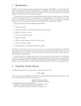
The graph macros provide the following functionality:
1. Automatic scaling
2. Automatic generation and labeling of tick marks or grid lines
3. Multiple coordinate systems
4. Linear and logarithmic scales
5. Separate data files
6. Ability to handle numbers outside the usual range
7. Arbitrary plotting symbols
8. Drawing, filling, and labeling commands for graphs
In addition to these items, the user also has access to all the features described in the MetaPost
user’s manual [6]. These include access to almost all the features of PostScript , ability to use and
manipulate typeset text, ability to solve linear equations, and data types for points, curves, pictures,
and coordinate transformations.
Section 2 describes the graph macros from a user’s perspective and presents several examples.
Sections 3 and 4 discuss auxiliary packages for manipulating and typesetting numbers and Section 5
gives some concluding remarks. Appendix A summarizes the graph-drawing macros, and Appendix B
describes some recent additions to the MetaPost language that have not been presented elsewhere.
1 METAFONT
is a trademark of Addison Wesley Publishing Company.
is a registered trademark of Adobe Systems Inc.
3 UNIX is a registered trademark of UNIX System Laboratories, Inc.
2 PostScript
1
2
Using the Graph Macros
A MetaPost input file that uses the graph macros should begin with
input graph
This reads a macro file graph.mp and defines the graph-drawing commands explained below. The
rest of the file should be one or more instances of
beginfig(hfigure numberi);
hgraphics commandsi endfig;
followed by end.
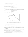
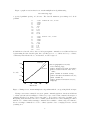
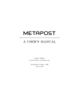
The following hgraphics commandsi suffice to generate the graph in Figure 1 from the data file
agepop91.d:
draw begingraph(3in,2in);
gdraw "agepop91.d";
endgraph;
(Each line of agepop91.d gives an age followed the estimated number of Americans of that age in
1991 [10].)
4×10⁶
3×10⁶
2×10⁶
106
0
20
40
60
80
Figure 1: A graph of the 1991 age distribution in the United States
2.1
Basic Graph-Drawing Commands
All graphs should begin with
begingraph(hwidthi,hheighti);
and end with endgraph. This is syntactically a hpicture expressioni, so it should be preceded by
draw and followed by a semicolon as in the example.4 The hwidthi and hheighti give the dimensions
of the graph itself without the axis labels.
The command
gdraw hexpressioni hoption listi
draws a graph line. If the hexpressioni is of type string, it names a data file; otherwise it is a path
that gives the function to draw. The hoption listi is zero or more drawing options
withpenhpen expressioni | withcolorhcolor expressioni | dashedhpicture expressioni
4 See
the User’s Manual [6] for explanations of draw commands and syntactic elements like hpicture expressioni.
2
that give the line width, color, or dash pattern as explained in the User’s Manual [6].
In addition to the standard drawing options, the hoption listi in a gdraw statement can contain
plot hpicture expressioni
The hpicture expressioni gives a plotting symbol to be drawn at each path knot. The plot option
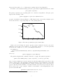
suppresses line drawing so that5
gdraw "agepop91.d" plot btex $\bullet$ etex
generates only bullets as shown in Figure 2. (Following the plot option with a withpen option
would cause the line to reappear superimposed on the plotting symbols.)
4×10⁶
••• •
•••
•
•• •• ••• •
••
••••• ••• • ••••
••••
•
•• •
••••••
3×10⁶
•••••
•
•••••
•••••••••••
•
•••
••
•••
•••
••
•••
•
2×10⁶
106
0
20
40
60
80
Figure 2: The 1991 age distribution plotted with bullets
Watch out for the following: the hpicture expressioni is placed with the lower-left corner at the
path knot, not its center. If you want it to be dead-center, you have to correct the placement
yourself. For the example above, you need something like this instead:
def MPbullet =
btex \lower\fontdimen22\cmsy \hbox to 0pt{\hss\cmsy\char15\hss} etex
enddef;
followed by:
gdraw "agepop91.d" plot MPbullet
The glabel and gdotlabel commands add labels to a graph. The syntax for glabel is
glabel. hlabel suffixi(hstring or picture expressioni, hlocationi) hoption listi
where hlocationi identifies the location being labeled and hlabel suffixi tells how the label is offset
relative to that location. The gdotlabel command is identical, except it marks the location with
a dot. A hlabel suffixi is as in plain MetaPost: hemptyi centers the label on the location; lft, rt,
top, bot offset the label horizontally or vertically; and ulft, urt, llft, lrt give diagonal offsets.
The hlocationi can be a pair of graph coordinates, a knot number on the last gdraw path, or the
special location OUT. Thus
gdotlabel.top(btex $(50,0)$ etex, 50,0)
5 Troff
users should replace btex $\bullet$ etex with btex \(bu etex.
3
would put a dot at graph coordinates (50,0) and place the typeset text “(50, 0)” above it. Alternatively,
glabel.ulft("Knot3", 3)
typesets the string "Knot3" and places it above and to the left of Knot 3 of the last gdraw path.
(The knot number 3 the path’s “time” parameter [6, Section 8.2].)
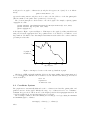
The hlocationi OUT places a label relative to the whole graph. For example, replacing “gdraw
"agepop91.d"” with
glabel.lft(btex \vbox{\hbox{Population} \hbox{in millions}} etex, OUT);
glabel.bot(btex Age in years etex, OUT);
gdraw "agepopm.d";
in the input for Figure 1 generates Figure 3. This improves the graph by adding axis labels and
using a new data file agepopm.d where the populations have been divided by one million to avoid
large numbers. We shall see later that simple transformations such as this can be achieved without
generating new data files.
4
3
Population
in millions
2
1
0
20
40
Age in years
60
80
Figure 3: An improved version of the 1991 age distribution graph
All flavors of TEX can handle multi-line labels via the \hbox within \vbox arrangement used
above, but LATEX users will find it more natural to use the tabular environment [9]. Troff user’s
can use nofill mode:
btex .nf
Population
in millions etex
2.2
Coordinate Systems
The graph macros automatically shift and rescale coordinates from data files, gdraw paths, and
glabel locations to fit the graph. Whether the range of y coordinates is 0.64 to 4.6 or 640,000 to
4,600,000, they get scaled to fill about 88% of the height specified in the begingraph statement. Of
course line widths, labels, and plotting symbols are not rescaled.
The setrange command controls the shifting and rescaling process by specifying the minimum
and maximum graph coordinates:
setrange(hcoordinatesi, hcoordinatesi)
where
4
hcoordinatesi → hpair expressioni
| hnumeric or string expressioni,hnumeric or string expressioni
The first hcoordinatesi give (xmin , ymin ) and the second give (xmax , ymax ). The lines x = xmin ,
x = xmax , y = ymin , and y = ymax define the rectangular frame around the graph in Figures 1–3.
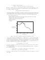
For example, an adding a statement
setrange(origin, whatever, whatever)
to the input for Figure 3 yields Figure 4. The first hcoordinatesi are given by the predefined pair
constant origin, and the other coordinates are left unspecified. Any unknown value would work as
well, but whatever is the standard MetaPost representation for an anonymous unknown value.
draw begingraph(3in,2in);
glabel.lft(btex \vbox{\hbox{Population} \hbox{in millions}} etex, OUT);
glabel.bot(btex Age in years etex, OUT);
setrange(origin, whatever,whatever);
gdraw "agepopm.d";
endgraph;
4
3
Population
in millions 2
1
0
0
20
40
Age in years
60
80
Figure 4: The 1991 age distribution graph and the input that creates it.
Notice that the syntax for setrange allows coordinate values to be given as strings. Many
commands in the graph package allow this option. It is provided because the MetaPost language
uses fixed point numbers that must be less than 32768. This limitation is not as serious as it sounds
because good graph design dictates that coordinate values should be “of reasonable magnitude” [2,
11]. If you really want x and y to range from 0 to 1,000,000,
setrange(origin, "1e6", "1e6")
does the job. Any fixed or floating point representation is acceptable as long as the exponent is
introduced by the letter “e”.
Coordinate systems need not be linear. The setcoords command allows either or both axes to
have logarithmic spacing:
hcoordinate settingi → setcoords(hcoordinate typei, hcoordinate typei)
hcoordinate typei → log | linear | -log | -linear
A negative hcoordinate typei makes x (or y) run backwards so it is largest on the left side (or bottom)
of the graph.
5
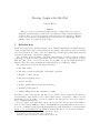
Figure 5 graphs execution times for two matrix multiplication algorithms using
setcoords(log,log)
to specify logarithmic spacing on both axes. The data file matmul.d gives timings for both algorithms:
20
30
40
60
80
120
160
240
320
480
.007861
.022051
.050391
.15922
.4031
1.53
3.915
18.55
78.28
279.24
standard MM: size, seconds
20
30
40
60
80
120
160
240
320
480
.006611
.020820
.049219
.163281
.3975
1.3125
3.04
9.95
22.17
72.60
Strassen: size, seconds
A blank line in a data file ends a data set. Subsequent gdraw commands access additional data sets
by just naming the same data file again. Since each line gives one x coordinate and one y coordinate,
commentary material after the second data field on a line is ignored.
Standard
100
10
Seconds
Strassen
1
0.1
0.01
20
50
100
Matrix size
200
draw begingraph(2.3in,2in);
setcoords(log,log);
glabel.lft(btex Seconds etex,OUT);
glabel.bot(btex Matrix size etex,
OUT);
gdraw "matmul.d" dashed evenly;
glabel.ulft(btex Standard etex,8);
gdraw "matmul.d";
glabel.lrt(btex Strassen etex,7);
endgraph;
500
Figure 5: Timings for two matrix multiplication algorithms with the corresponding MetaPost input.
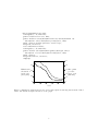
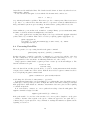
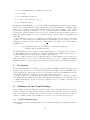
Placing a setcoords command between two gdraw commands graphs two functions in different
coordinate systems as shown in Figure 6. Whenever you give a setcoords command, the interpreter
examines what has been drawn, selects appropriate x and y ranges, and scales everything to fit.
Everything drawn afterward is in a new coordinate system that need not have anything in common
with the old coordinates unless setrange commands enforce similar coordinate ranges. For instance,
the two setrange commands force both coordinate systems to have x ranging from 80 to 90 and
y starting at 0.
6
draw begingraph(6.5cm,4.5cm);
setrange(80,0, 90,whatever);
glabel.bot(btex Year etex, OUT);
glabel.lft(btex \vbox{\hbox{Emissions in} \hbox{thousands of}
\hbox{metric tons} \hbox{(heavy line)}}etex, OUT);
gdraw "lead.d" withpen pencircle scaled 1.5pt;
autogrid(,otick.lft);
setcoords(linear,linear);
setrange(80,0, 90,whatever);
glabel.rt(btex \vbox{\hbox{Micrograms} \hbox{per cubic}
\hbox{meter of air} \hbox{(thin line)}}etex, OUT);
gdraw "lead.d";
autogrid(otick.bot,otick.rt);
endgraph;
0.5
60
0.4
0.3 Micrograms
per cubic
0.2 meter of air
(thin line)
0.1
Emissions in
40
thousands of
metric tons
(heavy line) 20
0
0
80
82
84
86
88
90
Year
Figure 6: Annual lead emissions and average level at atmospheric monitoring stations in the United
States. The MetaPost input is shown above the graph.
7
When you use multiple coordinate systems, you have to specify where the axis labels go. The
default is to put tick marks on the bottom and the left side of the frame using the coordinate system
in effect when the endgraph command is interpreted. Figure 6 uses the
autogrid(,otick.lft)
to label the left side of the graph with the y coordinates in effect before the setcoords command.
This suppresses the default axis labels, so another autogrid command is needed to label the bottom
and right sides of the graph using the new coordinate system. The general syntax is
autogrid(haxis label commandi, haxis label commandi) hoption listi
where
haxis label commandi → hemptyi | hgrid or ticki hlabel suffixi
hgrid or ticki → grid | itick | otick
The hlabel suffixi should be lft, rt, top, or bot.
The first argument to autogrid tells how to label the x axis and the second argument does the
same for y. An hemptyi argument suppresses labeling for that axis. Otherwise, the hlabel suffixi
tells which side of the graph gets the numeric label. Be careful to use bot or top for the x axis and
lft or rt for the y axis. Use otick for outward tick marks, itick for inward tick marks, and grid
for grid lines. The hoption listi tells how to draw the tick marks or grid lines. Grid lines tend to
be a little overpowering, so it is a good idea to give a withcolor option to make them light gray so
they do not make the graph too busy.
2.3
Explicit Grids and Framing
In case autogrid is not flexible enough, axis label commands generate grid lines or tick marks one
at a time. The syntax is
hgrid or ticki.hlabel suffixi(hlabel formati, hnumeric or string expressioni) hoption listi
where hgrid or ticki and hlabel suffixi are as in autogrid, and hlabel formati is either a format string
like "%g" or a picture containing the typeset numeric label.
The axis label commands use a macro
format(hformat stringi, hnumeric or string expressioni)
to typeset numeric labels. Full details appear in Section 4, but when the hformat stringi is "%g",
it uses decimal notation unless the number is large enough or small enough to require scientific
notation.
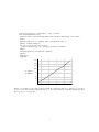
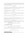
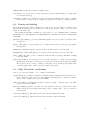
The example in Figure 7 invokes
format("%g",y)
explicitly so that grid lines can be placed at transformed coordinates. It defines the transformation
newy(y) = y/75 + ln y and shows that this function increases almost linearly.6 This is a little like
using logarithmic y-coordinates, except that y is mapped to y/75 + ln y instead of just ln y.
Figure 7 uses the command
frame.hlabel suffixi hoption listi
to draw a special frame around the graph. In this case the hlabel suffixi is llft to draw just the
bottom and left sides of the frame. Suffixes lrt, ulft, and urt draw other combinations of two
sides; suffixes lft, rt, top, bot draw one side, and hemptyi draws the whole frame. For example
frame dashed evenly
6 The
manual [6] explains how vardef defines functions and mlog computes logarithms.
8
vardef newy(expr y) = (256/75)*y + mlog y enddef;
draw begingraph(3in,2in);
glabel.lft(btex \vbox{\hbox{Population} \hbox{in millions}} etex, OUT);
path p;
gdata("timepop.d", $, augment.p($1, newy(Scvnum $2)); );
gdraw p withpen nullpen;
for y=5,10,20,50,100,150,200,250:
grid.lft(format("%g",y), newy(y)) withcolor .85white;
endfor
autogrid(grid.bot,) withcolor .85white;
gdraw p;
frame.llft;
endgraph;
250
200
150
100
Population
in millions
50
20
10
5
1800
1850
1900
1950
2000
Figure 7: Population of the United States in millions versus time with the population re-expressed
as p/75 + ln p. The MetaPost input shown above the graph assumes a data file ttimepop.d that
gives (year, p/75 + ln p) pairs.
9
draws all four sides with dashed lines. The default four-sided frame is drawn only when there is no
explicit frame command.
To label an axis as autogrid does but with the labels transformed somehow, use
auto.x or auto.y
for positioning tick marks or grid lines. These macros produce comma-separated lists for use in for
loops. Any x or y values in these lists that cannot be represented accurately within MetaPost’s
fixed-point number system are given as strings. A standard macro package that is loaded via
input sarith
defines arithmetic operators that work on numbers or strings. Binary operators Sadd, Ssub, Smul,
and Sdiv do addition, subtraction multiplication, and division.
One possible application is rescaling data. Figure 4 used a special data file agepopm.d that had
y values divided by one million. This could be avoided by replacing “gdraw "agepopm.d"” by
gdraw "agepop91.d";
for u=auto.y: otick.lft(format("%g",u Sdiv "1e6"), u); endfor
autogrid(otick.bot,)
2.4
Processing Data Files
The most general tool for processing data files is the gdata command:
gdata(hstring expressioni, hvariablei, hcommandsi)
It takes a file name, a variable v, and a list of commands to be executed for each line of the data
file. The commands are executed with i set to the input line number and strings v1, v2, v3, . . . set
to the input fields on the current line. A null string marks the end of the v array.
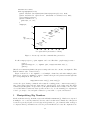
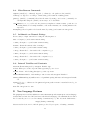
Using a glabel command inside of gdata generates a scatter plot as shown in Figure 8. The
data file countries.d begins
20.910 75.7 US
1.831 66.7 Alg
where the last field in each line gives the label to be plotted. Setting defaultfont in the first line
of input selects a small font for these labels. Without these labels, no gdata command would be
needed. Replacing the gdata command with
gdraw "countries.d" plot btex$\circ$etex
would change the abbreviated country names to open circles.
Both gdraw and gdata ignore an optional initial ‘%’ on each input line, parse data fields separated
by white space, and stop if they encounter an input line with no data fields. Leading percent signs
make graph data look like MetaPost comments so that numeric data can be placed at the beginning
of a MetaPost input file.
It is often useful to construct one or more paths when reading a data file with gdata. The
augment command is designed for this:
augment.hpath variablei(hcoordinatesi)
If the path variable does not have a known value, it becomes a path of length zero at the given
coordinates; otherwise a line segment to the given coordinates is appended to the path. The hcoordinatesi may be a pair expression or any combination of strings and numerics as explained at the
beginning of Section 2.2.
10
defaultfont:="cmr7";
draw begingraph(3in,2in);
glabel.lft(btex \vbox{\hbox{Life}\hbox{expectancy}} etex, OUT);
glabel.bot(btex Per capita G.N.P. (thousands of dollars) etex, OUT);
setcoords(log,linear);
gdata("countries.d", s,
glabel(s3, s1, s2);
)
endgraph;
80
70
Life
expectancy 60
50
Jap
Swi
Ita
Swe
Fra
Gre Spn Nth
Can
Aus
Bel
UK
Ger
US
Ven Por Tai
Chl
Yug Pol
BulCze
Mex
Rom
Hun
Sri
Col Arg
Chn
Tur
USS
SKo
Syr
NKo
Tha
Mal
Alg
Brz
Mor IrnPer
Phi
SAf
KenInn
Egy
Ind
Pak
Bur
ZaiGha
Ban
Sud
Mad
Tnz
Eth
Nep Uga
Nig
Moz
0.1 0.2
0.5 1
2
5 10 20
Per capita G.N.P. (thousands of dollars)
Figure 8: A scatter plot and the commands that generated it
If a file timepop.d gives t, p pairs, augment can be used like this to graph newy(p) versus t:
path p;
gdata("timepop.d", s, augment.p(s1, newy(scantokens s2)); );
gdraw p;
(MetaPost’s scantokens primitive interprets a string as if it were the contents of an input file. This
finds the numeric value of data field s2.)
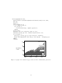
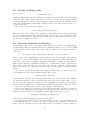
Figure 9 shows how to use augment to read multiple column data and make multiple paths.
Paths p2, p3, p4, p5 give cumulative totals for columns 2 through 5 and pictures lab2 through lab5
give corresponding labels. The expression
image(unfill bbox lab[j]; draw lab[j])
executes the given drawing commands and returns the resulting picture: “unfill bbox lab[j]”
puts down a white background and “draw lab[j]” puts the label on the background. The gfill
command is just like gdraw, except it takes a cyclic path and fills the interior with a solid color. The
color is black unless a withcolor clause specifies another color. See the manual [6] for explanations
of for loops, arrays, colors, and path construction operators like --, cycle, and reverse.
3
Manipulating Big Numbers
MetaPost inherits a fixed-point number system from Knuth’s METAFONT [8]. Numbers are expressed
in multiples of 2−16 and they must have absolute value less than 32768. Knuth chose this system
because it is perfectly adequate for font design, and it guaranteed to give identical results on all types
of computers. Fixed-point numbers are seldom a problem in MetaPost because all computations are
11
draw begingraph(3in,2in);
glabel.lft(btex \vbox{\hbox{Quadrillions}\hbox{of BTU}} etex, OUT);
path p[];
numeric t;
gdata("energy.d", $,
t:=0; augment.p1($1,0);
for j=2 upto 5:
t:=t+scantokens $[j]; augment.p[j]($1,t);
endfor)
picture lab[];
lab2=btex coal etex; lab3=btex crude oil etex;
lab4=btex natural gas etex; lab5=btex hydroelectric etex;
for j=5 downto 2:
gfill p[j]--reverse p[j-1]--cycle withcolor .16j*white;
glabel.lft(image(unfill bbox lab[j]; draw lab[j]), .7+length p[j]);
endfor
endgraph;
hydroelectric
60
natural gas
40
Quadrillions
of BTU
crude oil
20
coal
0
1900
1920
1940
1960
Figure 9: A graph of U.S. annual energy production and the commands that generated it
12
based on coordinates that are limited by the size the paper on which the output is to be printed. This
does not hold for the input data in a graph-drawing application. Although graphs look best when
coordinate axes are labeled with numbers of reasonable magnitude, the strict limits of fixed-point
arithmetic would be inconvenient.
A simple way to handle large numbers is to include the line
input sarith
and then use binary operators Sadd, Ssub, Smul, and Sdiv in place of +, -, *, and /. These operators
are inefficient but very flexible. They accept numbers or strings and return strings in exponential
notation with the exponent marked by “e”; e.g., "6.7e-11" means 6.7 × 10⁻¹¹ .
The unary operator7
Sabs hstringi
finds a string the represents the absolute value. Binary operators Sleq and Sneq perform numeric
comparisons on strings and return boolean results.
The operation
Scvnum hstringi
finds the numeric value for a string if this can be done without overflowing MetaPost’s fixed-point
number system. If the string does not contain “e”, it is much more efficient to use the primitive
operation
scantokens hstringi
The above operators are based on a low-level package that manipulates numbers in “Mlog form.”
A number x in Mlog form represents
µ2
16
x
,
−24
where µ = −e2
.
Any value between 1.61 × 10⁻²⁸ and 3.88 × 1055 can be represented this way. (There is a constant
Mten such that k ∗ Mten represents 10k for any integer k in the interval [−29, 55].)
The main reason for mentioning Mlog form is that it allows graph data to be manipulated as a
MetaPost path. The function
Mreadpath(hfile namei)
reads a data file and returns a path where all the coordinates are in Mlog form. An internal variable
Gpaths determines whether gdraw and gfill expect paths to be given in Mlog form. For example,
this graphs the data in agepop91.d with y coordinates divided by one million:
interim Gpaths:=log;
gdraw Mreadpath("agepop91.d") shifted (0,-6*Mten);
4
Typesetting Numbers
The graph package needs to compute axis labels and then typeset them. The macro
format(hstring expressioni, hnumeric or string expressioni)
does this. You must first input graph or input format to load the macro file. The macro takes a
format string and a number to typeset and returns a picture containing the typeset result. Thus
format("%g",2+2) yields
4
and
format("%3g","6.022e23") yields
6.02×10²³
A format string consists of
7 The
argument to a unary operator need not be parenthesized unless it is an expression involving binary operators.
13
• an optional initial string not containing a percent sign,
• a percent sign,
• an optional numeric precision p,
• one of the conversion letters e, f, g, G,
• an optional final string β.
The initial and final strings are typeset in the default font (usually cmr10), and the typeset number
is placed between them. For the e and g formats, the precision p is the number of significant digits
allowed after rounding; for f and G, the number is rounded to the nearest multiple of 10−p . If the
precision is not specified, the default is p = 3. The e format always uses scientific notation and the
f format uses ordinary decimal notation but reverts to scientific notation if the number is at least
10000. The g and G formats also revert to scientific notation for non-zero numbers of magnitude less
than 0.001.
The format macro needs a set of templates to determine what font to use, how to position the
exponent, etc. The templates are normally initialized automatically, but it is possible to set them
explicitly by passing five picture expressions to init numbers. For instance, the default definition
for TEX users is
init_numbers(btex$-$etex, btex$1$etex, btex${\times}10$etex,
btex${}^-$etex, btex${}^2$etex)
The first argument tells how to typeset a leading minus sign; the second argument is an example of
a 1-digit mantissa; third comes whatever to put after the mantissa in scientific notation; next come
a leading minus sign for the exponent and a sample 1-digit exponent.
Picture variable Fe_plus gives a leading plus sign for positive numbers, and Fe_base gives
whatever should precede the exponent when typesetting a power of ten. Calling init_numbers
initializes Fe_plus to an empty picture and constructs Fe_base from its second and third arguments.
5
Conclusion
The graph package makes it convenient to generate graphs from within the MetaPost language. The
primary benefits are the power of the MetaPost language and its ability to interact with TEX or troff
for typesetting labels. Typeset labels can be stored in picture variables and manipulated in various
ways such measuring the bounding box and providing a white background.
We have seen how to generate shaded regions and control line width, color, and styles of dashed
lines. Numerous other variations are possible. The full MetaPost language [6] provides many other
potentially useful features. It also has enough computing power to be useful for generating and
processing data.
A
Summary of the Graph Package
In the following descriptions, italic letters such as w and h denote expression parameters and words
in angle brackets denote other syntactic elements. Unless specified otherwise, expression parameters
can be either numerics or strings. An hoption listi is a list of drawing options such as withcolor
.5white or dashed evenly; a hlabel suffixi is one of lft, rt, top, bot, ulft, urt, llft, lrt.
A.1
Graph Administration
begingraph(w,h) Begin a new graph with the frame width and height given by numeric parameters
w and h.
14
endgraph End a graph and return the resulting picture.
setcoords(tx , ty ) Set up a new coordinate system as specified by numeric flags tx , ty . Flag values
are ±linear and ±log.
setrange(hcoordinatesi, hcoordinatesi) Set the lower and upper limits for the current coordinate
system. Each hcoordinatesi can be a single pair expression or two numeric or string expressions.
A.2
Drawing and Labeling
All of the drawing and labeling commands can be followed by an hoption listi. In addition to the
usual MetaPost drawing options, the list can contain a plot hpicturei clause to plot a specified
picture at each data point.
The drawing and labeling commands are closely related to a set of similarly named commands
in plain MetaPost. The gdrawarrow and gdrawdblarrow commands are included to maintain this
relationship.
gdotlabel.hlabel suffixi(p, hlocationi) This is like glabel except it also puts a dot at the location
being labeled.
gdraw p Draw path p, or if p is a string, read coordinate pairs from file p and draw a polygonal line
through them.
gdrawarrow p This is like dgraw p except it adds an arrowhead at the end of the path.
gdrawdblarrow p This is like dgraw p except it adds an arrowheads at each end of the path.
gfill p Fill cyclic path p or read coordinates from the file named by string p and fill the resulting
polygonal outline.
glabel.hlabel suffixi(p, hlocationi) If p is not a picture, it should be a string. Typeset it using
defaultfont, then place it near the given location and offset as specified by the hlabel suffixi.
The hlocationi can be x and y coordinates, a pair giving x and y, a numerc value giving a time
on the last path drawn, or OUT to label the outside of the graph.
A.3
Grids, Tick Marks, and Framing
auto.hx or yi Generate default x or y coordinates for tick marks.
autogrid(haxis label commandi, haxis label commandi) Draw default axis labels using the specified commands for the x and y axes. An haxis label commandi may be hemptyi or it may be
itick, otick, or grid followed by a hlabel suffixi.
frame.hlabel suffixi hoption listi Draw a frame around the graph, or draw the part of the frame
specified by the hlabel suffixi.
grid.hlabel suffixi(f ,z) Draw a grid line across the graph from the side specified by the hlabel
suffixi, and label it there using format string f and coordinate value z. If f is a picture, it
gives the label.
itick.hlabel suffixi(f ,z) This is like grid except it draws an inward tick mark.
otick.hlabel suffixi(f ,z) This is like grid except it draws an outward tick mark.
15
A.4
Miscellaneous Commands
augment.hvariablei(hcoordinatesi) Append hcoordinatesi to the path stored in hvariablei.
format(f , x) Typeset x according to format string f and return the resulting picture.
gdata(f , hvariablei, hcommandsi) Read the file named by string f and execute hcommandsi for
each input line using the hvariablei as an array to store data fields.
init numbers(s, m, x, t, e) Provide five pictures as templates for future format operations: s is
a leading minus; m is a sample mantissa; x follows the mantissa; t is a leading minus for the
exponent e.
Mreadpath(f ) Read a path for the data file named by string f and return it in “Mlog form”.
A.5
Arithmetic on Numeric Strings
It is necessary to input sarith before using the following macros:
Sabs x Compute |x| and return a numeric string.
x Sadd y Compute x + y and return a numeric string.
Scvnum x Return the numeric value for string x.
x Sdiv y Compute x/y and return a numeric string.
x Sleq y Return the boolean result of the comparison x ≤ y.
x Smul y Compute x ∗ y and return a numeric string.
x Sneq y Return the boolean result of the comparison x 6= y.
x Ssub y Compute x − y and return a numeric string.
A.6
Internal Variables and Constants
Autoform Format string used by autogrid. Default: "%g".
Fe base What precedes the exponent when typesetting a power of ten.
Fe plus Picture of the leading plus sign for positive exponents.
Gmarks Minimum number of tick marks per axis for auto and autogrid. Default: 4.
Gminlog Minimum largest/smallest ratio for logarithmic spacing with auto and autogrid. Default:
3.0.
Gpaths Code for coordinates used in gdraw and gfill paths: linear for standard form, log for
“Mlog form”.
Mten The “Mlog form” for 10.0
B
New Language Features
The graph.mp macros and the arithmetic routines in marith.mp and sarith.mp use various language
features that were introduced in Version 0.60 of the MetaPost language. We summarize these features
here because they are not covered in existing documentation [6, 5]. Also new is the built-in macro
image(hdrawing commandsi)
that was used in Section 2.4 to find the picture produced by a sequence of drawing commands.
16
B.1
Reading and Writing Files
A new operator
readfrom hfile namei
returns a string giving the next line of input from the named file. The hfile namei can be any primary
expression of type string. If the file has ended or cannot be read, the result is a string consisting
of a single null character. The preloaded plain macro package introduces the name EOF for this
string. After readfrom has returned EOF, additional reads from the same file cause the file to be
reread from the start.
The opposite of readfrom is the command
write hstring expressioni tohfile namei
This writes a line of text to the specified output file, opening the file first if necessary. All such files
are closed automatically when the program terminates. They can also be closed explicitly by using
EOF as the hstring expressioni. The only way to tell if a write command has succeeded is to close
the file and use readfrom to look at it.
B.2
Extracting Information from Pictures
MetaPost pictures are composed of stroked lines, filled outlines, pieces of typeset text, clipping paths,
and setbounds paths. (A setbounds path gives an artificial bounding box as is needed for TEX
output.) A picture can have many components of each type. They can be accessed via an iteration
of the form
for hsymbolic tokeni within hpicture expressioni: hloop texti endfor
The hloop texti can be anything that is balanced with respect to for and endfor. The hsymbolic
tokeni is a loop variable that scans the components of the picture in the order in which they were
drawn. The component for a clipping or setbounds path includes everything the path applies to.
Thus if a single clipping or setbounds path applies to everything in the hpicture expressioni, the
whole picture could be thought of as one big component. In order to make the contents of such a
picture accessible, the for. . . within iteration ignores the enclosing clipping or setbounds path in
this case.
Once the for. . . within iteration has found a picture component, there are numerous operators
for identifying it and extracting relevant information. The operator
stroked hprimary expressioni
tests whether the expression is a known picture whose first component is a stroked line. Similarly,
the filled and textual operators return true if the first component is a filled outline or a piece
of typeset text. The clipped and bounded operators test whether the argument is a known picture
that starts with a clipping path or a setbounds path. This is true if the first component is clipped
or bounded or if the entire picture is enclosed in a clipping or setbounds path.
There are also numerous part extraction operators that test the first component of a picture. If
p is a picture and stroked p is true, pathpart p is the path describing the line that got stroked,
penpart p is the pen that was used, dashpart p is the dash pattern, and the color is
(redpart p, greenpart p, bluepart p)
If the line is not dashed, dashpart p returns an empty picture.
The same part extraction operators work when filled p is true, except that dashpart p is
not meaningful in that case. For text components, textual p is true, textpart p gives the text
that got typeset, fontpart p gives the font that was used, and xpart p, ypart p, xxpart p,
17
xypart p, yxpart p, yypart p tell how the text has been shifted, rotated, and scaled. The redpart,
greenpart, and bluepart operators also work for text components.
When clipped p or bounded p is true, pathpart p gives the clipping or setbounds path and
the other part extraction operators are not meaningful. Such non-meaningful part extractions do
not generate errors—they return null values instead: the trivial path (0,0) for pathpart, nullpen
for penpart, an empty picture for dashpart, zero for redpart, greenpart, bluepart, and the null
string for textpart or fontpart.
One final operator for extracting information from a picture is
length hpicture primaryi
This returns the number of components that a for. . . within iteration would find.
B.3
Other New Features
The marith.mp and sarith.mp packages use numbers of magnitude 4096 more. Since such numbers
can cause overflow problems in MetaPost’s linear equation solving and path fitting algorithms, they
are normally allowed only as intermediate results. This limitation is removed when the internal
variable warningcheck is zero. In earlier versions of MetaPost, the limitation could be removed for
variables but explicit constants were always restricted to be less than 4096.
For completeness, we also mention one other new feature of MetaPost Version 0.60. When TEX
material is included in a picture via the btex. . . etex feature, the thickness of horizontal and vertical
rules gets rounded to exactly the right number of pixels; i.e., interpreting MetaPost output according
to the PostScript scan conversion rules [7] makes the pixel width equal to the ceiling of the unrounded
width. In fact, a similar relationship holds for all line widths. The generated PostScript sets line
widths by first transforming to device coordinates and rounding appropriately.
References
[1] Jon L. Bentley and Brian W. Kernighan. Grap—a language for typesetting graphs. In Unix
Research System Papers, volume II, pages 109–146. AT&T Bell Laboratories, Murray Hill, New
Jersey, tenth edition, 1990.
[2] William S. Cleveland. The Elements of Graphing Data. Hobart Press, Summit, New Jersey,
1985, revised 1994.
[3] William S. Cleveland. Visualizing Data. Hobart Press, Summit, New Jersey, 1993.
[4] William S. Cleveland. A model for studying display methods of statistical graphics (with
discussion). Journal of Computational and Statistical Graphics, 3, to appear.
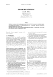
[5] John D. Hobby. Introduction to MetaPost. In EuroTEX ’92 Proceedings, pages 21–36, September
1992.
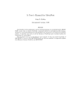
[6] John D. Hobby. A user’s manual for MetaPost. Computing Science Technical Report no. 162,
AT&T Bell Laboratories, Murray Hill, New Jersey, April 1992. Available as http://cm.belllabs.com/cs/cstr/162.ps.gz.
[7] Adobe Systems Inc. PostScript Language Reference Manual. Addison Wesley, Reading, Massachusetts, second edition, 1990.
[8] Donald E. Knuth. METAFONT the Program. Addison Wesley, Reading, Massachusetts, 1986.
Volume D of Computers and Typesetting.
[9] Leslie Lamport. LATEX: A Document Preparation System. Addison Wesley, Reading, Massachusetts, 1986.
18
[10] U.S. Bureau of the Census. Statistical Abstracts of the United States: 1992. Washington, D.C.,
112th edition, 1992.
[11] Edward R. Tufte. Visual Display of Quantitative Information. Graphics Press, Box 430,
Cheshire, Connecticut 06410, 1983.
19