Download MAGPRISM_MANU

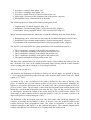
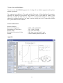
MAGPRISM
Version 1.1 © 2003 Markku Pirttijärvi
Introduction:
The objective of geophysical magnetic field method is to obtain indirect information about the
subsurface structures from the measurements made above Earth's surface. The most important
petrophysical parameter affecting the formation of a magnetic field anomaly is the magnetic
susceptibility, which defines the ability of a material to become magnetized under an external
magnetic field. In geophysical applications the external magnetic field is Earth's geomagnetic
field. Some minerals, especially the magnetite, have considerably higher susceptibility than
most other rock-forming minerals. Therefore, field measurements that are made in the vicinity
of a target that contains highly magnetized material reveal anomalous magnetic field. The
susceptibility, position, orientation and dimensions of the target as well as the intensity and
the direction (inclination and declination) of earth's geomagnetic field define the spatial
characteristics of the magnetic anomaly. Although the magnetic field data cannot be
interpreted uniquely, the information about the susceptibility and its distribution can be used
in geological and structural interpretation.
Another important factor affecting the geophysical magnetic field response is the remanent
(or remnant) magnetization, especially the thermal remanent magnetization, which was fixed
to the rock material when it crystallized from melted magma. The remanent magnetization
usually has different direction than the induced magnetization, because the direction of
geomagnetic field has changed and the position and orientation of the rock material has
changed in geological tectonic processes. The remanent magnetization should be taken into
account because it can affect the interpretations based on the "normal" induced magnetization.
X-position
Y-position
Z-position
Thickness
Susceptibility
Strike length
Strike angle
Depth extent
Dip angle
Figure 1. The parameters of a dipping prism model.
1
The MAGPRISM program computes the static magnetic field on a profile above an isolated,
dipping magnetized prism-like body. The parameters of the prism model are shown in Figure
1. In addition to the susceptibility, the Q-ratio and the inclination and declination of the
remanent magnetization of the prism as well as the demagnetization effect of a highly
magnetized target can be taken into account. Only one body and one profile can be used. The
forward computation is based on the analytical solution and the original algorithm of S.-E.
Hjelt (1972). The MAGPRISM program is intended primarily for educational purposes.
Installing the program:
The MAGPRISM program requires a PC with 32-bit Windows 9x/NT4/2000/XP operating
system and a graphics display capable for at least 1024×768 resolution. Memory requirements
and processor speed and are not critical, since the program uses dynamic memory allocation
and the analytical solution allows very fast computation even on slow computers. The
MAGPRISM program has a simple graphical user interface (GUI) that can be used to change
the parameter values, to handle file input and output, and to visualize the magnetic field
response and the model. The user interface and the data visualization are based on the
DISLIN graphics library.
The program requires following files:
MAGPRISM.EXE the executable file
DISLIN.DLL
dynamic link library for the graphics routines
The distribution file (MAGPRISM.ZIP) contains also a short description file
(_README.TXT), this user's manual (MAGPRISM_MANU.PDF), and an example input file
(EXAMPLE.INP). To install the program, create a new directory and copy or unzip (e.g.,
Pkunzip/Winzip) the distribution files there. To be able to start the program from a shortcut
that locates in a different directory one should move or copy the DISLIN.DLL file into the
WINDOWS\ SYSTEM (or SYSTEM32) folder or somewhere where a path always exists.
Getting started:
On startup the program reads the parameters of the model parameters from the MPRISM.INP
file and the graph parameters from the MPRISM.DIS file. If these files do not exist, default
parameters are used and the files are created automatically.
The program then computes the magnetic field response and builds up the user interface
shown in the Appendix. The response is plotted in the graph area along with a 3-D view of the
model and a description of the model parameters. All model parameters can be altered using
the controls on the left side of the MAGPRISM program window.
As shown in Appendix the main window of the MAGPRISM application contains two menus.
The "File" menu contains the following nine options:
Open Model
Read Data
Save Model
to open an existing model file.
to read in data for comparison (total field only).
to save the model into a file.
2
Save Data
Read disp.
Save Graph as PS
Save Graph as EPS
Save Graph as PDF
Save Graph as WMF
to save the results (description + response) into a file.
to read in new graph parameters from a *.DIS file.
to save the graph in Adobe's Postscript format.
to save the graph in Adobe's Encapsulated Postscript format.
to save the graph in Adobe's Acrobat PDF format.
to save the graph in Windows metafile format.
Selecting these menu options brings up a standard (Windows) file selection dialog that can be
used to provide the name of the file for open/save operation. Model and data (including other
information) files are saved in standard ASCII text format. The graphs are saved in landscape
A4 size (cf. Appendix).
The "Edit" menu contains four items:
Comp → Meas
Remove measured
Demagnet. on/off
Remanence on/off
Total/Anom field
to put current data as "measured" data for comparison.
to discard all information about "measured" data.
to include/exclude the demagnetization effect.
to include/exclude information about remanent magnetization.
to include/exclude the external magnetic field from total field.
The "Exit" menu has only one item, which is used to confirm the exit operation. On exit the
latest model and results are automatically saved in MPRISM.INP and MPRISM.OUT files
replacing the original ones. Errors that are encountered before the GUI starts up can be found
from the MPRISM.ERR file. When operating in GUI mode, run-time errors arising from
illegal parameter values are displayed on the screen.
Using program controls:
The "Change component" push button at the top of the control pane on the left side of the
MAGPRISM window can be used to change the field component that is shown in the graph.
The magnetic field components are shown in the following order:
1.
2.
3.
4.
5.
6.
7.
Total field anomaly (the magnetic field of the prism without earth's magnetic field).
Z-component (vertical field) anomaly.
X-component (horizontal field in NS direction) anomaly.
Y-component (horizontal field in EW direction) anomaly.
Horizontal field anomaly.
Total field (earth's magnetic field added)
All anomalous field components: (total, z, x, y, horis.)
The "Update parameters" button is used to read and update the model parameters and to
perform a new forward computation.
The following nine text fields define the parameters of the prism model (see Fig 1.), these are:
1.
2.
3.
4.
Thickness (m).
Length (along strike) (m).
Depth extent (vertical height) (m).
Dip angle (from horizontal plane) (degrees).
3
5.
6.
7.
8.
9.
X-position (easting) of the prism (m).
Y-position (northing) of the prism (m).
Z-position (depth of burial) of the top of the prism (m).
Strike angle (direction of the elongated side of the prism) (degrees).
Susceptibility value (dimensionless in SI-units).
The following three text fields define earth's geomagnetic field.
1. Total intensity of extenal magnetic field (nT).
2. Inclination (from horizontal plane) of the external field (degrees)
3. Declination (from geographic north) of the external field (degrees).
When remanent magnetization is taken into account the following three text fields define:
1. Köningsberg's ratio (ratio between the remanent and induced magnetic field, Mr/Mi).
2. Inclination of the remanent magnetization (from horizontal plane) (degrees)
3. Declination of the remanent magnetization (from geographic north) (degrees).
The last five text fields define the system parameters of the measurement profile ():
1.
2.
3.
4.
5.
The X-coordinate (easting) of the profile start position (m).
The Y-coordinate (northing) of the profile start position (m).
The X-coordinate (easting) of the profile end position (m).
The Y-coordinate (northing) of the profile end position (m).
The spatial spacing between the profile points (m).
The three slide controls below the graph window can be used to change the point of view for
the 3-D model. The view can be rotated horizontally and vertically, and the relative distance
of the viewing point can be changed (as if zooming in and out).
Notes on model parameters:
All distances and dimension are defined in meters (m) and all angles are defined in degrees
(°). For historical reasons the geophysical unit of the magnetic field is nano-Tesla (nT), which
equals to 10-9 Vs/m2.
As shown in Fig. 1 the xyz-position of the prism is defined by the center of the top of the
prism. In addition, the top and bottom surfaces of the prism are horizontal. Although, the
negative z-axis points downwards in the 3-D model view, the z-position (depth of burial) is
given a positive value. The dip angle is taken from the horizontal plane and the depth extent
means the vertical height of the prism (not along the dip). Thus, the dip can not be equal to 0
or 180 degrees, because the length of the prism along the dip would become infinite. The
strike angle is taken counter-clockwise from the positive x-axis. For example, if strike is 90
degrees the prism is oriented along the y-axis.
The definition of the declination angle may vary from some other modeling programs. For
example, in Finland the declination is about -6 degrees, since the magnetic north locates
counter-clockwise from geographical north. The value of inclination is positive on the
northern hemisphere and negative on the southern hemisphere. The remanent magnetization
(and the susceptibility) is considered to be constant inside the model prism.
4
Input file format:
The MAGPRISM program is intended for forward modeling only. More appropriate data
interpretation can be made using the MAGINV program. However, external data (total
magnetic field only) can be read in for comparison using the menuitem "Read data" in "File"
menu. Thus, interpretation of field data is possible on trial-and-error basis. The example
below illustrates the format of the simple column formatted data file.
21
3
-250 0 52000
-200 0 52010
-150 0 52040
... etc
The first line defines the number of data points, n, and the column number, i, from which the
data is to be read from. The next n lines then define the x- and y-coordinates (easting and
northing) of the data points, and the successive columns contain the data values. In the
example above only one data column is available. The data file should not contain any empty
lines. Note that the data can be irregularly spaced, and therefore, need not to be from a
straight profile. However, the MAGPRISM program displays the data only in profile format.
Note the input data must represent the total magnetic field. However, the total field
component does not need to include the total field component of the geomagnetic field. The
menuitem "Total/Anom field", which is available only when data has been read in, can be used
to include and to exclude Earth's field from the computation.
Output file format:
The following text illustrates the output file (MPRISM.DAT) format:
#
#
#
#
#
#
#
#
#
#
#
#
#
#
#
#
#
#
#
#
#
#
#
#
#
----------------------------------------------------Results from MAGPRISM: the magnetic field of a prism
----------------------------------------------------Copy of the input file (MPRISM.INP):
50.00
400.00
200.00
60.00
0.00
0.00
0.05000 52000.0
75.00
-5.00
0.00
0.00
0.00 -250.00
0.00
250.00
10.00
1
----------------------------------------------------Description:
Thickness
50.00
Strike length
400.00
Height
200.00
Dip angle
60.00
X-position
0.00
Y-position
0.00
Z-position= depth
20.00
Strike angle
-10.00
Susceptibility
0.05000
Normal field
52000.00
Field inclination
75.00
Field declination
-5.00
Köningsbergs ratio
0.00
Reman. inclination
0.00
Reman. declination
0.00
5
20.00
0.00
-10.00
#
X-start position
0.00
#
Y-start position
-250.00
#
X-end position
0.00
#
Y-end position
250.00
#
Point spacing
10.00
#
Demagn. coeffs.
0.000 0.000 0.000
# ---------------------------------------------------------------------------# X-pos, Y-pos, Dist., Total, Total anom., Z-comp, X-comp, Y-comp, Horiz-comp.
0.0 -250.0 0.0 0.5201E+05 0.1770E+02 0.3224E+01 0.5711E+02 -0.4576E+01 0.56354E+02
0.0 -240.0 10.0 0.5202E+05 0.2095E+02 0.5361E+01 0.6185E+02 -0.4714E+01 0.60970E+02
... etc
Note that the output file contains a copy of the input file, the format of which should become
clear from the example above. Since there should rarely be any need to edit model files
manually, a more detailed description of model files is not shown here. The only exception is
the single parameter on the last line of the model file that can be used to disable (0) or enable
(1) the GUI. Thus, setting this parameter to zero forces the program to just perform the
forward computation and to write the results without any additional hassle.
Graph options:
Several graph parameters can be changed by editing the MPRISM.DIS file. Note that the
format of the MPRISM.DIS file must be preserved. If the format of the file should become
invalid, one should delete the file and a new one with default parameter values will be
generated automatically the next time the program is started. The file format is shown below.
40
32
32
32
1
1
1
350 380 0.45 0.70
1100 130. 25.
8.
32
Magnetic field of a dipping prism
Total field anomaly
Z-component
X-component
Y-component
Horiz. field anomaly
Total field
Model parameters:
Distance (m)
Response (nT)
X / East (m)
Y / North (m)
Z / Depth (m)
• The 1.st line defines five character heights. The first one is used for the main title and the
graph axis titles, the second height is used for the axis labels, the third height is used for
the plot legend text, the fourth height is used for the model description text, and the last
height is used for the axis labels in the 3-D model view.
• The 2.nd line defines parameters that modify the graph appearance. The first one can be
used to include (1) or exclude (0) the model information text to/from the top-right corner
of the page. The second one can be used to include (1) or to exclude (0) the model view
to/from the bottom-right corner of the page. The third parameter is used to define the
corner where the legend text is positioned. Values 1-4 put the legend in SW, SE, NE or
NW corner of the page (outside the graph). Values 5-8 put the legend in the SW, SE, NE,
or NW corner inside the graph. The default values are 1, 1, 1.
6
• The 3.rd line defines the x- (horizontal) and y- (vertical) distance of the origin of the main
graph (in pixels) from the bottom-left corner of the page, and the length of the x- and y-axis
relative to the size of the remaining (origin shifted) width and height of the plot area. The
size of the total plot area is 2970×2100 pixels (landscape A4).
• The first parameter on the 4.th line defines the size (in pixels) of the square area reserved
for the 3-D model. The position of the model area is always next to the lower right corner
of the response graph. The remaining three parameters define horizontal and vertical
viewing angles and a perspective viewing distance for the 3-D model view.
• The 5.th line should be left empty.
• The following lines define various text items of the graph (max. 70 chars). These are:
• The first line defines the main title of the graph.
• The following 6 lines define the texts for possible response components.
• The next line is the title of the model description text.
• The next 2 lines define the axis titles of the graph.
• The last 3 lines define the axis title texts of the 3-D model view.
References:
A. Aharoni, 1998: Demagnetizing factors for rectangular ferromagnetic prisms. J. Appl.
Physics, 83, 3432-3434
S.-E. Hjelt., 1972: Magnetostatic anomalies of dipping prisms. Geoexploration, 10, 239-254.
R.I. Joseph and E. Schlöman, 1965: Demagnetizing field in non-ellipsoidal bodies. J. Appl.
Phys., 36, 1579-1593.
Additional information:
I started to develop the MAGPRISM program at the University of Oulu in May 2002, when I
began to work in a 3-D crustal model project funded by the Academy of Finland. The forward
computation is based on the MPRISM algorithm of Sven-Erik Hjelt (see the reference). The
algorithm for the demagnetizing factors was originally derived from and Joseph (1967) by J.
Lerssi (missing exact reference). The equations for the demagnetizing factors can be found
also from Aharoni (1998). More information about geophysical magnetic field method can be
found from any textbook on applied geophysics.
The MAGPRISM program is written in Fortran-90 style and compiled with Compaq Visual
Fortran 6.6. The graphical user interface is based on the DISLIN graphics library (version 8)
by Helmut Michels. The program distribution includes the DISLIN.DLL file that is required
for the GUI. The WWW homepage of DISLIN is <http://www.dislin.de>. Since the DISLIN
graphics library is independent form the operating system the MAGPRISM program could be
compiled on other operating systems (Solaris, Linux) without any major modifications. At the
moment, however, the source code is not made available and I do not intend to provide any
support for the program. If you find the computed results erroneous or if you have suggestions
for improvements, please, inform me.
7
Terms of use and disclaimer:
You can use the MAGPRISM program free of charge. If you find the program useful, please,
send me a postcard.
The program is provided as is. The author and the University of Oulu disclaim all warranties,
expressed or implied, with regard to this software. In no event shall the author or the
University of Oulu be liable for any indirect or consequential damages or any damages
whatsoever resulting from loss of use, data or profits, arising out of or in connection with the
use or performance of this software.
Contact information:
Markku Pirttijärvi
Division of Geophysics
Department of Geosciences
PO Box 3000
FIN-90014 University of Oulu
Finland
GSM: +358-40-5548959
Tel: +358-8-5531409
Fax: +358-8-5531484
URL: http://www.gf.oulu.fi/~mpi
E-mail: [email protected]
Appendix:
8