Download Clinical Applications Manual

SOUNDSCOPE -MANUAL OF
CLINICAL
APPLICATIONS
INSTRUMENTS DESIGNED AND
CREATED BY -Rebecca Leonard, Ph.D.
University of California, Davis
and
Tito Poza, M.S.
Poza Consulting Services
Menlo Park, CA
SOUNDSCOPE IS A PRODUCT OF
G.W. INSTRUMENTS, INC.
SOMERVILLE, MA
more detailed description of the functions and controls of this instrument than in the material for the other two instruments. (The idea is
that, once you've used these, the others will be similar and familiar.)
Some operations are described in the text for each instrument, making for some redundancies which you can probably skip over after
reading about them once.
INTRODUCTION
SoundScope was designed to be used with a Macintosh computer. It
works best on models that are at least as powerful as a Macintosh IIfx
equipped with a 1.4 meg floppy drive and at least 8 megs of RAM.
The monitor you use should be set to "color" and "256" (settings
under "Monitor" in the Control Panel). It is assumed that users will
have some familiarity with the Macintosh, i.e. understand its desktop,
know how to find and open up programs and understand the functions of a mouse. If you are a true novice, you might want to try
something like "Professor Mac," a software tutorial from Individual
Software, Inc. in Pleasanton, CA. Basic operations of the Mac are
reviewed extensively in this excellent primer.
The manual is designed to be used as you are working, with the
computer screen in front of you. There are some graphics in the
manual which serve as overviews of the kinds of things each instrument can do, and of the controls needed to use them. However, the
main "graphic" is the computer screen -- the illustrations in the
manual are intended to serve primarily as references.
Once you have selected Rate-Range Calculator and see it appear on
the monitor, the purpose of the instrument, and how to use it, will be
explained in the text. Just read along and try the operations described. It should be possible to use each of the demo instruments by
simply reading the text, perhaps occasionally referring to the graphics
for additional information. You will be able to load any of the demo
stimuli into any of the instruments, but you won't be able to record
into SoundScope from other sources. Nor will you be able to open up
materials you've manipulated and saved.
After you put the SoundScope -- Clinical Manual demo disk into
your computer's floppy drive, open the "Read Me" file and follow its
instructions to uncompress the files you'll need to carry out the
exercises described in this manual. Once you've done this you will
notice a new "SoundScope Clinical Manual ƒ" containing the
SoundScope program, the three clinical instruments available for
demonstration (Rate-Range Calculator, Stimulus Generator and
Speech Reconstructor), and two folders named Demo Stimuli 1 and
Demo Stimuli 2. The stimuli in the first folder should be used with
Rate-Range Calculator; the second folder contains stimuli for use
with Stimulus Generator and Speech Reconstructor. The program,
instruments and demo stimuli are the items you will need to be
concerned with for the demonstration. You must first open up the
SoundScope application itself (double click on it). When you see a
blank screen with a menubar at the top, press the mouse on the "File"
menu at the top left and select "Open." A dialog box will open up
with a list of things you can open further. Items listed include the
three demo instruments and the two folders of demo stimuli.
The three instruments demonstrated here were designed and created
using the basic "instrument design tools" which are a part of
SoundScope. We believe they are a good illustration of the kinds of
innovations in clinical instrumentation which are becoming more and
more possible with contemporary computer technology. As you use
them, you will hopefully think about other kinds of tools which might
facilitate your own clinical experiences. The instruments are fairly
user-friendly, intuitive and even fun to use. We think you'll enjoy
them!
The manual begins with an explanation of Rate-Range Calculator,
and it is probably best to start with this instrument. Highlight RateRange Calculator with the cursor and click on "Open." There is a
2
depress the LOAD SPEECH button and open the DEMO STIMULI 1
folder. (If you own SoundScope, of course, you can also RECORD
your own utterances, after setting record levels with SET REC LEVELS.) Double-click on "PA-PA-PA" DYS. You will see the waveform of the utterance loaded into the window at the bottom of the
screen. Each time you load anything into this window, it's a good
idea to click the "H" at the top right of the waveform window. This
shows you the entire waveform, and can return you to this display
quickly following compression/expansion.
RATE-RANGE CALCULATOR
Rate-Range Calculator is designed to be of particular use in the
evaluation of a speaker with a neurogenic disorder. It actually consists of two separate instruments that share the same screen. The
figure presented on the next page is an overview of the Rate-Range
instrument. A more detailed description of the functions and controls
for each of the two instruments (DIADO and PITCH), as well as for
those controls that are shared by both instruments (COMMON), is
presented in Appendix A on pages 22-27.
Once the waveform is drawn, listen to the entire utterance by clicking
PLAY. There are two additional options for listening to portions of
the utterance, including PLAY SEL (selected) and PLAY SEG (segment). The first requires highlighting, or "selecting," a portion of the
waveform that you'd like to hear. Do this by first clicking on the
label "UTT," if it's not already highlighted, in the left margin of the
waveform window. Then put the mouse cursor on some part of the
waveform, press and hold the mouse button down, drag the mouse
and cursor from left to right until you've isolated what you want, then
release the mouse button. The portion of the utterance you've selected should be highlighted. Now try clicking PLAY SELECTED.
You can "deselect" by simply clicking again on the selected area.
The Rate instrument can assist the clinician in assessing syllable
repetition tasks, also referred to as diadochokinetic tasks. Beyond a
simple calculation of rate (syllables/sec), however, the analyses
performed on rapidly repeated utterances can provide the clinician
with information regarding other articulatory parameters unique to
the speaker, including the temporal regularity of syllable pulses, and
the spectral integrity of utterances over one breath group.
The Range functions of Calculator are useful in evaluating preliminary fundamental frequency and durational characteristics of voicing.
The instrument is not intended for those situations in which a comprehensive voice evaluation is desired, but rather, for those instances
when information regarding possible limitations on a speaker's ability
to sustain sounds, turn the voice off and on, or generate a range of
frequencies and intensities, may be useful.
Another way to isolate part of the utterance is to "bound" it with two
"markers," vertical lines in the waveform window that create a
segment containing the portion desired. Each of the two vertical lines
can be moved by (1) holding down the "Option" key on the keyboard,
; (2) lining up the
which changes the cursor icon from an arrow to
vertical line of the cursor with the vertical line of the marker; and (3)
pressing and holding the mouse button while dragging the line to a
new location. If the marker seems "hidden," look for a dashed
vertical line at the extreme right or left edge of the window which
indicates that it is "off the screen." It can be brought into view by
lining the cursor up exactly with the dashed line, and carrying out the
process described above.
The dual purposes of Calculator are reflected in the control panel,
located in the middle of the display (see page 4). Those functions
related to syllable repetition tasks are positioned on the left, while
those having more to do with voice analyses are on the right. All
controls common to both instruments, for loading, storing and otherwise manipulating utterances, have been positioned in the middle of
the control panel. Controls which are in bold print will, when activated, cause the named operation to be performed; words not in bold
generally serve as labels or indicators. To try out Calculator, first
3
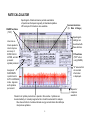
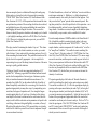
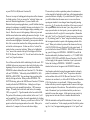
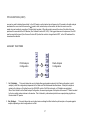
RATE CALCULATOR
Spectrogram of diado utterance permits examination
of spectral and temporal regularity of alternated syllables.
LPC analysis of formants is also available.
DIADO functions
("ON")
Common functions
(for Rate & Range )
Spectrogram
settings can
be altered with
these buttons.
User can estimate speaker's
rate to improve
accuracy of
RATE CALCULATOR, and can
preselect
syllable produced.
F0 functions
("OFF" when
using DIADO).
"H" assures that
all recorded
information
is displayed.
Analysis of
DIADO RATE
is performed in
AUTO or MANUAL
mode. Appears
as # syllables
per second.
Waveform of syllable productions is placed in this window. Syllables can
be automatically or manually segmented to include those desired for analysis.
Blue lines at bottom of window indicate energy concentrations SoundScope
interprets as syllables.
4
Expand or
compress
waveform.
Diado Rate
SYLLABIC RATE window (Diado Function #4).
Let's experiment, first, with the DIADO RATE instrument. The task
here, of course, is to determine how many syllables the speaker is
capable of producing per second. To begin, be sure that the button to
the right of DIADO RATE (Diado Function #7) is set to ON. Click
on CLIENT and type in a name -- this will now appear on the screen.
The RATE-RANGE CALCULATOR can automatically segment the
"pa pa pa" utterance for you, if you click on SEGMENT SPEECH
(Common Function #18). If you're not happy with this segmentation,
however, you can move the vertical lines as described above to
"bound" the segment you want included in the analysis. Try SEGMENT and observe where CALCULATOR places the segment
markers. The automatic segmentation may not include the last three
syllables. This is due to the break between the first 13 syllables and
the last 3. One could argue that including the entire utterance in the
segment would not give the appropriate rate for this speaker. However, if that is what is desired, the right marker can be moved manually to include the last 3 syllables in the segment, as well.
Before you accept RATE-RANGE's calculation, you must first check
to see which peaks the instrument included in its analysis. On your
monitor, note the blue vertical lines in the waveform window below
the red speech signal (colors will be black if you don't have a color
monitor). Each blue spike denotes a production which was interpreted by CALCULATOR as a syllable and thus included in its
calculation. If a dysarthric speaker has added some extraneous
utterances, or if two syllables are extremely close together, CALCULATOR may make errors -- including something in the analysis that
shouldn't be, or indicating only one syllable when there were really
two, for example. If the blue lines match up with the waveform, and
with what your ears tell you, then the rate calculated is probably fine.
In this example, in spite of the fact that the third syllable is inappropriately long, the automatic calculation worked correctly by counting
the extended syllable as just one and not two syllables. If it had
erred, however, you could try another rate selection or, alternatively,
a MANUAL calculation.
Now click under SPEECH RATE (Diado Function #2) to choose a
rate which you think characterizes the speaker's rate (we've selected
SLOW for this speaker). Go to UTTERANCE TYPE (Diado Function #5) and find "pa pa pa…" RATE-RANGE CALCULATOR
provides four options here, including repetitions of the syllables "pa,"
"ta" or "ka," as well as the alternated "pa ta ka…" These options are
included so that any data which might be stored in the journal will be
appropriately labeled, and you won't have to remember the order of
your analyses! Incidentally, if you re-SEGMENT "pa pa pa" with the
rate set to SLOW, all of the syllables will be included in the segment.
A MANUAL calculation is initiated by first selecting MANUAL on
the MANUAL/AUTOMATIC control (Diado Function #6). Clicking
on ANALYZE (Diado Function #3) in the MANUAL mode bypasses
the computer's syllable counting algorithm. Determine how many
syllables the segment contains by playing it and by counting the
appropriate peaks in the waveform -- once again, make sure the
segment includes only those productions you want interpreted as
syllables.
When you're satisfied, click on ANALYZE (Diado Function #3). A
dialog box will appear asking you to enter the number of syllables
which should be included in the analysis. Type in the appropriate
number and click OK. The calculated number of syllables/second
will again appear in the SYLLABIC RATE window (Diado Function
#4). If this value is acceptable, you may want to store it in the journal (SAV TO JNL, Common Function #14). You can also save the
Look at the MANUAL/AUTO control (Diado Function #6) and note
whether the window says AUTO or MANUAL. For this first example, set it to AUTO, and then click ANALYZE (Diado Function
#3). The number of syllables produced per second will appear in the
* The references in parentheses refer to the descriptions of the functions found in
Appendix A, pages 22-27.
5
entire journal with SAV JNL, but don't save it until you've included
everything in it you want. The journal can be examined at any time
by clicking SHOW JNL (Common Function #15). The information
you entered, and the repetition rate for "pa pa pa...", will be shown.
When you have completed all of your analyses and stored them in the
journal, you can select PRNJ (Common Function #18) to produce a
hard copy. The utterance, or a selected portion of the utterance, can
also be saved to disk by clicking on the appropriate save control
(Common Functions #10, SAV UTT and #11, SAV SEL). Clicking
on one of these controls will bring up a dialog box asking you to
name the information you want to save. Scroll through the list box
above the name to find the folder where you'd like to store your data.
Double-click on it, type in a name for your data, and click SAVE.
You can also SAV JNL (Common Function #12) to disk, but this will
clear your working journal, so wait until you have everything in it
you want!
temporal or spectral integrity over time may reflect fatigue, and
provide clues to utterance lengths which may be optimal for the
individual, while more generalized irregularities may provide insights
into the nature of the speaker's motor disorder. For comparison,
return to LOAD SPEECH (Common Function #4) and click "TA-TATA DYS." Remember to click on "H" when the waveform has
loaded. This time, draw the spectrogram immediately by pressing the
"Cal" button (Auxiliary Function #1) in the right margin of the top
window. You may want to change the setup of the spectrogram, for
example, to use a different analysis filter, or to expand a portion of
the frequency range. Click on "Set" (Auxiliary Function #2) and look
at the parameters you can change. (Some "Set" options are available
by clicking on the boxes; others require you to type in values.) Try
lowering the range of frequencies displayed, from 8 kHz to about 5
kHz. Click OK, and redraw the spectrogram (click "Cal"). Are the
formants easier to evaluate? If consonant characteristics are of
interest, expand the range of frequencies displayed to visualize higher
frequency components.
Repetition rate is one measure which can be elicited from a
diadochokinetic task. But clinicians who consider only rate may be
overlooking some very useful information. RATE-RANGE
CALCULATOR'S design facilitates a more comprehensive assessment of syllable repetition tasks. Let's consider some examples,
starting with the utterance you've already loaded.
Once you've characterized the spectrographic details, click on ANALYZE (DiadoFunction #3) to calculate the speaker's repetition rate
for "ta." If you use SEGMENT SPEECH (Common Function #18),
be sure to check the segmentation. To get an accurate rate, you may
have to move the markers manually and set the MANUAL/AUTOMATIC control (Diado Function #6) to MANUAL. Set UTT TYPE,
count the syllables within your new segment boundaries and reANALYZE (Diado Function #3).
Go to the window at the top of the screen display, look for "Cal"
(Auxiliary Function #1) in the right margin and click it. A spectrogram of the "pa pa pa" will be drawn. Examine the uniformity of the
syllables produced by this speaker. Is there a clear distinction between consonant and vowel? Are there instances where the consonant is very weak, unaspirated, voiced or even missing? Does the
formant structure for /a/ appear appropriate across all the syllables, or
does the vowel become more neutralized, more schwa-like (formants
equally spaced), with time? Are the syllables produced at equal
intervals, and are they all about equal in duration? Separate analyses
of beginning and ending segments may be revealing here. A loss of
*If you own SoundScope, you can open a saved Journal from the menu with "Journal" >
"Load Text" > "Journal" then "Edit" > "Show..." > "Journal"
How does the rate for "ta" compare to "pa?" If one or the other is
faster, it may reflect greater integrity of one articulatory structure, i.e.
lips versus tongue, over the other. Substantial differences in rates
may also provide insights regarding the speaker's ability to alternate
between structures, i.e. lips and tongue+jaw, to produce the consonant and vowel in "pa," as opposed to using the same primary structure, i.e. tongue+jaw, for both consonant and vowel in "ta" and "ka."
This kind of information may be helpful to the clinician in planning
6
strategies and ordering therapy objectives for particular speakers.
Now open "KA-KA-KA" DYS and scrutinize it just as you have "pa"
and "ta."
apparent between the normal and dysarthric speakers.
One further type of investigation possible with RATE CALCULATOR is formant tracking using SoundScope's LPC analysis capabilities. This further scrutiny of diado productions might be desired
when your initial impression is that the formant structure of the
speaker's vowels changes over time on the syllable repetition tasks.
When you have one of the waves loaded, go into the spectrogram
"Set" box where you previously changed the range of frequencies
displayed. At the bottom of the dialog box that opens when you click
on "Set" is an "Options" button. Clicking on this reveals choices you
can make regarding which formants you'd like tracked. The first two
or three are usually sufficient. Check the ones you'd like displayed
and then close the dialog box and redraw the spectrogram (click
"Cal").
Be especially careful in the analysis of diadochokinetic rate for "ka."
There are a number of "additions" in the utterance which reflect
phonatory and respiratory irregularities that you won't want CALCULATOR to interpret as syllables. Again, notice the repetition rate for
"ka," as compared to those determined for "pa" and "ta." Any insights regarding the integrity of anterior vs. posterior tongue?
Try expanding the waveform with the arrow on the left side of the
time window at the bottom right of the display. Expanding the signal,
and then redrawing the spectrogram (click "Cal"), provides graphic
evidence of the dipthongization apparent in the speaker's utterances.
Was this characteristic of the earlier productions, as well?
When the spectrogram redraws this time, you will be presented with a
message informing you that the LPC tracking operation is underway.
This may take a little while -- it's a complicated process. When the
operation is completed, you will see colored traces representing the
formants you selected for tracking. These will be difficult to see if
you don't have a color monitor -- sorry! Remember that the lowest
formant, in frequency, is always considered formant 1, the next
lowest in frequency, formant 2, and so on. If the syllables weren't
expanded in this initial analysis, you may want to expand the time
waveform and do the LPC analysis again. This might make it easier
to visualize the formant locations across the vowels. You might also
want to adjust the frequency range displayed to facilitate viewing the
formants. When you've changed the settings, try the LPC analysis
again. Do F1 and F2 appear to remain stable across the syllables?
Are they uniform in time? If the speaker has difficulty terminating
voicing, you may see a lot of transition activity in F1 and F2, as the
vocal tract changes shape while voicing continues. To the left of
DIADO RATE on the control panel, there is a button labeled LG
FMT (Diado Function #1). Clicking on this button activates
CALCULATORS's log-data-to-journal function. You should now see
Now, click LOAD SPEECH, find "TA" NORMAL, load it and draw
its spectrogram. In some contrast to the utterances you've just analyzed, the normal speaker's syllable repetition rate is greater than
seven syllables per second. But, as we've noted, there are many other
features of diadochokinetic tasks which may provide insights into a
speaker's articulatory finesse. In this example, consider the regularity
of the syllable pulses produced, in both temporal and spectral domains. Each syllable is of approximately the same duration, and the
intervals between them are also equal. There is a clear demarcation
between consonant and vowel, and the spectral characteristics of the
syllables appear homogeneous from start to finish. The formant
structure is appropriate for /a/, and, unlike the previous utterances,
there is little or no diphthongization of vowels. Voicing does not
continue from one syllable to the next, and, as apparent in both the
waveform and the spectrogram, the syllables appear to have been
produced with about the same intensity. In short, the "ta" repetitions
reflect the precision and orderliness typical of normal speech in the
adult. You may want to go back to the previous examples of "PA-PAPA" DYS and "TA-TA-TA" DYS, and note if other differences are
7
three vertical, black segment marker lines in the spectrographic
display. The one that appears at exactly 0.5 seconds activates the
logging process. (Selecting the wrong marker may cause the spectrogram to disappear again -- use "Cal" to redraw.) Place the cursor
icon) directly over this marker and perform a "press,
(now the
drag, release" to a steady-state portion of the speaker's first vowel,
that is, to a point where the LPC traces appear fairly flat. When you
release the mouse button you will see the formant values, and the
time of their occurrence, appear in the LOG window (Common
Function #20). By repeating this press, drag and release operation at
selected spots in the various syllables, you will record representative
formant data across the speech sample. When you've finished, you
can scroll through the log to see if the quantitative data support your
impressions of what was happening to the vowels over time. If you
want to save these data, in addition to your summaries for
diadochokinetic rates, just repeat the SAV TO JNL (Common Function #14) operation for printing now or later.
Pitch Analysis
The buttons on the right side of Rate-Range Calculator control the
instrument's fundamental frequency analysis functions. (See the
figure on the next page for an overview of the screens produced with
Pitch Analysis. See Appendix A, pages 26-27, for more detailed
descriptions of the pitch functions.) The Range portion of CALCULATOR was designed to assist the clinician in obtaining some preliminary information about a client's voice production capabilities. It
is useful in assessing a speaker's fundamental frequency range,
determining mean F0's in connected speech, and observing changes
in F0 associated with durational variables. For example, utterances
which become progressively longer, as "Many men made millions,"
"Many men made millions on rainy days," "Many men made millions
on rainy days in January and June," may reveal interesting variability
in F0, as well as in voice quality. Similarly, such tasks comprised,
first, of all voiced utterances, and then voiced+ voiceless components, may also provide insights into a speaker's capabilities. These
kinds of measures may be especially useful when the clinician is
trying to determine what sort of respiratory and phonatory support for
speech are available to a particular speaker.
One caution -- once the LPC traces are displayed, they stay on the
screen when you redraw the spectrogram, even if you go back into
"Set" and remove them by turning them "off" in the "Options" window. Since it takes a little time to do the LPC analysis, you probably
won't want to have this happen every time you redraw the spectrogram, in particular, when you're changing the range of frequencies
displayed to look at consonant characteristics, or experimenting with
expanding the time scale. In short, the LPC analysis should be the
last analysis you perform prior to loading a new utterance. You might
also want to turn off the LPC analysis when you finish with CALCULATOR so that, the next time you use it, you won't forget and start
with an LPC analysis the first time you draw a spectrogram. There is
a control, called NAN (Common Function #6), that enables you to
make portions or all of a formant trace invisible, and this function can
be used to get rid of formant traces without having to load a new
utterance. The description of the control, found on page 24 (Common Function #6), explains how to accomplish this.
In order to try out Range Calculator, you will first need to turn on the
PITCH ANALYSIS instrument by clicking the Pitch ON/OFF button
(Pitch Function #1). When the program is ON, the display at the top
will change from a spectrogram window to a pitch plot window. The
controls in the middle of the control panel are common to both
DIADO RATE and PITCH ANALYSIS, so click on LOAD SPEECH
(Common Function #4), and find "F0 Range" in the list of Demo
Stimuli 1. Click on it and wait for it to be loaded into the waveform
window at the bottom of screen. Once it's loaded, remember to click
on the "H" at the top of the right hand margin of the waveform
display so that you can see the entire waveform. Then segment the
portion of the waveform you want to analyze by using SEGMENT
SPEECH (Common Function #18) or by putting the segment markers
around the part of the waveform you want to consider.
* If the spectrogram disappears, just click "Cal" again.
8
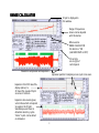
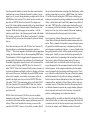
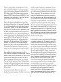
RANGE CALCULATOR
F0 plot is displayed in
this window.
Range of frequencies
shown can be adjusted
with this button.
When used as
RANGE CALCULATOR
this button is "ON
(and DIADO RATE is OFF)!
F0 controls
are on right of
control panel.
Waveform compression and expansion --
Expansion from 500 msec/Div.
display (above) to
20 msec/Div. reveals F0 plot
as series of red dots.
Expansion also reveals green,
vertical lines which correspond
to peaks in the F0 plot.
SoundScope uses these to
determine vibratory cycles.
"Holes" in plot can be edited
or eliminated.
9
expansion permits # samples per one cycle to be seen.
The first step in performing the range analysis is to set the F0 parameters to make CALCULATOR's F0 estimates as accurate as possible.
Click on CHANGE F0 PARAMETERS (Pitch Function #2). A
dialog box will open allowing you to adjust some analysis parameters. If you're looking for mean values from connected speech tasks,
you might want to check one of the boxes appropriate for an average
adult female or male. However, if you want to assess range data, the
third option is especially useful. This option allows you to enter a
low and high F0 value, respectively, which will determine the range
of allowable frequency values. Click on each box and type in your
selections. If you haven't had much experience estimating F0's by
ear, you may need to adjust the range and repeat ANALYZE (Pitch
Function #3) a couple of times.
the "Frame advance" setting in the F0 PARAMETERS dialog box
described below.
If there appear to be unanalyzed areas at the beginning or end of the
waveform, you may need to adjust the range parameters accordingly.
You might also want to experiment with F0 range settings to see how
the analysis varies. Going back into CHANGE F0 PARAMETERS
(Pitch Function #2) reveals two other variables which can be manipulated in performing analyses. "Frame advance" determines the
"sample rate" of the F0 plot. If it's set at 2 ms., the F0 wave will have
500 estimates for each second of speech. If the speech has a constant
pitch of 125 Hz (8 ms. period), there would always be 4 estimates for
each pitch period. One thing to watch out for with this parameter is
to make sure you don't make it bigger than the smallest pitch period
you expect to encounter, or you'll lose information. 2 ms. is usually
safe as it allows a 500 Hz F0 with no loss of information. The "Reject all peaks..." option allows you to make CALCULATOR more or
less tolerant of samples it includes for analysis. That is, if it's set to
10%, it will include for analysis only those pitch periods which vary
no more than 10% from adjacent periods.
When you've set the F0 parameters, close the dialog box and click on
ANALYZE (Pitch Function #3). When CALCULATOR is finished,
you will see the red (or black) F0 trace, or melody plot, in the upper
display. Values for mean F0 and standard deviation, duration of the
segment analyzed, and minimum and maximum values in the sample
assessed, will also be displayed (Pitch Function #'s 4,5,6,7 and 8). As
with DIADO RATE, you may choose to save these data in the journal
you've created. Before you do this, however, you may want to check
the F0 trace once more.
The "Reject..." feature can be particularly useful when you're trying
to analyze a voice that contains significant aperiodicity, or instability
in frequency and amplitude components. However, you should
recognize that making the analysis scheme more "tolerant" may also
compromise the accuracy of results obtained to some extent. The
analysis of F0, particularly in dysphonic voices, is a complex and
perilous task for any analysis scheme, not just SoundScope!
One easy way to see if any voiced portions of the speech waveform
have not been analyzed for pitch is to examine the green (or black)
trace in the lower window, above the red (or black) waveform trace.
This trace, labeled _Pea, is zero everywhere except where a pitch
peak was found by the pitch tracking program. By expanding the
waveform you can, if you wish, zoom in on any problem areas and
see what may have caused it. If you expand the waveform, you will
also see the green (or black) band become a series of vertical lines,
each of which indicates a time at which the pitch tracking program
found the start of a new pitch period. Expansion will further reveal
that the pitch track at the top of the display is actually a series of red
(or black) dots. The time between consecutive dots is determined by
When you're in doubt about data that you're obtaining, remember that
you can do a narrow-band analysis, or even expand a waveform to
evaluate individual periods, to help you decide if there is sufficient
periodicity in the sample to get at least an estimate of F0. In fact, it's
a good idea to do these other types of analyses regardless of the voice
sample -- they may help you to better understand, and appreciate, the
difficulty involved in F0 analysis.
10
If there appear to be areas in the F0 trace where "glitches" of some
type occurred (outlying points far removed, in frequency, from the
rest of the trace, or an area where no trace is present, for example),
you may want to do some manual editing of the trace. Click on the
EDIT button (Pitch Function #9) to the right of ANALYZE until it
) which can
becomes DRAW. The cursor will turn into a pencil (
be used to manually eliminate the spurious or blank portions of the
trace by means of a "press, drag, release" operation. The idea here is
to try to smooth out these areas by drawing lines connecting stable
portions of the F0 plot. After the "press, drag, release," the "redrawn"
trace will reflect the results of your edit. Click again on ANALYZE
(Pitch Function #3) before you click out of DRAW (back to LOG or
EDIT) and the pitch statistics will reflect the changes you made by
redrawing the plot. IMPORTANT: If you change DRAW back to
EDIT or LOG and click on ANALYZE, the pitch plot will be recalculated and your redrawn pitch trace will be replaced.
Some of the statistics may not be very different after a redraw to
"correct" glitches, but the MAX and MIN will often show a significant change if your redraw corrected a substantial outlier. More
importantly, if you're just trying to fill in the questionable areas by
following the progression of the plot as reasonably and carefully as
possible, the edit should enable a closer approximation to the F0
values actually produced by the speaker. Always keep in mind,
however, that whenever you redraw any portion of the pitch trace,
your data are now an approximation of the actual track. That is to
say, any statistics you calculate probably reflect the truth more
closely than before you redrew the trace, but they are not the result of
a pitch tracking calculation. An intermediate approach to correcting
obvious pitch tracking mistakes is to use the NAN function (Common
Function #6) to eliminate obvious pitch tracking mistakes. The name
of this control stands for "not a number," and it allows you to make
portions of the F0 trace "invisible" to the statistics calculations. It
only works in the DRAW mode of the EDIT control (Pitch Function
#9) and involves a two step operation. First, click on the NAN
button. This will bring up a dialog box asking you to select a portion
of the F0 plot that you want to transform into values of NAN. After
clicking OK on the dialog box, the cursor once again becomes an
arrow and you should select, with press, drag, release, the portion of
the F0 trace that contains the outliers, or obviously bad data. Now
click once more on the NAN button and the selected portion of the F0
trace will disappear and the cursor will revert to a pencil. As with the
redraw, clicking on ANALYZE (Pitch Function #3) while still in the
DRAW mode will recalculate the statistics on the modified data. You
may want to expand the pitch trace in order to assure greater precision in selecting the portions of the trace to eliminate.
A final feature of the Range instrument can be exercised by clicking
on the EDIT button (Pitch Function #9) until it becomes LOG. This
activates CALCULATOR's log F0-to-journal function. As you did
with the LG FMT function of DIADO RATE, find the vertical marker
that appears at 0.5 seconds in the upper display. As with the LG FMT
function, if you line up the cursor on this marker and use a press,
drag, release operation, you can move the marker to a desired point in
the F0 trace. When you release the mouse, the F0 value at the point
of the vertical marker, as well as the time, will be entered in the
journal. These values can be stored in the journal (SAV TO JNL,
Common Function #14) and eventually printed out (PRNJ, Common
Function #17), if you like.
11
back to "File" in the menubar, and select "Open." The figure presented on the next page is an overview of the Stimulus Generator
instrument. A more detailed description of the functions and controls
of this instrument is presented in Appendix B on page 28.
STIMULUS GENERATOR
Stimulus Generator is designed to facilitate stages of therapy in
which generalization or "carry-over" activities are critical. This
aspect of, perhaps, every behavioral therapy presents some unique
challenges for both clinician and client. The extension of skills
acquired and used with facility in the clinical environment to the
client's real world environment is the last and sometimes most difficult stage of the therapeutic process. Ideally, we would like those
stimuli which, in the context of therapy, seem to elicit desired responses in the client -- related to fluency, improved articulatory
patterns, voicing characteristics, etc. -- to travel with, and be retained
by, the client in nonclinical situations. Indeed, it is the client's demonstration of this facility which signals a successful treatment outcome.
If you were going to record your own stimuli, you could first set up
the Record parameters with SET REC (Stim. Gen. Function #1) and
then RECORD (Stim. Gen. Function #4) into the A, B, C or D window. For now, find the LOAD (Stim. Gen. Function #5) buttons at
the top of the display. Click on LOAD A and open Demo Stimuli 2.
For purposes of their use with Stimulus Generator, the four strategies
previously noted are referred to here as "Cushion of Air," "Eyes On,"
"Morph" and "Stabilizer." Load the first one into A, and the other
three stimuli into the B, C and D windows, respectively. Click on the
"H" in each window. Also, click on CLIENT and enter some identification.
Stimulus Generator is based on the premise (which seems reasonable
to its developers, at least) that the ideal "stimulus," i.e. an event
which prompts a client to utilize a strategy or target skill acquired
through therapy, is one which is unique to the client, not to the clinical environment, and is therefore always with the client. Beyond this,
it would be helpful if the stimulus always occurred during speech.
Obvious candidates are properties of the client's speech output, itself,
or events which co-occur with speech.
As you load each window, the name of the stimulus representing each
strategy will be placed over the appropriate set of PLAY and RESPOND buttons (Stim. Gen. Function #7) in the middle of the screen
at the top. When you've loaded all four, play each one of them. We
won't elaborate on therapy activities associated with the development
of each of the strategies represented by the four stimuli. However,
the stimuli do bear a close correspondence to the strategies.
For example, play the first stimulus, "cushion of air." The strategy
represented by this stimulus required the client to monitor his respiratory support for speech and to end each breath group while still
slightly above resting expiratory level. That is, when he finished the
last word prior to an inspiration, relaxation of the respiratory system
would produce passive exhalation, thus, a small "cushion of air." The
stimulus was constructed by recording the client using this strategy,
and then extracting a segment of passive exhalation from the recording using the CUT and SAVE tools in Stimulus Generator. Try your
hand at this by clicking on LOAD A and finding the item SGSMP
(Stimulus Generator Sample) in the Demo Stimuli folder. You will
Examples of such stimuli are presented on the Demo Stimuli 2 folder.
The particular stimuli included on the demo disk were actually used
with an adult fluency client, and were tailored specifically to his
needs. Over a period of several months, this client had developed a
number of strategies which promoted his fluency and which, in fact,
made the prospect of disfluency in his speech negligible. Each
strategy had been worked on individually until the client was adept at
using it in the treatment room and ready to implement it in a structured manner in his daily activities.
If you haven't yet done so, open Stimulus Generator. To do this, go
12
STIMULUS GENERATOR
Clinician first presents stimulus (PLAY), and then clicks (RESP) to
indicate client's response, if appropriate.
Stimuli are loaded
or recorded into
Windows A, B,
C and D. Stimuli can
also be saved.
Running tally of each S and R is noted under
each window (A, B, C, D).
Client's
name is entered.
Clicking on
"SHOW" under
TALLY produces
this summary
of stimuli
and responses
which can be
printed,
spooled or saved.
The name
of each stimulus
appears under each
window.
This window
can be used to
create new stimuli
using the Selection (Cut, Copy, Paste and Amp)
tools in the upper right of Stimulus Generator.
Spooling Tally allows data to be
saved as separate trials which can then
be compared to each other at end of
session by scrolling through (SHOW) or
printing (PRNT) Tally.
In example shown, short segments of /s/
become "eyes on."
13
hear an example of passive exhalation following the breath group.
Isolate and save it using the tools in the upper right surrounding
"SELECTION" (Stim. Gen. Function #14, which subsumes Stim.
Gen. Functions #'s 15-22). All the operations listed around this term
are performed on portions of the recording which have been selected,
or highlighted in green, by pressing and holding the mouse button
and dragging the mouse along the waveform. You can use this
feature to identify the passive exhalation in the sample you've loaded
-- just highlight something and click on PLAY (Stim. Gen. Function
#18.) When you've isolated the portion you want, you can SAVE
(Stim. Gen. Function #22) it.
The final stimulus here, referred to as "stabilizer," was extracted from
an utterance containing /s/. Stabilizers, i.e. slight prolongations of
sustainable sounds, were used by the client for a dual purpose. First,
they served as brief "pause" periods within connected speech. During these periods, the client did a quick check of his respiration -- was
he exhaling smoothly and was he aware of gradually diminishing
lung volume. On another occasion, he might use the stabilizer pause
to focus briefly on eye contact, and to re-establish it if needed.
From the sample utterance SGSMP included in the Demo Stimuli 2
file, it should be possible to construct stimuli similar to the ones
described here using the tools under "SELECTION ." "Saute," the
sample stimulus, contains components for "cushion of air," as well as
for "morph" and "stabilize." You could also create something like
"eyes on" from /t/. Extract a portion of /t/, COPY (Stim. Gen. Function #16) it, then PASTE (Stim. Gen. Function #17) it onto an empty
area on the waveform, and then paste a second copy next to the first.
Now you can experiment with the interval between them with CUT
(Stim. Gen. Function #15) until you're satisfied with the result. You
can also vary the amplitude of the new stimulus with AMP (Stim.
Gen. Function #19), which allows you to increase or decrease the
intensity of a selection.
Now play window B containing the stimulus "eyes on." This stimulus served as a cue to the client to maintain, or restore, eye contact
with a listener. It was constructed by extracting portions of two /p/'s
from something the client had said. This particular stimulus was felt
by the client to be especially appropriate -- the two rapid clicks
representing two eyes, and the abrupt, transient character of the noise
serving to quickly grab his attention.
Clicking on "morph" reveals an exaggerated production of CV
syllable "ka." In therapy, a great deal of attention had been focused
on the client's manipulation of various types of utterances, particularly on transition elements within and between utterances. For
example, the syllable "ka" can be produced with the /k/ and the /a/
almost completely coarticulated, or co-occurring. But it can also be
produced appropriately in many other ways, by manipulating voice
onset time, the degree of aspiration on /k/, the strength of tongue
contact against palate for /k/, and so on. Attention to this strategy
was helpful to the client's realization that he could control his own
output, could in effect orchestrate certain parameters of speech to his
own liking, without sacrificing intelligibility or content, or fluency!
He selected the particular form of "ka" presented here as a stimulus
which he felt would be a powerful cue to him to implement "morph"
in conversational exercises.
The spectrogram display at the bottom of Stimulus Generator is
useful for visualizing the stimuli you're constructing in more detail.
You can link waveform A, B, C, or D to the spectrogram display by
pressing on the square menu button just under "Spe" (to the right of
the spectrogram window), and selecting the stimulus (A,B,C or D)
you want to examine spectrographically. Adjust the time scale at the
bottom of the spectrogram to approximate that of the window that
contains the waveform you've chosen to analyze. Click on "Cal" to
draw the spectrogram. The CALC DUR (Stim. Gen. Functions #20
and #21) control, under "SELECTION," can be used to make time
measurements if there is a need for precise control of the length of
stimuli you want to construct.
14
Once the particular stimulus, or stimuli, have been constructed and
loaded into one or more of Stimulus Generator's windows, you can
begin to use it. In a real therapy situation, you might want to click on
ABORT (Stim. Gen. Function #3) to clear all previous records, and
then click on CLIENT (Stim. Gen. Function #2) to begin a new
record. The client would be presented with his or her stimuli through
an earphone connected to the audio output of SoundScope or your
computer. While the client engages in conversation -- with the
clinician, or with others -- the clinician presents him/her with stimuli.
The first time you click on PLAY (Stim. Gen. Function #7), Stimulus
Generator will ask you to enter a client name, if you haven't already
done so.
Notice that each time you click on PLAY (Stim. Gen. Function #7),
this presentation is recorded under the appropriate window as
"Played: " If the client responds to the stimulus with the appropriate
strategy, the clinician then clicks on the corresponding RESP button.
This information will also be logged under the appropriate window.
A running tally of the number of presentations of each stimulus, and
the number of appropriate responses to each, will continue until the
exercise is ended. Clicking on SHOW (Stim. Gen. Function #9)
under "TALLY" (Stim. Gen. Function #8) will produce a summary of
the client's performance and display it in the text window in the lower
right corner of the screen. You should only use the SHOW function
when a trial is complete, since a totally new summary will be appended to the display each time you click on SHOW. With other
tools under "TALLY," this information can be saved to disk (SAVE,
Stim. Gen. Function #10) or printed (PRNT, Stim. Gen. Function
#13), and the log cleared (CLEAR, Stim. Gen. Function #11) for the
next trial or task.
SPOOL (Stim. Gen. Function #12) allows you to save multiple
summaries in the journal. This feature is nice if you want to conduct
several trials with a client and then compare performances across all
of them. When you're finished with a session, you can save the
journal to disk (SAVE). However, if you do this, remember that all
the current journal information, including client identification, will be
erased in preparation for a new start. ABORT (Stim. Gen. Function
#3) will also clear all existing data. PRNT opens a dialog box presenting several options for printing, including the current tally, all the
tallies, or all the tallies and a Grand Total (summed across tallies) of
the results. PRNT also offers a fourth option which enables you to
see a summary of all tallies and totals on the monitor screen. This is
handy, since it lets you view the contents of the journal containing
tally information without having to print it out each time.
In our experience, Stimulus Generator has proved to be a useful
clinical tool in effecting the desirable treatment outcome referred to
earlier. That is, elements of the speaker's own speech output eventually provide the stimulation necessary to implement specific therapeutic strategies in nontherapy situations -- a source of stimuli which,
being self-generated, is always with the speaker, and always present
during speech. Initially, of course, the stimuli are presented by the
clinician, and the client is responding to this external intervention. In
time, however, and with frequent, intense practice, the same or
similar stimuli which occur naturally in the client's speech may
acquire the potential of the experimental stimuli, and elicit the same
desired responses. In the example described here, the four stimuli
were all presented to the client during each therapy exercise. However, it should be recalled that this client was well into his treatment,
and had demonstrated facility with each strategy, independently,
before he was asked to use combinations of them, first in pairs, then
in groups of three, and finally, all four of them, within a single conversational exercise. With another client, the clinician may want to
use Stimulus Generator to present only a single stimulus, perhaps at
discrete intervals, such as once in five sentences, or at particular
points in a reading passage, or at certain time intervals.
Another possibility, one which was beneficial with the adult fluency
client referred to here, is to make a tape recording of the stimuli and
to construct exercises for the client to practice away from the clinic.
Our client, for example, used a Walkman recorder with a small
15
headset to receive the stimuli during monologue and reading exercises, and even in conversations. A number of variables were manipulated during these exercises, including the number of stimuli
presented, and the frequency of their occurrence over the duration of
the tape. If you try this, it seems to work best if the stimuli from
SoundScope are recorded from your system's audio out onto a good
quality tape recorder at a fairly high amplitude. This should enable
the client to turn down the playback level of the portable cassette to a
very low (if not quite subliminal) level, making the loudness of the
stimuli unobtrusive and minimizing any tape hiss or other background noise.
A final note -- our discussion has focused on the use of this instrument with a fluency client, but Stimulus Generator lends itself to
other types of clients, with voice, articulation and perhaps even
language disorders, as well.
16
SPEECH RECONSTRUCTOR
The Speech Reconstructor tool represents one of the most novel
features of SoundScope’s clinical capabilities. A long-standing
problem in the remediation of articulation impairments is what
constitutes an appropriate, accurate “model” of a sound which is in
error, particularly when the speech sound in error is part of a child’s
phonetic repertoire. The problem, of course, is that the adult clinician
typically uses his or her own production of the “correct” sound as a
model of how the sound should be produced. Obviously, many
features of this accurate version of the sound differ from the child’s
production — not just place or manner of production, for example,
but also features such as fundamental frequency, formants and other
spectral or temporal characteristics. The child’s task is made more
formidable because, at some level, he must decide which of these
features he is actually being asked to modify.
Speech Reconstructor can be used to extract certain features of the
child’s own productions for use in “reconstructed” utterances. That
is, if a sound can be produced accurately in isolation, or in particular
contexts, it can be easily copied and used to replace an inaccurate
production in another context. The reconstructed utterance can then
serve as a model or stimulus in a variety of listening tasks.
From the "File" menu at the top of the screen, select "Open" and find
Speech Reconstructor. When you've opened it, notice that your
computer screen contains two spectrogram windows, each above a
corresponding oscillographic display, or the waveform window, of
the speech utterance being examined. The figure on page 18 presents
an overview of Reconstructor's functions. A more detailed explanation of each of the functions on the Reconstructor control panel can
be found in Appendix C, page 29. Between each spectrogram window and its associated waveform window is yet another, very short
text window. By pointing at it with the cursor and clicking the
mouse, you can type in information regarding the material displayed.
At the top of the display is a control panel with a variety of buttons
and indicators which are the primary tools for Reconstructor. Each
spectrograph window has 5 buttons along the right margin which are
used to control functions related to spectrographic analysis. Finally,
there is a button labeled “H” in the upper right corner of each waveform window. When this button is clicked, the time scale is automatically adjusted to display the entire waveform exactly within the
bounds of the screen.
In order to try out Reconstructor, you will first need the utterance
“saw, pencil, house” from the demo stimuli provided. Click on
LOAD A (Reconst. Function #3). When a dialog box appears listing
items which can be opened, find "Demo Stimuli 2" and double-click
on it. When it opens, find "saw, pencil, house" and double-click on
it. We recommend that you load the utterance on both the upper (A)
and lower (B) screens. So click on LOAD B (Reconst. Function #4)
and perform the same operation to load the utterance in the lower
display. Click on “H” in the upper right corner of each waveform
window to assure that you’re seeing the entire utterance. Check to
see that the time scale for each spectrogram (msec/Div) is the same.
The utterances will be loaded into the waveform windows below each
spectrogram. Click the button labeled “Cal” on the right margin of
the window to draw the spectrogram. You can click on the button
labeled “Set,” also on the right, and change various characteristics of
the spectrographic display. For this particular exercise, a filter of 300
Hz and a frequency range of 7-8 kHz is appropriate. Remember, you
can also type in the names of the utterances under each spectrogram
window.
The display can be expanded or compressed temporally at any time
by clicking the arrows below and to the right of the waveform display
(msec/Div). Anytime you do this the spectrogram will be erased and
you will need to redraw (“Cal”) it. Once you have the utterances
placed, experiment with the PLAY A (Reconst. Function #6) and
PLAY B (Reconst. Function #7) features to hear what you’ve loaded,
17
SPEECH RECONSTRUCTOR
Utterances are recorded or loaded into window A (top) or B (bottom).
Elements from utterances in window A
or B which have been selected can be
segmented ("bounded") and
played with these tools.
Operations below can be performed on
Segment A, Segment B or Selected.
Segment A
can replace
Segment B,
or B can
replace A.
The f/s produced
in "saw" can be
"reconstructed"
using a more
appropriate
production of /s/
extracted from the
same speaker's
production of
"pencil."
Weak fricatives in the productions can be selected or segmented
and then amplified (AMP) to provide better feedback.
18
or press PLAY A & B (Reconst. Function #8).
There are two ways of isolating particular portions of the utterances
for further scrutiny. First, you can use the “selecting” feature common to all Macintosh applications. If you are familiar with
Macintosh word processing applications, you will find that selecting
portions of an utterance is essentially the same as selecting text. For
example, locate the first word in the upper display containing waveform A. Move the cursor to the beginning of that word, press and
hold the mouse button down and drag the mouse to the right. As you
move from left to right you will see that the part of the waveform you
selected becomes highlighted. Incidentally, you may notice that the
first click in a waveform window after clicking somewhere else does
not start the selection process. It takes one click to "activate" the
window before you can start selecting. When you’ve highlighted
“saw,” move to the controls at the top of the display and click on
PLAY SL (Reconst. Function #13). You will now be able to hear the
word “saw” played in isolation.
You will also note that the child is substituting f/s in this word. If /f/
is difficult to hear, use your mouse to select only the fricative at the
beginning of the word, and then go to the controls and find the
INTERVAL indicator button (Reconst. Function #14). This button
will read “INTERVAL:,” followed by either SEGMENT A, SEGMENT B or SELECTED. You can change from one setting to the
other by clicking on the bar. When you have INTERVAL: SELECTED showing, push on the AMP (Reconst. Function #17) button
located just below the INTERVAL bar. A dialog box will open
requesting you to enter an amplification factor. 100% means no
change. It’s usually best to start with small values, for example,
120%, or a gain of 1.2. Type this number in the box and click OK.
The portion of the utterance you have selected, in this case /f/, will
now be amplified. You can hear the results immediately, by clicking
on PLAY A, or PLAY SL. However, you will have to click on “Cal”
again to redraw the spectrogram and see the results. When you've
redrawn the /f/, compare it to the one in the lower display.
The second way to isolate a particular portion of an utterance involves using the left and right vertical lines, called segment markers,
present in both sets of displays. If you hold down the “Option” key
you will find that when the mouse cursor is over a waveform or
spectrogram window its icon changes from a diagonally pointing
arrow to a . If you place the vertical line of this icon over one of
the segment markers and use the same “press, drag, release” technique you used earlier to select speech, you can reposition the segment marker to the left or right of its current position. (Remember
that a first "click" in a "deactivated" window is necessary to activate
it.) Try isolating "pencil" or "house" using this method by moving
the two segment markers to points at the beginning and end of the
word . When you've isolated a portion of the utterance in this way,
click PLAY SEG A (Reconst. Function #9) in the control panel. If
you click in the box where INTERVAL: SELECTED is now showing, you will change it to INTERVAL: SEGMENT A, and all the
functions indicated by the buttons beneath it, i.e., CUT, AMP, NORMALIZE, COPY, DUR and PASTE, (Reconst. Functions #15-#20)
will now apply to the segment of waveform A you've just created.
Notice that clicking to INTERVAL: SEGMENT A caused the
duration for the interval to appear in the DURATION indicator.
An alternative method of moving the segment markers to bound a
portion of an utterance is to first “select” the portion as described
earlier and then click on A-SL>SG (Reconst. Function #11) if the
selection is in waveform A, or click on B-SL>SG (Reconst. Function
#12) if the selection is in waveform B. Clicking on one of these
buttons will always cause the segment markers to move to the beginning and end points of the selection. This method allows you to keep
track of the material you've just isolated and lets you select new
material for some other purpose. At this point you may want to try
typing some text into one of the text windows described earlier.
With this introduction to Speech Reconstructor, it's time to try an
actual “reconstruction.” In the example provided, the child is producing f/s in “saw,” but approximating appropriate /s/'s in “pencil” and
19
“house.” In the upper display, select and isolate the f/s in "saw."
Move the vertical lines to delineate the exact portion you want to
isolate. Note the duration of the segment by checking the DURATION (Reconst. Function #20) indicator (remember you need to
change the INTERVAL indicator bar to read SEGMENT A). In the
bottom display, isolate a portion of the /s/ from “pencil” or “house,”
preferably one that is similar in duration to the /f/.
elements of a speaker's sound repertoire and add them to, or substitute them for, other elements, provides some exceptional opportunities. It affords a speaker with impaired articulation a chance to hear - from a “reconstruction” of his own productions -- how he or she
would sound if a particular error were corrected, or were made to
more closely approximate normal. Reconstructed segments can also
serve as stimuli in tasks requiring the child to make judgments about
reconstructed versus original productions. In our experience, even
young speakers have become intrigued with “cutting and pasting”
their own speech samples and then playing them. Speakers who are
mature enough to use the computer, themselves, to perform various
operations may also engage in a lot of “sound practice” aloud as they
manually manipulate their own utterances. Clinicians will also find
that the AMP feature may be particularly helpful in enhancing sounds
which are otherwise difficult to attend to in speech contexts, such as
the weak /f/ in the first example.
When you have the two sounds isolated, play each one of them
several times and compare them. As is apparent on the spectrogram,
/f/ is weak (before amplification) and is widely dispersed along the
frequency range. Typically, /s/ is more intense and contains little
energy below 4 kHz. This three year old's /s/ productions in “pencil”
and “house” are perhaps mildly distorted, but they do represent an
improvement over the f/s in “saw.” When you're satisfied with the
segments you have selected, go to the upper right of the control panel
and press PASTE B>A (Reconst. Function #25). The /f/ will be
replaced with the segment of correct /s/ you have isolated in the
bottom display. Play the upper utterance (PLAY A) and judge its
naturalness. You may need to do some fine tuning/editing, but
probably not very much. Re-draw the spectrogram and check the
visual results of your reconstruction. Compare the “corrected”
utterance, now “saw,” with the original “faw” in the lower display.
From the clinician's perspective, another advantage of Reconstructor
is its potential as a diagnostic tool. For example, in a speaker who
presents with a number of sounds in error, prioritizing the order in
which they should be considered in therapy can sometimes be difficult. Using the copy/paste tools of SoundScope, the clinician may be
able to "try out" some corrections a priori in an effort to estimate their
effect on the speaker's intelligibility. There are, of course, many
other criteria which need to be considered, but being able to forecast,
even in a small way, the possible effects of a particular correction, or
degree of improvement, is potentially quite powerful. Experimentation with Reconstructor will also provide the student of speech
science with some interesting and valuable lessons regarding the
nature of speech, particularly as it relates to coarticulatory phenomena and the multiplicity of cues which a listener responds to in
making decisions about what he's heard. The influence of transitions
and durational variables may become particularly apparent, for
example, if sounds from very different environments are interchanged. Some manipulations hopelessly violate the naturalness of
speech; others result in very natural-sounding productions. The
If you would like to try another reconstruction task, click on
LOAD A and find “kikenz/chickens” in the demo stimuli. When this
utterance is loaded, click on LOAD B and find “ch" isolation. In this
example, the child is substituting k/ch in contexts, but is able to
produce a reasonable /ch/ with a schwa vowel. Try your hand at
“correcting” the child's production of “kikenz” in the upper display.
Copy/paste functions can also be performed within a display (upper
or lower) by using COPY and PASTE controls under the interval bar.
Try these, as well.
As noted previously, Speech Reconstructor exploits one of
SoundScope's most interesting features. The ability to isolate certain
20
instrument is a great educational tool -- even if your speech science
background seems long ago and/or far away, you still have your ears
and brain to help you decide if what you've created with Speech
Reconstructor is appropriate, or not!
21
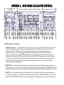
APPENDIX A. RATE-RANGE CALCULATOR CONTROLS
DIADOCHOKINETIC RATE
CALCULATOR
1
3
2
5
4
CONTROLS AND DISPLAYS COMMON TO BOTH INSTRUMENTS
7
6
2
8
1
4
3
6
5
10
8
7
9
14
12
11
13
15
16
18
17
20
19
PITCH ANALYSIS CALCULATOR
1
3
2
5
4
9
7
6
8
DIADOCHOKINETIC FUNCTIONS
1. LG FMT. (Log Formants)
This control alows the user to log formant values. It only works when the Diado instrument is turned on.
The function is "toggled" on and off by clicking on it. Clicking on it causes it to turn "off," if it is "on," and to turn "on," if it is "off."
As shown above, it is "off." When it is turned on, a vertical marker line will appear at a 0.5 seconds in the spectrogram
window and the cursor icon will become the
symbol, which, when lined up on the marker, will allow the user to move the
marker to a new location by executing a "click and drag" operation. When the marker is moved, the values of the formants at the
new position will be recorded in the "LOG" window. (See Common Function #20, LOG) If the logged values are to be preserved, the
LOG must be saved to the journal (See Common Function #13) before this control is turned off, as turning the Log Formant control
off clears the LOG window. Naturally, if formants have not been calculated (See Auxiliary Function #1, Cal) prior to using this
function, their values will be logged as zero.
2. SPEECH RATE. This control optimizes the diadochokinetic analysis algorithm on the basis of the relative syllabic rate of the talker.
The setting operates as a "three way toggle." It changes value each time it's clicked, cycling through "SLOW," "MODERATE" and "FAST."
Clicking on this control does not cause an observable result; it simply sets parameters for the ANALYZE (See Diado Function #3) function.
3. ANALYZE. This control initiates the calculation of the diadochokinetic rate of the speech bounded by the two vertical marker lines in
the waveform (lower) window. The method used to calculate the rate is determined by the "MANUAL/AUTOMATIC" control. (See Diado
Function #6) When AUTOMATIC is selected, (as shown in the figure) the rate is determined using a computer calculated syllabic count.
22
DIADO FUNCTIONS (CONT)
When MANUAL is selected, the analysis relies upon a user entered syllabic count to determine diado rate. The user can monitor the
validity of the count by observing the correlation between the peaks of the blue SYL wave with the appropriate peaks of the red UTT wave.
Regardless of calculation method, the result of the analysis is shown in the SYLLABIC RATE display. (See Diado Function # 4) By clicking
on SAV TO JNL (See Common Function #14, SAV TO JNL) the syllabic rate, the utterance type, along with the date, time and the client's
name, can be recorded to the Journal for later archiving to disk.
4. SYLLABIC RATE. This is a display that shows the results of the diadochokinetic analysis (See Diado Function #3, ANALYZE) in units of
syllables/sec.
5. UTT TYPE. This display allows the user to document which of four specific utterances is to be analyzed. The setting operates
as a "four way toggle." It changes each time it's clicked, cycling through "pa pa pa...," "ta ta ta...," "ka ka ka..." and "pa ta ka...."
This setting is transferred to the logging journal along with the calculated syllabic rate when the SAV TO JNL (See Common
Function #13, SAV TO JNL) function is actuated. Its' only purpose is to provide documentation of which utterance was analyzed,
and it has no effect on the diadochokinetic analysis algorithm.
6. MANUAL/AUTOMATIC. This control allows the user to determine the way the diadochokinetic rate is calculated (See Diado
Function #3, ANALYZE) This setting is a two way toggle that alternates between "MANUAL" and "AUTOMATIC" when clicked. When
AUTOMATIC is selected, (as shown in the figure) the rate is determined using a computer calculated syllabic count. When
MANUAL is selected, the user is prompted to enter the number of syllables within the segment boundaries and this number is used
by the program to determine diado rate.
7. ON/OFF. This control, along with the corresponding one for Pitch Analysis (See Pitch Function #1,) allows the user to choose
between Diadochokinetic (and Spectral) Analysis or Pitch Analysis. This setting takes on the values OFF and ON. When it is in the OFF
position (as shown in the Figure) none of the Diado Controls are functional.
8. EDIT. This control allows the user to change the cursor from its normal function (EDIT) to the DRAW function. This setting is a two
way toggle that alternates between "EDIT" and "DRAW" when clicked. In the EDIT mode the cursor can, as usual, be used to select portions
of the "active" wave in a window. Only one wave may be active in a window at one time. The active wave is the one whose name is
highlighted in the left margin of the window. In the DRAW mode the cursor changes from an arrow to a pencil (
) and can be used
to change the values of a wave by "drawing" over its current trace when it is the active wave in the window. The wave is changed by
pointing the tip of the pencil cursor at the desired place in the wave and doing a click and drag operation with the mouse. When in the
DRAW mode, the NAN function (See Common Function #6, NAN) may be used to make portions of a wave invisible to analysis or logging
functions. A function (See Pitch Function #9, EDIT) similar to this one is found in the Pitch Instrument for altering pitch data.
23
COMMON FUNCTIONS
1. CLIENT. This control allows the user to enter the name of the client or subject whose speech is being analyzed. This name will
appear, along with the current date and time, as a header to any data logged to a journal.
2. RECORD. This control allows the user to record speech into the wave named UTT. The duration of the recorded speech sample will
be determined by the current record settings. (See Common Function #3, SET REC LEVELS).
3. SET REC LEVELS. This control allows the user to set the duration of the recording initiated by the RECORD function (See Common
Function #2, RECORD) Record level adjustment and other hardware controls are also available using this function.
4. LOAD SPEECH. This control allows the user to load a pre-recorded speech utterance into the wave UTT. The pre-recorded utterance
must first be stored on the computer's hard disk using the SAV UTT function. (See Common Function #10, SAV UTT).
5. DURATION. This control loads the values of the current durations of the Selected wave (if any) and of the wave segment bounded
by the two vertical segment markers, into the displays SEL and SEG respectively. The two displays are located to its immediate right
(See Common Functions #13, SEL and #19, SEG).
6. NAN. (Not a Number)
This control is only operable when one of the two EDIT functions (See Diado Function #8 and Pitch
Function #9) is in the DRAW mode. In Diado (DRAW), click on NAN (and OK) and then click on F1, F2 or F3 in the left margin of the
spectrogram. Select the portion of the corresponding formant trace you want to discard, and click again on NAN. In Pitch Analysis, click
on NAN, select the portion of the pitch plot you want to eliminate, and click again on NAN. Unlike the value "zero," a point with the value
NAN is ignored during data analysis operations. Consequently, if incorrect formant or pitch values are changed to NAN values, subsequent
analyses will ignore the unwanted data points. (See Pitch Function #3, ANALYSIS).
7. PLAY. This control allows the user to play the speech in the wave UTT.
8. PLAY SEG. (Play Segment)
vertical markers.
9. PLAY SEL. (Play Selection)
This control allows the user to play the speech in the portion of the wave UTT that is bounded by the two
This control allows the user to play the selected speech segment.
10. SAV UTT. This control allows the user to save the speech in the wave called UTT as a file on the computer's disk drive.
11. SAV SEL. (Save Selection)
This control allows the user to save the selected speech segment as a file on the computer's disk drive.
12. SAV JNL. (Save Journal)
This control allows the user to save the data in the Journal as a file on the computer's disk drive. The
user may first wish to see the Journal (See Common Function #15, SHOW JNL) before saving it. (See also Common Function #14,
SAV TO JNL). The contents of the Journal are cleared after having been saved to disk.
24
COMMON FUNCTIONS (CONT)
13. SEL. (Selection Duration)
This display shows the user the duration of the selected portion of the wave UTT. It is loaded with
a new value whenever the DURATION (See Common Function #5, DURATION) control is clicked. If there is no selection when DURATION
is clicked, its value will be zero.
14. SAV TO JNL. (Save to Journal)
This control allows the user to save the data in the LOG window (See Common Function #20,
LOG) to the Journal. If the Journal already contains previously transferred data, the new data are appended to it. The user may see
the current contents of the Journal at any time. (See Common Function #15, SHOW JNL)
15. SHOW JNL. (Show Journal)
This control allows the user to see the current contents of the Journal. When the viewing is complete,
the user can return to the instrument by either closing the Journal (by clicking in the "close box" at the upper left hand corner of the
Journal window), or by clicking on any part of the instrument on the screen behind the Journal.
16. CLRJ. (Clear Journal)
This control allows the user to clear the contents of the Journal without having to save it first.
17. PRNJ. (Print Journal)
unchanged after printing.
This control allows the user to print the contents of the Journal. The contents of the Journal remain
18. SEGMENT SPEECH. This control allows the user to automatically create a segment within the wave UTT, by bounding a portion of
the speech by two vertical markers. This segment defines the speech interval that is to be processed by the various analysis functions.
(See Diado Function #2, ANALYZE, Common Function #8, PLAY SEG, Common Function #19, SEG, Pitch Function #3, ANALYZE)
Before initiating any analysis on this segment, the user should always listen to the bounded speech by clicking on PLAY SEG. If the
interval has not been appropriately segmented, the user can correct the segmentation by manually repositioning the vertical markers.
This is accomplished by holding the option key down, (which changes the cursor icon to ) placing the cursor icon over one of the
markers, and performing a click and drag operation to move the marker to a new location.
19. SEG. (Segment Duration)
This display shows the user the duration of the portion of the wave UTT bounded by the two vertical
markers. It is reset to a new value whenever the DURATION (See Common Function #5, DURATION) control is clicked.
20. LOG. (Logging Window)
This display holds any data that is recorded using one of the logging functions. (See Diado Function #1,
LG FMT, and Pitch Function #9, EDIT) When desired, the user may save the data to the Journal (See Common Function #14, SAV
TO JNL,) which also clears the window. This window may also be edited manually by the user.
25
PITCH FUNCTIONS
1. ON/OFF.
This control, along with the corresponding one for Diado Analysis (See Diado Function #7,) allows the user to choose
between Pitch Analysis or Diadochokinetic (and Spectral) Analysis. This setting takes on the values OFF and ON. When it is in the OFF
position none of the Pitch Controls are functional.
2. CHANGE F0 PARAMETERS. This control allows the user to modify three of the parameters that affect the pitch tracking algorithm.
The Acceptable Range should be adjusted to minimize outliers. The effect of the frame advance and allowable variation in adjacent
pitch periods controls is more complex and the user may wish to experiment with these parameters before collecting data.
3. ANALYZE. This control initiates the calculation of pitch rate data for the speech in the wave UTT bounded by the two vertical marker
lines in the waveform (lower) window. With the EDIT control (See Pitch Function #9, EDIT) set to EDIT, the pitch track is calculated
as well as the statistical measures shown in the accompanying displays (See Pitch Function #'s 4 DUR, 5 AVG, 6 STD DEV, 7 MIN, and
8 MAX) When the EDIT control is set to DRAW and ANALYZE is clicked, the statistics are recalculated based on the current pitch track.
THE PITCH TRACK IS NOT RECALCULATED. The ANALYZE function will not operate if the EDIT control is set to LOG. By clicking on SAV
TO JNL (See Common Function #14, SAV TO JNL) the pitch statistics, along with the date, time and the client's name can be recorded to
the Journal for later archiving to disk.
4. DUR. (Duration of F0 Analysis)
This Display shows the total duration of the speech for which pitch values were
calculated. Thus, if the segment duration (See Common Function #19, SEG) is 1.5 sec. but this display reads 0.5 sec., this
means that there was a total of 1 sec. for which pitch values were not calculated.
5. AVG. (Average of F0)
This display shows the average of the calculated pitch values.
6. STD DEV. (Standard Deviation of F0)
This display shows the standard deviation of the calculated pitch values.
7. MIN. (Minimum of F0)
This display shows the smallest of the calculated pitch values.
8. MAX. (Maximum of F0)
This display shows the largest of the calculated pitch values.
9. EDIT. This control allows the user to change the cursor from its normal function (EDIT) to a DRAW or a LOG function. This
setting is a three way toggle that alternates between "EDIT," "DRAW," and "LOG," when clicked. In the EDIT mode the cursor can,
as usual, be used to select portions of the "active" wave in a window. Only one wave may be active in a window at one time. The
active wave is the one whose name is highlighted in the left margin of the window. In the DRAW mode the cursor changes from an
arrow to a pencil (
) and can be used to change the values of a wave by "drawing" over its current trace when it is the active
wave in the window. The wave is changed by pointing the tip of the pencil cursor at the desired place in the wave and doing a click
and drag operation with the mouse. When in the DRAW mode, the NAN function (See Common Function #6, NAN) may be used to
make portions of a wave invisible to analysis or logging functions. A Diado Function (See Diado Function #8, EDIT) similar to this
26
PITCH FUNCTIONS (CONT)
one may be used for altering formant data. In the LOG mode, a vertical marker line will appear at a 0.5 seconds in the pitch analysis
window and the cursor icon will become the
symbol, which, when lined up on the marker, will allow the user to move the
marker to a new location by executing a "click and drag" operation. When the marker is moved, the value of the pitch at the new
position will be recorded in the LOG window. (See Common Function #20, LOG) If the logged values are to be preserved, the LOG
must be saved to the journal (See Common Function #13) before this control is changed back to EDIT, or the LOG window will be
cleared and the data lost.
AUXILIARY FUNCTIONS
Pitch Analysis
Configuration
Diado Analysis
Configuration
1
2
1. Cal. (Calculate)
This control allows the user to initiate either spectrographic analysis (in the Diado configuration) or pitch
analysis (in the Pitch configuration) independent of the Diado and Pitch instruments described above. When pitch analysis is
carried out by clicking on Cal rather than on the ANALYZE control of the Pitch instrument, no F0 statistics are calculated.
When Cal is clicked on in the Diado Analysis Configuration, the sound spectrogram of that portion of the wave UTT that is bounded
by the two vertical markers is drawn in the window. This is followed by a formant analysis that uses a peak picking algorithm on
the calculated LPC spectra.
2. Set. (Settings)
This control allows the user to adjust various settings that affect either the pitch analysis or the spectrographic
analysis, depending on which configuration is in effect.
27
1
2
1.
2.
3.
4.
5.
6.
7.
8.
9.
10.
11.
12.
13.
14.
15.
16.
17.
18.
19.
20.
22.
4
APPENDIX B. STIMULUS GENERATOR CONTROLS
5
6
7
8
3
9
10
14
11
12
15
16
18
19
20
21
22
Opens dialog box to allow user to change the record settings, e.g. time.
13
17
Opens dialog box to allow user to enter client/subject identification.
Opens dialog box to allow user to terminate current data run trial.
Initiates recording into waveform A, B, C or D, respectively (user selects which one by clicking).
Opens dialog box to allow user to load a stored speech utterance into waveform A, B, C or D.
Opens dialog box to allow user to save the utterance in waveform A, B, C or D to disk.
Initiates playback (PLAY) of speech utterance in waveform A, B, C or D. (RESP) allows user to log
client/subject's appropriate response to stimulus presented in (PLAY) A, B, C or D.
Indicates all operations related to Tally.
Opens Journal and allows user to observe number of times each stimulus (A, B, C and D) has
been presented, number of times client/subject has responded appropriately to each stimulus,
and percentage of times client/subject has responded appropriately to each stimulus.
Opens dialog box to allow user to save data in Tally.
Clears tally.
Saves current tally and allows user to begin new trial or run.
Allows user to print contents of Tally, individually or as totals, and allows user to see entire contents in Tally.
Indicates all operations related to Selection.
Cuts an interval selected out of a speech utterance and copies it to a clipboard that corresponds in duration to the interval cut.
Copies an interval selected out of a speech utterance and stores it in a clipboard.
Pastes an interval cut or copied into the entry point in an utterance where the cross hairs are currently located.
Initiates playback of the selected portion of an utterance.
Opens dialog box to allow user to amplify selected portion of a speech utterance by some factor.
Calculates the duration of a selected interval;
21. Shows duration of interval Calculated.
Opens dialog box to allow user to save the selected portion of an utterance to disk.
28
APPENDIX C. SPEECH RECONSTRUCTOR CONTROLS
1
3
2
4
5
6
8
7
9
11
10
12 13
14
15 16 17 18
21
19 20
22
23
1. Initiates recording into waveform A according to current control settings.
2. Initiates recording into waveform B according to current control settings.
3. Opens dialog box to allow user to load a stored speech utterance into waveform A.
4. Opens dialog box to allow user to load a stored speech utterance into waveform B.
5. Opens dialog box to allow user to change the record settings, e.g., time of recording.
6. Initiates playback of speech utterance in waveform A.
7. Initiates playback of speech utterance in waveform B.
8. Initiates playback of speech utterance in waveform A followed immediately by utterance in waveform B.
9. Initiates playback of that portion of the utterance in waveform A that lies within the two segment markers.
10. Initiates playback of that portion of the utterance in waveform B that lies within the two segment markers.
11. Moves the waveform A segment markers to coincide with the beginning and end of the selected portion of waveform A.
12. Moves the waveform B segment markers to coincide with the beginning and end of the selected portion of waveform B.
13. Initiates playback of the selected portion of a speech utterance.
14. Indicates the part of a speech utterance, either Segment A, Segment B or the Selected portion, that will be the target
of the five functions and one indicator located below. Clicking on the bold title changes the name of the target interval.
15. Cuts the interval indicated above out of the speech utterance and copies it to a clipboard that corresponds to the interval.
16. Copies the interval indicated above to the clipboard that corresponds to that interval.
17. Opens dialog box to allow user to amplify (or attenuate) the interval indicated above. 100% leaves it unchanged.
18. Pastes the interval currently on the clipboard to the entry point in the utterance that corresponds to the
interval indicated above, at the point where the crosshairs are currently located.
19. Normalizes the interval indicated above.
20. Shows the current duration of the interval indicated above.
21. Opens dialog box to allow user to save the utterance in waveform A to disk.
22. Opens dialog box to allow user to save the utterance in waveform B to disk.
23. Opens dialog box to allow user to save the selected portion of an utterance to disk.
24. Pastes segment A into the utterance of waveform B starting at the first segment marker for waveform B.
25. Pastes segment B into the utterance of waveform A starting at the first segment marker for waveform A.
29
24
25
Any questions, comments, etc. about the instruments or manual can be
directed to
Rebecca Leonard
Dept. Otolaryngology/Head and Neck Surgery
Univ. California, Davis Medical School
2500 Stockton Blvd.
Sacramento, CA 95817
We would appreciate your feedback!
The following demo packages may be ordered from GW Instruments, Inc.
35 Medford Street, Somerville, MA 02143
Tel: 617-625-4096, FAX: 617-625-1322
SoundScope Clinical Demo, $25
• Clinical Manual (spiral bound)
• Clinical instruments & sample waveforms on disk
(Rate-Range Calculator, Stimulus Generator,
Speech Reconstructor)
• SoundScope demo software & documentation
For Macintosh, order GWI-SoS-cm-demo
For Power Macintosh, order GWI-SoS-cm-demo-PPC
SoundScope Demo, $10
• SoundScope demo software & documentation
(Includes SoundScope User's Manual,
sample waveforms and numerous instruments:
1 Channel Analyzer, 2 Channel Analyzer,
Segment Analyzer, 2 Channel Editor, etc.)
For Macintosh, order GWI-SoS-demo
For Power Macintosh, order GWI-SoS-demo-PPC