Download Getting Started with PEST

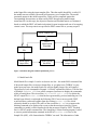
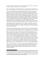
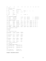
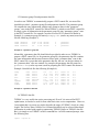
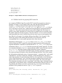
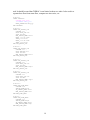
Getting Started with PEST
Zhulu Lin
Dept. of Crop and Soil Sciences
The University of Georgia, Athens, GA 30602
[email protected]
This note is by no means to try to replace the extensive PEST User’s Manual
(http://www.sspa.com/pest/) and Surface Water Utilities Manual
(http://www.sspa.com/pest/utilities.html). It only serves as a rudimentary guide for PEST
novices of using PEST as a parameter estimation tool. In order to use PEST more
efficiently, one is encouraged to read those two manuals very carefully. PEST is a modelindependent parameter estimation program. It can be used to calibrate any model and
conduct uncertainty analysis as long as the model reads in and prints out in ASCII format.
But, in this note, we will only describe basic procedures of how to use PEST to calibrate
SWAT model’s parameters. Regularization parameter estimation, predictive uncertainty
analysis and parameter sensitivity analysis are not included in this note. After setting up
SWAT simulation run in BASINS or AVSWAT interface, copy the entire txtinout
directory into your working directory and keep the original txtinout directory intact
so that if anything goes wrong, you will have backups to restore the damaged model input
files. PEST carry out all the calibration or uncertainty analysis tasks by itself, it normally
takes a few hours depending on model’s runtime and computer’s speed. User’s jobs
involve (1) selecting adjustable parameters; (2) preparing initial and boundary values for
the selected parameters; (3) preparing PEST files; and (4) running PEST and interpreting
or utilizing PEST outputs. The first two tasks require the user’s knowledge about the
model and they are implicitly included the task of preparing PEST files.
1. Preparing PEST files
In order to run PEST properly, at least four types of file need to be provided: (1) model
batch file; (2) model input template files; (3) model output reading instruction files; and
(4) PEST control file. Figure 1 is a schematic diagram that shows how PEST works with
a model to calibrate its parameters. PEST control file is a master file, which contains
central information pertaining to PEST optimization algorithm, initial and boundary
values of model parameters, observations that the model output is going to be calibrated
against, and other information depending on the use of PEST. Although PEST control file
is the most importance file, it is not difficult to prepare if TSPROC (Time Series
Processor, a PEST utility program) is used to do such a job. We shall cover using
TSPROC to prepare PEST control file later on. At each iteration of a PEST run, the PEST
optimization algorithm (with Levenberg-Marquart method as its core) adjusts the values
for model parameters to lessen the objective function’s value. The newly updated model
parameter values are then written to model input files using input template files. The
process involves deleting the old set of model input files and generating a new set of
1
model input files using the input template files. Then the model (batch file) is called. If
the model runs successfully, the model will generate a set of output files. The modelgenerated outputs in the model output files, which will be compared against the
corresponding observations, are then read by PEST through using model output
instruction file. At this stage, the objective function and Jacobian matrix are calculated,
based on which the PEST will make its decision for next iteration until one of its stopping
criteria is met. The stop criteria are specified in PEST control file as you may suspect.
PEST Control File
Input Template
File
Model Input
(input files)
PEST
Optimization
Algorithm
Model (model
batch file)
Output
Instruction File
Model Output
(output files)
Figure 1. Schematic diagram of PEST optimization process
1.1 Model batch file
Model batch file is simple. It can be as short as one line – the model DOS command. But
if the model output files are not text format files; or you plan to use TSPROC as your
model post-processor, the model batch file will get slightly longer, like in Example 1.
The purpose of each command in Example 1 is briefly explained as follows. The first line
of Example 1 (@echo off) is to tell the computer system not to display the commands
while executing them. The second line (del basins.rch > nul) is to delete the
SWAT output file basins.rch that has been generated by previous modeling run. If it
had not been deleted, even though the following SWAT run is not successful, PEST
would still have read model outputs from the existing basins.rch file, which
obviously should be avoided. The suffix of the second line (> nul) is to suppress the
deleting command to be displayed in screen so that the messages issued by system
commands (or model) will not interfered with the messages issued by PEST. The third
line is a SWAT model command line. The fourth line is a short Fortran program I coded
to convert partial information contained in the SWAT basins.rch file to a Site
Sample File (SSF), a file format that the TSPROC can read. The information of what
2
water quantity or quality time series (e.g., FLOW_OUT) in what reach segment (e.g.,
Reach 6) will be converted is provided in rch2ssf.dat file. The fifth line shows that
TSPROC is used as model post-processor, which is almost a standard when using PEST
to calibrate a surface water model. Otherwise, the task of preparing model output reading
instruction files (see above) is insurmountable. Example 1 is a simplest version of model
batch file for SWAT automatic calibration. We suppose it has been given a file name
called swat.bat. Batch file name must have .bat as its extension name. A few lines
may be added in front of SWAT model command to serve as a model pre-processor (for
example, par2par par2par.dat > nul). To know more information about batch
files, please go to website http://www.computerhope.com/batch.htm.
1
2
3
4
5
@echo off
del basins.rch > nul
swat2000 > nul
rch2ssf rch2ssf.dat
tsproc < tsproc.in > nul
Example 1. Model batch file for SWAT calibration (The numbers in left column are line labels; they
are not contained in the model batch file)
1.2 SWAT input template files
Usually, it is easy to prepare a model input template file. But, since SWAT requires
hundreds of input files, this job could become very tedious and error-prone. Before you
start to edit input template files, you should have decided what model parameters you
want PEST to calibrate. Then you need to find out which model input file contains the tobe-calibrated parameters and to build the corresponding template file based on that model
input file. For example, if I want to calibrate CN2 parameter in all .mgt (management)
files1, then I carry out the following steps for each .mgt file:
Step 1: use any text editor, such as Notepad, Wordpad, or NoteTab (www.notetab.com)
to open a .mgt file; Example 2 is the .mgt file for the first HRU in the first sub-basin
(i.e., 000010001). Notice that this .mgt file only contains planting and havest/kill
operations.
0
1
2
3
4
5
6
123456789012345678901234567890123456789012345678901234567890123456789
.mgt file Subbasin:1 HRU:1 Luse:PAST Soil:GA028 Fri Apr 23 15:42:28 2004
0 1
0
0
0.00
0.00
0.00
0.00
0.2074.00000
1.00
0.150
11904.348 12
0.000
0.000
0.000
0.000 0.000
1.200
5
0.000
Example 2. 000010001.mgt file for HRU 000010001 (The first two lines contain column labels; they
are not actual lines in .mgt file which should begin with “.mgt file …” in third line).
1
In this note, SWAT model is treated as a lumped model. That is, all model parameters in different subbasins or HRU’s take same values across entire watershed except those topographic and morphologic
parameters such as area, length, slope, depth, etc.
3
Step 2: Save the opened .mgt file as mgt010001.tpl file. The extension .tpl
stands for PEST template file, which is mandated. That is to say, all PEST template files
must have .tpl as their extension names. But the first three letters that replaced the first
three zeros in the file name are arbitrary. They can be any other combination of letters or
numbers. They even can be three zeros. But I used “mgt” to tell myself that these .tpl
files are template files for .mgt SWAT input files so that they can be easily
distinguished from any other .tpl files such as template files for .hru SWAT input
files, etc. It is worth reiterating that preparing template files for SWAT input files is a
very tedious work since SWAT reads too many input files2. If you want to automatically
calibrate hydrology and water quality in the same time, you almost need to go through all
the SWAT input files, which could be more than several hundreds. Therefore, the
following two advices may be helpful: First, at the stages of watershed delineation and
HRU distribution, keep the number of sub-basins and HRU’s as small as possible. The
total SWAT input files is approximately equal to 8 + 6 × (the number of subbasins) + 5 ×
(the number of HRU’s). Second, start with a simple problem with less than five
adjustable parameters; then progress to a more sophisticate problem step by step.
Step 3: Insert one line in the beginning of the newly saved (mgt010001).mgt file.
The line added is as simple as follows:
12345
ptf #
It merely contains 5 characters – ptf, which stands for PEST Template File, followed by a
space (blank), which, in turn, followed by a special character. This special character can
be any other ASCII character such as #, $, etc, as long as it is so special that it is not used
by the pre-existing model input file. This simple rule should be followed strictly.
Step 4: Change the parameter value for CN2 that you wanted to calibrate to a string that
is delimited by the special character you specified in the inserted first line. For example,
in our mgt010001.mgt file, the parameter value for CN2 is 74.00000 in line 2
(highlighted in pink color). You need to change it to #cn2 # as shown in Example 3.
0
1
2
3
4
5
6
123456789012345678901234567890123456789012345678901234567890123456789
ptf #
.mgt file Subbasin:1 HRU:1 Luse:PAST Soil:GA028 Fri Apr 23 15:42:28 2004
0 1
0
0
0.00
0.00
0.00
0.00
0.20#cn2
#
1.00
0.150
11904.348 12
0.000
0.000
0.000
0.000 0.000
1.200
5
0.000
Example 3. mgt010001.mgt file for HRU 000010001
2
If a SWAT input interface developed by Jing Yang ([email protected]) in Swiss Federal Institute for
Environmental Science and Technology (EAWAG) is used, the task of preparing the SWAT input template
file will become very easy. Only one input template file is needed. How to use the SWAT input interface
will be briefly discussed in the note entitled “Running SWAT in A Breeze”.
4
In this step, there are two places that need special attention. First, if the model input file
adopts fix format rather than free format for model parameter values, you should consult
SWAT User’s Manual to find out how many and what spaces are reserved for your
parameter of interest. For example, in .mgt file, SWAT uses fix format. In page 192 of
SWAT User’s Manual, it’s been specified that CN2 parameter takes the value from
Columns 53 to 60 in Line 2. Therefore, in the corresponding PEST input template file,
the to-be-calibrated parameter’s name (cn2) plus the two delimiters (#) should not be
placed outside the specified spaces (Columns 53-60 in Line 2). But, if the input file takes
free format, the absolute position for model parameters is not critical, as long as they are
separated by standard delimiters such as spaces, commas, tabs etc. Second, since PEST
employs finite-definite methods to calculate Jacobian matrix, it is important to have high
precisions for both model outputs and model parameters. Therefore, the reserved spaces
for adjustable parameters in PEST input template file should be as longer as possible. I
normally use 12-16 spaces for free-format parameters, and use all allowable spaces for
fix format parameters. Please note that the parameter spaces include parameter names,
two special characters, and the white spaces that are used to fill the rest of reserved
parameter spaces. It is important to use white spaces (blanks) rather than tabs to fill the
vacancies. If tabs are used, PEST will issue error messages.
1.3 Model output reading instruction files
As briefly discussed above, model output reading instruction files are used by PEST to
read, through model output files, the model-generated outputs that will be compared
against measured observations. They should be constructed based on model output files
(in ASCII text format); and their preparation could be very time-consuming if there are
many observations you want to incorporate in the automatic calibration process. For
example, if you want to calibrate 10-year SWAT model-generated daily flows against 10year daily flow observations, you will have to write an instruction file with more than
3650 lines. But if you use TSPROC as model postprocessor, the task of preparing model
output reading instruction files is trivial. You don’t even have to care about preparing
instruction files. All you need is to ask TSPROC to prepare them for you. TSPROC has
multiple purposes. It can be used not only as a model postprocessor, but also as a tool to
automatically generate instruction files and PEST control file. The usage of TSPROC
will be discussed later. It is important to note that the extension name for all model output
reading instruction files has to be .ins and that all instruction file must begin with pif
and a special character letter as its first line as shown below. As in model input template
files, pif standards for PEST Instruction File. The special letter (e.g., #, $, etc) may not be
used in the file but has to be present.
12345
pif #
5
1.4 PEST control file
As for model output reading instruction files, PEST control file may be prepared using
TSPROC program. Because all observations will be included in the PEST control file, if
there are more than scores of measured data, TSPROC will inevitably be used for
preparing PEST control file. Unlike model input template files and model output reading
instruction files, which can be many, there is only one PEST control file for one PEST
run. The PEST control file must begin with pcf as its first line (guess what pcf stands
for!). Example 4 displayed a basic PEST control file. A basic PEST control file is
designed for the purpose of simple parameter estimation only. In other words, it does not
include any prior information, or employ Tikhonov or singular value decomposition
(SVD) regularization methods, or SVD-assist scheme in automatic parameter estimation
process. It is not designed for predictive uncertainty analysis either. A brief explanation
of the contents of such a file is presented in the following paragraphs.
With the exclusion of first line, this PEST control file consists of 7 zones, with each zone
starting with an asterisk (*) followed by a space (blank) and zone name. The first zone is
“control data” zone. The first line in this zone (i.e., Line 3) only has two control variables.
In this file, it is shown that the values for these two control variables are “norestart” and
“estimation”, respectively. The first variable tells PEST that you want to turn off the
restart function so that PEST will not generate some output files that are used for
restarting. The alternative value is “restart”. I usually use “norestart”. The second
variable in this line tells PEST to run parameter estimation, rather than regularization or
predictive analysis, for which the variable value should be “regularisation” or
“prediction”. In this note, we only use PEST for parameter estimation.
Line 4 has 5 variables. The variable in Column 1 (C1) is the number of all parameters
listed in “parameter data” zone; therefore its value should be equal to the number of lines
in “parameter data” zone. The variable in Column 2 (C2) is the number of all
observations listed in “observation data” zone; therefore, its value should be equal to the
number of lines in “observation data” zone. The variable in Column 3 (C3) is the number
of all parameter groups listed in “parameter groups” zone; therefore, its value should be
equal to the number of lines in “parameter groups” zone. The variable in Column 4 (C4)
is the number of all prior information incorporated in parameter estimation process,
which should be listed in “prior information” zone, if there is any. Since we will not use
any prior information, therefore its value is always zero. Otherwise, its value is equal to
the number of lines in “prior information” zone (not shown in Example 4). The variable
in Column 5 (C5) is the number of all observation groups listed in “observation group”
zone; therefore, its value should be equal to the number of lines in “observation groups”
zone.
Line 5 consists of 7 variables. The variable in Column 1 (C1) is the number of pairs of
model input template files and their corresponding model input files; and the variable in
Column 2 (C2) is the number of pairs of model output reading instruction files and the
corresponding model output files; therefore, the sum of the values of these two variables
6
should be equal to the number of lines in “model input/output” zone. Don’t worry about
the rest of variables in this line, just leave what they are.
Don’t worry about the rest of variables in this zone, except for the first variable (C1) in
Line 9. Each variable in Line 9 is a stopping criterion. When any one of these criteria has
been met, PEST will stop the parameter estimation process and write its estimation
results into several files. The first variable is the maximum number of iterations that a
PEST run is allowed. Usually 30 iterations are sufficient for any PEST run. But there are
a couple of other options that have special meanings. If this variable is set to zero, the
PEST only requests one model run3 using the initial (default) parameter values. Then it
calculates the value of objective function and writes PEST output files. Usually, after I’ve
finished composing all files that are needed for running PEST, I then set this variable to
be zero and run PEST control file once before being engaged in a full PEST optimization
process. If this variable is set to minus one (-1), PEST will terminate execution
immediately after it has calculated the Jacobian matrix for the first time. Since Jacobian
matrix has been calculated, PEST output files may contain more information about your
estimation problem in the neighborhood of initial condition. For example, you may be
able to obtain parameter variance-covariance or correlation coefficient matrices in the
locality of initial condition if J T J is not singular. The parameter sensitivities will also be
written to the sensitivity file.
Next two zones are “parameter groups” and “parameter data”. It is easier to understand
why PEST control file contains “parameter data” (i.e., data about parameters) since we at
least need provide PEST with information such as what parameters are to be estimated by
PEST; what their initial values are, and what their lower and upper boundaries are, etc.
The parameter names are listed in C1 of “parameter data” zone. Their initial values are
listed in C4 while lower and upper boundary values are listed in C5 and C6 respectively.
If you want PEST to find a best (optimal) value for a parameter, you should assign
“none” or “log” to C2 for that parameter, otherwise assign “fixed” or “tied”. I suggest
you use “none” or “fixed” only and refer PEST User’s Manual if you want to try “log”
and “tied”. For C3, I always fill it with “factor” unless one of the following two situations
occurred: 1) One of the initial, lower or upper boundary values is zero; (2) lower and
upper boundary values have opposite signs. For example, in Line 20, initial value for
parameter “awc” is “0”; and its lower bounds is less than zero while its upper bounds is
greater than zero. Hence, I used “relative” for “awc” in C3. You may always assign “1.0”
for C8, “0.0” for C9, and “1” for C10. Don’t worry about what they mean by now. The
string values for C7 are the names from “parameter groups”. Each parameter should be
assigned to one parameter group. And one parameter group must have at least one
parameter assigned. Therefore, the number of parameter groups is less or equal to the
number of parameters.
3
Please note the difference between PEST run, iterations and model runs. A PEST run means that PEST is
used to estimate model parameters. An (optimization) iteration means that PEST has found a best λ, then
PEST updated model parameter values, run the model once, and updated (reduced) the objective function.
A model run means that the model has been run once. In one PEST run, the number of iterations is usually
substantially less than the number of runs since in each iteration it requires many model runs to find a best
λ, which will result in the most efficient objective function reduction.
7
In contrast, it is not very easy to understand why PEST requires all the parameters be
classified into different parameter groups. The classification of parameters into groups is
for the purpose of calculation of derivatives (Jacobian matrix). Actually, if you wish, you
can define a unique group for each individual parameter and set the derivative variables
for each parameter separately. But in many cases, parameters fall nicely into different
groups which can be treated similarly in terms of calculating derivatives so as to save
time for you. In calculating derivatives, PEST uses 2-point forward-difference or 3-point
central-difference numerical methods. The former is less accurate but requires less model
runs, while the latter is more accurate with more model runs. Therefore, normally, we
adopt a composite strategy – using 2-piont method in the beginning and then switching to
3-point method when parameter values are getting close to the optimal ones. In C6-7, the
string value “switch” means that we are using this very composite strategy. The other two
alternatives are “always_2” and “always_3”. The following two derivative variables are
relevant to 3-point methods. I respectively use “2” and “parabolic” for them.
In addition to this, there is other information we should provide PEST with regard to how
to increment parameter values in order to calculate their derivatives. First option you
have to face is HOW to increase a parameter’s value – increasing relatively based on
parameter’s current value or increasing by an absolute amount. I normally use “relative”
in C3 to increase parameter values relatively. The other two options are “absolute” and
“rel_to_max”. The meaning of the variable’s value in C4 depends on what value in C3. If
C3 is “relative”, the increment used for forward-difference calculation of derivatives with
respect to any parameter belonging to the group is calculated as a fraction of the current
value of that parameter; that fraction is provided as the real variable in C4. However, if
C3 is “absolute” the parameter increment for parameters belonging to the group is fixed,
being again provided as the variable in C4. Alternatively, if C3 is “rel_to_max”, the
increment for any group member is calculated as a fraction of the group member with
highest absolute value, that fraction again being the variable in C4. If a parameter
increment is calculated as “relative” or “rel_to_max”, it is possible that it may become
too low if the parameter becomes very small. If a parameter increment becomes too low,
it does not allow reliable derivatives to be calculated with respect to that parameter
because of round-off errors incurred in the subtraction of nearly equal model-generated
values. To circumvent this possibility, an absolute lower bound can be placed on
parameter increments; this lower bound will be the same for all group members, and is
provided as that variable in C5. Note that if C3 is “absolute”, the value in C5 is ignored.
I usually like to classify the parameter into different groups in terms of their magnitudes.
For example, if parameters are kinetic reaction coefficients, they are usually less than one;
but if parameters are concentrations, they are normally larger than one. Therefore, I put
all parameters that are less than one into one group, say “leone”, and those that are
greater than one but less than ten into another group, say “leten”, etc. Then, I like to
increase parameters by an absolute amount for group “leone”; and increase parameter by
a relative amount for the rest of groups. Variables C4 are set according to the average
magnitudes of the parameters in that group. I usually use “0.001” for C5. If you have a
very wide range of parameter values, you should pay more attention to assign values for
8
C4 and C5. It is wise to use PESTCHEK to check for this type of errors before you run
PEST (PESTCHEK will be discussed in the other PEST utilities section).
The next two zones – “observation groups” and “observation data” – are related to
observations (measured data). The sum of squares of the weighted mismatches between
these observations and model-generated counterparts will usually be defined as the
objective function that PEST is trying to minimize. If you want to calibrate stream
discharges and water quality altogether, the components of the objective function could
be diverse. For example, we want to calibrate flow, sediment and total phosphorus
concentrations simultaneously. The values of flow rate are usually much larger than those
of the total phosphorus concentration (in mg/l); and the measured points for flow are a lot
more than those of sediment or total phosphorus concentrations. If you did not
differentiate them in the objective function, PEST may not pay any respect to the
mismatches from water quality components because both the number of measurement
and magnitudes of the flow component dominate the total objective function. Therefore,
we need divide the observations into different groups, for example, “mflow”, “mtss”, and
“mtp”, which are listed in “observation groups”. Then assign each individual observation
to an observation group in C4 of the “observation data” zone. The name for each
observation should be unique but could be anything as long as it is a string of character
and number’s combination with a length of 12 at most. The observation names are listed
in C1 and the observed values are listed in C2. Values in C3 are weights that you
assigned to the observations. The weight for each observation could be different such as
those in group “mflow”; or all weights for the observations in an observation group could
be the same such as those in groups “mtss” and “mtp”. The weights are determined so
that the sum of squares from one observation group should be approximately equal to that
from any other observation group. The sum of squares that contributes to the total
objective function from each observation group will be printed out to screen (and PEST
run record file) along with the total objective function. Before you run a formal PEST
optimization, adjust the weights for different observations to make sure that the
contributions to the total objective function from all different observation groups are
approximately equal. Relevant discussions have been given in the early of this section on
setting the variable in C1 of Line 9 to zero to do this job; while how to adjust weights for
observations will be discussed in TSPROC data file section.
The sixth zone is the simplest one called “model command line”. It only contains one line
with the model batch file’s name (swat.bat is shown in Example 1). The last zone is
“model input/output”. Each line in this zone lists either a pair of model input template file
(C1-C2) with correspondent model input file (C3-C4), or a pair of model output reading
instruction file (C1-C2) with correspondent model output file (C3-C4). In this example,
Lines 44-49 are model input file pairs while Line 50 is a model output file pair. Chapter 4
in PEST User’s Manual can be referred to understand PEST control file more extensively.
9
Ln
1
2
3
4
5
6
7
8
9
10
11
12
13
14
15
16
17
18
19
20
21
22
23
24
25
26
27
28
29
30
31
32
33
34
35
36
37
38
39
40
41
42
43
44
45
46
47
48
49
50
C1
C2
C3
C4
pcf
* control data
norestart
estimation
8
950
3
0
50
1
single
5.0
2.0
0.3
0.03
5.0
5.0
0.001
0.1
aui
30
0.005
4
4
1
1
1
* parameter groups
leone
absolute
0.001
leten
relative
0.01
lehun
relative
0.1
* parameter data
surlg
none
factor
4.0
cn2
none
factor
70.0
ovn
none
factor
0.14
esco
none
factor
0.95
awc
none
relative 0.0
alphabf
none
factor
0.048
slope
fixed
factor
0.10
slsbsn
fixed
factor
60.0
* observation groups
mflow
mtss
mtp
* observation data
mflow1
41.06
0.0312
mflow
mflow2
57.49
0.0264
mflow
...
...
...
...
mflow900 44.75
0.0990
mflow
mtss1
12.5
150.0
mtss
mtss2
40.8
150.0
mtss
...
...
...
...
mtss25
122.3
150.0
mtss
mtp_1
0.02
200.0
mtp
mtp_2
0.01
200.0
mtp
...
...
...
...
mtp_25
0.90
200.0
mtp
* model command line
swat.bat
* model input/output
mgt010001.tpl
000010001.mgt
mgt010002.tpl
000010002.mgt
...
...
hru010001.tpl
000010001.hru
...
...
par2par.tpl
par2par.dat
modelout.ins
modelout.txt
Example 4. A basic PEST control file
10
C5
C6
C7
C8
C9
C10
3
point
10
1
0.005
4
.001
.001
.001
switch
switch
switch
2
2
2
parabolic
parabolic
parabolic
2.0
55.0
0.01
0.01
-0.1
0.01
0.001
40.0
8.0
80.0
0.6
1.0
0.1
0.3
0.3
90.0
1.0
1.0
1.0
1.0
1.0
1.0
1.0
1.0
0.0
0.0
0.0
0.0
0.0
0.0
0.0
0.0
0
leten
lehun
leone
leone
leone
leone
leone
lehun
0
1
1
1
1
1
1
1
1
1.5 Parameter group file and parameter data file
In order to use TSPROC to automatically prepare a PEST control file, two more files
should be provided – parameter group file and parameter data file. The parameter group
file contains the same information with the same format as those in the “parameter
groups” zone in the PEST control file. When TSPROC is asked to write PEST control file,
it simply copies all information in the parameter group file into “parameter groups” zone
in the PEST control file. For example, in order to write a PEST control file shown in
Example 4, a parameter group file named parmgrp.dat (can be any name) must look
like the following (Example 5).
leone absolute
leten relative
lehun relative
0.001 0.001 switch
0.01
0.001 switch
0.1
0.001 switch
2
2
2
parabolic
parabolic
parabolic
Example 5. A parameter group file
Meanwhile, a parameter data file should also be provided in order to use TSPROC to
prepare a PEST control file. As for parameter group file, the parameter data file contains
the same information and the same format as those in the “parameter data” zone in the
PEST control file, except that in the parameter data file, the one’s in the last column in
the “parameter data” zone are omitted. For example, the parameter data file named as
parmdata.dat (can be any name) used for preparing the PEST control file shown in
Example 4 should look like the following (Example 6).
surlg
cn2
ovn
esco
awc
alphabf
slope
slsbsn
none
none
none
none
none
none
fixed
fixed
factor
factor
factor
factor
relative
factor
factor
factor
4.0
2.0
8.0
70.0
55.0
80.0
0.14
0.01
0.6
0.95
0.01
1.0
0.0
-0.1
0.1
0.048 0.01
0.3
0.10
0.001 0.3
60.0
40.0
90.0
leten
lehun
leone
leone
leone
leone
leone
lehun
1.0
1.0
1.0
1.0
1.0
1.0
1.0
1.0
0.0
0.0
0.0
0.0
0.0
0.0
0.0
0.0
Example 6. A parameter data file
1.6 TSPROC data file
TSPROC is a very useful time series processing tool. Even if it is not used for PEST
optimization, it can also be used for some other basic time series computations. However,
I must admit that it is not an easy task to describe the usage of TSPROC clearly in a short
length. The Surface Water Utilities User’s Manual should always be referred when detail
information is needed with regard to constructing TSPROC blocks in TSPROC data file.
But, it is simple to use TSPROC in DOS command line. At DOS command prompt, write
the following line:
tsproc < tsproc.in
11
The tsproc before “<” is the TSPROC command, while tsproc.in behind “<” is
TSPROC input file, which is usually contains two or four lines depending on what
purpose TSPROC is serving. Note that the TSPROC input file is different from TSPROC
data file. Actually, the former contains the latter. The names for the TSPROC file could
be any legitimate file names. For convenience, I usually name it as tsproc.in. In
terms of using it for PEST optimization, TSPROC has two usages: 1) being used as a
model post-processor; 2) being used to prepare PEST control file and model output
reading instruction file when TSPROC is used as a model post-processor. If TSPROC is
used as a model post-processor, tsproc.in should have four lines as shown in
Example 7.
tsproc.tsp
tsproc.rec
n
n
Example 7. A typical TSPROC input file as TSPROC serving as postprocessor
The first line contains a TSPROC data file, which is the essence of TSPROC input file;
while the second line contains a TSPROC record file, which records some information
when TSPROC is processing TSPROC data file, for example, tsproc.tsp. But I never
looked at it. The last two lines are two n’s. They are answers for two potential TSPROC
prompting questions. However, if TSPROC is used to prepare a PEST control file,
tsproc.in only has to have the previous two lines shown in Example 7. Had any
questions been prompted for answers, you normally will answer them with “y”4.
However, this is not the only difference between the two TSPROC input files
(tsproc.in). Instead, the major difference comes from what it is contained in the
TSPROC data file (tsproc.tsp). How to construct such a TSPROC data file will
become the major topic of the following paragraphs.
1.6.1 TSPROC data file for model post-processor
An example of TSPROC data file used as model post-processor is shown in Example 9.
This simple TSPROC data file contains 10 blocks, each with a similar format. For each
block, first line begins with key word START followed by a space which in turn is
followed by the block’s name; while the last line begin with key word END followed by a
space which again is followed by the block’s name. Usually, from the name of block you
can tell which task the block is designed for. Each block with different name has different
task; and it has different key words within the block. There are 21 different blocks
available for 21 different tasks. Please go to the Surface Water Utilities User’s Manual
for their references. But all blocks have one common key word – CONTEXT, which is
always the second key word in the block. This CONTEXT statement (CONTEXT followed
by a space and a string variable) serves like an on/off switch. The CONTEXT statement in
SETTINGS block determines the “theme” of the entire TSPROC data file (for example,
4
Don’t worry about what kind of questions they are so far. We’ll come back for this.
12
in tsproc.tsp file). For each of the following blocks, if the string variable in the
CONTEXT statement is the same as the string variable in the CONTEXT statement in the
SETTINGS block, then the block is on, which means its specified task will be processed
by TSPROC and will be accomplished. While if the string variable in the CONTEXT
statement is different from the string variable in the CONTEXT statement in the
SETTINGS block, then the tasks specified in this block will not be executed.. For this
reason, it should be noted that SETTINGS block always has to be the first block in a
TSPROC data file and only one CONTEXT can be specified at one time. But if the string
variable in the CONTEXT statement of a block is “all”, then that block will always be
executed regardless what is in the CONTEXT statement in the SETTINGS block. For
example, Block 10 in Example 9 will always be executed.
If a line in the TSPROC data file begins with “#” then the line is a comment line that will
not be processed by TSPROC. You should always set DATE_FORMAT to mm/dd/yyyy as
shown in Example 9. The files FLOW_OUT.ssf, SEDCONC.ssf, MINP_OUT.ssf
and ORGP_OUT.ssf in Blocks 2-5 are so-called Sample Site Files. The time series
contained in these files were converted from basins.rch file (a SWAT output file)
through using a short Fortran program – RCH2SSF whose usages will be covered in the
other PEST utilities section. A typical Sample Site Files is shown in Example 8. In brief,
the task that has been achieved by this TSPROC data file (Example 9) is to convert all
these four Sample Site Files into modelout.txt file that is written in Block 10.
Therefore, this TSPROC data file is used as model post-processor. Based on this
generated modelout.txt, a TSPROC data file, which will serve to prepare the PEST
control file, can write a model output instruction file automatically.
REACH06
REACH06
REACH06
REACH06
REACH06
REACH06
REACH06
REACH06
REACH06
01/01/1985
01/02/1985
01/03/1985
01/04/1985
01/05/1985
01/06/1985
01/07/1985
01/08/1985
01/09/1985
00:00:00
00:00:00
00:00:00
00:00:00
00:00:00
00:00:00
00:00:00
00:00:00
00:00:00
0.708103E+01
0.123626E+02
0.475176E+02
0.818826E+02
0.105300E+03
0.679745E+02
0.697458E+02
0.359467E+02
0.360293E+02
... ...
... ...
... ...
... ...
Example 8. A typical Sample Site File
# Block 1
START SETTINGS
CONTEXT model_post
DATE_FORMAT mm/dd/yyyy
END SETTINGS
# Block 2
START GET_SERIES_SSF
CONTEXT model_post
FILE FLOW_OUT.ssf
SITE reach06
NEW_SERIES_NAME mflow
DATE_1 01/01/1983
13
TIME_1 00:00:00
DATE_2 12/31/1992
TIME_2 00:00:00
END GET_SERIES_SSF
# Block 3
START GET_SERIES_SSF
CONTEXT model_post
FILE SEDCONC.ssf
SITE reach06
NEW_SERIES_NAME mtss1
END GET_SERIES_SSF
# Block 4
START GET_SERIES_SSF
CONTEXT model_post
FILE MINP_OUT.ssf
SITE reach06
NEW_SERIES_NAME minp1
END GET_SERIES_SSF
# Block 5
START GET_SERIES_SSF
CONTEXT model_post
FILE ORGP_OUT.ssf
SITE reach06
NEW_SERIES_NAME orgp1
END GET_SERIES_SSF
# Block 6
START NEW_TIME_BASE
CONTEXT model_post
SERIES_NAME mtss1
TB_SERIES_NAME mflow
NEW_SERIES_NAME mtss
END NEW_TIME_BASE
# Block 7
START NEW_TIME_BASE
CONTEXT model_post
SERIES_NAME minp1
TB_SERIES_NAME mflow
NEW_SERIES_NAME minp
END NEW_TIME_BASE
# Block 8
START NEW_TIME_BASE
CONTEXT model_post
SERIES_NAME orgp1
TB_SERIES_NAME mflow
NEW_SERIES_NAME orgp
END NEW_TIME_BASE
# Block 9
START SERIES_EQUATION
CONTEXT model_post
NEW_SERIES_NAME mtp
EQUATION 0.01157 * (minp + orgp) / (mflow + 0.001)
END SERIES_EQUATION
# Block 10
START LIST_OUTPUT
CONTEXT all
14
FILE modelout.txt
SERIES_NAME mflow
SERIES_NAME mtss
SERIES_NAME mtp
SERIES_FORMAT short
END LIST_OUTPUT
Example 9. A simple TSPROC data file for model post-processor
1.6.2 TSPROC data file for preparing PEST control file
An example of TSPROC data file used for PEST control file preparation is shown in
Example 10. Blocks 1-9 in Example 10 have the same function of those blocks in
Example 9 – reading model-generated outputs from the Sample Site Files
(FLOW_OUT.ssf, SEDCONC.ssf, MINP_OUT.ssf, and ORGP_OUT.ssf). Blocks
10-12 read observed stream flow, sediment and total phosphorus concentration data at
Canton, GA. These observations had also been stored in Sample Site File format. In
general, water quality parameters are observed once a month or once two months, while
the model outputs are in daily frequency. Therefore, Blocks 13-15 are used to match the
model-generated time series with the observed time series in one-to-one mapping. Note
that, Block 16 in Example 10 is slightly different from Block 10 in Example 9. The
former only prints out the model-generated time series at the dates when the
corresponding flow or water quality parameters have been observed.
Immediately following the LIST_OUTPUT block, it is WRITE_PEST_FILES block
which will generate PEST control file and model output instruction file based on the
supplied information. It should be reiterated that the WRITE_PEST_FILES block must
immediately follow LIST_OUTPUT block that generates the model output file. The first
two statements behind the CONTEXT statement produce PEST control file that is named
as etowah.pst and model output reading instruction file that is named as
modelout.ins. The next three statements supply parameter group file, parameter data
file, and model batch file that have been discussed (prepared) before. These files contain
the information needed in the zones of “parameter groups”, “parameter data”, and “model
command line” in a PEST control file. Similarly, in the subsequent lines, the pairs of
model input template files and model input files have been provided to write information
in the “model input/output” zone; while the information supplied in the next three subblocks will be used to write the zones of “observation groups” and “observation data”.
The information needed to write the “control data” zone will be either calculated from the
existing data or using default values. It should be mentioned that if the any of the two tobe-generated files already exist in the current directory, one or both of the following
questions will be prompted to answer. Type “y” or “n” to proceed.
Question 1:
File modelout.ins already exist. Overwrite it? [y/n]
Question 2:
File etowah.pst already exist. Overwrite it? [y/n]
15
# Block 1
START SETTINGS
CONTEXT pest_prep
DATE_FORMAT mm/dd/yyyy
END SETTINGS
# Block 2
START GET_SERIES_SSF
CONTEXT pest_prep
FILE FLOW_OUT.ssf
SITE reach06
NEW_SERIES_NAME mflow
DATE_1 01/01/1983
TIME_1 00:00:00
DATE_2 12/31/1992
TIME_2 00:00:00
END GET_SERIES_SSF
# Block 3
START GET_SERIES_SSF
CONTEXT pest_prep
FILE SEDCONC.ssf
SITE reach06
NEW_SERIES_NAME mtss1
END GET_SERIES_SSF
# Block 4
START GET_SERIES_SSF
CONTEXT pest_prep
FILE MINP_OUT.ssf
SITE reach06
NEW_SERIES_NAME minp1
END GET_SERIES_SSF
# Block 5
START GET_SERIES_SSF
CONTEXT pest_prep
FILE ORGP_OUT.ssf
SITE reach06
NEW_SERIES_NAME orgp1
END GET_SERIES_SSF
# Block 6
START NEW_TIME_BASE
CONTEXT pest_prep
SERIES_NAME mtss1
TB_SERIES_NAME mflow
NEW_SERIES_NAME mtss
END NEW_TIME_BASE
# Block 7
START NEW_TIME_BASE
CONTEXT pest_prep
SERIES_NAME minp1
TB_SERIES_NAME mflow
NEW_SERIES_NAME minp
END NEW_TIME_BASE
# Block 8
START NEW_TIME_BASE
CONTEXT pest_prep
SERIES_NAME orgp1
TB_SERIES_NAME mflow
16
NEW_SERIES_NAME orgp
END NEW_TIME_BASE
# Block 9
START SERIES_EQUATION
CONTEXT pest_prep
NEW_SERIES_NAME mtp
EQUATION 0.01157 * (minp + orgp) / (mflow + 0.001)
END SERIES_EQUATION
# Block 10
START GET_SERIES_SSF
CONTEXT pest_prep
FILE canton_FLOW.ssf
SITE Canton
NEW_SERIES_NAME oflow1
END GET_SERIES_SSF
# Block 11
START GET_SERIES_SSF
CONTEXT pest_prep
FILE Canton_SS.ssf
SITE Canton
NEW_SERIES_NAME otss
DATE_1 10/15/1983
TIME_1 00:00:00
DATE_2 12/21/1992
TIME_2 00:00:00
END GET_SERIES_SSF
# Block 12
START GET_SERIES_SSF
CONTEXT pest_prep
FILE Canton_TP.ssf
SITE Canton
NEW_SERIES_NAME otp
DATE_1 1/25/1983
TIME_1 00:00:00
DATE_2 12/21/1992
TIME_2 00:00:00
END GET_SERIES_SSF
# Block 13
START NEW_TIME_BASE
CONTEXT pest_prep
SERIES_NAME oflow1
TB_SERIES_NAME mflow
NEW_SERIES_NAME oflow
END NEW_TIME_BASE
# Block 14
START NEW_TIME_BASE
CONTEXT pest_prep
SERIES_NAME mtss1
TB_SERIES_NAME otss
NEW_SERIES_NAME mtsso
END NEW_TIME_BASE
# Block 15
START NEW_TIME_BASE
CONTEXT pest_prep
SERIES_NAME mtp1
TB_SERIES_NAME otp
17
NEW_SERIES_NAME mtpo
END NEW_TIME_BASE
# Block 16
START LIST_OUTPUT
CONTEXT pest_prep
FILE modelout.txt
SERIES_NAME mflow
SERIES_NAME mtsso
SERIES_NAME mtpo
SERIES_FORMAT short
END LIST_OUTPUT
# Block 17
START WRITE_PEST_FILES
CONTEXT pest_prep
NEW_PEST_CONTROL_FILE etowah.pst
NEW_INSTRUCTION_FILE modelout.ins
# Information pertaining to general files.
PARAMETER_GROUP_FILE parmgrp.dat
PARAMETER_DATA_FILE parmdata.dat
MODEL_COMMAND_LINE swat.bat
# Information pertaining to template and model input files.
TEMPLATE_FILE mgt010001.tpl
MODEL_INPUT_FILE 000010001.mgt
TEMPLATE_FILE mgt010002.tpl
MODEL_INPUT_FILE 000010002.mgt
... ... ... ...
TEMPLATE_FILE hru010001.tpl
MODEL_INPUT_FILE 000010001.dat
... ... ... ...
TEMPLATE_FILE par2par.tpl
MODEL_INPUT_FILE par2par.dat
# Information pertaining to flow time series.
OBSERVATION_SERIES_NAME oflow
MODEL_SERIES_NAME mflowb
SERIES_WEIGHTS_EQUATION 1.5 / (@_abs_value+0.0001)
SERIES_WEIGHTS_MIN_MAX 1e-4 1e+4
# Information pertaining to sediment time series.
OBSERVATION_SERIES_NAME otss
MODEL_SERIES_NAME mtss
SERIES_WEIGHTS_EQUATION 0.1
# Information pertaining to phosphorus time series.
OBSERVATION_SERIES_NAME otp
MODEL_SERIES_NAME mtp
SERIES_WEIGHTS_EQUATION 50
END WRITE_PEST_FILES
Example 10. A simple TSPROC data file for PEST files preparation
A vigilant reader will find that Example 9 and Example 10 have many blocks in common.
It is possible to use only one TSPROC data file (tsproc.tsp) to carry out two tasks –
being a model post-processor and preparing PEST files. Actually this is the very reason
why each block has a CONTEXT statement in the previous examples. The two files can be
combined together with a little modification to serve both tasks with the aide of
CONTEXT statement. The combined TSPROC data file is shown Example 11. Only one
CONTEXT statement is allowed in one block, therefore, the other CONTEXT statement
should be commented out when the TSPROC data file is used to conduct one specific
18
task. It should be noted that TSPROC is not limited to these two tasks. I also used it to
separate base flow from storm flow, compare two time series, etc.
# Block 1
START SETTINGS
CONTEXT pest_prep
# CONTEXT model_post
DATE_FORMAT mm/dd/yyyy
END SETTINGS
# Block 2
START GET_SERIES_SSF
CONTEXT all
FILE FLOW_OUT.ssf
SITE reach06
NEW_SERIES_NAME mflow
DATE_1 01/01/1983
TIME_1 00:00:00
DATE_2 12/31/1992
TIME_2 00:00:00
END GET_SERIES_SSF
# Block 3
START GET_SERIES_SSF
CONTEXT all
FILE SEDCONC.ssf
SITE reach06
NEW_SERIES_NAME mtss1
END GET_SERIES_SSF
# Block 4
START GET_SERIES_SSF
CONTEXT all
FILE MINP_OUT.ssf
SITE reach06
NEW_SERIES_NAME minp1
END GET_SERIES_SSF
# Block 5
START GET_SERIES_SSF
CONTEXT all
FILE ORGP_OUT.ssf
SITE reach06
NEW_SERIES_NAME orgp1
END GET_SERIES_SSF
# Block 6
START NEW_TIME_BASE
CONTEXT all
SERIES_NAME mtss1
TB_SERIES_NAME mflow
NEW_SERIES_NAME mtss
END NEW_TIME_BASE
# Block 7
START NEW_TIME_BASE
CONTEXT all
SERIES_NAME minp1
TB_SERIES_NAME mflow
NEW_SERIES_NAME minp
END NEW_TIME_BASE
19
# Block 8
START NEW_TIME_BASE
CONTEXT all
SERIES_NAME orgp1
TB_SERIES_NAME mflow
NEW_SERIES_NAME orgp
END NEW_TIME_BASE
# Block 9
START SERIES_EQUATION
CONTEXT all
NEW_SERIES_NAME mtp
EQUATION 0.01157 * (minp + orgp) / (mflow + 0.001)
END SERIES_EQUATION
# Block 10
START LIST_OUTPUT
CONTEXT model_post
FILE generated.txt
SERIES_NAME mflow
SERIES_NAME mtss
SERIES_NAME mtp
SERIES_FORMAT short
END LIST_OUTPUT
# Block 11
START GET_SERIES_SSF
CONTEXT all
FILE canton_FLOW.ssf
SITE Canton
NEW_SERIES_NAME oflow1
END GET_SERIES_SSF
# Block 12
START GET_SERIES_SSF
CONTEXT all
FILE Canton_SS.ssf
SITE Canton
NEW_SERIES_NAME otss
DATE_1 10/15/1983
TIME_1 00:00:00
DATE_2 12/21/1992
TIME_2 00:00:00
END GET_SERIES_SSF
# Block 13
START GET_SERIES_SSF
CONTEXT all
FILE Canton_TP.ssf
SITE Canton
NEW_SERIES_NAME otp
DATE_1 1/25/1983
TIME_1 00:00:00
DATE_2 12/21/1992
TIME_2 00:00:00
END GET_SERIES_SSF
# Block 14
START NEW_TIME_BASE
CONTEXT all
SERIES_NAME oflow1
TB_SERIES_NAME mflow
NEW_SERIES_NAME oflow
20
END NEW_TIME_BASE
# Block 15
START NEW_TIME_BASE
CONTEXT all
SERIES_NAME mtss1
TB_SERIES_NAME otss
NEW_SERIES_NAME mtsso
END NEW_TIME_BASE
# Block 16
START NEW_TIME_BASE
CONTEXT all
SERIES_NAME mtp1
TB_SERIES_NAME otp
NEW_SERIES_NAME mtpo
END NEW_TIME_BASE
# Block 17
START LIST_OUTPUT
CONTEXT all
FILE modelout.txt
SERIES_NAME mflow
SERIES_NAME mtsso
SERIES_NAME mtpo
SERIES_FORMAT short
END LIST_OUTPUT
# Block 18
START WRITE_PEST_FILES
CONTEXT pest_prep
NEW_PEST_CONTROL_FILE etowah.pst
NEW_INSTRUCTION_FILE modelout.ins
# Information pertaining to general files.
PARAMETER_GROUP_FILE parmgrp.dat
PARAMETER_DATA_FILE parmdata.dat
MODEL_COMMAND_LINE swat.bat
# Information pertaining to template and model input files.
TEMPLATE_FILE mgt010001.tpl
MODEL_INPUT_FILE 000010001.mgt
TEMPLATE_FILE mgt010002.tpl
MODEL_INPUT_FILE 000010002.mgt
... ... ... ...
TEMPLATE_FILE hru010001.tpl
MODEL_INPUT_FILE 000010001.dat
... ... ... ...
TEMPLATE_FILE par2par.tpl
MODEL_INPUT_FILE par2par.dat
# Information pertaining to flow time series.
OBSERVATION_SERIES_NAME oflow
MODEL_SERIES_NAME mflowb
SERIES_WEIGHTS_EQUATION 1.5 / (@_abs_value+0.0001)
SERIES_WEIGHTS_MIN_MAX 1e-4 1e+4
# Information pertaining to sediment time series.
OBSERVATION_SERIES_NAME otss
MODEL_SERIES_NAME mtss
SERIES_WEIGHTS_EQUATION 0.1
# Information pertaining to phosphorus time series.
21
OBSERVATION_SERIES_NAME otp
MODEL_SERIES_NAME mtp
SERIES_WEIGHTS_EQUATION 50
END WRITE_PEST_FILES
Example 11. A combined TSPROC data file used for both tasks
1.7 Other PEST utility programs
1.7.1
TEMPCHEK, INSCHEK and PESTCHEK
After the model template files, model output instruction file(s), and the PEST control file
have been prepared, it is recommended to use TEMPCHEK, INSCHEK and PESTCHEK
PEST utility programs to check the syntax of these files. If the model output instruction
files are prepared using TSPROC program, INSCHEK is rarely used. But TEMPCHEK
and PESTCHEK are always very helpful to find syntax or human errors. The DOS
commands for TEMPCHEK and PESTCHEK are the same, that is,
tempchek template_file_name (extension name can be omitted), or
pestchek pest_control_file_name (extension name can be omitted)
It should be noted that each of these utilities checks one error at a time. Therefore, after
you fixed one error, you need to run the check utility program again. In the other words,
for one file (either template file or control file) you should run the check utility program
again and again until it does not issue any errors any more.
1.7.2
PARREP
I guess PARREP is a short for PARameter REPlication. It is usually used to generate a
new PEST control file from an old PEST control file and the correspondent optimal
parameter file that is written after the PEST optimization process of the old PEST control
is finished. Its DOS command is as follows.
parrep parameter_file old_control_file new_control_file
1.7.3
PSTOP
It is quite often when you find yourself have made some nonfatal mistakes that could
defer the whole optimization process or lead to undesirable results after you’ve
commenced PEST optimization. At situations like this, you don’t have to wait until the
undesired PEST run to finish or need to use Control-C command. You may open another
DOS command window, and type PSTOP at the DOS prompt in the current working
directory. Then PEST will stop after it finishes the current model run.
22
1.7.4
PAR2PAR
PAR2PAR is one of most frequently used PEST utility program. It is used to make
generic parameter transformations. If you only want to make a logarithmic transformation
for one of the adjustable parameters, you can do it within the PEST control file. You just
need to specify the variable of C2 in “parameter data” zone in Example 4 to “log” instead
of “none”. But if you want to make a parameter transformation other than a logarithmic
one, PAR2PAR has to be employed. However, it is confusing to include it into your
PEST optimization process if you haven’t used PEST before. Therefore, I suggest you
postpone its usage until you feel comfortable with a regular PEST run.
1.7.5
RCH2SSF
Strictly, this is not a PEST utility program. It was programmed by myself to convert a
SWAT-printed basins.rch to a series of Sample Site Files that will be read in
TSPROC no matter what role TSPROC plays. This is why it is called RCH2SSF (RCH
file to SSF files). The DOS command for RCH2SSF is as follows.
rch2ssf RCH2SSF_data_file
The text file of RCH2SSF_data_file can be any name with a format shown in
Example 12.
6
FLOW_OUT
SEDCONC
ORGP_OUT
MINP_OUT
Example 12. An RCH2SSF data file
The first line is the number of the sub-basin where the stream flow and water quality
parameters in the reach are of interest. The following lines are variables that are printed
in the SWAT basins.rch file. If they are listed in this RCH2SSF data file (called
rch2ssf.dat), one Sample Site File will be generated for each of them. The Sample
Site File will be named after the variable’s name followed by .ssf. For example,
according to Example 12, a Sample Site File will be generated for the downstream flow
for reach 6 and after5, whose name will be FLOW_OUT.ssf. Similarly, another three
Sample Site Files will be produced for sediment concentration, organic phosphorus load,
and mineral phosphorus load in reach 6 and after, which will be named as
SEDCONC.ssf, ORGP_OUT.ssf, and MINP_OUT.ssf, respectively. All eligible
variable’s names in basins.rch file include FLOW_IN, FLOW_OUT, EVAP,
TLOSS, SED_IN, SED_OUT, SEDCONC, ORGN_IN, ORGN_OUT, ORGP_IN,
5
If we want the downstream data for reach 6 only, then run rch2ssf1.exe instead of rch2ssf.exe.
23
ORGP_OUT, NO3_IN, NO3_OUT, NH4_IN, NH4_OUT, NO2_IN, NO2_OUT,
MINP_IN, MINP_OUT, CHLA_IN, CHLA_OUT, CBOD_IN, CBOD_OUT,
DISOX_IN, DISOX_OUT, SOLPST_IN, SOLPST_OUT, SORPST_IN,
SORPST_OUT, REACTPST, VOLPST, SETTLPST, RESUSP_PST,
DIFFUSEPST, REACBEDPST, BURYPST, BED_PST, BACTP_OUT,
BACTLP_OUT, CMETAL_1, CMETAL_2, CMETAL_3.
2. Running PEST and reading PEST output files
Running PEST is simple. After having PEST control file prepared and successfully
checked by PESTCHEK program, you just need to type the following command line at
DOS prompt.
pest pest_control_file (extension name can be omitted)
Before turning our attention to PEST output files, let’s summarize the whole process of
preparing PEST files that have been extensively discussed in the previous section. They
are outcomes of my personal experiences and don’t have to be followed stringently.
Step 1: Having set up the SWAT model and made a successful run of the SWAT model,
copy the txtinout directory to your working directory and rename it;
Step 2: Select adjustable parameters based on your goal for model calibration;
Step 3: Set initial, boundary values for the selected parameters;
Step 4: Write a parameter data file and a parameter group file;
Step 5: Write all appropriate model input template files, checking with TEMPCHEK
after each template file having been written;
Step 6: Convert any available measured data into SSF or WDM format which can be
read by TSPROC;
Step 7: Write model batch file if necessary;
Step 8: Prepare TSPROC data file for PEST file preparation;
Step 9: Run TSPROC to generate PEST control file;
Step 10: Prepare (or Reform) TSPROC data file as model post-processor;
Step 11: Run PESTCHEK to check the newly generated PEST control file;
24
Step 12: Adjust C1 in Line 9 of the PEST control file (shown in Example 4) to 0, and run
PEST once;
Step 13: If the values for all components of the total objective function are not equivalent
in magnitude, adjust the weights in the TSPROC data file prepared in Step 8;
Step 14: Repeat Step 8 through Step 13 until all components of the total objective
function have similar values;
Step 15: Change C1 in Line 9 of the PEST control file (shown in Example 4) to 30;
Step 16: Run PEST optimization.
After PEST having been stopped by one of its criteria, a set of PEST output files will be
written to disk immediately. The base names of these files are the same as that of the
PEST control file, but they differ from each other by their extension names. For example,
if the PEST control file name is test.pst, then all PEST output files resulted from the
PEST optimization for this case will be test.*, where the asterisk (*) represents
different extension names. The PEST output files were described in Chapter 5 in PEST
User’s Manual. A summary of these files is given in the following.
The most comprehensive output file is PEST record file (*.rec) . It has a detailed
record of the parameter estimation process from the beginning to the end. But I found it
has too much information to be helpful. Sometimes, it may have more than 10,000 lines
of materials. It is difficult to find what you want. Furthermore, except for the detailed
record of the estimation process, many of the rest recordings are also written into other
different files6, which have specific purposes and are easy to be converted into
spreadsheet.
For example, a parameter sensitivity file (*.sen) contains the “composite sensitivity” of
each parameter with respect to all observations (with the latter weighted by the userassigned weights). Recall that each column of the Jacobian matrix lists the derivatives of
all model-generated observations with respect to a particular parameter. Thus the
composite sensitivity of a parameter is the normalized (with respect to the number of
observations) magnitude of the column of the Jacobian matrix pertaining to that
parameter, with each element of that column multiplied by the weight pertaining to the
respective observation. The relative composite sensitivity of a parameter is obtained by
multiplying its composite sensitivity by the magnitude of the value of the parameter. It is
thus a measure of the composite changes in model outputs that are incurred by a
fractional change in the value of the parameter. Composite parameter sensitivities are
useful in identifying those parameters which may be degrading the performance of the
parameter estimation process through lack of sensitivity to model outcomes. The use of
relative composite sensitivities in addition to normal sensitivities assists in comparing the
6
There is slight discrepancy between some information recorded in the record file and that recorded in
other files. But it is an easy matter to overcome it.
25
effects that different parameters have one the parameter estimation process when these
parameters are of different type, and possibly of very different magnitudes.
A similar PEST output file is the observation sensitivity file (*.seo) that contains the
composite sensitivity of an observation with respect to all parameters involved in the
parameter estimation process. The composite sensitivity of observation j is the magnitude
of the jth row of the Jacobian matrix multiplied by the weight associated with that
observation; this magnitude is then divided by the number of adjustable parameters.
Though composite observation sensitivities can be of some use, they do not, in general,
convey as much useful information as composite parameter sensitivities. Therefore, I
rarely looked at the observation sensitivity file.
During each optimization iteration, immediately after it has calculated the Jacobian
matrix, PEST records composite parameter sensitivities to a parameter sensitivity file
(*.sen) for each iteration. But PEST only write the current composite observation
sensitivities to an observation sensitivity file (*.seo). The another file that will be
written after PEST calculates the Jacobian matrix is the matrix file (*.mtt), if any of the
three variables of Line 10 in the PEST control file (Example 4) are set to 1. The variable
in C1 indicates whether the parameter variance-covariance matrix is written or not; the
variable in C2 indicates for parameter correlation coefficient matrix; and the variable in
C3 indicates for the eigenvalues and normalized eigenvectors of the variance-covariance
matrix. If any of the three variables are set to zero, the corresponding matrix is not
written to the matrix file. Although all of these three matrices are useful, I used the
parameter correlation coefficient matrix most often. It tells me which two parameters
might be linearly dependent so that it should be avoided estimating both of them
simultaneously. One of my statistics teachers once told us that if the (Pearson’s)
correlation coefficient is greater than 0.8, the two random variables may be considered
linearly dependent. I used to use the eigenvalues printed in the matrix file to calcuate the
condition number for the variance-covariance matrix, but in the later versions of PEST,
the condition numbers for each iteration are given in the condition number file (*.cnd).
Don’t worry about this file if you don’t know what condition number is for it is more
useful, along with the singular value file (*.svd), when SVD-assist is employed in the
future.
Like the observation sensitivity file (*.seo), the matrix file (*.mtt) only contains the
information with regard to the current set of parameter values. Each time this file is
written, the previous file of the same name is overwritten. Because the optimal parameter
set does not necessarily result from the last optimization iteration, cautions should be
exercised if you want to check for the above-mentioned information pertaining to the
optimal parameter set. Usually, a small remedy should be done in this respect. We’ll
come back for this remedy shortly.
Besides the record file (*.rec), the other two important files that store the information
for the best achievement of the PEST optimization are the parameter value file (*.par)
and the residual file (*.res). At the end of its execution, PEST writes the residual file
listing in tabular form observation names, the groups to which various observations
26
belong, measured and modeled observation values, differences between these two (i.e.,
residuals), measured and model observation values multiplied by respective weights,
weighted residuals, measurement standard deviations and “natural weights”. While the
meanings for the rest of columns are apparent from their names, the last two data types
require a word of explanation. The measurement standard deviation is calculated as the
inverse of its weight multiplied by the square root of the reference variance (σ2) which is
calculated by the minimum objective function value being divided by the degrees of
freedom (the difference between the number of observations and the number of
adjustable parameters). It can serve as a valid measure of observation uncertainty only if
the model is a valid simulation the process that it is intended to represent. The “natural
weights” are the inverse of measurement standard deviations as determined above. It is
obvious that if these weights were used in the parameter estimation process, the reference
variance would be unity. Normally, I only used the measured and modeled observation
columns to plot graphs for visual comparisons between them.
The parameter value file (*.par) records the optimal parameter set of the PEST
optimization process. As discussed above, the last iteration does not necessarily result in
the optimal parameter set, therefore, if I want to look at the parameter sensitivities and
parameter correlation coefficients pertaining to the optimal parameter set, I will do the
following: (1) I use the PEST utility program PARREP to make a new PEST control file
based on the optimal parameter set and the old PEST control file; (2) change the variable
of C1 in Line 9 in the new PEST control file to -1; (3) run the new PEST control file.
Then the information contained in the PEST output files correspondent to the new PEST
control file is correct information.
In addition, the Jacobian matrix corresponding to the optimized parameter values is
recorded in a binary file (*.jco) that can be accessible by the JACWRIT utility program
for recording of the Jacobian matrix in text format. A residual file for each iteration
(*.rei) temporarily stores the measured and modeled observations for current iteration.
The information in this file may be used by PEST itself during the parameter estimation
process. I haven’t seen any usefulness of it. If the string variable of C1 in Line 3 is set to
“restart”, then another three files (*.rst, *.jac, *.jst) may be generated by PEST
for its restart features, although I never felt the need to use them.
3. Editing AUTOEXC.BAT file
In order to use PEST to calibrate the SWAT model, we need to do one more thing –
adding the directories where the SWAT executable file and PEST command files are
located into the autoexec.bat file. The autoexec.bat file is located in the root drive of your
computer. Since the autoexec.bat file is a system file, you shouldn’t tamper with it if you
don’t know what it is. Normally, the autoexec.bat is hidden under the Windows Explorer.
The following line can be added into the autoexec.bat file if the SWAT executable file
(swat2000.exe) and the swat.bat (described in Section 1.1), together with those
executable files contained in the swat.bat batch file are located in
C:\AVSWAT\AVSWATPR\ and PEST command files are located in C:\PEST.
27
SET PATH = C:\AVSWAT\AVSWATPR\; C:\PEST\
28