Download Software Engineering, Course notes 1996/1997

Software Engineering
Course Notes 96/97
Dr. Eric Dubuis
Ingenieurschule Biel
Abteilung Informatik
2501 Biel
IS Biel/DUE 96/97
Software Engineering
Copyright 1993, 1994, 1995, 1996, 1997 by Eric Dubuis.
All rights reserved.
IS Biel/DUE 96/97
Software Engineering
Table of Content
CHAPTER 1
Introduction
1-1
1.1 Software Engineering — Why?
1.2 Software Characteristics
1.2.1 Software Domains
1-1
1-2
1-2
1.3 Software Development Processes
1-3
1.3.1 The Classic Software Life Cycle 1-3
1.3.1.1 Problems with the Classical Life Cycle 1-4
1.3.2 Rapid Prototyping 1-4
1.3.2.1 Problems with Rapid Prototyping 1-5
1.3.3 Fourth Generation Techniques 1-5
1.3.3.1 Assessment of Fourth Generation Techniques
1.3.4 Formal Transformation Paradigm 1-6
1.3.5 The Spiral Model 1-6
1-6
1.4 Generic Views of the Software Development and Maintenance Process
1-7
1.5 Process-Oriented versus Product-Oriented Software Development Processes
1.5.1 Process-Oriented Paradigms
1.5.2 Product-Oriented Paradigms
1.5.3 Comparison 1-9
1.6 Some Definitions of Terms
1-9
1.6.1 Activity 1-9
1.6.2 Phase 1-10
1.6.3 Method 1-10
1.6.4 (Formal) Technique 1-10
1.6.5 Software Engineering Processes
1-10
1.7 A Definition for Software Engineering
Bibliography
CHAPTER 2
1-11
1-11
Computer System Engineering
2.1 Computer-Based Systems
2-1
2-1
2.1.1 Definition 2-1
2.1.2 Elements of Computer-Based Systems
2.2 Analysis Tasks
1-8
1-8
1-9
2-1
2-2
2.2.1 Identifying Customer’s Need 2-2
2.2.1.1 Purpose 2-2
2.2.1.2 Kind of Customers 2-2
2.2.1.3 Kind of Inputs 2-3
2.2.1.4 Techniques Used for Identifying Customer’s Need 2-3
2.2.1.5 Results 2-3
2.2.2 Economic Feasibility 2-3
2.2.3 Technical Feasibility 2-3
2.2.3.1 Techniques and Tools Used for Technical Feasibility Tasks
2.2.4 Allocation 2-4
2.2.4.1 Example 2-4
2.2.5 Cost and Scheduling 2-4
2.3 A Detailed Structure of the Analysis Process
2-3
2-5
2.3.1 Project Proposal 2-6
2.3.2 The Conceptualisation 2-6
2.3.3 The System Analysis 2-6
2.3.4 The Software Analysis 2-6
2.4 Initial/Software Requirements Specification
2.4.1 The Context 2-7
2.4.2 Functional Requirements
IS Biel/DUE 96/97
2-7
2-7
i
Software Engineering
2.4.3 Use Cases
2-8
2.5 Requirements Specification Outline
2.6 The Specification Review
Bibliography
Exercises
CHAPTER 3
2-9
2-11
2-11
2-12
Software Project Planning
3.1 Software Project Planning Overview
3.2 Resources
3-1
3-1
3-2
3.2.1 Human Resources 3-2
3.2.2 Hardware Resources 3-2
3.2.3 Software Resources 3-2
3.3 Software Metrics for Productivity Estimation
3-3
3.3.1 Size-Oriented Metrics 3-3
3.3.2 Function-Oriented Metrics 3-4
3.3.3 Size-Oriented and Function-Oriented Metrics Compared
3.3.4 Metrics Data Collection and Evaluation 3-6
3.4 Software Project Estimation
3-5
3-6
3.4.1 LOC and FP Estimation 3-6
3.4.2 Direct Effort Estimation 3-7
3.4.3 LOC/FP Estimates Compared with Direct Estimates 3-8
3.4.4 Empirical Estimation Models (also: Algorithmic Cost Estimation)
3.4.4.1 The COCOMO Model 3-8
3.5 Software Project Scheduling
3-8
3-9
3.5.1 Milestones 3-10
3.5.2 Task Definitions 3-11
3.5.3 Task Scheduling Techniques 3-11
3.5.3.1 Metra-Potential Method (MPM) 3-12
3.5.3.2 The Critical Path Method (CPM) 3-13
3.5.3.3 Bar Charts (or Gantt Charts or Gantt Diagrams)
3.6 Organisation of the Project
3-14
3-15
3.6.1 Task Force 3-15
3.6.1.1 An Informal (Democratic) Team 3-15
3.6.1.2 A Chief Programmer Team 3-15
3.6.2 Matrix Project Organisation 3-16
3.7 Software Development Process
3.8 Software Project Plan
3-19
3.9 On Software Project Controlling
Bibliography
Exercises
CHAPTER 4
3-17
3-20
3-21
3-21
Software Analysis Fundamentals
4.1 Software Analysis
4-1
4-1
4.2 Analysis Task and Results
4-2
4.2.1 Problem Recognition 4-3
4.2.2 Evaluation and Modelling 4-3
4.2.3 Documentation 4-3
4.2.4 Review 4-4
4.3 Potential Problems
4-4
4.3.1 Acquisition of Information 4-5
4.3.2 Handling Complexity 4-5
4.3.3 Accommodating Changes 4-5
IS Biel/DUE 96/97
ii
Software Engineering
4.4 Analysis Principles
4.5 Analysis Methods
4-5
4-6
4.6 Outline of the Software Analysis Model Document
Bibliography
CHAPTER 5
4-6
4-8
Object-Oriented Analysis
5.1 Object Orientation
5-1
5-1
5.1.1 Characteristics of Objects 5-1
5.1.1.1 Identity 5-1
5.1.1.2 Classification 5-2
5.1.1.3 Polymorphism 5-3
5.1.1.4 Inheritance 5-3
5.1.2 Further Concepts Used in Object Orientation
5.1.2.1 Abstraction 5-3
5.1.2.2 Encapsulation 5-3
5.1.2.3 Combining Data and Behaviour 5-4
5.1.3 Object-Oriented Development 5-5
5.1.4 The “OMT” Method 5-5
5.1.4.1 The Object Model 5-5
5.1.4.2 The Dynamic Model 5-5
5.1.4.3 The Functional Model 5-6
5.2 Object Modelling
5-3
5-6
5.2.1 Objects and Classes 5-6
5.2.1.1 Objects 5-6
5.2.1.2 Classes 5-6
5.2.1.3 Object Diagrams 5-6
5.2.1.4 Attributes 5-7
5.2.1.5 Operations and Methods 5-7
5.2.2 Links and Associations 5-8
5.2.2.1 General Concept 5-8
5.2.2.2 Representing Links and Associations in Object Diagrams
5.2.2.3 Higher Order Associations 5-9
5.2.2.4 Multiplicity (for Binary Associations) 5-10
5.2.3 Advanced Link and Association Concepts 5-11
5.2.3.1 Link Attributes 5-11
5.2.3.2 Modelling Associations as Classes 5-12
5.2.3.3 Role Names 5-12
5.2.3.4 Ordering 5-13
5.2.3.5 Qualification 5-14
5.2.4 Aggregation 5-14
5.2.5 Generalisation and Inheritance 5-16
5.2.5.1 Concept 5-16
5.2.5.2 Overriding Features 5-17
5.2.6 Aggregation versus Generalisation 5-18
5.2.7 Abstract Classes and Abstract Operations 5-18
5.2.8 Class Features 5-19
5.2.8.1 Class Attributes 5-19
5.2.8.2 Class Operations 5-19
5.2.9 Candidate Keys 5-20
5.3 OMT’s Dynamic Modelling
5-9
5-22
5.3.1 Events 5-22
5.3.2 Scenarios and Event Traces 5-23
5.3.3 States 5-23
5.3.4 State Diagrams 5-24
5.3.5 Conditions 5-25
5.3.6 Actions 5-25
5.3.7 Activities 5-26
5.3.8 Relations of Object Models and Dynamic Models 5-26
5.3.9 Guidelines for Constructing State Diagrams 5-26
5.4 OMT’s Functional Modelling
IS Biel/DUE 96/97
5-26
iii
Software Engineering
5.4.1 Components of the Functional Model 5-27
5.4.2 Relation of Functional Model to Object and Dynamic Model
5.4.3 An Example 5-27
5.5 The Object-Oriented Analysis Process
5-27
5-29
5.5.1 Object Modelling 5-29
5.5.1.1 Identifying Object Classes 5-29
5.5.1.2 Keeping the Right Classes 5-29
5.5.1.3 Preparing a Data Dictionary 5-30
5.5.1.4 Identifying Associations 5-30
5.5.1.5 Keeping the Right Associations 5-30
5.5.1.6 Identifying Attributes 5-31
5.5.1.7 Keeping the Right Attributes 5-32
5.5.1.8 Refining with Inheritance 5-32
5.5.1.9 Testing Access Paths 5-32
5.5.1.10 Iterating Object Modelling 5-32
5.5.2 Dynamic Modelling 5-32
5.5.2.1 Scenarios 5-32
5.5.2.2 Event Traces 5-32
5.5.2.3 Build State Diagrams 5-33
5.5.3 Functional Modelling 5-33
5.5.3.1 Provide a Context Diagram 5-33
5.5.3.2 Define Input and Output Values 5-33
5.5.3.3 Provide Data Flow Diagrams by Refining the Context Diagram
5.5.3.4 Provide Process Specifications 5-33
5.5.4 Adding Operations 5-34
5.5.4.1 Operations from the Object Model 5-34
5.5.4.2 Operation from the Dynamic Model 5-34
5.5.4.3 Operations form Process Specifications 5-34
5.5.5 Iterating the Analysis 5-34
5.6 Documenting the Object-Oriented Analysis Results
Bibliography
Exercises
CHAPTER 6
5-33
5-34
5-35
5-35
System Design
6-1
6.1 Decomposition of a System into Subsystems and Modules
6.1.1 A Textual Design Notation 6-2
6.1.2 A Graphical Design Notation 6-4
6.1.3 Relations Introduced so Far 6-5
6.1.4 Other Terms Often Encountered 6-5
6.1.4.1 Software Architecture 6-5
6.1.4.2 A Client of a Component 6-6
6.1.4.3 The Service, the Service Primitives, and the Protocol 6-6
6.1.4.4 Client/Server or Peer-to-Peer Relations among Components
6.1.5 Layering 6-7
6.2 Identifying Concurrency
6.2.1 Identifying Concurrent Components
6-9
6.3.1 Mapping Components to Computers 6-10
6.3.1.1 Guidelines 6-10
6.3.2 Mapping Components to Programs 6-10
6.3.2.1 Guidelines 6-10
6.3.3 Estimating Hardware Resource Requirements
6.3.4 Hardware-Software Trade-Off 6-11
6.5 Shared Resources
6-12
6.6 Software Control
6-12
6-6
6-7
6.3 Mapping Components to Computers and Programs
6.4 Data Storage Management
6-2
6-10
6-11
6-11
6.6.1 Procedure-Driven Software Control 6-13
6.6.2 Event-Driven Software Control 6-13
6.6.3 Concurrent Software Control 6-13
IS Biel/DUE 96/97
iv
Software Engineering
6.7 Initialisation, Termination, and Failure
6-13
6.7.0.1 Initialisation 6-13
6.7.0.2 Termination 6-14
6.7.0.3 Failure 6-14
6.8 Architectural Frameworks
6-14
6.8.1 Transformation Systems 6-14
6.8.2 Interactive Systems 6-15
6.8.3 Real-Time Systems 6-16
6.8.4 Transaction Systems 6-16
6.9 Detailed Design
6-17
6.10 Design Methods
6-17
6.11 Software Design Results
6.12 Bibliography
Exercises
CHAPTER 7
6-18
6-18
6-19
Module Design Fundamentals
7.1 An Example: Producing a KWIC Index
7-1
7-1
7.1.1 First Modularisation 7-2
7.1.1.1 Module 1, Input 7-2
7.1.1.2 Module 2, Shift 7-3
7.1.1.3 Module 3, Sorting 7-3
7.1.1.4 Module 4, Output 7-3
7.1.1.5 Module 5, Control 7-3
7.1.1.6 Result of Modularisation 1 7-3
7.1.2 Second Modularisation 7-4
7.1.2.1 Module 1, Store 7-5
7.1.2.2 Module 2, Input 7-5
7.1.2.3 Module 3, Shift 7-5
7.1.2.4 Module 4, Sorting 7-5
7.1.2.5 Result of Modularisation 2 7-6
7.1.3 Comparison of the Two Modularisations 7-6
7.1.3.1 General 7-6
7.1.3.2 Adaptability 7-6
7.1.3.3 Independent Development 7-7
7.1.3.4 Comprehensibility 7-8
7.1.4 Criteria Used in the Modularisations 7-8
7.2 Fundamentals on Module Design
7-8
7.2.1 Design For Change 7-9
7.2.2 Program Families 7-9
7.2.3 The Representation of Systems of Modules 7-9
7.2.3.1 Systems and Their Modules 7-10
7.2.4 The CALLS Relation 7-11
7.2.5 The USES Relation 7-11
7.2.5.1 Hierarchical USES Relations 7-12
7.2.5.2 Levelling 7-12
7.2.5.3 Static Definition of the USES Relation 7-12
7.2.5.4 Qualifying the USES Relation 7-12
7.2.5.5 Designing Module Interfaces 7-13
7.2.5.6 Program Families Revisited 7-14
7.2.6 The IS_COMPONENT_OF Relation 7-14
7.2.6.1 Virtual versus Concrete Modules 7-15
7.2.6.2 Module Copies and Generic Modules 7-15
7.2.7 The INHERITS_FROM Relation 7-16
7.2.8 Other Useful Relations 7-16
7.3 A Textual Design Notation for Modules
7.4 Guidelines for Module Design
7.4.1 Cohesion and Coupling
7.4.1.1 Cohesion 7-18
IS Biel/DUE 96/97
7-16
7-18
7-18
v
Software Engineering
7.4.1.2 Coupling 7-18
7.4.2 Separate Interfaces from Implementations
7.4.3 Anticipate Changes 7-18
7.4.4 Stable Interfaces 7-19
7.4.5 Hide Policies 7-19
7.4.6 Other, General Guidelines 7-19
7.5 Categories of Modules
7-18
7-19
7.5.1 Data Pool Module 7-19
7.5.2 Functional Modules 7-20
7.5.3 Abstract Data Objects 7-20
7.5.4 Abstract Data Types 7-21
7.5.4.1 Existence of an ADT Instance 7-22
7.5.4.2 Abstract Data Objects as Parameters in Operation Signatures
7.5.4.3 Equality and Duplication of Abstract Data Objects 7-23
7.5.5 Generic Abstract Data Types 7-23
7.5.6 Object-Oriented Modules: Classes 7-25
7.6 Modular Design of Persistent Data Types
7.7 Design Methods for Module Design
7-26
7-26
7.7.1 Functional Decomposition 7-27
7.7.1.1 Stepwise Refinement (Top-Down Design)
7.7.1.2 Bottom-Up Design 7-28
Bibliography
Exercises
CHAPTER 8
7-27
7-29
7-29
Object-Oriented Design
8.1 Overview
7-23
8-1
8-1
8.2 Adding Application Classes and Internal Classes
8.3 Obtaining Further Operations of Classes
8-2
8.3.1 Obtaining Operations from the Dynamic Models
8.3.2 Obtaining Operations from the Functional Model
8.4 Determine Algorithms
8-2
8-3
8-3
8-3
8.4.1 Choosing Algorithms 8-3
8.4.2 Choosing Predefined Classes 8-4
8.4.3 Defining Internal Classes and Operations 8-4
8.4.4 Assigning Responsibility for Operations 8-4
8.5 Design Optimisation
8-4
8.5.1 Adding Redundant Associations 8-4
8.5.2 Saving Derived Data to Avoid Recomputation
8.6 Design of Associations
8-5
8-7
8.6.1 Association Traversal Analysis
8.6.2 One-Way Associations 8-7
8.6.3 Two-Way Associations 8-7
8.6.4 Link Attributes 8-9
8.7 Adjustment of Class Structure
8-7
8-9
8.7.1 Rearranging Classes and Operations 8-9
8.7.2 Use Delegation to Share Implementation 8-10
8.8 Design Patterns
8-11
8.8.1 Creational Patterns 8-11
8.8.1.1 Abstract Factory 8-13
8.8.1.2 Factory Method 8-17
8.8.1.3 Singleton 8-19
8.8.2 Structural Patterns 8-20
8.8.2.1 Adapter 8-21
8.8.2.2 Decorator 8-24
8.8.2.3 Proxy 8-27
8.8.2.4 Composite 8-30
8.8.3 Behavioural Patterns 8-33
IS Biel/DUE 96/97
vi
Software Engineering
8.8.3.1 Command 8-33
8.8.3.2 Iterator 8-38
8.8.3.3 Observer 8-42
8.8.3.4 Mediator 8-46
8.9 Physical Packaging
8-51
8.10 Documenting Design Decisions
Bibliography
Exercises
CHAPTER 9
8-51
8-52
8-52
Implementation
9-1
9.1 Implementing Abstract Data Objects
9.2 Implementing ADTs
9-1
9-1
9.2.1 Organisation of the Header Files 9-1
9.2.2 Header File Included by the Client Module
9.2.3 Usage by the Client Module 9-5
9.3 Simulating Generic ADTs in ANSI C
9-3
9-6
9.4 Implementing Classes and Associations in ANSI C
9.4.1 Translating Classes into C Structure Declarations
9.4.2 Passing Arguments to Methods 9-7
9.4.3 Allocating Objects 9-8
9.4.4 Implementing Inheritance 9-9
9.4.5 Implementing Method Resolution 9-10
9.4.6 Implementing an Association 9-11
9-6
9-6
9.5 On the Realisation of Classes and Associations in ANSI C++
9.6 On Implementing Finite State Machines
9.6.1 Implementation Choices 9-14
9.6.2 Two-Dimensional Table Interpreter
9.6.3 Sparse Table Techniques 9-16
9.6.4 Programmed Realisations of FSM
9.7 General Programming Techniques
9-13
9-13
9-14
9-17
9-17
9.7.1 The Organisation of Dot-C and Dot-H Files Revisited
9.7.2 Prologue in Source Files 9-18
9.7.3 Conditional Compilation 9-19
9.7.4 Code for Tracing Program Activities 9-20
9.8 On Utilities of Programming Environments
9-17
9-21
9.8.1 The Program Preparation Utility “Make” 9-21
9.8.1.1 File Dependency Graph 9-22
9.8.1.2 Dependencies or Dependency List 9-23
9.8.1.3 A Simple Makefile 9-23
9.8.1.4 The Makefile 9-23
9.8.1.5 Target Entries 9-23
9.8.1.6 Macros 9-25
9.8.1.7 Simplifying Makefiles 9-26
9.8.2 Version Control 9-27
9.8.2.1 An Illustration of a Software Development Trajectory 9-28
9.8.2.2 More Complex Situations: A Version Tree 9-28
9.8.2.3 Principles of Version Control Tools 9-29
9.8.2.4 An Overview on the Revision Control System RCS 9-30
9.8.2.5 Putting a File under the Control of RCS 9-30
9.8.2.6 Extracting Read-Only Versions with co(1) 9-31
9.8.2.7 Extracting Writable Versions with co(1) 9-31
9.8.2.8 Making New Revisions 9-31
9.8.2.9 Making New Revision plus Retrieving 9-31
9.8.2.10 RCS Keywords 9-32
9.8.2.11 Some Administrative RCS Commands 9-33
9.9 Bibliography
9-33
IS Biel/DUE 96/97
vii
Software Engineering
Exercises
CHAPTER 10
9-34
Software Verification and Validation
10.1 Overview
10-1
10-1
10.2 Defect Testing
10-2
10.2.1 Goals for Testing 10-2
10.2.2 Some Testing Terminology 10-3
10.2.3 Empirical Testing Principles 10-4
10.3 Testing in the Small
10-5
10.4 White-Box Testing
10-5
10.4.1 Statement Coverage Criterion 10-6
10.4.1.1 Minimisation Problem 10-6
10.4.1.2 Interpretation Problem 10-6
10.4.2 Edge Coverage Criterion 10-7
10.4.3 Condition Coverage Criterion 10-9
10.4.4 Path Coverage Criterion 10-9
10.4.5 The Cyclomatic Complexity 10-10
10.4.6 General Problem with the Program Structure Coverage Principle
10.5 Black-Box Testing
10.5.1 Equivalence Partitioning 10-13
10.5.2 Boundary Value Analysis 10-14
10.5.3 The Cause-Effect Graph Technique
10.6 Testing in the Large
10-18
10-19
10.8.1 Bottom-Up Testing
10.8.2 Top-Down Testing
10.9 System Testing
10-20
10-20
10-20
10.10 Testing-Activity Planning
10.11 Structured Reviews
Bibliography
Exercises
10-14
10-18
10.7 Module Testing in Context
10.8 Integration Testing
10-12
10-13
10-21
10-22
10-22
10-22
CHAPTER 11
Software Project Management
CHAPTER 12
Configuration Management
CHAPTER 13
Software Documentation
13.1 Purpose of Documentation
13.2 Categories of Documents
13.3 Product Documentation
11-1
12-1
13-1
13-1
13-2
13-2
13.3.1 User Documentation 13-2
13.3.2 System Documentation 13-4
13.4 Project Documentation
13-4
13.5 Quality Assessment Documentation
13.6 QMS Documentation
13.7 Documentation Quality
IS Biel/DUE 96/97
13-5
13-5
13-5
viii
Software Engineering
13.7.1 Front Cover Issues 13-6
13.7.2 Writing Style 13-7
Bibliography
13-7
IS Biel/DUE 96/97
ix
CH APT E R 1
Introduction
1.1 Software Engineering — Why?
Programming versus Software Engineering
Somebody excellent in programming (writing programs for one or several target systems) might easily raise the question: “Why do I need software engineering? I know
how to code programs!”
Programming in the Small: The sort of software one person does by writing one or
several smaller programs (“single-person, single-version” software). It can be characterised as follows:
• The effort to write the software is rather small (less than a few person-months).
• Usually only one version of the software exists (usually the current one).
• No or only a few documentation is performed (software perhaps used by the same
programmer only).
Programming in the Large: The sort of software that usually involves more than one
person (“multi-person, multi-version” software). It can be characterised as follows:
•
•
•
•
The effort to write the software is rather large (more than a few person-months).
Several versions do exist at the same time.
The software is systematically documented.
The software is maintained.
Software becomes increasingly complex
In the past, the software was usually an afterthought of the hardware and/or system
design. However, today’s software is becoming more and more complex such that solid
engineering methods are required.
IS Biel/DUE 96/97
1-1
Software Engineering
Introduction
The often cited “Software Crisis”
Many software development projects faced a number of problems:
•
•
•
•
•
it took too long to finish the program
the development cost were much higher than expected
once delivered, the software product still contained too many errors
progress measures during the software development was not possible
the costs for software maintenance are extremely high.
Thus, the often cited term “software crisis” encompasses problems associated with the
development of software, how to maintain the growing volume of existing software, and
how to manage the expected growing demand of new software.
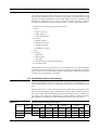
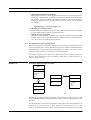
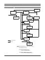
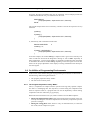
1.2 Software Characteristics
Software “construction” is different in many respects from the construction of classical
“objects” such as buildings, bridges, or VLSI circuits:
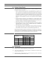
• Software is rather a logical than a physical system: the “elements” used in composing software cannot be expressed in physical units such as length, weight, or temperature. Software “elements” such as strings, records, and trees can rather be regarded
as mathematical elements.
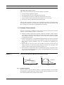
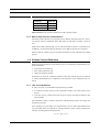
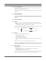
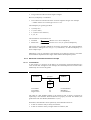
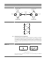
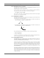
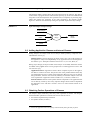
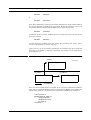
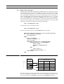
• Software is developed; it is not manufactured. Reproduction of software is comparably easy compared to the manufacturing of hardware which can lead to quality problems. Hence, software production costs are concentrated in engineering (see
Figure 1-1).
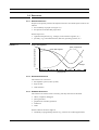
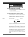
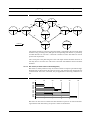
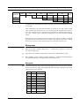
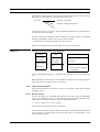
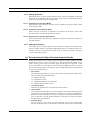
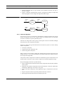
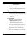
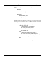
• Software does not wear out. Once in use, its behaviour (with all its errors) does not
change. However, its failure rate changes during its lifetime due to changes of the
software itself or changes of the environment (Figure 1-2).
• Most software is custom built, and not assembled from existing components. However, for the construction of physical systems, existing building blocks can be reused
such as screws, nuts and bolts.
FIGURE 1-1
Cost versus Life Phases for Hardware and Software Systems
costs
costs
engineering
production
production
hardware
engineering
phase
software
phase
1.2.1 Software Domains
Software products fall into different software or application domains. The procedures
and techniques required to develop software for these software domains are not unique.
The software domains can be summarised as follows:
IS Biel/DUE 96/97
1-2
Software Engineering
FIGURE 1-2
Introduction
Failure Rate versus Time (from [1])
failure rate
failure rate
hardware
time
software
time
System Software: Software that is destined to service other software such as operating
systems, compilers, editors, etc.
Real-Time Software: Software that receives real-world events and acts upon accordingly, within specified time intervals.
Business Software: Software that is used to treat business data. Software of this application domain facilitates business operation. It is the largest single application area [1].
Engineering and Scientific Software: Software that is used to ease the engineering or
scientific tasks. Often based on “number crunching” algorithms or sophisticated graphical drawing capabilities.
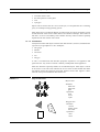
Artificial Intelligence Software: Software based on non-numerical algorithms to solve
complex problems [1]. Into this class fall expert systems (also called knowledge-based
systems), pattern recognition, neural networks, theorem proving, etc.
1.3 Software Development Processes
To master the problems in software development, a systematic approach for the “production” of software is required. However, there is no single best approach to a solution
of the software crisis. Several software development processes exist to achieve a discipline for the software development — a discipline called software engineering.
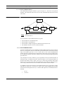
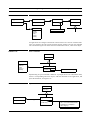
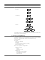
1.3.1 The Classic Software Life Cycle
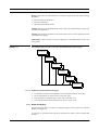
The classic software life cycle is a systematic, sequential approach for a set of activities
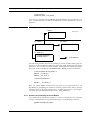
for the software development and maintenance process, see Figure 1-3.
System Engineering and Analysis: deals with requirements for all system components
such as
• hardware
• software
• human factors
Software Requirements Analysis: deals with software requirements such as
•
•
•
•
information domains (data contents and relationships)
required functions
performance aspects
required interfaces
IS Biel/DUE 96/97
1-3
Software Engineering
Introduction
Design: deals with the transformation of software requirements into detailed design
documents
• data structures and operations
• software architecture
• algorithms (procedural details)
Coding: deals with the implementation of the software by transforming the design into
machine-executable form
Testing: deals with the validation of the product with respect to the requirements of the
assessment of the design
Maintenance: deals with the corrections, adaptations, and enhancements of the software product
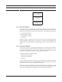
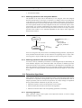
The Classical Software Life Cycle (the “Waterfall Model”) with “Loops”
FIGURE 1-3
system eng.
analysis
design
coding
testing
maintenance
1.3.1.1
Problems with the Classical Life Cycle
•
•
•
•
it is difficult to make the development process sequential (iteration will occur)
not all requirements are always known in an early stage
running product is available only at a late stage of the life cycle
some transformations between the activities are by far not trivial
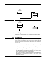
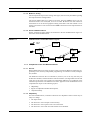
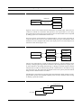
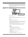
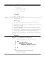
1.3.2 Rapid Prototyping
Rapid prototyping allows to realise a working prototype in early phases of a software
product, see Figure 1-4.
A prototype is generated from high-level specifications which is then evaluated and
refined.
IS Biel/DUE 96/97
1-4
Software Engineering
Introduction
Rapid Prototyping
FIGURE 1-4
requirements
“quick”
design
build
prototype
evaluate &
refine
engineer
product
1.3.2.1
Problems with Rapid Prototyping
• customer wants to keep the prototype in stead remaking it
• bad design decisions made during the prototyping phase may be kept in the final
product
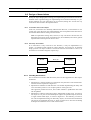
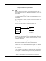
1.3.3 Fourth Generation Techniques
Fourth Generation Techniques (4GT) are based on the following principle: The SW
developer specifies the characteristics of a software at a “high level” using a Fourth
Generation Language (4GL). A 4GT development environment then automatically generates either source code or machine code of the SW system to be developed (see
Figure 1-5).
FIGURE 1-5
Fourth Generation Techniques
requirements
“design”
strategy
4GL
implementation
product
IS Biel/DUE 96/97
1-5
Software Engineering
1.3.3.1
Introduction
Assessment of Fourth Generation Techniques
• the software domain is limited to business information systems
• development time reduction for small or medium-sized applications
• development time saving is not so substantial through the elimination of coding
since much more time is used for analysis, design, and testing.
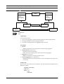
1.3.4 Formal Transformation Paradigm
The result of the software requirements analysis (the specification) is expressed using a
formal description technique. The formal specification is then transformed, using correctness-preserving transformations, to a program (see Figure 1-6).
Today, only a few, experimental systems have been built using correctness-preserving
transformations.
FIGURE 1-6
From a Formal Specification to a Program
analysis
formal
specification
first transformation
refinement 1
n-th transformation
refinement n
final transformation to a program
implementation
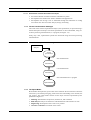
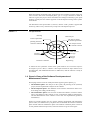
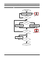
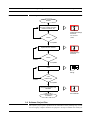
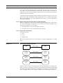
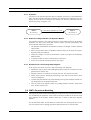
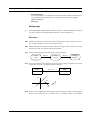
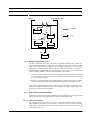
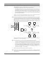
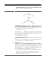
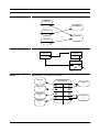
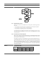
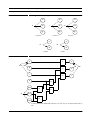
1.3.5 The Spiral Model
B.W. Boehm developed the spiral model which combines the best features of both the
classic life cycle and the prototyping, while at the same time adding a new element, the
risk analysis. The spiral model consists of four major activities represented by four
quadrants of Figure 1-7:
1 Planning: determination of objectives, alternatives, and constraints
2 Risk analysis: analysis of alternatives and identification and resolution of risks
3 Engineering: development of the “next-level” product
4 Customer evaluation: assessment of the results
IS Biel/DUE 96/97
1-6
Software Engineering
Introduction
With each iteration around the spiral, progressively more complete versions of the software are built. After each risk analysis phase, “go” or “no-go” decisions are made. If
risks are to great, the project can be terminated. According to Pressman [1], the spiral
model is currently the most realistic approach to the development of large scale systems
and software.
The drawback of the spiral model is, however, that the “final” product is approached
iteratively, and not every customer may accept such a development process.
FIGURE 1-7
The Spiral Model
Planning
initial requirements
planning based on
customer comments
customer
evaluation
Risk analysis
risk analysis based
on initial requirements
risk analysis based
on customer reaction
initial software
prototype
next level
prototype
Customer evaluation
Engineering
A similar but less systematic variant of the spiral model is the incremental software
development process. Here, a software is developed such that its major functions are
developed first, then additional functions are added next, until the software is ready to
be released.
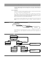
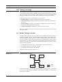
1.4 Generic Views of the Software Development and
Maintenance Process
Developing software involves usually the following three generic phases [1]:
1 The definition phase: The analysis of the system, the planning of the (software)
project, and the requirements analysis for the software.
2 The development phase: The definition of the software architecture and its lowlevel design, the coding, and the testing.
3 The maintenance phase: The correction of delivered software (corrective maintenance), the adaption of the software to new environments (adaptive maintenance),
and the enhancements of the software to meet new user requirements (perfective
maintenance).
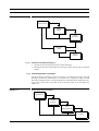
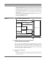
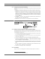
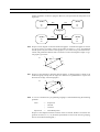
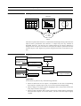
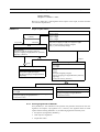
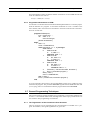
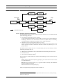
Figure 1-8 presents another view of a generic software development and maintenance
process. Here, two different life cycle phases can be identified: the software realisation
phase and the software maintenance phase. The software realisation phase consists of
several parallel mainstream processes, and some of them are given in the figure.
IS Biel/DUE 96/97
1-7
Software Engineering
Introduction
• The project management deals with the management of the whole project. Mainly
schedules and budgets are established and controlled based on periodic reporting
procedures. Quality assurance management may be part of this controlling process.
• The verification and validation activities involve the activities which ensure the
quality of the final software product. Activities include the testing of modules, parts
of the system, and the final system as well as other techniques such as reviews and
code inspections.
• The actual software definition, planning and development consists of the analysis design, and implementation phases.
• The software maintenance (as above).
FIGURE 1-8
Software Development with Parallel Processes
Project Management
development
Analysis
Design
definition
Maintenance
Implementation
Verification and Validation
time
1.5 Process-Oriented versus Product-Oriented
Software Development Processes
Figure 1-3 to Figure 1-7 represent different software development processes. However,
they all have something in common: their main emphasis is expressed by boxes which
represent activities. Activities are related with each other by arrows, leading from one
activity to another. Software development processes of this class are so-called “processoriented (SE) paradigms.” If emphasis lies on the results achieved by a certain activity
then one speaks of “product-oriented (SE) paradigms.”
1.5.1 Process-Oriented Paradigms
Definition:
A software development process is called “process-oriented” if it defines all activities needed for the realisation of the software system as well as the possible transitions between activities.
IS Biel/DUE 96/97
1-8
Software Engineering
Introduction
Components:
• development activities
• activities for the project management (to be discussed later)
• activities for the quality assurance (also to be discussed later)
1.5.2 Product-Oriented Paradigms
Definition:
A software development process is called “product-oriented” if it defines all intermediate and final products needed for the realisation of the software system.
Components:
• development results
• results of the project management (to be discussed later)
• results of the quality assurance (also to be discussed later)
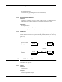
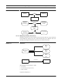
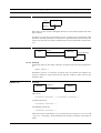
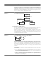
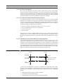
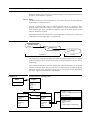
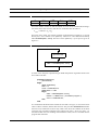
1.5.3 Comparison
The main difference between these two generic paradigms is that one can jump forth
and back between activities in the process-oriented paradigms, whereas one cannot (by
definition!) jump back between activities in the product-oriented paradigms (see
Figure 1-9).
FIGURE 1-9
Process-Oriented versus Product-Oriented Paradigms
process-oriented
paradigm
activityn
activityn+1
milestone
product-oriented
paradigm
activityn
activityn+1
deliverable d1,...,dn
1.6 Some Definitions of Terms
So far, several terms have been used in a loosely manner. In this section some of them
are described more precisely.
1.6.1 Activity
Definition:
a certain action
Examples:
• software requirements analysis
IS Biel/DUE 96/97
1-9
Software Engineering
Introduction
• software design
1.6.2 Phase
Definition:
like an activity, but phases are temporal ordered (one phase comes after another)
Examples:
see Examples in Section 1.6.1
1.6.3 Method
Definition:
systematically applied procedure for the achievement of predefined objectives
Examples:
•
•
•
•
•
•
•
•
•
•
•
•
Structured Analysis and Systems Specification (Tom DeMarco, 1979)
Structured Systems Analysis (Gane & Sarson, 1979)
Modern Structure Analysis (Yourdon, 1989)
Structured Development for Real-Time Systems (Ward & Mellor, 1985)
Strategies for Real-Time System Specification (Hatley & Pirbhai, 1988)
Information Engineering (James Martin)
Structured Systems Analysis and Design Method (Ashworth & Goodland, 1990)
IFAPASS (Institut für Automation)
HERMES (Bundesamt für Informatik)
Structured Design (Yourdon & Constantine, 1979)
Practical Guide to Structured System Design (Page-Jones, 1980)
OOA/OOD (several authors)
1.6.4 (Formal) Technique
Definition:
textual or graphical notation defined by a formal system of rules
Examples:
• data flow diagrams (bubble charts)
• entity-relationship diagrams
• structured charts
1.6.5 Software Engineering Processes
Definition:
a more or less well-defined way of developing software using software engineering
methods, techniques, and (optionally) tools
Examples:
• “waterfall model”
• fast prototyping
IS Biel/DUE 96/97
1-10
Software Engineering
Introduction
1.7 A Definition for Software Engineering
A definition as given in [1] follows:
“The establishment and use of sound engineering principles in order to obtain economically software that is reliable and works efficiently on real machines.”
IEEE (a professional society) even provides two definitions [3]:
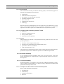
(1)“The application of a systematic, disciplined, quantifiable approach to the development, operation, and maintenance of software; that is, the application of engineering to software.”
(2)“The study of approaches as in (1).”
Bibliography
[1]
Roger S. Pressman, “Software Engineering — A Practitioner’s Approach”, third and
European edition, McGraw-Hill, 1992.
[2]
Carlo Ghezzi, Mehdi Jazayeri, and Dino Mandrioli, “Fundamentals of Software Engineering”, Prentice-Hall, 1991.
[3]
The Institute of Electrical and Electronics Engineers, Inc., 445 Hoes Lane, PO Box
1331, Piscataway, NJ 08855-1331, USA, http://www.ieee.org/.
IS Biel/DUE 96/97
1-11
CH APT E R 2
Computer System
Engineering
The following text deals with the aspects of the computer system engineering from the
viewpoint of the early phase of a software project. It is based mainly on [1].
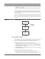
2.1 Computer-Based Systems
The word system is often used in different contexts. As a consequence, its meaning is
not a priori precisely defined; adjectives are often used to give a more precise meaning.
2.1.1 Definition
From [1] we borrow the following definition for a computer-based system:
“A set or arrangements of elements organised to accomplish some method, procedure, or control by processing information.”
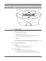
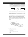
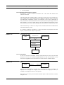
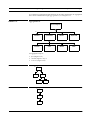
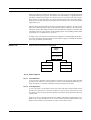
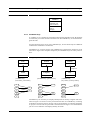
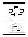
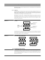
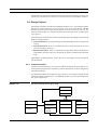
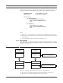
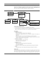
2.1.2 Elements of Computer-Based Systems
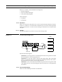
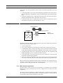
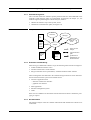
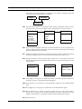
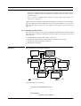
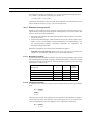
The key elements of a computer-based system are shown in Figure 2-1(based on [1]).
Note that recursion is present in Figure 2-1: computer-based systems may consist of
subsystems that are in turn computer-based systems. Computer system engineering is
also in place for these subsystems.
•
•
•
•
•
Software: programs, data structures, and documentation
Hardware: CPU, memory, peripherals, sensors, actuators
People: individuals that are users and/or operators
Data Base: large, organised collection of information
Procedures: steps required for the use and/or interworking of computer system elements
• Documentation: manuals and forms for the use and operation of the system
IS Biel/DUE 96/97
2-1
Software Engineering
Computer System Engineering
Elements of a Computer-Based System
FIGURE 2-1
computer-based
system
level N
software
data base
procedures
hardware
people
documentation
level N-1
computer-based systems
2.2 Analysis Tasks
Computer system engineering deals with the identification and analysis of system functions. The following tasks are typical:
•
•
•
•
•
•
identification of the customer’s need
bounding of the scope of the system
feasibility studies, in particular economic feasibility and technical feasibility
allocation of system functions to the elements of the system
cost
scheduling
The results obtained by carrying out the tasks leads to the system model. The document
containing these results and the system model is called system specification.
2.2.1 Identifying Customer’s Need
2.2.1.1
Purpose
• the capturing of the business processes of the customer
• the capturing of the functionality of the system
2.2.1.2
Kind of Customers
• a customer requiring a solution for a specific problem
• a marketing department requiring a solution for a common problem
• an information system department requiring a solution for an internal problem
IS Biel/DUE 96/97
2-2
Software Engineering
2.2.1.3
Computer System Engineering
Kind of Inputs
Make sure that the customer provides the following inputs, or that following inputs are
found by corresponding research activities:
•
•
•
•
•
•
•
system goals
market situation and competition
development cost and schedule constraints
reliability and quality issues
future extensions
manufacturing requirements
technology
Note that the presence and importance of some of the above points depends very on the
nature of the computer-based system to be produced. In Exercise 2.1 estimate the
importance of the above points for two different kind of computer-based systems.
2.2.1.4
Techniques Used for Identifying Customer’s Need
•
•
•
•
2.2.1.5
interviews
practice in the application area
surveys of user opinion
observation of user operations
Results
The investigation of customer’s need yields the following results that will occur in the
system specification:
•
•
•
•
interfaces of the computer-based system
functions to be performed by the computer-based system
performance criteria to be fulfilled
other constraints such as cost
The model of the computer-based system captures well the interfaces and the functions;
performance aspects must be added as a separate list of additional requirements.
2.2.2 Economic Feasibility
A very important part of the feasibility study is the cost-benefit analysis: costs of the
project development are compared with the potential benefit achieved with the produced product.
2.2.3 Technical Feasibility
Technical feasibility is investigated. At the same time, additional information concerning the reliability and performance is collected. Usually, mathematical modelling and
optimization techniques can be used.
2.2.3.1
Techniques and Tools Used for Technical Feasibility Tasks
With a sound mathematical background:
•
•
•
•
queuing theory
control theory
probability and statistics
Petri nets
IS Biel/DUE 96/97
2-3
Software Engineering
Computer System Engineering
With less or without a sound mathematical background:
• data flow diagrams
• state/event-based techniques
• entity relationship diagrams
Other techniques:
• simulation
• prototyping
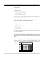
2.2.4 Allocation
Each system function is allocated to one or more system elements (hardware, software,
people, etc.). However, several alternative solutions may exist. Each of them represents
a functional allocation. To select one from among the alternatives an evaluation must
take place.
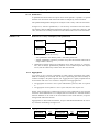
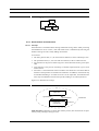
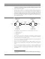
2.2.4.1
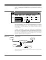
Example
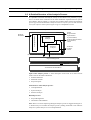
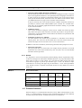
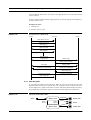
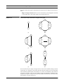
The following Figure 2-2 presents a conveyor line sorting system.
FIGURE 2-2
A conveyor line sorting system
Bins
1
Line motion
2
ID No.
ID No.
ID No.
3
Sorting
station
4
Bar code
Possible allocations might be:
Allocation 1: A sorting operator is trained and placed at the sorting station. He reads
the box and places it into the appropriate bin.
Allocation 2: A bar code reader is placed at the sorting station. Bar code output
passes to a controller that controls a mechanical switching mechanism. The switching mechanism moves the box into the appropriate bin.
Allocation 3: A bar code reader and controller are placed at the sorting station. Bar
code output passes to a robot arm that grasps the box and moves it to the appropriate
bin location.
2.2.5 Cost and Scheduling
Initial cost and scheduling constraints are established.
IS Biel/DUE 96/97
2-4
Software Engineering
Computer System Engineering
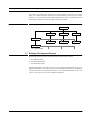
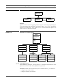
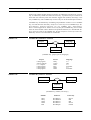
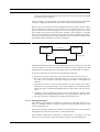
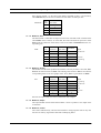
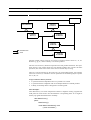
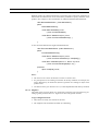
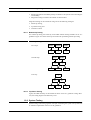
2.3 A Detailed Structure of the Analysis Process
It is possible to structure the analysis activity in more detail. One possibility is given
next. It is based on the unification of the rather traditional separation between system
and software analysis phases [1] and the more modern OMT software development
process [3]. It turns out that there is analysis on the level of the system as well as on the
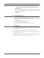
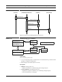
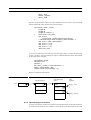
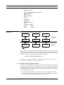
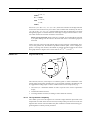
level of the software of the system. Figure 2-3 gives a simplified overview.
Substructures of the Analysis Process
FIGURE 2-3
Analysis
Conceptualisation
Problem
Statement
System
Analysis
Initial
Requirements
Specification
System models;
Software Requirements
Specification;
others
Software
Analysis
Software
models;
others
costs and schedule
initial costs and schedule
Project Management
Project Management
Reviews
Verification and Validation
Project Management
Input of the analysis process: A short description of the work to be done. Several
names exist for this kind of document:
• Problem Statement
• Statement of Work
• Project Proposal
Substructures of the analysis process:
• Conceptualisation
• System Analysis
• Software Analysis
Related processes:
• Project Management
• Verification and Validation
Note: There is no strict sequencing during the analysis process as suggested in Figure 23. Iteration may occur within the analysis process yielding “feed-back” from software
analysis to system analysis or even conceptualisation.
IS Biel/DUE 96/97
2-5
Software Engineering
Computer System Engineering
Note: The purpose of the analysis is to find out:
• What is the system going to do?
• What is the software of the system going to do?
2.3.1 Project Proposal
A short description of the project to be realised: the need; the goal; the results to be
achieved.
2.3.2 The Conceptualisation
Input of the conceptualisation: A project proposal.
Tasks of the conceptualisation: To understand the problem to be solved. Determine the
system, the boundary of the system (scope), and the external systems or actors. Write
down the Initial Requirements Specifications (IRS). Use the terminology of the problem
domain. Choose between:
• the traditional style of writing the IRS: the system, its scope, and essentially a list of
functional requirements
• a modern style of writing the IRS: the system, its scope, and use cases.
Results of the conceptualisation:
• The Initial Requirements Specification (IRS).
2.3.3 The System Analysis
Input of the system analysis: Initial Requirements Specifications.
Tasks of the system analysis: To understand a system approach that is a solution of the
problem. Try to determine the computer elements (hardware, software, data bases, procedures, documentation, and people) by providing the system model. Allocate the components of the system model to the computer elements.
Results of the system analysis:
•
•
•
•
•
The system models
The Software Requirements Specification (SRS)
Hardware requirements specification
Preliminary costs and schedule statements
Risk analysis, feasibility studies, performance analysis, etc.
Note: If the system is purely in software then the Software Requirements Specification
coincide with the Initial Requirements Specification.
Note: It may turn out that the first steps of system design must be carried out in order to
define all software requirements specifications, yielding the so-called System Architecture Specification.
2.3.4 The Software Analysis
Input of the software analysis:
• The Initial Requirements Specifications, and/or
• The Software Requirements Specification
IS Biel/DUE 96/97
2-6
Software Engineering
Computer System Engineering
• The System Architecture Specification (optional)
Tasks of the software analysis: To understand the software approach that is a solution
of the software problem. Describe the external behaviour of the software as a black box.
Determine or refine the scope of the software. Determine its data or object model.
Determine the software functions by listing the functional requirements. Provide use
cases or scenarios for capturing the dynamic behaviour of the software.
Results of the software analysis:
•
•
•
•
The software models
The Software Architecture Specification (optional)
Detailed costs and schedule statements about the software
others.
2.4 Initial/Software Requirements Specification
For the system or software level, the corresponding requirements specification consists
of:
1 A precise description of the context of the system or software consisting of the external systems or actors, and the interactions of these with the system or software.
2 An exhaustive list of functional requirements or use cases.
2.4.1 The Context
The context of the system or software describes the interaction or interfaces with other,
external systems. Main difficulty is to define the boundary between the system or software, and its external systems. The system (or software) and its boundary is sometimes
called the scope. External systems, also called actors, can be:
• human beings
• other computer-based systems
• technical systems such as robots, etc.
Often, an explicit list and corresponding description of external systems or actors is a
good starting point. Examples are (numbers refer the initial/software specification template given in Section 2.5):
3.2.1 External Library
External libraries are the providers of text books. Books can be ordered at, received
from, and returned to, external libraries. All external libraries together can be
regarded as one external entity that serves the system to be defined.
3.2.2 Some Other External System
The description of this external system and its relationship with the system to be
defined goes here.
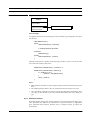
2.4.2 Functional Requirements
Part of a model is a list of functions (often called the functionality of the system or software) that describe what must be done. Again, several approaches support this documentation. One technique is the construction of a so-called event matrix list as proposed
in the “Modern Structured Analysis” method by Yourdon. Another technique is to
describe the system functions in term of input, task and output descriptions:
IS Biel/DUE 96/97
2-7
Software Engineering
Computer System Engineering
• Input: The description of the information (or, sometimes, material) needed to carry
out the desired function.
• Task: The description of the actions to be done by the system when performing the
desired function.
• Output: The description of the information (or, sometimes, material) produced by
the system when performing the desired function.
Often, a separate section with the list of functional requirements is given in the initial
requirements specification. Requirements are numbered for easier cross-reference
checking during later phases in the development of the system or software. The numbering scheme used coincides with the IRS/SRS template layout given in Section 2.5. An
example of a functional requirement is:
3.3.1 Requirement 1: Book Request
Input: A student makes a book request. The request must contain the student’s full
name or a unique abbreviation such as a user name of a computer system and specifications regarding the book(s) to order. Such a specification consists of a library
name and a book identification, or an author and a title, or both.
Task: A record is made per ordered book containing the full name of the student, the
informations regarding the ordered book, and the status of the order. Records are
stored in the system’s record data base.
Output: The system places a book order for each individual book at the respective
library.
2.4.3 Use Cases
A use case is a collection of interactions between the system or software and an external
system or actor about a particular way or purpose of using the system or software from
the user’s point of view [3]. A use case consists of:
• An initial event: An event caused by an actor (the initiator) and realised by the system or software.
• A series of events: Events between the actor, the system or software, and possibly
other actors. Some authors call this a sequence of transactions (or scenario) in the
dialogue with the system or software.
• A logical conclusion: The interaction initiated by the initial event results in a steady
state of the system or software.
Often, a separate section with the list of use cases is given in the initial requirements
specification. Use cases are numbered for easier cross-reference checking during later
phases in the development of the system or software. The numbering scheme used coincides with the IRS/SRS template layout given in Section 2.5. An example of a use case
is:
3.3.1 Use Case 1: Book Request
Initial event: A student makes a book request. The request must contain the student’s full name or a unique abbreviation such as a user name of a computer system
and specifications regarding the book(s) to order. Such a specification consists of a
library name and a book identification, or an author and a title, or both.
Series of events: The software system receives the book requests and notifies the
book administrator. The book administrator eventually orders the book at the library,
and updates the corresponding book record within the software system.
Logical conclusion: The book is ordered and the corresponding record is updated.
IS Biel/DUE 96/97
2-8
Software Engineering
Computer System Engineering
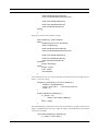
2.5 Requirements Specification Outline
The outline of the Initial Requirements Specification (IRS) and the Software Requirements Specification (SRS) consists of the following essential parts (from [4], text
emphasised when taken literally):
1. Introduction
Provides an overview of the entire IRS/SRS. It should contain the following subsections:
1.1 Purpose and Scope
This section identifies the project, the developer, and the customer. It states the
purpose of this document and defines the intended reader ship. It may specify
what the document is not intended to do.
1.2. Document overview
This section should outline the type of information that will be found in the document and the depth to which it will be presented.
1.3. Applicable Documents and References
This section should refer to all related documents that are separate from this
document. This section may be divided into Applicable Documents (documents
that form part of this specification) and Reference Documents (documents for
reference only).
1.4. Nomenclature and abbreviations
This section may be included if the specification uses specific nomenclature or
conventions. Some requirements specifications have specific verbs associated
with ‘binding’ requirements and ‘desirable’ requirements or features.
2. Overall Description
Describes the general factors that affect the product and its requirements. It usually
contains:
2.1 General description
Give an overview of the product being developed and state its purpose. If software is being developed under contract, refer to related purchaser projects. If
work is being subcontracted, refer to related supplier projects.
2.2. Project objectives
Specify the goals, objectives and needs of the project or product. Identify who
your customer is, and (if appropriate) what you are trying to sell. Establish a
link to product-line strategies and corporate (or department) strategies (where
appropriate).
2.3. Product perspective and life cycle
Do you intend to develop future upgrades, enhancements, or to build families of
products? Do you provide on-line help facilities or technical support? If so,
what is the life expectancy of these product additions? What is the life expectancy of the product or product release?
2.4. General constraints
Describe any physical, design, or platform constraints for the product or system.
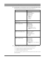
3. System/Software Requirements
Contains all the system/software requirements to a level of details sufficient to enable the designers to design a system/software to satisfy those requirements, and testers to test that the system/software satisfies those requirements.
3.1 System/software and its context
Provide an overview of the system and its functionality. Include a context diagram showing the external interfaces.
IS Biel/DUE 96/97
2-9
Software Engineering
Computer System Engineering
3.2. External systems or actors
This section identifies the interfaces between the system under consideration
and other systems or external devices. There should be a one to one correspondence between the interfaces described here and those shown in the context diagram in Section 3.1.
3.3. Functional requirements or use cases
Include a separate 3.3.x section for each functional capability. Differentiate
between ‘binding’ requirements and desirable features through the particular
use of verbs. (i.e. ‘Shall’ denotes a binding requirement. ‘Will’ or ‘should’
denotes a desire or a statement of fact.) All requirements should be stated in
clear, concise, measurable terms in order to avoid misinterpretation and in
order to validate each requirement.
3.4. Data requirements
This section should state any data requirements that have not already been covered by the Section 3.3, Functional Requirements, or Section 3.2, External
Interface Requirements. Data requirements include data storage capacity
requirements, data throughput requirements, and data types and format
requirements.
3.5. Physical requirements
This section states cabinet, hardware, or physical computer requirements.
There may not be any physical requirements if the cabinets, and computer are
provided by the customer or if the product is strictly software.
3.6. Human engineering requirements
This section specifies any human engineering requirements such as visual displays, keyboard layouts, use of windows, etc.
3.7. Expansion requirements
This section will contain requirements for future expansion and growth of the
system. It may specify spare capacity with reference to memory, disk space, and
serial ports. It may allow for future growth in specifying certain design considerations.
3.8. Quality factors
This section may be divided into subsections for each quality factor. System
quality factors may include reliability, maintainability, availability, correctness, integrity, security, verifiability, flexibility, portability, reusability, safety,
usability, and efficiency. Requirements should be stated in quantitative terms
where possible.
3.9. Documentation requirements
This section lists all documentation requirements. The document deliverables
are often due at the completion of specific life cycle phases. Documentation
requirements may also refer to existing documentation standards which outline
document content and form (i.e. IEEE Standards).
3.10.Training requirements
Training requirements will address the requirements for training courses, training materials, and training responsibilities. Training could be performed by the
developer or customer. Training could include anything from operational training to software maintenance training. Requirements for training courses could
include duration, time, location, materials, equipment, and skill level of trainees.
3.11.System verification and validation
This section states the verification and validation requirements of the system. It
is also commonly referred to as qualification requirements. Requirements for
unit, component, integration, system, or acceptance tests are stated here. This
IS Biel/DUE 96/97
2-10
Software Engineering
Computer System Engineering
section should reference any Test Plans that will identify individual tests. If no
Test Plans are required, then the individual tests should be listed here.
Glossary of Terms
A list of definitions of technical terms used in the document. Useful for non-technical users as well as for the development staff as it establishes a precise definition of
the terms used in the document.
References
List of references.
2.6 The Specification Review
The Initial/Software Requirements Specification Review evaluates the accuracy and
completeness of the definition contained in the document. The review is carried out by
both, the developer and the customer! Points to carefully review are:
•
•
•
•
definition of scope
functions, performance, and interfaces
justification of the project (development risk)
developer and customer have the same perception of the system
Bibliography
[1]
Roger S. Pressman, “Software Engineering — A Practitioner’s Approach”, second edition, McGraw-Hill, 1987.
[2]
Ian Sommerville, “Software Engineering”, third edition, Addison-Wesley, 1989.
[3]
James Rumbaugh, “OMT: The Development Process”, Journal of Object-Oriented Programming, Vol. 8, No. 2, 1995.
[4]
Software Productivity Centre, “Initial Requirements Specification Template”, Vancouver, British Columbia, Canada, V6B 5L1, http://www.spc.ca/spc/.
IS Biel/DUE 96/97
2-11
Software Engineering
Computer System Engineering
Exercises
E2.1 The development of a new text processing system and a patient monitoring system shall
be compared. Give the ratings “important” or “less important,” or “high” or low” for
aspect
text processing system
patient monitoring system
student
student
discussion
discussion
goals
market
costs
schedule
reliability
extensibility
manufacturing
N.A.a
technology
a. N.A. = not applicable
every cell in the rows “student” for every aspect.
E2.2 Provide the context for a system that allows to receive book requests from students, that
assists to place orders at and to receive books from external libraries, and that helps to
administer the books given to students.
E2.3 Provide at least two functional requirements for the system given in Exercise 2.2
E2.4 (Project) For a given project proposal, provide a complete system specification, using
the structure given in Section 2.5.
IS Biel/DUE 96/97
2-12
CH APT E R 3
Software Project Planning
To successfully conduct a software development project a careful planning is required.
A more or less precise understanding of the work to be done, the resources required, the
effort (or cost) to be expected, etc., is needed.
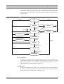
3.1 Software Project Planning Overview
Software project planning will be based on two tasks:
• The definition of the size of the software elements, as described in the preceding
chapter.
• A “look into the future” to tell something about the efforts and cost, also called estimation.
Dilemma: Quantitative estimates are required for establishing a project plan, but solid
information is not yet available. A detailed analysis of software requirements would
provide necessary information, but analysis takes weeks or months to complete. Estimates are needed “now.”
On Estimation:
• Whenever estimates are made, a look into the future is made and some degree of
uncertainty must be accepted.
• Access to historical software project data is mandatory.
• Estimates carry risks: software complexity (or nature of software), software size,
and degree of software structure details.
The availability of historical information of past software projects is achieved by collecting software metrics.
IS Biel/DUE 96/97
3-1
Software Engineering
Software Project Planning
3.2 Resources
3.2.1 Human Resources
People are the primary software development resource! Two main aspects must be considered:
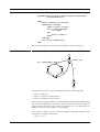
• the availability of people (see Figure 3-1)
• the experience and skill that people have
Further aspects are:
• organisational position (ie.g., manager, senior software engineer, etc.)
• speciality (e.g., telecommunications, data base, operating systems, etc.)
Project Participation
high
junior programmer
degree of project participation
FIGURE 3-1
senior SW engineer
manager
low
planning
analysis
design
project phase
coding
testing
3.2.2 Hardware Resources
The existence of or access to:
• development system (or host system)
• target system
• other hardware
3.2.3 Software Resources
The existence of software tools is necessary, but they must also be mastered:
•
•
•
•
•
editors, compilers, debuggers
parser generators
graphical user interface generators
CASE tool
others
Further software resources might be:
• availability of programming libraries (e.g., libraries for window applications)
IS Biel/DUE 96/97
3-2
Software Engineering
Software Project Planning
3.3 Software Metrics for Productivity Estimation
To carry out software project planning it is useful to look into the past by collecting
informations about other software projects. These informations allow to make estimates
about the “software productivity.” Here, the productivity can be loosely described as:
The software development “output” as a function of effort.
What can be measured?
Two kind of measures can be distinguished: direct measures or indirect measures. The
following table gives an overview:
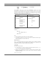
TABLE 3-1
Direct and Indirect Measures
direct measures:
cost
speed
effort
memory size
LOC (lines of code)
errors
indirect measures:
function
efficiency
quality
reliability
complexity
maintainability
It is in general difficult to asses indirect measures, whereas it is relatively easy to determine the direct measures. Software metrics domains can be further categorised in:
• productivity metrics: metrics that focus on the output of the software engineering
process
• quality metrics: metrics that provide an indication on how closely software conforms to implicit or explicit requirements
• technical metrics: metrics that refer to the character of the software (e.g., complexity, degree of modularity)
Yet another software metric domain categorisation is:
• size-oriented metrics: direct measures of aspects such as LOC, effort spent, cost,
etc.
• function-oriented metrics: indirect measures of aspects such as “functionality” or
program “utility”
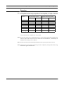
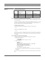
3.3.1 Size-Oriented Metrics
Simple records are maintained about the software projects carried out in the past. The
table may contain entries such as: project name, effort (person-months), cost (some currency unit, here US $), LOC, documentation (number of pages), errors encountered
after release to the customer within the first year of operation, and persons involved in
the project.
IS Biel/DUE 96/97
3-3
Software Engineering
TABLE 3-2
Software Project Planning
Simple Project Records
name
effort
cost
KLOC
pages.doc.
errors
people
Proj1
24
168
12.1
365
29
3
Proj2
62
440
27.2
1224
86
5
...
From the table above, some productivity or quality metrics can be derived easily:
productivity = KLOC / person-month
quality = error / KLOC
In addition, other interesting metrics can be computed:
relative cost = cost / KLOC
documentation “density” = pages.doc. / KLOC
In [2] we can read:
“For large, complex real-time systems, productivity may be as low as 30 lines/programmer-month whereas for straightforward business application systems which are
well understood it may be as high as 600 lines/month.”
Problems with the LOC metrics:
•
•
•
•
•
they are programming language-dependent
parts of the code may be generated (e.g., thanks to the use of parser generators)
they penalise well-designed but shorter programs
they are not very suitable for nonprocedural programming languages
for estimation purpose: they require a level of detail that is difficult to achieve at an
early stage of a software project
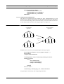
3.3.2 Function-Oriented Metrics
These metrics focus on program “functionality.” So-called function points are derived
using an empirical relationship based in countable measures of the software information
domain. Function points can be primarily applied to business information systems; they
may not be relevant to control-oriented or embedded applications. Software information
domains originally are:
• Number of user inputs: each user input that provides distinct application-oriented
data to the software is counted (e.g., name and address of a customer in a customer
data base)
• Number of user output: each user output that provides application-oriented information to the user is counted (e.g., reports, address lists, error messages, etc.)
• Number of user inquiries: an inquiry is an on-line input that results in the immediate generation of software response
• Number of files: each file containing logical grouping of data is counted
• Number of external interfaces: further, machine-readable interfaces are counted
that are used to transmit information relevant for the software
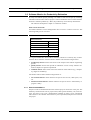
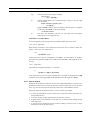
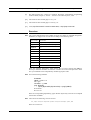
For every information domain, the count of the corresponding aspects is established,
and put into a table as shown below.
IS Biel/DUE 96/97
3-4
Software Engineering
TABLE 3-3
Software Project Planning
Computing Function Points
information
domain item
Weighting factor
count
FP
simple
avg.
complex
number of
user inputs
3
4
6
number of
user outputs
4
5
7
number of
user inquiries
3
4
5
number of
files
7
10
15
number of
ext. interfaces
5
7
10
total
The set of software information domains needs to be extended for the following applications:
• graphical window systems (e.g., number of windows and subwindows)
• communications protocol (e.g., number of main states and transitions between main
states)
• command interpreters (e.g., number of commands)
Once the function points have been determined they can be used analogous to the LOC
measures:
productivity = FP / person-month
quality = error / FP
and
relative cost = cost / FP
documentation “density” = pages.doc. / FP
Some positive aspects about function points:
• they are language-independent, making it ideal for applications using conventional
and nonprocedural languages
• function points are more likely to be known early in a software project
Problems with function points:
• the measure is based on subjective data
• the set of “software information domains” is not accurate in general
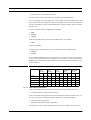
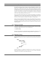
3.3.3 Size-Oriented and Function-Oriented Metrics Compared
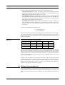
A number of studies have been made to compare LOC and function points. For the programming languages COBOL, PL/1, and a simple data base language (4GL) the following result has been obtained:
IS Biel/DUE 96/97
3-5
Software Engineering
TABLE 3-4
Software Project Planning
LOC versus Function Points (FP)
Language
LOC/FP
COBOL
110
PL/1
65
4GL
25
Important note: LOC and FP should not be used to qualify people!
3.3.4 Metrics Data Collection and Evaluation
The metrics data collection is an ongoing process. Before collecting however, a historical baseline must be established. Then, data must be collected in a simple, consistent
way.
Then, metrics data evaluation has to occur. This should also be done in a consistent way.
In addition, care should be taken if measures of too different projects are compared.
Metrics used for software project estimation should have been obtained from similar
projects.
3.4 Software Project Estimation
Software project estimation can be based on one or a combination of the following estimation techniques:
• LOC and/or FP estimations
• direct effort estimation, and
• empirical estimation models
Furthermore, to solve the estimation problem of the total software project the software
is usually decomposed into its components, and estimates on the components are collected.
3.4.1 LOC and FP Estimation
To carry out a LOC or FP estimation the following is needed:
• an estimation variable (such as LOC or FP) that is used to “size” each software component
• a baseline metrics collected from past projects (such as LOC/person-month or FP/
person-month)
The estimation variable is used in conjunction with the baseline metrics to develop cost
and effort projections.
First, optimistic (a), most likely (m), and pessimistic (b) LOC and/or FP estimates have
to be provided. Then, the expected (or average) number of LOC or FP is computed, for
instance, according the following formula:
E = (a + 4m + b) / 6
IS Biel/DUE 96/97
3-6
Software Engineering
Software Project Planning
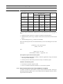
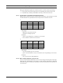
As soon as all average estimates Ei are known, the estimate for the total effort, for
instance, can be computed:
effort (PM) = Sum(Ei) / relative-effort
where “relative-effort” is obtained from the baseline metrics. Alternatively, adjusted
productivity values are used to take into account the perceived level of complexity of
each subfunction. Table 3-5 below illustrates an example.
TABLE 3-5
LOC Estimation Table
function
line/
month
a
m
b
avg.
$/line
cost
months
f1
1800
2400
2650
2340
14
315
32760
7.4
f2
4100
5200
7400
5380
20
220
107600
24.4
657000
144.5
...
total
33360
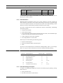
3.4.2 Direct Effort Estimation
Direct effort estimation is the most common technique used in any software engineering
development project. A project is decomposed into project tasks. Together with the
components of the software system a cost matrix as given in Table 3-6 can be developed.
TABLE 3-6
Cost Matrix Table
tasks resp.
functions
req.ana.
design
code
test
total
f1
1.0
2.0
0.5
3.5
7
f2
2.0
10.0
4.5
9.5
26
total
14.5
61
26.5
50.5
152.5
rate ($)
5200
4800
4250
4500
cost ($)
75400
292800
112625
227250
...
708075
In 1975, Barry Boehm already made an investigation about phase costs for different
kind of software systems. The following table is from [2] which in turn is based on
Boehm’s research.
TABLE 3-7
Costs of Software Development Activities (from [2])
phase costs (%)
system type
requirements/
design
coding
testing
control systems
46
20
34
space systems
34
20
46
operating systems
33
17
50
IS Biel/DUE 96/97
3-7
Software Engineering
Software Project Planning
phase costs (%)
system type
requirements/
design
coding
testing
scientific systems
44
26
30
business systems
44
28
28
3.4.3 LOC/FP Estimates Compared with Direct Estimates
If LOC/FP and direct estimates are provided they should match within a reasonable
range. If they do not then the following should be checked carefully:
• Is the software scope well defined?
• Are “productivity data” sufficient exact or applicable?
• Are the direct estimates realistic?
3.4.4 Empirical Estimation Models (also: Algorithmic Cost Estimation)
It would be nice to have one formula which, when given some easy to estimate parameters, would provide values for the efforts and cost. A so-called estimation model (or
resource model) uses empirically derived formulae to predict such data.
Resource models fall into four classes: static single-variable models, static multi-variable models, dynamic multi-variable models, and theoretical models, see Figure 3-2.
Classes of Resource Models
FIGURE 3-2
single-variable
static
multi-variable
resource model
dynamic
multi-variable
theoretical
In the following we shall mention only the static single-variable model. The model takes
the form:
resource = c1 (estimated characteristics)c2
where the resource could be effort (E), project duration (D), staff size (S), or lines of
software documentation (DOC). The constants c1 and c2 are derived from past projects.
The estimated characteristics is lines of source code, effort (if estimated), or other software characteristics.
3.4.4.1
The COCOMO Model
The COCOMO (COnstructive COst MOdel) is based on the above mentioned form.
However, it exists in three different forms: basic (simple), intermediate, and detailed
one. The basic model gives an order of magnitude estimation of software cost. The
intermediate model takes the basic efforts and cost computation as its starting point. It
then applies a series of “multipliers” to the basic model figures. The full or detailed
COCOMO model is a further refinement. In the sequel, only the basic model shall be
discussed.
IS Biel/DUE 96/97
3-8
Software Engineering
Software Project Planning
The basic model distinguishes between three classes of software projects:
Organic mode projects: Projects with relatively small teams working in familiar
environments, making applications that are familiar (i.e., low communication overhead, and team members know what they have to do).
Semi-detached projects: Projects between “organic mode” and “embedded mode”
discussed below. In semi-detached mode projects, project teams may be made up of
experienced and inexperienced staff, and some team members are unfamiliar with
some aspects of the software to be developed.
Embedded mode projects: Projects that are difficult due to strongly coupled complex of hardware, software, regulations, and operational procedures. Project team
members cannot have a great deal of experience in all aspects of the system to be
developed.
The basic COCOMO equations take the form
E = ab (KLOC) exp(bb)
D = cb (E) exp(db)
where E is the effort applied in person-months, D is the development time in chronological months, and KLOC is the estimated number of delivered lines of code (in thousands) for the project. The coefficients ab and cb and the exponents bb and db are given
in the following table:
TABLE 3-8
Parameters for the Basic COCOMO Model
SW project class
ab
bb
cb
db
organic
2.4
1.05
2.5
0.38
semi-detached
3.0
1.12
2.5
0.35
embedded
3.6
1.20
2.5
0.32
The basic COCOMO model is intended to give an order of magnitude estimate of the
effort required to complete a software project. It has some implicit productivity estimate
built into it which was derived from existing project data. In the case of the organic
mode the productivity is 352 LOC per person-month (here, a person-month consists of
152 hours of working time). The effort required for the embedded system requires 105
LOC per person-month.
A further interesting implication of the basic COCOMO model is that the time required
to complete the project is a function of the total effort required for the project and not a
function of the number of software engineers working on the project. This confirms the
observation that adding more people to a project which is behind the schedule is
unlikely to help that the schedule to be regained.
3.5 Software Project Scheduling
After having defined the scope and effort of all software functions (i.e., the sum of the
components that constitute the software element as described in chapter 2) it is now possible to perform the software project scheduling. Two rather different perspectives do
exist:
IS Biel/DUE 96/97
3-9
Software Engineering
Software Project Planning
• In the first, an end-date for the release of the computer-based system has already
been defined. The software development project is constrained to distribute effort
within the given time frame.
• In the second, the effort and/or cost of a software project is given. Rough time
bounds may also exist, but the delivery date is set by the software organisation. The
effort is distributed to make best use of the resources, and an end-date is set after
careful analysis of the software element.
3.5.1 Milestones
When planning a project, a series of milestones should be established. Each milestone
represents a point in time at which a predefined development result must be achieved.
Based on these results it is then decided whether to enter into the next phase of the
project.
Two kinds of milestones can be distinguished:
• external milestones: milestones at which the customer is involved in deciding
whether to continue the project or to stop it
•
internal milestones: milestones at which the decision is internal to the software
project
Milestones should denote a culmination of a distinct stage in the project. Important
events that could denote milestones could be:
• the release of the software requirements specification or
• the successful passing of the integration tests.
It is important that milestones are characterised by criteria that allow the software management (or the customer) to clearly decide whether a milestone is reached. For
instance, milestones can be characterised by finished documentation such as “Test plan
formulated and reviewed.”
For the decision to be taken at a milestones three different outcomes are possible:
• the input document is rejected: The document does not meet the set of predefined
criteria, it must be revised. Note that the software project plan may perhaps be
adapted to the new situation.
• the input document is accepted: The document meets the set of predefined criteria,
and the project continues according the software project plan.
• the whole project is stopped: The input document as well as other indicators such as
efforts and cost let the software management (or the customer) come to the conclusion to stop the project.
Milestones denote main events along the duration of a software development project.
They are often explicitly listed in a table. An example can be found in Table 3-9.
TABLE 3-9
List of Milestones
milestone
main event
planned date
M0
SW project plan established
day X
M1
SW requirement analysis performed
X + 10
M2
SW design completed
X + 22
IS Biel/DUE 96/97
actual date
3-10
Software Engineering
milestone
Software Project Planning
main event
planned date
M3
Test plan established
X + 20
M4
Acceptance tests performed
X + 48
actual date
Note that the dates in column “planned date” may possibly be revised after the software
project plan is made in detail.
3.5.2 Task Definitions
Milestones denote prominent events in any project. However, the work involved in
achieving these events must now be planed. The starting point for the work partitioning
is the set of software functions to be realised. Note that a clear understanding of these
functions in terms of functionality and effort should exist at this stage.
The work is partitioned into units so-called tasks. Tasks are described by establishing
the following items:
• a unique task identifier
• a brief task description
• a more elaborated task description describing the task results, the intermediate steps
to achieve the task, and critical resources involved
• a effort estimation for the task completion
• a list of dependencies on other tasks
Tasks may be structured along the following aspects:
• function-oriented aspects
• software development phase-oriented aspects
• others
All tasks are then summarised in a task duration and dependency table. As an example,
Table 3-10 is given. Such a table then serves for the detailed schedule planning.
TABLE 3-10
Task Durations and Dependencies
task ID
task description
duration (days)
dependencies
T1
SW requirements specification
10
T2
SW design specification
12
T1
T3
Implementation I1
8
T2
T4
Implementation I2
4
T2
T5
SW integration
10
T3, T4
T6
Test specification
10
T1
T7
Acceptance test and delivery
8
T5, T6
3.5.3 Task Scheduling Techniques
A number of scheduling techniques do exist for the software project planning. Among
others there are:
• activity networks and
• bar charts (also known as Gantt charts)
IS Biel/DUE 96/97
3-11
Software Engineering
Software Project Planning
Activity networks is a graphical means for project schedule illustration. When establishing an activity network an important assumption is implicitly made: The project development cycle is static and known in advance. The formal elements of a network are
directed arcs and nodes. Several different activity networks exist, among others:
• the Metra-Potential Method (MPM)
• the Critical Path Method (CPM), and
• the Program Evaluation and Review Technique (PERT)
Note: Although MPM as well as CPM are called method they rather denote techniques
according to the meanings that have given to the terms “methods” and “techniques” in
chapter 1.
PERT is a technique based on probabilities. Although similar in appearance to CPM its
underlying mathematical model is different and, thus, this technique shall not be discussed in the sequel.
Bar charts are widely used in practice. They are clear and easy to survey (as long as they
are not too big).
3.5.3.1
Metra-Potential Method (MPM)
Here, tasks are mapped onto nodes, and task dependencies are expressed using arcs that
connect nodes. To each task the following information is assigned:
•
•
•
•
•
•
•
•
task ID
task description
task duration
earliest beginning (EB)
latest beginning (LB)
earliest end (EE)
latest end (LE)
a time frame a task can be delayed without affecting the deadline of the project’s end
(slack time)
IS Biel/DUE 96/97
3-12
Software Engineering
Software Project Planning
An MPM Graph
FIGURE 3-3
T3
22
8
30
22
0
30
T2
T5
10
12
22
30
10
40
10
0
22
30
0
40
T1
T4
T7
0
10
10
22
4
26
40
8
48
0
0
10
26
4
30
40
0
48
task ID
T6
10
30
10
20
20
EB
dur.
EE
40
LB
slack
LE
A task can be started provided that all its predecessor tasks have been finished. The earliest beginning of a task (EB) is computed as the maximum of the earliest ends of all
preceding tasks. The earliest end of a task (EE) is the task’s earliest beginning plus its
duration. This chain of calculations is called forward computation.
The latest end of a task (LE) is the moment at which the task must have been completed
such that it does not delay its successors. It is computed by taking the minimum of the
latest beginning times of all successor tasks. The latest beginning of a task (LB) is the
task’s latest end minus its duration.
The time margin within which a task may be delayed without affecting the total project
duration is called the slack time.
If the earliest beginning of task is equal to its latest beginning and the earliest end is
equal to its latest end then this task is a so-called critical task. The sequence of all critical tasks through the network constitute the so-called critical path. Delays along the
critical path would imply a delay of the whole project.
3.5.3.2
The Critical Path Method (CPM)
When using CPM tasks are mapped onto directed arcs, and the events of the tasks’ completions are indicated by nodes. The nodes contain the information:
• event number (event ID)
• earliest moment an event can take place (EM)
• latest moment an event must take place (LM)
The arcs correspond to tasks. They contain the information:
• task ID
• task duration
IS Biel/DUE 96/97
3-13
Software Engineering
Software Project Planning
Critical Path Method (CPM)
FIGURE 3-4
3
22
4
T3
8
22
30
30
T2
1
0
10
0
12
2
T1
10
T5
10
T4
4
10
8
T7
40
5
T6
7
0
26
8
40
48
48
30
0
10
6
event ID
task ID
duration
20
40
EM
LM
The earliest moment an event may take place (EM) is computed as the sum of the latest
moment of any preceding event (LM) plus its corresponding task duration. A peculiarity
of CPM networks are null tasks. A null task consumes no time. Null tasks are used to
present and conjunctions.
The critical path is the path along the events with equal earliest and latest moments. A
task may have a slack time if it ends in an event node with different earliest and latest
moments.
3.5.3.3
Bar Charts (or Gantt Charts or Gantt Diagrams)
Bar charts are widely used since they are intuitive and do not require special knowledge.
Planned tasks are drawn along the time axis as bars. The length of each bar denotes the
consumed time. Slack time, if existent, may be appended to a bar using a different colour.
FIGURE 3-5
Bar chart
0
10
20
30
40
50
M0
T1
M1
T2
M2
T3
T4
T5
T6
M3
T7
M4
Bar charts are also used to visualise the task allocation to persons. In stead of mentioning milestones Mx and tasks Ty, the persons’ names are mentioned.
IS Biel/DUE 96/97
3-14
Software Engineering
Software Project Planning
The bar chart has some disadvantages: it is rather difficult to modify and/or correct; the
clearness is decreased if it gets too big; and it is not easy to “see” the critical path without careful investigation.
3.6 Organisation of the Project
Planning software development projects involves also planning the project organisation.
The availability of people and their existing integration into the organisation’s hierarchy
are constraining factors for this activity. Project organisation means to build one or more
project teams. Several forms of project organisation exist. In the following, some of
them are mentioned.
3.6.1 Task Force
A task force is a pure project organisation consisting of all members of the project.
Project members are recruited from existing departments of the organisation and fully
assigned to the project. A project manager is the leader of the project team.
The so-formed project team can be organised in several ways: hierarchical, functional,
or democratic, to name but a few. For the organisation of software projects, a specific
form has been proposed: “Chief programmer teams.”
3.6.1.1
An Informal (Democratic) Team
It has been recognised that software project teams should be relatively small. Rule of
thumb: not more than 8 members. If projects are too big then it should be split into parts,
each part is tackled by a relatively small team in an independent manner. Small teams
have a number of benefits:
•
•
•
•
a team quality standard can be developed
team members work closely together
egoless programming can be practised
team members can get to know each other’s work
Small teams can be organised in an informal way (i.e., with a minimum of fixed, internal structure). Although a titular team leader exists, he carries out the same tasks as
other team members.
In an informal team, work is carried out as decided by the team as a whole, and tasks are
allocated to each team member according to ability and experience.
Informal teams can be very successful, particularly where the majority of team members
are experienced and competent. The team functions as a democratic team, making decisions by consensus.
However, if their is a lack of experience and competence within the team, the informality can be a hindrance. No definite authority exists to direct the work.
3.6.1.2
A Chief Programmer Team
Here, a project team is created on the bases of utilising experienced and talented staff as
chief programmers, providing clerical support for these programmers using both human
and computer based procedures, and carrying out all communications by one or two persons (see Figure 3-6).
IS Biel/DUE 96/97
3-15
Software Engineering
Software Project Planning
The nucleus of a chief programmer team consists of the following members (from [2],
adapted):
1 A chief programmer who is experienced and highly qualified. He takes full responsibility for designing, programming, testing, and installing the system under development.
2 A backup programmer who is skilled and experienced. He works with the chief programmer and should be able to adopt that role if necessary.
3 A librarian whose role is to assume all the clerical work associated with a project.
He should be assisted by an automated library system.
FIGURE 3-6
The Chief Programmer Team
chief programmer
specialists
backup programmer
outside
communication
librarian
Depending on the size and type of the application, other experts might be involved temporarily or permanently with the team:
• a project administrator
• a tool “guru” responsible for providing the software tools required for the project
• a documentation editor for the final editing of the project documentation prepared
by the chief programmer and backup programmer (and, possibly, others, see below)
• a language/system expert who is prepared for advising the chief programmer and
backup programmer on how to make use of these facilities
• a tester whose task is to develop objective test cases to validate the work of the chief
programmer and backup programmer
• one or more support programmers if the scale of the project is such that the detailed
work cannot be carried out by the chief programmer and backup programmer alone
However, this project organisation form has also its drawbacks. One problem is the centralisation of knowledge and experience related to the project on two persons. Should
they fall ill or leave, the project may have to be abandoned.
3.6.2 Matrix Project Organisation
The hierarchical, vertical structure of an organisation is completed with a horizontal
dimension of projects. Employees now have two authorities each of which can make
assignments.
Divergences between authorities of different dimensions is expected in this organisation. One aim of this organisational form is to recognise problems or conflicts relatively
soon such that solutions can be found in an early stage
IS Biel/DUE 96/97
3-16
Software Engineering
Software Project Planning
One reason to introduce this organisation is the assumption that neither the superior
along the “normal” hierarchy nor the project leader alone are able to carry out the
project to a success. Whenever this matrix organisation is used it is important to fix the
responsibility domains of hierarchy superior and project leaders.
FIGURE 3-7
Matrix Project Organisation
management
head dep. 1
head dep. 2
head dep. 3
dep. 1
dep. 2
dep. 3
PL 1
PL 2
PL = project leader
3.7 Software Development Process
Developing software involves usually the following three generic phases:
1 the definition phase
2 the development phase
3 the maintenance phase
The following figures represent an overview of the software development process as it
might be described in the software project plan. Besides a description of the different
activities involved in developing the software, also planned deliverables such as the
software requirements specification should be mentioned
IS Biel/DUE 96/97
3-17
Software Engineering
FIGURE 3-8
Software Project Planning
The Definition Phase
software elements
allocated
establish scope, resources,
feasibility, cost, and schedule
software project
plan
management
review
no
determine functions,
interfaces, design constraints,
validation criteria
build prototype to
establish requirements
revision
yes
requirements
known
technical
review
software requirements
specification
acceptable
revise resources, cost,
and schedule
revision
plan
review
acceptable
development begins
IS Biel/DUE 96/97
3-18
Software Engineering
FIGURE 3-9
Software Project Planning
The Development Phase
software requirements
defined
define program and date
structure, module structure
module interfaces, etc.
architectural design
document
user manual
(draft)
review
revision
acceptable
specify procedural
aspects of each module
detailed design
document
review
revision
acceptable
code
listings
revision
code
walkthrough
acceptable
test (unit, integration) and
validation
software ready
for release
test certificate
3.8 Software Project Plan
The software project plan is produced at the culmination of the planning step. It need
not be a lengthy, complex document. Its purpose is to help to establish the viability of
IS Biel/DUE 96/97
3-19
Software Engineering
Software Project Planning
the software development effort. The plan concentrates on a general statement of what
and a specific statement of how much and how long. It must (1) communicate scope and
resources to software management, technical staff, and the customer; (2) define cost and
schedule for management review; and (3) provide an overall approach to software
development to all people associated with the project, including a list of deliverables.
An outline of the software project plan may look like:
1 Scope
a. Project objectives
b. Major functions
c. Other characteristics
2 Resources
a. Human resources
b. Hardware resources
c. Software resources
d. Availability windows
3 Cost
4 Schedule
a. Milestones
b. Task network
c. Bar charts
d. “Milestone plan” (to be discussed below)
5 List of deliverables
The presentation of certain points such as cost and schedule will vary with the audience
to whom it is addressed. If the plan is used only internally, the result of each cost estimation technique can be presented. When the plan is disseminated outside the organisation,
a summary of cost estimations is presented.
3.9 On Software Project Controlling
The following discussion belongs to the topic “Software Project Management.” It is
mentioned at this place since it is related with the discussion on the software project
plan.
Recall from Section 3.5.1 that a list of milestones is created early in the beginning of the
software plan establishment. When stabilised (for instance, after a number of revisions
due to the insights obtained during the detailed task planning activity, e.g., “M3 new”) a
new table can be created [3]. In this table, the project estimates in terms of delivery
dates (deadlines) and efforts are combined with actual delivery dates and efforts.
Milestone Plan, Checking, and Prognosis
TABLE 3-11
M0
M1
M2
M3 new
M4
milestone
M0
M1
M2
Total
deadline
deadline
effort
deadline
effort
deadline
effort
deadline
effort
X
X + 10
10
X + 22
12
X + 30
8
X + 48
18
48
X+9
9
X + 21
12
X + 29
8
X + 47
18
47
9
X + 23
13
X + 31
8
X + 49
18
48
IS Biel/DUE 96/97
3-20
Software Engineering
M0
M1
Software Project Planning
M2
M3 new
M4
milestone
Total
deadline
deadline
effort
deadline
M3
effort
deadline
effort
deadline
effort
22
M4
At milestone M0, the deadlines and efforts to spend to achieve the deadlines are inserted
in row “M0.”
After reaching M1, the actual date and effort is inserted in row “M1” under column
“M1,” and the sum of the efforts (0 + 9) is inserted in field “M1,M2/effort.” Furthermore, new estimates in terms of delivery date and efforts are inserted appropriately in
row “M1,” and the total is computed by adding the actual effort and the estimated
efforts.
When reaching a new milestone along the course of the project, the table is completed
appropriately with actual data and new estimates. The table itself provides a simple
means to get a quick overview about the project’s actual state versus its plan.
Bibliography
[1]
Roger S. Pressman, “Software Engineering — A Practitioner’s Approach”, second edition, McGraw-Hill, 1987.
[2]
Ian Sommerville, “Software Engineering”, third edition, Addison-Wesley, 1989.
[3]
Karol Frühauf, Jochen Ludewig, Helmut Sandmayer, “Software-Projektmanagement
und -Qualitätssicherung”, Verlag der Fachvereine, Zürich, 1991.
Exercises
E3.1 In the following table, tasks duration and task dependencies are given. Draw complete
activity networks according to the MPM and CPM techniques. Determine the critical
path(s) and the project duration.
task
duration
T1
10
T2
15
T1
T3
10
T1, T2
T4
15
T3
T5
20
T3
T6
35
T5
T7
15
T3, T4
T8
10
T6, T7
T9
20
T7, T8
T10
10
T9
IS Biel/DUE 96/97
dependencies
3-21
CH APT E R 4
Software Analysis
Fundamentals
The software analysis task is a process of discovery and refinement. The software
boundary, initially established during system engineering, is refined in detail. The aim
of the software analysis is to define a software model.
Both, the developer and customer usually take an active role in software analysis. The
customer attempts to formulate the software functions and performance requirements.
The developer acts as an interrogator, consultant, and problem solver. Note that the
terms of the application domain are predominant during this phase.
4.1 Software Analysis
Software analysis allows the software engineer to refine the software allocation (see
Chapter on “Computer System Engineering”) and to define the following software
views:1
• Information (or data) domain: Data objects (or entities), their properties in terms
of attributes, and relations among data objects.
• Dynamic behaviour: The software states and modes as conceived by the user.
• Data transformations: Software functions applied on data objects.
Examples of information domain objects: For an information system, the following
data entities have been defined:
• An entry “book” in a database having the attributes (or components) “user name”,
a “book identifier”, a “book title”, and “earliest date”, and a “latest date”.
• Information on persons; each entry “person” is identified using the following
attributes: “user name” and “full name”.
1. Software view is not a commonly agreed term.
IS Biel/DUE 96/97
4-1
Software Engineering
Software Analysis Fundamentals
• For the information system above, an association between persons and book entries
in the data base has been identified: For every entry “book”, an entry “person” of
the form “user name” and “full name” must be associated. In addition, for a given
entry “person”, zero or more entries of kind “book” may exist in the data base. This
can best be illustrated using a graphical notation such as an entity/relationship diagram (ERD):
person
1
has
book
n
book
Example for a dynamic behaviour: For instance, the dynamic behaviour of the above
information system may be as follows: A person must have been registered somewhere
before one or more entries can be made; or: before a person’s registration is deleted, all
its entries in the data base must also be deleted. In other words, the definition of the specific dynamic behaviour of a system imposes temporal constraints on all possible
dynamic behaviours of that system.
Example for a data transformation: A simple transformation is the following one:
Given a unique “user name”, the “full name” of a person shall be determined using a
user database. A more complex transformation of data is for example: given a “user
name”, determine all entries in the data base of books matching the given person.
The software views constitute the software analysis models. They can later be translated
into architectural, data, and procedural design. Finally, the software analysis model provides the developer and the customer with the means to validate the quality once the
software is built. Figure 4-1 illustrates the gap that is bridged then software analysis is
carried out.
FIGURE 4-1
Overlap of the Analysis Task (from [1])
computer
system
engineering
software
analysis
software
design
4.2 Analysis Task and Results
Software analysis mainly means building models of the software. Software analysis
may be divided in four areas of effort:
•
•
•
•
problem recognition
evaluation and synthesis of software models
documentation
review
IS Biel/DUE 96/97
4-2
Software Engineering
Software Analysis Fundamentals
4.2.1 Problem Recognition
This is the task where the software specific problems that have been identified in the
computer system analysis phase are reconsidered. In particular, the analyst (i.e., the
software engineer performing the software analysis) needs to:
• redefine the software scope of the system, and to
• establish the communication paths (see Figure 4-2)
FIGURE 4-2
Analysis Communication Paths
initial
req.
spec.
customer
system
model/
architecture
software
project
plan
manager
software
team
analyst
software
analysis
docs
inputs for the
analyst
communication
path
production or
modification of
documentation
4.2.2 Evaluation and Modelling
After having (re) defined the software scope, the following items must be investigated:
• models of different software views
• interface characteristics of the software
• design constraints such as performance, available hardware and/or software
These investigations will then lead to first software designs which are coarse characterisations of the kind of the system to be realised such as:
• interactive application with
- character-oriented user interface
- graphical user interface
• batch application
• data base management system
• others
If the level of confidence of the kind of software that must be built is small then prototyping is in place.
4.2.3 Documentation
The software analysis results in a number of documents that illustrate the software to be
constructed:
IS Biel/DUE 96/97
4-3
Software Engineering
Software Analysis Fundamentals
• Software Analysis Model Document (mandatory):
This document represents the software in a precise, unambiguous manner using that
terms of the application domain. It uses preferably formal languages and notations.
It states precisely the (software) requirements already given in the initial requirements specification document, if that one exists. See “Outline of the Software Analysis Model Document” on page 9-6 for an outline of this document.
It may be necessary that a less formal and more readable companion document is
provided, too, which is better understandable by the customer. It is a textual document with a lot of informal graphical illustrations and tables. Ideally, it is provided
by the customer himself.
• Validation criteria:
One or more documents setting the criteria used to validate the software product.
They define the aspects under which the customer may decide to accept the delivered software. Typical documents of this kind are the software test specification and
system test specifications.
• Preliminary Software User Manual:
An initial software user manual may be obtained as a side-effect of the software
analysis phase. The reason for this document then is that the software analyst and
software developer are forced to take a user’s view of the software.
In addition to the above documents, the following document must perhaps be revised:
• Software Project Plan:
The project plan may be revised since new insight into the problem to be solved
should exist now. New effort estimates may exist, and, thus, new cost and schedule
statements must be provided.
4.2.4 Review
It is important to review the documents produced during software requirements analysis. Review and approval of documents should be done for every major document of this
phase (and, of course, of other phases, too). The following table presents the major
involvement of groups of persons per document type. A cross “X” denotes a major
involvement in reviewing and approving the documents; a cross within parenthesis
“(X)” denotes a minor or optional involvement whereas no entry denotes no involvement at all.
TABLE 4-1
Review Involvement
customer
analyst
manager
software
engineer
software analysis model
document
X
X
X
(X)
validation criteria
X
X
X
(X)
software user manual
X
(X)
software project plan
(X)
X
(X)
X
X
4.3 Potential Problems
Software analysis is a communication intensive activity. When communication occurs,
noise (i.e., misinterpretation, omission) on the communication path can cause difficulty
for both, analyst and customer. Problems that may be encountered are:
IS Biel/DUE 96/97
4-4
Software Engineering
Software Analysis Fundamentals
• acquiring stable information
• handling problem complexity
• accommodating changes
4.3.1 Acquisition of Information
Problem recognition and solution evaluation and synthesis depend on the successful
acquisition of information. Often, the following problems can be identified when
acquiring information:
• customer-supplied information conflicts
• performance statements conflict with cost requirements
• the perception of the system’s goals changes with time
4.3.2 Handling Complexity
As the size of problems grows, the complexity of the analysis task also grows. Each new
information, new functional or other requirement, and other constraint may have an
effect on other requirements of the software. That is, the analysis effort grows drastically as the problem complexity increases.
4.3.3 Accommodating Changes
In coining the “first law of system engineering,” Bersoff said: “No matter where you are
in the system life cycle, the system will change, and the desire to change it will persist
throughout the life cycle” (from [1]). Applied to the software analysis phase, change
requests from the customer will occur even before the analysis task is complete.
4.4 Analysis Principles
Several software analysis methods exist, however, all of them have the following in
common:
• provision of software models
• partitioning of complexity
• extracting essence
Software views need to be defined precisely. The next phase, system design, should not
be entered until a complete understanding of the software requirements has been
accomplished. This is best done by providing precise and accurate software model.
To overcome the complexity of analysing large systems, we tend to partition or divide
such problems into parts that can be easily understood. In addition, interfaces must be
established between these parts so that overall function can be understood.
The last principle mentioned here is that software analysis should focus on the essence
of a (software) system. It is the sometimes difficult task of a software analyst to extract
the essence of a customer-supplied, vague concept.
In the sequel, a few principles in specifying and documenting software models are
given:
• Separate functionality from implementation: An analysis model is a “view” of what
is desired, rather than how. Avoid to provide solutions (i.e., architectural, data or
program structure, algorithmic details, others) when analysing the software require-
IS Biel/DUE 96/97
4-5
Software Engineering
Software Analysis Fundamentals
ments, unless a particular aspect (e.g., the software must be base on the client/server
paradigm) is give as a constraint.
• Use the terms of the application domain: In modelling the software you should still
use the terms and definitions that are commonly used in the application domain of
your software.
• Include the system of which the software is a component: Include in your software
model the aspects of the complete system.
• Include the environment of which the system is a component: Include in your system
model the most important aspects of the system’s environment.
4.5 Analysis Methods
A number of software analysis methods have been developed in the past. To complete
the analysis task, the analyst uses one method to perform the software requirements
specification. The software analysis methods can be roughly put into the following
classes:
• Function- or dataflow-oriented analysis methods such as Structured Analysis (SA)
or Modern Structured Analysis (MSA): Here, the analysis task focuses on the flow
of data through a system, and the transformations that are applied to data. Main
application area: business applications and information systems.
• Dataflow-oriented analysis methods with Real-Time extensions such as SA/RT: The
methods from the point above have been extended to accommodate the analysis of
real-time and embedded systems. Main application are: real-time and embedded systems.
• Data structure-oriented analysis methods: Here, the analysis task focuses on the
structure and relationship of data to be processed. Furthermore, data is assumed to
be hierarchically organised.
• Object-oriented analysis method: Here, in the analysis phase real-world objects are
identified, and the relations between objects as well as the operations performed on
objects are identified. Main application areas: many, especially graphic-oriented
user interface applications.
• Other analysis methods that do not fit into the above classes: Jackson System Development (JSD) that uses a data structure-oriented approach in its initial phase but
then goes on to realise the design as a set of cooperating sequential processes; context-free grammars that are used to define and generate front-ends of compilers; and
others.
4.6 Outline of the Software Analysis Model Document
Recognising the impact of a good understanding of the software to be realised it is easy
to see that a good and accurate model of the software is indispensable. The following
general structure of an software analysis model document is adapted from [3]:
1. Introduction
Provides an overview of the entire software analysis model document. It should contain the following subsections:
1.1 Purpose and scope
This section identifies the project, the system, the developer, and the customer.
It states that the purpose of this document is to define the software analysis
model.
IS Biel/DUE 96/97
4-6
Software Engineering
Software Analysis Fundamentals
1.2. Document overview
This section should outline the type of information that will be found in the document and the depth to which it will be presented.
1.3. Applicable documents and references
This section should refer to all related documents that are separate from this
document. This section may be divided into Applicable Documents (documents
that form part of this document) and Reference Documents (documents for reference only).
1.4. Nomenclature and abbreviations
This section may be included if the specification uses specific nomenclature or
conventions.
2. Overall Description
Describes the general factors of the software and its context. It usually contains:
2.1 General description
Give an overview of the software being developed and state its purpose. If software is being developed under contract, refer to related purchaser projects. If
work is being subcontracted, refer to related supplier projects.
2.2. Software perspective and life cycle
Do you intend to develop future upgrades, enhancements, or to build families of
the software? Do you provide on-line help facilities or technical support? If so,
what is the life expectancy of these software additions?
2.3. General constraints
Describe any other constraints for the software.
3. Information Domain Model
Captures the description of real world entities or objects for which information is
kept in the software.
3.1 Real world entities or objects
Provide an overview of all the entities or objects.
3.2. Definition of real world entities or objects
This section provides the information structure of the entities or objects in
terms of attributes.
3.3. Relations among real world entities or objects
List all user-relevant relations among entities or objects.
4. Behavioural Model(s)
Captures the description of the temporal behaviour of the software.
4.1 Software states and modes
This section should state the user-relevant software states and modes.
4.2. Events and actions
This section states the events that influence the software states and modes. It
should also define the actions undertaken by the software when events occur.
5. Functional Models
Captures the description of the functional properties of the software.
5.1 Pure functional aspects
This section should state the requirements on pure functional aspects of the
software.
5.2. Control aspects
This section states the control functions of the software.
Glossary of Terms
A list of definitions of technical terms used in the document. Useful for non-technical users as well as for the development staff as it establishes a precise definition of
the terms used in the document.
IS Biel/DUE 96/97
4-7
Software Engineering
Software Analysis Fundamentals
References
List of references.
Bibliography
[1]
Roger S. Pressman, “Software Engineering — A Practitioner’s Approach”, third edition, McGraw-Hill, 1992.
[2]
Ian Sommerville, “Software Engineering”, third edition, Addison-Wesley, 1989.
[3]
IEEE Std 830-1993, “Guide to Software Requirements Specifications (ANSI)”, in IEEE
Software Engineering Standards Collection, 1994 edition, IEEE, 1994.
IS Biel/DUE 96/97
4-8
Object-Oriented Analysis
CH APT E R 5
Object-oriented analysis, design, and implementation is a modern way of the development process of computer systems and software. This introductory text is based on the
text book on the “Object Modeling Technique” (OMT) from Rumbaugh [1].
5.1 Object Orientation
There is some dispute about the exact characterisation of what “object orientation”
means. The term “object orientation” superficially means:
“Software is organised as a collection of discrete objects that incorporate both data
structure and behaviour.”
This is in contrast to the more traditional view of the organisation of programs where
data structure and behaviour are loosely coupled only. Next, the concept of object orientation is further elaborated.
5.1.1 Characteristics of Objects
There is no common agreement about what characteristics are required for an objectoriented approach, but the following characteristics are included in general:
•
•
•
•
5.1.1.1
identity
classification
polymorphism, and
inheritance.
Identity
Identity means that data and behaviour is organised into discrete, distinguishable entities
called objects. Examples:
• a paragraph in a document
IS Biel/DUE 96/97
5-1
Software Engineering
•
•
•
•
Object-Oriented Analysis
a window on the screen
the white queen in a chess game
a list
a polygon
Objects can be concrete such as a wheel of a bicycle, or conceptual such as a scheduling
policy of a multiprocessing operating system.
Each object has its own inherent identity. In other words, two objects are distinct even if
all their attribute values such as name and size are identical. Example: The instance of
this letter “a” has its own identity, and is distinct from any other occurrences spatially
separated in the text of these course notes.
5.1.1.2
Classification
Classification means that objects with the same data structure (attributes) and behaviour
(operations) are grouped into a class. Examples:
•
•
•
•
•
Paragraph
Window
Chessman
List
Polygon
A class is an abstraction that describes properties important to an application and
ignores the rest. Any choice of classes is arbitrary and depends on the application.
Each class describes a possibly infinite set of individual objects. Each object is said to
be an instance of its class. Each instance has its own value of each attribute but shares
the attribute names and operations with other instances of the class. Figure 5-1 illustrates the concept of classification discussed so far.
FIGURE 5-1
Objects and Classes
Bicycle class
Attributes
frame size
wheel size
gears
Operations
shift
move
repair
Polygon class
Attributes
vertices
border colour
fill colour
Operations
draw
move
IS Biel/DUE 96/97
5-2
Software Engineering
5.1.1.3
Object-Oriented Analysis
Polymorphism
Polymorphism means that the same operation may be applied to instances of different
classes, and may behave differently on instances of different classes. For example, the
fill operation applied to an instance of a circle behaves different from the fill operation
applied to an instance of a polygon object.
An operation is an action or transformation that an object performs when applied to it.
move, scale, and rotate are examples of operations. A specific implementation of an
operation by a certain class is called a method. Because an object-oriented operation is
polymorphic, it may have more than one method implementing it.
5.1.1.4
Inheritance
Inheritance is the sharing of attributes and operations among classes based on a hierarchical relationship. A class can be defined broadly and then refined into successively
finer subclasses. Each subclass incorporates, or inherits, all of the properties (i.e., the
attributes and operations) of its superclass, and adds its own unique properties. Examples:
• ScrollingWindow and FixedWindow are subclasses of Window
• Triangle and Rectangle are subclasses of Polygon
The ability to have common properties of several classes in a common superclass and to
inherit the properties of the superclass reduces repetition within designs and programs.
5.1.2 Further Concepts Used in Object Orientation
There are several other concepts underlying the object-oriented technology. The most
important ones are mentioned here.
5.1.2.1
Abstraction
Abstraction means focusing on the essential aspects of an entity, and ignoring non-relevant details. Introducing the class of bicycles, for example, one might consider the
aspects:
• frame size
• wheel size
• number of gears
but ignore all other aspects such as:
• the colour
• the price.
Note that this aspect is not unique to the object-oriented technology; however, objectoriented technology has concepts such as inheritance and polymorphism that allow to
introduce in an easy way further details at later stages of the software development
process.
5.1.2.2
Encapsulation
Encapsulation (also information hiding) means the separation of external aspects of an
object from the internal implementation details. Only the external aspects are visible
from or accessible to other objects; the internal details remain hidden. An example using
Modula-2:
IS Biel/DUE 96/97
5-3
Software Engineering
Object-Oriented Analysis
DEFINITION MODULE Buffer;
EXPORT QUALIFIED Put, Get;
PROCEDURE Put (x: CARDINAL);
PROCEDURE Get (): CARDINAL;
END Buffer.
5.1.2.3
Combining Data and Behaviour
The caller of an operation need not consider how many implementations of a given
operation exist. Operator polymorphism shift the burden of deciding what implementation to use from the calling code to the class hierarchy. The classical data structure hierarchies and procedure hierarchies are merged together, see Figure 5-2.
FIGURE 5-2
Classical Hierarchies versus the Class Hierarchy
conventional
approach
data structure hierarchy
object-oriented
approach
is
replaced
by
class hierarchy
procedure hierarchy
Example of the classical way of programming the drawing of figures:
struct TfigureList *figures = {circle, polygon, triangle, ...};
struct Tfigure f;
// Tfigure defined elsewhere.
// Drawing figures: using corresponding drawing procedures.
foreach f in figures:
case f:
circle: drawCircle(f);
polygon: drawPolygon(f);
triangle: drawTriangle(f);
...
endcase
end /* for each */
// drawCircle(), drawPolygon(), etc., defined elsewhere.
Using the object-oriented way, this example might look like:
IS Biel/DUE 96/97
5-4
Software Engineering
Object-Oriented Analysis
Tfigures figures = {circle, polygon, triangle, ...};
// Tfigure, a class, defined elsewhere and includes the
// definition of attributes and operations.
// Drawing figures: the “right” procedure is used for each f via
// method resolution.
foreach f in figures:
draw(f);
end /* for each */
5.1.3 Object-Oriented Development
As with the traditional approaches for the software development process the object-oriented development of software typically consists of the following stages:
1 Analysis: The analysts builds a model of the real-world situation showing its important properties. The model is a concise, precise abstraction of what the desired system must do.
2 Design: The designer makes high-level decisions about the overall (software) architecture (system design or software architectural design). The target system is organised into subsystems based on the analysis model and the proposed architecture.
Later, the designer refines the subsystems and adds implementation details (lowlevel design). In the object-oriented approach, the designer starts replacing the application-domain objects by computer-domain objects.
3 Implementation: Using the object-oriented development approach object classes and
relationships are finally translated into a particular programming language.
For the other stages of the software life cycle such as testing and maintenance no special
treatment are necessary.
5.1.4 The “OMT” Method
Object Modeling Technique (OMT) is a method using three kinds of models to describe
a system:
1 an object model
2 a functional model
3 a dynamic model
5.1.4.1
The Object Model
The object model
• describes the static structure of the objects of the system, and
• describes the relationships among objects.
An object diagram is introduced for the object model. The object diagram is a graph:
• the nodes are object classes
• the arcs are relationships among object classes
5.1.4.2
The Dynamic Model
The dynamic model describes the aspects of a system that change over time: the control
aspects. For OMT, a state-transition diagram is used to model these time-dependant
aspects.
IS Biel/DUE 96/97
5-5
Software Engineering
5.1.4.3
Object-Oriented Analysis
The Functional Model
The functional model describes the data transformations within a system. For OMT, a
dataflow diagram is used for this purpose.
All three models are used for a complete description of a system. The models should be
consistent.
5.2 Object Modelling
Object modelling aims at analysing and modelling the information (or data) domain:
Data objects, their properties in terms of attributes, and relations among data objects are
modelled.
5.2.1 Objects and Classes
5.2.1.1
Objects
An object is a concept or a thing. All objects have identity and are distinguishable.
• Identity: means that two objects are distinguished by their inherent existence (and
not by descriptive properties that they may have in common).
Note that the term “object” sometimes refer to object instances, and sometimes to object
classes. The correct meaning can be inferred from the context:
a single thing
object instance
a set of similar things
object class
object =
5.2.1.2
Classes
An object class describes a group of objects with:
•
•
•
•
similar properties (attributes)
common behaviour (operators)
common relationship to other objects
common semantics (i.e., the meaning of the object with respect to the actual abstraction).
Each object “knows” its class (its an implicit property of an object).
Reasons for grouping objects into classes: Common definitions (class names,
attribute names) and operations are given once per class rather than once per instance.
5.2.1.3
Object Diagrams
Object diagrams are a graphical formalism to express models of objects, classes and
their relationships.
• class diagram: a template for describing many possible object instances
• instance diagram: describes object instances
The class diagram shows the general case, the instance diagram shows examples.
Figure 5-3 shows the symbols related to objects of class and instance diagrams.
IS Biel/DUE 96/97
5-6
Software Engineering
Object-Oriented Analysis
Class Diagram and Instance Diagram
FIGURE 5-3
Person
(Person)
Joe Smith
instance symbol
class symbol
5.2.1.4
(Person)
Peter Müller
Attributes
An attribute is a data value held by the objects in a class. For instance, the class Person
have the attributes:
• name
• age
• weight
Each attribute name is unique within a class (as opposed to being unique across all
classes). Thus class Person and class Company may each have an attribute called
address.
Attributes are listed in the second part the class and instance boxes, see Figure 5-4.
Attributes in Class and Instance Boxes
FIGURE 5-4
Person
name: string
age: integer
(Person)
(Person)
Joe Smith
24
Peter Müller
38
Note: Avoid using explicit object identifiers in an object model.
5.2.1.5
Operations and Methods
An operation is a transformation that may be applied to or by objects of a class. For
example, the class Windows may have the operations:
•
•
•
•
open
close
hide
redisplay
All objects in a class share the same operations.
If an operation with a given name may apply to different classes then such an operation
is called to be polymorphic. Examples of polymorphic operations:
• move for Polygons and Bicycles
• draw for Polygons and Circles
A method is the implementation of an operation for a given class. For example, the class
File may have the operation print. Different methods can be implemented to print
IS Biel/DUE 96/97
5-7
Software Engineering
Object-Oriented Analysis
ASCII files and digitised picture files. Both methods perform the same task: printing a
file. Thus it can be referred to as the generic operation print.
file print
method 1 (for ASCII)
method 2 (for digitised pictures)
...
An operation may have arguments. Such arguments parameterise the operation but do
not affect the choice of method.
The same operations of different classes should have the same signature: the number
and types of arguments, and the type of return value. Example:
• operation move for Polygons and Circles: move(Vector).
Operations are listed in the lower third of the class boxes, see Figure 5-5.
Attributes and Operations in Class Diagrams
FIGURE 5-5
Person
name: string
age: integer
change-address
change-job
File
file name
size in bytes
Geometric Object
colour
position
last update
print
move(delta: Vector)
select(p: Point): Boolean
rotate(angle)
In the programming language C++, attributes and operations of a class are called features.
Note: Sometimes, classes do have several different signatures for the same operation.
Then, this situation is called operation overloading.
5.2.2 Links and Associations
Links and associations are the means to express relationships among object instances
and object classes.
5.2.2.1
General Concept
A link is the physical or conceptual connection between object instances. Mathematically, a link is defined as a tuple, i.e., the link expressing a relationship between object
instance lecturer and object instance student is denoted as follows:
• <lecturer, student> or (lecturer, student)
Note that the order in the above lists is significant.
An association describes a group of links with a common structure and common semantics. It describes a set of potential links in the same way as a class describes a set of
potential object instances.
IS Biel/DUE 96/97
5-8
Software Engineering
Object-Oriented Analysis
A binary association is inherently bidirectional. The name of a binary association usually “reads” in a particular direction, but the binary association can be “traversed” in
either direction. The direction implied by the name is the forward direction; the opposite
direction is the inverse direction.
Associations could be thought of being attributes and pointers; however, a link is not
part of either object, but depends of both of them (again, we are speaking about binary
links and associations). For certain implementations, however, one-way implementations may be sufficient.
5.2.2.2
Representing Links and Associations in Object Diagrams
Figure 5-6 represents a one-to-one association and corresponding links. Each association in the class diagram corresponds to a set of links in the instance diagram, just as
each class corresponds to a set of objects.
• Association names: italic, start with upper-case letter.
• Association names: can be omitted if meaning is obvious.
5.2.2.3
Higher Order Associations
Associations can be:
• binary
• ternary
• or higher order
However, the higher the order of an association is, the more complicated it is to think
about.
FIGURE 5-6
One-to-One Association and Links
Country
Has-capital
City
(Country)
Has-capital
(City)
Ottawa
Has-capital
(City)
Paris
Has-capital
(City)
Rome
Canada
(Country)
France
(Country)
Italy
Figure 5-7 shows a ternary association: Person who are programmers use computer languages on projects. This ternary association is an atomic unit and cannot be subdivided
into binary associations without losing information. For instance, a programmer may
know a language and work on a project, but might not use the language on the project.
IS Biel/DUE 96/97
5-9
Software Engineering
Object-Oriented Analysis
Ternary Associations and Links
FIGURE 5-7
Project
Language
Person
(Language)
Cobol
(Project)
accounting sys.
(Person)
Mary
(Language)
C++
(Project)
CAD program
5.2.2.4
Multiplicity (for Binary Associations)
Multiplicity specifies how many instances of one class may relate to a single instance of
an associated class. In Figure 5-8, dir1 contains the files file1, file2, and file3. The corresponding class diagram models that a directory can contain several files.
FIGURE 5-8
Multiplicity
(File)
file1
(Directory)
(File)
dir1
file2
(File)
file3
Directory
Contains
File
The multiplicity of associations is often:
• one-to-one
• one-to-many (or many-to-one)
• many-to-many
In general, multiplicity is:
IS Biel/DUE 96/97
5-10
Software Engineering
Object-Oriented Analysis
• a single interval of the set of non-negative integers
However, multiplicity is sometimes:
• a set of disconnected intervals of the set of non-negative integers. For example:
- number of doors of a certain type of a car: 2 or 4.
The multiplicity is typically specified:
•
•
•
•
1 (exactly one)
1+ (one or more)
3 - 5 (three to five inclusive)
2, 4, 8, 16
Line terminators of associations are:
• solid ball:
• hollow ball:
denotes zero or more multiplicity
denotes zero or one (or optional) multiplicity
This section only considers multiplicity for binary associations. The solid and hollow
ball notation is ambiguous for n-ary (n > 2) associations, for which multiplicity is a
more complex topic.
Multiplicity is not too important at the beginning of an analysis; however, it becomes
more and more important in later stages of the software development process.
5.2.3 Advanced Link and Association Concepts
5.2.3.1
Link Attributes
A link attribute is a property of the links in an association. Each link attribute has a
value for each link. In Figure 5-9 for example, the relationship between a lecturer and a
student may also involve the grades.
FIGURE 5-9
Link with Attribute
Lecturer
Qualifies
Student
grade
Eric Dubuis
Eric Dubuis
Roger Cattin
5.5
4.5
5.0
Lorenz Dimmer
Beat Meier
Lorenz Dimmer
The value of a link attribute belongs to the respective link; it cannot, in general, be
replaced by a class attribute. Such an attribute is a property of a link. For instance, the
grade of the link <Eric Dubuis, Beat Meier> is (4.5).
Sometimes, link attributes can be replaced by class attributes. However:
• it does not work for many-to-many associations,
• it does not work for ternary or higher order associations, and
IS Biel/DUE 96/97
5-11
Software Engineering
Object-Oriented Analysis
• it is less general.
5.2.3.2
Modelling Associations as Classes
Sometimes it is useful to model an association as a class. Each link becomes one
instance of the class.
The link attribute box introduced above is actually a special case of an association as a
class, and may have a name and operations in addition to attributes. Figure 5-10 shows
the authorisation information for users of workstations. Users may be authorised on
many workstations. Each authorisation carries a priority and access privileges, shown as
link attributes. A user has a home directory for each authorised workstation, but the
same home directory can be shared among several workstations or among several users.
The home directory is shown as a many-to-one association between the authorisation
class and the directory class.
It is useful to model an association as a class when links can participate with other
objects, or when links are subject to operations.
Association as a Class
FIGURE 5-10
User
Authorised-on
Workstation
Authorisation
priority
privileges
start session
Directory
5.2.3.3
Role Names
A role is an end of an association. A binary association has two roles, each of which
may have a role name. A role name uniquely identifies one end of an association. A role
name can be regarded as a derived attribute. Its value is the set of related objects.
FIGURE 5-11
Roles
Person
employee
employer
Company
Works-for
The person’s role in Figure 5-11 is the one of an “employee”. That is, a person is an
employee of a company. The company’s role is the one of an “employer”. That is, a
company is an employer of zero or more persons.
Role names are necessary for associations between objects of the same class, as shown
in Figure 5-12.
IS Biel/DUE 96/97
5-12
Software Engineering
Object-Oriented Analysis
Roles in an Association of the Same Class
FIGURE 5-12
boss
Person
worker
Manages
Role names are also useful to distinguish between two associations between the same
pair of classes.
In Figure 5-13, both uses of role names are given. A directory may contain many other
directories and may optionally be contained in a parent-directory. Each directory has
exactly one user who is the owner, and many users who are authorised to use the directory.
Different Uses of Role Names
owner
User
FIGURE 5-13
authorised user
5.2.3.4
Directory
parent-directory
sub-directory
Ordering
Usually the objects on the “many” side have no explicit order, and can be regarded as a
set:
{object1, object2, ...}
Sometimes, however, it is necessary to express order. For instance, the windows on a
screen are ordered to express that only the top-most window is fully visible at any
moment in time.
FIGURE 5-14
Ordering
Window
{ordered}
Screen
Visible-on
Thus, the set
{<w1,screen>, <w2,screen>, ...} = {<w2,screen>, <w1,screen>, ...}
is replaced by the list
<<w1,screen>, <w2,screen>, ...>
which differs from the list
<<w2,screen>, <w1,screen>, ...>
Thus, there exists a total relation “is top of” between any two pairs of <wi,screen> and
<wj,screen>, i not equal j, which determines the visibility of windows with respect to
others.
IS Biel/DUE 96/97
5-13
Software Engineering
5.2.3.5
Object-Oriented Analysis
Qualification
A qualified association relates two object classes and a qualifier. A qualifier is a special
attribute of an association that reduces the effective multiplicity of an association.
The qualifier distinguishes among the set of objects at the “many” end of an association.
In Figure 5-15, without a qualification, a “one-to-many” association exists for directories and files. With the additional information “file name”, together with “directory” and
“file”, the above one-to-many association can be reduced into a one-to-one association
FIGURE 5-15
Reduction of a “many” Multiplicity with Qualification
Directory
Directory
File
File
file name
• Qualification improves the accuracy:
- with qualification: the directory name + file name yields a file.
- without qualification: a directory contains many files and each file name must be
unique within a directory.
• Qualification usually reduces the multiplicity from “many-to-many” to “many-toone”, but not always. Qualification partitions a set of related objects into disjoint
subsets, but the subsets may contain more than one element
5.2.4 Aggregation
Aggregation is the “a-part-of” relationship in which objects representing the components of something are associated with an object representing the entire assembly. A
common example is the parts explosion tree. Aggregation is a tightly coupled form of
an association with some extra semantics. Properties of an aggregation are:
• An aggregation is transitive: If A is a part of B and B is a part of C, then A is a part of
C.
• An aggregation is antisymmetric: If A is a part of B, then B is not part of A.
Finally, some properties of a composition propagate to the components as well, possibly
with some local modifications. For example, the environment of a statement within a
function definition is the same as the environment of the whole function, except for
changes made within the function.
Aggregations are drawn like associations, except a small diamond indicates the assembly end of the relationship, see Figure 5-16.
FIGURE 5-16
Aggregation with Operation Propagation
Document
copy
IS Biel/DUE 96/97
copy
Paragraph
copy
copy
Sentence
copy
5-14
Software Engineering
Object-Oriented Analysis
In a collection of components that all belong to the same composition, the aggregation
lines can be combined into single aggregation tree, as in Figure 5-17.
FIGURE 5-17
Aggregation Tree
Microcomputer
1+
Monitor
Systembox
Mouse
Keyboard
Chassis
CPU
RAM
Disk
An aggregation may be:
• fixed (Figure 5-18)
• variable (Figure 5-19), or
• recursive (Figure 5-20).
FIGURE 5-18
Fixed Aggregation
FIGURE 5-19
Variable Aggregation
IS Biel/DUE 96/97
5-15
Software Engineering
Object-Oriented Analysis
Recursive aggregation
FIGURE 5-20
Block
Comp.
Statem.
Single
Statem.
5.2.5 Generalisation and Inheritance
5.2.5.1
Concept
Generalisation is introduced when sharing similarities among classes while preserving
their differences. Given a class, a new and similar class is introduced by inheriting the
features of the given class, and by adding new features.
A few terms:
• The more general class (i.e., the class with less features) is the so-called superclass.
• The specialised class (i.e., the class with new features) is the so-called subclass.
• Specialisation is the process of deriving one or more subclasses from a given superclass.
• Generalisation is the process of forming a common superclass from a given set of
similar classes.
• Inheritance is the mechanism used to introduce new subclasses. This means that all
features of the superclass are reused in the subclasses. In addition, new features may
be introduced leading to so-called extensions of the superclass, and inherited features may be modified to become more specific leading to so-called refinements.
Figure 5-21 illustrates the concept.
FIGURE 5-21
Overview on Inheritance
superclass
specialisation
generalisation
extensions
refinements
inheritance
subclasses
OMT Notation: Subclasses are drawn like ordinary classes, but connected to its superclass by using a triangle, see Figure 5-22.
IS Biel/DUE 96/97
5-16
Software Engineering
FIGURE 5-22
Object-Oriented Analysis
OMT Notation for Inheritance
Superclass
Subclass 1
Subclass 2
Subclass n
Example:
Figure 5-23 shows classes of graphic geometric figures. It has some programming flavour, and emphasises the inheritance of operations. Move, select, rotate, and display
inherited by all subclasses. Scale applies to one- and two-dimensional figures. Fill
applies only to two-dimensional figures.
FIGURE 5-23
Inheritance for Graphic Figures
Figure
colour
pen thickness
pen type
move
select
rotate
display
0-Dimensional
1-Dimensional
2-Dimensional
orientation
orientation
fill type
scale
fill
scale
Point
Line
endpoints
display
display
Polygon
num of sides
vertices
display
Circle
diameter
display
5.2.5.2 Overriding Features
When introducing subclasses, existing features (i.e., attributes and operations) of the
superclass can be overridden. Some guidelines are given next.
Attributes: Default values of attributes may be overridden. However, you should not:
• change the type of an attribute
• change the meaning of an attribute
IS Biel/DUE 96/97
5-17
Software Engineering
Object-Oriented Analysis
Operations: A particular new method may be introduced for an operation in a subclass
that overrides the corresponding method of its superclass, such as rotate-circle in
Figure 5-23.
Whenever an operator such as rotate is applicable to instances of different classes we
say that the operator is polymorphic. Additionally, the polymorphic operator may be
implemented using more than one method. Overriding operations, that is, introducing
more specialised methods, can be done for the following reasons [1]:
• Overriding for Extension: The new operation is the same as the inherited one,
except that it adds some behaviour, usually affecting new attributes of the subclass.
• Overriding for Restriction: The new operation restricts the use of the operation of
the superclass such as tightening the type of arguments. This may be necessary to
keep the inherited operation inaccessible within the subclass.
• Overriding for Optimisation: The new operation has the same signature as the
inherited one, but its internal representation and algorithm may differ completely.
However the following semantic rules should be applied for overriding operations [1]:
• All query operations (operations that read, but do not change, attribute values) are
inherited by all subclasses.
• All update operations (operations that change attribute values) are inherited across
all extensions.
• Update operations that change constrained attributes or associations are blocked
across a restriction.
• Operations may not be overridden to make them behave differently (in their externally-visible manifestations) from inherited operations.
• Inherited operations can be refined by adding additional behaviour.
5.2.6 Aggregation versus Generalisation
Aggregation is not the same thing as generalisation:
• Aggregation relates instances: Two distinct objects are involved; one of them is a
part of the other.
• Generalisation relates classes and is a way of structuring the description of a single
object. Both, superclass and subclass refer to properties of a single object.
With generalisation, an object is simultaneously an instance of the superclass and an
instance of the subclass. Furthermore, one can say that:
• An aggregation tree is composed of object instances that are all part of a composite
object. Aggregation denotes a “part-of” relationship.
• A generalisation tree1 is composed of classes that describe an object. Generalisation
denotes a “kind-of” relationship.
5.2.7 Abstract Classes and Abstract Operations
An abstract class is a class that has no direct instances. A concrete class is a class that is
instantiable; that is, it can have direct instances.
1. This statement does not consider multiple inheritance.
IS Biel/DUE 96/97
5-18
Software Engineering
Object-Oriented Analysis
Figure 5-24 shows an example of an abstract class: An excerpt of a simplified model of
a computer drawing tool is given. The abstract class Closed Shape is a generalisation of
the subclass Ellipse and Polygon. It is abstract since at no point in time there exists a
direct instance of the class itself. Any object instances are belong to the classes Ellipse
and Polygon and, thus, belong to the superclass Closed Shape, too (see also the preceding Section 5.2.6).
Abstract classes organise features (attributes and operations) common to several classes.
Often, they define operations (that is, the signature and the method) to be inherited by
subclasses. On the other hand, an abstract class can define the signature (sometimes also
called the protocol) of an operation without supplying the corresponding method. Such
an operation is a so-called abstract operation.
In Figure 5-24, select denotes an operation that supplies a corresponding method. However, draw denotes an abstract operation which doesn’t supply a method; the methods
have to be provided by the subclasses.
Abstract Classes and Abstract Operations
FIGURE 5-24
Closed
Shape
select
draw {abstract}
Ellipse
draw
Polygon
draw
5.2.8 Class Features
5.2.8.1
Class Attributes
A class attribute describes a value common to an entire class of objects, rather than data
peculiar to each instance. Class attributes are useful to store default information for creating new objects, or summary information about all instances of the class.
5.2.8.2
Class Operations
A class operation is an operation on the class itself. The most common kind of class
operation are operations to create new instances of a given class. Operations to create
new instances must be class operations because the instance being operated on does not
initially exist.
Figure 5-25 shows a class Window with class features indicated by leading dollar signs.
Window has a class attribute for the set of all windows and the default window size.
Window also contains a class operation to create a new window object.
IS Biel/DUE 96/97
5-19
Software Engineering
Object-Oriented Analysis
A Class With Class Features
FIGURE 5-25
Windows
size
$default-size
$all-windows
$create
move
display
5.2.9 Candidate Keys
A candidate key is a minimal set of attributes that uniquely identifies a link. By minimal
we mean that you cannot discard an attribute from the candidate key set and still distinguish all links.
An association may have one or more candidate keys, each of which may have different
combinations and numbers of attributes.
Candidate key is a logical concept; each candidate key constrains the multiplicity of an
association. Figure 5-26 compares multiplicity and candidate keys for binary associations.
Multiplicity and Candidate Keys for Binary Associations
FIGURE 5-26
Line
Person
line-name
Country
person-name
country-name
Is-Capitol
Point
Company
point-name
comp-name
{candidate key:
(line-name, point-name)}
{candidate key: (person-name)}
l1
p1
City
city-name
c1
{candidate key:
(city-name), (country-name)}
Zürich
l2
p1
p2
Bern
l3
p2
p3
Biel
l4
p4
l5
p5
c2
Paris
CH
F
Lyon
Candidate keys are necessary to uniquely identify links for ternary or higher order associations. Figure 5-27 shows a ternary association that has one candidate key consisting
of attributes of all three classes. Persons who are programmers use computer languages
on projects. Several links are presented at the bottom of the figure. No combination of
just one or two attributes will uniquely identify each link.
IS Biel/DUE 96/97
5-20
Software Engineering
Object-Oriented Analysis
Figure 5-28 contains another ternary association. A student has one advisor at a university. A student may attend more than one university. A professor may be an advisor at
more than one university. Here the instances suggest that (student, university) is the
only candidate key. This candidate key involves only two of the related object instances.
Candidate keys are deduced by considering all possibilities. Student is not a candidate
key; two links have the value Mary. Professor or University are not candidate keys. Student+Professor, Professor+University are not candidate keys; Susan+Weaver,
Weaver+SUNY appear twice. Student+University may be a candidate key, since no links
share the same attribute values. Based on the problem statement, it is decided that Student+University really is the candidate key. Student+Professor+University is not a candidate key since it is not a minimal set of attributes.
FIGURE 5-27
Candidate Key with Three Attributes
Project
Language
project
language
Person
person
{candidate key: (project, person, language)}
FIGURE 5-28
Project
Person
Language
CAD program
control software
C++ compiler
CAD program
CAD program
CAD program
Mary
Susan
Mike
Bob
Mike
Mike
C++
Ada
C++
assembler
C++
assembler
Candidate Key with Two Attributes
Student
University
student
university
Professor
professor
{candidate key: (student, university)}
IS Biel/DUE 96/97
Student
Professor
University
Mary
Mary
Susan
Susan
Bob
Prof Weaver
Prof Rumrow
Prof Weaver
Prof Weaver
Prof Shapiro
SUNY
RPI
RPI
SUNY
Oxford
5-21
Software Engineering
Object-Oriented Analysis
5.3 OMT’s Dynamic Modelling
The class (and instance) diagrams introduced so far present a static structure of the system to be modelled. The static structure consists of objects and their relationships.
The dynamic model examines the changes to the objects and relationships over time.
OMT’s dynamic modelling technique is based on the notion of finite state machines, as
it is also used in Yourdon’s Modern Structured Analysis. However, OMT uses a different set of symbols, annotations on transitions and on states, and an elaborated concept of
nesting state diagrams (not discussed here). In the sequel, a brief introduction into
OMT’s dynamic behaviour modelling is given. See [1] for a more complete treatment of
this topic.
5.3.1 Events
An event is an abstraction of something that happens at a point in time. It is instantaneous, that is, it has no duration. Two events are logically related if one follows the other;
otherwise, the two events may be causally unrelated. Two events that are causally unrelated are said to be concurrent.
Examples of events:
• A person lifts the receiver of a telephone set.
• Somebody inserts a coin into a ticket vending machine.
• You press the call button of an elevator.
Examples of causally unrelated, concurrent events:
• You lift the receiver, and somebody else lifts the receiver, too.
• One airplane departs in Geneva, one in Tokyo.
• You call the elevator in the first floor, and somebody else calls it in the fifth.
Examples of causally related events:
• You dial your friend’s phone number, and your friend’s phone rings.
• The airplane departed from Geneva arrives in Zürich.
• Having inserted the last coin the ticket is given.
Every event is an unique occurrence, but events are grouped into event classes. “Flight
123 departs from Chicago” and “Flight 456 departs from Geneva” are both instances
from event class “airplane flight departs”.
The occurrence of an event conveys the information that something has happened.
Some classes of events may simply be signals indicating that something happened, such
as “Lifting the receiver”. Events of other event classes convey data values. Data values
are called attributes of an event. Examples of event classes are:
• phone receiver lifted
• digit dialled (digit)
• coin inserted (value)
An event that occurs in the system’s environment and denotes a stimulus to the system is
a so-called external event. Examples of such events are:
• The insertion of a coin into a vending machine.
• The pressing of a mouse button.
IS Biel/DUE 96/97
5-22
Software Engineering
Object-Oriented Analysis
Sometimes a system may produce a spontaneous event that is internal to the system.
Such an event is a so-called internal event. Examples of such events are:
• The closing of the coin insertion slot of a vending machine (this is rather the effect)
after the expiring of an internal timer (the cause).
• The sending of the busy tone (the effect) after waiting too long with dialling.
In OMT, an event is received by an object. It denotes a stimulus for it, causing it to execute one of the operations of the object. As a reaction to the stimulus, the object may
cause other events, or perform other operations, depending on the viewpoint one might
express.
5.3.2 Scenarios and Event Traces
A scenario is a sequence of events that occurs during one particular execution of a system [1]. Below is a scenario for making a phone call. Each event conveys information
from one object to another (or, alternatively, from one subsystem to another). For example, “dial tone begins” transmits a signal from the telephone network to the caller. A
possible scenario might be:
caller lifts receiver
dial tone begins
caller dials first digit
dial tone ends
caller dials second digit
....
caller dials n-th digit
called phone begins ringing
ringing tone begins in calling phone
called party answers
called phone stops ringing
ringing tone stops in calling phone
phones are connected
called party hangs up
phones are disconnected
caller hangs up
Identifying the sender and receiver objects for every event leads to an event trace for a
particular scenario. An event trace shows each object as a vertical line and each event as
a horizontal arrow from the sender object to the receiver object.
Figure shows an event trace for a phone call. Note that concurrent events can be sent.
For example, the “Network” sends event “ringing tone” to “Caller” and “phone rings” to
“Callee.”
5.3.3 States
A state is an abstraction of the values of attributes and links of a given object (or subsystem). For example, the telephone network is in the “Dialling” state when dialling, and
the exact sequence of already received digits is of no relevance.
An object (or subsystem) remains in its state until it receives an event. States represent
intervals of time. The state of an object depends on the past sequence of events it has
IS Biel/DUE 96/97
5-23
Software Engineering
Object-Oriented Analysis
received. But the future state of an object only depends from its current state, and the
event it receives.
A state is often associated with an ongoing activity such as the ringing of a telephone, or
waiting for more coins.
Examples of states:
• Dial tone on.
• Ready to receive coins.
FIGURE 5-29
Event Trace for a Phone Call
Caller
Network
Callee
caller lifts receiver
dial tone begins
dials digit d1
dial tone ends
dials digit d2
dials digit dn
ringing tone
phone rings
callee answers phone
tone stops
ringing stops
connection established
connection established
callee hangs up
connection released
connection released
caller hangs up
5.3.4 State Diagrams
A state diagram relates events and states. When an event is received, the next state
depends on the current state as well as the event; a change of state is called a transition.
A state diagram is a graph whose nodes are states and whose directed edges are transitions labelled by event names. Figure 5-31 shows the state diagram of a phone line.
FIGURE 5-30
Life Cycle of the Chess Game
Start
White’s turn
black
moves
white
moves
Black’s turn
IS Biel/DUE 96/97
checkmate
Black wins
Draw
checkmate
White wins
5-24
Software Engineering
Object-Oriented Analysis
A state diagram can express the initial state of an object or system. And it can express if
there are one or more terminating states, if any. A state diagram with terminating states
represents the life cycles of objects or systems. Figure 5-30 represents the life cycle of
the chess game.
FIGURE 5-31
State Diagram for a Phone Line
on-hook
on-hook
Idle
off-hook
time-out
Dial tone
digit(n)
digit(n)
Dialing
Busy tone
number busy
Time-out
time-out
invalid
number
valid number
Recorded
message
Connecting
Fast busy tone
trunk busy
routed
message
done
Ringing
callee answers
Connected
callee hangs up
Disconnected
5.3.5 Conditions
A condition is a boolean function on values of an object or system. Conditions can be
used as guards on transitions. A guarded transition fires when its event occurs, but only
if its guarded condition is true. Conditions are expressed between brackets “[” and “]”
after event names in a state diagram, see Figure 5-32.
5.3.6 Actions
An action is an instantaneous operation. It is associated with an event. The notation of
an action on a transition is a slash “/” and the name or description of the action, following the name of the event that causes it, see Figure 5-32.
IS Biel/DUE 96/97
5-25
Software Engineering
Object-Oriented Analysis
5.3.7 Activities
An activity is an operation that takes time to complete. An activity is associated with a
state. Activities include continuous operations such as displaying a blinking arrow on a
display to attract the user’s attention. The notation “do: activity” within the state box
denotes an activity, see Figure 5-32.
FIGURE 5-32
Summary of Simplified Notation for State Diagrams
State 1
do: activity 1
event(attribs) [condition] / action
State 2
do: activity 2
5.3.8 Relations of Object Models and Dynamic Models
An important question is the relation between a model which expresses the dynamic
behaviour over time, and a model that expresses objects and their relationships. The
most important relations are given here:
• The dynamic model defines the allowable sequences of changes to objects from the
object model.
• States are equivalent classes of attributes and link values for the object for which a
dynamic model is introduced.
• Temporary changes over time of the attributes’ values of an object are modelled by
different states.
• A dynamic model of a class is inherited by its subclasses.
• Events can be related with the operations of an object.
5.3.9 Guidelines for Constructing State Diagrams
In the sequel, some hints are given to help constructing state diagrams.
• Identify the object classes with meaningful dynamic behaviour. Construct state diagrams for these objects only.
• Identify scenarios. Concentrate on relevant ones first, treat special cases later.
• Define event traces by identifying stimulating events and involved objects. Draw
event trace diagrams.
• Consider relevant attributes only when defining states. Ignore attributes and link values unimportant for the dynamic behaviour.
• Draw an initial state diagram. Refine it by adding further transitions. Add conditions, actions and activities.
5.4 OMT’s Functional Modelling
The purpose of OMT’s functional modelling is to capture the flow of information necessary for defining the operations of the classes in the object models or the actions in the
state diagrams of the dynamic models. OMT uses a variant of data flow diagrams
(DFDs).
For the functional model, several DFDs are constructed, each showing the flow of values from external sources through operations and internal stores to external sinks.
IS Biel/DUE 96/97
5-26
Software Engineering
Object-Oriented Analysis
5.4.1 Components of the Functional Model
The functional model consists of several DFDs. The syntactical elements of this kind of
DFDs are:
• Process: A transformation of data given at its inputs to compute its output values.
• Data Flow: A connection between processes or between processes and other DFD
elements such as terminators1 and stores. In addition to ordinary data flows, OMT
introduces a new kind of arrow to model a dynamically created object instance
which is the result of a computation of a process. Figure 5-33 shows a portion of a
DFD showing the data store Account being the result of the selection computation
in process select [1].
• Terminator: A source for or sink of data values. Terminators may produce data values whilst others may consume data values.
• Data Store: A passive element for storing and later retrieval of information.
FIGURE 5-33
Selection of a Bank Account
accounts
Bank
select
Account
name
Customer
balance
request
update
5.4.2 Relation of Functional Model to Object and Dynamic Model
The functional model is another view of the system to be modelled. It models the functional behaviour, that is, the computations of data and information in the system. Some
correspondences are given next.
• A terminator denoting the primary source of a DFD corresponds to the target object
(i.e., the object which an operation is applied to).
• A process corresponds to an operation of a class and zero or more other operations
of the same or other classes.
• A process corresponds to an action in a state diagram of the dynamic model.
• Terminators correspond to active objects, i.e., objects that are the sources of events.
Data stores correspond to passive objects, i.e., objects which operations are applied
to as a consequence of a causal relationship.
• If necessary, DFDs are created for all major operations of classes in an object model.
DFDs must not necessarily be related with each other. OMT requires no context diagram.
• Processes of DFDs can be refined. A refined process can be related with an operation which in turn is composed of several operations.
• Data flows are either pure values or normal objects.
5.4.3 An Example
Figure 5-34 shows a class diagram for a table editor. Some properties of a table are:
1. In OMT, terminators are actually called actors.
IS Biel/DUE 96/97
5-27
Software Engineering
FIGURE 5-34
Object-Oriented Analysis
Class Diagram for Table Editor
Table
width
height
addRow
Row
Column
createRow
linkCell
Cell
createCell
• A table consists of rows and columns.
• A row consists of cells.
• A column consists of cells.
The i-th cell of row k and the k-th cell of column i are the same, unique cell, denoted as
cell C(i, k).
FIGURE 5-35
Functional Model for addRow Operation
User
i, mode
addRow
width
Table
i, mode,
width
createRow
newRow
Rows
i, newRow,
width
createCells
Cells
linkCells
Columns
i, cellList,
width
Figure 5-35 presents the DFD showing the flow of data values for the addRow operation. Argument i denotes the current row. Argument mode indicates whether the new
row has to be inserted below or above the current row. From the table in data store
IS Biel/DUE 96/97
5-28
Software Engineering
Object-Oriented Analysis
Table, the size width of the table is retrieved. Process createRow creates a new row
and adds it to data store Rows. Process createCells creates width times new cells and
links them with newRow. For every column k, 1 ≤ k ≤ width, of the table, process linkCells adds a link to the appropriate cell C(i, k).
5.5 The Object-Oriented Analysis Process
Before actually starting with an object-oriented analysis process, the requirements must
be stated. Either a statement of purpose or the initial requirements specification is given
stating what is to be done. Next, the real-world system must be understood, and its
essential features abstracted into a model.
The object-oriented analysis model addresses three aspects:
1 static structure (object model)
2 sequencing of interactions (dynamic model)
3 data transformations (functional model).
5.5.1 Object Modelling
With OMT, the first step in analysing the requirements is to construct an object model.
The object model shows the static data structure of the real-world system and organises
it into workable pieces.
Information for the object model comes from:
• the problem statement or the system specification
• the application domain
• general knowledge.
If the analyst is not a domain expert, the information must be obtained from the application expert and checked against the model repeatedly.
5.5.1.1
Identifying Object Classes
The first step is to identify relevant object classes from the application domain. Objects
includes physical entities such as houses, employees, and machines, as well as concepts,
such as trajectories, seating assignments, and payment schedules. Avoid computer
implementation constructs.
Examination of the nouns in the problem statement or system specification yields a tentative list of object classes. Do not worry too much about general classes; first get specific classes right.
5.5.1.2
Keeping the Right Classes
Now discard unnecessary and incorrect classes according to the following criteria:
• Redundant classes. If two classes express the same information, the most descriptive
name should be kept. For example, the word Customer and Passenger is used
throughout in system specification; Passenger is kept since it is more descriptive.
• Irrelevant classes. If a class has little or nothing to do with the problem, it should be
eliminated.
• Vague classes. A class should be specific. Some tentative classes may have illdefined boundaries or be too broad in scope.
IS Biel/DUE 96/97
5-29
Software Engineering
Object-Oriented Analysis
• Attributes. Names that primarily describe individual objects should be restated as
attributes. For example, name, age, and address are usually attributes.
• Operations. If a name describes an operation that is applied to objects and not
manipulated in its own right then it is not a class. Contrarily, an operation that has
features of its own should be modelled as a class.
• Roles. The name of a class should reflect its intrinsic nature and not the role it plays
in an association.
• Implementation constructs. Non real-world constructs, especially those from the
computer world should be eliminated from the analysis model. They may be needed
later during design, but not now.
5.5.1.3
Preparing a Data Dictionary
Prepare a data dictionary for all important modelling entities. Write a paragraph precisely describing each object class. For example:
Account — a single account in a bank against which transactions can be applied.
Accounts may be of various types, at leas checking or savings. A customer can hold
more than one account.
Sometimes it may be helpful to be even more precise in describing a data item. Then
you might use a BNF notation as it is used in “Modern Structured Analysis.” For example:
Account = CustomerInfo + AccountInfo
CustomerInfo = CustomerName + CustomerID + ...
AccountInfo = AccountNumber + AccountType + ...
5.5.1.4
Identifying Associations
Any dependency between two or more classes is an association. A reference from one
class to another is also an association.
Associations often correspond to verbs or verb phrases. These include physical location
(next to, part of, contained in), direct actions (drives), communication (talks to), ownership (has, part of), or satisfaction of some condition (works for, married to, manages).
If not obvious, delay to distinguish between association and aggregation until later.
aggregation is just an association with extra connotations. Use whichever seems most
natural at the time and continue.
5.5.1.5
Keeping the Right Associations
Discard unnecessary and incorrect associations using the following criteria:
• Associations between eliminated classes. If one of the classes in the association has
been eliminated then the association must be eliminated or restated in terms of other
classes.
• Irrelevant or implementation associations. Eliminate any association that are outside of the problem domain, or deal with implementation constructs.
• Actions. An association describes a structural property of the application domain,
not a transient event.
• Ternary associations. Many associations between three or more classes can be
decomposed into binary associations or phrased as qualified associations.
• Derived associations. Omit associations that can be expressed in terms of other
associations because they are redundant. For example, Grandparent can be
IS Biel/DUE 96/97
5-30
Software Engineering
Object-Oriented Analysis
expressed in terms of a pair of Parent of associations. Also omit associations defined
by conditions object attributes.
Classes, attributes, and associations in the object model should represent independent
information. Multiple paths between classes often indicate derived associations.
However, not all associations that form multiple paths between classes indicate redundancy. Sometimes the existence of an association can be derived from two or more
primitive associations, but the multiplicity can not. For example, in Figure 5-36 a company employs many persons and owns many computers. Each employee is assigned
zero or more computers for the employee’s personal use; some computers are for public
use and are not assigned to anyone. The multiplicity of the Assigned-to association cannot be deduced form the Employs and Owns associations.
Nonredundant Associations
FIGURE 5-36
Company
Employs
Owns
Person
Assigned-to
Computer
Although derived associations do not add information, they are useful in the real world
and in the design. You may show derived associations in object diagrams, but they
should be drawn using dotted lines to distinguish them from fundamental associations.
To specify the meaning of associations use the following guidelines:
• Misnamed associations. Don’t say how an association came about, say what it is.
• Role names. Add role names where appropriate. An association between objects of
the same class (a reflexive association) requires role names to distinguish the
instances.
• Qualified associations. Usually a name identifies an object within some context;
most names are not globally unique. The context and the name combined uniquely
identify the object. A qualifier distinguishes objects on the “many” side of an association.
• Multiplicity. Specify multiplicity, but don’t put too much effort into getting it right,
as multiplicity often changes during analysis. Try to get multiplicity values of “one.”
• Missing associations. Add missing associations that are discovered.
5.5.1.6
Identifying Attributes
Next identify object attributes. Attributes are properties of individual objects such as
name, etc. Attributes usually correspond to nouns followed by possessive phrases, such
as “the colour of that car.”
Get the most important attributes first; details can be added later. Give each attribute a
meaningful name. Omit derived attributes, or label them clearly.
Link attributes should also be identified. A link attribute is a property of the link
between two or more objects, rather than being a property of an individual object.
IS Biel/DUE 96/97
5-31
Software Engineering
5.5.1.7
Object-Oriented Analysis
Keeping the Right Attributes
Use the following criteria to eliminate unnecessary and incorrect attributes:
• Objects. If the independent existence of an entity is important, rather than just its
value, then it is an object. An entity that has features of its own within the given
application is an object.
• Qualifiers. If the value of an attribute depends on a particular context then consider
restating the attribute as a qualifier.
• Names. Names (of real world entities) are often better modelled as qualifiers rather
than object attributes.
A name is an object attribute when it does not depend on context, especially when it
need not be unique.
• Identifiers. Do not list object identifiers that are used purely for unambiguously referencing an object.
• Link attributes. If a property depends on the presence of a link, then the property is
an attribute of the link and not of the related object. Link attributes are usually obvious on many-to-many associations; they cannot be attached to either class because
of their multiplicity.
• Internal values. If an attribute describes the internal state of an object that is invisible outside the object then eliminate it from the analysis.
• Fine detail. Omit minor attributes which are unlikely to affect most operations.
5.5.1.8
Refining with Inheritance
The next step is to organise classes by using inheritance to share common properties.
Inheritance can be added in two directions:
• Generalisation of common aspects of existing classes into a superclass (bottom up).
• Specialisation of existing classes into distinct subclasses by providing extensions or
refinements (top down).
Inheritance is discovered by looking at classes with similar attributes, associations, and
operations (introduced later). Use existing concepts whenever possible.
5.5.1.9
Testing Access Paths
Access paths are a conceptual means to get access to values of attributes and to get
access to links. Trace access paths through the object model diagram to see if they yield
sensible results. For instance, make sure that there is a way which uniquely identifies
links of “many” associations.
5.5.1.10 Iterating Object Modelling
An object model is rarely complete and correct after a single pass. The entire analysis
phase is a continual iteration. Different parts of the model are often at different stages of
completion.
5.5.2 Dynamic Modelling
The dynamic model shows the time-dependent behaviour of a system.
5.5.2.1
Scenarios
Develop one or more typical scenarios that may take place between the system and its
environment.
5.5.2.2
Event Traces
Using the scenarios as a starting point. Start distinguishing between external events and
responses of the system. Identify also internal events. Start grouping events under a sinIS Biel/DUE 96/97
5-32
Software Engineering
Object-Oriented Analysis
gle name and introduce parameters for the events. Prepare event traces. Start including
error conditions and unusual events.
5.5.2.3
Build State Diagrams
For each major control object construct a state diagram such that every scenario and
event trace corresponds to a path through the sate diagram.
5.5.3 Functional Modelling
The functional model allows to define the computation of values. The functional model
is based on the data flow diagramming technique.
5.5.3.1
Provide a Context Diagram
A context diagram illustrates the system and its context. As with “Modern Structured
Analysis,” provide a context diagram showing the system and its external interfaces,
also called terminators. Provide a description of the terminators. Choose a good name
for the system. Provide the data flows from and to the system.
Note that no context diagram is required in [1]. However, it is a good practice to provide
one.
5.5.3.2
Define Input and Output Values
Define the input and output values from the data flows of the context diagram by providing a data dictionary. For example:
Order — an order consists of a customer name and the customer’s shipping address
and one or more occurrences of items.
Sometimes it may be helpful to be even more precise in describing a data item. Then
you might use a BNF notation as it is used in “Modern Structured Analysis.” For example:
Order = CustomerInfo + ShippingAddress + { OrderItem }
CustomerInfo = CustomerName + CustomerID + ...
ShippingAddress = ...
OrderItem = ItemNumber+ ItemDescription + ...
Relate input and output values with events found in the dynamic model. Input and output values are parameters of events or system responses.
5.5.3.3
Provide Data Flow Diagrams by Refining the Context Diagram
Refine the context diagram. You may apply the “event partitioning approach” as proposed in “Modern Structured Analysis.” Use the event traces as the primary source of
information for constructing the preliminary data flow diagram. Make the upward-and
downward-levelling of your preliminary DFD as done in MSA.
You may also provide DFDs not being members of a hierarchy of DFDs. In this case,
each of the DFD models distinct aspects of the system.
5.5.3.4
Provide Process Specifications
Provide process specifications for all leaf processes. Leaf processes are processes in a
DFD that are not refined any more.
IS Biel/DUE 96/97
5-33
Software Engineering
Object-Oriented Analysis
5.5.4 Adding Operations
Rumbaugh’s style of object-oriented analysis places much less emphasis on defining
operations at the beginning. Having the object, behavioural, and functional model at
hand, more operations of classes can be found.
5.5.4.1
Operations from the Object Model
Add operations from the object structure such as reading and writing attribute values
and association links.
5.5.4.2
Operation from the Dynamic Model
Each event sent to an object corresponds to an operation on the object. Actions and
activities may be related with operations on objects.
5.5.4.3
Operations form Process Specifications
Process specifications from data flow diagrams correspond to operations on objects of
the class diagram.
5.5.5 Iterating the Analysis
The analysis process usually requires several iterations to complete. One reason is that
the three models cannot be developed independently and in a completely linear way.
Another reason are the possible interactions with the customer necessary during the
course of the analysis process.
5.6 Documenting the Object-Oriented Analysis Results
During the finalisation of the analysis phase the software analysis models are documented in the software analysis model document. This document must undergo a thorough reviewing process until it becomes approved. Having been approved, it then
serves as the basis for the next phases of the software development process, the system
and the object design phases. The software analysis model document has the following
structure (see also Section 4.6):
1. Introduction
The introduction provides an overview of the entire software analysis model document. It should contain the subsections:
1.1 Purpose and scope
1.2. Document overview
1.3. Applicable documents and references
1.4. Nomenclature and abbreviations
2. Overall Description
Describes the general factors of the software and its context.
3. Object Model
The listing and the description of all class diagrams. Provide the reasoning for the
introduction of associations and inheritance relations. Give reasons for multiplicity
decisions. Provide a description for every class (purpose, meaning of attributes, purpose of operations). Provide instance diagrams, if necessary, to improve the understanding of the class diagrams.
4. Dynamic Model
List all scenarios, event traces, and state diagrams. Provide the corresponding
descriptions. Relate aspects of the dynamic model with aspects of the object model.
IS Biel/DUE 96/97
5-34
Software Engineering
Object-Oriented Analysis
5. Functional Model
Provide the DFDs for the computation of input and output values. Provide the process specifications. Relate leaf processes with operations of the class diagrams.
Glossary of Terms
References
Bibliography
[1]
James Rumbaugh, Michael Blaha, William Premerlani, Frederick Eddy, and William
Lorensen, “Object-Oriented Modeling and Design”, Prentice-Hall, 1991.
Exercises
E5.1 Identify the attributes and operations of the following object classes: Window (of a window system), computer Account, and a Student record.
E5.2 Identify attributes and operations of the superclass Polygon and its subclasses Triangle
and Rectangle that are common, and that are different.
E5.3 Prepare a class diagram from the following instance diagram:
(Country)
Borders
Spain
(Country)
Borders
France
(Country)
Belgium
E5.4 Given the following class diagram expressing many-to-many associations and given
sample data, draw the corresponding instance diagram.
Intersects
Line
Point
2+
name
name
L1
L2
P2
L3
P1
L5
L4
E5.5 Prepare a class diagram from the following instance diagram. Explain your multiplicity
decision. Each point has an x coordinate and a y coordinate. What is the smallest
IS Biel/DUE 96/97
5-35
Software Engineering
Object-Oriented Analysis
number required to construct a polygon? How can you express the fact that points are in
sequence?
(Point)
Has
Has
-10
10
(Point)
10
10
(Polygon)
(Point)
Has
Has
-10
-10
(Point)
10
-10
E5.6 Prepare a class diagram to describe undirected graphs. An undirected graph G consists
of a set of vertices (or nodes) V and a set of edges E, hence G = (V, E). Your diagram
should capture only the structure of the graphs (i.e., the connectivity), and need not concerned with geometrical details such as location of vertices and lengths of edges. A typical graph is given here:
e1
v5
G:
e2
v1
v4
e3
e6
v3
e5
e4
v2
E5.7 Prepare a class diagram to describe directed graphs. A directed graph is similar to an
undirected graph, except that the edges are oriented. Use qualification to express the
direction of an edge. A directed graph is:
v5
G:
e2
v1
e1
v4
e3
e4
e6
e5
v3
v2
E5.8 A term in a statement of a programming language is often defined using the following
grammar:
Term
Expression
::=
Expression
|
Variable
|
Constant
::=
Term BinOp Term
Prepare a class diagram such that common terms are shared. Produce an instance diagram for the term (d + 3) * d. (Note that parentheses are used in the term for grouping,
but are not needed in the diagram.)
IS Biel/DUE 96/97
5-36
Software Engineering
Object-Oriented Analysis
E5.9 Provide the analysis of a simple table editor. Some properties of a table are:
• A table consists of rows and columns.
• A row consists of cells.
• A column consists of cells.
The i-th cell of row k and the k-th cell of column i are the same, unique cell, denoted as
cell C(i, k). Prepare an initial class diagram expressing the above properties of a table.
E5.10 Extend the existing class diagram of Exercise 5.9 such that it models following properties:
• A table consists of heading rows.
• A cell is either a heading cell or a body cell.
E5.11 Given the class diagram of Exercise 5.9, provide an event trace diagram for the insertion
of a row at position pos in a table. Identify the necessary operations of involved classes.
E5.12 A stop watch has two buttons B1 and B2. Pressing button B1 starts measuring the elapsed
time, and the running time is displayed. Pressing button B1 once more causes the display
of the intermediate time, however the measurement of the running time continues.
When displaying the intermediate time, pressing button B1 switches to display the running time.
Pressing button B2 in the initial state of the stop watch has no effect. When displaying
the intermediate or running time, pressing button B2 causes the watch to display the
final elapsed time. Pressing B2 once more resets the stop watch to its idle state.
Draw a state diagram. Can you identify transitions not mentioned in the preceding
description?
E5.13 A simple elevator to transport goods only can be described as follows:
• The elevator serves three floors. On every floor there is exactly one call button Bi, i
= 1 ... 3. Pressing button Bi implies sending the signal bi, i = 1 ... 3, to the control
system of the elevator.
• On every floor there is an actuator for sensing the position Fi, i = 1 ... 3. An actuator
sends the signal fi, i = 1 ... 3, to the control system if the elevator is in floor i, or
passes floor i. (Simplification: stopping distances shall be neglected.)
• An engine moves the elevator. The control system of the engine receives the commands up, down, and stop. As soon as the control system for the engine receives a
command, it keeps the engine in motion or in the current halting position, respectively, until it receives an alternative command.
Draw a state diagram.
E5.14 Given the class diagram of Exercise 5.9, provide data flow diagrams showing how copying and pasting of rows, columns, and/or cells works.
IS Biel/DUE 96/97
5-37
CH APT E R 6
System Design
After having analysed the problem in the system or software requirements analysis
phase a solution must be synthesised. System design (or, alternatively, architectural or
high-level design) is the high-level strategy for solving the problem and implementing a
solution.
During analysis, the focus of interest is on what needs to be done. During design, decisions are made about how the problem will be solved, first at a high level, then at
increasingly detailed levels.
To start the design, a clear and accurate description of the software requirements must
exist, in terms of models.
System design can be regarded as the central activity during the software development
process. In other words, all other software-related activities can be seen as either preparation for, or completion of, design [1].
To carry out design we must not only understand the technical design process but also
have knowledge of other areas of computer science such as:
•
•
•
•
•
computer architecture
programming languages
human-computer interaction
algorithms and data structures
and others.
The overall organisation of a system is called the system architecture, a synonym for the
system’s structure. There are a number of common architectural frameworks, each of
which is suitable for certain kinds of applications. This chapter focuses on the partitioning of a system into one or more subsystems. Most of the issues discussed in this chapter are suitable for non-object-oriented as well as object-oriented systems.
IS Biel/DUE 96/97
6-1
Software Engineering
System Design
6.1 Decomposition of a System into Subsystems and
Modules
Except for small applications, the first step of the design of a software system is to
divide it into a set of components. Smaller components will collectively be called modules in these course notes, whereas we will refer to as subsystems if components are
meant which are composed of several modules or subsystems.
To be able to express software design issues we introduce two design notations, a textual and a graphical one. The purpose of precise design notations is two-fold:
1 It allows to specify the system’s structure. A precise description of the system’s
structure enables the designers to think and reason about it. Furthermore, it allows
the project managers to organise the software development project in terms of allocating work items to persons or groups.
2 It allows to document the system’s structure. A precise documentation of the system’s structure enhances the system changeability and maintainability.
6.1.1 A Textual Design Notation
We introduce a textual notation based on similar notations introduced in [2] and [3]. A
system therefore is:
system
::=
system module identifier
// The system’s interface
import
// Importations for the interface
{ import-declaration }
export
// The services the system provides
{ export-declaration }
semantics
{ description }
implementation
// The system’s body
import
// Non-local components
{ import-declaration }
is-composed-of
// Local components
{ component-declaration }
renamings
{ renaming }
end identifier
According to the definition above, a system has an interface consisting of its import and
export declarations, and its semantics descriptions. The export clause lists the exported
resources, that is, the resources accessible from the users of the system. The set of
exported resources of the system is in general a subset of the exported resources of the
system’s components. Other exported resources of local components may be used internally only. The import clause of an interface lists imported resources, if any, that are
necessary for defining the export clause. The system’s semantics clause describes the
meaning of the exported resource of the system.
IS Biel/DUE 96/97
6-2
Software Engineering
System Design
The system’s implementation consists of its import, is-composed-of, and renaming
clause. The implementation’s import clause lists the external components used by local
components. External components are externally to the system. The is-composed-of
clause lists the local components. The renaming clause can be used to avoid name
clashes if several components offer the same names for their resources.
If any of the lists is empty then the corresponding keyword may be omitted. A component declaration is either the component itself, or a reference to a corresponding definition of the component. References are introduced to avoid the textual explosion of
systems (and subsystems):
component-declaration
::=
component
|
component-reference
The components of systems (or subsystems, as shown below) are defined as follows: A
component is a subsystem, if it consists of further components. If a component is considered to be primitive then it is a module:
component
::=
subsystem
|
module
As with systems, the definition of subsystems allows to introduce meaningful textual
abstractions useful for the representation of a design. Except for the keyword subsystem
and the subsystem-qualifier, a subsystem is defined as the system above:
subsystem
::=
[ subsystem-qualifier ] subsystem module identifier
// The subsystem’s interface
import
// Importations for the interface
{ import-declaration }
export
// The services the subsystem provides
{ export-declaration }
semantics
{ description }
implementation
// The subsystem’s body
import
// Non-local components
{ import-declaration }
is-composed-of
// Local components
{ component-declaration }
renamings
{ renaming }
end identifier
The keyword subsystem distinguishes a subsystem from a system. The subsystem-qualifier allows to describe the characteristics of the subsystem. We will use the keyword
parallel to denote a subsystem that acts concurrently with other subsystems. We will use
the keyword remote if the subsystem resides on another computer (or at least in different
address space). Other qualifiers can be introduced if necessary.
IS Biel/DUE 96/97
6-3
Software Engineering
System Design
To summarise, a system has a set of components. A component is either a subsystem or
a module. A subsystem has an interface consisting of import and export declarations. In
addition, the subsystem’s is-composed-of clause consists of a list of local component
declarations. The component-declaration is either a definition of a component or a reference to its definition. Figure 6-1 illustrates the situation.
FIGURE 6-1
The Components of a System
System
is-composed-of
is-composed-of
Component
component-kind
Subsystem
Module
6.1.2 A Graphical Design Notation
It is often desirable to express and document a design using a graphical notation. Usually, graphical notations are easier to understand than textual, linear notations.
Figure 6-2 presents the symbols for a primitive module. The module’s name is Name,
and the kind of the module is Kind. The upper part of the module is its interface (the
interrupted border line denotes the part of the module which is accessible by clients).
The hidden part of the module is its body.
FIGURE 6-2
The Graphical Design Notation of a Primitive Module
Name
Kind
interface
body
Figure 6-3 presents the view of the system/subsystem provider. The system or subsystem with name Name consists of the primitive modules M1, M2, and M3, and of the subsystem SS1. The dark and thin arrows defines the USES relation. For instance, M1 uses
the resources provided by M2. The grey and thick arrows define which components contribute to the system/subsystems interface. In this example, only modules M1 and M2
contribute.
The introduction of systems and subsystem visualises the notion of direct and indirect
USES relations:
• Direct USES relations exist between either local components (such as M1 and M2) or
non-local components (such as system/subsystem Name and non-local module M4),
and are subject of the involved interfaces.
• Indirect
USES relations exist if local components of a system/subsystem use
resources of external components. These importations are subject of the interface
declaration of the system/subsystem.
IS Biel/DUE 96/97
6-4
Software Engineering
System Design
The Graphical Design Notation of a System or Subsystem
FIGURE 6-3
Name
System/Subsystem
M1
PROVIDES
M2
USES
SS1
Subsystem
M3
M4
6.1.3 Relations Introduced so Far
The above definition of systems, subsystems, and modules defines that a system consists of modules. Modules are primitive if their internal structure is of no interest at this
stage of the design. However, compositions of modules are modules, too. In this light,
everything is a module, and the relations among modules are of interest. The chapter on
“Module Design Fundamentals” will elaborate more on this topic, but we will list here
the two relations implicitly introduced in the definitions from above:
• The USES relation defines the resources one module uses from another one. Module
A uses module B if it must have access to module B’s exported resources in order to
provide its promised service.
• Systems or subsystem define the IS_COMPONENT_OF relation among the set of modules and subsystems (beside the fact the they also may involve the USES relation).
Thus, a design document defines some relations among components. In general, at least
the above to kinds of relations are present in any design of a larger system. Other relations will be introduced in later chapters.
6.1.4 Other Terms Often Encountered
Unfortunately, the literature dealing with design has introduced plenty of terms. In what
follows we list a few and explain them by using terms introduced so far.
6.1.4.1
Software Architecture
The software architecture is the set of systems, subsystems, modules and their relationships that defines the structure of the software. Architectural frameworks are commonly
used software architectures in existing software systems. Architectural frameworks are
discussed in Section 6.8.
IS Biel/DUE 96/97
6-5
Software Engineering
6.1.4.2
System Design
A Client of a Component
For a client of a component, the client’s primary interest is the interface of the component. The interface consists essentially of the export declarations of the component.
Since the resources declared in the export declarations may reference resources defined
in other components of the system, such referenced components must thus be imported
and made available to the clients through the components’s interface.
6.1.4.3
The Service, the Service Primitives, and the Protocol
A component provides a service to other subsystems. A service is a group of related
functions, the so-called service primitives, that share a common purpose. An example of
a service is a file system of a computer which provides service primitives for creating,
naming, renaming, manipulating, and deleting files and directories. A service primitive
is characterised by its signature and its semantics:
•
•
•
•
a name (or address, sometimes also called a service access point)
the type and number of parameters as arguments
the type of the result
the description.
The protocol of a service is characterised by the set of service primitives the component
provides, and by a set of communication rules (legal sequences of using the service
primitives) that specify the form of all interactions across the boundaries of the component.
6.1.4.4
Client/Server or Peer-to-Peer Relations among Components
The communication between two components can be client-server or peer-to-peer. In a
client-server relationship, the client calls on the server, which performs some service
and replies with a result. The client must know the server’s interface (i.e., informations
such as the service name and/or the address of the service), but the server does not have
to know the interfaces of its clients, because all interactions are initiated by the clients.
The communications relation is said to be asymmetric. The USES relation is not circular.
Figure 6-4 illustrates the temporal order of a client-server interaction.
FIGURE 6-4
Client-Server Interaction
Client
Server
client sets
up request
client waits
for response
server is
idle
server receives request
and prepares reply
client
continues
server is
idle
time
time
A peer-to-peer relationship has a symmetric communications relationship. Each component may call on the others. A communication from one component is not necessarily
followed by an immediate response. Peer-to-peer interactions are more complicated
because:
• each component must know each other’s interface
• it introduces a circular USES relation
• communication cycles can exist that are hard to understand.
IS Biel/DUE 96/97
6-6
Software Engineering
System Design
Whenever possible, choose the simpler client-server relationship for the communication
between subsystems.
6.1.5 Layering
Layering allows to introduce levels of abstractions. When speaking about layers, first
define the components you want to relate. Then think of the relation you are going to
define (USES, IS_COMPONENT_OF or any other relation). Several layerings may exist
simultaneously in one design as several relations coexist.
Knowledge is one-way only: A subsystem knows about the layers below, but has no
knowledge of the layers above it. A client-server relationship exists between lower layer
(the providers of services) and the upper layers (the users of services). Figure 6-5 illustrates the concept of layers.
FIGURE 6-5
Layering
Layer (N+1)
USES
Layer (N)
relation
between
layers
service access
points of
layer (N)
service access
points of
layer (N-1)
Layer (N-1)
A layered system is closed if every layer uses only the services provided by the immediate lower layer. A layered system is open if a layer can access services of any lower layers (from [4]). Figure 6-6 shows the difference.
FIGURE 6-6
Closed and Open Layered Systems
Layer (N+1)
Layer (N+1)
Layer (N)
Layer (N)
Layer (N-1)
Layer (N-1)
closed layered system
open layered system
6.2 Identifying Concurrency
In the analysis model, as in the real world, items of concern such as data flows, data
transformations, and object instances act concurrently. In an implementation, however,
not all corresponding software components are concurrent because they must share a
limited set of processors.
IS Biel/DUE 96/97
6-7
Software Engineering
System Design
The analysis of the dynamic behaviour is the guide to identifying concurrency among
components. Two components are inherently concurrent if they can participate in events
that are not temporarily ordered.
Figure 6-7 shows a condition-event net model of a producer-consumer system (based on
[5]). “Put” and “Get” are events of the system that may take place repeatedly. For
instance, the event “Put” may occur if the conditions “the producer has produced an
item” and “the channel is empty” are met. If the event “Put” actually takes place then
the producer is ready again to produce the next item, and the channel is full. “Get” is
also an event that is linked to two conditions: to the readiness of the consumer and to the
fact the channel must be full.
A Producer-Consumer System Model with a Petri Net
Producer ready
Consumer ready
to put item
to get item
FIGURE 6-7
Put
Channel
used
Get
Produce
Consume
Producer ready
to produce item
Consumer ready
to consume item
The components of this kind of Petri nets, a so-called condition/event net, are:
• conditions (the circles)
• events (the boxes)
• and arrows
An arrow from a circle b to box e means that b is a precondition of e, and an arrow from
box e to circle b means that b is a post condition of e. The conditions that are fulfilled in
a particular situation carry a black mark (or token).
If an event occurs then its (previously fulfilled) preconditions are no longer fulfilled, but
its (previously not fulfilled) postconditions.
Figure 6-7 thus shows two fulfilled and three not fulfilled conditions. The event “Put”
(and only this one) can take place. If it takes place, then the situation of Figure 6-8
results.
Now, two new events may take place concurrently, i.e., without any dependency. This
fact can be expressed by a so-called “process graph”, given in Figure 6-9, showing
events that are causally or temporally ordered, and such that are not causally or temporally ordered.1
1. A process graph can be derived from a contact-free condition-event net. The net of Figure 6-7
is not contact-free; however every condition-event net can be transformed into a corresponding
contact-free net.
IS Biel/DUE 96/97
6-8
Software Engineering
System Design
The New Configuration After the Event “Put”
Producer ready
to put item
FIGURE 6-8
Channel
used
Put
Consumer ready
to get item
Get
Produce
Consume
Producer ready
to produce item
FIGURE 6-9
Consumer ready
to consume item
Process Graph
Put
Consume
Produce
Get
Put
Consume
Produce
Get
6.2.1 Identifying Concurrent Components
The system designer must identify concurrent components. In additions, the designer
must carefully investigate if there is inherent concurrency within a component. Concurrent components or parts thereof that run concurrently possess a so-called thread of control. Figure 6-10 shows two components. The first one consists of one thread of control
only, i.e., it is a purely sequential component. The second one consists of several threads
of control.
FIGURE 6-10
Concurrent Subsystems and Threads of Control
t1
component 1
t2
t3
t4
t5
component 2
ti: thread of control, 1 ≤ i ≤ 5
Note that a thread of control may correspond to one of several things, all of different
granularity, in computers:
IS Biel/DUE 96/97
6-9
Software Engineering
System Design
• a (operating system) process
• a light weight process or thread (i.e., several concurrent threads of control within
one operating system process).
6.3 Mapping Components to Computers and Programs
The decomposition of a system into subsystems and modules is often influenced by
non-functional requirements such as reliability and performance. Reliability requirements perhaps imply that data is stored at a central place, possibly on redundant secondary storage systems. Performance requirements perhaps imply that data servers must be
replicated. In any case, the designer must ultimately map the components of the design
on computers and programs.
6.3.1 Mapping Components to Computers
If the physical distribution of a system is required then components must be allocated to
computers. Generally, a computer is either:
• a general purpose computer consisting of one or more general purpose processors
and, optionally, of specialised processors such as a digital signal processor, or
• a separated specialised processor such as a micro controller.
6.3.1.1
Guidelines
1 Identify concurrent components.
2 Select concurrent components at the subsystem (or system) level. If you have but
primitive modules in your design then raise them to subsystems. If you have not yet
identified concurrent components then look for potentially independent threads of
control, perhaps by having a strict alternation of one thread with another one.
3 Map concurrent subsystems on different computers.
4 Refine your system design by respecting the operating system and communication
interfaces of the host computer.
6.3.2 Mapping Components to Programs
Next, subsystems allocated to host computers must be implemented by programs. Several typical sorts of programs exists:
• Interactive, session-oriented programs, used by humans, with graphical or textual
user interfaces.
• Batch-oriented programs, performing one or more jobs, then terminating.
• Server programs, so-called daemons or services, waiting in the background for
receiving service requests.
6.3.2.1
Guidelines
1 Identify the components at the subsystem level.
2 Determine the sort of program that matches the selected subsystem.
3 Investigate the concurrency of the selected subsystem. If the subsystem is:
a. sequential: You can implement the subsystem as a single, sequential program acting as a single process or thread. However, if the subsystem is a server program
then performance issues may require that you consider the implementation to be a
multi-threaded or multi-process server application. And for interactive programs,
you may choose to use several threads in order to improve the program’s ability to
react on user events.
IS Biel/DUE 96/97
6-10
Software Engineering
System Design
b. concurrent: Identify the concurrent components at subsystem level and either
implement them as separate programs acting as processes, or use separate threads
for each concurrent component.
Concurrency support can be found on several levels in a computer system. For instance,
concurrency support can be provided on the levels:
• Programming language level: Languages that support concurrency on this level are,
for instance, Ada and Java.
• Operating system level: Most operating systems provide facilities to support concurrency. UNIX, for instance, possesses the fork() and exec() system calls for the use of
so-called heavy-weight processes using independent address spaces. In addition,
modern operating systems provide concurrency support in terms of so-called lightweight processes or threads. Threads usually share the same address space.
6.3.3 Estimating Hardware Resource Requirements
The decision to use multiple processors or hardware functional units is based on a need
of higher performance than a single CPU can provide. The system designer estimates
the required CPU processing power by computing the steady state load as the product of
the number of computations per second and the time required to process a computation.
Notice that the estimate will usually be imprecise.
Often, experience or customer constraints dictate the choice in number and type of
processing elements.
6.3.4 Hardware-Software Trade-Off
The system designer must decide which subsystems will completely be implemented in
hardware, and which at least in part in software.
For example, a data encryption/decryption subsystem can be realised in hardware or
software.
6.4 Data Storage Management
Data stores can be implemented in several ways. First, the system designer can differentiate between realisations of data stores as
• memory data, or as
• secondary storage (or disk) data.
The main criterion for differentiating between the two possibilities above is the lifetime
of data: If data must be stored for the lifetime of a user session only, memory can be
used. However, if data must outlive an application’s session then secondary storage is
mandatory. Such data is called to be persistent.
When persistent storage is mandatory then two further possibilities come across: Storing data
• as plain files, or
• in a database.
IS Biel/DUE 96/97
6-11
Software Engineering
System Design
Files are a cheap, simple, and permanent form of a data store. However, file operations
are low level, and applications must include additional code to provide a suitable level
of abstraction.
Characteristics of data that belongs into ordinary files:
• data that is voluminous in quantity but difficult to structure (such as graphics bit
maps)
• volatile data that is kept a short time and then discarded.
A database, managed by a database management system (DBMS), is another kind of a
data store. A database is powerful and makes applications easier to port to different
hardware and operating system platforms.
Characteristics of data that belongs in a database:
• data that requires access at fine levels of details by multiple users
• data that must port across many hardware and operating system platforms
• data that must be accessible by more than one application program.
The last point is due to the fact that a DBMS provides sophisticated locking mechanisms to control and enable access to data in database systems.
6.5 Shared Resources
The system designer must identify a global or shared resource and determine mechanisms for controlling access to it. A typical shared resource is a file from which one or
more concurrent subsystems want to read, and to which one or more other subsystems
want to write concurrently.
Access to shared resources can be controlled by:
• high-level “guardians” such as monitors, or
• low-level facilities such as locks or semaphores.
A monitor is a subsystem that allows a controlled way of access to a global resource
such as a file. Some programming languages have pre-defined language constructs
which permit the realisation of monitors.
A lock is a condition that signals that a resource is used or not. It is in the responsibility
of the programmer of a subsystem to set locks and to release them then no longer used.
A semaphore is similar to a lock. However, it is under control of the operating or runtime system. To operate on semaphores, the two well-defined operations p(sem) and
v(sem) must be used by the application programmer.
6.6 Software Control
During analysis, the behaviour of a system is expressed in terms of events. Some of the
events are externally visible; others are internal, and only their effect may be observed
from the outside of the system.
The software control for external events can be realised in several ways. The most
important ones are:
IS Biel/DUE 96/97
6-12
Software Engineering
System Design
• procedure-driven software control
• event-driven software control
• concurrent software control.
6.6.1 Procedure-Driven Software Control
In a procedure-driven system, control resides within the program code. Procedures issue
requests for external input and then wait for it; when input arrives, control resumes
within the procedure that made the call.
Procedure-driven control is easy to implement with conventional languages, as long as
external events match in speed and order the sequence of procedures used to implement
software control. Asynchronous input cannot easily be accommodated with this paradigm because the program must explicitly request input at a single entry point of the
program.
6.6.2 Event-Driven Software Control
In an event-driven sequential system, control resides within a dispatcher provided by
the programming language, subsystem, or operating system. Application procedures are
attached to events and are called by the dispatcher when the corresponding events occur.
All procedures return control to the dispatcher, rather than retaining control until input
arrives.
Events are handled directly by the dispatcher. Procedures must use global or static variables to maintain state. Event-driven control is more difficult to implement with standard languages than procedure-driven control.
Event-driven systems simulate cooperating activities within a single multi-threaded
task. An errant procedure can block the entire application, so care must be taken. Eventdriven user interfaces are particularly useful, such as the X Window System.
6.6.3 Concurrent Software Control
In concurrent software control, control resides concurrently in several independent
threads. A thread can wait for input, but other threads continue execution. The operating
system, or a so-called run-time system for concurrent languages such as Ada, supply a
queuing mechanism for events so events are not lost if a thread is executing when they
arrive.
6.7 Initialisation, Termination, and Failure
Apart from the investigation of the steady-state behaviour of a system the designer must
also consider the system’s
• initialisation
• termination, and
• failure.
6.7.0.1
Initialisation
The system must be brought into a steady state condition. Constant data, global variables, resource locks, threads, and other objects must be initialised.
IS Biel/DUE 96/97
6-13
Software Engineering
6.7.0.2
System Design
Termination
Before termination, the system must release locks that might otherwise disturb the correct execution of the program in a next run. Consistency of permanent data in files and
database should be assured, and all open files should be closed.
6.7.0.3
Failure
Failure is an unplanned termination of the system. Failure can arise from user errors,
from the exhaustion of the system resources, external breakdown, or internal inconsistency. The good system designer plans for orderly failures.
6.8 Architectural Frameworks
There are several architectural frameworks that are common in existing systems. These
architectural frameworks, or software architectures, are well understood. Whenever
possible use a corresponding architecture with similar characteristics to your system. In
the sequel, the following software architecture shall be mentioned:
•
•
•
•
transformation systems
interactive systems
real-time systems
transaction and client/server systems
6.8.1 Transformation Systems
A transformation system is an input-to-output transformation, i.e., input is transformed
into certain kind of output. Transformation systems can further be classified into
• batch transformation system such as compilers, payroll systems, finite element analysis systems, and others;
• continuous transformation system such as signal processing systems, process monitor systems, language-sensitive editors, and others.
In batch transformation systems, the complete input set of data is available prior to the
actual transformation.
A continuous transformation is a system in which the outputs actively depend on the
changing inputs. Unlike in a batch transformation system, the output must be updated
repeatedly. The repetition may be performed at regular intervals (signal processing,
process monitoring), or on user-driven demand (language-sensitive editors).
For both kind of transformation systems, a functional model is the most important. It
specifies how input values are transformed into output values. Dataflow diagrams can
be used for modelling data transformation systems such as payroll or process monitoring systems. Other formalism such as attributed grammars or term rewriting are often
used in conjunction with compilers and language-sensitive editors.
A data or object model can be used to precisely defined the data elements between
transformation stages. Each transformation stage represents one step towards the complete transformation of input data into output data. Figure 6-11 presents a simple dataflow diagram of a compiler.
Major design steps in designing a transformation system include:
• Divide the overall transformation into stages.
IS Biel/DUE 96/97
6-14
Software Engineering
System Design
• Define intermediate data or object models for the dataflows between each pair or
successive stages.
• And for continuous transformation systems, investigate the changes of input data
and the propagation of the changes through intermediate stages.
FIGURE 6-11
Dataflow Diagram of a Simple Compiler
source
text
token
list
lexical
analysis
parsing
parse
tree
object
code
format
object code
code
sequence
code
generation
6.8.2 Interactive Systems
An interactive system is a system that is dominated by interactions between the system
and its environment such as a user, another system, or a hardware device. In the sequel
we focus on interactive systems operated by users.
The users are independent of the system, so their inputs cannot be controlled, although
the system may solicit responses from them.
Figure 6-12 depicts the typical architecture of an interactive system. It consists mainly
of three subsystems:
• an interface subsystem,
• an application logic subsystem, and
• a data management subsystem.
Major concerns of the interface include the communication protocol between the user
and the system (i.e., the syntax and sequence of possible interactions) and the presentation of input and output data.
The dynamic model is important to model the communication protocol between the user
and the system. The data or object model is important to model the application logic.
Steps in designing an interactive system include:
• Isolate components that form the interface from components that form the semantics
of the system.
• Define the user interface components such as menu buttons, scroll bars, and the like,
preferably by adhering to an interface style guide.
• Link the essential components of the application logic to components of the interface.
• Prepare a dynamic model to represent possible interaction scenarios.
• Specify application functions that are invoked by the user.
IS Biel/DUE 96/97
6-15
Software Engineering
FIGURE 6-12
System Design
Typical Architecture of an Interactive System
user interface
application
logic
data
management
6.8.3 Real-Time Systems
A real-time system is a special kind of an interactive system for with severe time constraints on (re-) actions to external event of the system exists. Often, the system must be
guaranteed to respond within an absolute interval of time. Typical applications include:
•
•
•
•
process control systems
data acquisition systems
communications systems
and others.
Real-time design is complex and involves issues such as concurrent programming,
interrupt handling, setting of priority of processes or threads, and the coordination of
multiple CPUs. Real-time design is a specialised topic. It is not covered further in these
notes.
6.8.4 Transaction Systems
A transaction system is a system whose main function is to store and retrieve information. Most transaction systems must deal with multiple users and concurrency. A transaction must be handled as a single atomic entity without interference from other
transactions. Typically, a transaction succeeds or fails in its entirety.
Examples of transaction systems include:
• airline reservation systems
• automatic teller machines
• and other.
The object model is the most important. The functional model is often less important
since operations tend to focus on updating and querying information. The dynamic
model shows concurrent access of distributed information.
Transaction systems for multiple users are often realised using the client/server architecture. The user of the system sits at the client side of the system; information is stored
at the server side. Figure 6-13 and Figure 6-14 show two possible architectures.
IS Biel/DUE 96/97
6-16
Software Engineering
FIGURE 6-13
System Design
An Architecture of a Transaction System
client
workstation
server
user interface
application
logic
data
management
network
FIGURE 6-14
Another Architecture of a Transaction System
client
workstation
server
user interface
application
logic
data
management
network
6.9 Detailed Design
Detailed design, or sometimes module design, will be discussed in the next chapter.
6.10 Design Methods
System design involves a great deal of experience and common knowledge, and no
explicit method exists for deriving the system architecture from an analysis model. Surprisingly, not many text books discuss topics such structuring a system into subsystems,
defining the architecture of a system, etc. A book with a short but rather good discussion
of this topic is [4].
When entering into the detailed design, many so-called design methods exist. Design
methods can be classified as:
• Dataflow-oriented design methods (often called “structured design”). Dataflow-oriented design has its origins in early concepts that stressed modularity, top-down
design, and structured programming.
• Object-oriented design methods. Object-oriented design (OOD) is the natural way
when object-oriented analysis has been performed. The origin of OOD lies in concepts such as in the information hiding principle or data encapsulation, enhanced
with the generalisation/specialisation concept (inheritance).
• Data structure-oriented design methods. Here, the design is based on the hierarchical representation of data structures. The goal then is to derive program structure
and procedural description.
IS Biel/DUE 96/97
6-17
Software Engineering
System Design
6.11 Software Design Results
The design process involves describing the system at a number of different levels. The
descriptions of these levels include:
• System or software architecture document. The decomposition of a system or software into subsystems and modules; the relationship among subsystems (peer-topeer, client/server); the architectural framework; the interfaces of the subsystems;
the organisation of subsystems into layers; the identification of concurrency (threads
of control); the allocation of concurrent subsystems to processors, processes, and
threads; the collection of concurrency in one or more programs; the handling of global resources; data management; the used services provided by the host operating
system.
• Program architecture document(s). The organisation of a single program; single
threaded or multiple threaded program; the realisation of software control; the control and/or procedure or function hierarchy; global data structures; file formats; class
hierarchies; initialisation, termination, and failure; the packaging.
• Module design documents. For each module and subsystem: the service it provides
(the exportation); the services it uses (the importation); the kind of module it is
(functional module, an abstract object, an abstract data type, a parameterised
abstract data type, a class); used algorithms.
• User interface design document. The definition of the user interface; the characterisation (graphical user interface versus character-oriented user interface); the components (windows, menus, text fields, etc.) and commands; help facilities; etc.
Further design documents includes test specifications for module tests, subsystem or
program tests, and system integration tests. The purpose of a requirements cross-reference document is (1) to establish that all requirements are satisfied, and (2) to indicate
which modules are critical to the implementation of specific requirements.
Requirements Cross-reference
TABLE 6-1
Paragraph of
requirements or use
case
3.1.1
3.1.2
Component name
A
B
C
X
X
...
Z
X
3.1.3
X
...
3.m.n
X
6.12 Bibliography
[1]
Gregory W. Jones, “Software Engineering”, John Wiley, 1990.
[2]
Carlo Ghezzi, Mehdi Jazayeri, and Dino Mandrioli, “Fundamentals of Software Engineering”, Prentice-Hall, 1991.
[3]
Bernd-Uwe Pagel, and Hans-Werner Six, “Software Engineering”, Band 1: Phasen der
Softwareentwicklung, Addison-Wesly, 1994.
IS Biel/DUE 96/97
6-18
Software Engineering
System Design
[4]
James Rumbaugh, Michael Blaha, William Premerlani, Frederick Eddy, and William
Lorensen, “Object-Oriented Modeling and Design”, Prentice-Hall, 1991.
[5]
Wolfgang Reisig, “Systementwurf mit Netzen”, Springer-Verlag, 1985.
Exercises
E6.1 Given Figure 6-3 on page 6-5, identify first the set of all modules. Then, identify the
USES and the IS_COMPONENT_OF relations.
E6.2 Given Figure 6-3 on page 6-5, give a corresponding description using the textual notation introduced in Section 6.1.1 on page 6-2. You may fix yourself the resources
imported by modules or subsystems.
E6.3 The system DOCAR allows to store and retrieve documents such as letters, reports and
scripts that are stored in one archive among several archives. The users starts a interactive application on his PC to access an archive. The PC application communicates with
a server application which runs continuously on a server host. The server application
supports several simultaneous requests of PC applications. The server application supports several archives. To access an archive a user must specify the archive.
Tasks:
• Choose an appropriate architectural framework.
• Partition the system into subsystems and give good names. Identify the kind of relationship that exists between subsystems.
• Identify the services offered by the subsystems. For each service identify its name,
its parameters, and its result.
• Develop event trace diagrams for typical scenarios such as retrieving a list of documents of a given archive, or retrieving a particular document.
• Ts is the average time for the server application to service a request. Tr is the average
time between two subsequent requests. Determine the concurrency requirements for
the server application for the two cases:
Ts/Tr << 1 and Ts/Tr ≈ 1.
E6.4 Layering is an often used means to structure a system. Identify the layers of the following domains:
• The layers of an X11-based drawing tool using the Motif user interface style.
• The communication layers involved in well-known TCP/IP applications and subsystems such as
- Telnet and FTP; and
- Network File System (NFS) and Sun’s RPC.
Try to relate the identified layers with the layers of the so-called Open Systems
Interconnection (OSI) reference model of the ISO.
E6.5 Two trains, train A and train B, move on two different circular rails which have one single cross-point in common. A single signal-flag S, clearly visible from both trains
approaching the common cross-point shall be used to avoid any collision. The signalflag shall be used to communicate two conditions to either of the trains:
- cross-point is in use (S = in-use)
- cross-point is free (S = free)
IS Biel/DUE 96/97
6-19
Software Engineering
System Design
The engine-driver of the train wanting to pass the cross-point is responsible for setting
and resetting the signal-flag according to the following description:
When approaching the cross-point the engine-driver stops the train and waits until
the signal-flag shows the free condition. If the signal-flag is set to free then the
engine-driver walks to the signal-flag, sets it to in-use, goes back to the train, moves
the train behind the cross-point, and stops it. After that, the engine-driver walks once
more to the signal-flag and resets it to free. Then, he returns to the engine and moves
the train along his circular rail.
Analyse this system. Identify the concurrent units. Provide a condition-event net for
modelling a solution of the mutual exclusion problem of this system.
E6.6 Investigate the parallelism of a crossing. Cars coming from either direction can pass the
crossing along the arrows given in the figure below. For the sake of this investigation
the crossing is divided into sections A1, ..., K2. The cars moving in the directions A-A’,
B-B’ and C-A’ use in any moment one of the sections only. Cars moving from direction
C-B’ use first C1, then K1 and K2, and finally B2. Assume that there are no priority rules
and no collisions. Cars move one after the other.
C
C1
A
B’
A1
B2
K1
K2
A2
B1
A’
B
car on A1
car on B2
car on C1
car on A2
car on B1
Develop a condition-event net such that the model never allows two or more cars to be
on sections A1, ..., C1, K1, K2, K1+K2.
E6.7 The problem of Conway consists of following simplified problem statement:
“A program reads from a character-based input file with line lengths of 80 characters
each (the last line is padded with spaces if necessary) character after character and
writes every character individually on an output file with line length of 125 characters each (the last line must be padded with spaces if necessary). In addition, the program performs the following processing: after every input line a single space is
inserted into the output, and every sequence of two consecutive asterisks ‘**’ is
replaced by the character ‘^’ in the output.”
Define and discuss possible variants of software architectures.
E6.8 Consider the server side of the DOCAR system (Exercise 6.3). Compare a data base
solution with a solution based on the file system of the host server with respect to the
following issues:
IS Biel/DUE 96/97
6-20
Software Engineering
•
•
•
•
•
System Design
concurrency control,
data distribution,
crash recovery,
access control, and
performance.
Discuss advantages and disadvantages of either data management solution.
E6.9 For a multi-threaded solution of the Conway problem (Exercise 6.7) using Java, investigate how
• the mutual exclusion problem, and
• synchronisation problem
can be solved.
IS Biel/DUE 96/97
6-21
Software Engineering
IS Biel/DUE 96/97
System Design
6-22
CH APT E R 7
Module Design
Fundamentals
The main issue addressed by the design of software is the decomposition of a software
system into components (or parts) that each have a lower complexity than the system as
a whole, while the parts together solve the user’s problem. Module design can be
defined as follows:
The process of the decomposition of a problem into parts each having a lower complexity than the original problem, and such that the interaction of the parts is not too
complicated, while respecting the user’s performance and cost constraints.
The process of decomposition can be deployed at different stages during the development of a software system. Decomposition during system design aims at defining the
structure or architecture of a system. Then, the decomposition’s purpose is to define the
architecture of a system in terms of systems and related subsystems.
Decomposition during program design of a sequential program aims at defining the
structure of the program. In this context, one often speaks of module design. Although
the fundamentals on module design do also apply at system design, the main purpose of
this chapter is to address issues on module design for programs.
7.1 An Example: Producing a KWIC Index
The purpose of this section is to demonstrate the overall importance of the decomposition process. This shall be illustrated using the following example (borrowed from [1]):
The KWIC (key word in context) index production system accepts an ordered set of
lines, each line is an ordered set of words, and each word is an ordered set of characters. Any line may be “circularly shifted” by repeatedly removing the first word and
appending it at the end of the line. The KWIC index system outputs a listing of all
circular shifts of all lines in alphabetical order.
Thus, for each line we generate n “shifts”, where n is the number of words in that line. If
wi is the i-th word from a line, then the first shift equals w1,..., wn (i.e., the original line).
IS Biel/DUE 96/97
7-1
Software Engineering
Module Design Fundamentals
The second shift equals w2,..., wn, w1; the third shift w3,..., wn, w1, w2; and so on. Thus,
from a line such as
introduction to software engineering
the shifts will produce:
introduction to software engineering
to software engineering introduction
software engineering introduction to
engineering introduction to software
These shifts are then, together with those of other lines, sorted in a standard lexicographic order. The output is the so-called KWIC index.
When designing software to solve a problem like this one, it is tried to identify a number
of components that each solve part of the problem, and taken together, solve the whole
problem. Such a decomposition is often called a modularisation.
7.1.1 First Modularisation
A closer inspection of the problem formulation shows that the following tasks must be
accomplished:
1 reading and storing the input;
2 determining all shifts;
3 sorting the shifts;
4 output of sorted shifts.
These task are allocated to different modules, which will be called, in the appropriate
order, from a control module.
As a next step, the decision on the internal representation of data must be decided. For
the sake of this example, we assume that the module that determines all shifts must
know how the input is stored by the preceding input module. This agreement on the
internal representation of data is thus part of the design. Thus the following components
result:
7.1.1.1
Module 1, Input
It reads the input. The input is stored in memory such that all lines are available for further processing. The input will be stored in a table, called Store. Each entry holds up 10
characters. An otherwise not used character, termed EOL (EndOfLine), denotes the end
of a line. Thus, the line “introduction to software engineering” will be stored as follows:
Store:
Store
Index
IS Biel/DUE 96/97
WordIndex
1
i
n
t
r
o
2
o
n
t
o
3
w a
r
e
4
e
e
r
i
5
n
e
x
t
6
.
.
.
n
d
u
c
t
i
s
o
f
t
e
n
g
i
n
g
*
l
i
n
e
*
7-2
Software Engineering
Module Design Fundamentals
Note that the asterisk * in the above table denotes the EOL symbol. A second table,
called StartOfLine, will be used to indicate the start index of each input line:
StartOfLine:
7.1.1.2
Line
Index
StoreIndex
1
1
2
5
3
6
...
...
Module 2, Shift
The shift module is called after all input lines have been read and stored. It builds a table
called Shifts which contains, for each shift, the index and character position in table
Store of the first character of that shift, as well as the index in StartOfLine for the corresponding line.
Shifts:
7.1.1.3
Index
LineIndex
StoreIndex
WordInde
x
1
1
1
1
introduction
2
1
2
4
to
3
1
2
7
software
4
1
3
6
engineering
5
2
5
1
next
6
2
5
6
line
Word
Module 3, Sorting
This module uses the tables produced by modules 1 and 2. It produces a new table, Sort.
Sort has the same structure as Shifts. The ordering of the entries in Sort is such that the
corresponding shifts are in lexicographic order. Thus, Sort is a permutation of Shifts:
Sort:
Index
LineIndex
StoreIndex
WordInde
x
1
1
3
6
engineering
2
1
1
1
introduction
3
2
5
6
line
4
2
5
1
next
5
1
2
7
software
6
1
2
4
to
Word
Note that an input of only two lines is assumed for this example.
7.1.1.4
Module 4, Output
The output module uses the tables from modules 1 and 3 to produce a nice output of the
sorted shifts.
7.1.1.5
Module 5, Control
The control module mainly calls the other modules in the appropriate order. It may also
take care of memory organisation and other bookkeeping duties.
IS Biel/DUE 96/97
7-3
Software Engineering
7.1.1.6
Module Design Fundamentals
Result of Modularisation 1
The relationship among the modules is given in Figure 7-1. The boxes correspond to
modules. The solid lines denote the access of data; the dashed lines denote the call of
subroutines.
FIGURE 7-1
First Modularisation of the KWIC-Index Program
Control
Input
Shift
Sorting
Output
“calls”
“accesses data in”
A few comments on this modularisation are in place:
•
•
•
•
Each module has a well-defined task.
Each module is of limited size.
Each module is simple enough to be understood with relative ease.
The modules must have access to shared variables.
7.1.2 Second Modularisation
In the first modularisation various modules need knowledge about the precise storage of
data. As a consequence, decisions about data representation needs to be made at an early
stage. The modules get direct access to those data. In this second modularisation
another principle is applied: decision about data are kept locally, and a procedural interface is offered to the user of the data. The data can be accessed only through appropriate
procedure calls.
The consequence is that it suffices to get an agreement on this procedural interface at
the design stage. A module must know which procedures to call, which parameters to
provide, and which results to expect. The way in which the procedures obtain those
results is of no concern of the caller. The implementor of a module can make those decisions locally, and the decisions do not interfere with internals of other modules.
A candidate to apply this technique is the module that takes care of the input’s storage.
The input can be seen as a set of lines. In order to get a simple mapping between lines
stored and the subsequent retrieval, we assume that input lines are numbered from 1
onwards:
1
first line
2
second line
...
...
IS Biel/DUE 96/97
7-4
Software Engineering
Module Design Fundamentals
The rank number will later be used to retrieve information. Furthermore, each line consists of ordered number of words, and each word consists of an ordered number of characters. In both cases the numbering starts at 1.
7.1.2.1
Module 1, Store
This module contains the following set of routines, callable by users of the module:
• procedure InitStore (), to initialise the module. This module should be called
before any of the other routines;
• procedure PutCharacter (in r: int, in w: int, in c: int, in d: char), a routine to
actually store characters. Character d is stored at position c of word w of line r;
• procedure CloseStore (), a routine to finish local administration. It is called after
all input lines have been stored through successive calls of PutCharacter.
A sequential input of data is assumed to be stored in this module according to the following calling sequence:
InitStore -> {PutCharacter} -> CloseStore
After CloseStore has been called, the user of the module may retrieve the data stored
through the following routines:
• function Lines (): int, returns the number of lines stored;
• function Words (in r: int): int, returns the number of words in line r;
• function Characters (in r: int, in w: int): int, returns the number of characters in
word w of line r;
• function Character (in r: int, in w: int, in c: int): char, returns the character at
position c of word w of line r.
7.1.2.2
Module 2, Input
The input module starts by initialising module Store (through a call of InitStore). Next,
the lines to be processed are read and stored through a series of calls of PutCharacter.
Finally, CloseStore is called to close the administration kept in module 1.
7.1.2.3
Module 3, Shift
At the next step, the shifts have to be determined. For this modularisation, an abstract
view is taken. Rather than making any assumption about the exact representation of
shifts, the focus is laid on the agreements on the information that is needed and the way
this information can be obtained. This module offers the following routines:
• procedure InitShift (), a routine to initialise the module;
• function ShiftLines (): int, a routine that returns the total number of shifts;
• function ShiftWords (in l: int): int, a routine that returns the number of words in
shift l;
• function ShiftCharacters (in l: int, in w: int): int, a routine that returns the
number of characters in word w of shift l;
• function ShiftCharacter (in l: int, in w: int, in c: int): char, a routine that returns
the c-th character of word w of shift l.
Whereas module Store spoke about lines this module speaks about shifts. However,
shifts have to relate with lines, though. This can be done trough the following routine:
• function ShiftToLine (inout l: int): int, a routine that returns the line number containing shift l and, in l, the number of that shift within the line.
IS Biel/DUE 96/97
7-5
Software Engineering
7.1.2.4
Module Design Fundamentals
Module 4, Sorting
The last important step concerns sorting. Here again, decisions may be hidden regarding
data representations and algorithms.
The sorting module offers two routines to the users. The first, InitSort, serves as an initialisation routine. The second, Ith, serves as an index. Ith delivers the rank number of
the shift that is i-th in the lexicographic ordering of all shifts. This rank number is to be
used as a parameter to calls of routines from Shift to obtain the textual representation of
that shift.
7.1.2.5
Result of Modularisation 2
Finally, output and control modules are needed as in the first modularisation. Figure 7-2
shows the second modularisation.
Modularisation 2 of the KWIC-Index Program
FIGURE 7-2
CALLS
Control
USES
Input
Output
Store
Shift
Sorting
7.1.3 Comparison of the Two Modularisations
7.1.3.1
General
Both modularisations will work, the first is quite conventional. Both will reduce the programming to the relatively independent programming of a number of small, manageable, modules.
The differences between the two alternatives, however, are in the way that they are
divided into modules, and the interfaces between modules. (The algorithms used in both
cases may be the same.) The systems are substantially different even if identical in the
runnable representation. The difference becomes apparent if both modularisations are
compared with respect to the following aspects:
• adaptability;
• degree of independent module development;
• comprehensibility.
7.1.3.2
Adaptability
For both modularisations, a number of decisions are disputable. Some of these may be
subject to change:
1 The input format.
2 The decision to store all input in main memory.
3 The decision to store inputs in units of ten characters.
4 The decision to use a table from which shifts can be deduced.
IS Biel/DUE 96/97
7-6
Software Engineering
Module Design Fundamentals
5 The decision to sort the shifts all at once.
The first change remains restricted to one module in both modularisations.
The second change necessitate adaptions in each module in the first modularisation. The
same holds for the third change also because knowledge about internal representation is
shared by all modules. In the second modularisation, this knowledge is kept by the module Store only.
The fourth change requires modifications in modules
• Shift
• Sorting
• Output
of the first modularisation. In the second modularisation, only module
• Shift
needs to be adapted.
The fifth change also affects more than one module in the first modularisation:
• Sorting
• Output
In the second modularisation, the sorting process is not visible to the user. For instance,
it is not visible when the actual sorting takes place. It could be in either of the routines,
InitSort or Ith. The following table summarises the affected modules with respect to the
potential changes.
Summary on Affected Modules for Modularisations 1 and 2
TABLE 7-1
input
format
Input
main
memory
1
2
X
X
2
1
table for
shifts
2
1
2
X
start time
of sorts
1
2
X
X
X
Shift
X
X
X
Sorting
X
X
X
X
Output
X
X
X
X
Store
7.1.3.3
1
array
format
X
X
Independent Development
In the first modularisation the interfaces between the various modules consist of:
• fixed descriptions of complex data structures.
These correspond to design decisions that are essential to the final structure of the system. As a consequence, the following must be done early in the design phase:
• defining the data organisation
• detailed documentation of data organisation
The interfaces in the second modularisation are much more abstract. They consist of:
IS Biel/DUE 96/97
7-7
Software Engineering
•
•
•
•
Module Design Fundamentals
function names
number and type of parameters
type of return parameters
calling sequences.
Such decisions are fairly easy to make, and the independent development of modules
can easily be started. The following table compares the global versus the local design
decisions.
Global versus Local Design Decisions
TABLE 7-2
modularisation 1
7.1.3.4
modularisation 2
data organisation
global definition
local definition
procedural interface definition
not important
important
calling sequence
not important
important
independent development
restricted
less restricted
Comprehensibility
In order to understand the sorting module of the first modularisation one has to understand the input and the shift module. As a consequence, the system can be comprehended only as a whole. In the second modularisation it is possible to understand a
single module in terms of the ones immediately used, but completely independent from
the remaining ones.
7.1.4 Criteria Used in the Modularisations
In the first modularisation, emphasis is on the
• time ordering
of actions. Module 1 is executed first, module 2 is executed next, etc. It is as if a rough
diagram of the control flow has been made, and the modularisation follows directly
from that control flow diagram.
In the second modularisation, the focal point is on
• data and operations applied.
Decisions about the ultimate definition of data remains inside a module. This is called
• information hiding [1].
The data structures and the functions that operate on that data structures are incorporated in one module. Implementation languages such as Ada and Modula-2 offer language features to support this way of programming. The concept of data encapsulation
or information hiding is also central to the recent trend of object orientation in the whole
software development process.
7.2 Fundamentals on Module Design
There are, in principle, many ways to make decompositions into modules. Obviously,
not every decomposition is equally desirable. What is needed are:
• desirable properties of decompositions.
IS Biel/DUE 96/97
7-8
Software Engineering
Module Design Fundamentals
The degree of fulfilment of these properties with respect to an ideal situation can in
some sense be used as a measure for the quality of the design. Designs that have these
properties are considered superior to those that do not have them.
Before discussing criteria that may be used to modularise a system, two important
trends of modern software engineering are mentioned [2]:
• design for change
• program families.
7.2.1 Design For Change
Design for change is a way to do a software design that can be reused easily as requirements change. To apply this principle in the context of software design means to:
• anticipate the changes that software may undergo during its lifetime.
Potential changes are:
•
•
•
•
•
change of algorithms (e.g., to improve performance)
change of data representation (again, to improve performance)
change of software environment (e.g., operating system or hardware)
change of peripheral devices (e.g., user interface technology)
change of social environment (e.g., tax rates, currency units).
7.2.2 Program Families
Often, a new version of a program is simply another product that coexists with the previous one. For example:
• it is for a different hardware
• it uses less memory
• it provides different functions.
In program families, all members have much in common and are only partially different. By designing all members of the family jointly, the costs of designing the common
parts separately can be avoided.
7.2.3 The Representation of Systems of Modules
In the following, a system is characterised by its modules and the relationships between
them. Figure 7-3 is a graphical representation of a system. Modules are either primitive,
or can be composed of several other modules.
IS Biel/DUE 96/97
7-9
Software Engineering
Module Design Fundamentals
A System of Modules
m1
FIGURE 7-3
m2
m3
m4
m5
Note: The arrows in this figure
denote a particular binary relation
among the set of modules.
m6
It is not easy to give a precise definition of the term “primitive module.” With respect to
the design, we regard a primitive module to have the following property:
A primitive module is an identifiable unit in the design whose decomposition is of
no interest.
In general, we may view any module as a provider of computational resources or services. In what follows addresses the following issues:
• modules (primitive or composed ones) and their relationships
• precise definition of modular systems
• desirable properties of modular systems.
In the following, the term module shall refer to either a primitive or a composed module, unless explicitly noted.
7.2.3.1
Systems and Their Modules
The representation of a system S is a pair <M, R>, where M represents the set of modules of S, and R is a binary relation on M (R ⊆ M x M) representing the relationships
between the modules of S.1
Graphically, M is the set of all nodes, and R is the set of all arrows, in Figure 7-3. A relation can be represented in graphical form as a directed graph whose nodes are labelled
by members of S, and a direct arc exists from the node labelled mi to the node labelled
mj if and only if <mi, mj> ∈ R.
The relation R on S is a subset of S x S. If two modules mi and mj are in S, the fact that
the pair <mi, mj> is in R is represented by using the infix notation
mi R mj
Most often, we are only interested in describing the mutual relationships among different modules. Thus, it shall be assumed that the relations of interest are irreflexive. This
means that mi R mi cannot hold for any module mi in S.
1. Note that several binary relations can be defined simultaneously on system S.
IS Biel/DUE 96/97
7-10
Software Engineering
Module Design Fundamentals
The transitive closure of a relation R on S is again a relation on S, written R+. Let mi and
mj be any two modules of S. Then R+ can be defined recursively as follows:
mi R+ mj if and only if mi R mj, or
there is an mk in S such that mi R mk and mk R+ mj.
The transitive closure of a relation captures the intuitive notion of direct or indirect relationships. For example, for two modules a and b, a CALLS+ b implies that either a CALLS
b directly or indirectly through a chain of CALLS.
A relation on modules is a hierarchy if and only if there are no two modules mi, mj such
that mi R+ mj and mj R+ mi.
A relation is a hierarchy if and only if there are no cycles in the graph of the relation;
this type of graph is called a DAG (directed acyclic graph). Figure 7-3 illustrates a general (directed) graph, and Figure 7-4 illustrates a hierarchy (a DAG).
FIGURE 7-4
A Hierarchy Among Modules
m1
m2
m3
m4
m5
m6
m7
m8
“a kind of a relation”
m9
7.2.4 The CALLS Relation
If the code within module mi calls an operation exported by another module, say mj,
then we say module mi calls (an operation of) module mj. Hence, mi CALLS mj.
If we define all functions and procedures of a program to be modules in the sense of this
chapter then we obtain the CALLS hierarchy on functions and procedures. For sequential
programs, the CALLS hierarchy can be exploited using debuggers. Some programming
environments are able to make a graphical presentation of the CALLS hierarchy of a program.
7.2.5 The USES Relation
A useful relation describing the modular structure of a software system is the so-called
USES relation. For any two distinct modules mi and mj, we say that
mi USES mj
IS Biel/DUE 96/97
7-11
Software Engineering
Module Design Fundamentals
if and only if correct execution of mj is necessary for mi to complete the task described
in mi’s specification. If mi USES mj, we also say that
mi is a client of mj,
since mi requires the resources or services that mj provides.
A USES relation usually exists when module mi calls mj, i.e., mj is a procedure or a function. A USES relation also exists between modules mi and mj, if mi consults a global variable v after module mj has computed the value of v. Procedure or function calls often
correspond to the USES relation.
USES,
however, is not equivalent to “call a procedure or function.” There are examples
of calls that do not imply USES, as well as USES that do not correspond to procedure
calls:
• Not a USES relation despite the fact that “mi calls mj:” An module mi that calls
procedure in module mj on fatal error conditions; issuing the call is all that is
requested from mi, and mi is correct no matter what module mj actually does after
being called.
• A USES relation despite the fact that “ei does not call ej:” Modules mi and mj executing concurrently, where mi requests a service from mj by sending it a message and
then suspends itself waiting for a response to be received.
7.2.5.1
Hierarchical USES Relations
A good restriction to impose on the USES relation is that it should be a hierarchy. Reasons for this restriction are:
• Understandability:
After the provision of the necessary abstractions of involved modules, client components may be understood without looking at the internals of the used modules.
• Separation of Concern:
The USES graph can be traversed such that the modules that do not use services of
any other modules can first be understood. Next, new modules can be understood by
referring to the services provided by the used modules previously encountered.
Note: The presence of a cycle in the USES relation implies a strong coupling in all modules in the cycle, meaning that no subsets can be used or tested in isolation.
7.2.5.2
Levelling
A hierarchical USES relation allows to speak of
• levels of abstraction.1
The level of a module is defined as follows:
1 The level of a module that is not used by any other module is 0.
2 The level of any other module m is i, where i is the length of the longest path in the
directed acyclic graph (DAG) which connects the level-0 module to module m.
Given two modules mi and mj whose levels are i and j, respectively. Then, mi is a higherlevel module than mj if and only if i < j.
1. Note that if other relations are used then other kind of levels are defined.
IS Biel/DUE 96/97
7-12
Software Engineering
7.2.5.3
Module Design Fundamentals
Static Definition of the USES Relation
The USES relation is defined staticly, that is, the identification of all pairs <mi, mj> is
independent of the execution of the program.
Consider module m that uses modules m1 and m2 by calling one of their procedures p
and q, respectively. If the client module m contains the code fragment
if cond then m1.p else m2.q endif
then m USES p and m USES q, although during any particular execution it may happen
that either p or q is invoked, but not both.
7.2.5.4
Qualifying the USES Relation
The USES relation provides a way to reason about coupling in a precise manner. In the
USES graph, one can distinguish between:
• the module’s fan-out: The number of outgoing edges of a module. For instance, the
fan-out of module m1 in Figure 7-3 on page 7-10 is 2:
m1
• the module’s fan-in: The number of ingoing edges of a module. For instance, the
fan-in of module m4 in Figure 7-3 on page 7-10 is 3:
m4
For a good design structure, one should try to achieve the following coupling:
• fan-out: to keep it low
• fan-in: to keep it high
A high fan-in is an indication of a good design because a module with a high fan-in represents a meaningful abstraction that is often used by other modules.
7.2.5.5
Designing Module Interfaces
The USES relation is only a rough description of the software architecture. To allow for,
for instance, independent software development of components, a precise definition of
the interactions among components must be given.
Consider the collection of components into module mk. The set of services a module
provides is called its interface, see also chapter on “System Design.” The corresponding
services are said to be exported by the module and imported by the clients. The way
these services are accomplished by the module are called the module’s implementation.
A clear distinction between the interface of a module and its implementation is a key
aspect of good design.
The interface of module mk may be viewed as a contract between mk and its clients; clients may depend only on what is listed in the interface. The distinction between an
interface and an implementation introduces the concept of information hiding: The clients of a module know about its services only through its interface; the implementation
is hidden from them.
IS Biel/DUE 96/97
7-13
Software Engineering
Module Design Fundamentals
Hiding information form the clients makes it changeable. It forms a secret that is encapsulated from the module’s clients.
When designing modules, their interfaces should represent all and only the informations
that client modules need to know in order to use the module’s services. This obviously
requires a way to describe module interfaces precisely. Two guidelines are in place:
1 A clear distinction between the interface and the implementation must be provided,
and a precise definition of the interface is necessary for the (re-) usability.
2 The interface must contain all the information that is needed to characterise the
module’s behaviour as viewed by the clients. Examples of characterisations may
include function and procedure calls, shared data, or response time for exported
operations (for real-time applications); such characterisations may be part of the
interface.
7.2.5.6
Program Families Revisited
With the help of the USES relation we can explain the relationship of good design with
program families. Suppose that there is a system S consisting of a set of modules m1,
m2, ..., mi with some USES relation on it. When designing a particular mk, 1 ≤ k ≤ i, you
may realise that any design decision you take will separate one subset of family members from others; for example, mk is an output module, and its design may need to discriminate between graphical and textual output, to be dealt by two different family
members. Suppose following the design decision for mk for the graphical output leads
you to decompose mk into mk,1, ..., mk,ik, with some USES relation.
This design decision should be recorded carefully, so that future changes will be made
reliably. For instance, if at some later point a different member of the family needs to be
designed (for example, mk′ for the textual output), you should resume the design from
the decomposition of module mk, so that you provide a different implementation in
terms of lower-level modules, and the rest of the system will remain untouched.
You should never allow yourself to modify the final implementation of the first family
by changing the code in order to meet the new requirements for the second family!
7.2.6 The IS_COMPONENT_OF Relation
This relation allows to describe a structure in terms of an module that is component of
other modules that may themselves be components of other modules, and so on.
FIGURE 7-5
Representing IS_COMPONENT_OF And COMPRISES Relations
m7
m8
m9
m2
m5
m6
m3
m4
m1
m2
m3
m4
m5
m6
MS,2 =
{m7, m8, m9}
m1
(a) IS_COMPONENT_OF relation
m7
m8
m9
(b) COMPRISES relation
Let S be a set of modules. For any mi and mj in S, mi IS_COMPONENT_OF mj means that
mj is realised by aggregating several modules, one of them being mi, see Figure 7-5 (a).
IS Biel/DUE 96/97
7-14
Software Engineering
Module Design Fundamentals
Let MS,i be a set of modules, MS,i ⊆ S, defined as follows:
MS,i = {mk | mk is in S and mk IS_COMPONENT_OF mi }
Then one can say:
• mi IS_COMPOSED_OF MS,i and, conversely,
• MS,i IMPLEMENTS mi.
In a design, once mi is decomposed into the set MS,i of its constituents, it is replaced by
them, i.e., mi is an abstraction that is implemented in terms of simpler abstractions (see
Figure 7-6).
The reason to keep mi in the module description of a system is to be able to refer to it,
thus making the design structure more clear and understandable. At the end of the
decomposition process, however, only the modules that are not composed of any other
modules can be viewed as composing the software system. (The others are kept just for
descriptive purposes.)
Nested Modules
m3
FIGURE 7-6
m5
m6
MS,3 = {m5, m6}
COMPRISES is defined as the inverse relation of IS_COMPONENT_OF, i.e., for any two
modules mi and mj in S, we say that mi COMPRISES Mj if and only if mj
IS_COMPONENT_OF mi.
In practice, it is often useful to introduce the concept of levels with reference to the
COMPRISES relation. It is such that if mi is composed of {mi,1, mi,2,..., mi,n} then mi is
higher level than mi,1, mi,2,..., and mi,n.
Note: The concept of a level of abstraction is ambiguous unless it is explicitly specified
whether it is intended as a level with respect to the USES relation, or the COMPRISES
relation, or any other relation on modules.
7.2.6.1
Virtual versus Concrete Modules
In Figure 7-5 (b), the entire software system is composed of modules m4, m5,..., and m9.
The other modules that appear in the graph do not have a physical existence; their only
purpose is to help describe the modular structure in a hierarchical way. Thus, one can
distinguish between:
• concrete modules: m4, m5,..., and m9.
• virtual (or abstract) modules: m1,..., and m3.
Note: Modules are concrete in a
are leaf modules.
7.2.6.2
COMPRISES
hierarchy of modules if and only if they
Module Copies and Generic Modules
In this discussion of the IS_COMPONENT_OF relation we have assumed that a module is
a component of at most one module. However, it is possible to modify the tree in
IS Biel/DUE 96/97
7-15
Software Engineering
Module Design Fundamentals
Figure 7-5 (b) to obtain the graph of Figure 7-7. Here, an edge has been added from
node m4 to node m6 to indicate that m6 is a component of both, m3 and m4.
FIGURE 7-7
Repetition of Module Usage
m1
COMPRISES
m2
m7
m8
m9
m3
m4
m5
m6
When a module mi is component of both modules mj and mk it can be described as follows:
1 mi is component of just mj, and mi′, a copy of mi, is component of mk.
2 mi is a generic module, and the instances mi′ and mi′′ of mi are components of mj and
mk, respectively.
Note: Usually, generic modules are also parameterised. On instantiation, formal parameters are replaced by actual ones.
7.2.7 The INHERITS_FROM Relation
Relationships among classes (i.e., modules as termed object-oriented programming)
cannot be described with the USES relation. If, for instance, m2 is a subclass of m1, m2
has visibility to the internal structure (the secrets) of m1. The relation m2
INHERITS_FROM m1 is introduced for this purpose. Note that this relation is a radical
departure form the USES relation, where the internals of a module are hidden.
The relation
defines a hierarchy on components (i.e., classes). If m2
m1, we call m1 the superclass (or the parent) of m2, and m2 a subclass
INHERITS_FROM
INHERITS_FROM
(or a heir) of m1.
Inheritance introduces a classification scheme for similar, but not identical components.
Differences between a subclass and its superclass can be characterised as an extension
or a refinement.
• An extension is obtained by adding new functions or procedures (so-called operations) or state variables (so-called attributes) to subclasses.
• A refinement is obtained by changing existing functions or procedures or by restricting existing state variables.
7.2.8 Other Useful Relations
There exists further relations which can be used for describing the structure of software
systems. In Parnas [3], the following ones are described among others:
•
•
GIVES_WORK_TO: A relation between cooperating processes. If this relation defines
a hierarchy then every request to a process results in only a finite number of requests
to other processes.
ALLOCATES_RESOURCES_TO:
A relation to define the ownership of resources such
as memory.
IS Biel/DUE 96/97
7-16
Software Engineering
Module Design Fundamentals
7.3 A Textual Design Notation for Modules
This section defines the syntax of a textual notation for modules. It also defines some of
the non-terminals introduced in Section 6.1.1.
module
::=
[ module-qualifier ] module identifier
// The module’s interface
import
// Importations for the interface
{ import-declaration }
export
// The resources the module provides
{ export-declaration }
semantics
{ description }
implementation
// The modules’s body
import
// Further importations for the implementation
{ import-declaration }
body
// Further specifications
{ specifications }
end identifier
The specification of a module consists of two parts. Its first part (roughly from the module keyword to the implementation keyword) is the module’s interface. It consists of
export declarations. With the help of the export declarations, a module may export constants, data types, variables, and operations. If some of the exported resources are not
defined within the module under consideration then they must be imported using the
import declarations of the module’s interface. The meaning of the module’s interface
can be defined by the semantics clause. The qualification of a module specifies some
characteristics of a module (to be discussed later in this chapter).
The module body (from the implementation keyword to the end) forms the second part
of a module specification. It consists of import declarations, needed to declare further
imported resources that are not mentioned in the module’s interface, but used for the
realisation of the module’s body, and of zero or more specifications of the internal
details of the module.
There are two forms of import declarations:
import-declaration
::=
use module-identifier-list
|
from module-identifier use resource-identifier-list
The first form imports all resources of a module; the second form explicitly lists the
resources to be imported from a module. To avoid name clashes, such as when importing operations p from module m1 and p from module m2, qualification is necessary to
distinguish between the two different resources: m1.p and m2.p.
export-declaration
::=
consts constant-declaration-list
|
types type-declaration-list
IS Biel/DUE 96/97
7-17
Software Engineering
|
|
Module Design Fundamentals
vars variable-declaration-list
operations operation-declaration-list
We shall use a Pascal-like syntax for the declarations of constants, types, variables, and
operations (i.e., procedures and functions). When declaring formal parameters of operations we will use the keywords in, out, and inout having the following meanings:
• in: value parameter, a copy is provided to the body of the operation
• out: reference parameter, to which a value must be assigned before completing the
body of the operation
• inout: reference parameter, which can be read and modified within the operation’s
body.
7.4 Guidelines for Module Design
The decomposition of a system into modules and the relations between those modules
define the system’s structure. The system’s structure, however, is not the only criterion
that can be used for evaluating a design. The quality of the modules themselves and the
kind of relationships among modules lead to the following design guidelines:
•
•
•
•
try to achieve high cohesion, and low coupling,
keep interfaces from implementations of modules apart,
anticipate changes, and
others.
7.4.1 Cohesion and Coupling
Simple interfaces — strong cohesion between the module’s components and weak coupling between modules — are very important for the following reasons:
• Communication between programmers: It becomes simpler.
• Propagation of changes: Its likeliness is reduced.
• Reusability: It is increased since less assumptions are made about a module’s environment, thus, the chance of fitting into another environment is greater.
• Comprehensibility: It is also increased.
7.4.1.1
Cohesion
Cohesion is a measure for the mutual affinity or the degree of relationship among the
components (constants, types, variables, and procedures) that are defined by a module.
In general, one tries to make the cohesion of a module as strong as possible. Components that are strongly related should be put into the same modules. Components with a
low “functional relatedness” are put into different modules. Well-designed “data
abstractions” (see later in this chapter) lead to modules with a high cohesion.
7.4.1.2
Coupling
Coupling is a measure of the interdependence of two modules: if one module depends
on another one heavily, the former has a high coupling with regard to the latter.
Ideally, we would like modules in a system to exhibit low coupling, because if two modules are highly coupled, it will be difficult to analyse, understand, modify, test, or reuse
them separately [2].
IS Biel/DUE 96/97
7-18
Software Engineering
Module Design Fundamentals
7.4.2 Separate Interfaces from Implementations
To maximise the ease of changeability, the interface of a module should export the minimum possible amount of detail. Try to define narrow interfaces. Design versus an interface, not an implementation.
Define abstract interfaces, i.e., interfaces that consists of operations applied on data of
unknown structure (data encapsulation). Hide the implementation details completely
from the interface.
7.4.3 Anticipate Changes
Provide interfaces of modules that are robust with respect to changes of the module’s
implementation. For instance:
• avoid to publish secrets of internal data structures used for the implementation, since
they may change;
• hide low-level file system operations of the operating environment within the program executes since the operating environment may change;
• hide the concrete physical data storage procedures and provide abstract queries for
modifying data since the physical data storage may change.
7.4.4 Stable Interfaces
Provide (a subset of) stable interfaces early in the project for enabling the separate
development of the software by several groups or team members. Catch later extensions
during the project development (i.e., incremental software development process) by
extending the interfaces, probably leading to new implementations, rather by changing
the signatures of operations. Some programming languages have special support for this
kind of changes.
7.4.5 Hide Policies
Define interfaces that provide no hints about the implementation policies used in the
body of a module. For example, given a list of items which provides the operations
insert, delete, and print. Assume that print displays the items using a lexicographic
order. No provision should be made in the interface whether the sorting is done at the
time of inserting an item, or during printing.
However, policy cannot always completely be hidden. In real-time systems, for
instance, the scheduling policy must be known (for instance, FIFO, and not be changed
later) in order to guarantee that the application is correct.
7.4.6 Other, General Guidelines
A few, general guidelines complete this section:
• Avoid to transparently export type definitions. Use opaque, hidden type definitions.
• Avoid the modify-access of state variables. Introduce modify- (or set-) operations in
stead.
• Avoid the read-access of state variables since the representation of state is subject to
changes.
• Keep types of parameters of operations simple. Avoid the returning of complex data
by splitting operations. For example, replace a find operation on a list that returns all
items in the list matching the criterion of the find operation by, for instance, the
operations findFirst and findNext, returning also suitable Boolean conditions.
IS Biel/DUE 96/97
7-19
Software Engineering
Module Design Fundamentals
7.5 Categories of Modules
Although the designer can design a module that exports any combination of resources
(constants, types, variables, and operations), most modules can be classified into standard categories. Such a categorisation is useful because it provides a uniform classification scheme for documentation [2].
7.5.1 Data Pool Module
This kind of module provides a pool of data. Constants denote data which can be
accessed in a read-only manner by other modules. A typical example of a pool of constants is a module with configuration constants.
Global variables denote another kind of a data pool module. These variables are
imported by all client modules needing them. All client modules are then allowed to
manipulate the data directly, according to the structure used to represent the data, which
is visible to them [2].
Notice that data pool modules introduce USES relations among modules that do not
coincide with CALL relations. Client modules accessing the data use these modules.
Notice also the absence of the
modules.
CALLS
relations between other modules and data pool
7.5.2 Functional Modules
A functional module (FM) exports one or more functions or procedures (also commonly
named operations). The characteristics of functional modules are [5]:
• The only kind of resources that are exported are operations which transform input
data into output data. The types of input and output data are imported into the interface of the module. A functional module may use other modules, though it should
not alter their states.
• Functional modules are state-less, i.e., the body of the module implements only one
or more algorithms. Auxiliary data kept in memory during a computation is discarded after the returning of the result. The effect of a transformation depends only
on the given input data, and not of the past calls of operations of this module.
Functional modules provide procedural abstractions. The notion of procedural abstraction is fairly traditional. Instruction sequences that need to be repeated are collected and
named. Often, a procedural abstraction denotes an encapsulation of an algorithm.
Examples of functional modules are modules containing mathematical routines, or the
encapsulation of complex operations on abstract data objects.
The call of operations exported by functional modules introduces CALLS and USES relations between the client module and the functional module.
Example: The following is an excerpt of a mathematics library:
FM module Math
export
operations
sqrt (in x: real): real,
exp (in x: real): real,
IS Biel/DUE 96/97
7-20
Software Engineering
Module Design Fundamentals
// and others...
end Math
7.5.3 Abstract Data Objects
A very important type of abstraction is one that hides the details of data representation
and shields the clients from changes in them. Access to data is only possible via (interface) procedures or functions. Should the data representation change, all we need to
change are the algorithms that implement the access routines, but client modules continue to use the same calls.
IS Biel/DUE 96/97
7-21
Software Engineering
Module Design Fundamentals
The private data representation and the access routines are typically collected in a module. The module as a whole forms an abstract data object.
The hidden data provides the module with a state. The difference between an abstract
data object and a functional module can be summarised as follows:
abstract data object
functional module
state information
local
none
interface
no difference
no difference
Example: Compilers need a data area, the so-called symbol table, to store information
about various symbols such as type, variable, and procedure names. Assume a routine
install which inserts a new name and accompanying definition into the symbol table,
and a routine lookup which searches for a given symbol in the table. The following
module interface can be defined:
module SymbolTable
import
use Description;
export
operations
install (in sym: String; in def: Description);
lookup (in sym: String; out def: Description): boolean;
// ‘def’ will be valid if and only if lookup returns ‘true’.
end SymbolTable
Nothing is said about the hidden part of the module. It may be implemented using an
array, a list, or a anything else. The choice is the secret of the module.
The design of the abstract object from above may be criticised with respect to its reusability:
• One instance per program only
Only one instance of the table can exist within a given program. Although not likely
for a compiler, there might be other applications using more than one of such (similar) tables.
Abstract data objects introduce
sponding CALLS relations.
USES
relations in a program that coincide with corre-
7.5.4 Abstract Data Types
An abstract data object as introduced before has a big disadvantage: it can be used only
once in a program. What is needed is:
• The exportation of a type
A type allows to introduce one or more variables of the given type in the client modules. These variables then represent one or more instances of this type.
• The exportation of a set of operations
The operations allow to create and manipulate the instances of the given type. These
routines are the operations that are performed on the given abstract data type.
• The encapsulation of the implementation
The implementation of the operations performed on the abstract data type are best
isolated from the interface definition.
IS Biel/DUE 96/97
7-22
Software Engineering
Module Design Fundamentals
Example: The interface of a module defining a stack can then be illustrated as follows:
module StackHandler
export
types
stack: ?;
// This is an opaque data type definition; the details are
// hidden in the implementation part of the module.
operations
create (out s: stack),
push (inout s: stack; in val: integer),
pop (inout s: stack; out val: integer),
empty (in s: stack): boolean;
end StackHandler
• The opaque type stack allows the client modules to define variables of this type. For
instance, in a client module one can define:
var s: stack;
• The procedure create must be used to assign a (reference to a) stack instance (i.e.,
an abstract data object) to a variable. For instance:
var s: stack;
create (s);
• The procedures push and pop allow to manipulate a stack s. Note that the argument
s must always be given. Example:
var
s: stack;
x,y: integer;
push (s, x);
...
pop (s, y);
• The function empty returns true if the stack s is empty.
Instances of abstract data types are abstract data objects that behave exactly like those
discussed in Section 7.5.3. In particular, they can only be manipulated by the operations
exported in the module’s interface. The only syntactic difference in the case of an
abstract data type instance is that the object to which an operation must be applied is a
parameter of the operation.
ADT modules can be put into two different classes:
• The class of ADT modules that define templates for complex data structures whose
internal organisations remain encapsulated.
• The class of ADT modules that define containers for other (abstract) data objects.
As with abstract data objects, abstract data types introduce USES relations in a program
that coincide with corresponding CALLS relations.
7.5.4.1
Existence of an ADT Instance
Generating an “instance of the hidden type exported by the abstract data type module”,
or an instance of an ADT (or an abstract data object) for short, needs a specialised constructor operation. Typically called create, the constructor allocates and perhaps initialises memory. The definition of an ADT module in a program does not imply the
IS Biel/DUE 96/97
7-23
Software Engineering
Module Design Fundamentals
existence of corresponding ADT instances; the execution of the respective constructor
operations, however, are responsible for the creation of the ADT instances.
ADT instances cease to exist if corresponding destructor operations (we shall call it dispose for the sake of these course notes) are applied (or, alternatively, if the run-time
system automatically reclaims memory ranges which are no longer referenced).
7.5.4.2
Abstract Data Objects as Parameters in Operation Signatures
Passing abstract data objects as parameters in operations implies passing responsibility
for the abstract data object from one module to the other. Regarding operation parameters, the following rules can be given [5]:
• Actual out abstract data objects must not exist at the beginning of an operation.
• Out abstract data objects must be created either directly by an operation, or indirectly by passing the out parameter to another constructor operation.
• An operation must not have any internal read access to an out abstract object parameter.
• No write access must be made on in abstract data objects.
• Inout abstract data objects must not be deleted.
• The identity of inout abstract data objects must not be changed.1
The last two rules do not apply to the dispose operations.
7.5.4.3
Equality and Duplication of Abstract Data Objects
It is often necessary that two abstract data objects (i.e., two different object references)
can be tested on equality. For the case of instances of a template ADT, equality means
testing equality of all their internal attributes or states. Equality of the attributes is determined either
• by recursively testing the equality of the attributes (if the attribute type is again an
abstract data object), or
• by using the equality operator for elementary attributes.
Testing equality of instances of container ADTs is more complicated: The complete
internal state of two instances must be compared such as the number, order and equality
of all existing abstract data objects within the container instances.
An exact copy of an existing abstract data object is obtained by performing a duplication of it. A duplicate of a source instance of a template ADT is obtained by first creating a target instance of the considered ADT, and then by (recursively) updating the
attributes of the target instance such that it equals the original source instance.
Duplication of a source instance of a container ADT means first creating a structurally
equal target container instance, and then filling the target container with duplicates of
the subobjects of the source instance.
7.5.5 Generic Abstract Data Types
Suppose an application needs stacks not only for integers, but also for other data types
such as characters, or complex aggregates provided by the application programmer.
1. There are situations, however, where modifications of the internal state of the abstract data
objects perhaps lead to altered object references, for instance, if memory addresses are used, and
the objects need to be copied to different memory locations due to state modifications.
IS Biel/DUE 96/97
7-24
Software Engineering
Module Design Fundamentals
It is obviously useful to provide a single (abstract) description of all such stack handlers.
Such a single abstract description leads to the notion of generic ADTs.
A generic ADT module is a module that is parameterised with respect to a type (or several types in certain languages). For example, a generic stack handler looks like:
generic ADT module GenericStackHandler (T)
// Add possible constraints on T here: T is the type of
// the elements that are handled by the stacks.
import ...
export
type stack: ?;
// This is an opaque data type definition; the details are
// hidden in the implementation part of the module.
operations
create (out s: stack),
push (inout s: stack; val: in T),
pop (inout s: stack; val: out T),
empty (in s: stack): boolean;
end GenericStackHandler
Here, module GenericStackHandler is generic with respect to type T. The generic
operations such as push uses this type for its input parameters. A generic ADT module
is not directly usable by clients. In fact, it is a module template. To be used it must first
be instantiated by providing actual parameters. For example, to instantiate a stack for
integers, one writes:
module IntegerStack is GenericStackHandler (integer);
Now, module IntegerStack can be used in the same way as the abstract data type module StackHandler.
Sometimes it is necessary for a client to supply a specific set of operations at instantiation time of a module. This is necessary, for instance, if an operation depends on the
type T supplied by the client.
Example: In the following generic ADT module, the operation search requires an
instantiation of the operation isEqual in order to decide whether a particular entry is in
the list:
generic ADT module GenericList (T) with
isEqual (e1, e2 : in T): boolean
import ...
export
types ...
operations
search (in l: list; in el: T): boolean;
end GenericList
IS Biel/DUE 96/97
7-25
Software Engineering
Module Design Fundamentals
The user of the generic ADT module must supply an instantiation of the operation isEqual which checks for the equality of two elements of type T. The function search
needs this operations in order to perform the search: If isEqual fails for a given element
l1 and an element in the list l2 then the search must be continued, until it returns true or
it reaches the end of the list. The instantiation of the module looks like:
type Address: record ... end;
function equalAddress (Address, Address): boolean
...
end equalAddress
module AddressList is GenericList (Address)
with equalAddress (Address, Address)
Generic ADT modules introduce USES relations in a program that coincide with corresponding CALLS relations. In contrast to abstract data objects and abstract data types, the
USES relation is fully defined only at instantiation time of a generic ADT module.
Generic ADT modules can be viewed as the application of the principle of generality: a
problem is solved in a general way (say, for arbitrary types) and not several times individually (say, for integers, characters, etc.). Generic ADT modules can be useful for
developing program families.
7.5.6 Object-Oriented Modules: Classes
In object-oriented design, there is another kind of module, the so-called class, which is a
further development of either the abstract data type module or the generic ADT module.
Instead of exporting types, client modules can use the module’s name directly. Given
module X, a variable denoting an instance of this module is then declared var x: X.
Another substantial notational change occurs when invoking routines of the module.
Given an instance x of an object-oriented module, invoking routines or operations is
written as:
x.op (other_parameters)
and not as op (x, other_parameters). Thus, all operations exported by an object-oriented module implicitly operate on a current instance object, which is not named as a
parameter.
Example: Employees of a given company can be characterised by certain operations.
However, for certain kind of operations, one may distinguish between technical staff
and administrative staff.
module Employee
import ...
// Add here the list of modules that are in a USES
// relation.
export
operations
firstName: String,
lastName: String,
age: integer,
IS Biel/DUE 96/97
7-26
Software Engineering
Module Design Fundamentals
hire (...);
...
end Employee
module TechnicalStaff inherits Employee
import
use Project
// Project is an abstract data type whose instances are
// projects on which technicians are working.
export
operations
assign (inout P: Project);
// Assigns the current object (a technician) to a project.
...
end TechnicalStaff
module AdministrativeStaff inherits Employee
import
use Folder
// Folder is a work item to be done by the administrative
// employee.
export
operations
doThis (in f: Folder);
// The current employee receives a folder f containing the
// work to do.
end AdministrativeStaff
Generic types of object-oriented modules can also be introduced. These are called class
templates in C++. This kind of modules resembles the generic modules of Section 7.5.5.
Note that the modules TechnicalStaff and AdminstrativeStaff incorporate two kind of
relations: The USES relation occurs in the importation list of imported items, and the
INHERITS_FROM relation occurs after the inherits keywords.
7.6 Modular Design of Persistent Data Types
Data encapsulated in instances of ADTs, generic ADTs, or classes cease to exist after
program termination. To keep data alive after program termination it must be stored on
secondary memory such as disk. Data types of this kind are commonly known as persistent data types.
Note: This section on persistent data types (PDTs) will be completed in the next edition
of these course notes.
7.7 Design Methods for Module Design
Having discussed the properties of a good module or system decomposition, the problem of getting a decomposition is addressed in following chapters. Often used design
methods for module design are:
• functional decomposition (briefly discussed in the remainder of this chapter)
• dataflow-oriented design (not discussed in this course)
IS Biel/DUE 96/97
7-27
Software Engineering
Module Design Fundamentals
• data structure-oriented design (not discussed in this course)
• object-oriented design (discussed in the chapter on “Object Design”).
7.7.1 Functional Decomposition
7.7.1.1
Stepwise Refinement (Top-Down Design)
The very popular, systematic approach to program design is stepwise refinement. It is a
design strategy which is easy to describe and to understand.
Stepwise refinement is an iterative process. At each step, a problem P to be solved is
decomposed into subproblems P1, P2,..., Pn that are solved separately. The solutions
that comprise the solution of the original problem are then “linked together” by means
of simple control structures such as:
• sequence,
• alternation or selection, and
• iteration or recursion.
Design by stepwise refinement can be represented by graphically by means of a decomposition tree (DT). A DT is a tree in which the root is labelled by the name of the “top”
problem, and every other node is labelled by the names of the subproblems, etc. Consider the following example which yields the DT given in Figure 7-8 on page 7-29:
Step 1:
P;
P
is the problem to solve.
P1 ; P 2 ; P3
P
P1 ;
while C loop
P2,1;
end loop;
P3 ;
P2
Step 2:
is decomposed into the
subproblems P1, P2, and P3.
Step 3:
is decomposed into an
iteration.
Step 4:
P1 ;
while C loop
if C1 then
P2,1,1;
is decomposed into
a selection.
P2,1
else
P2,1,2;
end if;
end loop;
P3 ;
Actually, stepwise refinement should be considered more a method for describing the
logical structure of a given algorithm, implemented by a single module, rather than a
method for deriving a decomposition of a system into modules. It is a way of
describing — a posteriori — the rationale behind an algorithm by providing an ideal
and rational derivation process. Two shortcomings are:
• Isolation: Subproblems tend to be analysed in isolation in stead of trying to generalise it such that its solution can be reused.
IS Biel/DUE 96/97
7-28
Software Engineering
Module Design Fundamentals
• No information hiding: Stepwise refinement does not draw the designer’s attention
to the need of encapsulating changeable information within modules. In fact, modules that are derived, are pure procedural abstractions.
A Decomposition Tree
FIGURE 7-8
P
P1
P2
P3
while
C
P2,1
C1
P2,1,1
not
C1
P2,1,2
Relationship between DT and the IS_COMPOSED_OF Relation: Although similar, the
DT and the graph of the IS_COMPOSED_OF relation is not exactly the same. For example, suppose that the stepwise refinement illustrated in Figure 7-8 is described in terms
of the IS_COMPOSED_OF relation. Then, module m is introduced for P, m1 for P1, m2 for
P2, and m3 for P3. One cannot, however, simply state the relation
m IS_COMPOSED_OF {m1, m2, m3}
because there would be no “agent” in the system responsible for arranging for the
sequential execution of m1, m2, and m3, which is implicit in the figure. Thus, an additional module m4 is used to impose the sequential control flow from m1 to m2 to m3.
This then leads to the following relation:
m IS_COMPOSED_OF {m1, m2, m3, m4}
The same idea can be repeatedly applied for the comparison of the remaining part of the
DT and the IS_COMPOSED_OF relation.
This example shows that a design produced by stepwise refinement may also be
described top down in terms of the IS_COMPOSED_OF relation.
7.7.1.2
Bottom-Up Design
When adhering to the information hiding principle, bottom-up design is much more
appropriate. First, one must identify what should be encapsulated within a module and
then provide an abstract interface to define the module’s boundary as seen from the clients. Note however, that the decision of what to hide inside a module may depend on the
result of some top-down design activity. Thus, a typical design strategy may be partly
top down and partly bottom up, depending on the phase of design or the nature of the
application being designed, in a way that might be called yo-yo design.
Parnas [1] offers the following useful guidelines for a good functional decomposition:
1 Identify an initial set of modules (or components). Start with a minimal set.
2 Apply the information-hiding principle by defining proper module interfaces.
3 Extend this base set of modules step by step.
IS Biel/DUE 96/97
7-29
Software Engineering
Module Design Fundamentals
4 Apply the USES relation among the modules and place the dependencies thus
obtained into a hierarchy, if possible.
Bibliography
[1]
David L. Parnas, “On the Criteria to be Used in Decomposing Systems into Modules”,
Communications of the ACM, Vol. 15, No. 12, December 1972.
[2]
Carlo Ghezzi, Mehdi Jazayeri, and Dino Mandrioli, “Fundamentals of Software Engineering”, Prentice-Hall, 1991.
[3]
David L. Parnas, “On a Buzzword: Hierarchical Structure”, Proceedings IFIP Congress
(1974), North-Holland, Amsterdam, 1974.
[4]
Edward Yourdon and Larry L. Constantine, “Structured Design — Fundamentals of a
Discipline of Computer Program and Systems Design”, Yourdon Press, Prentice-Hall,
1979.
[5]
Bernd-Uwe Pagel and Hans-Werner Six, “Software Engineering, Band 1: Die Phasen
der Software-Entwicklung”, Addison-Wesley, 1994.
Exercises
E7.1 From the problem formulation of the KWIC index production system in Section 7.1 on
page 7-1 prepare a DFD.
E7.2 Define the USES relation for the first modularisation of the example of Section 7.1 on
page 7-1. Recall that the service provision criterion should be used for finding the USES
relation. Discuss the result.
E7.3 Given the following hierarchy. Define the levels for all modules.
m1
m2
m3
m4
m5
m6
m7
m8
E7.4 Define an abstract data type for a set of integers having the following operations:
•
•
•
•
•
create: creates a set of integers.
insert: inserts an integer into a set of integers.
union: computes the union of two sets of integers.
set_difference: computes the difference of two sets of integers.
empty: returns true if the set is empty.
Use the module description language introduced in this chapter. What other useful operations do you propose?
IS Biel/DUE 96/97
7-30
Software Engineering
Module Design Fundamentals
E7.5 Investigate the CALL and USES relations among the components main, pool, get, compute, and print of the C program given below. For each module provide a a module
specification using the Textual Design Notation defined in Section 7.3.
Interface
Implementation
/* main.c */
#include "get.h"
#include "compute.h"
#include "print.h"
int main( void ) {
get();
compute();
print();
return 0;
}
/* pool.h */
extern int x, y;
/* pool.c */
int x, y;
/* get.h */
extern void get( void );
/* get.c */
#include “get.h”
#include “pool.h”
#include <stdio.h>
void get( void ) {
(void) printf( “x = ? “);
(void) scanf( “%d”, &x);
return;
}
/* compute.h */
extern void compute( void );
/* compute.c */
#include “compute.h”
#include “pool.h”
void compute( void ) {
y = x*x;
return;
}
/* print.h */
extern void print( void );
/* print.c */
#include “print.h”
#include “pool.h”
#include <stdio.h>
void print( void ) {
(void) printf( “y = x*x = %d\n”, y);
return;
}
E7.6 A typical property of a list is that the order among the elements of type T in the list is
significant. Define the interface of an ADT for the following operations:
• An operation that allows to append an element of type T to a list.
• An operation that returns the head (the element) of a list.
• An operation that returns the tail of a list.
Are there other, mandatory operations? What other operations can be useful? Are there
potential problems?
IS Biel/DUE 96/97
7-31
Software Engineering
Module Design Fundamentals
E7.7 Extend the ADT of a list for elements T such that it provides a copy procedure. Provide
a sketch of its implementation.
E7.8 Turn the ADT of a list of elements T into a generic module. What changes do you have
to make? What must be provided by the clients of this generic module?
E7.9 Develop a module structure of the KWIC example using stepwise refinement. Compare
the obtained module structure with the modularisation of Section 7.1 on page 7-1.
E7.10 A program reads the nodes of a polygon, calculates the center of gravity, and then draws
the polygon and its center of gravity.
Input: The polygon is defined by a closed sequence of edges given by a corresponding sequence of points. The edges may not cross each other. The points are given
interactively in form or pairs of coordinates (x, y) whereas x and y are of type
REAL. The special end-of-input character “$” denotes the end of the input.
Processing: Details of calculating the center of gravity of a polygon are omitted.
Output: The polygon and the center of gravity are drawn on a display. The center of
gravity is marked by an ‘S’. For this, the program uses well-defined drawing utilities
drawPolygon(in pgn: TPolygon) and drawGC(in point: TPoint).
(x1, y1)
(x2, y2)
...
(xn, yn)
$
n
1
--- ⋅
n
∑ xi
S
i=1
Provide a modularisation using the Textual Design Notation defined in Section 7.3.
IS Biel/DUE 96/97
7-32
CH APT E R 8
Object-Oriented Design
In object-oriented design (OOD) the object design is the most specific object-oriented
activity. By doing object design, there is a shift in emphasis from application domain
concepts toward computer concepts.
The object design phase determines the full definitions of the classes and associations
used in the implementation, as well as the signatures and algorithms of the methods
used to implement the operations. The object design phase adds internal objects for
implementation and optimises data structures and algorithms. This brief introduction on
object design is based in part on [1] and [2].
Object-oriented programs are becoming more and more complicated, however, some
combinations of classes appear over and over. This is due to the fact that some problems
occur in many situations. The second part of this introduction discusses elements of
reusable object-oriented software, so-called design patterns, based on [3].
8.1 Overview
The object model describes classes of objects of the system, including their attributes
and operations. The information in the analysis object model (i.e., the object model
obtained during the object-oriented analysis) must be taken over into the object design:
• Take the analysis object model.
• Add details or new classes and associations.
• Make implementation decisions.
The functional model describes the operations that the system must implement. During
design it must be decided how each operation should be implemented, choosing an algorithm for the operation and breaking complex operations into simpler ones. If no functional model is available then the specifications of operations must be developed, for
instance by using pseudo-code.
IS Biel/DUE 96/97
8-1
Software Engineering
Object-Oriented Design
The dynamic model is used to derive the control structure for the software. The flow of
control within a program must be realised either explicitly (by an internal scheduler that
recognises events and maps them into operation calls) or implicitly (by choosing algorithms that perform the operations in the order specified by the dynamic model).
Figure 8-1 illustrates the relationship among the input and output of the object design.
FIGURE 8-1
Input and Output of Object Design
object model
from analysis
functional
model
object
design
refined
object
model
dynamic
model
8.2 Adding Application Classes and Internal Classes
During analysis, the analyst seeks for an analysis model primarily comprised of socalled domain classes [2].
Domain Classes: Objects belonging to theses classes carry real-world semantics of
the application. They exist independently of any application and are meaningful for
the domain expert. Examples of domain classes are User, Account, Book, etc.
During object design, the object model of the analysis is extended, and further classes
are added. Newly added classes can be grouped into so-called application classes and
internal classes [2].1
Application Classes: Application classes denote computer aspects of the application that are visible to the users. They do not exist in the problem domain itself; they
are meaningful only in the context of the application. However, they are not merely
design decisions, since the user sees them, and they are therefore subject to the software requirements. Application classes include views, controllers, and devices.
Internal Classes: Internal classes permit internal components of an application that
are not directly visible by users. They represent design choices made to implement
the application. Lists and other container classes are often internal classes of an
application.
8.3 Obtaining Further Operations of Classes
The analysis object model may show only some operations of classes. The designer
must find further operations of classes from various sources such as:
• the software requirements specification
• the dynamic model (see below)
1. Some of the application classes are perhaps obtained already during the analysis phase.
IS Biel/DUE 96/97
8-2
Software Engineering
Object-Oriented Design
• the functional model.
8.3.1 Obtaining Operations from the Dynamic Models
The dynamic of an object can be described by a state diagram. Each state diagram
describes the life history of an object. A transition is a change of state (or possibly back
to the same state) of the object and maps into an operation of the object. An operation is
associated with each event received by the object. The action transformed by the transition in the dynamic model of an object depends on both, the event and the object’s state.
Consequently, the operation implementing the transition depends on the state of the
object: If the same event can be received by more than one state of an object, then the
operation must contain a case statement dependent on the object’s state. Figure 8-2
illustrates the situation.
FIGURE 8-2
Transitions and Operations
File
modified
Save / save file
File not
modified
Save /
do nothing
procedure File_save(...)
begin
case state of
File_modified: ... |
File_not_modified: ...
end
end
Event trace diagrams may also be sources for finding missing operations, especially for
newly introduced internal classes. Events between an originating class or object and a
receiving class or object should map onto operations of the receiving class or object.
8.3.2 Obtaining Operations from the Functional Model
An action or activity initiated by a transition in a state diagram may be described by an
entire dataflow diagram in the functional model. The network of dataflow processes
represents the body of an operation. The dataflows in the diagram are intermediate values in the operation. The designer must convert the graph structure of the diagram into a
linear sequence of steps performed in the operation. See also the chapter on “Structured
Design.”
8.4 Determine Algorithms
Each operation defined in the object model and possibly in the functional model must be
formulated as an algorithm. The algorithm may be recursively subdivided into calls on
simpler operations, until the lowest-level operations are simple enough to implement
directly without further refinement. In particular, one must:
• define the sequence of lower-level operations to be invoked;
• define auxiliary data structures relevant for the algorithm;
• define new internal classes with corresponding operations as necessary.
8.4.1 Choosing Algorithms
Many operations simply traverse paths in the object-link network to read or change
attributes of objects or links.
IS Biel/DUE 96/97
8-3
Software Engineering
Object-Oriented Design
Other operations are specified as declarative constraints, without any procedural definition. For example, “return the list of books obtained more than 4 weeks ago” is a nonprocedural specification of a search operation. In such situations, you must use your
knowledge of the situation and appropriate reference books to devise an algorithm.
The level of detail of the algorithms should not go below the level of granularity of
objects in your object model (of the design), and it is not necessary to write algorithms
for trivial operations that are internal to one object, such as setting or accessing the
value of an attribute.
By choosing algorithms you must consider:
• Computational complexity. How does processor time increase as a function of the
number of your objects? Is it constant time, linear time, polynomial time, or even
exponential time?
• Flexibility. Design your programs and your algorithms such that they are easy to
change. Highly optimised algorithms often compromise the ease of change. Perform
the optimisation later, for instance during implementation, or even during a separate
performance tuning stage.
8.4.2 Choosing Predefined Classes
Defining algorithms involves choosing common classes they work on. Many implementation classes are so-called container classes. Start looking for predefined classes in
class libraries.
8.4.3 Defining Internal Classes and Operations
During the development of algorithms, new classes and operations may be needed to
hold intermediate results. You may add new classes that were not mentioned in the
requirements.
8.4.4 Assigning Responsibility for Operations
Some operations involve many different objects at several places in an algorithm. For
example, a drag operation applicable to diagram elements of a drawing tool involves the
objects of all connected elements. The drag operation propagates from object to object
along the links between the objects. Assigning responsibility, i.e., which class owns an
operation, is difficult if more than one object is involved. You must decide which object
plays the lead role in the operation.
8.5 Design Optimisation
The aim of the analysis is to achieve a logically correct object model. During design, the
analysis model is optimised to support efficient information access. Two design possibilities are given next:
• Adding redundant associations to minimise access and to maximise convenience;
and
• Saving derived attributes to avoid recomputation of complicated expressions.
8.5.1 Adding Redundant Associations
To improve the efficiency of an implementation we may rearrange the structure of the
object model. The associations that were useful during analysis may not form the most
IS Biel/DUE 96/97
8-4
Software Engineering
Object-Oriented Design
efficient object network when the access patterns and relative frequencies for accessing
informations are considered.
Figure 8-3 shows the analysis class diagram of a company’s employee skills database: A
company employs many persons; a person has many skills; and some skills are shared
among several persons.
FIGURE 8-3
Chain of Associations
Employs
Company
Has-skill
Person
Skill
For this example, suppose that the company has 1000 employees each of whom has 10
skills in the average. A simple nested loop would traverse Employs 1000 times and Hasskill 10’000 times. If only 5 employees actually speak Japanese then the test-to-hit-ratio
is 2000.
One improvement is that Has-skill need not be implemented as an unordered list but
instead as a hashed set. Hashing can be performed in constant time. This arrangement
reduces the number of tests from 10’000 to 1000, one per employee.
In cases there the number of hits from a query is very low because only fraction of
objects satisfy the test, we can build an index to improve access to objects that must be
frequently retrieved. For example, we can add a qualified association Speaks language
from Company to Employee, where the qualifier is the language spoken (Figure 8-4).
FIGURE 8-4
Index for Personal Skills Database
Employs
Company
language
Speaks language
Person
Speaks language is a derived association, defined in terms of underlying base associations. Derived associations do not add any information to the object network but permits
the information to be accessed in a more efficient manner.
8.5.2 Saving Derived Data to Avoid Recomputation
Data that is redundant because it can be derived from other data can be “cached” or
stored in its computed form to avoid the overhead of recomputing it. New attributes,
classes or associations can be defined to retain this information. Cached data must be
updated if any of the informations it depends on are changed.
IS Biel/DUE 96/97
8-5
Software Engineering
FIGURE 8-5
Object-Oriented Design
Classbox of OMT Editor
Attribute
{ordered}
Classbox
{ordered}
location
text
Operation
text
Figure 8-5 shows a use of derived class and attribute of an OMT editor. Each class box
contains an ordered list of attributes and operations, each represented as a text string.
Given the location of the class box itself, the location of each attribute can be computed
by adding up the size of all attributes in front of it.
Since the location of each attribute is needed frequently, it may be more performing to
compute and store the location of each attribute string. The region containing the entire
attribute list is also computed and saved so that input points not be tested against text
elements of other boxes (Figure 8-6).
FIGURE 8-6
Derived Classes and Attributes for OMT Editor
Attributelist
text
/location
region
Classbox
location
Attribute
Operationlist
Operation
text
/location
region
The use of an association as a cache is shown in Figure 8-7. A sheet contains a list of
partially overlapping drawing elements. Elements in the foreground have a higher priority than elements in the background. Moving or deleting an element requires that the
elements that are under the element being moved or deleted have to be redrawn. Using
only the priority list, this means that all elements with a lower priority than the element
being moved or deleted need to be redrawn.
Introducing the association Overlap that caches the information about partially overlapping elements permits the immediate updating of all necessary elements when moving
or deleting a particular element.
FIGURE 8-7
Derived Association
Priority-list
next
over
Overlaps
IS Biel/DUE 96/97
Element
previous
under
8-6
Software Engineering
Object-Oriented Design
8.6 Design of Associations
During the object design phase a strategy for implementing all associations must be formulated. Either a global strategy for implementing all associations uniformly or a particular technique for each association can be selected, taking into account the way
associations will be used in the implementation.
8.6.1 Association Traversal Analysis
Until now, associations are inherently bidirectional. However, if associations are traversed only in one direction, their implementation can be simplified. Note that associations define USES relations among involved classes.
Note: If requirements change later, however, it may well be the case that the onedirectional traversal of certain associations may be invalidated, and a more general
implementation technique must then be used.
8.6.2 One-Way Associations
If an association is only traversed in one direction, it may be implemented as a
pointer—an attribute which contains an object reference, see Figure 8-8. An attribute
being a pointer to an object contains a circle from which an arrow leads to a class (or to
an instance in an instance diagram, respectively).
FIGURE 8-8
Implementation of One-Way Association Using Pointers
Person
Person
employer
Works-for
Company
Company
employees
8.6.3 Two-Way Associations
For associations traversed in both directions, there are three approaches to their implementations:
1 Implement as a pointer attribute in one direction only. Perform a search when backward traversal is required. See Figure 8-9.
2 Implement as attributes in both directions. An attribute implementing the many side
of an association points to a set of object pointers. See Figure 8-10.
This approach permits fast access, but if either attribute is updated the other must
also be updated.
3 Implement as a distinct association object, independent of either class. An association object is a set pairs of associated objects (triples for qualified objects) stored in
a single variable-sized object, as shown in Figure 8-11. For efficiency, an association can be implemented using two dictionary objects, one for the forward direction
and one for the backward direction, as shown in Figure 8-12. Note that if hashing
techniques are used then access is still constant time.
IS Biel/DUE 96/97
8-7
Software Engineering
FIGURE 8-9
Object-Oriented Design
Implementation of Two-Way Association for One-Way Traversal Only
(Person)
(Company)
(Person)
(Company)
(Person)
FIGURE 8-10
Implementation of Two-Way Association Using Pointers
Person
Company
employer
employees
Set
FIGURE 8-11
Implementation of Association as an Object
(Person)
X
(Works-For)
(Company)
A
(Person)
Y
(Person)
Z
(Company)
B
(Person)
W
IS Biel/DUE 96/97
8-8
Software Engineering
FIGURE 8-12
Object-Oriented Design
Implementing an Association Object Using Two Dictionary Objects
(Person-Index)
X
(Person)
X
(Company)
Y
A
Z
(Person)
Y
(Person)
Z
W
(Company-Index)
A
(Company)
B
(Person)
W
B
8.6.4 Link Attributes
If an association has link attributes then its implementation depends in its multiplicity:
• If the association is one-to-one, then the link attributes can be stored as attributes of
the object at either end of a link.
• If the association is one-to-many, then the link attributes can be stored as attributes
of the objects at the “many” side of the links.
• If the association is many-to-many, then the link attributes cannot be associated with
either object; a good approach is to implement the association as a distinct class, in
which each instance represents one link and its attributes.
8.7 Adjustment of Class Structure
The goal of adjusting classes and operations is to increase the reusability of already
defined objects. You should:
• Rearrange classes to increase inheritance.
• Use delegation to share behaviour when inheritance is semantically invalid.
8.7.1 Rearranging Classes and Operations
Sometimes, the same operation is defined across several classes:
• Introduce a common ancestor class.
Often, operations in different classes are similar but not identical:
• Make a slight modification of the definitions of the operations or the classes such
that they can be covered by a single inherited operation.
However, before inheritance can be used, each operation must have the same interface
(signature) and the same semantics! The following kind of adjustments can be used to
increase the chance of inheritance:
IS Biel/DUE 96/97
8-9
Software Engineering
Object-Oriented Design
• Adjustment of Number of Arguments:
Some operations may have fewer arguments because they are special cases of more
general ones. Implement the special cases by calling the general one with appropriate parameter values. For example, appending an element to a list is a special case of
inserting an element into the list; the insert point simply follows the last element.
For example:
append(list, el) = insert(list, last(list), el)
• Adjustment of Attribute Names:
Similar attributes in different classes may have different names. Give the attributes
the same name and move them to a common ancestor.
• Adding “No-Op” Operations:
Operations may be defined in some classes of a group of classes, but be undefined
on other classes of the group. Move them to a common ancestor class and declare it
as an no-op on the class than don’t care about it.
8.7.2 Use Delegation to Share Implementation
Sometimes the designer is tempted to inherit from an existing class operations and associations to achieve part of a newly defined class. However, sharing of implementation is
justifiable only if a true generalisation relationship occurs. That is, only when it can be
said that the new subclass is a true special case of the superclass.
For example, suppose you are about to introduce the Stack class, and you already have
the List class available. You may be tempted to make Stack to inherit from List, as
shown in Figure 8-13 (a).
FIGURE 8-13
Alternative Implementations of a Stack
List
add
remove
first
last
Stack
List
body: List {private}
push
pop
add
remove
first
last
Stack
push
pop
(a)
(b)
Problem: By introducing the new class Stack, also the operations add, remove, first and
last are inherited. Thus, the intended meaning of Stack is not a true specialisation of the
List class.
A safer definition of Stack uses the principle of delegation rather than inheritance. In
Figure 8-13 (b) every instance of Stack contains a private instance of List. The
Stack::push operation delegates to the list by calling its last and add operation (here it is
IS Biel/DUE 96/97
8-10
Software Engineering
Object-Oriented Design
assumed that you can add an element to either end of the list). Similarly, the Stack::pop
operation is converted to a last and remove operation on the private instance of the list.
8.8 Design Patterns
Christopher Alexander, an architect of buildings and towns, says, “Each [design] pattern
describes a problem which occurs over and over again in our environment, and then
describes the core of the solution to that problem, in such a way that you can use this
solution a million times over, without ever doing it the same way twice” (citation given
in [3], page 2).
The introduction which follows presents some design patters belonging to the following
families of design patterns:
• Creational Patterns: They help making a system independent of how its objects are
created.
• Structural Patterns: They are concerned with how classes and objects are composed to form larger structures.
• Behavioural Patterns: They are concerned with algorithms and the assignment of
responsibility between objects by describing the kind of communication between
them.
Other families of design patterns, such as the one on concurrency, are not described in
this introduction.
8.8.1 Creational Patterns
The aim of creational patterns is to provide a uniform mechanism to create objects. Creational patterns become more important as systems depend more on object composition
than class inheritance.
The following example, borrowed from [3], shall serve as a common example for the
creational patterns presented here. A (simplified version of a) maze game might look
like given in Figure 8-14.
FIGURE 8-14
The Core Components of a Maze Game
4
MapSite
Enter
Maze
Room
Wall
roomNumber
AddRoom
RoomNo
Enter
SetSide
GetSide
Door
isOpen
Enter
Enter
2
IS Biel/DUE 96/97
8-11
Software Engineering
Object-Oriented Design
Each room has four sides:
enum Direction {North, South, East, West};
The class MapSite is the common abstract class for all components of our maze:
class MapSite {
public:
virtual void Enter() = 0;
}
Enter provides a simple basis for moving players from room to room. The subclass-specific Enter determines the details and effects of the operation.
Room is the concrete subclass of MapSite that defines the major relationships between
components in the maze. It maintains links to four other MapSite objects, and it stores a
room number:
class Room : public MapSite {
public:
Room(int roomNo);
MapSite* GetSide(Direction) const;
void SetSide(Direction, MapeSite*);
virtual void Enter();
private:
MapSite* _sides[4];1
int _roomNumber;
};
The walls and doors are presented by the following classes:
class Wall : public MapSite {
public:
Wall ();
virtual void Enter();
};
class Door : public MapSite {
public:
Door(Room* = 0, Room* = 0);
virtual void Enter();
Room* OtherSideFrom(Room*);
private:
Room* _room1;
Room* _room2;
1. We use the underscore “_” to denote private attributes of objects.
IS Biel/DUE 96/97
8-12
Software Engineering
Object-Oriented Design
bool _isOpen;
};
The class Maze represents a collection of rooms, walls, and doors:
class Maze {
public:
Maze();
void AddRoom(Room*);
Room* RoomNo(int) const;
private:
// ...
};
In another class, MazeGame, we finally define an instance of a maze game. One
straightforward way to create a maze is with a series operations that add components to
a maze and then interconnect them:
Maze* MazeGame::CreateMaze () {
Maze* aMaze = new Maze();
Room* r1 = new Room(1);
Room* r2 = new Room(2);
Door* theDoor = new Door(r1, r2);
aMaze->AddRoom(r1);
aMaze->AddRoom(r2);
r1->SetSide(North, new Wall);
r1->SetSide(East, theDoor);
r1->SetSide(South, new Wall);
r1->SetSide(West, new Wall);
r2->SetSide(North, new Wall);
r2->SetSide(East, new Wall);
r2->SetSide(South, new Wall);
r2->SetSide(West, theDoor);
return aMaze;
}
This operation is pretty complicated. The real problem with it, however, is its inflexibility. It hard-codes not only the maze layout, but also the concrete components of the
game. The creational patterns show how to make the design more flexible, not necessarily smaller.
8.8.1.1
Abstract Factory
An abstract factory provides an interface for creating families of related objects without
specifying their concrete classes.
Figure 8-15 shows the general structure. The classes for the concrete products A1, A2,
etc., denote variations of similar objects. The abstract class AbstractProductA relates the
concrete products and provides a common interface for all of them to be used by clients
(class Client in Figure 8-15).
IS Biel/DUE 96/97
8-13
Software Engineering
Object-Oriented Design
Abstract Factory Structure
FIGURE 8-15
Client
AbstractFactory
Abstract
ProductA
Concrete
Factory1
Concrete
ProductA1
Abstract
ProductB
INSTANTIATES
USES
Concrete
ProductB1
Abstract product classes exists for all variants of related concrete classes A1, A2, etc.
Products Ai, Bi, etc., denote a family i of concrete products.
The class AbsractFactory declares an operation for each product abstraction. This operation returns a new product object for each abstract product class. Clients call these
operations, but clients aren’t aware of the concrete classes they are using.
There is a concrete subclass of AbstractFactory for each product family. For example,
class ConcreteFactory1 introduces concrete operations for instantiating objects of products A1, B1, etc.
Usage of Abstract Factory Pattern:
• A system should be independent of how its products are created.
• A system should be configured with one of multiple families of related products.
• A family of related products is designed to be used together.
Maze Example:
Class MazeFactory can create components of mazes. It might be used by programs that
reads plans for mazes from a file and builds the corresponding maze. Or it might be
used by a program that builds mazes randomly:
class MazeFactory {
public:
MazeFactory();
virtual Maze* MakeMaze() const
{ return new Maze; }
IS Biel/DUE 96/97
8-14
Software Engineering
Object-Oriented Design
virtual Room* MakeRoom(int n) const
{ return new Room(n); }
virtual Wall* MakeWall() const
{ return new Wall; }
virtual Door* MakeDoor(Room* r1, Room* r2) const
{ return new Door(r1, r2); }
};
Programs that build mazes take a concrete maze factory as an argument so that the programmer can specify the classes of rooms, walls, and doors to construct:
Maze* MazeGame::CreateMaze (MazeFactory& factory) {
Maze* aMaze = factory.MakeMaze();
Room* r1 = factory.MakeRoom(1);
Room* r2 = factory.MakeRoom(2);
Door* aDoor = factory.MakeDoor(r1, r2);
aMaze->AddRoom(r1);
aMaze->AddRoom(r2);
r1->SetSide(North, factory.MakeWall());
r1->SetSide(East, aDoor);
r1->SetSide(South, factory.MakeWall());
r1->SetSide(West, factory.MakeWall());
r2->SetSide(North, factory.MakeWall());
r2->SetSide(East, factory.MakeWall());
r2->SetSide(South, factory.MakeWall();
r2->SetSide(West, aDoor);
return aMaze;
}
Class EnchantedMazeFactory, a factory for an enchanted maze, is created by subclassing MazeFactory. EnchantedMazeFactory overrides some operations of MazeFactory
and returns different objects of rooms and walls:
class EnchantedMazeFactory : public MazeFactory {
public:
EnchantedMazeFactory();
virtual Room* MakeRoom(int n) const
{ return new EnchantedRoom(n, CastSpell()); }
virtual Door* MakeDoor(Room* r1, Room* r2) const
{ return new DoorNeedingSpell(r1, r2); }
protected:
Spell* CastSpell() const;
};
Class BombedMazeFactory creates another maze game consisting of rooms with bombs
and bombed walls:
IS Biel/DUE 96/97
8-15
Software Engineering
Object-Oriented Design
Maze Factories
FIGURE 8-16
MazeGame
MazeFactory
Maze
Enchanted
MazeFactory
Enchanted
Maze
4
MapSite
Room
2
Enchanted
Room
Wall
...
Door
INSTANTIATES
USES
DoorNeeding
Spell
class BombedMazeFactory : public MazeFactory {
public:
BombedMazeFactory();
virtual Wall* MakeWall() const
{ return new BombedWall; }
virtual Room* MakeRoom(int n) const
{ return new RoomWithABomb(n); }
};
IS Biel/DUE 96/97
8-16
Software Engineering
Object-Oriented Design
Figure 8-16 shows the abstract factory pattern for the family maze games. A skeleton of
a program that builds a maze depending of the user’s choice might look as follows:
MazeGame game;
Maze* maze;
// The instance of a game.
// A pointer to a maze.
switch(choice) {
case ENCHANTED: {
EnchantedMazeFactory factory;
maze = game.CreateMaze(factory);
break;
}
case BOMBED: {
BombedMazeFactory factory;
maze = game.CreateMaze(factory);
break;
}
}
Notes:
• MazeFactory is just a collection of so-called factory methods (see Section 8.8.1.2).
• MazeFactory is not an abstract class; thus, it acts as both, the abstract factory and the
concrete factory.
• A concrete factory is often a singleton (see Section 8.8.1.3).
8.8.1.2
Factory Method
Given an interface for creating an object, but let subclasses decide which class to instantiate, then subclasses use factory methods. The factory method pattern lets a class defer
instantiation to subclasses.
FIGURE 8-17
Factory Method Structure
Product
Creator
FactoryMethod
AnOperation
ConcreteProduct
product = FactoryMethod()
ConcreteCreator
FactoryMethod
return new ConcreteProduct
Figure 8-17 shows the general structure of the factory method pattern:
• The class Product defines the interface of objects the factory method creates.
• The class ConcreteProduct implements the Product interface.
IS Biel/DUE 96/97
8-17
Software Engineering
Object-Oriented Design
• The class Creator
- declares the factory method, which returns an object of type Product. Creator
may also define a default implementation of the factory method that returns a
default ConcreteProduct object.
- may call the factory method to create a product object.
Usage of Factory Method Pattern:
• A class cannot anticipate the class of objects it must create.
• A class wants its subclasses to specify the objects it creates.
Maze Example:
We define the factory methods in class MazeGame for creating the maze with its room,
wall, and door objects by providing default implementations. Class MazeGame corresponds to class Creator in Figure 8-17.
class MazeGame {
public:
Maze* CreateMaze();
// factory methods:
virtual Maze* MakeMaze() const
{ return new Maze; }
virtual Room* MakeRoom(int n) const
{ return new Room(n); }
virtual Wall* MakeWall() const
{ return new Wall; }
virtual Door* MakeDoor(Room* r1, Room* r2) const
{ return new Door(r1, r2); }
};
The operation CreateMaze of class MazeGame uses the factory methods:
Maze* MazeGame::CreateMaze() {
Maze* aMaze = MakeMaze();
Room* r1 = MakeRoom(1);
Room* r2= MakeRoom(2);
Door* theDoor = MakeDoor(r1, r2);
aMaze->AddRoom(r1);
aMaze->AddRoom(r2);
r1->SetSide(North, MakeWall());
r1->SetSide(East, theDoor);
r1->SetSide(South, MakeWall());
r1->SetSide(West, MakeWall());
r2->SetSide(North, MakeWall());
r2->SetSide(East, MakeWall());
r2->SetSide(South, MakeWall();
r2->SetSide(West, theDoor);
return aMaze;
}
IS Biel/DUE 96/97
8-18
Software Engineering
Object-Oriented Design
Different games can subclass MazeGame to specialise parts of the maze. Subclasses of
MazeGame can redefine some or all of the factory methods to specify variations of the
products. For example, a maze with bombs can redefine MakeWall and MakeRoom:
class BombedMazeGame : public MazeGame {
public:
BombedMazeGame();
virtual Wall* MakeWall() const
{ return new BombedWall; }
virtual Room* MakeRoom(int n) const
{ return new RoomWithABomb(n); }
};
A class EnchantedMazeGame might be defined like this:
class EnchantedMazeGame : public MazeGame {
public:
EnchantedMazeGame();
virtual Room* MakeRoom(int n) const
{ return new EnchantedRoom(n, CastSpell()); }
virtual Door* MakeDoor(Room* r1, Room* r2) const
{ return new DoorNeedingSpell(r1, r2); }
protected:
Spell* CastSpell() const;
};
Notes:
• The class Creator can be an abstract as well as a concrete class.
• It’s good practice to use naming conventions for factory methods. For example, use
Class* MakeClass() to declare the (abstract) operation for creating an object of the
product Class.
• An abstract factory (see Section 8.8.1.1) is often implemented with factory methods.
8.8.1.3
Singleton
The intent of the singleton pattern is to ensure that a class has only one instance by providing a global point of access to it. Figure 8-18 shows the general structure.
Usage of Singleton Pattern:
• There must be exactly one instance of the class.
• The singleton class should be extensible by subclassing.
IS Biel/DUE 96/97
8-19
Software Engineering
FIGURE 8-18
Object-Oriented Design
Singleton Structure
Product
static uniqueInstance
singletonData
static Instance
SingletonOperation
GetSingletonData
return uniqueInstance
Maze Example:
A singleton of a factory of the maze game can be realised by providing the class operation Instance:
class MazeFactory {
public:
static MazeFactory* Instance();
// existing interface goes here
protected:
MazeFactory();
private:
static MazeFactory _instance;
};
The body of the Instance operation uses the private variable _instance to store the reference of the sole instance of the class:
MazeFactory* MazeFactory::_instance = 0;
MazeFactory* MazeFactory::Instance() {
if (_instance == 0) {
_instance = new MazeFactory;
}
return _instance;
};
Notes:
• Many patterns can make use of the singleton pattern such as the abstract factory patterns.
• The singleton pattern makes it easy to permit more than one instance of a class.
• Class operations could also be used to provide the singleton’s functionality, however, they are less flexible or provide a reduced functionality (for more details, see
[3]).
8.8.2 Structural Patterns
Structural patterns manage how classes and objects are composed to form larger structures. Structural class patterns use inheritance to compose interfaces or implementations. Structural object patterns describe ways to compose objects to realise new
functionality.
IS Biel/DUE 96/97
8-20
Software Engineering
8.8.2.1
Object-Oriented Design
Adapter
An adapter converts an interface into another interface clients expect. Also known as
wrapper.
A class adapter uses multiple inheritance to adapt one interface to another. An object
adapter uses object composition. Figure 8-19 presents the general structures of both variants.
FIGURE 8-19
Client
Adapter Structures
Adaptee
Target
SpecificRequest
Request
(implementation)
Adapter
Request
Client
SpecificRequest()
Adaptee
Target
SpecificRequest
Request
Adapter
adaptee
Request
adaptee -> SpecificRequest()
The Target defines the domain-specific interface that Client uses. The Client collaborates with objects conforming the Target interface. The Adaptee defines an existing
interface that needs adapting. The Adapter adapts the interface of the Adaptee to the
Target interface.
Usage of Adapter Pattern:
• An existing class should be used, but its interface does not match the one needed.
• (object adapter only) Several existing subclasses are needed, but it’s impractical to
adapt their interface by subclassing every one. An object adapter can adapt the interface of the parent class.
IS Biel/DUE 96/97
8-21
Software Engineering
Object-Oriented Design
Drawing Editor Example:
Consider a drawing editor that lets users draw graphical elements (lines, polygons, text,
etc.) into pictures and diagrams. A sketch of the implementation of the class adapter
beginning with the classes Shape and TextView is given next. Manipulator is an abstract
class for objects that know how to animate a Shape in response to user input, like dragging the shape to a new location.
class Shape {
public:
Shape();
virtual void BoundingBox(Point& bL, Point& tR) const;
virtual Manipulator* CreateManipulator() const;
};
class TextView {
public:
TextView();
void GetOrigin(Coord& x, Coord& y) const;
void GetExtent(Coord& width, Coord& height) const;
virtual bool IsEmpty() const;
};
Often the adapter is responsible for functionality the adapted class doesn’t provide. The
user should be able to drag every Shape object to a new location, but TextView isn’t
designed to do that. TextShape can add the missing functionality by implementing
Shape’s CreateManipulator operation which returns an instance of the appropriate
Manipualtor subclass.
A class adapter uses interface inheritance to adapt the interface, and implementation
inheritance to share code. The usual way to make this distinction in C++ is to inherit the
interface publicly, and inherit the implementation privately:
class TextShape : public Shape, private TextView {
public:
TextShape();
virtual void BoundingBox(Point& bL, Point& tR) const;
virtual bool IsEmpty() const;
virtual Manipulator* CreateManipulator() const;
};
The BoundingBox operation converts TextView’s interface to conform to Shape’s:
void TextShape::BoundingBox (Point& bL, Point& tR) const {
Coord bottom, left, width, height;
GetOrigin(bottom, left);
GetExtent(width, height);
bL = Point(bottom, left);
tR = Point(bottom+height, left+width);
}
The IsEmpty operation demonstrates the direct forwarding of requests common in
adapter implementations:
IS Biel/DUE 96/97
8-22
Software Engineering
Object-Oriented Design
bool TextShape::IsEmpty () const {
return TextView::IsEmpty();
}
Finally, we define CreateManipulator (which isn’t supported by TextView) from scratch.
Assume we’ve already implemented a TextManipulator class:
Manipulator* TextShape::CreateManipulator () {
return new TextManipulator (this);
}
The object adapter uses object composition by maintaining a pointer to a TextView
object:
class TextShape : public Shape {
public:
TextShape(TextView*);
virtual void BoundingBox(Point& bL, Point& tR) const;
virtual bool IsEmpty() const;
virtual Manipulator* CreateManipulator() const;
private:
TextView* _text;
};
TextShape must initialise the pointer to the TextView instance in the constructor. It must
also call operations on its TextView object whenever its own operations are called:
TextShape::TextShape (TextView* t) {
_text = t;
}
void TextShape::BoundingBox (Point& bL, Point& tR) const {
Coord bottom, left, width, height;
_text->GetOrigin(bottom, left);
_text->GetExtent(width, height);
bL = Point(bottom, left);
tR = Point(bottom+height, left+width);
}
bool TextShape::IsEmpty () const {
return _text->IsEmpty();
}
CreateManipulator’s implementation doesn’t change from the class adaptor version:
Manipulator* TextShape::CreateManipulator () {
return new TextManipulator (this);
}
IS Biel/DUE 96/97
8-23
Software Engineering
Object-Oriented Design
The object adapter requires a little bit more effort to write, but it’s more flexible. For
example, the object adapter version of TextShape will work equally well with subclasses
of TextView.
8.8.2.2
Decorator
The decorator’s intent is to attach capabilities to objects. A decorator provides a flexible
alternative to subclassing for extending functionality.
For example, a TextView object that displays text in a window has no scroll bars by
default, because it might not always be needed. When needed, a ScrollDecorator can be
added. Suppose also that a thick black border shall be added around the view of the text.
Here, too, a BorderDecorator can be added upon demand.
Figure 8-20 shows an object diagram which is the composition of a TextView object with
BorderDecorator and ScrollDecorator objects to produce a bordered, scrollable text
view.
Object Diagram of a Decorated Text View
FIGURE 8-20
(BorderDecorator)
(ScrollDecorator)
(TextView)
The ScrollDecorator and BorderDecorator classes are subclasses of Decorator, an
abstract class for visual components that decorate other visual components, see
Figure 8-21.
Decorator Classes for Visual Components
FIGURE 8-21
VisualComponent
Draw
TextView
Decorator
Draw
component
Draw
ScrollDecorator
component->Draw()
BorderDecorator
scrollPosition
borderWidth
Draw
ScrollTo
Draw
DrawBorder
IS Biel/DUE 96/97
Decorator::Draw();
DrawBorder();
8-24
Software Engineering
Object-Oriented Design
Usage of the Decorator Pattern:
Use the decorator
• to add capabilities to individual objects transparently, that is, without affecting other
objects.
• for capabilities that can be withdrawn.
• when extension by subclassing is impractical. Sometime a large number of independent extensions are possible but would produce an explosion of subclasses to
support every combination.
Participants:
• Component (VisualComponent)
- defines the interface for objects that can have capabilities added to them
• ConcreteComponent (TextView)
- defines an object to which additional capabilities can be attached
• Decorator
- maintains a reference to a Component object and defines an interface that conforms to Component’s interface
• ConcreteDecorator (BorderDecorator, ScrollDecorator)
- adds capabilities to the component
Sample Code:
The following sample code illustrates the use of the decorator pattern. Suppose there is
an abstract class called VisualComponent which completely defines the interface of any
visible component of a graphical user interface:
class VisualComponent {
public:
VisualComponent();
virtual void Draw();
virtual void Resize();
// ...
};
The abstract class Decorator is a subclass of VisualComponent which will be used for
providing different decorations:
class Decorator : public VisualComponent {
public:
Decorator(VisualComponent*);
virtual void Draw();
virtual void Resize();
// ...
private:
VisualComponent* _component;
};
An instance of Decorator decorates a VisualComponent object referenced by
_component. For each operation in VisualComponent’s interface, Decorator defines a
default implementation that passes the request on to _component:
IS Biel/DUE 96/97
8-25
Software Engineering
Object-Oriented Design
void Decorator::Draw () {
_component->Draw();
}
void Decorator::Resize () {
_component->Resize();
}
Subclasses of Decorator define specific decorations. The class BorderDecorator adds a
border to its enclosing component by overriding the Draw operation of Decorator, and
by using a private DrawBorder helper operation:
class BorderDecorator : public Decorator {
public:
BorderDecorator(VisualComponent*, int borderWidth);
virtual void Draw();
private:
void DrawBorder(int);
int _width;
void BorderDecorator::Draw () {
Decorator::Draw();
DrawBorder(_width);
}
The following code illustrates how decorators can be used. First, a way is needed to put
a visual component into a window object. Assume a Window class providing a SetContents operation:
void Window::SetContents (VisualComponent* contents) {
// ...
}
Then, a window object and a text view object can be created:
Window* window = new Window;
TextView* textView = new TextView;
An undecorated text view object is displayed in a window simply by adding it to the
window:
window->SetContents(textView);
However, a bordered and scrollable text view is obtained by using instances of the decorator classes accordingly:
window->SetContents(
new BorderDecorator(
new ScrollDecorator(textView), 1
)
);
IS Biel/DUE 96/97
8-26
Software Engineering
Object-Oriented Design
Because a Window object accesses its contents through its VisualComponent interface, it
is unaware of the decorator’s presence.
8.8.2.3
Proxy
The intent of the proxy structural pattern is to provide a surrogate or placeholder for
another object to control access to.
Consider a document editor that can embed graphical objects in a document. Some
graphical objects, like raster images, can be expensive to create. But opening a document should be fast. Thus, it should be avoided to create all expensive objects at once
when the document is opened.
One solution for the above situation is to use another object, an image proxy, that acts as
a stand-in for the real image object, see Figure 8-22.
A Document Composition Using a Proxy Object
FIGURE 8-22
(TextDocument)
image
(ImageProxy)
file
(Image)
data
in memory
on disk
The image proxy creates the real image only when the document editor asks it to display
itself by invoking its Draw operation. The proxy forwards subsequent requests directly
to the image.
Let’s assume that images are stored in separate files. Then the file names can be used as
reference to the real object. The proxy also stores its extent, that is, its width and height.
The extent lets the proxy respond to requests for its size without actually instantiating
the image. Figure 8-23 illustrates the class diagram.
A Proxy Class for an Image Class
FIGURE 8-23
Editor
Graphic
Draw
GetExtent
Store
Load
Image
imageImp
extent
ImageProxy
image
Draw
GetExtent
Store
Load
fileName
extent
Draw
GetExtent
Store
Load
IS Biel/DUE 96/97
if (image == 0) {
image = LoadImage(fileName);
}
image->Draw();
if (image == 0) {
return extent;
} else {
return image->GetExtent();
}
8-27
Software Engineering
Object-Oriented Design
Applicability:
Proxy is used whenever there is a need for a more sophisticated reference to an object
than a simple pointer:
• A remote proxy provides a local representative for an object in a different address
space.
• A virtual proxy creates expensive objects on demand.
• A protection proxy controls access to the original object.
• A smart reference is a replacement for a bare pointer that performs additional
actions when an object is accessed.
Participants:
• Proxy (ImageProxy)
- maintains a reference that lets the proxy access the real subject
- provides an interface identical to Subject’s interface so that a proxy can be substituted for the real subject
- controls access to the real subject
- other responsibilities depend on the kind of proxy such as encoding requests and
its arguments, information caching, and access protection
• Subject (Graphic)
- defines the common interface for RealSubject and Proxy so that Proxy can be used
anywhere a RealSubject is expected
• RealSubject (Image)
- defines the real object the proxy represents
Sample Code:
In this example, a virtual proxy is given. The class Graphic defines the interface for
graphical objects:
class Graphic {
public:
virtual ~Graphic();
virtual void Draw(const Point& at) = 0;
virtual void HandleMouse(Event& event) = 0;
virtual const Point& GetExtent () = 0;
virtual void Load(istream& from) = 0;
virtual void Save(ostream& to) = 0;
protected:
Graphic();
};
The Image class implements the Graphic interface to display image files. Image overrides HandleMouse to let users resize the image interactively.
class Image : Graphic {
public:
Image(const char* file);
virtual ~Image();
IS Biel/DUE 96/97
// loads image from file
8-28
Software Engineering
Object-Oriented Design
virtual void Draw(const Point& at);
virtual void HandleMouse(Event& event);
virtual const Point& GetExtent ();
virtual void Load(istream& from);
virtual void Save(ostream& to);
private:
// ...
};
ImageProxy has the same interface as Image:
class ImageProxy : public Graphic {
public:
ImageProxy(const char* imageFile);
virtual ~ImageProxy();
virtual void Draw(const Point& at);
virtual void HandleMouse(Event& event);
virtual const Point& GetExtent ();
virtual void Load(istream& from);
virtual void Save(ostream& to);
protected:
Image* GetImage();
private:
Image* _image;
Point _extent;
char* fileName;
};
The constructor saves a local copy of the name of the file that stores the image, and initialises _extent and _image:
ImageProxy::ImageProxy (const char* fileName) {
_fileName = strdup(fileName);
_extent = Point::Zero;
// don’t know extent yet
_image = 0;
}
Image* ImageProxy::GetImage () {
if (_image == 0) {
_image = new Image(_fileName);
}
return _image;
}
The implementation of GetExtent returns the cached extent if possible; otherwise the
image is loaded from the file. Draw loads the image, and HandleMouse forwards the
event to the real image.
const Point& ImageProxy::GetExtent () {
if (_extent == Point::Zero) {
IS Biel/DUE 96/97
8-29
Software Engineering
Object-Oriented Design
_extent = GetImage()->GetExtent();
}
return _extent;
}
void ImageProxy::Draw (const Point& at) {
GetImage()->Draw(at);
}
void ImageProxy::HandleMouse (Event& event) {
GetImage()->HandleMouse(event);
}
The Save operation saves the cached image extent and the image file name to a stream.
Load retrieves this information and initialises the corresponding members.
void ImageProxy::Save (ostream& to) {
to << _extent << _fileName;
void ImageProxy::Load (istream& from) {
from >> _extent >> _fileName;
}
Finally, suppose there is a class TextDocument that can contain Graphic objects:
class TextDocument {
public:
TextDocument();
void Insert(Graphic*);
// ...
};
An ImageProyx object can be inserted into a text document like this:
TextDocument* text = new TextDocument;
// ...
text->Insert(new ImageProxy(“anImageFileName”));
8.8.2.4
Composite
The composite pattern allows to compose objects into tree (or graph) structures to represent part-whole hierarchies. Composite lets clients treat individual objects and compositions of objects uniformly.
The key to the composite pattern is an abstract class that represents both, primitives and
their containers. For example, look at the graphics system of Figure 8-24. Graphic
declares operations like Draw that are specific to graphical objects. It also declares
operations that all composite objects share, such as operations for accessing and managing its children.
The subclasses Line, Rectangle, etc., define the primitive graphical objects. These
classes implement Draw. Since primitive graphics objects have no child graphics, non
of these subclasses implements child-related operations.
IS Biel/DUE 96/97
8-30
Software Engineering
Object-Oriented Design
The Picture class defines an aggregate of Graphic objects. Picture implements Draw to
call Draw on its children. Because the Picture interface conforms to the Graphic interface, Picture objects can compose other Picture objects recursively.
The Composite of Graphic Objects
FIGURE 8-24
Client
Graphic
Draw
Add(Graphic)
Remove(Graphic)
GetChild(int)
graphics
Line
Draw
Rectangle
Draw
Picture
Draw
Add(Graphic g)
Remove(Graphic)
GetChild(int)
for all g in graphics
g.Draw()
add g to list of graphics
Usage of the Composite Pattern:
• To present part-whole hierarchies (IS_COMPOSED_OF) of objects.
• To let clients ignore the difference between compositions of objects and individual
objects. Clients will treat all objects in the composite structure uniformly.
Participants:
• Component (Graphic)
- declares the interface for objects in the composition
- implements the default behaviour for the interface common to all classes, as
appropriate
- declares an interface for accessing and managing its child components
- (optional) defines an interface for accessing a component’s parent in the recursive
structure, and implements it if appropriate
• Leaf (Line, Rectangle)
- represents leaf objects in the composition
- defines behaviour for leaf objects
• Composite (Picture)
- defines the behaviour for components having children
- stores child components
- implements child-related operations inherited from the Component interface
• Client
- manipulates objects in the composition through the Component interface
Sample Code:
The following sample code sketches the construction of a graphic picture and its drawing. The class Graphic denotes the generic component. Graphic declares a Draw operation to display a graphic object, and declares the managing operations Add and Remove.
IS Biel/DUE 96/97
8-31
Software Engineering
Object-Oriented Design
Graphics also declares a CreateIterator operation that returns an Iterator object (to be
discussed later) for accessing its parts.
class Graphic {
public:
virtual ~Graphic();
virtual void Draw();
virtual void Add(Graphic*);
virtual void Remove(Graphic*);
virtual Iterator<Graphic*>* CreateIterator();
protected:
Graphic(const char*);
private:
const char* _name;
};
Subclasses of Graphic include leaf classes that represent primitive Graphic objects:
class Line : public Graphic {
public:
Line(const char*);
virtual ~Line();
virtual void Draw();
};
class Rectangle : public Graphic {
public:
Rectangle(const char*);
virtual ~Rectangle();
virtual void Draw();
};
Picture is the class which represents composites. It defines the operations for accessing
and managing graphics components. The operations Add and Remove insert and delete
graphics objects from the list of graphics stored in _graphics member. The operation
CreateIterator returns an iterator (specifically, an instance of ListIterator) that will
traverse the list.
class Picture : public Graphic {
public:
virtual ~Picture();
virtual void Draw();
virtual void Add(Graphic*);
virtual void Remove(Graphic*);
virtual Iterator<Graphic*>* CreateIterator();
protected:
Picture(const char*);
private:
IS Biel/DUE 96/97
8-32
Software Engineering
Object-Oriented Design
List<Graphict*> _graphics;
};
A standard way to draw all objects of a Picture instance might use the CreateIterator:
void Picture::Draw () {
Iterator<Graphic*>* i = CreateIterator();
for (i->First() ; !i->IsDone() ; i->Next() ) {
i->CurrentItem()->Draw();
}
delete i;
}
The following code fragment creates a complete picture Ptot containing a line l1, a rectangle r1, and a picture Psub, which in turn contains the line l2 and the rectangle r2:
// a line and a rectangle
Line* aLine = new Line(“l1”);
Rectangle* aRectangle = new Rectangle(“r1”);
// a picture containing another line and rectangle
Picture* aPicture = new Picture(“Psub”);
aPicture->Add(new Line(“l2”));
aPicture->Add(new Rectangle(“r2”));
// let’s construct the complete graphic
Picture* thePicture = new Picture(“Ptot”);
thePicture->Add(aLine);
thePicture->Add(aRectangle);
thePicture->Add(aPicture);
// draw the complete graphic picture
thePicture->Draw();
8.8.3 Behavioural Patterns
Behavioural patterns are concerned with the assignment of responsibilities between
objects. They also describe patterns of communication between objects.
8.8.3.1
Command
The Command pattern maps events or requests to objects such that clients can be
parameterised with different requests, can queue or log requests, and can support undoable operations.
Consider a toolkit including objects like buttons and menus that carry out a request in
response to user input. The toolkit cannot implement the request explicitly in the button
or menu, because only applications that use the toolkit know what should be done.
The Command pattern turns requests on unspecified application objects into an object
itself. This object can be stored and passed around like other objects. The key to this
pattern is an abstract Command class which declares an interface for executing commands. In its simplest form this interface includes an abstract Execute operation. Concrete Command subclasses specify a receiver-action pair by storing the receiver as an
instance variable and by implementing Execute to invoke the request, see Figure 8-25.
IS Biel/DUE 96/97
8-33
Software Engineering
Object-Oriented Design
Command Pattern
FIGURE 8-25
Application
Menu
MenuItem
Command
command
Add(Document)
Add(MenuItem)
Clicked()
Document
Execute()
command->Execute()
Open()
Close()
Cut()
Copy()
Paste()
An application can configure a MenuItem with an instance of a concrete Command subclass. For example, the class PasteCommand supports pasting text from the clipboard
into a document. Figure 8-26 shows the PasteCommand’s receiver, a Document object.
Paste Command
FIGURE 8-26
Command
Execute()
Document
Open()
Close()
Cut()
Copy()
Paste()
PasteCommand
document
Execute()
document->Paste()
Implementing an open command is different: it prompts the user for a document name,
creates a corresponding Document object, adds the document to the application, and
opens the document, see Figure 8-27.
FIGURE 8-27
Open Command
Command
Execute()
Application
OpenCommand
application
Add(Document)
Execute()
AskUser()
IS Biel/DUE 96/97
name = AskUser()
doc = new Document(name)
application->Add(doc)
doc->Open()
8-34
Software Engineering
Object-Oriented Design
Sometimes, a menu item executes a sequence of commands. Key idea is that every individual command of the sequence implements the Command interface, and that the command sequence itself implements the Command interface. Such a command sequence is
sometimes called a macro command. Figure 8-28 shows the class MacroCommand consisting of a sequence of Command objects.
FIGURE 8-28
Command Sequence
Command
Execute()
MacroCommand
commands
Execute()
for all c in commands
c->Execute()
Note that the MacroCommand has no explicit receiver because the individual commands define their own receiver.
In each of the above examples, notice how the command pattern decouples the object
that invokes the request from the one having to perform it.
Applicability
Use the command pattern when you want to
• parameterise objects by an action to perform.
• support undo. The Command’s Execute operation can store state information for
reversing its effects in the commands itself. The Command interface must have an
added Unexecute operation that reverses the effects of a previous call to Execute.
Executed commands are stored in a history list.
• support logging changes so that they can be reapplied in case of a system crash.
• structure a system around high-level operations built on more primitive operations.
Such a structure is common in information systems that support transactions.
Participants
• Command
- declares an interface for executing an operation
• ConcreteCommand (PasteCommand, OpenCommand)
- defines a binding between a Receiver object and a request
- implements Execute by invoking the corresponding operation(s) on Receiver
• Client (Application)
- creates a ConcreteCommand object and sets its receiver
• Invoker (MenuItem)
- asks the command to carry out the request
• Receiver (Document, Application)
- knows how to perform the operation associated with the request
IS Biel/DUE 96/97
8-35
Software Engineering
Object-Oriented Design
Sample Code
For the sake of this illustration assume an program consists of the following classes:
class Document {
public:
Document(const char*);
void Open();
void Paste();
// ...
};
class Application {
public:
Application();
void Add(Document*);
// ...
};
The code shown here sketches the implementation of the Command classes from above.
The class Command is common to other command classes:
class Command {
public:
virtual ~Command();
virtual void Execute() = 0;
protected:
Command();
};
OpenCommand opens a document whose name is supplied by the user. An Application
object must be given as an argument in its constructor. AskUser is a routine that prompts
the user for the name of the document to open.
class OpenCommand : public Command {
public:
OpenCommand(Application*);
virtual void Execute();
protected:
virtual const char* AskUser();
private:
Application* _application;
};
OpenCommand::OpenCommand (Application* a) {
_application = a;
}
void OpenCommand::Execute () {
const char* name = AskUser();
if (name != 0) {
Document* document = new Document(name);
_application->Add(document);
document->Open();
}
}
IS Biel/DUE 96/97
8-36
Software Engineering
Object-Oriented Design
A PasteCommand object must be passed a Document object as its receiver. The receiver
is given as a parameter to PasteCommand’s constructor.
class PasteCommand : public Command {
public:
PasteCommand(Document*);
virtual void Execute();
private:
Document* _document;
};
PasteCommand::PasteCommand (Document* doc) {
_document = doc;
}
void PasteCommand::Execute () {
_document->Paste();
}
A MacroCommand manages a sequence of subcommands and provides operations for
adding and removing subcommands. No explicit receiver is required, because the subcommands already define their receiver.
class MacroCommand : public Command {
public:
MacroCommand();
virtual ~MacroCommand();
virtual void Add(Command*);
virtual void Remove(Command*);
virtual void Execute();
private:
List<Command*>* _commands;
};
The hart of the MacroCommand is its Execute member function. It traverses all subcommands and performs an Execute operation on each of them using an iterator.
void MacroCommand::Execute () {
ListIterator<Command*> i(_commands);
for (i.First(); !i.IsDone(); i.Next()) {
Command* c = i.CurrentItem();
c->Execute();
}
}
Should the MacroCommand implement an Unexecute operation then its subcommands
must be unexecuted in reverse order relative to Execute’s implementation.
Finally, MacroCommand must provide operations to manage its subcommands.
void MacroCommand::Add (Command* c) {
_commands->Append(c);
}
IS Biel/DUE 96/97
8-37
Software Engineering
Object-Oriented Design
void MacroCommand::Remove (Command* c) {
_commands->Remove(c);
}
8.8.3.2
Iterator
The iterator pattern provides a uniform way to sequentially access the items of an
aggregate object such as a list or a tree without exposing the underlying structure of the
aggregate object.
To access the items of an aggregate object, a set of access operations are needed. However, you cannot anticipate all the ways the aggregate’s items need to be accessed. Even
if you would, you should not bloat the interface of your aggregate object with plenty of
access operations.
With the iterator pattern you take the responsibility for access and traversal out of the
aggregate and put it into an iterator object. The Iterator class defines an interface for
accessing the aggregate’s items. In iterator object keeps track of the current item; i.e., it
knows which items have been traversed already.
Figure 8-29 shows a List class with its corresponding ListIterator class.
FIGURE 8-29
List and its List Iterator
List
list
ListIterator
current
Count()
Append(Item)
Remove(Item)
Get(pos)
First()
Next()
IsDone()
CurrentItem()
To instantiate ListIterator you must supply the list object to traverse. Once you have the
iterator instance, you can access the list’s items sequentially. The CurrentItem operation
returns the current item in the list, First positions the iterator to the first item, Next positions the iterator to the next item, and IsDone tests whether the iterator is advanced
beyond the last item of the list.
Notice that the iterator and the list are coupled, and the client must know which iterator
to use. Hence the client commits to a particular aggregate/iterator pair. It would be better if we could change the aggregate class without changing the client code. We can do
this by generalising the iterator concept to support polymorphic iteration.
Assume that there is also a skiplist1 implementation of a list. The client code should
work with either kind of list. An abstract class AbstractList provides a common interface for manipulating lists. Similar, an abstract class Iterator defines a common iteration
interface. Then we can define concrete Iterator subclasses for different list implementations, see Figure 8-30.
To make the client code independent of a concrete iterator class, we make the list
objects responsible for creating their corresponding iterator. This is achieved by the CreateIterator operation through which clients request an iterator object.
1. A skiplist is a probabilistic data structure with characteristics similar to balanced trees.
IS Biel/DUE 96/97
8-38
Software Engineering
Object-Oriented Design
Polymorphic Iteration on Lists
FIGURE 8-30
AbstractList
Iterator
Client
CreateIterator()
Count()
Append(Item)
Remove(Item)
...
First()
Next()
IsDone()
CurrentItem()
List
ListIterator
SkipList
SkipListIterator
INSTANTIATES
USES
Applicability
Use the iterator pattern
• To access the aggregate’s contents without exposing its internal representation.
• To support different traversals of aggregate objects.
• To provide a uniform interface for aggregate object traversal.
Participants
• Iterator
- defines an interface for accessing items of and traversing aggregates
• ConcreteIterator (ListIterator)
- implements the Iterator interface
- keeps track of the current position of the traversal of the aggregate
• Aggregate (AbstractList)
- defines an interface for creating an iterator object
• ConcreteAggregate (List, SkipList, etc.)
- implements the iterator creation interface to return an instance of the proper ConcreteIterator
Sample Code
First we show a List and an Iterator interfaces. The latter enables the transparent use of
different traversals.
template <class Item>
class List {
public:
List();
List(List&);
IS Biel/DUE 96/97
8-39
Software Engineering
Object-Oriented Design
long Count() const;
Item Get(long index) const;
void Append(const Item&);
void Remove(const Item&);
// ...
};
template <class Item>
class Iterator {
public:
virtual void First() = 0;
virtual void Next() = 0;
virtual bool IsDone() const = 0;
virtual Item CurrentItem() const = 0;
};
ListIterator subclasses Iterator and provides concrete implementations for the operations.
template <class Item>
class ListIterator : public Iterator<Item> {
public:
ListIterator(const List<Item>*);
virtual void First();
virtual void Next();
virtual bool IsDone() const;
virtual Item CurrentItem() const;
private:
const List<Item>* _list;
long _current;
};
The constructor initialises the _list pointer attribute and its position index _current.
template <class Item>
ListIterator<Item>::ListIterator (const List<Item>* aList)
: _list(aList), _current(0) {
}
Implementation of the operations: First positions the iterator to the first item; Next
advances the current item; IsDone checks whether the position index refers to an item in
the list.
template <class Item>
void ListIterator<Item>::First () {
_current = 0;
}
template <class Item>
void ListIterator<Item>::Next () {
_current++;
}
IS Biel/DUE 96/97
8-40
Software Engineering
Object-Oriented Design
template <class Item>
bool ListIterator<Item>::IsDone () const {
return _current >= _list->Count();
}
CurrentItem returns the item at the current position. If the position index points beyond
the last item in the list then the IteratorOutOfBounds exception is thrown.
class IteratorOutOfBounds;
template <class Item>
Item ListIterator<Item>::CurrentItem () const {
if (IsDone()) {
throw IteratorOutOfBounds;
}
return _list->Get(_current);
}
The class definition of the ReverseListIterator is identical to the ListIterator definition.
The operations of its implementation are:
template <class Item>
void ReverseListIterator<Item>::First () {
_current = _list->Count()-1;
}
template <class Item>
void ReverseListIterator<Item>::Next () {
_current- -;
}
template <class Item>
bool ReverseListIterator<Item>::IsDone () const {
return _current < 0;
}
Using the iterator. Let’s assume that we have a List of Employee objects, and we would
like to print all contained employees. The Employee class supports a Print operation.
The application provides a PrintEmployees function.
class Employee {
public:
// ...
void Print();
};
void PrintEmployees (Iterator<Employee*>& i) {
for (i.First(); !i.IsDone(); i.Next()) {
i.CurrentItem()->Print();
}
}
Since we have iterators for both back-to-front and front-to-back traversals, we can reuse
PrintEmployees in both orders.
IS Biel/DUE 96/97
8-41
Software Engineering
Object-Oriented Design
List<Employee*>* employees;
// Add emplyee objects into the list...
ListIterator<Employee*> forward(employees);
ReverseListIterator<Employee*> backward(employees);
PrintEmployees(forward);
PrintEmployees(backward);
To avoid committing to a specific iterator we introduce a CreateIterator operation for
the List class which yields a proper iterator. To enforce a uniform interface we introduce
the AbstractList class.
template <class Item>
class AbstractList {
public:
virtual Iterator<Item>* CreateIterator() const = 0;
long Count() const;
Item Get(long index) const;
};
List overrides CreateIterator to return a ListIterator object:
template <class Item>
Iterator<Item>* List<Item>::CreateIterator () const {
return new ListIterator<Item>(this);
}
The client code can now be made independent of a concrete iterator:
List<Employee*>* employees;
// ...
Iterator<Employee*>* iterator = employees->CreateIterator();
PrintEmployees(*iterator);
delete iterator;
A problem with the code given above is that it is easy to forget deleting the iterator
object. If we forget, then we’ve created a storage leak. See [3] for a hint using a proxy
object which guarantees deleting the iterator object.
8.8.3.3
Observer
The intent of the observer pattern is to provide a one-to-many dependency between
objects so that when one object changes state, all its dependents are notified and updated
automatically.
For example, many applications separate the application data from presentation. Classes
defining application data and presentations can be reused independently. Consider
Figure 8-31 with an application data item being a triple <a = 50%, b = 30%, c = 20%>.
Both, a spreadsheet object and a bar object can depict information from the same application data item using different presentations. The spreadsheet and the bar chart don’t
know about each other, thereby letting you reuse only the one you need. But they
behave as though they do. When the user changes the information in the spreadsheet,
the bar chart reflects the changes immediately, and vice versa.
IS Biel/DUE 96/97
8-42
Software Engineering
Object-Oriented Design
Data Object and Its Presentations
FIGURE 8-31
observers
window
30
30 30 30
30
30 30 30
30
30 30 30
window
window
a
a
b
c
b
c
a = 50%
b = 30%
c = 20%
subject
The observer pattern describes how to establish the relationships among a data item (the
subject) and its presentations (the observers). A subject may have any numbers of
dependent observers. All observers are notified whenever the subject undergoes a
change in state. In response, each observer will query the subject to synchronise its state
with the subject’s state. Figure 8-32 presents the general structure of the observer pattern.
FIGURE 8-32
Subject
Attach(Observer)
Detach(Observer)
Notify()
Observer Pattern
observers
Observer
Update()
for all o in observers
o->Update()
subject
ConcreteSubject
observerState
state
GetState()
SetState()
ConcreteObserver
Update()
return subjectState
observerState =
subject->GetState()
Applicability
Use the observer pattern in any of the following situations:
• When an abstraction has two aspects, one dependent on the other. Encapsulating
these aspects in separate objects lets you vary and reuse them independently.
• When a change to one object requires changing the others, and you don’t know how
many objects need to be changed.
• When an object should be able to notify other objects without making assumptions
about who these objects are. In other words, you don’t want these objects tightly
coupled.
IS Biel/DUE 96/97
8-43
Software Engineering
Object-Oriented Design
Participants
• Subject
- knows its observers. Any number of observer objects may observe a subject.
- provides an interface for attaching and detaching Observer objects.
• Observer
- defines an updating interface for objects that should be notified of changes in a
subject.
• ConcreteSubject
- stores state of interest to ConcreteObserver objects.
- sends a notification to its observers when its state changes.
• ConcreteObserver
- maintains a reference to a ConcreteSubject object.
- stores state that should be consistent with the state of the subject.
- implements the Observer updating interface to keep its state consistent with the
state of the subject.
Sample Code
An abstract class defines the Observer interface:
class Subject;
class Observer {
public:
virtual ~Observer();
virtual void Update(Subject* theChangedSubject) = 0;
protected:
Observer();
};
This implementation supports multiple subjects for each observer. The subject passed to
the Update operation lets the observer determine which subject changed when it
observes more than one.
An abstract class defines the Subject interface:
class Subject {
public:
virtual ~Subject();
virtual void Attach(Observer*);
virtual void Detach(Observer*);
virtual void Notify();
protected:
Subject();
private:
List<Observer*> *_observers;
};
IS Biel/DUE 96/97
8-44
Software Engineering
Object-Oriented Design
void Subject::Attach (Observer* o) {
_observers->Append(o);
}
void Subject::Detach (Observer* o) {
observers->Remove(o);
}
void Subject::Notify () {
ListIterator<Observer*> i(_observers);
for (i.First(); !i.IsDone(); i.Next()) {
i.CurrentItem()->Update(this);
}
}
ClockTimer is a concrete subclass for storing and maintaining the time of the day. It
notifies its observers every second. ClockTimer provides the interface for retrieving
individual time units such as the hour, minute, and second.
class ClockTimer : public Subject {
public:
ClockTimer();
virtual int GetHour();
virtual int GetMinute();
virtual int GetSecond();
void Tick();
};
The Tick operation gets called by an internal timer at regular intervals to provide an
accurate time base. Tick updates the ClockTimer’s internal state and calls Notify to
inform observers of the change.
void ClockTimer::Tick () {
// update internal time-keeping state
// ...
Notify();
}
We can define a class DigitalClock that displays the time. It inherits its graphical functionality from a Widget class provided by a user interface toolkit. The Observer interface is mixed into the DigitalClock interface by inheriting from Observer.
class DigitalClock: public Widget, public Observer {
public:
DigitalClock(ClockTimer*);
virtual ~DigitalClock();
virtual void Update(Subject*);
// overrides Observer operation
virtual void Draw();
// overrides Widget operation;
// defines how to draw the digital clock
IS Biel/DUE 96/97
8-45
Software Engineering
Object-Oriented Design
private:
ClockTimer* _subject;
};
DigitalClock::DigitalClock (ClockTimer* s) {
_subject = s;
_subject->Attach(this);
}
DigitalClock::~DigitalClock () {
_subject->Detach(this);
}
Before the Update operation draws the clock face, it checks to make sure that the notifying subject is the ClockTimer subject.
void DigitalClock::Update (Subject* theChangedSubject) {
if (theChangedSubject == _subject) {
Draw();
}
}
void DigitalClock::Draw () {
// get the new values from the subject
int hour = _subject->GetHour();
int minute = _subject->GetMinute();
// etc.
// draw the digital clock
}
An AnalogClock can be defined in the same way.
class AnalogClock : public Widget, public Observer {
public:
AnalogClock(ClockTimer*);
virtual void Update(Subject*);
virtual void Draw();
// ...
};
The following client code creates an AnalogClock and a DigitalClock that always show
the same time:
ClockTimer* timer = new ClockTimer;
AnalogClock* analogClock = new AnalogClock(timer);
DigitalClock* digitalClock = new DigitalClock(timer);
8.8.3.4
Mediator
The intent of the mediator pattern is to promote loose coupling by keeping objects from
referring from each other explicitly, and it lets you vary their interaction independently.
Though partitioning a system into many objects generally enhances reusability, proliferating interconnections (i.e., the USES relations) tend to reduce it again. As an example,
IS Biel/DUE 96/97
8-46
Software Engineering
Object-Oriented Design
consider the implementation of dialogue boxes in a graphical user interface, see
Figure 8-33. The dialogue box consists of several widgets such as buttons, menus, and
entry fields.
Dialogue Box
FIGURE 8-33
Font Chooser
The quick brown fox...
Family
courier
avant garde
courier
helvetica
times roman
Weight
medium
bold
demibold
Slant
roman
italic
oblique
Size
24pt
Often there are dependencies between the widgets in the dialogue box. For example, a
button gets disabled when a certain entry field is empty. Selecting an entry in a list box
might change the contents of a text field. Thus, the dialogue box presents a collective
behaviour made up of several widget objects, where each object communicates with one
or more other objects.
To enhance the reusability of dialogue boxes and to reduce the interdependencies
among objects, the collective behaviour can be encapsulated into a separate mediator
object. A mediator is responsible for controlling and coordinating the interactions of a
group of objects. The mediator keeps objects from referring to each other explicitly. The
objects only know the mediator. For example, FontDialogueDirector is the mediator
between the widgets of Figure 8-33, see Figure 8-34.
Dialogue Director
FIGURE 8-34
(AClient)
(ListBox)
(FontDialogueDirector)
(Button)
(EntryField)
The event trace diagram of Figure 8-35 shows how objects cooperate to handle a change
in a list box’s selection.
IS Biel/DUE 96/97
8-47
Software Engineering
Object-Oriented Design
Events of a List Box Selection
FIGURE 8-35
(AClient)
(FontDialogueDirector)
(ListBox)
(EntryField)
ShowDialogue()
WidgetChanged()
GetSelection()
SetText()
Figure 8-36 shows the FontDialogueDirector abstraction.
FIGURE 8-36
FontDialogueDirector as a Mediator
director
DialogueDirector
ShowDialogue()
CreateWidgets()
WidgetChanged(Widget)
Changed()
list
FontDialogueDirector
CreateWidgets()
WidgetChanged(Widget)
Widget
director->WidgetChanged(this)
ListBox
EntryField
GetSelection()
SetText()
field
Applicability
Use the mediator pattern when
• A set of cooperating objects communicate in an unstructured way, and the interdependency is difficult to understand.
• Subclassing of constituent objects is an issue.
Participants
• Mediator (DialogueDirector)
- defines an interface for communicating with colleague objects
• ConcreteMediator (FontDialogueDirector)
- implements cooperative behaviour by coordinating colleague objects
- knows and maintains its colleagues
IS Biel/DUE 96/97
8-48
Software Engineering
Object-Oriented Design
• Colleague classes (ListBox, EntryField, etc.)
- each colleague class knows its mediator object
- each colleague communicates with its mediator whenever it would have otherwise
communicated with another colleague
Sample Code
The abstract class DialogueDirector defines the interface for directors:
class DialogueDirector {
public:
virtual ~DialogueDirector();
virtual void ShowDialogue();
virtual void WidgetChanged(Widget*) = 0;
protected:
DialogueDirector();
virtual void CreateWidgets() = 0;
};
Widget is the abstract base class for widgets. A widget knows its director.
class Widget {
public:
Widget(DialogueDirector*);
virtual void Changed();
virtual void HandleMouse(MouseEvent& event);
// ...
private:
DialogueDirector* _director;
};
Changed calls the director’s WidgetChanged operation. Widgets call it to inform the
director of a significant event.
void Widget::Changed () {
_director->WidgetChanged(this);
}
Subclasses of DialogueDirector override WidgetChanged to affect the appropriate
widgets. The widget passes a reference to itself as an argument to WidgetChanged to let
the director identify th e widget that changed. DialogueDirector subclasses redefine the
CreateWidgets abstract operation to construct the widgets in the dialogue.
Concrete components are subclasses of Widget for specialised user interface elements.
ListBox provides a GetSelection operation to get the current selection, and EntryField’s
SetText operation puts new text into the field.
class ListBox : public Widget {
public:
ListBox(DialogueDirector*);
virtual const char* GetSelection();
virtual void SetList(List<char*>* listItems);
virtual void HandleMouse(MouseEvent& event);
// ...
};
IS Biel/DUE 96/97
8-49
Software Engineering
Object-Oriented Design
class EntryField : public Widget {
public:
EntryField(DialogueDirector*);
virtual void SetText(const char* text);
virtual const char* GetText();
virtual void HandleMouse(MouseEvent& event);
// ...
};
Button is a simple widget that calls Changed whenever it is pressed. This is done in the
implementation of HandleMouse:
class Button : public Widget {
public:
Button(DialogueDirector*);
virtual void SetText(const char* text);
virtual void HandleMouse(MouseEvent& event);
// ...
};
void Button::HandleMouse (MouseEvent& event) {
// ...
Changed();
}
The FontDialogueDirector class mediates between widgets in the dialogue box. It is a
subclass of DialogueDirector:
class FontDialogueDirector : public DialogueDirector {
public:
FontDialogueDirector();
virtual ~FontDialogueDirector();
virtual void WidgetChanged(Widget*);
protected:
virtual void CreateWidgets();
private:
Button* _ok;
Button* _cancel;
ListBox* _fontList;
EntryField* _fontName;
};
FontDialogueDirector is responsible for the widgets it displays. It redefines CreateWidget to create the Widgets and initialises its references to them:
void FontDialogueDirector::CreateWidgets () {
_ok = new Button(this);
_cancel = new Button(this);
_fontList = new ListBox(this);
_fontName = new EntryField(this);
// fill the listBox with the available font names
// assemble the widgets in the dialogue
}
WidgetChanged ensures that the widgets cooperate properly:
IS Biel/DUE 96/97
8-50
Software Engineering
Object-Oriented Design
void FontDialogueDirector::WidgetChanged (
Widget* theChangedWidget
){
if (theChangedWidget == _fontList) {
_fontName->SetText(_fontList->GetSelection());
} else if (theChangedWidget == _ok) {
// apply font change and dismiss dialog
// ...
} else if (theChangedWidget == _cancel) {
// dismiss dialog
}
}
8.9 Physical Packaging
Programs are made of discrete physical units that can be edited and compiled. In some
languages such as C and C++, the units are source files. In any large project, careful partitioning of an implementation into packages is important to permit several persons to
cooperatively work on the same program.
8.10 Documenting Design Decisions
Design decision must be documented when they are made. It is important to remember
design details for any non-trivial software system, and documentation is the only way of
transmitting the design to others and recording it for reference during maintenance.
The Object Model Design Document should be an extension of the document on the
object model of the requirements analysis. It will include a revised and much more
detailed description of the object model. Additional notation is appropriate for showing
implementation decisions, such as arrows showing the traversal direction of associations and pointers from attributes to other objects.
The functional model must be kept current. Derived program or control structure for
operations, for instance as a structure chart, must be documented as well.
The way the dynamic behaviour, specified by the dynamic model, is implemented must
be documented, too. If the dynamic model is implemented using an explicit state of control or concurrent tasks, then the analysis model is perhaps adequate. If the dynamic
model is implemented by location within program code, then structured pseudocode for
algorithms is needed.
The following may serve as an outline of an Object Model Design Document:
1 Introduction
Gives an overall overview of the design, repeats the most essential things of the software or program architecture.
2 New Classes
Documents the decisions on newly introduced application classes and internal
classes (attributes and operations).
3 New Operations
Documents the decisions on newly introduced operations (argument types, return
types).
IS Biel/DUE 96/97
8-51
Software Engineering
Object-Oriented Design
4 Algorithms
Documentation of used algorithms.
5 Association Analysis
Documentation of the result of the association analysis; introduction of the association traversal direction on the object model; documentation of the implementation
strategy on implementing the associations.
6 Class Adjustment
Documentation of the adjustment of classes for the fitting into existing class hierarchies; documentation on sharing classes, etc.
7 Improved Object Model
Documentation of the revised and improved object model.
8 Changes Made to the Functional and/or Dynamic Model
Documentation of the changes and improvements of the functional and dynamic
model.
9 Packaging
Documentation on the mappings of the object model onto discrete physical units.
10 Appendix, Glossary, and Index
Bibliography
[1]
James Rumbaugh, Michael Blaha, William Premerlani, Frederick Eddy, and William
Lorensen, “Object-Oriented Modeling and Design”, Prentice-Hall, 1991.
[2]
James Rumbaugh, “OMT: The Development Process”, in “Journal of Object-Oriented
Programming”, Vol. 8, No. 2, 1995.
[3]
Erich Gamma, Richard Helm, Ralph Johnson, and John Vlissides, “Design Patterns”,
Addison-Wesley, 1995.
Exercises
E8.1 Given a sheet of a drawing editor and a particular overlap of a set of elements, investigate the differences between the either use of the associations Priority-list and Overlaps
in Figure 8-7 on page 8-6.
E8.2 The Metra-Potential Method (MPM) is a task scheduling technique based on a graphical
means to illustrate project schedules. Tasks are mapped onto nodes of a graph, and
directed arcs denote dependencies among tasks. Develop first an object model consisting of domain classes only. Then, identify application classes (views and controllers)
and add them to the object model.
E8.3 Given the view of a MPM graph from the system described in Exercise 8.1. Introduce a
“move” operation of a task node. Identify the low-level operations involved in this operation. Develop an algorithm.
E8.4 Improve following object diagram by generalising the classes Ellipse and Rectangle to
the class Shape, and transform the object diagram so that there is only a one-to-one
IS Biel/DUE 96/97
8-52
Software Engineering
Object-Oriented Design
association to the class Boundary. (A boundary is the smallest rectangular region that
will contain the associated ellipse or rectangle.)
Ellipse
Rectangle
Boundary
E8.5 Given the object diagram of a newspaper editor (from [1], modified). Define an operation that moves a page of a newspaper in terms of operations of columns and lines.
Page
width
length
left margin
right margin
top margin
bottom margin
Column
x location
y location
width
length
Line
text
E8.6 Given the object diagram of Exercise 8.5 and the definition of a move operation of a
column, characterise each association in terms of traversal directionality and ordering.
Describe implementation possibilities.
E8.7 In the object diagram of Exercise 8.5 introduce a means to make it possible to be able to
determine what page a line is on without first determining what column it is in.
E8.8 During the analysis of the newspaper editor of Exercise 8.5, several other classes have
been found. Redesign the object model of Exercise 8.5 such that it encompasses the following classes.
Headline
text: String
font: HL-Font
Body
text: String
font: B-Font
List Item
text: String
font: I-Font
number: Number
E8.9 Given Figure 8-14 on page 8-11 and the MazeGame::CreateMaze operation that follows
the figure, produce a corresponding instance diagram.
E8.10 Given Figure 8.8.1.2 on page 8-17, add instantiation relations for the enchanted maze
game.
E8.11 Given Figure 8.8.1.2 on page 8-17, add classes for the bombed maze game.
E8.12 Given Figure 8-17 on page 8-17 and the sample classes of the maze game of
Section 8.8.1.2, produce a class diagram displaying all classes. Introduce the factory
methods, the MazeGame::CreateMaze operation, and the instantiation relations.
E8.13 Abstract Factory
IS Biel/DUE 96/97
8-53
Software Engineering
Object-Oriented Design
E8.14 Factory Method
E8.15 Singleton
E8.16 (Adaptor) To display tables classes must implement the interface of class Tabular.
Given the classes HistoryList and Event. A HistoryList object stores a sequence of Event
objects, each representing the occurrence of an event of the form date and description.
Provide an adapter class for HistoryList that implements the Tabular interface.
// Class HistoryList stores and retrieves instances of the Event class.
class HistoryList {
public:
HistoryList();
virtual AddHistory(Event* e);
// Adds an Event instance e to the end of the list.
virtual int Lenght();
// Returns the current number of Event intsances in the list.
virtual Event* HistoryAt(int pos);
// Returns a pointer to an Event instance stored at
// given position pos.
private:
List <Event*>* items;
};
// Class Event records events.
class Event {
public:
Event(char* date, char* description);
virtual char* GetDate();
virtual char* GetDescription();
private:
char* _date;
char* _desciption;
};
// Class Table.
class Table {
public:
virtual int MaxCol() = 0;
// Returns the maximum number of columns in a table.
virtual int MaxRow() = 0;
// Returns the maximum number of rows in a table.
virtual char* GetValue(int row, int col);
// Returns the content of field (row, col) of a table.
};
E8.17 Decorator
E8.18 (Proxy) Objects of the class Map store key-value pairs on disk. The operation
Map::Find returns the value of a given key. The operation Map::Add stores the keyvalue pair. Both operations result in accessing the disk. Provide a proxy class MapProxy
for class Map which accelerates later Find operations of key-value pairs by providing a
cache buffer. Assume that MapProxy has the following private operations that operate
on a private dictionary object:
IS Biel/DUE 96/97
8-54
Software Engineering
Object-Oriented Design
• char* MapProxy::Lookup(char* key)
Returns a pointer to a string if the key is in the cache; returns a null pointer otherwise.
• void Insert(char* key, char* value)
Inserts a key-value pair into the cache.
The definition of the class Map is:
// Class Map stores and retrieves key-value pairs to and from a disk file.
class Map {
public:
Map(char* fileName);
virtual char* Find(char* key);
// Returns associated value for given argument key.
virtual void Add(char* key, char* value);
// Adds key-value pair to database on disk file
fileName.private:
char* _fileName;
};
E8.19 (Composite)The components of a PC are either elementary (Screen, Keyboard, Mouse,
Disk, PowerSupply, Motherboard, NetworkInterface, Chassis) of a composite (ChassisComposite, consisting of Chassis, Motherboard, etc., components). All components satisfy the interface of the abstract class Equipment:
class Equipment {
public:
Equipment(char* name);
char* GetName();
double NetPrice() = 0;
// returns the total price of a (composite) component
void PrettyPrint(int level, ostream& os) = 0;
// prints the name and the net price to ostream, intended
// some unit times the level
private:
char* _name;
};
Define the elementary subclasses satisfying the Equipment class. Define an abstract
CompositeEquipment class and its NetPrice and PrettyPrint operations. Introduce
appropriate child management operations. Define the class ChassisComposite as a subclass of CompositeEquipment. Assume the existence of a class List with its Count, Get,
and Append operations, a corresponding class ListIterator.
E8.20 Command
E8.21 (Iterator) An ordered tree aggregate consists of intermediate and leaf nodes. Define the
class TreeIterator satisfying the Iterator interface which visits all leaf nodes from left to
right. The tree classes are:
class Tree {
public:
virtual void GetName();
protected:
Tree(const char*);
IS Biel/DUE 96/97
8-55
Software Engineering
Object-Oriented Design
private:
const char* _name;
};
class Leaf : public Tree {
public:
Leaf(const char*);
};
class Intermediate : public Tree {
public:
Intermediate(const char*);
virtual Add(Tree*);
virtual Iterator<Tree*>* CreateIterator();
private:
List<Tree*> _children;
};
E8.22 Observer
E8.23 Mediator
IS Biel/DUE 96/97
8-56
CH APT E R 9
Implementation
During the design phase the software engineer identifies various “building blocks” that
are well understood in terms of comprehensibility and realisation. Among others, these
building blocks are Abstract Data Objects (ADOs), Abstract Data Types (ADTs),
Generic Abstract Data Types(GADTs), if a traditional (i.e., non-object-oriented) design
is applied. For an object-oriented design, the building blocks are (parameterised) classes
and associations, instead.
An important building block for implementing control parts of software systems is the
finite state machine. Several realisation possibilities are discussed. General programming techniques and useful programming utilities are also briefly discussed at the end
this chapter.
9.1 Implementing Abstract Data Objects
To be provided, but see also next section.
9.2 Implementing ADTs
This section discusses the concrete realisation of the interface aspects of ADTs (and, to
some extend, ADOs and GADTs) using the programming language ANSI C [1], [2].
The real implementation (i.e., the algorithms) is of no concern here. The discussion is
centred around a standard example, the integer stack.
9.2.1 Organisation of the Header Files
ANSI C does not have the module concept built into the language. But its compilers can
handle the independent compilation of so-called compilation units, and they make use
of preprocessors which allow to work with so-called preprocessor directives. The directive we are most interested in at this time is the include directive:
IS Biel/DUE 96/97
9-1
Software Engineering
Implementation
#include
“filename”
#include
<filename>
or
Files names delimited by quotes and file names deliminated by angle brackets differ in
how the specified file is located by the preprocessor. Both forms search for a file in a set
of (possibly different) implementation-defined places. Typically, the form
#include
<filename>
searches for the file in certain “standard” places according to the search rules of the preprocessor. The form
#include
“filename”
will also search the standard places, but usually after searching some “local” places,
such as the programmer’s “current” directory.
Clearly, the user (or client) interface specification of a module is put into a header file
belonging to the module’s realisation. Essentially, the situation can be illustrated as
given in Figure 9-1.
FIGURE 9-1
File Organisation
client.c:
client part
#include <int_stack.h>
int_stack.h:
int_stack.c:
#include <int_stack.h>
“is-included-in”
Now, the client’s include directive includes all the necessary information needed for
being able to compile file client.c. However, header file int_stack.h often includes definitions which need not to be known by the programmer of client.c. For example, in
/* this is private */
typedef struct IS_stack_s {
unsigned int size;
unsigned int count;
int *array_p;
} IS_stack_t;
IS Biel/DUE 96/97
9-2
Software Engineering
Implementation
/* this is public */
typedef IS_stack_t *Int_Stack;
the private part of header file int_stack.h should be hidden to the programmer of client.c. A often used “trick” to hide private definitions in public header files is given in
Figure 9-2.
FIGURE 9-2
File Organisation with Private Header File
client.c:
client part
#include <int_stack.h>
int_stack.h:
#include <int_stack_p.h>
int_stack.c:
#include <int_stack.h>
int_stack_p.h:
/* private definitions
of integer stack */
“is-included-in”
The same foreign header files may be included via several “include” paths by the preprocessor. To prevent duplicate definitions of the same items, header files must protect
themselves. The provider of reusable modules should adopt the following principle:
Protect the body of a header file with #ifndef name - #endif preprocessor directives:
/* start of header file int_stack.h */
#ifndef __int_stack_h
#define __int_stack_h
/* further declarations */
#endif /* __int_stack_h */
Here, the symbol name is derived from the name of the given header file, here
int_stack.h, by prepending two underscore symbols to the file name, and by replacing
the suffix “dot-h” by the suffix “underscore-h”. A similar convention is to use all uppercase letters plus one leading underscore such as: _INT_STACK_H.
9.2.2 Header File Included by the Client Module
For a header file for this kind of modules (i.e., ADTs, or GADTs) the first component
visible to a client module is a type definition using C’s typedef language constructs:
typedef something Int_Stack;
IS Biel/DUE 96/97
9-3
Software Engineering
Implementation
Int_Stack is then the type that must be used in the client’s module to declare variables
of this type. A comment informing the programmer of the client module on the usage of
variables of this type is often useful:
/*
* Note: variables of type Int_Stack are neither assignable nor
* compareable. For example, the following is not permitted:
*
* Int_Stack s1, s2;
* ...
* s2 = s1;
* ...
* if ( s1 == s2 ) {...}
* ...
*/
Here it is said that two objects of this type cannot neither be assigned nor compared
directly. To assign a stack s2 to another stack s1, a copy function must be used (which
may or may not be provided by this module). Similarly, to compare two stacks s1 and
s2, a function for testing equality must be used (again, this function may or may not be
provided by this module).
After the above typedef definition a set of function prototypes are added next. For ADTs
and GADTs, typical constructor (and destructor) functions are available. ADOs often
have special initialisation functions to initialise the single abstract object available in a
program. For the integer stack, the four most typical functions are:
int IS_create( Int_Stack * );
/*
* Given an address, creates a stack and assigns a reference to the
* given address. Returns OK on success, NOT_OK on failure.
*/
int IS_push( Int_Stack, int );
/*
* Given a stack and an integer variable, an integer is pushed
* onto the stack. Returns OK on success, NOT_OK on failure.
*/
int IS_pop( Int_Stack *, int * );
/*
* Given a non-empty stack and the address of an integer variable, the
* top-level value is put into the integer variable, and then removed.
* Returns OK on success, NOT_OK on failure.
*/
int IS_destroy( Int_Stack * );
/*
* Given an address of a stack, destroys the contents of the stack, and
* NULL is assigned to the given address. Returns OK on success,
* NOT_OK on failure. On failure, the contents of the given address
* is not changed.
*/
In addition, our implementation of an integer stack provides further functions such as:
IS Biel/DUE 96/97
9-4
Software Engineering
Implementation
int IS_top( Int_Stack, int * )
/*
* Given a non-empty stack and the address of an integer variable, the
* top-level value is put into the integer variable. The stack itself
* remains unchanged. Returns OK on success, NOT_OK on failure.
*/
int IS_copy( Int_Stack, Int_Stack * );
/*
* Given a stack and an address of a stack, the second stack is a copy
* of the first one. Returns OK on success, NOT_OK on failure.
*/
int IS_equal( Int_Stack, Int_Stack );
/*
* Given the addresses of two stacks, the stacks are checked on
* equality of all integer elements. Returns EQUAL on equality,
* NOT_EQUAL otherwise.
*/
9.2.3 Usage by the Client Module
The client module uses the imported module as follows. First, the appropriate header
file is included, int_stack.h in this example:
#include
<int_stack.h>
Then, one or more variables of type Int_Stack are defined:
Int_Stack s1, s2;
int status;
Before actually using one of the stacks s1 or s2, these objects must be initialised
(unless one of the variables is the “destination” variable of the stack’s copy function):
status = IS_create ( &s1 );
if ( status == NOT_OK ) {
/* error handling*/
}
Note that the return status, stored in variable status, must be checked in a corresponding statement immediately following the statement above, and an appropriate error
action must be performed, if an error occurs. C-programmers often like to re-write the
above code sequence adopting a typical C programming style:
if ( IS_create ( &s1 ) != OK ) {
/* error handling*/
}
One may argue that the above writing style makes programs unreadable. (In fact, functions returning error codes prevent the adoption of a functional programming style.)
However, either style must be used to make your program robust if the operations return
error codes.
IS Biel/DUE 96/97
9-5
Software Engineering
Implementation
9.3 Simulating Generic ADTs in ANSI C
To be provided.
9.4 Implementing Classes and Associations in ANSI C
The refinements of the classes and associations during the design phase ultimately lead
to the phase of realising the system. The following paths emerge when realising object
models:
• Implementation using a non-object-oriented programming language such as Modula-2 or (ANSI) C.
• Implementation using an object-oriented programming language such as C++,
Smalltalk or Eiffel.
• Implementation using a database system.
To make the concepts of classes and associations more concrete, their realisation is
illustrated using the non-object-oriented language ANSI C. For this purpose, the classes
of a simple graphics editor are used, as given in Figure 9-3. The following is based on a
similar discussion presented in [3].
9.4.1 Translating Classes into C Structure Declarations
Each class in the design becomes a C structure. Each attribute defined in the class
becomes a field in the C structure. For example, the structure of the Window class is
declared as:
struct Window {
Length xmin;
Length ymin;
Length xmax;
Length ymax;
};
Length is a C type defined with a C typedef statement to improve better changeability in
the definition of values:
typedef float Length;
Object reference is represented by a pointer to its object structure:
struct Window * window;
Length x1 = window -> xmin;
In the following, the typing of
struct object *
occurs frequently. To avoid the repeated typing of struct object * the following can be
introduced, as demonstrated for the class Window:
typedef struct Window * Window;
Then, object references can be defined as:
IS Biel/DUE 96/97
9-6
Software Engineering
Implementation
Window window;
Length x1 = window -> xmin;
However, to make the C code fragments more explicit in the sequel, we shall not make
use from this simplification.
Simple Graphics Editor
FIGURE 9-3
{subset}
root_items
selections
Item
cut() {abstract}
move(dx:Length,dy:Length) {abstract}
pick(px:Length,py:Length):Boolean {abstract}
ungroup() {abstract}
Window
xmin: Length
ymin: Length
xmax: Length
ymax: Length
$create(x0:Length,y0:Length,w:Length,h:Length):Window
add_box(x:Length,y:Length,w:Length,h:Length)
add_circle(x:Length,y:Length,r:Length)
add_to_selections(shape:Shape)
...
...
window
items
shapes
Shape
group
Group
cut()
move(dx:Length,dy:Length)
pick(px:Length,py:Length):Boolean
ungroup()
x: Length
y: Length
cut()
draw()
erase()
move(dx:Length,dy:Length)
pick(px:Length,py:Length):Boolean {abstract}
ungroup()
write(color:Color) {abstract}
Box
Circle
w: Length
h: Length
$create(x0:Length,y0:Length,w0:Length,h0:Length):Box
pick(px:Length,py:Length):Boolean
write(color:Color)
r: Length
$create(x0:Length,y0:Length,r:Length):Circle
pick(px:Length,py:Length):Boolean
write(color:Color)
9.4.2 Passing Arguments to Methods
Every method (i.e., the realisation of an operation of a particular class) has at least one
argument, the implicit self argument. In C, however, this argument must be made
explicit. When realising methods in C, the following arguments must/may exist:
• the explicit self argument (mandatory)
• other objects as arguments
• simple data values.
IS Biel/DUE 96/97
9-7
Software Engineering
Implementation
In passing an object as an argument to a method, a reference to the object must be
passed if the value of the object can be updated within the method:
method(self, &obj, other arguments...);
Use a consistent naming convention for method function names such as:
Class-name__operation-name
For example, a method for the class Window can be defined as follows:
void Window__add_to_selection(
struct Window * self,
struct Shape * shape);
Or, if you used the typedef mechanism mentioned before:
void Window__add_to_selection(Window self, Shape shape);
9.4.3 Allocating Objects
An object can be allocated:
• statically, i.e., a global object
• automatically, i.e., on the stack
• dynamically, i.e., on the heap
Statically allocated objects are implemented as global variables allocated by the compiler. Their lifetime is the duration of the program. They can be useful for system-level
objects, but it is poor practice to use too many of them.
Temporary or intermediate objects will be implemented as stack-based variables (automatic variables in C). The advantage is that they are automatically allocated and deallocated.
Dynamically allocated objects are needed when the number of them is not known at
compile time. Once allocated, dynamic objects persist until they are explicitly deallocated, so pointers to them can be stored in other objects. Knowing when to deallocated
objects is not always simple.
Global objects can be declared as top-level structure variables. They can be instantiated
at compile time:
struct Window top_window = { 0.0, 0.0, 210.0, 296.0};
When calling a method manipulating the window object, the address of the variable
top_window must be passed:
method-name(..., &top_window, ...);
To dynamically allocate objects, use malloc() or calloc():
struct Window * Window__create(
Length xmin,
Length ymin,
IS Biel/DUE 96/97
9-8
Software Engineering
{
Implementation
Length w, /* width */
Length h /* height */ )
struct Window * window;
window = (struct Window *) malloc (sizeof (struct Window));
/* Check the return value of malloc(), and exit if NULL. */
window -> xmin = xmin;
window -> ymin = ymin;
window -> xmax = xmin + w;
window -> ymax = ymin + h;
return window;
}
When an object is no longer needed, it must be deallocated using C’s free() function.
Make sure that there are no other pointers to it before deallocating it. Also be sure to
deallocate any component objects that are pointed to by instance variables.
9.4.4 Implementing Inheritance
To handle single inheritance, embed the declarations for the superclass as the first part
of each subclass declaration. The first field of each structure is a pointer to a common
class descriptor object shared by all instances of a class. Its format will be discussed
later. For example, the Shape class is an abstract class with concrete subclasses Box and
Circle. The C declarations are as follows:
struct Shape {
struct ShapeClass * class; /* pointer to class descriptor object */
Length x;
Length y;
};
struct Box {
struct BoxClass * class; /* pointer to class descriptor object */
Length x;
Length y;
Length w;
Length h;
};
struct Circle {
struct CircleClass * class; /* pointer to class descriptor object */
Length x;
Length y;
Length radius;
};
A pointer to Box or Circle structure can be passed to a C function expecting a pointer to
a Shape structure with the help of a cast:
struct Box * box;
struct Window * window;
Window__add_selection(window, (struct Shape *) box);
IS Biel/DUE 96/97
9-9
Software Engineering
Implementation
9.4.5 Implementing Method Resolution
To resolve run-time method resolution, a so-called descriptor object for each class is
used. The class descriptor contains a pointer to the method function of each operation of
the class, including inherited operations.
Class attributes for concrete classes, i.e., attributes that are shared by all instances of a
given class, can also easily be added to the class descriptor. This is, however, not illustrated here.
Each class descriptor is a C structure:
struct ShapeClass {
char * class_name;
void (* cut) ();
void (* move) ();
Boolean (* pick) ();
void (* ungroup) ();
void (* write) ();
};
struct BoxClass {
char * class_name;
void (* cut) ();
void (* move) ();
Boolean (* pick) ();
void (* ungroup) ();
void (* write) ();
};
struct CircleClass {
char * class_name;
void (* cut) ();
void (* move) ();
Boolean (* pick) ();
void (* ungroup) ();
void (* write) ();
};
Each class descriptor object is a global variable, the only instance of its class descriptor
structure. For example, class Box inherits operation move from class Shape but overrides operations pick and write with its own methods:
struct BoxClass boxClass = {
“Box”,
Shape__cut,
Shape__move,
Box__pick,
Shape__ungroup,
Box__write
};
struct CircleClass circleClass = {
“Circle”,
Shape__cut,
Shape__move,
IS Biel/DUE 96/97
9-10
Software Engineering
Implementation
Circle__pick,
Shape__ungroup,
Circle__write
};
Note that class descriptor objects are only needed for concrete classes. The class field
must be initialised with a pointer to the class descriptor:
struct Circle * Circle__create(
Length x0,
Length y0,
Length r0 /* radius */ )
{
struct Circle * new_circle;
new_circle =
(struct Circle *) malloc (sizeof (struct Circle));
/* Check the return value of malloc(), and exit if NULL. */
new_circle -> class = &circleClass;
new_circle -> x = x0;
new_circle -> y = y0;
new_circle -> r = r0;
return new_circle;
}
To resolve an operation at run time, the class descriptor object is used to determine the
correct C function. The class descriptor object is obtained from the object and indexed
by the name of the operation.
struct Shape * shape;
struct Box * box;
Length x, y;
box = Box__create ( /* some arguments */ );
shape = (struct Shape *) box;
(*shape->class->move) (shape, x, y);
Figure 9-4 illustrates the situation.
FIGURE 9-4
Run-Time Resolution of an Operation
object instance:
box:
class descriptor
object:
class
class
name
...
(*cut)()
“Box”
code
segment:
Shape__cut()
{
}
(*move)()
...
Shape__move()
{
}
9.4.6 Implementing an Association
A binary association is usually as a field in each associated object, if the links need to be
traversed in both directions. For example, a many-to-one association between Item and
IS Biel/DUE 96/97
9-11
Software Engineering
Implementation
Group would be implemented using a variable-sized array of pointers to Item structures
such as:
struct Item {
struct ItemClass * class;
/* Further attributes go here. */
struct Group * group;
};
struct Group {
struct GroupClass * class;
/* Further attributes go here. */
int item_count;
struct Item ** items;
};
Other data structures, such as linked lists or a hash table, can also be used to store sets of
references to objects. If a single new item can be added to a group, then both pointers
must be updated:
void Group__add_shape (Group self, Item item)
{
item -> group = self;
if (self -> item_count == 0) {
/* Group does not yet contain an item. */
self -> items = (struct Item **) malloc (
sizeof (struct Item *));
/* Check the return value of malloc(), and exit if NULL. */
self->item_count = 1;
self->items [0] = item;
} else {
/* Group contains already at least one item. */
self -> items = (struct Item **) realloc (self->items,
++self -> item_count * sizeof (struct Item *));
/* Check the return value of realloc(), and exit if NULL. */
self->items [self->item_count - 1] = item;
}
return;
}
Figure 9-5 illustrates the corresponding data structures for a group of three items.
IS Biel/DUE 96/97
9-12
Software Engineering
FIGURE 9-5
Implementation
A Group of Items
Group:
...
...
Array of
item references:
Items:
items [0]
items [1]
item_count = 3
items [2]
items
9.5 On the Realisation of Classes and Associations in
ANSI C++
To be provided, see also course notes on “Object Oriented Programming” [4].
9.6 On Implementing Finite State Machines
During the software analysis phase the dynamic (or temporal) behaviour of the software
is perhaps modelled using, for instance, Yourdon’s state-transition diagrams (STD) or
Rumbaugh’s state diagrams which are based on Harel’s statecharts [5]. Sometimes, the
dynamic behaviour of a program is determined later, during the design of the software.
Yourdon’s STDs correspond exactly to a particular kind of abstract machines, the socalled deterministic finite state machines (deterministic FSMs). Rumbaugh’s state diagram are also related with deterministic FSMs, but the correspondence is not so direct.
In this section, only the implementation of deterministic FSMs will be discussed. In
simple terms, a deterministic FSM has the property that for each given state s there is at
maximum one transition with a given label e which leaves state s. In other words, there
cannot be more than one transitions with the same label e leaving a particular state s. In
the sequel, the abbreviation FSM shall denote a deterministic FSM.
FSMs being expressed using Yourdon’s STD technique can systematically be implemented using a procedural programming language. For this illustration, the example
given in Figure 9-6 will be used. This FSM example consists of the set of states S = {0,
1, 2, 3}. The set of events E is {a, b, c, d}. To every transition, actions from the set Act =
{A, B1, B2, C, D} are carried out.
IS Biel/DUE 96/97
9-13
Software Engineering
FIGURE 9-6
Implementation
An FSM Example
0
b
B1
a
A
b
B2
1
c
C
2
event
action
d
D
3
9.6.1 Implementation Choices
FSMs can be realised in several different ways. Among others, the following possibilities exists:
• The possibility of using tables that are interpreted by a general-purpose program.
• The possibility of using a specially constructed program.
• The possibility of introducing classes (not discussed here).
An implementation of an FSM must essentially provide a mapping of all pairs <state,
next-event> into corresponding pairs <action, next-state>. This mapping is the so-called
transition function.
9.6.2 Two-Dimensional Table Interpreter
With the help a single, two-dimensional table and a corresponding interpreter of that
table, one can implement the above-mentioned mapping. The interpreter and a table as
given in Table 9-1 must be realised.
In the table, for each state s a corresponding row exists, and for each potential event e a
corresponding column exists. Given a state s, and the occurrence of an event e, then the
table’s cell of the form “next-state / action” denotes then next state to be entered, and an
action to be performed by the FSM. A pair of “-1 / —” denotes an invalid event for the
current state, for which the error state -1 is returned. Note also that state 3 in this example is a terminating state. That is, upon entering into state 3, the program implementing
the FSM then terminates.
TABLE 9-1
Two-Dimensional Table
Event
Current
State
a
b
c
d
0
1/A
-1 / —
-1 / —
-1 / —
1
-1 / —
0 / B1
2/C
1/—
IS Biel/DUE 96/97
9-14
Software Engineering
TABLE 9-1
Implementation
Two-Dimensional Table
2
-1 / —
0 / B2
-1 / —
3/D
3
3/—
3/—
3/—
3/—
Given the number of states NS and the number of events NE of an FSM and assuming a
size of the table’s cell of 2 units, then the size of the table has the order of
S2-dim = Order(2 x NS x NE).
Given the above table, the simplest method of implementing an FSM is to provide
directly for a state variable to be updated by reference to a two-dimensional lookup
table NextState[state, event]. The state is then updated by a cyclic process given in
Figure 9-7.
FIGURE 9-7
FSM Interpretation Cycle
get next event
state := NextState[state, event]
A sketch of an interpreter implementing an FSM interpretation algorithm based on the
above table looks like:
program FSMinterpret;
{declarations}
begin
{table initialisation}
state := 0;
event := GetNextEvent;
while state <> 3 do
begin
state := NextState[state, event];
if state = -1 then Error; (* terminates program *)
event := GetNextEvent;
end;
end;
It is assumed that the declarations include the state and event types, as well as the actual
values of those variables, and the table structure. The procedure GetNextEvent fetches
the next event; assume that it returns only valid events. Note the condition in the while
expression: the procedure terminates upon entering into state 3. If an error state -1 is
encountered then the error handling routine Error is called, and it is assumed that the
program then terminates.
IS Biel/DUE 96/97
9-15
Software Engineering
Implementation
9.6.3 Sparse Table Techniques
The table-lookup method for implementing an FSM has the virtue of simplicity and ease
of modification. However, the size of the table may become too large even for simple
cases. An alternative approach is to introduce two tables. The first table is an index
array indicating the starting position for each transition group in the second table. In
order to find the successor state from the tables, with current state s in {0, 1, 2, 3} and
event e, the NextState table is indexed from Start[s] to one position short of Start[s +
1], and each symbol entry is checked against e. If no match is found, then the next state
is the error state by default. The overall effect of this reorganisation is to leave the FSM
interpretation procedure unchanged except that the table lookup
state := NextState[state, event];
is replaced by a call to a NextState function:
state := NextState(state, event);
Given the two tables in Figure 9-8, the NextState function looks like:
function NextState(state: StateType; event: EventType): StateType;
var index, endmark: 0..MaxIndex;
found: BOOLEAN;
begin
index := start[state];
endmark := start[state + 1];
found := FALSE;
while not found and (index < endmark) do begin
if table[index].event = event then begin
found := TRUE;
NextState := table[index].next;
end
else
index := index + 1;
if not found then NextState := -1;
end; (* while *)
end;
FIGURE 9-8
Compacted Tables for FSM Implementation
Start table
state
start
Next state table
event
next state
action
0
a
1
A
1
b
0
B1
2
c
2
C
3
b
0
B2
d
3
D
Note that in Start table, the start cell for state 3 points right behind the last entry in Next
state table, yielding an invalid index for Next state table. However, this index is necessary to set the value in the endmark variable in function NextState given before.
IS Biel/DUE 96/97
9-16
Software Engineering
Implementation
Given the number of states NS and the number of transitions NT of an FSM then the size
of the two table has the order of
Scompact = Order(NS + 3 x NT).
9.6.4 Programmed Realisations of FSM
An alternative to the table-driven methods of FSM implementations is to directly implement the machine as a program. A convenient mechanism is to use a variable as the
state variable, and to use nested case statements to select the code relevant to the transitions out of each state.
program FSMinterpret;
type EventType = ...;
var state: -1..3;
event: EventType;
{further declarations}
begin
state := 0;
event := GetNextEvent;
while event in [‘a’, ‘b’, ‘c’, ‘d’] do begin
case state of
0:
case event of
‘a’:
A; state := 1;
otherwise: state := -1;
1:
case event of
‘b’:
B1; state := 0;
‘c’:
C; state := 2;
otherwise: state := -1;
2:
case event of
‘b’:
B2; state := 0;
‘d’:
D; state := 3;
otherwise: state := -1;
3:
Terminate; (* reached end state, terminate *)
-1:
Error; (* terminates program *)
end; (* case *)
event := GetNextEvent;
end; (* while *)
Error; (* invalid event, terminates program *)
end;
As in the examples shown before, the procedure Error catches error conditions, and it
terminates the program. The procedure Terminate signifies that the FSM entered an end
(or accepting) state. It is assumed here that the program halts within Terminate.
9.7 General Programming Techniques
This section mentions general guidelines for programming. It particularly addresses the
C and C++ environment under UNIX, although some of the topics presented next are
also valid for other programming environments.
9.7.1 The Organisation of Dot-C and Dot-H Files Revisited
There is no unique way of organising the dot-c and dot-h files of a ANSIC C/C++ program. Nevertheless, some general guidelines are given here:
IS Biel/DUE 96/97
9-17
Software Engineering
Implementation
• Introduce one global header file for the project containing major constants, that are
likely to be customised, and other definitions common to other source files, such as
type definitions.
• Try to achieve a modularisation based on ADOs, ADTs and GADTs, see
Section 9.2.1 on page 9-1.
Applying the above guidelines yields the following picture in Figure 9-10. Note that the
figure is nothing more than an indication on how to organise the files of a C program.
Note also that private header files (see Figure 9-2 on page 9-3) are not shown in
Figure 9-9.
9.7.2 Prologue in Source Files
For every source file of a given project, a standardised comment section should precede
the actual source code. Key information elements within the prologue section of a
source file are:
•
•
•
•
FIGURE 9-9
management date (project, author, date, version, etc.)
description of the interfaces (function names, parameters, return codes)
description of the “normal-case” behaviour
description of exceptions
File Organisation of an ANSI C Program
prog.c
prog.h
to other
files, too
b.c
b.h
a.c
a.h
d.c
d.h
c.c
c.h
e.c
e.h
“is-included-in”
“uses”
Typical prologue for a source file:
/*
* <give a precise identification here>
*/
/*
* Organisation:
*
<address of your affiliation>
IS Biel/DUE 96/97
9-18
Software Engineering
Implementation
*
* Copyright: <year>, <your affiliation>
*
* Project:
<project name>
*
* Description:
*
<provide a short description of the purpose of
*
this module>
*
* Original Author:
*
<full name>
*
* Author:
<author of last modification>
*
* Date:
<date>
*
* Version: <release level>
*
* Status:
<state>
*/
/*
* <description of the interfaces, if appropriate>
*
* <description of the “normal-case” behaviour>
*
* <description of exceptions>
*/
/*
* <log of recent changes>
*/
If a version control system is used, many of the above mentioned information element
can be updated automatically. Among others, such information elements are:
•
•
•
•
•
•
The file’s unique identification.
The system’s user name of the person who made the last modification.
The date then the most recent modification has been made.
The release level of the current version of the module.
The status of the file such as experimental, stable, or released.
The log of the most recent changes made in this file.
9.7.3 Conditional Compilation
To maintain several versions of a program family, basically two possibilities exist:
1 The modules are partitioned into a set of modules that are common to all versions of
the program family, and into several sets corresponding to each specific version of
the program. Figure 9-10 illustrates this situation.
2 The different versions are kept in the same modules, and a mechanism is used to
enable the selection of the appropriate version.
With the help of conditional compilation of ANSI C and C++, one can merge the three
modules “MS-DOS”, “Win31”, and “Unix” into one module, say “FileAccess”:
IS Biel/DUE 96/97
9-19
Software Engineering
Implementation
#include <stdio.h>
...
#if defined(MSDOS) || defined(WIN31)
#define DIRSEP ‘\’
#else
#define DIRSEP ‘/’
#endif
...
#ifdef UNIX
#ifdef BSD
#include <strings.h>
#else
#include <string.h>
#endif
/* BSD */
#endif
/* UNIX */
...
FIGURE 9-10
Program Family with Different Sets of Modules
main module
main module
main module
OS
independent
modules
File I/O
File I/O
File I/O
MS-DOS
Win31
Unix
OS
dependent
modules
“calls”
Upon compilation time, with the appropriate definition of the macros (for instance, in a
separate header file included by all OS dependant modules), the corresponding code
within module “FileAccess” will then be compiled. Another possibility is to define the
macros as command line arguments for the compiler command:
gcc -Wall -c -DUNIX -DBSD FileAccess.c
The above command then compiles the Unix/BSD version of module “FileAccess” to
produce the corresponding version of the program.
9.7.4 Code for Tracing Program Activities
Sometimes it is desirable that the activities of a program can be displayed for tracing
purposes during execution of the program. While this is certainly helpful during the
debugging phase of a program it may also be useful for the execution of the production
version of the program, for instance for tracking configuration problems. Among others,
the following possibilities exist:
• Introducing tracing statements into code sections that are compiled conditionally.
• Introducing tracing statements into the then clause of an if statement as well as an
auxiliary variable used within the expression of the if statement.
IS Biel/DUE 96/97
9-20
Software Engineering
Implementation
Of course, the above possibilities may also be combined. A first example presents the
conditional introduction of a print statement into the code:
#ifdef DEBUG
(void) fprintf(stderr, “Opened file %s\n”, filename);
#endif
The second example shows how an auxiliary variable is used in the expression of an if
statement:
int debug;
...
if (debug) {
(void) fprintf(stderr, “Opened file %s\n”, filename);
}
or, alternatively with a refinement of this idea:
#define DIAGLEVEL
3
int debug = 4;
...
if (debug > DIAGLEVEL) {
(void) fprintf(stderr, “Opened file %s\n”, filename);
}
In the last example, the variable debug is compared with a given level; and only if its
value exceeds this level then the diagnostics message is sent to stderr. Especially in
batch applications, a special signal handler is sometimes introduced which increments
or decrements the value of variable debug, depending on the Unix signal received. This
allows for the proper adjustment of the display of tracing information with the help of
user-sent signals.
9.8 On Utilities of Programming Environments
In this section some utilities being part of programming environments are described. At
the time being, utilities being described are:
• The program preparation utility “Make”
• The “Revision Control System”
9.8.1 The Program Preparation Utility “Make”
The (re-) compilation of complex software systems involving many separate compilation units is a challenging task. The dependency relation among the compilation units
must be respected. Make is a program that sorts out the dependency relation among
compilation units. See references [6], [7] and [8].
Within the classical software life cycle, make is useful at several different phases:
• During the implementation phase: Make helps during the development of the software by controlling the need of recompilation of all necessary components upon the
presence of changes.
• During the testing phase: Make allows to carry out automated tests, to collect the
test results, and to compile test reports.
IS Biel/DUE 96/97
9-21
Software Engineering
Implementation
• During the maintenance phase: When performing maintenance, make helps in
rebuilding and testing the software.
Figure 9-11 illustrates the functioning of make. Make reads the so-called description file
(or makefile), the files to be processed by the compilers, as well as the time stamps of the
files and/or updated targets, for deciding what to do.
Functioning of Make
FIGURE 9-11
description default files
makefile
file
time
stamps
make
updated
targets
9.8.1.1
File Dependency Graph
Suppose a C program prog consists of the following source files:
File:
defines:
a.c
main()
f1(),
const1
b.c
f1()
const1
b.h
defs.h
declares:
uses:
f1()
const1
The intermediate and final “products” of a compilation are: a.o, b.o, and prog.
Figure 9-12 illustrates the dependency graph among the source files, the intermediate
products, and the resulting program.
FIGURE 9-12
A File Dependency Graph
prog
a.o
a.c
b.o
defs.h
b.h
b.c
“depends on”
IS Biel/DUE 96/97
9-22
Software Engineering
9.8.1.2
Implementation
Dependencies or Dependency List
The information contained in the preceding dependency graph can also be presented in
an alternative way, as a table:
target
9.8.1.3
depends on
dependencies or dependency list
prog
a.o, b.o
a.o
a.c, defs.h, b.h
b.o
b.c, b.h
A Simple Makefile
The dependencies presented in the above table can be translated into the description file,
the so-called makefile,1 extended with rules which in turn tell how to updated targets:
prog: a.o b.o
<TAB>
gcc -o prog a.o b.o
a.o: a.c defs.h b.h
<TAB>
gcc -c a.c
b.o: b.c b.h
<TAB>
gcc -c b.c
Note that the lines containing the commands (here, gcc) must begin with the tab character, denoted by <TAB>.
9.8.1.4
The Makefile
The description file, usually called the makefile, consists of three kinds of entries:
• comments
• target entries2
• macro3 definitions.
Note: The above list presents the order how the components are introduced next. The
actual order is a little different: Macro definitions usually precede the target entries section, interspersed with comments.
Comments:
Comments start with the hash mark “#” in column 1 and last until the end of a line.
Example:
# This is a comment.
...
9.8.1.5
Target Entries
Format:
1. Default file names for the description file are makefile or Makefile. For alternative names see
the UNIX on-line manual make(1).
2. Target entries are sometimes also called rules.
3. Macros are sometimes also called variables.
IS Biel/DUE 96/97
9-23
Software Engineering
target...
<TAB>
<TAB>
Implementation
:[:] [ dependency... ]
[ command ]
...
[ ; command ]
Where target... denotes one or more targets, dependency... denotes one or more
dependencies, and command denotes an arbitrary command which may also contain
shell meta characters. Every new command line must begin with a tab character.
Appending a single command to the dependencies is a short hand; its usage is not recommended. Note that the following equivalency exist:
List of targets
List of dependencies
t1 t2 ... tn:
t:
dependency-list
command
d1 d2 ... dn
command
is equivalent with:
is equivalent with:
t1
t:
dependency-list
command
t2
dependency-list
d1
command
t:
d2
command
...
...
tn
dependency-list
t:
dn
command
Single Colon “:”
Example:
prog: c.o
gcc -o prog a.o b.o c.o
prog: a.o b.o
Note:
• Only one alternative may contain one or more commands.
• To build prog, dependencies for both its target entries are added to form the target’s
complete dependency list (here a.o b.o c.o).
Double Colon “::”
The “::” is the target terminator for alternate commands. That is, different commands
can be used to update a target. The double colon is mainly used in conjunction with
updating library archives; it shall not further be discussed here.
Commands
For newer versions of make:
1 If a command does not contain any (Bourne) shell meta characters (such as “;”, “|”,
“>”, etc.) then make executes the command directly.
2 Otherwise, each command line is passed to a Bourne shell for execution. (Sun’s
make allows to change the shell via a macro which is used to interpret the commands
contained in the rules.)
Older versions of make:
IS Biel/DUE 96/97
9-24
Software Engineering
Implementation
• Only case 2 from above applies.
Further comments related to the execution of commands are:
@: A command preceded by an “@” sign denotes that the command is executed
silently, i.e., it is not repeated by make before execution (either by make itself or by
the shell). Without the “@” sign, the command is echoed at the (diagnostic) output
before its execution.
-: A command preceded by an “-” sign tells make to continue even if the command
returns an exit status not equal to 0.
Without the “-”sign, make terminates upon encountering an non-zero exit status of a
command (and a more or less confusing error message is displayed).
9.8.1.6
Macros
A macro is a parameter used in the makefile. Macros can be used to save the repetition
of text in a makefile, or to keep makefiles flexible.
Macro Definition
Format:
NAME = value
Convention:
• Macro names are usually in upper-case letters.
Examples:
OBJS = a.o b.o
CC = gcc
Macro References
A macro can be used after it is defined. (References to undefined or not yet defined
macros are replaced by null-strings.)
Format:
$(NAME)
${NAME}
or
Note:
• Parenthesis or curly braces are mandatory for references to macro names longer than
a single character. For single letter macro names they may be omitted. Thus, $A,
$(A), and ${A} are identical.
Example:
OBJS = a.o b.o
CFLAGS = -g -Wall
prog: a.o b.o
$(CC) $(CFLAGS) -o prog $(OBJS)
IS Biel/DUE 96/97
9-25
Software Engineering
Implementation
Predefined Macros
Many macros are predefined.1 Some examples are given next:
macro name
value
CC
cc
CFLAGS
CPPFLAGS
COMPILE.c
$(CC) $(CFLAGS) $(CPPFLAGS) $(TARGET_ARCH) -c
LDFLAGS
LINK.c
$(CC) $(CFLAGS) $(CPPFLAGS) $(LDFLAGS) $(TARGET_ARCH)
Note:
• Local macro definitions override the predefined ones.
• The macros COMPILE.c and LINK.c are defined by Sun’s version of make.
• The macro TARGET_ARCH is a special-purpose macro provided with Sun’s version of make. By default, its value is the output of arch(1), prefixed with “-”.
• The macro MAKE is mainly used for nested calls of make.
• For a complete list of predefined macros, see make(1), section on “Predefined Macros”.
9.8.1.7
Simplifying Makefiles
Although the macros introduced in the preceding section do help to simplify makefiles
other simplification is useful. Look at the following example:
prog: main.o data.o
$(CC) $(CFLAGS) -o prog main.o data.o
main.o: main.c
$(CC) $(CFLAGS) -c main.c
data.o: data.c
$(CC) $(CFLAGS) -c data.c
Observe that the structure of the target entries for main.o and data.o is the same. Socalled implicit rules help in simplifying makefiles.
Predefined Suffixes
To understand implicit rules, the predefined list of suffixes must be explained. Make
knows the following list of standard suffixes via a corresponding macro definition in the
default makefile:
SUFFIXES = .o .c ... .mod .sym .def ... .h ...
Dynamic Macros
A dynamic macro2 can be described as follows: A dynamic macro is a macro that
obtains a value on a target-by-target basis. The most important dynamic macros are:
1. They are defined in the so-called default makefile, see make(1).
2. Sometimes also referred to as internal macro.
IS Biel/DUE 96/97
9-26
Software Engineering
$@
Implementation
The name of the current target. Example:
prog: prog.c
gcc -o $@ [email protected]
$?
The list of dependencies newer than the target. Cannot be used for suffix
rules. Example:
libops: interact.o sched.o gen.o
ar r $@ $?
Suppose sched.o has just been recompiled. Then the archive is updated
by the object file sched.o with the command
ar r libops sched.o
$<
The name of a dependency file. For use with suffix rules (and pattern
matching rules, not explained) only.
Suffix Rules (or Implicit Rules)
To avoid repeated writing of target entries predefined suffix rules can be used.
“dot-c-dot-o” Suffix Rule
With the help of the dot-c-dot-o suffix rules make knows how to obtain an object file
from a C source file. This suffix rule is:
.c.o:
$(COMPILE.c) $<
It tells make how to process a dependency, say main.c. In this example, the dynamic
macro $< then expands to main.c. $< stands for the dependency that triggered the suffix rule.
“dot-c” Suffix Rule
This suffix rule compiles and links a C source file:
.c:
$(LINK.c) -o $@ $< $(LDLIBS)
It tells make how to process a target, say prog. In this example, the dynamic macro $@
expands to the current target prog, and the dynamic macro $< expands to prog.c.
9.8.2 Version Control
During the development of software (source code and documentation) as well as in the
maintenance phase several version of the same software system may exist at the same
time. Any version control system may help to keep track on the different versions.
During the software development phase, a version control system helps:
• to keep all intermediate versions of the source code and relevant documents in a
storage-efficient way;
• to see the changes one has made between two arbitrary versions;
• to annotate the each individual version with text to document the changes having
been made; and
• to provide a lock mechanism for the exclusive editing of sources if two or more
developers work on the same project.
IS Biel/DUE 96/97
9-27
Software Engineering
Implementation
During the maintenance phase of a software system, a version control system helps:
• to easy extract old versions when errors are reported by the software users; and
• to reproduce any arbitrary intermediate version up to the most recent one.
9.8.2.1
An Illustration of a Software Development Trajectory
Suppose that a program consists of several files. From time to time changes are made
for individual files. To possibilities exist to keep track on consistent versions:
1
file
slice 1
slice 2
slice 3
defs.h
1.1
1.1
1.2
a.c
1.1
1.2
1.3
b.c
1.1
1.2
1.2
c.c
1.1
Advantages:
- differences only when necessary
- comments of changes per file
Problems:
- which version number for a common set of versions?
- how to obtain a common set of versions?
2
file
slice 1
slice 2
slice 3
defs.h
1.1
1.2 (= 1.1)
1.3
a.c
1.1
1.2
1.3
b.c
1.1
1.2
1.3 (=1.2)
c.c
1.3
Advantages:
- one version number per set of versions
- given a version number it is easy to reconstruct the corresponding set of versions
Problems:
- new versions also for null-differences
9.8.2.2
More Complex Situations: A Version Tree
So far, we discussed the introduction of new versions along the main path of a development trajectory. Sometimes it is necessary to create specific “subversions” within the
main trunk. Figure 9-13 illustrates a possible version tree (sometimes also referred to as
a revision tree).
IS Biel/DUE 96/97
9-28
Software Engineering
Implementation
A Version Tree for One File
FIGURE 9-13
1.2.1.1
1.2.1.2
1.3.1.1
main trunk
1.1
1.2
1.3
2.1
1.2.2.1
1.2.2.2
IS_PREDECESSOR_OF
9.8.2.3
head
2.2
1.2.2.1.1.1
Principles of Version Control Tools
Several different kinds of version control tools exist that share or can be differentiated
by the following principles:
• Lock-modify versus update-resolve conflicts:
A tool is based on the principle of “lock-modify” if a lock is set to a file for editing or
modifying; whereas a tool which allows concurrent updates and, if necessary,
resolving conflicts is based on the update-resolve conflicts principle.
• Operate on one file versus operate on directory tree(s):
A tool is said to be file-based, if the basic unit it operates on is a file; whereas a tool
which operates on trees of directories and files is said to be (directory) tree- or
project-based.
File-based version control tools use a so-called history file for each file they control.
The history file keeps track of:
• administrative informations such as informations for maintaining the version tree
• the initial version
• zero or more increments or deltas1
On Unix and, to some extend also on DOS, the following version control tools are
widely used:
SCCS: Source Code Control System, [9] and [10], one of the earliest version control
tool, still often used.
RCS: Revision Control System [11], a popular remake of SCCS, with additional
functions compared to SCCS.
CVS: Concurrent Versions System [12].
Table 9-2 compares the principles the tools are based on.
1. The version control tool RCS keeps the complete file of the latest revision, and all preceding
deltas, in its history file.
IS Biel/DUE 96/97
9-29
Software Engineering
Implementation
Version Control Tools Compared
TABLE 9-2
9.8.2.4
Name
Lock-modify
or
update-resolve
conflicts
File- or directorybased
Availability
SCCS
Lock-modify
file-based
UNIX
RCS
Lock-modify
file-based
UNIX/DOS
CVS
update-resolve conflicts
directory-based
UNIX/DOS
An Overview on the Revision Control System RCS
The Revision Control System (RCS) is a widely used tool to manage multiple versions
or revisions of files.
The basic user interface is simple. It consist of the commands ci(1) and co(1). ci, short
for “check-in,” deposits the contents of a file into archival file called an RCS file. co,
short for “check-out,” retrieves revisions from an RCS file.
The RCS Naming Convention
The naming convention when using RCS is as follows. If a file is called
file
then the corresponding RCS file is called:
file,v
(This naming convention is changed suitable if RCS is used under DOS). Typically, the
RCS files are also put into a common subdirectory. The preferred name of the subdirectory is RCS.
9.8.2.5
Putting a File under the Control of RCS
To put a file under the control of RCS the following steps are required:
1 Make an RCS subdirectory:
% mkdir RCS
(note that RCS should be in upper case letters)
2 Check-in the file(s):
% ci file(s)
RCS/file,v <-- file
enter description, terminated with single ‘.’ or end of file:
NOTE: This is NOT the log message!
>> input an appropriate description of the file
some output from ci
above procedure is repeated for every file
For every file the ci command, RCS creates a file called file,v in the subdirectory
called RCS.
Note also that the original files are removed in the current directory if not said otherwise.
IS Biel/DUE 96/97
9-30
Software Engineering
9.8.2.6
Implementation
Extracting Read-Only Versions with co(1)
Purpose: to get read-only copies for compiling, etc., the following commands can be
used:
To get the most recent versions:
% co file(s)
RCS/file,v --> file
revision rev
done
...
To get older versions:
% co -rrev file(s)
output from co
Note: You should not change the protection of the retrieved file(s). Note also that a
checked-out, read-only copy is said to be unlocked.
9.8.2.7
Extracting Writable Versions with co(1)
Purpose: to obtain writable copies for editing, etc., the following commands can be
used:
To get the most recent versions:
% co -l file(s)
RCS/file,v --> file
revision rev (locked)
done
...
Note: Extracting writable versions will set a lock on the file(s). This prevents other users
from getting writable version(s) at the same time.
To obtain older locked versions:
% co -[r|l]rev file(s)
RCS/file,v --> file
revision rev (locked)
done
...
Note: Extracting older versions for editing will not automatically create branches.
Branches will be created when using for instance the “-r rev.branch” option.
9.8.2.8
Making New Revisions
Whenever an new revision has to be made, use the ci(1) command, as described above.
9.8.2.9
Making New Revision plus Retrieving
When making new revision as discussed above the original files disappear in the working directory. However, making new revision and file retrieval can be combined.
Checking-in and retrieving files for editing:
% co -l file(s)
output from co
IS Biel/DUE 96/97
9-31
Software Engineering
Implementation
New versions of the file(s) are kept in the current working directory. The “-l” option sets
the corresponding locks. The file(s) are ready to be edited, for instance.
Checking-in and retrieving read-only copies:
% co -u file(s)
output from co
9.8.2.10 RCS Keywords
Purpose: Special keywords can be inserted in the original text. The keywords will be
expanded by RCS upon retrieving any kind of copies.
Format of the RCS identification strings:
$key[:...]$
RCS expands the keywords according to:
$key[:...]$ →
$key: value $
Some key/value pairs are as follows, see co(1):
key
value
Author
The login name of the user who checked-in the revision.
Date
The date and time (UTC) the revision was checked in.
Header
A standard header containing the full pathname of the RCS
file, the revision number, the date (UTC), the author, the
state, and the locker (if locked).
Id
Same as $Header$, except that the RCS filename is with
out a path.
Locker
The login name of the user who locked the revision (empty if
not locked).
Log
The log message supplied during check-in, preceded by a
header containing the RCS filename, the revision number,
the author, and the date (UTC). Existing log messages are
not replaced. Instead, the new log message is inserted after
$Log:...$. This is useful for accumulating a complete
change log in a source file.
RCSfile
The name of the RCS file without a path.
Revision
The revision number assigned to the revision.
Source
The full pathname of the RCS file.
State
The state assigned to the revision with the -s option of rcs(1)
or ci(1).
Keywords can not only be used in comment sections, but also in code sections. For
instance, object files of C programs can be “marked” in the following way:
#if !defined(lint)
static char *const RCSId = “$Id$”;
#endif
This will expand to:
IS Biel/DUE 96/97
9-32
Software Engineering
Implementation
#if !defined(lint)
static char *const RCSId = “$Id: file revision date time author state $”;
#endif
9.8.2.11 Some Administrative RCS Commands
The command
% rcs options file(s)
allows you to administer RCS files (e.g., setting or unsetting locks).
The command
% ident file(s)
searches for all occurrences of the pattern $key:...$ in the named files, and prints them.
The command
% rlog file(s)
tells you the status and the logs of the files.
The command
% rcsdiff file
prints differences between the working copy of file with the latest version of its history
file.
9.9 Bibliography
[1]
Brian W. Kernighan and Dennis M. Ritchie, “The C Programming Language, 2nd edition, ANSI C”, Prentice-Hall, 1988.
[2]
Samuel P. Harbison and Guy L. Steele, Jr., “C, a Reference Manual”, 3rd edition, Prentice-Hall, 1991.
[3]
James Rumbaugh, Michael Blaha, William Premerlani, Frederick Eddy, and William
Lorensen, “Object-Oriented Modeling and Design”, Prentice-Hall, 1991.
[4]
R. Cattin, “Object Oriented Programming”, Course notes, Biel School of Engineering,
1996.
[5]
David Harel, “Statecharts: a Visual Formalism for Complex Systems”, Science of Computer Programming, 8, 231 - 274, 1987.
[6]
A. Oram and S. Talbot, “Managing Projects with make”, 2nd edition, O’Reilley & Associates, 1991.
[7]
Sun Microsystems Inc., Solaris 2.5 Software Developer AnswerBook, Programming
Utilities Guide, Chapter 4, “make Utility”, 1995.
[8]
R.M. Stallman and R. McGrath, “GNU Make”, Free Software Foundation, Cambridge,
MA, USA.
IS Biel/DUE 96/97
9-33
Software Engineering
Implementation
[9]
Sun Microsystems Inc., Solaris 2.5 Software Developer AnswerBook, Programming
Utilities Guide, Chapter 5, “SCCS — Source Code Control System”, 1995.
[10]
The UNIX on-line manual pages sccs(1), etc.
[11]
The UNIX on-line manual pages rcsintro(1), etc.
[12]
CVS, http://www.loria.fr/~molli/cvs-index.html, or ftp://prep.ai.mit.edu/.
Exercises
E9.1 The “good” modularisation of the KWIC program (see chapter on “Module Design Fundamental”) is mapped onto several files according to the following table:
fi le n a me
i n clu d e s
kwic2.c
“input.h”, “output.h”
input.c
<stdio.h>, “store.h”, “input.h”
input.h
—
store.c
<stdio.h>, “store.h”
store.h
—
shift.c
<stdio.h>, “shift.h”, “store.h”
shift.h
—
sort.c
<stdio.h>, “sort.h”, “shift.h”
sort.h
—
output.c
“output.h”, “shift.h”, “sort.h”
output.h
—
Draw the complete dependency graph among files involved (without file stdio.h).
Develop a makefile and make use of macro variables for source and object files. Show
how your makefile can be simplified by introducing implicit rules.
E9.2 Given the following makefile:
# Makefile
OBJS = a.o b.o c.o
CC = gcc
CFLAGS = -g -Wall
prog: $(OBJS)
$(CC) $(CFLAGS) $(LDFLAGS) -o prog $(OBJS)
a.o b.o: b.h
b.o c.o: c.h
Draw the corresponding dependency graph. Which object file(s) need to be recompiled
if file b.h is modified?
E9.3 There exists the following versions of a file:
1.1, 1.2, 1.2.1.1, 1.2.1.2, 1.2.2.1, 1.2.2.1.1.1, 1.2.2.1.1.2, 1.3, 2.1, 2.2
Draw the version tree.
IS Biel/DUE 96/97
9-34
Software Engineering
Implementation
E9.4 Explain the purpose of RCS keywords. Which keywords would you use for your source
files? How can you use RCS keywords for identifying object files and executables from
C, C++, and Java?
IS Biel/DUE 96/97
9-35
CH APT E R 1 0
Software Verification and
Validation
This chapter is concerned with various aspects of software verification and validation.
The verification and validation is a continuing process through each stage of the software process. We will use the term “verification and validation” as a generic term for
the checking process to ensure that the software meets the requirements and that the
requirements meet the needs of the software users.
10.1 Overview
Verification and validation is a whole-life cycle process. It starts with requirements
reviews and continues through regular and structured reviews to product testing. In [1],
it is stated that this process has the following two objectives:
1 The discovery of errors in the system.
2 The assessment of whether or not the system is useable in an operational situation.
The field of software verification and validation is progressing rapidly, and there is no
consistent terminology. For some, the term “verification” is restricted to the application
of some rigour, mathematical method for showing that a program or product has some
properties, and they use the term “validation” to mean all activities that help to assess
the quality of a program or product. For others and for the sake of these course notes, to
the terms “verification” and “validation” the meanings are associated that can be found
by answering the questions given by B. Boehm:
• Validation: Are we building the right program or product?
• Verification: Are we building the program or product right?
Verification involves checking that the program conforms to its specification. Validation
involves checking that the program as implemented meets the expectations of the software users.
IS Biel/DUE 96/97
10-1
Software Engineering
Software Verification and Validation
For the verification and validation process, both static and dynamic techniques of system checking and analysis may be used:
• Static techniques are concerned with the analysis of the system representations such
as the requirements, design and program listings. They are applied at all stages of
the software process through, for instance, so-called structured reviews.
• Dynamic techniques involve exercising an implementation. In particular, defect testing involves data like the real data processed by the program, and is concerned to
establish the presence of defects or errors. Debugging is concerned with locating and
correcting these defects.
10.2 Defect Testing
Defect testing, or simply testing, is explicitly aimed at discovering program defects. It is
not unusual for software development organisations to expend 40 percent of the total
project effort on testing (from [2], p. 609).
In general, it is impossible to test a program under all possible operating conditions.
Thus, it is necessary to find suitable test cases that provide enough evidence that the
desired behaviour will be exhibited in all remaining cases. This is often a difficult, and
sometimes even impossible, job.
In the case of software testing, the usual analogies between traditional engineering
fields and software engineering fail to provide useful suggestions. Consider the example
of a bridge construction, and assume you wish to test the bridge’s ability to sustain
weight. If you have tested that the bridge can sustain 1000 tons, then it will sustain any
weight less than or equal to 1000 tons.
The same criterion cannot be applied to software. The difference between the software
and the bridge stems from the fact that the features of most engineering constructions
have a continuity property, so that we can rely on the fact that small differences in operating conditions will not result in dramatically different behaviours. Such a continuity
property is totally lacking in software.
10.2.1 Goals for Testing
The famous statement from Dijkstra on testing is:
“Program testing can be used to show the presence of bugs, but never to show their
absence.”
In other words, no absolute certainty can be gained from a pure testing activity. Testing,
however, is one means to enhance the confidence of the quality of the system.
Testing should be systematic, that is, with carefully chosen test data. Using randomly
chosen test data turns out to be inappropriate in many situations. For example, consider
the following program fragment:
read(x); read(y);
if x = y then
z := 2;
else
z := 0;
end if;
write(z);
IS Biel/DUE 96/97
10-2
Software Engineering
Software Verification and Validation
Suppose the programmer incorrectly wrote z := 2 instead of z := 22. The error is immediately discovered by supplying the program equal values for the variables x and y.
However, if a random number generator is used for generating their values to the program, it is very unlikely that the condition x = y will be tested.
Testing should be repeatable, that is, tests should be arranged in such a way that repeating the same experiment — supplying the same input data to the same piece of code —
produces the same results. Although this remark sound fairly obvious, hard-to-repeat
experiments are not infrequent, especially for systems embedded in non-deterministic
environments.
10.2.2 Some Testing Terminology
Testing terminology is introduced in a more precise manner. It is based on [3]. The terminology, however, is not standardised, so that the same terms may be used somewhere
else with a different meaning.
Let P be a program, and let D and R denote its input domain and its range. Both, D and
R may contain unbounded sequences of data if P contains several I/O statements, perhaps embedded within loops.
For simplicity, we will assume that P behaves as a (possibly partial) function with
domain D and range R. Thus, we denote the result of executing P on input datum d as
P(d).
For a given d in D, P is said to be correct for d in P(d) if P(d) satisfies the requirements
on output values. Thus, P is correct if and only if it is correct for every d in D.
The presence of an error or defect is demonstrated by showing that P(d) is incorrect for
some d, that is, P(d) does not satisfy the output requirements. We call such a situation
failure.
A test case is an element d of D. A test set T is a finite set of test cases, that is, a finite
subset of D. P is correct for T if it is correct for all elements in T. In such a case, we also
say that T is successful1 for P.
A test set T is said to be ideal if, whenever P is incorrect, there exists a d in T such that
P is incorrect for d. In other words, an ideal test set always shows the existence of an
error in a program, if an error exists. For a correct program, however, any test set is
ideal. Also, if T is an ideal test set and T is successful for P, then P is correct.
A test selection criterion C is a subset of P(DF), where P(DF) denotes the set of all
finite subsets of D. That is, C specifies a condition that must be satisfied by a test set.
For instance, for a program whose domain D is the set of integers, C could require that
test sets contain at least three elements, one of them being negative, one positive, and
one zero. A test set T satisfies C if it belongs to C. In general, C may be described by a
suitable formula that must be satisfied by all elements of any subsets of D that belong to
C. For example, the aforementioned requirement of C is described by the formula:
C = {<x1, x2, ..., xn> | n ≥ 3 ∧ ∃ i, j, k: xi < 0, xj = 0, xk > 0}
1. Some authors define the success of a test case in exactly the opposite way: a test succeeds if it
causes the program to fail.
IS Biel/DUE 96/97
10-3
Software Engineering
Software Verification and Validation
A test selection criterion C is consistent if, for any pair of test sets T1 and T2, both satisfying C, T1 is successful if and only if T2 is. Thus, if one is provided with a consistent
criterion, there is no theoretical reason to make a specific choice of a test set among
those satisfying C. However, there are practical reasons for preferring one test set over
another.
A test selection criterion C is complete if, whenever P is incorrect, there is an unsuccessful test set T that satisfies C. Thus, if we have a consistent and complete criterion C,
any test set T satisfying C could be used to decide P’s correctness.
Finally, we say that a test selection criterion C1 is finer than C2 if, for any program P,
for every test set T1 satisfying C1, there exists a subset of T1, say T2, that satisfies C2.
10.2.3 Empirical Testing Principles
The only testing of any system that can provide absolute certainty about the correctness
of system behaviour is exhaustive testing, i.e., testing the system under all possible circumstances. Unfortunately, such testing can never be performed in practice. Thus, test
strategies, i.e., some criterion for selecting significant test cases, are needed. The notion
of the significance of a test set, cannot be formalised. But it is an important intuitive
notion, being an empirical approximation of the concept of an ideal test set.
A significant test case is a test case that has a high potential to uncover the presence of
an error. Intuitively, rather than running a large number of test cases, the goal in testing
should be to run a sufficient number of significant test cases. If as significant test set T1
is a superset of another significant test set T2, we can certainly rely more on T1 than on
T2. On the other hand, since testing is costly, we must limit the number of possible
experiments.
A simple example shows that the number of test cases in a test set does not necessarily
contribute to the significance of the test set. An incorrect code fragment to compute the
maximum of two numbers might look like:
if x > y then
max := x;
else
max := x;
end if;
-- should read: max := y;
In this case, the test set {<x = 3, y = 2>, <x = 2, y = 3>} is able to detect the error,
whereas {<x = 3, y = 2>, <x = 4, y = 3>, <x = 5, y = 1>} is not, although it contains
more test cases.
Practical testing criteria are needed to define significant test sets. A testing criterion
attempts to group elements of the input domain into classes such that the elements of a
given class are expected to behave exactly the same way. This way, we can choose a single test case as a representative of each class. If the classes Di are such that ∪Di = D, we
say that the testing criterion satisfies the complete coverage principle.
If we divide the input domain into disjoint classes Di such that Di ∩ Dj = 0 for i ≠ j, i.e.,
if the classes constitute a partition of D, then there is no particular reason to choose one
element over another as a class representative. If the classes are not disjoint, however,
we have the possibility of choosing representatives to minimise the number of test
cases. For example, if Di ∩ Dj ≠ 0, a test case in Di ∩ Dj exercises both Di and Dj.
IS Biel/DUE 96/97
10-4
Software Engineering
Software Verification and Validation
The complete coverage principle is subject to many interpretations, including several
trivial ones. The application of the principle to produce significant test cases is a challenging task. A careful selection of test cases, with the goal of satisfying the complete
coverage principle, can in some sense approximate consistent and complete criteria. We
can increase the reliability of such criteria by choosing more than one element from
each class. For example, if we feel that a particular partition is “rather” consistent and
complete, but there could be exceptions, we could improve the method by generating
several cases, maybe randomly, from the same class.
It turns out that this general principle can be applied to many different, and sometimes
complementary, ways. To make most profit from it, testing activities must be well
organised in practice, and various empirical approaches to the determination of significant test cases must be applied in the light of the complete coverage principle.
Testing activities are usually divided into testing in the small and testing in the large.
Testing in the small addresses the issue of testing individual software components such
as procedures and small modules. Testing in the large, instead, addresses the issue of
decomposing and organising the testing activities according to the modular structure of
complex programs.
10.3 Testing in the Small
Testing in the small addresses the testing of individual procedures or functions, perhaps
collected in a single module. There are two main approaches:
• white-box testing
• black-box testing
Intuitively, both strategies are useful and somewhat complementary. White-box testing
tests what a program does, while black-box testing tests what it is supposed to do.
10.4 White-Box Testing
White-box testing is also called structural testing because it uses the internal structure
of the program to derive the test data. Consider the following well-known algorithm of
Euclid:
begin
read(x); read(y);
while x <> y loop
if x > y then
x := x - y;
else
y := y - x;
end if;
end loop;
gcd := x;
end;
The while condition x <> y suggests two possible cases: x = y and x <> y. Thus, by supplying as input data for instance x = 3, y = 3, and x = 4, y = 5, we obtain a first kind of
“completeness” with respect to exercising the main loop.
IS Biel/DUE 96/97
10-5
Software Engineering
Software Verification and Validation
Continuing this strategy, the condition x <> y can be refined by exercising both cases
x > y and x < y. Notice that by choosing, say, the test set
{<x = 3, y = 3>, <x = 4, y = 5>},
we exercise the program in such a way that all its statements are executed at least once.
This is called the statement coverage criterion discussed next.
10.4.1 Statement Coverage Criterion
Intuitively, the statement coverage criterion is based on the observation that an error
cannot be discovered if parts of the program containing the error are not executed. The
criterion, however, has some weaknesses:
1 Executing some statement once and observing that it behaves properly is no guarantee that it is correct.
2 In block structured languages, where statements may be part of more complex statements, it is not even clear what we mean by statement. Let us assume that for a simple block-structured language, elementary statements are assignments, I/O
statements, and procedure calls.
With these assumptions, the criterion can be formulated as follows:
Statement Coverage Criterion: Select a test set T such that, by executing P for
each d in T, each elementary statement in P is executed at least once.
10.4.1.1 Minimisation Problem
In general, the same input datum causes the execution of many statements. Thus, we are
left with the (general!) problem of trying to minimise the number of test cases and still
ensure the execution of all statements. Consider Euclid’s algorithm given before using
the test data x = 12 and y = 8:
if-part
executed
description
x=
y=
initially
12
8
at the beginning of the while statement
12
8
then-part
at the beginning of the while statement
4
8
else-part
at the beginning of the while statement
4
4
at the end of the while statement
4
4
10.4.1.2 Interpretation Problem
A weakness of the statement coverage criterion is illustrated by the following code fragment:
if x < 0 then
x := -x;
end if;
z := x;
Choosing a test set that, at the beginning of the execution of the fragment, x is negative
results in the execution of all statements. Not exercising the case x ≥ y is in some sense
a lack of completeness. In fact, the fragment can be regarded as a short-cut for:
if x < 0 then
x := -x;
IS Biel/DUE 96/97
10-6
Software Engineering
Software Verification and Validation
else
null;
end if;
z := x;
Thus, different syntactic conventions can lead to different interpretations of the same
criterion.
10.4.2 Edge Coverage Criterion
The coverage principle may also be applied to criteria on the basis of the program structure, described by a graphical representation of the program control flow, the so-called
control flow graph (CFG).
Assuming a simple block-structured language, the CFG GP of a program P is built
inductively in the following way:
1 For each I/O, assignment, or procedure-call statement, a graph of the type of
Figure 10-1 (a) is built. The graph has an edge representing the statement. The edge
connects two nodes, that represent entry into, and exit from, the statement.
2 Let S1, S2, ..., Sn denote n statements, and G1, G2, ..., Gn, denote their corresponding
graphs. Then
a. The graph of Figure 10-1 (b) is associated with the statement
if cond then
S1;
else
S2;
end if;
b. The graph of Figure 10-1 (c) is associated with the statement
if cond then
S1;
end if;
c. The graph of Figure 10-1 (d) is associated with the statement
case expr of
const1:
const2:
...
constn:
end case;
S 1;
S 2;
S n;
d. The graph of Figure 10-1 (e) is associated with the statement
while cond loop
S1;
end loop;
e. The graph of Figure 10-1 (f) is associated with the statement
S 1;
S 2;
IS Biel/DUE 96/97
10-7
Software Engineering
Software Verification and Validation
Once the control flow graph is obtained from a program one can apply the following criterion:
Edge Coverage Criterion: Select a test set T such that, by executing P for each d in
T, each edge of P‘s control flow graph is traversed at least once.
FIGURE 10-1
Construction of the Control Flow Graph of a Program
G1
(a)
G1
G2
(b)
G1
(c)
Gn
(d)
G1
G1
G2
(e)
(f)
Test sets derived by the edge coverage criterion exercise all conditions that govern the
control flow of a program, in the sense that the criterion requires test cases that make
each condition generate both true and false (or, for the case-statement, that make the
expression to produce values for all branches of the case-statement) at different times.
In general, the edge coverage criterion produces different results from, and is finer than,
the statement coverage criterion [3].
IS Biel/DUE 96/97
10-8
Software Engineering
Software Verification and Validation
10.4.3 Condition Coverage Criterion
The edge coverage criterion of the preceding section can be further strengthened, to
make it more likely to expose errors. Consider the following code fragment which
searches for an array within tables (implemented as an array of items):
found := false;
if number_of_items <> 0 then
counter := 1;
while (not found) and counter < number_of_items loop
if table(counter) = desired_element then
found := true;
end if;
counter := counter +1;
end loop;
end if;
if found then write(“desired element found”);
else write(“desired element not found”);
end if;
The code contains a trivial and common error: “<” appears in stead of “≤” in the loop
condition. If we choose the following test sets:
1 A table with no items, i.e., number_of_items = 0; this causes the execution of the
fragment without any iteration of the loop body.
2 A table with three items, the second being the desired one; this causes the execution
of the loop body twice, the first time without executing the then-branch, the second
time executing it.
Notice that both branches of the final if-then-else statement are executed, so the edge
coverage criterion is fulfilled.
The error is not discovered by this test set. Closer inspection of the program shows that
the loop-condition has two parts: “not found” and “counter < number_of_items”.
The two test cases provided exercised the two possible values of the first part (one for
each iteration), but only one of the possible outcomes of the second. A stricter criterion
requiring that both possible values of the second constituent of the condition are exercised, would have uncovered the error.
In general, a compound Boolean expression may be true or false depending on the values of its constituent expressions. As shown in the above example, the different values
taken by each individual constituent expression characterise significant test cases.
We can thus derive a new test criterion that is finer than the edge coverage criterion:
Condition Coverage Criterion: Select a test set T such that, by executing P for
each d in T, each edge of P‘s control flow graph is traversed, and all possible values
of the constituents of the compound conditions are exercised at least once.
10.4.4 Path Coverage Criterion
The following example shows that the edge coverage criterion may fail to identify significant test cases. In the program fragment
if x <> 0 then
y := 5;
else
IS Biel/DUE 96/97
10-9
Software Engineering
Software Verification and Validation
z := z - x;
end if;
if z > 1 then
z := z / x;
else
z := 0;
end if;
the test set {<x = 0, z = 1>, <x = 1, z = 3>} causes the execution of all edges but fails
to show the risk of a division by zero. Such a risk would become evident by the test set
{<x = 0, z = 3>, <x = 1, z = 1>}, which would exercise other possible flows of control
through the program. A natural extension of the edge coverage criterion leads to a criterion which ensures the traversal of all flows of execution
Path Coverage Criterion: Select a test set T such that, by executing P for each d in
T, all paths leading from the initial to the final node of P‘s control flow graph are
traversed.
Clearly, this new criterion is finer than the edge coverage criterion. Unfortunately, however, in the general case, the number of possible execution paths, even in simple programs, is too large. For instance, the number of possible execution paths of the control
flow graph shown in Figure 10-2 is in the order of 1014 (520 = 9.54 1013).
FIGURE 10-2
Program with a Loop
loop
20 times
G1
G5
The criterion, however, can be kept as a “reference guide” in order to determine a few
critical paths, among many possible ones, to be exercised. Generally, the following can
be suggested for testing loops: Look for conditions that exercise loops (from [3])
1 zero times (or a minimum number of times in special cases such as repeat-until
loops);
2 a maximum number of times;
3 an average number of times (according to some statistical criterion).
10.4.5 The Cyclomatic Complexity
Let’s define a path to be the sequence of consecutive edges from the input node to the
output node of a CFG. In the context of a CFG, an independent path involves at least one
edge that has not been traversed before the path is defined. Consider the following program fragment of a binary search procedure:
IS Biel/DUE 96/97
10-10
Software Engineering
Software Verification and Validation
procedure binary-search (key: in element; table: in elementTable;
found: out Boolean) is
begin
bottom := table’first; top := table’last;
while bottom < top loop
middle := (bottom + top) div 2;
if key <= table(middle) then
top := middle;
else
bottom := middle +1;
end if;
end loop;
found := (key = table(bottom));
end;
The control flow graph of the above program fragment is given in Figure 10-3.
FIGURE 10-3
Control Flow Graph of a Binary-Search Routine
1
e1
e2
key <= table(middle)
3
e3
(bottom < top)
e6
4
6
e7
e4
5
2
7
e5
e10
e9
e8
8
9
e11
10
The independent paths in the above program fragment are the following paths:
• Path 1: e1, e10, e11;
• Path 2: e1, e2, e3, e4, e5, e9, e10, e11;
• Path 3: e1, e2, e6, e7, e8, e9, e10, e11.
Thus, in the above program fragment, three independent paths exist. This number can be
discovered by computing the cyclomatic complexity from the control flow graph of a
program. It then provides an upper bound of independent test cases that must be provided to traverse each of the paths 1 to 3 independently.
The cyclomatic complexity CCG of a connected graph G (any graph, not just a control
flow graph of a program) is defined as:
CCG = E - N + 2,
IS Biel/DUE 96/97
10-11
Software Engineering
Software Verification and Validation
where E is the number of edges, and N is the number of nodes of graph G. For
Figure 10-3, E equals to 11 and N equals to 10. The cyclomatic complexity therefore is
3.
For block-structured programs without go-to statements, the cyclomatic complexity is
equal to the number of conditions (i.e., predicate nodes evaluating to TRUE or FALSE,
but not the case statements) in the program plus one. In Figure 10-3, nodes 2 and 3
denote conditions for the computation of the program fragment; thus, the cyclomatic
complexity is 3. Here, the interpretation of the cyclomatic complexity corresponds to
the edge selection criterion as discussed before. The CCG can also be determined by
counting the number of regions plus adding one.
Extended Cyclomatic Complexity: In the context of deriving test cases, some textbooks such as [1] make a refinement of the definition of the cyclomatic complexity: In
stead of only counting the predicate nodes, the number of constituent expressions of
compound Boolean expressions of predicate nodes are counted. Thus, if a predicate
node consists of a compound expression with n constituent expression, the cyclomatic
complexity is increased by n - 1. Given this definition of the cyclomatic complexity, its
interpretation corresponds to the condition selection criterion discussed earlier in this
section.
However, knowing the upper bound of the number of test cases required (for satisfying,
for instance, the edge coverage criterion or the condition coverage criterion) does not
necessarily make it easier for the tester to derive test cases.
10.4.6 General Problem with the Program Structure Coverage Principle
A problem with testing based on any program structure coverage principle is that the
program’s control complexity is experienced only, but not its data complexity. For
instance, the program fragment
A := ...
-- some string of the set {“one”, “two”, “three”}
case A of
“one”:
i := 1;
“two”:
i := 2;
“three”:
i := 3;
end case;
should be tested in the exactly same way as program fragment
Strings: array (1..3) of STRING := (“one”, “two”, “three”);
...
A := ...
-- some string of the set {“one”, “two”, “three”}
i := 1;
while (i < 4) and (Strings(i) <> A) loop
i := i + 1;
end loop;
These examples use different ways of presenting a table. The first code fragment has a
cyclomatic complexity of 3, and the second code fragment has a cyclomatic complexity
of only 2. Of course, deriving test cases using any code coverage principle discussed so
far provides different sets for each variant from above.
IS Biel/DUE 96/97
10-12
Software Engineering
Software Verification and Validation
This example illustrates a general problem with the program structure coverage principle: it does not consider data. This fact lead to further test criterion better respecting
data. However, these are not treated here. See also [5].
10.5 Black-Box Testing
Black-box testing, also called functional testing, is based on the definition of what (a
piece) of a program is intended to do. That is, this testing method uses the program’s
specification rather than its structure.
The complete coverage principle is applied to black-box testing by identifying relevant
classes of the input domain D for program P.
10.5.1 Equivalence Partitioning
An intuitive way to define the set of relevant classes of input domain D is to look at the
program’s specification, which determines the operating conditions on input values of
the program. Given an operating condition C on input domain D, a valid equivalence
class represents a set of elements di in D such that every di fulfils operation condition C.
Alternatively, an invalid equivalence class is a set of elements di in D such that every di
does not fulfil condition C. In order to carry out black-box testing, the program’s behaviour is analysed in at least one case for each equivalence class.
The activity of finding these equivalence classes is called equivalence partitioning (of
the input domain).
In [2], some guidelines for finding the equivalence classes Di such that ∪Di = D are
given:
1 If an operating condition specifies a range of Di then one valid and two invalid
equivalence classes are defined.
2 If an operating condition requires a specific value, then one valid and two invalid
equivalence classes are defined.
3 If an operating condition specifies a set Dvalid such that Dvalid ⊆ Di then one valid
and one invalid equivalence classes are defined.
4 If an operating condition is boolean, one valid and one invalid equivalence classes
are defined.
Consider the binary search example given earlier in this chapter. An informal description of it might read as:
The binary search procedure accepts a key of type integer and a table with size ≥ 1
of ascending sorted integers. The procedure returns true if the table contains an element equal to the key, and false otherwise.
If the given table is not sorted then the procedure’s behaviour is undefined.
Let us call the constraint on the input D which yields a well-defined behaviour of program P, an operating condition. Then we can identify two valid equivalence classes:
1 Table is sorted and key is in table.
2 Table is sorted and key is not in table.
Furthermore, two invalid equivalence classes can be identified:
3 Table not sorted and key in table.
IS Biel/DUE 96/97
10-13
Software Engineering
Software Verification and Validation
4 Table not sorted and key not in table.
It may not be necessary to distinguish between equivalent classes 3 and 4. If the tables
are not sorted, then the routine’s behaviour is undefined for any given key. Mandatory
tests, however, are test cases for equivalent classes 1 and 2.
10.5.2 Boundary Value Analysis
There remains the problem of deciding which members of the equivalence classes
should be selected. Since a great number of errors tends to be at the boundaries of the
equivalence classes of the input domain, boundary value analysis is the approach to test
selection which chooses test cases at the boundaries of the equivalence classes.
Applying this heuristic to the binary search example one easily identifies the boundary
between the sorted and the unsorted tables: The boundary consists of all tables with size
equal to one.
Thus, the following four equivalence classes can be identified adhering to the boundary
value analysis principle:
1 Table with size 1, key in table.
2 Table with size 1, key not in table.
3 Table with size > 1, key in table.
4 Table with size > 1, key not in table.
Experienced testers may also apply additional heuristics such as consideration on the
constellation of input data. For instance, for the above example this might be:
• Table sorted, key is first in table.
• Table sorted, key is last in table.
• Table sorted, key is in table, but neither first nor last.
Since an ordered collection (i.e., the table) is used, one might add:
• Table with even number of elements.
• Table with odd number of elements.
10.5.3 The Cause-Effect Graph Technique
Equivalence partitioning and boundary value analysis cannot effectively be used to test
combinations of (input) conditions and (output) actions. Cause-effect graphing is a test
case design method that provides a concise representation of the conditions and actions
of a program. The input conditions and corresponding output actions of a given program
are investigated according to the following four steps [2]:
1 Causes (input conditions) and effects (actions) are listed and an identifier is assigned
to each; each identifier then will act as a boolean variable.
2 A cause-effect graph is developed with the help of boolean functions for every effect
in terms of the causes.
3 The graph is converted to a decision table.
4 Decision table rules are converted to test cases.
To apply cause-effect graphing let us consider the following informal specification of a
word processor (a simplified version found in [3]):
IS Biel/DUE 96/97
10-14
Software Engineering
Software Verification and Validation
The word processor may present portions of text in three different formats: plain text
(p), boldface (b), and italics (c). The following commands may be applied to each
portion of the text: make text plain (P), make boldface (B), make italics (I), and
emphasise (E). A property can be chosen to dynamically set E to mean either B, or I,
or both. (We denote this property as E = B, or E = I, or E = B + I, respectively.)
Following the steps given above, we can identify the following causes:
1: Make text plain (P).
2: Make text boldface (B).
3: Make text italics (I).
4: Emphasise text (E).
5: Set emphasise to mean boldface (E = B).
6: Set emphasise to mean italics (E = I).
7: Set emphasise to mean both, boldface and italics (E = B + I).
Based on various combinations of causes, the following effects can be identified:
71: Format is plain text (p).
72: Format is boldface (b).
73: Format is italics (i).
Boolean functions can be represented graphically using standard symbols from logic
circuits design. The symbols used in these course notes are given in Figure 10-4.
One can generate test cases naturally on the basis of all input conditions or causes, trying to apply the complete coverage principle. The “blind” application of this principle is
too expensive in terms of the number of test cases obtained, due to the exponential
growth of the number of test cases with respect to the number of input conditions. In
fact, if the number of input conditions is n, then 2n test cases can be obtained.
FIGURE 10-4
Logical Symbols
&
≥1
1
“and”
“or”
“not”
Often, there exists further operational constraints on valid inputs and outputs. Suppose
that the informal specification also specifies the following constraints:
Both B and I exclude P (i.e., on cannot ask for both, plain text and italics for the
same portion of text).
Emphasis means either E = B, or E = I, or E = B+I.
Thus, the standard notation given in Figure 10-4 is enhanced with the following notation to specify constraints (on causes and effects):
• A dotted connection labelled E of the type of Figure 10-5 joining the causes A, B,
and C states that at most one among A, B, and C may be true.
• A dotted connection labelled I states that at least one of the arguments A, B, and C
must be true.
IS Biel/DUE 96/97
10-15
Software Engineering
Software Verification and Validation
Specifying Constraints on Logical Variables
FIGURE 10-5
A
E
A
B
I
A
B
C
O
B
C
exclusive
C
inclusive
only one
A
A
R
M
B
B
requires
masks
Cause-Effect Graph of the Word Processor
FIGURE 10-6
P
M
1
p
M
M
B
I
E
b
≥1
i
&
E=B
O
≥1
M
≥1
&
E=I
E=B+I
≥1
• A dotted connection labelled O states that one and only one of A, B, and C must be
true.
IS Biel/DUE 96/97
10-16
Software Engineering
Software Verification and Validation
• A dotted directed connection from A to B labelled R states that A requires B, that is,
A implies B.
• A dotted directed connection from A to B labelled M states that A masks B, that is, A
implies not B.
Given the symbols of Figure 10-4 and Figure 10-5, the cause-effect graph of the word
processor’s specification can be obtained by combining the graphical representation of
the boolean functions with the graphical representation of the constraints of the inputs
and the outputs. Figure 10-6 shows the resulting graph.
Having constructed the cause-effect graph, the step that follows is to construct a decision table. The causes become the conditions, and the effects become the actions of the
decision table. Each rule of the table corresponds to a test case. To reduce the size of the
decision table, and thus, the size of the test set T, the following procedure can be applied
[4], [3]:
1 Choose an admissible combination of effects which shall be in its true state.
2 By tracing back through the graph determine the combination of causes (by respecting their constraints) that make the chosen effect to be true.
3 For each combination of the causes introduce a rule in the decision table.
4 For each combination of the causes determine the states of all effects and add them
into the corresponding rule.
Performing step 2 from above, consider the following guidelines:
1 In tracing back through an or node whose output is true, we use only input combinations that have only one true value. This way, each cause is tried independently,
based on the assumption that combining two causes does not alter the effect of each
cause. For instance, if the output of an or node must be true, and I1 and I2 are the
inputs, we consider only {<I1 = true, I2 = false>, <I1 = false>, <I2 = true>}.
2 Similarly, in tracing back through an and node whose output is false, we use only
input combinations that have only one false value. For instance, if the output of an
and node must be false, and I1 and I2 are the inputs, we consider only {<I1 = true,
I2 = false>, <I1 = false>, <I2 = true>}.
Applying the above guidelines to our word processor example yields Table 10-1. Note
TABLE 10-1
Decision Table for Word Processor Example with Restricted Input
rules
P
actions
*
B
*
I
*
*
*
E
*
E=B
*
E= I
*
*
E=B+I
effects
p
b
i
*
*
*
*
*
*
*
*
*
*
*
that only true conditions are marked with an asterisk, “*”.
IS Biel/DUE 96/97
10-17
Software Engineering
Software Verification and Validation
10.6 Testing in the Large
The organisation of the testing in the large reflects the result of the design activity. That
is, the module structure and the relationship among modules is important for the execution of this testing activity. Choosing “good” module structures and relationships make
testing in the large easier, in particular, hierarchical USES relations among modules.
Testing in the large can be organised along several activities:
• Module testing: the testing of a module in isolation of other modules.
• Subsystem testing: the testing of collections of modules. This is also called integration testing.
• System testing: the testing of all modules constituting the system, usually performed using the development environment.
• Acceptance testing: the testing of the system with “real user data”.
Note that not always the same terminology regarding the testing activities is used
among the authors.
10.7 Module Testing in Context
A single module should be tested on the basis of the techniques described as testing in
the small. A module, however, often cannot be executed by itself. If the module mt to be
tested uses modules mi and mk, that is, mt USES mi and mt USES mk, then correct execution of mt requires a correct version of mi and mk to be available. If we wish to execute
mt in isolation, e.g., since mi and mk are not yet available, then we need to provide a
temporary context for mt’s execution that simulates the real context of mi and mk. In particular, it may happen that:
• The module uses operations, say, it calls procedures, that do not belong to it.
• The module accesses non-local data structures.
• The module itself is called by other modules.
Consider the module structure of Figure 10-7.
FIGURE 10-7
A Simple Module Structure
m1
m2
mt
USES
mi
mk
CALLS
Assume that module mt is to be tested, and that modules mi and mk are not yet available
(or are not yet tested). Then the simulation of the context of module mt consists of the
following new modules:
IS Biel/DUE 96/97
10-18
Software Engineering
Software Verification and Validation
• Test driver: a module that simulates the USES and the CALLS relations for the module under test, i.e., module mt.
• Stubs: one or more modules that simulate the not yet available modules mi and mk.
Stubs are simplified versions of the original modules. That is, they provide a set of procedures with the same I/O parameters (or, the same interface or signature) of the missing original procedures. One stub may represent one or more modules, depending on the
chosen testing strategy.
Test drivers simulate the use of the module being tested, and they set shared data as they
would be set in the real application by other modules. Figure 10-8 gives an intuitive picture of a module being tested. The module consists of a procedure, together with a stub
and a driver.
FIGURE 10-8
A Procedure Under Test
Driver
calls
access to
non-local
variables
Procedure
under
Test
calls
Stub
10.8 Integration Testing
Integration testing is the activity of testing collections of modules. That is, more than
one module are tested together. The collection of modules may or may not be a sub-system, i.e., a part of the complete system that can be executed in its own right.
Integration testing can be performed by following different strategies:
• “Big-bang” testing: With big-bang testing, integration testing disappears, and we
proceed abruptly from module testing to system testing. The problem that all intermodule dependencies are tested at once. If the system consists of many modules,
there are many interactions being tested.
• Incremental testing: With incremental testing, collection of modules are combined
as soon they are available.
Avoid “big-bang” testing. Reasons for incremental testing are:
• Modules are integrated (and the integration is tested) as soon as available.
• The localisation of errors is easier since it is likely that, if new errors occur, they
appear at the interfaces between the newly integrated module with the others.
IS Biel/DUE 96/97
10-19
Software Engineering
Software Verification and Validation
• Partial aggregations of modules perhaps constitute a sub-system with certain degree
of autonomy.
• Integration testing can reduce the number of stubs needed.
Integration testing can be carried out using one of the following strategies:
• bottom-up testing,
• top-down testing, and
• a mixture of both.
10.8.1 Bottom-Up Testing
For bottom-up testing, the hierarchy of the USES relation among modules serves as a
guideline. Figure 10-9 shows the steps involved when performing bottom-up testing.
FIGURE 10-9
Bottom-Up Testing
First steps:
Driver1
Driver2
Driver3
m1
m2
m3
Second steps:
Driver4
Driver5
m4
m5
m1
m2
Last step:
m3
m6
m4
m1
m5
m2
m3
10.8.2 Top-Down Testing
Again, the USES hierarchy of the module structure serves as a guide for testing. However, the testing begins at the hierarchy’s root.
10.9 System Testing
System testing is the testing together of all part constituting the system. The system and/
or software requirements will serve as the guidelines.
IS Biel/DUE 96/97
10-20
Software Engineering
FIGURE 10-10
Software Verification and Validation
Top-Down Testing
First step:
m6
s6
Second step(s):
m6
m4
m5
s4
s5
Last step:
m6
m4
m1
m5
m2
m3
The procedure consists of a series of black-box tests of the complete system that demonstrate conformity with the requirements.
10.10 Testing-Activity Planning
The planning of the testing can be carried out early in the definition phase of a computer
based system. The initial test plan may have the following structure [1]:
I
Scope of Testing
II Test Plan
a. Test phases and builds
b. Schedule
c. “Overhead” software (test drivers and stubs)
d. Environment and resources
III For every integration n: Test procedure n
a. Kind of integration
1. Purpose
2. Modules to be tested
b. Module tests
1. Description of tests for module m
2. Overhead software description
3. Expected results
IS Biel/DUE 96/97
10-21
Software Engineering
Software Verification and Validation
c. Test environment
1. Special tools or techniques
2. Overhead software description
d. Test cases
e. Expected results for integration n
IV Actual test results
V References
VI Appendices
10.11 Structured Reviews
Text to be provided.
Bibliography
[1]
Ian Sommerville, “Software Engineering”, Fourth Edition, Addison-Wesley, 1992.
[2]
Roger S. Pressman, “Software Engineering: A Practitioner’s Approach”, European 3rd
edition, McGraw Hill, 1994.
[3]
Carlo Ghezzi, Mehdi Jazayeri, Dino Mandrioli, “Fundamentals of Software Engineering”, Prentice-Hall, 1991.
[4]
Glenford J. Myers, “The Art of Software Testing”, John Wiley, 1979, also available as
Glenford J. Myers, “Methodisches Testen von Programmen”, Oldenbourg, 1991.
[5]
Hans van Vliet, “Software Engineering — Principles and Practice”, John Wiley & Sons,
1993.
Exercises
E10.1 (From [3], slightly modified) Given the following function:
1
2
3
4
5
6
7
8
9
10
11
function isIn( tab: array[1..n] of integer; n, el: integer ): bool;
var found: bool;
counter: integer;
begin
found := false; counter := 1;
while (counter <= n) and (not found) do
if tab[counter] = el then found := true endif;
counter := counter + 1;
endwhile;
isIn := found;
end;
Tasks:
1 Determine the minimal test sets T for the following criteria:
•the edge coverage criterion
•the condition coverage criterion
IS Biel/DUE 96/97
10-22
Software Engineering
Software Verification and Validation
•the statement coverage criterion.
2 Let in line 6 be the programming error counter < n. Which of the three criteria is
not necessarily sufficient to discover this error? Develop test sets for giving reasons
for your answer.
E10.2 (From [3]) Consider the following program fragment:
read(x); read(y);
if x > 0 or y ≤ 0 then
write( “1” );
else
write( “2” );
end if;
if y > 0 then
write( “3” );
else
write( “4” );
end if;
Discuss how to generate test cases using the statement coverage criterion.
E10.3 Investigate test cases for the operations of a list of integers. The list of integers is informally specified as follows (from [1]):
This specification defines a list [of integers] where elements are added at one end
and may be removed from the other end. List operations are Create, which brings an
empty list into existence, Cons, which [clones an existing list] with an additional
member added to the end, Length, which evaluates the list size, Head, which evaluates the front element of the list, and Tail, which [clones an existing list] with the
head element removed.
E10.4 Myers (from [2]) uses the following program as a self assessment for your ability to
specify adequate testing:
A program reads three integer values. The three values are interpreted as representing the lengths of the sides of a triangle. The program prints a message that states
whether the triangle is scalene, isosceles, or equilateral.
Develop a set of test cases using the equivalence partitioning principle.
E10.5 Develop a testing strategy for integration testing for the second modularisation of the
KWIC sample program of the chapter on “Module Design Fundamentals”.
IS Biel/DUE 96/97
10-23
CH APT E R 11
Software Project
Management
IS Biel/DUE 96/97
11-1
Software Engineering
IS Biel/DUE 96/97
Software Project Management
11-2
CH APT E R 1 2
Configuration
Management
IS Biel/DUE 96/97
12-1
Software Engineering
IS Biel/DUE 96/97
Configuration Management
12-2
CH APT E R 1 3
Software Documentation
A software product is composed of code and documentation. Documentation consists of
all information about software, except the code itself. In size, the code is often the
smaller part of the product. The production of effective documentation is sometimes
overlooked, but it is vital to the success of software engineering. Documentation is
aimed at three different audiences:
• the software engineer, who will depend on documents from previous live cycle
phases to guide continued development;
• the manager, who will use documents from past projects to plan and understand current projects;
• and the user, who will evaluate and learn the software from documentation.
The following general presentation is based on excerpts from [1], [2], and [3].
13.1 Purpose of Documentation
In order to produce good documentation of software systems it is necessary to know
what documentation is good for. The purpose of documentation is:
• to enable know-how transfer: Documentation enables the communication of knowhow between software engineers, users, and project managers.
• to enable validation: Brilliant concepts in one software engineer’s head are inaccessible to others. However, if brought on paper then enables others to get access and to
validate them.
• to measure progress: Documentation enables the project leader and project team
members to measure the progress of a project, provided that a project plan exists.
• to save experience: Documentation enables others to profit from experiences made
in past projects.
IS Biel/DUE 96/97
13-1
Software Engineering
Software Documentation
13.2 Categories of Documents
During the course of a project plenty of documentation is produced. In order to organise
documentation (i.e., the production, the assurance of quality, the distribution, and the
archiving of documents) it is useful to introduce document categories:
• Product documentation: Purpose of this category is to transfer and archive knowledge about the software product. There are mainly two sub-categories: user documentation, and system documentation.
• Project documentation:1 Purpose of this category is to manage the software development project.
• Quality assessment documentation: Purpose of this category is to document the
achieved quality of the software product.
Yet another category exists which will not further be discussed in this chapter: General
documents2 applicable to all projects such as a project development handbook, coding
rules, etc. Table 13-1 (adapted from [3]) motivates the introduction of document categories if several criteria are used to differentiate among them.
TABLE 13-1
Document Categories
quality
assessment
documentation
product
documentation
project
documentation
purpose
know-how transfer
project management
quality documentation
primary readers
developers, testers,
users
project managers
project managers,
customers
subject
description of the
system
course of the project
result of a validation
revising
required
undesirable
prohibited
preservation
end of product life
project end plus n
years
end of product life
Document categories lead to an important restriction of the content of a single document: The subject of the document must remain the same, i.e., it is not allowed to mix
information about the project and about the product in the same document.
13.3 Product Documentation
Product documentation describes the software product as is. It consists of the user documentation and the documentation of the software system.
13.3.1 User Documentation
Documentation provided for the users is usually the first contact they have with the software product. It should provide an accurate initial impression of the system. However, it
1. Sometimes also referred to as process documentation.
2. Sometimes referred to as quality management system (QMS) documentation.
IS Biel/DUE 96/97
13-2
Software Engineering
Software Documentation
is not sales literature! There are typically five documents (or chapters in a single document) which are an essential part of the user documentation. These are:
1 a functional description
2 an introductory manual
3 a reference manual
4 an installation manual
5 a system administrator’s guide
Functional Description: The functional description of the system outlines the systems
behaviour and briefly describes the aims of the system implementors. It should outline what the system can and cannot do, using small examples wherever possible.
Diagrams should be plentiful. However, the document should not attempt to go into
detail nor should it cover every system facility.
Target audience are the system evaluators.
Introductory Manual: The introductory manual should present an easy introduction to
the system, describing its “normal” usage. It should describe how to get started on
the system and how the user might make use of the common system facilities. It
should be illustrated by examples.
The introductory manual should also tell the user how to get out of trouble when
things go wrong. Easily discovered information on how to recover from mistakes
and restart useful work should be provided.
Target audience are novice users.
Reference Manual: The system reference manual is the definitive document on system
usage. The most important characteristics is that it should be complete. It is acceptable to sacrifice readability for completeness.
The writer of this document may assume that the reader is familiar with both, the
functional description and introductory manual. The writer may also assume that the
reader has made some use of the system and understands its concepts and terminology. In addition to describing the system facilities it should describe the error reports
generated by the system, and the situations where these errors arise. A comprehensive index is particularly important for this document.
Target audience are experienced users.
Installation Manual: The system installation manual should provide full details of how
to install the system in a particular environment. It must contain a description of the
machine-readable media on which the system is supplied.
Then, it should describe the minimal hardware configuration required to run the system as well as the necessary operating system releases. It should mention the permanent files that must be established, which configuration-dependent files that must be
configured, as well as how to start the system.
Target audience is the computer system administrator.
System Administrator’s Manual: For systems which require operator intervention, a
system administrator’s manual must be provided. It should describe how and where
to log system generated messages, and it might also explain the operator’s tasks that
IS Biel/DUE 96/97
13-3
Software Engineering
Software Documentation
must be carried out repeatedly.
Target audience is the computer system administrator.
13.3.2 System Documentation
System documentation encompasses all of the documents describing the implementation of the system from the system requirements specification to the final implementation. Documents describing the analysis, design, and implementation are essential if the
programs is to be understood and maintained. Test specifications belong also into this
category of documents.
The exact list of system documents to be produced depends on the kind of system realised, and on the nature of the software development process chosen to produce the software. Thus the following list is only an attempt:
The Initial Requirements Specification: The context of the system, its interfaces, and
the functional requirements of the system. Hardware, software or other constraints.
The System Architecture Specification: The mapping of system functions onto computer elements, the architecture of the system, and the identification and definition
of the software to be realised.
The Software Requirements Specification: The definition of information domains of
the software, the functions required for processing the informations, and initial validation criteria. User interface aspects of the software.
The Architectural Design Document: An architectural description of the system or
software and its rational. Software architecture; program architecture; module hierarchy; global data structure; and file structure. Integration test provisions.
Detailed Design Documents: For each program/module or any other, major software
component a corresponding detailed design document should be provided.
Module or Unit Test Specifications: Documents that define the module or unit tests.
13.4 Project Documentation
Project documentation encompasses all documents related with the course of the project
from the project proposal to the final project assessment. Among others documents of
this category are:
Project Proposal: A statement of work proposing a new project and its motivation.
The Software Project Plan: The usage and availability of resources, cost and schedule
considerations.
An Overall Validation Plan: An overall validation plan considering the final validating
and testing of the system as well as guidelines for individual unit validation and/or
test.
Acceptance Test Plan: A document that defines the procedures to be carried out for the
acceptance test.
IS Biel/DUE 96/97
13-4
Software Engineering
Software Documentation
Integration Test Plan: A document that defines the procedures to be performed for the
integrations tests.
A Software Maintenance Plan: A document that settles down the way how the system
should be maintained.
To-Do List: A document containing the major items to do.
Progress Reports: Documents that inform the management and the project leader on
the progress of the project and its tasks. Usually produced periodically.
A Project Assessment: A document collecting experiences, software metrics, quality
assessments, and other informations that are helpful for setting up new projects.
13.5 Quality Assessment Documentation
This category encompasses documents concerning the quality of the software product
such as:
Reports on Test Results: A set of individual documents that record the outcome of the
tests.
Reports on Review Results: A set of individual documents that record the outcome of
reviews of documents and source code.
13.6 QMS Documentation
In addition to these project specific documents, further project-independent documents
are valuable if they exists, such as:
•
•
•
•
a quality assurance plan
a software development handbook
coding styles
etc.
13.7 Documentation Quality
It is necessary that software documentation is of good quality. A few general attributes
for documents can be used to define good quality:
Complete: The total of documentation should be complete. All known information
should be given somewhere.
Consistent: The statements in different documents should not contradict each other.
Inconsistent documents will destroy the reader’s confidence in the documentation. The
biggest challenge is not consistency in the original documentation but maintaining consistency through all the changes the product may undergo.
Right Level: Documentation has to be set on the right level for the intended audience.
Hence, the audience has to be identified carefully, and their characteristics and background needs to be determined.
IS Biel/DUE 96/97
13-5
Software Engineering
Software Documentation
Right Approach: The appropriate form such as text, image, audio, video, on-line help,
manual, work book, tutorial, and so on, needs to be determined.
Producing documentation is a time-consuming matter. Boehm claims that approximately 30% of the total development effort goes into documentation; another author
indicates that this might sometimes exceed 50%. A rule of thumb: Documentation effort
is in the order of coding effort!
Quality of documentation is best achieve by having one or more documentation coordinators. These set up documentation standards to be followed by each individual writer.
A documentation standard typically defined a document production process. The document production process, similar to the software production process, defines the steps to
be performed for a document to be produced. Such steps may include:
•
•
•
•
•
•
Writing of initial draft
Review draft
Proofread text
Make layout of text
Review layout
Print copies and distribute
Part of a document production standard are issues such as the front cover, numbering of
headers and sections, references, etc. These things should be consistent for all documents in a given project (or even for several projects).
13.7.1 Front Cover Issues
For large documentation it is important to easy reference other documents. For that, a
consistent front cover and referencing scheme should be established. The front cover
should contain the following items:
Full Project or Product Name (optional): The name of the project or product.
Project or Product Abbreviation: An abbreviation of the project or product name,
especially if the name is too long.
Document Reference: A reference for the document which allows for easy identification. A general referencing scheme is needed therefore.
Title: The title and subtitle (optional) of the document.
Authors/Editors: The author/authors or editor/editors, if the document is a collection
of individual contributions, of the document. Optional if authors or editors are made visible in the history list of the document.
Date: Date of writing the document.
Release Date: Date when the document has been released after the event of a formal
review.
Version: The document’s version number. Presenting the history of the document in the
document’s prologue is very helpful.
IS Biel/DUE 96/97
13-6
Software Engineering
Software Documentation
Distribution (optional): In large projects not all documents are necessarily distributed
to all project members. The distribution list defines the intended audience.
Document Type (optional): For some projects, documents are categorised into certain
types. Types are such as: system document, user document, test case, deliverable, etc.
Document Status: The status of a document, such as under development, stable,
released or approved, etc.
Confidentiality (optional): In indication telling that the document is for internal use
only, restricted, confidential, or public.
In addition to the above items, a front cover typically has the following items, too:
• Organisation name
• Organisation’s logo
• Copyright notice
13.7.2 Writing Style
Good documentation requires good writing. However, writing documents is neither easy
nor is it a single-stage process (see above). A serious introduction into technical writing
cannot be given here. In stead, a few style guidelines are given (adapted from [1]):
• Make short sentences: It is better to use a number of shorter sentences.
• Avoid too many references: A document should be as much self-contained as possible. Too many references are difficult to follow. Repeat thing if necessary (although
this makes the maintenance of documentation much more difficult).
• Itemise facts wherever possible: Present facts a lists rather than in a sentence.
• Don’t be verbose: It is not the quantity that counts, but the quality. If you can say
something in using five words do so, rather than use ten words.
• Be precise and define the terms you use: Computing terminology is very fluid and
many terms have more than one meaning. Therefore, if specialised terms (such as
module and process) are used, provide a definition. Make sure that your definition is
clear.
• Keep paragraphs short: The reader’s capacity for holding immediate information is
limited, so by keeping paragraphs short all of the concepts in the paragraph can be
kept in short-term memory.
Bibliography
[1]
Ian Sommerville, “Software Engineering”, third edition, Addison-Wesley, 1989.
[2]
Gregory W. Jones, “Software Engineering”, John Wiley, 1990.
[3]
Karol Frühauf, “Gliederung der Dokumentation in Software-Projekten”, presentation at
the 7th TR workshop “Das gute Dokument”, 21./22. november 1996, Thun.
IS Biel/DUE 96/97
13-7