Download Floor Loading User Manual

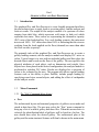
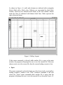
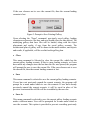
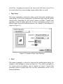
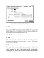
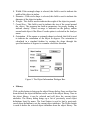
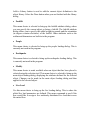
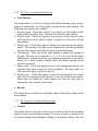
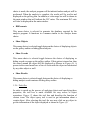
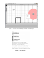
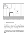
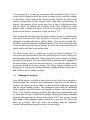
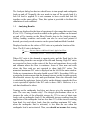
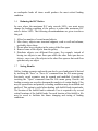
Reference Manual for the
Prepared For:
J. Paul Getty Museum
Prepared by:
Al Zeiny, Ph.D., P.E.
April 1999
Table of Content
Part 1:
1.1
1.2
1.3
1.4
1.5
1.6
1.7
Graphical Pre- and Post-Processor
Introduction
Menu Commands
Applying a Loading Scenario
Running the Analysis
Analyzing Results
Reducing the D/C ratio
Saving the Load Scenario
Part 2:
2.1
2.2
2.3
2.4
2.5
The Analysis Module
Introduction
Generating the Data Base of a Gallery:
Preparation of the Geometry of the Gallery:
Preparation of the Material Properties of the Gallery:
Preparation of the Capacity of Structural Elements in the
Gallery
Preparation of the Architectural Appearance of the Gallery and
D/C Colors Resolution
Evaluation of Analysis Results for Technical Users
2.6
2.7
Part 1
GRAPHICAL PRE- AND POST-PROCESSOR
1.1
Introduction
The graphical Pre- and Post-Processor is a user-friendly program that allows
the non technical user to apply loads to a certain gallery, run the analysis and
looks at results. The output of the analysis module is a spectrum of colors
ranging from dark blue, which represents cold status, to dark red, which
represents hot status. These colors are representing the demand to capacity
(D/C) ratio of the loaded gallery. For a safe loading scenario, this ratio must
not exceed 100%. D/C ratios more than 100% is indicating that the stresses
resulting from the loads applied on the floor (demand) are more than what
the floor can take (capacity).
The primarily tasks of the graphical Pre- and Post-Processor are to create a
gallery loading scenario, run the analysis module and display D/C ratios as
colors. Typical usage is to start with an unloaded gallery and then place the
desired objects and crowds on the floor of the gallery. The user specifies the
physical attributes of each object, such as dimensions and weight. Once
objects have been placed in the desired configuration, the analysis module is
performed to calculate D/C ratios. Results are displayed as a spectrum of
colors to be evaluated by the user. The program also allows special loading
features such as the ability to place forklifts, include people loading by
specifying crowd sizes around objects, and adding the effect of earthquakes
on the analysis results.
1.2
Menu Commands
1.2.1 The "File" Command Menu Group
• New
The architectural layout and structural properties of galleries were made and
stored in data base files. The user may select the "New" menu command to
bring up a list of available gallery data base files. When this menu choice is
selected, the identification labels of galleries will be listed in a list box. The
user should then select the desired gallery. The architectural plan of the
gallery and the main structural features will then be drawn in the main menu.
As shown in Figure (1), walls and columns are indicated with rectangular
blocks filled with a black color. Galleries are surrounded by thick black
outlines. Doorways are indicated with breaks in the wall outlines. Beams
under the floor are indicated with thinner black lines. Slabs represent the
spaces between beams.
Figure 1: Gallery Layout
If this menu command is selected while another file is open in the main
window, the program will prompt the user to save the current file. If the user
chooses not to save the current file, then the current loading scenario is lost.
• Open
This menu command is selected to bring up a list of previously saved gallery
loading scenarios. Similar to the "New" windows command, if the user
selects the "Open" menu command while another file is open, then the
program will prompt the user to save the current file, as shown in Figure (2).
If the user chooses not to save the current file, then the current loading
scenario is lost.
Figure 2: Prompt to Save Existing Gallery
Upon selecting the "Open" command, previously saved gallery loading
scenarios are shown in a list box, and user should select the one desired. The
underlying gallery data base files will be loaded, along with the object
placements and results, if any, from the saved gallery scenario. The
architectural plan of gallery will be drawn in the main window, and objects
and results, if applicable, will be overlaid on the gallery plan.
• Close
This menu command is Selected to close the current file, which has the
current gallery loading scenario. If this is a new loading scenario, or if user
have made any changes since the last time the file was opened, the program
will prompt the user to save the current file. If the user chooses not to save
the current file, then the current loading scenario is lost.
• Save
This menu command is selected to save the current gallery loading scenario.
If user have not previously named the current scenario, the program will
prompt for a name under which to save the scenario. If user have already
previously named the current scenario, it will be saved in place of the
previous version and the old file will be overridden by the new one.
• Save As
This menu command is selected to save the current gallery loading scenario
under a different name. User will be prompted for a name under which to
save the scenario. This option is provided to prevent overriding previously
saved files. Assigning new name to the current file will cause a new file to
be created where the current loading scenario and results are saved.
• Page Setup
This menu command is selected to bring up the Macintosh standard page
setup dialog. User will be prompted to set different page setup and printer
characteristics depending on the current printers available. Consult with
operating system or printer help files for more information on how to set
different page options for different printers. An example of this dialogue is
shown in Figure (3).
Figure 3: Example of Page Setup Dialogue
• Print
This menu command is selected to bring up the standard print dialog. An
example of this dialogue is shown in Figure (4). User will be prompted to
set various print job attributes such as number of copies. Consult with
operating system or printer help files for more information on how to set
print job attributes.
Figure 4: Example of Typical Print Dialogue
• Quit
This menu command is selected to quit the program. If user have not
previously saved the current gallery loading scenario, the program will
prompt the user to save the current file. If the user chooses not to save the
current file, then the current loading scenario is lost.
1.2.2 The "Edit" Command Menu Group
• Undo
This menu command is selected to undo the last editing operation
performed. Depending on the context in which it is selected, the last action
will be reversed, if possible.
• Cut
This menu choice is made available when an object is selected. This
command is selected to move an object from the main menu to the current
system clipboard. The object is then deleted from the current loading
scenario. User may select to paste the object to a new location or new file
using the "Paste" menu command.
• Copy
This menu choice is made available when an object is selected. This
command is selected to copy the object from the main menu to the system
clipboard, without deleting it from the current loading scenario. User may
select to paste the object to a new location or new file using the "Paste"
menu command. This command is mainly provided to allow user to
duplicate objects.
• Paste
This menu choice is made available when there is an object in the system
clipboard. It copies the object to the current loading scenario, in the current
main window without deleting it from the system clipboard. All object
attributes are maintained through the cut/copy and paste operations.
1.2.3 The "Loading" Command Menu Group
• Object
This menu choice is selected to bring up the main object loading dialog
window in order to specify the current object attributes. Specification of
object attributes is required when objects are placed on the architectural plan
of gallery. As shown in Figure (5). The object loading dialog window has
several fields that denote attributes of the object. The standard OK and
Cancel buttons work as expected. The following describes the other input
fields on the dialog:
1. Shape: Indicate the object shape by picking from the popup list of
available object shapes. Available shapes are a square, a rectangle, or a
circle. The shape selected will dictate other choices in this dialog.
2. Name: Indicate the name of the object in this field. Each object can be
named and will be displayed along with its name when placed on the
gallery outline. It is recommended that each object be named prior to its
being placed, although the name, along with most of the other attributes,
can be changed once an object has been placed.
3. Length: If the square or rectangle shape is selected, this field is used to
indicate the length of the object in inches. If the square shape is selected,
this is the length of all four sides of the square.
4. Width: If the rectangle shape is selected, this field is used to indicate the
width of the object in inches.
5. Diameter - If the circle shape is selected, this field is used to indicate the
diameter of the object in inches.
6. Weight - This field is used to indicate the weight of the object in pounds.
7. Crowd Size - This field is used to indicate the size of the crowd around
the object. The program has built-in parameters for people loading to
indicate density. Crowd coverage is indicated on the gallery outline
around each object if the Show Crowds option is selected in the Analyze
menu.
8. Orientation - If the square or rectangle shape is selected, this field is used
to indicate the orientation of the object in degrees. The orientation is
calculated in a standard fashion by rotating the shape through the
specified number of degrees in a counter-clockwise direction.
Figure 5: The Object Information Dialogue Box
• Library
Click on this button to bring up the object library dialog. Once an object has
been defined, the object definition can be saved to the object library. Once in
the object library, it can be selected and will drive the current object
attributes. The library dialog brings up a list of previously saved object
definitions listed by name. The Load button is used to load a previously
saved object definition to set the current object attributes. The Delete button
is used to delete the selected object definition from the object library. The
Add to Library button is used to add the current object definition to the
object library. Select the Done button when you are finished with the library
dialog.
• Forklift
This menu choice is selected to bring up the forklift attribute dialog, where
you can specify the current object as being a forklift. The forklift attribute
dialog allows you to specify the added weight in pounds and the orientation
(in degrees counter-clockwise) of the forklift. Other attributes such as the
outline and dimensions are built-in to the program.
• People
This menu choice is selected to bring up the people loading dialog. This is
currently not used in the program.
• Earthquake
This menu choice is selected to bring up the earthquake loading dialog. This
is currently not used in the program.
• Modify
This menu choice is made available when an object that has been placed is
selected using the selection tool. This menu choice is selected to bring up the
main object loading dialog, displaying the attributes defined for the selected
object. Changes can be made in the main object loading dialog and then
applied to the selected object.
• Live Load
Use this menu choice to bring up the live loading dialog. This is where the
global live load parameters are defined. This menu command is used if the
user would like to assign a live uniformly distributed live load that covers
the entire floor.
1.2.4 The "View" Command Menu Group
• View Options
This menu choice is selected to bring up the dialog allowing you to specify
options to control the view of the gallery scenario in the main window. The
following view options are available:
1. Display beams - Check this option if you want to see the outlines of the
beams under the gallery floor. Uncheck it to hide the beam outlines.
2. Display walls - Check this option if you want to see the outlines of the
walls and doors on the gallery outline. Uncheck it to hide the wall and
door outlines.
3. Display grid - Check this option to display the ruled grid on the gallery
outline. The spacing of the grid can be controlled, as can the mechanism
whereby the program snaps placed objects to grid coordinates.
4. Grid spacing - Select one of the radio buttons to control the spacing of
the grid. The grid can be spaced at 1, 2, 4, or 6 feet by selected those
radio buttons, or alternatively the user defined spacing can be selected, in
which case a field is made available where the desired spacing in feet
should be specified.
5. Snap to grid - Check this option to turn on the mechanism whereby the
program snaps placed objects to grid coordinates. The snap used is in
effect when an object is placed or moved.
6. Display ruler - Check this option to turn on the horizontal and vertical
rulers that are displayed along the side or the top of the main window.
When rules are turned on, small markers are used on each ruler to
indicate the exact position of the cursor.
• Refresh
This menu choice is selected to refresh the image of the gallery outline in the
main window.
1.2.5 The "Analysis" Command Menu Group
• Analyze
This menu choice is selected to when you are ready to run the floor loading
analysis on the current loading scenario. You have a choice or turning on or
off people loading and earthquake loading in the analysis dialog. Once the
choice is made, the analysis program will be initiated and an analysis will be
performed. When the analysis is complete, the results will be read in and
displayed on the gallery plan. In addition, a color range bar will be drawn in
the main window that will indicate the D/C ratios. The maximum D/C ratio
will also be displayed in the main window.
• DBGenerate
This menu choice is selected to generate the database required by the
analysis program. It functions in a manner similar to the Analyze menu
choice.
• Show Objects
This menu choice is selected toggle between the choice of displaying objects
on the gallery outline or hiding placed objects.
• Show Crowds
This menu choice is selected toggle between the choice of displaying or
hiding crowd coverage on the gallery outline. If this option is turned on, then
the crowd around the object will be displayed as Shown in Figure (6). A
person in the crowd must have a line of vision with the object not obstructed
by any other object or wall.
• Show Results
This menu choice is selected toggle between the choice of displaying or
hiding analysis result contours on the gallery outline.
1.2.6 Tools Box
In order to speed up the process of applying objects and specifying there
properties, the tool box is made available for easy access to object
operations. Figure (7) shows the tool box and describes the function of
various icons. The object query tool is used to get information about a
certain object. After selecting this tool, the user may click on any object to
get the information of the object displayed as shown in Figure (8).
Figure 6: Example of Crowd Display around a Circular Object
Figure 7: The Tools Box
Figure 8: The Dialogue Box Resulting from the Object Information Tool
1.3
Applying a Loading Scenario:
After a gallery data base files have been loaded, user may apply three kinds
of objects; circle, square and rectangle. The user may use the command
menu "Object" under "Loading" menu group to place the current object and
assign its attributes. The object may also be placed on the gallery plan using
the object placement tool. User can also use the Shape tools (Circle Object
Specifier, Square Object Specifier, and Circle Object Specifier) to go
directly to the Loading Object dialog for that particular shape.
A grid may be displayed on the screen to facilitate the accurate placement of
the object. The grid snap capability may be used through the view options in
order to turn on and off the snap capability, as well as change the spacing of
the grid.
User can specify a crowd size associated with a particular object. Once a
crowd size has been specified, the crowd coverage can be viewed by turning
on the Show Crowds item in the Analysis menu. Crowds are placed with
careful consideration to other objects, walls, sight lines, and proximity to
objects. Any member of the crowd must have a line of sight between him
and the object. In addition, the locations of the floor occupied by other
people, walls, columns and objects can not be occupied by the crowd. Each
person of the crowd is assumed to occupy an area of 2 ft2.
Once a shape has been placed on the gallery outline, it may be selected using
the Object Selection tool. Once an object is selected, its attributes can be
changed by invoking the Object Modify dialog. User can also cut and copy
the object using the standard clipboard functions. The Object Selection tool
is also useful for moving objects around. It can be used to grab and drag the
object with its title box on the gallery plan.
The Object Query tool is a quick way to query an object's attributes. Use
may select this tool and then click on a placed object to view a dialog box
describing the object properties. Objects properties can be changes including
the name of the object. User can rename objects and place their attributes in
an object library so they can be retrieved later. User can also delete entries
previously placed in the object library. The library button available on the
dialog box of each objects invokes the library editing functions, which are to
add, to delete and to modify an object.
1.4
Running the Analysis:
Once all the objects, crowd have been placed on the floor plan to simulate a
certain exhibit, the "Analysis" menu command is chosen to run the analysis
module. The user is given the choice to turn on/off the earthquake analysis
and the people loading options. The earthquake option adds the additional
loads resulting from the seismic acceleration of objects and crowd on the
floor. A site specific response spectrum that takes into considerations near
by faults and soil type is used for this purpose. Ruining the analysis module
when the floor plan has no objects will produce a D/C ratio of zero. On the
other hand, if the earthquake option is turned on, non zero D/C ratios will
show up in results. These D/C ratios are resulting from the additional
seismic load applied on the gallery due to it own weight.
The Analysis dialog box has two check boxes to turn people and earthquake
loads on and off. Normally, the user needs to turn off the people load if a
fork lift load is applied. It is not common to have crowd and fork lift
together on the same gallery. Thus, this option is provided to facilitate the
simulation of such condition.
1.4
Analyzing Results:
Results are displayed in the form of spectrum of color range that varies from
0% to 115%. Viewing of results overlaid on the gallery outline can be turned
on and off by turning on the Show Results item in the Analysis menu.
Gallery loading scenarios and results can also be saved and printed if
desired; previously saved scenarios can be opened and modified if needed.
Displayed results are the values of D/C ratios at a particular location of the
floor. The D/C ratio is defined as
Stresses Due to Additional Loads Appled on Floor
D
ratio =
C
Allowable Stresses − Stresses due to Dead Load
Where D/C ratio is the demand to capacity ratio, and the Dead load is the
load resulting from the own weight of the slab and flooring. High D/C ratios
are expected to show on the center of the floor and sometimes above walls
and columns where the floor is continuos. Areas of floor near end walls
where the floor ends are not expected to show high D/C ratios. The
numerical maximum D/C ratio is displayed on the left of the main window.
Under no circumstances this ratio should exceed 100%. Exceeding 100% on
a particular location means that the demand stresses on this location exceeds
the allowable stresses by codes and specifications. Since the allowable load
is calculated by applying a factor of safety on the ultimate strength, the floor
is not expected to rupture if the D/C ratio is above 100%. However, it is a
risk that should not be taken.
Turning on the earthquake load does not always give the maximum D/C
ratio. The user may wonder why?. The design specifications allow us to
increase the value of the allowable stresses by 33% in case of short term
loads, such as earthquake loads. If the additional stresses resulting from the
application of the earthquake load are less than 33% of the stresses resulting
from dead, live and object loads, then the resulting maximum D/C ratio,
when the earthquake load is activated, is less than the one when the
earthquake load is not activated. Thus, user should not assume that turning
on earthquake loads all times would produce the most critical loading
condition.
1.6
Reducing the D/C Ratios:
In cases where the maximum D/C ratio exceeds 100%, user must move
change the loading condition of the gallery to reduce the maximum D/C
ratio to below 100%. The following recommendations are given to achieve
this goal:
1. Allow less number of crowd around objects
2. Move heavy objects near structural supports, such as wall and columns,
preferably above them
3. Do not place heavy displays in the center of the floor span
4. Remove some of the objects from the gallery
5. Distribute objects over different floor spans. For example, instead of
having two objects in one floor span while the other floor span has no
objects., move one of the objects to the other floor span so that each floor
span has only one object
1.7
Saving Results:
Gallery loading scenarios and results can also be saved and printed if desired
by invoking the "Save" or "Save As" command from the File menu group.
Previously saved scenarios can be opened and modified if needed by
invoking the "Open" command from the File menu group. Results and
loading scenarios are saved to document the analysis of certain display. Files
may be opened later and printed, or loading conditions may be modified and
analyzed. This option is useful when dealing with forklift loads in particular.
The location of the forklift load is unknown. User is required to try several
critical locations of the forklift loads. For each location of the forklift, a file
may be saved to facilitate the future changing and testing of loading
conditions.
Part 2
THE ANALYSIS MODULE
2.1
Introduction:
In general, the floor loading package is used to analyze floors subjected to
variable loading conditions, such as galleries and warehouses. It consists of
two programs: the analysis program, and the pre- and post-processor
program. The pre-processor is used to read the pre-prepared data base files
for different portions of the floor and apply various types of loads, such as
forklift, crowd, uniform and concentrated loads, to them. The analysis
program is then invoked to analyze the floor under the applied loads with or
without adding the effects of earthquakes. The analysis output is a list of
demand to capacity ratios at the nodes of a fine grid that covers the floor.
These ratios are then displayed as range of colors by the post processor. The
red color is used to flag any areas of the floor that are over stressed.
The power of the program relies on the ease of use. The user does not have
to worry about the underlain finite element model or the strength of various
floor elements. These tasks are performed by HARZA and the corresponding
inverted stiffness matrix, finite element data and strength of floor elements
are stored in data base files during the data base generation phase of the
program. User's task is limited to invoking the portion of the floor to be
analyzed, loading it using the graphical pre-processor, invoking the analysis
from the menu and evaluation of the resulting spectrum of colors.
The analysis code was developed by HARZA and could be modified to
accommodate any specific requirement for the floor system. The analysis
program is written using standard ANSI C programming language, which
makes it possible to run on any machine that has a standard ANSI C
compiler. The pre- and post-processor program is an Apple Macintosh
specific application, which runs only on 68k Apple Macintosh computers or
better. Since the stored stiffness matrix is already inverted, the analysis
program runs fast. The average run time for an average model is less than
five seconds on a power PC Macintosh computer.
The second part of this manual is intended only for technical users who
would like to look at the finite element modeling and results of the analysis
module for the purpose of extending the power of the program to model
other floors or galleries. Part 1 is enough for the non-technical users who
would like to simply use the program for the already existing galleries.
2.2
Generating the Data Base of a Gallery:
The program DB_GENERATOR generates the database of the gallery. It
reads four files and writes several files, one of them is required to run the
ANALYSIS program, which is going to generate the D/C ratios displayed as
a spectrum of colors by the pre- and post- processor program. This files
name is <Gallery_Name>.dmp. The ANALYSIS program reads the data
base file <Gallery_Name>.dmp along with the <Gallery_Name>.cap which
has the capacity of the structural elements of the gallery. In the preparation
phase, the following files are prepared to run the DB_GENERATOR and
then the ANALYSIS program.
2.3
Preparation of the Geometry of the Gallery:
The file <Gallery_Name>.fe1 is the first input file to the program
DB_GENERATOR, which generates the database of the gallery. The file
contains the following data sections in order:
1.
Control Section: One line of data which provides the following
numbers in order:
Number of Key Points
Number of Segments
Number of Nodes (Estimated)
Number of Elements (Estimated)
Number of Restrained Lines
Number of Edge Loads
Number of Line Springs
2.
Coordinates of Key Points: Provide one line for each key point as
follows:
Node X-Coord
Y-Coord
3.
Segment Information: Provide one line of information for each
segment as follows
Segm N1 N2 N3 N4 NI NJ Cat. Code
4.
where N1,2,3,4 are the IDs of the key points connected to the segment,
NI & NJ are the number of elements that the segment will be divided to,
and the Category code gives the type of segment and its orientation
5.
Nodal Restraint Information: Provide one line of data for each line of
restraints as follows:
KeyP1 KeyP2 Div Z-Displ X-Rot Y-Rot
6.
Edge Load Data: Provide one line of data for each line of edge loads as
follows:
KeyP1 KeyP2 Div
Z-Load
Mx-Load
My-Load
7.
Line Spring Data: Provide one line of data for each line of edge
springs as follows:
KeyP1 KeyP2 Div
Z-Spring
X-Rot Spring
Y-Rot Spring
2.4
Preparation of the Material Properties of the Gallery:
The file <Gallery_Name>.mtr is the second input file to the program
DB_GENERATOR, which generates the database of the gallery. The file
contains number of data lines equal to the number of slabs and beams in the
gallery. Each line has the following sections in the order listed:
1.
Slab or beam type code to determine whether the beam or slab is
prismatic or not
2.
Modulus of Elasticity
3.
Poison's ratio
4.
Width and depth of the structural element
5.
Cross section area, and reduced area in the x- & y-planes
6.
Ix, Iy and Ixy for the element at each non-prismatic zone
7.
Modulus of rigidity
8.
Ratios to determine the zones of non prismatic structural elements
2.5 Preparation of the Capacity of Structural Elements in the
Gallery:
The file <Gallery_Name>.cap is the third input file to the program
DB_GENERATOR, which generates the database of the gallery. The file
contains number of data lines equal to the number of slabs and beams in the
gallery. Each line has the moment capacity of the structural elements for
each non prismatic zone. Each slab has nine non prismatic zones, each zone
has four capacities and two for the negative moment, two for the positive
moment in each direction. Each beam has three non prismatic zones, each
zone has two capacities, one for the positive moment, while the other is for
the negative one.
2.6 Preparation of the Architectural Appearance of the Gallery and
D/C Colors Resolution:
The file <Gallery_Name>.pln is the fourth input file to the program
DB_GENERATOR, which generates the database of the gallery. The file
contains the following sections in order:
1.
Orientation of the north direction
2.
Number of gallery outlines
3.
Start and end coordinates of each outline
4.
Number of slabs, beams, bearing walls or columns, non structural wall
and lines
5.
Coordinates of the south west and north east corner of each slab, along
with x- and y-resolution of the colors that show the D/C ratios
6.
Coordinates of the south west and north east corner of each beam,
along with the longitudinal resolution of the colors that show the D/C ratios
7.
Coordinates of the south west and north east corner of each bearing
wall or column
8.
Coordinates of the south west and north east corner of each non
structural wall
9.
Coordinates of the start and end points of each line
2.7
Evaluation of Analysis Results for Technical Users:
After applying loads on the gallery floor, the ANALYSIS program is
invoked from the menu of the pre- and post-processor graphical program.
The output of the analysis will be a spectrum of colors. A non technical user
should make sure that the color that represents a D/C ration of more than
100% is not present anywhere in the gallery. If this color shows up, then the
user must remove some of the loads, restrict the number of audience, or
move the heavy loads away from the middle of the gallery towards the
supports.
A technical user may have a deeper look into the results of the ANALYSIS
program by printing and reading the contents of the file
<Gallery_Name>.out. This file shows a detailed output of the response of
the structure following:
1.
Number of nodes and elements, as well as resolution of load
discretization
2.
Nodal coordinates
3.
Element connectivity and structural element assignment
4.
Nodal restraint codes
5.
Echo of the file "loadobj" produced by the pre processor that has a list
of loading objects type and coordinates
6.
7.
8.
9.
Nodal loads resulting from object loads
Additional seismic loads, floor period and spectral acceleration if the
earthquake flag is on
Nodal deflections and rotations
Internal stresses developed in element due to the applied loading
objects and boundary conditions
The analysis program also produce a file caled <Gallery_Name> that has the
nodal coordinates, element connectivity, boundary conditions and structural
element assignments in SAP90 format. The technical user may then use run
the SAP90 program followed by the SAPLOT program to plot the finite
element mesh and boundary conditions, as shown in Figure (9).
Figure 9: The Finite Element Discretization of Gallery G209