Download MPL - Supplementary User Manual

MPL - Supplementary User Manual
Christian Bogner
Version 1.0
1
Contents
1 Getting started
2
2 Computing with cubical coordinates
2.1 Differential 1-forms and iterated integrals . . . . . . . . . . . . . . . . . . . . . .
2.2 Differentiation . . . . . . . . . . . . . . . . . . . . . . . . . . . . . . . . . . . . .
3
3
7
2.3
2.4
The symbol map and the unshuffle map . . . . . . . . . . . . . . . . . . . . . . .
Integration over cubical coordinates . . . . . . . . . . . . . . . . . . . . . . . . .
3 Computing Feynman integrals
8
12
16
3.1
3.2
3.3
Setting up a simple example . . . . . . . . . . . . . . . . . . . . . . . . . . . . .
Checking the conditions . . . . . . . . . . . . . . . . . . . . . . . . . . . . . . .
Integration over Feynman parameters . . . . . . . . . . . . . . . . . . . . . . . .
17
18
22
3.4
Expressing hyperlogarithms in bar-notation . . . . . . . . . . . . . . . . . . . . .
23
4 Automated tests and troubleshooting checklist
24
1 Getting started
MPL is a collection of procedures for the computeralgebra system Maple. It was written and tested
with Maple 16. It supports a wide range of computations with homotopy invariant iterated integrals
on moduli spaces M0,n of curves of genus 0 with n ordered marked points. This class of functions
contains the widely used multiple polylogarithms as functions of several variables.
This manual shows how to apply the most important procedures of the program and might be
useful for looking up technical details or examples. It is just meant to supplement the detailed
introduction given in the article [2]. The main algorithms were presented in [4]. They are based
on the mathematical framework elaborated in [6].1 When using MPL for a scientific publication,
please cite (some of) these articles.
The latest version of MPL and this manual are available from the webpage
http://cbogner.com/software/mpl/
The entire program is obtained by downloading a txt-file MPLn_m.txt, where the integers n and m
indicate the number of the version. For example, the file of MPL version 1.0 is called MPL1_0.txt
and after saving the file in the same directory with your Maple worksheet, the program is started
with
1 A very useful introduction to
the general concept of iterated integrals and generalizations of polylogarithms can be
found in [7]. For an overview of the far-reaching applications of such classes of iterated integrals in particle physics,
we recommend [13, 14].
2
>read("MPL1_0.txt"):
Before starting with any computations, it is useful to let Maple read a file by which all multiple zeta
values up to a certain weight are automatically expressed in terms of a basis. While writing MPL,
we have been using the file mzv-1-12.txt provided by Bigotte, Jacob, Oussous, Minh and Petitot
for this purpose. The file is available from the webpage
http://www.lifl.fr/~petitot/recherche/MZV/mzv12/
After saving the file in the working directory and calling
>read("mzv-1-12.txt"):
every multiple zeta value up to weight 12 appearing from now on will be expressed in terms of a
basis, for example:
>zeta(3,2);
− 11
2 ζ(5) + 3ζ(2)ζ(3)
This will drastically simplify expressions and it is also necessary for automated tests discussed in
section 4 to check that certain parts of the program produce the expected results.
As a supplement to this manual, the above webpage also provides a maple worksheet which
contains all examples shown below.
2 Computing with cubical coordinates
2.1 Differential 1-forms and iterated integrals
In this section, we work with homotopy invariant iterated integrals on M0,n with n > 3. Here homotopy invariance implies, that these functions only depend on the end-points of some path. We
always consider the origin as one of these end-points. The other point has m = n − 3 coordinates,
which the iterated integral depends on as a function. Due to additional conditions with respect to a
basepoint, it is completely determined by the differential 1-forms and the order in which one integrates over them. Therefore it is customary to express such an iterated integral by a tensor product
of the involved 1-forms ak ⊗ ak−1 ⊗ ... ⊗ a1 which is often replaced by a notation with squared
brackets [ak |ak−1 |...|a1] called bar-notation.
bar(...)
The bar-notation is adapted in MPL. We use the reserved word bar to express every iterated integral. For example [a3 |a2 |a1 ] is expressed by
3
>bar(a[3],a[2],a[1]);
and stands for an iterated integral where we integrate over some 1-forms a1 , a2 , a3 in this ordering (i.e. from right to left in the argument of bar). More generally, iterated integrals are linear
combinations of such expressions over Q, for example
>3*bar(a[2],a[1])+5*bar(b[8])+9;
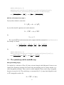
Numerical constants are factored out automatically, for example:
>bar(3*a,2*b)-bar(a-2*b,c);
6bar(a, b) − bar(a, c) + 2bar(b, c)
>bar(0,c);
0
BarToLists(expr), ListsToBar(list)
For some computations, the user may find it convenient to bring an expression of bar-terms in
the form of a list. This form is also used internally in some algorithms. For expr being a linear
combination of words in the bar-notation, the auxiliary procedure BarToLists(expr) returns a list
of two minor lists. The first of these lists contains the coefficients of the words and the second list
contains the words in the argument of bar(...), as lists. For example
>f:=bar(a)+bar(b,c)+99*bar(b,c)-y*bar(5*g,c,b):
>BarToLists(f);
[[1, 100, −5y], [[a], [b, c], [g, c, b]]]
The command ListsToBar(list) reverses this transformation. It takes such a list of coefficients
and words as input and returns the corresponding expression in bar-notation. For example, as
continuation of the above:
>ListsToBar(%);
bar(a) + 100bar(b, c) − 5ybar(g, c, b)
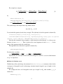
MPLShuffleProduct(expr1, expr2)
The multiplication of two iterated integrals expr1 and expr2 is computed by the well-known
shuffle-product, implemented in MPLShuffleProduct. For example:
>MPLShuffleProduct(bar(a,b)+3*bar(c)+7, bar(y,z));
3 bar(c, y, z)+3 bar(y, c, z)+3 bar(y, z, c)+bar(a, b, y, z)+bar(a, y, b, z)+bar(a, y, z, b)+
bar(y, a, b, z) + bar(y, a, z, b) + bar(y, z, a, b) + 7 bar(y, z)
4
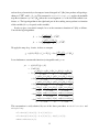
MPLCoproduct(expr)
The deconcatenation co-product ∆, defined by
∆ [ak |ak−1 |...|a1] = 1 ⊗ [ak |ak−1 |...|a1] + [ak ] ⊗ [ak−1 |...|a1] + ... + [ak |ak−1 |...|a1] ⊗ 1
is implemented in the procedure MPLCoproduct(expr), for example:
>MPLCoproduct(bar(a,b,c))
tens(ONE, bar(a, b, c))+tens(bar(a), bar(b, c))+tens(bar(a, b), bar(c))+tens(bar(a, b, c), ONE)
Here the reserved term ONE stands for the empty word and tens(...,...) is a formal expression
for the tensor-product of two iterated integrals. tens and ONE are mostly defined for internal use
and will usually not appear in any results below.
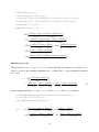
MPLCoordinates(letter, n), MPL_COORDINATES
As a preparation for many applications, it is necessary to declare a set of variables to be the cubical
coordinates we want to work with. For a positive integer n, the procedure MPLCoordinates(letter,
n) declares n cubical coordinates by use of the first argument letter for the names of the variables. The list of cubical coordinates defined in this way is stored in the global variable MPL_COORDINATES
until the procedure is called again. For example:
>MPLCoordinates(x, 5):
>MPL_COORDINATES;
[x1 , x2 , x3 , x4 , x5 ]
After calling MPLCoordinates, the variables declared in this way are internally recognized to be
cubical coordinates and they can be used to construct the corresponding differential 1-forms. For
example one has relations like d(x1 ) ∧ d(x1 ) = 0 :
>d(x[1]) &^ d(x[1]);
0
MPLFormsFiber(lifted::boolean), MPLFormsBase(), MPLFormsTotal()
After declaring x1 , ..., xm as cubical coordinates, MPL can compute with iterated integrals with
differential 1-forms of the following sets (as defined in [4]):
Ωm =
(
)
d
x
dxm
dx1
∏a≤i≤b i
for 1 ≤ a ≤ b ≤ m ,
, ...,
,
x1
xm ∏a≤i≤b xi − 1
5
Ω̄Fm
ΩFm
)
dxm ∏a≤i≤n−1 xi dxm
,
for 1 ≤ a ≤ m ,
=
xm
∏a≤i≤m xi − 1
(
)
dxm d ∏a≤i≤m xi
=
,
for 1 ≤ a ≤ m
xm ∏a≤i≤m xi − 1
(
(1)
where clearly Ωm = ΩFm ∪ Ωm−1 . In the context discussed in [4, 6] and with respect to a given n, it
makes sense to speak of these forms as:
• Ωm : forms on the total space,
• Ω̄Fm : forms on the fiber,
• ΩFm : forms on the lifted fiber,
• Ωm−1 : forms on the base.
Up to signs, these sets can be obtained from the auxiliary procedures MPLFormsTotal(),
MPLFormsFiber(false), MPLFormsFiber(true), MPLFormsBase() respectively. For example:
>MPLCoordinates(x, 3):
>MPLFormsTotal();
i
h
d(x1 ) d(x1 ) d(x2 ) x2 d(x1 )+x1 d(x2 ) d(x2 ) d(x3 ) x2 x3 d(x1 )+x1 x3 d(x2 )+x1 x2 d(x3 ) x3 d(x2 )+x2 d(x3 ) d(x3 )
,
,
,
,
,
,
,
,
x1
1−x1
x2
1−x1 x2
1−x2
x3
1−x1 x2 x3
1−x2 x3
1−x3
>MPLFormsFiber(false);
i
h
d(x3 ) x1 x2 d(x3 ) x2 d(x3 ) d(x3 )
,
,
,
x3
1−x1 x2 x3 1−x2 x3 1−x3
>MPLFormsFiber(true);
h
d(x3 ) x2 x3 d(x1 )+x1 x3 d(x2 )+x1 x2 d(x3 ) x3 d(x2 )+x2 d(x3 ) d(x3 )
,
, 1−x3
x3 ,
1−x1 x2 x3
1−x2 x3
>MPLFormsBase();
i
h
d(x1 ) d(x1 ) d(x2 ) x2 d(x1 )+x1 d(x2 ) d(x2 )
,
,
,
,
x1
1−x1
x2
1−x1 x2
1−x2
i
In the following we will denote the Q-vectorspaces of differential 1-forms, spanned by the bases
Ωm , Ω̄Fm , ΩFm by Am , ĀmF , AmF respectively. Furthermore, the corresponding Q-vectorspaces of ho
motopy invariant iterated integrals are denoted by V (Ωm ) ,V Ω̄Fm , V ΩFm (see [4, 2]).
MPLArnoldEquation(form1,form2)
The above differential 1-forms satisfy the following set of relations due to Arnol’d [1] (also see
[4]):
m−1
dxk d (xi ...xm )
dxm d (xi ...xm )
∧
= −∑
∧
,
xm xi ...xm − 1
xi ...xm − 1
k=i xk
! j−1
d x j ...xm
d
x
...x
d
x
...x
dxk d (xi ...xm )
d (xi ...xm )
d (xi ...xm )
i
j−1
j
m
−∑
∧
=
∧
−
∧
x j ...xm − 1 xi ...xm − 1
xi ...x j−1 − 1
xi ...xm − 1 x j ...xm − 1
xi ...xm − 1
k=i xk
6
for 1 ≤ i ≤ j ≤ m. Note that these equations are of the type
ωi ∧ ω j = ∑ αk ∧ ωk
k
where the 1-forms ωi are in ΩFm (the lifted fiber) and the 1-forms αi are in Ωm−1 (the base).
Internally, these relations are extensively used in the computations below. More conveniently,
for two given forms form1, form2 on the left-hand side of the above equations (in the sense
form1∧form2) the right-hand side of the Arnol’d equation can be obtained from
MPLArnoldEquation(form1,form2). For example for n = 3, the right-hand side of the equation
dx2 d (x2 x3 )
d (x2 x3 )
dx2
dx3
d (x2 x3 )
dx3
−
∧
=
∧
−
∧
x3 − 1 x2 x3 − 1 x2 − 1
x2 x3 − 1 x3 − 1
x2 x2 x3 − 1
is computed as2 :
>MPLCoordinates(x, 3):
>MPLArnoldEquation(d(x[3])/(x[3]-1), d(x[2]*x[3])/(x[2]*x[3]-1));
−
(d(x2 ))&∧ (d(x3 ))
(1−x2 )(1−x3 )
+
x2 (d(x2 ))&∧ (d(x3 ))
(1−x2 )(1−x2 x3 )
+
(d(x2 ))&∧ (d(x3 ))
(1−x2 x3 )
2.2 Differentiation
MPLd(expr)
Differentiation d with respect to the end-point of the path (w.r.t. which the iterated integral is
defined) is simply given by the de-concatenation of the leftmost differential 1-form:
d : V (Ωm ) → Am ⊗V (Ωm ) ,
∑
∑
cI [ωi1 |...|ωik ] 7→
J=(i1 , ..., ik )
cI ωi1 ⊗ [ωi2 |...|ωik ] .
J=(i1 , ..., ik )
For example, one computes
d
d (x2 x3 )
dx2
dx2 d (x2 x3 )
d (x2 x3 ) dx3
dx3
d (x2 x3 )
−
=
−
|
|
⊗
⊗
1 − x2 x3 x3
x2 1 − x2 x3
1 − x2 x3
x3
x2
1 − x2 x3
by
2 In principle, using the auxiliary procedure GetArnoldRHS(...), these equations can also be obtained in a different
output format, where forms of the fiber and the base are explicitely separated. Such a format is used internally.
7
>MPLCoordinates(x, 3):
>MPLd(bar((x[3]*d(x[2])+x[2]*d(x[3]))/(1-x[2]*x[3]),d(x[3])/x[3])
-bar(d(x[2])/x[2],(x[3]*d(x[2])+x[2]*d(x[3]))/(1-x[2]*x[3])));
x3 d(x2 )+x2 d(x3 )
x3 d(x2 )+x2 d(x3 )
dx3
dx2
− tens x2 , bar
, bar x3
tens
1−x2 x3
1−x2 x3
MPLTotalConnection(expr)
In [4] we have defined a connection
∇ : V Ω̄Fm → Am−1 ⊗V Ω̄Fm
by use of the Arnol’d equations and a total connection
∇T : V Ω̄Fm → Am ⊗V Ω̄Fm
by
∇T = d − ∇.
For a word in Ω̄Fm , the total connection can be computed with the command MPLTotalConnection.
For example, we obtain
∇T
d (x2 x3 )
dx2
dx3
x2 d (x3 )
x2 d (x3 ) dx3
=
−
|
⊗
⊗
1 − x2 x3 x3
1 − x2 x3
x3
x2
1 − x2 x3
by
>MPLCoordinates(x, 3):
>MPLTotalConnection(bar((x[2]*d(x[3])/(1-x[2]*x[3]),d(x[3])/x[3]));
x2 d(x3 )
x d(x2 )+x2 d(x3 )
dx2
dx3
−
tens
,
bar
,
bar
tens 3 1−x
x3
x2
1−x2 x3
2 x3
2.3 The symbol map and the unshuffle map
MPLSymbolMap(expr)
It is implied by a theorem of Chen [11] that an iterated integral with differential 1-forms in our
framework is homotopy invariant if and only if the corresponding word of 1-forms satisfies a socalled integrability condition. These words are called integrable. Every word in ĀmF is integrable,
but not every word in Am . The symbol map, as constructed in [3, 4], maps from integrable words
in ĀmF to integrable words in Am :
Ψ : V Ω̄Fm → V (Ωm ) .
8
For example we compute
Ψ
x2 d (x3 ) dx3
|
1 − x2 x3 x3
d (x2 x3 ) dx3
d (x2 ) d (x2 x3 )
=
|
−
|
1 − x2 x3 x3
x2 1 − x2 x3
(2)
by
>MPLCoordinates(x, 3):
>MPLSymbolMap(bar((x[2]*d(x[3]))/(1-x[2]*x[3]),d(x[3])/x[3]));
d(x2 ) x3 d(x2 )+x2 d(x3 )
x d(x2 )+x2 d(x3 ) dx3
−
bar
,
,
bar 3 1−x
x3
x2
1−x2 x3
2 x3
The symbol map is the unique linear map which satisfies
(id ⊗ Ψ) ◦ ∇T = d ◦ Ψ.
Let us check this equation for the above example. The left-hand side of the equation is obtained by
>f:=bar(x[2]*d(x[3])/(1-x[2]*x[3]), d(x[3])/x[3]):
>evalindets(MPLTotalConnection(f), ’specfunc(anything, tens)’, proc (h) options
operator, arrow; subsop(2 = MPLSymbolMap(op(2,h)),h) end proc);
Note that this command at first computes a total connection of the function f as a linear combination of terms tens(...). Then it replaces the second argument of each tens(...) by the
image of this argument under the symbol map.
The right-hand side of the above equation is obtained by
>MPLd(MPLSymbolMap(f));
For bothsides we obtain x3 d(x2 )+x2 d(x3 )
dx3
dx2
2 )+x2 d(x3 )
tens x3 d(x1−x
−
tens
,
bar
,
bar
x3
x2
1−x2 x3
2 x3
Note that this was already the result of the first example in section 2.2, as we used the function
in eq. 2 as input there.
MPLBasis(letter,m,w)
With the help of the symbol map, the command MPLBasis(letter,m,w) constructs a basis for the
vectorspace of integrable words (or homotopy invariant iterated integrals ) up to length w in the
alphabet Ωm .
For example the basis of all integrable words up to length 2 in Ω2 with variables y1 , y2 is
obtained by
>MPLBasis(y,2,2);
9
d (y2 )
y2 d (y1 ) + y1 d (y2 )
d (y1 )
d (y1 )
d (y2 )
, bar
, bar
, bar
, bar
,
bar
y2
1 − y2
1 − y1 y2
y1
1 − y1
d (y2 ) d (y2 )
d (y2 ) d (y2 )
d (y2 ) d (y2 )
bar
,
, bar
,
, bar
,
,
y2
y2
y2 1 − y2
1 − y2 y2
d (y1 ) y2 d (y1 ) + y1 d (y2 )
d (y2 ) y2 d (y1 ) + y1 d (y2 )
,
+ bar
,
,
bar
y2
1 − y1 y2
y1
1 − y1 y2
y2 d (y1 ) + y1 d (y2 ) d (y2 )
d (y1 ) y2 d (y1 ) + y1 d (y2 )
d (y2 ) d (y2 )
bar
− bar
, bar
,
,
,
,
1 − y1 y2
y2
y1
1 − y1 y2
1 − y2 1 − y2
d (y2 ) y2 d (y1 ) + y1 d (y2 )
d (y1 ) y2 d (y1 ) + y1 d (y2 )
d (y1 ) d (y2 )
bar
− bar
+ bar
,
,
,
1 − y2
1 − y1 y2
1 − y1
1 − y1 y2
1 − y1 1 − y2
y2 d (y1 ) + y1 d (y2 ) d (y2 )
d (y1 ) y2 d (y1 ) + y1 d (y2 )
, bar
,
,
−bar
y1
1 − y1 y2
1 − y1 y2
1 − y2
d (y1 ) y2 d (y1 ) + y1 d (y2 )
d (y1 ) d (y2 )
+bar
,
− bar
,
1 − y1
1 − y1 y2
1 − y1 1 − y2
y2 d (y1 ) + y1 d (y2 ) y2 d (y1 ) + y1 d (y2 )
d (y1 ) y2 d (y1 ) + y1 d (y2 )
,
, bar
,
,
+bar
y1
1 − y1 y2
1 − y1 y2
1 − y1 y2
d (y1 ) d (y2 )
d (y2 ) d (y1 )
d (y1 ) d (y2 )
bar
+ bar
, bar
,
,
,
y1
y2
y2
y1
y1 1 − y2
d (y1 ) y2 d (y1 ) + y1 d (y2 )
y2 d (y1 ) + y1 d (y2 ) d (y1 )
d (y2 ) d (y1 )
, bar
+ bar
,
,
,
,
+bar
1 − y2 y1
y1
1 − y1 y2
1 − y1 y2
y1
d (y1 ) d (y2 )
d (y2 ) d (y1 )
d (y1 ) d (y2 )
d (y2 ) d (y1 )
bar
+ bar
, bar
+ bar
,
,
,
,
,
1 − y1 y2
y2 1 − y1
1 − y1 1 − y2
1 − y2 1 − y1
y2 d (y1 ) + y1 d (y2 ) d (y1 )
d (y1 ) d (y1 )
d (y1 ) y2 d (y1 ) + y1 d (y2 )
,
+ bar
,
, bar
,
,
bar
1 − y1
1 − y1 y2
1 − y1 y2
1 − y1
y1
y1
d (y1 ) d (y1 )
d (y1 ) d (y1 )
d (y1 ) d (y1 )
bar
,
, bar
,
, bar
,
y1 1 − y1
1 − y1 y1
1 − y1 1 − y1
The output of this command is always a list of w lists, where for k ≤ w the k-th list contains the
words of length k.
MPLUnshuffle(expr,var)
The unshuffle map
Φ : V (Ωm ) → V (Ωm−1 ) ⊗V Ω̄Fm
as defined in [4] is the inverse of the map
µ (id ⊗ Ψ) : V (Ωm−1 ) ⊗V Ω̄Fm → V (Ωm )
10
(3)
(4)
and can be used recursively to decompose iterated integrals in V (Ωm ) into products of hyperloga
rithms in V Ω̄Fk with 1 ≤ k ≤ m. The command MPLUnshuffle(expr,var) applies the unshuffle
map Φ to a function expr in V (Ωm ) where the second argument var is the last of the cubical coordinates xm . The hyperlogarithm in the right-hand part of the resulting tensor-product is a function
of this variable (if expr depends on this variable).
In order to give a non-trivial example, let us at first construct a function in V (Ω3 ) as follows.
Consider the hyperlogarithms
f1
f2
x1 d (x2 )
= bar
∈ V Ω̄F2 ,
1 − x1 x2
x2 d (x3 ) d (x3 )
∈ V Ω̄F3 .
,
= bar
1 − x2 x3 x3
We apply the map of eq. 4 twice. At first we compute
d (x1 x2 )
g1 = µ (id ⊗ Ψ) (1 ⊗ f1 ) = Ψ ( f1 ) = bar
1 − x1 x2
∈ V (Ω2 ) .
Let us furthermore construct the function (or integrable word) g12 as
g12 = µ (id ⊗ Ψ) (g1 ⊗ f2 )
= f˜1 x Ψ ( f2 )
x3 d (x2 ) + x2 d (x3 ) d (x3 ) x2 d (x1 ) + x1 d (x2 )
,
,
= bar
1 − x2 x3
x3
1 − x1 x2
x3 d (x2 ) + x2 d (x3 ) x2 d (x1 ) + x1 d (x2 ) d (x3 )
+bar
,
,
1 − x2 x3
1 − x1 x2
x3
x2 d (x1 ) + x1 d (x2 ) x3 d (x2 ) + x2 d (x3 ) d (x3 )
,
,
+bar
1 − x1 x2
1 − x2 x3
x3
d (x2 ) x3 d (x2 ) + x2 d (x3 ) x2 d (x1 ) + x1 d (x2 )
−bar
,
,
x2
1 − x2 x3
1 − x1 x2
d (x2 ) x2 d (x1 ) + x1 d (x2 ) x3 d (x2 ) + x2 d (x3 )
,
,
−bar
x2
1 − x1 x2
1 − x2 x3
x2 d (x1 ) + x1 d (x2 ) d (x2 ) x3 d (x2 ) + x2 d (x3 )
−bar
.
,
,
1 − x1 x2
x2
1 − x2 x3
This construction is easily obtained by use of the above procedures MPLShuffleProduct and
MPLSymbolMap:
>f1:=bar(x[1]*d(x[2])/(1-x[1]*x[2])):
>f2:=bar(x[2]*d(x[3])/(1-x[2]*x[3]), d(x[3])/x[3]):
>MPLCoordinates(x,2):
11
>g1:=MPLSymbolMap(f1):
>MPLCoordinates(x,3):
>g12:=MPLShuffleProduct(g1,MPLSymbolMap(f2)):
By construction, the function g12 is in V (Ω3 ) and it is easy to check, that it is in the basis of this
vectorspace obtained by the command MPLBasis:
>B3:=MPLBasis(x,3,3):
>has(B3[3],g12);
true
Now let us reverse this construction by use of the unshuffle map. By computing
>MPLUnshuffle(g12,x[3]);
x2 d(x3 ) d(x3 )
1 x2 )
,
bar
tens bar d(x
,
1−x1 x2
1−x2 x3
x3
we clearly obtain the expected
Φ (g12 ) = g1 ⊗ f2 .
Furthermore computing
>MPLUnshuffle(g1,x[2]);
1 d(x2 )
tens ONE, bar x1−x
1 x2
we confirm the expected
Φ (g1 ) = 1 ⊗ f1 .
2.4 Integration over cubical coordinates
MPLPrimitive(a, f, w)
The procedure MPLPrimitive(a, f, w) computes the primitive
R
a ⊗ f ∈ V (Ωm ) of a function
f ∈ V (Ωm ) of maximal weight w with respect to the differential 1-form a ∈ ĀmF . For example let
R
us compute a ⊗ f for
x2 d (x3 )
a=
1 − x2 x3
and
x3 d (x2 ) + x2 d (x3 ) dx3
,
f = bar
1 − x2 x3
x3
d (x2 ) x3 d (x2 ) + x2 d (x3 )
d (x2 )
− bar
+ 5bar
+ 99.
,
x2
1 − x2 x3
x2
The words in f are at most of length w = 2. We compute:
12
>MPLCoordinates(x,3):
>a:=x[2]*d(x[3])/(1-x[2]*x[3]):
>f:=bar((x[3]*d(x[2])+x[2]*d(x[3]))/(1-x[2]*x[3]), d(x[3])/x[3])
-bar(d(x[2])/x[2], (x[3]*d(x[2])+x[2]*d(x[3]))/(1-x[2]*x[3]))
+5*bar(d(x[2])/x[2])+99:
>MPLPrimitive(a, f, 2);
x3 d (x2 ) + x2 d (x3 ) x3 d (x2 ) + x2 d (x3 ) dx3
,
,
bar
1 − x2 x3
1 − x2 x3
x3
x3 d (x2 ) + x2 d (x3 ) d (x2 ) x3 d (x2 ) + x2 d (x3 )
,
,
−bar
1 − x2 x3
x2
1 − x2 x3
x3 d (x2 ) + x2 d (x3 ) d (x2 )
x3 d (x2 ) + x2 d (x3 )
+5bar
+ 99bar
,
1 − x2 x3
x2
1 − x2 x3
d (x2 ) x3 d (x2 ) + x2 d (x3 )
+5bar
,
x2
1 − x2 x3
d (x2 ) x3 d (x2 ) + x2 d (x3 ) x3 d (x2 ) + x2 d (x3 )
,
,
−bar
x2
1 − x2 x3
1 − x2 x3
MPLLimit(f,x,u)
The procedure MPLLimit(expr,var,limit) returns the limit of a function f in V (Ωm ) at x=u
where x is one of the m cubical coordinates and u is either 0 or 1. As an example we consider
m = 3 and
x1 x2 d (x3 ) x2 d (x3 )
f = Ψ
,
1 − x1 x2 x3 1 − x2 x3
d (x1 x2 x3 ) d (x1 ) d (x2 x3 )
d (x1 ) d (x1 ) d (x1 x2 x3 )
=
+
(5)
−
,
+
,
1 − x1 x2 x3 1 − x1 1 − x2 x3
1 − x1
x1 1 − x1 x2 x3
and we compute the limits g1 = limx3 →1 f , g2 = limx2 →1 g1 , g3 = limx1 →1 g2 as follows:
>f:=MPLSymbolMap(bar(x[1]*x[2]*d(x[3])/(1-x[1]*x[2]*x[3]),
x[2]*d(x[3])/(1-x[2]*x[3]))):
>g1:=simplify(MPLLimit(f,x[3],1));
d (x1 ) d (x2 )
x2 d (x1 ) + x1 d (x2 ) d (x2 )
− bar
,
,
g1 : = bar
−1 + x1 x2
−1 + x2
−1 + x1 −1 + x2
d (x1 ) x2 d (x1 ) + x1 d (x2 )
d (x1 ) x2 d (x1 ) + x1 d (x2 )
+bar
,
− bar
,
−1 + x1
−1 + x1 x2
x1
−1 + x1 x2
13
>g2:=simplify(MPLLimit(g1,x[2],1));
d (x1 ) d (x1 )
g2 := −bar
,
x1 −1 + x1
d (x1 ) d (x1 )
+ bar
,
−1 + x1 −1 + x1
>g3:=simplify(MPLLimit(g2,x[1],1));
g3 := ζ(2)
There is a little subtlety we have to take care of, if we compute limits not starting with the last
cubical coordinate xm . For example, let us compute g4 = limx2 →1 f by
>g4:=simplify(MPLLimit(f,x[2],1));
d(x1 ) x3 d(x1 )+x1 d(x3 )
d(x1 ) x3 d(x1 )+x1 d(x3 )
1 )+x1 d(x3 ) d(x3 )
−bar
+bar
−
bar x3 d(x
,
,
,
x1
−1+x1 x3
−1+x1
−1+x1 x3
−1+x1 x3 −1+x3
d(x3 )
d(x1 )
,
bar −1+x
1 −1+x3
x d(x )+x d(x )
1
1
3
In this result, the differential 1-form 3 −1+x
does not belong to any Ωm defined in eq. 1,
1 x3
because it involves the product x1 x3 of non-consecutive cobical coordinates. However, we can
simply replace every x3 by x2 in this result, for example by
>g5:=subs(x[3]=x[2],g4):
Now in g5 every 1-form belongs to Ω2 and the result is recognized as a function of V (Ω2 ) . (It is
easy to check the integrability.) In general, after taking a limit with respect to a variable xk with
1 ≤ k < m, we have to re-name the coordinates by (xk+1 , ..., xm ) 7→ (xk , ..., xm−1 ) .
MPLMultipleLimit(expr,list)
Based on the previous procedure, the procedure MPLMultipleLimit(f,L) computes several limits
of a function f of V (Ωm ) successively. Here L is a list of the type xσ(1) = u1 , xσ(2) = u2 , ..., xσ(k) = uk
for 1 ≤ k ≤ m, σ a permutation on some subset of {1, ..., m} and all ui ∈ {0, 1}. This list fixes the
limits and also the order in which they are computed. The above command returns
lim ... lim f .
xσ(k)→uk
xσ(1)→u1
As an example, let us again consider the function f as defined in eq. 5. Then we obtain the above
results for g1 , g2 , g3 by
14
>g1:=simplify(MPLMultipleLimit(f,[x[3]=1])):
>g2:=simplify(MPLMultipleLimit(f,[x[3]=1,x[2]=1])):
>g3:=simplify(MPLMultipleLimit(f,[x[3]=1,x[2]=1,x[1]=1])):
It is briefly mentioned in [2] and discussed in more detail in [4] and [6] that the order of such
consecutive limits is crucial. For example, we have obtained g3 = ζ(2), but permuting the order of
the last two limits, we compute
>MPLMultipleLimit(f,[x[3]=1,x[1]=1,x[2]=1]);
0
Note that in a function of V (Ωm ) the terms with weight greater than zero are defined to vanish
at the origin of the space of cubical coordinates. Therefore, if we choose the above list L to
be xσ(1) = 0, xσ(2) = 0, ..., xσ(m) = 0 , the procedure MPLMultipleLimit returns the value that
remains after by replacing every bar(...) by zero in f ∈ V (Ωm ).
MPLCubicalIntegrate(f,var,n)
MPL can compute multiple integrals of the type
I=
Z 1
0
dxm
q
a f
∏i p i i
(6)
where where f ∈ V (Ωm ) , q is a polynomial in xm , the ai ∈ N and the pi are in {xm , 1 − xm , ..., 1 − x1 · · · xm } .
For f being an integrand of this type, the procedure MPLCubicalIntegrate(f,var,n) successively integrates over xm , xm−1 , ..., xm−n+1 in this order. The first argument of the procedure is the
integrand in bar-notation, the second argument is the variable to be first integrated out (i.e. xm in
the notation chosen here) and n is the number of integrations. As an example, we consider the
integrand
f=
u1 3 (1 − u1 ) u2 4 (1 − u2 ) u3 3 (1 − u3 ) u4 2 (1 − u4 )2
(1 − u1 u2 u3 )2 (1 − u2 u3 u4 )2 (1 − u1 u2 u3 u4 )2 (1 − u1 u2 )
We integrate out all four cubical coordinates u4 , u3 , u2 , u1 by
>f:=u[1]^3*(1-u[1])*u[2]^4*(1-u[2])*u[3]^3*(1-u[3])
*u[4]^2*(1-u[4])^2/((1-u[1]*u[2]*u[3])^2*(1-u[4]*u[2]
*u[3])^2*(1-u[4]*u[1]*u[2]*u[3])^2*(1-u[1]*u[2])):
>MPLCubicalIntegrate(f,u[4],4);
(5/3) ∗ Zeta(3) + (26/9) ∗ Zeta(2) − (17/5) ∗ Zeta(2)2 + 22/9
15
.
So we obtain
4
∏
i=1
Z
1
0
dxi
f=
26
17
22
5
ζ (3) + ζ (2) −
(ζ (2))2 + .
3
9
5
9
Intermediate results are too long to be shown here, but can easily be obtained by choosing the last argument of MPLCubicalIntegrate smaller than 4. Note that here the explicit use of MPLCoordinates
is not necessary (because it is called internally by MPLCubicalIntegrate).
MPLCubicalIntegrate already serves for the analytical computation of a large class of integrals and further example applications are shown in [2, 4]. In some cases, the procedure may even
be useful for the computation of Feynman integrals. However, in the case of Feynman integrals, the
denominators of the integrand usually involve more complicated polynomials than allowed here.
Therefore, appropriate changes of variables are necessary, to express the latter in terms of cubical
coordinates. These are subject of the following section.
3 Computing Feynman integrals
In this section, we consider integrals of the type
IF =
Z ∞
0
dα j
δ
∏Qi ∈Q Qi i Lw α j
βi
∏Pi∈PF Pi
(7)
where Q , P ⊂ Q α1 , ..., α j , ..., αN are sets of irreducible polynomials, all δi , βi ∈ N ∪ {0} and
Lw (αN ) is a hyperlogarithm, given by a word w in differential 1-forms in
ΩF =

 dα
 αj
j
,
dα j
where ρi = −
α j − ρi
Pi |α j =0
∂Pi
∂α j
, Pi ∈ P


.

Such integrals arise in the computation of Feynman integrals, possibly also in other contexts. In
[4, 2] we have discussed the conditions under which we can compute such integrals with MPL.
Here let us just recall briefly, that the integrals have to be finite and unramified and the set P has
to be linearly reducible and properly ordered. We assume, that the user has already expressed a
divergent Feynman integral in terms of finite integrals of this type, possibly by use of techniques
cited and partly demonstrated in [4, 2]. All remaining mentioned conditions can be explicitely
checked by procedures of MPL, as demonstrated below.
16
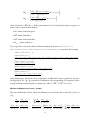
3.1 Setting up a simple example
As a simple standard example, let us consider the massless, off-shell one-loop traingle graph
throughout this section. The corresponding integral is finite. (More involved examples are discussed in [4, 2]). The two Symanzik polynomials (see e.g. [5]) of this graph are
U = x1 + x2 + x3 ,
F = −x1 x2 p23 − x2 x3 p21 − x1 x3 p22 ,
where the xi are the Feynman (or Schwinger, or alpha) parameters and the pi are the incoming
momenta. In section 4 of [2], we suggested to express the kinematical dependences in terms of
variables, which can be treated as additional Feynman parameters, which are not integrated out. In
this sense, we define the set of generalized Feynman parameters {x1 , x2 , x3 , x4 , x5 } where x4 and
x5 satisfy
p23
p21
=
x
x
and
= (1 − x4 )(1 − x5).
4
5
p22
p22
(C.f. [10].) We consider the kinematical region where 0 ≤ x4 , 0 ≤ x5 . (For a different kinematical
region, we recommend to change the definition of x4 and x5 accordingly, such that the region is still
given by 0 ≤ x4 , 0 ≤ x5 , if possible.) Using these variables, we define the auxiliary polynomial
F̃ = −
F
p22
= x1 x2 x4 x5 + x1 x3 + x2 x3 (1 − x4 ) (1 − x5 ) .
The corresponding scalar Feynman integral in D = 4 − 2ε dimensions (without any scalar products
in the numerator or raised propagator-powers) can be defined by
I (x4 , x5 , ε) = Γ (1 + ε) −p22
with
3
I(x4 , x5 , ε) = ∏
i=1
Z
0
∞
−1−ε
I(x4 , x5 , ε)
dxi δ(H)U −1+2ε F̃ −1−ε
where H is a hyperplane in the integration domain, which we can choose freely according to the
Cheng-Wu theorem [12]. We choose δ (1 − xn ) where xn is our last integration variable. The order
of integration variables still has to be chosen such that the mentioned conditions are satisfied.
We expand the integrand in ε and obtain
I(x4 , x5 , ε) = I (0) (x4 , x5 ) + εI (0) (x4 , x5 ) + O ε2
17
with
I
I
(0)
(1)
3
(x4 , x5 ) =
(x4 , x5 ) =
∏
Z
∞
0
i=1
3 Z ∞
∏
i=1
0
dxi δ(H)
dxi δ(H)
1
U F̃
,
(8)
2 ln (U ) − ln F̃
U F̃
.
(9)
In the following, we compute both of the latter integrals with MPL.
3.2 Checking the conditions
Before the computation of any integral over Feynman parameters with MPL, we recommend to
check, whether the mentioned conditions are satisfied. We assume, that the user already has
checked the finiteness of the integral. The following procedure can be used to check linear reducibility.
MPLPolynomialReduction(S,L[1..n],L), COMPATIBILITY_GRAPH
The command MPLPolynomialReduction(S,L[1..n],L) returns the reduction of a set S of polynomials with respect to n integration variables (i.e. Feynman parameters) L[1..n], which are the
first n entries in the list L of all variables of the problem (i.e. generalized Feynman parameters, given
by the Feynman parameters and kinematical invariants). If a global variable COMPATIBILITY_GRAPH=true,
the reduction is computed regarding compatibilities among the polynomials as introduced in [9].
The program uses the version of such compatibilities defined in [14]. If COMPATIBILITY_GRAPH=false,
the procedure returns a Fubini-reduction as introduced in [8]. See [2] for the details.
In order to interpret the output of this procedure, it is instructive to look at our example of the
triangle graph. For the computation of I (0) (x4 , x5 ) and I (1) (x4 , x5 ) we clearly should compute the
reduction of S = U , F̃ . The list of generalized Feynman parameters is x1 , x2 , x3 , x4 , x5 and the
integration variables are the first three elements of this list. Therefore we compute
>U:=x[1]+x[2]+x[3]:
>F:=x[1]*x[2]*x[4]*x[5]+x[1]*x[3]+x[2]*x[3]*(1-x[4])*(1-x[5]):
>GenFeyn:=[x[1],x[2],x[3],x[4],x[5]]:
>COMPATIBILITY_GRAPH=true: #This is also the default value.
>MPLPolynomialReduction([U,F],GenFeyn[1..3],GenFeyn);
[[{} , [x1 + x2 + x3 , x1 x2 x4 x5 + x1 x3 + x2 x3 (1 − x4 ) (1 − x5 )], [{1, 2}]],
[{x3 } , [x1 + x2 − x2 x5 − x4 x2 + x2 x4 x5 , x1 + x2 , x1 + x2 − x2 x5 , x1 + x2 − x4 x2 ],
18
[{3, 4} , {1, 3} , {1, 4} , {2, 3} , {2, 4}]],
[{x2 } , [x1 x4 x5 + x3 − x3 x5 − x3 x4 + x3 x4 x5 , x1 + x3 , −x3 + x1 x5 + x3 x5 , x1 x4 − x3 + x3 x4 ],
[{3, 4} , {1, 3} , {1, 4} , {2, 3} , {2, 4}]],
[{x1 } , [x2 x4 x5 + x3 , x2 + x3 , −1 + x4 , −1 + x5 , x4 x2 + x3 , x3 + x2 x5 ],
[{3, 4} , {1, 3} , {1, 4} , {2, 3} , {2, 4} , {3, 5} , {4, 5} , {5, 6} , {1, 5} , {1, 6} , {2, 5} , {2, 6} , {3, 6}]],
[{x1 , x2 } , [−1 + x5 , −1 + x4 , x4 − x5 ], [{1, 2} , {1, 3} , {2, 3}]],
[{x1 , x3 } , [−1 + x5 , −1 + x4 , x4 − x5 ], [{1, 2} , {1, 3} , {2, 3}]],
[{x2 , x3 } , [−1 + x4 , −1 + x5 , x4 − x5 ], [{1, 2} , {1, 3} , {2, 3}]],
[{x1 , x2 , x3 } , [−1 + x5 , −1 + x4 , x4 − x5 ], [{1, 2} , {1, 3} , {2, 3}]]]
This reduction is a list of 8 lists, each of which has three entries. The first entry is the set of variables
with respect to which the polynomials in S were reduced. The second entry is the list of resulting
polynomials at this stage. (In the language of [9, 14], these are the vertices of the compatibility
graph.) This list is ordered. With respect to this ordering, the third entry contains all compatible
pairs of polynomials (i.e. the edges of the compatibility graph) represented by their numbers with
respect to the order in the second entry.
For example let us consider the list in the second line from below:
[{x2 , x3 } , [−1 + x4 , −1 + x5 , x4 − x5 ], [{1, 2} , {1, 3} , {2, 3}]].
According to the first entry, reductions were computed with respect to x2 and x3 . Therefore, in the
notation of [2], the second entry is the set
S̃{2, 3} = {−1 + x4 , −1 + x5 , x4 − x5 }
and the third entry tells us, that all three polynomials are compatible with each other. If in this entry
for example {2, 3} would be missing, −1 + x5 would not be compatible with x4 − x5 .
The compatibilities are usually just of internal importance. If they are considered by the algorithm (i.e. if COMPATIBILITY_GRAPH is true), the reduction usually gives a better upper bound for
the polynomials appearing in the integration procedure, than the plain Fubini reduction (COMPATIBILITY_GRAPH
is false). In the output of latter, the third entry of each list is always the complete graph, i.e. it contains all possible pairs. The plain Fubini reduction obtained by
>COMPATIBILITY_GRAPH=false:
>MPLPolynomialReduction([U,F],GenFeyn[1..3],GenFeyn);
For this simple example, both reductions are exactly the same.
19
For the user, the important question is, whether the set S is linearly reducible and, if yes, which
are the allowed orders of integrations. This can information is easily obtained from the reduction,
by looking at the first entry of each list. The set S is linearly reducible with respect to a particular order xσ(1) , ..., xσ(n) of n integration variables, given by a permutation σ on {1, ..., n} , if the
reduction contains each of the sets xσ(1) , xσ(1) , xσ(2) , ..., xσ(1) , ..., xσ(n) .
For example, let us ask, whether S = U , F̃ is linearly reducible with respect to the order
x3 , x1 , x2 . We see that the above reduction contains lists whose first etries are {x3 } , {x1 , x3 } , {x1 , x2 , x3 } ,
so the answer is yes. If for example the list with {x3 } in the first entry would be missing, neither
x3 , x1 , x2 nor x3 , x2 , x1 would be an allowed order of integration.
MPLCheckOrder(reduction,L[1..n],L)
Consider a given polynomial reduction in the form as returned by the previous command (no matter whether compatibilities are regarded or not), and a given ordered list L of generalized Feynman parameters where the first n entries are the integration variables. For this data, the procedure MPLCheckOrder(reduction,L[1..n],L) checks with respect to the order of variables in L,
whether the integrand is linearly reducible, whether it is properly ordered at a tangential basepoint
(see [2, 4]) and whether all limits which have to be computed in the integration procedure are at 0 or
1.3 All three conditions are required for an automatic computation of the integral with MPL. If all
conditions are satisfied, the procedure returns a sequence of messages, all ending with the phrase
“Check OK.” If one of the conditions is violated, the procedure returns a corresponding error message. In this case, a fully automated computation of the integral in the order of integrations given
by L is not possible with MPL. We recommend to try the command again with a different order of
variables in L. In some cases, the problem also may be solved by a different choice of kinematical
invariants (see remarks in sections 4.2 and 4.3 of [2]).
Let us apply the procedure in our example of the triangle graph where GenFeyn is again the list
of generalized Feynman parameters defined above:
>Reduction:=MPLPolynomialReduction([U,F],GenFeyn[1..3],GenFeyn):
>MPLCheckOrder(Reduction,GenFeyn[1..3],GenFeyn);
Checks for integration over x[1]:
"All rho_i are smaller than zero at the tangential basepoint: Check OK."
"Limits in {0, 1}: Check OK."
3 Note that the latter property is implied by the condition of the integrand to be unramified as discussed in [2, 4]. The
procedure does not check unramifiedness but it checks the condition directly for the required limits at the tangential
basepoint.
20
Checks for integration over x[2]:
"All rho_i are smaller than zero at the tangential basepoint: Check OK."
"Limits in {0, 1}: Check OK."
Checks for integration over x[3]:
"All rho_i are smaller than zero at the tangential basepoint: Check OK."
"No limits to be computed: Check OK."
If each message ends with “Check OK.” and no error message appears, we can use the order given
by L to compute the integral by the command discussed below.
As a remark, let us briefly comment on the meaning of these messages and possible error
messages. The procedure MPLCheckOrder does the checks in three steps. At first it checks, that the
reduction implies linear reducibility with respect to the given order of parameters. If this is not the
case, it returns an error message immediatly. Then it goes through each set of polynomials of the
reduction, according to the given order of integrations. In order to construct an appropriate change
of variables to cubical coordinates, the program assumes the polynomials to be properly ordered at
a tangential basepoint (see [2, 4]). This means that there is a certain region in the parameter space,
where the m polynomials P1 , ..., Pm relevant at this stage are uniquely ordered by
0 > ρm > ρ1 > ρ2 > ... > ρm−2 > ρm−1
where ρi = −
Pi |xN =0
∂Pi
∂xN
with xN being the integration variable at this stage. The procedure checks at
first that all ρi < 0 in this region. The message "All rho_i are smaller than zero at the tangential
basepoint: Check OK." confirms this to be the case. If it is not the case, the error message will
return a polynomial Pi and the corresponding ρi causing the problem. In a third step the procedure
computes certain limits which are required for an integration (see [2, 4] for the details). These
limits need return values in {0, 1}, which the above messages confirm. If a limit different from 0 or
1 appears, a corresponding error message is returned, which also gives the change of coordinates
causing the problem. The computation of these limits implicitely also checks the uniqueness of the
above order among the ρi , as this order is used to set up the change of coordinates. If the order
is ambiguous, a corresponding error message is returned. This case is not expected, unless the list
of polynomials accidentally contains two equal elements Pi = Pj , i 6= j, which of course should
be avoided internally by the program, but might not be completely excluded in the case of very
complicated polynomials.
If all checks are OK, we are ready to integrate.
21
3.3 Integration over Feynman parameters
We assume a finite integral over one or several Feynman parameters from 0 to infinity with an integrand as in eq. 7. If the integral satisfies the mentioned criteria linear reducibility, unramifiedness
and properly ordered polynomials for a given order of (generalized) Feynman parameters, it can be
computed with the following command:
MPLFeynmanIntegrate(integrand, L[1..n], L)
The first argument is the integrand, where all possibly appearing logarithms or hyperlogarithms
in the numerator are expressed in bar-notation. (For this purpose, it may be useful to apply the
command MPLHlogToBar introduced below). The second and third argument are the same as in the
previous commands: L is the list of all generalized Feynman parameters in a chosen order and n is
the number of integrations to be computed, i.e. L[1..n] is the list of integration variables in the
given order. During the computation, the procedure returns messages indicating, which variable is
integrated out at present. In the end it returns the result in terms of hyperlogarithms in bar-notation.
In our example of the triangle graph, let is compute the integrals I (0) and I (1) as defined in eqs.
8 and 9. At first we call
>defform(x=0):
to make sure that every x[i] is recognized as a variable and every d(x[i]) as a differential 1-form
by Maple. Then we define the integrands according to eqs. 8 and 9:
>U:=x[1]+x[2]+x[3]:
>F:=x[1]*x[2]*x[4]*x[5]+x[1]*x[3]+x[2]*x[3]*(1-x[4])*(1-x[5]):
Integrand0:=1/(U*F):
Integrand1:=(2*bar(d(U)/U)-bar(d(F)/F))/(U*F):
Note that in the integrand of I (1) we have expressed the logarithms ln (U ) and ln F̃
notation.
As ordered list of generalized Feynman parameters we choose again:
in bar-
>GenFeyn:=[x[1],x[2],x[3],x[4],x[5]]:
From the tests conducted above, we know, that we can integrate in this order.
Notice that in eqs. 8 and 9 we still have δ(H) in the integrand. Now that we know our order
of integrations, we choose H to be the hyperplane, where the last of the integration variables is
equal to 1, so in our case: H = 1 − x3 . According to this choice, we only integrate over the first two
variables x1 , x2 and then set x3 = 1.
22
In this way, we compute I (0) by
>MPLFeynmanIntegrate(Integrand0,GenFeyn[1..2],GenFeyn):
>I0:=normal(subs(x[3]=1,%));
Integration over x[1].
Integration over x[2].
d (x4 ) d (x4 )
d (x4 )
d (x5 )
d (x4 ) d (x4 )
1
−bar
,
− bar
bar
,
+ bar
I0 : =
−x5 + x4
x4 −1 + x4
x4
−1 + x5
−1 + x4 x4
d (x4 )
d (x5 )
d (x5 ) d (x5 )
d (x5 ) d (x5 )
+bar
bar
+ bar
,
− bar
,
−1 + x4
x5
x5 −1 + x5
−1 + x5 x5
Note that the result of the integration depends just as a rational function on x3 and therefore
we can evaluate at x3 = 1 by Maple commands such as eval or subs. The messages such as
”Integration over x[1].” are just shown to give an indication, how far the computation is
already done. Below these messages, the result is given in bar-notation.
In the same way, we compute I (1) :
>I1:=simplify(subs(x[3]=1,MPLFeynmanIntegrate(Integrand1,GenFeyn[1..2],GenFeyn)));
The result is already a relatively long expression which we do not show here.
3.4 Expressing hyperlogarithms in bar-notation
The computations in section 2 were mostly based on iterated integrals in V (Ωm ) . In the present
section, the computation of Feynman integrals is reduced to integrations over functions in V (Ωm ) ,
but the result is returned in terms of hyperlogarithms in the generalized Feynman parameters and
also the integrand as in eq. 7 may involve such functions. The reader may be used to express
hyperlogarithms in a different notation, which may be close to the definition of the functions Hlog
in Erik Panzer’s program HyperInt [15]. Furthermore it may be interesting for the user, to compare
results of Panzer’s program with results of MPL or to use both programs in combination. For these
purposes, MPL provides the following procedure:
MPLHlogToBar(expr)
Here expr is a function involving hyperlogarithms in the notation Hlog as used in the program
HyperInt and defined in [15]. It returns the function in bar-notation.
For example, for the above integral I (0) , HyperInt returns the result
23
I0 = −(Hlog(x4 , [0, 1]) − Hlog(x4, [1, 0]) + Hlog(x5, [1, 0]) + Hlog(x5, [0]) ∗ Hlog(x5, [1])
−Hlog(x5 , [0, 1]) − Hlog(x4, [1]) ∗ Hlog(x5, [0]))/(−x5 + x4 )
Applying
>MPLHlogToBar(I0);
we obtain the result in bar-notation, which is the expression given for this integral in the previous
subsection.
4 Automated tests and troubleshooting checklist
MPLAutomatedTests()
With the command MPLAutomatedTests() you can run a sequence of automated computations,
checking the correctness of several parts of the program. Note that the file mzv-1-12.txt has to
be included for these tests to work correctly. The procedure should return a sequence of messages,
all ending with “ok”. If this is not the case, MPL does not run correctly on your system, for some
reason. We have tested MPL for version 16 of Maple and problems may arise when using it with
other versions.
Another way to check that MPL is running correctly is to run the worksheet which contains the
examples shown in this manual. You obtain the worksheet from the same webpage as the program.
Checklist
If MPL returns an unexpected result or error message in any of your applications, you may start
your search for the problem by going through the following questions:
• Did your current Maple worksheet open the txt-file which contains MPL? (See section 1.)
Is the file stored in the working directory?
You can check that the file is read by trying any of the above commands of MPL.
• Did you open the file mzv-1-12.txt or an equivalent alternative for the reduction of multiple zeta values to a basis? (See section 1.)
If you did not do so, the results should still be correct, but may be unexpectedly cumbersome.
• Do you use Version 16 of Maple?
MPL was written and tested using Maple 16 and we recommend to use it with this version.
24
• Did you run MPLAutomatedTests() and the worksheet with the examples?
The automated tests take less than 2 minutes on a standard PC. If they return error messages,
the problem is very likely still one of the above points.
If the automated tests and the worksheet with the examples of this manual run correctly with
a different version than Maple 16, chances are good that this version will not cause problems.
• Did you use the command MPLCoordinates wherever it is necessary? (See section 2.)
• Did you use the command defform(x=0) before you compute with Feynman parameters
x[...]?
• When using MPLCubicalIntegrate or MPLFeynmanIntegrate, did you check that the integrand is really of the appropriate type? (See eq. 6 and eq. 7.)
Here it is important to check, that logarithms and hyperlogarithms in the integrand are expressed as a linear combination of bar-terms. For example ln(x)2 has to be written as
dx
2bar dx
x | x . If you used MPLHlogToBar to convert a hyperlogarithm from Hlog to barnotation, it may involve products of bar-terms. These must be explicitely multiplied by use
of the shuffle product, such that the integral is a linear combination of bar-terms.
• When using MPLFeynmanIntegrate, are your integration variables ordered such that the integral is linearly reducible, properly ordered and unramified with respect to this order. We
recommend to always check these conditions with MPLPolynomialReduction and MPLCheckOrder
(see section 3.2) before attempting any integration over Feynman parameters. These checks
usually take much less computation time than the integrations.
• MPL uses a few global variables, some of which were mentioned above. In the very first lines
of the program file, you find a short list of these variables. You may check this list to exclude
the unlikely case, that you are using the same names for other purposes in your worksheet.
If your problem still remains or if you find any errors or typos in this manual, please inform the
author.
References
[1] V.I. Arnold, The cohomology ring of the coloured braid group, Mat. Zametki 5 (1969), 227231; Math Notes 5 (1969), 138-140.
[2] C. Bogner, MPL - a program for computations with iterated integrals on moduli spaces of
curves of genus zero, .
25
[3] C. Bogner and F. Brown, Symbolic integration and multiple polylogarithms, PoS LL2012
(2012) 053, arXiv:1209.6524 [hep-ph].
[4] C. Bogner and F. Brown, Feynman integrals and iterated integrals on moduli spaces of curves
of genus zero, Commun.Num.Theor.Phys. 09 (2015) 189-238, arXiv:1408.1862 [hep-th].
[5] C. Bogner and S. Weinzierl, Feynman Graph Polynomials, Int.J.Mod.Phys. A25 (2010) 25852618, arXiv:1002.3458 [hep-ph].
[6] F. Brown, Multiple zeta values and periods of moduli spaces M0,n , Ann. Sci. Ec. Norm. Sup’er.
(4) 42 (2009), 371-489, [math.AG/0606419].
[7] F. Brown, Iterated integrals in quantum field theory, in A. Cardona, I. Contreras and A.F.
Reyes-Lega, editors, Geometric and Topological Methods for Quantum Field Theory, chapter
5, pages 188-240, Cambridge University Press, 2013.
[8] F. Brown, The massless higher-loop two-point function, Commun. Math. Phys. 287(3):925958, (2009).
[9] F. Brown, On the periods of some Feynman integrals, 2009, math.AG/0910.0114.
[10] F. Chavez and C. Duhr, Three-mass triangle integrals and single-valued polylogarithms,
JHEP 1211 (2012) 114, arXiv:1209.2722 [hep-ph].
[11] K.T. Chen, Iterated path integrals, Bull. Amer. Math. Soc. 83, (1977), 831-879.
[12] H. Cheng and T.T. Wu, Expanding Protons: Scattering at High Energies, MIT Press, Cambridge, MA, 1987.
[13] C. Duhr, Mathematical aspects of scattering amplitudes, arXiv:1411.7538v1 [hep-ph].
[14] E. Panzer, Feynman integrals and hyperlogarithms, PhD thesis, Humboldt University,
arXiv:1506.07243 [math-ph].
[15] E. Panzer, Algorithms for the symbolic integration of hyperlogarithms with applications to
Feynman integrals, arXiv:1403.3385 [hep-th].
26
Index
A
Arnol’d equation, 7
B
bar, 3
bar-notation, 3
L
limit, 13
linearly reducible, 18
ListsToBar, 4
M
BarToLists, 4
base, 6
MPL_COORDINATES, 5
MPLArnoldEquation, 6, 7
basis, 9
MPLAutomatedTests, 24
C
compatibility, 18
COMPATIBILITY_GRAPH, 18
connection, 8
co-product, 5
cubical coordinates, 5
D
differential 1-forms, 5
differentiation, 7
F
Feynman integrals, 16
fiber, 6
Fubini-reduction, 18
G
generalized Feynman parameters, 17
H
Hlog, 23
HyperInt, 23
hyperlogarithms, 11, 23
I
integral (cubical coordinates), 15
iterated integral, 3
MPLBasis, 9
MPLCheckOrder, 20
MPLCoordinates, 5
MPLCoproduct, 5
MPLCubicalIntegrate, 15
MPLd, 7
MPLFeynmanIntegrate, 22
MPLFormsBase, 5
MPLFormsFiber, 5
MPLFormsTotal, 5
MPLHlogToBar, 23
MPLLimit, 13
MPLMultipleLimit, 14
MPLPolynomialReduction, 18
MPLPrimitive, 12
MPLShuffleProduct, 4
MPLSymbolMap, 8
MPLTotalConnection, 8
MPLUnshuffle, 10
O
ONE, 5
order, 14
P
polynomial reduction, 18
27
primitive, 12
properly ordered, 21
S
shuffle-product, 4
symbol, 8
T
tens, 5
test, 24
total connection, 8
total space, 6
U
unramified, 20
unshuffle map, 10
V
vectorspace, 9
28