Download Context-Aware Routing System in an indoor scenario

Equation Chapter 1 Section 1
Institute of Electronic Systems
Division of Telecommunications
Phone +45 96 35 80 80
Fredrik Bajers Vej 7
DK 9220 AALBORG Ø
DENMARK
TITLE
Context-Aware Routing
System in an Indoor
Scenario
PERIOD OF WORK
February 2005 – June 2005
PERFORMED BY
Alexis PORROS PÉREZ
David PÉREZ ÁLVAREZ
Joan MELIÀ SEGUÍ
SEMESTER
10th, M.Sc.E.E. in Mobile
Communications Thesis
SUPERVISORS
Zheng-Hua TAN
Hans-Peter SCHWEFEL
Hanane FATHI
CENSORS
Rasmus L. Olsen
Søren Vang Andersen
NUMBER OF COPIES
9
NUMBER OF PAGES
179
ABSTRACT
The main aim of this report is to develop, design and analyse a
system to simulate a context-aware routing algorithm in an
indoor scenario.
The context-aware purpose of this project is to take advantage
of the interaction of the routing system with an entity when it is
relevant. From all the context entities, the spatial environment
is one of the most important, and the one which more
information can be taken advantage of. Benefits can be
obtained from using context-awareness in many ways, which
have a special interest in the Information Technologies area.
The intention of this report is to create a new application using
context information related to the space, to be more precise, the
position of the entities within a concrete location, and its
preferences. The primary target is to design a supermarket in
which benefits can be obtained from the position of the
customers, their preferences (concretely the shopping list) and
also the location of the products, to create an intelligent and
efficient supermarket for the customer (but also for the
supermarket in itself) point of view.
Knowing the position of the customers and the location of the
products in the supermarket can be useful to draw up efficient
routes that can guide the customers through the corridors to
buy their products quickly, which is the main reason why the
system uses a shortest path routing algorithm to find the best
route from the customer to the wished product. This algorithm
considers the shortest distance and also the position of the rest
of the customers so the system is able to guide the customers
through another path in cases where they reach congested
zones in the supermarket.
Bluetooth wireless technology is used to accomplish the
localization and system communication task. In addition the
routing algorithm is adapted to fit the requirements of the
intelligent supermarket. The design and implementation of a
GUI simulator written in Java that represents the designed
system is the main goal of this project. This simulator serves as
a tool to test the system operation offering the possibility to
modify parameters such as the rate and distribution type of the
arrival of customers, the number of customers, subjective
criteria of congestion and speed of the simulation among other
parameters.
Different types of statistics and the possibility to generate files
with the information of the simulation are the main outcomes
of this project, besides the GUI. In addition, this information
can be translated into a Matlab script using a parser designed
for this purpose. Finally the results and conclusions of the
system are presented, and the future lines to follow the
development of this innovative project.
June 2005, project group 05gr1079 , Aalborg University
We would like to thank to our supervisors, Zheng-Hua Tan,
Hanane Fathi and Hans-Peter Schwefel, for the help they have offered us
and the useful input we have received from them.
Many thanks go as well to Jehan, who has kept us company a lot of days,
and for his magic tricks when they where really needed..
Special thanks to João for fruitful discussions about Bluetooth.
Thanks to Marylin for having kept an eye on us all over the semester
and to the pool to relieve our working day.
We also would like to thank Lisbeth for answering all our administrative
matters and knowing everything about Aalborg University.
And many thanks go to all the Erasmus people studying at
Aalborg University for making nicer and happier our stay here.
And last but not least, our family giving us support when we needed it,
specially our girlfriends, Ainara, Mar and Jessica.
And never to forget Joanma, who has been our special guide here in Aalborg,
and Chus, who helped us in the Erasmus experience.
Gracias a todos
Gràcies a tots
Preface
This report was written by project group 05gr1079 in the period from
February 2005 to June 2005, at the Center for Person Kommunikation,
Aalborg University.
The purpose of this report is to document our 10th semester work with
Context-Aware Routing Devices.
Report organization
The report is divided into 8 chapters where an Introduction, Pre-Analysis,
Analysis, Design, Simulation and Simulation Results sections are firstly
placed, and finally a Conclusion and Future Work is found.
Introduction
The purpose of our project is to simulate the performance of a routing
algorithm in an indoor scenario (a supermarket) according to different
context-aware parameters like customers’ moods, customers’ behaviours
and localization. In this chapter, these parameters are going to be
introduced. Finally, the structure of the report is presented, introducing the
topic of each chapter.
Pre-Analysis
With the purpose to reach all the aims, some theory background is needed
in order to start the study of all the limitations and possibilities of our
project. Three main blocks form our project; Localization, routing
algorithm and context-awareness. In this chapter, the most important
features of each one are explained, focusing on the explanations of our
necessities.
Analysis
In order to design an application or an entire system studying some existing
technologies is really needed, focusing the attention on the advantages and
disadvantages of them and what they can offer to the system. The main
goal is finding and using the best solutions for all our functionalities. In
this chapter the most important technologies are analyzed in order to select
the best option.
i
Design of simulator
Once all the possibilities have been explained, each one can begin to be
evaluated and to decide which the best solution for the system is. In this
chapter, all the solutions for the three main blocks (Context-Awareness,
Localization and Routing) and how they work together are explained in
detail. Then, a general description of the system is explained in order to
give a general vision and to show all of its features and possibilities.
Evaluation
Some results from the simulator are needed in order to check its good
performance. The results of the simulator are stored in files and they are
processed with Matlab’s scripts. In order to clarify the results, some
graphics are provided showing the most important parameters of the
simulation.
Conclusions
In this chapter some conclusions extracted not only from the Simulator
Results, but also from the study of the Analysis, Design and from the
implementation of the simulator are explained. In a nutshell, we mention
the problems we have found during the project and how we have solved
them.
Future Work
The possibilities of our project are very wide. The simulator can be
improved in a lot of different ways and can be added more functionalities
in order to adapt it to a more realistic performance with a great set of
options. In this chapter, some ideas and some features which can provide
an improved performance to our project are explained.
Appendices
This report finishes with the appendix pages. In the appendix, the following
sections can be found: User manual for the SimMarket simulator, Graphics
about the simulations performed during the project, References and
Acronyms.
Aalborg University, June 23rd 2005.
Alexis Porros Pérez
David Pérez Álvarez
ii
Joan Melià Seguí
Index
1
INTRODUCTION ..................................................................... 1
2
PRE-ANALYSIS ....................................................................... 5
2.1
Overall problem statement............................................................ 5
2.2
Context and Context-Awareness .................................................. 5
2.2.1
What is Context-Awareness? ................................................... 6
2.2.2
Context-Aware Applications.................................................... 7
2.2.3
Existing Context-Aware Applications ..................................... 7
2.2.4
Context-Aware information ..................................................... 9
2.3
Bluetooth background ................................................................. 10
2.3.1
Bluetooth................................................................................ 10
2.3.2
Bluetooth technology abstract................................................ 11
2.3.3
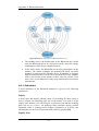
Bluetooth networking scheme................................................ 11
2.3.4
Connection scheme ................................................................ 11
2.3.5
Physical links ......................................................................... 12
2.3.6
Bluetooth packet .................................................................... 13
2.3.7
Bluetooth Classes ................................................................... 13
2.4
Localization................................................................................... 14
2.4.1
Spatial organization................................................................ 14
2.4.2
Localization application......................................................... 14
2.4.3
Available location technologies ............................................. 16
2.5
2.5.1
Routing Algorithms...................................................................... 18
2.6
Working principle of the algorithm ....................................... 20
2.6.1
Final problem statement.............................................................. 20
Possible outcome.................................................................... 21
iii
ANALYSIS.............................................................................. 23
3
3.1
Context-Awareness analysis........................................................ 23
3.1.1
Supermarket ........................................................................... 23
3.1.2
Mapping to supermarket geometry ........................................ 24
3.1.3
Type of customers to be located............................................. 25
3.1.4
Management of data............................................................... 25
3.2
Localization analysis .................................................................... 32
3.2.1
The chosen Technology ......................................................... 32
3.2.2
Technical aspects overview.................................................... 33
3.2.3
Description of localization method ........................................ 37
3.2.4
The system time adjust........................................................... 39
3.2.5
The system position accuracy ................................................ 39
3.2.6
APs Planning.......................................................................... 40
3.3
Routing analysis ........................................................................... 43
3.3.1
Shortest path algorithms......................................................... 44
3.3.2
Strategies and algorithms for routing..................................... 48
DESIGN .................................................................................. 53
4
4.1
Context-Awareness solution........................................................ 53
4.1.1
Customer behaviour ............................................................... 53
4.1.2
Transferring information solution .......................................... 55
4.2
Localization solution .................................................................... 58
4.2.1
Requirements.......................................................................... 58
4.2.2
High level localization process .............................................. 59
4.2.3
Localization algorithm ........................................................... 59
4.2.4
The localization network........................................................ 61
4.2.5
Bluetooth class election.......................................................... 62
4.2.6
Coverage radio ....................................................................... 63
4.3
Routing solution ........................................................................... 64
4.3.1
The costumer model............................................................... 65
4.3.2
Weight link assignment.......................................................... 66
4.3.3
High level routing algorithm.................................................. 75
iv
4.4
System description ....................................................................... 77
4.4.1
Network Architecture............................................................. 77
4.4.2
Working principle of the system ............................................ 80
SIMULATION ........................................................................ 83
5
5.1
Programming basics..................................................................... 83
5.1.1
Requirements.......................................................................... 83
5.2
Assumptions.................................................................................. 84
5.3
High-level block diagram ............................................................ 88
5.3.1
Main simulation controller..................................................... 89
5.3.2
Configuration input ................................................................ 89
5.3.3
DataBase ................................................................................ 89
5.3.4
GUI......................................................................................... 89
5.3.5
Context-Awareness ................................................................ 89
5.3.6
Routing................................................................................... 89
5.3.7
Statistics ................................................................................. 90
5.4
Whole System Process.................................................................. 90
5.5
Inputs............................................................................................. 92
5.5.1
Arrival Patterns ...................................................................... 92
5.5.2
Behaviours ............................................................................. 93
5.5.3
Total number of customers..................................................... 93
5.5.4
Threshold of congestion and trolleys per link........................ 93
5.5.5
Statistics ................................................................................. 94
5.6
6
Outputs.......................................................................................... 94
SIMULATION RESULTS ..................................................... 101
6.1
General Results .......................................................................... 101
6.2
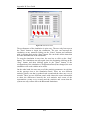
Graphics ...................................................................................... 103
7
CONCLUSIONS ................................................................... 111
7.1
System Conclusions.................................................................... 111
7.2
Simulator Conclusions............................................................... 113
v
7.3
Statistics Conclusions................................................................. 114
FUTURE WORK .................................................................. 117
8
8.1
Future Lines................................................................................ 117
8.1.1
System .................................................................................. 117
8.1.2
Simulator .............................................................................. 119
8.1.3
Statistics ............................................................................... 119
BLUETOOTH DETAILS ........................................................ III
A
A.1
Physical channel ...........................................................................III
A.2
Data communication .................................................................... IV
A.3
Time slots ...................................................................................... IV
A.4
Frequency Hop Spread Spectrum .............................................. IV
A.5
States of Bluetooth ........................................................................ V
A.5.1
Sub-states: .............................................................................. VI
A.5.2
Low power sub states ............................................................VII
A.6
Channel establishment..............................................................VIII
USER GUIDE .......................................................................... IX
B
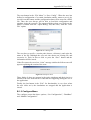
B.1
Simulator Manual ........................................................................ IX
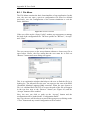
B.1.1
File Menu ................................................................................ X
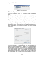
B.1.2
Configure Menu ..................................................................... XI
B.1.3
Simulation Menu...................................................................XV
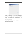
B.1.4
Post-Processing Panel ......................................................... XIX
B.1.5
Animation..............................................................................XX
B.1.6
About Menu ........................................................................ XXI
C
DATABASE .........................................................................XXIII
D
MATLAB GRAPHICS ....................................................... XXVII
D.1
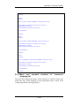
Introduction ...........................................................................XXVII
D.1.1
Graphics .......................................................................... XXVII
D.1.2
Number of customers in cash over the time.................... XXVII
vi
D.1.3
Code ................................................................................. XXIX
D.1.4
Mean and standard deviation of customers’ shopping listXXXI
D.1.5
Code ................................................................................ XXXII
D.1.6
Number of customers over the time ...............................XXXIII
D.1.7
Statistics Matlab Parser ...................................................XXXV
E
REFERENCES.................................................................XXXVII
F
ACRONYMS.....................................................................XXXIX
vii
List of figures
Figure 1 Scale Model of the supermarket. ................................................... 2
Figure 2 Piconets with a single slave operation (a), a multi-slave operation
(b) and a scatternet operation (c) [3]. ......................................................... 12
Figure 3 Bluetooth packet .......................................................................... 13
Figure 4 Example of information in PDA’s display. ................................. 16
Figure 5 Supermarket’s scale model reference. ......................................... 24
Figure 6 Signal Strength (triangulation method). ...................................... 34
Figure 7 Inquiry procedure......................................................................... 36
Figure 8 Converting SRI to RX power levels [9]. ..................................... 36
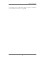
Figure 9 Relation of distance and RX power level, after 1000 measures for
each 65 experiment positions [9]. .............................................................. 37
Figure 10 Example of power distribution normalized to the free space path
loss [4]........................................................................................................ 38
Figure 11 Example of power distribution around the mean [4]. ................ 38
Figure 12 Area of error in the 90% of cases. ............................................. 40
Figure 13 Advantages of a defined scale model in a localization system.. 41
Figure 14 APs under the floor.................................................................... 42
Figure 15 APs on the shelves..................................................................... 42
Figure 16 APs on the ceiling...................................................................... 43
Figure 17 Supermarket’s scale model with discrete positions. .................. 44
Figure 18 Weighted graph [13]. ................................................................. 45
Figure 19 Relaxation [13]. ......................................................................... 46
Figure 20 Shortest path tree for Figure 18. ................................................ 48
Figure 21 Weighed directions. ................................................................... 49
Figure 22 Standard trolley’s size................................................................ 51
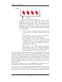
Figure 23 Link probabilities (loyal customer behaviour) .......................... 54
Figure 24 Link probabilities (absent-minded customer behaviour)........... 54
Figure 25 Link probabilities (random customer behaviour) ...................... 55
ix
Figure 26 Up-Link packet structure. .......................................................... 57
Figure 27 Down-Link packet structure. ..................................................... 57
Figure 28 Localization algorithm [2]. ........................................................ 61
Figure 29 AP position. ............................................................................... 61
Figure 30 Class 1 APs ................................................................................ 62
Figure 31 Coverage radio scheme.............................................................. 64
Figure 32 Supermarket’s scale model with enough discrete positions. ..... 65
Figure 33 Worst case in the supermarket................................................... 68
Figure 34 No default weight problem. ....................................................... 69
Figure 35 Second case without default weight problem. ........................... 70
Figure 36 Link weight assignment (loyal customer behaviour)................. 70
Figure 37 Link weight assignment (absent-minded customer behaviour) . 71
Figure 38 Link weight assignment (random customer behaviour) ............ 72
Figure 39 The weighted paths. ................................................................... 73
Figure 40 Scheme of the supermarket’s network....................................... 79
Figure 41 Numbered links of the supermarket........................................... 85
Figure 42 Supermarket divided in sections................................................ 86
Figure 43 System block diagram................................................................ 88
Figure 44 Numeration of the access points................................................ 97
Figure 45 Numeration of the cash points. .................................................. 98
Figure 46 Area where APs number 20, 9 and 14 are located................... 102
Figure 47 Area where links 1 and 136 are located................................... 103
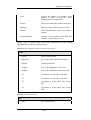
Figure 48 Mean and standard deviation of customers’ shopping times... 105
Figure 49 Number of customers over the time......................................... 106
Figure 50 Number of customers over the time......................................... 107
Figure 51 Number of customers over the time......................................... 108
Figure 52 Capture of the main screen of the simulator during a simulation
.................................................................................................................. 109
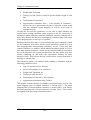
Figure 53 Number of customers in each cash point over the time........... 110
Figure 54 TDD and timing [3]. .................................................................. IV
Figure 55 Bluetooth states diagram............................................................. V
Figure 56 Different sub states of a Bluetooth device [3]. .......................... VI
Figure 57 Bluetooth connection process ................................................. VIII
Figure 58 First Panel of the Simulator. ...................................................... IX
x
Figure 59 File Menu unfolded. ................................................................... X
Figure 60 Open File Pop-up........................................................................ X
Figure 61 Open Dialog Box. ....................................................................... X
Figure 62 Save Dialog Box ........................................................................ XI
Figure 63 Example of Alert........................................................................ XI
Figure 64 Configuration Menu. ................................................................XII
Figure 65 Configuration Panel. .................................................................XII
Figure 66 DataBase Configuration Panel................................................ XIV
Figure 67 Matlab Configuration Panel......................................................XV
Figure 68 Simulation Panel..................................................................... XVI
Figure 69 Statistics Pop-up. ................................................................... XVII
Figure 70 Post-Processing Panel...............................................................XX
Figure 71 About Menu............................................................................ XXI
Figure 72 Pop-up student information. ................................................... XXI
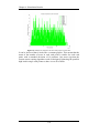
Figure 73 Number of cusotmers in cash 2 over the time. ..................XXVIII
Figure 74 Number of customers in cash 7 over the time. ..................XXVIII
Figure 75 Mean and Standard deviation of the customers shopping time
............................................................................................................. XXXII
Figure 76 Number of customers over the time...................................XXXIV
Figure 77 Number of customers over the time...................................XXXIV
xi
List of tables
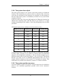
Table 1 Bluetooth Classes.......................................................................... 13
Table 2 Pictures file formats and size for a PDA screen............................ 29
Table 3 MP3 reductions [6]........................................................................ 30
Table 4 Bluetooth Local Positioning Application [9]. ............................... 34
Table 5 Mean inquiry time for a Multiple Access Point Scenario (n APs) 39
Table 6 Up-Link packet. ............................................................................ 56
Table 7 Down-Link Packet. ....................................................................... 57
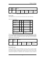
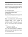
Table 8 Default weight per link according to the number of customers.... 69
Table 9 Percentage and weight relation. .................................................... 74
Table 10 Information about the customer. ............................................XXIII
Table 11 Device customer’s profile. .....................................................XXIII
Table 12 Localization of the customer................................................. XXIV
Table 13 List of the products that the customer wants to buy (Shopping
List). ..................................................................................................... XXIV
Table 14 Table with information about the products. .......................... XXIV
Table 15 Weight, neighbours and the localization of each link.............XXV
Table 16 Information about APs ............................................................XXV
xiii
Chapter 1: Introduction
1 Introduction
Introduction
The purpose of our project is to simulate the
performance of a routing algorithm in an indoor scenario
(a supermarket) according to different context-aware
parameters like customers’ moods, customers’
behaviours and localization. In this chapter, these
parameters are going to be introduced. Finally, the
structure of the report is presented, introducing the topic
of each chapter.
Countless times customers going shopping in big supermarkets have
suffered from frustration because of not knowing where the products are
located and because of losing their bearings. Not only do suffer they from
annoyance due to the fact of really long queues in the cash points but also
they get angry as a consequence of congestion in hallways, especially when
customers are in a hurry. Never to mention how affected people with
chronic diseases like agoraphobia are in overcrowded spaces like in the
hallways of big surfaces.
This project tries to solve all of these unpleasant situations for customers in
supermarkets by combining information related to the customer (context
information) with legacy computer applications. As a consequence, the
customer is given more accurate and suitable information (new
personalized offers) for him so he has a nicer time shopping in his favorite
supermarket. Hence, he will optimize his time spent in the supermarket and
he will finish his purchase as soon as possible.
Computer capabilities and network technology have been increasing and
improving quickly over the last few years. Nowadays, computers feature a
lot of functionalities even in tiny handheld devices. Moreover, the ubiquity
that wireless communications offers when using these devices lets the
customer be always online and capable of getting any kind of information
at any time, anywhere. In addition, the bandwidth of wireless links keeps
increasing, providing a large set of possibilities and services.
1
Chapter 1: Introduction
Following these steps, lately many reports ([1] [7] [18] [19]) have been
published about a new issue that will allow the intelligent networks to
achieve new features. Context-awareness is this new intelligent part of the
networks that allows the system to act according to the user’s information
related to his current environment and situation (his context). It means that
when humans interact with other persons or situations and with the
surrounding environment, we make use of implicit situational information.
The current situation context can be intuitively deduced and interpreted
reacting appropriately. For example, a person wants to go to buy something
to the supermarket, but it is raining when he leaves his house. Immediately,
this person will come back to his house and take an umbrella. This person
being aware of his environment, situation and context reacts appropriately
in front of his little trouble.
Computers are not as good as humans in deducing situational information
from their environment and in using it in interactions. They cannot easily
take advantage of such information in a transparent way, but if they can do
so, it usually requires that it is explicitly provided. This is a challenge for
computer systems as well as for human computer interaction.
Context-aware computing tries to provide this skill to our applications,
discovering and taking advantage of contextual information such as
customer location, time of day, nearby people and devices, etc.
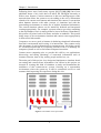
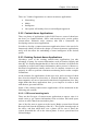
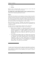
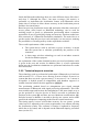
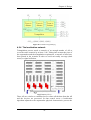
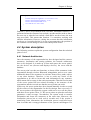
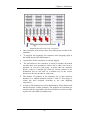
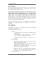
The main goal of this project is to design and implement a simulator based
on routing and context-aware information. Our efforts in this project are
invested in creating this kind of simulator to study and demonstrate the
usefulness of this context-aware system, focusing on a supermarket
environment, where the system try to offer a customized service to each
customer thus improving his experience during the visit.
Figure 1 Scale Model of the supermarket.
2
Chapter 1: Introduction
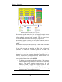
In order to reach our objective, three main parallel works have been
defined:
•
Context-awareness. As more parameters the application can
handle, more accurate the result will be. As a result, as much
information as possible have to be collected. Aspects like number
of current customers, customer preferences or shop descriptions
(products and offers) are considered.
•
Localization. It is very important to know where the customer is
and where he is going at any time. According to his position and
direction, the application will take one decision or another.
Although it could be considered inside of context-aware, it is better
to place it apart because it is not a trivial aspect: it needs an
accuracy implementation and detailed study of the technology and
the design.
•
Routing Algorithms. Once the application has all the information,
it must react appropriately. For example, the best path to the next
product (avoiding trolley’s congestion) or to show special offers
about a certain product that the customer needs. In the first
example, it will be necessary a background knowledge about
routing algorithms in order to calculate the best route to the
destination according to the cost of each path. This cost will be
determined by a policy of costs defined by our studies and research
about routing algorithms. Thus, it also will be necessary to design
and to define the structure of the supermarket on which our
application will work. On the other hand, the second example is
easier to implement and it is linked to the Localization section. The
application will display the best product offers to the customer,
considering his preferences and location.
These three main aspects allow our application to become a really useful
tool by using context-aware computing.
In the next three sections, theory backgrounds of all the technologies that
this project takes advantage of are explained.
First of all, context-aware will be explained in more detail, such as its
advantages and drawbacks, and its possibilities. Then, our work will focus
on studying and analyzing some localization technologies so that later the
best solution is chosen for this project. Finally, some theory background
about routing algorithms: advantages and disadvantages are given, and
later on, the best solution about routing algorithms will be chosen as well
as it will be explained what customized information consists on.
Next, the structure defined for the supermarket and everything about the
designed network will be designed in detail: architecture, devices, database
(tables, entries, records and fields), functionalities, technologies, protocols,
etc. The full implemented simulator will also be explained in this section:
how it was implemented, how it works, functionalities, capabilities, etc.
3
Chapter 1: Introduction
Sections 5 and 6 concern simulations and results about our simulator: what
kind of simulations is done, how we’ve tested it, scenarios, which are the
results, etc.
Finally, section 7 gives a final summary and our conclusions of this project
and section 0 gives some future lines for next works.
4
Chapter 2: Pre-Analysis
2 Pre-Analysis
Introduction
With the purpose to reach all the aims, some theory
background is needed in order to start the study of all
the limitations and possibilities of our project. Three
main blocks form our project; Localization, routing
algorithm and context-awareness. In this chapter, the
most important features of each one are explained,
focusing on the explanations of our necessities.
2.1 Overall problem statement
The Pre-Analysis section consists of the general knowledge about the
specific areas involved in the problem solution of this project. As it is said
in the introduction section, this project presents a solution to improve the
customer experience related to congestion in supermarket's corridors. This
project is a possible application of a more general technology which deals
with context information and routing algorithms.
Particularly, the main context information used by the system is the
position and shopping list (customer preferences), which provides an
intelligence to the system which allows the customers to be routed along
the supermarket, using modified routing algorithms which are applicable to
the supermarket scenario.
Providing a good shopping experience to the customer and valuable
information to the supermarket is possible with this technological solution.
The following sections offer the necessary background to start the analysis
of the proposed problem.
2.2 Context and Context-Awareness
First of all, the meaning of entity should be understood. "An entity is a
person, place, or object that is considered relevant to the interaction
5
Chapter 2: Pre-Analysis
between a user and an application, including the user and application
themselves." [7]
The following types of information could define the context of an entity:
•
Identity.
•
Spatial information - e.g. location, orientation, speed, and
acceleration.
•
Temporal information - e.g. time of the day, date, and season of
the year.
•
Environmental information - e.g. temperature, air quality, and
light or noise level.
•
Social situation - e.g. who you are with, and people that are
nearby.
•
Resources that are nearby - e.g. accessible devices, and hosts.
•
Availability of resources - e.g. battery, display, network, and
bandwidth.
•
Physiological measurements - e.g. blood pressure, hart rate,
respiration rate, muscle activity, and tone of voice.
•
Activity - e.g. talking, reading, walking, and running schedules and
agendas.
However, in this project only spatial information is used (to be more
precise, location of the customer) and the customer preference’s (mainly
the customer’s shopping list).
2.2.1 What is Context-Awareness?
Context-Awareness can be applied in different network ranges: Wireless
Cellular networks, WLAN or even WPAN. The main goal of contextawareness applications is to get all the information of the entity’s context,
gather it all together and use it in an intelligent way. For this purpose, there
is the need of a network of sensors. This type of network could be of any of
the following kinds: centralized, decentralized, any kind.
In addition, there is the need of a defined data structure in order to store
context information.
In context-awareness there are 3 types of profiles depending on what to
focus:
•
User
•
Device (mobile phone, ambulance)
•
Service
In this case, the customer profile is mainly focused, or customer contextinformation, as it will be seen later on.
6
Chapter 2: Pre-Analysis
There are 3 kinds of approaches to context-awareness applications:
•
Networking
•
Media
•
Intelligence
•
Our system will mainly focus on an intelligent approach
2.2.2 Context-Aware Applications
There are plenty of applications in this field. However, most of them have
not been yet commercialized. Office and meeting tools, tourist guides,
context-aware fieldwork tools, memory aids and a framework for
developing context-aware applications.
In order to develop a context-awareness application, there is the need of a
framework which will allow the design of context-awareness applications,
and it will also allow the embedding of some intelligence in the desired
profile.
2.2.3 Existing Context-Aware Applications
Nowadays, most of the existing context-aware applications just take
advantage of pretty few context information, such as location, identity and
time [1]. It is mainly thought that this is due to the fact that it is difficult for
computers to collect such context information, and to process it. Moreover,
this kind of applications usually needs a lot of computer resources to run
properly in order to perform continuous monitoring and to make complex
calculations.
At the moment few applications of this type exist, and even most of them
have been developed in universities or research laboratories. That means
that companies are not so interested in this kind of applications since they
might think that these applications have yet to improve in order to deal
with them to get some benefits.
Some of the existing context-aware applications will be mentioned in the
following sub-sections.
2.2.3.1 Office and meeting tools
These are the first type of context-aware applications to appear, since it is
much easier to get context information from an indoor and small space
such as an office than from an outdoor place.
One of the first ones to appear was the Active Badge system from Olivetti
Research Lab from the beginning of the 90’s. This system located people in
the office, and then when there was a phone call for one of them, the
system forwarded the call to the closest phone. It was a system based on
infrared badges.
7
Chapter 2: Pre-Analysis
Another application is the ParcTab system, which was developed at the
Xerox Palo Alto Research Center. It is based on a small infrared-based
palm-sized device continuously connected to a central server, and worked
as a personal digital office assistant. It could present information when the
user entered a room, helping the user find the closest local device (e.g.
printers), accessing a certain UNIX folder attached to a certain room, as
well as a location device.
Several applications have been developed by the Georgia Institute of
Technology, such as the In/Out board (a Java [21] application which main
feature is to inform if the user is in an office or not), Information Display
(displays information relevant to the user’s location and identity on a
display next to the user using IR or RF tags to locate and identify the user),
DUMMBO meeting board (an instrumented digitized whiteboard which
supports the capture and access of meetings, consisting on what is written
on the blackboard and on what is spoken), and Conference Assistant (it
displays conference timetables while remarking the events which are
interesting to the conference attendee).
2.2.3.2 (Tourist) Guides
This kind of applications is used to get information about the environment
surrounding the user. This was first experienced with the ParcTab system.
However, applications that use GPS positioning information can also be
considered as such.
One of these applications is called Cyberguide, which is based on the
user’s position and orientation (using infrared beacons for positioning) to
give information to the tourist about what he is currently watching in an
indoor scenario.
GUIDE is another application similar to Cyberguide, but in this case the
system works in an outdoor scenario (a city) using wireless technology
(IEEE802.11x) to deploy coverage dividing the scenario in cells.
2.2.3.3 Context-Aware Fieldwork Tools
Applications like an archeological assistant tool, a giraffe observation tool,
and a rhino identification tool allow researchers to take location dependent
notes.
2.2.3.4 Memory Aids
This kind of applications improves user performance when trying to
remember things, since humans remember things by associating them to
the current context. Hence, it will be easier for the user to retrieve
memories since these applications help the indexing of events.
Tools such as Forget-Me-Not (where the user is, with who and whom he is
phoning is stored in a database for later retrieval), Remembrance Agent
(continuously provides notes to the user, as well as summaries of notes,
8
Chapter 2: Pre-Analysis
emails or any other source of information based on context information)
and StartleCam are included in this type of context-aware applications.
The last one is quite interesting, since it is formed by a wearable camera, a
computer and a sensing system. The camera can be controlled at will or by
other unconscious means, such as basing the control on a skin conductivity
signal.
2.2.4 Context-Aware information
After see the existing applications, the most significative parameters to be
taken into account in the supermarket application can be approached. The
system will have to work with the following parameters as inputs to the
context-aware decisions:
•
Customer specific parameters:
o The number of customers, N, currently in the
supermarket: this parameter is important to know the cost
of the links, and also to have some statistics for the own use
of supermarket
o The location of the N customers (subject to in-accuracies
due to the positioning method): this parameter is related to
the previous one in order to know how many customers are
in each hallway, and also this information is needed to
compute the customer’s best route.
o The customer preferences: mainly device preferences,
such as screen resolution, brightness, contrast, colour and
language.
o The shopping lists (if available) of the N customers: the
customer will carry in a non-volatile memory the list of
items he/she wants to buy, or the system will download the
list from the Internet. It has to be defined a concrete format
of the shopping list, so all the customers will store it in the
same format which will make things easier to the system.
o A description of the goods already in the trolley of each
customer: ticking the customer’s shopping list or with
RFID tags.
•
Shop description:
o The number and location of active check-outs.
o The number and location of cash points, and the number
of customers queuing there: this parameter will be used to
give a cost to the path to each cash point
9
Chapter 2: Pre-Analysis
o The allocation of goods to the store's shelves (where they
are and how much is left): this information will be used to
decide the best route for the customer
o Pricing information and special offers: this information
will be used to pop up some commercials on the PDA
display.
2.3 Bluetooth background
This chapter will give a general description of the specificities and
capabilities of the Bluetooth technology regarding interconnections of
devices, communication types and states of devices.
2.3.1 Bluetooth
Bluetooth is an emerging standard for low-power, low-cost pico-cellular
wireless systems for personal area network connections among mobile
computers, mobile phones and other devices. The Bluetooth wireless
technology specification provides secure, radio-based transmission of data
and voice. It delivers opportunities for rapid, ad-hoc, automatic, wireless
connections, even when devices are not within the line of sight. The
Bluetooth wireless technology uses a globally available frequency range to
ensure interoperability no matter where you travel.
2.3.1.1 An actual rising technology
Created in 1994 by Ericsson, this technology was named as Bluetooth in
1998 after the foundation of the Special Interest Group (SIG). At the
beginning this industrial organization was composed of Ericsson, IBM,
Intel, Nokia and Toshiba. The SIG purpose is to define both Bluetooth
specifications and certifications (to verify the compatibility and interoperability of the products between them).
In 2001 appeared the first consumer products for mass market at the same
time specification 1.1 was released.
In 2004 the SIG has more than 2500 members. Moreover, the group has
launched Bluetooth specification 2.0 +Enhance Data Rate in November
2004.
10
Chapter 2: Pre-Analysis
2.3.2 Bluetooth technology abstract
Bluetooth operates in the unlicensed ISM1 band at 2.4-2.4835 GHz, which
is very crowded frequency band. Bluetooth tries to avoid this interference
by hopping in frequency 1600 times per second. The symbol rate is 1 Mb/s.
A slotted channel is applied with a nominal slot length of 625 µs. For full
duplex transmission, a Time-Division Duplex (TDD) scheme is used. On
the channel, information is exchanged through packets. Each packet is
transmitted on a different hop frequency. A packet nominally covers a
single slot, but can be extended to cover up to five slots. Bluetooth can
detect an error, if it should occur, with Cyclic Redundancy Check and
restore corrupted data with Forward Error Correction.
The Bluetooth protocol uses a combination of circuit and packet switching.
Slots can be reserved for synchronous packets. Bluetooth can support an
asynchronous data channel, up to three simultaneous synchronous voice
channels, or a channel which simultaneously supports asynchronous data
and synchronous voice. Each voice channel supports a 64 kb/s synchronous
(voice) channel in each direction. The asynchronous channel can support
maximum 723.2 kb/s asymmetric (and still up to 57.6 kb/s in the return
direction), or 433.9 kb/s symmetric. This point is widely explained at 2.3.5
[Physical links] section.
2.3.3 Bluetooth networking scheme
Bluetooth devices can operate within two different networking
frameworks:
•
The master-slave mode, in which devices communicate with each
other by first going through an Access Point.
•
The ad-hoc mode, in which devices or stations communicate
directly with each other, without using an Access Point.
An Access Point (AP) is a hardware device or a computer's software that
acts as a communications hub for users of a wireless device to connect to a
wired LAN.
2.3.4 Connection scheme
The Bluetooth system provides a point-to-point connection (only two
Bluetooth units involved), or a point-to-multipoint connection. In the point-
1
The industrial, scientific, and medical (ISM) radio bands were originally reserved
internationally for non-commercial use of RF electromagnetic fields for industrial,
scientific and medical purposes.
11
Chapter 2: Pre-Analysis
to-multipoint connection, the channel is shared among several Bluetooth
units. Two or more units sharing the same channel form a piconet. One
Bluetooth unit acts as the master of the piconet, whereas the other unit(s)
acts as slave(s). Up to seven slaves can be active in the piconet. In addition,
many more slaves can remain locked to the master in a so-called parked
state. These parked slaves cannot be active on the channel, but remain
synchronized to the master. Both for active and parked slaves, the channel
access is controlled by the master.
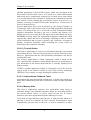
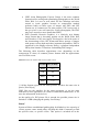
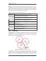
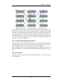
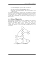
Multiple piconets with overlapping coverage areas form a scatternet. Each
piconet can only have a single master. However, slaves can participate in
different piconets on a time-division multiplex basis. In addition, a master
in one piconet can be a slave in another piconet. The piconets shall not be
frequency-synchronized. Each piconet has its own hopping channel.
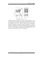
Figure 2 Piconets with a single slave operation (a), a multi-slave operation (b) and a
scatternet operation (c) [3].
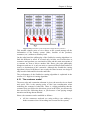
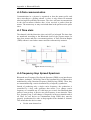
2.3.5 Physical links
Between master and slave(s), different types of links can be established.
Two link types have been defined:
•
Synchronous Connection-Oriented (SCO) links
•
Asynchronous Connection-Less (ACL) links
The SCO link is a synchronous point-to-point link between a master and a
single slave in the piconet. The master maintains the SCO link by using
reserved slots at regular intervals. The latency time is reduced as much as
possible. In this mode, packets are never re-transmitted. The maximum
throughput is 64 kb/s full-duplex.
The ACL link is a point-to-multipoint link between the master and all the
slaves participating on the piconet. In the slots not reserved for the SCO
link(s), the master can establish an ACL link on a per-slot basis to any
slave, including the slave(s) already engaged in an SCO link. This mode is
12
Chapter 2: Pre-Analysis
used for non real-time transmission where data integrity is important. The
packets are retransmitted until there are no more errors at the reception or if
an upper time limit is reached. Asynchronous connection can support
symmetrical or asymmetrical, packet-switching, point-to-multipoint
connections. In asymmetric connection, the maximum bit rate is 723.2 Kb/s
in one way and 57.6 Kb/s in the other way. In symmetrical connection, it is
433.9 Kb/s in both ways [2].
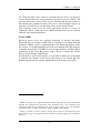
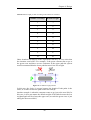
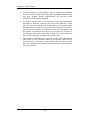
2.3.6 Bluetooth packet
Each Bluetooth device has a 48 bit IEEE MAC address that is used for the
derivation of the access code. The access code has pseudo-random
properties and includes the identity of the piconet master. All the packets
exchanged on the channel are identified by this master identity. That
prevents packets sent in one piconet to be falsely accepted by devices in
another piconet that happens to use the same hopping frequency in the
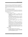
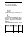
certain time slot. All packets have the same format, starting with an access
code, followed by a packet header and ending with the user payload.
Figure 3 Bluetooth packet
The access code is used to address the packet to a specific device. The
header contains all the control information associated with the packet and
the link. The payload contains the actual message information. The
Bluetooth packets can be 1, 3, or 5 slots long, but the multislot packets are
always sent on a single-hop carrier.
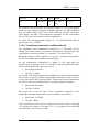
2.3.7 Bluetooth Classes
Bluetooth have implemented three different classes which principal
difference is the output power range that covers a range from 100m to
10cm.
Table 1 Bluetooth Classes.
Device Power
Class
Max. Output
Power (mW)
Max. Output
Power (dBm)
Expected
Range
Class 1
100 mW
20 dBm
100 m
Class 2
2.5 mW
4 dBm
10 m
Class 3
1 mW
0 dBm
10 cm
13
Chapter 2: Pre-Analysis
2.4 Localization
The main Context-Aware element that will be used in this report is
location. From the entire possible context information that can be collected
inside a supermarket, the most important and basic one is the customer
location, based on which all the necessary applications can be released.
As it is remarked in the Introduction (section 1), all possible services
offered to the customer depend on the context information. The system has
to be able to know the customer’s location on a real-time basis, hence
being able to avoid congestion in the supermarket corridors (for further
details, refer to the Routing Algorithms (section 2.5)). Furthermore, by
exploiting the customer’s location, it is possible to offer alternative
services, such as personalized offers on the closest screen, or even cash
queue management. All this services depend on the amount of information
that the system can take advantage of.
This section will treat the necessary details for a customer localization
purpose. Based on this information, the high level characteristics of the
system are explained, the different possible applications such as routing the
customers depending on the rest of buyers’ location, the personalized offers
displayed on screens and any other possible applications. This section will
finish with a discussion about the existing technologies that can be used for
location in this project scenario.
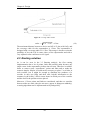
2.4.1 Spatial organization
Localization in an indoor scenario depends on the spatial characteristics of
the place, which means that it is not possible to establish a general
localization criterion suitable for any indoor scenario, but starting with a
known and defined scenario. The conclusion is that a spatial organization
has to be defined first.
This concrete project starts from a clearly defined scenario which is the
supermarket. But not all supermarkets have the same spatial organization,
so a determined space is defined, that will be used for all the requirements
of this project.
That supermarket model is explained in section 3.1.1; a new technology
infrastructure will be suitably designed for this concrete spatial
organization.
2.4.2 Localization application
The main and basic aim is to be able to know at every moment the
approximate position of every customer that can be located (meaning each
customer carries a device that allows its localization). Based on this
amount of information it is possible to build applications with added value
for the supermarket and for the customer.
14
Chapter 2: Pre-Analysis
Between the different applications, two of them stick out because they
represent the two main aims of this project: routing customers to avoid
hallway congestion, and the possibility of displaying personalized offers on
a screen, based on the nearest customers.
These two features will be the project starting point, although the final
system will be defined in the section 4 (Design).
2.4.2.1 Routing customers
The localization feature is very important to realize a good routing system.
The basic issue of routing customers is to know where the customers are
(with a problem of uncertainty) and to know where the shelves and the
consumer goods are. Just inputting this simple information (just a set of
coordinates in a map) to a routing algorithm it is possible to engage the
routing system.
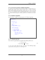
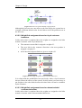
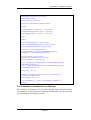
while (supermarket is open; at every X seconds)
Get location of N customers;
Determine possible congestions (comparing supermarket map & customers
location);
if (new customer enters in supermarket)
Show route*(depending on congestion);
* Note that the routing system is not detailed in this high level algorithm since it is
not part of the localization problem. Routing system can be consulted on section
3.3.1.
There are some limitations associated to the localization system. The
following limitations can be considered:
•
Errors in the localization measurements.
•
Discreet mapping of the supermarket
•
Delays in the Bluetooth network
The system will be always calculating the devices position, and the
frequency of iteration can be adjusted depending on the complexity of the
localization. This point will be discussed in the Design section [chapter 4]
section.
The determination of possible congestions will be done comparing the
supermarket spatial distribution with the customers’ location. In this point
additional information (provided by the map) can be used such as the
shelves’ position to make more precise the customers’ location (note that a
customer cannot stay on top of a shelf, so this area is not a possible
customer location).
Finally, if a new customer enters the supermarket, the system will check if
there are some signs of congestion, and if so, the routing algorithm will be
executed so that it shows the new customer a new non-congested route.
15
Chapter 2: Pre-Analysis
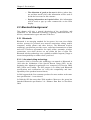
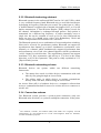
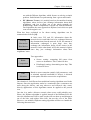
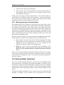
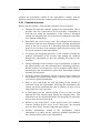
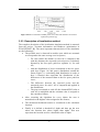
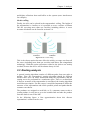
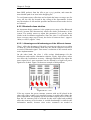
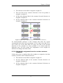
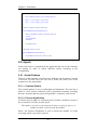
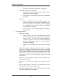
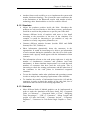
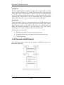
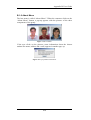
2.4.2.2 Context-awareness information on screens
Apart of routing customers, the other main feature is the context-awareness
information on screens (Supermarket’s screens and PDA’s displays). The
main functionality of this system is to show personalized offers to the
customer whenever he is close to any screen. These offers are also showed
individually in each customer’s PDA display.
Figure 4 Example of information in PDA’s display.
For a well operating of this service, the system needs some additional
information which is the customer preferences. These preferences can be
for example; the shopping list, the offers list, a history of the customer’s
goods list, etc...
For example, the system can process the shopping list of every customer
and collect statistics of the preferred goods of customers that are close to
any screen at that moment. Hence the system will display on these screens
offers related to this kind of products.
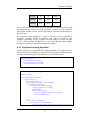
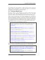
A possible high level code is:
for (all customers close to screenX)
Release a statistic of all shopping lists of customers close to screen;
Display on screenX the most popular product;
2.4.3 Available location technologies
From technologies existing in the market at the present time, that can
satisfy the necessities with location, the following ones are considered for
this project: GPS, IR, RFID, 802.11 and Bluetooth.
2.4.3.1 GPS
The Global Positioning System (GPS) is a satellite navigation system used
for determining one's precise location and providing a highly accurate time
16
Chapter 2: Pre-Analysis
reference almost anywhere on Earth. It uses a satellite constellation of at
least 24 satellites.
GPS technology can reach a valid accuracy for this project requirements
(from 1 to 3 meters), and the equipment do not represent a considerable
expense.
In any case, there exist 2 reasons for which this option is rejected:
•
First, although it is public access, American Defence Department
controls this network of satellites and the system would be
unusable if the Department decides stop the system.
•
In addition, GPS technology works just in satisfactory way in
opened surroundings in which there is direct visibility with the sky,
case that does not occur inside a supermarket.
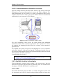
2.4.3.2 IR
Infra-red (IR) radiation is electromagnetic radiation of a wavelength longer
than visible light, but shorter than microwave radiation. Infra-red radiation
spans three orders of magnitude and has wavelengths between 700 nm and
1 mm.
This kind of radiation can be used in some devices with localization
purposes. This devices use infra-red light-emitting diodes (LEDs) to emit
infra-red radiation which is focused by a plastic lens into a narrow beam. If
there is a reflection means that a user is close to the sensor.
That is a good way to detect presence of a user in a specific location.
The problem is that a light-of-sight is necessary and, in the case of a
congestion of some customers, there would be a possibility of several
customers can not be detected. For this reason infra-red cannot be used by
general location purposes.
2.4.3.3 RFID
Radio frequency identification (RFID) is a method of remotely storing and
retrieving data using devices called RFID tags/transponders. An RFID tag
is a small object, such as an adhesive sticker, that can be attached to or
incorporated into a device. RFID tags contain antennas to enable them to
receive and respond to radio-frequency queries from an RFID transceiver.
RFID works in several frequencies as UHF (868 and 956 MHz) and
microwave (2.45 GHz), and it can be used as a location system by the way
is a very short recognition range, and it permits an identification of the
device that wears the RFID chip (for example, putting RFID readers on the
shelves).
The problem is that because is a very short range, a big number of RFID
readers are needed and it complicate a lot the system. Furthermore, some
17
Chapter 2: Pre-Analysis
open areas (far away from the shelves) will not have coverage, and subfloor readers will be needed. Finally, RFID can not transport a great
amount of data so it is only applicable for localization, but a data
transmission is needed so in the case that RFID system will be used, a
second transmission technology should be used.
2.4.3.4 802.11
802.11 or Wi-Fi denotes a set of wireless LAN standards developed by
working group 11 of the IEEE [23] 802 committee. It uses the free ISM
radio frequency band 2.45 GHz, and their capabilities for location (with an
accuracy of 1.5 meters) have been proved [5]. Furthermore there are
commercial applications that use this kind of localization.
802.11 is a valid technology for localization purposes, but have two major
inconvenients in our project scenario. Firstly, the wide coverage range of
this protocol (with LoS can reach 100 meters), compared with the
relatively short dimension of the supermarket, can induce interferences,
fading or other types of signal failures, as well as a bad localization
accuracy. Besides of this ,Wi-Fi technology needs a great amount of power
for a correct performance (maybe trolleys will be not recharged in a whole
day). For this reason, a short range coverage technology with lower energy
compsumtion is needed to solve the localization problem in our scenario.
2.4.3.5 Bluetooth
As it is said in section 2.3 Bluetooth is an industrial specification for
wireless personal area networks (PANs). Bluetooth provides a way to
connect and exchange information between devices like personal digital
assistants (PDAs), mobile phones, laptops, PCs, printers and digital
cameras via a secure, low-cost, globally available (in a ISM band) short
range radio frequency.
The coverage area in this technology is 10 meters for class 2 [3] (can be
also 100 meters, with class 1), so can be perfectly adapted to our scenario.
On the other hand Bluetooth technology do not need a high amount of
energy for its correct performance, and it is possible to work without power
supply the entire day. The document “Location Information and Handover
optimization in WLAN/WPAN” [2] establish the basis for a Bluetooth
localization using triangulation technology.
2.5 Routing Algorithms
Traditionally, for legacy Internet networks (most of them mainly based on
the IP protocol), two main approaches have been used for routing purposes:
•
LS (Link State): it is mainly based on a centralized or global
routing, where all the routers in the network have a global image or
understanding of the whole network. Route computation is carried
18
Chapter 2: Pre-Analysis
out with the Dijkstra algorithm, which focuses on solving a simple
problem: find minimal cost path starting from a given node/router.
•
DV (Distance Vector): it is mainly based on decentralized routing
algorithms, where devices just exchange information about their
neighbours, and just to them, not to the whole network (no
broadcasting). Route computation is carried out with the BellmanFord algorithm, the same approach as Dijkstra, but in this case path
costs can be negative too.
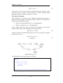
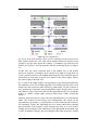
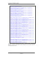
What has been explained so far about routing algorithms can be
summarised as follows [12] :
Routing
Information
Distribution
In both cases, DV and LS, information about the
network devices and links has to be exchanged between
the elements that form the network. In LS, the amount of
information exchanged is quite huge, since they
exchange the information about all the routers in the
network. On the other hand, in DV this amount is lighter
since they just exchange information about their
neighbours’ state.
Two approaches:
Route
Computation
Path
Selection
•
Source routing: computing full routes from
source to destination. This is what LS does.
•
Distributed routing: determining next hop. This
is what DV does.
Based on some constrains (mainly QoS parameters, such
as minimal required bandwidth or delays), it discards
certain paths which do not meet the requirements.
Our situation is far different from traditional routing algorithms used in the
Internet. Since the application works in a continuous space (customers can
walk along the shelves, and stop wherever and whenever they want),
directly applications of this algorithms cannot be applied to the present
case.
Our aim is to make a discrete scenario where users could probably stop.
Hence, the Dijkstra algorithm is applied instead of the Bellman-Ford one
since the infrastructure will be static (nodes will not show up and disappear
out of the blue, and neither links will), but not the cost of the links.
However, our modified Dijkstra routing algorithm will have to handle the
following characteristics:
19
Chapter 2: Pre-Analysis
•
Links between nodes are the hallways.
•
Link costs are based on the number of moving or idle trolleys in
each hallway, thus our scenario will be dynamic because of the
moving nature of trolleys.
Taking into account the previous characteristics, if for instance there are
some trolleys in a hallway in some other customer’s way to his purchase,
the system could see these trolleys as a high cost in the path, and so then
dynamically compute another path around the shelf.
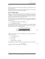
2.5.1 Working principle of the algorithm
The starting point of the customer’s route will always be the place where
the trolley is initially parked, and its destination will change according to
the nearest item he/she has to buy. Then, when he/she gets his/her item,
this will be his/her starting point, and then another route will be worked out
to his/her new destination (his/her next item to purchase). And successively
until he/she gets his/her last item, when the destination point will be a cash
point. At this moment, the system will compute the best route to the cash
point with less queuing people.
How the system will know when the customer has finished buying all that
he/she wanted is a topic that can be addressed in two different ways:
•
The customer can tick each item in his/her shopping list in the
PDA whenever he/she puts the item in his/her trolley (the PDA
application will be implemented to be easy enough for the
customer to mark the items in the shopping list)
•
RFID tags can be used in each good in the supermarket, and a
RFID tag reader can be placed in each trolley so the system can
know at every moment what the customer has placed in his/her
trolley.
These are two equal possible and suitable solutions. However, the former
one seems to be less expensive. On the other hand, the customer can make
some mistakes in ticking some items, so it seems that the latter approach is
the more accurate.
2.6 Final problem statement
Once the overall problem statement is known, and a background about
context-awareness, localization and routing algorithms is released in this
Pre-Analysis section, the basic knowledge is reached, and so the Analysis
section can be faced. In this section there is also a basic background about
the Bluetooth wireless technology which is used in further chapters of this
report.
With the knowledge of this three areas (context-awareness, localization and
routing), an analysis of the problem can be performed. Next section
20
Chapter 2: Pre-Analysis
presents the peculiarities related to the supermarket scenario, and the
possible solutions to release the routing system using context information.
2.6.1 Possible outcome
Before start the analysis, some possible outcomes can be proposed:
•
Optimize the time the customer spends in the supermarket. This is
possible since the system have all the necessary information to
route the user along the supermarket. If the system is intelligent
enough, the shopping time can be decreased compared to the same
case without routing help.
•
Personalize the service to any client. The system has the customer
information and can take advantage of this, offering personalized
offers in the device screen. It is interesting from the supermarket
point of view because if the customer appreciates this service will
be a loyal customer of that supermarket.
•
To improve the shopping experience of the customer offering the
products information in the screens, and guiding the customer
through the supermarket to buy the shopping list items of the
customer.
•
Taking advantage of the customer context information, to improve
the items location (use this information for marketing purposes).
Besides of this, if a corridor have a lot of customer traffic maybe is
interesting for the supermarket to place there determined products
(promote this products).
•
Using the context information, logistic processes can be improved.
For example, the system knows when a concrete item is sold out,
so it can be replaced immediately.
•
More or less cash points are used depending on the number of
customers inside the supermarket. Knowing this information, the
system can decide automatically (and in advance) if more or less
cash points have to be operative.
•
Is interesting from the customer point of view to know at each
moment the total amount spent during the shopping time. This
information can be calculated with the user shopping list each time
the user gets an item from a shelf.
•
Related to the point before, if the system knows the customer
concrete products before arrive to the cash point, the payment
process can be faster, and the cash point queue shorter.
•
Another optimization related to the supermarket context
information is to share out the employers schedule depending on
the customer traffic peaks in the supermarket.
21
Chapter 2: Pre-Analysis
•
Optimize the knowledge of the supermarket about the customer’s
behaviour or preferred products. The supermarket can have all the
information related to the shopping: time of shopping, customers
routes, the most products bought, etc. Supermarket can use this
information to improve their service and provide a better shopping
experience to his customers.
These are the possible high level outcomes from a first whole view of the
possible system. Next sections define the concret solution to the contexaware routing system.
22
Chapter 3: Analysis
3 Analysis
Introduction
In order to design an application or an entire system
studying some existing technologies is really needed,
focusing the attention on the advantages and
disadvantages of them and what they can offer to the
system. The main goal is finding and using the best
solutions for all our functionalities. In this chapter the
most important technologies are analyzed in order to
select the best option.
3.1 Context-Awareness analysis
The following sub sections are related to the context-awareness applied to
our scenario.
3.1.1 Supermarket
Every supermarket can be different and it depends on the characteristics
and the kind of shopping. As the localization system depends on the
physical organization of the space, as a result of reflections, coverage,
etc..., it is mandatory to define a specific space organization to develop our
system in order to adjust the localization results.
On the other hand, in order to optimize the routing algorithm a physical
scale model reference of our supermarket have been designed, which is
very important in order to locate the customers and to route the trolleys.
Before knowing more about the network architecture, it is mandatory to
define what the supermarket contains and which its distribution is. Like
real supermarkets, it has different sections that can be classified as food,
clothes, music, health, home, magazine, electronic, etc, the food’s section
being the largest one.
23
Chapter 3: Analysis
In this way, a physical architecture is designed based on some real
supermarkets from Spain and Denmark, defining the shelves, corridors,
cash points, the entrance and the exit. The supermarket’s scale model for
our localization and routing system is introduced as follows:
Figure 5 Supermarket’s scale model reference.
This supermarket’s scale model is used to represent the location, movement
and events of the customers during their shopping experiences. Grey zones
define walls and shelves, and the red ones define cash points. Entrance and
exit are also defined.
3.1.2 Mapping to supermarket geometry
As have been seen in the previous subsection, a scale structure model has
been defined in order to design the localization network and the routing
algorithm. In the following sections it is explained the advantage of
defining a scale model of the supermarket.
First the analysis focuses in the localization problem and how the devices
of the localization can adapt to the defined structure. This structure has to
be studied in detail before to place the BT access points on the ceiling in
order to reach all the corners of the supermarket. Moreover, each point of
the supermarket has to be covered by at least three BT access points to
locate the costumer, and transfer to him the routing and context-aware
information.
Second, the routing system is explained adapting it to the defined structure.
The set of nodes and links are logical entities that the system uses on the
scale supermarket model in order to have some guidelines to route the
customers in a suitable way and to manage the possible paths that they can
take.
24
Chapter 3: Analysis
3.1.3 Type of customers to be located
There are several types of customers which can go shopping in our
supermarket scenario.
•
Customers with trolleys: it is quite easy to embed a PDA in the
trolley, since there is plenty of space where to stick this device. In
addition, the customer has not to worry about the PDA because it is
perfectly fixed to the trolley chassis; hence the customer’s focus is
only on his/her buying task.
•
Customers with baskets: it is not possible to offer the same
functionalities to a customer that carry a shopping basket than one
that carry a trolley, as a result of the difficulty of put a screen
(PDA or similar) in the shopping basket. But that does not mean
that this customer cannot be located, because small localization
devices can be added to the shopping basket. Then, although the
system could locate and route these customers, they are not been
taken into account for the system.
•
Walking customers: customers that do not carry a trolley or a
shopping basket are supposed to remain just a few minutes in the
supermarket (they usually buy just one or two items). This kind of
customer do not affect almost in the cash point, so these customers
are not been taken into account for the system.
3.1.4 Management of data
Based on what it has been explained so far, it is obvious that the system
needs to take into account some information related to the customer, such
as location, direction or shopping list. For this reason, this information has
to be stored somewhere in some way. Hence there are several approaches
to solve this problem, regarding collecting information, storage support,
and transferring information.
3.1.4.1 Collecting information
Three types of collecting can be used to solve this problem:
•
Centralized way: in this way, all the information is collected in a
single and only point. This makes easier and more consistent the
gathering of information since it is performed by just a unique
element. However, this is a weak point to take care of as the entire
system might fail on condition that this element fails. The
implementation of this storing type is the simplest one.
•
Decentralized way: in this way, all the information is collected by
several elements. This is more difficult than gathering all the
information in a single point, but has the advantage of having the
information duplicated in several elements. Nevertheless, there
25
Chapter 3: Analysis
should be some mechanism or protocol in order to synchronize the
contents in all the elements.
•
Hybrid way: this way of storing and collecting information makes
use of both types of storing information explained previously. It
combines both advantages and drawbacks of these two both types
seen previously. Its implementation is trickier than the previous
one since it is based on it.
3.1.4.2 Storage support
In addition to these types of storing information, there are several
possibilities based on the storage support which is used.
•
Non-volatile: this means that the information is stored in a
permanent way, so the system can make use of it in case the system
has to be rebooted or shut down. This type includes databases and
files. The latter is used mainly in simple applications, where the
amount of information to store is not quite huge, whereas the
former is used for almost everything, and nowadays it is the usual
way of storing information.
•
Volatile: using this type of storage support is a common practice
for computers, which take advantage of this kind of memory to
make applications performance easier and quicker. This includes
mainly xRAM memories. Despite good for computers, this type is
not suitable for applications which work with large amounts of
information, and which have to make use of old information after
system reboots (needing a permanent storage support).
3.1.4.3 Transferring information to the devices
This can mainly be done in two ways:
•
Direct provision: the customer carries his own information in an
external memory stick that he will plug to the trolley to upload this
information to the server’s database. This way is annoying for the
customer since he has to take care of carrying his memory stick to
the supermarket, hence he gets worried about having to carry his
memory stick at all times when he wants to go shopping. This can
be done plugging memory cards into some slot or even by wireless
transfers from mobile phones or PDAs which the customer carries.
•
Downloading from the Internet: the system accesses an external
or internal server where the customer’s information is stored, so
the system knows the customer’s information. This way is easier
and more comfortable for the customer since he just has to upload
his information to a server on the Internet, and then go shopping
with no worries.
26
Chapter 3: Analysis
3.1.4.4 Managing special and personalized offers
In order to show the customer special and personalized offers, the system
has to show them in the PDA, and for that purpose the system has to make
the PDA show some multimedia contents, which can be done in two
different ways:
•
One approach could be having a PDA in the trolley without any
storage support, and so, if any information has to be shown in its
display, the only way of doing this is by transferring these contents
wirelessly with Bluetooth. Since Bluetooth rates are up to 734
Kbps.
•
The second approach, based partially on the previous one, could be
to have a minimum storage support in the PDA (where to store the
information), and just transfer wirelessly some text or some
commands to make the application in the PDA show the
information. However, if new information is to be included in the
supermarket, they could also be transferred or maybe copied to the
storage support system in the PDA after the customer returns back
the trolley. It decreases drastically the information transferred, and
hence more and more customers could be associated to any single
Bluetooth AP without bandwidth constrains.
3.1.4.5 Kind of information to be transferred
The kind of information that can be transferred to the device is:
•
Text (Information about the customer, routing and the products
related to the route)
•
Images (For the GUI, the offers and the supermarket map)
•
Sound (Help for blind persons)
Let us analyse the importance and weight of transferring text, images and
sounds in the system.
Text
The device is always transmitting information related to the Bluetooth
connexion (this is necessary to release the localization). Furthermore, the
system sends and receives other kind of text from the devices. For example
the device will send the information associated to the customer (ID,
shopping list, commands, etc...) and receive commands from the server
(routing orders, offers related with the shopping list or the customer profile,
etc.).
A Bluetooth baseband packet is composed of three parts:
•
Access Code
27
Chapter 3: Analysis
•
Header
•
Payload
Packets can be constructed either: Access code only, Access Code and
Header, and Access Code, header and Payload.
The diagram for a generic Bluetooth packet can be consulted in Figure 3.
The detailed kind of information transfer and the specific packet will be
defined in the Transferring information solution.
Images
Other kind of data that the system transmits are images. Images are used to
compose some parts of the device's GUI, and also to show special offers to
the customer. The supermarket map and the images of the GUI are part of
the device application, so there no affects to the data transmission of the
system. But images from special offers are really variable (it depends on
the customer preferences, the shopping list or in his location).
PDA screens have a small size. Normally, these images do not need to be
very big as a result of the little screen. The screen size is quantified by his
resolution in pixels2.
Actual devices have an approximate resolution of 250 x 350 pixels.
Nowadays the most common graphic formats are the following:
•
BMP (Windows Bitmap) is a bitmapped graphics format used
internally by the Microsoft Windows graphics subsystem (GDI),
and used commonly as a simple graphics file format on that
platform. BMP files are usually not compressed, so they are
typically much larger than compressed image file formats for the
same image.
•
GIF (Graphics Interchange Format) is a bitmap image format that
is widely used on the World Wide Web, both for still images and
for animations. GIF became popular because it used LZW data
compression, which was more efficient than the run-length
encoding that formats such as PCX and MacPaint used, and fairly
large images could therefore be downloaded in a reasonable
amount of time, even with very slow modems.
2
A pixel is one of the many tiny dots that make up the representation of a picture in a
computer's memory. Usually the dots are so small and so numerous that, when printed on
paper or displayed on a computer monitor, they appear to merge into a smooth image. The
colour and intensity of each dot is chosen individually by the computer to represent a
small area of the picture.
28
Chapter 3: Analysis
•
JPEG (Joint Photographic Experts Group) is the most common
format used for storing and transmitting photographs on the World
Wide Web. It is not as well suited for line drawings and other
textual or iconic graphics because its compression method
performs badly on these types of images (the PNG and GIF
formats are in common use for that purpose; GIF, having only 8
bits per pixel is not well suited for colour photographs, but PNG
may have as much or more detail than JPEG).
•
PNG (Portable Network Graphics) is a relatively new bitmap
image format that is becoming popular on the World Wide Web
and elsewhere. PNG was largely developed to deal with some of
the shortcomings of the GIF format and allows storage of images
with greater colour depth and other important information. PNG is
supported by the libpng reference library, a platform independent
library that contains C functions for handling PNG images.
The following table describes approximate sizes (depending on the
compression if exists) of common picture formats with the approximate
size of a PDA screen:
Table 2 Pictures file formats and size for a PDA screen.
Format Size (in KB)*
BMP
257
GIF
69
JPEG
24
PNG
133
[* All the formats represents the same pictures and have the same size in
pixels (250x350px)]
JPEG files are the smallest for the same resolution, so are the most
indicated for this application (as valid for Bluetooth transmission, as for
store the information in the device).
As the quality of a JPG picture file is enough, the possible picture size is
limited to 24 KB (changing the quality if necessary).
Sound
System will have an additional guiding help for blinded (or low capacity of
vision) persons, some sound orders will help this kind of customer to find
the specific route, or specific offers. This option is switched off in the
29
Chapter 3: Analysis
default option, and will only run if the customer activates it, so will not be
taken into account in future sections and designs.
The sound orders will be the following spoken words:
•
Go straight
•
Turn right
•
Turn left
•
Go back
And additional spoken sentences:
•
Name of products
•
Amount spent.
The length of this sentences is variable (depends on the words) but an
approximate value of 1.5s can be taken. The following digital audio
formats are the most common nowadays:
•
WAV
•
MP3
•
Vorbis OGG
The first one, WAV, short for WAVEform audio format, is a Microsoft and
IBM audio file format standard for storing audio on PCs. The other two are
compressed audio formats. MP3 was started to develop by Fraunhofer IIS
in 1987 as a requirement for the Digital Audio Broadcast (DAB). Vorbis is
an open and free audio compression (codec) project from the Xiph.org
Foundation, it was started following a September 1998 letter from
Fraunhofer Gesellschaft [6] announcing plans to charge licensing fees for
the MP3 format.
A table from the Fraunhofer IIS documentation is extracted with
information related to the MP3 codec:
Table 3 MP3 reductions [6].
Sound Quality
Bandwidth Mode Bitrate
Reduction
ratio
Telephone sound
2.5 kHz
Mono 8 kbps
96:1
Better
wave
that
short 4.5 kHz
Mono 16 kbps
48:1
Better
radio
than
AM 7.5 kHz
Mono 32 kbps
24:1
Stereo 56..64 kbps
26..24:1
Similar to FM radio
11 kHz
30
Chapter 3: Analysis
Near CD
15 kHz
Stereo 96 kbps
16:1
CD
> 15 kHz
Stereo 112..128
kbps
14..12:1
As it can be seen in the table, for a quality similar to AM or FM (spoken
words are just needed, not music or higher qualities) the MP3 reduction
ratio is 24 times from a WAV file. Vorbis OGG has a similar size from a
same quality, but MP3 is most hardware supported, for this reason MP3
files will be used for the audio section of application.
An audio file with approximate length of 1.5s, with FM quality has an
approximate size of 10 KB.
3.1.4.6 Transferring information via Bluetooth link
The maximum active simultaneous costumers in a Bluetooth AP are
limited. The AP can serve to seven active simultaneous costumers [3]. That
means that the system can track 147 costumers (7 for each 21 AP).
Bluetooth permits to have “parked” or “inactive” costumers associated to
the AP, but without the possibility of transfer data.
As the transmission information is higher in the down-link, the
Asynchronous Connection Less (ACL) will be used in the Bluetooth links.
The maximum Bluetooth capacity per AP is:
•
Down-link: 90.4 KB/s
•
Up-link: 7.2 KB/s
As a result of the Bluetooth packet description, not all the transferred bits
will be data. In all the packets with payload information exists 72 bits of
access code and 54 bits of packet header. That means that real information
is a 95.6% of the total information (for a complete payload structure):
•
Down-link: 86.4 KB/s
•
Up-link: 6.9 KB/s
The worst case is an AP with 7 active costumers connected. If the
bandwidth is divided between these seven costumers, the result is:
•
Down-link: 12.3 KB/s
•
Up-link: 1 KB/s
If the refresh time of the system is taken as a reference, that is 4 seconds
(15 refreshes per minute, see section 3.3.2.3), the customer can send 4 KB
of information, and receive 49.2 KB.
31
Chapter 3: Analysis
The upload information is enough to send the localization information, and
other information like the shopping list. The download capacity is enough
to receive:
•
2 pictures and approximately 2 KB of text information (approx.
330 words).
•
1 picture, 2 spoken words and text information
•
Up to 4 spoken words and text information
•
Text information
This way to transfer information represents a problem. Only the active
costumers can receive data from the system, it means that only seven
costumers close to an AP can transfer information each iteration.
3.1.4.7 Information stored in the device
This option makes use of a combination of transferring information via
Bluetooth, and a physical storage. System works in the same way than in
3.1.4.6 but with the exemption of the image and sound transferring.
That means that the system will combine both possibilities depending on
the variability of the data. Variable information depending on the customer
or the time will be transferred dynamically by the Bluetooth link to all
devices. This kind of information is all the text traffic like identification of
customer, shopping list, commands, routing orders, offers related with the
shopping list or the customer profile …
On the other hand, the heaviest traffic like images and sound will be stored
in the device, and only the orders from the system to show or play this data
will be sent via Bluetooth. With this solution, a great amount of data is
saved from the wireless link. All this static data can be replaced every time
the supermarket requires it, for example at night when all trolleys are
connected to the parking.
3.2 Localization analysis
After the localization background written in the Pre-Analysis section, there
is an analysis of the specific localization in the supermarket with concrete
technologies.
3.2.1 The chosen Technology
Since the different available technologies have been seen in Section 2.4.3,
for indoor localization purpose, the chosen technology is Bluetooth. This
technology is able to be used with localization purposes [4][8][9], have the
ideal coverage area for our indoor scenario and finally can be used also to
transfer information to the devices [3], so a complementary technology is
not needed for this purpose.
32
Chapter 3: Analysis
Inside the Bluetooth technology there are some different classes like class 1
and class 2. Although the class 1 has more coverage (100 meters), is
preferable to implement the localization feature with Bluetooth access
points class 2 because it allows better accuracy in the localization process
and have less interference.
Based on previous localization works [4], and on the idea that a network of
access points (APs) based on Bluetooth technology can be used for
tracking people or goods, or information provisioning when a customer
approaches an access point [11], timing and accuracy location results have
been extracted, of a Bluetooth localization simulation. The main idea is to
get the results from this previous work and apply it to our project, studying
the possibilities of locating trolleys in the supermarket scenario.
The overall requirements of this section are:
•
The system has to work in real-time or quasi real-time, it means
that the system has to calculate periodically the position of the
customers.
•
A short range wireless technology to work in an indoor scenario
for the localization purpose.
An explanation of the results obtained in these previous localization works
is given in the next sub section. In addition, there is a brief explanation
about how the localization simulation was performed and about its results
and conclusions.
3.2.2 Technical aspects overview
The technology used to perform the localization is Bluetooth, as it has been
said in section 3.2.1. Context Aware Routing System in Indoor Scenario is a
system that does not need a great accuracy, so an error of 2 or 3 meters is
acceptable. A hybrid system of triangulation with database support is a
suitable location solution for this application [4][9][8].
The positioning method based on triangulation uses signal strength
measurements of Bluetooth, with signal processing adjustments. This is the
most suitable approach because the triangulation is the most simple way to
get the position of a device (device in itself is not able to introduce the
position in the system [8] and does not need hardware modifications [4]),
and also because a database is needed to develop our system, and to make
possible the ubiquitous computing needed for the context awareness.
The timing aspect is more critical than accuracy for our system, so that
value has to be adjusted to the system requirements, but without affecting
the localization results. The customer’s location is updated in frequency
which has to be found, and it depends on the Bluetooth inquiry procedure
time (section 2.3).
33
Chapter 3: Analysis
Finally the scenario is the supermarket defined in section 3.1.2, it is
important to remark that this scenario is not the same as the one used in the
previous localization simulation work, but timing results can be applied to
this scenario, and the development of a simulation of localization in the
supermarket scenario can be part of a future work.
Table 4 Bluetooth Local Positioning Application [9].
Exploitation
Presenting position estimate on user interface
Computation Post-processing of the location data
Converting RX power levels to distance estimates
Converting RSSI values to RX power levels
Distribution
Exchanging positions of neighbour devices and measured
RSSI values
Measurement Measuring RSSI values
Connectivity
Connecting Bluetooth devices
Finding Bluetooth devices
3.2.2.1 Triangulation
Triangulation is a localization technique that does not need hardware
modifications. This technique makes use of at least three Access Points
(APs) that can measure the distance to the customer and correlate this
information in order to locate the device.
Figure 6 Signal Strength (triangulation method).
Triangulation can be used with the signal strength of the signal or with
timing differences. With signal strength measurements that are used in [4],
the device measures the strength of the AP signal and sends it back to the
34
Chapter 3: Analysis
AP. With the RSSI value, which is calculated by the device, the distance
can be obtained because is proportional to the power received. When 3 AP
gets this information, three circles can be obtained and the intersection of
them defines the probable location of the device. This technique requires at
least three AP and LoS to avoid fading effects in the measurements.
This technique seems to be the more appropriate because it is easy to
implement and to adapt. Moreover RSSI measurements can be directly
obtained from Bluetooth packets.
3.2.2.2 RSSI
Received power levels are typically measured in wireless networks.
Bluetooth devices measure it indirectly by using Received Signal Strength
Indication (RSSI), which is implemented in the Bluetooth module (since
the version 1.2 of Bluetoth [3]) and can be read through HCI [9] (with the
command Read_RSSI). The RSSI is an 8-bit signed integer. Its unit is dB in
proportion to the ideal RX power range, which is called the Golden
Receive Power Range (GRPR3) [9].
As Bluetooth is used in this project, it is possible to make use of the RSSI
to calculate the distance to the device that wants to be located [4]. The
RSSI measurements are already implemented in the inquiry procedure4.
3
GRPR is limited by an upper threshold and lower threshold. The lower threshold is
between the minimum and maximum lower threshold levels. The minimum lower
threshold is defined to be 6 dB above the actual receiver sensitivy level. The maximum
lower threshold is –56 dBm. The dynamic range of GRPR is 20±6 dB [3].
4
Inquiry procedure is used to permit a master device discover other Bluetooth slave
devices in its range. It is composed by three sub states: Inquiry, Inquiry Scan and Inquiry
Response
35
Chapter 3: Analysis
Figure 7 Inquiry procedure.
During this inquiry time5 the power control system is not activated yet,
what ensures that inquiry is always done with the maximum transmitted
power allowed by the AP [2].
The time for successful inquiry can be reduced significantly if the usual 79
channel frequencies are reduced to 32 channel frequencies. This is possible
because the Access Code used for Inquiry transmissions meets the Federal
Communications Commission (FCC) rules for a hybrid Spread Spectrum
system [3].
The following graphics of “Experiments on Local Positioning with
Bluetooth” from the Tampere University of Technology (Finland) shows
the relation between RSSI value, RX power level and distance:
Figure 8 Converting SRI to RX power levels [9].
5
The inquiry time is defined as the time interval since the first AP starts inquiring until the
last AP has discovered the device[2].
36
Chapter 3: Analysis
Figure 9 Relation of distance and RX power level, after 1000 measures for each 65
experiment positions [9].
3.2.3 Description of localization method
The complete description of the localization simulation method is extracted
from the project “Location information and Handover optimization in
WLAN/WPAN” [2]. The most important characteristics of the simulation
are the followings:
•
The possible area is clustered in smaller areas which are assumed
to correspond to the same average received power;
o For each cluster the distance to each AP is computed, and
with this distance the expected received power is obtained,
dictated by the free space path loss equation (1) for each
AP;
o Add the distribution of power normalized to the free space
path loss (Figure 10) and power distribution around the
mean (Figure 11) convoluting both distribution in order to
have a function that represents the distribution of the
differences of the measured data to the free space path loss
curve;
o The difference between the expected power and the
measured power for each 3 AP is computed and applied in
the distribution;
o The power measured to each AP, the obtained PDF value to
each AP is multiplied and the resultant value is assigned to
the considered cluster;
•
After executing the algorithm for every cluster the area is
normalized to the highest value assigned to the clusters;
•
The maximum likelihood location is considered as the calculated
location;
•
Finally it is defined a threshold of alpha and then get the area
where the function has values higher than alpha. That area
represents the location area for a threshold value of alpha.
37
Chapter 3: Analysis
Additional characteristics of the localization method are the following:
•
The system takes into account the single reflection effect. All the
reflection are considered perfect (module 1 and phase π), devices
works with omni-directional antennas. The AP power level was
0dBm and the antenna gain was about 3dB. The Device antenna
gain was about 0dB.
•
In order to get localization information, the radio channel shall be
characterized. Important functions are the path loss curve and the
distribution of received power relative to the free space path loss at
a known location.
⎛ λ ⎞
PdBd ( d ) = 10 log ( PTx GTx GRx ) + 20 log ⎜
⎟
⎝ 4π d ⎠
Figure 10 Example of power distribution normalized to the free space path loss [4].
Figure 11 Example of power distribution around the mean [4].
Comparing values of the RSSI with the theoretical free space path loss and
the theoretical multipath curve for our scenario brings us the approximate
position (adjusting values with statistical distributions).
38
(1)
Chapter 3: Analysis
3.2.4 The system time adjust
The most critical aspect in our system is the time accuracy to obtain the
location. That means that our system works in a discrete time, and every
cycle the new positions of the customers are obtained. As the position is
the basic input in the system, it is mandatory to obtain at every cycle all the
customers position.
In Ph.D. work in this University [4] studying the Bluetooth location has
obtained the following table with the time to get location of a single
customer depending on the number of the AP participating in the location
procedure:
Table 5 Mean inquiry time for a Multiple Access Point Scenario (n APs)
Number of AP (n) Minimum time Mean time Maximum time
1
625µs
1.9s
3.8s
2
6ms
2.8s
37s
3
52ms
3.4s
46s
4
138ms
3.9s
41s
5
272ms
4.5s
58s
10
1.1s
7.8s
76s
15
2.3s
11.3s
137s
20
3.9s
14.5s
132s
Following this table, a trade off between time of localization and spatial
accuracy (more AP) have to be found. It is known that for localization
purposes with triangulation technique, 3 APs are already enough to get a
possible location area for the device [2], so 3 AP can be used. That means
that the cycle time can be 4s. With this approximation, there are 0.6s of
margin, and the frequency of the system is 15 locations per minute. That
means that every minute, the customers’ position is 15 times refreshed.
3.2.5 The system position accuracy
As the localization system is not perfect, an error range has to be defined to
advise to the simulation application possible errors in the customer’s
location.
39
Chapter 3: Analysis
These errors are not generalized and depend on the scenario where the
localization is performed, but it can be approximated if the system has the
following features:
•
Line of Sight
•
At least 3 AP for triangulation
•
Signal strength measurement
With these characteristics the error is in 90% of the cases less than 3
meters, and in 10% rest it can be up to 6 meters [4].
Figure 12 Area of error in the 90% of cases.
With these results, a probabilistic addition of error can be added to the
customers’ localization, to simulate the real system:
If(random integer from 0 to 10 < 9)
Customer_position(X ± random float from 0 to 3 meters);
else
Customer_position(X ± random float from 3 to 6 meters);
This high level code is an approximation to the statistical error that will be
introduced to the localization system in the simulation, to emulate a real
case.
3.2.6 APs Planning
Defining a scale model is important for the localization because it helps us
to know exactly where the customer is. An accuracy of 2 or 3 meters is
reached with wireless triangulations, but if the structure is known, better
accuracy can be obtained removing those areas which the customers can
not reach (shelves, cash and so on). For example, the following figure
shows three access points which are trying to determine the customer’s
position through wireless triangulation.
40
Chapter 3: Analysis
Figure 13 Advantages of a defined scale model in a localization system.
In this case, the black access point detects the customer in the third ring,
whereas the blue and green access points detect the customer in the third
ring and in the second ring respectively. Then, the system has an area of 2
or 3 meters where the customer could be, but if it analyzes the structure of
the supermarket it can realize that most of that area is occupied by shelves,
and as a result, the customer can only be in the red sub-area. Hence the
accuracy to 1 meter is improved.
3.2.6.1 Placement of the Bluetooth AP
The placement of the Bluetooth APs has to be considered to avoid in a
possible way, dark zones or signal reflection. That means that the APs have
to be visible by the devices in every place of the supermarket.
Three positions of the APs in the supermarket can be possible. In the next
sub-sections there are explained the advantages and disadvantages of each
one.
AP under the floor
With this solution, the APs are placed under the floor, in a special cavity
for this purpose.
41
Chapter 3: Analysis
Figure 14 APs under the floor.
The advantage of this solution is that the wiring connection between the
APs is under the floor too, so there is no visual effect in the supermarket,
but there are a lot of disadvantages. The first one is that placing the APs
under the floor, the signal level received by the device is lower than with
LoS, so the coverage area is small too. Another disadvantage is that the
coverage is only limited to the corridor where the AP is placed, because the
shelves are also tall to leave a costumer in other corridor receive signal
from the neighbour AP. This is especially inappropriate for the localization
process, because the signal of 3 AP is needed. Finally if a costumer put this
trolley over the AP, the operation of that AP almost completely disappears.
On the Shelves
APs can be placed in the shelves also with many possibilities, for example
in the shelve side or on the top.
Figure 15 APs on the shelves
The advantage of this placement is that the APs are in the closer position to
the costumer, and the corridor is well covered by the AP signal. The
disadvantage is the same that in case before (under the floor), the coverage
is limited to the same corridor (better than under the floor, but not enough),
42
Chapter 3: Analysis
and higher reflections that could affect to the system (more interferences
for example).
On the ceiling
Finally, the APs can be placed in the supermarket's ceiling. The height of
the supermarket is 4 meters so it is possible to cover a surface of almost
500 m2 (covering more than one corridor) including shelves. A more
accurate calculation can be found in section 4.2.6.
Figure 16 APs on the ceiling
This is the chosen option because offers the widely coverage area from all
the cases (including more than one corridor) and allows the triangulation
technology. With this option reflections related to the shelves are mainly
avoided, because the device will be almost always in LoS.
3.3 Routing analysis
A general routing algorithm consists of different paths from one node to
another. First, the supermarket’s routing algorithm should be different
because there were no nodes distributed along the supermarket and the
routing was to be performed in a continuous space. Then, we realized that
if discrete scenario of the supermarket is considered, the routing algorithm
would become simpler. For this reason, it would be important to define the
structure of the supermarket and all the possible points and paths that the
customer can choose.
The products are assigned to each link, so if a customer wants to take a
certain product, it only has to go to the suitable link and take the product
from the shelves near of the link.
In the following figure a first approximation about this discrete
supermarket’s scenario can be seen.
43
Chapter 3: Analysis
Figure 17 Supermarket’s scale model with discrete positions.
Now, the space of the supermarket has been made discrete (the
supermarket space is walkable through some defined guidelines) and, for
this reason, it is more easy to manage by the system.
3.3.1 Shortest path algorithms
The goal of the system is to route customers in a supermarket scenario
depending on their preferences and congestion of the corridors. The
abstraction of this system is to engage a routing system based in a
mathematical algorithm. As the system is designed to offer to the customer
the best path to the products, that means that this path had to be the shortest
one (if it is not congested) or the most effective one.
For this reason, the algorithm on the system have been constructed, has
been related to a kind of shortest path algorithm. The system has to be able
to calculate efficient routes to all the products from a single position origin
(the position of the customer). The most efficient solutions are the Dijkstra
algorithm and the Bellman-Ford algorithm [12].
Because the design of the system, the link paths in the supermarket cannot
have negative weights (the links have a default weight because the
distance, and this weight increases depending on the customers' position
and direction) so for this reason the Dijkstra algorithm is the reference to
design the SimMarket routing algorithm. The routing system for the
supermarket is a shortest path algorithm, modified to take into account the
possibility of the congestions, and the distinctive features of the system
scenario.
44
Chapter 3: Analysis
3.3.1.1 Single source shortest path problem
The Dijkstra shortest path problem can be visualized as a weighted graph
problem where the shortest path between two vertices is a path with the
shortest length (least number of edges), that is called link-distance.
G = (V , E )
(2)
ω ( u, v )
(3)
Figure 18 Weighted graph [13].
Let (2) be a weighted graph, where the weights are defined by (3). The
length of a path p={ v 0, v 1, ..., v k} is the sum of the weights of its
constituent edges (4).
k
length ( p ) = ∑ ω ( vi −1 , vi )
i =1
The distance from two nodes (u to v), typically denoted d(u,v) is the length
of the minimum length path if there is a path from u to v, and ∞ otherwise.
Dijkstra is an efficient algorithm that finds the shortest path tree in which
the distance from the source to the final vertex or node is the length of the
shortest path from source to node. The intuition behind Dijkstra's algorithm
is report the vertices in increasing order of their distance from the source
node, and construct the shortest path tree edge by edge (at each step adding
one new edge) corresponding to construction of shortest path to the current
new node.
3.3.1.2 The idea of Dijkstra algorithm
The idea of the Dijkstra algorithm can be resumed in a few points. The
algorithm maintains an estimate distance of the length (from the source to a
determined vertex) of the shortest path for each vertex. Along the
execution of this distance is always greater or equal than the length of a
known path (the distance is infinite if there are no path). The algorithm
processes the vertices (looking for adjacent vertices) one at a time in a
determined order, and will be validated when rises the real shortest
distance (5).
45
(4)
Chapter 3: Analysis
d [ v ] = δ ( u, v )
(5)
Processing a vertex means find news path and update the distance of the
vertexes from the sources. This processed is called relaxation [13].
Relaxation finishes when the equation (5) is valid.
The idea of relaxation
The relaxation is the process in the Dijkstra algorithm that permits to
discover the entire graph by looking for adjacent vertices. The relaxation is
based in the following two points:
•
There is a shortest path from s to u with length d[u].
•
There is a path from s to v with length d[v].
If the weight of the new edge is known can be added to the previous
distance and compare with the length of the entire path (6):
d [u ] + ω ( u, v ) < d [ v ]
(6)
If the new distance is smaller than the previous one, the old path is replaced
with the new one (7):
d [ v ] = d [u ] + ω ( u , v )
pred [ v ] = u
Figure 19 Relaxation [13].
The algorithm for relaxing an edge is as follows:
Relax(u, υ)
{
if (d[u] + ω (u, υ) < d[υ])
{
d[υ] = d[u] + ω (u, υ);
pred[υ]=u;
}
}
Note that the predecessor pointer pred[] is for determining the shortest path.
46
(7)
Chapter 3: Analysis
3.3.1.3 Processing vertexes in Dijkstra algorithm
An efficient way to select the order of the vertices is storing them in a
priority queue, where the key value of each vertex v is d[v]. A priority
queue can be implemented with a heap (where the insert, extract_min, and
decrease_key operations can be performed) [13]. When a vertex is reached,
it is removed from the queue, and the system tries to find the next closest
one.
3.3.1.4 Dijkstra's algorithm
The following is a high-level implementation of a Dijkstra algorithm:
Dijkstra (G, ω,s)
{
for (each u Є V)
{
d[u] = infinite;
}
d[s] = 0;
pred[s] = NULL;
Q = (queue with all vertices);
while (Non-Empty(Q))
{
u = Extract_Min (Q);
for (each υ Є Adj[u])
if (d[u] + ω (u, υ) < d[υ])
{
d[υ] = d[u] + ω(u, υ);
Decrease_Key (Q, υ,d[υ]);
pred[υ] = u;
}
}
}
3.3.1.5 Shortest path tree
The result after apply Dijkstra to a graph is the shortest path tree (8):
T = (V , A) , where
A=
{( pred [v] , v ) v ∈V \ {s}}
A tree can be built with the array of pred[v]. The following image
represents the shortest path tree for the Figure 18:
47
(8)
Chapter 3: Analysis
Figure 20 Shortest path tree for Figure 18.
3.3.2 Strategies and algorithms for routing
To ensure the best path from the current position of each customer to their
next product it is necessary to define an optimized routing algorithm for the
supermarket.
In this sub-section, it is discussed all the issues about the routing
algorithms like requirements, costs, functionalities, etc.
3.3.2.1 Requirements for the routing algorithm
The routing algorithm has to be aware of a lot of things in the supermarket
before calculating the best paths for each customer. So, it is important to
have a good implementation of context-awareness information.
Information needed for the routing algorithm is:
•
Location of the customers: Probably, this is the most important
thing to consider in the routing algorithm. Knowing where all the
customers are at any time can be useful to avoid congestion in the
corridors and to distribute all the trolleys in an optimized way.
•
Direction of the customers: The customer direction information can
also be useful to assign weights more suitably.
•
Shopping list of each customer: This information is essential to
know the different possible destinations of the customer. The
product to buy is always chosen according to path of less weight.
•
Location of all the products: Of course, it is important to get this
information for identifying all the destinations of each customer.
•
Cash point congestion: This is concerned with the information
about the queue of each cash point and how many customers are
queuing in each one of them.
•
Amount of products in each trolley: This information together with
the previous one can be very useful to indicate to the customer
which is the best cash for him.
48
Chapter 3: Analysis
3.3.2.2 Assignment of weights
The goal is to avoid the congestion of the trolleys. The best path is chosen
according to its assigned weight, and these weights are obtained from the
features seen previously. Therefore, the most important thing to optimize
the routing algorithm is to assign a suitably cost to each link.
Two ways of weights assignment are considered for the supermarket
scenario: one for assigning costs to the cash point links and another one for
assigning costs to the rest of the links in the supermarket.
Assigning weights to the links in the supermarket (not cash point
links)
To Assign weights to the links of the supermarket allows to the system
avoid congestion in some corridors and route the customers through the
suitable and shortest paths. This assignment has to consider the direction of
the customer, his behaviour, speed and other features of the costumer. It is
important to note that if the customer wants to take a certain product and he
follows the system directions, the probability that the costumer reaches the
next link (indicated by the system) to the product is very high, so this next
link has to have a suitable weight according to its probability.
Therefore, the main goal of the SimMarket routing algorithm is to take into
account all the features of the customers and assign weights according to
their behaviour.
An example of the assignment of these weights is showed in the next
figure, where an Absent-minded customer wants to reach a certain product
(red cross).
Figure 21 Weighed directions.
In the previous pictures only the weights of the links are shown due to the
presence of the customer. Hence, the system should add to those links their
49
Chapter 3: Analysis
own weight (the links have a default value according to a configuration
parameter to be aware about the distance) and/or the weights of the other
customers.
On the other hand, the customer’s direction is showed by the red narrow.
The previous links (green links) have been assigned with only 1 weight
because the probability of the customer going backward is small and
unusual. The link where the product is located has a weight of 3 due to the
customer wants to take this product, so the probability that the customer
takes this path is high. Finally the other two links have assigned a weight of
2 because it is an absent-minded customer and there is a certain probability
that the customer takes another path or forgets the product at issue.
Assigning weights to the cash point links
The weight assignment of the cash point links have to be different of the
other ones for several reasons. The cash point links are stubs (final
destinations), it means that the customers are not going to walk through
them else just only wait in a queue and pay their products. For this reason,
the system can not manage these links like the others. Of course, the
amount of customers is considered to choose the less loaded cash point, but
maybe it is also interesting to take into account the amount of products that
each customer has in his trolley because a customer with a lot of products
in his trolley spends more time in the cash than the other with only a few.
Anyway, the weights of the customers’ direction that are walking around
the other supermarket links are not considered in the cash point links.
3.3.2.3 Congestion and threshold
In principle, the system tries to reach the closest product (less weight path)
for each customer, but some times it is not possible due to different
problems like congestion of the trolleys or not enough stock in the shelves.
The main goals of this routing algorithm are to make the shop customer
experience more enjoyable and easier, spending less time shopping and
avoiding unnecessary walks around the shelves.
The sizes of each link in the supermarket are approximately 5 meters long
and 2 meters width. In the first design of the algorithm the threshold for
each link was defined at 5 trolleys because a standard trolley is
approximately 80 centimetres long and 50 centimetres width, and to drive a
trolley through a corridor that contains this number of trolleys could be
very tricky and annoying.
50
Chapter 3: Analysis
Figure 22 Standard trolley’s size
Nevertheless, the routing algorithm and his weights changed to a more
accurate performance, taking into account more information and using
more variables to calculate the weights and the best paths. For this reason,
the threshold is not so clear, and it can depend on the supermarket’s
structure, distribution of the products, kind of customers, etc. Thus, it
would be a good idea to be able to work with different values of thresholds
and observe the behaviour of the entire system. Depending of the results,
the user of the simulator can define the best threshold value for his
simulations (the threshold that causes less congestion).
51
Chapter 4: Design
4 Design
Introduction
Once all the possibilities have been explained, each one
can begin to be evaluated and to decide which the best
solution for the system is. In this chapter, all the
solutions for the three main blocks (Context-Awareness,
Localization and Routing) and how they work together
are explained in detail. Then, a general description of
the system is explained in order to give a general vision
and to show all of its features and possibilities.
4.1 Context-Awareness solution
After analize the general solutions, a concrete design for our system will be
explained in the following sections.
4.1.1 Customer behaviour
The customer model is affected by a lot of parameters (i.e. customer’s
mood, how the costumer is feeling or even taking another corridor than the
one given as a direction because he wants to avoid meeting somebody he
just saw in a corridor), so it has been simplified it into a model based on a
behaviour type, which can be one of the following types explained in the
next sub-sections.
Basically, these behaviours are based on a certain probability which
indicates what links are more likely the costumer is going to take.
4.1.1.1 Loyal behaviour
The customer follows all the directions the system gives him. Hence, it is
absolutely certain that he is going to go to the next link specified by the
system, so it is for sure the customer is not going to take any of the other
links. The following figure explains better this distribution of probabilities:
53
Chapter 4: Design
Figure 23 Link probabilities (loyal customer behaviour)
The behaviour of a loyal customer is predictable because it takes always
the link and path recommended by the system. For this reason, the system
assigns a 100% of probability to the next link to the product.
4.1.1.2 Absent-minded behaviour
The customer sometimes forgets about the directions he has been given,
and follows his own instinct. In this case, it has been decided to assign a
probability of 50 % to the right next link and the other 50 % to the other
adjacent links. Nevertheless, the probability of the wrong links is not
equally distributed between them but a probability of 30 % is distributed
between the wrong links in the customer forward current direction, whereas
the system assigns the 20 % left equally between the backward links.
•
Probability of the correct next link: 50 %.
•
Probability of the other forward links: 30 % / n of links.
•
Probability of the backward links: 20 % / n of backward links.
The following figure depicts an example about how these probabilities are
assigned:
Figure 24 Link probabilities (absent-minded customer behaviour)
54
Chapter 4: Design
In this case, the correct next link has a probability of 50 % and the 30 % is
equally distributed between the other two links. In the example, there are
three backward links, so the probability of 20% left is distributed between
them.
4.1.1.3 Random behaviour
The customer never follows any directions. This case is a little bit odd
since the same probability cannot be distributed to all the adjacent links to
the current link because then the customer will never finish shopping, or at
least it will take him a long while. Hence, similarly to the absent-minded
behaviour, it has been decided to give an equally distributed 60 %
probability to the adjacent links in the customer’s forward current
direction, and an equally distributed 40 % to the adjacent links in his
backward current direction. The following figure makes this probability
assignment clearer:
Figure 25 Link probabilities (random customer behaviour)
Although in principle all the links have the same probability, the next step
of the costumer is not random (is more probable forward links) due to force
the customer to end the shopping experience and by his own inertia as well.
4.1.2 Transferring information solution
The Bluetooth AP network is used to perform the localization and to
transfer information. The localization information also has to be transferred
from the system to the device, furthermore other kind of information like
the information of the path the costumer is following, or special offers. But
not with the same APs used for localization purposes, but with another
network of APs (21 BT APs more) placed in the same location than the BT
APs for localization. This information will be transferred one time per each
iteration (one up-link and one down-link), that means one time each 4
seconds.
55
Chapter 4: Design
On the other hand and taking into account the analysis done in the section
3.1.4), the most scalable option is the combining Bluetooth transfers with a
device with storage capacity. With this option the number of customers the
system can accept is greater than with only Bluetooth transference because
the information remains in the device and the size of the information to be
transmitted is lower (the bandwidth of the Bluetooth link is limited).
4.1.2.1 Structure of the information to be transferred
In this section, the Bluetooth packet for our application is defined, using
the necessary bits to transfer the required information. This packets
information are transferred one time each 4 seconds are the only
information that is transferred via Bluetooth (apart of the inquiry
procedure) (see section 3.1.4.5).
Firstly the up-link and the down-link have to be separated, because the
information to be transferred into these two links is different.
Up-Link
The information to be transferred in the up-link is the following:
Table 6 Up-Link packet.
Information
Bits (2b)
Bits (round up) (2bru)
ID customer
8
8
256
ID product reached (up to 4) 9 x 4 2048 16 x 4
Total
44
256
262144
72
Total + Header
198 bits
The customer identification is a number that identifies the customer in the
system, for this value 8 bits of the Bluetooth packet are used (enough for
the 147 possible customers). The product reached identifies the items
marked in the shopping list, as there are 428 unique products 9 bits are
used, that are well enough. With the assumptions that the system only
permits to mark one item of the shopping list each second, the packet allow
four items to be transferred.
The table presents the name of the value to be transferred, the necessary
bits, the bits rounded up to be byte sized (multiple of 8) and the number of
possibilities allowed by these bytes. The lower file gives the final size of
the complete Bluetooth packet (including headers).
56
Chapter 4: Design
Access Packet
Code
Header
Payload
72
8
(ID- 16 (ID- 16 (ID- 16 (ID- 16 (IDCustomer) Product) Product) Product) Product)
54
Figure 26 Up-Link packet structure.
Down-Link
The information to be transferred in the down-link is the following:
Table 7 Down-Link Packet.
Information
Bits (2b) Bits (round up) (2bru)
ID Link
8
256 8
256
Directions
3
8
256
8
ID Next Product 9
512 16
512
ID Special Offer 9
512 16
512
Total
29
48
Total + Header
174 bits
The first value in the down-link packet is the link identification, as there
are 139 links, 8 bits are enough. The direction to be followed (8 possible)
so 3 bits are enough. The next product to be reached recommended by the
system uses 9 bits, and finally the special offer related to the customer
position that uses also 9 bits.
Access
Code
Packet
Header
Payload
72
54
8 (ID- 8
16
(ID- 16
(IDLink)
(Directions) Product)
Product)
Figure 27 Down-Link packet structure.
Bandwidth usage
As the information will be transferred one time each 4 second, and this
information is only 372 bits per second and customer (up and down link),
the potentially Bluetooth bandwidth is almost not used. The reason of this
is that more importance is attached to the localization accuracy instead of
57
Chapter 4: Design
transferring offers to the customer. If the system transfer low amount of
information, the localization can be done more efficiently and using less
time.
A particularity of these packets is that there is more information in the uplink than in the down-link. That could seem incoherence because the ACL
Bluetooth link is used (with more down-link capacity than up-link). The
reason is that in future implementations, the down-link capacity can be
used (because the customer will never transmit a great amount of data) for
example to transmit offers or other kink of information.
4.2 Localization solution
Once the requirements for the localization problem have been studied, and
the range of possibilities to implement that, a detailed localization process
is explained according to the supermarket scenario.
4.2.1 Requirements
The technology chosen for the localization problem has been decided in the
Analysis section according to the requirements of the application and the
scenario:
•
Bluetooth technology
•
Triangulation with signal strength measurements
Bluetooth give us a good trade-off between simplicity, accurate location
and speed of transmission. It represents a good way to combine localization
and information transfer in the same technology.
To perform the localization, the election is a triangulation system
measuring signal strength. With this performance, localization
requirements for the application are achieved using a simple
implementation because does not need hardware modification (just
combine measurements of at least 3 AP) and the signal measurement is
taken directly from a Bluetooth packet without any kind of additional
hardware.
Putting together these two technologies the following parameters can be
obtained:
•
Refreshing location each 4 seconds
•
Until 3 meters error in the 90% of the cases
Using the Inquiry process to get the RSSI value, the mean time to get a
location with 3 AP is approximately 3.6s. This time is used to fix the
refresh location frequency of the system in 4 seconds (meaning that each
minute the position is updated 15 times). Apart from the time adjust; the
location accuracy using this method can be approximated in 0 to 3 meters
in any direction in the 90% of the cases.
58
Chapter 4: Design
4.2.2 High level localization process
To engage the routing system, costumers need to be located in the scenario
to know its position and to route the costumers to the specific items in the
shelves. As it has explained in the localization analysis (section 3.2), each
zone of the supermarket scenario is covered by at least 3 AP, to ensure the
triangulation with the device. When a customer access to the supermarket,
start to receive signal from the Bluetooth APs.
Bluetooth devices are in an inquiry scan sub-state, that means that when
they receive an inquiry from the AP, the device answers with an inquiry
response (section 3.2.2.2) that is used by the AP to calculate the RSSI
value and send this value to the central server for process it and get an
approximated distance.
When the system calculates the RSSI values from the 3 APs involved in the
location of that costumer, defines a spatial location with two coordinates X
and Y. With the location of the costumer, the system gets the location of
the next item in his shopping list, and with the shortest path algorithm finds
the short path (with no congestion) from the costumer to the item.
Once the device gets contact with the AP, the inquiry and paging process
make way to the active state, where data can be transferred from the device
to the AP and viceversa. For a properly performance of the system the
assumption that the device can participate simultaneously in the basic
piconet physical channel and in the inquiry scan physical channel (as it is
said in the section A.1) is needed.
Meanwhile the costumer is walking to the next item, system is taking his
position every 4 seconds to check that he is following the desired route, if
not, system processes again their position to recalculate the route to the
next item.
When the next item is reached, system check next item to be taken, and
process the new path. When the shopping list is over, system route the
costumer to the less congested cash point (that means the cash with less
products in the cue, not costumers) and when all the products are
processed, system put off the costumer from the system.
4.2.3 Localization algorithm
Localization is performed in two steps. The first step consists in deduce the
PDF of the distance between the device and the AP. With this PDF the
second step can be performed, that is the triangulation with the PDFs of the
distance. The result of these two steps is a PDF of the location [2]. The
following is a high level explanation about the possible algorithm to define
distances and location.
First of all the basic variables had to be defined:
•
Wx; real power received by the AP x from the device
59
Chapter 4: Design
•
dx; approximated distance obtained from the power received
•
(X,Y); the position defined after calculate the three distances
The process to obtain the results with those variables is:
W1,2,3 ⇒ d1 , d 2 , d 3 ⇒ ( X , Y )
(9)
The second aspect to take into account is that values of distance extracted
from the RSSI values cannot be translated directly into distances values,
but they can be approximated if previously some measurements where
done empirically in the same scenario, and adjusting a PDF relating RSSI
values (signal power) with distances.
That means that a PDF of signal received and distances is known for every
one of the APs in the supermarket:
PDF( d RSSI =W )
x
(10)
Third aspect in the localization algorithm is the triangulation. Once 3
measurements of 3 AP from a device are known, a triangulation operation
have to be done:
PDF( X ,Y ) ( X , Y RSSI = W1 , W2 , W3 )
Now, an approximate relative coordinates of the device are given. Added to
the known APs position an absolute position of the device is obtained.
Finally the localization algorithm can be abstracted in the three following
points [2]:
•
The RSSI is measured.
•
The PDF of the distance related to the RSSI values is calculated.
•
With the three PDFs of the distance knowing the RSSI value, the
PDF of the location is found.
60
(11)
Chapter 4: Design
Figure 28 Localization algorithm [2].
4.2.4 The localization network
Triangulation process needs a network of an enough number of AP to
cover the entire scenario by at least 3 AP. Taking into account the sizes of
the supermarket and the triangulation requirement, a network of APs have
been placed in the scenario in order to avoid not totally coverage (dark
zones) or signal reflection.
Figure 29 AP position.
These AP are wired to a centralized server where all the data from the AP
and the devices are processed. In that central server a localization
algorithm adjusted to the supermarket physical characteristics process the
61
Chapter 4: Design
data (RSSI packets) from the APs to get a (x,y) position, and return the
most suitable path to an item in the shopping list.
To avoid unnecessary reflections and to obtain the better coverage area for
every AP, the APs are located in the ceiling of the Supermarket. In that
way the number of APs and the possible interferences between the devices
are reduced.
4.2.5 Bluetooth class election
An important design parameter is the output power range of the Bluetooth
devices, because this characteristic affects the whole performance of the
system. The mainly reason to adjust this parameter is to get the better
results in the localization application. Since the class 3 is obviated for his
lower coverage range (up to 10cm), the choice is between class 1 (approx.
100m) or class 2 (approx. 10m).
4.2.5.1 Advantages and disadvantages of the different classes
Class 1 offers the advantage of his wide coverage area that covers a radius
of 100m in a LoS environment. With only one AP the complete scenario is
covered of Bluetooth signal. That means a reduction of the network and a
easier implementation.
On the other hand, the class 1 offer serious disadvantages for the
localization and transfer information solution. Firstly, high power values
can affect the localization accuracy. Although Bluetooth can adjust the
power signal level, some customers can be affected by a high level power
signal near of them. Figure 30 shows an example of that problem:
Figure 30 Class 1 APs
If for any reason, the green customer connects with an AP placed in the
other side of the scenario (it is possible because is smaller than 100m), the
power adjustment will probably set the maximum output power to the AP,
then the red customer will be affected by that wide signal and probably
affect the accuracy of his location. A second disadvantage is related to the
information transfer, because since active customers are needed to
62
Chapter 4: Design
currently transfer data, several APs are needed, and no high output power
levels are needed.
For this reasons the 10m coverage radius Class 2 is chosen to provide the
wireless connectivity in the supermarket scenario.
4.2.6 Coverage radio
Since an average distance have been used as a Bluetooth coverage radio
(10 meters for Class 2), this have been used as a reference to develop the
system. Now, the exact position of the Bluetooth AP is known, so the exact
radio coverage can be checked of each one of the AP.
In first place, concrete commercial devices have to be chosen to define the
exact power value used in the system. For this supermarket the following
devices are used:
•
Devices adapter: Digicom 10 CX [16].
•
AP: BlipNode L1 [17].
Starting from the lower reception level of the device, it is possible to know
the real maximum distance that customer can connect with an AP. The
following is the process to obtain that distance:
d
10⋅log ( PTx GTx GRx ) + 20⋅log ( λ ) − PdB
d=
10
20
4π
(12)
Taking as a reference the free space path loss (1), and the ideal power
values of the devices:
•
Ptx= 4dBm (Class 2)
•
Gtx= 0 dB
•
Grx= 0 dB
•
Pd (sensibility)= -84 dBm
The ideal maximum distance between an AP and a device can be obtained:
d = 15.9m
With this value, a radio coverage can be obtained:
63
(13)
Chapter 4: Design
Figure 31 Coverage radio scheme
radioC = 15.92 − 3.082 = 15.6m
The maximum distance between a device and AP is 15.9m (with LoS), and
the coverage radio for the supermarket is 15.6m. The supermarket is
designed with a coverage radio of 11.25m. This marge is because exists the
posibility of loss the LoS in some places of the supermarket and with a
very adjusted value could not receive signal.
4.3 Routing solution
As it can be seen in the 3.3 Routing analysis, the first routing
implementation has a lot of points, links and possible paths because any
single corner in the supermarket is taken into account. Therefore it could be
better to remove some “superfluous” points and links and to make the
scenario simpler. Maybe it would not be necessary to place 5 or 6 links in
each corridor, but it might be enough to distribute the products of a
corridor in only two links and then offer helpful information to the
customer in the trolley’s PDA screen about in which part of the corridor
and the shelf is the product at issue placed.
Moreover, if fewer points and links are considered, and then we consider
that our nodes are static (they do not move, appear or disappear suddenly),
a routing algorithm can be implemented easily and quickly.
64
(14)
Chapter 4: Design
Figure 32 Supermarket’s scale model with enough discrete positions.
This another simpler point of view allows to the system manage all the
information of the routing system (links, location of the products,
customers, etc.) without so memory load.
On the other hand, the philosophy of the SimMarket routing algorithm is a
little bit different as usual. It is based only in links, not in nodes due to
customers and products are associated to links and the main movements of
a customer are from a link to another link. Hence, the point philosophy
disappears and now it is only an entity to connect different links and not a
source or destination of the customers. Although the SimMarket routing
algorithm is based in Dijkstra is not exactly the same because our design is
only based in links and not in nodes and links.
The performance of the SimMarket routing algorithm is explained in the
section 4.3.3 High level routing algorithm.
4.3.1 The costumer model
The more rules and constraints a human is given, the more he tries to break
and avoid. This is the starting point to take into consideration when
modelling the customer’s behaviour. There is a slight probability that the
customer does not follow the directions given in the PDA, just because he
does not feel like following them, or just because of not paying enough
attention and being absent-minded.
Hence, the customer can be modelled as follows:
•
All the costumers analyzed are using trolleys (not walking or
basket customers have been taking into account for the system).
65
Chapter 4: Design
•
Speed: taking into account that the customers are in an indoor
scenario, and that they are looking for items, they should not run
but walk. So the speed of the customer should range from 0 m/s to
1.5 m/s.
•
Behaviour: The customer may react properly to our directions or
unfortunately may not. Several psychological patterns might be
used to define the customers.
o Loyal behaviour: The customer is very interesting in our
advices and he tries to follow all of them.
o Absent-Minded behaviour: The customer thinks that the
advices are useful but some times he prefers to wander
around the supermarket.
o Random behaviour: Definitely, the costumer doesn’t care
our advices and he prefers to walk around the supermarket
in order to see almost all the products and the special offers.
4.3.2 Weight link assignment
Before to apply the routing algorithm the system has to assign the total
weight of each link according to the features commented previously
(customers, directions, products in the cash queue, etc.). These weights are
assigned each 4 second due to the Bluetooth adjust time to perform the
localization (triangulation process).
The system assigns weights to the customer current link and to the closest
ones (which are the adjacent links to the customer current link). The reason
of this weight assignment responds to physical reasons.
A link in the supermarket has a length of approximately 6 meters and the
defined speed of a costumer is 1.2m/s [8]. Following these parameters, a
customer can only go to one of the closest links (or remain in the current
link), so there are no reasons to assign weights to more links than the
adjacent links to the customer current link at each iteration.
Besides, the weight units (3, 2 and 1) are a design decision which makes
easier the definition of a threshold by the system. The higher the numbers
are, the more difficult it can be to define a threshold and understand or
compute them.
The rules and facts that the system has to take into account to assign the
weights are explained in the next lines:
•
Each link has a weight as default. It is important because the
system has to be aware of the distance to the possible destinations.
So, due to the default weight, the farthest products paths have more
weight because the sum of all the cost links located between the
customer and the products are also high in contrast with the near
products. In the simulator, this default weight can take different
values according to a configuration parameter called “Max.
66
Chapter 4: Design
customers in link”. The user of the simulator can choose the maxim
number of trolleys that he considers being annoying for the other
customers who want to walk through that link.
•
The current location of one customer in a certain link is weighted
with a cost of 3. Thus, if the link contains two customers, it is
weighted with a cost of 6.
•
The system has also to take into account the behaviour of the
costumer; loyal, absent-minded and random. The system applies
different weights to the neighbour links of the current customer
link according to his behaviour.
•
The direction of the customer is weighted in different ways; the
previous links of the customer, the probably next link of him and
the rest of the forward links. Taking into account that the
probability of the customer to go back into his steps is less than the
probability to reach the next links in his direction, they have been
weighted different. The direction is related with the behaviour in
the weighted process and it is explained in detail in the next subsection.
•
Moreover, it is necessary to define a threshold to limit the access of
the trolleys in a link or corridor with high weight because the main
goal is avoid the trolley’s jam. The threshold not depends
exclusively of the number of customers in the link, but the
customers around it and their direction as well. It would be a good
idea to be able to choose different threshold values and, in this
way, the system can investigate the best one for the scenario.
4.3.2.1 Default weight link assignment to each link
The default weight link assignment to each link depends on a parameter
configuration called “Trolleys per link”. The user of the simulator decides
the maxim number of trolleys in a link from as to walk through the corridor
is annoying or difficult for another customer. It doesn’t mean that another
customer can not walk trough a link which has more trolleys than the ones
defined in this parameter. This parameter is useful only to define a suitable
default weight to all the links of the supermarket.
To find the relation between the number of customers and the default
weight of the link, the worst case that can happen in the supermarket have
been studied. An example is showed in the next figure:
67
Chapter 4: Design
Figure 33 Worst case in the supermarket.
The green customer wants to go to the green cross and he can choose two
paths; upper path and lower path. The first design was assigning a cost of
one to each link and, in this way, the system could be aware about the
distance from one link to the others, but then we realized that some bad
performances could happen. Looking at the previous picture, if there are
two customers in the upper link (each one wants to go in different
directions), the weight of the upper path (weight of 14) is clearly higher
than the lower path (weight of 10). Thus, the system would recommend to
the green customer to take the lower path and it is also longest one. Maybe
is not worthy walk around the lower path if there are only two customers in
the upper one.
This is the worst case because both customers are loyal and there is one in
each upper link, so the weight of the lower path is as small as it can happen
and the weight of the upper path is as big as it can happen (with a maxim of
one costumer per link).
Hence, the best way to fix this problem is assigning higher default weight
to the links. It means to give more importance to the distance of the links
(and at the same time, less importance to the presence of few costumers in
the links). In this way, although there was more than one customer in each
link, the green customer would choose the upper path instead the lower
path. This number of customer in each link is defined by the user of the
simulator and it has a directly relation with the default weight of each link
according to the next formula:
12 × n + 2 × k (upper link)
6 × n + 4 × k (lower link)
(15)
Where n is the number of customers in each link and k is the default weight
of the links. In order to find the optimized default weight, different values
have to be tried of customers per link and isolate the k variable in the
formula. Thus:
3n = k
The result is as follow:
68
(16)
Chapter 4: Design
Table 8 Default weight per link according to the number of customers.
Number of trolleys
Default Weight
1
3
2
6
3
9
4
12
5
15
6
18
7
21
8
24
9
27
10
30
Other situations can happen in the supermarket but they are less critics that
the situation seen before. For example, if the green customer has to go to
the green cross and there are two customers in the upper path the system
would recommend him the lower path because it has less weight.
Figure 34 No default weight problem.
In this case, the choice is correct because the length of both paths is the
same, so is better to take the path with fewer trolleys.
Another example is when the customer wants to go just to the next link. In
this case, it does not matter the default weight of the links because the less
weighted path will be always the upper one (to reach the green cross is just
taking the direct next link).
69
Chapter 4: Design
Figure 35 Second case without default weight problem.
Although the last two cases not affect to the first design, the system has to
reassign a different default value for the links to solve the problem seen in
the first case.
4.3.2.2 Weight link assignment based on loyal customer
behaviour
In this sub-section is explained how the weights are assigned to the links
around a customer with a loyal behaviour:
•
The customer current link is assigned a weight of 3.
•
The next link in the customer direction to the next product is
assigned a weight of 3.
•
All of the other adjacent links are given a weight of 0.
Figure 36 Link weight assignment (loyal customer behaviour)
It is related with the probabilities seen previously, where a loyal customer
always follows the advices of the system, for this reason is not necessary to
put weights in the other links because the other links will not be reachable
by the customer.
4.3.2.3 Weight link assignment based on absent-minded
customer behaviour
In this sub-section is explained how the weights are assigned to the links
around a customer with an absent-minded behaviour:
70
Chapter 4: Design
•
The customer current link is assigned a weight of 3.
•
The next link in the customer direction to the next product is
assigned a weight of 3.
•
All the other adjacent links in the customer forward direction are
assigned a weight of 2.
•
All the adjacent links in the customer backward direction are
assigned a weight of 1.
Figure 37 Link weight assignment (absent-minded customer behaviour)
An absent-minded customer is that customer that takes the system
recommended next link with a percentage of 50 % and in the other 50 %
left it takes one of the other links. Of course, the links in the forward
direction of the customer are more probable to be chosen than the
backward ones. For this reason, the assignments of the weights are
different according to the kind of link.
4.3.2.4 Weight link assignment based on random customer
behaviour
In this sub-section is explained how the weights are assigned to the links
around a customer with a random behaviour:
•
The customer current link is assigned a weight of 3.
•
All the adjacent links in the customer forward direction are
assigned a weight of 2.
•
All the adjacent links in the customer backward direction are
assigned a weight of 1.
71
Chapter 4: Design
Figure 38 Link weight assignment (random customer behaviour)
The philosophy of a random customer is difficult to define and to know
because he can go to any neighbour link. Nevertheless, the inertia of the
costumer is almost always to go to the forward links according to his
direction, for this reason, a weight of 2 is assigned to the forward links and
a weight of one is assigned for the backward ones.
In the example, although the customer has the product in his left side,
maybe he prefers to look first in the right side to know what he can find
there or to look for special offers.
4.3.2.5 Routing rules working together
The following picture illustrates an example in which the algorithm assigns
the weights to each link according to all the rules listed in the previous
subsection.
72
Chapter 4: Design
Figure 39 The weighted paths.
As can be seen in the picture, there are five customers in the scenario; two
with random behaviour, two with absent-minded behaviour and one loyal
customer. On the other hand, the number of customers per link has been
defined to 4 trolleys. It means that any link has as default value a weight of
12.
In this way, the most congested link is the middle one of the picture
because it contains 2 customers in its corridor (a weight of 6) and there are
2 more possible trolleys with random behaviour that can reach that area (it
means that an increment of 4 has to be added to the link weight). Hence,
the total weight of the link is 22.
As a result of this high weight, and depending of the threshold defined by
the simulator’s user, the routing algorithm can consider that this link is also
much busy and reroute the other trolleys to other paths. For this reason it is
very important to determine a good threshold because maybe there is room
for another trolley in the busy link and the algorithm decides to reroute the
trolley to another longer path, causing unnecessary walks around the
shelves.
Another important aspect is how often the algorithm has to recalculate the
paths. The location of the trolleys and, consequently, the context of the
supermarket can change very quickly due to the movement and actions of
the customers. Hence, the algorithm has to be aware about these changes
and recalculate all the paths of each customer as often as it is necessary.
Taking into account the time limitations of the Bluetooth localization seen
in the Localization Chapter, the mean length of the links (6 meters) and the
73
Chapter 4: Design
mean velocity defined in this sub-section (1.2m/s), the algorithm calculates
the paths each 4 seconds.
4.3.2.6 Threshold of congestion and trolleys per link
Taking as a reference the Dijkstra algorithm for our routing algorithm, it
has to be taken into account that we have though of so far (taking hallways
as links in the system, and applying costs based on the number of trolleys
in each hallway). It may work in an additive way, but probably not in a
monotonous way. For example, if there is a path with cost 24 with 2 hops
to the destination, but one link has 20 trolleys (with congestion, impossible
to drive the trolley through it), and on the other hand there is another path
with cost 25 but with 5 hops of cost 5 each, maybe the system choose (as
Dijkstra works) the path with the minimum cost and hence the customer
will be leaded to the hallway with congestion. Then he/she would be
confused about the situation, and the system will not be able to find an
alternative route since it thinks that this is the best one. This is a failure in
the system, a bug to be fixed, so the Dijkstra algorithm should be modified
in some way, or the costs should be applied more carefully.
For this reason two new parameters are defined for the system called
“Threshold” and “Trolleys per link”. The first one means that if a link has a
weight over the threshold, the system set its weight to an infinite number
and, in this way, it avoids that other costumers try to walk around the
congested link. The second one is useful to define the default weight of the
links of the supermarket and avoid the problem explained above fixing
some problems about weights and distances. This parameter defines the
number of trolleys in a link which from to walk through this link can be
annoying for another costumer and is worthy to take a longer link but less
congested. It doesn’t means that the maxim number of trolleys per link is
this value. The maxim number of customers in a link depends on the
weight defined in the threshold parameter, not in the “Trolleys per link”
parameter.
4.3.2.7 Percentage and weights relation
The customers' behaviour is defined by a probability to follow the forward
and backward paths (section 4.1.1). The system uses the knowledge of this
behaviour to assign determined weights to the paths, to engage the routing
system. That means that routing systems routes basically depending on the
path's congestion.
The weights are related to the customer's behaviour, but are not exactly the
percentages (but they are related). The following table shows the relation
between weights and percentages of each customer’s behaviour.
Table 9 Percentage and weight relation.
Weight 1 Weight 2 Weight 3
74
Chapter 4: Design
Loyal
X
X
100%
Absent
20%
30%
50%
Random
40%
60%
X
As it can be seen in the table, every percentage is different for each weigh
depending on the behaviour of the customer, because not all customers
uses all the weights variety, and the percentage is shared out depending on
the behaviour.
The reason to assign weights of 1, 2 and 3 is because we have established a
weighted reference between customers and paths (congestions and
distance) depending on the customer desired trolleys per link (section
4.3.2.1). The customer weights have to be lower than the path weights
because the distance is more relevant than one trolley.
4.3.3 High level routing algorithm
In this sub-section is explained the routing algorithm in a high level way.
The aim of this sub-section is to keep clear how the system manages all the
variables commented previously and how to get the final results:
Function 1 (thread) {
While (opened hours)
Send the localization requests
Get the position of each customer
Store all the locations in the DB
}
Function 2 (each 4 seconds) {
Initialize weights();
For each link of the supermarket{
For each customer () {
Get the position of the use;
if (the customer is not in the cash point links){
if (customer has finished){
if (customer is in the link analyzed){
Assign weight to the current link;
Find direction;
Switch (Find behaviour);
Assign weights to the neighbours according to
direction and behaviour;
}
}
}else{
if (customer has finished){
if (customer is in the link analyzed){
Assign weight according to the number of products in the trolley;
75
Chapter 4: Design
}
}
}
if (the customer is not in the cash point links){
if (weight of the link is higher than threshold){
Set the weight of the link to infinite;
}
}
}
Function 3 (routing algorithm based on Dijkstra, called from each customer){
Get next product and step {
Calculate the best path();
If(shopping list not empty){
For each product in the shopping list {
Get next product;
Get next Link;
}
}else{
Find the less congested cash;
Get next Link;
}
}
Get next step {
Calculate the best path();
Get next Link according to the current product;
}
Calculate the best path {
Initialization of the predecessors and cost paths Vectors;
Get all links of the supermarket;
Avoid the weights of the current customer;
Set the cost of the path to the current Link of the customer to 0;
Set the Predecessor of the current Link of the costumer to current Link;
Set source Link like current link;
For each link {
Remove source Link from the links vector;
For each neighbour of the source Link {
If(neighbour is not already in neighbour vector and it is in links vector){
Set its predecessor to source link;
Add it to neighbours vector;
}
}
For each link in neighbours vector {
If(cost to the link in path vector is higher than new path founded){
Set new cost to the link;
Set predecessor;
76
Chapter 4: Design
}
}
Find the link of the neighbours’ vector with less cost;
Remove this link from neighbours’ vector;
Remove this link from links vector;
Set it like the new source link;
}
}
}
Function 1 and 2 are performed each 4 seconds; meanwhile function 3 is
performed when the customer has reached a product and he needs to know
the next one or when he has reached a link and he needs to know the next
step (next link). This means that function 3 is sometimes working with
obsolete information. However, taking into account that this information
can be up to 4 seconds obsolete, it is not so important since the position of
the customer can not change so fast in this short period of time.
4.4 System description
The following sections explain the system configuration from the technical
point of view.
4.4.1 Network Architecture
Once the structure of the supermarket has been designed and the contextawareness, localization and routing solutions, the network architecture
have to be designed. It is made up of four main parts: the access point’s
net, the devices net (Screens and displays devices), the server and the
database.
The access point’s net has two functions; to locate all the customers in the
supermarket through wireless Bluetooth triangulation and to serve some
multimedia data to the customers in real time about offers, paths, advices
or any other business. Therefore, it has to reach any corner of the
supermarket to be able to locate and send information to any customer,
which means full coverage in the entire supermarket. Thus the best location
of the access points has been aimed according to the structure of the
supermarket and the covered area that the access points can reach.
In this way, the access points have been located manually in order to reach
all the corners of the supermarket. In the first design, there were only 13
BT access points with which the system could not to cover all the places
with three access points. Then, 21 BT access points are placed to more that
guarantees a total coverage. Nevertheless, the system needs to transfer
information and locate the customers at the same time. Moreover, the
localization process has to work each 4 seconds and, if the system is
transferring some information, the localization process could need more
than 4 seconds and a wrong performance of the system could happen. For
77
Chapter 4: Design
this reason, the final total number of BT access points is 42; twenty-one BT
APs for the localization system and twenty-one for the transferring data
system (information about routing and context-awareness).
The maxim number of customers in the supermarket at the same time is
147 (7 customers per Bluetooth AP x 21 Bluetooth AP) and it is limited by
the BT transfer technology. In order to locate the customers, transfer
routing information and show special offers the customer’s device has to be
actively connected to 3 Bluetooth AP so the system can get its location. In
the same way, if the system wants to show the customer the routing
information or special offers, it has to be in an active Bluetooth connection
between the device and any Bluetooth AP, which can be one of the three
the device is actively connected to when the system is performing the
location calculation. Hence, the most restrictive limitation is due to that the
BT APs can only transmit to 7 customers at the same time. Moreover, the
option about to use the Bluetooth’s modes (Active, hold and parking) can
not be use because of the system needs to get the localization information
each 4 seconds and to change the status of all the devices requires more
time.
On the other hand, the server (cluster) is the brain of all the system and it is
implemented using Java language and it calculates the best route (with an
own routing algorithm based in Dijkstra) for each customer according to
his necessities. In addition it serves the general and customized multimedia
data and it has to connect with the database to get all the information about
localizations, products left, profiles, etc., and use all this information to
calculate the best paths and to serve the most suitable data to each
customer.
The MySQL database has to compile all the information and to store it in a
classified and clear way. It has a few tables, each of them concerning
different types of information such as the customer’s profile, information
about the products, links, the customer’s localization, the customer’s
products and their locations, etc. It is implemented using MySQL because
it is a simple and powerful technology for this application.
Next, a simple scheme of the network can be seen:
78
Chapter 4: Design
Figure 40 Scheme of the supermarket’s network.
On the shelves there are big screens where it is showed special general
offers and other general information. In any case, each customer has a little
screen (PDA) in his trolley where he receives the customized offers
according to his necessities and preferences. Moreover, each trolley has a
little iButton [20] reader or USB reader where the customer can insert his
own new information like his shopping list or his new profile, or even the
customer can download his shopping list or any other information from the
Internet without the need of carrying any device and plugging it to the
trolley. Anyway, the first solution (USB device or iButton) is the most easy
and comfortable way to insert his shopping list whereas the second one is
more difficult and takes more time.
The server is formed by several machines (a cluster of computers) because
it runs a lot of functionalities: to send multimedia information to the
supermarket’s screen (and the possibility send multimedia information to
the customers); to work with all the features concerning context-awareness;
to manage the localization of the customers, and so on. The server connects
with other devices using the TCP/IP protocol.
4.4.1.1 Abstract of the PDA application
The PDA application shows the customer's shopping list, consisting of the
price of each item the customer is going to buy next to each one of these
items. Moreover, the application displays the total amount of money the
customer has spent so far on his purchase. In addition, the application
shows the customer special and customized offers the customer could be
interested in, which means the customer is going to see some images or
videos, as well as he is going to hear some pieces of audio.
79
Chapter 4: Design
Besides this shopping information, the customer is given directions thanks
to the routing algorithm in the form of:
•
Arrows to follow.
•
Trajectories to follow in a section or the entire map of the
supermarket.
Furthermore there is a blinking timer indication to inform the customer of
the next direction update from the system (which is a countdown timer
from 4 to 0 seconds). Hence his waiting time is not so frustrating and
annoying. To improve his feeling of disturbance and dislike, he can see the
special offers on the PDA screen, as stated previously.
4.4.2 Working principle of the system
Once the main parts of the system (the supermarket, its network and the
routing algorithm) have been explained, the general performance of the
system is discussed in this sub-section, focusing the attention on other
important elements of the system like the trolleys, products, etc.
The system begins to work when the supermarket is opened and it finishes
when the supermarket closes. All the other time the system is inactive.
Referring to the trolleys, they are parked in the entrance of the
supermarket. When a customer arrives to the supermarket, he can buy
taking a basket (no localization is needed) or with a trolley. If he wants to
get a trolley, he has to unlock it logging in the system. If the customer is
not still registered in the supermarket, he can register a new username in
the Supermarket Information Office or in the official website of the
supermarket. This process is needed in order to be able to use the system
and to avoid somebody steal a trolley with the PDA because the devices are
expensive. If the customer has to introduce, for example, a login and a
password, the system knows where the trolleys are all the time and who is
using each one.
Once the customer has introduced his information, the system asks him
about his shopping list. Hence, the customer has to insert his shopping list
in the PDA or other reader device associated to it. Then, the system will
read the information (products) and will insert them to the shopping list of
the customer in the DataBase.
Finally, after all this process, the system begins to scan this trolley and to
calculate all its information and paths. That means the system only tries to
locate the trolleys when they are unlocked from the trolleys’ bank and the
customer has introduced his username and password.
Note that whereas the trolleys are in the trolleys’ bank not to being used,
their batteries (or the batteries of the PDAs) are charging through the
contact of the lock system.
The system uses the shopping list to calculate the next product and its best
path to reach it. In this way, the system takes into account all those
80
Chapter 4: Design
products and theirs links to estimate the path’s cost to each one. Then, the
system decides which is the less weight path and sends the routing
information to the customer.
The behaviour of the customer is known thanks to previous studies of his
behaviour. The first time that a costumer arrive to the supermarket is
considered to be a random costumer but if the system sees that he is
following its directions, he will be classified like loyal or absent-minded
according to his probability to follow the system directions. The behaviour
is stored in the DataBase.
In the PDA’s screen there are three main sections; the section where the
system indicates the route to the next product, information about the next
product with picture and price and another part showing the special offers
of the section where the customer is. Once the customer reaches a product
he has to remove it from the shopping list. To remove it is easy, the
customer has only to click on the “Accept” button of the product section
and automatically it is added in the products already bought and it will be
remove from the shopping list. If finally he doesn’t want to buy that
product, he can click on the “Cancel” button and the product will not be
added to the product list already bought but it will be remove from the
shopping list.
While the customers are walking around the supermarket, they can see the
special offers on the screens that there are almost on all the screens. When
a customer needs to buy a product of a certain section, the system can
detect the customer and the product that he wants to buy and show in the
screen the special offer related with that product. If there are more
customers in the same place, the screen can be divided in some parts and
show in each part the special offer of each customer. If there are also many
customers in the same place the system can just show a general special
offer of that section.
81
Chapter 5: Simulation
5 Simulation
Introduction
Some results from the simulator are needed in order to
check its good performance. The results of the simulator
are stored in files and they are processed with Matlab’s
scripts. In order to clarify the results, some graphics are
provided showing the most important parameters of the
simulation.
5.1 Programming basics
This application has been implemented using the JAVA programming
language because of all the advantages that this supposes, such as
multiplatform support or its garbage collector (no worries about memory
allocation).
The server knows at every moment all the relevant information in the
supermarket thanks to the dynamic information manage by the Java
simulator and the static information stored in a data storage support, such
as a database.
5.1.1 Requirements
The simulator releases a great amount of calculations to define the paths
and localization of all the customers, for this reason a minimum hardware
and software requirements are needed for a correct operation of the
program. As a result of our experience using the simulator to analyse the
tool and extract results from it, a few recommendations are exposed:
5.1.1.1 Software
As it is said, the simulator is implemented in Java, so the Java Virtual
Machine has to be installed in the computer. The simulator is compiled
83
Chapter 5: Simulation
with the 1.5 version, and the user have to upgrade to this version to be able
to execute it.
Other required software is a MySQL database (from where the simulator
gets the starting information). The database can be installed in the local
host or in other computer using the TCP/IP protocol.
On the other hand, Java has a time accuracy of milliseconds, but this is not
a handicap since the entities that the simulator takes into account are
human beings, who have a minimum reaction time that can vary from
quarter a second to a second.
5.1.1.2 Hardware
Java environment is multi platform, so it can be executed in several
architectures and O.S. At the moment it has been tested only in Intel x86
architectures using the Windows XP O.S. The hardware requirement
depends on the arrival rate and number of customers simulating in the
application, but for heavy tests is strongly recommendable to use a last
generation processor like a Pentium IV or Centrino. The memory is not a
critical aspect, so 128 MB RAM is completely enough to execute the
simulator.
As the statistics are shown during the simulation, is recommendable to
have a big screen (17” or more) or a good resolution (1280x1024px). If the
user cannot use one of these screens, he can resize the statistics window
and view all the fields correctly.
Due to all the calculations that the simulator has to work out, there is a
limit in the amount of customers that can be inside the supermarket at the
same time, beyond which the simulator does not reflect the reality. This
can be solved running the simulator in more computing powerful machines,
or even in clusters of computers.
5.2 Assumptions
A real world or a real situation has also many parameters to care about if it
is to be simulated in a limited programming environment. A real indoor
scenario is being simulated, a supermarket scenario, and so (that cannot
take into account) all the parameters that are relevant to mime the reality as
close as possible. Hence all the following assumptions have to be taken
into account:
•
To discretize the supermarket space with links and nodes assigning
a ID number to each link. As it can see in the Design chapter, the
customers and the products are located in a certain link, so the
number of the possible steps of the costumer is limited. In the next
pictures can be seen all the links with a number. In this way, the
simulator can identify each one according to its number.
84
Chapter 5: Simulation
Figure 41 Numbered links of the supermarket.
•
Only customers with trolleys have been taking into account in the
simulator.
•
To simplify the beginning, the customer starts shopping right in
the middle point of the link number 1.
•
In principle, all the customers are already logged.
•
The movement of the customers is based on random movement
towards their next destination (which can be their next item to
purchase or even the cash point). It means that the customer
doesn’t walk in a straight line from his current position to the
destination, but he can walk in a random way in the correct
direction to the next product or cash point.
•
The number of products in the shopping list of each customer
depends on a random number between 1 and 50. This range of
values has been assigned according to our own shopping
experiences.
•
A total of 428 products have been distributed by all the links (each
link has between 2 and 4 products). The products are classified per
sections and the supermarket has been divided in section in order
to place the same kind of products near.
85
Chapter 5: Simulation
Figure 42 Supermarket divided in sections.
•
The customer spends some time idle and stopped when he gets to
the place where the current item he was looking for is. This time is
chosen randomly between 1 and 3 seconds. This is a convenience
we have decided based on our own shopping experiences.
•
The customer spends 2 seconds per item in the cash point while he
is being cashed. Hence there is a queue of customers waiting to be
cashed.
•
The customer finishes his purchase in any of the 8 links that lead to
the 8 cash points in the supermarket.
•
All the media contents are stored in the PDA. Only a few set of
commands are transferred from the system to the PDA and
viceversa.
•
The localization is done via Bluetooth. The primary goal of the
simulator is to route the costumers along the supermarket, so the
Bluetooth localization is not performed in detail. Instead of a
detailed simulation of the localization, the simulator uses the
results obtained in previous works [4][8][9].
o To obtain more realistic results, the position of the costumer
is modified following some errors related to the localization
process. That means that the system not use the real
costumer position to engage the routing system, but uses
one with some defined random error (Figure 12).
o The customer' position is modified with the following
parameters (units in seconds and meters):
Each 4 seconds
86
Chapter 5: Simulation
{
(Xreal,Yreal) = get costumers position;
condition = random from 0 to 10;
IF(condition<9)
{
Xrandom= random number from -3 to 3;
Yrandom= random number from -3 to 3;
(Xlocated,Ylocated) = (Xreal + Xrandom,Yreal + Yrandom);
}
ELSE
{
Xrandom= random number from -6 to -3 or 3 to 6;
Yrandom= random number from -6 to -3 or 3 to 6;
(Xlocated,Ylocated) = (Xreal + Xrandom,Yreal + Yrandom);
}
return (Xlocated,Ylocated);
}
o With this assumption, we apply an approximated realistic
result to the costumer location. The first assumption is taken
from the results of time adjust in localization using a certain
number of APs with the Bluetooth inquiry procedure
(section 3.2.4). The second assumption is taken from the
spatial accuracy results using triangulation with signal
strength (section 3.2.5).
•
A special table has been created in the simulator’s DataBase with
the default paths for the random customers. The default paths have
a length between 50 and 75 links and the number of products
bought depends on the random number between 1 and 50, too. The
reason is that to define the behaviour of the random customers in
the simulator has been difficult for us due to the customers had to
begin to shop, follow a path without taking into account the
simulator’s advices and to end the shopping experience. First, we
decided to implement a random behaviour with more probability to
the forward links than the backward links, but the customers spent
also much time shopping and the simulation was very long. Then,
we thought about what the random customer does when he is
shopping. The conclusion was than a customer that doesn’t know
what to buy just walk around the supermarket (almost all the
shelves) and buy the special offers or interesting products for him.
For this reason, we have defined these some default paths for the
random customers in order to model their behaviour.
87
Chapter 5: Simulation
5.3 High-level block diagram
To get a general idea of the whole simulator, a general diagram with all the
active blocks is needed. This diagram is a high-level explanation of the
system composition.
Figure 43 System block diagram.
As we can see in the diagram, a concrete number of blocks are involved in
the whole system. These blocks are the following:
•
Graphical User Interface (GUI)
•
Configuration input
•
DataBase
•
Main simulation controller
•
Statistics
•
Context-Awareness
•
Routing
The “main simulator controller” (like the main flow) is the entity that
controls the entire simulator. The most important blocks related to the
routing application are the Context-Awareness one, and the routing one.
Both of them are formed by additional sub blocks where more specific
functions are released. The GUI and the DataBase are related to the entire
simulator (the former deals with the look and feel, and the latter is the way
to store and get data to work on it). Finally the statistics are the output of
the simulator, where the results are showed in the screen, or stored in a
formatted file. Next section explains in detail the functionalities of each
one.
88
Chapter 5: Simulation
5.3.1 Main simulation controller
Is the entity that controls the different sections of the system, it means the
brain of the entire system. The finality of the main simulator controller is to
manage the routing and context-awareness processes and use the available
resources to convert the input information in a readable statistics.
5.3.2 Configuration input
Simulator parameters can be configured in several ways to obtain different
results changing the customer arrival pattern, rate, customers’ behaviour,
threshold and trolleys per link. This is the input information of the
simulator.
5.3.3 DataBase
The DataBase stores information about the customers, links, APs,
localization, shopping lists and products. With all this information, the
system can simulate the location of the customers and calculate the best
paths according to many variables.
5.3.4 GUI
The GUI is the look and feel or layout of the system. This module gives to
the user a friendly interface to introduce data, watch the results, and
operate the system. The GUI offers to the user a menu with the simulating
options, and the map of the supermarket with a graphical simulation of the
customers’ behaviour. Finally the GUI presents also the statistics of the
simulation.
5.3.5 Context-Awareness
Context is all the information the system can get from the environment and
use it in benefit of the system. Inside Context-Awareness there are different
sections like the location, the shopping list and the customer behaviour. All
this three sections affects the way in that the system routes the customers.
5.3.6 Routing
The routing is the essential part of the system. Using the ContextAwareness and the input information, the simulator routes the customers
finding the less congested path. The routing process can be divided in two
sections; link weights (to calculate the weights of each link according to
the customers and several configuration parameters) and the Dijkstra
algorithm (To find the less congested paths according to a certain product).
89
Chapter 5: Simulation
5.3.7 Statistics
Statistics are the output section of the simulator, and where the user of the
simulator can see the results. The statistics are displayed in the screen using
the GUI layout and can be stored in a file in the computer.
5.4 Whole System Process
In this sub-section is explained the algorithm of the simulator in a highlevel sequential way. The most important processes like localization,
routing and context-awareness has been divided to let the performance
more clear.
IF (Check configuration and input information is OK)
{
IF first time
{
Read walkable area
Get information of the AP
Get information about the Links
Get information about the Products
}
EACH 1s {Refresh costumer position}
EACH 4s {Perform localization}
Arrival of costumers {each x seconds on depends on the type of arrival
distribution}
}
ELSE { Alert message error }
// Painting costumers
FOR (each customer)
{
IF (customer has finished)
{
Delete customer layer
Delete customer from system
}
ELSE
Draw customer (getting location)
}
//Routing Algorithm
EACH 4s
{
Get location of all costumers
Assign weights to link
FOR (each customer)
{
Apply some random location error (defined in report)
90
Chapter 5: Simulation
IF (costumer has taken next item)
Calculate next item and next link
ELSE
Calculate next link
}
}
//Customer arrival process (thread)
EACH x seconds
{
Define customer behaviour and speed
Add customer to system
IF (arrival distribution == Poisson)
Increment of interarrival time = IIT (18)
}
//Customer
EACH 1s
{
IF (costumer haven't finished)
{
IF (costumer is in cash point)
{
Apply a delay for each item
Finish custom
}
IF (reached item)
Apply a delay after take the item
ELSE
{
Move the costumer with random speed
Apply a delay
}
}
}
//Random
Random (1s-3s)
{
Set a random between 1 and 3 seconds
}
//Location Error
91
Chapter 5: Simulation
LocationError()
{
Set a random location error with this patterns:
90% = x_error 0-3m y_error 0-3m
10% = x_error 3-6m y_error 3-6m
}
//Choose random customer behaviour
ChooseRandomCustomerBehaviour()
{
Choose randomly customer behaviour between:
- Loyal
- Absentminded
- Random
Set default Loyal
}
//Random customer speed
ChooseRandomCustomerSpeed()
{
Set random speed between 0 and 1.5 m/s
}
5.5 Inputs
In this sub-section is explained all the inputs that the user of the simulator
can change in order to obtain different results according to the
configuration.
5.5.1 Arrival Patterns
The user of the simulator can choose two different arrival patters; Constant
or Poisson. In both cases, the user has to define the arrival rate of the
customers to the supermarket.
5.5.1.1 Constant Pattern
The constant pattern is easy to understand and implement. The user has to
define a λ rate, and the customers will be generated constantly according
this rate. It means that the system will generate λ costumers each second.
5.5.1.2 Poisson distribution
A Poisson process [15] is a stochastic process which is defined in terms of
the occurrences of events in some space:
“The number of events in each interval of time or region in space is a
random variable with a Poisson distribution”
Hence, the Poisson distribution is used to model the number of events
occurring within a given time interval.
92
Chapter 5: Simulation
If the average number of random occurrences per interval is λ, the
probability p of x occurrences in the interval is:
e−λ λ x
p ( x, λ ) =
x!
for x=0,1,2,...
(17)
This stochastic process is a (time-homogeneous, one-dimensional) Poisson
process if:
•
The numbers of events occurring in two disjoint (non-overlapping)
subintervals are independent random variables.
•
The equation is applicable to "intervals" on the space or time axes.
In the simulator, we want to know and simulate the time of the arrival of
the customers according to the Poisson process. In this way, the formula to
know it is called “Increment of interarrival time” and it is as follow:
IIT =
−1
λ
(ln(1 − random))
Using this formula the customers are generated each IIT time in the
simulation following a Poisson distribution.
5.5.2 Behaviours
The user of the simulator has to define the proportions of the three different
behaviours of the customers; loyal, absent-minded and random.
5.5.3 Total number of customers
Another input parameter is the total number of customers. It is limited to
147 due to the transferring process problem seen in the previous sections.
This parameter is very important to define an end of the simulation.
5.5.4 Threshold of congestion and trolleys per link
The user of the simulator also has to define the threshold of the congestion.
It means that if a link has a weight over the threshold, the system set its
weight to an infinite number and, in this way, it avoids that other costumers
try to walk around the congested link.
On the other hand, there is a parameter called “Trolleys per link” that is
useful to define the default weight of the links of the supermarket. It is a
subjective parameter defined by the user that allow to the system fix some
problems about weights and distances. This parameter defines the number
of trolleys in a link which from to walk through this link can be annoying
for another costumer and is worthy to take a longer link but less congested.
It doesn’t means that the maxim number of trolleys per link is this value.
The maxim number of customers in a link depends on the weight defined in
the threshold parameter, not in the “Trolleys per link” parameter”.
93
(18)
Chapter 5: Simulation
5.5.5 Statistics
The last input parameter is about statistics. The user of the simulator has to
decide if he wants to store the statistics or not. If he wants, he has to choose
the format file and the file to save them.
Based on the information we can gather from the simulation, two types of
statistics can be collected. The first one of them is the data which can be
collected each 4 seconds approximately due to the Bluetooth location
limitation timing. Hence, some data could be missed in the gathering of
this statistics (i.e. 2 customers could reach and leave any link in less than 4
seconds, and the system could not be able to detect that). On the other
hand, the other type of statistics are collected each second, making this data
similar to the real situation. This has the main advantage over the other
type of statistics of studying the supermarket performance in a more
throughout way without missing any detail.
Once all the parameters are correctly configured, the user can begin the
simulation. All the input parameters are validated before to start the
simulation.
5.6 Outputs
The outputs are a set of files and graphics about the most important
information of the simulation.
The statistics that can be observed are:
•
Costumers
o N Total of Costumers: Total number of customers defined
for the simulation.
o N Costumers inside of the Supermarket: The number of
customers that have entered in the supermarket.
o N Costumers left: The number of customers left to be
simulated.
•
Customer Patterns
o Mean Time to buy (Loyal Costumers): The mean time that
the loyal customers spend to buy.
o Mean Time to buy (Absent Costumers): The mean time that
the absent-minded customers spend to buy.
o Mean Time to buy (Random Costumers): The mean time
that the random customers spend to buy.
o Mean Total Time: The mean total time that all customers
spend to buy. This is a mean taking into account all kind of
customers (Loyal, absent-minded and random).
•
Customers Statistics
94
Chapter 5: Simulation
o Link with more Costumers
ƒ
Link with more Costumers: Identification of the link
that contains more customers than the other links.
This link is often also the most congested link. That
means, the “Most Congested link” and “Link with
more Costumers” statistics are much related and they
will be the same quite often.
ƒ
Max Costumers in a Link: The number of customers
of this link and, at the same time, the maxim number
of customers in a link.
ƒ
Weight associated at this link: The weight of the link
with more customers than the other links.
o Link with maxim customers
•
ƒ
Link has registered the maxim number of customers:
Identification of the link that has registered the
maxim number of the customers in a certain
moment.
ƒ
Max Costumers in this Link: The number of
customers of this link when it reached this mark.
ƒ
Weight associated at this link: The weight of the link
when it reached the maxim number of customers.
Congestion
o Most Congested Link
ƒ
Most Congested Link (each moment): Identification
of the most congested link of the simulation taking
into account the weights of all the links.
ƒ
Number of costumers in this Link: Number of
customers in the most congested link.
ƒ
Weight associated at this Link: The weight of the
most congested link. It can be very useful to
determine the most suitable threshold.
o Link Most Times Congested
ƒ
Identification of the most times congested link.
ƒ
The number of times that the most congestion link
has suffered congestion.
o Link with maxim Congestion Time
ƒ
Identification of the link that has been more time
congested.
95
Chapter 5: Simulation
ƒ
The time in seconds of this maxim congestion.
o Link Most Times Over Threshold
ƒ
Identification of the link that has suffered more
congestion over the threshold.
ƒ
The number of times that the link has exceeded the
threshold.
o Weights
•
ƒ
Mean weight of all the links. This value is very
useful to determine the suitable threshold of the
links. The system can analyze this value during all
the simulations and assign different thresholds
according to the situation.
ƒ
The peak value of the weight registered during the
all simulation.
Coverage Statistics
o AP more Crowded
ƒ
Identification of the access point that has been more
times crowded during the simulation. The simulator
looks for the AP with the maxim number of
customers assign to it the most crowded AP. In this
parameter, the statistics show the most crowded AP
during the simulation
ƒ
Number of times that this AP has been the crowded
one.
o Number of customers that have suffered a lost of coverage
during the simulation. The number of customers associated
to each AP is limited to 7. If one zone is very crowded,
maybe some customers can not be associated to any AP and,
in this way, the system can not locate them and, at the same
time, they can not receive the routing and context-awareness
information.
o Mean time of the customers without coverage (without to be
associated to any AP).
o The peak value of the time without to be associated to any
AP.
o ID Link Most Times Congested: The identification of the
Link that has suffered these congestions.
o Max. Time with Congestion: In this field appears the maxim
time that a link has been congested.
96
Chapter 5: Simulation
o ID Link Max. Time with Congestion: The identification of
the Link that has suffered this maxim time of congestion.
•
Total Time of the simulation. This value is the total time simulated,
no the real time duration of the simulation. Note, that with the
speed parameter of the Configuration Panel, the user can simulate a
lot of hours in a few minutes.
•
Access Points
Figure 44 Numeration of the access points.
o Access Point 1: The system provides some useful statistics
information for every access point. Here there is only is
explained the statistics fields of the Access Point number
one because the information is the same for each one. The
numeration of the access points is showed in the Figure 44.
The information of the all the following fields is refreshed
every four seconds.
ƒ
Current Costumers: In this field the system shows
the current number of customers associated at this
Access Point.
ƒ
BW used: The current bandwidth used in the access
point.
ƒ
Max Costumers: The maxim number of the
customers detected in this Access Point during the
simulation. This value only changes when the AP
detects a number of current customers bigger than
the previous one.
ƒ
Max BW used: The maxim bandwidth peak detected
by the Access Point during the entire simulation.
This value only changes when the AP detects more
bandwidth used than the previous value.
97
Chapter 5: Simulation
•
Cashes
Figure 45 Numeration of the cash points.
o Cash Point 1: The system provides some useful statistics
information for every cash point. Here, there is only
explained the statistics fields of the cash point number one
because the information is the same for each one. The
numeration of the cash points is showed in the Figure 45.
The information of the all the following fields is refreshed
every four seconds
ƒ Current Costumers: In this field the system shows the
current number of customers queued in the cash
point.
ƒ Current Products: The current number of products of
all the queued customers in the cash point.
ƒ Max Costumers: The maxim number of the
customers detected in this cash point during the
simulation. This value only changes when the
system detects a number of customers in the queue
bigger than the previous one.
ƒ Max Products: The maxim number of products
detected by the system in the cash point during the
entire simulation. This value only changes when the
number of products surpasses the previous value.
The “Save instant” button is useful to store an interesting moment in time
of the simulation. If the user sees a very special moment in the statistics
during the simulation, he can store that moment in the output statistics file
and to continue with the simulation. The instant information is saved with a
timestamp (day, hour and the time of the simulation) and it is added to the
other information already stored. When the simulation finishes, the last
statistics (final results) are also saved at the end of the file, with the other
previous statistics.
In the Statistics sub-section of the Simulator Manual (Appendices) there is
an example about a XML output statistics file of a simulation.
These results are very useful to understand the problem of the supermarket
and to try to improve the shopping experience of the customers and do this
more enjoyable. For example, if there is a link that is congested very often,
98
Chapter 5: Simulation
the supermarket owners could reallocate the goods located in that hallway
in a more efficient way to avoid the congestion.
99
Chapter 6: Simulation Results
6 Simulation
Results
Introduction
Some results from the simulator are needed in order to
check the good performance of it. The results of the
simulator are stored in files and memory and they are
processed with Matlab’s scripts. In order to clarify the
results, some graphics are provided showing the most
important parameters of the simulation.
6.1 General Results
After all the simulations we run, it can be said that a supermarket should
have more than one entrance so customers are not out of coverage when
they start shopping just at the entrance of the supermarket. Normally a
supermarket has more than one entrance so customers use all of them to
enter the supermarket, not just a single one.
Considering the maximum amount of products in each cash point, we can
conclude that the routing algorithm works well since the mean of this data
is similar for all the cash points (68 products), meaning the customers are
assigned a cash point according to their location in the supermarket, the
customers already waiting to be charged in each cash point and last but not
least the congestion of the supermarket links.
When the arrival rate tends to be high, meaning more than one customer
per second, the APs located in the main entrance are the first ones which
get into congestion, though this exactly depends on the number of
customers in the APs coverage area (remember here the Bluetooth
limitation of 7 customers per AP).
101
Chapter 6: Simulation Results
When customers start shopping, they get associated to the closest AP to the
main entrance (which is number 20) as long as they remain inside the
coverage area of AP number 20. At that point, they usually get associated
to AP number 9 (located in the middle of the main corridor), what looks
strange since AP number 14 is closest to the point where customers lose
AP coverage. However, this is due to the fact that when other customers
enter the supermarket, and AP number 20 is congested, they get associated
to AP number 14, which gets congested at the time the first customers to
come need coverage after getting outside the coverage area of AP number
20. This fact confirms that this simulator can help the user in AP planning.
Nevertheless, this event just happens when the arrival rate tends to be high
(for values from 0.2 customers/s on), so an amount of more than 7
customers gets inside an area where an AP has coverage.
Figure 46 Area where APs number 20, 9 and 14 are located
If we take a look at the statistics panels, we can observe that the mean of
the time without coverage for a customer is quite low, though the peaks are
quite high. Despite not being desirable that any customer loses coverage, it
is suitable that most of them are under the coverage of any AP.
Over all the simulations we run, we noticed that the most frequented links
or corridors are number 1 and 136. The former is obvious, since all the
customers start in the main entrance. But the latter is a sign that the routing
algorithm is working properly because it is giving the customers directions
to go to the closest cash point, which in most cases is cash point number
136 (the closest one to the entrance).
102
Chapter 6: Simulation Results
Figure 47 Area where links 1 and 136 are located
6.2 Graphics
In order to be able to interpret the simulations and to get some conclusions,
it is possible to get some representative and statistical data which can be
later on converted into a Matlab script thanks to a post processing tool
implemented for this purpose in the project.
Since the simulator takes into account a lot of parameters, there are plenty
of possible graphics that could be obtained running simulations varying
these parameters. Hence, we fix some of them, whereas some of the others
vary so we can study the advantages and drawbacks of the simulator.
It has to be mentioned that the simulations were run with different
durations, most of them over a real supermarket opening period of 8
working hours.
The graphics in this section are the output of some simulations run with the
following parameters.
•
Customers behaviours/types percentages:
o Loyal customers percentage: 50 %
o Absent-minded customers percentage: 30 %
o Random percentage: 20 %
•
Maximum amount of products to buy: 30 products
We run some simulations varying the following parameters:
•
Type of customer arrival: Constant or Poisson.
•
Arrival rate (lambda).
103
Chapter 6: Simulation Results
•
Weight Link Threshold.
•
Trolleys per link, which is useful to get the default weight of each
link.
•
Total amount of customers.
•
Approximated simulation time = Total amount of customers /
Arrival rate (it is approximated because it depends on how much
time the customers spend shopping, as well as on the type of
customer arrival).
Varying the five previous parameters, we are able to check whether our
context-aware routing algorithm works properly or not. We run plenty of
simulations under different parameter conditions, and after studying all of
them, they showed that the most meaningfully statistical data is the mean
of the shopping time of each type of customer.
Studying carefully this data, we can conclude that loyal customers, which
are the customers that follow all the system directions, spend 40 % less
time shopping than absent-minded customers, and 45 % less time than
random customers. In addition, absent-minded customers spend 10 % less
time than random customers, which are the customers that do not follow
any of the directions the system provides them, but they follow their own
instinct wandering up and down the supermarket looking for some
attractive items. This reflects that the context-aware routing algorithm is
working in a proper way.
The following graphic was obtained from running a simulation with the
following parameter values:
•
Type of customer arrival: Poisson
•
Arrival rate (lambda): 0.01 customer/s
•
Weight Link Threshold: 40
•
Trolleys per link: 4 trolleys
•
Total amount of customers: 360 customers
•
Approximated simulation time: 36000 s
This graphic confirms that the percentages stated previously are true. The
mean shopping time of random customers is around 4100 s. The mean
shopping time of absent-minded customers is around 3000 s. And finally,
the mean shopping time of loyal customers is around 1900 s. These values
correspond to the percentages mentioned above.
104
Chapter 6: Simulation Results
Figure 48 Mean and standard deviation of customers’ shopping times
The following graphics depicts the total amount of customers inside the
supermarket. To get accurate results, these graphics should be studied in
the steady state, whose starting point varies depending on the arrival
pattern and the type of arrival, as well as on the duration of the simulation.
The following graphic was obtained from running a simulation with the
following parameter values:
•
Type of customer arrival: Deterministic
•
Arrival rate (lambda): 0.02 customer/s
•
Weight Link Threshold: 40
•
Trolleys per link: 4 trolleys
•
Total amount of customers: 5000 customers
•
Approximated simulation time: 250000 s
105
Chapter 6: Simulation Results
Figure 49 Number of customers over the time
The previous figure illustrates a simulation run with a low arrival rate of
0.02 customer/s with a constant arrival type, so a customer enters the
supermarket each 50 s. In the first 10000 seconds, there are 200 customers
inside the supermarket. However this can not be noticed in the graphic
because it is not the incremental amount of customers inside the
supermarket but the absolute amount of customers inside it. That means
that in 10000 seconds there should be 200 customers inside the
supermarket, but since some of them have already left because they
finished shopping, there are just around 70 customers inside the
supermarket. Another observation is that the total amount of customers to
enter the supermarket was to be stopped by second 250000 s. Hence, this is
really the early state of the simulation, where just slope ups appear, so the
steady state is not reached yet.
The following figure depicts the customers inside the supermarket, as well
as the arrival and leaving process of customers, as the previous one did.
•
Type of customer arrival: Deterministic
•
Arrival rate (lambda): 0.2 customer/s
•
Weight Link Threshold: 25
•
Trolleys per link: 3 trolleys
•
Total amount of customers: 500 customers
•
Approximated simulation time: 2500 s
106
Chapter 6: Simulation Results
Figure 50 Number of customers over the time
It can be observed that in the very beginning, from time 0 s to time 1000 s,
the are slope ups, when the first customers arrive. Then, after that moment,
the simulation reaches its steady state, where customers keep on entering
the supermarket and also leaving it. Then, when the second 2500 is
reached, there are slope downs showing that during this period there are
more customers leaving the supermarket than entering it, so the simulation
is finishing.
The following figure is another example of a graphic showing the
customers inside the supermarket, as well as the previous ones, which has
been run with the following simulation parameters:
•
Type of customer arrival: Poisson
•
Arrival rate (lambda): 0.05 customer/s
•
Weight Link Threshold: 30
•
Trolleys per link: 4 trolleys
•
Total amount of customers: 200 customers
•
Approximated simulation time: 4000 s
107
Chapter 6: Simulation Results
Figure 51 Number of customers over the time
The following screenshot of the simulator was captured during the steady
state a simulation. It can be noticed that a lot of customers are still
shopping whereas other ones are waiting to be charged in the cash points.
In addition, it can be seen that the fixed percentage of each type of
customer is working in this graphic. The colors of the dots in the main
screen capture are related to the ones in the previous graphics.
•
Type of customer arrival: Poisson
•
Arrival rate (lambda): 0.1 customer/s
•
Weight Link Threshold: 40
•
Trolleys per link: 4 trolleys
•
Total amount of customers: 5000 customers
•
Approximated simulation time: 50000 s
108
Chapter 6: Simulation Results
Figure 52 Capture of the main screen of the simulator during a simulation
The following graphic, showing the number of customers in all the cash
points over the time, was obtained from running a simulation with the
following parameter values:
•
Type of customer arrival: Deterministic
•
Arrival rate (lambda): 0.1 customer/s
•
Weight Link Threshold: 40
•
Trolleys per link: 4 trolleys
•
Total amount of customers: 1000 customers
•
Approximated simulation time: 10000 s
109
Chapter 6: Simulation Results
Figure 53 Number of customers in each cash point over the time
It can be observed that it looks like a constant graphic. This means that the
mean of the number of users in each cash point is similar for each cash
point, with a standard deviation of 19 products. One more sign that the
context-aware routing algorithm works as designed, lightening the possible
high load in single cash points to share it over all of them.
110
Chapter 7: Conclusions
7 Conclusions
Introduction
In this chapter some conclusions extracted not only from
the Simulator Results, but also from the study of the
Analysis, Design and from the implementation of the
simulator are explained. In a nutshell, we mention the
problems we have found during the project and how we
have solved them.
7.1 System Conclusions
The most used context-aware information is the spatial location. This
information is used to know where the products are placed in the shelves,
and where the customers are walking. The first one is a semi-static
information (the products position do not change usually, for example once
a week or once a month), but the second one is dynamic information that
cannot be fixed or supposed.
For this reason it was necessary to find a localization technology to satisfy
this system requirement. Some technologies where proposed and studied,
and finally Bluetooth was chosen (Section 3.2.1) for its suitability to be
used for indoor localization purposes, and for information transmission. As
the localization is not a final goal of this project, results from current
studies about localization have been used [4].
After using it in the routing system we can conclude that Bluetooth is not
the more appropriate technology. Bluetooth has good advantages like the
following: signal strength measurement is included into Bluetooth
architecture, hardware modifications are not needed and there is enough
spatial accuracy for a roughly localization. On the other hand, it presents
some paramount important limitations that affect the system.
111
Chapter 7: Conclusions
As a result of the triangulation method and the Bluetooth inquiry process,
the mean time to locate a device is 3.5s Table 5. That means that the
customers’ information can only be updated every 4 seconds
approximately. As we have seen working with the simulator, where the
context information was presented every 4 seconds (like the real system)
and every 1 second, it exists big differences between the results. So we can
determine that the updating time is not enough for the routing system,
because a lot of details (like congested links, congested cash points or
congested APs) are obviated in the 4 seconds updating time statistics.
Bluetooth has another important problem that is the actively associated
customers’ limitation. Bluetooth technology only accepts 7 active
connections from devices to one AP (multi-slave piconet). That is not a
problem for the strict localization purpose, because the localization is
released taking advantage of the inquiry process (before the active state),
but as a result of the routing necessity customers have to send and receive
information each system update (4s). That means that only active
customers can be routed in the system, so the maximum number of
customers is limited by the number of AP. Simulations with a high number
of customers demonstrate that several customers have suffered lost of
coverage.
In our opinion, we think that these limitations are decisive for a good
system performance, and an alternative location technology has to be
implemented in order to improve the system.
For the routing system, an adaptation of the Dijkstra shortest path routing
algorithm has been implemented in order to adapt the scenario to a
concrete one needed for the system. However, the philosophy of the
SimMarket routing algorithm is a little bit different because it has been
developed a “net” where the links are the most important entities and nodes
are just a crossing site. Hence the customers move from links to links, the
weights are associated only to links and the products are located in links.
The reason to obviate this is due to multiple reasons, one of them is
because the customers do not move from one node to another node, but
they can go everywhere and not only to a fixed point. Hence, the simulator
associates multiples positions to one link allowing more freedom to move.
This “only links” routing algorithm can be also applied to a simplified road
scheme, where the links are the roads and the nodes are the crosses (just
crossing sites). When the drivers want to access the road net, they have to
drive through a road so the car is just in a link when it begins to circulate.
In this way, the drivers move from links to links until they reach another
place (like a house) which is associated to a road (like the products
associated to the links).
Not only does the simulator serve to realize that the designed contextaware routing algorithm works fine, but it also can help in Bluetooth AP
planning. By taking a look at the statistics panels, this task can be eased so
there is no need of a real implementation and installation of the Bluetooth
112
Chapter 7: Conclusions
APs, but a virtual simulation of the location of the APs can instead be
performed.
Furthermore, the simulator can give the user some kind of orientation of
where to place the items, since it can be noticed what links in the
supermarket are the more frequented by the customers. In addition, it can
help the user in redistributing the items in the supermarket to avoid the
possible congestion in the links.
It would be advisable to enable and place one or more entrances in the
supermarket so the links and APs in the main entrance are not as
overcrowded and congested as they are with a supermarket with one
entrance.
7.2 Simulator Conclusions
One of the most important conclusions that we can extract from this project
is that creating a supermarket simulator is not trivial at all. Many
parameters have to be taken into account in order to simulate a real
behavior in the supermarket. The first idea was to implement the entire
system (localization, routing algorithm and context-aware functionalities)
but finally we focused our efforts on creating a simulator that reproduces
the performance of these functionalities. The main goal was to create a
suitable routing algorithm for the trolleys in order to avoid congestion in
the corridors and reduce the time spent in the supermarket. To do that, we
had to define certain rules of the routing algorithm like weights, paths,
links and nodes. But later, other functionalities were added to improve the
shopping experiences, and then the rules of the routing algorithm mixed
with the context-aware ones because of the necessity to route the customers
in a different way according to their behavior. Hence, routing and contextawareness began to mix in a same thing that finally, adding the location
functionality became an entire system that could not be separated in any
way. Nevertheless, some functionalities have been more implemented than
others.
Some difficulties have been found during the implementation. Defining the
weights and the behavior of the customers was very difficult because we
had to implement certain artificial intelligence that was difficult to define.
An example of this is the random behavior; first it was just a customer that
had the same probability to go to any neighbor link but then we realized
that it was bad for the simulator because the random customers never
ended shopping. Defining a random behavior without taking into account
the routing information and forcing its end became difficult and complex.
Finally a random behavior based in real experiences was implemented; to
go through all the corridors just to see all the products and offers is a usual
habit for the customers, moreover you can see one product that the
customers forgot in their shopping list. For this reason, we defined default
paths through the supermarket in order to simulate those customers that
113
Chapter 7: Conclusions
want to follow a certain path in order to see as many products as they can.
The results were very satisfactory and finally a well-working random
behavior was implemented.
Another problem we found during the implementation was the difficulty to
implement animations in Java and to manage the events and movements in
a defined picture. Moreover, the synchronization of the great amount of
events that can happen during the simulation is also tricky. However, the
result was quite satisfactory and the experienced acquired is worth the
project.
On the other hand, in principle there are no limits with the number of
customers, but the more customers there are in the supermarket, the worse
will be the simulation because the simulator will need to do too many
calculations in a short period of time (taking into account that a number of
customers higher than 147 would be unstable for the performance because
a real system cannot locate so many customers and route them in a suitable
way). Moreover, if the number of the customers is very high, the
simulation needs too much time to work. Therefore if we want to reduce
this time raising the speed of the simulation we are forcing the simulator to
work more quickly (it means, to do more calculations), so it is needed to
pay attention to the configuration parameters in order to obtain suitable
simulations.
Finally, and thanks to the implementation of the simulator, we have
reached the conclusion that our modified context-aware routing algorithm
worked as we designed it, since the loyal customers (the ones that follow
the system directions) spent 50 % less time than the random ones (these
ones do not follow any directions at all).
The simulator has been designed and implemented in a realistic way, so
with long simulations, and paying attention to the steady state of the
simulation, reliable results can be obtained.
7.3 Statistics Conclusions
The APs in the supermarket are placed in a 'pre-fixed' way where the only
rule is to provide coverage from three different AP at each position in the
supermarket. But as a result of the supermarket spatial configuration, there
are zones where the mean number of customers is higher than in other
zones. In this way, it could be possible to have some APs saturated whereas
other APs would have free space to locate more customers. A good
solution would be to put more APs in the most crowded zones or
redistribute the APs in a better way. In fact, now we are able to design a
more efficient AP network configuration thanks to the simulation results.
For this purpose, the following parameters have to be taken into account:
•
There are zones like the supermarket entrance, or even the cash
points, where the APs are overused.
114
Chapter 7: Conclusions
•
There are zones like the farthest from the main entrance (in the
pictures, the upper corners) where the APs are not as used as they
should be.
•
The time the customer does not have coverage.
Getting the mean value of the weight of the links can be really helpful in
order to decide a suitable link threshold value.
Running several simulations has helped us to observe that the maximum
number of products in each cash point is similar in all of them, with a
standard deviation of 19 products. This is a sign indicating that our routing
algorithm works as designed.
115
Chapter 8: Future Works
8 Future Work
Introduction
The possibilities of our project are very wide. The
simulator can be improved in a lot of different ways and
can be added more functionalities in order to adapt it to
a more realistic performance with a great set of options.
In this chapter, some ideas and some features which
can provide an improved performance to our project are
explained.
8.1 Future Lines
Context-Aware Routing System in an Indoor Scenario is not a closed
system. This project has developed a firs step of a routing system based on
context information, and implemented an application based on an
intelligent supermarket.
This section present possible future work lines to develop news steps of
this project. The first line is destined to improve the whole system, and the
second one is destined to improve the simulator created for the supermarket
application:
8.1.1 System
•
Development of the simulation of localization in the supermarket
scenario. Simulate all the parameters related to the Bluetooth
technology like fading, fast-fading, dark zones, the isolation of the
shelves, dynamic coverage (depending on the number of
customers), etc.
•
Increase the number of APs to allow more customers in the system
and avoid lost of coverage of the customers.
•
Allow to the devices in the system to use information of neighbour
devices, or transfer information inside a Scatternet formation. It
117
Chapter 8: Future Works
could solve the problem of the lost of coverage of the customers
because the information of the localization could be sent through
other device and reach an AP (the system network).
•
Take into account the cases when customers do not receive signals
from any AP. Some times the customer has not coverage but the
simulator continues routing them. A real behaviour would be not to
route them if they do not have coverage. This functionality is not
implemented in the simulator. In principle a possible solution is not
route customers without coverage and uses that time to show offers
to the customers.
•
To solve the problem of the AP coverage when the AP is
congested. There are some possible solutions; one of them is to
prioritize determined customers, in detriment of other. For
example, is more important to serve to loyal or absent-minded
customers than random customers, because the first ones take
advantage of the system, but random customers do no use the
system. This can be a future simulator improvement.
•
The non AP coverage problem can be solved in several ways to
improve the system. One possible improvement is to include the
availability of coverage in the routing parameters, and change the
route to avoid non covered areas. Now there is an approximation of
that solution, it consists in route the customers to other places if a
link is congested (that means a great amount of customers and in
consequence problems with coverage).
•
The routing system uses the Dijkstra shortest path algorithm. The
implemented ways to find the closest item in the simulator consists
in calculates all the paths of the whole supermarket, and then get
the shortest one. This obviously waste a great amount of computer
calculations, because usually the next item is close to the
customers (actually check the path to the next item is always
shortest than calculate all the possible paths). A possible future
system improvement is to implement a modification of Dijkstra
algorithm that check the 4 or 5 closest paths from the source
(customer) to find the next item to buy. If in that area there are not
any item, the system will enlarge one per one the path size until
find an item. It means, make an adaptive relaxation algorithm to
find next product in a determined number of links, and increase
this distance if no product has found. This solution can improve the
performance of the simulator avoiding unnecessary calculations
because the nearest products have more probability to have less
path cost than the farthest ones. In this way, the system can begin
calculating only the products that there are only with a distance of
4 links and if it can not find any product increase the range and to
search the products again.
118
Chapter 8: Future Works
•
Another future work would be to try to implement the system with
another location technology. The system has some restrictions due
to the limitations of the Bluetooth, maybe with another wireless
technology other functionalities or services could be offered.
8.1.2 Simulator
•
Adjust the products position inside the links. Nowadays the
products are only associated to a link. Most accuracy performance
would be to associate the products to a specific part of the shelf.
•
Generate different levels of statistics with more or less detail
according to the necessities of the user of the simulator. For
example, it would be interesting to get statistics of only one
customer or of only congestions parameters, etc.
•
Generate different statistics formats (besides XML and SMM
formats) like CSV, Tabbed, etc.
•
Show information dynamically about the customers in the
supermarket. It would be interesting to be able to get information
of each customer during the simulation. One idea is to click on the
customer and a pop-up would appear with the information of that
customer.
•
The information referent to the cash points right now is only the
number of simultaneous customers and products (and both
maximums). A future simulator improvement is to count the total
numbers of customers that have used the cash point. This is
interesting to check the routing performance and the behaviour of
the customers in the cash points in determined congested
situations.
•
To test the simulator under other platforms and operating systems
in order to analyze the computing requirements of the simulator.
•
To simulate the transfer of information between the AP and the
customers in order to obtain the quality of the radio link, lost of
information that can affect to the routing algorithm, etc.
8.1.3 Statistics
•
More different kinds of Matlab graphics can be implemented in
order to study the simulation with more detail, like “Congested
Links vs Customers”, “ Congested Links vs Time”, “Shopping
Time Percentages”, “ BW vs Customers”, “Mean Length and
weight of Links and Paths”, “Customer Arrival”, “Customers
Departure”, “Customers in Cash Point Single Graphic vs Time”,
etc.
119
Chapter 8: Future Works
•
Another parameter for the Statistics pop-up would be the standard
deviation of the weights of the links that, in addition with the mean
and peak weights already implemented, will provide useful
information to define the threshold.
•
To find the mean value of the costumers inside the supermarket
according to different values of the arrival rate (lambda). In this
way, we can reach which is the mean number of customers inside
the supermarket in steady state, because the simulation will reach a
limit where the number of customers living the supermarket and
the number of customers arriving to it per second will be more or
less the same. How more high is the lambda value, more customers
there will be inside the supermarket in steady state.
•
The simulator should be able to provide or start with a determined
initial state (so the simulation starts in steady state rather than in
the initial state, so the user of the simulator does not have to wait
until the simulation environment reaches this state when statistics
are more reliable).
120
Appendices
Appendices
I
Appendix A: Bluetooth Details
A Bluetooth
Details
A.1 Physical channel
The channel is represented by a pseudo-random hopping sequence hopping
trough the 79 or 32 RF channels. The hopping sequence is unique for the
piconet and is determined by the Bluetooth device address of the master.
The phase in the hopping sequence is determined by the Bluetooth clock of
the master. The channel is divided into time slots where each slot
corresponds to an RF hop frequency. Consecutive hops correspond to
different RF hop frequencies. The nominal hop rate is 1600 hops/s. All
Bluetooth units participating in the piconet are time (and hop)
synchronized to the channel.
A Bluetooth device can only use one of these physical channels at any
given time. In order to support multiple concurrent operations the device
uses time division multiplexing between the channels. In this way a
Bluetooth device can appear to operate simultaneously in several piconets,
as well as being discoverable and connectable.
The following physical channels are defined:
•
Basic piconet physical channel
•
Adapted piconet physical channel
•
Page scan physical channel
•
Inquiry scan physical channel
Advanced devices may capable of connecting simultaneously to more than
one physical channel, but the specification does not assume that this is
possible [3].
III
Appendix A: Bluetooth Details
A.2 Data communication
Communication in a piconet is organized so that the master polls each
slave according to a polling scheme. A slave is only allowed to transmit
after having been polled by the master. The slave will start its transmission
in the slave-to-master timeslot after it has received a packet from the
master. The master may or may not include data in the packet used to poll a
slave.
A.3 Time slots
The channel is divided into time slots, each 625 µs in length. The time slots
are numbered according to the Bluetooth clock of the piconet master. In
time slots, master and slave can transmit packets. A Time-Division Duplex
(TDD) scheme is used where master and slave alternatively transmit.
Figure 54 TDD and timing [3].
A.4 Frequency Hop Spread Spectrum
Bluetooth uses Frequency Hop Spread Spectrum (FHSS) as an interference
avoidance technique. The binary data in the baseband level of Bluetooth is
modulated by using Gaussian Frequency Shift Keying (GFSK). Then, they
are transmitted using a carrier determined by a frequency synthesizer.
Instead of producing only a single carrier frequency, the synthesizer is
controlled by a hop code generator that causes it to change carrier
frequency at a nominal rate of 1.600 hops per second. One Bluetooth data
packet is sent per hop. A Device uses one frequency in one timeslot. Then,
by a frequency hop, it will change of frequency in the next timeslot and so
on. Thus, for two devices to communicate using FHSS, they must be
properly synchronized in order to hop together from channel to channel.
This means that the devices must:
•
Use the same channel set
IV
Appendix A: Bluetooth Details
•
Use the same hopping sequence within that channel set
•
Be time-synchronized within the hopping sequence
•
Ensure that one transmits while the other receives, and vice versa
(TDD principle).
All of these synchronization parameters are determined by the piconet
master. The master passes the FHSS synchronization parameters to a slave
during the Page process [3]. When an external device wants to enter the
piconet, it has to acknowledge this continuation of frequency hoping to be
able to follow it.
A.5 States of Bluetooth
Figure 56 shows a state diagram illustrating the different states used in the
Bluetooth link controller. There are two major states: standby and
connection; in addition, there are seven sub-states: page, page scan,
inquiry, inquiry scan, master response, slave response, and inquiry
response. The sub-states are interim states that are used to add new slaves
to a piconet.
Figure 55 Bluetooth states diagram
V
Appendix A: Bluetooth Details
Figure 56 Different sub states of a Bluetooth device [3].
•
The standby state is the default state in the Bluetooth unit. In this
state, the Bluetooth unit is in a low-power mode, where the energy
consumption of the device is highly reduced.
•
In the active mode, the Bluetooth unit actively participates on the
channel. The master schedules the transmission based on traffic
demands to and from the different slaves. In addition, it supports
regular transmissions to keep slaves synchronized to the channel.
Active slaves listen in the master-to-slave slots for packets. If an
active slave is not addressed, it may sleep until the next new master
transmission.
A.5.1 Sub-states:
A brief definition of the Bluetooth substates is given in the following
subsections:
Inquiry
A node enters the inquiry substate when it is searching for other nodes to
form a piconet; the inquiring node acts as the master. If a node is in the
inquiry scan substate, it is searching for a piconet to join and the scanning
node will act as a slave. An inquiring node transmits inquiry packets
frequently while a scanning node changes frequencies at a slower rate
allowing the two devices to find each other relatively quickly [10].
Inquiry Scan
VI
Appendix A: Bluetooth Details
Used by the slave to listen to an Inquiry.
Inquiry response
The state of the device switches from the Inquiry scan substate to the
Inquiry by sending its address and its clock state.
Once the master has received the Inquiry response, a connection is
established for the Paging procedure.
Paging
Used by a master to establish a piconet with a particular slave whose
Bluetooth device address is known.
Page scan
Used by a slave to listen to its page.
Slave response
Device’s state after to receive the message from the master for a
connection. Then the slave will send its Access Code to the master.
Master response
After the reception of the slave response, the master will send a packet
called Frequency Hopping Synchronization (FHS) which will permit the
slave to be synchronized with the master clock.
Connected
The connection has been established and packets can be sent back and
forth. The channel (master) Access Code and the master Bluetooth clock
are used to determine the sequence of Frequency Hopping used in this
piconet.
A.5.2 Low power sub states
Bluetooth have three non active substates with the ability of save power,
these substates are: Sniff, Hold and Park (in decreasing order of power
efficiency). This allows the devices to adjust the power depending on the
range of communication.
Sniff Mode
Devices synchronized to a piconet can enter power-saving modes in which
device activity is lowered. In the sniff mode, a slave device listens to the
piconet at reduced rate, thus reducing its duty cycle. The sniff interval is
programmable and depends on the application. It has the highest duty cycle
(least power efficient) of all 3 power saving modes (sniff, hold & park).
VII
Appendix A: Bluetooth Details
Hold Mode
Devices synchronized to a piconet can enter power-saving modes in which
device activity is lowered. The master unit can put slave units into hold
mode, where only an internal timer is running. Slave units can also demand
to be put into hold mode. Data transfer restarts instantly when units
transition out of hold mode. It has an intermediate duty cycle (medium
power efficient) of the 3 power saving modes (sniff, hold & park).
Park Mode
In the park mode, a device is still synchronized to the piconet but does not
participate in the traffic. Parked devices have given up their MAC address
and occasional listen to the traffic of the master to re-synchronize and
check on broadcast messages. It has the lowest duty cycle (power
efficiency) of all 3 power saving modes (sniff, hold & park).
These modes can be used to:
•
Enabling more than seven slaves to be in a piconet
•
Giving the master time to bring other slaves into this piconets
•
Conserving energy
A.6 Channel establishment
The following diagram represents the channel establishment process in
Bluetooth technology.
Figure 57 Bluetooth connection process
VIII
Appendix B: User Guide
B User Guide
B.1 Simulator Manual
This section discusses the functionalities and options of the simulator
application showing all the panels that it contains and explaining in detail
each one.
Once the simulator is running, the user will be able to see the main menu
and the logo of the simulator in the main panel of the simulator.
Figure 58 First Panel of the Simulator.
In the top section of the window the main menu of the simulator is placed
with 6 different options: File, Configuration, Simulation, Post-Processing,
Animation and About. All these possibilities are explained in the follow
subsections.
IX
Appendix B: User Guide
B.1.1 File Menu
The File Menu contains the basic functionalities of any application. In this
case, the user can open a preview configuration file stored or defined
previously, save the configuration of the current simulation or exit the
entire simulator.
Figure 59 File Menu unfolded.
If the user clicks on the “Open Config” another pop-up appears to manage
the load of the configuration file. The new options are “Browse”, “Accept”
and “Close”.
Figure 60 Open File Pop-up.
The user can not press on the accept button without to choose any file to
open before. Hence, the first action that the user must do is click on
“Browse” button and a new dialog will appear.
Figure 61 Open Dialog Box.
This is an exploration window that helps to the user to find the file he is
looking for. The allowed files the user can open are the ones with XML
(Extensible Markup Language [14]) extension. When the user chooses a
file, it is validated and if all of it is correct, the path of the file will appear
in the text box near to the “Browse” button (see Figure 60) and the
“Accept” button will be enabled.
Now, the user can click or push on the “Accept” button and the
configuration will be loaded in the “Configuration Panel”.
Any way, the user will be always to cancel the open process clicking on the
“Close” button and any certain configuration will be loaded.
X
Appendix B: User Guide
The next button in the “File Menu” is “Save Config”. When the user has
defined a configuration of a certain simulation and he wants to save it, he
can click on this button and the configuration data will be stored in a XML
file. Thus, the user always will be able to load this configuration and
simulate again the scenario. The appeared dialog when user clicks on the
button is similar than the “Open Dialog” but, this time, with the “Save
File” option.
Figure 62 Save Dialog Box
The user has to specify a certain path (choose a directory) and write the
name of the file (although the user can also choose an existing file and
overwrite it). Then, he has to click or press the “Save” button and the
information will be stored.
If the file can not be saved, an “Alert” message similar the follows one will
appear explaining the reason of the error.
Figure 63 Example of Alert.
These kinds of alerts are present in the entire simulator and their aim is to
inform to the user about all the events that are happening during the use of
the application.
Finally, the last button is the “Exit”. Its functionality is very clear, when
the user clicks on it, the simulations are stopped and the application is
closed.
B.1.2 Configure Menu
The configure menu has three options; “Set Configuration”, “DataBase”
and “Matlab Configuration”.
XI
Appendix B: User Guide
Figure 64 Configuration Menu.
B.1.2.1 Configuration Panel
The “Set Configuration” option is a direct access to the Configuration
Panel.
The Configuration Panel is divided in five main sections; Arrival Pattern,
Customer Patterns, Threshold and Trolleys per Link, General
Configuration and Output Statistics. In the first one, the user can define the
pattern of the customers. The customers’ arrival can be Constant or
Poisson. If the “Arrival Pattern” selected is Constant, the customers will
arrive every certain time each one according to the rate determined by the
user. However, if the pattern is Poisson, the customers will arrive
according to the Poisson distribution taking into account the lambda
determined by the user. The rate of the arrival pattern (Lambda) can not be
more than one. Hence, the best values for these parameters are between 0.1
and 0.2 that it means a rate between one customer each 10 or 5 seconds
respectively.
Figure 65 Configuration Panel.
The second sub-panel is “Costumers Patterns”. The user has to define the
number of customers that he wants to introduce in the simulation. Within
this total number of customers, some of them will be Loyal customers (they
follow the advices of the system in a 100%), the Absent-minded customers
(they usually follow the advices of the system but some times they take
their own decisions) and random customers (they don’t care the advices of
the system and take their own paths). Finally the last parameter of this subXII
Appendix B: User Guide
section is the maxim random number of products per customer. The
number of products to each customer is assigned according to a random
number between 1 and this maxim parameter. Anyway, the “Maxim
Random Number of Products” can not exceed 50 products.
The third one is related with the congestion of the supermarket. The user
can choose the threshold that he wants to determine to the links and the
suitable number of trolleys per link that are not annoying to walk through
them in a corridor. The values allowed for the first parameter are different
according to the second parameter due to the parameter called “Trolleys
per Link” has a direct relation with the assignment of the weights to the
links. Hence, if the “Trolleys per Link” parameter can get only a value
between 1 and 10, the threshold value has a limit between a minimum
value (related to the “trolleys per link” value) and a maxim weight of 500.
In the panel called “General Configuration” can be found general
parameters of the simulation, like the number of customers the user wants
to simulate and the speed of the simulation. The number of customers is
not limited but the speed can only get values between one and ten.
Finally, the user can choose if he wants to save the statistics of the
simulation or not. To save the statistics, the “Enable Output Statistics”
checkbox has to be checked and then, the user has to specify the format of
the output statistics that he wants and the name of the file where he wants
to store them.
The allowed format files the user can use to save the information are CSV
(Comma separated values), Tabbed files and XML. The most important
format is the last one because it follows a standard and allows storing the
information in an ordered and structured way. Nevertheless, the other
formats can be also useful for certain applications. The CSV format stores
the information in a txt file separating the data by commas, thus it can store
the information without to need also much hard disk memory but in an
almost incomprehensible way. On the other hand, there are a lot of
applications that can read tabbed information and manage it in tables or
something like that. An example of these applications could be
spreadsheets’ processors. Any case, the most intelligible and standard way
is to store the data in a XML file, labelling the information suitably.
Moreover, the user can see the information stored only with a XML
reading application or in any Browser.
The last options found also in the “Output Statistics” Panel are two
checkboxes related with the Simulation experiences. If the user select the
checkboxes, he will be able to see all the statistics in real-time while the
simulation is running. The statistics are showed in two Pop-ups.
Finally, when all the options have been configured, the user has to press or
click on the “Accept” button and all the configuration will be validated. If
XIII
Appendix B: User Guide
all of the chosen options are correct, the Simulation Panel will appear
automatically.
Whatever way, the user can always restart the values of the configuration
to their default values clicking on the “Restart Default Values” button.
B.1.2.2 DataBase
The DataBase Configuration Panel is useful to connect the application with
the database where all the information about products, links and APs are
stored.
The user has to specify the IP address and the port of the database machine.
Figure 66 DataBase Configuration Panel.
Optional information that can be required is related with the username,
password and the name of the database.
When the user fills this information, he has to click on the “Save” button
and the simulator will validate the parameters and the connection. If all the
information is correct, the Configuration Panel appears automatically.
B.1.2.3 Matlab Configuration
The user can configure these parameters if he wants to store some
information of the simulation to process it later with Matlab. The
information stored in the file has a specially format that only can be read
with the Post-Proccessing Tool of the Simulator.
XIV
Appendix B: User Guide
Figure 67 Matlab Configuration Panel.
To enable the Matlab Statistics, the user has to click on the checkbox and
the “Browse” button will appear enabled. The user has to specify a file
with a SMM extension and then click on the “Accept” button. The file is
validated and the simulator redirects automatically the user to the
Configuration Panel.
B.1.3 Simulation Menu
The Simulation Menu doesn’t have any other submenu. Hence, the user
only has to click on the Simulation Menu and the Simulation Panel will
appear with the Statistics pop-ups.
XV
Appendix B: User Guide
Figure 68 Simulation Panel.
The performance of the simulation is quite easy. The user only has to press
the “Start” button to begin the simulation. The user can interrupt the
simulation at any moment clicking on the “Pause” button and continues
with it clicking again on the “Start” button. He can do this all the times that
he wants until the end of the simulation.
To stop the simulation in any time, the user has to click on the “Stop”
button. The simulation can start again since the beginning clicking on the
“Stop” button and then clicking again in the “Start” button. If the
configuration of the simulation (Configuration Panel) has changed, the new
simulation will work with the new values.
On the other hand, the user can see all the statistics parameters in real time
on the pop-ups next to the Simulation Panel. There are two different
statistics panels; one that is updated each second and the other one every 4
seconds. There are two different panels with almost the same information
to show the differences between the real statistics and events of the
supermarket (events every second) and the statistics and events that the
system can only collect due to the Bluetooth limitations.
XVI
Appendix B: User Guide
Figure 69 Statistics Pop-up.
These statistics can be stored in a file each time that the user wants just
clicking on the “Save Instant” button.
An example of the XML statistics file can be seen in the next box:
<?xml version="1.0" encoding="UTF-8" ?>
- <sStatistics1s>
- <Customers>
<sTotalUsers>1800</sTotalUsers>
<sNumUsersInside>1</sNumUsersInside>
<sNumUsersLeft>0</sNumUsersLeft>
</Customers>
- <UserPatterns>
<sMeanTimeLoyal>2485</sMeanTimeLoyal>
<sMeanTimeAbsent>4219</sMeanTimeAbsent>
<sMeanTimeRandom>5296</sMeanTimeRandom>
<sMeanTimeTotal>3552</sMeanTimeTotal>
</UserPatterns>
- <CustomersStatistics>
- <sLinkWithMoreCustomers>
136
<sCustomersOfThisLink>1</sCustomersOfThisLink>
<sWeightOfThisLink>124</sWeightOfThisLink>
</sLinkWithMoreCustomers>
- <sLinkMaxCustomers>
60
XVII
Appendix B: User Guide
<sMaxCustomersOfThisLink>8</sMaxCustomersOfThisLink>
<sWeightOfThisLink>39</sWeightOfThisLink>
</sLinkMaxCustomers>
</CustomersStatistics>
- <Congestion>
<sNumberOfLinksCongested>0</sNumberOfLinksCongested>
- <sLinkMostCongestioned>
136
<sWeightOfThisLink>124</sWeightOfThisLink>
<sCustomersOfThisLink>1</sCustomersOfThisLink>
</sLinkMostCongestioned>
- <sLinkMostTimesCongested>
136
<sTimesCongested>2575</sTimesCongested>
</sLinkMostTimesCongested>
- <sLinkWithMaxTimeCongested>
134
<sTimeCongestedInSeconds>266</sTimeCongestedInSeconds>
</sLinkWithMaxTimeCongested>
- <sLinkMostTimesOverThreshold>
27
<sTimesOverThreshold>11</sTimesOverThreshold>
</sLinkMostTimesOverThreshold>
<sMeanWeightOftheLinks-NoCashesAndCongestedLinks>12</sMeanWeightOftheLinks-NoCashesAndCongestedLinks->
<sPeakWeight>40</sPeakWeight>
</Congestion>
- <CoverageStatistics>
- <sAPmoreCrowded>
9
<sTimesCrowded>12441</sTimesCrowded>
</sAPmoreCrowded>
<sNumberCustomersHaveSufferedLostOfCoverage>1294</sNumberCustomer
sHaveSufferedLostOfCoverage>
<sMeanTimeWithoutCoverage>8</sMeanTimeWithoutCoverage>
<sPeakTimeWithoutCoverage>2677</sPeakTimeWithoutCoverage>
</CoverageStatistics>
<sTotalTimeOfTheSimulationInSeconds>16:09:48.370</sTotalTimeOfTheSim
ulationInSeconds>
- <APs>
- <AP1>
<sCurrentUsersAP1>0</sCurrentUsersAP1>
<sBWUsedAP1>0</sBWUsedAP1>
<sMaxUsersAP1>7</sMaxUsersAP1>
<sMaxBWUsedAP1>329</sMaxBWUsedAP1>
</AP1>
- <AP2>
<sCurrentUsersAP2>0</sCurrentUsersAP2>
<sBWUsedAP2>0</sBWUsedAP2>
<sMaxUsersAP2>7</sMaxUsersAP2>
<sMaxBWUsedAP2>329</sMaxBWUsedAP2>
</AP2>
- <AP3>
<sCurrentUsersAP3>0</sCurrentUsersAP3>
<sBWUsedAP3>0</sBWUsedAP3>
<sMaxUsersAP3>7</sMaxUsersAP3>
<sMaxBWUsedAP3>329</sMaxBWUsedAP3>
XVIII
Appendix B: User Guide
</AP3>
+ <AP4>
+ <AP5>
+ <AP6>
+ <AP7>
+ <AP8>
+ <AP9>
+ <AP10>
+ <AP11>
+ <AP12>
+ <AP13>
+ <AP14>
+ <AP15>
+ <AP16>
+ <AP17>
+ <AP18>
+ <AP19>
+ <AP20>
+ <AP21>
</APs>
- <Cashes>
- <Cash1>
<sCurrentUsersCash1>0</sCurrentUsersCash1>
<sBWUsedCash1>0</sBWUsedCash1>
<sMaxUsersCash1>4</sMaxUsersCash1>
<sMaxBWUsedCash1>92</sMaxBWUsedCash1>
</Cash1>
- <Cash2>
<sCurrentUsersCash2>0</sCurrentUsersCash2>
<sBWUsedCash2>0</sBWUsedCash2>
<sMaxUsersCash2>3</sMaxUsersCash2>
<sMaxBWUsedCash2>47</sMaxBWUsedCash2>
</Cash2>
- <Cash3>
<sCurrentUsersCash3>0</sCurrentUsersCash3>
<sBWUsedCash3>0</sBWUsedCash3>
<sMaxUsersCash3>2</sMaxUsersCash3>
<sMaxBWUsedCash3>39</sMaxBWUsedCash3>
</Cash3>
+ <Cash4>
+ <Cash5>
+ <Cash6>
+ <Cash7>
+ <Cash8>
</Cashes>
</sStatistics1s>
B.1.4 Post-Processing Panel
The Post-Processing Panel is a tool implemented inside the simulator in
order to process the information (statistics) of the simulations from a
specific SMM format to a Matlab format. First, the simulator extract all the
interesting information from the simulation and, then, store it in a file.
Later, the user can process this file and to get another output file
XIX
Appendix B: User Guide
compatible with Matlab and, in this way, to obtain some interesting
graphics of the simulations.
Figure 70 Post-Processing Panel.
The user has to choose the graphic that he wants to obtain. There are three
different graphics at the moment; customers inside the supermarket versus
time, customers in the cash points versus time and customers associated to
each AP versus time.
Once the user has chosen a certain graphic, he has to specify the input file
where the information has been stored and then the output file where he
want to stored the Matlab’s code. Hence, the format of the input files has to
be SMM and the format of the output files is M.
When all the information has been defined, the user has to click on the
“Accept” button and the tool will begin to process the file. Then, a pop-up
will appear saying the result of the processing. If all is correct, a Matlab
file will have been created and the user will be able to see the graphic using
Matlab.
B.1.5 Animation
In the Animation Menu the user can choose which kind of icons he wants
to specify the three different behaviours. Three different options are
available; dots, creators and supervisors. The dots option consists on a
three simple dots with different colours (green, blue and red) that represent
the three different behaviours (loyal, absent-minded and random
respectively). The same assignment is done with the other two options, but
instead to use dots, the simulator uses pictures of the creators of the
simulator or of the supervisors of the project.
XX
Appendix B: User Guide
B.1.6 About Menu
The last menu is called “About Menu”. When the customer clicks on the
“About Menu” button, a pop-up appears with the pictures of the three
components of the group.
Figure 71 About Menu.
If the user clicks on the pictures, some information about the chosen
student like name, address and e-mail, appears in another pop- up.
Figure 72 Pop-up student information.
XXI
Appendix C: Database
C Database
The database of the system has to store all the necessary information about
localization, context-awareness and routing functionalities.
First, it is showed the main information about the customer and his
preferences. It can be divided in the four tables defined below: customer’s
information, his profile, his location in the supermarket and the products
that he wants to buy.
Table 10 Information about the customer.
Customers
IdCustomer
Customer’s identification
Name
The name of the customer
Address
The real address of the customer.
Telephone
Customer’s Telephone
Preferences
Preferences about products, brands, etc.
Behaviour
Behaviour of the customer
IdList
List’s identification
Table 11 Device customer’s profile.
Profiles
IdCustomer
Customer’s identification
XXIII
Appendix C: Database
Brightness
Brightness of the PDA’s display
Contrast
Contrast of the PDA’s display
Colour
Colour of the PDA’s display
Size
Size of the screen
Language
Customer’s main language
Table 12 Localization of the customer.
Localization
IdCustomer
Customer’s identification
CurPos
Current position of the customer
PrePos
Previous position of the customer
Table 13 List of the products that the customer wants to buy (Shopping List).
Lists
IdList
List’s identification
IdProduct
Name of the product
Quantity
How many items of the product does
the customer want to buy?
Bought
A flag meaning if the product is already
bought or not.
Then, there is another table with information about each product in the
supermarket.
Table 14 Table with information about the products.
Products
IdProduct
Product’s identification
Name
Product’s Name
Brand
Product’s Brand.
XXIV
Appendix C: Database
Type
Type of the product (For example, if the
product is milk it could be whole,
skimmed and semi-skimmed).
Section
The section which the product belongs to.
Quantity
Quantity of the product left in the shelf.
IdLink
Link’s identification where the product is
located.
LocationInShelf
Location of the product in the shelf (For
example, “upper right corner”).
Finally, there is another table with useful information for the routing
algorithm and for the localization process.
Table 15 Weight, neighbours and the localization of each link.
Links
IdLink
Link’s identification
IdSection
The section which the link belongs to
Weight
Weight of the link
Neighs1
List of the neighbours of one side
Neighs2
List of the neighbours of the other side
X1
Coordinate x of one side of the link
Y1
Coordinate y of one side of the link
X2
Coordinate x of the other side of the
link
Y2
Coordinate y of the other side of the
link
Table 16 Information about APs
APs
IdAP
AP’s identification
XXV
Appendix C: Database
X
Coordinate x of the AP
Y
Coordinate y of the AP
Most of the tables are only for store static information like APs position,
products in the supermarket, information about the links, so the number of
SQL transactions between the system and the DataBase is high only the
first seconds after to turn on the system
XXVI
Appendix D: Matlab Graphics
D Matlab Graphics
D.1 Introduction
In order to analyze the correct performance of the simulator, some scripts
have been implemented to represent the result of the simulation in a
friendly way.
Moreover the graphics studied in the Simulation Results Chapter, here
there are represented more examples of them according to our simulations
taken upon maturity during the last part of the project.
D.1.1 Graphics
Three different graphics can be observed in this section; number of
customers in cash over the time, number of customers over the time and
mean and standard deviation of costumers’ shopping time. All the graphics
have been taken with the same parameters of configuration but each one
analyzes different aspects of the simulation.
D.1.2 Number of customers in cash over the time
The “Number of customers in cash over the time” graphic tries to represent
how long the queue of the cash is during the simulation. There are
represented two graphics of two different cashes:
XXVII
Appendix D: Matlab Graphics
Figure 73 Number of cusotmers in cash 2 over the time.
As it can be seen in the previous graphic, the number of customers in the
queue is almost constant during all the simulation, except for few moments
where the queue could reach a value of two or three. The constant
behaviour is due to the arrival of the customers was constant as well and,
although the customers have a different size of the shopping list and they
follow different paths, the mean their behaviour in a long simulation is also
constant.
See the next graphic:
Figure 74 Number of customers in cash 7 over the time.
The graphic of the cash number 7 is quite similar of the number 2 and the
other ones. It means that the arrival of the costumers to the cashes are also
XXVIII
Appendix D: Matlab Graphics
constant, but also that the distribution of the customers by the system is
working properly as well. It confirms that the routing algorithm distributes
correctly the costumers in order to avoid long queues in the supermarket.
D.1.3 Code
Here there is an example about the Matlab code used to obtain the graphics
show above. Note that this Matlab code[22] has been created automatically
thank to the Post-Processing tool of the simulator.
x_Cash1=[0 544 554 674 .... 13162 13572];
y_Cash1=[0 1 0 2 0 1 0 ...2 1 0 1 0];
x_Cash2=[0 433 457 ... 13474];
y_Cash2=[0 1 0 1 0 ... 1 0 1 0 1 0];
x_Cash3=[0 786 790 ... 13002 13062];
y_Cash3=[0 1 0 ... 1 0];
x_Cash4=[0 404 412 ... 12973];
y_Cash4=[0 1 0 ... 1 2 1 0];
x_Cash5=[0 784 ... 12755 12789];
y_Cash5=[0 1 0 1 ... 1 0];
x_Cash6=[0 13991 ... 14056];
y_Cash6=[0 1 0 2 ... 1 0 1 0 1 0];
x_Cash7=[0 445 ... 13054 13075];
y_Cash7=[0 1 0 1 ... 0 1 0 1 0];
x_Cash8=[0 422 13599 ... 13913 13967];
y_Cash8=[0 1 1 1 0 ... 1 0 1 0 1 0];
x_CashTotal=[0 381 4989 ... 13991 14056];
y_CashTotal=[0 2 1 3 ... 2 1 2 3 2 3 4 2];
hold on;
plot(x_Cash1,y_Cash1,'LineWidth',2,'Color',[0 0.5 0]);
title('Number of customers in cash 1 over the time');
xlabel('Time (seconds)');
ylabel('Number of customers in cash 1');
legend('Cash 1');
hold off;
figure;
hold on;
plot(x_Cash2,y_Cash2,'LineWidth',2,'Color',[0 1 0.5]);
XXIX
Appendix D: Matlab Graphics
title('Number of customers in cash 2 over the time');
xlabel('Time (seconds)');
ylabel('Number of customers in cash 2');
legend('Cash 2');
hold off;
figure;
hold on;
plot(x_Cash3,y_Cash3,'LineWidth',2,'Color',[0.5 0 0]);
title('Number of customers in cash 3 over the time');
xlabel('Time (seconds)');
ylabel('Number of customers in cash 3');
legend('Cash 3');
hold off;
figure;
hold on;
plot(x_Cash4,y_Cash4,'LineWidth',2,'Color',[0.5 0 0.5]);
title('Number of customers in cash 4 over the time');
xlabel('Time (seconds)');
ylabel('Number of customers in cash 4');
legend('Cash 4');
hold off;
figure;
hold on;
plot(x_Cash5,y_Cash5,'LineWidth',2,'Color',[0.5 0 1]);
title('Number of customers in cash 5 over the time');
xlabel('Time (seconds)');
ylabel('Number of customers in cash 5');
legend('Cash 5');
hold off;
figure;
hold on;
plot(x_Cash6,y_Cash6,'LineWidth',2,'Color',[0.5 0.5 0]);
title('Number of customers in cash 6 over the time');
xlabel('Time (seconds)');
ylabel('Number of customers in cash 6');
legend('Cash 6');
XXX
Appendix D: Matlab Graphics
hold off;
figure;
hold on;
plot(x_Cash7,y_Cash7,'LineWidth',2,'Color',[0.5 0.5 0.5]);
title('Number of customers in cash 7 over the time');
xlabel('Time (seconds)');
ylabel('Number of customers in cash 7');
legend('Cash 7');
hold off;
figure;
hold on;
plot(x_Cash8,y_Cash8,'LineWidth',2,'Color',[0.5 0.5 1]);
title('Number of customers in cash 8 over the time');
xlabel('Time (seconds)');
ylabel('Number of customers in cash 8');
legend('Cash 8');
hold off;
figure;
hold on;
plot(x_CashTotal,y_CashTotal,'LineWidth',2,'Color',[0.5 1 0]);
title('Number of customers in cash 9 over the time');
xlabel('Time (seconds)');
ylabel('Number of customers in cash 9');
legend('Cash 9');
hold off;
D.1.4 Mean and standard
shopping list
deviation
of
customers’
The mean and standard deviation of the customers is useful to know how
much time they spend shopping in the supermarket and to check if the
routing algorithm is working properly.
XXXI
Appendix D: Matlab Graphics
Figure 75 Mean and Standard deviation of the customers shopping time
As it can be seen in the Simulation Results and in the previous picture, the
time spent during the shopping experience is lower for the loyal behaviour
than the other behaviours, whereas the time spent for the other two
behaviours are more similar. At the beginning of the simulations the time
of the random and absent-minded are quite similar but some time later the
absent-minded time begin to be stabilized and finally it is situated around
100 or 200 seconds below the random behaviour time (of course, this
difference is not the same for all the simulations, it depends on a lot of
configuration parameters).
D.1.5 Code
Here there is an example about the Matlab code used to obtain the graphics
show above.
x_Loyal=[849 849 ... 39111 39635];
y_Loyal=[0 1 211 10 ... 9 8 4 3 2 1 0];
x_AbsentMinded=[23 23 ... 29450 39362 42647];
y_AbsentMinded=[0 1 2 ... 7 5 4 3 2 1 0];
x_Random=[289 289 ... 39748 41317];
y_Random=[0 1 2 3 4 3 ... 4 6 2 1 0];
x_Total=[0 23 186 ... 41317 42647];
y_Total=[0 1 8 7 6 ... 5 4 3 2 1 0];
hold on;
plot(x_Loyal,y_Loyal,'LineWidth',2,'Color',[0 1 0]);
plot(x_AbsentMinded,y_AbsentMinded,'LineWidth',2,'Color',[0 0 1]);
plot(x_Random,y_Random,'LineWidth',2,'Color',[1 0 0]);
plot(x_Total,y_Total,'LineWidth',2,'Color',[0 0 0]);
XXXII
Appendix D: Matlab Graphics
title('Number of customers over the time');
xlabel('Time (seconds)');
ylabel('Number of customers');
legend('Loyal','AbsentMinded','Random','Total');
hold off;
loyalShoppingTimes=[3539 1476 ... 2077 576 800];
absentMindedShoppingTimes=[2518 ... 682 3528];
randomShoppingTimes=[4915 3788 ... 3710 3754];
figure;
hold on;
plot(1,loyalShoppingTimes,'o','Color',[0 1 0]);
plot(2,absentMindedShoppingTimes,'o','Color',[0 0 1]);
plot(3,randomShoppingTimes,'o','Color',[1 0 0]);
meanLoyal = mean(loyalShoppingTimes);
meanAbsentMinded = mean(absentMindedShoppingTimes);
meanRandom = mean(randomShoppingTimes);
plot(1,meanLoyal,'*','Color',[0 0 0]);
plot(2,meanAbsentMinded,'*','Color',[0 0 0]);
plot(3,meanRandom,'*','Color',[0 0 0]);
min_y = floor(min([loyalShoppingTimes absentMindedShoppingTimes
randomShoppingTimes]) - 1);
max_y = ceil(max([loyalShoppingTimes absentMindedShoppingTimes
randomShoppingTimes]) + 1);
axis([0 4 min_y max_y]);
title('Mean and standard deviation of customers'' shopping time');
xlabel('Customer Behaviours');
ylabel('Shopping time (s)');
set(gca,'XTickLabel',{'';'';'Loyal';'';'AbsentMinded';'';'Random';''});
hold off
D.1.6 Number of customers over the time
The “number of customers over the time” graphic shows the total number
of customers of each behaviour inside the supermarket over the time and
the total number of customers as well.
XXXIII
Appendix D: Matlab Graphics
Figure 76 Number of customers over the time.
This graphic represents 200 customers arriving one by one each 20 seconds
with a Poisson distribution. The graphic represents 75 minutes of real
simulation. After 10 minutes the system enters in a steady state (that is not
completely constant as a result of the Poisson distribution and the number
of customers are leaving). This state follows until the 200 customers are
entered or already bought in the supermarket that is when no more arriving
happen and the number of customers start to decrease.
Figure 77 Number of customers over the time.
This graphic represents a simulation of 5 hours with a Poisson distribution
of 360 customers arriving one per one each 50 seconds. This graphic
represents few customers because it never arrives to 20 customers inside
the supermarket due to the small value of the lambda (arrival rate).
XXXIV
Appendix D: Matlab Graphics
The Matlab code of this graphic is similar to the previous on but just
putting another information in the vectors that allow us to obtain the
information of the number of customer per time.
D.1.7 Statistics Matlab Parser
We have created a syntax language to be able to represent the most
meaningful events happening during simulation time so we can study
deeply the statistics of the simulation with this helpful mathematical tool.
These events are written into a file during simulation time, and later on
when the simulation is finished, we can process this data with a parser we
have also implemented specially for this purpose. This tool transforms the
events happening during the simulation time into a Matlab script. We have
used Matlab because it is a tool with a lot of functionalities and powerful.
The definition of this syntax language is as follows.
TIME:time SUBJECT:simulation ACTION:started ARRIVAL_TYPE:at
ARRIVAL_PARAMETER:ap LOYAL_PERC:lp ABSENT_MINDED_PERC:amp
RANDOM_PERC:rp TOTAL_AMOUNT_OF_CUSTOMERS:taoc SPEED:s
THRESHOLD:t
TIME:time SUBJECT:customer CUSTOMER_TYPE:type CUSTOMER_ID:id
ACTION:enters OBJECT:supermarket
TIME:time SUBJECT:customer CUSTOMER_TYPE:type CUSTOMER_ID:id
ACTION:leaves OBJECT:supermarket
TIME:time SUBJECT:customer CUSTOMER_TYPE:type CUSTOMER_ID:id
ACTION:reaches OBJECT:cash_point CASH_POINT_ID:id
TIME:time SUBJECT:customer CUSTOMER_TYPE:type CUSTOMER_ID:id
ACTION:leaves OBJECT:cash_point CASH_POINT_ID:id
TIME:time SUBJECT:link LINK_ID:id_link ACTION:enters OBJECT:congestion
TIME:time SUBJECT:link LINK_ID:id_link ACTION:leaves OBJECT:congestion
TIME:time SUBJECT:customer CUSTOMER_TYPE:type CUSTOMER_ID:id
ACTION:associates OBJECT:ap AP_ID:id
TIME:time SUBJECT:customer CUSTOMER_TYPE:type CUSTOMER_ID:id
ACTION:dissassociates OBJECT:ap AP_ID:id
TIME:time SUBJECT:simulation ACTION:finished
The following is a small snippet of code of this new syntax language which
depicts a concrete moment of a simulation (times are in milliseconds):
TIME:0 SUBJECT:simulation ACTION:started ARRIVAL_TYPE:Poisson
ARRIVAL_PARAMETER:0.05 LOYAL_PERC:0.5 ABSENT_MINDED_PERC:0.3
RANDOM_PERC:0.2 TOTAL_AMOUNT_OF_CUSTOMERS:200 SPEED:6
THRESHOLD:30 MAXIM_RANDOM_PRODUCTS:30 TROLLEYS_PER_LINK:4
TIME:4200 SUBJECT:customer CUSTOMER_TYPE:2 CUSTOMER_ID:1
ACTION:enters OBJECT:supermarket
TIME:4562 SUBJECT:customer CUSTOMER_TYPE:2 CUSTOMER_ID:1
ACTION:associates OBJECT:ap AP_ID:20
XXXV
Appendix D: Matlab Graphics
TIME:59906 SUBJECT:customer CUSTOMER_TYPE:1 CUSTOMER_ID:2
ACTION:enters OBJECT:supermarket
TIME:60438 SUBJECT:customer CUSTOMER_TYPE:1 CUSTOMER_ID:2
ACTION:associates OBJECT:ap AP_ID:20
TIME:63094 SUBJECT:customer CUSTOMER_TYPE:1 CUSTOMER_ID:3
ACTION:enters OBJECT:supermarket
TIME:63438 SUBJECT:customer CUSTOMER_TYPE:1 CUSTOMER_ID:3
ACTION:associates OBJECT:ap AP_ID:20
TIME:72062 SUBJECT:customer CUSTOMER_TYPE:1 CUSTOMER_ID:4
ACTION:enters OBJECT:supermarket
TIME:72438 SUBJECT:customer CUSTOMER_TYPE:1 CUSTOMER_ID:4
ACTION:associates OBJECT:ap AP_ID:20
TIME:88376 SUBJECT:customer CUSTOMER_TYPE:2 CUSTOMER_ID:5
ACTION:enters OBJECT:supermarket
[...]
TIME:4138990 SUBJECT:customer CUSTOMER_TYPE:3 CUSTOMER_ID:191
ACTION:reaches OBJECT:cash_point CASH_POINT_ID:136
TIME:4145958 SUBJECT:customer CUSTOMER_TYPE:3 CUSTOMER_ID:176
ACTION:reaches OBJECT:cash_point CASH_POINT_ID:136
TIME:4153958 SUBJECT:customer CUSTOMER_TYPE:3 CUSTOMER_ID:199
ACTION:leaves OBJECT:cash_point CASH_POINT_ID:134
TIME:4153958 SUBJECT:customer CUSTOMER_TYPE:3 CUSTOMER_ID:199
ACTION:leaves OBJECT:supermarket
TIME:4182616 SUBJECT:customer CUSTOMER_TYPE:3 CUSTOMER_ID:175
ACTION:reaches OBJECT:cash_point CASH_POINT_ID:134
TIME:4188990 SUBJECT:customer CUSTOMER_TYPE:3 CUSTOMER_ID:191
ACTION:leaves OBJECT:cash_point CASH_POINT_ID:136
TIME:4188990 SUBJECT:customer CUSTOMER_TYPE:3 CUSTOMER_ID:191
ACTION:leaves OBJECT:supermarket
TIME:4191616 SUBJECT:customer CUSTOMER_TYPE:3 CUSTOMER_ID:174
ACTION:reaches OBJECT:cash_point CASH_POINT_ID:124
TIME:4196960 SUBJECT:customer CUSTOMER_TYPE:2 CUSTOMER_ID:183
ACTION:leaves OBJECT:cash_point CASH_POINT_ID:126
TIME:4196960 SUBJECT:customer CUSTOMER_TYPE:2 CUSTOMER_ID:183
ACTION:leaves OBJECT:supermarket
TIME:4204990 SUBJECT:customer CUSTOMER_TYPE:3 CUSTOMER_ID:176
ACTION:leaves OBJECT:cash_point CASH_POINT_ID:136
TIME:4204990 SUBJECT:customer CUSTOMER_TYPE:3 CUSTOMER_ID:176
ACTION:leaves OBJECT:supermarket
TIME:4206272 SUBJECT:customer CUSTOMER_TYPE:2 CUSTOMER_ID:196
ACTION:dissassociates OBJECT:ap AP_ID:6
[...]
TIME:4400056 SUBJECT:customer CUSTOMER_TYPE:2 CUSTOMER_ID:196
ACTION:leaves OBJECT:cash_point CASH_POINT_ID:136
TIME:4400056 SUBJECT:customer CUSTOMER_TYPE:2 CUSTOMER_ID:196
ACTION:leaves OBJECT:supermarket
TIME:4400086 SUBJECT:simulation ACTION:finished
We can see that the simulation takes about 1.1 hours to finish. And during
that time, customers enter and leave the simulator, as well as they associate
and dissasociate to APs.
XXXVI
Appendix E: References
E References
[1] Mari Korkea-Aho, “Context-Aware Applications Survey”, 25/04/2000,
http://www.hut.fi/~mkorkeaa/doc/context-aware.html
[2] S. Reddy, K. Lam, Y. Malidor, C. Martineau, G. Monghal, K. Mohan,
”Location information and handover optimization in WLAN/WPAN”, 9th
semester thesis of Mobile Communication, Aalborg University, autumn
2004
[3] Bluetooth SIG, Specification of the Bluetooth System, Core, Vol 2,
Version 1.2, November 2003 at http://bluetooth.org
[4] J. Figueiras, H, Schwefel, I. Kovaks, ”Accuracy and timing aspects of
location information based on signal-strength measurements in Bluetooth,
May 2005
[5] A. Ladd, K. Bekris, G. Marceau, A. Rudys, D. Wallach, L. Kavraki,
”Using Wireless Ethernet for Localization”, Rice University, IEEE,
October 2002
[6] Fraunhofer Institut Integrierte Schaltungen (IIS), MPEG Audio Layer-3
website: http://www.iis.fraunhofer.de/amm/techinf/layer3/index.html
[7] Dey, A.K. and Abowd, G.D. (1999). Toward a better understanding of
context and contextawareness, GVU Technical Report GIT-GVU-99-22,
College of Computing, Georgia Institute of Technology at
ftp://ftp.cc.gatech.edu/pub/gvu/tr/1999/99-22.pdf
[8] J. Hallbert, M. Nilsson, K. Synnes, ”Positioning with Bluetooth”, 10th
International Conference on Telecommunications, 2003. ICT 2003, pp 954958
[9] A, Kotanen, M. Hannikainen, H. Leppakoski, T. Hamalainen,
”Experiments on Local Positioning with Bluetooth”, in Proceedings of the
International Conference on Information Technology: Computers and
Communication 2003 IEEE
XXXVII
Appendix E: References
[10] B. Peterson, R. Baldwin, J. Kharoufeh, ”A Specification-Compatible
Bluetooth Inquiry Simplification”, United States Air Force Institute of
Technology, IEEE 2004.
[11] T. Madsen, F. Gudmundsson, S. Sverrison, H. Schwefel, R. Prasad,
”Bluetooth Scatternet with Infraestructure Support: Formation
Algorithms”, Aalborg University, IEEE 2004.
[12] H.P. Schwefel, T.P.Knudsen, ”Algorithms and architectures: Module
1”, WING group, Aalborg University, 2005.
[13] D. Wu, ”Dijkstra’s shortest path algorithm”, Hong Kong University of
Science
&
Technology,
http://www.cs.ust.hk/~dekai/271/notes/L10/L10.pdf
[14] Extensible Markup Language by World Wide Web Consortium. URL:
http://www.w3.org/TR/1998/REC-xml-19980210
[15] Physics Daily. The Physics Encyclopedia. Poisson Process. URL:
http://www.physicsdaily.com/physics/Poisson_process
[16]
Digicom
Bluetooth
Adapter,
model
10CX:
http://www.digicom.it/digisit/prodotti.nsf/ENProdottiIDX/palladioUsbBlue
tooth10CX
[17] BlipSystems
Bluetooth
http://www.blipsystems.com/Default.asp?ID=250
AP:
[18] G. Chen, D. Kotz, “A Survey of Context-Aware Mobile Computing
Research”, Department of Computer Science, Dartmouth College,
Dartmouth Computer Science Technical Report TR2000-381,
http://www.cs.dartmouth.edu/reports/abstracts/TR2000-381/
[19] T. P. Moran, Paul Dourish, “Introduction to This Special Issue* on
Context-Aware Computing”, IBM Almaden Research Center, University of
California, Irvine, (*Special Issue of Human-Computer Interaction,
Volume 16, 2001), http://hci-journal.com/editorial/si-context-awareintro.pdf
[20] Ibutton: http://www.maxim-ic.com/products/ibutton/
[21] Java Technology – Sun Developer Network. http://java.sun.com
[22] Eva Pärt-Enander, Anders Sjöberg, The Matlab 5 handbook, Prentice
Hall, 1999
[23] Institute of Electrical & Electronics Engineers. http://ieee.org
XXXVIII
Appendix F: Acronyms
F Acronyms
ACL
Asynchronous Connection-Less
AM
Amplitude Modulation
AP
Access Point
BMP
Windows Bitmap
BT
Bluetooth
BW
Bandwidth
CSV
Comma Separated Value
DAB
Digital Audio Broadcasting
DB
Decibels
dBm
Decibels per milliwatt
DUMMBO
Dynamic Ubiquitous Mobile Meeting Board
DV
Distance Vector
FCC
Federal Communications Commission
FHSS
Frequency Hopping Spread Spectrum
FM
Frequency Modulation
GDI
Graphical Device Interface
GFSK
Gaussian Frequency Shift Keying
GIF
Graphics Interchange Format
GPS
Global Position System
GRPR
Golden Receive Power Range
GUI
Graphical User Interface
HCI
Host Controller Interface
XXXIX
Appendix F: Acronyms
IBM
International business machines
ID
Identification
IEEE
Institute of Electrical and Electronic Engineers
IIT
Increment Interarrival Time
IR
Infra-Red
ISM
Industrial, Scientific and Medical
LAN
Local Area Network
LED
Light emitting diode
LoS
Line of Sight
LS
Link State
LZW
Lempel-Ziv Welch
MAC
Medium Access Control
MP3
MPEG Layer 3
MPEG
Moving Picture Experts Group
MySQL
My Structure Query Language
OGG
Operation Good Guys
JPEG
Joint Photographic Expert Group
PAN
Personal Area Network
PCX
PC Paintbrush
PDA
Personal Digital Assistant
PDF
Probability Density Function
PhD
Philosophiae Doctor
PNG
Portable Network Graphic
QoS
Quality of Service
RF
Radio Frequency
RFID
Radio Frequency Identification
RSSI
Received Signal Strength Indication
SCO
Synchronous Connection-Oriented
SIG
Special Interest Group
SMM
SimMarket Matlab
SimMarket
Simulation Supermarket
TCP/IP
Transport Control Protocol / Internet Protocol
TDD
Time Division Duplex
XL
Appendix F: Acronyms
UHF
Ultra High Frequency
USB
Universal Serial Bus
WAV
Windows Wave
WiFi
Wireless Fidelity
WLAN
Wireless LAN
WPAN
Wireless PAN
XML
Extensible Markup Language
XLI