Download Development of the SystemC model of the LEON2/3 Processor

Dipartimento di Elettronica e
Informazione
Politecnico
di Milano
20133 Milano (Italia)
Piazza Leonardo da Vinci, 32
Tel. (39) 02-2399.3400
Fax (39) 02-2399.3411
Development of the SystemC model of
the LEON2/3 Processor
TRAP version 0.58 (revision 822)
LEON2/3 models version 0.3 (revision 822)
Contract Change Notice for ESA contract 20921/07/NL/JD
Contract carried out by Luca Fossati,
Politecnico di Milano (Italy): 2009-2010
European Space Agency/ESTEC: 2010-2012
Partita IVA 04376620151 - Codice fiscale 80057930150
TABLE OF CONTENTS
1
Introduction ......................................................................................................................................... 4
1.1
Aim of the Contract .................................................................................................................... 4
1.2
Hardware modeling using SystemC and TLM ........................................................................ 5
1.2.1
Modeling in SystemC .......................................................................................................... 5
1.2.2
Modeling at Transactional Level ....................................................................................... 7
1.2.3
Verification and Testing ..................................................................................................... 9
1.3
Processor Modeling using Architectural Description Languages ....................................... 10
1.3.1
2
Transactional Automatic Processor Generator (TRAP) ............................................................. 13
2.1
Processor Architecture Description ............................................................................... 15
2.1.2
Instruction Set Description.............................................................................................. 17
Alias Registers .................................................................................................................... 19
2.2.2
Interrupt Modeling ............................................................................................................ 20
2.2.3
Decoding Buffer ................................................................................................................ 20
2.2.4
Helper Tools ...................................................................................................................... 21
Tutorial: processor modeling using TRAP ............................................................................ 22
2.3.1
Describing the Architecture ............................................................................................. 22
2.3.2
Describing the instruction coding................................................................................... 27
2.3.3
Describing the instruction behavior ............................................................................... 28
LEON2/3 Processor Description .................................................................................................. 30
3.1
Architecture Description .......................................................................................................... 30
3.2
Instruction’s Encoding ............................................................................................................. 31
3.3
Instruction-Set Description ...................................................................................................... 31
3.4
Differences Between LEON2 and LEON3 .......................................................................... 32
3.5
Tutorial: Generating the Different Processor Flavors with TRAP .................................... 32
LEON2/3 Simulator Structure ....................................................................................................... 34
4.1
2
Generated Processors ............................................................................................................... 19
2.2.1
2.3
4
Language Structure .................................................................................................................... 14
2.1.1
2.2
3
Instruction Set Simulators ................................................................................................ 12
Runtime Library ......................................................................................................................... 34
4.1.1
Operating System Emulator ............................................................................................ 35
4.1.2
GDB Debugger ................................................................................................................. 35
4.1.3
Application Loader............................................................................................................ 36
4.1.4
Profiler ................................................................................................................................ 36
4.2
Decoder....................................................................................................................................... 38
4.3
TLM Interfaces .......................................................................................................................... 38
4.3.1
TLM Loosely-Timed Memory Interfaces ...................................................................... 38
4.3.2
TLM approximately-Timed Memory Interfaces ........................................................... 39
4.3.3
TLM Interrupt Ports ......................................................................................................... 39
4.3.4
TLM PIN ports ................................................................................................................. 39
4.4
5
The Processor Models ............................................................................................................. 40
4.4.1
Processor ............................................................................................................................ 40
4.4.2
Pipeline Stage ..................................................................................................................... 41
4.5
Behavioral Testing ..................................................................................................................... 41
4.6
Assessing Timing Accuracy ...................................................................................................... 42
4.7
Tutorial: Using the Generated Models ................................................................................... 43
4.7.1
Cross-Compiling ................................................................................................................ 44
4.7.2
Running a Simple Program .............................................................................................. 45
4.7.3
Exploiting the OS Emulator Capabilities ...................................................................... 45
4.7.4
Using GDB Debugger ...................................................................................................... 48
4.7.5
Using the Profiler .............................................................................................................. 49
Performance Measures ..................................................................................................................... 50
5.1
Instruction-Accurate vs Cycle-Accurate................................................................................. 50
5.2
Influence of the Decoding Buffer Threshold........................................................................ 53
5.3
Influence of the Decoder Memory Weights .......................................................................... 54
6
Current Status .................................................................................................................................... 55
7
Possible Extensions .......................................................................................................................... 56
8
References .......................................................................................................................................... 57
3
1 Introduction
1.1
Aim of the Contract
The Objectives of this activity consist of producing and delivering to ESA the following simulatable
models of the LEON2 and LEON3 processors:
A. SIA-simulator: Standalone Instruction-Accurate simulator: fast simulator used by software developers to
verify functional correctness/behavior of the software which will run on the target architecture;
SystemC is used to keep track of time.
B. SCA-simulator: Standalone Cycle-Accurate simulator: fast simulator used by software developers to
verify functional and timing correctness/behavior of the software which will run on the target
architecture; SystemC is used to keep track of time.
C. LT/AT-IA-simulator: Loosley-Timed/Approximately-Timed Instruction-Accurate simulator: relatively fast
simulator fully based on SystemC and on the TLM library; this simulator cannot be executed
standalone, but it is built on purpose to be integrated with other SystemC components to form a
system-level model of the target SoC. Depending on the desired trade-off between simulation
speed and timing accuracy two different styles for modeling communication are implemented.
D. AT-CA-simulator: Approximately-Timed Cycle-Accurate simulator: slow simulator fully based on
SystemC and on the TLM library; this simulator cannot be executed standalone, but it is built on
purpose to be integrated with other SystemC components to form a system-level model of the
target SoC. The timing details of both the pipeline and the external processor interfaces are
accurately taken into consideration.
All these models include support for:
1 - system call emulation, providing the possibility of simulating the computational part of software
applications without the need to also simulate a fully flagged Operating System;
2 – profiler, to gather statistics about the software application being simulated;
3 – debugger, to help in finding and correcting bugs in the software application being simulated.
All these models are automatically generated using the TRAP tool from a single description.
The produced models were tested and verified using the following methodology:
 Execution of Unit Tests as dictated by standard software testing mechanisms. Each instruction of
the Instruction Set has been exercised with different inputs and the correctness of the result
verified.
 Execution of benchmarks on the processor simulator to verify the correct interaction among the
different Instruction Set instructions.
Timing verification was mandated only for the Approximate Timed Cycle Accurate model, with a
requirement to be between 97.5% and 100% with respect to the real processor. it was mandated
to be measured as the average accuracy over the execution of a large set of benchmarks,
representative enough of a realistic processor work-load. The adopted reference models is
GRSIM: simulation was set-up so that the only measurable latencies are due to the processor
code. As shown in Section 6 accuracy was also measured for the Loosely-Timed, Instruction
Accurate simulator, with an accuracy of over 99% over the reference model.
The development of the LEON2/3 SystemC model was based on the TRAP tool (Transactional
Automatic Processor generator, available at http://code.google.com/p/trap-gen/), an open-source
architectural description language targeted to the generation of fast Instruction Set Simulators.
TRAP, and the scripts for the cross-compiler creation are licensed under the LGPL license of which we
report here the main points:
4
TRAP is free software; you can redistribute it and/or modify it under the terms of the GNU Lesser General Public License
as published by the Free Software Foundation; either version 3 of the License, or (at your option) any later version.
This program is distributed in the hope that it will be useful, but WITHOUT ANY WARRANTY; without even the
implied warranty of MERCHANTABILITY or FITNESS FOR A PARTICULAR PURPOSE. See the GNU
Lesser General Public License for more details.
You should have received a copy of the GNU Lesser General Public License along with this program; if not, write to the
Free Software Foundation, Inc.,
51 Franklin Street, Fifth Floor, Boston, MA 02110-1301 USA
or see <http://www.gnu.org/licenses/>.
For what concerns the LEON2/3 models, they are delivered to ESA under the following conditions:
The LEON2/3 SystemC models are owned by the Politecnico di Milano, and are delivered to ESA with a nonexclusive license that authorizes ESA to make use of them freely for any ESA desired purposes, without any
restrictions. ESA is therefore free to use them internally and also distribute the models to ESA contractors or any
other third parties that ESA considers appropriate, in order to maximize the re-use of these models, improve them
with users’ feedback and facilitate R&D and commercial developments supported by the use of these models.
1.2
Hardware modeling using SystemC and TLM
This Section aims at providing an overview of the SystemC and TLM libraries and of the design
methodologies based on them. Such libraries are the foundations on which TRAP and the Instruction SetSimulators generated with it are based.
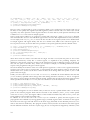
1.2.1
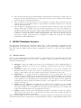
Modeling in SystemC
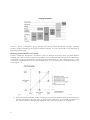
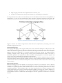
``SystemC is a system design language that has evolved in response to a need for a language that improves
overall productivity for designers of electronic systems'' (1). SystemC offers real productivity gains by
letting engineers design both the hardware and the software components together as they would exist on
the final system, but at a higher level of abstraction. This means that it is possible to concentrate on the
actual functionality of the system more than on its implementation details. Moreover, since the detailed
implementation has not been finalized yet, it is still possible to perform consistent changes to the system,
enabling an effective evaluation of different architectural alternatives (including the partitioning of the
functionalities between hardware and software). SystemC is also characterized by a high simulation speed;
note that this high simulation speed is not only due to the SystemC language itself, but it is mainly caused
by the high level system descriptions enabled by the use of SystemC.
5
Figure 1-1: Comparison among SystemC and other HDLs
Figure 1-1 shows a comparison among SystemC and other hardware description languages. Although
SystemC supports modeling at the register-transfer level (RTL), it is more often used for the description at
higher abstraction levels.
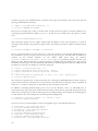
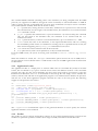
Modeling Styles and Abstraction Levels
SystemC enables the description of hardware systems at different abstraction levels and with different
modeling styles. The accuracy of SystemC descriptions can be independently analyzed on two dimensions:
communication among the components and their internal functionality (i.e. the computation aspect of the
component). Gajski introduces in (2) such modeling styles, by representing them in a diagram such as the
one in Figure 1-2.
Figure 1-2: Orthogonality of computation and communication aspects in SystemC descriptions
1) System Architectural Model (SAM): no timing is used in the description, both the communication
and the functionality take zero time. At this level we simple have an executable specification of
the system; behavior is modeled algorithmically. This style corresponds to A in Figure 1-2.
6
2) System Performance Model (SPM): timed executable specification of the system; communication
takes place in zero time, while approximate timing 1 annotation is used for the functionality. This
style corresponds to B in Figure 1-2.
3) Bus arbitration (BA): approximate timing annotation is used for modeling communication. This
style corresponds to C in Figure 1-2.
4) Bus Functional (BF): approximate timing is used to describe model functionality, while pin- and
cycle accurate, interfaces connect the models together. This style corresponds to D in Figure 1-2.
5) Cycle Accurate (CA): communication still takes place through approximate timed interfaces, but
functionality is modeled with cycle accuracy. This style corresponds to E in Figure 1-2.
6) RTL: both functionality and communication are fully timed and synchronized with a global clock.
Every register, every bus, and every bit is described for every clock cycle. This style corresponds
to F in Figure 1-2.
Model
RTL (F)
CA (E)
BF (D)
BA (C)
SPM (B)
SPM (A)
Communication
CT
AT
CT
AT
UT
UT
Table 1-1: Timing in SystemC descriptions; note the correspondence with Figure 1-2
Functionality
CT
CT
AT
AT
AT
UT
Despite the ability of operating at all abstraction levels, SystemC is particularly powerful for the
description of systems at Transaction Level. We define Transaction Level Modeling (TLM) the modeling style
where at least one, between communication and computation, introduces an approximate concept of time
(B, C, D, E in Figure 1-2). Almost always, TLM designs serve as an executable platform that is accurate
enough to execute software on.
Verification Library
Beyond the inherent C++ features, SystemC comes with a verification library (SystemC Verification
Library, SVC) (3) with multiple useful features for generating stimulus and verifying the results. In
particular it offers:
• Data Introspection and callbacks enabling the manipulation of arbitrary data types in a consistent
way, including C/C++ built-in types.
• Guided randomization of stimulus values, which help the generation of appropriate stimulus for a
complete verification of the Device Under Test.
• Utility data-types.
• Transaction Recording for an off-line inspection.
1.2.2
Modeling at Transactional Level
The underlying concept of TLM consists of modeling only the details that are needed in the first stages of
the design. By avoiding going into too many details, design teams can obtain huge gains in simulation
speed. At this level, changes to the design are also relatively easy because the development team has not
yet delved in low-level details such as parallel bus implementation versus a serial bus.
As briefly described above, TLM data transfers are modeled as transactions (i.e. function calls) and the
interfaces do not have pin-level details. In other words, at transaction-level, the emphasis is more on the
functionality of the data transfers (what data is transferred and from what location) and less on their actual
1 An approximately timed model provides a reasonable (accuracy may vary) estimate of the time required to execute its
functionality or communication mechanism
7
implementation. Simulation at TLM is much faster than RTL because pin level detail is not present, model
descriptions are simpler and timing is not clock-driven.
According to the OSCI TLM 2.0 library (4) (soon to become an IEEE standard) there are mainly two
different modeling styles (in the standard called coding styles): Loosely Timed (LT) and Approximately
Timed (AT) . These style are distinguished by the abstraction level and by the timing accuracy at which
the external IP interface is described. Referring to Figure 1-2 and to Table 1-1, Loosely Timed
corresponds to Bus Arbitration, while Approximately Timed to Bus Functional. Note how going from
one level to the other involves refinement in the interface, but the structure of the IP does not necessarily
change; in particular, the internal IP structure is usually modeled at a behavioral level.
It is worth noting that the TLM 2.0 modeling styles trade-off between simulation accuracy and speed only
at the module boundary, i.e. it is possible to have fully behavioral models whose timing is described by an
interchangeable LT or AT interface.
Loosely Timed
When first defining a model of the system, the exact bus-timing details do not affect the design decisions,
so they can be left out of the model. At this abstraction level, every communication event (e.g. read/write
to/from a memory location) is modeled with a single transaction. The loosely-timed coding style is
appropriate for software development in an MPSoC environment. This coding style supports modeling of
timers and coarse-grained process scheduling, sufficient to boot and run an operating system. The most
important aspect of this coding style is that it supports temporal decoupling: each SystemC thread is allowed
to run ahead of SystemC scheduler, in a local “time warp”. In few words this means that the different
SystemC models of the architecture do not synchronize with each other at every clock cycle.
With Loosely-Timed interfaces, the synchronization mechanisms among the components of a system
introduce a continuous trade-off between the amount of temporal decoupling and the simulation speed.
It does not make much sense to require an accuracy of 100% at the interface of IPs described at this
modeling style since, anyway, the timing accuracy of the whole system will be compromised by the
temporal decoupling. Of course it is not possible to generalize the required accuracy, it depends from the
type of IP. For the processor model, for example, we will use an instruction accurate model: the static
amount of clock cycles is counted for each instruction (i.e. we shall count the number of cycles for which
the instruction is in the execute stage, for example 4 for the multiplication instructions of the LEON3
processor) and pipeline details are not considered.
Approximately Timed
At this level the number of bus cycles is important: the information that the bus transfers for each clock
cycle is grouped in one transaction; this coding style is appropriate for the use case of architectural and
performance analysis. At this level a transaction is broken down into multiple phases (corresponding to
bus transfer phases), with an explicit synchronization point marking the transition between phases. This
coding style does not use temporal decoupling. Despite its name, this coding style can accurately model
the timing of the communication. For the processor model, for example, we propose to take into account
the pipeline structure and to correctly model hazards among instructions, etc. This anyway does not mean
that the IP-model will be described at an RTL level, only that the timing obtained at the interface is
correct.
Use Case
Software Development
Software Performance Analysis
Hardware Architecture Analysis
Hardware Performance Verification
Table 1-2: Mapping between use cases for transaction level
8
Coding Style
Untimed / Loosely-Timed
Loosely-Timed
Loosely-Timed / Approximately-Timed
Approximately-Timed / RTL
Table 1-2 summarizes the mapping between use cases for transaction level modeling and coding styles.
Note that, apart from the described modeling styles, all the techniques cited into the TLM 2.0 Standard (4)
(namely Direct Memory Access and Debug Interface) for improving simulation speed, controllability, and
observability over communication among the IP-models should be taken into consideration (and
employed whenever possible) when modeling SystemC IP-models at Transaction Level.
1.2.3
Verification and Testing
As it is normal for standard software designs, the verification activity occupies a consistent portion of the
development schedule. When developing models of hardware IPs, the situation is made even worse since
we are not only interested in verifying the functionality but also the timing accuracy of the generated
models. Another difference with respect to standard software testing is that, usually, golden models (the
actual RTL implementation) of each IP that we want to model are available. Having said all this, several
activities shall be used to properly check and verify the developed models with respect to the golden ones.
Traditional Software Testing Techniques
SystemC is nothing but a C++ library written using the C++ language; as such, IP models written in
SystemC are software programs. The techniques traditionally used for software testing (5) can, thus, be
successfully applied to the testing of SystemC IPs. In particular we suggest to test every single routine of
the IP model using both white and black box testing techniques (i.e. testing, respectively, the internal
structure of the code or only considering the IP interface). Many unit testing libraries are freely available
(e.g. Boost Test Library, CppUnit, etc.) to help in the task; the Boost Test Library was chosen for this
activity.
Using Test-Benches
Most of the IP-models described in SystemC (in general all the passive or peripheral IPs, which respond
only to external events, such as memories, UARTs, etc.) can be tested using testbenches: a testbench
generates the stimulus for the device under test (DUT) in order to set-up the scenario in which the DUT's
behavior is monitored. The testbench should also take care of verifying the result of the test. The testing
methodology using test-benches and the one using software unit testing are complementary: with testbenches the aim is the verification of the overall functionality of the IP, while during unit test we test each
routine of the IP model independently from the rest of the system.
Co-Verification
We can and have to take advantage of the availability of golden models (if possible) and verify both the
functionality and the timing accuracy of the IPs with respect to the RTL IPs. Such a verification, is not
always possible or easy to perform and, in general, it depends on the particular IP under analysis. For
instance, the developer should take into account that SystemC models are developed at transactional level,
thus transactors should be used to transform the information exchanged by the IP in a format comparable
with the input/output of the RTL golden model or of the eventually employed testbench. During this
activity, co-verification against the processor RTL model was deemed to complex.
Timing Verification
This is probably the most critical point in the verification activity of SystemC IP models for mainly two
reasons:
1. for functional verification we clearly want a behavior which is 100% correct from an external
perspective; on the other hand the timing objective is not that clear: slightly sacrificing timing
accuracy for simulation speed is usually acceptable at TLM. So the question is, what is an acceptable
accuracy?
2. it is not always easy to set-up an environment for the timing comparison between the SystemC IP
and the relative RTL reference model. This is particularly true for active IPs, such as processor
9
models. Moreover, timing does not only depends on the current inputs but it often depends also
on the internal status of the system
In general it is not possible to define a priori guidelines for timing assessment and verification, but ad-hoc
solutions have to be determined for each IP and for the different abstraction levels at which it is specified;
we can say that speed should be preferred to accuracy for loosely timed models; however, even the
accuracy of LT models should be characterized. When, instead, the approximately timed modeling style is
used, at the IP interface we should be able to observe an accuracy close to 100% (again, depending on the
IP, a 100% accuracy can be required, while for some other IPs a skew of 2.5% can be tolerated). For
certain components (usually for simple, passive components such as UARTs) it is also possible to use the
same behavioral core with two different interfaces, LT and AT, without affecting the overall simulation
speed or reducing the overall simulation accuracy.
1.3
Processor Modeling using Architectural Description Languages
Instruction Set Simulators (ISS) are high level models of hardware processing units; such models could be
hand-crafted, but this is a tedious, lengthy, and error-prone task because instruction-set simulators are
complex pieces of software which are difficult to write, debug, and maintain (6). In particular, the
application of optimization techniques for speeding up the simulation, like, e.g., flattening the instructioncoding tree, makes manual changes to the simulator code extremely prone to error.
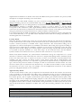
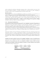
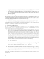
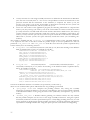
For those reasons Architecture Description Languages (ADLs) have been devised to enable automatic
generation of tools to support the design process starting from high-level abstract descriptions. Such
descriptions enable the generation of other tools in addition to ISSs, aiding processor's development flow:
(a) Instruction Set Simulators, ISSs, (simulating the functionality of the real processor), (b) Register
Transfer Level models (enabling hardware synthesis of the described processor), (c) Compilers, and (d)
Model Checkers, Formal Verifiers, etc.
Figure 1-3: ADL-based design methodology
Partly automating the processor design process and centralizing its specification into a single, formal, and
high level description brings numerous advantages:
• Speeds-up the exploration and the evaluation of the different design alternatives.
• Aids the validation of early design decisions.
10
•
•
Helps keeping the model and its implementation consistent, and
It improves communication among team members, by centralizing the specification.
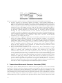
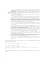
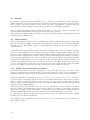
In the past decade many ADLs were introduced, each one with different characteristics and capabilities; as
described in (7), they can be classified into three categories: structural, behavioral, and mixed; this
classification is based on the nature of the information that the developer has to provide (see Figure 1-4).
Figure 1-4: Classification of Architectural Description Languages
Figure 1-4 shows also another categorization, which will be not explored here, consisting of the tools
which the languages can create.
Structural Languages
The languages belonging to this category mainly focus on the structural description of the processor: they
capture the structure in terms of architectural elements and of their connectivity. In the trade-off between
level of abstraction and generality, the latter is favored by lowering the abstraction level of the description.
Register transfer level (RT-level) is a popular abstraction level, lower enough for detailed behavior
modeling of digital systems, and high enough to hide gate-level implementation details; at this level of
abstraction operations are represented as data movements among registers or between registers and
storage units, and as arithmetical or logical data transformations.
While structural ADLs are suitable for hardware synthesis and cycle-accurate simulation, they are unfit for
functional simulation and retargetable compiler generation, since abstracting the high level behavior of the
operations from the low level detailed description is almost infeasible. Most of the earliest ADLs belong
to this category.
Behavioral Languages
Behavioral languages avoid the difficulty of extracting the instruction set information from an RT-level
description by abstracting the behavior information out of the micro-architecture: the instructions'
semantics are explicitly specified, while detailed hardware structures and timing information are almost
completely ignored by these languages. This is also their main limitation: an accurate estimation of the
system performance can no more be performed and the possibility of creating cycle accurate simulators or
synthesizable hardware descriptions is also almost eliminated. Typically there is a one-to-one
correspondence between a behavioral ADL description and the processor’s instruction-set reference
manual.
11
Almost all behavioral Architecture Description Languages share a common property: they all use some
kind of hierarchical mechanism to describe and represent the instruction-set, greatly simplifying its
description, which can, then, be implemented with a relatively moderate effort.
Mixed Languages
Mixed languages, such as LISA (8), EXPRESSION (9), MADL (10), and ArchC (11), as the name says, are
a mixture of the previous two types: they include both behavioral and structural information.
They try to benefit from the fact that behavioral languages do not need to infer the instruction set
architecture from an RTL description, and from the fact that structural descriptions easily take into
account timing details and other information, such as hazards between the instructions due to the
presence of the pipeline. These ADLs are suitable for various design automation activities, including
retargetable software toolkit generation (i.e., compilers, simulators, debuggers, etc.), exploration of design
alternatives, architecture synthesis, and functional validation.
1.3.1
Instruction Set Simulators
Even though all ADLs enable the generation of a wide range of instruments and tools aiding the design of
micro-processors, during system-level simulation we are particularly interested in Instruction Set
Simulators: for almost all computer architecture research and design, quantitative evaluation of future
architectures is possible only by using simulators. Such tools reduce the cost and time of a project by
allowing the architect to quickly evaluate the performance of a wide range of architectures (12).
Good simulators should be fast, accurate, faithfully predicting whatever metrics are being measured (i.e.
timing and power consumption), complete, modeling the entire system and being able to run unmodified
applications and operating systems, transparent, providing visibility into the simulated system, and easy-touse.
With respect to RTL or Gate-Level descriptions, ISSs eliminate much of the overhead by focusing on the
architecture status that is visible to programmers according to the Instruction-Set-Architecture; other
architectural features are only modeled when strictly necessary. Simulation performance is a key factor for
the overall design efficiency, given that ISSs are often the bottleneck of the overall simulation; much
research has, thus, focused on studying efficient mechanisms for managing simulation, improving its
speed.
Currently, the majority of ISS tools rely on the following techniques to carry out simulation (13):
interpretation, static compilation, and dynamic compilation. Interpretation offers the lowest simulation
speed (as at every new instruction issued has to be decoded), but adopting it for the description of a new
architecture can be relatively easy. The two compilation techniques, instead, translate instruction
sequences of the simulated architecture into machine instructions of the host machine. In the case of static
systems this is done offline, i.e. before the simulation is actually run. Dynamic compilation systems perform
this translation during the simulation run.
Figure 1-5: Interpretive simulation cycle
12
Figure 1-6: Compiled simulation cycle
Braun et al. (6) present a good overview of the different mechanisms driving ISS-based simulation:
• Interpretive Simulation: An interpretive simulator is basically a virtual machine implemented in
software, which interprets the loaded object code to perform appropriate actions on the host.
Similar to the operation of the hardware, an instruction word is fetched, decoded, and executed at
runtime (sequence of operations also called simulation loop), which enables the highest degree of
simulation accuracy and flexibility. However, unlike in real hardware, instruction decoding is a
very time-consuming task; especially for modern very large instruction word (VLIW) architectures
the decoding overhead dominates the simulation time. An interpretive simulator performs
decoding for every executed instruction; in some situations this represents an enormous
overhead: for instance, in applications with a high execution locality, the repeated decoding of a
static loop kernel for each iteration is redundant and slows down the simulation. To mitigate this
issue, an Instruction Buffer is often employed to keep track of the most recently decoded
instructions as, for example, done in (14).
• Compiled Simulation: A significant improvement in simulation performance has been achieved
through the compiled-simulation technique. The idea behind this technique is to shift timeconsuming operations from simulation-time into an additional step before the simulation (at
compile-time, during simulation generation). A simulation compiler performs the instruction
decoding at compile time, by analyzing each binary instruction word of the applicative program in
order to determine instructions, operands, and execution modes. Since compiled simulators
decode the entire application before simulation, the simulation time per instruction is much
reduced, consistently speeding-up simulation.
• Binary Translation: Binary translation is the instruction-wise, direct transformation of target
machine code into host machine code (15). In order to achieve this, the simulation compiler
employs a translation table containing the equivalent host instruction(s) for each target
instruction. Binary translation can be static or dynamic, that means, the entire target application
can be translated before simulation (i.e. compiled simulation), or the corresponding object code
can be generated just before a target instruction has to be executed. The latter brings greater
flexibility, since it can cope with runtime dynamic code. However, simulators based on binary
translation are highly target- and host- specific, which makes it very difficult to port them to a
new host platform. Generally, such simulators are not retargetable, although some of them have
proven to deliver high simulation performance and degree of flexibility. Braun et al. (6) show,
among the experimental results, that just-in-time compiled simulation reaches a simulation speed
more than one order of magnitude higher than traditional interpretive simulation.
2 Transactional Automatic Processor Generator (TRAP)
This Chapter presents TRAP (TRansactional Automatic Processor generator), a tool for the automatic
generation of processor simulators starting from high level descriptions. This means that the developer
only needs to provide basic structural information (i.e. the number of registers, the endianness etc.) and
the behavior of each instruction of the processor ISA; this data is then used for the generation of C++
code emulating the processor behavior. Such an approach consistently eases the developer's work (with
respect to manual coding of the simulator) both because it requires only the specification of the necessary
details and because it forces a separation of the processor behavior from its structure. The tool is written
13
in Python and it produces SystemC based simulators. According to the description given in Section 1.3,
TRAP is classified as a mixed language, requiring not only information about the behavior of the target
processor, but also some (limited) details about the structure in terms of architectural elements and their
connectivity.
The tool consists of a Python library: the processor specification is given through appropriate calls to its
APIs. With respect to standard ADLs, which use custom languages, directly specifying the input in Python
eliminates the need for an ad-hoc front-end; such feature simplifies the development of the ADL and its
use by the designer: (a) there is no need to learn a new language, (b) during model creation the full power
of the Python language can be exploited, and (c) no ad-hoc parser is needed.
The Instruction Set Simulators generated by TRAP are based on the SystemC library and on the new TLM
2.0 standard for modeling the processor's communication interfaces. Depending on the desired
accuracy/simulation speed tradeoff, different flavors of simulators can be created. With respect to the
already existing Architectural Description Languages, some of which are described in Section 1.3, TRAP
has the following advantages:
• it is Open Source,
• the descriptions are based on the Python language, enabling the use of the full capabilities of this
language and eliminating the need to learn a new language,
• it has simple structure, as it is restricted to generating only Instruction Set Simulators, and
• it is deeply integrated with SystemC and TLM libraries, generating processors based on the latest
hardware modeling technologies.
The rest of this Section will be devoted to presenting in detail the TRAP language itself and the structure
and peculiar features of the generated simulators.
2.1
Language Structure
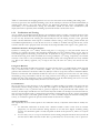
TRAP, as shown in Figure 2-1, is built as a library on top of the Python programming language. Instead of
defining our own language for the description of processor architectures, we implemented a set of
methods which should be called for creating the processor model. The architectural designer greatly
benefits from such an organization in that it can exploit a fully-fledged programming language: not only
TRAP's directives are allowed in processor description, but any valid Python statement can be used.
Moreover there is no need to learn a new language, reducing the learning curve when starting using TRAP.
14
Figure 2-1: Architecture of the TRAP language
Three elements compose a processor model in TRAP:
1. architecture description, where the structural elements (registers, pipeline stages, etc.) are described.
2. ISA coding, specifying the encoding of each instruction.
3. ISA behavior, which contains the behavior of each instruction.
A fourth element, ISA testing, can be part of a TRAP description; ISA testing defines the tests to be
applied to the Instruction Set description to make sure that it has been correctly implemented.
Once completed, the Python files containing those elements are “executed” (remember that they are
composed of calls to TRAP APIs): the whole TRAP description can indeed be thought as a Python
program having the aim of producing text files containing the C++ code implementing the processor
simulator. During the execution, TRAP's intermediate representation is created, in the form of Python
objects; in a subsequent phase such objects are translated, thanks to our cxx_writer library, into C++
code implementing both the simulator and the tools helping in the tasks of architectural analysis and of
embedded software development.
2.1.1
Processor Architecture Description
TRAP, being a mixed ADL, requires a minimum amount of structural details, restricting them only to
what is strictly necessary in order to enable generation of functional and cycle-accurate simulators and of
the necessary support tools (described later in detail in this document).
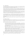
Here we show an example of the LEON3 architecture description; note how it is exclusively composed of
calls to TRAP APIs and that it is written in pure Python language:
01.
02.
03.
04.
05.
06.
07.
08.
09.
10.
15
processor = trap.Processor('LEON3')
processor.setBigEndian()
processor.setWordsize(4, 8)
globalRegs = trap.RegisterBank('GLOBAL', 8, 32)
processor.addRegBank(globalRegs)
tbrBitMask = {'TBA' : (12, 31), 'TT' : (4, 11)}
tbrReg = trap.Register('TBR', 32, tbrBitMask)
tbrReg.setDefaultValue(0)
processor.addRegister(tbrReg)
regs = trap.AliasRegBank('REGS', 32, ('GLOBAL[0-7]', 'WINREGS[0-23]'))
11.
12.
13.
14.
processor.addAliasRegBank(regs)
fetchStage = trap.PipeStage('fetch')
processor.addPipeStage(fetchStage)
..........................
Few details need to be modeled: (i) the number and size of the registers, (ii) the internal memory and/or
the memory ports, (iii) the interrupt ports with the behavior associated with the interrupts, and (iv) the
pipeline stages, with the possible hazards, as shown below.
Depending on the complexity of the processor and/or on the desired accuracy of the simulator, more
elements might need to be inserted in the description:
• Application Binary Interface, which encodes the standard conventions for register usage, stack frame
organization, and function parameter passing of software programs running on the processor
being described.
• External PINs, defining additional ports with which the processor communicates with the rest of
the system.
Hazards
Two kinds of hazards exist in a simple RISC processor (which, currently, is the target of TRAP): data
hazards and control hazards. TRAP automates their management as much as possible in order to enable
effective, simple, and efficient specification of such situations.
Data Hazards are created whenever there is a data dependence between instructions, and they are close
enough that the overlap caused by pipelining would change the order of access to the operands involved
in the dependence. This, for example, means that if instruction A produces a result used by B, then B has
to delay execution until A has terminated. In order to enable TRAP-based processor simulators to deal
with it, the processor designer has to take two actions:
1. specification of the pipeline stages where registers are read from the register file and written back
into it (the latter one commonly called “write back stage”): such stages are the decode and the write
back ones for the LEON2 and LEON3 processors.
2. specification, for each instruction, of what are the input and output operands and, in case there
are any, of what are the other read or modified registers (such as, for example, the processor
status register, register PSR, in the LEON2/3 architecture).
With such data TRAP generates the simulator so that the pipeline is stalled in case instruction A has not
yet reached the write back stage before B enters the register read stage. An exception to this rule is raised
when register bypasses exist; a register bypass is a mechanism through which the result of an instruction A is
available to a following instruction B before A has actually written such result to the register file. In such
situation the developer has to manually “unlock” the pipeline when the result is written to the bypass
register.
A Control Hazard determines the ordering of an instruction (for example C), with respect to a preceding
branch instruction so that the instruction C is executed in the correct program order and only when it
should be. As opposed to the automatic management of data hazards, the processor designer has to
manually deal with such situations, depending on the behavior of the processor being modeled. The most
common action consists of flushing the pipeline in case the branch is taken (so in case the next instruction
to be executed does not correspond to the next instruction in memory); note that this is not necessary in
the LEON2/3 processor models as a branch instruction is resolved in the decode stage and there is the
presence of a one instruction long delay slot: this means that the instruction in the fetch stage will be always
execute no matter what is the outcome of the branch instruction being resolved in the decode stage, so
there is no need to perform any flush.
Interrupts
Interrupt modeling is necessary for the execution of an Operating System on top of the generated
simulators and, in general, for the correct modeling of a LEON-based System-on-Chip; interrupts are
16
necessary for correct communication with most system peripherals, in particular, at least, with a timer,
generating the clock which enables the OS to keep track of time. The notion of time can be used, for
example, to manage the time quantum associated to threads/processes in a multi-threaded environment.
As for the behavior of the instructions, the reaction of the processor to an incoming interrupt signal is
specified using C++ code, in an analogous way to what happens for standard instructions.
Application Binary Interface (ABI)
The ABI specifies the rules with which the tools (compiler, debugger, etc.) access and use the processor
and with which the compiler compiles the software (for example the routine-call conventions). Two types
of information are encoded in the ABI:
• conventions concerning the software used on the processor architecture, and
• correspondence among the elements of the description and the architectural elements used in the
ABI.
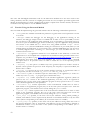
For example, the following code (taken from the LEON2/3 descriptions) specifies that register 24, in
registers bank called REGS in the description, holds the routines’ return values, registers 24-29 hold the
routine arguments, and that registers called PC, LR, SP, and FP in the description hold the program
counter, the link register, the stack pointer, and the frame pointer, respectively. Finally, the
correspondence among GDB register numbers and the registers in the description is given.
01.
02.
67,
03.
abi = trap.ABI('REGS[24]', 'REGS[24-29]', 'PC', 'LR', 'SP', 'FP')
abi.addVarRegsCorrespondence({'REGS[0-31]': (0, 31), 'Y': 64, 'PSR': 65, 'WIM': 66, 'TBR':
'PC': 68, 'NPC': 69})
…………………………………………………………
In synthesis the ABI description enables:
1) generation of a debugger interface to enable the use of the GDB debugger for checking the
correctness of the software running on the ISS;
2) system call emulation: by knowing the convention with which function calls are implemented, it is
possible to inhibit the execution of Operating System related calls on the ISS and forward them to
the host environment, thus enabling simulation of software without the need to also simulate an
OS;
3) generation of a software profiler, for gathering statistics on the software running on top of the
instruction set simulator.
If such tools are not going to be used, then you can avoid specifying the ABI.
2.1.2
Instruction Set Description
The instruction set description is organized into two parts: encoding and behavior description. Following
what introduced in most ADLs (8) both descriptions are given in a hierarchical way: the specification is
given only for the basic building blocks, which are, then, composed into the final instructions. Such
organization consistently reduces the development efforts and it simplifies the description.
01. opCodeRegsImm = cxx_writer.writer_code.Code("""
02. rs1_op = rs1;
03. rs2_op = SignExtend(simm13, 13);
04. """)
05. opCodeExec = cxx_writer.writer_code.Code("""
06. result = rs1_op + rs2_op;
07. """)
08. add_imm_Instr = trap.Instruction('ADD_imm', True, frequency = 11)
09. add_imm_Instr.setMachineCode(dpi_format2, {'op3': [0, 0, 0, 0, 0, 0]}, ('add r', '%rs1', '
', '%simm13', ' r', '%rd'))
10. add_imm_Instr.setCode(opCodeRegsImm, 'regs')
11. add_imm_Instr.setCode(opCodeExec, 'execute')
12. add_imm_Instr.addBehavior(WB_plain, 'wb')
13. add_imm_Instr.addBehavior(IncrementPC, 'fetch', pre = False)
17
14.
15.
16.
17.
add_imm_Instr.addVariable(('result', 'BIT<32>'))
add_imm_Instr.addVariable(('rs1_op', 'BIT<32>'))
add_imm_Instr.addVariable(('rs2_op', 'BIT<32>'))
isa.addInstruction(add_imm_Instr)
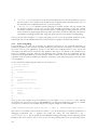
This code shows an example of the ISA description for the LEON3 processor; note how only the
instruction specific behavior is explicitly given, while the other parts are specified using behaviors (which
are like methods in standard high level languages); this consistently simplifies the description and
improves its clarity and conciseness since behaviors can be used for multiple instructions. Instructions
encoding is given in terms of “generic machine codes”: instructions are first divided into categories (e.g.
data processing, load/store instructions, etc.) and, for each category, the bits are grouped according to
what they refer to (opcode, register operands, etc.). The group(s) uniquely identifying each instruction are,
then, assigned a value during the specification of the instruction itself. In the following we show the
machine code for the branch and sethi instructions of the LEON3 processor: note how the first two
bits are fixed for both these instructions and thus they are specified in the machine code; instead, bits
called op2 specify if we are dealing with the branch or sethi instruction and, as such, those bits are assigned
a value during the specification of the instruction itself.
01. b_sethi_format1 = trap.MachineCode([('op', 2), ('rd', 5), ('op2', 3), ('imm22', 22)])
02. b_sethi_format1.setBitfield('op', [0, 0])
03. b_sethi_format1.setVarField('rd', ('REGS', 0), 'out')
Machine-Code Decoder
The machine-code decoder is the simulator portion responsible for instruction decoding, which means
associating the bits which represent each machine instruction in the executable application to the
instruction itself. the implementation of the decoder is of particular importance since, often, instruction
decoding is the speed bottleneck of the whole simulation, being an operation repeated for each executed
instruction. TRAP implements the decoding algorithm devised in 2003 by Qin and Malik (16) by
constructing a min-cost search tree with carefully chosen decoding primitives and cost models. The
algorithm has no limitation on the input instruction patterns and it requires only the least amount of
knowledge about the instruction encoding. Decoding is the process of traversing the tree from the root to
the leaf which contains the identifier of the instruction; traversing is done on the basis of the machine
code to be decoded and using the “decision function” associated with every node. Two kinds of decision
functions are determined in (16): (1) pattern decoding, obtained by matching the machine code with a
specified pattern: two edges (True or False) can exit from such a node and (2) table decoding, using m
contiguous bits of the machine code as identifiers of the edge to be taken: as such there are 2^m edges
exiting from such a node.
In order to decide, for each node, what is the best decoding function, a cost model, which takes into
consideration both decoding speed and memory usage, is devised. The decoding speed can be
approximated by the average length of the path from the current node to the reachable leaves; such a
length is measured by the Huffman tree corresponding to the partial bit string associated with the node.
For what concerns memory usage, we have to discriminate between pattern decoding (consuming 1 unit
of memory) and table decoding, consuming 1 + 2^m units. Weights are used to give more or less
importance to memory consumption with respect to decoding speed. Heuristic rules are also used to
reduce the space of the possible decoding functions, thus enabling generation of the decoding tree in a
reasonable time.
A peculiarity of the algorithm consists of the fact that multiple leaves might map to the same instruction:
depending on the variable parts of the machine code (i.e. the operands) the decoding process might endup in different leaves, all, anyway, mapped to the same correct instruction: this features might increase
memory usage, but it reduces the height of the tree. Depending on the user-defined weights given to the
cost functions (decoding speed and memory usage), the tradeoff between memory and speed is varied,
generating the best performing decoder for each instruction set (even though results, as shown later, the
18
overall simulation speed is not influenced much by such weights). Refer to paper (16) for more details on
the algorithm devised to build the instruction decoder.
Once all the three elements of the specification (architecture description, ISA coding, and ISA behavior)
are given, the chosen types of Instruction Set Simulators can be created by automatically translating the
high level TRAP specification into the C++ code implementing the simulator, as detailed in Section 3.5.
2.2
Generated Processors
The Instruction Set Simulators generated by TRAP are based on the SystemC library and, for modeling
the processor's communication interfaces, on the new OSCI TLM 2.0 standard. Depending on the
accuracy of the input specification and on the developer needs, different simulators can be created:
1) Functional (or Standalone) without the use of SystemC: this model cannot be plugged in a
system-level simulation platform, and it can just be used for the emulation of the described
processor, with the aim of validating and debugging software. No performance results can be
extracted from such a model, apart from statistics concerning the number of executed instructions.
2) Instruction Accurate with Loosely Timed (LT) or Approximately Timed (AT) TLM 2.0 interfaces;
such models exhibit high simulation speed, but limited timing accuracy, since only static timing is
considered, and dynamic events, such as pipeline stalls and hazards, are not taken into account.
When LT interfaces are used, temporal decoupling mechanisms improve simulation speed, at the
expense of an approximate synchronization of events when the ISS is inserted in a Multi-Processor
environment. Refer to the OSCI TLM 2.0 standard for more details on the temporal decoupling
mechanisms.
3) Cycle Accurate with AT interfaces, enabling accurate timing with respect to both the
communication with external memories and the processor structure (pipeline stages, hazards,
bypasses, etc.). Such a model is more than one order of magnitude slower than the Instruction
Accurate versions.
Generated processors are written according to the object-oriented programming paradigm using C++
code. The processor module contains the fetch/decode/execute main loop; for the cycle accurate version of
the processor this corresponds to activating the different pipeline stages. The processor module is also the
place where the architectural elements (registers, ports, memories, etc.) are instantiated.
Three of the most interesting and useful features of TRAP, not possessed by many other ADLs, are:
1) automatic detection of data hazards (as described above),
2) support for alias registers, and
3) support for interrupt modeling.
2.2.1
Alias Registers
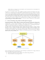
Alias Registers are special types of registers having no correspondence in the physical architecture, but
helping and simplifying the description of the processor behavior and the implementation of the
simulator. This features is used when the architecture being modeled has n registers but only k < n are
visible at a time: in such a situation k aliases and n registers are declared and, depending on the processor
status, the visible k registers, among the n ones, are mapped to the k aliases; in this way the Instruction Set
description can simply refer to the k aliases, without the need to directly access the registers they are
currently mapped to. The processor description only needs to deal with standard registers when updating
the aliases. This mechanism, in addition to consistently easing the developer's job, speeds-up simulation
since it removes the need to check, inside every instruction, what are the k registers, among the n, which
need to be accessed.
19
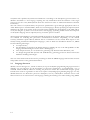
Figure 2-2: Alias mechanisms for dealing with the register windows of the LEON3 processor.
The register window mechanisms of the LEON2 and LEON3 processors, described in Figure 2-2, is a
good example for such mechanism; only 32 registers are visible at a time, 8 belonging to the GLOBAL
register bank and 24 out of the 128 of the general purpose registers. In order to uniformly access the 32
registers, a 32 registers wide alias bank was declared, and all the ISA instructions access it without any
knowledge of the two register banks. When appropriate (e.g. in presence of routine calls), the aliases are
updated to point to the correct registers.
2.2.2
Interrupt Modeling
Interrupts necessarily have to be taken into account in order to effectively test and analyze applications
featuring communication with peripherals, sensors, etc. as are most embedded systems. Moreover, a
correct modeling of interrupts is required for the simulation of Operating Systems. Interrupt handling is
trivial and it mainly consists of two steps: declaration of interrupt ports and implementation of the
behavior triggered by the interrupt itself. Interrupt ports can be specified as TLM 2.0 ports and,
depending on the architecture being described, they can either carry Boolean values (triggered or not
triggered) or other types (e.g. integer values). Instruction Accurate simulators react to interrupts by
checking their status (if they have been triggered or not) at the beginning of the processor main loop,
before the issue of every new instruction. Cycle Accurate simulators, instead, check for the interrupt
presence before fetching new instructions; again no other special actions are executed, and only the
behavior specified by the developer is taken into account.
The LEON2/3 processor models, for example, declare a single interrupt port carrying an integer value:
the value associated to the interrupt (between 1 and 15) specifies the interrupt priority.
2.2.3
Decoding Buffer
The simulator incorporates a Decoding Buffer for caching individual decoded instructions, thus avoiding the
need of re-decoding them when re-encountered. With this mechanism, shown in the pseudo-code below,
the slow instruction decoding process is amortized by the high hit rate of the buffer.
01. while(True){
02.
Fetch Instruction
03.
if(Instruction in Buffer){
20
04.
05.
06.
07.
08.
09.
10.
11.
12.
13.
14.
15.
16. }
Execute From Buffer
}
else{
Decode Instruction
Execute Instruction
if(Instruction Count > threshold){
Add Instruction to Buffer
}
else{
Increment Instruction Count
}
}
TRAP's decoding buffer is implemented through a hash map (part of the standard C++ library) indexed
by the machine code of the instruction: this mechanism has the advantage that, with respect to using the
program counter as an index, equal instructions, located at different points in the program, result in cache
hits; in addition, self-modifying code does not need special handling for its execution. Using the decoding
buffer, anyway, has a cost, given by the insertion of a new entry in the buffer, and by the search of an
entry, the latter one being proportional to the total number of entries present in the buffer itself. For such
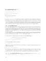
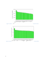
a reason, only the instructions most often used shall be added to the buffer: a heuristic was found, that
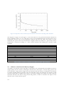
adds an instruction to the buffer if it has been encountered at least n = 256 times. Experimental results
show, as in Figure 5-6, how different configurations of the heuristic (i.e. different values of n) affect the
overall simulation speed.
Figure 2-3: Standard Fetch/Decode/Execute loop
Figure 2-4: Fetch/Decode/Execute loop using the decoding buffer
2.2.4
Helper Tools
In addition to the processor model itself, a number of helper tools are necessary in order to effectively use
the ISS for software development, performance evaluation, etc. TRAP provides these tools in a runtime
library interfaced with the ISS thanks to an automatically generated interface. This interface, based on the
data provided by the user in the ABI description, specifies the mapping between architectural elements
21
(e.g. registers), as seen by GDB and by the compiler, and the variables representing these elements in the
ISS code. So far three tools are provided:
OS emulator
Operating System Emulation is a technique which allows the execution of application programs on an
Instruction Set Simulator (ISS) without the need to simulate a complete OS. The low level calls made by
the application to the OS routines (system calls, SC) are identified and intercepted by the ISS, and then
redirected to the host environment which takes care of their actual execution. Suppose, for example, that
the application program that we need to execute on top of the simulated architecture contains a call to the
open routine to open file “filename”. Such a call is identified by the ISS using the mechanisms described
below and routed to the host OS, which actually opens “filename” on the PC's filesystem. The file handle is
then passed back to the simulated environment for the use by the application program. Having an
Instruction Set Simulator with System Call Emulation capabilities allows the application developers to
start working as early as possible, even before a definite choice about the target OS is performed. These
capabilities are also used for ISS validation, by enabling fast benchmark execution.
Debugger
A debugger is a tool used for the analysis of software programs in order to catch errors and, possibly, help
correcting them. Being used for software development, Instruction Set Simulators often feature a
debugger; TRAP was integrated with the GNU/GDB (17) debugger using its capabilities of connecting to
remote targets through TCP/IP or serial interfaces (the same mechanisms used to debug software running
on physical boards). The ABI specification provides the information necessary for interpreting GDB
requests with respect to the architecture being modeled.
Profiler
Debugging is not the only useful activity during software development: profiling is necessary to determine
application's bottlenecks; such an activity can be used also for hardware optimization, for example by
moving computational-intensive routines from the software to the hardware domain, or for optimizing the
single processor instructions which are executed more often. A profiler, communicating with the
Instruction Set Simulator through the information specified with the ABI, enables function profiling, call
graph generation, and statistics gathering on the single assembly instructions.
Automatic Instruction Testing
Another important feature of TRAP consists of the automatic generation of the tests for each ISA
instruction: the developer only needs to specify the processor state (in terms of the registers relevant to
the instruction under test) before the execution of the instruction and the desired state after the
instruction execution. TRAP takes care of automatically generating the C++ code which initializes the
status of the processor and the relevant portions of each instruction, executes the instruction, and finally
checks if the execution yields the expected results. Per-instruction testing increases the confidence in the
correctness of the simulator and, in case of implementation bugs, it consistently reduces the effort needed
to locate and correct the problem.
2.3
Tutorial: processor modeling using TRAP
This Section aims at explaining, with examples, how to describe a processor model with the TRAP
language; the shown snippets of code are taken from the description of the LEON3 processor.
2.3.1
Describing the Architecture
The architecture description consists of the indication of the registers, ports, and issue width of the real
processor. Not much information is needed in this section since we target the generation of high level
22
simulators (more details would be needed, for example, for the generation of RTL code); see file
LEON3Arch.py for the complete description of the LEON3 architecture.
import trap
Let’s import the core trap modules; note that if they are not in the standard python search path we can
specify their path using the instruction sys.path.append(trap_path) before the import directive.
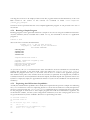
We can, then proceed with the actual creation of the processor:
01. processor
= trap.Processor('LEON3', version
instructionCache = True, cacheLimit = 256)
02. processor.setBigEndian()
03. processor.setWordsize(4, 8)
04. processor.setISA(LEON3Isa.isa)
=
'0.2.0',
systemc
=
False,
This means that the processor will be called LEON3 and that the current version is 0.2. SystemC will not
be used for keeping time, so all will be executed in the same delta cycle; this option is valid only for
Instruction-Accurate descriptions and it cannot be used if TLM ports are employed for communication
with external IPs. Note how SystemC will not be used for keeping time, but the structure of the
architectural components will anyway be based on this library. At processor construction we also indicate
that the decoding instruction buffer shall be used; it is simply a buffer holding already decoding
instructions in order to avoid re-decoding them. The use of the decoding buffer consistently speeds up
simulation. We also specify the threshold of the decoding buffer: after an instruction has been
encountered that number of times it is added to the buffer. The other two instructions are selfexplanatory: we are going to describe a big endian system with 4 bytes per word, 8 bits per byte. Finally
the Python object holding the Instruction Set Architecture (ISA) Description is indicated. Additional
parameters can be specified during processor construction, see the TRAP source files for more details.
Optionally the following directives can also be used to further customize the generated processor:
processor.setIpRights('esa', 'Luca Fossati', '[email protected]', banner)
processor.invalid_instr = LEON3Isa.isa.instructions['UNIMP']
processor.setPreProcMacro('tsim-comp', 'TSIM_COMPATIBILITY')
processor.setBeginOperation(‘… some C++ code …’)
LEON3Isa.isa.addConstant(cxx_writer.writer_code.uintType, 'NUM_REG_WIN',
numRegWindows)
01.
02.
03.
04.
05.
Line 1 specifies that the produces simulator will be released under a specific ESA license, lists the
author(s), its e-mail address and the banner to be printed in the header of each generated file.
Line 2 specifies what is the behavior to be associated to each pattern not recognized by the instruction
decoder; in this case we instruct TRAP to associate the behavior described in the 'UNIMP' instruction.
Line 3 customizes the compilation steps, adding the configuration switch tsim-comp: when used it
triggers the definition of the TSIM_COMPATIBILITY macro.
Line 4 specifies some C++ code which is executed at the beginning the simulation (e.g. to perform some
initialization, etc.)
Finally, Line 5 describes a constant which is visible from all the instructions and which can be used from
the code defining the instruction behavior.
Now we can start describing the architectural elements:
01. globalRegs = trap.RegisterBank('GLOBAL', 8, 32)
02. globalRegs.setConst(0, 0)
03. processor.addRegBank(globalRegs)
04.
23
05. psrBitMask = {'IMPL': (28, 31), 'VER': (24, 27), 'ICC_n': (23, 23), 'ICC_z':
(22, 22), 'ICC_v': (21, 21), 'ICC_c': (20, 20), 'EC': (13, 13), 'EF': (12, 12),
'PIL': (8, 11), 'S': (7, 7), 'PS': (6, 6), 'ET': (5, 5), 'CWP': (0, 4)}
06. psrReg = trap.Register('PSR', 32, psrBitMask)
07. psrReg.setDefaultValue(0xF3000080)
08. processor.addRegister(psrReg)
Here we create a register bank (a group of registers) called GLOBAL composed of 8 registers each one 32
bit wide; we also specify that register 0 (the first argument) will be constant and set to value 0 (the second
argument): any write operation on this register will have no effect and any read operation will always read
0. Method setConst also exists for simple registers.
Next a single register called PSR is created: it is 32 bit wide. Note how a mask (psrBitMask) is defined:
this mask easies the access to the individual registers bits: from the ISA implementation code (see below)
we can simply write PSR[key_CWP] to access the five four bits of the regsiter (masks can be defined both
for simple registers and register banks). We also set a default value, which is the value that register PSR
have at processor reset; As shown below it is possible to also specify special keywords as default values.
01.
02.
03.
04.
05.
06.
07.
regs = trap.AliasRegBank('REGS', 32, ('GLOBAL[0-7]', 'WINREGS[0-23]'))
regs.setFixed([0, 1, 2, 3, 4, 5, 6, 7])
regs.setCheckGroup()
processor.addAliasRegBank(regs)
FP = trap.AliasRegister('FP', 'REGS[30]')
FP.setFixed()
processor.addAliasReg(FP)
These lines create two aliases: one bank and one single. An alias is used (from the point of view of the
processor instructions) exactly like a normal register, as explained in the preceding Chapters; the
difference is that, during execution, an alias can be remapped to point to different registers (or aliases: an
alias can also point to another alias). Aliases are useful, for example, for handling architectures which
expose to the programmer only part of their registers.
Note how initially the 32 aliases of the REGS bank point to registers 0-7 of the GLOBAL register bank and to
registers 0-23 of the WINREGS register bank. FP (representing the frame pointer) points to the alias 30 in
the alias bank REGS (in this case we have a chain of aliases: if we change what REGS points to, also FP will
point to the new target).
Finally, note the calls to the setFixed and setCheckGroup methods: the former indicates that the alias
(or set of aliases) specified cannot change their value during simulator execution, i.e. the set of registers
they point to cannot change; the latter method, instead, specifies that the whole alias bank (apart from the
aliases specified in the body of setFixed) has to be checked to see if the aliases have to be updated.
01.
02.
03.
04.
pcReg = trap.Register('PC', 32)
pcReg.setDefaultValue('ENTRY_POINT')
pcReg.setWbStageOrder(['exception', 'decode', 'fetch'])
processor.addRegister(pcReg)
For aliases and registers we can set default values; in this case we use a special default value: it is the entry
point of the software program which will be executed on the simulator (ENTRY_POINT). Other special
values are PROGRAM_LIMIT (the highest address of the loaded executable code) and PROGRAM_START (the
lowest address of the loaded executable code).
In addition we can see the call to the setWbStageOrder method to specify that this registers is not
propagated in the standard way among pipeline stages; normally register values are written in the register
file in the write back stage, and read from it in the decode stage (this holds for the LEON3 processor, as we
will see that more in detail later). The program counter, instead, needs to be written in the main register
file into different moments: from the exception stage (in case an exception has happened), otherwise, if the
24
exception stage has not modified the PC, from the decode stage (for branches) and, in the end, from the
fetch stage (standard PC increment).
01. regMap = trap.MemoryAlias(0x400000, 'Y')
02. processor.addMemAlias(regMap)
Here we have another type of alias: a memory alias. It maps processor registers to memory addresses: by
accessing the specified memory address (0x400000 in this case) we actually access the register (Y in this
case).
01. processor.setFetchRegister('PC')
This instruction simply sets the register which holds the address of the next instruction: to fetch an
instruction from memory, the processor simply reads a word from the memory address contained in this
register.
01. processor.setMemory('dataMem', 10*1024*1024)
We set an internal memory for the processor; to access this memory from the ISA implementation we
have methods read_word, read_half, read_byte, write_word, write_half, write_byte, lock and unlock. In addition to
(instead of) the internal memory, we can declare TLM ports using the directive
processor.addTLMPort('instrMem', fetch = True): the fetch parameter specifies that this is the
TLM port from which instruction are fetched (useful for modeling Harvard architectures, with separate
instruction and data ports for communicating with memory). Even though more than one TLM port can
be added, one and only one TLM port can be the fetch port.
01.
02.
03.
04.
05.
06.
irqPort = trap.Interrupt('IRQ', 32)
irqPort.setOperation(code_string_fetch, 'fetch')
irqPort.setOperation(code_string_decode, 'decode')
………………………….
irqPort.setCondition('PSR[key_ET] && (IRQ == 15 || IRQ > PSR[key_PIL])')
processor.addIrq(irqPort)
The code above specifies how to add an interrupt port: a TLM port called IRQ will be created; such port
carries 32 bits wide data. The behavior of the processor executed when an interrupt arrives is specifies in
terms of C++ code in a similar way to what done for the instructions of the ISA.
In addition to declaring TLM interrupt ports, we can use the directive addPin to add TLM ports as
external processor pins; such ports can be both in-bound or out-bound. In general all the processor ports
which are not memory ports and not interrupt ports are called PINports. For example, the following piece
of code declares the out-bound port for the interrupt acknowledgement:
01. irqAckPin = trap.Pins('irqAck', 32, inbound = False)
02. processor.addPin(irqAckPin)
Now we can move to the description of the seven pipeline stages of the LEON3 processor:
01.
02.
03.
04.
05.
06.
07.
08.
25
fetchStage = trap.PipeStage('fetch')
processor.addPipeStage(fetchStage)
decodeStage = trap.PipeStage('decode')
decodeStage.setHazard()
processor.addPipeStage(decodeStage)
regsStage = trap.PipeStage('regs')
processor.addPipeStage(regsStage)
executeStage = trap.PipeStage('execute')
09.
10.
11.
12.
13.
14.
15.
16.
17.
18.
executeStage.setCheckUnknownInstr()
processor.addPipeStage(executeStage)
memoryStage = trap.PipeStage('memory')
processor.addPipeStage(memoryStage)
exceptionStage = trap.PipeStage('exception')
processor.addPipeStage(exceptionStage)
wbStage = trap.PipeStage('wb')
wbStage.setWriteBack()
wbStage.setEndHazard()
processor.addPipeStage(wbStage)
Some methods can be called to specify the behavior each pipeline stage:
•
•
•
•
setWriteBack: defaults to False, sets the stage as a write back stage, where intermediate results
are committed into the registers. This means that following operation can read from the registers
destination of the ISA operation in this stage.
setCheckUnknownInstr: defaults to False, instructs the stage to raise an exception in case an
unknown instruction reaches this stage (i.e. in case in case an opcode not corresponding to any
declared instruction reaches this stage)
setHazard: defaults to False, specifies that instructions are checked for hazards when entering
the stage; in case a hazard exists, the pipeline is stalled. (usually the decode stage is a hazard stage).
Usually this method is called for the stage were the register file is written.
setEndHazard: defaults to False, specifies that registers locked in the stage marked as setHazard
because the current instruction was writing them, are unlock and, as such, if a following
instruction tries to read/write them, no hazard is generated.
01. abi = trap.ABI('REGS[24]', 'REGS[24-29]', 'PC', 'LR', 'SP', 'FP')
02. abi.addVarRegsCorrespondence({'REGS[0-31]': (0, 31), 'Y': 64, 'PSR': 65, 'WIM':
66, 'TBR': 67, 'PC': 68, 'NPC': 69})
03. pre_code = """
04. unsigned
int
newCwp
=
((unsigned
int)(PSR[key_CWP]
1))
%
"""
+
str(numRegWindows) + """;
05. PSR.immediateWrite((PSR & 0xFFFFFFE0) | newCwp);
06. """
07. pre_code += updateAliasCode_abi()
08. post_code = """
09. unsigned
int
newCwp
=
((unsigned
int)(PSR[key_CWP]
+
1))
%
"""
+
str(numRegWindows) + """;
10. PSR.immediateWrite((PSR & 0xFFFFFFE0) | newCwp);
11. """
12. post_code += updateAliasCode_abi()
13. abi.processorID('(ASR[17] & 0xF0000000) >> 28')
14. abi.setECallPreCode(pre_code)
15. abi.setECallPostCode(post_code)
16. abi.returnCall([('PC', 'LR', 8), ('NPC', 'LR', 12)])
17. abi.addMemory('dataMem')
18. abi.setCallInstr([LEON3Isa.call_Instr, None, None])
19. abi.setReturnCallInstr([(LEON3Isa.restore_imm_Instr, LEON3Isa.restore_reg_Instr,
LEON3Isa.jump_imm_Instr,
LEON3Isa.jump_reg_Instr),
(LEON3Isa.jump_imm_Instr,
LEON3Isa.jump_reg_Instr, LEON3Isa.restore_imm_Instr, LEON3Isa.restore_reg_Instr)])
20. processor.setABI(abi)
These instructions declare the conventions composing the ABI (Application Binary Interface) of the
current processor. Such information is used for the implementation of the GDB Stub (in order to be able
to debug software running on the created simulator), the Operating System Emulation (in order to be able
to execute software without the need to also simulate a fully flagged OS), and the profiler.
26
Instruction abi = trap.ABI('REGS[24]', 'REGS[24-29]', 'PC', 'LR', 'SP', 'FP') means that
function return value is stored in REGS[24], that registers REGS[24-29] are used for parameter passing
and that the program counter is contained in register PC. The following information are optional: LR is the
register representing the link register, SP the stack pointer and, finally, FP the frame pointer.
Directive abi.addVarRegsCorrespondence({'REGS[0-31]': (0, 31), 'Y': 64, 'PSR': 65,
'WIM': 66, 'TBR': 67, 'PC': 68, 'NPC': 69}) is used to set the correspondence between the
architectural elements and the register numbers as seen by GDB for the architecture under description.
abi.processorID('(ASR[17] & 0xF0000000) >> 28') specifies the mechanisms to get a unique ID
which identifies the processor (in general it is necessary to specify it only if the processor needs to be used
in a multi-processor environment).
specifies the code (if any) which needs to be called for moving into
the environment of a called routine; in the case of the LEON3 processor this code moves all registers to
the previous register window.
abi.setECallPreCode(pre_code)
specifies the code (if any) which needs to be called for moving
into the environment back to the caller routine; in the case of the LEON3 processor this code moves all
registers to the next register window.
abi.returnCall([('PC', 'LR', 8), ('NPC', 'LR', 12)]) specifies the mechanisms to return
from a routine; only register moves can be specifies, in this case we specify the, when returning from a
routine, PC = LR + 8 and NPC = LR + 12. The default (when no returnCall is specified) consists of
copying the LR register into the PC.
abi.setECallPostCode(post_code)
abi.addMemory('dataMem')
specifies
the
memory
(or
processor.addTLMPort('instrMem', fetch = True)) containing the
TLM
data.
memory
port:
abi.setCallInstr([LEON3Isa.call_Instr, None, None]) specifies the sequence of instructions
that identifies a call to a routine (None means that any instruction can be in that place)
setReturnCallInstr, instead, specifies the sequence of instructions identifying the return from a subroutine. This information is only used by the profiler, so if you do not need to use the software profiler,
there is no need to specify it.
The last line of the main architectural file (for example file LEON3Arch.py) contains the call to the write
method; for more details refer to Section 3.5.
2.3.2
Describing the instruction coding
The instruction set encoding is described through a series of machine codes; they are described as they
appear in the architecture reference manual. Each instruction is then assigned a machine code; different
instructions can have the same machine code, with the instruction identification bits set for the particular
instruction.
This is an example of the machine code for the branch and sethi instructions:
01. b_sethi_format1 = trap.MachineCode([('op', 2), ('rd', 5), ('op2', 3), ('imm22',
22)])
02. b_sethi_format1.setBitfield('op', [0, 0])
03. b_sethi_format1.setVarField('rd', ('REGS', 0), 'out')
27
The machine code (called also instruction format) is composed of various fields: the first 2 bits represent
the opcode (i.e. the instruction identifier), then the next 5 bits are the destination register identifier, etc.
After specifying the various fields which compose the instruction format, we have to associate these fields
with their type:
b_sethi_format1.setVarField('rd', ('REGS', 0), 'out')
this code says that field rd is the id of a register in the REGS register bank and that, in particular, it refers to
register REGS[rd + 0]; it also specifies that this is an output register, in the sense that it will be written by
the instructions using this machine code. Other valid values are out and inout, to specify respectively that
the register is only written or both read and written by the instructions specified with this machine code.
Finally, the following piece of specification says that field op is always assigned the bits 00.
b_sethi_format1.setBitfield('op', [0, 0])
Note that it is possible to use special fields name: all the fields called zero are automatically assigned a
sequence of 0s, while fields called one are assigned a sequence of 1s.
2.3.3
Describing the instruction behavior
This Section explains how we can combine all the details described so far in order to describe the actual
Instruction Set together with its behavior in each pipeline stage. As an example we will use the AND
instruction of the LEON3 processor:
opCodeReadRegs1 = cxx_writer.writer_code.Code("""
rs1_op = rs1;
""")
opCodeExecImm = cxx_writer.writer_code.Code("""
result = rs1_op & SignExtend(simm13, 13);
""")
opCodeWb = cxx_writer.writer_code.Code("""
rd = result;
""")
and_imm_Instr = trap.Instruction('AND_imm', True, frequency = 5)
and_imm_Instr.setMachineCode(dpi_format2, {'op3': [0, 0, 0, 0, 0, 1]}, ('and r',
'%rs1', ' ', '%simm13', ' r', '%rd'))
12. and_imm_Instr.setCode(opCodeExecImm, 'execute')
13. and_imm_Instr.setCode(opCodeReadRegs1, 'regs')
14. and_imm_Instr.setCode(opCodeWb, 'wb')
15. and_imm_Instr.addBehavior(IncrementPC, 'fetch')
16. and_imm_Instr.addVariable(('result', 'BIT<32>'))
17. and_imm_Instr.addVariable(('rs1_op', 'BIT<32>'))
18. and_imm_Instr.addTest({'rd': 0, 'rs1': 10, 'simm13': 0xfff}, {'REGS[10]' :
0xffffffff, 'PC' : 0x0, 'NPC' : 0x4}, {'REGS[10]' : 0xffffffff, 'REGS[0]' : 0, 'PC'
: 0x8, 'NPC' : 0x8})
19. isa.addInstruction(and_imm_Instr)
01.
02.
03.
04.
05.
06.
07.
08.
09.
10.
11.
First of all, in the opCodeReadRegs1, opCodeExecImm, and opCodeWb operations we define the C++
code implementing the behavior of the AND instruction respectively in the regs, execute, and wb stages. Inside
such directives it is possible to write normal C++ code, including declarations of new variables, etc. We
also have access to all the registers, aliases, and memories previously declared in the architecture of the
processor. Moreover we can access the different bit of the instruction coding as specified in the
instruction format (in this case dpi_format2). For example, dpi_format2 is defined as:
28
01. dpi_format2 = trap.MachineCode([('op', 2), ('rd', 5), ('op3', 6), ('rs1', 5),
('one', 1), ('simm13', 13)])
02. dpi_format2.setBitfield('op', [1, 0])
03. dpi_format2.setVarField('rd', ('REGS', 0), 'out')
04. dpi_format2.setVarField('rs1', ('REGS', 0), 'in')
In this case we can access op, op3, and simm13 as integer variables; regarding the parts of the instruction
coding which reference architectural elements (rd and rs1), two variables are created: rd_bit and
rs1_bit which contain the value of the rd and rs1 fields, while variables rd and rs1 are registers aliases
directly pointing, respectively, to REGS[rd_bit + 0] and REGS[rs1_bit + 0]. In addition we can access
all the variables declared using the addVariable directive; note how these variables retain their value
throughout the pipeline stages of the instruction being declared.
Concerning the Instruction constructor, the first parameter is the instruction name, the second specifies
whether the instruction can modify or not the program counter (this information is not used yet) and the
third parameter specifies how often this instruction is found in normal programs; this information is used
in the construction of the decoder: the higher the frequency parameter, the faster will be the decoder in
decoding this instruction (so instructions more often executed should have a high value for this
parameter). Specifying the frequency parameter is not mandatory.
The setMachineCode construct takes three parameters:
• the first one specifies what is the machine code of this instruction
• the second what are the bits, in the machine code, that uniquely identify this instruction
• the third one is used to build the disassembler: the different parts of the assembly code
representing this instruction are the different elements of the list, elements staring with % refer to
the parts of the instruction encoding and are substituted with the value of the corresponding part
in the actual bitstring.
It is also possible to give more complex directives to the disassembler:
('b', ('%cond', {int('1000', 2) : 'a',
int('0000', 2) : 'n', int('1001', 2) : 'ne', int('0001', 2) : 'e', int('1010', 2) :
'g', int('0010', 2) : 'le',
int('1011', 2) : 'ge', int('0011', 2) : 'l', int('1100', 2) : 'gu', int('0100', 2) :
'leu', int('1101', 2) : 'cc',
int('01010', 2) : 'cs', int('1110', 2) : 'pos', int('0110', 2) : 'neg', int('1111',
2) : 'vc', int('0111', 2) : 'vs',}),
('%a', {1: ',a'}), ' ', '%disp22'))
Here (taken from the specification of the branch instruction of the LEON3 processor) we specify that
after the literal b we have to write a if the cond field has the binary value 1000, n if it has value 0000, etc.
Finally we describe the tests for checking the correctness of the instruction implementation; note that it is
possible to add an unlimited number of tests for each instruction (the more the better) and that the tests
are automatically generated only when creating a functional simulator without SystemC. The code for a
test is divided into three parts:
and_imm_Instr.addTest({'rd': 0, 'rs1': 10, 'simm13': 0xfff}, {'REGS[10]' :
0xffffffff, 'PC' : 0x0, 'NPC' : 0x4}, {'REGS[10]' : 0xffffffff, 'REGS[0]' : 0, 'PC'
: 0x8, 'NPC' : 0x8})
The first one specifies the values of the machine code with which we want to exercise the instruction, the
second one the state of the processor before the execution of the instruction, and the third one the
desired state of the processor after the execution of the instruction.
One final note: the addBehavior construct has three additional parameters:
29
•
•
•
specifies whether the behavior has to be added before or after the instruction code
for the specified pipeline stage
accurateModel = True specifies that this behavior has to be added when a cycle accurate model
is being created
functionalModel = True specifies that this behavior has to be added when a functional model
is being created
pre = True
Behavior IncrementPC is declared as a helper method: since this method is used by many instructions, its
behavior is factored in a separate routine, instead of repeating its code inside each instruction. Such
routine could be declared inside the ISA file or, in order to keep things clearer, in a separate python file (in
the LEON3 description it is declared inside file LEON3Mehotds.py):
01.
02.
03.
04.
opCode = cxx_writer.writer_code.Code("""PC = NPC;
NPC += 4;
""")
IncrementPC = trap.HelperOperation('IncrementPC', opCode)
In addition to the HelperOperation construct there are available for easing the description of the ISA
behavior are HelperMethod:
opCode = cxx_writer.writer_code.Code("""
if((bitSeq & (1 << (bitSeq_length - 1))) != 0)
bitSeq |= (((unsigned int)0xFFFFFFFF) << bitSeq_length);
return bitSeq;
""")
SignExtend_method = trap.HelperMethod('SignExtend', opCode, 'execute')
SignExtend_method.setSignature(('BIT<32>'),
[('bitSeq',
'BIT<32>'),
cxx_writer.writer_code.Parameter('bitSeq_length', cxx_writer.writer_code.uintType)])
08. isa.addMethod(SignExtend_method)
01.
02.
03.
04.
05.
06.
07.
This is a normal method and it can be freely called from the C++ code of the instruction, as shown
above.
Note that HelperMethod and HelperOperation can be declared with many parameters and in different ways;
refer to the LEON3 description for more details on how to use these constructs.
3 LEON2/3 Processor Description
This Chapter gives few details on the LEON2/3 processor descriptions in TRAP aiming, together with
Section 2.3, at providing the knowledge necessary to fully understand and, possibly, modify, correct, and
improve such descriptions.
3.1
Architecture Description
The architecture description given in TRAP is very simple, as shown in Section 2.3, being composed of, in
sequence, a) base architectural details, b) register and register bank declaration, c) alias and alias bank
declaration, d) interrupt declaration, e) pipeline declaration, and f) Application Binary Interface.
There are anyway a few points which might need further clarification:
a) Interrupts are specified into two parts: the width of the interrupt port and the behavior of the
processor when the interrupt signal is triggered. A condition which specifies whether the interrupt
has to be serviced or not can also be indicated; for example the LEON processor services the
interrupt only in case PSR[key_ET] && (IRQ == 15 || IRQ > PSR[key_PIL]), which
30
means that exceptions must be enabled in the processor and the interrupt priority has to be high
enough. The behavior is given in terms of C++ code as it is for the instructions.
b) The ABI specifies the conventions with which software is created by the compiler, the
conventions used by the GNU/GDB debugger, etc. Such information is mainly used by the
tools: e.g. knowing which registers hold the function parameters during function calls enable the
OS-routines emulation.
3.2
Instruction’s Encoding
The instruction encoding part of the model specifies how the 32 bits of the machine code relate to the
assembly instructions; all the information specified in the instruction encoding is used to create the decoder.
In particular, each bit of the machine code can be categorized into 3 ways:
1) fixed, identifying the instruction itself; this is what is usually called op-code in the processor
reference manual;
2) variable, which, for example, compose the immediate value for the instructions to which it applies;
3) registers refer to the bits of the machine code identifying registers of the register bank.
15 different instructions encoding templates were identified; such templates are then specialized for each
instruction by completing the assignment of the values of the fixed bits.
3.3
Instruction-Set Description
The core of the Instruction-Set description is composed of C++ code encoding each instruction’s
behavior; examples of how to specify the instruction-set behavior are contained in Section 2.3. Few
peculiar elements might need a more in depth explanation:
a) Registers propagation through the pipeline happens with the following procedure: the values of the
registers of the main register file are copied inside the decode stage registers; then, at each clock
cycle, registers are propagated onwards until they reach the write back stage: at this point the
values are copied back into the main register file. The decode stage is also the stage where we
check for the presence of data hazards: if an instruction A already in the pipeline writes a register
which is needed by an instruction B preceding it, then B is stalled until A has reached the write
back stage. All the code to perform these operations is automatically created. There might be
situations in which B can proceed before A has reached the write back stage, by reading an
intermediate pipeline register; such operation is called register bypass. In order to describe this, the
developer has to manually read from the appropriate stage register; for example, in the LEON3
processor model the BRANCH instruction needs to access the PSR register of the execute stage,
not waiting until that any preceding instruction has reached the write back stage:
int PSR = PSR_execute
In this case we also need to specify that BRANCH does not need to wait until the preceding
instruction has reached the write back stage, but only until it has completed the execute stage:
branch_Instr.addSpecialRegister('PSR', 'in', 'execute')
b) There are some cases in which instructions of the cycle accurate processor have to execute a
different behavior from the instructions of the instruction-accurate one (this might be necessary,
for example, to code register bypasses). For this reason, two pre-processor directives are used:
ACC_MODEL and FUNC_MODEL, the former defined when building the cycle-accurate model and
the latter one for the instruction accurate one.
Refer to files LEON3Isa.py and LEON2Isa.py for a more in depth insight on the specification of the
instruction-set.
31
3.4
Differences Between LEON2 and LEON3
The main differences between the LEON2 and the LEON3 processor descriptions consists of the
different length of the pipeline, being composed of 7 stages for the LEON3 processor and only 5 for the
LEON2. In particular we do not have anymore the register read and the exception stage: the former is used in
the LEON3 to read the register values being used by the instruction and the latter to trigger an exception
(e.g. to modify the processor state and to branch to the interrupt vector). To take this into account, the
operations performed by the LEON3 into the register stage has been moved to the decode stage of the
LEON2 processor and the ones of the exception stage to the write back one.
Another difference concerns the static timing of a few instructions: JUMP, UMUL/SMUL, and Software
Trap.
The rest of the code is identical among the two processor models.
3.5
Tutorial: Generating the Different Processor Flavors with TRAP
Once TRAP itself is correctly installed (refer to the User Manual for more details), simply execute the
main Python script of your processor model to generate the C++ code implementing the simulator. For
the LEON3 processor, for example, go into the folder containing its source files (LEON3Arch.py
LEON3Coding.py LEON3Isa.py LEON3Methods.py LEON3Tests.py LEONDefs.py) and run the
command python LEON3Arch.py. The C++ files implementing the different flavors of simulators
should be generated. Note that, in case the TRAP python files are installed in a custom folder and not in
the Python default search path, the first lines of the main script (LEON3Arch.py in this case ) should be
modified to specify this path.
There are different commands and options which can be specified in the LEON3Arch.py file to
customize the generated simulator; such options are specified in two places: in the constructor of the
processor class and when calling the write method to start the actual processor creation.
The main architectural file (LEON3Arch.py, for example) is indeed organized as follows:
01. ……………………………………………………………………
02. processor = trap.Processor('LEON3', version = '0.2.0', systemc = True,
instructionCache = True, cacheLimit = 256)
03. ……………………………………………………………………
04. ……………………………………………………………………
05. processor.write(folder = 'processor', models = ['accLT', 'funcAT', 'accAT',
'funcLT'], dumpDecoderName = 'decoder.dot', trace = False, combinedTrace = False,
forceDecoderCreation = False, tests = True, memPenaltyFactor = 4)
06. ……………………………………………………………………

32
Line 02 contains the processor constructor:
o The first parameter specifies the name of the processor being generated
o The second parameter is a string specifying its version
o The third parameter specifies whether SystemC should be used or not for keeping track
of time: note that it is possible to avoid using SystemC (thus consistently speeding up
simulation) with the standalone Instruction-Accurate model (called later funcLT) and
when no TLM ports are specified.
o The fourth parameter (instructionCache) specifies whether the instruction buffer
should be used or not: generally it should be used as it delivers high simulation speed
without introducing any drawback in the generated models
o The fifth parameter (cacheLimit) specifies the threshold with which instructions are
added to the instruction buffer: only after an instruction has been encountered

cacheLimit times it is added to the buffer. The value of this parameter is a tradeoff
among having many instructions in the buffer (thus avoiding to decode them every time)
and the effort due to adding the instructions to the buffer and searching for instructions
in a huge buffer.
Line 05 contains the write method; this method is the one actually triggering the creation of
the C++ code implementing the simulator:
o folder parameter: specifies the folder, relative to the current one, in which the
simulator’s C++ code will be created
o models parameter: the models which will be created; four different types of models can
be created: funcLT, funcAT, accLT, accAT; they respectively represent the InstructionAccurate with loosely-timed TLM interfaces, the Instruction-Accurate with
approximately-timed TLM interfaces, the Cycle-Accurate with loosely-timed TLM
interfaces and the Cycle-Accurate with approximately-timed interfaces. Note that the
Instruction-Accurate models can also be created standalone (so not able to connect with
any external IP), by specifying an internal memory instead of TLM port(s).
o dumpDecoderName specifies the file in which the tree representing the decoder is saved
using the dot format; this is useful just for debugging purposes, if no name is specified,
no file is printed.
o trace specifies that the processor is created with tracing capabilities: after the execution
of each instruction (or at each clock cycle for the cycle accurate processor), a dump of
the whole processor status is printed on standard error.
o combinedTrace, if used in combination with trace, enables the creation of the same
structure for the dump of both the functional and cycle accurate processors (by default
these processors have a different dump format): this can be used to ease the development
of the Cycle-Accurate processor, if an Instruction-Accurate version already exists.
o forceDecoderCreation: as generating the decoder is an expensive operation, it is
usually executed only once and saved in cache; when this option is set to true, the cache
is discarded and the decoder re-created.
o tests: when set to True, it enables the creation of the executable running the tests for
the single instructions; note that such tests are created only when SystemC is not used, so
they can only be created for the funcLT standalone simulator.
o memPenaltyFactor: this parameter affects the way the decoder is created: higher values
give preferences to if structures in the decoder, lower values to switch/case
statements.
Other minor options can influence the generated code, as shown in the following snippet of code again
taken from file LEON3Arch.py:
01.
02.
03.
04.
05.
……………………………………………………………………
processor.addTLMPort('instrMem', fetch = True)
processor.addTLMPort('dataMem')
#processor.setMemory('dataMem', 10*1024*1024)
#processor.setMemory('dataMem', 10*1024*1024, debug = True, programCounter =
'PC')
06. ……………………………………………………………………
Lines 02-03/04/05 are exclusive with each other, and they determine how the processor connects to
memory:
33
•
•
•
Lines 02-03 specify that the generated simulator will instantiate two TLM ports, with the first one
being the one from which instructions are fetched (two memory ports are declared as the LEON3
processor features a Harward architecture).
Line 04 declares an internal memory: both instructions and data will be fetched from this
memory; the use of an internal memory is only suitable for standalone simulators, not connected
with any other SystemC IP.
Line 05 declares a debugging memory: it is an internal memory which also tracks each location
written and the time at which each write operation happened; in case the fourth parameter is
specified (containing the name of the register representing the program counter), the value of the
program counter in correspondence of each memory write is saved. The resulting memory dump
is saved in a binary file always called memoryDump.dmp; such file can be parsed with the
memAnalyzer program created during the compilation of TRAP and contained, after TRAP’s
installation, in folder PREFIX/bin.
4 LEON2/3 Simulator Structure
The generated simulators are exclusively made of C++ files, generated, as explained in the
preceding part of the document, with the TRAP ADL; the final executable simulator contains
such files and the TRAP runtime library (composed of other C++ files, this time manually
written).
4.1
Runtime Library
The C++ code composing the generated simulators is partly based on auto-generated code and partly
from TRAP’s runtime library. Its source code is contained in folder trap/runtime; in particular we can
identify the following parts:
•
debugger: contains the GDB server used for the communication with the GDB debugger of
your target architecture (i.e. in case we are simulating a LEON3 processor with the sparc-elf-gdb
debugger).
• osEmulator: enables the execution of software applications (on top of the Instruction Set
Simulator) without the need to also execute an operating system; calls made to the OS (e.g. for
writing to stdout) will be sent to the emulator and, from this, forwarded to the host OS.
• elfFrontend: C++ wrapper around the libELF library used for parsing ELF files i.e. the
application being executed with the generated simulator. The elfFrontend library is used by the
loader, the osEmulator, and the profiler. In synthesis, it provides methods for reading all the symbols
in the application, for determining their correspondence with the addresses in the application
executable file, and for parsing the different sections of the application to extract the machine
code, the static data, etc.
• loader: given the application executable file, it extracts the text segment (i.e. the assembly
instructions which implement the application behavior), the data segment (containing the static
data, global variables, etc.), it determines the entry point (the first instruction to be executed) and
all the other information necessary for application execution.
• profiler: computes statistics about the application program: the number of times each routine is
called and the time spent into it, and the number of times each single assembly instruction is
called and the time spent in its execution.
When compiling TRAP, all the just mentioned tools are linked together in a runtime library (called libtrap)
provided both in the form of static (libtrap.a) and dynamic library (libtrap.so); during TRAP installation such
34
libraries are copied into folder PREFIX/lib, while the corresponding header files into PREFIX/include.
Note that, in a 64 bit environment, dynamic linking is possible only if all files are compiled using the –
fPIC – DPIC compilation flags; so, in case SystemC, and/or libELF have not been created with such
flags (as it is the default case for SystemC 2.2, not anymore with SystemC 2.3) the dynamic TRAP library
will not be created.
4.1.1
Operating System Emulator
Operating System Emulation is a technique which allows the execution of application programs on an
Instruction Set Simulator (ISS) without the need to also simulate a complete OS. The low level calls made
by the application to the OS routines (system calls, SC) are identified and intercepted by the ISS, and then
redirected to the host environment which takes care of their actual execution. Suppose, for example, that
an application program, that we need to execute on top of the simulated architecture, contains a call to the
open routine to open file ``filename''. Such a call is identified by the ISS and routed to the host OS, which
actually opens ``filename'' on the PC's filesystem. The file handle is then passed back to the simulated
environment for the use by the application program.
Having an Instruction Set Simulator with Operating System Emulation capabilities allows the application
developers to start working as early as possible, even before a definite choice about the target OS is
performed. These capabilities are also used for ISS validation, by enabling fast benchmark execution.
Operating System emulation is enabled by default in TRAP’s created simulators, as the OSEmulator tool
(see below for more details) is always added to the processor’s generated code; note, anyway, that the
emulator is not intrusive in the ISS core, and it can be disabled by commenting the following line in the
main.cpp file of the generated processor:
01. procInst.toolManager.addTool(osEmu);
In addition to simply emulating system calls, the OS emulator fakes a linux-like environment for program
execution; such environment can be specified through the following command line options of the
generated ISS (for more details look inside the main.cpp generated file and read the User Manual).
• -- arguments: comma separated list of the simulated application arguments (which are passed
to the main routine of the simulated application); note that, even if no argument is specified by
the user, the name of the application program is always passed to the main routine of the
simulated application as first parameter.
• -- environment: comma separated list of the environmental variables that we want to make
visible to the application program; they are in the form option=value,option=value. From the
application program, such variables can be read by calling the getenv routine.
• -- sysconf: comma separated list of the environmental variables that we want to make visible
to the application program; they are in the form option=value,option=value. From the application
program, such variables can be read by calling the sysconf routine.
4.1.2
GDB Debugger
A debugger is a tool used for the analysis of software programs in order to catch and, possibly, help
correcting errors. Being used for software development, Instruction Set Simulators often feature a
debugger; TRAP was integrated with the GNU/GDB debugger using its capabilities of connecting to
remote targets through TCP/IP or serial interfaces (the same mechanisms used to debug software running
on physical boards). The specifications on the GDB remote protocol are present at
http://sourceware.org/gdb/current/onlinedocs/gdb_33.html According to this protocol a TCP/IP
server has been implemented inside TRAP; by default it listens for connections on port 1500; from GDB
the directive for connecting to such remote target is: target remote localhost:1500.
35
The standard GDB commands (including all the ones mandatory for being compliant with the GDB
protocol) are supported. In addition, through the monitor command, we add functionalities to GDB in
order to manage the flow of simulated time (of course these commands can only be used in a simulator
created with SystemC enabled, which has the notion of time):
• go n: specifies that, starting from the current time, simulation has to proceed for n nanoseconds;
this command only sets the length of the simulation time, but simulation is not resumed until the
cont command is issued.
• go_abs n: specifies that simulation has to proceed until time n (in nanoseconds); this command
only sets the length of the simulation time, but simulation is not resumed until the cont
command is issued.
• hist n: prints the history of the last n executed instructions, up to a maximum of n = 1000.
• status: returns the status of the simulation, i.e. the elapsed simulation time and if it is running
for an indefinite period of time or if simulation is running only for a specified amount of time, the
latter situation happening after a go or go_abs command has been issued.
• time: returns the current simulation time in microseconds.
• help: prints the list, with a short explanation, of the just listed commands.
From the GDB console, the syntax for issuing such commands is “monitor command” (e.g. monitor
help).
When the simulator is started, the --debugger command line option activates the use of GDB; refer to
the next Chapter for more details and for a small tutorial on the use of GDB together with the Instruction
Set Simulators.
4.1.3
Application Loader
The application loader is a simple piece of software which takes an executable file (usually in the ELF
format, but not limited to it), it parses such file and it extracts the different sections of the executable
program (the code, the data, and it determines the entry point). The loader is not intrusive at all in the
Instruction Set Simulator core as it is instantiated in the main.cpp file and simply used to initialize the
memory with the code and data of the application program to be simulated and to initialize the processor
with the size of the whole application program and with the value of the entry point. The following
snippet of code performs such actions:
01. ……………………………………………………………………
02. ExecLoader loader(application_name);
03. //Lets copy the binary code into memory
04. unsigned char * programData = loader.getProgData();
05. for(unsigned int i = 0; i < loader.getProgDim(); i++){
06.
procInst.dataMem.write_byte_dbg(loader.getDataStart() + i,
programData[i]);
07. }
08. procInst.ENTRY_POINT = loader.getProgStart();
09. procInst.PROGRAM_LIMIT = loader.getProgDim() + loader.getDataStart();
10. procInst.PROGRAM_START = loader.getDataStart();
11. ……………………………………………………………………
The --application command line option of the generated simulator is used to specify the software
application which has to be simulated.
4.1.4
Profiler
The profiler is used to compute and produce statistics on the software application being executed on the
simulator; in particular it produces statistics about single assembly instructions and function calls:
36
•
assembly instructions: for each single assembly instruction as defined in the Instruction Set Simulator
(note that not necessarily there is a one-to-one correspondence between the instructions in the
processor manual and the instructions in the simulator) it computes the number of calls, the
percentage of the number of calls on the total number of instructions executed, the total SystemC time
spent in executing this instruction, and the SystemC time per call.
• routines: for each routine of the application program, the following information is computed: the
number of calls, the percentage of the number of calls on the total number of routines executed, the number
of assembly instructions executed inside this routine and the subroutines called from it, the number of
assembly instructions executed exclusively inside this routine (not considering sub-routines), the
number of assembly instructions per call, the SystemC time spent inside this routine and the subroutines
called from it, and the SystemC time spent exclusively inside this routine (not considering subroutines).
The profiler is enabled with the –profiler file command line option of the generated simulator;
file represents the name of the file in which the profiler output is saved; in particular two files are
produced: file_instr.csv and file_fun.csv. Such files are in the CSV (comma separated value)
format and they have the following structure:
• file_instr.csv: name;numCalls;numCalls %;time;Time per call, where the meaning of the different
fields is explained above; here is an example of such file:
name;numCalls;numCalls %;time;Time per call
ORcc_reg;1;0.0254000508001016;0;0
LDSH_imm;16;0.4064008128016256;0;0
SMUL_reg;1;0.0254000508001016;0;0
FLUSH_imm;1;0.0254000508001016;0;0
LDUH_imm;13;0.33020066040132079;0;0
LD_imm;57;1.4478028956057911;0;0
LD_reg;40;1.0160020320040639;0;0
•
file_fun.csv:
name;numCalls;numCalls
%;totalNumInstr;exclNumInstr;NumInstr
per
call;totalTime;exclTime;Time per call, where the meaning of the different fields is explained above;
here is an example of such file:
name;numCalls;numCalls %;totalNumInstr;exclNumInstr;
NumInstr per call;totalTime;exclTime;Time per call
memset;3;4.225352112676056;156;156;52;0;0;0
_fwrite_r;1;1.408450704225352;386;35;35;0;0;0
__do_global_ctors_aux;1;1.408450704225352;7;7;7;0;0;0
software_init_hook;1;1.408450704225352;129;38;38;0;0;0
f2;1;1.408450704225352;2512;53;53;0;0;0
f5;1;1.408450704225352;2285;87;87;0;0;0
f8;1;1.408450704225352;2024;87;87;0;0;0
Note how the different elements of such files are separated by a semi-colon ‘;’.
There are two command line options which affect the way profiling is performed:
• –prof_range start-end: computes the profiling statistics only among the assembly
instructions contained at addresses start and end; such addresses can be both specified as decimal
of hexadecimal numbers or also giving the name of the symbol they correspond to (e.g. the main
routine).
• –disable_fun_prof: it disables statistics gathering on software routines: the only statistics
that the profiler computes are the ones on the single assembly instructions. Using this options
consistently accelerates execution speed with respect to a fully fledge profiling; moreover, in a few
corner situations it might happen that the profiler (and, hence, the whole simulation) fails because
of problems in tracking function calls: using this option prevents such failures from happening.
37
4.2
Decoder
The decoder, automatically created by TRAP, is a C++ class used to translate the 32 bits composing a
SPARC instruction into the instruction itself. In particular, the decode method takes in input the 32 bits
and it produces an integer number between 0 and 144, where 144 identifies an invalid instruction
(meaning that the 32 bits in input to the decoder do not identify a valid SPARC instruction).
The C++ code composing the decoder is made of sequences of if and switch clauses organized in a way
to first discriminate instructions with a higher frequency and, then, the others.
The algorithm according to which the decoder is created is carefully described in (16) and implemented in
file decoder.py among TRAP sources.
4.3
TLM Interfaces
There are three different kind of ways of communicating with the external world: through TLM memory
ports (for the memory mapped communication), through TLM interrupt ports (for communication with
interrupt sources), and through TLM pins (user-defined ports which can be used for any kind of
communication).
Communication through the TLM interfaces takes place according to the processor's endiannes: big-endian
processors (as the LEON processor) send data through the interface using big-endian ordering, while littleendian ones (as the ARM processor) send it with little-endian ordering, independently of the byte-order of
the host machine. All the processor models, anyway, internally work with the host endiannes, in order to
ease the processor description and to improve execution speed. This means that the developer describing
the processor model should not care about endianess details and simply code the processor behavior as if
it had the same endianness of the host: everything is taken care of by TRAP. From an external point of
view (i.e., from the point of view of the use of the processor model), instead, the data visible on the TLM
ports has the endianess of the processor model, no matter what is the endianess of the host.
4.3.1
TLM Loosely-Timed Memory Interfaces
The loosely-timed memory interface is produced for the funcLT and accLT processor flavors when
SystemC is employed and no internal memory is used; refer to Section 2.3 and 3.5 for the description of
the different processor models and of the specification of TLM interfaces into the processor models.
The memory interface is contained into the externalPorts.hpp and externalPorts.cpp files; it
uses the concepts of blocking transports interface (for standard communication), direct memory interface
(dmi) to improve simulation speed by directly accessing the target memory storage, and the debug
interface for non standard communication (such as the memory traffic generated by the Operating System
emulator and by the GDB debugger).
Instruction-Accurate processors also make use of the tlm_quantumkeeper concept to improve simulation
speed by reducing the synchronization points with the SystemC scheduler. Cycle-Accurate processors,
instead, do not employ the tlm_quantumkeeper as each pipeline stage is composed of a different SystemC
thread (SC_THREAD) and such stages must be always synchronized with respect to each other.
For more details on the inner working of the cited elements, refer to the TLM 2.0 user manual (contained
in folder doc of the TLM 2.0 distribution)
The TLM port itself is implemented with a simple_initiator_socket (as defined in the tlm_utils namespace)
with a width of 32 bits.
38
4.3.2
TLM approximately-Timed Memory Interfaces
The approximately-timed memory interface is produced for the funcAT and accAT processor flavors; refer
to Sections 2.3 and 3.5 for the description of the different processor models and of the specification of
TLM interfaces into the processor models.
The memory interface is contained into the externalPorts.hpp and externalPorts.cpp files; it
uses the concepts of non-blocking transports interface (for standard communication) and the debug
interface for non standard communication (such as the memory traffic generated by the Operating System
emulator and by the GDB debugger). Even though the non-blocking interface is used, the port itself is
blocking, which means that calls to the write or read methods of the ports do not return until the memory
transaction has not correctly completed.
The TLM port itself is implemented with a simple_initiator_socket (as defined in the tlm_utils namespace)
with a width of 32 bits.
4.3.3
TLM Interrupt Ports
The interrupt ports are implemented in the irqPorts.cpp and irqPort.hpp generated files; they use
the concept of blocking interface for receiving the interrupts.
The port itself is implemented with a multi_passthrough_target_socket which allows the connection of at most
1 initiator socket (this means that there might even be no interrupt source connected with the processor if
it is not needed).
The interrupt port defined in the LEON2/3 models has a width of 32 bits; two different data values can
be sent through this port: if the data value is different from 0 then the address of the transaction can have
a value between 1 and 15 and it corresponds to the interrupt priority (1 being the lowest and 15 the
highest priority level). The interrupt is level triggered: once an interrupt has been raised, to lower it is
needed to write a transaction with a data value equal to 0. Note that interrupts are not buffered: if the
interrupt source lowers the interrupt before the processor has been able to service it, the interrupt is lost,
it will not be serviced.
When an interrupt is sent to the processor through the interrupt port, the IRQ variable of the processor
class is set to the interrupt priority level (i.e. to the address of the received interrupt transaction): then, at
each cycle (for the Cycle-Accurate processor) or before issuing a new instruction (for the InstructionAccurate processor) there is a check to see if the interrupt has to be serviced:
(IRQ != -1) && (PSR[key_ET] && (IRQ == 15 || IRQ > PSR[key_PIL]))
if it is the case, the interrupt behavior is executed.
4.3.4
TLM PIN ports
PIN ports are defined in files externalPins.hpp and externalPins.cpp generated files; they use
the concept of blocking interface for communicating with the external world. A PIN port is a TLM port
not related to interrupts or to memory-mapped communication; it is possible to declare an arbitrary
number of PIN ports in TRAP’s based designs.
In general PIN ports can be both initiator or target ports (i.e. inbound or outbound) and they can transfer
any arbitrary value, depending on the declaration in the main architectural file of the processor model (e.g.
LEON3Arch.py). In the LEON2/3 case, a single initiator port was declared to be used for interrupt
acknowledgement, transporting an integer value of 32 bits. Such value represent the priority level (1 to 15)
39
of the interrupt being acknowledged. Internally the port is declared as a multi_passthrough_initiator_socket
allowing the connection of at most 1 target socket (this means that there might even be no pin target
connected with the processor if it is not needed). The blocking transport method is used for
communication through this port.
4.4
The Processor Models
The processor models are composed of different elements (each one contained in a separate C++ class):
• Registers are divided into different classes, depending on whether the register is constant (writing
to it has not effect, for example register GLOBAL[0]), depending on the mask used to access the
individual register bits, etc. The cycle accurate processor also features special registers which
simply hold pointers to the actual register of the register file and to the corresponding pipeline
stage registers. Register classes redefine all the standard operators (+,-,*,>>, etc.) so that, from
the developer’s point of view, accessing a register is like accessing a standard variable.
• Aliases simply contain pointers to the register they currently point to; they also redefine all the
standard operators (+, -, *, >>, etc.) so that, from the developer’s point of view, accessing an
alias is like accessing a standard variable.
• TLM ports, described above in details, implement (for the processor models to which it applies)
the TLM 2.0 ports for communicating with external IPs. Such ports are divided into three classes:
memory ports (for memory mapped communication), interrupt ports (for receiving interrupts
from interrupt sources), PIN ports for all other types of communication (for example, in the
LEON2/3 processor model an outbound PIN port has been implemented for interrupt
acknowledgment).
• Instructions classes implement the behavior of each assembly instruction, with one class for each
instruction; such classes are more or less the same for both the Instruction- and Cycle- Accurate
processors, with the difference that the behavior is contained in only one method for the
Instruction-Accurate model and in as many methods as the pipeline stages for the Cycle-Accurate
model.
• Interface class implements communication among the processor core and the Tools, as described in
Section 2.2.4.
• Processor is the main class, responsible for instantiating all the elements mentioned above and for
initializing them; in the Instruction-Accurate models it also implements the fetch/decode/execute
loop.
• Pipeline Stages are present only in the Cycle-Accurate model and they implement the mechanisms
for fetching, decoding, and executing the instructions together with the means necessary for
synchronizing together the stages.
The Processor class and the pipeline stages classes need a more in depth explanation as they are the
components actually driving the simulation and gluing together all the other components and classes
mentioned above.
4.4.1
Processor
The processor class implements, in the Instruction-Accurate model, the fetch/decode/execute loop; this has
the aim of reading a word from memory, passing it to the decoder for associating it to the related
instruction, and, finally, for the execution of the instruction behavior. All this is performed making use of
the instruction buffer, for caching already decoded instruction, thus avoiding the need to re-decode them.
Section 2.2.3 explains in detail those mechanisms.
40
4.4.2
Pipeline Stage
In the Cycle-Accurate processor model, the processor has simply the aim of instantiating the different
structural elements (registers, aliases, TLM ports, etc.) but is does not contain the implementation of the
processor behavior which is, instead, modeled by the pipeline stages.
The fetch stage implements the fetch/decode/execute loop that was contained in the processor class for the
Instruction-Accurate model; the only difference is that, instead of calling the whole behavior of the
instruction, it simply calls the method implementing the behavior of the fetch stage (usually consisting of
only the Program Counter increment). After this, the instruction is passed to the following stage (decode for
instance), which, at the subsequent clock cycle takes care of calling the appropriate behavior method (the
one implementing the behavior for the decode stage), and so on.
Note that in the decode stage the processor also checks for the presence of hazards: if one of the registers
read by the current instruction A is being written by a preceding instruction B still in the pipeline, A is not
propagated to the next stage until B has reached the write back stage (as said above, register bypasses are
an exception to this rule); instead of propagating A, the decode stage propagates NOPs.
All the different pipeline stages are implemented through SystemC threads (SC_THREADs), thus
executing in parallel with respect to each other; synchronization takes place at the end of each stage and
before the beginning of each stage: when each stage has completed executing the behavior of the
instruction for that stage, all the stages synchronize and then instruction propagation takes place. When
propagation has ended, there is another synchronization point, then all the stages can start processing the
new instructions.
Being the stages implemented through SystemC threads, all synchronization takes place using SystemC
events.
4.5
Behavioral Testing
Behavioral testing consists of checking that the generated processor core has the same behavior of the
original processor being modeled; it does not absolutely consider timing, in that tests succeed if the
application program being simulated has the expected result even though the simulated time taken for the
simulation has nothing to do with the one of the LEON2/3 core.
Behavioral Testing has been performed at three different levels:
1) Single instruction level: each instruction has been separately tested using TRAP ; as show in Section
2.3 the developer specifies the relevant status of the processor before the execution of the
instruction, the relevant bits of the instruction (which, for example, identify what are the input
and output registers) and the expected status after the execution. The testing infrastructure is then
automatically generated by TRAP. We have implemented an average of 10 tests for each of the
single assembly instructions.
2) Syhnthetic benchmarks: simple C programs checking single issues, such as the correct behavior of
memory loads, or memory store, shifts, etc. The return value of the main routine of such
programs gives information on the result of the execution (0 meaning that a correct computation
happened). 40 different C benchmarks were written, each one compiled with four different
optimization flags, yielding a total of 160 different application programs.
3) Full-fledged benchmarks: real-world C programs (video compression/decompression, signal
processing, etc.) whose execution result is given by the return value of the main routine of such
application programs gives information on the result of the execution (0 meaning that a correct
computation happened). 26 different C benchmarks were written, each one compiled with four
different optimization flags, yielding a total of 104 different application programs.
With the single instruction tests we mainly eliminate the coding-errors, with synthetic benchmarks we
detect the errors due to wrong synchronization and communication among the instructions (such
benchmarks are short, so when there is failure it is easy to detect and correct the error), while with realworld benchmarks we finally make sure that everything is indeed working as expected.
41
4.6
Assessing Timing Accuracy
The methodology used to assess the timing accuracy (i.e. how accurate is the simulation time reported by
the simulator model) is more complicated, requiring the use of a golden model as a mean of comparison.
In the frame of this work, we were presented with different alternatives: (a) use of a simulator, like TSIM
or GRSIM, (b) use of the TSIM-HW emulator, 100% accurate as execution is performed on the real
hardware, but less controllable than a standard simulator, and (c) execution on an FPGA prototype of the
system. Refer to website www.gaisler.com for more details on such tools.
The main difficulty in performing the validation lies in the fact that TSIM, TSIM-HW, GRSIM, etc.
represent the whole LEON2/LEON3 System-on-Chip, including not only the processor core, but also
the surrounding peripherals as the caches, the AMBA bus, etc. As aim of this project consists of only the
processor core (also called integer unit), there is the need to isolate it also in the golden models; in
particular, the only interaction, between the integer unit and the rest of the system, that we need to
eliminate is the central memory access.
The following path was followed to make it completely predictable:
1. At the very beginning of the main routine both data and instruction caches are disabled, also
disabling instruction burst fetch.
2. Execution of the benchmark, measuring only the number of cycles from the entry of the main
routine to its exit; this eliminates from the statistics the instructions executed when the cache was
enabled.
3. Measurement of the number of instructions (num_instr), and of the number of load
(num_load) and store operations (num_store) from the entry of the main routine to its exit.
4. Given tot_cycles, the number of cycles elapsed between the entry of the main routine to its
exit in the whole system simulator, the number of cycles elapsed in the integer unit are:
iu_cycles
=
tot_cycles
store_lat*num_store
–
fetch_lat*num_instr
–
load_lat*num_load
–
The latency of the different operations (fetch, load, and store) can be measured as follows:
1. Execute on the whole system simulator a simple program composed of thousands of nop
instructions, first with the instruction cache enabled (measuring the CPI = CPI_cache) and then
with the instruction cache disabled (measuring the CPI = CPI_no_cache). The bus and memory
latency of the fetch operation is then fetch_lat = CPI_no_cache - CPI_cache.
2. Execute on the whole system simulator a simple program composed of thousands of load
instructions, first with the data cache enabled (measuring the CPI = CPI_cache) and then with
the data cache disabled and the instruction one enabled (measuring the CPI = CPI_no_cache).
The bus and memory latency of the load operation is then load_lat = CPI_no_cache CPI_cache.
3. Execute on the whole system simulator a simple program composed of thousands of store
instructions, first with the data cache enabled (measuring the CPI = CPI_cache) and then with
the data cache disabled and the instruction one enabled (measuring the CPI = CPI_no_cache).
The bus and memory latency of the store operation is then store_lat = CPI_no_cache CPI_cache.
To assess the accuracy of our simulator, we can then simply compare iu_cycles with the number of
cycles of our simulator.
This whole methodology has a small problem anyway: it is only valid as long as fetch_lat, load_lat,
and store_lat can be statically computed. This is not true in general, as the LEON processor has a
Harward architecture, with separate instruction and data ports, thus simultaneous accesses to the bus for
instruction fetch and load/store can happen, causing unexpected and unpredictable delays. Such effect has
indeed been measured with TSIM and TSIM-HW, making impossible to use them as golden models for
the validation. GRSIM, instead, does not present this problem, with the latencies being perfectly
predictable: this means that GRSIM does not correctly reflect the timing of the LEON System-on-Chip,
but it makes it the perfect candidate for the use as a golden model for the validation.
42
The same 104 full-fledged benchmarks used for the behavioral validation have also been used for the
timing validation; this time, instead of compiling them with the cross-compilers provided together with
TRAP, the benchmarks have been compiled with the BCC compiler from Aeroflex Gaisler, otherwise it
would have been impossible to use the GRSIM simulator.
4.7
Tutorial: Using the Generated Models
The executable file implementing the generated simulator has the following command line parameters:
•
•
•
•
•
•
•
•
•
•
•
43
--help: prints the available command line parameters together with a brief explanation on how
to use them.
--debugger: enables the debugger for the debugging of the applications running on the
simulator; the debugger simply consists of a GDB stub. In order to use it open GDB (of course
the one relative to the architecture being simulated, if we are simulating a sparc-based processor,
we need to open the GDB debugger for that architecture), open the application being simulated
and connect to the GDB stub as a remote host using GDB command target remote
localhost:1500 (since the GDB Stub is waiting for connections on port 1500). Then you can
normally debug the application as you would do using a standard GDB debugger; only note that,
as normally happens when connecting to a remote target, you start execution with the cont
command and not with run.
--application arg: application which has to be simulated on the simulator; of course this
application has to be compiled with a compiler for the architecture being simulated. Some crosscompilers are provided at page http://home.dei.polimi.it/fossati/downloads.html and on the
delivered CD; note when using these cross-compilers, the -specs=osemu.specs command
line option have to be passed to GCC in order to enable the use of the Operating System
emulator tool.
--frequency arg: this option is available only if the generated processor model is based on
SystemC and it specifies the processor clock frequency; the frequency is expressed in MHz, the
default value is 1 MHz.
--profiler arg: activates the use of the software profiler, specifying, as argument the name of
the output file; two files are created: arg_instr.csv and arg_fun.csv.
--disassembler: prints to standard output the disassembly of the application; it works in a
similar way to the objdump –d program (part of the binutils tools).
--arguments arg: comma separated list of the simulated application arguments (which are
passed to the main routine of the simulated application); note that, even if no argument is
specified by the user, the name of the application program is always passed to the main routine
of the simulated application as first parameter.
--environment arg: comma separated list of the environmental variables that we want to
make visible to the application program; they are in the form option=value,option=value. From the
application program, such variables can be read by calling the getenv routine.
--sysconf arg: comma separated list of the environmental variables that we want to make
visible to the application program; they are in the form option=value,option=value. From the
application program, such variables can be read by calling the sysconf routine.
--prof_range arg: specifies, in the form start-end, the addresses among which profiling is
enabled; such addresses can be represented by decimal or hexadecimal numbers or by the name
of the symbol corresponding to the address (be it a function name of a variable).
--cycles_range arg: specifies, in the form start-end, the addresses among which the count of
the elapsed simulation cycles if performed; such addresses can be represented by decimal or
hexadecimal numbers or by the name of the symbol corresponding to the address (be it a
function name of a variable).
•
•
saves the history of all the executed instructions on the file specified in arg; note
that this option is not available if the model has been compiled without instruction history (i.e., if
the model has been compiled without the --enable-history option)
--disable_fun_prof: it disables statistics gathering on software routines: the only statistics that
the profiler computes are the ones on the single assembly instructions. Using this options
consistently accelerates execution speed with respect to a fully fledge profiling; moreover, in a few
corner situations it might happen that the profiler (and, hence, the whole simulation) fails because
of problems in tracking function calls: using this option prevents such failures from happening.
--history arg:
Now we present some examples, as a step-by-step guide, on how to use the generated simulators. In the
following we will use the LEON3 simulator, but the tutorial also applies to the LEON2 simulator.
4.7.1
Cross-Compiling
Cross-compiling is the first step in running an application program on the generated instruction set
simulators (actually it is also the first step when running any piece of code on a board); it consists in taking
the source code of your application, passing it to the GCC cross-compiler which, in turn, creates the
executable code which can be executed on the simulator. This step is very similar to the standard use of
GCC for compiling programs, with the only difference that normally both the compilation and the
execution steps are performed on the same machine, while now GCC runs on one machine (your PC), but
it produces code for another machine (the LEON2/3 simulator). From this heterogeneity comes the name
cross-compilation.
So, let’s start with a simple program (which we save in file test.c):
01. #include <stdlib.h>
02. #include <stdio.h>
03.
04. void foo1(){
05.
printf(“inside foo1\n”);
06. }
07.
08. void foo2(){
09.
printf(“calling foo1\n”);
10.
11.
foo1();
printf(“called foo1\n”);
12. }
13.
14. int main(int argc, char * argv[]){
15.
foo2();
16.
17.
foo1();
return 0;
18. }
19.
Now, get the cross-compiler for sparc architectures: go into folder cross_compilers of the CD and
de-compress file sparc-elf-4.3.3.tar.bz2 in any location on you filesystem. Supposing you have it in folder
/home/fossati/, in order to cross-compile the previous program simply issue the command:
/home/fossati/sparc/bin/sparc-elf-gcc -o test –g –specs=osemu.specs test.c
The syntax is very similar to the normal use of GCC (-g is the normal flag to enable the production of
debugging information and –o specifies the output file name); the only difference is the –
specs=osemu.specs flag: it specifies that the BSP (Board Support Package) for the Operating System
Emulation has to be used; as such, in case you are not using emulation but your own operating system,
44
such flag does not have to be employed. The source files, together with some documentation, of the osemu
BSP created in the context of this contract are contained in folder cross-compilers
/cross_gcc_scripts.
Now that we have produced the first cross-compiled application program we can proceed to the rest of
the tutorial.
4.7.2
Running a Simple Program
Running programs on the generated simulators is simple: in case we are using the standalone InstructionAccurate simulator (whose executable file is called funcLT), the command to run the test application
program is:
funcLT –a test
The result of the execution should look like:
SystemC 2.2.0 --- Dec 15 2008 10:29:20
Copyright (c) 1996-2006 by all Contributors
ALL RIGHTS RESERVED
calling foo1
inside foo1
called foo1
inside foo1
Program exited with value 0
SystemC: simulation stopped by user.
Elapsed 0 sec.
Executed 3481 instructions
Execution Speed inf MIPS
Elapsed 4119 cycles
As you can see, the printf instructions have been forwarded to the host OS which has executed them,
printing their argument to the Linux shell. After such prints, line Program exited with value 0
indicates the program return value, i.e. the return value of the main routine of the applicative program.
The simulator then prints some statistics about the execution, in particular: host elapsed time, number of
assembly instructions executed, Simulator Execution Speed, simulated elapsed time (SystemC time in case
SystemC is employed, simply the approximated number of cycles for the Standalone non-SystemC-base
simulator).
4.7.3
Exploiting the OS Emulator Capabilities
Actually the OS Emulation capabilities have already been exploited in the previous example for redirecting
the printf instructions to the host Operating System: it is clear that the emulator is totally transparent to
the user, a part from using the –specs=osemu.specs compilation flag no special actions have to be taken.
In this paragraph we show how to write simple programs that read the command line arguments, the
environmental variables, and the system configuration information; note that such programs do not use
any special instruction, but the standard C directives for performing such tasks:
01. #include <stdlib.h>
02. #include <stdio.h>
03.
04. int main(int argc, char * argv[]){
05.
int i = 0;
06.
07.
45
printf("There are %d arguments\n", argc);
for(i = 0; i < argc; i++){
08.
09.
10.
printf("The %d-th argument is %s\n", i, argv[i]);
}
return 0;
11. }
12.
Let’s now cross-compile the program with the instructions given above into the executable file test; then
we can simulated it as:
funcLT –a test –-arguments one,two,three,four
The output of the run is:
SystemC 2.2.0 --- Dec 15 2008 10:29:20
Copyright (c) 1996-2006 by all Contributors
ALL RIGHTS RESERVED
There are 5 arguments
The 0-th argument is test
The 1-th argument is one
The 2-th argument is two
The 3-th argument is three
The 4-th argument is four
Program exited with value 0
SystemC: simulation stopped by user.
Elapsed 0 sec.
Executed 9664 instructions
Execution Speed inf MIPS
Elapsed 10965 cycles
Note the use of the
arguments.
--arguments
command line argument to specify the application command line
15. #include <stdlib.h>
16. #include <stdio.h>
17.
18. int main(int argc, char * argv[]){
19.
printf("The env ONE is -%s-\n", getenv("ONE"));
20.
printf("The env TWO is -%s-\n", getenv("TWO"));
21.
22.
if(getenv("THREE") == NULL){
printf("Not found THREE");
23.
24.
}
else{
25.
26.
}
27.
28.
return 0;
29. }
46
printf("Found THREE");
30.
Let’s now cross-compile the program with the instructions given above into the executable file test; then
we can simulated it as:
funcLT -a test --environment ONE=foo,TWO=fii
The output of the run is:
SystemC 2.2.0 --- Dec 15 2008 10:29:20
Copyright (c) 1996-2006 by all Contributors
ALL RIGHTS RESERVED
The env ONE is -fooThe env TWO is -fiiNot found THREE
Program exited with value 0
SystemC: simulation stopped by user.
Elapsed 0.01 sec.
Executed 3907 instructions
Execution Speed 0.3907 MIPS
Elapsed 4577 cycles
Note the use of the --environment command line argument to specify the environment.
01. #include <stdlib.h>
02. #include <stdio.h>
03. #include <unistd.h>
04.
05. int main(int argc, char * argv[]){
06.
07.
printf("The _SC_NPROCESSORS_ONLN value is %ld\n", sysconf(_SC_NPROCESSORS_ONLN));
printf("The _SC_CLK_TCK value is %ld\n", sysconf(_SC_CLK_TCK));
08.
09.
return 0;
10. }
11.
Let’s now cross-compile the program with the instructions given above into the executable file test; then
we can simulated it as:
funcLT -a test --sysconf _SC_NPROCESSORS_ONLN=2,_SC_CLK_TCK=500
The output of the run is:
SystemC 2.2.0 --- Dec 15 2008 10:29:20
Copyright (c) 1996-2006 by all Contributors
ALL RIGHTS RESERVED
47
The _SC_NPROCESSORS_ONLN value is 2
The _SC_CLK_TCK value is 500
Program exited with value 0
SystemC: simulation stopped by user.
Elapsed 0.01 sec.
Executed 3637 instructions
Execution Speed 0.3637 MIPS
Elapsed 4319 cycles
Note the use of the --sysconf command line argument to specify the system configuration information;
with respect to the other two examples, which can take an arbitrary environment and arbitrary command
line parameters, the system configuration can only be specified for the _SC_NPROCESSORS_ONLN and
_SC_CLK_TCK parameters, which respectively identify the number of online (available) processors and the
number of clock ticks per second. In case it is necessary to consider other configuration parameters, the
file syscCallB.hpp, part of TRAP’s runtime in folder runtime/osEmulator, must be accordingly modified.
4.7.4
Using GDB Debugger
The standard GDB debugger can be used for debugging programs running on the generated simulators,
so a more in depth guide on the use of GDB can be found on the internet; anyway this Section aim at
showing in brief a sample debugging session. Note that, as for the GCC compiler, the plain debugger of
the host system cannot be used, but the cross-debugger (running on your host system, able to debug sparc
architectures) for sparc architectures have to be employed; such debugger is contained in the same folder
of the cross-compiler.
For this example we will use the application program written in Section 4.7.1: lets run it on the simulator
(for this example we do not use the standalone simulator anymore, but the one featuring the use of
SystemC to keep track of time) with the --debugger command line option:
Now the simulator is stopped waiting for the connection of the GDB debugger:
SystemC 2.2.0 --- Dec 15 2008 10:29:20
Copyright (c) 1996-2006 by all Contributors
ALL RIGHTS RESERVED
GDB: waiting for connections on port 1500
Let’s now start GDB in a different terminal:
sparc-elf-gdb test
GDB can be connected to the remote target (i.e. the simulator) by typing the following instruction in the
GDB command prompt:
(gdb) target remote localhost:1500
Now simulation is still stopped, but the connection between the debugger and the simulator has been
successfully performed. At this time it is possible to set breakpoints, watchpoints, etc. or simply to resume
simulation with the cont GDB command. Let’s set a breakpoint on main and then resume simulation:
(gdb) break main (which
responds with Breakpoint 1 at 0x940: file prova.c, line 15.)
the main routine is encountered, with Breakpoint 1, main
(gdb) cont (which responds, when
argv=0x13da4) at test.c:15, 15
48
foo2();)
(argc=1,
Now simulation is stopped at the beginning of the main routine: we can use the monitor commands, which
can be listed with the monitor help command at the GDB command prompt:
(gdb) monitor help
which responds with:
Help about the custom GDB commands available for TRAP generated simulators:
monitor help:
prints the current message
monitor time:
returns the current simulation time
monitor status:
returns the status of the simulation
monitor go n:
after the 'continue' command is given, it simulates for n (ns)
starting from the current time
monitor go_abs n:
after the 'continue' command is given, it simulates up to instant
n (ns)
monitor history n: prints the last n (up to a maximum of 1000) instructions
Let’s use monitor
time
(gdb) monitor time
to examine the simulated flow of time:
(which responds with 1501
(us))
We can also inspect the value of some variables, for example the argv parameter of the main function:
(gdb) p argv[0]
and we see that it correctly is a string containing the name of the application program being simulated:
$1 = 0x13dac "test"
Finally we resume simulation, which runs until the end:
(gdb) cont
which responds with:
Program Correctly Ended
Program exited normally.
4.7.5
Using the Profiler
For this example we will use the application program written in Section 4.7.1: lets run it on the simulator
with the --profiler command line option:
funcLT –a test --profiler prof_out
After
the execution, profiling results will be saved in files prof_out_instr.csv and
such files have the following structure:
• assembly instructions: for each single assembly instruction as defined in the Instruction Set Simulator
(note that not necessarily there is a one-to-one correspondence between the instructions in the
processor manual and the instructions in the simulator) it computes the number of calls, the
percentage of the number of calls on the total number of instructions executed, the total SystemC time
spent in executing this instruction, and the SystemC time per call.
• routines: for each routine of the application program, the following information is computed: the
number of calls, the percentage of the number of calls on the total number of routines executed, the number
of assembly instructions executed inside this routine and the subroutines called from it, the number of
prof_out_fun.csv;
49
assembly instructions executed exclusively inside this routine (not considering sub-routines), the
number of assembly instructions per call, the SystemC time spent inside this routine and the subroutines
called from it, and the SystemC time spent exclusively inside this routine (not considering subroutines).
5 Performance Measures
5.1
Instruction-Accurate vs Cycle-Accurate
Simulator performance has been measured on a set of 26 applications and benchmarks taken from the
MiBench suite (18), from standard kernels such as fft, aes, des, and complete applications like jpeg; each of
these applications has been compiled using the -O0, -O1, -O2, and -O3 optimization levels, yielding a
total of 104 different executable files.
Figure 5-1, Figure 5-2, Figure 5-3, Figure 5-4, and Figure 5-5 show, for such benchmarks, the execution
speed of the functional and cycle accurate simulator versions of the LEON3 processor.
Figure 5-1: Simulation speed of the standalone Instruction-Accurate simulator with the instruction buffer enabled
50
Figure 5-2: Simulation speed of the Loosely-Time Cycle-Accurate simulator with the instruction buffer enabled
Figure 5-3: Simulation speed of the standalone Instruction-Accurate simulator with the instruction buffer disabled
51
Figure 5-4: Simulation speed of the Loosely-Time Cycle-Accurate simulator with the instruction buffer disabled
Figure 5-5: Average simulation speed of the different simulator types
It is clear that the use of the decoding buffer (Figure 5-1 and Figure 5-2) greatly improves execution
speed, reaching over 11 Million of Instructions Per Second (MIPS) for some benchmarks executed on the
Instruction-Accurate standalone simulator. Unfortunately, while most of the benchmarks execute much
faster with the aid of a decoding cache, this does not hold for all of them; in particular, comparing Figure
5-1 and Figure 5-3, we can observe a much higher variability over different benchmarks for the decoding
buffer version with respect to the plain version: while the plain version has a speed ranging from 1.9 to 3.3
MIPS, the speed of the version using the decoding buffer ranges from 2.6 to 11.7 MIPS. Such variability is
explained with the relative frequency of the instructions in the applications being simulated: while the
applications executing faster execute many times a small set of instructions (thus they greatly benefit from
the decoding buffer mechanism), the slower applications' execution path goes through a large set of
different instructions. In one situation (the fft kernel) each instruction is seldom repeated, and the cost of
managing the decoding buffer is higher than the benefits given by using it, resulting in slightly faster
execution when the buffer is not employed. Such motivations drove us to believe that the overall
simulation speed can be improved by addressing this high variability when the decoding buffer is used.
52
The following paragraphs show how simulation speed is affected by some of the parameters determining
TRAP's behavior.
Figure 5-5 shows the average execution speed for the different simulator flavors: if is immediately clear the
pipeline-accurate models (last two columns) are orders of magnitude slower than the instruction-accurate
models. As shown in Table 6-1, this is not balanced by a significantly higher timing accuracy, thus
discouraging the use of the pipeline-accurate model.
5.2
Influence of the Decoding Buffer Threshold
The decoding buffer threshold n is the parameter governing the speed with which the decoding buffer is
filled: only after an instruction has been encountered n times it is added to the buffer. Such a mechanism is
used instead of adding the instruction to the buffer the first time it is encountered since adding an entry to
the buffer has a cost; moreover, the more entries are present in the buffer the higher is the cost of the
search in the buffer for a specific instruction. It would be thus useless to add to the buffer an instruction
which is seldom used: the advantage of having it in the buffer would be lower than the associated
overhead; on the other hand, by using a too high threshold n we might end-up in not using the buffer at
all.
Figure 5-6: Dependence of the simulation speed from the decoding buffer threshold n
53
Figure 5-7: Dependence of the simulation speed standard deviation from the decoding buffer threshold n
The diagrams of Figure 5-6 and Figure 5-7 show the behavior if the generated functional simulator in
front of different values of n: it is clear that, at least for the LEON3 processor model on this set of
benchmarks, the best value for the threshold is between 256 and 512: while, with respect to lower
thresholds, the speed of the fastest benchmarks is slightly reduced (see Table 5-1), speed of the slowest
benchmarks is increased, resulting in a faster overall execution and reducing the execution speed
variability.
Threshold
1
2
4
8
16
32
64
128
256
512
1024
Fastest
11.75
11.71
11.71
11.67
11.63
11.63
11.63
11.65
11.61
11.54
11.45
Slowest
1.76
1.95
2.04
2.16
2.31
2.28
2.37
2.39
2.44
2.64
2.69
Table 5-1: Fastest and slowest benchmarks for the different decoding buffer thresholds
5.3
Influence of the Decoder Memory Weights
According to the decoder creation algorithm as described in (16) and implemented in TRAP, the memory
weights specify how the memory consumption should count, with respect to the decoding speed, in the
created decoder: a high memory weight means the decoders with low memory consumption are preferred,
so pattern decoding shall be used more often in the decoder. Figure 5-8 and Figure 5-9 draw the overall
execution speed and its variability with respect to the memory weight; such results were taken using the
functional simulator and without using the decoding buffer, in order to maximize the impact of the
decoder on the overall execution speed.
54
Figure 5-8: Dependence of the simulation speed from the memory weights used during decoder creation
Figure 5-9: Dependence of the simulation speed standard deviation from the memory weights used during decoder
creation
Even though results presented in paper (16) show that simulation speed is affected by the memory
weights more than what shown in our case, it is clear that carefully chosen memory weights might bring
simulation speed-ups.
6 Current Status
This Chapter presents the current development status of the LEON2/3 processor simulators; both of
them are in the same status. The maturity level of TRAP itself and, in particular, of the runtime library is
also considered.
The status is summarized in Table 6-1; the features which still need completing or a more careful testing
are the analyzed more in depth. Note that LT and AT indicate, respectively, the loosely-timed and the
approximately-timed TLM interfaces; IA and CA, instead, represent the accuracy with which the processor
is modeled, indicating the Instruction-Accurate and Cycle-Accurate accuracy level.
55
Model
Standalone
IA
LT-IA
AT-IA
LT-CA
AT-CA
Individual
Testing
Synthetic
Tests
Real-World
Bench
Success
on
1.4K tests
not
applicable
Not
applicable
Not
applicable
Ok
Ok
Ok
Ok
Ok
Ok
Ok
Ok
Not
applicable
Ok
Ok
TimingAccuracy
Assessment
Not
applicable
99.3%
accuracy
99.3%
accuracy
100%
accurate
100%
accurate
Tools
Comments
profiler needs more testing
profiler needs
more testing
profiler needs
more testing
Debugger,
profiler need
more testing
Debugger,
profiler need
more testing
All Interrupt
and memory
interfaces need
a
more
carefully
testing through
integration in a
fully-system
simulator.
Table 6-1: Current status of the processor models
The main issues which need to be taken into consideration either to complete the simulators or to be fully
confident with it are:
1. More extensive testing of the tools (in particular debugger and profiler) with the Cycle-Accurate
models, to check that they always behave correctly and produce the expected result. So far no
problems have been encountered, but, as testing such tools cannot be automatically performed,
we have been unable to execute extensive testing campaigns (a more extensive manual testing
was, instead, performed for IA models).
2. Integration in a full-system simulation platform (so, for example, connection of the LEON3
model together with the rest of the IPs of the LEON3 SoC) is necessary in order to increase the
confidence in the TLM interfaces (memory, interrupts, and PINs). So far, to test them, simple
external components (memories and interrupt generators) were implemented and connected to
such interfaces; the source code of such external components is shipped together with TRAP.
7 Possible Extensions
In addition to the necessary improvements and corrections described in Section 6, the work on TRAP and
on the generated models might continue in order to add new features; in this Section we try to show some
directions which can be taken in the future:
1. Improvements of the simulation speed, concentrating on the instruction buffer, trying to reduce
the speed variability (mainly observed in the IA model) over different benchmarks. For example a
buffering algorithm based on an adaptive threshold might be explored: this means that the
threshold after which instructions are buffered is dynamically varied as the simulation proceeds,
adjusting to the best value for each benchmark.
2. Improving of the simulation speed (at the expense of timing accuracy) using dynamic binary
translation techniques: groups of SPARC instructions are translated, as they are encountered, into
instructions of the host platform (e.g. Intel). The next time the same sequence of instructions is
met, the host version of them is directly executed.
3. Using the information contained inside TRAP’s descriptions, automatic compiler retargeting
might be implemented, thus enabling the use of custom processors for which a compiler does not
exist yet.
56
4. Using mechanisms analogous to the ones devised for the individual instruction testing, assembly
programs which perform an analogous job can be synthesized; such programs can, for example,
be used to testing the correct behavior of other simulators or of the actual hardware processor
implementation.
8 References
1. David C. Black, Jack Donovan, Bill Bunton, Anna Keist. SystemC: From the Ground Up. s.l. :
Kluwer, 2004.
2. Transaction level modeling: an overview. Gajski, Lukai Cai and Daniel. 2003. CODES+ISSS '03:
Proceedings of the 1st IEEE/ACM/IFIP international. pp. 19--24.
3. A Tutorial Introduction on the New SystemC Veridication Standard. Swan, C. Norris Ip and S. 2003.
Design Automation and Test in Europe (DATE '03).
4. OSCI. OSCI TLM-2.0 Language Reference Manual. 2009.
5. Myers, Glenford J. The Art of Software Testing. s.l. : John Wiley and Sons, 1978.
6. G. Braun, A. Nohl, A. Hoffmann, O. Schliebusch, R. Leupers, and H. Meyr. A universal
technique for fast and flexible instruction-set architecture simulation. IEEE Transactions on
Computer-Aided Design of Integrated Circuits and Systems. 2004.
7. Dutt, Mishra Prabhat and Nikil. Processor Description Languages. s.l. : Elsevier Science Ltd,
2008.
8. V. Zivojnovic, S. Pees, and H. Meyr. LISA-machine description language and generic
machine model for HW/SW co-design. Workshop on VLSI Signal Processing. 1996.
9. A. Halambi, P. Grun, V. Ganesh, A. Khare, N. Dutt, and A. Nicolau. EXPRESSION: a
language for architecture exploration through compiler/simulator retargetability. Design,
Automation and Test in Europe Conference and Exhibition. 1999.
10. Wei Qin, Subramanian Rajagopalan, and Sharad Malik. A formal concurrency model
based architecture description language for synthesis of software development tools.
SIGPLAN/SIGBED conference on Languages, compilers, and tools for embedded systems. 2004.
11. S. Rigo, G. Araujo, M. Bartholomeu, and R. Azevedo. ArchC: a SystemC-based
architecture description language. Computer Architecture and High Performance Computing. 2004.
12. Lilja, Yi and. Simulation of computer architectures: simulators, benchmarks, methodologies,
and recommendations. IEEE Transactions on Computer. 2006.
13. Florian Brandner, Andreas Fellnhofer, Andreas Krall, and David Riegler. Fast and
Accurate Simulation using the LLVM Compiler Framework. Rapid Simulation and Performance
Evaluation: Methods and Tools (RAPIDO’09). 2009.
14. Lv Mingsong, Deng Qingxu, Guan Nan, Xie Yaming, and Yu Ge. ARMISS: An
Instruction Set Simulator for the ARM Architecture. International Conference on Embedded Software
and Systems, 2008. 2008.
15. Walkabout - a retargetable dynamic binary translation framework. Cristina Cifuentes, Brian Lewis,
and David Ung. 2002.
16. Malik, Wei Qin and Sharad. Automated synthesis of efficient binary decoders for
retargetable software toolkit. Design Automation Conference. 2003.
17.
GNU
Project.
GDB:
The
GNU
Project
Debugger.
[Online]
http://www.gnu.org/software/gdb/.
57
18. M. R. Guthaus, J. S. Ringenberg, D. Ernst, T. M. Austin, T. Mudge, and R. B. Brown.
MiBench: A free, commercially representative embedded benchmark suite. Proceedings of IEEE
International Workshop on the Workload Characterization. 2001.
58