Download Theodolite Cetacean Tracking - Texas A&M University at Galveston

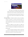
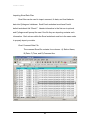
PYTHAGORAS
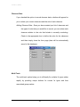
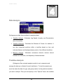
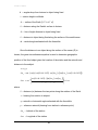
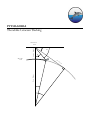
Theodolite Cetacean Tracking
Observation
Station Height
Point
Mean Sea
Level
α
ϖ
β
Earth Radius
Distance
δ
α
Ho
ri
zo
n
MARINE MAMMAL RESEARCH PROGRAM
Texas A&M University at Galveston
2000 Glenn Gailey and Joel Ortega-Ortiz
4700 Avenue U Building 303
Galveston, TX 77551
Table of Contents
Introduction
i
CHAPTER
CHAPTER
1
4
Data Analysis
44
Main Menu
1
Trackline Analysis
44
Pythagoras’ Database
2
Trackline Distances
46
Station Setup
4
Behavioral Data Analysis
48
Station Options
13
Wizards
22
CHAPTER
Theodolite Setup
23
Saving Data
51
Saving GIS Trackline(s)
53
Printing Data
54
Importing Data
54
CHAPTER
2
5
Collecting Data
26
Fix Data
27
Environmental Data
28
CHAPTER
Non-Fix Data
29
Calculations
60
Comment Data
30
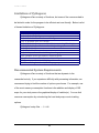
Limitations of Pythagoras
63
Observer Data
31
Recommended System Requirements
63
Multi-Track
31
Troubleshooting
64
Group Dispersion
33
Focal Behavior
34
Acknowledgements
66
Short-Cut Keys
37
References
66
CHAPTER
3
Viewing Tracks
39
Viewing Data
40
Modifying Data
42
6
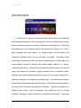
P Y T H A G O R A S
Introduction
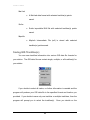
A theodolite is a surveyor's instrument which, when placed on an elevated
shore-based vantage point, can be successfully used as a research tool to obtain
data on cetacean movement, behavior, distribution, and habitat use. These data
are collected in a non-invasive manner, as described by Würsig et al. (1991).
Both cetaceans and other objects, for instance boats, can be tracked, and
interactions between them can be continually monitored.
Theodolites allow
researchers to determine "fixed" positions by measuring horizontal angles from
some arbitrary reference azimuth and vertical angles relative to a gravityreferenced level vector. Although this technique has been used for more than 20
years, and despite the increase in digital theodolite use for cetacean studies,
relatively few computer-based theodolite programs exist to assist researchers in
collecting, managing, and analyzing theodolite data. A computer-based system
benefits theodolite-based studies in many ways. Vertical and horizontal angles to
an object can be recorded accurately and efficiently.
Real-time calculations of
distance and location can be performed, and trackline(s) can be visually
displayed, allowing for rapid corrections of possible tracking errors.
i
Once data
P Y T H A G O R A S
are collected, a computer-based system reduces time to manage and analyze
data.
Pythagoras allows researchers to customize the program interface
according to their particular necessities. The user can define the fix type (e.g.
dolphins, whales, boats), the behavior associated with the fix, and other data
such as group size, species, environmental conditions, etc.
The position of the fixed object is estimated automatically by Pythagoras
every time a “fix” is entered. The estimated position and all data associated with
that fix (fix type, behavior, distance to the station, environmental conditions,
species, group size, etc.) are recorded into a Microsoft Access database file.
The database can be exported into Microsoft Access, Microsoft Excel, Text
(ASCII), or comma delimited files.
Pythagoras can graphically represent the area around your station if the
appropriate GIS information is provided. The location of the fixed object is plotted
in real-time, allowing the observer to rapidly check data as they are being
collected. Analysis modules are included to provide further trackline information
by calculating distance, course, linearity, reorientation rate, and leg speed of
each track.
ii
P Y T H A G O R A S
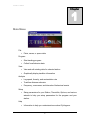
Chapter
1
Main Menu
File
•
Prints, saves, or opens data
Program
•
Start tracking program
•
Collect focal behavior data
View
•
View and edit existing data for selected station
•
Graphically display trackline information
Analysis
•
Leg speed, linearity, and reorientation rate
•
Trackline distance estimator
•
Frequency, occurrence, and intervals of behavioral events
Setup
•
Setup parameters for your Station, Theodolite, Options, and various
wizards to help you setup parameters for the program and your
station.
Help
•
Information to help you understand more about Pythagoras
1
P Y T H A G O R A S
Pythagoras' Database
Pythagoras utilizes Microsoft Access for storing information pertaining to
your station, preferences, fix data, environmental data, non-fix data, focal
behavior data, and the other data specified in your station preferences. The
database is continually updated; therefore if your computer "crashes", your data
should be saved. All relevant data can be exported into various file formats
(Chapter 5).
Pythagoras maintains two separate databases: 1) Station Settings File
(contains parameters, variables, and options related to each station) and 2)
Database (contains all tracking and behavioral data registered).
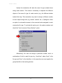
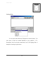
Opening Pythagoras’ Database - Database and Station Settings files of
Pythagoras contain the extension PDB (Pythagoras DataBase) and SDB
(Station DataBase), respectively. To open an existing Pythagoras
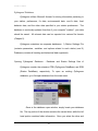
database, go to file\open database from the main menu.
Once at the database open window, simply locate your database
file. The top portion of the window contains the current drive, while the left
hand portion contains folder information. Once you select the drive and
2
P Y T H A G O R A S
folder containing the database file, your database will be displayed on the
right hand portion of the screen.
You must also specify the type of
database (i.e. Station settings file or Database file).
If you do not see your database file, make sure you are looking in
the correct directory and the file contains the extension PDB or SDB.
Once you select the file, double-click on the file to open the database file
as a station settings or database file. Pythagoras will then prompt you if
you would like the selected file to be your default database or station
settings file.
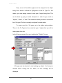
Creating Pythagoras’ Database - To create a new Station Settings File or a new
Database, select create a database or station settings file from the main
menu. Once selected, the program will prompt the user for the location
they would like to store the database. The program will then proceed in
creating the database and ask the user if they would like the newly
created database to be their default database.
3
P Y T H A G O R A S
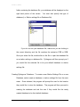
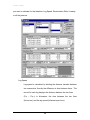
Station Setup
The station is the observation site where the researcher sets up the
theodolite. For Pythagoras, the station is represented by a set of parameters that
characterize the observation site and differentiate it from other stations. The
parameters of at least one station must be entered for the program to work, but
the user can define up to 11 different stations. Once a station has been defined,
Pythagoras stores all the parameters in the Station Settings Database; therefore,
unless you want to define a new fix type or behavior category, only eye height
and environmental conditions need to be updated.
4
P Y T H A G O R A S
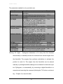
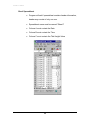
The parameters needed to set up a station are:
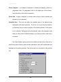
Station Parameter
Station Name
Description
A unique textual and/or numeric identifier to
that station.
Station Height
The exact height from the mean sea level to
the platform or site where you set up your
theodolite.
Eye Height
The height from the theodolite platform to
the eyepiece of your theodolite. This
distance will most likely change every time
you set up your theodolite at the station and
must be updated accordingly.
Latitude & Longitude The geographic position of your theodolite
station.
Reference Name
A textual/numerical name of the reference
point for your station.
This helps the
researcher remember the point that was
used as a reference.
Reference Azimuth
The
angle
(degrees)
between
the
geographic north bearing from your station
and the line formed by the bearing from your
station to the specified reference point. This
angle allows reference from bearings taken
from the station to geographic north.
Fix Type
The object(s) you attend on fixing.
Fix Type Behaviors
Associated behavior(s) for each fix type.
Non-Fix Types
Data not associated with the fix itself.
Environmental
Environmental variables determined by the
Conditions
user.
Environmental
Time interval at which the program reminds
Check Interval
the user to record environmental conditions.
Example
“My Station”
48.23 m
1.23 m
29°45’04.3’’ N
“Lighthouse”
79.88
“Dolphins”
“Traveling”
“Group Size”
“Beaufort”
01:00
Defining Fix Types - Pythagoras determines a fix every time the observer
electronically or manually records the horizontal and vertical angles from
the theodolite. The program then performs calculations to estimate the
position for each fix. The angles from the theodolite can be entered
manually, by writing theodolite readings into a notebook for their later input
into Pythagoras; or automatically, by connecting a digital theodolite to a
computer and executing the command (clicking the "Fix" button or shortcut
key – Chapter 2) to save the data.
5
P Y T H A G O R A S
Every record of theodolite angles must be assigned to the object
being fixed, which is referred in Pythagoras as the Fix Type. For this
reason, you must assign a name to each type of object being fixed. This
can be done by giving a textual description to each fix type, such as
"dolphin", "whale", or "boat". The researcher thereby creates a customized
list of fix types. This list is uniquely configured for each station.
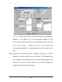
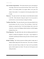
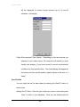
To create your list of fix types, go to the station setup window.
Then, in the Fix Type text box, write the type of objects that you will be
tracking and click Add.
In the following example, the user is adding the "Dolphin" fix type:
A fix type must be selected to start tracking any object. If no fix type is
selected before clicking the "Fix" button, an error message will be
displayed.
6
P Y T H A G O R A S
Usually the researcher will track the same fix type multiple times
during each session. This makes it necessary to separate the different
objects of the same fix type for each session (e.g. the different whales
tracked that day). The researcher may want to assign a different number
to each object being fixed (e.g. whale1, whale2, etc.). Pythagoras offers
an option for automatic increase in the numerical value assigned to each
consecutive fix type. To activate this option go to the options window and
check the "Auto Increment Group Number" option:
Alternatively, the user can assign a particular number, word, or
combination of both to each fix type (e.g. “boat blue”, where “boat” is the
fix type and “blue” is the identifier). In this case the user must specify the
group identifier in the tracking window:
7
P Y T H A G O R A S
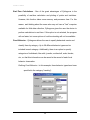
The researcher may also define the associated behaviors for each
fix type. The associated behavior, as well as the date, time, theodolite
reading, and position are entered together as a row in the database for
every fix that the researcher makes. Ancillary non-fix data (i.e. group size,
species, etc.) can be defined by the researcher and saved with the
corresponding fix.
Defining Behaviors Associated with Fix Types - Many of the studies that use
theodolites for tracking cetaceans involve ethological observations. The
researcher may want to record the behavior of the animals being tracked
8
P Y T H A G O R A S
and record that information with the position of each fix. Pythagoras allows
the researcher to include up to eleven different behavioral categories
associated with each fix type. The user may create a list of possible
behavioral categories for each fix type.
The associated behavioral categories are defined in the station
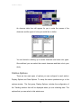
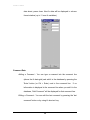
setup, after fix types have been determined. To enter a behavioral
category, go to the station setup window and select the fix type for which
you want to enter the associated behavior. Then, write the category in the
"Fix Type Behavior" text box and click on the "Add" button.
In this example, the "Feeding" behavioral category is being added
to the list for the "Dolphin" fix type for "My station":
The list of behavioral categories will be displayed in the tracking
window when the user selects the fix type.
9
P Y T H A G O R A S
A behavioral category does not necessarily have to be selected
when tracking cetaceans or ships. If no category is selected in the “Fix
Behavior” menu when the fix button is clicked, the “Behavior” field in the
database will be empty.
Although the “Fix Behavior” option is available for all the fix types,
some objects being fixed, such as boats, will not display behavior.
However, this option may be useful to researchers because it allows them
to enter information about the fixed object that, although is not precisely
behavior, may be of particular interest. For example, the researcher can
enter categories such as “fishing”, “trawling”, “stopped”, “swimmers enter
water”, etc., and link this information to the spatial and temporal location of
the boat or object being fixed.
Defining Non-Fix Type Data - The researcher can define non-fix variables (data
not related to the position of the fix type) to be recorded. Some examples
of non-fix data are species, group size, number of calves, number of
adults, etc.
The data for non-fix variables are usually entered only once for
each object being tracked. For this reason, the "Non-fix" window does not
need to be on the screen permanently, and it is not automatically
displayed when the tracking window is open. The user must click the
"Non-fix" button (or press Ctrl + n) in the tracking window to open the nonfixed variables window. After clicking the "Non-fix" button, a window with
the list of non-fix variables that were defined by the user are displayed
10
P Y T H A G O R A S
along with text boxes for the user to enter the corresponding text or
numerical value.
Warning:
Non-Fix data are recorded in sequence into Pythagoras'
database. If you delete one of the non-fix variables, you will restructure
the sequence, which can cause subsequent data to be stored in the wrong
column. Therefore, once you have defined your non-fix variables, it is
recommended that you do not delete any of them.
Defining Environmental Variables - Many theodolite studies may want to include
the environmental conditions of their study area (Beaufort, Swell, Wind
speed, etc). Pythagoras allows you to define up to 10 environmental
variables. Tide height is automatically included as an environmental
variable and used for distance calculations due to its effect on observation
height.
There is a list of environmental variables for each station. You can
add a new environmental variable by opening the station setup window
and by either adding a new station or editing a current station.
Type in the name of the environmental variable in the text box
provided next to "Env Data" and then press "Add" under the text box.
After you have added the variable, it will be displayed in the list box below
the "Add" button. These data are stored in Pythagoras' database to be
used later in adding environmental data in the field.
In this example, the "Swell Height" environmental variable is being
added to the list for "My station":
11
P Y T H A G O R A S
Warning: Environmental data are recorded in sequence into Pythagoras’
database.
If you delete one of the environmental variables, you will
restructure the sequence, which can cause subsequent data to be stored
in the wrong column.
Therefore, once you have defined your
environmental variables, it is recommended that you do not delete any of
them.
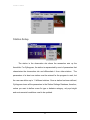
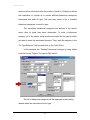
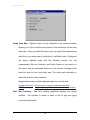
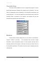
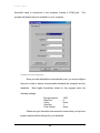
Defining Observers and Observer’s Role - Pythagoras allows you to create a
database of observers and their role in your study. This database allows
you to register the time and position for each observer participating in data
collection. If you want to use this option you must create a database by
selecting the option from the setup menu.
12
P Y T H A G O R A S
An observer data form will appear for you to enter the names of the
observers and the types of roles you would like to define.
You are limited in defining up to seven observers and seven role types.
Once defined, you can select the current observers and their role in your
study.
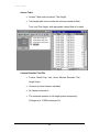
Station Options
There are two main types of options you can configure for each station:
Display Options and Data Options. To setup the station preferences go to the
options window. The first group, Display Options, includes the configuration of
the Tracking window that will be displayed when you are collecting data. The
options that you can select in this window are:
13
P Y T H A G O R A S
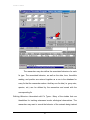
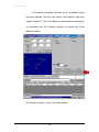
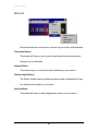
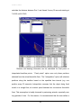
Study Area Map - Digitized maps can be displayed in the tracking window,
allowing you to plot in real time the position of the trackline(s) on the study
area map. Once you select this option, you can specify the digitized map
data file for your study area by clicking the “Load Map” button. Pythagoras
can import digitized maps with the following formats: Arc Info
(ungenerated), Mat Lab, MapGen, and Surfer. Based on the position of
the station and the estimated distance to the horizon, Pythagoras will
scale the map for your local study area. The study area information is
saved into a file for future reference.
Suggested web sites to obtain digitized maps of your study area:
Coastline Extractor http://crusty.er.usgs.gov/coast/getcoast.html
USGS
http://edc.usgs.gov/doc/edchome/ndcdb/ndcdb.html
Real Time Tracking - Real time tracking graphically displays the current
trackline.
The trackline is unique in terms of the fix type and group
currently being tracked.
14
P Y T H A G O R A S
Show Compass - A compass is displayed to indicate the bearing, referred to
geographic north (i.e. geographic north on the upper part of the screen),
from the station to the last fix registered.
Show Grid - A grid is displayed to indicate each minute in both longitude and
latitude of your study area.
Viewable Area - The user can adjust the viewable area of the digitized map
displayed in the tracking window. To do this, you must enter the distance
in kilometers that you want to display in the tracking window. If this option
is not selected, Pythagoras will automatically select the displayed area
based on the minimal distance between your station and the track line(s)
of interest.
The Data Options group specifies the additional data menus that will be
used during data collection and real time calculations that will be performed and
displayed in the tracking window. The options that you can select in this window
are:
15
P Y T H A G O R A S
Auto Increment Group Number - This function helps the user to start tracking a
new subject. Each time the user clicks the button "Next" in the Fix Type
section of the tracking window, the program adds a new group and
assigns it the number i+1 (i corresponds to the last group number for that
fix type).
Observers - The name and role of each observer can be defined and recorded
in the field. When observers change role types, the user only needs to
push the button or use shortcut keys to change the settings.
Trackline Critical Time - This option allows the user to be warned when the time
interval between two fixes is too long. The user defines a "critical time"
between two consecutive fixes. If the interval between fixes is above the
critical time, a broken line (Pythagoras default trackline is solid) will appear
between the two fixes.
Group Dispersion - This option allow users who are tracking groups/schools of
animals to estimate the dispersion of the group.
Group dispersion is
estimated by calculating the distance along two axes of the area occupied
by the group.
Multiple Tracking - This function provides an efficient method to keep track of
multiple objects being fixed at the same time. If this option is selected,
then the user starts fixing an object, the fix type and fix type identifier
(group number) appear as a button. The user can fix this group by just
clicking the button.
16
P Y T H A G O R A S
Real-Time Calculations - One of the great advantages of Pythagoras is the
possibility of real-time calculation and plotting of points and tracklines.
However, this function takes some memory and processor time. For this
reason, and thinking about the users who may not have a "fast" computer
available for field data collection, Pythagoras gives the user the choice to
perform calculations in real time. If this option is not selected, the program
will run faster, but some options of real time tracking will not be available.
Focal Behavior - Pythagoras allows the user to specify behavioral events and
classify them by category. Up to 28 different behavior types can be
included in each category. Additionally, there is an option to specify
categories of individuals, like adult, juvenile, mother/calf, male, female,
etc., so that this information can be saved in the record of each focal
behavior observation.
Defining Focal Behavior - In this example, three behavior types have been
specified in the category “traveling”:
17
P Y T H A G O R A S
If this option is selected, and after the list of behavior types
has been defined, the user can collect focal behavior data very
easily (Chapter 2). The Focal Behavior data collection window can
be accessed from the Tracking window, by clicking the 'Focal
Behavior' button:
Or from the ‘Program’ menu in the main window:
18
P Y T H A G O R A S
Once opened, the Focal Behavior data collection window
offers an easy and fast way to collect behavioral data. Although this
window does not have a fix function to estimate location, the user
can record detailed observations with clicking a button. Moreover, it
allows the user to define their own categories and lists of behavior
types.
Tide Height Database - Tide height can affect the accuracy of the distance
estimations, and therefore is an important environmental variable to be
considered. Pythagoras gives the user the option to import tide height data
stored in Microsoft Excel or Access format and use them in distance
calculations.
Once the database has been imported, the program will
automatically search the closest tide height value according to the date
and time of the observations in the database and the date and time when
the fix was made.
In order to be imported into Pythagoras, predicted or observed tide
height data can be retrieved from tide tables or from the Internet and
saved in Excel or Access files. The format should be as follows:
19
P Y T H A G O R A S
Excel Spreadsheet
o Program will ask if spreadsheet contains header information,
header may consist of only one row.
o Spreadsheet name must be named “Sheet1”
o Column A must contain the Date
o Column B must contain the Time
o Column C must contain the Tide Height Value
20
P Y T H A G O R A S
Access Table
o Access Table must be named “Tide Height”
o Tide height table must contain the columns named as Date,
Time, and Tide Height, with appropriate values filled in for each.
Comma Delimited Text File
o Format: Month, Day, Year, Hours, Minutes, Seconds, Tide
Height Value
o Commas must be between variables
o No Header information
o The maximum number of tide height points accepted by
Pythagoras is 10,000 entries per file.
21
P Y T H A G O R A S
Wizards
Several wizards were developed to help set up your station and theodolite.
Theodolite Wizard
This wizard will help you set up your theodolite and communication port
settings for your theodolite
Station Wizard
This wizard helps you setup information pertaining to your station.
Station Height Wizard
The Station Height wizard provides calculations and visualizations to help
you determine the height of your station.
Option Wizard
This wizard will help you select appropriate options for your station.
22
P Y T H A G O R A S
Theodolite Setup
This setup window enables the user to configure the program to ensure
proper data transference between the computer and the theodolite. You must
select the appropriate options depending on the theodolite manufacturer and
model being used. You must also specify the communication port by which the
theodolite cable is connected to the computer, and configure the port (see
theodolite user manual for port specifications).
Manufacturer
Currently there are three settings that you can choose for manufacturer:
Topcon™, Sokkia™, and None.
If the researcher does not have a digital
theodolite or cannot successfully connect it to the computer, the data can be
manually entered into the computer. In this case, the user must select “None” as
the theodolite manufacturer. This option can also be used to analyze previously
collected data.
23
P Y T H A G O R A S
Theodolite Model
Although most models of the same manufacturer have the same
communication settings, there can be some difference between models. The
following models have been tested or assured by the manufacturer to have the
same communication protocol.
Topcon™
Topcon models can be configured for real-time reading. The user
may choose to select this option or not. If you do select real-time reading
for the theodolite, you may also choose the time interval (in milliseconds)
at which the program updates the information. We recommend 500 msec
time interval.
Current Models: DT-102
Sokkia™
Sokkia models are point fixes. When the user clicks the ‘Fix’ button
on the data collection form, the computer sends a command to the
theodolite and reads the current position.
Current Models: DT2, DT4, DT5, DT5A, Set2, Set3, Set4, Set5, and E-Series
None
No settings are necessary (data entered manually).
Communication Port
Most digital theodolites communicate via a RS-232 type cable that is
connected to the computer’s serial port.
24
The user must define where the
P Y T H A G O R A S
theodolite cable is connected to the computer (usually a COM port).
The
program will display all ports available on your computer.
Communication Port Configuration
Once you have defined the communication port, you must configure
the port in order to assure communication between the computer and the
theodolite.
Most digital theodolites tested for this program have the
following settings:
Bits per second:
Data bits:
Parity:
Stop bits:
Flow Control:
1200
8
None
1
None
Please see your theodolite user manual to ensure that you input the
proper communication settings for your theodolite.
25
P Y T H A G O R A S
Chapter
2
Collecting Data
You can control the data collection sheet by either using a mouse or by
various shortcut keys. The following provides information to guide you through
the main data gathering-tracking window:
26
P Y T H A G O R A S
Fix Data
Vertical and Horizontal Position - The 'Position' frame, located in the upper
left portion of the window, displays the vertical and horizontal
bearings to the object being fixed. If a theodolite is connected to
your computer and it has been properly configured, the vertical and
horizontal angles will be displayed automatically (Topcon™ models
can be configured for real time reading, while Sokkia™ models are
point fixes - Chapter 1). If you are entering the data manually, click
in the appropriate box to start typing the bearing angles.
Horizontal and vertical angles are recorded as degrees,
minutes, and seconds. You must select your fix type and group
number/name before recording a fix of the group.
Behavioral
information is optional and can be edited later. Once you fix a
group, information pertaining to that fix will be illustrated at the
bottom of the data grid.
Selecting Fix Type and Associated Behavior - You can either click on the
fix type or use Ctrl + a (plus moving your up/down arrow keys) to
select your fix type.
Once you select a fix type, the behaviors
associated with the fix type will be displayed on the right of the fix
type. You can select the behavior with the mouse or by pressing
Ctrl + z.
Group Information - Each trackline of the same fix type is separated by
group number/name. The program keeps track of the last group
27
P Y T H A G O R A S
number/name for a fix type, therefore avoiding retyping the entry
when moving between fix types. You can select the option to auto
increment the group number/name or simply click on or press Ctrl +
I, to increment the group number for that fix type.
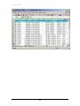
Data for your station are displayed only for that current day.
Therefore, each day you go out into the field, you will begin with an
empty data sheet. Once you fix a group, the date, time, fix type,
group, behavior, latitude, longitude, distance to station, and bearing
are displayed in the data grid. The data for the last fix are also
displayed above the comment line.
Modifying Data - There are two methods of modifying data after they have
been entered into the database. One pertains to the immediate last
fix and the other pertains to all fix data for that day. In order to
modify the last fix you made, you can either select the 'Edit last fix'
or 'Delete last fix' button. To modify any of the other data for that
day, simply double click on the fix information in the data grid box.
Environmental Data
You can open your environmental variable(s) data sheet by
pressing the 'Environment' button or shortcut key for environmental data.
Adding Environmental Data - Type in the data you want to record and
press “Save” to add the information to your database. Once you
are finished with the data sheet, press close. Environmental data
28
P Y T H A G O R A S
will be displayed in column format window (up to 10 non-fix
variables + tide height).
Check Environmental Time Interval - Depending on the time interval you
selected in your station setup, the computer will remind you both
visually and auditory (if you have sound) to record environmental
conditions for that specified time. The visual display will appear at
the bottom text box and the auditory signal is given in the form of a
"beep".
Non-Fix Data
You can open the non-fix data sheet by pressing the 'NonFix' button or
shortcut key.
Adding Non-Fix Data - Enter the type of data you want to record and press
“Save” to add it to your database. Once you are finished with the
29
P Y T H A G O R A S
data sheet, press close. Non-fix data will be displayed in column
format window (up to 11 non-fix variables).
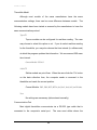
Comment Data
Adding a Comment - You can type a comment into the comment line
(above the fix data grid) and add it to the database by pressing the
'Enter' button (or Ctrl + Enter) next to the comment line.
If no
information is displayed in the comment line when you add it to the
database, "Add Comment" will be displayed for that comment line.
Editing a Comment - You can edit the last comment by pressing the 'last
comment' button or by using it's shortcut key.
30
P Y T H A G O R A S
Observer Data
If you checked the option to record observer data, a button will appear for
you to select your current observers and the role of each observer.
Adding Observer Data - Once you have created your list of observers and
the types of roles that you would like to record, you can select each
observer relative to the role that he/she is currently conducting.
Check in the appropriate box to define the roles for the observers
and then simply close the form page (data will be automatically
saved to the database).
Multi-Track
The multi-track option helps you to efficiently fix multiple fix types rather
rapidly by providing unique buttons for current fix types and their
associated group number.
31
P Y T H A G O R A S
Once you make an initial fix of the group, a multi-track button will appear
with the unique fix type and group number/name. Behaviors associated
with the fix type will also appear to the right of the button for ease in
selecting the various behaviors you defined. When the object is no longer
in sight, simply click on remove and then press the button for the object
you want to remove. You can have up to 13 objects in the multi-track
window.
32
P Y T H A G O R A S
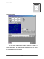
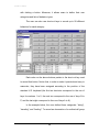
Group Dispersion
This option allows the users who are tracking groups/schools of
animals to estimate the dispersion of the group.
Group dispersion is
estimated by calculating the distance along two axes of the area occupied
by the group. The fixes are taken by clicking the button “Grp Dispersion”,
then a window appears indicating, one by one, the four points (back, front,
left, and right) on the edge of the group that need to be fixed by the user.
For example, in the Group dispersion window below, the Fix field indicates
“back”.
This means that the user must fix a point in the back edge of the
group. After this point is fixed (by finding the point with the theodolite and
clicking the button “fix” in this window), the window will ask for the next
points: “front”, “left”, and “right”. After the four points have been fixed, the
window displays the length of the front-back and left-right axes (m) and
the area (m2) of the group.
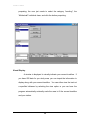
33
P Y T H A G O R A S
The area is estimated in the shape of a quadrilateral. Although the
area occupied by cetacean schools is often other than a quadrilateral,
estimating it with only four fixes saves the user valuable time in the field.
This is an important aspect if we consider that the fixes used to estimate
group dispersion should be taken in the shortest possible time, especially
for groups that move quickly. Moreover, the user can continue to fix the
track and record behavior by spending a short amount of time estimating
group dispersion by taking only four fixes. Those users who are interested
in obtaining a more accurate estimation can do so by quickly fixing as
many points on the edge of the school as possible, and displaying a track
of these points.
Bearing Compass
A graphical compass is shown next to the vertical and horizontal
information in the upper left of the form page. This display graphically
illustrates the current bearing of your last fix.
Focal Behavior
If you selected the focal behavior option, a button will be displayed
for collecting focal behavior data. Once selected, the focal data window
will be displayed for user to collect focal behavior data.
The Focal Behavior data collection window offers an efficient way
to collect behavioral data. Although this window does not have a fix
function to estimate location, the user can record detailed observations
34
P Y T H A G O R A S
with clicking a button. Moreover, it allows users to define their own
categories and lists of behavior types.
The user can also use short-cut keys to record up to 28 different
behaviors for each category:
Each value on the above buttons pertain to the short-cut key used
to record that button. Notice that, in order to make it practical and easy to
memorize, they have been assigned according to the position of the
standard U.S. keyboard (the first ten shortcuts correspond to the row of
keys for numbers 1 to 0, the next ten correspond to the row of keys Q to
P, and the last eight correspond to the row of keys A to K).
In the example below, the user defined three categories: “diving”,
“traveling”, and “feeding”. To record an observation of a mother/calf group
35
P Y T H A G O R A S
porpoising, the user just needs to select the category “traveling”, the
“Mother/calf” individual class, and click the button porpoising.
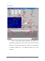
Visual Display
A window is displayed to visually indicate your current trackline. If
you have GIS data for you study area, you can import the information to
display along with your current trackline. You can either view the track at
a specified distance by selecting the view option or you can have the
program automatically minimally scale the area to fit the current trackline
and your station.
36
P Y T H A G O R A S
Shortcut Keys
Since a mouse might become obstructive and inefficient for
collecting data, Pythagoras has many shortcut keys to help you efficiently
collect data. The shortcut keys consist of a Ctrl key on your keyboard plus
an additional operation key.
The additional operation key is case
insensitive.
37
P Y T H A G O R A S
Operation
Fix Location
Delete Last Fix
Edit Last Fix
Open or Set Focus on Environment Sheet
Open or Set Focus on NonFix Data Sheet
Set focus on Fix Type
Set focus on Fix Behavior
Move to Comment line
Add Comment
Edit Last Comment
Move to Group Number/Name
Manual Increment Group Number/Name
Change View Area
Open or Set Focus on Group Dispersion
Open or Set Focus on Multi-Track
Open or Set Focus on Observer Data Sheet
38
ShortCut Key
Ctrl + f
Ctrl + ]
Ctrl + [
Ctrl + e
Ctrl + n
Ctrl + a
Ctrl + z
Ctrl + c
Ctrl + Enter
Ctrl + L
Ctrl + g
Ctrl + I
Ctrl + v
Ctrl + d
Ctrl + m
Ctrl + o
P Y T H A G O R A S
Chapter
3
Viewing Tracks
You can visually display your trackline(s) by selecting 'View track' in the
main menu.
displayed.
By selecting the fix type, all tracklines for that fix type will be
You can narrow down the number of trackline(s) displayed by
selecting a date that you are interested in viewing.
Once you selected a
specified date, all trackline(s) for that day will be displayed and all groups will be
displayed for that day. You can concentrate on a certain group by selecting the
group number/name from the list. Once the group is selected, the graphical
display will show the trackline for that group and indicate where your initial fix
("Start") occurred for that group and the last fix point ("Stop") for that group.
39
P Y T H A G O R A S
Viewing Data
Database
Pythagoras offers an easy way to display and manage your data. You can
view your data by selecting ‘view data’ in the main menu. When you initially
open the data sheet, all your data will be presented for that station. You may
narrow down your data search by selecting the date, fix type, and group
identifier. The data management program provides sort functions that allow you
to structure similar data together and a search option to find a specified text or
numeric value in a specified column. Distance and course calculations can also
be recalculated with updated values (i.e. station height, eyepiece height,
reference azimuth value, etc.).
40
P Y T H A G O R A S
Sorting
In order to sort your data, you must first choose the dataset you
want to sort (i.e. fix, environmental, non-fix, comments). After selecting
your dataset, you may select the variable by which you would like to sort.
All sorts are ascending.
Searching
You can find a certain value or text in a data set by selecting the
data set’s name, the variable, and value/text you want to find. Once you
have the above information, press find to search for the value/text. The
search engine will proceed down the variable and stop once it finds the
specified value/text. You may continue by pushing the find next button.
The program will notify you when it reached the end of the database.
41
P Y T H A G O R A S
Recalculating Fix Data
The recalculation option will only appear when fix data option is
selected. You can recalculate all fix data or a specified portion of the fix
data. Single fix recalculation can be performed by simply double clicking
on that fix. Once you have chosen all or selected portion of your fix data,
then specify which parameters you would like to change for recalculations
(i.e. station height, eyepiece height, reference azimuth value, etc.) and
place the value you would like to change in the text box provided and
press the ‘Recalculate’ button.
Modifying Data
Editing Comments
Your comment information may be modified by changing the date,
time, and/or comment line information. Click on the save button to record
changes.
42
P Y T H A G O R A S
Editing Fix Data
You may modify your fix data by changing any of the parameters
indicated above except for the station name. If you change your vertical
and/or horizontal position, all calculations are performed again* with the
new edited data. After editing, press ‘Save’ to store the new information
into the program’s database.
* Recalculating the distance will be based on station information recorded
when the object was fixed (i.e. station’s geographic position, station
height, eye height, and reference azimuth).
43
P Y T H A G O R A S
Chapter
4
Data Analysis
Pythagoras provides three modules for analyzing data:
o Trackline Analysis - Estimates Leg Speed, Linearity, and Reorientation
rate of a trackline.
o Trackline Distances - Calculates the Distance & Course of a trackline. It
can also interpolate positions within a trackline based on time and
estimate distance and bearing between points of two different tracklines.
o Behavior Analysis - Estimates occurrence, behavior interval, interval
between two behaviors, and frequency of behavioral data.
Trackline Analysis
Pythagoras offers a simple analysis module to sort, summarize and
manage the data you collected for each trackline(s). To start the analysis you
must first select the date, fix type, and group number for the particular trackline
you want to analyze. Then you must specify, in the "Options" frame, the variables
44
P Y T H A G O R A S
you want to estimate for that trackline: Leg Speed, Reorientation Rate, Linearity
or all the previous.
Leg Speed
Leg speed is calculated by dividing the distance traveled between
two consecutive fixes by the difference in time between them. The
record for each leg displays the distance between the two fixes
(Fixi – Fixi+1) in kilometers, the time between the two fixes
(hh:mm:ss), and the leg speed (kilometers per hour).
45
P Y T H A G O R A S
Linearity
Linearity is calculated by dividing the distance between the initial
and end points (net distance) of a trackline by the total sum of the
distances (cumulative distances) along the track. Linearity values
range between 0 and 1. Linearity values close to one represent a
straight trackline, while values close to zero represent a track with
no constant direction (Batschellet, 1980).
Reorientation Rate
Reorientation rate is a magnitude of course changes along a
trackline. Reorientation rate is calculated by summing all course
changes (degrees) along the trackline divided by duration (minutes)
of the trackline (Smultea and Würsig, 1995).
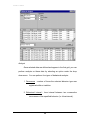
Trackline Distances
This analysis module can be used to estimate the distance and course
within and between trackline(s). Tracklines can be analyzed by selecting the
"Reference track combo box", the date, fix type and group number. Once a
"reference track" has been selected, you can compare it to other tracklines of the
same or different fix type(s) by checking the appropriate box in the "Compare
Reference Track To:" frame. For example, in the "Track Distance Estimator"
window displayed below, the track for Pod 1 recorded on 01 May 1999, has been
selected as the reference track. Vessel 2 has been selected as the track for
comparison from 7:40:55 to 8:33:49 at 30 seconds intervals. Pythagoras will
46
P Y T H A G O R A S
calculate the distance between Pod 1 and Vessel 2 every 30 seconds starting at
7:40:55 until 8:33:49.
Distance and bearing information can be calculated for fixed points or
interpolated trackline points.
“Fixed points” option uses only those positions
obtained from the actual theodolite fixes. The “Interpolation” option will calculate
positions along the trackline based on the specified time interval (e.g. one
position every 30 seconds). Interpolation assumes that the object being fixed
travels in a straight line, at constant speed between two consecutive theodolite
fixes. This assumption is hardly observed by swimming animals, especially over
long periods of time. For this reason, it is recommended that the user define a
47
P Y T H A G O R A S
critical time between fixed points before interpolating. When the critical time
option has been selected, Pythagoras will exclude those fixes collected with a
difference of time greater than the critical interval (the greater the time difference
between fixes, the more probability of violating the “constant speed - straight line”
assumption). You can also narrow the time interval for the program to calculate
the interpolated points only for those periods when you recorded a good number
of fixes with short time difference between them. Interpolation calculations are
also computationally intensive, therefore a relatively “fast” computer is
recommended.
Behavioral Data Analysis
This module of Pythagoras allows researchers to analyze collected
behavioral data for occurrence, behavioral interval, interval between two
behaviors, and frequency of a particular behavior within a trackline. Both, focal
and fixed related behavioral data can be analyzed in this module. To start the
Behavioral Data Analysis, first select the data type you would like to analyze (i.e.
focal or fix related data) and the fix type or category of behavioral data. Once
these two parameters have been defined, the program will display the associated
behaviors with check boxes. You can then select the behaviors of interest by
checking the box next to the behavior type.
48
P Y T H A G O R A S
Analysis
Once selected data are defined and appear in the first grid, you can
perform analysis on these data by selecting an option under the drop
down menu. You can perform four types of behavioral analysis:
1. Occurrence - number of times the selected behavior type was
registered within a trackline.
2. Behavioral interval - time interval between two consecutive
occurrences of the specified behavior (i.e. blow interval).
49
P Y T H A G O R A S
3. Interval between two behaviors – duration of a behavior
measured as the time interval between consecutive
occurrences of two specified behaviors (i.e. first surface dive = surface time).
4. Frequency - number of times a behavior type occurred divided by
the entire time of the trackline.
Graphs
Analyzed data can be visually displayed by selecting the graph
button on this window. Unique columns contain a fix type, group, and
date.
50
P Y T H A G O R A S
Chapter
5
Saving Data
You can export data collected by Pythagoras into various formats. Two
main types of output are created depending on your selection: 1) Fix,
Environment, Non-fix and option related data, and 2) GIS Sighting Data. A
description of each type is given below.
51
P Y T H A G O R A S
Fix, Environment, Non-fix and option related data:
Microsoft Access
o Several Access tables are created to save Fix data,
Environmental Data, Non-Fix Data, and various other
optional data.
Microsoft Excel
o An Excel Workbook is created with various worksheets
pertaining to the Fix Data, Environmental Data, Non-Fix
Data, and the various options you selected for your station.
Comma Delimited
o A text formatted data file that separates each variable with a
comma. Fix Data, Environmental Data, Non-Fix Data, and
your various option data are saved in this format.
Text File
o A space delimited text-formatted file with all relevant data
saved.
GIS Sighting Data:
Arc Info
o An ungenerated Arc Info data file with a series of longitude
and latitude points of selected trackline(s).
52
P Y T H A G O R A S
Mat Lab
o A Mat Lab data format with selected trackline(s) points
saved.
Surfer
o Surfer importable BLN file with selected trackline(s) points
saved.
MapInfo
o MapInfo Intermediate File (mif) is stored with selected
trackline(s) points saved.
Saving GIS Trackline(s)
You can save trackline information into various GIS data file formats for
your station. The GIS data file can contain single, multiple, or all trackline(s) for
your station.
If you decide to select all tracks, no further information is needed and the
program will produce your GIS data file in the specified format and location you
provided. If you decide to save only one trackline or multiple tracklines, then the
program will prompt you to select the trackline(s).
53
Once you decide on the
P Y T H A G O R A S
trackline(s) to save, then simply press save and your information will be saved to
the file you specified.
Printing Data
You may printout your data for the currently selected station. The data are
formatted as an Excel spreadsheet and printed to the computer system’s default
printer.
Importing Data
Pythagoras’ MetaFile
Data can be imported into an existing Pythagoras database by means of a
comma-delimited metafile. The file contains a command (telling Pythagoras what
to add), the station name, relevant variables and an End command. Below is a
list of commands to add data to Pythagoras. All Commands are case sensitive.
54
P Y T H A G O R A S
Add Station Command (Command = AddStation)
(AddStation, Name of Station, Eye Height, Reference Name, Reference
Azimuth, Station Height, Environmental Check interval (as Integer),
Station Latitude Hemisphere, Latitude Degrees, Latitude Minutes, Latitude
Seconds, Longitude Hemisphere, Longitude Degrees, Longitude Minutes,
Longitude Seconds, Tide Height, END)
Add Observer Name (Command = AddObsName)
(AddObsName, Name of Station, Observer Name, END)
Add Observer Data (Command = AddObsData)
(AddObsData, Name of Station, Date, Time, Observer Name, Observer
Role, END)
Add Non-Fix Related Data (Command = AddNonFix)
(AddNonFix, Name of Station, Date, Time, Fix Type, Group, NonFix Type,
Value, NonFix Type, Value, ….., …., END)
Add Environmental Data (Command = AddEnv)
(AddEnv, Name of Station, Date, Time, Tide Height, Environmental Type,
Value, Environmental Type, Value,…,…,END)
Add Fix Data (Command = AddFixData)
(AddFixData, Name of Station, Date, Time, Group, Fix Type, Fix Type
Behavior, Vertical Degrees, Vertical Minutes, Vertical Seconds, Horizontal
Degrees, Horizontal Minutes, Horizontal Seconds, Reference Azimuth,
Station Height, Eye Height, Station Latitude Hemisphere, Station Latitude
(decimal degrees), Station Longitude Hemisphere, Station Longitude
(Decimal Degrees), Tide Height, END)
55
P Y T H A G O R A S
Add Comment (Command = AddComment)
(AddComment, Name of Station, Date, Time, Comment, END)
Add Tide Height Value (Command = AddTideHeight)
(AddTideHeight, Name of Station, Date, Time, Tide Height Value, END)
Add Focal Behavior Data (Command = “AddBehavior”)
(AddBehavior, Name of Station, Date, Time, Fix Type, Group, Behavior
Category, Behavior, Individual, END)
Data can also be edited as a process from the beginning to end of file. Editing
Data commands are:
Edit Reference Azimuth (Command = “EditRef”)
(EditRef, Name of Station, Reference Name, Reference Azimuth, END)
Edit Station Eye Height Value (Command = “EditEyeHeight”)
(EditEyeHeight, Name of Station, Eye Height value, END)
Below is an example of a Pythagoras’ Metafile:
56
P Y T H A G O R A S
Importing Excel Data Files
Excel files can be used to import comment, fix data, and focal behavior
data into Pythagoras’ database. Each Excel worksheet must have Excel’s
default worksheet title “Sheet1”. Header information in the first row is optional
and Pythagoras will prompt the user if the file they are importing contains such
information. Each column within the Excel worksheet must be in the same order
to properly import your data.
Excel Comment Data File
The comment Excel file contains four columns: A) Station Name,
B) Date, C) Time, and D) Comment line.
57
P Y T H A G O R A S
Excel Fix Data File
The fix data Excel file contains 20 columns: A) Station Name, B)
Date, C) Time, D) Fix Type, E) Group, F) Behavior, G) Vertical
degrees, H) Vertical minutes, I) Vertical seconds, J) Horizontal
degrees, K) Horizontal minutes, L) Horizontal seconds, M) Station’s
Latitude Hemisphere, N) Station’s Latitude location (decimal
degrees), O) Station’s Longitude Hemisphere, P) Station’s
Longitude location (decimal degrees), Q) Tide height value, R)
Station’s height, S) Eyepiece height, and T) Reference Azimuth.
Excel Focal Behavior Data File
The focal behavior data Excel file contains eight columns: A)
Station Name, B) Date, C) Time, D) Fix Type, E) Group, F)
Behavioral Category, G) Behavior, and H) Individual.
58
P Y T H A G O R A S
59
P Y T H A G O R A S
Chapter
6
Calculations
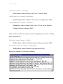
Pythagoras uses a modification of the approximation proposed by Lerczak
and Hobbs (1998) to determine the distance along the surface of the ocean from
the station to the object being fixed:
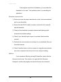
β=
π
− α − θ = 180 − ϖ
2
D0 = (RE + h ) ⋅ cos(β ) −

D
δ = arcsin sin (β ) 0
RE

(RE + h )2 ⋅ cos(β)2 − (2hRE + h 2 )



D = δ ⋅ RE
and the distance from the station to the horizon:
 2hR + h 2
E
α = arctan

RE





H = α ⋅ RE
where
α = angle from horizontal (90°) to horizon and central arc angle from
horizon to station.
β = angle from object being fixed to station
δ = central arc from object being fixed to station
60
P Y T H A G O R A S
θ = angular drop from horizon to object being fixed
h = station height or altitude
(
RE = radius of the Earth 6.371 × 10 6 m
)
H = distance along the Earth’s surface to horizon
D0 = line-of-sight distance to object being fixed
D = distance to object being fixed along the surface of the earth/ocean
ϖ = vertical angle estimated with the theodolite
Once the distance to an object along the surface of the ocean (D) is
known, the great circumference equation is used to determine geographic
position of the fixed object given the location of the station and the azimuth and
distance to the subject:
τ = η−ρ
Lat F = sin −1 (cos(τ ) ⋅ sin (D / 60 / 1852 ) ⋅ cos(Lat S ) + [sin (Lat S ) ⋅ cos(D / 60 / 1852 )])
 cos(D / 60 / 1852 ) − [sin (Lat S ) ⋅ sin (Lat F )]
 + Lon S
Lon F = cos −1 
(
)
(
)
cos
cos
Lat
⋅
Lat
S
F


where
D = distance (m) between the two points along the surface of the Earth.
τ = bearing from station to subject.
η= azimuth or horizontal angle estimated with the theodolite
ρ = reference azimuth (bearing from station to reference point)
Lat S = Latitude of the station
Lon S = Longitude of the station
61
P Y T H A G O R A S
Lat F = Latitude of the fixed object
Lon F = Longitude of the fixed object
The great circumference equation is also used by Pythagoras to
determine the distance of two points along the surface of the Earth when the
geographic coordinates (latitude and longitude) of both points are known:
(
)
D = 60 ⋅ cos −1 [(sin (Lat1 ) ⋅ sin (Lat 2 )) + (cos(Lat1 ) ⋅ cos(Lat 2 )) ⋅ cos(Lon2 − Lon1 )] ⋅ 1852
 sin (Lat 2 ) − [sin (Lat1 ) ⋅ cos(D 60 )]
ζ = cos −1 

sin (D 60 ) ⋅ cos(Lat1 )


where
D = distance (m) between the two points along the surface of the Earth.
ζ = bearing from point 1 to point 2
Lat1 = Latitude of point 1
Lon1 = Longitude of point 1
Lat 2 = Latitude of point 2
Lon 2 = Longitude of point 2
62
P Y T H A G O R A S
Limitations of Pythagoras
Pythagoras offers a variety of functions, but some of the resources had to
be limited in order for the program to be efficient and user friendly. Below is a list
of known limitations of Pythagoras.
Limitation
Only 11 Stations possible
Only 11 Definable Fix Types
Only 11 Definable Behaviors for each Fix Type
Only 11 Definable Non-Fix Variables
Only 10 Definable Environmental Variables (not including Tide Height)
Only 28 Definable Focal Behavior Variables per Category
Only 7 Definable Observers
Only 7 Definable Observer roles
Only 13 Objects allowed for the Multiple tracking option
View Trackline for fix type limited to 20,000 fix points
View Trackline for entire day limited to 10,000 fix points
GIS Data import is limited to 500,000 points
Real-Time tracking limited to 1,000 fixes per group
Recommended System Requirements
Pythagoras offers a variety of functions that are dynamic to the
researcher's study. If you experience difficulty with processing information, we
recommend trying to limit the number of options you choose. For example, one
of the most memory consumptive functions is the addition and display of GIS
maps for your study area or the graphical display of trackline(s). You can limit
resource consumption by not selecting the load study map or auto tracking
options.
Pythagoras’ setup files = 15.4 MB
63
P Y T H A G O R A S
Initially, Pythagoras needs a large amount (90 MB) of hard drive space to
install data access components that may or may not be on your system. Once
installed, Pythagoras should take up less then 10 MB.
Minimum Requirements
Processor
75 MHz
Operating System
Windows 95/98/ME/2000
Memory (RAM)
32 MB
Hard Drive Space
20 MB
Recommended Requirements
Processor
266 MHz
Memory (RAM)
64 MB
Hard Drive Space
50 MB
Additional Software Recommendation
GIS Software (Arc Info, Surfer, MapInfo) to plot out sighting data
Microsoft Office 2000
Troubleshooting
Pythagoras
Display
If you experience problems with the display of the main
menu it could be due to the font size of your operating system. Try
changing the font size in Windows (see Windows help menu).
Database
64
P Y T H A G O R A S
If the program cannot find it’s database, you may select the
database for it to read. If the problems persist, try reinstalling the
application.
Theodolite Communication
1) Ensure you have the proper manufacturer, model, and communication
port for your theodolite.
2) Ensure that the RS-232 cable is properly connected to the computer
and the theodolite.
3) Observe if the theodolite is properly balanced and displaying both
horizontal and vertical readings.
4) Check if your theodolite port is open to send data (See theodolite
manual).
5) Evaluate the communication port settings for your theodolite (See your
theodolite manual).
6) Check if another device, such as a mouse, is using the communication
port (some computers have two ports for one serial port setting).
GIS Data
If you experience difficulty opening GIS data files, ensure that the
files are in text format. One solution is to open the file in Windows
Notepad or another text program and save the file as a text document.
65
P Y T H A G O R A S
Acknowledgements
This program would have not been possible without the generous support
and advise from many individuals. We thank Bernd Würsig, Leszek Karczmarski,
and Dave Weller for their support towards the development of this program and
for editing this manual. We appreciate Adam Frankel’s help by providing
previous source codes of theodolite programs. We also thank Lars Bejder, Lisa
Schwarz, and Suzanne Yin for their helpful suggestions. Thanks to Alice Mackay
for providing endless hours trying to find potential bugs in the program. We are
also very appreciative of the support and camaraderie from the graduate
students and interns at the Marine Mammal Research Program at Texas A&M
University at Galveston.
References
Batschellet, E. 1980. Circular Statistic in Biology. Academic Press, New York, NY. USA.
Lerczak, J. A. and R. C. Hobbs. 1998. Calculating sighting distances from angular readings
during shipboard, aerial, and shore-based marine mammal surveys. Marine Mammal
Science 14(3): 590-599.
Smultea, M.A. and B. Würsig. 1995. Behavioral reactions of bottlenose dolphins to the
Mega Borg oil spill, Gulf of Mexico 1990. Aquatic Mammals. 21(3): 171-181.
Würsig, B., F. Cipriano and M. Würsig. 1991. Dolphin movement patterns: Information
from radio and theodolite tracking studies. Pages 79-111 in K. Pryor and K. S.
Norris, ed. Dolphin Societies. University of California Press, Los Angeles, CA.
66