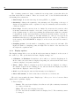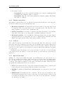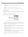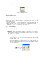
1
WinScatter
User Manual
Applied Photonics Group
2
Contents
1 Introduction
7
2 Installation procedures
9
3 Operating instructions
3.1 Connecting to the oscilloscope . . . . . . . . . . . .
3.2 Overview of the control panel and the main menu .
3.3 Control panel . . . . . . . . . . . . . . . . . . . . .
3.3.1 Scanning the waveform . . . . . . . . . . .
3.3.2 Display options . . . . . . . . . . . . . . . .
3.3.3 Display operations . . . . . . . . . . . . . .
3.3.4 Cursors . . . . . . . . . . . . . . . . . . . .
3.3.5 Special functions . . . . . . . . . . . . . . .
3.3.6 Data transfer . . . . . . . . . . . . . . . . .
3.3.7 Waveform data . . . . . . . . . . . . . . . .
3.4 Main menu options . . . . . . . . . . . . . . . . . .
3.4.1 File . . . . . . . . . . . . . . . . . . . . . .
3.4.2 Edit . . . . . . . . . . . . . . . . . . . . . .
3.4.3 Operations . . . . . . . . . . . . . . . . . .
3.4.4 View . . . . . . . . . . . . . . . . . . . . . .
3.4.5 Help . . . . . . . . . . . . . . . . . . . . . .
3.5 Working off-line . . . . . . . . . . . . . . . . . . . .
.
.
.
.
.
.
.
.
.
.
.
.
.
.
.
.
.
11
11
12
13
13
14
15
15
15
16
17
18
19
20
21
22
22
22
4 Troubleshooting
4.1 Errors when running the application . . . . . . . . . . . . . . . . . . . . . . .
4.2 Errors when using functions of the application . . . . . . . . . . . . . . . . .
4.3 Errors in GPIB communications . . . . . . . . . . . . . . . . . . . . . . . . .
25
25
26
27
.
.
.
.
.
.
.
.
.
.
.
.
.
.
.
.
.
.
.
.
.
.
.
.
.
.
.
.
.
.
.
.
.
.
.
.
.
.
.
.
.
.
.
.
.
.
.
.
.
.
.
.
.
.
.
.
.
.
.
.
.
.
.
.
.
.
.
.
.
.
.
.
.
.
.
.
.
.
.
.
.
.
.
.
.
.
.
.
.
.
.
.
.
.
.
.
.
.
.
.
.
.
.
.
.
.
.
.
.
.
.
.
.
.
.
.
.
.
.
.
.
.
.
.
.
.
.
.
.
.
.
.
.
.
.
.
.
.
.
.
.
.
.
.
.
.
.
.
.
.
.
.
.
.
.
.
.
.
.
.
.
.
.
.
.
.
.
.
.
.
.
.
.
.
.
.
.
.
.
.
.
.
.
.
.
.
.
.
.
.
.
.
.
.
.
.
.
.
.
.
.
.
.
.
.
.
.
.
.
.
.
.
.
.
.
.
.
.
.
.
.
.
.
.
.
.
.
.
.
.
.
.
.
.
.
.
.
.
4
CONTENTS
List of Figures
3.1
3.2
3.3
3.4
3.5
3.6
3.7
3.8
3.9
3.10
3.11
3.12
3.13
3.14
3.15
3.16
Preparing the oscilloscope for external control through
Connecting to the oscilloscope. . . . . . . . . . . . . .
Control panel and main menu. . . . . . . . . . . . . .
Data transfer between computer and oscilloscope. . . .
Warning message. . . . . . . . . . . . . . . . . . . . . .
Internal Memory Storage. . . . . . . . . . . . . . . . .
Special functions. . . . . . . . . . . . . . . . . . . . . .
Parameters of the waveform. . . . . . . . . . . . . . .
Samples of the waveform. . . . . . . . . . . . . . . . .
Box displaying a waveform. . . . . . . . . . . . . . . .
Main menu. . . . . . . . . . . . . . . . . . . . . . . . .
Dialog box for mathematical operations. . . . . . . . .
Explanation window . . . . . . . . . . . . . . . . . . .
About window. . . . . . . . . . . . . . . . . . . . . . .
Off-line warning window. . . . . . . . . . . . . . . . . .
Communication error message. . . . . . . . . . . . . .
GPIB.
. . . .
. . . .
. . . .
. . . .
. . . .
. . . .
. . . .
. . . .
. . . .
. . . .
. . . .
. . . .
. . . .
. . . .
. . . .
.
.
.
.
.
.
.
.
.
.
.
.
.
.
.
.
.
.
.
.
.
.
.
.
.
.
.
.
.
.
.
.
.
.
.
.
.
.
.
.
.
.
.
.
.
.
.
.
.
.
.
.
.
.
.
.
.
.
.
.
.
.
.
.
.
.
.
.
.
.
.
.
.
.
.
.
.
.
.
.
.
.
.
.
.
.
.
.
.
.
.
.
.
.
.
.
.
.
.
.
.
.
.
.
.
.
.
.
.
.
.
.
.
.
.
.
.
.
.
.
.
.
.
.
.
.
.
.
.
.
.
.
.
.
.
.
.
.
.
.
.
.
.
.
11
12
13
16
17
17
18
18
19
19
19
21
22
22
23
23
6
LIST OF FIGURES
Chapter 1
Introduction
This manual is intended for operators who are responsible for operating the Sampling Optical
Oscilloscope OOS-01 of Hamamatsu. This manual aims to:
• explain in detail how the application works,
• give the points to keep in mind when operating on the different devices for measuring
the bandwidth in optical fibers, and
• advise how to obtain the highest performance.
This manual requires a user knowledge of Microsoft Windows operating systems as well
as a working knowledge of terms related to optical fibers.
Furthermore, it is strongly recommended to read the user manual of the Optical Oscilloscope [1], since it is an extremely sensitive device and an incorrect usage could result in
permanent damage.
Next, we are going to show the main features of the application and we will explain how
it operates.
8
Introduction
Chapter 2
Installation procedures
WinScatter works on Intel-based computers under Windows 95, Windows 98, Windows NT
4.0, Windows 2000 or Windows XP1 . The minimum requirements are the following: 16 MB
RAM, 1.2 GB hard disk and a GPIB card.
In order to install the application, insert the WinScatter CD-ROM, select the WinScatter
folder, and copy it into your computer. Next, open the WinScatter folder and run the batch
file “RegisterMsFlxGrd.bat” in order to register the Microsoft FlexGrid ActiveX component
(this action is absolutely necessary in order to be able to run the application). Afterwards,
open the “WinScatter.ini” configuration file (using an ASCII text editor) and set the proper
address parameters of your GPIB board and the Hamamatsu OOS-01 oscilloscope.
Once the application has been installed and properly configured, double click the “WinScatter.exe” application file and it will start up automatically.
1
The window style varies depending on the operating system. The figures shown later in this manual were
taken using Windows XP.
10
Installation procedures
Chapter 3
Operating instructions
3.1
Connecting to the oscilloscope
First of all, preparations have to be made in the oscilloscope so as to enable the external
control through the GPIB interface. This is done following these steps:
1. Power on the oscilloscope and the laser driver.
2. Select CONT in the TRIG. MODE switch of the laser drive in order to input the trigger
signal in the oscilloscope.1
3. Using the control panel of the oscilloscope, press the SEL key twice and then the F4
(REMOTE) key as shown in Fig. 3.1.
DIRECTORY
CURRENT
REM/LOCAL >
SCALE
STORE
RECALL
FUNC
SCALE
STORE
RECALL
FUNC
DISPLAY
SAMPLE
OUTPUT
PLOTTER
MATH
FFT
CAL
REMOTE
RESET
LOCAL
Figure 3.1: Preparing the oscilloscope for external control through GPIB.
Now the oscilloscope is in the remote control status.
If you now run the application, the window shown in Fig. 3.2 will be displayed. If the
connection to the oscilloscope is successful, you will be able to choose between working on-line
(all features enabled) or off-line (you can only access to certain functions). If the connection
has failed, it can be due to one of the following three reasons:
1
From now on the laser diode is emitting. Therefore, special care should be taken.
12
Operating instructions
• You are working on a computer which has no connection to the oscilloscope through
GPIB. In that case, you will be able to work only off-line. It is important to note that
this is not an error; this operation mode has been intentionally designed to allow the
user to work with previously stored measurements in computers with no connection
to the oscilloscope. This operation mode will be explained in detail in section 3.5 on
page 22.
• The oscilloscope has not been correctly configured to enable external control through the
GPIB card installed in the computer. Make sure that you have followed the instructions
previously explained in this section. Then try to connect to the oscilloscope clicking the
button “Try again”. After that, the application should display the button “On-line”.
• There is an error in the GPIB bus or the GPIB card installed in your computer. If you
cannot connect to the oscilloscope in spite of having followed the steps explained before
in this section, perhaps the GPIB cable is damaged or the GPIB card does not work
properly. It is recommendable to note down the error code and refer to section 4.3 on
page 27.
Figure 3.2: Connecting to the oscilloscope.
3.2
Overview of the control panel and the main menu
The control panel and the main menu are shown in Fig. 3.3.
The main options of the application are the following:
• File. It allows you to open or save files. You can also exit the application through this
menu.
• Edit. It allows you to copy selected data from the grid “Waveform data” or export
waveform data to other applications.
• Operations. This option allows you to display the dialog boxes corresponding to the
data transfer between the computer and the oscilloscope, the internal memory storage
3.3 Control panel
13
Figure 3.3: Control panel and main menu.
and the performance of mathematical operations with previously stored waveforms. It
also allows you to switch off-line (the link to the oscilloscope is cut off).
• View. It allows to switch to the first or the second channel of the oscilloscope. It also
allows to display the waveform obtained from the oscilloscope in the computer.
• Help. It displays a small window with operating instructions and gives information
about version number and copyright.
Besides, the different options of the menu can be accessed quickly using the shortcut keys,
such as, Ctrl+Underlined Key, Alt+Underlined Key, or the function keys (F1, F2, etc.).
3.3
Control panel
This section explains the operations available on the control panel and the menu.
3.3.1
Scanning the waveform
Inside the “Action” frame you can choose the scanning waveform method:
• Stop. It stops scanning waveform immediately.
• Normal. It starts scanning waveform.
• Accumulate. It accumulates waveform data. The combo box next to the radio button
allows you to specify from 1 to 10000 accumulations.
• Rolling average. It averages waveforms while scanning. Each average is performed
with the latest scan and the previously averaged results. The combo box next to the
radio button allows you to specify from 1 to 100 averages.
14
Operating instructions
The “Scanning parameters” frame contains the most important options that affect the
way that waveforms are scanned. There are several combo boxes and sliders that allow
customizing these parameters:
• Time Range. It sets the time range from 20 ps/DIV to 1 µs/DIV.
• Sensitivity. Changes the sensitivity of the intensity scale. Depending on the type of
display chosen (this issue will be explained below), the sensitivity is shown in watts or
counts per division.
• Scan range. Sets the scan rate from 1 to 10000. If you increase the scan rate, there
is an improvement in the signal–to–noise ratio, but special care must be taken, since:
i) the acquisition time becomes longer (making the measurement results more sensitive
to fluctuations in time and temperature), and ii) the internal circuitry of the photomultiplier tube is more sensitive to the light intensity (i.e. there is a decrease in the
maximum value allowed for the light intensity incident on the oscilloscope). Therefore,
if the message A/D SATURATED is displayed on the screen, the scan rate must be
decreased.
• Sampling points. Sets the number of sampling points between 256 and 4096. The
higher the number of sampling points, the higher the resolution of the waveform, but
the higher the acquisition time.
3.3.2
Display options
The display settings allow you to modify how the waveforms are displayed on the screen of
the oscilloscope. The options inside the frame “Display settings” are:
• 1 Window / 2 Windows. It switches to the 1-window or 2-window displaying mode.
In the former, the waveforms are displayed superimposed, whereas in the latter waveforms are displayed on separate windows.
• Lines / Dots. When dot-display is specified waveforms are displayed according to
the samples acquired in the scanning process; whereas when line-display is specified,
waveforms are displayed connected by lines.
• Grid. A grid showing the time and the intensity axes is displayed.
• Clear 2nd window. A click on this button clears the second waveform.
The radio buttons inside the frame “Display type” allow you to choose between a linear
display and a logarithmic display:
• Linear display:
– Linear. The waveform is displayed in a linear scale (the sensitivity is measured
in counts per division).
– Watt. The waveform is displayed in watts.
– %. The waveform is normalized and it is displayed in %. The sensitivity cannot
be changed.
3.3 Control panel
• Logarithmic display:
– Logarithmic (log10 ). The waveform is displayed in common logarithm (base-10
logarithm). The sensitivity cannot be changed.
– Logarithmic (ln). The waveform is displayed in natural logarithm. The sensitivity cannot be changed.
3.3.3
Display operations
The display operations allow you to modify the vertical and horizontal axes of the waveform,
as well as to shift it along the horizontal time axis.
• Horizontal expansion. It expands the waveform in relation to the time axis. It can
be expanded twice (×2), three times (×3) or four times (×4). The selection of the
single expansion (×1) restores the original time axis.
• Vertical expansion. It expands or compresses the waveform relative to the intensity
axis. This option cannot be modified if the logarithmic display mode is used.
• Horizontal position. You can shift the waveform display along the time axis by
typing the time in picoseconds inside the edit box. With negative values the waveform
shifts to the right, whereas with positive values it shifts to the left.
3.3.4
Cursors
The oscilloscope has two cursors that move along the time axis. The cursors are of great
importance since they delimit the region where the special functions are applied. Each cursor
is controlled by means of scroll bars placed at the bottom of the frame “Cursors”; the left side
of the screen of the oscilloscope is specified by position 0, whereas the right side is specified
by position 599.
Clicking the radio buttons placed above the scroll bars, you can choose between moving
both cursors in the 1st window or in the 2nd window, provided that two waveforms are
displayed.
3.3.5
Special functions
Clicking one of the buttons inside the frame “Special Functions” you can perform one of
the seven special functions available. These functions are performed inside the limits defined
by both cursors; therefore you should place correctly the cursors before performing these
operations. The results are displayed on the grid located inside the frame “Waveform data”
as explained in detail in subsection 3.3.7 on page 17.
• I1/I2. It determines the ratio between the intensities measured in the positions given
by the respective cursors and the difference in time between them.
• FWHM. It calculates the Full Width at Half Maximum of a peak placed between both
cursors.
• RISE/FALL. It determines the rise or fall time. The rise time is determined for the
case when the intensity at the position of the cursor set at the left side of the screen is
lower than the intensity at the position of the cursor set at the right side; otherwise,
the fall time is determined.
15
16
Operating instructions
• MOD. It determines the modulation factor of the area between cursors.
• MIN/MAX. It determines the maximum and minimum values in the area between
cursors.
• MEAN. It determines the mean value of the intensities between cursors.
• AREA. It determines the accumulated value of the intensities between cursors.
3.3.6
Data transfer
The buttons inside the frame “Data transfer” allow you to exchange waveform data between
the computer and the oscilloscope, or to store them in any of the four internal memories of
the oscilloscope.
Data transfer between computer and oscilloscope
Figure 3.4 shows the button that pops up the “Data transfer” dialog box.
Figure 3.4: Data transfer between computer and oscilloscope.
By clicking the button that shows the arrow towards the right, the transfer takes place
from the computer to the oscilloscope (upload), whereas if the button showing the arrow
towards the left is clicked, the transfer takes place from the oscilloscope to the computer
(download). There are six options available in the list box:
• CH1. When downloading, the waveform scanned by the photomultiplier tube connected
to the port CH1 is transferred to the computer. When uploading, the waveform data
is displayed on the 1st window.
• CH2. When downloading, the waveform scanned by the photomultiplier tube connected
to the port CH2 is transferred to the computer. When uploading, the waveform data
is displayed on the 2nd window.
• M1, M2, M3, and M4. The data transfer takes place between the computer and one
of the four internal memories of the oscilloscope. If you request data from an empty
memory, the application shows a warning message (see Fig. 3.5).
At the bottom of the control panel a progress bar shows the progress of the transfer.
This dialog box can also be reached via the “Operations” menu.
3.3 Control panel
17
Figure 3.5: Warning message.
Internal Memory Storage
Figure 3.6 shows the button that pops up the “Internal Memory Storage” dialog box.
When clicking the button that shows the arrow towards the right, the field “1st window”
of the list box “Display Window” refers to the photomultiplier tube connected to the port
CH1 of the oscilloscope, whereas the field “2nd window” refers to the tube connected to CH2.
Therefore, the data storage takes place from one of the channels of the oscilloscope to the
chosen internal memory.
Instead, when clicking on the button that shows the arrow towards the left, the data
exchange takes place from the chosen internal memory to the chosen display window.
This dialog box can also be reached via the “Operations” menu.
3.3.7
Waveform data
The information corresponding to the waveform transferred to the computer is shown in the
grid placed inside the frame “Waveform data”. The three buttons above the grid change the
information type shown in the grid.
• Functions. Clicking this button the results for the special functions performed previously are shown. “No data” is displayed whenever a function has not been performed.
An example is shown in Fig. 3.7.
• Parameters. Clicking this button the nine parameters of the waveform are shown (see
Fig. 3.8 on page 18):
– Source. It shows the source of the measured waveform sent to the computer: CH1,
CH2, M1, M2, M3, or M4.
– Time Range. It shows the time range used during waveform acquisition.
– Horizontal exp. It shows the horizontal expansion used to acquire waveform data.
– Aperture time. This parameter only makes sense when using CCD sensors instead
of a photomultiplier tube.
Figure 3.6: Internal Memory Storage.
18
Operating instructions
Figure 3.7: Special functions.
– Sampling points. It shows the resolution used during waveform acquisition.
– Sensitivity. It shows the sensitivity used to acquire waveform data.
– Scan rate. It shows the scan rate used during waveform acquisition.
– Accum. count It shows the total number of accumulated waveforms.
– Channel no. It shows the number of the photomultiplier tube used to scan the
waveform. If there is only one tube connected to CH1, this parameter is always
set to 0.
Figure 3.8: Parameters of the waveform.
• Samples. Clicking this button the samples of the measured waveform are shown. Each
sample consists of a pair of values: the first value shows the time in ps and the second
value shows raw data related to the number of intensity counts (these raw data do
not take into account the selected scan rate and the number of accummulations). An
example is shown in Fig. 3.9.
Finally, clicking the button “Display waveform” placed at the bottom of the grid, a box
displaying the acquired waveform is shown (normalized to its maximum value). Figure 3.10
on page 19 shows the latter.
3.4
Main menu options
This section explains the options available through the main menu (those options already
explained in the previous section will be briefly mentioned). Figure 3.11 shows the main
menu.
3.4 Main menu options
19
Figure 3.9: Samples of the waveform.
Figure 3.10: Box displaying a waveform.
3.4.1
File
It allows you to open or save files. You can also exit the application through this menu.
Open
It opens waveform data stored in a file with the *.sct default extension. If you attempt to
open a file which does not contain valid data an error message will be displayed.
You can also access the dialog box “Open” using the shortcut key Ctrl+O.
Save and Save as. . .
The application stores the waveform data with the *.sct default extension. Selecting Save,
you will overwrite previously saved data with the latest parameters, whereas selecting Save
Figure 3.11: Main menu.
20
Operating instructions
as. . . , the application will ask you a new name for the file to be created.
You can also access the dialog box “Save” using the shortcut key Ctrl+S.
Exit
You can exit the application in one of the following ways.
• Selecting “Exit” through “File” menu.
• Clicking the close special button on the right top of the window.
• Using the shortcut key Alt+F4.
• While maintaining Alt key, press F, release it and then press X.
To restore the control in the oscilloscope and, therefore, to make it possible to operate its
front panel, you must press the F3 (RESET) key and then the F4 (REMOTE) key.
3.4.2
Edit
It allows you to copy selected data from the grid “Waveform data” or export waveform data
to other applications.
It is also possible to display a pop-up menu with the same content as the “Edit” option
with a right mouse click.
Export waveform to. . .
This option allows you to export the waveform data stored on your computer to other applications. WinScatter will automatically format the data in order to make them suitable for
the application you have chosen to export to, and it will put them on the clipboard. In the
following, there will be explained what you have to do to paste successfully the data on each
application.
• Spreadsheets. WinScatter allows you to export waveform data to Microsoft Excel or
OriginPro:
– Microsoft Excel: open Microsoft Excel; create a new sheet, select the first cell and
then click the button “Paste”.
– OriginPro: open OriginPro; create a new workbook, select the first cell and then
click the button “Paste”.
• Mathematical applications. WinScatter creates automatically the required code in
order to export this to Mathematica (version 3.0 or higher) or MATLAB (version 5.1
or higher).
– MATLAB. Open MATLAB; Select “M-file” through “File/New” menu and then
the M-file editor will be displayed. Paste the content of the clipboard and change
the name “winscatt” next to the function command with that one you will use to
save the file. You can finally run it typing the file name in “MATLAB Command
Window”.
– Mathematica. Open Mathematica; paste the content of the clipboard on the command window and press “Intro”. Mathematica will automatically display the
waveform.
3.4 Main menu options
Copy from grid
This option allows you to copy the selected data on the grid placed inside the frame “Waveform
data” and put them on the clipboard. Then, they can be pasted in any other application,
such as word processors or spreadsheets.
You can also copy the content using the shortcut key Ctrl+C.
3.4.3
Operations
It allows you to display the dialog boxes corresponding to the data transfer between the
computer and the oscilloscope, the internal memory storage, and the performance of mathematical operations with previously stored waveforms. It also allows you to switch off-line
(interrupting the communication with the oscilloscope).
Mathematical operations
If you select this option the dialog box shown in Fig. 3.12 is displayed.
Figure 3.12: Dialog box for mathematical operations.
You can perform 4 different arithmetic operations on two waveforms. The measurement
parameters (time range, sensitivity, number of samples, etc.) for both waveforms must be
the same.
First of all, you have to select the first operand, then the operant (sum, rest, multiplication
or division), then the second operand and finally the memory or window you want to store
the result.
Clicking the button “Perform”, the oscilloscope performs the arithmetic operation. If you
want to exit this dialog box without performing any operation, just click the button “Cancel”.
Data transfer
This is the same option as explained in subsection 3.3.6 on page 16.
Internal memory storage
This is the same option as explained in subsection 3.3.6 on page 17.
Off-line
Finally, this option allows you to switch off-line (the link to the oscilloscope is cut off). The
latter will be discussed in section 3.5 on page 22.
21
22
Operating instructions
3.4.4
View
This option allows to switch to the first or the second channel of the oscilloscope. It also
allows to display the waveform obtained from the oscilloscope in the computer (the latter has
been explained in subsection 3.3.7 on page 17).
3.4.5
Help
This option displays a small window with operating instructions and gives information about
version number and copyright.
Figure 3.13 shows the operating instructions displayed when selecting “Operations”.
Figure 3.13: Window showing operating instructions.
Finally, Fig. 3.14 shows the window popped up when selecting “About WinScatter. . . ”.
Figure 3.14: About window.
3.5
Working off-line
There are two ways to work off-line:
1. Clicking the button “Off–line” in the dialog box Connecting to the optical oscilloscope
when you initialize the application (see Fig. 3.2 on page 12).
2. Selecting the option “Off–line” through the Mathematical operations menu (see subsection 3.4.3 on page 21). If you do this, the window shown in Fig. 3.15 will pop up.
When you work off-line, you can only access to a limited set of options:
• Main Menu. You can open and save files, display the waveform, and export waveform
data to other applications.
3.5 Working off-line
23
Figure 3.15: Off-line warning window.
• Control panel. You can only access to the controls located inside the frames “Special
functions” and “Waveform data”. Working off-line, the special function buttons behave
in the same way as the button “Functions” inside the frame “Waveform data”.
It is important to notice that when the communication link between the computer and
the oscilloscope has been cut off, the application switches automatically to off-line, displaying
an error message with the reasons for the failure (see Fig. 3.16).
Figure 3.16: Communication error message.
In such a case, it is recommendable to note down the error code and refer to section 4.3
on page 27.
24
Operating instructions
Chapter 4
Troubleshooting
4.1
Errors when running the application
• The application does not run or there is a warning message showing there are not enough
resources available.
This means that there is not enough memory. The minimum required memory is 16MB.
If your computer fulfills these requirements but this message still appears, make sure
there are no other applications running at the same time. Make also sure that there
are at least 20MB free on the hard disk.
Although WinScatter works on the different 32-bit Windows operating systems, it is
strongly recommended to use it on those systems based on NT technology (namely,
Windows NT 4.0, Windows 2000 and Windows XP)1 .
• When running the application there is a message in the “Connecting to the oscilloscope...” window showing that the connection has failed.
This can be due to one of the following three reasons:
1. You are working on a computer which has no connection to the oscilloscope through
GPIB. In that case, you can only work off-line. You should have a GPIB card
installed on your computer and a GPIB cable connected to the oscilloscope.
2. The oscilloscope has not been correctly configured to enable external control
through the GPIB card installed in the computer. Make sure that you have followed the instructions explained in section 3.1 on page 11. Then try to connect
to the oscilloscope clicking the button “Try again”. After that, the application
should display the button “On-line”.
3. There is an error in the GPIB bus or in the GPIB card installed in your computer.
If you cannot connect to the oscilloscope in spite of having followed the steps
explained before in this section, perhaps the GPIB cable is damaged or the GPIB
card does not work properly. It is recommendable to note down the error code
and refer to section 4.3 on page 27.
1
WinScatter has not been tested on Windows Vista or Windows 7 operating systems.
26
Troubleshooting
4.2
Errors when using functions of the application
• When selecting any of the options of the control panel there is a message showing a
GPIB error.
This can be due to the following reasons:
1. You have gone back to the LOCAL mode pressing the F4 key on the front panel
of the oscilloscope, disabling the external control of the latter through the GPIB
interface. For security reasons, the application will switch to off-line. If you want
to restore the connection to the oscilloscope, you have to exit the application and
run it again, preparing the oscilloscope by following the instructions explained in
section 3.1 on page 11.
2. There is an error in GPIB bus or the GPIB card installed in your computer.
Perhaps the GPIB cable is damaged or the GPIB card does not work properly. It
is recommendable to note down the error code and refer to section 4.3 on page 27.
In this case, the application will also switch off-line.
• Sensitivity cannot be changed.
The combo box “Sensitivity” is disabled when:
–
–
–
–
The waveform scanning has been stopped with the command “Stop”.
The execution of the commands “Accumulate” or “Rolling average” has finished.
The “%” linear display type has been selected.
Waveform data have been transferred from the computer to one of the channels
(CH1 or CH2).
– The contents of one of the four internal memories has been transferred to one of
the channels.
• Vertical expansion cannot be changed.
The combo box “Vertical expansion” is disabled when:
– There has been selected the “%” linear display type.
– There has been selected one of the two logarithmic display types Logarithmic
(log10 ) or Logarithmic (ln).
• Horizontal expansion cannot be changed.
The combo box “Horizontal expansion” is disabled when:
– The waveform scanning has been stopped with the command “Stop”.
– The execution of the commands “Accumulate” or “Rolling average” has finished.
– Waveform data have been transferred from the computer to one of the channels
(CH1 or CH2).
– The contents of one of the four internal memories has been transferred to one of
the channels.
• The cursors cannot be changed to the 2nd window.
In order to be able to select this option, it is necessary to have waveform data on
the 2nd window. To achieve this you have to transfer data from the computer (see
subsection 3.3.6 on page 16) or use the dialog box “Internal Memory Storage” (see
subsection 3.3.6 on page 17).
4.3 Errors in GPIB communications
• The frame “Waveform data” does not display any information about the waveform
displayed in the screen of the oscilloscope.
It is necessary to transfer this waveform data from the oscilloscope to the computer (see
subsection 3.3.6 on page 16).
• When trying to transfer waveform data from one of the four internal memories to the
computer there is a message showing “No data”.
If you want to transfer data from one of the four internal memories it is necessary
to have previously stored waveform data on that memory, transferring data from the
computer (see subsection 3.3.6 on page 16) or using the dialog box “Internal Memory
Storage” (see subsection 3.3.6 on page 17).
• Cannot export waveform data.
If you want to export waveform data to different applications, it is necessary to have
waveform data on the computer. This can be achieved by transferring the waveform
data from the oscilloscope to the computer (see subsection 3.3.6 on page 16) or by
opening a file.
• Cannot open a file or an error message is displayed.
Since the application stores the waveform data with the *.sct default extension, you
should only open this type of files (note that the application lets you open files with
any other extension by selecting All files (*.*) in the list box). Opening a file which
does not contain valid data will lead to displaying an error message.
It could also happen that the file is corrupted because the storage system has been
damaged or any inconsistence in the File System of the operative system.
4.3
Errors in GPIB communications
In the following section the possible GPIB errors are enumerated and described. For more
information, please refer to [2].
• (EDVR) System error.
This error occurs when you try to access a board or device that is not installed or
configured properly.
• (ECIC) Function requires GPIB board to be CIC.
This error occurs when a command is sent to the GPIB board and the latter is not
configured as the CIC or there are conflicts because of having multiple controllers.
• (ENOL) No Listeners on the GPIB.
This error usually occurs when a writing operation is attempted with no Listeners
addressed. For a device writing, ENOL indicates that the GPIB address configured for
that device in the software does not match the GPIB address of any device connected
to the bus, that the GPIB cable is not connected to the device, or that the device is
not powered on.
27
28
Troubleshooting
• (EADR) GPIB board not addressed correctly.
This error occurs when the GPIB board is CIC and is not properly addressing itself
before the read and write functions. This error is usually associated with board-level
functions.
• (EARG) Invalid argument to function call.
This error results when an invalid argument is passed to a function call.
• (ESAC) GPIB board not System Controller as required.
This error results when the functions requiring that the GPIB board be the System
Controller are called and the latter has not this capability.
• (EABO) I/O operation aborted (timeout).
This error indicates that an I/O operation has been cancelled, usually due to a timeout
condition.
• (ENEB) Nonexistent GPIB board.
This error occurs when no GPIB board exists at the I/O address specified in the configuration file. This occurs when the board is not physically plugged into the system, the
I/O address specified during the configuration does not match the actual board setting,
or there is a system conflict with the base I/O address.
• (EDMA) DMA error.
This error occurs if a system DMA error is encountered when the GPIB software attempts to transfer data over the GPIB using DMA.
• (EOIP) Asynchronous I/O in progress.
This error occurs when an asynchronous I/O operation has not finished before some
other call is made. During asynchronous I/O, you can only use ibstop, ibwait, and
ibonl, or perform other non-GPIB operations.
• (ECAP) No capability for operation.
This error results when your GPIB board cannot carry out an operation or when a
particular capability has been disabled in the software and a call that requires the
capability is made.
• (EFSO) File system error.
This error results when an ibrdf or ibwrtf call encounters a problem performing a file
operation. Specifically, this error indicates that the function is unable to open, create,
seek, write, or close the file being accessed.
• (EBUS) GPIB bus error.
This error results when a certain GPIB bus error occurs during device functions. All device functions send command bytes to perform addressing and other bus managements.
Devices are expected to accept those command bytes within the time limit specified
by the default configuration or the ibtmo function. EBUS results if a timeout ocurred
while sending these command bytes.
4.3 Errors in GPIB communications
• (ESTB) Serial poll status byte queue overflow.
This error is reported only by the ibrsp function. ESTB indicates that one or more
serial poll status bytes received from automatic serial polls have been discarded because
of a lack of storage space.
• (ESRQ) SRQ stuck in ON position.
This error can only be returned by a device-level ibwait call with RQS set in the mask.
ESRQ indicates that a wait for RQS is not possible because the GPIB SRQ line is stuck
on.
• (ETAB) Table problem.
This error occurs only during the FindLstn and FindRQS functions. ETAB indicates
that there was some problem with a table used by these functions.
29
30
Troubleshooting
Bibliography
[1] Hamamatsu Photonics K. K., Sampling optical oscilloscope OOS-01. [Online]. Available:
http://www.hamamatsu.com/
[2] GPIB user manual for Win32, National Instruments, Austin, Texas, June 1998.