Download Origin 5 LabTalk Developer`s Guide

Origin 6.1
LabTalk
Developer's Guide
OriginLab Corporation
Copyright
OriginLab, Origin, and LabTalk are either registered trademarks or trademarks of OriginLab
Corporation.
Microsoft, Windows, and Windows NT are registered trademarks of the Microsoft Corporation.
2000 OriginLab Corporation. All rights reserved.
The software (including any images, "applets," photographs, animations, video, audio, music and text
incorporated into the software) is owned by OriginLab Corporation or its suppliers and is protected by
United States copyright laws and international treaty provisions. Therefore, you must treat the software
like any other copyrighted material (e.g., a book or musical recording) except that you may either (a)
make one copy of the software solely for backup or archival purposes, or (b) transfer the software to a
single hard disk provided you keep the original solely for backup or archival purposes. You may not
copy the printed materials accompanying the software, nor print copies of any user documentation
provided in "online" or electronic form.
Grant of License
This OriginLab Corporation End-User License Agreement ("License") permits you to use one copy of
the OriginLab Corporation product Origin, which may include user documentation provided in "online"
or electronic form ("software"), on any single computer, provided the software is in use on only one
computer at any one time. If this package is a license pack, you may make and use additional copies of
the software up to the number of licensed copies authorized. If you have multiple licenses for the
software, then at any time you may have as many copies of the software in use as you have licenses.
The software is "in use" on a computer when it is loaded into the temporary memory (i.e., RAM) or
installed into the permanent memory (e.g., hard disk, CD-ROM, or other storage device) of that
computer, except that a copy installed on a network server for the sole purpose of distribution to other
computers is not "in use". If the anticipated number of users of the software will exceed the number of
applicable licenses, then you must have a reasonable mechanism or process in place to ensure that the
number of persons using the software concurrently does not exceed the number of licenses.
OriginLab Corporation Technical Support
Support hours are 8:30 A.M. to 6:00 P.M. EST. Users must have their Origin serial number and
registration code ready. Users who have not yet registered with OriginLab Corporation should be
prepared to register upon calling for technical support.
1-800-969-7720 (U.S. & Canada)
OriginLab Corporation
Tel: + 413-586-2013
One Roundhouse Plaza
Fax: + 413-585-0126
Northampton, MA 01060
[email protected]
USA
Contents
Contents
Getting Started
1.1
1.2
1.3
1.4
5
Introduction.........................................................................................................................5
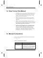
How To Use This Manual ...................................................................................................6
Manual Conventions ...........................................................................................................6
Quick Start Tutorials ...........................................................................................................7
1.4.1 The Script Window............................................................................................8
1.4.2 Window Buttons ................................................................................................8
1.4.3 Script Files .......................................................................................................10
1.4.4 Macros .............................................................................................................13
Advanced Origin
15
2.1 Overview of Origin ...........................................................................................................15
2.1.1 Projects ............................................................................................................15
2.1.2 Child Windows ................................................................................................15
2.1.3 Datasets............................................................................................................16
2.1.4 Templates.........................................................................................................17
2.1.5 Graphs and Layers ...........................................................................................19
2.1.6 LabTalk............................................................................................................20
2.1.7 Curve Fitting ....................................................................................................21
2.1.8 Origin's Window Objects.................................................................................22
2.2 Advanced Use of Layers ...................................................................................................28
2.2.1 Linked Layers ..................................................................................................29
2.2.2 Scaling .............................................................................................................33
2.3 Additional Tips .................................................................................................................36
2.3.1 Merging Pages .................................................................................................36
2.3.2 Extracting Layers to Separate Pages ................................................................37
2.3.3 Extracting Data Plots to Separate Layers.........................................................37
2.3.4 Showing Only Every nth Symbol.....................................................................37
2.3.5 Using Datasets as a Plotting Enhancement ......................................................39
2.3.6 Using Escape Sequences to Format Labels......................................................45
2.3.7 View Modes.....................................................................................................46
Contents • i
Contents
2.3.8 Updating the Display .......................................................................................46
2.3.9 Control Regions ...............................................................................................49
2.3.10 Screen Plotting Speed ....................................................................................50
2.3.11 Printing...........................................................................................................50
LabTalk
53
3.1 Introduction .......................................................................................................................53
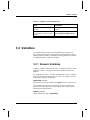
3.2 Variables ...........................................................................................................................55
3.2.1 Numeric Variables ...........................................................................................55
3.2.2 String Variables ...............................................................................................56
3.2.3 Numeric to String Conversion..........................................................................57
3.2.4 Deleting Variables ...........................................................................................57
3.3 Operators...........................................................................................................................57
3.3.1 Arithmetic Operators........................................................................................57
3.3.2 Assignment Operators......................................................................................58
3.3.3 Logical and Relational Operators.....................................................................58
3.3.4 Bitwise Operators.............................................................................................59
3.3.5 Conditional Operators......................................................................................59
3.4 Calculations.......................................................................................................................60
3.4.1 Scalar Operations .............................................................................................60
3.4.2 Vector Operations ............................................................................................60
3.4.3 Writing Speedy Calculations............................................................................66
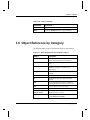
3.5 Command Reference by Category.....................................................................................67
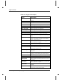
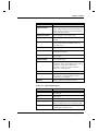
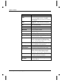
3.6 Object Reference by Category...........................................................................................71
3.7 Control Flow .....................................................................................................................75
3.7.1 Statements and Statement Blocks.....................................................................75
3.7.2 Break Command ..............................................................................................77
3.7.3 Continue Command .........................................................................................77
3.7.4 Doc Command .................................................................................................78
3.7.5 For Command ..................................................................................................79
3.7.6 If Command .....................................................................................................80
3.7.7 Layer -o Command ..........................................................................................81
3.7.8 Loop Command................................................................................................81
3.7.9 Repeat Command .............................................................................................82
3.7.10 Run Object Methods ......................................................................................82
3.7.11 Switch Command ...........................................................................................83
3.7.12 Win -o Command...........................................................................................84
3.8 Passing Arguments ............................................................................................................84
3.8.1 Passing Numeric Variables by Reference ........................................................85
3.8.2 Passing Numeric Variables by Value...............................................................86
3.9 Input ..................................................................................................................................87
3.9.1 Getnumber Command ......................................................................................87
3.9.2 Getpts Command..............................................................................................88
ii • Contents
Contents
3.10 Output .............................................................................................................................92
3.10.1 Literal Strings ................................................................................................92
3.10.2 Object's Text Property ...................................................................................94
3.10.3 Customizing Output Using the Type Command and Escape Sequences........94
3.10.4 Formatted Output with $( ) ............................................................................95
3.10.5 Redirecting Output to the Notes Window......................................................96
3.10.6 Redirecting Output to the Results Log...........................................................97
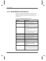
3.11 Useful Built-in Functions ................................................................................................98
3.11.1 Data Function.................................................................................................99
3.11.2 Exist Function ................................................................................................99
3.11.3 Int Function..................................................................................................100
3.11.4 List Function ................................................................................................100
3.11.5 Mod Function...............................................................................................100
3.11.6 Sqrt Function ...............................................................................................101
3.11.7 Sum Function ...............................................................................................101
3.11.8 Table Function .............................................................................................101
3.11.9 Xof Function ................................................................................................102
3.11.10 Xvalue Function.........................................................................................102
3.12 Macros ..........................................................................................................................102
3.13 Worksheet Tips .............................................................................................................104
3.13.1 Missing Values ............................................................................................104
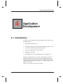
Application Development
105
4.1
4.2
4.3
4.4
Introduction.....................................................................................................................105
The LabTalk Development Environment ........................................................................106
Developing Script Files with the LabTalk Editor............................................................109
Running Script Files........................................................................................................111
4.4.1 Running Script from a Custom Toolbar Button .............................................111
4.4.2 Running Script from the Custom Routine Button on the Standard Toolbar...115
4.4.3 Running Script from the Label Control Dialog Box of an Object..................115
4.4.4 Running Script from New Menu Items (Commands).....................................117
4.4.5 Running Script from the Script Window........................................................118
4.4.6 Creating Templates for Your Custom Applications.......................................118
4.4.7 Useful Child Window Scripting Tips.............................................................119
4.5 Debugging Your Script ...................................................................................................120
4.5.1 The LabTalk Debugger ..................................................................................120
4.5.2 The Echo System Variable.............................................................................121
4.5.3 The List Command ........................................................................................122
4.5.4 Tracking Values of Variables ........................................................................122
4.5.5 The #!script Notation.....................................................................................122
4.5.6 Checking Variable Values at Breakpoints .....................................................123
4.6 Building Applications with OriginPro.............................................................................124
4.7 Distributing Your Custom Applications..........................................................................124
Contents • iii
Contents
4.7.1 Creating the Export (.OPK) File ....................................................................125
4.7.2 Installing the .OPK File .................................................................................127
4.7.3 Exchanging Your Custom Application on the OriginLab Web Site...............128
Index
iv • Contents
129
Chapter 1, Getting Started
1
Getting Started
1.1 Introduction
Origin®-based applications can be constructed for many purposes. For
example, you can create applications to handle statistical process control,
analyze pharmaceutical data, control sophisticated data acquisition
devices, and even to evaluate eyesight! Though each of these
applications address specialized data analysis and plotting needs, in each
case it is the Origin software that serves as the foundation for the customdesigned scientific application.
The LabTalk Developer’s Guide provides tips to assist you in building
your own well-written Origin application. However, this manual is not
intended as an Origin or LabTalk® reference. Nor is it intended as a
reference for the development tools available with OriginPro.
For assistance using Origin, see the Origin User’s Manual or the Origin
Help file.
For reference information on LabTalk, see the LabTalk Manual or the
LabTalk Help file.
To learn about the development tools available with OriginPro, see the
OriginPro Manual.
1.1 Introduction • 5
Chapter 1, Getting Started
1.2 How To Use This Manual
•
The Quick Start tutorials at the end of this chapter illustrate some of
the ways that you can run LabTalk scripts in Origin. In just a few
minutes, you'll learn different script execution methods to output
Hello World to an Attention dialog box.
•
Chapter 2 provides a brief overview of Origin. It also includes
advanced Origin issues and tips that are often included in custom
applications.
•
Chapter 3 surveys the LabTalk language, focusing on issues of
particular interest to the application developer. These issues include
the use of variables, operators, calculations, control flow statements,
input and output, built-in functions, and macros.
•
Chapter 4 guides you through the process of developing a custom
application. Detailed examples are provided illustrating different
script execution methods. Debugging methods are discussed.
Information is provided on building custom applications using
OriginPro tools. Additionally, information is provided on creating
and exchanging your custom tools with other Origin users.
1.3 Manual Conventions
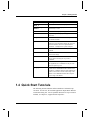
Table 1.1 lists the documentation conventions observed in the LabTalk
Developer’s Guide.
Table 1.1: Documentation Conventions
Convention
Description
Plot:Graph Type
Italicized text indicates the information is not
literal. Rather, the italicized text serves as a
placeholder for literal text. Supply or interpret the
appropriate literal text. For example, Plot:Scatter.
(Note: Text may also be italicized for emphasis.
This difference should be clear by context.)
Layer n dialog box
6 • 1.2 How To Use This Manual
Chapter 1, Getting Started
Convention
Description
Data1_A
The names of datasets are displayed in bold.
Window:Script
Window
Menu commands are displayed in bold. Levels are
separated by a colon.
ORIGIN61.EXE
File names are displayed in uppercase characters.
TAB
Keyboard keys are displayed in uppercase
characters.
Script
Arial + bold font indicates LabTalk script that can
be entered verbatim.
Syntax
Used with LabTalk. Italicized + bold font
indicates a user-supplied argument that cannot be
entered verbatim. Serves as a placeholder for
literal text. Usually used in syntax examples.
[]
Used with LabTalk. Items in brackets are
optional.
()
Used with LabTalk. Parentheses are used to
enclose text strings.
{}
Used with LabTalk. Braces are used around a
script, when associating the script with a
command.
<>
Used with LabTalk. Angle brackets indicate that
the argument(s) to a command can only be used
when no option is given.
Used with LabTalk. Appears in the command
syntax line of commands that take a dataset as an
argument. It indicates that the range modification
options can be used to set the active range of the
dataset. The command will then affect only the
active range of the dataset.
[range]
1.4 Quick Start Tutorials
The following tutorials illustrate different methods of LabTalk script
execution. In each case, the resultant application outputs Hello World to
an Attention dialog box. For an expanded discussion of script execution
methods, see Chapter 4, "Application Development."
1.4 Quick Start Tutorials • 7
Chapter 1, Getting Started
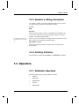
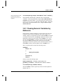
1.4.1 The Script Window
The Script window is a text editor with the additional feature of carrying
out LabTalk script execution. It is most useful for executing single lines
or short scripts, or for troubleshooting longer scripts before storing and
executing elsewhere.
The Script window is not a child window - as are the graph, worksheet,
matrix, workbook, and layout page windows. When you save a project,
the contents of the Script window are not saved with the project, as are
the child windows.
To open the Script window, select Window:Script Window.
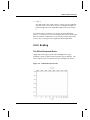
Figure 1.1: The Script Window
Type the following in the Script window. (Note that throughout this
manual, (ENTER) indicates that you press the ENTER key.)
type –b "Hello World" (ENTER)
Origin outputs Hello World to an Attention dialog box.
1.4.2 Window Buttons
Window buttons are objects located on Origin child windows that are
programmed with script in their associated Label Control dialog box.
They are created so users can initiate the script when the object's event is
triggered. For example, script can be triggered by clicking on an object
that appears as a button on a child window. Because the object is located
on the child window, the object and its script can be saved as part of a
template, window, or project.
8 • 1.4 Quick Start Tutorials
Chapter 1, Getting Started
In addition to the button triggering method, Origin provides a variety of
conditions for script execution, including (but not limited to):
Execute when a window is opened, closed, or moved.
Execute before the project is saved.
Execute when the graph axes are rescaled.
Execute when the object's child window is saved.
To learn more about buttons, perform the following procedure:
1) Open a new project and then click the Text Tool button
Tools toolbar.
on the
2) Click to the right of the two empty columns in the default Data1
worksheet. This action opens the Text Control dialog box.
3) Type Start Button in the text box provided and click OK. The text
now displays to the right of the columns. (Resize the worksheet if
needed.)
4) Press ALT while double-clicking on the text object. This action
opens the Label Control dialog box.
5) Type the following script in the text box provided:
type –b "Hello World";
6) Select Button Up from the Script, Run After drop-down list and click
OK. The text now displays as a button.
7) Click the button to execute the script. Origin outputs Hello World to
an Attention dialog box.
In this example, the script that is executed when the object is triggered is
fully contained in the object's Label Control dialog box. However, it is
common LabTalk programming practice to call script that is located in a
script file from the object's Label Control dialog box. Script files are
introduced in the following section. However, for a complete discussion
on calling script in script files, see Chapter 4, "Application
Development."
1.4 Quick Start Tutorials • 9
Chapter 1, Getting Started
1.4.3 Script Files
For more information on
script files, see Chapter 4,
"Application Development."
Script files are ASCII text files containing LabTalk script. When
developing your Origin application, it is recommended that you write
and develop your LabTalk scripts in script files. Script files are easy to
edit and replace, and their script can be executed from any object's Label
Control dialog box, from a custom toolbar button, or from other script
files, menu commands, the Script window, macros, configuration files,
etc.
When you construct script files, you should write small sections of code
that perform specific tasks. To help you get started, review the script
files (*.OGS) located in the Origin software folder.
OriginPro 6.1 includes a
new LabTalk script editor
and debugger.
Note: To open a script file associated with a menu command or toolbar
button, press CTRL+SHIFT and then select the menu command or click
on the toolbar button. If that command or toolbar button runs a script
file section, Origin opens the script file in a new instance of the LabTalk
Editor.
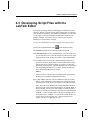
The following tutorial uses the run.section( ) object method to run the
script in the specified section of a script file. In the first part of the
tutorial, the script file section is called from the Script window. In the
section part, it is called from a custom toolbar button.
To create a script file and run its script, perform the following
procedure:
1) Click the New LabTalk Editor button
on the Standard toolbar.
This action opens a new instance of the LabTalk Editor.
The LabTalk Editor is a unique window type in Origin, designed for
developing and editing LabTalk script files. Like other window
types, you can open multiple LabTalk Editor windows in an instance
of Origin. You cannot, however, open the same script file multiple
times in an instance of Origin.
2) Type the following text into the LabTalk Editor window:
[Main]
type –b "Hello World";
3) Select File:Save As from the LabTalk Editor menu bar. Save this
file as HELLO.OGS in the Origin software folder.
10 • 1.4 Quick Start Tutorials
Chapter 1, Getting Started
4) Activate Origin and then select Window:Script Window from the
Origin menu bar (if the Script window is not already open).
5) Type the following in the Script window:
run.section(Hello,Main) (ENTER)
Because this script runs the Main section of the HELLO.OGS file,
Origin outputs Hello World to an Attention dialog box.
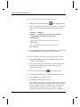
To run this script from a custom toolbar button, perform the following
procedure:
1) Select View:Toolbars. This menu command opens the Customize
Toolbar dialog box.
2) Select the Button Groups tab.
3) Select User Defined from the Groups list box.
4) Select a button from the Buttons group. For example, select the
button.
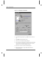
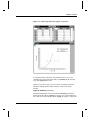
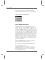
5) Click the Settings button in the Button group. This action opens the
Button Settings dialog box.
1.4 Quick Start Tutorials • 11
Chapter 1, Getting Started
Figure 1.2: Configuring a Custom Button
2. Select a button.
1. Select User
Defined.
3. Click Settings.
6) In the Button Settings dialog box, type Hello in the File Name text
box.
7) Type Main in the Section Name text box.
8) Click OK to close the Button Settings dialog box.
9) In the Customize Toolbar dialog box, drag the button (whose settings
you just edited) from the Buttons group into the Origin workspace.
Origin creates a new toolbar containing your button.
10) Click Close to close the Customize Toolbar dialog box.
11) Click on your new button. Origin outputs Hello World to an
Attention dialog box.
12 • 1.4 Quick Start Tutorials
Chapter 1, Getting Started
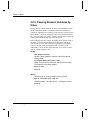
1.4.4 Macros
For more information on
macros, see Chapter 3,
"LabTalk."
A macro is a convenient method of aliasing a LabTalk script. When you
define a macro, you are associating an entire script with a specific name.
This name can then be used as a command that invokes the associated
script. Thus, if a user wants to perform an operation within an Origin
session, a macro can be defined during the Origin session. However, if a
user wants to perform the same operation in more than one Origin
session, it is best to define the macro in a configuration file (*.CNF)
which is executed each time Origin is started.
To define and call a macro, perform the following procedure:
1) Open a new Origin project and select Window:Script Window (if
the Script window is not already open).
2) Type the following in the Script window:
define hello { type –b "Hello World"; } (ENTER)
This script defines a macro named hello with the associated script
located between the braces.
3) To execute this macro, type the following in the Script window:
hello (ENTER)
Origin outputs Hello World to an Attention dialog box.
1.4 Quick Start Tutorials • 13
Chapter 1, Getting Started
This page is intentionally left blank.
14 • 1.4 Quick Start Tutorials
Chapter 2, Advanced Origin
2
Advanced Origin
2.1 Overview of Origin
Origin provides a broad range of data analysis and plotting features.
These built-in features are sufficient for most data analysis and plotting
needs. However, when these built-in features are coupled with the ability
to write LabTalk scripts for user-input or user-action, then Origin itself
becomes a scientific application development platform.
2.1.1 Projects
An Origin project is a collection of child windows contained within the
Origin application workspace. When you save an Origin project, the
current collection of child windows (including the data and any objects
that they contain) and all global variables are saved to the specified file
name. When you re-open the (saved) project, all child windows in the
project are opened in the state in which they were saved (minimized,
hidden, window, full screen).
2.1.2 Child Windows
Origin projects can include worksheet, graph, layout page, function
graph, Excel workbook, matrix, and notes child windows. Whereas notes
windows are created from script, worksheet, graph, layout page, function
graph, Excel workbook, and matrix child windows are created from
templates. Built-in templates can be customized and re-saved, or they
2.1 Overview of Origin • 15
Chapter 2, Advanced Origin
can be saved to new template files (except for the layout page). For
example, you can open a child window from a selected template, make
modifications to the window (such as changing the background color,
axis scale, and number of layers on the page), save the window to a
template file, and in the future create a child window based on the
customized template.
Having various child windows in a project allows you to simultaneously
view different visual representations of your data, such as data in a
worksheet versus a graph, simplifying data manipulation and analysis.
Since each child window displays a copy of an internally-held dataset,
changing the dataset in one child window will cause the dataset to be
displayed differently in other child windows that are displaying the same
dataset.
In addition to customizing the elements in a child window, programmable
objects can be added to child windows - allowing you to develop a
custom Graphical User Interface (GUI). For example, you can develop
routines to automate a repetitive process like importing data, plotting, and
fitting. Additionally, you can simplify the analysis of data by developing
routines to perform pre-defined actions at the click of a button.
In addition to using the default interface, you can use LabTalk commands
to open and close child windows in an Origin project. Thus, you need not
have every application-specific child window open at the same time,
cluttering the workspace. Opening a child window in a project can be as
simple as clicking a button on one child window to run a script that opens
another specified child window.
2.1.3 Datasets
To learn how to create
datasets with LabTalk, see
the LabTalk Manual.
16 • 2.1 Overview of Origin
A dataset is an object consisting of a one-dimensional array that can
contain numeric, text, or numeric and text values (including time, date,
and day of week). Individual values in a dataset are called elements.
Each element is associated with a particular index number. When a
dataset is displayed in a worksheet, the index number directly
corresponds to the row number. Unlike C conventions, the dataset index
numbers start at one.
Chapter 2, Advanced Origin
Displaying Datasets in Worksheets
A dataset is directly associated with the worksheet column in which it is
displayed. To emphasize this association, the name of the dataset object
contains the worksheet name and the column name. Origin uses the
following convention when naming datasets:
WorksheetName_ColumnName
Dataset names appear in
bold font style in the
LabTalk Developer’s Guide.
where WorksheetName is the name of the worksheet that displays the
dataset and ColumnName is the name of the column containing the data.
For example, if the Data1 worksheet contains two columns A and B,
then these datasets are named data1_a and data1_b.
Displaying Datasets in Matrices
A matrix window displays a single dataset containing Z values. Instead
of displaying the dataset as a single column (as in a worksheet), a matrix
window displays the dataset in a specified dimension of rows and
columns. X values are associated with the columns and Y values are
associated with the rows.
Displaying Datasets in Graph Windows
When data is plotted into a graph window, the graph window displays an
image of the dataset(s) held in memory. If you modify the contents of the
dataset(s) held in memory (for example, by modifying the associated
worksheet data), then the data plot updates accordingly. However, if you
change the X column designation in the worksheet containing the plotted
data, the graph window will not change. It will still display the data plot
based on the originally set X column.
2.1.4 Templates
Child window template files contain all of the attributes of the respective
window except the data contained in the window. These attributes can be
controlled by editing the child window’s dialog boxes, or by controlling
the window properties using LabTalk script.
2.1 Overview of Origin • 17
Chapter 2, Advanced Origin
•
Dialog Box Settings Saved with a Worksheet Template
Worksheet Display Control, Page Color, Worksheet Column Format,
ASCII Import Options for Worksheet, Data Import Options for
Worksheet, Import Verification, Import Multiple ASCII, ASCII
Export Into, Set Column Values, Extract Worksheet Data, Worksheet
Script, Label Control (if an object is located on the worksheet).
•
Dialog Box Settings Saved with a (Function) Graph Template
Plot Details, Axis, Layer n, Label Control, Text Control, Color Scale
Control (if a color scale is located on the graph window).
•
Dialog Box Settings Saved with a Matrix Template
Matrix Dimensions, Matrix Properties, Set Matrix Values, Matrix
Display Control, Page Color, ASCII Import Options for Matrix, Data
Import Options for Matrix, ASCII Export Into.
•
Dialog Box Settings Saved with the Layout Page Template
Plot Details, Text Control (if text labels), other annotation dialog
boxes, Label Control.
If a custom child window is required for an application, it is best to
construct the desired child window at design-time, and then save the
window to a template file. At run-time, your script need only open the
child window based on the customized template file, instead of
performing time-consuming manipulation of a default window during
run-time.
To open a worksheet named WindowName that is based on the
TemplateName template, use the following syntax:
win -t data TemplateName WindowName;
To open a graph window named WindowName that is based on the
TemplateName template, use the following syntax:
win -t plot TemplateName WindowName;
To open a matrix named WindowName that is based on the
TemplateName template, use the following syntax:
win -t matrix TemplateName WindowName;
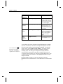
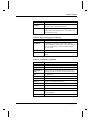
Table 2.1 lists the extensions for template files.
18 • 2.1 Overview of Origin
Chapter 2, Advanced Origin
Table 2.1: Template File Extensions
Window Type
Template File Extension
Worksheet
OTW
Graph, Layout Page, Function Graph
OTP
Matrix
OTM
2.1.5 Graphs and Layers
Each graph window contains a single page, which is represented by the
white area in the graph window. Each page must contain at least one
layer. A layer is defined as a set of X and Y axes. Each layer that exists
on the page is controlled by a layer icon that displays as a button in the
upper-left corner of the graph window. A graph page can contain
multiple layers, and thus multiple layer icons. However, at any given
time only one layer in the graph window can be “active.” A layer is
active when its layer icon is depressed. The active layer is the layer
which receives the next operation. For example, if the layer 2 icon is
depressed and you select Analysis:Fit Linear, then linear regression is
performed on the active data plot in layer 2.
When a graph window is saved to a template file, the number of layers
and their arrangement on the page are saved as part of the file. Thus, if
your application requires a graph with multiple layers, you can create the
page (including the layer arrangement) ahead of time and save the graph
window to a template file. The custom graph can then be quickly created
at a later time from the associated template file.
For more information on
control regions, see page
49.
The gray area of a graph window is useful for placing objects that you
don’t want to print out. Some of Origin’s templates have preprogrammed buttons located in this area. Additionally, you can use
script to add a control region to a graph, function graph, or layout page
window. A control region is an area for object placement located above
or to the left of the page. You can control the height or width of this
region, as well as the color, through script. Like the area to the right of
the page, objects in the control region do not print out.
2.1 Overview of Origin • 19
Chapter 2, Advanced Origin
Figure 2.1: Locating Buttons Outside the Page
2.1.6 LabTalk
Origin is based on its own scripting language, LabTalk. LabTalk is a
full-featured programming language that has access to most of Origin's
functionality, as well as to user-written DLLs (Dynamic Link Libraries).
LabTalk has similarities with C, DOS batch commands, and Visual Basic.
•
LabTalk contains expressions, operators, and control flow keywords
and structure similar to C.
•
LabTalk’s syntax and convention are similar to DOS batch
commands.
•
LabTalk includes object properties and methods comparable to those
in Visual Basic.
LabTalk is an interpreted language that receives and executes LabTalk
script. LabTalk script is defined as a block of text that is sent to the
LabTalk interpreter as a single unit. By writing and executing script, you
can customize Origin’s operation.
20 • 2.1 Overview of Origin
Chapter 2, Advanced Origin
2.1.7 Curve Fitting
Origin's curve fitting is implemented as a separate DLL called
ONLSF60.DLL. Origin’s nonlinear regression method is based on the
Levenberg-Marquardt (LM) algorithm and is the most widely used
algorithm in nonlinear least squares fitting. The Simplex minimization
method is provided as well.
As you develop Origin applications, there are three basic options for
providing curve fitting to users:
•
Let the user use Origin’s standard fitting options.
The user can learn how to use Origin’s fitter by reviewing the Origin
User’s Manual and the Tutorial Manual. Tutorials are provided
covering topics such as defining a function with one independent
variable (Tutorial Manual), defining a function with multiple
independent variables, and fitting multiple datasets to a function.
Tips are provided on using the fitter. A troubleshooting section is
also provided. Additionally, reference sections are provided on each
of the fitter’s dialog boxes.
•
Construct special fitting functions and make them available to the
user.
New fitting functions can be added to Origin within the fitter’s
Define New Function dialog box. After defining a function and
pressing Save in the Define New Function dialog box, a function
definition file with the function’s name and an .FDF extension is
created in the Origin FITFUNC folder. Additionally, the function
name is appended to the NLSF.INI file. Specifically, the function
name is added to the NLSF.INI section representing the function
category that was active when you defined the function. For the
function to be available to the user, you must copy the .FDF file to
the user’s Origin FITFUNC folder, and modify their NLSF.INI file.
•
Take complete control of the fitter using LabTalk script to control
the fitting process.
This is accomplished by using the ONLSF60.DLL as an external
object. This external object is called nlsf. The nlsf object properties
and methods are documented in the LabTalk Manual.
2.1 Overview of Origin • 21
Chapter 2, Advanced Origin
2.1.8 Origin's Window Objects
Origin child windows can contain basic elements (objects) such as pages,
layers, axes, axis breaks, worksheets, and columns. These objects each
have pre-defined names and unique properties that can be controlled
using LabTalk. For example, the page (page object) can display in
portrait or landscape orientation, axes (layer.axis objects) have specific
“to” and “from” end point values, and worksheets (wks object) can
display or hide column labels.
In addition to these elements, you can also create objects in Origin. For
example, you can create squares, circles, lines, arrows, and text labels.
Text labels include axis labels and legends, as well as other annotations.
Before controlling the properties of these objects with LabTalk script,
you must name the object in its Label Control dialog box. Axis labels
and legends are automatically named by Origin during creation.
Origin provides two methods to simplify identification of objects that
have been named via the Label Control dialog box:
•
To display each object’s name in the upper-left corner of the
respective object, select Edit:Button Edit Mode to enter the editing
mode. Re-select Edit:Button Edit Mode to exit the editing mode.
•
To view a list of all the objects contained in the active child window,
or the current layer of the active child window, type the following in
the Script window:
list o (ENTER)
You can view a list of the properties and methods associated with Origin
window objects (including those you have created) by typing the object
name in the Script window, followed by a period and an equal sign. For
example, to view the properties and methods associated with the page
object, type the following in the Script window:
page.= (ENTER)
Origin displays the properties and methods of the page object in the
Script window.
The Origin object properties and methods are fully documented in
Chapter 4, "Object Reference" in the LabTalk Manual. A summary of
the page, layer, layer.axis, and wks objects follows:
22 • 2.1 Overview of Origin
Chapter 2, Advanced Origin
•
page
The page object can be used to set various properties of the current
page, including (but not limited to) the width (width), the height
(height), the measurement units (unit), the active layer number
(active), the show-status of the layer icons (icons), the maximum
number of data points to display for each data plot (maxpts), the
mouse clicking status of objects on the page (noclick), the window
closing behavior (closebits), the number of layers (nlayers), the
horizontal resolution (resx), and the vertical resolution (resy).
For example, to set the base color of the active graph window to the
fifth color in the color drop-down lists, you can use:
page.basecolor=5;
•
layer
The layer object's properties can control the display of various
elements of the layer including (but not limited to) the display state
of the axes (showx, showy), the display state of the data (showdata),
the display state of labels and other objects (showlabel), the active
data plot number (plot), the layer height (height), the layer width
(width), and the measurement units (unit).
For example, to display the active graph layer with a marble border,
you can use:
layer.border=2;
•
axis
The axis objects are sub-objects of the layer object. As such, they
are named using the following syntax: layer.axis. For example, for
a 2D graph, there are two axis objects: layer.x and layer.y.
Properties of these objects control the attributes for both the bottom
and top X axes and the left and right Y axes, respectively. The
attributes controlled by the properties include (but are not limited to)
the first axis scale value (from), the last axis scale value (to), the
major tick increment (inc), the number of minor ticks (minorticks),
and the axis scale type (type).
For example, to hide the X axis and ticks in the active layer of the
active graph window, you can use:
layer.x.showaxes=0;
2.1 Overview of Origin • 23
Chapter 2, Advanced Origin
•
wks
The wks object is the worksheet representation of a layer object.
This object is indispensable for determining the selection of data
made by the user (r1, r2, c1, c2), adding columns to the worksheet
(addcol method), inserting columns in the worksheet (insert
method), and for manipulating general worksheet settings.
For example, to find the number of columns in the active worksheet,
you can use:
val=wks.ncols;
val=;
Object Properties
Objects may possess properties that hold either a numeric value or a
string constant.
•
Setting an Object's Property Values
To assign a numeric value to a numeric object property, use the
following syntax:
ObjectName.PropertyName=NumericValue;
To assign a numeric value to a numeric object property for an object
located on a window other than the active window, use the following
syntax:
[WinName!]ObjectName.PropertyName=NumericValue;
To assign a string constant to a text object property, use the
following syntax:
ObjectName.PropertyName$=StringConstant;
To assign a string constant to a text object property for an object
located on a window other than the active window, use the following
syntax:
[WinName!]ObjectName.PropertyName$=StringConstant;
24 • 2.1 Overview of Origin
Chapter 2, Advanced Origin
•
Reading an Object's Property Values
To read the current numeric value of a numeric object property in the
Script window, use the following syntax:
ObjectName.PropertyName=
To read the current numeric value of a numeric object property for
an object located on a window other than the active window, use the
following syntax in the Script window:
[WinName!]ObjectName.PropertyName=
To read the current string constant of a text object property, assign
the string constant to a string variable (for example, %Z) and then
read the value of the string variable:
StringVariable=ObjectName.PropertyName$;
StringVariable=;
To read the current string constant of a text object property for an
object located on a window other than the active window, use the
following syntax in the Script window:
StringVariable=[WinName!]ObjectName.PropertyName$;
StringVariable=;
Example: Reading and Setting an Axis Title Object's
Properties from the Script Window
To experiment reading and setting an object's property value, open a new
worksheet, enter some data, and create a new graph of this data. Most of
Origin's graph types will automatically display X and Y (and Z, for 3D)
axis titles in the graph window. The properties of these visual objects can
be controlled through script via the xb, xt, yl, yr, zf, and zb objects.
To view the X coordinate of the right edge of the bottom X axis title, type
the following in the Script window:
xb.x= (ENTER)
Origin displays the bottom X axis title's X coordinate value in the Script
window.
2.1 Overview of Origin • 25
Chapter 2, Advanced Origin
In addition to reading this property value, you can also directly change
the property value in the Script window. To move the right edge of the
bottom X axis title to X=5, type the following in the Script window:
xb.x=5 (ENTER)
The right edge of the bottom X axis title is now aligned with the line
X=5.
The text that displays in the bottom X axis title is controlled by the xb
object's text$ string property. The following script assigns the current
string constant of the text$ property to a string variable, displays this
string constant in an Attention dialog box, and then assigns a new string
constant to the text$ property (which displays in the bottom X axis title).
To run this script from the Script window, type in each line of code
including the semicolon at the end of each line. Then highlight the three
lines of code and press ENTER.
%A=xb.text$;
type "The object's text is %A";
xb.text$=New Text Here!;
In general, any option that can be controlled in the Origin window
object’s associated dialog box can also be set using the appropriate
LabTalk object property. For attributes that are controlled from a
combination box or drop-down list value in a dialog box, you can usually
set the object property to the associated entry number in the dialog box
list.
Object Methods
Objects can also perform actions including running their script, redrawing themselves, or simulating a click on themselves. Since these
actions are directly linked for a particular object, the actions are referred
to as object methods.
When using object methods
in your scripts, make sure
you don't include a space
between the method name
and the opening
parenthesis.
26 • 2.1 Overview of Origin
Object methods use the following syntax:
ObjectName.MethodName(Argument1, ... , Argumentn);
Some object methods take no arguments. Thus, nothing appears within
the parentheses. However, even when the method has no arguments, the
parentheses must still be included. The parentheses indicate that
MethodName is a method of the ObjectName object - not a property.
Chapter 2, Advanced Origin
Programming with the
Label Control dialog box is
discussed in Chapter 4,
"Application Development."
The Label Control dialog box is used to set the object's name, define its
script, and specify the trigger for script execution. You can open the
Label Control dialog box by clicking on the object and then selecting
Format:Label Control. Alternatively, press ALT while doubleclicking on the object.
Figure 2.2: The Label Control Dialog Box
Example: Reading and Setting an Axis Title Object's
Properties Using the ObjectName.Run( ) Method
In the "Object Properties" section, you ran a script from the Script
window that assigned the current string constant of the xb.text$ property
to a string variable, displayed this string constant in an Attention dialog
box, and then assigned a new string constant to the xb.text$ property
(which displayed in the bottom X axis title).
Alternatively, this script can be copied to the xb object's Label Control
dialog box and then run using the xb.run( ) object method from the
Script window.
1) First, return the bottom X axis title's text back to the default text by
typing the following in the Script window:
xb.text$=X Axis Title (ENTER)
2.1 Overview of Origin • 27
Chapter 2, Advanced Origin
2) Highlight the three lines of script in the Script window (from the
previous example):
%A=xb.text$;
type "The object's text is %A";
xb.text$=New Text Here!;
and then select Edit:Copy from the Script window menu bar.
3) Press ALT while double-clicking on the bottom X axis title in the
graph window. This action opens the Label Control dialog box.
4) With the pointer active in the lower text box, click Paste. The three
lines of script display in the text box.
5) Select Moved from the Script, Run After drop-down list.
6) Click OK to close the dialog box.
7) To run the script in the bottom X axis title's Label Control dialog
box, type the following in the Script window:
xb.run( ) (ENTER)
Note: You can also run the object's script by moving the object, as
Moved was selected in the object's Label Control dialog box in step
5.
2.2 Advanced Use of Layers
A layer is a set of X and Y axes on the page of a graph window. Layers
have attributes that control their appearance. For example, a layer can:
•
Contain multiple data plots.
•
Link to another layer so that it changes position and size whenever
the layer that it is linked to changes position or size.
•
Link to another layer so that its axes maintain a mathematical
relationship with the axes in the layer it is linked to.
•
Display superimposed on another layer.
28 • 2.2 Advanced Use of Layers
Chapter 2, Advanced Origin
•
Display or hide one or more axes.
•
Display different X and Y axis scales.
As you develop your application, you should customize the appearance of
the layer in the graph window, and then save the custom graph as a
template. This custom graph template can then be available to the users
of your application.
2.2.1 Linked Layers
A graph page can contain one or more layers. If the graph page contains
more than one layer, then links can be set up between layers on that page.
When you link two layers, you can link them spatially so that if one layer
is moved or resized, the other layer also moves and is resized to maintain
the original spatial arrangement. You can also link two layers to set up a
mathematical relationship between the axes in the layers.
To re-order the layers, use
the page.reorder(n,[m])
method. For more
information, see page 36.
Origin has restrictions on linking layers. When you create multiple layer
graphs, Origin numbers the layers sequentially (starting with 1), based
on the order in which the layers were created. When linking layers, the
layer that you are linking to (parent layer) must always be less than the
layer you are linking from (child layer). For example, layer 2 (child)
can be linked to layer 1 (parent), and layer 8 (child) can be linked to
layer 3 (parent). However, layer 1 (child) cannot be linked to layer 2
(parent), and layer 3 (child) cannot be linked to layer 8 (parent).
To link two layers:
To link two layers, press CTRL while double-clicking on the layer icon
for the layer that you want to be the child layer. This is the layer that will
follow the parent layer spatially or whose axes will update based on the
parent layer's axes. This action opens the child layer's Plot Details dialog
box. Select the Link Axes Scales tab. Link this child layer to a parent
layer by selecting a parent layer from the Link To drop-down list.
To establish a spatial link between the parent and child layers:
After you link a child layer to a parent layer, you can establish a spatial
relationship between layers so that if the parent layer moves or is resized,
the child layer also moves or is resized to maintain the original spatial
arrangement. To set this spatial arrangement, select the Size/Speed tab of
the child layer's Plot Details dialog box and then select % of Linked
Layer from the Units drop-down list in the Layer Area group.
2.2 Advanced Use of Layers • 29
Chapter 2, Advanced Origin
To establish a mathematical axes link between the parent and child
layers:
After you link a child layer to a parent layer, you can create a
mathematical relationship between the X (or Y) axes in the child layer
and the X (or Y) axes in the parent layer. In this case, the parent layer
provides the source axis information. To establish this axis linking
relationship, select the Link Axes Scales tab of the child layer's Plot
Details dialog box if it is not already selected and then edit the X Axis
Link and the Y Axis Link groups.
Note that after you establish spatial and axes links between a parent and a
child layer, the child layer will update its position/size and axes scales
whenever the parent layer is redrawn. Therefore, after specifying the
linking relationship between the parent and the child layer, you may need
to refresh the graph window by selecting Window:Refresh or by using
plot -c in script.
In the following example, you will create a graph with four layers (in a 1
column and 2 rows grid) and establish links between layers. The final
graph is shown in Figure 2.3.
To create layers 1 and 2, perform the following steps:
1) Click the New Graph button
on the Standard toolbar.
2) Select Edit:New Layer (Axes):(Linked): Right Y. This menu
command adds a new layer displaying a right Y axis. The X axis in
the new layer is linked by a straight one-to-one relationship to the X
axis in layer 1. The X axis in the new layer (2) is not, however,
displayed.
3) Press CTRL while double-clicking on the layer 2 icon in the upperleft corner of the graph window. This action opens the Background
tab of the layer's Plot Details dialog box.
4) Select the Link Axes Scales tab. Note that Layer 1 is selected from
the Link To drop-down list.
5) Select the Size/Speed tab. Note that % of Linked Layer is selected
from the Units drop-down list in the Layer Area group. This setting
ensures that the layer measurements are in a percentage of the height
and width of the linked layer frame. Furthermore, since 100 is
displayed in both the Width and Height text boxes, and 0 is displayed
30 • 2.2 Advanced Use of Layers
Chapter 2, Advanced Origin
in both the Left and Top text boxes, layer 2 is set to be the exact size
of layer 1, and is set to be superimposed on layer 1.
6) Re-select the Link Axes Scales tab. Note that the Straight (1 to 1)
radio button is selected from the X Axis Link group. Additionally,
no link is set between the Y axes.
7) Click OK to close the Plot Details dialog box.
To create layers 3 and 4, perform the following steps:
1) Select Edit:Add & Arrange Layers. This menu command opens
the Total Number of Layers dialog box.
2) Type 2 in the Number of Rows text box. Leave the Number of
Columns text box at its default value of 1.
3) Click OK.
4) Click Yes at the Attention prompt.
5) Click OK to accept the default spacing in the Spacings in % of Page
Dimension dialog box. Origin adds a third layer to the graph,
positioned above the first two layers.
6) To add a fourth layer which is linked to layer 3, make sure the layer
3 icon is selected and then select Edit:New Layer (Axes):(Linked):
Right Y.
To link layer 3 to layer 1, perform the following steps:
1) Press CTRL while double-clicking on the layer 3 icon in the upperleft corner of the graph window. This action opens the Background
tab of the layer's Plot Details dialog box.
2) Select the Link Axes Scales tab.
3) Select Layer 1 from the Link To drop-down list.
4) Select the Straight (1 to 1) radio button in the X Axis Link group.
5) Select the Size/Speed tab.
6) Select % of Linked Layer from the Units drop-down list in the Layer
Area group. After making this selection, the Width and Height text
2.2 Advanced Use of Layers • 31
Chapter 2, Advanced Origin
boxes update to 100, the Left text box updates to 0, and the Top text
box updates to -114. Leave these values at their new settings.
7) Click OK to close the Plot Details dialog box.
Figure 2.3: A Graph with Four Linked Layers
•
Layer 1
The lower-left Y axis and the lower X axis are part of layer 1.
•
Layer 2
The lower-right Y axis is part of layer 2. This Y axis is not linked to
the Y axis in layer 1. The X axis in layer 2 is not displayed, though
it is linked (straight one-to-one mathematical link) to the X axis in
layer 1.
•
Layer 3
The upper-left Y axis and upper X axis are part of layer 3. The Y
axis in layer 3 is not linked to any other Y axis. The X axis in layer
3 is linked (straight one-to-one mathematical link) to the X axis in
layer 1.
32 • 2.2 Advanced Use of Layers
Chapter 2, Advanced Origin
•
Layer 4
The upper-right Y axis is part of layer 4. This Y axis is not linked to
any other Y axis. The X axis in layer 4 is not displayed, though it is
linked (straight one-to-one mathematical link) to the X axis in layer
3.
If you click on layer 1 and move it or resize it, all of the child layers
(layers 2, 3, and 4) move (or resize) to maintain their relative position and
their axes relations. Furthermore, if you reset the axis scale range for the
X axis in layer 1, the upper X axis displays the same modification.
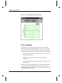
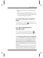
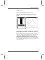
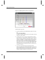
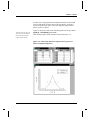
2.2.2 Scaling
The Offset Reciprocal Scale
Origin offers several types of axes scales including linear, log10,
probability, probit, reciprocal, offset reciprocal, logit, ln, and log2. The
offset reciprocal scale is a common scale type in the physical sciences.
Figure 2.4: An Offset Reciprocal Scale
2.2 Advanced Use of Layers • 33
Chapter 2, Advanced Origin
The offset reciprocal axis scale type is defined as x'=1/(x+273.14) where
273.14 is the absolute temperature corresponding to zero degrees Celsius.
Such a relation between axes is useful for showing temperature in
reciprocal of absolute temperature while the data in the graph is in
degrees Celsius.
To create a graph with an offset reciprocal axis scale, perform the
following:
1) Click the New Graph button
on the Standard toolbar.
2) Double-click on the X axis. This action opens the Scale tab of the
Axis dialog box.
3) Type 0 in the From text box and 200 in the To text box.
4) Select Offset Reciprocal from the Type drop-down list.
5) Type 50 in the Increment text box.
6) Click OK to close the dialog box.
7) Select Edit:New Layer (Axes):(Linked): Top X.
8) Press CTRL while double-clicking on the layer 2 icon in the upperleft corner of the graph window. This action opens the Background
tab of the layer's Plot Details dialog box.
9) Select the Link Axes Scales tab.
10) Select the Custom radio button in the X Axis Link group.
11) Type 1/(X1+273.14) in the X1 text box.
12) Type 1/(X2+273.14) in the X2 text box.
13) Click OK to close the Plot Details dialog box.
Setting Particular Axis Ranges
Origin includes axis rescale options so that you can control the conditions
that trigger the axis to rescale. These rescale options are set from the
Rescale drop-down list on the Scale tab of the Axis dialog box. The
Fixed From (Fixed To) drop-down list option causes the "from" ("to")
value of the axis to remain fixed unless the user manually changes the
34 • 2.2 Advanced Use of Layers
Chapter 2, Advanced Origin
value in the From (To) text box on the Scale tab. The Fixed From and
Fixed To options are most useful when you are constructing a template
that you know will always be used to plot data starting or ending at the
origin.
In addition to controlling the axis rescale options from the interface, you
can control the rescale options from script. The layer.axis.rescale object
property controls the rescale mode. For example, to keep the "from" X
axis value fixed in the active layer of the active graph window, you can
use the following script:
layer.x.rescale=4;
Setting Rescale Margins
When plotting, Origin automatically rescales the graph to display all the
data points and includes a margin to the left and the right of the data.
This margin is controlled by layer.x.rescalemargin for the X axis and
layer.y.rescalemargin for the Y axis. The rescalemargin properties
specify the % of the data range that is used to produce a margin around
the data. You can set these properties from script, and then force a
refresh of the graph window by using plot -clear or force a rescale by
using layer -all. For example, to display the data in the graph with no
margin, use the following script:
layer.x.rescalemargin=0;
layer -all;
Rescaling to a Major Tick
Many developers like being able to construct graphs such that the axes
will rescale to a major tick mark. LabTalk provides the layer -all
command which rescales the graph to show all the data, and leaves the
axes ending on a major or minor tick. When the layer -all command is
used with the layer.x.minorticks object property, a simple trick can be
used to rescale and leave an axis ending on a major tick.
The following script illustrates how to rescale a graph such that the X
axis ends on a major tick:
oldsetting=layer.x.minorticks;
layer.x.minorticks=0;
layer -all;
// save number minor ticks
// set minor ticks to 0
// rescale, no minor ticks so axes end at major tick
layer.x.minorticks=oldsetting;
// restore number minor ticks
2.2 Advanced Use of Layers • 35
Chapter 2, Advanced Origin
Rescaling Only the XY Plane of a 3D Graph
The layer -az command rescales the XY plane of a 3D graph without
rescaling the Z axis.
2.3 Additional Tips
The following features can be accessed through Origin's user-interface, or
by using LabTalk.
2.3.1 Merging Pages
You can merge all non-minimized graph windows into a single graph
page by selecting Edit:Merge All Graph Windows or by clicking the
on the Graph toolbar. From script, you can use the
Merge button
win -m command to merge all non-minimized graph windows into a
single page, or you can use the win -ma command to open a warning
prompt before merging the pages.
When merging graph windows, the following tips may help you control
the merging process:
•
You can use the win -i command to minimize any windows which
you do not want merged.
•
You can use the page.reorder(n,[m]) object method to reorder the
layers after merging. If m is not specified, then the page object
method changes the current layer to the nth position. Otherwise, it
changes the nth layer to be the mth layer. Every layer after n would
then move up one layer. For example, if you have a graph with four
layers and you want to renumber layer 4 as layer 2, you can use the
following script:
page.reorder(2,4);
When this script is executed, layer 4 becomes layer 2, layer 2
becomes layer 3, and layer 3 becomes layer 4. To move the layers so
that they display in the default locations for layer number, select
36 • 2.3 Additional Tips
Chapter 2, Advanced Origin
Edit:Add & Arrange Layers after executing the page.reorder( )
method.
•
You can use the Layer tool for adding and moving layers. Use the
Add tab controls to add layers and the Arrange tab controls to move
layers. The Move Layers group on the Arrange tab includes controls
to exchange layer positions and to overlay layers.
2.3.2 Extracting Layers to Separate
Pages
You can extract the layers of a multiple layer graph into separate pages
by clicking the Extract to Graphs button
script, you can use the page -j command.
on the Graph toolbar. From
2.3.3 Extracting Data Plots to
Separate Layers
You can extract data plots in a single layer graph to new layers in the
on the
same graph window by clicking the Extract to Layers button
Graph toolbar. From script, you can use the layer -j command.
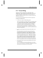
2.3.4 Showing Only Every nth Symbol
To minimize the screen redraw time when plotting large datasets, Origin
provides a speed mode that is accessible through the Size/Speed tab of
the layer's Plot Details dialog box and page.maxpts object property.
Speed mode allows you to specify the maximum number of data points to
display for each data plot on the graph. The displayed data points are
then evenly distributed through the data plot. However, if your data plot
includes very sharp peaks, using speed mode could significantly alter the
peak display.
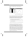
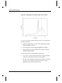
An alternative method for reducing the screen redraw time when plotting
large datasets is to display only every nth data point symbol in a line +
symbol or scatter data plot. In this method, all the data points in a line +
symbol data plot are connected by a line. However, only a specified
2.3 Additional Tips • 37
Chapter 2, Advanced Origin
frequency of the symbols (every nth) are displayed. This method is
accessible through the Drop Lines tab of the data plot's Plot Details
dialog box and the set dataset -skip n command.
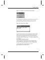
For example, to display every 3rd data point symbol in the active line +
symbol data plot, type the following in the Script window:
set %C -skip 3 (ENTER)
Figure 2.5: Controlling the Display Frequency of Data Points in a
Data Plot
38 • 2.3 Additional Tips
Chapter 2, Advanced Origin
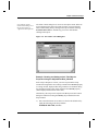
2.3.5 Using Datasets as a Plotting
Enhancement
Useful graph enhancements can be created by using an additional dataset
that marks or tags specific data points of another dataset.
Creating a Specialized Legend
Many elements of a data plot can be controlled based on values from
another dataset. For example, you can control the size of the symbols in
a scatter data plot based on values in a selected worksheet (or Excel
workbook) column. When you select a dataset to control the display of
an element in a data plot, for each data point in the data plot, Origin uses
the associated worksheet row value in the specified column.
These "dataset control" options are available from drop-down lists and
combination boxes in the Plot Details dialog box. The dataset control
options include: color, symbol shape, symbol interior, symbol size,
vector angle, and vector magnitude.
In Figure 2.6, columns A and B supply the X and Y values for each of the
data points in the data plot. Column C supplies the index numbers for the
shape of each of the data point symbols. In this example, Col(C) was
selected from the Shape drop-down list (in the Show Construction group)
on the Symbol tab of the Plot Details dialog box. Origin maps dataset
values and symbol shapes as follows: 0 = no symbol, 1 = square, 2 =
circle, 3 = up triangle, 4 = down triangle, 5 = diamond, 6 = cross (+), 7 =
cross (x), 8 = star (*), 9 = bar (-), 10 = bar (|), 11 = number, 12 =
LETTER, 13 = letter, 14 = right arrow, 15 = left triangle, 16 = right
triangle, 17 = hexagon, 18 = star, 19 = pentagon, 20 = sphere.
2.3 Additional Tips • 39
Chapter 2, Advanced Origin
Figure 2.6: Controlling the Display of a Data Plot Based on a
Dataset
When you control a data plot element based on a dataset, because the
element (for example, data plot symbol) is not uniform, the default legend
cannot display an accurate representation of the data plot. To ensure that
the graph legend displays a data plot type icon that is representative of
the custom data plot, you can perform the following operations:
1) Include empty datasets in the layer (one dataset for each symbol you
want to display in the legend's data plot type icon).
2) For each of the empty datasets, specify the desired symbol by editing
the Plot Details dialog box.
3) Modify the default legend text to access the symbols specified in step
2.
For example, after creating the data plot in Figure 2.6, create a new
worksheet (Data2) with two Y columns (B and C). Double-click on the
layer 1 icon (Graph1) to include these two new datasets in the layer.
Press CTRL and select Data:Data2 : A(X), B(Y) to open the Plot Details
dialog box for this dataset. On the Symbol tab, select Square from the
Shape drop-down list (in the Show Construction group). Double-click on
the Data2 : A(X), C(Y) data plot icon on the left side of the Plot Details
dialog box. On the Symbol tab, select Up Triangle from the Shape dropdown list (in the Show Construction group). Because these datasets
contain no data, these changes to the Plot Details dialog box will have no
affect on the data plots in the graph. Now, to update the legend, doubleclick on the "B" in the legend to open the Text Control dialog box.
Change the text in the center text box to:
40 • 2.3 Additional Tips
Chapter 2, Advanced Origin
\L(2)\L(3) %(1)
Click OK to update the graph with your custom legend.
Figure 2.7: Displaying the Custom Data Plot Type Icon in the
Legend
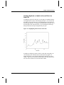
Displaying Vertical Lines at a Data Plot's X Values
Vertical or horizontal lines that span the height or width of the layer can
add clarity or emphasis to a graph. Origin provides the draw -l -v value
command and the draw -l -h value command to draw a vertical or
horizontal line at the specified position value. However, if you want to
display multiple vertical lines in a graph that are at actual X data point
positions in a data plot, you can create a subset of your data plot and then
use the set dataset -k 58 command. This command draws vertical lines at
each X value in dataset.
2.3 Additional Tips • 41
Chapter 2, Advanced Origin
Figure 2.8: Displaying Vertical Lines Using a Source Dataset
To create vertical lines at distinct data point values, you can perform the
following operations:
1) Include the dataset which is a subset of the original data plot using
the layer -i dataset command.
2) Set the data plot to scatter using the set dataset -l 0 command.
3) Set the symbol for the subset data plot as a vertical line using the
set dataset -k 58 command.
The subset dataset can be created in many different ways:
42 • 2.3 Additional Tips
•
You can write a script to find certain values in a data plot and then
extract these values and store them in a new worksheet.
•
The user can be prompted to click on interesting points. Once done,
the subset can be compiled and included in the layer with the
appropriate symbol of 58 being set by script.
Chapter 2, Advanced Origin
Creating Symbols or Labels to Accent Data in a
Data Plot
To highlight a region of a data plot, you can display an additional dataset
in the graph that is a subset of the full range data plot. You can then edit
the display of the subset data plot - thus highlighting the desired range of
the full range data plot. For example, you can increase the symbol size of
the data points in the subset data plot, or you can display the full range
data plot and subset data plot using different plot types.
Figure 2.9: Highlighting Data Points in a Data Plot
In addition to displaying a subset of data as a data plot in the graph, you
can also display text or numeric data as data labels in the graph. To
display data labels, set the column containing the data labels as a label
column. When selected, the label column will provide data labels for the
first selected Y column to the left of this label column.
2.3 Additional Tips • 43
Chapter 2, Advanced Origin
Figure 2.10: Setting up a Worksheet Column with Data Labels
Figure 2.11: Adding Data Labels to the Graph
The labels are positioned at the X and Y coordinates specified by the X
and Y data in the worksheet. Note that you need not include the Y
dataset associated with the label dataset in the graph layer. It is only
necessary that the label dataset has an associated X and Y dataset in its
worksheet.
44 • 2.3 Additional Tips
Chapter 2, Advanced Origin
2.3.6 Using Escape Sequences to
Format Labels
For a complete list of
escape options, see Chapter
11 in the Origin User's
Manual.
Origin allows you to use escape sequences in a string to control the
display of labels. These sequences begin with the '\' character. All text
objects (those created with the Text Tool or the LabTalk label
command) as well as text plotted from a Label column will display
according to the rules of these sequences.
The following examples illustrate the use of escape sequences:
String:
Appearance:
Some \b(bold) text
Some bold text
Some \i(italic) text
Some italic text
Display of a '\' character presents a problem. If an unsupported escape
option or no parenthesis follows the escape character, then the
character(s) are ignored. Following standard conventions, sequential '\\'
will be interpreted as one '\'. For example:
String:
Appearance:
C:\My Documents
C:My Documents
C:\\My Documents
C:\My Documents
There is also a special notation to ignore escape sequences:
String:
Appearance:
\v(C:\My Documents)
C:\My Documents
The \v( ) notation is particularly useful when you are substituting the
value of a string variable such as %Y in a text label. %Y contains the
path of the Origin executable file, and thus includes the '\' character. In
the following examples using the label command, the Origin string
variable %Y is equal to D:\ORIGIN61\. (These text labels could also be
created with the Text Tool as long as you select the Link to Variables
check box in the associated Label Control dialog box.):
LabTalk Command:
Label displays as:
label -n title1 Path is %Y;
Path is %Y
label -s -n title2 Path is %Y;
Path is D:ORIGIN61
label -s -n title4 Path is \v(%Y);
Path is D:\ORIGIN61\
Note that the first label did not substitute the %Y with its value
(D:\ORIGIN61\). An additional command option (-s) was needed. This
is equivalent to selecting the Link to Variables check box in the Label
2.3 Additional Tips • 45
Chapter 2, Advanced Origin
Control dialog box of a text object. Once substituted, the text displayed,
but without the '\' characters, which require the special \v( ) notation.
2.3.7 View Modes
Origin offers four graph page view modes which are available from the
View menu (Print View, Page View, Window View, and Draft View).
The different view modes are provided so that you can benefit from
reduced redraw time as you are developing a graph, as well as accurate
object placement before printing or exporting the graph.
When Page View is selected,
the WYSIWYG In Page View
Mode check box on the Text
Fonts tab of the Options
dialog box allows you to
view text labels in the graph
using the printer driver,
while all other objects are
drawn with the screen
driver.
The default view mode, Page View, is the ideal view mode as you
develop your graph. Page View mode uses the screen driver to draw the
screen image, thus providing fast screen redraw. However, Page View
mode does not provide a What You See Is What You Get (WYSIWYG)
view of the graph. To ensure that objects on your graph are in the exact
location you desire, you should switch to Print View mode before
printing or exporting your graph. Print View mode uses the current
printer driver to draw the screen image. Use this view mode to fine tune
object placement on the graph.
In Origin version 3.54 and up, when you select Edit:Copy Page in any
view mode, Origin automatically uses the Print View mode to copy the
page. Thus, Origin creates a very accurate Windows Metafile image
using the printer driver.
2.3.8 Updating the Display
Master Page
Origin provides a master page feature to simplify the global annotation of
graphs. The master page feature lets you easily display a consistent
background, a company logo, or other labels and images on graph
windows in your project.
To use the master page feature, you must first create your master graph
that contains the objects and background that you want to display on
other graph windows. To do this, you can customize the display of any
graph window and then rename the graph window master
(Window:Rename). Alternatively, Origin provides a graph template
(MASTER.OTP) in which the axes and labels are already hidden, thus
46 • 2.3 Additional Tips
Chapter 2, Advanced Origin
making it an ideal master page. To open this template, select File:New
and then select Graph from the list box and Master from the Template
Name drop-down list (in the Origin folder) and click OK. You can now
customize the display of this window and rename it master.
After you create a master page (a graph window named master), you can
then control the display of the master items in other graph windows in the
project. There are two aspects to this control:
•
You can control whether or not the master items will be included
when you export, copy, or print the graph window. This control is
available on each graph page's Plot Details dialog box. Select
Format:Page to open the Plot Details dialog box. Select the
Display tab. Select the Use Master Items check box to include
master items when you export, copy, or print this graph window.
•
You can control whether or not the master items will display as you
view the graph in Origin. To access this control, select
View:Show:Master Items on Screen when the graph window is
active. Note: This menu command is not available if the Plot
Details Use Master Items check box is cleared.
Figure 2.12: Creating a Master Page
2.3 Additional Tips • 47
Chapter 2, Advanced Origin
Figure 2.13: Displaying Master Items in a Graph Window
Additional Master Page Notes:
1) To open a graph based on the MASTER.OTP template from script,
use:
win -t plot master Master;
In addition to opening a graph window from the template, this script
renames the window "Master."
2) To display master items exclusively in graph windows in portrait
page orientation or in graph windows in landscape page orientation,
instead of renaming your master graph window "master," rename it
"portrait" or "landscape." If you have renamed your graph window
portrait and you open a second graph window that is also in the
portrait page orientation, after selecting View:Show:Master Items
on Screen, the objects in the portrait graph window display in the
second graph window (assuming the Plot Details Use Master Items
check box is selected).
3) You can also include master items in layout page windows.
However, by default, the Use Master Items check box on the layout
page's Plot Details dialog box is cleared by default. Therefore, you
must select this check box to include master items when exporting,
copying, or printing. Furthermore, you must select the
48 • 2.3 Additional Tips
Chapter 2, Advanced Origin
View:Show:Master Items on Screen menu command to display the
master items as you view the layout page in Origin.
Forcing a Refresh of a Window
When you plot worksheet data, the resultant graph window displays an
image of the dataset that it contains. At times the graph window may
require an update to refresh its image of the dataset contained in the
worksheet. To do so, type the following in the Script window:
plot -c (ENTER)
2.3.9 Control Regions
The control region is useful when building a template-based application
that requires multiple buttons or other objects. Control regions can be
located above or to the left of the page in the graph, function graph, or
layout page windows. When you place objects in a control region, the
objects do not scale with the page or layer.
Figure 2.14: The Control Region in the FUNCTION.OTP Template
Control regions are activated and sized using the LabTalk page object
properties. To activate the display of a control region, set
2.3 Additional Tips • 49
Chapter 2, Advanced Origin
page.cntrlregion=1. After activating the display of a control region, you
then specify the height of the region (if you want it to display above the
page) or the width of the region (if you want it to display to the left of the
page). To control the height, set page.cntrlheight=value. To control the
width, set page.cntrlwidth=value. For both the height and width, value
is in units of pixels. To control the color of the control region, set
page.cntrlcolor=value. In this case, value is the number of the color in
Origin's color drop-down lists.
Note: To display objects in the control region, you must create the object
directly in the control region. You cannot drag objects on and off the
control region.
2.3.10 Screen Plotting Speed
During data analysis and plotting, users will often need to perform
various operations on a dataset being displayed in a graph window.
When the dataset is very large, it may become time consuming when the
screen redraws after every mathematical and graphical operation
performed on the dataset. If it is not necessary to view every data point
during these operations, you can speed up the screen redraw time for the
user by displaying a limited number of data points in the data plot.
To display a specified
frequency of data points,
see "2.3.4 Showing Only
Every nth Symbol" on page
37.
To set this data point limit, select Format:Layer to open the
Background tab of the layer's Plot Details dialog box. Select the
Size/Speed tab. The Speed Mode, Skip Points if Needed group controls
the speed viewing mode for worksheet and matrix data in the respective
layer. These controls are saved with the graph template, so you can
customize this setting for the user by resaving the template.
2.3.11 Printing
Setting the Page Orientation
You can set the page orientation of the current graph window by editing
the Page Setup dialog box (File:Page Setup). Additionally, page
dimension controls are provided on the Print/Dimensions tab of the page's
Plot Details dialog box (Format:Page). If you select the "Set to Printer
Dimension When Creating Graphs From this Template" check box, save
the graph window as a template, and then at a later time open a graph
50 • 2.3 Additional Tips
Chapter 2, Advanced Origin
window based on this template, the graph page dimensions will reflect the
current printer page settings - not the page dimensions when the template
was saved. If you clear this check box, when you open a graph window
based on this template, the graph page will always reflect the page
dimensions when the template was saved - independent of the current
printer page settings.
When a graph template is saved with the "Set to Printer Dimension When
Creating Graphs From this Template" check box selected, you can use the
page -O L (for landscape) or page -O P (for portrait) commands in the
Script window to set the page orientation of a graph window that will be
opened from this template. These script commands change the current
printer driver orientation.
To update the active graph window with the current printer page setting,
run the page.dimupdate( ) method from the Script window.
Avoiding Printing Problems
For more information, see
"2.3.7 View Modes" on
page 46.
To make sure the objects on the page print in the exact location you
desire, switch to Print View mode before printing. Print View mode
uses the current printer driver to draw the screen image, and will thus
show an exact representation of the printed page.
Printing Every Graph Window
LabTalk provides the option to send script to each of a particular kind of
object. Therefore you can develop an application that sends the print
command to each graph in the current project, causing each graph to be
printed.
doc -e P {print};
To print only the graphs in the active Project Explorer folder, use:
doc -ef P {print};
Note: To print only the graphs in the active Project Explorer folder using
this command, the Project Explorer view mode must be set to View
Windows in Active Folder.
2.3 Additional Tips • 51
Chapter 2, Advanced Origin
This page is intentionally left blank.
52 • 2.3 Additional Tips
Chapter 3, LabTalk
3
LabTalk
3.1 Introduction
LabTalk is an interpreted, full-featured language which offers economical
expression size, modern C-like control flow, and is totally specialized to
Origin scientific plotting and data analysis. As an interpreted language,
LabTalk code, called script, is processed one statement at a time. In
LabTalk, each statement must end with a semicolon. When running
LabTalk script, the LabTalk interpreter reads in a statement, interprets it,
carries out the specified action, or returns the result of the expression.
Table 3.1: Sample LabTalk Statements
LabTalk
Statement
Example
Results
Variable
Assignment
apples=4;
A global variable called
apples is set to 4.
Macro Call
AddThese 3 5;
The AddThese macro is
passed two parameters then
called.
Command
layer -i Data1_B;
Dataset Data1_B is included
in the current graph layer.
Arithmetic
apples=4*pears+5;
A variable called apples is
set to 4 times the current
value of pears plus 5.
Function
Definition
myfunc(x)=5.3*x+2;
A function called myfunc is
defined so that it returns 5.3
times its argument plus 2.
3.1 Introduction • 53
Chapter 3, LabTalk
The LabTalk Editor
is
available for developing
script files. See Chapter 4,
"Application Development."
LabTalk
Statement
Example
Results
Function Call
apples=myfunc(3);
The function myfunc is
passed a parameter value of
3 and then called. The result
is then returned and assigned
to the variable apples.
Control Flow
Statement
if (X1<0) {X1=0} else {x1=1};
Based on the value of the
variable X1, either a script
which sets X1 equal to 0 or a
script which sets X1 equal to
1 is executed.
Object Call
Method
apples=myObject.run( );
The object method run( )
executes the script associated
with the object myObject
and any returned number is
passed to the variable
apples.
Object
Property
Assignment
myObject.Color=5;
The property color of the
object myObject is set to 5.
To learn about the various elements of the LabTalk language (variables,
operators, calculations, control flow, and input and output), it is useful
to use the Script window to issue immediate commands. To open the
Script window, select Window:Script Window. The Script window
floats over all other windows and offers an immediate method for
executing script. You can type in a single line of script (without a
semicolon at the end) and the script will be interpreted and executed.
To execute a block of script, type each line of script, making sure to type
a semicolon at the end of each line. Then highlight the block of script
and press ENTER.
Though LabTalk is similar to C, there are important syntactical
differences between LabTalk and C. These differences are listed in Table
3.2.
54 • 3.1 Introduction
Chapter 3, LabTalk
Table 3.2: Summary of Syntax Differences
Item
Description
% is used to designate a string
variable.
%A through %Z are the available string
variables.
A $( ) operator converts and
formats numeric variables to string
variables.
x=1.23456; type "x=$(x)";
type "2 significant digits: $(x,*2)";
3.2 Variables
All variables that you create are stored with the project when saved.
User-defined variables can be either numeric or string variables. When
naming a numeric variable, you should avoid using Origin keywords such
as commands, macros, and system variables.
3.2.1 Numeric Variables
A numeric variable contains a single value. A variable is always a scalar
quantity in LabTalk. All numeric variables are double precision real
numbers.
The assignment operator, =, is used to simultaneously create a variable (if
it does not already exist) and assign to it a value. For example, open the
Script window and type the following:
apples=634 (ENTER)
This statement creates the variable called apples and sets it equal to 634.
You can check the contents of a variable by typing the variable name
followed by an equal sign in the Script window. For example, type the
following in the Script window:
apples= (ENTER)
Origin responds by typing: apples=634
3.2 Variables • 55
Chapter 3, LabTalk
3.2.2 String Variables
LabTalk uses the % notation to define a string variable. A legal string
variable name must be a % character followed by a single alphabetic
character (a letter from A to Z). String variable names are caseinsensitive.
For more information on
the string variables used by
Origin, see the LabTalk
Manual.
Of all the 26 string variables that exist, Origin itself uses 14. However,
you need only avoid using four of these: %C, %E, %G, and %H.
%C contains the name of the current active dataset, %E contains the
name of the window containing the latest worksheet selection, %G
contains the name of the current project, and %H contains the name of
the current active child window.
%A and %B are commonly used in development scripts. %A is used by
Origin to contain the file name returned by the most recent GetFileName
command. %B is used by Origin to contain the string returned by the
most recent GetString command. The values of these string variables
change as the user opens projects and templates. Because these aren't
"static" variables reserved by Origin, you should use them in your
development scripts.
String Variables and Object String Properties
Although numeric object properties (for example, legend.x) can be used
anywhere a literal number or numeric variable would be used, string
properties (for example, legend.text$) cannot be used wherever a literal
string or a string variable would be used. In order to output or check the
contents of an object's string property, you must first assign it to a string
variable, and then use that variable. An example illustrating this method
follows:
%A=myLabel.text$;
if (%A=="Hello") {myLabel.text$="Good Bye";};
56 • 3.2 Variables
Chapter 3, LabTalk
3.2.3 Numeric to String Conversion
To evaluate a variable or expression and interpret the result as a string,
you must use the $( ) operator on the numeric variable.
Example:
K=9;
type "K";
In the first line of script, the value 9 is assigned to the variable K. The
second line of script causes the given string to be output to the Script
window. The Script window prints K.
For another example using
the $( ) operator, see page
90.
However, if you use the numeric-to-string conversion notation to convert
K to a value before printing to the Script window:
type "$(K)" (ENTER)
then the value of K is found first, and the result (9) is output to the
Script window.
3.2.4 Deleting Variables
You can delete a variable using the delete -v variableName command.
3.3 Operators
3.3.1 Arithmetic Operators
LabTalk recognizes the following arithmetic operators:
+
Addition.
-
Subtraction.
*
Multiplication.
/
Division.
^
Exponentiate.
3.3 Operators • 57
Chapter 3, LabTalk
3.3.2 Assignment Operators
LabTalk recognizes the following assignment operators:
=
Assign the argument to the variable.
+=
Add the argument to the variable contents and assign to the
variable.
-=
Subtract the argument by the variable contents and assign to the
variable.
*=
Multiply the argument by the variable contents and assign to the
variable.
/=
Divide the variable contents by the argument and assign to the
variable.
^=
Raise the variable contents to the argument and assign to the
variable.
++
Add 1 to the variable contents and assign to the variable.
--
Subtract 1 from the variable contents and assign to the variable.
--O
(Also: +-O, *-O, /-O, ^-O) Perform an interpolation outside of
the domain of the second dataset for all X values of the first dataset
and then perform the subtraction. For example:
data1_b --O data2_b;
For more information, see "Vector Calculations Requiring
Interpolation" on page 61.
3.3.3 Logical and Relational Operators
LabTalk recognizes the following logical and relational operators:
>
Greater than.
>=
Greater than or equal to.
<
Less than.
<=
Less than or equal to.
==
Equal to.
!=
Not equal to.
&& AND.
||
58 • 3.3 Operators
OR.
Chapter 3, LabTalk
The logical and relational operators follow standard C programming
language notation. An expression involving logical or relation operators
will evaluate to either true (non-zero) or false (zero).
3.3.4 Bitwise Operators
LabTalk recognizes the following bitwise operators:
&
Bitwise AND.
|
Bitwise inclusive OR.
Examples:
value=3|5;
Value is set to 7.
value=3&5;
Value is set to 1.
3.3.5 Conditional Operators
The ternary operator, ?:, can be used in the form:
Expression1?Expression2:Expression3
This expression first evaluates Expression1. If Expression1 is true
(evaluates to a non-zero value), then Expression2 is evaluated. The value
of Expression2 becomes the value for the conditional expression. If
Expression1 is false (evaluates to zero), then Expression3 is evaluated
and becomes the value for the entire conditional expression.
Example:
value=test>=0?1:0;
In this example, Expression2 and Expression3 are literal values. The
statement sets value equal to either 0 or 1 depending on whether the
variable test is greater than or equal to 0. If test is greater than or equal
to 0, then value is set to 1. If not, value is set to 0. Thus, this statement
can replace the following script:
if (test>=0) {value=1} else {value=0};
3.3 Operators • 59
Chapter 3, LabTalk
3.4 Calculations
3.4.1 Scalar Operations
You can use LabTalk to express a calculation and store the result in a
numeric variable. Such a calculation is referred to as a scalar operation,
as only a single value is involved. For example, consider the following:
inputVal=21;
myResult=4*32*inputVal;
The second line of this example performs a calculation and creates the
variable, myResult. The value of the calculation is stored in myResult.
When a variable is being used as an operand, and will also store a result,
shorthand notation can be used. For example, you could write:
B=B*3;
or you could equivalently write:
B*=3;
In this example, multiplication is performed with the result assigned to
the variable B. Similarly, you can use +=, -=, /=, and ^=. Using
shorthand notation produces script that is faster in execution time as
compared to the longer syntax method.
3.4.2 Vector Operations
Row-by-Row Calculations
In your scripts, you may need to perform a calculation on a whole set of
numbers which are contained in a column. Such a calculation is called a
vector operation, and as such, the assignment operator must have a
dataset specified both on the left and right. For example:
data1_b=3*data1_a;
This operation multiplies every element of the data1_a dataset by 3.
Because the operand is a dataset, the result must be a dataset. In this
example, the result is put into the data1_b dataset.
60 • 3.4 Calculations
Chapter 3, LabTalk
If you were to write:
newData=3*data1_A;
then a temporary dataset called newData is created and assigned the
result of the vector operation. Elements of the temporary dataset can be
accessed in the same way you would access an element of a dataset
contained in a worksheet.
Mathematical operations can also be performed between elements of
datasets. Such operations are also vector operations. For example:
data1_C=data1_A*data1_B;
This operation multiplies the elements of the data1_A and data1_B
datasets, row by row, and puts the product of each multiplication in the
data1_C dataset.
Vector Calculations Requiring Interpolation
The previous discussion of vector operations assumed that when you use
two datasets as operands, the datasets have the same number of elements,
or rows. When the dataset operands do not have the same number of
rows, then linear interpolation can be used to perform the calculation.
This requires using a different kind of vector operator notation of the
form: dataset operator dataset
As an example, consider the following two dependent datasets in Figure
3.1, each with its own set of independent data.
3.4 Calculations • 61
Chapter 3, LabTalk
Figure 3.1: Sample Datasets
If you were to subtract baseline_b from signal_b using the −= operator
in the Script window:
signal_b−=
−=baseline_b
(ENTER)
−=
then the subtraction would be performed row by row (with no linear
interpolation) as shown in Figure 3.2.
62 • 3.4 Calculations
Chapter 3, LabTalk
Figure 3.2: Subtracting Datasets Using the −= Operator
It is apparent that the subtraction was performed row by row, as the
calculation was only performed on four rows (baseline_b only had four
rows while signal_b had seven).
However, if you use a dataset operator dataset assignment-operation
statement (starting with the initial worksheet values) in the Script
window:
signal_b−
−baseline_b (ENTER)
then linear interpolation of the second dataset (baseline_b) within the
domain of the first dataset (signal_b) is used to carry out the subtraction.
The results are stored in the first dataset (signal_b). Figure 3.3 shows the
3.4 Calculations • 63
Chapter 3, LabTalk
results of this calculation, when starting with the initial worksheet values
(from Figure 3.1).
Figure 3.3: Subtracting Datasets Using the Dataset Operator Dataset
Assignment Operation
In this example, interpolation was used to find the Y values of baseline_b
using the X values given by signal_a. Note that although X=2 and X=6
are outside the range of baseline_b, interpolated values were found and
used in the subtraction. This is because this type of assignment operator
always interpolates within the domain of the second dataset plus one
point on either side. (Note: In Origin 6.1, interpolation is performed
within the domain of the second dataset only. To return to the pre-6.1
behavior, set @IE = 1. The new default is @IE = 0.)
64 • 3.4 Calculations
Chapter 3, LabTalk
In order to have Origin perform the interpolation outside of the domain
of the second dataset for all X values of the first dataset, you need to
specify an option switch (-O). The syntax using this option switch is:
dataset operator-O dataset
Figure 3.4 shows the results of the statement typed in the Script window:
You must leave at least one
space between the dataset
names and the operator
with its option switch.
signal_b −−O
−− baseline_b (ENTER)
when starting with the initial worksheet values (from Figure 3.1).
Figure 3.4: Subtracting Datasets Using the Dataset Operator-O
Dataset Assignment Operation
3.4 Calculations • 65
Chapter 3, LabTalk
This option switch is
available for all the
arithmetic operators
(+-O, --O, *-O, /-O, and
^-O).
In this example, the option switch caused linear interpolation of
baseline_b to be used within and outside of its domain in order to
perform the calculation for the entire domain of signal_b.
Note: When data is unsorted or there are duplicate Y values for any
given X value, there will be inconsistencies in the linear interpolation
results.
3.4.3 Writing Speedy Calculations
In your scripts, you may need to perform complex vector operations. For
example, suppose the first column of a worksheet contains time values,
and you want the second column to contain the amplitude of a sinusoidal
function like the following:
y = 1.5 sin(5t+3)
One option is to use the following script:
col(2)=1.5*sin(5*col(1)+3);
However, this operation would take quite some time to perform because
the LabTalk interpreter has to break this statement down piece by piece
and interpret this for each row in col(1). To find out how long this script
takes to execute, you must get the time from the system clock, perform
the script, and then get the elapsed time since the system clock was
checked. This is accomplished with the second command.
For example:
sec;
// Get the time from the system clock
col(2)=1.5*sin(5*col(1)+3);
watch;
// perform operation
// Type elapsed time to Script window
The elapsed time prints to the Script window. (Additionally, you can
check the elapsed time by reading the value of the v1 variable.)
Instead of writing the vector operation in one statement, it would be
considerably faster to write multiple statements that modify the entire
dataset. Because the entire dataset is modified in a uniform way, Origin
can perform these tasks very quickly. For example, the following script
runs much faster than the previous script:
66 • 3.4 Calculations
Chapter 3, LabTalk
sec;
// Get the time from the system clock
col(2)=col(1);
// set col(2) equal to the time column
col(2)*=5;
// set col(2) to be 5 times its value
col(2)+=3;
// add 3 to every element
col(2)=sin(col(2));
// compute the sine for every element
col(2)*=1.5;
// multiply by 1.5
watch;
// Type elapsed time to Script window
Internal calculation shortcuts are used to perform these calculations very
quickly.
3.5 Command Reference by Category
The following tables categorize the LabTalk commands by their function.
Table 3.3: Data Manipulation and Calculation Commands
Command
Description
average
Replace a dataset with a running average.
copy
Copy one dataset to another.
create
Create a dataset, worksheet, or function.
delete
Delete a dataset, function, macro, or variable.
derivative
Take the derivative of a dataset.
edit
Open the worksheet for a dataset.
integrate
Integrate a dataset.
limit
Find the minimum and maximum X and Y values for a
dataset.
lr
Perform linear regression on a dataset.
mark
Delete or mask data points in a dataset.
math
Perform mathematical operations on or between datasets.
matrix
Set the dimensions and values of a matrix. Transpose a
matrix.
nlsf
Perform nonlinear least squares fitting.
3.5 Command Reference by Category • 67
Chapter 3, LabTalk
Command
Description
plot
Append values to a dataset.
sort
Sort worksheet data.
undo
Undo various procedures.
Table 3.4: Display Control Commands
Command
Description
axis
Open the Axis dialog box. Edit the axis scale type, grid
display, tick, and tick label display. Display additional
axes in a layer.
document -t
Open a window based on a template.
dotoolbox
Select or block selection of a Tools toolbar tool. Hide the
Tools toolbar. Display a picture of a worksheet or graph
window in a layout page window.
draw
Draw a line and edit its properties. Hide an object. Update
an object. Edit the location of an object. Read a metafile,
bitmap, or object from a file into an object. Update an
object's numeric or text fields.
edit
Open the worksheet for a dataset. Open the Color Palette
dialog box.
get
Read the display properties of a dataset or data plot.
label
Create and edit a text label, including axis titles.
layer
Edit the properties of a layer. Add data to a layer. Add
layers to a graph page. Open layer-related dialog boxes
including the Plot Details dialog box. Extract multiple data
plots to separate layers.
legend
Display or update the legend for a graph layer.
page
Edit the properties of a page. Add data to separate layers of
a graph page. Open page-related dialog boxes including
the Plot Details dialog box. Extract multiple layers to
separate graph pages.
plot
Update the layer or the page.
select
Edit the display of the selected objects including alignment
and grouping.
set
Edit the display properties of a dataset or data plot. Open
the Plot Details dialog box.
type
Hide the Script window or the status bar.
undo
Undo various procedures.
68 • 3.5 Command Reference by Category
Chapter 3, LabTalk
Command
Description
window
Open, close, hide, minimize, maximize, rename, and
activate a window. Merge graph windows.
worksheet
Edit the properties of a worksheet. Duplicate a worksheet.
Open worksheet-related dialog boxes. Plot worksheet data.
Run a worksheet's script.
Table 3.5: Project Management Commands
Command
Description
document
Append projects. Close the current project. Open a
project. Rename the current project. Count the number of
layers in a graph window. Count the number of object
types in a project.
file
Copy one file to another.
list
List all datasets, macros, system variables, or data plot style
holders.
Table 3.6: Control Flow Commands
Command
Description
break
Exit from a loop, a script, or a progress dialog box.
continue
Skip to the next iteration of the current loop.
document -e
(-ef)
Loop to execute a script that affects every object of the
specified type (-ef = in the active Project Explorer folder).
exit
Exit from Origin.
for
Loop for repeated operation.
if [else]
Test a condition and branch accordingly.
layer -o
Execute a script for the specified layer.
loop
Loop while incrementing a variable.
repeat
Execute the same script multiple times.
return
Return a value from a script and exit the script.
switch
Test an expression against a series of constant values and
branch accordingly.
win -o
Execute a script for the specified window.
3.5 Command Reference by Category • 69
Chapter 3, LabTalk
Table 3.7: Input/Output Commands
Command
Description
clipboard
Copy the current page to the clipboard. Save the specified
graph page as a Windows metafile.
copy
Copy one dataset to another.
draw -fb, -fm
Read a bitmap or metafile from a file into an object.
getfilename
Open the Open or Import Multiple ASCII dialog boxes.
getnumber
Get input of up to six numbers or strings.
getpts
Graphically get points or screen coordinates from a data
plot.
getsavename
Open the Save As dialog box.
getstring
Get a user-supplied text string.
getyesno
Open a Yes/No/Cancel dialog box.
open
Import a data file.
print
Print the active (or specified) page. Open the Print or Page
Setup dialog boxes.
save
Save the project or save a window in the project. Export
worksheet data.
type
Output text to the Script window, status bar, or various
dialog boxes.
Table 3.8: Script Management Commands
Command
Description
define
Define a macro.
draw
Run an object's Label Control dialog box script.
menu
Manipulate menus, submenus, and menu commands.
queue
Place a script at the end of the window update queue.
run
Execute a script file or run a Windows program.
Table 3.9: External Access Commands
Command
Description
dde
Client DDE support.
dll
Execute a function from a user-supplied DLL.
70 • 3.5 Command Reference by Category
Chapter 3, LabTalk
Table 3.10: Timer Commands
Command
Description
seconds
Elapsed time counter. Perform timer-related operations.
timer
Execute the TimerProc macro's script periodically.
3.6 Object Reference by Category
The following tables categorize the LabTalk objects by their function.
Table 3.11: Data Manipulation and Calculation Objects
Object
Description
curve
Perform smoothing, integration, differentiation, and
baseline and peak operations on a data plot.
excel
Run Excel macros or VB application functions from
Origin.
fft
Perform forward and backward fast Fourier
transforms, correlation, convolution, and
deconvolution.
integ
Read the integration results from the integrate
command.
limit
Read the limit results from the limit command.
lr
Read the linear regression results from the lr
command.
mat
Convert data between a worksheet and matrix.
Perform mathematical operations on matrix data.
nlsf
Perform nonlinear least squares fitting.
sort
Sort worksheet data.
stat, stat.ds, stat.lr,
stat.mr, stat.pr
Perform linear, polynomial, and multiple regression.
Calculate descriptive statistics.
sum
Read the statistics results from the sum( ) function
or from Statistics on Columns.
3.6 Object Reference by Category • 71
Chapter 3, LabTalk
Table 3.12: Display Control Objects
Object
Description
create
Create worksheets. Delete worksheet columns and
datasets.
draw
Edit objects in Button Edit Mode.
ed
LabTalk Editor control.
layer
Edit the properties of a layer. Add data to a layer.
layer.axis
Edit the properties of an axis.
layer.axis.break
Edit the properties of an axis break.
layer.axis.grid
Edit the properties of axis grid lines.
layer.axis.label
Edit the properties of axis tick labels.
layer.plotn.boxchart
Edit the bin and box properties of a box chart.
page
Edit the properties of a page (for example, the graph
page).
system
Read the general project properties including the
current date and time, the Origin version number,
and the starting menu level.
system.axis
Edit the default axis color and width for graphs that
aren't created from a template.
system.dash
Edit the dash line settings and hatch line settings.
system.datadisplay
Edit the properties of the Data Display toolbar.
system.date
Edit the custom date formats available from the
Date Format drop-down lists.
system.dialog
Edit the open and close properties of the Options
dialog box.
system.display
Edit the display properties for balloon help, window
updating, and axis blinking when double-clicked.
system.excel
Edit the settings for using Excel in Origin.
system.font
Edit the font-related settings for text labels.
system.graph
Edit the graph-related settings that aren't saved with
a template.
system.grid
Edit the properties of axis grid lines for graphs that
aren't created from a template.
system.math
Set the angular units to radians, degrees, or
gradians.
system.notes
Control the size of a notes window. Display a
prompt when closing a notes window.
72 • 3.6 Object Reference by Category
Chapter 3, LabTalk
Object
Description
system.numeric
Edit the numeric display settings including the
number of digits displayed after a decimal point, the
numeric separator, and the conversion threshold for
decimal to scientific notation.
system.operations
Control the display of the toolbar spacer.
system.page
Edit the spacing of the axis grid lines and the object
grid lines.
system.project
Edit the Project Explorer display settings. Control
the type of child window that displays when you
open a new project.
system.script
Display a prompt when closing the Script window.
system.symbol
Edit the symbol border width and the line and
symbol gap for data plots.
system.tick
Edit the tick and tick label settings that aren't saved
with a template.
system.toolbar
Custom toolbar control.
system.wks
Display a prompt when closing an Excel workbook,
worksheet, or matrix. Delete datasets when deleting
a worksheet. Delete empty columns after
transposing a worksheet. Set new columns to
Numeric or to Text & Numeric.
type
Hide the Script window or the status bar.
wks
Edit the properties of a worksheet. Add, select, and
insert columns. Combine worksheets. Open a
worksheet based on a template.
wks.col
Edit the properties of a worksheet column.
Table 3.13: Input/Output Objects
Object
Description
copy
Read the number of elements copied when using the
copy command.
db
ODBC import.
export
Export a graph to a file.
export.image
Control the display of an advanced dialog box for
editing the image attributes when exporting a graph.
fdlog
Edit the properties and open the Save As, Open, and
Open Multiple Files dialog boxes.
3.6 Object Reference by Category • 73
Chapter 3, LabTalk
Object
Description
getpts
Read or set the points/screen coordinate properties
when using the getpts command. The getpts
command graphically gets points/screen coordinates
from a data plot.
image
Export graphs. Import and export raster graphic
images.
mail
Basic email functionality.
OFTP
FTP access.
OPack
Exchanging custom tools.
OWks2HTM
Convert worksheet to HTML.
rt
Read the properties of the real-time data block
coming into Origin.
system.copypage
Edit the Copy Page and export graph settings.
system.display
Control the setting when pasting images from the
Clipboard (metafile or bitmap).
system.fileext
Add and remove file extension groups and add file
extension types to the Save As and Open dialog
boxes. Track the default file paths within an Origin
session or between Origin sessions.
system.operations
Use OLE in-place activation when editing Origin
objects embedded in another application.
system.print
Edit the print-related settings.
system.project
Back-up the current project file before saving.
type
Copy the contents of a worksheet to the Script
window. Redirect analysis output to the Script
window or a notes window. Display a modal
message box. Append a header to the Results Log.
wks
Copy the contents of a worksheet into %A. Paste
the variable contents into a worksheet.
wks.export
Control the data export options for a worksheet.
wks.import
Open the Import Verification dialog box before
importing a data file.
74 • 3.6 Object Reference by Category
Chapter 3, LabTalk
Table 3.14: Script Management Objects
Object
Description
ini
Create sections in an initialization file. Assign
values to keywords. Create new keywords.
macro
Read the number of arguments passed to a macro.
menu
Manipulate menu commands.
run
Execute script from a script file.
3.7 Control Flow
To specify the order of execution of statements in a program, control flow
statements and statement blocks are needed. Control flow statements can
make a decision and then take appropriate action, repeat the same code
for either a specified number of times or until a certain criteria is
satisfied, stop executing a particular routine and go back to where the
script was called, or simply stop execution of a script completely.
3.7.1 Statements and Statement
Blocks
A statement is a word in the LabTalk language set followed by a
semicolon (for example, type "Hello World";) or an expression
involving a LabTalk operator followed by a semicolon (for example,
x=3;).
In the following sections, some of the control flow statements require a
statement block. The block is interpreted depending on the control flow
statement. A statement block is always surrounded by braces { } and
followed by a semicolon. For example, the following program defines a
given block of script to be a macro.
3.7 Control Flow • 75
Chapter 3, LabTalk
define myMacro
{
type "Running macro...";
lr %C;
type "Slope of dataset is $(LR.B)";
};
Note: Do not use braces { } instead of parentheses ( ) in arithmetic and
conditional expressions. Braces take up stack space and can cause a
stack overflow error if they are improperly used. Braces should only be
used for embracing blocks of script, as with if [else], loop, and for
statements.
Table 3.15: Summary of the Control Flow Statements
76 • 3.7 Control Flow
Command or
Object Method
Description
break
Unconditional exit from a loop or script.
continue
Break out of the current iteration of a loop and go
to the beginning of the loop.
doc -e
doc -ef
(-e) For each instance of a specified object type
that exists within the current project, perform the
given script.
(-ef) Perform the given script for objects in the
active Project Explorer folder only. (The Project
Explorer view mode must be set to View Windows
in Active Folder.)
exit
Exit Origin.
for
For loop for a repeated operation.
if [else]
Test a condition and branch accordingly.
layer -o
Direct the given script to a specified layer.
loop
Loop through a script. This is faster than a for
loop because there is no termination condition
specified in the command.
repeat
Execute the same script multiple times.
return [value]
Exit from a loop or script and return the specified
value to the calling script.
run.file(fileName)
run.section(arguments)
Execute the specified LabTalk script file.
Execute the named section of the specified
LabTalk script file.
Chapter 3, LabTalk
Command or
Object Method
Description
switch
Test an expression against a series of constant
values and branch accordingly.
win -o
Direct the given script to a specified window.
3.7.2 Break Command
Syntax:
break;
Break out of the current loop (or entire script if the command is not in a
loop).
Note: To break out of a script, it is recommended that you use the return
command, as the return command can return a particular value back to
wherever the script was called.
3.7.3 Continue Command
Syntax:
continue;
This command is intended for use with the for and loop commands.
When encountered, the incrementation statements are executed, and the
loop starts again.
This command is useful when a condition is found which indicates that
the current iteration of the loop may end and the next iteration begin.
Example:
for (ii=0;ii<=10;ii+=1)
{
if ((ii/2)!=int(ii/2)) {continue};
type "$(ii) is an Even number";
};
3.7 Control Flow • 77
Chapter 3, LabTalk
The output is:
0 is an Even number
2 is an Even number
4 is an Even number
6 is an Even number
8 is an Even number
10 is an Even number
3.7.4 Doc Command
Syntax:
doc -e object {script};
For each instance of a specified object type (Table 3.16), direct the given
script. Since the script is actually directed at a particular kind of object,
you can write in assumptions into the script. For example, to delete all
the graph windows in the project, type the following in the Script
window:
%Z="";
//clear contents of %Z
doc -cp;
//count number graph windows
doc -e P {%Z=%Z %H;};
//concatenate window names
//loop through and delete graph windows
loop (ii,1,count) {
win -c %[%Z,#ii];
};
Note: Use doc -ef object {script}; to direct the given script to each
instance of the specified object in the active Project Explorer folder.
When you use this command, the Project Explorer view mode must be set
to View Windows in Active Folder.
Table 3.16: Object Notation for the Doc -e Command
78 • 3.7 Control Flow
Object
Description
D
Data plot in the active layer.
DY
Data plot in the active layer excluding error bars and labels.
Chapter 3, LabTalk
Object
Description
G
Labels and other named objects in the active layer.
L
Layer (worksheet and matrix each have one layer).
LW
Layers in the current window.
M
Matrix.
O
Any non-minimized window.
P
Graph window.
S
Dataset in the project.
W
Worksheet.
3.7.5 For Command
Syntax:
for (expression1; expression2; expression3) {script};
The loop command provides
faster looping through a
block of script. For more
information, see the "3.7.8
Loop Command" on page
81.
In the for statement, expression1 is evaluated. This specifies
initialization for the loop. Second, expression2 is evaluated and if true
(non-zero), then script is executed. Third, expression3, often an
incrementation, is executed. The process repeats at the second step.
The loop terminates when expression2 is found to be false (zero). Any
expression can consist of multiple statements, each separated by a
comma.
The for loop can be used to simulate the C-style while loop. To do this,
do not include expression1 and expression2 in the for statement. For
example:
p=1;
for ( ;p>0; ) {
getn -s (Enter 0 to quit) p (Next value);
};
3.7 Control Flow • 79
Chapter 3, LabTalk
3.7.6 If Command
Syntax 1:
if (testCondition) sentence1 [else sentence2;]
Syntax 2:
if (testCondition) {script1} [else {script2}];
If testCondition evaluates to a non-zero value (true), then sentence1 or
script1 is executed. If the optional else is present and testCondition
evaluates to zero (false), then sentence2 or script2 is executed.
You can use the logical and relational operators for making compound
conditions for testCondition. For example:
if ((b==4)&&(a<3))
{
type "Condition found to be true!";
};
prints Condition found to be true! in the Script window if the variable b
stores the value four and the variable a stores a value less than three.
Furthermore, you can use a variable or an object property as
testCondition. For example:
test=1; if (test) {type "True";};
prints True in the Script window.
For more information on
the run.section( ) method,
see "3.7.10 Run Object
Methods" on page 82.
Additionally, testCondition can be the return value from a section of a
LabTalk script file (*.OGS). For example:
if (run.section(sample,op1)) {type "Err has been set to 1";};
prints Err has been set to 1 in the Script window if the return value from
the [op1] section of the SAMPLE.OGS file is non-zero.
80 • 3.7 Control Flow
Chapter 3, LabTalk
3.7.7 Layer -o Command
Syntax:
layer -o layerNumber {script};
Execute the specified script for the specified layer. The layerNumber
layer is temporarily set as the active layer, the script is executed, then the
original active layer is restored.
This command is useful for passing values between objects on different
layers of the graph window. For example, if two buttons are in different
layers of a graph window, then there can be no communication between
the buttons unless the layer -o command is used.
In the following example, if a button named one is in layer 1 and a button
named two is in layer 2, then the following script will not work:
one.x=two.x;
However, if layer 1 is currently active, then the following script:
layer -o 2 {temp=two.x;}; one.x=temp;
will work properly (button one in layer 1 moves to the X location of
button two in layer 2).
3.7.8 Loop Command
Syntax:
loop (variable,startVal,endVal) {script};
A simple increment loop structure. Initializes variable with a value of
startVal. Executes script. Increments variable and tests if it is greater
than endVal. If it is not, executes script and continues to loop.
For example, if you open a new worksheet and add data to the first ten
rows of the first column, you can then print the data to the Script window
by running the following script in the Script window:
loop (ii,1,10) {type "%(%H,1,ii)";};
Note: The loop command provides faster looping through a block of
script than does the for command. The enhanced speed is a result of not
having to parse out a LabTalk expression for the condition required to
stop the loop, as is the case with the for command.
3.7 Control Flow • 81
Chapter 3, LabTalk
3.7.9 Repeat Command
Syntax:
repeat value {script};
Execute script the number of times specified by value, or until an error
occurs, or until the break command is executed.
The repeat command is useful for looping through a script a known
number of times without regard to any condition being satisfied.
Example:
repeat 3 {type "line of output";};
// types text on three lines
3.7.10 Run Object Methods
Syntax 1:
run.file(fileName);
Execute the specified LabTalk script file.
Syntax 2:
run.section(fileName,sectionName[,arg1 arg2 ... arg5]);
Execute the named section of the specified LabTalk script file (*.OGS).
If fileName has an OGS extension, you need not include the extension in
the argument. Sections in the script file must be separated by [section
names]. For example, [Graph].
For more information on
passing arguments to script
file sections, see "3.8
Passing Arguments" on
page 84.
82 • 3.7 Control Flow
This method can pass up to five arguments to a script file section.
Arguments in the script can be referred to using the temporary string
variables %1, %2, %3, %4, and %5.
Note: If you use the run.section( ) method to call a section from the
same file (fileName), you need not include the fileName argument.
Chapter 3, LabTalk
3.7.11 Switch Command
Syntax:
switch (argument) {case 1: ...case 2: ... case n: ... [default: ...]};
The switch command is a special multi-way decision maker that tests
whether argument matches one of a number of values, and branches
accordingly. Argument can be either a constant or an identifier.
Each case requires a break command so that the following commands are
not executed. A default case can also be used. The default case is
executed only when no other case is matched.
Example:
ii=2;
switch (ii)
{
case 1:
type "a";
break;
case 2:
type "b";
break;
case 3:
type "c";
break;
default:
type "none";
break;
};
The output is b.
3.7 Control Flow • 83
Chapter 3, LabTalk
3.7.12 Win -o Command
Syntax:
win -o winName {script};
Use the win -o command to
direct script to a window
that is currently not active.
Execute the specified script for the specified window (winName). For
example, if Data2 is the currently active window, then the following
script:
win -o Data1 {col(1)=data(1,20);};
fills the first column in Data1 with values using the data( ) function, even
though Data2 is currently active.
3.8 Passing Arguments
When you use the run.section( ) object method (to call a script file
section) or when you call a macro, you can pass arguments to the script
file section or to the macro. Arguments can be literal text, numbers,
numeric variables, or string variables.
For more information on
the run.section( ) object
method, see "3.7.10 Run
Object Methods" on page
82. For more information
on macros, see "3.12
Macros" on page 102.
When you pass arguments to script file sections or to macros, the section
call or the macro call must include a space between each argument being
passed. Furthermore, when you pass literal text or string variables as
arguments, each argument should always be surrounded by quotation
marks (in case the argument contains more than one word). Passing
numbers or numeric variables doesn't require quotation mark protection,
except when passing negative values.
You can pass up to five arguments to script file sections or macros. In
the script file section or macro definition, argument placeholders receive
the passed arguments. These placeholders are %1, %2, %3, %4, and
%5. The placeholder for the first passed argument is %1, the second is
%2, etc. These placeholders work just like string variables in that they
are always substituted prior to execution of the command in which they
are embedded.
As an example of passing literal text as an argument that is received by
%1, %2, etc., suppose a TEST.OGS file includes the following section:
[output]
type "%1 %2 %3";
and you execute the following script:
84 • 3.8 Passing Arguments
Chapter 3, LabTalk
If the script file has an OGS
extension, you need not
include the extension in the
argument.
run.section(test.ogs,output, "Hello World" "from" "LabTalk");
Then %1 holds "Hello World," %2 holds "from," and %3 holds
"LabTalk." After string substitution, Origin outputs Hello World from
LabTalk to the Script window. If you had omitted the quotation marks
from the script file section call, then %1 would hold "Hello," %2 would
hold "World," and %3 would hold "from." Origin would then output
Hello World from.
3.8.1 Passing Numeric Variables by
Reference
Passing numeric variable arguments by reference allows the code in the
script file section or macro to change the value of the variable. For
example, suppose your application used the variable LastRow to hold the
row number of the last row in the data1_b column that contains a value.
Furthermore, suppose that the current value of LastRow is 10. If you
pass the variable LastRow to a script file section whose code appends
five values to data1_b (starting at the current last row), then after
appending the values, the script file section could increment the value of
the LastRow variable so that the updated value of LastRow is 15.
Thus, if a TEST.OGS file includes the following section:
[adddata]
loop (n, 1, 5)
{
data1_b[%1+n]=100;
};
%1=%1+(n-1);
return 0;
And you execute the following script:
data1_b=data(1,10); //fill data1_b with values 1-10
get data1_b -e lastrow; //store last row of values in lastrow
run.section(test.ogs, adddata, lastrow);
Then the LastRow variable is passed by reference and then updated to
hold the value 15.
3.8 Passing Arguments • 85
Chapter 3, LabTalk
3.8.2 Passing Numeric Variables by
Value
Passing numeric variable arguments by value is accomplished by using
the $( ) substitution notation. This notation forces the interpreter to
evaluate the argument before sending it to the script file section or macro.
This technique is useful for sending the value of a calculation for future
use. If the calculation were sent by reference, then the entire expression
would require calculation each time it was interpreted.
In the following script file example, the [main] section includes a call to
the [Part1] section in which the numeric variable var1 is passed by
reference and by value. %1 will hold the argument that is passed by
reference and %2 will hold the argument that is passed by value.
Additionally, a string variable (%A) consisting of two words is sent by
value as a single argument to %3.
[main]
%A="degrees Celcius";
//Define a string variable to hold the units of the variable
//being output
run.section(,Part1,var1 $(var1) "%A");
//Pass 1st argument by reference, 2nd argument by value,
//3rd argument as a string variable
delete -v var1;
return 0;
[Part1]
//Assumed Input: 1st Arg=Variable, 2nd Arg=Value
type -b “The value of %1 = %2 %3”;
//Example output: The value of var1 = 22 degrees Celcius
return 0;
86 • 3.8 Passing Arguments
Chapter 3, LabTalk
3.9 Input
LabTalk provides a number of 'get' commands that simplify getting input
from the user. These include getfilename, getnumber, getpts,
getsavename, getstring, and getyesno. All of these commands use a
dialog box to present a string of information, and then set variables
according to the buttons pressed in the dialog box.
3.9.1 Getnumber Command
The getnumber command allows you to easily construct a multi-format,
multi-option dialog box. The resultant dialog box allows the user to
select a string from a specified list (even a system list of colors or fonts),
enter string values and numeric constants, and set on/off options. For
example, type the following in the Script window:
%Z=(One Two Three); ii=2;
getnumber (Your Choice:) ii:Z (User Input);
This script produces a dialog box with a Your Choice drop-down list
containing One, Two, and, Three. Two is the default selection.
Figure 3.5: Sample Getnumber Dialog Box
When the user makes a selection, the variable ii is set to the token in the
list (the list here is contained in %Z) which was selected. Therefore, in
order to extract the selected token, a substring parsing operation is
required.
%A=%[%Z,#ii];
type -b "You picked %A";
3.9 Input • 87
Chapter 3, LabTalk
These two lines of script parse out the selected token from the list
contained in %Z, and display the selection in an Attention dialog box.
Figure 3.6: Resultant Attention Dialog Box
3.9.2 Getpts Command
The getpts command behaves a bit differently than the other 'get'
commands. For example, with the getnumber command, first a dialog
box opens and then the user makes a selection in that dialog box. Any
script after the getnumber command is not executed until the user makes
a selection. This allows your script to take different routes depending on
the user's selection. However, after the getpts command is executed, the
next LabTalk statements are executed without waiting for any user input.
The getpts command is often used in script for the user to pick points on
their graph, and then perform some custom analysis. If you use the
getpts command incorrectly, your script could complete before the user
actually picks a point on their graph. To avoid this problem and to help
you understand the getpts command, review the following information.
An example is also provided.
When using the getpts command, data is entered via two methods:
By double-clicking on a data point in the graph.
By clicking on a data point in the graph and then pressing ENTER.
The getpts command works as follows:
First, the getpts.count object property is set to zero. Next, the
getpts.max object property is set to the number of requested points.
Lastly, the getpts command runs the script in the [GetPtsNoDraw]
section of the ORIGIN.OGS file.
88 • 3.9 Input
Chapter 3, LabTalk
The [GetPtsNoDraw] section of the file performs the following:
Sets the dataset name for X position to _xpos.
Sets the dataset name for row index to _indx.
Sets the dataset name for reading points to the active dataset.
Creates the datasets (if needed) for X position and row index.
Defines the pointproc macro as follows:
def PointProc
{
#!type click;
%B=getpts.xData$;
%B[getpts.count]=x;
%B=getpts.indexData$;
%B[getpts.count]=index;
if (getpts.count>=getpts.max)
{
type end toolbox;
{EndToolbox};
doTool 0;
}
else
doTool -next;
};
The pointproc macro executes each time the user selects a data point either by double-clicking on the point, or single-clicking and pressing
ENTER. Once the points are selected, Origin internally traps the
selection, sets X to the selected X position and index to the row for this X
value, and increments the getpts.count object property. Then, the
pointproc macro actually executes. In this case, this causes the X value
and row index to be added to the appropriate datasets. The macro then
tests to see if the getpts.count object value is greater than or equal to
getpts.max. If getpts.count is greater than getpts.max, then the
endtoolbox macro executes and the cursor is switched back to a pointer
(dotool 0).
3.9 Input • 89
Chapter 3, LabTalk
The endtoolbox macro is normally not defined by Origin. It is available
so that you can define it to perform a custom routine. For example, if
your script prompts the user to pick points on the graph, and then the
script performs some custom analysis, you could define the endtoolbox
macro to set a data range for analysis using the Data Selector tool. This
tool sets the mks1 and mks2 variables to a row index which defines a
region for analysis routines. In such an example, you can define the
endtoolbox macro to set these markers based on the information gathered
by the getpts command, and then execute a command that both carries
out an integration (or other analysis) and types the results to the Script
window:
def EndToolBox {
mks1=_indx[1];
mks2=_indx[2];
integrate %C;
type -a "The Area under %C from $(_xpos[1]) to $(_xpos[2])
is $(INTEG.AREA).";
};
In this macro definition, the integrate command puts its results in the
integ object. In particular, the calculated area is in the integ.area
property. Note that %C contains the active dataset name and the $( )
notation is used to evaluate a variable or expression and interpret the
result as a string.
To test the getpts command with the endtoolbox macro, perform the
following:
1) Plot some sample data.
2) Open the Script window and turn off script execution (Edit:Script
Execution).
3) Type the endtoolbox macro definition into the Script window.
4) Type the following in the Script window:
getpts 2;
5) Turn script execution back on by reselecting Edit:Script Execution.
6) Highlight all the lines of script and press ENTER to execute the
entire script.
90 • 3.9 Input
Chapter 3, LabTalk
The endtoolbox macro gets defined and getpts begins - allowing you (or
the user) to select two points on the graph to mark a particular region.
The actual analysis is held off until getpts is done - which triggers the
endtoolbox routine embedded in the pointproc macro. When the last
point is selected, the endtoolbox macro finally runs and the area is
calculated with the results typed to the Script window.
Redefining the Pointproc Macro
Because the pointproc macro executes whenever the user selects a data
point or a screen location, you can customize the pointproc macro to
meet your specific application needs. In the following script example, the
user selects a data point on a graph, and then selects a location to display
the X and Y coordinates of the selected data point. For this example, you
must first plot some data. Then, with the graph window active, run the
following script from the Script window:
def pointproc {
xx1=x;
yy1=y;
dotool 0;
def pointproc {
label -s -j 1 -a x y "($(xx1),$(yy1))";
dotool 0;
};
dotool 2;
};
dotool 3;
This script works as follows: First the pointproc macro is defined. After
the macro definition (which includes a redefinition of pointproc), the
Data Selector tool is activated (dotool 3). When the Data Selector tool is
active, the user selects a data point (for example, a peak position). After
selecting the data point, by default the pointproc macro runs. The
pointproc macro assigns the X and Y values of the selected data point to
the two variables (xx1 and yy1), it temporarily makes the Pointer tool
active, and then redefines the pointproc macro. Next, the Screen Reader
tool is activated (dotool 2). When the Screen Reader tool is active, the
user selects a screen location for the data point label. After selecting the
location, by default the pointproc macro runs again (the second
3.9 Input • 91
Chapter 3, LabTalk
definition of it). This results in a label displaying on the graph at the
specified location. Finally, the Pointer tool is reactivated.
3.10 Output
The type command is commonly used in scripts to output a string to a
specified device.
3.10.1 Literal Strings
Your applications may have to print out messages regarding what
operations were done, or which errors occurred. To accomplish this, you
can use the type command followed by a literal string to be output:
type [-q|-b|-c|-n|-l] string;
In this syntax example:
-q outputs to the status bar.
-b outputs to a dialog box with an OK button.
-c outputs to a dialog box with Yes and Cancel buttons.
-n outputs to a dialog box with Yes and No buttons.
-l outputs to the Script window.
For example, the following script:
type -b "Error! Division by Zero.";
results in the dialog box in Figure 3.7.
92 • 3.10 Output
Chapter 3, LabTalk
Figure 3.7: Dialog Box Created with the Type -b Option
The -l option suppresses the carriage return at the end of the line typed to
the Script window. Therefore, any subsequent output to the Script
window will start at the end of the printed string (see Figure 3.8).
Figure 3.8: Using the Type -l Option
In general, string arguments need not be embraced by quotation marks.
However, there is one case where quotation marks are required: If the
string has as its first character a minus sign. Such a problem usually
results when the $(variable) operator is the first part of the output string
and variable contains a negative number. For example, if myVar=-1 and
you were to use:
type $(myVar) is the current value;
then an error would result in the output because the interpreter first
resolves $(myVar) to -1 and then tries to interpret the type statement.
The minus, or en dash, is then understood to denote an option switch.
To resolve this conflict, the script should be re-written:
type "$(myVar) is the current value";
3.10 Output • 93
Chapter 3, LabTalk
3.10.2 Object's Text Property
Using a literal string for the output message requires embedding the
message in the LabTalk script. This can make it a tedious process to later
modify or translate the output messages. A solution is to contain the
message text in a hidden text label, and have the application's script type
out the hidden object's text property. This solution uses the type
command but proceeds the option switches discussed on page 92 with a t.
type -t[q|b|c|n] ObjectName.StringPropertyName;
As an example using this option switch, suppose you constructed a text
label and named it msg. You could then enter in text to the label directly
at design time, or dynamically change the object's text property during
run time. Suppose you entered "Error! Division by Zero." in the Text
Control dialog box for the msg object.
Your script to open an OK dialog box would then be:
type -tb msg.text;
Note that since only an object's string property can be an argument for the
type -t[q|b|c|n|l] statement, there is no need for the $ at the end of the
argument. In fact, its presence would cause an error.
3.10.3 Customizing Output Using the
Type Command and Escape
Sequences
For information on
additional escape sequences
available with the label
command, see Chapter 2,
"Advanced Origin."
Origin allows you to use escape sequences in a string to control output
using the type command. These sequences begin with the '\' character,
and are summarized in Table 3.17.
Table 3.17: Escape Sequences with the Type Command
94 • 3.10 Output
Escape Sequence
Description
\n
Line feed.
\r
Carriage return.
\r\n
Carriage return and line feed.
Chapter 3, LabTalk
Escape Sequence
Description
\d
Delete/backspace.
\t
Tab.
\xhh
Any characters, where hh are two hex digits.
For example, the following script:
type -b "Here is the first line. \r\nHere is the second line.";
results in the dialog box in Figure 3.9.
Figure 3.9: Carriage Return and Line Feed Escape Sequences
Note: If you use the \r or \n escape sequences with the type command
(no option, so that you type to the Script window), then Origin displays
an unknown character in the Script window at the location of the escape
sequence, and the text displays on one line. However, if you copy the
Script window text output to another application, the text output will
display correctly (multiple lines, without the unknown character). To
avoid this problem when you type text to the Script window, the
recommended escape sequence for displaying text on multiple lines is
\r\n, not \r or \n.
3.10.4 Formatted Output with $( )
The $( ) notation can be used together with C-like formatting conversion
specifications - like the %f conversion specifier and the . decimal place
modifier - to format output. Table 3.18 summarizes the available options.
3.10 Output • 95
Chapter 3, LabTalk
Table 3.18: $(n, format) Options
Option
Output
Input
Range
Example
-2^31
to
2^31 -1
n = -247.56;
SIGNED
d or i
Integer values (of
decimal or integer
value)
type "Value: $(n,%d)";
Value: -247
SIGNED
f
Decimal
e or E
Scientific
g or G
Decimal or
Scientific
±1e290
to
±1e-290
n = 1.23456e5;
type "Values: $(n,%9.4f), $(n,%9.4E), $(n,%g)";
Values: 123456.0000, 1.2346E+005, 123456
---------------------------------------------------------------------n = 1.23456e6;
type "Values: $(n,%9.4f), $(n,%9.4E), $(n,%g)";
Values: 1234560.0000, 1.2346E+006, 1.23456e+006
UNSIGNED
o, u, x, X
Octal
-2^31
to
2^32 -1
Integer
n = 65551;
type "Values: $(n,%o), $(n,%u), $(n,%X)";
hexadecimal
Values: 200017, 65551, 1000F
HEXADECIMAL
(Negative values expressed as twos complements.)
3.10.5 Redirecting Output to the Notes
Window
For a complete discussion
of the type object properties
and methods, see the
LabTalk Manual.
The type object is most often used in development to redirect output
from the Script window to a notes window. The type.notes$ object
property holds the name of the notes window that output is redirected to.
The type.redirection property controls the redirection.
To illustrate how you could use these object properties in your
applications, type the following into the Script window:
window -n notes Results;
//create new Results notes window
type.notes$=system.notes.created$;
//set notes window to receive output from type command
type.redirection=6;
96 • 3.10 Output
Chapter 3, LabTalk
//output to type.notes$, errors to Script window
type "This output is in the notes window";
type.redirection=5;
//Set redirection back to Script window
Note that the window -n notes command enumerates the window name
provided if a notes window of that name already exists. Therefore,
instead of assigning "Results" to type.notes$, you can assign the notes
window name held by the system.notes.created$ property. This object
property holds the name of the last created notes window, which in this
case is Results - or an enumeration of Results.
3.10.6 Redirecting Output to the
Results Log
Origin automatically routes results from most commands on the Analysis
menu as well as results from the Baseline, Linear Fit, Polynomial Fit, and
Sigmoidal Fit tools to the Results Log. Each entry in the Results Log
includes a date/time stamp, the project file location, the dataset, the type
of analysis performed, and the results.
To have results from your analysis routines print to the Results Log, use
the type object. The following script example illustrates the use of the
type object for redirection.
Redirect=type.Redirection(16,3);
//Set the redirection to the
//Results Log and turn off redirection for the Script Window and
//Notes window
type.BeginResults();
//Begin the block of results
type "This output is in the Results Log.";
type.EndResults();
//End the block of results
type.Redirection=Redirect; //Restore the redirection
3.10 Output • 97
Chapter 3, LabTalk
3.11 Useful Built-in Functions
There are several functions in LabTalk which are extremely useful for
application development. These functions are listed in Table 3.19.
Additionally, examples are provided for some of these functions in the
following sections.
Table 3.19: Sample Listing of Built-in Functions
Function
Description
data(beginval, endval, inc)
Returns a dataset beginning at beginval,
ending at endval, in steps of inc.
exist(name)
Returns a value indicating what the object is:
0 does not exist, 1 dataset, 2 worksheet, 3
graph, 4 variable, 5 matrix, 6 macro, 7 tool, 9
notes window.
exist(name, n)
If n=0, returns a non-zero value (see return
values for exist(name)) if the named window
is active and is not hidden. Otherwise, it
returns zero.
If n=10, returns a non-zero value (see return
values for exist(name)) if the named window
is active. Otherwise, it returns zero.
int(x)
Returns the integer part of a number.
list(value, dataset)
Searches dataset for the first occurrence of
value, and returns its row number.
mod(x, y)
Returns the remainder from division of
integer x divided by integer y.
sqrt(x)
Returns the square root of a number.
sum(dataset)
Finds statistical information (mean, sd, etc.)
on dataset.
table(dataset1, dataset2,
dataset3)
Used after performing linear or nonlinear
fitting. Returns new X or Y values,
depending on the order of the dataset
arguments.
xindex(x, dataset)
Returns the index number (row number) of
the first cell in the X dataset associated with
dataset, where the cell value is less than or
equal to x. Dataset must be a designated Y
dataset.
98 • 3.11 Useful Built-in Functions
Chapter 3, LabTalk
Function
Description
xindex1(x, dataset)
Returns the index number (row number) of
the first cell in the X dataset associated with
dataset, where the cell value is greater than or
equal to x. Dataset must be a designated Y
dataset.
xof(dataset)
Returns the name of the independent dataset
corresponding to the specified dependent
dataset.
xvalue(i, dataset)
Returns the corresponding X value for
dataset at row number i in the active
worksheet.
3.11.1 Data Function
The data( ) function is indispensable for creating a quick dataset. For
example, if you want to fill column A of the Data1 worksheet with values
ranging from 2 to 6 in steps of 0.25, you could use the following script:
data1_a=data(2,6,0.25);
3.11.2 Exist Function
For information on the
object type, see Table 3.19.
The exist( ) function is useful for error trapping. Often you need to be
sure that a certain window is a graph window, or a worksheet window,
or that a certain object is a variable or a dataset. This function returns a
number which indicates the object's type. For example, to break out of a
script if the active window is not a graph window, you could use the
following script:
if (exist(%H)!=3) break;
The exist( ) function can also be used with two arguments to return a nonzero value if the given name belongs to the specified object type. For
example, to check whether Data1 is a worksheet, you could use the
following script:
3.11 Useful Built-in Functions • 99
Chapter 3, LabTalk
N=exist(data1,2);
N=;
If data1 is a worksheet, this script returns a non-zero number.
3.11.3 Int Function
The int( ) function returns the truncated integer. For example, to get the
integer part of the number 6.7, you could use the following script:
int(6.7)=;
3.11.4 List Function
The list( ) function - not to be confused with the list command - searches
a specified dataset for a particular value, and if found it returns the row
number of the first occurrence. If not found, it returns zero. For
example, to search the Data1_B dataset for the cell that contains the
value 5, you could use the following script:
Val=list(5,data1_b);
Val=;
3.11.5 Mod Function
The mod( ) function returns the integer modulus of one integer divided
by a second integer. For example, to get the remainder of 6 divided by 4,
you could use the following script:
value=mod(6,4);
value=;
Origin returns value=2.
100 • 3.11 Useful Built-in Functions
Chapter 3, LabTalk
3.11.6 Sqrt Function
The sqrt( ) function returns the square root of a number. For example, to
get the square root of 25, you could use the following script:
sqrt(25)=;
3.11.7 Sum Function
The sum( ) function performs basic statistics on a dataset and returns the
results to the sum object properties (sum.mean, sum.total, etc.). For
example, to get the mean value of the data1_b dataset, you could use the
following script:
sum(data1_b);
sum.mean=;
3.11.8 Table Function
The table( ) function is used after performing a linear or nonlinear fit and
returns a dataset of X or Y values, depending on the order of the dataset
arguments. For example, the following script could be used to return new
Y values from a fit curve:
Fit_Ynew=table(fit_a,fit_colb,fit_b);
In this example, fit_a is the X fit dataset, fit_colb is the Y fit dataset, and
fit_b holds the X values for the predicted Y values.
The next example returns new X values from a fit curve:
Fit_Xnew=table(fit_colb,fit_a,fit_b);
In this example, fit_colb is the Y fit dataset, fit_a is the X fit dataset, and
fit_b holds the Y values for the predicted X values.
3.11 Useful Built-in Functions • 101
Chapter 3, LabTalk
3.11.9 Xof Function
The xof( ) function is very useful when you need to manipulate the
independent values of a particular dataset. The function returns the entire
dataset name of the associated X values. For example, to return the name
of the X dataset associated with the data1_b column, you could use the
following script:
%A=xof(data1_b);
%A=;
3.11.10 Xvalue Function
The xvalue( ) function returns the X value at the specified index value.
For example, to get the X value at row number 3 that is associated with
the data1_b Y dataset, you could use the following script:
Val=xvalue(3,data1_b);
Val=;
3.12 Macros
For information on the
pointproc macro which is
executed when a user selects
a data point in a graph, see
"3.9.2 Getpts Command"
on page 88.
A macro is a short script which is defined to run whenever its name is
used like a command. Macros are useful to use when you must perform
a simple task more than once. They can be very dynamic since they can
process an argument list. Macro scripts can clear worksheets, make a
child window based on a particular kind of template, check a value, or
perform a calculation. The define command is used to define a macro.
To delete a macro from memory use, you should use:
del -m macroName;
when done with the macro.
102 • 3.12 Macros
Chapter 3, LabTalk
The following script defines a macro which can later be called by the
name MultColAandB.
define MultColAandB
{
col(c)=col(b)*col(A);
};
This macro can now be used just like any other LabTalk command. For
example:
col(a)={1,2,3};
col(b)={4,5,6};
multcolaandb;
For more information on
passing arguments, see "3.8
Passing Arguments" on
page 84.
By passing arguments to macros, you can make very useful macro
routines. You can pass an argument list to a macro by typing the macro
name followed by a parameter list which is separated by spaces. Each
parameter can be accessed by the script using special string variables.
For example:
def minval
{
if (%1<%2) {type "Minimum is %1";}
else {type "Minimum is %2";};
};
This macro assumes the existence of two string variables called %1 and
%2. Since the LabTalk interpreter replaces the string variable names
with their contents, you can use string variables in logical and
mathematical expressions as well as in string expressions.
The two string variables in the previous macro will be assigned when you
use an argument list after the macro name in a command. For example,
try defining the macro and then typing the following:
minval 3 53 (ENTER)
minval 3 -1 (ENTER)
The macro specifies the minimum value.
3.12 Macros • 103
Chapter 3, LabTalk
3.13 Worksheet Tips
3.13.1 Missing Values
A missing value in a worksheet is often a useful value since it indicates
that something went wrong in the data collection at that point, or that it is
not appropriate to perform a calculation at that point. To enter a missing
value from the keyboard into a numeric worksheet column, you can enter
some alphabetic characters.
To assign a missing value or to search for a missing value using script,
you can use the quantity (0/0). For example:
data1_A[1]=(0/0);
assigns a missing value to the first cell in column A of the Data1
worksheet.
104 • 3.13 Worksheet Tips
Chapter 4, Application Development
4
Application
Development
4.1 Introduction
The process of developing a custom Origin application generally involves
the following steps:
1) Defining the application's task.
2) Creating the Origin elements for that task including templates, script
files, menu commands, and user defined toolbars.
3) Testing your application for proper function.
4) Debugging your scripts.
5) Developing a process for distributing your custom application.
Defining your application (step 1) requires a knowledge of your user's
plotting and analysis needs, as well as an understanding of Origin and
LabTalk. Before proceeding, make sure you are familiar with the Origin
and LabTalk concepts discussed in Chapter 2, "Advanced Origin," and
Chapter 3, "LabTalk."
Steps 2-5 are reviewed in the following sections.
4.1 Introduction • 105
Chapter 4, Application Development
4.2 The LabTalk Development
Environment
When developing your Origin application, it is recommended that you
write and develop your LabTalk scripts in script files. In previous
versions of Origin, most scripts were hidden in the Label Control dialog
boxes of text buttons or other graphic objects located on child windows.
When the script associated with an object required modification, the
developer would open the template containing the object and edit the
script in the respective Label Control dialog box. This process could
require opening multiple templates and editing script associated with
multiple objects.
Script files provide a modular solution for script development. Script
files are ASCII text files with an .OGS extension. They are external to
the Origin application, and are easily created and edited in Origin's
LabTalk Editor window. As such, they are easy to edit or replace, and do
not require that you recompile the application each time you make a
change.
As an example of the utility of developing applications using script files,
consider an application that must initialize variables, get input, make a
calculation, modify a graph, and add data to a worksheet. When written
as a single script in an object's Label Control dialog box (or in a series of
Label Control dialog boxes), this script could prove cumbersome to write,
troubleshoot, and read. Additionally, this script could contain lines of
code that need not be executed every time. Alternatively, when this script
is developed in a script file with multiple sections - each section
performing a specific task - the script becomes easier to develop and
maintain. Because each script file section performs a specific task, the
sections contain a relatively small amount of script - simplifying the
development process.
For more information on
passing arguments to script
file sections, see "Passing
Arguments" in Chapter 3,
"LabTalk."
The run.file(fileName) and run.section(fileName,sectionName[,arg1
arg2 ... arg5]) methods are provided to execute script in a script file. In
the following example, the run.section( ) method is used to pass
arguments to and run a specified section of a script file. The
run.section( ) method can pass up to five arguments to a section.
Arguments in the script can be referred to using the temporary string
variables %1, %2, %3, %4, and %5.
106 • 4.2 The LabTalk Development Environment
Chapter 4, Application Development
[Main]
if (run.section(,Init, cc ee ii jj)==0)
{
if (run.section(,Input, cc ee ii jj)==0)
{
//get input from the user
run.section(,Calcpoly, cc ee);
//Create a new function
run.section(,Plot, 200 jj);
//Plot the data as line
run.section(,DeleteVars);
//Delete created variables
}
else
{
run.section(,DeleteVars);
//Delete created variables
return;
}
}
[Init]
%A=My Graph;
%W=%H;
%1=3.5;
%2=2;
%3=0;
%4=1;
return 0;
//Store current window name into %W
//This is the constant in the function
//This is the exponent
//Return value of 0 to indicate success
[Input]
getnumber
(Const) %1
(Exp) %2
(Options) %3:2s
Color %4:@C
(Graph Title) %%A
(MyFunc(X)=Const * X^Exp);
return 0;
4.2 The LabTalk Development Environment • 107
Chapter 4, Application Development
[CalcPoly]
if (exist(Poly)!=2) win -t data origin Poly;
//Open wks
Poly_A=data(-100,100,.2);
//Set the X column
Poly_B=%1*Poly_A^%2;
//Set the Y column
return 0;
[Plot]
if (exist(PolyGraph)!=3)
win -t plot origin PolyGraph;
else
win -a PolyGraph;
//Open graph template or activate it
label -s -p 30 (-10) -n Mylabel %A;//Title the graph
layer.plotxy(Poly_A, Poly_B, %1);
set Poly_B -c %2;
//Set the color to jj from the color list
rescale;
//Rescale to show all the data
return 0;
[DeleteVars]
delete -v cc;
//Delete created variables
delete -v ee;
delete -v ii;
delete -v jj;
This script file prompts the user for parameters, calculates some
worksheet data, then plots the data as a line graph. Notice that each
section uses the return command. The [Main] section checks if an error
occurred after calling the other sections. Upon execution of
run.section(,Init, cc ee ii jj), the interpreter runs the [Init] script,
encounters the return 0 statement, and then uses the value of 0 in the if
statement. If an error occurs before the code reaches the return 0
statement, the script will stop and the other sections will not run. Thus, it
is good practice to use the return command when using sections in script
files.
108 • 4.2 The LabTalk Development Environment
Chapter 4, Application Development
4.3 Developing Script Files with the
LabTalk Editor
To simplify developing, editing, and debugging of LabTalk script files,
Origin 6.1 includes a context-coloring editor and debugger for LabTalk.
(The debugger component is only available in OriginPro 6.1.) Like other
window types, you can open multiple LabTalk Editor windows in an
instance of Origin. You cannot, however, open the same script file
multiple times in an instance of Origin.
To open the LabTalk Editor, perform one of the following operations:
Click the New LabTalk Editor button
on the Standard toolbar.
Select File:New and then select LabTalk Script and click OK.
Select File:Open and then select LabTalk Script (*.OGS) from the Files
of Type drop-down list. Select the desired script file and click Open.
Origin opens the script file in a new instance of the LabTalk Editor.
You can double-click on a script file (.OGS) in Windows Explorer to
open the script file in a new instance of the LabTalk Editor (Origin
will also start if not currently running). To do this, you must first
perform the following steps: Open the DOFILE.OGS file (located in
your Origin program folder) in a text editor and add the following
line to the [FileTypeRegistration] section:
OGS=1
Then save the file. The next time you launch Origin it will register
the file type .OGS with the Origin LabTalk Editor.
Press CTRL+SHIFT and select a menu command or click on a toolbar
button. If that command or toolbar button runs a script file section,
Origin opens the script file in a new instance of the LabTalk Editor.
Note: The value of the @ed system variable determines whether or
not the script file opens in the LabTalk Editor. By default, @ed = 2.
This means that you can press CTRL+SHIFT on either the right or
left side of the keyboard to open the script file in the LabTalk Editor.
Set @ed = 0 to activate this feature for the keys on the right side of
the keyboard only. Set @ed = 1 to activate this feature for the keys
on the left side of the keyboard only. (Some keyboards do not
support "left only" or "right only" access.)
4.3 Developing Script Files with the LabTalk Editor • 109
Chapter 4, Application Development
To save the script in the active LabTalk Editor, select File:Save or
File:Save As from the LabTalk Editor menu bar.
Figure 4.1: The LabTalk Editor and Debugger
For information on the
Debug options, see "4.5
Debugging Your Script" on
page 120.
The LabTalk Editor window includes a title bar, menu, toolbars and a
shortcut menu. It also provides Minimize, Maximize, and Restore
buttons. The LabTalk Editor stays maximized or minimized
independent of Origin (for example, it can be maximized when Origin is
minimized). The LabTalk Editor's five menus are File, Edit, Tools,
Help, and Debug.
The Edit menu allows you to search and replace text, move the cursor to
the corresponding opening or closing brace { } or parenthesis ( ), undo
and redo editing, and cut, copy, and paste text. Additionally, you can
insert bookmarks and navigate between bookmarks (from the toolbar).
You can also insert a bookmark by right-clicking in the left, gray margin
for the corresponding line of script. A bookmark allows you to mark a
line of script so that you can easily return to the line later. A bookmark is
indicated by a blue-filled rectangle
in the margin.
The Tools menu allows you to comment and uncomment the selected line
of script. Additionally, the Tools:Options menu command opens the
Script Editor Options dialog box. You can edit this dialog box to change
the colors for context coloring. Context coloring can be set for LabTalk
keywords, comments, strings, numbers, operators, LabTalk commands
and objects, script file sections, and variables. To edit the font and font
size, click the Font button to open and edit the Font dialog box.
110 • 4.3 Developing Script Files with the LabTalk Editor
Chapter 4, Application Development
4.4 Running Script Files
Origin provides several options for running script files:
You can create a custom toolbar button that runs the specified section of
an OGS file. You can add this button to any toolbar or create a new
toolbar.
Origin includes a Custom Routine button
on the Standard toolbar.
This button runs the [Main] section of the CUSTOM.OGS file.
A button can be placed on an Origin child window to execute the script in
a specified script file. The script in the script file is executed using
the run.file( ) or run.section( ) methods from the object's Label
Control dialog box.
You can use the menu command to create a menu item that runs the
script in a script file using one of the run object methods.
You can use the Script window to run the script in a script file using one
of the run object methods.
The following sections provide examples for running the previous sample
script from a script file.
4.4.1 Running Script from a Custom
Toolbar Button
Custom toolbar buttons are created and modified on the Button Groups
tab of the Customize Toolbar dialog box (View:Toolbars). When
clicked, a custom toolbar button will run a specified section of a script
file.
4.4 Running Script Files • 111
Chapter 4, Application Development
To create the script file, perform the following procedure:
1) Click the New LabTalk Editor button
on the Standard toolbar.
2) Type the following text (in place of "Type script here.", overtype the
script in "4.2 The LabTalk Development Environment" on page
107):
// Filename:
Sample.ogs
// Purpose:
Prompt the user for parameters, calculate
// worksheet data, plot the data as a line graph.
// Modifications:
////////////////////////////////////////////////////////////////////////////////
// Main Code
////////////////////////////////////////////////////////////////////////////////
Type script here.
3) Select File:Save As from the LabTalk Editor menu bar and then save
this file as SAMPLE.OGS in the Origin software folder.
To create the custom toolbar button, perform the following procedure:
1) Select View:Toolbars, then select the Button Groups tab of the
Customize Toolbar dialog box.
2) Select User Defined from the Groups list box. The default buttons
are displayed in the Buttons group. These buttons are not yet
associated with any script.
3) Select the first (left-most) button
in the Buttons group.
4) Click the Settings button to open the Button Settings dialog box.
5) Type Sample in the File Name text box.
6) Type Main in the Section Name text box.
Note: In the Context group, you can restrict the button's availability
when a window created from a particular template is active, or when
a specific window type is active. Furthermore, you can restrict the
button's availability based on the value of a specified variable.
If you enter a variable name in the Variable text box, Origin will
112 • 4.4 Running Script Files
Chapter 4, Application Development
check the current numeric value of the variable. If the current
variable value is zero, Origin will disable the button. Otherwise,
Origin will enable the button. For example, if you enter wks.sel in
the Variable text box, then whenever there is a selection in the
worksheet, wks.sel would be non-zero. Therefore, the button would
be enabled.
If you entered a test condition in the Variable text box, Origin then
checks if the test condition is False (zero) or True (non-zero). If the
test condition is False, Origin will disable the button. If the test
condition is True, Origin will enable the button. For example, if you
entered wks.sel == 8, then whenever a range of data is selected in the
worksheet, this condition would be True. Therefore, the button
would be enabled.
7) Click OK.
8) Drag the first (left-most) button
from the Buttons group to the
Origin workspace. A toolbar titled Toolbar1 is added to the
workspace with the new button on it.
9) Click Close in the Customize Toolbar dialog box.
10) Click the new user defined toolbar button.
Origin runs the [Main] section of the SAMPLE.OGS file. The script
opens a dialog box for inputting a constant and exponential value, and
optional color and title controls. After clicking OK, Origin opens a Poly
worksheet and a PolyGraph graph window that displays a data plot based
on the specified function.
Creating New Button Groups
In addition to customizing the User Defined button settings, you can add
new groups of custom buttons to Origin. There are two ways you can do
this. You can create a new button group or you can copy a button group
that another Origin user has created to your Origin program folder. (You
can also exchange button groups that have been exported to a .OPK file.
For more information on exchanging .OPK files, see "4.7 Distributing
Your Custom Applications" on page 124.)
Creating a New Button Group
To create a new custom button group, click the Create button in the
Button Group group. This opens the Create Button Group dialog box.
4.4 Running Script Files • 113
Chapter 4, Application Development
Edit this dialog box to specify the button group name, the number of
buttons in the group, and the bitmap file for the buttons. The maximum
number of buttons for a group is 50. The selected bitmap must be a 16
color bitmap. After you click OK, if all the information you provided
was valid, Origin opens the Save As dialog box. By default, the Group
Name displays in the File Name text box. Click Save to save your new
group settings to the specified initialization file.
After completing these steps, your new button group displays in the
Groups list box. You can now customize the button settings for the
buttons in the group.
Copying a Custom Button Group from Another Location
A custom button group (including the User Defined group) has an
associated initialization file, a bitmap file, and at least one LabTalk script
file.
The initialization file is created when you click the Create button in the
Button Group group and then edit the Create Button Group and the
Save As dialog boxes.
The bitmap file is specified in the Create Button Group dialog box. This
information is then added to the button group's initialization file.
The LabTalk script files are specified for each button in the group in the
respective Button Settings dialog box. This information is then
added to the button group's initialization file.
If another Origin user (for example, a user on your network) has a custom
button group that you want access to, you can copy the user's custom
initialization file, bitmap file, and LabTalk script file to your Origin
folder. You can then add that custom button group to your version of
Origin by clicking the Add button in the Button Group group. This opens
the Add Button Group dialog box. Specify the initialization file for the
button group and then click the OK button. The new button group now
displays in the Groups list.
Note: You can also exchange button groups that have been exported to a
.OPK file. For more information on exchanging .OPK files, see "4.7
Distributing Your Custom Applications" on page 124.
114 • 4.4 Running Script Files
Chapter 4, Application Development
4.4.2 Running Script from the Custom
Routine Button on the Standard
Toolbar
In addition to running the script in "4.2 The LabTalk Development
Environment" on page 107 from a user defined toolbar button, you can
run the script from the Custom Routine button on the Standard toolbar.
The Custom Routine button runs the script in the [Main] section of the
CUSTOM.OGS script file.
1) Press CTRL+SHIFT and then click on the Custom Routine button
on the Standard toolbar. This action opens the Custom Routine
button's script file, CUSTOM.OGS, in a new instance of the LabTalk
Editor.
2) Type the script from "4.2 The LabTalk Development Environment"
on page 107 into this script file, overtyping the current script.
3) After typing in the script, resave the CUSTOM.OGS file.
To run this script in your application, the user clicks on the Custom
Routine button
on the Standard toolbar.
4.4.3 Running Script from the Label
Control Dialog Box of an Object
You can also run the script from the SAMPLE.OGS file created in "4.4.1
Running Script from a Custom Toolbar Button" on page 111 from the
Label Control dialog box of an Origin object. To do this, perform the
following steps:
1) Select the Text Tool button
on the Tools toolbar and create a
text label displaying the text "Start" in the default Origin worksheet.
(Tip: Type a space before the "S" and after the "t" to enhance the
text's display as a button.)
4.4 Running Script Files • 115
Chapter 4, Application Development
2) Press ALT and double-click on the text label. This action opens the
Label Control dialog box.
3) Select Button Up from the Script, Run After drop-down list.
4) Type the following script in the text box:
run.section(sample.ogs,main);
Figure 4.2: Editing the Label Control Dialog Box
5) Click OK to close the dialog box.
(Tip: If you need to re-open the Text Control dialog box of a button,
press CTRL and double-click on the button. If you need to re-open
the Label Control dialog box of a button, press ALT and doubleclick on the button.)
116 • 4.4 Running Script Files
Chapter 4, Application Development
Figure 4.3: Creating a Button (Programmed Object)
6) To save this modified worksheet as the ORIGIN.OTW template,
select File:Save Template As to open the Save As dialog box and
then click Save.
To run this script in your application, the user clicks the Start button on
the default worksheet.
4.4.4 Running Script from New Menu
Items (Commands)
To run the SAMPLE.OGS file from a new menu item, perform the
following:
1) Create the SAMPLE.OGS file as instructed in "4.4.1 Running Script
from a Custom Toolbar Button" on page 111.
2) Open the Script window and run the following script:
When you create this new
menu and menu item, you
may need to make a graph
window active and then
redirect activity to the
worksheet to view the menu
changes.
menu -w;
//to the worksheet window.
menu 7 &Sample;
menu (Sample Application) {
run.section(sample.ogs,main);
};
This script creates a new menu called Sample. The menu contains
one item called Sample Application.
4.4 Running Script Files • 117
Chapter 4, Application Development
To run this script in your application, the user selects Sample:Sample
Application when a worksheet is active.
4.4.5 Running Script from the Script
Window
To run the SAMPLE.OGS file (see "4.4.1 Running Script from a Custom
Toolbar Button" on page 111) from the Script window, the user opens the
Script window and types the following:
run.section(sample.ogs,main) (ENTER)
4.4.6 Creating Templates for Your
Custom Applications
In addition to creating templates with programmed objects that run script
from a script file, you can customize the attributes of a child window and
then save your changes to a template file. For example, when creating a
custom worksheet, you can preset the number of columns that display in
the worksheet, as well as each column's designation and type. When
creating graph window templates, you can customize the number of layers
in the graph and their arrangement, the axis scale type and range, as well
as other visual attributes in the graph. These changes can be saved to a
custom template file. When you preset the window attributes at
development time, you do not need to provide lengthy scripts that
customize the windows at run time.
To open a child window based on a template in your script, use the
following syntax:
window -t winType template [winName];
The options for winType are plot for a graph window and data or wks for
a worksheet window.
This command checks for a path in template and will use this path if
specified.
118 • 4.4 Running Script Files
Chapter 4, Application Development
For example:
window -t plot c:\MyDir\MyTemp MyGraph;
opens a graph window based on the MyTemp template located in the
C:\MYDIR folder and names this graph window MyGraph.
window -t plot %Y\MyTemp MyGraph;
opens a graph window based on the MyTemp template located in the
MyDir subfolder of the Origin software folder and names this graph
window MyGraph. (Note: %Y contains the path of the ORIGIN.INI
file.)
4.4.7 Useful Child Window Scripting
Tips
You can add layers to the active graph window using the following script
syntax:
page -l template;
This command reads the specified template file and adds all of its layers
to the page in the active graph window.
To close a window from script, use the following script syntax:
win -ca winName;
This command closes the winName window.
When saving or closing a
window from an object's
Label Control dialog box,
precede the line of script
with a semicolon.
When creating a programmed object on a layer or child window that
runs script to either close the layer or window, or to save the window,
you must make a modification to the standard script. For example, if
you create a button on a graph window with the following script in the
button's Label Control dialog box:
run.section(file.ogs,savewindow); // Open Save As dialog box
The graph window will appear to save correctly when you click the
button and edit the dialog box. However, if you re-open the saved graph
window, the button will no longer be operational. This occurs because
the button's script was executing as the window was saved. To prevent
this problem, you must precede the script line that saves or closes the
window (or closes the layer) with a semicolon. In this example, you
would modify the script as follows:
;run.section(file.ogs,savewindow); // Open Save As dialog box
4.4 Running Script Files • 119
Chapter 4, Application Development
4.5 Debugging Your Script
4.5.1 The LabTalk Debugger
The OriginPro version of the LabTalk Editor includes a debugger. The
debugger helps you find bugs in your LabTalk script file, so that your
script file performs as you desire when it is run in Origin. When
debugging your script, it is useful to set breakpoints. Breakpoints are
locations in your script file where script execution will pause (in debug
mode). To set a breakpoint in a script file that is open in the LabTalk
Editor, either click in the line of script where you want to insert a
breakpoint and select Debug:Toggle Breakpoint, or (left) click in the
left, gray margin for the corresponding line of script. The breakpoint is
indicated by a red-filled circle
in the margin.
To Start Debugging
To start debugging, select one of the following commands from the
Debug menu: Run from Current Section or Go to Origin.
Run from Current Section
The current section is the section in which the cursor is active. When this
menu command is selected, execution of this section begins until the first
breakpoint in the section is reached. Execution pauses at this breakpoint
until you provide input to the debugger on how it should proceed. The
script file is saved in a temporary file, which is used for the execution, so
if any changes are made in the script they are not permanently saved
while debugging.
Go to Origin
When this menu command is selected, Origin becomes the active
window. When the Origin menu command is selected that runs the script
in the LabTalk Editor, execution begins until the first breakpoint is
reached. Execution pauses at this breakpoint until you provide input to
the debugger on how it should proceed.
120 • 4.5 Debugging Your Script
Chapter 4, Application Development
To Resume Script Execution at a Breakpoint
To resume script execution that has paused at a breakpoint, select one of
the following Debug menu commands:
Go to Next Breakpoint
Select this menu command to continue script execution until the next
breakpoint is reached.
Step Over
Select this menu command to execute the next line of script. If the next
line is a call to run.section( ), the specified section is executed. Script
execution pauses after running the section.
Step In
Select this menu command to execute the next line of script. If the next
line is a call to run.section( ), script execution steps into the specified
section, but pauses at the first line of this section.
Step Out
Select this menu command to continue executing the script in the current
section. After completing script execution in this section, script
execution returns to the "calling section", but pauses at the line after the
section call.
To Stop Debugging
To stop debugging, select Debug:Stop Debugging. If the current section
is being debugged from the LabTalk Editor, this menu command will
remove all breakpoints. If debugging from Origin, the breakpoints in all
open LabTalk Editor windows are removed. In both cases, script
execution stops.
4.5.2 The Echo System Variable
You can change the value of the echo variable to instruct Origin to echo
different types of scripts to the Script window. For example, you can set
echo=1 to show any script that generates an error, or set echo=7 to
display all scripts that are executed. During normal operation, echo=0.
4.5 Debugging Your Script • 121
Chapter 4, Application Development
4.5.3 The List Command
The list command can be used to examine your system environment. For
example, the list s; command outputs all dataset names present in the
project to the Script window. This output includes temporary datasets.
You can delete all temporary datasets using the del -a; command.
4.5.4 Tracking Values of Variables
You can examine the value of any variable by using the varName=
notation. You can embed this in your script to display intermediate
variable values during your script execution. For example, if your script
includes the variable MyVar, and you include the following line in your
script:
MyVar=;
Origin outputs MyVar=value to the Script window when this line is
executed.
For an additional method of
viewing variable values, see
"4.5.6 Checking Variable
Values at Breakpoints."
Alternatively, you could direct output of a variable value using the type
command in your script. For example:
type -b "MyVar = $(MyVar)";
This line of script opens an Attention dialog box displaying the text
MyVar = value.
4.5.5 The #!script Notation
You can embed debugging statements in your script using this notation.
The # character tells the LabTalk interpreter to ignore the text until the
end of the line. However, when followed by the ! character, the script is
executed if the @B system variable (or system.debug) is set to 1. The
following example illustrates this option:
for (i=1;i<=10;i+=1)
{
#!i=;Data1_A[i]=;
Data1_A[i] += i*10;
};
122 • 4.5 Debugging Your Script
// embedded debugging script
Chapter 4, Application Development
If, before this script is run, if you enter the following in the Script
window:
@B=1 (ENTER)
the previous script then reports the cell value at each loop count. During
normal operation, when @B=0, the loop performs quietly.
4.5.6 Checking Variable Values at
Breakpoints
It is often useful to stop execution of a script at a particular point and to
check the value of a specific variable. One way to do this is to use the
#!script notation with the getnumber command.
For example, if your script includes the variable MyVar, and you embed
#!getnumber MyVar MyVar; in your script, then to halt execution at
this line of script and check the value of MyVar, you need only set
@B=1 before running the script. Thus, if MyVar=3 when the script gets
to this debugging line, then Origin opens the dialog box shown in Figure
4.4.
Figure 4.4: Checking the Value of a Variable
To close the dialog box and stop the script at this point, press Cancel. To
close the dialog box and continue the script, press OK.
4.5 Debugging Your Script • 123
Chapter 4, Application Development
4.6 Building Applications with OriginPro
OriginPro includes all the features found in Origin. Additionally,
OriginPro includes tools for developing custom Origin applications.
After development, custom applications can be run on the standard Origin
version or the OriginPro version.
Key OriginPro features include:
Dialog Builder - Create sophisticated custom tools, dialog boxes, and
wizards. Use Microsoft Visual C++ to design your custom interface,
then program its operation with Origin's LabTalk scripting language.
MOCA - Create custom DLLs that directly operate on Origin's
worksheets, matrices, and graphs. Your custom interface can
directly call your external DLL to perform calculation-intensive
routines.
LabTalk Script Editor and Debugger - The LabTalk Editor is available in
both Origin 6.1 and OriginPro 6.1. However, the debugger is only
available in OriginPro. Edit and debug LabTalk programs for
custom tool operation, data analysis, and automation routines. Set
breakpoints and run code line-by-line.
OriginPro also includes LabTalk commands for import and export of
ASCII and proprietary binary files, custom worksheet and graph
window user interface objects, and Dynamic Data Exchange for realtime graphing.
For more information on these tools, see the OriginPro Manual.
4.7 Distributing Your Custom Applications
To learn how to create a
custom button group, see
"Creating New Button
Groups" on page 113.
The easiest way to share your custom Origin application is to create a
custom button group to start your application, and then exchange your
custom button group with other Origin 6.1 (or higher) users. This
exchange is accomplished by exporting your custom files to a special
file with a .OPK extension, and then sending that file to the intended
Origin user. The Origin user can install your custom files by dragging
the .OPK file onto their Origin program button on the taskbar or onto
their Origin program window, or they can double-click on the .OPK file.
124 • 4.6 Building Applications with OriginPro
Chapter 4, Application Development
For example, if you create a Dialog Builder wizard with OriginPro (and
Visual C++) and a button from a custom button group to open this wizard
in Origin, you can then share the button group and associated files with
any other Origin 6.1 user.
4.7.1 Creating the Export (.OPK) File
It is recommended that you
save your custom button
group files to a custom
subfolder of the Origin
program folder.
When you create a custom button group that you intend to export to a
.OPK file, it is recommended that you save your button group's
initialization file, bitmap file, script files, and any other support files to a
custom subfolder of the Origin program folder. Then when you create
the .OPK file and provide it to another Origin user to install, the custom
subfolder will automatically be created in the user's Origin folder during
the .OPK installation, and this subfolder will contain the files for the
custom button group. Using Origin subfolders in this way allows you to
keep your custom files separate from the Origin files. This is
particularly helpful if a user installs many .OPK files.
Note: Do not save your button group's files to a folder outside of the
Origin program folder.
To export your custom button group (or the User Defined button group)
to a .OPK file, open the Customize Toolbar dialog box (View:Toolbars),
select the Button Groups tab, and then select your custom button group
from the Groups list box. Click the Export button in the Button Group
group. This action opens the Export Button Group dialog box.
4.7 Distributing Your Custom Applications • 125
Chapter 4, Application Development
Figure 4.5: The Export Button Group Dialog Box
The upper view box lists the current files that will be exported to the
.OPK file when you click Export. By default, this view box lists the
initialization file and the bitmap file for the custom button group, and the
LabTalk script files associated with the buttons in the group.
To add files to the list that will be exported to the .OPK file, click the
Add File button. This action opens the Open dialog box. Select any
additional files using this dialog box. Additional files are displayed in the
Additional Files view box. To delete an additional file, select the file you
want to delete and then click the Remove File button.
Note: You can only select files to include in the .OPK file that are
located in the Origin folder or one of its subfolders.
The For Use By drop-down list allows you to restrict the type of Origin
user who can open your .OPK file and install your custom button group.
(Note: When version 6.1 is specified, the actual requirement is version
6.1 or higher.)
126 • 4.7 Distributing Your Custom Applications
Chapter 4, Application Development
Select All Users to allow anyone who receives your .OPK file to install
your custom button group into their Origin folder. The user who
receives your .OPK file must have Origin 6.1, OriginPro 6.1, the
Origin 6.1 Evaluation (demo) copy, or the Origin 6.1 Student version
installed.
Select Licensed Users to allow only users of Origin 6.1 and OriginPro 6.1
to install your custom button group.
Select Registered Users to allow only users of Origin 6.1 and OriginPro
6.1 who have registered their copy of Origin and received and
entered a registration code to install your custom button group.
To export your custom button group to a .OPK file, click the Export
button. This opens the Save As dialog box. By default, Origin lists the
custom button group name in the File Name text box. You can change
the file name and path and then click Save to create the .OPK file.
Note: The file name extension must be .OPK. You do not need to enter
this extension as Origin will add it automatically. If you enter an
extension other than .OPK, .OPK will be appended on the file name.
See the following section for installation information.
4.7.2 Installing the .OPK File
For information on
restricting use of a .OPK
file, see the previous
section.
To install a .OPK file, you must have Origin 6.1, OriginPro 6.1, the
Origin 6.1 Evaluation (demo) copy, or the Origin 6.1 Student version
installed, depending on the "restriction" setting when the .OPK file was
created. (Access restrictions are set in the Export Button Group dialog
box which is opened by clicking the Export button on the Button Groups
tab of the Customize Toolbar dialog box.)
To install the .OPK file, perform one of the following operations:
Double-click on the .OPK file.
Drag the .OPK file onto a running Origin window.
Drag the .OPK file (but do not release the mouse button) onto the Origin
button on the taskbar (Origin is thus running). Keep the mouse
button depressed as the Origin window is activated. Then, with the
mouse button still depressed, drag the cursor up into the Origin
window and release the mouse button.
4.7 Distributing Your Custom Applications • 127
Chapter 4, Application Development
When you perform one of these three operations, the .OPK file will
install into the specified installation of Origin. If you double-clicked on
the .OPK file, the .OPK file will install into the most recently run
installation of Origin 6.1 (if you have multiple installations). During the
.OPK installation, the custom button group is added to the Groups list
box on the Button Groups tab of the Customize Toolbar dialog box
(View:Toolbars). Additionally, a toolbar containing the buttons from
the custom button group is automatically created in the Origin workspace.
Note: When you install the .OPK file, Origin will save the custom files
so that it maintains the folder structure that existed when the .OPK file
was created. For example, if the custom button group's initialization file,
bitmap file, script files, and other support files were saved in a
\CUSTOM subfolder of the Origin program folder when the .OPK file
was created, this \CUSTOM subfolder will be created in the "target's"
Origin program folder. The custom button group's files will also be saved
to this \CUSTOM subfolder.
4.7.3 Exchanging Your Custom
Application on the OriginLab Web Site
OriginLab offers custom tools that are developed by both OriginLab and
by other application developers on the OriginLab web site
(www.OriginLab.com). Some tools are available free of charge and
others are available at a cost. The tools add specific enhancements to
Origin and OriginPro. For example, the Peak Fitting tool allows you to
analyze data with many peaks using an intuitive wizard.
To learn more about offering your custom application to other Origin
users from the OriginLab web site, visit www.OriginLab.com or contact
the Technical Services department at OriginLab.
128 • 4.7 Distributing Your Custom Applications
Index
.
Index
.OGS
script files 106
.OPK
exchanging on OriginLab web site
128
exporting custom tools 125
installing custom tools 127
/
/ division operator 57
/= assignment operator 58
- subtraction operator 57
@
!
@B system variable
debugging script 122
!= not equal to operator 58
#
#! debugging notation 122
%
%1 argument placeholder 84, 103
%A string variable 56
%B string variable 56
%C string variable 56
%E string variable 56
%G string variable 56
%H string variable 56
&
& bitwise AND operator 59
&& logical AND operator 58
(
( ) parentheses 7
*
[
[ ] brackets 7
\
\d (delete) escape sequence 95
\n (newline) escape sequence 94
\r (carriage return) escape sequence
94
\r\n (carriage return line feed) escape
sequence 94
\t (tab) escape sequence 95
\x hexadecimal escape sequence 95
^
^ exponentiate operator 57
{
{ } braces 7, 75
|
| bitwise inclusive OR operator 59
|| logical OR operator 58
* multiplication operator 57
*= assignment operator 58
Index • 129
Index
+
+ addition operator 57
+= assignment operator 58
<
< > angle brackets 7
< less than operator 58
<= less than or equal operator 58
=
= assignment operator 58
-= assignment operator 58
== equal to operator 58
>
> greater than operator 58
>= greater than or equal operator 58
3
3D
rescaling XY axes 36
A
Addition (+) operator 57
Alias See Macros
Angle brackets < > 7
Applications See also Programming,
Script
.OPK file 125, 127
developing with OriginPro 124
distributing 124
exchaning on OriginLab web site
128
using templates 18
Arguments
object methods 26
passing to macros 84, 103
passing to script files 84, 107
placeholders 84, 103
run object method 82
Arithmetic
expressions 60
operators 57
130 • Index
Assigning
object property values 24
Assignment
operators 58
Axes
controlling data margins 35
controlling the rescale options 35
multiple sets See Layers
offset reciprocal scale 33
rescaling to major tick 35
rescaling XY in 3D 36
setting to and from values 34
B
Backslash character
in text labels 45
Bitwise AND operator (&) 59
Bitwise inclusive OR operator (|) 59
Block See Script
Bold font style escape sequence 45
Braces { } 7, 75
Brackets [ ] 7
Branching See If command, Switch
command
Break command 77, 83
Breakpoints
for debugging script 120, 123
Button groups See also Toolbars
creating new groups 113
exchanging on OriginLab web site
128
exporting to .OPK 125
installing .OPK files 127
Buttons See also Objects
creating custom 111
excluding from printing 19, 49
programming 9, 111
C
Calculations
between datasets 61
enhancing script execution 66
on datasets 60
scalar 60
vector 60
Carriage return escape sequence 94
Index
Carriage return line feed escape
sequence 94
Charts See Data plots, Graphs
Child windows See also Graphs,
Worksheets, Layout page
closing 119
current active
string variable 56
directing script to 84
listing objects in 22
opening from templates 118
overview 15
returning type 99
saving 119
Closing
child windows 119
Code See Script
Coding See Programming
Columns See also Datasets
calculations between 61
calculations on 60
Commands
break 77
continue 77
document 78
for 79
getnumber 87
getpts 88
if 80
layer 81
list 122
loop 81
menu 117
overview by category 67
repeat 82
switch 83
type 92
window 84
Conditional
operators 59
Continue command 77
Control region
graphs 49
Conventions
LabTalk Developer's Guide 6
Conversion specifiers 95
Converting
for loop to while 79
scientific format 95
Curve fitting See Fitting
Curves See Data plots
Custom Routine button
running script files 115
D
Data See also Datasets, Data plots
finding the square root 101
missing values 104
returning the truncated integer 100
skipping points in graph 37, 50
vector calculations 60
Data labels
adding to graphs 43, 44
Data plots
adding data labels 43, 44
controlling margins in graph 35
customizing data points 39
extracting from graphs 37
picking points 88
skipping points 37, 50
Data Selector tool
activating with getpts 88
Data( ) function 99
Datasets
as source for graph enhancement
39, 41, 43
calculations between 61
calculations on 60
creating with data( ) function 99
current active
string variable 56
definition 16
displaying in graphs 17
fitting look-up table 101
listing names in Script window
122
missing values 104
naming convention 17
performing statistics on 101
returning X dataset name 102
returning X value 102
searching for value 100
temporary 122
vector calculations 60
Debugging script
with #! 122, 123
with @B 122
with echo 121
Index • 131
Index
with LabTalk Editor and Debugger
120
Decision structure
if, if else 80
switch 83
Default case 83
Defining
macros 75
Delete escape sequence 95
Dialog boxes
Label Control 27, 115
Display
skipping points in graph 37, 50
Division
integer modulus 100
Division (/) operator 57
Document
manual conventions 6
Document command 78
printing all graphs 51
printing graphs in PE folder 51
E
Echo system variable
debugging script 121
Else See If command
Endtoolbox macro 90
Entry-condition loops
for command 79
Equality operator (==) 58
Escape sequences
ignoring 45
output strings 94
with labels 45
Exist( ) function 99
Exponentiate (^) operator 57
Exporting
custom applications 125, 127
Expressions
arithmetic 60
conditional 59
logical and relational 59, 80
vector 60
Extracting
data plots 37
layers 37
132 • Index
F
False
evaluating conditional expressions
59
evaluating if expressions 80
evaluating logical expressions 59
File extensions
templates 19
Files See also Projects
returned by getfilename
string variable 56
Fitting
look-up table 101
overview 21
For
conversion to while 79
For command 79
Functions
data( ) 99
exist( ) 99
int( ) 100
list( ) 100
mod( ) 100
sqrt( ) 101
sum( ) 101
table( ) 101
xof( ) 102
xvalue( ) 102
G
Getnumber command 87
for debugging scripts 123
Getpts command 88
Graphs
adding data labels 43, 44
adding layers 119
adding vertical lines 41
checking object placement 46
closing 119
control region 49
controlling data margins 35
deleting all 78
different viewing modes 46
display same background 46
displaying data in 17
extracting data plots 37
extracting layers 37
master page 46
Index
merging pages 36
minimizing screen redraw 46
multiple layers 19
opening from templates 118
page orientation when printing 50
picking points on data plot 88
printing all 51
printing in PE folder 51
refreshing 35, 49
reordering layers in 36
skipping points 37, 50
templates 18
tutorial creating multiple layers 30
Greater than operator (>) 58
Greater than or equal operator (>=)
58
H
Hexadecimal value escape sequence
95
Horizontal tab escape sequence 95
I
I/O
getnumber command 87
getpts command 88
type command 92
type object 96, 97
If command 80
Inequality operator (!=) 58
Input See also I/O
pick points 88
Input and output See I/O
Int( ) function 100
Integer modulus 100
Interpolation
dataset calculations 61
Italic font style escape sequence 45
Iterations
loops
continue 77
for 79
loop 81
repeat 82
J
Jump statements
break command 77, 83
continue command 77
K
Keywords See Commands, Macros,
System variables
L
Label
case 83
default 83
Label Control dialog box 27
programming 9
running script files 115
Labels
displaying a backslash character 45
excluding from printing 19, 49
formatting with escape sequences
45
LabTalk See also Script
command overview 67
differences with C 55
object overview 71
overview 20, 53, 54
LabTalk Developer's Guide
document conventions 6
LabTalk Editor
debugging script files 120
developing script files 10, 109
Landscape
page orientation 50
Layer command 81
Layers
adding to graphs 119
directing script to 81
extracting from graphs 37
in graphs 19
linking 29
reordering 36
tutorial 30
Layout page
templates 18
Legends See also Text labels
customizing 39
Less than operator (<) 58
Index • 133
Index
Less than or equal operator (<=) 58
Lines
adding to graphs 41
Linking
layers 29
List command 122
listing objects in window 22
List( ) function 100
Logical
operators 58
Logical AND operator (&&) 58
Logical OR operator (||) 58
Look-up table
after fitting 101
Loop command 81
Loops
break 77
continue 77
doc -e 78
for 79
loop 81
repeat 82
simulated while 79
case labels 83
Multiplication (*) operator 57
Multi-way decision structure 83
N
Newline escape sequence 94
Notation
scientific format 95
Notes window
output to 96
Numbers
passing arguments 84
Numeric object properties See
Object properties
Numeric variables
as operands 60
assigning values 55
converting to string 57
creating 55
deleting 57
naming standards 55
passing arguments 84, 85, 86
reading values 55, 122, 123
M
Macros
calling 103
defining 75, 90, 102
deleting 102
endtoolbox 90
passing arguments 84, 103
pointproc 89, 91
running 90
Manual
conventions 6
Master page
graphs 46
Matrices
overview 17
templates 18
Menu
running script files 117
Menu command 117
Merging graphs 36
Methods
listing for an object 22
Mod( ) function 100
Multiple
134 • Index
O
Object methods 26
Object properties
reading values 25
setting values 24
Objects
checking placement on graph 46
excluding from printing 19, 49
Label Control dialog box 27, 115
listing properties and methods 22
listing those in window 22
overview 22
overview by category 71
reading X coordinate 25
run 82
setting X coordinate 26
string properties 56
sum 101
type 96, 97
viewing names 22
Offset reciprocal axis scale 33
Operations
scalar 60
Index
vector 60
Operators
arithmetic 57
assignment 58
bitwise 59
conditional 59
logical 58
relational 58
Optimizing speed
redraw time 46
skipping points in graph 37, 50
Orientation
of graph page 50
Origin
child windows 15
datasets 16
exchanging custom applications
125, 127, 128
projects 15
OriginLab web site
exchanging custom applications
128
OriginPro
overview 124
Output See also I/O
conversion specifications 95
list datasets in project 122
non-printable characters 94
numeric variable as string 57, 122
object's text property 94
printf format 95
strings 92, 96, 97
suppress carriage return 93
using quotation marks 93
P
Pages See also Graphs
merging 36
Parentheses ( ) 7
Passing arguments
macros 84, 103
script files 84, 107
Placeholders
passing arguments 84, 103
Plots See Data plots, Graphs
Pointproc macro 89, 91
Portrait
page orientation 50
Printing
all graphs in PE folder 51
all graphs in project 51
excluding buttons on page 19, 49
page orientation 50
Program jumps 82
Programming
buttons 9
calculations 60
control flow 75
decision structure 80, 83
faster scripts 66
functions 98
loops
break 77
continue 77
doc -e 78
for 79
loop 81
repeat 82
macros 102
operators 57
recommendations 106
script files 10, 106
statements 75
switch statements 83
with OriginPro tools 124
Programs See Script
Project Explorer
doc -ef command 78
printing graphs in folder 51
Projects
name of
string variable 56
overview 15
Properties
listing for an object 22
Property values
reading for objects 25
reading X coordinate 25
setting for objects 24
setting X coordinate 26
R
Reading
property values 25
X coordinate of objects 25
Refreshing
Index • 135
Index
graphs 35, 49
Relational
operators 58
Reordering
layers in graph 36
Repeat command 82
Results Log
output to 97
Run object 82, 116, 117, 118
S
Scalar operations 60
Scientific notation 95
Script See also LabTalk,
Programming
debugging 120, 122, 123
echoing 121
elapsed time 66
opening Script window 54
pausing 123
Script examples
analyzing region of data 88
calculating and plotting data 107
closing window with no prompt
119
deleting all graph windows 78
enhancing execution speed 66
labeling point in graph 91
no margin in graph 35
output to Results window 96
rescale to major tick 35
returning minimum value 103
Script execution
directing to layer 81
directing to window 84
enhancing speed 66
Label Control dialog box 9
script files 82, 106, 111, 115, 117,
118
Script window 90
stopping 123
Script files
creating with LabTalk Editor 109
passing arguments 84, 107
programming 10, 106
running 82
running from Custom Routine
button 115
136 • Index
running from Label Control dialog
box 115
running from menu command 117
running from Script window 118
running from User Defined toolbar
button 111
Script window 54
echoing script 121
output to 92
running script files 118
Second command
script running time 66
Sentences See Statements
Setting
object property values 24
X coordinate of objects 26
Speed
minimizing screen redraw 46
script execution 66
skipping points in graph 37, 50
Sqrt( ) function 101
Standard toolbar
Custom Routine button 115
Statements 75
break 77
continue 77
for 79
functions 98
if 80
layer -o 81
loop 81
macros 75, 90, 102
repeat 82
switch 83
win -o 84
Statistics
on datasets 101
Status bar
output to 92
String constant
assigning to property value 24, 26,
28
reading from object 25
String variables 56
deleting 57
passing arguments 84
placeholders for passed arguments
84
Strings
output 92, 96, 97
Index
passing arguments 84
returned by getstring
string variable 56
Subtraction (-) operator 57
Sum object 101
Sum( ) function 101
Switch command 83
System variables 56
@B 122
debugging script 121, 122
echo 121
T
Tab escape sequence 95
Table( ) function 101
Templates
file extensions 19
opening through script 18, 118
overview 17
Temporary datasets
deleting 122
Temporary string variables
placeholders for passed arguments
84
Terminating
doc -e loop 78
Ternary operator 59
Test conditions
for loop 79
if statement 80
loop loop 81
switch statement 83
Text
assigning to property value 24, 26,
28
escape sequences 94
passing arguments 84
reading from object 25
Text labels See also Legends
displaying a backslash character 45
formatting with escape sequences
45
programming 9, 115
Text object properties See Object
properties
Ticks See also Axes
rescaling to major tick 35
Time
for script execution 66
Tokens
parsing from string 87
passing arguments 84
Toolbars See also Button groups
user defined buttons
running script files 111
Tools toolbar
Data Selector tool 88
True
evaluating conditional expressions
59
evaluating if expressions 80
evaluating logical expressions 59
Truncated integer function 100
Type command 92
Type object 96, 97
U
Updating
graphs 35, 49
User defined toolbar button
running script files 111
V
Variables See also Numeric
variables, String variables,
System variables
deleting 57
for debugging 122, 123
numeric 55
overview 55
string 56
Vector operations 60
Vertical lines
adding to graphs 41
Viewing modes
graphs 46
W
Web site
OriginLab
exchanging custom applications
128
Window command 84
Windows See also Child windows
Index • 137
Index
directing script to 84
Origin
overview 15
Worksheets
closing 119
current active
string variable 56
missing values 104
templates 18, 118
WYSIWYG viewing mode 46
X
X coordinate
reading property value of objects
25
setting property value of objects 26
Xof( ) function 102
Xvalue( ) function 102
Z
Z values
in matrices 17
138 • Index