Download as a PDF

The ECJ Owner’s Manual
A User Manual for the ECJ Evolutionary Computation Library
Sean Luke
Department of Computer Science
George Mason University
Zeroth Edition
Online Version 0.1
April, 2010
Where to Obtain ECJ
http://cs.gmu.edu/∼eclab/projects/ecj/
Copyright
2010 by Sean Luke.
Thanks to
Carlotta Domeniconi.
Get the latest version of this document or suggest improvements here:
http://cs.gmu.edu/∼eclab/projects/ecj/
This document is licensed under the Creative Commons Attribution-No Derivative Works
3.0 United States License, except for those portions of the work licensed differently as described in the next
section. To view a copy of this license, visit http://creativecommons.org/licenses/by-nd/3.0/us/ or send a
letter to Creative Commons, 171 Second Street, Suite 300, San Francisco, California, 94105, USA. A quick
license summary:
•
•
•
•
You are free to redistribute this document.
You may not modify, transform, translate, or build upon the document except for personal use.
You must maintain the author’s attribution with the document at all times.
You may not use the attribution to imply that the author endorses you or your document use.
This summary is just informational: if there is any conflict in interpretation between the summary and the
actual license, the actual license always takes precedence.
0
Contents
I
Introduction
0.0
0.1
0.2
0.3
0.4
0.5
II
1
Overview . . . . . . .
Introductory Tutorial
Tutorial 1 . . . . . . .
Tutorial 2 . . . . . . .
Tutorial 3 . . . . . . .
Tutorial 4 . . . . . . .
5
.
.
.
.
.
.
.
.
.
.
.
.
.
.
.
.
.
.
.
.
.
.
.
.
.
.
.
.
.
.
.
.
.
.
.
.
.
.
.
.
.
.
.
.
.
.
.
.
.
.
.
.
.
.
.
.
.
.
.
.
.
.
.
.
.
.
.
.
.
.
.
.
.
.
.
.
.
.
.
.
.
.
.
.
.
.
.
.
.
.
.
.
.
.
.
.
.
.
.
.
.
.
.
.
.
.
.
.
.
.
.
.
.
.
.
.
.
.
.
.
.
.
.
.
.
.
.
.
.
.
.
.
.
.
.
.
.
.
.
.
.
.
.
.
.
.
.
.
.
.
.
.
.
.
.
.
.
.
.
.
.
.
.
.
.
.
.
.
.
.
.
.
.
.
.
.
.
.
.
.
.
.
.
.
.
.
.
.
.
.
.
.
.
.
.
.
.
.
.
.
.
.
.
.
.
.
.
.
.
.
.
.
.
.
.
.
.
.
.
.
.
.
ECJ The Hard Way
7
15
15
15
15
15
17
ECJ Basics
1.1 ec.Evolve and Utility Classes . . . . . . . . . . . . . . . . . . . . . . . . . .
1.1.1 The Parameter Database . . . . . . . . . . . . . . . . . . . . . . . .
Inheritance . . . . . . . . . . . . . . . . . . . . . . . . . . . . . . . .
Kinds of Parameters . . . . . . . . . . . . . . . . . . . . . . . . . .
Namespace Hierarchies and Parameter Bases . . . . . . . . . . . .
Loading Parameters . . . . . . . . . . . . . . . . . . . . . . . . . .
Debugging . . . . . . . . . . . . . . . . . . . . . . . . . . . . . . . .
1.1.2 Output . . . . . . . . . . . . . . . . . . . . . . . . . . . . . . . . . .
Creating and Writing to Logs . . . . . . . . . . . . . . . . . . . . .
The ec.util.Code Class . . . . . . . . . . . . . . . . . . . . . . . . . .
1.1.3 Checkpointing . . . . . . . . . . . . . . . . . . . . . . . . . . . . .
1.1.4 Threads and Random Number Generation . . . . . . . . . . . . .
Random Numbers . . . . . . . . . . . . . . . . . . . . . . . . . . .
Selecting from Distributions . . . . . . . . . . . . . . . . . . . . . .
1.1.5 Jobs and the Evolve Top-level . . . . . . . . . . . . . . . . . . . . .
1.2 ec.EvolutionState and the ECJ Evolutionary Process . . . . . . . . . . . . .
1.2.1 Common Patterns . . . . . . . . . . . . . . . . . . . . . . . . . . .
Setup . . . . . . . . . . . . . . . . . . . . . . . . . . . . . . . . . . .
Singletons and Cliques . . . . . . . . . . . . . . . . . . . . . . . . .
Prototypes . . . . . . . . . . . . . . . . . . . . . . . . . . . . . . . .
The Flyweight Pattern . . . . . . . . . . . . . . . . . . . . . . . . .
Groups . . . . . . . . . . . . . . . . . . . . . . . . . . . . . . . . . .
1.2.2 Populations, Subpopulations, Species, Individuals, and Fitnesses
How Species Make Individuals . . . . . . . . . . . . . . . . . . . .
Reading and Writing Populations and Subpopulations . . . . . .
1
.
.
.
.
.
.
.
.
.
.
.
.
.
.
.
.
.
.
.
.
.
.
.
.
.
.
.
.
.
.
.
.
.
.
.
.
.
.
.
.
.
.
.
.
.
.
.
.
.
.
.
.
.
.
.
.
.
.
.
.
.
.
.
.
.
.
.
.
.
.
.
.
.
.
.
.
.
.
.
.
.
.
.
.
.
.
.
.
.
.
.
.
.
.
.
.
.
.
.
.
.
.
.
.
.
.
.
.
.
.
.
.
.
.
.
.
.
.
.
.
.
.
.
.
.
.
.
.
.
.
.
.
.
.
.
.
.
.
.
.
.
.
.
.
.
.
.
.
.
.
.
.
.
.
.
.
.
.
.
.
.
.
.
.
.
.
.
.
.
.
.
.
.
.
.
19
19
20
21
22
23
25
27
29
30
31
33
35
35
37
38
40
42
42
42
42
43
44
44
47
48
1.2.3
1.2.4
1.2.5
1.2.6
1.2.7
2
3
About Individuals . . . . . . . . . . . . .
About Fitnesses . . . . . . . . . . . . . . .
Initializers and Finishers . . . . . . . . . .
Evaluators and Problems . . . . . . . . .
Problems . . . . . . . . . . . . . . . . . . .
Implementing a Problem . . . . . . . . .
Breeders . . . . . . . . . . . . . . . . . . .
Breeding Pipelines and BreedingSources
SelectionMethods . . . . . . . . . . . . . .
BreedingPipelines . . . . . . . . . . . . .
Setting up a Pipeline . . . . . . . . . . . .
Exchangers . . . . . . . . . . . . . . . . .
Statistics . . . . . . . . . . . . . . . . . . .
Implementing a Statistics Object . . . . .
.
.
.
.
.
.
.
.
.
.
.
.
.
.
.
.
.
.
.
.
.
.
.
.
.
.
.
.
.
.
.
.
.
.
.
.
.
.
.
.
.
.
Basic Evolutionary Processes
2.1 Generational Evolution . . . . . . . . . . . . . . . . . .
2.1.1 The Genetic Algorithm (The ec.simple Package)
2.1.2 Evolution Strategies (The ec.es Package) . . . .
2.2 Steady-State Evolution (The ec.steadystate Package) .
.
.
.
.
.
.
.
.
.
.
.
.
.
.
.
.
.
.
.
.
.
.
.
.
.
.
.
.
.
.
.
.
.
.
.
.
.
.
.
.
.
.
.
.
.
.
.
.
.
.
.
.
.
.
.
.
.
.
.
.
.
.
.
.
.
.
.
.
.
.
.
.
.
.
.
.
.
.
.
.
.
.
.
.
.
.
.
.
.
.
.
.
.
.
.
.
.
.
.
.
.
.
.
.
.
.
.
.
.
.
.
.
.
.
.
.
.
.
.
.
.
.
.
.
.
.
.
.
.
.
.
.
.
.
.
.
.
.
.
.
.
.
.
.
.
.
.
.
.
.
.
.
.
.
.
.
.
.
.
.
.
.
.
.
.
.
.
.
.
.
.
.
.
.
.
.
.
.
.
.
.
.
.
.
.
.
.
.
.
.
.
.
.
.
.
.
.
.
.
.
.
.
.
.
.
.
.
.
.
.
.
.
.
.
.
.
.
.
.
.
.
.
.
.
.
.
.
.
.
.
.
.
.
.
.
.
.
.
.
.
.
.
.
.
.
.
.
.
.
.
.
.
49
52
54
56
57
58
59
60
62
65
68
71
71
74
.
.
.
.
.
.
.
.
.
.
.
.
.
.
.
.
.
.
.
.
.
.
.
.
.
.
.
.
.
.
.
.
.
.
.
.
.
.
.
.
.
.
.
.
.
.
.
.
.
.
.
.
.
.
.
.
.
.
.
.
77
77
77
81
84
Representations
3.1 Vector and List Representations (The ec.vector Package) . . .
3.1.1 Vectors . . . . . . . . . . . . . . . . . . . . . . . . . . .
3.1.2 Lists . . . . . . . . . . . . . . . . . . . . . . . . . . . .
3.1.3 Arbitrary Genes: ec.vector.VectorGene . . . . . . . . .
3.2 Genetic Programming (The ec.gp Package) . . . . . . . . . . .
3.2.1 GPNodes, GPTrees, and GPIndividuals . . . . . . . .
3.2.2 Basic Setup . . . . . . . . . . . . . . . . . . . . . . . .
3.2.3 Defining the Representation, Problem, and Statistics .
3.2.4 Initialization . . . . . . . . . . . . . . . . . . . . . . . .
3.2.5 Breeding . . . . . . . . . . . . . . . . . . . . . . . . . .
3.2.6 A Complete Example . . . . . . . . . . . . . . . . . . .
3.2.7 GPNodes in Depth . . . . . . . . . . . . . . . . . . . .
3.2.8 GPTrees and GPIndividuals in Depth . . . . . . . . .
3.2.9 Ephemeral Random Constants . . . . . . . . . . . . .
3.2.10 Automatically Defined Functions and Macros . . . .
3.2.11 Strongly Typed Genetic Programming . . . . . . . . .
Inside GPTypes . . . . . . . . . . . . . . . . . . . . . .
3.2.12 Parsimony Pressure (The ec.parsimony Package) . . .
3.3 Rulesets and Collections (The ec.rule Package) . . . . . . . .
3.3.1 RuleIndividuals and RuleSpecies . . . . . . . . . . . .
3.3.2 RuleSets and RuleSetConstraints . . . . . . . . . . . .
3.3.3 Rules and RuleConstraints . . . . . . . . . . . . . . .
3.3.4 Initialization . . . . . . . . . . . . . . . . . . . . . . . .
3.3.5 Mutation . . . . . . . . . . . . . . . . . . . . . . . . . .
.
.
.
.
.
.
.
.
.
.
.
.
.
.
.
.
.
.
.
.
.
.
.
.
.
.
.
.
.
.
.
.
.
.
.
.
.
.
.
.
.
.
.
.
.
.
.
.
.
.
.
.
.
.
.
.
.
.
.
.
.
.
.
.
.
.
.
.
.
.
.
.
.
.
.
.
.
.
.
.
.
.
.
.
.
.
.
.
.
.
.
.
.
.
.
.
.
.
.
.
.
.
.
.
.
.
.
.
.
.
.
.
.
.
.
.
.
.
.
.
.
.
.
.
.
.
.
.
.
.
.
.
.
.
.
.
.
.
.
.
.
.
.
.
.
.
.
.
.
.
.
.
.
.
.
.
.
.
.
.
.
.
.
.
.
.
.
.
.
.
.
.
.
.
.
.
.
.
.
.
.
.
.
.
.
.
.
.
.
.
.
.
.
.
.
.
.
.
.
.
.
.
.
.
.
.
.
.
.
.
.
.
.
.
.
.
.
.
.
.
.
.
.
.
.
.
.
.
.
.
.
.
.
.
.
.
.
.
.
.
.
.
.
.
.
.
.
.
.
.
.
.
.
.
.
.
.
.
.
.
.
.
.
.
.
.
.
.
.
.
.
.
.
.
.
.
.
.
.
.
.
.
.
.
.
.
.
.
.
.
.
.
.
.
.
.
.
.
.
.
.
.
.
.
.
.
.
.
.
.
.
.
.
.
.
.
.
.
.
.
.
.
.
.
.
.
.
.
.
.
.
.
.
.
.
.
89
89
90
96
99
104
104
107
109
117
121
127
131
135
139
143
148
154
154
157
158
159
162
164
165
2
.
.
.
.
.
.
.
.
.
.
.
.
3.3.6
4
5
Crossover . . . . . . . . . . . . . . . . . . . . . . . . . . . . . . . . . . . . . . . 166
Parallel Processes
4.1 Distributed Evaluation (The ec.eval Package)
4.1.1 The Master . . . . . . . . . . . . . . . .
4.1.2 Slaves . . . . . . . . . . . . . . . . . .
4.1.3 Opportunistic Evolution . . . . . . . .
4.1.4 Asynchronous Evolution . . . . . . .
4.1.5 The MasterProblem . . . . . . . . . . .
4.2 Island Models (The ec.exchange Package) . .
4.2.1 Islands . . . . . . . . . . . . . . . . . .
4.2.2 The Server . . . . . . . . . . . . . . . .
Synchronicity . . . . . . . . . . . . . .
4.2.3 Internal Island Models . . . . . . . . .
4.2.4 The Exchanger . . . . . . . . . . . . .
.
.
.
.
.
.
.
.
.
.
.
.
.
.
.
.
.
.
.
.
.
.
.
.
.
.
.
.
.
.
.
.
.
.
.
.
.
.
.
.
.
.
.
.
.
.
.
.
.
.
.
.
.
.
.
.
.
.
.
.
.
.
.
.
.
.
.
.
.
.
.
.
.
.
.
.
.
.
.
.
.
.
.
.
.
.
.
.
.
.
.
.
.
.
.
.
.
.
.
.
.
.
.
.
.
.
.
.
.
.
.
.
.
.
.
.
.
.
.
.
.
.
.
.
.
.
.
.
.
.
.
.
.
.
.
.
.
.
.
.
.
.
.
.
.
.
.
.
.
.
.
.
.
.
.
.
.
.
.
.
.
.
.
.
.
.
.
.
.
.
.
.
.
.
.
.
.
.
.
.
Additional Evolutionary Algorithms
5.1 Coevolution (The ec.coevolve Package) . . . . . . . . . . . . . . . . . . .
5.1.1 Grouped Problems . . . . . . . . . . . . . . . . . . . . . . . . . .
5.1.2 One-Population Competitive Coevolution . . . . . . . . . . . .
5.1.3 Multi-Population Coevolution . . . . . . . . . . . . . . . . . . .
5.2 Differential Evolution (The ec.de Package) . . . . . . . . . . . . . . . . .
5.3 Multiobjective Optimization (The ec.multiobjective Package) . . . . . .
5.4 Particle Swarm Optimization (The ec.pso Package) . . . . . . . . . . . .
5.5 Spatially Embedded Evolutionary Algorithms (The ec.spatial Package)
5.6 Utility Operators . . . . . . . . . . . . . . . . . . . . . . . . . . . . . . .
5.6.1 Resets (The ec.evolve Package) . . . . . . . . . . . . . . . . . . . .
3
.
.
.
.
.
.
.
.
.
.
.
.
.
.
.
.
.
.
.
.
.
.
.
.
.
.
.
.
.
.
.
.
.
.
.
.
.
.
.
.
.
.
.
.
.
.
.
.
.
.
.
.
.
.
.
.
.
.
.
.
.
.
.
.
.
.
.
.
.
.
.
.
.
.
.
.
.
.
.
.
.
.
.
.
.
.
.
.
.
.
.
.
.
.
.
.
.
.
.
.
.
.
.
.
.
.
.
.
.
.
.
.
.
.
.
.
.
.
.
.
.
.
.
.
.
.
.
.
.
.
.
.
.
.
.
.
.
.
.
.
.
.
.
.
.
.
.
.
.
.
.
.
.
.
.
.
.
.
.
.
.
.
.
.
.
.
169
169
170
171
172
173
175
176
177
178
180
180
182
.
.
.
.
.
.
.
.
.
.
185
185
185
188
190
193
193
193
193
193
193
4
Part I
Introduction
5
ECJ is an evolutionary computation framework written in Java. The system was designed
for large, heavyweight experimental needs and provides tools which provide many popular EC
algorithms and conventions of EC algorithms, but with a particular emphasis towards genetic
programming. ECJ is free open-source with a modified academic license which requires acknowledgment of use of the system in the body of significant published work.
ECJ is now well over ten years old and is a mature, stable framework which has (fortunately)
exhibited relatively few serious bugs over the years. Its design has readily accommodated many
later additions, including multiobjective optimization algorithms, island models, master/slave
evaluation facilities, coevolution, steady-state and evolution strategies methods, parsimony pressure techniques, and various new individual representations (for example, rule-sets). The system
is widely used in the genetic programming community and is reasonably popular in the EC
community at large. I myself have used it in over thirty or forty publications.
A toolkit such as this is not for everyone. ECJ was designed for big projects and to provide
many facilities, and this comes with a relatively steep learning curve. We provide tutorials and
many example applications, but this only partly mitigates ECJ’s imposing nature. Further, while
ECJ is extremely “hackable”, the initial development overhead for starting a new project is relatively
large. As a result, while I feel ECJ is an excellent tool for many projects, other tools might be more
apropos for quick-and-dirty experimental work.
Why ECJ was Made ECJ’s primary inspiration comes from lil-gp [14], from which it owes much.
Homage to lil-gp may be found in ECJ’s command-line facility, how it prints out messages, and
how it stores statistics.
Work on ECJ commenced in Fall 1998 after experiences with lil-gp in evolving simulated soccer
robot teams [4]. This project involved heavily modifying lil-gp to perform parallel evaluations, a
simple coevolutionary procedure, multiple threading, and strong typing. Such modifications made
it clear that lil-gp could not be further extended without considerable effort, and that it would be
worthwhile developing an “industrial-grade” evolutionary computation framework in which GP
was one of a number of orthogonal features. I intended ECJ to provide at least ten years of useful
life, and I believe it has performed well so far.
0.0
Overview
ECJ is a general-purpose evolutionary computation framework which attempts to permit as many
valid combinations as possible of individual representation and breeding method, fitness and
selection procedure, evolutionary algorithm, and parallelism.
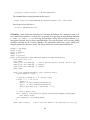
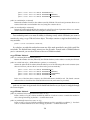
Top-level Loop ECJ hangs the entire state of the evolutionary run off of a single instance of a
subclass of EvolutionState. This enables ECJ to serialize out the entire state of the system to a
checkpoint file and to recover it from the same. The EvolutionState subclass chosen defines the
kind of top-level evolutionary loop used in the ECJ process. We provide two such loops: a simple
generational loop with optional elitism, and a steady-state loop.
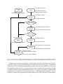
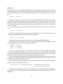
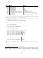
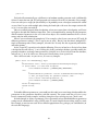
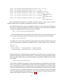
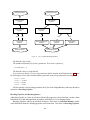
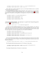
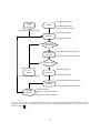
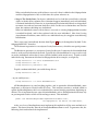
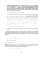
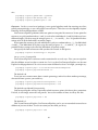
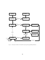
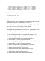
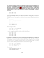
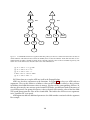
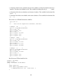
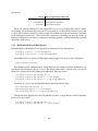
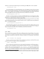
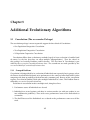
Figure 0 shows the top-level loop of the simple generational EvolutionState. The loop iterates
between breeding and evaluation, with an optional “exchange” period after each. Statistics hooks
are called before and after each period of breeding, evaluation, and exchanging, as well as before
and after initialization of the population and “finishing” (cleaning up prior to quitting the program).
7
Pre-Initialization Statistics
Recover
from
Checkpoint
Initializer
Post-Initialization Statistics
Initialize Exchanger, Evaluator
Reinitialize Exchanger, Evaluator
Pre-Evaluation Statistics
Evaluator
Post-Evaluation Statistics
YES
Out of time or
found the ideal?
NO
Pre-Pre-Breeding Exchange Statistics
Pre-Breeding
Exchange
Post-Pre-Breeding Exchange Statistics
YES
Found the ideal?
NO
Pre-Finishing Statistics
Pre-Breeding Statistics
Finisher
Breeding
Post-Breeding Statistics
Shut Down Exchanger, Evaluator
Pre-Post-Breeding Exchange Statistics
Post-Breeding
Exchange
Post-Post-Breeding Exchange Statistics
Increment Generation
Optionally
Checkpoint
Optional Pre-Checkpoint Statistics
Optional Post-Checkpoint Statistics
Figure 0 Top-Level Loop of ECJ’s SimpleEvolutionState class, used for basic generational EC algorithms. Various
sub-operations are shown occurring before or after the primary operations. The full population is revised each iteration.
Breeding and evaluation are handled by singleton objects known as the Breeder and Evaluator
respectively. Likewise, population initialization is handled by an Initializer singleton, and finishing
is done by a Finisher. Exchanges after breeding and after evaluation are handled by an Exchanger.
The particular versions of these singleton objects are determined by the experimenter, though
we provide versions which perform common tasks. For example, we provide a traditional-EA
SimpleEvaluator, a steady-state EA SteadyStateEvaluator, a “single-population coevolution” CompetitiveEvaluator, and a multi-population coevolution MultiPopCoevolutionaryEvaluator, among others.
8
Parameter
Database
1
Mersenne Twister
RNG
Evolve
1
1
Output
Log
makes
Initializer
1
Population
makes
1
EvolutionState
updates
Breeder
Breeding Pipeline
applies
1
Evaluator
1
prototype
Problem
updates
Exchanger
1
evaluates
Finisher
Fitness
1
Statistics
1
0..n
1
n
Individual
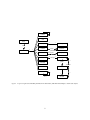
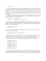
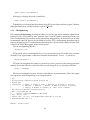
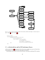
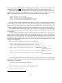
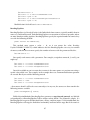
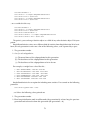
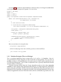
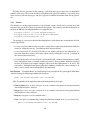
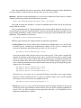
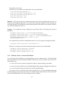
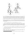
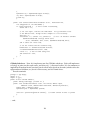
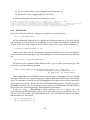
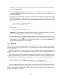
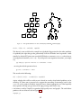
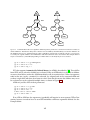
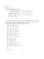
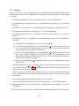
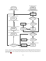
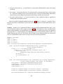
Figure 1 Top-Level operators and utility facilities in EvolutionState, and their relationship to certain state objects.
9
There are likewise custom breeders and initializers for different functions. The Exchanger provides
an opportunity for other hooks, notably internal and external island models. For example, postbreeding exchange might allow external immigrants to enter the population, while emmigrants
might leave the population during post-evaluation exchange. These singleton operators comprise
most of the high-level “verbs” in the ECJ system, as shown in Figure 1.
Parameterized Construction ECJ is unusually heavily parameterized: practically every feature
of the system is determined at runtime from a parameter. Parameters define the classes of objects,
the specific subobjects they hold, and all of their initial runtime values. ECJ does this through a
bootstrap class called Evolve, which loads a ParameterDatabase from runtime parameter files at
startup. Using this database, Evolve constructs the top-level EvolutionState and tells it to “setup”
itself. EvolutionState in turn calls subsidiary classes (such as Evaluator) and tells them to “setup”
themselves from the database. This procedure continues down the chain until the entire system is
constructed.
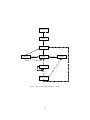
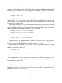
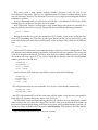
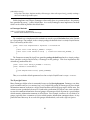
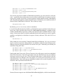
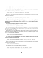
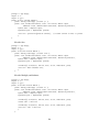
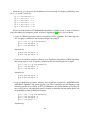
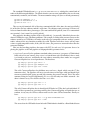
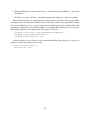
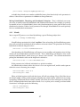
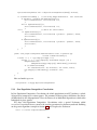
State Objects In addition to “verbs”, EvolutionState also holds “nouns” — the state objects
representing the things being evolved. Specifically, EvolutionState holds exactly one Population,
which contains some N (typically 1) Subpopulations. Multiple Subpopulations permit experiments in
coevolution, internal island models, etc. Each Subpopulation holds some number of Individuals and
the Species to which the Individuals belong. Species is a flyweight object for Individual: it provides a
central repository for things common to many Individuals so they don’t have to each contain them
in their own instances.
While running, numerous state objects must be created, destroyed, and recreated. As ECJ only
learns the specific classes of these objects from the user-defined parameter file at runtime, it cannot
simply construct them using Java’s new operator. Instead such objects are created by constructing
a prototype object at startup time, and then using this object to stamp out copies of itself as often
as necessary. For example, Species contains a prototypical Individual. When new Individuals must
be created for a given Subpopulation, they are copied from the Subpopulation’s Species and then
customized. This allows different Subpopulations to use different Individual representations.
In keeping with its philosophy of orthogonality, ECJ defines Fitnesses separate from Individuals
(representations), and provides both single-objective and multi-objective Fitness subclasses. For
historical reasons, Subpopulation stores the Fitness prototype, rather than keeping it in Species.
Different Subpopulations may likewise use different Fitness forms.
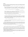
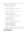
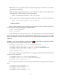
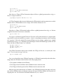
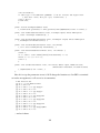
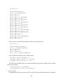
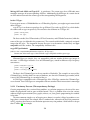
Breeding A Species holds a prototypical breeding pipeline which is cloned by the Breeder and
used per-thread to breed individuals and form the next-generation population. Breeding pipelines
are tree structures where a node in the tree filters incoming Individuals from its child nodes and
hands them to its parents. The leaf nodes in the tree are SelectionMethods which simply choose
Individuals from the old subpopulation and hand them off. There exist SelectionMethods which
perform tournament selection, fitness proportional selection, truncation selection, etc. Nonleaf
nodes in the tree are BreedingPipelines, many of which copy and modify their received Individuals
before handing them to their parent nodes. Some BreedingPipelines are representation-independent:
for example, MultiBreedingPipeline asks for Individuals from one of its children at random according
to some probability distribution. But most BreedingPipelines act to mutate or cross over Individuals
in a representation-dependent way. For example, the GP CrossoverPipeline asks for one Individual
10
EvolutionState
1
1
Population
1
1..n
Subpopulation
1
1
1..n
1
Individual
1
1
prototype
1
Species
1
prototype
Fitness
prototype
1
flyweight
1
1..n
prototype
1
0..n
uses
Breeding Pipeline
child of
1
1
uses
child of
0..n
Selection Method
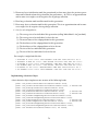
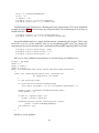
Figure 2 Top-Level data objects used in evolution.
11
of each of its two children, which must be genetic programming Individuals, performs subtree
crossover on those Individuals, then hands them to its parent.
A tree-structured breeding pipeline allows for a rich assortment of experimenter-defined
selection and breeding proceses. Further, ECJ’s pipeline is copy-forward: BreedingPipelines must
ensure that they copy Individuals before modifying them or handing them forward, if they have not
been already copied. This guarantees that new Individuals are copies of old ones in the population,
and furthermore that multiple pipelines may operate on the same Subpopulation in different threads
without the need for locking. ECJ may apply multiple threads to parallelize the breeding process
without the use of Java synchronization at all.
Evaluation The Evaluator performs evaluation of a population by passing one or (for coevolutionary evaluation) several Individuals to a Problem subclass which the Evaluator has cloned off of
its prototype. Evaluation may too be done in multithreaded fashion with no locking, using one
Problem per thread. Individuals may also undergo repeated evaluation in coevolutionary Evaluators
of different sorts.
In most projects using ECJ, the primary task is to construct an appropriate Problem subclass.
The task of the Problem is to assess the fitness of the Individual(s) and set its Fitness accordingly.
Problem classes also report if the ideal Individual has been discovered.
Utilities In addition to its ParameterDatabase, ECJ also uses a checkpointable Output convenience
facility which maintains various streams, repairing them after checkpoint. Output also provides for
message logging, retaining in memory all messages during the run, so that on checkpoint recovery
the messages are printed out again as before. Other utilities include population distribution
selectors, searching and sorting tools, etc.
The quality of a random number generator is important for a stochastic optimization system.
As such, ECJ’s random number generator was the very first class written in the system: it is a Java
implementation of the highly respected Mersenne Twister algorithm [9] and is the fastest such
implementation available. Since ECJ’s release, the ECJ MersenneTwister and MersenneTwisterFast
classes have found their way in a number of unrelated public-domain systems, including the
popular NetLogo multiagent simulator [17]. MersenneTwisterFast is also shared in ECJ’s sister
software, the MASON multiagent simulation toolkit [6].
Representations and Genetic Programming ECJ allows you to specify any genome representation you like. Standard representation packages in ECJ provide functionality for vectors of all Java
data types; arbitrary-length lists; trees; and collections of objects (such as rulesets).
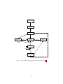
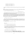
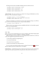
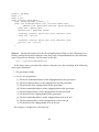
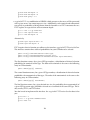
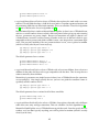
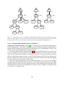
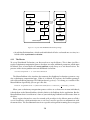
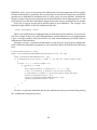
ECJ is perhaps best known for its support of “Koza”-style tree-structured genetic programming
representations. ECJ represents these individuals as forests of parse-trees, each tree equivalent
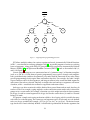
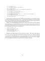
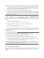
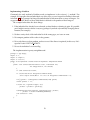
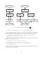
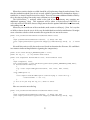
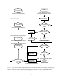
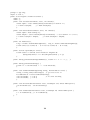
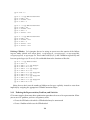
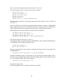
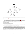
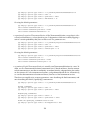
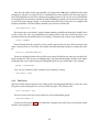
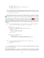
to a single Lisp s-expression. Figure 3 shows a parse-tree for a simple robot program, equivalent to the Lisp s-expression (if (and on-wall (tick> 20) (∗ (ir 3) 6) 2.3). In C this might look like
(onWall && tick > 20) ? ir(3) * 6 : 2.3. This notionally says “If I’m on the wall and my tick-count
is greater than 20, then return the value of my third infrared sensor times six, else return 2.3”. Such
parse-trees are typically evaluated by executing their programs in a test environment, and modified via subtree crossover (swapping subtrees among individuals) or various kinds of mutation
(replacing a subtree with a randomly-generated one, perhaps).
12
tree
int, float
float
if
int, float
int, float
bool
float
bool
and
bool
bool
onwall
float
2.3
*
bool
int, float int, float
bool
float
tick>
ir
int
int
int
int
20
3
int
6
Figure 3 A typed genetic programming parse tree.
ECJ allows multiple subtrees for various experimental needs: Automatically Defined Functions
(ADFs — a mechanism for evolving subroutine calls [3]), or parallel program execution, or evolving
teams of programs. Along with ADFs, ECJ provides built-in support for Automatically Defined
Macros (ADMs) [15] and Ephemeral Random Constants (ERCs [2], such as the numbers 20, 3, 6,
and 2.3 in Figure 3).
Genetic programming trees are constructed out of a “primorial soup” of function templates
(such as on-wall or 2.3. Early forms of genetic programming were typeless: though such templates
had a predefined arity (number of arguments), any node could be connected to any other. Many
genetic programming needs require more constraints than this. For example, the node if might
expect a boolean value in its first argument, and integers or floats in the second and third arguments,
and return a float when evaluated. Similarly and might take two booleans as arguments and return
a boolean, while ∗ would take ints or floats as arguments and return a float.
Such types are often associated with the kinds of data passed from node to node, but they do
not have to be. For example, typing might be used to constrain certain nodes to be evaluated in
groups or in a certain order: for example, a function type-block might insist that its first argument
be of type foo and its second argument be of type bar to make certain that a foo node be executed
before a bar node.
ECJ permits a simple static typing mechanism called set-based typing, which is suitable for many
such tasks. In set-based typing, the return type and argument types of each node are each defined
to be sets of type symbols (for example, {bool} or {foo, bar, baz}, or {int, float}. The desired return
type for the tree’s root is similarly defined. A child node is permitted to fit into the argument slot
13
of a parent node if the child node’s return type and type of the that argument slot in the parent are
compatible. We define types to be compatible if their set intersection is nonempty (that is, they share
at least one type symbol).
Set-based typing is sufficient for the typing requirements found in many programming languages, including ones with type hierarchies. It allows, among other things, for nodes such as
∗ to accept either integers or floats. However there are considerable restrictions on the power of
set-based typing. It’s often useful for the return type of a node to change based on the particular
nodes which have plugged into it as arguments. For example, ∗ might be defined as returning a
float if at least one of its arguments returns floats, but returning an integer if both of its arguments
return integers. if might be similarly defined not to return a particular type, but to simply require
that its return type and the second and third argument types must all match. Such “polymorphic”
typing is particularly useful in situations such as matrix multiplication, where the operator must
place constraints on the width and height of its arguments and the final returned matrix. In this
example, it’s also useful to have an infinite number of types (perhaps to represent matrices of
varying widths or heights).
ECJ does not support polymorphic typing out of the box simply because it is difficult to implement many if not most common tree modification and generation algorithms using polymorphic
typing: instead, set-based typing is offered to handle as many common needs as can be easily done.
Out of the Box Capabilities ECJ provides support out-of-the-box for a bunch of algorithm
options:
• Generational algorithms: (µ, λ) and (µ + λ) Evolution Strategies, the Genetic Algorithm,
Genetic Programming variants, and Differential Evolution
• Steady-State evolution
• Particle Swarm Optimization
• Parsimony pressure algorithms
• Spatially-embeded evolutionary algorithms
• Random restarts
• Multiobjective optimization, including the NSGA-II and SPEA2 algorithms.
• Cooperative, 1-Population Competitive, and 2-Population Competitive coevolution.
• Multithreaded evaluation and breeding.
• Parallel synchronous and asynchronous Island Models spread over a grid of computers.
• Internal synchronous Island Models internally in a single ECJ process.
• Massive parallel generational fitness evaluation of individuals on remote slave machines.
• Asynchronous Evolution, a version of steady-state evolution with massive parallel fitness
evaluation on remote slave machines.
14
• Opportunistic Evolution, where remote slave machines run their own mini-evolutionary
processes for a while before sending individuals back to the master process.
• Internal synchronous Island Models internally in a single ECJ process.
• A large number of selection and breeding operators
ECJ also has a GUI, though in truth I nearly universally use the command-line.
Idiosyncracies ECJ was developed near the introduction of Java and so has a lot of historical
idiosyncracies.1 . Some of them exist to this day because of conservatism: refactoring is disruptive.
If you code in ECJ, you’ll definitely have to get used to one or more of the following:
• No generics at all, few iterators or enumerators, no Java features beyond 1.4 (including
annotations), and little use of the Java Collections library. This is part historical, and part my
own dislike of Java’s byzantine generics implementation, but it’s mostly efficiency. Generics
are very slow when used with basic data types, as they require boxing and unboxing. The
Java Collections library is unusually badly written in many places internally: and anyway,
for speed we tend to work directly with arrays.
• Hand-rolled socket code. ECJ’s parallel facility doesn’t rely on other libraries.
• ECJ loads nearly every object from its parameter database. This means that you’ll rarely
see the new keyword in ECJ, nor any constructors. Instead ECJ’s “constructor” method is a
method called setup(...), which sets up an object from the database.
• A proprietary logging facility. ECJ was developed before the existence of java.util.logging.
Partly out of conservatism, I am hesitant to rip up all the pervasive logging just to use Sun’s
implementation (which isn’t very good anyway).
• Parameter database derived from Java’s old java.util.Properties list rather than XML. This is
historical of course. But seriously, do I need a justification not to use XML?
• Mersenne Twister random number generator. java.lang.Random is grotesquely bad, and
systems which use it should be shunned.
• A Makefile. ECJ was developed before Ant and I’ve personally never needed it.
0.1
Introductory Tutorial
0.2
Tutorial 1
0.3
Tutorial 2
0.4
Tutorial 3
0.5
Tutorial 4
1 It
used to have a lot more — I’ve been weeding out ones that I think are unnecessary nowadays!
15
16
Part II
ECJ The Hard Way
17
Chapter 1
ECJ Basics
1.1
ec.Evolve and Utility Classes
ECJ’s entry point is the class ec.Evolve. This class is little more than bootstrapping code to set up
the ECJ system, construct basic datatypes, and get things going.
To run an ECJ process, you fire up ec.Evolve with certain runtime arguments.
java ec.Evolve -file myParameterFile.params -p param=value -p param=value (etc.)
ECJ sets itself up entirely using a parameter file. To this you can add additional command-line
parameters which override those found in the parameter file. More on the parameter file will be
discussed starting in Section 1.1.1.
ECJ can also restart from a checkpoint file it created in a previous run, like this:
java ec.Evolve -checkpoint myCheckpointFile.gz
Checkpointing will be discussed in Section 1.1.3.
The purpose of ec.Evolve is to construct an ec.EvolutionState instance, or load one from a
checkpoint file; then get it running; and finally clean up. The ec.EvolutionState class actually
performs the process. Most of the stuff ec.EvolutionState holds is associated with evolutionary
algorithms or other stochastic optimization procedures. However there are certain important utility
objects or data which are created by ec.Evolve prior to creating the ec.EvolutionState, and are then
stored into ec.EvolutionState after it has been constructed. These objects are:
• The Parameter Database, which holds all the parameters ec.EvolutionState uses to build and
run the process.
• The Output, which handles logging and writing to files.
• The Checkpointing Facility to create checkpoint files as the process continues.
• The Number of Threads to use, and the Random Number Generators, one per thread.
• A simple declaration of the Number of Jobs to run in the process.
The remainder Section 1.1 discusses each of these items. It’s not the most exciting of topics: but
it’s important in order to understand the rest of the ECJ process.
19
1.1.1
The Parameter Database
To build and run an experiment in ECJ, you typically write three things:
• (In Java) A problem which evaluates individuals and assigns fitness values to them.
• (In Java) Depending on the kind of experiment, various components from which individuals
can be constructed — for example, for a genetic programming experiment, you’ll need to
define the kinds of nodes which can be used to make up the individual’s tree.
• (In one or more Parameter Files) Various parameters which define the kind of algorithm you
are using, the nature of the experiment, and the makeup of your populations and processes.
Let’s begin with the third item. Parameters are the lifeblood of ECJ: practically everything in
the system is defined by them. This makes ECJ highly flexible; but it also adds complexity to the
system.
ECJ loads parameter files and stores them into the ec.util.ParameterDatabase object, which is
available to nearly everything. Parameter files are an extension of the files used by Java’s old
java.util.PropertyList object. Parameter files usually end in ".params", and contain parameters
one to a line. Parameter files may also contain blank (all whitespace) lines, which are ignored, and
also lines which start with "#", which are considered comments and also ignored. An example
comment:
# This is a comment
The parameter lines in a parameter file typically look like this:
parameter.name = parameter value
A parameter name is a string of non-whitespace characters except for "=". After this comes
some optional whitespace, then an "=", then some more optional whitespace.1 A parameter value
is a string of characters, including whitespace, except that all whitespace is trimmed from the
front and end of the string. Notice the use of a period the parameter name. It’s quite a common
convention to use periods in various parameter names in ECJ. We’ll get to why in a second.
Here are some legal parameter lines:
generations = 400
pop.subpop.0.size
pop.subpop=
=1000
ec.Subpopulation
Here are some illegal parameter lines:
generations
= 1000
pop subpop = ec.Subpopulation
1 Actually,
you can omit the "=", but it’s considered bad style.
20
Inheritance
Parameter files may be set up to derive from one or more other parameter files. Let’s say you have
two parameter files, a.params and b.params. Both are located in the same directory. You can set up
a.params to derive from b.params by adding the following line as the very first line in the a.params
file:
parent.0 = b.params
This says, in effect: “include in me all the parameters found in the b.params file, but any
parameters I myself declare will override any parameters of the same name in the b.params file.”
Note that b.params may itself derive from some other file (say, c.params). In this case, a.params
receives parameters from both (and parameters in b.params will likewise override ones of the same
name in c.params).
Let’s say that b.params is located inside a subdirectory called foo. Then the line will look like
this:
parent.0 = foo/b.params
Notice the forward slash: ECJ was designed on UNIX systems. Likewise, imagine if b.params
was stored in a sibling directory called bar: then we might say:
parent.0 = ../bar/b.params
Long story short: parameter files are declared using traditional UNIX path syntax.
A parameter file can also derive from multiple parent parameter files, by including each at the
beginning of the file, with consecutive numbers, like this:
parent.0 = b.params
parent.1 = yo/d.params
parent.2 = ../z.params
This says in effect: “first look in a.params for the parameter. If you can’t find it there, look in
b.params and, ultimately, all the files b.params derives from. If you can’t find it in any of them, look
in d.params and all the files it derives from. If you can’t find it in any of them, look in z.params and
all the files it derives from. If you’ve still not found the parameter, give up.”
This is essentially a depth-first search, with children overriding their parents and earlier siblings
overriding later siblings. Note that this multiple inheritance scheme is not the same as C++ or
Lisp/CLOS, which use a distance measure!
When you fire up ECJ, you point it at a single parameter file, and you can provide additional
parameters at the command-line, like this:
java ec.Evolve -file parameterFile.params -p command-line-parameter=value \
-p command-line-parameter=value ...
Furthermore, your program itself can submit parameters to the parameter database, though it’s
very unusual to do so. When a parameter is requested from the parameter database, here’s how it’s
looked up:
21
1. If the parameter was declared by the program itself, this value is returned.
2. Else if the parameter was provided on the command line, this value is returned.
3. Else the parameter is looked up in the provided parameter file and all derived files using the
inheritance ordering described earlier.
4. Else the database signals failure.
Kinds of Parameters
ECJ supports the following kinds of parameters:
• Numbers. Either long integers or double floating-point values. Examples:
generations = 500
tournament.size = 3.25
minimum-fitness = -23.45e15
• Arbitrary Strings trimmed of whitespace. Example:
crossover-type = two-point
• Booleans. Any value except for "false" (case-insensitive) is considered to be true. It’s best
style to use lower-case "true" and "false". The first two of these examples are false and the
second two are true:
print-params = false
die-silently = fAlSe
pop.subpop.0.perform-injections = true
quit-on-run-complete = whatever
• File Path Names. Paths can be of three types. Absolute paths, which (in UNIX) begin with a
"/", stipulate a precise location in the file system. Relative paths, which do not begin with a
"/", are defined relative to the parameter file in which the parameter was located. You’ve seen
relative paths already used for derived parameter files. Finally, Execution relative paths are
defined relative to the directory in which the ECJ process was launched. Execution relative
paths look exactly like relative paths except that they begin with the special character "$".
Examples of all three kinds of paths:
stat.file = $out.stat
eval.prob.map-file = ../dungeon.map
temporary-output-file = /tmp/output.txt
• Class Names. Class names are defined as the full class name of the class, including the
package. Example:
22
pop.subpop.0.species = ec.gp.GPSpecies
• Arrays. ECJ doesn’t have direct support for loading arrays, but has a convention you should
be made aware of. It’s common for arrays to be loaded by first stipulating the number
of elements in the array, then stipulating each array element in turn, starting with 0. The
parameter used for the number of elements differs from case to case. Note the use of periods
prior to each number in the following example:
gp.fs.0.size =
gp.fs.0.func.0
gp.fs.0.func.1
gp.fs.0.func.2
gp.fs.0.func.3
gp.fs.0.func.4
gp.fs.0.func.5
6
=
=
=
=
=
=
ec.app.ant.func.Left
ec.app.ant.func.Right
ec.app.ant.func.Move
ec.app.ant.func.IfFoodAhead
ec.app.ant.func.Progn2
ec.app.ant.func.Progn3
The particulars vary. Here’s another, slightly different, example:
exch.num-islands
exch.island.0.id
exch.island.1.id
exch.island.2.id
exch.island.3.id
exch.island.4.id
exch.island.5.id
exch.island.6.id
exch.island.7.id
=
=
=
=
=
=
=
=
=
8
SurvivorIsland
GilligansIsland
FantasyIsland
TemptationIsland
RhodeIsland
EllisIsland
ConeyIsland
TreasureIsland
Anyway, you get the idea.
Namespace Hierarchies and Parameter Bases
ECJ has lots of parameters, and by convention organizes them in a namespace hierarchy to maintain
some sense of order. The delimiter for paths in this hierarchy is — you guessed it — the period.
The vast majority of parameters are used by one Java object or another to set itself up immediately after it has been instantiated for the first time. ECJ has an important convention which uses
the namespace hierarchy to do just this: the parameter base. A parameter base is essentially a path
(or namespace, what have you) in which an object expects to find all of its parameters. The prefix
for this path is typically the parameter name by which the object itself was loaded.
For example, let us consider the process of defining the class to be used for the global population.
This class is found in the following parameter:
pop = ec.Population
ECJ looks for this parameter, expects a class (in this case, ec.Population), loads the class, and
creates one instance. It then calls a special method (setup(...), we’ll discuss it later) on this class so
it can set itself up from various parameters. In this case, ec.Population needs to know how many
subpopulations it will have. This is defined by the following parameter:
23
pop.subpops = 2
ec.Population didn’t know that it was supposed to look in pop.subpops for this value. Instead,
it only knew that it needed to look in a parameter called subpops. The rest (in this case, pop) was
provided to ec.Population as its parameter base: the text to be prepended — plus a period — to all
parameters that ec.Population needed to set itself up. It’s not a coincidence that the parameter base
also happened to be the very parameter which defined ec.Population in the first place. This is by
convention.
Armed with the fact that it needs to create an array of two subpopulations, ec.Population is
ready to load the classes for those two subpopulations. Let’s say that for our experiment we want
them to be of different classes. Here they are:
pop.subpop.0 = ec.Subpopulation
pop.subpop.1 = ec.app.myapp.MySpecialSubpopulation
The two classes are loaded and one instance is created of each of them. Then setup(...) is
called on each of them. Each subpopulation looks for a parameter called size to tell it how may
individuals will be in that subpopulation. Since each of them is provided with a different parameter
base, they can have different sizes:
pop.subpop.0.size = 100
pop.subpop.1.size = 512
Likewise, each of these subpopulations needs a “species”. Presuming that the species are
different classes, we might have:
pop.subpop.0.species = ec.vector.VectorSpecies
pop.subpop.1.species = ec.gp.GPSpecies
These species objects themselves need to be set up, and when they do, their parameter bases
will be pop.subpop.0.species and pop.subpop.1.species respectively. And so on.
Now imagine that we have ten subpopulations, all of the same class (ec.Subpopulation), and all
but the first one has the exact same size. We’d wind up having to write silly stuff like this:
pop.subpop.0.size
pop.subpop.1.size
pop.subpop.2.size
pop.subpop.3.size
pop.subpop.4.size
pop.subpop.5.size
pop.subpop.6.size
pop.subpop.7.size
pop.subpop.8.size
pop.subpop.9.size
=
=
=
=
=
=
=
=
=
=
1000
500
500
500
500
500
500
500
500
500
That’s a lot of typing. Though I am saddened to report that ECJ’s parameter files do require a
lot of typing, at least the parameter database facility offers an option to save our fingers somewhat
in this case. Specifically, when the ec.Subpopulation class sets itself up each time, it actually looks in
24
not one but two path locations for the size parameter: first it tacks on its current base (as above),
and if there’s no parameter at that location, then it tries tacking on a default base defined for its
class. In this case, the default base for ec.Subpopulation is the prefix ec.subpop. Armed with this
we could simply write:
ec.subpop.size = 500
pop.subpop.0.size = 1000
When ECJ looks for subpopulation 0’s size, it’ll find it as normal (1000). But when it looks for
subpopulation 1 (etc.), it won’t find a size parameter in the normal location, so it’ll look in the
default location, use what it finds there (500). Only if there’s no parameter to be found in either
location will ECJ signal an error.
It’s important to note that if a class is loaded from a default parameter, this doesn’t mean that
the default parameter will become its parameter base: rather, the original expect location will
continue to be the base. For example, imagine if both of our Species objects were the same class,
and we had defined them using the default base. That is, instead of
pop.subpop.0.species = ec.vector.VectorSpecies
pop.subpop.1.species = ec.vector.VectorSpecies
...we simply said
ec.subpop.species = ec.vector.VectorSpecies
When the species for subpopulation 0 is loaded, its parameter base is not going to be
ec.subpop.species. Instead, it will still be pop.subpop.0.species. Likewise, the parameter
base for the species of subpopulation 1 will still be pop.subpop.1.species.
Keep in mind that all of this is just a convention. You can use periods for whatever you like
ultimately. And there exist a few global parameters without any base at all. For example, the
number of generations is defined as
generations = 200
...and the seed for the random number generator the fourth thread is
seed.3 = 12303421
...even though there is no object set up with the seed parameter, and hence no object has seed as its
parameter base. Random number generators are one of the few rare objects in ECJ which are not
specified from the parameter file.
Loading Parameters
Parameters are looked up in the ec.util.ParameterDatabase class, and parameter names are specified
using the ec.Parameter class. The latter is little more than a cover for Java strings. To create the
parameter pop.subpop.0.size, we say:
25
Parameter param = new Parameter("pop.subpop.0.size");
Of course, usually we don’t want to just make a direct parameter, but rather want to construct
one from a parameter base and the remainder. Let’s say our base (pop.subpop.0) is stored in the
variable base, and we want to look for size. We do this as:
Parameter param = base.push("size");
Here are some common ec.util.ParameterDatabase methods:
ec.util.ParameterDatabase Methods
public boolean exists(Parameter parameter, Parameter default)
If either parameter exists in the database, return true. Either parameter may be null.
public String getString(Parameter parameter, Parameter default)
Look first in parameter, then failing that, in default parameter, and return the result as a String, else null
if not found. Either parameter may be null.
public File getFile(Parameter parameter, Parameter default)
Look first in parameter, then failing that, in default parameter, and return the result as a File, else null if
not found. Either parameter may be null.
public Object getInstanceForParameterEq(Parameter parameter, Parameter default, Class superclass)
Look first in parameter, then failing that, in default parameter, to find a class. The class must have
superclass as a superclass, or can be the superclass itself. Instantiate one instance of the class using the
default (no-argument) constructor, and return the instance. Throws an ec.util.ParamClassLoadException
if no class is found.
public Object getInstanceForParameter(Parameter parameter, Parameter default, Class superclass)
Look first in parameter, then failing that, in default parameter, to find a class. The class must have
superclass as a superclass, but may not be superclass itself. Instantiate one instance of the class using the
default (no-argument) constructor, and return the instance. Throws an ec.util.ParamClassLoadException
if no class is found.
public int getBoolean(Parameter parameter, Parameter default, double defaultValue)
Look first in parameter, then failing that, in default parameter, and return the result as a boolean, else
defaultValue if not found or not a boolean. Either parameter may be null.
public int getIntWithDefault(Parameter parameter, Parameter default, int defaultValue)
Look first in parameter, then failing that, in default parameter, and return the result as an int, else
defaultValue if not found or not an int. Either parameter may be null.
public int getInt(Parameter parameter, Parameter default, int minValue)
Look first in parameter, then failing that, in default parameter, and return the result as an int, else
minValue−1 if not found, not an int, or < minValue. Either parameter may be null.
public int getIntWithMax(Parameter parameter, Parameter default, int minValue, int maxValue)
Look first in parameter, then failing that, in default parameter, and return the result as an int, else
minValue−1 if not found, not an int, < minValue, or > maxValue. Either parameter may be null.
public long getLongWithDefault(Parameter parameter, Parameter default, long defaultValue)
Look first in parameter, then failing that, in default parameter, and return the result as a long, else
defaultValue if not found or not a long. Either parameter may be null.
26
public long getLong(Parameter parameter, Parameter default, long minValue)
Look first in parameter, then failing that, in default parameter, and return the result as a long, else
minValue−1 if not found, not a long, or < minValue. Either parameter may be null.
public long getLongWithMax(Parameter parameter, Parameter default, long minValue, long maxValue)
Look first in parameter, then failing that, in default parameter, and return the result as a long, else
minValue−1 if not found, not a long, < minValue, or > maxValue. Either parameter may be null.
public float getFloatWithDefault(Parameter parameter, Parameter default, float defaultValue)
Look first in parameter, then failing that, in default parameter, and return the result as a float, else
defaultValue if not found or not a float. Either parameter may be null.
public float getFloat(Parameter parameter, Parameter default, float minValue)
Look first in parameter, then failing that, in default parameter, and return the result as a float, else
minValue−1 if not found, not a float, or < minValue. Either parameter may be null.
public float getFloatWithMax(Parameter parameter, Parameter default, float minValue, float maxValue)
Look first in parameter, then failing that, in default parameter, and return the result as a float, else
minValue−1 if not found, not a float, < minValue, or > maxValue. Either parameter may be null.
public double getDoubleWithDefault(Parameter parameter, Parameter default, double defaultValue)
Look first in parameter, then failing that, in default parameter, and return the result as a double, else
defaultValue if not found or not a double. Either parameter may be null.
public double getDouble(Parameter parameter, Parameter default, double minValue)
Look first in parameter, then failing that, in default parameter, and return the result as a double, else
minValue−1 if not found, not a double, or < minValue. Either parameter may be null.
public double getDoubleWithMax(Parameter parameter, Parameter default, double minValue, double maxValue)
Look first in parameter, then failing that, in default parameter, and return the result as a double, else minValue−1 if not found, not a double, < minValue, or > maxValue. Either parameter may be
null.
Debugging
Your ECJ experiment is loading silently and running, but how do you know you didn’t make a
mistake in your parameters? How do you know ECJ is using the parameters you stated rather than
some default values? If you include the following parameter in your collection:
print-params = true
...then ECJ will print out all the parameters which were used or tested for existence. For example,
you might get things like this printed out:
27
!P:
P:
<P:
P:
<P:
!E:
P:
<P:
P:
<P:
E:
<E:
pop.subpop.0.file
pop.subpop.0.species = ec.gp.GPSpecies
ec.subpop.species
pop.subpop.0.species.pipe = ec.breed.MultiBreedingPipeline
gp.species.pipe
pop.subpop.0.species.pipe.prob
pop.subpop.0.species.pipe.num-sources = 2
breed.multibreed.num-sources
pop.subpop.0.species.pipe.source.0 = ec.gp.koza.CrossoverPipeline
breed.multibreed.source.0
pop.subpop.0.species.pipe.source.0.prob = 0.9
gp.koza.xover.prob
A P means that a parameter was used. An E means that a parameter was tested for existence.
An ! means that the parameter did not exist. A < means that the parameter existed in the default
base as well as the primary base, but the value of the primary base was the one used. In this last
case, the primary base is printed out on the line immediately prior.
There are a few other debugging parameters of less value. At the end of a run, ECJ can dump
all the parameters in the database; all the parameters accessed (retrieved or tested for existence); all
the parameters used (retrieved); all the parameters not accessed; and all the parameters not used.
Pick your poison. Here are the relevant parameters:
print-all-params = true
print-accessed-params = true
print-used-params = true
print-unaccessed-params = true
print-unused-params = true
Typically you’d only want to set one of these to true.
The most useful one is
print-unaccessed-params, since by examining the results you can see if a parameter you set
was used or not: if not, probably because it wasn’t typed right. It also tells you about old, disused
parameters. In fact, as I was writing this manual and needed print-unaccessed-params examples,
I ran the Lawnmower problem (in ec/app/lawnmower) and got the following:
28
Unaccessed Parameters
===================== (Ignore parent.x references)
gp.fs.2.info = ec.gp.GPFuncInfo
stat.gather-full = true
gp.koza.grow.min-depth = 5
gp.tc.0.init.max = 6
gp.koza.mutate.build.0 = ec.gp.koza.GrowBuilder
gp.tc.1.init.max = 6
parent.0 = ../../gp/koza/koza.params
gp.koza.grow.max-depth = 5
gp.tc.2.init.max = 6
gp.koza.mutate.ns.0 = ec.gp.koza.KozaNodeSelector
gp.fs.0.info = ec.gp.GPFuncInfo
gp.koza.half.growp = 0.5
gp.tc.0.init.min = 2
gp.koza.mutate.source.0 = ec.select.TournamentSelection
gp.koza.mutate.tries = 1
gp.tc.1.init.min = 2
gp.fs.1.info = ec.gp.GPFuncInfo
gp.tc.2.init.min = 2
gp.koza.mutate.maxdepth = 17
Most of these unaccessed parameters are perfectly fine; standard boilerplate stuff for genetic
programming that didn’t happen to be used by this application. But then there’s the first parameter:
gp.fs.2.info = ec.gp.GPFuncInfo, and two others like it later. I had deleted the GPFuncInfo
class from the ECJ distribution well over a year ago. But apparently I forgot to remove a vestigial
parameter which referred to it. Oops!
By the way, note the request to ignore “parent.x references” — this means to ignore the stuff like
parent.0 = ../../gp/koza/koza.params that gets printed out with everything else.
1.1.2
Output
ECJ has its own idiosyncratic logging and output facility called ec.util.Output. This is largely
historical: ECJ predates any standard logging facilities available in Java. The facility is in part
inspired by a similar facility that existed in the lil-gp C-based genetic programming system. The
system has generally worked out well so we’ve not seen fit to replace it.
The primary reason for the central logging and output facility is to survive checkpointing and
restarting from checkpoints (see Section 1.1.3). Except for the occasional debugging statement
which we’ve forgotten to remove, all output in ECJ goes through ec.util.Output.
The output facility has four basic features:
• Logs, attached to Files or to Writers, which output text of all kinds. Logs can be restarted,
meaning that they can be reopened when ECJ is restarted from a checkpoint.
• Two dedicated Logs, the Message Logs, which write text out to stdout and stderr respectively.
• The ability to print arbitrary text to any Log.
29
• Short Announcements of different kinds. Announcements are different from arbitrary text in
that they are not only written out to Logs (usually the stderr message Log) but are also stored
in memory. This allows them to be checkpointed and automatically reposted after ECJ has
started up again from a checkpoint.
The least important announcements are simple messages. One special kind of message is the
system message generated by ECJ itself. Next in importance are warnings. One special kind
of warning, the once-only-warning, will be written only once to a Log even if it’s posted
multiple times. Next are various kinds of errors, which can cause ECJ to quit. First, a whole
bunch of basic errors can piled on before ECJ finally decides to quit. Second, fatal errors will
cause ECJ to quit immediately rather than wait for more errors to accumulate.
Creating and Writing to Logs
There are many methods in ec.util.Output for creating Logs. Here are the two most common ones:
ec.util.Output Methods
public int addLog(File file, boolean appendOnRestart)
Add a log on a given file.If ECJ is restarted from a checkpoint, and appendOnRestart is true, then the
log will be appended to the current file contents. Else they will be replaced. The Log is registered with
ec.util.Output and its log number is returned.
public int addLog(File file, boolean appendOnRestart, boolean gzip)
Add a log on a given file. If ECJ is restarted from a checkpoint, and appendOnRestart is true, then the
log will be appended to the current file contents. Else they will be replaced. If gzip is true, then the log
will be gzipped. You cannot have both appendOnRestart and gzip true at the same time. The Log is
registered with ec.util.Output and its log number is returned.
Two logs are always made for you automatically: a log to stdout (log number 0); and another
log to stderr (log number 1). The stderr log prints all announcements, but the stdout log does not.
To write arbitrary text to a log, here are the most common methods:
ec.util.Output Methods
public void print(String text, int log number )
Prints a string to a log.
public void println(String text, int log number )
Prints a string to a log, plus a newline.
To post a message or generate a warning or error (all of which ordinarily go to the stderr log, and
are also stored in memory):
ec.util.Output Methods
public void message(String text)
Posts a message.
public void warning(String text)
Posts a warning.
30
public void warning(String text, Parameter Parameter parameter, Parameter Parameter default)
Posts a warning, and indicates the parameters which caused the warning. Typically used for cautioning
the user about the parameters he chose.
public void warnOnce(String text)
Posts a warning which will not appear a second time.
public void warnOnce(String text, Parameter Parameter parameter, Parameter Parameter default)
Posts a warning which will not appear a second time, and indicates the parameters which caused the
warning. Typically used for cautioning the user about the parameters he chose.
public void error(String text)
Posts an error message. The contract implied in using this method is that at some point in the near
future you will call exitIfErrors().
public void error(String text, Parameter Parameter parameter, Parameter Parameter default)
Posts an error message, and indicates the parameters which caused the warning. Typically used for
cautioning the user about the parameters he chose. The contract implied in using this method is that
at some point in the near future you will call exitIfErrors().
public void exitIfErrors()
If an error has been posted, exit.
public void fatal(String text)
Posts an error message and exits immediately.
public void fatal(String text, Parameter Parameter parameter, Parameter Parameter default)
Posts an error message, indicates the parameters which caused the warning, and exits immediately.
Typically used for cautioning the user about the parameters he chose.
The ec.util.Code Class
ECJ Individuals, Fitnesses, and various other components sometimes need to write themselves to a
file in a way which can both be read by humans and be read back into Java resulting in perfect copies
of the original. This means that neither printing text nor writing raw data binary is adequate.
ECJ provides a utility facility to make doing this task a little simpler. The ec.util.Code class
encodes and decodes basic Java data types (booleans, bytes, shorts, ints, longs, floats, chars, Strings)
into Strings which can be emitted as text. They all have the same pattern:
ec.util.Code Methods
public static String encode(int integer )
Encodes integer into a String and returns it
... (etc.)
These methods encode their data in an idiosyncratic way. Here’s a table describing it:
31
Data Type
boolean
byte
short
int
long
float
double
char
String
Encoding
Example
T or F
bvalueAsDecimalNumber|
svalueAsDecimalNumber|
ivalueAsDecimalNumber|
lvalueAsDecimalNumber|
fvalueEncodedAsInteger|valuePrintedForHumans|
dvalueEncodedAsLong|valuePrintedForHumans|
’characterWithEscapes’
"stringWithEscapes"
T
b59|
s-321|
i42391|
l-342341232
f-665866527|-9.1340002E14|
d4614256656552045848|3.141592653589793|
’w’ or ’ ’ or ’\n’ or ’\’’ or ’\u2FD3’
"Dragon in Chinese is:\n\u2FD3"
These are of course idiosyncratic,2 but lacking a Java standard for doing the same task, they do
an adequate job. You’re more than welcome to go your own way.
To decode a sequence of values from a String, you begin by creating an ec.util.DecodeReturn
object wrapped around the String:
DecodeReturn decodeReturn = new DecodeReturn(string);
To decode the next item out of the string, you call:
Code.decode(decodeReturn);
The type of the decoded data is stored here:
int type = decodeReturn.type;
... and is one of the following ec.util.DecodeReturn constants:
public
public
public
public
public
public
public
public
public
public
static
static
static
static
static
static
static
static
static
static
final
final
final
final
final
final
final
final
final
final
byte
byte
byte
byte
byte
byte
byte
byte
byte
byte
DecodeReturn. T
DecodeReturn. T
DecodeReturn. T
DecodeReturn. T
DecodeReturn. T
DecodeReturn. T
DecodeReturn. T
DecodeReturn. T
DecodeReturn. T
DecodeReturn. T
ERROR = -1;
BOOLEAN = 0;
BYTE = 1;
CHAR = 2;
SHORT = 3;
INT = 4;
LONG = 5;
FLOAT = 6;
DOUBLE = 7;
STRING = 8;
If the type is a boolean (false = 0, true = 1), byte, char, short, int, or long, the result is stored
here:
long result = decodeReturn.l;
If the type is a double or float, the result is stored here:
2 The eccentricities in this class stem from it being developed well before Java had any standard way to do such
things itself — indeed Java still doesn’t have a standard way to do most of this. I might improve it in the future, at the
very least, by not requiring type symbols (like b|) in front of integer types. And including methods named things like
DecodeReturn.getFloat() which throws exceptions rather than requiring one to look up type information.
32
double result = decodeReturn.d;
If the type is a String, the result is stored here:
double result = decodeReturn.s;
To decode the next element out of the String, just call Code.decode(decodeReturn) again. Continue
doing this until you’re satisfied or reach a type of T ERROR.
1.1.3
Checkpointing
ECJ supports checkpointing, meaning the ability to save the state of the stochastic optimization
process to a file at any point in time, and later start a new ECJ process resuming in that exact
state. Checkpointing is particularly useful when doing long processes on shared servers or other
environments where the process may be killed at any time. ECJ’s checkpointing procedure largely
consists of applying Java’s serialization mechanism to the ec.EvolutionState object, which in turn
serializes the entire object graph of the current system.
Turn on checkpointing like this:
checkpoint = true
ECJ typically writes out checkpoint files every n generations (or, in the steady-state evolution
situation, every n generations’ worth of evaluations of individuals). To set n = 4, you’d say:
checkpoint-modulo = 4
ECJ writes to checkpoint files named ec.generation.gz, where generation is the current generation
number. If you don’t like the ec prefix for some reason, change it to, say, curmudgeon like this:
prefix = curmudgeon
Whenever a checkpoint is written, this fact is also added as an announcement. Here’s the output
of a typical run with checkpointing every two generations.
|
|
|
|
|
|
|
|
|
|
|
|
ECJ
An evolutionary computation system (version 19)
By Sean Luke
Contributors: L. Panait, G. Balan, S. Paus, Z. Skolicki, R. Kicinger, E. Popovici,
K. Sullivan, J. Harrison, J. Bassett, R. Hubley, A. Desai, A. Chircop,
J. Compton, W. Haddon, S. Donnelly, B. Jamil, and J. O’Beirne
URL: http://cs.gmu.edu/~eclab/projects/ecj/
Mail: [email protected]
(better: join ECJ-INTEREST at URL above)
Date: July 10, 2009
Current Java: 1.5.0_20 / Java HotSpot(TM) Client VM-1.5.0_20-141
Required Minimum Java: 1.4
Threads:
breed/1 eval/1
33
Seed: -530434079
Job: 0
Setting up
Initializing Generation 0
Subpop 0 best fitness of generation:
Generation 1
Subpop 0 best fitness of generation:
Checkpointing
Wrote out checkpoint file ec.2.gz
Generation 2
Subpop 0 best fitness of generation:
Generation 3
Subpop 0 best fitness of generation:
Checkpointing
Wrote out checkpoint file ec.4.gz
Generation 4
Subpop 0 best fitness of generation:
...
Fitness: -1542.1932
Fitness: -1499.354
Fitness: -1497.0482
Fitness: -1481.9377
Fitness: -1426.816
Imagine that at this point the power failed and we lost the process. We’d like to start again from
the checkpoint file ec.4.gz. We can do that by typing:
java ec.Evolve -checkpoint ec.4.gz
Notice that we don’t provide a parameter file or optional command-line parameters. That’s
because the parameter database has already been built and stored inside the checkpoint file. When
ECJ starts up from a checkpoint file, it starts right where it left off, but first spits out all the
announcements that had been produced up to that point, with one exception. See if you can catch
it:
Restoring from Checkpoint ec.4.gz
|
|
|
|
|
|
|
|
|
|
|
|
ECJ
An evolutionary computation system (version 19)
By Sean Luke
Contributors: L. Panait, G. Balan, S. Paus, Z. Skolicki, R. Kicinger, E. Popovici,
K. Sullivan, J. Harrison, J. Bassett, R. Hubley, A. Desai, A. Chircop,
J. Compton, W. Haddon, S. Donnelly, B. Jamil, and J. O’Beirne
URL: http://cs.gmu.edu/~eclab/projects/ecj/
Mail: [email protected]
(better: join ECJ-INTEREST at URL above)
Date: July 10, 2009
Current Java: 1.5.0_20 / Java HotSpot(TM) Client VM-1.5.0_20-141
Required Minimum Java: 1.4
Threads: breed/1 eval/1
Seed: -530434079
Job: 0
Setting up
Initializing Generation 0
34
Subpop 0 best fitness of generation:
Generation 1
Subpop 0 best fitness of generation:
Checkpointing
Wrote out checkpoint file ec.2.gz
Generation 2
Subpop 0 best fitness of generation:
Generation 3
Subpop 0 best fitness of generation:
Checkpointing
Generation 4
Subpop 0 best fitness of generation:
Generation 5
Subpop 0 best fitness of generation:
Checkpointing
Wrote out checkpoint file ec.6.gz
Generation 6
Subpop 0 best fitness of generation:
...
1.1.4
Fitness: -1542.1932
Fitness: -1499.354
Fitness: -1497.0482
Fitness: -1481.9377
Fitness: -1426.816
Fitness: -1336.0835
Fitness: -1302.0063
Threads and Random Number Generation
In many cases ECJ supports multiple threads at two stages of the evolutionary process: during
breeding and during evaluation. You can specify the number of threads for each of these processes
like this:
breedthreads = 4
evalthreads = 4
Typically, but not always, you’d want to set these numbers to match the number of cores or
processors on your computer. And usually these two numbers should be the same. If you don’t
know the number of cores, you can let ECJ try to figure it out for you by saying:
breedthreads = auto
evalthreads = auto
ECJ is still capable of producing replicable results even when threading is turned on: you’ll
get the same results if you use the same number of evaluation and breeding threads and the same
random number generator seeds. Which brings us to...
Random Numbers
As befitting its name, stochastic optimization is stochastic, meaning involving randomness. This
means that a random number generator is central to the algorithms in ECJ, and it’s crucial to have
a fairly good generator. Unfortunately, Java’s default random number generator, java.util.Random,
is notoriously bad. It creates highly nonrandom sequences, so much so that websites have been
developed to show off how awful it is.3 Never, ever, use java.util.Random in your ECJ code.
3 See
for example http://alife.co.uk/nonrandom/
35
ECJ comes with a high quality random number generator ready for you to use:
ec.util.MersenneTwisterFast. This is a fast implementation of a famous random number generator, the Mersenne Twister.4 The Mersenne Twister has a very high period and good statistical
randomness qualities.
If you’re comfortable with java.util.Random, you’ll be fine. ec.util.MersenneTwisterFast has all the
methods that java.util.Random has, plus one or two more.
In ECJ, Mersenne Twister is seeded with a single 32-bit integer other than zero (actually, it’s a
long, but only the first 32 bits are used). You specify this seed with the following parameter:
seed.0 = -492341
Setting the seed this way gives you control over ECJ’s results: if you set the seed to the same
value, ECJ will produce the exact same results again. But if you like you can also let ECJ set the
seed to the current wall clock time in milliseconds, which is almost always different for different
runs:
seed.0 = time
One reason ECJ’s Mersenne Twister implementation is fairly fast is that it’s not threadsafe. Thus
ECJ maintains one random number generator for each thread used by the program. This means that
if you have more than one thread, you’ll have more than one random number generator, and each
one of them will need a seed. Let’s say you’ve settled on two threads. You can set both random
number generator seeds like this:
evalthreads = 2
breedthreads = 2
seed.0 = -492341
seed.1 = 93123
You can also use wall clock time. Specifically, if you instead do the following:
evalthreads = 2
breedthreads = 2
seed.0 = time
seed.1 = time
...ECJ will guarantee that the two seeds differ. Last, if you set your threads automatically:
evalthreads = auto
breedthreads = auto
...then ECJ will automatically set all the seeds using wall clock time, except the ones you specify by
hand. After all, you don’t know how many seeds you’ll get!
The Mersenne Twister random number generators are stored in an array, located in a variable
called random in the ec.EvolutionState object. The size of the array is the maximum of the number of
breed and evaluation threads being used. How do you know which random number generator you
should use? Many methods in ECJ are passed a thread number. This number is the index into the
4 http://www.math.sci.hiroshima-u.ac.jp/∼m-mat/MT/emt.html
36
random number generator array for the thread in which this method is being called. For example,
to get a random double, you typically see things along these lines:
double d = state.random[threadnum].nextDouble();
If you’re in a single-threaded portion of the program, you can just use generator number 0.
Selecting from Distributions
Selecting from distributions is a common task in stochastic optimization. ECJ has a utility class,
ec.util.RandomChoice, which makes it easy to set up and select from histogram-style (arbitrary)
distributions, such as selecting randomly from a Population by Fitness.
The distributions in question come in the form of arrays of floats, doubles, or special objects
which can provide their own float or double values. The values in these arrays are expected to form
a probability density function (PDF). The objective is to select indexes in this array proportional to
their value. To begin, you call one of the following methods on your array to have RandomChoice
convert it into a Cumulative Density Function (CDF) to make selection easier:
ec.util.RandomChoice Methods
public static void organizeDistribution(float[ ] probabilities, boolean allowAllZeros)
If the array is all zeros, then if allowAllZeroes is false, then an ArihmeticException is thrown, else the
array is converted to all ones. Then the array is converted to a CDF. If the array has negative numbers
or is of zero length, an Arithmetic Exception is thrown.
public static void organizeDistribution(float[ ] probabilities)
If the array is all zeros, then if allowAllZeroes is false, then an ArihmeticException is thrown. If not, then
the array is converted to a CDF. If the array has negative numbers or is of zero length, an Arithmetic
Exception is thrown.
public static void organizeDistribution(double[ ] probabilities, boolean allowAllZeros)
If the array is all zeros, then if allowAllZeroes is false, then an ArihmeticException is thrown, else the
array is converted to all ones. Then the array is converted to a CDF. If the array has negative numbers
or is of zero length, an Arithmetic Exception is thrown.
public static void organizeDistribution(float[ ] probabilities)
If the array is all zeros, then if allowAllZeroes is false, then an ArihmeticException is thrown. If not, then
the array is converted to a CDF. If the array has negative numbers or is of zero length, an Arithmetic
Exception is thrown.
public static void organizeDistribution(Object[ ] objs, RandomChoiceChooser chooser, boolean allowAllZeros)
The objects in objs ae passed to chooser to provide their floating-point values (and to set them if needed).
If the array is all zeros, then if allowAllZeroes is false, then an ArihmeticException is thrown, else the
array is converted to all ones. Then the array is converted to a CDF. If the array has negative numbers
or is of zero length, an Arithmetic Exception is thrown.
public static void organizeDistribution(Object[ ] objs, RandomChoiceChooser chooser )
The objects in objs ae passed to chooser to provide their floating-point values (and to set them if needed).
If the array is all zeros, then if allowAllZeroes is false, then an ArihmeticException is thrown. Then
the array is converted to a CDF. If the array has negative numbers or is of zero length, an Arithmetic
Exception is thrown.
37
public static void organizeDistribution(Object[ ] objs, RandomChoiceChooserD chooser, boolean allowAllZeros)
The objects in objs ae passed to chooser to provide their double-floating-point values (and to set them if
needed). If the array is all zeros, then if allowAllZeroes is false, then an ArihmeticException is thrown,
else the array is converted to all ones. Then the array is converted to a CDF. If the array has negative
numbers or is of zero length, an Arithmetic Exception is thrown.
public static void organizeDistribution(Object[ ] objs, RandomChoiceChooserD chooser )
The objects in objs ae passed to chooser to provide their double-floating-point values (and to set them if
needed). If the array is all zeros, then if allowAllZeroes is false, then an ArihmeticException is thrown.
Then the array is converted to a CDF. If the array has negative numbers or is of zero length, an
Arithmetic Exception is thrown.
These
methods
rely
on
two
special
interfaces,
RandomChoiceChooser
(ec.util.RandomChoiceChooser) and RandomChoiceChooserD (ec.util.RandomChoiceChooserD).
RandomChoiceChooser requires two method which map between Objects and floating-point
values.
public float getProbability(Object obj);
public void setProbability(Object obj, float probability);
RandomChoiceChooserD is the same, except that it’s used for double values:
public double getProbability(Object obj);
public void setProbability(Object obj, double probability);
Once the array has been modified, you can then select random indexes from it. This is done by
first generating a random floating-point number from 0...1, then passing that number into one of
the following methods.
ec.util.RandomChoice Methods
public static int pickFromDistribution(float[ ] probabilities, float probability )
Selects and returns an index in the given array which contains the given probability.
public static int pickFromDistribution(double[ ] probabilities, double probability )
Selects and returns an index in the given array which contains the given probability.
public static int pickFromDistribution(Object[ ] objs, RandomChoiceChooser chooser, float probability )
Selects and returns an index in the given array which contains the given probability. The chooser will
provide the floating-point values of each element in the array.
public static int pickFromDistribution(Object[ ] objs, RandomChoiceChooserD chooser, double probability )
Selects and returns an index in the given array which contains the given probability. The chooser will
provide the floating-point values of each element in the array.
1.1.5
Jobs and the Evolve Top-level
Perhaps you need to run ECJ 50 times and collect statistics from all 50 runs. ECJ’s ec.Evolve class
provides a rudimentary but extensible jobs facility to do this. You specify the number of jobs as
follows:
38
jobs = 50
Each job will automatically use a different set of random number generator seeds. Additionally,
if there is more than one job, ECJ will prepend each statistics file with job.jobnumber. For example,
if we ran with just a single job (the default) we’d probably create an output statistics file called
out.stat. But if we ran with multiple jobs, during the fourth job we’d create the output statistics file
as job.3.out.stat (jobs start with 0).
Jobs are restarted properly from checkpoints: when you resume from a checkpoint, you’ll start
up right in that job and continue from there. This is accomplished by storing the job parameter,
and the runtime arguments, in the ec.EvolutionState object. See extended comments in the ec.Evolve
source code for more information.
What if you need more job complexity? For example, what if you want to run ECJ with 10
different parameter settings? This is up to you to write. But it’s not that hard: though ECJ’s
top-level bootstrap code is fairly complex, it needn’t be. It’s only like this to provide job facilities
and other gizmos.
In fact, to run ECJ you only need to do the following. First, try to load an ec.EvolutionState from
a checkpoint file and call run(...) on it. Failing this, load a parameter database, possibly modify the
parameter database to change some parameters, initialize an ec.EvolutionState from the database,
and call run(...) on it. In either case, when you’re finally done, clean up and exit.
Here’s the basic code. As you can see, it’s not very complex.
public static void main(String[] args)
{
EvolutionState state = Evolve.possiblyRestoreFromCheckpoint(args);
if (state!=null) // loaded from checkpoint
state.run(EvolutionState.C_STARTED_FROM_CHECKPOINT);
else
{
ParameterDatabase parameters = Evolve.loadParameterDatabase(args);
// here you might modify the parameter database, then...
state = Evolve.initialize(parameters, 0);
state.run(EvolutionState.C_STARTED_FRESH);
}
Evolve.cleanup(state);
System.exit(0);
}
To handle different parameters, you could put this code in an outer loop which modifies the
parameters in the parameter database each time around. The source code for ec.Evolve is very
heavily commented with examples and ideas along these lines to help you out. Check it out!
In truth though, in all my experiments, I have personally always handled different parameter
settings on the command line using a UNIX script. It’s much simpler than mucking with Java code.
For example, to run ten runs each of five different population sizes, perhaps you could do this (in
the tcsh shell language):
39
Parameter
Database
1
Mersenne Twister
RNG
Evolve
1
1
Output
Log
makes
Initializer
1
Population
makes
1
EvolutionState
updates
Breeder
Breeding Pipeline
applies
1
Evaluator
1
prototype
Problem
updates
Exchanger
1
evaluates
Finisher
Fitness
1
Statistics
1
0..n
1
n
Individual
Figure 1.1 Top-Level operators and utility facilities in EvolutionState, and their relationship to certain state objects. A
repeat of Figure 1. Compare to Figure 2.2.
@ seed = 92341
foreach size (2 4 8 16 32)
foreach job (1 2 3 4 5 6 7 8 9 10)
@ seed = ${seed} + 17
java ec.Evolve -file ant.params \
-p seed.0=${seed} \
-p pop.subpop.0.size=${size} \
-p stat.file=out.${size}.${job}.stat
end
end
1.2
ec.EvolutionState and the ECJ Evolutionary Process
As discussed in Section 1.1, the purpose of the ec.Evolve class is simply to set up an ec.EvolutionState
and get it going. ec.EvolutionState is the central object in all of ECJ.
An ECJ process has only one ec.EvolutionState instance. Practically everything in ECJ, except for
40
ec.Evolve itself, is pointed to somehow from ec.EvolutionState, so if you checkpoint ec.EvolutionState,
the entire ECJ process is written to disk. Various subclasses of ec.EvolutionState define the stochastic
optimization process. And a great many methods are handed the ec.EvolutionState instance, and so
have essentially global access to the system.
If you peek inside ec.EvolutionState, you will find a number of objects, as shown in Figure 1.1:
• Some familiar objects, placed there by ec.Evolve after it created the ec.EvolutionState: the
Parameter Database, Output, and array of Random Number Generators. Additionally, the
number of breeding threads and evaluation threads (and various checkpoint and job stuff,
not shown below):
public
public
public
public
public
ec.util.ParameterDatabase parameters;
ec.util.MersenneTwisterFast[] random;
ec.util.Output output;
int breedthreads;
int evalthreads;
• A Population, which holds the individuals in the evolutionary process; plus the current
generation (iteration) of the evolutionary process and the total number of generations to
run (how or whether these last two variables are used depends on the evolutionary process
in question):
public ec.Population population;
public int generation;
public int numGenerations;
• An Initializer, whose job is to create the initial ec.Population at the beginning of the run, and
a Finalizer, whose job is to clean up at the very end of the run.
public ec.Initializer initializer;
public ec.Finalizer finalizer;
• An Evaluator, whose job is assign quality assessments (fitnesses) to each member of the
Population, and a Breeder, whose job is to produce a new Population from the previousgeneration’s Population through some collection of selection and modification operators.
public ec.Evaluator evaluator;
public ec.Breeder breeder;
• An Exchanger, which optionally exports Population members to other ECJ processes, or
imports ones to add to the Population. And finally, a Statistics object, whose methods are
called at many points in the run to output statistics on the current run performance.
public ec.Exchanger exchanger;
public ec.Statistics statistics;
41
1.2.1
Common Patterns
Most of ECJ’s classes follow certain patterns which you’ll see many times, so it’s useful to review
them here.
Setup
Nearly all classes adhere to the ec.Setup interface. This interface is java.io.Serializable (which is why
ECJ can serialize all its objects) and defines a single additional method:
ec.Setup Methods
public void setup(EvolutionState state, Parameter base)
Constructs the Setup object from the Parameter Database using base as the primary parameter base.
Nearly all ECJ classes implement this method.
ECJ objects are born from ECJ’s Parameter Database, which constructs them with the default
(no-argument) constructor. Then they have setup(...) called on them, and are expected to construct
themselves by loading parameters as necessary from the Parameter Database (state.parameters),
using the provided Parameter base. Thus the setup(...) method is, for all intents and purposes, the
constructor.
When implementing setup(...) always call super.setup(...) if a superclass exists.
Singletons and Cliques
Singletons (ec.Singleton) are Setups which create a single instance and that’s it. For example,
ec.EvolutionState is a Singleton, as are ec.Initializer, ec.Finalizer, ec.Evaluator, ec.Breeder, ec.Exchanger,
and ec.Statistics. Singletons are generally meant to be globally accessible.
Though Singleton are single objects, Cliques (ec.Clique) are objects for which only a small
number (but usually more than 1) are created. Cliques are also generally meant to be globally
accessible. Most Cliques have a globally accessible registry of some sort in which all Clique
members can be found.
Because they are global, Prototypes and Singletons usually are set up from a single parameter
base (the one provided by setup(..)).
Prototypes
Prototypes (ec.Prototype) are by far the most common objects in ECJ. Prototypes are Setups which
follow the following design pattern: only one instance is loaded from the Parameter Database and
set up; this object is the prototype. Then many objects are created by deep cloning the prototype. One
example of a Prototype is an Individual (ec.Individual): a single prototypical Individual is created
when ECJ starts up; and further Individuals are deep cloned from this prototype to fill Populations.
Because they can are deep cloned, Prototypes implement the java.lang.Cloneable interface, so
you must implement the method:
ec.Prototype Methods
42
public Object clone()
Deep-clones the object. Implemented by all Prototypes. Must call super.clone(), possibly catching a
thrown CloneNotSupportedException.
Unlike Singletons and Cliques, Prototypes also usually have two parameter bases: the primary
base provided by setup(...), and a default base. As a result, Prototypes must implement a method
which can be called to provide this default base:
ec.Prototype Methods
public ec.util.Parameter defaultBase()
Returns the default base for the Prototype.
The standard way to implement this method is to consult a special defaults class in the Parameter’s Java package. For example, in the ec.simple package the defaults class is ec.simple.SimpleDefaults.
Here’s the entirety of this class:
public final class SimpleDefaults implements ec.DefaultsForm
{
public static final String P_SIMPLE = "simple";
public static final Parameter base() { return new Parameter(P_SIMPLE); }
}
The Parameter returned by base() here provides package default base for the ec.simple package.
Now consider ec.simple.SimpleFitness, a Prototype in this package. This class implements the
defaultBase() method like this:
public static final String P_FITNESS = "fitness";
public Parameter defaultBase()
{
return SimpleDefaults.base().push(P_FITNESS);
}
Thus, as a result the default parameter base for ec.simple.SimpleFitness is simple.fitness.
The Flyweight Pattern
Many Prototypes follow what is commonly known as the flyweight pattern. Prototypes are often
great in number and Java is a memory hog: so it’s helpful for groups of Prototypes to place shared
information common to them in a single central location rather than keep copies of their own. For
various reasons (particularly because it’s hard to do serialization) ECJ doesn’t use static variables
to store this common information. Instead groups of Prototypes often all point to a special object
which contains information common to all of them. For example, instances of ec.Individual, in
groups, typically share a common ec.Species which contains information common to them. At any
particular time there may be several such groups of Individuals, each with a different Species.
43
Groups
Groups are similar to Prototypes in that a single object is loaded from the Parameter Database
and further objects are created by a cloning procedure. Groups are likewise java.lang.Cloneable.
However, Groups are different in that there is no prototype per se: the object loaded from the
Parameter Database isn’t held in reserve but is actively used. It must not just clone another object,
but actually create a new, fresh, clean object ready to be used. This is done by implementing the
method:
ec.Group Methods
public ec.util.Parameter emptyClone()
Returns a pristine, new clone of the Group which has been emptied of members.
This method is normally implemented by cloning the object, cleaning out the clone, and
returning it in the same pristine state that it would be if it had been created directly from the
Parameter Database. At present there are only a few ECJ objects which implement Group: namely,
ec.Population, ec.Subpopulation, and certain specialized subclasses of ec.Subpopulation.
1.2.2
Populations, Subpopulations, Species, Individuals, and Fitnesses
Populations, Subpopulations, and Individuals are the “nouns” of an evolutionary system, and
Fitnesses are the “adjectives”. They’re pretty central to the operation of any evolutionary or
sample-based stochastic search algorithm.
In ECJ, an individual is a candidate solution to a problem. Some M Individuals are grouped
together into a sample of solutions known as a subpopulation. Some N subpopulations are
grouped together into the system’s population. There’s only one population per evolutionary
process. The most common scenario is for ECJ to have M individuals grouped into a single
subpopulation, which then is the sole member of ECJ’s population. However, coevolutionary
algorithms (Section 5.1) typically have N > 1 subpopulations: as do a special and little-used
internal island model scheme (see Section 4.2).5
Usually ECJ’s population is an instance of the class ec.Population and its subpopulations are
instances of the class ec.Subpopulation. Both of these are Groups. Let’s say that there’s a single
subpopulation, which must contain 100 individuals. We’re express this as follows:
pop = ec.Population
pop.subpops = 1
pop.subpop.0 = ec.Subpopulation
pop.subpop.0.size = 100
Obviously further subpopulations would be pop.subpop.1, pop.subpop.2, etc. The population
is found in an instance variable in the EvolutionState:
public Population population;
5 Because these two techniques use the subpopulations in different ways, they cannot be used together (a rare situation
in ECJ).
44
EvolutionState
1
1
Population
1
1..n
Subpopulation
1
1
1..n
1
Individual
1
1
prototype
1
Species
1
prototype
Fitness
prototype
1
flyweight
1
1..n
prototype
1
0..n
uses
Breeding Pipeline
child of
1
1
uses
child of
0..n
Selection Method
Figure 1.2 Top-Level data objects used in evolution. A repeat of Figure 2.
45
The Population is little more than an array of Subpopulations. To get Subpopulation 0, with the
EvolutionState being state, you’d say:
Subpopulation theSubpop = state.population.subpops[0];
Subpopulations themselves contain arrays of individuals. To get Individual 15 of Subpopulation
0, you’d say:
Individual theIndividual = state.population.subpops[0].individuals[15];
In addition to an array of individuals, each subpopulation contains a species which defines the
individuals used to fill the subpopulation, as well as their fitness and the means by which they
are modified. Subpopulations also contain some basic parameters for creating initial individuals,
though the procedure is largely handled by Species.6 We’ll get to creation and modification later.
Species have an odd relationship to Individuals and to Subpopulations. First recall the Flyweight
pattern in Section 1.2.1. Individuals are related to a common Species using the Flyweight pattern:
they use Species to store a lot of common information (how to modify themselves, for example).
Ordinarily you’d think that the Subpopulation would be a good place for this storage. However
different Subpopulations can share the same Species. This allows you to, for example, have one
Species guide an entire evolutionary run that might have twenty Subpoulations in it.7 The species
of Subpopulation 0 may be found here:
Species theSpecies = state.population.subpops[0].species;
A Species contains three major elements: first, the prototypical Individual for Subpopulations
which use that Species. Recall that Individuals are Prototypes and new ones are formed by cloning
from a prototypical individual held in reserve. This “queen bee” individual, so to speak, is found
here:
Individual theProto = state.population.subpops[0].species.i_prototype;
A Species also contains a prototypical Fitness object. In ECJ fitnesses are separate from individuals. Individuals define the candidate solution, and Fitnesses define how well it has performed. Like
Individuals, Fitnesses are also Prototypes. The prototypical Fitness for Subpopulation 0 may be
found here:
Fitness theProtoFitness = state.population.subpops[0].species.f_prototype;
The Species class you pick is usually determined by the kind of Individual you pick, that is, by
the kind of representation of your solution. You define the class of the Species for Subpopulation
0, and its prototypical Fitness and prototypical Individual, as follows. For example, let’s make
Individuals which are arrays of integers, and a simple Fitness common to many evolutionary
algorithms:
6 You
might be asking: if Species are responsible for making individuals, why are Subpopulations involved at all? A
very good question indeed.
7 Granted, this isn’t very common.
46
pop.subpop.0.species = ec.vector.IntegerVectorSpecies
pop.subpop.0.species.ind = ec.vector.IntegerVectorIndividual
pop.subpop.0.species.fitness = ec.simple.SimpleFitness
By way of explanation, IntegerVectorIndividual, along with various other “integer” vector individuals like LongVectorIndividual, ShortVectorIndividual, and ByteVectorIndividual, requires an
IntegerVectorSpecies. And ec.simple.SimpleFitness is widely used for problems such as Genetic
Algorithms or Evolution Strategies. The prototypical Individual is never assigned a Fitness (it’s
null). But once assembled in a Subpopulation, each Individual has its very own Fitness. To get the
Fitness of individual 15 in Subpopulation 0, you’d say:
Fitness theFitness = state.population.subpops[0].individuals[15].fitness;
Last, a Species contains a prototypical Breeding Pipeline to modify individuals. We’ll get to
that in Section 1.2.5.
Since they’re Prototypes, Individuals, Fitnesses, and Species all have default bases. We’ll talk
about the different kinds of Individuals, Fitnesses, and Species later, plus various default bases for
them.
How Species Make Individuals
Species have two ways to create new individuals: from scratch, or reading from a stream. To
generate an individual from scratch, you can call (in ec.Species):
ec.Species Methods
public Individual newIndividual(EvolutionState state, int thread)
Returns a brand new, randomized Individual.
The default implementation of this method simply clones an Individual from the prototype and
returns it. Subclasses of Species override this to randomize the Individual in a fashion appropriate
to its representation.
Another way to create an individual is to read it from a binary or text stream. ec.Species provides
two methods for this:
ec.Species Methods
public Individual newIndividual(EvolutionState state, LineNumberReader reader ) throws IOException
Produces a new individual read from the stream.
public Individual newIndividual(EvolutionState state, DataInput input) throws IOException
Produces a new individual read from the given DataInput.
These methods create Individuals by cloning the prototype, then calling the equivalent readIndividual(...) method in ec.Individual. See Section 1.2.2 for more information on those methods.
47
Reading and Writing Populations and Subpopulations
Populations and Subpopulations have certain predefined methods for reading and writing, which
you should know how to use. If you subclass Population or Subpopulation (relatively rare) you
may need to reimplement these methods. Population’s methods are:
public
public
public
public
void
void
void
void
printPopulationForHumans(EvolutionState state, int log);
printPopulation(EvolutionState state, int log);
printPopulation(EvolutionState state, PrintWriter writer);
readPopulation(EvolutionState state, LineNumberReader reader)
throws IOException;
public void writePopulation(EvolutionState state, DataOutput output)
throws IOException;
public void readPopulation(EvolutionState state, DataInput input)
throws IOException;
Subpopulation’s methods are nearly identical:
In Subpopulation:
public
public
public
public
void
void
void
void
printSubopulationForHumans(EvolutionState state, int log);
printSubopulation(EvolutionState state, int log);
printSubopulation(EvolutionState state, PrintWriter writer);
readSubopulation(EvolutionState state, LineNumberReader reader)
throws IOException;
public void writeSubopulation(EvolutionState state, DataOutput output)
throws IOException;
public void readSubopulation(EvolutionState state, DataInput input)
throws IOException;
These methods employ similar methods in ec.Individual to print out, or read, Individuals. Those
methods are discussed next in Section 1.2.2.
The first Population method, printPopulationForHumans(...), prints an entire population to a log
in a form pleasing to the human eye. It begins by printing out the number of subpopulations, then
prints each Subpopulation index and calls printSubpopulationForHumans(...) on each Subpopulation
in turn. printPopulationForHumans(...) then prints out the number of individuals, then for each
Individual it prints the Individual index, then calls printIndividualForHumans to print the Individual.
Overall, it looks along these lines:
48
Number of Subpopulations: 1
Subpopulation Number: 0
Number of Individuals: 1000
Individual Number: 0
Evaluated: T
Fitness: 0.234
-4.97551104730313 -1.7220830524609632
2.3277606156190496 3.5616099573877404
Individual Number: 1
Evaluated: T
Fitness: 4.91235
3.1033182498148575 -3.613847679151146
-2.860926011046968 1.9007479097991151
...
1.7908415218297096
-3.8002895023118617
-0.562978505270439
-3.051348823625001
The next two Population methods, both named printPopulation(...), print an entire population to
a log in a form that can be (barely) read by humans but can also be read back in perfectly by ECJ,
resulting in identical Populations These operate similarly to printPopulationForHumans(...), except
that various data types are emitted using ec.util.Code (Section 1.1.2).
Number of Subpopulations: i1|
Subpopulation Number: i0|
Number of Individuals: i1000|
Individual Number: i0|
Evaluated: F
Fitness: f0|0.0|
i6|d4600627607395240880|0.3861348728170766|d4616510324226321041|4.284844300646584|
d4614576621171274054|3.2836854885228233|d4616394543356495435|4.182010230653371|
Individual Number: i1|
Evaluated: F
Fitness: f0|0.0|
i6|d4603775819114015296|0.6217914592919627|d4612464338011645914|2.345643329183969|
d-4606767824441912859|-4.368233761797886|d4616007477858046134|3.919113503960115|
...
The Population method readPopulation(..., LineNumberReader) can read in this mess to produce
a Population. It in turn does its magic by calling the equivalent method in Subpopulation.
The last two methods, writePopulation(...) and readPopulation(..., DataInput), read and write
Populations (or Subpopulations) to binary files.
About Individuals
Individuals have four basic parts:
• The Individual’s fitness.
public Fitness fitness;
49
• The Individual’s species.
public Species species;
• Whether the individual has been evaluated and had its Fitness set to a legal value yet.8
public boolean evaluated;
• The representation of the Individual. This could be anything from an array to a tree structure —
representations of course vary and are defined by subclasses. We’ll talk about them later.
Implementing an Individual For many purposes you can just use one of the standard “off-therack” individuals — vector individuals, genetic programming tree individuals, ruleset individuals —
but if you need to implement one yourself, here are some methods you need to be aware of. First
off, Individuals are Prototypes and must override the clone() method to deep-clone themselves,
including deep-cloning their representation and their Fitness, but not their Species (which is
just pointer-copied). Individuals must also implement the setup(...), and defaultBase() methods.
Additionally, Individuals have a number of method which either should or must be overridden.
Let’s start with the “must override” ones:
public abstract int hashCode();
public abstract boolean equals(Object individual);
These two standard Java methods enable hashing by value, which allows Subpopulations to
remove duplicate Individuals. hashCode() must return a hashcode for an individual based on value
of its representation. equals(...) must return true if the Individual is identical to the other object
(which in ECJ will always be another Individual).
The next two methods are optional and may not be appropriate depending on your representation:
public long size();
public double distanceTo(Individual other);
size() returns an estimate of the size of the individual. The only hard-and-fast rule is that 0 is the
smallest possible size (and the default returned by the method). Size information is largely used by
the ec.parsimony package (Section 3.2.12) to apply one of several parsimony pressure techniques.
distanceTo(...) returns an estimate of the distance, in some metric space, of the Individual
to some other Individual of the same type. In the future this method may be used for various
crowding or niching methods. At present no package uses it, though all vector individuals
implement it. The default implementation returns 0 if the other Individual is identical, else
Double.POSITIVE INFINITY.
Last come a host of functions whose purpose is to read and write individuals. You’ve seen this
pattern before in Section 1.2.2. Some of these are important to implement; others can wait if you’re
in a hurry to get your custom Individual up and running.
8 Why
isn’t this in the Fitness object? Another excellent question.
50
public
public
public
public
void
void
void
void
printIndividualForHumans(EvolutionState state, int log);
printIndividual(EvolutionState state, int log);
printIndividual(EvolutionState state, PrintWriter writer);
readIndividual(EvolutionState state, LineNumberReader reader)
throws IOException;
public void writeIndividual(EvolutionState state, DataOutput output)
throws IOException;
public void readIndividual(EvolutionState state, DataInput input)
throws IOException;
These six methods only need to be overridden in certain situations, and in each case there’s
another method which is typically overridden instead. Here’s what they do:
• printIndividualForHumans(...) prints an individual, whether it’s been evaluated, and its fitness,
out a log in a way that’s pleasing and useful for real people to read. Rather than override this
method, you probably should instead override this method:
public String genotypeToStringForHumans();
... which should return the representation of the individual in a human-pleasing fashion. Or,
since genotypeToStringForHumans() by default just calls toString(), you can just override:
public String toString();
Overriding one or both of these methods is pretty important: otherwise Statistics objects will
largely be printing your individuals as gibberish. Here’s a typical output of these methods:
Evaluated: T
Fitness: 0.234
-4.97551104730313 -1.7220830524609632 1.7908415218297096
2.3277606156190496 3.5616099573877404 -3.8002895023118617
• Both printIndividual(...) methods print an individual, and its fitness, out in a way that can be
perfectly read back in again with readIndividual(...), but which can also be parsed by humans
with some effort. Rather than override this method, you probably should instead override
this method:
public String genotypeToString();
This method is important to implement only if you intend to write individuals out to files in
such a way that you can load them back in later. If you don’t implement it, toString() will be
used, which probably won’t be as helpful. This returns a String which can be parsed in again
in the next method. Note that you need to write an individual out so that it can perfectly be
read back in again as an identical individual. How do you do this? ECJ’s classes by default
all use the aging and idiosyncratic package ec.util.Code package developed long ago for this
purpose, but which still works well. See Section 1.1.2.
51
Here’s a typical output of these methods (note the use of ec.util.Code):
Evaluated: F
Fitness: f0|0.0|
i6|d4600627607395240880|0.3861348728170766|d4616510324226321041|4.284844300646584|
d4614576621171274054|3.2836854885228233|d4616394543356495435|4.182010230653371|
• readIndividual(..., LineNumberReader) reads an individual, and its fitness, in from a LineNumberReader. The stream of text being read is assumed to have been generated by printIndividual(.... Rather than override this method, you probably should instead override this
method:
protected void parseGenotype(EvolutionState state, LineNumberReader reader)
throws IOException;
This returns a String which can be parsed in again in the next method. Note that you need to
write an individual out so that it can perfectly be read back in again as an identical individual.
How do you do this? ECJ’s classes by default all use the aging and idiosyncratic package
ec.util.Code package developed long ago for this purpose, but which still works well. See
Section 1.1.2. You only need to override this method if you plan on reading individuals in
from files (by default the method just throws an error).
• The last two methods (writeIndividual(...) and readIndividual(..., DataInput) read and write an
individual, including its representation, fitness and evaluated flag, in a purely binary fashion
to a stream. Don’t write the Species. It’s probably best instead to override the following
methods to just read and write the genotype:
public void writeGenotype(EvolutionState state, DataOutput output)
throws IOException;
public void readGenotype(EvolutionState state, DataInput input)
throws IOException;
These methods are probably only important if you plan on using ECJ’s distributed facilities
(distributed evaluator, island models). The default implementations of these methods throw
exceptions.
About Fitnesses
Fitnesses are separate from Individuals, and various Fitnesses can be used depending on the
demands of the evolutionary algorithm. The most common Fitness is ec.simple.SimpleFitness, which
represents fitness as a single number from negative infinity to positive infinity, where larger values
are “fitter”. Certain selection methods (notably fitness proportionate selection) require that the
fitness be non-negative; and ideally between 0 and 1 inclusive.
There are other Fitness objects. For example, there are various multiobjective fitnesses (see
Section 5.3), in which the fitness value is not one but some N numbers, and either higher or
52
lower may be better depending on the algorithm. Other Fitnesses, like the one used in genetic
programming (Section 3.2), maintain a primary Fitness statistic and certain auxiliary ones.
You probably won’t need to implement a Fitness object. But you may need to use some of the
methods below. Fitnesses are Prototypes and so must implement the clone() (as a deep-clone),
setup(...), and defaultBase() methods. Fitness has four additional required methods:
public
public
public
public
abstract
abstract
abstract
abstract
float fitness();
boolean isIdealFitness();
boolean equivalentTo(Fitness other);
boolean betterThan(Fitness other);
The first method, fitness(), should return the fitness cast into a value from negative infinity to
positive infinity, where higher values are better. This is used largely for fitness-proportionate and
similar selection methods. If there is no appropriate mechanism for this, you’ll need to fake it. For
example, multiobjective fitnesses might return the maximum or sum over their various objectives.
The second method, isIdealFitness(), returns true if the fitness in question is the best possible.
This is largely used to determine if it’s okay to quit. It’s fine for this method to always return false
if you so desire.
The third and fourth methods compare against another fitness object, of the same type. The
first returns true if the two Fitnesses are in the same equivalence class: that is, neither is fitter
than the other. For simple fitnesses, this is just equality. For multiobjective fitnesses this is Paretonondomination of one another. The second method returns true if the Fitness is superior to the one
provided in the method. For simple fitnesses, this just means fitter. For multiobjective fitnesses this
implies Pareto domination.
Fitnesses also have similar printing facilities to Individuals:9
public
public
public
public
void
void
void
void
printFitnessForHumans(EvolutionState state, int log);
printFitness(EvolutionState state, int log);
printFitness(EvolutionState state, PrintWriter writer);
readFitness(EvolutionState state, LineNumberReader reader)
throws IOException;
public void writeFitness(EvolutionState state, DataOutput output)
throws IOException;
public void readFitness(EvolutionState state, DataInput input)
throws IOException;
As usual: the first method, printFitnessForHumans(...), prints a Fitness in a way pleasing for
humans to read. It simply prints out the result of the following method (which you should override
instead if you ever need to):
public String fitnessToStringForHumans();
The default implementation of fitnessToString() simply calls:
public String toString();
9 Starting
to get redundant? Sorry about that.
53
The next two methods, both named printFitness(...), prints a Fitness in a way that can be (barely)
read by humans, and can be read by ECJ to produce an identical Fitness to the original. These
methods just print out the result of the following method (which you should override instead if
you ever need to):
public String fitnessToString();
The default implementation of this method calls toString(), which is almost certainly wrong.
But all the standard Fitness subclasses implement it appropriately using the ec.util.Code tools
(Section 1.1.2).
The method readFitness(..., LineNumberReader) reads into ECJ a Fitness written by these last two
printers. Finally, the last two methods, writeFitness(...) and readFitness(..., DataInput), read and
write the Fitness in a binary fashion. The default implementation of these methods throws an error,
but all standard subclasses of Fitness implement them properly.
Fitnesses have one auxiliary variable:
javapublic int trials;
This variable is used by the coevolutionary processes (see Section 5.1) to keep track of the
number of trials used to compute the Fitness value. Outside of coevolution it’s presently unused.
Ultimately the variable doesn’t matter once the Fitness has been computed.
1.2.3
Initializers and Finishers
The Initializer is called at the beginning of an evolutionary run to create the initial population. The
Finisher is called at the end of a run to clean up. In fact, it’s very rare to use any Finisher other than
ec.simple.Finisher, which does nothing at all. So nearly always you’ll have this:
finish = ec.simple.SimpleFinisher
Initializers vary largely based on representation, but not for the reason you think. Initializers
generally don’t need to know anything about the representation of an individual in order to
construct it. Instead, certain representations require a lot of pieces which need to be in a central
repository (they’re Cliques). For example, the genetic programming facility (Section 3.2) has various
types, function sets, tree constraints, node constraints, etc. It’s not in ECJ’s style to store these things as
static variables because of the difficulty it presents for serialization. Instead ECJ needed a global
object to hold them, and Initializers were chosen for that task. It’s probably not been the smartest
of decisions: Finishers (which have historically had little purpose) could have been recruited to the
job, or some generic type repository perhaps. As it stands, Initializers aren’t an optimal location,
but there it is.10
Unless you’re doing genetic programming (ec.gp) or using the ec.rule package, you’ll probably
use a ec.simple.SimpleInitializer:
init = ec.simple.SimpleInitializer
ECJ’s generational11 initialization procedure goes like this:
10 This
makes it problematic to have both a “rule” representation and a genetic programming representation in the
same run without a little hacking, since both require their own Initializer. Perhaps this might be remedied in the future.
11 ECJ’s Steady State evolution mechanism has a different initialization procedure. See Section 2.2 for more information.
54
1. The EvolutionState asks the Initializer to build a Population by calling:
population = state.initializer.initialPopulation(state, 0);
The 0 is thread index 0: this portion of the code is single-threaded.
2. The Initializer then creates and sets up a Population by calling the following on itself. It then
tells the Population to populate itself with individuals:
Population pop = setupPopulation(state, 0);
pop.populate(state, 0);
Why break this out? Because there are a few EvolutionState subclasses which don’t want
to populate the population immediately or at all — they just want to set it up. For example,
steady state evolution sets up a Population but may only gradually fill it with initial population members. In this case, the steady state system will just call setupPopulation(...) directly,
bypassing initialPopulation(...).
3. The Population’s populate(...) method is straightforward: it calls populate(...) in turn on each
Subpoulation in the Population’s subpopulation array.
4. A Subpopulation’s populate(...) method usually works like this. First, it determines if it
should create new individuals from scratch or if it should fill its array by reading Individuals
from a file. This is determined by (as usual) a parameter! If Subpopulation 0 should be read
in from the file /tmp/population.in, the parameter setting would be:
pop.subpop.0.file = /tmp/population.in
Subpopulation will try to read individuals from this file using their readIndividual(..., LineNumberReader) method. However if the number of individuals in the file doesn’t match the
size of the Subpopulation, the Subpopulation will be resized to match the file, deleting the
original Individuals. Subpopulation will then read individuals using the newIndividual(...,
LineNumberReader) method in ec.Species (slightly less efficient). (See Section 1.2.2).
If no file is provided, the Subpopulation assumes that it is generating individuals from scratch.
This is by far the most common case. To do this, Subpopulation generates new individuals
using the standard newIndividual(...) method in ec.Species (see Section 1.2.2). ECJ can also
check to make sure that the Subpopulation does not produce duplicate individuals, if you set
the following parameter (in this case, in Subpopulation 0):
pop.subpop.0.duplicate-retries = 100
The default value is no retries.
This says that if the Subpopulation creates a duplicate individual, it will try up to 100 times
to replace it with a new, original individual. After that it will give up and use the duplicate
individual.
55
1.2.4
Evaluators and Problems
ECJ evaluates (assesses the fitness of) Individuals in a Population by passing it to an ec.Evaluator.
Various evolutionary algorithms and other stochastic search algorithms have their own special
kinds of Evaluators. Evaluators perform this fitness assessment by cloning one or more Problems,
discussed in the next Section, and asking these Problems to evaluate the individuals on their behalf.
Evaluators hold the prototypical Problem here:
public Problem p problem;
This problem is loaded from parameters. For example, to specify that we will use the Artificial
Ant Problem to test our genetic programming Individuals, we’d say:
eval.problem = ec.app.ant.Ant
The basic Evaluator is ec.simple.SimpleEvaluator. This class evaluates a Population first by
determining how many threads to use. To use four threads (for example), we say:
evalthreads = 4
The default value is a single thread.
Recall from Section 1.1.4 that his will require at least four random number generator seeds, for
example:
seed.0
seed.1
seed.2
seed.3
=
=
=
=
1234
-503812
992341
-16723
When evaluating a Population, ec.simple.SimpleEvaluator will construct N Problems cloned from
the Problem prototype. Then, for each Subpopulation, the Evaluator will break the Subpopulation
into N chunks (one per thread), and assign each chunk to a different Problem instance. This enables
the Population to be evaluated in parallel. Most commonly, we just set N = 1.
Certain Evaluator methods are required. The primary method an Evaluator must implement is
public abstract void evaluatePopulation(EvolutionState state);
This method must take the Population (that is, state.population) and evaluate all the individuals
in it in the fashion expected by the stochastic search algorithm being employed. Additionally, an
Evaluator must implement the method
public abstract boolean runComplete(EvolutionState state);
... which returns true if the Evaluator believes the process has reached a terminating state. Typically
this is done by scanning through the Population and determining if any of the Individuals have
ideal fitnesses. If you don’t want to be bothered, it’s fine to have this method always return false.
56
Problems
Evaluators assess the fitness of individuals typically by creating one or more Problems and handing
them chunks of Subpopulations to evaluate. There are two ways that an Evaluator can ask a
Problem to perform evaluation:
• For each Individual, the Evaluator can call the Problem’s evaluation method. This
method varies depending on the kind of Problem.
Problems which adhere to
ec.simple.SimpleProblemForm — by far the most common situation — use the following method:
public void evaluate(EvolutionState state, Individual ind,
int subpopulation, int threadnum);
When this approach is taken, the Problem must assign a fitness immediately during the
evaluate(...) method. In practice, ECJ doesn’t do this all that much.
• The more common approach allows a Problem to perform fitness evaluation in bulk. In this
approach, the Evaluator will first call the following method once:
public void prepareToEvaluate(EvolutionState state, int thread);
This signals to the Problem that it must prepare itself to begin evaluating a series of Individuals, and then afterwards assign fitness to all of them. Next the Evaluator calls the Problem’s
evaluation method for each Individual, typically using the method evaluate(...) as before.
Finally, the Evaluator calls this method:
public void finishEvaluating(EvolutionState state, int thread);
Using this approach, the Problem is permitted to delay assigning fitness to Individuals until
finishEvaluating(...) is called.
When ECJ is preparing to exit various Statistics objects sometimes construct a Problem in order
to re-evaluate the fittest Individual of the run, solely to have such evaluation print out useful
information to tell the user how the Individual operates. This special version of evaluation is done
with the following ec.simple.SimpleProblemForm method:
public void describe(EvolutionState state, Individual ind, int subpopulation,
int threadnum, int log);
When this method is called, the expectation is that the individual will be evaluated for the
purpose of writing out interesting descriptive information to the log. For example, a fit Artificial
Ant agent might show the map of the trail it produces as it wanders about eating pellets of food. If
you prefer you don’t have to implement this method: and in fact many Problems don’t. The default
version (in ec.Problem) does nothing at all.
Problem is a Prototype, and so it must implement the clone() (as a deep-clone), setup(...), and
defaultBase() methods: although in truth the default base is rarely used. Problem’s “default” default
base is problem, which is very rarely used.
57
Implementing a Problem
Commonly the only method a Problem needs to implement is the evaluate(...) method. For
example, let’s imagine that our Individuals are of the class ec.vector.IntegerVectorIndidual, discussed
in Section 3.1. The genotype for IntegerVectorIndividual is little more than an array of integers. Let
us presume that the fitness of these individuals is defined as the product of their integers.
The example below does five basic things:
1. If the individual has already been evaluated, we don’t bother evaluating it again. It’s possible
you’d might want to evaluate it anyway (perhaps if you had a dynamically changing fitness
function, for example).
2. We do a sanity check: if the individual is of the wrong type, we issue an error.
3. We compute product of the values in the genome.
4. We set the fitness to that product, and test to see if the fitness is optimal (in this case, if it’s
equal to Double.POSITIVE INFINITY.
5. We set the individual’s evaluated flag.
The implementation is pretty straightforward:
package ec.app.myapp;
import ec.*;
import ec.simple.*;
import ec.vector.*;
public class MyProblem extends Problem implements SimpleProblemForm
{
public void evaluate(EvolutionState state, Individual ind,
int subpopulation, int thread)
{
if (ind.evaluated) return;
if (!(ind instanceof IntegerVectorIndividual))
state.output.fatal("Whoa! It’s not an IntegerVectorIndividual!!!");
int[] genome = ((IntegerVectorIndividual)ind).genome;
double product = 1.0;
for(int x=0; x<genome.length; x++)
product = product * genome[x];
((SimpleFitness)ind.fitness).setFitness(state, product,
product == Double.POSITIVE_INFINITY);
ind.evaluated = true;
}
}
58
1.2.5
Breeders
Individuals are selected bred to create new Individuals using a subclass of ec.Breeder. Because
this is so central to the differences among various evolutionary algorithms, many such algorithms
implement their own Breeder subclasses. A Breeder consists of a single method:
public abstract Population breedPopulation(EvolutionState state);
This method is required to take the current Population, found here...
state.population
... and return a Population to be used for the next generation, consisting of individuals selected
and bred from the previous Population in a manner appropriate for the algorithm being used. The
Population returned can be the original Population, or it can be an entirely new Population cloned
from the original (Population is a Group, recall — see Section 1.2.1).
The most common Breeder is ec.simple.SimpleBreeder, which implements a basic form of generational breeding common to the Genetic Algorithm and to Genetic Programming, among others.
SimpleBreeder has facilities for multithreaded breeding and a simple form of elitism, and works as
follows:
1. For each Subpopulation in the Population,
(a) Determine the N fittest Individuals in the Subpopulation.
(b) Create a new Subpopulation.
(c) Load these N individuals (the “elites”) into last (highest) slots of the new Subpopulation’s individuals array.
(d) Break the remaining unfilled region of this individuals array into M chunks, one chunk
per thread.
(e) For each of the M threads (in parallel),
i. Construct a new Breeding Pipeline.
ii. Use this Breeding Pipeline to populate the thread’s chunk with newly-bred Individuals.
2. Assemble all the new Subpopulations into a new Population and return it.
The number of elites (N) in each Subpopulation is a parameter. To set 10 elites for Subpopulation
0 (for example), you’d say:
breed.elite.0 = 10
The default value is no elites.
Ordinarily elites never have their fitness reevaluated. But if you have a dynamic fitness function,
you may wish to reevaluate their fitness each generation to see if it’s still the same. To do this for
Subpopulation 0, you say:
breed.reevaluate-elites.0 = true
59
New Subpopulation
New Subpopulation
Vector Mutation
Pipeline
Multi-Breeding
Pipeline
Vector Crossover
Pipeline
Copy
Reproduction
Pipeline
Copy
Copy
Tournament
Selection
(GP) Crossover Pipeline
Copy
Fitness Proportionate
Selection
Old Subpopulation
Tournament
Selection
Copy
Sigma Scaling
Selection
Old Subpopulation
Figure 1.3
Two example Breeding Pipelines.
The default value is false.
The number of threads (M) is also a parameter. To set it to 4, you’d say:
breedthreads = 4
The default value is a single thread.
As was the case for the evalthreads parameter (for Evaluator), recall from Section 1.1.4 that
his will require at least four random number generator seeds, one per thread. For example:
seed.0
seed.1
seed.2
seed.3
=
=
=
=
1234
-503812
992341
-16723
All that remains is the breeding procedure itself, for which SimpleBreeder (and many Breeders)
constructs a Breeding Pipeline.
Breeding Pipelines and BreedingSources
A Breeding Pipeline is a chain of selection and breeding operators whose function is to draw from
Individuals in an old Subpopulation to produce individuals in a new Subpopulation.
Breeding Pipelines consist of two kinds of objects. First there are Selection Methods, which
select Individuals from the old Subpopulation and return them. Then there are Breeding Pipelines
60
(what would have better been called Breeding Operators), which take Individuals from Selection
Methods or from other Breeding Pipelines, modify them in some way, and return them.
The Breeding Pipeline structure isn’t actually a pipeline: it’s really a tree (or in some situations,
a directed acyclic graph). The leaf nodes in the graph tree are the Selection Methods (subclasses
of ec.SelectionMethod, and the nonleaf nodes are the Breeding Pipeline objects (subclasses of
ec.BreedingPipeline).
Each BreedingPipeline object can have some N sources (children) from which it draws Individuals. Both ec.SelectionMethod and ec.BreedingPipeline are subclasses of the abstract superclass
ec.BreedingSource, and so can function as sources for BreedingPipelines. SelectionMethods do not
have sources: rather, they draw Individuals directly from the old Subpopulation.
BreedingSources (and BreedingPipeline, and SelectionMethods) are Prototypes, and so must
implement the clone(), defaultBase(), and setup(...) methods. BreedingSources also implement three
special methods which perform the actual selection and breeding, which we describe here. When
a Breeder wishes to produce a series of new Individuals from an old Subpopulation, it begins by
calling the method
public abstract void prepareToProduce(EvolutionState state, int subpopulation,
int thread);
This instructs the BreedingSource to prepare for a number of requests for Individuals drawn
from subpopulation number subpopulation. During this method the BreedingSource will, at a
minimum, call prepareToProduce(...) on each of its sources.
Next, the Breeder calls the following zero or more times to actually produce the Individuals:
public abstract int produce(int min, int max, int start, int subpopulation,
Individual[] inds, EvolutionState state, int thread);
This instructs the BreedingSource to produce between min and max Individuals drawn from
subpopulation number subpopulation. The Individuals are to be placed in the inds array at slots
inds[start], inds[start+1], ... Finally the method returns the actual number of Individuals produced.
Last, the Breeder calls the following method to give the BreedingSource an opportunity to clean
up. The BreedingSource in turn, at a minimum, will call the same method on each of its sources.
public abstract void finishProducing(EvolutionState state, int subpopulation,
int thread);
Additionally, BreedingSources implement three other methods. The first:
public abstract int typicalIndsProduced();
This method returns the number of individuals a BreedingSource would produce by default if
not constrained by min and max. The method can return any number > 0.
The next method:
public abstract boolean produces(EvolutionState state, Population newpop,
int subpopulation, int thread);
... returns true if the BreedingSource believes it can validly produce Individuals of the type described
61
by the given Species, that is, by newpop.subpops[subpopulation].species. This is basically a sanity
check. At the minimum, the BreedingSource should call this method on each of its sources and
return false if any of them return false.
Last, we have the hook...
public void preparePipeline(Object hook);
You don’t have to implement this at all. ECJ does not call this method nor implement it in any
of its BreedingSources beyond the default implementation (which in BreedingPipeline calls the
method in turn on each of its sources). This method simply exists in the case that you need a way
to communicate with all the methods of a BreedingPipeline at some unusual time.
SelectionMethods
Selection Methods by default implement the typicalIndsProduced() method to return SelectionMethod.INDS PRODUCED (that is, 1).
Furthermore, the default implementation of the produces method,
public abstract boolean produces(EvolutionState state, Population newpop,
int subpopulation, int thread);
...just returns true. But you may wish to use this method to check to make sure that your SelectionMethod knows how to work with the kind of Fitnesses found in the given subpopulation, that is,
state.population[subpopulation].f prototype.
The default implementations of prepareToProduce(...) and finishProducing(...) do nothing at all; though some kinds of SelectionMethods, such as Fitness Proportionate Selection
(ec.select.FitProportionateSelection), use prepareToProduce(...) to prepare probability distributions
based on the Subpopulation in order to select properly.
SelectionMethods are sometimes called upon not to produce an Individual but to provide an
index into a subpopulation where the Individual is located — perhaps to kill that Individual and
place another Individual in its stead. To this end, SelectionMethods have an alternative form of the
produce(...) method:
public abstract int produce(int subpopulation, EvolutionState state,
int thread);
This method must return the index of the selected individual in the Subpopulation given by
state.population.subpops[subpopulation].individuals;
The standard form of produce(...) is written for you to simply call this alternative form, so the
only method you need to implement is the alternative form.
Many Subpopulations do their job by selecting from random distributions. See Section 1.1.4 for
utilities to make this easier.
Standard Classes There are a number of standard SelectionMethods available in ECJ, all found
in the ec.select package.
62
• ec.select.FirstSelection always returns the first individual in the Subpopulation. This is largely
used for testing purposes.
• ec.select.RandomSelection returns an Individual chosen uniformly at random.
• ec.select.FitProportionateSelection12 uses Fitness-Proportionate Selection, sometimes called
Roulette Selection, to pick individuals. Thus ec.select.BestSelection requires that all fitnesses
be non-negative.
• ec.select.SUSSelection selects individuals using Stochastic Universal Sampling, a lowvariance version of Fitness-Proportionate selection in which highly fit individuals are unlikely
to never be chosen. Every new generation, and M selection events thereafter, it shuffles
the Subpopulation, then computes the next M individuals to be selected in the future. ECJ
assumes that M is the size of the Subpopulation. Fitnesses must be non-negative. You have
the option of whether or not to shuffle the Subpopulation first:
base.shuffle = true
The default value is false.
• ec.select.SigmaScalingSelection (written by Jack Compton, a former undergraduate at GMU) is
another low-variance version of Fitness-Proportionate Selection, in which modified versions
of the Individuals’ fitnesses are used to reduce the variance among them. This is done by first
computing the mean µ and standard deviation σ among the fitnesses. If σ = 0 no change is
f −µ
made. Otherwise each modified fitness g is then treated as g ← 1 + 2σ . This can result in
negative modified fitnesses, so we introduce a fitness floor: modified fitnesses are bounded
to be no less than the floor. Original fitnesses must be non-negative To set this floor to 0.1 (a
common value), you’d say:
base.scaled-fitness-floor = 0.1
0.1 is the default value already, so this is redundant.
SigmaScalingSelection default base is select.sigma-scaling.
• ec.select.BestSelection picks among the best or worst N individuals in the population, depending on a parameter. The selection procedure among these N is fitness-proportionate selection.
Thus ec.select.BestSelection requires that all fitnesses be non-negative. To make BestSelection
pick among the best 5 Individuals, you could say:
base.pick-worst = false
base.n = 5
The default value for pick-worst is false; and 1 for n.
BestSelection’s default base is select.best.
12 It’s
called FitProportionateSelection rather than FitnessProportionateSelection for a historical reason: MacOS 9 didn’t
allow filenames longer than 32 characters, and FitnessProportionateSelection.class is 35 characters long.
63
• ec.select.BoltzmanSelection (also written by Jack Compton) works like Fitness-Proportionate
Selection, but uses modified fitness values according to a Boltzman (Simulated-Annealingstyle) cooling schedule. Initially BoltzmanSelection has a high temperature T, and for each
successive generation it decreases T by a cooling rate R as T ← T ∗ R. Each modified fitness g is
computed as g ← e f /T , where f is the original fitness. Fitnesses must be non-negative. When
the temperature reaches 1.0, BoltzmanSelection reverts to FitnessProportionateSelection. To
set the initial temperature to 1000 and the cooling rate to 0.99, you’d say:
base.starting-temperature = 1000
base.cooling-rate = 0.99
The default temperature is 1.0; and the default cooling rate is 0.0, which causes BoltzmanSelection to behave exactly like FitProportionateSelection.
BoltzmanSelection’s default base is select.boltzman.
• ec.select.GreedyOverselection is a variation of Fitness-Proportionate Selection which was common in the early genetic programming community (see Section 3.2), but no longer. The
Individuals are sorted and divided into the “fitter” and “less fit” groups. With a certain
probability the “fitter” individuals will be selected (using Fitness-Proportionate Selection),
else the “less fit” individuals will be selected (also using Fitness-Proportionate Selection).
Fitnesses must be non-negative. To specify that the “fitter” group is 25% of the Subpopulation,
and that individuals are chosen from it 40% of the time, you’d say:
base.top = 0.25
base.gets = 0.40
GreedyOverselection’s default base is select.greedy.
• ec.select.TournamentSelection first chooses N individuals entirely at random with replacement
(thus the same Individual may be chosen more than once). Then from among those N it
returns the fittest (or least fit, a parameter setting) Individual, breaking ties randomly. N is
often an integer but in fact it doesn’t have to be: it can be any real-valued number N > 0.
If N isn’t an integer, it’s interpreted as follows: with probability N − b N c we choose d N e
individuals at random, else we choose b N c individuals at random. Fitnesses must be nonnegative. The most common setting for N is 2. To use 2, and return the fittest individual
rather than the least-fit one, say:
base.size = 2
base.pick-worst = false
By default, pick-worst is false, so the second parameter is redundant here.
TournamentSelection’s default base is select.tournament.
• Finally, ec.select.MultiSelection is a special version of a SelectionMethod with N other SelectionMethods as sources. Each time it must produce an individual, it picks one of these
SelectionMethods at random (using certain probabilities) and has it produce the Individual
instead. To set up MultiSelection with two sources, TournamentSelection (chosen 60% of the
time) and FitnessProportionateSelection (chosen 40% of the time), you’d say:
64
base.num-selects = 2
base.select.0 = ec.select.TournamentSelection
base.select.0.prob = 0.60
base.select.1 = ec.select.FitnessProportionateSelection
base.select.1.prob = 0.40
MultiSelection’s default base is select.multiselect.
BreedingPipelines
BreedingPipelines (ec.BreedingPipeline) take Individuals from sources, typically modify them in
some way, and hand them off. Some BreedingPipelines are mutation or crossover operators; others
are more mundane utility pipelines. BreedingPipelines specify the required number of sources they
use with the following method:
public abstract int numSources();
This method must return a value > 0, or it can return the value BreedingPipeline.DYNAMIC SOURCES, which indicates that the BreedingPipeline can vary its number
of sources, and that the user must specify the number of sources with the parameter like this:
base.num-sources = 3
You specify each source with a parameter. For example, to stipulate sources 0, 1, and 2, you
might say:
base.source.0 = ec.select.TournamentSelection
base.source.1 = ec.select.TournamentSelection
base.source.2 = ec.select.GreedyOverselection
One trick available to you is to state that a source is the same source as a previous one using a
special value called same. For example, in the example above two TournamentSelection operators
are created. But if you said the following instead:
base.source.0 = ec.select.TournamentSelection
base.source.1 = same
base.source.2 = ec.select.GreedyOverselection
...then sources 0 and 1 will be the exact same object. At any rate, the sources are then stored in the
following instance variable:
public BreedingSource[] sources;
Unlike SelectionMethods, BreedingPipelines guarantee a copy-forward protocol: any Individual produced by a BreedingPipeline will be unique to that thread. The protocol is simple: if a
BreedingPipeline requests an Individual from a source, and that source is a SelectionMethod, the
BreedingPipeline will copy the Individual and modify and hand off the copy. But if the source is
65
another BreedingPipeline, the BreedingPipeline will not copy the Individual but instead will just
modify it directly and hand it off. What’s the point of this? It enables multiple BreedingPipelines,
one per thread, to be attached to an old Population and have all of them selecting Individuals out
of that Population, modifying them, and generating new Individuals without the need for any
locking.
Some BreedingPipelines, like crossover pipelines, have a very specific number of children they
produce by default (the value returned by typicalIndsProduced()). However many others (mutation
operators, etc.) simply return whatever Individuals they receive from their sources. For these,
BreedingPipeline has a default implementation of typicalIndsProduced() which should work fine: it
simply calls typicalIndsProduced() on all of its sources, and returns the minimum. This computation
is done via a simple utility function, minChildProduction(), one of two such methods which might
be useful to you:
public int minChildProduction();
public int maxChildProduction();
BreedingPipeline has default implementations of the produces(...), prepareToProduce(...), finishProducing(...), and preparePipeline(...) methods, all of which call the same methods on the
BreedingPipeline’s children.
Standard Classes Most BreedingPipelines are custom for your representation: vectors and trees
etc. all have their own special ways of being crossed over or mutated. However there are some
utility BreedingPipelines you should be aware of, all stored in the ec.breed package:
• ec.breed.ReproductionPipeline is by the most common utility BreedingPipeline. In response
to a request for N individuals, ReproductionPipeline requests the same number from its
single source, then simply returns them (copying if necessary). ReproductionPipeline has one
rarely-used parameter, which indicates if it must copy the indivdiuals even if it’s not required
to maintain the copy-forward protocol:
base.must-clone = true
By default, must-clone is false.
• Also common is ec.breed.MultiBreedingPipeline, which takes some M sources — determined
by the user — and when asked to produce Individuals, chooses randomly among its sources
to produce the Individuals for it. It then returns those Individuals. This is a common
BreedingPipeline used in genetic programming (Section 3.2). Recall that to stipulate the
number of sources, you say:
base.num-sources = 2
Each source can be accompanied with a probability that this source will be chosen. For
example, to state that the first Source is a ReproductionPipeline, chosen 90% of the time, and
that the second is a Tournament Selection, chosen 10% of the time, we’d say something like:
66
base.source.0 = ec.select.TournamentSelection
base.source.0.prob = 0.90
base.source.1 = ec.breed.ReproductionPipeline
base.source.1.prob = 0.10
You can also state that the number of Individuals returned by any source must be exactly the
same — specifically, the maximum that any one of them would return in response to a given
request. For example, if you had a Crossover pipeline (which normally returns 2 Indivdiuals)
and a Reproduction pipeline (which normally returns 1 Individual), you could force both of
them to return 2 Individuals if called on. This is done by saying:
base.generate-max = true
By default, generate-max is true, so this is redundant.
• ec.breed.BufferedBreedingPipeline buffers up Individual requests and then hands them out
one by one. When you first call produce() on a BufferedBreedingPipeline, regardless of the
number of Individuals requested, it will in turn demand some N children from its single
source. It then stores them in a buffer and hands them to this and later produce() requests
until they are depleted, at which time it requests N more, and so on. This value of N is set
like this:
base.num-inds = 10
Why would you want to do this? Primarily tricks like the following. Let’s say you want to
create a crossover operator which produces two children, which are then fed into another
different crossover operator and thus are crossed over again. Ordinarily you’d think you
could do it along these lines:
pop.subpop.0.pipe.0 = ec.app.myCrossover
pop.subpop.0.pipe.0.source.0 = ec.app.myOtherCrossover
pop.subpop.0.pipe.0.source.1 = same
Looks good, right? Not so fast. The myCrossover class will request exactly one individual
from each of its sources. First it’ll request from source 0, which will cross over two children,
return one, and throw away the other. Then it’ll request from source 1, which will do exactly the
same thing again even though it’s the same object. As a result you’re not crossing over two
individuals twice. You’re crossing over individuals which are the result of separate earlier
crossovers. But if you did it instead like this:
pop.subpop.0.pipe.0 = ec.app.myCrossover
pop.subpop.0.pipe.0.source.0 = ec.select.BufferedBreedingPipeline
pop.subpop.0.pipe.0.source.1 = same
pop.subpop.0.pipe.0.source.0.num-inds = 2
pop.subpop.0.pipe.0.source.0.source.0 = ec.app.myOtherCrossover
pop.subpop.0.pipe.0.source.0.source.1 = same
Now myCrossover requests one child from BufferedBreedingPipeline, which in turn demands
67
two children from myOtherCrossover, which crosses over two Individuals and returns them.
BufferedBreedingPipeline returns one of the Individuals. Then myOtherCrossover requests
the second child, and BufferedBreedingPipeline returns the other Individual out of its buffer.
Problem solved.
• ec.breed.ForceBreedingPipeline takes a single source. In response for a request for N individuals,
ForceBreedingPipeline in turn requests up to some M Individuals from its source. If M > N,
then ForceBreedingPipeline requests exactly N indivdiuals. If M < N, then ForceBreedingPipeline repeatedly requests M individuals to fill the N, until possibly the last request, where
it requests the remainder. For example, if N = 15 and M = 4, then ForceBreedingPipeline
will request 4, then 4, then 4, then 3 Individuals and return them all.
This trick is sort of the counterpart to BufferedBreedingPipeline: it gives you a way of
demanding a certain number of individuals from a pipeline (like a CrossoverPipeline) which
doesn’t normally return that number. It’s only occasionally useful in practice though.
• Last, ec.breed.GenerationSwitchPipeline takes two sources. In response to a request for individuals, for generations 1 through N − 1 GenerationSwitchPipeline will request Indivduals from
source 0. For generations N and on, GenerationSwitchPipeline will request Individuals from
source 1. You specify the switch-generation N as:
base.switch-at = 15
Like ReproductionPipeline, GenerationSwitchPipeline can guarantee that both of its sources
always return the same number of individuals (the maximum of the two) with:
base.generate-max = true
By default, generate-max is true, so this example is redundant.
Setting up a Pipeline
Setting up a pipeline using parameters sometimes isn’t entirely obvious. Let’s do the two examples
shown in Figure 1.4, in both cases setting up a pipeline for Subpopulation 0.
A Genetic Algorithm Pipeline The left figure is a Breeding Pipeline common to the Genetic
Algorithm: two Individuals are selected from the old Subpopulation, then copied and crossed over,
and the two children are then mutated and added to the new Subpopulation. To build the pipeline,
we work our way backwards: first defining the mutator as the top element, then the crossover as
its source, then the selector as the crossover’s two sources.
First the mutator. We’ll use ec.vector.VectorMutationPipeline, a common mutator for vector
individuals. Subpopulation 0’s species holds the prototypical pipeline:
pop.subpop.0.species.pipe = ec.vector.VectorMutationPipeline
Next we define its sole source: the crossover operator (ec.vector.VectorCrossoverPipeline)
68
New Subpopulation
New Subpopulation
Vector Mutation
Pipeline
Multi-Breeding
Pipeline
Vector Crossover
Pipeline
Copy
Reproduction
Pipeline
(GP) Crossover Pipeline
Copy
Copy
Fitness Proportionate
Selection
Tournament
Selection
Copy
Copy
Old Subpopulation
Tournament
Selection
Sigma Scaling
Selection
Old Subpopulation
Figure 1.4
Two example Breeding Pipelines (Repeat of Figure 1.3).
pop.subpop.0.species.pipe.source.0 = ec.vector.VectorCrossoverPipeline
Back to building the Pipeline. Crossover has two sources. We’d like them to both be the
Tournament Selector (they could be different Tournament Selectors; it doesn’t really matter):
pop.subpop.0.species.pipe.source.0.source.0 = ec.select.TournamentSelection
pop.subpop.0.species.pipe.source.0.source.1 = same
Tournament Selection has a tournament size operator. Since we’re using the same selector for
both sources, we only need to set it once:
pop.subpop.0.species.pipe.source.0.source.0.size = 2
We could also just set the default parameter for all tournament selectors:
select.tournament.size = 2
Perhaps we’d like the second source to use a tournament size of 4. To do this we’d need to use
a separate selector, so we could do this:
69
pop.subpop.0.species.pipe.source.0.source.1 = ec.select.TournamentSelection
pop.subpop.0.species.pipe.source.0.source.1.size = 4
This would also override the default we just set, so it’d work whether or not we used the
default-setting approach for source 0.
VectorCrossoverPipeline and VectorMutationPipeline, discussed later, have various parameters; to simplify the pipeline-building procedure, the ec.vector package (Section 3.1) puts these
parameters in the Species, not the pipeline. For completeness sakes, let’s include some of them
here:
pop.subpop.0.species = ec.vector.FloatVectorSpecies
pop.subpop.0.species.crossover-type = one
pop.subpop.0.species.mutation-prob = 1.0
pop.subpop.0.species.mutation-type = gauss
pop.subpop.0.species.mutation-stdev = 0.01
A Genetic Programming Pipeline The right figure is a typical Genetic Programming pipeline
(see Section 3.2). We begin with the root:
pop.subpop.0.species.pipe = ec.breed.MultiBreedingPipeline
As discussed earlier, MultiBreedingPipeline can take any number of sources, so we have to
specify it (to 2 here). We also need to state the sources and the probabilities for each source. We’ll
do 10% Reproduction for the first source and 90% Genetic Programming Crossover for the second.
We won’t require the two sources to produce the same number of individuals:
pop.subpop.0.species.pipe.num-sources = 2
pop.subpop.0.species.pipe.generate-max = false
pop.subpop.0.species.pipe.source.0 = ec.breed.ReproductionPipeline
pop.subpop.0.species.pipe.source.0.prob = 0.10
pop.subpop.0.species.pipe.source.1 = ec.gp.koza.CrossoverPipeline
pop.subpop.0.species.pipe.source.1.prob = 0.90
In Genetic Programming normally we’d use Tournament Selection for all selectors. But we’ll do
various selectors as shown in the Figure. First the Fitness Proportionate Selection source for the
ReproductionPipeline:
pop.subpop.0.species.pipe.source.0.source.0 = ec.select.FitProportionateSelection
Next TournamentSelection (tournament size 7) as Crossover’s first source:
pop.subpop.0.species.pipe.source.1.source.0 = ec.select.TournamentSelection
pop.subpop.0.species.pipe.source.1.source.0.size = 7
Last, Sigma Scaling Selection as Crossover’s second source:
70
pop.subpop.0.species.pipe.source.1.source.1 = ec.select.SigmaScalingSelection
pop.subpop.0.species.pipe.source.1.source.1.scaled-fitness-floor = 0.1
(The default setting for pop.subpop.0.species.pipe.source.1.source.1.scaled-fitness-floor
is already 0.1, so it doesn’t really need to be set.)
1.2.6
Exchangers
An Exchanger is a subclass of ec.Exchanger, and is called both before and after breeding. Exchangers
form the basis of Island Models in ECJ and will be discussed in-depth in Section 4.2.
Besides setup(...), Exchangers have three basic functions, called at different times in the evolutionary cycle:
public abstract Population preBreedingExchangePopulation(EvolutionState state);
public abstract Population postBreedingExchangePopulation(
EvolutionState state);
public abstract String runComplete(EvolutionState state);
The first method is called prior to breeding a population. It’s largely available for Island Models
to ship off members of the Population to remote ECJ processes. The second method is called
immediately after breeding a Population, and enables Island Models to import members from
remote ECJ processes, possibly displacing newly-bred individuals. The third method is called after
preBreedingExchangePopulation(...) to determine whether or not the Exchanger thinks ECJ should
shut down its process because some other process has found the optimal individual. To cause ECJ
to shutdown, return a String with a shutdown message of some sort (which will get printed out);
otherwise return null.
Unless you’re doing Island Models, almost certainly you’ll use a default Exchanger called
ec.simple.SimpleExchanger which does nothing to the Population at all. To wit:
exch = ec.simple.SimpleExchanger
1.2.7
Statistics
ECJ provides a large number of statistics hooks, places where ECJ will call arbitrary methods
on a Statistics object throughout the process. Statistics objects are subclasses of ec.Statistics and
often follow one or more statistics forms which provide alternate Statistics hooks. For example,
ec.steadystate.SteadyStateStatisticsForm, discussed later in Section 2.2, stipulates hooks for Statistics
in steady-state evolution. The Statistics class ec.simple.SimpleStatistics and has hooks for both
regular generational evolution (defined in ec.Statistics) and SteadyStateStatisticsForm. Another
basic Statistics class, ec.simple.SimpleShortStatistics, has hooks only for generational evolution. Other
Statistics classes exist, such as those found in Genetic Programming (Section 3.2).
You can have as many Statistics objects as you want, but one Statistics object (usually arbitrarily
chosen) must be the statistics root. To define an ec.simple.SimpleStatistics as the root, you say:
stat = ec.simple.SimpleStatistics
71
Statistics objects usually, but not always, have a file which they log their statistics results out to.
It’s common to stipulate that file as:
stat.file = $out.stat
This tells SimpleStatistics to write to a file called out.stat, located right where the user launched
ECJ (for a reminder on the meaning of the “$”, see Section 1.1.1). If you are running with multiple
jobs (Section 1.1.5), ECJ will automatically append the prefix ”jobs.n.” to this filename, where n
is the job number. Thus the statistics file for job number 5 will be ”jobs.5.out.stat”. If no file is
provided, SimpleStatistics will simply print out to the screen.
If ECJ is restarted from a checkpoint, SimpleStatistics will append to existing files rather than
overwriting them. SimpleStatistics also has an option to compress the file using GZIP (and thus
add a ”.gz” suffix at the very end, as in ”jobs.5.out.stat.gz”. Note that if this option is used,
SimpleStatistics will simply overwrite the file if restarted from a checkpoint. The parameter is:
stat.gzip = true
For each generation, the SimpleStatistics object prints out the best Individual of the generation
using the printIndividualForHumans(...) method. For example, generation 0 might have:
Generation: 0
Best Individual:
Subpopulation 0:
Evaluated: T
Fitness: -1503.8322
2.4502202187677815 0.9879236448665667 0.7631586426217085 0.6854305126240172
At the end of the run, the SimpleStatistics object prints out the best Individual of the run:
Best Individual of Run:
Subpopulation 0:
Evaluated: T
Fitness: -185.78166
-1.0393115193403102 -2.006026366200021 -0.03642166362331428 -1.1196984643947918
If your Problem implements the describe(...) method, SimpleStatistics will also ask the best-ofrun Individual to describe itself at the very end of the file.
So how do you add additional Statistics objects? As children of the root, or of one another. Any
Statistics object can have some n children. Children are called the same hooks as their parents are.
To add another Statistics object (say, ec.simple.SimpleShortStatistics, we might add a child to the root:
stat.num-children = 1
stat.child.0 = ec.simple.SimpleShortStatistics
stat.child.0.file = $out2.stat
Notice that the file has changed: you don’t want both Statistics objects writing to the same file!
If we wanted to add a third Statistics object (say, another ec.simple.SimpleShortStatistics), we could
do it this way:
72
stat.num-children = 2
stat.child.0 = ec.simple.SimpleShortStatistics
stat.child.0.file = $out2.stat
stat.child.1 = ec.simple.SimpleShortStatistics
stat.child.1.file = $out3.stat
...or we could do it this way:
stat.num-children = 1
stat.child.0 = ec.simple.SimpleShortStatistics
stat.child.0.file = $out2.stat
stat.child.0.num-children = 1
stat.child.0.child.0 = ec.simple.SimpleShortStatistics
stat.child.0.child.0.file = $out3.stat
The point is, you can hang a Statistics object as a child of any other Statistics object. Pick your
poison.
SimpleShortStatistics writes out a different kind of statistics from SimpleStatistics In its basic
form, for each generation it writes out a line of the following values, each separated by a space.
1. The generation number
2. Once for each subpopulation...
(a) The mean fitness of the subpopulation for this generation
(b) The best fitness of the subpopulation for this generation
(c) The best fitness of the subpopulation so far in the run
For example, we might have values like this...
0
1
2
3
4
5
-1851.9916400146485 -1559.68 -1559.68
-1801.2400487060547 -1557.7627 -1557.7627
-1758.2322434082032 -1513.4955 -1513.4955
-1715.5276463623047 -1420.0074 -1420.0074
-1675.379030883789 -1459.842 -1420.0074
-1637.332774291992 -1426.798 -1420.0074
SimpleShortStatistics has an option for including more statistics. If we turned on the following
parameter:
stat.child.0.gather-full = true
...we’d have the following values printed out:
1. The generation number
2. How long initialization took in milliseconds (for generation 0), or how long the previous
generation took to breed to form this generation (for generations > 0).
73
3. How many bytes initialization took (for generation 0), or how many bytes the previous generation took to breed to form this generation (for generations > 0). This is an approximation
and in some cases might even be negative due to garbage collection.
4. How long evaluation took in milliseconds for this generation.
5. How many bytes evaluation took for this generation. This is an approximation and in some
cases might even be negative due to garbage collection.
6. Once for each subpopulation...
(a) The average size of an individual this generation (calling Indivdidual’s size() method).
(b) The average size of an individual so far in the run.
(c) The mean fitness of the subpopulation for this generation
(d) The best fitness of the subpopulation for this generation
(e) The best fitness of the subpopulation so far in the run
(f) The size of the best individual this generation.
(g) The size of the best individual so far in the run.
For example, it might look like this:
0
1
2
3
4
5
58
69
50
56
50
59
619752 11 0 100.0 100.0 -1851.16737622 -1536.3141 -1536.3141 100.0 100.0
858032 13 8528 100.0 100.0 -1797.0600598 -1517.8112 -1517.8112 100.0 100.0
852264 10 0 100.0 100.0 -1747.270633307 -1460.2653 -1460.2653 100.0 100.0
-904648 9 6600 100.0 100.0 -1703.4300143 -1423.7004 -1423.7004 100.0 100.0
861328 9 0 100.0 100.0 -1659.892714477 -1464.9053 -1423.7004 100.0 100.0
-836488 9 0 100.0 100.0 -1619.276935424 -1347.0051 -1347.0051 100.0 100.0
Implementing a Statistics Object
A basic Statistics object implements one or more of the following hooks:
public
public
public
public
public
public
public
public
public
public
public
public
public
void
void
void
void
void
void
void
void
void
void
void
void
void
preInitializationStatistics(EvolutionState state);
postInitializationStatistics(EvolutionState state); // Generational
preCheckpointStatistics(EvolutionState state);
postCheckpointStatistics(EvolutionState state);
preEvaluationStatistics(EvolutionState state);
// Generational
postEvaluationStatistics(EvolutionState state);
// Generational
prePreBreedingExchangeStatistics(EvolutionState state);
postPreBreedingExchangeStatistics(EvolutionState state);
preBreedingStatistics(EvolutionState state);
// Generational
postBreedingStatistics(EvolutionState state);
// Generational
prePostBreedingExchangeStatistics(EvolutionState state);
postPostBreedingExchangeStatistics(EvolutionState state);
finalStatistics(EvolutionState state, int result);
74
When these statistics hooks are called should be self-explanatory from the method name. Note
that the methods marked Generational are only called by generational EvolutionState objects —
notably the ec.simple.SimpleEvolutionState object. There are also some additional hooks called by
the ec.steadystate package for steady-state evolution (see Section 2.2).
The finalStatistics(...) method, called at the end of an evolutionary run, contains one
additional argument, result. This argument will be either ec.EvolutionState.R SUCCESS or
ec.EvolutionState.R FAILURE. Success simply means that the optimal individual was discovered,
and nothing more.
Whenever you override one of these methods, make certain to call super(...) first. Let’s say that
we’d like to know what the size is of the very first individual created after initialization. We might
create a Statistics subclass which overrides this to print this size out to the screen:
public void postInitializationStatistics(EvolutionState state)
{
super.postInitializationStatistics(state); // always call this
state.output.println(state.population.subpops[0].individuals[0].size(), 0);
}
// stdout
We could also write to a file, but to do so we’d need to determine the file name. We could do it
in a manner similar to SimpleStatistics (ignoring the compression):
public static final String P_STATISTICS_FILE = "file";
public int log = 0;
// 0 by default means stdout
public void setup(final EvolutionState state, final Parameter base)
{
super.setup(state, base);
File statisticsFile = state.parameters.getFile(base.push(P_STATISTICS_FILE),null);
if (statisticsFile!=null) try
{
log = state.output.addLog(statisticsFile, true, false, null, false);
}
catch (IOException i)
{
state.output.fatal("An IOException occurred trying to create the log "
+ statisticsFile + ":\n" + i);
}
// else we’ll just keep the log at 0, which is stdout
}
Now we can write out to the log:
public void postInitializationStatistics(EvolutionState state)
{
super.postInitializationStatistics(state); // always call this
state.output.println(state.population.subpops[0].individuals[0].size(), log);
}
75
76
Chapter 2
Basic Evolutionary Processes
2.1
Generational Evolution
ECJ is most commonly used for generational evolution: where a whole Population is evaluated,
then updated, at a time. There are a number of packages which use generational evolution, but
the two most common are the ec.simple package, which does Genetic Algorithm style generational
evolution, and the ec.es package which does Evolution Strategies.
2.1.1
The Genetic Algorithm (The ec.simple Package)
We’ve pretty much covered everything in the ec.simple package throughout Section 1.2. But just a
quick reminder:
• ec.simple.SimpleEvolutionState subclasses ec.EvolutionState to provide the generational toplevel loop shown in Figure 2.1. Each generation the entire Population is handed to the
Evaluator, then the Breeder. The class adds no new parameters beyond those defined in
EvolutionState.
• ec.simple.SimpleBreeder subclasses ec.Breeder to provide multithreaded breeding and elitism.
SimpleBreeder was discussed at length in Section 1.2.5.
• ec.simple.SimpleEvaluator subclasses ec.Evaluator to provide multithreaded evaluation. SimpleEvaluator adds no new parameters beyond those defined in Evaluator, and was discussed
at length in Section 1.2.4.
• ec.simple.SimpleFitness subclasses ec.Fitness to provide a simple fitness consisting of a single
floating-point number, where higher fitness values are preferred. SimpleFitness also holds
a boolean flag indicating whether the fitness assigned is the optimal fitness. SimpleFitness
adds no new parameters beyond those defined in Fitness, and was discussed at length in
Section 1.2.2.
• ec.simple.SimpleProblemForm defines the kind of methods which must be implemented by
Problems used by a SimpleEvaluator, and was discussed at length in Section 1.2.4. As a
reminder, the two methods defined by SimpleProblemForm are evaluate(...), which evaluates
an individual and sets its fitness; and describe(...), which evaluates an individual solely for
77
Pre-Initialization Statistics
Recover
from
Checkpoint
Initializer
Post-Initialization Statistics
Initialize Exchanger, Evaluator
Reinitialize Exchanger, Evaluator
Pre-Evaluation Statistics
Evaluator
Post-Evaluation Statistics
YES
Out of time or
found the ideal?
NO
Pre-Pre-Breeding Exchange Statistics
Pre-Breeding
Exchange
Post-Pre-Breeding Exchange Statistics
YES
Found the ideal?
NO
Pre-Finishing Statistics
Pre-Breeding Statistics
Finisher
Breeding
Post-Breeding Statistics
Shut Down Exchanger, Evaluator
Pre-Post-Breeding Exchange Statistics
Post-Breeding
Exchange
Post-Post-Breeding Exchange Statistics
Optionally
Checkpoint
Increment Generation
Optional Pre-Checkpoint Statistics
Optional Post-Checkpoint Statistics
Figure 2.1 Top-Level Loop of ECJ’s SimpleEvolutionState class, used for basic generational EC algorithms. Various
sub-operations are shown occurring before or after the primary operations. The full population is revised each iteration.
A repeat of Figure 0.
78
public void evaluate(EvolutionState state, Individual ind,
int subpopulation, int threadnum);
public void describe(EvolutionState state, Individual ind,
int subpopulation, int threadnum, int log);
• ec.simple.SimpleInitializer subclasses ec.Initializer to provide multithreaded breeding and elitism.
SimpleInitializer adds no new parameters beyond those defined in Initializer, and was
discussed at length in Section 1.2.3.
• ec.simple.SimpleFinisher subclasses ec.Finisher and does nothing at all. SimpleFinisher was
discussed at length (so to speak) in Section 1.2.3.
• ec.simple.SimpleExchanger subclasses ec.Exchanger and does nothing at all. SimpleExchanger
was mentioned in Section 1.2.6.
• ec.simple.SimpleStatistics subclasses ec.Statistics and outputs the best-of-generation individual
each generation, plus the best-of-run individual at the end. SimpleStatistics was discussed at
length in Section 1.2.7.
• ec.simple.SimpleShortStatistics subclasses ec.Statistics and gives numerical statistics about the
progress of the generation. SimpleStatistics was also discussed at length in Section 1.2.7.
• ec.simple.SimpleDefaults implements ec.DefaultsForm and provides the package default parameter base.
Example Let’s put these together to do a simple genetic algorithm. We start with the basic
parameters:
# Threads and Seeds
evalthreads = 1
breedthreads = 1
seed.0 = time
# Checkpointing
checkpoint = false
checkpoint-modulo = 1
prefix = ec
Next a basic generational setup:
79
# The basic setup
state = ec.simple.SimpleEvolutionState
init = ec.simple.SimpleInitializer
finish = ec.simple.SimpleFinisher
exch = ec.simple.SimpleExchanger
breed = ec.simple.SimpleBreeder
eval = ec.simple.SimpleEvaluator
stat = ec.simple.SimpleStatistics
pop = ec.Population
# Basic parameters
generations = 200
quit-on-run-complete = true
pop.subpops = 1
pop.subpops.0 = ec.Subpopulation
pop.subpop.0.size = 1000
pop.subpop.0.duplicate-retries = 0
breed.elite.0 = 0
stat.file = $out.stat
We’ll use Individuals of the form ec.vector.IntegerVectorIndividual, discussed later in Section 3.1.
This is not much more than a cover for a one-dimensional array of integers:
# Representation
pop.subpops.0.species = ec.vector.IntegerVectorSpecies
pop.subpop.0.species.ind = ec.vector.IntegerVectorIndividual
pop.subpop.0.species.genome-size = 100
For fitness, we’ll use SimpleFitness:
# Fitness
pop.subpop.0.species.fitness = ec.simple.SimpleFitness
In Section 1.2.5 we laid out a simple Genetic Algorithm Pipeline:
# Pipeline
pop.subpop.0.species.pipe = ec.vector.VectorMutationPipeline
pop.subpop.0.species.pipe.source.0 = ec.vector.VectorCrossoverPipeline
pop.subpop.0.species.pipe.source.0.source.0 = ec.select.TournamentSelection
pop.subpop.0.species.pipe.source.0.source.1 = same
select.tournament.size = 2
Because they are so common, Vector pipelines are unusual in that they define certain probabilities in Species rather than in the Pipeline, mostly for simplicity. We haven’t discussed these yet
(we’ll get to them in Section 3.1), but here’s one possibility:
pop.subpop.0.species.crossover-type = one
pop.subpop.0.species.mutation-prob = 0.01
80
In Section 1.2.4 we defined a simple Problem in which the fitness of an IntegerVectorIndividual
was the product of the integers in its genome. Let’s use it here.
package ec.app.myapp;
import ec.*;
import ec.simple.*;
import ec.vector.*;
public class MyProblem extends Problem implements SimpleProblemForm
{
public void evaluate(EvolutionState state, Individual ind,
int subpopulation, int thread)
{
if (ind.evaluated) return;
if (!(ind instanceof IntegerVectorIndividual))
state.output.fatal("Whoa! It’s not an IntegerVectorIndividual!!!");
int[] genome = ((IntegerVectorIndividual)ind).genome;
double product = 1.0;
for(int x=0; x<genome.length; x++)
product = product * genome[x];
((SimpleFitness)ind.fitness).setFitness(state, product,
product == Double.POSITIVE_INFINITY);
ind.evaluated = true;
}
}
Now we state that we’re using this class:
eval.problem = myapp.MyProblem
... and we’re ready to go! Save out as the file ga.params, we then run ECJ as:
java ec.Evolve -file ga.params
2.1.2
Evolution Strategies (The ec.es Package)
The ec.es package implements basic versions of the (µ, λ) and (µ + λ) algorithms. Since it’s
also generational, it largely depends on and extends the ec.simple package. The way these algorithms are done is via special Breeders: the aptly named ec.es.MuCommaLambdaBreeder and
ec.es.MuPlusLambdaBreeder. These work in conjunction with a specially formulated Selection
operator called ec.es.ESSelection.
Evolution Strategies differs from the Genetic Algorithm mostly in that it does truncation
selection: an entire segment of the Population (all but the best µ) is simply lopped off, and breeding
occurs among the remainder. ECJ does this by having ESSelection only select among the best µ
Individuals in the Population. In truncation selection, each remaining Individual gets the same
number of opportunities to breed. ESSelection works with the two Breeders to guarantee this: each
81
time the BreedingPipeline is pulsed for an individual, the parent has been pre-determined by the
Breeder, and ESSelection simply returns that parent.
ESSelection doesn’t have to be the only selection operator in your BreedingPipeline: you can
have various other ones. But you should have at least one ESSelection operator in your pipeline, else
it just isn’t Evolution Strategies any more. Also note that ESSelection always returns the Individual
pre-determined by the Breeder: thus if you have multiple ESSelection operators in your pipeline,
they will all return that same Individual.
(µ, λ) The µ variable stipulates the number of parents left after truncation selection has lopped
off the population. The λ variable stipulates how many children are generated by the µ parents in
total. Each Indivdiual in the µ gets to produce exactly λµ children. Obviously µ must divide evenly
into λ. Often λ is also the initial population size: but this doesn’t have to be the case. If not, it will
be the population size of the second and later generations.
The MuCommaLambdaBreeder has two parameters, which, not surprisingly, specify the values
of µ and λ in a given Subpopulation. For Subpopulation 0, this will provide µ = 1 and λ = 10, to
make a (10, 100) Evolution Strategy.
breed = ec.es.MuCommaLambdaBreeder
es.mu.0 = 10
es.lambda.0 = 100
(µ + λ) This algorithm differs from (µ, λ) in that, after creating the children, the µ parents join the
λ children to form the next generation Population. Thus the next generation is µ + λ in size. Again,
the initial population can be any size (traditionally I think it’s µ + λ). The MuPlusLambdaBreeder
subclasses MuCommaLambdaBreeder and adds no new parameters, though you’d change the
Breeder of course:
breed = ec.es.MuPlusLambdaBreeder
It’s common in Evolution Strategies to use a mutation-only pipeline. Here’s one:
pop.subpop.0.pipe = ec.vector.VectorMutation
pop.subpop.0.pipe.source.0 = ec.es.ESSelection
Last but not least, ec.es.ESDefaults provides the package default parameter base.
Example We build off of the example shown in Section 2.1.1, so let’s use that file:
parent.0 = ga.params
Next, let’s override some parameters to use Evolution Strategies:
82
breed = ec.es.MuCommaLambdaBreeder
es.mu.0 = 10
es.lambda.0 = 100
pop.subpop.0.pipe = ec.vector.VectorMutation
pop.subpop.0.pipe.source.0 = ec.es.ESSelection
Evolution Strategies also often uses a floating-point array representation. The Genetic Algorithm
example in Section 2.1.1 used an integer array representation. We could change it to an array of
Doubles like this:
pop.subpop.0.species = ec.vector.FloatVectorSpecies
pop.subpop.0.species.ind = ec.vector.DoubleVectorIndividual
IntegerVectorIndividual has a simple default mutator: randomizing the integers. This is why
the mutation-prob is set low (to 0.01). Since we’re using floating-point values, let’s change the
mutation type to gaussian mutation with a standard deviation of 0.01, happening 100% of the time:
pop.subpop.0.species.mutation-type = gauss
pop.subpop.0.species.mutation-stdev = 0.01
pop.subpop.0.species.mutation-prob = 1.0
Since we’re using a different representation, we need to change our Problem a bit:
package ec.app.myapp;
import ec.*;
import ec.simple.*;
import ec.vector.*;
public class MySecondProblem extends Problem implements SimpleProblemForm
{
public void evaluate(EvolutionState state, Individual ind,
int subpopulation, int thread)
{
if (ind.evaluated) return;
if (!(ind instanceof DoubleVectorIndividual))
state.output.fatal("Whoa! It’s not an DoubleVectorIndividual!!!");
double[] genome = ((DoubleVectorIndividual)ind).genome;
double product = 1.0;
for(int x=0; x<genome.length; x++)
product = product * genome[x];
((SimpleFitness)ind.fitness).setFitness(state, product,
product == Double.POSITIVE_INFINITY);
ind.evaluated = true;
}
}
Finally, we set the problem:
83
eval.problem = ec.app.myapp.MySecondProblem
... and we’re ready to go! Save out the file as es.params, and then run ECJ as:
java ec.Evolve -file es.params
2.2
Steady-State Evolution (The ec.steadystate Package)
In Steady-state Evolution, each iteration some n individuals are breed from the existing Population,
have their fitnesses assessed, and then are stuck back in the Population, displacing n others. ECJ’s
implementation of Steady-State Evolution sets n = 1, which is the most common case.
To implement Steady-State Evolution ECJ requires special versions of: an EvolutionState, a
Breeder, and an Evaluator:
state = ec.steadystate.SteadyStateEvolutionState
breed = ec.steadystate.SteadyStateBreeder
eval = ec.steadystate.SteadyStateEvaluator
Additionally Breeding Sources must adhere to certain rules, as must Exchangers and Statistics.
ECJ’s top-level Steady-State Evolution loop,
implemented in the class
ec.steadystate.SteadyStateEvolutionState, is shown in Figure 2.2. Compare to Figure 2.1,
which shows a generational loop. At this abstract level, the two are very similar: the primary
differences lie in the Statistics methods called. But inside the Breeder and Evaluator there are
some significant differences. One important detail: Steady-State Evolution must at present be
single-threaded:
evalthreads = 1
breedthreads = 1
SteadyStateEvolutionState can either run until some n evaluations have been processed, or until
some m “generations” have been processed. Normally SteadyStateEvolutionState uses generations.
If you’d prefer to work in evaluations, you can say something like this:
evaluations = 10000
What does a “generation” mean in this context? ECJ sums up the sizes of all of the subpopulations to form the total population size p. Whenever p individuals have been evaluated, that’s a new
generation.
Steady-State evolution in ECJ works in two stages:
• Stage 1: Initialization. The Subpopulation begins completely empty. One-by-one, individuals are created at random and then sent off to be evaluated. In Steady-State evolution, this
evaluation happens immediately and each individual is returned immediately. However in a
distributed version called Asynchronous Evolution (discussed in Section 4.1), individuals are
shipped off to remote sites and may not come back for a while. In this case evolution does
not wait for them, but continues generating new individuals.
84
Pre-Initialization Statistics
Initializer
Recover from
Checkpoint
(Set up popuation,
but don't populate)
Initialize Exchanger, Evaluator
Entering-Initial-Population Statistics
Post-Initialization Statistics
Reinitialize Exchanger, Evaluator
Choose a
Subpoulation
(Round-robin)
Optional Post-Checkpoint Statistics
Evaluator Ready
for an Indivdiual?
Optionally
Checkpoint
NO
YES
Optional Pre-Checkpoint Statistics
Make an
Indivdiual
NO
Is the
Subpopulation
Full?
YES
Post-Post-Breeding Exchange Statistics
Post-Breeding
Exchange
Evaluator
Breeder
(Begin evaluation
of Individual)
(Breed an
Individual)
Pre-Post-Breeding Exchange Statistics
Individuals-Bred Statistics
Post-Pre-Breeding Exchange Statistics
Pre-Breeding
Exchange
NO
Pre-Pre-Breeding Exchange Statistics
YES
Add Individual to
Subpopulation
Generation
Boundary?
NO
Is the
Subpopulation
Full?
YES
First? Entering-Steady-State Statistics
YES
NO
Is an Evaluated
Indivdiual Ready?
Add Individual to
Subpopulation,
Displacing Other
Breeder
(Pick Individual
to displace)
Indivdiuals-Evaluated Statistics
Figure 2.2 Top-Level Loop of ECJ’s SteadyStateEvolutionState class, used for simple steady-state EC and Asynchronous
Evolution algorithms. “First?” means to perform the Statistics whenever the Subpopulation in question is picking an
Individual to displace for the very first time. (Each Subpopulation will do it once, but possibly at different times).
85
When an individual returns with its fitness assessed, it then is added to the Subpopulation
until the Subpopulation is full, at which time the system advances to...
• Stage 2: The Steady State. One-by-one, individuals are bred and then sent off to be evaluated.
Again, in Steady-State evolution, this evaluation happens immediately and each individual
is returned immediately. However in Asynchronous Evolution individuals are shipped off
to remote sites and may not come back for a while. In this case evolution does not wait for
them, but continues breeding new individuals.
When an individual returns with its fitness assessed, an existing Subpopulation member
is marked for death, and is then replaced with the new individual. Note that if using
Asynchronous Evolution, some of these new individuals may be stragglers created during
Initialization.
These stages aren’t immediately obvious from Figure 2.2: they’re distinguished by both “Is the
Subpopulation Full?” branches.
The Evaluator in question is ec.steadystate.SteadyStateEvaluator, which has no special parameters.
The Breeder in question is ec.steadystate.SteadyStateBreeder. It contains the SelectionMethod
which is used to select individuals for death. Typically this SelectionMethod is set up to select unfit
or random individuals rather than fit ones (which wouldn’t make much sense). To pick an unfit
individual using Tournament Selection for Subpopulation 0, for example, we might say:
steady.deselector.0 = ec.select.TournamentSelection
steady.deselector.0.size = 2
steady.deselector.0.pick-worst = true
To pick a random individual, you could change this to
steady.deselector.0.size = 1
...or you could just use...
steady.deselector.0 = ec.select.RandomSelection
All BreedingSources in your breeding pipeline, and in particular SelectionMethods, must
implement ec.steadystate.SteadyStateBSourceForm. This interface contains a method called to
update the BreedingSource that a new individual has entered into the population, displacing an
old one. This is important because some SelectionMethods, such as FitProportionateSelection, rely
on precomputed statistics which will be no longer correct. This method is:
public void individualReplaced(SteadyStateEvolutionState state,
int subpopulation, int thread, int individual);
At the very least, a BreedingSource must implement this method to call the same method on its
sources. This means that they must be of SteadyStateBSourceForm as well. To guarantee this, the
following check method must be implemented:
86
public void sourcesAreProperForm(SteadyStateEvolutionState state);
This method should likewise call its namesake on all sources. If the sources are not of SteadyStateBSourceForm, it should then issue an ordinary Output “error” (not a fatal error) indicating this
problem.
SteadyStateBSourceForm is implemented by TournamentSelection and its variations; and also by
FirstSelection (of course), and by RandomSelection. You can implement SteadyStateBSourceForm
for FitProportionateSelection and its ilk but it’s not implemented by default because they’d be so
inefficient. I strongly suggest sticking with TournamentSelection.
Exchangers are called every generation worth of evaluations. Since Exchangers also modify
individuals in the population, they also need to update the BreedingSources of this fact. This
is done by having them call the following method in the Breeder, which lets all the relevant
BreedingSources know:
public void individualReplaced(SteadyStateEvolutionState state,
int subpopulation, int thread, int individual);
(Yes, it’s the same name). If an Exchanger makes this promise, it gets to implement the
ec.steadystate.SteadyStateExchangerForm interface as a badge of honor.
The steady state nature of evolution requires a different set of Statistics hooks. These hooks
are defined in the interface ec.steadystate.SteadyStateStatisticsForm. Note that no ECJ Statistics class presently implements these hooks; but SteadyStateEvolutionState can handle nonSteadyStateStatisticsForm Statistics objects gracefully.
Several hooks you’ve already seen in Section 1.2.7:
public
public
public
public
public
public
public
void
void
void
void
void
void
void
preCheckpointStatistics(EvolutionState state);
postCheckpointStatistics(EvolutionState state);
prePreBreedingExchangeStatistics(EvolutionState state);
postPreBreedingExchangeStatistics(EvolutionState state);
prePostBreedingExchangeStatistics(EvolutionState state);
postPostBreedingExchangeStatistics(EvolutionState state);
finalStatistics(EvolutionState state, int result);
Other hooks are special to steady-state evolution. First, we have:
public void enteringInitialPopulationStatistics(
SteadyStateEvolutionState state);
public void enteringSteadyStateStatistics(int subpop,
SteadyStateEvolutionState state);
public void generationBoundaryStatistics(EvolutionState state);
The first method is called immediately after the Population has been constructed but before
any Individuals have been created. The second method is called when a Subpopulation enters
its “steady state”, that is, it has been filled with Indivdiuals. The third method is called whenever
a generation boundary is reached, that is, when a Population’s worth of individuals has been
evaluated.
87
Last, we have two hooks which are called whenever an individual is bred or evaluated:
public void individualsBredStatistics(SteadyStateEvolutionState state,
Individual[] individuals);
public void individualsEvaluatedStatistics(SteaPodyStateEvolutionState state,
Individual[] newIndividuals, Individual[] oldIndividuals,
int[] subpopulations, int[] indices);
The first method is called when one or more Individuals has just been bred (at present only
one individual will be bred at a time). The second method is called when one or more Individuals have just been evaluated and inserted into the Population, dispersing other Individuals (at
present, it’ll only be one individual evaluated). The Subpopulations and Individual indices in the
Subpopulations where the event occurred are provided as well.
Last but not least, ec.steady.SteadyStateDefaults provides the package default parameter base.
Example We again build off of the example shown in Section 2.1.1, and continue to use generation
boundaries rather than evaluations to keep things simple. So let’s use that file:
parent.0 = ga.params
Steady-State evolution doesn’t allow multiple threads:
evalthreads = 1
breedthreads = 1
Next, let’s override some parameters to use Steady-State Evolution:
state = ec.steadystate.SteadyStateEvolutionState
breed = ec.steadystate.SteadyStateBreeder
eval = ec.steadystate.SteadyStateEvaluator
Traditionally, steady-state evolutionary algorithms try hard not to produce duplicates during
initialization:
steady.duplicate-retries = 100
We’ll need to specify a deselector for each supopulation too. Let’s do random selection:
steady.deselector.0 = ec.select.ec.select.RandomSelection
...and we’re done! We don’t bother changing the Statistics object. SimpleStatistics will do in a pinch
when we’re observing generation boundaries.
88
Chapter 3
Representations
3.1
Vector and List Representations (The ec.vector Package)
The ec.vector package defines one of the most common representations used in evolutionary
algorithms: one-dimensional arrays of numbers or objects. In Genetic Algorithms such things have
often been referred to as chromosomes. ECJ supports Individuals consisting of a single vector of
the following types:
Array Type
boolean
byte
short
int
long
float
double
Subclasses of ec.vector.VectorGene
Individual
ec.vector.BitVectorIndividual
ec.vector.ByteVectorIndividual
ec.vector.ShortVectorIndividual
ec.vector.IntegerVectorIndividual
ec.vector.LongVectorIndividual
ec.vector.DoubleVectorIndividual
ec.vector.DoubleVectorIndividual
ec.vector.GeneVectorIndividual
Species
ec.vector.VectorSpecies
ec.vector.IntegerVectorSpecies
ec.vector.IntegerVectorSpecies
ec.vector.IntegerVectorSpecies
ec.vector.IntegerVectorSpecies
ec.vector.FloatVectorSpecies
ec.vector.FloatVectorSpecies
ec.vector.GeneVectorSpecies
Note that all the integer-type Individuals (byte, short, int, long) share the same species:
ec.vector.IntegerVectorSpecies. Likewise, all the float-type Individuals (float, double) share
ec.vector.FloatVectorSpecies. Last, GeneVectorIndividual holds an array of subclasses of the abstract
class ec.vector.VectorGene, which you can subclass to do or hold any data type. All these Individuals are subclasses of the abstract class ec.vector.VectorIndividual; and all Species are subclasses of
ec.vector.VectorSpecies.
Each of these Individuals has the same crossover operators and support for vector manipulation.
They differ in the default initialization and mutation mechanisms available to them: obviously
Gaussian mutation makes little sense on integers, for example.
To make matters simple, ECJ has a single set of BreedingPipelines for all of these data types. To
do this, the BreedingPipelines call crossover or mutation functions in the Individuals themselves
(or more properly, in their Species). This is different from other representations and results in some
breeding parameters (crossover type, mutation probability) being found in the Species and not in
the BreedingPipeline in question. But as it makes the package much smaller and simpler, so be it.
89
ECJ does not use generics in this package: each of the data types above has an Individual
subclass all its own. The reason for this is straightforward: generics would be exceptionally slow.
These are arrays of basic data types, and Java’s generics would box and unbox them. So no generics
it is.
3.1.1
Vectors
The default use of this representation is as fixed-length vectors which can be crossed over and
mutated. The size of the vectors is specified in the Species. For example, to define Individuals of
the form of 100 bytes in Subpopulation 0, we might do this:
pop.subpop.0.species = ec.vector.IntegerVectorSpecies
pop.subpop.0.species.ind = ec.vector.ByteVectorIndividual
pop.subpop.0.species.genome-size = 100
The package ec.vector.breed contains BreedingPipelines which know how to manipulate all such
vectors. Specifically:
• ec.vector.breed.VectorMutationPipeline takes a single source and mutates Individuals from that
source by calling the mutate(...) method on them (discussed later).
• ec.vector.breed.VectorCrossoverPipeline takes a two sources and draws one Individuals at a
time each from these sources, then crosses them over by calling the crossover(...) method on
one of them (discussed later).
• ec.vector.MultipleVectorCrossoverPipeline, by Beenish Jamil, a former undergraduate at GMU,
takes Individuals from a variable number of sources, then performs uniform crossover
between all of them. For example, imagine if there were three Individuals, A, B, and C. For
each index i, MultipleVectorCrossoverPipeline randomly shuffles the values among Ai , Bi ,
and Ci with a certain crossoverProbability, described next.
Initialization VectorIndividuals are initialized by being cloned from the prototypical Individual,
and then having the following method called on them:
public void reset(EvolutionState state, int thread);
How VectorIndividuals implement this method depends on their type:
• Floating Point (float, double): each gene is set to a random value between its legal minimum
and maximum values, inclusive.
• Integer (byte, short, int, long): each gene is set to a random value between its legal minimum
and maximum values, inclusive.
• Boolean: each gene is set to a random value.
• Gene: each gene is randomized by calling the following method on its ec.vector.VectorGene:
public void reset(EvolutionState state, int thread);
90
Floating Point and Integer individuals need minimum and maximum values for their genes.
These values can be set in any combination of three ways:
• Global settings for the entire Individual. For example:
pop.subpop.0.species.min-gene = -14
pop.subpop.0.species.max-gene = 92
• Settings for segments along the Individual. The number of segments is:
pop.subpop.0.species.num-segments = 4
Segments may be either specified by stating the start indices of each segment:
pop.subpop.0.species.segment-type = start
pop.subpop.0.species.segment.0.start
pop.subpop.0.species.segment.1.start
pop.subpop.0.species.segment.2.start
pop.subpop.0.species.segment.3.start
=
=
=
=
0
15
50
80
... or they may be specified by stating the end indices of each segment.1
pop.subpop.0.species.segment-type = end
pop.subpop.0.species.segment.0.end
pop.subpop.0.species.segment.1.end
pop.subpop.0.species.segment.2.end
pop.subpop.0.species.segment.3.end
=
=
=
=
14
49
79
100
Then we specify the min and max gene values for all genes in each segment:
pop.subpop.0.species.segment.0.min-gene
pop.subpop.0.species.segment.0.max-gene
pop.subpop.0.species.segment.1.min-gene
pop.subpop.0.species.segment.1.max-gene
pop.subpop.0.species.segment.2.min-gene
pop.subpop.0.species.segment.2.max-gene
pop.subpop.0.species.segment.3.min-gene
pop.subpop.0.species.segment.3.max-gene
=
=
=
=
=
=
=
=
-14
92
0
100
0
50
-0
1
The code for segments was provided by Rafal Kicinger, then a PhD student at GMU.
• Last, settings for individual genes may be stated. Not all genes have to be stated this way, just
the ones you want. For example:
1 Why
do this? It’s a long story, with no good excuses.
91
pop.subpop.0.species.min-gene.59
pop.subpop.0.species.max-gene.59
pop.subpop.0.species.min-gene.72
pop.subpop.0.species.max-gene.59
=
=
=
=
2
26
3
19
The rule is: individual gene settings override segment settings, which in turn override global
settings.
Crossover The class ec.vector.breed.VectorCrossoverPipeline works by calling the following method
on one of the Individuals, passing in the other:
public void defaultCrossover(EvolutionState state, int thread,
VectorIndividual ind);
The two Individuals must be of the same type. You could override this method in a custom
VectorIndivdual of some sort to do your own crossover type.
All VectorIndividuals have default implementations of this method, which follow parameters
specified in their Species. The first thing to know about crossover in vectors is that most forms
(one-point, two-point, uniform) only occur along chunk boundaries. By default chunks are the
size of a single gene; but you can make them larger. For example, you could specify that crossover
can only occur every seven bytes in our ByteVectorIndivdiual:
pop.subpop.0.species.chunk-size = 7
Why would you do this? Mostly because you have encoded genes such that groups of seven
genes together constitute a unit of some sort which shouldn’t be broken up arbitrarily via crossover.
ECJ’s ec.vector.breed.VectorCrossoverPipeline supports five typoes of crossover. The crossover
type is specified like this:
pop.subpop.0.species.crossover-type = one-point
The types are:
• one-point performs standard One-Point crossover.
• two-point performs standard Two-Point crossover.
• uniform performs parameterized Uniform crossover, where every gene is crossed over independently with a certain probability. ec.vector.MultipleVectorCrossoverPipeline also uses this
probability. The probability is stated like this:
pop.subpop.0.species.crossover-prob = 0.25
(It doesn’t make sense to use a probability over 0.5).
• line performs Line Recombination. Look up who wrote this The two individuals are treated as points in space. A straight line is drawn through both points, and two
92
children are created along this line. If the individuals are ~x and ~y, we draw two random
values α and β, each between − p and 1 + p inclusive. Then the two children are defined as
α~x + (1 − α)~y and β~y + (1 − β)~x respectively. For Integer vector individuals, the values of
each index are then rounded to the nearest integer. The most common setting of p is 0.25,
which allows children to be somewhat outside the hypercube formed with the parents at
corners. To set the value of p, we state:
pop.subpop.0.species.line-extension = 0.25
Line Recombination cannot be performed on BitVectorIndivdiuals or GeneVectorIndividuals.
• intermediate performs Intermediate Recombination. Look up who wrote this
This is very similar to Line Recombination. The two individuals are again treated as points
in space. Children are created somewhere in the vicinity of the hypercube formed with the
two individuals as corners. If the individuals are ~x and ~y, for every index i we draw two
independent random values αi and β i , each between − p and 1 + p inclusive. Then genes
at index value i of the two children are defined as αi xi + (1 − αi )yi and β i yi + (1 − β i ) xi
respectively. For Integer vector individuals, the values of each index are then rounded to the
nearest integer. Again, the most common setting of p is 0.25, which allows children to be
somewhat outside the hypercube formed with the parents at corners. Again, to set the value
of p, we state:
pop.subpop.0.species.line-extension = 0.25
Intermediate Recombination cannot be performed on BitVectorIndivdiuals or GeneVectorIndividuals.
VectorCrossoverPipeline can be set to return both crossed-over children or just one of them.
This parameter isn’t in the Species but is actually in the Pipeline proper. Let’s say that VectorCrossoverPipeline was the root Pipeline for Subpopulation 0. To set it to return just one child,
you’d say:
pop.subpop.0.species.pipe = ec.vector.breed.VectorCrossoverPipeline
pop.subpop.0.species.pipe.toss = true
Alternatively you could use the default base:
vector.xover.toss = true
The default value is false.
Multi-Vector Crossover The class ec.vector.MultipleVectorCrossoverPipeline performs uniform
crossover among the Indivdiuals in question as described earlier. It ignores the crossover-type
parameter, but it does respect, and indeed require, the parameter:
pop.subpop.0.species.crossover-prob = 0.25
93
This is the probability that a given gene index will be shuffled among the various Individuals.
As before, it doesn’t make much sense for this to be set to any value over 0.5.
Mutation Similarly, the BreedingPipeline ec.vector.breed.VectorMutationPipeline does its work by
calling the following method on the Individual in question:
public void defaultMutate(EvolutionState state, int thread);
You could override this method in a custom VectorIndivdual of some sort to do your own
custom kind of mutation.
Every VectorIndivdiual has a default implementation of this method. Mutation parameters are
also specified in the Species of each Individual. At present the default mutation procedures do not
respect chunk boundaries, unlike Crossover. However, each gene is only mutated with a certain
probability. This probability is defined as:
pop.subpop.0.species.mutation-probability = 0.1
Different representations have different kinds of mutations. Specifically:
• Floating Point (float, double): allows either uniform gene randomization (reset) or Gaussian
mutation (gauss). Uniform gene randomization simply sets the gene to a random value
between its minimum and maximum legal values. To use it, you say:
pop.subpop.0.species.mutation-type = reset
Gaussian mutation adds Gaussian noise to the current value. If the result is outside the
bounds of minimum and maximum legal values, another Gaussian noise is tried instead,
and so on, until a legal value is found. You will need to specify a standard deviation for the
Gaussian random noise and also the number of times ECJ should attempt to apply Gaussian
noise within the minimum and maximum bounds before giving up and simply keeping the
original value. For example:
pop.subpop.0.species.mutation-type = gauss
pop.subpop.0.species.mutation-stdev = 0.1
pop.subpop.0.species.out-of-bounds-retries = 20
Note that if out-of-bounds-retries is 0, then ECJ behaves specially: it never stops retrying.
Because Gaussian mutation can be set to be very minor in effect (with a small standard
deviation), you may wish to have its probability be 1.0:
pop.subpop.0.species.mutation-probability = 1.0
• Integer (byte, short, int, long): the default mutation operator simply randomizes the integer
value between the legal minimum and maximum values (with the mutation probability of
course). There are almost certainly smarter approaches than this — you’ll probably want to
implement something in a subclass.
94
• Boolean (boolean): the default mutation operator simply flips the boolean value with the
given mutation probability.
• Gene: the default mutation operator for ec.vector.GeneVectorIndividual, with the given mutation probability, calls the following VectorGene method:
public void mutate(EvolutionState state, int thread);
You are responsible for implementing this method. The default version of the method calls:
public void reset(EvolutionState state, int thread);
...on the VectorGene.
Numeric representations (integer, floating-point) provide two utility methods which may be
useful to you in creating or debugging a custom mutator:
public boolean isInRange();
public void clamp();
The first method returns true if all the genes in the representation are within their minimum
and maximum per-gene bounds. The second method insures that this is the case: if a gene is larger
than its maximum, it is set to the maximum; and if it is smaller than the minimum, it is set to the
minimum.
Example In the Genetic Algorithms section (Section 2.1.1), we provided an example for a pipeline
for crossing over and mutating VectorIndividuals:
pop.subpop.0.species.pipe = ec.vector.VectorMutationPipeline
pop.subpop.0.species.pipe.source.0 = ec.vector.VectorCrossoverPipeline
pop.subpop.0.species.pipe.source.0.source.0 = ec.select.TournamentSelection
pop.subpop.0.species.pipe.source.0.source.1 = same
select.tournament.size = 2
The example used IntegerVectorIndividuals. Let’s change it to DoubleVectorIndividuals, and
also specify some constraints.
pop.subpops.0.species = ec.vector.FloatVectorSpecies
pop.subpop.0.species.ind = ec.vector.DoubleVectorIndividual
pop.subpop.0.species.genome-size = 100
Let’s also add some minimum and maximum gene information, both globally and for the first
gene:
pop.subpops.0.species.min-gene =
pop.subpops.0.species.max-gene =
pop.subpops.0.species.min-gene.0
pop.subpops.0.species.max-gene.0
0.0
1.0
= 0.0
= 2.0
95
We’ll do gaussian mutation with 100% likelihood, and some uniform crossover:
pop.subpop.0.species.crossover-type = uniform
pop.subpop.0.species.crossover-prob = 0.25
pop.subpop.0.species.mutation-prob = 1.0
pop.subpop.0.species.mutation-type = gauss
pop.subpop.0.species.mutation-stdev = 0.1
Another Example Bit vectors used to be very common. Let’s change our Individual to one. Note
that it uses ec.vector.VectorSpecies as its Species:
pop.subpops.0.species = ec.vector.VectorSpecies
pop.subpop.0.species.ind = ec.vector.BooleanVectorIndividual
pop.subpop.0.species.genome-size = 128
Perhaps our encoding uses each 32 bits to represent some important concept, so we’d like to
prevent crossover from occurring anywhere except on 32-bit boundaries:
pop.subpops.0.species.chunk-size = 32
Booleans only have one mutation parameter: probability of bit-flip. Let’s also include two-point
crossover on the chunk boundaries:
pop.subpop.0.species.crossover-type = one
pop.subpop.0.species.mutation-prob = 0.01
3.1.2
Lists
While vectors are arrays of fixed length, Lists are arrays of arbitrary and possibly changing length.
List representations are much less common in evolutionary algorithms.
With a few changes, the classes in ECJ’s ec.vector package may be used for lists as well as for
vectors. ECJ supports list representations in four ways:
• Useful utility methods for manipulating lists.
• List-oriented initialization
• List-oriented crossover procedures.
• Default vector mutation also works fine for lists.
Let’s cover each in turn. But first read the previous section on Vectors (Section 3.1.1). And note
that lists completely ignore the chunk facility: it’s to complex.
Utility Methods VectorIndividual provides methods for manipulating the genome without knowing the type of the object in question First, the genome (the array) may be retrieved and set:
96
public Object getGenome();
public void setGenome(Object genome);
Second, the genome length can be changed. If the length is shortened, the array will be truncated.
If the length is lengthened, the extra area will be set as follows: boolean array slots will be set to
false. Numeric array slots will be set to 0. VectorGene array slots will be set to a blank VectorGene
cloned from the prototype. The methods for checking or changing the length are:
public
public
public
public
int size();
int genomeLength();
void setGenomeLength(int length);
void reset(EvolutionState state, int thread, int newSize);
The first to methods are synonymous. The last method resizes the individual, then resets it
entirely (randomizes its values).
Third, VectorIndividual supplies methods for cutting a splicing genome arrays, which is quite
useful for manipulating variable-length lists. For example, you can split a genome into some n
pieces. To do this you provide n − 1 split points. The first piece will start at index 0 and run up to,
but not including, the first split point; the second piece will start with the spit point and run up
to, but not including, the second split point; and so on. The final piece will run to the end of the
genome. The n pieces are placed into the provided Object array.
public void split(int[] points, Object[] pieces);
VectorIndividual can also join certain pieces — concatenate them — to form the genome, replacing the original genome.
public void join(Object[] pieces);
Initialization The initial size of the genome can be hard-coded in parameters (just like it was for
vectors), or you can specify one of two algorithms for picking a size. To hard-code the size, just do
it like a vector:
pop.subpop.0.species.genome-size = 100
Alternatively you can ask ECJ to pick the genome size uniformly from between a minimum
and maximum size inclusive:
pop.subpop.0.species.genome-size = uniform
pop.subpop.0.species.min-initial-size = 10
pop.subpop.0.species.max-initial-size = 80
Last, you can ask ECJ to pick the genome size from the geometric distribution. Here ECJ will
start at the minimum size, then flip a coin of a given probability. If the coin comes up heads (true),
ECJ will increase the size by one, then flip the coin again, and so on, until the coin comes up tails
(false). That’ll be the resulting size. For this you need to provide the probability and the minimum
97
size:
pop.subpop.0.species.genome-size = geometric
pop.subpop.0.species.min-initial-size = 10
pop.subpop.0.species.geometric-prob = 0.95
Crossover In the ec.vector.breed package is one special pipeline made for crossing over lists,
called, not surprisingly, ec.vector.breed.ListCrossoverPipeline. This class was developed by Stephen
Donnelly, then an undergraduate at GMU.
ListCrossoverPipeline performs either one-point or two-point list crossover. In one-point list
crossover, we pick random indexes i and j in each of two individuals A and B (which may have
different lengths). We then swap the string of genes Ai , ..., Aend and Bj , ..., Bend . It’s possible for these
strings to be all of the Individual, or entirely empty.
In two-point list crossover, for each individual we pick two random indexes: i ≤ j for Individual
A and k ≤ l for Individual B. We then swap the string of genes Ai , ..., A j with Bk , ..., Bl . Again, it’s
possible for these strings to be all of the Individual, or entirely empty.
You specify the form of crossover like you do with Vectors: in the Species.
pop.subpop.0.species.crossover-type = one-point
(or two-point, if you prefer).
ListCrossoverPipeline’s crossover can be constrained in several ways. First, you can stipulate
that the children are no less than a certain size. Let’s say that ListCrossoverPipeline was the root
Pipeline for Subpopulation 0. To set it to never return children less than 5 in length, you might say:
pop.subpop.0.species.pipe = ec.vector.breed.ListCrossoverPipeline
pop.subpop.0.species.pipe.min-child-size = 5
The default is 0.
To set it to never remove more than a certain percentage, and no less than another percentage,
of material from a parent, you could say:
pop.subpop.0.species.pipe.min-crossover-percent = 0.25
pop.subpop.0.species.pipe.max-crossover-percent = 0.50
The defaults are 0.0 and 1.0 respectively.
ListCrossoverPipeline will try repeatedly to find crossover points which met these constraints.
If it fails, it will simply return the two parents. You set the number of times it will try like this:
pop.subpop.0.species.pipe.tries = 100
The default is 1.
Like VectorCrossoverPipeline, ListCrossoverPipeline can be set to return both crossed-over
children or just one of them. To set it to return just one child, you’d say:
pop.subpop.0.species.pipe.toss = true
98
The default value is false.
Alternatively you could use the default base for any or all of these:
vector.list-xover.min-child-size = 5
vector.list-xover.min-crossover-percent = 0.25
vector.list-xover.max-crossover-percent = 0.50
vector.list-xover.tries = 100
vector.list-xover.toss = true
Mutation ECJ at present has no mutation operators special to lists (nothing that increases or
decreases their length), though there’s no reason such an operator couldn’t be easily written given
the utility functions. The standard vector mutation operator will work fine in list mode: it doesn’t
care what the length of the array is.
Example Let’s modify the Vector example given previously. First, we’ll change the crossover
procedure:
pop.subpop.0.species.pipe = ec.vector.VectorMutationPipeline
pop.subpop.0.species.pipe.source.0 = ec.vector.ListCrossoverPipeline
pop.subpop.0.species.pipe.source.0.source.0 = ec.select.TournamentSelection
pop.subpop.0.species.pipe.source.0.source.1 = same
select.tournament.size = 2
Let’s stipulate that crossed-over individuals must be at least two genes in length if possible:
pop.subpop.0.species.pipe.source.0.min-child-size = 2
Finally, let’s change the procedure for determining the initial size of an Individual:
pop.subpop.0.species.genome-size = geometric
pop.subpop.0.species.min-initial-size = 10
pop.subpop.0.species.geometric-prob = 0.95
3.1.3
Arbitrary Genes: ec.vector.VectorGene
Last, some discussion should be reserved regarding vectors of “arbitrary genes”. The idea behind
this is to provide you with maximum flexibility as to what you can create vectors out of. The classes
involved here are:
• ec.vector.VectorGene, the abstract superclass of objects which can fill gene positions.
• ec.vector.GeneVectorIndividual, the VectorIndividual which contains nothing but VectorGenes.
• ec.vector.GeneVectorSpecies, the Species for GeneVectorIndividuals.
To use these classes, you’ll not only need to specify the use of GeneVectorIndividual and
GeneVectorSpecies, but you’ll also need to state which subclass of VectorGene will be used to fill
the GeneVectorIndividual. These three things are done as follows:
99
pop.subpop.0.species = ec.vector.GeneVectorSpecies
pop.subpop.0.species.ind = ec.vector.GeneVectorIndividual
pop.subpop.0.species.gene = ec.app.MySubclassOfVectorGene
As mentioned earlier, GeneVectorIndividual’s reset(...) method, used to initialize the Individual,
in turn calls this method on your VectorGene subclass:
public abstract void reset(EvolutionState state, int thread);
Furthermore, mutation on GeneVectorIndividuals call this method on each VectorGene (with
the mutation probability):
public abstract void mutate(EvolutionState state, int thread);
The default form of this method just calls reset(...).
VectorGene is a Prototype, and so requires setup(...), clone(...), and defaultBase(). Default
implementations are already provided for you. Except for clone(...) you’re unlikely to need to
override them.
You do need to provide two additional VectorGene methods:
public abstract int hashCode();
public abstract boolean equals(Object other);
The first method should provide an intelligent hash code based on the value of the VectorGene
contents. The second method should test this VectorGene against another for equality and return
true if they contain the same thing.
Technically that’s all you need to provide. But in reality VectorGene is not going to be very
useful unless you at least provide a way to describe the gene when it’s printed to a log. The easiest
way to do this is to override this method:
public String printGeneToStringForHumans();
The default version of this method simply calls toString() (which you could override too if you
wanted). This method is in turn called by
public void printGeneForHumans(EvolutionState state, int verbosity, int log);
If you’re writing Individuals with the intent that they be read back in again later, you’ll probably
want to override this method:
public String printGeneToString();
This method is called in turn by the following two methods:
public void printGene(EvolutionState state, int verbosity, int log);
public void printGene(EvolutionState state, PrintWriter writer);
100
The default form simply calls toString(), which is definitely wrong. You’ll also want to override
the method which reads in the gene again:
public void readGeneFromString(String string, EvolutionState state);
To write out the gene in a computer-readable fashion, I suggest using ECJ’s Code package
(Section 1.1.2), but it’s up to you. This method is called by
public void readGene(EvolutionState state, LineNumberReader reader)
throws IOException;
Finally if you’re intending to send your Individual over the network, either for distributed
evaluation or island models, you’ll need to implement these methods:
public void writeGene(EvolutionState state, DataOutput output)
throws IOException;
public void readGene(EvolutionState state, DataInput input) throws IOException;
Example The following VectorGene contains two doubles and mutates them by performing a
random affine rotation on them (why not?). We’ll implement it fully here, though keep in mind
that this isn’t entirely necessary. For fun, we’ll use an elaborate hash code which XORs all four
32-bit segments of the two doubles together (I hope I wrote that right!).
First the parameters:
pop.subpop.0.species = ec.vector.GeneVectorSpecies
pop.subpop.0.species.ind = ec.vector.GeneVectorIndividual
pop.subpop.0.species.gene = ec.app.trig.TrigGene
Now the implementation:
101
package ec.app.trig;
import ec.util.*;
public class TrigGene extends VectorGene {
double x;
double y;
public void reset(EvolutionState state, int thread) {
double alpha = state.random[thread].nextDouble() * Math.PI * 2;
x = Math.cos(alpha);
y = Math.sin(alpha);
}
public void mutate(EvolutionState state, int thread) {
double alpha = Math.atan2(y,x);
double dalpha = (state.random[thread].nextDouble() - 0.5) * Math.PI * 2 / 100.0;
x = Math.cos(alpha + dalpha);
y = Math.sin(alpha + dalpha);
}
public int hashCode() {
long a = Double.doubleToRawLongBits(x); long b = Double.doubleToRawLongBits(y);
return (int) ((a & (int)-1) ^ (a >> 32) (b & (int)-1) ^ (b >> 32));
}
public boolean equals(Object other) {
return (other != null && other instanceof TrigGene &&
((TrigGene)other).x == x && ((TrigGene)other).y == y);
}
public String printGeneToStringForHumans() { return ">" + x + " " + y ;
}
public String printGeneToString() {
return ">" + Code.Encode(x) + " " + Code.Encode(x);
}
public void readGeneFromString(String string, EvolutionState state) {
string = string.trim().substring(0); // get rid of the ">"
DecodeReturn dr = new DecodeReturn(string);
Code.decode(dr); x = dr.d;
// no error checking
Code.decode(dr); y = dr.d;
}
public void writeGene(EvolutionState state, DataOutput out) throws IOException {
out.writeDouble(x); out.writeDouble(y);
}
public void readGene(EvolutionState state, DataOutput in) throws IOException {
x = in.readDouble(); y = in.readDouble();
}
}
102
Individual
Species
1..n
1
flyweight
GPIndividual
GPSpecies
1
1..n
1..n
1
flyweight
GPTree
GPTree
Constraints
1..n
root type
1
1..n 1
0..n
1
root of
1
1..n
1
flyweight
GPNode
0..n
GPFunctionSet
GPType
GPAtomicType
1..n
argument and
return types
n
GPSetType
GPNode
Constraints
child of
prototype
1
1..n
Figure 3.1 Data objects common to tree-based “Koza-style” genetic programming Individuals.
103
3.2
Genetic Programming (The ec.gp Package)
The ec.gp package is far and away the most developed and tested package in ECJ. ECJ was largely
developed in order to support his package, and much of our existing literature is based on it.
ECJ’s genetic programming package uses “Koza-style” tree structures [2, 3] which represent the
parse trees of Lisp s-expressions. For an introduction to genetic programming, see [13]. Much of
ECJ’s approach to GP is inspired by lil-gp [14], an earlier C-based GP system. However lil-gp and
many other GP systems pack the parse trees into arrays to save memory. ECJ does not: the parse
trees are stored as tree structures in memory. This is much more wasteful of memory but it is faster
to evaluate and far easier to manipulate.
GP’s top-level class is an Individual called ec.gp.GPIndividual. GPIndividual holds an array of
GP trees, held by ec.gp.GPTree objects. Each GP tree is a tree of ec.gp.GPNode objects. One GPNode,
the root of the tree, is held by the GPTree.
GPIndividual, GPTree, and GPNode are all Prototypes, and furthermore they all adhere to the flyweight pattern (Section 1.2.1). GPIndividual’s flyweight relationship is with a
Species (of course), called ec.gp.GPSpecies. GPTrees have a flyweight relationship with subclasses of ec.gp.GPTreeConstraints. GPNodes have a flyweight relationship with subclasses of
ec.gp.GPNodeConstraints.
GP’s tree nodes are typed, meaning that they can have certain constraints which specify which
nodes may serve as children of other nodes. These types are defined by an abstract class called
ec.gp.GPType, of which there are two concrete subclasses, ec.gp.GPAtomicType and ec.gp.GPSetType.
The primary function of GPSpecies is to build new GPIndividuals properly. The primary
function of GPTreeConstraints is to hold onto the function set (ec.gp.GPFunctionSet) for a given tree.
This is a set of prototypical GPNodes, copies of which are used to construct the tree in question.
GPTreeConstraints also contains typing information for the tree root. The primary purpose of
GPNodeConstraints is to provide typing and arity information for various GPNode.
3.2.1
GPNodes, GPTrees, and GPIndividuals
Figure 3.2 shows two example trees of GPNodes (shown as ovals). The top of each tree is a GPTree,
and directly under it is the root GPNode. As can be seen from the figure, each GPNode has both
a parent and zero or more children; and each GPTree has exactly one child. Both GPNodes and
GPTrees implement ec.gp.GPNodeParent, and can serve as parents of other GPNodes (the root has
the GPTree as its parent).
GPNodes A basic GPNode consists of four items:
public
public
public
public
GPNodeParent parent;
GPNode children[];
byte argposition;
byte constraints;
The parent should be self-explanatory. The children[] is an array holding the children to the
GPNode. Leaf nodes in a GP tree (traditionally called terminals are permitted to either have a
zero-length array or a null value for children[].
The argposition is the position of the node in its parent’s children[] array. The root’s argposition is 0.
Last, the constraints is a tag which refers to the GPNode’s GPNodeConstraints object. It’s a byte
104
GP
Tree
GP
Tree
sin
Root
progn3
if-foodahead
+
cos
–
x
sqrt
left
x
move
Root
left
progn2
move
right
x
Figure 3.2 Two example genetic programming parse trees. At top is a single ec.gp.GPTree instance, which holds onto a
single ec.gp.GPNode designated the root of the tree. GPNodes form the tree itself, and so have a parent and zero or more
children. The parent of the root is the GPTree object itself. Leaf nodes, denoted with dotted ovals, are traditionally called
terminals, and non-leaf nodes, including the root, are traditionally called nonterminals. Normally GPNodes have fixed
arity. That is, all if-food-ahead GPNodes will always have two children, and all cos nodes will always have one child, etc.
rather than a full pointer to save a bit of space: GPNodes make up by far the bulk of memory in a
genetic programming experiment. You can get the GPNodeConstraints by calling the following
GPNode method:
public final GPNodeConstraints constraints(GPInitializer initializer);
Why the GPInitializer? Because GPNodeConstraints, GPTreeConstraints, GPTypes, and GPFunctionSets are all accessible via Initializer, which must be a GPInitializer.2 More on that later.
Assuming you have access to the EvolutionState (probably called state) can call this function like
this:
GPNodeConstraints constraints = myGPNode.constraints((GPInitializer)(state.initializer));
You will make various subclasses of GPNode to define the kinds of functions which may appear
in your genetic programming tree.
GPTrees Unlike GPNode, which is liberally subclassed, you’ll rarely subclass GPTree. The
ec.gp.GPTree class holds onto the root GPNode here:
2 It
wasn’t a good decision to use the Initializer in this fashion, and one day we may change it to something else.
105
public GPNode child;
Each GPTree also has a backpointer to the GPIndividual which holds it:
public GPIndividual owner;
GPTree also has a pointer to its GPTreeConstraints object. Like GPNode, GPTree uses a byte
rather than a full pointer.3
public byte constraints;
Just like GPNode, you can access GPTree’s constraints using this function:
public final GPTreeConstraints constraints(GPInitializer initializer);
...which is typically called like this:
GPTreeConstraints constraints = myGPTree.constraints((GPInitializer)(state.initializer));
GPIndividual The GPIndividual contains an array of GPTrees. In most cases, this array has a
single GPTree in it:
public GPTree[] trees;
GPNodeConstraints The GPNodeConstraints contains several data elements shared by various
GPNodes:
public
public
public
public
public
public
byte constraintNumber;
GPType returntype;
GPType[] childtypes;
String name;
float probabilityOfSelection;
GPNode zeroChildren[] = new GPNode[0];
The first element is obvious: it’s number of the constraints which the GPNode objects point
to. The next two items hold the return type and children types of the node: more on that later.
Specifically, the return type of a child in slot 0 must be compatible with the child type declared
for slot 0. For now what matters is that you can determine the expected number of children to a
GPNode by the length of the childtypes array.
The name variable holds the name of the GPNodeConstraints (not the GPNodes which refer to
them): we’ll define some in the next section. The probabilityOfSelection variable holds an auxiliary
variable used by certain tree-building operators. Last, zeroChildren[] holds a blank, zero-length
GPNode which terminals are free to use in lieu of null for their children.
3 This is mostly historic: GPTree doesn’t fill nearly as much memory as GPNode and so doesn’t really need this tight
reference approach.
106
public GPTree[] trees;
GPTreeConstraints The GPTreeConstraints contains data elements shared by GPTrees:
public
public
public
public
public
byte constraintNumber;
GPType treetype;
String name;
GPNodeBuilder init;
GPFunctionSet functionset;
The first element is again obvious. The treetype variable declares the GPType for the tree as a
whole: the return type of the root must be compatible with this type. The name works similarly to
the one in GPNodeConstraints.
The last two variables are critical. The init variable holds the algorithm used to generate trees or
subtrees for this GPTree. We will discuss tree builders later. Last, the functionset variable holds the
function set for this tree: all GPNodes appearing in this GPTree must be cloned from this function
set.
GPFunctionSet The GPFunctionSet contains a name (like GPNodeConstraints and GPTreeConstraints) and a set of GPNodes, clones of which may appear in the GPTree. This set is stored in
various hash tables and arrays to make lookup easy for different common queries (such as “give
me all terminals”) or (“give me all nodes whose return type is foo”). Usually you don’t need to
access this class directly: instead, we’ll set up the function set using parameters.
3.2.2
Basic Setup
Now let’s work towards setting a GP problem. We begin by defining the GPIndividual and
GPSpecies. Usually, we’ll just use those classes directly:
pop.subpop.0.species = ec.gp.GPSpecies
pop.subpop.0.species.ind = ec.gp.GPIndividual
Let’s presume for now that we just want a single tree per GPIndividual. This is the usual case.
Typically this class is defined by GPTree unless we’re doing something odd. We say:
pop.subpop.0.species.ind.numtrees = 1
pop.subpop.0.species.ind.tree.0 = ec.gp.GPTree
Different trees can have different GPTreeConstraints objects, or share them. This is done by
defining a set of GPTreeConstraints (which is a Clique, Section 1.2.1) and giving each member of
the set a unique identifier. Then GPTrees identify with a given GPTreeConstraints by using that
identifier.
Since we have only one tree, we really only need to create one GPTreeConstraints. We’ll call it
“tc0”.
107
gp.tc.size = 1
gp.tc.0 = ec.gp.GPTreeConstraints
gp.tc.0.name = tc0
Note that as a Clique, GPTreeConstraints objects all have a global parameter base of gp.tc.
Now we assign it to the tree:
pop.subpop.0.species.ind.tree.0.tc = tc0
A GPTreeConstraints object in turn holds onto the GPFunctionSet used to construct trees which
identify with it. GPFunctionSet is also a clique. We’ll call the function set “f0”:
gp.fs.size = 1
gp.fs.0 = ec.gp.GPFunctionSet
gp.fs.0.name = f0
Note that as a Clique, GPFunctionSet objects all have a global parameter base of gp.fs. We now
assign this function set to our tree constraints:
gp.tc.0.fset = f0
As to types: we’ll discuss typed GP later on. For now we’ll assume that there is a single atomic
type which is used universally by everyone — that is, everything can connect with everything
(it’s “typeless”). This is the classic GP scenario. GPTypes are also a clique: and they have a global
parameter base of gp.type. We define zero GPSetTypes and one GPAtomicType (which we will
name, for lack of a better word, “nil”) like this:
gp.type.a.size = 1
gp.type.a.0.name = nil
gp.type.s.size = 0
Our GPTreeConstraints object needs to define the GPType of the tree as a whole (the “root
type”). To se it to our nil type, we’d say:
gp.tc.0.returns = nil
Last, we need to define some GPNodeConstraints. A GPNodeConstraint object describes three
things about the GPNodes related to them via the Flyweight pattern:
• The number of children of the GPNode.
• The GPTypes that the children of the GPNode must be consistent with.
• The GPType of that the parent of the GPNode must be consistent with.
More on types later. But for now we’ll define a few GPNodeConstraints for nodes with zero,
one, and two children. Since we only have one type, the types of all the children and the parent are
all going to be nil. We’ll call these GPNodeConstraints nc0, nc1, and nc2.
108
gp.nc.size = 3
gp.nc.0 = ec.gp.GPNodeConstraints
gp.nc.0.name = nc0
gp.nc.0.returns = nil
gp.nc.0.size = 0
gp.nc.1 = ec.gp.GPNodeConstraints
gp.nc.1.name = nc1
gp.nc.1.returns = nil
gp.nc.1.size = 1
gp.nc.1.child.0 = nil
gp.nc.2 = ec.gp.GPNodeConstraints
gp.nc.2.name = nc2
gp.nc.2.returns = nil
gp.nc.2.size = 2
gp.nc.2.child.0 = nil
gp.nc.2.child.1 = nil
Defining GPNodes Let’s imagine that we’re trying to create trees that consist of the following tree nodes (which we’ll create later): ec.app.myapp.X, ec.app.myapp.Y, ec.app.myapp.Mul,
ec.app.myapp.Sub, ec.app.myapp.Sin. These nodes take 0, 0, 2, 2, and 1 children respectively and
have no special types (we’ll use nil). We could add them to the function set like this:
gp.fs.0 = ec.gp.GPFunctionSet
gp.fs.0.size = 5
gp.fs.0.func.0 = ec.app.myapp.X
gp.fs.0.func.0.nc = nc0
gp.fs.0.func.1 = ec.app.myapp.Y
gp.fs.0.func.1.nc = nc0
gp.fs.0.func.2 = ec.app.myapp.Mul
gp.fs.0.func.2.nc = nc2
gp.fs.0.func.3 = ec.app.myapp.Sub
gp.fs.0.func.3.nc = nc2
gp.fs.0.func.4 = ec.app.myapp.Sin
gp.fs.0.func.4.nc = nc1
Notice that we don’t state the number of children or the types explicitly: instead we state them
implicitly by assigning the appropriate GPNodeConstraints object.
3.2.3
Defining the Representation, Problem, and Statistics
GP is more complex than most other optimization procedures because of its representation. When
you create a GP problem, you have two primary tasks:
• Create the GPNodes with which a GPIndividual may be constructed
• Create a Problem which tests the GPIndividual
109
GP
Tree
sin
–
x
Figure 3.3
y
A simple GP tree representing the mathematical expression sin( x − y).
Let’s start with the first one. As an example, we’ll build a simple Symbolic Regression example
on two variables, X and Y. The GP tree can have GPNodes which subtract, multiply, and perform
sine, just as was done earlier. 4 This means we’ll need two terminals (X and Y), and three
nonterminals (subtract and multiply, each of arity 2 — two children each — and cosine, with arity
1).
Recall from Section 3.2.2 that our function set would look like this:
gp.fs.0 = ec.gp.GPFunctionSet
gp.fs.0.size = 5
gp.fs.0.func.0 = ec.app.myapp.X
gp.fs.0.func.0.nc = nc0
gp.fs.0.func.1 = ec.app.myapp.Y
gp.fs.0.func.1.nc = nc0
gp.fs.0.func.2 = ec.app.myapp.Mul
gp.fs.0.func.2.nc = nc2
gp.fs.0.func.3 = ec.app.myapp.Sub
gp.fs.0.func.3.nc = nc2
gp.fs.0.func.4 = ec.app.myapp.Sin
gp.fs.0.func.4.nc = nc1
We need to make each of these classes. Each of these are GPNodes with a single crucial method
overridden:
public abstract void eval(EvolutionState state, int thread, GPData input,
ADFStack stack, GPIndividual individual, Problem problem);
This method is called when the GPNode is being executed in the course of executing the tree.
Execution proceeds depth-first like the evaluation of a standard parse tree. For example, in order to
compute the expression sin( x − y) (shown in GP form in Figure 3.3) we will call eval(...) on the Sin
object, which will in turn call eval(...) on the Sub object. This will then call eval(...) on the X object,
then on the Y object. X and Y will return their values. The Sub object will then subtract them and
4 Ridiculously
limited, but what did you expect? This is a demonstration example!
110
return the result, and finally Sin will return the sine of that.
Execution doesn’t have to be just in terms of calling eval(...) on children, processing the results,
and returning a final value. In fact, for some problems the return value may not matter at all, but
simply which nodes are executed. In this case, likely the nodes themselves are doing things via
side effects: moving a robot around, for example. Execution could also be tentative: an “if” node
might evaluate one or another of its children and leave it at that. Execution could also be repetitive:
you might make a “while” node which repeatedly evaluates a child until some test is true. Basically
you can execute these nodes any way that might appear in a regular programming language.
GPData The eval(...) method has several arguments, only two of which should be nonobvious:
ec.gp.ADFStack and ec.gp.GPData. We will discuss ADFStack later in Section 3.2.10. The GPData
object is a simple data object passed around amongst your GPNodes when they execute one another.
It’s your opportunity to pass data from node to node. In the example above, it’s how the values are
passed from the children to their parents: for example, it’s how the Sub node returns its value to
the Sin node. It’s also possible that the parent needs to pass data to its child: and the GPData object
can be used like that as well.
Typically a single GPData object is created and handed to the GPNodes, and then they hand it
to one another during execution, reusing it. This avoids making lots of clones of a GPData object
during execution.
Our GPData object needs to hold the return value from a child. You also need to implement a
single method which copies the data from your GPData object into another, then returns it:
public abstract GPData copyTo(GPData other);
All this couldn’t be simpler:
package ec.app.myapp;
import ec.gp.*;
public class MyData extends GPData
{
public double val;
public GPData copyTo(GPData other)
{ ((MyData)other).val = val; return other;
}
}
KozaFitness You can use any fitness you like for GP. But it’s common to use a particular fitness
function popularized by John Koza [2]. This fitness object contains a standardized fitness in which 0
is the ideal result and Infinity is worse than the worst possible result. Note that this isn’t yet the
correct fitness according the ec.Fitness. Instead, when asked for fitness, the function converts this to
an adjusted fitness in which 1 is the ideal result and 0 is worse than the worst possible result, using
1
the function 1+standardized
. The adjusted fitness makes this a valid Fitness subclass. The GP fitness
also has an auxiliary variable, hits, which originally was meant to indicate how many optimal
subsolutions were discovered: it’s printed out in the statistics and used for nothing else; use it as
you like. This fitness is set as:
111
pop.subpop.0.species.fitness = ec.gp.koza.KozaFitness
The standard fitness-setting function for this class is:
public final void setStandardizedFitness(EvolutionState state, float value);
You can get (or set) the hits as:
int hits = myKozaFitness.hits;
GPProblem With all that out of our hair, let’s construct the Problem. Let’s attempt to create a GP
tree which closely matches a set of data we’ve created: we’ll generate the data from the function
z = sin( x × y) − sin( x ) − x × y, in the range [0, 1) for both x and y. What we’ll do is define n h x, yi
data points up front, then evaluate our individuals. For each data point, we’ll set some global
variables accessible by the X and Y GPNodes. The individual will return a value, which we’ll
compare against the expected z result. The fitness will be the sum of squared differences.
package ec.app.myapp;
import ec.gp.*;
import ec.simple.*;
import ec.*;
import ec.gp.koza.*;
public class MyProblem extends GPProblem implements SimpleProblemForm {
final static int N = 20;
int current;
double[] Xs = new double[N]; // will be pointer-copied in clone(), which is okay
double[] Ys = new double[N]; // likewise
double[] Zs = new double[N]; // likewise
MyData data;
public void setup(EvolutionState state, Parameter base) {
super.setup(state, base);
// generate N random <x, y, z = f(x,y)> tuples
for(int i = 0; i < N; i++) {
double x, y;
Xs[i] = x = state.random[0].nextDouble();
Ys[i] = y = state.random[0].nextDouble();
Zs[i] = Math.sin(x * y) - Math.sin(x) - x * y;
}
// create a GPData object
data = (MyData) state.parameters.getInstanceForParameterEq(base.push(P_DATA),
null, MyData.class);
data.setup(state, base.push(P_DATA));
}
public Object clone()
// we’ll clone the GPData so each thread has its own copy
112
{
MyProblem obj = (MyProblem)(super.clone());
obj.data = (MyData)(data.clone());
return obj;
}
public void evaluate(final EvolutionState state, Individual ind,
int subpopulation, int threadnum) {
if (!ind.evaluated) {
// don’t bother reevaluating
double sum = 0.0;
// for each tuple, evaluate the individual. For good measure reset
// the GPData first, though in this example it’s not necessary
data.val = 0;
for(current = 0; current < N; current++)
// note: an instance variable
((GPIndividual)ind).trees[0].child.eval(
state, threadnum, data, stack, ((GPIndividual)ind),this);
sum += (data.val * data.val);
// set the fitness and the evaluated flag
KozaFitness f = (KozaFitness)(ind.fitness);
f.setStandardizedFitness(state, sum);
f.hits = 0; // don’t bother using this
ind.evaluated = true;
}
}
}
GPNode Subclasses Now let’s implement our five GPNode subclasses. Each will implement
toString() to print out the node name, and also eval(...) discussed earlier. It’s also common to
implement the method checkConstraints() to do a final sanity-check on the node (whether it has the
right number of children, etc.) but it’s not necessary, and we’ll omit it here.
First the terminals:
package ec.app.myapp;
import ec.*;
import ec.gp.*;
public class X extends GPNode {
public String toString() { return "x" };
public void eval(EvolutionState state, int thread, GPData input,
ADFStack stack, GPIndividual indivdiual, GPProblem problem) {
MyData data = (MyData) input;
MyProblem prob = (MyProblem) problem;
data.val = problem.Xs[problem.current];
}
}
... and...
113
// return current X value to parent
package ec.app.myapp;
import ec.*;
import ec.gp.*;
public class Y extends GPNode {
public String toString() { return "y" };
public void eval(EvolutionState state, int thread, GPData input,
ADFStack stack, GPIndividual indivdiual, GPProblem problem) {
MyData data = (MyData) input;
MyProblem prob = (MyProblem) problem;
data.val = problem.Ys[problem.current];
}
// return current Y value to parent
}
Next the Sine:
package ec.app.myapp;
import ec.*;
import ec.gp.*;
public class Sin extends GPNode {
public String toString() { return "sin" };
public void eval(EvolutionState state, int thread, GPData input,
ADFStack stack, GPIndividual indivdiual, GPProblem problem) {
MyData data = (MyData) input;
MyProblem prob = (MyProblem) problem;
children[0].eval(state, thread, data, stack, individual, prob);
data.val = Math.sin(data.val);
}
}
Next the Multiply and Subtract:
package ec.app.myapp;
import ec.*;
import ec.gp.*;
public class Mul extends GPNode {
public String toString() { return "*" };
public void eval(EvolutionState state, int thread, GPData input,
ADFStack stack, GPIndividual indivdiual, GPProblem problem) {
MyData data = (MyData) input;
MyProblem prob = (MyProblem) problem;
children[0].eval(state, thread, data, stack, individual, prob);
double val1 = data.val;
children[1].eval(state, thread, data, stack, individual, prob);
data.val = val1 * data.val;
}
}
114
package ec.app.myapp;
import ec.*;
import ec.gp.*;
public class Sub extends GPNode {
public String toString() { return "-" };
public void eval(EvolutionState state, int thread, GPData input,
ADFStack stack, GPIndividual indivdiual, GPProblem problem) {
MyData data = (MyData) input;
MyProblem prob = (MyProblem) problem;
children[0].eval(state, thread, data, stack, individual, prob);
double val1 = data.val;
children[1].eval(state, thread, data, stack, individual, prob);
data.val = val1 - data.val;
}
}
Statistics The default statistics class for GP is SimpleStatistics. However, the GP package has a
Statistics subclass designed for doing the same basic stuff as SimpleShortStatistics, but with some
extra GP-specific tree statistics. You can turn it on like this:
stat = ec.gp.koza.KozaShortStatistics
In this form, once a generation the statistics will print out a line consisting of the following
items (space-delimited):
1. The generation number
2. Once for each subpopulation...
(a) The mean standardized fitness of the subpopulation for this generation
(b) The mean adjusted fitness of the subpopulation for this generation
(c) The mean hits of the subpopulation for this generation
(d) The best standardized fitness of the subpopulation for this generation
(e) The best adjusted fitness of the subpopulation for this generation
(f) The best hits of the subpopulation for this generation
(g) The best standardized fitness of the subpopulation so far in the run
(h) The best adjusted fitness of the subpopulation so far in the run
(i) The best hits of the subpopulation so far in the run
For example, we might have values like this...
115
0
1
2
3
4
5
85.52637 0.011589747 3.4736328125 64.0 0.015384615 25 64.0 0.015384615 25
81.93652 0.0121164825 7.0634765625 59.0 0.016666668 30 59.0 0.016666668 30
78.8916 0.012612895 10.1083984375 53.0 0.018518519 36 53.0 0.018518519 36
76.83887 0.012973738 12.1611328125 55.0 0.017857144 34 53.0 0.018518519 36
74.421875 0.013421775 14.578125 51.0 0.01923077 38 51.0 0.01923077 38
71.825195 0.013957807 17.1748046875 49.0 0.02 40 49.0 0.02 40
KozaShortStatistics has an option for including more statistics. If we turned on the following
parameter:
stat.child.0.gather-full = true
...we’d have the following values printed out:
1. The generation number
2. How long initialization took in milliseconds (for generation 0), or how long the previous
generation took to breed to form this generation (for generations > 0).
3. How many bytes initialization took (for generation 0), or how many bytes the previous generation took to breed to form this generation (for generations > 0). This is an approximation
and in some cases might even be negative due to garbage collection.
4. How long evaluation took in milliseconds for this generation.
5. How many bytes evaluation took for this generation. This is an approximation and in some
cases might even be negative due to garbage collection.
6. Once for each subpopulation...
(a) The average number of GPNodes used per individual this generation (its size)
(b) In the form [a|b|c...], the average number of GPNodes used for the first tree (a), second
tree (b), third tree (c), etc., of individuals this generation.
(c) The average number of GPNodes used per individual so far in the run
(d) The average depth of any tree per individual this generation
(e) In the form [a|b|c...], the average depth of the first tree (a), second tree (b), third tree (c),
etc., of individuals this generation.
(f) The average depth of any tree per individual so far in the run
(g) The mean standardized fitness of the subpopulation for this generation
(h) The mean adjusted fitness of the subpopulation for this generation
(i) The mean hits of the subpopulation for this generation
(j) The best standardized fitness of the subpopulation for this generation
(k) The best adjusted fitness of the subpopulation for this generation
(l) The best hits of the subpopulation for this generation
(m) The best standardized fitness of the subpopulation so far in the run
116
(n) The best adjusted fitness of the subpopulation so far in the run
(o) The best hits of the subpopulation so far in the run
It’d look something like this (made tiny to fit one to a line):
0
1
2
3
4
27 -241424 0 0 34.1 [8.9|18.2|7.0] 34.1 3.3 [4.1|2.9|2.9] 9.9 60.0 0.016445229 4.0 53.0 0.018518519 11 53.0 0.018518519 11
1 9680 0 0 36.5 [14.0|15.0|7.5] 35.3 3.9 [5.8|2.8|3.1] 10.8 56.2 0.017573431 7.8 49.0 0.02 15 49.0 0.02 15
0 9680 1 0 28.7 [15.6|3.0|10.1] 33.1 3.966666666666667 [6.3|2.0|3.6] 11.166666666666666 50.4 0.019522537 13.6 46.0 0.021276595 18 46.0 0.021276595 18
1 19352 1 0 39.5 [17.3|3.0|19.2] 34.7 4.666666666666667 [6.6|2.0|5.4] 11.875 47.1 0.02080979 16.9 45.0 0.02173913 19 45.0 0.02173913 19
1 19368 1 0 40.9 [18.6|3.0|19.3] 35.94 4.8 [7.0|2.0|5.4] 12.38 46.2 0.021393415 17.8 40.0 0.024390243 24 40.0 0.024390243 24
3.2.4
Initialization
To use GP we’ll need to define the initializer as a subclass of ec.gp.GPInitializer:
init = ec.gp.GPInitializer
ECJ has traditionally followed the lil-gp default for disallowing duplicates in the initial Population: if a duplicate is created, ECJ will try 100 times to create another non-duplicate Individual in
its stead. If this fails, the last duplicate created will be allowed. We say this in the standard way:
pop.subpop.0.duplicate-retries = 100
To create trees. ECJ relies on a tree-creation algorithm in the form of an ec.gp.GPNodeBuilder,
part of the GPTreeConstraints object. The GPNodeBuilder for GPTreeConstraints 0 is specified like
this:
gp.tc.0.init = ec.gp.koza.HalfBuilder
ECJ provides quite a number of node builders in the ec.gp.koza and ec.gp.build packages. You
request a tree with the following function:
public abstract GPNode newRootedTree(EvolutionState state, GPType type,
int thread, GPNodeParent parent, GPFunctionSet set,
int argposition, int requestedSize);
This method builds a tree of GPNodes whose root return type is compatible with type, attached
to the given GPNodeParent, at position argposition, and built from clones of GPNodes in the function
set set. The root node is returned. Several GPNodeBuilders also produce the tree of the requestedSize:
others ignore this function. You can also ask the GPNodeBuilder to pick its own tree size from a
distribution specified by the user in parameters, by passing ec.gp.GPNodeBuilder.NOSIZEGIVEN for
the size (this is the usual thing done by most initialization procedures).
If you are using a GPNodeBuilder which generates trees of a certain size, and
ec.gp.GPNodeBuilder.NOSIZEGIVEN is used (as usual), then you can specify a distribution of sizes in
two ways. First, you can have the GPNodeBuilder pick a size uniformly from among a minimum
and maximum size, for example:
gp.tc.0.init.min-size = 10
gp.tc.0.init.max-size = 20
117
Alternatively you can specify the distribution of sizes manually. To stipulate probabilities sizes
for 1, 2, 3, 4, and 5, you’d say:
gp.tc.0.init.num-sizes = 5
gp.tc.0.init.size.0 = 0.2
gp.tc.0.init.size.1 = 0.1
gp.tc.0.init.size.2 = 0.2
gp.tc.0.init.size.3 = 0.25
gp.tc.0.init.size.4 = 0.25
ECJ has a whole bunch of GPNodeBuilder algorithms available to you. I wrote a shoot-out
paper describing and comparing nearly all of these algorithms [7]. Here is the run-down:
• ec.gp.koza.FullBuilder generates full trees using Koza’s FULL algorithm. You cannot request a
size. It requires a minimum and maximum depth, for example:
gp.tc.0.init = ec.gp.koza.FullBuilder
gp.tc.0.init.min-depth = 2
gp.tc.0.init.max-depth = 6
Alternatively:
gp.koza.full.min-depth = 2
gp.koza.full.max-depth = 6
• ec.gp.koza.GrowBuilder generates arbitrary trees depth-first using Koza’s GROW algorithm.
You cannot request a size. It requires a minimum and maximum depth, for example:
gp.tc.0.init = ec.gp.koza.GrowBuilder
gp.tc.0.init.min-depth = 2
gp.tc.0.init.max-depth = 6
Alternatively:
gp.koza.grow.min-depth = 2
gp.koza.grow.max-depth = 6
• ec.gp.koza.HalfBuilder generates arbitrary trees depth-first using Koza’s RAMPED HALFAND-HALF algorithm. You cannot request a size. This is nothing more than flipping a coin
to decide whether to use GROW or FULL. HalfBuilder is the default builder for creating GP
trees in ECJ, but it’s not particularly good. It requires a minimum and maximum depth, and
the probability of doing GROW, for example:
gp.tc.0.init = ec.gp.koza.HalfBuilder
gp.tc.0.init.min-depth = 2
gp.tc.0.init.max-depth = 6
gp.tc.0.init.growp = 0.5
Alternatively:
118
gp.koza.half.min-depth = 2
gp.koza.half.max-depth = 6
gp.koza.half.growp = 0.5
• ec.gp.build.PTC1 is a modification of GROW which guarantees that trees will be generated
with a given mean. You cannot request a size. Additionally, each terminal and nonterminal
can specify its probability of being chosen from the function set as PTC1 constructs the tree.
PTC1 requires an expected size and a maximum depth:
gp.tc.0.init = ec.gp.build.PTC1
gp.tc.0.init.expected-size = 10
gp.tc.0.init.max-depth = 6
Alternatively:
gp.build.ptc1.expected-size = 10
gp.build.ptc1.max-depth = 6
PTC1 requires that its function sets adhere to the interface ec.gp.build.PTCFunctionSetForm.
This interface contains three tables of probabilities for your GPNodes to be selected:
public float[] terminalProbabilities(int type);
public float[] nonterminalProbabilities(int type);
public float[] nonterminalSelectionProbabilities(int expectedTreeSize);
The first function returns, for a given GPType number, a distribution of desired selection
probabilities for terminals of that type. The order of the terminals is the same as the following
array in GPFunctionSet:
public GPNode[type][] terminals;
The second function returns, for a given GPType number, a distribution of desired selection
probabilities for nonterminals of that type. The order of the nonterminals is the same as the
following array in GPFunctionSet:
public GPNode[type][] nonterminals;
The final function returns, for a given desired tree size, the probability that a nonterminal (of
a given GPType return type) should be selected over a terminal of the same GPType. This is
only used by PTC1, not PTC2 below.
You don’t need to implement this interface: the ec.gp.build.PTCFunctionSet class does it for
you:
gp.fs.size = 1
gp.fs.0 = ec.gp.build.PTCFunctionSet
gp.fs.0.name = f0
119
This function set computes all the above probabilities from user-specified probabilities as
parameters. The probabilities are specified by each GPNodeConstraints object. Following
the example we started in Section 3.2.2, we might state that the terminals X and Y (node
constraints 0) should be picked with 0.5 probability each, and the nonterminals Mul, Sub
(node constraints 2) and Cos (node constraints 1) should be picked with 0.3, 0.3, and 0.4
probability:
gp.nc.0.prob = 0.5
gp.nc.1.prob = 0.3
gp.nc.2.prob = 0.4
What if you wanted Mul and Sub to have different probabilities? You’d need to create different
GPNodeConstraints. For example, we could create a new, separate GPNodeConstraints for
Sub:
gp.nc.size = 4
gp.nc.3 = ec.gp.GPNodeConstraints
gp.nc.3.name = nc3
gp.nc.3.returns = nil
gp.nc.3.size = 2
gp.nc.3.child.0 = nil
gp.nc.3.child.1 = nil
Now we assign it to Sub:
gp.fs.0.func.3 = ec.app.myapp.Sub
gp.fs.0.func.3.nc = nc3
...and last change the probabilities of Sub and Mul to be different:
gp.nc.0.prob
gp.nc.1.prob
gp.nc.2.prob
gp.nc.3.prob
=
=
=
=
0.5
0.3
0.25
0.35
• ec.gp.build.PTC2 generates trees near to a desired size (which you request) by picking randomly from the current outer edge in the tree and adding a node. When the tree is large
enough, all the remaining edge slots are filled with terminals. Additionally, each terminal
and nonterminal can specify its probability of being chosen from the function set as PTC2
constructs the tree. PTC2 requires a desired size and a maximum depth:
gp.tc.0.init = ec.gp.build.PTC2
gp.tc.0.init.expected-size = 10
gp.tc.0.init.max-depth = 6
Alternatively:
gp.build.ptc2.expected-size = 10
gp.build.ptc2.max-depth = 6
120
Like PTC1, PTC2 requires that function sets adhere to the PTCFunctionSetForm interface.
Just use PTCFunctionSet.
• ec.gp.build.RandomBranch generates trees near to a desired size (which you request) using
the RANDOMBRANCH algorithm. Beyond the size distributions, this algorithm has no
additional parameters.
• ec.gp.build.Uniform generates trees near to a desired size (which you request) using the
UNIFORM algorithm, which selects trees of any tree size. You can select sizes either using
the user distribution, or according to the natural distribution of tree sizes. To do the second,
you’d say:
gp.tc.0.init = ec.gp.build.Uniform
gp.tc.0.init.true-dist = true
Alternatively:
gp.breed.uniform.true-dist = true
WARNING: This algorithm is complex and I fear it may be suffering from bit-rot. I have been
told it’s not working properly any more but have not debugged it yet.
• ec.gp.build.RandTree (by Alexander Chircop) generates trees near to a desired size (which you
request) using the RAND TREE algorithm, which selects trees distributed uniformly using
Dyck words. No extra parameters are needed beyond the tree size selection. WARNING: I
suspect this algorithm may have some bugs.
3.2.5
Breeding
ECJ has a large number of breeding pipeline operators for GP trees. This includes the most common
operators used in GP (ec.gp.koza.Crossover, ec.gp.koza.Mutation), and several more found in the
ec.gp.breed package.
Pipelines generally pick a single GPTree in a given GPindividual in which to do mutation or
crossover. In most cases you can lock down the specific GPTree, or let the pipeline choose it at
random.
Once they’ve picked a GPTree, GP breeding operators often need to choose GPNodes in the tree
in which to perform crossover, mutation, etc. To do this, they make use of a ec.gp.GPNodeSelector.
A GPNodeSelector is a simple interface for picking nodes, consisting of the following methods:
public abstract void reset();
public abstract GPNode pickNode(EvolutionState s, int subpopulation,
int thread, GPIndividual ind, GPTree tree);
When a breeding pipeline needs to pick a node in a particular GPTree of a particular GPIndividual, it first will call the reset() to get the GPNodeSelector to ready itself, then it will call pickNode(...)
to select a node. If the breeding pipeline needs another node in the same tree, it can call pickNode(...)
again as many times as necessary.
121
The standard GPNodeSelector is ec.gp.koza.KozaNodeSelector, which picks certain kinds of
nodes with different probabilities. The kinds of nodes you can state probabilities for are: the root,
nonterminals, terminals, and all nodes. The most common settings are (here as default parameters):
gp.koza.ns.terminals = 0.1
gp.koza.ns.nonterminals = 0.9
gp.koza.ns.root = 0.0
This says to pick terminals 10% of the time, nonterminals 90% of the time, the root (specifically)
0% of the time and any arbitrary node 0% of the time. The arbitrary-node percentage is whatever is
left over from the other three percentages. (The root could still be picked, since it’s a nonterminal
or a terminal — but it won’t be specially picked).
Why might the breeding pipeline need to call pickNode(...) repeatedly? Most likely because the
chosen GPNode has type constraint problems. For example, in order to do crossover between the
subtrees rooted by two GPNodes, the nodes need to be type-compatible with one another’s parent
nodes: otherwise the tree locations wouldn’t be valid. Pipelines with these issues will try some
n times to pick compatible nodes; if they fail all n times, the parents are returned rather than the
generated children.
Here are the breeding pipelines that come with ECJ. In each case, let’s presume that we’re
placing the pipeline as the root pipeline of Subpopulation 0, parameter-wise:
• ec.gp.koza.CrossoverPipeline performs standard subtree crossover: it requests a GPIndividual
from each of its two sources; then a tree is selected from each GPndividual, then a node
is selected in each tree, and finally the two subtrees rooted by those nodes are swapped.
CrossoverPipeline has several parameters. The first three:
pop.subpop.0.species.pipe.tries = 1
pop.subpop.0.species.pipe.maxdepth = 17
pop.subpop.0.species.pipe.toss = false
This tells CrossoverPipeline that children may not have a depth which exceeds 17 (the
common value). The pipeline will to try just one times to find type-valid and depth-legal
crossover points before giving up and just returning the parents instead. This is the most
common setting in Genetic Programming. If toss=true then only one child is returned — the
other is thrown away. The default value for toss is false.
pop.subpop.0.species.pipe.tree.0 = 0
pop.subpop.0.species.pipe.tree.1 = 0
This tells CrossoverPipeline that it should pick GPNodes in GPTree 0 of each individual. If
either of these parameters is missing entirely, then CrossoverPipeline will pick that tree at
random. At any rate, the GPTrees chosen must have the same GPTreeConstraints. Finally we
have:
pop.subpop.0.species.pipe.ns.0 = ec.gp.koza.KozaNodeSelector
pop.subpop.0.species.pipe.ns.1 = same
This states that the GPNodeSelector for both GPIndividuals should be a KozaNodeSelector.
122
You can state them independently or node selector 1 can be same.
The default parameter base versions for all of these would be:
gp.koza.xover.tries = 1
gp.koza.xover.maxdepth = 17
gp.koza.xover.toss = false
gp.koza.xover.tree.0
gp.koza.xover.tree.1
gp.koza.xover.ns = ec.gp.koza.KozaNodeSelector
Important note: the default version of the parameter for node selectors is just ns. There’s no
ns.0 or ns.1.
• ec.gp.koza.MutationPipeline performs standard subtree mutation: it requests a GPIndividual
from a single source; then a tree is selected; then a node is selected in that tree; and finally the
subtree rooted by that node is replaced in its entirety by a randomly-generated tree.
MutationPipeline has many parameters similar to CrossoverPipeline:
pop.subpop.0.species.pipe.tries = 1
pop.subpop.0.species.pipe.maxdepth = 17
pop.subpop.0.species.pipe.tree.0 = 0
pop.subpop.0.species.pipe.ns = ec.gp.koza.KozaNodeSelector
Note that the node selector is just ns, not ns.0.
The replacing subtree is generated using a GPNodeBuilder. The standard GPNodeBuilder is
a GrowBuilder with the following default values:
gp.koza.grow.min-depth = 5
gp.koza.grow.max-depth = 5
These are strange default values, but that’s common GP original settings. You stipulate the
GPNodeBuilder as:
pop.subpop.0.species.pipe.build.0 = ec.gp.koza.GrowBuilder
Though GrowBuilder ignores size demands, if you replaced with another builder such as
PTC2, you can also optionally stipulate that the replacing subtree must be about the same
size as the original subtree. Here’s the parameter:
pop.subpop.0.species.pipe.equal = true
The default setting is false.
The default parameter base versions for all of these would be:
123
gp.koza.mutate.tries = 1
gp.koza.mutate.maxdepth = 17
gp.koza.mutate.tree.0 = 0
gp.koza.mutate.pipe.ns = ec.gp.koza.KozaNodeSelector
gp.koza.mutate.build.0 = ec.gp.koza.GrowBuilder
gp.koza.mutate.equal = true
• ec.gp.breed.InternalCrossoverPipeline selects two GPNodes in the same GPIndividual, such
that neither GPNode is in the subtree rooted by the other. The GPNodes may be in different
GPTrees, or they may be in the same GPTree. It then swaps the two subtrees.
InternalCrossoverPipeline’s parameters are essentially identical to those in CrossoverPipeline.
For example:
pop.subpop.0.species.pipe.tries = 1
pop.subpop.0.species.pipe.maxdepth = 17
pop.subpop.0.species.pipe.tree.0 = 0
pop.subpop.0.species.pipe.tree.1 = 0
pop.subpop.0.species.pipe.ns.0 = ec.gp.koza.KozaNodeSelector
pop.subpop.0.species.pipe.ns.1 = same
The default parameter base versions for all of these would be:
gp.breed.internal-xover.tries = 1
gp.breed.internal-xover.maxdepth = 17
gp.breed.internal-xover.toss = false
gp.breed.internal-xover.tree.0
gp.breed.internal-xover.tree.1
gp.breed.internal-xover.ns = ec.gp.koza.KozaNodeSelector
Important note: just as is the case for CrossoverPipeline, the default version of the parameter
for node selectors is just ns. There’s no ns.0 or ns.1.
• ec.gp.breed.MutatePromotePipeline selects a GPNode, other than the root, and replaces its
parent (and its parent’s subtree) with the GPNode and its subtree. This was called the
PromoteNode algorithm in [1] and is similar to the Deletion algorithm in [10].
MutatePromotePipeline’s parameters are pretty simple. Because its constraints are tighter,
it doesn’t use a GPNodeSelector: instead it searches among all nodes in the tree to find one
which is type-compatable with its parent. thus its parameters are simply the number of times
it tries before giving up, and returning the original tree. Like previous methods, if the tree
parameter doesn’t exist, a tree is picked at random (which is usually what’d you’d want
anyway).
pop.subpop.0.species.pipe.tries = 1
pop.subpop.0.species.pipe.tree.0 = 0
The default parameter base versions:
124
gp.breed.mutate-promote.tries = 1
gp.breed.mutate-promote.tree.0
• ec.gp.breed.MutateDemotePipeline selects a GPNode, then replaces the node with a new nonterminal. The old Node becomes a child of the new node at a random argument location, and
the remaining child slots are filled with terminals. This was called the DemoteNode algorithm
in [1] and is similar to the Insertion algorithm in [10].
MutatePromotePipeline is similar to MutatePromotePipeline: it doesn’t use a GPNodeSelector,
and tries a certain number of times to find valid node points before giving up and returning
the tree. parameters are pretty simple. Because its constraints are tighter, it doesn’t use
a NodeSelector: instead it searches among all nodes in the tree to find one which is typecompatable with its parent, and which wouldn’t create a tree deeper than a maximum legal
value. Like previous methods, if the tree parameter doesn’t exist, a tree is picked at random
(which is usually what’d you’d want anyway).
pop.subpop.0.species.pipe.tries = 1
pop.subpop.0.species.pipe.maxdepth = 17
pop.subpop.0.species.pipe.tree.0 = 0
The default parameter base versions:
gp.breed.mutate-demote.tries = 1
gp.breed.mutate-demote.maxdepth = 17
gp.breed.mutate-demote.tree.0 = 0
• ec.gp.breed.MutateSwapPipeline selects a GPNode with at least two children, then selects two
children of that node such that each is type-compatable with the other. Then it swaps the two
subtrees rooted by those children.
MutateSwap’s parameters are simple because it doesn’t use a GPNodeSelector (the constraints
are too complex). You simply specify the tree (or have one picked at random if none is
specified) and the number of tries:
pop.subpop.0.species.pipe.tries = 1
pop.subpop.0.species.pipe.tree.0 = 0
The default parameter base versions for all of these would be:
gp.breed.mutate-swap.tries = 1
gp.breed.mutate-swap.tree.0
• ec.gp.breed.MutateOneNodePipeline selects a GPNode, then replaces that node with a different
node of the same arity and type constraints. This was called the OneNode algorithm in [1].
MutateOneNodePipeline uses a GPNodeSelector to pick the node. You also specify the tree
number: or if you don’t specify anything, one will be picked at random (which is usually
what’d you’d want).
125
pop.subpop.0.species.pipe.ns.0 = ec.gp.koza.KozaNodeSelector
pop.subpop.0.species.pipe.tree.0 = 0
The default parameter base versions:
gp.breed.mutate-one-node.ns.0 = ec.gp.koza.KozaNodeSelector
gp.breed.mutate-one-node.tree.0 = 0
• ec.gp.breed.MutateAllNodesPipeline selects a GPNode, then for every node in the subtree rooted
by the GPnode, it replaces each node with a different node of the same arity and type
constraints. This highly destructive operator was called the AllNodes algorithm in [1].
MutateAllNodesPipeline uses a GPNodeSelector to pick the GPNode. You also specify the
tree number: or if you don’t specify anything, one will be picked at random (which is usually
what’d you’d want).
pop.subpop.0.species.pipe.ns.0 = ec.gp.koza.KozaNodeSelector
pop.subpop.0.species.pipe.tree.0 = 0
The default parameter base versions:
gp.breed.mutate-one-node.ns.0 = ec.gp.koza.KozaNodeSelector
gp.breed.mutate-one-node.tree.0 = 0
• ec.gp.breed.RehangPipeline is an oddball mutator of my own design mean to be highly destructive. It selects a nonterminal other than the root, and designates it the “new root”. It
then picks a child subtree of this new root, which is disconnected from its parent. The new
root becomes the root of the tree. The original parent of the new root becomes the new root’s
child, filling the spot vacated by the disconnected subtree. The grandparent then fills the spot
vacated by the parent, and so on, clear up to the root. Then finally the disconnected subtree
fills remaining spot. Figure 3.4 shows this procedure. There are two parameters, as usual:
pop.subpop.0.species.pipe.tries = 1
pop.subpop.0.species.pipe.tree.0 = 0
The default parameter base versions for all of these would be:
gp.breed.rehang.tries = 1
gp.breed.rehang.tree.0
Warning: Because of the complexity of its rehanging process, RehangPipeline ignores all
typing information.
• ec.gp.breed.MutateERCPipeline works similarly to the Gaussian algorithm in [1]. The algorithm
picks a random node in a random tree in the GPIndividual, then for every Ephemeral Random
Constant (ERC) in the subtree rooted by that node, it calls mutateERC() on that ERC. ERCs
are discussed later in Section 3.2.9. As usual, the two common parameters:s
126
Old
Root
move
GP
Tree
GP
Tree
progn3
if-foodahead
left
left
progn2
if-foodahead
move
left
New
Root
New Root
Subtree
progn2
move
New
Root
progn2
move
progn3
move
left
Old
Root
progn2
move
right
New Root
Subtree
right
Figure 3.4 Rehanging a tree. A new root is chosen at random from among the nonterminals except for the
original root. Then a subtree of that new root is chosen at random and disconnected. The tree is then rehung as
shown: the parent of the new root becomes its child; the grandparent becomes the parent’s child, and so on up to
the root. The disconnected subtree then fills the remaining spot.
pop.subpop.0.species.pipe.tries = 1
pop.subpop.0.species.pipe.tree.0 = 0
The default parameter base versions for all of these would be:
gp.breed.mutate-erc.tries = 1
gp.breed.mutate-erc.tree.0
If you wished to mutate the ERCs in the entire tree, you could set the node selector parameters
like this:
gp.breed.mutate-erc.ns.0.terminals = 0.0
gp.breed.mutate-erc.ns.0.nonterminals = 0.0
gp.breed.mutate-erc.ns.0.root = 1.0
3.2.6
A Complete Example
Much of these initial parameters could have been entered simply by including the parameter file
ec/gp/koza/koza.params. But we’ll go through it in detail. First some basic generational parameters:
127
# Threads and Seeds
evalthreads = 1
breedthreads = 1
seed.0 = time
# Checkpointing
checkpoint = false
checkpoint-modulo = 1
prefix = ec
# The basic setup
state = ec.simple.SimpleEvolutionState
finish = ec.simple.SimpleFinisher
exch = ec.simple.SimpleExchanger
breed = ec.simple.SimpleBreeder
eval = ec.simple.SimpleEvaluator
stat = ec.simple.SimpleStatistics
pop = ec.Population
pop.subpops = 1
pop.subpops.0 = ec.Subpopulation
pop.subpop.0.duplicate-retries = 0
pop.subpop.0.size = 1024
breed.elite.0 = 0
stat.file = $out.stat
quit-on-run-complete = true
Genetic programming typically doesn’t run very long, and (for the time being) require their
own Initializer. We’ll also use KozaFitness. Following the lil-gp example, we’ll set the duplicate
retries to 100:
init = ec.gp.GPInitializer
generations = 51
pop.subpop.0.species.fitness = ec.gp.koza.KozaFitness
pop.subpop.0.duplicate-retries = 100
For good measure, let’s attach KozaShortStatistics to the statistics chain. This isn’t standard in
the koza.params file, but what the heck.
stat.num-children = 1
stat.child.0 = ec.gp.koza.KozaShortStatistics
stat.child.0.gather-full = true
stat.child.0.file = $out2.stat
Our initializer will work by using HalfBuilder to build trees. We define its parameters here:
# HalfBuilder
gp.koza.half.min-depth = 2
gp.koza.half.max-depth = 6
gp.koza.half.growp = 0.5
128
We begin by defining the tree constraints, node constraints, types, and function sets for the
problem:
# Types
gp.type.a.size = 1
gp.type.a.0.name = nil
gp.type.s.size = 0
# Basic Function Set Parameters (more later)
gp.fs.size = 1
gp.fs.0 = ec.gp.GPFunctionSet
gp.fs.0.name = f0
# Tree Constraints
gp.tc.size = 1
gp.tc.0 = ec.gp.GPTreeConstraints
gp.tc.0.name = tc0
gp.tc.0.fset = f0
gp.tc.0.returns = nil
gp.tc.0.init = ec.gp.koza.HalfBuilder
# Node Constraints
gp.nc.size = 3
gp.nc.0 = ec.gp.GPNodeConstraints
gp.nc.0.name = nc0
gp.nc.0.returns = nil
gp.nc.0.size = 0
gp.nc.1 = ec.gp.GPNodeConstraints
gp.nc.1.name = nc1
gp.nc.1.returns = nil
gp.nc.1.size = 1
gp.nc.1.child.0 = nil
gp.nc.2 = ec.gp.GPNodeConstraints
gp.nc.2.name = nc2
gp.nc.2.returns = nil
gp.nc.2.size = 2
gp.nc.2.child.0 = nil
gp.nc.2.child.1 = nil
Now we define the GP elements of the Species and the Individual:
# Representation
pop.subpop.0.species = ec.gp.GPSpecies
pop.subpop.0.species.ind = ec.gp.GPIndividual
pop.subpop.0.species.ind.numtrees = 1
pop.subpop.0.species.ind.tree.0 = ec.gp.GPTree
pop.subpop.0.species.ind.tree.0.tc = tc0
129
Here’s a basic GP breeding pipeline:
# Pipeline
pop.subpop.0.species.pipe = ec.breed.MultiBreedingPipeline
pop.subpop.0.species.pipe.generate-max = false
pop.subpop.0.species.pipe.num-sources = 2
pop.subpop.0.species.pipe.source.0 = ec.gp.koza.CrossoverPipeline
pop.subpop.0.species.pipe.source.0.prob = 0.9
pop.subpop.0.species.pipe.source.1 = ec.breed.ReproductionPipeline
pop.subpop.0.species.pipe.source.1.prob = 0.1
For no good reason, we’ll define the selection methods, and various other parameters using the
default parameter bases for CrossoverPipeline and ReproductionPipeline:
# Reproduction
breed.reproduce.source.0 = ec.select.TournamentSelection
# Crossover
gp.koza.xover.source.0 = ec.select.TournamentSelection
gp.koza.xover.source.1 = same
gp.koza.xover.ns.0 = ec.gp.koza.KozaNodeSelector
gp.koza.xover.ns.1 = same
gp.koza.xover.maxdepth = 17
gp.koza.xover.tries = 1
# Selection
select.tournament.size = 7
Since Crossover is using a node selector, let’s define some parameters for that:
# Node Selectors
gp.koza.ns.terminals = 0.1
gp.koza.ns.nonterminals = 0.9
gp.koza.ns.root = 0.0
Let’s presume that we have created the X, Y, Sin, Mul, and Sub methods described in Section 3.2.3.
We’ll now hook them up.
130
# Our Function Set
gp.fs.0 = ec.gp.GPFunctionSet
gp.fs.0.size = 5
gp.fs.0.func.0 = ec.app.myapp.X
gp.fs.0.func.0.nc = nc0
gp.fs.0.func.1 = ec.app.myapp.Y
gp.fs.0.func.1.nc = nc0
gp.fs.0.func.2 = ec.app.myapp.Mul
gp.fs.0.func.2.nc = nc2
gp.fs.0.func.3 = ec.app.myapp.Sub
gp.fs.0.func.3.nc = nc2
gp.fs.0.func.4 = ec.app.myapp.Sin
gp.fs.0.func.4.nc = nc1
Also we’re using the MyProblem and MyData classes defined in Section 3.2.3 as our Problem.
Even though we’re not using ADFs (see Section 3.2.10), we need to define a few items here as well.
# Our Problem eval.problm = ec.app.myapp.MyProblem
eval.problem.data = ec.app.myapp.MyData
eval.problem.stack = ec.gp.ADFStack
eval.problem.stack.context = ec.gp.ADFContext
Phew! That was a lot of parameters. Thankfully nearly all of them are already defined for you
in ec/gp/koza/koza.params.
3.2.7
GPNodes in Depth
GPNode has a gazillion utility methods to assist various crossover, mutation, statistics, and treebuilding operators in their tasks of making, breaking, printing, reading, writing and examining
trees of GPNodes. Let’s look at some of them here, and divvy up the rest in later sections where
they’re more appropriate.
First, the two abstract methods which you must override:
public String toString();
public abstract void eval(EvolutionState state, int thread, GPData input,
ADFStack stack, GPIndividual individual, Problem problem);
The first method prints out the node in a human-readable fashion, with no whitspace. Except
for rare cases such as Ephemeral Random Constants (Section 3.2.9), this should be a single simple
symbol like “cos” or “if-food-ahead”. The second method we introduced in Section 3.2.3, of course.
One method which is commonly overridden by example applications in ECJ, but it’s not
necessary for you to do so:
public void checkConstraints(EvolutionState state, int tree, GPIndividual
typicalIndividual, Parameter individualBase)
This method is called after the prototypical GPNode is loaded into a function set to give it an
opportunity to double-check that everything is okay: that the GPNode has the right number of
131
children, that it has children, that it has a parent, etc., and issue an error if not. The primary function
of this method is to allow Automatically Defined Functions (Section 3.2.10) a chance to make sure
that everything is working. You don’t really need to override this method (if you do, be sure to call
super(...)) but you’ll see it often implemented in the examples.
Next come some methods which are usually overridden by Ephemeral Random Constants but
rarely by any other kind of GPNode (the default implementation suffices):
ec.gp.GPNode Methods
public int nodeHashCode()
Returns a hash code appropriate to your GPNode (hash by value, not by address).
public boolean nodeEquals(GPNode node)
Returns true if this method is identical to the given node.
public boolean nodeEquivalentTo(GPNode node)
Returns true if the two nodes are the same “kind” of node — usually meaning they could have been
cloned from the same prototype node. The default form of this function returns true if the two
nodes are the same class, have the same length child array, and have the same constraints. Often
nodeEquals(...) and nodeEquivalentTo(...) may return the same thing, but in Ephemeral Random
Constants, they often return different values. For example, two ERCs that are the same class, and have
the same constraints, may hold different values (2.34 vs. 3.14 say). These ERCs would be equivalent to
one another but not equal to one another. You’d rarely need to override this method.
public String toStringForHumans()
Writes the node to a String in a fashion readable by humans. The default version simply calls toString.
public void resetNode(EvolutionState state, int thread)
Randomizes the node. Ephemeral Random Constants randomize their internal values; other GPNodes
typically do nothing.
Next, some test functions:
ec.gp.GPNode Methods
public int atDepth()
Returns the depth of the node (the root is at depth 0).
public int depth()
Returns the depth of the subtree rooted by the node (terminals have a subtree depth of 1).
public GPNodeParent rootParent()
Returns the parent of the root of the tree in which the GPNode resides. Though the method returns a
GPNodeParent, this returned object should always be some kind of GPTree.
public boolean contains(GPNode subnode)
Returns true subnode exists somewhere within the subtree rooted by the GPNode.
public pathLength(int nodesearch)
Returns the sum of all paths from all nodes in the GPNode’s subtree to the GPNode itself. The
nodesearch parameter allows us to restrict which nodes have paths included in the sum: only leaf nodes
(terminals), non-leaf nodes (nonterminal), or all nodes:
132
public static final int GPNode. NODESEARCH ALL;
public static final int GPNode. NODESEARCH TERMINALS;
public static final int GPNode. NODESEARCH NONTERMINALS;
public int numNodes(int nodesearch)
Returns the number of nodes in the subtree rooted by GPNode. The nodesearch parameter allows us to
restrict which nodes are included in the total, using the constants above.
public int meanDepth(int nodesearch)
Returns the path length divided by the number of nodes.The nodesearch parameter allows us to restrict
which nodes are included in the total, using the constants above.
Two methods permit even more flexibility in filtering exactly which GPNodes you want to
consider, by using a ec.gp.GPNodeGatherer object. This object contains a single method which you
may override:
public boolean test(GPNode thisNode);
In a subclass, override this method to return true if the node provided is one which you’d like
to include. The default form simply returns true for all nodes. Armed with a GPNodeGatherer
you’ve constructed, you can then call one of the two GPNode methods:
ec.gp.GPNode Methods
public int numNodes(GPNodeGatherer gatherer )
Returns the number of nodes (filtered by the GPNodeGatherer) in the subtree rooted by the GPNode.
public int nodeInPosition(int p, GPNodeGatherer gatherer, int nodesearch)
returns the pth node in the subtree, filtered either by one of the following node search constants (note
there are four here, whereas there were three in the previous methods):
public
public
public
public
static
static
static
static
final
final
final
final
int
int
int
int
GPNode. NODESEARCH
GPNode. NODESEARCH
GPNode. NODESEARCH
GPNode. NODESEARCH
ALL;
TERMINALS;
NONTERMINALS;
CUSTOM;
In the case of the first three constants, the GPNodeGatherer should be null. The fourth constant
indicates that we should use the GPNodeGatherer instead (and it must be provided).
And now we come to rigamarole which should look familiar to you if you’ve trudged through
the Vector chapter.
ec.gp.GPNode Methods
public int printNodeForHumans(EvolutionState state, int log )
Prints a node to a log in a fashion readable by humans. You don’t want to override this method: it
calls toStringForHumans() by default — override that instead.
public int printNode(EvolutionState state, int log )
Prints a node to a log in a fashion readable by humans and also parsable by readNode(...). You don’t
want to override this method: it calls toString() by default — override that instead.
133
public int printNode(EvolutionState state, PrintWriter writer )
Prints a node to a writer in a fashion readable by humans and also parsable by readNode(...). You don’t
want to override this method: it calls toString() by default — override that instead.
public String toStringForError()
Writes a node to a string in a fashion useful for error messages. The default writes out the name and
the tree the node is in, which works fine.
public GPNode readNode(DecodeReturn dret)
Generates a GPNode from the DecodeReturn via a light clone: children and parents are not produced.
The default version clones the the node, then reads a string from the DecodeReturn. This string should
match toString() exactly. If not, returns null to indicate an error. Otherwise returns the GPNode.
This default implementation should be fine in most cases: though Ephemeral Random Constants
(Section 3.2.9) require a different procedure.
public void writeNode(EvolutionState state, DataOutput output) throws IOException
Writes the node, but not any of its children or parents, out to output.
public void readNode(EvolutionState state, DataInput input) throws IOException
Reads a node from input. Children and parents are not produced.
Last are a host of different ways of cloning a GPNode or tree. In most cases the default
implementations work just fine:
ec.gp.GPNode Methods
public GPNode lightClone()
Light-clones a GPNode, including its children array, but not any children or parents.
public Object clone()
Deep-clones a GPNode, except for its parent. All children are cloned as well.
public final GPNode cloneReplacing(GPNode newSubtree, GPNode oldSubtree)
Deep-clones a GPNode, except that, if found within its cloned subtree, oldSubtree is replaced with a
deep-cloned version of newSubtree.
public final GPNode cloneReplacing(GPNode[] newSubtrees, GPNode[] oldSubtrees)
Deep-clones a GPNode, except that, if found within its cloned subtree, each of the oldSubtrees is
replaced with a clone of the corresponding member of newSubtrees.
public final GPNode cloneReplacingNoSubclone(GPNode newSubtree, GPNode oldSubtree)
Deep-clones a GPNode, except that, if found within its cloned subtree, oldSubtree is replaced with
newSubtree (not a clone of newSubtree).
public final GPNode cloneReplacingAtomic(GPNode newNode, GPNode oldNode)
Deep-clones a GPNode, except that, if found within its cloned subtree, oldNode is replaced with
newNode (not a clone of newNode).
public final GPNode cloneReplacingAtomic(GPNode[] newNodes, GPNode[] oldNodes)
Deep-clones a GPNode, except that, if found within its cloned subtree, each of the oldNodes is replaced
with the corresponding member of newNodes (not a clone).
public final void replaceWith(GPNode newNode)
Replaces the GPnode with newNode right where it lives in its GPTree.
134
These are the primary public methods. There are plenty of other public methods, but they’re
largely used internally and you’ll rarely need them.
3.2.8
GPTrees and GPIndividuals in Depth
Unlike GPNode, there’s nothing in a GPTree that you have to override or modify. It’s pretty rare to
subclass GPTree, though it’s perfectly reasonable to do so. But there are a number of methods you
should be aware of, many of which are probably very familiar by now. First, let’s cover the three
non-familiar ones:
ec.gp.GPTree Methods
public int treeNumber()
Returns the position of the GPTree in its GPIndividual’s trees[] array. This is an O(n) operation — it
works by scanning through the array until it finds the GPTree. If the tree is not found (which would
indicate an error), then GPTree.NO TREENUM is returned.
public final void verify(EvolutionState state)
An auxillary debugging method which verifies many features of the structure of the GPTree and all of
its GPNodes. This method isn’t called by ECJ but has proven useful in determining errors in GPTree
construction by various tree building or breeding algorithms.
public void buildTree(EvolutionState state, int thread)
Builds a tree and attaches it to the GPTree, displacing the original, using the tree-generation algorithm
defined for its GPTreeConstraints. No specific tree size is requested.
Next come cloning and tests for removing duplicates:
ec.gp.GPTree Methods
public boolean treeEquals(GPTree tree)
Returns true if the GPNodes which make up the GPTree are structured the same and equal in value to
one another. Override this to provide more equality if necessary.
public int treeHashCode()
Returns a hash code generated for the structure and makeup of the GPNodes in the GPTree. Override
this to add additional hash information.
public GPTree lightClone()
Performs a light clone on the GPTree: the GPNodes are not cloned but are instead the pointer to the
root is simply copied.
public Object clone()
Performs a deep clone on the GPTree, including all of its GPNodes but not its parent GPIndividual.
Last, the standard methods for printing and reading:
ec.gp.GPTree Methods
135
public void printTreeForHumans(EvolutionState state, int log )
Prints the tree in a human-readable fashion to log.
public void printTree(EvolutionState state, int log )
Prints to log the tree in a fashion readable both by humans and also by readTree(..., LineNumberReader).
By default this uses the Code package (Section 1.1.2).
public void printTree(EvolutionState state, PrintWriter writer )
Prints to writer the tree in a fashion readable both by humans and also by readTree(..., LineNumberReader). By default this uses the Code package.
public void readTree(EvolutionState state, LineNumberReader reader ) throws IOException
Reads a tree produced by printTree(...). By default, this uses the Code package (Section 1.1.2).
public void writeTree(EvolutionState state, DataOutput output) throws IOException
Writes a tree to output in binary fashion such that it can be read by readTree(..., DataInput).
public void readTree(EvolutionState state, DataInput input) throws IOException
Reads a tree from input in binary fashion that had been written by writeTree(...).
Pretty-Printing Trees GPTrees have a particular gizmo that’s not well known but is quite nice:
you can print out GPTrees in one of (at present) four styles:
• Lisp (the default):
(* (+ x (- (% x x) (cos x))) (exp x))
• A style easily converted to C, C++, Java, or C#:
(x + ((x % x) - cos(x))) * exp(x)
To print out trees this way you’d use a parameter along these lines (notice the lower-case “c”):
pop.subpop.0.species.ind.tree.0.print-style = c
...or using the default parameter base:
gp.tree.print-style = c
Printing in C-style has two options. First, by default ECJ prints out two-child GPNodes as
if they were operators "b a c" rather than as "a(b, c)". This is what’s being done above.
But if you’re not using mathematical operators and would prefer to see 2-child GPNodes as
functions, you can do it like this:
pop.subpop.0.species.ind.tree.0.c-operators = false
...or using the default parameter base:
gp.tree.c-operators = false
This results in the following:
136
! #
*
" $
*
+
exp
-
x
x
x
Figure 3.5
%
cos
x
x
% '
+
& (
! #
x
" $
! #
" $
% '
exp
& (
! #
x
" $
% ' % '
%
cos
& ( & (
! # ! # ! #
x
x
x
" $ " $ " $
Auto-generated trees: in “.dot” format (left) and in LATEX format (right)
*(+(x, -(%(x, x), cos(x))), exp(x))
This doesn’t seem useful for the example here (Symbolic Regression) but for other problems
it’s probably the right thing to do, particularly if all the GPNodes aren’t operators. Additionally, by default ECJ prints out zero-child GPNodes as constants, as in "a", rather than as
zero-argument functions, as in "a()". If you’d prefer zero-argument functions, you might
say:
pop.subpop.0.species.ind.tree.0.c-variables = false
...or using the default parameter base:
gp.tree.c-variables = false
This results in the following:
x() + ((x() % x()) - cos(x()))) * exp(x())
Again, whether this will be useful to you is based on exactly what kind of problem you’re
emitting. ECJ does not at present have support for converting if-statements (such as the
"if-food-ahead" node in Artificial Ant) into a brace format appropriate to C. But hopefully
these options will help you get most of the ugly parsing work out the way.
• .dot format: used by GraphViz to produce high-quality trees and graphs. The code below
produces the tree shown at left in Figure 3.5:
digraph g {
137
1
node [shape=rectangle];
n[label = "*"];
n0[label = "+"];
n00[label = "x"];
n0 -> n00;
n01[label = "-"];
n010[label = "%"];
n0100[label = "x"];
n010 -> n0100;
n0101[label = "x"];
n010 -> n0101;
n01 -> n010;
n011[label = "cos"];
n0110[label = "x"];
n011 -> n0110;
n01 -> n011;
n0 -> n01;
n -> n0;
n1[label = "exp"];
n10[label = "x"];
n1 -> n10;
n -> n1;
}
To generate trees in .dot format, you’d say:
pop.subpop.0.species.ind.tree.0.print-style = dot
...or using the default parameter base:
gp.tree.print-style = dot
• LATEXformat, which emits the following code:
\begin{bundle}{\gpbox{*}}\chunk{\begin{bundle}{\gpbox{+}}\chunk{\gpbox{x}}
\chunk{\begin{bundle}{\gpbox{-}}\chunk{\begin{bundle}{\gpbox{%}}
\chunk{\gpbox{x}}\chunk{\gpbox{x}}\end{bundle}}\chunk{\begin{bundle}
{\gpbox{cos}}\chunk{\gpbox{x}}\end{bundle}}\end{bundle}}\end{bundle}}
\chunk{\begin{bundle}{\gpbox{exp}}\chunk{\gpbox{x}}\end{bundle}}\end{bundle}
To generate trees in LATEX format, you’d say:
pop.subpop.0.species.ind.tree.0.print-style = latex
...or using the default parameter base:
gp.tree.print-style = latex
This code works with the LATEX ecltree and fancybox packages to produce a tree. Note that
you’ll have to replace the “%” with “\%” to make it legal LATEX. The code works with the
following boilerplate to produce the tree shown at right in Figure 3.5.
138
\documentclass[]{article}
\usepackage{epic}
% required by ecltree and fancybox packages
\usepackage{ecltree} % to draw the GP trees
\usepackage{fancybox} % required by \Ovalbox
\begin{document}
% minimum distance between nodes on the same line
\setlength{\GapWidth}{1em}
% draw with a thick dashed line, very nice looking
\thicklines \drawwith{\dottedline{2}}
% draw an oval and center it with the rule. You may want to fool with the
% rule values, though these seem to work quite well for me. If you make the
% rule smaller than the text height, then the GP nodes may not line up with
% each other horizontally quite right, so watch out.
\newcommand{\gpbox}[1]{\Ovalbox{#1\rule[-.7ex]{0ex}{2.7ex}}}
% And now the code
\begin{bundle}{\gpbox{*}}\chunk{\begin{bundle}{\gpbox{+}}\chunk{\gpbox{x}}
\chunk{\begin{bundle}{\gpbox{-}}\chunk{\begin{bundle}{\gpbox{\%}}
\chunk{\gpbox{x}}\chunk{\gpbox{x}}\end{bundle}}\chunk{\begin{bundle}
{\gpbox{cos}}\chunk{\gpbox{x}}\end{bundle}}\end{bundle}}\end{bundle}}
\chunk{\begin{bundle}{\gpbox{exp}}\chunk{\gpbox{x}}\end{bundle}}\end{bundle}
% Finally end the document
\end{document}
GPIndividuals Okay, there’s not much in-depth here. GPIndividual implements all the standard Individual methods discussed in Section 1.2.2. Note that the distanceTo(...) method is not
implemented. Two methods you might want to be aware of:
ec.gp.GPIndividual Methods
public final void verify(EvolutionState state)
An auxillary debugging method which verifies many features of the structure of the GPIndividual
and ll of its GPTrees (and their GPNodes). This method isn’t called by ECJ but has proven useful in
determining errors in GPTree construction by various tree building or breeding algorithms.
public long size()
By default, returns the number of nodes in all the trees held by the GPIndividual.
3.2.9
Ephemeral Random Constants
An Ephemeral Random Constant or ERC [2] is a special GPNode, usually a terminal, which
represents a constant such as 3.14159 or true or 724 or complex: 3.24 + 5i or “aegu”. Usually ERCs
are used to add constants to programs which rely on math (such as Symbolic Regression).
An ERC needs to be able to do three things:
139
• Set itself to a random value when first created.
• Mutate to a new value when asked to do so.
• Stay fixed at that value all other times (as a constant).
In ECJ, ERCs are usually subclasses of ec.gp.ERC, an abstract superclass which provides basic
functionality. For example, if we were building a subclass of ERC which represents a floating point
numerical constant, we might add a single instance variable to hold its value:
package ec.app.myapp;
import ec.gp.*;
public class MyERC extends ERC {
public double value;
// other methods go here...
}
We’ll also probably need to implement some or most of the following methods to modify, read,
write, or compare the ERC.
public
public
public
public
public
public
public
public
public
public
String name();
boolean nodeEquals(GPNode node);
int nodeHashCode();
void resetNode(EvolutionState state, int thread);
void mutateERC(EvolutionState state, int thread);
String toStringForHumans();
String encode();
boolean decode(DecodeReturn ret);
void readNode(EvolutionState state, DataInput input) throws IOException
void writeNode(EvolutionState state, DataOutput output)
throws IOException
public abstract void eval(EvolutionState state, int thread, GPData input,
ADFStack stack, GPIndividual individual, Problem problem);
Let’s go through these in turn:
public String name();
When an ERC prints itself out in various ways, it writes “ERC”, then its name, then its value.
By default the name is empty, and if you have only one ERC type, you don’t have to override it.
For example, an ERC printed out might be ERC[3.14159]. However if you have more than one
class of ERCs, holding different kinds of values, you’ll want to distinguish them both for humans
and for ECJ to read back in again. To do this, override name() to return a unique symbol for each
kind of ERC. For example, you might just return “1” versus “2”, resulting in ERC1[3.14159] versus
ERC2[921].
public boolean nodeEquals(GPNode node);
public int nodeHashCode();
140
Override the first method to test for equality with the second node: it’s the same kind of ERC,
the same class, has the same values, etc. Override the second method to provide a hash code for
the ERC based on its type and the values it contains. By default you can avoid implementing this
second method, and just implement the encode() method, discussed later. The default version of
nodeHashCode() calls encode() and then hashes the String.
public void resetNode(EvolutionState state, int thread);
public void mutateERC(EvolutionState state, int thread);
Override the first method to entirely randomize the value of the ERC. Override the second
method to mutate the value of the ERC when called to do so by the MutateERCPipeline. By default,
mutateERC(...) just calls resetNode(...), which is probably not what you want. Instead the mutation
will likely need to be a small deviation from the current value.
public String toStringForHumans();
public String encode();
public boolean decode(DecodeReturn ret);
public void readNode(EvolutionState state, DataInput input) throws IOException
public void writeNode(EvolutionState state, DataOutput output) throws
IOException
As usual, override toStringForHumans() to provide a pretty version of the ERC for human
consumption, used by GPNode’s printer functions. The default version just calls toString(). You
probably want to write something prettier. The encode() and decode(...) methods are supposed to
use the Code package (Section 1.1.2) to encode and decode the ERC in a reasonable fashion.
Finally, the readNode(...) and writeNode(...) methods, as usual, read and write the ERC in binary
fashion. You only need to implement these methods if you’re planning on writing over the network
(such as using distributed evaluation or island models). But they’re easy so why not? And of
course, there’s the method to actually execute the ERC as code. This typically returns the ERC’s
internal value (it’s a constant after all):
public abstract void eval(EvolutionState state, int thread, GPData input,
ADFStack stack, GPIndividual individual, Problem problem);
Example Let’s create an ERC and add it to our existing example from Section 3.2.6. We’ll make
an ERC which represents constants between 0.0 and 1.0, not including 1.0. Our mutator will add a
little Gaussian noise to the node. Here’s a full class:
package ec.app.myapp;
import ec.gp.*;
public class MyERC extends ERC {
public double value;
public String toStringForHumans() { return "" + value; }
public String encode() { return Code.encode(value); }
public boolean decode(DecodeReturn ret) {
int pos = dret.pos;
String data = dret.data;
141
Code.decode(dret);
if (dret.type != DecodeReturn.T_DOUBLE) // uh oh! Restore and signal error.
{ dret.data = data; dret.pos = pos; return false; }
value = dret.d
return true;
}
public boolean nodeEquals(GPNode node)
{ return (node.getClass() == this.getClass() && ((MyERC)node).value == value); }
public void readNode(EvolutionState state, DataInput input) throws IOException
{ value = dataInput.readDouble(); }
public void writeNode(EvolutionState state, DataOutput output) throws IOException
{ dataOutput.writeDouble(value); }
public void resetNode(EvolutionState state, int thread)
{ val = state.random[thread].nextDouble(); }
public void mutateNode(EvolutionState state, int thread) {
double v;
do v = value + state.random[thread].nextGaussian() * 0.01;
while( v < 0.0 || v >= 1.0 );
value = v;
}
public void eval(EvolutionState state, int thread, GPData input, ADFStack stack,
GPIndividual individual, Problem Problem)
{ ((MyData)data).val = value; }
}
Now let’s set up the parameters to use it. We’ll change the function set. Our ERC is a terminal
so it takes no arguments: we’ll use nc0 as its constraints.
# Our Function Set
gp.fs.0 = ec.gp.GPFunctionSet
gp.fs.0.size = 6
gp.fs.0.func.0 = ec.app.myapp.X
gp.fs.0.func.0.nc = nc0
gp.fs.0.func.1 = ec.app.myapp.Y
gp.fs.0.func.1.nc = nc0
gp.fs.0.func.2 = ec.app.myapp.Mul
gp.fs.0.func.2.nc = nc2
gp.fs.0.func.3 = ec.app.myapp.Sub
gp.fs.0.func.3.nc = nc2
gp.fs.0.func.4 = ec.app.myapp.Sin
gp.fs.0.func.4.nc = nc1
gp.fs.0.func.5 = ec.app.myapp.MyERC
gp.fs.0.func.5.nc = nc0
... and we’re done.
142
GP
Tree
progn3
if-foodahead
left
move
ADF
1
if-foodahead
Root
ADF 1
ADF 2
progn2
move
ADF
2
Root
move
progn2
move
progn2
Root
left
ADF 2
ADF 2
Figure 3.6 A GPIndividual with two no-argument (terminal) ADFs. The primary GP Tree has functions in its function
set that can call the other two trees; in turn the ADF 1 tree has a function in its function set that can call the ADF 2 tree.
The return values of the various ADF trees become the return values of their respective calling functions.
3.2.10
Automatically Defined Functions and Macros
Automatically Defined Functions (ADFs) [3] are a standard way of creating some modularism in
Genetic Programming. They define multiple trees in the GPIndividual and essentially define a
function calling structure where certain trees can call other trees as subfunctions. ADFs are the
primary reason why GPIndividual has multiple GPTrees.
The simplest kind of ADF is found in Figure 3.6. Here each ADF function is a terminal, and
when it is evaluated, it simply evaluates the corresponding ADF tree, then returns the tree’s return
value. The ADF function is a GPNode, an instance of ec.gp.ADF. It’s very rare to further specialize
this class. Notice that calling is nested — an ADF can call another ADF and so on. However it’s
not very common to have recursive calls because you’ll need to construct some kind of stopping
base-case criterion to avoid infinite recursive loops.
ADFs add a two more parameters to the standard GPNode suite. Let’s say we’re adding a
zero-argument ADF. Beyond the node constraints, we also need to specify which tree will be called
when the ADF is executed; and also a simple name for the ADF to distinguish it from other ADFs
and GPNodes. Ideally this name should only have lowercase letters, numbers, and hyphens (that
is, “Lisp-style”). A number is fine:
143
GP
Tree
ADF
1
sin
Root
+
sin
ADF1
cos
–
x
sqrt
ARG 1
x
Root
–
sin
ARG 2
x
x
Figure 3.7 A GPIndividual with one 2-argument ADF. The primary GP Tree has a function in its function set that can
call the ADF tree. This function first evaluates its children, then executes the ADF tree. In the ADF tree there are two
terminal functions (ARG 1 and ARG 2) which, when evaluated, return the values of the two children respectively. The
return value of the ADF tree becomes the return value of the ADF function.
gp.fs.0.func.5 = ec.gp.ADF
gp.fs.0.func.5.nc = nc0
gp.fs.0.func.5.tree = 1
# This will be called "ADF1"
gp.fs.0.func.5.name = 1
We’ll show how to set up the ADF tree itself in the Example below.
ADFs can also have arguments to the functions. In Figure 3.7, we have an ADF with two
arguments. The way this works is as follows: when an ADF function is called, we first evaluate
its children, then hold their return values in storage. We then call the corresponding ADF tree. In
that tree there may be one or more special terminal GPNodes, two different kinds of instances of
ec.gp.ADFArgument. One group of instances, when evaluated, will return the value of the first child.
The second group return the value of the second child. This enables the ADF tree to use arguments
in its “function call” so to speak.
ADFArguments add one additional parameter: the child number associated with the argument.
For example:
144
GP
Tree
progn3
ADM 1
left
move
ADM
1
Root
progn2
left
ARG 1
if-foodahead
progn2
progn2
move
Root
move
right
ARG 1
ARG 2
Figure 3.8 A GPIndividual with one 2-argument ADM. The primary GP Tree has a function in its function set that can
call the ADM tree. This function delays the evaluation of its its children, and immediately executes the ADM tree. In
the ADM tree there are two terminal functions (ARG 1 and ARG 2) which, when evaluated, evaluate (or, as necessary,
re-evaluate) the original children to the ADM function and then return their values. Notice that in this example child # 1
may be evaluated twice, and child #2, depending on whether there’s food ahead, may be never evaluated.
gp.fs.1.func.6 = ec.gp.ADFArgument
gp.fs.1.func.6.nc = nc0
gp.fs.1.func.5.arg = 0
ECJ also supports Automatically-Defined Macros (or ADMs), described in [15]. These differ
from ADFs only in when the children are evaluated. When an ADM node is evaluated, its children
are not evaluated first; rather the ADM immediately calls its associated tree. When an argument
node in that tree (again, a terminal) is evaluated, we teleport back to the associated child and
evaluate it right then and there, then return its value. Note that this means that children may never
be evaluated; or can be evaluated multiple times, as shown in Figure 3.8.
ADMs are just like ADFs in their parameters:
gp.fs.0.func.6 = ec.gp.ADM
gp.fs.0.func.6.nc = nc2
gp.fs.0.func.6.tree = 1
# This will be called "ADM1"
gp.fs.0.func.6.name = 1
If an ADF or ADM tree has arguments, it probably will require its own separate GPTreeConstraints, because it needs to have its own GPFunctionSet with those arguments defined. See the
Example below.
145
About ADF Stacks ADFs and ADMs are a bit complex. To do their magic, they need a special
object called an ec.gp.ADFStack. This is actually two stacks of ec.gp.ADFContext objects which
store the location and current return values of various children. These classes are almost never
overridden: here’s the standard parameters for them:
eval.problem.stack = ec.gp.ADFStack
eval.problem.stack.context = ec.gp.ADFContext
Example ADFs and ADMs are fairly straightforward to implement but they can require a fair
number of parameters. Continuing with the example in started in Section 3.2.6 and extended in
Section 3.2.9, let’s add a 2-argument ADF to the individual. This will require adding a second
GPTree and its own GPTreeConstraints.
Let’s begin by modifying the GPFunctionSet of the original tree to include this ADF:
# Our Function Set
gp.fs.0 = ec.gp.GPFunctionSet
gp.fs.0.size = 7
gp.fs.0.func.0 = ec.app.myapp.X
gp.fs.0.func.0.nc = nc0
gp.fs.0.func.1 = ec.app.myapp.Y
gp.fs.0.func.1.nc = nc0
gp.fs.0.func.2 = ec.app.myapp.Mul
gp.fs.0.func.2.nc = nc2
gp.fs.0.func.3 = ec.app.myapp.Sub
gp.fs.0.func.3.nc = nc2
gp.fs.0.func.4 = ec.app.myapp.Sin
gp.fs.0.func.4.nc = nc1
gp.fs.0.func.5 = ec.app.myapp.MyERC
gp.fs.0.func.5.nc = nc0
gp.fs.0.func.6 = ec.gp.ADF
gp.fs.0.func.6.nc = nc2
gp.fs.0.func.6.tree = 1
gp.fs.0.func.6.name = 1
Let’s create a second function set for our second (ADF) tree. This set will have all the same
functions as the main tree, except for the ADF function (we don’t want to call ourselves recursively!)
Instead we’ll add two ADFArgument nodes to represent the two children.
146
gp.fs.size = 2
# Our Second Function Set
gp.fs.1 = ec.gp.GPFunctionSet
gp.fs.1.name = f1
gp.fs.1.size = 8
gp.fs.1.func.0 = ec.app.myapp.X
gp.fs.1.func.0.nc = nc0
gp.fs.1.func.1 = ec.app.myapp.Y
gp.fs.1.func.1.nc = nc0
gp.fs.1.func.2 = ec.app.myapp.Mul
gp.fs.1.func.2.nc = nc2
gp.fs.1.func.3 = ec.app.myapp.Sub
gp.fs.1.func.3.nc = nc2
gp.fs.1.func.4 = ec.app.myapp.Sin
gp.fs.1.func.4.nc = nc1
gp.fs.1.func.5 = ec.app.myapp.MyERC
gp.fs.1.func.5.nc = nc0
gp.fs.1.func.6 = ec.gp.ADFArgument
gp.fs.1.func.6.nc = nc0
gp.fs.1.func.6.arg = 0
gp.fs.1.func.7 = ec.gp.ADFArgument
gp.fs.1.func.7.nc = nc0
gp.fs.1.func.7.arg = 1
Now we create a new GPTreeConstraints which uses this function set:
gp.tc.size = 2
# Our Second Tree Constraints
gp.tc.1 = ec.gp.GPTreeConstraints
gp.tc.1.name = tc1
gp.tc.1.fset = f1
gp.tc.1.returns = nil
gp.tc.1.init = ec.gp.koza.HalfBuilder
Next we add the second tree to the GPIndividual:
pop.subpop.0.species.ind.numtrees = 2
pop.subpop.0.species.ind.tree.1 = ec.gp.GPTree
pop.subpop.0.species.ind.tree.1.tc = tc1
The ADF stack and ADF context were already defined in the previous examples, but we’ll do it
again here for clarity:
eval.problem.stack = ec.gp.ADFStack
eval.problem.stack.context = ec.gp.ADFContext
...and we’re done!
An important note: because the main GP Tree and the ADF have different function sets and thus
147
different GPTreeConstraints, standard GP Crossover (see Section 3.2.5) won’t cross over the ADF
tree with a main tree of some other individual or vice versa. But if, for example, your GPIndividual
had two ADF trees that had the same GPTreeConstraints, they could get crossed over with arbitrary
other ADF trees in another GPIndividuals.
3.2.11
Strongly Typed Genetic Programming
Sometimes it’s useful to constrain which GPNodes may serve as children of other GPNodes, or the
root of the GPTree. For example, consider a GPNode called (if test then else). This node evaluates
test, and based on its result (true or false) it either evaluates and returns then or else. Let’s presume
that then and else (and if) return doubles. On the other hand, test is intended to return a boolean. So
you’ll need to have some GPNodes in your function set which return doubles and others which
return booleans; the (if ...) node itself returns a double.
The problem is not that you have nodes which return different values — this is easily handled by
hacking your GPData object. The problem is that you now have constraints on valid tree structures:
you can’t plug a node which returns a double (say, (sin ...)) into the test slot of your (if ...) node,
which is expecting a boolean.5 . This is where strong typing comes in.
ECJ’s typing system is simple but sufficient for many common uses. It’s not as sophisticated as
a full polymorphic typing system but it also doesn’t have the hair-raising complexity that such a
system requires. ECJ is complex enough as it is thank you very much!
ECJ’s system is based on type objects, subclasses of the abstract superclass ec.gp.GPType, and
nodes are allowed to connect as parent and child if their corresponding type objects are type
compatible. ECJ’s type objects of two kinds: atomic types and set types. An atomic type is just a
single object (in fact, it’s theoretically just a symbol, or in some sense, an integer). A set type is a set
of atomic types. Type compatibility is as follows:
• Two atomic types are compatible if they are the same.
• A set type is compatible with an atomic type if it contains the atomic type in its set.
• Two set types are compatible if their intersection is nonempty.
Every GPNode is assigned a type object to represent the “return type” of the GPNode. Furthermore every nonterminal GPNode is assigned a type object for each of its children: this is called
the “child type” or “argument type” or that particular child slot. Last, the GPTree itself is assigned
“root type”: a type for the root of the tree. Each GPTree in a GPIndividual can have a different root
type. Here’s what must be true about any given GPTree.
• For any parent and child in a tree, with the child in slot C, the return type of the child must be
compatible with the child type of the parent for slot C.
• The return type of the root GPNode must be compatible with the GPTree’s root type. This
ensures that the tree is returning
5 Well, you could if you assumed that 0.0 was false and anything else was true. But this is a hack. The right way to do
it is to constrain things properly
148
tree
int, float
float
if
int, float
int, float
bool
float
bool
and
bool
bool
onwall
float
2.3
*
bool
int, float int, float
bool
float
tick>
ir
int
int
int
int
20
3
int
6
Figure 3.9 A typed genetic programming parse tree. Types of the form “int, float” are set types. All others are atomic
types. A repeat of Figure 3.
You can see an example of a GPTree with type constraints listed in Figure 3.9.
Every GPNodeBuilder and GP Breeding Pipeline must maintain the constraints guaranteed by
typing. The issue is guaranteeing that if you replace one GPNode with another, that the second
GPNode will be legal. This is done primarily with the following two utility functions:
ec.gp.GPNode Methods
public GPType parentType(GPInitializer initializer)
If the GPNode’s parent is another GPNode, this returns the type of the parent’s child slot presently
filled by the GPNode. If the GPNode’s parent is a GPTree, this returns the type of the tree’s root.
public final boolean swapCompatibleWith(GPInitializer initializer, GPNode node)
Returns true swapping the GPNode into the slot presently occupied by node is acceptable, type-wise.
Before you can assign types, you’ll need to define them. Each type is given a unique symbol.
As an example, let’s begin by creating two atomic types, called (uninterestingly) “boolean” and
“nil” (we say “nil” instead of “double” so we don’t have to redefine the GPTreeConstraints and
GPNodeConstraints we defined earlier, which all use “nil” as their types). We’d say:
149
gp.type.a.size = 2
gp.type.a.0.name = boolean
gp.type.a.1.name = nil
We might also define a set type or two. For fun, let’s create a set type which contains both
booleans and doubles. We’ll also have to stipulate the atomic types encompassed by the set type:
gp.type.s.size = 1
gp.type.s.0.name = boolean-or-nil
gp.type.s.0.size = 2
gp.type.s.0.member.0 = boolean
gp.type.s.0.member.1 = nil
What’s the point of set types, you might ask. Why not just atomic types? Set types are
particularly useful for describing situations where a given GPNode can adapt to several different
kinds of children in a given slot. This is particularly useful for simulating notions of subtyping
or subclassing. For example, a GPNode like (sin ... ) might declare that its child can either be
an “integer” or a “double”, by having its child type defined as a set type of “number” which
encapsulates both integers and doubles.
What this typing facility cannot do is dynamically change types as necessary. For example, you
cannot say that a GPNode like (+ ... ...) returns a double if either of its children is of type double,
but if both of its children are of type integer, then it returns an integer.
You are also restricted to a finite number of types. For example, consider a GPNode called
(matrix-multiply ... ...) which takes two children which return matrices. You cannot say that if
the left child is an MxN matrix, and your right child is an NxP matrix, that the return type will
be an MxP matrix. This is partly because you can’t define dynamic typing, but it’s also because
M, N, and P can be any of an infinite number of numbers, resulting in an infinite number of
types: that would be hard on your fingers. There exist polymorphic typing systems for genetic
programming but they’re fairly bleeding-edge. If you need things like this, I suggest instead to
look at Grammatical Encoding.
Example Let’s add some typing to the example we started in Section 3.2.6 and continued in
Sections 3.2.9 and 3.2.10. We’ll add a boolean type as before, and a few functions which rely on it.
First the boolean type:
gp.type.a.size = 2
gp.type.a.0.name = boolean
gp.type.a.1.name = nil gp.type.s.size = 1
gp.type.s.0.name = boolean-or-nil
gp.type.s.0.size = 2
gp.type.s.0.member.0 = boolean
gp.type.s.0.member.1 = nil
Next we’ll need to modify the node constraints. We’ll not add a new tree constraints because
we don’t want any trees which return booleans.
For the node constraints, let’s add three new GPNodeConstraints:
150
• A function which returns a double (nil), has three children, and the first child needs to be a
boolean. The other two children are nil. This would be for things like the (if ... ... ...) node.
• A function which takes two booleans and returns a boolean. This would be for functions like
(nand ... ...).
• A function which takes two doubles and returns a boolean. This would be for functions like
(> ... ...).
These three new GPNodeConstraints would be:
gp.nc.size = 6
# ...
first come the original node constraints, then these:
# Example: (if ... ... ...)
gp.nc.3 = ec.gp.GPNodeConstraints
gp.nc.3.name = nc3
gp.nc.3.returns = nil
gp.nc.3.size = 3
gp.nc.3.child.0 = boolean
gp.nc.3.child.1 = nil
gp.nc.3.child.2 = nil
# Example: (nand ... ...)
gp.nc.4 = ec.gp.GPNodeConstraints
gp.nc.4.name = nc2
gp.nc.4.returns = boolean
gp.nc.4.size = 2
gp.nc.4.child.0 = boolean
gp.nc.4.child.1 = boolean
# Example: (> ... ...)
gp.nc.5 = ec.gp.GPNodeConstraints
gp.nc.5.name = nc2
gp.nc.5.returns = boolean
gp.nc.5.size = 2
gp.nc.5.child.0 = nil
gp.nc.5.child.1 = nil
Recall that our GPData looks like this:
package ec.app.myapp;
import ec.gp.*;
public class MyData extends GPData
{
public double val;
public GPData copyTo(GPData other)
{ ((MyData)other).val = val; return other;
}
151
}
We could modify this to include a boolean data type as well, but we’ll just use the val variable to
store both boolean and real-valued data. Let’s define our three new GPNodes. First our If-statement:
package ec.app.myapp;
import ec.*;
import ec.gp.*;
public class If extends GPNode {
public String toString() { return "if" };
public void eval(EvolutionState state, int thread, GPData input,
ADFStack stack, GPIndividual indivdiual, GPProblem problem) {
MyData data = (MyData) input;
children[0].eval(state, thread, data, stack, individual, prob);
if (data.val != 0.0) // true
children[1].eval(state, thread, data, stack, individual, prob);
else
children[2].eval(state, thread, data, stack, individual, prob);
// the result be stored in data
}
}
Next, the nand node:
package ec.app.myapp;
import ec.*;
import ec.gp.*;
public class Nand extends GPNode {
public String toString() { return "nand" };
public void eval(EvolutionState state, int thread, GPData input,
ADFStack stack, GPIndividual indivdiual, GPProblem problem) {
MyData data = (MyData) input;
children[0].eval(state, thread, data, stack, individual, prob);
boolean left = (data.val != 0.0);
children[1].eval(state, thread, data, stack, individual, prob);
boolean right = (data.val != 0.0);
data.val = !(left && right) ? 1.0 : 0.0;
}
}
Next, the > node:
152
package ec.app.myapp;
import ec.*;
import ec.gp.*;
public class GreaterThan extends GPNode {
public String toString() { return ">" };
public void eval(EvolutionState state, int thread, GPData input,
ADFStack stack, GPIndividual indivdiual, GPProblem problem) {
MyData data = (MyData) input;
children[0].eval(state, thread, data, stack, individual, prob);
double left = data.val;
children[1].eval(state, thread, data, stack, individual, prob);
double right = data.val;
data.val = (left > right) ? 1.0 : 0.0;
}
}
Notice that these functions hijack the double value to store boolean information. This is okay
because we know that the recipient of this information will understand it. How do we know?
Because the typing constraints have made it impossible to be otherwise.
So let’s add these functions to the function set of our main GP Tree:
# Our Main Tree Function Set
gp.fs.0 = ec.gp.GPFunctionSet
gp.fs.0.size = 10
gp.fs.0.func.0 = ec.app.myapp.X
gp.fs.0.func.0.nc = nc0
gp.fs.0.func.1 = ec.app.myapp.Y
gp.fs.0.func.1.nc = nc0
gp.fs.0.func.2 = ec.app.myapp.Mul
gp.fs.0.func.2.nc = nc2
gp.fs.0.func.3 = ec.app.myapp.Sub
gp.fs.0.func.3.nc = nc2
gp.fs.0.func.4 = ec.app.myapp.Sin
gp.fs.0.func.4.nc = nc1
gp.fs.0.func.5 = ec.app.myapp.MyERC
gp.fs.0.func.5.nc = nc0
gp.fs.0.func.6 = ec.gp.ADF
gp.fs.0.func.6.nc = nc2
gp.fs.0.func.6.tree = 1
gp.fs.0.func.6.name = 1
gp.fs.0.func.7 = ec.app.myapp.If
gp.fs.0.func.7.nc = nc3
gp.fs.0.func.8 = ec.app.myapp.Nand
gp.fs.0.func.8.nc = nc4
gp.fs.0.func.9 = ec.app.myapp.GreaterThan
gp.fs.0.func.9.nc = nc5
...and we’re done!
153
Mixing ADF and ADMs and Typed GP A quick note. The return type of an ADF node must
match the root type of its corresponding ADF tree. Additionally, the child type of a certain slot in
an ADF node must match the return type of the corresponding ADFArgument.
Inside GPTypes
If you want to create a GPNodeBuilder or a GP Breeding Pipeline, you ought to go in more detail
about GPTypes.
ec.gp.GPType is an abstract superclass of ec.gp.GPAtomicType and ec.gp.GPSetType, which define
the atomic and set types respectively. The two basic data elements in a GPType are:
public String name;
public int type;
The first variable, like GPFunctionSet, GPTreeConstraints, and GPNodeConstraints, holds the
name of the type (as defined in the parameters). The second variable holds a uniquely-assigned
integer for this type. The important feature for types is to determine whether they are typecompatible with one another. The compatibility function is this:
ec.gp.GPType Methods
public boolean compatibleWith(GPInitializer initializer, GPType type)
Returns true if the return type of this GPNode is type-compatible with the given type.
GPAtomicTypes are simple: they are compatible with one another if their type integer is
the same. A GPSetType instead is a set of GPAtomicTypes, stored in different ways for query
convenience:
public Hashtable types h;
public int[] types packed;
public boolean[] types sparse;
The first is the GPAtomicTypes in the set stored in a Hashtable. The second is an array of the
GPAtomicTypes. And the third is an array of booleans, one for each GPAtomicType number, which
is true if that GPAtomicType is a member of the set.
A GPSetType is compatible with a GPAtomicType if the GPSetType contains the GPAtomicType
as an element. Two GPSetTypes are compatible with one another if their intersection is nonempty.
3.2.12
Parsimony Pressure (The ec.parsimony Package)
Genetic programming has a serious bloat problem: as evolution progresses, the size of the trees
inside the population tend to grow without bound. This is a problem that exists for various
arbitrary-length representations (lists, graphs, rulsests, etc.) but genetic programming has studied
it the most.
The most common simple way of keeping trees down is to make it illegal to produce a tree
larger than a certain depth. For example, Koza’s standard rules, adhered to by the basic parameters
in ECJ, stipulate that crossover and mutation operators may not produce a child which is deeper
than 17 nodes [2], for example:
154
gp.koza.xover.tries = 1
gp.koza.xover.maxdepth = 17
Here if the crossover operation produces a child greater than 17, it is not forwarded on; but
rather its (presumably smaller) parent is forwarded on in its stead. This is a fairly crude approach
to parsimony pressure, but it’s fairly effective. Another approach — which can be done at the
same time — is to modify the selection operator to favor smaller individuals. This notion is called
parsimony pressure.
In the ec.parsimony package, ECJ has several SelectionMethods which select both based on
fitness and on size (smaller size being preferred). These methods compute size based on GPNode’s
size() function. Many of these selection methods were compared and discussed at length in [8].
Here they are:
• ec,parsimony.LexicographicTournamentSelection is a straightforward TournamentSelection operator, except that the fitter Individual is preferred (as usual), but when both Individuals are
the same fitness, the smaller Individual is preferred. Parameters for this operator are basically
the same as for TournamentSelection.
Let us presume that the SelectionMethod is the first source of the pipeline of Subpopulation 0.
Then the basic parameters are the same as in TournamentSelection:
pop.subpop.0.species.pipe.source.0 = ec.parsimony.LexicographicTournamentSelection
pop.subpop.0.species.pipe.source.0.size = 7
pop.subpop.0.species.pipe.source.0.pick-worst = false
Or using the default parameters:
pop.subpop.0.species.pipe.source.0 = ec.parsimony.LexicographicTournamentSelection
select.lexicographic-tournament.size = 7
select.lexicographic-tournament.pick-worst = false
The problem with this method is that bloat control only comes into effect for problems where
lots of fitness ties occur. This problem lead us to two modifications of the basic idea:
• ec,parsimony.BucketTournamentSelection is like LexicographicTournamentSelection, except that
first individuals are placed into N classes (“buckets”) based on fitness. The subpopulation
subpopulation size
is first sorted by fitness. Then the bottom
individuals are placed in the worst
N
bucket, plus any individuals remaining in the subpopulation with the same fitness as the
subpopulation size
best individual in that bucket. Next the bottom remaining
are placed in the
N
second worst bucket, plus any individuals remaining in the population with the same fitness
as the best individual in that bucket. This continues until all the individuals are exhausted.
BucketTournamentSelection then works like LexicographicTournamentSelection except that
instead of comparing based on fitness, it compares based on the bucket the individual is in.
The number of buckets is defined by num-buckets:
155
pop.subpop.0.species.pipe.source.0 = ec.parsimony.BucketTournamentSelection
pop.subpop.0.species.pipe.source.0.size = 7
pop.subpop.0.species.pipe.source.0.pick-worst = false
pop.subpop.0.species.pipe.source.0.num-buckets = 10
Or using the default parameters:
pop.subpop.0.species.pipe.source.0 = ec.parsimony.BucketTournamentSelection
select.bucket-tournament.size = 7
select.bucket-tournament.pick-worst = false
select.bucket-tournament.num-buckets = 10
• ec,parsimony.ProportionalTournamentSelection is like TournamentSelection, except that it either
selects based on fitness or selects based on size. It determines which one to do by flipping a
coin of a certain probability that fitness will be used. The parameters are:
pop.subpop.0.species.pipe.source.0 = ec.parsimony.ProportionalTournamentSelection
pop.subpop.0.species.pipe.source.0.size = 7
pop.subpop.0.species.pipe.source.0.pick-worst = false
pop.subpop.0.species.pipe.source.0.fitness-prob = 0.9
Or using the default parameters:
pop.subpop.0.species.pipe.source.0 = ec.parsimony.ProportionalTournamentSelection
select.bucket-tournament.size = 7
select.bucket-tournament.pick-worst = false
select.bucket-tournament.fitness-prob = 0.9
• ec,parsimony.DoubleTournamentSelection is actually two TournamentSelections in a row. In
short, we do a TournamentSelection of tournament size N based on fitness: but the entrants
to that tournament are not chosen uniformly at random from the subpopulation, but rather
are the winners of N other tournament selections, each performed based on size. Alternatively,
we can first do tournament selections on fitness, then have a final tournament on size.
Thus there are roughly twice as many parameters: ones describing the final tournament, and
ones describing the initial (“qualifying”) tournaments
pop.subpop.0.species.pipe.source.0 = ec.parsimony.DoubleTournamentSelection
# Final tournament
pop.subpop.0.species.pipe.source.0.size = 2
pop.subpop.0.species.pipe.source.0.pick-worst = false
# Qualifying tournaments
pop.subpop.0.species.pipe.source.0.size2 = 2
pop.subpop.0.species.pipe.source.0.pick-worst2 = false
# Make the qualifying tournament based on size
pop.subpop.0.species.pipe.source.0.do-length-first = true
156
Or using the default parameters:
pop.subpop.0.species.pipe.source.0 = ec.parsimony.DoubleTournamentSelection
# Final tournament
select.double-tournament.size = 7
select.double-tournament.pick-worst = false
# Qualifying tournaments
select.double-tournament.size2 = 7
select.double-tournament.pick-worst2 = false
# Make the qualifying tournament based on size
select.double-tournament.do-length-first = true
• ec,parsimony.TarpeianStatistics implements the “Tarpiean” parsimony pressure method [12].
This method identifies the individuals in the subpopulation with above-average size. Notice
that this may not be half the subpopulation: it could be a very small number if they are very
large and the others are very small. Then a certain proportion of these individuals, picked
randomly, are assigned a very bad fitness, and their evaluated flags are set. This happens before
evaluation, so the evaluation procedure doesn’t bother to evaluate those individuals further.
The Tarpiean method isn’t a selection procedure: it’s a fitness assignment procedure. As such
it’s not implemented as a SelectionMethod but rather as a Statistics subclass which hooks into
the evolutionary loop prior to evaluation.
Let’s say that TarpieanStatistics is the only child of our primary Statistics object. The parameters would look like this:
stat.num-children = 1
stat.child.0 = ec.parsimony.TarpeianStatistics
stat.child.0.kill-proportion = 0.2
3.3
Rulesets and Collections (The ec.rule Package)
Let’s get one thing out of the way right now. Though we had rulesets in mind when we developed
it, the ec.rule package isn’t really for rulesets. Not only can the package be used for things other
than rules, but it’s not even sets: it’s collections (or “bags” or “multisets”) of arbitrary objects.
The representation defined by this package is fairly straightforward: an ec.rule.RuleIndividual
contains one or more ec.ruleRuleSets, each of which contain zero or more ec.rule.Rules. A Rule is an
abstract superclass which can contain anything you want. And that’s about it.
Problem domains for which the ec.rule package is appropriate are often also good candidates
for the variable-length lists found in the ec.vector package. You’ll need to think about which is a
better choice for you. Also beware that of the various representation packages in ECJ, ec.rule is
definitely the least used and least tested. So its facilities are somewhat cruder than the others and
it’s possible you may see bugs.
Each level of the ec.rule package (individual, ruleset, rule) is a Prototype and has a Flyweight
relationship with a central object special to that level (for a reminder on Flyweights, see Section 1.2.1).
157
Specifically:
Object
ec.rule.RuleIndividual
ec.rule.RuleSet
ec.rule.Rule
In Flyweight Relationship With
ec.rule.RuleSpecies
ec.rule.RuleSetConstraints
ec.rule.RuleConstraints
The ec.rule package follows the same approach as the ec.vector package does when it comes
to breeding: two basic breeding operators are provided (ec.rule.breed.RuleCrossoverPipeline and
ec.rule.breed.RuleMutationPipeline) which simply call default mutation and crossover functions
in the Individuals themselves. Thus to do more sophisticated breeding you have the choice of
either overriding these functions or creating new breeding pipelines which perform more detailed
operations on their own.
3.3.1
RuleIndividuals and RuleSpecies
RuleIndividuals and RuleSpecies are specified in parameters in the standard way:
pop.subpop.0.species = ec.rule.RuleSpecies
pop.subpop.0.species.ind = ec.rule.RuleIndividual
A RuleIndividual is a subclass of Individual which simply consists of an array of RuleSets:
public RuleSet[] rulesets;
Each RuleSet can be a different class. You’d think that the number and class of RuleSets was
specified in the RuleSpecies (like in ec.vector). But for no good reason it’s not the case: you specify
them in the parameters for the prototypical individual, along these lines:
pop.subpop.0.species.ind.num-rulesets = 2
pop.subpop.0.species.ind.ruleset.0 = ec.rule.Ruleset
pop.subpop.0.species.ind.ruleset.1 = ec.app.myapp.MyRuleset
Alternatively, you can use the RuleIndividual’s default parameter base:
rule.individual.num-rulesets = 2
rule.individual.ruleset.0 = ec.rule.Ruleset
rule.individual.ruleset.1 = ec.app.myapp.MyRuleset
Though for many applications you will probably just have a single RuleSet, and it’ll probably
just be an ec.rule.Ruleset:
pop.subpop.0.species.ind.num-rulesets = 1
pop.subpop.0.species.ind.ruleset.0 = ec.rule.Ruleset
158
3.3.2
RuleSets and RuleSetConstraints
A RuleSet contains an arbitrary number of Rules (ec.rule.Rule), anywhere between zero and up.
It’s largely your job to customize the breeding and initialization procedures appropriate to your
problem to constraint the number and type of rules. They’re defined here:
public Rule[] rules;
public int numRules;
Notice that the number of rules in the array may be less than the array size, that is, numRules ≤
rules.length. The rules themselves run from rules[0] ... rules[numRules − 1]. This is done because,
like ArrayList etc., rules is variable in size and an grow and shrink. RuleSet contains a number of
utility methods for manipulating the order and number of these rules:
ec.rule.RuleSet Methods
public int numRules()
Returns the number of rules in the RuleSet.
public void randomizeRulesOrder(EvolutionState state, int thread)
An auxillary debugging method which verifies many features of the structure of the GPTree and all of
its GPNodes. This method isn’t called by ECJ but has proven useful in determining errors in GPTree
construction by various tree building or breeding algorithms.
public void addRule(Rule rule)
Adds the rule to the end of the ruleset, increasing the length of the RuleSet array as necessary.
public void addRandomRule(EvolutionState state, int thread)
Produces a new randomly-generated rule and adds it to the RuleSet. The Rule is created by cloning
the prototypical Rule from the RuleSet’s RuleSetConstraints, then calling reset(...) on it.
public Rule removeRule(int index)
Removes a rule located at the given index from the RuleSet and returns it. All rules are shifted down
to fill the void.
public Rule removeRandomRule(EvolutionState state, int thread)
Removes a random rule returns it. All rules are shifted down to fill the void.
public RuleSet[] split(int[] points, RuleSet[] sets)
Breaks the RuleSet into n disjoint groups, then clones the rules in those groups and adds them to the
respective sets, which must be provided in the given array. The first group of rules starts at 0 and ends
below points[0]: this goes into sets[0]. Intermediate groups, which go into sets[i], start at points[i] and
end below points[i+1]. The final group, which goes into sets[points.length], starts at points[points.length
− 1] and continues to the end of the rule array. If points.length = 0, then all rules simply get put into
sets[0]. Note that the size of sets must be one more than the size of points. The sets are returned.
public RuleSet[] split(EvolutionState state, int thread, RuleSet[] sets)
For each rule in the RuleSet, clones the rule and adds the clone to a randomly chosen RuleSet from
sets. Returns sets.
public RuleSet[] splitIntoTwo(EvolutionState state, int thread, RuleSet[] sets, float probability)
For each rule in the RuleSet, clones the rule and, with the given probability, adds the clone to sets[0],
else sets[1]. Note that sets must be two in length.
159
public void join(RuleSet other )
Copies the rules in the other RuleSet, then adds them to the end of this RuleSet.
public void copyNoClone(RuleSet other )
Deletes all the rules in the RuleSet. Then places all the rules from the other RuleSet into this RuleSet.
No cloning is done: both RuleSets now have pointers to the same rules.
Groups of RuleSets have a flyweight relationship with a RuleSetConstraints object. RuleSetConstraints is a Clique. You specify the number and class of RuleSetConstraints and assign each a
unique name. Let’s say you need two RuleSetConstraints objects, both instances of RuleSetConstraints itself. You’d write this:
rule.rsc.size = 2
rule.rsc.0 = ec.rule.RuleSetConstraints
rule.rsc.0.name = rsc1
rule.rsc.1 = ec.rule.RuleSetConstraints
rule.rsc.0.name = rsc2
RuleSetConstraints specify a number of constraints which guide the initialization and mutation
of RuleSets, specifically:
• A distribution for choosing the number of Rules an initial RuleSet will have. This guides
how the RuleSet’s reset(...) method operates. The distribution can either be uniform with a
minimum and maximum, or you can specify a histogram of possible size probabilities. We’ll
do the first case for Ruleset 0 and the second case for Ruleset 1 below:
# RuleSetConstraints 0 will have between 5 and 10 rules inclusive
rule.rsc.0.reset-min-size = 5
rule.rsc.0.reset-min-size = 10
# RuleSetConstraints 1 will have 0 to 4 rules with these probabilities...
rule.rsc.1.reset-num-sizes = 5
rule.rsc.1.size.0 = 0.1
rule.rsc.1.size.1 = 0.2
rule.rsc.1.size.2 = 0.2
rule.rsc.1.size.3 = 0.3
rule.rsc.1.size.4 = 0.4
• The probability of adding, deleting, and rearranging rules, when the RuleSet’s mutate(...)
method is called, typically by the BreedingPipeline ec.rule.RuleMutationPipeline. When this
method is called, the Ruleset first mutates all of its rules by calling mutate(...) on them. Then
it repeatedly flips a coin of a given probability: each time the coin comes up true, or until
the number of rules is equal to the minimum number of initial rules as specified above, one
rule is deleted. Afterwards it repeatedly flips a coin of another probability: each time the
coin comes up true, or until the number of rules is equal to the maximum number of initial
rules, one new rule is added at random. Finally, with a certain probability the rule ordering is
shuffled. Here’s some examples of specifying these probabilities:
160
rule.rsc.0.p-add = 0.1
rule.rsc.0.p-del = 0.1
rule.rsc.0.rand-order = 0.25
rule.rsc.1.p-add = 0.5
rule.rsc.1.p-del = 0.6
rule.rsc.1.rand-order = 0.0
Once you’ve specified a RuleSetConstraints, you then attach one to each RuleSet. For example:
pop.subpop.0.species.ind.ruleset.0.constraints = rsc2
pop.subpop.0.species.ind.ruleset.1.constraints = rsc1
... or alternatively use the default parameter base...
rule.individual.constraints = rsc2
Once set, you can access the constraints with the following method:
ec.rule.RuleSet Methods
public final RuleSetConstraints ruleSetConstraints(RuleInitializer initializer)
Returns the RuleSet’s RuleSetConstraints
RuleSetConstraints one method for choosing random initial values under the constraints above:
ec.rule.RuleSetConstraints Methods
public int numRulesForReset(RuleSet ruleset, EvolutionState state, int thread)
Returns a random value from the initial (reset(...)) distribution, to use as the number of rules to
initialize or reset the RuleSet.
Additionally, the various addition, deletion, and randomization probabilities can be accessed
like this:
RuleSetConstraints rsc = myRuleSet.ruleSetConstraints((RuleInitializer)(state.init));
float addition = rsc.p add;
float deletion = rsc.p del;
float shuffling = rsc.p randorder;
RuleSets also contain all the standard reading and writing methods, none of which you’ll need
to override unless you’re making a custom RuleSet.
ec.rule.RuleSet Methods
public void printRuleSetForHumans(EvolutionState state, int log)
Writes a RuleSet to a log in a fashion easy for humans to read.
public void printRuleSet(EvolutionState state, int log)
Writes a RuleSet to a log in a fashion that can be read back in via readRule(...), typically by using the
Code package.
161
public void printRuleSet(EvolutionState state, PrintWriter writer)
Writes a RuleSet to a Writer in a fashion that can be read back in via readRule(...), typically by using
the code package.
public void readRuleSet(EvolutionState state, LineNumberReader reader) throws IOException
Reads a RuleSet written by printRuleSet(...) or printRuleSetToString(...), typically using the Code
package.
public void writeRuleSet(EvolutionState state, DataOutput output) throws IOException
Writes a RuleSet in binary fashion to the given output.
public void readRuleSet(EvolutionState state, DataInput input) throws IOException
Reads a RuleSet in binary fashion from the given input.
3.3.3
Rules and RuleConstraints
RuleSetConstraints also contain the prototypical Rule for RuleSets adhering to a given constraints.
RuleSets will clone this Rule to create Rules to fill themselves with. ec.rule.Rule is an abstract
superclass which doesn’t do anything by itself: you’re required to subclass it to make the Rule into
the kind of thing you want to create a collection of in your Ruleset.
The prototypical Rule is specified like this:
pop.subpop.0.species.ind.ruleset.0.rule = ec.app.MyRule
pop.subpop.0.species.ind.ruleset.1.rule = ec.app.MyOtherRule
You can get the prototypical rule like this:
RuleSetConstraints rsc = myRuleSet.ruleSetConstraints((RuleInitializer)(state.init));
Rule prototype = rsc.rulePrototype;
Each Rule has a flyweight-related RuleConstraints object, which is defined similarly to RuleSetConstraints (it’s also a Clique). For example, to create a single RuleConstraints in the clique, you
might say:
rule.rc.size = 1
rule.rc.0 = ec.rule.RuleConstraints
rule.rc.0.name = rc1
RuleConstraints are essentially blank: they define no special parameters or variables. You can
use them however you see fit. If you don’t really care, you can just make a single RuleConstraints
object as above and assign it to your prototypical rules, such as:
pop.subpop.0.species.ind.ruleset.0.rule.constraints = rc1
pop.subpop.0.species.ind.ruleset.1.rule.constraints = rc1
...or use the default parameter base:
rule.rule.constraints = rc1
162
A Rule is abstract, and so has certain abstract methods which must be overridden, as well as
others which ought to be overridden. First the required ones:
ec.rule.Rule Methods
public abstract int hashCode()
Returns a hash code for the rule, based on value, suitable for weeding out duplicates.
public abstract int compareTo(Object other)
Returns 0 if this Rule is identical in value to other (which will also be a Rule), -1 if this Rule is “less”
than the other rule in sorting order, and 1 if the Rule is “greater” than the other rule in sorting order.
public abstract void reset(EvolutionState state, int thread)
Randomizes the value of the rule.
Rules are Prototypes and so implement the clone(), setup(...), and defaultBase() methods. You’ll
most likely need to override the clone() and setup(...) methods as usual. Additionally, you may
want to override:
ec.rule.Rule Methods
public void mutate(EvolutionState state, int thread)
Mutates the Rule in some way and with some probability. The default implementation simply calls
reset(...), which is probably much too harsh.
public abstract int compareTo(Object other)
Returns 0 if this Rule is identical in value to other (which will also be a Rule), -1 if this Rule is “less”
than the other rule in sorting order, and 1 if the Rule is “greater” than the other rule in sorting order.
public abstract void reset(EvolutionState state, int thread)
Randomizes the value of the rule.
Then there are the standard printing and reading methods. You’ll need to override at least
printRuleToStringForHumans(), and probably will want to override toString(). The others you can
optionally override depending on the kind of experiments you’re doing.
ec.rule.Rule Methods
public String toString()
Writes the Rule to a String, typically in a fashion that can be read back in via readRule(...). You’ll want
to override this method or printRuleToString(). You probably want to use the Code package to write
the rule out. You only really need to implement this method if you expect to write Individuals to files
that will be read back in later.
public String printRuleToStringForHumans()
Writes the Rule to a String in a fashion easy for humans to read. The default implementation of this
method simply calls toString(). You’ll probably want to override this method.
public void printRuleForHumans(EvolutionState state, int log)
Writes a Rule to a log in a fashion easy for humans to read. The default implementation of this method
calls printRuleToStringForHumans(), which you should probably override instead.
163
public String printRuleToString()
Writes the Rule to a String, typically in a fashion that can be read back in via readRule(...). The
default implementation of this method simply calls toString(). You’ll want to override this method
or toString(). You probably want to use the Code package to write the rule out. You only need to
implement this method if you expect to write Individuals to files that will be read back in later.
public void printRule(EvolutionState state, int log)
Writes a Rule to a log in a fashion that can be read back in via readRule(...). The default implementation
of this method calls printRuleToString(), which you should probably override instead.
public void printRule(EvolutionState state, PrintWriter writer)
Writes a Rule to a Writer in a fashion that can be read back in via readRule(...). The default implementation of this method calls printRuleToString(), which you should probably override instead.
public void readRule(EvolutionState state, LineNumberReader reader) throws IOException
Reads a Rule written by printRule(...) or printRuleToString(...), typically using the Code package. The
default does nothing. You only need to implement this method if you expect to read Individuals from
files.
public void writeRule(EvolutionState state, DataOutput output) throws IOException
Writes a Rule in binary fashion to the given output. The default does nothing. You only need to
implement this method if you expect to read and write Rules over a network (such as the distributed
evaluation or island models).
public void readRule(EvolutionState state, DataInput input) throws IOException
Reads a Rule in binary fashion from the given input. The default signals an error. You only need to
implement this method if you expect to read and write Rules over a network (such as the distributed
evaluation or island models).
3.3.4
Initialization
Basic Initialization works as follows:
1. The RuleSpecies method newIndividual(EvolutionState, int) produces a RuleIndividual by calling super.newIndividual(...) — cloning a RuleIndividual prototype-̇– and then calling reset(...)
on the resultant RuleIndividual.
2. The RuleIndividual’s reset(...) by default just calls reset(...) on each of the RuleSets.
3. A RuleSet’s reset(...) method calls numRulesForReset(...) on the RuleSetConstraints to pick
a random number of rules to generate (see Section 3.3.2). It then produces an array of that
size and fills it with rules cloned from the RuleSetConstraint’s prototypical Rule. Then it calls
reset(...) on each of the Rules.
4. You are responsible for implementing a Rule’s reset(...) method.
You can of course intervene and modify any of these methods as you see fit.
164
3.3.5
Mutation
As in the case in the ec.vector package, the ec.rule.breed.RuleMutationPipeline class doesn’t mutate
rules directly, but rather calls a method on them to ask them to mutate themselves. The procedure
is as follows:
1. The RuleMutationPipeline calls preprocessIndividual(...) on the RuleIndividual.
2. The RuleIndividual’s preprocessIndividual(...) method calls preprocessRules(...) on each of the
RuleSets.
3. The RuleSet’s preprocessRules(...) method by default does nothing: override it as you like.
4. The RuleMutationPipeline then calls mutate(...) on the RuleIndividual.
5. The RuleIndividual’s mutate(...) method by default just calls mutate(...) on each of its
RuleSets.
6. The RuleSet’s mutate(...) method does several modifications to the rules in the RuleSet, in
this order:
(a) All the Rules in the RuleSet have mutate(...) called on them.
(b) A coin of is repeatedly flipped of a certain probability (p del), and each time it comes up
true, a rule is deleted at random using removeRandomRule(...). The indivdiual will not
shrink smaller than its specified minimum size.
(c) A coin of is repeatedly flipped of a certain probability (p add), and each time it comes up
true, a rule is added at random using addRandomRule(...). That method clones a new
Rule from the prototypical Rule, then calls reset(...) on it. The indivdiual will not grow
larger than its specified maximum size.
(d) With a certain probability (p randorder), the order of the rules is shuffled using randomizeRulesOrder(...).
The three probabilities (p del, p add, and p randorder), and the minimum and maximum rule
sizes, are discussed in Section 3.3.2, and are determined by RuleSetConstraints parameters,
also discussed in that Section.
7. A Rule’s mutate(...) method by default simply calls reset(...), which is probably not what you
want. You’ll probably want a much more subtle mutation if any, and so will need to override
this method.
8. You are responsible for implementing a Rule’s reset(...) method.
9. Finally, the RuleMutationPipeline calls postprocessIndividual(...) on the RuleIndividual.
10. The RuleIndividual’s postprocessIndividual(...) method calls postprocessRules(...) on each of
the RuleSets.
11. The RuleSet’s postprocessRules(...) method by default does nothing: override it as you like.
165
Often rules need to be in a carefully-constructed dance of constraints to be valid in an Individual. The intent of the preprocessIndividual(...), postprocessIndividual(...), preprocessRules(...), and
postProcessRules(...) methods is to give your RuleIndividual a chance to fix RuleSets that have been
broken by crossover or mutation. The default implementation of these methods doesn’t do much:
ec.rule.RuleSet Methods
public void preprocessRules(EvolutionState state, int thread)
A hook called prior to mutation or crossover to prepare for possible breakage of Rules due to the
mutation or crossover event. The default implementation does nothing.
public void postprocessRules(EvolutionState state, int thread)
A hook called after to mutation or crossover to fix possible breakage of Rules due to the mutation or
crossover event. The default implementation does nothing.
ec.rule.RuleIndividual Methods
public void preprocessIndividual(EvolutionState state, int thread)
Calls preprocessRules(...) on each RuleSet in the Individual.
public void postprocessIndividual(EvolutionState state, int thread)
Calls postprocessRules(...) on each RuleSet in the Individual.
3.3.6
Crossover
Unlike RuleMutationPipeline, the ec.rule.breed.RuleCrossoverPipeline performs direct crossover on
two RuleIndividuals. Here is the procedure:
1. The RuleCrossoverPipeline calls preprocessIndividual(...) on each RuleIndividual.
2. The RuleIndividual’s preprocessIndividual(...) method calls preprocessRules(...) on each of the
RuleSets.
3. The RuleSet’s preprocessRules(...) method by default does nothing: override it as you like.
4. For each pair of RuleSets, one per RuleIndividual...
(a) Each RuleSet A and B is split into two pieces, A1 and A2 (and B1 and B2 ) by calling
splitIntoTwo(...)
(b) A new RuleSet A0 is formed from the union of A1 and B1 , and likewise, a new RuleSet
B0 is formed from the union of A2 and B2 .
(c) If A0 and B0 do not minimum and maximum size constraints (see Section 3.3.2), go to (a)
and try again.
(d) Else A0 and B0 replace A and B respectively in each RuleIndivdiual.
5. Finally, the RuleCrossoverPipeline calls postprocessIndividual(...) on each RuleIndividual.
166
6. The RuleIndividual’s postprocessIndividual(...) method calls postprocessRules(...) on each of
the RuleSets.
7. The RuleSet’s postprocessRules(...) method by default does nothing: override it as you like.
RuleCrossoverPipeline has a few parameters which guide its operation. First, any given Rule
will migrate from one Individual’s RuleSet to the other only with a certain probability. Second,
the CrossoverPipeline can be set up to return only one child (tossing the second) rather than
returning two. By default it returns both children. To set both of these parameters, let’s say that the
RuleCrossoverPipeline is the root pipeline for the species. We’d say:
pop.subpop.0.species.pipe = ec.rule.breed.RuleCrossoverPipeline
pop.subpop.0.species.pipe.crossover-prob = 0.1
pop.subpop.0.species.pipe.toss = true
It doesn’t make any sense to have a rule crossover probability higher than 0.5. As usual, you
could use the default parameter base as well:
rule.xover.crossover-prob = 0.1
rule.xover.toss = true
167
168
Chapter 4
Parallel Processes
ECJ has various built-in methods for parallelism, and they can be used in combination with one
another:
• Multiple breeding and evaluation threads, already discussed in Section 1.1.4.
• Distributed evaluation: sending chunks of Individuals to remote computers to be evaluated.
This is typically done in a generational fashion, but a variation of this is asynchronous
evolution, in which Individuals are sent to multiple remote computers in a steady-state
fashion. Additionally, remote computers can (given time) engage in a little evolutionary
optimization of their own on the chunks they’ve received before sending them back. This is
known as opportunistic evolution.1
• Island models: multiple parallel evolutionary processes occasionally send fit individuals to
one another.2
4.1
Distributed Evaluation (The ec.eval Package)
Distributed Evaluation is connects one master ECJ process with some N slave ECJ processes. The
master handles the evolutionary loop, but when Individuals are evaluated, they are shipped off to
the remote slaves to do this task. This way evaluation can be parallelized.
Distributed Evaluation is only useful if the amount of time you save by parallelizing evaluation
exceeds the amount of time lost by shipping Individuals over the network (and sending at least
Fitnesses back). Generally this means that evaluation needs to take a fair bit of time per Individual:
perhaps several seconds.
There are two kinds of EvolutionState objects which can work with Distributed Evaluation:
• SimpleEvolutionState, which sends entire Populations off to be evaluated in parallel.
1 ECJ’s
built-in distributed evaluation is meant for clusters. However, Parabon Inc. has developed a grid-computing
version, called Origin, which runs on hundreds of thousands or even millions of machines. See the ECJ main website for
more information.
2 ECJ’s built-in island models are meant for clusters. However, a version of ECJ was ported to run on top of the
DR-EA-M system, a peer-to-peer evolutionary computation network facility developed from a grant in Europe. See the
ECJ main website for more information.
169
Evaluator
Slave
problem
manages
Master
Problem
Slave
Monitor
Posts
Jobs to
1
"actual" problem
Works with
and Sends
Jobs to
Evolution State
evaluator
*
Your Problem
Slave
Connection
1
Evaluator
problem
*
Job
Master Computer
Figure 4.1
Your Problem
Slave Computer
Layout of the Distributed Evaluation package.
• SteadyStateEvolutionState, which sends individuals off to be evaluated one at a time, in a
fashion called asynchronous evolution.
4.1.1
The Master
To set up Distributed Evaluation, you first need to set up the Master. This is done just like a
regular evolutionary computation process: but there are some additional parameters which must
be defined. First, we must define the master problem, nearly always as ec.eval.MasterProblem. The
presence of the master problem turns on distributed evaluation:
eval.masterproblem = ec.eval.MasterProblem
The MasterProblem is the interface that connects the distributed evaluation system to a regular evolutionary computation loop. When it is defined, ECJ replaces the Problem prototype
with a MasterProblem prototype The Problem doesn’t go away — it’s rehung as a variable in the
MasterProblem. Specifically, you can get it like this:
Problem originalProblem = ((MasterProblem)(state.evaluator.p problem)).problem;
When your evolutionary computation process wishes to evaluate one or more individuals,
it hands them to the MasterProblem, which it thinks is the Problem for the application. But the
MasterProblem doesn’t send them to a clone of your underlying Problem but rather routes them to
the Slave.
Slaves register themselves over the network with an object in the Master process called a
ec.eval.SlaveMonitor, which maintains one ec.eval.SlaveConnection per Slave to communicate with
the remote Slave. The SlaveMonitor listens in on a specific socket port for incoming Slaves to register
170
themselves. You’ll need to define this port (to something over 2000). Here’s what’s standard:
eval.master.port = 15000
Your MasterProblem will submit Individuals to the SlaveMonitor, which will in turn direct
them to one of the SlaveConnections. SlaveConnections don’t just ship of single Individuals to
Slaves — that would be far too inefficient use of network bandwidth. Instead, they often batch
them up into jobs for the Slave to perform. Here’s how you define the size of a job:
eval.masterproblem.job-size = 100
The idea is to make the job large enough to pack Individuals into a network packet without
wasting space. If your Individuals are large, then a large job size won’t have any efficiency benefit.
If they’re very small, the job size will have a huge benefit.
You also need to keep the Slaves humming along, ideally by keeping the TCP/IP streams filled
with waiting jobs queued up. Increasing this number can have a significant effect on performance.
Here’s a reasonable minumum:
eval.masterproblem.max-jobs-per-slave = 3
ECJ would prefer to compress the network streams to make them more efficient. But it can’t do
it without the jzlib/ZLIB library which you must install separately3 (see the ECJ main webpage or
http://www.jcraft.com/jzlib). Once it’s installed, you can turn it on like this:
eval.compression = true
4.1.2
Slaves
Slaves are started up on separate CPUs, often in different machines from the Master. You can have
as many Slaves as you like: the more the merrier. The Slave class replaces ec.Evolve to handle its
own startup, so you don’t start up a Slave using the standard ec.Evolve procedure. Instead you’d
type:
java ec.eval.Slave -file slave.params
The slave parameters must include all the evolutionary parameters and also all the master
parameters (in fact, you might as well say something like...)
parent.0 = master.params
Slaves set themselves up with their own nearly complete EvolutionState and Evaluator objects —
enough to evaluate Individuals and also perform evolution if necessary. A slave distinguishes
itself by setting a special internal parameter: eval.i-am-slave = true. You don’t need to set this
parameter — it’s set programmatically by ec.eval.Slave when it’s fired up. But you should be aware
of it: it’s used by ec.Evaluator to determine whether to replace the Problem with the MasterProblem
3 Sure,
Java has compression routines. Unfortunately they’re entirely broken for network streams: they don’t support
“partial flush”, a critical item for sending stuff across networks. They’re only really useful for compressing files on disks.
171
(it needs to know if the process is a Master or a Slave, and since your Slave probably included the
Master parameters — including the eval.masterproblem parameter — it looks confusingly like a
Master).
The first thing a Slave needs to know is where the Master is so it can set itself up. This is done
with something like this:
eval.master.host = 129.8.2.4
Remember that you’ll also need the port (among other Master parameters!)
Next the Slave needs to know whether it should return entire Individuals or just the Fitnesses
of those Individuals. Individuals are generally much bigger than Fitnesses, and if you only return
Fitnesses you can cut your network traffic in half. The problem is that in some custom experiments
your fitness evaluation procedure might modify the Individual (it depends on the nature of your
experiment). You’ll need to state whether to return entire Individuals or not:
eval.return-inds = false
Slaves can come and go at any time dynamically. If new slaves show up, the Master will
immediately start taking advantage of them. If a Slave disappears, the Individuals it was responsible
for will be reassigned to another Slave.
4.1.3
Opportunistic Evolution
Slaves have the option of doing some evolutionary computation of their own, a procedure known
as opportunistic evolution [16]. The procedure works like this:
1. The Master sends the Slave a large Job.
2. The Slave evaluates the Individuals in the Job.
3. The Slave has a maximum allotted time to evaluate the Individuals. If it has not yet exceeded
this time, it treats the Job as a Population and does some evolution on the Slaves.
4. When the time is up, the Slave returns the most recent Individuals in the Population in
lieu of the original Individuals. The new Individuals replace the old ones in the Master’s
evolutionary process. This means that the Slave cannot just return Fitnesses, but must return
whole Individuals.
This procedure is turned on with:
eval.run-evolve = true
You’ll also need to specify the amount of time (in milliseconds) allotted to the Slave. Here’s
how you’d set it to six seconds:
eval.runtime = 6000
Last, if you’re doing opportunistic evolution, you must return whole Individuals, not just
Fitnesses. After all, you could have entirely different individuals after running on the Slave. Thus
you’ll need to set:
172
eval.return-inds = true
There’s absolutely no reason the Slave can’t have its own evolutionary algorithm that’s different
from the Master’s evolutionary algorithm — just specify it differently in the Slave’s parameters.
The only thing that’d be required is that the Slave and the Master have exactly the same kinds of
Individuals, Fitnesses, and Species in their Subpopulations.
Note that Opportunistic Evolution won’t work with coevolution or other procedures which
require GroupedProblemForm. Additionally, although Steady-State Evolution (via Asynchronous
Evolution, see Section 4.1.4) can work with Opportunistic Evolution in theory, it’d be quite odd to
do so.
4.1.4
Asynchronous Evolution
ECJ’s distributed evaluation procedure works intuitively with generational methods (such
as ec.simple.SimpleEvolutionState but it also works nicely with Steady-State evolution
(ec.simple.SteadyStateEvolutionState). This procedure is called asynchronous evolution. See [16]
for more information.
The procedure is similar to Steady State Evolution, as discussed in Section 2.2. The Population
starts initially empty. Then the algorithm starts creating randomly-generated Individuals and
shipping them off to remote Slaves to be evaluated. If a Slave is available, the algorithm will
generate an Individual for it to work on. When a Slave has finished evaluating an Individual and
has returned it (or its Fitness), the Individual is then placed into the Population.
At some point the Population will fill up. At this point the algorithm shifts to “steady state”
mode. When a Slave returns an Individual, and there’s no space in the Population, the algorithm
makes room by marking an existing Individual for death and replacing it with the newcomer, just
like it’s done in Steady State Evolution. And when a Slave becomes available, an Individual will
no longer be created at random to give to it: rather, the Individual will be bred from the existing
Population.
This procedure requires some careful consideration. First, note that at the point that the
algorithm shifts to “steady state” mode, there are probably a large number of Individuals being
evaluated on Slaves which were not bred from the Population but were created at random. Until
those Individuals have made their way into the Population, we won’t be in a true “steady state”.
Second, Steady-State Evolution assumes the production of one Individual at a time: but distributed evaluation allows more than one individual per Job. This is reconciled as follows. when
Steady-State Evolution starts up, it calls prepareToEvaluate(...) on the Problem (the MasterProblem)
once. Thereafter whenever an individual is sent to the Problem to be evaluated, it calls evaluate(...).
Recall from Section 1.2.4 that this process does not require the Problem to immediately assign
Fitness — it can bulk up Individuals for evaluation and is only required to provide Fitness on or
prior to a call to finishEvaluating(...). However, Steady-State Evolution never calls finishEvaluating(...).
As a result, the distributed evaluator is free to assess Individuals in any order and any way it
likes, and take as long as it wishes to assign them a Fitness. The distributed evaluator will wait
for up to job-size worth of calls to evaluate(...), then pack those Individuals together in one Job
and ship them out to a remote Slave for evaluation. In “steady-state” mode, when the Individuals
come back, they are placed in the Population, killing and replacing other individuals already there.
Depending on the selection process for marking Individuals for death, it’s entirely possible that an
173
Pre-Initialization Statistics
Initializer
Recover from
Checkpoint
(Set up popuation,
but don't populate)
Initialize Exchanger, Evaluator
Entering-Initial-Population Statistics
Post-Initialization Statistics
Reinitialize Exchanger, Evaluator
Choose a
Subpoulation
(Round-robin)
Optional Post-Checkpoint Statistics
Evaluator Ready
for an Indivdiual?
Optionally
Checkpoint
NO
YES
Optional Pre-Checkpoint Statistics
Make an
Indivdiual
NO
Is the
Subpopulation
Full?
YES
Post-Post-Breeding Exchange Statistics
Post-Breeding
Exchange
Evaluator
Breeder
(Begin evaluation
of Individual)
(Breed an
Individual)
Pre-Post-Breeding Exchange Statistics
Individuals-Bred Statistics
Post-Pre-Breeding Exchange Statistics
Pre-Breeding
Exchange
NO
Pre-Pre-Breeding Exchange Statistics
YES
Add Individual to
Subpopulation
Generation
Boundary?
NO
Is the
Subpopulation
Full?
YES
First? Entering-Steady-State Statistics
YES
NO
Is an Evaluated
Indivdiual Ready?
Add Individual to
Subpopulation,
Displacing Other
Breeder
(Pick Individual
to displace)
Indivdiuals-Evaluated Statistics
Figure 4.2 Top-Level Loop of ECJ’s SteadyStateEvolutionState class, used for simple steady-state EC and Asynchronous
Evolution algorithms. “First?” means to perform the Statistics whenever the Subpopulation in question is picking an
Individual to displace for the very first time. (Each Subpopulation will do it once, but possibly at different times). A
repeat of Figure 2.2.
174
Individual newly placed into the Population may be immediately marked for death and replaced
with another Individual from the same Job! You can get around this by setting the job-size and
max-jobs-per-slave to as low as 1:
eval.masterproblem.job-size = 1
eval.masterproblem.max-jobs-per-slave = 1
...but of course this will make the network utilization poor.
4.1.5
The MasterProblem
The MasterProblem is where much of the magic lies in the interface between ECJ and the distributed
evaluator, so it’s worth mentioning some of its details.
To start, let’s discuss how MasterProblem handles checkpointing. Evaluators also three methods,
which we didn’t discuss in Section 1.2.4:
public void initializeContacts(EvolutionState state);
public void reinitializeContacts(EvolutionState state);
public void closeContacts(EvolutionState state, int result);
These methods in turn call similar methods in the prototypical Problem:
public void initializeContacts(EvolutionState state);
public void reinitializeContacts(EvolutionState state);
public void closeContacts(EvolutionState state, int result);
result will be one of EvolutionState.R FAILURE (the most common case) or EvolutionState.R SUCCESS (which only happens if the Evaluator in this process or some external process
found the ideal individual).
The default implementation of these Problem methods does nothing at all. But in MasterProblem
these methods are used to handle reconnection of Slaves after a checkpoint recovery. The first two
methods create both a new SlaveMonitor. The final method shuts down the monitor cleanly.
MasterProblem also has special methods used only by Steady-State Evolution (and thus Asynchronous Evolution:
ec.eval.MasterProblem Methods
public boolean canEvaluate()
Returns true if a Slave is available to take an Individual.
public boolean evaluatedIndividualAvailable()
Returns true if a Slave has a completed Individual waiting to be introduced to the Population.
public QueueIndividual getNextEvaluatedIndividual()
Blocks until an Individual is available from a Slave. Then returns it as an ec.steadystate.QueueIndividual.
A QueueIndividual is a very simple class which just contains the Individual and the Subpopulation
that the Individual should be introduced into. It has the following instance variables:
public Individual ind;
public int subpop;
175
MasterProblem also implements all the methods defined in SimpleProblemForm and GroupedProblemForm, in addition to the following two methods normally implemented by Evaluator (and
which are called on the MasterProblem from the Evaluator’s methods of the same names):
ec.eval.MasterProblem Methods
public void prepareToEvaluate(EvolutionState state, int threadnum)
Creates a new queue of Individuals who are out waiting to be sent to be processed.
public void finishEvaluating(EvolutionState state, int threadnum)
Sends all Individuals presently in the queue out in a Job. Then waits for all slaves to complete
evaluation of all Individuals.
4.2
Island Models (The ec.exchange Package)
In addition to Distributed Evaluation, ECJ supports Island Models: separate ECJ processes (“islands”) which connect over the network and occasionally hand highly-fit Individuals to one another.
This facility is handled by an Exchanger called ec.exchange.IslandExchange which ships individuals
off to other islands immediately before breeding, and immediately after breeding brings in new
individuals provided it by other islands. You’ll run your separate islands as ordinary processes.
Most of the issues in Island models surround the particular topology being chosen. Which
islands will send Individuals to which other islands? How many at a time? How often? Are
Individuals sent synchronously or asynchronously? Etc. ECJ manages all topology and connection
parameters via a special ECJ process called the island model server. Each island will connect to and
register itself with the server. When the islands have all connected, the server will tell them which
islands need to hook up to which other islands and how. After the islands have hooked up, they’re
given the go-ahead to start their evolutionary processes. If the islands are acting synchronously,
each generation will wait for the server to give them the go-ahead to continue to the next generation;
this go-ahead only occurs after all islands have finished the previous generation. Finally, when an
island discovers an optimal individual, it will signal the server to let the other islands know (so
they can shut down).
As you can see, the server really does little more than tell the islands how to connect and act as
a referee. Thus it’s actually a very lightweight process. You can run the server either as its own
process like this:
java ec.exchange.IslandExchange -file server.params -p param=value ...
(etc.)
...or an ECJ island can also do double-duty, serving as the server. All islands, whether ordinary
islands or double-duty island-server combos, are fired up in the same standard ECJ fashion:
java ec.Evolve -file island.params -p param=value -p param=value ...
...or (as usual):
176
(etc.)
java ec.Evolve -checkpoint myCheckpointFile.gz
A double-duty island-server combo would differ from a plain island solely in the parameters it
defines: it’d need server parameters in addition to client parameters.
Mixing Island Models, Threading, and Distributed Evaluation There’s absolutely no reason
you create an unholy union of Island Models and Distributed Evaluation. For example, it’s perfectly
reasonable to have an Island Model, where each island maintains its own pool of Slaves to do
distributed evaluation. It’d be a lot of parameter files though! Island Models also work perfectly
fine in a multithreaded environment.
4.2.1
Islands
You set up an ECJ process as an island by defining a special Exchange object for it:
exch = ec.exchange.IslandExchange
IslandExchange maintains the island’s mailbox. Prior to breeding, the IslandExchange procedure will send some fit individuals off to mailboxes of remote islands. The procedure for selecting
Individuals is defined along these lines:
exch.select = ec.select.TournamentSelection
After breeding, the IslandExchange will empty its own mailbox and introduce into the Population all of the Individuals contained therein. These Individuals will displace some of the
recently-bred Individuals, which never get a chance to be selected.4 The selection method for
picking the Individuals to die and be displaced is defined as:
exch.select-to-die = ec.select.RandomSelection
If this parameter isn’t defined, individuals are picked at random.
An Island needs to know where the Server is so it can register itself, and the socket port on
which the server is listening, for example:
exch.server-addr = 128.2.30.4
exch.server-port = 8999
When an Island registers itself with the Server, it’ll tell it two things. First, it’ll tell the Server
the island’s name, a String which uniquely identifies the island (and by which the Server looks
up topology information for the island). Second, it’ll tell the Server the socket port on which it’ll
receive incoming Individuals from other islands. Let’s say that you’re creating an island called
StatenIsland. You might specify the following:
exch.id = StatenIsland
exch.client-port = 9002
4 Life’s
not fair.
177
Note that the client socket port should be (1) higher than 2000 and (2) different from other
client ports, and the server port, if they’re running on the same machine or in the same process.
You’ll also probably want to have compressed network streams. Like was the case in Distributed
Evaluation, this can’t be done without the jzlib/ZLIB library, which you must install separately
(see the ECJ main webpage or http://www.jcraft.com/jzlib). This is because Java’s compression
facilities are broken. Once this library installed, you can turn it on like this:
exch.compression = true
Be certain to give your island a unique random number seed different from other islands! Don’t
set the seed to time, since it’s possible that two islands will have the same seed because they were
launched within the one millisecond of one another. I’d hard-set the seed on a per-island basis.
seed.0 = 5921623
If your islands share the same file system, you’ll want to make sure they don’t overwrite each
other’s statistics files etc. To do this, for example, StatenIsland might change its statistics file name
to:
stat.file = $statenisland.stat
If you have multiple Statistics files you’ll need to change all of them; the same goes for other files
being written out. Also, if you are checkpointing, and your islands might overwrite each others’
checkpoint files, you need to change the checkpoint prefix on a per-island basis. For example:
prefix = statenisland
Last, you can cut down on the verbosity of the islands by setting...
exch.chatty = false
4.2.2
The Server
The Server holds all the parameters for setting up the island topology. But first we must clue your
ECJ process into realizing that it is a Server in the first place. This is done with:
exch.i-am-server = true
Next we need to state how many islands are in the island model graph:
exch.num-islands = 3
As discussed in Section 4.2.1, each island has a unique name (id). Here you will state which
island in your graph has which id:
178
exch.island.0.id = StatenIsland
exch.island.1.id = ConeyIsland
exch.island.2.id = EllisIsland
Each island has some number of connections to other islands (the islands it’ll send Individuals,
or migrants, to). In this example, we’ll say that StatenIsland sends migrants to ConeyIsland, which
sends migrants to EllisIsland, which sends migrants to both StatenIsland and ConeyIsland:
exch.island.0.num-mig
exch.island.0.mig.0 =
exch.island.1.num-mig
exch.island.1.mig.0 =
exch.island.2.num-mig
exch.island.2.mig.0 =
exch.island.2.mig.1 =
= 1
ConeyIsland
= 2
EllisIsland
= 2
StatenIsland
ConeyIsland
StatenIsland and ConeyIsland send 10 migrants to each of the islands they’re connected to. But
we want EllisIsland to send 50 migrants to each of the (two) islands it’s connected to:
exch.island.0.size = 10
exch.island.1.size = 10
exch.island.2.size = 50
Altenatively you can use a default parameter base of sorts:
exch.size = 10
Each island has a maximum mailbox capacity: if there is no room, further immigrants will
be dropped and disappear into the ether. You should make your mailbox big enough to accept
immigrants at a reasonable rate, but not so large that in theory they could entirely overwhelm your
population! I suggest a mailbox three or four times the size of the expected immigrants. How about
100 or 200?
exch.island.0.mailbox-capacity = 200
exch.island.1.mailbox-capacity = 200
exch.island.2.mailbox-capacity = 200
Altenatively you can use a default parameter base of sorts:
exch.mailbox-capacity = 10
Last you’ll need to stipulate two additional parameters on a per-island basis: the startgeneration (in which generation the island will start sending Individuals out) and modulus (how
many generations the island will wait before it sends out another batch of Individuals). These
are mostly set to maximize network utilization: perhaps you may wish the islands to send out
individuals at different times so as not to clog your network, for example. Here we’ll tell each
island to send out individuals every three generations, but to start at different initial generations so
to be somewhat staggered:
179
exch.island.0.mod =
exch.island.1.mod =
exch.island.2.mod =
exch.island.0.start
exch.island.1.start
exch.island.2.start
3
3
3
= 1
= 2
= 3
Altenatively you can use a default parameter base of sorts:
exch.mod = 3
exch.start = 2
Synchronicity
Island models can be either synchronous or asynchronous. In a synchronous island model, islands
wait until they all have reached the next generation before sending immigrants to one another.
In the asynchronous island model, islands go at their own pace and send immigrants whenever
they feel like it. This means that one evolutionary process on one computer may run much faster
than another one (good, because it doesn’t waste resources waiting for the other one to catch up)
but it may overwhelm the other process with multiple generations of immigrants before the other
process can get around to processing them (usually bad). Generally speaking asynchronicity is
preferred — and is the default setting.
If for some reason you want to turn on synchronicity, you do this:
exch.sync = true
Note that the modulo and start-generation of islands results in a predictable behavior for
synchronous island models: but since asynchronous islands can go at their own pace, the modulo
and start-generation happen when they happen for each island.
Note too that because asynchronous island models go at their own pace, and are subject to the
whims of the speed of the operating system and the CPU time allotted to the process, there’s no
way to guarantee replicability.
4.2.3
Internal Island Models
ECJ’s Internal Island Model facility simulates islands using separate Subpopulations: each Subpopulation is an island, and occasionally highly fit Individuals migrate from Subpopulation to
Subpopulation. Like any other Exchanger, the Internal Island Model facility takes Individuals from
other Subpopulations immediately before Breeding, stores them, and then introduces them into
their destination Subpopulations immediately after Breeding.
There are four important things to note about this facility:
• Obviously each Subpopulation must have an identical Species and Individual and Fitness
prototypes.
• Internal Island Models are always synchronous.
180
• Because they use the Subpopulation facility, Internal Island Models are incompatible with
any other ECJ procedure which relies on Subpopulations: notably coevolution.
• Because they define an Exchanger, Internal Island Models are incompatible with any other
ECJ procedure which uses an Exchanger: in particular, you can’t mix Internal Island Models
with regular Island Models!
Why would you use Internal Island Models? I think mostly for academic purposes: to study
and simulate synchronous Island Models without having to rope together a bunch of machines.
You could also use Internal Island Models to run N evolutionary processes in parallel — just set the
number of immigrants to zero.
Internal
Island
Models
depend
solely
on
a
specific
Exchanger,
ec.exchange.InterPopulationExchange. To build an Internal Island Model, you first define
three subpopulations and their species, individuals, breeding pipelines, the whole works, using a
standard generational algorithm. Then you define the exchanger:
exch = ec.exchange.InterPopulationExchange
Let’s say you have four Subpopulations acting as islands. You’ll first need to stipulate the
Selection Method used to select individuals to migrate to other Subpopulations and the Selection
Method used to kill Individuals to make way for incoming immigrants:
exch.subpop.0.select = ec.select.TournamentSelection
exch.subpop.1.select = ec.select.TournamentSelection
exch.subpop.2.select = ec.select.TournamentSelection
exch.subpop.3.select = ec.select.TournamentSelection
exch.subpop.0.select-to-die = ec.select.RandomSelection
exch.subpop.1.select-to-die = ec.select.RandomSelection
exch.subpop.2.select-to-die = ec.select.RandomSelection
exch.subpop.3.select-to-die = ec.select.RandomSelection
If you don’t define a selection method for death, ECJ will assume you mean to select individuals
randomly. Alternatively you can use the default parameter base:
exch.select = ec.select.TournamentSelection
exch.select-to-die = ec.select.RandomSelection
Next you need to state the number of immigrants sent at a time; the first generation in which
they’ll be sent; and the modulus (the interval, in terms of generations, between successive migrations). These are basically the same as the standard Island Model. The parameters might look like
this:
181
exch.subpop.0.size = 5
exch.subpop.1.size = 5
exch.subpop.2.size = 5
exch.subpop.3.size = 15
exch.subpop.0.start = 1
exch.subpop.1.start = 2
exch.subpop.2.start = 3
exch.subpop.3.start = 4
exch.subpop.0.mod = 8
exch.subpop.1.mod = 8
exch.subpop.2.mod = 8
exch.subpop.3.mod = 8
It’s here where you could convert these to separate independent evolutionary processes: just
set the size parameter to 0 for all subpopulations. Anyway, you can also use default parameter
bases for these:
exch.size = 5
exch.start = 1
exch.mod = 8
Now we need to define the topology. For each island we’ll define the number of Subpopulations
it sends migrants to, and then which ones. Imagine if Subpopulation 2 sent migrants to everyone
else, but the other Subpopulations just sent migrants to Subpopulation 2. We would define it like
this:
exch.subpop.0.num-dest =
exch.subpop.0.dest.0 = 2
exch.subpop.1.num-dest =
exch.subpop.1.dest.0 = 2
exch.subpop.2.num-dest =
exch.subpop.2.dest.0 = 0
exch.subpop.2.dest.1= 1
exch.subpop.2.dest.2 = 3
exch.subpop.3.num-dest =
exch.subpop.3.dest.0 = 2
1
1
3
1
Last, Internal Island Models tend to be verbose. To make them less chatty, you can say:
exch.chatty = false;
4.2.4
The Exchanger
In Section 1.2.6 we talked about various basic Exchanger methods. But three were not discussed,
mostly becuase they’re only used for Island Models (not even Internal Island Models). They are:
182
public void initializeContacts(EvolutionState state);
public void reinitializeContacts(EvolutionState state);
public void closeContacts(EvolutionState state, int result);
If these look similar to the methods in Section 4.1.5, it’s with good reason. Their function is to set
up networking connections, re-establish networking connections after restarting from a checkpoint,
and shut down networking connections in a clean way. IslandExchange implements them but not
InterPopulationExchange.
183
184
Chapter 5
Additional Evolutionary Algorithms
5.1
Coevolution (The ec.coevolve Package)
The coevolution package is meant to provide support for three kinds of Coevolution:
• One-Population Competitive Coevolution
• Two-Population Competitive Coevolution
• N-Population Cooperative Coevolution
Coevolution differs from evolutionary methods largely in how evaluation is handled (and
of course, by the fact that there are often multiple subpopulations). Thus the classes in
this package are basically Problems and Evaluators. The first form of Coevolution is provided by the ec.coevolve.CompetitiveEvaluator class. The second two are made possible by the
ec.coevolve.MultiPopCoevolutionaryEvaluator class.
5.1.1
Grouped Problems
Coevolution is distinguished by its evaluation of Individuals not separately but in groups, where
the Fitness of an Individual depends on its performance in the context of other Individuals (either
competing with them or working with them towards a common goal). Because of this, coevolution
requires a new kind of Problem which takes multiple Individuals at a time. This Problem Form is
defined by ec.coevolve.GroupedProblemForm.
Evaluation in coevolution involves multiple trials, along these lines:
1. Performance scores of Individuals are cleared.
2. Individuals are tested against each other in various matches (or with one another in various collaborative problems). These trials cause performance scores of the Individuals to
accumulate.
3. The final Fitnesses of the Individuals are set based on the performance scores over all the
trials.
185
It’s up to you to store the trial results and eventually form them into final Fitness values.
GroupedProblemForm will help you by defining three methods to do these various portions of the
evaluation process. You’ll need to implement all three methods:
ec.coevolve.GroupedProblemForm Methods
public abstract void preprocessPopulation(EvolutionState state, int thread, boolean countVictoriesOnly)
Called prior evaluation of a Population, to clear the performance scores of Individuals. Note that
although this method is not static, you should not assume that this method will be called on the same
Problem as is used later for evaluate(...). Thus don’t use this method to set any instance variables in
the Problem for later use. If countVictoriesOnly is true, the method being used is SingleEliminationTournament. In either case, you should set the Fitness values of all the Individuals to 0.
void evaluate(EvolutionState state, Individual[] individuals, boolean[] updateFitness, boolean countVictoriesOnly,
int[] subpops, int thread)
Evaluates the individuals in a single trial, setting their performance scores for that trial. Each individual
will be from a certain subpopulation, specified in subpops. In some versions of coevolution, only certain
individuals are supposed to have their performance scores updated (the others are acting as foils). In
this case, the relevant individuals will be indicated in the updateFitness array. Fitness is set in different
ways depending on the coevolutionary method used: for example, Single-Elimination Tournament
requires that Fitness be incremented with every win in a trial; but in other methods you’d build up
Fitness gradually as a combination (maximum, average, etc.) of various trials. You can tell that it’s
Single-Elimination Tournament because countVictoriesOnly will be set.
public abstract void postprocessPopulation(EvolutionState state, int thread, boolean countVictoriesOnly)
Called after evaluation of a Population to form final Fitness scores for the individuals based on the
various performance scores they accumulated during trials. Note that although this method is not
static, you should not assume that this method will be called on the same Problem as was used earlier
for evaluate(...). If countVictoriesOnly is true, the method being used is SingleEliminationTournament.
In this case, you probably should do nothing except set the Indivdiduals’ evaluated flags. If it’s false,
you want to postprocess the Fitness: either by averaging it or taking the maximum over the number of
trials.
Do not assume that Individuals will have the same number of trials: in several versions of
Coevolution this will not be the case.
You’re going to have to do some work to make sure that your Fitnesses are properly updated,
and this depends on the kind of Coevolution you choose to do. So how do you keep track of trials?
If you’re just accumulating scores or wins, then you could use SimpleFitness and just increment
it with each new win. But since different Individuals may have different numbers of trials, it’s
possible that you may need to keep track of the number of trials, or keep track of each trial result
separately. ECJ provides a variable in Fitness called trials which you can use to keep track of the
number of trials. If you need to keep track of separate trial results, you’ll need to make a Fitness
object something like this:
import ec.*;
import ec.simple.*;
public class MyCustomCoevolutionaryFitness extends SimpleFitness {
public double[] trialResults;
}
You typically use GroupedProblemForm like this:
186
1. In preprocessPopulation(...), set the Fitness’s trials to 0 for all Individuals, and set the fitness
itself to 0.
2. In evaluate(...), increment the trials. If countVictoriesOnly, increment the Fitness of the winner
by 1. Otherwise modify (by the trial result) the Fitness values of the Individuals indicated by
updateFitness, or by taking the maximum of the Fitness and the new trial result.
3. In postprocessPopulation(...), if countVictoriesOnly is false, modify the fitness, typically by
dividing it by the number of trials.
Notice that unlike in SimpleProblemForm (Section 1.2.4) there’s no describe(...) method. This is
because to describe an Individual, you’d need to do so in the context of other Individuals. So we
left it out.
Example Assume we’ve replaced the Fitness with our MyCoevolutionaryFitness class. Let’s
create a Problem similar to the example in Section 2.1.1. In our Problem we take two Individuals,
and the trial performance of an Individual is his vector values’ product minus that of his opponent.
Obviously this is a stupid example since Individuals are in a total ordering Fitness-wise: so it
hardly illustrates the issues in Coevolution. But it’ll suffice for the demonstration here. What we’ll
do is set an Individual’s fitness to his average score over the trials performed.
package ec.app.myapp;
import ec.*;
import ec.simple.*;
import ec.vector.*;
import ec.coevolve.*;
public class MyCoevolutionaryProblem extends Problem implements GroupedProblemForm {
public void preprocessPopulation(EvolutionState state, Population pop,
boolean countVictoriesOnly) {
for(int i = 0; i < pop.subpops.length; i++)
for(int j = 0; j < pop.subpops[i].individuals.length; j++) {
SimpleFitness fit =
(SimpleFitness)(pop.subpops[i].individuals[j].fitness);
fit.trials = 0;
fit.setFitness(state, 0);
}
}
public void evaluate(EvolutionState state, Individual[] ind, boolean[] updateFitness,
boolean countVictoriesOnly, int[] subpops, int threadnum) {
int[] genome1 = ((IntegerVectorIndividual)ind[0]).genome;
int[] genome2 = ((IntegerVectorIndividual)ind[1]).genome;
double product1 = 1.0;
double product2 = 1.0;
for(int x=0; x<genome1.length; x++) product1 = product1 * genome1[x];
for(int x=0; x<genome2.length; x++) product2 = product2 * genome2[x];
MyCoevolutionaryFitness fit1 = (MyCoevolutionaryFitness)(ind[0].fitness);
187
MyCoevolutionaryFitness fit2 = (MyCoevolutionaryFitness)(ind[1].fitness);
if (countVictoriesOnly) {
//
if (product1 > product2 &&
fit1.setFitness(state,
}
else if (updateFitness[1])
fit2.setFitness(state,
}
else {
//
if (updateFitness[0]) {
fit1.setFitness(state,
fit1.trials++;
}
if (updateFitness[1]) {
fit2.setFitness(state,
fit2.trials++;
}
}
}
were doing Single Elimination.
updateFitness[0]) {
fit1.fitness() + 1);
Just track wins
{
fit2.fitness() + 1);
add in the trial results
fit1.fitness() + product1 - product2, false);
fit2.fitness() + product2 - product1, false);
public void postprocessPopulation(EvolutionState state, Population pop
boolean countVictoriesOnly) {
for(int i = 0; i < pop.subpops.length; i++)
for(int j = 0; j < pop.subpops[i].individuals.length; j++) {
SimpleFitness fit =
(SimpleFitness)(pop.subpops[i].individuals[j].fitness);
if (!countVictoriesOnly)
fit.setFitness(state, fit.fitness() / fit.trials, false);
pop.subpops[i].individuals[j].evaluated = true;
}
}
}
Now we hook it up as so:
eval.problem = ec.myapp.MyCoevolutionaryProblem
5.1.2
One-Population Competitive Coevolution
In One-Population Competitive Coevolution, the whole population (or in ECJ parlance, a whole
Subpopulation) competes in various games. The outcomes of those games determines the fitness
of Individuals in the Subpopulation. Thus the Fitness of an Individual depends on which other
Individuals it plays against.
ECJ does One-Population Competitive Coevolution with a special Evaluator called
ec.coevolve.CompetitiveEvaluator, meant to be used in generational evolutionary methods. Building
on the genetic algorithm example in Section 2.1.1, we’ll replace the Evaluator:
eval = ec.coevolve.CompetitiveEvaluator
188
The main issue in One-Population Competitive Coevolution is the layout of the trials (competitions) between various Individuals. CompetitiveEvaluator provides the following options:1
• Round Robin. Every Individual of the Subpopulation is paired up and evaluated with every
other Individual, not including the Individual itself. The Fitness of both Individuals is
updated. This is stipulated as:
eval.style = round-robin
• K-Random-Opponents (One-Way). Every Individual of the Subpopulation is paired up with
K random opponents other than himself, picked at random with replacement. Only the
Individual’s fitness is updated, not his opponents’. This is stipulated, plus the size of K, as:
eval.style = rand-1-way
eval.group-size = 8
Our experiments have tended to suggest that K = 6 to 8 are good values. Remember that
larger group sizes result in many more evaluations.
• K-Random-Opponents (Two-Way). Every Individual of the Subpopulation is paired up with
at least K random opponents other than himself, picked at random with replacement. Both
Individuals’ fitnesses are updated; thus being selected as an “opponent” allows an Individual
to need fewer “regular” tests in order to fill his own K quota. Overall this results in about
half the total number of tests as One-Way.
eval.style = rand-2-way
eval.group-size = 8
A few individuals would be expected to be tested more than K times. If your fitness procedure
simply cannot permit this, you can have the algorithm turn off fitness updating for those
Individuals with:
eval.over-eval = false
• Single Elimination Tournament. All Individuals in the Subpopulation are paired up and
evaluated. In each pair, the “winner” is the individual which winds up with the superior
performance. If neither Individual is superior, then the “winner” is chosen at random. The
winners advance to the next level: they’re paired up and evaluated, and so on, just like in a
single-elimination tournament. Important note: It is important that the Subpopulation size
be a power of two for a proper Single-Elimination Tournament.
You stipulate Single-Elimination Tournament with:
eval.style = single-elim-tournament
1 Note that we used to have a number of other options at one point, many of which are still in the CompetitiveEvaluator
source code of various ECJ versions, such as double-elimination tournament, world cup style, etc. But these have fallen
by the wayside.
189
After a single trial, you need to increment the Fitness of the winning Individual: this will tell
Single-Elimination Tournament who to advance to the next round.2 After all the trials have
completed, we will treat the Fitness of an Individual simply to be the number of trials it won,
and so not modify the Fitness during postprocessPopulation. You can tell Single-Elimination
Tournament is being used because countVictoriesOnly is true in the GroupedProblemForm
methods.
One-Population Competitive Coevolution can be prohibitively expensive. So if you can use it,
we suggest you not use Round Robin. Here’s why. Round Robin is O(n2 ). K-Random-Opponents
(One-Way) is O(kn). K-Random-Opponents (Two-Way) is roughly O( 2k n). But Single-Elimination
Tournament is O(n). When cast in terms of performance by number of evaluations, sometimes
Single-Elimination Tournament performs best, though often K-Random-Opponents performs best
with K set to somewhere between 6 and 8. We did a comparison paper on the two [11].
ec.coevolve.CompetitiveEvaluator is multithreaded and responds to the evalthreads parameter.
5.1.3
Multi-Population Coevolution
There are two common kinds of multi-population coevolution: 2-Population Competitive Coevolution and N-Population Cooperative Coevolution. Both are handled by the
ec.coevolve.MultiPopCoevolutionaryEvaluator class. In 2-Population Competitive Coevolution Individuals in each of two Subpopulations are tested by pitting them against Individuals in the
opposing Subpopulation. The Fitness of an Individual is based on several such tests. Typically one
Subpopulation is of interest; the other largely acts as a foil to challenge it.
In N-Population Cooperative Coevolution, a problem is broken into N subparts, and solutions
for each subpart are optimized in separate Subpopulations. An Individual in a Subpopulation is
tested by combining it with one member from each of the other Subpopulations to form a joint
solution, which is then evaluated. Again, the Fitness of an Individual is based on several such tests.
When ec.coevolve.MultiPopCoevolutionaryEvaluator tests Individuals together, it typically selects
one Individual from each Subpopulation and passes them to the evaluate(...) method: the order
of the array of Individuals passed in should correspond to the order of the Subpopulations. Pay
attention to the passed-in updateFitness array: only these individuals should be assessed based on a
given test.
ec.coevolve.MultiPopCoevolutionaryEvaluator tests a given Individual in a Subpopulation in
combination with Individuals selected from the other Subpopulations in various ways. The number
of trials of each type that an Individual receives, on a per-Subpopualtion basis, is determined by an
associated parameter.
• Randomly chosen Individuals from the current generation. The number of trials of this type
for Individuals of Subpopulation 0 is:
eval.subpop.0.num-rand-ind = 4
• Individuals from the previous generation (or from the current generation if we’re at the first
generation). You provide the selection method for them. For example, to use TournamentSelection, we might do:
2 Keep
in mind that two Individuals compete with one another only because they’ve advanced to the same level, and
so have the same Fitness initially.
190
eval.subpop.0.num-ind = 6
eval.subpop.0.select = ec.select.TournamentSelection
eval.subpop.0.select.size = 2
• The very fittest Individuals from the previous generation (or randomly chosen if we’re at the
first generation). The number of fittest Individuals stored is the same as the number of trials:
eval.subpop.0.num-elites = 5
Note that these options enable the “Parallel” and “Parallel Previous” coevolutionary techniques
[5], but not the “Serial” (or “Sequential”) technique whereby each Subpopulation is evaluated in
turn.
For competitive coevolution, you can use the same example as in Section 5.1.1 (GroupedProblemForm). For Cooperative Coevolution it’s typical to base Fitness instead on the maximum of tests
with N other collaborators. For example, let’s revise the evaluate(...) and postprocessPopulation(...)
methods to assess trial performance as the sum of all the products of the genomes in the various
Individuals:
public void evaluate(EvolutionState state, Individual[] ind, boolean[] updateFitness,
boolean countVictoriesOnly, int[] subpops, int threadnum) {
double sum = 0.0;
for(int i = 0; i < ind.length; i++) {
int[] genome = ((IntegerVectorIndividual)ind[i]).genome;
double product = 1.0;
for(int x=0; x<genome.length; x++)
product = product * genome[x];
sum += product;
}
for(int i = 0; i < ind.length; i++) {
if (updateFitness[i]) {
SimpleFitness fit = (SimpleFitness)(ind[i].fitness);
fit.setFitness(state, Math.max(fit.fitness(), sum), false);
}
}
public void postprocessPopulation(EvolutionState state, Population pop,
boolean countVictoriesOnly) {
// do nothing
}
ec.coevolve.MultiPopCoevolutionaryEvaluator is not at present multithreaded. It does not respond
to the evalthreads parameter.
Printing Joint Collaborations At present ec.coevolve.MultiPopCoevolutionaryEvaluator provides
no mechanism for storing the Individuals which collaborated with or competed against a highly fit
191
Individual. So it’s up to you to print out the collaborators or testing competitors of, for example,
the fittest Individual of a generation. This is particularly of concern with cooperative coevolution:
printing out an Individual is insufficient since it’s only a piece of a joint solution. Furthermore,
though ec.simple.SimpleStatistics will print out the best Individual of each Subpopulation: it’s not
necessarily the case that those Individuals happened to become best by working with one another.
To fix this, I suggest keeping them around stored in your Individual. For example, your
Individual might contain an array of collaborators like this:
public Individual[] context;
I’d have one collaborator per Subpopulation; the Individual itself would have its context slot
null. For example, if there were three Subpopulations, and the Individual was in Subpopulation
1, then context[1] would be null, but the other two slots would (ultimately) be filled with best
collaborators of the Individual.
During the evaluate(...) method, each Individual uses this array to keep track of the collaborators
which enabled the Individual to perform best. You could then add to the Individual the following
hack:
boolean dontPrintContext = false;
public void printIndividualForHumans(EvolutionState state, int log)
{
super.printIndividualForHumans(state, log);
if (!dontPrintContext && context != null) // not sure why context would be null...
{
for(int i = 0; i < context.length; i++)
if (context[i] != null)
{
state.output.println("--Collaborator " + i + ":", log);
// this is a hack but it should be fine because printing
// individuals for humans is essentially always single-threaded
context[i].dontPrintContext = true;
context[i].printIndividualForHumans(state, log);
context[i].dontPrintContext = false;
}
}
}
}
The idea is to print the individual and also his collaborators (but prevent them from printing
their collaborators during this process).
192
5.2
Differential Evolution (The ec.de Package)
5.3
Multiobjective Optimization (The ec.multiobjective Package)
5.4
Particle Swarm Optimization (The ec.pso Package)
5.5
Spatially Embedded Evolutionary Algorithms (The ec.spatial Package)
5.6
Utility Operators
5.6.1
Resets (The ec.evolve Package)
193
194
Bibliography
[1] Kumar Chellapilla. A preliminary investigation into evolving modular programs without
subtree crossover. In John R. Koza, Wolfgang Banzhaf, Kumar Chellapilla, Kalyanmoy Deb,
Marco Dorigo, David B. Fogel, Max H. Garzon, David E. Goldberg, Hitoshi Iba, and Rick Riolo,
editors, Genetic Programming 1998: Proceedings of the Third Annual Conference, pages 23–31,
University of Wisconsin, Madison, Wisconsin, USA, 22-25 July 1998. Morgan Kaufmann.
[2] John R. Koza. Genetic Programming: On the Programming of Computers by Means of Natural
Selection. MIT Press, 1992.
[3] John R. Koza. Genetic Programming II: Automatic Discovery of Reusable Programs. MIT Press,
1994.
[4] Sean Luke. Genetic programming produced competitive soccer softbot teams for robocup97.
In John R. Koza, Wolfgang Banzhaf, Kumar Chellapilla, Kalyanmoy Deb, Marco Dorigo,
David B. Fogel, Max H. Garzon, David E. Goldberg, Hitoshi Iba, and Rick Riolo, editors,
Genetic Programming 1998: Proceedings of the Third Annual Conference, pages 214–222, University
of Wisconsin, Madison, Wisconsin, USA, 1998. Morgan Kaufmann.
[5] Sean Luke.
Essentials of Metaheuristics.
http://cs.gmu.edu/∼sean/book/metaheuristics/.
2009.
Available
at
[6] Sean Luke, Cladio Cioffi-Revilla, Liviu Panait, Keith Sullivan, and Gabriel Balan. MASON: A
multiagent simulation environment. Simulation, 81(7):517–527, July 2005.
[7] Sean Luke and Liviu Panait. A survey and comparison of tree generation algorithms. In
Lee Spector, Erik D. Goodman, Annie Wu, W. B. Langdon, Hans-Michael Voigt, Mitsuo Gen,
Sandip Sen, Marco Dorigo, Shahram Pezeshk, Max H. Garzon, and Edmund Burke, editors,
Proceedings of the Genetic and Evolutionary Computation Conference (GECCO-2001), pages 81–88,
San Francisco, California, USA, 7–11 July 2001. Morgan Kaufmann.
[8] Sean Luke and Liviu Panait. A comparison of bloat control methods for genetic programming.
Evolutionary Computation, 14(3):309–344, Fall 2006.
[9] Makato Matsumoto and Takuji Nishimura. Mersenne twister: a 623-dimensionally equidistributed uniform pseudo-random number generator. ACM Transactions on Modeling and
Computer Simulation, 8(1):3–30, 1998.
[10] Una-May O’Reilly. An Analysis of Genetic Programming. PhD thesis, Carleton University,
Ottawa-Carleton Institute for Computer Science, Ottawa, Ontario, Canada, 22 September 1995.
195
[11] Liviu Panait. A comparison of two competitive fitness functions. In GECCO 2002: Proceedings
of the Genetic and Evolutionary Computation Conference, pages 503–511. Morgan Kaufmann
Publishers, 2002.
[12] Ricardo Poli. A simple but theoretically-motivated method to control bloat in genetic programming. In Genetic Programming, Proceedings of EuroGP’2003, pages 204–217. Springer, 14-16
April 2003.
[13] Riccardo Poli, William B. Langdon, and Nicholas Freitag McPhee. A Field Guide to Genetic
Programming. Available in print from lulu.com, 2008.
[14] Bill Punch and Douglas Zongker. lil-gp 1.1. A genetic programming system. Available at
http://garage.cse.msu.edu/software/lil-gp/, 1998.
[15] Lee Spector. Simultaneous evolution of programs and their control structures. In Peter J.
Angeline and K. E. Kinnear, Jr., editors, Advances in Genetic Programming 2, chapter 7, pages
137–154. MIT Press, 1996.
[16] Keith Sullivan, Sean Luke, Curt Larock, Sean Cier, and Steven Armentrout. Opportunistic
evolution: efficient evolutionary computation on large-scale computational grids. In GECCO
’08: Proceedings of the 2008 GECCO conference companion on Genetic and evolutionary computation,
pages 2227–2232, New York, NY, USA, 2008. ACM.
[17] Seth Tisue and Uri Wilensky. Netlogo: A simple environment for modeling complexity. In
International Conference on Complex Systems, pages 16–21, 2004.
196