Download HERE - Convergent Science Network (CSN)

iqr: Simulator for large scale neural systems
Paul Verschure
Ulysses Bernardet
Copyright © 2013 SPECS
All rights reserved
Published by CSN Book Series
Series ISSN Pending
Table of Contents
Title Page
Acknowledgements
Chapter 1: Introduction to iqr
1. Epistemological background
1.1 The synthetic approach
1.2 Convergent validation
1.2.1 Real-world biorobotics
1.2.2 Large-scale models
2. What iqr is
2.1 Models in iqr
2.2 Conventions used in the manual
Chapter 2: Working with iqr
3. Starting iqr
4. The User-interface
4.1 Diagram editing pane
4.2 Diagram editing toolbar
4.2.1 Splitting the diagram pane
4.3 Navigating the diagram
4.4 Browser
4.5 Copy and Paste elements
4.6 Print and save the diagram
4.7 iqr Settings
4.8 Creating a new system
4.9 System properties
4.10 Opening an existing system
4.11 Saving the system
4.12 Creating processes
4.13 Process properties
4.14 External processes
4.15 Creating groups
4.16 Group properties
4.16.1 Group neuron type
4.16.2 Group topology
4.17 Connections
4.17.1 Patterns and arborizations
4.18 Creating connections
4.18.1 Connection across processes
4.19 Specifying connections
4.19.1 Pattern
4.19.1.1 PatternForeach
4.19.1.2 PatternMapped
4.19.1.3 PatternTuples
4.19.2 Arborization
4.19.3 DelayFunction
4.19.4 AttenuationFunction
4.20 Running the simulation
4.21 Visualizing states and collecting data
4.21.1 State Panel
4.21.2 Drag & drop
4.21.3 Space plots
4.21.4 Time plots
4.21.5 Connection plots
4.21.6 Data Sampler
4.21.7 Saving and loading configurations
4.22 Manipulating states
4.23 Support for work-flow of simulation experiments
4.24 Modules
Chapter 3: Writing User-defined Types
5. Concepts
5.1 Object model
5.2 Data representation
5.2.1 The StateArray
5.2.2 States in neurons and synapses
5.2.2.1 State related functions in neurons
5.2.2.2 State related functions in synapses
5.2.3 Using history
5.2.4 Modules and access to states
5.2.4.1 Access protection
5.3 Defining parameters
5.3.1 Usage
5.4 Where to store the types
6. Example implementations
6.1 Neurons
6.1.1 Header
6.1.2 Source
6.2 Synapses
6.2.1 Header
6.2.2 Source
6.3 Modules
6.3.1 Header
6.3.2 Source
6.4 Threaded modules
6.5 Module errors
Chapter 4: Tutorials
7. Introduction
8. Tutorial 1: Creating a simulation
8.1 Aims
8.2 Advice
8.3 Building the System
8.4 Exercise
9. Tutorial 2: Cell Types, Synapses & Run-time State Manipulation
9.1 Aims
9.2 Introduction
9.3 Building the System
9.4 Exercise
10. Tutorial 3: Changing Synapses & Logging Data
10.1 Aims
10.2 Building the System
10.3 Exercise
11. Introduction
12. Tutorial 4: Classification
12.1 Introduction
12.2 Example: Discrimination between classes of spots in an image
12.3 Implementation
12.4 Links to other domains
12.5 Exercises
13. Tutorial 5: Negative Image
13.1 Introduction
13.2 Implementation
13.3 Links to other domains
13.4 Exercises
Chapter 5: Appendices
14. Appendix I: Neuron types
14.1 Random spike
14.2 Linear threshold
14.3 Integrate & fire
14.4 Sigmoid
15. Appendix II: Synapse types
15.1 Apical shunt
15.2 Fixed weight
15.3 Uniform fixed weight
16. Appendix III: Modules
16.1 Threading
16.2 Robots
16.2.1 Khepera and e-puck
16.2.2 Video
16.2.3 Lego MindStorm
16.3 Serial VISCA Pan-Tilt
Chapter 6: Publications
Cerebellar Memory Transfer and Partial Savings during Motor Learning: A
Robotic Study
1. Introduction
2. Materials and Methods
2.1 Cerebellar Neuronal Model
2.2 Model Equations
2.3 Simulated Conditioning Experiments
2.4 Robot Associative Learning Experiments
3. Results
3.1 Results of the Simulated Cerebellar Circuit
3.2 Robotic Experiments Results
4. Discussion
Paper’s References
References
Acknowledgements
We would like to thank the Convergence Science Network of Biomimetics and Biohybrid
Systems - FP7 248986 for supporting the publication of this ebook which represents a
unique documentation of iqr - a simulator for large scale neural systems that provides a
mean to design neuronal models graphically, and to visualize and analyze data on-line.
We are grateful to the laboratory of Synthetic, Perceptive, Emotive and Cognitive Systems
- SPECS, which was involved in the development of this multi-level neuronal simulation
environment.
We wish to express our appreciation to all the students that successfully used iqr in their
research projects and helped to improve it further.
Finally, we would like to thank Anna Mura and Sytse Wierenga for designing the book
cover. Image adapted from the human connectome data simulated using iqr in the context
of the project Collective Experience of Empathic Data Systems - CEEDS - FP7-ICT-20095.
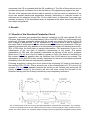
1. Epistemological background
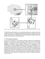
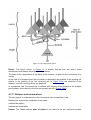
The brain is an extraordinarily complex machine. The workings of this machine can be
described at a multitude of levels of abstractions and in various description languages
(Figure 1).
These description levels range from the study of the genome and the use of genes in
genomics; the investigation of proteins in proteomics; the detailed models of neuronal substructures like membranes and synapses in compartmental models; the networks of simple
point neurons; the assignment of function to brain areas using e.g. brain imaging
techniques; the mapping of input to output states as in psychophysics and the abstraction
of symbol manipulation.
Figure 1: The levels of organization of the brain range from neuronal sub-structures to circuits to brain areas.
These different levels of abstraction are not mutually exclusive, but must be combined into
a multi-level description. Focusing on a single level of abstraction can fall short where only
a holistic, systemic view can adequately explain the system under investigation. One such
example can be found in the phenomenon of behavioural feedback which indicates that
behaviour itself can induce neuronal organization.
1.1 The synthetic approach
We argue that an essential tool in our arsenal of methods to advance our understanding of
the brain is the construction of artificial brain-like systems. The maxim of the synthetic
approach is “truth and the made are convertible”, put forward by the 17th century
philosopher Giambattista Vico. The apparent argument is that the structure and the
parameters of man-made, synthetic product are fostering our understanding of the
modelled system. Yet Vico’s proposition brings about two other important aspects. Firstly, it
is the process of building as such that is yielding new insights; in building we are
compelled to explicitly state the target function of the system (and herein possibly err).
Since we build all elements of the system to fulfil certain functions, we explicitely assign
meaning to all elements and relations between elements of the system, which implies an
understanding of the role of the elements and their interactions within the system to
achieve its goal. Moreover, construction entails that we make explicit statements about the
abstractions we make. Secondly, man-made devices are open to unlimited manipulation
and measurement.
With respect to manipulation, modern investigation techniques allow the manipulation of
biological system at different levels and in different domains. For example induction of
magnetic fields effects permit manipulations at a global level, whereas current injection
causes local changes to the system. Contrary to this, synthetic systems can be
manipulated at all levels, as well as at the local and global scale. As an example,
properties of ion channels can be altered on a single dendrite of a neuron, or of all neurons
system-wide. Additionally, changes in a synthetic system are always reversible, and can
be applied and removed as often as required. Last but not least, manipulation of synthetic
systems does not (yet) have ethical ramifications.
The development of measurement methods has undergone rapid progress in the past
decades. Yet, the access to internal states of biological systems is still strongly limited,
especially the simultaneous recording at the detail level over large area. Measurement
techniques applied to biological systems are often invasive and alter the very system
under investigation. Synthetic systems in comparison provide unlimited access to all
internal states of the system, and therefore pave the way to a much deeper understanding
of their internal workings.
1.2 Convergent validation
The synthetic approach as laid out by Giambattista Vico, is a necessary but not sufficient
basis for the development of meaningful models. Modelling a system can be compared to
fitting a line through a number of points; the smaller the number of points, the more underconstrained the fit is. Applied to modelling, this means that for a small number of
constraints, the number of models that produce the same result is very large. Hence, for
the synthetic approach to be useful in biological sciences, we need to apply as many
constraints as possible. Constraint are applicable at two levels; the level of the
construction of the model and at the level of the validation of the behaviour of the model.
For a large number of constraints – as for fitting a line though a large number of points – it
is difficult to find a good fit initially.
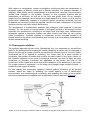
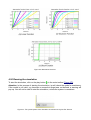
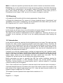
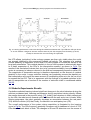
For this reason, the convergent validation method defines modelling as an iterative
process, where the steps of validating the model against a set of behavioural,
environmental, and neurobiological constraints, and adapting the model to be compliant
with theses constraints are repeated until a satisfactory result is achieved (Figure 2).
Figure 2: In the “Convergent Validation” method, modelling is regarded as an iterative process. At the initial
stage of model building, only a subset of all possible constraints can be taken into account. The convergent
validation itself consists of an iterating between validating the model against a set of constraints, and
adapting the model to be compliant with these constraints. Examples of construction constraints are the
operation that neurons can perform, and the known neuronal architecture. Validation constraints include the
behaviour of the biological system, e.g. the behaviour of a rat in a water maze.
When evaluating the system it is important to define an a priori target criteria that the
actual behaviour of the system can be compared to. The validation comes at different
levels of rigour: In the weak form, the validation consists of assessing whether the system
is at all able to perform a given task in the real world. The stronger form of validation
consists of comparing the mechanisms underlying the behaviour of the synthetic system,
i.e. the manner in which a task is solved, with a biological target system. Biology provides
validation criteria of the weak type in the form of ethological data and in the stronger form
as neurobiology boundary conditions.
1.2.1 Real-world biorobotics
The usage of robots in cognitive sciences has been heralded at the start of the 20 th century
by Hull and Tolman. Hull undertook the construction of the “psychic” machine by applying a
framework of physics to psychology. Tolman, exploring an alternative conceptual route and
striving at uniting the methods of behaviourism with the concepts of Gestalt psychology, in
1939 proposed the robot “Sowbug”. The shortcoming of many of the above mentioned
approaches is that they are lacking a clear conceptualisation of the employment of robots
in biological sciences. We see the main gain of using robots in the fact that the “real world”
provides clear constraints at both, the construction and validation level: The properties of
the elements of the model have to obey the laws of physics in their construction as well as
in the interaction with the real world. If the agent is to operate in the real world, the
mechanical properties have to take into account inertia, friction, gravity, energy
consumption etc. Moreover, acquiring information from the environment will have a limited
bandwidth and the data will most likely be noisy.
One of the key properties of biorobotics approach is that it circumvents the problem of the
low degree of generalizability of models developed in simulation only. This problem stems
from the limited input space to the model and the hidden a priori assumptions about the
environment in which the system is to behave. Support for real-world systems and the
convergent validation method is the first cornerstone design philosophy behind iqr.
1.2.2 Large-scale models
If we want to build systems able to generate a meaningful behaviour in the real world, they
have to be complete in the sense that they must spawn from sensory processing to the
behavioural output. Systems compliant with this requirement will inevitably be of a largescale, where the overall architecture is of critical importance.
An human brain consists of about 80 billion neurons. Neurons, in turn, are vastly
outnumbered by synapses; the estimations of the numbers of synapses per average
neuron ranging from 1,000 to 10,00. This impressive ratio of number of neurons
vs. number of synapses speaks in favour of the view that biological neuronal networks
draw their computational power from the large-scale integration of information in the
connectivity between neurons. The second cornerstone of iqr’s design philosophy
therefore is the support for large-scale neuronal architecture and sophisticated
connectivity.
2. What iqr is
iqr is a tool for creating and running simulations of large-scale neural networks. The key
features are:
● graphical interface for designing neuronal models;
● graphical on-line control of the simulation;
● change of model parameters at run-time;
● on-line visualization and analysis of data;
● the possibility to connect neural models to real world devices such as cameras, mobile
robots, etc;
● predefined interfaces to robots, cameras, and other hardware;
● open architecture for writing own neuron, synapse types, and interfaces to hardware.
Every simulation tool is implicitly or explicitly driven by assumptions about the best
approach to understand the system in question.
The heuristic approach behind iqr is twofold: Firstly we have to look at large-scale
neuronal systems, with the connectivity between neurons being more important than
detailed models of neurons themselves. Secondly, simulated systems must be able to
interact with the real-world.
iqr therefore provides sophisticated methods to:
● define connectivity;
● to perform high speed simulations of large neuronal systems that allow the control realworld devices – robots in the broader sense – in real-time, and;
● to interface to a broad range of hardware devices.
Simulations in iqr are cycle-based, i.e. all elements of the model are updated in a pseudo
parallel way, independent of their activity. The computation is based on difference
equation, as opposed to the approximation of differential equations. The neuron model
used is a point neuron with no compartments.
As a simulation tool, iqr fits in between high-level, general purpose simulation tools such
as
Matlab®
(http://www.mathworks.com/includes_content/domainRedirect/country_select.html?
uri=/index.html&domain=mathworks.com) and highly specific, low-level, neuronal systems
simulators such as NEURON (http://www.neuron.yale.edu/). The advantages over a
general purpose tool are on the one hand the predefined building blocks that allow easy
and fast creation of complex systems, and on the other hand the constraints that guide the
construction of biologically realistic models. The second point is especially important in
education, where the introduction into a biological “language” is highly desirable.
Low-level simulators are not in the same domain as iqr, as in their heuristic approach,
detailedness is favored over size of the model and speed of the simulation.
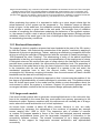
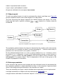
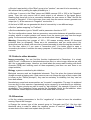
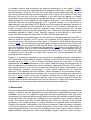
2.1 Models in iqr
Figure 3: The structure of models in iqr.
Models in iqr are organized within different levels (Figure 3): the top level is the system,
which contains an arbitrary number of processes, and connections. Processes in turn
consist of an arbitrary number of groups.
On the level of processes the model can be broken down into logical units. This is also the
level where interfaces to external devices are specified.
A group is defined as a specific aggregation of neurons of identical type, specific in terms
of the topology of the neurons in the group being a property of the group.
Connections are used to feed information from group to group. A connection is defined as
an aggregation of synapses of identical type, plus the definition of the arrangement of the
synapses.
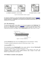
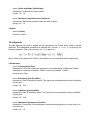
Figure 4: The group and connection framework.
Figure 4 diagrams the simplest case of two connected neurons. It is important to notice
which elements belong to which framework. Groups effectively only comprise of the
neuron soma, where all inputs are summed using the function of the specific neuron type
(see Appendix Neuron types).
The connection framework deals with axon, synapse, and dendrite of the neurons. The
computational element is the synapse which is calculating its own internal state, and the
signal transmission according to the type (see Appendix II: Synapse types).
Hint: The distinction between group and connection is not a biological fact per se, but an
abstraction within the framework of iqr that allows an easier approach to modeling
biological systems.
2.2 Conventions used in the manual
There are a few conventions that are used trough out this manual: Text in a gray box refers
to entries in iqr’s menu, and also to text on dialog boxes.
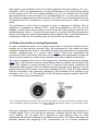
3. Starting iqr
To start iqr enter ‘iqr.exe’ (Windows) or ‘iqr.exe’ (Linux) at the prompt in a terminal window
or double-click on the icon
on the desktop.
The table below lists the command-line options iqr supports:
The arguments -f <filename>, -c <filename>, and -r can be combined arbitrarily, but -r
only works in combination with -f <filename>.
4. The User-interface
4.1 Diagram editing pane
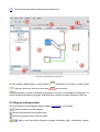
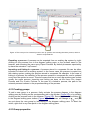
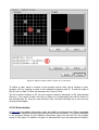
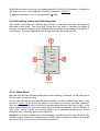
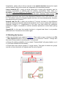
The main diagram editing pane (Figure 5①) serves to add processes, groups and
connections to the model. The definition of a new process automatically adds a new tab
and therein a new diagram. To switch between diagram panes use the tab-bar (Figure
5②). The left-most tab always presents the system-level.
Figure 5: iqr graphical user-interface.
On the diagram editing pane, a gray square
a group, and a line with an arrow head
represents a process, a white square
a connection.
A single process or group is selected by clicking on its icon in the diagram editing pane. To
select multiple processes or groups, hold down the control-key while clicking on the icon.
4.2 Diagram editing toolbar
The functionality of the diagram editing toolbar (Figure 5③) is as follows:
Zoom in and out of the diagram.
Add a new process to the system level.
Add a new group to the current process.
Add a new connection between groups: excitatory (red), modulatory (green),
inhibitory (blue).
A more detailed description on how to use the diagram editing toolbar will be given when
outlining the editing of the system.
4.2.1 Splitting the diagram pane
Split the diagram editing pane into two separate views by using the splitter
(Figure 5⑤). From left to right: split vertically, horizontally, revert to single window view.
4.3 Navigating the diagram
To navigate on a large diagram that does not fit within the diagram editing pane, the
panner (Figure 5④) can be used to change to the visible section of the panel.
4.4 Browser
On the left side of the screen (Figure 5⑥) a tree-view of the model, the browser, can be
found. It provides direct access to the elements of the system. The top node of the tree
represents the system level, the second level node reflects the processes and the third
level node points to the groups. By double-clicking on the system or process node you can
open the corresponding diagram in the diagram editing pane. Right-clicking on any node
brings up the context-menu.
4.5 Copy and Paste elements
You can copy and paste a process, one or more groups, and a connection to the clipboard.
To copy an object, right-click on it and select Copy ... from the context-menu.
To paste the object, select Edit→Paste ... from the main menu. Processes can only be
pasted at the system level, groups and connections only at the process level.
4.6 Print and save the diagram
You can export the diagram as PNG or SVG image. To do so, use the menu
Diagram→Save. The graphics format will be determined by the extension of the filename.
Hint: If you choose SVG as the export format, the diagram will be split into several files
(due to the SVG specification). It is therefore advisable to save the diagram to a separate
folder.
To print the diagram use the menu Diagram→Print.
4.7 iqr Settings
Via the menu Edit→Settings you can change the settings for iqr.
General
● Auto Save: Change the interval at which iqr writes backup files. The original files are not
overwritten, but auto save will create a new backup file, the name of which is based on the
name of the currently open system file, with the extension, autosave appended.
● Font Name: Set the font name for the diagrams. The changes will only be effective at
the next start of iqr.
● Font Size: Set the font size for the diagrams. The changes will only be effective at the
next start of iqr.
NeuronPath / SynapsePath / ModulePath
The options for NeuronPath, SynapsePath, ModulePath refer to the location where the
specific files can be found. As they follow the same logic the description below applies to
all three.
● Use local ... Specifies whether iqr loads types from the folder specified by Path to local
below.
● Use user defined ... Specifies whether iqr loads types from the folder specified by Path
to user defined below.
● Path to standard ... The folder into which the types were stored at installation time.
● Path to local ... The folder where system-wide non-standard types are stored.
● Path to user defined ... The folder into which the user stores her/his own types.
4.8 Creating a new system
A new system is created by selecting from the main toolbar (Figure 5⑦) or via the menu
File→New System. Creating a new system will close any open systems.
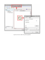
4.9 System properties
To change the properties of the system right-click on the system name in the browser (topmost node), and select Properties from the context-menu, or via the menu File→System
Properties. The options for NeuronPath, SynapsePath, ModulePath refer to the location
where the specific files can be found. As they follow the same logic the description below
applies to all three.
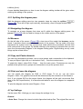
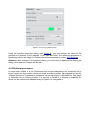
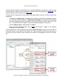
Figure 6: System properties dialog.
Using the system properties dialog (Figure 6), you can change the name of the system,
the author, add a date, and notes (Hostname has no meaning in the present release).
The most important property is Cycles Per Second, with which you can define the speed at
which the simulation is updated.
A value of 0 means, the simulation is running as fast as possible, values larger than zero,
denotes how many updates per cycle are executed. The value entered reflects “best effort”
in two ways. On the one hand, the simulation cannot run faster than a certain maximum
speed, as given by the complexity of the system, and the speed of the computer. On the
other hand, slight variations in the length of the individual update cycles can occur.
4.10 Opening an existing system
An existing system is opened by selecting the button
from the main toolbar (Figure 5⑦)
or via the menu File→Open. If you open an existing system, the current system will be
closed.
4.11 Saving the system
To save the system, press the button in the main toolbar (Figure 5⑦) or via menu select
File→Save System. To save a system under a new name, select menu File→Save System
As.
Figure 7: Warning dialog for saving invalid systems.
If your system contains inconsistencies, e.g. connections that have no source and/or target
defined, a dialog as shown in Figure 7 will show up. Please take this warning seriously.
The system will be saved to disk, but you should fix the problems mentioned in the
warning dialog or you might not be able to re-open the system.
4.12 Creating processes
To add a new process to the system, activate the system-level in the diagram editing pane
by clicking on the left-most tab in the tab-bar (Figure 5②) or by double-clicking on the
system node in the browser (Figure 5⑥). Thereafter, click the “Add Process” button
in
the diagram editing pane toolbar (Figure 5③). The cursor will change to
and you can
put down the new process by left-clicking in the diagram editing pane. To abort the action,
right-click into any free space in the diagram editing pane.
4.13 Process properties
To change the properties of a process, either:
● double-click on the process icon in the diagram editing pane;
● or right-click on the process icon or the process name in the browser, and select
Properties from the context-menu.
Figure 8: Process properties dialog.
Using the process properties dialog (see Figure 8), you can change the name of the
process as it appears on the diagram, or you can add notes. The remaining properties in
this dialog refer to the usage of modules and will be explained in section 4.24 Modules.
Attention: After changes in the property dialog, you must click on Apply before closing the
dialog, otherwise the changes will be lost.
4.14 External processes
In large-scale models it is not uncommon that several subsystems are combined into a
larger model, and that certain circuits are used in multiple models. iqr supports this via the
“external processes” mechanism; processes can be exported to a separate file, and linked
or imported into an existing system. If a process is linked-in, it remains a separate file
which can be worked with independently of system it is integrated in.
Figure 9: The concept of an “external process”: two iqr systems are including the same process, which is
stored in a separate file.
Exporting a process: A process can be exported from an existing iqr system by rightclicking on the process icon in the diagram editing pane, or the process name in the
browser, and choosing the menu entry Export Process. By default processes exported by
iqr have the extension “.iqrProcess”.
Importing and linking-in a process: A process stored in a separate file can be either
imported or linked into an existing system. In the former case, the process is copied into
the existing system, making the process stored in a separate file obsolete. In the case of
linking-in a process, the definition of the process remains in a separate file, and is updated
every time the system is saved. This also means that two or more iqr systems can include
exactly the same process. Importing and linking are done via the menu File→Import
Process and File→Link-in Process. In the case of a linked-in process, the path to the
external process is shown in the properties dialog of the process.
4.15 Creating groups
To add a new group to a process, firstly activate the process diagram in the diagram
editing pane by clicking on the corresponding tab in the tab-bar (Figure 5②) or by doubleclicking on the process node in the browser (Figure 5⑥). Secondly, click on the button
in the diagram editing pane toolbar (Figure 5③). The cursor will change to
and you
can put down the new group by left-clicking in the diagram editing pane. To abort the
action, right-click in any free space in the diagram editing pane.
4.16 Group properties
To change the properties of a group, either:
● double-click on the group icon in the diagram editing pane;
● or right-click on the group icon or on the group name in the browser, and select
Properties from the context-menu.
You can change the name of the group as it appears on the diagram, or you can add notes
by activating the group properties dialog (Figure 10).
Figure 10: Group properties dialog.
Attention: After changes in the property dialog, you must click on Apply before closing the
dialog, otherwise the changes will be lost.
Two additional group properties, the neuron type and the group topology, will subsequently
be explained in more detail.
4.16.1 Group neuron type
By default, a newly created group has no neuron type associated to it. To select the
neuron type for the group, take the following steps:
● select the neuron type from the pull-down list (Figure 10①);
● press the Apply button (Figure 10②);
● Now change the parameters for the neuron type by clicking on Edit (Figure 10③).
An extended explanation of the meaning of these parameters for each type of neuron is
given in 14. Appendix I: Neuron types.
4.16.2 Group topology
The term topology as used in this manual refers to the packing of the cells within the
group. The basic concept behind it refers to cells in a group being arranged in a regular
lattice. To define the group’s topology, proceed as follows:
● select the topology type from the pull-down list;
● press Apply;
● press Edit.
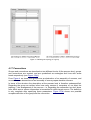
Topology types: If we refer to a TopologyRect, every field in the lattice is occupied by one
neuron. TopologyRect is therefore defined by the Width and the Height parameters. In
case of TopologySparse the user can define which fields in the lattice are occupied by
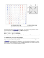
neurons. In Figure 11 the dialog to define the TopologySparse (a), and the graphical
representation of the defined topology (b) are shown.
To enter a new location for a neuron:
● select add row and
● enter the x and y coordinates in the appropriate field of the table.
To delete neurons:
● select the row you want to delete by clicking on it and
● press delete row.
Attention: The coordinates of the lattice start at (1,1) in the top-left corner.
Figure 11: Defining the topology of a group.
4.17 Connections
Groups and connections are described on two different levels. At the process level, groups
and connections are created, and are symbolized as rectangles and lines with arrow
heads respectively (see Figure 12(a)).
From Figure 4 we know, that groups are an abstraction of an assembly of neurons, and
connections are abstractions of an assembly of axon-synapse-dendrite nexuses.
In terms of the structure the description at the process level is therefore underspecified.
Regarding the group we neither know how many neurons it comprises of, nor what the
topology – the arrangement of the neurons – is. Regarding the connection we don’t know
from which source neuron information is transmitted to which target neuron. The definition
is only complete after specifying these parameters. Figure 12(b) shows one possible
complete definition of the group and the connection.
Figure 12: Levels of description for connections.
In the framework of iqr, the following assumptions concerning connections are made:
● there is no delay in axons,
● the computation takes place in synapses,
● the transmission delay is dependent on the length of the dendrite,
● any back-propagating signals are limited to the dendrite.
In principle, the complete definition of a connection is twofold, in that it comprises of the
definition of the update function of the synapse, and the definition of the connectivity. In
this context, the term connectivity refers to the spacial layout of the axons, synapses and
dendrites.
But update function and connectivity are not as easily separable, as the delays in the
dendrites are derived from the connectivity.
Multiplicity: As mentioned above, a single connection is an assembly of axon-synapsedendrite nexuses. A single nexus in turn can connect several pre-synaptic neurons to one
post-synaptic cell, or feed information from one pre-synaptic into multiple post-synaptic
neurons.
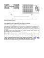
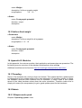
A nexus can hence comprise of several axons, synapses, and dendrites. In Figure 13 two
possible cases of many-to-one, and one-to-many are diagrammed. The first case (a) can
be referred to as “receptive field” (RF), the second one as “projective field” (PF).
Figure 13: The axon-synapse-dendrite nexus and distance.
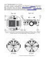
For reasons of ease of understanding the connectivity depicted in Figure 13 is only onedimensional, i.e. the pre-synaptic neurons are arranged in one row. This is not the
standard case; most of the times a nexus will be defined in two dimensions as shown in
Figure 14.
Figure 14: Two dimensional nexus.
Delays: The layout shown in Figure 13 is directly derived from the above listed
assumptions that delays are properties of dendrites.
The basis of the computation of the delay is the distance, as given by the eccentricity of a
neuron.
In the case of a receptive field, the eccentricity is defined by the position of the sending cell
relative to the position of the one receiving cell. In Figure 13(a) this definition of the
distance, and the resulting values are depicted.
In a projective field, the eccentricity is defined with respect of the position of the multiple
post-synaptic cells relative to the one pre-synaptic neuron (Figure 13(b)).
4.17.1 Patterns and arborizations
The next step is to understand how the connectivity can be specified in iqr.
Defining the connectivity comprises of two steps:
● define the pattern
● define the arborization
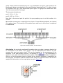
Pattern: The Pattern defines pairs of points in the lattice of the pre- and post-synaptic
group. These points are not neurons, but (x,y) coordinates. In Figure 15 the points in the
pre-synaptic group are indicated by the arrow labeled “projected point”. For sake of ease
of illustration we’ll use a one dimensional layout again. The groups are defined with size
10x1 for source and 2x1 for target.
The two pairs of points are:
pair 1: (3,1)pre, (1,1)post
pair 2: (8.5,1)pre, (2,1)post
Note that in the second pair the point in the pre-synaptic group is not the location of a
neuron.
iqr provides several ways to specify the list of pairs. These different methods are referred
to as pattern types. The meaning of the pattern types and how to define them is explained
in detail below.
Figure 15: Nexuses, pattern, and arborization.
Arborization: As previously mentioned, the pattern does not relate to neurons directly, but
to coordinates in the lattice of the groups. It is the arborization that defines the real
neurons that send and receive input. This can be imagined as the arrangement of the
dendrites of the post-synaptic neurons, as depicted in Figure 15. The arborization is
applied to every pair of point defined by the pattern. Whether the arborization is applied to
the pre- or the post-synaptic group is defined by the direction parameter. If applied to the
source group, the effect is a fan-in receptive field. A fan-out, projective field, is the result of
applying the arborization to the target group (see also Figure 13).
Figure 16: Rectangular arborization.
iqr provides a set of shapes of arborizations. Figure 16 shows an example of a rectangular
arborization of a width and height of 2. The various types of arborizations are described in
detail below.
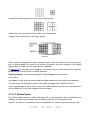
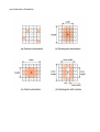
Combining pattern and arborization: The combination of pattern and arborization is
illustrated in Figure 17. The source group is on the left side, the target group on the right
side. In the lower part you find the pattern denoted by a gray arrow. The pattern consists of
four pairs of points. On the upper left tier, the arborization is applied to the points defined
by the pattern. For each cell that lies within the arborization, one synapse is created. In
the case presented in Figure 17 there are 16 synapses created.
For each synapse the distance with respect to the pattern point is calculated. This
distance serves as basis to calculate the delay. Several functions are available, for details
see the DelayFunction section further below.
Figure 17: Combining pattern and arborization.
4.18 Creating connections
To add a new connection, click on the corresponding button in the diagram editing pane
toolbar (Figure 5③).
(red arrow) will create an Excitatory,
(green arrow) a
Modulatory and
(blue arrow) an Inhibitory connection.
Figure 18
After clicking on one of the buttons to create a connection, you will notice the cursor
changing to
. To position the connection, first click on one of the yellow squares
(Figure 18) at the edge of the source group icon and then on one of the yellow squares at
the edge of the icon for the target group.
To cancel the creation of a connection, right-click into any free space in the diagram editing
pane.
Adding and removing vertexes: To add a new vertex to the connection, hold down the
ctrl-key and click on the connection. To remove a vertex from a connection, right-click on it
and select delete from the context-menu.
4.18.1 Connection across processes
Connecting groups from different processes requires two preparatory steps. First you need
to split the diagram editing pane into two views, by clicking on the split vertical
or split
horizontal
button from diagram editing toolbar (Figure 5⑤). Secondly you will use the
tab-bar (Figure 5②) to make each separate view of the diagram editing pane display one
of the processes containing the groups you want to connect. Now you can connect the
groups from the two processes just as described above.
Upon completion, you can return to the single window view by clicking on
.
Figure 19
After connecting groups from different processes, you will notice a new icon as shown in
Figure 19 at the top edge of the diagram. This “phantom” group represents the group in
the process currently not visible, which the connection targets to or originates from.
4.19 Specifying connections
Via the context-menu or by double-clicking on the connection in the diagram, you can
access the properties dialog for a connection.
Attention: Click on the connection line, not the arrowhead.
In the properties dialog, you can change the name and the notes for a connection as well
as the connection type.
To select and edit the synapse type, the same procedure applies as when setting and
editing the neuron type for the group (section 4.16.1 Group neuron type).
4.19.1 Pattern
This section explains the meaning of the different types of patterns and how to define them
in iqr.
4.19.1.1 PatternForeach
Figure 20
This pattern type defines a full connectivity, where each cell from one group receives
information from all the cells of the other group as shown in Figure 20. You can select all
cells, limit the selection to a region, or define a list of cells.
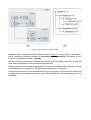
Property dialog: Figure 21 shows the dialog to set the properties for the PatternForeach.
To define which cells from the source and target group are included, use the pull-down
menu ①, and select from ∙All, ∙Region, or ∙List.
Figure 21
To define a list of cells, click on each cell you want to add to the list. Clicking Set will
define the list, and the coordinates of the selected cells will be displayed in the Selection
window ③. To clear the drawing area and to delete the list press Clear.
To define a region, click on the cell you want to be the first corner in the drawing area ②,
move the mouse while keeping the mouse button pressed, and release the button when in
the opposite corner. Once done, click on Set to define the region. The definition of the
region will be shown in ④. To delete a defined region click on Clear.
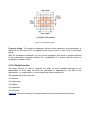
4.19.1.2 PatternMapped
In PatternMapped a mapping is used to determine the projection points. The procedure is
as follows:
● determine the small group (fewer neurons):
● scale the smaller group to the size of the larger group:
● determine the coordinates of the cells in the scaled group
● apply these coordinates to the larger groups
Figure 22
Which group is mapped onto which depends solely on the size and not on which group is
pre-, or post-synaptic. We refer to the surface covered by a neuron location in the scaled
group, when overlaid over the larger group, as sector.
In Figure 22 the concept of the mapping is illustrated. As you can see from the depiction,
projected points need not be at neuron positions.
Property dialog: In the property dialog for PatternMapped you can select:
● All cells or,
● a Region of cells from the source and the target population to be used in the mapping.
The procedure for setting the region is the same as explained for PatternForeach.
If the mapping type is set to center, only the central projection points are used, whereas if
all is selected, all cells in the mapped sector are used.
4.19.1.3 PatternTuples
The PatternTuples serves to define individual cell to cell projections. You can associate an
arbitrary number of pre-synaptic with an arbitrary number of post-synaptic cells.
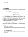
A tuple t, as used in this definition, is the combination of n source cells with p target cells:
For the set of pre-synaptic and post-synaptic cells the Cartesian product will be calculated.
The pattern p itself is the list of tuples:
An example illustrates the concept. We have two tuples t0 and t1:
After the Cartesian product, the tuples are:
The pattern p consists of the combination of the two tuples:
Property dialog
Figure 23: Dialog to define pattern "Tuples" for a connection.
To define a tuple, select a number of pre-synaptic source cells, and a number of postsynaptic cells, by clicking on them in the respective drawing area ①. To add the tuple to
the list click on Add. To clear the drawing area, click on Clear.
The list of tuples is shown in ②. You can remove a tuple by selecting it in ②, and pressing
Remove. If you select a tuple, and click on Show, its corresponding cells will be shown in
the drawing area ①. Now you can add new cells, and save the tuple as a new entry by
clicking on Add again.
4.19.2 Arborization
In Figure 24 all available arborization types, bar ArbAll, are diagrammed. Where applicable
the red cross indicates the projection point as defined by the pattern. The options available
in the property dialogs for the different arborization types are derived from the lengths
shown in the figure. In addition all types of arborizations have the parameters Direction,
and Initialization Probability.
Figure 24: Arborization types
Property dialog: The direction parameter defines which population the arborization is
applied to: in the case of RF it is applied to the source group, in case of PF to the target
group.
With the initialization probability you can set the probability with which a synapse defined
by the arborization is actually created. E.g. a probability of .5 means, that the chance a
synapses is created, is 50%.
4.19.3 DelayFunction
The delay function is used to compute the delay for each synapse belonging to an
arborization. In most delay functions the calculation is depending on the size of the
arborization, i.e. height/width, or outer height/outer width respectively.
The possible delay functions are:
● FunLinear
● FunGaussian
● FunBlock
● FunRandom
● FunUniform
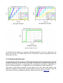
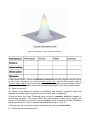
Figure 25 shows the meaning of the parameters for the three least trivial functions.
Figure 25: Delay functions
In FunRandom the delays are randomly distributed between 0 and max. Distance is not
taken into account. The same holds true for FunUniform, where all synapses have the
same delay of value.
4.19.4 AttenuationFunction
The attenuation function is used to compute the attenuation of the signal strength for each
synapse belonging to an arborization. The larger the attenuation, the weaker the signal will
be that arrives at the soma. In most attenuation functions the calculation is depending on
the size of the arborization, i.e. height/width, or outer height/outer width respectively.
The types of attenuation functions are the same as for the delay (see above). Key
difference between the delay and the attenuation function is that in the former case the
values are continuous, whereas in the latter case they are discrete (Figure 25).
Figure 26: Attenuation functions
4.20 Running the simulation
To start the simulation, click on the play button
in the main toolbar (Figure 5⑦).
Attention: In the process of starting the simulation, iqr will check the model’s consistency.
If the model is not valid, e.g. because a connection target was not defined, a warning will
pop up. You will not be able to start the simulation, unless the system is consistent.
Figure 27: The update speed of the simulation is indicated as Cycles Per Second.
While the simulation is running, the update speed in C(ycles) P(er) S(econd) is indicated in
the lower left corner of the application window as shown in Figure 27.
To stop the simulation, click on the play button
again.
4.21 Visualizing states and collecting data
This section introduces the facilities iqr provides to visualize and save the states of
elements of the model. Time plots and Group plots are used to visualize the states of
neurons, Connection plots serve to visualize the connectivity and the states of synapses of
a connection. The Data Sampler allows to save data from the model to a file.
Figure 28
4.21.1 State Panel
iqr plots and the Data Sampler share part of their handling. Therefore, we will first have a
look at some common features.
On the right side of the plots and the Data Sampler, you find a State Panel which looks
similar to Figure 28 ① shows the name of the object from which the data originates.
Neurons and synapses have a number of internal states that vary from type to type. In the
frame entitled states you can select which state ② should be plotted or saved. Squares in
front of the names indicate that several states can be selected simultaneously, circles
mean that only one single state can be selected.
Attention: In a newly created plot or Data Sampler, the check-box live data ③ will not be
checked, which means that no data from this State Panel is plotted or saved. To activate
the State Panel, check the tic by clicking the check-box.
To hide the panel with the states of the neuron or synapse, drag the bar ④ to the right
side.
4.21.2 Drag & drop
The visualizing and data collecting facilities of iqr make extensive use of drag & drop.
You can drag groups from the Browser (Figure 5⑥), the symbol in the top-left corner of
State Panels (Figure 29①), or regions from Space plots.
Figure 29
To drag, click on any of the above mentioned items, and move the mouse while keeping
the button pressed. The cursor will change to . Move the mouse over the target and
drop by releasing the mouse button.
The table below summarized what can be dragged where.
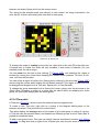
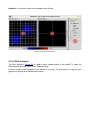
4.21.3 Space plots
A Space plot as shown in Figure 30 displays the state of each cell in a group in the plot
area ①.
To create a new Space plot, right click on a group in the diagram editing pane or the
browser and select Space plot from the context-menu.
The value for the selected state (see above) is color coded, the range indicated in the
color bar ②. A Space plot solely plots one state of one group.
Figure 30: iqr Space plot.
To change the mode of scaling for the color bar, right-click on the axis ③ to the right size.
If expand only is ticked, the scale will only increase; if auto scale is selected, you can
manually enter the value range.
You can zoom into the plot by first clicking
(Figure 30④), and selecting the region of
interest by moving the cursor while keeping the mouse button pressed. To return to fullview, click into the plot area.
You can select a region of cells in the Space plot by clicking in the plot area (Figure 30①)
and moving the mouse while holding the left button pressed. This region of cells can now
be dragged and dropped onto a Time plot, Space plot, or Data Sampler.
To change the group associated to the Space plot, drop a group onto the plot area or the
State Panel. Dropping a region of a group has the same effect as dropping the entire
group, as Space plot always plots the entire group.
4.21.4 Time plots
A Time plot (Figure 31) serves to plot the states of neurons against time.
To create a new Time plot, right click on a group in the diagram editing pane or the
browser and select Time plot from the context-menu.
Time plots display the average value of the states of an entire group or region of a group.
A Time plot can plot several states, and states from different groups at once. Each state is
plotted as a separate trace.
To add a new group to the Time plot use drag & drop as described in section 4.21.2 Drag
and drop, or drag and drop a region from a Space plot onto the plot area or one of the
State Panels. If dropped onto the plot area, the group or region will be added, if dropped
onto a State Panel, you have the choice to replace the State Panel under the drop point, or
add the group/region to the plot.
To remove a group from the Time plot close the State Panel by clicking in the top-right
corner.
The State Panels for Time plots are showing which region of a group is plotted by means
of a checker board (Figure 31②). Depending on the selection, the entire group or the
region will be high-lighting in red.
Figure 31: iqr Time plot.
You can zoom into the plot by first clicking
(Figure 31④), and selecting the region of
interest by moving the cursor while keeping the mouse button pressed. To return to fullview, click into the plot area.
To change the scaling of the y-axis, use the context-menu of the axis ③ (for detail see
section 4.21.3 Space plots).
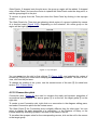
4.21.5 Connection plots
Connection plots (Figure 32) are used to visualize the static and dynamic properties of
connections and synapses. The source group ① is on the left, the target group ② on the
right side.
To create a new Connection plot, right click on a connection in the diagram editing pane,
and select Connection plot from the context-menu.
The State Panel ③ for Connection plots is slightly different than for other plots. You can
select to display the static properties of a connection, i.e. the Distance or Delay, or the
internal states by selecting Synapse, and one of the states in the list.
To visualize the synapse value for the corresponding neuron, click on the cell in the source
or the target group.
Attention: Connection plots do not support drag & drop.
Figure 32: iqr Connection plot.
4.21.6 Data Sampler
The Data Sampler (Figure 33) is used to save internal states of the model. To open the
Data Sampler use the menu Data→Data Sampler.
A newly created Data Sampler is not bound to a group. To add groups or regions from
groups use drag & drop as described earlier.
Figure 33: Data Sampler.
Like for the Time plots, the State Panel for the Data Sampler indicates which region of the
group is selected. Moreover you will find an average check-box which allows you to save
the average of the entire group or region of cells instead of the individual values.
The Data Sampler has the following options:
● Sampling: Defines at what frequency data is saved.
● Every x Cycle: Specifies how often data is saved in relation to the updates of the model,
e.g. a value of 1 means data is saved at every update cycle of the model, a value of 10
that the data is saved only every 10th cycle.
● Acquisition: These options define for how long data is saved.
● Continuous: Data is saved until you click on Stop.
● Steps: Data is saved for as many update cycles as you define.
● Target
● Save to: Name of the file where the data is saved.
● Overwrite: Overwrite the file at every start of sampling.
● Append: Append data to the file at every start of sampling.
● Sequence: Create a new file at every start of sampling. The name of the new file is
composed of the base name from
● Save to: with a counter appended.
● Misc
● auto start/stop: Automatically start and stop sampling when the simulation is started
and stopped.
If the Sampling, Acquisition, and Target options are set, and one or more groups/regions of
cells are added, you can start sampling data. To do this, click on the Sample button. While
data is being sampled you will see the lights next to the Sample button blinking. To stop
sampling, click on the Stop button.
Attention: You will only be able to start sampling data if you specified the Sampling,
Acquisition, and Target options, and one or more groups were added.
4.21.7 Saving and loading configurations
You can save the arrangement and the properties of the current set of plots and Data
Sampler. To do so:
● go to Data→Save Configuration;
● select a location and file name.
To read an existing configuration file, select: Data→Open Configuration.
Attention: If groups or connections were deleted, or sizes of groups changed between
saving and loading the configuration, the effect of loading a configuration is undefined.
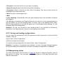
4.22 Manipulating states
The State Manipulation tool as shown in Figure 34 serves to change the activity (Act) of
the neurons in a group. You can draw patterns, add them to a list, play them back with
different parameters.
Figure 34: State Manipulation tool.
Primer: As the State Manipulation is a fairly complex tool, we will start with a step-by-step
primer. The details are specified further below.
● create a pattern by selecting
from ② to draw in the drawing area ①;
● add the pattern to the list ③;
● press Send.
Attention: Only patterns in the pattern list are sent to the group.
Drawing a pattern: To create a new pattern:
● set the value using the Value spin-box in the ② drawing toolbar;
● select the
, and draw the pattern in the drawing area ①.
To clear the pattern drawing area, press clear, or to selectively erase points from pattern,
press the button.
You can now add the pattern to the pattern list ③ by clicking on Add, or you can replace
the selected pattern in the list with your new pattern by pressing Replace.
Pattern list: To manipulate the list of patterns, use the toolbar ④ below the list of patterns.
Move the selected pattern up or down in the list
Invert the order of the list
Delete the selected pattern
Save the list of pattern
Save the list of pattern under a new name
Open an existing list of pattern
Sending options: As mentioned previously, the State Manipulation affects the activity of
neurons. You can choose from three different modes ⑤:
● Clamp - The activity of the neurons is set to the values of the pattern
● Add - The values from the pattern are added to the activity of the neuron
● Multiply- The values from the pattern are multiplied to the activity of the neuron
In the frame Play Back ⑥, you can specify how many times the patterns in the list will be
applied; either select Forever or Times and change the value in the spin-box next to it.
The Interval determines the number of time steps to wait prior to sending the next pattern
to the group. E.g. a step size of 1 will send a pattern at each time step, step size 2 only at
time step 1, 3, 5 etc.
StepSize controls which patterns from the list should be applied; 1 means every pattern, 2
means only the first, third, fifth etc. pattern.
Sending: To send the patterns in the list to the group, press Send. If you have chosen to
send the patterns Forever, Revoke will stop applying patterns to the group.
4.23 Support for work-flow of simulation experiments
Working with simulations employs a number of generic steps: Designing the system,
running the simulation, visualising and analysing the behaviour of the model, perturbing
the system, and tuning of parameters. Next to these steps, the automation of experiments
and the documentation of the model form important parts of the work-flow. Subsequently
we will describe the mechanisms iqr provides to support these tasks.
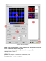
Central control of parameters and access from Modules: The Harbor
When running simulations, users frequently adjust the parameter of only a limited number
of elements. Using the Harbor, users can collect system elements such as parameters of
neurons and synapses in a central place (Figure 35), and change the parameters directly
from the Harbor. A second function of the Harbor is to expose parameters to an iqr
Module: All parameters collected in the Harbor can be queried and changed from within a
Module. Using this method, parameter optimization methods can be implemented directly
inside iqr.
Figure 35: Using the Harbor, users can collect system elements such as parameters of neurons and
synapses in a central place. Items are added to the Harbor by dragging them form the Browser. Harbor
configurations can be saved and loaded.
Remote control of iqr: In a number of use-cases, being able to control a simulation from
outside the simulation software itself is useful. For this purpose, iqr is listening to incoming
message on a user defined TCP/IP port. This allows to control the simulation and change
parameters of the system. Concretely, this remote control interface supports the following
syntax:
cmd:<COMMAND>
[;itemType:<TYPE>;
[itemName:<ITEM NAME>|itemID:<ITEM NAME>];
paramID:<ID>;value:<VALUE>;]
The supported COMMAND are: start, stop, quit, param, startsampler, stopsampler.
The param command allows to change the parameter of elements, and needs as an
argument the type of item (ItemType: PROCESS, GROUP, NEURON, CONNECTION,
SYNAPSE), the name (itemName) or ID (itemID) of the element, the ID of the parameter
(ParamID), and the value to be set. Items can be addressed either by their name or their
ID. In the case of name, all items with this name are changed. This feature can be used to
change multiple elements at the same time.
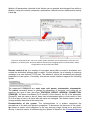
Documentation of the system: The documentation of a system comprises the
descriptions of its static and dynamic properties. To document the structure of the model,
iqr allows to export circuit diagrams in the svg and png image format or to print them
directly. A second avenue of documenting the system is based on the Extensible Markup
Language (XML) (http://www.w3.org/XML/) format of the system files in iqr. XML formatted
text can be transformed into other text formats using the Extensible Stylesheet Language
Family (XSL). One example of such an application is the transformation of a system file
into the dot language for drawing directed graphs as hierarchies (http://www.graphviz.org/).
Another transform is the creation of system descriptions in the LATEX typesetting system.
4.24 Modules
A Module in iqr is a plug-in to exchange data with an external entity. This entity can be a
sensor (camera, microphone, etc.), an actor (robot, motor) or an algorithm.
● Modules read and write the activity of groups.
● A process can have only one single module associated to it.
● A module reads from and writes to groups that belong to the process associated with the
module.
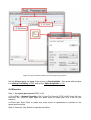
To assign a module to a group, open the process properties dialog, select the module type
from the pull-down menu of the Module frame, and press Apply.
Figure 36
If a process has a module associated to it, the process icon in the diagram will appear as
in Figure 36.
Clicking on the Edit button in the Module frame will bring up the module property dialog.
The parameters for the module vary from type to type and are explained in detail in
Appendix "Modules".
Figure 37
Most modules will feed data into and/or read from groups. Tabs Groups to Module and
Module to Groups contain the allocation information between modules and groups. The
pull-down menu next to the name of the reference will list all groups local to the current
process. In the diagram you can identify a module’s group input (blue arrow in the top right
as shown in Figure 37) or groups with output to a module (blue arrow in the bottom right
corner).
Attention: For reasons of system consistency, all references in the Groups to Module and
Module to Groups tab must be specified. You can disable the update of a module during
the simulation by un-checking the Enable Module check-box in the process properties
dialog.
5. Concepts
This document gives an overview on how to write your own neurons, synapses, and
modules.
The first part will explain the basic concepts, the second part will provide walk-through
example implementations, and the appendix lists the definition of the relevant member
variables and functions for the different types.
iqr does not make a distinction between types that are defined by the user, and those that
come with the installation; both are implemented in the same way.
The base-classes for all three types, neurons, synapses, and modules, are derived from
ClsItem (Figure 38).
Figure 38: Class diagram for types.
The classes derived from ClsItem are in turn the parent classes for the specific types; a
specific neuron type will be derived from ClsNeuron, a specific synapse type from
ClsSynapse. In case of modules, a distinction is made between threaded and nonthreaded modules. Modules that are not threaded are derived from ClsModule, threaded
ones from ClsThreadModule.
The inheritance schema defines the framework, in which:
● parameters are defined,
● data is represented and accessed,
● input, output, and feedback is added.
All types are defined in the namespace iqrcommon.
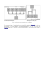
5.1 Object model
To write user-defined types, it is vital to understand the object model iqr uses. Figure 39
shows a simplified version of the class diagram for an iqr system.
The lines connecting the objects represent the relation between the objects. The arrow
heads and tails have a specific meaning:
stands for a relation where A
contains B.
Figure 39: Simplified class diagram of an iqr system.
The multiplicity relation between the objects is denoted by the numbers at the start and the
end of the line. E.g. a system can have 0 or more processes (0…* near the arrow head). A
process in turn can only exist in one system (1 near the ♢).
On the phenomenological level, to a user, a group consists of a n ≥ 1 neuron(s), and a
connection of n ≥ 1 synapse(s). In terms of the implementation though, as can be seen in
Figure 2, a group contains only one instance of a neuron object, and a connection only
one instance of a synapse object. This is independent of the size of the group or the
number of synapses in a connection.
5.2 Data representation
In the concept of iqr, neurons and synapses do have individual values for parameters like
the membrane potential or weight associated to them. In this document, type-associated
values, that change during the simulation, are referred to as “states”.
There are essentially two ways in which individual value association can be implemented:
● multiple instantiations of objects with local data storage (Figure 40a), or
● single-instance with states for individual “objects” in vector like structure (Figure 40b).
Figure 40: Representation of data in iqr types.
For reasons of efficiency, iqr uses the single-instance implementation (see also Figure 39).
For authors of types, the drawback is a somewhat more demanding handling of states and
update functions. To compensate for this, great care was taken to provide an easy to use
framework for writing types.
5.2.1 The StateArray
The data structure used to store states of neurons and synapses is the StateArray. The
structure of a StateArray is depicted in Figure 41. It is used like a two-dimensional matrix,
with the first dimension being the time and the second dimension the index of the
individual item (neuron or synapse). Hence StateArray[t][n] is the value of item n at time t.
Figure 41: Concept of StateArray.
Internally StateArrays make use of the valarray class from the standard C++ library.
To extract a valarray containing the values for all the items at time t - d use
std::valarray<double> va(n);
va = StateArray[d];
The convention is that StateArray[0] is the current valarray, whereas StateArray[2]
denotes the valarray that is 2 simulation cycles back in time.
Valarrays provide a compact syntax for operations on each element in the vector, the
possibility to apply masks to select specific elements, and a couple of other useful
features. A good reference on the topic is .
5.2.2 States in neurons and synapses
The subsequently discussed functions are the main functions used to deal with states.
Additional functions for the individual types are listed in the appendix.
Adding an internal state to neurons and synapses is done via the wrapper class
ClsStateVariable:
ClsStateVariable *pStateVariable;
pStateVariable = addStateVariable("st" /*identifier*/,
"A state variable" /*visible name*/);
To manipulate the state we first extract the StateArray, where after we can address and
change the state as described above:
StateArray &sa = pStateVariable->getStateArray();
sa[0][1] = .5;
The output state is a special state for neurons and synapses. For most neurons the output
state will be the activity. The neuronal output state is used as input to synapses and
modules. For synapses, the output state acts as an input to neurons. A neuron or synapse
can only have one output state.
An output state is defined by means of the addOutputState(...) function:
ClsStateVariable *pActivity;
pActivity = addOutputState("act" /*identifier*/,
"Activity" /*name*/);
States created in this framework are accessible in the GUI for graphing and saving.
5.2.2.1 State related functions in neurons
The base-class for the neuron type automatically creates three input states: the excitatory,
inhibitory, and modulatory. Therefore, you do not create any input state when implementing
a neuron type. To access the existing ones, use the following functions, which return a
reference to a StateArray:
StateArray &excitation = getExcitatoryInput();
StateArray &inhibition = getInhibitoryInput();
StateArray &modulation = getModulatoryInput();
The user is free as to which of these functions to use.
5.2.2.2 State related functions in synapses
Synapses also must have access to the input state, which is actually the output state of
the pre-synaptic neuron. The implementation of the pre-synaptic neuron type thus defines
the input state of the synapse.
To access the input state the function getInputState() is employed, which returns a pointer
to a ClsStateVariable:
StateArray &synIn
= getInputState()->getStateArray();
To use feedback from the post-synaptic neuron use the addFeedbackInput() function:
ClsStateVariable *pApicalShunt;
pApicalShunt = addFeedbackInput("apicalShunt" /*identifier*/,
"Apical dendrite shunt" /*description*/);
StateArray &shunt = pApicalShunt->getStateArray();
5.2.3 Using history
To be able to make use of previous states, i.e. to use the history of a state, you explicitly
have to declare a history length when you create the StateArray using the
addStateVariable(...), addOutputState(...), or addFeedbackInput(...) functions. The
reference for the syntax is given in the Appendix I: Neurons types and Appendix II:
Synapses.
5.2.4 Modules and access to states
Unlike neurons and synapses, modules do not need to use internal states to represent
multiple elements. Modules require to read states from neurons, and feed data into states
of neurons. The functions provided for this purpose are using a naming schema that is
module centered: data that is read from the group is referred to as “input from group”, data
fed into a group is pointed to as “output to group”. The references for theses states will be
set in the module properties of the process (see iqr Manual)
Defining the output to a group is done with the addOutputToGroup(...) function:
ClsStateVariable* outputStateVariable;
outputStateVariable = addOutputToGroup("output0" /*identifier*/,
"Output 0 description" /*description*/);
StateArray &clsStateArrayOut = outputStateVariable->getStateArray();
Specifying input from a group into a module employs a slightly different syntax using the
StateVariablePtr class:
StateVariablePtr* inputStateVariablePtr;
inputStateVariablePtr = addInputFromGroup("input0" /*identifier*/,
"Input 0 description" /*description*/);
StateArray &clsStateArrayInput =
inputStateVariablePtr->getTarget()->getStateArray();
Once the StateArray references are created, the data can be manipulated as described
above.
Please do not write into the input from group StateArray. The result might be catastrophic.
When adding output to groups, or input from groups, no size constraint for the state array
can be defined. It is therefore advisable to either write the module in a way that it can cope
with arbitrary sizes of state arrays, or to throw a ModuleError in the init() function if the
size criteria is not met.
5.2.4.1 Access protection
If a module is threaded, i.e. the access to the input and output states is not synchronized
with the rest of the simulation, the read and write operations need to be protected by a
mutex. The ClsThreadedModule provides the qmutexThread member class for this
purpose. The procedure is to lock the mutex, to perform any read and write operations,
and then to unlock the mutex:
qmutexThread->lock();
/*
any operations that accesses the
input or the output state
*/
qmutexThread->unlock();
As the locked mutex is impairing the main simulation loop, as few as possible operations
should be performed between locking and unlocking.
Failure to properly implement the locking, access, and unlocking schema will eventually
lead to a crash of iqr.
5.3 Defining parameters
The functions inherited from ClsItem define the framework for adding parameters to the
type. Parameters defined within this framework are accessible through the GUI and saved
in the system file. To this end, iqr defines wrapper classes for parameters of type double,
int, bool, string, and options (list of options).
5.3.1 Usage
The best way to use these parameters, is to define a pointer to the desired type in the
header, and to instantiate the parameter-class in the constructor, using the add [Double,
Int, Bool, String, Options] Parameter functions. The value of the parameter object can
be retrieved at run-time by virtue of the getValue() function. Examples for the usage are
given in sections 6.1 Neurons, 6.2 Synapses, and 6.3 Modules. The extensive list of these
functions is provided in the documentation for the ClsItem class in section 3.1.
5.4 Where to store the types
The location where iqr loads types from, is defined in the iqr settings NeuronPath,
SynapsePath, and ModulePath (see iqr Manual). Best practice is to enable.
Use user defined nnn (where nnn stands for Neuron, Synapse, or Module), and to store
the files in the location indicated by the Path to user defined nnn. As the neurons,
synapses, and modules are read from disk when iqr starts up, any changes to the type,
while iqr is running, has no effect; you will have to restart iqr if you make changes to the
types.
6. Example implementations
6.1 Neurons
6.1.1 Header
Let us first have a look at the header file for a specific neuron type. As you can see in
Listing 1, the only functions that must be reimplemented are the constructor [11] and
update() [13]. Hiding the copy-constructor [17] is an optional safety measure. Lines [2021] declare pointers to parameter objects. Line [24] declares the two states of the neuron.
Listing 1: Neuron header example
1#ifndef NEURONINTEGRATEFIRE_HPP
2#define NEURONINTEGRATEFIRE_HPP
3
4#include <Common/Item/neuron.hpp>
5
6namespace iqrcommon {
7
8
class ClsNeuronIntegrateFire : public ClsNeuron
9
{
10
public:
11
ClsNeuronIntegrateFire();
12
13
void update();
14
15
private:
16
/* Hide copy constructor. */
17
ClsNeuronIntegrateFire(const ClsNeuronIntegrateFire&);
18
19
/* Pointers to parameter objects */
20
ClsDoubleParameter *pVmPrs;
21
ClsDoubleParameter *pProbability, *pThreshold;
22
23
/* Pointers to state variables.*/
24
ClsStateVariable *pVmembrane, *pActivity;
25
};
26}
27
28#endif
6.1.2 Source
Next we’ll walk through the implementation of the neuron, which is shown in Listing 2. Line
[4-5] defines the precompile statement that iqr uses to identify the type of neuron (see
section 3.2.3). In the constructor we reset the two StateVariables [9,10]. On line [12-38]
we instantiate the parameter objects (see section 3.1), and at the end of the constructor
we instantiate one internal state [41] with addStateVariable(...), and the output state [42]
with addOutputState(...). As for all types, the constructor is only called once, when iqr
starts, or the type is changed. The constructor is not called before each start of the
simulation.
The other function being implemented is update() [46]. Firstly, we get a reference to the
StateArray for the excitatory and inhibitory inputs [47-48] (see section 1.2.2).
For clarity, we create a local reference to the state arrays [49-50]. Thus, the state array
pointers need only be dereferenced once, which enhances performance.
For ease of use the parameter values can be extracted from parameter objects [52-55]. On
line [58-60] we update the internal state, and the output state [64-65]. The calculation of
the output state may seem strange, but becomes clearer when taking into account that
StateArray[0] returns a valarray. The operation performed here is referred to as “subset
masking” [1].
Listing 2: Neuron code example
1#include ~neuronIntegrateFire.hpp~
2
3/* Interface for dynamic loading is built using a macro. */
4MAKE_NEURON_DLL_INTERFACE(iqrcommon::ClsNeuronIntegrateFire,
5
~Integrate & fire~)
6
7iqrcommon::ClsNeuronIntegrateFire::ClsNeuronIntegrateFire()
8
: ClsNeuron(),
9
pVmembrane(0),
10
pActivity(0) {
11
12
pExcGain = addDoubleParameter(~excGain~, ~Excitatory gain~,
13
1.0, 0.0, 10.0, 4,
14
~Gain of excitatory inputs.\n~
15
~The inputs are summed before\n~
16
~being multiplied by this gain.~,
17
~Input~);
18
19
pInhGain = addDoubleParameter(~inhGain~, ~Inhibitory gain~,
20
1.0, 0.0, 10.0, 4,
21
~Gain of inhibitory inputs.\n~
22
~The inputs are summed before\n~
23
~being multiplied by this gain.~,
24
~Input~);
25
26
/* Membrane persistence. */
27
pVmPrs = addDoubleParameter(~vmPrs~, ~Membrane persistence~,
28
0.0, 0.0, 1.0, 4,
29
~Proportion of the membrane potential\n~
30
~which remains after one time step\n~
31
~if no input arrives.~,
32
~Membrane~);
33
34
pProbability = addDoubleParameter(~probability~, ~Probability~,
35
0.0, 0.0, 1.0, 4,
36
~Probability of output occuring\n~
37
~during a single timestep.~,
38
~Membrane~);
39
40
/* Add state variables. */
41
pVmembrane = addStateVariable(~vm~, ~Membrane potential~);
42
pActivity = addOutputState(~act~, ~Activity~);
43}
44
45void
46iqrcommon::ClsNeuronIntegrateFire::update() {
47
StateArray &excitation = getExcitatoryInput();
48
StateArray &inhibition = getInhibitoryInput();
49
StateArray &vm
= pVmembrane->getStateArray();
50
StateArray &activity
= pActivity->getStateArray();
51
52
double excGain
= pExcGain->getValue();
53
double inhGain
= pInhGain->getValue();
54
double vmPrs
= pVmPrs->getValue();
55
double probability = pProbability->getValue();
56
57
/* Calculate membrane potential */
58
vm[0] *= vmPrs;
59
vm[0] += excitation[0] * excGain;
60
vm[0] -= inhibition[0] * inhGain;
61
62
activity.fillProbabilityMask(probability);
63
/* All neurons at threshold or above produce a spike. */
64
activity[0][vm[0] >= 1.0] = 1.0;
65
activity[0][vm[0] < 1.0] = 0.0;
66}
6.2 Synapses
6.2.1 Header
The header file for the synapse shown in Listing 3 is very similar to the one for the neuron.
The major difference lies in the definition of a state variable that will be used for feedback
input [20].
Listing 3: Synapse header example
1#ifndef SYNAPSEAPICALSHUNT_HPP
2#define SYNAPSEAPICALSHUNT_HPP
3
4#include <Common/Item/synapse.hpp>
5
6namespace iqrcommon {
7
8
class ClsSynapseApicalShunt : public ClsSynapse
9
{
10
public:
11
ClsSynapseApicalShunt();
12
13
void update();
14
15
private:
16
/* Hide copy constructor. */
17
ClsSynapseApicalShunt(const ClsSynapseApicalShunt&);
18
19
/* Feedback input */
20
ClsStateVariable *pApicalShunt;
21
22
/* Pointer to output state. */
23
ClsStateVariable *pPostsynapticPotential;
24
};
25}
26
27#endif
6.2.2 Source
The source code for the synapse is shown in Listing 4. The precompile statement [4-5] at
the beginning of the file identifies the synapse type. In the constructor [7] we define the
output state for the synapse [10]. In deviation to neurons, a definition of a feedback input
[14] using addFeedbackInput(...) is introduced. The remains of the synapse code are
essentially the same as for the neuron explained above.
Listing 4: Synapse code example
1#include ~synapseApicalShunt.hpp~
2
3/* Interface for dynamic loading is built using a macro. */
4MAKE_SYNAPSE_DLL_INTERFACE(iqrcommon::ClsSynapseApicalShunt,
5
~Apical shunt~)
6
7iqrcommon::ClsSynapseApicalShunt::ClsSynapseApicalShunt()
8
: ClsSynapse() {
9
10
/* Add state variables. */
11
pPostsynapticPotential = addOutputState(~psp~, ~Postsynaptic potential~);
12
13
/* Add feedback input */
14
pApicalShunt = addFeedbackInput(~apicalShunt~, ~Apical dendrite shunt~);
15}
16
17void
18iqrcommon::ClsSynapseApicalShunt::update() {
19
StateArray &synIn
= getInputState()->getStateArray();
20
StateArray &shunt
= pApicalShunt->getStateArray();
21
StateArray &psp
= pPostsynapticPotential->getStateArray();
22
23
psp[0] = synIn[0] * shunt[0];
24}
6.3 Modules
6.3.1 Header
Listing 5 shows the header file for a module. As for the neurons and the synapses, the
constructor for the module is only called once during start-up of iqr, or if the module type is
changed. The constructor is not called before each start of the simulation. During the
simulation iqr will call the update() function of the module at every simulation cycle.
During the process of starting the simulation, init() is called, at the end of the simulation
cleanup(). Any opening of files and devices should therefore be put in init(), and not in the
constructor. It is crucial to the working of the module, that cleanup() resets the module to a
state in which init() can be called safely again. cleanup() must hence close any files and
devices that were opened in init().
Modules can receive information from group output state. This is achieved with a
StateVariablePtr as defined on line [21].
Listing 5: Module header example
1#ifndef MODULETEST_HPP
2#define MODULETEST_HPP
3
4#include <Common/Item/module.hpp>
5
6namespace iqrcommon {
7
8
class ClsModuleTest : public ClsModule
9
{
10
public:
11
ClsModuleTest();
12
13
void init();
14
void update();
15
void cleanup();
16
17
private:
18
ClsModuleTest(const ClsModuleTest&);
19
20
/* input from group */
21
StateVariablePtr* inputStateVariablePtr;
22
23
/* output to group */
24
ClsStateVariable* outputStateVariable;
25
26
ClsDoubleParameter *pParam;
27
};
28}
29
30#endif
6.3.2 Source
In the implementation of the module (Listing 6) we first define the precompile statement [34] to identify the module vis-à-vis iqr. As seen previously, a parameter is added [8-13] in
the constructor. Using the function addInputFromGroup(...), which returns a pointer to a
StateVariablePtr, we define one input from a group, and via addOutputToGroup(...) one
output to a group.
In the update() function starting on line [28], we access the input state array with
getTarget()->getStateArray() [31], and the output with getStateArray() [35].
Listing 6: Module code example
1#include ~moduleTest.hpp~
2
3MAKE_MODULE_DLL_INTERFACE(iqrcommon::ClsModuleTest,
4
~test module 1~)
5
6iqrcommon::ClsModuleTest::ClsModuleTest() :
7
ClsModule() {
8
pParam = addDoubleParameter(~dummy Par0~,
9
~short description~,
10
0.0, 0.0,
11
1.0, 3,
12
~Longer description~,
13
~Params~);
14
15
/* add input from group */
16
inputStateVariablePtr = addInputFromGroup(~_nameIFG0~, ~IFG 0~);
17
18
/* add output to group */
19
outputStateVariable = addOutputToGroup(~_nameOTG0~, ~OTG 0~);
20}
21
22
23void
24iqrcommon::ClsModuleTest::init(){
25
/* open any devices here */
26};
27
28void
29iqrcommon::ClsModuleTest::update(){
30
/* input from group */
31
StateArray &clsStateArrayInput =
32
inputStateVariablePtr->getTarget()->getStateArray();
33
34
/* output to group */
35
StateArray &clsStateArrayOut = outputStateVariable->getStateArray();
36
37
for(unsigned int ii=0; ii<clsStateArrayOut.getWidth(); ii++){
38
clsStateArrayOut[0][ii] = ii;
39
}
40};
41
42void
43iqrcommon::ClsModuleTest::cleanup(){
44
/* close any devices here */
45};
6.4 Threaded modules
Threaded modules are derived from the ClsThreadModule class, as shown in the code
fragment in Listing 7.
Listing 7: Threaded module header fragment
1#include <Common/Item/threadModule.hpp>
2
3namespace iqrcommon {
4
class moduleTTest : public ClsThreadModule {
5
...
The main difference in comparison with a non-threaded module is the protection of the
access to the input and output data structures by means of a mutex as shown in Listing 8.
On line [3] we lock the mutex, then access the data structure, and unlock the mutex, when
done [8]
Listing 8: Threaded module update() function
1void
2iqrcommon::moduleTTest::update(){
3
qmutexThread->lock();
4
StateArray &clsStateArrayOut = clsStateVariable0->getStateArray();
5
for(unsigned int ii=0; ii<clsStateArrayOut.getWidth(); ii++){
6
clsStateArrayOut[0][ii] = ii;
7
}
8
qmutexThread->unlock();
9
10};
6.5 Module errors
To have a standardized way of coping with errors occurring in modules the ModuleError
class is used. Listing 9 shows a possible application of the error class for checking the size
of the input and output states.
Listing 9: Throwing a ModuleError code example
1void
2iqrcommon::ClsModuleTest::init(){
3
if(inputStateVariablePtr->getTarget()->getStateArray().getWidth()!=9 ){
4
throw ModuleError(string(~Module \~~) +
5
label() +
6
~\~: needs 9 cells for output~);
7
}
8
9
if(outputStateVariable->getStateArray().getWidth()!=10){
10
throw ModuleError(string(~Module \~~) +
11
label() +
12
~\~: needs 10 cells for input~);
13
}
14}
7. Introduction
These tutorials will provide you with a practical introduction to using the neural simulation
software and give you an insight into the principles of connectionist modeling. They are
intended to be complementary to the detailed operation manual. Detailed instructions on
which buttons to press are not included here in most cases.
8. Tutorial 1: Creating a simulation
8.1 Aims
● Understand and assimilate the basic principles and concepts of iqr:
•
System
•
Process
•
Group & its properties (neuron type, topology)
•
Random Spike Neuron & properties (probability, amplitude)
•
Cycles Per Second (CPS)
•
Space plot, Time plot & Sync plots
● Create a simulation containing a group of cells that spike randomly
● Run the simulation and see the output using Space Plots and Time Plots.
● Build your first iqr system
8.2 Advice
● Go slowly.
● It is important that you understand what you are doing. Try to assimilate the concepts
(group of neurons, process, synapses, time plot, CPS, arborization, etc) when their
appear. Otherwise you will be lost for future exercises.
● Keep a copy of the “iqr User Manual” handy, and make sure you read the
corresponding section in the manual when new concepts are introduced. Checking each
concept there will save a lot of time.
● It is also important that after the practicum you create back-ups of every file.
● Don't forget to save your simulation after you make modifications: File → Save As and
give it a name like Tutorial 1.
8.3 Building the System
● First of all, you have to create a process using the process button in the button bar. This
will happen at the system level. To do this, press the process ('P') button and then move
the mouse to the “diagram editing panel” and press left button again. A grey square 'New
Process 1' should have been created (Figure 42).
● Once the process is created, you edit its name by editing its properties. Change the
name to “Tut 1 Process”. A new tab appears when the process is created. If you click on
it, it shows the contents of that process (i.e.: groups and connections) as shown in Figure
43.
● Click the “Tut 1 Process” tab. Start adding groups that will performance inside the
process by clicking on the group icon.
● Now edit the properties of the new group and set:
● Set 'Group Name' as 'RandomSpikeGroup'.
● Set the type of the Topology as 'TopologyRect' and click there 'edit'. Make it 10 cells
wide and 10 cells high (it will be used again in later exercises). Note: Topology refers to the
packing of the cells within the group. In this case TopologyRect means that every field in
the lattice is occupied by one neuron.
Figure 42: Process creation and process properties.
Figure 43: Group creation inside a process and group properties.
Set the 'Neuron type', the type of the neuron, to RandomSpike. Then press edit and give
it a spiking 'Probability' of 0.42 and set the 'Spike Amplitude' to 1.0.
8.4 Exercise
Step 1. Set cycles per second (CPS) to 25:
● Go to File → System Properties. Set 'Cycles Per Second' (CPS) to 25. Press 'tab' key
and then OK. (CHECK: open again the same menu to make sure CPS is set as you
wanted. ).
● Check also 'Sync Plots' to make sure every event is represented in real-time in the
space and time plots.
Step 2. Press the Play button to start the simulation.
● Press right button over the neuron group, and bring up the space plot to watch the cells
spiking - don't forget to select the 'live data' check box and choose the cell state variable
that you want to watch (activity means only when the cell spikes). In brief, the space plot
shows the state of each cell in a group in the plot area.
Q1. What do you see? Which is state is being represented? Is it similar to the bottom
diagram in Figure 44?
Q2. What does each small square represent?
Q3. Can you see activity of two different times in space plot or it is just instantaneous
information?
● Press right button again over the neuron group (without quitting the space plot) and bring
up a time Plot as well. Check again 'live data' and the same cell state variable as the
space Plot. In brief, time plot shows the states of neurons against time.
Q1. Explain what you see.
Q2. Are you watching in the time plot the activity of one neuron, the average of the whole
group of the total activity of the whole group?
● Try to play with the properties of the neuron group (such as Probability, Spike Amplitude
and Size of the Group). STOP the simulation before changing those parameters.
Q1. What does that 'Probability' means?
Q2. What happens if you set probability to '1'?
Q3. What happens in the space plot if you change spike amplitude? And in the time plot?
Q4. What about the size of the group? Describe the effects in both type of diagrams.
Q5. Can you perceive any substantial difference in the space plot?
● Now, drag only 1 cell from the space plot in the time plot.
Q1. What do you see?
Q2. What about dragging a group of 4 cells for example?
Q3. Does it give you the sum of the individual activities of the average of the selected
group? Play with different combination of cells to discover it.
● What does the "CPS:" in the bottom-left corner of the window mean? Change the values
in File → System Properties and check how the simulation speed changes (e.g.: CPS =
1; CPS = 2; CPS = 10. Take care because CPS=0 gives you the maximum speed the
machine can give and it might freeze the system).
Q1. What is a CYCLE in IQR?
Q2. Can you see different cycles at the same time in a space Plot?
Q3. Can you see different cycles at the same time in a time Plot?
Figure 44: Time and space plots.
9. Tutorial 2: Cell Types, Synapses & Run-time State Manipulation
9.1 Aims
● Understand and assimilate the basic principles and concepts of iqr:
● Neuron groups: Random spike, Linear threshold, Sigmoid, Integrate and Fire.
● Neuron properties: threshold, excitatory gain, membrane persistence.
● Link multiple cell groups of different types using connections:
● Synapses & connection properties (synapse type: 'uniform fixed weight', pattern map).
● Connection plot
9.2 Introduction
In iqr models, the main difference between types of neurons (for mathematical
formalization, please refer to the iqr manual) is the transfer-function between the inputs
and the outputs, and how the inputs are integrated in the membrane potential.
Linear threshold (LT): it sums up all the inputs with a certain gain (excitatory gain for
excitatory connections or inhibitory gain for inhibitory connections). Then, there is a
threshold. Once the integration of the inputs (what constitutes the membrane potential) is
over the threshold, the output follows linearly the input, otherwise output is zero . The
integration of the inputs can be also manipulated by a parameter called persistence. This
parameter determines how much of the Membrane Potential in time t still remains in time
t+1. This allows a neuron to integrate signals over time, not only instantaneously, therefore
providing some sort of memory.
Integrate and Fire (IF): it works very similar to LT neuron, but there is a big difference
when the membrane potential reaches the threshold: the IF neuron spikes with maximum
amplitude (usually is 1), independently of the input, and then resets the membrane
potential to 0. Again, it is possible to use the membrane persistence to allow faster spiking
activity.
Sigmoid (S): In this case the transfer function is a sigmoid and there is not possible
threshold to set. Persistence does matter again.
9.3 Building the System
● Open the simulation you created in Tutorial 1. Then create a copy: to do this is use File
→ Save System As option in the main menu. Give it a name like 'Tutorial 2'. Change also
the name of the process to something like 'Tut 2 process'.
● Change the spiking probability of your original "RandomSpike" cell group slightly, e.g. to
0.1 (the exact number does not matter).
● Create three more neuron groups of 1 single neuron. The types for these new groups
must be: a linear threshold, an integrate and fire and a Sigmoid.
Figure 45: Connection Icons.
● Now create excitatory connections from the RandomSpike cell group to each of your
new cell groups, using the red connection creation button that appears in Figure 45. The
result of the connection scheme is in Figure 46.
● Every red line represents a connection. Click right button over one of them and choose
properties:
•
Change the synapse type (it appears at the bottom of the Error: Reference source
not found) for each connection to Uniform fixed weight. This means that the weight
does not change during the simulation and it will be fixed to certain value (if it is set
to '1', it means there is no gain or loose of potential during the connection).
•
Set the pattern map to “all” instead of “center”.
•
Once you have changed that, press Apply and Accept. If apply is not pressed
changes will not be stored.
● Click right button in the connection and select connection plot. It gives you a the idea of
how each neuron is connected to the other one. This is a useful tool that you may want to
use every time you create a new connection to check if the mapping you want is correctly
set.
Figure 46: Excitatory connection scheme and Connection properties dialog.
● Play with it. Click in both 'squares' that represent the neuron groups. Arrow shows the
'source' (origin of the arrow), and the 'target' (arrow end) of the connection. This means
that one spike in a neuron (or group of neurons) of the source is propagated through the
connection to another neuron (or group of neurons) of the target, making them to spike
(according to the neuron transfer function, threshold, etc). Best thing is to create bigger
groups of neurons and define different patterns to check this tool.
9.4 Exercise
● Bring up space and time plots for each cell group and start the simulation. Every one has
the name of the group, so check if you can identify each one. What do you see?
A. Connection between Random Spike (RS) and Linear Threshold (LT) groups.
Q1. Space plot: is the cell spiking continuously?
Q2. Time plot: is it following the source? Why? (Note: think of the pattern map and also in
the definition of LT neuron.)
B. Connection between RS and Integrate and Fire (IF) groups.
Q3. Space plot: why is all the time spiking?
Q4. Time plot: is it following the source? Why?
C. Connection between RS and Sigmoid.
Q5. Space plot: why is all the time spiking?
Q6. Time plot: is it following the source? Why?
● Inside the properties of the neuron groups, play with the excitatory gain, threshold
and membrane persistence (check the time and space plots the option 'vm' that is the
membrane potential:
Q1. Explain what these parameters do:
Q2. Explain what is the membrane potential and its relation with the input and the
threshold.
Q3. Explain also the role of persistence in the input, the membrane potential and the
output.
● Write down the parameters you have used.
● Stop the simulation and change the PatternMapped to 'center'. Check again the
connection plot.
Q1. Run the simulation watching the plots. What was the effect and why?
Q2. Play with the size of the neuron groups. One detail to take into account is whether the
different sizes are even or odd. Play with this and use the connection plot and change the
pattern maps between 'center' and 'all' to see what happens.
Q3. Try to explain what the difference is. Take a look to the manual if you do not know
what is going on. Write down a brief explanation.
10. Tutorial 3: Changing Synapses & Logging Data
10.1 Aims
● Understand and assimilate the basic principles and concepts of iqr:
● Connection type: inhibitory
● Neuron properties
● Arborization
● Try out different connection types.
● Manipulate the states of cell groups at run-time and see how the cells are affected.
● Draw some patterns using the state manipulation panel and play them. Save the
patterns for future uses.
● Record simulation data for later analysis using the data sampler.
10.2 Building the System
● Create a copy of the simulation you used in Tutorial 2 and call it Tutorial 3 and start with
it. Rename also the process.
● Delete the Sigmoid neuron group.
● Set the Linear Threshold group properties:
•
Threshold = 0;
•
Membrane Persistence = 0;
● Change the size of the Linear Threshold group using the Topology option to 30 by 30
neurons (if the computer goes slow, reduce it to 10x10 for example).
● Change the size of the Random Spike group to 1 single neuron. Save the simulation
when you have finished.
Figure 47: Data sampler.
10.3 Exercise
● Start the simulation, and bring up the Space Plot and observe the activity in the Linear
Threshold group.
● We want to modify the connection parameters to generate a rectangular, circular and
elliptic activation of the post-synaptic neuron group. For that modify the arborization
properties (Projective Field) and the attenuation. In the circular and elliptic case, when
using attenuation, you should get space plots similar to Figure 48. It may be a good idea to
check the connection plot to make sure the connection scheme is well set.
Q1. Write values in the table
Figure 48: Circular and elliptic activation.
● Now, repeat the exercise trying to get a Gaussian activation of the post-synaptic neuron
group. Again, modify the arborization properties (Projective Field) of the synapse and the
attenuation. You should get a space plot similar to Figure 49. The 3-d view of this
activation should be similar to Figure 50.
Q1. Write values in the table
Figure 49: Gaussian activation.
Figure 50: Example in 3d of a gaussian distribution.
● Stop the simulation. Create an inhibitory connection from the Integrate and Fire group
to the Linear Threshold one using the blue arrow icon, and set the synapse type to
"Uniform fixed weight" (this means that every connection between the pre-synaptic neuron
group and the post-synaptic neuron has the same weight/gain). Run the simulation again.
Q1. What do you see?
Q2. Which is the difference between an excitatory and inhibitory synapse? Check the
membrane potential state using the time plot to verify what is happening.
● Now we want the Linear Threshold group to have a receptive field that respond to
surrounding excitation. This means that every post-synaptic neuron must integrate the
activity of more than one neuron of the pre-synaptic group. Change the Linear Threshold
group dimensions to 1 neuron and the RandomSpike group to 10 by 10.
● Change also the connection settings to achieve the correct receptive field.
Q1. Which are the new parameters?
● Use the state manipulation panel on the RandomSpike group to generate a circular,
rectangular and gaussian like activation. Bring up the Time Plot of the Linear Threshold
group.
Q1. When is it responding maximally?
● Open the Data Sampler under the "Data" menu. Save some data from the cell groups of
your choice. Open the data file in OpenOffice or Excel.
Q1. What you see in the file?
11. Introduction
For the next tutorials we will use the WEBCAM SPC220NC and the iqr "video module". In
general we can consider a camera as a matrix of sensors; each pixel gives the reading of
a particular sensor in terms of amount of light. If we use a 160x120 camera output we are
dealing with almost 20 thousand individual sensors.
Figure 51: Output of the camera seen as a “space plot” of the group “CameraOutput”. The group has approx.
100 rows (A) and approx. 150 columns (B) (the true values are 120 and 160). From the upper (C) and lower
(D) values of the “color bar” we see that the maximum value mapped is between 0.9 and 1.0 and the
minimum between 0.3 and 0.4.
When we use a sensor device, the first step is to check the range of its output signal. In iqr
we can this by setting the output of the sensor module to a neuron group of linear
thresholds and then check for the output in the space plot. The min and max values in the
bar of the space plot will give us an idea of the approximate range.
12. Tutorial 4: Classification
In this tutorial we will learn to discriminate a group input into two different classes. We will
apply this operation to real time video in order to obtain a 2-color output.
The result of this exercise is implemented in the file “classification.iqr”. However, the file is
not complete. As an exercise, you have to set the missing parameters while reading
the tutorial.
12.1 Introduction
Most information that we can get via sensors is expressed as numerical values in a range.
For instance, the value of pixel in a monochrome image indicates the luminosity level in a
region of the image. In some cases this may be encoded by an integer number between 0
and 255, thus providing 256 different possible values. In the case of the output of our video
module the values are encoded as decimal numbers between 0 and 1, and to fulfill your
curiosity, there are 256 different values as well (256 is an important number for
computers).
In some situation though we may be interested in reducing all this amount of information,
256 or more different values, to just two: 0 and 1. And with 0 and 1 we may be encoding
dark or clear, too close or far away, noisy or silent, etc.
This is one of the easiest operation that we can apply to the data given by a sensor, it
consists in setting a threshold and consider that only values above that threshold
correspond to the "active" class or 1.
12.2 Example: Discrimination between classes of spots in an image
Let's think of a task where we have to search for a white object in an image, for instance a
football or a (pale) face. If we are provided with a monochrome camera, a first step
towards finding a white ball could be to discriminate clear spots form darker ones. We can
do this by setting a threshold.
Quite likely, the main object that your webcam will find in its visual field is your face. With
such working material one of the games you can play is to search for the threshold value
that better isolates your face from the background. Based on luminance (gray level), this
will be an easy task if, for instance, your skin color is clearer than the background (if your
skin color is darker that the background you have to jump to the "Negative Image"
exercise).
12.3 Implementation
Processes: To implement this operation in IQR we only need one process with its type set
to "video module". We have to select the "output" of the camera to monochrome ("Process
properties", tab "output", checkbox "monchrome").
We will need two groups "CameraOutput" and "dummy". We will send to "camera output"
the information we want to process and to "dummy" the one we discard. To see that, check
the properties of the the process "camera" in the tab "module to groups". See that the
"Grayscale" output is sent to "CameraOutput".
Groups: The iqr implementation of this tutorial is quite minimalistic, as said above we
need two groups, but only one of them (“CameraOutput”) is involved in the classification
(Figure 52).
Both groups size has to match the camera resolution: 160x120. This is set in the group
"properties", section "topology", for the "topologyRect" (press the "edit" button) the values
160 and 120. Whenever we refer to a groups "size" we refer to this "width" and "height".
For the group "dummy" we do not care of anything else.
The group "cameraOutput" does the job. First of all, recall that we want to give only two
kind of outputs: 0 and 1. The neuron type "Integrate and Fire" does it, when it "spikes" it
outputs "1". When it is not spiking it outputs 0. Therefore all we have to do is set the
appropiate properties:
"persistence" and "probability": unless otherwise stated, is safe to set these values to
"0" and "1" in most of the cases (this holds for "Integrate and Fire", "Linear threshold" and
"Sigmoid neurons".
"membrane potential reset": if "persistence" is set to 0 this parameter has no effect, but
again, set this value to "0" unless you have good reasons to do otherwise.
"threshold": this is the only parameter that matters for this exercise. By setting its value
we decide the extent of the "active are" that we will see in the image.
Figure 52: Face of the bearded author of this exercise with a messy office landscape as background. The
output of the camera appears in green in the top right. The yellow space plot shows the result of the
thresholding process.
As you will see, IQR does a good job in processing the data at real time. Keep in mind that
you CAN modify parameter values while an IQR model is running, you can not modify the
neuron types, connections, etc. Changes to parameters are effective once you press the
apply button. In this exercise you can modify the "threshold" value up and down until you
get your favorite output. Test the «0» and «1» cases.
12.4 Links to other domains
Maths: In maths the operation performed by this module is known as Heaviside function.
Photoshop: If you ever worked with an image processing software, like Adobe Photoshop,
you can find this manipulation in the program. Indeed in Photoshop its name "threshold"
and it does exactly the same as our exercise. The difference is that what you do in
Photoshop for one image, in IQR you do it to a stream of images in real time.
12.5 Exercises
● Complete the IQR module with the missing parameters. Report them.
● Change the Integrate and Fire neuron to a Linear threshold neuron ("persistence" and
"probability" set to 0 and 1 respectively). Set the threshold to the same value you used for
the “Integrate-and-Fire” neuron. Describe the result.
13. Tutorial 5: Negative Image
In this tutorial we will learn how to invert the activity of a group. We will see that if we apply
this operation to the camera output, we can obtain a "negative" image.
The result of this tutorial is implemented in the file “negative.iqr”. However, the file is not
complete. As an exercise, you have to set the missing parameters while reading the
tutorial.
13.1 Introduction
In the previous tutorial we searched for the brightest spot in an image. This task was easy
because the video module represents brighter spots with higher values. Therefore we
could just use an Integrate and Fire (IaF) neuron and set a threshold so that only neurons
with higher inputs were active. But had we searched for the darker spots instead of the
brighter spots, then we would had faced a problem. How can we set a threshold and let
pass only the things that are below it?
A solution is to invert the original image, inverting an image results in the "negative image"
(as the negatives produced by old-fashioned cameras) where the darker spots are now the
clearer. In our case, we obtain a group whose output is the negative of the original group's
output; higher values are now encoded with lower values and vice-versa. The file
"Negative.iqr" shows how this can be simply done using three groups.
Before proceeding we have to consider that IQR has certain limitations inspired by
biological neural networks: in IQR standard neurons only encode positive values.
Therefore in iqr the inversion of a certain positive value 'x' can't be coded as '-x', because
a neuron's activity can't be negative.
Then, a first constrain for our operation is that the result of the inversion has to be positive.
A second desirable feature is to preserve the range of the output values. An example: if the
pixel values of the original image range from 0 to 1, then we want the pixel values of the
negative image to range from 0 to 1 as well.
The simpler inversion operation that respect both constrains is '1-x'.
Formula
Negative = 1 – Original
13.2 Implementation
Processes: again, we will use just one process "camera" with its properties set as in
Tutorial 1.
Groups: we need 3 groups + "Dummy". "Original", "Negative" and "Bias".
We send the output of the "camera" module to the "Original" group, as we did in the
previous tutorial. This group is connected to the group "Negative", where we will obtain the
negative image. For the inversion operation we require the "bias" group as well that will
play the role of the "1" in the formula. For technical reasons we still need the "Dummy"
group.
Figure 53: iqr circuit, original mug (bottom) and negative mug (top).
We connect "Original" and "Negative" with an inhibitory connection. As both groups have
the same size, by adding a connection we will obtain 1-to-1 links between the neurons in
both groups; this means that a neuron in a certain position within the source group will
send its output to a neuron in the same position in the target group. This is the default
setup, it can be modified using the connection properties as we will see later. However, the
default is setup is the one we want for this connection.
The result we obtain after the linking these two groups is that the higher the value in
"Original" the lower the value in "Negative" (and vice versa). At this point we are still not
done because the values in "Negative" are negative; we are only obtaining "-x" and not "1x" . For the "Negative" group we still need a "default" excitatory input. We solve this using
the "Bias" group. It consists of a single "random spike" neuron connected to the group
"Negative" with an excitatory connection.
There are two important points:
● We don't want activity of the "Bias" group to be "random"; we want it to be constantly on.
We achieve this by setting the spike probability to 1.
● We have 1 neuron in the "Bias" group and 19800 neurons (160 x 120) in the "Negative"
group. Then this only neuron has to send output to all neurons in the target group,
meaning that there has to be a connection between the one neuron in "Bias" and all the
neurons in "Negative". If this is the case, then each time the source neuron generates an
output (as 1), all the neurons in "Negative" receive this 1.
At the level of IQR we can generate this kind of connectivity in two different ways:
● Set the "pattern mapping" to "ForEach".
● Set the arborization type to "ArbAll" and its parameter direction to "PF".
The first configuration means that we generate a connection between all possible neuron
couples, where a couple contains one neuron from the source and one from the target
group. For the second configuration, you can check what it does Tutorial 2.
Warning: Connecting two groups of 160 x 120 means creating almost 20 thousand
individual links (or synapses). These are a lot connections, and you could notice it by
seeing that now iqr needs a bit more time (several seconds) to start running the simulation.
You can also notice it if you open a "connection plot". You better avoid to open a
connection plot when it contains so many synapses. It could hang your IQR for more than
a minute.
13.3 Links to other domains
Image processing: You can find this function implemented in Photoshop. It is simply
called "invert". A difference is that photoshop does this in a color image, whereas we only
did it for a grayscale image. However, we could attain the same result working with three
channels (RGB) and inverting each of them separately (and then we sent them to an
output module)
Biology: systems controlled by dis-inhibition.
Biological neurons work as thresholded elements. They fire when the internal electrical
charge exceeds a tipping point. Real neurons can not change the sign of their output (this
is known as the "Dale's principle"): they can be excitatory or inhibitory, but they can not
have both effects.
Nonetheless, some brain areas perform an "inversion" computation. The way it is achieved
is as we did it in this exercise: a persistently active neuron(s) is controlled by an inhibitory
neuron(s). These circuits are said to work by "dis-inhibition". An example is found in the
cerebellum: The Cerebellar Cortex controls the Cerebellar Nuclei by dis-inhibition: when
the cerebellar cortex stops the cerebellar nuclei starts and vice versa.
13.4 Exercises
● Set the missing parameters in the file “negative.iqr” in order to have the simulation
running. Report the changes.
● Change the neuron type of the second group to "Integrate and Fire". Set the right
threshold value in order to obtain the negative version of result of Tutorial 4. Provide
screen shots of the result and explain how you did it.
14. Appendix I: Neuron types
This section of the Appendix gives an overview of the neuron types most frequently used
in iqr.
Input types: Depending on the connection type, neurons in the post-synaptic group will
receive either:
● excitatory (excIn);
● inhibitory (inhIn) or
● modulatory (modIn) input.
Attention: Not all types of neurons make use of all three types of inputs.
14.1 Random spike
A random spike cell produces random spiking activity with a user-defined spiking
probability. Unlike the other cell types, it receives no input and has no membrane potential.
The output of a random spike cell i at time t + 1, ai(t + 1), is given by:
● Parameters
name: Probability (Prob)
description: Probability of a spike occurring during a single time step
range: 0.0 - 1.0
name: Spike amplitude (SpikeAmpl)
description: Amplitude of each spike
range: 0.0 - 1.0
● States
name: Activity (act)
description
14.2 Linear threshold
Graded potential cells are modelled using linear threshold cells. The membrane potential
of a linear threshold cell i at time t + 1, vi(t + 1), is given by:
where VmPrsi {0,1} is the persistence of the membrane potential, ExcGain i and InhGaini
are the gains of the excitatory (excIn) and inhibitory (inhIn) inputs respectively, m is the
number of excitatory inputs, n is the number of inhibitory inputs, wiJ and wjk are the
strengths of the synaptic connections between cells i and j and i and k respectively, aj and
ak are the output activities of cells j and k respectively, and δij ≥ 0 and δik ≥ 0 are the delays
along the connections between cells i and j and cells i and k respectively. The values of w
and δ are set by the synapse type and are described in Appendix "Synapse types".
The output activity of cell i at time t + 1, ai(t + 1), is given by:
where ThSet is the membrane potential threshold, Rand ∈ {0,1} is a random number and
Prob is the probability of activity.
● Parameters
name: Excitatory gain (ExcGain)
description: Gain of excitatory inputs. The inputs are summed before being multiplied
by this gain.
range: 0.0 - 10.0
name: Inhibitory gain (InhGain)
description: Gain of inhibitory inputs. The inputs are summed before being multiplied
by this gain.
range: 0.0 - 10.0
name: Membrane persistence (VmPrs)
description: Proportion of the membrane potential remaining after one time step if no
input arrives.
range: 0.0 - 1.0
name: Clip potential (Clip)
description: Limits the membrane potential to values between VmMax and VmMin.
Parameters: maximum potential, VmMax; minimum potential, VmMin
options: true, false
name: Minimum potential (VmMin)
description: Minimum value of the membrane potential
range: 0.0 - 1.0
name: Maximum potential (VmMax)
description: Maximum value of the membrane potential
range: 0.0 - 1.0
name: Probability (Prob)
description: Probability of output occurring during a single time step
range: 0.0 - 1.0
name: Threshold potential (ThSet)
description: Membrane potential threshold for output activity
range: 0.0 - 1.0
● States
name: Membrane potential (vm)
name: Activity (act)
14.3 Integrate & fire
Spiking cells are modeled with an integrate-and-fire cell model. The membrane potential is
calculated using the following equation. The output activity of an integrate-and-fire cell at
time t + 1, ai(t + 1) is given by:
where SpikeAmpl is the height of the output spikes, ThSet is the membrane potential
threshold, Rand ∈{0,1} is a random number and Prob is the probability of activity.
After cell i produces a spike, the membrane potential is hyperpolarized such that:
where vi′(t + 1) is the membrane potential after hyperpolarization and VmReset is the
amplitude of the hyperpolarization.
● Parameters
name: Clip potential (Clip)
description: Limits the membrane potential to values between VmMax and VmMin.
Parameters: maximum potential, VmMax; minimum potential, VmMin
options: true, false
name: Excitatory gain (ExcGain)
description: Gain of excitatory inputs. The inputs are summed before being multiplied
by this gain.
range: 0.0 - 10.0
name: Inhibitory gain (InhGain)
description: Gain of inhibitory inputs. The inputs are summed before being multiplied
by this gain.
range: 0.0 - 10.0
name: Membrane persistence (VmPrs)
description: Proportion of the membrane potential remaining after one time step if no
input arrives.
range: 0.0 - 1.0
name: Minimum potential (VmMin)
description: Minimum value of the membrane potential
range: 0.0 - 1.0
name: Maximum potential (VmMax)
description: Maximum value of the membrane potential
range: 0.0 - 1.0
name: Probability (Prob)
description: Probability of output occurring during a single time step
range: 0.0 - 1.0
name: Threshold potential (ThSet)
description: Membrane potential threshold for output of a spike
range: 0.0 - 1.0
name: Spike amplitude (SpikeAmpl)
description: Amplitude of output spikes
range: 1.0 - 1.0
name: Membrane potential reset (VmReset)
description: Membrane potential reduction after a spike
range: 0.0 - 1.0
● States
name: Activity
direction: output
14.4 Sigmoid
The iqr sigmoid cell type is based on the perception cell model often used in neural
networks. The membrane potential of a sigmoid cell i at time t + 1, vi(t + 1), is given by the
following equation. The output activity, ai(t + 1) is given by:
where Slope is the slope and ThSet is the midpoint of the sigmoid function respectively.
● Parameters
name: Clip potential (Clip)
description: Limits the membrane potential to values between VmMax and VmMin.
Parameters: maximum potential, VmMax; minimum potential, VmMin
options: true, false
name: Excitatory gain (ExcGain)
description: Gain of excitatory inputs. The inputs are summed before being multiplied
by this gain.
range: 0.0 - 10.0
name: Inhibitory gain (InhGain)
description: Gain of inhibitory inputs. The inputs are summed before being multiplied
by this gain.
range: 0.0 - 10.0
name: Membrane persistence (VmPrs)
description: Proportion of the membrane potential remaining after one time step if no
input arrives.
range: 0.0 - 1.0
name: Minimum potential (VmMin)
description: Minimum value of the membrane potential
range: 0.0 - 1.0
name: Maximum potential (VmMax)
description: Maximum value of the membrane potential
range: 0.0 - 1.0
name: Midpoint
description: Midpoint of the sigmoid
range: 0.0 - 1.0
name: Slope
description: Slope of the sigmoid
range: 0.0 - 1.0
● States
name: Activity (act)
name: Membrane potential (vm)
15. Appendix II: Synapse types
15.1 Apical shunt
● States
name: Postsynaptic potential
direction: output
description
● Feedback
name: Apical dendrite backpropogation
description
name: Apical dendrite shunt
description
15.2 Fixed weight
● Parameters
name: Weight
description: Uniform synaptic weight.
range/options:
-1.0 - 1.0
● States
name: Postsynaptic potential
direction: output
description
15.3 Uniform fixed weight
● Parameters
name: Weight
description: Uniform weight for all synapses.
range/options: -1.0 - 1.0
● States
name: Postsynaptic potential
direction: output
description
16. Appendix III: Modules
In this appendix, the various modules, their application and parameters are presented. The
list below gives an overview of the standard modules that come with iqr.
Additional modules can be found at: http://sourceforge.net/projects/iqr-extension/
16.1 Threading
Some of the modules are running in their own thread. This means that their update speed
is independent of the update speed of the main simulation. All modules relating to robots
are threaded, whereas video modules are not threaded. In some cases a low update
speed of the video hardware slows down the entire simulation. Therefore make sure to
employ all means (like compression) to get a good update speed for the hardware.
16.2 Robots
16.2.1 Khepera and e-puck
Khepera: Operating system: Linux
e-puck: Operating system: Linux, Windows
This chapter describes the iqr interfaces to the Khepera® (K-Team S.A (http://www.kteam.com/). Lausanne, Switzerland) and e-puck mobile robot (http://www.e-puck.org/).
More information about the robots can be found in the e-puck Mini Doc
(http://www.gctronic.com/files/miniDocWeb.png) and the Khepera User Manual (http://ftp.kteam.com/khepera/documentation/KheperaUserManual.png).
Figure 54: Schematic drawing for the Khepera robot (from Khepera User Manual) 1. LEDs, 2. Serial line
connector, 3. Reset button, 4. Jumpers for the running mode selection, 5. Infra-Red sensors, 6. Battery
recharge connector, 7. ON - OFF battery switch, 8. Second reset button.
Figure 55: Arrangement of infra-red sensors.
A full description of the features of the robots can be found in the respective manuals, here
only the most important features are described.
Communication: The communication with the computer is done over a serial cable
(Khepera) or via BlueTooth (E-puck).
● Parameters
name: Serial Port
description: Path to Serial Port. Under Linux this will be for example if connected via
a cable “/dev/tty0” or “/def/rfcomm0” if connected via BlueTooth. Under Windows this
will be for example “COM20”
default: Khepera: /dev/ttyS0. E-puck: /dev/rfcomm0
name: Show output
description: Show Khepera Display
options: true, false
name: Frontal LED on
description: Turn Frontal LED on
options: true, false
name: Lateral LED on
description: Turn Lateral LED on
options: true, false
● Control
● Parameters
name: Max Speed (MaxSpeed)
description: Maximum speed for the robot
range: 0.0 - 1000.
name: Type of Motor-Map
description: See below and Figure 56a and Figure 56b
options: VectorMotorMap or TabularMotorMap
name: Speed Controller Proportional
description: Set Speed Controller Proportional Value
range: 0 - 3800
name: Speed Controller Integral
description: Set Speed Controller Integral Value
range: 0 - 3800
name: Speed Controller Differential
description: Set Speed Controller Differential Value
range: 0 - 3800
● States
name: Proximal Sensors Output
direction: Module → Group
description
size: 9
range: 0.0 - 1.0
name: Ambient Sensors Output
direction: Module → Group
description
size: 9
range: 0.0 - 1.0
name: Position Monitor Output
direction: Module → Group
description: Two cells that can be used to monitor the x and y position of the robot.
size: 2
range: 0.0 - 1.0
name: Motor Input
direction: Group → Module
description: Motor command for the robot
size: 9*9 for TabularMotorMap, 2*2 for VectorMap
range: 0.0 - 1.0
Tabular vs. Vector Motor-Map: There are two ways to control the motors of the robot. In
Tabular motor-map, the cell with the highest activity in the Motor Input group is taken, and
from the position of this cell in the lattice of the group, the movement of the robot is
computed. Figure 56(a) shows the Tabular motor-map. For each cell, the corresponding
direction and the speed of the left (red) and right (blue) motor is shown.
Figure 56: Moto-map types used for the Khepera and e-puck robots.
In Vector motor-map (Figure 56(b)) vector for the direction and speed of motion is
computed from the activity of all cells in the Motor Input group.
Motorleft = (Act(1,1) - Act(1,2)) * MaxSpeed∕2
Motorright = (Act(2,1) - Act(2,2)) * MaxSpeed∕2
Infra-red sensors: KRobots are equipped with infra-red sensors. These sensors are used
in two ways:
● in passive mode, they function as light sensors;
● in active mode, they emit infra-red light and measure the amount of reflected light, which
allows the robot to detect nearby objects.
In Figure 57 the characteristics of the passive and active mode of the sensors is shown.
Output of the passive sensing is fed into the Ambient Sensors cell group, active mode
sensor readings into the Proximal Sensors cell group.
Figure 57: Khepera Infra-red sensors characteristics
16.2.2 Video
Operating system: Linux, Windows
The below the most important parameters of the video module are listed. Some
parameters are only available under Linux.
Hint: Linux: If you encounter problems with the video module, run the application “xawtv”
to check whether video capturing works for your computer.
● Parameters
name: Video Device (Linux Only)
description: Path to Video Device. If the computer has more than one capture card,
or an USB video device is attached in addition to an existing capture card, you will
have to change to /dev/video1 or higher.
default: /dev/video0
name: Show output
description: Show camera output
options: true, false
name: Image Width (Linux Only)
description: Width of the image to grab
range/options: 160 - 640
name: Image Height (Linux Only)
description: Height of the image to grab
range/options: 120 - 480
name: HSV
description: This option allows to choose between the hue, value, saturation (HSV),
and red, green, blue (RGB) color spaces
options: true, false
name: Monochrome
description: If set to true, one a monochrome image will be acquired. The values will
be written into the "Red/Hue" group.
options: true, false
● Output States
name: Video Output Red/Hue/Grey
direction: Module → Group
range: 0.0 - 1.0
name: Video Output Green/Saturation
direction: Module → Group
range: 0.0 - 1.0
name: Video Output Blue/Value
direction: Module → Group
range: 0.0 - 1.0
Attention: The sizes of the three color groups have to be the same.
16.2.3 Lego MindStorm
Operating system: Linux
This module provides an interface to the Robotics Invention System 1.0 from Lego®
MindStorms™. It is used for online control of the motors and sensors.
The hardware consists of a serial infra-red transmitter, the RCX microcomputer brick,
motors, and sensors for touch, light, and rotation. The serial infra-red transmitter is
connected to the serial port of the computer. The RCX microcomputer brick receives
information from the transmitter and interfaces to motors and sensors (Figure 58).
Figure 58: RCX Interface brick for Lego MindStorm (© LEGO Company)
● Parameters
name: SensorMode
description: Mode for each sensor
options: set, raw, boolean
name: SensorType
description: Type for each sensor
options: raw, touch, temp, light, rot
name: Serial Port
description: Path to Serial Port
default: /dev/ttyS0
● States
name: Sensors
direction: Module → Group
description: Sensor readings
size: 3
name: Motor Input
direction: Group → Module
description: Motor power. The used range is ≥ 0,≤ 1
size: 6 (even number required)
name: Float Input
direction: Group → Module
description: A value > 0 sets the motor to zero resistance mode
size: 3
name: Flip Input
direction: Group → Module
description: A value > 0 changes the direction of the motor
size: 3
16.3 Serial VISCA Pan-Tilt
Operating system: Linux
This module can control VISCA based pan-tilt cameras such as the Sony® EVID100. A
Pan-tilt device is a two-axis steerable mounting for a camera. Pan is the rotation in the
horizontal, tilt the rotation in the vertical plane (Figure 59(a)).
● Parameters
name: Camera ID
description: ID of the camera (can be set on the camera itself)
default: 1
name: Pan/Tilt Device
description: Path to Serial Port.
default: /dev/ttyS0
name: Pan/Tilt Mode
description: Pant-Tilt Mode
range/options: relative or absolute
name: Nr. Steps Pan
description: Number of steps for pan in relative mode
range: 1 - 1000
name: Nr. Steps Tilt
description: Number of steps for tilt in relative mode
range: 1 - 1000
● States
name: Pan/Tilt Input
direction: Group → Module
description: In relative Pan/Tilt
size: 2*2
Figure 59
Pan/Tilt Mode : In Figure 59(b), the association between the cells in the Pan/Tilt Input
group and the motion of the pan-tilt device is shown.
In absolute mode, the activity of the cells in the Pan/Tilt Input group, defines the absolute
position of the device:
Pan = Act(1,1) – Act(2,1)
Tilt = Act(1,2) - Act(2,2)
If the mode is set to relative the pan and the tilt angles are increased, based one the cell’s
activity in the Pan/Tilt Input group:
Δpan = (Act(2,1) - Act(1,1)) * PanFactor
Δtilt = (Act(1,2) - Act(2,2)) * TiltFactor
where:
PanFactor = (Panmax – Panmin)∕nrsP
TiltFactor = (Tiltmax - Tiltmin)∕nrsT
Cerebellar Memory Transfer and Partial Savings during Motor Learning: A Robotic
Study
Riccardo Zucca, Paul F.M.J. Verschure
T.J. Prescott et al. (Eds.): Living Machines 2012, LNAI 7375, pp. 321–332, 2012. Springer-Verlag Berlin Heidelberg 2012
1. Introduction
A common observation when we learn a new motor skill is that re–learning the same
activity later in time appears to be faster. In the context of Pavlovian classical conditioning
of motor responses this phenomenon is known as savings and it has been subject of
different studies [1,2]. Classical conditioning of discrete motor responses, such as the
eye–blink reflex, involves the contiguous presentations of a neutral conditioned stimulus
(CS; e.g. a tone or a light, which normally does not elicit a response) with a reflex evoking
unconditioned stimulus (US; e.g. an air–puff towards the cornea that causes the closure of
the eyelid) [3]. The repeated paired presentations of these two stimuli, CS and US, finally
result in the expression of a conditioned response (CR) that predicts and anticipates the
occurrence of the US (e.g., the eyelid closure in response to the tone). Non–reinforced
presentations of a previously reinforced CS induce a progressive elimination of the CR that
is known as extinction. However, even if no more CR is produced, a residual of the original
learning is conserved as demonstrated by the faster reacquisition of the CR when the CS
is again paired with the US [1].
A large number of lesion, inactivation and electro–physiological studies generally agree
that classical conditioning of motor responses is strictly dependent on the cerebellum (see
[4,5] for a comprehensive review). However, the relative contributions of the cerebellar
cortex and the deep nucleus in the acquisition and retention of the CR still remain quite
elusive. A change in synaptic efficacy seems to be involved in both sites and to be
responsible in controlling different aspects of the CR.
One hypothesis [6,7] is that two mechanisms of plasticity – at cortical and nuclear level –
jointly act to regulate different sub–circuits (fast and slow) involved in the acquisition and
retention of the CR. In a sort of ’cascade’ process a faster sub–circuit – including the
Purkinje cells, the deep nucleus and the inferior olive – 1) is responsible for learning a
properly timed CR, as indicated by the fact that lesions of the cerebellar cortex produce
responses which are disrupted in time [8,9,10], and, 2) it signals to the second circuit that
the two stimuli are related. A slower sub–circuit – involving the Pontine nuclei, the deep
nucleus and the Purkinje cells – driven by the faster one, regulates then the expression of
the CR and stores a long–term memory of the association.
In the context of the Distributed Adaptive Control (DAC) framework [11], a computational
neuronal model – VM model from now on – based on the anatomy of the cerebellum has
been previously developed to control a behaving robot [12,13]. In those studies, the
authors investigated how plasticity in the cerebellar cortex can be sufficient to acquire and
adaptively control the timing of the CR. Nevertheless, the model was limited to the role of
the cerebellar cortex and deliberately did not include other components of the cerebellar
circuit that are supposed to be related to classical conditioning (i.e. the role of the deep
nucleus). Here we propose, in the light of different findings on bi–directional synaptic
plasticity in the deep nucleus [10,14,15,16], an extension of the VM model with the goal of
investigating whether synaptic plasticity between the mossy fibre collaterals originating
from the Pontine nuclei and the deep nucleus can support partial transfer and
consolidation of the memory of the CS–US association. The plausibility and robustness of
the model has been tested on a mobile robot solving an obstacle avoidance task within a
circular arena.
2 Materials and Methods
2.1 Cerebellar Neuronal Model
The cerebellar model used in this study extends the original VM neural model [ 12,13] and
it has been implemented within the IQR neuronal network simulator [17] running on a
Linux machine. The original model follows the classical Marr–Albus idea that learning in
the cerebellum is dependent on the depression of the parallel fibres synapses in the
cerebellar cortex [18,19] and it includes several assumptions. The representation of time
intervals between conditioned and unconditioned stimulus events is assumed to depend
on intrinsic properties of the parallel fibre synapses (spectral timing hypothesis). The
model also integrates the Cerebellar Memory Consolidation and Savings 323 idea that
cerebellar cortex, deep nucleus and the inferior olive form a negative feedback loop which
controls and stabilizes cerebellar learning [20].
A schematic representation of the model components and connections and its anatomical
counterparts is illustrated in Fig.1.
Fig. 1: The cerebellar circuitry. CS– and US–inputs converge on a Purkinje cell (which is composed of three
compartments: PuSy, PuSp, and PuSo referring respectively to the dendritic region, the spontaneous
activity and the soma of the Purkinje cell). The inferior olive (IO), Purkinje cell and deep nucleus (AIN) form a
negative feedback loop. The CS– indirect pathway conveys the CS from the Pontine nuclei (Po) through the
mossy fibres (mf), the granular layer (Gr) and the parallel fibres (pf) to the Purkinje cell. A CS– direct
pathway conveys the CS signal from Po to the AIN through the collaterals of the mossy fibres (mfc). The
US–signal is conveyed to the Purkinje cell through the climbing fibres (cf) generating from IO. The inhibitory
inter–neurons (I) receive input from pf and inhibit PuSp. Excitatory connections are represented by filled
squares, inhibitory connections by filled circles and sites of plasticity by surrounded squares.
The main modification to the original model is based on the assumption that long–term
potentiation (LTP) and long–term depression (LTD) can be also induced in the synapses
between the mossy fibres collaterals and the deep nucleus by release of Purkinje cell
inhibition [6,10,14,15,16].
2.2 Model Equations
As in the original model, the network elements are based on a generic type of integrate–
and–fire neurons. The dynamics of the membrane potential of neuron i at time t + 1, V (t +
1), is given by:
where β ∈ (0, 1) is the persistence of the membrane potential, defining the speed of
decay towards the resting state, Ei(t) represents the summed excitatory and Ii(t) the
summed inhibitory input. Ei(t) and Ii(t) are defined as:
where
is the excitatory and
the inhibitory gain of the input. N is the number of
afferent projections, Ai(t) is the activity of the presynaptic neuron j ∈ N, at time t, and wij
the efficacy of the connection between the presynaptic neuron j and the postsynaptic
neuron i. The activity of an integrate–and–fire neuron i at time t is given by:
where θA is the firing threshold and H is the Heavyside function:
If Vi exceeds the firing threshold θA, the neuron emits a spike. The duration of a spike is 1
simulation time–step (ts) and is followed by a refractory period of 1 ts. Pontine nuclei,
granule cells and inferior olive are modelled with such integrate–and–fire neurons.
Purkinje Cell. The Purkinje cell is defined by three different compartments: PuSp
accounts for the tonic, spontaneous activity of the Purkinje cell, PuSo represents the soma
and PuSy represents the dendritic region where synapses with parallel fibres are formed.
PuSp is spontaneously active as long as it is not inhibited by the inhibitory inter–neurons
(I). PuSo receives excitation from PuSp, PuSy and IO. PuSy represents the postsynaptic
responses in Purkinje cell dendrites to parallel fibres stimulation. PuSy does not emit
spikes but shows continuous dynamics according to:
In order for the Purkinje cell to form an association between the CS and the US, the model
assumes that a prolonged trace of the CS (an eligibility trace) is present in the dendrites
(PuSy). An exponentially decaying trace with a fixed time constant defines the duration of
this eligibility trace for synaptic changes in Purkinje dendrites.
Deep Nucleus. AIN neurons are constantly inhibited by Purkinje cell activity unless a
pause in PuSo activity occurs. Following disinhibition, the AIN neuron shows a
characteristic feature called rebound excitation [21]. The output of the AIN is then
responsible for the activation of the CR pathway downstream of the deep nucleus and for
the inhibition of the IO. A variant of a generic Cerebellar Memory Consolidation and
Savings 325 integrate–and–fire neuron was used to model rebound excitation of the AIN.
The membrane potential of neuron i at time t + 1, Vi(t + 1), is given by:
where θR is the rebound threshold and μ is the rebound potential. The potential of AIN is
kept below θR by tonic input from PuSo. When disinhibited, AIN membrane potential can
repolarize and, if the rebound threshold is met, the membrane potential is set to a fixed
rebound potential. AIN is then active until it is above its spiking threshold.
Simulation of Plasticity. Two sets of connections undergo bi–directional plasticity: (1) pf–
Pu synapse, defined as the connection strength between PuSy and PuSo; (2) mf–AIN
synapse, defined as the connection between Po and AIN, can both undergo long–term
potentiation (LTP) and long–term depression (LTD). In order to learn, the pf–Pu synaptic
efficacy has to be altered during the conditioning process. LTD can occur only in the
presence of an active CS driven stimulus trace (APuSy > 0) coincident with cf activation [22].
At each time–step the induction of LTD and LTP depends on:
The learning rate constants (∈and η) are set to allow one strong LTD event as the result
of simultaneous cf and pf activation, and several weak LTP events following a pf–input. As
a result, pf stimulation alone leads to a weak net increase of pf–Pu synapse, while pf
stimulation followed by cf stimulation leads to a large net decrease.
A second mechanism of plasticity is implemented at the mf–AIN synapse.Contrarily to the
well–established induction of LTP and LTD at pf–Pu synapse, evidence for a potentiation
of the mossy fibres collaterals to deep nucleus synapses has been sparse. LTP and LTD
effects of this synapses in vitro [23,15,16] as well as increases in the intrinsic excitability of
the AIN [21] have been shown. Theoretical studies [24] also suggest that LTP in the nuclei
should be more effective when driven by Purkinje cells. Hence, in our model the induction
of LTP depends on the expression of a rebound current (δ R) in the AIN after release from
PuSo inhibition and the coincident activation of mf s, while LTD depends on the mfs
activation in the presence of inhibition. The weights at this synapses are updated
according to the following rule:
The learning rate constants at mf–AIN synapse are chosen in order to obtain a slower
potentiation and depression than at the pf–Pu synapse.
2.3 Simulated Conditioning Experiments
Our simulations implement an approximation of Pavlovian conditioning protocols [3] and
their impact on the cerebellar circuit. CS events triggered in the direct pathway ( Po→mf –
collaterals→AIN ) are represented by a continuous activation of the mossy fibres lasting
for the duration of the CS. In the indirect pathway (Po→Gr→pf→Purkinje cell) CS events
are represented by a short activation of pf, corresponding to 1 ts, at the onset of the CS.
US events are represented by a short activation (1 ts) of the cf co–terminating with the CS.
The behavioural CR is simulated by a group of neurons receiving the output of the AIN
group.
The performance of the circuit is reported in terms of frequency of effective CRs. A
response is considered an effective CR if, after the presentation of the CS, the CR
pathway is active before the occurrence of the US and the AIN is able to block the US–
related response in the IO. To avoid the occurrence of un–natural late CRs as observed in
the previous study due to the long persistence of the eligibility trace, a reset mechanism is
introduced to inhibit the CS trace whenever the US reaches the cerebellar cortex.
2.4 Robot Associative Learning Experiments
In order to assess the ability of our model to generalize to real–world conditions and a
variable set of inter–stimulus intervals (ISIs), the performance of the model has been
evaluated interfacing the circuit to a simulated E–puck robot performing an unsupervised
obstacle avoidance task in a circular arena (Fig.2). During the experiments the
occurrences of the CSs and the USs were not controlled by the experimenter, instead the
stimuli occurred simply as a result of the interaction of the device with the environment.
The robot is equipped with a set of URs triggered by stimulating the proximity sensors
(Fig.2 right). The activation of the four frontal sensors due to a collision with the wall of the
arena (US) triggers a counter–clockwise turn. A camera (16x16 pixels) constitutes the
distal sensor and a group of cells in a different process responds to the detection of a red
painted area around the border of the arena signalling the CS. Visual CSs and collision
USs are conveyed to the respective pathways of the cerebellar circuit resulting in an
activation of A = 1 for 1 ts. The activation of the CR pathway triggers a specific motor CR,
i.e. a deceleration and a clockwise turn.
Fig. 2: Robot simulation environment. Left : the robot is placed in a circular arena where a red patch, acting
as a CS stimulus, allows to predict the occurrence of the wall (US stimulus). Right : top view of the E–puck
sensor model.
During the experiment the robot is placed in a circular arena exploring its environment at a
constant speed. Thus, in the UR–driven behaviour, collisions with the wall of the arena
occur regularly. The red patch CS is detected at some distance when the robot
approaches the wall and is followed by a collision with the wall. The collision stimulates the
proximity sensors thus triggering a US. Consequently, as in a normal conditioning
experiment, the CS is correlated with the US, predicting it. The ISIs of these stimuli are not
constant during this conditions due to the variations in the approaching angle to the wall.
The aim of the experiments with the robot is twofold: on the one hand, to determine if the
circuit can support behavioural associative learning, reflected by a reduced number of
collisions due to adaptively timed CRs. On the other hand, to determine if the robot can
maintain a memory of the association when re–exposed to the same stimuli after the CRs
have been extinguished.
3. Results
3.1 Results of the Simulated Cerebellar Circuit
Acquisition, extinction and reacquisition sessions consisting of 100 trials (paired CS–US,
CS alone, and paired CS–US presentations) with a fixed ISI of 300 ts (1 ms timestep) were
performed. We have previously shown that the model can acquire the timing of the CR
over a range of different ISIs [13]. As illustrated in Fig.3a the circuit is able to reproduce
the same kind of performance usually observed during behavioural experiments. CRs are
gradually acquired until they stabilize to an asymptotic performance fluctuating around 80–
90% of CRs after the third block of paired presentations. CRs acquisition is due to the
collaboration of the two sites of plasticity implemented in the model. The paired
presentation of CSs and USs gradually depresses the efficacy of the pf–Pu synapses
(black line in Fig.3d) and in turns it leads to a pause in PuSo (not shown). Potentiation at
the nuclear site is only possible after the inhibition from PuSo starts to be revoked. The
appearance of the first CR is then critically dependent on the level of membrane potential
excitability of the AIN that can subsequently repolarize.
Following acquisition, training the circuit without the reinforcing US leads to extinction of
the acquired CRs (Fig.3b). This is primarily due to the reversal effect of LTP in the pf–Pu
synapse (Fig.3e) which gradually restores the activity in the Purkinje cell during the CS
period. A partial transfer of the memory will then still occur during the first part of the
extinction training until the Purkinje cell activity is not completely recovered.
Fig. 3: Performance of the circuit during simulated acquisition, extinction and reacquisition. Top: Learning
curves for experiments with an inter–stimulus interval of 300 ts. The percentage of CRs is plotted over ten
blocks of ten trials. Bottom row: Synaptic weights changes induced by plasticity at the pf–Pu synapse (black
trace) and mf–AIN (grey trace) synapse over the entire sessions.
Fig. 4: Learning performance of the robot during the obstacle avoidance task. Top: Effective CRs per blocks
of 10 CSs. Bottom: changes in the inter–stimulus interval (CS–US, triangles) and CR latency (CS–CR,
circles) for the 300 CSs occurred during an experiment.
Net LTD effects (extinction) in the nuclear synapse are then only visible when the nuclei
are strongly inhibited by the recovered Purkinje cell activity. The retention of a residual
nuclear plasticity is dependent on the small LTD ratio chosen to reverse the effects of the
long term potentiation. This residual plasticity in the mf–AIN synapse is what actually leads
to a faster expression of the CRs in the reacquisition session, as shown in Fig.4. The
results of this simulation illustrate that, due to its increased excitability, less plasticity in the
cortex is necessary to induce a rebound in the AIN and consequently express a robust CR.
The magnitude of observable savings is therefore dependent on the amount of residual
plasticity in the nuclei. Longer extinction training can completely reverse the plasticity so
that reacquisition will require the same amount of conditioning trials as in the na¨ıve circuit
to express the first CR. This is in agreement with the findings of a graded reduction in the
rate of reacquisition as a function of the number of extinction trials in conditioned rabbits
[24,25].
3.2 Robotic Experiments Results
Cerebellar mediated learning induced significant changes in the robot behaviour during the
collision avoidance task. Learning performance during acquisition training directly follows
the results observed in the previous study [13]. Initially, the behaviour is solely determined
by the URs, the robot moves forward until it collides with the wall and a turn is made. While
training progresses, the robot gradually develops an association between the red patch
(CS) and the collision (US) that, finally, is reflected in an anticipatory turn (CR).
The overall performance of the system during acquisition is illustrated by the learning
curve in Fig.4a. The CRs frequency gradually increases until it stabilises to a level of 70%
CRs after the fourth block of trials. The changes in ISI and CR latencies over the course of
a complete session help explaining the learning performance of the model ( Fig.4b).
During the first part of the experiment the CS is always followed by a collision (US) with
latencies between 70–90 ts. The first CR occurs with a longer latency that can not avoid
the collision with the wall and consequently more LTD at the pf-PU is induced. These long
latencies CRs are due to the low excitability of the AIN that just started to undergo
potentiation and a strong rebound can not be induced. As a result of LTD induction, in the
following trials the circuit adapts the CRs latencies until most of the USs are prevented.
When the CSs are no more followed by a US, a gradual increase in the CR latency is
observed due to the sole effect of LTP. By the end of the session the balanced induction of
LTD and LTP stabilizes the CRs latencies at a value of 15–20 ts shorter than the ISI. In a
couple of cases very short latencies responses were elicited because the CS was
intercepted while the robot was still performing a turn. These short ISIs didn’t allow the AIN
membrane potential to return at rest, therefore inducing a new rebound. In some other
cases the robot occasionally missed the CS and a UR was then observed.
The next experiment was designed to test the extinction of the previously acquired CRs. In
order to avoid the induction of LTD at the pf–Pu synapse, the US pathway of the circuit
was disconnected. The extinction performance of the robot is illustrated by the learning
curve in Fig.4b. The CRs frequency gradually drops during the first two blocks of CSs until
no more responses are observed after the fifth block. The consecutive presentations of
CSs not followed by the US increase the CRs latencies ( Fig.4e) due to the effect of LTP at
the pf–Pu synapse, that is no more counterbalanced by the LTD. Some residual CRs are
still expressed for longer ISIs and are more resistive to extinction (i.e. trial 38 and 52). This
is explained by the fact that for longer ISIs a pause can still be expressed by PuSo
allowing the AIN to rebound.
Finally, a re–acquisition experiment was performed to investigate whether a new paired
CS–US training session leads to a faster expression of the first CR. As illustrated by the
learning curve in Fig.4c a CR is already expressed during the first block of CS–US
presentations while the performance of the system stabilizes during the second block of
trials. As observed in the simulation results, the faster expression of the first CR is due to
the residual plasticity in the mf–AIN synapse that allows for a faster repolarization of the
AIN membrane potential. Consequently, a more robust rebound can be observed
whenever PuSo releases AIN from inhibition. When compared to the acquisition session,
the performance also appears more stable both in terms of USs avoided and latencies to
the CR ( Fig.4f). Since during the acquisition session the mf–AIN synapse is still
undergoing potentiation and a robust rebound can not be elicited until late during the
training, weaker CRs are elicited that can not fully inhibit the IO. More LTD events are then
induced at the pf–Pu synapse and a shortening of the latency is observed.
4. Discussion
Here we investigated the question whether the AIN provides the substrate of the cerebellar
engram. In order to test this hypothesis we have presented a computational model of the
cerebellar circuit that we explored using both simulated conditioning trials and robot
experiments. We observed that the model is able to acquire and maintain a partial memory
of the associative CR through the cooperation of the cerebellar cortex and the cerebellar
nuclei. The results show how nuclear plasticity can induce an increase in the general
excitability of the nuclei resulting in a higher facilitation of rebound when released from
Purkinje cell inhibition. Nevertheless, the minimum numbers of trials necessary to produce
a CR are still dependent on the induction of plasticity in the cortex. A limit of the model is
that learning parameters in the two sites of plasticity need to be tuned in order to obtain a
stable behaviour and prevent a drift of the synaptic weights. Moreover, given no direct
evidence of a slower learning rate in the nuclear plasticity, we based our assumption on
the evidence that, following extinction, short latency responses have been observed in
rabbits after disconnection of the cerebellar cortex [24]. Savings have been shown to be a
very strong phenomena and normally very few paired trials are sufficient to induce again a
CR [2]. Our model showed that part of the memory can be copied to the nuclei, however
this does not exclude that other mechanisms dependent on alternative parts of the
cerebellar circuit could complement the ones we investigated so far. Different forms of
plasticity have been discovered in almost all the cerebellar synapses [26] and they could
be the loci of storage of long–term memories as well. In a different modelling study Kenyon
[27], for example, proposed that memory transfer could take place in the cerebellar cortex
due to bi–directional plasticity at the synapses between parallel fibres and the inhibitory
interneurons, but this direct dependence has not been confirmed.
In relation to other models of the cerebellum, the present approach lays between purely
functional models [28] and more detailed bottom-up simulations [7]. It embeds
assumptions already implemented in those models – like the dual plasticity mechanism –
but with the aim of keeping the model minimal in order to allow simulations with real–world
devices.
In future work we aim to investigate other alternative hypothesis of memory transfer to be
tested with robots in more realistic tasks.
Acknowledgments. This work has been supported by the Renachip (FP7–ICT–2007.8.3 FE BIO–ICT
Convergence) and eSMC (FP7–ICT–270212) projects.
References
[1] Napier, R., Macrae, M., Kehoe, E.: Rapid reaquisition in conditioning of the rabbit’s
nictitating membrane response. Journal of Experimental Psychology 18(2), 182–192
(1992)
[2] Mackintosh, N.: The psychology of animal learning. Academic Press, London (1974)
[3] Gormezano, I., Schneiderman, N., Deaux, E., Fuentes, I.: Nictitating membrane:
classical conditioning and extinction in the albino rabbit. Science 138(3536), 33 (1962)
[4] Hesslow, G., Yeo, C.: The functional anatomy of skeletal conditioning. In: A
Neuroscientist’s Guide to Classical Conditioning, pp. 88–146. Springer, New York (2002)
[5] Thompson, R., Steinmetz, J.: The role of the cerebellum in classical conditioning of
discrete behavioral responses. Neuroscience 162(3), 732–755 (2009)
[6] Miles, F., Lisberger, S.: Plasticity in the vestibulo ocular reflex: a new hypothesis.
Annual Review of Neuroscience 4(1), 273–299 (1981)
[7] Mauk, M., Donegan, N.: A model of Pavlovian eyelid conditioning based on the synaptic
organization of the cerebellum. Learning & Memory 4(1), 130–158 (1997)
[8] Perrett, S., Ruiz, B., Mauk, M.: Cerebellar cortex lesions disrupt learningdependent
timing of conditioned eyelid responses. The Journal of Neuroscience 13(4), 1708–1718
(1993)
[9] Bao, S., Chen, L., Kim, J., Thompson, R.: Cerebellar cortical inhibition and classical
eyeblink conditioning. Proceedings of the National Academy of Sciences of the United
States of America 99(3), 1592–1597 (2002)
[10] Ohyama, T., Nores, W., Mauk, M.: Stimulus generalization of conditioned eyelid
responses produced without cerebellar cortex: implications for plasticity in the cerebellar
nuclei. Learning & Memory (Cold Spring Harbor, N.Y.) 10(5), 346–354 (2003)
[11] Verschure, P., Kr¨ose, B., Pfeifer, R.: Distributed adaptive control: The selforganization
of structured behavior. Robotics and Autonomous Systems 9, 181– 196, ID: 114; ID: 3551
(1992)
[12] Verschure, P., Mintz, M.: A real-time model of the cerebellar circuitry underlying
classical conditioning: A combined simulation and robotics study. Neurocomputing 38-40,
1019–1024 (2001)
[13] Hofst¨otter, C., Mintz, M., Verschure, P.: The cerebellum in action: a simulation and
robotics study. European Journal of Neuroscience 16(7), 1361–1376 (2002)
[14] Ohyama, T., Nores, W., Medina, J., Riusech, F.A., Mauk, M.: Learning-induced
plasticity in deep cerebellar nucleus. The Journal of Neuroscience 26(49), 12656–12663
(2006)
[15] Pugh, J., Raman, I.: Mechanisms of potentiation of mossy fiber EPSCs in the
cerebellar nuclei by coincident synaptic excitation and inhibition. The Journal of
Neuroscience 28(42), 10549–10560 (2008)
[16] Zhang, W., Linden, D.: Long-term depression at the mossy fiber-deep cerebellar
nucleus synapse. The Journal of Neuroscience 26(26), 6935–6944 (2006)
[17] Bernardet, U., Verschure, P.: iqr: A tool for the construction of multilevel simulations of
brain and behaviour. Neuroinformatics 8, 113–134 (2010), doi:10.1007/s12021-010-9069-7
[18] Marr, D.: A theory of cerebellar cortex. J. Neurophysiology 202, 437–470 (1969)
[19] Albus, J.: A theory of cerebellar function. Math. Biosci. 10, 25–61 (1971)
[20] Hesslow, G., Ivarsson, M.: Inhibition of the inferior olive during classical conditioned
response in the decerebrate ferret. Exp. Brain. Res. 110, 36–46 (1996)
[21] Aizenman, C., Linden, D.: Rapid, synaptically driven increases in the intrinsic
excitability of cerebellar deep nuclear neurons. Nature Neuroscience 3(2), 109–111 (2000)
[22] Ito, M.: Cerebellar long-term depression: characterization, signal transduction, and
functional roles. Physiological Reviews 81(3), 1143–1195 (2001)
[23] Racine, R., Wilson, D.A., Gingell, R., Sunderland, D.: Long-term potentiation in the
interpositus and vestibular nuclei in the rat. Experimental Brain Research 63(1), 158–162
(1986)
[24] Medina, J., Garcia, K., Mauk, M.: A mechanism for savings in the cerebellum. The
Journal of Neuroscience: the Official Journal of the Society for Neuroscience 21(11),
4081–4089 (2001)
[25] Weidemann, G., Kehoe, E.: Savings in classical conditioning in the rabbit as a
function of extended extinction. Learning & Behavior 31, 49–68 (2003)
[26] Hansel, C., Linden, D., DAngelo, E.: Beyond parallel fiber ltd: the diversity of synaptic
and non-synaptic plasticity in the cerebellum. Nature Neuroscience 4, 467–475 (2001)
[27] Kenyon, G.: A model of long-term memory storage in the cerebellar cortex: a possible
role for plasticity at parallel fiber synapses onto stellate/basket interneurons. PNAS 94,
14200–14205 (1998)
[28] Porrill, J., Dean, P.: Cerebellar motor learning: when is cortical plasticity not enough?
PLoS Computational Biology 3, 1935–1950 (2007)
Baernstein, H. D., & Hull, C. L. (1931). A mechanical model of the conditioned reflex.
Journal of General Psychology, 5, 99–106.
Hull, C L. (1952). A Behavior System: An introduction to behavior theory concerning the
individual organism. New Haven: Yale University Press.
Hull, C L, & Krueger, R. G. (1931). An electro-chemical parallel to the conditioned reflex.
Journal of General Psychology, 5, 262–269.
Hull, C. L., & Baernstein, H. D. (1929). A mechanical parallel to the conditioned reflex.
Science, 70(1801), 14–15.
Josuttis, N. M. (1999). The C++ Standard Library: A Tutorial and Reference (p. 832).
Addison-Wesley Professional. Retrieved from http://www.amazon.com/The-StandardLibrary-Tutorial-Reference/dp/0201379260
Shepherd, G. M. (2003). The Synaptic Organization of the Brain. Oxford University Press.
Tolman, E. C. (1939). Prediction of vicarious trial and error by maens of the schematic
sowbug. Psychological Review, 46, 318–336.
Verschure, P. F. M. J., Voegtlin, T., & Douglas, R. J. (2003). Environmentally mediated
synergy between perception and behaviour in mobile robots. Nature, 425, 620–624.
Verschure, Paul F.M.J. (1997). Connectionist Explanation: Taking positions in the MindBrain dilemma. In G. Dorffner (Ed.), Neural Networks and a New Artificial Intelligence (pp.
133–188). International Thomson Computer Press. Retrieved from
http://tinyurl.com/yatltoo
Vico, G. (1711). De antiquissima Italorum sapientia ex linguae originibus eruenda librir
tres; On the Most Ancient Wisom of the Italians Unearthed form the Origins of the Latin
Language, including the Disputation with “The Giornale de Letterati D’Italia” [1711],
translate. Cornell Paperbacks.