Download DAC Distributed Adaptive Control - BCBT

DAC
Distributed Adaptive Control:
Theory and Practice
CSN Book Series
Paul Verschure & Armin Duff Eds.
2
Index
1. Preface 4
Acknowledgements Anna Mura 5
Two EU Projects at Work in a Creative and
Collaborative Writing Effort Anna Mura
7
Abstract Paul Verschure 10
2. DAC Theoretical Framework
The Science of Brain and Mind Tony Prescott and Paul Verschure
Distributed Adaptive Control: A Primer Paul Verschure and
Tony Prescott
CyberneticsIvan Herreros and Stéphane Lallée
12
13
3. 52
53
62
71
76
82
DAC Tutorial on Foraging
DAC5 Armin Duff, Encarni Marcos and Riccardo Zucca
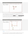
Tutorial 1: Getting Started Armin Duff and Riccardo Zucca
Tutorial 2: DAC Reactive Layer Riccardo Zucca and Armin Duff
Tutorial 3: DAC Adaptive Layer Armin Duff and Riccardo Zucca
Tutorial 4: DAC Contextual Layer Encarni Marcos and Armin Duff
4. DAC Applications
Rehabilitation Gaming System Tony Prescott and Anna Mura
Renachip: A Neuroprosthetic Learning Device Ivan Herreros
ADA: A Neuromorphic Interactive Space Based on DAC Anna Mura
DAC Incarnation (iCub) Stéphane Lallée
24
36
88
89
92
95
97
5. Appendix112
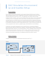
DAC Simulation Environment: iqr and Gazebo Setup Armin Duff and Riccardo Zucca113
iqr Basics Riccardo Zucca120
iCub Material Stéphane Lallée128
3
1 | Preface
1 | Preface
4
Acknowledgments
Acknowledgments
We would like to thank the Convergent Science Network for Neurotechnology and
Biomimetic systems project CSN II - FP7 601167 for supporting the publication
of this ebook on the biologically-inspired cognitive Distributed Adaptive Control
(DAC) architecture. This DAC architecture is one of the very few examples of
biomimetic architectures of perception cognition and action that has been applied to
a range of artificial behaving systems i.e. robots, while having a strong grounding in
the pertinent neuroscience of both invertebrate and vertebrate systems.
As a subject for teaching material DAC will introduce researchers and students to
key concepts of minds and brains, at both the functional level and at the level of how
the physiology and anatomy of brains shape and realise these functions.
We are grateful to the laboratory of Synthetic, Perceptive, Emotive and Cognitive
Systems (SPECS), which was involved in the development of the different versions
of the DAC architecture. We also wish to express our gratitude to all the students
that successfully used DAC in their studies and research projects and have thus
helped to improve it further.
Finally we would like to thank the Book Sprints team and the FLOSS Manuals team
for making this book possible!
This book was written in five days during a Book Sprint collaborative writing
session, from April 23 to April 27, 2014, in St. Feliu de Guíxols, Spain. This session
was executed within the framework of the BS4ICTRSRCH - Book Sprints for ICT
Research project in cooperation with CSNII - Convergent Science Network for
Neurotechnology and Biomimetic systems project.
The Book Sprint was facilitated by Barbara Rühling of BookSprints.net.
Layout and Design: Henrik van Leeuwen
Proofreader: Rachel Somers Miles
Original cover from Sytse Wierenga and Anna Mura
BS4ICTRSRCH
Book Sprints for ICT Research, Support Action project is funded by the European
Commission under the FP7-ICT Work Programme 2013. Project number: 323988.
http://booksprints-for-ict-research.eu
5
1 | Preface
CSNII - Convergent Science Network for Neurotechnology and Biomimetic systems,
funded by the European Commission under the FP7-ICT Work Programme 2013.
Project Number: 601167
http://www.csnetwork.eu
FLOSS Manuals Foundation
FLOSS Manuals creates free documentation about free software. It is an online
community of some 4-5000 volunteers creating manuals in over 30 languages.
http://www.flossmanuals.org
Book Sprints
Book Sprints is a rapid development methodology for producing books in 3-5 days.
The methodology was founded by Adam Hyde of BookSprints.net.
http://www.booksprints.net
6
Two EU Projects at Work in a Creative and Collaborative Writing Effort
Two EU Projects at Work in a Creative and Collaborative
Writing Effort
The publication of this book on the Distributed Adaptive Control theory (DAC) is part
of the CSN Book Series and is a collaborative effort between the EU coordination
action CSNII - Convergent Science Network for Neurotechnology and Biomimetic
systems, and the EU project Book Sprints for ICT Research.
The goal of CSN is to contribute and advance the training of future generations
of researchers who will shape the field of biomimetics and biohybrid systems by
producing teaching materials (e.g. video lectures, podcast interviews, tutorials and
books) and also by providing visibility and access to all of the material produced in
the context of the CSN educational objectives. Through these dissemination actions
CSN hopes to further enhance the impact of the field.
The goal of Book Sprints for ICT Research project is to adopt and test the Book
Sprints methodology within the context of academic ICT research. This means that
Book Sprints will apply their method of collective writing to the CSNII group formed
by the authors of the DAC book.
www.booksprints.net
www.booksprints-for-ict-research.eu
According to the Book Sprints method, the authors of the DAC book worked closely
together with a facilitator, a professional editor and a designer, who helped with
the overall production of the book. The duration of a Book Sprint writing event is
normally 4-5 days.
The resulting book was finished at the end of this event with the goal to be made
available as both printed and electronic publication.
On the one hand CSN profits from this collaboration because it has been able to
deliver a book in a very short period of time, and on the other hand, the Book Sprints
for ICT Research project has had the opportunity to evaluate the Book Sprints
method for an academic publication with an ICT research group such as CSN.
7
1 | Preface
Location of Event
This event took place in the spring of 2014 at the coast of Barcelona in Spain.
Book Theme
CSN teaching material and the 2nd CSN book series on the Distributed Adaptive
Control theory (DAC).
Book Authors
A group of 8 scientists agreed to participate in this book endeavour. These are experts
(PhDs, postdocs, professors) from different disciplines such as neuroscience, psychology,
biology, physics and engineering.
Paul Verschure is an ICREA professor and director of the Center of Autonomous Systems
and Neurorobotics at Universitat Pompeu Fabra where he leads the SPECS Laboratory.
With a background in psychology and AI he aims to find a unified theory of mind and brain
using synthetic methods, and to apply it to quality of life-enhancing technologies. He is
the founder of the DAC theory. Co-author of the chapters 'The Science of Brain and Mind'
and 'Distributed Adaptive Control: A Primer'.
Tony Prescott is Professor of Cognitive Neuroscience and the Director of SCentRo at the
University of Sheffield, UK. He has worked since 1992 on investigating parallels between
natural and artificial control systems. Co-author of the chapters 'The Science of Brain and
Mind', 'Distributed Adaptive Control: A Primer', and 'Rehabilitation Gaming Systems'.
Armin Duff is a visiting professor at the Universitat Pompeu Fabra Barcelona, Spain, and a senior researcher at the SPECS laboratory. His main research interest is how
intelligent systems extract and learn the rules and regularities of the world in order to act
autonomously. In particular he evolved the Distributed Adaptive Control (DAC) architecture
proposing a new learning rule called Predictive Correlative Subspace Learning. Co-author
of the chapters 'DAC5', 'DAC Tutorial on Foraging' and 'DAC Simulation Environment: iqr
and Gazebo Setup'.
Stéphane Lallée is a postdoctoral fellow at the SPECS laboratory, Universitat Pompeu
Fabra, Barcelona, Spain. With a background in computer science and a PhD in Cognitive
Neuroscience, his main expertise is on the conceptual framework and the development
of large-scale integrated cognitive architecture for humanoid robots. Author of the
chapters 'DAC Incarnation (iCub)' and 'iCub Material', and co-author of the chapter
'Cybernetics'.
8
Two EU Projects at Work in a Creative and Collaborative Writing Effort
Ivan Herreros is a teaching professor at the Universitat Pompeu Fabra Barcelona and
research scientist at the SPECS laboratory, Universitat Pompeu Fabra, Barcelona. He
has a background in engineering and linguistics and his actual research work deals
with the modelling of different areas of the brain, such as the Auditory Cortex and
the Cerebellum, with the purpose of building a complete brain model that accounts for
the Two Phase theory of Classical Conditioning. Author of the chapter 'Cybernetics',
and co-author of the chapter 'Renachip: A Neuroprosthetics Learning Device'.
Encarni Marcos is a PhD student at the SPECS laboratory, Universitat Pompeu Fabra,
Barcelona and is actively working in implementing the neuronal, cognitive
and behavioural principles underlying decision making in animals and robots. Co-author of the chapters 'DAC5' and 'Tutorial 4: DAC Contextual Layer'.
Riccardo Zucca is a psychologist currently finishing his PhD at the SPECS
laboratory, Universitat Pompeu Fabra, Barcelona. His main interest is on the
mechanisms underlying adaptive behaviour. In particular, his research is focused on
the cerebellar mechanisms of acquisition and encoding of timely adaptive responses
in the context of Pavlovian classical conditioning. Author of the chapter 'iqr Basics',
and co-author of the chapters 'DAC5', 'Tutorial 1', Tutorial 2', 'Tutorial 3', and 'DAC
Simulation Environment: iqr and Gazebo Setup'.
Anna Mura is a biologist with a PhD in natural sciences and is a teaching professor
and senior scientist at the SPECS laboratory, Universitat Pompeu Fabra, Barcelona.
Presently she is dealing with science communication and outreach activities in the
field of brain research and creativity. CSN book series editor, author of the chapter
'ADA: A Neuromorphic Interactive Space Based on DAC', and co-author of the
chapter 'Rehabilitation Gaming System'.
9
1 | Preface
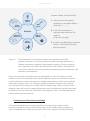
Abstract Distributed Adaptive Control (DAC) is a theory of the design principles underlying
the Mind, Brain, Body Nexus (MBBN) that has been developed over the last 20
years. DAC assumes that the brain maintains stability between an embodied agent,
its internal state and its environment through action. It postulates that in order
to act, or know how, the brain has to answer 5 fundamental questions: who, why,
what, where, when. Thus the function of the brain is to continuously solve the socalled H5W problem with ‘H’ standing for the ‘How’ an agent acts in the world. The
DAC theory is expressed as a neural-based architecture implemented in robots and
organised in two complementary structures: layers and columns. The organisational
layers are called: reactive, adaptive and contextual, and its columnar organisation
defines the processing of states of the world, the self and the generation of action.
Each layer is described with respect to its key hypotheses, implementation and
specific benchmarks. After an overview of the key elements of DAC, the mapping of
its key assumptions towards the invertebrate and mammalian brain is described.
In particular, this review focuses on the systems involved in realising the core
principles underlying the reactive layer: the allostatic control of fundamental
behaviour systems in the vertebrate brain and the emergent non-linearity through
neuronal mass action in the locust brain. The adaptive layer is analysed in terms
of the classical conditioning paradigm and its neuronal substrate the amygdalacerebellum-neocortex complex together with episodic memory and the formation
of sense-act couplets in the hippocampus. For the contextual layer, the ability of
circuits in the prefrontal cortex to acquire and express contextual plans for action
is described. The general overview of DAC’s explanation of MBBN is combined
with examples of application scenarios in which DAC has been validated, including
mobile and humanoid robots, neurorehabilitation and the large-scale interactive
space Ada. After 20 years of research DAC can be considered a mature theory of
MBBN.
10
Abstract
11
2 | DAC Theoretical Framework
2 | DAC Theoretical
Framework
12
The Science of Brain and Mind
The Science of Brain and Mind
This book describes an approach to understanding the human mind and brain
that the authors have been developing for more than two decades. In this opening
chapter we try to explain the motivation for our approach by placing it in a wider
context. Specifically, we explore how the different sciences of mind and brain—from
neuroscience and psychology, to cognitive science and artificial intelligence (AI)—
stand in relation to each other at this moment in the 21st century. Our aim in doing
so is to persuade you that despite the fact that our knowledge is expanding at everaccelerating rates, our understanding—particularly of the relationship between mind
and brain—is, in some important sense, becoming less and less. An explanatory gap
is building that, for us, can only be bridged by a kind of multi-tiered and integrated
theoretical framework, Distributed Adaptive Control (DAC), which is developed and
described in this volume.
A second goal of this chapter is to show that, in bridging this explanatory gap,
we directly contribute to advancing new technologies that improve the human
condition. Indeed, our view is that the development of technologies that instantiate
principles gleaned from the study of the mind and brain, or biomimetic technologies,
is a key part of the validation process for the scientific theory that we will present.
We call this strategy for the integration of a science and engineering ‘Vico’s loop’
after the 18th-century Neapolitan philosopher Giambattista Vico who famously
proposed that we can only understand that which we create: ‘Verum et factum
reciprocantur seu convertuntur.’ We aim to show both here, and in the ‘DAC
Applications’ section of this book, that following the creative path proposed by Vico
can lead not only to better science (understanding), and useful engineering (new
life-like technologies in form and function), but can also guide us towards a richer
view of human experience and of the boundaries and relationships between science,
engineering and art.
Matter over Mind
To begin, let us consider some concrete examples of how the science of the mind
and brain is currently being pursued. Since mind emerges from brain, an important
trend that we have noticed is increasing the focus of resources and efforts towards
the brain side of the mind-brain duality, seemingly in the hope that this will unlock
the secrets of both. We call this trend ‘matter over mind’ because we feel that it is
drawing attention towards things that can be measured—brain processes—but in a
manner that risks losing sight of what those processes achieve—instantiating the
mind.
13
2 | DAC Theoretical Framework
Two concrete and significant examples of this trend are as follows. In 2013, the
European Commission initiated the Human Brain Project (HBP)—a decade-long,
€1 billion effort to understand and emulate the human brain. In the same year, the
US Government announced the BRAIN Initiative—projected to direct funding of $3
billion to brain research over a similar ten-year period. With this level of investment
and enthusiasm you would hope that great advances in brain science are surely just
around the corner. Knowing so much more about the brain, we should surely also
know much more about the mind and thus about ourselves.
However, although this increased international enthusiasm for brain science is
exciting and in many ways welcome, there are some niggles. Looking at these
flagship projects we are struck by how both initiatives are convinced that an
understanding of the brain, and hence the mind, will proceed from a very largescale, systematic approach to measuring the brain and its physical properties.
More precisely both of these projects intend to leverage powerful 21st-century
technologies—such as the latest human brain imaging, nanotechnology and
optogenetic1 methods—that can make the connectivity and activity of the brain
more apparent. They will then apply the tools of ‘big data’, such as automated
reconstruction and machine learning, powered by the accelerating power and
capacity of computers, to help make sense of what will amount to a tsunami of new
measurements.
While all of this is well and good, we see a significant gap. Will we know ourselves
once we have all the facts in our database? Where are the theories of brain function
that are going to explain all of this new anatomical detail? How are we going to
make the connection between the understanding of the brain at a tissue level and
the understanding of mind at a psychological level? In this fascination with the
brain as the physiologically most complex organ in the human body, are we losing
sight of what is needed to understand and explain the role of the brain in guiding
and generating behaviour and shaping experience? While many have argued that
we need better data to drive theory building, we contend that there is already
a mountain of unexplained data about the brain, and what is needed are better
theories for trying to make sense of it all.
Part of the solution to the challenge of connecting brain physiology to behaviour
is—as we explore further below and throughout this book—computational modelling,
either using computer simulation, or, to understand the link between brain and
behaviour more directly, by embedding brain models in robots. Naturally these
large-scale projects that are exploring the human brain will apply and extend current
computational neuroscience models and methods so, on the surface, all seems
well. In particular, they will develop computer simulations that seek to capture
rich new datasets at an unprecedented level of accuracy using hugely powerful
massively parallel machines (HBP, for instance, will invest heavily in building these
14
The Science of Brain and Mind
on neuromorphic principles), in an attempt to show how interactions among the
microscopic elements that constitute a brain can give rise to the global properties
that we associate with the mind or its maladies. One of the goals of these projects
is to better understand/treat mental illness, thus showing societal relevance.
Indeed, this programme of brain simulation has ambitions to match those of the
corresponding endeavour of brain measurement, so why worry?
Well, our concern lies in the observation that the technical possibility of amassing
new data seems to have become the main driving force. The analogy is often
made with the human genome whose decoding has unlocked new avenues for
research in biology and medicine. However, whilst the genome is large (3 billion
base pairs) it is finite and discrete (each pair can only be one of a fixed number of
known patterns), and the case could be (and was) made that deciphering it would
concretely and permanently address a key bottleneck for research. With the brain,
on the other hand, there is no equivalent target to the genome—no template for brain
design that once we have described it we can say we are finished. There will always
be another level of description and accuracy that we can strive for and which, for
some, will be the key to unlocking the brain’s secrets from microtubules and CAM
kinase to gamma range oscillations and fMRI scans. Further, whilst the new tools
of 21st-century brain science are attractive in terms of their greater accuracy and
power, what we see with many of their results is confirmation of observations that
had already been made in previous decades albeit in a more piecemeal fashion. To
unlock the value of these new datasets, we believe, will require the development of
multi-tiered explanations of brain function (of which there is more below), and data
analysis tools will help, but the theory-building activity itself will largely be a human
endeavour of which abstraction will remain an important part.
A key point for us is that description and measurement whilst vital to doing good
research are not the ultimate goal of science. Rather, we describe in order to explain.
As the physicist David Deutsch noted in 1997, there are an infinite number of facts
that we could collect about the natural world (and this will include a countless
number of brain facts), but this kind of knowledge is not, by itself, what we would
call understanding. The latter comes when we are able to explain the amassed data
by uncovering powerful general principles. In astronomy, for instance, Ptolemy,
followed by Copernicus, Galileo, Newton, and then Einstein all developed theories
that sought to explain observations of the motion of stars and planets. Each new
theory succeeded in explaining more of the assembled data and did so more
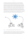
accurately and more succinctly. For instance, Copernicus explained data that
had been problematic for Ptolemy’s geocentric cosmology by replacing the earth
with the sun as the centre point around which the planets turn. Einstein showed
that Newton’s law of gravitation breaks down when gravity becomes very strong,
and was thus able to better (or more succinctly) explain some data on planetary
orbits. In physics the search for a theory with more explanatory power than general
15
2 | DAC Theoretical Framework
relatively continues, with the hope to one day explain the origin of everything,
beginning with and including the Big Bang, according to a single set of over-arching
principles.
In comparison to astronomy, how far have we come in developing powerful theories
for understanding brain data? The answer is not very far yet. With the current
focus on large-scale datasets there is an interest in discovering principles for sure,
but there also seems to be an expectation that these will bubble up through the
accumulation of observations; a process of induction if you will, powered by the
tools of data mining and computational modelling. Moreover, in place of striving
for the kind of compact theoretical description seen in physical science, there is
an increasing focus on models that can capture more of the potentially relevant
detail. The boundary becomes blurred between capturing principles and what can
become, in the end, an exercise in function fitting. In our admiration of the elegance
and beauty of brain data, and with the power of modern ICT systems to simulate
it, we can come to believe that the best model of the brain is the most exact
model. Following this path, however, can only lead to the conclusion that the brain
is its own best explanation, an idea satirised by Rosenbleuth and Wiener in their
comment that ‘the best material model for a cat is another, or preferably the same
cat’ (Rosenblueth & Wiener, 1945), and reminiscent of Borge’s famous story of the
cartographical institute whose best map was identical to the landscape it described
and thus lost its usefulness. A second way of summarising this concern is that the zeitgeist seems to favour
more reductionist descriptions rather than theoretical explanations. The logic
appears to go that we still don’t know enough of the key facts about the brain—cells,
circuits, synapses, neurotransmitters, and so forth—therefore lets go and find out
these details. Once we know these things we will necessarily better understand both
brain and mind. However, while neuroscience tilts towards more data gathering,
it is interesting to note that other areas of biology are becoming more holistic in
their approach, adopting what is often described as a ‘systems’ view. Indeed, in
systems biology, explanations are sought that go across levels from the molecular
through, the cellular, organismic, and the ecological. No one level of explanation (or
description) is privileged, and understanding at each level informs and constrains
understanding at the levels above and below it. In much the same way, and within
the sciences of the mind, parallel complementary explanations can be sought at the
psychological level (mind) and at the biological level (the brain), and we can allow
that there may be other useful explanatory levels between these two. Indeed, we
contend, as do many others, that useful theories of mind and brain can be motivated
that abstract away from the biological details of the brain but at the same time
capture regularities at a level below that of our direct intuitions (what some have
called ‘folk psychology’), and that in this area some of the most powerful explanatory
ideas might lie.
16
The Science of Brain and Mind
Cognitive Science Turf Wars
The notion of a multi-tiered understanding of the mind and brain is of course
nothing new. Indeed, in many ways it is captured in a research programme that
since the mid 20th century has gone by the name of cognitive science (e.g.
Gardner 2008). Acting as a kind of scientific umbrella, cognitive science has
fostered interdisciplinary dialogues across the sciences of the mind and brain for
the last seventy years, promoting the complementarity of explanations emanating
from neuroscience, psychology, linguistics, philosophy, and computer science. At
the same time, however, cognitive science has never really succeeded in building a
consensus around a core set of scientific principles. Instead, it has seen struggles
between different communities as to what should be the preferred level of
description of mind and brain and it has hosted heated debates over the meaning
and relevance of central concepts such as representation and computation. Perhaps
this is the nature of a healthy science, however, unlike neuroscience, for instance,
which holds a successful annual conference for more than 30,000 delegates, the
focus of cognitive scientists is dispersed across dozens of events each favouring a
particular perspective or approach. Moreover, despite its potential relevance to both
the scientific understanding of brain disease and the development of new smart
technologies it has surrendered much of its ground on the former to neuroscience
and on the latter to robotics and AI. Finally, whilst neuroscience as a community
has been able to mobilise support at the highest levels for endeavours such as
HBP and the Brain Initiative, funding for cognitive science appears to be flagging
at least momentarily (the EU, for example, recently scrapped its Robotics and
Cognitive Systems programme in favour of one solely focused on robotics, partly
due to the failure, as they saw it, of cognitive systems to address society-relevant
challenges). Standing back for a moment, we wonder if the current resurgence of
a more reductionist brain science programme is, at least in part, due to the failure
of cognitive science to really capitalise on the great start that it made more than
half a century ago. A commitment to interdisciplinarity has till now failed to lead to
powerful interdisciplinary theories that command broad assent, leaving a vacuum to
be filled by explanations couched at only one level.
A further way to look at the current status of the field is to recognise that, in
terms of the sociology of science as described by Thomas Kuhn, cognitive
science sometimes appears to be ‘pre-paradigmatic’. For Kuhn, work within any
given domain of science begins with multiple competing general theories, or
‘paradigms, but then progresses to a point where one of these is clearly more
successful than the rest, comes to dominate the field, and attracts more and more
supporters to work within it—this then is the normal state for a mature scientific
field. According to this narrative, it is possible for an alternate paradigm to arise
building on any weaknesses in the current dominant general theory, such as a
failure to adequately explain key data, and questioning some of its core precepts.
17
2 | DAC Theoretical Framework
If sufficiently persuasive, such an alternative can provoke a ‘scientific revolution’
in which the current dominant paradigm is overthrown to be replaced by a new
orthodoxy. Whilst a scientific revolution can come about because the new paradigm
is more explanatory (in the sense discussed above), a key element of the Kuhnian
analysis is that trends in scientific research are partly determined by social
and political forces rather than purely scientific ones. The dominant paradigm
might crumble, for instance, not simply because it is weaker but because it has
become unfashionable, conversely an alternate paradigm might fail to thrive not
because it does not offer better explanations but simply because it fails to attract
enough supporters, or resources, to mount a serious challenge—as in politics, the
incumbent can have power and influence that allows them to suppress contenders
at least for a while. The Kuhnian narrative appears to work well in physics, a domain that Kuhn was
trained in, and where the Newtonian view succeeded the Galilean view then
to be replaced by the special relativity/quantum view. Applied to sciences of
the brain and mind, the picture is more complicated. From one view, cognitive
science stands as a distinct scientific domain still looking to find its feet (i.e. preparadigmatic), with symbolic AI, connectionism, dynamic systems, and perhaps
cognitive neuroscience, all vying as competing paradigms within it. Within the
field, the navel-gazing continues but with the vague assumption that eventually
a consensus will emerge and cognitive science will have come of age. From an
alternative view, cognitive science is itself a paradigm competing within the broader
domain of the natural sciences to be the approach to understanding the mind
and brain. From this perspective, cognitive science replaced behaviourism as the
dominant paradigm in the mid-20th century and has succeeded to hold its ground
till now despite a lack of consensus and internal division. At this point we might
ask if cognitive science is now at risk, in Kuhn’s sense, of being overthrown and,
if so, who would be the contender? Surveying the landscape, does the new breed
of assertive reductionist neuroscience have, as its ambition, the desire to replace
the cognitive science consensus in favour of multidisciplinary explanations? Could
neuroscience potentially succeed in eliminating cognitivist theories, and all their
conceptual intermediaries, in favour of explanations couched directly in terms of
brain states and dynamics? Will a future retelling of the history of science conclude
that cognitive science was a useful approximation, like Newtonian physics, effective
in plugging the explanatory gap left by predecessors such as behaviourism, but
ultimately not as powerful as a fully-formed ‘quantum’ neuroscientific theory of the
relationship between mental phenomena and brain activity (note that this analogy
has been suggested before in relationship to Connectionism (Smolensky, 1988),
which now might be viewed as another partial step to a full neuroscientificallygrounded account)?
18
The Science of Brain and Mind
We describe this scenario not because we think it is likely, or because we think an
eliminativist neuroscience really is the better paradigm. However, we recognise, with
Kuhn, that science is a societal activity, and that the field of cognitive science could
wane, or perhaps is already waning. We would like cognitive science to wake up,
move its focus away from turf wars about privileged levels of explanation, and get
back to its core agenda of building powerful multi-tiered theories of the mind and
brain. We worry that a neuroscientific agenda that increasingly sees the brain as the
best theory of itself is actually a retreat from properly advancing the sciences of the
mind or any science for that matter. Like behaviourism seventy years ago, the brain
again becomes a box whose contents is ultimately unanalysable; this time we can
describe what is inside, but we surrender the hope of a theoretical explanation of
the emergence of the mind in favour of the aspiration that if we copy it accurately
enough we will somehow replicate interesting aspects of mental function.
Towards a Multi-Tiered Theoretical Framework
So what should a 21st-century approach to understanding the mind and brain look
like? In the study of mind and brain there is currently no accepted general theory
and the last attempt to define one came to a halt in the early 1950s with Clark Hull’s
theory of the behaving system that followed the logical-positivist school. Since then,
it has gone relatively quiet in terms of attempts to postulate theories that show how
a physical system like the brain can give rise to mind and behaviour; at best we have
seen micro-theories that are highly specialised. This is the explanatory gap that
needs to be filled—a general theory, or framework, connecting brain and mind.
In broader terms, what should we look for in such a theory? First, as we discussed
above, a theory must explain, in this case, the scientific observations that
constitute the relevant ‘facts’ of empirical science concerning measurement of
the brain and behaviour, and this data must be interpreted in such a way that
provides an explanation of human experience. Second, a theory must make
testable predictions that can be validated with available methods and technologies
(making predictions that require measurements to be made with science fiction
technologies cannot be taken too seriously). Third, a scientific theory must be able
to control natural phenomena. This means, for instance, to be able to define a set of
manipulations that constitute an experiment or the principles on the basis of which
a useful artefact can be constructed. In addition to these primary requirements, we
can include that it must be supported by a broad base of observations, generate
multiple predictions in a range of areas, and display continuity with pre-existing
knowledge and theories. Furthermore, it must follow Adelard of Bath’s dictum that
nature is a closed system and all natural phenomena must be explained as caused
by other natural agents (formulated in the 12th century) and Occam’s razor, which
asks for parsimony in scientific theories.
19
2 | DAC Theoretical Framework
Our commitment value of models, particularly those that make useful impact in the
world, derive from the dictum ‘verum et factum’—we understand by making. Another
way of expressing this idea is that the machine is the theory concretely embodied
and observable. We can contrast this view with 20th-century notions of how
science should work. Specifically, in the first half of the 20th century, the notion of
scientific theory was strongly dominated by a syntactic formal interpretation where
a scientific theory comprised axioms that allowed the deduction of observations,
which upon being tested against reality would lead to an update of the axioms. In
this logical positivist view a language of science could be constructed that would
specify an ordered way to shape scientific progress. In the second half of the
20th century, however, there was a shift to a so-called semantic, or model-based,
interpretation where a scientific theory describes aspects of reality not unlike a map
describes a physical landscape. However, theories and models face the problem of
being under-constrained. From this view, there are many possible ways to interpret
observations. We can think of the model as a fit of a curve through a cloud of data
points. There is a practically infinite number of lines we can draw; which ones to
retain and which to ignore? In the study of mind and brain we consider that we can
reduce this search space by imposing the requirements that theories of mind and
brain must be able to relate to multiple levels of description—minimally the structure
and function of the brain, or to its anatomy and physiology, and the behaviour it
generates. This method is called convergent validation. In more practical terms
our strategy is to build computational models to emulate the brain’s anatomy and
physiology and to embody these models using interfaces to the physical world
(for instance, via a robot). In this form our theory as a model can explain anatomy,
physiology and behaviour, make predictions at multiple levels of description and
control a physical device. In addition, it instantiates Vico’s loop: we have made an
artefact with life-like capabilities that can potentially be deployed in a useful task.
An additional form of constraint and a critical aspect of understanding the mind,
and not just its parts, is that we need to develop theoretical frameworks that
have the potential to inclusively explain all of the interesting capabilities of mind
and brain including, but not limited to, perception, sensorimotor control, affect,
memory, learning, language, imagination, creativity, planning, consciousness, etc.
In short, work within particular subdomains, and most work in cognitive science,
is necessarily of this character, must have the potential to be incorporated within
the bigger picture, and this evolving idea of the full architecture of the mind and
brain should reveal how underlying principles operate across these subdomains
at the same time as identifying that specific subdomains may also have their
own specialisms. Occam’s razor—the requirement to have an overall succinct
theory—should be applied, with the aim that this framework is assembled at a high
level of abstraction whilst retaining the possibility to be a complete explanation
of how the brain gives rise to mind. Naturally, the framework we are assembling
does not adopt an a priori view about privileged levels of explanation. Indeed, it is a
20
The Science of Brain and Mind
requirement of our commitment to convergent validation that we should generate
models at multiple levels of abstraction—some very close to mechanisms revealed
through the microscope of neuroscience, others very high-level and connecting to
principles identified in engineering or computer science. Finally, we recognise the
value of different methodologies for acquiring explanatory concepts. For instance,
we can work inductively and bottom-up, using the powerful data analysis tools
now being developed, to identify the ‘good tricks’ (Dennett, 1995) that have been
discovered in the evolution of nervous systems. Likewise, we can work top-down
and deductively, going from computational analyses (in the sense of David Marr) of
the functions of mind to ideas about the mechanisms that can give rise to them.
Here advances made in engineering and AI furnish us with candidate principles that
could be instantiated by the brain and mind. We do not prefer bottom-up or topdown approaches, but rather strive for the completeness of our theory, and to have
elements of both in order to have strong constraints in these two directions. It is important to build on previous scientific attempts at a general theory of the
mind and brain. In this book you will find ideas that originated with the invention
of control and information theory in engineering, digital computers in ICT, and
systems theory in biology. Amongst these we would highlight the insights of the
early cyberneticians such as Norbert Wiener, Warren McCulloch, Rosh Ashby, and
William Grey Walters who combined the theory of feedback-based control from
engineering, with the notion of homeostasis from biology, to produce a theory of
the brain as a mechanism for maintaining balance that can be applied to diverse
areas of brain function from autonomic function (the regulation of bodily processes
such as breathing, circulation and metabolism) and motor control, to cognitive
processes such as learning and memory. During the emergence of cognitive science
in the 1950s, leading figures were also concerned with general theories of the mind.
For instance, building on attempts to understand decision-making, Alan Newell
and John Anderson both elaborated general theories of cognitive architecture
using if-then rules (productions) as their primary building block. These models
explored and demonstrated the power of a simple principle, recursively applied,
in generating mind-like properties, but they also revealed some of the limitations
of prematurely settling on a specific level of analysis, or computational primitive.
Indeed, partly in reaction to this model of the brain as a symbol-cranking system,
a view which emerged from computer science and rather arrogantly declared the
independence of theories of mind from theories of brain, namely, the connectionist
architectures developed by David Rumelhart, Jay McClelland, Geoffrey Hinton,
Terry Sejnowski and others, looked much more at the specific structural properties
of the brain, particularly its massively distributed nature, as inspiration for their
models of brain architecture. The excitement around these models, which had the
capacity to explain facets of learning and memory that were problematic for symbolbased approaches, encouraged claims to be made that this was the privileged
level of explanation at which theories of mind should be couched. This is one
21
2 | DAC Theoretical Framework
of many examples in cognitive science where success in applying one particular
kind of explanatory principle in a number of subdomains led to premature
conclusions of this nature. Looking back, thirty years on from the connectionist
‘scientific revolution’, that approach has succumbed to the same criticism, but
this time from computational neuroscience—that the more abstract version of
brain architecture favoured by the connectionists overlooked critical details. But the
answer is not to go deeper and deeper to find the perfect model, but to recognise
that different scientific questions can be addressed at these many different levels
(Churchland & Sejnowski, 1992). A dynamic systems view, emerging in the 1990s,
and championed by Scott Kelso, Esther Thelen, Jeffrey Elman, and others attempted
a synthesis between connectionist theory (or ‘new’ AI more broadly) and systems
biology. However, once again, the effort to distinguish itself from what had gone
before, in this instance by declaring itself to be non-computational, limited the
impact of the approach. More recently, new bandwagons have emerged based on
the notion of the brain as a machine for doing Bayesian inference, or prediction
(minimising its own ability to be surprised by the world). The most ambitious
versions of these theories hope to be full accounts of how mind emerges from
brain. The attraction that we have as scientists to the possibility of uncovering core
principles that succinctly explain many of the things we want to understand (as
the physicists managed to do in explaining the motion of the stars and planets),
must be tempered by the recognition that such notions have so far only captured a
small fraction of the competencies of the human mind and so have a very long way
to go before they can make any claim to theoretical completeness. As an evolved
system that must solve many different types of challenges in order to survive and
thrive, we must also be open to the possibility that there is no one principle, or even
a small cluster of principles that will explain the mind/brain. We certainly hope for a
theory that is much simpler than the brain, but we expect, nevertheless, that it will be
extremely complex.
As we have explained in this chapter, we consider that an important element of
theory development and testing is its instantiation as a machine; this allows us to
achieve a level of completeness not possible at the purely theoretical level or even
in simulation, and allows us to test theories whose complexity we cannot easily
entertain in our own minds. More emphatically we consider, following Vico, that a
mark of a good theory of the human mind and brain is that it can be instantiated in
this way, and an advantage of this approach is that it can also lead to the develop of
new biomimetic technologies that have value to society. The remainder of this book
describes an attempt at a framework that seeks to address this challenge, and its
instantiation in multi-tiered models (some embodied) as a means of testing/refining
the framework. Finally, in the applications section we show how this approach
is beginning to lead to technologies for/of rehabilitation, neuroprosthetics, and
assistive robots, that we hope will show how our approach to the science of the
mind and brain can lead to useful innovation and ultimately to broad societal benefit.
22
The Science of Brain and Mind
References
Churchland, P. & Sejnowski, T. (1992) The Computational Brain.
Dennett, D. C. (1995) Darwin’s Dangerous Idea.
Deutsch, D. (1997) The Fabric of Reality.
Gardner, H. (2008) The Mind’s New Science: A History of the Cognitive Revolution.
Kuhn, T. (1962) The Structure of Scientific Revolutions. Smolensky, P. (1988) On the Proper Treatment of Connectionism. Footnotes
1
Optogenetics is a technique that uses genetic manipulations to make neurons in animal brains emit light when they are active, thus offering exciting new
ways of finding out how cells connect to each other and of identifying how and
when particular types of cells are active during behaviour.
23
2 | DAC Theoretical Framework
Distributed Adaptive Control:
A Primer
‘Won’t somebody tell me, answer if you can!
Want somebody tell me, what is the soul of a man?’
Blind Willie Johnson—1930s blues song
The Greek rationalist philosopher Plotinus asked, in about 250BC: ‘And we, who
are we anyhow?’ ‘Zombies’ we are told by Daniel Dennett, one of the leading
philosophers of the 20th-century cognitive era, or ‘Meat Machines’ according
to Marvin Minsky one of the founding fathers of artificial intelligence. Is that
it? Is that what the soul of humans has become? Reduced and brushed away
into a mechanical universe. Here, ‘soul’ is referred to as synonymous with the
more modern construct of mind (Blind Willie Johnson, however, would disagree
with that). To become even more specific we can define ‘mind’ as the functional
properties of brains that can be expressed in overt behaviour. ‘Behaviour’ is
defined as autonomous changes in the position or shape of a body or soma.
Once behaviour serves internally-generated goals we can speak of ‘action’. The
‘brain’ is defined as a distributed, wired-controlled system that exploits the spatial
organisation of connectivity combined with the temporal response properties
of its units to achieve transformations from sensory states, derived from the
internal and external environments, into actions. The core variable this mind/brain
maintains in a dynamic equilibrium is the integrity of the organism in the face
of the second law of thermodynamics, the organism’s needs and environmental
changes that continuously challenge this integrity and threaten survival, and
thus compromise reproduction. The mind/brain is the result of a centralisation of
mediation following the increasing complexity of the morphology, sensory repertoire,
sensorimotor capabilities and the niche organisms that emerged during the
Cambrian explosion about 560M years ago. The incrementally tighter bi-directional
coupling between the organism and its environment we observe through the
progression of phylogeny, implies that in order to answer Plotinus with respect to us
humans and other animals, we do have to consider as our explanandum the nexus
of mind, brain, body and environment.
The Distributed Adaptive Control theory of mind and brain (DAC) is formulated
against the backdrop of the main developments in psychology, artificial intelligence,
cognitive science and neuroscience during the 19th and 20th century. It aims at
integrating across the dominant paradigms and approaches, as opposed to a priori
24
Distributed Adaptive Control: A Primer
negate any of them. The story of the study of mind and brain is essentially one of a
sequence of paradigms that are defined by negating their predecessors. This trend
starts with the focus on the study of consciousness in the nascent continental
school of the psychology of Fechner, Helmholtz, Donders and Wundt in the second
half of the 19th century. Structuralism was followed by behaviourism that saw its
heydays during the first half of the 20th century and constituted a direct reaction
to structuralism by negating its core dogmas. With the wish to develop a rigorous
experimental science of adaptive behaviour, behaviourism largely rejected the use
of constructs that were not directly observable, leading to the extreme position
of Watson and Skinner that constructs related to ‘mind’ had no place in a science
of psychology. Important sources of inspiration for this approach were the
pragmatism of Peirce, James and Dewey, which anchors knowledge in practical
outcomes and a simplified interpretation of the developments of physics, the most
successful science of that era and its method of operationalisation: the definition
of phenomena through the operations deployed to make measurements on them.
Behaviourism in this extreme form rejected mind in favour of the study of an empty
embodied organism. Behaviourism advanced important experimental paradigms
and insights in the study of learning, in particular the paradigms of classical and
operant conditioning introduced by Pavlov and Thorndike respectively in the early
20th century. Behaviourism served the agenda of the ideal of a unity of science
where the psychology of adaptive behaviour could be reduced to the biology of
the brain, which would map to chemistry and physics. However, after about half
a century of trying, behaviourism failed to deliver on its promise of identifying
universal principles of adaptive behaviour grounded in the ‘atom’ of the reflex that
would be isomorphic with their physical instantiation in the brain, and to scale up to
more advanced forms of behaviour beyond salivating, twitching, freezing, pushing
levers or pecking targets. Most importantly, organisms were not enslaved by the
reinforcement they received from the environment, as the empty organism dogma
prescribed, but rather involved with self-structured learning and behaviour. Fuelled
by the development of adaptive control systems during the Second World War, the
movement of the cybernetics of Wiener, Rosenblueth, McCulloch, Pitts, Grey Walter
and Ashby emerged that proposed a multidisciplinary approach towards adaptive
behaviour, centring on the mathematical and engineering principles of control
and interaction such as homeostasis, feedback control and neuronal operations.
Cybernetics included a synthetic component where the emulation of these principles
was sought using artificial systems, most notably the homeostasis of Ashby and
the robot turtles of Grey Walter. In parallel, a second contender was based on the
advances in computing machinery in breaking codes and sorting large amounts
of information, leading up to the computer metaphor of mind pursued in artificial
intelligence and the cognitive science of the second half of the 20th century.
Pioneers of this movement starting with Alan Turing had shown that machines
could display functional properties that resembled human problem solving. This
analogy inspired a young generation of upcoming researchers in the US bolstered by
25
2 | DAC Theoretical Framework
generous government support, to declare the computer metaphor a new science of
the mind, and giving rise to the artificial intelligence (AI) of Newell, Simon and Minsky,
and the linguistics of Chomsky. AI overshadowed cybernetics and heralded a brave
new world of the study of the logical operations performed by the disembodied mind,
which negated behaviourism and its link to empirical investigation at the level of brain
and behaviour. This so-called functionalist view, where explanations of mind focused
on the rules and representations of the software of the mind, ruled for a few decades.
It was exactly this functionalist view and the so-called multi-instantiation it implied,
that severed the link to the study of the brain in order to explain the mind: logical
operations can be implemented in various physical substrates and the latter does
not inform on the properties of the former. AI and the computer metaphor stumbled
over its own claims of being able to synthesise intelligence, largely due to a critical
dependence on the human programmer and the knowledge they implanted in the AI
system leading to what has been called the symbol grounding problem, or in more
general terms, the problem of priors: a system can follow predefined rules operating
on predefined representations and not ‘know’ what it is doing, thus lacking the ability
to understand and adapt to the real world in which it is embedded. Lacking impact in
the real world, the disembodied mind of AI was followed in the 1990s by a period of
research in which biological metaphors guided the construction of artificial systems
and their associated claims on the mind, such as in behaviour-based AI, artificial
life, genetic algorithms and neural networks and connectionism combined with a
philosophy of eliminative materialism, where the whole human experience would
be described in ‘brain speak’. The ‘new’ AI directly negated its predecessor by
proposing a non-representational behaviour-based explanation of mind, while
connectionism was seeking out the ‘subsymbols’ that would link substrate to mind.
Neither of these approaches have had a lasting impact on the study of mind and
brain beyond facilitating the advancement of computational modelling in the life
sciences, such as computational neuroscience. The last step in this regression of
the study of mind and brain is the surrender to the seduction of big data or a bottomup modelling approach driven by the force of data. The human mind dissolved into
petabytes of data.
DAC aims at reintroducing necessary theoretical considerations into the study of
mind and brain and to combine these with a well-defined synthetic method: the
machine is the theory. It is from the perspective theory that we investigate nature
and answer Plotinus’ challenge. Data as such is meaningless and if pursued in its
own right will solely generate more noise in our understanding of reality. DAC is
defined with the ambition to explain the conscious, embodied mind, or the MBBN,
thus connecting it to 19th-century structuralism and its explanandum. Furthermore,
DAC adopts from behaviourism the objectives to develop an objective multi-scale
science of mind and brain starting from its key paradigms of classical and operant
conditioning, in realising its theories in an embodied quantitative form starting from
the perspective of control links DAC to the agenda of cybernetics, while scaling
26
Distributed Adaptive Control: A Primer
up towards high-level cognitive functions such as problem solving, language and
decision-making incorporating the agenda of traditional AI. Hence, DAC takes the
obstacles faced by preceding paradigms as the objectives of its research programme
with the goal to unify them rather than negate the preceding paradigm. The latter
would be difficult at this stage because there is currently no dominant paradigm, but
the study of mind and brain exists in a highly fragmented conceptual world of microtheories, relatively small research communities pursuing highly specialised questions
all glued together by the drive to generate more and more data. DAC is taking the
explicit and firm position that if we want to answer Plotinus we have to get back to
theorising about mind and brain.
Given DAC’s research agenda of solving the challenges faced by the different
attempts to explain mind and brain, the question is what should our explanandum
be, the phenomenon that we want to specifically explain? DAC proposes that this
should again be the structuralist goal of developing a science of consciousness.
Given that consciousness lacks a clear definition, this might sound surprising,
so lets spend a few words on why this is a good choice. The explanandum of
behaviourism, also inspired by the Darwinian revolution and the specific dynamics
of the 19th-century society of the developing new world, was adaptive behaviour or
learning. With the switch to the computer metaphor the explanandum changed to
reasoning, reflecting the outcome of the symbol manipulation that computers are
built for or artificial intelligence, a label coined by one of its first researchers John
McCarthy for a 1956 seminal conference at Dartmouth College co-organised with
Claude Shannon and Marvin Minsky. With the choice of the naming of the field and
implicitly its objectives, the machine mind of AI would target a rather ill-defined
and relatively suspect construct. Intelligence became a concept of great interest to
the science of the mind due to the work of Galton in the late 19th century. Seeking
a single scale with which to quantify human mental capabilities, he settled on the
notion of intelligence as measured through a self-devised test battery and reflecting
a single inherited factor, also called g. This operational approach, also adopted by the
behaviourists, was further expanded by Binet who settled the debate on intelligence
by equating it with a more elaborate test battery that became of great practical value
in the large-scale assessment required for the assimilation of hundreds of thousands
of recruits in the armies that fought the First World War. By resorting to a pure
operational definition of intelligence its ontology was murky and presumed to reside
in the single underlying g factor with unknown and assumed irrelevant links to natural
processes, thus challenging the dictum of Adelart of Bath. Artificial intelligence set
itself up for a research programme anchored to an ill-defined construct, thus making
it very difficult to assess success or failure. Indeed, now we know by using brain
imaging techniques on humans performing intelligence tests that as opposed to a
single g factor, intelligence appears to depend on a number of interaction cognitive
processes (Hampshire, Highfield, Parkin & Owen, 2012). Hence, this raises the
question of whether the target of the field designated by ‘artificial intelligence’ should
27
2 | DAC Theoretical Framework
be rephrased in order to align it with the natural processes underlying perception,
cognition, emotion and action in a more general sense. Indeed, this drift to a more
fragmented view of ‘intelligence’ and its possible deconstruction is also reflected in
the current standards of diagnosing mental deficits in DSM5 which, as opposed to
a single factor as used to be the case, stresses a number of capabilities including:
verbal comprehension, working memory, perceptual reasoning, and cognitive
efficacy. Combining these observations it would seem foolish to insist on developing
a science and technology of intelligence.
Despite these concerns about the mind as a computation school of thought, a
message is propagating through different media that we are reaching the limits
of human-driven advancement and that we are facing a post-human era that
essentially follows the dystopic scenario of the Terminator movie series (Kurzweil,
2005). As with the Skynet AI systems in the movies, machine intelligence is
predicted to reach a point where machines will become autonomous and outsmart
humans, leading to the realisation of the former that the latter are obsolete and/
or a hindrance to the propagation of intelligence and computation into the universe
(Kurzweil, 2005). After this ‘intelligence explosion’ or ‘singularity’ as it is oft-called,
Cyber Armageddon is upon us and robosapiens will emerge and supersede
homosapiens terminating the progression of biological evolution and thus forcing
biological life forms like ourselves to co-opt into a union with machines, which
will in return provide us with eternal existence. Although the estimates of when
this will happen exactly have been gradually shifting further into the future, the
day of its revelation, or ‘s-day’ (‘singularity day’) is now set to occur around 2045.
The conviction about this coming singularity has also been called ‘technologism’
because of its merging of anticipated technological capabilities, proposed to be
the ultimate operationalisation of intelligence, with religious motives such as divine
power of a future technology, the redefinition of nature and the revelation of a
route to reach eternal existence (e.g. Noble, 1997). The evidence upon which the
plausibility of these beliefs is based is scant and usually points to Moore’s law, our
putative rapidly-increasing understanding of the brain and assumed unstoppable
advances in AI research. Indeed, a brave new world awaits us once our minds are
all downloaded to the matrix. However, why would one believe these claims, what
is its utility and most importantly how will this be realised? Having ever-increasing
computer processors as such does not answer Plotinus: we have observed
the deterioration of brain science into a mindless collection of ever-increasing
amounts of data and the failure of the AI research programme pursuing the mirage
of ‘intelligence’. In this respect the singularity movement aims at giving itself
plausibility by ‘defending’ humanity from cyberdoom, but it makes the question of
which natural phenomenon to target in a science of mind and brain more salient,
and in addition, raises the fundamental question: for what purpose do we develop
such a science?
28
Distributed Adaptive Control: A Primer
Through integrating across all prevailing paradigms in the study of mind and brain,
DAC seeks to explain a specific natural phenomenon that many brains share:
consciousness. It translates this explanandum into a very concrete research
programme by linking it to the multi-faceted nature of consciousness and its
realisation in brains. Let’s first take a look at the mind/brain and inspect the question
of how it serves fitness in an evolutionary sense, or as Dobzhansky phrased it:
‘Nothing in biology makes sense except in the light of evolution.’ DAC starts with the
fundamental consideration, following Claude Bernard and Ivan Pavlov, that brains
evolved to act, establishing a metastable equilibrium between the organism and its
environment. But what does it take to act? DAC assumes that the how of action is
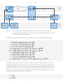
realised through five fundamental processes that brains implement:
1. Why: the motivation for action in terms of needs, drives and goals.
2. What: the objects in the world that actions pertain to as they can
be perceived.
3.
4.
5.
Where: the knowledge of the location of objects in the world and the self.
When: the timing of action relative to the dynami CS of the world and
the self.
Who: the inferred hidden states of other agents.
This defines the so-called H5W problem (five questions, all starting with ‘W’) shortly,
where each of the Ws designates a larger set of sub-questions of varying
complexity. The H5W problem is hypothesised to be an exclusive and solitary
animals engaging with the physical world solve the H4W problem excluding ‘Who’.
This implies that the more standard constructs inherited from psychology such as
motivation, perception, emotion, cognition, memory and action are now reorganised
in the context of the top-level functional goal functions that brains optimise: H5W.
DAC proposes that the unifying phenomenon we should focus on both to explain
mind and brain and to construct it in artificial systems is consciousness. This
phenomenon has become part of the neuroscience agenda due to the initial but
separate efforts of Nobel laureates Francis Crick and Gerald Edelman. The DAC
theory proposes that consciousness is a key component of the solution to the H5W
problem, especially dealing with ‘Who’, and that it emerged during the Cambrian
explosion 560M years ago when suddenly many animal species had to co-exist and
the 30 basic body plans defining phylogeny, and their nervous systems, emerged.
Essentially the proposal is that the interaction with the social real world requires fast
real-time action that depends on parallel control loops. The conscious scene in turn
allows the serialisation of real-time processing, its valuation, and the subsequent
29
2 | DAC Theoretical Framework
optimisation of the parallel control loops underlying real-time action.
Irrespective of the validity of this H5W hypothesis on consciousness it is a concept
that can drive a more integrated approach towards mind and brain. In particular, if
we look at the state of the art of the study of consciousness we can observe that it
is organised around five complementary dimensions. More specifically we can say
the content of conscious states or qualia are:
1.
Grounded in the experiencing physically- and socially-instantiated self
(Nagel, Metzinger & Edelman; Damassio).
2.
Co-defined in the sensorimotor coupling of the agent to the world
(O’Regan).
3.
Maintained in the coherence between sensorimotor predictions of
the agent and the dynamics of the interaction with the world
(Hesslow, Merker).
4.
Combine high levels of differentiation (each conscious scene is unique)
with high levels of integration
(Edelman, Tononi).
5.
Consciousness depends on highly parallel, distributed implicit factors
with metastable, continuous and unified explicit factors
(Baars, Changeux Dehaene).
These core principles of theories of consciousness are called the Grounded
Enactive Predictive Experience (GePe) model. We propose that by moving from the
explanandum of intelligence to that of consciousness, a new and integrated science
and engineering of body, brain and mind can be found that will not only allow us to
realise advanced machines, but also to directly address the last great outstanding
challenge faced by humanity: the nature of subjective experience1 and Plotinus’
challenge.
Now that we have the preliminaries out of the way we can turn to the actual DAC
theory, its structure and relation to the processes of H5W and GePe.
30
Distributed Adaptive Control: A Primer
Self Model
Declarative Memory
World Model
Long Term Memory
Working Memory
Sequence / Interval Memory
Event
Memory
Goals
Contextual
Internal Simulation (Recursion)
Plans
Allostatic
Control
Action
Shaping/Selection
Behaviours
Reactive
Sensation
Internal States
(valence/salience/arousal)
Effectors
Somatic
Perception
Adaptive
Value/Utility
Needs
Sensors
World
World
Exteroception
Encoding
Self
Interoception
Evaluating
31
Action
Selecting
2 | DAC Theoretical Framework
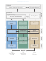
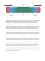
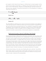
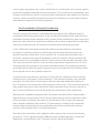
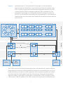
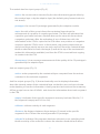
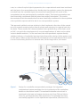
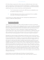
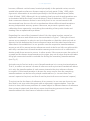
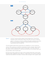
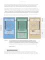
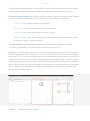
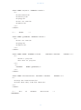
Figure 1.
The DAC theory of mind and brain and its components proposes that the
brain is based on four tightly coupled layers called: soma, reactive, adaptive
and contextual. Across these layers we can distinguish three functional
columns of organisation: exosensing, the sensation and perception of the
world (left, blue); endosensing, detecting and signalling states derived from
the physically instantiated self (middle, green); and the interface between self
and the world through action (right, yellow). The arrows show the primary
flow of information mapping exo- and endosensing into action defining a
continuous loop of interaction with the world. At each level of organisation,
increasingly more abstract and memory dependent mappings from sensory
states to actions are generated.
DAC proposes that solving H5W depends critically on the interaction between
several layers of control that continuously cooperate and compete for the
control of action (Fig.1). The somatic level (SL) of DAC designates the body
itself and defines three fundamental processes: exosensing of states of the
environment, endosensing of states of the body and its essential variables of
survival, defining needs and actuation through the control of the skeletal-muscle
system. The reactive layer (RL) comprises fast predefined sensorimotor loops,
i.e. reflexes and stereotyped behaviours that support the basic functionality of
the SL, together with the control signals that drive and modulate the engagement
of higher control layers and their epistemic functions. These sensorimotor loops
are organised in fundamental and opposing behaviour systems that can be
characterised as the 5Fs of fight, flight, freeze, feed and fornicate (Gray), and
others would include seeking, care and play (Panksepp). These basic behaviour
systems encapsulate sets of essential variables defined by the SL and put in place
operational procedures to maintain them in dynamic equilibrium-supporting survival.
DAC proposes that the fundamental organisation of these basic behaviour systems
is along two dimensions of attraction and aversion and that they are differentiated
in terms of their specific triggering stimuli and specific motor programmes. Each
of the RL reflexes is triggered by low complexity signals largely, but not exclusively,
conveyed through proximal sensors, to ensure fast operation and genetic
prespecification. In addition, each reflex and behaviour system is directly coupled to
specific internal affective states of the agent or valence markers. In this way reactive
behaviour serves not only the reduction of needs as proposed by Hull but is also
labelling events in affective terms to serve epistemic functions such as the tuning
of perceptual systems to pertinent states of the world, shaping action patterns and
composing goal-oriented behavioural strategies realised at subsequent levels of
the DAC architecture. Hence, the primitive organisational elements of the reactive
layer are sense-affect-act triads and the activation of such a triad triggers action and
carries essential information on the interaction between the agent and the world
that is a key control signal for subsequent layers of the architecture.
32
Distributed Adaptive Control: A Primer
The adaptive layer (AL) extends the predefined sensorimotor loops of the reactive
layer with acquired sensor and action states. Hence, it allows the agent to
escape from the strictly predefined reflexes of RL through learning. The AL is
interfaced to the full sensorium of the agent, its internal needs and effector
systems receiving internal state information from RL and in turn generates
motor output. The AL constructs a state space encoding of both the external and
internal environment, together with the shaping of the amplitude-time course of
the predefined RL reflexes. It crucially contributes to exosensing by allowing the
processing of states of distal sensors, e.g. vision, haptics and audition, which are
not predefined, but rather, are tuned in somatic time to properties of the interaction
with the environment. The acquired sensor and motor states are in turn associated
through the valence states signalled by the RL, following the paradigm of classical
conditioning where initially neutral or conditioned stimuli (CS) obtain the ability
to trigger actions, or conditioned responses (CR), by virtue of their contiguous
presentation with intrinsically motivational stimuli or unconditioned stimuli (US)
as introduced by Pavlov. The AL expands the sensorimotor loops of RL into sensevalence-act triplets that are now augmented through learning to assimilate a
priori unknown states of the world and the self (affect and action). In this way
the AL allows the agent to adapt to and master the fundamental unpredictability of
both the internal and the external environment.
Overall, the AL allows the agent to overcome the predefined behavioural repertoire
of the reactive layer and to successfully engage an a priori unpredictable world.
The behaviour systems of the reactive layer combined with the perceptual and
behavioural learning mechanisms of the adaptive layer allows the DAC system to
bootstrap itself to deal with novel and a priori unknown state spaces, in this way
solving the notorious symbol grounding problem that lead to the demise of classical
artificial intelligence and a range of other approaches (Searle, 1980). However,
the adaptation provided for by the AL occurs in a restricted temporal window of
relatively immediate interaction, i.e. up to about one second. Thus, in order to escape
from the ‘now’, further memory systems must be engaged that are provided by the
contextual layer of DAC.
The contextual layer (CL) of DAC allows the development of goal-oriented behavioural
plans comprising the sensorimotor states acquired by the AL (Fig. 1). The contextual
layer comprises systems for short-term, long-term and working memory (STM, LTM
and WM respectively). These memory systems allow for the formation of sequential
representations of states of the environment and actions generated by the agent.
The acquisition and retention of these sequences is conditional on the goal
achievement of the agent as signalled by the RL and AL. CL behavioural plans can
be recalled through sensory matching and internal chaining among the elements of
the retained memory sequences. The dynamic states that this process entails define
DAC´s WM system.
33
2 | DAC Theoretical Framework
The CL organises LTM along behavioural goals, and we have shown, that this
together with valance labelling of LTM segments is required in order to obtain
a Bayesian optimal solution to foraging problems. Goals are initially defined in
terms of the drives that guide the behaviour systems of the RL, such as finding a
food item (i.e. feed) or solving an impasse (i.e. flight). Goal states, as termination
points of acquired behavioural procedures or habits, together with the behavioural
sequence itself, exert direct control over how decision-making and action selection
are performed. DAC realises this so-called goal and sequence fidelity by including
a memory-based bias term in decision-making: if segment n of sequence k is
associated with the executed action it will reduce the activation threshold of its
associated segments in order to influence their perception-driven activation.
DAC proposes that the H4W challenge is solved through a multi-layer architecture
that increasingly depends on memory to bootstrap predefined need reduction
reflexes to acquired goal-oriented behaviours. These layers are tightly coupled
and cannot be seen as independent encapsulated modules. Rather, each layer
is predicated on the semantics and/or control signals generated by the other
layers. As such we can see that ‘what’ and ‘where’ span a column of processing
stages across the layers of the architecture that all deal with states of the world.
‘Why’ spans across the layers reflecting states of the self, from needs to goals
and utility. ‘When’ is encapsulated within the learning and memory mechanisms
of AL and CL supporting timing and sequencing. Finally, ‘how’ defines a last
column of processes across the layers of the DAC architecture that define action
orchestration and selection.
How can this proposal of layers and columns be a theory of consciousness? Well
now we are in a position to map GePe to DAC:
1. Grounded in the experiencing physically and socially-instantiated self:
the SL constitutes the foundation of the embodied hierarchy.
2. Co-defined in the sensorimotor coupling of the agent to the world:
the RL and AL both establish immediate sensorimotor loops with the world.
3. Maintained in the coherence between sensorimotor predictions of the
agent and the dynamics of the interaction with the world: the AL relies
on prediction-based systems for both perceptual and behavioural learning.
4.
Combines high levels of differentiation (each conscious scene is unique)
with high levels of integration: the CL integrates across all sensory
modalities and memory systems and provides selection mechanisms to
define a unique interpretation of the state of the world and the agent.
34
Distributed Adaptive Control: A Primer
5.
Consciousness depends on highly parallel, distributed implicit factors
with metastable, continuous and unified explicit factors: the CL integrates
memory-dependent implicit biases in decision-making and interpretation
of states of the world with explicit perceptual states.
It would be premature to say that DAC has explained consciousness but we can
observe that it does capture the main components of an integrated theory of
consciousness while advancing a concrete research agenda that poses specific
questions on perception, emotion, cognition and actions structured along H4W.
References
Dobzhansky, T. (1973) Nothing in biology makes sense except in the light of
evolution. The American Biology Teacher 35 (3) p.125-129.
Hampshire, A., Highfield, R., Parkin, B. & Owen, A. (2012) Fractionating Human
Intelligence. Neuron 76 (6). p.1225-1237. Footnotes
1. The other two being the origins of the universe and of life on which significant progress has been made in the 20th century.
35
2 | DAC Theoretical Framework
Cybernetics
Control
Cybernetics was originally defined by Wiener (1948) as ‘the scientific study of control
and communication in the animal and the machine’. In this sense, DAC belongs to the
cybernetic field as it aims at explaining behaviour generation in embodied agents, be
it to understand the brain of animals or to build sentient artefacts. By building control
systems that allow a sensorimotor device (i.e. a robot) to react to environmental
changes or to reach a specific state, we are borrowing principles about how such
things are achieved in biological beings. We are also challenging our standpoint in
this domain by proposing alternative and improved models that may bring additional
hypotheses and constraints to our view about wet brains. Specifically, this deals with
adaptive control, which builds upon reactive control mechanisms in order to provide
an increase of the control quality through experience. In order to reach a system
that can experiment and learn from its own actions, a more basic level of control is
required. From an evolutionary point of view many behaviours that facilitate survival
(e.g. motor reflexes, contact avoidance, foraging) could be achieved in simple ‘hard
wired’ ways that would require none or few learning capabilities. However, learning
from experience at the lifetime scale is a feature that offers an even greater ability
to survive, especially combined with mechanisms such as teaching and learning
from observation. Without entering any consideration between innate and acquired
mechanisms, it is reasonable to assume that the combination of both control system
levels allows an overall improvement of the sustainability of the agent.
Perception-Action System
The main point of any control system is to create a transformation from a
perceptual input to a command that is addressed to an effector. An effector can be
a muscle/motor, the release of a chemical substance, or whatever leaves a signal in
the world (e.g. physical contact, light, sound signals, chemicals). The perceptual side
can be decomposed into:
1. Exteroception: perception of signals originating from the outside world,
including from other agents. 2. Interoception: perception of signals originating from the agent’s own
body, such as physiological substances (e.g. hormonal levels, sugar
level), as well as the whole limbic system describing the emotional state.
36
Cybernetics
Through action, the agent in the world will produce a mixture of interoceptive
and exteroceptive signals. The term perception refers to a generic combination
of exteroception and interoception, and represents a generic signal to be used as
an input by a control system. With all its simplicity, the combination of elementary
perception action loops can give rise to what will appear as complex, goal-oriented
behaviour. The Braitenberg vehicles are a famous example (Braitenberg, 1986). The
simplest kind of Braitenberg vehicle had just two perception-action loops, where a
light sensor was coupled to a motor controlling a wheel. Having the light sensors in
opposite sides of the vehicle’s front, and the wheels set up in parallel, very simple
arrangements of the control loops resulted in the robots moving towards or away
from a light source or even circling around it. An external observer would then attribute
special characteristics to each vehicle, for instance, the characteristic of ‘fear’ to the
vehicle that when it perceives a light will escape in the opposite direction, since it will
appear that this vehicle prefers to remain unnoticed in dark places (see Fig. 1).
+
+
+
+
Figure 1. Example of Braitenberg vehicles expressing ‘fear’ and ‘love’.
These synthetic examples of direct sensorimotor coupling driving navigation has
its biological counterpart in bacterial chemotaxis. Bacteria can orient themselves
towards food sources or flee poison provided that chemical receptors result in the
excitation of their ipsilateral or contralateral motor effectors, the flagella.
37
2 | DAC Theoretical Framework
Perpection-Action-Feedback Loop
During the Industrial Revolution arose the problem of needing to automatically regulate
the performance of machines. An earlier example of automatisation was posed by the
steam engine machine which was used to power factories. The power was delivered via
a spinning wheel and it was desirable that the amount of power stayed as consistent
as possible, that is, that the wheel rotated at a consistent speed. For this, the machine
had to sense its own speed and adjust the amount of fuel needed to increase or
decrease it within a narrow range. This was achieved by a centrifugal governor, a
mechanical device that solved this sense-act problem. The proliferation of these types
of automatisation problems, sadly fuelled by the technological developments occurring
during the Second World War, gave rise in the 20th century to the control engineering
discipline and a body of theoretical work known as control theory. From a control
perspective the solution to the problem of the steam engine machine relies in the socalled feedback control. A feedback controller compares the actual performance with a
desired one and applies a corrective action to reduce the mismatch.
The minimal requirement for setting up a feedback controller is knowing in which
direction to act in order to reduce the mismatch between the desired and actual state.
In control theory terms, this mismatch is referred to as the error. Likewise, once we
detect that we are in an undesired state, we can react to avoid it. For instance, if an
object burns the tip of our fingers, flexing the arm will help to avoid the contact with
the source of heat whereas if the heat is felt in the back of the hand, extending the
arm will be the correct action. Another example of this mechanism is found in the
pupillary light reflex (PLR) which adapts the diameter of the pupil in order to maintain
the quantity of light hitting the retina and balances the levels of lightness/darkness
of a scene. This example also introduces the concept of homeostasis which is the
act of maintaining a system in a desirable state through action upon effectors that
have direct consequences at the input level. In the case of the PLR, a specific range of
luminosity is acceptable and desired. If the input sits outside of this range the reflex
will either dilate the pupil in order to allow more light in, or on the contrary contract it to
reduce exposure.
By comparing the perceived state to the target state a feedback controller gets an
estimation of the error, and subsequently acts to minimise it. If the variable being
regulated is an internal state of the agent, like body temperature, blood sugar concentration, or emotional state, the act of maintaining this process within a physiologically
adequate range is known as homeostasis. A living organism, as well as complex
artefacts, have many homeostatic modules, each one controlling different variables.
This type of formalism, depicted in Figure 2, is present at multiple behavioural levels
that can be extended beyond the simple reactive mechanism. In particular it also
defines the formulation of the drives mechanism that acts as the root for motivation of
autonomous living systems.
38
Cybernetics
Under homeostasis
Homeostatic range
Action A
Ideal Target Regime
Figure 2.
Over homeostasis
Action B
Homeostatic range.
The feedback control scheme is applied by engineers to deal with many automation
problems, but more importantly, it is used by living organisms at multiple levels
of behaviour. For instance, when we ride a bike, or when we stand upright, we
have the goal of maintaining a vertical position and we apply corrective actions,
through the bike handles, or activating our muscles, to stay in that position. Another
example is when the level of blood glucose rises, the pancreas releases a hormone,
insulin, which causes the liver to take up glucose from the blood and store it as
glycogen. Likewise, the blood glucose level is maintained in a desired level. Each
of these reflex arcs is an example of a perception action loop, where a perceived
state (contact with an intense heat source) causes an action (withdraw the limb)
that at its turn changes the perceived state (diminution of the heating sensation).
It is the assumption in feedback control that the action affects the perception that
caused it. The relation between these homeostatic loops may be independent, and
thus feedback loops will be arranged in parallel, with minimal interaction or conflict
between them, or in contrast in a hierarchical manner, where a general state of
equilibrium is achieved when a set of subsystems are themselves at equilibrium. It
is also possible that a same effector will be included in different loops, and in that
case there can be conflicts where two homeostatic goals require contradictory
actions. Say, that an animal is both tired and cold. For the subsystem regulating
body temperature, it will be convenient to increase the metabolic rate, for instance
through an increase of the amount of physical activity. However, at the same time
the system controlling the energy storage will push towards the diminution of
energy consumption by triggering resting activities like laying down or sleeping. This
type of situation illustrates the necessity of what we will discuss later in this book
as allostatic control: how to orchestrate the agent objectives in order to maintain a
good global inner state over time.
39
2 | DAC Theoretical Framework
Predictive Control
Reactive controllers perceive the world and react to it in a predetermined way in order
to maintain their perception in an optimal regime. They can also use an error signal as
feedback information in order to adapt to dynamic environments. However, the most
successful control can be achieved by acting in anticipation, instead of in reaction,
to error. If a system can predict its own error in the future, it can act pre-emptively to
avoid it. We refer to this as anticipatory or predictive control.
Coming back to the spinal reflex that reacts to pain perception with a flexion or an
extension of the limbs—the spino-nociceptive withdrawal reflex—the goal of this reflex
is to maintain a state of no-pain. As such, even better than reacting rapidly to the pain
perception is to avoid pain altogether. For instance, if a heavy object is falling to your
feet you will respond by retracting the feet before the object hits them. This action,
which can be subjectively experienced as a reflex, is anticipatory because it minimises
the error by avoiding its arise, and to do so, uses information coming from outside of
the reflex arc. In this case, the visual information is used to avoid a pain perception
that otherwise would have caused the activation of the spino-nociceptive withdrawal
reflex. From a control perspective, this type of control scheme is considered
feedforward since it predicts evolution of the world state in the future.
Indeed, anticipatory actions can be considered as reactive actions to predicted
states: as much as a reflex is a reaction to a perceived stimulus, an anticipatory reflex
is a reaction to a predicted stimulus. Indeed, in this case, the neurons that would
have been activated by the pain stimulus, and causing an activation of an agonistantagonist set of muscles, are driven by a neural activity, that coming from a higher
level area, can be interpreted as predicted pain. The forward model, given the current
state and its previous dynamic, predicts a signal that can then be used by the reactive
controllers mentioned above.
The very first sensorimotor contingencies upon which anticipatory actions can be
learned compose the peripersonal space of the agent. Through motor babbling, even
in pre-natal conditions, an agent is able to perceive the effects of its effectors on its
own body: through self-touch the initial body schema necessary for control of the
limbs and localisation of tactile stimuli are built. This phenomenon in humans has
been called ‘primary circular-reaction hypothesis’ by Piaget (PIaget & Cook, 1952), it
also includes the early interaction of visual and proprioceptive modality. Indeed, this
self-oriented exploration provides the learning system with very regular sensorimotor
patterns that are fully observable as they depend only on the agent status (even in
the visual case if we consider a static environment not involving much movement in
the landscape). Many of the elements composing the peripersonal space are learned
early on in development, and are therefore acting as core reactive mechanisms, thus
they blur the limit between reflexes and acquired actions.
40
Cybernetics
Whereas many of the reactive feedback actions can be innate, anticipatory actions
are acquired through experience, even in cases where they are apparently universal.
For instance, the well-known system of regulation of blood sugar also has anticipatory
components. Eating sweet food directly triggers the release of insulin into the blood
stream that occurs before the autonomic nervous system has time to measure the
increase of glucose in the blood. So, even though this is a response common to all
animals it is not a reflex arc or a feedback control system. The response, insulin
release, does not affect the triggering stimulus, sweet taste in the tongue, but instead
it allows a more successful control of the glucose level in the blood.
Other types of anticipatory control will differ markedly between
individuals since these associations are built based on regularities occurring in the
environment they experience and those may not be the same. For instance, one
can imagine that an animal living in an environment where sweet taste only comes
from artificial sweeteners will lose the anticipatory release of insulin since now the
sweet taste will no longer be predictive of an increase in blood sugar. For an agent
to acquire adaptive anticipatory responses it needs to have the capacity to capture
regularities in the environment, that is, to act in the environment and experience how
to change the world.
Learning
Learning in animals is mainly achieved by a neural substrate that provides an
interconnected network of cells that can adapt to external stimuli. The parallel
researches in brain learning mechanisms and their algorithmic counterparts
converge by categorising learning into different subclasses with different
requirements and fields of application.
Three Different Categories of Learning
Computer science defines three different categories of learning processes according
to the nature of the information available and to the goal of the task. These are
unsupervised, supervised and reinforcement learning. Such a division can guide the
implementation of the learning mechanisms of a cybernetic system and can also
help to understand the components of animal learning.
We can first introduce the different types of learning intuitively with an informal
example: consider the enormous endeavour of learning a language by being
immersed in it, as a child learns it or as an adult moving to a foreign country. Such a
task involves all three learning strategies at different stages.
41
2 | DAC Theoretical Framework
The first task we are faced with is the identification of those meaningful sounds that
are the constituents of the languages, the phonemes, from what initially constitutes
a seamless stream of speech. This will pave the way for identifying some basic
words of the language. The most important requisite for achieving this is to simply
be exposed to the speech, to hear it. Likewise, the learner will incrementally acquire
a better representation of the language sounds, which will enable identification of
them in a stream of speech. This process is an instance of an unsupervised learning
task since there is only one type of data available, the inputs, and the goal is simply
to acquire representations that will later assist in categorising them. For instance
acquiring sufficient representational accuracy to later distinguish a ‘t’ from a ‘d’. An
important phenomenon to take into consideration at this level is the simultaneous
learning of motor representation regarding how to produce these sounds. As the
infant experiments in sending commands to its vocal apparatus, he will produce and
hear sounds. This will provide the required material for learning a mapping between
a motor command and the phoneme it produces. Thus, we can see that unsupervised
learning can take place either in the pure sensory domain or in the sensorimotor one.
Secondly, as the learner begins to speak a new language, other speakers, or
teachers, will eventually correct them by explicitly providing the correct output. This
may happen at many levels, for instance, correcting pronunciation or a verb inflection.
Consider the case of verb inflection, the learner will know the correct form to use
the next time that same or a similar verb needs to be used in the same grammatical
context. In computational terms this process would be classified as supervised
learning. In supervised learning the learner is provided with examples of how to map
from the input to the output. In this example, we have the verb (e.g. 'to eat') and the
grammatical context (e.g. third person singular, past tense) as the input and the
target inflected form as the output (e.g. 'ate' instead of 'eated').
Finally, the use of language has the pragmatic value of achieving a communication
goal. If this goal is achieved, e.g. the kid gets her baby bottle, that success will
reinforce the learner to repeat that same communication when a similar situation
reoccurs. On the other hand, if the communication fails, she will be motivated to try
a different strategy. This is an example of a reinforcement learning process. In this
case, given a certain state and a goal, he or she will produce an output, for instance
an action. Subsequently, the learner will evaluate the outcome as a success or a
failure, or more generally, in terms of reward, lack of reward or loss. One should not confuse these computational descriptions of the general learning
categories with their particular implementations or algorithms proposed in the
machine learning literature. From a DAC framework perspective, and more in general
from a cybernetics perspective, these descriptions anticipate the types of problems
that an autonomous system will have to solve, but not all algorithmic solutions are
relevant for our approach.
42
Cybernetics
Indeed, one can recast some animal learning processes, such as classical
conditioning or perceptual learning, in terms of supervised and unsupervised learning,
and then, more importantly, one can ask how does the neural substrate implement
the required learning mechanisms? What follows is a description of the three types of
learning, and how they are used within different components of DAC.
Unsupervised Learning—Perceptual Learning—Cortex
Unsupervised learning involves only inputs, without feedback. Essentially, it extracts
the prototypes that best represent the input space in terms of its statistical
properties. Unsupervised learning has been proposed to occur mainly at the
cortical level and creates abstract representations of concepts ranging from pure
sensorimotor units (e.g. a hand posture, a circular shape, etc.), to higher-level amodal
concepts (e.g. a tool, an animal, etc.).
Following these learning processes, a learner can efficiently represent a highdimension input space (i.e. perceptual world) by compressing it into a low-dimension
representation space. This low-dimension space can be excited by bottom-up
perceptive input, therefore activating a specific perceptual archetype (i.e. concept)
or used in the top-down direction by recreating the sensory signal associated with a
specific archetype.
One can formulate the goal of unsupervised learning as the minimisation of a
loss function that is defined as the mean distance between the input data sample
(e.g. words, faces, abstract concepts, etc.) and the representations of the items
stored in the system (these representations are referred to as prototypes). As an
abstract illustrative example, one can imagine that both the input stimuli and the
prototypes are coded as vectors, such that we can define a distance between inputs
in the same way that we can define a distance between two points in a map. The
smaller the distance, the more faithfully the stored prototype represents that item. As
a further example, consider the difference, between, say, individual perceptions of the
phoneme /t/ and the internal representation (or representations) of the /t/ phoneme.
In neural terms, we can informally interpret that the prototype(s) of a given
input are encoded in the neurons that activate the input stimulus. In general, the
larger the neural response to a stimulus, both in number of neurons and in the
intensity of their response, the larger the stimulus representation in the brain (or, in
abstract terms, the smaller the distance between the input stimulus and its closer
prototype). However, the capacity of the brain is bound, not allowing it to store
an accurate representation of all the stimuli perceived through life. Thus, stored
representations are generalisations that mostly reflect the regularities in the input
domain. Indeed, minimisation of the average loss function suggests that more
43
2 | DAC Theoretical Framework
frequent items should be more faithfully represented. In other words, a supervised
learning process will provide more representational resources, memory or neural
tissue, to the more frequently encountered stimuli.
The process known as perceptual learning, which consists of increasing the
granularity of the sensory representations, is underpinned by an unsupervised
learning process. Clearly, an animal recognises stimuli that it has previously
experienced more accurately, than the ones it has not. In humans, we can come back
to the language example: when we listen to some speech, we do not recognise the
phonemes of a second language as distinctly as we do with the ones of our first
language. And, obviously, we have been exposed more often to the phonemes of our
own language than from another language learned later in life. However, frequency alone might be a poor indicator of what needs to be stored in
memory. Indeed, some relevant but infrequent stimuli should nonetheless be faithfully
represented. To address this issue mathematically, we can set a loss function where
the mean distance between input and prototype is weighed by a relevance factor.
Then, our perceptual knowledge will not only reflect our sensory history in terms of
frequency, but also in terms of the relevance of the stimuli.
In computational neuroscience, the cerebral cortex has been associated with
unsupervised learning processes. Especially in the early sensory cortices, extracting
perceptual archetypes, but also arguably in the cortical motor areas, such that
recurrent patterns of coactivation can be stored as motor primitives. Back to perceptual learning, the phenomena of the reorganisation of the cortical
sensory areas, can be seen as a vast unsupervised learning process. For example, the
A1 area of the auditory cortex is tonotopically organised according to the stimulus
frequency, in other words, neighbouring neurons respond to stimulus of similar
frequencies. Different animals, mice, monkeys and humans cover different ranges
of the frequency spectrum, likely reflecting both evolutionary and environmental
constraints. But this organisation is not static and can rapidly adapt, reflecting
sudden changes in the animal’s environment. For instance, a mother becomes rapidly
attuned to the sound frequency of her newborn’s cry.
Experimental psychologists have reproduced this process of retuning the auditory
cortex to increase the response to stimuli that suddenly become more relevant. For
example, in the paradigm of fear conditioning an animal, such as when a rat hears
a pure tone sound—the conditioning stimulus (CS)—which precedes an electrical
footshock. Using electrophysiological measurements, it has been shown that after
very few trials of paired stimulation, the rat’s neural response to the CS increases
dramatically. i.e. both the response of individual neurons and the number of neurons
attuned to the CS increase.
44
Cybernetics
This mechanism of the relevance-modulated building of sensory representation, or
sensory maps, has been reproduced in several works inspired by the DAC framework,
for instance, the reorganisation of the auditory cortex in response when a neutral
conditioning stimulus is associated to a naturally aversive one. As the machine
learning field grew, several unsupervised learning models have been proposed which
all follow the same principle. The historical example and most simple instance of
learning implementation is the Hebbian rule which is based on the observation that
two neurons firing together tend to facilitate the synapse between them in order to
increase their coactivation over time. Mathematically, the simplest formalisation of
this principle is as described in Equation (1) where Wij represents the connection
weights between neurons i and j, Xi represents the activity of neuron i and Xi the
activity of neuron j.
Equation (1)
Assuming that a group of neurons is wired together and receive input from external
sources, this learning rule will tend to create clusters of neurons that will be
simultaneously active for specific input patterns. These clusters will adapt as much
as possible to fit the statistical properties of the input space and to categorise it into
classes. A simple example of this principle is the Hopfield network: by observing
the receptive field of a specific neuron it is also possible to recreate the input signal
prototype that it is encoding for, therefore allowing the example retrieval of the whole
signal from partial cues.
Supervised Learning—Classical Conditioning—The Cerebellum
Mathematically, supervised learning aims to fit a function that maps elements
from an input to an output space. Given an input X and an output Y, the goal of
supervised learning is to approximate F such that Y = F(X). As in the previous case
of unsupervised learning, for supervised learning we define a loss function that
measures the difference between the output produced by the system and the correct
output, that is given to the system. The goal of the learning process is to minimise
that mean difference.
Learned anticipatory control can, in some cases, be understood as the outcome of
a supervised learning process. Consider the case of classical conditioning introduced
previously. In a classical conditioning setup, the neutrality of the CS causes the
naive animal not to respond to it. In other words, he implicitly produces an output to
the CS stimulus that is a no-action. However, as the animal closes the eye to minimise
45
2 | DAC Theoretical Framework
the disturbance caused by the introduction of a puff of air pointed directed towards
it, such activation of the sensorimotor loop becomes an error signal indicating that the
eyes should have been closed at the arrival of the Unconditioned Stimulus (US). With
this in mind, we can interpret the eyeblink conditioning setup as a supervised learning
problem where the input is provided by the CS, the agent’s output is whatever action
is taken or not taken in response to that CS, and the US presence dictates that the
correct output should have been to close the eye. Therefore, we can see that acquiring
an anticipatory avoidance reflex can be seen as the result of a supervised learning
process. The DAC framework situates this kind of process in the adaptive layer.
In classical conditioning, learning occurs principally in the cerebellum which suggests
that the cerebellum should implement a supervised learning algorithm. Indeed, in the
cerebellar cortex it is possible to identify all the information pathways that would be
necessary for carrying all the inputs and outputs involved in a supervised learning
problem. Coming back to the eyeblink example, there is an area in the cerebellum where
the output of a particular class of neurons, the Purkinje cells, controls the eyelid closure.
These neurons are powerfully innervated by the climbing fibres, originated in the inferior
olive. These climbing fibres signal the activation of the reactive loop of the eyelid closure,
that is triggered by the US. The CS stimulus information reaches these same cells
via the parallel fibre, a different and segregated pathway. From a supervised learning
perspective, the Purkinje cells receive an input (the CS—via the parallel fibres), produce
an output (through their axons) and receive an additional input signal that indicates the
correctness of the output (via the climbing fibres). Over trials, the climbing fibre signal
will adjust the transformation of the parallel fibre input into an output such that the cell
will respond to the CS with a timely command to close the eyelids. In this case, by having provided the desired output, it is possible to adapt the transformation in the right direction, using gradient descent for example. At the lowest level
it allows the agent to learn the sensorimotor changes induced by a motor command. In general, a supervised learning system can be used to predict the consequences
of a specific action given a specific context. This predictive mechanism can then be
used in the context of forward chaining (i.e. predicting the consequences of several
successive actions) or backward chaining (i.e. inferring the goal, or initial state that led
to plan the execution).
The artificial neural implementation of supervised learning, extends unsupervised
learning principles such as the Hebbian rule. Layout of neurons and connections can
lead to a situation where the activity of certain neurons depends only on other neurons
of the network and not directly on the input to the system. Such an organisation is
typically the multilayered architecture deployed by multilayer perceptron (MLP) or Deep
Learning models. In such a case the neurons are segregated into two categories: the
one activated by the external input to the system (Input layer, Xi), and the one receiving
46
Cybernetics
pre-synaptic activity from the input layer (or a hidden layer) and post-synaptic activity
from a desired output (Output layer, Yi). Following, the predicted activity of the output
layer Ŷi can be formulated as in Equation (2) with ƒ() being the activation function of
the neuron (e.g. sigmoid). The learning mechanism lies in the adaptation of weights as
expressed in Equation (3)
Equation (2)
Equation (3)
The main difference with the previous case of unsupervised learning is the apparition
of the teaching signal as a difference between the current prediction computed from
the input and the current real signal observed. The coefficient λ represents the speed
of adaptation of the weights and is a parameter common to most of the supervised
learning algorithms. It can be set either in a fixed or adaptive manner, as a way for
example to emulate neuromodulators of learning like dopamine or acetylcholine.
Reinforcement Learning—Operant Conditioning—Basal Ganglia
Reinforcement learning is different from other types of learning in the sense that it does
use feedback about the prediction, but it is only qualitative (i.e. good or bad) and therefore does not have explicit access to the optimal direction to follow in the landscape of
possible transformations. It is tightly linked to the concept of reward, which we frame
as the general improvement of the inner state of the agent. More than the sensorimotor
consequences of an action, reinforcement learning can be used to predict an expected
reward, making it the ideal candidate to deal with action selection at the behavioural
level. The main brain structure dealing with reinforcement learning is the basal ganglia,
especially the striatum, which receives input from the substantia nigra and occurs in
dopamine release, therefore increasing or decreasing the plasticity of synapses.
Reinforcement learning is the main way of dealing with action selection. Considering
that an agent’s goal is to maximise the overall reward it will get from its actions in the
future, reinforcement learning provides the predictive mechanism necessary to select
actions in order to achieve such a maximisation.
47
2 | DAC Theoretical Framework
Another crucial part of reinforcement learning lies in its ability to work on the output
of supervised learning; since you can consider the quality of a prediction an intrinsic
reward, it allows you to select the action that will make you learn the most. Such a
process can be used to guide exploratory behaviours like motor babbling to portions
of space that are more likely to benefit the agent in terms of its representation and
prediction capabilities. This has been used to make behavioural patterns such as
walking emerge from motor babbling. Machine Learning and the Behavioural Feedback
Historically, machine learning did not evolve to explain the generation of adaptive
behaviour in autonomous agents. Its goal instead was centred on the practical
development of information processing applications that, for instance, classify
images automatically, forecast the evolution of the stock market, and produce
automatic translations, among others tasks. Indeed, the idea that embodiment
imposes constraints for a learning algorithm is not usually considered in the
machine learning literature, and, on the other side, the use of machine learning
techniques usually assumes requirements not met by a behaving agent.
For instance, an agent’s learning depends on its experience, but since an active
agent determines his experiences through behaviour, the shaping of the behaviour
through learning will change the agent’s experiences. Such a tight link between
the structure of perception and behaviour is referred to as behavioural feedback.
In an adaptive system, by way of behavioural feedback, the inputs at the onset
of a learning process will differ from the ones received by the end of it. This
observation, which might seem completely trivial for the layman, violates one of
the assumptions usually taken in the machine learning connectionist literature,
that is, that input samples are independent and identically distributed (i.i.d.). This
is, that the algorithm draws input samples as though they were lottery pellets
randomly extracted from a bag. Violation of the so-called i.i.d. assumption does
not immediately disqualify connectionist solutions as an explanation of learning in
biological systems. However, it does implicate that the findings or constructs from
the machine learning connectionist literature may not be translatable to the domain
of embodied adaptive systems.
Behavioural feedback affects even the simplest learning paradigms. For instance, in
an avoidance learning paradigm, such as the conditioning of the eyeblink response
with a puff of air, an animal learns to produce an adaptive response that anticipates
a perturbation. However, classical conditioning is an unconscious learning process
that is driven by the sensory perception of the airpuff alone, not by a categorical
knowledge about the stimulus presence, and learning affects the perception of the
airpuff. In the naive animal the puff of air reaches the unprotected cornea, causing
48
Cybernetics
a strong pain perception, but as the animal learns to anticipate it, the closing eyelids
protect the eyeball lessening the pain perception. Thus, even in this elementary case
of supervised learning, there is a sensorimotor contingency that makes it so that the
sensory state successfully predicted at the end of learning is not the same sensory
state that was experienced at the beginning. Two Phase Model of Classical Conditioning
Even the simplest processes of animal learning might involve different types of
computational learning processes. So far, we have separately introduced relevancemodulated unsupervised learning in the context of fear conditioning, and supervised
learning in the context of classical conditioning, but a finer analysis will reveal that in
classical conditioning we can already individuate both learning processes.
In the 1960s the Polish psychologist Konorski proposed that the associative
processes underlying classical conditioning can be separated into a fast nonspecific learning system and a slow specific one. He proposed that after just a
few trials of paired tone-airpuff stimulations, the non-specific learning system will
indeed acquire the knowledge that the CS precedes a motivationally relevant event.
This first process will result in a non-specific preparatory response to the CS, such
as freezing the body position. As paired stimulation trials accumulate, the animal
gradually builds a specific motor response tuned to counteract the US effect, which
in the airpuff case is the eyeblink response.
In general, the more salient a stimulus is, the higher its capacity to induce plastic
changes; this is, the faster it drives learning. Thus, besides eliciting a non-specific
response, the first phase of learning boosts the internally attributed saliency of
the CS stimulus, increasing the neural response to the tone. This increased response
may enable learning in cases where the initial response of the sensory cortices to
the CS was insufficient to recruit the plasticity mechanism of the cerebellum.
Whereas the cerebellum interprets the US-evoked activation of the climbing fibre
signals that a concrete motor action should have been produced, activation of the
nucleus basalis, evoked by the same US, broadcasts to the cortex the message
that a relevant stimulus was received. This message is coded by the unspecific
release of the acetycholine a neuromodulator, that once reaching the sensory
cortices, will converge with CS-evoked activation. Therefore, the acquisition of an adaptive reflex requires two concurrent learning
processes. This is captured by the different levels of implementation of the DAC
framework, as described in the ‘Tutorials’ section of this publication.
49
2 | DAC Theoretical Framework
References
Braitenberg, V. (1986) Vehicles: Experiments in Synthetic Psychology.
Piaget, J. & Cook, M. (1952) The Origins of Intelligence in Children.
Wiener, N. (1948) Cybernetics: Or Control and Communication in the Animal
and the Machine.
50
Cybernetics
51
3 | DAC Tutorial on Foraging
3 | DAC Tutorial on
Foraging
52
DAC5
DAC5
DAC is based on the fundamental assumption that foraging can be explained
on the basis of the interaction of three layers of control: reactive, adaptive and
contextual. DAC5 was proposed as a model for classical and operant conditioning
(Pavlov, 1927; Thorndike, 1911; Verschure, 1998). The reactive layer provides a set of
reflexes allowing the system to interact with the environment—unconditioned stimuli
(US) to unconditioned response (UR). The adaptive layer is a model of classical
conditioning and fulfills a two-fold task. On the one hand it learns to associate the
conditioned stimuli (CS) to the UR, forming the conditioned response (CR). On the
other hand, it forms internal representations of the CS used by the contextual layer.
The contextual layer is a model for operant conditioning; it provides the system with
short- and long-term memory structures. The sensorimotor contingencies formed at
the level of the adaptive layer are acquired and retained in these memory structures,
forming behavioural sequences. The representations stored in the contextual layer
are constantly matched against the ongoing perceptions allowing for the retrieval
of successful behavioural sequences in similar contexts.
The prototypical robot test case for DAC5 is a foraging task in an open arena. In
this task, the robot, equipped with proximal and distal sensors, explores the arena in
search of light sources while avoiding collisions with the surrounding wall. Coloured
patches scattered on the floor serve as landmarks for the navigation. In the
framework of classical conditioning, the proximal (e.g. distance and light) sensors
serve as aversive and appetitive USs. Close to the light or at a collision a UR is
triggered such that the robot approaches the light or turns away from the wall. The
coloured patches serve as CSs.
Reactive and Adaptive Layer
In DAC5, the adaptive layer learns sensorimotor contingencies generated
by the reactive layer and forms internal representations of the environment
based on the classical conditioning paradigm (Pavlov, 1927). An unconditioned
stimulus US triggers an unconditioned response UR (see Fig. 1). A US event also
induces activity in populations of units which reflect an internal state (IS). Learning
consists of associating a conditioned stimulus CS to the US such that after learning,
the CS on its own can trigger a conditioned response CR (see Fig. 1). In doing so
it combines perceptual and behavioural learning. Behavioural learning associates
the different CSs to the correct CRs. Perceptual learning compresses the higher
dimensional CS to the lower dimensional CR.
53
3 | DAC Tutorial on Foraging
CS
y
W
x
CR
Adaptive
IS
e
U
V
r
Light
sensors
Camera
Figure 1.
UR
a
Reactive
US
Motors
Somatic
AS
s
U
The Adaptive and the Reactive layer: squared boxes stand for neuronal
groups, arrows stand for static (solid line), and adaptive (dashed line) synaptic
transitions between the groups.
We define the following abbreviations for the activities in the different cell groups:
a
Usually the dimensionality N of the CS is higher than the dimensionality K of the IS.
The dimensionality M of the US is in general but not necessarily similar or equal to
the dimensionality K of the IS cell group. In the general case the activity of the US and
the CS cell can be a nonlinear function of the sensor readings. Usually, however, the
function is the identity function. With these definitions the forward dynamics of the
adaptive and reactive layer can be written as:
54
DAC5
The US cell group can be comprised of neurons for different values of USs such as
appetitive and aversive stimuli. To simplify the notation they are all represented in the
vector s. The predefined weight matrix V determines what actions are triggered by the
different states of US. It connects the elements of US to specific elements of IS and
thus via the action selection AS sets specific actions. W describes the association of
CS to IS and is subject to learning. The slow dynamics describing the change of the weights W follow the learning rule
called correlative subspace learning (CSL) (Duff et al., 2011):
The parameter η is the learning rate and may vary with time. Learning is driven by the
two product terms
and
. The parameter varies between -1 and 1
and balances the influence of the two terms
and
on learning. With a of -1
only
drives learning and for a of 1 the learning dynamics are determined by
only. The term
is related to the auto-correlation of the CS. With the assumption
that the learning rate is small and the mean of x over time is zero, we can regard
as the instantaneous estimate of the real auto-correlation. Thus, we can identify
this term with perceptual learning as it depends only on the CS. The term
relates
to the correlation of the CS and the UR. Again it can be seen as the instantaneous
estimate of the real correlation. We identify this term with behavioural learning as it
contributes to learning the association between the CS and the UR. However, with
only these two terms the weights would grow exponentially and never converge. The
negative normalisation term -W y depresses the weights and assures convergence.
The parameter allows to control the influence of the terms
and
on
learning, and thus allows to balance perceptual and behavioural learning. With a of
-1 learning is only driven by the CS and the learning rule corresponds to the subspace
learning algorithm proposed by Oja. A of -1 corresponds to purely perceptual
learning.
The perceptual representations defined by the extracted subspace are the so-called
prototypes defined as
. The prototypes are the basic elements used
to store and recall action sequences in the long-term memory of the contextual
layer (Verschure, 2003; Verschure, 2003a). The prototype corresponds to the linear
projection of x to the learned subspace defined by the weight matrix W. Thus the
prototypes directly depend on the extracted subspace and the parameter allows
to control if the prototypes are defined more by the auto-correlation of the CSs or
by the correlation between the CS and the UR. What is the optimal balance between
perceptual and behavioural learning, i.e. what is the optimal value for is not clear in
advance and will strongly depend on the task at hand and the statistics of the CS and
55
3 | DAC Tutorial on Foraging
the UR. In this way, the adaptive layer fulfills its twofold task of learning the sensory
motor associations and forming internal representations, i.e. the prototypes e for the
planning system of the contextual layer.
Contextual Layer
The contextual layer provides mechanisms for memorising and recalling behavioural
sequences. It comprises two memory structures: a short-term memory (STM), and a
long-term memory (LTM) for the permanent storage of information (see Fig. 2 below).
These allow the system to acquire, retain and express sequences of the sensorimotor
contingencies the adaptive layer generates. The acquisition of information into
memory is done in two steps:
1. Sensorimotor events generated by the adaptive layer are stored in the STM, forming a behavioural sequence.
2.
When a goal state is reached the sequence of sensorimotor events stored
in the STM are copied into the LTM and the STM is initialised.
The information stored in the LTM is then recalled to reach goal states, as follows:
1.
Whenever a new sensory event is generated it is compared with all the
ones stored in the LTM.
2.
The segments of the LTM that are similar enough (similarity defined by
a matching criteria) to the generated one are retrieved.
3.
Retrieved segments from memory contribute to compute the selected
action.
4.
The selection of segments from the LTM is biased by previous experience
to achieve sequential chaining
56
DAC5
Figure 2. Contextual layer: (1) The generated CS prototype e from the adaptive
layer and the executed action a are stored as a behavioural couplet in the
STM. (2) When a goal state is achieved the information stored in the STM
is copied into the LTM as a sequence and the STM is initialised. (3) The
generated CS prototype e is compared with all the prototypes e stored in
the LTM. (4) The action a proposed by the contextual layer is calculated as a
weighted sum over the actions associated with the sensory events selected
from the LTM.
a1
aNS
e7 a7
a6
a2
a5
e6
STM
a3 e3
a4
e4
LTM
2
e12 a12
e13 a13
e21 a21
e22 a22
e23 a23
e2NS a2NS
eN 1 aN 1
eN 2 aN 2
eN 3 aN 3
eN NS aN NS
L
1
4
3
e15
L
L
L
L
L
L
L
1
IS
e
CS
e11 a11
e1NS a1NS
Contextual control
eNS
e2
y
W
x
CR
Adaptive
e1
U
Camera
s
r
V
Light
sensors
UR
a
Reactive
US
Motors
Somatic
AS
U
The STM is the structure that temporarily stores the behavioural sequence that is
being experienced by the robot and that did not lead to a goal state yet. It is a ring
buffer formed by a sequence of NS segments. Each segment contains the action
executed a by the robot together with the CS prototype e that was generated at
that time. When a goal state is reached the content of the STM is copied into the
LTM and the STM is initialised. The LTM contains NL sequences of maximum size
57
3 | DAC Tutorial on Foraging
of NS segments. Each sequence stored in the LTM has a value that relates to the goal
states they lead to (e. g. +1 for an aversive state such as collision, +1 for an appetitive
state such as reward).
The retrieval of the proper action from memory is based on the similarity between the
current CS prototype e and the CS prototypes elq previously stored in the LTM. This
similarity is calculated using a distance measurement as follows:
The degree of matching of segment l in sequence q determines the input to its socalled collector:
The collector determines the contribution of the segment to the final proposed
action by the contextual layer. Its activity depends on the distance d(.) between the
current generated CS e prototype and the CS elq prototype stored in segment l and
sequence q and on a so-called trigger value t that is associated with each
segment lq in memory. The trigger value is used to ensure chaining through a sequence. Its value depends on
whether the segment that temporarily precedes it in a sequence was selected in the
previous cycle. If it was not selected the trigger has a default value of 1 and therefore it
does not bias the selection of the segment. However if segment l-1 in sequence q was
selected then the trigger value of segment l in sequence q is set to a higher value than
1. This means that the collector unit associated with that segment will increase its
value and that therefore the segment will have more probability of being selected in
future decision-making. The trigger value decreases asymptotically as:
where
. When a segment is selected its trigger value is reset to 1.
The action proposed by the contextual layer is calculated using the activity of the
collectors, but only if these collectors satisfy two criteria: (1) Its activity is above
a predefined threshold (
); and (2) Its activity is inside a predefined percentage
range from the maximum collector’s activity, e. g. the collectors compete in an
E%-Max Winner Take All (WTA) mechanism (Almeida et al., 2009) in which only the
58
DAC5
collectors inside with an activation equal or greater than E% from the maximum
collector’s activity contribute to the action. These two criteria can be dynamically
adjusted so that they change their value according to the certainty or uncertainty of
the robot, e. g. when the robot is still learning it will have a low value of
and E% so
that it can take into account a greater number of proposals. The selected collectors
contribute to the contextual action as:
where
is the distance measured as the number of segments needed to reach
the goal state from the current state, i. e. distance between selected segment and
the last segment in the sequence. The plus sign means that the selected segment
corresponds to an appetitive goal state sequence whereas the minus sign means
that it belongs to an aversive goal state sequence. Only if the computed action is
positive it is executed. In this way, backwards actions are avoided.
The activation of the contextual layer depends on the quality of the generated
prototypes CS e from the adaptive layer. This quality is assessed by using a
discrepancy measure that runs an average distance between the predicted prototypes CS e and the actual CS x value:
where
defines the integration time constant and the distance d(x,e) between
actual CS x and estimated CS e prototypes. Only when this discrepancy measure
falls bellow a certain threshold (confidence threshold) the contextual layer is enabled.
An action selection mechanism receives three actions, one from each layer of the
architecture: reactive action ( ), adaptive action ( ) and contextual action ( ).
The final action executed by the robot is selected through a priority mechanism in
which the most priority action is the reactive action, then the contextual action, and
finally the adaptive action.
59
3 | DAC Tutorial on Foraging
References
de Almeida, L., Idiart, M. & Lisman, J. E. (2009) A Second Function of GammaFrequency Oscillations: An E%-Max Winner-Take-All Mechanism Selects which Cells
Fire. Journal of Neuroscience 29 (23). p.7497-7503.
Duff, A., Sanchez-Fibla, M. & Verschure, P. F. M. J. (2011) A biologically based model
for the integration of sensory-motor contingencies in rules and plans: A prefrontal
cortex based extension of the Distributed Adaptive Control architecture. Brain
Research Bulletin 85 (5). p.289-304.
Oja, E., Ogawa, H. & Wangviwattana, J. (1992) Principal component analysis
by homogeneous neural networks, Part I: The weighted subspace criterion. IEICE
Trans Inf Syst 75. p.366-375 Pavlov, I. P. (1927) Conditioned Reflexes: An Investigation of the Physiological Activity of
the Cerebral Cortex.
Thorndike, E. (1911) Animal Intelligence. Verschure, P. F. M. .J. (1998) Synthetic epistemology: The acquisition, retention,
and expression of knowledge in natural and synthetic systems. In: Proceedings
of IEEE World Conference on Computational Intelligence, Anchorage, Alaska. p.147-152. Verschure, P.F.M.J., Voegtlin, T. & Douglas, R.J. (2003a) Environmentally mediated
synergy between perception and behaviour in mobile robots. Nature 425
(6958). p.620-624.
Verschure, P.F.M.J. & Althaus, P. (2003) A real-world rational agent: Unifying old and
new. AI. Cogn Sci 27. p.561-590.
60
DAC5
61
3 | DAC Tutorial on Foraging
Tutorial 1: Getting Started
Foraging
Foraging, i.e. the capability of an animal to search and find food, critically determines
its evolutionary fitness as it plays an important role in its ability to survive and
reproduce. In behavioural terminology, foraging represents a goal-oriented
exploration for resources normally motivated by food deprivation. Foraging is
an advanced, goal-oriented behaviour where prior knowledge of an environment
and acquired behavioural strategies must be matched to the novelty and hazards
presented by an unpredictable world and the varying allostatic requirements of the
behaving system itself, e.g. energetic and reproductive needs. These constraints
are defined at varying spatial and temporal scales, where a successful forager
must simultaneously satisfy local and global constraints, such as performing
obstacle avoidance while staying on course to reach a known feeding site whilst
also allocating resources consistent with its allostatic needs. As such, foraging
represents an excellent test case for an autonomous control system.
Figure 1. Simulated agent (red cylinder with the grey dot on top) and environment for
the resticted arena foraging task. 62
Tutorial 1: Getting Started
In the following tutorials we explore how the different layers of DAC5 contributes
to solving a foraging task. In particular, we test DAC5 in a restricted arena foraging
task (see Fig. 1). The squared arena contains coloured patches and a light source
visible by the downward-pointing camera of the robot. The light intensity decays
with the distance and it is only detectable for the light sensors of the robot at a
limited distance. The robot is placed in one of the three starting positions (grey
circles) facing the patches, and the goal of the robot is to reach the light. Every time
the robot collides with the wall a new trial starts and randomly repositions the robot
at one of the three start positions. This task can be described in terms of classical
conditioning: the light serves as US where the patches serve as CSs. As in this
configuration of the task, all of the top patches have the same colour and the task is
ambiguous and cannot be solved without the context given by the bottom patches.
Thus, to solve the task it is essential for the robot to form adequate internal
representations of the bottom patches. Only stable and reliable prototypes will allow
the memory structures of the contextual layer to store and later recall the correct
actions for the ambiguous cues.
The restricted open arena foraging task isolates a core situation of an open arena
foraging task in limiting the agent to specific start positions. For an agent endowed
only with egocentric inputs, cues in an open arena foraging task are ambiguous
and the correct action can only be determined when taking into account the current
context (see Fig. 2A). If the agent comes from the left side (solid line) it has to
turn left at the red patch. If it comes from the right side it has to turn right. Thus,
the red cue is ambiguous but can be disambiguated by the patches the agent
encounters before the red patch. Figure 2B is the very same situation in a different
configuration. When restricted to the three start positions defined in figure, the agent
encounters the same stimuli as in Figure 2A; this is the configuration we use to test
the contextual layer. For the adaptive layer this configuration is not solvable since
the adaptive layer does not have any contextual information. To be able to test the
adaptive layer the red patches were disambiguated by changing the colours (Fig.
2C). In this configuration the three upper patches serve as cue patches and the three
lower patches lose their role and become distractor patches. The restricted open
arena foraging task in this special configuration is designed to assess the two-fold
task of the adaptive layer systematically. For behavioural learning, the patches
that can be associated to a US should elicit the corresponding action (CR). For the
perceptual learning all the different patches, cue and distractor patches, should be
represented in the IS, but only lead to an action if they are associated to a US. For the
distractor patches, the IS activity should remain sub-threshold.
63
3 | DAC Tutorial on Foraging
A.
B.
C.
Figure 2. Patch configuration: A. General situation in an open arena foraging
task. B. Equivalent constellation of patches as in A in the restricted open
arena foraging task. C. Disambiguation of the patches for testing the
adaptive layer that is not context aware.
In this tutorial you will get aquainted with the iqr (Bernardet & Verschure, 2010) and
the Gazebo simulation environment (Koenig et al., 2004), and learn how to control
the robot. In the remaining tutorials you will analyse the behaviour of the different
layers and how they have to be tuned in order to solve the restricted open arena
foraging tasks.
Tutorial
Start iqr and Gazebo
Gazebo and iqr work as a server-client application running on two separate
processes.
In a new terminal window (Ctrl+Alt+t to open it) start an instance of Gazebo and load
the world template that will be used throughout the entire tutorial, by typing:
cd $HOME/iqr-gazebo/DAC_files
gazebo DAC_basic_arena.world
Gazebo GUI will open with a configuration similar to the one illustrated in Figure 3.
During this tutorial and the following ones you will not need to modify any aspect of
the simulated world, nevertheless, interested readers can find the reference manual
of Gazebo at the project website (http://www.gazebosim.org).
64
Tutorial 1: Getting Started
Figure 3.
Gazebo GUI with a fly-view of the foraging task arena.
Open a second terminal window, start iqr and open the DACReactiveBug_ex system
by typing the following command:
cd $HOME/iqr-gazebo/DAC_files
iqr -f DACReactiveBug_ex.iqr
The iqr GUI will open and the DacReactiveBug controller will be in place as
illustrated in Figure 4. The system is not complete and during this tutorial you will
be required to figure out how to build the final system. A final version of the file
(DacReactiveBug.iqr) with the complete solution to the system is also provided in
the same folder.
Bug: is the built-in module that interfaces iqr with Gazebo. The small rounded icon
at the bottom right part of the Bug icon indicates that this process is interfacing with
an external module. All the necessary connections to interface iqr and Gazebo are
already made for you, but if interested you can have a look at the properties of the
process by right-clicking the Bug process icon, and selecting Properties from the
contextual menu.
Reactive layer: is the process where the mapping between the sensory stimuli and
the pre-wired unconditioned responses takes place.
Selection: is the process in charge of selecting the action to be executed. The output
of this process is a motor command that is mapped to the actuators of the robot.
65
3 | DAC Tutorial on Foraging
Figure 4. iqr GUI and the DACReactiveBug system as it appears in the diagram pane.
You can inspect each process by clicking on the corresponding tab in the tab bar,
while to change the process parameters you can double-click on the process icon
or use the contextual menu to open the Properties dialogue (right-click->Properties).
For this tutorial you don’t have to worry about changing any of the processes’
properties since all of the necessary connections were already made for you.
Now, move to the Bug diagram pane. You should see something like this:
Figure 5.
The Bug process.
The Bug process (Fig. 5) is made by an assembly of 15 different groups of neurons
that can receive inputs or send outputs from/to the Gazebo robot. The robot
66
Tutorial 1: Getting Started
comes equipped with different sensors (camera, proximity sensors, light sensors,
microphone, GPS, gripper sensor) and effectors (motor, gripper and a speaker),
but to implement the reactive layer of DAC we will only need two of them: the light
sensors that input to the Light group of the Bug process, and the motor joints that
execute the commands received from the Motor group of the process.
To get started and gain some confidence with the robot and all of its features, we
will start exploring the robot sensors and effectors. For more details about the other
available sensors we point the user to read the iqr-gazebo wiki (https://code.google.
com/p/iqr-gazebo/wiki/iqrBugFeatures).
The motors: The motors of the robot are controlled via the 9x9 neurons Motor
group (see Fig. 6) of the Bug process. The movement of the robot is computed
from the position of the cell with the highest activity in the Motor group lattice. The
Y axis represents the force applied to each joint to move the robot while the X axis
represents the Rotation applied to it.
Figure 6. Schematic representation of the Motor group mapping. The black dot
represents the stationary condition where no force and rotation are
applied to the robot wheels.
Light sensors: the robot is equipped with 32 light sensors equally spaced on the
robot body that are mapped into the Light group of the Bug process.
Camera sensor: a colour camera placed in the frontal part of the robot and facing
downwards receives information from the environment. The input of the camera
is then split into three channels (RGB is the default) and transmitted to the three
colour channel groups in the Bug process. The resolution of the camera and its input
modality can be changed in the Properties dialogue (right-click and select Properties
from the contextual menu).
67
3 | DAC Tutorial on Foraging
Exercise 1: Moving the Robot Forward
Start the simulation by pressing the Run button. Move to the Bug process diagram
pane and open the State Manipulation panel of the Motor group (right-click the
group icon and select State Manipulation Panel from the contextual menu). The
State Manipulation panel is a tool that is used to directly change the activity of
single neurons in the groups.
To move the robot forward left-click the fifth cell of the first row in the motor lattice
grid (see Fig. 7). Set it to a value of 1 and click on Add. The command will then be
added on a list in the right pane.
Figure 7. State Manipulation panel configuration to move the robot forward.
Now you can click Send to execute the command. The robot will start moving in
the forward direction.
To stop executing the command click on the Revoke button.
68
Tutorial 1: Getting Started
Q1. Which cell do you need to activate to make the robot turn to its left?
and to its right?
Q2. Which cell do you need to activate to make the robot move backwards?
Q2. How do you control the speed of the robot?
Exercise 2: Make the Robot Move Autonomously
Using the State Manipulation panel is not the most effective way to control your robot.
We want the robot to behave autonomously in its environment.
Stop your simulation and close the State Manipulation panel. Move to the Selection
process diagram pane (see Fig. 8).
Figure 8.
The action selection process.
The action selection process: this process is made up of six different groups that
define the default robot behaviour (i.e. Explore the environment) and a pre-wired
reflexive behaviour (i.e. Approach).
The most basic behaviour of the robot is to explore its environment on a straight direction.
To make the robot move autonomously along a straight path we will have to
constantly activate the exploratory behaviour of the robot. This stereotyped behaviour
can be achieved by feeding the Explore group with a constant input:
69
3 | DAC Tutorial on Foraging
Create an excitatory connection from the Const Speed to the Explore group.
Click on the red Add Connection button in the Diagram edit toolbar and then click
on the Const Speed group. Now click on one of the yellow squares at the edge of
the Explore group to connect the two groups. The Const Speed group is made up of
a single cell that is always active and represents the constant driving force for the
exploratory behaviour.
Now let’s try to make the robot move on its own.
Q1. The Motor In group is an interface to the Motor group of the Bug process.
How do you have to connect the Explore group to the Motor In group to make
the robot move forward? Connect the two groups then run the simulation to
observe if the robot behaves as expected.
Before we continue with the implementation of the Reactive layer, try to observe how
the different sensors of the robot react to the environment. Move to the Bug process
diagram pane and open the Space plot of the Red/Hue group (right-click the group
icon and select Space Plot from the contextual menu). The Space Plot is a useful
tool that plots the instantaneous activation of the group cells in a two-dimensional
space. In this case what the plot shows is the input received by the camera of the
robot while exploring the arena.
Try by yourself and inspect through the respective Space plots the behaviour of the
light sensors and the proximity sensors.
Q2. How do the light sensors behave?
You can now save your system (press Ctrl+s or select Save from the File menu) and
go on with the second tutorial.
References
Bernardet, U. & Verschure, P.F.M.J. (2010) iqr: A Tool for the Construction of Multilevel Simulations of Brain and Behaviour. Neuroinformatics 8 (2). p.113-134. Koenig, N. & Howard, A. (2004) Design and use paradigms for Gazebo, an opensource multi-robot simulator. In: Proceedings of IEEE/RSJ International Conference
on Intelligent Robots and Systems. p.2149-2154.
70
Tutorial 2: DAC Reactive Layer
Tutorial 2: DAC Reactive Layer
In the previous tutorial we built a first system that allowed the robot to explore
its environment in a very primitive way. The next step, now, is to make the robot
responsive to its environment and behave accordingly.
For a behaving system the basic competence for it to be able to interact in an
effective way with its environment is derived from a a reactive control structure.
By solely relying on a set of pre-wired relationships between US events and URs, the
agent will reflexively react to immediate events in the environment.
The triggering stimuli, USs, are derived from the proximal sensors (i.e. light sensors
of the robot) and the URs are mapped into motor actions.
Nevertheless, as we will see in the next tutorial, the activation of any reflex will also
provide cues for learning that are used by the DAC adaptive layer.
Exercise 1: The Reactive Layer Implemented—Reflexively Approach a
Source of Light
If not already opened, start iqr and Gazebo using the same commands as in Tutorial 1.
The DAC Reactive layer is implemented in iqr in the Reactive layer process (see Fig. 1)
which you can access by clicking the Reactive layer tab in the tab bar. Figure 1.
The Reactive layer implemented in the iqr system.
71
3 | DAC Tutorial on Foraging
As depicted in Figure 2, the Reactive layer is composed of two different groups of linear
threshold neurons:
The US group, which receives a compressed version of the light sensors
and constitutes the input to the second group.
The Approach group, which defines the mapping to the reflexive behaviours.
Information from the latter is then passed to the Action Selection process to trigger the
unconditioned response (i.e. the appropriate sequence of motor commands).
Figure 2. US and Approach groups: The US group is a 7x1 group of cells that
receives a compressed version of the light sensor’s input. Abbreviations for
the US group: LS, left frontal sensor; FS, frontal sensor; and RS, right frontal
sensor. The Approach group is a 9x1 group of cells that defines the repertoire
of pre-wired behaviours. Abbreviations for the Approach group: L, turn left; F, go
forward, and R, turn right.
In order for the robot to directly approach the light source when it is sensed by one of its
sensors, we need to create a correct mapping between the sensors and the effectors.
Q1. Try to figure out how to map the US group to trigger the correct reflexes in the
Approach group in order for the robot to approach the light source once it is
detected.
To set the connectivity pattern, open the Connection properties dialogue (right-click
on the connection between US and Approach groups and select Properties from the
contextual menu). Set the Pattern type to PatternTuples from the set type drop-down
menu (see Fig. 3, left side of the panel). This kind of pattern is used to define individual
cell-to-cell projections between groups. Click Apply to confirm and then click the Edit
button near the PatternTuples label. Your dialogue should now look similar to the one
illustrated in Figure 3.
72
Tutorial 2: DAC Reactive Layer
Figure 3. Connection Properties dialogue.
Q2. Implement the connectivity pattern that you defined in the previous step. To
set a connection select a cell in the Source group and the corresponding target
cell in the Target group. Next click Add to accept the tuple. To define a new
tuple, you first have to click the Clear button and then you can repeat the same
operations as in the previous step. Once you are done click Apply and Close.
Remember to save your system whenever you make changes.
Q3. Do you expect that the system will work properly? If not, try to explain why?
Q4. Run the simulation and check if your response was correct. (You can find the
correct solution to the connectivity pattern in the file DacReactiveBug.iqr).
Exercise 2: The Reactive Layer Implemented—Actions Selection and
Conflict Resolution
For the robot to properly behave through a purely reactive system one more step is
missing. We defined the reactive controller by mapping the occurrence of a US onto a
specific action of the robot, approach in our case. Nevertheless this was not sufficient for
the robot to correctly approach the light since the ‘go forward’ behaviour took priority. We
thus need a mechanism to resolve the conflicts between different concurrent actions.
73
3 | DAC Tutorial on Foraging
To implement this mechanism, open the Selection process diagram pane. To
prioritise the approaching behaviour over the exploratory one, the latter mechanism
needs to be shut down so that the unconditioned response can be expressed.
Q5. Try to figure out what is the most plausible way to inhibit the expression of the
exploratory behaviour and make the robot reach the light source.
Q6. Make the necessary changes to your model and run the simulation. (You can
find the one-step solution in the file DacReactiveBug.iqr).
Stop the simulation. Move to the Reactive layer diagram pane and open the
Properties dialogue of the Approach group. Click on the Edit button of the Neuron
type panel. Click the Membrane tab and change the Threshold value to a lower value
(e.g. 0.3). Run the simulation.
Q7. How does this change affect the behaviour of your robot?
Exercise 3: Recording and Plotting Data
iqr includes the Data Sampler tool (Fig. 4) which allows you to save the internal
states of all or part of the elements of the model. In what follows we will record and
plot the trajectories of the robot while performing the navigation task.
Open the Data Sampler (form the Data menu select Data Sampler) to record
the robot position coordinates from the GPS group of the Bug process.
Figure 4.
Data Sampler dialogue.
74
Tutorial 2: DAC Reactive Layer
Click the Bug tab in the tab bar and open the Space plot of the GPS group (rightclick on the group icon and select the State Plot). Drag the small icon highlighted in
Figure 5 and drop it to the Data Sampler window. Alternatively you can drag the GPS
group from the browser GUI to the Data Sampler dialogue.
Figure 5. GPS Space Plot: to copy the output of the GPS group to the Data Sampler drag the icon in the red circle to the Data Sampler dialogue.
In the Data Sampler dialogue choose the destination folder and file where to save
your data.
Select auto start/stop to automatically record the GPS coordinates when the
simulation starts.
(Optional) If you have Matlab or Octave installed on the computer you can
try to generate a trajectory plot like the one in Figure 6. The Matlab script
(plotTrajectory.m) is located in the DAC Files folder.
Figure 6.
Trajectories plot.
75
3 | DAC Tutorial on Foraging
Tutorial 3: DAC Adaptive Layer
The Adaptive layer is a model for classical conditioning in that it learns
the association between CS and US. In doing so it does not only associate
the unconditioned responses to different CSs but it also generates internal
representations of the world, i.e. the prototypes. In this step of the tutorial we will
explore both the perceptual and behavioural learning aspects of the Adaptive layer.
To get started please open two terminals. In the first one we run the Gazebo
simulation environment by typing:
cd $HOME/iqr-gazebo/DAC_files
gazebo DAC_basic_arena.world
In the second terminal we run iqr by typing:
cd $HOME/iqr-gazebo/DAC_files
iqr -f DACBugBasicArena.iqr
In iqr the Adaptive layer is implemented as a module called Adaptive layer. As such
it defines all the necessary input and output cell groups including: CS, CR, UR but
also a cell group for the discrepancy and an additional cell group to display the
current weights of the Adaptive layer. If you open the Adaptive layer process tab
you can see how the different cell groups are integrated within the DAC system (Fig.
1). The UR cell group receives its input from the Reactive layer process. The CS cell
group receives its input from the colour vision module. The outputs of the Adaptive
layer module are the CR and the discrepancy. The display cell group serves as a
space plot of the connection weights. 76
Tutorial 3: DAC Adaptive Layer
Figure 1. The Adaptive layer process.
The parameters of the Adaptive layer can be changed in the Properties dialogue
of the Adaptive process (Fig. 2). You can access it by double-clicking the Adaptive
process icon in the Gazebo system diagram pane or through the browser GUI. Once
the dialogue is opened, press the Edit button. The main parameters are the learning
rate η which determines the learning speed, and the balance ζ which changes the
balance between perceptual and behavioural learning. The parameter ρ determines
the error correction term that we will not be changing in this tutorial. The weights W of the Adaptive layer are initialised randomly at the start of each simulation.
So learning starts anew every time you stop and start the simulation. To avoid
initialising the weights, you can pause the stimulation instead of stopping it. The
weights can also be saved and loaded from an external source. Click on the Read
Write tab, choose a file and tick the read or write box if you want to load or save the
weight matrix respectively.
Figure 2. Properties of the Adaptive layer module. In the first part of the tutorial we connected the sensors and motors in such a
way that the robot approaches the target light source based on the unconditioned
responses (UR) only. Now we want to see how the Adaptive layer can learn the
association between the patches on the floor and the target. To better analyse
the actions learned by the Adaptive layer we have suppressed the actions of the
Reactive layer by increasing the threshold of the reactive actions. The input to the
Adaptive layer is however still the pre threshold activity of the reactive actions so
that the Adaptive layer can learn the associations between the patches and the
activity of the light sensors. You can examine this change in the Reactive layer
process tab (Fig. 3).
77
3 | DAC Tutorial on Foraging
Figure 3. The Reactive layer.
Exercise 1: Reactive vs. Adaptive
First we want to compare the Reactive vs. the Adaptive layer. To do so open the
Properties dialogue of the Adaptive process and set the learning rate η to zero. With
a learning rate of zero the weights W of the Adaptive layer will not change and thus
the Adaptive layer will not perform any actions. As we suppress the actions of the
reactive layer the robot should go straight on all of the positions.
Now increase the learning rate η to 0.001. After a few trials the robot should start
to approach the light source target. You can repeat the simulation with different
learning rates. The higher the learning rate the faster the learning, i.e. after fewer
trials the robot will turn towards the target. However, keep in mind that too high
learning rates often lead to instability both in the weights as well as in the behaviour.
Try to experiment with different learning rates. Q1: At what learning rate does the Adaptive layer learn the association within
just one trial?
In a next step we want to examine the weights matrix W and how the weights change
over time. To do so we can open a Space plot of the Display group. The Display space
plot shows the weight matrix W along the action space, i.e. the first rectangle of the
size of the CS cell group represents the weight connecting the CS cell group to the
first cell of the CR cell group and so one. Please restart the simulation and observe
how the weights evolve. Three regions of weights should stand out. 78
Tutorial 3: DAC Adaptive Layer
Q2: What regions do stand out? Why this regions? What do they represent?
The learning of these three regions is mostly driven by behavioural learning and
are learned first. If you continue the simulation you can observe how over time
other parts of the weight matrix are filled in. This is mostly driven by perceptual
learning; you can change the learning rate and observe how the speed of the
weights vary with the size of the learning rate.
In order to examine the perceptual learning of Adaptive learning we can first look
at the discrepancy D. The discrepancy measures the difference between the
conditional stimulus x and the prototype p, i.e. the difference between the perception
and the predicted perception. You can visualise the discrepancy by opening a Time
plot of the Discrepancy group (right-click the group icon and select Time Plot from
the contextual menu). Q3: For the three different learning rates 0.1, 0.01 and 0.001 how long does it
take for the discrepancy to fall bellow 0.1?
Exercise 2: Prototypes
The difference in the weight matrix distinguishing behavioural and perceptual
learning should also be reflected in the prototypes. You can examine this distinction
by opening the space plots of the CS and prototype cell groups. It might be
convenient if you elongate the size of the space plot so the the cells become
squared (just drag the lower right corner of the plot window). When you start the
simulation you can see how, at the beginning, the prototype hardly corresponds
to the CS. However, over time the prototype will resemble the CS more and more.
First the CSs that are associated to the UR will be represented in the prototypes.
Also over time, the patches that are not associated to an action will be represented
in the prototypes. These are however represented with a lower amplitude than the
patches associated to actions. You can visualise this difference by opening a time
plot of the prototype. You can clearly distinguish two consecutive peaks in the time
plot. The first is lower and belongs to a patch that is not associated with an action.
The second is higher and belongs to a patch that is associated to an action (Fig.
4). This difference can be seen as a bias of the internal representations towards
behaviourally relevant stimuli. 79
3 | DAC Tutorial on Foraging
Figure 4.
Time plot of the prototype's amplitudes. The low peak corresponds to a
patch that is not associated to an action.
Q4: Compare the peaks in the time plot, and estimate the relative amplitude of
the peaks. The difference between the amplitude of the prototype of patches associated to
an action and patches not associated to a particular action is mainly influenced by
the balance between behavioural and perceptual learning. In the Adaptive layer this
balance is set through the balance parameter ζ.
Q5: Change the balance parameter to values lower than 0.98. How do the relative
amplitude of the peaks in the time plot change?
You might notice that after a short while the patches not associated with a reactive
action will trigger an action anyway. This happens as the perceptual learning drives
the weights, and thus the CR, over the threshold potential. You can eliminate this
actions by increasing the threshold of the CR threshold cell group. This, however, is
only possible within a certain range as high thresholds will impede the CR to trigger
any action. Exercise 3: Dealing with an Ambiguous Task
Finally, we will go back to the ambiguous arena. Close both Gazebo and iqr and
reopen both by typing the following commands in two different terminals:
80
Tutorial 3: DAC Adaptive Layer
cd $HOME/iqr-gazebo/DAC_files
gazebo DAC_basic_ambiguous_arena.world
In the second terminal we run the same iqr system as before by again typing:
cd $HOME/iqr-gazebo/DAC_files
iqr -f DACBugBasicArena.iqr
Figure 5. The ambiguous arena from a sideview.
In order for the Contextual layer to be able to learn this task, the Adaptive layer
has to provide the Contextual layer successful trails for the different cue patches.
The rationale is that through constant fast adaptation the contextual layer will, by
chance (i.e. when the robot starts several consecutive times in the same position),
learn the correct response. Start the simulation and observe the behaviour of the
robot. Q6: How is the chance of the robot going towards the target related to the
learning rate?
(Optional):
Q7: Use the Matlab script plotTrajectory.m to generate a plot of the trajectories of
the robot. To do so you need to log the GPS cell group using the iqr data logger
as in Tutorial 2. 81
3 | DAC Tutorial on Foraging
Tutorial 4: DAC Contextual Layer
To analyse the behaviour of the contextual layer we will first test it with the DAC
basic restricted arena and then we will use the DAC basic ambiguous restricted
arena. In the first case the contextual layer is not fundamental to solve the task (as
you have already seen in section ‘Tutorial 3: Adaptive Layer’—the adaptive layer can
successfully learn the association between patches and actions since there is no
ambiguity between them), but it is helpful to understand the principles underlying this
layer. In the second case, the contextual layer is essential for the robot to sucessfully
reach the light because context is needed to disambiguate between the last patches
and therefore to perform the correct action. To investigate the first example we need
to open two terminals. In the first one we will run the gazebo environment:
cd $HOME/iqr-gazebo/DAC_files
gazebo DAC_basic_arena.world
And in the second terminal we will run the iqr system:
cd $HOME/iqr-gazebo/DAC_files
iqr -f DACBugBasicArena.iqr
In the file DACBugBasicArena.iqr you will find the complete DAC architecture (Fig.
1). It has a Bug module that has all the interfaces with the robot (sensors, motors,
etc.), a vision module that pre-processes the input from the robot’s camera, a
selection module that performs action selection from the actions proposed by
each layer of the architecture, and the three modules of the layers from the DAC
architecture: the reactive, the adaptive and the contextual layer.
Figure 1. Overall view of the DAC architecture and the Gazebot robot in iqr.
82
Tutorial 4: DAC Contextual Layer
The contextual layer module implements the mechanisms for storing and recalling
information from memory, as explained in the chapter on DAC5. It has seven
parameters that can be set by the user (Fig. 2):
height: number of sequences (NL) that can be stored in the LTM.
width: maximum number of segments (NS) that can form a sequence in
the STM and in the LTM.
discrepancy threshold: this parameter determines when the contextual layer
will be activated, i. e. when the distance between the current CS prototype
generated by the adaptive layer and the currentcs is below the discrepancy
threshold, the contextual layer is enabled.
selection threshold: only the collectors that have an activity above this selection threshold are selected and compete in an E%-WTA.
%-WTA: the percentage value that defines the WTA competition, i.e. only if
the activity of the collector is equal or greater than the %-WTA of the maximum
collector’s activity it is selected. Higher value of %-WTA means that less
collectors are selected and vice versa.
trigger reset: value that the trigger of a segment following a selected one gets
so that it has more probability of being selected later on.
trigger decay: defines how rapidly the trigger value decays back to its default
value of 1 so that with time the segment does not have more priority over the
others anymore.
Figure 2.
Properties panel of the contextual layer module. The user can set the
parameters that will be used by the contextual layer in the acquisition
and retrieval of information.
83
3 | DAC Tutorial on Foraging
The module has four input groups (Fig. 3):
action: the current action executed by the robot that was triggered either by
the reactive layer or by the adaptive layer (the default going forward action is
not stored).
prototype: the current CS prototype generated by the adaptive module.
stats: the cells of this group inform the contextual layer about the
achievement of a positve or negative goal state. The first cell indicates that
a positive goal state has been reached whereas the second informs about
a negative goal state. After the activation of one of these two cells, the
information in the STM is copied in the LTM either as a positive or a negative
sequence and the STM is reset. In this tutorial, only positve sequences are
stored and the proximity sensors are only used to inform the contextual layer
that the robot failed to reach the target (a wall at the top of the environment
makes this information available) and then the STM is reset without copying
its content into the LTM.
discrepancy: it is an average measurement of the quality of the CS prototype's
generated by the adaptive layer.
And one output group (Fig. 3):
action: action proposed by the contextual layer computed from the actions
contained in the selected segments.
And five output groups (Fig. 3) that are basically used to display information
about the internal states of the contextual layer so that the user can have a better
understanding of how the information is being acquired and retrieved from memory.
All five groups have a size of NSxNL and show the information about each segment
in the LTM.
empty: it indicates if the specific segment in memory has been filled in (1 if
the segment is empty and 0 if it is not).
collector: collector activity of each segment.
distance: the distance between the prototype CS stored in the specific
segment in the LTM and the actual generated CS prototype.
selected: it indicates if the segment has been selected or not, satisfying both
that the activity of the collector is above the selection threshold and above
84
Tutorial 4: DAC Contextual Layer
a %-WTA from the maximum collector's activity (1 indicates that is has been
selected and 0 that it has not been selected).
trigger: the value of the trigger for each segment.
Figure 3. The group of cells that form the contextual layer module in iqr.
In the selection module the action from the contextual layer has been added (Fig. 4).
Whenever the contextual layer proposes an action it inhibits any action coming from
the adaptive layer. The reactive actions are the ones with highest priority, then the
contextual actions and then the adaptive ones.
Figure 4. Action selection: the actions proposed by each layer compete to take the
control of the robot. The inhibitory connections are used to give different
priority to the layers: the action proposed by the reactive layer is the one with
highest priority, then the contextual action and lastly the adaptive one.
85
3 | DAC Tutorial on Foraging
First, we want to see if the contextual layer can solve the task as the adaptive layer
does. To do so, we first need to enable the contextual layer. Under the contextual
layer property tab please tick the ‘enable’ box and apply the changes. Run the
simulation. After the discrepancy falls below the predefined threshold, the memory
sequences of the STM will be transferred to the LTM. When sufficient sequences
are stored in the LTM (for instance, that the robot experienced more than five
correct sequences for each of the three possible trajectories), we want to test if
the contextual layer is able to solve the task. To do so please disable the actions of
reactive and the adaptive layers by setting the excitatory gain of their corresponding
neuron groups in the selection process to 0.
Q1: Can the robot still successfully solve the task? Are the trajectories
different to the trajectories generated by the adaptive layer?
Now, we will have a look at the LTM of the contextual layer. In the empty cell group
you can see the number of segments of memory that are filled in. You can do so
by opening the space plot of the empty cell group. As you might notice, even if the
trajectories that the robot must follow to reach the light consist only of two patches,
the sequences seem much longer.
Q2: Estimate the average length of a sequence in the memory? Why are they,
in general, longer than 2?
To understand the different parameters of the module we will now vary some of
them and test the behaviour of the robot. To start with, we will have a look at the
selection mechanism. Open the properties panel of the contextual layer module
and try to increase or decrease the value of the %-WTA parameter and the selection
threshold. This varies the amount of memory segments that are selected.
Q3: What is a good value range for the %-WTA parameter so that the robot
successfully completes the task?
To investigate the interaction between adaptive and contextual layers we will
now check the influence that the learning rate (η) of the adaptive layer has on the
contextual layer. In a previous part of the tutorial we have seen the impact that this
parameter has on the duration of the learning process and with this exercise we will
see the importance that it also has on the performance of the contextual layer. To
do so, open the dialogue box of the adaptive layer module and modify the value of
the learning rate (η).
Q4: What happens when you decrease or increase the value of this parameter? Why? 86
Tutorial 4: DAC Contextual Layer
We will now work with the DAC basic ambiguous restricted arena. To do so, please,
close the iqr and Gazebo programs that are open. In the first terminal write:
cd $HOME/iqr-gazebo/DAC_files
gazebo DAC_basic_ambiguous_arena.world
And in a second terminal run the same iqr system as before:
cd $HOME/iqr-gazebo/DAC_files
iqr -f DACBugBasicArena.iqr
As you have seen before, the adaptive layer by itself cannot solve this task because
the upper patches are ambiguous. It tries to continuously learn the correct action
associated with a patch and it might go to the goal if the robot starts from the
same position during a few consecutive trials. However, it will fail again to reach
the target if a different position in the arena is used as a starting point. To properly
solve the task and disambiguate between the last patches, context (i. e. previous
patch that was seen) is needed. The contextual layer, which implements operant
conditioning, can pick up this information and successfully lead the robot to the
goal position in the arena (light). If we let the system run during enough time (for
instance, until the LTM is full), we will see that the robot starts increasing the ratio
targets reached by trials. We can again follow the same steps as in the previous task
to see how they generalise to the ambiguous task.
In the space plot of the cell group selected you can observe what segments are
selected. To understand the importance of chaining when recalling information
from memory, we will check the effect of the trigger reset and trigger decay in the
selection of segments from memory. Try to vary them and see what the effect is of
this modification in the robot’s performance.
Q5: If you look at the selection output group of the contextual layer, can you tell what happens when the value of the trigger reset is high and the decay very low? And what happens in the reverse case?
87
4 | DAC Applications
4 | DAC Applications
88
Rehabilitation Gaming System
Rehabilitation Gaming System
One approach to empirical validation of the DAC framework is to investigate whether
it can be applied to clinical challenges.
According to the World Health Organization, 15 million people across the world suffer
from stroke each year. Of these, one third die, and another third are permanently
disabled. An interesting implication of this statistic is that perhaps one third make
close to a full recovery. Is it possible that more stroke sufferers could regain more of
their lost function?
In Barcelona, a few hundred stroke patients have now been successfully treated by
a novel neurorehabilitation system, called the Rehabilitation Gaming System or RGS
(Cameirão et al., 2011) that is based on insights gleaned from the development of
DAC (Verschure, 2012) (Fig. 1). The RGS system makes use of virtual reality (VR) to
mobilise the power of brain plasticity and its reorganisation to speed up functional
recovery after stroke. In a recent study (Cameirão et al., 2012), using standard
clinical assessment scales, the RGS method significantly impacted on functional
recovery. This result opens up a possible path for the introduction of this novel
technology in future clinical practice.
So what has RGS to do with DAC? RGS builds on an underlying hypothesis that
functional recovery can be promoted by capitalising on the life-long plasticity of
the brain and the assumption that neuronal plasticity is governed by only a few
computational principles or objectives (see Verschure, 2011). More specifically, relevant
learning principles defined in DAC include the balancing of perception and behaviour
in Correlative Sub-space Learning (Duff et al., 2010). In practice, RGS integrates a
paradigm of action execution (movement, with motor imagery), thinking about and
imagining movement, and action observation (watching the movement of a virtual
limb) (See Fig. 2). The hypothesis behind the choice to combine movement execution
with the observation of correlated action of virtual limbs in a first-person perspective is
that, within this specific scenario, recovery can be accelerated and enhanced by driving
the so-called Mirror Neuron system (MNS). A mirror neuron is a brain cell that fires both
during an action and when watching another person performing the same action—that
is it mirrors the action of the other person as though the observer performed the action
themselves. In the DAC framework we conceive the MNS as a critical interface between
the neuronal substrates of visual perception and motor planning and execution (see
Verschure, 2011). Applied to stroke, we hypothesise that the MNS can define a taskand context-relevant state of the afferent and efferent pathways that were disrupted
by the (stroke-induced) lesion, promoting activation of these pathways and facilitating
functional recovery and rescue.
89
4 | DAC Applications
Figure 1.
Using the RGS system: the RGS user watches a virtual rendering of his/her arms
on a screen while performing a task, for instance intercepting spheres that move
towards them from different directions and at different speeds.
Motor Cortex
Other Connected Regions
Observation
& Execution
Train Muscle Control
Figure 2.
90
Rehabilitation Gaming System
Figure 2.
How RGS works: the user's own movements control those of the virtual body
and it is exactly this relationship between perceived and executed movement
that provides a key ingredient in creating conditions for recovery. More
specifically, studies of the Mirror Neuron System (MNS) have shown that
perceiving actions also leads to activity in the areas of the brain responsible
for executing these actions. RGS exploits this principle to induce activity in
damaged parts of the brain that can promote functional recovery.
More generally, as a rehabilitation and diagnostics technology, RGS incorporates
essential features of successful rehabilitation while reducing the need for direct
supervision by therapists and clinicians. Thus, by using RGS, stroke sufferers could
continue to rehabilitate themselves after a period of supervised rehabilitation has
been completed. Extending the period of time available for rehabilitation means that
relatively slow processes of self-repair have more time to operate, potentially leading
to increased functional recovery
References
Cameirão, M., Bermúdez i Badia, S., Duarte, E., Frisoli, A. & Verschure, P. (2012) The
combined impact of Virtual Reality Neurorehabilitation and its interfaces on upper
extremity functional recovery in patients with chronic stroke. Stroke 43 (10). p.27202728.
Cameirão, M., Bermúdez i Badia, S., Duarte, E. & Verschure, P. (2011) Virtual reality
based rehabilitation speeds up functional recovery of the upper extremities after
stroke: A randomized controlled pilot study in the acute phase of stroke using the
Rehabilitation Gaming System. Restorative Neurology and Neuroscince 29. p.287-298.
Duff, A. & Verschure, P. (2010) Unifying perceptual and behavioral learning with a
correlative subspace learning rule. Neurocomputing 73 (10). p.1818-1830.
Verschure, P. (2012) Distributed Adaptive Control: A theory of the Mind, Brain, Body
Nexus. Biologically Inspired Cognitive Architectures 1. p.55-72.
Verschure, P. (2011) Neuroscience, virtual reality and neurorehabilitation: Brain repair
as a validation of brain theory. Engineering in Medicine and Biology Society, EMBC,
2011 Annual International Conference of the IEEE.
91
4 | DAC Applications
Renachip: A Neuroprosthetic Learning Device
Interfaces between the central nervous system and peripheral systems have existed
for some time and now include retinal and cochlear implants—sensory prostheses,
and brain-computer interface systems that can control artificial limbs—also known
as motor prostheses (for a review see Wood, 2013). Indeed, recently it has been
shown that human patients can control anthropomorphic robot arms using brain
activity alone (Collinger et al., 2013). However, the big challenge of bi-directional
coupling of a prosthetic system with the central nervous system is only just
beginning to be addressed (Berger, 2011; Giovannucci, 2010). In order to realise such
a bi-directional system, three fundamental problems must be overcome (Verschure,
2011). First, the function of the circuit to be replaced must be understood and
captured in a real-time form. Second, the inputs and outputs to and from the circuit
that is to be replaced must be identified and their signals correctly analysed and
synthesised. Third, steps 1 and 2 must be physically realised in a small, efficient and
low-power form that can support implantation.
Some of the most advanced neuroprosthetic systems for bi-directional replacement,
realised so far, have targeted the hippocampus and the cerebellum (Fig. 1).
Here two approaches can be distinguished. The first one relies on targetting the
hippocampus: Berger et al. have emphasised a model-fitting approach in which a
transfer function between inputs and outputs is inferred and subsequently used to
replace a neuronal circuit. An alternative approach (Giovannucci, 2010),, building on
DAC, emphasises the emulation of the fundamental physiological and anatomical
properties of the underlying cerebellar circuit in order to get higher precision in the
reconstruction of its functional properties. This is of great importance since the
exact conditions under which neuroprosthetic systems are to be interfaced to the
brain are not fully specified. In addition, in the latter case, not only is an engineering
problem solved, but basic principles underlying mind, brain and behaviour are
identified and validated.
More concretely, the Renachip, by developing a neuroprosthetic model of the brain,
demonstrated that it is possible for an animal to acquire an eyeblink anticipatory
response even when the underlying biological circuit, the cerebellum, was
inactivated by anesthesia. The Renachip was built through a two steps process.
First, there was the development of a computational model of the cerebellar
microcircuit involved in the acquisition of conditioned reflexes. Such a design was
inspired by properties of the adaptive layer of the DAC framework.
92
Renachip: A Neuroprosthetic Learning Device
Later, in a closed-loop bio-hybrid preparation, the computational model was interfaced
with the brain of an anaesthetised rat; feeding into the synthetic system the biosignals
recorded from the cerebellar input structures and injected back the result of the
computation into an area targeted by cerebellar output. This bionic preparation was
then classically conditioned with the paired tone-airpuff stimulation. The results
demonstrated that the anaesthetised rat was classically conditioned to the acquisition
of an eye-blink response with the aid of our neuroprosthetic system. PN
IO
DN
Event
detection
Cerebellar model
Cerebellar cortex
Signal
acquisition
Stimulation
Synthetic Cerebellum
This approach yielded a unique solution in that it replaced a function of the central
nervous system receiving inputs from the brain and returning its outputs back into
the brain. These results are a demonstration that a global theory of the brain, such
as DAC, can guide the development of concrete applications of what can be called
‘science-based medicine’. On the one hand, the neuroprosthetic system directly
validated a theory of cerebellar learning that informed the design of the system, and
on the other, it takes a step towards the development of neuroprostheses that could
recover lost learning functions in animals and, on the longer term, in humans.
PN
FN
Figure 1. Design for a cerebellar neuroprosthetic prototype. An integrated
computational system emulates the circuit properties of the cerebellum
based on a theoretical model. This emulated cerebellar microcircuit is
interfaced to the input and output structures, the Pons (PN) and Inferior
Olive (IO), and Deep Nucleus (DN) respectively. This paradigm has been
successfully applied in in-vivo replacement experiments (Herreros et al.).
93
IO
4 | DAC Applications
References
Berger, T. et al. (2011) A cortical neural prosthesis for restoring and enhancing
memory. Journal of Neural Engineering 8. p.046017.
Collinger, J.L., et al. (2013) High-performance neuroprosthetic control by an
individual with tetraplegia. The Lancet 381(9866). p.557-564.
Giovannucci, A. et al. (2010) Replacing a cerebellar microcircuit with an autonomous
neuroprosthetic device. Annual meeting of the Society for Neuroscience, abstract no.
786.18.
Herreros Alonso, I., Giovannucci, A. & Verschure, P. (Under review) A cerebellar
neuroprosthetic system: computational architecture and in vivo experiments.
Verschure, P. (2011) Neuroscience, virtual reality and neurorehabilitation: Brain
repair as a validation of brain theory. Annual International Conference of the IEEE
Engineering in Medicine and Biology Society (EMBC).
Wood, H. (2013) Neural repair and rehabilitation: Achieving complex control of a
neuroprosthetic arm. Nature Reviews Neurology 9 (2). p.62-62.
94
ADA: A Neuromorphic Interactive Space Based on DAC
ADA: A Neuromorphic Interactive Space Based on DAC
Mankind has always been fascinated with building artefacts that are a close
approximation of natural organisms. Mechanical devices, from the early 17th century
such as the Duck of Vaucasoun or the automatan of the Doux brothers to more
complex humanoid robots such as the iCub, have tried to capture, in the machine,
the principles underlying brain and body function. In this sense, building real-world
interactive systems is a checkpoint for any theory dealing with brain, mind and
behaviour. However, the construction of these real-world artefacts needs to satisfy
essential needs such as energy consumption, real-time behaviour and embodiment
constraints; a brain needs a body to act and interact with the world.
One of the latest and most complex brain-based artefacts was an installation for the
Swiss national exhibition Expo.02 called Ada: Intelligent space, an 180m2 interactive
space embedded in a 400m2 exhibit that attracted over 550,000 visitors from May
until October 2002 (Eng et al., 2003).
Ada is an interactive brain-based synthetic creature that has been implemented
and embodied to act and aquire knwolodge in real-time and learn from humans. To
realise Ada, research was conducted in real-time neuromorphic control systems,
tactile person tracking, audio processing and localisation, and real-time synthetic
music composition.
The Ada exhibit consisted of several different regions, which visitors passed through
in a sequence (Delbrück et al., 2003).
Voyeur area: this was a wall of half-silvered mirrors surrounding the main
space that allowed visitors to gain an impression of the main space before
they entered without being seen by the people currently inside.
Ada main space: the main space could host groups of about 15 to 30 people
and was made of a sensitive pressure floor and half-silvered mirror walls. Brainarium: this area consisted of six real-time displays showing some of
the data processing occurring within Ada, together with a multi-lingual
explanatory text. Here people could observe correlations between the data
and the actions of the space interacting with its visitors. Explanatorium: this was the exit area with an artistic installation (by H.R.
95
4 | DAC Applications
Giger) and three video screens offering interviews of the scientists related
to the project making short statements were shown. This area also contained
an information desk and a guestbook. People visiting Ada were immersed in an environment where their only sensory
stimulation came from Ada herself (and other visitors). Ada was made of sensors
and effectors closely resembling those of a natural organism: a skin (a light
pressure-sensitive floor) to sense the presence of each of its visitors, a visual
system with cameras and a tracking system to see and locate people in the space,
and audio processing and a compsition system to be able to listen and respond
to people’s responsive behaviour.
Ada was designed to have a certain level of organism-like coherence and convey
an impression of a basic unitary sentience to her visitors, and to this it was
equiped with a brain-like structure. Ada’s effectors and sensors were driven by the
Reactive, Adaptive and Contextual layers of the DAC brain architecure, which in realtime, controlled Ada’s four main behaviours.
Track: to know about its visitors' trajectory.
Identify: to test individuals’ response to cues (floor tiles light changes).
Group: to influence the distribution/behaviour of people in the space.
Play: to engage people in interactive games such as football and pong.
Given its nature Ada has allowed investigating both fundamental and applied
questions including: large-scale sensory integration in the context of ongoing goaloriented behaviour, the construction of the software and hardware technology that
allows us to reliably run these large-scale real-world systems, and the interaction
and communication between humans and artefacts. References
T. Delbrück et al. (2003) Ada: A playful interactive space, Interact 2003, Sept 1-5,
Zurich, Switzerland.
Eng, K., Klein, D., Bäbler, A., Bernardet, U., Blanchard M. J. & Costa M. (2003) Design
for a brain revisited: The neuromorphic design and functionality of the interactive
space ‘Ada’. 96
DAC Incarnation (iCub)
DAC Incarnation (iCub)
iCub as an H5W Solver
As a global theory about the mind-body nexus, DAC aims at giving a functional
explanation of phenomenons like the self-other distinction, behaviour generation,
or emergence of consciousness. The DAC theory is tested through convergent
validation, meaning that as long as the framework assumptions assist an
implementation, each successful experimental result provides evidence supporting
the theory. As the highest validation, DAC should provide the guidelines for
implementing a robot that replicates the human behaviour. Such high-level aspects
of the mind, like the self-other distinction or introspective mechanisms, requires the
architecure scale to reach a level where it can interact with others in a ‘human-like
manner’ and learn from this interaction as a child would. All along the way to this
goal the robot will display increasingly convincing behaviours, allowing the testing
of various hypotheses about human-robot interaction (HRI), in particular, which
behavioural channels or parameters are relevant to induce a feeling of empathy and
a theory of mind attribution towards a non-biological artefact. In this section, we
present how DAC principles have been applied to a humanoid robot up to the point
of generating convincing social behaviours. These behaviours are able to trigger
reflexive emotions and, to a certain extent, attribution of intelligence and lifelikeness
to the robot.
The Setup: Hardware and Software
We designed a setup to study human-robot interaction in a smart environment
(Fig. 1). The components were a humanoid robot iCub (Metta, Sandini & Vernon,
2008) mounted on an omnidirectional-wheeled mobile base, iKart, and a Reactable
(Geiger, Alber, Jordà & Alonso, 2010), which is a tabletop tangible display and an
RGB depth sensor which is used to provide accurate detection of humans in the
environment. The different reference frames induced by this setup are depicted
in Figure 2. This installation has been heavily demonstrated in open public events
(Barcelona Robotics Meeting 2014, Festa de la Ciencia 2013, Barcelona; Living
Machines 2013, London; ICT 2013, Vilnius.), allowing therefore an easy-generation of
HRI interaction with naive users.
97
4 | DAC Applications
Kinect
Head/Gaze
Reactable
Hands
iKart
Figure 1. A human-robot interaction platform showing all of the different
reference frames used for actions (Reactable, iKart, Kinect, the two
robot hands and its head).
In terms of sensory apparatus, the iCub is equipped with two RGB cameras
mounted in the eyes, force sensing and an artificial skin covering the upper body
providing tactile sensing. The presence of the synthetic skin of the robot and a
human’s interaction through physical contact may tighten the social bond between
them. The combination of all of the setup components, principally the Reactable, allows
the implementation of various interactive scenarios, including the robot and the
human playing video games, such as Pong, Tic Tac Toe or a cooperative DJ task.
These interaction scenarios require both the human and the robot to act on a
shared physical space either in cooperative or competitive stances.
98
DAC Incarnation (iCub)
All of the software components of this setup are available through various open
sources repositories. However, the process of deployment is a complex procedure
that goes beyond the scope of this book. For more extensive technical information,
tutorials and source code you should rely on the following links:
1. The iCub framework (including the YARP library) is multiplatform and
accessible from http://icub.org
2.
The EFAA framework, which relies on and extends iCub, is available from http://sourceforge.net/projects/efaa/
In the following, we chiefly explain how DAC concepts were implemented in a
complex, multimodal robotic platform. Sensorimotor Abstraction
Technological development provides us with new types of sensors on an almost
daily basis. These sensors can be independent devices or part of complex integrated
architectures (e.g. robot systems embedding cameras, lasers, arms encoders), all of
them providing information about their environment in their own reference, sensorcentric way. Therefore, in order to contribute to a global understanding of the
environmental scene, these devices should be coordinated and calibrated with each
other. In particular, a mobile robot operating in such an environment could benefit
from all of these sensing apparatus in order to overcome its specific limitations.
Although the range and type of information provided by sensors is wide, the most
important aspect for a robot that has to act on its environment is localisation: where
is the sensed information in relation to its own body? Calibration among sensors is
a problem that arises in any multisensor platform (Ackerman & Chirikjian, 2013). In
this respect a robot should be able to calibrate autonomously with all the sensors
available in its environment, and should be able to use the information acquired in a
spatially meaningful way. The main issue of such a calibration process is finding out
what the transformation to be applied on the sensor-centric information in order to
have it represented in the robot’s egocentric context is, and to a certain extent, being
able to estimate the error induced by such a transformation. This problem does not
only imply external sensors, but body-attached sensors as well. Indeed, a possible
solution to this problem is that both robots and biological beings represent a single
frame of reference for the information that comes from multiple sources distributed
throughout their body.
Animal brains are exceptionally good at finding such transformations
between various sensor-centric information and a unified egocentric scene. In
99
4 | DAC Applications
humans, different cortical areas, located principally in the parietal cortex, encode
spatial information reference frames centred on body parts (Colby, 1998), while
egocentric information is encoded specifically in the fronto-parietal zone (Vallar,
Lobel & Galati, 1999). Although it is not entirely clear how such transformations are
orchestrated within the brain, recent findings (Cohen & Andersen, 2002) suggest
that a common reference frame is used as a pivot. In our current research we
demonstrate how the use of such a mechanism allows efficient transformations
among independent sensory spaces. Moreover, we present a generic way of
calibrating those spaces by considering the matching of two-point clouds and
treating it as an optimisation problem.
Regarding the case of the humanoid robot iCub, the setup involves several codependent sensors and effectors as demonstrated in Figure 1. Taking the Kinect
sensor as an example, in order to use its information so that the robot can look at
objects, the link between the Kinect reference frame and the robot head reference
frame has to be established. In our specific case the respective transformations
among a set of five sensorimotor references needs to be found. We can achieve this
with only a minimal set of transformations among sensors since it is sufficient to
obtain a path from sensor to sensor. In other words, if the sensors were the nodes of
a graph and the known transformations its edges, any set of edges that would make
the graph connected would be suitable for finding the remaining transformations
(see Fig. 2).
A simple way to find out such a set of transformations is to use a pivot mechanism.
This is, to select one sensor’s frame of reference as the pivot and translate all others
to it: only the transformation of each sensor towards the pivot reference frame
is required. If this transformation is known for every sensor, then the remaining
transformations can be found by simple combinations (i.e. convert from first
sensor’s space to the pivot, and then from the pivot to the second sensor’s space).
The pivot can be the frame of reference of any sensor. In our case we chose to use
the robot’s root to provide the agent with an egocentric representation. Once the
choice is done, the known positions of a same object in different frames of reference
from an input output pair that allow a supervised learning process to learn the
transformation from one frame of reference to the other. 100
DAC Incarnation (iCub)
A
Sensor 2
Sensor 3
Sensor 1
Sensor 4
B
Pivot
...
Sensor 1
Figure 2. Sensor N
A) A set of sensors and the relations known between them. The red transformations can be found easily as long as the green ones form a connected
graph (i.e. as long as no sensor is outside of the graph, unrelated to the others).
B) The pivot mechanism is applied to complementing the already-known
transformations with missing links. Once the global transformation graph has been established, it can be used by the
sensors of the system to provide their information (location of people, objects, limbs,
etc.) into a common reference frame centred on the agent. Once this is done, this
information can be assembled in a coherent scene that acts as an abstract layer over
the specificities of the somatic layer. By having solved this problem the robot can then integrate information coming from
all sensors and coordinately use its effectors. In other words, it is in position to demonstrate how these abilities can subserve functions that are higher in the cognitive scale.
101
4 | DAC Applications
Solving H5W
Representing Knowledge
The H5W problems stands for How, Who, What, Where, When, and Why. As an agent
is evolving in a world filled with other creatures, it needs, at any given moment, to
give an answer to these five questions in order to survive. DAC as a whole cognitive
architecture provides a solution to this problem, but we also adopt this standpoint
in a more formal way at the implementation level. Starting at the reactive layer,
processes of the architecture start to exchange knowledge chunks that gravitate
around the H5W problem. We propose a software formalisation of this problem as
a way to facilitate the information exchange between modules of the architecture
as well as a common material that can be used by the system to create a coherent
view of its sensorimotor world. Following software engineering principles, we
have used object programming as our main constraint for our model.
The agent has to manipulate concepts that answer the questions of the H5W
problem. Some of these concepts belong to categories of items that an agent
deals with when interacting physically with the world; manipulable objects and
agents belong to a generic category as they both share some spatial properties
(i.e. they are physically situated in the world). Agents however possess specific
properties as they embed a model of drives, emotions and beliefs as will be seen
later in this chapter. Other types of symbols need to be handled by the robot but do
not share this spatial common ground, such as actions (verbs) or abstract concepts
like ‘red’ or ‘liberty’. At the code level, the adopted model follows these hierarchical
properties by providing the developers with a set of inheriting classes as described
in Figure 3.
102
DAC Incarnation (iCub)
p
plu
m
high
disgusting
g
n
rvi
sta
ly
e
v
lo
bad
inc
e
bl
rri rible
r
ho
fat
Action
tall larg
e
te
GRASP
red
ible
Entity
Adjective
Object
Agent
Reactable
Object
Figure 3. Entities are formalising elements of the world, grounding a sensorimotor
representation at the soma level to an abstract representation in the form of a
manipuable concept. However, even if an entity can represent a solution to one of the H5W questions,
the full description of a situation should be composed of several entities, linked
together by semantic links (for example, Who=iCub, How=Recharging, What=Battery,
Where=Power Supply Station, When = Now, Why = Low_Energy). In order to do so
we elaborate on the Relation structure, which links up to six entities together and
represents a single instance of one specific solution to the H5W problem (see Fig. 4).
103
4 | DAC Applications
e
g
plu
e
bl
rri rible
r
ho
fat
mp
tall larg
te
rvin
sta
ly
love
high
disgusting
bad
inc
red
ible
Human > What does iCub like?
Subject
(Who)
GRASP
Verb
(How)
Time
(When)
2. Look for this relation in
memory and retrieve a full
relation
(iCub, like, octopus)
Relation
plu
mp
tall larg
e
e
bl le
rri
te orrib
h
fat
Object
(What)
g
rvin
sta
ly
love
disgusting
high
bad
inc
red
ib
le
Manner
(How++?)
1. Interpret an interrogative
sentence as a partial relation
(iCub, like, ?, - , -, -, -)
Place
(Where)
3. Produce an affirmative sentence
Robot > I know that iCub does
like the octopus
Figure 4. The formalisation of a semantic relation as a solution to the H5W
problem, and how it is used to generate a question/answer behaviour. A
Relation expresses a semantic link between a subset of Entities, framing
their respective roles within an H5W solution. Both Entities and Relations
compose a coherent view of the world by integrating all the sensorimotor and
semantic representation.
Every concept that an architecture can manipulate is called an Entity, a single
instance of each is allocated in the robot’s working memory so that all processes
in the architecture can be accessed or updated depending on their needs and the
information they provide. For example, spatial properties of objects and agents
are assigned by the sensors’ modules of the somatic layer, while modules of the
adaptive layer will read the spatial information and complement it with higher-level
properties such as emotions and beliefs in the agent’s case, or information about
motion and top-down saliency.
Populating and Retrieving Knowledge
The most straightforward way to populate and inspect the content of the
robot knowledge is through natural language. As the H5W problem states, it is
very compatible with a typical sentence of the form Subject Verb [Object] [Place]
104
DAC Incarnation (iCub)
[Time] [Manner]. Therefore, we provide the speech recognition engine with a generic
grammar allowing the robot to recognise affirmations, questions and orders. The
output of this grammar is then sent to a parser which transforms a spoken sentence
into a semantic relation that can be stored in the working memory. An example of the
grammar used is provided in the ‘iCub Material’ appendix of this publication.
The different types of sentences (question, affirmation, order) leads to a different
reaction on the robot side. A question is formulated as a relation with a missing
argument (see Fig. 4). Orders are defined by the use of an imperative form without a
subject (e.g. ‘Grasp the toy’), and trigger a direct command to the robot. They do not
directly modify the content of the working memory in terms of semantic relations, but
are mapped to a motor action that the robot can execute. The remaining sentences
are considered as affirmations; they are interpreted as a Relation that is included in
the working memory and that can be retrieved by a further question.
Those three mechanisms coupled together allow a minimal yet generic form of
dialogue between the user and the robot. They also allow natural access to the mental
state of the robot and its knowledge representation. As the spoken interaction goes
on, the robot maintains a model of his own beliefs but also of its partner’s knowledge.
When an affirmation is expressed, the relation is added to the robot memory as well
as to the memory of the partner model, allowing the robot to remember what his
partner should already know or not. Moreover, if the current partner is identified (using
face recognition for example), the robot will maintain a different mental model for
each social agent he knows.
However, being able to inquire and populate the semantic knowledge of the agent
through speech is not enough. The most prominent part of the understanding of
the world we have, comes from the sensorimotor contingencies we experience
continuously while interacting with the world. Therefore, we will now explain how the
autonomous behaviour of the robot is generated, and shows that it uses semantic
knowledge in the same manner as the pedagogic example of spoken interaction.
The Role of Emotions and Allostatic Control
As stated earlier, our framework defines an agent in the robot knowledge as a spatial
object that holds some more properties, in particular, any agent that embeds a set
of drives and emotions following the homeostatic model defined in the Cybernetics
section. Drives in biological beings can be roughly mapped to chemical substances
in the agent body (e.g. hormones and molecule concentration), they have a direct
influence on the behaviours of an individual and are tighly linked to emotions as the
two systems influence each other. Our efforts regarding the DAC implementation
on the iCub mainly focused on creating a social agent, a robot that could interact
105
4 | DAC Applications
proactively with people; this will is therefore reflected in our choice about the set
of drives implemented (physical interaction, spoken interaction, social interaction
and energy) as they are the main levers to act on in order to tune the behaviour
of the robot. The behavioural engine constantly monitors the drives system
and triggers alerts whenever a drive is detected as being out of its homeostatic
boundaries. The satisfaction of each drive also impacts the evolution of the emotional
model, mainly by moving towards a negative emotion when drives are not satisfied
and positive when they are. The agent also maintains semantic knowledge about its
drives, which requires attention (e.g iCub, need, social interaction) in order to express
them through speech or to interpret them at a higher level.
The emotional model adopted in our case was the classical 6 emotions of Ekman,
from which we also adopted the facial expressions of the robot. However, we are now
adopting a two-dimensional Valence-Arousal view which turns out to be more generic
and biologically defendable than the classical model. The emotions and drives have
their own internal dynamic that can be expressed as the variation of an homeostatic model Hj which consists of a constant decay as well as an influence from all of
the semantic stimulis Si, either excitatory or inhibitory depending of the connection Wij.
As usual, ƒ() represents an activation function (e.g. threshold, sigmoid).
(1)
As the sensors of the robot are interpreted into semantic relations, they modulate the
natural decay of the homeostatic models by compensing it, accentuating it or reversing
it. The parameters of the drive dynamic can be tuned from a configuration file and
provide the most direct way to control the robot’s personality. A higher decay for the
physical interaction drive will create a much more ‘tactile’ behaviour, while for the spoken
interaction drive, it will make the robot engage verbally with his partner more often.
The influence of the stimuli can also be defined from configuration files by
implementing reflex arcs used by the DAC reactive layer. The role of drives and
emotions is twofold: 1) to provide the robot with an internal model of itself that it can
observe and express through facial expression, 2) to influence the action selection
and execution. The overall satisfaction of drives is called Allostatic Control, which tries
to minimise the out of homeostasis signals at different scales of time by triggering
compensatory actions. The emotional model acts on the top of the selected action by
setting a stance (an angry agent would perform the same action in a more aggressive
way than a happy one).
The combination of both ensures the selection of the best action in terms of drives
and its customisation depending on the current emotions of the robot. These
mechanisms define the main control loop of the reactive layer.
106
DAC Incarnation (iCub)
Drives
Physical interaction
Emotions
Beliefs
Happiness
Vicky is-in office
Toy is-on table
Spoken interaction
Sadness
Social interaction
Disgust
Energy
Anger
...
Fear
Surprise
Figure 5. The iCub internal state is composed of the agent’s drives, emotions and beliefs.
The same model is replicated for the representation of others as an attempt
to have the robot attribute them with a limited theory of mind. The beliefs,
emotions and drives of two agents can differ, although the robot is simulating
their evolution by mirroring its own.
Reactive Controller
Being able to understand and formulate spoken sentences as a set of H5W instances
is one thing, but this knowledge having a result in action is another. As described
in the DAC and Cybernetics chapters, through different levels of control (namely
Reactive, Adaptive and Contextual), the robot experiences the world, acts and
induces changes in it. At the Reactive level, some specific perceptions will trigger an
automatic response on the effectors (e.g. facial expression, body/head posture and
sound generation). These reactive loops are hardcoded in the system and will always
occur unless they are suppressed by the top-down influence of some higher-level
layer. From a programming point of view, they are simply given to the behavioural
engine as (stimulus, response) couples following the scheme defined in Figure 6. In
107
4 | DAC Applications
Allostatic Control:
Body Level
Relation
(iClub, is caressed,
left_arm)
+x drive: physical
interaction
+x valence
+x arousel
Exteroception:
— Vision
— Haptic
— Audition
Drives & Emoticons
Figure 6.
Interoception:
— Proprioception
— Physiological Variables
— Hormones
Motor
primitives
Action
(engaging posture)
Speech (“I like that“)
Effectors:
— Motors
— Facial Expression
— Speech Synthesis
The iCub reactive layer flow with the example of a 'to caress' reaction.
Different reactions can be easily customised by following the structure
given in the configuration file example. A reflex arc is formed by a stimulus
(relation), it affects the internal state of the robot through modifying drives
and emotions, and it is expressed through a specific set of postures and
speech output.
Human Robot Interaction
The integration of all DAC components as a whole implemented architecture
allows the robot to achieve a level of interactivity and robustness that is the state
of the art on this platform. As a result of this, we are able to maintain long-running
108
Reactive
Sensed
Body State
Soma
Working Memory
this figure example we present how the iCub reacts to a tactile stimulus: the tactile
sensor module creates the relation (iCub is caressed left_arm) which produces
satisfaction for the drive for physical interaction, as well as impacts the robot’s
emotional model by increasing the valence and arousal (note that the system can
use both the valence/arousal formalism or the six emotions of Ekman (Ekman et al.,
1987). On the action side, an engaging gesture is produced and the spoken sentence
‘I like that’ is expressed. Several possible gestures and sentences can be associated
to the same stimulus to increase diversity in the response. The user can customise
the frequency of the spoken/gestural response, as well as an absence of reaction,
therefore customising the level of expressivity of the robot.
DAC Incarnation (iCub)
interaction with naive people in the lab or during public events. A video of the overall
demonstration is available as a video submission in HRI2014 (Lallée et al., 2014).
A typical interaction unfolds as:
A human enters the visual field of the robot.
The robo salutes them through waving/spoken interjection.
A process of interpersonal distance regulation is engaged and the robot moves
towards the human, trying to keep a given distance with them. This regulation
process is implemented as another homeostatic model. As the human moves,
the robot also orients towards him.
Depending on its current drives level the robot may express its current feeling, for
example by telling that he has an artificial skin and inviting the partner to touch him.
In the case of physical contact with the sensorised limbs of the robot, it will
categorise the type of touch (a caress, a strong grab, tickling, etc.) and react with
a specific emotionally-grounded response.
In the case of speech expressed by the human, the robot will try to catch H5W
statements (affirmations, questions or orders) and reply to them in appropriate
ways (either by increasing its knowledge or parsing it). Specific sentences are
used to trigger the reactable interaction; by saying ‘Let’s play [Pong/Tic Tac Toe/
music]’ the user will command the robot to go to the reactable, and engage a
specific scenario (see Fig. 7).
Figure 7.
The different Reactable applications implemented for the EFAA agent. Tic
Tac Toe demonstrates long-term memory and extraction of strategy, Pong is
all about motor-control and anticipatory movements, and finally the DJ Droid
emphasises reinforcement learning and artistic cooperation.
109
4 | DAC Applications
The reactable games involve the manipulation of objects that the robot calls
‘paddle’ that can act on the display. For example, in Tic Tac Toe the paddles are
used to draw crosses and circles while in the music game they are used to move
a slider and press buttons to change the music. When the robot reaches the table
it scans for its paddle, it may then ask the human to bring it closer so that he can
grasp it, and after grasping it, the robot sends a command to the reactable that will
run the corresponding game. At the end of the game the robot can propose another
game or state that he would like to stop playing, depending on its drives. As long as
the human stays in the room, the robot will interact with him.
Such a scenario involves a lot of different behavioural components and
communication channels. There are levers on which we can act in order to test
the hypothesis about the human perception of the robot. Indeed, a benchmark of
artificial cognitive agents would be if humans exposed to them consider them
as having a self, a theory of mind, and some level of consciousness. By impairing
different components of the interaction, such as eye contact, facial expression,
speech, or interpersonal distance regulation, we are able to evaluate how much they
contribute to social reflection mechanisms and induce empathy, and the general
level of intelligence and lifelikeness attributed to the robot. At the time of writing this,
the results of this study are being submitted to Living Machines 2014. Such a study
would have been impossible without a distributed, layered architecture like DAC as it
allows a robust interaction between a large number of components, and therefore is
resistant to impairement, much like the brain itself.
References
Ackerman, M. & Chirikjian, G. (2013) A Probabilistic Solution to the AX= XB Problem:
Sensor Calibration without Correspondence. Geometric Science of Information. http://
link.springer.com/chapter/10.1007/978-3-642-40020-9_77.
Cohen, Y. & Andersen, R. (2002) A common reference frame for movement plans in
the posterior parietal cortex. Nature Reviews Neuroscience. http://www.nature.com/
nrn/journal/v3/n7/abs/nrn873.html.
Colby, C. (1998) Action-Oriented Spatial Review Reference Frames in
Cortex. Neuron 20: p.15-24.
Ekman, P., Friesen, W. V., O’Sullivan, M., Chan, A., Diacoyanni-Tarlatzis, I., Heider, K. et
al. (1987) Universals and cultural differences in the judgments of facial expressions
of emotion. Journal of personality and social psychology 53 (4). p.712.
110
DAC Incarnation (iCub)
Geiger, G., Alber, N., Jordà, S. & Alonso, M. (2010) The Reactable: A collaborative
musical instrument for playing and understanding music. Heritage & Museography 4.
p.36-43.
Metta, G., Sandini, G. & Vernon, D. (2008). The iCub humanoid robot: An open platform
for research in embodied cognition. In: Proceedings of the 8th workshop on performance
metrics for intelligent systems. p.50–56.
Lallée, S., Vouloutsi, V., Wierenga, S., Pattacini, U. & Verschure, P. (2014) EFAA: a
companion emerges from integrating a layered cognitive architecture. In: Proceedings
of the 2014 ACM/IEEE international conference on Human-robot interaction. p. 105-105.
Vallar, G., Lobel, E. & Galati, G. (1999) A fronto-parietal system for computing the
egocentric spatial frame of reference in humans. Experimental Brain Research 124 (3).
p.281–286.
111
5 | Appendix
5 | Appendix
112
DAC Simulation Environment: iqr and Gazebo Setup
DAC Simulation Environment:
iqr and Gazebo Setup
The iqr Simulator
iqr is a multi-level neuronal simulation environment designed with the aim of dealing
with the different levels of brain’s organisation (from the sub-cellular level to the overall
system) (Bernardet & Verschure, 2010). The graphical user interface and the large
number of built-in modules, neurons and synapses allows the design of neuronal systems
at different levels of complexity, which can be easily controlled online and interfaced to
real-world devices, and without the need of learning any specific programming language.
Model’s parameters can be modified at run-time and the internal states of the model can
be visualised and analysed online through different plots. Its open architecture allows the
user to program its own neurons, synapses types, and interfaces to new hardware.
iqr has been successfully adopted both as a scientific tool to understand biological
phenomena like classical conditioning, navigation, decision-making, attention (Bermúdez i
Badia, Bernardet & Verschure, 2010; Eng & Verschure, 2005; Hofstotter, Mintz & Verschure,
2002; Mathews, Bermúdez & Verschure, 2012; Proske, Jeanmonod & Verschure, 2011), and as an educational tool to teach the basics of modelling principles at master-level
courses and scientific workshops. iqr is released under the Gnu Public Licence.
iqr Basic Principles
A model in iqr is organised in a hierarchical structure (see Fig. 1).
System
Process
Group
Group
Group
Process
Group
Module
Group
Group
Module
Figure 1. Diagram of the structural organisation of an iqr model.
113
5 | Appendix
At the highest level there is the System, which encapsulates an arbitrary number
of logical units (Processes) and connections between processes. At this level the
interfaces to the external devices are also defined. Each process consists of an arbitrary number of Groups, which are aggregations
of neuronal units of the same kind. A group is specified in terms of its topology (i.e.
the two-dimensional spatial arrangement of the neurons within the group), and
information between different groups is exchanged through Connections. The latter
consists of synapses of identical type, plus the arrangement of the dendrites and
axons (i.e. the arborisation pattern).
Gazebo Simulator
Gazebo is an open-source multi-robot simulator platform (www.gazebosim.org) for
the simulation of populations of robots, sensors and objects in a three-dimensional
world (Koenig & Howard, 2004). The possibility to generate realistic sensor
feedback and plausible physical interactions between objects made it a widely
used experimental and development tool for robotic research. Gazebo is actively
developed at the Open Source Robotics Foundation (www.osrfoundation.org) and is
licensed under the Apache 2.0 Licence.
How to Setup iqr and Gazebo
System Requirements
The instructions and the exercises provided in this publication are intended for users
running a Linux system equipped with Ubuntu (www.ubuntu.com), version 12.04
or higher. At the time of writing this book the tutorial was tested with iqr version
2.4.0 and Gazebo version 2.2. We take for granted that users already have a fully
working Ubuntu workstation and have a basic knowledge of Linux usage. For further
information on how to install the Ubuntu operating system or work with a terminal
session please refer to the many ‘how-to’ pages available on the web.
Common Packages Required
Before downloading iqr and Gazebo you have to install some extra common
packages. Open a new terminal window (press Ctrl+Alt+t) and type the following
commands at the prompt, then hit Enter:
114
DAC Simulation Environment: iqr and Gazebo Setup
sudo apt-get update
sudo apt-get install gdebi subversion build-essential
cmake libqt4-dev
The installation process could require some time to check for all the dependecies.
When required by the system to confirm the choices type Y and hit Enter.
After the installation you could be required to restart the session to make the changes
effective. Once completed you can continue with the installation of iqr and Gazebo.
If you have already installed both iqr and gazebo on your computer you can skip the next
sections and move directly to the install the iqr-gazebo section at the end of this appendix.
Download and Install iqr
Pre-compiled binary packages of iqr are available for different Linux environments.
Open the web browser and download the binary installation package compatible with
your platform from the iqr web repository at the following link:
http://sourceforge.net/projects/iqr/files/iqr/2.4.0
In the terminal window type the following commands (replace with the folder name
where you downloaded the package and replace the UbuntuXX-XXX-XXX.deb with the
name corresponding to the OS version of your choice):
cd $HOME/
sudo gdebi iqr-2.4.0.UbuntuXX-XXX-XXX.deb
Open the web browser and download the iqr-dev_2.0-0.ubuntu_debian.i386.
deb package from the following web repository:
http://sourceforge.net/projects/iqr/files/iqr-devel/2.0.0/
In your terminal window install the package by typing the following command, and
hit Enter:
sudo dpkg -i iqr-dev_2.0-0.ubuntu_debian.i386.deb
When asked for confirmations type y and confirm with Enter.
You can check that iqr has been successfully installed by typing iqr in a terminal
115
5 | Appendix
window and confirm with Enter. If everything went fine the iqr graphical user
interface should open as shown in Fig. 2.
Figure 2. iqr interface once the software is started from a terminal.
You can now close iqr (open the File menu and click on Quit or just click on the small
red x at the top left corner of the window) and proceed with the Gazebo installation
Download and Install Gazebo
Depending on your Ubuntu configuration you will need to download Gazebo from
a different repository. If you are not sure about the Ubuntu release installed on
your computer, open a terminal window and type the following command, followed
by Enter:
lsb_release -a
Annotate what appears under the voice ‘Release’ and in the same terminal window
type one of the following commands (i.e. the one corresponding to the Ubuntu
release installed on your machine):
rel. 12.04 (precise)
sudo sh -c ‘echo “deb http://packages.osrfoundation.org/
gazebo/ubuntu precise main” > /etc/apt/sources.list.d/gazebo-
latest.list’
116
DAC Simulation Environment: iqr and Gazebo Setup
rel. 12.10 (quantal)
sudo sh -c ‘echo “deb http://packages.osrfoundation.org/gazebo/
ubuntu quantal main” > /etc/apt/sources.list.d/gazebo-latest.list’
rel. 13.04 (raring)
sudo sh -c ‘echo “deb http://packages.osrfoundation.org/gazebo/
ubuntu raring main” > /etc/apt/sources.list.d/gazebo-latest.list’
rel. 13.10 (saucy)
sudo sh -c ‘echo “deb http://packages.osrfoundation.org/gazebo/
ubuntu saucy main” > /etc/apt/sources.list.d/gazebo-latest.list’
Once your computer is setup to access the correct repository you need to retrieve
and install the keys for the Gazebo repositories by typing in a terminal window:
wget http://packages.osrfoundation.org/gazebo.key -O - | sudo apt-key
add -
Update apt-get database of packages and install Gazebo 2.2 by typing:
sudo apt-get update
sudo apt-get install gazebo-current
To see if the installation process ended correctly you can check the Gazebo
installation by typing gazebo in a terminal window. The first time it could take some
time to execute since Gazebo needs to download some models from the web
repository and create the local model database.
Once you are done with the Gazebo installation you can proceed to downloading the iqr-gazebo interface and the files needed to run the tutorials.
Gazebo distributions are updated on a regular base. Please refer to the official
Gazebo wiki pages (gazeboism.org/wiki) for up-to-date instructions on how to install
Gazebo or if you want to compile Gazebo by yourself from source.
117
5 | Appendix
Download iqr-gazebo Files
Get the files to your home directory by typing the following commands in a terminal
window, and confirm by pressing Enter:
cd $HOME
svn checkout http://iqr-gazebo.googlecode.com/svn/trunk/ iqr-gazebo
If everything worked fine you can skip directly to the Install iqr-gazebo section.
In case you are not able to access the svn repository you can obtain the latest
source code using wget command. This last operation will overwrite your current iqr-gazebo folder. Type the following command in a terminal window and confirm
each line by pressing Enter:
cd $HOME
rm -rf iqr-gazebo
wget
http://iqr-gazebo.googlecode.com/svn/trunk/ mv trunk iqr-gazebo
-r
-np
-nH --cut-dirs=1 --reject
“index.htm”
Install iqr-gazebo
To install the iqr-gazebo files run the installation script by typing the following
commmands in terminal window:
cd $HOME/iqr-gazebo
source ./update_compile.sh
If the script exits with an error please refer to the troubleshooting web page
(code.google.com/p/iqr-gazebo/wiki/QuestionAndAnswers) for an updated list of
common errors and solutions.
If everything went fine your system is now setup and ready to run!
118
DAC Simulation Environment: iqr and Gazebo Setup
References
Bernardet, U. & Verschure, P.F.M.J. (2010) iqr: A Tool for the Construction of Multi-level
Simulations of Brain and Behaviour. Neuroinformatics 8 (2). p.113-134.
Bermùdez i Badia, S, Bernardet, U. & Verschure, P.F.M.J. (2010) Non-linear neuronal
responses as an emergent property of afferent networks: a case study of the locust
lobula giant movement detector. PLoS Computational Biology 6 (3).
Eng, K., Douglas, R.J. & Verschure, P.F.M.J. (2005) An Interactive Space That Learns to
Influence Human Behavior, IEEE Transactions on Systems, Man, and Cybernetics 35 (1).
p.66-77.
Hofstoetter, C., Mintz, M. & Verschure, P.F.M.J. (2002) The cerebellum in action:
A simulation and robotics study. European Journal of Neuroscience 16 (7). p.361-1376.
Koenig, N. & Howard, A. (2004) Design and use paradigms for Gazebo: An opensource multi-robot simulator. In: Proceedings of IEEE/RSJ International Conference
on Intelligent Robots and Systems (IROS 2004). p.2149-2154.
Mathews, Z., Bermudez, S. & Verschure, P.F.M.J. (2012) PASAR: An integrated model of
prediction, anticipation, sensation, attention and response for artificial sensorimotor
systems. Information Sciences 186 (1). p.1-19.
Proske H., Jeanmonod, D. & Verschure, P.F.M.J. (2011) A computational model of
thalamocortical dysrhythmia. European Journal of Neuroscience 33 (7). p.1281-1290.
Verschure, P.F.M.J., Voegtlin, T. & Douglas, R.J. (2003) Environmentally mediated
synergy between perception and behaviour in mobile robots. Nature 425 (6958). p.620624.
119
5 | Appendix
iqr Basics
Introduction
This appendix is not intended to be an exhaustive manual of iqr but rather an
introduction to the main components and functions offered by iqr. We invite the
reader to go through the accompanying official iqr reference manual for a detailed
description of all the GUI components, tools and functions, which can be accessed
through the iqr Help menu.
How to Start/Quit iqr
To run iqr open a new terminal window and type iqr, then hit Enter. A new
blank graphical user interface should open as illustrated in Figure 1. To
quit iqr select File-> Quit from the main toolbar. If a system is open and not already
saved you will be prompted to save the file before quitting.
Figure 1.
The main iqr application.
120
iqr Basics
GUI Main Components
Figure 2. iqr main graphical user interface (GUI).
Main toolbar: File: allows the user to deal with the typical operations of creating/opening a
file, closing/saving a model, import external processes to be embedded in the
current model, set the system properties and quit the application.
Edit: allows opening and setting the application properties window and to
validate your model.
Diagram: allows to save/print the diagram as an image. Data: includes additional tools for data recording (Data sampler), data broadcasting to a remote application (Data Broadcasting), load/save customised
GUI configuration settings (Load/Save configuration) and direct runtime
manipulation of the model parameters (Harbor).
Help: contains the links to the application reference manuals.
Toolbar: with the Toolbar you can directly create a new system, open an existing file,
save the current system and start/stop the simulation.
Diagram pane and tab bar: the main Diagram pane is used to add processes, groups
and connections to the model. When you define a new process a new diagram pane is
automatically added (see Fig. 3). To switch between diagram panes use the tab bar on
the top of the Diagram pane. The left-most tab always presents the system-level.
121
5 | Appendix
On the diagram editing pane, a square with a thick black border represents a process,
a white square a group, and a line with an arrowhead a connection (see Fig. 3).
Diagram editing toolbar: the diagram editing toolbar is used to add processes, groups
and connections to the model. The funcionality of the toolbar is as follows:
Zoom in/out: to magnify/reduce the diagram.
New Process: add a new process to the system level.
New Group: add a new group to the current process.
New connection: add a new connection between groups of type excitatory (red),
modulatory (green), inhibitory (blue)
Toolbar splitting: split the diagram editing pane into two separate views (split
vertically, horizontally or revert to single window view, see Fig. 3).
Browser: on the left part of the GUI a tree-view of the model provides a direct access
to all the elements of the system. The top node of the tree corresponds to the system
level (see Fig. 3), the second entry shows the connections between groups and can be
expanded by clicking on it to list all the connections between groups. The third entry
shows the processes. Clicking on it, the tree expands revealing all the groups that are
part of the process. By double-clicking on the system or a process node you can open
the corresponding diagram in the diagram editing pane. Right-clicking on any node
brings up the context-menu.
Figure 3. Split view of an iqr system.
122
iqr Basics
Working with iqr
How to Create a New System
To create a new system you can either press the New File icon in the Toolbar or select File->New from the main toolbar. Creating a new system will close the currently open
system.
How to create a process. The first step in building an iqr system is to create a new
process in the diagram pane. Press the Add Process icon in the Diagram editing toolbar,
the pointer will change to a small process icon with a plus sign indicating that you are
creating a new process. Left-click the cursor in the Diagram pane and a new process will
be created. By double-clicking the process you just created the Properties dialogue will
show up. Here you can assign a name to the process and change other properties (e.g.
interface the system to an external module through the set type drop-down menu). To
commit the changes press Apply and then Close. It is important to always apply before
closing the dialogue otherwise the changes will be lost. For a detailed explanation of the
available built-in modules and their use please refer to the iqr user manual.
How to create a group. To add a group to a process, activate the process diagram by
clicking on the corresponding tab in the tab bar and then click on the Add Group button
in the Diagram edit toolbar. The cursor will change and you can place the new group
by left-clicking in the diagram pane. If for any reason you want to abort the action just
right-click in any free space within the diagram pane.
To change the properties of a group, double-click on the group icon or right-click on
the group icon and select Properties from the contextual menu. A Properties dialogue
will open and you can assign a name or add some notes to the group. Here you can
also select the type of neuron that you want to use and the group topology (how many
neurons and how they are spatially distributed on the bidimensional plane).
iqr comes with a set of predefined neuronal types (see the manual for a list of the
available types and their features). For the topics covered in this book we will only
use a subset of three types of neurons: random spike, linear threshold and numeric (a
description is given in Appendix C). How to create a connection. Information is transmitted from one group to the other
through connections. In iqr a connection corresponds to an assembly of axon-synapsedendrite nexuses and is defined both by the update function of the synapse and by
the defintion of the connectivity pattern (for a more exhaustive explanation about
connectivity we refer the reader to the user’s manual).
123
5 | Appendix
To add a connection, click on the corresponding Add Connection button in the
diagram edit toolbar. Click on one of the edges of the source group icon and then on
one of the yellow squares at the edge of the target group. You can add more vertexes
to the connection holding-down the Ctrl key and clicking on the connection. To remove
a vertex right-click on the vertex and select Delete from the contextual menu.
To connect groups belonging to different processes you first need to split the diagram
pane into two different views (one for each process) by clicking one of the split-view
options in the Toolbar splitting. Then you can connect the two groups as described
in the previous paragraph. When you connect groups from different processes a
‘phantom’ group will show up at the top of the diagram pane of each process to
indicate the target/origin group to which they are connected.
You can change the properties of a connection via the context menu or by doubleclicking the connection line. In the dialogue you can change the name of the
connection, the type of synapse you want to use, the connectivity pattern, the type of
arborisation and other features. For a full description of the different kind of synapses
and patterns and how to use them, we refer the reader to the relative chapter in the
user manual.
How to open/save a system. To open an existing system press the Open File button
in the Toolbar or select File->Open from the main toolbar. Opening an existing system
will close the currently open system.
To save a system press the Save File button or select File->Save from the main
toolbar. To save the system with a different name select File->Save as from the main
toolbar.
How to select and duplicate elements of a system. A single process or group can
be selected by clicking on its icon in the diagram editing pane. To select multiple
processes or groups, hold down the Ctrl key while clicking on the icon.
Processes, groups and connections can be copied to the clipboard and pasted in the
diagram pane. To copy an object right-click on it and select Copy from the contextual
menu. To paste it select Edit->Paste from the main toolbar. You can only paste
processes at the system level whereas groups and connections can only be copied at
the process level.
How to run a simulation. To start a simulation click on the Run button (the green
‘Play’ icon) in the Toolbar. While the simulation is running the update speed (cycles per
second) will be indicated in the bottom left corner of the iqr window.
To stop the simulation click on the play button again.
124
iqr Basics
How to visualise the internal states of the system. The internal states of each
element of the system can be visualised through different plots: time plots and space
plots are used to visualise the states of the neurons (Fig. 4, left panel and middle
panel) while the connection plot (Fig. 4, right panel) is used to visulise the states of the
synapses of a connection. Figure 4. Space plot, time plot and connection plot.
Manipulating and Recording Data
iqr offers two different tools to manipulate and record the states of the elements of
your model. The state manipulation panel can be accessed by right-clicking on the
group icon and select State manipulation panel from the contextual menu. With this
tool you can change the activity of the neurons in a group, adding them to a list and
playing them back using different parameters. Please refer to the user manual for a
detailed description.
To save the internal states of your model you can open the Data Sampler (select
Data Sampler from the Data Menu) and drag a group from the GUI browser into the
Data Sampler dialogue. With the Data Sampler you can decide at which frequency to
sample your data, how much data you want to save and where you want to save your
file. The file can then be imported into a statistical software like Excel or Matlab for
further analysis.
125
5 | Appendix
References
Bernardet, U. & Verschure, P. (2010) iqr: A tool for the construction of multi-level
simulations of brain and behaviour. Neuroinformatics 8 (2). p.113-134.
http://dx.doi.org/10.1007/s12021-010-9069-7.
iqr documentation. http://iqr.sourceforge.net.
126
iqr Basics
127
5 | Appendix
iCub Material
While giving an explanation about how to run the software is out of the scope of this
book, all the necessary documentation and software is available from the subversion
repository of the FP7 EFAA project (http://sourceforge.net/projects/efaa/). EFAA rely of
course on YARP and iCub, which you can get information about at http://icub.org.
This appendix provides the following resources that are compatible regarding the iCub
example description. The generic H5W grammar used with the speech recogniser.
Configuration files for the drives, emotions and reflex arcs.
Configuration of the Drives Model
This configuration file defines the different drives handled by the robot. It can be
extended by the user to implement more drives, or customised to change the default
dynamic and parameters on which the homeostatic regulation will take place.
drives (physicalInteraction spokenInteraction socialInteraction energy
play)
physicalInteraction-homeostasisMin 0.25
physicalInteraction-homeostasisMax 0.75
physicalInteraction-decay 0.001
physicalInteraction-over-sentences ("You are not very tactile."
"Did you know that I
have sensitive skin?")
physicalInteraction-under-sentences ("You are quite tactile. Aren't you?"
"I feel touched enough.")
spokenInteraction-homeostasisMin 0.25
spokenInteraction-homeostasisMax 0.75
128
iCub Material
spokenInteraction-decay 0.002
spokenInteraction-over-sentences ("You speak a lot."
"Silence is nice,
sometime.")
spokenInteraction-under-sentences ("Why nobody talks with
me?" "Yahoo! Nobody
is around?")
socialInteraction-homeostasisMin 0.25
socialInteraction-homeostasisMax
1.0
socialInteraction-decay
0.003
socialInteraction-over-sentences
("I could use some privacy." "There are
many people here.")
socialInteraction-under-sentences
("I feel alone."
"I miss my programer.")
energy-homeostasisMin
0.25
energy-homeostasisMax
0.95
energy-decay
0.0001
energy-over-sentences
("I feel full of energy
today!")
energy-under-sentences
("My energy is running low. What about shutting
me down?"
"Could you please turn me
off?")
play-homeostasisMin
0.25
play-homeostasisMax
0.95
play-decay
0.002
129
5 | Appendix
play-over-sentences ("I played too much!" "Too much playing kills
the pleasure.")
play-under-sentences
("I want to play." "What about
a game?")
Configuration of the Reflex Arcs
The reflex arcs can be defined through configuration files. They mainly consist of
an entity (stimulus) that the robot will check for at runtime. For example, the tactile
module is creating relations of type (iCub, feels, simplePoke, right_arm) with simplePoke
being a stimulus defined in the configuration file. Whenever this relation is detected
in the working memory of the robot, the corresponding action consequences will
be generated; those ones are also defined in the configuration file (i.e simplePokeeffect for defining the drives/emotions impact, simplePoke-sentence for the possible
verbal responses and simplePoke-chore triggering a pre-recorded gesture—refer
to choregraphyServer in the EFAA repository for more information about gestures
definition).
[TACTILE]
stimuli
(simplePoke multiPoke pinch
softCaress strongCaress strongGrab)
simplePoke-sentence ("Yes? What do you want?" "Hey!
What's up?" )
simplePoke-effect (surprise 0.2)
simplePoke-chore (what oh_my)
multiPoke-sentence ("Stop that! It is tickling!"
"Hee-Hee-Hee!")
multiPoke-effect (anger 0.1 surprise 0.5)
multiPoke-chore (surprise_open surprise_closed)
strongGrab-sentence ("Ouch! It is hurting!" "Why are you bad with me?")
130
iCub Material
strongGrab-effect (sadness 0.7 surprise 0.1 fear
0.2)
strongGrab-chore (fear stop sadness)
pinch-sentence ("Do you like to hurt innocent
robots?" "What did I do to deserve that?")
pinch-effect (anger 0.7 surprise 0.1)
pinch-chore (anger what)
softCaress-sentence ("Hoho! You have soft hands!"
"Please, caress me again!")
softCaress-effect (joy 0.5 surprise 0.1 fear -0.1
anger -0.1)
softCaress-chore (soft)
strongCaress-sentence ("Oooh... I like that..." "Yes..
This is good...")
strongCaress-effect (joy 1.0 surprise 0.2 fear -0.2
anger -0.2)
strongCaress-chore (soft)
The same kind of configuration is used to handle signals incoming from the various
sensors of the platform, such as the Kinect for the social and gesture perception:
[SOCIAL]
salutationLifetime
10.0
preferedDistanceToPeople
0.9
stimuli
(humanEnter humanLeave)
humanEnter-sentence ("He! Hello!" "How are you, my
friend?" "Hello stranger!"
"Welcome
to the EFAA boot.")
131
5 | Appendix
humanEnter-effect (surprise 0.2)
humanLeave-sentence ("See you soon!" "Bye, bye!" )
humanLeave-effect (surprise 0.0)
[GESTURES]
stimuli
(thumbsUp thumbsDown)
thumbsUp-sentence
("This is a happy gesture.")
thumbsUp-2-effect
(joy 0.5 surprise 0.2)
thumbsDown-3-sentence
("This is a sad gesture.")
thumbsDown-3-effect
(sadness 0.5 surprise 0.2)
H5W Grammar
The grammar follows the specification of W3C accessibility at http://www.w3.org/TR/
speech-grammar.
<GRAMMAR
LANGID=”409”>
<DEFINE>
<ID
NAME=”agent”
VAL=”1”/>
<ID
NAME=”action”
VAL=”2”/>
<ID
NAME=”object”
VAL=”3”/>
<ID
NAME=”rtobject”
<ID
NAME=”keyword”
VAL=”4”/>
VAL=”5”/>
</DEFINE>
<RULE
NAME=”AFFIRMATIVE”
TOPLEVEL=”ACTIVE”
<RULEREF
NAME=”groupSubject”/>
<RULEREF
NAME=”groupVerbal”/>
<O>
<RULEREF
NAME=”groupObject”/>
</O>
132
EXPORT=”1”>
iCub Material
<O>
<RULEREF
NAME=”groupPlace”/>
</O>
</RULE>
<RULE
NAME=”INTERROGATIVE_WHO”
TOPLEVEL=”ACTIVE”
EXPORT=”1”>
<P>Who</P>
<RULEREF
NAME=”groupVerbal”/>
<O>
<RULEREF
NAME=”groupObject”/>
</O>
<O>
<RULEREF
NAME=”groupPlace”/>
</O>
</RULE>
<RULE
NAME=”INTERROGATIVE_WHAT”
TOPLEVEL=”ACTIVE”
EXPORT=”1”>
<P>What</P>
<RULEREF
NAME=”groupVerbal”/>
<O>
<RULEREF NAME=”groupSubject”/>
</O>
<O>
<RULEREF NAME=”groupPlace”/>
</O>
</RULE>
<RULE
NAME=”INTERROGATIVE_WHERE”
<P>Where</P>
<RULEREF
NAME=”groupSubject”/>
<RULEREF
NAME=”groupVerbal”/>
<O>
<RULEREF
NAME=”groupObject”/>
</O>
</RULE>
133
TOPLEVEL=”ACTIVE”
EXPORT=”1”>
5 | Appendix
<RULE
NAME=”INTERROGATIVE_HOW”
TOPLEVEL=”ACTIVE”
EXPORT=”1”>
<P>How</P>
<RULEREF
NAME=”groupSubject”/>
<RULEREF
NAME=”groupVerbal”/>
<O>
<RULEREF
NAME=”groupObject”/>
</O>
<O>
<RULEREF
NAME=”groupPlace”/>
</O>
</RULE>
<RULE
NAME=”INTERROGATIVE_WHEN”
TOPLEVEL=”ACTIVE”
<P>When did</P>
EXPORT=”1”>
<RULEREF
NAME=”groupSubject”/>
<RULEREF
NAME=”groupVerbal”/>
<O>
<RULEREF
NAME=”groupObject”/>
</O>
<O>
<RULEREF
NAME=”groupPlace”/>
</O>
</RULE>
<!--
Subnodes
<RULE
-->
NAME=”SUBNODE”
TOPLEVEL=”ACTIVE”
<L>
<RULEREF
NAME=”ABOUT”/>
</L>
</RULE>
<!--
Vocabularies
-->
<RULE NAME=”action” DYNAMIC=”TRUE”>
</RULE>
134
EXPORT=”1”>
iCub Material
<RULE NAME=”agent” DYNAMIC=”TRUE”>
</RULE>
<RULE NAME=”object” DYNAMIC=”TRUE”>
</RULE>
<RULE NAME=”rtobject” DYNAMIC=”TRUE”>
</RULE>
<RULE NAME=”groupSubject” DYNAMIC=”TRUE”>
<L>
<RULEREF
NAME=”agent”/>
<RULEREF
NAME=”object”/>
<RULEREF
NAME=”rtobject”/>
</L>
</RULE>
<RULE NAME=”groupVerbal” DYNAMIC=”TRUE”>
<RULEREF
NAME=”action”/>
</RULE>
<RULE NAME=”groupObject” DYNAMIC=”TRUE”>
<O>
<P>the</P>
<P>with</P>
<P>with the</P>
</O>
<L>
<RULEREF
NAME=”agent”/>
<RULEREF
NAME=”object”/>
<RULEREF
NAME=”rtobject”/>
</L>
</RULE>
<RULE NAME=”groupPlace” DYNAMIC=”TRUE”>
<L>
<P>on the</P>
<P>in the</P>
<P>to the</P>
<P>at the</P>
</L>
135
5 | Appendix
<L>
<RULEREF
NAME=”object”/>
<RULEREF
NAME=”rtobject”/>
</L>
</RULE>
<RULE NAME=”groupTime” DYNAMIC=”TRUE”>
</RULE>
<RULE NAME=”groupManner” DYNAMIC=”TRUE”>
</RULE>
<!--
Keywords
-->
<RULE NAME=”ABOUT” DYNAMIC=”FALSE”>
<P>Let’s talk about</P>
<RULEREF NAME=”keyword”/>
</RULE>
<RULE NAME=”keyword” DYNAMIC=”FALSE”>
<L>
<P>childhood</P>
<P>history</P>
<P>pong</P>
<P>tic tac toe</P>
<P>music</P>
</L>
</RULE>
<!--
Games
-->
<RULE NAME=”gameName” DYNAMIC=”FALSE”>
<L>
<P>tic tac toe</P>
<P>pong</P>
<P>music</P>
</L>
</RULE>
<RULE NAME=”GAME” DYNAMIC=”FALSE”
TOPLEVEL=”ACTIVE”
<L>
<P>Let’s play</P>
<P>I want to play</P>
136
EXPORT=”1”>
iCub Material
</L>
<L>
<RULEREF
NAME=”gameName”/>
</L>
</RULE>
<RULE NAME=”miscSentences” TOPLEVEL=”ACTIVE”
EXPORT=”1”>
<L>
<P>Stop the interaction</P>
<P>Lets move away from the table</P>
</L>
</RULE>
<!--
End
of
Grammar
definition
</GRAMMAR>
</L>
</RULE>
<!--
Vocabularies
-->
<RULE NAME=”action” DYNAMIC=”TRUE”>
</RULE>
<RULE NAME=”agent” DYNAMIC=”TRUE”>
</RULE>
<RULE NAME=”object” DYNAMIC=”TRUE”>
</RULE>
<RULE NAME="rtobject" DYNAMIC="TRUE">
</RULE>
<RULE NAME="groupSubject" DYNAMIC="TRUE">
<L>
<RULEREF
NAME="agent"/>
<RULEREF
NAME="object"/>
<RULEREF
NAME="rtobject"/>
</L>
</RULE>
137
-->
5 | Appendix
<RULE NAME="groupVerbal" DYNAMIC="TRUE">
<RULEREF
NAME="action"/>
</RULE>
<RULE NAME="groupObject" DYNAMIC="TRUE">
<O>
<P>the</P>
<P>with</P>
<P>with the</P>
</O>
<L>
<RULEREF
NAME="agent"/>
<RULEREF
NAME="object"/>
<RULEREF
NAME="rtobject"/>
</L>
</RULE>
<RULE NAME="groupPlace" DYNAMIC="TRUE">
<L>
<P>on the</P>
<P>in the</P>
<P>to the</P>
<P>at the</P>
</L>
<L>
<RULEREF
NAME="object"/>
<RULEREF
NAME="rtobject"/>
</L>
</RULE>
<RULE NAME="groupTime" DYNAMIC="TRUE">
</RULE>
<RULE NAME="groupManner" DYNAMIC="TRUE">
</RULE>
<!--
Keywords
-->
<RULE NAME="ABOUT" DYNAMIC="FALSE">
<P>Let's talk about</P>
<RULEREF NAME="keyword"/>
</RULE>
138
iCub Material
<RULE NAME="keyword" DYNAMIC="FALSE">
<L>
<P>childhood</P>
<P>history</P>
<P>pong</P>
<P>tic tac toe</P>
<P>music</P>
</L>
</RULE>
<!--
Games
-->
<RULE NAME="gameName" DYNAMIC="FALSE">
<L>
<P>tic tac toe</P>
<P>pong</P>
<P>music</P>
</L>
</RULE>
<RULE NAME="GAME" DYNAMIC="FALSE"
TOPLEVEL="ACTIVE"
EXPORT="1">
<L>
<P>Let's play</P>
<P>I want to play</P>
</L>
<L>
<RULEREF
NAME="gameName"/>
</L>
</RULE>
<RULE NAME="miscSentences" TOPLEVEL="ACTIVE"
EXPORT="1">
<L>
<P>Stop the interaction</P>
<P>Lets move away from the table</P>
</L>
</RULE>
<!--
End
of
Grammar
definition
</GRAMMAR>
139
-->
140