Download Functional Reactive Programming for Robotics with Elm Abstract

Functional Reactive Programming for
Robotics with Elm
Adrian Victor Velicu
4th Year Project Report
Artificial Intelligence and Computer Science
School of Informatics
University of Edinburgh
2014
Abstract
Robot controllers are typically written in imperative programming
languages, in a loop that consists of reading sensor values, performing
computation and sending motor commands back to the robot. Imperative
programs that rely heavily on state can be difficult to debug; more so
when dealing with robots moving in a real world environment, where the
compile-run-debug cycle might involve resetting or repositioning a robot
on every iteration.
This report describes a framework for programming robots using a
discrete, event-driven programming language called Elm. The framework
consists of a layer that provides functional reactive programming abstractions for interacting with robots, a library of several useful functions for
common operations, and a set of sample controllers that showcase the
functionality of the framework. We show that controller programs written
in Elm are shorter and clearer than their imperative equivalents, and on
par in terms of performance.
2
Acknowledgements
I would like to express my appreciation to Prof. Philip Wadler, for agreeing to
supervise me, and for his continous support and advice.
Table of Contents
1
Introduction
1.1 Functional Reactive Programming . . . . . . . . . . . . . . . . . . .
2
Theoretical Considerations
2.1 Behaviour Switching . . . . . . . . . . . . . .
2.1.1 Behaviour switching in continuous FRP
2.1.2 Introduction to our solution . . . . . .
2.1.3 Run-through of example . . . . . . . .
2.1.4 Implementation . . . . . . . . . . . . .
2.2 Previous states of signals . . . . . . . . . . . .
2.3 Delayed signals . . . . . . . . . . . . . . . . .
2.4 Synchronizing signals . . . . . . . . . . . . . .
3
4
5
6
.
.
.
.
.
.
.
.
9
9
9
10
10
13
15
16
17
.
.
.
.
.
.
.
.
.
.
.
.
.
.
.
.
.
21
21
21
22
22
22
24
26
27
30
32
32
33
35
36
36
38
40
Sample Controllers
4.1 Manual Control . . . . . . . . . . . . . . . . . . . . . . . . . . . . .
4.2 Wall Following Explorer . . . . . . . . . . . . . . . . . . . . . . . .
4.2.1 First attempt . . . . . . . . . . . . . . . . . . . . . . . . . .
43
43
44
44
.
.
.
.
.
.
.
.
.
.
.
.
.
.
.
.
.
.
.
.
.
.
.
.
Library Implementation
3.1 Hardware and software . . . . . . . . . . . . . . . .
3.1.1 The Khepera II robot . . . . . . . . . . . . .
3.1.2 The Webots simulator . . . . . . . . . . . .
3.1.3 The communication protocol . . . . . . . . .
3.1.4 Elm Runtime (Node.js and node-webkit) . .
3.2 Communication with robot and simulator . . . . . .
3.3 Parsing of signal values . . . . . . . . . . . . . . . .
3.4 Odometry . . . . . . . . . . . . . . . . . . . . . . .
3.5 Infrared measurements . . . . . . . . . . . . . . . .
3.6 GUI . . . . . . . . . . . . . . . . . . . . . . . . . .
3.6.1 Heads Up Display . . . . . . . . . . . . . .
3.6.2 Map . . . . . . . . . . . . . . . . . . . . . .
3.7 Maps and persistent storage . . . . . . . . . . . . . .
3.8 Pathfinding . . . . . . . . . . . . . . . . . . . . . .
3.8.1 Constructing a navigational mesh . . . . . .
3.8.2 Constructing a path in the navigational mesh
3.9 Individual robot configuration . . . . . . . . . . . .
3
.
.
.
.
.
.
.
.
.
.
.
.
.
.
.
.
.
.
.
.
.
.
.
.
.
.
.
.
.
.
.
.
.
.
.
.
.
.
.
.
.
.
.
.
.
.
.
.
.
.
.
.
.
.
.
.
.
.
.
.
.
.
.
.
.
.
.
.
.
.
.
.
.
.
.
.
.
.
.
.
.
.
.
.
.
.
.
.
.
.
.
.
.
.
.
.
.
.
.
.
.
.
.
.
.
.
.
.
.
.
.
.
.
.
.
.
.
.
.
.
.
.
.
.
.
.
.
.
.
.
.
.
.
.
.
.
.
.
.
.
.
.
.
.
.
.
.
.
.
.
.
.
.
.
.
.
.
.
.
.
.
.
.
.
.
.
.
.
.
.
.
.
.
.
.
.
.
.
.
.
.
.
.
.
.
.
.
.
.
.
.
.
.
.
.
.
.
.
.
.
4
TABLE OF CONTENTS
4.3
4.4
5
6
4.2.2 Second attempt . . .
Navigator . . . . . . . . . .
4.3.1 Global navigation . .
4.3.2 Local navigation . .
4.3.3 Issues . . . . . . . .
4.3.4 Running on Khepera
Infrared reading calibrator .
.
.
.
.
.
.
.
.
.
.
.
.
.
.
Evaluation
5.1 Introduction . . . . . . . . . . .
5.2 Methodology . . . . . . . . . .
5.3 Individual controller comparison
5.3.1 SimpleWanderer . . . .
5.3.2 FSMSquare . . . . . . .
5.3.3 JoystickMap . . . . . .
5.4 Conclusion . . . . . . . . . . .
Conclusions
Bibliography
.
.
.
.
.
.
.
.
.
.
.
.
.
.
.
.
.
.
.
.
.
.
.
.
.
.
.
.
.
.
.
.
.
.
.
.
.
.
.
.
.
.
.
.
.
.
.
.
.
.
.
.
.
.
.
.
.
.
.
.
.
.
.
.
.
.
.
.
.
.
.
.
.
.
.
.
.
.
.
.
.
.
.
.
.
.
.
.
.
.
.
.
.
.
.
.
.
.
.
.
.
.
.
.
.
.
.
.
.
.
.
.
.
.
.
.
.
.
.
.
.
.
.
.
.
.
.
.
.
.
.
.
.
.
.
.
.
.
.
.
.
.
.
.
.
.
.
.
.
.
.
.
.
.
.
.
.
.
.
.
.
.
.
.
.
.
.
.
.
.
.
.
.
.
.
.
.
.
.
.
.
.
.
.
.
.
.
.
.
.
.
.
.
.
.
.
.
.
.
.
.
.
.
.
.
.
.
.
.
.
.
.
.
.
.
.
.
.
.
.
.
.
.
.
.
.
.
.
.
.
.
.
.
.
.
.
.
.
.
.
.
.
.
.
.
.
.
.
.
.
.
.
.
.
.
.
.
.
.
.
.
.
.
.
.
.
.
.
.
.
.
.
.
47
49
49
50
50
51
52
.
.
.
.
.
.
.
55
55
55
56
56
57
58
59
61
63
Chapter 1
Introduction
Elm[2] is a new programming language originally created as a research project in
2013. It is a pure functional reactive programming language specialized in declarative
programming of Graphical User Interfaces on the web. Elm source code compiles to
JavaScript and HTML, so Elm programs can be run on any modern browser with no
need for additional plugins. Its qualities have attracted a community of developers
worldwide - the GitHub project, at the time of writing, has 46 contributors, and the
mailing list elm-discuss has 442 members. In addition, the project is commerciallybacked by the company Prezi; the creator and main developer of Elm, Evan Czaplicki,
is currently employed for them and working full time on the programming language.
The ElmRobotics framework that was developed as part of this project aims to push
Elm to the limits by experimenting with using it for Robotics programming - a very
different purpose than what it was originally designed for.
We first create a library for Robotics programming in the style of the Elm standard
library; where the latter contains reactive primitives that deal with responding to user
input and displaying graphics, in our library we create similar primitives that deal with
reacting to robot sensory input and sending actuator output to robots. We add several
functions to the library that perform operations common to robotics controllers, such
as odometry, mapping and path finding. We then implement several sample controllers
for the Khepera 2 robot using the library.
At the time of this writing, the framework developed as part of this project is the first
and only such framework written in the Elm language. The major components of the
Robotics library include:
• A module that exposes robot sensor data and allows sending of commands to
robots using Elm Signals, described in section 3.2.
• An Odometry module, that uses information obtained from the robot’s wheel
encoders to estimate the position of the robot in the world at any given time,
described in section 3.4.
• A module that uses infrared sensor data to construct maps of obstacles that the
robot encounters as it travels around the environment, described in section 3.5.
5
6
Chapter 1. Introduction
• Functions that transform information regarding obstacles in a continuous environment into a navigation mesh that can be used for pathfinding, described in
section 3.8.1.
In addition to the library, the following sample Robotics controllers were created:
• A manual controller, which allows users to move a robot around by using their
computer keyboard, described in section 4.1
• A wall following and exploration controller, which moves around an unknown
environment while avoiding bumping into obstacles and following walls, and
gathers information about the location of obstacles, described in section 4.2.
• A navigator controller, which, in addition to blind exploration, can also be
ordered by a user to navigate to a specific point in the world, described in
section 4.3.
It was necessary to develop many components from scratch; some of them can stand
alone as contributions to the Elm community, to be used in other, non-Robotics related
Elm projects. These include:
• A behaviour switching library which reads as a clean domain-specific language,
providing functionality similar to the untilB function in Hudak’s original formulation for Functional Reactive Programming[3]. This is described in detail in
section 2.1.
• Several functions that deal with delaying and synchronizing signals, described
in sections 2.2 and 2.4.
• Native Elm implementations of the Dijkstra and A* graph path finding algorithms, described in sections 3.8.2.1 and 3.8.2.2.
• A library to persist data to disk, described in section 3.7.
• A library for parsing command line arguments, described in section 3.9.
We evaluate the ElmRobotics framework against a Python-based framework called
PyroRobotics. We reimplement some of the controllers distributed with PyroRobotics,
demonstrating the flexibility of the ElmRobotics framework. We show that the equivalent Elm code is simpler and shorter, and with similar performance characteristics.
1.1
Functional Reactive Programming
Functional Reactive Programming is a programming paradigm which extends functional programming with values that change over time.
FRP systems can be classified into continuous and discrete FRP depending on the way
time is modelled. The original FRP proposal in Fran[3] was based on the former, with
the domain of time defined as the set of real numbers, and the following concepts:
1.1. Functional Reactive Programming
7
• Behaviours, which are values that change over time; the value of a behaviour b
(of type Behaviourα ) at time t is given by the function at[[b]]t and has type α
• Events, which refer to “happenings in the real world” (such as mouse button
presses), predicates based on behaviours (such as the first time a behaviour
becomes true after a certain time), and combinations of other events; the first
occurrence of event e (of type Eventα ) is given by the function occ[[e]] and has
type Time × α, i.e. a tuple of time and the event value.
By contrast with Fran, Elm[2] is based on discrete, push-based FRP - there is no
concept of continuous time, and Behaviours and Events do not exist as primitives.
Instead, Elm defines the concept of Signals - these are containers for values that vary
over time, but they contain a single value at any given moment in the execution of the
program.
There are two types of signals:
• Input signals, whose values depend only on the external environment.
For example, the signal Mouse.position has the value a tuple (X,Y) representing
the X and Y coordinates of the mouse; the signal Keyboard.enter has the Boolean
value True while the Enter key is being pressed, and False at all other times.
Because Elm is push-based, the runtime monitors external events (in the case
of the example signals, by subscribing to the corresponding onmousemove and
onkeydown JavaScript events) and updates the value of input signals accordingly.
• Computed signals, whose values are defined as depending on zero or more
input or computed signals.
If a computed signal S is defined in terms of signals S1 , S2 ...Sn , whenever the
value of any underlying signal changes, the runtime will ensure that the value of
S is recomputed.
It is forbidden for a signal to directly or indirectly depend on itself. Thus, if we
visualize signals as vertices in a graph and define a directed edge from signal Sa to
signal Sb to mean “signal Sb ’s value depends on signal Sa ’s value”, the resulting graph
is acyclic. Furthermore, we can visualize the propagation of a value update in an input
signal as a search starting from that signal, recursively triggering recomputations of
the nodes that it touches.
In Elm, computed signals are defined in terms of other signals using the functions
foldp and lift. We will introduce them here, as we will be referring to them throughout
the rest of the report.
The lift function is a primitive that allows us to define new signal that depends
on the value of another signal. It has the following type:
lift
1
2
lift : (a -> b) -> Signal a -> Signal b
lift function signal
8
Chapter 1. Introduction
It creates a new result signal.
Whenever the value of signal changes, the function function is evaluated on the new
value of signal, and whatever is returned is stored as the new value of result signal.
There exist also li f tn variants which are similar to the above, but they take a function
of arity n and n signals. For example, lift2 has the type:
1
lift2 : (a -> b -> c) -> Signal a -> Signal b -> Signal c
The infix operators <˜ and ˜ can also be used to express signal lifting in a more concise
way. For example, the following two declarations are equivalent:
1
2
new_signal_1 = lift3 f signal_1 signal_2 signal_3
new_signal_2 = f <˜ signal_1 ˜ signal2 ˜ signal_3
is an Elm primitive that allows us to define signals that depend on their
own past value, as well as the current value of another signal. It has the following
type:
foldp
1
2
foldp
foldp : (a -> b -> b) -> b -> Signal a -> Signal b
foldp update_function initial_value new_values_signal
It creates a new result signal with the initial value initial_value. Whenever the
value of new_values_signal is updated, update_function is called with the new value
of new_values_signal and the current value of result signal; whatever this function
returns is stored as the new value of the result signal.
For example, the following signal counts the number of mouse clicks:
1
2
3
4
5
click_count =
let update isClicked oldCount =
if | isClicked -> oldCount+1
| otherwise -> oldCount
in foldp update 0 Mouse.isClicked
is a Boolean signal defined in the Elm standard in the library; it
becomes True when the left mouse button is pressed, and False when it is released.
click_count starts with an initial value of 0.
Mouse.isClicked
When the first mouse click occurs, the update function is called with isClicked bound
to True and oldCount bound to 0; it returns 1, which becomes the new value of
click_count.
When the mouse is released, the update function is called with isClicked bound to True
and oldCount bound to 1; it returns 1, so the value of click_count remains unchanged.
Chapter 2
Theoretical Considerations
2.1
Behaviour Switching
An interesting challenge when implementing complex behaviours using Functional
Reactive Programming is defining actions that follow a sequence of states. These are
usually trivial to define using imperative programming models.
As an example, let’s attempt to write a program that initially displays the time, and
switches to displaying the mouse position when the user presses Enter, and the constant
string “Thanks” when the user presses Enter again. In imperative pseudocode, this
would be:
1
2
3
while not (pressed Enter): display time
while not (pressed Space): display mouse position
while True: display "Thanks"
2.1.1
Behaviour switching in continuous FRP
Based on these two concepts and the at and occ functions, Hudak introduces several
primitives for combining behaviours and events in an expressive way. One such
primitive, which can be used to implement the behaviour described in section 2.1, is
untilB. It is defined as follows:
The behaviour b untilB e exhibits b’s behaviour until e occurs, and
then switches to the behaviour associated with e.
In the above definition, b is of type Behaviourα , and e is of type EventBehaviourα , i.e.,
the value associated with the event e is a behaviour of the same kind as the initial
behaviour b.
9
10
Chapter 2. Theoretical Considerations
2.1.2
Introduction to our solution
There is no function equivalent to Fran’s untilB in the standard library of Elm. Given
the difference in FRP paradigms that exists between the two, a direct reimplementation
is impossible. This section describes my effort to create a library of functions
which take advantage of the discrete nature of signal changes in Elm to provide an
implementation with similar semantics.
As explained, there are no events in Elm, so instead we will create a library that
switches behaviours based on the value of boolean signals - we will consider a
pseudoevent to have fired every time its corresponding Boolean signal switches from
False to True.
Fortunately, Elm has sufficient expressive power to allow the creation of this library
using only existing primitives. We will define the functions startWith, until, andThen
and andEternally, which will allow us to define the behaviour previously described
using the following code:
1
2
3
4
time = every second
mains = (((((startWith (lift asText time)) ‘until‘ Keyboard.enter)
‘andThen‘ (lift asText Mouse.position)) ‘until‘ Keyboard.enter)
‘andEternally‘ (constant "Thanks"))
In this listing, we are using the following standard Elm functions and signals:
• every second: A signal (of type Int) which represents the current time since the
program started, updated every second
• Mouse.position: A signal (of type (Int,Int)) which represents the mouse position
as X and Y coordinates, respectively
• asText: A pure polymorphic function which takes any value and turns it into its
string representation
• lift: A function that lifts a pure function to a “signal function” - in our case,
lift asText time turns the time signal of type Int into a signal of type String
containing its representation.
• constant: A function which takes a value v and creates a constant signal that
always has the value v.
• Keyboard.enter: A boolean signal that becomes True when the Enter key is
pressed.
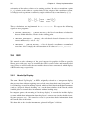
2.1.3
Run-through of example
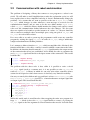
We will first examine what each of these functions does, and then we will show their
listing and explain how they do it. Our goal is to produce a Signal String, which, at
different stages during the execution of the program, will contain the current time, the
mouse position, and the constant string “Thanks”. Let’s call this signal the overall
value signal.
2.1. Behaviour Switching
11
Let’s make note of the types of each of these functions:
1
2
3
4
startWith : Signal a -> Signal (Bool, a)
until : Signal (Bool, a) -> Signal Bool -> Signal (Bool, a)
andThen : Signal (Bool, a) -> Signal a -> Signal (Bool, a)
andEternally : Signal (Bool, a) -> Signal a -> Signal a
We observe two things:
• All these functions are polymorphic on the type a. This is the type of the overall
value signal. In our example, a is String.
• They all operate with pairs of type Signal (Bool, a). From now on, we will
refer to the Boolean component as the switch signal and the a component as the
value signal.
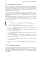
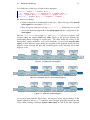
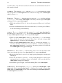
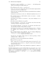
The first until, andThen, the second until and andEternally operate as a chain, each
element taking the output switch and value signals of the previous element and
transforming them according to certain rules. We show below the values of the
intermediate signals emitted by each of the functions, as well as the overall value
signal, at three different stages during the execution of the program: before the first
keypress event, between the first and second keypress event, and after the second
keypress event.
Figure 2.1: Before the first keypress
Figure 2.2: Between the first and second keypress
Figure 2.3: After the second keypress
As it can be seen from the figure above, the keypress events trigger changes in the
signals emitted by the two until functions; these changes propagate towards the end
of the chain yielding a different overall value signal in each of the time intervals
12
Chapter 2. Theoretical Considerations
described above. We will now describe the behaviour of each individual function in
this example in detail.
The function startWith takes the Signal String representing the current
time, and produces a value signal which is identical to its input, and a switch signal
which is always True.
startWith
The first until function takes the output of startWith and the condition
As its output value signal it will always emit its input value signal
unchanged. For its output switch signal,
First until
Keyboard.enter.
• While the condition is False (i.e. the user has not pressed Enter yet), it will emit
False.
• After the condition becomes True for the first time (i.e. the user pressed Enter),
it will start emitting True indefinitely.
The andThen function takes the output of until and a new value signal of
the same type as a, in our case, String. As its output switch signal, it will always emit
its input switch signal unchanged. For its output value signal,
andThen
• While its input switch signal is False (i.e. the previous until is still emitting
False, because the user has not pressed Enter yet), it will emit its input value
signal unchanged - in our case, the current time.
• When its input switch signal becomes True (i.e. because the previous until
started to emit True, because the user pressed Enter), it will start emitting the
new value signal indefinitely - in our case, the mouse position. Note that the
new switch signal is being passed through.
Second until The second until will have three states. Just as the first until, it will
always pass through the value of its value signal. For its output switch signal,
• Before the first Enter is pressed, it is simply passing through the switch signal
unchanged.
• After the first Enter is pressed, it is still passing through its switch signal
unchanged, but it is starting to observe its condition. Also, note that the new
value signal is being passed through.
• After Enter is pressed again, it will start emitting True as its switch signal.
The final function, andEternally, unwraps the switch signal - value
signal tuple into the overall value signal. It simply passes through its input value
signal while its switch signal is False, and starts emitting the new value signal once
its switch signal becomes True.
andEternally
2.1. Behaviour Switching
13
In our example, we must analyse three states.
• Before the first Enter is pressed, andEternally is passing through its input value
signal, which is the time.
• After the first Enter is pressed, andEternally continues passing through its input
value signal, which is the mouse position.
• After Enter is pressed again, andEternally will start emitting its new value
signal, which is the constant “Thanks” message.
2.1.4
Implementation
Now that we have explained the role of the four library functions through an example,
let’s analyse their implementation.
startWith
1
2
3
4
startWith : Signal a -> Signal (Bool, a)
startWith valS =
let f val _ = (True, val)
in lift2 f valS onStart
This function pairs a signal of type a with a boolean value that is constantly True.
Here, onStart is a signal of unit value, which fires exactly once at the start of the
program. We are forced to define startWith like this to work around the following
problem in the Elm runtime regarding propagation of constant signals over foldps in
Elm:
If a constant signal x is used as the input to a foldp, like this:
y = foldp func default_value x
then the value of y will always be default_value, and not the result of applying
func to the value of x.
For example, the value of the signal below will be 0, not 1:
y = foldp (_ _ -> 1) 0 (constant 0)
For ease of understanding, one can pretend that this problem does not exist and simply
regard the definition of startWith as:
1
startWith = lift (\val -> (True, val))
until
1
2
3
4
5
until : Signal (Bool, a) -> Signal Bool -> Signal (Bool, a)
until bothS nextSwitchS =
let
(switchS, valS) = decomposeS bothS
14
6
7
8
Chapter 2. Theoretical Considerations
f val switch nextSwitch everFlipped =
if | everFlipped && nextSwitch && switch -> (True, val)
| otherwise -> (False, val)
9
10
11
nextSwitchEverFalseSinceSwitchBecameTrueS =
stickyS (switchS ‘andS‘ (notS nextSwitchS))
12
13
in f <˜ valS ˜ stickyS switchS ˜ nextSwitchS ˜ nextSwitchEverFalseSinceSwitchBecameTrueS
14
15
16
stickyS : Signal Bool -> Signal Bool
stickyS s = foldp (||) False s
Here we are using several functions which are not part of the standard library of Elm:
• decomposeS : Turns a signal of tuple into a tuple of signals.
• stickyS : Turns a Bool signal S into a “sticky” signal. stickyS S will be True if S
ever had the value True since the start of the program.
This function takes a switch/value signal tuple (switchS, valS) and a condition in the
form of a boolean signal nextSwitchS.
If switchS it is not True, until does not do any processing; it simply passes through the
previous value of the value signal valS, and False for the switch signal.
Once switchS becomes True, until starts checking the value of the nextSwitchS signal,
i.e. the event that it is waiting on.
While nextSwitchS is False, until will continue to emit False and pass through the value
of valS. When nextSwitchS becomes True, until will start to emit True indefinitely.
The signal nextSwitchEverFalseSinceSwitchBecameTrueS needs an additional explanation. Its role is to prevent successive untils that are waiting on the same event (for
example, the Enter key) to be immediately bypassed by a single event occurrence.
True to its name, nextSwitchEverFalseSinceSwitchBecameTrueS will only become True
once the event that we are waiting on has been False at least once since we started
observing it.
With our example, ‘until‘ Keyboard.enter ‘andThen‘ ... ‘until‘ Keyboard.enter, since
at the beginning of the program the Enter key is not pressed, the first until’s one will
be immediately True. However, the second until’s one will only become True once
the key is no longer pressed. This achieves the desired effect of requiring two separate
presses of Enter to reach the end of the chain.
andThen
1
2
3
4
andThen : Signal (Bool, a) -> Signal a -> Signal (Bool, a)
andThen bothS nextValS =
let
(switchS, valS) = decomposeS bothS
5
6
7
f : Bool -> a -> a -> (Bool, a)
f switch oldVal nextVal = if | switch -> (True, nextVal)
2.2. Previous states of signals
8
9
15
| otherwise -> (False, oldVal)
in f <˜ stickyS switchS ˜ valS ˜ nextValS
This function takes a switch/value signal tuple (switchS, valS) and a new value
signal nextValS. It always appears after an until, so its input signals are the outputs of
an until.
While the corresponding until is emitting a switch signal of False (i.e. switchS is
False), it will pass through its inputs unmodified. Once the corresponding until starts
emitting a switch signal of True (i.e. switchS becomes True), it will also pass through
True as the value signal and the new value signal nextValS as its output value signal.
andEternally
1
2
3
4
andEternally : Signal (Bool, a) -> Signal a -> Signal a
andEternally bothS eternalValS =
let
(switchS, valS) = decomposeS bothS
5
6
7
8
9
f : Bool -> a -> a -> a
f switch oldVal eternalVal = if | switch -> eternalVal
| otherwise -> oldVal
in f <˜ stickyS switchS ˜ valS ˜ eternalValS
This function, meant to be placed last in the chain of behaviour switching commands,
behaves in a manner similar to andThen, except it also unwraps the switch signal/value
signal tuple by discarding the switch signal. In fact, it could be defined more
succinctly as:
1
andEternally bothS eternalValS = lift snd (andThen bothS eternalValS)
The full source code for this part of the library can be found in lib/BehaviourSwitching
.elm.
2.2
Previous states of signals
In order to keep track of the Khepera robot’s position as it moves, it was necessary to
implement dead reckoning. This process is described in detail in section 3.4; here we
will only briefly describe one of its inputs in order to motivate the creation of the FRP
function last_two_states.
We have a signal wheels_mm whose value is a pair [left, right] representing the
distance travelled by each wheel of the robot since the start of the program. To
perform dead reckoning, we need to know how much the left and right wheels of the
robot have travelled between the last two updates of wheels_mm. We are essentially
interested in a term-by-term difference between wheels_mm and the previous state of
wheels_mm.
We introduce the following function:
16
1
2
3
4
5
6
Chapter 2. Theoretical Considerations
last_two_states : (Signal a) -> a -> Signal (a, a)
last_two_states signal defa =
let initial_value = (defa, defa)
shift_left : a -> (a, a) -> (a, a)
shift_left a3 (a1, a2) = (a2, a3)
in foldp shift_left initial_value signal
last_two_states is a function that, given a signal of type a, creates a signal of type
(a, a), where the second value is the current value of the original signal, and the first
value is the previous value of the original signal.
Note that since signals in Elm must always have a well defined value, it is necessary to
pass an initial value that we want the signal to have, which it takes when the underlying
signal has not yet fired at least twice.
Using this function, we can easily define our term-by-term difference as follows:
1
2
3
wheels_mm_diff =
let wheel_update ([left,right],[left’,right’]) = [left’-left,right’-right]
in wheel_update <˜ last_two_states wheels_mm [0,0]
The source code for this part of the library can be found in lib/Utils.elm, and a usage
example in lib/Odometry.elm.
2.3
Delayed signals
Another useful feature is obtaining the value of a signal delayed from the realtime
value of that particular signal by a certain amount of time.
Hudak introduces[3] the generic function timeTrans f orm:
timeTrans f orm :: Behavioura → BehaviourTime → Behavioura
This function allows arbitrary transformations of time such as slowing down, speeding
up and shifting. However, allowing arbitrary time transformations is impossible in
Elm, for the following reasons:
• The future value of a signal is impossible to know in advance, thus both shifting
time forwards and accelerating time are impossible.
• It is theoretically possible to store a history of all values of a signal which would
allow us to go back in time arbitrarily; however memory usage for this history
would be unbound (i.e. it would grow constantly as the program runs). Even if
we wouldn’t allow arbitrary transformations and only allow slowing down time
by a constant factor, memory usage would still be unbound.
However, we can define a particularization of Fran’s timeTrans f orm function that can
only shift time backwards, as follows:
2.4. Synchronizing signals
1
2
3
4
5
17
all_delay_signal delay signal defa =
let add (time, value) li = let too_old (the_time, _) = time-the_time >= delay
in dropWhile too_old li ++ [(time, value)]
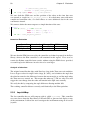
timeshifted_values = foldp add [(0,defa)] <| (,) <˜ every (100*millisecond) ˜ signal
in (map snd) <˜ timeshifted_values
6
7
delay_signal delay signal defa = head <˜ all_delay_signal delay signal defa
Here we are using dropWhile, which is not part of the standard Elm library but can be
easily defined, and which drops items at the beginning of a list while they conform to
a predicate.
The function all_delay_signal stores a queue of signal values paired with timestamps;
when a new event occurrs, it discards all pairs from the queue that are too old to be
relevant (i.e. they are older than the interval by which we want to delay the original
signal) and appends the new timestamped value at the end of the queue. At any
given time, the head of this queue will contain the oldest event that is at most 100
milliseconds older than the interval requested. The function’s memory usage is bound,
because the queue is pruned of old values on every update.
These functions can be used to create the stuck signal: a signal that becomes True if
the robot has moved less than one millimetre in the past 3 seconds.
1
2
3
4
5
earlier_position = delay_signal (3*second) robo.position (0,0,0)
moved_lately =
let do (x, y, _) (ox, oy, _) = sqrt ((x-ox)ˆ2 + (y-oy)ˆ2)
in do <˜ robo.position ˜ earlier_position
stuck = (\moved_lately -> moved_lately < 1) <˜ moved_lately
We can also very easily check if the robot has been stuck at any time in the past few
seconds by applying or over all_delay_signal (3*second) stuck - i.e. the list of stuck’s
values in the past 3 seconds.
1
stuck_recently = or <˜ all_delay_signal (3*second) stuck False
The source for this part of the library can be found in Navigator2.elm.
2.4
Synchronizing signals
Another interesting problem within the context of event-driven FRP is synchronizing
two signals.
Let’s assume we have two Signal Strings, outgoing and incoming, representing messages send and received, respectively, to and from a remote system, such as a robot.
These signals change their values exactly once for each line of data we send and
receive, and we further assume that the order in which the signals fire corresponds to
the order of the send and receive events in real life. An example of communication we
could have using this system follows (with signal updates represented in bold):
18
Chapter 2. Theoretical Considerations
Time
0
1
2
3
4
Event
Start of program
We send "read-ir"
We send "read-light"
Robot responds "1,2,3"
Robot responds "7,8,9"
Value of outgoing
Value of incoming
""
"read-ir"
"read-light"
"read-light"
"read-light"
""
""
""
"1,2,3"
"7,8,9"
Obviously, in order to do any meaningful processing, we need a way to pair "read-ir"
with "1,2,3", and "read-light" with "7,8,9". How could we do this?
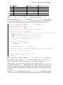
We define the function sync_signals, which takes a Signal a, a Signal b, default values
of type a and b, and creates a Signal (a, b), which will fire once for each distinct pair
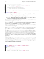
of values from the given signals, in the order in which they fired. Here is the code:
1
2
3
4
5
sync_signals : Signal a -> Signal b -> a -> b -> Signal (a, b)
sync_signals sa sb defa defb =
let sa_sync_stream = (\a -> Left a) <˜ sa
sb_sync_stream = (\b -> Right b) <˜ sb
both_sync_stream = merges [sa_sync_stream, sb_sync_stream]
6
do new_sync (left_queue, right_queue) =
let (tr_left_queue, tr_right_queue) = trim_heads_if_exist (left_queue, right_queue)
in case new_sync of
Left left -> (tr_left_queue++[left], tr_right_queue)
Right right -> (tr_left_queue, tr_right_queue++[right])
7
8
9
10
11
12
both_pair_stream = foldp do ([], []) both_sync_stream
13
14
doo (xs, ys) = case (xs, ys) of
(x::xtail, y::ytail) -> Just (x, y)
_ -> Nothing
15
16
17
18
both_current_heads = doo <˜ both_pair_stream
19
20
heads_updated_if_just = keepIf isJust (Just (defa, defb)) both_current_heads
21
22
23
in
extractJust <˜ heads_updated_if_just
24
25
26
27
trim_heads_if_exist (xs, ys) = case (xs, ys) of
(x::xtail, y::ytail) -> (xtail, ytail)
_ -> (xs, ys)
First, on lines 3-4, we define the signals sa_sync_stream and sb_sync_stream, which turn
the stream of as into a stream of Left as, and the stream of bs into a stream of Left bs.
This is very helpful, as these two signals are now of the same datatype, Either a b.
Then, on line 5, we merge these two signals into a single signal both_sync_stream,
using the Elm function merges. This function takes a list of signals of the same type
and creates a new signal that contains the union of the updates for all the signals in this
list. Note that the order in which the resulting signal updates respects the real ordering
of updates.
On lines 7-13, we are building two queues in both_pair_stream, containing the signal
values (in proper order) from the left and right signal, respectively. Note that before
2.4. Synchronizing signals
19
adding a new value to the left or right queue, we pop the top of both queues if it exists
(i.e. if we have a valid pairing of events of type a and b already - we will see in a
moment why it’s appropriate to discard this here).
On lines 13-17, we are constructing a signal based on the queues, which at any
moment is either Just a valid pairing, or Nothing. This is why it is OK to trim the top
of both_pair_stream when it exists - the pairing on top will have already been copied
into both_current_heads during the previous event.
Finally, on line 21, we use the built-in Elm function keepIf to filter valid pairings
from both_current_heads (using the default values provided to the function if no valid
pairing ever existed). Since this means that heads_updated_if_just will always contain
a Just (a, b), we can safely extract it into an (a, b) on line 23.
Here are the values of these intermediate signals for the previous example:
Time
0
1
2
3
4
sa sync stream
Left ””
Left ””
Left ”read-ir”
Left ”read-light”
Left ”read-light”
Left ”read-light”
sb sync stream
Right ””
Right ””
Right ””
Right ””
Right ”1,2,3”
Right ”4,5,6”
both sync stream
Left ””
Right ””
Left ”read-ir”
Left ”read-light”
Right ”1,2,3”
Right ”4,5,6”
both pair stream
([””],[])
([””],[””])
([”read-ir”],[])
([”read-ir”,”read-light”],[])
([”read-ir”,”read-light”],[”1,2,3”])
([”read-light”],[”4,5,6”])
both current heads
Nothing
Just (””,””)
Nothing
Nothing
Just (”read-ir”,”1,2,3”)
Just (”read-light”,”4,5,6”)
The source code for this definition can be found in lib/Utils.elm.
Result
(””,””)
(””,””)
(””,””)
(””,””)
(”read-ir”,”1,2,3”)
(”read-light”,”4,5,6”)
Chapter 3
Library Implementation
3.1
3.1.1
Hardware and software
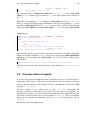
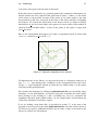
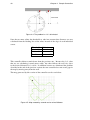
The Khepera II robot
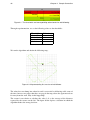
(a) View of robot
(b) Location of sensors and wheels
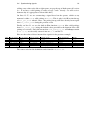
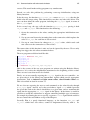
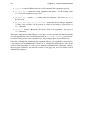
Figure 3.1: The Khepera 2 robot
The robot that the present project was modelled on is the Khepera 2 robot[6] (Figure 3.1a). The Khepera is a small, circular robot with two independently controllable
wheels and eight light/infrared sensors located around its circumference.
It has two major modes of operation:
1. Direct control over a serial connection, using a simple, ASCII-based protocol
briefly described in Section 3.1.3.
2. Upload of C programs cross-compiled for the onboard CPU. The robot has a
Motorola 68331 CPU clocked at 25 MHz, 512 KB of RAM and 512 KB of flash
storage.
To run Elm programs directly on the robot, one would need to cross-compile and fit an
entire JavaScript runtime on it; given the weak specifications of the CPU and memory,
this task is most probably impossible. Instead, the purpose of this project was to
21
22
Chapter 3. Library Implementation
use Elm to successfully control a Khepera robot tethered to a computer using a serial
cable.
3.1.2
The Webots simulator
In addition to controlling a physical robot, it was convenient to set up a robot simulator
for faster development. The chosen package was Webots, a mature, commercial
product for which the University of Edinburgh holds a site license.
Webots already contains the appropriate models for the Khepera 2 robot, including
several simple controller programs written in C; one of these was a TCP/IP server
which opens a socket that accepts commands using the same protocol as the serial
protocol for real Khepera robots. Some modifications were performed on this stock
controller to fix several bugs and make it more suitable for communication with the
external Elm programs.
In particular, the stock controller had a bug where it would not tokenize incoming
socket data by newlines (making the assumption that the data in one packet contains
exactly one command), which meant that sending it messages rapidly would cause it
to crash or not respond to them.
In addition to fixing this bug, the controller was adapted to send sensor data on its own
instead of waiting to be polled by clients - this is a violation of the original Khepera
protocol, but it is very convenient as it allows for running the simulation faster than
real-time.
3.1.3
The communication protocol
When connecting to a Khepera robot over a serial port (or to Webots over a TCP/IP
socket), the controller sends commands to the robot and receives responses. The robot
never1 sends any data except as a response to a command. Each command ends with a
newline, and solicits exactly one response which also ends with a newline.
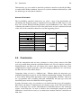
The commands that will be used as part of the project are described in Table 3.1. In
this table, monospaced text represents literal strings that are sent and received exactly
as presented, and italic text represents variables, whose meaning is described in the
third column. All variables are integer values. All commands and responses end with
a newline, which is not explicitly shown.
3.1.4
Elm Runtime (Node.js and node-webkit)
The existing implementation for Elm compiles to JavaScript and HTML, which can be
run directly in a web browser. However, JavaScript code running in a regular browser
1
With the exception of a power on message, which we filter out.
3.1. Hardware and software
Command Response
D,Vl ,Vr
d
N
n,S0 ,S1 ,S2 ,
S3 ,S4 ,S5 ,S6 ,
S7
O
o,S0 ,S1 ,S2 ,
S3 ,S4 ,S5 ,S6 ,
H
S7
h,Dl ,Dr
G,0,0
g
23
Meaning
The controller asks the robot to set the speed of the
left wheel to Vl and the speed of the right wheel to Vr .
The controller asks the robot for a reading of its
infrared sensors. The robot responds with values
S0 ...S7 corresponding to sensors 0...7 as labelled in
Figure 3.1b.
The controller asks the robot for a reading of its light
sensors. The robot responds with values S0 ...S7 corresponding to sensors 0...7 as labelled in Figure 3.1b.
The controller asks the robot for the reading of its
wheel encoders. The robot responds with values Dl
and Dr , corresponding to the left and right wheels
as labelled in Figure 3.1b. These values represent the
number of pulses that each wheel has performed since
the start of the program (or the last reset), where one
pulse corresponds to 0.07mm.
The controller asks the robot to reset its wheel encoders to zero. This will be done every time we
connect to the robot.
Table 3.1: Khepera communication protocol
is not sufficiently privileged to communicate over a serial port or a TCP/IP socket1 , so
this setup is not sufficient for our purposes.
Node.js is a platform that allows running JavaScript applications as privileged, regular
processes inside an operating system, and there exist Node.js libraries for serial and
socket communication. The Elm runtime does not run unmodified on Node.js because
it assumes the existence of several DOM objects (such as window, document and the
addEventListener method), and my initial contribution to this project was to adapt it
to run. I was successful in stubbing out these objects and replacing the regular DOM
event mechanism with the Node.js-specific one, and I was able to run Elm programs
that connect and control robots in the command-line.
However, one of the greatest strengths of Elm is its ability to declaratively create
rich user interfaces, and since the pure Node.js solution described above completely
negates that, I considered it to be suboptimal. Instead, I found and configured nodewebkit, an “app runtime based on Chromium and node.js” which combines the best
of both worlds: applications running inside of it have access to both the regular
DOM (thanks to which Elm can run unmodified and display graphics) and to Node.js
modules (thanks to which the library I am creating can communicate over serial ports
and TCP/IP sockets).
1
Websockets could potentially allow communication between an unprivileged webpage and a modified
simulator, but not with an unmodified, raw TCP/IP socket.
24
3.2
Chapter 3. Library Implementation
Communication with robot and simulator
The problem of designing a library that connects a user program to a robot is not
trivial. We will make a small simplification to make the explanation easier (we will
later explain what we have simplified and why it doesn’t fundamentally change the
problem): let’s assume that we want to provide to the user a Signal String called
raw_input, which changes its value whenever a new message is received over the
communication channel, and we want to let the user define another Signal String
called raw_output, which the library should monitor for changes and send its current
value over the communication channel whenever the value changes. We also want
these two signals to be bound to specific instances of a robot - i.e., the user should be
able to connect to multiple robots on multiple ports, using one pair of raw_input and
raw_output for each of these robots.
If we were able to set such a system up, the programmer could create any controller
program by writing the signal raw_output in terms of raw_input, using a sufficiently
complex transformation with Elm primitives.
Let’s attempt to define a function make_robot which accomplishes this. Obviously, this
function would have a side effect - namely, it would establish a connection to the robot.
In addition, the function should return the raw_input signal bound to the output stream
of the connection that it has just established, and it should also take as parameter the
user’s raw_output signal and bind it to the input stream of the connection. This would
look like this:
1
2
raw_input : Signal String
raw_input = Robotics.make_robot raw_output
3
4
raw_output : Signal String
The problem with the above code is that, while it is possible to write a trivial
raw_output signal (such as a constant one), it is not possible to write raw_output in
terms of raw_input. A library in which we can only write robot controllers whose
actions do not depend on values from sensors is obviously very limited in usability.
One way to remedy this chicken-and-egg problem is to have Robotics.make_robot take
a Signal String -> Signal String instead, i.e. a function that turns an input signal into
an output signal. This would look like this:
1
2
3
4
5
6
7
8
_ = Robotics.make_robot connection_params robot_func
robot_func : Signal String -> Signal String
robot_func raw_input =
let user_signal_1 = ...
user_signal_2 = ...
user_signal_3 = ...
raw_output = ...
in raw_output
While this would work, it would involve either wrapping the entire user program in a
huge let .. in block (to have the raw_input signal bound to a name), or passing the
raw_input signal as the first argument to all user functions that need to deal with robot
3.2. Communication with robot and simulator
25
sensors. This would make writing programs very cumbersome.
Instead, we solve this problem by performing a two-step initialization, using two
library functions.
In the first step, the function Robotics.make_robot returns a Signal String that has the
initial value the empty string. This function does not have any other side effects. The
user can then define the entire program, including the raw_output signal, in terms of
this raw_input signal.
In the second step, the user calls the function Robotics.run_robot passing it both
raw_input and raw_output. This function does the following:
1. Opens the connection to the robot, sending the appropriate initialization commands
2. Sets up an event listener for incoming data on the connection, which updates the
value of raw_input for each line of data received
3. Sets up an event listener for changes to raw_output’s value, which sends each
new value over the connection as a line of data
The return value of this function is unit, and can be ignored by the user. We are only
using it to trigger the side effects mentioned above.
The user program would then look like this:
1
2
3
4
5
6
raw_input = Robotics.make_robot
user_signal_1 = ...
user_signal_2 = ...
user_signal_3 = ...
raw_output = ...
_ = Robotics.run_robot raw_input raw_output
This is the essence of the way user programs are written using the Robotics library.
However, let’s revisit the simplification mentioned at the beginning of this section.
There are two issues that need to be clarified.
Firstly, we are not actually exposing the raw_input signal to the user controller - we
are processing it in the library into intermediate signals which provide appropriate
abstractions, such as infrared and light sensor values, wheel encoder values etc.
This is described in detail in section 3.3.
We are also not expecting the user to send commands to the robot directly through
a raw_output signal - instead, we let the user define a signal motors which represents
the speed that each of the wheels should have at a given time, and we transform this
signal into the appropriate raw_output signal in the library. In the future, it would be
possible to extend the architecture to support controlling multiple types of actuators,
for example by allowing the user to specify a separate blinkers signal which would let
the user control the two blinkers on top of the Khepera.
Secondly, Elm is a purely functional language, so the functions make_robot and
run_robot, which have side effects, cannot be implemented directly with it. In-
26
Chapter 3. Library Implementation
stead, they are backed by two native (JavaScript) functions create_incoming_port and
set_outgoing_port, which we will define in a native module.
Native modules are an undocumented feature within Elm, but they are used extensively
throughout the standard library. In fact, the only way to set up an input signal (i.e. a
signal whose value depends only on external input, as described in section 1.1) is in a
native JavaScript module. A thorough inspection of the existing Elm source code was
necessary in order to deduce the conventions by which this is done. Care has been
taken to make the native module as thin as possible - in fact, it only exposes the two
functions described in this section and one additional function, emergency_stop, which
will be described later, in section 4.3.3.
The function create_incoming_port simply creates a new Signal String with an empty
string as the initial value. The function set_outgoing_port opens the connection to the
robot, sends the initialization commands, and sets up the bidirectional communication
between the raw_input and raw_output signals and the incoming and outgoing data
stream, respectively, as previously described in the simplification.
The source code for this part of the library is in lib/Robotics.elm and lib/Native/
Robotics.js.
3.3
Parsing of signal values
In order to obtain the sensor values for the robot’s infrared and light sensors and wheel
encoders, we must poll the robot according to the protocol described in section 3.1.3.
The Khepera manual[6] states that the robot, internally, generates a new value for all
sensor readings every 25 milliseconds. However, we experimentally found that polling
every 25 milliseconds often causes the robot to stop responding; we settle instead
for a default polling interval of 300 milliseconds, which was still a sufficiently high
resolution for our purposes.
This parameter, like many others, can be overridden by library users through command
line parameters or explicit instantiation of robots, as described in section 3.9.
Section 2.4 describes how we could solve the problem of matching robot responses to
controller commands; however, in the particular case of the Khepera serial protocol,
we have a much simpler solution. As previously mentioned, each robot response
begins with an echo of the command that it is responding to - that is, n for infrared
sensor readings, o for light sensor readings, h for wheel encoder values etc. We
can thus deliberately ignore our own commands and simply perform filtering on the
incoming messages based on this echoed value.
The function inputByType, defined in lib/Sensors.elm, performs the appropriate filtering. We expose the following raw sensor data to user programs:
• infrared : Signal [Int], a list of the instantaneous values for each of the 8
infrared sensors, in the order shown in Figure 3.1b.
3.4. Odometry
27
• light : Signal [Int], a similar list for the 8 light sensors.
• wheels_mm : Signal [Int], a list of two values, representing the distance, in
millimetres, that the left and right wheels, respectively, have travelled since the
start of the program.
In addition to these raw values, we provide additional helper signals based on them.
These are described in the following two sections.
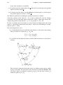
3.4
Odometry
As was briefly mentioned in section 3.3, we use the wheel encoders equipped on the
Khepera robot to obtain the signal wheels_mm, representing the distance travelled by
each of the two wheels, in millimetres.
We want to use this information to estimate the position of the robot relative to its
starting point. We will encode the position of the robot as the triplet (x, y, α); the
first two values encode the displacement of the robot relative to the origin, and α will
encode its orientation relative to its original orientation.
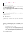
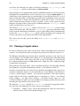
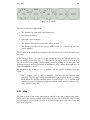
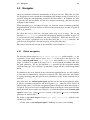
In figure 3.2, we can see an example of robot movements and the values of the
corresponding position triplets.
(a)
(b)
(c)
(d)
Figure 3.2: Four example robot positions
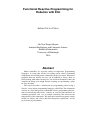
(a) The initial value for the position triplet is (0, 0, 0).
(b) If we move the robot 10 millimetres forward, we would expect the position
triplet to become (0, 10, 0) - meaning that the robot is at coordinates (0, 10) and
28
Chapter 3. Library Implementation
at the same orientation as originally.
(c) If we then rotate the robot in place by
triplet to become (0, 10, π2 ).
π
2
to the left, we would expect the position
(d) If we then order the robot to go 10 millimetres forward again, we would expect
the position triplet to become (−10, 10, π2 ).
We define the problem of estimating the position recursively as follows:
Given the position of the robot P0 = (x0 , y0 , α0 ) at moment T0 , and the distance
travelled by the left and right wheel respectively L, R in a short time interval ∆T ,
estimate the position of the robot P1 = (x1 , y1 , α1 ) at time T1 = T0 + ∆T .
In order to calculate the new position, we need to know the length of the axle of the
robot, i.e. the distance between the two wheels. In the case of the Khepera 2 robot,
this has value l = 53mm.
We can distinguish two cases.
1. L = R: Both wheels have travelled the same distance, so the robot is not rotating.
This is a trivial case; obviously α1 = α0 and
Ç
å
Ç
x1
x + L cos α0
= 0
y1
y0 + L sin α0
å
2. L 6= R: The left and right wheel have travelled different distances, so the robot is
rotating.
The left wheel, right wheel and robot center are collinear points and are rigidly
fixed to each other. We will call the line described by them the axle line. The
axle line at time T0 is defined by points L0 , D0 , R0 ; the axle line at time T1 is
defined by points L1 , D1 , R1 .
3.4. Odometry
29
We can see that if the robot has rotated between positions P0 = (x0 , y0 , α0 ) and
P1 = (x1 , y1 , α1 ), it must have rotated around an external point O, located at the
intersection of the axle line at position P0 and the axle line at position P1 .
We want to calculate the rotation angle θ, i.e. the angle between the two axle
lines.
˙
˘
We can clearly see that L˘
0 L1 , D0 D1 and R0 R1 are arcs of concentric circles of
center O. We can write their length as a function of the radii of the circles, and
the angle θ, as follows:
L˘
0 L1 = θ · OL0
˙
D
0 D1 = θ · OD0
R˘
0 R1 = θ · OR0
We can also see that
OR0 = OL0 + l
So we can write
˘
R˘
0 R1 − L0 L1 = θ · (OR0 − OL0 )
= θ·l
Thus, the formula for the turn angle θ is:
θ=
˘
R˘
R−L
0 R1 − L0 L1
=
l
l
Now that we know the turn angle θ, we can easily write the angle at time T1 :
α1 = α0 + θ
We also know that the turn radius T R = OD0 is:
˘
L˘
0 L1 + R0 R1
2·θ
R−L
=
2·θ
T R = OD0 =
Ç
å
x
Then, to obtain the final coordinates 1 , we use the formula[1]:
y1
Ç
å
Ç
å
Ç
x1
x
cos α0 − sin α0
= 0 +TR·
y0
sin α0 cos α0
y1
åÇ
sin θ
cos θ − 1
å
30
Chapter 3. Library Implementation
This part of the library exports the following user signals:
• wheels_mm_diff : Signal [Int]: A signal representing the distance, in millimetres, travelled by the left and right wheel, respectively, since the last sensor
reading. We use the function last_two_states described in Section 2.2 to obtain
it.
• position : Signal (Float,Float,Float): A signal representing the position, calculated by applying the formula described above to wheels_mm_diff.
The source code for this part of the library can be found in lib/Odometry.elm.
3.5
Infrared measurements
The values returned from the Khepera infrared sensors are integers ranging between
0 and 1020, which we will denote as r0 , r1 , r2 ...r7 . A higher reading indicates that an
obstacle is very close to the sensor; the reading value decreases as the distance to the
obstacle increases.
We want to transform these values into something that is easier to reason with while
writing controller programs. Specifically, we would like to create an instantaneous
map of obstacles that the robot perceives at a given moment - that is, a list of
coordinates (x0 , y0 )...(xn , yn ) of obstacles relative to the robot’s center. Note that each
sensor can yield zero or one obstacles at any given time, so the number of obstacles n
is smaller or equal to 8.
First, we need to transform each individual sensor’s raw reading into a value that
represents the actual distance, in millimetres, between that sensor and the obstacle that
it is detecting at a given time. We provide two configurable ways to fit distances (di )
against sensor readings (ri ):
1. A linear equation: di = A + B · ri , with A and B fittable parameters
2. An exponential equation: di = AeB·ri , with A and B fittable parameters
We also define a parameter MaxDist, which represents the maximum distance at which
a sensor can detect an object.
We provide sensible defaults for the kind of fit and the parameters1 , but we also
offer the possibility for users to control these parameters manually as described in
section 3.9.
By applying the equation to our raw sensor values r0 , r1 ...r7 , we obtain a list of
distances d0 , d1 ...d7 .
1
For the real robot, we use the method described in section 4.4 to determine the exponential equation
with parameters A = 87.62 and B = −0.0066 to be a good fit, and we choose MaxDist = 40.
For the simulator, we read the parameters from the Khepera model configuration and determine the
linear equation with parameters A = 50 and B = −0.05 to be the best fit, and we choose MaxDist = 50.
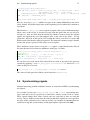
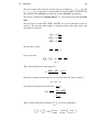
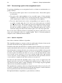
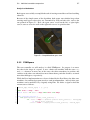
3.5. Infrared measurements
31
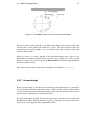
Figure 3.3: Obstacle calculation example for Sensor 2. Because this sensor is pointing
straight forward the angle δ2 is zero and thus not visible.
Second, we want to transform each of these distances into coordinates of the obstacles
that they refer to. For this, we need to know:
• The angle at which each sensor is positioned, relative to the robot’s front:
γ0 , γ1 , ...γ7
• The angle at which each sensor is pointing, relative to the robot’s front:
δ0 , δ1 , ...δ7
• The radius of the robot, r
We measure the angles, in degrees, as follows:
(γ0 γ1 γ2 γ3 γ4 γ5 γ6 γ7 ) = (68.4 44 13 −13 −44 −68.4 −158 158)
(δ0 δ1 δ2 δ3 δ4 δ5 δ6 δ7 ) = (68.4 44 0
0 −44 −68.4 −180 180)
We can then write the equation for obstacles as follows:
xi = r cos γi + di cos δi
yi = r sin γi + di sin δi
Figure 3.3 shows an example of distance calculation for an obstacle detected by sensor
2.
The points (xi , yi ) are in a system of coordinates relative to the robot’s position. We
are also interested in obtaining the actual coordinates of these points on a map.
Recall that the Odometry module described in the previous section gives us the position
of the robot as the tuple (x, y, α), representing the coordinates and the angle of the
32
Chapter 3. Library Implementation
orientation of the robot, relative to its starting position. In order to transform a point
(xi , yi ) relative to the robot to a point relative to the origin of this coordinate system,
we simply need to perform a rotation by angle α followed by a translation by (x, y):
Ç 0å
Ç å
Ç
åÇ å
xi
x
cos α − sin α
=
+
y0i
y
sin α cos α
xi
yi
These calculations are implemented in lib/Infrared.elm. We expose the following
signals to user programs:
• current_obstacles : [(Float,Float)], the list of coordinates of obstacles
that are within MaxDist, relative to the starting point.
• obstacle_distances : [Float], the calculated obstacle distances for each
sensor, unfiltered (i.e. d0 , d1 ...d7 ).
• obstacles : [(Float,Float)], a list of obstacle coordinates accumulated
over time - this is simply the concatenation of all values of current_obstacles.
3.6
GUI
We wanted to take advantage of the good support for graphics in Elm to provide
library users with easy ways to visualize the robot’s sensor values and internal belief
states. Here we will describe the two modules that we have constructed, which display
a HUD and a map, respectively.
3.6.1
Heads Up Display
The term “Heads Up Display”, or HUD, originally referred to a “transparent display
that presents data without requiring users to look away from their usual viewpoints”. It
is a technology created for military aircraft, which overlaid data from flight instruments
(such as “airspeed, altitude, heading” etc.) on the front window of the aircraft, which
enabled pilots to consult these instruments without looking away.
In computer games, the meaning of “heads up display” is extended to include display
systems which show information about the player’s current state (such as health, items,
in-game progress etc.). We wanted to create a system that shows information about
the current state of the robot.
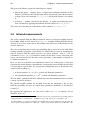
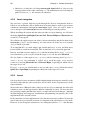
We show this as five circular instruments, pictured in Figure 3.4 below.
3.6. GUI
33
Figure 3.4: The HUD
The dials, from left to right, show:
1. The distances to each of the sensed obstacles
2. Raw infrared readings
3. Raw light sensor readings
4. The distance travelled by each of the wheels in total
5. The distance travelled in the last few milliseconds (i.e. between the last two
sensor updates).
The location of the numbers corresponds to the location of the sensors and wheels on
the robot.
In the example above, we can see on the second dial that the infrared reading for
the two frontal sensors non-zero - i.e., the robot is sensing an obstacle in front of it.
We can see this raw reading translated into a distance reading on the first dial - the
front-left sensor is detecting an object 42 millimetres away, and the front-right one, an
object 44 millimetres away.
We implement this in the lib/Hud.elm module, and we provide to library users the
signal:
• hud : Signal (Int -> Int -> Element): The user calls this function with
two integer signals representing the width and height, in pixels, that the resulting
HUD should be, and the function returns a signal of type Element, an Elm type
which represents a rectangular graphical element, which the user is then free to
place anywhere they like.
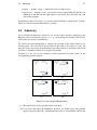
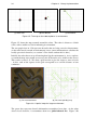
3.6.2
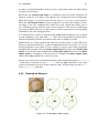
Map
We want to show a map of the environment, centred in the start position of the robot,
which shows the current position of the robot, the location of obstacles sensed at the
current moment, as well as the location of all obstacles that have been sensed since the
start of the program.
34
Chapter 3. Library Implementation
(a) initial state
(b) first obstacle
(c) zoomed out
Figure 3.5: The map as the robot explores its environment
Figure 3.5 shows the map zoomed around the robot. The robot is shown as a black
circle, with a smaller red circle indicating its orientation.
The two purple dots in 3.5b represent obstacles that are being sensed at that moment.
As the robot travels around an environment, it uses sensor information to calculate the
locally-perceived obstacles (see section 3.5 for details on how this is done).
Initially, the robot has no way of knowing how big the environment is. As we explore,
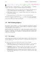
we zoom the map out as much as necessary for all obstacles to be visible on the screen.
This can be seen in 3.5c. We draw a grid in order to give the viewer a sense of scale
- in fact, each of the squares in the grid corresponds to a real-life distance of one
centimetre.
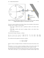
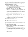
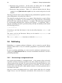
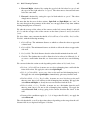
(a) The simulated world
(b) The corresponding map
Figure 3.6: A partial map of a larger environment
The green dots represent obstacle information accumulated over time. As the robot
detects local obstacles, it accumulates them in a global obstacle list. Figure 3.6b
3.7. Maps and persistent storage
35
shows a larger map constructed using this technique; we can see the robot is accurately
mapping the outline of the walls from the simulated world depicted in figure 3.6a.
We provide the following signals for library users:
• basic_map : Signal (Int -> Int -> Element):
The user calls this function with two integer signals representing the width and
height, in pixels, that the resulting map should be. The function returns an Elm
Element, which the user is free to place anywhere they like.
• overlaid_map : Signal (Form -> Int -> Int -> Element:
Similar to basic_map, except the user also passes a Form signal that they wish
to have overlaid on top of the map. Form is another Elm primitive type, like
an Element but with an arbitrary shape. The shapes provided by the user are
expected to be at a scale of one; the library takes care to rescale them so that
they overlay correctly on the map.
This signal is used extensively by the Navigator controller described in section
4.3, in order to overlay a navigation grid on top of the regular map.
• mouse_to_coordinate : Signal (Int -> Int -> (Int, Int)-> (Float,
Float):
This signal converts mouse clicks in the browser window into coordinates on
the map. It takes into account the coordinate of the top-left corner and the width
and height of the map. It expects these values to be passed in by the user.
The code for this part of the library is in lib/Map.elm.
3.7
Maps and persistent storage
It is convenient to be able to store and load the global obstacle information in the form
of maps. However, mainline Elm does not provide any mechanism for persisting data.
We create a small library, Persist, with a native counterpart, Native.Persist. The
Persist library exports the following functions:
• read_value : String -> String: Reads the contents of the file whose filename is passed as a parameter.
• persist : String -> Signal String -> (): Persists the content of the second argument signal into the filename passed as the first argument. Whenever
the signal changes, the new content is written to disk. This function call must
appear once in the program body to set up persistence for the rest of the program.
The Robotics library can function in three modes.
1. No map persistence. In this mode, the initial value for the global obstacles
signal is an empty list.
36
Chapter 3. Library Implementation
2. Read-only map persistence. In this mode, the initial value for the global
obstacles signal is constructed by parsing an input map file.
3. Read-write map persistence. Same as 2, with the addition that the library
samples its own global obstacles signal every five seconds and persists it to the
map file.
The map persistence mode can be configured using command-line arguments or direct
robot configuration, as described in section 3.9.
The format for storing obstacle data is very simple. Each obstacle is a tuple of floats
representing its coordinates; its representation is the string formed by concatenating
the X and Y values, joined by the character , (a comma). The entire map is represented
by concatenating individual pairs, joined by the character ; (a semicolon). Thus, a
map file containing obstacles at positions (0, 0), (10, 20) and (20, 30) would contain
the following plain text:
0,0;10,20;20,30
Converting to and from this format is done by the utility functions readPoints and
showPoints.
The source code for the Persistence library can be found in lib/Persist.elm and
lib/Native/Persist.elm.
The readPoints and showPoints functions are defined in lib/Utils.elm.
3.8
Pathfinding
Pathfinding is a common problem in Robotics, and we wanted to provide library
functions which make it easy for controller programmers to perform this common
operation.
In order to perform pathfinding, we need to turn the continuous environment represented by the global obstacle list into a discrete environment on which we can run a
pathfinding algorithm.
3.8.1
Constructing a navigational mesh
One typical representation is a navigation mesh - a data structure where each node
represents an abstract location accessible to the robot, which corresponds to a set of
concrete points in the real world. We want to choose these abstract locations in a way
such that their corresponding real world point sets are disjoint. We also associate a
boolean value with each node, which signifies whether or not that particular node is
accessible to the robot.
One way to create a navigation mesh is to overlay squares with sides of a constant
length f ineness over the continuous environment, and associate the set of points
3.8. Pathfinding
37
covered by each square with one node in the mesh.
If the robot detects an obstacle at a particular point in the continuous environment, we
should consider the disc centred in that point and of radius r (where r is the radius
of the robot) as inaccessible, because if the center of our robot would at any time
be positioned on this disc, one point in the body of the robot would be overlapping
the obstacle. To convert this observation to our discrete mesh, we define an integer
threshold mesh threshold and define each square to be inaccessible if the number of
obstacles detected within radius r of any of the points in the square is larger than
mesh threshold.
Here is the environment from figure 3.6a with a navigational mesh overlaid (with
f ineness = 30 and mesh threshold = 3):
Figure 3.7: Map with navigational mesh overlaid
To implement this in our library, we represent the mesh as a dictionary with keys of
type (Int,Int), representing node coordinates in the navigational mesh, and values
of type Int, representing the amount of points that are within radius r of the square
associated to that particular node.
We construct our dictionary by folding the global obstacle list over an initially empty
dictionary; in our fold function, we inspect each point, determine the main square
that it belongs to (by dividing its x and y coordinates by f ineness), determine the
neighbours that have points within radius r of our original point, and increment the
count in the dictionary for all these squares.
If we are loading a map from disk, as described in section 3.7, at the start of the
program we need to process the entire global obstacle list; once this is done, however,
we only need to process additional obstacles one at a time, as they are detected by the
robot as it explores the environment.
38
Chapter 3. Library Implementation
3.8.2
Constructing a path in the navigational mesh
To perform pathfinding on our navigational mesh, we define its transformation to a
graph as follows:
• For each accessible square, there is an associated vertex. Inaccessible squares
are discarded.
• For each of the eight neighbours of an accessible square, if that particular
neighbour is also accessible, there is an edge between the vertex corresponding
to the original square, and the vertex corresponding to the neighbour.
• For every edge between two vertices corresponding to two squares S1 and S2 ,
we√define a weight with value 1 if S1 and S2 are on the same row or column,
or 2 if they are not. This weight represents the straight line distance between
the centres of squares S1 and S2 , assuming squares with sides of unit length;
the sides are actually of length f ineness, but scaling the path cost by f ineness
would not change our choice of the shortest path, so we can safely ignore this.
We are now faced with the problem of calculating the shortest path between a start
vertex and a destination vertex in a weighted graph. This is a classical problem in
computer science with many known solutions.
3.8.2.1
Dijkstra’s Algorithm
One of these solutions is Dijkstra’s algorithm.
This algorithm attempts to construct a table of path lengths (distances) between the
start node and all nodes in the graph (henceforth called costs).
It initializes this table with all distances as infinite, and also initializes a set of nodes to
explore (henceforth called unexplored), which initially consists of just the start node.
On each iteration, it extracts the node current from unexplored which is closest to the
start node. For each neighbour neighbour of current, it calculates the potential cost
to reach neighbour from the start node via current, as the sum between the current
cost to reach current (stored in costs[current]) and the weight of the edge between
current and node; if the resulting cost is lower than the value previously stored in
costs[neighbour], it updates it and adds neighbour to unexplored.
We must note that when this algorithm selects a node current to explore next, the
distance stored in costs[current] is definitely the smallest one to it. Thus, if we are
only interested in the path to a single destination, we can simply stop this algorithm
when we have selected the destination as current.
The algorithm also terminates when we no longer have nodes in the unexplored set. If
we haven’t reached the destination node by the time this happens, it means that there
exists no path between the start node and destination node.
We implement Dijkstra’s algorithm as a pure function, as follows:
3.8. Pathfinding
1
2
3
39
dijkstra : comparable -> (comparable -> Bool) -> (comparable -> Set.Set comparable) ->
(comparable -> comparable -> number) -> Maybe (number, [comparable])
dijkstra start_node goal_fun neighbour_fun cost_fun = ...
Elm does not have explicit type classes. Instead, one can use the special keywords
comparable and number as in the above definition. This is equivalent to the Haskell
definition:
dijkstra :: (Ord a, Num b) => a -> (a -> Bool) -> (a -> Set a)
-> (a -> a -> b) -> Maybe (b, [a])
In the Elm definition, our nodes are of type comparable, and the cost between a pair
of nodes is a number. The function goal_fun should return True if it is passed the
destination node. The function neighbour_fun should return a set of neighbours for the
node passed as its argument. The function cost_fun is given two nodes and should
return the weight of the edge between them. It is never called for a pair of nodes that
were not returned as neighbours for each other by neighbour_fun.
We implement this iterative algorithm in a purely functional environment using a
recursive function. We define a record called state which holds the unexplored list
and the costs dictionary; in each step of the recursion, we update the state according
to the algorithm described above and call the function again with the new state. We
terminate the recursion when we have reached either of the two terminating conditions.
The function returns a Just with the total cost of the shortest path, as well as a list of
nodes, in order, that the path is composed of, or Nothing if no path exists.
3.8.2.2
A* Algorithm
Dijkstra’s algorithm expands nodes in the order of their distance to the start point; this
means that, in a 2D environment such as the map that we are trying to explore, we
are just growing paths around the start point without making any attempt to guide the
search towards the destination point.
A-star is a faster algorithm that attempts to expand the path biased towards the
destination node. It uses a heuristic function which estimates the distance from each
node to the destination node; this heuristic function must be admissible, i.e. it must
never overestimate the distance, in order for the A-star algorithm to find the shortest
path.
For our 2D map, an obvious admissible heuristic function for an arbitrary node c is
the Euclidean distance between the centres of the squares corresponding to c and the
destination node. Since this is the straight line distance, we can know for sure that
there cannot be a path shorter than this.
A* works similarly to Dijkstra, with the exception that when choosing the next node
current to expand from unexplored, we choose the node for which the sum between
the cost so far (from costs[current]) and the heuristic function at that node (i.e. the
estimated distance to the destination) is the smallest.
40
Chapter 3. Library Implementation
We also provide the A-star algorithm as a pure function, as follows:
1
2
3
4
astar : comparable -> (comparable -> Bool) -> (comparable -> Set.Set comparable) ->
(comparable -> comparable -> number) -> (comparable -> number) ->
Maybe (number, [comparable])
astar start_node goal_fun neighbour_fun cost_fun futurecost_fun = ...
In addition to dijkstra, the astar function also takes a function futurecost_fun, which
should return the heuristic estimate of the distance from the argument passed to the
goal.
The implementations for Dijkstra and A*, as well as functions that create a navigation
mesh from a set of points, can be found in lib/Navigation.elm.
3.9
Individual robot configuration
As mentioned throughout this report, the behaviour of the ElmRobotics library can
be configured through various parameters, whose appropriate value is specific to each
robot. These parameters are part of the record type RobotParams, defined in lib/Types
.elm; a RobotParams value is passed by the Robotics library to the various submodules
whose behaviour can be altered by it.
When the library user instantiates a robot in their main program, they have two options
to configure it:
1. By explicitly constructing a RobotParams record and passing it to the function
Robotics.make_robot
2. By calling the function Robotics.make_default_robot, in which case the robot
parameters will be configured from the command line.
The former option can be useful if one is constructing, for example, a controller
program for multiple robots; in this case, the programmer could instantiate each robot
instance separately, instructing the library to connect to a different serial port or TCP
socket.
However, the latter option provides a very convenient shortcut for most use cases;
it also allows the user to separate the actual controller code from what is essentially
configuration data specific to each individual robot. The Robotics.make_robot_function
parses the passed command line arguments, constructs an appropriate RobotParams
record (substituting sensible default values when a corresponding command line
argument is not present) and passing it to MakeRobot.
Here are the command line arguments that the base Robotics library accepts:
• The connection string for the robot, in the form of either:
--serial=SerialPort,
--tcpip=Host :Port,
to connect to the serial port SerialPort
to connect via TCP to host Host and port Port
3.9. Individual robot configuration
41
By default, we connect via TCP to localhost on port 10020, the default port that
Webots runs the Khepera TCPIP controller on.
• The polling interval for sensors: --poll=Interval
If Interval is non-zero, the library will ask the robot for infrared, light and wheel
encoder data every Interval milliseconds.
If Interval is zero, no polling will be performed, expecting the robot or simulator
to push sensor data.
By default, for real robots we set Interval = 300, and for simulators Interval = 0.
• The maximum distance at which infrared sensors are accurate: --ir-maxaccurate-dist=Distance.
By default, for real robots we set Distance = 40, and for simulators we set
Distance = 50.
• The infrared sensor calibration (see page 30).
For linear calibration, --ir-lin-a=A --ir-lin-b=B - this will fit sensor data
according to formula 1 with parameters A and B
For exponential calibration, --ir-exp-a=A --ir-exp-b=B - this will fit sensor
data according to formula 2 with parameters A and B.
By default, for real robots we use exponential calibration with A = 87.62 and
B = −0.0066, and for simulators we use linear calibration with A = 50 and
B = 0.05.
• The overridden infrared sensor calibration. One can override calibration for
infrared sensor i using the command line arguments --ir-i-lin-a, --ir-i-lin-b,
--ir-i-exp-a, --ir-i-exp-b, using the same format as above.
Note that one can disable a faulty sensor on a robot by passing it a linear
calibration with a = 100 and b = 0.
By default, we do not override individual sensor calibration.
• Map persistence (see page 35).
Either --mapro=File to read the initial global obstacle list from file File, but
not persist updates back to that file, or --map=File to both read the initial global
obstacle list and persist it
The module that instantiates robots using command line arguments is defined in
lib/CLIRobot.elm.
Regarding implementation, note that mainline Elm does not provide a way to read
and parse command line parameters; we again need to define a library to do so. Our
library, lib/CLI.elm (with its native counterpart lib/Native/CLI.elm) parses command
line arguments in long form, i.e. of the type --key=value, and exports the following
values and functions:
42
Chapter 3. Library Implementation
• arg_dict, a standard Elm dictionary of all command line arguments passed.
• get_arg k defa : returns the string argument with name k, or the default value
defa if no such argument was passed
• get_maybe_arg k : returns Just a string value for argument k if it exists, or Nothing
if it does not
• get_float_arg k defa, get_int_arg k defa : return the float or integer argument
k if they exist and they can be parsed as a float or an integer, respectively, or
defa, otherwise
• has_arg k : returns a Boolean value that is True if an argument k was passed,
False otherwise.
The native component of this library is very thin - it only contains one function which
uses the appropriate native JavaScript function in Node.js or node-webkit, respectively,
to return a string of the entire argument list. All parsing is done in pure Elm code.
Note that, although the command-line argument library was originally constructed as
a dependency of the ElmRobotics library, it is completely independent, and can be
used in client programs as well to parse arbitrary command line arguments. In fact,
the Navigator controller, described in section 4.3 (on page 49), uses it to define several
additional parameters.
Chapter 4
Sample Controllers
4.1
Manual Control
The simplest controller, implemented in Manual.elm, allows direct control of the robot
using the w, a, s and d keys on the keyboard.
The wasd keys are typically used in computer games for controlling the movement of a
character on screen. Elm provides a signal Keyboard.wasd of type { x: Int, y: Int },
where x and y are calculated as follows:
• x is 0 if neither a nor d are pressed, -1 if a is pressed, and +1 if d is pressed.
• y is 0 if neither w nor s are pressed, -1 if s is pressed, and +1 if w is pressed.
In other words, x and y contain the acceleration on the x and y axis, respectively, that
the user wants to impose on the game character.
We want to create a controller that uses the a and d keys to impose a rotation on the
robot, and w and s to move the robot forward and backward, respectively.
If we define a speed speed, the maximum speed that we want the robot to move by, we
can easily define the robot controller as follows:
1
2
manual_control_f speed { x, y } = { left = speed*x + speed*y, right = -speed*x + speed*y }
manual_control speed = lift (manual_control_f speed) Keyboard.wasd
This very concisely formulated program allows us to move forward and backward,
spin in place, and even turn while moving forward or backward - note that if both a and
w are pressed, for example, the result will be { left = 0, right = 2*speed }, meaning
the robot will spin around its left wheel.
Having the ability to manually control a robot is very useful while debugging controller
programs. We wanted to export this functionality into a controller that can be easily
added on top of a user’s controller, which can be toggled on and off using the Space
key. We created the following function:
1
2
with_manual_control speed ac =
let mc = manual_control speed
43
44
3
4
Chapter 4. Sample Controllers
active = foldp (\a -> \space -> if space then not a else a) False Keyboard.space
in (\active’ -> \mc’ -> \ac’ -> if active’ then mc’ else ac’) <˜ active ˜ mc ˜ ac
This function takes a constant integer speed and a robot controller ac (“automatic
control”), and creates a composite controller which does the following:
• When the Space key is pressed, toggles the state of manual control between off
and on. In the listing above, the boolean signal active holds this state.
• When manual control is on, ac is ignored, and the robot can be controlled only
by keyboard commands
• When manual control is off, the value of ac is used to control the robot
The manual controller is implemented in Manual.elm, but we also provide the functions
manual_control and with_manual_control in lib/Controllers.elm, as part of the library,
so they can be easily used in other user programs.
4.2
Wall Following Explorer
The purpose of this controller is to explore an unknown environment by moving
forward by default, unless it encounters a wall, in which case it should move along the
wall, maintaining a constant distance to it.
When the robot senses a wall close to it, it could either attempt to follow it with its
left side or its right side. We could choose which side to follow the wall on based on
which one is closest; however, for simplicity, we will arbitrarily decide to follow walls
on the left side all the time.
4.2.1
First attempt
A first attempt at this controller is to write the motor outputs as a direct function of the
distances from the sensors to the closest obstacle (i.e. the values defined on page 32 as
obstacle_distances).
We define five possible actions that the robot can take at any given time:
1. Spin Left, obtained by setting the speed of the left wheel to −speed, and the
speed of the right wheel to speed. The robot spins around its center point.
2. Spin Right, obtained by setting the speed of the left wheel to speed, and the
speed of the right wheel to −speed. The robot spins around its center point.
3. Forward Left, obtained by setting the speed of the left wheel to 2 ∗ speed, and
the speed of the right wheel to speed. The robot moves forward and turns right
at the same time.
4.2. Wall Following Explorer
45
4. Forward Right, obtained by setting the speed of the left wheel to speed, and
the speed of the right wheel to 2 ∗ speed. The robot moves forward and turns
left at the same time.
5. Forward, obtained by setting the speed of both wheels to speed. The robot
simply moves forward.
We note that the first two of these actions, Spin Left and Spin Right, are “safe”, in
the sense that given the geometry of the robot, we can apply them at any time without
risking bumping into an obstacle.
We take the average of the values of the sensors on the left (sensors 0 and 1) and call
it le f t, and the average value of the sensors on the front (sensors 2 and 3) and call it
f ront.
We also define some constant thresholds, CriticalFront, CriticalSide, Per f ectSide,
FarSide, with the following meaning:
1. CriticalFront: The minimum distance at which we allow the robot to approach
a frontal wall.
2. CriticalSide: The minimum distance at which we allow the robot to approach a
side wall.
3. Per f ectSide: The ideal distance that the robot should maintain from the wall.
4. FarSide: The furthest that a wall is allowed to be in order to be followed (i.e. if
we sense a wall farther than this, we do not move towards it to start following
it).
We can now define the action to take depending on the values of le f t and f ront.
• If f ront ≤ CriticalFront, it means we are close to bumping into a wall with the
front of our robot. We apply the safe action Spin Right.
• If le f t ≤ CriticalSide, we are very close to the wall and risk bumping into it.
We apply the safe action Spin Right to immediately spin away from the wall.
• If CriticalSide < le f t ≤ Per f ectSide, it means we are a bit closer to the wall
than we want, but we are still not at risk of bumping into anything. We apply the
action Forward Right, to slowly increase our distance from the wall.
• If Per f ectSide < le f t ≤ FarSide, it means we are a bit further from the wall
than we want, but we are not at risk of bumping into anything. We apply the
action Forward Left, to keep going in the current direction but closer to the
wall.
• If none of the conditions apply (i.e. le f t is larger than FarSide), we apply the
action Forward.
The side thresholds, as well as the action chosen depending on the range that the side
distance falls in, are depicted in Figure 4.1 below.
46
Chapter 4. Sample Controllers
Figure 4.1: The thresholds and corresponding action bands for wall following
Through experimentation, we set the following values to the thresholds:
Threshold
CriticalFront
CriticalSide
Per f ectSide
FarSide
Value (mm)
20
10
20
40
We run the algorithm and obtain the following map:
Figure 4.2: Map created by first version of wall follower
The robot does not bump into obstacles and is successful at following walls some of
the time, however we notice that there are gaps in the map where the agent moved too
far away from the wall. Why is this happening?
The reason is our choice to calculate the value le f t as the average of the distances
reported by the sensors on the left. The figure below depicts a situation in which the
algorithm makes the wrong decision:
4.2. Wall Following Explorer
47
Figure 4.3: The problem with the first version of the wall follower
Here, the distance from sensor 0, d0 , and the actual distance between the robot edge
and the wall, is only slightly lower than Per f ectSide. The correct action in this case
would be to keep going straight, as we are following the wall at almost exactly the
distance that we want.
However, sensor 1 is seeing a portion of the wall much farther away; since we are
performing an arithmetic mean between d0 and d1 , the resulting le f t value is larger
than Per f ectSide, so we choose the action Forward Left, and end up approaching the
wall more than necessary.
The source code for this version of the controller can be found in Explorer.elm.
4.2.2
Second attempt
In our second attempt, we use the local obstacle map (described on page 31) instead of
the raw distance data from each of the sensors. This is a richer source of information,
as it correctly takes into account the geometry of the robot, the position of the sensors
and the angle at which they are viewing obstacles.
We project the obstacle points detected by the sensors on the line h representing the
heading of the robot, obtaining distances d00 and d10 . We take the average of these two
values as le f t and apply the same algorithm as before.
48
Chapter 4. Sample Controllers
Figure 4.4: The problem in 4.3 is eliminated
Note that we must adjust the thresholds to take into account that distances are now
calculated from the heading line of the robot, instead of the edge of each individual
sensor.
Threshold
CriticalSide
Per f ectSide
FarSide
Value (mm)
45
55
70
This controller behaves much better than the previous one. Because the le f t value
that we are calculating is much more stable, the robot follows the wall very close
to the desired distance Per f ectSide. In addition, because we eliminated the problem
described at the end of the previous section, the new controller does not create gaps in
the map by moving away from the wall.
The map generated by this version of the controller can be seen below.
Figure 4.5: Map created by second version of wall follower
4.3. Navigator
4.3
49
Navigator
Our next controller extends the functionality of the previous one. When idle, we want
the Navigator to move around the environment and attempt to map as much of it as
possible, using the wall following controller described above. In addition, we want
to give the user the possibility to click on a location on the map, and have the robot
navigate to that location.
While navigating to a user-imposed target, we want the robot to continue gathering
map information. If a new obstacle is detected, the robot needs to be able to replan its
path to go around it.
We allow the user to click on a location on the map to set a target. We use the
function mouse_to_coordinate provided by the mapping module (described on page 35)
to convert mouse click coordinates into map coordinates. When the user has set a
target, we overlay a graphical cross on the map using the overlaid_map function. We
give the user the option to clear the target by pressing the Enter key.
The source code for this version of the controller can be found in Explorer2.elm.
4.3.1
Global navigation
We store the current target in a Signal (Maybe (Float,Float)), which contains Just the
coordinates of the target when it exists, or Nothing if no target is has been set. We
create a current path signal Signal (Maybe Path); this contains Nothing if there is no
target, or if there is no path to the target, or Just a list of mesh coordinates that form
the path, otherwise. We use the function astar provided by the navigation module
(described on page 39) to calculate a path from a target and the current navigational
mesh.
In addition to the costs defined in the standard navigational mesh, we add penalties
to cells that are immediately adjacent to occupied cells. This will cause the planner
to avoid generating paths that pass in close proximity to walls, if this situation can be
avoided.
Note that since the current path signal depends on the current navigational mesh,
it will be recalculated whenever our mesh updates (i.e. when the robot detects an
obstacle that causes a cell in the navigational grid to change state from unoccupied to
occupied). To prevent a lot of recomputations from occurring in a short period of time
when the robot detects many new obstacles, we limit the update of the current path
signal to once every update interval seconds, with update interval a configurable
parameter of default value 1.
We define a signal next target, of type Signal (Maybe (Float,Float)), with the value
calculated as follows:
• If the value of current path signal is Nothing, its value is also Nothing
50
Chapter 4. Sample Controllers
• Otherwise, we find the cell along current path signal which is closest to the
current position of the robot, and return Just the immediately next cell along the
path if it exists, or Just the current cell, otherwise.
4.3.2
Local navigation
We now have a global, high-level path through the discrete navigational mesh to
follow to our destination, and we know the next location that we want to get to in our
continuous environment, through the next target signal. Next, we need to define a
way to navigate to this next target location considering our current position.
When describing the actions that the robot can take at a given timestep, we will reuse
the names Spin Left, Spin Right, Forward Left, Forward Right and Forward from
section 4.2.1 on page 44.
We calculate the angle between our robot’s current orientation and the location of the
next target, as angle. At each timestep, we want to move in such a way so as to make
angle as small as possible.
To accomplish this, we could simply spin around until angle is zero, and then move
forward until we reach our destination. This is obviously a very wasteful approach.
Instead, we define a narrow angle per f ect with the meaning that if |angle| < per f ect,
our orientation is good enough to reach the target, so we can just move Forward.
We also define a wider angle decent > per f ect with the meaning that if per f ect <
|angle| < decent, our orientation is slightly off to reach the target, so we need to
correct it by moving Forward Left or Forward Right, depending on which side of
the target we are on.
If |angle| > decent, we consider that we are very off course, so we perform the actions
Spin Left or Spin Right, depending on which side of the target we are on.
4.3.3
Issues
One issue that we have encountered while implementing the navigator controller is the
non-trivial time that the path search takes and its effect on the responsiveness of the
robot controller.
We note that once a Khepera robot’s wheel speeds are set by a command, the robot will
continue to move at that speed until a different command is issued. We also note that
the JavaScript engine that Elm runs under is a single-threaded environment - although
the Elm language itself supports asynchronous programming conceptually, this is not
implemented in the current version.
In the controllers we have implemented so far, this has not been a problem, because the
time it takes for us to calculate an action as a function of the robot inputs is very small.
However, in our Navigator controller we are calling the function astar - this function
4.3. Navigator
51
can take several hundred milliseconds to execute, during which time our robot will not
respond to sensor inputs.
Recall that our current path signal is recalculated when the robot encounters an
obstacle it had not seen before, that changes the navigational mesh configuration.
When this happens, it usually means that the robot is very close to said obstacle.
While the current path signal is being recomputed, our robot will continue to move
according to the last command that it had been sent, which most likely puts it
on a collision trajectory with the newly detected obstacle. The lack of asynchronous
processing in Elm means that we cannot process sensory input and issue corresponding
commands to the robot during this time.
As a workaround, we choose to send the robot a stop command whenever we are about
to start computing a new path with astar. This solves the problem described above,
with the disadvantage that the movement of the robot is slightly less fluid.
Unfortunately, we cannot program the behaviour described above in pure Elm code.
When in a particular timestep t a path recomputation becomes necessary, we can see
that this happened as the result of a new reading of sensor values being propagated
throughout the program. Since the motor output signal depends on the current path
signal, we necessarily must compute the current path signal first before the motor
output signal is recomputed, so by the time we recompute the motor output signal
value to be a stop command, it is already too late.
Instead, we are forced to code the workaround as a pure JavaScript function emergency_stop
, which takes a function (of type () -> a), sends the stop command to the robot,
executes the function passed to it and returns its value. We then wrap our call to astar
in the emergency_stop function.
4.3.4
Running on Khepera
(a)
(b)
(c)
(d)
(e)
(f)
Figure 4.6: The Navigator robot in action
52
Chapter 4. Sample Controllers
Figure 4.6 above shows the Navigator module running on a real Khepera robot. Figure
(a) shows the real world environment that we have prepared for this test; figures (b)
through (f) show the robot as it starts moving towards a target, encounters a wall it had
not previously known about and updates its global map, generates a new plan to go
around the wall and finally reaches its destination.
The code for the Navigator robot can be found in lib/Navigator2.elm.
4.4
Infrared reading calibrator
As previously described, we wanted a way to reliably convert raw infrared sensor
values given by the Khepera robot to accurate millimetre distances.
We have created a calibration controller which works as follows:
1. We instruct the user to position the Khepera robot with its front side facing a
wall, as close to the it as possible, with the two frontal sensors perpendicular to
the wall.
2. After the user has confirmed that the robot is in place, we start moving the
robot slowly backwards (i.e. with a constant, negative speed, identical on both
wheels).
We can use odometry data to determine with reasonable precision how far
away from our original position the robot is at any given moment. Every 300
milliseconds, we take the current value of this distance di , as well as the average
of the raw values of the two front sensors, ri , and add it to a list.
After we have moved a preconfigured distance (by default, 100 millimetres), we
move on to stage 3.
3. We order the robot to stop, and display the list of value pairs to the user.
The user can take the list of values that we generated and input it into a mathematics
package, such as MATLAB, to fit a curve against it. The user obtains an equation of
either of these two forms (as mentioned in section 3.5 on page 30):
1. A linear equation: di = A + B · ri
2. An exponential equation: di = AeB·ri
Now, the user can pass the type of equation and the parameters A and B using command
line parameters or explicit robot instantiation, as described in section 3.9. Future robot
controllers that are started using this method will have well-calibrated distance values
for the infrared sensors and accurate placement of obstacles in the local obstacle list
and the global obstacle list signals.
We run the calibration controller on our Khepera unit 3 times, and use an online
regression tool1 on the combined data to obtain the equation:
1
http://www.xuru.org/rt/ExpR.asp
4.4. Infrared reading calibrator
53
di = 87.620 · e−0.007x
We use the parameters A = 87.620 and B = −0.007 as defaults in our library.
The code for the calibration controller can be found in IRCalibration.elm. It can be
run as-is by library users to calibrate their own robots.
Chapter 5
Evaluation
5.1
Introduction
In order to evaluate the ElmRobotics library, we have searched the Internet for a
software package which provides similar functionality.
We have found Pyro (short for PyroRobotics), a Python-based “programming environment for easily exploring advanced topics in artificial intelligence and robotics”.
Pyro is a relatively large package, including its own simulator, interface modules for
connecting to multiple types of robots, including the Khepera, a library of useful
functions and a set of sample controller programs.
Pyro is freely downloadable from http://pyrorobotics.com/.
5.2
Methodology
To be able to perform a fair comparison, we needed an environment that can support
running programs written both in ElmRobotics and in Pyro. We have chosen the
Webots simulator for this purpose.
Pyro supports connecting to a serial port, using the standard Khepera protocol; rather
than attempting to modify it to connect to a socket, we used the socat utility to create
a virtual serial port. We used the following invocation:
socat -d -d pty,raw,echo=0,link=/tmp/robo tcp-connect:localhost:10020
This creates a virtual serial port under /dev/ (with an arbitrary name on each run),
creates a symbolic link /tmp/robo pointing to it, connects to localhost at port 10020 via
TCP, and starts a data transfer loop between the two.
We have written equivalent controllers in ElmRobotics to match some of those distributed with Pyro. We will compare pairs of controllers on the following criteria:
55
56
Chapter 5. Evaluation
1. Number of lines of code needed to implement said functionality. This count will
exclude comments and blank lines. For Python, we use the cloc.pl1 script, a
utility to count line numbers in source code differentiated on blank, comment
and code lines; for Elm, there is no known tool that performs this function, so
we use sed to remove blank lines and wc -l to count what remains.
2. The total CPU time spent while running the controller for a fixed wall time of
30 seconds
3. The amount of memory in use at the end of the period of 30 seconds
4. Ability to accomplish task at hand.
We cannot evaluate 4 numerically in the general case, so we will provide a description.
For node-webkit, we calculate memory and CPU usage by summing over all processes
which match the string "node-webkit". Pyro uses a single process running under the
Python interpreter, which we can reliably identify by matching against the string "bin
/pyrobot". We pass the string to match against as an argument to the following helper
script to obtain the counts:
ps -p ‘pgrep -d , -f $1‘ -o cputime,vsize | tail +2 | awk -F ’[,:\.]| *’
’{time+=$3*60+$4;vsz+=$5} END { print "CPU " time " VSZ " vsz }’
All Pyro controllers we refer to are located in eval/pyroagents/. The equivalent Elm
controllers are located in eval/elmagents/, bearing the same name, with the extension
.elm instead of .py.
5.3
5.3.1
Individual controller comparison
SimpleWanderer
The simplest controller we have found in pyro is the SimpleWanderer. This controller
lets the robot moves forward at constant speed by default, unless it senses a wall either
in front, to the left or to the right; when it does, it rotates away from it, biased towards
turning right if an obstacle is present on both sides.
Numerical Evaluation
Controller
SimpleWanderer.py
SimpleWanderer.elm
1
Lines of code
19
10
Available at http://cloc.sourceforge.net/
Memory (kb)
2619580
2820440
CPU time (ms)
100
165
5.3. Individual controller comparison
57
Analysis of behaviour
Both agents successfully accomplish the task of moving around the world and avoiding
obstacles.
Because of the simple nature of the algorithm, both agents enter infinite loops when
entering small spaces where they are surrounded by walls on both sides, such as the
one pictured in Figure 5.1. Here, the agent senses a wall on the left, so spins right;
soon, it starts to sense the wall on the right and reverses its spin direction.
Figure 5.1: SimpleWanderer gets stuck
5.3.2
FSMSquare
The next controller we will analyse is called FSMSquare. Its purpose is to move
the robot in the shape of a square. It uses a finite state machine with the states edge
and turn; whenever it enters one of the states, the robot remembers its position, and
switches to the other state when it has moved more than a particular distance, or turned
more than 90 degrees, respectively.
While the Pyro implementation uses classes defined by the Pyro library for finite state
machines, our translated program needs no such instrumentation - indeed, finite state
machines can be modelled very elegantly using Elm. We define a signal to hold the
current state as follows:
1
(wanted_edge, wanted_angle) = (50, pi/2)
2
3
4
data State = Edge | Turn
switch state = if state == Edge then Turn else Edge
5
6
7
8
9
10
state_and_start_position =
let update position (state, start_position) =
if | state == Edge && (distance position start_position) > wanted_edge
-> (switch state, position)
| state == Turn && (angle position start_position) > wanted_angle
58
Chapter 5. Evaluation
11
12
13
in
-> (switch state, position)
| otherwise -> (state, start_position)
foldp update (Edge, (0,0,0)) robo.position
We store both the FSM state and the position of the robot at the time that state
was entered as a tuple in state_and_start_position; if we had more states with more
complicated transition rules, we could choose to store additional data in the state
constructors instead.
We can now define the motor output as a simple function of the state:
1
2
3
4
5
motors =
let do (state, _) = case state of
Edge -> { left = 6, right = 6 }
Turn -> { left = -3, right = 3 }
in do <˜ state_and_start_position
Numerical Evaluation
Controller
FSMSquare.py
FSMSquare.elm
Lines of code
31
19
Memory (kb)
2621048
2859940
CPU time (ms)
352
209
We note that the FSM classes used by the controller are defined separately in the Pyro
library, whereas the Elm controller is self-contained in this regard. If we were to
rewrite the Python controller from scratch, without using the FSM classes provided,
we would expect the difference in code size to be even larger.
Analysis of behaviour
The original controller that ships with Pyro has a bug in the Turn state exit condition.
It uses degree values for angles in the range [0◦ , 360◦ ), and calculates the angle that
the robot has turned as the difference between the current angle, α, and the angle when
the Turn state was entered, α0 . This means that when α0 ≥ 270, no value of α will
trigger the state change, thus the robot will remain in the Spin state eternally.
We easily fix this by comparing the angle difference floating modulo 360.
The resulting controller behaves correctly and identically to the Elm equivalent.
5.3.3
JoystickMap
The last controller that we will compare with is called JoystickMap. This controller
uses two classes from the Pyro library, LPS and GPS, to generate and display a map
of the environment. It allows the user to navigate the environment using an on-screen
joystick.
5.4. Conclusion
59
Unfortunately, we were unable to make this particular controller work with the Khepera robot in the Webots simulator. Instead, we used the simulator built into Pyro, with
the default type of robot that it simulates.
Numerical Evaluation
The JoystickMap controllers themselves are trivial - most of the functionality for
calculating and displaying maps is implemented in the LPS and GPS classes on the
Pyro side, and the Infrared and Map modules on the ElmRobotics side. Thus, when
evaluating the number of lines of code in the table below, we have considered the sum
of the sizes of the controllers themselves and the supporting classes.
Controller
Pyro (total)
JoystickMap.py
map/ init .py
map/lps.py
map/gps.py
JoystickMap (total)
JoystickMap.elm
lib/Map.elm
lib/Infrared.elm
5.4
Lines of code
359
50
93
106
110
119
8
69
42
Memory (kb)
CPU time (ms)
2644364
724
2940284
524
Conclusion
In all the comparisons that we have performed, we have always observed the Elm
code to be much shorter than the equivalent Python code. For our simplest controller,
SimpleWanderer, the Elm code was almost twice shorter than the equivalent; when
comparing more complex programs, such as the mapping sublibraries, we can observe
the Elm code to be three times shorter.
Comparing clarity of code is a difficult issue. Without doubt, the imperative programming paradigm in general, and the Python programming language in particular,
is more widely known than functional reactive programming and Elm. However,
for a programmer who is familiar with both, undoubtably the rigid type-safety and
functional purity enforced within Elm will be appealing.
In terms of memory usage, we can observe very similar amounts across all controllers.
Most likely, the figure is dominated by the memory usage of the Tk-based GUI for
Pyro, on the Pyro side, and the Chromium-based embedded browser and JavaScript
engine, on the Elm side. In order to obtain a more meaningful comparison on this
dimension, it would be necessary to use much more memory-intensive controllers on
both sides.
60
Chapter 5. Evaluation
On the ElmRobotics side, we expect the Navigator controller (described in section
4.3) to be quite memory-hungry. Since the astar search is implemented as a recursive
function, and the current version of Elm lacks tail recursion elimination, we would
expect the results of a comparison to not be in our favour. Unfortunately, we have
found no equivalent controller in Pyro with which to compare.
It is worth mentioning that the Pyro supports more types of robots than just the
Khepera, and provides some interesting abstractions for dealing with the differences
between them. For example, the library provides an abstract kind of sensor called
range, which can be backed by a sonar or infrared sensor, depending on the kind of
robot; the individual robot class is responsible for providing an appropriate conversion.
The value of the range sensor is provided in multiple units; in addition to the usual
ones, such as millimeters, Pyro also provides an abstract unit called ROBOTS, where
one ROBOT is equal to the diameter of the circle that encompasses the physical body of
the robot (in the case of the round Khepera, the radius of the robot itself). Controller
programmers can write their programs in terms of ROBOT units; a properly written
controller program would then be able to run unmodified on multiple types of robots.
Chapter 6
Conclusions
The original proposal for this project involved creating a system suitable for usage
in demonstrations of functional programming using robotics in the “Informatics 1 Functional Programming” course. As the project progressed, it became clear that it
would be unreasonable to expect students of the course to learn another programming
language in addition to Haskell, the principal language of that course, so this particular
objective was abandoned.
Instead, we succesfully accomplished the objective of creating a library for programming robots using Elm. Programs written using this library can run on both real
Khepera robots tethered to a computer using a serial cable, as well as simulated robots
within Webots. We demonstrate the capabilities of the library by creating several controller agents of increasing complexity - a program that allows robots to be controlled
manually using a computer’s keyboard, a robot that explores an unknown environment, creating a map of it, and a robot that is capable of navigating a partially-known
environment, updating its knowledge and navigation plan as it progresses towards its
objective.
We evaluate control programs written using the ElmRobotics library against those
written in the PyroRobotics programming framework. We confirm that it is on par in
terms of computing performance, and better in terms of code clarity and conciseness.
During the course of the development of the Robotics library, we develop several
components which can have value on their own for the Elm community, especially
towards extending Elm beyond its original purpose as a web graphical user interface
declarative language to a more general-purpose language.
Future work regarding this library would be to extend it to allow control of robots of
different kinds than the Khepera. The PyroRobotics framework is a good example of
how this could be done.
In the current state, ElmRobotics has quite a high barrier of entry for new users
because of its dependency on either the Webots simulator (a commercial package), or
on a physical Khepera robot. Another direction of future work would be to create a
self-contained Robotics simulator module, which could perhaps allow more users to
61
62
get started with Robotics programming.
Chapter 6. Conclusions
Bibliography
[1] Introduction to Vision and Robotics course lecture notes, University of Edinburgh.
www.inf.ed.ac.uk/teaching/courses/ivr/lectures/ivr11.ppt.
[2] Evan Czaplicki and Stephen Chong. Asynchronous functional reactive programming for GUIs. In Proceedings of the 34th ACM SIGPLAN Conference on Programming Language Design and Implementation, pages 411–422, New York, NY,
USA, June 2013. ACM Press. http://people.seas.harvard.edu/˜chong/
pubs/pldi13-elm.pdf.
[3] Conal Elliott and Paul Hudak. Functional reactive animation. In International
Conference on Functional Programming, 1997. http://conal.net/papers/
icfp97/.
[4] Paul Hudak. The Haskell School of Expression – Learning Functional Programming through Multimedia. Cambridge University Press, New York, 2000.
[5] Paul Hudak, Antony Courtney, Henrik Nilsson, and John Peterson. Arrows,
robots, and functional reactive programming. In Summer School on Advanced
Functional Programming 2002, Oxford University, volume 2638 of Lecture Notes
in Computer Science, pages 159–187. Springer-Verlag, 2003.
[6] K-Team S.A. Khepera 2 User Manual, March 2002. http://ftp.k-team.com/
khepera/documentation/Kh2UserManual.pdf.
63