Download downloaded

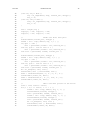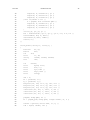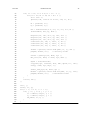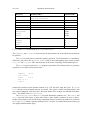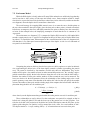
10/17/06
NAB Users’ Manual
Version 5.1
Thomas J. Macke1, W.A. Svrcek-Seiler2, Russell A. Brown3,
and David A. Case4
1
Telik, Inc., Palo Alto, CA 94304
2
University of Vienna, A-1010 Vienna, Austria
3
Sun Microsystems, Inc., Menlo Park, CA 94025
4
The Scripps Research Institute, La Jolla, CA 92037
10/17/06
This source code and manual is copyright (C) 2002, 2004, by Tom Macke, W.A. Svrcek-Seiler,
Russell A. Brown, and David A. Case.
This program is free software; you can redistribute it and/or modify it under the terms of the
GNU General Public License as published by the Free Software Foundation; either version 1, or (at
your option) any later version. The GNU General Public License should be in a file called COPYING;
if not, write to the Free Software Foundation, Inc., 59 Temple Place, Suite 330, Boston, MA
02111-1307 USA
This program is distributed in the hope that it will be useful, but WITHOUT ANY WARRANTY; without even the implied warranty of MERCHANTABILITY or FITNESS FOR A PARTICULAR PURPOSE. See the GNU General Public License for more details.
Some of the force field routines were adapted from similar routines in the MOIL program package: R. Elber, A. Roitberg, C. Simmerling, R. Goldstein, H. Li, G. Verkhivker, C. Keasar, J. Zhang
and A. Ulitsky, "MOIL: A program for simulations of macromolecules" Comp. Phys. Commun. 91,
159-189 (1995).
The "trifix" routine for random pairwise metrization is based on an algorithm designed by Jay
Ponder and was adapted from code in the Tinker package; see M.E. Hodsdon, J.W. Ponder, and D.P.
Cistola, J. Mol. Biol. 264, 585-602 (1996) and http://dasher.wustl.edu/tinker/. The
"molsurf" routines for computing molecular surface areas were adapted from routines written by Paul
Beroza. The "sasad" routine for computing derivatives of solvent accessible surface areas was kindly
provided by S. Sridharan, A. Nicholls and K.A. Sharp. See J. Computat. Chem. 8, 1038-1044 (1995).
The preprocessor (ucpp) was written by Thomas Pornin <[email protected]>,
http://www.di.ens.fr/˜pornin/ucpp/, and is distributed under a separate, BSD-style
license. See ucpp-0.7/README for details.
The cifparse routines to deal with mmCIF formatted files were written by John Westbrook, and
are distributed with permission. See cifparse/README for details.
The teLeap code comes from the Amber suite; this portion is also distributed here (and elsewhere) under the GNU General Public License. The "readparm" routine to access Amber topology
and parameter files was adapted from code written by Bill Ross.
The authors thank Jarrod Smith, Garry Gippert, Paul Beroza, Walter Chazin, Doree Sitkoff and
Vickie Tsui for advice and encouragement. Special thanks to Neill White (who helped in updating
documentation, in preparing the distance geometry database, and in testing and porting portions of the
code), and to Will Briggs (who wrote the fiber-diffraction routines). Thanks also to Chris Putnam and
M.L. Dodson for bug reports.
Sun, Sun Microsystems and Sun Performance Library are trademarks or registered trademarks of
Sun Microsystems, Inc. in the United States and other countries.
The basic literature reference for the code is: T. Macke and D.A. Case. Modeling unusual
nucleic acid structures. In Molecular Modeling of Nucleic Acids, N.B. Leontes and J. SantaLucia, Jr.,
eds. (Washington, DC: American Chemical Society, 1998), pp. 379-393. Users are requested to
include this citation in papers that make use of NAB.
Table of Contents
1. Installation and Getting Started. ..........................................................................................
1.1. Installation. .....................................................................................................................
1.2. Compiling nab Programs. ...............................................................................................
1.3. Parallel Execution ............................................................................................................
1.4. Tested platforms ...............................................................................................................
1.5. Contacting the developers ................................................................................................
2. General introduction and overview. .....................................................................................
2.1. Background ......................................................................................................................
2.1.1. Conformation build-up procedures .........................................................................
2.1.2. Base-first strategies .................................................................................................
2.2. Methods for structure creation .........................................................................................
2.3. First Examples. ...............................................................................................................
2.3.1. B-form DNA duplex. .............................................................................................
2.3.2. Superimpose two molecules. .................................................................................
2.3.3. Place residues in a standard orientation. ................................................................
2.4. Molecules, Residues and Atoms. ....................................................................................
2.5. Creating Molecules. ........................................................................................................
2.6. Residues and Residue Libraries. .....................................................................................
2.7. Atom Names and Atom Expressions. .............................................................................
2.8. Looping over atoms in molecules. ..................................................................................
2.9. Points, Transformations and Frames. .............................................................................
2.9.1. Points and Vectors. .................................................................................................
2.9.2. Matrices and Transformations. ..............................................................................
2.9.3. Frames. ...................................................................................................................
2.10. Creating Watson Crick duplexes. ..................................................................................
2.10.1. bdna() and fd_helix(). ..........................................................................................
2.10.2. wc_complement(). ...............................................................................................
2.10.3. wc_helix() Overview. ...........................................................................................
2.10.4. wc_basepair(). ......................................................................................................
2.10.5. wc_helix() Implementation. .................................................................................
2.11. Structure Quality and Energetics. .................................................................................
2.11.1. Creating a Parallel DNA Triplex. .........................................................................
2.11.2. Creating Base Triads. ...........................................................................................
2.11.3. Finding the lowest energy triad. ...........................................................................
2.11.4. Assembling the Triads into Dimers. ....................................................................
3. NAB Language Reference. ....................................................................................................
3.1. Introduction. ....................................................................................................................
3.2. Language Elements. ........................................................................................................
i
3
3
4
4
8
8
9
10
10
11
12
14
14
14
15
17
17
19
21
22
24
24
24
25
26
26
27
28
29
32
36
36
37
40
40
46
46
46
Table of Contents
3.2.1. Identifiers. ..............................................................................................................
3.2.2. Reserved Words. ....................................................................................................
3.2.3. Literals. ..................................................................................................................
3.2.4. Operators. ...............................................................................................................
3.2.5. Special Characters. ................................................................................................
3.3. Higher-level constructs. ..................................................................................................
3.3.1. Variables. ...............................................................................................................
3.3.2. Attributes. ..............................................................................................................
3.3.3. Arrays. ...................................................................................................................
3.3.4. Expressions. ...........................................................................................................
3.3.5. Regular expressions. ..............................................................................................
3.3.6. Atom Expressions. .................................................................................................
3.3.7. Format Expressions. ...............................................................................................
3.4. Statements. ......................................................................................................................
3.4.1. Expression Statement. ............................................................................................
3.4.2. Delete Statement. ...................................................................................................
3.4.3. If Statement. ...........................................................................................................
3.4.4. While Statement. ....................................................................................................
3.4.5. For Statement. ........................................................................................................
3.4.6. Break Statement. ....................................................................................................
3.4.7. Continue Statement. ...............................................................................................
3.4.8. Return Statement. ..................................................................................................
3.4.9. Compound Statement. ............................................................................................
3.5. Functions. ........................................................................................................................
3.5.1. Function Definitions. .............................................................................................
3.5.2. Function Declarations. ...........................................................................................
3.6. Points and Vectors. ..........................................................................................................
3.7. String Functions. .............................................................................................................
3.8. Math Functions. ..............................................................................................................
3.9. System Functions. ...........................................................................................................
3.10. I/O Functions. ...............................................................................................................
3.10.1. Ordinary I/O Functions. .......................................................................................
3.11. Molecule Creation Functions. .......................................................................................
3.12. Creating Biopoloymers ..................................................................................................
3.13. Fiber Diffraction Duplexes in NAB ...............................................................................
3.14. Reduced Representation DNA Modeling Functions. ....................................................
3.15. Molecule I/O Functions. ...............................................................................................
3.16. Other Molecular Functions. ..........................................................................................
3.17. Debugging Functions. ...................................................................................................
3.18. Time and date routines ...................................................................................................
4. Rigid-Body Transformations .................................................................................................
ii
46
46
46
47
48
48
48
49
51
52
53
53
54
57
57
57
57
58
59
60
60
61
61
61
61
62
62
63
64
66
66
66
68
69
70
70
71
73
74
75
77
Table of Contents
4.1. Transformation Matrix Functions. ..................................................................................
4.2. Frame Functions. ............................................................................................................
4.3. Functions for working with Atomic Coordinates. ..........................................................
4.4. Symmetry Functions. ......................................................................................................
4.4.1. Matrix Creation Functions. ....................................................................................
4.4.2. Matrix I/O Functions. ............................................................................................
4.5. Symmetry server programs ..............................................................................................
4.5.1. matgen .....................................................................................................................
4.5.2. Symmetry Definition Files. ....................................................................................
4.5.3. matmerge ................................................................................................................
4.5.4. matmul ....................................................................................................................
4.5.5. matextract ................................................................................................................
4.5.6. transform .................................................................................................................
5. Distance Geometry. ................................................................................................................
5.1. Metric Matrix Distance Geometry. .................................................................................
5.2. Creating and manipulating bounds, embedding structures ..............................................
5.3. Distance geometry templates. .........................................................................................
5.4. Bounds databases. ...........................................................................................................
6. Molecular mechanics and molecular dynamics. .................................................................
6.1. Basic molecular mechanics routines ................................................................................
6.2. Typical calling sequences. ..............................................................................................
6.3. Second derivatives and normal modes .............................................................................
7. Sample NAB applications. .....................................................................................................
7.1. Duplex Creation Functions. ............................................................................................
7.2. nab and Distance Geometry. ...........................................................................................
7.2.1. Refine DNA Backbone Geometry. .........................................................................
7.2.2. RNA Pseudoknots. .................................................................................................
7.2.3. NMR refinement for a protein ................................................................................
7.3. Building Larger Structures. .............................................................................................
7.4. Closed Circular DNA. .....................................................................................................
7.5. Nucleosome Model ..........................................................................................................
7.6. “Wrapping” DNA Around a Path. ..................................................................................
7.6.1. Interpolating the Curve. .........................................................................................
7.6.2. Driver Code. ...........................................................................................................
7.6.3. Wrap DNA. ............................................................................................................
7.7. Building peptides .............................................................................................................
8. LEaP .........................................................................................................................................
8.1. Introduction ......................................................................................................................
8.2. Concepts ..........................................................................................................................
8.2.1. Commands ..............................................................................................................
8.2.2. Variables .................................................................................................................
iii
77
77
78
78
78
80
81
81
81
83
84
84
84
86
86
87
93
96
99
99
104
106
108
108
110
111
113
118
122
122
126
128
129
132
133
137
143
143
143
143
144
Table of Contents
8.2.3. Objects ....................................................................................................................
8.2.3.1. NUMBERs .....................................................................................................
8.2.3.2. STRINGs .......................................................................................................
8.2.3.3. LISTs .............................................................................................................
8.2.3.4. PARMSETs (Parameter Sets) ........................................................................
8.2.3.5. ATOMs ...........................................................................................................
8.2.3.6. RESIDUEs .....................................................................................................
8.2.3.7. UNITs ............................................................................................................
8.2.3.8. Complex objects and accessing subobjects ...................................................
8.3. Basic instructions for using LEaP with NAB ..................................................................
8.3.1. Building a Molecule For Molecular Mechanics .....................................................
8.3.2. Amino Acid Residues .............................................................................................
8.3.3. Nucleic Acid Residues ............................................................................................
8.3.4. Miscellaneous Residues ..........................................................................................
8.4. Commands .......................................................................................................................
8.4.1. add ...........................................................................................................................
8.4.2. addAtomTypes ........................................................................................................
8.4.3. addIons ....................................................................................................................
8.4.4. addIons2 ..................................................................................................................
8.4.5. addPath ....................................................................................................................
8.4.6. addPdbAtomMap ....................................................................................................
8.4.7. addPdbResMap .......................................................................................................
8.4.8. alias .........................................................................................................................
8.4.9. bond ........................................................................................................................
8.4.10. bondByDistance ....................................................................................................
8.4.11. check .....................................................................................................................
8.4.12. combine .................................................................................................................
8.4.13. copy .......................................................................................................................
8.4.14. createAtom ............................................................................................................
8.4.15. createParmset ........................................................................................................
8.4.16. createResidue ........................................................................................................
8.4.17. createUnit ..............................................................................................................
8.4.18. deleteBond ............................................................................................................
8.4.19. desc .......................................................................................................................
8.4.20. edit ........................................................................................................................
8.4.21. groupSelectedAtoms .............................................................................................
8.4.22. help .......................................................................................................................
8.4.23. impose ...................................................................................................................
8.4.24. list .........................................................................................................................
8.4.25. loadAmberParams .................................................................................................
8.4.26. loadAmberPrep .....................................................................................................
iv
144
144
144
145
145
145
146
146
147
150
150
150
152
152
153
153
154
154
154
155
155
155
156
157
157
157
158
158
159
159
159
159
160
160
161
161
162
162
163
163
163
Table of Contents
8.4.27. loadOff ..................................................................................................................
8.4.28. loadMol2 ...............................................................................................................
8.4.29. loadPdb .................................................................................................................
8.4.30. loadPdbUsingSeq ..................................................................................................
8.4.31. logFile ...................................................................................................................
8.4.32. measureGeom .......................................................................................................
8.4.33. quit ........................................................................................................................
8.4.34. remove ..................................................................................................................
8.4.35. saveAmberParm ....................................................................................................
8.4.36. saveOff ..................................................................................................................
8.4.37. savePdb .................................................................................................................
8.4.38. sequence ................................................................................................................
8.4.39. set ..........................................................................................................................
8.4.40. solvateCap .............................................................................................................
8.4.41. solvateShell ...........................................................................................................
8.4.42. source ....................................................................................................................
8.4.43. transform ...............................................................................................................
8.4.44. translate .................................................................................................................
8.4.45. verbosity ................................................................................................................
8.4.46. zMatrix ..................................................................................................................
9. References ................................................................................................................................
10. Index .......................................................................................................................................
v
164
165
165
166
166
167
167
167
168
169
169
169
170
172
172
173
173
174
174
175
176
179
Table of Contents
vi
10/17/06
Installation and Getting Started
3
1. Installation and Getting Started.
1.1. Installation.
The nab package is available via anonymous ftp at ftp://ftp.scripps.edu/pub/case/nab-5.1.x.tar.gz
as a compressed tar file. The first step in setting up the nab package is to unzip the tar file using the
UNIX commands gunzip:
gunzip nab-5.1.x.tar.gz
tar xvf nab-5.1.x.tar
The path to this new directory (e.g. /usr/local/nab-5.1.x, if you unpacked the distribution in
/usr/local) should be defined as the environment variable $NABHOME. If you are using sh, zsh
or bash as your shell:
export NABHOME=insertyourpathhere/nab-5.1.x
If you are using csh or tcsh as your shell:
setenv NABHOME insertyourpathhere/nab-5.1.x
Now, in the top-level ($NABHOME) directory, you should run the configure script:
./configure --help
will show you the options. Choose a compiler and flags you want; for Linux systems, the following
should work:
./configure gcc
You may need to edit the resulting config.h file to change any variables that don’t match your compilers and OS. The comments in the config.h file should help. Then,
make
will construct the compiler. If the make fails, it is possible that some of the entries in "config.h" are
not correct.
This can be followed by
make test
which will run tests and will report successes or failures.
Now, add the path to the binary executable of nab to your own path and rehash the search path, e.g.,
set path = ( $NABHOME/bin $path )
rehash
10/17/06
Installation and Getting Started
4
Now, you should be able to compile nab programs. Eventually, you may wish to define the environment variable $NABHOME and add the path to the binary executable of nab explicitly in your .cshrc
file (or equivalent in other shells) to avoid having to redefine these variables at each new login.
1.2. Compiling nab Programs.
Compiling nab programs is very similar to compiling other high-level language programs, such as C
and FORTRAN. The command line syntax is
nab [-O] [-c] [-v] [-noassert] [-nodebug] [-o file] [-Dstring] file(s)
where
-O optimizes the object code
-c suppresses the linking stage with ld and produces a .o file
-v verbosely reports on the compile process
-noassert causes the compiler to ignore assert statements
-nodebug causes the compiler to ignore debug statements
-o file names the output file
-Dstring defines string to the C preprocessor
Linking FORTRAN and C object code with nab is accomplished simply by including the source files
on the command line with the nab file. For instance, if a nab program bar.nab uses a C function
defined in the file foo.c, compiling and linking optimized nab code would be accomplished by
nab -O bar.nab foo.c
The result is an executable a.out file.
1.3. Parallel Execution
The generalized Born energy routines (for both first and second derivatives) include directives
that will allow for parallel execution on machines that support this option. Once you have some level
of comfort and experience with the single-CPU version, you can enable parallel execution by supplying one of several parallelization options (-openmp, -mpi or -scalapack) to configure, by re-building
the NAB compiler (see section 1.1 above) and by recompiling your NAB program (see section 1.2
above).
The -openmp option enables parallel execution under OpenMP on shared- memory machines. To
enable OpenMP execution, add the -openmp option to configure, re-build the NAB compiler and recompile your NAB program. Then, if you set the OMP_NUM_THREADS environment variable to
10/17/06
Installation and Getting Started
5
the number of threads that you wish to perform parallel execution, the Born energy computation will
execute in parallel.
The -mpi option enables parallel execution under MPI on either clusters or shared-memory
machines. To enable MPI execution, add the -mpi option to configure and re-build the NAB compiler.
You will need to modify your NAB program prior to re-compilation in order to initialize MPI as the
first step of your program, and in order to shut down MPI as the final step of your program. The initialization and shut down are supported by the mpiinit() and mpifinalize() functions. In addition, the
mpierror() function performs I/O error checking across all of the MPI processes. Below is a simple
NAB program that reads in a molecular model from a protein data bank (PDB) file, performs conjugate gradients minimization followed by molecular dynamics, and writes the result to another PDB
file. The details of this program will be understandable after the user reads Section 6. This program is
provided here to demonstrate how to use the mpiinit(), mpifinalize() and mpierror() functions:
// Try some conjugate gradients followed by molecular dynamics.
molecule m;
int ier, mytaskid, numtasks;
float m_xyz[dynamic], f_xyz[dynamic], v_xyz[dynamic];
float dgrad, fret;
point dummy;
// Initialize MPI.
if ( mpiinit(argc, argv, mytaskid, numtasks) != 0 ) {
printf("Error in mpiinit!\n");
fflush(stdout);
exit (1);
}
// Check for correct number of calling parameters.
if (argc != 4) {
if (mytaskid == 0) {
printf("Usage: %s pdbin prmtop pdbout\n", argv[1]);
fflush(stdout);
}
ier = -1;
} else {
ier = 0;
}
if ( mpierror(ier) != 0) {
if (mytaskid == 0) {
printf("Error in mpierror!\n");
fflush(stdout);
}
exit (1);
}
10/17/06
Installation and Getting Started
// Create a molecule from a pdb file and a "prmtop" file.
m = getpdb(argv[2]);
readparm(m, argv[3]);
// Allocate the arrays.
allocate m_xyz[3*m.natoms];
allocate f_xyz[3*m.natoms];
allocate v_xyz[3*m.natoms];
// Load the molecular coordinates into the m_xyz array.
setxyz_from_mol(m, NULL, m_xyz);
// Initialize molecular mechanics.
mme_init(m, NULL, "::ZZZZ", dummy, NULL);
mm_options("cut=20.0, rgbmax=20.0, nsnb=10, gb=1, diel=C");
mm_options("tautp=0.4, temp0=100.0, tempi=50.0");
mm_options("ntpr_md=100, ntpr=100");
fret = mme(m_xyz, f_xyz, 0);
if (mytaskid == 0) {
printf("Initial energy is %f0\n", fret);
}
// Do some conjugate gradient minimization.
If (mytaskid == 0) {
printf("Starting with conjugate gradients...\n\n");
}
mm_options("cut=20.0, rgbmax=20.0, ntpr=100");
mm_options("nsnb=10, gb=1, diel=C");
dgrad = 0.00001;
ier = conjgrad(m_xyz, 3*m.natoms, fret, mme, dgrad, 0.0001, 50000);
// Do some molecular dynamics.
if (mytaskid == 0) {
printf("Starting with molecular dynamics...\n\n");
}
ier = md(3*m.natoms, 1000, m_xyz, f_xyz, v_xyz, mme);
if (mytaskid == 0) {
printf("\n...Done, md returns %d\n", ier);
}
// Load the molecular coordinates into the m_xyz array and
// write the result as a pdb file.
6
10/17/06
Installation and Getting Started
7
setmol_from_xyz(m, NULL, m_xyz);
putpdb(argv[4], m);
// Shut down MPI.
if ( mpifinalize() != 0) {
if (mytaskid == 0) {
printf("Error in mpifinalize!\n");
fflush(stdout);
}
}
To reiterate, the details of this NAB program will be made clear in section 6. However, this program
demonstrates that the first step of an MPI- compatible NAB program is a call to mpiinit(), that the last
step of an MPI- compatible NAB program is a call to mpifinalize(), and that I/O error checking is performed by mpierror(). One further point that is illustrated by this NAB program is that it is preferable
for an MPI-compatible NAB program to use the readparm() function instead of the getpdb_prm()
function (see Section 6.1). Because the mpiinit(), mpifinalize() and mpierror() functions are ignored
by NAB unless the -mpi option is specified, all NAB programs may include these functions which will
be utilized only if the -mpi option is specified (or if the -scalapack option is specified, see below).
The -scalapack option enables parallel execution under MPI on either clusters or shared-memory
machines, and in addition uses the Scalable LAPACK (ScaLAPACK) library for parallel linear algebra
computation that is required to calculate the second derivatives of the generalized Born energy, to perform Newton-Raphson minimization or to perform normal mode analysis (see Section 6.3). For computations that do not involve linear algebra (such as conjugate gradients minimization or molecular
dynamics) the -scalapack option functions in the same manner as the -mpi option. Do not use the -mpi
and -scalapack options simultaneously. Use the -scalapack option only when ScaLAPACK has been
installed on your cluster or shared- memory machine.
In order that the -mpi or -scalapack options result in a correct build of the NAB compiler, the
configure script must specify linking of the MPI library, or ScaLAPACK and BLACS libraries, as part
of that build. These libraries are specified for Sun machines in the solaris_cc section of the configure
script. If you want to use MPI or ScaLAPACK on a machine other than a Sun machine, you will need
to modify the configure script to link these libraries in a manner analogous to what occurs in the
solaris_cc section of the script.
There are three options to specify the manner in which NAB supports linear algebra computation. The -scalapack option discussed above specifies ScaLAPACK. The -perflib option specifies
SunTM Performance LibraryTM, a multi-threaded implementation of LAPACK. If neither -scalapack
nor -perflib is specified, then linear algebra computation will be performed by a single CPU using
LAPACK. In this last case, the Intel MKL library will be used if the MKL_HOME environment variable is set at configure time.
The parallel execution capability of NAB was developed primarily on Sun machines, and has
also been tested on the SGI Altix platform. But it has been much less widely-used than have other
parts of NAB, so you should certainly run some tests with your system to ensure that single-CPU and
parallel runs give the same results.
10/17/06
Installation and Getting Started
8
1.4. Tested platforms
We have carried out the compilation and test programs on many Unix/Linux machines, and
things are generally pretty portable. In particular, things should work on HP/UX, Solaris, IRIX,
Linux, and MacOS X, as well as on windows using the Cygwin deveopment kit, available from
http://sources.redhat/com. Look at the config.h.* files in the main directory for information about porting the code.
1.5. Contacting the developers
Please send suggestions and questions to [email protected] or [email protected].
10/17/06
General overview
9
2. General introduction and overview.
Nucleic acid builder (nab) is a high-level language that facilitates manipulations of macromolecules and their fragments. nab uses a C-like syntax for variables, expressions and control structures (if, for, while) and has extensions for operating on molecules (new types and a large number
of builtins for providing the necessary operations). We expect nab to be useful in model building and
coordinate manipulation of proteins and nucleic acids, ranging in size from fairly small systems to the
largest systems for which an atomic level of description makes good computational sense. As a programming language, it is not a solution or program in itself, but rather provides an environment that
eases many of the bookkeeping tasks involved in writing programs that manipulate three-dimensional
structural models.
The current implementation is version 5.0, and incorporates the following main features:
(1)
Objects such as points, atoms, residues, strands and molecules can be referenced and manipulated as named objects. The internal manipulations involved in operations like merging several
strands into a single molecule are carried out automatically; in most cases the programmer
need not be concerned about the internal data structures involved.
(2)
Rigid body transformations of molecules or parts of molecules can be specified with a fairly
high-level set of routines. This functionality includes rotations and translations about particular axis systems, least-squares atomic superposition, and manipulations of coordinate frames
that can be attached to particular atomic fragments.
(3)
Additional coordinate manipulation is achieved by a tight interface to distance geometry methods. This allows allows relationships that can be defined in terms of internal distance constraints to be realized in three-dimensional structural models. nab includes subroutines to
manipulate distance bounds in a convenient fashion, in order to carry out tasks such as working with fragments within a molecule or establishing bounds based on model structures.
(4)
Force field calculations (e.g. molecular dynamics and minimization) can be carried out with an
implementation of the AMBER force field. This works in both three and four dimensions, but
periodic simulations are not (yet) supported. However, the generalized Born models implemented in Amber are also implemented here, which allows many interesting simulations to be
carried out without requiring periodic boundary conditions. The force field can be used to
carry out minimization, molecular dynamics, or normal mode calculations.
(5)
nab also implements a form of regular expressions that we call atom regular expressions,
which provide a uniform and convenient method for working on parts of molecules.
(6)
Many of the general programming features of the awk language have been incorporated in
nab. These include regular expression pattern matching, hashedarrays (i.e. arrays with
strings as indices), the splitting of strings into fields, and simplified string manipulations.
(7)
There are built-in procedures for linking nab routines to other routines written in C or Fortran,
including access to most library routines normally available in system math libraries.
Our hope is that nab will serve to formalize the step-by-step process that is used to build complex model structures, and will facilitate the management and use of higher level symbolic constraints.
Writing a program to create a structure forces more of the model’s assumptions to be explicit in the
program itself. And an nab description can serve as a way to show a model’s salient features, much
like helical parameters are used to characterize duplexes.
10/17/06
General overview
10
The first three chapters of this document both introduces the language through a series of sample
programs, and illustrates the programming interfaces provided. The examples are chosen not only to
show the syntax of the language, but also to illustrate potential approaches to the construction of some
unusual nucleic acids, including DNA double- and triple-helices, RNA pseudoknots, four-arm junctions, and DNA-protein interactions. A separate reference manual (in Chapter 4) gives a more formal
and careful description of the requirements of the language itself.
The basic literature reference for the code is: T. Macke and D.A. Case. Modeling unusual
nucleic acid structures. In Molecular Modeling of Nucleic Acids, N.B. Leontes and J. SantaLucia, Jr.,
eds. (Washington, DC: American Chemical Society, 1998), pp. 379-393. Users are requested to
include this citation in papers that make use of NAB.
2.1. Background
Using a computer language to model polynucleotides follows logically from the fundamental
nature of nucleic acids, which can be described as “conflicted” or “contradictory” molecules. Each
repeating unit contains seven rotatable bonds (creating a very flexible backbone), but also contains a
rigid, planar base which can participate in a limited number of regular interactions, such as base pairing and stacking. The result of these opposing tendencies is a family of molecules that have the potential to adopt a virtually unlimited number of conformations, yet have very strong preferences for regular helical structures and for certain types of loops.
The controlled flexibility of nucleic acids makes them difficult to model. On one hand, the limited range of regular interactions for the bases permits the use of simplified and more abstract geometric representations. The most common of these is the replacement of each base by a plane, reducing
the representation of a molecule to the set of transformations that relate the planes to each other. On
the other hand, the flexible backbone makes it likely that there are entire families of nucleic acid structures that satisfy the constraints of any particular modeling problem. Families of structures must be
created and compared to the model’s constraints. From this we can see that modeling nucleic acids
involves not just chemical knowledge but also three processes−abstraction, iteration and testing−that
are the basis of programming.
Molecular computation languages are not a new idea. Here we briefly describe some past
approaches to nucleic acid modeling, to provide a context for nab.
2.1.1. Conformation build-up procedures
MC-SYM [1-3] is a high level molecular description language used to describe single stranded
RNA molecules in terms of functional constraints. It then uses those constraints to generate structures
that are consistent with that description. MC-SYM structures are created from a small library of conformers for each of the four nucleotides, along with transformation matrices for each base. Building
up conformers from these starting blocks can quickly generate a very large tree of structures. The key
to MC-SYM’s success is its ability to prune this tree, and the user has considerable flexibility in
designing this pruning process.
In a related approach, Erie et al. [4] used a Monte-Carlo build-up procedure based on sets of low
energy dinucleotide conformers to construct longer low energy single stranded sequences that would
be suitable for incorporation into larger structures. Sets of low energy dinucleotide conformers were
created by selecting one value from each of the sterically allowed ranges for the six backbone torsion
angles and χ. Instead of an exhaustive build- up search over a small set of conformers, this method
10/17/06
General overview
11
samples a much larger region of conformational space by randomly combining members of a larger set
of initial conformers. Unlike strict build-up procedures, any member of the initial set is allowed to follow any other member, even if their corresponding torsion angles do not exactly match, a concession
to the extreme flexibility of the nucleic acid backbone. A key feature determined the probabilities of
the initial conformers so that the probability of each created structure accurately reflected its energy.
Tung and Carter [5,6] have used a reduced coordinate system in the NAMOT (nucleic acid modeling tool) program to rotation matrices that build up nucleic acids from simplified descriptions. Special
procedures allow base-pairs to be preserved during deformations. This procedure allows simple algorithmic descriptions to be constructed for non-regular structures like intercalation sites, hairpins, pseudoknots and bent helices.
2.1.2. Base-first strategies
An alternative approach that works well for some problems is the "base-first" strategy, which
lays out the bases in desired locations, and attempts to find conformations of the sugar-phosphate
backbone to connect them. Rigid-body transformations often provide a good way to place the bases.
One solution to the backbone problem would be to determine the relationship between the helicoidal
parameters of the bases and the associated backbone/sugar torsions. Work along these lines suggests
that the relationship is complicated and non-linear [7]. However, considerable simplification can be
achieved if instead of using the complete relationship between all the helicoidal parameters and the
entire backbone, the problem is limited to describing the relationship between the helicoidal parameters and the backbone/sugar torsion angles of single nucleotides and then using this information to
drive a constraint minimizer that tries to connect adjacent nucleotides. This is the approach used in
JUMNA [8], which decomposes the problem of building a model nucleic acid structure into the constraint satisfaction problem of connecting adjacent flexible nucleotides. The sequence is decomposed
into 3’-nucleotide monophosphates. Each nucleotide has as independent variables its six helicoidal
parameters, its glycosidic torsion angle, three sugar angles, two sugar torsions and two backbone torsions. JUMNA seeks to adjust these independent variables to satisfy the constraints involving sugar
ring and backbone closure.
Even constructing the base locations can be a non-trivial modeling task, especially for non-standard structures. Recognizing that coordinate frames should be chosen to provide a simple description
of the transformations to be used, Gabarro-Arpa et al. [9] devised “Object Command Language”
(OCL), a small computer language that is used to associate parts of molecules called objects, with
arbitrary coordinate frames defined by sets of their atoms or numerical points. OCL can “link”
objects, allowing other objects’ positions and orientations to be described in the frame of some reference object. Information describing these frames and links is written out and used by the program
MORCAD [10] which does the actual object transformations.
OCL contains several elements of a molecular modeling language. Users can create and operate
on sets of atoms called objects. Objects are built by naming their component atoms and to simplify
creation of larger objects, expressions, IF statements, an iterated FOR loop and limited I/O are provided. Another nice feature is the equivalence between a literal 3-D point and the position represented
by an atom’s name. OCL includes numerous built-in functions on 3-vectors like the dot and cross
products as well as specialized molecular modeling functions like creating a vector that is normal to an
object. However, OCL is limited because these language elements can only be assembled into functions that define coordinate frames for molecules that will be operated on by MORCAD. Functions
producing values of other data types and stand-alone OCL programs are not possible.
10/17/06
General overview
12
2.2. Methods for structure creation
As a structure-generating tool, nab provides three methods for building models. They are rigidbody transformations, metric matrix distance geometry, and molecular mechanics. The first two methods are good initial methods, but almost always create structures with some distortion that must be
removed. On the other hand, molecular mechanics is a poor initial method but very good at refinement.
Thus the three methods work well together.
Rigid-body transformations. Rigid-body transformations create model structures by applying
coordinate transformations to members of a set of standard residues to move them to new positions
and orientations where they are incorporated into the growing model structure. The method is especially suited to helical nucleic acid molecules with their highly regular structures. It is less satisfactory
for more irregular structures where internal rearrangement is required to remove bad covalent or nonbonded geometry, or where it may not be obvious how to place the bases.
nab uses the matrix type to hold a 4×4 transformation matrix. Transformations are applied to
residues and molecules to move them into new orientations or positions. nab does not require that
transformations applied to parts of residues or molecules be chemically valid. It simply transforms the
coordinates of the selected atoms leaving it to the user to correct (or ignore) any chemically incorrect
geometry caused by the transformation.
Every nab molecule includes a frame, or “handle” that can be used to position two molecules in a
generalization of superimposition. Traditionally, when a molecule is superimposed on a reference
molecule, the user first forms a correspondence between a set of atoms in the first molecule and
another set of atoms in the reference molecule. The superimposition algorithm then determines the
transformation that will minimize the rmsd between corresponding atoms. Because superimposition is
based on actual atom positions, it requires that the two molecules have a common substructure, and it
can only place one molecule on top of another and not at an arbitrary point in space.
The nab frame is a way around these limitations. A frame is composed of three orthonormal
vectors originally aligned along the axes of a right handed coordinate frame centered on the origin.
nab provides two builtin functions setframe() and setframep() that are used to reposition this
frame based on vectors defined by atom expressions or arbitrary 3-D points, respectively. To position
two molecules via their frames, the user moves the frames so that when they are superimposed via the
nab builtin alignframe(), the two molecules have the desired orientation. This is a generalization
of the methods described above for OCL.
Distance geometry. nab’s second initial structure-creation method is metric matrix distance
geometry [11,12], which can be a very powerful method of creating initial structures. It has two main
strengths. First, since it uses internal coordinates, the initial position of atoms about which nothing is
known may be left unspecified. This has the effect that distance geometry models use only the information the modeler considers valid. No assumptions are required concerning the positions of unspecified atoms. The second advantage is that much structural information is in the form of distances.
These include constraints from NMR or fluorescence energy transfer experiments, implied propinquities from chemical probing and footprinting, and tertiary interactions inferred from sequence analysis. Distance geometry provides a way to formally incorporate this information, or other assumptions,
into the model-building process.
Distance geometry converts a molecule represented as a set of interatomic distances into a 3-D
structure. nab has several builtin functions that are used together to provide metric matrix distance
geometry. A bounds object contains the molecule’s interatomic distance bounds matrix and a list of
its chiral centers and their volumes. The function newbounds() creates a bounds object
10/17/06
General overview
13
containing a distance bounds matrix containing initial upper and lower bounds for every pair of atoms,
and a list of the molecule’s chiral centers and their volumes. Distance bounds for pairs of atoms
involving only a single residue are derived from that residue’s coordinates. The 1,2 and 1,3 distance
bounds are set to the actual distance between the atoms. The 1,4 distance lower bound is set to the
larger of the sum of the two atoms Van der Waals radii or their syn (torsion angle = 0°) distance, and
the upper bound is set to their anti (torsion angle = 180°) distance. newbounds() also initializes the
list of the molecule’s chiral centers. Each chiral center is an ordered list of four atoms and the volume
of the tetrahedron those four atoms enclose. Each entry in a nab residue library contains a list of the
chiral centers composed entirely of atoms in that residue.
Once a bounds object has been initialized, the modeler can use functions to tighten, loosen or
set other distance bounds and chiralities that correspond to experimental measurements or parts of the
model’s hypothesis. The functions andbounds() and orbounds() allow logical manipulation of
bounds. setbounds_from_db() Allows distance information from a model structure or a
database to be incorporated into a part of the current molecule’s bounds object, facilitating transfer
of information between partially-built structures.
These primitive functions can be incorporated into higher-level routines. For example the functions stack() and watsoncrick() set the bounds between the two specified bases to what they
would be if they were stacked in a strand or base-paired in a standard Watson/Crick duplex, with
ranges of allowed distances derived from an analysis of structures in the Nucleic Acid Database.
After all experimental and model constraints have been entered into the bounds object, the
function tsmooth() applies “triangle smoothing” to pull in the large upper bounds, since the maximum distance between two atoms can not exceed the sum of the upper bounds of the shortest path
between them. Random pairwise metrization [13] can also be used to help ensure consistency of the
bounds and to improve the sampling of conformational space. The function embed() finally takes
the smoothed bounds and converts them into a 3-D object. The newly embedded coordinates are subject to conjugate gradient refinement against the distance and chirality information contained in
bounds. The call to embed() is usually placed in a loop to explore the diversity of the structures
the bounds represent.
Molecular mechanics. The final structure creation method that nab offers is molecular mechanics. This includes both energy minimization and molecular dynamics − simulated annealing. Since
this method requires a good estimate of the initial position of every atom in a structure, it is not suitable for creating initial structures. However, given a reasonable initial structure, it can be used to
remove bad initial geometry and to explore the conformational space around the initial structure. This
makes it a good method for refining structures created either by rigid body transformations or distance
geometry. nab has its own 3-D/4-D molecular mechanics package that implements several AMBER
force fields and reads AMBER parameter and topology files. Solvation effects can also be modelled
with generalized Born continuum models.
Our hope is that nab will serve to formalize the step-by-step process that is used to build complex model structures. It will facilitate the management and use of higher level symbolic constraints.
Writing a program to create a structure forces one to make explicit more of the model’s assumptions in
the program itself. And an nab description can serve as a way to exhibit a model’s salient features,
much like helical parameters are used to characterize duplexes. So far, nab has been used to construct
models for synthetic Holliday junctions [14], calcyclin dimers [15], HMG-protein/DNA complexes
[16], active sites of Rieske iron-sulfur proteins [17], and supercoiled DNA [18]. The Examples chapter below provides a number of other sample applications.
10/17/06
General overview
14
2.3. First Examples.
This section introduces nab via three simple examples. All nab programs in this user manual
are set in Courier, a typewriter style font. The line numbers at the beginning of each line are not parts
of the programs but have been added to make it easier to refer to specific program sections.
2.3.1. B-form DNA duplex.
One of the goals of nab was that simple models should require simple programs. Here is an nab
program that creates a model of a B-form DNA duplex and saves it as a PDB file.
1
2
3
4
5
// Program 1 - Average B-form DNA duplex
molecule m;
m = bdna( "gcgttaacgc" );
putpdb( "gcg10.pdb", m );
Line 2 is a declaration used to tell the nab compiler that the name m is a molecule variable,
something nab programs use to hold structures. Line 4 creates the actual model using the predefined
function bdna(). This function’s argument is a literal string which represents the sequence of the
duplex that is to be created. Here’s how bdna() converts this string into a molecule. Each letter
stands for one of the four standard bases: a for adenine, c for cytosine, g for guanine and t for
thymine. In a standard DNA duplex every adenine is paired with thymine and every cytosine with
guanine in an antiparallel double helix. Thus only one strand of the double helix has to be specified.
As bdna() reads the string from left to right, it creates one strand from 5’ to 3’ (5’-gcgttaacgc
-3’), automatically creating the other antiparallel strand using Watson/Crick pairing. It uses a uniform
° rise and 36.0° twist. Naturally, nab has other ways to create helical molecules
helical step of 3.38A
with arbitrary helical parameters and even mismatched base pairs, but if you need some “average”
DNA, you should be able to get it without having to specify every detail. The last line uses the nab
builtin putpdb() to write the newly created duplex to the file gcg10.pdb.
Program 1 is about the smallest nab program that does any real work. Even so, it contains several elements common to almost all nab programs. The two consecutive forward slashes in line 1
introduce a comment which tells the nab compiler to ignore all characters between them and the end
of the line. This particular comment begins in column 1, but that is not required as comments may
begin in any column. Line 3 is blank. It serves no purpose other than to visually separate the declaration part from the action part. nab input is free format. Runs of white space characters—spaces, tabs,
blank lines and page breaks—act like a single space which is required only to separate reserved words
like molecule from identifiers like m. Thus white space can be used to increase readability.
2.3.2. Superimpose two molecules.
Here is another simple nab program. It reads two DNA molecules and superimposes them
using a rotation matrix made from a correspondence between their C1’ atoms.
1
2
3
4
// Program 2 - Superimpose two DNA duplexes
molecule m, mr;
float r;
10/17/06
General overview
5
6
7
8
9
10
15
m = getpdb( "test.pdb" );
mr = getpdb( "gcg10.pdb" );
superimpose( m, "::C1’", mr, "::C1’" );
putpdb( "test.sup.pdb", m );
rmsd( m, "::C1’", mr, "::C1’", r );
printf( "rmsd = %8.3f\n", r );
This program uses three variables—two molecules, m and mr and one float, r. An nab declaration can include any number of variables of the same type, but variables of different types must be in
separate declarations. The builtin function getpdb() reads two molecules in PDB format from the
files test.pdb and gcg10.pdb into the variables m and mr. The superimposition is done with the
builtin function superimpose(). The arguments to superimpose() are two molecules and two
“atom expressions”. nab uses atom expressions as a compact way of specifying sets of atoms. Atom
expressions and atom names are discussed in more detail below but for now an atom expression is a
pattern that selects one or more of the atoms in a molecule. In this example, they select all atoms with
names C1’.
superimpose() uses the two atom expressions to associate the corresponding C1’ carbons in
the two molecules. It uses these correspondences to create a rotation matrix that when applied to m will
minimize the root mean square deviation between the pairs. It applies this matrix to m, “moving” it on
to mr. The transformed molecule m is written out to the file test.sup.pdb in PDB format using the
builtin function putpdb(). Finally the builtin function rmsd() is used to compute the actual root
mean square deviation between corresponding atoms in the two superimposed molecules. It returns the
result in r, which is written out using the C-like I/O function printf(). rmsd() also uses two
atom expressions to select the corresponding pairs. In this example, they are the same pairs that were
used in the superimposition, but any set of pairs would have been acceptable. An example of how this
might be used would be to use different subsets of corresponding atoms to compute trial superimpositions and then use rmsd() over all atoms of both molecules to determine which subset did the best
job.
2.3.3. Place residues in a standard orientation.
This is the last of the introductory examples. It places nucleic acid monomers in an orientation
that is useful for building Watson/Crick base pairs. It uses several atom expressions to create a frame
or handle attached to an nab molecule that permits easy movement along important “molecular directions”. In a standard Watson/Crick base pair the C4 and N1 atoms of the purine base and the H3, N3
and C6 atoms of the pyrimdine base are colinear. Such a line is obviously an important molecular
direction and would make a good coordinate axis. Program 3 aligns these monomers so that this
hydrogen bond is along the Y-axis.
1
2
3
4
5
6
7
8
// Program 3 - orient nucleic acid monomers
molecule m;
m = getpdb( "ADE.pdb" );
setframe( 2, m,
"::C4",
"::C5", "::N3",
"::C4", "::N1" );
// also for GUA
10/17/06
9
10
11
12
13
14
15
16
17
18
General overview
16
alignframe( m, NULL );
putpdb( "ADE.std.pdb", m );
m = getpdb( "THY.pdb" );
setframe( 2, m,
"::C6",
"::C5", "::N1",
"::C6", "::N3" );
alignframe( m, NULL );
putpdb( "THY.std.pdb", m );
// also for CYT & URA
This program uses only one variable, the molecule m. Execution begins on line 4 where the
builtin getpdb() is used to read in the coordinates of an adenine (created elsewhere) from the file
ADE.pdb. The nab builtin setframe() creates a coordinate frame for this molecule using vectors
defined by some of its atoms as shown in Figure 1. The first atom expression (line 6) sets the origin of
this coordinate frame to be the coordinates of the C4 atom. The two atom expressions on line 7 set the
X direction from the coordinates of the C5 to the coordinates of the N3. The last two atom expressions
set the Y direction from the C4 to the N1. The Z-axis is created by the cross product X×Y. Frames are
thus like sets of local coordinates that can be attached to molecules and used to facilitate defining
transformations; a more complete discussion is given in the section Frames below.
nab requires that the coordinate axes of all frames be orthogonal, and while the X and Y axes as
specified here are close, they are not quite exact. setframe() uses its first parameter to specify
which of the original two axes is to be used as a formal axis. If this parameter is 1, then the specified X
axis becomes the formal X axis and Y is recreated from Z×X; if the value is 2, then the specified Y
axis becomes the formal Y axis and X is recreated from Y×Z. In this example the specified Y axis is
used and X is recreated. The builtin alignframe() transforms the molecule so that the X, Y and Z
axes of the newly created coordinate frame point along the standard X, Y and Z directions and that the
Y
N1
ADE
C5
N3
C4
H3 Y
N3
THY
X
N1
C5
X
C6
Figure 1. ADE and THY after execution of Program 3.
10/17/06
General overview
17
origin is at (0,0,0). The transformed molecule is writen to the file ADE.std.pdb. A similar procedure is performed on a thymine residue with the result that the hydrogen bond between the H3 of
thymine and the N1 of adenine in a Watson Crick pair is now along the Y axis of these two residues.
2.4. Molecules, Residues and Atoms.
We now turn to a discussion of ways of describing and manipulating molecules. In addition to
the general-purpose variable types like float, int and string, nab has three types for working
with molecules: molecule, residue and atom. Like their chemical counterparts, nab molecules
are composed of residues which are in turn composed of atoms. The residues in an nab molecule are
organized into one or more named, ordered lists called strands. Residues in a strand are usually
bonded so that the “exiting” atom of residue i is connected to the “entering” atom of residue i + 1. The
residues in a strand need not be bonded; however, only residues in the same strand can be bonded.
Each of the three molecular types has a complex internal structure, only some of which is
directly accessible at the nab level. Simple elements of these types, like the number of atoms in a
molecule or the X coordinate of an atom are accessed via attributes—a suffix attached to a molecule,
residue or atom variable. Attributes behave almost like int, float and string variables; the only
exception being that some attributes are read only with values that can t be changed. More complex
operations on these types such as adding a residue to a molecule or merging two strands into one are
handled with builtin functions. A complete list of nab builtin functions and molecule attributes can be
found in the nab Language Reference.
2.5. Creating Molecules.
The following functions are used to create molecules. Only an overview is given here; more
details are in chapter 3.
molecule newmolecule();
int
addstrand( molecule m, string str );
residue getresidue( string rname, string rlib );
residue transformres( matrix mat, residue res, string aex );
int
addresidue( molecule m, string str, residue res );
int
connectres( molecule m, string str,
int rn1, string atm1, int rn2, string atm2 );
int
mergestr( molecule m1, string str1, string end1,
molecule m2, string str2, string end2 );
The general strategy for creating molecules with nab is to create a new (empty) molecule then
build it one residue at a time. Each residue is fetched from a residue library, transformed to properly
position it and added to a growing strand. A template showing this strategy is shown below. mat, m
and res are respectively a matrix, molecule and residue variable declared elsewhere. Words
in italics indicate general instances of things that would be filled in according to actual application.
10/17/06
General overview
1
2
3
4
5
6
7
8
9
10
11
12
18
...
m = newmolecule();
addstrand( m, str-1 );
...
for( ... ){
...
res = getresidue( res-name, res-lib );
res = transformres( mat, res, NULL );
addresidue( m, str-name, res );
...
}
...
In line 2, the function newmolecule() creates a molecule and stores it in m. The new
molecule is empty—no strands, residues or atoms. Next addstrand() is used to add a strand
named str-1. Strand names may be up to 255 characters in length and can include any characters
except white space. Each strand in a molecule must have a unique name. There is no limit on the number of strands a molecule may have.
The actual structure would be created in the loop on lines 5-11. Each time around the loop, the
function getresidue() is used to extract the next residue with the name res-name from some
residue library res-lib and stores it in the residue variable res. Next the function transformres() applies a transformation matrix, held in the matrix variable mat to the residue in res,
which places it in the orientation and position it will have in the new molecule. Finally, the function
addresidue() appends the transformed residue to the end of the chain of residues in the strand strname of the new molecule.
Residues in each strand are numbered from 1 to N, where N is the number of residues in that
strand. The residue order is the order in which they were inserted with addresidue(). While nab
does not require it, nucleic acid chains are usually numbered from 5’ to 3’ and proteins chains from
the N-terminus to the C-terminus. The residues in nucleic acid strands and protein chains are usually
bonded with the outgoing end of residue i bonded to the incoming end of residue i+1. However, as this
is not always the case, nab requires the user to explicitly make all interresidue bonds with the builtin
connectres().
connectres() makes bonds between two atoms in different residues of the same strand of a
molecule. Only residues in the same strand can be bonded. connectres() takes six arguments.
They are a molecule, the name of the strand containing the residues to be bonded, and two pairs each
of a residue number and the name of an atom in that residue. As an example, this call to connectres(),
connectres( m, "sense", i, "O3’", i+1, "P" );
connects an atom named "O3’" in residue i to an atom named "P" in residue i+1, creating the
phosphate bond that joins two nucleic acid monomers.
The function mergestr() is used to either move or copy the residues in one strand into
another strand. Details are provided in chapter 3.
10/17/06
General overview
19
2.6. Residues and Residue Libraries.
nab programs build molecules from residues that are parts of residue libraries, which are exactly
those
distributed
with
the
Amber
molecular
mechanics
programs
(see
http://amber.scripps.edu).
nab provides several functions for working with residues. All return a valid residue on success
and NULL on failure. The function getres() is written in nab and it source is shown below.
transformres() which applies a coordinate transformation to a residue and is discussed under the
section Matrices and Transformations.
residue getresidue( string resname, string reslib );
residue getres( string resname, string reslib );
residue transformres( matrix mat, residue res, string aexp );
getresidue() extracts the residue with name resname from the residue library reslib.
reslib is the name of a file that either contains the residue information or contains names of other
files that contain it. reslib is assumed to be in the directory $NABHOME/reslib unless it begins
with a slash (/)
A common task of many nab programs is the translation of a string of characters into a structure
where each letter in the string represents a residue. Generally, some mapping of one or two character
names into actual residue names is required. nab supplies the function getres() that maps the single character names a, c, g, t and u and their 5’ and 3’ terminal analogues into the residues ADE,
CYT, GUA, THY and URA. Here is its source:
1
2
3
4
5
6
7
8
9
10
11
12
13
14
15
16
17
18
19
// getres() - map 1 letter names into 3 letter names
residue getres( string rname, string rlib )
{
residue res;
string map1to3[ hashed ];
// convert residue names
map1to3["A"] = "ADE";
map1to3["G"] = "GUA";
map1to3["U"] = "URA";
map1to3["C"] = "CYT";
map1to3["T"] = "THY";
map1to3["a"] = "ADE";
map1to3["g"] = "GUA";
map1to3["u"] = "URA";
map1to3["c"] = "CYT";
map1to3["t"] = "THY";
if( r in map1to3 ) {
res = getresidue( map1to3[ r ], rlib );
}else{
fprintf( stderr, "undefined residue %s\n", r );
exit( 1 );
10/17/06
20
21
22
General overview
20
}
return( res );
};
getres() is the first of several nab functions that are discussed in this User Manual. The following explanation will cover not just getres() but will serve as an introduction to user defined
nab functions in general.
An nab function is a named group of declarations and statements that is executed as a unit by
using the function’s name in an expression. nab functions can have special variables called parameters that allow the same function to operate on different data. A function definition begins with a
header that describes the function, followed by the function body which is a list of statements and declarations enclosed in braces ({}) and ends with a semicolon. The header to getres() is on line 2
and the body is on lines 3 to 22.
Every nab function header begins with the reserved word that specifies its type, followed by the
function’s name followed by its parameters (if any) enclosed in parentheses. The parentheses are
always required, even if the function does not have parameters. nab functions may return a single
value of any of the 10 nab types. nab functions can not return arrays. In symbolic terms every nab
function header uses this template:
type name( parameters? )
The parameters (if present) to an nab function are a comma separated list of type variable pairs:
type1 variable1, type2 variable2, ...
An nab function may have any number of parameters, including none. Parameters may of any of the
10 nab types, but unlike function values, parameters can be arrays, including hashed arrays. The function getres() has two parameters, the two string variables resname and reslib.
Parameters to nab functions are “called by reference” which means that they contain the actual
data—not copies of it—that the function was called with. When an nab function parameter is
assigned, the actual data in the calling function is changed. The only exception is when an expression
is passed as a parameter to an nab function. In this case, the nab compiler evaluates the expression
into a temporary (and invisible to the nab programmer) variable and then operates on its contents.
Immediately following the function header is the function body. It is a list of declarations followed by a list of statements enclosed in braces. The list of declarations, the list of statements or both
may be empty. getres() has several statements, and a single declaration, the variable res. This
variable is a local variables. Local variables are defined only when the function is active. If a local
variable has the same name as variable defined outside of a it the local variable hides the global one.
Local variables can not be parameters.
The statement part of getres() begins on line 6. It consists of several if statements organized
into a decision tree. The action of this tree is to translate one of the strings A, , , T, etc., or their lower
case equivalents into the corresponding three letter standard nucleic acid residue name and then extract
that residue from reslib using the low level residue library function getresidue(). The value
returned by getresidue() is stored in the local variable res, except when the input string is not
one of those listed above. In that case, getres() writes a message to stderr indicating that it can
not translate the input string and sets res to the value NULL. nab uses NULL to represent non-
10/17/06
General overview
21
existent values of the types string, file, atom, residue, molecule and bounds. A value of
NULL generally means that a variable is uninitialized or that an error occurred in creating it.
A function returns a value by executing a return statement, which is the reserved word
return followed by an expression. The return statement evaluates the expression, sets the function value to it and returns control to the point just after the call. The expression is optional but if
present the type of the expression must be the same as the type of the function or both must be
numeric (int, float). If the expression is missing, the function still returns, but its value is undefined. getres() includes one return statements on line 20. A function also returns with an undefined value when it "runs off the bottom", i.e. executes the last statement before the closing brace and
that statement is not a return.
2.7. Atom Names and Atom Expressions.
Every atom in an nab molecule has a name. This name is composed of the strand name, the
residue number and the atom name. As both PDB and off formats require that all atoms in a residue
have distinct names, the combination of strand name, residue number and atom name is unique for
each atom in a single molecule. Atoms in different molecules, however, may have the same name.
Many nab builtins require the user to specify exactly which atoms are to be covered by the operation. nab does this with special strings called atom expressions. An atom expression is a pattern that
matches one or more atom names in the specified molecule or residue. An atom expression consists of
three parts—a strand part, a residue part and an atom part. The parts are separated by colons (:). Not
all three parts are required. An atom expression with no colons consists of only a strand part; it selects
all atoms in the selected strands. An atom expression with one colon consists of a strand part and a
residue part; it selects all atoms in the selected residues in the selected strands. An empty part selects
all strands, residues or atoms depending on which parts are empty.
nab patterns specify the entire string to be matched. For example, the atom pattern C matches
only atoms named C , and not those named CA, HC, etc. To match any name that begins with C, use
C*, to match any name ending with C, use *C and to match a C in any position use *C*. An atom
expression is first parsed into its parts. The strand part is evaluated selecting one or more strands in a
molecule. Next the residue part is evaluated. Only residues in selected strands can be selected. Finally
the atom part is evaluated and only atoms in selected residues are selected. Here are some typical
atom expressions and the atoms they match.
10/17/06
General overview
:ADE:
::C,CA,N
A:1-10,13,URA:C1’
::C*[ˆ’]
::P,O?P,C[3-5]?,O[35]?
:: or :
22
Select all atoms in any residue named ADE. All three parts are
present but both the strand and atom parts are empty. The atom expression :ADE selects the same set of atoms.
select all atoms with names C, CA or N in all residues in all strands—
typically the peptide backbone.
Select atoms named C1’ (the glycosyl-carbons) in residues 1 to 10
and 13 and in any residues named URA in the strand named A.
Select all non-sugar carbons. The [ˆ’] is an example of a negated
character class. It matches any character in the last position except ’.
The nucleic acid backbone. This P selects phosphorous atoms. The
O?P matches phosphate oxygens that have various second letters
O1P, O2P or OAP or OBP. The C[3-5]? matches the backbone carbons, C3’, C4’, C5’ or C3*, C4*, C5*. And the O[35]? matches the backbone oxygens O3’, O5’ or O3*, O5*.
Select all atoms in the molecule.
An important property of nab atom expressions is that the order in which the strands, residues,
and atoms are listed is unimportant. i.e., the atom expression "2,1:5,2,3:N1,C1’" is the exact
same atom expression as "1,2:3,2,5:C1’,N1". All atom expressions are reordered, internal to
nab, in increasing atom number. So, in the above example, the selected atoms will be selected in the
following sequence:
1:2:N1
1:2:C1’
1:3:N1
1:3:C1’
1:5:N1
1:5:C1’
2:2:N1
2:2:C1’
2:3:N1
2:3:C1’
2:5:N1
2:5:C1’
The order in which atoms are selected internal to a specific residue are the order in which they appear
in a nab PDB file. As seen in the above example, N1 appears before C1’ in all nab nucleic acid
residues and PDB files.
2.8. Looping over atoms in molecules.
Another thing that many nab programs have to do is visit every atom of a molecule. nab provides a special form of its for-loop for accomplishing this task. These loops have this form:
for( a in m )
stmt;
10/17/06
General overview
23
a and m represent an atom and a molecule variable. The action of the loop is to set a to each atom
in m in this order. The first atom is the first atom of the first residue of the first strand. This is followed by the rest of the atoms of this residue, followed by the atoms of the second residue, etc until all
the atoms in the first strand have been visited. The process is then repeated on the second and subsequent strands in m until a has been set to every atom in m. The order of the strands in a molecule is
the order in which they were created with addstrand(), the order of the residues in a strand is the
order in which they were added with addresidue() and the order of the atoms in a residue is the
order in which they are listed in the residiue library entry that the residue is based on.
The following program uses two nested fCfor-in loops to compute all the proton-proton distances in a molecule. Distances less than cutoff are written to stdout. The program uses the second argument on the command to hold the cutoff value. The program also uses the =˜ operator to
compare a character string , in this case an atom name to pattern, specified as a regular expression.
1
2
3
4
5
6
7
8
9
10
11
12
13
14
15
16
17
18
19
20
21
22
// Program 4 - compute H-H distances <= cutoff
molecule
m;
atom
ai, aj;
float
d, cutoff;
cutoff = atof( argv[ 2 ] );
m = getpdb( "gcg10.pdb" );
for( ai in m ){
if( ai.atomname !˜ "H" )continue;
for( aj in m ){
if( aj.tatomnum <= ai.tatomnum )continue;
if( aj.atomname !˜ "H" )continue;
if(( d=distp(ai.pos,aj.pos))<=cutoff){
printf(
"%3d %-4s %-4s %3d %-4s %-4s %8.3f\n",
ai.tresnum, ai.resname, ai.atomname,
aj.tresnum, aj.resname, aj.atomname,
d );
}
}
}
The molecule is read into m using getpdb(). Two atom variables ai and aj are used to hold
the pairs of atoms. The outer loop in lines 9-22 sets ai to each atom in m in the order discussed above.
Since this program is only interested in proton-proton distances, if ai is not a proton, all calculations
involving that atom can be skipped. The if in line 10 tests to see if ai is a proton. It does so by testing to see if ai’s name, available via the atomname attribute doesn’t match the regular expression
"H". If it doesn’t match then the program executes the continue statement also on line 10, which
has the effect of advancing the outer loop to its next atom.
From the section on attributes, ai.atomname behaves like a character string. It can be compared against other character strings or tested to see if it matches a pattern or regular expression. The
two operators, =˜ and !˜ stand for match and doesn’t-match They also inform the nab compiler that
the string on their right hand sides is to be treated like a regular expression. In this case, the regular
10/17/06
General overview
24
expression "H" matches any name that contains the letter H, or any proton which is just what is
required.
If ai is a proton, then the inner loop from 11-21 is executed. This sets aj to each atom in the
same order as the loop in 9. Since distance is reflexive (disti,j = distj,i), and the distance between an
atom and itself is 0, the inner loop uses the if on line 12 to skip the calculation on aj unless it follows ai in the molecule’s atom order. Next the if on line 13 checks to see if aj is a proton, skipping
to the next atom if it is not. Finally, the if on line 14 computes the distance between the two protons
ai and aj and if it is <= cutoff writes the information out using the C-like I/O function
printf().
2.9. Points, Transformations and Frames.
nab provides three kinds of geometric objects. They are the types point and matrix and the
frame component of a molecule.
2.9.1. Points and Vectors.
The nab type point is an object that holds three float values. These values can represent
the X, Y and Z coordinates of a point or the components of 3-vector. The individual elements of a
point variable are accessed via attributes or suffixes added to the variable name. The three point
attributes are "x", "y" and "z". Many nab builtin functions use, return or create point values.
Details of operations on points are given in chapter 3.
2.9.2. Matrices and Transformations.
nab uses the matrix type to hold a 4×4 transformation matrix. Transformations are applied to
residues and molecules to move them into new orientations and/or positions. Unlike a general coordinate transformation, nab transformations can not alter the scale (size) of an object. However, transformations can be applied to a subset of the atoms of a residue or molecule changing its shape. For example, nab would use a transformation to rotate a group of atoms about a bond. nab does not require
that transformations applied to parts of residues or molecules be chemically valid. It simply transforms
the coordinates of the selected atoms leaving it to the user to correct (or ignore) any chemically incorrect geometry caused by the transformation. nab uses the following builtin functions to create and use
transformations.
matrix
newtransform( float dx, float dy, float dz,
float rx, float ry, float rz );
matrix rot4( molecule m, string tail, string head, float angle );
matrix rot4p( point tail, point head, float angle );
matrix trans4( molecule m, string tail, string head, float distance );
matrix trans4p( point tail, point head, float distance );
residue transformres( matrix mat, residue r, string aex );
int
transformmol( matrix mat, molecule m, string aex );
nab provides three ways to create a new transformation matrix. The function newtransform() creates a transformation matrix from 3 translations and 3 rotations. It is intended to position
objects with respect to the standard X, Y, and Z axes located at (0,0,0). Here is how it works. Imagine
two coordinate systems, X, Y, Z and X’, Y’, Z’ that are initially superimposed. newtransform()
10/17/06
General overview
25
first rotates the the primed coordinate system about Z by rz degrees, then about Y by ry degrees, then
about X by rx degrees. Finally the reoriented primed coordinate system is translated to the point
(dx,dy,dz) in the unprimed system. The functions rot4() and rot4p() create a transformation
matrix that effects a clockwise rotation by an angle (in degrees) about an axis defined by two points.
The points can be specified implicitly by atom expressions applied to a molecule in rot4() or explicitly as points in
rot4p(). If an atom expression in rot4() selects more that one atom, the average coordinate of
all selected atoms is used as the point’s value. (Note that a positive rotation angle here is defined to be
clockwise, which is in accord with the IUPAC rules for defining torsional angles in molecules, but is
opposite to the convention found in many other branches of mathematics.) Similarly, the functions
trans4() and trans4p() create a transformation that effects a translation by a distance along the
axis defined by two points. A positive translation is from tail to head.
transformres() applies a transformation to those atoms of res that match the atom expression aex. It returns a copy of the input residue with the changed coordinates. The input residue is
unchanged. It returns NULL if the new residue could not be created. transformmol() applies a
transformation to those atoms of mol that match aex . Unlike transformres(), transformmol() changes the coordinates of the input molecule. It returns a 0 on success and 1 on failure. In
both functions, the special atom expression NULL selects all atoms in the input residue or molecule.
2.9.3. Frames.
Every nab molecule includes a frame, a handle that allows arbitrary and precise movement of
the molecule. This frame is set with the nab builtins setframe() and setframep(). It is initially set to the standard X, Y and Z directions centered at (0,0,0). setframe() creates a coordinate
frame from atom expressions that specify the the origin, the X direction and the Y direction. If any
atom expression selects more that one atom, the average of the selected atoms’ coordinates is used. Z
is created from X×Y. Since the initial X and Y directions are unlikely to be orthogonal, the use
parameter specifies which of the input X and Y directions is to become the formal X or Y direction. If
use is 1, X is chosen and Y is recreated from Z×X. If use is 2, then Y is chosen and X is recreated
from Y×Z. setframep() is identical except that the five points defining the frame are explicitly
provided.
int setframe( int use, molecule mol, string origin,
string xtail, string xhead,
string ytail, string yhead );
int setframep( int use, molecule mol, point origin,
point xtail, point xhead,
point ytail, point yhead );
int alignframe( molecule mol, molecule mref );
alignframe() is similar to superimpose(), but works on the molecules’ frames rather
than selected sets of their atoms. It transforms mol to superimpose its frame on the frame of mref. If
mref is NULL, alignframe() superimposes the frame of mol on the standard X, Y and Z coordinate system centered at (0,0,0).
Here’s how frames and transformations work together to permit precise motion between two
molecules. Corresponding frames are defined for two molecules. These frames are based on molecular
10/17/06
General overview
26
directions. alignframe() is first used to align the frame of one molecule along with the standard
X, Y and Z directions. The molecule is then moved and reoriented via transformations. Because its
initial frame was along these molecular directions, the transformations are likely to be along or about
the axes. Finally alignframe() is used to realign the transformed molecule on the frame of the
fixed molecule.
One use of this method would be the rough placement of a drug into a groove on a DNA
molecule to create a starting structure for restrained molecular dynamics. setframe() is used to
define a frame for the DNA along the appropriate groove, with its origin at the center of the binding
site. A similar frame is defined for the drug. alignframe() first aligns the drug on the standard
coordinate system whose axes are now important directions between the DNA and the drug. The drug
is transformed and alignframe() realigns the transformed drug on the DNA’s frame.
2.10. Creating Watson Crick duplexes.
Watson/Crick duplexes are fundamental components of almost all nucleic acid structures and
nab provides several functions for use in creating them. They are
residue getres( string resname, string reslib );
molecule bdna( string seq );
molecule fd_helix( string helix_type, string seq, string acid_type );
string wc_complement( string seq, string reslib, string natype );
molecule wc_basepair( residue sres, residue ares );
molecule wc_helix( string seq, string rlib, string natype,
string aseq, string arlib, string anatype, float xoff,
float incl, float twist, float rise, string opts );
All of these functions are written in nab allowing the user to modify or extend them as needed without having to modify the nab compiler.
Note: If you just want to create a regular helical structure with a given sequence, use the "fiberdiffraction" routine fd_helix(), which is discussed in Section 3.13. The methods discussed next
are more general, and can be extended to more complicated problems, but they are also much harder to
follow and understand. The construction of "unusual" nucleic acids was the original focus of NAB; if
you are using NAB for some other purpose (such as running Amber force field calculations) you
should probably skip to Chapter 3 at this point.
2.10.1. bdna() and fd_helix().
The function bdna() which was used in the first example converts a string into a Watson/Crick
DNA duplex using average DNA helical parameters.
1
2
3
4
5
// bdna() - create average B-form duplex
molecule bdna( string seq )
{
molecule m;
string cseq;
10/17/06
7
8
9
10
11
12
General overview
27
cseq = wc_complement( seq, "", "dna" );
m = wc_helix( seq, "", "dna",
cseq, "", "dna",
2.25, -4.96, 36.0, 3.38, "s5a5s3a3" );
return( m );
};
bdna() calls wc_helix() to create the molecule. However, wc_helix() requires both strands of
the duplex so bdna() calls wc_complement() to create a string that represents the Watson/Crick
complement of the sequence contained in its parameter seq. The string "s5a5s3a3" replaces both the
sense and anti 5’ terminal phosphates with hydrogens and adds hydrogens to both the sense and anti 3’
terminal O3’ oxygens. The finished molecule in m is returned as the function’s value. If any errors had
occurred in creating m, it would have the value NULL, indicating that bdna() failed.
Note that the simple method used in bdna() for constructing the helix is not very generic, since
it assumes that the internal geometry of the residues in the (default) library are appropriate for this sort
of helix. This is in fact the case for B-DNA, but this method cannot be trivially generalized to other
forms of helices. One could create initial models of other helical forms in the way described above,
and fix up the internal geometry by subsequent energy minimization. An alternative is to directly use
fiber-diffraction models for other types of helices. The fd_helix() routine does this, reading a
database of experimental coordinates from fiber diffraction data, and constructing a helix of the appropriate form, with the helix axis along z. More details are given in Section 3.13.
2.10.2. wc_complement().
The function wc_complement() takes three strings. The first is a sequence using the standard
one letter code, the second is the name of an nab residue library, and the third is the nucleic acid type
(RNA or DNA). It returns a string that contains the Watson/Crick complement of the input sequence in
the same one letter code. The input string and the returned complement string have opposite directions. If the left end of the input string is the 5’ base then the left end of the returned string will be the
3’ base. The actual direction of the two strings depends on their use.
1
2
3
4
5
6
7
8
9
10
11
12
13
14
15
// wc_complement() - create a string that is the W/C
// complement of the string seq
string wc_complement( string seq, string rlib, string rlt )
// (note that rlib is unused: included only for backwards compatibility
{
string acbase, base, wcbase, wcseq;
int i, len;
if( rlt == "dna" )
acbase = "t";
else if( rlt == "rna" ) acbase = "u";
else{
fprintf( stderr,
"wc_complement: rlt (%s) is not dna/rna, no W/C comp.", rlt );
return( NULL );
}
10/17/06
16
17
18
19
20
21
22
23
24
25
26
27
28
29
30
31
32
General overview
28
len = length( seq );
wcseq = NULL;
for( i = 1; i <= len; i = i + 1 ){
base = substr( seq, i, 1 );
if( base == "a" || base == "A" )
wcbase = acbase;
else if( base == "c" || base == "C" ) wcbase = "g";
else if( base == "g" || base == "G" ) wcbase = "c";
else if( base == "t" || base == "T" ) wcbase = "a";
else if( base == "u" || base == "U" ) wcbase = "a";
else{
fprintf( stderr, "wc_complement: unknown base %sn", base );
return( NULL );
}
wcseq = wcseq + wcbase;
}
return( wcseq );
}
wc_complement() begins its work in line 9, where the nucleic acid type, as indicated by rlt
as DNA or RNA is used to determine the correct complement for an a. The complementary sequence
is created in the for loop that begins in line 18 and extends to line 30. The nab builtin substr() is
used to extract single characters from the input sequence beginning with with position 1 and working
from left to right until entire input sequence has been converted. The if-tree from lines 20 to 28 is
used to set the character complementary to the current character, using the previously determined
acbase if the input character is an a or A. Any character other than the expected a, c, g, t, u (or A,
C, G, T, U) is an error causing wc_complement() to print an error message and return NULL, indicating that it failed. Line 29 shows how nab uses the infix + to concatenate character strings. When
the entire string has been complemented, the for loop terminates and the complementary sequence
now in wcseq is returned as the function value. Note that if the input sequence is empty, wc_complement() returns NULL, indicating failure.
2.10.3. wc_helix() Overview.
wc_helix() generates a uniform helical duplex from a sequence, its complement, two residue
libraries and four helical parameters: x-offset, inclination, twist and rise. By using two residue
libraries, wc_helix() can generate RNA/DNA heteroduplexes. wc_helix() returns an nab
molecule containing two strands. The string seq becomes the "sense" strand and the string aseq
becomes the "anti" strand. seq and aseq are required to be complementary although this is not
checked. wc_helix() creates the molecule one base pair at a time. seq is read from left to right,
aseq is read from right to left and corresponding letters are extracted and converted to residues by
getres(). These residues are in turn combined into an idealized Watson/Crick base pair by
wc_basepair(). An AT created by wc_basepair() is shown in Figure 2.
A Watson/Crick duplex can be modeled as a set of planes stacked in a helix. The numbers that
describe the relationships between the planes and between the planes and the helical axis are called
helical parameters. Planes can be defined for each base or base pair. Six numbers (three displacements
and three angles) can be defined for every pair of planes; however, helical parameters for nucleic acid
bases are restricted to the six numbers describing the the relationship between the two bases in a base
pair and the six numbers describing the relationship between adjacent base pairs. A complete
10/17/06
General overview
29
description of helical parameters can be found in Dickerson [19]
wc_helix() uses only four of the 12 helical parameters. It builds its helices from idealized
Watson/Crick pairs. These pairs are planar so the three intra base angles are 0. In addition the displacements are displacements from the idealized Watson/Crick geometry and are also 0. The A and the T in
Figure 2 are in plane of the page. wc_helix() uses four of the six parameters that relate a base pair
to the helical axis. The helices created by wc_helix() have a single axis (the Z axis, not shown)
which is at the intersection of the X and Y axes of Figure 2. Now imagine keeping the axes fixed in the
plane of the paper and moving the base pair. X-offset is the displacement along the X axis between the
Y axis and the line marked Y’. A positive X-offset is toward the arrow on the X-axis. Inclination is the
rotation of the base pair about the X axis. A rotation that moves the A above the plane of page and the
T below is positive. Twist involves a rotation of the base pair about the Z-axis. A counterclockwise
twist is positive. Finally, rise is a displacement along the Z-axis. A positive rise is out of the page
toward the reader.
2.10.4. wc_basepair().
The function wc_basepair() takes two residues and assembles them into a two stranded nab
molecule containing one base pair. Residue sres is placed in the "sense" strand and residue ares
is placed in the "anti" strand. The work begins in line 14 where newmolecule() is used to create an empty molecule stored in m. Two strands, sense and anti are added using addstrand().
In addition, two more molecules are created, m_sense for the sense residue and m_anti for the anti
residue. The if-trees in lines 26-61 and 63-83 are used to select residue dependent atoms that will be
used to move the base pairs into a convenient orientation for helix generation. The purine:C4 and
pyrimidine:C6 distance which is residue dependent is also set. In line 62, addresidue() adds
sres to the strand sense of m_sense. In line 84, addresidue() adds ares to the strand
anti of m_anti. Lines 86 and 87 align the molecules containing the sense residue and anti residue
so that sres and ares are on top of each other. Line 88 creates a transformation matrix that rotates
m_anti ( containing ares ) 180° about the X-axis. After applying this transformation, the two bases
ADE
THY
C5
Y
Y’
C1’
N3
X
Figure 2. ADE:THY from wc_basepair().
C1’
10/17/06
General overview
30
are still occupying the same space but ares is now antiparallel to sres. Line 90 creates a transfor° . The properly positioned
mation matrix that displaces m_anti and ares along the Y-axis by sep A
molecules containing sres and ares are merged into a single molecule, m, completing the
base pair. Lines 97-98 move this base pair to a more convenient
orientation for helix generation. Initially the base as shown in
Figure 2 is in the plane of page with origin on the C4 of the A. The calls to
setframe() and alignframe() move the base pair so that the origin is at the intersection of the
lines marked X and Y’.
1
2
3
4
5
7
8
9
10
11
12
13
14
15
16
17
18
19
20
21
22
23
24
25
26
27
28
29
30
31
32
33
34
35
36
37
38
// wc_basepair() - create Watson/Crick base pair
#define AT_SEP 8.29
#define CG_SEP 8.27
molecule wc_basepair( residue sres, residue ares )
{
molecule m, m_sense, m_anti;
float sep;
string srname, arname;
string xtail, xhead;
string ytail, yhead;
matrix mat;
m = newmolecule();
m_sense = newmolecule();
m_anti = newmolecule();
addstrand( m, "sense" );
addstrand( m, "anti" );
addstrand( m_sense, "sense" );
addstrand( m_anti, "anti" );
srname = getresname( sres );
arname = getresname( ares );
ytail = "sense::C1’";
yhead = "anti::C1’";
if( ( srname == "ADE" ) || ( srname == "DA" ) ||
( srname == "RA" ) || ( srname =˜ "[DR]A[35]" ) ){
sep = AT_SEP;
xtail = "sense::C5";
xhead = "sense::N3";
setframe( 2, m_sense,
"::C4", "::C5", "::N3", "::C4", "::N1" );
}else if( ( srname == "CYT" ) || ( srname =˜ "[DR]C[35]*" ) ){
sep = CG_SEP;
xtail = "sense::C6";
xhead = "sense::N1";
setframe( 2, m_sense,
"::C6", "::C5", "::N1", "::C6", "::N3" );
10/17/06
39
40
41
42
43
44
45
46
47
48
49
50
51
52
53
54
55
56
57
58
59
60
61
62
63
64
65
66
67
68
69
70
71
72
73
74
75
76
77
78
79
80
81
82
83
84
85
General overview
31
}else if( ( srname == "GUA" ) || ( srname =˜ "[DR]G[35]*" ) ){
sep = CG_SEP;
xtail = "sense::C5";
xhead = "sense::N3";
setframe( 2, m_sense,
"::C4", "::C5", "::N3", "::C4", "::N1" );
}else if( ( srname == "THY" ) || ( srname =˜ "DT[35]*" ) ){
sep = AT_SEP;
xtail = "sense::C6";
xhead = "sense::N1";
setframe( 2, m_sense,
"::C6", "::C5", "::N1", "::C6", "::N3" );
}else if( ( srname == "URA" ) || ( srname =˜ "RU[35]*" ) ){
sep = AT_SEP;
xtail = "sense::C6";
xhead = "sense::N1";
setframe( 2, m_sense,
"::C6", "::C5", "::N1", "::C6", "::N3" );
}else{
fprintf( stderr,
"wc_basepair : unknown sres %s\n",srname );
exit( 1 );
}
addresidue( m_sense, "sense", sres );
if( ( arname == "ADE" ) || ( arname == "DA" ) ||
( arname == "RA" ) || ( arname =˜ "[DR]A[35]" ) ){
setframe( 2, m_anti,
"::C4", "::C5", "::N3", "::C4", "::N1" );
}else if( ( arname == "CYT" ) || ( arname =˜ "[DR]C[35]*" ) ){
setframe( 2, m_anti,
"::C6", "::C5", "::N1", "::C6", "::N3" );
}else if( ( arname == "GUA" ) || ( arname =˜ "[DR]G[35]*" ) ){
setframe( 2, m_anti,
"::C4", "::C5", "::N3", "::C4", "::N1" );
}else if( ( arname == "THY" ) || ( arname =˜ "DT[35]*" ) ){
setframe( 2, m_anti,
"::C6", "::C5", "::N1", "::C6", "::N3" );
}else if( ( arname == "URA" ) || ( arname =˜ "RU[35]*" ) ){
setframe( 2, m_anti,
"::C6", "::C5", "::N1", "::C6", "::N3" );
}else{
fprintf( stderr,
"wc_basepair : unknown ares %s\n",arname );
exit( 1 );
}
addresidue( m_anti, "anti", ares );
10/17/06
86
87
88
89
90
91
92
93
94
95
96
97
98
99
100
General overview
32
alignframe( m_sense, NULL );
alignframe( m_anti, NULL );
mat = newtransform( 0., 0., 0., 180., 0., 0. );
transformmol( mat, m_anti, NULL );
mat = newtransform( 0., sep, 0., 0., 0., 0. );
transformmol( mat, m_anti, NULL );
mergestr( m, "sense", "last", m_sense, "sense", "first" );
mergestr( m, "anti", "last", m_anti, "anti", "first" );
freemolecule( m_sense ); freemolecule( m_anti );
setframe( 2, m, "::C1’", xtail, xhead, ytail, yhead );
alignframe( m, NULL );
return( m );
};
2.10.5. wc_helix() Implementation.
The function wc_helix() assembles base pairs from wc_basepair() into a helical duplex.
It is a fairly complicated function that uses several transformations and shows how mergestr() is
used to combine smaller molecules into a larger one. In addition to creating complete duplexes,
wc_helix() can also create molecules that contain only one strand of a duplex. Using the special
value NULL for either seq or aseq creates a duplex that omits the residues for the NULL sequence.
The molecule still contains two strands, sense and anti, but the strand corresponding to the NULL
sequence has zero residues. wc_helix() first determines which strands are required, then creates
the first base pair, then creates the subsequent base pairs and assembles them into a helix and finally
packages the requested strands into the returned molecule.
Lines 20-34 test the input sequences to see which strands are required. The variables has_s
and has_a are flags where a value of 1 indicates that seq and/or aseq was requested. If an input
sequence is NULL, wc_complement() is used to create it and the appropriate flag is set to 0. The
nab builtin setreslibkind() is used to set the nucleic acid type so that the proper residue ( DNA
or RNA ) is extracted from the residue library.
The first base pair is created in lines 42-63. The two letters corresponding the 5’ base of seq and
the 3’ base of aseq are extracted using the nab builtin substr(), converted to residues using
getresidue() and assembled into a base pair by wc_basepair(). This base pair is oriented as
in Figure 2 with the origin at the intersection of the lines X and Y’. Two transformations are created,
xomat for the x-offset and inmat for the inclination and applied to this pair.
Base pairs 2 to slen-1 are created in the for loop in lines 66-87. substr() is used to
extract the appropriate letters from seq and aseq which are converted into another base pair by
getresidue() and wc_basepair(). Four transformations are applied to these base pairs − two
to set the x-offset and the inclination and two more to set the twist and the rise. Next m2, the molecule
containing the newly created properly positioned base pair must be bonded to the previously created
molecule in m1. Since nab only permits bonds between residues in the same strand, mergestr()
must be used to combine the corresponding strands in the two molecules before connectres() can
create the bonds.
10/17/06
General overview
33
Because the two strands in a Watson/Crick duplex are antiparallel, adding a base pair to one end
requires that one residue be added after the last residue of one strand and that the other residue added
before the first residue of the other strand. In wc_helix() the sense strand is extended after its last
residue and the anti strand is extended before its first residue. The call to mergestr() in line 79
extends the sense strand of m1 with the the residue of the sense strand of m2. The residue of m2
is added after the "last" residue of of the sense strand of m1. The final argument "first" indicates that the residue of m2 are copied in their original order m1:sense:last is followed by
m2:sense:first. After the strands have been merged, connectres() makes a bond between
the O3’ of the next to last residue (i-1) and the P of the last residue (i). The next call to
mergestr() works similarly for the residues in the anti strands. The residue in the anti strand
of m2 are copied into the the anti strand of m1 before the first residue of the anti strand of m1
m2:anti:last precedes m1:anti:first . After merging connectres() creates a bond between
the O3’ of the new first residue and the P of the second residue.
Lines 121-130 create the returned molecule m3. If the flag has_s is 1, mergestr() copies
the entire sense strand of m1 into the empty sense strand of m3. If the flag has_a is 1, the anti
strand is also copied.
1
2
3
4
5
6
7
8
9
10
11
12
13
14
15
16
17
18
19
20
21
22
23
24
25
26
27
28
// wc_helix() - create Watson/Crick duplex
string wc_complement();
molecule wc_basepair();
molecule wc_helix(
string seq, string sreslib, string snatype,
string aseq, string areslib, string anatype,
float xoff, float incl, float twist, float rise,
string opts )
{
molecule m1, m2, m3;
matrix xomat, inmat, mat;
string arname, srname;
string sreslib_use, areslib_use;
string loup[ hashed ];
residue sres, ares;
int
has_s, has_a;
int i, slen;
float
ttwist, trise;
has_s = 1; has_a = 1;
if( sreslib == "" ) sreslib_use = "all_nucleic94.lib";
else sreslib_use = sreslib;
if( areslib == "" ) areslib_use = "all_nucleic94.lib";
else areslib_use = areslib;
if( seq == NULL && aseq == NULL ){
fprintf( stderr, "wc_helix: no sequence\n" );
return( NULL );
10/17/06
General overview
29
30
31
32
33
34
35
36
37
38
39
40
41
42
43
44
45
46
47
48
49
50
51
52
53
54
55
56
57
58
59
60
61
62
63
64
65
66
67
68
69
70
71
72
73
74
75
}else if( seq == NULL ){
seq = wc_complement( aseq, areslib_use, snatype );
has_s = 0;
}else if( aseq == NULL ){
aseq = wc_complement( seq, sreslib_use, anatype );
has_a = 0;
}
slen = length( seq );
loup["g"] = "G"; loup["a"] = "A";
loup["t"] = "T"; loup["c"] = "C";
//
handle the first base pair:
setreslibkind( sreslib_use, snatype );
srname = "D" + loup[ substr( seq, 1, 1 ) ];
if( opts =˜ "s5" )
sres = getresidue( srname + "5", sreslib_use );
else if( opts =˜ "s3" && slen == 1 )
sres = getresidue( srname + "3", sreslib_use );
else sres = getresidue( srname, sreslib_use );
setreslibkind( areslib_use, anatype );
arname = "D" + loup[ substr( aseq, 1, 1 ) ];
if( opts =˜ "a3" )
ares = getresidue( arname + "3", areslib_use );
else if( opts =˜ "a5" && slen == 1 )
ares = getresidue( arname + "5", areslib_use );
else ares = getresidue( arname, areslib_use );
m1 = wc_basepair( sres, ares );
freeresidue( sres ); freeresidue( ares );
xomat = newtransform(xoff, 0., 0., 0., 0., 0. );
transformmol( xomat, m1, NULL );
inmat = newtransform( 0., 0., 0., incl, 0., 0.);
transformmol( inmat, m1, NULL );
//
add in the main portion of the helix:
trise = rise; ttwist = twist;
for( i = 2; i <= slen-1; i = i + 1 ){
srname = "D" + loup[ substr( seq, i, 1 ) ];
setreslibkind( sreslib, snatype );
sres = getresidue( srname, sreslib_use );
arname = "D" + loup[ substr( aseq, i, 1 ) ];
setreslibkind( areslib, anatype );
ares = getresidue( arname, areslib_use );
m2 = wc_basepair( sres, ares );
freeresidue( sres ); freeresidue( ares );
transformmol( xomat, m2, NULL );
34
10/17/06
76
77
78
79
80
81
82
83
85
86
87
88
89
90
91
92
93
94
95
96
97
98
99
100
101
102
103
104
105
106
107
108
109
110
111
112
113
114
115
116
117
118
119
120
121
122
123
General overview
transformmol( inmat, m2, NULL );
mat = newtransform( 0., 0., trise, 0., 0., ttwist );
transformmol( mat, m2, NULL );
mergestr( m1, "sense", "last", m2, "sense", "first" );
connectres( m1, "sense", i-1, "O3’", i, "P" );
mergestr( m1, "anti", "first", m2, "anti", "last" );
connectres( m1, "anti", 1, "O3’", 2, "P" );
trise = trise + rise;
ttwist = ttwist + twist;
freemolecule( m2 );
}
i = slen;
// add in final residue pair:
if( i > 1 ){
srname = substr( seq, i, 1 );
srname = "D" + loup[ substr( seq, i, 1 ) ];
setreslibkind( sreslib, snatype );
if( opts =˜ "s3" )
sres = getres( srname + "3", sreslib_use );
else
sres = getres( srname, sreslib_use );
arname = "D" + loup[ substr( aseq, i, 1 ) ];
setreslibkind( areslib, anatype );
if( opts =˜ "a5" )
ares = getres( arname + "5", areslib_use );
else
ares = getres( arname, areslib_use );
m2 = wc_basepair( sres, ares );
freeresidue( sres ); freeresidue( ares );
transformmol( xomat, m2, NULL );
transformmol( inmat, m2, NULL );
mat = newtransform( 0., 0., trise, 0., 0., ttwist );
transformmol( mat, m2, NULL );
mergestr( m1, "sense", "last", m2, "sense", "first" );
connectres( m1, "sense", i-1, "O3’", i, "P" );
mergestr( m1, "anti", "first", m2, "anti", "last" );
connectres( m1, "anti", 1, "O3’", 2, "P" );
trise = trise + rise;
ttwist = ttwist + twist;
freemolecule( m2 );
}
m3 = newmolecule();
addstrand( m3, "sense" );
addstrand( m3, "anti" );
35
10/17/06
124
125
126
127
128
129
130
131
General overview
36
if( has_s )
mergestr( m3, "sense", "last", m1, "sense", "first" );
if( has_a )
mergestr( m3, "anti", "last", m1, "anti", "first" );
freemolecule( m1 );
return( m3 );
};
2.11. Structure Quality and Energetics.
Up to this point, all the structures in the examples have been built using only transformations.
These transformations properly place the purine and pyrimidine rings. However, since they are rigid
body transformations, they will create distorted sugar/backbone geometry if any internal sugar/backbone rearrangements are required to accommodate the base geometry. The amount of this distortion
depends on both the input residues and transformations applied and can vary from trivial to so severe
that the created structures are useless. nab offers two methods for fixing bad sugar/backbone geometry. They are molecular mechanics and distance geometry. nab provides distance geometry routines
and has its own molecular mechanics package. The latter is based on the LEaP program, which is part
of the AMBER suite of programs developed at the University of California, San Francisco and at The
Scripps Research Institute. The text version of LEaP, called tleap is distributed as a part of NAB.
2.11.1. Creating a Parallel DNA Triplex.
Parallel DNA triplexes are thought to be intermediates in homologous DNA recombination.
These triplexes, investigated by Zhurkin et al. [20] are called R-form DNA, and are believed to exist in
two distinct conformations. In the presence of recombination proteins (eg. RecA), they adopt an
extended conformation that is underwound with respect to standard helices (a twist of 20°) and very
° ). However, in the absence of recombination proteins, Rlarge base stacking distances (a rise of 5.1A
form DNA exists in a "collapsed" form that resembles conventional triplexes but with two very important differences—the two parallel strands have the same sequence and the triplex can be made from
any Watson/Crick duplex irregardless of its base composition. The remainder of this section discusses
how this triplex could be modeled and two nab programs that implement that strategy.
If the degrees of freedom of a triplex are specified by the helicoidal parameters required to place
the bases, then a triplex of N bases has 6(N - 1) degrees of freedom, an impossibly large number for
any but trivial N. Fortunately, the nature of homologous recombination allows some simplifying
assumptions. Since the recombination must work on any duplex, the overall shape of the triplex must
be sequence independent. This implies that each helical step uses the same set of transformational
parameters which reduces the size of the problem to six degrees of freedom once the individual base
triads have been created.
The individual triads are created by assuming that they are planar, that the third base is hydrogen
bonded on the major groove side of the base pair as it appears in a standard Watson/Crick duplex, that
the original Watson Crick base pair pair is essentially undisturbed by the insertion of the third base and
finally that the third base belongs at the point that maximizes its hydrogen bonding with respect to the
original Watson/Crick base pair. After the optimized triads have been created, they are assembled into
dimers. The dimers assume that the helical axis passes through the center of the circle defined by the
positions of the three C1’ atoms. Several instances of a two parameter family (rise, twist) of dimers
are created for each of the 16 pairs of triads and minimized.
10/17/06
General overview
37
2.11.2. Creating Base Triads.
Here is an nab program that computes the vacuum energy of XY:X base triads as a function of
the position and orientation of the X (non-Watson/Crick) base. A minimum energy AU:A found by the
program along with the potential energy surface keyed to the position of the second A is shown in Figure 3. The program creates a single Watson/Crick DNA base pair and then computes the energy of a
third DNA base at each position of a user defined rectangular grid. Since hydrogen bonding is both
distance and orientation dependent the program allows the user to specify a range of orientations to try
at each grid point. The orientation giving the lowest energy at each grid point and its associated energy
are written to a file. The position and orientation giving the lowest overall energy is saved and is used
to recreate the best triad after the search is completed.
1
2
3
4
5
6
7
8
9
10
11
12
13
14
15
16
17
18
19
20
21
22
23
24
25
26
27
28
29
30
31
32
33
34
// Program 5 - Investigate energies of base triads
molecule m;
residue tr;
string sb, ab, tb;
matrix rmat, tmat;
file ef;
string mfnm, efnm;
point txyz[ 35 ];
float x, lx, hx, xi, mx;
float y, ly, hy, yi, my;
float rz, lrz, hrz, rzi, urz, mrz, brz;
int prm;
point xyz[ 100 ], force[ 100 ];
float me, be, energy;
scanf(
scanf(
scanf(
scanf(
"%s %s %s", sb, ab, tb );
"%lf %lf %lf", lx, hx, xi );
"%lf %lf %lf", ly, hy, yi );
"%lf %lf %lf", lrz, hrz, rzi );
mfnm = sprintf( "%s%s%s.triad.min.pdb", sb, ab, tb );
efnm = sprintf( "%s%s%s.energy.dat", sb, ab, tb );
m = wc_helix(sb, "", "dna", ab,
"", "dna", 2.25, 0.0, 0.0, 0.0 );
addstrand( m, "third" );
tr = getres( tb, "all_nucleic94.lib" );
addresidue( m, "third", tr );
setxyz_from_mol( m, "third::", txyz );
putpdb( m, "temp.pdb" ); m = getpdb_prm( "temp.pdb", "learpc.ff94", "", 0 );
10/17/06
35
36
37
38
39
40
41
42
43
44
45
46
47
48
49
50
51
52
53
54
55
56
57
58
59
60
61
62
63
64
65
66
67
68
69
70
71
72
73
74
75
76
77
General overview
38
mme_init( m, NULL, "::ZZZ", xyz, NULL );
ef = fopen( efnm, "w" );
mrz = urz = lrz - 1;
for( x = lx; x <= hx; x = x + xi ){
for( y = ly; y <= hy; y = y + yi ){
brz = urz;
for( rz = lrz; rz <= hrz; rz = rz + rzi ){
setmol_from_xyz( m, "third::", txyz );
rmat=newtransform( 0., 0., 0., 0., 0., rz );
transformmol( rmat, m, "third::" );
tmat=newtransform( x, y, 0., 0., 0., 0. );
transformmol( tmat, m, "third::" );
setxyz_from_mol( m, NULL, xyz );
energy = mme( xyz, force, 1 );
if( brz == urz ){
brz = rz; be = energy;
}else if( energy < be ){
brz = rz; be = energy;
}
if( mrz == urz ){
me = energy;
mx = x; my = y; mrz = rz;
}else if( energy < me ){
me = energy;
mx = x; my = y; mrz = rz;
}
}
fprintf( ef, "%10.3f %10.3f %10.3f %10.3fn",
x, y, brz, be );
}
}
fclose( ef );
setmol_from_xyz( m, "third::", txyz );
rmat = newtransform( 0.0, 0.0, 0.0, 0.0, 0.0, mrz );
transformmol( rmat, m, "third::" );
tmat = newtransform( mx, my, 0.0, 0.0, 0.0, 0.0 );
transformmol( tmat, m, "third::" );
putpdb( mfnm, m );
Program 5 begins by reading in a description of the desired triad and data defining the location
and granularity of the search area. It does this with the calls to the nab builtin scanf() on lines
18-21. scanf() uses its first argument as a format string which directs the conversion of text
10/17/06
General overview
39
versions of int, float and string values into their internal formats. The first call to scanf()
reads the three letters that specify the bases, the next two calls read the X and Y location, extent and
granularity of the the search rectangle and the last call reads in the first, last and increment values that
will be used specify the orientation of the third base at each point on the search grid.
Lines 23 and 24 respectively, create the names of the files that will hold the best structure found
and the values of the potential energy surface. The file names are created using the builtin
sprintf(). Like scanf() this function also uses its first argument as a format string, used here to
construct a string from the data values that follow it in the parameter list. The action of these calls is
to replace the each format descriptor (%s) with the values of the corresponding string variable in the
parameter list. The file names created for the AU:A shown in Figure 3 were AUA.triad.min.pdb
and AUA.energy.dat. Format expressions and formatted I/O including the I/O like sprintf()
are discussed in the sections Format Expressions and Ordinary I/O Functions of the nab Language Reference.
The triad is created in two major steps in lines 26-32. First a Watson/Crick base pair is created
° and an inclination of 0.0 meaning it lies in
with wc_helix(). The base pair has an X-offset of 2.25A
the XY plane. Twist and rise although they are not used in creating a single base pair are also set to
0.0. The X-offset which is that of standard B-DNA was chosen to facilitate extension of triplexes
made from the triads created here with standard duplex DNA. Absent this consideration any X-offset
including 0.0 would have been satisfactory. A third strand ("third") is added to m, the string tb is
converted into a DNA residue and this residue is added to the new strand. Finally in the coordinates of
the third strand are saved in the point array txyz. Referring to Figure 3, the third base is located
directly on top of the Watson/Crick pair. A purine would have its C4 atom at the origin and its C4-N1
vector along the Y axis; a pyrimidine its C6 at the origin and its C6-N3 vector along the Y axis. Obviously this is not a real structure; however, as will be seen in the next section, this initial placement
greatly simplifies the transformations required to explore the search area.
10/17/06
General overview
40
2.11.3. Finding the lowest energy triad.
The energy calculation begins in line 34 and extends to line 69. Elements of the general molecular mechanics code skeleton discussed in the Language Reference chapter are seen at lines 34-35 and
lines 50-51. Initialization takes place in lines 34 and 35 with the call to getpdb_prm() to prepare
the information needed to compute molecular mechanics energies. The force field routine is initialized
in line 35, asking that all atoms be allowed to move. The actual energy calculation is done in lines 50
and 51. setxyz_from_mol() copies the current conformation of mol into the point array xyz
and then mme() evaluates the energy of this conformation. Note that the energy evaluation is in a
loop, in this case nested inside the three loops that control the conformational search.
The search area shown in Figure 3 is on the left side of the Watson/Crick base pair. This corresponds to inserting the third base into the major groove of the duplex. Now as the third base is initially
positioned at the origin with its hydrogen bonding edge pointing towards the top of the page, it must
be both moved to the left or in the -X direction and rotated approximately -90° so that its hydrogen
bonding sites can interact with those on the left side of the Watson/Crick pair.
The search is executed by the three nested for loops in lines 40, 41 and 43. They control the
third base’s X and Y position and its orientation in the XY plane. Two transformations are used to
place the base. The first step of the placement process is in line 44 where the nab builtin setmol_from_xyz() is used to restore the original (untransformed) coordinates of the base. The call to
newtransform() in line 45 creates a transformation matrix that will point the third base so that its
hydrogen bonding sites are aimed in the positive X direction. A second transformation matrix created
on line 47 is used to move the properly oriented third base to a point on the search area. The call to
setxyz_from_mol() extracts the coordinates of this conformation into xyz and mme() computes
and returns its energy.
The remainder of the loop determines if this is either the best overall energy or the best energy
for this grid point. Lines 53-57 compute the best energy at this point and lines 58-64 compute the best
overall energy. The complexity arises from the fact that the energy returned by mme() can be any
float value. Thus it is not possible to to pick a value that is guaranteed to be higher than any value
returned during the search. The solution is to use the value from the first iteration of the loop as the
value to test against. The two variables mrz and brz are used to indicate the very first iteration and
the first iteration of the rz loop. The gray rectangle of Figure 3 shows the vacuum energy of the best
AU:A triad found when the origin of the X’ Y’ axes are at that point on the rectangle. Darker grays
are lower energies. Figure 3 shows the best AU:A found.
2.11.4. Assembling the Triads into Dimers.
Once the minimized base triads have been created, they must be assembled into triplexes. Since
these triplexes are believed to be intermediates in homologous recombination, their structure should be
nearly sequence independent. This means that they can be assembled by applying the same set of helical parameters to each optimized triad. However, several things still need to be determined. These are
the location of the helical axis and just what helical parameters are to be applied. This code assumes
that the three backbone strands are roughly on the surface of a cylinder whose axis is the global helical
axis. In particular the helical axis is the center of the circle defined by the three C1’ atoms in each
triad. While the four circles defined by the four minimized triads are not exactly the same, their radii
° of each other with the XY:X triad having the largest offset of YA
° . The code makes two
are within XA
additional assumptions. The sugar rings are all in the C2’-endo conformation and the triads are not
inclined with respect to the helical axis. The program that creates and evaluates the dimers is shown
below. A detailed explanation of the program follows the listing.
10/17/06
General overview
41
URA
Y
6.5
ADE
X
Y’
-4.5
X’
-10
-6
ADE
Figure 3. Minimum energy AUA triad and Potential Energy Surface.
1
2
3
4
5
6
7
8
9
10
11
12
13
14
15
16
17
18
19
// Program 6 - Assemble triads into dimers
molecule
gettriad( string mname )
{
molecule
m;
point
p1, p2, p3, pc;
matrix
mat;
if( mname == "a" ){
m = getpdb( "ata.triad.min.pdb" );
setpoint( m, "A:ADE:C1’", p1 );
setpoint( m, "B:THY:C1’", p2 );
setpoint( m, "C:ADE:C1’", p3 );
}else if( mname == "c" ){
m = getpdb( "cgc.triad.min.pdb" );
setpoint( m, "A:CYT:C1’", p1 );
setpoint( m, "B:GUA:C1’", p2 );
setpoint( m, "C:CYT:C1’", p3 );
}else if( mname == "g" ){
m = getpdb( "gcg.triad.min.pdb" );
10/17/06
20
21
22
23
24
25
26
27
28
29
30
31
32
33
34
35
36
37
38
39
40
41
42
43
44
45
46
47
48
49
50
51
52
53
54
55
56
57
58
59
60
61
62
63
64
65
66
General overview
42
setpoint( m, "A:GUA:C1’", p1 );
setpoint( m, "B:CYT:C1’", p2 );
setpoint( m, "C:GUA:C1’", p3 );
}else if( mname == "t" ){
m = getpdb( "tat.triad.min.pdb" );
setpoint( m, "A:THY:C1’", p1 );
setpoint( m, "B:ADE:C1’", p2 );
setpoint( m, "C:THY:C1’", p3 );
}
circle( p1, p2, p3, pc );
mat = newtransform( -pc.x, -pc.y, -pc.z, 0.0, 0.0, 0.0 );
transformmol( mat, m, NULL );
setreskind( m, NULL, "DNA" );
return( m );
};
int mk_dimer( string ti, string tj )
{
molecule
mi, mj;
matrix
mat;
int
sid;
float
ri, tw;
string
ifname, sfname, mfname;
file
idx;
int
float
float
float
float
float
natoms;
dgrad, fret;
box[ 3 ];
xyz[ 1000 ];
fxyz[ 1000 ];
energy;
sid = 0;
mi = gettriad( ti );
mj = gettriad( tj );
mergestr( mi, "A", "3’", mj, "A",
mergestr( mi, "B", "5’", mj, "B",
mergestr( mi, "C", "3’", mj, "C",
connectres( mi, "A", 1, "O3’", 2,
connectres( mi, "B", 1, "O3’", 2,
connectres( mi, "C", 1, "O3’", 2,
"5’" );
"3’" );
"5’" );
"P" );
"P" );
"P" );
putpdb( "temp.pdb", mi );
mi = getpdb_prm( "temp.pdf", "leaprc.ff94", "", 0 );
ifname = sprintf( "%s%s3.idx", ti, tj );
idx = fopen( ifname, "w" );
10/17/06
67
68
69
70
71
72
73
74
75
76
77
78
79
80
81
82
83
84
85
86
87
88
89
90
91
92
93
94
95
96
97
98
99
100
101
102
103
104
105
106
107
108
109
110
111
General overview
43
for( ri = 3.2; ri <= 4.4; ri = ri + .2 ){
for( tw = 25; tw <= 45; tw = tw + 5 ){
sid = sid + 1;
fprintf( idx, "%3d %5.1f %5.1f", sid, ri, tw );
mi = gettriad( ti );
mj = gettriad( tj );
mat = newtransform( 0.0, 0.0, ri, 0.0, 0.0, tw );
transformmol( mat, mj, NULL );
mergestr( mi, "A", "3’", mj, "A",
mergestr( mi, "B", "5’", mj, "B",
mergestr( mi, "C", "3’", mj, "C",
connectres( mi, "A", 1, "O3’", 2,
connectres( mi, "B", 1, "O3’", 2,
connectres( mi, "C", 1, "O3’", 2,
"5’" );
"3’" );
"5’" );
"P" );
"P" );
"P" );
sfname = sprintf( "%s%s3.%03d.pdb", ti, tj, sid );
putpdb( sfname, mi );
// starting coords
natoms = getmolyz( mi, NULL, xyz );
mme_init( mi, NULL, "::ZZZ", xyz, NULL );
dgrad = 3*natoms*0.001;
conjgrad( xyz, 3*natoms, fret, mme, dgrad, 10., 100 );
energy = mme( xyz, fxyz, 1 );
setmol_from_xyz( mi, NULL, xyz );
mfname = sprintf( "%s%s3.%03d.min.pdb", ti, tj, sid );
putpdb( mfname, mi );
// minimized coords
}
}
fclose( idx );
};
int i, j;
string ti, tj;
for( i = 1; i <= 4; i = i + 1 ){
for( j = 1; j <= 4; j = j + 1 ){
ti = substr( "acgt", i, 1 );
tj = substr( "acgt", j, 1 );
mk_dimer( ti, tj );
}
}
10/17/06
General overview
44
Program 6 assembles, minimizes and writes the final energies of a family of dimers for each of
the 16 pairs of optimized triads. The program is long but straightforward. It is organized into two subroutines followed by a main program. The first subroutine gettriad() is defined in lines 2-34, the
second subroutine mk_dimer() in lines 36-101 and the main program in lines 103-111. The overall
organization is that the main program controls the sequence of the dimers beginning with AA and continuing with AC, AG, ... and on up to TT. Each time it selects the sequence of the dimer, it calls
mk_dimer() to explore the family of structures defined by variation in the rise and twist.
mk_dimer() in turn calls gettriad() to fetch and orient the specified base triples.
The function gettriad() (lines 2-34) takes a string with one of the four values "a", "c",
"g" or "t". The if-tree in lines 8-28 uses this string to select the coordinates of the corresponding
optimized triad. The if-tree sets the value of the three points p1, p2 and p3 that will be used to
define the circle whose center will intersect the global helical axis. Once these points are defined, the
nab builtin circle() (line 29) returns the center of the circle they define in pc. The builtin circle() returns a 1 if the three points do not define a circle and a 0 if they do. In this case it is known
that the positions of the three C1’ atoms are well behaved, so the return value is ignored. The selected
triad is properly centered in lines 30-31. Each residue of the triad is set to be of type "DNA" via the
call to setreskind() in line 32 so that its atomic charges and forcefield potentials can be set correctly to perform the minimization. The new molecule is returned as the function’s value in line 33.
The dimers are created by the function mk_dimers() that is defined in lines 36-101. The process uses two stages. The molecule is first prepared for molecular mechanics in lines 53-63 and then
dimers are created and minimized in the two nested loops in lines 67-99. The results of the minimizations are stored in a file whose name is derived from the name of the triads in the dimer. For example,
the results for an AA would be in the file "aa3.idx". There is one file for each of the 16 dimers.
The file name is created in line 65 and opened for writing in line 66. It is closed just before the function returns in line 100. Each line of the file contains a number that identifies the dimer’s parameters
followed by its rise, twist and final (minimized) energy.
In order to perform molecular on a molecule the nab program must create a parameter structure
for it. This structure contains the topology of the molecule and parameters for the various terms of
forcefield--things like bond lengths and angles, torsions, chirality and planarity. This is done in lines
53-63. The particular dimer is created. The function gettriad() is called twice to return the two
properly centered triads in the molecules mi and mj. Next the three strands of mj are merged into the
three strands of mi to create a triplex of length 2. The "A" and "B" strands form the Watson/Crick
pairs of the triplex and the "C" strand contains the strand that is parallel to the "A" strand. The three’
calls to connectres() create an O3’-P bond between the newly added residue and the existing
residues in each of the three strands. After all this is done, the call to getpdb_prm() in line 63
builds the parameter structure, returning 1 on failure and 0 on success.
This section of code seems simple enough except for one thing—the two triads in the dimer are
obviously directly on top of each other. However, this is not a problem because getpdb_prm()
ignores the molecule’s coordinates. Instead it uses the molecule’s residue names to get each residue’s
internal coordinates and other information from a library which it uses to up the parameter and topology structure required by the minimization routines.
The dimers are built and minimized in the two nested loops in lines 69-104. The outer loop
° to 4.4A
° by 0.2A
° and the inner loop varies the twist from 25° to 45° in steps
varies the rise from 3.2A
of 5° creating 35 different starting dimers. The variable sid is a number that identifies each
(rise,twist) pair. It is inserted into the file names of the starting coordinates (lines 85-86) and minimized coordinates (lines 96-97) to make it easy to identify them.
10/17/06
General overview
45
Each dimer is created in lines 72-83. The two specified triads are returned by the calls to gettriad() as the molecule’s mi and mj. Next the triad in mj is transformed to give it the current rise
and twist with respect to the triad in mi. The transformed triad in mj is merged into mi and bonded to
mi. These starting coordinates are written to a file whose name contains both the dimer sequence and
sid. For example, the first dimer for AA would be "aa3.01.pdb", the 01 indicating that this dimer
° and a twist of 25°.
used a rise of 3.2A
The minimization is performed in lines 88-95. The call to setxyz_from_mol() extracts the
current atom positions of mi into the array xyz. The coordinates are passed to mme_init() which
initializes the molecular mechanics system. The actual minimization is done with the call to conjgrad() which performs 100 cycles of conjugate gradient minimization, printing the results every 10
cycles. The final energy is written to the file idx and the molecule’s original coordinates are updated
with the minimized coordinates by the call to setmol_from_xyz(). Once all dimers have been
made for this sequence the loops terminate. The last thing done by mk_dimer() before it returns to
the main program is to close the file containing the energy results for this family of dimer.
The very simple main program follows mk_dimer(). It consists of two nested loops that produce the pairs of strings ("a","a"), ("a","c"),...,("t","t") calling mk_dimer() for each pair.
10/17/06
NAB Language Reference
46
3. NAB Language Reference.
3.1. Introduction.
nab is a computer language used to create, modify and describe models of macromolecules,
especially those of unusual nucleic acids. The following sections provide a complete description of the
nab language. The discussion begins with its lexical elements, continues with sections on expressions,
statements and user defined functions and concludes with an explanation of each of nab’s builtin functions. Two appendices contain a more detailed and formal description of the lexical and syntactic elements of the language including the actual lex and yacc input used to create the compiler. Two other
appendices describe nab’s internal data structures and the C code generated to support some of nab’s
higher level operations.
3.2. Language Elements.
An nab program is composed of several basic lexical elements: identifiers, reserved words, literals, operators and special characters. These are discussed in the following sections.
3.2.1. Identifiers.
An identifier is a sequence of letters, digits and underscores beginning with a letter. Upper and
lower case letters are distinct. Identifiers are limited to 255 characters in length. The underscore (_) is
a letter. Identifiers beginning with underscore must be used carefully as they may conflict with operating system names and nab created temporaries. Here are some nab identifiers.
mol
i3
twist
TWIST
Watson_Crick_Base_Pair
3.2.2. Reserved Words.
Certain identifiers are reserved words, special symbols used by nab to denote control flow and
program structure. Here are the nab reserved words:
allocate
continue
else
if
point
assert
deallocate
file
in
residue
atom
debug
for
int
return
bounds
delete
float
matrix
string
break
dynamic
hashed
molecule
while
3.2.3. Literals.
Literals are self defining terms used to introduce constant values into expressions. nab provides
three types of literals: integers, floats and character strings. Integer literals are sequences of one or
more decimal digits. Float literals are sequences of decimal digits that include a decimal point and/or
are followed by an exponent. An exponent is the letter e or E followed by an optional + or - followed
by one to three decimal digits. The exponent is interpreted as “times 10 to the power of exp” where
exp is the number following the e or E. All numeric literals are base 10. Here are some integer and
float literals:
1
3.14159
5
.234
3.0e7
1E-7
10/17/06
NAB Language Reference
47
String literals are sequences of characters enclosed in double quotes ("). A double quote is
placed into a string literal by preceding it with a backslash (\). A backslash is inserted into a string by
preceding it with a backslash. Strings of zero length are permitted.
""
"a string"
"string with a \""
"string with a \\"
Non-printing characters are inserted into strings via escape sequences: one to three characters following a backslash. Here are the nab string escapes and their meanings:
\a
\b
\f
\n
\r
\t
\v
\"
\\
\ooo
\xhh
Bell (a for audible alarm).
Back space.
Form feed (New page).
New line.
Carriage return.
Horizontal tab.
Vertical tab.
Literal double quote.
Literal backslash.
character with value ooo where ooo is 1 to 3 octal digits (0-7).
character with value hh where hh is 1 or 2 hex digits (0-9,a-f,A-F).
Here are some strings with escapes:
"Molecule\tResidue\tAtom\n"
"\252Real quotes\272"
Two tabs and a newline.
Octal values, \252, the left double quote “ and \272 the right
double quote ”.
3.2.4. Operators.
nab uses several additional 1 or 2 character symbols as operators. Operators combine literals
and identifiers into expressions.
10/17/06
NAB Language Reference
Operator
Meaning
Precedence
( )
[ ]
.
Unary !
ˆ
@
*
/
%
+
Binary <
<=
==
!=
>=
>
=˜
!˜
in
Expression grouping
Array indexing
Select attribute
Negation
Not
Cross product
Dot product
Multiplication
Division
Modulus
Addition, concatenation
Subtraction
Less than
Less than or equal to
Equal
Not equal
Greater than or equal to
Greater than
Match
Doesn’t match
Member of hashed array, or atom in a
molecule
And
Or
Assignment
9
9
8
8
8
7
6
6
6
6
5
5
4
4
4
4
4
4
4
4
4
&&
||
=
3
2
1
48
Associates
Right to left
Left to right
Left to right
Left to right
Left to right
Left to right
Left to right
Right to left
3.2.5. Special Characters.
nab uses braces ({}) to group statements into compound statements and statements and declarations into function bodies. The semicolon (;) is used to terminate statements. The comma (,) separates items in parameter lists and declarations. The sharp (#) used in column 1 designates a preprocessor directive, which invokes the standard C preprocessor to provide constants, macros and file inclusion. A # in any other column, except in a comment or a literal string is an error. Two consecutive forward slashes (//) indicate that the rest of the line is a comment which is ignored. All other characters
except white space (spaces, tabs, newlines and formfeeds) are illegal except in literal strings and comments.
3.3. Higher-level constructs.
3.3.1. Variables.
A variable is a name given to a part of memory that is used to hold data. Every nab variable has
type which determines how the computer interprets the variable’s contents. nab provides 10 data
types. They are the numeric types int and float which are translated into the underlying C com-
10/17/06
NAB Language Reference
49
piler’s int and double respectively.* The string type is used to hold null (zero byte) terminated
(C) character strings. The file type is used to access files (equivalent to C’s FILE *). There are
three types—atom, residue and molecule for creating and working with molecules. The point
type holds three float values which can represent the X, Y and Z coordinates of a point or the components of a 3-vector. The matrix type holds 16 float values in a 4×4 matrix and the bounds
type is used to hold distance bounds and other information for use in distance geometry calculations.
nab string variables are mapped into C char * variables which are allocated as needed and
freed when possible. However, all of this is invisible at the nab level where strings are atomic
objects. The atom, residue, molecule and bounds types become pointers to the appropriate C
structs. point and matrix are implemented as float [3] and float [4][4] respectively.
Again the nab compiler automatically generates all the C code required to makes these types appear
as atomic objects.
Every nab variable must be declared. All declarations for functions or variables in the main
block must precede the first executable statement of that block. Also all declarations in a user defined
nab function must precede the first executable statement of that function. An nab variable declaration
begins with the reserved word that specifies the variable’s type followed by a comma separated list of
identifiers which become variables of that type. Each declaration ends with a semicolon.
int i, j, j;
matrix mat;
point origin;
Six nab types—string, file, atom, residue, molecule and bounds use the predefined
identifier NULL to indicate a non-existent object of these types. nab builtin functions returning objects
of these types return NULL to indicate that the object could not be created. nab considers a NULL
value to be false. The empty nab string "" is not equal to NULL.
3.3.2. Attributes.
Four nab types—atom, residue, molecule and point—have attributes which are elements of their internal structure directly accessible at the nab level. Attributes are accessed via the
select operator (.) which takes a variable as its left hand operand and an attribute name (an identifier)
as its right. The general form is
var.attr
Most attributes behave exactly like ordinary variables of the same type. However, some attributes are
read only. They are not permitted to appear as the left hand side of an assignment. When a read only
attribute is passed to an nab function, it is copied into temporary variable which in turn is passed to
the function. Read only attributes are not permitted to appear as destination variables in scanf()
*This translation of float to double is new at version 3.0. Previous versions of the code used (single-precision) float variables
in both C and NAB programs. Carrying out manipulations in double-precision generally helps numerical stability, especially for distance geometry and molecular mechanics calculations. The earlier behavior can be re-obtained by changing the defreal.h header file.
10/17/06
NAB Language Reference
50
parameter lists. Attribute names are kept separate from variable and function names and since
attributes can only appear to the right of select there is no conflict between variable and attribute
names. For example, if x is a point, then
x
// the point variable x
x.x // x coordinate of x
.x // Error!
Here is the complete list of nab attributes.
Atom attributes
Type
Write?
Meaning
atomname
string
Yes
atomnum
int
No
tatomnum
int
No
fullname
string
No
Ordinarily taken from columns 13-16 of an input pdb
file, or from a residue library. Spaces are removed.
The number of the atom starting at 1 for each strand
in the molecule.
The total number of the atom starting at 1. Unlike
atomnum, tatomnum does not restart at 1 for each
strand.
The fully qualified atom name, having the form
strandnum:resnum:atomname.
resid
string
Yes
resname
resnum
string
int
Yes
No
tresnum
int
No
strandname
strandnum
string
int
Yes
No
The name of the strand containing this atom.
The number of the strand containing this atom.
pos
x
y
z
charge
radius
int1
float1
point
float
float
float
float
float
int
float
Yes
Yes
Yes
Yes
Yes
Yes
Yes
Yes
point variable giving the atom’s position.
The atom’s X coordinate.
The atom’s Y coordinate.
The atom’s Z coordinate.
The resid of the residue containing this atom; see the
Residue attributes table.
The name of the residue containing this atom.
The number of the residue containing the atom.
resnum starts at 1 for each strand.
The total number of the residue containing this atom
starting at 1. Unlike resnum, tresnum does not
restart at 1 for each strand.
User settable int value.
User settable float value.
10/17/06
NAB Language Reference
Residue attributes
Type
Write?
Meaning
resid
string
Yes
A 6-character string, ordinarily taken from columns
22-27 of a PDB file. It can be re-set to something
else, but should always be either empty or exactly 6
characters long, since this string is used (if it is not
empty) by putpdb.
resname
resnum
string
int
Yes
No
tresnum
int
No
Three-character identifier.
The number of the residue starting at 1. resnum
starts at 1 for each strand.
The total number of the residue starting at 1. Unlike
resnum tresnum does not restart for each strand.
for each strand.
strandname
strandnum
string
int
Yes
No
The name of the strand containing this residue.
The number of the strand containing this residue.
Molecule attributes
Type
Write?
Meaning
natoms
nresidues
nstrands
int
int
int
No
No
No
The total number of atoms in the molecule.
The total number of residues in the molecule.
The total number of strands in the molecule.
51
3.3.3. Arrays.
nab supports two kinds of arrays—ordinary arrays where the selector is a comma separated list
of integer expressions and associative or “hashed” arrays where the selector is a character string. The
set of character strings that is associated with data in a hashed array is called its keys. Array elements
may be of any nab type. All the dimensions of an ordinary array are indexed from 1 to Nd, where Nd
is the size of the dth dimension. Non parameter array declarations are similar to scalar declarations
except the variable name is followed by either a comma separated list of integer constants surrounded
by square brackets ([]) for ordinary arrays or the reserved word hashed in square brackets for associative arrays. Associative arrays have no predefined size.
float
energy[ 20 ], surface[ 13,13 ];
int
attr[ dynamic, dynamic ];
molecule structs[ hashed ];
The syntax for multi-dimensional arrays like that for Fortran, not C. The nab2c compiler linearizes all index references, and the underlying C code sees only single-dimension arrays. Arrays are
stored in "column-order", so that the most-rapidly varying index is the first index, as in Fortran. Multidimensional int or float arrays created in nab can generally be passed to Fortran routines expecting the analogous construct.
10/17/06
NAB Language Reference
52
Dynamic arrays are not allocated space upon program startup, but are created and freed by the
allocate and deallocate statements:
allocate attr[ i, j ];
....
deallocate attr;
Here i and j must be integer expressions that may be evaluated at run-time. It is an error (generally
fatal) to refer to the contents of such an array before it has been allocated or after it has been deallocated.
3.3.4. Expressions.
Expressions use operators to combine variables, constants and function values into new values.
nab uses standard algebraic notation (a+b*c, etc) for expressions. Operators with higher precedence
are evaluated first. Parentheses are used to alter the evaluation order. The complete list of nab operators with precedence levels and associativity is listed under Operators.
nab permits mixed mode arithmetic in that int and float data may be freely combined in
expressions as long as the operation(s) are defined. The only exceptions are that the modulus operator
(%) does not accept float operands, and that subscripts to ordinary arrays must be integer valued. In
all other cases except parameter passing and assignment, when an int and float are combined by
an operator, the int is converted to float then the operation is executed. In the case of parameter
passing, nab requires (but does not check) that actual parameters passed to functions have the same
type as the corresponding formal parameters. As for assignment (=) the right hand side is converted to
the type of the left hand side (as long as both are numeric) and then assigned. nab treats assignment
like any other binary operator which permits multiple assignments (a=b=c) as well as “embedded”
assignments like:
if( mol = newmolecule() ) ...
nab relational operators are strictly binary. Any two objects can be compared provided that both
are numeric, both are string or both are the same type. Comparisons for objects other than int,
float and string are limited to tests for equality. Comparisons between file, atom, residue,
molecule and bounds objects test for “pointer” equality, meaning that if the pointers are the same,
the objects are same and thus equal, but if the pointers are different, no inference about the actual
objects can be made. The most common comparison on objects of these types is against NULL to see
if the object was correctly created. Note that as nab considers NULL to be false the following expressions are equivalent.
if( var == NULL )...
if( var != NULL )...
is the same as
is the same as
if( !var )...
if( var )...
10/17/06
NAB Language Reference
53
The Boolean operators && and || evaluate only enough of an expression to determine its truth
value. nab considers the value 0 to be false and any non-zero value to be true. nab supports direct
assignment and concatenation of string values. The infix + is used for string concatenation.
nab provides several infix vector operations for point values. They can be assigned and
point valued functions are permitted. Two point values can be added or subtracted. A point can
be multiplied or divided by a float or an int. The unary minus can be applied to a point which
has the same effect as multiplying it by −1. Finally, the at sign (@) is used to form the dot product of
two points and the circumflex (ˆ) is used to form their cross product.
3.3.5. Regular expressions.
The =˜ and !˜ operators (match and not match) have strings on the left-hand-sides and regular
expression strings on their right-hand-sides. These regular expressions are interpreted according to
standard conventions drawn from the UNIX libraries.
3.3.6. Atom Expressions.
An atom expression is a character string that contains one or more patterns that match a set of
atom names in a molecule. Atom expressions contain three substrings separated by colons (:). They
represent the strand, residue and atom parts of the atom expression. Each subexpression consists of a
comma (,) separated list of patterns, or for the residue part, patterns and/or number ranges. Several
atom expressions may be placed in a single character string by separating them with the vertical bar
(|).
Patterns in atom expressions are similar to Unix shell expressions. Each pattern is a sequence of
1 or more single character patterns and/or stars (*). The star matches zero or more occurrences of any
single character. Each part of an atom expression is composed of a comma separated list of limited
regular expressions, or in the case of the residue part, limited regular expressions and/or ranges. A
range is a number or a pair of numbers separated by a dash. A regular expression is a sequence of
ordinary characters and “metacharacters”. Ordinary characters represent themselves, while the
metacharacters are operators used to construct more complicated patterns from the ordinary characters.
All characters except ?, *, [, ], -, ,(comma), : and | are ordinary characters. Regular expressions
and the strings they match follow these rules.
10/17/06
NAB Language Reference
aexpr
matches
x
?
*
An ordinary character matches itself.
A question mark matches any single character.
A star matches any run of zero of more characters. The pattern *
matches anything.
A character class. It matches a single occurrence of any character between the [ and the ].
A “negated” character class. It matches a single occurrence of any character not between the [ˆ and the ]. Character ranges, f - l , are permitted in both types of character class. This is a shorthand for all characters beginning with f up to and including l. Useful ranges are 0-9
for all the digits and a-zA-Z for all the letters.
The dash is used to delimit ranges in characters classes and to separate
numbers in residue ranges.
The dollar sign is used in a residue range to represent the “last” residue
without having to know its number.
The comma separates regular expressions and/or ranges in an atom expression part.
The colon separates the parts of an atom expression.
The vertical bar separates atom expressions in the same character
string.
The backslash is used as an escape. Any character including metacharacters following a backslash matches itself.
[xyz]
[ˆxyz]
$
,
:
|
\
54
Atom expressions match the entire name. The pattern C, matches only C, not CA, HC, etc. To
match any name that begins with C use C*; to match any name that ends with C, use *C; to match any
name containing a C, use *C*. A table of examples was given in chapter 2.
3.3.7. Format Expressions.
A format expression is a special character string that is used to direct the conversion between the
computer’s internal data representations and their character equivalents. nab uses the underlying C
compiler’s printf()/scanf() system to provide formatted I/O. This section provides a short
introduction to this system. For the complete description, consult any standard C reference. Note that
since nab supports fewer types than its underlying C compiler, formatted I/O options pertaining to the
data subtypes (h,l,L) are not applicable to nab format expressions.
An input format string is a mixture of ordinary characters, spaces and format descriptors. An
output format string is mixture of ordinary characters including spaces and format descriptors. Each
format descriptor begins with a percent sign (%) followed by several optional characters describing the
format and ends with single character that specifies the type of the data to be converted. Here are the
most common format descriptors. The ... represent optional characters described below.
10/17/06
NAB Language Reference
% ...
% ...
% ...
% ...
%%
c
d
lf
s
55
convert a character
convert an integer
convert a float
convert a string
convert a literal %
Input and output format descriptors and format expressions resemble each other and in many
cases the same format expression can be used for both input and output. However, the two types of format descriptors have different options and their actions are sufficiently distinct to consider in some
detail. Generally, C based formatted output is more useful than C based formatted input.
When an input format expression is executed, it is scanned at most once from left to right. If the
current format expression character is an ordinary character (anything but space or %), it must match
the current character in the input stream. If they match then both the current character of the format
expression and current character of the stream are advanced one character to the right. If they don’t
match, the scan ends. If the current format expression character is a space or a run of spaces and if the
current input stream is one or more “white space” characters (space, tab, newline), then both the format and input stream are advanced to the next non-white space character. If the input format is one or
more spaces but the current character of the input stream is non-blank, then only the format expression
is advanced to the next non-blank character. If the current format character is a percent sign, the format
descriptor is used to convert the next “field” in the input stream. A field is a sequence of non-blank
characters surrounded by white space or the beginning or end of the stream. This means that a format
descriptor will skip white space including newlines to find non blank characters to convert, even if it is
the first element of the format expression. This implicit scanning is what limits the ability of C based
formatted input to read fixed format data that contains any spaces.
Note that lf is used to input a NAB float variable, rather than the f argument that would be used
in C. This is because float in NAB is converted to double in the output C code (see defreal.h if you
want to change this behavior.) Ideally, the NAB compiler should parse the format string, and make the
appropriate substitutions, but this is not (yet) done: NAB translates the format string directly into the C
code, so that the NAB code must also generally use lf as a format descriptor for floating point values.
nab input format descriptors have two options, a field width, and an assignment suppression
indicator. The field width is an integer which specifies how much of current field and not the input
stream is to be converted. Conversion begins with the first character of the field and stops when the
correct number of characters have been converted or white space is encountered. A star (*) option
indicates that the field is to be converted, but the result of the conversion is not stored. This can be
used to skip unwanted items in a data stream. The order of the two options does not matter.
The execution of an output format expression is somewhat different. It is scanned once from left
to right. If the current character is not a percent sign, it placed on the output stream. Thus spaces have
no special significance in formatted output. When the scan encounters a percent sign it replaces the
entire format descriptor with the properly formatted value of the corresponding output expression.
Each output format descriptor has four optional attributes—width, alignment, padding and precision. The width is the minimum number of characters the data is to occupy for output. Padding controls how the field will be filled if the number of characters required for the data is less than the field
width. Alignment specifies whether the data is to start in the first character of the field (left aligned) or
end in the last (right aligned). Finally precision, which applies only to string and float conversions
controls how much of the string is be converted or how many digits should follow the decimal point.
10/17/06
NAB Language Reference
56
Output field attributes are specified by optional characters between the initial percent sign and
the final data type character. Alignment is first, with left alignment specified by a minus sign (-). Any
other character after the percent sign indicates right alignment. Padding is specified next. Padding
depends on both the alignment and the type of the data being converted. Character conversions (%c)
are always filled with spaces, irregardless of their alignment. Left aligned conversions are also always
filled with spaces. However, right aligned string and numeric conversions can use a 0 to indicate that
left fill should be zeroes instead of spaces. In addition numeric conversions can also specify an
optional + to indicate that non-negative numbers should be preceded by a plus sign. The default action
for numeric conversions is that negative numbers are preceded by a minus, and other numbers have no
sign. If both 0 and + are specified, their order does not matter.
Output field width and precision are last and are specified by one or two integers or stars (*) separated by a period (.). The first number (or star) is the field width, the second is its precision. If the
precision is not specified, a default precision is chosen based on the conversion type. For floats (%f), it
is six decimal places and for strings it is the entire string. Precision is not applicable to character or
integer conversions and is ignored if specified. Precision may be specified without the field width by
use of single integer (or star) preceded by a period. Again, the action is conversion type dependent.
For strings (%s), the action is to print the first N characters of the string or the entire string, whichever
is shorter. For floats (%f), it will print N decimal places but will extend the field to whatever size if
required to print the whole number part of the float. The use of the star (*) as an output width or precision indicates that the width or precision is specified as the next argument in the conversion list
which allows for runtime widths and precisions.
Output Format Options
Alignment.
default
left justified.
right justified.
Padding.
0
+
default
%d, %f, %s only, left fill with zeros, right fill with spaces.
%d, %f only, precede non-negative numbers with a +.
left and right fill with spaces.
Width & Precision.
W
W.P
.P
default
minimum field width of W. W is either an integer or a * where the star
indicates that the width is the next argument in the parameter list.
minimum field width of W, with a precision of P. W,P are integers or
stars, where stars indicate that they are to be set from the appropriate
arguments in the parameter list. Precision is ignored for %c and %d.
%s, print the first P characters of the string or the entire string whichever is shorter. %f, print P decimal places in a field wide enough to hold
the integer and fractional parts of the number. %c and %d, use whatever width is required. Again P is either an integer or a star where the star
indicates that it is to be taken from the next expression in the parameter
list.
%c, %d, %s, use whatever width is required to exactly hold the data.
%f, use a precision of 6 and whatever width is required to hold the data.
10/17/06
NAB Language Reference
57
3.4. Statements.
nab statements describe the action the nab program is to perform. The expression statement
evaluates expressions. The if statement provides a two way branch. The while and for statements
provide loops. The break statement is used to “short circuit” or exit these loops. The continue
statement advances a for loop to its next iteration. The return statement assigns a function’s value
and returns control to the caller. Finally a list of statements can be enclosed in braces ({}) to create a
compound statement.
3.4.1. Expression Statement.
An expression statement is an expression followed by a semicolon. It evaluates the expression.
Many expression statements include an assignment operator and its evaluation will update the values
of those variables on the left hand side of the assignment operator. These kinds of expression statements are usually called “assignment statements” in other languages. Other expression statements consist of a single function call with its result ignored. These statements take the place of “call statements” in other languages. Note that an expression statement can contain any expression, even ones
that have no lasting effect.
mref = getpdb( "5p21.pdb" );
m = getpdb( "6q21.pdb" );
superimpose( m,"::CA",mref,"::CA" );
// "assignment" stmt
0;
// expression stmt.
// "call" stmt
3.4.2. Delete Statement.
nab provides the delete statement to remove elements of hashed arrays. The syntax is
delete h_array[ str ];
where h_array is a hashed array and str is a string valued expression. If the specified element is
in h_array it is removed; if not, the statement has no effect.
3.4.3. If Statement.
The if statement is used to choose between two options based on the value of the if expression. There are two kinds of if statements—the simple if and the if-else. The simple if contains an expression and a statement. If the expression is true (any non-zero value), the statement is
executed. If the expression is false (0), the statement is skipped.
if( expr )
true_stmt;
10/17/06
NAB Language Reference
58
The if-else statement places two statements under control of the if. One is executed if the
expression is true, the other if it is false.
if( expr )
true_stmt;
else
false_stmt;
The single statement in a simple if or the two statements in an if-else can be any nab statement(s) including other if statements. This can introduce ambiguity as to which if is associated with
an else:
if( expr_1 )
if( expr_2 )
stmt_1;
else
stmt_2;
Which if has the else, the if on the first line or the if on the second? The rule is that an else is
associated with the nearest unpaired if. In this example, the else is associated with the if on the
second line. To associate the else with the if on line 1 would require hiding the inner if inside
braces:
if( expr_1 )
{
if( expr_2 )
stmt_1;
}
else
stmt_2;
The braces convert the inner if into a compound statement removing the ambiguity.
3.4.4. While Statement.
The while statement is used to execute the statement under its control as long as the the while
expression is true (non-zero). A compound statement is required to place more than one statement
under the while statement’s control.
while( expr )
stmt;
10/17/06
NAB Language Reference
59
while( expr )
{
stmt_1;
stmt_2;
...
stmt_N;
}
3.4.5. For Statement.
The for statement is a loop statement that allows the user to include initialization and an increment as well as a loop condition in the loop header. The single statement under the control of the for
statement is executed as long as the condition is true (non-zero). A compound statement is required to
place more than one statement under control of a for. The general form of the for statement is
for( expr_1; expr_2; expr_3 )
stmt;
which behaves like
expr_1;
while( expr_2 )
{
stmt;
expr_3;
}
expr_3 is generally an expression that computes the next value of the loop index. Any or all of expr_1,
expr_2 or expr_3 can be omitted. An omitted expr_2 is considered to be true, thus giving rise to an
“infinite” loop. Here are some for loops.
for( i = 1; i <= 10; i = i + 1 )
printf( "%3d\n", i );
for( ; ; )
{
getcmd( cmd );
docmd( cmd );
}
// print 1 to 10
// "infinite" loop
// Exit better be in
// getcmd() or docmd().
nab also includes a special kind of for statement that is used to range over all the entries of a hashed
10/17/06
NAB Language Reference
60
array or all the atoms of a molecule. The forms are
// hashed version
for( str in h_array )
stmt;
// molecule version
for( a in mol )
stmt;
In the first code fragment, str is string and h_array is a hashed array. This loop sets str to each key or
string associated with data in h_array. Keys are returned in increasing lexical order. In the second
code fragment a is an atom and mol is a molecule. This loop sets a to each atom in mol. The first
atom is the first atom in the first residue of the first strand. Once all the atoms in this residue have
been visited, it moves to the first atom of the next residue in the first strand. Once all atoms in all
residues in the first strand have been visited, the process is repeated on the second and subsequent
strands in mol until all atoms have been visited. The order of the strands of molecule is the order in
which they were created using addstrand(). Residues in each strand are numbered from 1 to N.
The order of the atoms in a residue is the order in which the atoms were listed in the reslib entry or
pdbfile that that residue derives from.
3.4.6. Break Statement.
Execution of a break statement exits the immediately enclosing for or while loop. By placing the break under control of an if conditional exits can be created. break statements are only
permitted inside while or for loops.
for( expr_1; expr_2; expr_3 )
{
...
if( expr )
break;
...
}
// "break" out of loop
3.4.7. Continue Statement.
Execution of a continue statement causes the immediately enclosing for loop to skip to its
next value. If the next value causes the loop control expression to be false, the loop is exited. continue statements are permitted only inside while and for loops.
for( expr_1; expr_2; expr_3 )
{
...
10/17/06
NAB Language Reference
if( expr )
continue;
...
61
// "continue" with next value
}
3.4.8. Return Statement.
The return statement has two uses. It terminates execution of the current function returning
control to the point immediately following the call and when followed by an optional expression,
returns the value of the expression as the value of the function. A function’s execution also ends when
it “runs off the bottom”. When a function executes the last statement of its definition, it returns even if
that statement is not a return. The value of the function in such cases is undefined.
return expr;
return;
// return the value expr
// return, function value undefined.
3.4.9. Compound Statement.
A compound statement is a list of statements enclosed in braces. Compound statements are
required when a loop or an if has to control more than one statement. They are also required to associate an else with an if other than the nearest unpaired one. Compound statements may include
other compound statements. Unlike C, nab compound statements are not blocks and may not include
declarations.
3.5. Functions.
A function is a named group of declarations and statements that is executed as a unit by using the
function’s name in an expression. Functions may include special variables called parameters that
enable the same function to work on different data. All nab functions return a value which can be
ignored in the calling expression. Expression statements consisting of a single function call where the
return value is ignored resemble procedure call statements in other languages.
All parameters to user defined nab functions are passed by reference. This means that each nab
parameter operates on the actual data that was passed to the function during the call. Changes made to
parameters during the execution of the function will persist after the function returns. The only exception to this is if an expression is passed in as a parameter to a user defined nab function. It this case,
nab evaluates the expression, stores its value in a compiler created temporary variable and uses that
temporary variable as the actual parameter. For example if a user were to pass in the constant 1 to an
nab function which in turned used it and then assigned it the value 6, the 6 would be stored in the
temporary location and the external 1 would be unchanged.
3.5.1. Function Definitions.
An nab function definition begins with a header that describes the function value type, the function name and the parameters if any. If a function does not have parameters, an empty parameter list is
still required. Following the header is a list of declarations and statements enclosed in braces. The
function’s declarations must precede all of its statements. A function can include zero or more
10/17/06
NAB Language Reference
62
declarations and/or zero or more statements. The empty function—no declarations and no statements
is legal.
The function header begins with the reserved word specifying the type of the function. All nab
functions must be typed. An nab function can return a single value of any nab type. nab functions
can not return nab arrays. Following the type is an identifier which is the name of the function. Each
parameter declaration begins with the parameter type followed by its name. Parameter declarations
are enclosed in parentheses and separated by commas. If a function has no parameters, there is nothing
between the parentheses. Here is the general form of a function definition:
ftype fname( ptype1 parm1, ... )
{
decls
stmts
};
3.5.2. Function Declarations.
nab requires that every function be declared or made known to the compiler before it is used.
Unfortunately this is not possible if functions used in one source file are defined in other source files or
if two functions are mutually recursive. To solve these problem, nab permits functions to be declared
as well as defined. A function declaration resembles the header of a function definition. However, in
place of the function body, the declaration ends with a semicolon or a semicolon preceded by either
the word c or the word fortran indicating the external function is written in C or FORTRAN instead
of nab.
ftype fname( ptype1 parm1, ... ) flang;
3.6. Points and Vectors.
The nab type point is an object that holds three float values. These values can represent
the X, Y and Z coordinates of a point or the components of 3-vector. The individual elements of a
point variable are accessed via attributes or suffixes added to the variable name. The three point
attributes are "x", "y" and "z". Many nab builtin functions use, return or create point values.
When used in this context, the three attributes represent the point’s X, Y and Z coordinates. nab
allows users to combine point values with numbers in expressions using conventional algebraic or infix
notation. nab does not support operations between numbers and points where the number must be
converted into a vector to perform the operation. For example, if p is a point then the expression p
+ 1. is an error, as nab does not know how to expand the scalar 1. into a 3-vector. The following table contains nab point and vector operations. p, q are point variables; s a numeric expression.
10/17/06
NAB Language Reference
Operator
Example
Precedence
Unary ˆ
@
*
/
+
Binary ==
!=
=
-p
p ˆ q
p @ q
s * p
p / s
p + q
p - q
p == q
p != q
p = q
8
7
6
6
6
5
5
4
4
1
63
Explanation.
Vector negation, same as -1 * p.
Compute the cross or vector product of p, q.
Compute the scalar or dot product of p, q.
Multiply p by s, same as p * s.
Divide p by s, s / p not allowed.
Vector addition
Vector subtraction
Test if p and q equal.
Test if p and q are different.
Set the value of p to q.
3.7. String Functions.
nab provides the following awk-like string functions. Unlike awk, the nab functions do not
have optional parameters or builtin variables that control the actions or receive results from these functions. nab strings are indexed from 1 to N where N is the number of characters in the string.
int
length( string s );
int
int
index( string s, string t );
match( string s, string r, int rlength );
string
substr( string s, int pos, int len );
int
split( string s, string fields[], string fsep );
int
int
sub( string r, string s, string t );
gsub( string r, string s, string t );
length() returns the length of the string s. Both "" and NULL have length 0. index()
returns the position of the left most occurrence of t in s. If t is not in s, index() returns 0. match
returns the position of the longest leftmost substring of s that matches the regular expression r. The
length of this substring is returned in rlength. If no substring of s matches r, match() returns 0
and rlength is set to 0. substr() extracts the substring of length len from s beginning at position pos. If len is greater than the rest of the string beginning at pos, return the substring from pos
to N where N is the length of the string. If pos is < 1 or > N, return "".
split() partitions s into fields separated by fsep. These field strings are returned in the array
fields. The number of fields is returned as the function value. The array fields must be allocated
before split() is called and must be large enough to hold all the field strings. The action of
split() depends on the value of fsep. If fsep is a string containing one or more blanks, the fields
of s are considered to be separated by runs of white space. Also, leading and trailing white space in s
do not indicate an empty initial or final field. However, if fsep contains any value but blank, then
fields are considered to be delimited by single characters from fsep and initial and/or trailing fsep
characters do represent initial and/or trailing fields with values of "". NULL and the empty string ""
10/17/06
NAB Language Reference
64
have 0 fields. If both s and fsep are composed of only white space then s also has 0 fields. If fsep
is not white space and s consists of nothing but characters from fsep, s will have N + 1 fields of ""
where N is the number of characters of s.
sub() replaces the leftmost longest substring of t that matches the regular expression r.
gsub() replaces all non overlapping substrings of t that match the regular expression r with the
string s.
3.8. Math Functions.
nab provides the following builtin mathematical functions. Since nab is intended for chemical
structure calculations which always measure angles in degrees, the argument to the trig functions—
cos(), sin() and tan()— and the return value of the inverse trig functions—acos(), asin(),
atan() and atan2()—are in degrees instead of radians as they are in other languages.
10/17/06
NAB Language Reference
65
nab Builtin Mathematical Functions
Inverse Trig Functions.
float acos( float x );
Return cos−1( x ) in degrees.
float asin( float x );
Return sin−1( x ) in degrees.
float atan( float x );
float atan2( float y, float x );
Return tan−1( x ) in degrees.
Return tan−1( y / x ) in degrees. By keeping x and y
separate, 90° can be returned without encountering a
zero divide. Also, atan2 will return an angle in the
full range [-180o, 180o].
Trig Functions.
float cos( float x );
float sin( float x );
float tan( float x );
Conversion Functions.
float atof( string str );
int
atoi( string str );
Other Functions.
float rand2( int iseed );
float gauss( float mean, float sd, int i);
float ceil( float x );
float cosh( float x );
Return cos( x ), where x is in degrees.
Return sin( x ), where x is in degrees.
Return tan( x ), where x is in degrees.
Interpret the next run of non blank characters in str
as a float and return its value. Return 0 on error.
Interpret the next run of non blank characters in str
as an int and return its value. Return 0 on error.
Return pseudo-random number in (0,1). If iseed > 0,
it is ignored; (the true seed is stored internally in the
routine). If iseed < 0, its absolute value is used as a
seed to reset the sequence, and the first value of the
new pseudo-random sequence is returned.
Return a pseudo-random number taken from a Gaussian distribution with the given mean and standard
deviation. The value of i is ignored, and is only
present for backward compatibility. If you wish to
reset the seed, call rand2() with a negative argument;
the rand2() and gauss() routines share a common
seed.
Return  x .
Return the hyperbolic cosine of x.
float log( float x );
float log10( float x );
Return ex.
Return | x |.
Return  x .
Return r, the remainder of x with respect to y. | r | < |
y |; the signs of r and y are the same.
Return the natural logarithm of x.
Return the base 10 logarithm of x.
float
float
float
float
Return xy , x > 0.
Return the hyperbolic sine of x.
Return positive square root of x, x >= 0.
Return the hyperbolic tangent of x.
float
float
float
float
exp( float x );
fabs( float x );
floor( float x );
fmod( float x, float y );
pow( float x,
sinh( float x
sqrt( float x
tanh( float x
float y );
);
);
);
10/17/06
NAB Language Reference
66
3.9. System Functions.
int
int
exit( int i );
system( string cmd );
The function exit() terminates the calling nab program with return status i. system() invokes a
subshell to execute cmd. The subshell is always /bin/sh. The return value of system() is the
return value of the subshell and not the command it executed.
3.10. I/O Functions.
nab uses the C I/O model. Instead of special I/O statements, nab I/O is done via calls to special
builtin functions. These function calls have the same syntax as ordinary function calls but some of
them have different semantics, in that they accept both a variable number of parameters and the parameters can be various types. nab uses the underlying C compiler’s printf()/scanf() system to
perform I/O on int, float and string objects. I/O on point is via their float x, y and z
attributes. molecule I/O is covered in the next section, while bounds can be written using dumpbounds(). Transformation matrices can be written using dumpmatrix(), but there is currently no
builtin for reading them. The value of an nab file object may be written by treating as an integer.
Input to file variables is not defined.
3.10.1. Ordinary I/O Functions.
nab provides these functions for stream or FILE * I/O of
int, float and string objects.
int
file
int
fclose( file f );
fopen( string fname, string mode );
unlink( string fname );
int
int
string
printf( string fmt, ... );
fprintf( file f, string fmt, ... );
sprintf( string fmt, ... );
int
scanf( string fmt, ... );
int
fscanf( file f, string fmt, ... );
int
sscanf( string str, string fmt, ... );
string getline( file f );
fclose() closes (disconnects) the file represented by f. It returns 0 on success and −1 on failure. All open nab files are automatically closed when the program terminates. However, since the
number of open files is limited, it is a good idea to close open files when they are no longer needed.
The system call unlink removes (deletes) the file.
fopen() attempts to open (prepare for use) the file named fname with mode mode. It returns
a valid nab file on success, and NULL on failure. Code should thus check for a return value of
NULL, and do the appropriate thing. (An alternative, safe_fopen() sends an error message to
10/17/06
NAB Language Reference
67
stderr and exits on failure; this is sometimes a convenient alternative to fopen() itself, fitting
with a general bias of nab system functions to exit on failure, rather than to return error codes that
must always be processed.) Here are the most common values for mode and their meanings. For
other values, consult any standard C reference.
fopen() mode values.
"r"
"w"
"a"
Open for reading. The file fname must exist and be readable
by the user.
Open for writing. If the file exists and is writable by the user,
truncate it to zero length. If the file does not exist, and if the
directory in which it will exist is writable by the user, then create it.
Open for appending. The file must exist and be writable by the
user.
The three functions printf(), fprintf() and sprintf() are for formatted (ASCII) output to stdout, the file f and a string. Strictly speaking, sprintf() does not perform output,
but is discussed here because it acts as if “writes” to a string. Each of these functions uses the format
string fmt to direct the conversion of the expressions that follow it in the parameter list. Format
strings and expressions are discussed Format Expressions. The first format descriptor of fmt is used
to convert the first expression after fmt, the second descriptor, the next expression etc. If there are
more expressions than format descriptors, the extra expressions are not converted. If there are fewer
expressions than format descriptors, the program will likely die when the function tries to covert nonexistent data.
The three functions scanf(), fscanf() and sscanf() are for formatted (ASCII) input
from stdin, the file f and the string str. Again, sscanf() does not perform input but the function
behaves like it is “reading” from str. The action of these functions is similar to their output counterparts in that the format expression in fmt is used to direct the conversion of characters in the input and
store the results in the variables specified by the parameters following fmt. Format descriptors in fmt
correspond to variables following fmt, with the first descriptor corresponding to the first variable, etc.
If there are fewer descriptors than variables, then extra variables are not assigned; if there are more
descriptors than variables, the program will most likely die due to a reference to a non-existent
address.
There are two very important differences between nab formatted I/O and C formatted I/O. In C,
formatted input is assigned through pointers to the variables (&var). In nab formatted I/O, the compiler automatically supplies the addresses of the variables to be assigned The second difference is
when a string object receives data during an nab formatted I/O. nab strings are allocated when
needed. However, in the case of any kind of scanf() to a string or the implied (and hidden) writing to a string with sprintf(), the number of characters to be written to the string is unknown until
the string has been written. nab automatically allocates strings of length 256 to hold such data with
the idea that 256 is usually big enough. However, there will be cases where it is not big enough and
this will cause the program to die or behave strangely as it will overwrite other data.
Also note that the default precision for floats in nab is double precision (see $NABHOME/src/defreal.h, since this could be changed, or may be different on your system.) Formats
for floats for the scanf functions then need to be "%lf" rather than "%f".
The getline() function returns a string that has the next line from file f. The end-of-line
character has been stripped off.
10/17/06
NAB Language Reference
68
3.11. Molecule Creation Functions.
The nab molecule type has a complex and dynamic internal structure organized in a three level
hierarchy. A molecule contains zero or more named strands. Strand names are strings of any characters except white space and can not exceed 255 characters in length. Each strand in a molecule must
have a unique name. Strands in different molecules may have the same name. A strand contains zero
or more residues. Residues in each strand are numbered from 1. There is no upper limit on the number
of residues a strand may contain. Residues have names, which need not be unique. However, the combination of strand-name:res-num is unique for every residue in a molecule. Finally residues contain
one or more atoms. Each atom name in a residue should be distinct, although this is neither required
nor checked by nab. nab uses the following functions to create and modify molecules.
molecule newmolecule();
molecule copymolecule( molecule mol );
int freemolecule( molecule mol );
int freeresidue( residue r );
int
addstrand( molecule mol, string sname );
int
addresidue( molecule mol, string sname, residue res );
int
connectres( molecule mol, string sname,
int res1, string aname1, int res2, string aname2 );
int
mergestr( molecule mol1, string str1, string end1,
molecule mol2, string str2, string end2 );
newmolecule() creates an “empty” molecule—one with no strands, residues or atoms. It
returns NULL if it can not create it. copymolecule() makes a copy of an existing molecule and
returns a NULL on failure. freemolecule() and freeresidue() are used to deallocate memory set
aside for a molecule or residue. In most programs, these functions are usually not necessary, but
should be used when a large number of molecules are being copied. Once a molecule has been created, addstrand() is used to add one or more named strands. Strands can be added at any to a
molecule. There is no limit on the number of strands in a molecule. Strands can be added to molecules
created by getpdb() or other functions as long as the strand names are unique. addstrand()
returns 0 on success and 1 on failure. Finally addresidue() is used to add residues to a strand.
The first residue is numbered 1 and subsequent residues are numbered 2, 3, etc. addresidue()
also returns 0 on success and 1 on failure.
nab requires that users explicitly make all inter-residue bonds. connectres() makes a bond
between two atoms of different residues of the strand with name sname. It returns 0 on success and 1
on failure. Atoms in different strands can not be bonded. The bonding between atoms in a residue is
set by the residue library entry and can not be changed at runtime at the nab level.
The last function mergestr() is used to merge two strands of the same molecule or copy a
strand of the second molecule into a strand of the first. The residues of a strand are ordered from 1 to
N, where N is the number of residues in that strand. nab imposes no chemical ordering on the residues
in a strand. However, since the strands are generally ordered, there are four ways to combine the two
strands. mergestr() uses the two values "first" and "last" to stand for residues 1 and N. The
four combinations and their meanings are shown in the next table. In the table, str1 has N residues
and str2 has M residues.
10/17/06
NAB Language Reference
end1
end2
Action
first
first
first
last
last
first
last
last
The residues of str2 are reversed and then inserted before those of
str1: M , ..., 2, 1 : 1 , 2 , ..., N
The residues of str2 are inserted before those of str1: 1 , 2, ..., M : 1
, 2 , ..., N
The residues of str2 are inserted after those of str1: 1 , 2 , ..., N : 1 ,
2 , ..., M
The residues of str2 are reversed and then inserted after those of
str1: 1 , 2 , ..., N : M , ..., 2 , 1
69
3.12. Creating Biopoloymers
molecule
molecule
molecule
linkprot( string strandname, string seq, string reslib );
link_na( string strandname, string seq, string reslib,
string natype, string opts );
getpdb_prm( string pdbfile, string leaprc, string leap_Cmd2,
int savef )
Although many nab functions don’t care what kind of molecule they operate on, many operations require molecules that are compatible with the Amber force field libraries (see Chapter 6). The
best and most general way to do this is to use tleap commands, described in Chapter 8). The
link_prot() and link_na() routines given here are limited commands that may sometimes be useful, and
are included for backwards compatibility with earlier versions of NAB.
linkprot() takes a strand identifier and a sequence, and returns a molecule with this
sequence. The molecule has an extended structure, so that the φ , ψ and ω angles are all 180o. The
reslib input determines which residue library is used; if it is an empty string, the AMBER 94 all-atom
library is used, with charged end groups at the N and C termini. All nab residue libraries are denoted
by the suffix .rlb and LEaP residue libraries are denoted by the suffix .lib. If reslib is set to
"nneut", "cneut" or "neut", then neutral groups will be used at the N-terminus, the C-terminus, or both,
respectively.
The seq string should give the amino acids using the one-letter code with upper-case letters.
Some non-standard names are: "H" for histidine with the proton on the δ position; "h" for histidine
with the proton at the ε position; "3" for protonated histidine; "n" for an acetyl blocking group; "c" for
an HNMe blocking group, "a" for an NH2 group, and "w" for a water molecule. If the sequence contains one or more "|" characters, the molecule will consist of separate polypeptide strands broken at
these positions.
The link_na() routine works much the same way for DNA and RNA, using an input residue
library to build a single-strand with correct local geometry but arbitrary torsion angles connecting one
residue to the next. natype is used to specify either DNA or RNA. If the opts string contains a "5",
the 5’ residue will be "capped" (a hydrogen will be attached to the O5’ atom); if this string contains a
"3" the O3’ atom will be capped.
The newer (and generally recommended) way to generate biomolecules uses the getpdb_prm()
function described in Chapter 6.
10/17/06
NAB Language Reference
70
3.13. Fiber Diffraction Duplexes in NAB
The primary function in NAB for creating Watson-Crick duplexes based on fibre-diffraction data
is fd_helix:
molecule fd_helix( string helix_type, string seq, string acid_type );
fd_helix() takes as its arguments three strings - the helix type of the duplex, the sequence of one
strand of the duplex, and the acid type (which is "dna" or "rna"). Available helix types are as follows:
Helix type options for fd_helix()
arna
Right Handed A-RNA (Arnott)
aprna
Right Handed A’-RNA (Arnott)
lbdna
Right Handed B-DNA (Langridge)
abdna
Right Handed B-DNA (Arnott)
sbdna
Left Handed B-DNA (Sasisekharan)
adna
Right Handed A-DNA (Arnott)
The molecule returns contains a Watson-Crick double-stranded helix, with the helix axis along z.
For a further explanation of the fd_helix code, please see the code comments in the source file
fd_helix.nab.
References for the fibre-diffraction data:
(1)
Structures of synthetic polynucleotides in the A-RNA and A’-RNA conformations. X-ray
diffraction analyses of the molecule conformations of (polyadenylic acid) and (polyinosinic
acid).(polycytidylic acid). Arnott, S.; Hukins, D.W.L.; Dover, S.D.; Fuller, W.; Hodgson, A.R.
J.Mol. Biol. (1973), 81(2), 107-22.
(2)
Left-handed DNA helices. Arnott, S; Chandrasekaran, R; Birdsall, D.L.; Leslie, A.G.W.;
Ratliff, R.L. Nature (1980), 283(5749), 743-5.
(3)
Stereochemistry of nucleic acids and polynucleotides. Lakshimanarayanan, A.V.; Sasisekharan, V. Biochim. Biophys. Acta 204, 49-53.
(4)
Fuller, W., Wilkins, M.H.F., Wilson, H.R., Hamilton, L.D. and Arnott, S. (1965). J. Mol. Biol.
12, 60.
(5)
Arnott, S.; Campbell Smith, P.J.; Chandraseharan, R. in Handbook of Biochemistry and Molecular Biology, 3rd Edition. Nucleic Acids--Volume II, Fasman, G.P., ed. (Cleveland: CRC Press,
1976), pp. 411-422.
3.14. Reduced Representation DNA Modeling Functions.
nab provides several functions for creating the reduced representation models of DNA described
by R. Tan and S. Harvey [21]. This model uses only 3 pseudo-atoms to represent a base pair. The
pseudo atom named CE represents the helix axis, the atom named SI represents the position of the
sugar-phosphate backbone on the sense strand and the atom named MA points into the major groove.
The plane described by these three atoms ( and a corresponding virtual atom that represents the anti
sugar-phosphate backbone ) represents quite nicely an all atom watson-crick base pair plane.
10/17/06
NAB Language Reference
71
molecule
dna3( int nbases, float roll, float tilt, float twist,
float rise );
molecule
dna3_to_allatom( molecule m_dna3, string seq, string aseq,
string reslib, string natype );
molecule
allatom_to_dna3( molecule m_allatom, string sense,
string anti );
The function dna3() creates a reduced representation DNA structure. dna3() takes as
parameters the number of bases nbases, and four helical parameters roll, tilt, twist, and
rise.
dna3_to_allatom() makes an all-atom dna model from a dna3 molecule as input. The
molecule m_dna3 is a dna3 molecule, and the strings seq and aseq are the sense and anti sequences
of the all-atom helix to be constructed. Obviously, the number of bases in the all-atom model should
be the same as in the dna3 model. If the string aseq is left blank ( "" ), the sequence generated is the
wc_complement() of the sense sequence. reslib names the residue library from which the allatom model is to be constructed. If left blank, this will default to dna.amber94.rlb. The
last parameter is either "dna" or "rna" and defaults to dna if left blank.
The allatom_to_dna3() function creates a dna3 model from a double stranded all-atom
helix. The function takes as parameters the input all-atom molecule m_allatom, the name of the
sense strand in the all-atom molecule, sense and the name of the anti strand, anti.
3.15. Molecule I/O Functions.
nab provides several functions for reading and writing molecule and residue objects.
residue getresidue( string rname, string rlib );
molecule getpdb( string fname [, string options ] );
molecule getcif( string fname, string blockId );
int
int
int
int
putpdb( string fname, molecule mol [, string options ] );
putcif( string fname, molecule mol );
putbnd( string fname, molecule mol );
putdist( string fname, molecule mol );
The function getresidue() returns a copy of the residue with name rname from the residue
library named rlib. If it can not do so it returns the value NULL.
The function getpdb() converts the contents of the PDB file with name fname into an nab
molecule. getpdb() creates bonds between any two atoms in the same residue using this rule:
10/17/06
NAB Language Reference
72
 1. 20 Angstroms if either atom is a hydrogen

bond(atom i, atom j ) if dist(atom i, atom j ) <  2. 20 Angstroms if either atom is a sulphur
 1. 85 Angstroms otherwise

Atoms in different residues are never bonded by getpdb(). getpdb() creates a new strand each
time the chain id changes or if the chain id remains the same and a TER card is encountered. The
strand name is the chain id if it is not blank and "N", where N is the number of that strand in the
molecule beginning with 1. For example, a PDB file containing chain with no chain ID, followed by
chain A, followed by another blank chain would have three strands with names "1", "A" and "3".
getpdb() returns a molecule on success and NULL on failure.
The optional final argument to getpdb can be used for a variety of purposes, which are outlined
in the table below.
The (experimental!) function getcif is like getpdb, but reads an mmCIF (macro-molecular
crystallographic information file) formatted file, and extracts "atom-site" information from data block
blockID. You will need to compile and install the cifparse library in order to use this.
The next group of builtins write various parts of the molecule mol to the file fname. All return
0 on success and 1 on failure. If fname exists and is writable, it is overwritten without warning.
putpdb() writes the molecule mol into the PDB file fname. If the "resid" of a residue has been set
(either by using getpdb to create the molecule, or by an explicit operation in an nab routine) then
columns 22-27 of the output pdb file will use it; otherwise, nab will assign a chain-id and residue
number and use those. In this latter case, a molecule with a single strand will have a blank chain-id; if
there is more than one strand, each strand is written as a separate chain with chain id "A" assigned to
the first strand in mol, "B" to the second, etc.
Options flags for putpdb
keyword
-pqr
-nobocc
-brook
-nocid
-tr
meaning
Put charges and radii into the columns following the xyz coordinates.
Do not put occupancy and b-factor into the columns following the xyz coordinates. than occupancies and charges. This is implied if -pqr is present, but may
also be used to save space in the output file, or for compatibility with programs
that do not work well if such data is present.
Convert atom and residue names to the conventions used in Brookhaven PDB
files. This often gives greater compatibility with other software that may expect
these conventions to hold, but the conversion may not be what is desired in many
cases. Also, put the first character of the atom name in column 78, a preliminary
effort at identifying it as in the most recent PDB format. If the -brook flag is not
present, no conversion of atom and residue names is made, and no id is in column 78.
Do not put the chain-id (see the description of getpdb, above) in the output (i.e.
if this flag is present, the chain-id column will be blank). This can be useful
when many water molecules are present.
Do not start numbering residues over again when a new chain is encountered,
i.e. the residue numbers are consecutive across chains, as required by some
force-field programs like Amber.
10/17/06
NAB Language Reference
73
putbnd() writes the bonds of mol into fname. Each bond is a pair of integers on a line. The
integers refer to atom records in the corresponding PDB-style file. putdist() writes the interatomic
distances between all atoms of mol ai, aj where i < j, in this seven column format.
rnum1
rname1
aname1
rnum2
rname2
aname2
distance
3.16. Other Molecular Functions.
matrix
int
float
float
float
float
float
float
int
int
int
int
float
superimpose( molecule mol, string aex1,
molecule r_mol, string aex2 );
rmsd( molecule mol, string aex1,
molecule r_mol, string aex2, float r );
angle( molecule mol, string aex1, string aex2, string aex3 );
anglep( point pt1, point pt2, point pt3 );
torsion( molecule mol, string aex1, string aex2,
string aex3, string aex4 );
torsionp( point pt1, point pt2, point pt3, point pt4 );
dist( molecule mol, string aex1, string aex2 );
distp( point pt1, point pt2 );
countmolatoms( molecule mol, string aex );
sugarpuckeranal( molecule mol, int strandnum,
int startres, int endres );
helixanal( molecule mol );
plane( molecule mol, string aex, float A, float B, float C );
molsurf( molecule mol, string aex, float probe_rad );
superimpose() transforms molecule mol so that the root mean square deviation between corresponding atoms in mol and r_mol is minimized. The corresponding atoms are those selected by the
atom expressions aex1 applied to mol and aex2 applied to r_mol. The atom expressions must
select the same number of atoms in each molecule. No checking is done to insure that the atoms
selected by the two atom expressions actually correspond. superimpose() returns the transformation matrix it found. rmsd() computes the root mean square deviation between the pairs of corresponding atoms selected by applying aex1 to mol and aex2 to r_mol and returns the value in r.
The two atom expressions must select the same number of atoms. Again, it is the user’s responsibility
to insure the two atom expressions select corresponding atoms. rmsd() returns 0 on success and 1
on failure.
angle() and anglep() compute the angle in degrees between three points. angle() uses
atoms expressions to determine the average coordinates of the sets. anglep() takes as an argument
three explicit points. Similarly, torsion() and torsionp() compute a torsion angle in degrees
defined by four points. torsion() uses atom expressions to specify the points. These atom expression match sets of atoms in mol. The points are defined by the average coordinates of the sets. torsionp() uses four explicit points. Both functions return 0 if the torsion angle is not defined.
dist() and distp() compute the distance in Angstroms between two explicit atoms.
dist() uses atom expressions to determine which atoms to include in the calculation. An atom
10/17/06
NAB Language Reference
74
expression which selects more than one atom results in the distance being calculated from the average
coordinate of the selected atoms. distp() returns the distance between two explicit points. The
function countmolatoms() returns the number of atoms selected by aex in mol.
sugarpuckeranal() is a function that reports the various torsion angles in a nucleic acid
structure. helixanal() is an interactive helix analysis function based on the methods described by
Babcock et al. [22]
The plane() routine takes an atom expression aex and calculates the least-squares plane and
returns the answer in the form z = Ax + By + C. It returns the number of atoms used to calculate the
plane.
The molsurf() routine is an NAB adaptation of Paul Beroza’s program of the same name. It
takes coordinates and radii of atoms matching the atom expression aex in the input molecule, and
returns the molecular surface area (the area of the solvent-excluded surface), in square Angstroms. To
compute the solvent-accessible area, add the probe radius to each atom’s radius (using a for( a in
m ) loop), and call molsurf with a zero value for probe_rad.
3.17. Debugging Functions.
nab provides the following builtin functions that allow the user to write the contents of various
nab objects to an ASCII file. The file must be opened for writing before any of these functions are
called.
int
dumpmatrix( file, matrix mat );
int
dumpbounds( file f, bounds b, int binary );
float
dumpboundsviolations( file f, bounds b, int cutoff );
int
int
int
dumpmolecule( file f, molecule mol,
int dres, int datom, int dbond );
dumpresidue( file f, residue res, int datom, int dbond );
dumpatom( file f, residue res, int anum, int dbond );
int
int
assert( condition );
debug( expression(s) );
dumpmatrix() writes the 16 float values of mat to the file f. The matrix is written as four rows
of four numbers. dumpbounds() writes the distance bounds information contained in b to the file f
using this eight column format:
atom-number1
atom-number2
lower
upper
If binary is set to a non-zero value, equivalent information is written in binary format, which can
save disk-space, and is much faster to read back in on subsequent runs.
10/17/06
NAB Language Reference
75
dumpboundsviolations() writes all the bounds violations in the bounds object that are
more than cutoff, and returns the bounds violation energy. dumpmolecule() writes the contents of
mol to the file f. If dres is 1, then detailed residue information will also be written. If datom or
dbond is 1, then detailed atom and/or bond information will be written. dumpresidue() writes
the contents of residue res to the file f. Again if datom or dbond is 1, detailed information about
that residue’s atoms and bonds will be written. Finally dumpatom() writes the contents of the atom
anum of residue res to the file f. If dbond is 1, bonding information about that atom is also written.
The assert() statement will evaluate the condition expression, and terminate (with an error
message) if the expression is not true. Unlike the corresponding "C" language construct (which is a
macro), code is generated at compile time to indicate both the file and line number where the assertion
failed, and to parse the condition expression and print the values of subexpressions inside it. Hence,
for a code fragment like:
i=20; MAX=17;
assert( i < MAX );
the error message will provide the assertion that failed, its location in the code, and the current values
of "i" and "MAX". If the -noassert flag is set at compile time, assert statements in the code are
ignored.
The debug() statement will evaluate and print a comma-separated expression list along with
the source file(s) and line number(s). Continuing the above example, the statement
debug( i, MAX );
would print the values of "i" and "MAX" to stdout, and continue execution. If the -nodebug flag is set
at compile time, debug statements in the code are ignored.
3.18. Time and date routines
NAB incorporates a few interfaces to time and date routines:
string
string
string
float
date();
timeofday();
ftime( string fmt );
second();
The date() routine returns a string in the format "03/08/1999", and the timeofday() routine
returns the current time as "13:45:00". If you need access to more sophisticated time and date functions, the ftime() routine is just a wrapper for the standard C routine strftime, where the format
string is used to determine what is output; see standard C documentation for how this works.
The second() routine returns the number of seconds of CPU utilization since the beginning of
the process. It is really just a wrapper for the C function clock()/CLOCKS_PER_SEC, and so the
meaning and precision of the output will depend upon the implementation of the underlying C compiler and libraries. Generally speaking, you should be able to time a certain section of code in the following manner:
t1 = second();
10/17/06
NAB Language Reference
..... // code to be timed
t2 = second();
elapsed = t2 - t1;
76
10/17/106
Rigid-Body Transformations
77
4. Rigid-Body Transformations
This chapter describes NAB functions to create and manipulate molecules through a variety of
rigid-body transformations. This capability, when combined with distance geometry (described in the
next chapter) offers a powerful approach to many problems in initial structure generation.
4.1. Transformation Matrix Functions.
nab uses 4×4 matrices to hold coordinate transformations. nab provides these functions to create transformation matrices.
matrix
matrix
matrix
newtransform( float dx, float dy, float dz,
float rx, float ry, float rz );
rot4( molecule mol, string aex1, string aex2, float ang );
rot4p( point p1, point p2, float angle );
newtransform() creates a 4×4 matrix that will rotate an object by rz degrees about the Z axis, ry
degrees about the Y axis, rx degrees about the X axis and then translate the rotated object by dx, dy,
dz along the X, Y and Z axes. All rotations and transformations are with respect the standard X, Y and
Z axes centered at (0,0,0). rot4() and rot4p() create transformation matrices that rotate an object
about an arbitrary axis. The rotation amount is in degrees. rot4() uses two atom expressions to
define an axis that goes from aex1 to aex2. If an atom expression matches more that one atom in
mol, the average of the coordinates of the matched atoms are used. If an atom expression matches no
atoms in mol, the zero matrix is returned. rot4p() uses explicit points instead of atom expressions
to specify the axis. If p1 and p2 are the same, the zero matrix is returned.
4.2. Frame Functions.
Every nab molecule has a “frame” which is three orthonormal vectors and their origin. The
frame acts like a handle attached to the molecule allowing control over its movement. Two frames
attached to different molecules allow for precise positioning of one molecule with respect to the other.
These functions are used in frame creation and manipulation. All return 0 on success and 1 on failure.
int
int
int
setframe( int use, molecule mol, string org,
string xtail, string xhead,
string ytail, string yhead );
setframep( int use, molecule mol, point org,
point xtail, point xhead,
point ytail, point yhead );
alignframe( molecule mol, molecule r_mol );
setframe() and setframep() create coordinate frames for molecule mol from an origin and
two independent vectors. In setframe(), the origin and two vectors are specified by atom expressions. These atom expressions match sets of atoms in mol. The average coordinates of the selected
sets are used to define the origin (org), an X-axis (xtail to xhead) and a Y-axis (ytail to
yhead). The Z-axis is created as X×Y. Since it is unlikely that the original X and Y axes are
10/17/106
Rigid-Body Transformations
78
orthogonal, the parameter use specifies which of them is to be a real axis. If use == 1, then the
specified X-axis is the real X-axis and Y is recreated from Z×X. If use == 2, then the specified
Y-axis is the real Y-axis and X is recreated from Y×Z. setframep() works exactly the same way
except the vectors and origin are specified as explicit points.
alignframe() transforms mol to superimpose its frame on the frame of r_mol. If r_mol
is NULL, alignframe() transforms mol to superimpose its frame on the standard X,Y,Z directions
centered at (0,0,0).
4.3. Functions for working with Atomic Coordinates.
nab provides several functions for
getting and setting user defined sets of molecular coordinates.
int
int
int
int
int
int
residue
setpoint( molecule mol, string aex, point pt );
setxyz_from_mol( molecule mol, string aex, point pts[] );
setxyzw_from_mol( molecule mol, string aex, float xyzw[] );
setmol_from_xyz( molecule mol, string aex, point pts[] );
setmol_from_xyzw( molecule mol, string aex, float xyzw[] );
transformmol( matrix mat, molecule mol, string aex );
transformres( matrix mat, residue res, string aex );
setpoint() sets pt to the average value of the coordinates of all atoms selected by the atom
expression aex. If no atoms were selected it returns 1, otherwise it returns a 0.
setxyz_from_mol() copies the coordinates of all atoms selected by the atom expression aex to
the point array pt. It returns the number of atoms selected. setmol_from_xyz() replaces the
coordinates of the selected atoms from the values in pt. It returns the number of replaced coordinates.
The routines setxyzw_from_mol and setmol_from_xyzw work in the same way, except that
they use four-dimensional coordinates rather than three-dimensional sets.
transformmol() applies the transformation matrix mat to those atoms of mol that were
selected by the atom expression aex. It returns the number of atoms selected. transformres()
applies the transformation matrix mat to those atoms of res that were selected by the atom expression aex and returns a transformed copy of the input residue. It returns NULL if the operation failed.
4.4. Symmetry Functions.
Here we describe a set of NAB routines that provide an interface for rigid-body transformations
based on crystallographic, point-group, or other symmetries. These are primarily higher-level ways to
creating and manipulating sets of transformation matrices corresponding to common types of symmetry operations.
4.4.1. Matrix Creation Functions.
int
int
int
int
int
int
MAT_cube( point pts[3], matrix mats[24] )
MAT_ico( point pts[3], matrix mats[60] )
MAT_octa( point pts[3], matrix mats[24] )
MAT_tetra( point pts[3], matrix mats[12] )
MAT_dihedral( point pts[3], int nfold, matrix mats[1] )
MAT_cyclic( point pts[2], float ang, int cnt,
matrix mats[1] )
10/17/106
Rigid-Body Transformations
79
int MAT_helix( point pts[2], float ang, float dst,
int cnt, matrix mats[1] )
int MAT_orient( point pts[4], float angs[3], matrix mats[1] )
int MAT_rotate( point pts[2], float ang, matrix mats[1] )
int MAT_translate( point pts[2], float dst, matrix mats[1] )
These two groups of functions produce arrays of matrices that can be applied to objects to generate point group symmetries (first group) or useful transformations (second group). The operations are
defined with respect to a center and a set of axes specified by the points in the array pts[]. Every
function requires a center and one axis which are pts[1] and the vector pts[1]→pts[2]. The
other two points (if required) define two additional directions: pts[1]→pts[3] and
pts[1]→pts[4]. How these directions are used depends on the function.
The point groups generated by the functions MAT_cube(), MAT_ico(), MAT_octa() and
MAT_tetra() have three internal 2-fold axes. While these 2-fold are orthogonal, the 2 directions
specified by the three points in pts[] need only be independent (not parallel). The 2-fold axes are
constructed in this fashion. Axis-1 is along the direction pts[1]→pts[2]. Axis-3 is along the
vector pts[1]→pts[2] × pts[1]→pts[3] and axis-2 is recreated along the vector axis-3 ×
axis-1. Each of these four functions creates a fixed number of matrices.
Dihedral symmetry is generated by an N-fold rotation about an axis followed by a 2-fold rotation
about a second axis orthogonal to the first axis. MAT_dihedral() produces matrices that generate
this symmetry. The N-fold axis is pts[0]→pts[1] and the second axis is created by the same
orthogonalization process described above. Unlike the previous point group functions the number of
matrices created by MAT_dihedral() is not fixed but is equal to 2 × nfold.
MAT_cyclic() creates cnt matrices that produce uniform rotations about the axis
pts[1]→pts[2]. The rotations are in multiples of the angle ang beginning with 0°, and increasing by ang until cnt matrices have been created. cnt is required to be > 0, but ang can be 0, in
which case MAT_cyclic returns cnt copies of the identity matrix.
MAT_helix() creates cnt matrices that produce a uniform helical twist about the axis
pts[1]→pts[2]. The rotations are in multiples of ang and the translations in multiples of dst.
cnt must be > 0, but either ang or dst or both may be zero. If ang is not 0, but dst is,
MAT_helix() produces a uniform plane rotation and is equivalent to MAT_cyclic(). An ang of
0 and a non-zero dst produces matrices that generate a uniform translation along the axis. If both
ang and dst are 0, the MAT_helix() creates cnt copies of the identity matrix.
The three functions MAT_orient(), MAT_rotate() and MAT_translate() are not
really symmetry operations but are auxiliary operations that are useful for positioning the objects
which are to be operated on by the true symmetry operators. Two of these functions MAT_rotate()
and MAT_translate() produce a single matrix that either rotates or translates an object along the axis
pts[1]→pts[2]. A zero ang or dst is acceptable in which case the function creates an identity
matrix. Except for a different user interface these two functions are equivalent to the nab builtins
rot4p() and tran4p().
MAT_orient() creates a matrix that rotates a object about the three axes pts[1]→pts[2],
pts[1]→pts[3] and pts[1]→pts[4]. The rotations are specified by the values of the array
angs[], with ang[1] the rotation about axis-1 etc. The rotations are applied in the order axis-3,
axis-2, axis-1. The axes remained fixed throughout the operation and zero angle values are acceptable.
10/17/106
Rigid-Body Transformations
80
If all three angles are zero, MAT_orient() creates an identity matrix.
4.4.2. Matrix I/O Functions.
int
int
int
int
MAT_fprint( file f, int nmats, matrix mats[1] )
MAT_sprint( string str, int nmats, matrix mats[1] )
MAT_fscan( file f, int smats, matrix mats[1] )
MAT_sscan( string str, int smats, matrix mats[1] )
string MAT_getsyminfo()
This group of functions is used to read and write nab matrix variables. The two functions
MAT_fprint() and MAT_sprint() write the the matrix to the file f or the string str. The number of matrices is specified by the parameter nmats and the matrices are passed in the array mats[].
The two functions MAT_fscan() and MAT_sscan() read matrices from the file f or the
string str into the array mats[]. The parameter smats is the size of the matrix array and if the
source file or string contains more than smats only the first smats will be returned. These two functions return the number of matrices read unless there the number of matrices is greater than smat or
the last matrix was incomplete in which case they return -1.
In order to understand the last function in this group — MAT_getsyminfo() it is necessary to
discuss both the internal structure the nab matrix type and one of its most important uses. The nab
matrix type is used to hold transformation matrices. Although these are atomic objects at the nab
level, they are actually 4 × 4 matrices where the first three elements of the fourth row are the X Y and
Z components of the translation part of the transformation. The matrix print functions write each
matrix as four lines of four numbers separated by a single space. Similarly the matrix read functions
expect each matrix to be represented as four lines of four white space (any number of tabs and spaces)
separated numbers. The print functions use %13.6e for each number in order to produce output with
aligned columns, but the scan functions only require that each matrix be contained in four lines of four
numbers each.
Most nab programs use matrix variables as intermediates in creating structures. The structures are then saved and the matrices disappear when the program exits. Recently nab was used to
create a set of routines called a “symmetry server”. This is a set of nab programs that work together
to create matrix streams that are used to assemble composite objects. In order to make it most general,
the symmetry server produces only matrices leaving it to the user to apply them. Since these programs
will be used to create hierarchies of symmetries or transformations we decided that the external representation (files or strings) of matrices would consist of two kinds of information — required lines of
row values and optional lines beginning with the character # some of which are used to contain information that describes how these matrices were created.
MAT_getsyminfo() is used to extract this symmetry information from either a matrix file or
a string that holds the contents of a matrix file. Each time the user calls MAT_fscan() or
MAT_sscan(), any symmetry information present in the source file or string is saved in private
buffer. The previous contents of this buffer are overwritten and lost. MAT_getsyminfo() returns
the contents of this buffer. If the buffer is empty, indicating no symmetry information was present in
either the source file or string, MAT_getsyminfo() returns NULL.
10/17/106
Rigid-Body Transformations
81
4.5. Symmetry server programs
This section describes a set of nab programs that are used together to create composite objects
described by a hierarchical nest of transformations. There are four programs for creating and operating on transformation matrices: matgen, matmerge, matmul and matextract, a program,
transform, for transforming PDB or point files, and two programs, tss_init and tss_next for
searching spaces defined by transformation hierarchies. In addition to these programs, all of this functionality is available directly at the nab level via the MAT_ and tss_ builtins described above.
4.5.1. matgen
The program matgen creates matrices that correspond to a symmetry or transformation operation. It has one required argument, the name of a file containing a description of this operation. The
created matrices are written to stdout. A single matgen may be used by itself or two or more
matgen programs may be connected in a pipeline producing nested symmetries.
matgen -create sydef-1 | matgen symdef-2 | ... | matgen symdef-N
Because a matgen can be in the middle of a pipeline, it automatically looks for an stream of matrices
on stdin. This means the first matgen in a pipeline will wait for an EOF (generally Ctl-D) from the
terminal unless connected to an empty file or equivalent. In order to avoid the nuisance of having to
create an empty matrix stream the first matgen in a pipeline should use the -create flag which tells
matgen to ignore stdin.
If input matrices are read, each input matrix left multiplies the first generated matrix, then the
second etc. The table below shows the effect of a matgen performing a 2-fold rotation on an input
stream of three matrices.
Input:
Operation:
Output:
IM1, IM2, IM3
2-fold rotation: R1, R2
IM1 × R1, IM2 × R1, IM3 × R1, IM1 × R2, IM2 × R2, IM3 × R2
4.5.2. Symmetry Definition Files.
Transformations are specified in text files containing several lines of keyword/value pairs. These
lines define the operation, its associated axes and other parameters such as angles, a distance or count.
Most keywords have a default value, although the operation, center and axes are always required.
Keyword lines may be in any order. Blank lines and most lines starting with a sharp (#) are ignored.
Lines beginning with #S{, #S+ and #S} are structure comments that describe how the matrices were
created. These lines are required to search the space defined by the transformation hierarchy and their
meaning and use is convered in the section on “Searching Transformation Spaces”. A complete list of
keywords, their acceptable values and defaults is shown below.
10/17/106
Keyword
symmetry
transform
name
noid
axestype
center
axis, axis11
axis2
axis3
angle, angle11
angle2
angle3
dist
count
Rigid-Body Transformations
Possible Values
cube, cyclic, dihedral, dodeca, helix, ico, octa, tetra.
orient, rotate, translate.
Any string of nonblank characters.
true, false.
absolute, relative.
Any three numbers separated by tabs or spaces.
Any number.
Any integer.
82
Default Value
None
None
m Pid
false
relative
None
None
None
None
0
0
0
0
1
1. axis and axis1 are synonyms as are angle and angle1.
The symmetry and transform keywords specify the operation. One or the other but not both must
be specified.
The name keyword names a particular symmetry operation. The default name is m immediately
followed by the process ID, eg m2286. name is used by the transformation space seaarch routines
tss_init and tss_next and is described later in the section “Searching Transformation Spaces”.
The noid keyword with value true suppresses generation of the identity matrix in symmetry
operations. For example, the keywords below
symmetry
cyclic
noid false
center
0 0 0
axis 0 0 1
count 3
produce three matrices which perform rotations of 0°, 120° and 240° about the Z-axis. If noid is
true, only the two non-identity matrices are created. This option is useful in building objects with
two or three orthogonal 2-fold axes and is discussed further in the example “Icosahedron from Rotations”. The default value of noid is false.
The axestype, center and axis* keywords defined the symmetry axes. The center and
axis* keywords each require a point value which is three numbers separated by tabs or spaces.
Numbers may integer or real and in fixed or exponential format. Internally all numbers are converted
to nab type float which is actually double precision. No space is permitted between the minus sign
of a negative number and the digits.
10/17/106
Rigid-Body Transformations
83
The interpretation of these points depends on the value of the keyword axestype. If it is
absolute then the axes are defined as the vectors center→axis1, center→axis2 and center→axis3. If it relative, then the axes are vectors whose directions are O→axis1,
O→axis2 and O→axis3 with their origins at center. If the value of center is 0,0,0, then
absolute and relative are equivalent. The default value axestype is relative; center and
the axis* do not have defaults.
The angle keywords specify the rotation about the axes. angle1 is associated with axis1
etc. Note that angle and angle1 are synonyms. The angle is in degrees, with positive being in the
counterclockwise direction as you sight from the axis point to the center point. Either an integer
or real value is acceptable. No space is permitted between the minus sign of a negative number and its
digits. All angle* keywords have a default value of 0.
The dist keyword specifies the translation along an axis. The positive direction is from center to axis. Either integer or real value is acceptable. No space is permitted between the minus
sign of a negative number and its digits. The default value of dist is 0.
The count keyword is used in three related ways. For the cyclic value of the symmetry it
specifies ount matrices, each representing a rotation of 360/count°. It also specifies the same rotations about the non 2-fold axis of dihedral symmetry. For helix symmetry, it indicates that
count matrices should be created, each with a rotation of angle°. In all cases the default value is 1.
This table shows which keywords are used and/or required for each type of operation.
symmetry
name
noid
axestype
center
axes
angles
dist
count
cube
cyclic
dihedral
dodeca
helix
ico
octa
tetra
m Pid
m Pid
m Pid
m Pid
m Pid
m Pid
m Pid
m Pid
false
false
false
false
false
false
false
false
relative
relative
relative
relative
relative
relative
relative
relative
Required
Required
Required
Required
Required
Required
Required
Required
1,2
1
1,2
1,2
1
1,2
1,2
1,2
1,D=0
-
D=0
-
D=1
D=1
D=1
-
transform
name
noid
axestype
center
axes
angles
dist
count
orient
rotate
translate
m Pid
m Pid
m Pid
-
relative
relative
relative
Required
Required
Required
All
1
1
All,D=0
1,D=0
-
D=0
-
4.5.3. matmerge
The matmerge program combines 2-4 files of matrices into a single stream of matrices written
to stdout. Input matrices are in files whose names are given on as arguments on the matmerge
command line. For example, the command line below
matmerge A.mat B.mat C.mat
copies the matrices from A.mat to stdout, followed by those of B.mat and finally those of
10/17/106
Rigid-Body Transformations
84
C.mat. Thus matmerge is similar to the Unix cat command. The difference is that while they are
called matrix files, they can contain special comments that describe how the matrices they contain
were created. When matrix files are merged, these comments must be collected and grouped so that
they are kept together in any further matrix processing. All of this is described in the section “Searching Transformation Spaces”.
4.5.4. matmul
The matmul program takes two files of matrices, and creates a new stream of matrices formed
by the pair wise product of the matrices in the input streams. The new matrices are written to stdout. If the number of matrices in the two input files differ, the last matrix of the shorter file is replicated and applied to all remaining matrices of the longer file. For example, if the file 3.mat has three
matrices and the file 5.mat has five, then this command
matmul 3.mat 5.mat
would result in the third matrix of 3.mat multiplying the third, forth and fifth matrices of 5.mat.
4.5.5. matextract
The matextract is used to extract matrices from the matrix stream presented on stdin and
writes them to stdout. Matrices are numbered from 1 to N, where N is the number of matrices in
the input stream. The matrices are selected by giving their numbers as the arguments to the matextract command. Each argument is comma or space separated list of one or more ranges, where a
range is either a number or two numbers separated by a dash (-). A range beginning with - starts with
the first matrix and a range ending with - ends with the last matrix. The range - selects all matrices.
Here are some examples.
Command
matextract 2
matextract 2,5
matextract 2 5
matextract 2-5
matextract -5
matextract 2matextract matextract 2-4,7 13 15,19-
Action
Extract matrix number 2.
Extract matrices number 2 and 5.
Extract matrices number 2 and 5.
Extract matrices number 2 up to and including 5.
Extract matrices 1 to 5.
Extract all matrices beginning with number 2.
Extract all matrices.
Extract matrices 2 to 4, 7, 13, 15 and all matrices
numbered 19 or higher.
4.5.6. transform
The transform program applies matrices to an object creating a composite object. The matrices are read from stdin and the new object is written to stdout. transform takes one argument,
the name of the file holding the object to be transformed. transform is limited to two types of
objects, a molecule in PDB format, or a set of points in a text file, three space/tab separated numbers/line. The name of object file is preceded by a flag specifying its type.
10/17/106
Rigid-Body Transformations
Command
transform -pdb X.pdb
transform -point X.pts
Action
Transform a PDB format file.
Transform a set of points.
85
10/17/106
Distance Geometry
86
5. Distance Geometry.
The second main element in NAB for the generation of initial structures is distance geometry.
The next subsection gives a brief overview of the basic theory, and is followed by sections giving
details about the implementation in NAB.
5.1. Metric Matrix Distance Geometry.
A popular method for constructing initial structure that satisfy distance constraints is based on a
metric matrix or "distance geometry" approach [11,23]. If we consider describing a macromolecule in
terms of the distances between atoms, it is clear that there are many constraints that these distances
must satisfy, since for N atoms there are N (N − 1)/2 distances but only 3N coordinates. General considerations for the conditions required to "embed" a set of interatomic distances into a realizable threedimensional object forms the subject of distance geometry. The basic approach starts from the metric
matrix that contains the scalar products of the vectors xi that give the positions of the atoms:
gij ≡ xi ⋅ x j
(1)
These matrix elements can be expressed in terms of the distances d ij, d i0 , and d j0 :
gij =
1
2
2
(d i0
+ d 2j0 − d ij2 )
(2)
If the origin ("0") is chosen at the centroid of the atoms, then it can be shown that distances from this
point can be computed from the interatomic distances alone. A fundamental theorem of distance
geometry states that a set of distances can correspond to a three-dimensional object only if the metric
matrix g is rank three, i.e. if it has three positive and N-3 zero eigenvalues. This is not a trivial theorem, but it may be made plausible by thinking of the eigenanalysis as a principal component analysis:
all of the distance properties of the molecule should be describable in terms of three "components,"
which would be the x, y and z coordinates. If we denote the eigenvector matrix as w and the eigenvalues λ k , the metric matrix can be written in two ways:
gij =
3
Σ
x ik x jk =
k=1
3
Σ wik w jk λ k
(3)
k=1
The first equality follows from the definition of the metric tensor, Eq. (1); the upper limit of three in
the second summation reflects the fact that a rank three matrix has only three non-zero eigenvalues.
Eq. (3) then provides an expression for the coordinates x ik in terms of the eigenvalues and eigenvectors
of the metric matrix:
1
x ik = λ k2 w ik
(4)
If the input distances are not exact, then in general the metric matrix will have more than three
non-zero eigenvalues, but an approximate scheme can be made by using Eq. (4) with the three largest
eigenvalues. Since information is lost by discarding the remaining eigenvectors, the resulting distances will not agree with the input distances, but will approximate them in a certain optimal fashion.
A further "refinement" of these structures in three-dimensional space can then be used to improve
agreement with the input distances.
In practice, even approximate distances are not known for most atom pairs; rather, one can set
upper and lower bounds on acceptable distances, based on the covalent structure of the protein and on
10/17/106
Distance Geometry
87
the observed NOE cross peaks. Then particular instances can be generated by choosing (often randomly) distances between the upper and lower bounds, and embedding the resulting metric matrix.
Considerable attention has been paid recently to improving the performance of distance geometry by examining the ways in which the bounds are "smoothed" and by which distances are selected
between the bounds [24,25]. The use of triangle bound inequalities to improve consistency among the
bounds has been used for many years, and NAB implements the "random pairwise metrization" algorithm developed by Jay Ponder [13]. Methods like these are important especially for underconstrained
problems, where a goal is to generate a reasonably random distribution of acceptable structures, and
the difference between individual members of the ensemble may be quite large.
An alternative procedure, which we call "random embedding", implements the procedure of
deGroot et al. for satisfying distance constraints [26]. This does not use the embedding idea discussed
above, but rather randomly corrects individual distances, ignoring all couplings between distances.
Doing this a great many times turns out to actually find fairly good structures in many cases, although
the properties of the ensembles generated for underconstrained problems are not well understood. A
similar idea has been developed by Agrafiotis [27], and we have adopted a version of his "learning
parameter" strategy into our implementation.
Although results undoubtedly depend upon the nature of the problem and the constraints, in
many (most?) cases, randomized embedding will be both faster and better than the metric matrix strategy. Given its speed, randomized embedding should generally be tried first.
5.2. Creating and manipulating bounds, embedding structures
A variety of metric-matrix
distance geometry routines are included as builtins in nab.
bounds
newbounds( molecule mol, string opts );
int
andbounds( bounds b, molecule mol,
string aex1, string aex2, float lb, float ub );
orbounds( bounds b, molecule mol,
string aex1, string aex2, float lb, float ub );
setbounds( bounds b, molecule mol,
string aex1, string aex2, float lb, float ub );
showbounds( bounds b, molecule mol,
string aex1, string aex2 );
useboundsfrom( bounds b, molecule mol1, string aex1,
molecule mol2, string aex2, float deviation );
setboundsfromdb( bounds b, molecule mol,
string aex1, string aex2, string dbase, float mul );
setchivol( bounds b, molecule mol, string aex1,
string aex2, string aex3, string aex4, float vol );
setchiplane( bounds b, molecule mol, string aex );
int
int
int
int
int
int
int
float
float
getchivol( molecule mol, string aex1, string aex2,
string aex3, string aex4 );
getchivolp( point p1, point p2, point p3, point p4 );
10/17/106
Distance Geometry
int
tsmooth( bounds b, float delta );
int
geodesics( bounds b );
int
dg_options( bounds b, string opts );
int
embed( bounds b, float xyz[] );
88
The call to newbounds() is necessary to establish a bounds matrix for further work. This routine sets lower bounds to van der Waals limits, along with bounds derived from the input geometry for
atoms bonded to each other, and for atoms bonded to a common atoms (i.e. so-called 1-2 and 1-3 interactions.) Upper and lower bounds for 1-4 interactions are set to the maximum and minimum possibilities (the max ( syn , "Van der Waals limits" ) and anti distances). newbounds() has a string as
its last parameter. This string is used to pass in options that control the details of how those routines
execute. The string can be NULL, "" or contain one or more options surrounded by white space. The
formats of an option are
-name=value
-name to select the default value if it exists.
The options to newbounds() are listed below.
Option
type
Default
Action
newbounds()
-rbm
string
None
int
4
The value of the option is the name of a file containing the bounds matrix for this molecule. This file
would ordinarily be made by the dumpbounds command.
If this flag is present, bounds read in with the -rbm
will expect a binary file created by the dumpbounds
command.
If this flag is present, no covalent (bonding) information will be used in constructing the bounds matrix.
The option containing the keyword nchi allocates n
extra chiral atoms for each residue of this molecule.
This allows for additional chirality information to be
provided by the user. The default is 4 extra chiral
atoms per residue.
-binary
-nocov
-nchi
The next five routines use atom expressions aex1 and aex2 to select two sets of atoms. Each
of these four routines returns the number of bounds set or changed. For each pair of atoms (a1 in
aex1 and a2 in aex2) andbounds() sets the lower bound to max ( current_lb, lb ) and the upper
bound to the min ( current_ub, ub ). If ub < current_lb or if lb > current_ub, the bounds for that pair
are unchanged. The routine orbounds() works in a similar fashion, except that it uses the less
restrictive of the two sets of bounds, rather than the more restrictive one. The setbounds() call
updates the bounds, overwriting whatever was there. showbounds() prints all the bounds between
10/17/106
Distance Geometry
89
the atoms selected in the first atom expression and those selected in the second atom expression. The
useboundsfrom() routine sets the the bounds between all the selected atoms in mol1 according to
the geometry of a reference molecule, mol2. The bounds are set between every pair of atoms selected
in the first atom expression, aex1 to the distance between the corresponding pair of atoms selected by
aex2 in the reference molecule. In addition, a slack term, deviation, is used to allow some variance
from the reference geometry by decreasing the lower bound and increasing the upper bound between
every pair of atoms selected. The amount of increase or decrease depends on the distance between the
two atoms. Thus, a deviation of 0.25 will result in the lower bound set between two atoms to be 75%
of the actual distance separating the corresponding two atoms selected in the reference molecule. Similarly, the upper bound between two atoms will be set to 125% of the actual distance separating the
corresponding two atoms selected in the reference molecule. For instance, the call
useboundsfrom(b, mol1, "1:2:C1’,N1", mref, "3:4:C1’,N1", 0.10 );
sets the lower bound between the C1’ and N1 atoms in strand 1, residue 2 of molecule mol1 to 90% of
the distance between the corresponding pair of atoms in strand 3, residue 4 of the reference molecule,
mref. Similarly, the upper bound between the C1’ and N1 atoms selected in mol1 is set to 110% of the
distance between the corresponding pair of atoms in mref. A deviation of 0.0 sets the upper and lower
bounds between every pair of atoms selected to be the actual distance between the corresponding reference atoms. If aex1 selects the same atoms as aex2, the bounds between those atoms selected will be
constrained to the current geometry. Thus the call,
useboundsfrom(b, mol1, "1:1:", mol1, "1:1", 0.0 );
essentially constrains the current geometry of all the atoms in strand 1, residue 1, by setting the upper
and lower bounds to the actual distances separating each atom pair. useboundsfrom() only
checks the number of atoms selected by aex1 and compares it to the number of atoms selected by
aex2. If the number of atoms selected by both atom expressions are not equal, an error message is output. Note, however, that there is no checking on the atom types selected by either atom expression.
Hence, it is important to understand the method in which nab atom expressions are evaluated. For
more information, refer to Section 2.6, “Atom Names and Atom Expressions”.
The useboundsfrom() function can also be used with distance geometry "templates", as
discussed in the next subsection.
The routine setchivol() uses four atom expressions to select exactly four different atoms
and sets the volume of the chiral (ordered) tetrahedron they describe to vol. Setting vol to 0 forces
the four atoms to be planar. setchivol() returns 0 on success and 1 on failure. setchivol()
does not affect any distance bounds in b and may precede or follow triangle smoothing.
Similar to setchivol(), setchiplane() enforces planarity across four or more atoms by
setting the chiral volume to 0 for every quartet of atoms selected by aex. setchiplane() returns
the number of quartets constrained. Note: If the number of chiral constraints set is larger than the
default number of chiral objects allocated in the call to newbounds(), a chiral table overflow will
result. Thus, it may be necessary to allocate space for additional chiral objects by specifying a larger
number for the option nchi in the call to newbounds().
10/17/106
Distance Geometry
90
getchivol() takes as an argument four atom expressions and returns the chiral volume of the
tetrahedron described by those atoms. If more than one atom is selected for a particular point, the
atomic coordinate is calculated from the average of the atoms selected. Similarly, getchivolp()
takes as an argument four parameters of type point and returns the chiral volume of the tetrahedron
described by those points.
After bounds and chirality have been set in this way, the general approach would be to call
tsmooth() to carry out triangle inequality smoothing, followed by embed() to create a threedimensional object. This might then be refined against the distance bounds by a conjugate-gradient
minimization routine. The tsmooth() routine takes two arguments: a bounds object, and a tolerance parameter delta, which is the amount by which an upper bound may exceed a lower bound without triggering a triangle error. For most circumstances, delta would be chosen as a small number, like
0.0005, to allow for modest round-off. In some circumstances, however, delta could be larger, to allow
some significant inconsistencies in the bounds (in the hopes that the problems would be fixed in subsequent refinement steps.) If the tsmooth() routine detects a violation, it will (arbitrarily) adjust the
upper bound to equal the lower bound. Ideally, one should fix the bounds inconsistencies before proceeding, but in some cases this fix will allow the refinements to proceed even when the underlying
cause of the inconsistency is not corrected.
For larger systems, the tsmooth() routine becomes quite time-consuming as it scales O(Nˆ3).
In this case, a more efficient triangle smoothing routine, geodesics() is used. geodesics()
smoothes the bounds matrix via the triangle inequality using a sparse matrix version of a shortest path
algorithm.
The embed routine takes a bounds object as input, and returns a four-dimensional array of coordinates; (values of the 4-th coordinate may be nearly zero, depending on the value of k4d, see below.)
Options for how the embed is done are passed in through the dg_options routine, whose option string
has name=value pairs, separated by commas or whitespace. Allowed options are listed in the following table.
10/17/106
Distance Geometry
Options parameters for dg_options
keyword
ddm
rdm
default
none
none
dmm
rmm
none
none
gdist
0
randpair
0.
eamax
10
seed
-1
meaning
Dump distance matrix to this file.
Instead of creating a distance matrix, read it from this
file.
Dump the metric matrix to this file.
Instead of creating a metric matrix, read it from this
file.
If set to non-zero value, use a Gaussian distribution
for selecting distances; this will have a mean at the
center of the allowed range, and a standard deviation
equal to 1/4 of the range. If gdist=0, select distances
from a uniform distribution in the allowed range.
Use random pair-wise metrization for this percentage
of the distances, i.e., randpair=10. would metrize
10% of the distance pairs.
Maximum number of embed attempts before bailing
out.
Initial seed for the random number generator.
91
10/17/106
Distance Geometry
92
Options parameters for dg_options (cont.)
keyword
pembed
default
0
shuffle
1
rbox
20.0
riter
1000
slearn
1.0
kchi
1.0
k4d
1.0
sqviol
0
lbpen
3.5
ntpr
10
pencut
-1.0
meaning
If set to a non-zero value, use the "proximity embedding" scheme of de Groot et al., [26] and Agrafiotis
[27], rather than metric matrix embedding.
Set to 1 to randomize coordinates inside a box of dimension rbox at the beginning of the pembed scheme;
if 0, use whatever coordinates are fed to the routine.
Size, in Angstroms, of each side of the cubic into
which the coordinates are randomly created in the
proximity-embed procedure, if shuffle is set.
Maximum number of cycles for random-embed procedure. Each cycle selects 1000 pairs for adjustment.
Starting value for the learning parameter in proximity
embedding; see [27] for details.
Force constant for enforcement of chirality constraints.
Force constant for squeezing out the fourth dimensional coordinate. If this is non-zero, a penalty function will be added to the bounds-violation energy,
which is equal to 0.5 * k4d * w * w, where w is the
value of the fourth dimensional coordinate.
If set to non-zero value, use parabolas for the violation energy when upper or lower bounds are violated;
otherwise use functions based on those in the dgeom
program. See the code in embed.c for details.
Weighting factor for lower-bounds violations, relative
to upper-bounds violations. The default penalizes
lower bounds 3.5 times as much as the equivalent
upper-bounds violations, which is frequently appropriate distance geometry calculations on molecules.
Frequency at which the bounds matrix violations will
be printed in subsequent refinements.
If pencut >= 0.0, individual distance and chirality violations greater than pencut will be printed out (along
with the total energy) every ntpr steps.
Typical calling sequences. The following segment shows some ways in which these routines can
be put together to do some simple embeds:
1
2
3
4
5
6
molecule m;
bounds b;
float fret, xyz[ 10000 ];
int ier;
m = getpdb( argv[2] );
10/17/106
7
8
9
10
11
12
13
14
15
16
Distance Geometry
93
b = newbounds( m, "" );
tsmooth( b, 0.0005 );
dg_options( b, "gdist=1, ntpr=50, k4d=2.0, randpair=10." );
embed( b, xyz );
ier = conjgrad( xyz, 4*m.natoms, fret, db_viol, 0.1, 10., 200 );
printf( "conjgrad returns %d\n", ier );
setmol_from_xyzw( m, NULL, xyz );
putpdb( "new.pdb", m );
In lines 6-8, the molecule is created by reading in a pdb file, then bounds are created and
smoothed for it. The embed options (established in line 10) include 10% random pairwise metrization,
use of Gaussian distance selection, squeezing out the 4-th dimension with a force constant of 2.0, and
printing every 50 steps. The coordinates developed in the embed step (line 11) are passed to a conjugate gradient minimizer (see the description below), which will minimize for 200 steps, using the
bounds-violation routine db_viol as the target function. Finally, in lines 15-16, the setmol_from_xyzw
routine is used to put the coordinates from the xyz array back into the molecule, and a new pdb file is
written.
More complex and representative examples of distance geometry are given in the Examples
chapter below.
5.3. Distance geometry templates.
The useboundsfrom() function can be used with structures supplied by the user, or by
canonical structures supplied with the nab distribution called "templates". These templates include
stacking schemes for all standard residues in a A-DNA, B-DNA, C-DNA, D-DNA, T-DNA, Z-DNA,
A-RNA, or A’-RNA stack. Also included are the 28 possible basepairing schemes as described in
Saenger[28 ]. The templates are in PDB format and are located in $NABHOME/dgdb/basepairs/
and $NABHOME/dgdb/stacking/.
A typical use of these templates would be to set the bounds between two residues to some percentage of the idealized distance described by the template. In this case, the template would be the
reference molecule ( the second molecule passed to the function ). A typical call might be:
useboundsfrom(b,
m,
"1:2,3:??,H?[ˆ’T]",
"gc.bdna.pdb" ), "::??,H?[ˆ’T]", 0.1 );
getpdb(
PATH
+
where PATH is $NABHOME/dgdb/stacking/. This call sets the bounds of all the base
atoms in residues 2 ( GUA ) and 3 ( CYT ) of strand 1 to be within 10% of the distances found in the
template.
The basepair templates are named so that the first field of the template name is the one-character
initials of the two individual residues and the next field is the Roman numeral corresponding to same
bonding scheme described by Sanger, p. 120. Note: since no specific sugar or backbone conformation
is assumed in the templates, the non-base atoms should not be referenced. The base atoms of the templates are show in figures 5 and 6.
The stacking templates are named in the same manner as the basepair templates. The first two
letters of the template name are the one-character initials of the two residues involved in the stacking
aa.II.pdb
aa.V.pdb
aa.Va.pdb
ag.IX.pdb
ag.VIII.pdb
ag.X.pdb
ag.IX.pdb
at.XXIII.pdb
(Hoogsteen)
ca.XXV.pdb
ct.XVII.pdb
10/17/106
ga.X.pdb
at.XXIV.pdb
au.XX.pdb
(Reversed Hoogsteen)
(Watson-Crick)
ca.XXVI.pdb
cc.XIV.pdb
ct.XVIII.pdb
cu.XVII.pdb
ga.XI.pdb
gc.XIX.pdb
(Watson-Crick)
au.XXI.pdb
(Reversed Watson-Crick)
cc.XV.pdb
ac.XXV.pdb
ac.XXVI.pdb
at.XX.pdb
at.XXI.pdb
(Watson-Crick)
(Reversed Watson-Crick)
au.XXIII.pdb
(Hoogsteen)
cg.XIX.pdb
au.XXIV.pdb
(Reversed Hoogsteen)
cg.XXII.pdb
(Watson-Crick)
(Reversed Watson-Crick)
cu.XVIII.pdb
ga.IX.pdb
ga.VIII.pdb
gc.XXII.pdb
gg.III.pdb
gg.IV.pdb
(Reversed Watson-Crick)
Figure 5. Basepair templates for use with useboundsfrom() (aa-gg).
94
Distance Geometry
aa.I.pdb
gu.XXVII.pdb
gu.XXVIII.pdb
ta.XX.pdb
(Watson-Crick)
gg.VIa.pdb
ta.XXI.pdb
(Reversed Watson-Crick)
gt.XXVII.pdb
ta.XXIII.pdb
gt.XXVIII.pdb
ta.XXIV.pdb
(Hoogsteen)
(Reversed Hoogsteen)
tc.XVII.pdb
tc.XVIII.pdb
tg.XXVII.pdb
tg.XXVIII.pdb
tt.XII.pdb
tt.XIII.pdb
tt.XVI.pdb
tt.XVIa.pdb
tu.XII.pdb
tu.XIII.pdb
tu.XVI.pdb
ua.XX.pdb
ua.XXI.pdb
ua.XXIII.pdb
uc.XVII.pdb
uc.XVIII.pdb
ug.XXVII.pdb
uu.XII.pdb
uu.XIII.pdb
(Reversed Watson-Crick)
10/17/106
gg.VIIa.pdb
ua.XXIV.pdb
(Hoogsteen)
(Reversed Hoogsteen)
ug.XXVIII.pdb
ut.XII.pdb
ut.XIII.pdb
uu.XVI.pdb
uu.XVIa.pdb
ut.XVI.pdb
(Watson-Crick)
scheme ( 5’ residue, then 3’ residue ) and the second field is the actual helical pattern ( note: a-rna
represents the helical parameters of a’rna ). The following stacking shemes are included in the nab
gg.VII.pdb
Figure 6. Basepair templates for use with useboundsfrom() (gg-uu).
95
Distance Geometry
gg.VI.pdb
10/17/106
Distance Geometry
96
distribution:
aa.a-rna.pdb
aa.adna.pdb
aa.arna.pdb
aa.bdna.pdb
aa.cdna.pdb
aa.ddna.pdb
aa.tdna.pdb
ac.a-rna.pdb
ac.adna.pdb
ac.arna.pdb
ac.bdna.pdb
ac.cdna.pdb
ac.ddna.pdb
ac.tdna.pdb
ag.a-rna.pdb
ag.adna.pdb
ag.arna.pdb
ag.bdna.pdb
ag.cdna.pdb
ag.ddna.pdb
ag.tdna.pdb
at.adna.pdb
at.bdna.pdb
at.cdna.pdb
at.ddna.pdb
at.tdna.pdb
au.a-rna.pdb
au.arna.pdb
ca.a-rna.pdb
ca.adna.pdb
ca.arna.pdb
ca.bdna.pdb
ca.cdna.pdb
ca.ddna.pdb
ca.tdna.pdb
cc.a-rna.pdb
cc.adna.pdb
cc.arna.pdb
cc.bdna.pdb
cc.cdna.pdb
cc.ddna.pdb
cc.tdna.pdb
cg.a-rna.pdb
cg.adna.pdb
cg.arna.pdb
cg.bdna.pdb
cg.cdna.pdb
cg.ddna.pdb
cg.tdna.pdb
cg.zdna.pdb
ct.adna.pdb
ct.bdna.pdb
ct.cdna.pdb
ct.ddna.pdb
ct.tdna.pdb
cu.a-rna.pdb
cu.arna.pdb
ga.a-rna.pdb
ga.adna.pdb
ga.arna.pdb
ga.bdna.pdb
ga.cdna.pdb
ga.ddna.pdb
ga.tdna.pdb
gc.a-rna.pdb
gc.adna.pdb
gc.arna.pdb
gc.bdna.pdb
gc.cdna.pdb
gc.ddna.pdb
gc.tdna.pdb
gc.zdna.pdb
gg.a-rna.pdb
gg.adna.pdb
gg.arna.pdb
gg.bdna.pdb
gg.cdna.pdb
gg.ddna.pdb
gg.tdna.pdb
gt.adna.pdb
gt.bdna.pdb
gt.cdna.pdb
gt.ddna.pdb
gt.tdna.pdb
gu.a-rna.pdb
gu.arna.pdb
ta.adna.pdb
ta.bdna.pdb
ta.cdna.pdb
ta.ddna.pdb
ta.tdna.pdb
tc.adna.pdb
tc.bdna.pdb
tc.cdna.pdb
tc.ddna.pdb
tc.tdna.pdb
tg.adna.pdb
tg.bdna.pdb
tg.cdna.pdb
tg.ddna.pdb
tg.tdna.pdb
tt.adna.pdb
tt.bdna.pdb
tt.cdna.pdb
tt.ddna.pdb
tt.tdna.pdb
ua.a-rna.pdb
ua.arna.pdb
uc.a-rna.pdb
uc.arna.pdb
ug.a-rna.pdb
ug.arna.pdb
uu.a-rna.pdb
uu.arna.pdb
5.4. Bounds databases.
In addition to canonical templates, it is also possible to specify bounds information from a
database of known molecular structures. This provides the option to use data obtained from actual
structures, rather than from an idealized, canonical conformation.
The function setboundsfromdb() sets the bounds of all pairs of atoms between the two
residues selected by aex1 and aex2 to a statistically averaged distance calculated from known structures plus or minus a multiple of the standard deviation. The statistical information is kept in database
files. Currently, there are three types of database files - Those containing bounds information between
Watson-Crick basepairs, those containing bounds information between helically stacked residues, and
those containing intra-residue bounds information for residues in any conformation. The standard
deviation is multiplied by the parameter mul and subtracted from the average distance to determine the
lower bound and similarly added to the average distance to determine the upper bound of all base-base
atom distances. Base-backbone bounds, that is, bounds between pairs of atoms in which one atom is a
10/17/106
Distance Geometry
97
base atom and the other atom is a backbone atom, are set to be looser than base-base atoms. Specifically, the lower bound between a base-backbone atom pair is set to the smallest measured distance of
all the structures considered in creating the database. Similarly, the upper bound between a base-backbone atom pair is set to the largest measured distance of all the structures considered. Base-base, and
base-sugar bounds are set in a similar manner. This was done to avoid imposing false constraints on
the atomic bounds, since Watson-Crick basepairing and stacking does not preclude any specific backbone and sugar conformation. setboundsfromdb() first searches the current directory for dbase
before checking the default database location, $NABHOME/dgdb
Each entry in the database file has six fields: The atoms whose bounds are to be set, the number
of separate structures sampled in constructing these statistics, the average distance between the two
atoms, the standard deviation, the minimum measured distance, and the maximum measured distance.
For example, the database bdna.basepair.db has the following sample entries:
A:C2-T:C1’
A:C2-T:C2
A:C2-T:C2’
A:C2-T:C3’
A:C2-T:C4
A:C2-T:C4’
A:C2-T:C5
A:C2-T:C5’
A:C2-T:C6
A:C2-T:C7
424
424
424
424
424
424
424
424
424
424
6.167
3.986
7.255
8.349
4.680
8.222
5.924
9.385
6.161
7.205
0.198
0.175
0.304
0.216
0.182
0.248
0.168
0.306
0.163
0.184
5.687
3.554
5.967
7.456
4.122
7.493
5.414
8.273
5.689
6.547
6.673
4.505
7.944
8.897
5.138
8.800
6.413
10.104
6.679
7.658
The first column identifies the atoms from the adenosine C2 atom to various thymidine atoms in a
Watson-Crick basepair. The second column indicates that 424 structures were sampled in determining
the next four columns: the average distance, the standard deviation, and the minimum and maximum
distances.
The databases were constructing using the coordinates from all the known nucleid acid structures
from the Nucleic Acid Database (NDB - http://www.ndbserver.ebi.ac.uk:5700/NDB/.
If one wishes to remake the databases, the coordinates of all the NDB structures should be downloaded
and kept in the $NABHOME/coords directory. The databases are made by issuing the command
$NABHOME/dgdb/make_databases dblist where dblist is a list of nucleic acid types (i.e., bdna,
arna, etc. ). If one wants to add new structures to the structure repository at $NABHOME/coords, it
is necessary to make sure that the first two letters of the pdb file identify the nucleic acid type. i.e., all
bdna pdb files must begin with bd.
The nab functions used to create the databases are located in $NABHOME/dgdb/functions.
The stacking databases were constructed as follows: If two residues stacked 5’ to 3’ in a helix have
° or larger than 9.0A
° , and if the normals
fewer than ten inter-residue atom distances closer than 2.0A
between the base planes are less than 20.0°, the residues were considered stacked. The base plane is
calculated as the normal to the N1-C4 and midpoint of the C2-N3 and N1-C4 vectors. The first atom
expression given to setboundsfromdb() specifies the 5’ residue and the second atom expression
specifies the 3’ residue. The source for this function is getstackdist.nab.
Similarly, the basepair databases were constructed by measuring the heavy atom distances of corresponding residues in a helix to check for hydrogen bonding. Specifically, if an A-U basepair has an
° and 3.2A
° and a N6-O4 distance of between 2.3A
° and 3.3A
° , then the
N1-N3 distance of between 2.3A
A-U basepair is considered a Waton-Crick basepair and is used in the database. A C-G basepair is
10/17/106
Distance Geometry
98
° and 3.3A
° , the N4-O6 distance
considered Watson-Crick paired if the N3-N1 distance is between 2.3A
° and 3.2A
° , and the O2-N2 distance is between 2.3A
° and 3.2A
°.
is between 2.3A
The nucleotide databases contain all the distance information between atoms in the same residue.
No residues in the coordinates directory are excluded from this database. The intent was to allow the
residues of this database to assume all possible conformations and ensure that a nucleotide residue
would not be biased to a particular conformation.
For the basepair and stacking databases, setting the parameter mul to 1.0 results in lower bounds
being set from the average database distance minus one standard deviation, and upper bounds as the
average database distance plus one standard deviation, between base-base atoms. Base-backbone and
base-sugar upper and lower bounds are set to the maximum and minimum measured database values,
respectively. Note, however, that a stacking multiple of 0.0 may not correspond to consistent bounds.
A stacking multiple of 0.0 will probably have conflicting bounds information as the bounds information is derived from many different structures.
The three different database types provided with the nab distribution are named
nucleic_acid_type.database_type.db. The following databases are included in the distribution:
adna.basepair.db
adna.stack.db
adna.nucleotide.db
arna.basepair.db
arna.stack.db
arna.nucleotide.db
bdna.basepair.db
bdna.stack.db
bdna.nucleotide.db
trna.nucleotide.db
trna.stack.db
zdna.basepair.db
zdna.stack.db
zdna.nucleotide.db
10/17/106
Molecular mechanics and molecular dynamics
99
6. Molecular mechanics and molecular dynamics.
The initial models created by rigid-body transformations or distance geometry are often in need
of further refinement, and molecular mechanics and dynamics can often be useful here. nab has facilities to allow molecular mechanics and molecular dynamics calculations to be carried out. At present,
this uses the AMBER program LEaP to set up the parameters and topology; the force field calculations
and manipulations like minimization and dynamics are done by routines in the nab suite. A version
of LEaP is included in the NAB distribution, and is accessed by the leap() discussed below. A later
chapter gives a more detailed description.
6.1. Basic molecular mechanics routines
molecule
int
int
int
float
float
getpdb_prm( string pdbfile, string leaprc, string leap_cmd2,
int savef);
readparm( molecule m, string parmfile );
mme_init( molecule mol, string aexp, string aexp2,
point xyz_ref[], file f );
mm_options( string opts );
mme( point xyz[], point grad[], int iter );
mme_rattle( point xyz[], point grad[], int iter );
int
conjgrad( float x[], int n, float fret, float func(),
float rmsgrad, float dfpred, int maxiter );
int
md( int n, int maxstep, point xyz[], point f[],
float v[], float func );
int
getxv( string filename, int natom, float start_time,
float x[], float v[] );
int
putxv( string filename, string title, int natom, float start_time,
float x[], float v[] );
getxyz( string filename, int natom, float xyz[] );
putxyz( string filename, int natom, float xyz[] );
mm_set_checkpoint( string filename );
int
int
void
The getpdb_prm() is a lot like getpdb() itself, except that it creates a molecule (and the
associated force field parameters) that can be used in subsequent molecular mechanics calculations. It
is often adequate to covert an input PDB file into a NAB molecule. (If this routine fails, you be able to
fix things up by editing your input pdb file, and/or by modifying the leaprc or leap_cmd2 strings; if
this doesn’t work you will have to run tleap by hand, create a prmtop file, and use readparm() to read
this in.)
The leaprc string is passed to LEaP, and identifies which parameter and force field libraries to
load. Sample leaprc files are in $NABHOME/leap/cmd, and there is no default. The leap_cmd2
10/17/106
Molecular mechanics and molecular dynamics
100
string is interpreted after the molecule has been read in to a unit called "X". Typically, commands_2
would modify the molecule, say by adding or removing bonds, etc. The final parameter, savef will
save the intermediate files if non-zero; otherwise, all intermediate files created will be removed. getpdb_prm() returns a molecule whose force field parameters are already populated, and hence is
ready for further force-field manipulation.
readparm reads an AMBER parameter-topology file, created by tleap or with other AMBER
programs, and sets up a data structure which we call a "parmstruct". This is part of the molecule, but
is not directly accessible (yet) to nab programs. You would use this command as an alternative to
using getpdb_prm(). You need to be sure that the molecule used in the readparm() call has
been created by calling getpdb() with a PDB file that has been created by tleap itself (i.e. that has
exactly the Amber atoms in the correct order). As noted above, the readparm() routine is primarily
intended for cases where getpdb_prm() fails (i.e. when you need to run tleap by hand.
setxyz_from_mol() copies the atomic coordinates of mol to the array xyz. setmol_from_xyz() replaces the atomic coordinates of mol with the contents of xyz. Both return
the number of atoms copied with a 0 indicating an error occurred.
The getxv() and putxv() routines read and write Amber-style restart files that have coordinates and velocities. These getxyz() and putxyz() routines read and write restart files that have
coordinates only (and not velocities). The coordinates are written at higher precision than to an
AMBER restart file, i.e., with sufficiently high precision to restart even a Newton-Raphson minimization where the error in coordinates may be on the order of 10-12. The putxyz() routine is used in
conjunction with the mm_set_checkpoint() routine to write checkpoint or restart files. The
checkpoint files are written at iteration intervals that are specified by the nchk or nchk2 parameters to
the mm_options() routine (see below). The checkpoint file names are determined by the filename
string that is passed to mm_set_checkpoint(). If filename contains one or more %d format
specifiers, then the file name will be a modification of filename wherein the leftmost %d of filename
is replaced by the iteration count. If filename contains no %d format specifier, then the file name will
be filename with the iteration count appended on the right.
The mme_init function must be called after mm_options and before calls to mme. It sets up
parameters for future force field evaluations, and takes as input an nab molecule. The string aexp is
an atom expression that indicates which atoms are to be allowed to move in minimization or dynamics:
atoms that do not match aexp will have their positions in the gradient vector set to zero. A NULL
atom expression will allow all atoms to move. The second string, aexp2 identifies atoms whose positions are to be restrained to the positions in the array xyz_ref. The strength of this restraint will be
given by the wcons variable set in mm_options. A NULL value for aexp2 will cause all atoms to be
constrained. The last parameter to mme_init is a file pointer for the output trajectory file. This
should be NULL if no output file is desired.
mm_options is used to set parameters. mm_options must be called before mme_init; if
you change options through a call to mm_options without a subsequent call to mme_init you may
get incorrect calculations with no error messages. Beware. The opts string contains keyword/value
pairs of the form keyword=value separated by white space or commas. Allowed values are shown
in the accompanying table.
10/17/106
Molecular mechanics and molecular dynamics
Options parameters for mm_options
keyword
ntpr
default
10
e_debug
0
gb_debug
0
gb2_debug
0
nchk
10000
nchk2
10000
nsnb
cut
scnb
25
8.0
2.0
scee
1.2
wcons
0.0
dim
3
k4d
1.0
meaning
Frequency of printing of the energy and its components.
If non-zero printout additional components of the energy.
If non-zero printout information about Born first
derivatives.
If non-zero printout information about Born second
derivatives.
Frequency of writing checkpoint file during first
derivative calculation, i.e., in the mme() routine.
Frequency of writing checkpoint file during second
derivative calculation, i.e., in the mme2() routine.
Frequency at which the non-bonded list is updated.
Non-bonded cutoff, in Angstroms.
Scaling factor for 1-4 nonbonded interactions; default
corresponds to the all-atom Amber force fields.
Scaling factor for 1-4 electrostatic interactions; default corresponds to the 1994 and later Amber force
fields.
Restraint weight for keeping atoms close to their positions in xyz_ref (see mme_init).
Number of spatial dimensions; supported values are 3
and 4.
Force constant for squeezing out the fourth dimensional coordinate, if dim=4. If this is non-zero, a
penalty function will be added to the bounds-violation energy, which is equal to 0.5 * k4d * w * w,
where w is the value of the fourth dimensional coordinate.
101
10/17/106
Molecular mechanics and molecular dynamics
Options parameters for mm_options (continued)
keyword
dt
t
rattle
default
0.001
0.0
0
tautp
2.0
gamma_ln
0.
meaning
time step, ps.
initial time, ps.
If set to 1, bond lengths will be constrained to their
equilibrium values, for dynamics; default is not to include such constraints. Note: if you want to use rattle
(effectively "shake") for minimization, you do not
need to set this parameter; rather, pass the
mme_rattle() function to conjgrad().
temperature coupling parameter, in ps. The time constant determines the strength of the weak-coupling
("Berendsen") temperature bath [29]. Set tautp to a
very large value (e.g. 9999999.) in order to turn off
coupling and revert to Newtonian dynamics. This
variable only has an effect if gamma_ln remains at its
default value of zero; if gamma_ln is not zero,
Langevin dynamics is assumed, as discussed below.
Collision frequency for Langevin dynamics, in ps-1.
Values in the range 2-5 ps-1 often give acceptable
temperature control, while allowing transitions to
temp0
vlimit
300.
20.
ntpr_md
ntwx
zerov
10
0
0
tempi
0.
genmass
10.
take place [30]. Values near 50 ps-1 correspond to the
collision frequency for liquid water, and may be useful if rough physical time scales for motion are desired. The so-called BBK integrator is used here
[31].
target temperature, K
maximum absolute value of any component of the velocity vector
printing frequency for dynamics information to stdout
frequency for dumping coordinates to traj_file
if non-zero, then the initial velocities will be set to
zero.
if zerov=0 and tempi>0, then the initial velocities will
be randomly chosen for this temperature. If both
zerov and tempi are zero, the velocities passed into
the md() function will be used as initial velocities;
this is combination is useful to continue an existing
trajectory.
The general mass to use for MD if individual masses
are not read from a prmtop file; value in amu.
102
10/17/106
Molecular mechanics and molecular dynamics
Options parameters for mm_options (continued)
keyword
diel
default
C
dielc
1.0
gb
0
rgbmax
999.
gbsa
0
surften
gb_debug
0.005
0
epsext
78.5
kappa
0.0
meaning
Code for the dielectric model. "C" gives a dielectric
constant of 1; "R" makes the dielectric constant equal
to distance in Angstroms; "RL" uses the sigmoidal
function of Ramstein & Lavery, PNAS 85, 7231
(1988); "RL94" is the same thing, but speeded up assuming one is using the Cornell et al force field;
"R94" is a distance-dependent dielectric, again with
speedups that assume the Cornell et al. force field.
This is the dielectric constant used for non-GB simulations. It is implemented in routine mme_init()
by scaling all of the charges by sqrt(dielc).
This means that you need to set this (if desired) in
mm_options() before calling mme_init().
If set to 1, use the Hawkins, Cramer Truhlar (HCT)
form of pairwise generalized Born model for solvation. See ref [32]. for details of the implementation;
this is equivalent to the igb=1 option in Amber. Set
diel to "C" if you use this option.
Setting gb=2 turns on the "Onufriev, Bashford, Case"
(OBC) variant of GB [33,34], with α =0.8, β =0.0 and
γ =2.909. This is equivalent to the igb=2 option in
Amber8. Setting gb=5 just changes the values of α ,
β and γ to 1.0, 0.8, and 4.85, respectively, corresponding to the igb=5 option in Amber8.
A maximum value for considering pairs of atoms to
contribute to the calculation of the effective Born
radii. The default value means that there is effectively no cutoff. Calculations will be sped up by using smaller values, say around 15. Å or so.
If set to 1, add a surface-area dependent energy equal
to surfen*SASA, where surften is discussed below,
and SASA is an approximate surface area term. NAB
uses the "LCPO" approximation developed by Weiser, Shenkin, and Still [35].
Surface tension (see gbsa, above) in kcal/mol-Å2 .
If set to 1, print out detailed information about the
generalized Born calculations. Only useful for small
molecules, since it generates voluminous output.
Exterior dielectric for generalized Born; interior dielectric is always 1.
Inverse of the Debye-Huckel length, if gb is turned
on, in Å-1.
103
10/17/106
Molecular mechanics and molecular dynamics
104
The mme() function takes a coordinate set and returns the energy in the function value and the
gradient of the energy in grad. The input parameter iter is used to control printing (see the ntpr variable) and non-bonded updates (see nsnb). The mme_rattle() function has the same interface, but
constrains the bond lengths and returns a corrected gradient. If you want to minimize with constrained
bond lengths, send mme_rattle and not mme to the conjgrad routine.
The conjgrad() function will carry out conjugate gradient minimization of the function
func that depends upon n parameters, whose initial values are in the x array. The function func
must be of the form func( x[], g[], iter ), where x contains the input values, and the function value is returned through the function call, and its gradient with respect to x through the g array.
The iteration number is passed through iter, which func can use for whatever purpose it wants; a
typical use would just be to determine when to print results. The input parameter dfpred is the
expected drop in the function value on the first iteration; generally only a rough estimate is needed.
The minimization will proceed until maxiter steps have been performed, or until the root-meansquare of the components of the gradient is less than rmsgrad. The value of the function at the end
of the minimization is returned in the variable fret. conjgrad can return a variety of exit codes:
>0
-1
-2
-3
-4
Return codes for conjgrad routine
minimization converged; gives number of final iteration
bad line search; probably an error in the relation of the
function to its gradient (perhaps from round-off if you
push too hard on the minimization).
search direction was uphill
exceeded the maximum number of iterations
could not further reduce function value
Finally, the md function will run maxstep steps of molecular dynamics, using func as the
force field (this would typically be set to a function like mme.) The number of dynamical variables is
given as input parameter n: this would be 3 times the number of atoms for ordinary cases, but might be
different for other force fields or functions. The arrays x[], f[] and v[] hold the coordinates, gradient of the potential, and velocities, respectively, and are updated as the simulation progress. The
method of temperature regulation (if any) is specified by the variables tautp and gamma_ln that are set
in mm_options().
Note: In versions of NAB up to 4.5.2, there was an additional input variable to md() called minv
that reserved space for the inverse of the masses of the particles; this has now been removed. This
change is not backwards compatible: you must modify existing NAB scripts that call md() to remove
this variable.
6.2. Typical calling sequences.
The following segment shows some ways in which these routines can be put together to do some
molecular mechanics and dynamics:
1
2
3
4
5
// carry out molecular mechanics minimization and some simple dynamics
molecule m, mi;
int ier;
float m_xyz[ dynamic ], f_xyz[ dynamic ], v[ dynamic ];
float dgrad, fret, dummy[2];
10/17/106
6
7
8
9
10
11
12
13
14
15
16
17
18
19
20
21
22
23
24
25
26
27
28
Molecular mechanics and molecular dynamics
105
mi = bdna( "gcgc" );
putpdb( mi, "temp.pdb" );
m = getpdb_prm( "temp.pdb", "leaprc.ff94", "", 0 );
allocate m_xyz[ 3*m.natoms ]; allocate f_xyz[ 3*m.natoms ];
allocate v[ 3*m.natoms ];
setxyz_from_mol( m, NULL, m_xyz );
mm_options( "cut=25.0, ntpr=10, nsnb=999, gamma_ln=5.0" );
mme_init( m, NULL, "::ZZZ", dummy, NULL );
fret = mme( m_xyz, f_xyz, 1 );
printf( "Initial energy is %8.3f0, fret );
dgrad = 0.1;
ier = conjgrad( m_xyz, 3*m.natoms, fret, mme, dgrad, 10.0, 100 );
setmol_from_xyz( m, NULL, m_xyz );
putpdb( "gcgc.min.pdb", m );
mm_options( "tautp=0.4, temp0=100.0, ntpr_md=10, tempi=50." );
md( 3*m.natoms, 1000, m_xyz, f_xyz, v, mme );
setmol_from_xyz( m, NULL, m_xyz );
putpdb( "gcgc.md.pdb", m );
Line 7 creates an nab molecule; any nab creation method could be used here. Then a temporary
pdb file is created, and this is used to generate a NAB molecule that can be used for force-field calculations (line 9). Lines 11-13 allocate some memory, and fill the coordinate array with the molecular
position. Lines 15-17 initialize the force field routine, and call it once to get the initial energy. The
atom expression "::ZZZ" will match no atoms, so that there will be no restraints on the atoms; hence
the fourth argument to mme_init can just be a place-holder, since there are no reference positions for
this example. Minimization takes place at line 21, which will call mme repeatedly, and which also
arranges for its own printout of results. Finally, in lines 25-28, a short (1000-step) molecular dynamics
run is made. Note the the initialization routine mme_init must be called before calling the evaluation routines mme or md.
Elaboration of the the above scheme is generally straightforward. For example, a simulated
annealing run in which the target temperature is slowly reduced to zero could be written as successive
calls to mm_options (setting the temp0 parameter) and md (to run a certain number of steps with
the new target temperature.) Note also that routines other than mme could be sent to conjgrad and
md: any routine that takes the same three arguments and returns a float function value could be used.
In particular, the routines db_viol (to get violations of distance bounds from a bounds matrix) or
mme4 (to compute molecular mechanics energies in four spatial dimensions) could be used here. Or,
you can write your own nab routine to do this as well. For some examples, see the gbrna, gbrna_long
and rattle_md programs in the $NABHOME/test directory.
10/17/106
Molecular mechanics and molecular dynamics
106
6.3. Second derivatives and normal modes
Russ Brown has contributed new codes that compute analytically the second derivatives of the
Amber functions, including the generalized Born terms. This capability resides in the three functions
described here.
float
float
float
mme2( float x[], float g[], float h[], float mass[], int iter );
newton( float x[], int n, float fret, float func1(), float func2(),
float rms, float nradd, int maxiter );
nmode( float x[], int n, float func(), int eigp );
These routines construct and manipulate a Hessian (second derivative matrix), allowing one (for
now) to carry out Newton-Raphson minimization and normal mode calculations. The mme2() routine
takes as input a 3*natom vector of coordinates x[], and returns a gradient vector g[], a Hessian
matrix, stored columnwise in a 3*natom x 3*natom vector h[], and the masses of the system, in a
vector m[] of length natom. The iteration variable iter is just used to control printing. At present,
these routines only work for gb = 0 or 1.
Users will generally not call mme2() directly, but will pass this as an argument to one of the
next two routines.
The newton() routine takes a input coordinates x[] and a size parameter n (must be set to
3*natom). It performs Newton-Raphson optimization until the root-mean-square of the gradient vector is less than rms, or until maxiter steps have been taken. For now, the input function func1()
must be mme() and func2() must be mme2(). The value nradd will be added to the diagonal of
the Hessian before the step equations are solved; this is generally set to zero, but can be set something
else under particular circumstances, which we do not discuss here [36].
Generally, you only want to try Newton-Raphson minimization (which can be very expensive)
after you have optimized structures with conjgrad() to an rms gradient of 10-3 or so. In most
cases, it should only take a small number of iterations then to go down to an rms gradient of about
10-12 or so, which is somewhere near the precision limit.
Once a good minimum has been found, you can use the nmode() function to compute normal
modes and thermochemical parameters. The first three arguments are the same as for newton(), and
the final integer gives the number of eigenvectors to compute. These will be written to an Ambercompatible "vecs" file. There are currently no nab routines that use this format.
Here is a typical calling sequence:
1
2
3
4
5
6
7
8
molecule m;
float x[4000], fret;
m = getpdb_prm( "mymolecule.pdb" );
mm_options( "cut=999., ntpr=50, nsnb=99999, diel=C, gb=1, dielc=1.0" );
mme_init( m, NULL, "::Z", x, NULL);
setxyz_from_mol( m, NULL, x );
10/17/106
9
10
11
12
13
14
15
16
17
Molecular mechanics and molecular dynamics
// conjugate gradient minimization
conjgrad(x, 3*m.natoms, fret, mme, 0.1, 0.001, 2000 );
// Newton-Raphson minimization
mm_options( "ntpr=1" );
newton( x, 3*m.natoms, fret, mme2, 0.00000001, 0.0, 6 );
// get the normal modes:
nmode( x, 3*m.natoms, mme2, 0);
107
10/17/06
Sample NAB applications
108
7. Sample NAB applications.
This chapter provides a variety of examples that use the basic NAB functionality described in
earlier chapters to solve interesting molecular manipulation problems. Our hope is that the ideas and
approaches illustrated here will facilitate construction of similar programs to solve other problems.
7.1. Duplex Creation Functions.
nab provides a variety of functions for creating Watson/Crick duplexes. A short description of
four of them is given in this section. All four of these functions are written in nab and the details of
their implementation is covered in the section Creating Watson/Crick Duplexes of the User Manual.
You should also look at the function fd_helix() to see how to create duplex helices that correspond to fibre-diffraction models. As with the PERL language, "there is more than one way to do it."
molecule bdna( string seq );
string wc_complement( string seq, string rlib, string rlt );
molecule wc_helix( string seq, string rlib, string natype,
string cseq, string crlib, string cnatype,
float xoffset, float incl, float twist, float rise,
string options );
molecule dg_helix( string seq, string rlib, string natype,
string cseq, string crlib, string cnatype,
float xoffset, float incl, float twist, float rise,
string options );
molecule wc_basepair( residue res, residue cres );
bdna() converts the character string seq containing one or more A, C, G or Ts (or their lower
case equivalents) into a uniform ideal Watson/Crick B-form DNA duplex. Each basepair has an X-off° , an inclination of -4.96° and a helical step of 3.38A
° rise and 36.0° twist. The first characset of 2.25A
ter of seq is the 5’ base of the strand "sense" of the molecule returned by bdna(). The other
strand is called "anti". The phosphates of the two 5’ bases have been replaced by hydrogens and
and hydrogens have been added to the two O3’ atoms of the three prime bases. bdna() returns
NULL if it can not create the molecule.
wc_complement() returns a string that is the Watson/Crick complement of its argument
seq. Each C, G, T (U) in seq is replaced by G, C and A. The replacements for A depends if rlt is
DNA or RNA. If it is DNA, A is replaced by T. If it is RNA A is replaced by U. wc_complement()
considers lower case and upper case letters to be the same and always returns upper case letters.
wc_complement() returns NULL on error. Note that the while the orientations of the argument
string and the returned string are opposite, their absolute orientations are undefined until they are used
to create a molecule.
wc_helix() creates a uniform duplex from its arguments. The two strands of the returned
molecule are called "sense" and "anti". The two sequences, seq and cseq must specify Watson/Crick base pairs. Note the that must be specified as lower-case strings, such as "ggact". The
nucleic acid type ( DNA or RNA ) of the sense strand is specified by natype and of the complementary strand cseq by cnatype. Two residue libraries—rlib and crlib— permit creation of
DNA:RNA heteroduplexes. If either seq or cseq (but not both) is NULL only the specified strand of
what would have been a uniform duplex is created. The options string contains some combination
10/17/06
Sample NAB applications
109
of the strings "s5", "s3", "a5" and "a3"; these indicate which (if any) of the ends of the helices should
be "capped" with hydrogens attached to the O5’ atom (in place of a phosphate) if "s5" or "a5" is specified, and a proton added to the O3’ position if "s3" or "a3" is specified. A blank string indicates no
capping, which would be appropriate if this section of helix were to be inserted into a larger molecule.
The string "s5a5s3a3" would cap the 5’ and 3’ ends of both the "sense" and "anti" strands, leading to a
chemically complete molecule. wc_helix() returns NULL on error.
dg_helix() is the functional equivalent of wc_helix() but with the backbone geometry
minimized via a distance constraint error function. dg_helix() takes the same arguments as
wc_helix().
wc_basepair() assembles two nucleic acid residues (assumed to be in a standard orientation)
into a two stranded molecule containing one Watson/Crick base pair. The two strands of the new
molecule are "sense" and "anti". It returns NULL on error.
10/17/06
Sample NAB applications
110
7.2. nab and Distance Geometry.
Distance geometry is a method which converts a molecule represented as a set of interatomic distances and related information into a 3-D structure. nab has several builtin functions that are used
together to provide metric matrix distance geometry. nab also provides the bounds type for holding
a molecule’s distance geometry information. A bounds object contains the molecule’s interatomic
distance bounds matrix and a list of its chiral centers and their volumes. nab uses chiral centers with a
volume of 0 to enforce planarity.
Distance geometry has several advantages. It is unique in its power to create structures from very
incomplete descriptions. It easily incorporates “low resolution structural data” such as that derived
from chemical probing since these kinds of experiments generally return only distance bounds. And it
also provides an elegant method by which structures may be described functionally.
The nab distance geometry package is described more fully in the section NAB Language Reference. Generally, the function newbounds() creates and returns a bounds object corresponding
to the molecule mol. This object contains two things—a distance bounds matrix containing initial
upper and lower bounds for every pair of atoms in mol and a initial list of the molecules chiral centers
and their volumes. Once a bounds object has been initialized, the modeller uses functions from the
middle of the distance geometry function list to tighten, loosen or set other distance bounds and chiralities that correspond to experimental measurements or parts of the model’s hypothesis. The four functions andbounds(), orbounds(), setbounds and useboundsfrom() work in similar fashion. Each uses two atom expressions to select pairs of atoms from mol. In andbounds(), the current distance bounds of each pair are compared against lb and ub and are replaced by lb, ub if they
represent tighter bounds. orbounds() replaces the current bounds of each selected pair, if lb, ub
represent looser bounds. setbounds() sets the bounds of all selected pairs to lb, ub. useboundsfrom() sets the bounds between each atom selected in the first expression to a percentage of
the distance between the atoms selected in the second atom expression. If the two atom expressions
select the same atoms from the same molecule, the bounds between all the atoms selected will be constrained to the current geometry. setchivol() takes four atom expressions that must select exactly
four atoms and sets the volume of the tetrahedron enclosed by those atoms to vol. Setting vol to 0
forces those atoms to be planar. getchivol() returns the chiral volume of the tetrahedron
described by the four points.
After all experimental and model constraints have been entered into the bounds object, the
function tsmooth() applies a process called “triangle smoothing” to them. This tests each triple of
distance bounds to see if they can form a triangle. If they can not form a triangle then the distance
bounds do not even represent a Euclidean object let alone a 3-D one. If this occurs, tsmooth()
quits and returns a 1 indicating failure. If all triples can form triangles, tsmooth() returns a 0. Triangle smoothing pulls in the large upper bounds. After all, the maximum distance between two atoms
can not exceed the sum of the upper bounds of the shortest path between them. Triangle smoothing can
also increase lower bounds, but this process is much less effective as it requires one or more large
lower bounds to begin with.
The function embed() takes the smoothed bounds and converts them into a 3-D object. This
process is called “embedding”. It does this by choosing a random distance for each pair of atoms
within the bounds of that pair. Sometimes the bounds simply do not represent a 3-D object and
embed() fails, returning the value 1. This is rare and usually indicates the that the distance bounds
matrix part of the bounds object contains errors. If the distance set does embed, conjgrad() can
subject newly embedded coordinates to conjugate gradient refinement against the distance and chirality information contained in bounds. The refined coordinates can replace the current coordinates of
the molecule in mol. embed() returns a 0 on success and conjgrad() returns an exit code
10/17/06
Sample NAB applications
111
explained further in the Language Reference section of this manual. The call to embed() is usually
placed in a loop with each new structure saved after each call to see the diversity of the structures the
bounds represent.
In addition to the explicit bounds manipulation functions, nab provides an implicit way of setting bounds between interacting residues. The function setboundsfromdb() is for use in creating
distance and chirality bounds for nucleic acids. setboundsfromdb() takes as an argument two
atom expressions selecting two residues, the name of a database containing bounds information, and a
number which dictates the tightness of the bounds. For instance, if the database bdna.stack.db is specified, setboundsfromdb() sets the bounds between the two residues to what they would be if they
were stacked in strand in a typical Watson-Crick B-form duplex. Similarly, if the database arna.basepair.db is specified, setboundsfromdb() sets the bounds between the two residues to what they
would be if the two residues form a typical Watson-Crick basepair in an A-form helix.
7.2.1. Refine DNA Backbone Geometry.
As mentioned previously, wc_helix() performs rigid body transformations on residues and
does not correct for poor backbone geometry. Using distance geometry, several techniques are available to correct the backbone geometry. In program 7, an 8-basepair dna sequence is created using
wc_helix(). A new bounds object is created on line 14, which automatically sets all the 1-2, 1-3,
and 1-4 distance bounds information according the geometry of the model. Since this molecule was
created using wc_helix(), the O3’-P distance between adjacent stacked residues is often not the
° , and hence, the 1-2, 1-3, and 1-4, distance bounds set by newbounds() are incoroptimal 1.595 A
rect. We want to preserve the position of the nucleotide bases, however, since this is the helix whose
backbone we wish to minimize. Hence the call to useboundsfrom() on line 17 which sets the
bounds from every atom in each nucleotide base to the actual distance to every other atom in every
other nucleotide base. In general, the likelihood of a distance geometry refinement to satisfy a given
bounds criteria is proportional to the number of ( consistent ) bounds set supporting that criteria. In
other words, the more bounds that are set supporting a given conformation, the greater the chance that
conformation will resolve after the refinement. An example of this concept is the use of useboundsfrom() in line 17, which works to preserve our rigid helix conformation of all the
nucleotide base atoms.
We can correct the backbone geometry by overwriting the erroneous bounds with more appropriate bounds. In lines 19-29, all the 1-2, 1-3, and 1-4 bounds involving the O3’-P connection between
strand 1 residues are set to that which would be appropriate for an idealized phosphate linkage. Similarly, in lines 31-41, all the 1-2, 1-3, and 1-4 bounds involving the O3’-P connection among strand 2
residues are set to an idealized conformation. This technique is effective since all the 1-2, 1-3, and 1-4
distance bounds created by newbounds() include those of the idealized nucleotides in the nucleic
acid libraries dna.amber94.rlb, rna.amber94.rlb, etc. contained in reslib. Hence, by
setting these bounds and refining against the distance energy function, we are spreading the ’error’
across the backbone, where the ’error’ is the departure from the idealized sugar conformation and idealized phosphate linkage.
On line 43, we smooth the bounds matrix, and on line 44 we give a substantial penalty for deviating from a 3-D refinement by setting k4d=4.0. Notice that there is no need to embed the molecule in
this program, as the actual coordinates are sufficient for any refinement.
1
//
Program 7 - refine backbone geometry using distance function
10/17/06
2
3
4
5
6
7
8
9
10
11
12
13
14
15
16
17
18
19
20
21
22
23
24
25
26
27
28
29
30
31
32
33
34
35
36
37
38
39
40
41
42
43
44
45
46
47
48
Sample NAB applications
112
molecule m;
bounds b;
string seq, cseq;
int i;
float xyz[ dynamic ], fret;
seq = "acgtacgt";
cseq = wc_complement( "acgtacgt", "", "dna" );
m = wc_helix( seq, "dna.amber94.rlb", "dna", cseq, "dna.amber94.rlb",
"dna", 2.25, -4.96, 36.0, 3.38, "" );
b = newbounds(m, "");
allocate xyz[ 4*m.natoms ];
useboundsfrom(b, m, "::??,H?[ˆT’]", m, "::??,H?[ˆT’]", 0.0 );
for ( i = 1; i < m.nresidues/2 ; i = i + 1 ){
setbounds(b,m, sprintf("1:%d:O3’",i),
sprintf("1:%d:P",i+1),
1.595,1.595);
setbounds(b,m, sprintf("1:%d:O3’",i),
sprintf("1:%d:O5’",i+1), 2.469,2.469);
setbounds(b,m, sprintf("1:%d:C3’",i),
sprintf("1:%d:P",i+1),
2.609,2.609);
setbounds(b,m, sprintf("1:%d:O3’",i),
sprintf("1:%d:O1P",i+1), 2.513,2.513);
setbounds(b,m, sprintf("1:%d:O3’",i),
sprintf("1:%d:O2P",i+1), 2.515,2.515);
setbounds(b,m, sprintf("1:%d:C4’",i),
sprintf("1:%d:P",i+1),
3.550,4.107);
setbounds(b,m, sprintf("1:%d:C2’",i),
sprintf("1:%d:P",i+1),
3.550,4.071);
setbounds(b,m, sprintf("1:%d:C3’",i),
sprintf("1:%d:O1P",i+1), 3.050,3.935);
setbounds(b,m, sprintf("1:%d:C3’",i),
sprintf("1:%d:O2P",i+1), 3.050,4.004);
setbounds(b,m, sprintf("1:%d:C3’",i),
sprintf("1:%d:O5’",i+1), 3.050,3.859);
setbounds(b,m, sprintf("1:%d:O3’",i),
sprintf("1:%d:C5’",i+1), 3.050,3.943);
setbounds(b,m, sprintf("2:%d:P",i+1),
sprintf("2:%d:O3’",i),
1.595,1.595);
setbounds(b,m, sprintf("2:%d:O5’",i+1),
sprintf("2:%d:O3’",i),
2.469,2.469);
setbounds(b,m, sprintf("2:%d:P",i+1),
sprintf("2:%d:C3’",i),
2.609,2.609);
setbounds(b,m, sprintf("2:%d:O1P",i+1),
10/17/06
49
50
51
52
53
54
55
56
57
58
59
60
61
62
63
64
65
66
67
68
69
70
Sample NAB applications
sprintf("2:%d:O3’",i),
setbounds(b,m, sprintf("2:%d:O2P",i+1),
sprintf("2:%d:O3’",i),
setbounds(b,m, sprintf("2:%d:P",i+1),
sprintf("2:%d:C4’",i),
setbounds(b,m, sprintf("2:%d:P",i+1),
sprintf("2:%d:C2’",i),
setbounds(b,m, sprintf("2:%d:O1P",i+1),
sprintf("2:%d:C3’",i),
setbounds(b,m, sprintf("2:%d:O2P",i+1),
sprintf("2:%d:C3’",i),
setbounds(b,m, sprintf("2:%d:O5’",i+1),
sprintf("2:%d:C3’",i),
setbounds(b,m, sprintf("2:%d:C5’",i+1),
sprintf("2:%d:O3’",i),
113
2.513,2.513);
2.515,2.515);
3.550,4.107);
3.550,4.071);
3.050,3.935);
3.050,4.004);
3.050,3.859);
3.050,3.943);
}
tsmooth( b, 0.0005 );
dg_options(b, "seed=33333, gdist=0, ntpr=100, k4d=4.0" );
setxyzw_from_mol( m, NULL, xyz );
conjgrad( xyz, 4*m.natoms, fret, db_viol, 0.1, 10., 500 );
setmol_from_xyzw( m, NULL, xyz );
putpdb( "acgtacgt.pdb", m );
The approach of Program 7 is effective but has a disadvantage in that it does not scale linearly
with the number of atoms in the molecule. In particular, tsmooth() and conjgrad() require
extensive CPU cycles for large numbers of residues. For this reason, the function dg_helix() was
created. dg_helix() takes uses the same method of Program 7, but employs a 3-basepair helix
template which traverses the new helix as it is being constructed. In this way, the helix is built in a
piecewise manner and the maximum number of residues considered in each refinement is less than or
equal to six. This is the preferred method of helix construction for large, idealized canonical duplexes.
7.2.2. RNA Pseudoknots.
In addition to the standard helix generating functions, nab provides extensive support for generating initial structures from low structural information. As an example, we will describe the construction of a model of an RNA pseudoknot based on a small number of secondary and tertiary structure
descriptions. Shen and Tinoco (J. Mol. Biol. 247, 963-978, 1995) used the molecular mechanics program X-PLOR to determine the three dimensional structure of a 34 nucleotide RNA sequence that
folds into a pseudoknot. This pseudoknot promotes −1 frame shifting in Mouse Mammary Tumor
Virus. A pseudoknot is a single stranded nucleic acid molecule that contains two improperly nested
hairpin loops as shown in Figure 4. NMR distance and angle constraints were converted into a three
dimensional structure using a two stage restrained molecular dynamics protocol. Here we show how a
three-dimensional model can be constructed using just a few key features derived from the NMR
investigation.
Program 8 uses distance geometry followed by minimization and simulated annealing to create a
model of a pseudoknot. Distance geometry code begins in line 20 with the call to newbounds() and
ends on line 53 with the call to embed(). The structure created with distance geometry is further
refined with molecular dynamics in lines 58-74. Note that very little structural information is given -
10/17/06
Sample NAB applications
114
5’-
-3’
5’-
-3’
Figure 4. Single stranded RNA (top) folded into a pseudoknot (bottom). The black and dark gray base
pairs can be stacked.
only connectivity and general base-base interactions. The stacking and base-pair interactions here are
derived from NMR evidence, but in other cases might arise from other sorts of experiments, or as a
model hypothesis to be tested.
The 20-base RNA sequence is defined on line 9. The molecule itself is created with the
link_na() function call which creates an extended conformation of the RNA sequence and caps the
5’ and 3’ ends. Lines 15-18 define arrays that will be used in the simulated annealing of the structure.
The bounds object is created in line 20 which automatically sets the 1-2, 1-3, and 1-4 distance bounds
in the molecule. The loop in lines 22-25 sets the bounds of each atom in each residue base to the
actual distance to every other atom in the same base. This has the effect of enforcing the planarity of
the base by treating the base somewhat like a rigid body. In lines 27-45, bounds are set according to
information stored in a database. The setboundsfromdb() call sets the bounds from all the atoms
in the two specified residues to a 1.0 multiple of the standard deviation of the bounds distances in the
specified database. Specifically, line 27 sets the bounds between the base atoms of the first and second
residues of strand 1 to be within one standard deviation of a typical aRNA stacked pair. Similarly, line
39 sets the bounds between residues 1 and 13 to be that of typical Watson-Crick basepairs. For a
description of the setboundsfromdb() function, see Chapter 1.
Line 47 smooths the bounds matrix, by attempting to adjust any sets of bounds that violate the
triangle equality. Lines 49-50 initialize some distance geometry variables by setting the random number generator seed, declaring the type of distance distribution, how often to print the energy refinement
process, declaring the penalty for using a 4th dimension in refinement, and which atoms to use to form
the initial metric matrix. The coordinates are calculated and embedded into a 3D coordinate array, xyz
by the embed() function call on line 51.
The coordinates xyz are subject to a series of conjugate gradient refinements and simulated
annealing in lines 53-63. Line 65 replaces the old molecular coordinates with the new refined ones,
and lastly, on line 66, the molecule is saved as "pseudoknot.pdb".
1
2
3
4
// Program 8 - create a pseudoknot using distance geometry
molecule m;
float
xyz[ dynamic ],f[ dynamic ],v[ dynamic ];
bounds b;
10/17/06
5
6
7
8
9
10
11
12
13
14
15
17
18
19
20
21
22
23
24
25
26
27
28
29
30
31
32
33
34
35
36
37
38
39
40
41
42
43
44
45
46
47
48
49
50
51
52
Sample NAB applications
int
float
string
115
i, seqlen;
fret;
seq, opt;
seq = "gcggaaacgccgcguaagcg";
seqlen = length(seq);
m = link_na("1", seq, "rna.amber94.rlb", "rna", "35");
allocate xyz[ 4*m.natoms ];
allocate f[ 4*m.natoms ];
allocate v[ 4*m.natoms ];
b = newbounds(m, "");
for ( i = 1; i <= seqlen; i = i + 1) {
useboundsfrom(b, m, sprintf("1:%d:??,H?[ˆ’T]", i), m,
sprintf("1:%d:??,H?[ˆ’T]", i), 0.0 );
}
setboundsfromdb(b,
setboundsfromdb(b,
setboundsfromdb(b,
setboundsfromdb(b,
setboundsfromdb(b,
m,
m,
m,
m,
m,
"1:1:",
"1:2:",
"1:3:",
"1:18:",
"1:19:",
"1:2:",
"1:3:",
"1:18:",
"1:19:",
"1:20:",
"arna.stack.db",
"arna.stack.db",
"arna.stack.db",
"arna.stack.db",
"arna.stack.db",
1.0);
1.0);
1.0);
1.0);
1.0);
setboundsfromdb(b,
setboundsfromdb(b,
setboundsfromdb(b,
setboundsfromdb(b,
setboundsfromdb(b,
m,
m,
m,
m,
m,
"1:8:",
"1:9:",
"1:10:",
"1:11:",
"1:12:",
"1:9:",
"1:10:",
"1:11:",
"1:12:",
"1:13:",
"arna.stack.db",
"arna.stack.db",
"arna.stack.db",
"arna.stack.db",
"arna.stack.db",
1.0);
1.0);
1.0);
1.0);
1.0);
setboundsfromdb(b, m, "1:1:",
setboundsfromdb(b, m, "1:2:",
setboundsfromdb(b, m, "1:3:",
"1:13:", "arna.basepair.db", 1.0);
"1:12:", "arna.basepair.db", 1.0);
"1:11:", "arna.basepair.db", 1.0);
setboundsfromdb(b, m, "1:8:", "1:20:", "arna.basepair.db", 1.0);
setboundsfromdb(b, m, "1:9:", "1:19:", "arna.basepair.db", 1.0);
setboundsfromdb(b, m, "1:10:", "1:18:", "arna.basepair.db", 1.0);
tsmooth(b, 0.0005);
opt = "seed=571, gdist=0, ntpr=50, k4d=2.0, randpair=5.";
dg_options( b, opt );
embed(b, xyz );
10/17/06
53
54
55
56
57
58
59
60
61
62
63
64
65
66
Sample NAB applications
116
for ( i = 3000; i > 2800; i = i - 100 ){
conjgrad( xyz, 4*m.natoms, fret, db_viol, 0.1, 10., 500 );
dg_options( b, "ntpr=1000, k4d=0.2" );
mm_options( "ntpr_md=50, zerov=1, temp0=" +sprintf("%d.",i));
md( 4*m.natoms, 1000, xyz, f, v, db_viol );
dg_options( b, "ntpr=1000, k4d=4.0" );
mm_options( "zerov=0, temp0=0., tautp=0.3" );
md( 4*m.natoms, 8000, xyz, f, v, db_viol );
}
setmol_from_xyzw( m, NULL, xyz );
putpdb( "pseudoknot.pdb", m );
The resulting structure of Program 8 is shown in Figure 5. This structure had an final total
energy of 9.41 units. The helical region, shown as polytubes, shows stacking and wc-pairing interactions and a well-defined right-handed helical twist. Of course, good modeling of a "real" pseudoknot
would require putting in more constraints, but this example should illustrate how to get started on
problems like this.
10/17/06
Sample NAB applications
Figure 5. 20-base example RNA pseudoknot
117
10/17/06
Sample NAB applications
118
7.2.3. NMR refinement for a protein
Distance geometry techniques are often used to create starting structures in NMR refinement.
Here, in addition to the covalent connections, one makes use of a set of distance and torsional
restraints derived from NMR data. While NAB is not (yet?) a fully-functional NMR refinement package, it has enough capabilities to illustrate the basic ideas, and could be the starting point for a flexible
procedure. Here we give an illustration of how the rough structure of a protein can be determined
using distance geometry and NMR distance constraints; the structures obtained here would then be
candidates for further refinement in programs like X-plor or Amber.
The program below illustrates a general procedure for a primarily helical DNA binding domain.
Lines 15-22 just construct the sequence in an extended conformation, such that bond lengths and
angles are correct, but none of the torsions are correct. The bond lengths and angles are used by newbounds() to construct the "covalent" part of the bounds matrix.
1
2
3
4
5
6
7
8
9
10
11
12
13
14
15
16
17
18
19
20
21
22
23
24
25
26
27
28
29
30
31
32
// Program 8a. General driver routine to do distance geometry
// on proteins, with DYANA-like distance restraints.
#define MAXCOORDS 12000
molecule m;
atom
a;
bounds
b;
int
ier,i, numstrand, ires,jres;
float
fret, rms, ub;
float
xyz[ MAXCOORDS ], f[ MAXCOORDS ], v[ MAXCOORDS ];
file
boundsf;
string iresname,jresname,iat,jat,aex1,aex2,aex3,aex4,line,dgopts,seq;
// sequence of the mrf2 protein:
seq = "RADEQAFLVALYKYMKERKTPIERIPYLGFKQINLWTMFQAAQKLGGYETITARRQWKHIY"
+ "DELGGNPGSTSAATCTRRHYERLILPYERFIKGEEDKPLPPIKPRK";
// build this sequence in an extended conformation, and construct a bounds
// matrix just based on the covalent structure:
m = linkprot( "A", seq, "" );
b = newbounds( m, "" );
// read in constraints, updating the bounds matrix using "andbounds":
// distance constraints are basically those from Y.-C. Chen, R.H. Whitson
// Q. Liu, K. Itakura and Y. Chen, "A novel DNA-binding motif shares
// structural homology to DNA replication and repair nucleases and
// polymerases," Nature Sturct. Biol. 5:959-964 (1998).
boundsf = fopen( "mrf2.7col", "r" );
while( line = getline( boundsf ) ){
10/17/06
33
34
35
36
37
38
39
40
41
42
43
44
45
46
47
48
49
50
51
52
53
54
55
56
57
58
59
60
61
62
63
64
65
66
67
68
69
70
71
72
73
74
75
76
77
78
79
Sample NAB applications
sscanf( line, "%d %s %s %d %s %s %lf", ires, iresname, iat,
jres, jresname, jat, ub );
// translations for DYANA-style pseudoatoms:
if( iat == "HN" ){ iat = "H"; }
if( jat == "HN" ){ jat = "H"; }
if(
if(
if(
if(
if(
if(
if(
if(
if(
if(
if(
if(
if(
if(
if(
if(
if(
if(
if(
if(
if(
if(
if(
if(
iat
jat
iat
jat
iat
jat
iat
jat
iat
jat
iat
jat
iat
jat
iat
jat
iat
jat
iat
jat
iat
jat
iat
jat
==
==
==
==
==
==
==
==
==
==
==
==
==
==
==
==
==
==
==
==
==
==
==
==
"QA" ){ iat = "CA"; ub += 1.0; }
"QA" ){ jat = "CA"; ub += 1.0; }
"QB" ){ iat = "CB"; ub += 1.0; }
"QB" ){ jat = "CB"; ub += 1.0; }
"QG" ){ iat = "CG"; ub += 1.0; }
"QG" ){ jat = "CG"; ub += 1.0; }
"QD" ){ iat = "CD"; ub += 1.0; }
"QD" ){ jat = "CD"; ub += 1.0; }
"QE" ){ iat = "CE"; ub += 1.0; }
"QE" ){ jat = "CE"; ub += 1.0; }
"QQG" ){ iat = "CB"; ub += 1.8; }
"QQG" ){ jat = "CB"; ub += 1.8; }
"QQD" ){ iat = "CG"; ub += 1.8; }
"QQD" ){ jat = "CG"; ub += 1.8; }
"QG1" ){ iat = "CG1"; ub += 1.0; }
"QG1" ){ jat = "CG1"; ub += 1.0; }
"QG2" ){ iat = "CG2"; ub += 1.0; }
"QG2" ){ jat = "CG2"; ub += 1.0; }
"QD1" ){ iat = "CD1"; ub += 1.0; }
"QD1" ){ jat = "CD1"; ub += 1.0; }
"QD2" ){ iat = "ND2"; ub += 1.0; }
"QD2" ){ jat = "ND2"; ub += 1.0; }
"QE2" ){ iat = "NE2"; ub += 1.0; }
"QE2" ){ jat = "NE2"; ub += 1.0; }
aex1 = ":" + sprintf( "%d", ires) + ":" + iat;
aex2 = ":" + sprintf( "%d", jres) + ":" + jat;
andbounds( b, m, aex1, aex2, 0.0, ub );
}
fclose( boundsf );
// add in helical chirality constraints to force right-handed helices:
// (hardwire in locations 1-16, 36-43, 88-92)
for( i=1; i<=12; i++){
aex1 = ":" + sprintf( "%d", i ) + ":CA";
aex2 = ":" + sprintf( "%d", i+1 ) + ":CA";
aex3 = ":" + sprintf( "%d", i+2 ) + ":CA";
aex4 = ":" + sprintf( "%d", i+3 ) + ":CA";
setchivol( b, m, aex1, aex2, aex3, aex4, 7.0 );
}
119
10/17/06
80
81
82
83
84
85
86
87
88
89
90
91
92
93
94
95
96
97
98
99
100
101
102
103
104
105
106
107
108
109
110
111
112
113
114
115
116
117
118
119
120
121
122
123
124
125
126
Sample NAB applications
120
for( i=36; i<=39; i++){
aex1 = ":" + sprintf( "%d", i ) + ":CA";
aex2 = ":" + sprintf( "%d", i+1 ) + ":CA";
aex3 = ":" + sprintf( "%d", i+2 ) + ":CA";
aex4 = ":" + sprintf( "%d", i+3 ) + ":CA";
setchivol( b, m, aex1, aex2, aex3, aex4, 7.0 );
}
for( i=88; i<=89; i++){
aex1 = ":" + sprintf( "%d", i ) + ":CA";
aex2 = ":" + sprintf( "%d", i+1 ) + ":CA";
aex3 = ":" + sprintf( "%d", i+2 ) + ":CA";
aex4 = ":" + sprintf( "%d", i+3 ) + ":CA";
setchivol( b, m, aex1, aex2, aex3, aex4, 7.0 );
}
// set up some options for the distance geometry calculation
// here use the random embed method:
dgopts = "ntpr=10000,rembed=1,rbox=300.,riter=250000,seed=8511135";
dg_options( b, dgopts );
// do triangle-smoothing on the bounds matrix, then embed:
geodesics( b ); embed( b, xyz );
// now do conjugate-gradient minimization on the resulting structures:
// first, weight the chirality constraints heavily:
dg_options( b, "ntpr=20, k4d=5.0, sqviol=0, kchi=50." );
conjgrad( xyz, 4*m.natoms, fret, db_viol, 0.02, 1000., 300 );
// next, squeeze out the fourth dimension, and increase penalties for
// distance violations:
dg_options( b, "k4d=10.0, sqviol=1, kchi=50." );
conjgrad( xyz, 4*m.natoms, fret, db_viol, 0.02, 100., 400 );
// transfer the coordinates from the "xyz" array to the molecule
// itself, and print out the violations:
setmol_from_xyzw( m, NULL, xyz );
dumpboundsviolations( stdout, b, 0.5 );
// do a final short molecular-mechanics "clean-up":
putpdb( m, "temp.pdb" );
m = getpdb_prm( "temp.pdb", "leaprc.ff94", "", 0 );
setxyz_from_mol( m, NULL, xyz );
mm_options( "cut=10.0" );
mme_init( m, NULL, "::ZZZ", xyz, NULL );
conjgrad( xyz, 3*m.natoms, fret, mme, 0.02, 100., 200 );
10/17/06
127
128
Sample NAB applications
121
setmol_from_xyz( m, NULL, xyz );
putpdb( argv[3] + ".mm.pdb", m );
Once the covalent bounds are created, the the bounds matrix is modified by constraints constructed from an NMR analysis program. This particular example uses the format of the DYANA program, but NAB could be easily modified to read in other formats as well. Here are a few lines from
the mrf2.7col file:
1
4
5
5
85
5
5
6
6
ARG+
GLUGLN
GLN
ILE
GLN
GLN
ALA
ALA
QB
HA
QB
HA
HA
HN
N
HN
N
2
93
8
9
92
1
1
2
2
ALA
LYS+
LEU
VAL
ILE
ARG+
ARG+
ALA
ALA
QB
QB
QQD
QQG
QD1
O
O
O
O
7.0
7.0
9.9
6.4
6.0
2.0
3.0
2.0
3.0
The format should be self-explanatory, with the final number giving the upper bound. Code in lines
31-69 reads these in, and translates pseudo-atom codes like "QQD" into atom names. Lines 71-93 add
in chirality constraints to ensure right-handed alpha-helices: distance constraints alone do not distinguish chirality, so additions like this are often necessary. The "actual" distance geometry steps take
place in line 101, first by triangle-smoothing the bounds, then by embedding them into a three-dimensional object. The structures at this point are actually generally quite bad, so "real-space" refinement
is carried out in lines 103-112, and a final short molecular mechanics minimization in lines 119-126.
It is important to realize that many of the structures for the above scheme will get "stuck", and
not lead to good structures for the complex. Helical proteins are especially difficult for this sort of distance geometry, since helices (or even parts of helices) start out left-handed, and it is not always possible to easily convert these to right-handed structures. For this particular example, (using different values for the seed in line 97), we find that about 30-40% of the structures are "acceptable", in the sense
that further refinement in Amber yields good structures.
10/17/06
Sample NAB applications
122
7.3. Building Larger Structures.
While the DNA duplex is locally rather stiff, many DNA molecules are sufficiently long that they
can be bent into a wide variety of both open and closed curves. Some examples would be simple
closed circles, supercoiled closed circles that have relaxed into circles with twists and the nucleosome
core fragment where the duplex itself is wound into a short helix. This section shows how nab can be
used to “wrap” DNA around a curve. Three examples are provided: the first produces closed circles
with or without supercoiling, the second creates a simple model of the nucleosome core fragment and
the third shows how to wind a duplex around a more arbitrary open curve specified as a set of points.
The examples are fairly general but do require that the curves be relatively smooth so that the deformation from a linear duplex at each step is small.
Before discussing the examples and the general approach they use, it will be helpful to define
some terminology. The helical axis of a base pair is the helical axis defined by an ideal B-DNA duplex
that contains that base pair. The base pair plane is the mean plane of both bases. The origin of a base
pair is at the intersection the base pair’s helical axis and its mean plane. Finally the rise is the distance
between the origins of adjacent base pairs.
The overall strategy for wrapping DNA around a curve is to create the curve, find the points on
the curve that contain the base pair origins, place the base pairs at these points, oriented so that their
helical axes are tangent to the curve and finally rotate the base pairs so that they have the correct helical twist. In all the examples below, the points are chosen so that the rise is constant. This is by no
means an absolute requirement, but it does simplify the calculations needed to locate base pairs, and is
generally true for the gently bending curves these examples are designed for. In examples 1 and 2, the
curve is simple, either a circle or a helix, so the points that locate the base pairs are computed directly.
In addition, the bases are rotated about their original helical axes so that they have the correct helical
orientation before being placed on the curve.
However, this method is inadequate for the more complicated curves that can be handled by
example 3. Here each base is placed on the curve so that its helical axis is aligned correctly, but its
helical orientation with respect to the previous base is arbitrary. It is then rotated about its helical axis
so that it has the correct twist with respect to the previous base.
7.4. Closed Circular DNA.
This section describes how to use nab to make closed circular duplex DNA with a uniform rise
° . Since the distance between adjacent base pairs is fixed, the radius of the circle that forms the
of 3.38A
axis of the duplex depends only on the number of base pairs and is given by this rule:
rad = rise/(2 sin(180/nbp))
where nbp is the number of base pairs. To see why this is so, consider the triangle below formed by the
center of the circle and the centers of two adjacent base pairs. The two long sides are radii of the circle
and the third side is the rise. Since the the base pairs are uniformly distributed about the circle the
angle between the two radii is 360/nbp. Now consider the right triangle in the top half of the original
triangle. The angle at the center is 180/nbp, the opposite side is rise/2 and rad follows from the definition of sin.
10/17/06
Sample NAB applications
123
base i+1
rad
rise/2
180/nbp
C
base i
In addition to the radius, the helical twist which is a function of the amount of supercoiling must
also be computed. In a closed circular DNA molecule, the last base of the duplex must be oriented in
such a way that a single helical step will superimpose it on the first base. In circles based on ideal BDNA, with 10 bases/turn, this requires that the number of base pairs in the duplex be a multiple of 10.
Supercoiling adds or subtracts one or more whole turns. The amount of supercoiling is specified by the
∆linking number which is the number of extra turns to add or subtract. If the original circle had nbp/10
turns, the supercoiled circle will have npb/10 + ∆lk turns. As each turn represents 360° of twist and
there are nbp base pairs, the twist between base pairs is:
(nbp/10 + ∆lk) × 360/nbp
At this point, we are ready to create models of circular DNA. Bases are added to model in three
stages. Each base pair is created using the nab builtin wc_helix(). It is originally in the XY plane
with its center at the origin. This makes it convenient to create the DNA circle in the XZ plane. After
the base pair has been created, it is rotated around its own helical axis to give it the proper twist, translated along the global X axis to the point where its center intersects the circle and finally rotated about
the Y axis to move it to its final location. Since the first base pair would be both twisted about Z and
rotated about Y 0°, those steps are skipped for base one. A detailed description follows the code.
1
2
3
4
5
6
7
8
9
10
11
12
13
14
15
16
17
18
19
20
// Program 9 - Create closed circular DNA.
#define RISE
3.38
int
b, nbp, dlk;
float
rad, twist, ttw;
molecule
m, m1;
matrix
matdx, mattw, matry;
string
sbase, abase;
int
getbase();
if( argc != 3 ){
fprintf( stderr, "usage: %s nbp dlk\n", argv[ 1 ] );
exit( 1 );
}
nbp = atoi( argv[ 2 ] );
if( !nbp || nbp % 10 ){
fprintf( stderr,
"%s: Num. of base pairs must be multiple of 10\n",
argv[ 1 ] );
10/17/06
21
22
23
24
25
26
27
28
29
30
31
32
33
34
35
36
37
38
39
40
41
42
43
44
45
46
47
48
49
50
51
52
53
54
55
56
57
58
59
60
61
62
63
64
65
66
67
Sample NAB applications
exit( 1 );
}
dlk = atoi( argv[ 3 ] );
twist = ( nbp / 10 + dlk ) * 360.0 / nbp;
rad = 0.5 * RISE / sin( 180.0 / nbp );
matdx = newtransform( rad, 0.0, 0.0, 0.0, 0.0, 0.0 );
m = newmolecule();
addstrand( m, "A" );
addstrand( m, "B" );
ttw = 0.0;
for( b = 1; b <= nbp; b = b + 1 ){
getbase( b, sbase, abase );
m1 = wc_helix(
sbase, "", "dna", abase, "",
"dna", 2.25, -4.96, 0.0, 0.0 );
if( b > 1 ){
mattw = newtransform( 0.,0.,0.,0.,0.,ttw );
transformmol( mattw, m1, NULL );
}
transformmol( matdx, m1, NULL );
if( b > 1 ){
matry = newtransform(
0.,0.,0.,0.,-360.*(b-1)/nbp,0. );
transformmol( matry, m1, NULL );
}
mergestr( m, "A", "last", m1, "sense", "first" );
mergestr( m, "B", "first", m1, "anti", "last" );
if( b > 1 ){
connectres( m, "A", b - 1, "O3’", b, "P" );
connectres( m, "B", 1, "O3’", 2, "P" );
}
ttw = ttw + twist;
if( ttw >= 360.0 )
ttw = ttw - 360.0;
}
124
10/17/06
68
69
70
71
72
Sample NAB applications
125
connectres( m, "A", nbp, "O3’", 1, "P" );
connectres( m, "B", nbp, "O3’", 1, "P" );
putpdb( "circ.pdb", m );
putbnd( "circ.bnd", m );
The code requires two integer arguments which specify the number of base pairs and the ∆linking number or the amount of supercoiling. Lines 11-24 process the arguments making sure that they
conform to the model’s assumptions. In lines 11-14, the code checks that there are exactly three arguments (the nab program’s name is argument one), and exits with a error message if the number of
arguments is different. Next lines 16-22 set the number of base pairs (nbp) and test to make certain it
is a nonzero multiple of 10, again exiting with an error message if it is not. Finally the ∆linking number (dlk) is set in line 24. The helical twist and circle radius are computed in lines 26 and 27 in accordance with the formulas developed above. Line 29 creates a transformation matrix, matdx, that is
used to move each base from the global origin along the X-axis to the point where its center intersects
the circle.
The circular DNA is built in the molecule variable m, which is initialized and given two strands,
"A" and "B" in lines 30-32. The variable ttw in line 34 holds the total twist applied to each base pair
The molecule is created in the loop from lines 35-66. The base pair number (b) is converted to the
appropriate strings specifying the two nucleotides in this pair. This is done by the function getbase(). This source of this function must be provided by the user who is creating the circles as only
he or she will know the actual DNA sequence of the circle. Once the two bases are specified they are
passed to the nab builtin wc_helix() which returns a single base pair in the XY plane with its center at the origin. The helical axis of this base pair is on the Z-axis with the 5’-3’ direction oriented in
the positive Z-direction.
One or three transformations is required to position this base in its correct place in the circle. It
must be rotated about the Z-axis (its helical axis) so that it is one additional unit of twist beyond the
previous base. This twist is done in lines 43-46. Since the first base needs 0° twist, this step is skipped
for it. In line 48, the base pair is moved in the positive direction along the X-axis to place the base
pair’s origin on the circle. Finally, the base pair is rotated about the Y-axis in lines 50-54 to bring it to
its proper position on the circle. Again, since this rotation is 0° for base 1, this step is also skipped for
the first base.
In lines 56-57, the newly positioned base pair in m1 is added to the growing molecule in m. Note
that since the two strands of DNA are antiparallel, the "sense" strand of m1 is added after the last
base of the "A" strand of m and the "anti" strand of m1 is added before the first base of the "B"
strand of m. For all but the first base, the newly added residues are bonded to the residues they follow
(or precede). This is done by the two calls to connectres() in lines 59-60. Again, due to the
antiparallel nature of DNA, the new residue in the "A" strand is residue b, but is residue 1 in the "B"
strand. In line 63-65, the total twist (ttw) is updated and adjusted to keep in in the range [0,360).
After all base pairs have been added the loop exits.
After the loop exit, since this is a closed circular molecule the first and last bases of each strand
must be bonded and this is done with the two calls to connectres() in lines 67-68. The last step is
to save the molecule’s coordinates and connectivity in lines 71-72. The nab builtin putpdb() writes
the coordinate information in PDB format to the file "circ.pdb" and the nab builtin putbnd()
saves the bonding as pairs of integers, one pair/line in the file "circ.bnd", where each integer in a
pair refers to an ATOM record in the previously written PDB file.
10/17/06
Sample NAB applications
126
7.5. Nucleosome Model
While the DNA duplex is locally rather stiff, many DNA molecules are sufficiently long that they
can be bent into a wide variety of both open and closed curves. Some examples would be simple
closed circles, supercoiled closed circles that have relaxed into circles with twists, and the nucleosome
core fragment, where the duplex itself is wound into a short helix.
The overall strategy for wrapping DNA around a curve is to create the curve, find the points on
the curve that contain the base pair origins, place the base pairs at these points, oriented so that their
helical axes are tangent to the curve, and finally rotate the base pairs so that they have the correct helical twist. In the example below, the simplifying assumption is made that the rise is constant at 3.38
angstromÅ.
The nucleosome core fragment [37] is composed of duplex DNA wound in a left handed helix
around a central protein core. A typical core fragment has about 145 base pairs of duplex DNA forming about 1.75 superhelical turns. Measurements of the overall dimensions of the core fragment indicate that there is very little space between adjacent wraps of the duplex. A side view of a schematic of
core particle is shown below.
110 A
60 A
θ ≈ 5°
Computing the points at which to place the base pairs on a helix requires us to spiral an inelastic
wire (representing the helical axis of the bent duplex) around a cylinder (representing the protein
core). The system is described by four numbers of which only three are independent. They are the
number of base pairs n, the number of turns its makes around the protein core t, the “winding” angle θ
(which controls how quickly the the helix advances along the axis of the core) and the helix radius r.
Both the the number of base pairs and the number of turns around the core can be measured. The
leaves two choices for the third parameter. Since the relationship of the winding angle to the overall
particle geometry seems more clear than that of the radius, this code lets the user specify the number
of turns, the number of base pairs and the winding angle, then computes the helical radius and the displacement along the helix axis for each base pair:
d = 3. 38 sin(θ ); φ = 360t/(n − 1)
(_&dy)
3. 38(n − 1) cos(θ )
(_&rad)
2π t
where d and φ are the displacement along and rotation about the protein core axis for each base pair.
r=
These relationships are easily derived. Let the nucleosome core particle be oriented so that its
helical axis is along the global Y-axis and the lower cap of the protein core is in the XZ plane. Consider the circle that is the projection of the helical axis of the DNA duplex onto the XZ plane. As the
duplex spirals along the core particle it will go around the circle t times, for a total rotation of 360t°.
The duplex contains n − 1 steps, resulting 360t/(n − 1)° of rotation between successive base pairs.
10/17/06
1
2
3
4
5
6
7
8
9
10
11
12
13
14
15
16
17
18
19
20
21
22
23
24
25
26
27
28
29
30
31
32
33
34
35
36
37
38
39
40
41
42
43
44
Sample NAB applications
127
// Program 10. Create simple nucleosome model.
#define PI 3.141593
#define RISE
3.38
#define TWIST
36.0
int
b, nbp; int getbase();
float
nt, theta, phi, rad, dy, ttw, len, plen, side;
molecule
m, m1;
matrix
matdx, matrx, maty, matry, mattw;
string
sbase, abase;
nt = atof( argv[ 2 ] );
// number of turns
nbp = atoi( argv[ 3 ] );
// number of base pairs
theta = atof( argv[ 4 ] ); // winding angle
dy = RISE * sin( theta );
phi = 360.0 * nt / ( nbp-1 );
rad = (( nbp-1 )*RISE*cos( theta ))/( 2*PI*nt );
matdx = newtransform( rad, 0.0, 0.0, 0.0, 0.0, 0.0 );
matrx = newtransform( 0.0, 0.0, 0.0, -theta, 0.0, 0.0 );
m = newmolecule();
addstrand( m, "A" ); addstrand( m, "B" );
ttw = 0.0;
for( b = 1; b <= nbp; b = b + 1 ){
getbase( b, sbase, abase );
m1 = wc_helix( sbase, "", "dna", abase, "", "dna",
2.25, -4.96, 0.0, 0.0 );
mattw = newtransform( 0., 0., 0., 0., 0., ttw );
transformmol( mattw, m1, NULL );
transformmol( matrx, m1, NULL );
transformmol( matdx, m1, NULL );
maty = newtransform( 0.,dy*(b-1),0., 0.,-phi*(b-1),0.);
transformmol( maty, m1, NULL );
mergestr( m, "A", "last", m1, "sense", "first" );
mergestr( m, "B", "first", m1, "anti", "last" );
if( b > 1 ){
connectres( m, "A", b - 1, "O3’", b, "P" );
connectres( m, "B", 1, "O3’", 2, "P" );
}
ttw += TWIST; if( ttw >= 360.0 ) ttw -= 360.0;
}
putpdb( "nuc.pdb", m );
Finding the radius of the superhelix is a little tricky. In general a single turn of the helix will not
contain an integral number of base pairs. For example, using typical numbers of 1.75 turns and 145
base pairs requires ≈ 82. 9 base pairs to make one turn. An approximate solution can be found by considering the ideal superhelix that the DNA duplex is wrapped around. Let L be the arc length of this
helix. Then L cos(θ ) is the arc length of its projection into the XZ plane. Since this projection is an
10/17/06
Sample NAB applications
128
overwound circle, L is also equal to 2π rt, where t is the number of turns and r is the unknown radius.
Now L is not known but is approximately 3. 38(n − 1). Substituting and solving for r gives Eq. (_&rad).
The resulting nab code is shown in Program 2. This code requires three arguments—the number of turns, the number of base pairs and the winding angle. In lines 15-17, the helical rise (dy),
twist (phi) and radius (rad) are computed according to the formulas developed above.
Two constant transformation matrices, matdx and matrx are created in lines 19-20. matdx is
used to move the newly created base pair along the X-axis to the circle that is the helix’s projection
onto the XZ plane. matrx is used to rotate the new base pair about the X-axis so it will be tangent to
the local helix of spirally wound duplex. The model of the nucleosome will be built in the molecule m
which is created and given two strands "A" and "B" in line 23. The variable ttw will hold the total
local helical twist for each base pair.
The molecule is created in the loop in lines 25-43. The user specified function getbase()
takes the number of the current base pair (b) and returns two strings that specify the actual nucleotides
to use at this position. These two strings are converted into a single base pair using the nab builtin
wc_helix(). The new base pair is in the XY plane with its origin at the global origin and its helical
axis along Z oriented so that the 5’-3’ direction is positive.
Each base pair must be rotated about its Z-axis so that when it is added to the global helix it has
the correct amount of helical twist with respect to the previous base. This rotation is performed in lines
29-30. Once the base pair has the correct helical twist it must rotated about the X-axis so that its local
origin will be tangent to the global helical axes (line 31).
The properly-oriented base is next moved into place on the global helix in two stages in lines
32-34. It is first moved along the X-axis (line 32) so it intersects the circle in the XZ plane that is projection of the duplex’s helical axis. Then it is simultaneously rotated about and displaced along the
global Y-axis to move it to final place in the nucleosome. Since both these movements are with respect
to the same axis, they can be combined into a single transformation.
The newly positioned base pair in m1 is added to the growing molecule in m using two calls to
the nab buitin mergestr(). Note that since the two strands of a DNA duplex are antiparallel, the
base of the "sense" strand of molecule m1 is added after the last base of the "A" strand of
molecule m and the base of the "anti" strand of molecule m1 is before the first base of the "B"
strand of molecule m. For all base pairs except the first one, the new base pair must be bonded to its
predecessor. Finally, the total twist (ttw) is updated and adjusted to remain in the interval [0,360) in
line 42. After all base pairs have been created, the loop exits, and the molecule is written out. The
coordinates are saved in PDB format using the nab builtin putpdb().
7.6. “Wrapping” DNA Around a Path.
This last code develops two nab programs that are used together to wrap B-DNA around a more
general open curve specified as a cubic spline through a set of points. The first program takes the initial set of points defining the curve and interpolates them to produce a new set of points with one point
at the location of each base pair. The new set of points always includes the first point of the original set
but may or may include that last point. These new points are read by the second program which actually bends the DNA.
The overall strategy used in this example is slightly different from the one used in both the circular DNA and nucleosome codes. In those codes it was possible to directly compute both the orientation
and position of each base pair. This is not possible in this case. Here only the location of the base
pair’s origin can be computed directly. When the base pair is placed at that point its helical axis will be
10/17/06
Sample NAB applications
129
tangent to the curve and point in the right direction, but its rotation about this axis will be arbitrary. It
will have to rotated about its new helical axis to give the proper amount of helical twist to stack it
properly on the previous base. Now if the helical twist of a base pair is determined with respect to the
previous base pair, either the first base pair is left in arbitrary orientation, or some other way must be
devised to define the helical of it. Since this orientation will depend both on the curve and its ultimate
use, this code leaves this task to the user with the result that the helical orientation of the first base pair
is undefined.
7.6.1. Interpolating the Curve.
This section describes the code that finds the base pair origins along the curve. This program
takes an ordered set of points
p1, p2, . . . , p n
and interpolates it to produce a new set of points
np1, np2, . . . , np m
such that the distance between each npi and npi+1 is constant, in this case equal to 3.38 which is the
rise of an ideal B-DNA duplex. The interpolation begins by setting np1 to p1 and continues through the
pi until a new point np m has been found that is within the constant distance to p n without having gone
beyond it.
The interpolation is done via spline() [38] and splint(), two routines that perform a
cubic spline interpolation on a tabulated function
y i = f (x i )
In order for spline()/splint() to work on this problem, two things must be done. These functions work on a table of (x i, y i ) pairs, of which we have only the y i . However, since the only requirement imposed on the x i is that they be monotonically increasing we can simply use the sequence 1 , 2 ,
... , n for the x i , producing the producing the table (i, y i ). The second difficulty is that
spline()/splint() interpolate along a one dimensional curve but we need an interpolation along
a three dimensional curve. This is solved by creating three different splines one for each of the three
dimensions.
spline()/splint() perform the interpolation in two steps. The function spline() is
called first with the original table and computes the value of the second derivative at each point. In
order to do this, the values of the second derivative at two points must be specified. In this code these
points are the first and last points of the table, and the values chosen are 0 (signified by the unlikely
value of 1e30 in the calls to spline()). After the second derivatives have been computed, the interpolated values are computed using one or more calls to splint().
What is unusual about this interpolation is that the points at which the interpolation is to be performed are unknown. Instead, these points are chosen so that the distance between each point and its
successor is the constant value RISE, set here to 3.38 which is the rise of an ideal B-DNA duplex.
Thus, we have to search for the points and most of the code is devoted to doing this search. The details
follow the listing.
1
2
// Program 11 - Build DNA along a curve
#define RISE
3.38
10/17/06
3
4
5
6
7
8
9
10
11
12
13
14
15
16
17
18
19
20
21
22
23
24
25
26
27
28
29
30
31
32
33
34
35
36
37
38
39
40
41
42
43
44
45
46
47
48
49
Sample NAB applications
#define EPS 1e-3
#define APPROX(a,b) (fabs((a)-(b))<=EPS)
#define MAXI
20
#define MAXPTS 150
int npts;
float
a[ MAXPTS ];
float
x[ MAXPTS ], y[ MAXPTS ], z[ MAXPTS ];
float
x2[ MAXPTS ], y2[ MAXPTS ], z2[ MAXPTS ];
float
tmp[ MAXPTS ];
string
line;
int i, li, ni;
float
dx, dy, dz;
float
la, lx, ly, lz, na, nx, ny, nz;
float
d, tfrac, frac;
int spline();
int splint();
for( npts = 0; line = getline( stdin ); ){
npts = npts + 1;
a[ npts ] = npts;
sscanf( line, "%lf %lf %lf",
x[ npts ], y[ npts ], z[ npts ] );
}
spline( a, x, npts, 1e30, 1e30, x2, tmp );
spline( a, y, npts, 1e30, 1e30, y2, tmp );
spline( a, z, npts, 1e30, 1e30, z2, tmp );
li = 1; la = 1.0; lx = x[1]; ly = y[1]; lz = z[1];
printf( "%8.3f %8.3f %8.3f\n", lx, ly, lz );
while( li < npts ){
ni = li + 1;
na = a[ ni ];
nx = x[ ni ]; ny = y[ ni ]; nz = z[ ni ];
dx = nx - lx; dy = ny - ly; dz = nz - lz;
d = sqrt( dx*dx + dy*dy + dz*dz );
if( d > RISE ){
tfrac = frac = .5;
for( i = 1; i <= MAXI; i = i + 1 ){
na = la + tfrac * ( a[ni] - la );
splint( a, x, x2, npts, na, nx );
130
10/17/06
50
51
52
53
54
55
56
57
58
59
60
61
62
63
64
65
66
67
68
69
70
71
72
Sample NAB applications
131
splint( a, y, y2, npts, na, ny );
splint( a, z, z2, npts, na, nz );
dx = nx - lx; dy = ny - ly; dz = nz - lz;
d = sqrt( dx*dx + dy*dy + dz*dz );
frac = 0.5 * frac;
if( APPROX( d, RISE ) )
break;
else if( d > RISE )
tfrac = tfrac - frac;
else if( d < RISE )
tfrac = tfrac + frac;
}
printf( "%8.3f %8.3f %8.3f\n", nx, ny, nz );
}else if( d < RISE ){
li = ni;
continue;
}else if( d == RISE ){
printf( "%8.3f %8.3f %8.3f\n", nx, ny, nz );
li = ni;
}
la = na;
lx = nx; ly = ny; lz = nz;
}
Execution begins in line 25 where the points are read from stdin one point or three numbers/line and stored in the three arrays x, y and z. The independent variable for each spline, stored in
the array a is created at this time holding the numbers 1 to npts. The second derivatives for the three
splines, one each for interpolation along the X, Y and Z directions are computed in lines 32-34. Each
call to spline() has two arguments set to 1e30 which indicates that the second derivative values
should be 0 at the first and last points of the table. The first point of the interpolated set is set to the
first point of the original set and written to stdout in lines 36-37.
The search that finds the new points is lines 39-72. To see how it works consider the figure
below. The dots marked p1, p2,.... , pn correspond to the original points that define the spline. The circles marked np1, np2, np3 represent the new points at which base pairs will be placed. The curve is a
function of the parameter a, which as it ranges from 1 to npts sweeps out the curve from (x1, y1, z1) to
(x npts, y npts, z npts ). Since the original points will in general not be the correct distance apart we have to
find new points by interpolating between the original points.
The search works by first finding a point of the original table that is at least RISE distance from
the last point found. If the last point of the original table is not far enough from the last point found,
the search loop exits and the program ends. However, if the search does find a point in the original table that is at least RISE distance from the last point found, it starts an interpolation loop in lines 47-61
to zero on the best value of a that will produce a new point that is the correct distance from the previous point. After this point is found, the new point becomes the last point and the loop is repeated until
the original table is exhausted.
The main search loop uses li to hold the index of the point in the original table that is closest to,
but does not pass, the last point found. The loop begins its search for the next point by assuming it will
10/17/06
Sample NAB applications
132
be before the next point in the original table (lines 40-42). It computes the distance between this point
(nx,ny,nz) and the last point (lx,ly,lz) in lines 43-44 and then takes one of three actions depending
it the distance is greater than RISE (lines 46-62), less than RISE (lines 64-65) or equal to RISE (lines
67-68).
If this distance is greater than RISE, then the desired point is between the last point found which
is the point generated by la and the point corresponding to a[ni]. Lines 46-61 perform a bisection
of the interval (la,a[ni]], a process that splits this interval in half, determines which half contains
the desired point, then splits that half and continues in this fashion until the either the distance between
the last and new points is close enough as determined by the macro APPROX() or MAXI subdivisions
have been at made, in which case the new point is taken to be the point computed after the last subdivision. After the bisection the new point is written to stdout (line 62) and execution skips to line
70-71 where the new values na and (nx,ny,nz) become the last values la and (lx,ly,lz) and then
back to the top of the loop to continue the interpolation. The macro APPROX() defined in line 4, tests
to see if the absolute value of the difference between the current distance and RISE is less than EPS,
defined in line 3 as 10−3 . This more complicated test is used instead of simply testing for equality
because floating point arithmetic is inexact, which means that while it will get close to the target distance, it may never actually reach it.
If the distance between the last and candidate points is less than RISE, the desired point lies
beyond the point at a[ni]. In this case the action is lines 64-65 is performed which advances the candidate point to li+2 then goes back to the top of the loop (line 38) and tests to see that this index is
still in the table and if so, repeats the entire process using the point corresponding to a[li+2]. If the
points are close together, this step may be taken more than once to look for the next candidate at
a[li+2], a[li+3], etc. Eventually, it will find a point that is RISE beyond the last point at which
case it interpolates or it runs out points, indicating that the next point lies beyond the last point in the
table. If this happens, the last point found, becomes the last point of the new set and the process ends.
The last case is if the distance between the last point found and the point at a[ni] is exactly
equal to RISE. If it is, the point at a[ni] becomes the new point and li is updated to ni. (lines
67-68). Then lines 70-71 are executed to update la and (lx,ly,lz) and then back to the top of the
loop to continue the process.
np3
p3
p2
np1
p1
p3
np2
p2
pn
np1
p1
p3
np2
p2
pn
pn
np1
p1
7.6.2. Driver Code.
This section describes the main routine or driver of the second program which is the actual DNA
bender. This routine reads in the points, then calls putdna() (described in the next section) to place
base pairs at each point. The points are either read from stdin or from the file whose name is the
second command line argument. The source of the points is determined in lines 8-18, being stdin if
the command line contained a single arguments or in the second argument if it was present. If the argument count was greater than two, the program prints an error message and exits. The points are read in
the loop in lines 20-26. Any line with a # in column 1 is a comment and is ignored. All other lines are
10/17/06
Sample NAB applications
133
assumed to contain three numbers which are extracted from the string, line and stored in the point
array pts by the nab builtin sscanf() (lines 23-24). The number of points is kept in npts. Once
all points have been read, the loop exits and the point file is closed if it is not stdin. Finally, the
points are passed to the function putdna() which will place a base pair at each point and save the
coordinates and connectivity of the resulting molecule in the pair of files dna.path.pdb and
dna.path.bnd.
1
2
3
4
5
6
7
8
9
10
11
12
13
14
15
16
17
18
19
20
21
22
23
24
25
26
27
28
29
30
31
// Program 12 - DNA bender main program
string
line;
file
pf;
int
npts;
point
pts[ 5000 ];
int
putdna();
if( argc == 1 )
pf = stdin;
else if( argc > 2 ){
fprintf( stderr, "usage: %s [ path-file ]\n",
argv[ 1 ], argv[ 2 ] );
exit( 1 );
}else if( !( pf = fopen( argv[ 2 ], "r" ) ) ){
fprintf( stderr, "%s: can’t open %s\n",
argv[ 1 ], argv[ 2 ] );
exit( 1 );
}
for( npts = 0; line =
if( substr( line,
npts = npts +
sscanf( line,
pts[ npts
}
}
getline( pf ); ){
1, 1 ) != "#" ){
1;
"%lf %lf %lf",
].x, pts[ npts ].y, pts[ npts ].z );
if( pf != stdin )
fclose( pf );
putdna( "dna.path", pts, npts );
7.6.3. Wrap DNA.
Every nab molecule contains a frame, a movable handle that can be used to position the
molecule. A frame consists of three orthogonal unit vectors and an origin that can be placed in an arbitrary position and orientation with respect to its associated molecule. When the molecule is created its
frame is initialized to the unit vectors along the global X, Y and Z axes with the origin at (0,0,0).
nab provides three operations on frames. They can be defined by atom expressions or absolute
points (setframe() and setframep()), one frame can be aligned or superimposed on another
(alignframe()) and a frame can be placed at a point on an axis (axis2frame()). A frame is
10/17/06
Sample NAB applications
134
defined by specifying its origin, two points that define its X direction and two points that define its Y
direction. The Z direction is X×Y. Since it is convenient to not require the original X and Y be orthogonal, both frame creation builtins allow the user to specify which of the original X or Y directions is to
be the true X or Y direction. If X is chosen then Y is recreated from Z×X; if Y is chosen then X is
recreated from Y×Z.
When the frame of one molecule is aligned on the frame of another, the frame of the first
molecule is transformed to superimpose it on the frame of the second. At the same time the coordinates of the first molecule are also transformed to maintain their original position and orientation with
respect to their own frame. In this way frames provide a way to precisely position one molecule with
respect to another. The frame of a molecule can also be positioned on an axis defined by two points.
This is done by placing the frame’s origin at the first point of the axis and aligning the frame’s Z-axis
to point from the first point of the axis to the second. After this is done, the orientation of the frame’s
X and Y vectors about this axis is undefined.
Frames have two other properties that need to be discussed. Although the builtin alignframe() is normally used to position two molecules by superimposing their frames, if the second
molecule (represented by the second argument to alignframe()) has the special value NULL, the
first molecule is positioned so that its frame is superimposed on the global X, Y and Z axes with its
origin at (0,0,0). The second property is that when nab applies a transformation to a molecule (or just
a subset of its atoms), only the atomic coordinates are transformed. The frame’s origin and its orthogonal unit vectors remain untouched. While this may at first glance seem odd, it makes possible the following three stage process of setting the molecule’s frame, aligning that frame on the global frame,
then transforming the molecule with respect to the global axes and origin which provides a convenient
way to position and orient a molecule’s frame at arbitrary points in space. With all this in mind, here is
the source to putdna() which bends a B-DNA duplex about an open space curve.
1
2
3
4
5
6
7
8
9
10
11
12
13
14
15
16
17
18
19
20
// Program 13 - place base pairs on a curve.
point
s_ax[ 4 ];
int
getbase();
int putdna( string mname, point pts[ 1 ], int npts )
{
int p;
float
tw;
residue r;
molecule
m, m_path, m_ax, m_bp;
point
p1, p2, p3, p4;
string sbase, abase;
string aex;
matrix mat;
m_ax = newmolecule();
addstrand( m_ax, "A" );
r = getresidue( "AXS", "axes.rlb" );
addresidue( m_ax, "A", r );
setxyz_from_mol( m_ax, NULL, s_ax );
10/17/06
21
22
23
24
25
26
27
28
29
30
31
32
33
34
35
36
37
38
39
40
41
42
43
44
45
46
47
48
49
50
51
52
53
54
55
56
57
58
59
60
61
62
63
64
65
66
Sample NAB applications
135
m_path = newmolecule();
addstrand( m_path, "A" );
m = newmolecule();
addstrand( m, "A" );
addstrand( m, "B" );
for( p = 1; p < npts; p = p + 1 ){
setmol_from_xyz( m_ax, NULL, s_ax );
setframe( 1, m_ax,
"::ORG", "::ORG", "::SXT", "::ORG", "::CYT" );
axis2frame( m_path, pts[ p ], pts[ p + 1 ] );
alignframe( m_ax, m_path );
mergestr( m_path, "A", "last", m_ax, "A", "first" );
if( p > 1 ){
setpoint( m_path, sprintf( "A:%d:CYT",p-1 ), p1 );
setpoint( m_path, sprintf( "A:%d:ORG",p-1 ), p2 );
setpoint( m_path, sprintf( "A:%d:ORG",p ), p3 );
setpoint( m_path, sprintf( "A:%d:CYT",p ), p4 );
tw = 36.0 - torsionp( p1, p2, p3, p4 );
mat = rot4p( p2, p3, tw );
aex = sprintf( ":%d:", p );
transformmol( mat, m_path, aex );
setpoint( m_path, sprintf( "A:%d:ORG",p ), p1 );
setpoint( m_path, sprintf( "A:%d:SXT",p ), p2 );
setpoint( m_path, sprintf( "A:%d:CYT",p ), p3 );
setframep( 1, m_path, p1, p1, p2, p1, p3 );
}
getbase( p, sbase, abase );
m_bp = wc_helix( sbase, "", "dna",
abase, "", "dna",
2.25, -5.0, 0.0, 0.0 );
alignframe( m_bp, m_path );
mergestr( m, "A", "last", m_bp, "sense",
mergestr( m, "B", "first", m_bp, "anti",
if( p > 1 ){
connectres( m, "A", p - 1, "O3’", p,
connectres( m, "B", 1, "P", 1, "O3’"
}
}
putpdb( mname + ".pdb", m );
putbnd( mname + ".bnd", m );
};
"first" );
"last" );
"P" );
);
10/17/06
Sample NAB applications
136
putdna() takes three arguments—name, a string that will be used to name the PDB and bond
files that hold the bent duplex, pts an array of points containing the origin of each base pair and
npts the number of points in the array. putdna() uses four molecules. m_ax holds a small artificial
molecule containing four atoms that is a proxy for the some of the frame’s used placing the base pairs.
The molecule m_path will eventually hold one copy of m_ax for each point in the input array. The
molecule m_bp holds each base pair after it is created by wc_helix() and m will eventually hold
the bent dna. Once again the function getbase() (to be defined by the user) provides the mapping
between the current point (p) and the nucleotides required in the base pair at that point.
Execution of putdna() begins in line 16 with the creation of m_ax. This molecule is given
one strand "A", into which is added one copy of the special residue AXS from the standard nab
residue library "axes.rlb" (lines 17-19). This residue contains four atoms named ORG, SXT, CYT
° along the
and NZT. These atoms are placed so that ORG is at (0,0,0) and SXT, CYT and NZT are 1 A
X, Y and Z axes respectively. Thus the residue AXS has the exact geometry as the molecules initial
frame—three unit vectors along the standard axes centered on the origin. The initial coordinates of
m_ax are saved in the point array s_ax. The molecules m_path and m are created in lines 22-23
and 25-27 respectively.
The actual DNA bending occurs in the loop in lines 29-62. Each base pair is added in a two stage
process that uses m_ax to properly orient the frame of m_path, so that when the frame of new the
base pair in m_bp is aligned on the frame of m_path, the new base pair will be correctly positioned
on the curve.
Setting up the frame is done is lines 30-49. The process begins by restoring the original coordi°
nates of m_ax (line 30), so that the the atom ORG is at (0,0,0) and SXT, CYT and NZT are each 1A
along the global X, Y and Z axes. These atoms are then used to redefine the frame of m_ax (line
32-33) so that it is equal to the three standard unit vectors at the global origin. Next the frame of
m_path is aligned so that its origin is at pts[p] and its Z-axis points from pts[p] to pts[p+1]
(line 34). The call to alignframe() in line 34 transforms m_ax to align its frame on the frame of
m_path, which has the effect of moving m_ax so that the atom ORG is at pts[p] and the ORG—
NZT vector points towards pts[p+1]. A copy of the newly positioned m_ax is merged into m_path
in line 35. The result of this process is that each time around the loop, m_path gets a new residue that
resembles a coordinate frame located at the point the new base pair is to be added.
When nab sets a frame from an axis, the orientation of its X and Y vectors is arbitrary. While
this does not matter for the first base pair for which any orientation is acceptable, it does matter for the
second and subsequent base pairs which must be rotated about their Z axis so that they have the proper
helical twist with respect to the previous base pair. This rotation is done by the code in lines 37-48. It
does this by considering the torsion angle formed by the fours atoms—CYT and ORG of the previous
AXS residue and ORG and CYT of the current AXS residue. The coordinates of these points are determined in lines 37-40. Since this torsion angle is a marker for the helical twist between pairs of the bent
duplex, it must be 36.0°. The amount of rotation required to give it the correct twist is computed in
line 41. A transformation matrix that will rotate the new AXS residue about the ORG—ORG axis by this
amount is created in line 42, the atom expression that names the AXS residue is created in line 43 and
the residue rotated in line 44. Once the new residue is given the correct twist the frame m_path is
moved to the new residue in lines 45-48.
The base pair is added in lines 51-60. The user defined function getbase() converts the point
nubmer (p) into the names of the nucleotides needed for this base pair which is created by the nab
builtin wc_helix(). It is then placed on the curve in the correct orientation using by aligning its
frame on the frame of m_path that we have just created (line 55). The new pair is merged into m and
bonded with the previous base pair if it exits. After the loop exits, the bend DNA duplex coordinates
10/17/06
Sample NAB applications
137
are save as PDB and it connectivity as a bnd file in the calls to putdpb() and putbnd() in lines
64-65, whereupon putdna() returns to the caller.
7.7. Building peptides
The next example was created by Paul Beroza to construct peptides with given backbone torsion
angles. The idea is to call linkprot to create a peptide in an extended conformation, then to set
frames and do rotations to construct the proper torsions. This can be used as just a stand-alone program to perform this task, or as a source for ideas for constructing similar functionality in other nab
programs.
// Program
14 -- build a peptide sequence
// "peptide" is an nab program that will generate a pdb file given a structure
// type and a sequence. It was created by Paul Beroza.
// The command line syntax for peptide is:
// % peptide
structure sequence pdbout [ -lib libfile ]
// where "structure" defines the type of structure to be created and "sequence"
// is a string o of 1 letter amino acid codes. For example:
// % peptide ALPHA
AAAAA aaaa.pdb
// will create and alanine pentapeptide in an alpha helical structure.
// The structure definitions are stored in a library file that can be specified
// on the command line (the "-lib libfile" option), or by default is in
// $NABHOME/reslib/conf.lib.
// I’ve included a sample library
// -------------------// ALPHA 1
alpha helix
// phi
-57.0 psi
-47.0 omega
"conf.lib" This file looks like:
180.0
// ABETA 1
anti-parallel beta sheet
// phi
-139.0 psi
135.0 omega -178.0
//
.
//
.
//
.etc.
// -------------------// The file contains sets of definitions, one for each structure type. The
// definitions above are separated by a blank line, but that is not necessary.
// Each time peptide finds a line that begins with an alphanumeric character,
10/17/06
Sample NAB applications
138
// it initializes a new structure type with the first string in the line as its
// identifying string. The <structure> on the command line must match one of
// the structure types in the "conf.lib" file.
//
//
//
//
//
The next field on the structure type line is the number of residues in the
structure. The following lines must contain the phi psi and omega values
for each of the residues in the structure type. The angles may be in any
order, but the string defining the angle must precede its floating point
value.
//
//
//
//
//
//
If the number of residues = 1, it is a special structure for which the phi
psi and omega values are the same for all residues in the structure. For
these structure types, the <sequence> may be of any length. For other
structure types, the number of residues in <sequence> must agree with the
number of residues in the corresponding structure type in the "conf.lib"
file. The resulting pdb file is written to standard out.
// Please let me know of any bugs or suggestions.
// Enjoy,
// Paul Beroza
<[email protected]>
#define MAXRES 500
#define USAGE "Usage: %s structure_type sequence pdbout <-lib XXX>\n", argv[1]
int fix_angles( molecule m1, int i, int nr, float omega, float psi, float phi)
{
//atom expressions to rotate about angles:
string omega_string, psi_string, phi_string;
//atom expressions for backbone atoms:
string npos, cpos, capos, nm1pos, cm1pos, cam1pos;
point n_xyz, ca_xyz, c_xyz; //coords for res i bb
point cm1_xyz; //coords for res i - 1 bb
point u, v, zax, p_head, p_tail;
point
va, vb, vc;
float
a0, rot_angle, phi0, psi0, omega0;
atom
a;
int
ii;
matrix
mat;
if (i > nr) nr = i;
omega_string = sprintf(":%d-%d:", i, nr);
psi_string = sprintf(":%d:O|:%d-%d:", i - 1, i, nr);
10/17/06
Sample NAB applications
phi_string = sprintf(":%d:C*,O*,?[A-Z]*|:%d-%d:*", i, i + 1, nr);
npos = sprintf(":%d:N", i);
cpos = sprintf(":%d:C", i);
capos = sprintf(":%d:CA", i);
cm1pos = sprintf(":%d:C", i - 1);
cam1pos = sprintf(":%d:CA", i - 1);
nm1pos = sprintf(":%d:N", i - 1);
//create z - axis for rotation to get
// C(i - 1) - N(i) - CA(i) bond angle = 121.9;
setpoint(m1,
setpoint(m1,
setpoint(m1,
setpoint(m1,
npos, n_xyz);
capos, ca_xyz);
cpos, c_xyz);
cm1pos, cm1_xyz);
u = ca_xyz - n_xyz;
v = cm1_xyz - n_xyz;
zax = u ˆ v;
a0 = angle(m1, cm1pos, npos, capos);
rot_angle = 121.9 - a0;
p_tail = n_xyz;
p_head = n_xyz + zax;
mat = rot4p(p_head, p_tail, rot_angle);
transformmol(mat, m1, omega_string);
psi0 = torsion(m1, nm1pos, cam1pos, cm1pos, npos);
rot_angle = psi - psi0;
mat = rot4(m1, cam1pos, cm1pos, rot_angle);
transformmol(mat, m1, psi_string);
omega0 = torsion(m1, cam1pos, cm1pos, npos, capos);
rot_angle = omega - omega0;
mat = rot4(m1, cm1pos, npos, rot_angle);
transformmol(mat, m1, omega_string);
phi0 = torsion(m1, cm1pos, npos, capos, cpos);
rot_angle = phi - phi0;
mat = rot4(m1, npos, capos, rot_angle);
transformmol(mat, m1, phi_string);
return 0;
};
#define MAXTEMPLATES 50
139
10/17/06
Sample NAB applications
140
int match_template(file f, float phi[1], float psi[1], float omega[1],
string struct_type, int nres)
{
string
line;
int
ir, template_nres, ntemp, found;
string
ttype, template_name[MAXTEMPLATES];
string
s1, s2, s3;
float
f1, f2, f3;
string
ftmp;
found = 0;
ntemp = 0;
while (line = getline(f)) {
sscanf(line, "%s %d", ttype, template_nres);
if (ttype == "")
continue;
if (template_nres < 1) {
fprintf(stderr, "template has no residues\n");
exit(0);
}
++ntemp;
template_name[ntemp] = ttype;
if (ttype != struct_type) {
for (ir = 1; ir <= template_nres; ir++)
line = getline(f);
continue;
}
found = 1;
if (template_nres != 1 && template_nres != nres) {
fprintf(stderr, "template has %d atoms and sequence has %d\n",
template_nres, nres);
exit(0);
}
for (ir = 1; ir <= template_nres; ir++) {
line = getline(f);
sscanf(line, "%s %lf %s %lf %s %lf", s1, f1, s2, f2, s3, f3);
if (s1 == "phi") phi[ir] = f1;
else if (s1 == "psi") psi[ir] = f1;
else if (s1 == "omega") omega[ir] = f1;
if (s2 == "phi") phi[ir] = f2;
else if (s2 == "psi") psi[ir] = f2;
else if (s2 == "omega") omega[ir] = f2;
if (s3 == "phi") phi[ir] = f3;
else if (s3 == "psi") psi[ir] = f3;
else if (s3 == "omega") omega[ir] = f3;
}
10/17/06
Sample NAB applications
141
//template_nres == 1 is a special case for which all
// residues in the sequence adopt the 1 triplet of phi / psi / omega values
if (template_nres == 1) {
for (ir = 2; ir <= nres; ir++) {
phi[ir] = phi[1];
psi[ir] = psi[1];
omega[ir] = omega[1];
}
}
break;
}
if (!found) {
fprintf(stderr, "template not found\n");
fprintf(stderr, "must be one of:");
for (ir = 1; ir <= ntemp; ++ir)
fprintf(stderr, " %s", template_name[ir]);
fprintf(stderr, "\n");
exit(0);
}
return 0;
};
//main routine: process the input, then call the above routines
int
string
molecule
float
point
atom
file
string
int
ir, nr;
seq, struct_type;
m1;
omega[MAXRES], psi[MAXRES], phi[MAXRES];
ax, center;
a;
conformation_file;
outfile;
ac;
if (argc != 4 && argc != 6) {
fprintf(stderr, USAGE);
exit(1);
}
if (argc > 4) {
if (argv[5] != "-lib") {
fprintf(stderr, USAGE);
exit(1);
}
conformation_file = fopen(argv[6], "r");
if (conformation_file == NULL) {
fprintf(stderr, "conformation file not found %s\n", argv[6]);
exit(1);
10/17/06
Sample NAB applications
142
}
} else {
conformation_file = fopen(getenv("NABHOME") + "/reslib/conf.lib", "r");
if (conformation_file == NULL) {
fprintf(stderr, "conformation file not found %s\n",
getenv("NABHOME") + "/reslib/conf.lib" );
exit(1);
}
}
struct_type = sprintf("%s", argv[2]);
seq = sprintf("%s", argv[3]);
nr = length(seq);
outfile = argv[4];
if (nr > MAXRES) {
fprintf(stderr, "MAXRES exceeded\n");
exit(0);
}
//get the needed phi, psi and omega values from a template:
match_template(conformation_file, phi, psi, omega, struct_type, nr);
//generate a structure in the extended conformation:
m1 = linkprot("new", seq, "");
//adjust the phi, psi, and omega angles:
for (ir = 2; ir <= nr; ++ir){
fix_angles(m1, ir, nr, omega[ir], psi[ir - 1], phi[ir]);
}
putpdb(outfile, m1);
LEaP
Introduction
Page 143
8. LEaP
8.1. Introduction
LEaP is a module from the AMBER suite of programs, which can be used to generate force field
files compatible with NAB. Using tleap, the user can:
Read AMBER PREP input files
Read AMBER PARM format parameter sets
Read and write Object File Format files (OFF)
Read and write PDB files
Construct new residues and molecules using simple commands
Link together residues and create nonbonded complexes of molecules
Modify internal coordinates within a molecule
Generate files that contain topology and parameters for AMBER and NAB
This is a simplified version of the LEaP documentation. It does not describe elements that are not supported by NAB; these include the graphical user interface, commands related to periodic boundary
simulations, and items related to perturbation calculations. A more complete account can be had in the
the Amber Users’ Manual, which is available at http://amber.scripps.edu.
8.2. Concepts
In order to effectively use LEaP it is necessary to understand the philosophy behind the program,
especially of concepts of LEaP commands, variables, and objects. In addition to exploring these concepts, this section also addresses the use of external files and libraries with the program.
8.2.1. Commands
A researcher uses LEaP by entering commands that manipulate objects. An object is just a basic
building block; some examples of objects are ATOMs, RESIDUEs, UNITs, and PARMSETs. The
commands that are supported within LEaP are described throughout the manual and are defined in
detail in the "Command Reference" section.
The heart of LEaP is a command-line interface that accepts text commands which direct the program to perform operations on objects. All LEaP commands have one of the following two forms:
command argument1 argument2 argument3 ...
variable = command argument1 argument2 ...
For example:
edit ALA
trypsin = loadPdb trypsin.pdb
Each command is followed by zero or more arguments that are separated by whitespace. Some commands return objects which are then associated with a variable using an assignment (=) statement.
Each command acts upon its arguments, and some of the commands modify their arguments’ contents.
LEaP
Concepts
Page 144
The commands themselves are case- insensitive. That is, in the above example, edit could have been
entered as Edit, eDiT, or any combination of upper and lower case characters. Similarly, loadPdb
could have been entered a number of different ways, including loadpdb. In this manual, we frequently use a mixed case for commands. We do this to enhance the differences between commands
and as a mnemonic device. Thus, while we write createAtom, createResidue, and createUnit in the manual, the user can use any case when entering these commands into the program.
The arguments in the command text may be objects such as NUMBERs, STRINGs, or LISTs or
they may be variables. These two subjects are discussed next.
8.2.2. Variables
A variable is a handle for accessing an object. A variable name can be any alphanumeric string
whose first character is an alphabetic character. (Alphanumeric means that the characters of the name
may be letters, numbers, or special symbols such as "*". The following special symbols should not be
used in variable names: dollar sign, comma, period, pound sign, equal sign, space, semicolon, double
quote, or list open or close characters { and }. LEaP commands should not be used as variable names.
Variable names are case-sensitive: "ARG" and "arg" are different variables. Variables are associated
with objects using an assignment statement not unlike regular computer languages such as FORTRAN
or C.
mole = 6.02E23
MOLE = 6.02E23
myName = "Joe Smith"
listOf7Numbers = { 1.2 2.3 3.4 4.5 6 7 8 }
In the above examples, both mole and MOLE are variable names, whose contents are the same
(6.02E23). Despite the fact that both mole and MOLE have the same contents, they are not the same
variable. This is due to the fact that variable names are case-sensitive. LEaP maintains a list of variables that are currently defined and this list can be displayed using the list command. The contents
of a variable can be printed using the desc command.
8.2.3. Objects
The object is the fundamental entity in LEaP. Objects range from the simple objects NUMBERS
and STRINGS to the complex objects UNITs, RESIDUEs, ATOMs. Complex objects have properties
that can be altered using the set command and some complex objects can contain other objects. For
example, RESIDUEs are complex objects that can contain ATOMs and have the properties: residue
name, connect atoms, and residue type.
8.2.3.1. NUMBERs
NUMBERs are simple objects and they are identical to double precision variables in FORTRAN
and double in C.
8.2.3.2. STRINGs
STRINGS are simple objects that are identical to character arrays in C and similar to character
strings in FORTRAN. STRINGS are represented by sequences of characters which may be delimited
by double quote characters. Example strings are:
"Hello there"
LEaP
Concepts
Page 145
"String with a "" (quote) character"
"Strings contain letters and numbers:1231232"
8.2.3.3. LISTs
LISTs are made up of sequences of other objects delimited by LIST open and close characters.
The LIST open character is an open curly bracket ({) and the LIST close character is a close curly
bracket (}). LISTs can contain other LISTs and be nested arbitrarily deep. Example LISTs are:
{ 1 2 3 4 }
{ 1.2 "string" }
{ 1 2 3 { 1 2 } { 3 4 } }
LISTs are used by many commands to provide a more flexible way of passing data to the commands.
The zMatrix command has two arguments, one of which is a LIST of LISTs where each subLIST
contains between three and eight objects.
8.2.3.4. PARMSETs (Parameter Sets)
PARMSETs are objects that contain bond, angle, torsion, and nonbond parameters for AMBER
force field calculations. They are normally loaded from e.g. parm94.dat and frcmod files.
8.2.3.5. ATOMs
ATOMs are complex objects that do not contain any other objects. The ATOM object is similar
to the chemical concept of atoms. Thus, it is a single entity that may be bonded to other ATOMs and it
may be used as a building block for creating molecules. ATOMs have many properties that can be
changed using the set command. These properties are defined below.
name
This is a case-sensitive STRING property and it is the ATOM’s name. The names for
all ATOMs in a RESIDUE should be unique. The name has no relevance to molecular mechanics force field parameters; it is chosen arbitrarily as a means to identify
ATOMs. Ideally, the name should correspond to the PDB standard, being 3 characters
long except for hydrogens, which can have an extra digit as a 4th character.
type
This is a STRING property. It defines the AMBER force field atom type. It is important that the character case match the canonical type definition used in the appropriate
"parm.dat" or "frcmod" file. For smooth operation, all atom types need to have element and hybridization defined by the addAtomTypes command. The standard
AMBER force field atom types are added by the default "leaprc" file.
charge
The charge property is a NUMBER that represents the ATOM’s electrostatic point
charge to be used in a molecular mechanics force field.
element
The atomic element provides a simpler description of the atom than the type, and is
used only for LEaP’s internal purposes (typically when force field information is not
available). The element names correspond to standard nomenclature; the character "?"
is used for special cases.
LEaP
Concepts
Page 146
position
This property is a LIST of NUMBERS. The LIST must contain three values: the (X,
Y, Z) Cartesian coordinates of the ATOM.
8.2.3.6. RESIDUEs
RESIDUEs are complex objects that contain ATOMs. RESIDUEs are collections of ATOMs,
and are either molecules (e.g. formaldehyde) or are linked together to form molecules (e.g. amino acid
monomers). RESIDUEs have several properties that can be changed using the set command. (Note
that database RESIDUEs are each contained within a UNIT having the same name; the residue GLY is
referred to as GLY.1 when setting properties. When two of these single-UNIT residues are joined, the
result is a single UNIT containing the two RESIDUEs.)
One property of RESIDUEs is connection ATOMs. Connection ATOMs are ATOMs that are
used to make linkages between RESIDUEs. For example, in order to create a protein, the N-terminus
of one amino acid residue must be linked to the C-terminus of the next residue. This linkage can be
made within LEaP by setting the N ATOM to be a connection ATOM at the N-terminus and the C
ATOM to be a connection ATOM at the C-terminus. As another example, two CYX amino acid
residues may form a disulfide bridge by crosslinking a connection atom on each residue.
There are several properties of RESIDUEs that can be modified using the set command. The
properties are described below:
connect0
This defines an ATOM that is used in making links to other RESIDUEs. In UNITs
containing single RESIDUEs, the RESIDUEs’ connect0 ATOM is usually defined
as the UNITs’ head ATOM. (This is how the standard library UNITs are defined.)
For amino acids, the convention is to make the N-terminal nitrogen the connect0
ATOM.
connect1
This defines an ATOM that is used in making links to other RESIDUEs. In UNITs
containing single RESIDUEs, the RESIDUEs’ connect1 ATOM is usually defined
as the UNITs’ tail ATOM. (This is done in the standard library UNITs.) For amino
acids, the convention is to make the C-terminal oxygen the connect1 ATOM.
connect2
This is an ATOM property which defines an ATOM that can be used in making links
to other RESIDUEs. In amino acids, the convention is that this is the ATOM to which
disulphide bridges are made.
restype
This property is a STRING that represents the type of the RESIDUE. Currently, it can
have one of the following values: "undefined", "solvent", "protein",
"nucleic", or "saccharide". Some of the LEaP commands behave in different ways depending on the type of a residue. For example, the solvate commands
require that the solvent residues be of type "solvent". It is important that the
proper character case be used when defining this property.
name
The RESIDUE name is a STRING property. It is important that the proper character
case be used when defining this property.
8.2.3.7. UNITs
UNITs are the most complex objects within LEaP, and the most important. UNITs, when paired
with one or more PARMSETs, contain all of the information required to perform a calculation using
AMBER. UNITs have the following properties which can be changed using the set command:
LEaP
Concepts
Page 147
head
tail
These define the ATOMs within the UNIT that are connected when UNITs are joined
together using the sequence command or when UNITs are joined together with the
PDB or PREP file reading commands. The tail ATOM of one UNIT is connected to
the head ATOM of the next UNIT in any sequence. (Note: a "TER card" in a PDB
file causes a new UNIT to be started.)
box
This property can either be null, a NUMBER, or a LIST. The property defines the
bounding box of the UNIT. If it is defined as null then no bounding box is defined.
If the value is a single NUMBER then the bounding box will be defined to be a cube
with each side being NUMBER of angstroms across. If the value is a LIST then it
must be a LIST containing three numbers, the lengths of the three sides of the bounding box.
cap
This property can either be null or a LIST. The property defines the solvent cap of
the UNIT. If it is defined as null then no solvent cap is defined. If the value is a
LIST then it must contain four numbers, the first three define the Cartesian coordinates (X, Y, Z) of the origin of the solvent cap in angstroms, the fourth NUMBER
defines the radius of the solvent cap in angstroms.
Examples of setting the above properties are:
set dipeptide head dipeptide.1.N
set dipeptide box { 5.0 10.0 15.0 }
set dipeptide cap { 15.0 10.0 5.0 8.0 }
The first example makes the amide nitrogen in the first RESIDUE within "dipeptide" the head
ATOM. The second example places a rectangular bounding box around the origin with the (X, Y, Z)
dimensions of ( 5.0, 10.0, 15.0 ) in angstroms. The third example defines a solvent cap centered at (
15.0, 10.0, 5.0 ) angstroms with a radius of 8.0 Å. Note: the "set cap" command does not actually solvate, it just sets an attribute. See the solvateCap command for a more practical case.
UNITs are complex objects that can contain RESIDUEs and ATOMs. UNITs can be created using the
createUnit command and modified using the set commands. The contents of a UNIT can be
modified using the add and remove commands.
8.2.3.8. Complex objects and accessing subobjects
UNITs and RESIDUEs are complex objects. Among other things, this means that they can contain other objects. There is a loose hierarchy of complex objects and what they are allowed to contain.
The hierarchy is as follows:
•
UNITs can contain RESIDUEs and ATOMs.
•
RESIDUEs can contain ATOMs.
The hierarchy is loose because it does not forbid UNITs from containing ATOMs directly. However,
the convention that has evolved within LEaP is to have UNITs directly contain RESIDUEs which
directly contain ATOMs.
Objects that are contained within other objects can be accessed using dot "." notation. An example
would be a UNIT which describes a dipeptide ALA-PHE. The UNIT contains two RESIDUEs each of
which contain several ATOMs. If the UNIT is referenced (named) by the variable dipeptide, then
the RESIDUE named ALA can be accessed in two ways. The user may type one of the following
LEaP
Concepts
Page 148
commands to display the contents of the RESIDUE:
desc dipeptide.ALA
desc dipeptide.1
The first translates to "some RESIDUE named ALA within the UNIT named dipeptide". The second form translates as "the RESIDUE with sequence number 1 within the UNIT named dipeptide". The second form is more useful because every subobject within an object is guaranteed to
have a unique sequence number. If the first form is used and there is more than one RESIDUE with the
name ALA, then an arbitrary residue with the name ALA is returned. To access ATOMs within
RESIDUEs, the notation to use is as follows:
desc dipeptide.1.CA
desc dipeptide.1.3
Assuming that the ATOM with the name CA has a sequence number 3, then both of the above commands will print a description of the $alpha$−carbon of RESIDUE dipeptide.ALA or dipeptide.1. The reader should keep in mind that dipeptide.1.CA is the ATOM, an object, contained within the RESIDUE named ALA within the variable dipeptide. This means that dipeptide.1.CA can be used as an argument to any command that requires an ATOM as an argument.
However dipeptide.1.CA is not a variable and cannot be used on the left hand side of an assignment statement.
In order to further illustrate the concepts of UNITs, RESIDUEs, and ATOMs, we can examine
the log file from a LEaP session. Part of this log file is printed below.
> loadOff all_amino94.lib
> desc GLY
UNIT name: GLY
Head atom: .R<GLY 1>.A<N 1>
Tail atom: .R<GLY 1>.A<C 6>
Contents:
R<GLY 1>
> desc GLY.1
RESIDUE name: GLY
RESIDUE sequence number: 1
RESIDUE PDB sequence number: 0
Type: protein
Connection atoms:
Connect atom 0: A<N 1>
Connect atom 1: A<C 6>
Contents:
A<N 1>
A<HN 2>
A<CA 3>
A<HA2 4>
A<HA3 5>
A<C 6>
LEaP
Concepts
Page 149
A<O 7>
> desc GLY.1.3
ATOM
Normal
Perturbed
Name:
CA
CA
Type:
CT
CT
Charge: -0.025
0.000
Element: C
(not affected by pert)
Atom position: 3.970048, 2.845795, 0.000000
Atom velocity: 0.000000, 0.000000, 0.000000
Bonded to .R<GLY 1>.A<N 1> by a single bond.
Bonded to .R<GLY 1>.A<HA2 4> by a single bond.
Bonded to .R<GLY 1>.A<HA3 5> by a single bond.
Bonded to .R<GLY 1>.A<C 6> by a single bond.
In this example, command lines are prefaced by ">" and the LEaP program output has no such character preface. The first command,
> loadOff all_amino94.lib
loads an OFF library containing amino acids. The second command,
> desc GLY
allows us to examine the contents of the amino acid UNIT, GLY. The UNIT contains one RESIDUE
which is named GLY and this RESIDUE is the first residue in the UNIT (R<GLY 1>). In fact, it is
also the only RESIDUE in the UNIT. The head and tail ATOMs of the UNIT are defined as the Nand C-termini, respectively. The box and cap UNIT properties are defined as "null". If these latter
two properties had values other than "null", the information would have been included in the output of
the desc command.
The next command line in the session,
> desc GLY.1
enables us to examine the first residue in the GLY UNIT. This RESIDUE is named GLY and its
residue type is that of a protein. The connect0 ATOM (N) is the same as the UNITs’ head
ATOM and the connect1 ATOM (C) is the same as the UNITs’ tail ATOM. There are seven
ATOM objects contained within the RESIDUE GLY in the UNIT GLY.
Finally, let us look at one of the ATOMs in the GLY RESIDUE.
> desc GLY.1.3
The ATOM has a name (CA) that is unique among the atoms of the residue. The AMBER force field
atom type for CA is CT. The type of element, atomic point charge, and Cartesian coordinates for this
ATOM have been defined along with its bonding attributes. Other force field parameters, such as the
van der Waals well depth, are obtained from PARMSETs.
LEaP
Concepts
Page 150
8.3. Basic instructions for using LEaP with NAB
This section gives an overview of how LEaP is most commonly used. Detailed descriptions of
all the commands are given in the following section
8.3.1. Building a Molecule For Molecular Mechanics
In order to prepare a molecule within LEaP for AMBER, three basic tasks need to be completed.
(1)
Any needed UNIT or PARMSET objects must be loaded;
(2)
The molecule must be constructed within LEaP;
(3)
The user must output topology and coordinate files from LEaP to use in AMBER.
The most typical command sequence is the following:
source leaprc.ff94
load a force field
x = loadPdb trypsin.pdb
load in a structure
....
add in cross-links, solvate, etc.
set default OldPrmtopFormat on NAB uses an older version format
saveAmberParm x prmtop prmcrd save files for sander or gibbs
There are a number of variants of this:
(1)
Although loadPdb is by far the most common way to enter a structure, one might use loadOff,
or loadAmberPrep, or use the zmat command to build a molecule from a z-matrix. See the
Commands section below for desciptions of these options. For case where you do not have a
starting structure (in the form of a pdb file) LEaP can be used to build the molecule; you will
find, however, that this is not always as easy as it might be. Many experienced Amber users
turn to other (commerical and non-commerical) programs to create their initial structures.
(2)
Be very attentive to any errors produced in the loadPdb step; these generally mean that LEaP
has mis-read the file. A general rule of thumb is to keep editing your input pdb file until LEaP
stops complaining. It is often convenient to use the addPdbAtomMap or addPdbResMap commands to make systematic changes from the names in your pdb files to those in the Amber
topology files; see the leaprc files for examples of this.
(3)
The saveAmberParm command cited above is appropriate for calculations that do not compute
free energies; for the latter you will need to use saveAmberParmPert. For polarizable force
fields, you will need to add Pol to the above commands (see the Commands section, below.)
8.3.2. Amino Acid Residues
The accompanying table shows the amino acid UNITs and their aliases are defined in the LEaP
libraries.
For each of the amino acids found in the LEaP libraries, there has been created an n-terminal and
a c-terminal analog. The n-terminal amino acid UNIT/RESIDUE names and aliases are prefaced by
the letter N (e.g. NALA) and the c-terminal amino acids by the letter C (e.g. CALA}. If the user
models a peptide or protein within LEaP, they may choose one of three ways to represent the terminal
amino acids. The user may use 1) standard amino acids, 2) protecting groups (ACE/NME), or 3) the
charged c- and n-terminal amino acid UNITs/RESIDUEs. If the standard amino acids are used for the
terminal residues, then these residues will have incomplete valences. These three options are illustrated below:
LEaP
Using LEap with AMBER
Group or residue
Acetyl beginning group
Amine ending group
N-methylamine ending group
Alanine
Arginine
Asparagine
Aspartic acid
Aspartic acid--protonated
Cysteine
Cystine, S--S crosslink
Glutamic acid
Glutamic acid--protonated
Glutamine
Glycine
Histidine, delta H
Histidine, epsilon H
Histidine, protonated
Isoleucine
Leucine
Lysine
Methionine
Phenylalanine
Proline
Serine
Threonine
Tryptophan
Tyrosine
Valine
Page 151
Residue Name, Alias
ACE
NHE
NME
ALA
ARG
ASN
ASP
ASH
CYS
CYX
GLU
GLH
GLN
GLY
HID
HIE
HIP
ILE
LEU
LYS
MET
PHE
PRO
SER
THR
TRP
TYR
VAL
{ ALA VAL SER PHE }
{ ACE ALA VAL SER PHE NME }
{ NALA VAL SER CPHE }
The default for loading from PDB files is to use n- and c-terminal residues; this is established by the
addPdbResMap command in the default leaprc files. To force incomplete valences with the standard residues, one would have to define a sequence (" x = { ALA VAL SER PHE }") and use
loadPdbUsingSeq, or use clearPdbResMap to completely remove the mapping feature.
Histidine can exist either as the protonated species or as a neutral species with a hydrogen at the
delta or epsilon position. For this reason, the histidine UNIT/RESIDUE name is either HIP, HID, or
HIE (but not HIS). The default "leaprc" file assigns the name HIS to HID. Thus, if a PDB file is read
that contains the residue HIS, the residue will be assigned to the HID UNIT object. This feature can
be changed within one’s own "leaprc" file.
The AMBER force fields also differentiate between the residue cysteine (CYS) and the similar
residue which participates in disulfide bridges, cystine (CYX). The user will have to explicitly define,
using the bond command, the disulfide bond for a pair of cystines, as this information is not read from
LEaP
Using LEap with AMBER
Page 152
the PDB file. In addition, the user will need to load the PDB file using the loadPdbUsingSeq
command, substituting CYX for CYS in the sequence wherever a disulfide bond will be created.
8.3.3. Nucleic Acid Residues
The following are defined for the 1994 force field.
Group or residue
Adenine
Thymine
Uracil
Cytosine
Guanine
Residue Name, Alias
DA,RA
DT
RU
DC,RC
DG,RG
The "D" or "R" prefix can be used to distinguish between deoxyribose and ribose units; with the
default leaprc file, ambiguous residues are assumed to be deoxy. Residue names like "DA" can be
followed by a "5" or "3" ("DA5", "DA3") for residues at the ends of chains; this is also the default
established by addPdbResMap, even if the "5" or "3" are not added in the PDB file. The "5" and "3"
residues are "capped" by a hydrogen; the plain and "3" residues include a "leading" phosphate group.
Neutral residues capped by hydrogens are end in "N," such as "DAN."
8.3.4. Miscellaneous Residues
Miscellaneous Residue
TIP3P water molecule
TIP4P water model
TIP5P water model
SPC/E water model
Cesium cation
Potassium cation
Rubidium cation
Lithium cation
Sodium cation
Chlorine
Large cation
unit/residue name
TP3
TP4
TP5
SPC
Cs+
K+
Rb+
Li+
Na+ or IP
Cl- or IM
IB
"IB" represents a solvated monovalent cation (say, sodium) for use in vacuum simulations. The cation
UNITs are found in the files "ions91.lib" and "ions94.lib", while the water UNITs are in the file "solvents.lib". The leaprc files assign the variables WAT and HOH to the TP3 UNIT found in the OFF
library file. Thus, if a PDB file is read and that file contains either the residue name HOH or WAT, the
TP3 UNIT will be substituted. See Chapter 3 for a discussion of how to use other water models.
A periodic box of 216 TIP3P waters (WATBOX216) is provided in the file "solvents.lib". The
box measures 18.774 angstroms on a side. This box of waters has been equilibrated by a Monte Carlo
simulation. It is the UNIT that should be used to solvate systems with TIP3P water molecules within
LEaP. It has been provided by W. L. Jorgensen. Boxes are also available for chloroform, methanol,
and N-methylacetamide; these are described in Chapter 2.
LEaP
Commands
Page 153
8.4. Commands
The following is a description of the commands that can be accessed using the command line
interface in tleap, or through the command line editor in xleap. Whenever an argument in a command
line definition is enclosed in brackets ([arg]), then that argument is optional. When examples are
shown, the command line is prefaced by "> ", and the program output is shown without this character
preface.
Some commands that are almost never used have been removed from this description to save
space. You can use the "help" facility to obtain information about these commands; most only make
sense if you understand what the program is doing behind the scenes.
8.4.1. add
add
a
b
UNIT/RESIDUE/ATOM
a,b
Add the object b to the object a. This command is used to place ATOMs within RESIDUEs,
and RESIDUEs within UNITs. This command will work only if b is not contained by any
other object.
The following example illustrates both the add command and the way the tip3p water
molecule is created for the LEaP distribution tape.
>
>
>
>
>
>
>
>
>
>
>
>
>
>
>
>
>
>
>
>
>
>
>
>
>
>
h1 = createAtom H1 HW 0.417
h2 = createAtom H2 HW 0.417
o = createAtom O OW -0.834
set h1 element H
set h2 element H
set o element O
r =
add
add
add
createResidue TIP3
r h1
r h2
r o
bond h1 o
bond h2 o
bond h1 h2
TIP3 = createUnit TIP3
add TIP3 r
set TIP3.1 restype solvent
set TIP3.1 imagingAtom TIP3.1.O
zMatrix TIP3 {
{ H1 O 0.9572 }
{ H2 O H1 0.9572 104.52 }
LEaP
Commands
Page 154
> }
>
> saveOff TIP3 water.lib
Saving TIP3.
Building topology.
Building atom parameters.
8.4.2. addAtomTypes
addAtomTypes { { type element hybrid } { ... } ... }
STRING type
STRING element
STRING hybrid
Define element and hybridization for force field atom types. This command for the standard
force fields can be seen in the default leaprc files. The STRINGs are most safely rendered
using quotation marks. If atom types are not defined, confusing messages about hybridization
can result when loading PDB files.
8.4.3. addIons
addIons unit ion1 numIon1 [ion2 numIon2]
UNIT
UNIT
NUMBER
UNIT
NUMBER
unit
ion1
numIon1
ion2
numIon2
Adds counterions in a shell around unit using a Coulombic potential on a grid. If numIon1 is
0, then the unit is neutralized. In this case, numIon1 must be opposite in charge to unit and
numIon2 cannot be specified. If solvent is present, it is ignored in the charge and steric calculations, and if an ion has a steric conflict with a solvent molecule, the ion is moved to the center of said molecule, and the latter is deleted. (To avoid this behavior, either solvate _after_
addions, or use addIons2.) Ions must be monoatomic. This procedure is not guaranteed to
globally minimize the electrostatic energy. When neutralizing regular-backbone nucleic acids,
the first cations will generally be placed between phosphates, leaving the final two ions to be
placed somewhere around the middle of the molecule.The default grid resolution is 1 Å,
extending from an inner radius of ( maxIonVdwRadius + maxSoluteAtomVdwRadius ) to an
outer radius 4 Å beyond. A distance-dependent dielectric is used for speed.
8.4.4. addIons2
addIons2 unit ion1 numIon1 [ion2 numIon2]
UNIT
unit
UNIT
ion1
NUMBER numIon1
LEaP
Commands
Page 155
UNIT
ion2
NUMBER numIon2
Same as addIons, except solvent and solute are treated the same.
8.4.5. addPath
addPath path
STRING path
Add the directory in path to the list of directories that are searched for files specified by other
commmands. The following example illustrates this command.
> addPath /disk/howard
/disk/howard added to file search path.
After the above command is entered, the program will search for a file in this directory if a file
is specified in a command. Thus, if a user has a library named "/disk/howard/rings.lib" and
the user wants to load that library, one only needs to enter load rings.lib and not load
/disk/howard/rings.lib.
8.4.6. addPdbAtomMap
addPdbAtomMap list
LIST
list
The atom Name Map is used to try to map atom names read from PDB files to atoms within
residue UNITs when the atom name in the PDB file does not match an atom in the residue.
This enables PDB files to be read in without extensive editing of atom names. Typically, this
command is placed in the LEaP start-up file, "leaprc", so that assignments are made at the
beginning of the session. The LIST is a LIST of LISTs. Each sublist contains two entries to
add to the Name Map. Each entry has the form:
{ string string }
where the first string is the name within the PDB file, and the second string is the name in the
residue UNIT.
8.4.7. addPdbResMap
addPdbResMap list
LIST
list
The Name Map is used to map RESIDUE names read from PDB files to variable names within
LEaP. Typically, this command is placed in the LEaP start-up file, "leaprc", so that assignments are made at the beginning of the session. The LIST is a LIST of LISTs. Each sublist
contains two or three entries to add to the Name Map. Each entry has the form:
LEaP
Commands
Page 156
{ double string string }
where double can be 0 or 1, the first string is the name within the PDB file, and the second
string is the variable name to which the first string will be mapped. To illustrate, the following
is part of the Name Map that exists when LEaP is started from the "leaprc" file included in the
distribution tape:
ADE --> DADE
: :
0 ALA --> NALA
0 ARG --> NARG
: :
1 ALA --> CALA
1 ARG --> CARG
: :
1 VAL --> CVAL
Thus, the residue ALA will be mapped to NALA if it is the N-terminal residue and CALA if it is
found at the C-terminus. The above Name Map was produced using the following (edited)
command line:
> addPdbResMap {
> { 0 ALA NALA } { 1 ALA CALA }
> { 0 ARG NARG } { 1 ARG CARG }
:
:
> { 0 VAL NVAL } { 1 VAL CVAL }
>
: :
> { ADE DADE }
: :
> }
8.4.8. alias
alias [ string1 [ string2 ] ]
STRING string1
STRING string2
This command will add or remove an entry to the Alias Table or list entries in the Alias Table.
If both strings are present, then string1 becomes the alias to string2, the original command. If
only one string is used as an argument, then this string is removed from the Alias Table. If no
arguments are given with the command, the current aliases stored in the Alias Table will be
listed.
The proposed alias is first checked for conflict with the LEaP commands and it is rejected if a
conflict is found. A proposed alias will replace an existing alias with a warning being issued.
The alias can stand for more than a single word, but also as an entire string so the user can
quickly repeat entire lines of input.
LEaP
Commands
Page 157
8.4.9. bond
bond atom1 atom2 [ order ]
ATOM
atom1
ATOM
atom2
STRING order
Create a bond between atom1 and atom2. Both of these ATOMs must be contained by the
same UNIT. By default, the bond will be a single bond. By specifying "-", "=", "#", or ":" as
the optional argument, order, the user can specify a single, double, triple, or aromatic bond,
respectively. Example:
bond trx.32.SG trx.35.SG
8.4.10. bondByDistance
bondByDistance container [ maxBond ]
CONT
container
NUMBER maxBond
Create single bonds between all ATOMs in container that are within maxBond angstroms of
each other. If maxBond is not specified then a default distance will be used. This command is
especially useful in building molecules. Example:
bondByDistance alkylChain
8.4.11. check
check unit [ parms ]
UNIT
unit
PARMSET parms
This command can be used to check the UNIT for internal inconsistencies that could cause
problems when performing calculations. This is a very useful command that should be used
before a UNIT is saved with saveAmberParm or its variants. Currently it checks for the following possible problems:
•
•
•
•
•
long bonds
short bonds
non-integral total charge of the UNIT.
missing force field atom types
close contacts (< 1.5 Å) between nonbonded ATOMs.
The user may collect any missing molecular mechanics parameters in a PARMSET for subsequent editing. In the following example, the alanine UNIT found in the amino acid library has
LEaP
Commands
Page 158
been examined by the check command:
> check ALA
Checking ’ALA’....
Checking parameters for unit ’ALA’.
Checking for bond parameters.
Checking for angle parameters.
Unit is OK.
8.4.12. combine
variable = combine
list
object variable
LIST
list
Combine the contents of the UNITs within list into a single UNIT. The new UNIT is placed in
variable. This command is similar to the sequence command except it does not link the
ATOMs of the UNITs together. In the following example, the input and output should be
compared with the example given for the sequence command.
> tripeptide = combine { ALA GLY PRO }
Sequence: ALA
Sequence: GLY
Sequence: PRO
> desc tripeptide
UNIT name: ALA
!! bug: this should be tripeptide!
Head atom: .R<ALA 1>.A<N 1>
Tail atom: .R<PRO 3>.A<C 13>
Contents:
R<ALA 1>
R<GLY 2>
R<PRO 3>
8.4.13. copy
newvariable = copy
variable
object newvariable
object variable
Creates an exact duplicate of the object variable. Since newvariable is not pointing to the
same object as variable, changing the contents of one object will not alter the other object.
Example:
> tripeptide = sequence { ALA GLY PRO }
> tripeptideSol = copy tripeptide
> solvateBox tripeptideSol WATBOX216 8 2
LEaP
Commands
Page 159
In the above example, tripeptide is a separate object from tripeptideSol and is not solvated.
Had the user instead entered
> tripeptide = sequence { ALA GLY PRO }
> tripeptideSol = tripeptide
> solvateBox tripeptideSol WATBOX216 8 2
then both tripeptide and tripeptideSol would be solvated since they would both point to the
same object.
8.4.14. createAtom
variable = createAtom
ATOM
STRING
STRING
NUMBER
name type charge
variable
name
type
charge
Return a new and empty ATOM with name, type, and charge as its atom name, atom type, and
electrostatic point charge. (See the add command for an example of the createAtom command.)
8.4.15. createParmset
variable = createParmset
name
PARMSET variable
STRING name
Return a new and empty PARMSET with the name "name".
> newparms = createParmset pertParms
8.4.16. createResidue
variable = createResidue
name
RESIDUE variable
STRING name
Return a new and empty RESIDUE with the name "name". (See the add command for an
example of the createResidue command.)
8.4.17. createUnit
variable = createUnit
UNIT
variable
STRING name
name
LEaP
Commands
Page 160
Return a new and empty UNIT with the name "name". (See the add command for an example
of the createUnit command.)
8.4.18. deleteBond
deleteBond atom1 atom2
ATOM
ATOM
atom1
atom2
Delete the bond between the ATOMs atom1 and atom2. If no bond exists, an error will be displayed.
8.4.19. desc
desc variable
object variable
Print a description of the object. In the following example, the alanine UNIT found in the
amino acid library has been examined by the desc command:
> desc ALA
UNIT name: ALA
Head atom: .R<ALA 1>.A<N 1>
Tail atom: .R<ALA 1>.A<C 9>
Contents:
R<ALA 1>
Now, the desc command is used to examine the first residue (1) of the alanine UNIT:
> desc ALA.1
RESIDUE name: ALA
RESIDUE sequence number: 1
Type: protein
Connection atoms:
Connect atom 0: A<N 1>
Connect atom 1: A<C 9>
Contents:
A<N 1>
A<HN 2>
A<CA 3>
A<HA 4>
A<CB 5>
A<HB1 6>
A<HB2 7>
A<HB3 8>
A<C 9>
A<O 10>
LEaP
Commands
Page 161
Next, we illustrate the desc command by examining the ATOM N of the first residue (1) of the
alanine UNIT:
> desc ALA.1.N
ATOM
Name:
N
Type:
N
Charge: -0.463
Element: N
Atom flags: 20000|posfxd- posblt- posdrn- sel- pertnotdisp- tchd- posknwn+ int - nmin- nbldAtom position: 3.325770, 1.547909, -0.000002
Atom velocity: 0.000000, 0.000000, 0.000000
Bonded to .R<ALA 1>.A<HN 2> by a single bond.
Bonded to .R<ALA 1>.A<CA 3> by a single bond.
Since the N ATOM is also the first atom of the ALA residue, the following command will give
the same output as the previous example:
> desc ALA.1.1
8.4.20. edit
edit unit
UNIT
unit
In xleap this command creates a Unit Editor that contains the UNIT unit. The user can view
and edit the contents of the UNIT using the mouse. The command causes a copy of the object
to be edited. If the object that the user wants to edit is "null", then the edit command assumes
that the user wants to edit a new UNIT with a single RESIDUE within it. PARMSETs can
also be edited. In tleap this command prints an error message.
8.4.21. groupSelectedAtoms
groupSelectedAtoms unit name
UNIT
unit
STRING name
Create a group within unit with the name, "name", using all of the ATOMs within the UNIT
that are selected. If the group has already been defined then overwrite the old group. The desc
command can be used to list groups. Example:
groupSelectedAtoms TRP sideChain
An expression like "TRP@sideChain" returns a LIST, so any commands that require LIST ’s
can take advantage of this notation. After assignment, one can access groups using the "@"
notation. Examples:
LEaP
Commands
Page 162
select TRP@sideChain
center TRP@sideChain
The latter example will calculate the center of the atoms in the "sideChain" group. (see the
select command for a more detailed example.)
8.4.22. help
help [string]
STRING string
This command prints a description of the command in string. If the STRING is not given then
a list of help topics is provided.
8.4.23. impose
impose unit seqlist internals
UNIT
LIST
LIST
unit
seqlist
internals
The impose command allows the user to impose internal coordinates on the UNIT. The list of
RESIDUEs to impose the internal coordinates upon is in seqlist. The internal coordinates to
impose are in the LIST internals.
The command works by looking into each RESIDUE within the UNIT that is listed in the
seqlist argument and attempts to apply each of the internal coordinates within internals. The
seqlist argument is a LIST of NUMBERS that represent sequence numbers or ranges of
sequence numbers. Ranges of sequence numbers are represented by two element LISTs that
contain the first and last sequence number in the range. The user can specify sequence number
ranges that are larger than what is found in the UNIT. For example, the range { 1 999 } represents all RESIDUEs in a 200 RESIDUE UNIT.
The internals argument is a LIST of LISTs. Each sublist contains a sequence of ATOM names
which are of type STRING followed by the value of the internal coordinate. An example of the
impose command would be:
impose peptide { 1 2 3 } {
{ N CA C N -40.0 }
{ C N CA C -60.0 }
}
This would cause the RESIDUE with sequence numbers 1, 2, and 3 within the UNIT peptide
to assume an alpha helical conformation. The command
impose peptide { 1 2 { 5 10 } 12 } {
{ CA CB 5.0 } }
LEaP
Commands
Page 163
will impose on the residues with sequence numbers 1, 2, 5, 6, 7, 8, 9, 10, and 12 within the
UNIT peptide a bond length of 5.0 angstroms between the alpha and beta carbons. RESIDUEs
without an ATOM named CB (like glycine) will be unaffected.
Three types of conformational change are supported: bond length changes, bond angle
changes, and torsion angle changes. If the conformational change involves a torsion angle,
then all dihedrals around the central pair of atoms are rotated. The entire list of internals are
applied to each RESIDUE.
8.4.24. list
List all of the variables currently defined. To illustrate, the following (edited) output shows
the variables defined when LEaP is started from the leaprc file included in the distribution
tape:
> list
A
ACE
ARG
:
:
VAL
WAT
ALA
ASN
W
Y
8.4.25. loadAmberParams
variable = loadAmberParams
filename
PARMSET variable
STRING filename
Load an AMBER format parameter set file and place it in variable. All interactions defined in
the parameter set will be contained within variable. This command causes the loaded parameter set to be included in LEaP ’s list of parameter sets that are searched when parameters are
required. General proper and improper torsion parameters are modified during the command
execution with the LEaP general type "?" replacing the AMBER general type "X".
> parm91 = loadAmberParams parm91X.dat
> saveOff parm91 parm91.lib
Saving parm91.
8.4.26. loadAmberPrep
loadAmberPrep filename [ prefix ]
STRING filename
STRING prefix
This command loads an AMBER PREP input file. For each residue that is loaded, a new UNIT
is constructed that contains a single RESIDUE and a variable is created with the same name as
LEaP
Commands
Page 164
the name of the residue within the PREP file. If the optional argument prefix is provided it will
be prefixed to each variable name; this feature is used to prefix UATOM residues, which have
the same names as AATOM residues with the string "U" to distinguish them. Let us imagine
that the following AMBER PREP input file exists:
0
0 2
Crown Fragment A
cra.res
CRA INT 0
CORRECT NOMIT DU BEG
0.0
1 DUMM DU M 0 0 0
2 DUMM DU M 0 0 0
3 DUMM DU M 0 0 0
4 C1
CT M 0 0 0
5 H1A
HC E 0 0 0
6 H1B
HC E 0 0 0
7 O2
OS M 0 0 0
8 C3
CT M 0 0 0
9 H3A
HC E 0 0 0
10 H3B
HC E 0 0 0
CHARGE
0.2442 -0.0207 -0.0207
-0.0207 -0.0207
0.
1.000
1.000
1.540
1.098
1.098
1.430
1.430
1.098
1.098
0.
0.
90.
112.
109.47
109.47
112.
112.
109.47
109.47
-0.4057
0.
0.
0.
169.
-110.0
110.0
-72.
169.
-49.0
49.0
0.2442
DONE
STOP
This fragment can be loaded into LEaP using the following command:
> loadAmberPrep cra.in
Loaded UNIT: CRA
8.4.27. loadOff
loadOff filename
STRING filename
This command loads the OFF library within the file named filename. All UNITs and PARMSETs within the library will be loaded. The objects are loaded into LEaP under the variable
names the objects had when they were saved. Variables already in existence that have the same
names as the objects being loaded will be overwritten. Any PARMSETs loaded using this
command are included in LEaP ’s library of PARMSETs that is searched whenever parameters
are required (The old AMBER format is used for PARMSETs rather than the OFF format in
the default configuration). Example command line:
LEaP
Commands
Page 165
> loadOff parm91.lib
Loading library: parm91.lib
Loading: PARAMETERS
8.4.28. loadMol2
variable = loadMol2 filename
STRING
object
filename
variable
Load a Sybyl MOL2 format file in a UNIT. This command is very much like loadOff, except
that it only creates a single UNIT.
8.4.29. loadPdb
variable = loadPdb filename
STRING filename
object variable
Load a Protein Databank format file with the file name filename. The sequence numbers of the
RESIDUEs will be determined from the order of residues within the PDB file ATOM records.
This function will search the variables currently defined within LEaP for variable names that
map to residue names within the ATOM records of the PDB file. If a matching variable name
is found then the contents of the variable are added to the UNIT that will contain the structure
being loaded from the PDB file. Adding the contents of the matching UNIT into the UNIT
being constructed means that the contents of the matching UNIT are copied into the UNIT
being built and that a bond is created between the connect0 ATOM of the matching UNIT and
the connect1 ATOM of the UNIT being built. The UNITs are combined in the same way
UNITs are combined using the sequence command. As atoms are read from the ATOM
records their coordinates are written into the correspondingly named ATOMs within the UNIT
being built. If the entire residue is read and it is found that ATOM coordinates are missing,
then external coordinates are built from the internal coordinates that were defined in the
matching UNIT. This allows LEaP to build coordinates for hydrogens and lone-pairs which
are not specified in PDB files.
> crambin = loadPdb 1crn
Loading PDB file
Matching PDB residue names to LEaP variables.
Mapped residue THR, term: 0, seq. number: 0 to: NTHR.
Residue THR, term: M, seq. number: 1 was not
found in name map.
Residue CYS, term: M, seq. number: 2 was not
found in name map.
Residue CYS, term: M, seq. number: 3 was not
found in name map.
Residue PRO, term: M, seq. number: 4 was not
found in name map.
LEaP
Commands
Page 166
:
:
:
Residue TYR, term: M, seq. number: 43 was not
found in name map.
Residue ALA, term: M, seq. number: 44 was not
found in name map.
Mapped residue ASN, term: 1, seq. number: 45 to: CASN.
Joining NTHR - THR
Joining THR - CYS
Joining CYS - CYS
Joining CYS - PRO
:
:
:
Joining ASP - TYR
Joining TYR - ALA
Joining ALA - CASN
The above edited listing shows the use of this command to load a PDB file for the protein
crambin. Several disulphide bonds are present in the protein and these bonds are indicated in
the PDB file. The loadPdb command, however, cannot read this information from the PDB
file. It is necessary for the user to explicitly define disulphide bonds using the bond command.
8.4.30. loadPdbUsingSeq
loadPdbUsingSeq filename unitlist
STRING filename
LIST
unitlist
This command reads a Protein Data Bank format file from the file named filename. This command is identical to loadPdb except it does not use the residue names within the PDB file.
Instead the sequence is defined by the user in unitlist. For more details see loadPdb.
> peptSeq = { UALA UASN UILE UVAL UGLY }
> pept = loadPdbUsingSeq pept.pdb peptSeq
In the above example, a variable is first defined as a LIST of united atom RESIDUEs. A PDB
file is then loaded, in this sequence order, from the file "pept.pdb".
8.4.31. logFile
logFile filename
STRING filename
This command opens the file with the file name filename as a log file. User input and all output is written to the log file. Output is written to the log file as if the verbosity level were set to
2. An example of this command is:
> logfile /disk/howard/leapTrpSolvate.log
LEaP
Commands
Page 167
8.4.32. measureGeom
measureGeom atom1 atom2 [ atom3 [ atom4 ] ]
ATOM
ATOM
ATOM
ATOM
atom1
atom2
atom3
atom4
Measure the distance, angle, or torsion between two, three, or four ATOMs, respectively.
In the following example, we first describe the RESIDUE ALA of the ALA UNIT in order to
find the identity of the ATOMs. Next, the measureGeom command is used to determine a distance, simple angle, and a dihedral angle. As shown in the example, the ATOMs may be identified using atom names or numbers.
> desc ALA.ALA
RESIDUE name: ALA
RESIDUE sequence number: 1
Type: protein
Connection atoms:
Connect atom 0: A<N 1>
Connect atom 1: A<C 9>
Contents:
A<N 1>
A<HN 2>
A<CA 3>
A<HA 4>
A<CB 5>
A<HB1 6>
A<HB2 7>
A<HB3 8>
A<C 9>
A<O 10>
> measureGeom ALA.ALA.1 ALA.ALA.3
Distance: 1.45 angstroms
> measureGeom ALA.ALA.1 ALA.ALA.3 ALA.ALA.5
Angle: 111.10 degrees
> measureGeom ALA.ALA.N ALA.ALA.CA ALA.ALA.C ALA.ALA.O
Torsion angle: 0.00 degrees
8.4.33. quit
Quit the LEaP program.
8.4.34. remove
remove a b
LEaP
Commands
CONT
CONT
Page 168
a
b
Remove the object b from the object a. If b is not contained by a then an error message will be
displayed. This command is used to remove ATOMs from RESIDUEs, and RESIDUEs from
UNITs. If the object represented by b is not referenced by some variable name then it will be
destroyed.
> dipeptide = combine { ALA GLY }
Sequence: ALA
Sequence: GLY
> desc dipeptide
UNIT name: ALA
!! bug: this should be dipeptide!
Head atom: .R<ALA 1>.A<N 1>
Tail atom: .R<GLY 2>.A<C 6>
Contents:
R<ALA 1>
R<GLY 2>
> remove dipeptide dipeptide.2
> desc dipeptide
UNIT name: ALA
!! bug: this should be dipeptide!
Head atom: .R<ALA 1>.A<N 1>
Tail atom: null
Contents:
R<ALA 1>
8.4.35. saveAmberParm
saveAmberParm unit topologyfilename coordinatefilename
UNIT
unit
STRING topologyfilename
STRING coordinatefilename
Save the AMBER/NAB topology and coordinate files for the UNIT into the files named topologyfilename and coordinatefilename respectively. This command will cause LEaP to search its
list of PARMSETs for parameters defining all of the interactions between the ATOMs within
the UNIT. This command produces topology files and coordinate files that are identical in format to those produced by AMBER PARM and can be read into AMBER and NAB for calculations. The output of this operation can be used for minimizations, dynamics, and thermodynamic perturbation calculations.
In the following example, the topology and coordinates from the all_amino94.lib UNIT ALA
are generated:
> saveamberparm ALA ala.top ala.crd
Building topology.
Building atom parameters.
Building bond parameters.
LEaP
Commands
Building
Building
Building
Building
Page 169
angle parameters.
proper torsion parameters.
improper torsion parameters.
H-Bond parameters.
8.4.36. saveOff
saveOff object filename
object object
STRING filename
The saveOff command allows the user to save UNITs and PARMSETs to a file named filename. The file is written using the Object File Format (off) and can accommodate an unlimited number of uniquely named objects. The names by which the objects are stored are the
variable names specified in the argument of this command. If the file filename already exists
then the new objects will be added to the file. If there are objects within the file with the same
names as objects being saved then the old objects will be overwritten. The argument object
can be a single UNIT, a single PARMSET, or a LIST of mixed UNITs and PARMSETs. (See
the add command for an example of the saveOff command.)
8.4.37. savePdb
savePdb unit filename
UNIT
unit
STRING filename
Write UNIT to the file filename as a PDB format file. In the following example, the PDB file
from the "all_amino94.lib" UNIT ALA is generated:
> savepdb ALA ala.pdb
8.4.38. sequence
variable = sequence
UNIT
LIST
list
variable
list
The sequence command is used to create a new UNIT by combining the contents of a LIST of
UNITs. The first argument is a LIST of UNITs. A new UNIT is constructed by taking each
UNIT in the sequence in turn and copying its contents into the UNIT being constructed. As
each new UNIT is copied, a bond is created between the tail ATOM of the UNIT being constructed and the head ATOM of the UNIT being copied, if both connect ATOMs are defined. If
only one is defined, a warning is generated and no bond is created. If neither connection
ATOM is defined then no bond is created. As each RESIDUE is copied into the UNIT being
constructed it is assigned a sequence number which represents the order the RESIDUEs are
LEaP
Commands
Page 170
added. Sequence numbers are assigned to the RESIDUEs so as to maintain the same order as
was in the UNIT before it was copied into the UNIT being constructed. This command builds
reasonable starting coordinates for all ATOMs within the UNIT; it does this by assigning internal coordinates to the linkages between the RESIDUEs and building the external coordinates
from the internal coordinates from the linkages and the internal coordinates that were defined
for the individual UNITs in the sequence.
> tripeptide = sequence { ALA GLY PRO }
Sequence: ALA
Sequence: GLY
Joining ALA - GLY
Sequence: PRO
Joining GLY - PRO
> desc tripeptide
UNIT name: ALA
!! bug: this should be tripeptide!
Head atom: .R<ALA 1>.A<N 1>
Tail atom: .R<PRO 3>.A<C 13>
Contents:
R<ALA 1>
R<GLY 2>
R<PRO 3>
8.4.39. set
set default variable value
STRING variable
STRING value
or
set container parameter object
CONT
container
STRING parameter
object object
This command sets the values of some global parameters (when the first argument is "default")
or sets various parameters associated with container. The following parameters can be set
within LEaP:
For "default" parameters
OldPrmtopFormat
If set to "on", the saveAmberParm command will write a prmtop file in the format used in Amber6 and before; if set to "off" (the default), it will use the new
format.
Dielectric
If set to "distance" (the default), electrostatic calculations in LEaP will use a
distance-dependent dielectric; if set to "constant", and constant dielectric will be
used.
LEaP
Commands
Page 171
PdbWriteCharges
If set to "on", atomic charges will be placed in the "B-factor" field of pdb files
saved with the savePdb command; if set to "off" (the default), no such charges
will be written.
For ATOMs:
name
A unique STRING descriptor used to identify ATOMs.
type
This is a STRING property that defines the AMBER force field atom type.
charge
The charge property is a NUMBER that represents the ATOM’s electrostatic
point charge to be used in a molecular mechanics force field.
position
This property is a LIST of NUMBERS containing three values: the (X, Y, Z)
Cartesian coordinates of the ATOM.
pertName
The STRING is a unique identifier for an ATOM in its final state during a Free
Energy Perturbation calculation.
pertType
The STRING is the AMBER force field atom type of a perturbed ATOM.
pertCharge
This NUMBER represents the final electrostatic point charge on an ATOM during a Free Energy Perturbation.
For RESIDUEs:
connect0
This defines an ATOM that is used in making links to other RESIDUEs. In
UNITs containing single RESIDUEs, the RESIDUEsS connect0 ATOM is usually defined as the UNIT’s head ATOM.
connect1
This is an ATOM property which defines an ATOM that is used in making links
to other RESIDUEs. In UNITs containing single RESIDUEs, the RESIDUEsS
connect1 ATOM is usually defined as the UNIT’s tail ATOM.
connect2
This is an ATOM property which defines an ATOM that can be used in making
links to other RESIDUEs. In amino acids, the convention is that this is the
ATOM to which disulphide bridges are made.
restype
This property is a STRING that represents the type of the RESIDUE. Currently,
it can have one of the following values: "undefined", "solvent", "protein",
"nucleic", or "saccharide".
name
This STRING property is the RESIDUE name.
For UNITs:
head
Defines the ATOM within the UNIT that is connected when UNITs are joined
together: the tail ATOM of one UNIT is connected to the head ATOM of the
subsequent UNIT in any sequence.
tail
Defines the ATOM within the UNIT that is connected when UNITs are joined
together: the tail ATOM of one UNIT is connected to the head ATOM of the
subsequent UNIT in any sequence.
box
The property defines the bounding box of the UNIT. If it is defined as null then
no bounding box is defined. If the value is a single NUMBER then the
LEaP
Commands
Page 172
bounding box will be defined to be a cube with each side being NUMBER of
angstroms across. If the value is a LIST then it must be a LIST containing three
numbers, the lengths of the three sides of the bounding box.
cap
The property defines the solvent cap of the UNIT. If it is defined as null then no
solvent cap is defined. If the value is a LIST then it must contain four numbers,
the first three define the Cartesian coordinates (X, Y, Z) of the origin of the solvent cap in angstroms, the fourth NUMBER defines the radius of the solvent
cap in angstroms.
8.4.40. solvateCap
solvateCap solute solvent position radius [ closeness ]
UNIT
UNIT
object
NUMBER
NUMBER
solute
solvent
position
radius
closeness
The solvateCap command creates a solvent cap around the solute UNIT. The solute UNIT is
modified by the addition of solvent RESIDUEs. The solvent box will be repeated in all three
spatial directions to create a large solvent sphere with a radius of radius angstroms.
The position argument defines where the center of the solvent cap is to be placed. If position is
a RESIDUE, ATOM, or a LIST of UNITs, RESIDUEs, or ATOMs, then the geometric center
of the ATOMs within the object will be used as the center of the solvent cap sphere. If position
is a LIST containing three NUMBERS, then the position argument will be treated as a vector
that defines the position of the solvent cap sphere center.
The optional closeness parameter can be used to control how close, in angstroms, solvent
ATOMs can come to solute ATOMs. The default value of the closeness argument is 1.0.
Smaller values allow solvent ATOMs to come closer to solute ATOMs. The criterion for rejection of overlapping solvent RESIDUEs is if the distance between any solvent ATOM to the
closest solute ATOM is less than the sum of the ATOMs VANDERWAAL’s distances multiplied by the closeness argument.
This command modifies the solute UNIT in several ways. First, the UNIT is modified by the
addition of solvent RESIDUEs copied from the solvent UNIT. Secondly, the cap parameter of
the UNIT solute is modified to reflect the fact that a solvent cap has been created around the
solute.
>> mol = loadpdb my.pdb
>> solvateCap mol WATBOX216 mol.2.CA 8.0 2.0
Added 3 residues.
8.4.41. solvateShell
solvateShell solute solvent thickness [ closeness ]
LEaP
Commands
UNIT
UNIT
NUMBER
NUMBER
Page 173
solute
solvent
thickness
closeness
The solvateShell command adds a solvent shell to the solute UNIT. The resulting solute/solvent UNIT will be irregular in shape since it will reflect the contours of the solute. The solute
UNIT is modified by the addition of solvent RESIDUEs. The solvent box will be repeated in
three directions to create a large solvent box that can contain the entire solute and a shell
thickness angstroms thick. The solvent RESIDUEs are then added to the solute UNIT if they
lie within the shell defined by thickness and do not overlap with the solute ATOMs. The
optional closeness parameter can be used to control how close solvent ATOMs can come to
solute ATOMs. The default value of the closeness argument is 1.0. Please see the solvateBox
command for more details on the closeness parameter.
>> mol = loadpdb my.pdb
>> solvateShell mol WATBOX216 8.0
Solute vdw bounding box:
Total bounding box for atom centers:
Solvent unit box:
Added 147 residues.
7.512 12.339 12.066
23.512 28.339 28.066
18.774 18.774 18.774
8.4.42. source
source filename
STRING filename
This command executes commands within a text file. To display the commands as they are
read, see the verbosity command.
8.4.43. transform
transform atoms, matrix
CONT
LIST
atoms
matrix
Transform all of the ATOMs within atoms by the ( 3 × 3 ) or ( 4 × 4 ) matrix represented by
the nine or sixteen NUMBERS in the LIST of LISTs matrix. The general matrix looks like:
r11
r21
r31
0
r12
r22
r32
0
r13
r23
r33
0
-tx
-ty
-tz
1
The matrix elements represent the intended symmetry operation. For example, a reflection in
the (x, y) plane would be produced by the matrix:
LEaP
Commands
1
0
0
0
1
0
Page 174
0
0
-1
This reflection could be combined with a six angstrom translation along the x-axis by using
the following matrix.
1
0
0
0
0
1
0
0
0
0
-1
0
6
0
0
1
In the following example, wrB is transformed by an inversion operation:
transform wrpB {
{ -1 0 0 }
{ 0 -1 0 }
{ 0 0 -1 }
}
8.4.44. translate
translate atoms direction
CONT
LIST
atoms
direction
Translate all of the ATOMs within atoms by the vector defined by the three NUMBERS in the
LIST direction.
Example:
translate wrpB { 0
0 -24.53333 }
8.4.45. verbosity
verbosity level
NUMBER level
This command sets the level of output that LEaP provides the user. A value of 0 is the default,
providing the minimum of messages. A value of 1 will produce more output, and a value of 2
will produce all of the output of level 1 and display the text of the script lines executed with
the source command. The following line is an example of this command:
> verbosity 2
Verbosity level: 2
LEaP
Commands
Page 175
8.4.46. zMatrix
zMatrix object zmatrix
CONT
LIST
object
matrix
The zMatrix command is quite complicated. It is used to define the external coordinates of
ATOMs within object using internal coordinates. The second parameter of the zMatrix command is a LIST of LISTs; each sub-list has several arguments:
{ a1 a2 bond12 }
This entry defines the coordinate of a1 by placing it bond12 angstroms along the x-axis from
ATOM a2. If ATOM a2 does not have coordinates defined then ATOM a2 is placed at the origin.
{ a1 a2 a3 bond12 angle123 }
This entry defines the coordinate of a1 by placing it bond12 angstroms away from ATOM a2
making an angle of angle123 degrees between a1, a2 and a3. The angle is measured in a right
hand sense and in the x-y plane. ATOMs a2 and a3 must have coordinates defined.
{ a1 a2 a3 a4 bond12 angle123 torsion1234 }
This entry defines the coordinate of a1 by placing it bond12 angstroms away from ATOM a2,
creating an angle of angle123 degrees between a1, a2, and a3, and making a torsion angle of
torsion1234 between a1, a2, a3, and a4.
{ a1 a2 a3 a4 bond12 angle123 angle124 orientation }
This entry defines the coordinate of a1 by placing it bond12 angstroms away from ATOM a2,
making angles angle123 between ATOMs a1, a2, and a3, and angle124 between ATOMs a1,
a2, and a4. The argument orientation defines whether the ATOM a1 is above or below a plane
defined by the ATOMs a2, a3, and a4. If orientation is positive then a1 will be placed in such a
way so that the inner product of (a3-a2) cross (a4-a2) with (a1-a2) is positive. Otherwise a1
will be placed on the other side of the plane. This allows the coordinates of a molecule like
fluoro-chloro-bromo-methane to be defined without having to resort to dummy atoms.
The first arguments within the zMatrix entries ( a1, a2, a3, a4 ) are either ATOMs or STRINGS
containing names of ATOMs within object. The subsequent arguments are all NUMBERS.
Any ATOM can be placed at the a1 position, even those that have coordinates defined. This
feature can be used to provide an endless supply of dummy atoms, if they are required. A predefined dummy atom with the name "*" (a single asterisk, no quotes) can also be used.
There is no order imposed in the sub-lists. The user can place sub-lists in arbitrary order, as
long as they maintain the requirement that all atoms a2, a3, and a4 must have external coordinates defined, except for entries that define the coordinate of an ATOM using only a bond
length. (See the add command for an example of the zMatrix command.)
10/17/06
References
176
9. References
1.
F. Major, M. Turcotte, D. Gautheret, G. Lapalme, E. Fillon, and R. Cedergren, “The Combination of Symbolic and Numerical Computation for Three-Dimensional Modeling of RNA,”
Science 253, (5025)1255-1260 (1991).
2.
D. Gautheret, F. Major, and R. Cedergren, “Modeling the three-dimensional structure of RNA
using discrete nucleotide conformational sets,” J. Mol. Biol. 229, 1049-1064 (1993).
3.
M. Turcotte, G. Lapalme, and F. Major, “Exploring the conformations of nucleic acids,” J.
Funct. Program. 5, 443-460 (1995).
4.
D.A. Erie, K.J. Breslauer, and W.K. Olson, “A Monte Carlo Method for Generating Structures
of Short Single-Stranded DNA Sequenes,” Biopolymers 33, (1)75-105 (1993).
5.
C.-S. Tung and E.S. Carter, II, “Nucleic acid modeling tool (NAMOT): an interactive graphic
tool for modeling nucleic acid structures,” CABIOS 10, 427-433 (1994).
6.
E.S. Carter, II and C.-S. Tung, “NAMOT2--a redesigned nucleic acid modeling tool: construction of non-canonical DNA structures,” CABIOS 12, 25-30 (1996).
7.
V. B. Zhurkin, Yu. P. Lysov, and V. I. Ivanov, “Different Families of Double Stranded Conformations of DNA as Revealed by Computer Calculations,” Biopolymers 17, 277-312 (1978).
8.
R. Lavery, K. Zakrzewska, and H. Skelnar, “JUMNA (junction minimisation of nucleic
acids),” Comp. Phys. Commun. 91, 135-158 (1995).
9.
J. Gabarro-Arpa, J.A.H. Cognet, and M. Le Bret, “Object Command Language: a formalism
to build molecule models and to analyze structural parameters in macromolecules, with applications to nucleic acids,” J. Mol. Graph. 10, 166-173 (1992).
10.
M. Le Bret, J. Gabarro-Arpa, J. C. Gilbert, and C. Lemarechal, “MORCAD an object-oriented molecular modeling package,” J. Chim. Phys. 88, 2489-2496 (1991).
11.
G.M. Crippen and T.F. Havel, Distance Geometry and Molecular Conformation, Research
Studies Press, Taunton, England, 1988.
12.
D.C. Spellmeyer, A.K. Wong, M.J. Bower, and J.M. Blaney, “Conformational analysis using
distance geometry methods,” J. Mol. Graph. Model. 15, 18-36 (1997).
13.
M.E. Hodsdon, J.W. Ponder, and D.P. Cistola, “The NMR solution structure of intestinal fatty
acid-binding protein complexed with palmitate: Application of a novel distance geometry
algorithm,” J. Mol. Biol. 264, 585-602 (1996).
14.
T. Macke, S.-M. Chen, and W.J. Chazin, in Structure and Function, Volume 1: Nucleic Acids,
R.H. Sarma and M.H. Sarma, Ed. (Adenine Press, Albany, 1992). pp. 213-227.
15.
B.C.M. Potts, J. Smith, M. Akke, T.J. Macke, K. Okazaki, H. Hidaka, D.A. Case, and W.J.
Chazin, “The structure of calcyclin reveals a novel homodimeric fold S100 Ca2+-binding proteins,” Nature Struct. Biol. 2, 790-796 (1995).
16.
J.J. Love, X. Li, D.A. Case, K. Giese, R. Grosschedl, and P.E. Wright, “DNA recognition and
bending by the architectural transcription factor LEF-1: NMR structure of the HMG domain
complexed with DNA,” Nature 376, 791-795 (1995).
17.
R.J. Gurbiel, P.E. Doan, G.T. Gassner, T.J. Macke, D.A. Case, T. Ohnishi, J.A. Fee, D.P. Ballou, and B.M. Hoffman, “Active site structure of Rieske-type proteins: Electron nuclear double resonance studies of isotopically labeled phthalate dioxygenase from Pseudomonas
10/17/06
References
177
cepacia and Rieske protein from Rhodobacter capsulatus and molecular modeling studies of a
Rieske center,” Biochemistry 35, 7834-7845 (1996).
18.
T.J. Macke, NAB, a Language for Molecular Manipulation,.ie !"Ph.D. thesis, The Scripps
Research Institute"" Ph.D. thesis, The Scripps Research Institute 1996.
19.
R. E. Dickerson, “Definitions and Nomenclature of Nucleic Acid Structure Parameters,” J.
Biomol. Struct. Dyn. 6, (4)627-634 (1989).
20.
V. B. Zhurkin, G Raghunathan, N. B. Ulynaov, R. D. Camerini-Otero, and R. L. Jernigan, “A
Parallel DNA Triplex as a Model for the Intermediate in Homologous Recombination,” Journal of Molecular Biology 239, 181-200 (1994).
21.
R. Tan and S. Harvey, “Molecular Mechanics Model of Supercoiled DNA,” J. Mol.
Biol. 205, 573-591 (1989).
22.
M.S. Babcock, E.P.D. Pednault, and W.K. Olson, “Nucleic Acid Structure Analysis,” J. Mol.
Biol. 237, 125-156 (1994).
23.
T.F. Havel, I.D. Kuntz, and G.M. Crippen, “The theory and practice of distance geometry,”
Bull. Math. Biol. 45, 665-720 (1983).
24.
T.F. Havel, “An evaluation of computational strategies for use in the determination of protein
structure from distance constraints obtained by nuclear magnetic resonance,” Prog. Biophys.
Mol. Biol. 56, 43-78 (1991).
25.
J. Kuszewski, M. Nilges, and A.T. Brünger, “Sampling and efficiency of metric matrix distance geometry: A novel partial metrization algorithm,” J. Biomolec. NMR 2, 33-56 (1992).
26.
B.L. deGroot, D.M.F. van Aalten, R.M. Scheek, A. Amadei, G. Vriend, and H.J.C. Berendsen, “Prediction of protein conformational freedom from distance constraints,” Proteins 29, 240-251 (1997).
27.
D.K. Agrafiotis, “Stochastic Proximity Embedding,” J. Computat. Chem. 24, 1215-1221
(2003).
28.
W. Saenger, in Principles of Nucleic Acid Structure, (Springer-Verlag, New York, 1984).
pp. 120.
29.
H.J.C. Berendsen, J.P.M. Postma, W.F. van Gunsteren, A. DiNola, and J.R. Haak, “Molecular
dynamics with coupling to an external bath,” J. Chem. Phys. 81, 3684-3690 (1984).
30.
R.J. Loncharich, B.R. Brooks, and R.W. Pastor, “Langevin dynamics of peptides: The frictional dependence of isomerization rates of N-actylananyl-N’-methylamide,” Biopolymers 32, 523-535 (1992).
31.
C. Brooks, A. Brünger, and M. Karplus, “Active site dynamics in protein molecules: A
stochastic boundary molecular-dynamics approach,” Biopolymers 24, 843-865 (1985).
32.
V. Tsui and D.A. Case, “Theory and applications of the generalized Born solvation model in
macromolecular simulations,” Biopolymers (Nucl. Acid. Sci.) 56, 275-291 (2001).
33.
A. Onufriev, D. Bashford, and D.A. Case, “Modification of the Generalized Born Model Suitable for Macromolecules,” J. Phys. Chem. B 104, 3712-3720 (2000).
34.
A. Onufriev, D. Bashford, and D.A. Case, “Exploring protein native states and large-scale
conformational changes with,” Proteins 55, 383-394 (2004).
35.
J. Weiser, P.S. Shenkin, and W.C. Still, “Approximate Atomic Surfaces from Linear Combinations of Pairwise Overlaps (LCPO),” J. Computat. Chem. 20, 217-230 (1999).
10/17/06
References
178
36.
D.T. Nguyen and D.A. Case, “On finding stationary states on large-molecule potential energy
surfaces,” J. Phys. Chem. 89, 4020-4026 (1985).
37.
B. Lewin, in Genes IV, (Cell Press, Cambridge, Mass., 1990).
38.
W. H. Press, S. A. Teukolsky, W. T. Vettering, and B. P. Flannery, in Numerical Recipes in C,
(Cambridge, New York, 1992). pp. 113-117.
pp. 409-425.
10/17/06
Index
179
10. Index
A
acos() 65
add 153
addAtomTypes 154
addIons 154
addIons2 154
addPath 155
addPdbAtomMap 155
addPdbResMap 155
addresidue() 17, 18, 68
addstrand() 17, 18, 68, 75
alias 156
alignframe() 16, 25, 77
allatom_to_dna3() 71
allocate statement 52
AMBER 36
andbounds() 87, 88, 110
angle() 73
anglep() 73
arrays 51
asin() 65
assert() 74
atan() 65
atan2() 65
atof() 65
atoi() 65
atom expressions 21, 53
atom names 21
attributes 49
B
base triads 37
basepair templates 93
bdna() 14, 26, 108
biopolymer creation functions 69
bond 157
bondByDistance 157
bounds 49, 88, 96
break 60
C
ceil() 65
check 157
combine 158
compound statement 61
conjgrad() 99
connectres() 17, 18, 68
continue 60
coordinate axes 15
copy 158
copymolecule() 68
cos() 65
cosh() 65
countmolatoms() 73
createAtom 159
createParmset 159
createResidue 159
createUnit 159
creating molecules 17
cut 100
D
date() 75
db_viol() 92
deallocate statement 52
debug() 74
delete 57
deleteBond 160
desc 160
dg_helix() 108
dg_options() 88
diel 102
dielc 102
dim 100
dist() 73
distance geometry 86, 110
distp() 73
dna3() 71
dna3_to_allatom() 71
dt 102
dumpatom() 74
dumpatom 75
dumpbounds() 74
10/17/06
Index
dumpboundsviolations() 74
dumpmatrix() 74, 75
dumpmolecule() 74, 75
dumpresidue() 74, 75
duplex creation functions 108
dynamic arrays 52
180
functions, other molecular 73
functions, string 63
functions, system 66
functions, transformation matrix 77
functions, trigonometric 64
G
E
edit 161
embed() 88, 110
energetics 36
epsext 102
exit() 66
exp() 65
expression statement 57
expressions 52
F
fabs() 65
fclose() 66
fd_helix() 26, 70
file 66
floor() 65
fmod() 65
fopen() 66
for 59
for-in loop 22
format expressions 54
fprintf() 66, 67
frames 25
freemolecule() 68
freeresidue() 68
fscanf() 66, 67
ftime() 75
function declarations 62
function definition 20
function definitions 61
function parameters 20
functions 61
functions, AMBER interface 99
functions, atomic coordinate 78
functions, debugging 74
functions, frame 77
functions, I/O 66
functions, math 64
functions, molecule creation 68
gamma_ln 102
gauss() 65
gb 102
gbsa 102
genmass 102
geodesics() 88, 90
getchivol() 87, 90
getchivolp() 87, 90
getcif() 71
getline() 66, 67
getpdb() 15, 16, 71
getpdb_prm() 69, 99
getres() 19, 26
getresidue() 17, 18, 19, 71
getxv 99
getxyz 99
groupSelectedAtoms 161
gsub() 63
H
hashed arrays 60
helix analysis 73
helixanal() 73
help 162
I
identifiers 46
if 57
if-else 57
impose 162
index() 63
K
k4d 100
kappa 102
10/17/06
Index
L
length() 63
link_na() 69, 114
linkprot() 69
list 163
literals 46
loadAmberParams 163
loadAmberPrep 163
loadMol2 165
loadOff 164
loadPdb 165
loadPdbUsingSeq 166
log() 65
log10() 65
logFile 166
looping 22
loops 60
lowest energy triad 40
181
mme_init() 99
mme_rattle() 99
mm_options 99
mm_set_checkpoint 99
molecular dynamics. 99
molecular mechanics 99
molecule 49
molsurf() 73
N
newbounds() 87
newmolecule() 17, 18, 68
newton() 106
newtransform() 24, 77
nmode() 106
nsnb 100
ntpr 100
ntpr_md 102
ntwx 102
M
O
match() 63
MAT_cube() 78
MAT_cyclic() 79
MAT_dihedral() 78
matextract 84
MAT_fprint() 80
MAT_fscan() 80
matgen 81
MAT_getsyminfo() 80
MAT_HELIX() 79
MAT_ico() 78
matmerge 83
matmul 84
MAT_octa() 78
MAT_orient() 79
matrices and transformations 24
MAT_rotate() 79
MAT_sprint() 80
MAT_sscan() 80
MAT_tetra() 78
MAT_translate() 79
md() 99
measureGeom 167
mergestr() 17, 18, 68
mme() 99
mme2() 106
object file format (OFF) files 69
operators 47
orbounds() 87, 88, 110
output format options 56
P
plane() 73
point 49
points and vectors 24, 62
pow() 65
printf() 15, 66, 67
putbnd() 71
putcif() 71
putdist() 71
putpdb() 14, 15, 16, 71
putxv 99
putxyz 99
Q
quit 167
10/17/06
Index
R
rand2() 65
rattle 102
readparm() 99
regular expression 23, 53
regular expressions 53
remove 167
reserved words 46
residue 49
residue libraries 19, 69
residues 19
return 61
return statement 21
rigid-body transformations 77
rmsd() 15, 73
rot4() 24, 77
rot4p() 24, 77
S
safe_fopen() 66
saveAmberParm 168
saveOff 169
savePdb 169
scanf() 38, 66, 67
scee 100
scnb 100
second() 75
sequence 169
set 170
setbounds() 87, 88, 110
setboundsfromdb() 87, 88, 111, 114
setchiplane() 87, 89
setchivol() 87, 89, 110
setframe() 15, 25, 77
setframep() 25, 77
setmol_from_xyz() 78
setmol_from_xyzw() 78
setpoint() 78
setxyz_from_mol() 78
setxyzw_from_mol() 78
showbounds() 87, 88
sin() 65
sinh() 65
solvateCap 172
solvateShell 172
source 173
182
special characters 48
split() 63
sprintf() 39, 66, 67
sqrt() 65
sscanf() 66, 67
stacking templates 93
statements 57
string escapes 47
strings 47
structure quality 36
sub() 63
substr() 28, 63
sugarpuckeranal() 73
superimpose() 15, 25, 73
superimposing two molecules 14
symmetry definition files 81
symmetry server 81
system() 66
T
t 102
tan() 65
tanh() 65
tautp 102
temp0 102
tempi 102
timeofday() 75
torsion() 73
torsionp() 73
trans4() 24
trans4p() 24
transform 84, 173
transformmol() 24, 78
transformres() 17, 18, 19, 24, 78
translate 174
triangle smoothing 110
tsmooth() 88, 90, 110
type atom 17
type molecule 17
type residue 17
U
unlink() 66
useboundsfrom() 87, 88, 110
10/17/06
Index
V
variables 48
vector operations 62
verbosity 174
vlimit 102
W
Watson/Crick duplexes 26
wc_basepair() 26, 29, 108
wc_complement() 26, 27, 28, 108
wc_helix() 26, 28, 32, 108
wcons 100
while 58
Z
zerov 102
zMatrix 175
183
10/17/06
Index
184