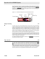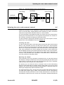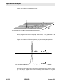
1
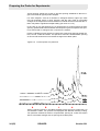
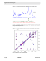
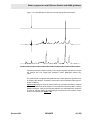
High Resolution Magic
Angle Spinning
Spectroscopy
User Manual
Version
BRUKER
001
The information in this manual may be altered without notice.
BRUKER accepts no responsibility for actions taken as a result
of use of this manual. BRUKER accepts no liability for any mistakes contained in the manual, leading to coincidental damage,
whether during installation or operation of the instrument. Unauthorised reproduction of manual contents, without written
permission from the publishers, or translation into another language, either in full or in part, is forbidden.
This manual was written by
Frank Engelke
© March 4, 1998: Bruker Elektronik GmbH
Rheinstetten, Germany
P/N: Z31437
DWG-Nr: 1147001
Contents
Contents .............................................................. iii
1
1.1
2
2.1
2.2
3
3.1
3.2
3.3
3.4
4
4.1
4.2
4.3
4.4
4.5
5
5.1
5.2
5.3
5.4
6
6.1
6.2
7
7.1
7.2
7.3
7.4
7.5
A
Version 001
Introduction ............................................................ 5
Introduction ......................................................................... 5
System Description ................................................ 7
Probe Description ................................................................ 7
Site and Parts Requirements ............................................... 8
Installation of the Probe and Peripherals .............. 9
Probe Installation ................................................................ 9
Pneumatic connections ........................................................ 9
Electronic connections ....................................................... 11
MAS Sample Changer ....................................................... 11
Operation of the HR-MAS System ........................ 13
MAS Rotors, Caps and Inserts ........................................... 13
Sample loading .................................................................. 14
Cap removal ...................................................................... 14
Spinning the rotor under manual control ............................ 15
Spinning the rotor under computer control ......................... 16
Preparing the Probe for Experiments .................. 19
RF Tuning ......................................................................... 19
Adjusting the magic angle .................................................. 19
Shimming a HR-MAS probe ............................................... 21
Choosing the appropriate spinning speed. ......................... 23
Gradient HR-MAS Spectroscopy .......................... 25
Magic Angle Gradient Design ............................................ 25
Setting up the magic angle gradient ................................... 26
Application Examples ........................................... 31
Hr-MAS of small organic molecules ................................... 31
HR-MAS of swollen polymers ............................................. 35
MAS of biological samples ................................................. 36
Gradient hr-MAS spectroscopy .......................................... 39
Water suppression and Diffusion Studies with MAS gradients.
42
Shipping List ....................................................... 45
BRUKER
iii
Contents
B
Spherical Inserts ................................................. 47
C
References ........................................................... 49
Figures ................................................................. 51
Tables .................................................................. 53
iv
BRUKER
Version 001
Introduction
1
Introduction
1
1.1
The line width of an NMR resonance depends strongly on the microscopic environment of the nucleus under study. Interactions such as the chemical shift and dipole-dipole coupling between neighboring spins are anisotropic and impose a
dependence on the NMR frequency based on the orientation of a spin or molecule
with respect to the main magnetic field direction. Furthermore, the magnetic susceptibility of the sample and susceptibility differences within the sample lead to a
broadening of the resonances.
In liquid state spectroscopy the rapid isotropic motion of the molecules averages
the anisotropic interactions, resulting in an isotropic chemical shift frequency and
a disappearance of the line broadening due to dipolar couplings. Furthermore the
sample geometry, a cylinder parallel to the main magnetic field, is chosen such
that the susceptibility broadening is minimized.
In solid samples on the other hand, the lack of molecular mobility results in broad
lines. This line broadening can be reduced by spinning the sample rapidly around
an axis which is oriented at an angle θ m=54.7° with the direction of the magnetic
field. By spinning at this so-called 'Magic Angle' (the angle between the z-axis
and the (1,1,1) vector), at a rate larger than the anisotropic interactions, these interactions are averaged to their isotropic value, resulting in substantial line narrowing. In addition, magic angle spinning removes the magnetic susceptibility
broadening.
In addition to pure solids or pure liquids there is a wide range of materials which
exhibit either reduced or anisotropic mobility. Examples include polymer gels1,
lipids2, tissue samples3,4, swollen resins (used as supports in combinatorial
chemistry)5,6,7, plant and food samples. While these samples generally have sufficient mobility to greatly average anisotropic interactions, the spectral resolution
for the static samples are still much lower than that which is achieved for liquid
samples. The excess broadening under static conditions is due to a combination
of residual dipolar interactions and variations in the bulk magnetic susceptibility8.
For a variety of samples, including the aforementioned examples, magic angle
spinning is efficient at averaging these left-over components of the solid state line
width, and leads to NMR spectra that display resolution approaching that of liquid
samples. Such methods have been termed High Resolution MAS (HR-MAS)
NMR.
Bruker has developed a series of dedicated probes for standard bore magnets, to
accommodate the rapidly expanding field of HR-MAS. These probes are available
in double and triple resonance modes and come equipped with a deuterium lock
channel. The probes have automatic sample ejection and insertion capability, with
the availability of an optional sample changer, enabling fully automated sample
runs. A B0 gradient, directed along the magic angle, is optional.
Version 001
BRUKER
5 (55)
Introduction
Figure 1 demonstrates the gain in resolution that can be achieved with a HR-MAS
probe, compared to a standard high resolution probe. The spectra are proton
spectra of a human lipoma tissue, obtained at a frequency of 500 MHz.
Figure 1.1. 500 MHz proton spectra of a human Lipoma tissue.
6.0
5.0
4.0
3.0
2.0
1.0
ppm
The top spectrum is acquired in a conventional high resolution probe (spinning at
20 Hz // B0), while the lower spectrum is acquired in a HR-MAS probe (spinning at
5 kHz).
6 (55)
BRUKER
Version 001
System Description 2
2
Probe Description
2.1
The HR-MAS probes have been designed to perform solution type experiments,
while spinning the sample at the magic angle. The probes are either doubly tuned
(e.g. 1H and 13C) or triply tuned (e.g. 1H, 13C and 15N), in addition to a 2H lock
channel. All three (or four) channels are operating via a single NMR transmit/receive solenoid coil located inside the MAS turbine (see figure 2.1). The probes are
capable of performing either direct or indirect (inverse) detection experiments.
Properties of the HR-MAS probes include:
1. MAS at spinning rates of up to 16 kHz for 4 mm o.d. Zirconia rotors for liquid or
liquid-like samples and up to 6 kHz with spherical volume PTFE or Kel-F inserts;
2. Sample insertion/ejection without removal of the probe (up to 600 MHz);
3. Magic angle adjustment with micrometer screw at probe bottom;
4. Built-in heater/dewar and thermocouple for VT operation from -20°C to +70°C;
5. Optical spin rate counter with trigger signal output for rotor synchronized experiments;
6. Automatic insert and eject of the sample using the MAS sample changer.
Figure 2.1. Upper probe chamber with MAS stator in magic angle position.
Version 001
BRUKER
7 (55)
System Description
Site and Parts Requirements
2.2
Air requirements:
1. Free of oil and dust (0.01 micron filter);
2. Dew point of at least -30°C;
3. 4m3/h flow of air at more than 6 bar for stable, fast spinning;
4. Dry nitrogen gas for low temperature operation either from a pressurized liquid
nitrogen tank with a nitrogen boil off device (a 60 liters gas cylinder (200 bar)
lasts for approximately 1 hour);
5. B-VT 2000 or 3000 variable temperature unit for all variable temperature (VT)
operation and a 25 liters liquid nitrogen dewar for low temperature operation.
MAS equipment
1. MAS pneumatic control unit for sample spinning, display of the spinning rate,
as well as sample insert and eject;
2. Set of air hoses and spinning rate cable;
3. Pneumatic sample transfer system for standard bore magnets;
4. MAS sample changer for automatic multiple sample insert and eject (optional).
RF amplifiers
HR-MAS probes are designed to operate with the standard RF transmitters. No
high-power transmitters are needed!
B0 gradient option
For HR-MAS probes equipped with a magic angle gradient in addition to the
above mentioned items, a gradient amplifier is needed. Gradient amplifiers capable of preemphasis and 10 A output current are recommended, such as the GREATTM or ACCUSTARTM.
8 (55)
BRUKER
Version 001
Installation of the
Probe and
Peripherals
3
3
Probe Installation
3.1
3.1 Probe Installation
•
Insert the probe into the lower shim stack. For easy shimming it is recommended to align the probe with the y-gradient direction, as described in section 5.3:
“Shimming the HR-MAS probe”;
•
•
Lower the sample transfer tube into the top of the shim stack;
Place the MAS sample changer (optional) on top of the sample transfer tube
(see section 3.4 MAS Sample Changer).
Figure 3.1. Pneumatic connections of the HR-MAS probe.
Pneumatic connections
•
•
Version 001
3.2
Connect the MAS pneumatic unit to the main gas supply (see section 2.2);
Connect the RS232 port of the pneumatic unit to tty08 on the console;
BRUKER
9 (55)
Installation of the Probe and Peripherals
•
For the connection of air hoses between the MAS control unit and the probe,
refer to figure 3.1 and figure 3.2;
•
For low-temperature experiments the bearing gas connection has to be removed and the outlet of a heat exchanger has to be connected instead. See
figure 3.3 for low-temperature operation;
•
Please note: Kel-F caps for Zirconia rotors can be used in the temperature range from +10°C to +50°C. For a more extended VT range (-30 to
+70°C) the usage of caps made of macor or boron nitride are mandatory!
Figure 3.2. Diagram for the pneumatic connections for operation at ambient temperature.
Figure 3.3. Set-up for low-temperature operation
The bearing gas (preferably dry N2 gas) is cooled by an heat exchanger immersed in liquid N2, and is directly fed into the glass dewar inlet at the bottom of
the probe.
10 (55)
BRUKER
Version 001
Electronic connections
Electronic connections
3.3
•
Connect the X-channel of the probe to the X-BB HPPR preamplifier using a
proton reject or a low pass filter;
•
Connect the 1H-channel of the probe to the proton using a proton band pass
filter;
•
•
•
Connect the 2H-lock channel of the probe with the lock preamplifier;
•
(Connect the gradient cable to the gradient connector on the side of the
probe);
•
(Connect the Y-channel to the probe via a low pass filter).
Connect the spin rate cable from the MAS unit;
For variable temperature operation connect the heater cable and the thermocouple from the rear panel of BVT 2000 unit or the front panel of the BVT 3000
unit;
MAS Sample Changer
3.4
The Bruker MAS sample changer is designed to allow the acquisition and processing of MAS data from up to 20 samples without operator intervention. The
sample changer is mounted on top of the sample transfer tube and controlled via
the insert and eject pneumatic lines of the MAS controller. To install the device, remove the upper sleeve of the sample transfer tube and place the sample changer
on top of the tube. Connect the air lines as indicated in figure 3.4.
The rotors are stacked in the sample changer (with the rotor caps upward) and after ejection are gathered in the collection tray. The rotor collection tray may be removed and emptied, and additional rotors may be inserted into the sample
changer while the system is in operation, allowing for indefinite operation with only
infrequent operator intervention. In order to distinguish the samples, numbered rotor barrels are available.
Version 001
BRUKER
11 (55)
Installation of the Probe and Peripherals
Figure 3.4. Installation of the MAS sample changer.
VDPSOHFKDQJHU
0$6XQLW
287
$1*/(
(-(& 7
VDPSOH
WUDQVIHU
WXEH
,1 6 ( 5 7
7R3UREH
0 $* 1 (7
12 (55)
BRUKER
Version 001
Operation of the HRMAS System
4
MAS Rotors, Caps and Inserts
4
4.1
The rotors most commonly used for MAS are made of zirconium oxide (Zirconia).
Rotors can be either filled entirely with sample or they can be used with rotor inserts. Inserts are provided to improve shimming and RF in homogeneity, and are
useful when the amount of sample is limited. The maximum spinning rate for 4
mm Zirconia rotors is about 15 kHz, but is limited to lower speeds when using the
spacers. A full rotor has a sample volume of about 80 ml; with a spherical insert
the volume is reduced to about 25 µ l. Numbered rotors are available to easily distinguish between different samples.
The function of the rotor cap is twofold: firstly, to close the rotors, and secondly, to
provide the driving of the rotor. There are several types of caps available. The
standard caps are made of Kel-F, which can be used in a temperature range from
10°C to +50°C. This material will shrink at lower temperatures and soften at more
elevated temperatures. However, for a more extended VT range (-30°C to +70°C)
caps made from macor or boron nitride can be used. Those materials have temperature coefficients similar to Zirconia.
Figure 4.1. Zirconia rotor with Kel-F cap, upper spacer, cylinder head screw,.
and sealing grub screw to provide a spherical sample volume
Version 001
BRUKER
13 (55)
Operation of the HR-MAS System
The most common type of rotor spacers provide a sample volume that is approximately spherical in order to improve the shimming of the probe (see figure 4.1
and figure 4.2. Appendix B is an example of an instruction sheet showing how to
handle this type of insert. For other inserts please refer to the accompanying instructions provided with the spacers.
Figure 4.2. Schematic drawing of the rotor with spherical insert.
Upper spacer
Sample
Lower Spacer
Sample loading
Grub
Screw
Rotor Cap
4.2
In order for the rotor to spin stable and fast, the rotor has to be well balanced.
Load the sample loosely into the rotor barrel and tap the rotor lightly on a hard
surface. Do not attempt to pack the material tightly into the spinner. If you wish to
add more sample into the rotor, it is better to spin up the rotor first, so that the
sample is packed against the walls of the barrel, and then add additional material.
Liquid or viscous samples are easily loaded using a syringe or a small pipette.
Solvent swelling can be done with the powdered sample in the rotor.
Push the rotor cap on all the way; if the cap is improperly positioned the rotor may
not spin. Clean the outside of the rotor with a tissue, so that no sample ends up in
the MAS stator. Mark half of the beveled rim on the bottom of the rotor with a black
marker for optical spin rate detection.
For loading samples using spherical inserts, see Appendix B or the instruction
sheet that came with the inserts.
Cap removal
4.3
The rotor cap is easily removed with a dedicated cap removal tool (see figure
4.3). Screw the tool body loosely to the cap clamp. Insert the cap all the way into
the teeth of the clamp. Screw the tool body snugly, but not too tight, onto the
clamp. Insert the rotor into the barrel clamp and remove the cap by simultaneously
rotating and pulling the barrel clamp. Unscrew the cap clamp and push the cap
out with the push pin. Be careful not to damage the caps. (For more complete instructions please refer to the guidelines delivered with the cap removal tool).
14 (55)
BRUKER
Version 001
Spinning the rotor under manual control
Figure 4.3. Schematic drawing of the cap removal tool.
cap clamp
tool body
barrel clamp
cap
push pin
rotor
Spinning the rotor under manual control
4.4
Prepare the pneumatic unit for operation by setting the proper probe parameters
such as rotor size (BL4), magnet (SB) and rotor material (e.g. ZrO2). Consult the
manual for the pneumatic unit and/or section 4.4 of this manual.
For manual operation of the MAS pneumatic unit, set the unit in the local mode by
pressing the local/remote button on the keypad of the pneumatic unit. Choose either manual or automatic for spinning control (see below).
It is also possible to operate the pneumatic unit from your host computer. For this,
please refer to the XWINNMR manual and section 4.5.
Inserting the rotor
In order to make sure that the rotor will properly drop into the stator press the eject
button on the pneumatic unit first. This will set the stator into a vertical position
and ensure that a rotor which might be inside the probe will be ejected. After the
eject air is on (and after removal of a rotor which has been in the probe) press
stop. Then the packed rotor can be dropped into the probe via the transfer tube
with the cap up. Close the insert tube and press the button insert on the pneumatic unit. This will automatically set the stator into the magic angle position after 10
seconds, if the pneumatic unit is operated in automatic mode. In manual mode
you have to press the stop button again.
Spinning the sample
If the pneumatic unit is set to operate in automatic mode, you may start spinning
the sample by setting the desired spin rate (Vd) and pressing the go button on the
control panel. In case the rotor does not reach the desired spin rate in automatic
mode, the rotor has to be spun up in manual mode.
For spinning up 4 mm Zirconia rotors in automatic mode, set the start bearing
pressure to about 800 mbar, the default setting of 2000 mbar is too much for most
samples. This can be done by pressing the bearing button in automatic mode and
reducing the displayed Bp start to the desired value.
For manual spinning of the 4 mm Zirconia rotors use 800 mbar bearing (Bp) and
150 mbar drive pressure (Dp) to obtain a spin rate above 2.5 kHz. If the spinning
rate achieved at these pressures is lower, slowly decrease BP to 100 mbar and
immediately increase BP as soon as the rotor accelerates. Standard samples will
Version 001
BRUKER
15 (55)
Operation of the HR-MAS System
easily spin in a 4 mm system, problems can be encountered for conductive materials or very heavy solid samples.
Stopping sample spinning
In automatic as well as in manual operation the rotation can be stopped by pressing the stop button. If you want to stop rotation manually from the keypad, decrease the drive pressure (Dp) first, and then lower the bearing pressure (Bp)
slowly.
In order to stop spinning after variable temperature experiments, make sure
that the heater is off and that gas of ambient temperature is used for the
bearing!
Sample Ejection
After the rotor has stopped press the eject button on the pneumatic unit. The stator will switch back to the vertical position and the rotor be ejected. For this procedure the eject air pressure has to be adjusted by a little adjust knob on the rear of
the pneumatic unit such that the pressure is high enough for the rotor to lift off, but
not too high, such that the cap is not damaged when the rotor knocks against the
closure of the transfer tube.
Spinning the rotor under computer control
4.5
The MAS window
In order to operate the MAS pneumatic unit from XWINNMR, the unit has to be
run in remote mode, which can be selected on the keypad on the front of the unit.
The set-up of and communication with the pneumatic unit is established by typing
cfmas on the XWINNMR command line and answering the questions in accordance with your set-up.
The control of the pneumatic unit from the host computer is initiated by typing
MAS on the command line. This brings up the MAS control window, shown in figure 4.4. Start by selecting the correct probe parameters or reading them in from a
previously saved probe setup file.
Press Eject Sample to flip the stator in the upright position and eject a rotor which
might be in the probe. After the eject air is off, insert the rotor and click Insert
Sample to flip the stator to the magic angle position.
Enter the desired spinning rate and select spinning on to start spinning. By pressing Continuous Update the actual values of the bearing and drive pressure and
the spinning rate will be updated every 10 s. After the rotor reaches the desired
spinning rate and the spinning is stable, the Spin Locked parameter will be set to
Yes.
Exit the menu by pressing cancel. The spin rate can still be monitored on the computer screen by selecting MAS rate monitor from the windows menu of XWINNMR.
Spinning can be halted by re-entering the MAS menu and selecting spinning off
(note that when you enter the MAS window, spinning is always set to off, however,
you will have to activate this to stop the spinner). Press Continuous Update to
monitor the spinning rate. Once the spinner is stopped press Eject Sample to remove the sample.
16 (55)
BRUKER
Version 001
Spinning the rotor under computer control
Figure 4.4. MAS pneumatic unit control window.
Command line control
In addition to using the MAS window (figure 4.4) the following commands can be
used to control the spinner from the command line of XWINNMR:
•
•
•
•
•
•
Version 001
masr:
set the spinning rate (Hz)
masg:
start spinning
mash:
stop spinning
mase:
eject sample
masi:
insert sample
masrmon:
MAS spinning rate monitor (continuous).
BRUKER
17 (55)
Operation of the HR-MAS System
18 (55)
BRUKER
Version 001
Preparing the Probe
for Experiments
5
RF Tuning
5
5.1
The RF tuning is performed by centering the dip of the wobble curve on the
screen through turning the tuning and matching rods at the bottom of the probe.
The rods for the 1H channel are labeled yellow, the rods for the 13C channel are
labeled blue. The tuning bandwidth of the 13C channel is equal to a few MHz. The
2
H lock channel is fixed, i.e., no external matching and tuning adjustment is necessary.
Always tune the probe while the sample is spinning. When tuning the probe pay
attention to the wobble curve. If modulations are superimposed on the wobble
curve, this is usually a sign that the sample spinning is not stable. Adjusting the
drive and bearing pressures or restarting the spinner can stabilize the spinning. If
problems persist, repack the sample.
Adjusting the magic angle
5.2
The precise setting of the magic angle is mandatory to obtain the maximum spectral resolution obtained by MAS. In order to adjust the magic angle, a sample is
needed with an NMR line that is very sensitive to angle misalignment. Suitable
samples are BaClO3H2O (1H observe) and KBr (79Br observe). For both samples,
to adjust the angle the sample has to be spun at about 5 to 6 kHz. Note that either
sample can be used to set the angle, irrespective of what nucleus will be observed
in the HR-MAS experiments.
For the proton sample a spectrum is acquired and Fourier transformed. The magic angle setting is then slightly changed by turning the micrometer screw at the
bottom of the probe. Take another spectrum and repeat the procedure until the
magic angle setting is optimal (see figure 5.1).
Version 001
BRUKER
19 (55)
Preparing the Probe for Experiments
Figure 5.1. Proton NMR spectra of BaClO3H2O
off magic angle
at magic angle
Obtained off the magic angle (top) and obtained with the correct angle setting
(bottom). Experimental parameters: ns = 1, swh = 125kHz, pulse program zg, p1
= 3µs, pl1 = 0 dB, d1 = 5s, spinning rate 6000 Hz.
The 79Br resonance frequency is very close to the 13C resonance frequency, thus
no or just a slight tuning of the RF-circuit is necessary. Furthermore KBr provides
a very sensitive signal with a very short T1. Already at moderate spin rates the
satellite transition will be split into sidebands, which have to be as narrow as possible for the optimum angle setting. With a rotor completely filled with KBr, the angle setting procedure can be performed in “gs” mode on the free induction decay
(FID). In “gs” mode, go to the “acqu” window, separate the real and imaginary part
of the FID and adjust for an on resonance decay. This can be done by changing
“o1” or adjusting the field. Make sure that the field sweep is off and remains
off!
If the angle is close to the magic angle, you will see rotational echoes on top of an
exponential decay (figure 5.2). Far off angle only the exponential decay is visible.
Turn the micrometer screw until the rotational echoes last up to 4 ms. Write down
the setting of the micrometer screw at the probe bottom for the correct angle position. Check for the optimal setting by acquiring 32 scans and maximizing the number of sidebands in the spectrum (figure 5.3).
20 (55)
BRUKER
Version 001
Shimming a HR-MAS probe
Figure 5.2.
79Br
FID’s KBr.
off magic angle
at magic angle
Experimental parameters for acquisition: pulse program = zg, swh = 100kHz, td =
2k, d1 = 30ms, p1 = 2µs, pl1 = 0dB, spinning rate 6000 Hz.
Figure 5.3.
79
Br NMR spectra corresponding to the FID's shown in figure 5.2.
off magic angle
at magic angle
Shimming a HR-MAS probe
5.3
When shimming a high resolution probe one distinguishes between on-axis (z)
and off-axis (x, y etc.) shims. Spinning the sample parallel to the magnetic field di-
Version 001
BRUKER
21 (55)
Preparing the Probe for Experiments
rection averages the off-axis in homogeneity, which may result in spinning sidebands.
In MAS spectroscopy the spinner axis is at an angle θ m with the magnetic field direction and the distinction between the traditional on-axis and off-axis shims no
longer holds. The spinning rates in MAS spectroscopy, however, are typically at
least a few kilohertz, which is much larger than the magnetic field in homogeneity.
As a result the amplitudes of the sidebands are small and shimming may be done
with a set of shims that is cylindrically symmetric about the MAS spinner axis.
Such a set of shims can be constructed from combinations of the standard laboratory frame shims, via a transformation to the tilted magic angle frame9. In the simplest implementation the MAS probe is aligned such that the spinner axis is in the
laboratory xz-plane (figure 5.4).
Figure 5.4. The magic angle spinner axis
z
shim plate
y
x
leads
The magic angle spinner axis is aligned with the xz-plane of the shims by positioning the front plate of the probe parallel to the direction of the shim leads.
The ’magic angle z-shims’ are listed below for orders Z through Z5. The simplest
approach is to use the laboratory shims with the largest coefficient, so for instance
the X shim is used as the normal high resolution Z shim. Complete shimming can
then in principle be accomplished using only X, ZX, Z2X, Z4 and Z5 as the surrogate nth order on-axis shims. Note, however, that the coefficients given for the
magic angle shims do not take into account the efficiencies of the shim coils and
the use of the other shims listed below may be needed.
22 (55)
BRUKER
Version 001
Choosing the appropriate spinning speed.
To shim the HR-MAS probe, a sample of 3%CHCl3 in Acetone-d6 is suggested,
using a rotor with a spherical insert. Make sure the magic angle is adjusted prior
to shimming the probe. Spin the sample at a rate suggested in the following section. It is always best to shim up the probe already under the conditions used later
for the real samples.
Make sure, that the correct gas is used for temperature control and spinning, the
coils can be optimized for air or nitrogen gas. To obtain best results, the gas indicated should be used.
Lock the sample, tune the probe and start shimming using the X, ZX, Z2X, Z4 and
Z5 shims as described above. If one of the shims requires an excessive shim current, reduce the current and continue shimming by adding current to another shim
from the same group as shown in the table. For instance if the current in ZX is too
high, reduce the value and optimize the line shape by adding current to the (X2Y2)Z shim. If the probe is not exactly aligned with the xz plane (see figure 5.4),
then a small amount of Y and YZ may be needed for optimal shimming.
A second shim set should be obtained for rotors without spacers, and the optimal
shim settings for these will be somewhat different. Under normal conditions the
shim values obtained as described above, will be close to optimal for all other
samples. When changing samples one usually only needs to adjust Z (and ZX).
Both shim value sets should be stored on disk. Make sure when the shim values
are stored that the HR-MAS probe is defined as the current probe in the EDHEAD
command, then shims can be recalled with the correct lock conditions like phase
and power.
Choosing the appropriate spinning speed.
5.4
The correct spinning speed depends strongly on the sample under study. A minimum spinning speed is recommended, which depends on the field strength of the
magnet:
Version 001
300 MHz
2400 Hz spinning
400 MHz
3200 Hz spinning
500 MHz
4000 Hz spinning
600 MHz
4800 Hz spinning
BRUKER
23 (55)
Preparing the Probe for Experiments
These spinning speeds are chosen to prevent spinning sidebands to fall into regions of interest for typical proton samples.
For some samples, such as for instance in biological tissues, higher spin rates
may be beneficial. Keep in mind, however, that this may result in irreversible
changes in the sample due to the breakdown of cellular structures and that the rotation may lead to significant sample heating (as much as 10°C).
In the case of very fast spinning it is a good practice to acquire spectra at lower
spinning speeds both before and after the fast spinning and compare those spectra to ensure that no changes have occurred in the sample.
Figure 5.5 displays proton spectra of a plant leaf, acquired at spinning speeds of 4
kHz, 10 kHz, 19 kHz and 6 kHz. The spectrum at 6 kHz is obtained after spinning
at 19 kHz and shows that no irreversible changes have taken place.
Figure 5.5. Proton spectra of a plant leaf
Effect of spinning speed on 400 MHz HR-MAS proton spectra of a plant leaf, cut
and flushed in water. The spectra are displayed with absolute intensity scaling.
The spectrum obtained at 6 kHz is acquired after spinning at 19 kHz and shows
that no irreversible changes due to spinning have taken place.
24 (55)
BRUKER
Version 001
Gradient HR-MAS
Spectroscopy
6
6
The addition of a magnetic field gradient to a high resolution MAS probe leads to
further advances in this type of spectroscopy10. Based on the broad acceptance
of gradient methods in high resolution solution state NMR studies11, it is not surprising that gradients can be of use in HR-MAS measurements, particularly since
the NMR methods are adopted from the liquid state, rather than from the solid
state class of methods. As in high resolution liquid state studies, the gradient is
essential for removing t1 noise and is extremely helpful in coherence pathway selection.
Magic Angle Gradient Design
6.1
In conventional high resolution spectroscopy with gradients, the gradient field
most commonly used is aligned with the main magnetic field direction, a so-called
z-gradient. Although the sample is usually stationary in gradient spectroscopy, for
reasons discussed later, it is in principle possible to rotate the sample, since the
isoplanes of the gradient field are perpendicular to the rotation axis (see figure
6.1). This means that a rotating spin will always experience the same magnetic
field strength.
Figure 6.1. Use of a z-gradient in MAS spectroscopy
γGz
z
z
x
x
If in conventional high resolution spectroscopy with a z-gradient the sample would
be spun, then the spins will always experience the same magnetic field strength.
In MAS spectroscopy, however, the use of a z-gradient would cause a rotating
spin to sample different values of the magnetic field.
Version 001
BRUKER
25 (55)
Gradient HR-MAS Spectroscopy
If a z-gradient would be applied to a sample spinning at the magic angle, the rotating spin would pass through different isoplanes, since the axis of rotation is no
longer parallel to the direction of the magnetic field gradient (figure 6.1). This
would result in a partial averaging of the gradient field as experienced by the
spins, and would necessitate the need to synchronize one’s experiments with the
spinner rotation (which may be difficult or even impossible due to the finite rise
and fall times of the pulsed gradient fields).
A better solution is to implement gradient spectroscopy experiments in a MAS
probe in such a way that the gradient should introduce a resonance that is not
temporally modulated. This may be accomplished with a time-independent gradient field where the gradient is oriented such that the z-component of the magnetic
field increases along the axis of the spinner and the z-component of the magnetic
field gradient is uniform in the planes perpendicular to the spinner axis (see figure
6.2).
Figure 6.2. Gradient field is directed along the magic angle spinner axis
z
γGmas
y
x
If in MAS spectroscopy the gradient field is directed along the magic angle spinner
axis then a rotating spin will always sample the same magnetic field strengths.
The HR-MAS probe is optionally equipped with a magic angle gradient12. The gradient coil design is compatible with commonly used MAS stators (for widebore
and standard bore probes) and does not interfere with the automatic sample ejection and insertion capabilities. Gradient strengths of up to 45 G/cm (at 10A) can
be achieved.
Setting up the magic angle gradient
6.2
Before the magic angle gradient can be used in a routine fashion a few adjustments have to be made. In order to ensure short rise and fall times of the pulsed
field gradients it is necessary to compensate for Eddy currents generated by the
gradient pulses and for the switching times of the gradient amplifier. This is done
through so-called pre-emphasis adjustment. Furthermore the gradient strength
26 (55)
BRUKER
Version 001
Setting up the magic angle gradient
needs to be calibrated. Before initiating these adjustment procedures make sure
that the gradient amplifier has been installed correctly.
Adjusting the pre-emphasis
Figure 6.3. Pre-emphasis controller window.
For this procedure use a rotor with H2O/D2O, preferably doped with CuSO4 (2
mMol). Spin the sample at approximately 3 kHz, lock and shim to a proton line
width of better than 5 Hz at half height.
Set the offset a few kHz off resonance from the water peak. Use a sweep width of
20 ppm, D1=1-2s, and choose TD such that the FID has decayed about 50% in
amplitude after approximately 1/8th of the acquisition time.
Next set the pulse program to preempgs (for RX22 based systems set the second
channel to proton as well). Use a gradient program which defines a single square
gradient pulse (e.g. gradprog=1squa) and define a variable delay list (vdlist=preemp) which contains the following values:
100 µ l, 300 µ l, 1m, 3m, 10m, 30m, 100m, 300m.
This pulse program will acquire 8 FID’s and display them sequentially in a single
acquisition window (see figure 6.4). Each FID is acquired at a time vd after a gradient pulse. Set the gradient pulse length to 50 ms and its strength to 20%.
The pre-emphasis is controlled by a set of three time constants and amplitudes.
These values can be addressed through the Pre-emphasis Controller window,
which is invoked by setpre (figure 6.3). Select for the time constants 20 ms, 2 ms
and 200 µ s and start with 50% for all time settings and 0% for all gain settings.
Start the acquisition in gs mode and observe the FID’s in the acquisition window.
With the time constants set as described above, the first FID’s will seem distorted,
as can be seen in the example of figure 6.4 (top spectra). Adjust the pre-emphasis values by changing the time constants and gain settings. Start with the settings for the slowest time constant and adjust the 5th and 6th FID, so that they
appear similar to the last two FID’s. Repeat the procedure for the mid and fast
Version 001
BRUKER
27 (55)
Gradient HR-MAS Spectroscopy
time constants, for FID’s 3 and 4, and FID’s 1 and 2, respectively. If all values are
set correctly all FID’s should appear equal (figure 6.4, bottom).
The pre-emphasis values are dependent on both the probe and the gradient amplifier and once correctly set up, will remain the same. The settings can be stored
on the computer by saving the set-up from the file menu in the Pre-emphasis Controller window.
Figure 6.4. 8 consecutive FID’s
0.2
0.4
0.6
0.8
1.0
1.2
1.4
1.6
1.8
2.0
2.2
sec
0.2
0.4
0.6
0.8
1.0
1.2
1.4
1.6
1.8
2.0
2.2
sec
Acquired at different times after the application of a gradient pulse. Top: without
pre-emphasis; bottom: with pre-emphasis properly adjusted.
Calibrating the gradient
Gradient calibration is performed by measuring the gradient profile of a sample of
known size. Usually a proton spectrum of a sample of water is acquired.
The profile is obtained with a gradient spin-echo, which can be acquired with the
pulse program calib. Set the gradient amplifiers to a low output, e.g. 10 or 20%
and acquire 4 scans. Multiply the FID with a sinebell (ssb=0), Fourier transform
and represent the data in magnitude mode (mc). The resulting profile represents a
projection of the sample’s density along the magic angle spinner axis. For a sample of known length the gradient strength can be determined by measuring the
width of the spectrum ( ∆ω) and dividing it by the length of the sample (l, in cm), by
the gyromagnetic constant of protons ( γ =4250 Hz/G) and by the current of the
gradient amplifier (I in A):
28 (55)
BRUKER
Version 001
Setting up the magic angle gradient
G=
∆ω
, in Gcm-1 A -1
γ lI
In figure 6.5 below, water in a spherical insert is used to calibrate the gradient
strength. The profile represents the spherical sample volume plus a small amount
of water in the fill hole of the inserts. From the width of the profile ( ∆ω=12000 Hz)
and the known length of the sample (l=0.27 cm) and gradient amplifier output
(20% of 10A), the gradient strength is determined as 5.2 Gcm-1A-1.
Figure 6.5. Gradient profile for a spherical sample of water.
sphericalsample
volume
fillhole
15000
10000
5000
0
-5000
-10000
-15000
Hz
The gradient strength is obtained from the width of the profile.
Version 001
BRUKER
29 (55)
Gradient HR-MAS Spectroscopy
30 (55)
BRUKER
Version 001
Application
Examples
7
7
High resolution MAS provides an easy means of obtaining high resolution spectra
of a variety of samples that would otherwise result in poorly resolved spectra, due
to residual anisotropic interactions. The addition of a HR-MAS probe and a MAS
pneumatic unit to a standard high resolution spectrometer is all that is needed to
open a gate to the world of HR-MAS spectroscopy and access to a vast amount of
highly interesting samples.
In this section a number of application examples are shown from a variety of compounds. All spectra are acquired with standard high resolution techniques.
Hr-MAS of small organic molecules
7.1
There is a wide variety of conceivable applications for HR-MAS probes. Among
others, one important field for pharmaceutical research concerns combinatorial
chemistry.
In combinatorial chemistry, small organic molecules are synthesized on resin
beads, consisting of a polymer matrix and a linker material. NMR is advantageous
in analyzing these samples since the reactions can be monitored without cleaving
off the substrate. High resolution NMR spectra are obtained by swelling the beads
in a deuterated solvent in combination with Magic Angle Spinning.
An example from this field is illustrated in figure 7.1. The proton spectrum is obtained from 2 mg of a meta- and para-disubstituted aromatic ring on tentagel resin, swollen in d-chloroform and acquired with a CPMG sequence. The broad
resonances of the polymer resin are distinguished from the substrate resonances
by exploiting the differences in proton T2’s using the CPMG sequence as is demonstrated in figure 7.2.
Further information on these compounds is obtained from two dimensional NMR
techniques. Figures 7.4 and 7.5 show a J-resolved and a double quantum filtered
Cosy spectrum of the same compound, respectively.
Version 001
BRUKER
31 (55)
Application Examples
Figure 7.1. 1H hr-MAS NMR spectrum of small organic molecules
Tentagel
bead
O
O
O
n
O
(n = 10 -15)
Polystyrene resin
O
Linker
O
N
H
Substrate
a
a
a: para disubstituted aromatic
b: meta disubtituted aromatic
b
b
7.2
7.1
b
b
7.0
6.9
6.8
6.7
6.6
6.5
(ppm)
including a meta- and para-disubstituted aromatic ring on tentagel resin, obtained
under the following NMR conditions: DRX400, 2mg in 4mm rotor with spherical
spacer, swollen in d-chloroform, cpmg 40msec, 3200Hz spinning, smallest line
width at half height 2.7 Hz.
Figure 7.2. Comparison of proton spectra
8.0
7.8
7.6
7.4
7.2
7.0
6.8
6.6
6.4
6.2
6.0
(ppm)
obtained with a single pulse (top) and with a CPMG sequence (bottom). The resonances of the resin are suppressed in the lower spectrum, by employing a CPMG
32 (55)
BRUKER
Version 001
Hr-MAS of small organic molecules
sequence ( τ - π - τ )*n, with τ =1.5 ms and n=20. Avance 400 MHz, 3200 Hz spinning, 2 mg sample on Tentagel substrate, swollen in deuterated chloroform.
Figure 7.3. Figure 23: 400 MHz proton spectra of a single 100 µ m bead
re s in
8.4
8.0
7.6
7.2
6.8
6.4
(ppm)
(top), separated under the microscope (volume 0.5 nl,1056 scans, weight 600
picograms) and 2mg of the same sample, swollen in CDCl3, (8scans). Avance
400, 3200 Hz spinning.
Figure 7.4. 2D J-resolved proton spectrum of 2 mg sample on a Tentagel resin,
swollen in CDCl3. Avance 400 MHz, 4 scans, MAS 3200 Hz.
Version 001
BRUKER
33 (55)
Application Examples
Figure 7.5. Double Quantum filtered Cosy of a small organic molecule
on a Tentagel resin. Avance 400 MHz, 16 scans, 2 mg sample, MAS 3200 Hz.
In a different application of hr-MAS to the study of small organic molecules, spots
were scratched off a TLC plate and made into a slurry with D2O. Figure 7.6
shows the proton spectrum of approximately 15 µ g of salicylic acid from a TLC
plate.
34 (55)
BRUKER
Version 001
HR-MAS of swollen polymers
Figure 7.6. Hr-MAS spectra of TLC-plate spots.
3.50
7.80
7.70
7.5
7.60
7.0
7.50
(ppm)
6.5
7.40
6.0
3.45
3.40 3.35
(ppm)
3.30
7.30
5.5
5.0
4.5
4.0
(ppm)
3.5
3.0
2.5
2.0
1.5
1.0
0.5
The compound is 15 micrograms of salicylic acid, scratched of the TLC plate and
slurried with D2O. Avance-600 MHz, 64 scans, 4200 Hz spinning.
HR-MAS of swollen polymers
7.2
Some polymers are nearly insoluble and as a result, obtaining high resolution
NMR spectra may become impossible. An example is a range of poly acethylene
derived polymers. These samples show an extremely low solubility in most common solvents and attempts to obtain solution spectra result in low signal to noise
ratios and long measurement times. Solid state spectra, on the other hand, can be
obtained but generally display a poor resolution.
A solution to this dilemma is to swell the polymer with a solvent and to acquire
spectra while spinning at the magic angle. Figure 7.7 displays proton and carbon
spectra of a derivative of poly acethylene, swollen in chloroform. The carbon spectrum was obtained in about two hours.
Version 001
BRUKER
35 (55)
Application Examples
Figure 7.7. 500 MHz proton (top) and carbon (bottom) spectra
8
7
180
6
160
5
140
4
120
3
100
2
80
1
60
0
40
ppm
20
ppm
of a derivative of poly acethylene, swollen in deuterated chloroform.
MAS of biological samples
7.3
Plant, tissue and food samples can be investigated by HR-MAS NMR. The usefulness of magic angle spinning within these fields of study is demonstrated in the
examples shown below.
Figure 7.8 shows a 1H 2D TOCSY spectrum of a sample of orange peel under
MAS. In figure 7.9 the 800 MHz proton spectrum of red perch filet is shown. Figure 30 shows spectra of benign and malignant prostate tissues, obtained via biopsies. The cancerous tissue shows a strongly enhanced lipid content. Figure 7.11
displays a TOSCY spectrum, obtained from a living white worm, which allows one
to study drug metabolism in vivo.
36 (55)
BRUKER
Version 001
MAS of biological samples
Figure 7.8. 2D TOCSY/ hr-MAS spectrum of orange peel,
cut to small pieces, flushed and measured in D2O, obtained under the following
NMR-conditions: Avance-400, 2800Hz spinning, 4mm-rotor with spherical insert,
2.7mg of sample, phase sensitive 2D-TOCSY with presaturation of the residual
water signal, 8 scans/400 increments, linear prediction to 800 points in f1, window
function shifted sine bell squared in both directions (ssb=2).
Figure 7.9. 8 mg red perch filet, cut, flushed and measured in D2O.
9
8
7
(ppm)
9
8
7
6
5
4
3
2
(ppm)
Avance-800, 128 scans 15KHz spinning.
Version 001
BRUKER
37 (55)
Application Examples
Figure 7.10. Hr-MAS of benign versus malignant human prostate tissue
x 10
3.2
2.8
2.4
2.0
(ppm)
1.6
1.2
0.8
Hr-MAS of benign (top two spectra) versus malignant (bottom) human prostate
tissue. Avance 400 MHz, 4000 Hz spinning. The cancerous tissue shows a
strongly enhanced lipid content.
Figure 7.11. TOCSY-presat of a living white worm (enchytraed) in 95% H2O/5%
D2O.
Avance-400 8scans/300incr. MAS 2800 Hz.
38 (55)
BRUKER
Version 001
Gradient hr-MAS spectroscopy
Gradient hr-MAS spectroscopy
7.4
The benefits of using magnetic field gradients in high resolution spectroscopy
have been well documented. In high resolution MAS similar benefits are seen
from the use of gradients, in particular a reduction in a variety of artifacts, such as
t1-ridges and repetition artifacts, while also saving time by eliminating the need to
complete a full phase cycle. A number of gradient high resolution MAS experiments are shown below on a variety of samples.
Figure 7.12 shows the gradient COSY of a swollen Wang resin, used in combinatorial chemistry. The use of gradients eliminates the repetition artifacts and t1-ridges. Note that the spinning sidebands in the f1-direction are aliased since no
bandwidth filters are used in the indirect domain and the spectrum is not symmetrized.
Figure 7.12. Gradient COSY of a swollen Wang resin
-6
-4
-2
0
2
4
ppm
ppm
8
6
4
2
0
500 MHz gradient 1H-1H COSY spectrum of an N-FMOC-N-Boc-L-Lysine derivatized Wang resin swollen with CDCl3. MAS 3.5 kHz, 1 ms gradients, 10 G/cm.
Gradients are frequently used in inverse detected heteronuclear correlation experiments to select the magnetization from protons coupled to a 13C spin and suppress the uncoupled protons magnetization. The spectra below show 1H-13C hrMAS HMQC (figure 7.13) and HMBC (figure 7.14) spectra of a Wang resin, used
in combinatorial chemistry. Note the excellent suppression of t1-noise in the gradient HMQC spectrum (figure 7.13, left) versus the phase cycled spectrum (figure
7.13, right) and the clean noise floor in the HMBC spectrum (figure 7.14). Note
Version 001
BRUKER
39 (55)
Application Examples
that no attempts were made to improve the spectral quality (e.g. by t1-ridge subtraction).
Figure 7.15 shows another example of a gradient HR-MAS HMBC spectrum. The
spectrum is obtained from a human lipoma tissue and demonstrates the usefulness of this type of high resolution MAS spectroscopy to the study of biological tissues.
Figure 7.13. 400 MHz 1H-13C HMQC spectra of an N-FMOC-N-Boc-L-Lysine
25
50
75
25
100
50
75
125
100
125
150
150
ppm
ppm
ppm
ppm
8
6
4
2
8
6
4
2
0
0
derivatized Wang resin swollen with CDCl3. The left spectrum is acquired using
gradients to suppress the magnetization from uncoupled proton spins, while the
spectrum on the right is obtained with phase cycling. No attempt was made the
improve the appearance of the spectra. MAS 5 kHz, 1 ms gradients, 10,10 and 5
G/cm.
40 (55)
BRUKER
Version 001
Gradient hr-MAS spectroscopy
Figure 7.14. 400 MHz 1H-13C HMBC spectra of an N-FMOC-N-Boc-L-Lysine
25
50
75
25
50
100
75
125
100
125
150
150
ppm
ppm
ppm
ppm
8
6
4
2
8
6
4
2
0
0
derivatized Wang resin swollen with CDCl3. A J-evolution time of 50 ms is used to
reveal long-range proton- carbon correlations. No 13C decoupling is applied during acquisition. The right spectrum shows the noise floor and demonstrates excellent artifact suppression. MAS 5 kHz, 1 ms gradients, 10,10 and 5 G/cm.
Figure 7.15. 500 MHz 1H-13C Gradient hr-MAS HMBC spectrum
0
25
50
75
100
125
150
ppm
ppm
5
4
3
2
1
of a human Lipoma tissue (sample courtesy of Dr. Singer, Brigham and Women’s
Hospital). MAS 5 kHz; 1 ms sine-shaped gradient pulses.
Version 001
BRUKER
41 (55)
Application Examples
Water suppression and Diffusion Studies with MAS gradients.
7.5
Gradients allow for fast and efficient water suppression. Figure 7.16 shows spectra of a hydrogel in which the water is suppressed with the Watergate13 sequence.
An alternative gradient method is the so-called Dryclean14 sequence in which a
stimulated echo sequence is used to attenuate resonances based on differences
in the diffusion rates of the molecules. Figure 7.17 shows spectra of a biological
tissue in which the water signal is suppressed using Watergate and Dryclean, respectively.
Figure 7.16. 500 MHz single pulse proton spectrum of an acrylamide hydrogel
9.0
8.0
7.0
6.0
5.0
4.0
3.0
2.0
1.0
ppm
(top). The spectrum below is acquired with the Watergate method. 1 ms sineshaped gradient pulses are use with a strength of 30 G/cm. (sample courtesy of
Prof. Tanaka, Massachusetts Institute of Technology).
42 (55)
BRUKER
Version 001
Water suppression and Diffusion Studies with MAS gradients.
Figure 7.17. 500 MHz proton spectra of human high grade Pleiomorphic
5 .5
5.0
4.5
4.0
3.5
3.0
2 .5
2 .0
1.5
1.0
0.5
ppm
Liposarcoma tissue (sample courtesy of Dr. Singer, Brigham and Women’s Hospital). MAS 5 kHz. Top: single pulse excitation; center: Watergate; bottom: Dryclean.
The combination of magnetic field gradients and hr-MAS spectroscopy allows one
to measure the diffusion constants of molecules in tissue samples under high resolution conditions.
Figure 7.18 displays a series of proton spectra of a Liposarcoma tissue, obtained
with a Stimulated Echo (STE) sequence. The spectra are acquired with increasing
gradient strengths. Apart from measuring diffusion, the stimulated echo sequence
is used for spectral editing by attenuating the resonances from mobile components in the sample (see figure 7.19).
Version 001
BRUKER
43 (55)
Application Examples
Figure 7.18. 500 MHz STE diffusion spectra
G
10
9
8
7
6
5
4
3
2
1
0
-1 ppm
of a high grade human Pleomorphic Liposarcoma tissue (sample courtesy of Dr.
Singer, Brigham and Women’s Hospital). MAS 10 kHz; 10 ms gradients,0-40 G/
cm, TE=100 ms.
Figure 7.19. 500 MHz STE proton spectrum (top) and single pulse spectrum
9
8
7
6
5
4
3
2
1
0
p
9
8
7
6
5
4
3
2
1
0
p
(bottom) of a high grade human Pleomorphic Liposarcoma tissue (sample courtesy of Dr. Singer, Brigham and Women’s Hospital). MAS 10 kHz; 10 ms gradients,30 G/cm, TE=100 ms.
44 (55)
BRUKER
Version 001
Shipping List
Table A.1.
A
A
Shipping List
Item
Quantity
1
1
HR-MAS probe
2
3
Zirconia rotors, each rotor including
3 KEL-F rotor caps,
1 pair of rotor spacers (upper and lower part),
1 sealing screw
3
1
Cylinder screw M2(25
4
1
HR spacer tool
5
1
Small screw driver
6
1
Rotor packer (hand tool)
7
1
Screw driver for tuning rods
8
1
Marker pen (black)
9
1
Cap removal assembly
10
1
Repair declaration form
11
1
Installation and Operation Manual
Version 001
Description
BRUKER
45 (55)
46 (55)
BRUKER
Version 001
Spherical Inserts
B
B
Ò Important Note: The rotor bore and the spacer must be absolutely clean.
The lower spacer will be destroyed if it is removed after being inserted into
the bore.
1. Spray the “lower spacer” with coolant spray, or dip it into liquid nitrogen, insert
it slightly into the rotor bore and align the rotor axis (figure B.1).
Figure B.1.
Spray lower spacer with coolant spray
a) Spray the spacer a second time with coolant spray and press it completely into the bore. Apply more coolant spray if needed. (figure B.2) or
b) In the case where the spacer fits very tightly, first dip the rotor and spacer
in liquid nitrogen and let them cool. The spacer can now be inserted much
easier into the rotor (figure B.2)
Figure B.2. Inserting the rotor is now easier
2. Insert the sample into the rotor. Screw the cylinder head screw M2 x25 into the
“upper spacer”, but do not tighten it! (figure B.3). Use the screw as a handle.
Spray the “upper spacer” with coolant spray or dip it into liquid nitrogen and
press it completely into the bore. Excessive sample will spill out through the
center hole and the thread.
Version 001
BRUKER
47 (55)
Figure B.3. Spray upper spacer with coolant spray
3. Put the grub screw on a screwdriver and screw it completely into the upper
spacer. (figure B.4)
Figure B.4. Screw grub screw completely
When the assembly is done correctly, the distance between the end of the upper
spacer and the end of the rotor will be 3mm. The short end of the rotor packer
(K8111001) is 2.9 mm long, which will allow you to easily check for the correct fit.
4. 4) Push the rotor cap (KELF) all the way into the rotor. (figure B.5)
Figure B.5. Push the rotor cap into the rotor
48 (55)
BRUKER
Version 001
References
C
C
1. H.D.H. St(ver and J.M.J. Fr3/4chet, Macromolecules, 1991, 24, 883
2. J.D. Gross, P.R. Costa, J.B. Dubacq, D.E. Warschawski, P.N. Lirsca, P.F.
Devaux and R.G. Griffin, J. Magn. Reson, 1995, 106, 187
3. L. L. Cheng, C. L. Lean, A. Bogdanova, S. C. Wright, Jr., J. L. Ackerman, T.
J.Brady and L. Garrido, Magn. Reson. Med. 1996, in press
4. K. Millis, W.E. Maas, S. Singer and D.G. Cory, Magn. Reson. Med. 1997, in
press
5. R.C. Anderson, M.A. Jarema, M.J. Shapiro, J.P. Stokes and M. Ziliox, J.Org.
Chem. 1995, 60, 2650
6. P. Keifer, L. Baltusis, D.M. Rice, A. Tymiak and J.N. Shoolery, J. Magn. Reson.
1996, A119, 65
7. S. K. Sarkar, R.S. Garigipati, J.L. Adams and P.A. Keifer, J. Am. Chem. Soc.
1996, 118, 2305
8. A.N. Garroway, J. Magn. Reson. 1982, 49, 168
9. A. Sodickson and D.G. Cory, submitted to J. Magn. Reson.
10. W.E. Maas, F.H. Laukien and D.G. Cory, J. Am. Chem. Soc. 1996, 118, 13085
11. R.E. Hurd and B.K. John, J. Magn. Reson. 1991, 91, 648
12. W.E. Maas, F.H. Laukien and D.G. Cory, J. Am. Chem. Soc. 1996, 118, 13085
13. M. Piotto, V. Saudek and V. Sklenar, J. Biomol.NMR 1992, 2, 661
14. P.C.M van Zijl and C.T.W. Moonen, J. Magn. Reson. 1990, 87, 18
15. High Resolution MAS Spectroscopy 27
Version 001
BRUKER
49 (55)
50 (55)
BRUKER
Version 001
Figures
1
Introduction
Figure 1.1.
2
Figure 3.3.
Figure 3.4.
Figure 4.2.
Figure 4.3.
Figure 4.4.
5
Figure 5.4.
Figure 5.5.
6
7
7.1.
7.2.
7.3.
7.4.
25
Use of a z-gradient in MAS spectroscopy .............................25
Gradient field is directed along the magic angle spinner axis 26
Pre-emphasis controller window. .........................................27
8 consecutive FID’s .............................................................28
Gradient profile for a spherical sample of water. ..................29
Application Examples
Figure
Figure
Figure
Figure
Version 001
6.1.
6.2.
6.3.
6.4.
6.5.
19
Proton NMR spectra of BaClO3H2O ....................................20
79
Br FID’s KBr. .....................................................................21
79
Br NMR spectra corresponding to the FID’s shown in figure
5.2. .....................................................................................21
The magic angle spinner axis ..............................................22
Proton spectra of a plant leaf ...............................................24
Gradient HR-MAS Spectroscopy
Figure
Figure
Figure
Figure
Figure
13
Zirconia rotor with Kel-F cap, upper spacer, cylinder head
screw ..................................................................................13
Schematic drawing of the rotor with spherical insert. ............14
Schematic drawing of the cap removal tool. .........................15
MAS pneumatic unit control window. ....................................17
Preparing the Probe for Experiments
Figure 5.1.
Figure 5.2.
Figure 5.3.
9
Pneumatic connections of the HR-MAS probe. .......................9
Diagram for the pneumatic connections for operation at ambient
temperature. .......................................................................10
Set-up for low-temperature operation ...................................10
Installation of the MAS sample changer. ..............................12
Operation of the HR-MAS System
Figure 4.1.
7
Upper probe chamber with MAS stator in magic angle position.
............................................................................................. 7
Installation of the Probe and Peripherals
Figure 3.1.
Figure 3.2.
4
500 MHz proton spectra of a human Lipoma tissue. ...............6
System Description
Figure 2.1.
3
5
31
1H hr-MAS NMR spectrum of small organic molecules .........32
Comparison of proton spectra ..............................................32
Figure 23: 400 MHz proton spectra of a single 100 m bead ..33
2D J-resolved proton spectrum of 2 mg sample on a Tentagel
BRUKER
51 (55)
Figures
Figure
Figure
Figure
Figure
Figure
Figure
Figure
7.5.
7.6.
7.7.
7.8.
7.9.
7.10.
7.11.
Figure 7.12.
Figure 7.13.
Figure 7.14.
Figure 7.15.
Figure 7.16.
Figure 7.17.
Figure 7.18.
Figure 7.19.
resin ................................................................................... 33
Double Quantum filtered Cosy of a small organic molecule .. 34
Hr-MAS spectra of TLC-plate spots. .................................... 35
500 MHz proton (top) and carbon (bottom) spectra .............. 36
2D TOCSY/ hr-MAS spectrum of orange peel, ..................... 37
8 mg red perch filet, cut, flushed and measured in D2O. ...... 37
Hr-MAS of benign versus malignant human prostate tissue . 38
TOCSY-presat of a living white worm (enchytraed) in 95% H 2O/
5% D 2O. .............................................................................. 38
Gradient COSY of a swollen Wang resin ............................. 39
400 MHz 1H- 13C HMQC spectra of an N-FMOC-N-Boc-L-Lysine
............................................................................................ 40
400 MHz 1H- 13C HMBC spectra of an N-FMOC-N-Boc-L-Lysine
............................................................................................ 41
500 MHz 1H- 13C Gradient hr-MAS HMBC spectrum .............. 41
500 MHz single pulse proton spectrum of an acrylamide hydrogel ...................................................................................... 42
500 MHz proton spectra of human high grade Pleiomorphic 43
500 MHz STE diffusion spectra ........................................... 44
500 MHz STE proton spectrum (top) and single pulse spectrum
............................................................................................ 44
A Shipping List
45
B Spherical Inserts
47
Figure
Figure
Figure
Figure
Figure
47
47
48
48
48
B.1.
B.2.
B.3.
B.4.
B.5.
Spray lower spacer with coolant spray ...............................
Inserting the rotor is now easier .........................................
Spray upper spacer with coolant spray ...............................
Screw grub screw completely .............................................
Push the rotor cap into the rotor .........................................
C References
52 (55)
BRUKER
49
Version 001
Tables
1
Introduction
5
2
System Description
7
3
Installation of the Probe and Peripherals
9
4
Operation of the HR-MAS System
13
5
Preparing the Probe for Experiments
19
6
Gradient HR-MAS Spectroscopy
25
7
Application Examples
31
A Shipping List
Table A.1.
Version 001
45
Shipping List ...................................................................45
B Spherical Inserts
47
C References
49
BRUKER
53 (55)
Tables
54 (55)
BRUKER
Version 001
Lastpage
Version 001
BRUKER
55 (55)