Download An Introductory Course on Constraint Logic Programming

An Introductory Course on
Constraint Logic Programming
Coordination:
With input from:
Manuel Carro
Manuel Hermenegildo
Francisco Bueno
Daniel Cabeza
Ma Jose Garca
Pedro Lopez
German Puebla
Computer Science School
Technical University of Madrid, UPM
VOCAL ESPRIT Project P23182
Contents
1 What is Constraint (Logic) Programming?
1.1
1.2
1.3
1.4
1.5
1.6
1.7
Introduction . . . . . . . . . . . . . . . . . . . .
Typical Applications and Approaches . . . . .
Constraints: Representation and Solving . . . .
Constraints as (Extended) Equations . . . . . .
Why Constraints and Programming? . . . . . .
Constraint{Programming Language Interfaces .
An Example: SEND + MORE = MONEY . .
1.7.1 Prolog: Generate and Test . . . . . . .
1.7.2 ILOG Solver (C++ Version) . . . . . .
1.7.3 ILOG Solver (Le Lisp Version) . . . . .
1.7.4 Eclipse Version . . . . . . . . . . . . . .
1.8 Use Prolog as Host Language? . . . . . . . . .
1.9 How Does a CLP System Work? . . . . . . . .
1.9.1 Modeling the Problem . . . . . . . . . .
1.9.2 Be a Solver . . . . . . . . . . . . . . . .
1.9.3 Don't Be a Solver! . . . . . . . . . . . .
2 A Basic Language
2.1 A Basic Constraint Language . . . . . . . .
2.1.1 Clauses . . . . . . . . . . . . . . . .
2.1.2 Implicit Equality . . . . . . . . . . .
2.1.3 Facts . . . . . . . . . . . . . . . . . .
2.1.4 Predicates . . . . . . . . . . . . . . .
2.1.5 Programs and Queries . . . . . . . .
2.2 Searching . . . . . . . . . . . . . . . . . . .
2.3 Logical Variables . . . . . . . . . . . . . . .
2.4 The Execution Mechanism . . . . . . . . . .
2.5 Database Programming . . . . . . . . . . .
2.6 Datalog and the Relational Database Model
3 Adding Computation Domains
3.1
3.2
3.3
3.4
Domains . . . . . . . . . . . . .
Linear (Dis)Equations . . . . .
Linear Problems with Prolog IV
Fibonacci Numbers . . . . . . .
.
.
.
.
.
.
.
.
.
.
.
.
.
.
.
.
i
.
.
.
.
.
.
.
.
.
.
.
.
.
.
.
.
.
.
.
.
.
.
.
.
.
.
.
.
.
.
.
.
.
.
.
.
.
.
.
.
.
.
.
.
.
.
.
.
.
.
.
.
.
.
.
.
.
.
.
.
.
.
.
.
.
.
.
.
.
.
.
.
.
.
.
.
.
.
.
.
.
.
.
.
.
.
.
.
.
.
.
.
.
.
.
.
.
.
.
.
.
.
.
.
.
.
.
.
.
.
.
.
.
.
.
.
.
.
.
.
.
.
.
.
.
.
.
.
.
.
.
.
.
.
.
.
.
.
.
.
.
.
.
.
.
.
.
.
.
.
.
.
.
.
.
.
.
.
.
.
.
.
.
.
.
.
.
.
.
.
.
.
.
.
.
.
.
.
.
.
.
.
.
.
.
.
.
.
.
.
.
.
.
.
.
.
.
.
.
.
.
.
.
.
.
.
.
.
.
.
.
.
.
.
.
.
.
.
.
.
.
.
.
.
.
.
.
.
.
.
.
.
.
.
.
.
.
.
.
.
.
.
.
.
.
.
.
.
.
.
.
.
.
.
.
.
.
.
.
.
.
.
.
.
.
.
.
.
.
.
.
.
.
.
.
.
.
.
.
.
.
.
.
.
.
.
.
.
.
.
.
.
.
.
.
.
.
.
.
.
.
.
.
.
.
.
.
.
.
.
.
.
.
.
.
.
.
.
.
.
.
.
.
.
.
.
.
.
.
.
.
.
.
.
.
.
.
.
.
.
.
.
.
.
.
.
.
.
.
.
.
.
.
.
.
.
.
.
.
.
.
.
.
.
.
.
.
.
.
.
.
.
.
.
.
.
.
.
.
.
.
.
.
.
.
.
.
.
.
.
.
.
.
.
.
.
.
.
.
.
.
.
.
.
.
.
.
.
.
.
.
.
.
.
.
.
.
.
.
.
.
.
.
.
.
.
.
.
.
.
.
.
.
.
.
.
.
.
.
.
.
.
.
.
.
.
.
.
.
.
.
.
.
.
.
.
.
.
.
.
.
.
.
.
.
.
.
.
.
.
.
.
.
.
.
.
.
.
.
.
.
.
.
.
.
.
.
.
.
.
.
.
.
.
.
.
.
.
.
.
.
.
.
.
.
.
.
.
.
.
.
.
.
.
.
.
.
.
.
.
.
.
.
.
.
.
.
.
.
.
.
.
.
.
.
.
.
.
.
.
.
.
.
.
.
.
.
.
.
.
.
.
.
.
.
.
.
.
.
.
.
.
.
.
.
.
.
.
.
3
3
4
6
7
7
8
9
10
10
11
12
13
14
14
15
17
19
19
20
21
21
22
22
24
25
27
28
29
33
33
34
36
39
3.5 Non-Linear Solver: Intervals . . . . . . .
3.6 Some Useful Primitives . . . . . . . . . .
3.6.1 The Bounds of a Variable . . . .
3.6.2 Enumerating Variables . . . . . .
3.7 A Project Management Problem . . . .
3.8 Other Constraints and Operations . . .
3.9 Herbrand Terms . . . . . . . . . . . . .
3.10 Herbrand Terms: Syntactic Equality . .
3.11 Structured Data and Data Abstraction .
3.12 Structuring Old Problems . . . . . . . .
3.13 Constructing Recursive Data Structures
3.14 Recursive Programming: Lists . . . . . .
3.15 Trees . . . . . . . . . . . . . . . . . . . .
3.16 Data Structures in General . . . . . . .
3.17 Putting Everything Together . . . . . .
3.17.1 Systems of Linear Equations . .
3.17.2 Analog RLC circuits . . . . . . .
3.18 Summarizing . . . . . . . . . . . . . . .
4 The Prolog Language
4.1 Prolog . . . . . . . . . . . . . .
4.2 Control Annotation . . . . . . .
4.2.1 Goal Ordering . . . . .
4.2.2 Clause Ordering . . . .
4.3 Arithmetic . . . . . . . . . . . .
4.4 Type Predicates . . . . . . . .
4.5 Structure Inspection . . . . . .
4.6 Input/Output . . . . . . . . . .
4.7 Pruning Operators: Cut . . . .
4.8 Meta-Logical Predicates . . . .
4.9 Meta-calls (Higher Order) . . .
4.10 Negation as Failure . . . . . . .
4.11 Dynamic Program Modication
4.12 Foreign Language Interface . .
.
.
.
.
.
.
.
.
.
.
.
.
.
.
.
.
.
.
.
.
.
.
.
.
.
.
.
.
.
.
.
.
.
.
.
.
.
.
.
.
.
.
.
.
.
.
.
.
.
.
.
.
.
.
.
.
.
.
.
.
.
.
.
.
.
.
.
.
.
.
.
.
.
.
.
.
.
.
.
.
.
.
.
.
.
.
.
.
.
.
.
.
.
.
.
.
.
.
.
.
.
.
.
.
.
.
.
.
.
.
.
.
.
.
.
.
.
.
.
.
.
.
.
.
.
.
.
.
.
.
.
.
.
.
.
.
.
.
.
.
.
.
.
.
.
.
.
.
.
.
.
.
.
.
.
.
.
.
.
.
.
.
.
.
.
.
.
.
.
.
.
.
.
.
.
.
.
.
.
.
.
.
.
.
.
.
.
.
.
.
.
.
.
.
.
.
.
.
.
.
.
.
.
.
.
.
.
.
.
.
.
.
.
.
.
.
.
.
.
.
.
.
.
.
.
.
.
.
.
.
.
.
.
.
.
.
.
.
.
.
.
.
.
.
.
.
.
.
.
.
.
.
.
.
.
.
.
.
.
.
.
.
.
.
.
.
.
.
.
.
.
.
.
.
.
.
.
.
.
.
.
.
.
.
.
.
.
.
.
.
.
.
.
.
.
.
.
.
.
.
.
.
.
.
.
.
.
.
.
.
.
.
.
.
.
.
.
.
.
.
.
.
.
.
.
.
.
.
.
.
.
.
.
.
.
.
.
.
.
.
.
.
.
.
.
.
.
.
.
.
.
.
.
.
.
.
.
.
.
.
.
.
.
.
.
.
.
.
.
.
.
.
.
.
.
.
.
.
.
.
.
.
.
.
.
.
.
.
.
.
.
.
.
.
.
.
.
.
.
.
.
.
.
.
.
.
.
.
.
.
.
.
.
.
.
.
.
.
.
.
.
.
.
.
.
.
.
.
.
.
.
.
.
.
.
.
.
.
.
.
.
.
.
.
.
.
.
.
.
.
.
.
.
.
.
.
.
.
.
.
.
.
.
.
.
.
.
.
.
.
.
.
.
.
.
.
.
.
.
.
.
.
.
.
.
.
.
.
.
.
.
.
.
.
.
.
.
.
.
.
.
.
.
.
.
.
.
.
.
.
.
.
.
.
.
.
.
.
.
.
.
.
.
.
.
.
.
.
.
.
.
.
.
.
.
.
.
.
.
.
.
.
.
.
.
.
.
.
.
.
.
.
.
.
.
.
.
.
.
.
.
.
.
.
.
.
.
.
.
.
.
.
.
.
.
.
.
.
.
.
.
.
.
.
.
.
.
.
.
.
.
.
.
.
.
.
.
.
.
.
.
.
.
.
.
.
.
.
.
.
.
.
.
.
.
.
.
.
.
.
.
.
.
.
.
.
.
.
.
.
.
.
.
.
.
.
.
.
.
.
.
.
.
.
.
.
.
.
.
.
.
.
.
.
.
.
.
.
.
.
.
.
.
.
.
.
.
.
.
.
.
.
.
.
.
.
.
.
.
.
.
.
.
.
.
.
.
.
.
.
.
.
.
.
.
.
.
.
.
.
.
.
.
.
.
.
.
.
.
.
.
.
.
.
.
.
.
.
.
.
.
.
.
.
.
.
.
.
.
.
.
.
.
.
.
.
.
.
.
.
.
.
40
42
42
43
43
47
47
48
49
52
52
55
60
62
64
64
65
67
69
69
69
70
70
71
73
74
77
78
81
83
85
86
87
5 Pragmatics
89
6 Conclusions and Further Reading
7 Small Projects
93
95
5.1 Programming Tips . . . . . . . . . . . . . . . . . . . . . . . . . . . . . . . . .
5.2 Controlling the Control . . . . . . . . . . . . . . . . . . . . . . . . . . . . . .
5.3 Complex Constraints . . . . . . . . . . . . . . . . . . . . . . . . . . . . . . . .
7.1
7.2
7.3
7.4
The Blocks World . . . . . . . . . . . . . . . . . . .
A Discussion on DONALD + GERALD = ROBERT
Ordinary Dierential Equations . . . . . . . . . . . .
A Scheduling Program . . . . . . . . . . . . . . . . .
ii
.
.
.
.
.
.
.
.
.
.
.
.
.
.
.
.
.
.
.
.
.
.
.
.
.
.
.
.
.
.
.
.
.
.
.
.
.
.
.
.
.
.
.
.
.
.
.
.
.
.
.
.
89
90
91
. 96
. 100
. 103
. 105
A Solutions to Proposed Problems
111
iii
iv
List of Figures
1.1 External programming library . . . . . . . . . . . . . . . . . . . . . . . . . . .
1.2 Language with extended semantics . . . . . . . . . . . . . . . . . . . . . . . .
1.3 Precendence net . . . . . . . . . . . . . . . . . . . . . . . . . . . . . . . . . .
8
9
15
2.1
2.2
2.3
2.4
A tree . . . . . . . . . . . . . . . . . . . . .
Traversing an execution tree . . . . . . . . .
An electronic circuit . . . . . . . . . . . . .
Two tables in the relational database model
.
.
.
.
.
.
.
.
.
.
.
.
.
.
.
.
.
.
.
.
.
.
.
.
.
.
.
.
.
.
.
.
.
.
.
.
.
.
.
.
.
.
.
.
.
.
.
.
.
.
.
.
.
.
.
.
.
.
.
.
.
.
.
.
.
.
.
.
.
.
.
.
.
.
.
.
24
28
30
30
3.1
3.2
3.3
3.4
3.5
Project 2: F can be speeded up!
Two tasks with length not xed .
A tree corresponding to a term .
A tree . . . . . . . . . . . . . . .
Modeling a circuit . . . . . . . .
.
.
.
.
.
.
.
.
.
.
.
.
.
.
.
.
.
.
.
.
.
.
.
.
.
.
.
.
.
.
.
.
.
.
.
.
.
.
.
.
.
.
.
.
.
.
.
.
.
.
.
.
.
.
.
.
.
.
.
.
.
.
.
.
.
.
.
.
.
.
.
.
.
.
.
.
.
.
.
.
.
.
.
.
.
.
.
.
.
.
.
.
.
.
.
45
45
48
60
67
4.1 Eects of cut . . . . . . . . . . . . . . . . . . . . . . . . . . . . . . . . . . . .
79
7.1 A scenario in the blocks world . . . . . . . . . . . . . . . . . . . . . . . . . . .
96
.
.
.
.
.
.
.
.
.
.
.
.
.
.
.
v
.
.
.
.
.
.
.
.
.
.
.
.
.
.
.
vi
List of Tables
1.1 Being a solver . . . . . . . . . . . . . . . . . . . . . . . . . . . . . . . . . . . .
16
3.1 Intervals and their representation in Prolog IV . . . . . . . . . . . . . . . . . .
3.2 Correspondence between keywords for the linear and non-linear solvers . . . .
3.3 Syntaxes for lists . . . . . . . . . . . . . . . . . . . . . . . . . . . . . . . . . .
40
41
56
4.1
4.2
4.3
4.4
4.5
4.6
72
72
73
78
81
82
Some arithmetic-related terms . . . . . . . .
Some arithmetic-related builtins . . . . . .
Predicates checking types of terms . . . . .
DEC-10 I/O predicates . . . . . . . . . . .
Some meta-logical Prolog predicates . . . .
Predicates which implement standard order
vii
.
.
.
.
.
.
.
.
.
.
.
.
.
.
.
.
.
.
.
.
.
.
.
.
.
.
.
.
.
.
.
.
.
.
.
.
.
.
.
.
.
.
.
.
.
.
.
.
.
.
.
.
.
.
.
.
.
.
.
.
.
.
.
.
.
.
.
.
.
.
.
.
.
.
.
.
.
.
.
.
.
.
.
.
.
.
.
.
.
.
.
.
.
.
.
.
.
.
.
.
.
.
.
.
.
.
.
.
.
.
.
.
.
.
viii
Acknowledgments
Many persons have contributed to the contents of this course. Special thanks are due to
the members of the CLIP laboratory (http://www.clip.dia.fi.upm.es) at the Technical
University of Madrid. They not only provide a delightful environment to work in, but their
always insightful remarks and comments foster a continuous desire to do a better job.
Many thanks are also due to people who have produced invaluable seminal work in the
topics of logic and constraint logic programming, and that we have worked with and learnt
from over the years. Listing all the names is an impossible job, but those of D.H.D. Warren,
Joxan Jaar, A. Colmerauer (and all his colleagues), Michael Maher, Peter Stuckey, and Kim
Marriot cannot be left out of that list.
The preparation of this course was supported in part by Esprit project P23182, \VOCAL".
We wish to thank also all the partners in the project for their feedback on earlier versions of
the course.
)
ix
x
Introduction
The purpose of this document is to serve as the printed material for the seminar \An Introductory Course on Constraint Logic Programming". The intended audience of this seminar
are industrial programmers with a degree in Computer Science but little previous experience
with constraint programming. The seminar itself has been eld tested, prior to the writing
of this document, with a group of the application programmers of Esprit project P23182,
\VOCAL", aimed at developing an application in scheduling of eld maintenance tasks in the
context of an electric utility company.
The contents of this paper follow essentially the ow of the seminar slides. However,
there are some dierences. These dierences stem from our perception from the experience
of teaching the seminar, that the technical aspects are the ones which need more attention
and clearer explanations in the written version. Thus, this document includes more examples
than those in the slides, more exercises (and the solutions to them), as well as four additional
programming projects, with which we hope the reader will obtain a clearer view of the process
of development and tuning of programs using CLP.
On the other hand, several parts of the seminar have been taken out: those related with
the account of elds and applications in which C(L)P is useful, and the enumerations of C(L)P
tools available. We feel that the slides are clear enough, and that for more information on
available tools, the interested reader will nd more up-to-date information by browsing the
Web or asking the vendors directly. More details in this direction will actually boil down to
summarizing a user manual, which is not the aim of this document.
)
1
2
Chapter 1
What is Constraint (Logic)
Programming?
In this chapter we will give an introduction to Constraint (Logic) Programming. We will
briey review the types of applications for which C(L)P is well suited, and we will give
examples of the solution for a problem using dierent C(L)P languages. We will also compare
the C(L)P programming paradigm approach to other related approaches.
1.1 Introduction
The C(L)P programming paradigm has some resemblance to traditional Operations Research
(OR) approach, in that the general path to a solution is:
1. Analyzing the problem to solve, in order to understand clearly which are its parts
2. determining which conditions/relationships hold among those parts: these relationships
and conditions are key to the solving, for they will be used to model the problem
3. stating such conditions/relationships as equations to achieve this step not only the
right variables and relationships must be chosen: as we will see, C(L)P usually oers a
series of dierent constraint systems, some of which are better suited than others for a
given task
4. setting up these equations and solving them to produce a solution this is usually transparent to the user, because the language itself has built-in solvers.
There are, however, notable dierences with OR, mainly in the possibility of selecting
dierent domains of constraints, and in the dynamic, generation of those constraints. This
seamless combination of programming and equation solving accounts for some of the unique
components of Constraint Programming :
the use of sound mathematical methods: well-known and proved algorithms are provided
as intrinsic, builtin components of C(L)P languages and tools
the provision of means to perform programmed search, especially in CLP (were search
is implicit in language itself)
3
4
CHAPTER 1. WHAT IS CONSTRAINT (LOGIC) PROGRAMMING?
the possibility of developing modular, hybrid models, when necessary: many C(L)P
systems oer dierent constraint systems, which can be combined to model the various
parts of the problem using the tool more adequate for them
the exibility provided by the programming language used, which allows the programmer to create the equations to be solved dynamically, possibly depending on the input
data.
1.2 Typical Applications and Approaches
As with any other computational approach, all problems are amenable to be tackled with
C(L)P notwithstanding, there are some types of problems which can be solved with comparatively little eort using C(L)P based tools. Those applications share some general characteristics:
No general, ecient algorithms exist (NP-completeness): specic techniques / heuristics must be used. These are usually problems with a heavy combinatorial part, and
enumerating solutions is often impractical altogether. A fast program using usual programming paradigms is often too hard and complicated to produce, and normally it is
so tied to the particular problem that adapting it to a related problem is not easy.
The problem specication has a dynamic component: it should be easy to change programs rapidly to adapt. This has points in common with the previous item: C(L)P tools
have builtin algorithms which have been tuned to show good behavior in a variety of
scenarios, so updating the program to new conditions amounts to changing the setting
up of the equations.
Decision support required: either automatically in the program or in cooperation with
the user. Many decisions can be encoded in mathematical formulae, which appear as
rules and which are handled by the internal solvers, so (although, of course, not always)
there is no need to program explicit decision trees.
Among the applications with these characteristics, the following may be cited: planning,
scheduling, resource allocation, logistics, circuit design and verication, nite state machines,
nancial decision making, transportation, spatial databases, etc.
)
Let us review some approaches to solving problems with the aforementioned characteristics:
Operations Research systems, and also genetic algorithms, simulated annealing, etc., have
a medium development eort, since most of the core technique (e.g., the solving algorithms themselves) are already coded an optimized, so the problem has only to be
modeled and fed into the system. They have the drawback of being not exible (equations cannot be updated dynamically), and heuristic search of solutions is not always
easy to include in the problem, or the modication according to the desires of the user.
1.2. TYPICAL APPLICATIONS AND APPROACHES
5
Conventional programs can potentially give the most ecient solution, but this eciency
comes at a high cost: reaching a solution needs a uphill development phase, in which
all solving|not only the particular problem conditions|has to be explicitly described
usually the solving/search part of the problem is tailored for the particular application
(which accounts for the high performance of the program), which in turn makes the
program not amenable to be adapted to other scenarios, even related ones. Success in
this approach also requires a deep knowledge of constraint solving algorithms, which in
CLP systems is built in.
Rule-based systems receive a good rate in heuristic possibilities, but on the other hand
they lack constraint solving capabilities, and an algorithmic style is dicult to embed.
Constraint-based approaches especially when combined with Logic Programming, try to
combine the best of all the previous points. Not only constraint solving is included as
a part of the systems, but algorithmic components are provided for being used when
needed (e.g., in the cases in which parts of a problem can be worked out more advantageously using an explicit algorithm). Also, this algorithmic part interacts with the
constraint solving part by creating dynamically the equations to be solved, and communicating the solutions by means of the variables of the language. Also, rules as means
of expressing heuristics are available when using logic programming-based constraint
tools.
)
Since usual programming techniques are commonly well understood, we will review the
tradeos between using Operation Research and Constraint Programming approaches:
The OR Edge OR is a good approach when the problems to be solved have some specic
characteristics:
A good degree of staticity in the problem to be solved: the only dierences among runs
of the program are some coecients which can be easily changed or tuned, and that in
no way aect the modeling of the problem (which is the most dicult part to change).
Can be expressed using classical, well-known OR models. This makes good, ecient
algorithms available, and guidelines and examples for modeling the problem clear and
well understood.
The size of the problem (usually measured in the number of variables needed) is very
large. If well suited OR methods are available, then probably they will be highly
optimized, and then large problems could be solved within a reasonable amount of
time.
The CP Edge CP has short development time, exibility, and good eciency as main
advantages:
Fast prototyping is easy with CP preliminary models of the problem, often working
correctly as reduced versions of the nal program are fast to build. The program
evolves through successive renements, in which experiments to nd the best approach
can be performed.
CHAPTER 1. WHAT IS CONSTRAINT (LOGIC) PROGRAMMING?
6
Flexibility, adaptability, and maintainability are also strong points in favor of constraint
programming. Due to the dynamic equation set up, the code tends to be adaptable,
easy to change, and to maintain: conditions are not encoded directly in the equations,
but rather in the way they are created.
The performance of CP systems is good: in fact, internal solving algorithms are usually
very optimized (in most cases they are inherited from O.R.), and can deal with sizeable
problems exhibiting a reasonably good performance. The fact that prototyping is fast
also adds to the global performance of the approach, and since successive renements
are used to reach to a solution, there is no need to perform a complete rewriting of the
code to obtain a \robust" production program.
1.3 Constraints: Representation and Solving
The idea underlying in Constraint Programming is that constraints can be used to represent
a problem, to solve it, and to represent a solution|which, in fact, is no more than a simplication of the initial constraints, arrived at by following deduction rules hardwired in the
solver.1
We will give an example of how a problem can be represented by using constraints: let us
think of a puzzle such as those commonly found in magazines:
The murderer is older than Joe
The man in yellow does not have green eyes
..
.
This puzzle can be viewed as constraints expressed in a language which has some primitive
constraints (such as \is older than"), which relate elements pertaining to the domain of the
constraint system (such as the actors and their characteristics: \the man in yellow", \Joe",
\green eyes"). Some of the actors are denitely identied (\Joe"), and some others are
represented by an identier, or a characteristic which does not allow its identication them
(yet): \the murderer".
A solution is an assignment of domain values to those actors not completely identied
which agrees with all the initial constraints:
Murderer: Lopez, green eyes, Magnum gun
Sometimes a single solution cannot be reached. This can be due to the way in which
the solver works (incomplete solver), or due to a lack of initial constraints which dene
completely the problem (underconstrained problem|probably not correctly modeled) or just
because there are many dierent solutions for that particular problem. In that case the initial
constraint system cannot be completely reduced, and the nal answer is a constraint itself,
such as:
The murderer is older than the man in yellow
1
Although some CLP systems allow the user to de ne their own constraint domains and solvers.
1.4. CONSTRAINTS AS (EXTENDED) EQUATIONS
7
Note that it is often possible to perform an enumeration (search) through all the individuals
in our initial problem to check which ones meet this nal constraint. This path could have
been followed right from the beginning (try all the combinations of possible actors and domain
values, and check which ones meet all the constraints), but a (partial) solving of the constraints
can sometimes solve the problem, and, in any case, the number of equations and domain values
to try is greatly reduced.
1.4 Constraints as (Extended) Equations
Constraints can be actually viewed as equations: in both cases, variables are related by
properties, and solving a set of equations amounts to nding which assignment of values
to variables meets all the equations. Mathematical equations can be solved if appropriate
methods are known, and the same happens with constraints. But constraint tools usually
provide domains which are not commonly treated by classical mathematics or, at least,
constraint systems for which solving methods are not a central point of the usual mathematical
background.
Using the appropriate domain for each problem is essential: constraint domains have
specic characteristics and solving methods which make them more appropriate than others
for some problems. Fortunately, deciding which constraint system has to be used is often not
dicult: in most cases the problem itself strongly suggests which constraint system to use.
In general, the process of solving a problem is a combination of propagation (a general term
to refer to equation solving) and search, when an incomplete solution is found.
But looking at constraints as a kind of extended equations does not allow the perception
of the whole scenario: equations (even in their extended constraint-like version) suer from
the same drawbacks as OR: lack of modularity (the whole problem is a big set of interrelated
equations), lack of dynamic creation of equations, sometimes lack of power to solve completely
the equation system proposed, or the solution, as returned by the solver (assignments of values
to variables) not coming out in the appropriate format (which, for example, might have to be
shared with other tools).
Solutions to these problems can be worked out by coupling constraints and programming.
1.5 Why Constraints and Programming?
There are some practical problems when using constraints (viewed as extended equations)
alone to solve some real-life problems. As the set of equations is commonly static, it must
be dened once for every problem. Usually there are decisions to be made while solving the
problem, and those decisions can be dynamic in that they are not known beforehand they
have to be somehow anticipated for every set of initial data. Even if those decisions can
be encoded as formulae (using special variables) the resulting mathematical model is often
unnatural and dicult to solve. C(L)P addresses this problem with a series of programming
facilities as, for example, search.
Sometimes there is a hierarchy of preferences which denes mandatory constraints, or
imposes a penalty for constraint violation. Sometimes these penalties are not easy to determine (because, for example, the user has only some limited knowledge about the relative
importance). Sometimes the penalties might change dynamically and be dierent for every problem instance. A programming-based approach tackles this by, for example, placing
8
CHAPTER 1. WHAT IS CONSTRAINT (LOGIC) PROGRAMMING?
some rules before others, or incorporating some heuristics to the program which sets up the
constraints.
It is not uncommon that large problems can be split into smaller, easier to work out tasks,
such that solving and combining their results is cheaper than solving the whole problem at
once. While solving equations is normally a process which takes into account all the available
data at the same time, divide-and-conquer is a widely used programming technique which
can as well be used to set up constraints | and to help solve them faster.
Constraint-enriched languages inherit very interesting capabilities: they oer for free data
abstraction, with which modules aimed at solving well-dened problems (which, in this scenario, involves setting up constraints among variables) can be written. Also, dedicated algorithms can be coded when an ecient way to solving the task at hand is known. Dynamic
setting up of constraints has already been mentioned: what a C(L)P program does can be
viewed as dening a skeleton of the equations needed to solve a class of problems, the particular instance being generated from the input data. And, last, a program-based approach
allows runtime external communication (with the user, with other programs, with databases),
and reacting adequately to the conditions of the environment. The actual constraint solver
in the program is a black box (with, possibly, some switches which can be adjusted by the
user) as in a OR tool.
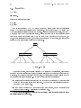
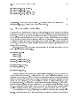
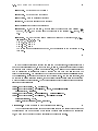
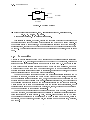
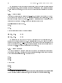
1.6 Constraint{Programming Language Interfaces
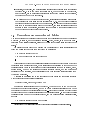
There are two basic ways of using constraints from inside a programming language. One
is providing a library with data structures and classes which implements objects such as
variables, equations, etc., and methods to combine formulae using mathematical (or other)
operations to give more formulae, combining formulae using mathematical relations to give
equations, putting together equations in sets, testing their solvability (and trying to solve
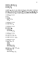
them), etc. This is exemplied in Figure 1.1.
Constraints
Constraints
Library
Host Language
Answers
(values/constraints)
Figure 1.1: External programming library
As good as it can be, it will not integrate seamlessly with the semantics of the host
language, for the constrained variables are not language variables, and the same happens with
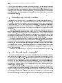
the equations, relationships: the do not belong to the language. For that, an alternative path
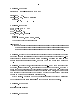
to coupling constraints and programming is making the language semantics richer by adding
high-level mathematical properties to the basic building blocks of the language: variables can
now be related to other variables, and can hold non-denite values. Constraint solving is
performed automatically as program execution progresses, since the constraint solver is part
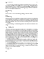
of the runtime system. This is depicted in Figure 1.2.
It is not surprising that functional and logic languages (specially the latter ones, because
1.7. AN EXAMPLE: SEND + MORE = MONEY
9
Constraint Programming Language
Programming
Language
Constraint
Solver
Figure 1.2: Language with extended semantics
they already provide logical variables and implicit search) are the ones more amenable to this
approach: their mathematical foundation and independence from the machine oer leeway to
for adapting their semantics self-congruently.
Regardless of the approach taken towards the construction of a constraint language, there
are some essential services that such a language must provide:
A solver, which solves equations or communicates their non-solvability (the way this is
done depends on the actual interface with the host language).
Means to express constraints, formulas, etc. from the language.
An interface to the solver, which allows constraints to be passed to it, and, upon successful constraint solving, asking for the values assigned to the constraint variables.
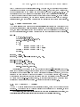
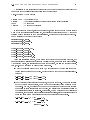
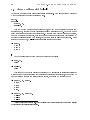
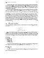
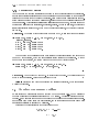
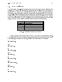
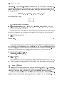
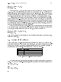
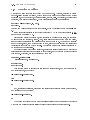
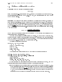
1.7 An Example: SEND + MORE = MONEY
the variables S E N D M O R Y
represent digits between 0 and 9, and the task is nding values for then such that the following
arithmetic operation is correct:
SEND + MORE = MONEY is a classical \crypto-arithmetic" puzzle:
+
M
S
M
O
E
O
N
N
R
E
D
E
Y
Moreover, all variables must take unique values, and all the numbers must be well-formed
(which implies that M > 0 and S > 0. Conventional programming needs to express an
explicit search in general (though in this particular case nested loops can be used). Logic
languages, such as Prolog, will use directly a built-in search: the programming is easy, but it
might not be highly ecient (of course, rened programs can achieve good performance, but
advanced skills and an eort in time is needed to write them).
This is, in fact, a typical problem for nite domains: all variables take values from a nite
set of numbers, the constraints to satisfy can be easily expressed, and there is some amount
of search to perform. Finite domain variables always have as values a set of integers, taken
CHAPTER 1. WHAT IS CONSTRAINT (LOGIC) PROGRAMMING?
10
from a nite number of possible initial values. For example, it is natural to use program
variables in our problem to represent the dierent digits. In that case, every variable (say,
the one corresponding to the digit D) can take values in the set f1 2 3 4 5 6 7 8 9g. The
nal solution must be an assignment of singleton sets to every variable in the problem, and
we take the unique value in this set as the denite value for that variable. If, at any point in
the execution of the program, the domain of a variable happens to become the empty set, a
failure is caused, and the program backtracks to the nearest (in time) choice point created2 .
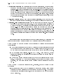
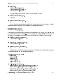
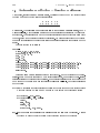
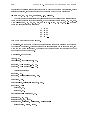
1.7.1 Prolog: Generate and Test
The Prolog solution below (one among several possibilities) is typical of the Generate and Test
paradigm: variables from a list are assigned values from another list after this assignment is
done, the list of variables is checked for compliance with the constraints of the problem. If
any of the constraints fail, the system backtracks to nd another assignment for the variables.
smm :X = S,E,N,D,M,O,R,Y],
Digits = 0,1,2,3,4,5,6,7,8,9],
assign_digits(X, Digits),
M > 0,
S > 0,
1000*S + 100*E + 10*N + D +
1000*M + 100*O + 10*R + E =:=
10000*M + 1000*O + 100*N + 10*E + Y,
write(X).
select(X, X|R], R).
select(X, Y|Xs], Y|Ys]):- select(X, Xs, Ys).
assign_digits(], _List).
assign_digits(D|Ds], List):select(D, List, NewList),
assign_digits(Ds, NewList).
Unsurprisingly, the program is not very ecient: there are 10!2 possibilities for the assignment of values to digits, Better programs are not dicult to write, but the one above
is possibly the non totally nave one which most directly expresses the problem, and whose
algorithm is more natural to write and understand by the average programmer. Improvements include not taking into account the value 0 for M and S explicitly (which can arguably
be viewed as a divide-and-conquer approach), or other techniques which may include using
explicitly an internal carry (see Section 7.2) or automatic delays (Section 5.2).
1.7.2 ILOG Solver (C++ Version)
The ILOG () Solver version is a proper constraint program, based on the Finite Domains
paradigm. The program has to be linked against the appropriate ILOG libraries, in order
As we will see later, these choice points are created every time there is an alternative in the program, and
these alternatives appear almost inevitably even if the program do not explicitly create them.
2
1.7. AN EXAMPLE: SEND + MORE = MONEY
11
for the FD routines to be available. The basic structure of the program (which is actually
shared, with minor changes, by the rest of the implementations of this example) is as follows:
1. The library is initialized,
2. The FD variables are declared, and initial bounds to them assigned (note the special
bounds for the variables M and S),
3. An array packing all FD variables is created,
4. The rest of the constraints are generated (all variables must be dierent, and the equality
dening the arithmetic operation must hold),
5. A call to the solver is made, to search for values and assign them to the variables, and
6. The nal solution is printed
#include <ilsolver/ctint.h>
CtInt dummy = CtInit()
CtIntVar S(1, 9), E(0, 9), N(0, 9), D(0, 9),
M(1, 9), O(0, 9), R(0, 9), Y(0, 9)
CtIntVar* AllVars]=
{&S, &E, &N, &D, &M, &O, &R, &Y}
int main(int, char**) {
CtAllNeq(8, AllVars)
CtEq(
1000*S
+ 1000*M
10000*M + 1000*O
CtSolve(CtGenerate(8,
+ 100*E + 10*N + D
+ 100*O + 10*R + E,
+ 100*N + 10*E + Y)
AllVars))
PrintSol(CtInt, AllVars)
CtEnd()
return 0
}
Since the FD variables are special objects not belonging to the C++ language itself, but
dened as part of a class, they cannot be treated in the program in the same way as primary
C++ objects: for example, printing them or accessing their values has to be done with special
methods provided by the class.
1.7.3 ILOG Solver (Le Lisp Version)
The Lisp version is actually very similar to the C++ one: this is not surprising, since the
underlying engine is basically the same. The same comments as for the C++ version apply
here. Only some additional remarks are needed:
12
CHAPTER 1. WHAT IS CONSTRAINT (LOGIC) PROGRAMMING?
There is no need to initialize the library. Since the constraints library is part of the Lisp
runtime system, the initialization takes place automatically.
The constraints for M and S appear explicitly, instead of being given when the variables
are declared.
Since the Lisp variables have in fact a complex internal structures (tags, pointers etc.),
they can be hooked by the implementation so that a more direct access from the language
is possible. For example, printing and accessing their values can be made using standard
Lisp functions.
(defun smm ()
(ct-let-vars
((S E N D M O R Y)
(ct-fix-range-var 0 9) l-var)
(ct-neq M 0)
(ct-neq S 0)
(ct-all-neq S E N D M O R Y)
(ct-eq
(ct-add
(ct-add (ct-add (ct-add
(ct-mul 1000 S) (ct-mul 100 E)) (ct-mul 10 N)) D)
(ct-add (ct-add (ct-add
(ct-mul 1000 M) (ct-mul 100 O)) (ct-mul 10 R)) E))
(ct-add (ct-add (ct-add (ct-add
(ct-mul 10000 M) (ct-mul 1000 O)) (ct-mul 100 N))
(ct-mul 10 E)) Y))
(ct-solve (ct-generate l-var () ()))
(print S E N D M O R Y)))
Unfortunately, the Lisp syntax is arguably not the best to write equations clearly.
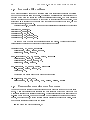
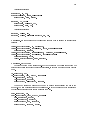
1.7.4 Eclipse Version
ECLi PSe is a programming system initially developed at ECRC, and now maintained at
IC-Park, which combines Logic Programming with constraint solving capabilities. Having
explained the previous examples, the program should be pretty obvious. Only some remarks
concerning the program below:
All variables are rst objects of the language: they can be manipulated and accessed
using the same primitives as for non-FD variables. The results of this manipulation, of
course might not be the same, since we are treating objects with dierent semantics,
but the program syntax is homogeneous.
Declaring the list of variables X is actually not needed, but it is convenient since it is
used elsewhere in the program.
1.8. USE PROLOG AS HOST LANGUAGE?
13
The versions for other CLP languages (for example, Prolog IV and CHIP) may dier
in the syntax, but the structure and programming is basically the same, and even the
syntax changes are recognizable without any eort.
smm :X
X
M
S
= S,E,N,D,M,O,R,Y],
:: 0 .. 9,
#> 0,
#> 0,
1000*S + 100*E + 10*N + D +
1000*M + 100*O + 10*R + E #=
10000*M + 1000*O + 100*N + 10*E + Y,
alldistinct(X),
labeling(X),
write(X).
This program has the combined advantage of being at the same time a direct encoding of
the problem and a highly ecient solution.
1.8 Use Prolog as Host Language?
The last example shows that Prolog syntax (and semantics) and nite domains go quite
well together. Actually, it is more than that: due to the incremental nature of constraint
programming (prototyping and building an application incrementally is easy and natural),
the availability of interactive interpreters for CLP languages (inherited from Prolog) is a plus,
as experimentation and debugging are parts inherent to the development of a program.
Also, the built-in backtracking of logic programming allows the easy customization of
search procedures for the cases in which standard CLP procedures are not good enough: this
may happen when there are hints as to what is the best direction to search in. Small examples
might not show that, due to small search times, but large examples often make the dierence
apparent.
Some interesting characteristics from Prolog are also inherited, which are not found in
other languages:
A built-in database, which can be used (with caution) to implement global variables,
but whose main strength is in saving intermediate results which do not need to be
recomputed (lemmas ) and, in the extreme, to generate and change program code dynamically.
Meta-programming facilities, which allow the program to be managed as if it were data,
examine its code while running, calling goals and collecting the solutions produced on
backtracking, and other goods which are only available to logic programming.
Easy denition of meta-languages and easy developing of interpreters for those languages. This allows the user to create a high-level language suited for her/his needs,
with which developing the nal application will be easier, and to code an interpreter for
such a language.
CHAPTER 1. WHAT IS CONSTRAINT (LOGIC) PROGRAMMING?
14
Of course, there are some disadvantages in using Prolog as host language, mainly concerned with the dierence of the logic programming paradigm with respect to other paradigms:
It might be not as well accepted as other languages: Prolog is sometimes not part of
standard curriculum in Computer Science, and therefore some training is usually needed,
and some programmers might be reluctant to undertake learning a new paradigm.
There are notable dierences with respect to conventional languages in the way data
structures are handled: but these dierences, in the end, favor the programmer, for they
turn out to be easier to work with and to dene, and more secure in what respect errors
caused by illegal memory accesses, etc. Control is also quite dierent: the embedded
search, once understood, is a very powerful way of programming.
Last, but not least, there are dierent products which implement the CLP paradigm.
Depending on the problem some of them might be more adequate than others. But very
probably the nal application in an industrial environment will have to interact with other
programs, so the possibility of having an interface (other than a raw text le) is a point to
take into account. Fortunately this is the case for all commercially available Prolog and CLP
systems.
1.9 How Does a CLP System Work?
The reader might wonder how a CLP system actually works and solves equations. Equation
solving in general might be radically dierent from the well-known methods for solving linear
arithmetic equations. CLP programs set up equations just by expressing them these equations, in an internally coded form, are communicated to an internal solver in which values
for the variables are worked out. We will not be concerned with way these equations are
encoded, but, for the sake of having more knowledge (which will help us in a future to write
better CLP programs), we will become solvers of nite domain equations for a while.
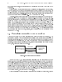
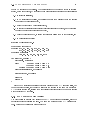
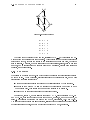
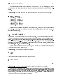
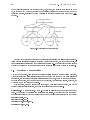
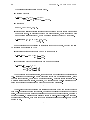
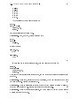
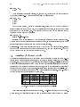
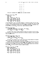
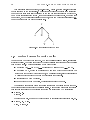
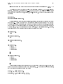
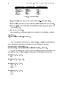
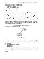
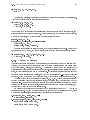
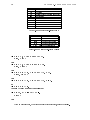
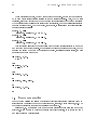
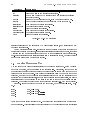
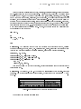
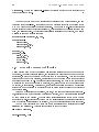
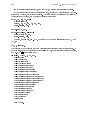
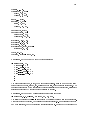
1.9.1 Modeling the Problem
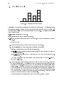
Suppose we have the precedence net (for example, for a project) and the task lengths3 in
Figure 1.3.
Usual O.R. methods to nd out critical tasks, the slacks in the tasks, the earliest nish
time, etc. include the PERT and CPM algorithms. We will show how a simple, general
nite domains algorithm performs the same task as those methods, and can even tackle more
dicult problems within the same setting.
Supposing that a hard limit for the length of the project is 10 time units, and that we
choose each FD variable to represent the time in which the corresponding task can start, a
model of the problem can be the following:
abcdefg
a
3
2 f0
: : : 10g
bcd
We will use nodes to represent tasks the problem is the same where nodes or edges are used to that end.
1.9. HOW DOES A CLP SYSTEM WORK?
15
0 G
4
E
1
F
1
B
2
C
0
A
3
D
Figure 1.3: Precendence net
b+1
c+2
c+2
d+3
e+4
f +1
e
e
f
f
g
g
The value of each variable (which is a set, initialized to f0 : : : 10g) represents the moments in time the corresponding task can start. This equation cannot be solved using linear
arithmetic methods, because the values of the variables are not real numbers, but rather
sets of integers. Of course, it might reformulated in this particular, linear, case to use real
numbers, but in general nite domains can always nd a solution, because enumeration is
possible, as we will see later.
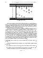
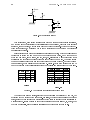
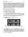
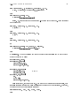
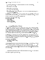
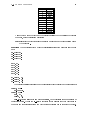
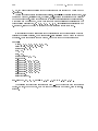
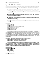
1.9.2 Be a Solver
We will set up a tableau (Table 1.1) in which current domains for the variables will be stored
at each moment. At the beginning, all variables will have the initial domain, and we will
iterate using the following strategy:
Choose one equation analyze the values of the variables related by that equation.
Sometimes the maximum / minimum values of the variables can be updated to make
the equation hold. This causes the domain of the variable to be narrowed.
Finish when no equation gives raise to a variable updating.
For example, in step 1, we have selected equation b + 1 e. Since previously b 2 f0::10g
and e 2 f0::10g, it is not dicult to deduce that b can be, at most, 9, and that e can be, at
least, 1. So this step updates the domain of b and e to be, respectively, f0::9g and f1::10g.
The rest of the steps perform similar operations, selecting other equations and rening values
of variables until a xpoint, in which no further changes can be made, is reached.
CHAPTER 1. WHAT IS CONSTRAINT (LOGIC) PROGRAMMING?
16
Step
0
1
2
3
4
5
6
7
8
9
10
11
Final domains
a
Variables and Domains
b
c
d
e
f
g
0..10 0..10 0..10 0..10 0..10 0..10 0..10
0..9
1..10
0..8
2..10
2..10
0..7
3..10
2..6
6..10
3..9
0..7
0..5
0..4
0..6
0..4
0..4 0..5 0..4 0..6 2..6 3..9 6..10
Table 1.1: Being a solver
Although the general idea behind nite domain solver is as shown above, actual algorithms
are much more complicated, and take into account issues like inequality constraints, global
constraints, heuristics, enumeration, etc. More complex constraint solvers make a series of
decisions (such as which equation is to be to chosen next) and, even if those do not aect
correctness, performance depends heavily on them.
What are in this cases the dierences with respect to classical methods, such as CPM?
A central point is that this is just a particular application of nite domains, and not an
algorithm dedicated to project scheduling. In fact, it gives more information than CPM, and
can, using the same ideas, be used for more advanced tasks. For example, exact slacks of tasks
in the critical path can be found just by setting g = 6 (which is just a way of writing g 2 f6g,
another equation similar to those we already have) and repeating the process. In fact, restart
the solving from scratch is not necessary: as an example of the dynamic, incremental nature
of CLP, we only need to add to our initial set of constraints the aforementioned equation,
update the domain of g and then continue the process where it stopped before: more updates
are now possible. The result will give us slacks for the variables and the start time for every
task so that the project is nished in the shortest time possible.
Problem 1.1 Solve the problem with the added constraint that the nal task must end at
time 6.
Modeling other relationships without resorting to very dierent algorithms is also possible:
for example,
Two tasks do not depend on each other, but they cannot start at the same time: b 6= c.
A resource r, of which there is a limited amount, is needed by two tasks b and d, and
allocating more resource to one of these tasks speeds up its completion:
b + rb
e
1.9. HOW DOES A CLP SYSTEM WORK?
17
d + rd f
rb + rd = 6
1.9.3 Don't Be a Solver!
But the programmer using CLP tools does not need to build tableaus, keep track of communicating with the solver when a new constraint is added, or jump back to a point where a
selection was previously done. CLP languages take care of all of these tasks by themselves,
transparently to the programmer. Built-in solvers are provided for several constraint domains,
FD being just one of them. Others, which we will talk about later, include linear equations,
non-linear equations with intervals, boolean equations, etc.
In the next chapter we will have a look at a basic language, based on concepts taken from
Logic Programming, and we will introduce the concepts of logical variables and backtracking.
We will add constraint solving capabilities upon this simple language, and we will see how
non-trivial problems are easy to express. We have chosen to use a logic programming basic
language because, although some initial acquaintance with its peculiarities is needed, once
this is mastered, the resulting language and syntax merges much better than other approaches
with the idea of programming using constraints.
)
18
CHAPTER 1. WHAT IS CONSTRAINT (LOGIC) PROGRAMMING?
Chapter 2
A Basic Language
In this chapter we will dene a basic language based on rst order logic, but which will not
have the full capabilities of Prolog: it will be pure, in the sense that no side eects of metaprogramming facilities are available, and it will not have data structures. But we will add to
it some symbols (like predened numbers and operators for common arithmetical operations)
which are needed to write constraints.
2.1 A Basic Constraint Language
We will dene the skeleton of a constraint language, without many interesting capabilities,
but which will be enough to understand the principles of constraint programming without
the burden of having to cope with unneeded details.
The basic components of our language are the following:
Variables which hold values throughout the execution. Dierently from other languages,
variables do not need to be typed or declared anywhere, and so they are distinguished
from other elements by their syntax. Variables will always be written starting with an
uppercase character: X , Y , Speed.
Constants which are immutable values. Usual languages can use only numbers as constants,
or, at most, a set of predened strings which make up an enumerated or cardinal type|
in fact, this is just another way of assigning names to numbers. Constants are either
numbers, including oating point numbers, or names starting with a lowercase character:
87, ;45:87, bogus.
Underscores are allowed either in the names of variables or non-numerical constants to
improve readability: Second Task, a dog.
Atoms which will play a syntactic r^ole similar to procedure denitions and procedure calls.
Atoms have the form p(X1 : : : Xn ), where p is the name of a procedure or, more strictly,
a predicate. X1 to Xn are the arguments of the atom, and the number of arguments n
is termed the arity of p. This is commonly written p=n. Examples of atoms are
hates(dog cat)
predates(big fish small fish)
19
CHAPTER 2. A BASIC LANGUAGE
20
Constraints which allow writing equations relating variables and constants in the program
are written. For now we will use only the constraint = of arity 2, which will denote
syntactic equality. We will give examples of their use.
Although constraint languages include builtin atoms which can be used in programs to
perform several tasks (e.g., opening and writing to les), this small language will not have
them: all the atoms which appear in bodies must be dened by the user somewhere in the
program|although they will not always appear explicitly dened in the examples. Conversely,
some constraint languages allow the user to dene and augment the constraints available,
besides those already available in the system, but we will not allow that either at this point.
2.1.1 Clauses
A clause represents a way of achieving a goal. Clauses have the form
p b1 : : : bn :
(2.1)
where p is an atom, as dened in the previous section, and b1 : : : bn are either atoms or
constraints. In this expression, p is commonly called the head of the clause, and b1 : : : bn is
called the body. The symbol (which, for typographical convenience, is often written as :-)
is called the neck, for it connects the body and the head.
Example 2.1 The following are syntactically correct clauses, as usually written in a computer:
animal(X):- dog = X.
likes(C, F):- C = cat, F = fish.
bigger(M1, M2):- M1 = men, M2 = mice.
In this example, animal/1, dog/1, likes/2, and bigger/2 are atoms. X, C, F, M1, M2 are
variables, and cat, fish, men, and mice are non-numerical constants. Note that variables
and constants can be written on both sides of the equality symbol|it does not matter in
which side they appear.
The program has no meaning in itself as it is written, in the same sense that writing x
= 3 + y in a conventional language has no meaning other than a mathematical operation
whose purpose in the program we do not know. The only a priori possible interpretation
comes from the semantics of rst order logic: a expression such as that in (2.1) is to be read
as for p to be true, b1 : : : bn have to be true. Then, under an interpretation directed by the
names in the code, the example 2.1 can be interpreted as expressing the following:
X is an animal if X equals \dog" , or
\dog" is an animal
\cat" likes \sh"
M1 is bigger than M2 if M1 equals \men" and M2 equals \mice" , or
\men" are bigger than \mice"
2.1. A BASIC CONSTRAINT LANGUAGE
21
These clauses contained only calls to constraints. Clauses can also refer to other clauses
written by the programmer (atoms). The variables in the clauses are used to pass arguments
to the atoms in the body (and constants can be passed as well, of course).
Example 2.2 The following clauses have atoms dened by the user in the body:
eats(X, Y):- bigger(X, Y).
pet(X):- animal(X), sound(X,Y), Y=bark.
Their reading depends on the interpretation of the user atoms, but a likely meaning of
them is:
The big eat the small, or
If some X is bigger than some Y, then X eats Y
For X to be a pet, it must be an animal and the sound it produces must be a bark , or
If X is and animal and X barks, then X is a pet, or
An animal which barks is a pet
Of course, the nal answer to the real meaning of this piece of code is what the programmer
actually had in mind when writing animal/a, sound/2, and bigger/2.
2.1.2 Implicit Equality
Equality is a very common constraint in all domains, and so it is customary to write it in a
shorter form: the clause
p(X):- X = something.
can also be written, with exactly the same meaning as
p(something).
i.e., every time a variable of a clause appears anywhere within a clause, the atom (or variable)
this variable is equated to can replace every appearance of that variable.
Example 2.3 The clauses in Example 2.1 can also be written as follows:
bigger(men, mice).
pet(X):- animal(X), sound(X, bark).
and their meaning and behavior is exactly the same as in the original example.
2.1.3 Facts
The previous section introduced a new type of clause, which is actually a shorthand expression
for clauses we already know how to write: the expression
p:
where p is an atom, is called a fact. The rst clause in Example 2.3 is a fact, which appears
because an equality constraint has been implicitly moved to the head of the clause.
22
CHAPTER 2. A BASIC LANGUAGE
Example 2.4 The rst and second clauses in Example 2.1 can also be written as facts:
animal(dog).
likes(cat, fish).
2.1.4 Predicates
A predicate is simply a collection of clauses which have the same head name and arity. Recall
that the constraints and atoms in the body of a clause represent conditions to be fullled
in order to achieve a goal|the head|, so they logically represent a conjunction of goals.
Dierent clauses, in turn, represent a disjunction: alternative possibilities to accomplish a
target. From a more logical point of view, dierent clauses of a predicate oer alternative
possibilities for the predicate to be true.
Example 2.5 The following predicate expands our idea of what a pet can look like:
pet(X):- animal(X), sound(X, bark).
pet(X):- animal(X), sound(X, bubbles).
What is the meaning of this example? In addition to the rst, already known clause,
which casted animals which bark into the category of pets, we are not including animals
whose sound is bubbles (probably shes) into the very same category. So, in a more colloquial
form, the example above can be read as
Animals which bark and animals which make bubbles are pets
Note that when we describe the predicate in a goal-oriented form, the description must
take a disjunctive form, closer to the logical meaning of the predicate, but less natural from
the point of view of the human language:
For something to be a pet, it must either be an animal and bark, or else be an animal and
make bubbles.
Note also that the same variable X appears in both clauses: the names of the variables in
a clause are local to that clause, very much like local variables in procedural languages have
an scope limited to the procedure/function they are dened in.
2.1.5 Programs and Queries
We are now ready to write programs in our constraint language. A program is simply a
collection of predicates, much in the same way that a program in other languages is a collection
of procedures or functions.
Example 2.6 The following code implements a program which has knowledge about what is
a pet, and, using a database of facts dening some animals and characteristics, infers which
animals are (to its knowledge), pets.
2.1. A BASIC CONSTRAINT LANGUAGE
23
pet(X):- animal(X), sound(X, bark).
pet(X):- animal(X), sound(X, bubbles).
animal(spot).
animal(barry).
animal(hobbes).
sound(spot, bark).
sound(barry, bubbles).
sound(hobbes, roar).
Since most CLP systems provide an interactive shell for the interpreter / compiler, the user
can usually issue commands to load the program, call predicates in it, change the program,
and load it again. Calling a predicate from the interpreter yields the same results as calling
it from inside a program.
A query issued by the user is just a conjunction of atoms, and has exactly the same form
and meaning as the body of a clause. The answer to a query is a set of bindings for the
variables which make the query true with respect to the program. Since some predicates may
have several clauses which hold for a given query, multiple solutions are possible.
Example 2.7 We will give an example of a possible session with a CLP system. The prompt
of the system will be shown as ?-. We will use the program in Example 2.6.
Load the le where the program is stored
?- consult(pet).
Make queries!
?- sound(spot, X).
X = bark
?- sound(A, roar).
A = hobbes
?- animal(barry).
yes
?- animal(X).
X = spot X = barry X = hobbes
Problem 2.1 What will be the answer(s) to the query
?- sound(A, S).
CHAPTER 2. A BASIC LANGUAGE
24
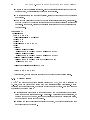
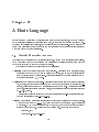
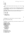
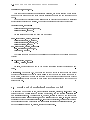
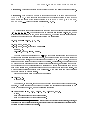
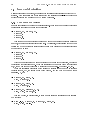
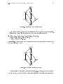
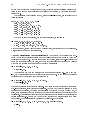
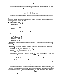
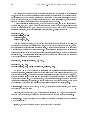
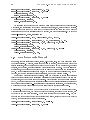
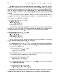
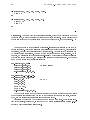
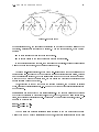
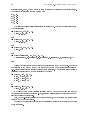
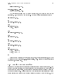
2.2 Searching
The query
?- pet(X).
returns the following answers:
X = spot
X = barry
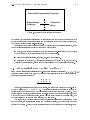
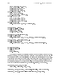
How is this achieved? The CLP system performs a search using all the possibilities
oered by having several clauses for the predicates. This is best depicted by a search tree
which represents all possible paths in the program. Without entering into details, every time
a predicate with more than a clause is called, a choice point is made at that execution point:
this choice points keeps information about the state of the execution at that moment, so
that, if more solutions are needed, the engine can backtrack up to that point, and resume the
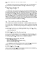
search with the next untried clause of that predicate.
pet(X)
animal(X), sound(X, bark)
animal(X), sound(X, bubbles)
animal(spok) animal(barry) animal(hobbes) sound(spok, bark) animal(spok) animal(barry) animal(hobbes) sound(barry, bubbles)
Figure 2.1: A tree
The search process, automatically triggered by a failure in the resolution, allows logic
programming based languages to return all possible solutions to a query: after having reached
a solution, if the user requests for more answers, the toplevel just causes a failure and the
backtracking process is (re)started1 . The order of backtracking is as follows:
Clauses within a predicate are tried from top to bottom backtracking on a predicate will
cause the next untried clause to be executed. The order in which clauses are executed
is dened by the search rule.
Atoms within a clause body are executed from left to right, and so backtracking is
attempted right to left. This is called the selection rule.
There are also special all-solutions predicates which encapsulate a search in a single objective and return
all possible solutions for a given query.
1
2.3. LOGICAL VARIABLES
25
Other strategies to select which clause and which atom to try are possible, and those
dierent search and selection rules give raise to dierent operational semantics for logic languages.
Example 2.8 The following query has been executed using the program in Example 2.6:
?- pet(X), animal(Y).
X = spot, Y = spot X = spot, Y = barry X = spot, Y = hobbes X = barry, Y = spot X = barry, Y = barry X = barry, Y = hobbes
Solutions for the clauses of animal/1 are generated rst, in the order in which the clauses
are written. After that, a new solution for pet/1 is generated, following the rules for atoms
and clauses stated above.
2.3 Logical Variables
Variables in CLP languages are termed logical variables. The adjective logical stems from
a unique character not present in other languages: these variables do not necessarily hold
values|and yet they are completely legal, and run-time access exception errors are not generated by accessing them2 |, and they can be assigned (or, better, bound ) to other uninitialized
variables. The value of an uninitialized variable is not NULL or other esoteric, special value:
that variable, simply, has no value at all yet.
Logical variable assignment is monotonic, which means that a logical variable cannot
mutate its value within a search path.
Example 2.9 The variable X can take the value a:
?- X = a.
X = a
But it cannot take the value a and then change it to
b
?- X = a, X = b.
no
Problem 2.2 Then, how is it possible that the following queries work perfectly?
In fact, the kind of fatal errors which are raised in some languages because of the dereferencing of uninitialized pointers, or because or arithmetical operations with numbers holding senseless values, cannot appear
in CLP systems (and, if they do, it is the system's, not the programmer's, fault) and, at most, a runtime
error is returned, which usually can be caught and recovered from. This results in an easier construction and
management of complex data structures, as we will see.
2
CHAPTER 2. A BASIC LANGUAGE
26
?- X
X
?- X
X
=
=
=
=
a.
a
b.
b
Hint:
state.
the toplevel interpreter backtracks between goals, in order to recover the initial
The constraint =/2 we have introduced before not only assigns values to variables (or,
better, binds variables to values), but it can also bind free variables, constraining them to
have the same value.
Example 2.10 Variables can be bound one to each other, constraining them to take the same
value, and this constraint is taken into account during the rest of the execution:
?- X = Y, X = a.
X = a, Y = a.
?- X = Y, pet(X).
X = spot, Y = spot X = barry, Y = barry
Problem 2.3 Explain the following behavior: why the query has no solutions?
?- X = Y, pet(X), sound(Y, roar).
no
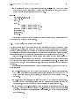
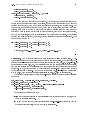
Problem 2.4 Given the following program, which is intended to model kinship in a family:
father_of(juan, pedro).
father_of(juan, maria).
father_of(pedro, miguel).
mother_of(maria, david).
grandfather_of(L,M):father_of(L,N),
father_of(N,M).
grandfather_of(X,Y):father_of(X,Z),
mother_of(Z,Y).
answer the queries:
?- father_of(juan, pedro).
?- father_of(juan, david).
?- father_of(juan, X).
2.4. THE EXECUTION MECHANISM
????-
27
grandfather_of(X, miguel).
grandfather_of(X, Y).
X = Y, grandfather\_of(X, Y).
grandfather_of(X, Y), X = Y.
Problem 2.5 Augment the code in Problem 2.4 to contain rules for the relationship
grandmother of(X, Y),
following the spirit of the program.
2.4 The Execution Mechanism
Execution of CLP languages can be seen as a tree traversal, where the nodes of the tree are
conjunctions of atoms to be proved (similar to bodies of clauses, which are also conjunctions
of atoms). The root of the tree is the initial query posed by the user, and there might be
one or several branches starting at every node, each branch corresponding to the clauses
with matching heads for the rst (leftmost) goal in the conjunction. The tree is explored
by selecting the leftmost goal in a conjunction, and the leftmost untried branch (clause) for
that goal. The tree can be explored partially or totally in the latter case, all solutions to the
initial query are returned.
Figure 2.2 shows how the execution tree is traversed for the following program and the
query ?- grandparent(charles,X).
grandparent(C,G):parent(C,P),
parent(P,G).
parent(C,P):- father(C,P).
parent(C,P):- mother(C,P).
father(charles,philip).
father(ana,george).
mother(charles,ana).
Execution starts at the toplevel query grandparent(charles, X), which is equated to
the rst clause of the program. Variables in the body of the clause are substituted by the
constants in the query, and the body (with some constants in place of the textual variables)
is left to be solved as a conjunction of goals. The execution continues by selecting the rst
goal in the body (parent(C, P), now rewritten at runtime to parent(charles, P)), and
the process continues. There are two matching clauses for parent(charles, P), and the two
are tried in textual order: that is the reason why two dierent subtrees are rooted at this
node. The execution proceeds until a node with no atoms to solve is obtained (this is possible
because a resolution against a fact, which has no body, removes an atom from the node).
The nal result of the query, X = george, is obtained in the leaf labeled (precisely) X =
george. This binding for X can be seen as propagated upwards in the tree and communicated
CHAPTER 2. A BASIC LANGUAGE
28
to the variable present in the toplevel query, but, in fact, the variable this binding is made
to, is the same one which was present in the toplevel query: as atoms were reduced in the
execution process, variables in the same position in atoms and clause heads were unied, i.e.,
equated.
grandparent(charles,X)
parent(charles,P),parent(P,X)
father(charles,P),parent(P,X)
mother(charles.P),parent(P,X)
parent(philip,X)
parent(ana,X)
father(philip,X)
mother(philip,X)
failure
failure
father(ana,X)
X = george
mother(ana,X)
failure
Figure 2.2: Traversing an execution tree
)
Knowing the operational behavior of the language is necessary for larger programs (especially because it is instrumental for achieving better performance), but for the time being, it
is not essential: understanding the declarative semantics (i.e., the grandfather of someone is
the father of his/her mother or the father or his father) is far more important at this stage.
2.5 Database Programming
The code in Example 2.4 is a case of the so called database programming : it acts as a database,
where facts store the basic relationships among data (in much the same way as in relational
databases), and the rules express new relationships among data, based on the ones we already
have: in other words, they provide views to the database, but everything is seen, together, as
a program which can answer to queries.
This language, although limited (for example, no data structures are used), can model
quite sophisticated relationships, and answer queries which are not trivial.
Example 2.11 A logical circuit. Figure 2.3 depicts an electronic circuit implementing logic
gates. Some parts of it (resistors and transistors) are labeled. We will use facts to construct a
small database stating which components connect the dierent points highlighted in the circuit:
resistor(power,n1).
resistor(power,n2).
transistor(n2,ground,n1).
transistor(n3,n4,n2).
2.6. DATALOG AND THE RELATIONAL DATABASE MODEL
29
transistor(n5,ground,n4).
Note that current direction is meaningless in resistors, but for simplicity we have chosen
to use the rst argument of the facts dening resistors to denote the end connected to the
power.
Some knowledge of electronic gates tells us that an inverter can be built of a transistor
appropriately connected to a resistor. The needed connections are reected in this rule:
inverter(Input,Output):transistor(Input,ground,Output),
resistor(power,Output).
Similar rules can be written for nand and and gates:
nand_gate(Input1,Input2,Output):transistor(Input1,X,Output),
transistor(Input2,ground,X),
resistor(power,Output).
and_gate(Input1,Input2,Output):nand_gate(Input1,Input2,X),
inverter(X, Output).
The following query and answer demonstrate the knowledge of the problem about our
circuit:
?- and_gate(In1,In2,Out).
In1=n3, In2=n5, Out=n1}
Similarly, queries could be made to nd out the connection points of inverters and and
gates.
Problem 2.6 In Example 2.11, how could the code be modied so that it does not matter
whether the resistors are dened as having power in the rst or in the second argument? In
other words, change and/or augment the rules for the circuit components so that whoever
denes resistor/2 does not have to know about the dierences between the rst and the
second argument.
2.6 Datalog and the Relational Database Model
The language we have seen so far, having (logical) variables, constants, user-dened predicates (which can be assimilated to program procedures), and the equality constraint =/2
is a constraint language. This language is, however, severely impeded by the lack of data
structures and arithmetical operations, and we will introduce them later. In fact, its power is
equivalent to that of propositional logic (i.e., logic without variables), because every program
in our rst language can be rewritten to a semantically equivalent propositional program, and
any propositional program is, directly, correct in our language.
CHAPTER 2. A BASIC LANGUAGE
30
Power
r1
n1
t1
r2
n2
t2
n3
n4
n5
t3
Figure 2.3: An electronic circuit
Notwithstanding, augmenting this language with numbers and arithmetical operations,
and (for the sake of practicality) other facilities (such as negation), produces a far superior
language, termed Datalog, which is often used in advanced databases. Without adding anything to our language, we will show how it can be directly used to model common operations
in relational databases.
Basic structural components of relational databases are tables, which are collections of
tuples (rows) having the same number of components in each tuple. Each component of
every row has a type, such a string, number, date, etc., usually from a set of predened types
available in the database we will not deal with such types at the moment. The arguments in
the same position of all the rows in each table belong to the same column, and every column
has an attribute, which usually names that column. Figure 2.4 shows two tables which can be
part of a database which collects information about persons and cities where they have lived.
Name Age Sex
Brown
Jones
Smith
20
21
36
Person
M
F
M
Name
Town
Brown London
Brown
York
Jones
Paris
Smith Brussels
Smith Santander
Years
15
5
21
15
5
Lived{in
Figure 2.4: Two tables in the relational database model
The order of rows in immaterial, since they are not accessed and retrieved by number, but
according to the matching of the arguments. Similarly, the order of columns is not important
either, since they are labeled with attributes but it will be important for our translation to
a logic language. It is important to note that duplicate rows are not allowed, or, rather, that
they are meaningless, since duplicated solutions are not taken into account at all.
2.6. DATALOG AND THE RELATIONAL DATABASE MODEL
31
A translation to our logic language takes every part of the database and casts it into the
component of the constraint language following the paths below:
Relat. Database ! Logic Program
Relation Name
Relation
Tuple
Attribute
!
!
!
!
Predicate symbol
Predicate consisting of ground facts (facts without variables)
Ground fact
Argument of predicate
It is important to note that, since in our language, arguments of an atom cannot receive
a name (but other logic languages allow it), the correspondence attribute name ! argument
position must be respected in the whole translation. The fragment of database in Figure 2.4
can be translated to the set of facts below:
person(brown,20,male).
person(jones,21,female).
person(smith,36,male).
lived_in(brown,london,15).
lived_in(brown,york,5).
lived_in(jones,paris,21).
lived_in(smith,brussels,15).
lived_in(smith,santander,5).
Using this translation scheme, which uses a set of facts to model a static database, the
usual operations on relational databases can be easily dened, an implemented using clauses.
As mentioned before, the result is that not only the database, but also the dierent queries,
views, etc. can be programmed using the same language.
S
Union: two clauses dene that a table r s is constructed by taking elements which
belong either to table s or to table r. Extending it to more than two tables is straightforward:
X : : :,Xn )
X : : :,Xn )
r union s( 1 ,
r union s( 1 ,
r(X1 ,: : :,Xn ).
s(X1 ,: : :,Xn ).
Set Dierence: tuples belonging to one table, but not to the other. The implementation
of Set Dierence needs negation, which we have not discussed yet: we will come back
to it later. For now, it will suce to know that a general and proper implementation
of negation in logic languages is very dicult, and usually only a restricted version of
the full logical negation is available. Fortunately, for the purpose at hand (relational
databases), implementing a sound logical negation is possible, since the tables are always
nite and there are no data structures which can construct innite objects.
X : : :,Xn)
r(X1 ,: : :,Xn ),
X : : :,Xn)
s(X1 ,: : :,Xn ),
r diff s( 1 ,
r diff s( 1 ,
not s(X1,: : :,Xn).
not r(X1,: : :,Xn).
CHAPTER 2. A BASIC LANGUAGE
32
We will later discuss negation more in depth.
Cartesian Product:
X ::: X X
X ::: X
: : : Xm+n) Xm+1 ,: : :,Xm+n ).
r X s( 1 , , m , m+1 , ,
r( 1 , , m ), s(
Projection:
X X
X X X
r13( 1 , 3 ) r( 1 , 2 , 3 ).
Selection: the selection criteria is just another predicate which can fail or have success
for a tuple of data. In general it could be any user predicate, but in this case we will
use the arithmetical predicate , which we assume is already dened by the system.
X X X
X X X
X X
r selected( 1 , 2 , 3 ) r( 1 , 2 , 3 ),
( 2 , 3 ).
Some operations can be expressed as derivatives from the above ones, but they can also
be expressed more directly in CLP:
Intersection : tuples which are in r and s at the same time:
X : : :,Xn)
r meet s( 1 ,
r(X1 ,: : :,Xn ),
X : : :,Xn).
s( 1 ,
Join : tuples which have an element in common in two tables:
X ::: X
X X X : : : Xn ),
X X X : : : Xn ).
r joinX2 s( 1 , , n ) r( 1 , 2 , 3 , ,
s( 10 , 2 , 30 , ,
0
The appearance of duplicate answers, even if there are no duplicates in the original table
(e.g., projecting the table lived-in on its rst argument) is not a theoretical problem, since
they are simply ignored, but it can be a practical problem. Database implementations automatically discard repeated tuples. Similarly, CLP languages have built-in primitives which
allow the gathering of all answers to a query and remmoving duplicates.
)
The so-called deductive databases are relational databases which use heavily concepts
from rst-order logic to implement (actually, to program) explicitly deduction and coherence
rules. They use commonly a language similar to the one we have just developed, plus some
extended facilities. This language is usually a subset of a logic-based full-edged language.
It is language of this kind, even augmented with constraint solving capabilities, which we are
aiming at now.
)
Chapter 3
Adding Computation Domains
In this chapter we will add dierent constraint domains to our language, and we will see
how they greatly expand its usefulness. Several examples, which could not have been realised
before, will be developed here.
3.1 Domains
A constraint domain introduces new symbols and their associated semantics in the language.
This gives the language an ability to express computations which go well beyond what was
available until this moment.
Example 3.1 In a language like C or Pascal, integer numbers and real numbers are provided
by default. Think of an application which needs to deal with complex numbers. Two paths are
possible:
Writing some libraries which create, access the real and imaginary parts of, and make
arithmetical operations with such numbers, or
p
Augment the language with a new, primitive data type complex, a new symbol for ;1
(usually written as { or |), and an expanded meaning for the usual arithmetical operators.
While both approaches are equally valid, if the embedding is correctly made, and ts nicely
with the rest of the language, the second is probably more elegant and leads to languages
easier to understand. We will see that using constraints together with logic programming is
actually a natural step towards a more powerful language.
There is a variety of constraint domains to choose, and CLP languages choose which
one to implement (several at once, in some cases). The reason for having them is that
dierent problems call for dierent constraint domains (due to its nature), and nding the
right constraint domain is usually not dicult. But, in any case, the rst step is deciding a
modelization of the problem.
Choosing a constraint domain has another impact: the capabilities of the solvers for
that domain. Not all constraint domains are equally solvable: some have algorithms which
generate a solution (e.g., linear equations), some need enumeration and trial and error (e.g.,
33
34
CHAPTER 3. ADDING COMPUTATION DOMAINS
nite domains), and some need an iterative xpoint-based algorithm which approximates a
solution (e.g., non-linear equations).
Having dierent constraint systems available is, actually, an advantage, in that it allows
the programmer to model the problem freely, and then try to adapt (if needed) that model to
the constraint system which more closely resembles the modelization. We will present some
constraint domains which will allow us to perceive the dierences among them, and, at the
same time, to understand how all of them blend easily with the underlying LP machinery.
3.2 Linear (Dis)Equations
Linear (dis)equations were, in practice, pioneered by the CLP(<) system, which oered a
Prolog-like interface, where arithmetical symbols were enriched to express constraints. Other
implementations (namely, Prolog IV, CHIP, SICStus . . . ) have chosen to implement this
constraint system as well, as it has a well-known solving procedure, and is useful in a range
of applications. We will use Prolog IV in the examples, as it is a quite reasonably known logic
programming system, and it has several constraint systems available.
A note on syntax: CLP systems tend to have some variations in the syntax
of similar operations. This may be slightly confusing at rst, but it is not a real
problem: dierent syntaxes are easily understood, once the underlying language
design principles are known.
We will augment the language with the following components:
Numbers, both integers and oating point numbers (which aproximate real numbers),
written as usual. Addiotinally, expressions like 3.7e5 represent the number 3:7 105 .
Arithmetic operators (+, ;, *, /) , written in the usual inx form. They allow us to
construct arithmetic terms, using numbers and variables: 3 + 4, X + 3 (6 ; Y ). Those
arithmetic terms stand for the corresponding arithmetic expressions.
The constraint =/2, which now stands for arithmetical equality : two expressions are now
said to be equal if they can be arithmetically reduced to the same expression.
More arithmetical constraints, which act as the corresponding arithmetical relational
operators:
Prolog IV name
gelin(X,
gtlin(X,
lelin(X,
ltlin(X,
Y)
Y)
Y)
Y)
Arithmetical meaning
X Y
X >Y
X Y
X <Y
Note that all of them have the sux lin, which stands for linear: the reason for that
will become clear later.
3.2. LINEAR (DIS)EQUATIONS
35
Prolog IV (and other CLP languages) can solve equations directly typed in the top-level
prompt. These examples are taken from a Prolog IV session:
?- 4
Y
?- X
Y
=
=
=
Y = 3.
1
3*Y - X/2, X+Y = Y - 4*X + 7.
7/10, X = 7/5.
(The prompt of the Prolog IV interpreter is >>, but we will be using ?- throughout this
paper). By default, answers are returned as fractions because Prolog IV uses innite precision
arithmetic when possible. The equations above had a unique solution, but equations may
have no solutions:
?- X = 3*Y - X/2, X+Y = Y - 4*X + 7, lelin(X, Y).
false.
And sometimes there exists an innite number of solutions:
?- X = Y + 3.
X ~ real, Y ~ real
which means that X and Y are just real numbers. The syntax needs further explanation,
but we will delay it until later: it will suce by now to understand it as meaning \belongs
to the class of"|in this case, \X belongs to the class of the real numbers".
Prolog IV does not output complex relationships, although it is of course aware of them.
In the previous example, Yreal, Xreal is actually a weak answer, for the constraint
X + Y = 3 is known by the system. A clearer example is the one below:
Example 3.2 The following query represents the constraint X
X = Y can be deduced:
YY
X, from which
?- gelin(X, Y), gelin(Y, X).
Y ~ real, X ~ real
No output of constraints is given, but the solver is internally aware of the constraint
X =Y.
?- gelin(X, Y), gelin(Y, X), X = 4.
Y = 4, X = 4
There is a problem in generating output for complex answer constraints: the constraint
system, after simplication, has to be projected onto the query variables (because these are
the ones the user knows about), and this is not easy (or even feasible) in some constraint
domains.
CHAPTER 3. ADDING COMPUTATION DOMAINS
36
3.3 Linear Problems with
Prolog IV
Let us give a couple of examples of using linear constraints. We will rst dene a predicate
which can generate (and test) natural numbers.
nat(0).
nat(N):gtlin(N, 0),
nat(N-1).
This can be read as \zero is a natural number, and any number greater than zero is a
natural number, provided that is predecessor is also a natural number". Note that we are
using the actual number zero to represent zero. This is an example of a recursive denition,
in which a problem (in this case, knowing when something is a natural number) is solved by
reducing the initial problem to a similar, but in some sense smaller or simpler task. After
loading the above code, Prolog IV returns a series of integer numbers:
?- nat(X).
X = 0 X = 1 X = 2 ..
.
And it can also test whether a given number is or not natural:
?- nat(3.4).
false
?- nat(-8).
false
This is one of the most important properties of CLP languages: as logical properties are
written without paying attention1 to the internal operations of the language, the code can be
used in various modes : it can either generate or test, or perform a mixture of both:
?- gelin(3, X), nat(X).
X = 0
X = 1
X = 2
X = 3.
?- gelin(3, X), nat(X+5).
X = -5
X = -4
X = -3
This can be assumed at this moment. Later we will see that a better knowledge of how the system actually
works is needed for writing certain programs.
1
3.3. LINEAR PROBLEMS WITH PROLOG IV
X
X
X
X
X
X
37
= -2
= -1
= 0
= 1
= 2
= 3.
The denition above can also be written as
nat(0).
nat(N + 1):gelin(N, 0),
nat(N).
and it works exactly in the same way.
Problem 3.1 How, and why, will the following code
nt(0).
nt(N):nt(N-1).
behave if queried
?- nt(3.4).
(???)
?- nt(-8).
(???)
In a similar way to the natural numbers, even numbers can be dened as
even(0).
even(N+2):gtlin(N+2, 0),
even(N).
which is to be read as \zero is an even number, and any even number plus two is also an even
number".
Problem 3.2 Write code, similar to the one for
and test for oddity. Call the predicate
odd/1.
even/1,
which can generate odd numbers
Problem 3.3 Write an alternative denition for odd/1 which uses the denition of
but which is not based on it. It should not contain any recursive call.
Problem 3.4 Write a predicate
multiple of another number B.
multiple(A, B)
which tests if a number
A
even/1,
is an integer
CHAPTER 3. ADDING COMPUTATION DOMAINS
38
Problem 3.5 It should be trivial to give denitions for odd/1 and even/1 using multiple/2.
Problem 3.6 Find whether a number N is congruent modulo K to some other number M
(M N mod K ). This means that the remainder of the integer division of M by K is the
same as the remainder of the integer division of N by K: 12 7 mod 5, 32 2 mod 2,
32 2 mod 30, . . . . Call the predicate congruent(M, N, K).
)
A more involved example is generating the value of e based on a (slowly) convergent series:
1
1
1
1
=
4
1 ; 2 + 3 ; 4 + . The predicate which implements this is called is E(N, E), where
N is the number of terms to add, and E is the value of e. We will make this toplevel call an
interface to a predicate which will actually perform the calculation:
e
is_E(N, E4*4):- is_E(N, 1, 1, E4).
is_E(0, Mult, Sign, 0).
is_E(N, Mult, Sign, Sign/Mult + RestE):gtlin(N, 0),
is_E(N-1, Mult+1, -Sign, RestE).
The bulk of the work is performed by is E/4, which has in its rst argument the number
of elements in the series remaining to be added, in the second argument the denominator for
each element of the series, in the third argument the sign (+1 or ;1) to be used, and in the
last argument the result of adding the rest of the series. Operationally, the predicate works
by nding out the rst element of the series (which is Sign/Mult), and stating (in the head
of the clause) that the whole series is to be calculated by adding this rst element with the
rest of the series then, a recursive call works out the value of this rest of the series. All
mathematical operations are solved when possible (i.e., when a sucient number of variables
have been reduced to denite values).
Finding an approximation of e is as easy as writing:
?- is_E(10, E).
E = 1627/630.
The problem, in that case, is that we do not have any idea of the accuracy of this approximation. A better control can be obtained by forcing two successive approximations of e to
dier by a small amount2 . So, an easy possibility is writing:
?- lelin(abs(E1 - E2), 0.1), is_E(N, E1), is_E(N+1, E2), !.
N = 39,
E2 = 3637485804655193/1335732864265800,
E1 = 3771059091081773/1335732864265800.
Mathematically speaking, this is not a good idea: the error of the approximation in a series is, in general, an
expression which is to be calculated separately, and usually working out this expression is not as straightforward
as testing the value of an element of that series.
2
3.4. FIBONACCI NUMBERS
39
Thirtynine elements may seem a lot for an accuracy of only 0.1, but if one thinks carefully,
the 40th element is 401 , and since the series itself returns 4e , the dierence among the 39th and
the 40th element is just 0.1 concerning the accuracy of the approximation, it is not really
meaningful, and should be looked mainly as an exercise of using CLP in innovative ways, not
possible in other languages.
Some primitives not yet explained are used in this example: abs/1 returns the absolute
value of a number. The ! sign forces Prolog IV (and any other Prolog or CLP language) to
stop after nding the rst answer to a query. We will return to them (especially to !) later.
Problem 3.7 There is some redundancy in this example. Two of the arguments perform
similar roles: the rst one counts the number of elements in the series still to be worked out,
and it thus goes from N to 0 the second one has the denominator of the fractions, and it goes
from 1 to N. The only reason for doing that is automatically calculating whether to add or
substract each element in the series by reversing the sign of the third argument. CLP can help
to have a simpler program: we can start at N1 and progress towards 11 , leaving undetermined
the sign of every element of the series, but reversing its sign, until the rst element is reached.
Write this program.
3.4 Fibonacci Numbers
The Fibonacci series is a classical problem in mathematics and computer science. It is usually
dened as:
F0 = 0
F1 = 1
Fn+2 = Fn+1 + Fn
I.e., the numbers of Fibonacci are 0, 1, 1, 2, 3, 5, 8, 13. . . It is easy to straightforwardly
translate it to a logical denition, mimicking each equation with a clause. The rst argument of the predicate is the index of the Fibonacci number, and the second argument is the
Fibonacci number itself. Note that there is an explicit check of the index in the last clause:
fib(0, 0).
fib(1, 1).
fib(N, F1+F2):gelin(N, 2),
fib(N-1, F1),
fib(N-2, F2).
There are two recursive calls in this case. This will be important later. As usual, queries
can be issued to nd out which number corresponds to a given index:
?- fib(10, F).
F = 55.
But, as in previous examples, other calls are possible, as, for example, nding out the
index of a Fibonacci number:
CHAPTER 3. ADDING COMPUTATION DOMAINS
40
?- fib(N, 8).
N = 6
Other interesting queries are possible, as, for example, nding which are the xpoints of
the Fibonacci series (i.e., which numbers are equal to their indexes):
?- fib(N, N).
N = 0
N = 1
N = 5
But the above program, having two recursive calls, needs too much memory because of
repeated calls: F100 needs F99 and F98 , but F99 itself needs F98 again, so not only many calls
are needed: they are repeated, too. The program can use up the memory allocated for the
process in medium sized computations:
?- fib(100, F).
error: too_many_scols
Increasing the memory allocated by the process only pushes the problem a little bit forward: it is much better to reformulate the program (which, in this case is quite easy) to make
another faster (and cheaper in terms of memory) implementation.
Problem 3.8 Write a simply recursive program which denes the Fibonacci series.
Hint:
use two arguments to store the current Fibonacci number, and the previous one. Find the
1000th Fibonacci number (the last four digits are 8875).
3.5 Non-Linear Solver: Intervals
The linear equations solver we have been seeing has the attractive of being complete (i.e., it
always nds a correct solution if it exists, and says that no solution exists only when this is
the case). But, on the other hand, it can solve only linear equations. Prolog IV implements
a second numerical constraint system which is based on intervals: variables take values in
intervals (and combinations thereof) of real numbers, which in fact associates a (potentially)
innite number of points to each variable. Intervals have a special syntax in Prolog IV, and
the usual mathematical combinations of open / closed interval are available. Table 3.1 shows
the four dierent types of intervals and their syntax.
Interval
#X Y ]
(X Y ]
#X Y )
(X Y )
From
X (included)
X (excluded)
X (included)
X (excluded)
Y
Y
Y
Y
To
(included)
(included)
(excluded)
(excluded)
Prolog IV
cc(X,
oc(X,
co(X,
oo(X,
Y)
Y)
Y)
Y)
Table 3.1: Intervals and their representation in Prolog IV
Using intervals brings advantages in some cases. Non-linear equations can be approximately solved, and intervals can also be used to simulate easily nite domains (by forcing
3.5. NON-LINEAR SOLVER: INTERVALS
41
the interval to contain only integer values). On the other hand, it is not sure that a solution
will be found for non-linear problems. For this reasons, it is convenient to know when the
linear solver has to be used, and when the non-linear solver is the correct choice. Thus, it is
necessary to be able to tell Prolog IV which solver we want to use in every particular case.
This is done by using dierent keywords to express operations in the linear and non-linear
solver the two versions are shown in Table 3.2. The sux lin is removed from the relational
constraints, and dots are added in before and after the arithmetical operators. The equality
constraint =/2 remains the same. But the \compatible with" operator, , particular to Prolog
IV, is to be used to bind variables to intervals:
?- X = A .+. B, A ~ cc(1, 3), B ~ cc(3, 7).
B ~ cc(3,7), A ~ cc(1,3), X ~ cc(4,10).
?- X = A .-. B, A ~ cc(1, 3), B ~ cc(3, 7).
B ~ cc(3,7), A ~ cc(1,3), X ~ cc(-6,0).
In their basic version, operations on intervals just add, subtract, etc. the maxima and
minima of the ranges of the variables, which are updated to make the operations true|
always in the direction of narrowing the intervals. In more complex problems, the intervals
are successively narrowed using an iterative procedure until a xpoint is reached:
?- X = A .-. B, A ~ cc(1,3), ge(X,0), B ~ cc(3,7).
B = 3, A = 3, X = 0.
Linear version Non-linear (intervals) version
+
*
/
gtlin(
gelin(
ltlin(
lelin(
,
,
,
,
)
)
)
)
.+.
.-.
.*.
./.
gt( ,
ge( ,
lt( ,
le( ,
)
)
)
)
Table 3.2: Correspondence between keywords for the linear and non-linear solvers
A note on Prolog IV and The use of in Prolog IV is a shorthand for writing more
complex relations: an expression like A cc(1, 3) is a shortened form of cc(A, 1, 3)
where cc/3 is a relation which states that A can take values in the interval #1 3]. Similarly,
the expression gt(A, 0), which stands for A > 0, can also be written A gt(0), and other
constructions as for example .*. are abbreviated forms for relations: writing X = A .*. B
is akin to writing times(X, A, B).
CHAPTER 3. ADDING COMPUTATION DOMAINS
42
3.6 Some Useful Primitives
Besides those already mentioned, it is usual that additional primitives are provided in CLP
systems. We will mention some primitives which are available in Prolog IV the reader is
advised to refer to the manual of the CLP system being used.
3.6.1 The Bounds of a Variable
Sometimes accessing the bounds of a variable is useful. Could this be made using the interval
constructors to access the bounds of the variables?
?- A
U
L
A
~
~
~
~
co(1, 3), A ~ co(L, U).
gt(1),
lt(3),
co(1,3).
This does not work as expected: the lower and upper bounds are not returned as simple
numbers, but rather as (innite) sets of numbers. Additionally, the intervals might not be as
desired if we do not access the variable using the same combination of open/closed interval
it has at that moment:
?- A
U
L
A
~
~
~
~
co(1, 3), A ~ oc(L, U).
ge(1),
lt(3),
co(1,3).
What happens here is that we are not accessing the bounds of the variable A, but rather
constraining the variables L and U. When L is constrained to be a lower bound of the interval
#1 3), then L can take any value from 3 (excluded) downwards (i.e., the range (;1 3)).
There are specialized primitives which access the greatest lower bound of an interval
variable (glb(A, L)), the lowest upper bound (lub(A, U)) and both at the same time:
bounds(A, L, U):
?- A ~ co(1, 3), glb(A, L).
L = 1, A ~ co(1,3).
?- A ~ co(1, 3), lub(A, U).
U = 3, A ~ co(1,3).
?- A ~ co(1, 3), bounds(A, L, U).
U = 3, L = 1, A ~ co(1,3).
This can be used, in certain cases, to force a maximization/minimization of the solution
of a problem:
?- X = A .-. B, A ~ cc(1,3), B ~ cc(3,7), glb(X,X).
B = 7, A = 1, X = -6.
3.7. A PROJECT MANAGEMENT PROBLEM
43
3.6.2 Enumerating Variables
Very commonly the problem constraints do not suce to give denite values to the variables.
In this case obtaining solutions must be made resorting to an enumeration of the remaining
values in the domain of each (or some) variables. With nite domain variables this enumeration poses no problem other than performance, since the number of possible values in the
domain is nite. With interval variables the situation is more awkward, because the set of
points in the interval of the variable is, in principle, innite. To help in this case, the primitive
enum/1 instantiates its argument, which must be an interval variable, to the integer values in
its domain.
Example 3.3 This piece of code decomposes a number (1001, in this case) into two factors:
?- Num = 1001, Num = A .*.
enum(B), enum(A).
B = 1, A = 1001, Num =
B = 7, A = 143, Num =
B = 11, A =
91, Num =
B = 13, A =
77, Num =
B, A ~ cc(1,Num), B ~ (1,A),
1001
1001
1001
1001.
The key point for the solution is the enumeration: it generates integer numbers in the
domain of the variables, which are automatically tested against the constraints. If those
numbers are not generated, the system does not have any way of factoring Num:
?- Num = 1001, Num = A .*. B, A ~ cc(1,Num), B ~ cc(1,A).
Num = 1001, B ~ cc(1,1001), A ~ cc(1,1001).
Problem 3.9 Use the code in Example 3.3 to factor bigger numbers. Try interchanging the
order of the enumeration. Is there any dierence? Why?
Prolog IV provides a number of enumeration and splitting primitives, which are useful in
a variety of contexts.
3.7 A Project Management Problem
In this section we will address the same problem we did in Section 1.9.1, but we will leave
the task of solving the resulting equations to a CLP system. Recall the precedence net in
Figure 1.3, and suppose that we want the whole job to be nished in 10 units of time or less.
In that example we used nite domain variables, and in this programming example we will
use interval variables to simulate FD variables.
Recall that the constraints for the precedence net were
abcdefg
a
2 f0
: : : 10g
bcd
44
CHAPTER 3. ADDING COMPUTATION DOMAINS
b+1
c+2
c+2
d+3
e+4
f +1
e
e
f
f
g
g
These can be translated into Prolog IV using the following clause:
pn1(A, B, C, D, E, F, G):ge(A, 0),
le(G, 10),
ge(B, A), ge(C, A), ge(D, A),
ge(E, B .+. 1), ge(E, C .+. 2),
ge(F, C .+. 2), ge(F, D .+. 3),
ge(G, E .+. 4), ge(G, F .+. 1).
where variables in the head of the clause correspond to nodes in the graph, and the maximum and minimum starting times for the corresponding job are precisely the bounds of the
variables. Time constraints are directly encoded as Prolog IV constraints. After loading this
simple program in the system, making a query yields the following result:
?- pn1(A,B,C,D,E,F,G).
G ~ cc(6,10), F ~ cc(3,9), E ~ cc(2,6), D ~ cc(0,6),
C ~ cc(0,4), B ~ cc(0,5), A ~ cc(0,4).
The allowed range for each variable represents the slack in the start time for the corresponding task. We can minimize the total time of the project by setting the time of the end
task to its lower bound:
?- pn1(A,B,C,D,E,F,G), glb(G, G).
G = 6, E = 2, C = 0, A = 0,
F ~ cc(3,5), D ~ cc(0,2), B ~ cc(0,1).
As expected, some variables do not have slack: those are the ones corresponding to critical
tasks, whose delay would imply a delay of the whole project.
A variant of the project is presented in Figure 3.1. In that gure, there is a task (F) whose
duration we can change. Speeding it up will cost more resources, slowing it down will make
it cheaper. We want to know what is the minimum resource consumption so that the project
is not delayed. We can model this by using the following clause:
pn2(A, B, C, D, E, F, G, X):ge(A, 0), le(G, 10),
ge(B, A), ge(C, A), ge(D, A),
ge(E, B .+. 1), ge(E, C .+. 2),
ge(F, C .+. 2), ge(F, D .+. 3),
ge(G, E .+. 4), ge(G, F .+. X).
3.7. A PROJECT MANAGEMENT PROBLEM
45
0 G
4
E
X F
1
B
2
C
0
A
3
D
Figure 3.1: Project 2: F can be speeded up!
X,
the length of task F, is added to the variables in the head, since we want to access it.
A possible query which minimizes project time and maximizes F's duration is:
?- pn2(A, B, C, D, E, F, G, X), glb(G,G), lub(X,X).
X = 3, G = 6, F = 3, E = 2, D = 0,
C = 0, A = 0, B ~ cc(0,1).
Problem 3.10 What happens if the primitives glb/2 and lub/2 are called in reverse order
in the example above? Why?
0 G
E
1
F
X B
2
C
0
A
4
Y D
Figure 3.2: Two tasks with length not xed
The last variant of this problem is depicted in Figure 3.2. Two tasks, B and D have a length
which is not xed, but there are some additional constraints which relate their lengths: any
CHAPTER 3. ADDING COMPUTATION DOMAINS
46
of them can be nished in 2 units of time at best, but shared resources disallow nishing both
tasks in the minimum time possible: the addition of the duration of both tasks is always 6
units of time.
The constraints which describe the net, again in Prolog IV syntax, are expressed in the
following clause:
pn3(A, B, C, D, E, F, G, X, Y):ge(A, 0), le(G, 10),
ge(X, 2), ge(Y, 2), X .+. Y = 6,
ge(B, A), ge(C, A), ge(D, A),
ge(E, B .+. X), ge(E, C .+. 2),
ge(F, C .+. 2), ge(F, D .+. Y),
ge(G, E .+. 4), ge(G, F .+. 1).
The query to ask for a solution, and the answer returned, is as follows:
?- pn3(A,B,C,D,E,F,G,X,Y), glb(G,G).
Y = 4, X = 2, G = 6, E = 2, C = 0,
B = 0, A = 0, F ~ cc(4,5), D ~ cc(0,1).
which means that, since X has the minimum possible value, task B is the one to be accelerated.
Also, all tasks but F and D are critical now.
A note on minimization (and maximization): The approach we have followed to max-
imize / minimize a constraint problem is a very nave one: taking the maximum value of a
variable and sticking to it. This does not always work because, since the non-linear solver (as
nite domain solvers) is not complete, and there are often values in the range of a variable
which are not actually compatible with the problem constraints:
?- X ~ cc(-2, 2), X .*. X
X ~ cc(-2, 2).
= 1.
The solver did not work out a solution for this quadratic equation (e.g., X = 1 and X =
and the initial interval for the variable remains unchanged. If one adds the additional
constraint that the solution must be smaller than 1:
-1),
?- X ~ cc(-2, 2), X .*. X
X ~ cc(-2,-0.5).
= 1, X ~ lt(1).
the answer approximates better the solution. But since there is no algorithm for solving
non-linear equations, these are left as constraints. The only way to reach a solution to those
problems is enumerating, or waiting for variables in the problem to become ground (or, at
least, more constrained) so that the solver can decide if the values are compatible with the
constraints. For specialized cases (such as maximization or minimization) the solvers include
builtin strategies (e.g., branch and bound) which converge to a solution faster than blind
enumeration. These strategies are accessible by calling ad-hoc predicates:
?- X ~ cc(-2, 2), X .*. X
X = -1.
= 1, min(X, 0, X), realsplit(X]).
3.8. OTHER CONSTRAINTS AND OPERATIONS
47
3.8 Other Constraints and Operations
What we have sketched here is just a brief look at the possibilities available in CLP programming systems: most of them oer a whole gamut of primitive predicates and operations,
which implement useful goodies and specialized complex constraints found to be interesting
in practical cases. In particular, as an example, Prolog IV has also:
Complementary intervals, which implement the exclusion of an interval.
Boolean operations and constraints on them.
Extended real operations, such as trigonometric operations, logarithms and other transcendental operations.
Constraints on lists (about which we will see an example later).
Constraints on integers, which force interval variables to take only integer values (or
to exclude them), thus allowing the interval solver to be used with problems modeled
using nite domains.
3.9 Herbrand Terms
Herbrand terms are a representation of nite trees. Technically, they are non-interpreted
function symbols of rst-order logic, but their main use, and the approach we will follow in
presenting them, is as constructors of data structures. They are interesting because they
are present in all the CLP languages, which means that data structuring and abstraction is
handled uniformly in all CLP languages. Moreover, Herbrand terms themselves can be viewed
as a constraint system itself, where the only constraint allowed is the syntactic equality (very
similar to the one in the rst language we presented|actually, the data in that language was
a simplication of Herbrand terms).
A formal denition of a Herbrand term is:
A variable is a Herbrand term
A constant is a Herbrand term
A function symbol f with arity n applied to n terms is a Herbrand term: f (t1 t2 : : : tn )
For example, following the syntax for variables and constants presented in Section 2.1,
the following are examples of Herbrand terms (which we will call henceforth only \terms"):
X
mum
45
identity(Name, Number)
task(Start, End, window(front), needs_carpenter)
f(a, X, g(Y, t))
CHAPTER 3. ADDING COMPUTATION DOMAINS
48
Terms represent trees in a attened, text-only form. Figure 3.3 shows a tree-like depiction
for the last term in the previous list. The function symbols in the written form correspond
to nodes of the tree their arity correspond to the number of subtrees rooted at that node.
From a data structures point of view, the atoms correspond to closed nodes, where the tree
cannot grow, and the variables represent open nodes, which can be further instantiated (i.e.,
bound to another term) to produce a larger tree.
f
a
g
X
Y
t
Figure 3.3: A tree corresponding to a term
3.10 Herbrand Terms: Syntactic Equality
Terms can only be equated between them. The only constraint allowed is =/2, representing
syntactic equality. Two terms are equated by binding variables to subterms so that the initial
terms become equal. The formal algorithm which does that is:
An equation f (t1 : : : tn ) = f (u1 : : : un ) is solved by solving t1 = u1 : : : tn = un .
An equation v = t, where v is a variable and t is a term which does not contain v is
solved with the binding v=t (in other words, v = t is already solved, since this represents
a variable which is equated to a term not containing that variable).
Equations like t = t can be deleted.
If none of the above can be applied, the initial terms cannot be unied.
The algorithm is written in terms of equality equations to emphasize the fact that Herbrand terms are just another kind of constraint system. Below are some examples of equating
terms those examples have been directly taken from the toplevel of a CLP interpreter:
?- X = f(a, b).
X = f(a, b)
Equating X with f(a,b) is made by just binding X (a previously free variable) to f(a,b).
?- X = f(T, a), T = b.
T = b, X = f(b,a)
3.11. STRUCTURED DATA AND DATA ABSTRACTION
X.
49
In this case T is bound to b in turn T appears in the term f(T, a), which is equated to
After performing all possible substitutions of variables, X becomes bound to f(b, a)
?- f(X, g(X, Y), Y) = f(a, T, b).
X = a, Y = b, T = g(a, b)
In this example we try to equate two terms. Both have the same toplevel functor (f/3),
so that the subterms in corresponding argument positions are compared one by one, and all
the resulting equations solved. First, X = a because of the rst argument. Then, T = g(X,
Y), but, since X = a previously, in fact the equation generated is T = g(a, Y). In the last
argument, Y = b. As Y appeared in a previous equation, this one is rewritten to T = g(a,
b). The nal result is a system of equations in solved form : there are only variables at the left
hand side of the equations, and none of them appear at the right hand side of the equations.
This can be viewed as a binding of variables to terms. Note: choosing left hand side or right
hand side is not important: the equations can be rotated.
3.11 Structured Data and Data Abstraction
How can terms be used to construct data structures? A rst step is observing that terms can
be as a whole bound to variables, and thus they can be passed to predicates as arguments.
For example, a fact in a database of teacher, subjects, hours and classes, could be written as
follows:
course(comp logic, mond, 19, 21, 'Manuel', 'Hermenegildo', building 3, 1302).
A call to this predicate is:
?- course(comp logic, Day, Start, End, C, D, E, F).
in which we are only really interested in the day, start, and end hours of the course. Some
arguments can be easily put together to make up more structured data: for example, name
and surname, date, location. . . The clause can then be rearranged as follows:
course(comp_logic, Time, Lecturer, Location):Time = time(mond, 19, 21),
Lecturer = lecturer('Manuel', 'Hermenegildo'),
Location = location(new, 1302).
The constraints have been taken out of the head (remember Section 2.1.3) for the sake of
clarity. A query to nd out the date, start, and end of the lecture, would be:
?- course(comp logic, Time,
,
).
(using the anonymous variable \ " to denote variables whose value we are not interested in,
and thus they are not displayed at all) and the answer:
CHAPTER 3. ADDING COMPUTATION DOMAINS
50
Time = time(mond, 19, 21)
)
The previous examples use terms to implement records. This is one of the main (but not
the only) ways of using terms to build data structures. We will develop a larger example of
using terms to structure and hide data. We will start with a facts database about people and
friendship relations among them:
friends(peter, mark).
friends(anna, marcia).
friends(anna, luca).
Some queries to this program be:
?- friends(anna, X).
X = marcia X = luca
?- friends(X, anna).
no
The last answer is correct: although we intuitively think that if Anna and, say, Marcia are
friends, then Anna is a friend of Marcia and Marcia is a friend of Anna, the program has no
way of knowing this unless explicitly told|argument position matters. So we have to write
another predicate which implements the symmetry of the friendship:
are_friends(A, B):- friends(A, B).
are_friends(A, B):- friends(B, A).
Note that there are no constants in this predicate: only variable passing. Everything
works as expected now:
?- are_friends(anna, X).
X = marcia X = luca
?- are_friends(X, anna).
X = marcia X = luca
Some of the people in the friends database are married:
married(couple(peter, anna)).
married(couple(mark, kathleen)).
married(couple(alvin, marcia)).
Note that we are putting together the couple in a data structure:
denes couples of persons:
married/1
actually
3.11. STRUCTURED DATA AND DATA ABSTRACTION
51
?- married(A).
A = couple(peter,anna) A = couple(mark,kathleen) A = couple(alvin,marcia)
Then, as before, we might want to know who is married to who:
?- married(couple(peter, S)).
S = anna
?- married(couple(marcia, S)).
no
And we have a similar problem: couple/2 also keeps an order on the marriage. A possible
solution is using a predicate which constructs / deconstructs couples :
spouse(couple(A, B), A).
spouse(couple(A, B), B).
which says that \A is one of the spouses in the couple formed by A and B, and B is also one
of the spouses in the same couple.". Then we can ask for marriages given only one of the
spouses, and regardless of the order in which it appears in the denition of the couples:
?- spouse(C, peter), married(C).
C = couple(peter,anna)
?- married(C), spouse(C, marcia).
C = couple(alvin,marcia)
?- spouse(C, luca), married(C).
no
Last, we will dene conditions for going out to have dinner: two couples will have dinner
together if spouses in the two couples are friends:
go_out_for_dinner(Ma, Mb):married(Ma),
married(Mb),
spouse(Ma, A),
spouse(Mb, B),
are_friends(A, B).
?- go_out_for_dinner(A, B).
A=couple(peter,anna), B=couple(mark,kathleen) A=couple(peter,anna), B=couple(alvin,marcia) A=couple(mark,kathleen), B=couple(peter,anna) A=couple(alvin,marcia), B=couple(peter,anna)
Problem 3.11 Do repeated solutions appear? Why?
CHAPTER 3. ADDING COMPUTATION DOMAINS
52
3.12 Structuring Old Problems
Some examples already seen can be rewritten using data structures to increase modularity
and to oer more information to the user. We will show an alternative implementation of the
program which nds out inputs and outputs of electronic logic gates. The main dierence
is that we will augment the program to keep track of the structure of the gate also. This
structure will be returned to the user so that the basic components of every gate, and not
only its connections, are known.
Recalling Figure 2.3, we will add the names of the transistors and resistors to the database:
resistor(r1, power,n1).
resistor(r2, power,n2).
transistor(t2, n3, n4, n2).
transistor(t1, n2, ground, n1).
transistor(t3, n5, ground, n4).
We can now know what are the connections of every component. The rest of the program
clauses relate the structure of gates with their inputs and outputs:
inverter(inv(T, R), Input, Output):transistor(T, Input, ground, Output),
resistor(R, power, Output).
nand_gate(nand(T1, T2, R), Input1, Input2, Output):transistor(T1, Input, X, Output),
transistor(T2, Input2, ground, X),
resistor(R, power, Output).
and_gate(and(N, I), Input1, Input2, Output):nand_gate(N, Input1, Input2, X),
inverter(I, X).
Queries can now return also the components of the gates:
?- and_gate(G, In1, In2, Out).
G=and(nand(t2, t3, r2), inv(t1, r1)), In1=n3, In2=n5,
Out=n1
3.13 Constructing Recursive Data Structures
Terms can be used to construct data structures more complex than those we have been using
so far. A (simply) recursive data structure is a data structure which has a eld which has
a structure similar to the initial data structure. The simplest recursive data structure is the
so-called Peano numbers. Peano numbers allow the modellization of natural numbers in a
simple, homogeneous way, without actually dening dierent symbols for the digits. Peano
numbers are constructed using these two rules:
z
is a Peano number (meaning zero, 0)
3.13. CONSTRUCTING RECURSIVE DATA STRUCTURES
s(N) is a
53
Peano number if N is a Peano number (meaning the successor of N , i.e., N +1)
The following Peano numbers symbolize what is usually written 0, 1, 2, 3, 4. . . : z, s(z),
numbers can very easily be dened using
terms, as every Peano number is, directly, a rst-order term. This code characterizes Peano
numbers:
s(s(z)), s(s(s(z))), s(s(s(s(z)))).. . Peano
natural(z).
natural(s(N)):- natural(N).
It is interesting to note that this denition is, actually, very similar to the second one given
in Section 3.3. Testing for \zero" and \greater than zero" is automatically made through
matching (z does not match s(z), and the same happens the other way around). Subtracting
one to continue the recursion is also made implicitly, since when the argument of the predicate
matches s(N), N is, by the denition of Peano numbers, the predecessor of s(N). As usual,
this allows us to make queries to test and also to generate numbers:
?- natural(z).
yes
?- natural(potato).
no
?- natural(s(s(s(z)))).
yes
?- natural(X).
X = z X = s(z) X = s(s(z))
..
.
?- natural(s(s(X))).
X = z X = s(z) X = s(s(z))
..
.
All usual integer arithmetic operations can be dened using Peano numbers. For example,
below we dene the addition of Peano numbers: plus(A, B, C) is true if A plus B equals C,
and the three arguments are Peano numbers:
plus(z, X, X):- natural(X).
plus(s(N), X, s(Y)):- plus(N, X, Y).
CHAPTER 3. ADDING COMPUTATION DOMAINS
54
Note the call to natural/1 in the rst clause, to ensure that in fact, the second and third
arguments are Peano numbers. plus/3 implements the following two equations:
0+x = x
(1 + y) + z = 1 + (y + z )
Adding one / subtracting one to a Peano number amounts to putting a functor s/1 around
it, or to equate it with s(X), where X is the variable which will be bound to the number minus
one. Since this is a logical denition, it can be used with dierent call modes: it can add,
subtract, and decompose a number:
?- plus(s(s(z)), s(z), R).
R = s(s(s(z)))
?- plus(s(s(s(z))), T, s(s(s(s(s(z))))).
T = s(z)
?- plus(s(s(s(s(z)))), T, s(s(s(z)))).
no
?- plus(X, Y, s(s(z))).
X = z, Y = s(s(z)) X = s(z), Y = s(z) X = s(s(z)), Y = z
Problem 3.12 Recall the even/1 program of Section 3.3. Write a version which uses Peano
arithmetic.
Problem 3.13 Dene the following predicates. All of them should use Peano arithmetic.
which is true if X Y = Z .
exp(N, X, Y), which is true if Y = X N .
factorial(N, F), which is true if F = N !, i.e., F = 1 2 3 N . Note that
factorial is commonly dened so that 0! = 1: respect this.
minimum(A, B, M), which is true if M is the minimum of A and B.
ltn(X, Y), which is true if X < Y .
times(X, Y, Z),
)
Commonly, predicates can be dened in several ways, all of them logically equivalent, but
which may dier greatly in their performance. For example, let us have a look at a couple
of denitions of X mod Y , dened as follows: rem(X, Y, Z) is true if there is an integer Q
(for quotient) such that X = Y Q + Z and Z < Y , i.e., Z is the remainder of the integer
division of X by Y . A straightforward translation is as follows:
3.14. RECURSIVE PROGRAMMING: LISTS
55
rem(X, Y, Z):- ltn(Z, Y), times(Y, Q, W), plus(W, Z, X).
which actually works|but quite ineciently. A typical call with X and Y instantiated to Peano
numbers rst generates Zs less than Y, and then pairs of numbers Q, W such that Y * Q = W,
and after that, it is checked that W + Z = X. A much better (but less direct) implementation
is the one below:
rem(X,Y,Z):plus(X1,Y,X),
rem(X1,Y,Z).
rem(X,Y,X):- ltn(X, Y).
The idea is subtracting Y from X until X is less than Y3 then X will be the remainder sought
for. Note that plus/3 is used to perform a subtraction, and that both clauses are mutually
exclusive: if X < Y, then it is not possible that X1 + Y = X (remember that we are dealing
with natural numbers). This implementation is much more ecient than the rst one, as it
does not perform a generate-and-test procedure: it goes straight down to the solution. Also,
it does not suer from the problem of looping in the case of choosing the wrong branch to
search, as it was the case of the rst implementation for certain calls.
3.14 Recursive Programming: Lists
Lists are one of the most useful data structures. They are present as primitive constructs in
many languages (e.g., virtually all functional and logic languages) and available as libraries
in many others. Lists can be dened by the user as any other structure in CLP languages,
but they appear so often that there is a special syntax for them.
Formally, a list of elements is either the empty list (usually called nil and written ]), or
an element consed (\put as head of") with another list. Thus a list is always either an empty
list or a head followed by a tail. This is modeled using a functor of arity 2, called cons. The
name of the functor is usually `.'. For example the list composed by the elements a, b and c
is formally written .(a, .(b, .(c, ]))). The rst argument of each of the cons functor
is the head of the list the second is the tail of the list. A list term is logically dened (and
recognized) by the predicate is list/2, dened as follows:
is_list(]).
is_list(.(Head, Tail)):- is_list(Tail).
This syntax for lists reects the logical idea, but it is not very readable nor descriptive for
an intuitive use of lists. Furthermore, the dot is overloaded by its use as clause terminator,
and should be written quoted. It is customary to use a combination of square brackets and
the inx operator `j' to write lists. To make life easier, there is a special syntax for writing
lists without having to separate explicitly the head(s) and tail(s). Table 3.3 shows examples
of the three syntaxes.
List matching behaves as in any other structure. Some remarks will help to understand
the element syntax:
3
We are obviously abusing the notation for variables: each variable is dierent in dierent iterations.
CHAPTER 3. ADDING COMPUTATION DOMAINS
56
Formal object
.(a,# ])
.(a,.(b,# ]))
.(a,.(b,.(c,# ])))
.(a,X)
.(a,.(b,X))
Cons
pair syntax \Element" syntax
#aj# ]]
a]
#aj#bj# ]]]
a,b]
#aj#bj#cj# ]]]]
a,b,c]
#ajX]
ajX]
#aj#bjX]]
a,bjX]
Table 3.3: Syntaxes for lists
and ajX] unify with X = b] (X is the tail of a list|another list itself).
a] and ajX] unify with X = ] (the tail of the singleton list is always the empty list).
a] and a,bjX] do not unify (since the rst list has one element, and the second one
has, at least, two).
] and X] do not unify.
a,b]
With this notation, the denition of lists can be expressed with the following predicate:
is_list(]).
is_list(Head|Tail]):- is_list(Tail).
)
A common operation is checking for membership in a list. The member/2 predicate is true
if the rst argument is an element of the list which appears as second argument:
member(Element, Element|List]).
member(Element, AnElement|RestList]):- member(Element, RestList).
And, as in other cases, it can be used to check membership, to return on backtracking all
elements which are members of a list, or to force a list to have an element as member:
?- member(b, a, b, c]).
yes
?- member(plof, a, b, c]).
no
?- member(X, a, b, c]).
X = a ? X = b ? X = c ?
?- member(a, a, X, c]).
true X = a
3.14. RECURSIVE PROGRAMMING: LISTS
Problem 3.14 What does the query member(gogo,
Another useful predicate is append/3: append(A,
by concatenating the lists A and B. The denition is:
append(], X, X).
append(X|Xs], Ys, X|Zs]):-
57
return? Why?
B, C) is true if C
is the list constructed
L)
append(Xs, Ys, Zs).
and it can be used in multiple ways:
?- append(1, 2, 3], g, h, t], L).
L = 1, 2, 3, g, h, t].
?- append(T, g, h, t], 0, m, g, X, Y]).
Y = t, X = h, T = 0, m].
?- append(X, Y, f, p, r]).
Y = f, p, r], X = ]
Y = p, r], X = f]
Y = r], X = f, p]
Y = ], X = f, p, r].
A note on Prolog IV lists Prolog IV lists, apart from the usual behavior we have just
sketched, can be constrained using special primitives: size/2, which relates a list with the
number of its elements, o/3, which relates two lists with their concatenation, and index/3,
which relates a list and a number with the element which is placed in the list at the position
given by that number. o/3 is, in some sense, similar to append/3, but the crucial dierence
is that, similarly to other constraints, it does not enumerate, but instead leaves a constraint
among lists. o/3 can also be written using the notation. The examples below (specially
the last one) will make this clearer:
?- Z = 1, 2, 3] o 4, 5, 6].
Z = 1, 2, 3, 4, 5, 6].
?- 1, 2, 3, 4, 5, 6] = X o 4, 5, 6].
X = 1, 2, 3].
o/3
does not enumerate, though:
?- 1, 2, 3, 4, 5, 6] = X o Y.
Y ~ list, X ~ list.
But o/3 does constrain (and size/2 does, too):
?- 1|Xs] = Xs o \_], 4 ~ size(Xs).
Xs = 1, 1, 1, 1].
Problem 3.15 Use append/3 to make the last query. Could you explain how the answer is
reached in the constraints case? Try to reason without thinking of solvers: act as a solver,
and perform a step by step reasoning.
CHAPTER 3. ADDING COMPUTATION DOMAINS
58
)
We will look at another example of a useful predicate and two feasible implementations
of it. Sometimes the order in a list is important (although the list could not be called ordered
in the sense of the word sorted : its order may derive from other considerations, such as the
order of words in a le), and a utility predicate in many cases is reverse/2, which relates a
list with the result of traversing it from the last element to the rst.
A rst possibility is reasoning that, if we have an empty list, the empty list is its own
reversed list, and, if we have a nonempty list and take apart head and tail, reverse the tail
(which is a simpler problem), and append the head at the end (for which we can use the
append/3 predicate), then the original list will be reversed. Putting it in code:
reverse(],]).
reverse(X|Xs],Ys ):reverse(Xs,Zs),
append(Zs,X],Ys).
This is a correct denition, but it is very inecient: for every element in the list, the
predicate has to reverse the corresponding tail, and then put that element at the end, which
needs traversing the reversed list completely again. This makes this predicate to be quadratic
with respect to the length of the rst argument. A better strategy is using a common technique
called accumulation parameter : an extra parameter is internally used, in which the nal result
is constructed. The original list is traversed and each element is pushed onto the argument
which will be returned as nal solution:
reverse(Xs, Ys):- reverse(Xs, ], Ys).
reverse(], Ys, Ys).
reverse(X|Xs], Acc, Ys):- reverse(Xs, X|Acc], Ys).
Do not be ba&ed by the presence of reverse/2 and reverse/3: dierent arities dene
dierent predicates. reverse/3 could have been called with a completely dierent name, but
it is just not necessary. The second argument of reverse/3 is called with an empty list, and,
at every recursion step, the rst element in the list to be reversed is pushed as rst element
of that second argument. The result is that, when recursion nishes, the second argument
contains the initial list, but reversed. It is then unied with the third argument, which holds
the result and which is the same variable as the result variable in the toplevel call.
Problem 3.16 What is the eciency, in time, of this second implementation, with respect
to the length of the rst list?
Lists are, without any doubt, the most useful data structure in CLP, and thus it is worth
knowing how to use them, even if some of this knowledge might not always be necessary.
Problem 3.17 Write denitions for the following predicates (previously dened predicates
may be freely used):
len(L, N): N
is the length (using Peano arithmetic) of the list L
3.14. RECURSIVE PROGRAMMING: LISTS
suffix(S, L): S
is a sux of the list L
prefix(P, L): P
is a prex of the list L
sublist(S, L): S
last(E, L): E
59
is a sublist of the list L
is the last element of the list L
palindrome(L):
the list L is a palindrome
evenodd(L, E, O):
for any list L, E is the list of the elements in even position (i.e.,
the 2nd, 4th, etc.), and O is the list of the elements in odd position (i.e., the 1st, 3rd,
etc.)
select(E, L1, L2): L2 is the
?- select(X, a,c,n], L).
L = c ,n], X = a L = a, n], X = c L = a, c], X = n
list L1 without one (any one) of its elements, E, e.g.,
Try to give as many solutions as you can, and pay attention to the dierences in performance.
)
In many cases keeping items ordered in a list can be advantageous, because search time
can be reduced insertion time, on the other hand, is slower, because the right place to insert
an element must be found, while in an unordered list, a new list with an additional element
can be constructed in constant time just by consing the new head (the element) with the
tail (the previous list). We will assume that there is a generic predicate precedes/2 such
that precedes(A, B) is true if A precede B in the desired order. For numeric elements, this
amounts to an arithmetical comparison, but in arbitrary pieces of information it can require a
more complicated implementation. The code for inserting a piece of information in an ordered
list without repetitions is:
insert_ordlist(Element, ], Element]).
insert_ordlist(Element, This|Rest], This, Element|Rest]):precedes(This, Element).
insert_ordlist(Element, Element|Rest], Element|Rest]).
insert_ordlist(Element, This|Rest], This|NewList]):precedes(Element, This),
insert_ordlist(Element, Rest, NewList).
Problem 3.18 Write a variant in which repetitions are allowed.
The code for searching an element in an ordered list can stop the search before going past
the last item: when we nd an item which should be placed after the element we are looking
for, we know that the sought for term is actually not present in the list.
60
CHAPTER 3. ADDING COMPUTATION DOMAINS
search_ordlist(Element, Element|Rest]).
search_ordlist(Element, This|Rest]):precedes(This, Element),
search_ordlist(Element, Rest).
3.15 Trees
We will now turn to a more sophisticated data structure: trees. We will actually only deal
with binary trees, because other trees are easily derived. Binary trees are either an empty
node, or a node which contains a piece of information, and from which two subtrees are
hanging. At the moment we will not suppose any order in the elements of the tree. We will
also use trees to exemplify the construction of data structures in CLP languages.
In general, complex data structures are built using functors|much like records are used
in C, C++, or Pascal. A signicant dierence is that there is no need to declare a type,
since the structure of the data and the access to their elements is automatically performed
by matching and unication. We will use the functor tree/3 as the basic structure for a
nonempty node, and the constant void to denote empty nodes. The rst argument of tree/3
will be the element in the node, and the second and third ones will be the left and right
subtrees, respectively. Thus, an expression like
tree(hen, tree(cow, void, void), void)
represents the tree depicted in Figure 3.4.
hen
cow
Figure 3.4: A tree
As we did with lists, we can write a predicate which is true if its argument is a tree, as
we have agreed to represent it we do not pay any attention the the elements actually stored
in the tree:
is_tree(void).
is_tree(tree(Info, Left, Right):is_tree(Left),
is_tree(Right).
Checking whether an element is stored or not in a tree is slightly more involved than in
the case of the lists, since that element might be present in any of the two subtrees: dierent
clauses are used for elements present in the root of the tree, in the left child, or in the right
child:
3.15. TREES
61
tree_member(Element, tree(Element, L, R)).
tree_member(Element, tree(E, L, R)):- tree_member(Element, L).
tree_member(Element, tree(E, L, R)):- tree_member(Element, R).
Note that there is no clause for the case of a void tree: if the tree is void, then the call to
the predicate must fail, because there is no information in it. Not having a case for a void
tree makes the call fail in this case.
Updating a tree is also an interesting task: we want to dene a predicate update tree(OldElem,
NewElem, OldTree, NewTree), whose meaning is quite obvious. The implementation resembles the code for tree member/2:
update_tree(Old, New, tree(Old, R, L), tree(New, R, L)).
update_tree(Old, New, tree(Other, R, L), tree(Other, NR, L)):update_tree(Old, New, R, NR).
update_tree(Old, New, tree(Other, R, L), tree(Other, R, NL)):update_tree(Old, New, L, NL).
Trees can be traversed, and the contents of their nodes stored in lists. We give below a
predicate which relates a tree with a list which stores the items in this tree in the order in
which they are found when the tree is traversed in preorder (root rst, then left child, then
right child):
pre_order(void, ]).
pre_order(tree(X, Left, Right), X|Order]):pre_order(Left, OrdLft),
pre_order(Right, OrdRght),
append(OrdLft, OrdRght, Order).
Problem 3.19 Dene, similarly to the example before,
in_order(Tree, Order)
post_order(Tree, Order)
Problem 3.20 Make versions of the predicates in Problem 3.19 using Prolog IV's o/3 constraint.
)
One of the good things about binary trees is that if they are kept ordered, searching is
relatively cheap. In a well-balanced binary tree, where an order relation is dened among the
items it contains (suppose a precedes/2 predicate, as in the lists case), searching for an item
can be made in O(log n), where n is the number of nodes in the tree. This search procedure
can be implemented as follows:
62
CHAPTER 3. ADDING COMPUTATION DOMAINS
search_ordtree(Element, tree(Element, L, R)).
search_ordtree(Element, tree(This, L, R)):precedes(Element, This),
search_ordtree(Element, L).
search_ordtree(Element, tree(This, L, R)):precedes(This, Element),
search_ordtree(Element, R).
We are assuming that items which precede a given element are stored in the left subtree.
Conversely, the construction of the tree must respect this order, so, as it happened with lists,
a new ordered tree cannot be built just by putting together two sons and a new piece of
information: we want the resulting tree to be ordered, and without repetitions. The code for
insert ordtree(El, Tree, NewTree) is:
insert_ordtree(Element, void, tree(Element, void, void)).
insert_ordtree(Element, tree(Element, L, R), tree(Element, L, R)).
insert_ordtree(Element, tree(This, L, R), tree(This, NL, R)):precedes(Element, This),
insert_ordtree(Element, L, NL).
insert_ordtree(Element, tree(This, L, R), tree(This, N, NR)):precedes(This, Element),
insert_ordtree(Element, R, NR).
3.16 Data Structures in General
In general, all data structures (queues, stacks, n-ary trees, etc.) can be implemented using
the ideas presented. Moreover, as all data is dynamic (in fact, there is no such concept as
\static variable"), and the user does not need to worry about memory management, dangling
pointers, and the like, more sophisticated data structures can be used. Once familiar with
the language, the programmer is able to focus on using the best data for the application at
hand. Garbage collection is also automatic, so no memory leaks are possible (and, if they
happen, they are the language implementor's fault, and not the programmer's).
More rened data structures are possible, using the advantage of having free variables
inside the data: this leaves the interesting possibility of incrementally adding more items to
the structure, and can be seen as \open pointers". Probably using them is not often necessary
in CLP, where the focus is more in constraint solving than in building intricate data structure
and coding rened algorithms|the solver already contains such algorithms. Notwithstanding,
we will give two examples of using open data structures for problems already seen.
Example 3.4 We have shown how to insert pieces of information in a sorted binary tree.
This takes three arguments, the rst for the element to insert, the second for the old tree, and
the third for the tree after insertion. Empty trees appeared as the constant void. We can
use only two arguments by having free variables in the leaves, instead of void: when a leaf is
reached, the variable is just further instantiated.
insert_ordtree(Element, tree(Element, L, R)):- !.
insert_ordtree(Element, tree(This, L, R)):-
3.16. DATA STRUCTURES IN GENERAL
63
precedes(Element, This),
insert_ordtree(Element, L).
insert_ordtree(Element, tree(This, L, R)):precedes(This, Element),
insert_ordtree(Element, R).
There is a trick and something not yet known. The `!' sign is a control primitive, which
in this case means that \after trying this clause, do not try the others below: commit to the
decision you have made, even if you fail in the program afterwards", and is called a cut. The
trick is that, as the tree is traversed down, going left or right, using the second and third
clauses, there must be a point in which the rst clause matches: either we have found the
element we want to insert (and there is no need to insert it, then) or we have reached a leaf,
which is a free variable, and then it is instantiated and matches the rst clause. This variable
is bound to a tree/3 structure, with fresh, unbound variables for the right and left sons. Here
is an example of using it:
?- insert_ordtree(k, X), insert_ordtree(l, X),
insert_ordtree(a, X), insert_ordtree(f, X),
insert_ordtree(z, X).
X = tree(k,tree(a,_,tree(f,_,_)),tree(l,_,tree(z,_,_)))
Example 3.5 One of the best uses of open data structures is called dierence lists. A difference list is a list which is expressed as the dierence between two lists. We will use the construction Prefix-Suffix to denote a dierence list with this in mind, a,b,c,d,e,f]-d,e,f]
is representing the list a,b,c]. The interesting case is when the Suffix is a free variable,
and this free variable can be instantiated to make the list grow at the tail without the need of
appending. In fact, this can be seen in most cases as an constant-time append which does not
need to traverse the whole list. If we have the construction a,b,c|X]-X, and we instantiate
X to be d,e], then the Prefix will be instantiated to a,b,c,d,e] in constant time.
We will use dierence lists to rewrite the pre order/2 program without the need of append
at the end:
pre_order(Tree, List):- pre_order_open(Tree, List-]).
pre_order_open(void, List-List).
pre_order_open(tree(X, Left, Right), X|PrefLeft]-FinalRest):pre_order_open(Left, PrefLeft-Pref),
pre_order_open(Right, Pref-FinalRest).
Some hints to understand this code:
L-L is the dierence between two
is ] in the closed lists case.
identical lists: thus it represents the empty list, which
The sux of the list in the rst recursive call to pre order open/2 is handed down to
the second recursive call, in order for it to be instantiated.
CHAPTER 3. ADDING COMPUTATION DOMAINS
64
We want the toplevel call to return a closed list (but we may choose not to do so,
actually). For this, we specify that the result of calling pre order open/2 should have
] as sux.
In real applications, and when this technique is fully understood, the prex and sux of
the lists are usually passed as separate arguments.
3.17 Putting Everything Together
We will now develop a couple of small examples in which we will mix constraint handling and
the use of data structures. This is a combination available in all CLP systems, and increases
the constraints part of the language with the possibility of structuring data at the same time,
it allows the setting up of constraints among components of data structures.
3.17.1 Systems of Linear Equations
Our rst example will use lists to construct a very simple interface to the constraint solver. In
fact, this will not add anything to the capabilities of the solver: linear systems can be solved
just by writing them in the prompt, like in
?- 3 * X + Y = 5, X + 8 * Y = 3.
Y = 4/23, X = 37/23
But in a program we will probably want to manipulate the coecients and the solutions
as a whole. Data structures will allow us to dene systems of equations in a simple way, and
manage them as a data structure which can be handled, transformed, and accessed at will.
We will rst code a procedure for making dot product of vectors, mathematically dened
as
: <n <n ;! <
(x1 x2 : : : xn ) (y1 y2 : : : yn ) = x1 y1 + + xn yn
The rst problem is how to represent vectors. A customary and easy representation uses
lists, where each element is one of the coordinates of the vector. Therefore we can write our
code as follows:
prod(], ], 0).
prod(X|Xs], Y|Ys], X * Y + Rest):prod(Xs, Ys, Rest).
We are adopting the convention (very convenient, for our case) that multiplying two
vectors of zero dimensions yields zero as result. The product of two vectors is then worked
out by multiplying elements pairwise and adding this to the result of multiplying the elements
in the rest of the vector. The code behaves as expected:
?- prod(2, 3], 4, 5], K).
K = 23
3.17. PUTTING EVERYTHING TOGETHER
65
?- prod(2, 3], 5, X2], 22).
X2 = 4
Note that it multiplies, but it also nds values of coordinates which satisfy a multiplication.
This can be directly used to solve equation systems:
?- prod(3,1], X,Y], 5),
prod(1,8], X,Y], 3).
Y = 4/23, X = 37/23.
but it is not yet what is needed: processing each equation is done with a separate call, and
free coecients are not grouped together. Another predicate, which takes a matrix of factors,
a vector of variables, and a vector of free coecients will do the job:
system(_Vars, ], ]).
system(Vars, Co|Coefs], Ind|Indeps]):prod(Vars, Co, Ind),
system(Vars, Coefs, Indeps).
Matrices are expressed as lists of vectors, and vectors as lists of numbers. Calls to the
predicate can be now made, and all the needed data is packed in separate data structures:
?- system(X,Y], 3,1],1,8]], 5,3]).
Y = 4/23, X = 37/23.
3.17.2 Analog RLC circuits
We will develop a simple program which receives a data structure (which we will write down
directly, but which could be constructed from reading a description le) and information
about the voltage, current, and frequency. The program will try to nd out values for the
variables so that all these parameters match together. We will suppose the circuit is in steady
state, so that transients have not to be considered. We will also consider that elements are
connected either in series or in parallel, so that Ohm laws will suce|no Kircho analysis
is needed. If you do not know what all this means, do not be intimidated: it is pretty easy.
The entry point will be the predicate circuit(C, V, I, W), which states that across the
network C (this is where the data structure goes), the voltage is V, the current is I and the
frequency is W. Voltage and current are complex numbers: this is needed because we will be
dealing with inductors and capacitors, which react dierently with dierent frequencies, and
the frequency will be kept in the imaginary part.
We will model complex numbers using the c/2 structure the number X + Y { will be
represented as c(X, Y), and we will implement the addition and multiplication (which, since
we are using constraints, implicitly perform subtraction and division) as
c_add(c(Re1,Im1), c(Re2,Im2), R):R = c(Re1+Re2,Im1+Im2).
c_mult(c(Re1,Im1),c(Re2,Im2),c(Re3,Im3)):Re3 = Re1 * Re2 - Im1 * Im2,
Im3 = Re1 * Im2 + Re2 * Im1.
66
CHAPTER 3. ADDING COMPUTATION DOMAINS
We will now have a look at composing the parts of the circuit. On one hand we have
individual components which behave according to certain laws relating voltage, current, and
frequency these components can be connected among them to build larger units, and these
units can again be connected to make bigger circuits. We will use functors for each simple components, which will give their characteristics, as well as for grouping these elements
together.
The Ohm laws state that two circuits in series have the same current running through
them, they have the same frequency, but the voltage in the endpoints is the sum of the
voltages at the endpoints of both circuits:
circuit(series(N1, N2), V, I, W):c_add(V1, V2, V),
circuit(N1, V1, I, W),
circuit(N2, V2, I, W).
The situation for circuits in parallel is the complementary: the voltage at the endpoints
is the same in both, and the same as in their connection in parallel, but the total current of
the circuit is divided between them. The frequency is the same in both sub circuits:
circuit(parallel(N1, N2), V, I, W):c_add(I1, I2, I),
circuit(N1, V, I1, W),
circuit(N2, V, I2, W).
We now have to nd out how simpler components react to the conditions they are subject
to. We will consider resistors, capacitors, and inductors:
A resistor obeys the Ohm law V = I (R + 0i), where V is the voltage, I is the current,
R is its resistance, and the frequency is not important. We will model a resistor with
the structure resistor(R):
circuit(resistor(R), V, I, W):c_mult(I, c(R, 0), V).
Inductors follow the law V = I (0+ WLi), where W is the frequency and L the inductor's
inductance. Similarly to resistors, they are modeled as
circuit(inductor(L), V, I, W):c_mult(I, c(0, W * L), V).
1
And nally, capacitors meet the equation V = I (0 ; WC
i), where C is the capacitance.
The corresponding clause is
circuit(capacitor(C), V, I, W):c_mult(I, c(0, -1 / (W * C)), V).
Figure 3.5 shows a circuit, where \?" denotes unknown values. A query which models the
circuit in a data structure and automatically nds out the unknown values is as follows:
3.18. SUMMARIZING
67
R=?
C=?
V = 4.5
ω = 2400
I = 0.065
L = 0.073
Figure 3.5: Modeling a circuit
?- circuit(parallel(inductor(0.073), series(capacitor(C), resistor(R))),
c(4.5, 0), c(0.65, 0), 2400).
R = 24939720/3608029, C = 3608029/2365200000.
This solution is possible, of course, because the execution converts the traversal of the
data structure into a set of equations which are linear and which can be solved directly. If
the equation system were not linear, a more sophisticated solving method (for example, a
nonlinear solver, probably with the help of some search method to isolate a solution) would
be needed. The equations generated depend on the description of the circuit, which is input
data.
3.18 Summarizing
There is an obvious relation between C(L)P languages and Operations Research: results and
algorithms from O.R. are vital, and are found at the heart of C(L)P languages, because the
solving methods for constraint systems are most times taken from O.R. But there is also
a good deal of implementation techniques (which we have not even mentioned, and which
we will not study) which come from Computer Science, and do not make sense in a setting
of static equations: incremental addition of constraints, propagation of values, and dierent
solving heuristics based on the problem under consideration.
The use of a programming language oers many advantages: explicit algorithms can be
programmed if needed, equations can be set up (and changed) dynamically, the solvability
of the constraints forces backtracking (and, thus, the removal of some constraints and the
addition of some others) by failing when a non-consistent state is reached, and there is always
the possibility of performing search among the possible values in the domain of the variables.
This is the only way to reach a denite solution when the problem is underconstrained, or the
constraint solver is too weak to solve them directly, or, simply, there is no known algorithm
to work out a solution to the generated constraints.
The use of the data structures of the language favors a more modular, portable way
to attack problems, and assimilating language variables to constraint variables results in a
clean semantics and in clear programs. Also, the rule-based programming in CLP allow
the expression of algorithms in a declarative way which is often more compact, easier to
understand, debug (because of, for example, the implicit memory management), maintain,
and update.
)
68
CHAPTER 3. ADDING COMPUTATION DOMAINS
The next chapter will deal with Prolog. Prolog is a constraint language over the domain of
Herbrand terms, and since most CLP languages are based on extending Prolog, they inherit
lots of builtin predicates and control expressions from Prolog: we will review them. And,
nally, Prolog itself is a nice language for writing many applications.
)
Chapter 4
The Prolog Language
4.1 Prolog
Prolog is a logic language based on a subset of rst order logic. Some constructions of rst
order logic have been removed to allow performance to be competitive, and some extralogical features (mainly related to ow control, input/output, and meta-programming) have
been added. High performance Prolog compilers are available, and integration with other
languages is not dicult.
One of the main dierences with Logic Programming is the restriction of formulae to a
special subclass, called Horn clauses, for which fast resolution procedures are known. Also,
the way programs are executed has been xed by a rule establishing a left-to-right, depth-rst
search. This has the drawback of being incomplete (there might be correct problem models
which do not lead to solutions, but there are always alternative models which do result in the
nding of a solution), but in turn allows ecient implementations.
Most CLP systems are built extending Prolog, and their internal machinery is full of
implementation techniques developed for Prolog. Thus it is not strange that there is a good
deal of programming techniques, builtins, and miscellaneous facilities which are shared among
Prolog and other CLP languages. Prolog IV itself can be put in a \ISO Prolog mode", in which
only Prolog programs are accepted and executed|no constraints are available.
This chapter will give some hints about Prolog programming and its general philosophy,
plus a general discussion on several well-known Prolog builtin predicates. The reader is
referred to a Prolog manual for the system of choice for a more detailed listing of the facilities
available.
4.2 Control Annotation
Control annotation allows the programmer to have some command on the execution ow of
the program. There are three ways in which a given execution path can be forced by the
programmer:
Ordering of goals in a clause.
Ordering of clauses in a predicate.
Pruning operators.
69
CHAPTER 4. THE PROLOG LANGUAGE
70
We will describe the use of pruning operators later, as they are really additions external
to a logical language, while the ordering of goals and clauses stem from decisions regarding
mainly performance matters, and which happen to be also useful for controlling the execution
ow.
4.2.1 Goal Ordering
Execution of goals is always1 performed left-to-right. This allows the programmer to know
the behavior of the program and the order in which variables will be instantiated. It also
impacts the performance of the program|precisely by instantiating some variables to some
values after or before some points. Consider the following piece of code:
p(a):- <something really big>.
p(b).
q(b).
which is called using these two dierent queries:
?- p(X), q(X).
%% (1)
?- q(X), p(X).
%% (2)
(1) will execute the big chunk of code in the rst clause of p/1 to fail afterwards, and
succeed with the second clause of q/1. (2) will instantiate X to b, and will not even try to
execute the rst clause of p/1|so the eect is more profound than just reorganizing the
order of the clauses of p/1. Moreover, the optimal ordering of goals depends ultimately on
the query mode, i.e., the values the variables have at runtime.
4.2.2 Clause Ordering
The order of clauses in a predicate determine the order in which alternative branches for a
computation are taken. Therefore, in the case of several solutions, it determines the order in
which these solutions are returned. Compare the code
p(a).
p(b).
p(c).
with the code
p(b).
p(a).
p(c).
Not always: most Prolog and some CLP systems have means to declare predicates to be concurrent: calls
to them are delayed until some conditions are met, and they are resumed when these conditions hold.
1
4.3. ARITHMETIC
71
In the former case, a query ?- p(X). will return the solutions X = a, X = b, X = c, and
in the latter, the solutions will be returned as X = b, X = a, X = c. Therefore, putting the
clauses more likely to lead to a solution in the rst place is sensible, because this would
shorten the computation needed to reach this solution. In fact, a wrong order of clauses can
lead to non termination: the following code
n(s(X)):- n(X).
n(z).
loops ad innitum when the query ?-
p(X).
is issued. Switching the clauses
n(z).
n(s(X)):- n(X).
returns an innite number of solutions (of course, there is an innite number of solutions).
When all solutions are required, the whole search tree is explored, so if it is innite, the
search will never end, yielding either an innite number of solutions, or falling into the socalled \innite failure": a branch which does not lead to a solution, but with a pattern which
repeats itself.
Pruning operators, to be discussed later, will help us in achieving more control on these
cases.
4.3 Arithmetic
Arithmetic in Prolog is, at most, pale in comparison with what is available in CLP systems,
and resembles more what is available in common languages. It was designed not for constraint
programming (which was not coupled with Prolog then), but rather for ease of implementation. The interface between arithmetics and the rest of the Prolog machinery is the evaluation
of arithmetic terms. Certain terms (those constructed with designed functors, such as +/2,
*/2, etc., variables, and numeric constants), can be evaluated as arithmetic expression by
some builtins, thus providing arithmetical operations. Table 4.1 shows some usually available
functor names which are used to perform arithmetical operations, and Table 4.2 has some
common builtins related to arithmetic. Note that functors are dened as operators, so that
they can also be used inx / prex.
Examples of correct arithmetical terms are 1 + 2, (56 // 4) mod (3 + 1), 45 / (X +
8) (if X is instantiated to a number at runtime otherwise an error is raised). Syntactically
incorrect arithmetical terms are, for example a + 3 (since a is not an arithmetical term), or
X + (1 / (3 * f(o, H))).
The evaluation of arithmetical terms is performed via the predicate is/2: Z is T evaluates the arithmetical term T and the result is unied with the variable Z. If the unication
fails, the predicate fails, and backtracking is forced. The following are examples of queries
(which may be part of bodies of clauses):
?- X is 3 + 5.
X = 8 ?
yes
CHAPTER 4. THE PROLOG LANGUAGE
72
Functor Meaning
+/2
+/1
-/2
-/1
/ / 2
// / 2
mod/2
log/1
Addition
Positive prex (usually unneeded)
Subtraction
Negative prex
Division
Integer division
Module
Logarithm
Table 4.1: Some arithmetic-related terms
Functor
is/2
=:=
=n=
<, >, =<, >=
R^ole
Evaluation
Arithmetic equality
Arithmetic inequality
Order relationship
Table 4.2: Some arithmetic-related builtins
?- X is 3 + 5, Y is X * X mod (X + 1).
X = 8, Y = 1 ?
yes
?- X is 3 + 5, Y is X * (X mod (X + 1)).
X = 8, Y = 64 ?
yes
?- X is 5 * (9 // 2), Y is (X * 2) // 3, X > Y.
X = 20, Y = 13 ?
yes
?- X is 5 * (9 // 2), Y is (X * 2) // 3, X =< Y.
no
?- X is 5 * (9 // g).
{ERROR: illegal arithmetic expression}
?- X is 32, X / 4 =:= (X // 3) -2.
X = 32 ?
yes
When an error is found, the system usually aborts execution, instead of failing.
4.4. TYPE PREDICATES
73
4.4 Type Predicates
The introduction of extra-logical predicates (such as, for example, the arithmetical ones just
presented, and others we will see later), causes the need of testing the type of terms at
runtime: we may want to check whether an argument is a number or not, to react accordingly
at runtime. This is a feature not taken into account in formal logic, since the type of an object
has, actually, no sense at all: all data in formal logic are Herbrand terms, and have no specic
meaning per se. But, for practical reasons, it is often advantageous knowing when a variable
has been bound to a number, or to a constant, or to a complex structure, or when it is still
free. There are a number of unary predicates which deal with the types of terms
Name
integer(X)
float(X)
number(X)
atom(X)
atomic(X)
Meaning
X
X
X
X
X
is an integer
is a oating point number
is a number
is a constant other than a number
is a constant
Table 4.3: Predicates checking types of terms
These predicates behave approximately as if they where dened via an innite set of facts.
The dierence is that they do not enumerate, as facts would have done: when handed down
a free variable, they fail (as they should, because a free variable is not a constant):
?- integer(3).
yes
?- float(3).
no
?- float(3.0).
yes
?- atom(3).
no
?- atom(logo).
yes
?- atomic(logo).
yes
?- atom(X).
no
?- atomic(X).
74
CHAPTER 4. THE PROLOG LANGUAGE
no
These predicates can fail, but they cannot produce an error. In fact they are intended
to be used before calling certain builtins so that no errors are raised. Also, they do not
constrain, since they succeed only when the argument is instantiated to the type expressed
by the predicate: they will fail when called with a free variable, or when a variable instantiated
to a term not in such type. They can be used, for example, to restore some of the lost exibility
to arithmetical predicates:
plus(X, Y, Z):number(X), number(Y), Z is X + Y.
plus(X, Y, Z):number(X), number(Z), Y is Z - X.
plus(X, Y, Z):number(Y), number(Z), X is Z - Y.
This predicate will succeed whenever called with two arguments instantiated to a number
and the third being a free variable. It can fail if the three arguments are numbers, but the
rst and the second do not add up the third and nally, it will not generate errors, and will
not split a number in other two:
?- plus(4, 5, K).
K = 9 ?
yes
?- plus(X, 7, 3).
X = -4 ?
yes
?- plus(8, 7, 3).
no
?- plus(8, must, must).
no
?- plus(X, Y, 10).
no
4.5 Structure Inspection
Part of Prolog builtins are related to structure (functors) inspection: variables bound to
structures can be accessed to nd out the functor name, its arity, a given argument, etc. The
two basic predicates for doing that are functor/3 and arg/3.
functor(F, N, A) succeeds when F is a complex structure whose arity is N and whose
arity is A. It can be used to build new functors with fresh variables, or to obtain the name
and arity of already built functors:
4.5. STRUCTURE INSPECTION
75
?- X = corn(loki, K, straight), functor(X, N, A).
A = 3, N = corn, X = corn(loki,K,straight)
yes
?- functor(X, steam, 10).
X = steam(_,_,_,_,_,_,_,_,_,_)
arg(F, N, Arg)
numbering at 1:
succeeds when Arg is the N-th argument of functor F. Arguments start
?- arg(1, corn(loki, K, straight), A).
A = loki ?
yes
?- arg(2, corn(loki, K, straight), A).
K = A ?
yes
?- arg(0, corn(loki, K, straight), A).
no
?- functor(X, steam, 10), arg(8, X, engine).
X = steam(_,_,_,_,_,_,_,engine,_,_) ?
yes
Example 4.1 The above builtins can be used to test whether
subterm contained in
Term:
SubTerm
can be unied with a
subterm(Term, Term).
subterm(Sub,Term):functor(Term,F,N),
subterm(N,Sub,Term).
subterm(N,Sub,Term):arg(N,Term,Arg),
subterm(Sub,Arg).
subterm(N,Sub,Term):N>1,
N1 is N-1,
subterm(N1,Sub,Term).
% N > 0
is traversed, element by element. If an argument of Term unies with SubTerm, then
is already contained in Term (possibly after unifying one of its variables). Otherwise,
the argument at hand is recursively traversed:
Term
SubTerm
?- subterm(f(g), h(11, oc, f(g)], loc)).
yes
76
CHAPTER 4. THE PROLOG LANGUAGE
?- subterm(f(T), h(11, oc, f(g)], loc)).
T = g ? no
?- subterm(f(T), h(11, oc, f(g)], I)).
I = f(T) ? T = g ? no
Problem 4.1 The above example instantiates variables, either in the containing or in the
contained term, in order to satisfy the requirement of being contained. Where exactly in the
code is this performed? We will see later a way to work around this, if it is not desired. )
Another example of the application of structure-inspecting primitives is to use them to
implement arrays. Arrays themselves are not available as a Prolog datatype, with associated
operations, but they are easily simulated with structures. Any element of a structure can
be accessed using its position. The name of the functor does not matter, actually. As an
example, we will implement the predicate add arrays/3 which will add the arrays passed in
the rst and second argument, and will leave the result in the third argument. The functor
name we have chosen for the arrays is array/3:
add_arrays(A1,A2,A3):functor(A1,array,N),
functor(A2,array,N),
functor(A3,array,N),
add_elements(N,A1,A2,A3).
add_elements(0,_A1,_A2,_A3).
add_elements(I,A1,A2,A3):arg(I,A1,X1),
arg(I,A2,X2),
arg(I,A3,X3),
X3 is X1 + X2,
I1 is I - 1,
add_elements(I1,A1,A2,A3).
%% Equal length
%% I > 0
The code rst checks that the three arguments have the same functor name and arity
then the arrays are traversed from the end to the beginning (to use only one index, stopping
at 0), and the corresponding elements in the arrays are added.
Note: some Prolog (and CLP) systems have a maximum xed arity. Other implementation schemes (lists, for example, as done in the CLP arrays multiplication in Section 3.17.1)
should be used for simulating larger arrays.
4.6. INPUT/OUTPUT
77
Problem 4.2 Write an add matrices/3 predicate which can add matrices of arbitrary dimensions. Matrices will be represented using the functor mat/3, and are implemented by
allowing the arguments of mat/3 to be themselves matrices, and not only numbers. For example, the structure
mat(mat(1, 2, 3), mat(4, 5, 6), mat(7, 8, 9))
would represent the matrix
01
@4
2 3
5 6
7 8 9
1
A
I.e., its behavior should be as follows:
?- add_matrices(mat(mat(1, 2), mat(4, 3)), mat(mat(7, -2), mat(10, 4)), X).
X = mat(mat(8, 0), mat(14, 7))
It should fail if the matrices to add do not have the same dimensions or the proper functor
name. For simplicity, a number itself can be considered a matrix, so the query and answer
?- add_matrices(7, 4, X).
X = 11
are both legal.
)
There is also a utility predicate which converts (in a quite bizarre way) lists into structures
and vice versa. The \conversion" is done as follows: the name of the structure is the rst
atom in the list, and the rest of elements of the list are the arguments of the structure. It is
called univ, and its predicate name is =.., which is also dened as an inx operator:
?- date(9,february,1947) =.. L.
L = date,9,february,1947].
?- X =.. +,a,b].
X = a + b.
This builtin should be avoided unless really necessary: it is expensive in time and memory,
and most time using it is a last resort for badly designed data structures and/or programs.
4.6 Input/Output
The easiest way of doing input/output in Prolog is using the so-called DEC-10 predicates.
They are based on the idea of having a current input and output, which can be redirected to
write to and read from les. The basic DEC-10 I/O predicates are shown in Table 4.4.
There are more sophisticated I/O predicates based on opening and closing streams explicitly: handles to the les are returned, which can be passed to the I/O predicates. The
CHAPTER 4. THE PROLOG LANGUAGE
78
Predicate
write(X)
nl
read(X)
put(N)
get(N)
see(File)
seeing(File)
seen
tell(File)
telling(File)
told
Explanation
Write the term X on the current output stream.
Start a new line on the current output stream.
Read a term (nished by a full stop) from the current input stream
and unify it with X.
Write the ASCII character code N. N can be a string of length one.
Read the next character code and unify its ASCII code with N.
File becomes the current input stream.
The current input stream is File.
Close the current input stream.
File becomes the current output stream.
The current output stream is File.
Close the current output stream.
Table 4.4: DEC-10 I/O predicates
interface is similar to what is provided by most operating systems, and available in many
programming languages.
All I/O predicates perform side-eects : they change the state of the world (changing the
contents of the screen or a disk le, in this case broadcasting messages over the net, if writing
/ reading is made on a socket stream) in such a way that persists even after backtracking.
Side-eects predicates are not easily formalized from a logical point of view, because the state
of the whole world has to be taken into account.
4.7 Pruning Operators: Cut
The cut is one of the Prolog operators related to the program control ow. It can be placed
anywhere a goal can, and it is written as the predicate !/0. Technically, the cut commits
the execution to all the choices made since the parent goal was unied with the head of the
clause in which the cut appears. This means that all clauses below the one with the cut are
discarded, as if they did not exist for this particular call (so they are not considered if the
execution of the current clause fails, in which case the call to the predicate fails), and all the
alternatives left by the execution of the goals at the left of the cut in that clause are also
discarded. The goals at the right of the cut are executed normally (i.e., they can backtrack).
Figure 4.1 shows the eect of the cut in the code below, with the query ?- s(A), p(B,
C).:
s(a).
s(b).
r(a).
r(b).
p(X,Y):- l(X).
p(X,Y):- r(X),!,.....
p(X,Y):- m(X)........
(note the cut in the second clause of p/2). The parts of the tree outlined with a dashed loop
are not explored. After traversing the subtree generated by the rst clause of p/2 (regardless
4.7. PRUNING OPERATORS: CUT
79
s(A),p(B,C)
A/b
A/a
p(B,C)
l(B)
r(B),!,....
B/a
B/b
!,.....
!,....
p(B,C)
m(B)
r(B),!,....
l(B)
B/a
!,...
m(B)
B/b
!,....
Figure 4.1: Eects of cut
it has solutions or not, but supposing backtracking is made into the second clause of that
predicate), a solution for the call to r/1 is found. Then the cut is executed, which has two
eects:
The third clause for p/2 is not taken into account.
The second clause of r/1 is not taken into account (for this call).
If the predicates after the cut fail, the whole call to p/2 will fail, because the last clause
will not be taken into account, nor the second clause of r/1.
)
Cuts are meta-logical predicates, which have a non-local eect on the computation: in the
previous example, the call to r/1 did not respect the usual backtracking semantics, because
only one solution is returned, but other calls outside the scope of a cut in the same program
would have had a normal behavior: thus, the cut aects the behavior of predicates whose
implementation does not imply that.
Cuts, according to the way they aect the program execution, can be divided in several
types, regarding their logical safeness, i.e., how much they change (if at all) the logical reading
of the program.
White cuts are those which do not discard solutions. They improve performance because
they avoid backtracking (which should fail, anyway), and they, in some Prolog implementations, avoid creating choicepoints at all. Their use in CLP is not always as clear, though. An
example of white cut is:
max(X,Y,X):- X > Y,!.
max(X,Y,Y):- X =< Y.
The two tests are mutually exclusive: since (because of the way arithmetic works in
Prolog) both X and Y must be instantiated to numbers, if the rst clause succeeds (which will
80
CHAPTER 4. THE PROLOG LANGUAGE
happen if the cut is reached), then the second will not conversely, if the second clause is to
succeed, then the rst one could not have succeeded, and the cut in it would not have been
reached.
In a CLP language, however, since instantiation of variables is not necessary (the predicate
can just constrain and backtrack upon failure), the cut would break the declarative semantics.
Green cuts are those which discard correct solutions which are not needed. Sometimes
a predicate yields several solutions, but one is enough for the purposes of the program|or
one is preferred over the others. Green cuts discard solutions not wanted, but all solutions
returned are correct.
For example, if we had a database of addresses of people and their workplaces, and we
wanted to know the address of a person, we might prefer his/her home address, and if not
found, we should resort to the business address. This predicate implements this query:
address(X, Add):- home_address(X, Add), !.
address(X, Add):- business_address(X, Add).
Another useful example is checking if an element is member of a list, without neither
enumerating (on backtracking) all the elements of a list nor instantiating on backtracking
possible variables in the list. The membercheck/2 predicate does precisely this: when the
element sought for is found, the alternative clause which searches in the rest of the list is not
taken into account:
membercheck(X, X|Xs]):- !.
membercheck(X, Y|Xs]):- membercheck(X, Xs).
Again, it might be interesting in some situations, mainly because of the savings in memory
and time it helps to achieve. But it should be used with caution, ensuring that it does not
remove solutions which are needed.
Red cuts, nally, both discard correct solutions not needed, and can introduce wrong
solutions, depending on the call mode. This causes predicates to be wrong according to
almost any sensible meaning.
For example, if we wanted to know how many days there are in a year, taking into account
leap years, we might use the following predicate:
days_in_year(X, 366):- number(X), leap_year(X), !.
days_in_year(X, 365).
The idea behind is: \if X is a number and a leap year, then we succeed, and do not need
to go to the second clause. Otherwise, it is not a leap year". But the query ?- leap year(z,
D) succeeds (with D = 365), because the predicate does not take into account that, in any
case, a year must be a number. It is arguable that this predicate would behave correctly if
it is always called with X instantiated to a number, but the check number(X) would not be
needed, and correctness of the predicate will then be completely dependent on the way it is
called|which is not a good way of writing predicates.
Another example is the following implementation of the max/3 predicate which works out
the maximum of two numbers:
4.8. META-LOGICAL PREDICATES
81
max(X, Y, X):- X > Y, !.
max(X, Y, Y).
The idea is: if X > Y, then there is no need to check whether X =< Y or not, hence the
cut. And, if the rst clause failed, then clearly the case is that X =< Y. But there are two
serious counterexamples to this: the rst is the query ?- max(5, X, X)., which succeeds
binding nothing (instead of failing or giving an error, which would in any case be a better
behavior, at least indicating that there has been a call with a wrong instantiation mode).
A possible argument against of this counterexample is that it is violates the supposedly
allowed \call modes" (i.e., trying to nd the maximum of two numbers, one of which is not
instantiated), but good programs (logic programs or not) should exhibit a sensible behavior
no matter what input is received. In any case, the second counterexample does not violate
any sensible assumption: the call ?- max(5, 2, 2). succeeds instead of failing, because the
rst head unication fails and the second succeeds!
What happens here is a case of the so-called \output unication": there are unications
made before the cut, which means that data is changed prior to the tests which determine if
the (rst, in this case) clause is the right one or not. Changing the program to
max(X, Y, Z):- X > Y, !, X = Z.
max(X, Y, Y).
will make the predicate behave correctly in both counterexamples (giving an error in the rst,
failing in the second).
4.8 Meta-Logical Predicates
Prolog includes some meta-logical predicates (predicates which cannot be modeled in rstorder logic) because they make programming simpler, and they allow the users to have more
control on the program executions, controlling clause execution and restoring exibility to
programs using certain builtins. We are listing some of them in Table 4.5.
Name
Meaning
var(X)
nonvar(X)
ground(X)
X
X
X
is currently a free variable
is not a free variable
is a term not containing variables
Table 4.5: Some meta-logical Prolog predicates
They never cause error, or instantiate variables, but the state of variables can be inspected
safely. They do not have a rst-order reading, since the ordering of the goals matters for them:
?- var(X), X = 3.
yes
?- X = 3, var(X).
no
CHAPTER 4. THE PROLOG LANGUAGE
82
)
Although programs usually sort numbers, or strings, or similar entities, Prolog has a notion
of a so-called standard order among all terms. This means that, apart from the arithmetical
order among numbers, any two terms (being them atoms, structures, variables, numbers, etc.),
can be compared for equality, disequality, and precedence. Of course this order is somewhat
arbitrary, but it is usually adequate for most applications|in fact, since we are imposing an
ordering among heterogeneous entities, either this ordering is highly application-dependent,
or it is used just for the sake of keeping those items sorted somehow. Standard order checking
primitives are shown in Table 4.6. It is interesting to note that the identity comparison == /
2 compares variables without binding them. In fact, it does not report two variables being
equal unless they are the same:
?- X == Y.
no
?- X = Y, X == Y.
Y = X ?
yes
Example 4.2 The following chunk of code can maintain an ordered list of terms, possibly
including variables, numbers, atoms, etc. insert(List, Term, NewList) adds Term to List
(ordered and without repetitions) to obtain NewList, also ordered without repetitions.
insert(], It, It]).
insert(H|T], It, H|T]):- H == It.
insert(H|T], It, It, H|T]):- H @> It.
insert(H|T], It, H|NewT]) :H @< It,
insert(T, It, NewT).
Note the use of ==
instantiating them.
/ 2
to check for identity, so that variables can be added without further
Example 4.3 In Sections 3.14 and 3.15 we assumed a precedes/2 implementation-dependent
predicate. For a general sorted tree implementation, the standard order predicate
be used.
Name
== / 2
n== / 2
@> / 2, @>= / 2, @< / 2, @=< / 2
Meaning
Identity of terms
Nonidentity of terms
Precedence comparison
Table 4.6: Predicates which implement standard order
The order among terms is the following:
@< / 2
can
4.9. META-CALLS (HIGHER ORDER)
83
Variables, oldest rst. The order is not related to the names of variables.
Floats, in numeric order.
Integers, in numeric order.
Atoms, in alphabetical order.
Structures, ordered rst by arity, then by the name of the principal functor, then by
the arguments left-to-right.
Example 4.4 In Example 4.1 we saw how to check a term for uniability of one of its
subterms with another given term. We might not want to instantiate any term. This is
achieved by changing the two clauses of subterm/2 to:
1.
2.
3.
4.
5.
subterm(Sub,Term):- Sub == Term.
subterm(Sub,Term):nonvar(Term),
functor(Term,F,N),
subterm(N,Sub,Term).
4.9 Meta-calls (Higher Order)
Meta-calls allow performing \on the y" calls to terms which, if they correspond literally
to the name of a program predicate, will be executed as program code. The basic metacall predicate is call/1, which accepts a term and calls it as if it appeared in the program
text. Thus, call(p(X)) is equivalent to the appearance of p(X) in the program text. The
argument X of call(X) (and this is really where the power of meta-calls is) does not need
to be explicitly present in the source code, but only correctly instantiated at run-time.
Example 4.5 The following code implements a nave apply/2 which takes as argument an
atom (which should be a predicate name) and a list of terms (which are intended to be the arguments of the predicate) and makes the corresponding call (i.e., apply(foo, 1, X, best]))
makes the call foo(1, X, best):
apply(Atom, ListArgs):Term =.. Atom|ListArgs],
call(Term).
(Incidentally, this is one of the few cases where the use of =.. / 2 is justied). This code
allows constructing calls to predicates which are not known at compile time.
The more important use of meta-calls is to implement general predicates which perform
tasks using the result of calls as data. The best known of them are the all-solutions predicates
and the negation.
)
\All solutions" predicates gather in a list all the solutions to a query. The more relevant
are findall/3, bagof/3, and setof/3.
CHAPTER 4. THE PROLOG LANGUAGE
84
leaves in List an instance of
We will use the following program as example:
findall(Term, Goal, List)
p(a,
p(b,
p(1,
p(2,
p(3,
Term
for each success of
Goal.
a).
a).
1).
b).
1).
The following queries collect all solutions for calls to p/2. Note that duplicates appear in
the solutions list:
?- findall(A, p(A, B), L).
L = a,b,1,2,3] ?
yes
?- findall(B, p(A, B), L).
L = a,a,1,b,1] ?
yes
?- findall(A, p(A, 1), L).
L = 1,3] ?
yes
?- findall(example(A, B), p(A, B), L).
L = example(a,a),example(b,a),example(1,1),example(2,b),example(3,1)] ?
yes
will return the empty list if no solutions are found for the goal. It ignores
all variables in the query which do not appear in the term whose instances are collected
(i.e., solutions are gathered for all bindings of these variables). The predicate bagof/3 allows
(selective) backtracking on the free variables of the goal:
findall/3
?- bagof(A,
B = 1, L
B = a, L
B = b, L
p(A, B), L).
= 1,3] ? = a,b] ? = 2] ? no
?- bagof(A, B^p(A, B), L).
L = a,b,1,2,3] ?
In the second case we are explicitly signaling that we do not want to take into account
backtracking for dierent bindings of B. Also, bagof/3 will fail (instead of reporting an empty
list) if the called predicate fails.
Last, the meta-predicate setof/3 behaves as bagof/3, but in addition the returned list
is sorted and has no repetitions.
Note that no bindings are returned for the variables appearing in the rst argument of all
three predicates.
4.10. NEGATION AS FAILURE
85
4.10 Negation as Failure
Negation in Prolog is implemented based on the use of cut. Actually, negation in Prolog
is the so-called negation as failure, which means that to negate p one tries to prove p (just
executing it), and if p is proved, then its negation, not(p), fails. Conversely, if p fails during
execution, then not(p) will succeed. The implementation of not/1 is as follows:
not(Goal) :- call(Goal), !, fail.
not(Goal).
(fail/0 is a builtin predicate which always fails. It can be trivially dened as fail:- a =
b.)
not/1 is usually available as the (prex) predicate n+ / 1 in most Prolog systems. I.e.,
not(p) would be written n+ p .
Since not(p) will try to execute p, if the execution of p does not terminate, the execution
of not(p) will not terminate, either. Also, since not(p) succeeds if and only if p failed,
not(p) will not instantiate any variable which could appear in p. This is not a logically
sound behavior, since, from a formal point of view, not(p) should succeed and instantiate
variables for each term for which p is false. The problem is that this will very likely lead to
an innite number of solutions.
But using negation with ground goals (or, at least with calls to goals which do not further
instantiate free variables which are passed to them) is safe, and the programmer should ensure
this to hold. Otherwise, unwanted results may show up:
unmarried_student(X):not(married(X)), student(X).
student(joe).
married(john).
This program seems to suggest that joe is an unmarried student, and that joe is not an
unmarried student, and indeed:
?- unmarried_student(joe).
yes
?- unmarried_student(john).
no
But, for logical consistence, asking for unmarried students should return joe as answer,
and this is not what happens:
?- unmarried_student(X).
no
The reason for this is that the call to not(married(X)) is not returning the students
which are not married: it is just failing because there is at least a married student.
CHAPTER 4. THE PROLOG LANGUAGE
86
Problem 4.3 Change the
three queries shown above.
unmarried student/1
predicate so that it works correctly in the
)
The use of cut and a fail in a clause forces the failure of the whole predicate, and is a
technique termed cut-fail. It is useful to make a predicate fail when a condition (which
may be a call to an arbitrary predicate) succeeds. An example of cut-fail combinations is
implementing in Prolog the predicate ground/1, which succeeds if no variables are found in a
term, and fails otherwise. The technique is recursively traversing the whole term, and forcing
a failure as soon as a variable is found:
ground(Term):- var(Term), !, fail.
ground(Term):nonvar(Term),
functor(Term,F,N),
ground(N,Term).
ground(0,T).
ground(N,T):arg(N,T,Arg),
ground(Arg),
N1 is N-1,
ground(N1,T).
4.11 Dynamic Program Modication
Prolog programs can modify themselves while running: clauses can be added and removed
at runtime. Normally this is not allowed, and clauses which will be changed must be marked
specically, in order for the system to compile them in a special way. This very powerful
feature must be used very carefully, as reasoning about a program which changes while it
is running is not easy at all. Sometimes this is quite useful, but most of the times this is
a mistake: the code becomes hard to maintain, and, since (a part of) the compiler has to
be invoked, it is quite slow. Furthermore, the standard semantics for program modication
states that no modication to a predicate becomes active until the calls to that predicate
have nitely failed.
Program modications can be justied, however, when used as a global switch: for example, asserting a fact which drives some options in a program, and which is consulted scarcely
at some points in the program. There is also a logical justication (which might be used
sometimes) to self-modication of code: when the clauses asserted are logical consequences
from the program (this is called memoization ), or when the clauses retracted are redundant.
The two main predicates (but there are more) for assertion and retraction are called
assert/1 and retract/1. Their use is exemplied in the code below:
:- dynamic related/2.
relate_terms(X, Y):-
4.12. FOREIGN LANGUAGE INTERFACE
87
assert(related(X, Y)).
unrelate_terms(X, Y):retract(related(X, Y)).
The rst clause is called with two terms as arguments, and it simply adds the fact
where X and Y are the terms. The second clause just retrieves the fact:
related(X, Y),
?- related(X, Y).
no
?- relate_terms(a, b).
yes
?- related(X, Y).
X = a, Y = b ?
yes
?- unrelate_terms(a, b).
yes
?- related(X, Y).
no
?- relate_terms(a, b).
yes
?- relate_terms(c, f).
yes
?- related(X, Y).
X = a, Y = b ? X = c, Y = f ? no
Rules can also be asserted and retracted in this case, for syntactical reasons, they must
be surrounded with parentheses, e.g., assert((a:- b, c)). Asserted code is usually slower
than normal, compiled code.
4.12 Foreign Language Interface
Interfaces to other languages are available for virtually all commercial Prolog systems. They
dier on the implementation, but the idea is shared among them: linking an object le to the
executable of the Prolog engine, and then using an internal convention to call from Prolog and
to pass and retrieve data. Calling Prolog from other languages is also possible: the Prolog
engine is stored as a library which is linked against the program which will use it. As an
88
CHAPTER 4. THE PROLOG LANGUAGE
example, we will make a low level, complete developing of an example of accessing to a UNIX
standard library.
The library we will use is the so-called curses library, which allows cursor control in a
variety of terminals, independently of the actual terminal used. There is a lot of functionality
in that library, including making text-based subwindows, etc. But, in order to keep the
example short, we will make interfaces only to two functions: initsrc(), which initializes
the library, and move(), which positions the cursor at the coordinates given. We will access
those C functions using the Prolog predicates init term/0 and tmove/2.
The rst step is writing some C glue code:
#include <curses.h>
static WINDOW * prolog_window
void init_term()
{ prolog_window = initscr() }
void tmove(h, v)
long h, v
{ move((int)h, (int)v)
These C functions will be accessed from Prolog. init term() just calls initsrc() and
saves the returned WINDOW * structure in a variable. This variable is not used anywhere else,
but it could be needed if other library functions are accessed. This code is compiled to an
object le (for example, term control.o), and that is all what is needed to do in the C side
of the project.
On the Prolog side we have to declare some things: which object le we want to link, which
additional libraries are needed by that object le, if any (as in our case), which functions
need to be called when the corresponding predicates are accessed, and how the data is to be
converted (because Prolog data is usually stored dierently from data in other languages).
Fortunately, almost all the low-level details are taken care of by Prolog. The necessary
declarations are:
foreign_file('term_control.o', init_term,tmove]).
foreign(init_term, init_term).
foreign(tmove, tmove(+integer, +integer)).
The rst fact says that the object le term control.o has the C functions init term
and tmove. foreign/2 keeps information about which C function should be called for every
Prolog predicate, and which arguments the C functions expect to receive. All that is needed
now is to call a builtin predicate which makes the linkage at runtime, and installs Prolog
entries for these C predicates. This is done by calling
?- load_foreign_files('term_control.o'], '-lcurses', '-ltermcap']).
either at the prompt or somewhere in the program. Note that it also provides names of
libraries which are needed by the C code we have just written.
)
Chapter 5
Pragmatics
In this chapter we will briey discuss some programming tips and advanced features which
are treated more in depth in specialized literature on constraint logic programming. Our aim
is mainly to draw attention on their existence, because sometimes using them can make the
dierence among a complicated, sluggish system, and a clean, neat one.
5.1 Programming Tips
Control primitives should be used carefully, at least for a rst implementation: they can lead
to incorrect programs in CLP more easily than in Prolog. This is so because some implicit
assumptions on the classication of cuts for Prolog, which was based on the behavior of some
builtins, cannot be extended to CLP. The Prolog-safe code for max/3 in Section 4.7, translated
below to Prolog IV, is not safe any more:
max(X,Y,X):- gtlin(X, Y),!.
max(X,Y,Y):- lelin(X, Y).
The fact is that the comparison performed by gtlin/2 can now succeed on two free
variables, so on backtracking lelin/2 might be called as well|and this is disallowed by the
cut. The following call exhibits a wrong behavior:
?- max(5, X, Y), X = 8.
false.
since the correct answer would have been X = 8, Y = 8. The programmer has to ensure that
the proper instantiation mode is used when calling such predicates (which in fact breaks their
declarative transparency), or be aware that answers can be lost, depending on the constraint
system supported by the language.
)
One of the initial tasks in CLP is making up a correct model of the problem. When
coming to a neat model, people naturally try to be frugal in the use of relationships, and
not to set up too many equations. This is a sensible advice in general, but for some cases
putting redundant constraints is advantageous: the reason is that it shortens communication
paths inside the solver, so that faster reductions are possible. As an example, if we have
89
90
CHAPTER 5. PRAGMATICS
the constraints X > Y, Y > 0, X + Y = Z, then the constraint Z > 0 is implied by all of
them but trying to assign a negative number to Z and failing takes some propagation steps
which would not be needed if the (redundant) constraint Z > 0 were directly added to the
system: this is called overconstraining. Its impact in the execution time depends heavily on
the actual language and its implementation, but in general it can be tried if the problem to be
solved is very complex, or if the constraint solver is weak. Excessive overconstraining can be
negative, though: too much equations, many of which are redundant, add up to the amount
of information to be processed.
5.2 Controlling the Control
Very often the programmer knows quite a bit about when parts of a program can be executed,
due to the state of instantiation of data. Some CLP (and Prolog) systems include concurrencyrelated primitives which allow delaying the execution of user predicates until certain conditions
(usually related to the instantiation state of the variables) hold: block and wait declarations
are particular cases of a more general
:- delay Goal until Condition.
declaration. The allowed Conditions dier between systems. With such a declaration, a
predicate like plus/3 in Section 4.4 could be put anywhere, provided that a condition stating
that at least two of its three arguments must be numbers. This allows a simulation of
constraint solving. In the same way, constraint languages can be augmented with concurrency
for predicates involving operations which are not part of the constraint system, and which
need a given call mode.
In any case, having the possibility of some kind of concurrency is interesting, because
concurrent predicates can act as daemons waiting for a condition on the variables to be
triggered their use can range from I/O communication to error raising.
)
Enumeration also impacts the performance of constraint programs. The order in which
variables are enumerated, and which values in the variable are selected rst, impact greatly
the amount of work (and, therefore, the time and memory spent) used to gure out a solution.
Constraint languages usually allow the user to specify heuristics for these two possibilities.
On one hand, it is important to cut search paths as fast as possible (this is a general
rule in writing search procedures, and is termed the rst-fail principle). This is aected
by the selection of the variable to enumerate, as setting value(s) for a variable simplies the
constraint system and removes values from the other variable's domains. Selecting the most
constrained variables rst for enumeration is a simple, sensible heuristic: these variables are
more likely to aect the domains of other variables. Also, when selecting values for a variable,
there are two general possibilities: enumerating values (for example, minimum to maximum,
or the other way around), or setting a constraint (associated to a choicepoint) which splits
the domain of the variable in two halves.
The selection of the heuristics depends greatly on the problem and the relationships among
the variables.
5.3. COMPLEX CONSTRAINTS
91
5.3 Complex Constraints
Some languages include specialized primitives which set up complex systems of equations for
solving problems which appear often (for example, scheduling tasks subject to a maximum
instantaneous availability of resources). These primitives may also perform enumeration,
often taking into account how the constraints have been set up, and trying to work out a
solution as eciently as possible.
Other complex constraints allow expressing simpler constraints as a special case. They
allow also setting up in a simple, compact expression, constraints which would otherwise be
verbose to construct. For example, the complex constraint #(L, c1 , ..., cn ], U), called
cardinality operator, states that the number of true constraints in c1 , ..., cn is, at least
L, and, a most U. The numbers L and U act as parameters which change the eect of the
constraint:
If L and U are equal to n, then all constraints must be true: this boils down to the
conjunction of c1 : : : cn .
If L and U are equal to one, then only one of the constraints can (and must) be true.
if L and U are both zero, then none of the constraints can be true: this is tantamount
to requiring the conjunction of the negated constraints to be true.
A specially interesting constraint is the so-called disjunctive constraint: c1 _ c2 expresses
that at least one of these constraints (c1 or c2 ) is true this is a particular case of the cardinality
operator, when L is equal to one and U is equal to 2. It can also be written using a predicate
with several clauses. However, disjunctive constraints may sometimes have advantages. The
following predicate expresses that a number does not belong to the interval -1, 1]:
n1(X):- X > 1.
n1(X):- X < -1.
If this predicate is called with its argument not denitely inside or outside that interval,
and due to the constraint semantics, the execution does not actually select among the dierent
clauses immediately, but a choicepoint is set instead, a constraint added, and the execution
is continued. Backtracking may happen later if the alternative chosen was not the right one.
A disjunctive constraint such as
n1(X):- X > 1 _ X < -1.
will add the disjunctive constraint, and execution will continue as long as any of the disjuncted
constraints hold. In this case, a possibly expensive backtracking would have been avoided.
)
92
CHAPTER 5. PRAGMATICS
Chapter 6
Conclusions and Further Reading
C(L)P, as programming paradigm, is relatively novel, but it has its roots in a combination
of programming concepts with the AI techniques of constraint solving and others from Operations Research. This provides mathematical tools of proven soundness, the possibility of
programming (which oers modularity, encapsulation of data, and use of algorithms when
available/advantageous), and built-in search if required. A variety of tools for C(L)P exist. Some have been described in part in the text, and the reader is referred to the seminar
slides for an account of others. Also, many industrial applications developed using constraints
technology.
Being a new technology, there is learning curve involved with C(L)P: the techniques
and approach to using constraint programming is dierent from, for example, procedural or
object-oriented programming. However, in C(L)P the analysis-design-implementation process
is supported in a much more exible way, and the nal products can evolve as the evolution
of a series of prototypes, each one being more complete and robust than those preceding it.
CLP oers clear advantages in many elds: the use of symbolic knowledge representation,
possibility of writing rules and performing automatic search, together with the expressiveness
of constraints and their automatic solving, allows the programmer to focus on the core of
the programming task, leaving many tedious details to the implementation of the language.
Quite importantly, the use of data structures in CLP languages relieves the programmer
from dealing with pointers, indexes, etc., while at the same time allowing a clear view of the
construction of data.
)
Further information can be obtained in the following articles, books, and WWW repositories:
Overview of the eld in the 10th Anniversary Special Issue of the \Journal of Logic
Programming", May-July 1994, North-Holland #JM94].
Issues of the \Constraints Journal", published by Kluwer Academic.
Review of the eld and future directions in ACM Computing Surveys #HSB+ 96].
Articles in IEEE Computer, Byte (February 1995), ...
Documentation of ILOG Solver / COSYTEC / PrologIA / ... systems.
93
94
CHAPTER 6. CONCLUSIONS AND FURTHER READING
COSYTEC (H. Simonis) ICLP'95 (MIT Press) / PAP (Royal Society of Arts) Tutorials.
Series on \The Practical Application of Constraint Technology" (The Practical Application Company) #PAC].
Pascal Van Hentenryck's book #Van89].
Newsgroups comp.lang.prolog and comp.constraints.
Several WWW sites related to constraints:
{ The page on constraints at the Oregon University
(http://www.cirl.uoregon.edu/constraints/),
where papers and pointers to many other pages are stored.
{ The Prolog Resource Guide at Carnegie Mellon
(http://www.cs.cmu.edu/Web/Groups/AI/html/faqs/lang/prolog/prg/top.html)
Look also in the bibliography section of this document.
)
Chapter 7
Small Projects
In this section we will develop four small projects:
The blocks world: a program of relations in a world made up of blocks, using the simple
constraint language presented in Section 2.1.
DONALD + GERALD = ROBERT has the same idea as SEND + MORE = MONEY,
which we have already seen, but it takes longer to solve: we will see how dierent
constraint setups and enumeration heuristics aect the performance of the program.
A very simple program to solve numerically dierential equations.
A program to schedule a project, given a generic description of the tasks, their precedence, and their length.
95
CHAPTER 7. SMALL PROJECTS
96
7.1 The Blocks World
g
b
a
h
c
e
i
d
f
j
Figure 7.1: A scenario in the blocks world
Problem: For this project we will only need a language having the =
constraint, meaning syntactic equality. Consider a world with blocks having the setup shown in Figure 7.1.
We will identify blocks with the names appearing in the picture. The following predicates
will model the world:
on floor(B): B is leaning on the oor.
on(B1, B2): block B1 is put directly on block B2.
at left(B1, B2): blocks B1 and B2 are put on the oor, and block B1 is directly at the left
of B2.
The task to do is:
1. Write a database of facts which models the world in the picture.
2. Based exclusively on these facts, write the following predicates:
base(B1, B2): B2 is the base of the pile containing B1.
base at right(B1, B2): B1 and B2 are on the oor, and b2 is at the right (but perhaps
not directly) of B1.
object at right(B1, B2): B1 is in a pile which is at the right (but perhaps not directly) of B1.
The above predicates must work for any world dened using the facts on floor/1,
on/2, and at left/2.
3. There are several types of blocks, which can be piled or not on each other, depending
on their physical shape. The following types of objects can appear: cubes, spheres,
pyramids and toruses. We want to know if a conguration is physically stable using
certain rules. A torus can be piled on any object, and, in fact, it is the only object
which can be piled on a pyramid in that case, the top of the pyramid will stick out
from the torus, and the only object which can be piled on that torus is another torus.
Any object can then be piled on that second torus. In particular, a torus is the only
object on which a sphere can be piled (oor included).
Write a predicate which relates every object with its type, as shown below:
/ 2
7.1. THE BLOCKS WORLD
97
Object
a
b
c
d
e
f
g
h
i
j
Type
pyramid
torus
cube
sphere
cube
torus
torus
sphere
torus
pyramid
Using the type of each object and the predicates related to the position of objects in
the world, write the following predicate:
: the object O is placed unstably on its base in the conguration known
by the program.
unstable(O)
Solution: The predicates which model the basic relationships of the world are easy to work
out:
on_floor(a).
on_floor(d).
on_floor(f).
on_floor(j).
on(c,
on(b,
on(e,
on(i,
on(h,
on(g,
d).
c).
f).
j).
i).
h).
at_left(a, d).
at_left(d, f).
at_left(f, j).
The predicate base/2 traverses down the pile until the block directly on the oor is found:
base(X, X):on_floor(X).
base(X, Y):on(X, Z),
base(Z, Y).
base at right/2 follows the same idea as base/2, but it traverses the oor in search of
contiguous blocks. We use the at left/2 predicate (which ensures that both blocks are on
the oor) and the recursion stops when both blocks are directly one at the left of the other.
CHAPTER 7. SMALL PROJECTS
98
base_at_right(X, Y):at_left(X, Y).
base_at_right(X, Y):at_left(X, Z),
base_at_right(Z, Y).
Identifying X and Y such that the pile of X is to the right of that of Y is done by nding
which object is at the bottom of each pile, and then ensuring that the rst base (Xb) is at the
right of the second one (Yb).
object_at_right(X, Y):base(X, Xb),
base(Y, Yb),
base_at_right(Xb, Yb).
Relating the object with its type boils down to applying the techniques discussed in
Section 2.6. Using a set of predicates of the form pyramid(a)., torus(b)., and so on, could
have been possible, but in that case querying for the type of a block would not have been
easy.
type_of(a,
type_of(b,
type_of(c,
type_of(d,
type_of(e,
type_of(f,
type_of(g,
type_of(h,
type_of(i,
type_of(j,
pyramid).
torus).
cube).
sphere).
cube).
torus).
torus).
sphere).
torus).
pyramid).
The predicate for instability is the less straightforward one, due to the number of possible
cases. We will divide the unstable objects in three cases, which summarize the possible
non-stable congurations:
1. A sphere standing directly on the oor.
2. A sphere standing on a cube.
3. An object which is not a torus, and which is standing on a conguration which is convex
we dene a conguration as being convex if there is no at surface at its top on which
a non-torus can stand still (i.e., pyramids, spheres, and pyramids which have only one
torus on top of them).
no_torus(O):- type_of(O, pyramid).
no_torus(O):- type_of(O, cube).
no_torus(O):- type_of(O, sphere).
convex(O):- type_of(O, pyramid).
7.1. THE BLOCKS WORLD
convex(O):- type_of(O, sphere).
convex(O):type_of(O, torus),
on(O, O1),
type_of(O1, pyramid).
unstable(O):type_of(O, sphere),
on_floor(O).
unstable(O):type_of(O, sphere),
on(O, O1),
type_of(O1, cube).
unstable(O):no_torus(O),
on(O, O1),
convex(O1).
99
CHAPTER 7. SMALL PROJECTS
100
7.2 A Discussion on DONALD + GERALD = ROBERT
This puzzle, similar to SEND + MORE = MONEY, consists of trying to nd out integer values
between 0 and 9 so that the arithmetical operation
+
D
G
R
O
E
O
N
R
B
A
A
E
L
L
R
D
D
T
makes sense. We will follow an approach similar to that of SEND + MORE = MONEY, but we
will use Prolog IV, which will allow us showing how enumeration predicates can be built upon
simpler ones. This will also show us how to use interval arithmetic in order to simulate nite
domains, using the appropriate primitive constraints. We will as well explore how choosing
the order of variables and the right primitive to enumerate will aect the total time of the
search.
Our rst program is as follows:
dgr(X):X = D,O,N,A,L,G,E,R,B,T],
allintin(X, 0, 9),
gt(D, 0),
gt(G, 0),
all_diff(X),
100000.*.D .+. 10000.*.O .+. 1000.*.N .+. 100.*.A .+. 10.*.L .+. D .+.
100000.*.G .+. 10000.*.E .+. 1000.*.R .+. 100.*.A .+. 10.*.L .+. D =
100000.*.R .+. 10000.*.O .+. 1000.*.B .+. 100.*.E .+. 10.*.R .+. T,
enumlist(X).
Recall the SEND + MORE = MONEY program in Section 1.7, and pay attention to the similarities. Since we want to simulate FD with interval arithmetic, we are using the non-linear,
intervals version of the arithmetic operations. Some predicates called in the code before have
to be dened by the user (they are not directly available in Prolog IV, but their denition is
not dicult):
expresses that all variables in the list of the rst argument have integer values
which are between a minimum and a maximum (the second and third arguments):
allintin/3
allintin(], _Min, _Max).
allintin(X|Xs], Min, Max):int(X),
ge(X, Min),
ge(Max, X),
allintin(Xs, Min, Max).
imposes the constraint that all elements in the list must be dierent. This is
programmed using the dif/2 builtin which forces two terms to be dierent:
all diff/1
7.2. A DISCUSSION ON DONALD + GERALD = ROBERT
101
all_diff(]).
all_diff(X|Xs]):diffs(X,Xs),
all_diff(Xs).
diffs(_X, ]).
diffs(X, Y|Ys]):dif(X,Y),
diffs(X, Ys).
performs a enumeration of the elements in the list by enumerating the variables
in the order of the list.
enumlist/1
enumlist(]).
enumlist(X|Xs]):enum(X),
enumlist(Xs).
This program takes 134.3 seconds to solve the problem.1 Of course, this is quite high|
but, on the other hand, the program is really simple. We may try to improve the performance
of the program by making a smarter selection of order of enumeration of the variables: a
feasible heuristic, as mentioned in Section 5.2, is enumerating rst the most constrained
variables. Simply counting how many times a variable appears in the main equation of the
problem allows us to sort the list of variables in this order: D, R, O, A, L, E, N, G, B,
T], where variables which appear more often go rst. Setting X = D, R, O, A, L, E, N,
G, B, T] at the beginning of the program cuts the execution time down to 28.2 seconds.
Reversing this order (T, B, G, N, E, L, A, O, R, D]) increases the execution time to
36.8 seconds, which suggests that the most-constrained ordering of variables is not necessarily
the winner, since the less-constrained order is not as bad as the quasi-random one we chose
rst. Trying new orderings, and seeing which ones make sense, would need an auxiliary tool
to help understand how constraint solving behaves these tools, usually graphical displays of
the constraint solving, exist, but it is not a task of this introductory paper dealing with them.
We will try two new variable orderings, in the hope that some light is shed on the direction
of the optimal search path.
First we will try the order D, T, L, R, A, E, N, B, O, G], i.e., enumerating the variables as they appear in a right-to-left column-by-column traversal of the operation (as it is
done when making the addition by hand). The result is all but encouraging: this time nding
the solution takes 369 seconds. The reverse ordering, (G, O, B, N, E, A, R, L, T, D]),
is surprisingly good: the puzzle is solved in 15.8 seconds. A feasible explanation is that,
since the leftmost digits are the ones which have more height in the whole operation, a wrong
selection will be detected before. This may be true, but it is only partially exemplied in
the ordering selected: due to the removing of duplicates in the list, the order of \less signicant digits before" reversed is not \most signicant digits before", but \less signicant
digits after". The \most signicant digits before" is actually D, G, R, O, E, N, B, A,
All the times reported in this section will refer to the nding of the rst solution, not to traversal of the
whole search tree. Also, all programs were run in a SUN Sparc 10 with SunOS 4.1.3 and
v1.0.1.
1
Prolog IV
CHAPTER 7. SMALL PROJECTS
102
L, T],
and using this enumeration order the execution time is lowered to a better mark of
7.1 seconds.
Usually other enumeration primitives are available. In Prolog IV the builtin intsplit/1,2,3]
performs a dynamic, intelligent (and, if desired, user-programmed) selection of the variable
to be enumerated next. Using it does not help to achieve better results with the last ordering,
which seems to be quite good, but it does help with other orderings: the results with the
third ordering proposed (T, B, G, N, E, L, A, O, R, D]) results in an execution time of
1.1 seconds, although the time to explore the whole execution tree is quite high.
)
It is possible to write an alternative set of constraints for the problem: instead of coding
directly the desired equation, the manual carry-based algorithm can be coded as a set of
equations. Carry is generated for each column, and added from the previous column:
dgr(X):X = D, T, L, R, A, E, N, B, O, G],
Carry = C1, C2, C3, C4, C5],
allintin(X, 0, 9),
gt(M, 0),
gt(S, 0),
allintin(Carry, 0, 1),
all_diff(X),
add_carry(0, D, D, T, C1),
add_carry(C1, L, L, R, C2),
add_carry(C2, A, A, E, C3),
add_carry(C3, N, R, B, C4),
add_carry(C4, O, E, O, C5),
add_carry(C5, D, G, R, 0),
enumlist(X),
enumlist(Carry).
add_carry(Ci, S1, S2, R, Co):- Ci .+. S1 .+. S2 = 10 .*. Co .+. R .
The results with this coding are extremely good | much better than with the previous
coding. In fact, the code above, with the rest of the program unchanged, runs in just 0.5
seconds.
7.3. ORDINARY DIFFERENTIAL EQUATIONS
103
7.3 Ordinary Dierential Equations
Problem: Solve an ordinary dierential equation:
y = f (x y)
0
using a numerical (e.g., trapezoidal) method. Is should be understood that there is a mathematical relationship between x and y, e.g., x = g(y), and this relationship is what we want
to nd out numerically.
Solution: Numerical methods return functions as an explicit set of pairs (x y) instead of
as an analytic expression. We need to supply the boundaries x0 and xn 1 of the interval in
which the function is to be calculated, and the number of points n to be taken into account in
that interval. Thus, n is the number of integration steps, x0 and xn 1 the integration limits,
and h = xn;n1 x0 the integration step|the distance between two consecutive sampling points.
Then the equation
yi+1 = yi + h f (xi yi ) + f2(xi+1 yi+1)
can be used to numerically approximate the function y = g(x) (this is the expression of the
trapezoidal method of integration).
Note that the expression for yi+1 involves yi+1 itself. The eect of the above formula,
applied to all the points in the integration segment, is to originate a set of equations for
them to be solved we need at least one yi to be dened. The top level call gives us access
both to y0 and yn 1 , but setting any yi will actually suce.
Modelling the recurrence equation:
;
;
;
;
yn1(H, Xi, Yi, Xi1, Yi1):Yi1 = Yi + H*(Fi+Fi1)/2,
Xi1 = Xi + H,
f(Xi, Yi, Fi),
f(Xi1, Yi1, Fi1).
The recurrent loop relates points of yi = g(xi ) using the previous predicate:
loop(_H, Xn, Yn, Xn, Yn, Xn], Yn]).
loop( H, Xi, Yi, Xn, Yn, Xi|Xs], Yi|Ys]):lelin(Xi, Xn),
yn1(H, Xi, Yi, Xi1, Yi1),
loop(H, Xi1, Yi1, Xn, Yn, Xs, Ys).
In this predicate the rst clause implements the stop condition of the loop, and the
recursive clause extends the recurrence equation to the selected interval:
Stop condition: when the current pair (xi yi ) equals the boundary condition (xn yn ).
If the constraint solver is not accurate enough in the mathematical operations, this stop
condition could fail: adding xn n x0 with itself n times may not come out with the result
xn ; x0 , due to approximation problems. This can be worked around by stopping the
recurrence when the current x coordinate has gone beyond the upper boundary.
;
CHAPTER 7. SMALL PROJECTS
104
The recursive clause relates (xi yi ) with (xi+1 yi+1 ) using the recurrence equation.
The top level call computes the integration step, the list of x coordinates and the corresponding y values, and writes the result. We could return the results as two lists of x
coordinates and y values, but we will do a little of formatting:
sv(X0, Y0, Xn, Yn, N):H = (Xn - X0)/N,
loop(H, X0, Y0, Xn, Yn, Xs, Ys),
write_res(Xs, Ys).
write_res(], ]).
write_res(X|Xs], Y|Ys]):write(y(X) = Y), nl,
write_res(Xs, Ys).
To solve, for example, y = ;2xy, we just need to dene the relationship among x, y and
f (x y):
0
f(X, Y, -2*X*Y).
(the program above will work for other dierential equations just changing this clause). An
example call, where the integration bounds are -3 and 3, twenty sampling points where used,
1
and g(;3) = 2000
is the following:
?- sv(-3, 1/2000, 3, Yn, 20).
y(-3)=1/2000
y(-27/10)=1/200
y(-12/5)=181/5600
y(-21/10)=7783/51800
y(-9/5)=1268629/2382800
y(-3/2)=1268629/851000
y(-6/5)=36790241/10892800
y(-9/10)=625434097/99396800
y(-3/5)=79430130319/8150537600
y(-3/10)=4686377688821/370849460800
y(0)=510815168081489/37084946080000
y(3/10)=4686377688821/370849460800
y(3/5)=79430130319/8150537600
y(9/10)=625434097/99396800
y(6/5)=36790241/10892800
y(3/2)=1268629/851000
y(9/5)=1268629/2382800
y(21/10)=7783/51800
y(12/5)=181/5600
y(27/10)=1/200
y(3)=1/2000
Yn = 1/2000.
7.4. A SCHEDULING PROGRAM
105
7.4 A Scheduling Program
We want to develop a program to schedule a project, decomposed in a set of tasks. Each task
has successor tasks and a length. A high level view of the whole program has this layout:
Construct the data structure dening the project this could be made reading from a
external le, but for the sake of simplicity, we will store it as a fact in the program.
The rest of the program works exactly in the same way if this structure is built from a
external source.
Some checks are made regarding the integrity of the data|i.e., we want the data describing the project to make sense.
After that, the project data is used to generate the constraints which model the relationships among the tasks.
Finally, the total time in the project is minimized, and the results are written to standard
output.
sched(P):project(P, Td),
check_data(Td),
build_constraints(Td, FinalTask, Dict),
minimize(FinalTask, Dict),
close_structure(Dict),
write_results(Dict).
The denition of the project is (for this example) just a fact with relates a project name
(the non-imaginative a) with a list of tasks, which dene the initial and final tasks, and for
each task, its name (an atom), its length, and the tasks which depend on it (atoms, again).
This list will be used to built the constraint network and a dictionary where information
about the tasks will be stored. The nal task has, associated to it, an absolute limit for the
project span.
project(a, initial(a), task(a,0,b,c,d]), task(b,1,e]),
task(c,2,e,f]), task(d,3,f]), task(e,4,g]),
task(f,1,g]), final(g,10), task(g,0,])]).
Checking the correctness of the data is one of the less elegant parts of the program. Each
element in the list is checked to make sure that it denes the initial task, the nal task, or
an intermediate task. For each of them, we will also check that atoms appear where are
expected, and that numbers appear where task lengths are expected.
check_data(]).
check_data(T|Ts]):check_datum(T),
check_data(Ts).
check_datum(Task):-
106
CHAPTER 7. SMALL PROJECTS
Task = task(Name, Dur, Foll),
check_atoms(Name], Task),
check_number(Dur, Task),
check_atoms(Foll, Task), !.
check_datum(Initial):Initial = initial(Name),
check_atoms(Name], Initial), !.
check_datum(Final):Final = final(Name, Limit),
check_atoms(Name], Final),
check_number(Limit, Final), !.
check_datum(What):write_atoms('Found ' ,What, ' (unknown).']).
check_atoms(], _Where).
check_atoms(A|As], Where):check_atom(A, Where),
check_atoms(As, Where).
check_atom(A, _Where):- atom(A), !.
check_atom(A, Where):write_atoms('Found ', A, ' in ', Where, ', expecting atom.']).
check_number(N, _Where):- number(N), !.
check_number(N, Where):write_atoms('Found ', N, ' in ', Where, ', expecting number.']).
write_atoms(]):- nl.
write_atoms(A|As]):write(A),
write_atoms(As).
The process of building the constraints actually makes two things: it sets up the constraints themselves, but it also constructs a dictionary which relates the task (the Key of
each dictionary entry) with the task's< Start and Length (the Value associated to the Key).
This is implemented using an open list (a list whose tail ends in a free variable), so that only
one argument has to be used for the dictionary. In the case of a larger project, it might be
advantageous replacing it by a binary sorted tree. The predicate lookup/4 is the only entry
point for the dictionary: it retrieves and, in case of non-existence, adds new items.
lookup(Task, Start, Len, Dict):insert(Task, data(Start, Len), Dict).
insert(Key, Value, pair(Key, ThisValue)|_Rest]):- !, Value = ThisValue.
insert(Key, Value, _OtherPair|Rest]):- insert(Key, Value, Rest).
7.4. A SCHEDULING PROGRAM
107
As a utility predicate, and to make clearer the nal printing of the list of tasks, close structure/1
closes the dictionary, i.e., it will make the nal variable of the list a ].
close_structure(]):- !.
close_structure(_|R]):- close_structure(R).
The core of the program is the constraint generation. For each item in the project definition we add the corresponding constraint. Tasks are related one to each other through
constraints which are actually put on the variables associated to the tasks names in the dictionary. The name of the nal task is returned, so that the minimization predicate can use
it to reduce the length of the project as much as possible. The actions taken for creating the
constraints are:
The initial task is searched for in the dictionary, and simultaneously the associated
Start time is set to zero.
The nal task is looked up in the dictionary, and its end time is bounded using the limit
which was associated to the project.
For every other task (among which the rst and last task can also appear), the successor
tasks are scheduled to be started after the current task is nished. Their names are
looked up in the dictionary, and their start time are forced to be greater than the current
tasks' nish time.
build_constraints(], _FinalTask, Dict).
build_constraints(Task|Tasks], FinalTask, Dict):add_constraint(Task, FinalTask, Dict),
build_constraints(Tasks, FinalTask, Dict).
add_constraint(task(Name, Len, Succ), _Final, Dict):lookup(Name, Start, Len, Dict),
End = Start .+. Len,
previous(Succ, End, Dict).
add_constraint(initial(Name), _Final, Dict):lookup(Name, 0, _Len, Dict).
add_constraint(final(Name, Limit), Name, Dict):le(End, Limit),
End = Start .+. Len,
lookup(Name, Start, Len, Dict).
previous(], _End, Dict).
previous(NextTask|Tasks], EndThisTask, Dict):lookup(NextTask, StartNextTask, _Len, Dict),
ge(StartNextTask, EndThisTask),
previous(Tasks, EndThisTask, Dict).
Minimizing is made navely, which is enough for this application: the start of the last
task (which has length zero) is forced to be at its minimum. In other cases special builtin
predicates will have to be used.
CHAPTER 7. SMALL PROJECTS
108
minimize(FinalTask, Dict):lookup(FinalTask, Start, _Len, Dict),
glb(Start, Start).
Finally, writing the results takes advantage of the structure of the dictionary, and dumps
it in a more readable form:
write_results(]).
write_results(pair(TaskName, TaskData)|Ps]):TaskData = data(TaskStart, TaskLen),
bounds(TaskStart, Lbound, Ubound),
write_bounds(TaskName, TaskLen, Lbound, Ubound),
write_results(Ps).
write_bounds(Task, Le, L, L):write_atoms('Task ', Task, ' with length ', Le,
' starts at ', L, '.']).
write_bounds(Task, Le, L, U):lt(L, U),
write_atoms('Task ', Task, ' with length ', Le,
' can start from ', L, ' to ', U, '.']).
And a query, with the results, is:
?- sched(a).
Task
Task
Task
Task
Task
Task
Task
a
b
c
d
e
f
g
with
with
with
with
with
with
with
length
length
length
length
length
length
length
0
1
2
3
4
1
0
starts at
can start
starts at
can start
starts at
can start
starts at
0.
from 0 to 1.
0.
from 0 to 2.
2.
from 3 to 5.
6.
)
Bibliography
#Col87]
#Col90]
#COS96]
#DEDC96]
#Fer81]
#Her97]
#HSB+ 96]
#JM94]
#MDV90]
#MS98]
#PAC]
#Pro]
A. Colmerauer. Opening the Prolog-III Universe. In BYTE Magazine, August
1987.
A. Colmerauer. An Introduction to Prolog III. Communications of the ACM,
28(4):412{418, 1990.
COSYTEC, Parc Club Orsay Universit(e, 4 Rue Jean Rostand, 91893 Orsay Cedex,
France. CHIP V5 System Docmentation, April 1996.
P. Deransart, A. Ed-Dbali, and L. Cervoni. Prolog: The Standard. SpringerVerlag, 1996.
R. Ferguson. Prolog: A step towards the ultimate computer language. Byte,
November 1981.
M. Hermenegildo. Some Challenges for Constraint Programming. The Constraints
Journal, 2(1):63{69, 1997. Special issue on strategic directions in constraint programming.
P. Van Hentenryck, V. Saraswat, A. Borning, A. Brodski, P. Codognet, R. Dechter,
M. Dincbas, E. Freuder, M. Hermenegildo, J. Jaar, S. Kasif, J.-L. Lassez,
D. McAllester, Ken McAloon, A. Macworth, U. Montanari, W. Older, J.-F. Puget,
R. Ramakrishnan, F. Rossi, G. Smolka, and R. Wachter. Strategic Directions in
Constraint Programming. ACM Computing Surveys, 28(4):701{726, 1996. 50th
Anniversary Issue on Strategic Directions in Computer Research.
J. Jaar and M.J. Maher. Constraint Logic Programming: A Survey. Journal of
Logic Programming, 19/20:503{581, 1994.
H. Simonis M. Dincbas and P. Van Hentenryck. Solving Large Combinatorial
Problems in Logic Programming. Journal of Logic Programming, 8(1 & 2):72{93,
1990.
Kim Marriot and Peter Stuckey. Programming with Constraints: An Introduction.
The MIT Press, 1998.
The practical application of constraint technology conference series. The Practical
Application Company, 54 Knowle Avenue, Blackpool, Lancs FY2 9UD, U.K.
PrologIA, Parc Technologique de Luminy - Case 919, 13288 Marseille cedex 09,
France. Prolog IV Manual.
109
110
#SS86]
#Swe95]
#Van89]
#VD92]
BIBLIOGRAPHY
L. Sterling and E.Y. Shapiro. The Art of Prolog. MIT Press, Cambridge MA,
1986.
Swedish Institute of Computer Science, P.O. Box 1263, S-16313 Spanga, Sweden.
Sicstus Prolog V3.0 User's Manual, 1995.
P. Van Hentenryck. Constraint Satisfaction in Logic Programming. MIT Press,
1989.
P. Van Roy and A.M. Despain. High-Performace Logic Programming with the
Aquarius Prolog Compiler. IEEE Computer Magazine, pages 54{68, January 1992.
Appendix A
Solutions to Proposed Problems
Problem 1.1 (page 16):
The tableau continues the one in Table 1.1 like this:
Variables and Domains
Step
12
13
14
15
16
a b
c
d
0..3 0..2
0..1 0
0
Final domains 0 0..1
0
0..2
e
f
g
2
3..5
2
3..5 6
6
Tasks a and c must start at the beginning of the project. Task e has to start at time 2,
and cannot be delayed. Tasks b, d, and f have a slack in their start time.
Problem 2.1 (page 23):
?- sound(A, S).
A = spot, S = bark ? A = barry, S = bubbles ? A = hobbes, S = roar ? no
Problem 2.2 (page 25): Both queries are independent. The rst one binds X to a then the
toplevel backtracks and clears the bindings made so far, thus reverting to the state previous
to the query. That is why the second query, binding X to a dierent value, succeeded: at this
point the state of the interpreter is the same as if the rst query had never been issued.
Problem 2.3 (page 26): The answer to ?- pet(X), sound(Y, roar). is X =
spot, Y =
and X = barry, Y = hobbes. No solution has the same value for an animal which
is pet and for an animal with roars (in other words, no pet roars). When both are forced to
be the same (using the constraint X = Y), the query fails.
hobbes
Problem 2.4 (page 26):
111
112
APPENDIX A. SOLUTIONS TO PROPOSED PROBLEMS
?- father_of(juan, pedro).
yes
?- father_of(juan, david).
no
?- father_of(juan, X).
X = pedro ? X = maria ? no
?- grandfather_of(X, miguel).
X = juan ? no
?- grandfather_of(X, Y).
X = juan, Y = miguel ? X = juan, Y = david ? no
?- X = Y, grandfather_of(X, Y).
no
?- grandfather_of(X, Y), X = Y.
no
Problem 2.5 (page 27):
grandmother_of(L,M):mother_of(L,N),
father_of(N,M).
grandmother_of(X,Y):mother_of(X,Z),
mother_of(Z,Y).
Problem 2.6 (page 29): Symmetry of relationships can, of course, be achieved by dupli-
cating the predicates (facts, in this case) which express this relationship, i.e., adding the
following two facts:
resistor(n1, power).
resistor(n2, power).
But this is not a good solution: changes to the database will have to be duplicated. Writing a
bridge predicate is much better. In this case, and in order not to change the program dealing
with the circuits, we will rewrite the denition of resistor/2 (and the part of the database
which stores the information about resistors) to become
113
resistor(A, B):- rst(A, B).
resistor(A, B):- rst(B, A).
rst(power, n1).
rst(power, n2).
Problem 3.1 (page 37): Both queries loop forever, and neither solution nor failure is
reached. The cause is the absence of a test for non-negativity of the argument. Thus, the call
?- nt(3.4). has, in successive invocations, the arguments 2.4, 1.4, 0.4, -1.4, -2.4, etc.,
and the recursion never stops. The call ?- nt(-8). starts directly in the negative case.
Problem 3.2 (page 37):
odd(1).
odd(N+2):gtlin(N+2, 1),
odd(N).
Problem 3.3 (page 37):
odd(N):- even(N+1).
Problem 3.4 (page 37):
multiple(0, B).
multiple(A, B):gtlin(A, 0),
multiple(A - B, B).
Problem 3.5 (page 38):
even(X):- multiple(X, 2).
odd(X):- multiple(X + 1, 2).
Problem 3.6 (page 38):
congruent(M, N, K):int(M),
int(N),
int(K),
remainder(M, K, R),
remainder(N, K, R).
remainder(X, Y, X):- ltlin(X, Y).
remainder(X, Y, Z):gelin(X, Y),
remainder(X -Y, Y, Z).
APPENDIX A. SOLUTIONS TO PROPOSED PROBLEMS
114
Problem 3.7 (page 39):
better_E(N, E4*4):- better_E(N, Sign, E4).
better_E(1, 1, 1).
better_E(N, Sign, Sign/N + RestE):gtlin(N, 1),
better_E(N-1, -Sign, RestE).
Problem 3.8 (page 40):
fib(N, F):- fib(N, 0, 1, F).
fib(0, 0, 1, 0).
fib(1, _Prev, F, F).
fib(N, Prev, Curr, Final):gtlin(N, 1),
fib(N - 1, Curr, Prev + Curr, Final).
The proposed query and its answer are:
?- fib(1000, F).
F = 434665576869374564356885276750406258025646605173717804024817290895365554
179490518904038798400792551692959225930803226347752096896232398733224711
61642996440906533187938298969649928516003704476137795166849228875.
Problem 3.10 (page 45): The duration of the project is not actually minimized. The queries
in the example minimize the resource consumption after minimizing the project length|thus
giving priority to nishing the project as soon as possible. Reversing the calls will make
resource consumption as small as possible, and then try to make the task length as short as
it can.
Problem 3.11 (page 51): Yes, there are repeated solutions|or not? From the point of view
of the user, if A has dinner with B, then it is clear the B is having dinner with A. But it can be
argued they are not repeated: they bind dierent variables. We say they are repeated only
because of our perception dictates that going for dinner is symmetrical, and does not need
to be repeated. Which is actually the way around we thought of being friends. Everything
depends on whether we are consulting or retrieving data.
\Why" is easier. Duplicated or too much solutions are always produced by alternative
clauses giving several paths for the solution, or too few constraints leaving too much freedom
to the variables. In this case it is spouse/2 which causes the \excess" of answers.
Problem 3.12 (page 54):
even(z).
even(s(s(E))):- even(E).
Problem 3.13 (page 54):
115
times(z, _, z).
times(s(X), Y, Z):plus(Y, Z1, Z),
times(X, Y, Z1).
exp(z, _, s(z)).
exp(s(N), Y, Z):exp(N, Y, Z1),
times(Y, Z1, Z).
factorial(z, s(z)).
factorial(s(N), F):factorial(N, F1),
times(s(N), F1, F).
minimum(z, s(_), z).
minimum(s(_), z, z).
minimum(z, z, z).
minimum(s(A), s(B), s(M)):minimum(A, B, M).
ltn(z, s(_)).
ltn(s(A), s(B)):- ltn(A, B).
Problem 3.14 (page 57): The query behaves as follows:
?- member(gogo, L).
L = gogo|_] ? L = _,gogo|_] ? L = _,_,gogo|_] ? L = _,_,_,gogo|_] ? L = _,_,_,_,gogo|_] ?
.
.
.
The answers returned are, in fact, the most general possible. gogo is member of the list L
either being in the rst, second, etc. position in that list, which continues indenitely. The
rst answer is returned by the rst clause (the fact) of member/2 on backtracking, alternative
solutions are returned by prepending free variables to the list.
Problem 3.15 (page 57): A possible solution is the following query:
?- append(Xs, _], 1|Xs]), Xs = X1, X2, X3, X4].
The size/1 constraint of Prolog IV is simulated by explicitly writing a list of four variables.
This query solves the problem, but falls into an innite failure (i.e., an endless loop trying to
nd more solutions), due to backtracking generating lists of 1s. Putting at the beginning the
APPENDIX A. SOLUTIONS TO PROPOSED PROBLEMS
116
generation of the list Xs solves this problem (remember that a property of constraints, unlike
algorithmic solving, is the independence or the order in which they are generated):
?- Xs = X1, X2, X3, x4], append(Xs, _], 1|Xs]).
The query is automatically solved as follows: suppose we are dealing with a list Xs of length
4 let us denote its elements (free variables, at the beginning) as Xs = X1, X2, X3, X4].
Then 1|Xs] is 1, X1, X2, X3, X4], and Xs o ] is X1, X2, X3, X4, ]. Equating
these two lists generates the following:
1
X1
X2
X3
X4
=
=
=
=
=
X1
X2
X3
X4
from which every element of the list is 1.
Problem 3.16 (page 58): The second implementation runs in time linear with the length
of the list to be reversed. This is so because that list is traversed downwards only once, and
when the end of the list is found, the answer (in the second argument) is unied with the
output argument (the third one).
Problem 3.17 (page 58):
len(], z).
len(X|Xs], s(L)):- len(Xs, L).
suffix(S, L):- append(_, S, L).
prefix(P, L):- append(P, _, L).
Alternative solution:
suffix(X, X).
suffix(S, X|Xs]):- suffix(S, Xs).
prefix(], Xs).
prefix(X|P], X|Xs]):- prefix(P, Xs).
sublist(S, L):prefix(P, L),
suffix(S, P).
palindrome(L):- reverse(L, L).
evenodd(], ], ]).
evenodd(E1], ], E1]).
evenodd(E1, E2|Rest], E2|Evens], E1|Odds]):evenodd(Rest, Evens, Odds).
117
Alternative solution:
evenodd(], ], ]).
evenodd(E|Rest], Evens, E|Odds]):evenodd(Rest, Odds, Evens).
select(E, L1, L2):append(Head, E|Rest], L1),
append(Head, Rest, L2).
Alternative solution:
select(X, X|Xs], Xs).
select(X, Y|Xs], Y|Ys]):- select(X, Xs, Ys).
Problem 3.18 (page 59): Simply duplicate the element when it is found in the list (third
clause):
insert_ordlist(Element, ], Element]).
insert_ordlist(Element, This|Rest], This, Element|Rest]):precedes(This, Element).
insert_ordlist(Element, Element|Rest], Element, Element|Rest]).
insert_ordlist(Element, This|Rest], This|NewList]):precedes(Element, This),
insert_ordlist(Element, Rest, NewList).
Problem 3.19 (page 61):
Note that the item of the current non-empty node is consed to the list coming from the
right subtree before appending the left and right lists, in order to make it appear in between
them.
in_order(void, ]).
in_order(tree(X, Left, Right), InOrder):in_order(Left, OrdLft),
in_order(Right, OrdRght),
append(OrdLft, X|OrdRght], InOrder).
The need of placing an element at the end of a list makes necessary the use of two
appends. The item of information in the current non-empty node is appended to the list from
the traversal of the rightmost tree to minimize the work.
post_order(void, ]).
post_order(tree(X, Left, Right), Order):post_order(Left, OrdLft),
post_order(Right, OrdRght),
append(OrdRght, X], OrderMid),
append(OrdLft, OrderMid, Order).
118
APPENDIX A. SOLUTIONS TO PROPOSED PROBLEMS
Problem 4.1 (page 76): The unication (both in the containing and in the contained term)
is made in the very rst clause, which reads
subterm(Term, Term).
Problem 4.2 (page 77): The same predicate
numbers: there is a clause for each case.
add matrices/3
is used for matrices and
add_matrices(M1, M2, M3):number(M1),
number(M2),
M3 is M1 + M2.
add_matrices(M1, M2, M3):functor(M1, mat, N),
N > 0,
functor(M2, mat, N),
functor(M3, mat, N),
add_matrices(N, M1, M2, M3).
add_matrices(0, _, _, _).
add_matrices(N, M1, M2, M3):N > 0,
arg(N, M1, A1),
arg(N, M2, A2),
arg(N, M3, A3),
add_matrices(A1, A2, A3),
N1 is N - 1,
add_matrices(N1, M1, M2, M3).
Problem 4.3 (page 86): Ensure that the goal in not/1 is ground:
unmarried_student(X):student(X), not(married(X)).
student(joe).
married(john).
)