1
BUREAU OF MINERAL RESOURCES,
GEOLOGY AND GEOPHYSICS
RECORD
RECORD 1986/12
NAWSON GEOPHYSICAL ODSERVATORY
ANNUAL REPORT , 1984
BY
Peter CROSTHWAITE
,
u
The information contained in this raport has bean obtainad by the Bureau of Mineral Resources. Geology and Geophysics as
part of the policy of the Australian Government to assist in the exploration and development of minerel resources. It may not be
published in any form or used in a company prospectus or statement without the permission in writing of the Director.
Peter CROSTHWAITE
\\ppm
Contents·
SUMMARY
1
INTRODUCTION
2
MAWSON MAGNETIC OBSERVATORY
2.1
Absolute Instruments . . . . .
2.2
La Cour Magnetograph . . . . .
2.3 Photo-electric Magnetograph .
2.4 Compari son of La Cour/PEI~ Data
2.5 Temperature Control . . . . .
2.6 Surveyed Reference r·larks . . . . . . . . . . .
2.7 Comparisons for QHM302 as a field declinometer
2.8 Data Communications . . . . . . . . . . . . .
3
4
5
2-1
2-2
2-5
2-11
2-12
. 2-12
. 2-13
2-14
OTHER ANTARCTIC OBSERVATORIES
3.1
Davis . . . . . . . . .
3.2 Casey . . . . . . . . .
3.3 Macquarie Island . . . .
3.4 Remote Automatic Observatories
3-2
3-2
SEISMOLOGICAL OBSERVATORY
4.1 Operation ..
4.2 Calibrations
4.3 Data . . . .
4-3
4-3
4-1
CONTROL EQUIPMENT
5.1
Power Supply.
5.2 Timing Control '.'
5.3 Cables . . . .
5-1
5-2
5-4
6
BUILDINGS AND BUILDING MAINTENANCE
7
OTHER DUTIES
ACKNOWLEDGEMENTS
REFERENCES
APPENDIX A
HISTORY OF
APPENDIX B
P-P-PEN'N'PAPER PEM PARAMETERS
APPENDIX C
FUTURE PROCESSING OF PEM DATA
APPENDIX D
QHMs AND VARIOMETER CONTROL
APPENDIX E
USING THE QHM IN 'ODD PI' MODE
APPENDIX F
EAST BAY ICEFALL, JULY 1984
INSTRUj~ENl
3-1
3-1
AlIOl1 UP TO 1985
Contents
TABLES
1
2
3
4
5
6
7
8
9
10
11
12
13
14
15
16
17
18
19
20
21
STATION DATA FOR MAWSON 1984
RESULTS OF ORIENTATION TESTS ON La Cour MAGNETOGRAPH
SCALE VALUE AND ORIENTATION COIL CONSTANTS 1984
INTERCOMPARISONS OF MAGNETOMETERS, Mawson February 1984
INTERCOMPARISONS OF MAGNETOMETERS, Mawson February 1985
OBSERVED BASELINE VALUES FOR LA COUR MAGNETOGRAPH, 1984
QHM RESIDUAL TORSION CORRECTIONS (at Mawson)
LA COUR MAGNETOGRAPH PARAMETERS 1984
PRELIMINARY INSTRUMENT CORRECTIONS, 1984
PRELIMINARY MEAN MONTHLY AND K-INDEX VALUES 1984/5
GEOMAGNETIC ANNUAL MEAN VALUES, 1974-1984
PEM AND La Cour DATA COMPARISON
INTERCOMPARISONS OF MAGNETOMETERS, Davis January 1984
INTERCOMPARISONS OF MAGNETOMETERS, Casey March 1985
HORIZONTAL SEISMOGRAPH PARAMETERS,1983 - May 1984
VERTICAL SEISMOGRAPH PARAMETERS, pre-February 1985
SEISMOGRAPH PARAMETERS, post-February 1985
SPZ SEISMOGRAPH CALIBRATION, October 1984
SPZ SEISMOGRAPH CALIBRATION, January 1985
LPZ SEISMOGRAPH CALIBRATION, January 1985
TIME SERVICES, FREQUENCIES, PROPAGATION DELAYS
FIGURES
1
2
3
4
5
6
7
8
9
10
Reference Marks and Azimuths
Seismic Vault Layout
SPH electronics rack wiring diagram
SPZ Calibration Curve, October 1984
SPZ Calibration Curve, January 1985
LPZ Calibration Curve, January 1985
Time-mark relay driver box circuit
QHM odd pi mode geometry
East Bay Icefall Map
East Bay Icefall Seismogram
SUMMARY
The work described in this report was part of the BMR contribution to the
1984 Australian National Antarctic Research Expeditions at Mawson.
This
contribution consisted of continuous recording of seismic activity and the
geomagnetic field.
The geomagnetic field was recorded using a normal La Cour magnetograph
(recording H, D, and Z components photographically) for the entire year. In May,
a two component (X and Y) Photo-electric Magnetometer (PEM) was connected to a
digital recorder (an EDAS unit utilizing a magnetic cassette drive) and a visual
multichannel chart recorder.
Seismic activity was recorded using a Benioff short period seismograph and a
Press-Ewing long period seimograph onto two hot pen helicorders. In addition two
Benioff short period horizontal seismometers recorded activity on a photographic
drum recorder until the photographic system was disconnected in May 1984.
The
seismometers were relocated and connected to the visual recording system in
February 1985.
Preliminary magnetic data were forwarded monthly to Australia. Preliminary
seismic data were forwarded weekly to Australia and all Antarctic geophysical
stations. In addition, special seismic data were forwarded daily to Australia
and all other International Data Centres during the Group of Scientific Experts
Technical Test (nuclear monitoring) from September to December.
CHAPTER 1:
INTRODUCTION
Mawson Geophysical Observatory is operated by the Bureau of Mineral
Resources (BMR), Division of Geophysics, as part of the Australian National
Antarctic Research Expeditions (ANARE) at Mawson, Australian Antarctic Territory.
Logistic support is provided by the Antarctic Division of the Department of
Science and Technology. Station details are listed in Table 1.
The observatory commenced operation in 1955 with the installation of a three
component La Cour magnetograph from Heard Island (Oldham, 1957).
Since then
numerous instrument changes have taken place (see Appendix A).
The author arrived at Mawson on 1st Februry 1984 on the M.V. Nella Dan, to
relieve Bob Cechet, who departed on the 3rd February.
The replacement
geophysicist, Peta Kelsey, arrived on the Ice Bird on the 6th Febuary 1985, and
after an extended changeover, the author departed on the 5th March on the
Ice Bird.
BMZ comparisons were attempted at Davis in January 1984 with the assistance
of Warwick Williams during a very brief stop.
BMZ and OHM (H and D) comparisons
were performed at Casey in March 1985 on the return voyage.
A check of the
automatic magnetic observatory at Macquarie Island was also made on the return
voyage.
H, D and F comparisons were performed at Mawson both at the beginning and
end of the author's term.
Introduction
1-1
CHAPTER 2:
MAWSON MAGNETIC OBSERVATORY
The H, D and Z components of the geomagnetic field were continuously
recorded using a La Cour magnetograph accompanied by frequent baseline and scale
value observations.
A two component (X and Y) horizontal PEM magnetometer was operated and
recorded both digitally and on analogue charts from May 1984. The purpose of
operating this system was to gain experience operating PEM's (which are
relatively new and unique to BMR) and to determine the operating parameters of
the magnetograph, which would soon replace the La Cour.
The PEM was a very
useful tool, and was used to calculate delta-D corrections to QHM observations,
once its scale values were determined, and to calculate delta-D and delta-H
corrections during instrument comparisons and measurements of the strengths of
the magnets used for La Cour orientation tests.
A reference azimuth line was laid in the floor of the new variometer
building, and a new mark for declination observations was installed to replace an
old mark which has been obscured by the new variometer building. In conjunction
with this, the azimuths of old marks were checked.
The geographic coordinates of the magnetic buildings were surveyed and
determined more accurately than previously so that greater accuracy in sunshot
calculations could be achieved. These are listed in Table 1.
2.1
Absolute Instruments
The instruments used were QHMs 300, 301, 302, using thermometers 2143, 1416 and
1401 respectively, Askania Declinometer 630332, Askania circle 611665, and BMZ 62
using thermometers 2501 and 2161 according to the prevailing temperature.
The proton precession magnetometer MNS2/1 had not worked since mid-1983 and
was never used during 1984. All attempts to fix it early in 1984 failed. After
a last attempt to fix it just before the 1985 changeover the instrument finally
began to work with some small degree of reliability.
The BMZ required frequent cleaning and the telescope mounting was loose
(leading to a very large variation in the neutral division).
Otherwise it
performed adequately.
The QHMs gave few problems. The clamping mechanism on QHM 301 is sticky and
introduces nuisance vibrations at the beginning of an observation which take
several minutes to damp out.
The thermometer on QHM 301 is obviously
inconsistent with other thermometers (Cechet, 1984), and an instrument correction
discontinuity will be expected when it is eventually replaced.
The declinometer worked satisfactorily throughout the year.
Unfortunately
the observation procedure for using declinometers was incorrect. The base of the
declinometer was left on the circle during the mark siting causing refraction
errors. This led to a declination correction of 1.2'WEST.
This error in
technique relates to all D baseline reductions and preliminary mean values from
February 1984 to January 1985 inclusive, and to the February 1984 D comparisons.
In January 1985, mark sitings were made using the correct and incorrect technique
to determine the above mentioned correction.
Mawson Magnetic Observatory
2-1
2.2
La Cour Magnetograph
The La Cour was operated continuously from 1st February 1984 until 31st
January 1985 except for the following periods of record loss:
February
March
April
June
1984 17th
18th
1984 15th
1984 01st
02nd
1984 11th
12th
09-24
00-03
01-02
03-06
00-06
20-24
00-09
UT
UT
UT
UT, 12-24 UT
UT
UT
UT, 11-13 UT
This was a total of 55 hours, or 0.6% of the total recording period.
Data
quality was reduced on several other occasions but the data was recoverable.
The primary reasons for data loss and degradation of data quality were:
1. failure of the 12V supply to the variometer building
2. jammed drum motor gears
3. failure of station power supply
4. loose/intermittent connections in the power supply and timing circuits and
failures in the timing electronics in the variometer building
5. unable to perform chart change because of blizzards
6. overfixation of the photographic records
7. faint or off scale traces during active magnetic storms
8. adjustments to the variometers
9. magnetic interference from quarry vehicles
10. variometer malfunction caused by quarry blasts
Upon
existed:
the author's
arrival
the following
problems with the magnetograph
1. there was no D timemark trace (Marks, 1982)
2. the
z trace
was almost at the limit of its adjustment
3. D and Z reserve traces were either absent or out of adjustment
Following the failed attempts to rectify the D timemark and reserve
problem by Silberstein and Cechet, no further attempts were made until the
Z baselines were adjusted. However this attempt was also unsuccessful.
trace was adjusted up the record on November 19th when data losses during
magnetic storms began to occur.
The H trace was considered to be
it throughout the year.
trace
D and
The D
1arge
acceptable and no adjustments were made to
Mawson Magnetic Observatory
2-2
The Z trace eventually drifted upwards to the top of the record until data
began to be lost during magnetic storms.
On November 19th the Z traces were
adjusted down the record.
Some baseline changes of unknown orlgln occurred during the year, not always
to all traces at the same time.
Some possible reasons are the deposition of
magnetic building materials in the proximity of the variometer building on
occasions, vibrations from machinery and quarry blasts and rearrangement of
magnetic materials in the rock crusher/quarry site.
Other baseline changes were caused directly from quarry blasts less than 100
meters from the variometer building. One blast dislodged the Balance de Godhaven
magnet and affected Z measurements for over a week until all of the associated
(The Z trace appeared almost normal even when the
problems were rectified.
magnet was not resting,on its agate, however baseline reductions and scale value
observations were very scattered.
Replacing the magnet failed to solve the
problem until the magnet and agate were thoroughly cleaned.) It is suspected that
the end result of the incident was to change the scale value of the Z variometer.
Continuing observations by the 1985 geophysicist will be required to confirm
this.
Other results of blasting included vibrating some of the very old wiring in
the variometer hut to the point where a few critical connections broke and some
timing relay driver circuits failed.
Such problems were always very time
consuming to fix as there were virtually no wiring diagrams of the old system
left, and many modifications had been made in an ad hoc undocumented fashion.
The relay drivers in the variometer side of the timing circuitry caused many
problems (relay chatter, transistor failures, etc.).
They were eventually
removed from the system and replaced by a reliable wire shunt.
Apparently they
had been installed when the Science Building end of the circuitry was not capable
of driving the relays in the variometer building.
For about a month (around July) while the Advance Electronic Inverter was
running, the entire recording system was virtually unaffected by station power
failures. While relying on station power however, there were many short periods
of data loss and the occasional day when the chart would not last for 24 hours as
the station power frequency was exceptionally high.
2.2.1
Parallax Tests
Parallax tests were performed shortly before or after every set of absolute
observations for baseline determination and instrument comparison. This was done
to allow the event marks for the observations to be accurately transferred to the
data traces using a parallel rule.
There is a small parallax between both the Hand Z traces and their
respective timemark traces. In both cases the data trace is one minute of time
to the left of the corresponding timemark (i.e.
the parallax corrections are
+1.0 minutes). As mentioned above, there is no D timemark trace.
Either the H
or Z timemarks can be used.
The D trace is five minutes to the right of the
corresponding H timemark and eight minutes to the right of the corresponding Z
timemark (i.e. the parallax corrections for the D trace are -5.0 minutes using
the H timemarks and -8.0 minutes using the Z timemarks).
Mawson Magnetic Observatory
2-3
2.2.2
Orientation Tests
Orientation tests were carried out on the Hand D variometers on the 18th
September 1984. The orientation coils were assumed to be aligned at 296 True.
The current for the test was derived from a BWD Minilab constant voltage source
fed through a variable resistor. The currents used were 350mA. The results are
consistent with previous years. (See Table 2.)
0
The Z variometer was tested on the 12th and 24th of November 1984.
The
deflector magnet was measured by the following method to be 484.2 nT/m3. (It was
previously measured as 491.4 nT/m3. Wolter, 1981.)
1. the deflector magnet was positioned exactly magnetic east of Pier A in a
magnetic East-West orientation at the same level as a QHM magnet resting on
the pier, and levelled.
2. the field was measured without the presence of the deflector magnet, then
with the magnet East-West, then West-East, and then with the magnet absent
again.
3. the PEM data was used to correct for Hand 0 variations
Before the Z tests, the holder for the deflector magnet was levelled and
oriented correctly with respect to the Z variometer magnet.
Both tests were
consistent but differed markedly from 1982 and 1983 results.
The coil constants are given in Table 3.
2.2.3
Baseline Control
Absolute observations and scale value observations were performed on average
seven times per month to determine H, D and Z baselines on the La Cour
magnetograph, and X and Y baselines on the PEM. The observing schedule was:
1. BMZ62,BMZ62
2. DEC332,QHM300,QHM301,QHM302,DEC332
The BMZ was removed from the hut to its shelter in the cold after completion of
Z observations so that the other measurements were not disturbed.
With
only very
selecting
Hence, on
the availability of the PEM analogue display, it was possible to select
quiet periods during which to do absolutes.
Emphasis was given to
quiet periods rather than rigidly doing absolutes twice per week.
occasions more than a week passed between sets of absolutes.
Additional observations were performed when baselines changed.
Before the 18th September, all
QHM observations were corrected for
declination variations measured from the La Cour magnetograms. Subsequently, the
variations were calculated from PEM data.
In February 1984 and February 1985 instrument intercomparisons through
baselines were performed with the travelling standards.
These results are
tabulated in Tables 4 and 5, and take into account residual torsion of all the
QHMs. Baseline derivations in Table 6 use the standard QHM programs and do not
Mawson Magnetic Observatory
2-4
include this correction.
Table 7 lists
observatory QHMs and travelling standards.
the torsion
corrections
to
all
The constants for the scale value coils for H, D, and Z variometers are
listed in Table 3. During every scale value observation, the calibration current
was monitored using a Fluke digital multimeter.
The approximate calibration
currents used were 60mA for H, 40mA for D, and 70mA for Z.
Temperature coefficients for the Hand Z variometers were determined by a
least squares analysis of baseline vs temperature data. The results for H were
very speculative due to a large scatter in the data.
However it is fairly
certain that the temperature coefficients for the La Cour are quite small (but
not negligible). See Table 8.
2.2.4
Temperature baseline and scale values
The temperature of the Hand Z variometer thermometers was read every chart
change and before and after every set of absolute observations.
These
measurements were related to scalings on the magnetograms, and a least squares
analysis was used to determine the temperature scale values. An adopted scale
value was then used to determine baselines. See Tables 6 and 8.
2.2.5
Data
Although the author was present from February 1984 until March 1985, only
the data from February 1984 until
January 1985 inclusive was processed.
Discontinuities in the La Cour baselines and possible scale value changes to the
Z variometer during January 1985, accompanied by a change in absolute observation
procedure in February 1985 (i.e. the reintroduction of a PPM to measure F and
hence determine Z baselines, and the abbreviation of the measurement of H by
excluding QHMs 301 and 302 from normal observations), made it more appropriate
for the data to be considered with the remainder of the 1985 data. My apology to
my successor for the apparent shunni ng of lnespons i bi 1 i ty.
The preliminary mean monthly field and K-index values for the months of data
processed based on the preliminary instrument corrections and magnetograph
parameters in Tables 8 and 9 are summarised in Table 10. The preliminary values
of various field components over the last decade are summarised in Table 11.
2.3
Photo-electric Magnetograph
On the author's arrival the Y-PEM was not functioning. The PEMs had been
recording on single channel HP chart recorders. The electronics in the V-PEM was
recalibrated (but not replaced) according to the description in the manual. The
scale value coils of the X and V PEMs were connected in series with the X scale
value current output.
A 24V backup power supply was installed in the PEM
controller, and a faulty current monitor jack was replaced. The chart recorders
were replaced by a Linseis recorder and a digital (EDAS cassette) recorder was
installed.
During the alterations the X-PEM was knocked while replacing
cover. It was reoriented.
the thermal
The only deliberate discontinuity tu the operation of the PEM that occurred
following the initial changes was the relocation of the Doric thermistor from the
X-PEM to the V-PEM on the 17th June. Digita"] recording began on the 20th May.
Mawson Magnetic Observatory
2-5
There appeared to be no discontinuities in the data until 13th January 1985
when a quarry blast may have caused a base line jump.
2.3.1
Notes on installation and orientation
The PEM electronics were set up according to the manual.
The only problem
encountered arose from the photographic safelight positioned above the V unit.
Contrary to the 1983 report (Cechet, 1984) safelights do interfere with the
operation of the PEM.
The orientation of the X unit was carried out using a theodolite.
The
orientation of the theodolite was determined from the standard wall markings and
the orientation coils were aligned using the theodolite telescope. Difficulties
were encountered because the floor of the building was not a sufficiently rigid
base for the theodolite, and the depth of focus of the theodolite was shallow
(less than the diameter of the coils).
The unit was very easily moved when
replacing the thermal covers due to the bulk of the cover and the small clearance
around the PEM (necessitated by small piers). The thermal covers were slightly
modified to help avoid the problem in future.
The installation of the Y-PEM was slightly different to the method described
in early versions of the PEM manual, and to the method used by Cechet.
The
orientation coils were assumed to be aligned true East-West from the previous
installation (this may not however have been the case as Cechet used a different
installation technique). After the majority of the procedure recommended in the
manual had been followed, the orientation of the QHM magnet was adjusted by
moving the position of the photodiode until the application of a large
orientation current produced no effect. The QHM fibre torsion was adjusted until
the quiet field output of the QHM was 300 to 400 nT above the midpoint of the
(This was
instrument output (0 volts) for X and a similar amount below for V.
done as the depression in H caused by magnetic storms is equivalent to East and
South variations to the field.) Care was taken to ensure that positive changes in
voltages and currents corresponded to North and East variations of the field. It
should also be noted that for Mawson (declination 63.5°West) that the X-QHM
magnet needs to be rotated west and not east as described in the manual.
The scale value of the analogue records was adjusted to be
15 nT/mm as possible.
as near
to
In future installations it would be desirable to countersink a hole in the
instrument pier for one of the levelling feet of the unit so that it can be
repositioned if knocked. One of the other feet can be marked precisely so that
it too can be repositioned to achieve the same orientation or differ by an
exactly measurable angle (should reorientation be desirable).
2.3.2
PEM Baselines
An attempt was made to reduce the observations taken during the year to the
PEM X and Y baselines. Only observatiolls from the 17th June 1984 until the 13th
January 1985 were considered as there appears to be discontinuities in the data
outside of those times.
Both the X and V PEMs exhibited relaxation of the QHM fibres in the form of
a decaying term in the baselines, which one would intuitively feel to be
exponential. Hence the aim of the baseline reductions was to find an expression
which gave the asymptotic baseline, and to choose the constants in the expression
to give the minimum scatter in the reductions.
Mawson Magnetic Observatory
2-6
The calculated preliminary QHM differences between individual observations
within the same set throughout the year (after exclusion of some wild values)
derived from the PEM data displayed a standard deviation of 1 to 2 nT (See Table
5). The EDAS exhibitted a drift corresponding to about 0.5nT in its analogue to
digital conversion.
The tolerences in the derived constants could not be
expected to be any smaller than those that would lead to a scatter in the final
reductions of at least a similar amount.
The expressions that were chosen to reflect the asymptotic baselines were:
x-
sx * (x-xs) - qx * (t-ts) - ex * (V - Vs) - Rx * exp(-d/Dx)
V - sy * (y-ys) - qy * (t-ts) - ey * (X - Xs) - Ry * exp(-d/Dy)
where X,V are the measured values of the NS and EW components of the field
sX,sy are the scale values of the X and V PEMs
qx,qy are the temperature toefficients of the X and V PEMs
eX,ey are the errors in aligilment of the X and V PEMs in radians
RX,Ry are the terms arising from the relaxation of the QHM fibres
Dx,Dy are the time constants for relaxation of the X and Y QHM fibres
x,y are the EDAS values corresponding to the horizontal field X,V
t is the temperature of the variometers
ts,Xs,Vs are arbitrarily assigned standard values for t,X and V
xS,ys are arbitrarily assigned standard values for x and y
d is the number of days from an arbitrarily assigned time origin
The time origin was taken to be Julian day number 170 of 1984 (18th June),
the standard temperature ts was taken to be O°C, the standard values for the
field, XS and Ys, were taken to be 8200nT and -16500nT, and the standard values
for the EDAS values, xs and ys, were taken to be 5000 (although the values for a
null input to the EDAS were (for both x and y) 4991).
The observations were
170nT for Y, although only
100nT in X and 65nT in Y.
about 1000nT.
Hence the
extremes of the data by
baseline reductions.
taken over a range in the field of 250nT for X, and
a few observations actually fell outside of a range of
The range in X and V at Mawson would be expected to be
errors in the derivation of misalignment effect the
an amount ten times as great as the effect on the
The derived values of H from QHM observations used in processing the PEM
data were made taking into consideration the effect of residual torsion. These
derivations differed from the standard La Cour Data Processing Programs by a
small amount. See Table 7.
No instrument corrections were made. In particular, no correction was made
for the error in observation technique while using the declinometer (see Section
2.1 'Absolute Instruments').
The analysis procedure was as follows:
1. make
a data fil e of all the QHM and declinometer results with the
corresponding EDAS values of X and V, and the value of the Doric
temperature.
2. exclude any individual QHM observation which disagrees with the other QHM
observations in the same set.
Mawson Magnetic Observatory
2-7
3. use the average declination and horizontal field strength during a set of
observations taking into account the field variation in all calculations.
4. make the initial assumption that qx and qy can be calculated from the
constants of the QHMs in the PEMs (see Appendix B), and that sx and sy are
as measured by scale value tests throughout the year, and that ex, ey, Rx,
Ry are zero.
5. determine graphically the initial estimates of Rx, Ry, Ox and Oy.
6. determine graphically the values of ex and ey.
7. redetermine, using linear regression analysis, better values for qx and qy.
8. redetermine the values of Rx, Ry, Dx and Dy by the following method:
(i) assuming a reasonable asymptotic baseline, perform a regression analysis
of LOG(deviation from the asymptotic baseline) vs time.
(ii) repeat step (i) for a range of baselines either side of the estimated
asymptotic baseline.
(iii) choose the baseline and associated constants which give the best
correlation result in the step (ii).
9. redetermine sx and sy using regression analysis.
10. redetermine ex and ey using regression analysis.
11. repeat as many steps as necessary to refine the data.
The initial values chosen were:
qx
qy
sx
sy
= 3.02 nT;oC
=-7.97 nT;oC
= 0.1974 nT/count
= 0.2050 nT/count
After the analysis was complete the following values were accepted:
qx
qy
sx
sy
ex
ey
Rx
Ry
= 3.15 nT/Doric degree (see
=-8.53 nT/Doric degree (see
= 0.1968 nT/count
= 0.2065 nT/count
= 0.0041
= 0.051
= 19 nT,
Dx = 250
Dy = 500
=-58 nT,
'Temperature Coefficients' below)
'Temperature Coefficients' below)
days
days
It is questionable whether it was justifiable to adopt the above values of
sx, sy, ex, and ey given the scatter in the data relative to the range in x, y, Y
and X respectively, particularly for the Y component. Also, quite a range of Rx,
Ry, Dx and Oy values can reduce the data to a reasonable straight line.
Nevertheless, the above procedure gives an objective way of choosing reasonable
values.
The accepted constants give asymptotic baseline values of:
7876.9 nT +/- 1.4 nT for X
-16090.2 nT +/- 1.6 nT for Y
To make these baselines comparable to the La Cour baselines
is necessary to apply a D correction of 1.2'WEST (for the error
Mawson Magnetic Observatory
2-8
in Table 6, it
in observation
technique using the declinometer - see Section 2.1 'Absolute Instruments') and an
H correction of -1.3nT (as the PEM processing used an average QHM 300, 301, 302
value rather than just the QHM 300 value as in La Cour processing).
This
corresponds to a correction of -6.4nT to X and -1.7nT to Y.
In order to achieve more reliable estimates of the constants, it would be
necessary to both reduce the scatter in the observations, and to extend the range
of field values over which the observations are made.
This means making
observations during non-quiet periods, and reducing the sampling interval of the
digital display.
See Appendix C for details of the computer programs
above analysis.
2.3.3
used to
perform the
Temperature coefficients
The temperature response of the system depends on the QHM magnet
coefficient, the response of the PEM electronics, and the response of the
analogue to digital conversion electronics.
These temperatures are not
necessarily dependant. The primary component of the coefficient will be from the
QHM magnet. See Appendix B for the justification of the following statement.
The temperature coefficient is the product of the QHM temperature coefficent and
the PEM baseline value.
For X-PEM (using QHM 292) , q = 3.02 nT/oC.
For Y-PEM (using QHM 291) , q =-7.97 nT/oe.
The Doric temperature sensor used at Mawson in 1984 was never calibrated
against a thermometer, but in adjusting the electronics it was found that the
temperature corresponding to expected thermistor characteristics was beyond the
range of adjustment of the Doric. The unit was slightly nonlinear, but over the
range of measured temperature, the actual temperature should probably be
increased by 5 per cent over the Doric readout.
Hence the temperature
coefficients derived from the observation data are actually:
For X-PEM, q = 2.99 nT/oC
For Y-PEM, q =-8.10 nT/oC
2.3.4
Orientation calculations
If the above accepted constants are reasonable, then the X PEM has
orientation error of 0.23° and the Y PEM has an orientation error of 2.9°.
2.3.5
an
PEM baseline drifts
The PEMs were installed in July 1983 (Cechet,1984).
From the determined
constants, the X PEM would enjoy a baseline drift of InT/month due to fibre
relaxation about 18 months after installation, and InT/year after a further two
years. The Y PEM would take three years to stabilise to InT/month, and six years
to stabilise to InT/year.
2.3.6
Improvements to the digital recording system
The EDAS recording system performs well on the analogue/digital conversion
side (having a short term drift of about 0.5 nT), but it records and displays the
data in an inflexible manner, and provides no means of playing back the data for
Mawson t'lagnet i c Observatory
2-·9
processing or verification. It is restrictive in that the display of data cannot
occur at a different rate to the recording rate and the display format causes
Also there have been a great
almost unacceptable levels of paper consumption.
many problems reading the EDAS cassettes - it is a time consuming error prone
process.
It is
desirable to be ab7e to perform abso7utes over the entire range of
recorded data, then correcUons
that need to be applied to the
data would be as
obvious as they are important (eg. orientation errors in the PEM al ignment). It
is a fact of life that at the extremes of the data, the field is very active, and
at such a level of activity very good variometer control of the observations is
essential to reduce the baseline reduction scatter enough to determine the
corrections. For this reason, a high display rate is desirable during absolutes.
There are two ways of improving the system
I. A cheap way.
The EDAS coul d be reprogrammed to collect data at a fast rate (say every
10 seconds or faster), and to display and record at different rates.
The
recording could then carryon as ususal, and the display could occur at a
much higher rate during calibrations (scale values and absolutes), and at a
much lower rate all the time (to print out mean hourly ordinates).
This
would eliminate all analogue scaling, allow more accurate preliminary data
to be produced at the observatory,
greatly improve the results of
calibrations, and provide the mean hourly ordinates as backup to the full
digital recording.
2. An expensive way.
Install a programmable micro or minicomputer to record the data.
A
multi-tasking system could concurrently acquire and record data at any rate
and display or process current or noncurrent data, absolutes, etc., and be
used as a general data analysis, graphics, report writing tool. This would
improve the quality of the output data, reduce the amount of work to be done
on RTA, and free the geophysicist to perform research or assist in other
scientific duties.
It is important to chose a multi-tasking computer for the acquisition
system so that a modern, versatile and useful system capable of real time
display and instant data recall can be developed - this would be far in
advance of anything available at Mawson to date.
The computer would either need its own analogue/digital conversion
ability or an external device to perform the conversions. In the short term
the EDAS itself could function as such a device, but in the long term a
cheap micro-controlled unit such as the one developed in BMR for digital
seismic acquisition or the relevant parts of the array magnetometer
developed at Flinders University by Francois Chamalaun could be installed.
The latter option could retain data in a buffer and be backed up with a low
voltage power supply to avoid the more expensive power backup requirements
of the computer.
If it was designed such that information (such as mean
hourly values) could be extracted using a printer terminal, it could also
provide backup in the case of main computer failure or a cut cable, and run
off the same emergency power supply as the PEM in the case of a mains power
failure.
Transmitting the infonnation from the variometer hut to the
Science Building in digital form via a modem interface along a single pair
cable would reduce the noise introduced along the transmission path from
radio transmissions etc.
and reduce the requirements on the cable
connecting the buildings.
The Hewlett-Packard Integral Personal Computer operates under the UNIX
Mav'lson Magnetic Observatory
2-10
multitasking operating system and provides graphics capability; it is an
example of a microcomputer capable of performing the tasks required at the
observatory, similar tasks in field surveys, and many other tasks in the
office at BMR. Other possible computers are Convergent Technology machines
using the CTOS operating system, and the IBM Personal Computer using
Concurrent DOS.
2.4
Comparison of La Cour/PEM Data
The facilities for reading the EDAS cassettes at Canberra were occupied
reading the cassettes from other observatories. As the PEM was not the primary
magnetometer during 1984 at Mawson, only a small part of the data was processed.
The lack of accurate temperature information on the PEM was a source of some
uncertainty as to the meaning of the magnetic traces, but nevertheless a
comparison between the mean hourly values of the PEM and La Cour variometers for
certain periods was attempted.
Cassette MAW 84/008 was submitted to the computer room to be copied to disc.
After several failed attempts to read the cassette, three of the eleven days data
on the cassette were transferred to disc. The data began on 4th August 1985 at
1300UT (day 217) and ended on 7th August 1985 at 2000UT (day 220). The X PEM
baseline at this time was 7885.5 nT (i.e.
the asymptotic baseline of 7876.2 nT,
a decay term of 15.7 nT, and an instrument correction term of -6.4 nT).
The Y
PEM baseline was -16144.6 nT (i.e.
the asymptotic baseline of -16090.2 nT, a
decay term of -52.7 nT, and an instrument correction of -1.7 nT). See subsection
2.3.2 'PEM Baselines' for the derivation of these baselines (at standard
temperature).
The uncertainties in the X and Y baselines are equivalent to uncertainties
in the derived values of II and 0 of 2.1 nT and 0.4' respectively.
The
uncertainties in the La Cour 11 and 0 baselines during the above period are 2.1 nT
and 0.5' respectively.
The tolerence in the scaling of La Cour mean hourly
values is 0.4mm or 8.5 nT for Hand 1.0' for D. Hence one may expect a PEM/La
Cour difference of about 12 nT for Hand 2' for D for any particular hour
interval, and an average difference for a large number of hours of 4 nT for Hand
l' for D.
The temperature coefficients of the derived values of Hand D from the PEM
data are +9.0 nT/oC and -0.2 ,/oC (calculated from qx and qy).
The temperature
trace for the PEM was extremely insensitive, and the actual temperature can only
be estimated from spot checks taken daily at record changes.
The adopted temperatures and the hOUl'ly La Cour-PEM differences are shown in
Table 12.
The average differences between the mean hourly values from the two
magnetographs for the 78 hours considered were 0.5' (+/- 1.3') for D, and -1.0 nT
(+/- 9.5 nT) for H.
After exclusion of a few wild values, the differences were
0.6' (+/- 0.7') for 0, and -0.4 nT (+/- 7.9 nT) for H.
The comparison results are well within the expected tolerences, although the
sample size is not large enough to be thoroughly convincing.
Mawson Magnetic Observatory
2-11
2.5
Temperature Control
The variometer building is heated by four bar heaters controlled by a PZC-1
thermistor control unit. The temperature sensor is located on the ceiling above
the La Cour magnetograph.
It failed only once during the year when the
temperature in the hut began to be controlled at about -8·C. The cause was never
discovered as the unit recovered of its own accord.
Only three heaters were
connected to the PZC-I, and the fourth was only used during the failure of
another heater. As far as possible the same set of heaters was used to try and
keep the huts isotherms fixed, and tllerefore make temperature corrections more
meani ngful . (Note that the tempera ture of all La Cour vari ometers is measured
from the one thermograph, and the temperature of both the X and Y PEMs is
measured by the same thermocouple.)
The PZC-I unit restricted the dally temperature variation in the hut to 1 or
2 ·C.
During summer the temperature of the hut rose to well above 5·C, but nothing
could be done about this.
All of the heater elements required replacing during
the year.
The electronics room in the variometer building is not heated. This caused
several problems with some of the PEM electronics which is only rated down to
O·C. In the new building it will be desirable to keep all of the electronics at
above O·C.
The temperature in the variometer building varies by 5·C between floor and
instrument level, and several degrees at the same level at different distances
from the heaters. It also varies by 3°C at the PEM location in response to the
thermostat cycle period.
(In winter it is about a forty minute cycle).
This
cycle was very apparent during the operation of the Doric thermistor which was
recorded on chart paper.
It is not however apparent on the La Cour records,
which leads to some degree of mistrust in the correlation between the temperature
traces and the measured temperatures in the hut.
The new vari ometer buil di ng is
far better insulated than the old one, and heating requirements would be expected
A circulating air heating system to maintain a much more even
to be much less.
temperature through the new hut was suggested.
The Absolute Hut is heated by a twin bar heater.
During winter, the
temperature at instrument height can be -5°C and nearly out of range of the QHM
thermometers. Also there is a considerable temperature differential between the
pier position and the bench where the magnetomers are kept - this leads to
temperature stabilisation problems. A better heating system could be installed.
The heaters from the old variometer building will soon be available.
2.6
Surveyed Reference Marks
See Figure 1 for details of reference marks.
See Major (1971) for other
versions of azimuths and reference marks in the Old Variometer Building.
Mawson Magnetic Observatory
2-12
2.6.1
New Variometer Building
A primary mark, Nl, and a reference mark, Rl, were embedded in the floor of
the building to provide a reference azimuth for installation of the
Photo-electric Magnetograph.
The Inarks consist of hexagonal brass plugs (25mm
diameter, 25mm long) with turned raisod centre marks surrounded by blue tinted
epoxy resin, coated with a clear layer of epoxy.
N1 is located in the northeast
corner of the building (i.e.
the instrument room) and Rl is located in the
southeast corner (i.e. the electronics room). Rl is visible from Nl through the
doorways of the two rooms. The azimuth of R1 from N1 was measured by sunshots
using the Department of Housing and Construction's Sokkisha Theodolite before the
erection of the walls to be 131 49' 10" +/- 1011.
0
2.6.2
Declination Marks
The NI-Rl azimuth line was transferred to Pier A to measure the azimuth of
the brass peg installed by J.A. Major (1971) and the 1983 reference mark SOH
reinstalled by Cechet (1984).
The measured azimuths from Pier A were:
1. brass peg - 355
2. Mark SOH - 274
0
0
result 355
0
24.9')
14.8' (cf Cechet's rGsult 274
0
14.4')
25.3~
(cf
~lajol"s
The brass peg actually subtellus a significant angle from the pier and so
surveyed angles may vary a little. It is also tall and a little bent. There is
no definite point on the peg to refer to. The mark is now obscured from view
from the pier by the New Variometer building.
The mark SOH is near the quarry site, and with future extensions
quarry planned, it is in danger of being damaged or destroyed.
to the
A new declination reference mark engraved 'BMR 1985/2' was installed as a
backup mark following the loss of the brass peg.
It is a hexagonal brass rod
extending some 15cm from the ground south southwest of the pier. It is coloured
with blue and yellow tinted epoxy and conical at the top to provide a definite
reference mark. The top of the peg is also turned with a raised centre so that a
theodolite can be exactly positioned over the reference mark. Hence the mark can
be used as a sunshot station. . It is suggested that sunshots from the mark be
used to determine its azimuth from Pier A in the near future.
Its approximate
azimuth determined by measuring the angle between SOH and BMR 1985/2 from Pier A
is 241 03.7'.
0
2.7
Comparisons for QHM302
~~~~fi~ld_1eclinometer
In preparation for an expected opportullity to measure the field at Scullin
Monolith, comparisons between Q!lM302/cil'cle 49 (the field declinometer), Askania
declinometer 630332/circle 611665 and QHM300 were carried out on the 15th
December 1984. Two sets of comparisons sandWiching QHM302 (H and 0 obs) between
Oec332 and QHM300 were made.
The 0 comparisons showed that QIIM302 had a correction of +26.0' (i.e.
an
eastwards correction) relative to the standard 630332.
This correction was made
up of a collimation correction of +26.4' and an alpha (residual torsion)
Mawson
~lagnet i c
2-13
Observatory
correction of -0.4'.
The H comparisons showed that QHM302 had a correction of -4.4nT (compared to
the annual average of -4.9nT) relative to the standard QHM300.
2.8
Data Communications
Data was frequently transmitted to Canberra via handwritten telexes passed
to the radio operators, but whenever the UAP or IPS computing facilities were
available, the telex tapes were generated from computer files. This reduced the
workload on the operators and provided the opportunity to check the final telexed
data immediately before transmission to remove transcription errors.
A few
computer programs would have been useful to perform standard report processing
(calculating K-indices from II and 0 indices for example) and eliminate other
sources of errors in the monthly repoy'ts.
Mawson Magnetic Observatory
2-14
CHAPTER 3:
3.1
OTHER ANTARCTIC OBSERVATORIES
Davis
BMZ comparisons were carried out on the
with the assistance of Warwick Williams.
The
ideal, and the observations were necessarily
stopover. The comparisons were performed by
results are listed in Table 13.
voyage to Mawson in January 1984
observing conditions were far from
rushed due to the brevity of the
simultaneous observation, and the
They were not very successful.
Only two observations of each BMZ was made
at each of the two stations (eight observations in all). The two derived station
differences differed by 60nT.
3.2
Casey
QHM (H and D) and BMZ cOlllpar-j sons vJere carri ed out on the return voyage from
Mawson in March 1985.
Consecutive observations were made according to the
following schedule:
1. BMZ and QHM comparisons
instruments QHMI72, PPMI023, BMZ64, BMZ236
order HI72,FI023,Z236,Z64,Z64,Z236,FI023,11172,HI72,H493,H493,HI72,HI72
three sets of observations VJere pel'fol'med
In addition one set of observations
order HI72,FI023,Z64,Z64,Z23G,Z23G,ZG4,FI023,H172
was performed.
2. Declination comparisons
instruments Askania declinometer 640505/circle 508813, QHM493
order D505,H493,H493,D505
three sets of observations were performed
The following problems were encountered.
1. The field was, not unexpectedly, active, and in the absence of both
variometer control
and a second observer to perform simultaneous
observations, there was a large scatter in the derived field values.
2. The observat i on procedure recommended ~',/as very slow, part i cul arl y where BMZs
were used.
The BMZs could either be moved from the warm hut to the cold
outside storage pier and back
again resulting in large temperature
stabilisation problems and condensation problems, lengthening the time
between observations and increasing scatter, or dismantled and stored in
insulated boxes again lengthC?ning the time between observations (but
avoiding the condensation problems).
3. The hut temperature could not be reduced to the external temperature even
with the door open and the heating off because of the thermal absorbtion on
sunny days. Cloudy days were better.
Other Antarctic Observatories
3-1
4. Performing pairs of observations under the circumstances was worse than
useless. For example the last QII~1 172 observation in each set was never
used in any of the calculations.
Under these conditions, where the major
source of error (in the 1985 comparisons, this was 10 - 50nT) is the field
variation, the prime concern is to reduce the time between observations with
different instruments.
A suggested alternative schedule is:
HI72,FI023,Z64,Z236,FI023,HI72,H493,H493,H172 using only the first zero pi and
+n pi readings for all H observations (and ommitting subsequent +/- n pi
readings).
D505,H493,H493,D505 using only zero pi
+n pi and -n pi readings).
readings for QHM (i.e.
omitt i ng
the
The correction for QHM torsion in 0 and 11 calculations, and the estimation of the
average phi value from the 'plus' phi value in H calculations can be made from a
know1 edge of the instrument parame ters detenni lIed from the accumu1 at i on of recent
observatons using the particular in~truments (i.e.
a knowledge of alpha and the
average asymetry of the +/- n pi readings).
The results of the comparisons are listed in Table 14.
It appears that the Casey observer was not properly briefed on the
importance of maintaining a magnetically clean environment in the Absolute Hut,
and that there were no suitable non-magnetic tools that could be used in
repairing magnetometers.
Ordinary SCrel'! drivers etc.
were probably used
instead, possibly altering the magnetometer constants.
3.3
Macquarie Island
A brief examination in passing of the Maquarie Island observatory was made.
All equipment appeared to be working correctly, the installation was impressively
neat and tidy, all personnel assisting BMR in running the observatory appeared
keen and capable, and it was a beautiful warm sunny day and the absence of any
problems was much appreciated.
3.4
Remote Automatic Observatories
These observatories do not exist as yet, but the power supplies and
communications facilities of Automatic Weather Stations that have been deployed
around Antarctica and other places by the Bureau of Meteorology could be used to
provide otherwise unobtainable continuous recordings of the field from very
The movement of icebound stations would be a source of
remote locations.
baseline drift, but it may be \'JOrthwhile looking into building gimbled F, Z, D
magnetometers which would Ilave to be corrected for 0 during possible rotations of
(The British have a full
the magnetometer along with the surrounding ice.
magnetic observatory on a moving rotating ice shelf at Halley in the Weddell
Sea. )
Other Antarctic Observatories
3-2
CHAPTER 4:
SEISMOLOGICAL OBSERVATORY
Mawson seismic observatory consists of a four component seismograph system.
(see Table 1 for details of seismograph locations)
Vertical seismometers
a Press-Ewing long period seismometer
a Benioff short period seismometer
Horizontal seismometers
two Benioff short period seismometers
The vertical seismometers were in operation throughout 1984 and were located
in the Cosray vault 13m underground, and recorded on Geotech Helicorder hot-pen
recorders.
The horizontal seismometers were in operation until 7th May in the Old
Seismic Vault and were recorded on a Benioff three drum photographic recorder.
On the 23rd June, with the help of several other expeditioners, they were moved
to the BMR seismometer room in the Cosray vault.
During changeover in February 1985, the SPZ seismometer was moved to make
room on the seismometer platform for the two horizontal seismometers, and the
horizontal seismometers were orientated and connected to a separate pre-amplifier
rack.
The Helicorders were converted to dual pen operation and all four
seismometers were subsequently recorded on the visual system, with the LPZ and
SPN seismometers on one recorder set at 30 mm/min, and the SPZ and SPE
seismometers on the other set at 60 mm/min.
See Tables
configurations.
15,·16 and 17 for the
seismograph parameters
in the
various
See Figure 2 for the layout of the Seismometer Room in the Cosray Vault.
4.1
Operation
The horizontal seismometer photographic recording system suffered the same
noise problems as previous years, and required occasional adjustment to the time
mark mirrors and lamp intensities.
As the system is no longer in operation, it
will not be described in this report. See Silberstein (1984) and Cechet (1984)
for details of the system.
No challges were made in 1984 other than essential
maintenance.
On the author's arrival, the SPZ system was working satisfactorily. The LPZ
system was unsatisfactory in many respects - the TAM5 preamplifier was separated
from its rack and attached to its own mains-fed transformer power supply (and
hence not backed up by battery power during station power failures), the
calibration circuitry was disconnected, the temperature compensating circuitry
was disconnected, and the seismometer was completely undamped.
This situation
had persisted for some time according to previous reports. The following action
was taken.
1. The temperature compensating ciruit board was removed and RTA'd.
Seismological Observatory
4-1
2. The TAM5 amplifier was ·returned to the equipment rack and
battery-fed PP2 power supply.
powered from the
3. The output from the rack to the calibration coil was located.
4. A 5.1K damping resistor was installed (on the 24th September 1984).
Many problems then occurred, and no problems (principally noise problems) were
solved. In particular, there was an interaction between the LPZ and SPZ systems,
causing, for example, the SPZ calibration pulse responses to be superimposed on
the LPZ record.
There was no suitable Cannon plug available to tap the
cal ibration output from the rack and ad hoc all igator cl ips had to be used. The
two systems were found to be wired differently (the rack wiring used the LOW gain
output form the TAM5 while the ad hoc wiring used the HIGH gain output).
The
detailed rack wiring diagra~ was not to be found, and although it appeared that
the seismometers and seismometer to TAM5 cable shields were not connected to the
appropriate TAM5 pins, any problems with the rack could not be located without
shutting down the seismic system and rebuilding the circuit.
Rather than doing
this, the LPZ amplifier was returned to the top of the baked bean box from whence
it came and a combined SPZ, LPZ, SPN, and SPE circuit rack (or parts) was ordered
for the following year.
Unfortunately it was never supplied and the
unsatisfactory arrangement persisted at the author's departure.
The vertical seismometer system suffered many problems, most of which are
described in earlier reports. A higl1 frequency noise problem which was expected
to be solved by the installation of a nevJ ·shielded multi-twisted pair cable and
balanced AR-320 helicorder amplifiers persisted. The noise was observed to come
from two distinct sources. One was the Stabilac voltage stabiliser (see Chapter
5 'CONTROL EQUIPMENT'), and the other was radio transmissions (in particular, ARQ
radio transmissions to Casey).
Various attempts to fix the problem by earthing
various parts of the system failed, and the 'dirty contacts rectification
phenomenom' described in previous reports was investigated without success. The
effects of the problem were minimised by maintaining a high attenuation in the
recorder amplifiers and a high gain in the TAM5 preamplifiers. This caused some
problems during isolated noisy days (principally during blizzards) as the
attenuation at the recorders could not be increased enough, but as the likelihood
of recording an event against a high noise level was minute, no further action
was taken.
The gearing and transmission in the LPZ helicorder gave several
problems and caused the loss of data on several occasions until all the necessary
adjustments and repairs were located and performed.
A temporary rack for the horizontal seismometer amplifiers was assembled
(see Figure 3), and with the help of Peta Kelsey the helicorders were converted
to dual pen operation, the SPZ seismometer was moved and the SPH seismometers
were prepared for installation by connecting their eight (nominally 125 ohm)
coils in series and orienting them north-south and east-west on the seismometer
platform. The horizontal system was merged with the vertical system and suffered
the same radio interference noise problem.
The noise problem occurred on only
two of the four Signals, and occurred on only one signal on each recorder, one
signal on each of the two AR320 racks and one signal of the two horizontals
installed in the same rack using the sa~e PP2 power supply - in short the problem
was traceable to no specific cOlllmon component between any pair of seismic
signals.
During the initial power up of the new AR320 amplifiers for the
Horizontals, the negative voltage regulators in the AR320s vapourized - it was
disappointing that the equipment had never been tested before being sent to
Mawson (and apparently not since its construction in the factory).
The general lack of detailed circuit descriptions and lack of rack building
hardware at the observatory seems to be the cause of the persistence of the
untidy and less than fully reliable system.
Seismological Observatory
4-2
4.2
Calibrations
The polarity of the horizontal sy'stem was checked soon after arrival in
February 1984 and found to be:
South is up, East is up.
Daily calibration pulses were applied at the beginning and end of each chart. No
complete calibration was performed before the seismometers were moved to the
Cosray vault. The last calibration of the seismometers appears to have been in
1982 (see Silberstein, 1984).
The polarity of the vertical seismometers was checked whenever system
connections were altered, and daily calibration pulses were applied at the start
and end of each SPZ chart, but not t!1e LPZ chart.
As far as possible, the
recording polarities of the seismometers VJere kept to the standards (Up, North,
East are all up).' These polarities, and any brief anomalies are recorded on the
seismograms. Complete cal ibrations \.'t~l'e carried out on the SPZ system on the
14th October 1984 and the 21st January 1985. See Tables 18 and 19, and Figures 4
and 5. A complete LPZ calibration was carried out on the 24th January 1985. See
Table 20 and Figure 6.
The calibrations were performed using the BWD minilab function generator and
the Fluke digital multimeter to monitor the input signals. The minilab frequency
settings were found to be very inaccurate and had to be precalibrated (the final
signal periods were measured directly from the seimograms).
The multimeter was
used to obtain the positive and negative peak voltages by reversing the leads of
the meter, and the overall peak to peak voltage derived by addition. An attempt
was made to perform the calibrations remotely from the Science Building, but it
was found that high frequency noise in the cable made it difficult to measure the
peak current values and so the usual seismometer-site calibrations were
performed.
On the departure of the author, following reinstallation of all seismometers
and installation of new AR320amplifiers, the entire system was uncalibrated.
4.3
Data
During the Group of Scientific Experts Technical Test (GSETT) from October
15th 1984 until December 15th 1984, special effort was taken to report all
events, including very weak events that would normally not have been considered.
The information scaled from the seismograms (principally the SPZ, and to a very
limited extent the LPZ seismograms) was telexed to all International Data
Centres.
In all, 550 events were reported during the test, and they were
described by 2924 parameters.
Of these reported events, 145 were actually used
in epicentre determination - this was 13 per cent of all of the global events
recorded by all stations participating in the test.
During the entire year, P, and occasionally other phase arrival times were
reported to Canberra weekly, and tile data ~as relayed to US Geological Survey,
National Earthquake Information Service, Denver, Colorado. In all, 1600 events
were reported from February 1984 to January 1985.
Of these, 1183 occurred
between August and December.
During the months when there was no sea-ice
(February and March 1984, and JanuJ.ry 1985) felfJer than 50 events per month were
reported, and on about half of the days, no events at all were reported.
Reported SPZ amplitudes were incorrect following the October calibrations
due to an incorrect determin~rti(}n of G. See Table 18. LPZ amplitudes have been
Seismological Observatory
4-3
reported incorrectly since the installation of the seismometer as the seismometer
mass has always been assumed to be 11.2 kg.
Manufacturer's specifications
indicate that the actual seismometer mass is 6.9 kg. The system magnification
It is still quite
should have been reduced by 6.9/11.2 in past c~librations.
likely that the assumed distance to tile centre of gravity of the boom/mass system
is not 308mm as has been assumed in 1984 and previous calibrations, and so the
determined magnifications are probably still incorrect.
One significant ice breakout was recorded only a few kilometers
station. Details of the breakout are described in Appendix F.
Seismological Observatory
4-4
from the
CHAPTER 5:
CONTROL EQUIPMENT
On arrival at the observatory the author was faced with a terminal board
that collected and redistributed all of the 240V, backup 240V, 115V, 24V, 12V
supplies and in addition the data signals and timing signals. The high voltage
and timing signals passed through the PPT-1 board (power and timing control) and
a power monitor board.
Most of the high voltage was put through exposed
terminals, and none of the wiring was relocatable with ease as it was all
terminated in screw terminal boards.
This wiring was not only untidy and incomprehensible (being undocumented),
but also extremely dangerous to anyone who needed access to the rack.
This board was gradually dismantled. The 240V devices were fitted with
standard 240V plugs and the power was supplied through standard wall sockets.
The 110V system was similarly treated, although it was not required after the
.shutdown of the photographic seismic system and was removed. The 24V devices
were fitted with low voltage two pin plugs and power was distributed through
power sockets. The 12V system was converted to a 6 pin Jones plug setup - not
ideal, but the only other type of plug available. The original system no doubt
originated from the lack of general hardware available to Mawson geophysicists.
The power monitor board was removed from service for safety reasons.
Switchover power relay boxes were ordered so that the PPT-1 could be removed also
for safety reasons.
5.1
Power Supply
The primary sources of power are station mains (240V 50Hz), a battery 24V
supply, and a battery 12V supply.
The 240V system drives most of the equipment. Station power was not totally
reliable and suffered from poor frequency regulation and variations in supply
voltage. The new power house is a vast improvement on the old, but still suffers
from reliablity problems.
Station povler \'Ias regulated by a Stabilac voltage
stabiliser, and was for a time used only as a secondary supply as backup to
inverter power.
.
The low voltage devices are the Time Mark Unit, the GED clocks (24V backup
power), the magnetic photogtaphic recordillg lamps, and the timing circuitry. The
remote equipment rack in the Cosray vault also has its own 12V battery supply.
Low voltages were supplied from standard car batteries charged by Boss chargers.
5.1.1
Stabilac voltage stabiliser
The Stabilac was of questionable use. It was not capable of providing noise
free power at 240V and was turned down· to under 210V to prevent induced noise in
the seismic recorders. At one stage the voltage output surged to 300V and melted
the seismic recorder pens. Another similar surge nicely toasted a couple of
seismic charts (i.e. if you like your charts crisp). It was unsatisfactory when
used as backup to inverter supply as there was too great a voltage difference
between the output of the two devices. These problems occurred both before and
Control Equipment
5-1
after all of the valves in the unit were replaced. The installation of a line
filter on the output of the unit did not solve the noise problem.
It was
retained in use as the station power voltage variations caused fadeouts on the
seismic charts.
5.1.2
Advance Electronic Inverter
The inverter functioned very well for about a month providing reliable and
high quality power. Initial problems were caused by its very high synchronising
load which could not be supplied by the clock's 50Hz output. Its characteristics
seemed to change, and fuses began blowing more and more frequently until it
completely failed. This was very disapPointing as it provided a means of making
the entire system totally unaffected by brief power failures.
5.2
5.2.1
Timing Control
Time Signals
A Labtronics radio receiver contlected to a borrowed long wire antenna was
used to receive time signals from various time services.
The quality of
reception was extremely poor, and at times no time signal was received for 15 or
20 days.
This was mainly due to the radio receiver, although one Polar Cap
Absorption event obliterated all HF radio reception for one week. A borrowed HF
communications receiver (available during the worst reception period, midwinter,
courtesy of IPS) performed manyfold better than the BMR counterpart, even though
it did not have any notch filters to select the audio time signal.
Generally, VNG (Lyndhurst, Victoria) was used to provide accurate time
corrections for the GED crystal oven clock.
Occasionally, WWV was used although
it was sometimes difficult to be certain whether the time signal originated from
WWVH Hawaii or WWV Colorado, or indeed ZUO Olifantsfontein (South Africa) which
transmits on the same frequencies.
See Table 21 for stations, frequencies, and propagation delays to Mawson.
Advice from physicists at Macquarie Island suggests that a more reliable
method of receiving the time signals may be via an Omega very low frequency
receiver. It may be well worthwhile looking into this possibility in the future
if the performance of the HF receivers and antennae continue to be unreliable.
5.2.2
GED digital crystal oven clock
The GED clock was used to provide timemarks to the seismic system and to the
La Cour recording system.
The inverter card on . one of the clocks malfunctioned early in the year
depriving the clock of a display.
The clock was still usable, albeit with
difficulty and was not used subsequently.
The comparator display digits on the other clock failed at a later time.
This was not considered significant as connecting the radio output to the clock
comparator was a difficult method of performing clock corrections owing to the
many spurious pips received. An alLel'native method of comparing the clock and
the time pips was used - the (filtered) audio output of the radio and the one
Control Equipment
5-2
second pulses from the clock were fed into a dual channel CRO and the time
difference was measured.
(This required the construction of a delay circuit to
trigger the CRO approximately 950rns after a second mark from the GED clock so
that all of the second mark and time pip could be seen whether the clock was fast
or slow.
See Figure 7.)' This method allowed the observer to use judgement in
detecting the start of a time pip and the quality of reception of individual
pips, and also to disregard spurious pips, and distinguish between multiple pips
on the same frequency.
The timemarks
the La Cour system
(TMU-l). The end
closures to the La
from the clock drove the seismic system via a relay board and
via the same relay board and the Programmable Time Mark Unit
result was to supply 12V pulses to the seismic recorders and
Cour system.
During the 1985 changeover the l'elay board and the Time Mark Unit were
removed from circuit and replaced with a relay driver (see Figure 7) which
directly drove the seismic system and drove the magnetics via a single relay.
This was done to avoid the alternative of introducing a string of relays with
multiple relay action delays into the timemark circuitry of the seismic system,
and to reduce the load on the GED timemark transistors. Unfortunately, the clock
derived timemarks are not as clear as the TMU timemarks, and occur only every 10
minutes, with an emphasised mark every hour (compared to the TMU marks every 5
minutes and also on the 59th and 01st minutes).
The relay driver box containeJ a delayed triggering circuit to drive a CRO
and a one second pulse output that coulJ be monitored on the CRO to make time
correct ions. '
The clock was also used to synchronise the Advance Electronic Inverter.
This gave problems as the clock was not capable of driving the 50 ohm load at a
sufficient voltage to synchronise the inverter. Consequently an impedance buffer
and transistor drive were connected to the 50Hz clock output.
The rate of the clock was careful'ly adjusted throughout the year so that the
required 50ms accuracy was maintained during long periods of poor radio
reception. Most of the time it was kept within 5 ms/day. At one stage the clock
hiccoughed and went from a nice 1 ms/day rate to a 100 ms/day rate.
No reason
was obvious and the clock eventually settled down again and resumed being nice.
5.2.3
Timemark Programming Unit (TMU-l)
The TMU was used until the 1985 changeover.
year other than:
1. occasional minute
wiring
It gave few problems during the
jumps from static or while altering the
2. twice when the unit failed
(alt~ough
instrument rack
it worked again when it was reset)
3. an occassion when it compleLe'ly lost track of the time
The TMU is antiquated and there is little need for
longer be used once the La Cour is withdrawn from service.
5.2.4
it now.
It
will no
PEM /'Linsejs Clock
This cheap
and nasty little clock was used to provide hour marks to the
for the PEt1 atla 1ogue system.
It suffered from stat i c
Li nsei s chart recorder
Control Equipment
5-3
related time increments, and failed to provide any timemarks from 2000 to 2359.
It is due to be made redundant by the GED clock (which can directly drive a W&W
recorder, but not a Linseis) and retired.
This clock annotated the analogue charts via a multichannel
relay box; the digital recorder was not sent.time mark signals.
5.3
split output
Cables
The following cables were superseded and removed:
1. the pyrotenax cable from the Cosray building to the Science Building.
2. the multi-core shielded cable from the Cosray building to the Science
Building.
3. the multi-core
Buil di ng.
shielded
cable from the Old Seismic Vault
4. a variety of cables originating in the office,
buildings and leading nowhere in particular.
magnetic
to Science
and
seismic
5. a variety of cables witflin the Cosray and Science buildings which were not
in use.
The removal of these cables cleared up a great deal of confusion about how
data got into and control out of the Science Building. Very little of the cable
was retrievable in sufficient lengths to be reusable - most of the plastic
covering of the shielded cable had been cracked by the cold, and some cables had
been cut by vehicles.
In addition, the pyrotanex cable from the Science Building to the Old
Seismic Vault was not in use and was offered to the Bureau of Meteorology for
their use.
This left the following cables, other than station power services, which are
of relevance to BMR:
for lony term usage ..
1. the 10 twisted pair shielded cable from the Cosray vault to the Science
This cable was
building carrying seismicinfol'lllation and control signals.
damaged near the Pump House, and had a new section spliced into it. It was
laid in February 1984.
2. the 10 twisted pair shielded cable from the New Variometer Building to the
Science Building carrying magnetic information and control signals.
This
cable was partially laid in February 1985 during changeover, and completed
during 1985 by Pet a Kelsey.
3. the cable carrying 12V from the Cosrologists office to the Cosray vault.
for
ShOl't
term usage ..
4. the 7 core pyrotanex cable from the Science Building to the Old Variometer
Building carrying 240V for the recorder drum motor, timemark closures, and
12V for the recorder lamps.
CAUTION: This cable has an unusable 7th core which is shorted to the 240V
pair.
Control Equipment
5-4
5. the multichannel shielded cable from the Science Building to the Old
Variometer Building carrying PEM information and control signals.
This
cable was cut numerous times during the year, and has some discontinuous
pairs, and some pairs whlch are shorted to each other. It is not in good
condit ion.
6. the cable from the Science Building to the PPM box that used to carry PPM
data, a heater relay switch drive, and maybe other things.
This cable had
at least three cuts, only two of which could be found, at the author's
departure. It was left in an UI.Lls<:.ule condition.
7. the cable between the Absolute Hut and the Old Variometer Building which
carries event mark signals to the La Cour recorder.
All of those cables between the Science Building and the Old Variometer
Building run through the,quarry site, via several underground road crossings.
They are all in grave danger of being damaged, and indeed frequently were during
1984. The cable route is no longer viable. No new cables should follow this
route, and it is doubtful that any of the cables could be recovered in usable
lengths. These cables will not be required when the Old Variometer Building is
shutdown.
.
The 10 pair cables for the magnetic and seismic systems are 10 twisted pairs
of insulated solid conductors.
It was found that the most suitable joining
method employed Scotchlock crimping connectors.
In summer the join should be
encased in epoxy resin, but in winter when it is difficult to prevent the resin
from freezing, the join should be covered with heavy duty heat shrink tubing.
The shield material cannot be soldarcd, and it was suggested that automotive
coolant system hose clamps ue used to make physical and electrical connections in
the join.
Control Equipmerit
5-5
CHAPTER 6:
BUILDINGS AND BUILDING MAINTENANCE
The buildings used in the operation of the BMR observatories are
1) Magnetic Absolute Building
2) Magnetic Variometer Building
3) New Magnetic Variometer GLrilding
4) Micropulsations Building ( or Variometer Power Supply Building)
5) Old Seismic Vault
6) Cosray Building
7) Science Building ( or Wombat)
The Magnetic Absolute.Building is blasted by snow and ice particles carried
by the prevailing winds.
It is in moderately good condition.
The only
maintenance carried out was painting the windward wall with one coat of undercoat
and two layers of silver topcoat. In addition, another hole with internal and
external sliding covers was made in the southern wall to observe a new mark from
Pier A.
The Magnetic Variometer Building will cease to be used some time in 1985.
No problems were encountered with this building other than an occasional buildup
of drift around the instrument piers during blizzards.
The New Magnetic Variometer Building was completed in Autumn 1985, after the
It will be fitted out during 1985 with the four
departure of the author.
component PEM/PPM system.
The Variometer Power Supply BuilJ~ng resides in the midst of the quarry. It
is very vulnerable to damage hom VCdl icles and, flying boulders, and indeed was
damaged on several occassions by qUJiTying activities. The hut originally housed
the 12V power supply for the La Cour lamps, but this was moved in April 1984 to
Its only function now is to house a switchboard for the
the Science Building.
station power supply to the variOllietet' building.
With the transfer to the New
Variometer Building, it will no longe}' be required by BMR.
The Old Seismic Vault once housed the seismometers. Since May 1984 it has
not been used for any specific reason. The only reason for retaining it is the
Advice from Dr. P.
presence of a GRAVITY STATION on the instrument pier.
Wellman of the BMR was that the station was not vital; alternative gravity
stations exist at Mawson.
It is currently used as a store room by BMR and the
Antarctic Division. If it is to remain in service, it will require painting in
the near future.
The Cosray Building houses all of the seismometers and a preamplifier/
calibration rack deep in its Ilrine shaft, and a 12V power supply in the office. I
suggest that a ceiling be added to the BMR side of the shaft to stop dust from
being washed down onto the instruments during the summer melt, and that shelving
be installed into the cavities in the rock walls to improve working conditions in
the vault. At frequent intervals during the melt the sump in the shaft has to be
emptied by hauling buckets of water up on a pulley system.
This has been so
since the sump pump ceased operatioll.
It would be worthwhile persuading the
Antarctic Division to install a lle\'1 pLi!llp.
In the Science Building, affectionately known as Wombat, BMR has possession
of a workroom, an office, and a d~rkroom.
A very time consuming part of a
geophysicists life at Mawson is spent Horking out what is in Wombat, where it is
stored, how it works and what to do with it.
On the author's arrival, the
workroom was unwalkable and unusable.
As appears to be the case with my
Buildings and Building Maintenance
6-1
predecessor, a great deal of time was spent discarding or preparing for RTA as
much old junk as possible to make roonl for as much new junk as possible, as it
appears that out of the way places such as Antarctic Observatories are the last
resting ground for such things.
Of course the geophysics rooms were totally
reorganised to suit the occupant, and no doubt they have already been reorganised
by the new occupant.
There is more than enough furniture in the office, and an
excess of archaic equipment. It could be hoped that only useful and reliable
equipment will be allowed to clutter the halls of Mawson science in the future.
By the way, Wombat is at the end of all of those cables originating from the
out-buildings and houses the PEM digital and analogue recorders, the seismic
recorders and most of the control equipment and low voltage and backup power
supplies.
Buildings and Building Maintenance
6-2
CHAPTER 7:
OTHER DUTIES
The author was the Sea Ice Observer for 1984. This involved taking
measurements of the depth of the sea ice either weekly or monthly at various
sample points in the Mawson area, and noting the formation and decay pattern of
the ice. It also involved at times reconnaisance of the ice to judge its safety
regarding travel and recreation.
Tile author was also the iceberg watcher,
counter and measurer on the voyage from Australia to Antarctica.
t
The usual station duties were performed.
This included one night per month
nightwatch, 14 days full time kitchen duties, Saturday afternoon council duties
(garbage disposal, etc.).
Some assistance was given to tile Ionospheric Prediction Service
performing daily routines during tile absence of their observer.
Other Duties
7-1
in
ACKNOWLEDGEMENTS
The author wishes to express his thanks to the Mawson 1984 and 1985
wintering and summering parties for their assistance and co-operation.
In
particular, special thanks are due to Grant Lamont for his frequent and helpful
advice on electronic matters, and assistance in performing the daily routine
during the author's absence, to Robin Ttlomas for his assistance in performing the
daily routine during the author's absence, to Neil Christie for paying meticulous
attention to the quality of the output of the new power house (and improving the
appearance and readability of the 'seismic charts immensely), and to the DHC
foremen, Mike Hartnett and Danny O'Reilly, for doing all in their power to
minimise the disruption caused by the rebuilding program and for their assistance
in surveying the observatory site~.
A word of praise to Tim Sandford, who
operated a rock crusher and quarry only 50 meters (and on occasions much less)
from the variometer building, for never causing direct damage to the building.
Many thanks also to all those people and their sponsoring organisations who
knowingly or otherwise contributed to BMR's inadequate supply of electronic parts
and hardware.
Acknowledgements
REFERENCES
Cechet, R.P., 1984 - Mawson Geophysical Observatory Annual Report, 1983.
Bureau of Mineral Resources, Austra7ia, Record 1984/36.
Draper and Smith - Applied Regression Analysis.
Wiley Series in Probability and Mathematica7 Statistics
Major, J.A., 1971 - Mawson Geophysical Observatory Annual Report, 1969.
Bureau of Mineral Resouces, Austra7ia, Record 1957/79
Marks, A.S., 1982 - Mawso~ Geophysical Observatory Annual Report, 1981.
Bureau of Mineral Resources, Austra7ia, Record 1982/28.
McGregor, P.M., Notes on the use of the QIIM magnetometer in the
measurement of horizontal intensity and declination.
Bureau of Minera7 Resources, Australia, Record 1967/140.
Oldham, W.H., 1957 - Magnetic Work at Mawson Antarctica 1955/56.
Bureau of Minera7 Resources, Australia, Record 1957/79.
QHM The Quartz Hori zonta 1-Force Magnetol'leter. User Manual.
Danish Meteorological Institute, DK-2100 Copenhagen February 1978.
Silberstein, R.P., 1984 - Mawson Geophysical Observatory Annual Report, 1982.
Bureau of Minera7 Resources, Australia, Record 1984/35.
Wolter, P.J., 1981 - Mawson Geophysical Observatory Annual Report, 1976.
Bureau of Mineral Resources, Australia, Record 1981/7.
References
APPENDIX A:
HISTORY OF INSTRUMENTATION UP TO 1985
A brief summary of the development of Mawson Geophysical Observatory in terms of
instrumentation until 1985 is presented below.
May 1955
Absolute instruments used for regular observations of H, 0 &Z
(Oldham, 1957).
Jul 1955
Continuous recording commenced by three-component normal
Cour magnetograph (Oldham, 1957).
1957
La
Bar-fluxmeter magnetograph installed (Pinn, 1961).
Jan 1961
Three-component insensitive La Cour magnetograph installed and
recording commenced (Merrick, 1961).
Dec 1967
Bar-fluxmeter magnetograph withdrawn (Dent, 1971).
Sep 1968
Insensitive· La Cour magnetograph converted to medium
sensitivity and renamed normal magnetograph.
The normal La
Cour magnetograph was renamed sensitive magnetograph (Smith,
1971) .
Feb 1975
15 mm/hr normal recorder replaced by 20 mm/hr recorder (Hill,
1978).
Dec 1975
15 mm/hr sensit-ive recorder replaced by 20 mm/hr recorder.
Mar 1981
MNS2 proton precessioll magnetometer
measurements.
Aug 1982
Sensitive recorder removed.
Jul 1983
Photo-electric
i nsta 11 ed.
Jul 1983
MNS2/1 Proton precession magnetometer ceased operation.
May 1984
Digital recording of PEM X and Y component data began.
Jul 1956
Three-component
Leet-8lumberg
recorder) installed.
1960
Three-component
magnetometer
(PEM)
installed for
X
and
seismograph
Y
absolute
components
(Pen-and-ink
seisllio9raph installed consisting of Benioff
Append-ices
A-I
seismometers (free period 1.0 s) and three- channel BMR single
drum recorder. Z galvanometer 0.2 s free period, horizontal
ga 1vanollleters Ft'ee per ioJ 70 s (Merri ck, 1961).
Feb 1963
BMR recorder replaced by Benioff 60 mm/min three- channel
recordel'. 14 s f\'\:,i.' ;)criod horizontal galvanometers installed
(Black, 1965).
Sep 1970
14 s free period horizontal galvanbometers replaced
period (0.2 s) galva~ometers (Robertson, 1972).
Dec 1973
Z seismometer transferred to vault beneath Cosray building
by short
(Almond, 1975).
Apr 1977
1978
Transfer of Geophysics office, including power and
Wombat (Science Block).
timing to
Recording of SP-N Benioff seismometer discontinued (Petkovic
in prep,).
Jul 1981
Helicorder hot-pen recorder
SP-N Benioff restored.
Mar 1983
Vault beneath Cosray building fully concreted in readiness for
movement of SP-tl and SP-E.
Thermostatically controlled
heating introduced to stabilise lPZ.
Aug 1983
Four Teledyne-Geotech seismic amplifiers (AR320) installed for
connecti on to tilO LI'J i n hoL pen recorders.
May 1984
Horizontal scismomelet's and the
disconnected.
Feb 1985
Horizontal seismometers connected to visual hot pen recorders
after reinstallation in Cosray vault and conversion of
recorders to dual channel.
Appendices
A-2
installed for SP-Z and
lP-Z; and
Benioff photographic recorder
APPENDIX B:
P-P-PEN'N'PAPER PEM PARAMETERS
Temperature coefficients
It should be possible to calculate a good approximation to the horizontal
PEM temperature coefficients given that the magnets in the QHMs have been
calibrated at the Rude Skov Observatory accurately enough for absolute
observations.
The equation of equilibrium of a QHM magnet in a PEM is
M.(C+F):T.D
where M:
MO:
C:
F:
T:
o:
moment of the magnet
moment of the magnet at O°C
component of the f'jeld the PU1 is measuring
feedback field produced ~y the PEM
tors i on constant of the GHI~ fi bre
torsion in the QHM fibre introduced during the PEM installation
Mcan be written as MO.(l-kl.t) where kl is the QHM temperature coefficient
and t is the temperature (in degrees centigrade).
Consequently, the above
equation can be written as :
C+F = R.(l + kl.t)
for a constant R: T.D/MO (assuming that T, 0, and MO are constant,
valid over a short time period, and that kl is small, as it is).
which is
Let Bt be the baseline at temperature t, Bts be the baseline at standard
temperature ts corresponding to a reference PEM feedback field (which is the
measure of the field variation) of Fr.
Then Bt + Fr : R.(l + kl.t)
and Bts + Fr : R.(1 + k1.ts)
hence Bt - Bts : R.kl.(t - ts)
i.e.
Q_=
R.kl
As Fr is small (often zero) compared to Bt, and k1 is small, R is very nearly the
value of the baseline.
Hence the te!llf-leratul'e coefficient is the product of the
baseline and the QHM constant kl.
Exorientation angles
The geometry of a PEM system is very simple as the feedback system keeps the
magnet steady. The analysiS is therefore simple compared to a La Cour system.
Assuming a PEM has a true base'line 8t for the component of the field C it is
measuring, then
8t = H.cos(b-e) - S.c
where
H = horizontal field
b = angle between the horizontal field and the nominal PEM
AI]pencJices
8-1
e
s
c
hence
=
=
Bt
where Bt'
o
alignment
error in PEM alignment
scale value of the PEM
output of the PEM measuring the field variation
=
H.(cos(b).cos(e) + sin{b).sin(e)) - S.c
H.cos(b).cos(e) - S.c + H.sin(b).sin(e)
Bt' .'cos(e) + D.sin(e)
=
=
calculated basel "ille asslll~ing the nominal orientation
complementary component of lhe,one measured by the PEM
For small values of e this translales to :
true X-PEM baseline = apparent X-I'E~1 baseline - e.Y
true V-PEM baseline = apparent V-PEM baseline + e.X
where the sign of e may be confusing! "
I\ppendices"
8-2
APPENDIX C:
FUTURE PROCESS ING OF perl DlHA
The computer programs available for processing data on the CSIRONET are not
well documented, not particularly l'eliable, and not completely relevant to the
PEM data. The plotting facilities both on CSIRONET and the BMR computers do not
provide fast enough turnaround to enable processing of data to proceed with
Consequently there is a need
reasonable speed (and minimal loss of enthusiasm).
for new computer processing software for the Antarctic data.
Of course, there is nothing special about Antarctic data, so the processing
would overlap to a large extent with Canberra, Gnangara, etc.
data processing.
Several ad hoc programs written by the author to process 1984 PEM data would be
useful if rewritten in a more leisurely, better documented and more generalised
fashion. Programs that are transportable between the BMR HP system, CSIRONET,
and small personal computers (hopefully, to be installed at the remote
observatories and for possible use in field surveys) are highly desirable. Also
interactive plotting facilit'ies that can be \voven into statistical analysis
programs on personal computers (and possibly on mainframes as well) would greatly
increase the speed of parameter determinations and increase the depth to which
the data can be studied.
The following programs on the
B~1R
liP system were found necessary:
1. a QHM observat i on reduction pl'ogY'am
2. an Askania declinometer reduction program
3. a program to process sets of ,4skania dec7inometer and QHM observations using
the PEM data as control to find PEM baselines.
4. a linear regression'program to calculate
values, exorientation angles, etc
temperature coefficients,
scale
5. a data editting
program to reject data that lies too far off a given
straight line as a preprocessor for the above regression program
6. a semi-logarithmic regression program to
PEM fibre torque
calculate the exponential decay of
7. a quick and nasty plot progralll (tlsin~ Dr. Hopgoods basic subroutine) to get
a variety of data plots from input text data with a minimum of effort.
Many of these programs could be combined into larger more general programs. For
example, the QHM and Declinometer reduction programs could be combined into a
program to process any absolute instrument observation recorded on any
observat ion schedul e form supp" ementea by any relevant data (such as vari ometer
data). Another program could process sets of abso7ute observations (supplemented
by variometer data) to produce lists of all seven basic components (F, H, Z, D,
I, X and Y) at a standard time with the relevant variometer outputs.
The
regression/plotting programs could be combined to a multilinear regression
analysis and plotting package, with builtin data editing and data rejection
facilities. It is likely that much of the statistical programs could be aquired
from software vendors.
Alternatively, Draper and Smith describe in detail
methods in both multilinear and nonlinear regression.
I suggest that future QHM reduction programs, particularly when used on
Antarctic observations or on observations made during times of high field
Appendices
C-l
activity, use the procedures outlined in Appendix D to compensate for field and
temperature variations during the ollservation to reduce scatter in the calculated
value of alpha (and hence H) and to simplify the correlation of variometer output
to measured field values.' Similar procedures can be developed for any other
instrument which relies on more than one instantaneous measurement.
When QHMs
are used in the odd pi mode, I suggest that they be thoroughly tested for
angularity of the QHM mirror according to the tests outlined in Appendix E.
Appendices
C-2
APPENDIX D:
QHMs AND VARIOMETER CONTROL
A variety of techniques have been proposed for the use of the QHM, either
alone or combined with the use of a Declinometer, to control the horizontal
components of a variometer, be it·a PEM or some other device. What follows is a
suggested method of calculating the value of H from a quiet-field QHM observation
(which differs from the method GMR has until now used) and a method of reducing
an active field to an apparent quiet field in order to relate the circle readings
of a QHM observation to a single output from a multicomponent variometer.
Cal~~Jation
of a QHWs H
The formula given in a nUlIlber of publications, such as the QHM User's
Manual, Danish Meteorological Institute, gives the full QHM formula as :
H = K.n / (1-kl.t).{I+k2.H.cos(phi)).sin(phi).cos(b)
where H
K
n
=
kl
=
k2 =
t
=
phi =
b
=
phi+ =
phi- =
a
=
(tan a=
horizontal field strength
QHM constant
number of pi rotations used
QHM temperature coefficient
QHM induction coefficient
QHM temperature
average +/- n pi circle deviation from the zero pi reading
a + {phi+ - phi-)/2
+n pi circle deviation from the zero reading
-n.pi circle deviation from the zero reading
alpha, as usual the residual deviation
(sin{phi+) - sin(phi-)) / (2 - (cos(phi+)+cos(phi-)))
The effect of the final term, cos(b), is often only a few tenths of a
nanotesla and can be ignored.
110wever it is not a7ways safe to assume that the
QHM is so well adjusted that the neglection of this term is justified. Although
the correction that arises from the term can be accounted for in comparisons when
the QHM is used in the' same field strength as the one it is compared in, the
correction will vary if the field strength changes (from Australia to Antarctica,
say). In one case (QHM305), the residual deviation was about 200' in Canberra,
and about 130' in Papua New Guinea, leading to a correction of many tens of
nanoteslas in both locations, and a final error, after extrapolating the Canberra
comparisons to the PNG field, of many tens of nanoteslas.
It is advisable in future to include this term in all computer QHM reduction
programs, and to determine a standard correction for each QHM in the field in
which it is used for hand calculations.
A table of such corrections for
instruments used at Mawson is included in this report. See Table 7.
It should be noted that the change in method of calculation may cause
apparent discontinuities in the long term comparison graphs.
Appendices
U-1
Quiet-ing a noisy field
The availability of digital data and computer processing of observations
makes it more desirable to reduce a QII~1 observation to a single moment in time
( .. a moment can be redefined these days as a digital aquisition period). The
advantages are :
1. all circle readings then refer to the
digital output of the variometer at a
Otherwise, averages of several moments must be taken, and
single moment.
the moments chosen for looking at the H observation are different from the
moments chosen for looking at the 0 side of a QHM observation, which leads
to a few complications in keeping track of the data.
2. since all circle readings
then become relative to the same field both zero
readings, both +n pi readings, and both -n pi readings should be identical,
and the +n pi and -n pi deviations from the zero reading should differ by a
predictable amount.
This makes quality checking of the combination of an
observation and the variometer very simple, and highlights errors in each
part of the observation.
The analysis that follows ignores the effect of induction, and commences by
differentiating the equation of equilibrium of a OHM magnet:
M.H.sin(p) = T.O
where
.... (1)
M = moment of the QHM Illayrlet
= MO.(l-kl.t)
... ignoring induction
kl= 'OHM temperature coefficient
H = hori zonta 1 fi e1d stl~engtll
T = OHM fi bre tors i on constat. t
o torsion in the QHM fibre
p = angle between the magnet and the horizontal field
t = OHM temperature
dH/H - kl.dt/(I-kl.t) + cot(p)dp = dO/O
i.e.
dp =-tan(p).[dH/H - kl.dt/(I-kl.t) - dO/O]
First consider the zero reading.
.... (2)
Then
p = a (i.e. alpha)
Q = B (the residual torsion in the fibre)
dp=-dO
=-dB
= da
from (I)
B = M.H.sin(a)/l"
.... (3)
dp =-tan(a).[dH/H - kl.dt/(l-kl.t) + dp/B]
dp =-tan(a).[dH/H kl.dt/(I-kl.t)] / (1 + tan(a)/B)
.. .. (4)
from (2)
i.e.
Next consider the +n poi reading.
T:1en:
p = phi+ + a
Q = n.pi + B
from (1)
n.pi + B = M.H.sin(phi+ + aliT
.... (5)
Appendices
0-2
from (2)
dp =-tan(ph'i+ + a).[dH/fi - kl.cJt/(l-kl.t) - dB/(n.pi+B)]
Next consider the -n pi reading.
.... (6)
Tllen:
p =-phi- + a
Q =-n.pi + B
from (1)
.... (7)
-n.pi + B = M.H.sin(-phi- + aliT
from (2)
dp =-tan(-phi- + a).[dH/H - kl.dt/(l-kl.t) - dB/(-n.pi+B)] .... (8)
Substituting for dB from
(4)
into
(6):
dp =-tan(phi+ + a).[dH/H - kl.dt/(l-kl.t)]
.[1 - tan(a)/«I + tan(a)/B).(n.pi + B»]
Substituting for dB from
(4)
dp =-tan(-phi- +
into
a).
.... (9)
(8):
[c.lH/H - kl.c.lt/{l-kl.t)]
~. tan(a)/B).(-n.pi + B»]
.[1 - tnn(a)/«l
.... (10)
From (3), (5) and (7):
T/(M.H) = sin(a)
/(
B)
= sin(phi+ + a) /(in.pi + B)
= sin(-phi- + a)/(-n.pi + 8)
From the standard formula for a QHM calculation:
T/(M.H) = K / (H . pi)
This quantity is
l/pi) .
typically of the order 0.1, and at most it may be 0.32 (i.e.
Equations (4), (9)
the case of (4» to:
and (10) can be therefore approximated
(very roughly in
dp =-tan(p).(dH/H - kl.dt/(l - kl.t))
for whatever value of p is relevant.
If the actual circle reading 'c' is now considered, then:
dc = dD + dp
where D is the declination.
Hence the
written as :
effect of field changes on
the circle readings can
dc = dD - tan(p).(dH/H - kl.dt/(I-kl.t»
Substituting dD = -(sin(D)/H).dX + (cos(D)/H).dY
and dH = cos (D)
.dX + sin(D)
.dY
(and remembering to take into account the unit of angle is the radian)
Appendices
D-3
finally be
for zero readings:
dc
tan(a).k1.dt
+ (-tan(a).cos(D) - sin(D».dX/H
+ (-tan(a).sin(D) + cos(D».dY/H
for plus readings:
dc = tan(phi+ + a).k1.dt
+ (-tan(phi+ + a).cos(D) - sin(D».dX/H
+ (-tan(phi+ + a).sin(D) + sin(D».dX/H
for minus readings:
dc = tan(-phi- + a).k1.dt
+ (-tan(-phi- + a).cos(D) - sin(D)).dX/H
+ (-tan(-phi- + a).sin(D) + cos(D».dY/H
Not all of the terms are relevullt all of the time.
Taking an extreme case
with phi = 60°, dt = 2°e, dH = 50nT, H = 8000nT, and a = 3° (with k1 = .00005),
tan(phi).dH/H is about 35'
1'
tan(a) .dH/H
0.6'
k1.tan(phi).dt
0.2'
kl.tan(a) .dt
T ••
In this example the calculated value of H varies by about 1nT for a variation in
phi of 1'. The temperature correction for the zero readings is not therefore
very significant, and the H correction for the zero reading is required only for
a very badly adjusted QHM.
The quiet-ing coefficients could be calculated accurately enough assuming
that a = 0° and phi+ and phi- are an 'average value for phi for most cases.
However, if computers are going to do all of the work, then why bother
approximating anyway?
The above technique \I/as . appl ied to a very 1imited set of observations from
Macquarie Island. The observations were not made in such a manner that the
circle readings coincided with the miJ~oillt of the EDAS sampling interval, so the
variometer corrections were not as good as they could have been. The Hand D
values derived from the observations processed in this manner were compared to
the values derived from the usual pr'ocessing after being reduced to the same
point in time (by averaging the four EDAS ouputs at the + and - readings for the
H observation and calculating the relevant delta-H, and by averaging the two EDAS
outputs at the zero readings and calculating the relevant delta-D).
The H
calculations were virtually identical, and.the D calculations differed only in
the term involving the residual torsion angle (alpha). The value of alpha
calculated by the above method displayed a reduced scatter when compared to the
usual processing method. (The scatter reduced from 0.9' to 0.5', equivalent to a
reduction in the scatter the derived X and Y values of about InT.) The
improvement would be expected to be better with better variometer control. (The
corrections outlined in this appendix are equivalent, insofaras the calculation
of alpha, to the correction given in the QHM User's Manual, Danish Meteorological
Institute, for the calculation of alpha in ~ varying field.)
Another application of this processing technique would be to investigate the
importance of QHM observation schedules referred to by McGregor (1967) by
observing the minute by minute ~reep in the QHM fibre in the torsioned position
after correcting. for all field variations.
The time period of the creep
displayed by QHMs installed in PEMs is. of the order of hundreds of days, which
indicates that the creep during an observation should be unimportant.
(See
Section 2.3 'PEM Baselines'.) This is inconsistent with McGregor's report and the
assumption in this report that the fibre relaxation decays exponentially.
Appt!nd ices
D-4
APPENDIX E:
USING THE QHM IN 'ODD PI' MODE
QHMs are used in 1 pi, 2 pi, 3 pi,
modes making the assumption that
= 1 pi, 2 pi = 2 pi, etc.. While it is obvious that 2 pi = 2 pi, it is not
quite so obvious that 1 pi = 1 pi. What this means is that it may not be true
that the front and back mirrors of a QHM are exactly parallel. For instruments
that are used in odd pi modes, it is worthwhile confirming that the mirrors are
close enough to parallel, or if not, determining the error. Of course it may not
be possible to compare some 1 pi instruments to the 2 pi mode unless they are
taken to a place of high field by natural or artificial means, so Antarctic QHMs
should be tested in Australia.
1 pi
Let
Then
m = an odd integer
e = the angle between the back and front mirrors of the QHM
a = the residual deviation angle, alpha
phi+' = apparent deviation of the magnet in the +m pi position
from the zero position
phi-' = apparent deviation of L~e magnet in the -m pi position
from the zero position
phi' = average of phi+' and phi-'
phi+
actual deviation of the magnet in the +m pi position
from the zero' pas it i on
phiactual deviation of the magnet in the -m pi position
from the zero position
phi
= average of phi+ and phiM = moment of the QHM magnet.
H = horizontal field strength.
QHM fibre torsion constant.
T
B = residual torsion in the fibre.
phi+'
phi+ + e
phi- -e
phi-'
phi+' - phi-' = phi+ - phi- + 2e
phi+' + phi-'
phi+ + phiphi' = phi.
During a 'plus odd pi' rotation,
the QHM head
[m.pi + phi+'], and the QHM magnet rotates through phi+.
developed in the fibre is In.p'i t· ph'i I·' - phi+ = m.pi + e.
rotates through
Hence the twist
During a 'minus odd pi' rotation, the QHM head
[-m.pi - phi-'], and the QHM magnet rotates through -phi-.
developed in the fibre is -m.pi - phi-' + phi- =-m.pi + e.
rotates through
Hence the twist
See Figure 8 for some help in visualising the geometry of the situation.
So the equations
become:
of equilibrium
ill the zero, +n.pi
and -n.pi
positions
M.H.sin(a) = T.B
M.H.sin(phi+ + a) = T.(B + m.pi + e)
M.H.sin(-phi- + a) = ,T.(B - m.pi i' e)
and so:
M.H.[sin(phi+ + a) + sin(-phi- + a)]
=
2.T.8 + 2.T.e
2.M.H.sin(a) + 2.T.e
and
Appendices
E-1
.... (1)
M.H.[sin(phi+ + a) - sin(-ph-i- + a)]
=
2.m.pi.T
.... (2)
From (2)
M.H.[sin(phi).cos(b)"] = tn.pi.T
i.e.
H = m.(T.pi/M) / (sin(phi).cos(b))
= K.m / «l-kl.t).sin(phi).cos(b))
where
b
=
.... (3)
a + (phi+ - phi-)/2
which is very much like the standard QHM formula; in fact it is the same. The
only difference is that phi+ and phi- are not directly measureable angles. Only
phi+' and phi-' are directly measurable.
So it is only reasonable to express b in terms of these quantities.
b
a - e + (phi+' - phi-')/2
=
and e must be determined.
observations.
Thus:
.... (4)
This can be done by comparing 'even
pi' and 'odd pi'
From equation (11,
M.H.sin(a).(2-cos(phi+)-cos(phi-))
~
tan(a).(2-cos(phi+)-cos(phi-))
=
M.H.cos(a).(sin(phi+)-sin(phi-))
- 2.T.e
i.e.
Substituting
tan(a)
sin(phi).cos(b)/(m.pi)
=
(sin(phi+)-sin(phi-))
- 2.e.T/(M.H.cos(a))
for T/(lvJ.fI)
(see (3) above)
(sin(phi+)-sin(phi-))/(2-cos(phi+)-cos(phi-))
- 2.e.sin(phi).cos(b)/(m.pi.cos(a).(2-cos(phi+)-cos(phi-))
approximating, this becomes:
a = (phi+ - phi-).cos(phi)/(2.(l - cos(phi))
- 2.e.sin(phi)/(m.pi ._2. (l-cos(phi)))
=
(phi+' - phi-').cos(phi')/(2.(l--cos(phi'))
- 2.eicos(phi')/(2.(1-cos(phi'))
- 2.e.sin(plli' )/(2. (l-cos(phi') .m.pi)
(phi+' - phi-').cos(phi')/(2.(1-cos(phi'))
- e.[cos(phi') + sin(phi')/(m.pi)]/(l-cos(phi'))
.... (5)
Equation (5) gives a as it is normally approximated plus a term in e and a
measurable angle phi'. Hence comparing a as derived by standard formulae for odd
and even observations can yield the term in e and therefore e itself. The effect
on the H calculations can then be determined from (4).
Appendices
E--2
APPENDIX F:
EAST BAY ICEFALL, JULY 1984
A moderate icefall occurred in East Bay on lOth July and made a great
impression on the seismic charts between 0300 and 0400 UT.
The amount of ice
The largest
involved in the fall was surveyed using theodolite and sextant.
icebergs were measured and positioned and the extent of the effects of the fall
were mapped. Figure 9 shows the positions of the icebergs, and Figure 10 shows
the seismic recording of the event. The following data was recorded.
The area south of Rouse Islands extending from the coast to Jocelyn Islands
and Teyssier Island (an area 1800m by 1500m) was effected by upheaval and ridging
of the plates of seaice along the perimeter and between the islands.
The area
extending 800m out from the 1800m of coast was completely shattered by the
movement of the icebergs breaking away from the icecliffs.
There was a water wave associated the fall - the shores of Horseshoe Harbour
were very broken up by the wave and pools of water were left behind higher than
usual in the rocks.
Some sea ice was seen on: some of the sma 11 bergs at the north of the
breakout, but it was not possible to examine the larger bergs.
The bergs remained virtually fixed by the s~aice until summer but after the
breakout of the seaice, they rapidly and freely floated away passing to the north
of Petersen Island and through Jocelyn Islands.
Some bergs obviously rolled, some tipped partially, but many of the larger
bergs (if not all) seemed to just drift out without tipping or rolling.
There were four large bergs whose nonsubmarine portions measured:
1. 159m by 238m in area, '-'Ii th a max"imuill height of 50m
2. 378m by 401m in area, with a maximum height of 58m
3. 315m by 211m in area, with a maximum height of 25m
4. 212m by 262m in area, with a maximum height of 57m
The accumulation of drift and icelitter at the base of the bergs could lead
The
to an error of up to 6m in the apparent height of the bergs and cliffs.
average height of the bergs was estimated to be 70% of the maximum height for the
major bergs. The height of the remaining icecliffs were 3m to 50m.
The size and location of the bergs were measured by the angles subtended by
them at the Cosray Building (using a theodolite) and Petersen Island (using a
sextant) and their angular displacement from Welch Island and the trig station on
Rouse Islands from the same locations. The locations of the bergs may seem odd
when related to the Mawson map, but the shape of the coast has changed
considerably since the map was made.
Appendices
F-1
1
STATION DATA FOR MAWSON 1984
Pier A (instrument level)
6r36'14.2"S 62°52'45.4"E
73.1 S
102.9 E (as stated in previous reports)
73.34S
105.86E (from IGRF 1980,pole 78.80S
109.24E)
106.44E (from IGRF 1980 extrapolated
Geomagnetic coordinates 73.35S
to 1984,
pole 78.91S
109.03E)
Elevation (m)
12
Foundation
Precambrian Granite
Magnetic Absolute Hut Geographic coordinates
Geomagnetic coordinates
Geomagnetic coordinates
Magnetic Variometer Building - NEW, Mark Nl.
Geographic coordinates 6r36'11.4"S 62°52'44.5"E
Elevation (m)
09.
Foundation
Precambrian Granite
Magnetic Variometer Building - OLD
Geographic coordinates 6r36'13.0"S 62°52'38.5"E
Foundation
Precambrian Granite
Cosray building, Seismometer platform
Geographic coordinates 6r36'16.6"S 62°52'16.6"E
Elevation (m)
17
Foundation
Precambrian Granite
Old Seismic Vault, location of SPH seismometers until May 1984.
Geographic coordinates 67°36'04.2"S 62°52'24.1"E
Elevation (m)
08
Foundation
Precambrian Granite
The co-ordinates of Pier A, Mark Nl, and the Cosray building seismometer
platform were measured by the author using ISTS 51 as a reference location.
This reference is a satellite trig station positioned by the road near the
Old Seimic Vault and the Bureau of Meteorology buildings. Its location is
6r36'04.95"S 62°52'23.66"E, its height above mean sea level is 9.79m, and
its spheroidal height is 39.37m.
The co-ordinates of all buildings were measured by Australian Survey Office
surveyors, and the WGS 72 co-ordinates provided by ASO agree within 0.2" of
latitude and longitude with the instrument pier co-ordinates measured by the
author.
Elevations quoted are Height Above Mean Sea Level. The elevations of Pier A,
Mark Nl, and the top of the Cosray shaft were measured relative to ISTS 51.
The quoted elevation of the seismometer platform assumes the shaft to be 13m
deep. The elevation of the Old Seismometer Vault was taken from the 1983
Mawson report.)
Tables
RESULTS OF ORIENTATION TESTS ON La Cour MAGNETOGRAPH
2
Component
LDate
H 18Sep84
D 18Sep84
Z 12Nov84
3
Reference
Field
Magnet N
18450
63°34.0' West
-46388 nT
Ex Orientation
degrees
E
0.9
0.4
2.3
N
N
SCALE VALUE AND ORIENTATION COIL CONSTANTS 1984
Component
X
Y
H
D
Z
Scale Value Constant
nTLmA
8.03
8.03
8.07
8.07
7.49
Orientation Constant
nTLmA
8.03
8.03
8.07
8.07
Tables
N-Pole
South
West
Down
4
INTERCOMPARISONS OF MAGNETOMETERS; Mawson February 1984
Date
Instrument A
Feb 19/23 84
Feb 19/23 84
Feb 15/16 84
HTM
QHM
Dec
Cir
570704
174
640505
508813
The values of
observations were:
0.8'
HTM 704
QHM 174 15.5'
QHM 300 -2.5'
the
Instrument B
Difference (A-B) at
H = 18500 nT
QHM 300
QH~1 300
Dec 630332
Ci r 611665
-6.2 +/- 0.8 nT =-0.00034H
35.4 +/- 0.5 nT = 0.00191H
-0.9'+/- 0.3'
residual
torsion deviation
(alpha)
for
these
+/- 2.0'
+/- 1.2'
+/- 1.0'
Values are given with no instrument corrections applied.
La Cour data
were used to reduce all observations to baselines.
Four sets of H
comparisons (HTM704, QHMI74, QHM300, QHM300, QHMI74, HTM704) were made. Four
sets of D comparisons (640505, 630332, 630332, 640505) were made.
Declination observations were made using an improper procedure - the
declinometer base was left on the circle while siting the reference mark.
This will introduce a refraction error into the comparison results.
No
attempt was made to correct these results as the refraction error for
640505/508813 was not known.
As a quality check on observer performance/variometer sensitivity, and
absolute instrument reliability, one may note the following observation
scatters:
Instrument
HTM
QHM
QHM
DEC
DEC
570704
174
300
640505
630332
Difference between observations in the SAME set
Average
Maximum
7.3 nT
12.0 nT
2.1 nT
4.1 nT
1. 6 nT
3.5 nT
0.2 '
0.8 '
0.3 '
0.5 '
The results quoted for the
are incorrect.
HTM 704 / OHM 300 comparisons
Tables
in Cechet (1984)
5
INTERCOMPARISONS OF MAGNETOMETERS, Mawson February 1985
Instrument A
Date
Instrument B
HTM 570704
QHM 172
Dec 640505
Cir 508813
85 Geometrics 816
QHM 300
-3.9 +/QHM 300
40.9 +/Dec 630332 ) -0.4'+/Cir 611665 )
MNS2/2
-9.2 +/-
Feb 13/16 85
Feb 13/16 85
Feb 15/16 85
Feb 21
The values of
observations were:
HTM 704
1.1'
QHM 172 -5.3'
QHM 300 -3.0'
the
Difference (A-B) at
H = 18500 nT
residual
torsion deviation
1.3 nT =-0.00021H
0.8 nT = 0.00221H
0.3'
3.1 nT
(alpha)
for
these
+/- 1.0'
+/- 0.5'
+/- 0.8'
Values are given with no instrument corrections applied. PEM/EDAS data
were used to calculate delta-H and delta-D to reduce all H comparisons and
all D comparisons to a common time for each set. Four sets of H comparisons
(HTM704, QHMI72, QHM300, QHM300, QHMI72, HTM704) were made. Four sets of D
comparisons (640505, 630332, 630332, 640505) were made.
F comparisons were performed by alternating F measurements on Pier A
until the average instrument difference ceased to vary appreciably. 15 pairs
of F measurements were made.
Declination observations were made
comparison comments)
in the
proper way.
(see Feb 84
Through routine baseline determinations from February 1984 to January
1985 using reductions from La Cour variometer magnetograms
QHM 300 - QHM 301 = 1.7 nT +/- 0.6 nT
QHM 300 - QHM 302 = -5.4 nT +/- 0.5 nT
The above calculations are not subject to torsion correction, see Table 7.
Standard Deviations are those of the various baselines calculated between
baseline discontinuities.
Statistically grouping the observations in this
way would be expected to reduce the standard deviation by a factor of four or
five.
Through routine baseline determinations from June 1984 to January 1985
using reductions from PEM/EDAS digital recordings :
QHM 300 - QHM 301 = 0.7 nT +/- 1.6 nT
QHM 300 - QHM 302 = -4.9 nT +/- 1.8 nT
The above calculations are subject to torsion correction, see Table 7.
Standard Deviations are those of the individual observations; the results
compare more favourably than would appear with the La Cour results.)
As a quality check on observer performance, variometer sensitivity, and
absolute instrument reliability, one may note the following observation
scatters:
Tables
Instrument
HTM
QHM
QHM
DEC
DEC
570704
172
300
640505
630332
Difference between observations in the SAME set
Average
Maximum
0.7 nT
1.3 nT
1. 7 nT
1.0 nT
1.1 nT
0.6 nT
0.4 '
0.8 '
0.5 '
0.2 '
This is a considerable improvement on February 1984 results due to an
observer with one year's more experience and a much better variometer to
control the comparisons (namely, the PEM/EDAS).
6
OBSERVED BASELINE VALUES FOR LA (OUR MAGNETOGRAPH, 1984
f.3aseline
Date
Remarks
Horizontal Intensity
1984
Feb 01 OOOOUT - Mar 10 1800UT
+Mar 10 1800UT - May 07 0900UT
+May 07 0900UT - Nov 19 2000UT
17435.0nT +/-3.3nT
17432.7nT +/-3.5nT
17433.2nT +/-3.4nT
17428.1nT +/-2.3nT
17425.5nT +/-1.8nT
17433.2nT +/-2.4nT
17421.5nT +/-2.1nT
17419.9nT +/-1.8nT
17426.6nT +/-1.9nT
Nov 19 2000UT - Jan 03 1330UT
17421.9nT +/-3~6nT
17420.8nT +/-2.6nT
17426.7nT +/-3.6nT
1985
Jan 03 1330UT - Jan 12 1320UT
17418.2nT
17416.9nT
17424.0nT
Jan 12 1320UT - Jan 31 2400UT
17396.5nT +/-1.9nT
17395.0nT +/-1.3nT
17402.6nT +/-3.3nT
new observer
QHM 300
QHM 301
QHM 302
unknown
QHM 300
QHM 301
QHM 302
unknown
QHM 300
QHM 301
QHM 302
Tz baseline change
QHM 300
QHM 301
QHM 302
quarry blast
QHM 300
QHM 301
QHM 302
quarry blast
QHM 300
QHM 301
QHM 302
Declination
1984
Feb 01
+May 18
Nov 19
1985
Jan 03
Jan 14
OOOOUT - May 18 1800UT
1800UT - Nov 19 0900UT
0900UT - Jan 03 1330UT
-61°44.3'
-61°43.3'
-61°42.7'
+/-0.5'
+/-0.5'
+/-0.5'
new observer
unknown
optics adjustment
1330UT - Jan 14 1020UT
1020UT - Jan 31 2400UT
-61°39.8'
-61°40.4'
+/-0.5'
+/-0.4'
quarry blast
quarry blast
Tables
Vertical Intensity
1984
Feb 01
Nov 19
1985
Jan 03
++Jan 12
*Jan 14
Jan 16
OOOOUT - Nov 19 2000UT
2000UT - Jan 03 1330UT
-46428.7nT +/-3.0nT
-46192.2nT +/-1.9nT
new observer
optics adjustment
1320UT
1029UT
1900UT
0535UT
-46159.2nT +/-4.1nT
-46226.7nT
-46254.1nT
-46183.6nT +/-0.8nT
++Jan 20 0535UT - Jan 31 2400UT
-46165.6nT +/-2.8nT
quarry blast
quarry blast
quarry blast
Z magnet
repositioned
Z magnet/agate
cleaned
1330UT
1320UT
1020UT
1900UT
-
Jan
Jan
Jan
Jan
12
14
16
20
Temperature - Vertical Thermograph
1984
Feb 01 OOOOUT - Nov 19 2000UT
Nov 19 2000UT - Jan 31 2400UT
-84.17 °C +/- 0.22 °C new observer
-102~67°C +/- 0.42 °C optics adjustment
Temperature - Horizontal Thermograph
1984
Feb 01 OOOOUT - Jan 31 2400UT
-35.98 °C +/- 0.35·C new observer
See Table 7 for residual torsion corrections to the H baselines which
have not been applied to the data in this table.
The baselines for declinatibn measured using declinometer 630332 have
been adjusted for an error in observation technique**. This correction is
completely independent of the instrument correction which should be applied
additionally in the final derivation of mean hourly values.
** the error in technique involved leaving the base of the declinometer
on the circle while siting th~ mark.
This required a declination correction
of 1.2'WEST.
+ these times for baseline changes are approximate. The baseline shift
could only be definitely ascertained to a period between observations.
* the baseline for tllis period was derived from the measured baseline
shift on the magnetogram as no observations were made during this period.
++ the Z baselines during the period January 12th to 20th 1985 are
uncertain due to a malfunction in the variometer during this period.
See
comments in section 2.2 'La Cour Magnetograph'.
Tables
QHM RESIDUAL TORSION CORRECTIONS (at Mawson)
7
Instrument
ph i (0)
QHM
QHM
QHM
QHM
QHM
HTM
63.46
56.69
59.47
57.77
40.87
300
301
302
172
174
704
- 3.7
-16.1
- 8.4
- 5.3
15.5
l.0
-0.11
-0.67
-0.23
-0.17
0.45
0.01
residual torsion (nT)
correction
0.0
l.0
0.2
0.1
0.7
0.0
* significant
* significant
LA COUR MAGNETOGRAPH PARAMETERS 1984.
8
Component
Preliminary
Scale Value
21.2
2.43
22.8
1. 73
2.48
H
D
Z
Tz
Th
9
58.25
phi ( ° ) derived ( , )
differellce alpha
nT/mm
'/mm
nT/mm
°C/mm
°C/mm
Pre 1 imi nary
Temperature
Coefficient
Adopted
Scale Value
Adopted
Temperature
Coefficient
+0.8 nTrC
21.21 +/- 0.02 nT/mm
2.423+/- 0.004 '/mm
22.65 +/- 0.08 nT/mm
1.738
°C/mm
2.36
°C/mm
+0.6 nTrC
-1.0 nTrC
-1.1 nTrC
PRELIMINARY INSTRUMENT CORRECTIONS, 1984
Instrument
QHM 300
QHM 301
QHM 302
Askania Dec 630332
BMZ 62
Correction at
H = 18433 nT
- 5 nT
Correction
-.000271H
-.000163H
-.000434H
nT
- 8 nT
- 3
o
o
Tables
10
PRELIMINARY MEAN MONTHLY AND K-INDEX VALUES 1984/5
H
nT
0
D(W)
,
Z
nT
F **
nT
K-INDEX
avo med max
1984 (Cechet)
January 18437
1984 (Crosthwaite)
February 18445
March
18448
18448
April
May
18445
June
18436
18430
July
August
18451
September 18443
October 18450
November 18458
December 18458
1985
January 18466
-63 29.7
-46426
49953
3.8
-63
-63
-63
-63
-63
-63
-63
-63
-63
-63
-63
29.2
32.0
32.3
31. 5
33.8
34.4
34.2
35.1
35.6
34.4
35.0
-46438
-46424
-46426
-46412
-46410
-46393
-46386
-46390
-46388,
-46387
-46371
49967
49955
49957
49943
49938
49920
49921
49922
49922
49924
49910
3.9
4.0
3.8
3.8
3.8
4.1
3.8
4.1
4.0
4.1
4.2
3
5
3
3
4
3
4
3
3
4
4
8
8
9
8
8
8
7
8
7
8
8
-63 35.0
-46368
49910
3.8 3
7
Mean
1984
18446
-63 33.1
-46404
49936
4.0
Feb84 Jan85
18448
-63 33.5
-46399
49932
4.0
** F values are derived from Hand Z data.
Tables
No PPM measurements were made.
GEOMAGNETIC ANNUAL MEAN VALUES, 1974-1984
11
D(W),
YEAR
1974
1975
1976
1977
1978
1979
1980
1981
1982
1983
1984 **
-62
-62
-62
-62
-62
-62
-63
-63
-63
-63
-63
24.8
31.4
37.3
43.9
51.9
57.9
05.8
14.6
21.2
26.6
33.1
o
-68
-68
-68
-68
-68
-68
-68
-68
-68
-68
-68
I
H
X
nT
47.2
44.0
40.0
36.9
35.5
32.9
29.8
27.1
25.5
22.3
19.2
18390
18397
18418
18525
18421
18425
18432
18443
18433
18439
18446
nT
Y
nT
8516 -16298
8488 -16321
8470 -16354
8442 -16376
8402 -16392
8375 -16411
8340 -16436
8303 -16467
8267 -16475
8245 -16493
8216 -16515
Z
F
nT
nT
-47380
-47269
-47157
-47051
-46986
-46890
-46784
-46705
-46616
-46503
-46398
50824
50723
50626
50530
50468
50380
50284
50215
50128
50025
49930
Mean annual changes
1974-1984
1974-1979
1979-1984
-6.8
-6.6
-7.0
2.8
2.9
2.7
5.6
7.0
4.2
-30.0
-28.2
-31.8
-21.7
-22.6
-20.8
98.2
98.0
98.4
-89.4
-88.8
-90.0
** 1984 results have a Z correction of +6nT applied to the annual
average as the preliminary means used a correction of OnT for
BMZ62. This correction is applied nowhere else in this record.
Tables
12
PEM AND La Cour DATA COMPARISON
Date
Hour
I
IK
I
04
H-dif D-dif
nT
'
I
IK
I
01
02
05
H-dif D-dif
nT
'
6 -48
3
03
04
05
06
07
08
09
10
4
I
4
4
0.2
1
-0.1
-5
0.3
0.6
0.4
1. 8
2.0
1.1
1.5
0.8
0.8
1.4
1. 2
1.8
o
1
-3
5
-1
14
12
13
14
15
16
17
18
19
20
21
22
-3
7
23
2
12
-6
4
3
2
-8
-7
5
-4
2.0
17
0.9
12
0.6 2 11
9
1.0
9
-0.8
0.4 4 9
19
0.4
-5
7 -26
-19
24
av
-6
This table
from the 4th to
provided.
I
4
0.7
13
11
3
-8.1
I
IK
06
H-dif D-dif
nT
'
1
-9
4
1
-3
3
-4
-6
1
-1
-6
2
1
2
5
2
3
-6
1
3
-7
I
IK
I
0.7
0.6
-0.3
3
1.0
3
1.3
-4
1.1
0.9
1.1
0.4
1.5
-6
I
I
1
11
I
1.3
11
I
7
4
8
0.9 4 -14
1. 3
-7
0.8
-11
1.0 5 -10
0,'9
-13
1.2
-15
0.6 I
4
0.6
0.3
3
-4
lists the difference
the 7th August 1984.
-4
3
0.6
5
0.8
2
0.4 2 -3
-0.1
2
-1
0.8
0.9 1 o
1.6
0.0 14
0.7 I
-6
-5
-1
-2
1. 0
1.3
07
H-dif D-dif
nT
'
1.5 I
0.8 I
1.0
-1
-7
0.9
0.1
0.2
-0.4
0.2
0.2
0.9
0.1
0.0
0.5
0.6
0.2
0.3
0.0
-1
0.5
-0.1
-0.2
-0.1
-0.5
-0.2
-1
0.2
0
-2
1
8
7
I
-0.4 I
-l.6
-3.6
I
I
0.5 I
between La Cour and PEM Hand D data
The corresponding K indices are also
The adopted temperatures for the PEM were taken from spot readings
during chart changes and are not fully-indicative of the temperature
variations. Hence some temperature correction errors will exist in the PEM
data. The temperatures were 2°C on the 4th, 1°C on the 5th, 1.SoC on the
6th, and 0.5°C on the 7th.
The differences are in the sense La Cour value - PEM value (eastwards
declinations reckoned positive).
Tables
13
INTERCOMPARISONS OF MAGNETOMETERS, Davis January 1984
Date
Instrument A
Jan 15 1984
BMZ 121
Instrument B
Difference (A-B)
BMZ 115
358.5 nT
Values are given with no instrument corrections applied. Thermometer
corrections were not available and assumed to be zero. BMZ 121 was used
with long range magnet A set at division 16.
BMZ 115 was used with magnet
A set at division 17, however the BMZ constants only give divisions 16 and
18.
Cubic interpolation was used to estimate the nominal division 17
calibration.
14
INTERCOMPARISONS OF MAGNETOMETERS, Casey March 1985
Date
Mar
Mar
Mar
Mar
Instrument A
13/14
13/14
13/14
15
** alpha
85
85
85
85
=
QHM
QHM
BMZ
DEC
+CIR
172
172+PPM 1023
64
640505
508813
-15.8' +/- 5.9',
Instrument B
QHM
BMZ
BMZ
QHM
Difference (A-B) at
H = 9600 nT
493
40.8 +/-13.3 nT
236
-105.6 +/-44.7 nT
236
-77.8 +/-33.7 nT
91.6'+/- 6.5'
493 **
collimation angle
=
0.00425H
75.8' +/- 5.7'.
The values of the residual torsion deviation
observations were:
QHM 172 -38.5' +/- 2.8'
QHM 493 -15.3' +/- 4.2'
(alpha)
Values are given with no instrument corrections applied.
Tables
=
for these
15
HORIZONTAL SEISMOGRAPH PARAMETERS,1983 - May 1984
Com~onent
SP-NS
SP-EW
Seismometer
Type
Free Periods
Mass (kg)
Benioff
1.0
107.5
Benioff
1.0
107.5
Galvanometer
Type
Free Period(s)
Geotech
0.2
Lehner-Griffith
0.2
Recorder
Type
Model
Chart Rate
Benioff
Benioff
Photographic Photograpll i c
60 mm/min
60 mm/min
Calibrator
Motor constant(N/A)
1.27
Coil Resistance(ohm) 249
System
Damping
Magnification at
1 sec
Peak Magnification
(Period)
Polarity
1. 25
258
8: 1
8: 1
25.5K
21.8K
157K (0.2)
South-up
49K (0.5)
East-up
The contents of this table are taken directly from Silberstein (1984).
No
later calibrations or system changes have been made.
The magnification
settings on the system until May 1984 are identical to that reported by
Cechet (1984).
Tables
16
VERTICAL SEISMOGRAPH PARAMETERS, pre-February 1985
Component
SP-Z
Seismometer
Type
Free Periods
Mass (kg)
Benioff
1.0
107.5
Power supply
PP2
Preamp 1ifi er
Type
Gain setting
Attenuator
sett i ng
Bandpass filter
LP-Z
Press-Ewing
12.0
6.9
ad hoc
TAMS
TAMS
96dB
72dB
(gain - attenuation recorded
on seismogram)
.1-10 Hz
.01-20 Hz
Recorder Amplifier
Type
Geotech.
Geotech
Model
AR320
AR320
Attenuator setting .. Recorded on seismogram ..
Recorder
Type
Model
Chart Rate
Geotech.
RV-301
60 mm/min
Geotech.
RV~301
15 mm/min
Calibrator
Motor constant(N/A)
1.50
Coil Resistance(ohm) (247)
0.21
3.3
System
Pol arity
Up-up
Up-up
Bracketted values () are those taken from previous reports.
Tables
17
SEISMOGRAPH PARAMETERS, post-February 1985
Component
SP-Z
Seismometer
Type
Ben i off
Free Periods
1.0
107.5
Mass (kg)
Coil Res i stance 1000 ohms
Power supply
PP2
SP-EW
LP-Z
Beni off
1.0
107.5
1000 ohms
Ben i off
1.0
107.5
1000 ohms
Press-Ewing
12.0
6.9
500 ohms ++
PP2
PP2
SP-NS
ad hoc
Preamplifier
Type
TAM5
TAM5
TAM5
Gain setting
96dB
Attenuator setting (gain - attenuation recorded on seismogram)
Bandpass filter
.1-10 Hz
TAM5
72dB
.01-20 Hz
Recorder Amplifier
Type
Geotech.
Geotech
Geotech
Geotech
AR320
AR320
Model
AR320
AR320
Attenuator setting .......... Recorded on sei smog rams ................... .
Recorder
Type
Model
Chart Rate
Geotech.
RV-301
60 mm/min
Calibrator
1. 50
Motor constant(N/A)
Coil Resistance(ohm) (247)
System
Polarity
Up-up
Geotech
RV-301
30 mm/min
Geotech
RV-301
60 mm/min
not measured not measured
(249)
(258)
North-up
East-up
Bracketted values () are taken from previous reports.
nominal values only. The actual
less than the nominal values.
++ The coil values are
Tables
Geotech
RV-301
30 mm/min
0.21
3.3
Up-up
values are slightly
18
SPZ SEISMOGRAPH CALIBRATION, October 1984
Period (secs)
0.2
0.25
0.3
0.4
0.5
0.6
0.7
0.8
0.9
1.0
1.1
1.2
1.3
1.5
2.0
3.0
4.0
5.1
Magnifi cat i on
{measured)
23.4 x 1000
41.0
65.7
102.3
135.0
168.5
192.6
195.6
180.5
151. 2
115.2
90.8
72.0
45.6
18.4
5.4
2.2
1.1
Magnifi cat ion
{corrected}
20.1 x 1000
35.3
56.5
88.0
116.1
144.9
165.6 ) maximum
168.2 ) magnifi cat ion
155.2
130.0
99.1
78.1
61.9
39.2
15.8
4.6
1.9
1.0
Magnifications are given at TAMS set to 96db gain
Odb attenuation
0.1-10Hz passband
AR320
-24db attenuation
Seismometer Free Period
0.96 secs
Damping Resistor
386 ohms
Weight lift tests
0.141 mm/mg
Current pulse tests 18.6 mm/mA
Motor Constant, G
1.29 N/A
currents used : 500 microamps
(approx p-p value)
masses used
100mg
currents used : ImA, 2mA.
The results of weight lift tests are certainly incorrect due to a certified
100mg mass used in the tests being other than its stamped mass.
The results of
the weight lift test are inconsistent with subsequent tests and the derived motor
constant is similarly inconsistent. The first column of magnifications has been
corrected by a factor of 1.29/1.50 (the ratio of the derived motor constants in
the calibrations in October 84 and January 85) to give the second column of
magnifi cat ions.
Tables
19
SPZ SEISMOGRAPH CALIBRATION, January 1985
Period (secs)
Magn ifi cat ion
8.23
11.1
16.5
19.6
22.1
21.5
18.5
15.4
0.31
0.41
0.51
0.62
0.72
0.82
0.93
1.02
1.12
1.19
1.31
1. 53
2.03
3.03
4.08
5.10
x 1000
maximum
magnification
11.8
9.88
7.28,
4.53
1.88
0.56
0.22
0.11
Magnifications are given at TAM5 set to 96db gain
-12db attenuation
0.1-10Hz passband
AR320
-30db attenuation
0.96 secs (from Oct 84 results)
Seismometer Free Period
Damping Resistor
386 ohms
Weight lift tests
Current pulse tests
Motor Constant, G
0.015 mm/mg
2.29 mm/mA
1.50 N/A
currents used : 3mA - 6mA
(approx p-p value)
masses used
: 100mg - 1000mg
currents used : ImA - 5mA
Magnification Conversion Tables
TAM5
Attenuation
o db
-6 db
-12db
-18db
0.504
0.127
0.251
0.497
1
o db
-6 db
-12 db
-18 db
1
1. 98
3.92
7.89
1. 98
3.98
0.255
0.506
1
2.01
AR320
Attenuation
-18 db
-24 db
-30db
-36db
1
1. 93
3.79
7.89
0.518
1
1. 96
4.09
0.264
0.510
1
2.08
0.127
0.245
0.480
1
-18
-24
-30
-36
db
db
db
db
1
Tables
20
LPZ SEISMOGRAPH CALIBRATION, January 1985
Period (sees)
5.90
7.93
8.97
10.06
11.78
11.87
11.95
12.23
12.98
13.33
14.62
15.60
17.08
18.07
19.44
20.76
21.85
24.30
27.27
30.24
35.07
39.76
49.80
62.53
Magnifi cat ion
440
380
373
355
300
301
300
288
254
232
177
137
100
81
62
48
41
27
18
14
8.6
5.4
2.8
1.3
Magnifications are given at TAM5 set to 72db gain
-24db attenuation
0.01-20Hz passband
AR320
-30db attenuation
Seismometer Free Period
12.0 secs
Damping Resistor
5110 ohms
Weight lift tests
613 mm/mg
Current pulse tests 10.88 mm/mA
Motor Constant, G
0.21 N/A
currents used : 600 microamps
(approx p-p value)
masses used
31mg, 62mg
currents used : 0.2 to 0.5 rnA
The pivot to weight lift point for the tests was 370mm.
The calculations
assume that the pivot to centre of gravity of the mass is 308mm (see
Silberstein(1984)). The seismometer mass used in calculations was 6.9 kg. This
is different from the assumed mass of 11.2 kg used in previous reports.
See Cechet(1984) for Magnification Conversion Tables for TAM5 and AR320.
Tables
21
TIME SERVICES, FREQUENCIES, PROPAGATION DELAYS
Station Location
Frequency Schedule
(kHz)
Delay Bearing
(ms)
VNG
Lyndhurst
Australia
- 38° 3'
-145°16'
1500
7500
12000
9h45m - 21h30m
22h45m - 22h30m
21h15m - 9h30m
22
101°
WWV
Fort Collins
USA
+ 40°41'
+105° 2'
2500
5000
10000
15000
20000
25000
continuous
60
201°
WWVB
Fort Coll ins
USA
+ 40°40'
+105° 3'
60
continuous
WWVH Kauai
USA
+ 21°59'
+159°46'
2500
5000
10000
15000
20000
continuous
50
128°
YVTO Caracas
Venezuaela
+ 10°30'
+ 66°56'
6100
12hOOm - 20hOOm
Oh30m - 1h30m
45
236°
2500
5000
10000
18hOOm - 01hOOm
continuous
continuous
20
316°
ZUO
VNG
Olifantsfontein
South Africa
- 25°58'
- 28° 14'
second markers of 50 cycles· of 1kHz modulation; 5 cycles only for
second markers 55 to 58. Seconds marker 59 is omitted. 500 cycles
for minute markers.
During the 5th, 10th, 15th,
minutes, 5
cycles for seconds markers 50 to 58.
Identification by voice
announcement during the 15th, 30th, 45th and 60th minutes.
DUT1: CCIR code 45 cycles of 900 Hz modulation immediately following
the normal second markers.
WWV
pulses of 5 cycles of 1kHz modulation. 59th and 29th second pulse
omitted. Hour is identified by 0.8s long 1500Hz tone. Beginning of
each minute identified by 0.8s long 1000Hz tone.
DUT1: CCIR code by double
corrections.
pulse.
Tables
Additional
information
on
WWVB
second pulses given by reduction of the amplitude of the carrier.
Coded announcement of the date and time and of the correction to
obtain UTI. No CCIR code.
WWVH pulses of 6 cycles of 1200Hz nlodulation. 59th and 29th second pulse
omitted. Hour is identified by 0.8s long 1500Hz tone. Beginning of
each minute identified by 0.8s long 1200Hz tone.
OUT1: CCIR code by double pulse.
corrections.
Additional
information on UTI
YVTG
second pulses of 1kHz modulation with O.ls duration. The minute is
identified by a 800Hz tone of 0.5s duration. Between seconds 52 and
57 of each minute, voice announcement of hour, minute, and second.
ZUG
pulses of 5 cycles of 1kHz modulation.
Second 0 is prolonged.
OUT1: CCIR code by lengthening.
For VNG, WWV and WWVH, OUTI is defined as UTI - UTC. The sign of DUTI is
positive if the first emphasised marker of a group is seconds marker 1.
The sign of OUTI is negative if the first emphasised marker of a group is
seconds marker 9.
The magnitude of OUTl is given by the number of
consecutive emphasised seconds markers, each one representing 0.1 second.
Tables
I
1
1
1
1
ABSOLUTE HUT
61° 36.2' S
62° 52.S' E
~I
E/
~I
.-1
~I
0/
?.I
'1"
"'I
I
I
I
d
'BMR 1985/2 '
Fig. I Reference M arks and Azimuths
Record 1986/12
24/09/231
SPE
L PZ
SPN
SEISMOMETER
PLATFORM
SEISMOMETER PLATFORM
EQUIPMENT
EQUIPMENT
RACK
__--------------------------------~~S
0
NORTH
SOUTH REFERENCE
REFERENCE
NORTH SOUTh
P
(SURVEYED
ASSUMING COSMIC
RAYRAY
TELESCOPE
RAILS
240 TRUE
TRUE )\
(SURVEYED ASSUMING
COSMIC
TELESCOE
RAILSSET
SET AT
AT 240°
N*"
5
7
CABLE
TERMINATION
/
BOARD
/
/
/
/
/
/
BENCH
I
I
^
Fig.2
Fig. 2
Record
Record 1986/12
Seismic
Vault layout
Seismic Vault
24/09/241
24/09 /241
TAM 5
LO
OUTPUT
INPUT
SUPPLY
INPUT
TAM 5
LO
OUTPUT
IOSL-3P
14S-7S
14S -7P
14S-7S
IOSL-3P
~~j.
\
\
TAM5
rro:7 [jG
____~
(;
CIRCUIT BOARD
\
12 V
TAM5
FOR ADDITIONAL
CIRCUITRY IF
REQUI RED
Fio
'O~v
D~7 ~~~
L_1;j
BLI(
JiG
r
0>(
BANANA PLUG FOR
DAMPING RESISTOR
._ _ _ _ _ _ _-/----,
i
RDCIRCUIT BOARD FOR
INPUT POWER CIRCUITRY
TAM 5
SN/22
PP 2
SN/6
TAM 5
SN/24
28 _ B l
26 -GN
24-GY
Bl---. 28
GN
- - - 26
GY ______
24
,I
RD_15
I
e-- 10 GN
- 8 RD
_ 6 BlK
10
10--.
6
6
6 ___
6
ON
TAM 5 H I OUTPUT
(NOT CONNECTED)
GN
5
WH
4
2
I
~PR
GN
0
5
OFF
L
I
_
GN
I
4
2
I
I
I
I
I
I
"j
WH
~~~
PLUGGERY
Fig. '3 SPH electronics rack wiring diagram
Record
1986/12
24/09/243
1000
100
o
o
o
~
c
o
o
<J
10
Period (s )
Fig.4
SPZ
Record 1986/12
Calibration curve, October 1984
24/09/238
100
10
o
o
Q
1·0
Period (5)
Fig.5
SPZ Calibration curve, January 1985
Record 1986/12
24/09/239
1000
•
100
c
o
10
10
100
Per iod (s)
Fig.6 LPZ Calibration curve, January 1985
Record 1986/12
24/09/240
LA
COUR
WS.W
RECORDER
SPN
LPZ
SPZ
SPE
r-------------~--~------~--~------~~~~------~~~------+12V
Hour
+ Minute
t Radio pips
lN4B41
I MIn
10Min
I Hour
Pi ps
•
•
]
CLOSURE TO
GROUND FROM
GED CLOCK
]
CLOSURE TO
GROUND FROM
RADIO RELAY
CLOSURE TO
GROUND FROM
GED CLOCK
6 Hour]
10 Sec
ISec
I SEC
GED
MONITOR
CRO
TRIGGER
PULSE
0'1 )J. F
NOISE
REDUCING
CAPACITORS
IfOJ.lF (Tantaluml
86 K
4-1,u F'
35 UW
22 K
4·1K
25 K
+ 12V
BROWN:
RADIO CLOSURE
0
2EXTERNAL
SUPPLY
RIBBON CABLE TO
GED CLOCK SK 106
2,Sv
END
VIEW
BNC
CRO
TRIGGER
PULSE
0
BNC
GED
ISEC
MONITOR
o
o DELAY
SIDE
Fig. 7
0
ADJUS
VIEW
Pin
18 +Supply
ORANGE:
11 Ground
YELLOW
14
+
BLUE:
9
510Hz
GREEN:
6 6 Hour
12 V
PURPLE;
5
I Hour
BLUE:
4
10 Min
GREY:
:3
I Min
WHITE:
2
10 Sec
WHITE;
I
I Sec
o
o
H
H
o
o
BANANA SOCKETS
TO RELAYS
t 110M
SIDE
H
+IM
H+IM
+RADIO
VIEW
Time-mark relay driver box circuit
Record 1986/12
24/09/242
/
¢;
I
I
r--_~'
\
/
\
\
I
I
\ let?
~I
\\
\
/
/
PLUS POSITION:
\
\
4>- \
<p~ = <P++ c;
MINUS POSITION:
ck-' = 4>_ -
e
ZERO POSITION
Fig.8 QHM odd pi mode geometry
Record 1986/12
24/09/244
0
Petersen Island
Rouse
ISland5~
GO
---- --
()
~
~S
~
C0
Jocelyn
Islands
~
cOl
IB2
183
I
I
IB4
Limits of effects on ice sheet
MAWSON
•
Limits of scattered sea ice and ice debris
IBn
Location of the four major icebergs
Fig.9 East Bay icefa II map
Record 1986/12
24/09/245
o9
•
"""-')
,
,
..
-
I
'
or
r
d
i'-
r.
c,
'_',
r
'"
,
-
... '
,t·---
~
't •
~ "i
l:~ I t
-
.....'
,'
_, ....
, ..
..
.
•
',.>
.....
~
'
F....
"
.
r'
,~
, c
\
~I;\\"""""'"
......
','
r'
r'
........
...
I
"
'-
.
~,
L.. ,;
(,:'-. J
:
~::
::,-,:
I '
"";,:: : : :
--'
..
"
r
.
::::
,
:
-
UI
:J;jl~
-,
:
-
-"
..;
::: ::z:;: :
: :: ---f"~\iii,.
v:: :
:::I'rI\.~
• "4
....
:~,::
:
:
:::: : ::
~'
r'-"
:::: :
---
,
~,.....'
...
.,....
r-'"
, o..
.. ----------,
-~
-'
:::::;-;!'"'
~
.,'
~
~I
".,
'
,'
.
..
-
,
.,
~
•
.."...........,
....
,
r
'-"I'I>
:-::=:
~
~'
:, .
:
::;:::;::;::::::
.....
r-
::::::::::::::::..
,...
,.,
-,.....
-,
;:.::::::::::::: : ::
-
.-
"
..,;-
r'
---,....-
...
r
It-',
'''''
-
-"
,
: :::::;:
•i
•
---
~
"'"
:: :;:
:::
,~ .
•
.
-,'
..,. ..
r '
~
""W"N'~
r'
-
/
,~I
,
,,j
r-'
-,...,-
,
,.
..
"'-
.... ~
•
'
....
'""
j
....
1'"'
:,::::::
,.'
••
-~
--'
:
,
,~"
,.....
r',
,. . '
f
•
~
-
It'"--,,
.
-....
-
r,
;",.=>
i
,
..,
-..
.
,r-~
, I '" f"'~
~,A, l . ;~"'W
...........-..-~)
:"', ,
-~'
r'
~----
.....
.-
,
-
,..'"
----,....
~
'to..
fOi,
-...
~:,
•
-~
~'
--
rO,
,..,
i )
.......
~
i!
.r------..:
-..-J
--------- ..
,
•
~
.
r
......,
..
'
~
.-
... ,
-
...
....
".,..
..... ..............-.....
"
I ......
.,....'
..
...
'-
"
.. 1") ............
~\V ·JI~
j
•
,
---
~
,-::: :
...........--.,'
.. J
~.....
"
V"_~_
"-
....
~
...-.....-.--
~
-'"
.....
,
, ,~
.
'r
,..........
,
~'ft-,
"
,
~
.--------
r'
,.,..-.-.r
~
~.
....-..-.
~
~.........,....
~
•...........
,.......
I,"
;~
,,
.
..
,-'"
"
.
,
.
'
24/09-246
:,,:':::14
(
\
''''F
l~ij
Fig, 10 East Bay icefall
RH"'~
1986/ 12
seismograph. 10 July 1984
.",',"" .
-


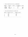


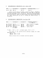


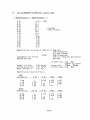

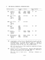


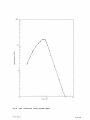

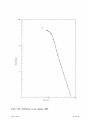
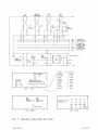


![the file [< 1 MB]](http://vs1.manualzilla.com/store/data/005663565_1-91d1e4bcdfd7b45b626a6b88ab809728-150x150.png)