Download 0.4.0 PDF - Read the Docs

Dyna Documentation
Release 0.4 git=fb40b6a
Jason Eisner, Nathaniel Wesley Filardo, Tim Vieira, et al.
September 17, 2013
CONTENTS
i
ii
Dyna Documentation, Release 0.4 git=fb40b6a
Dyna is an new declarative programming language developed at Johns Hopkins University.
This site documents the new version being developed at http://github.com/nwf/dyna. The new version has been used
to teach but is not yet complete or efficient; you may file issues at http://github.com/nwf/dyna/issues. An older design
with a fairly efficient compiler can be found at http://dyna.org.
Warning: Please be advised that this documentation, the implementation, and indeed the language itself are
rapidly changing.
Warning: Some programs may not terminate. Control-C will interrupt the program’s execution.
Contents:
CONTENTS
1
Dyna Documentation, Release 0.4 git=fb40b6a
2
CONTENTS
CHAPTER
ONE
TUTORIAL
Warning: This tutorial is incomplete.
1.1 Hello World
Welcome to the Dyna tutorial!
It is traditional to start by writing and running a program that prints hello world. Downlad Dyna and follow the
instructions in README.md to build it. Then, look at the file examples/helloworld.dyna (or here). It should
contain:
goal += hello*world.
hello := 6.
world := 7.
% an inference rule for deriving values
% some initial values
This does not print hello world. It was the closest we could come. Dyna is a pure language. It focuses on computation,
and sniffs haughtily at mundane concerns like input and output.
1.1.1 Running Hello World
After building Dyna, you may ask our interpreter to run helloworld by executing
./dyna examples/helloworld.dyna
At this point, you should see:
Charts
============
goal/0
=================
goal
:= 42
hello/0
=================
hello
:= 6
world/0
=================
world
:= 7
3
Dyna Documentation, Release 0.4 git=fb40b6a
What has happened? Dyna has compiled and executed the program requested and printed out its conclusions. Notably,
the item goal is seen to have value 42. Whenever the runtime prints all of its conclusions, they are organized by
functor
1.1.2 The Interactive Interpreter
Dyna also comes with an interactive interpreter. This mode allows you to
• append new rules to the program and observe the consequences
• make custom queries of the conclusions
• visualize the information flow within the program
To run a program interactively, add -i to the dyna command line:
./dyna -i examples/helloworld.dyna
In addition to the chart printout above, you will be greeted with the interpreter’s prompt, :-. Interactive help is
available by typing help at the prompt.
Let’s try adding a new rule to the program. Suppose that our goal is not merely to multiply hello by world but to
additionally square hello. At the prompt, type:
goal += hello**2.
The interpreter will respond with:
goal := 78
Here you can see that goal‘s value has changed to be 78. But wait, is that right? We can check by typing at the
prompt:
query hello**2
bug
The output for the query is not especially friendly. There’s a bug filed about that and it’s being worked on.
If we modify one of the inputs hello or world, by typing:
hello += 1.
The interpreter will respond with:
goal := 120
hello := 8
out(3) := [(64, {})]
So not only is it telling us that hello has changed, and that goal now takes on a new value as a result, but it reminds
us that the query we ran earlier also has a new value.
At this point, we invite you to continue the tutorial by finding the shortest path.
1.2 Shortest Path in a Graph
We hope that Dyna offers the shortest ever shortest path program:
4
Chapter 1. Tutorial
Dyna Documentation, Release 0.4 git=fb40b6a
path(start) min= 0.
path(B) min= path(A) + edge(A,B).
goal min= path(end).
This program already highlights one of the features of Dyna: the first rule and last rules are dynamic: the value of the
start item determines which vertex in the graph is used as the start, and similarly the value of end is used to select
which vertex matters to goal.
This program is available in examples/dijkstra.dyna (or here).
1.2.1 Encoding the Input
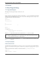
The following input graph is adapted from Goodrich & Tamassia’s data structures textbook. It shows several available
flights between U.S. airports, with their distances in miles. We would like to get from a friend’s house, 10 miles from
Boston (BOS), to our destination, 20 miles from Chicago (ORD).
2582
187
FriendHouse
10
BOS
SFO
802
1391
JFK
1090
1258
1121
MIA
802
DFW
1235
2342
ORD
20
MyHouse
1749
LAX
Shortest Paths
If we work things out
“FriendHouse” is
Destination
FriendHouse
BOS
JFK
MIA
DFW
ORD
MyHouse
SFO
LAX
by hand (or just ask Dyna) we will discover that the shortest path to each node from
Total
0
10
197
1268
1588
2390
2410
2779
2823
This is encoded into Dyna, using strings to identify vertices of the graph, thus:
edge("BOS","JFK")
edge("BOS","MIA")
edge("JFK","DFW")
edge("JFK","SFO")
edge("JFK","MIA")
edge("MIA","DFW")
edge("MIA","LAX")
edge("DFW","ORD")
edge("DFW","LAX")
edge("ORD","DFW")
edge("LAX","ORD")
:=
:=
:=
:=
:=
:=
:=
:=
:=
:=
:=
187.
1258.
1391.
2582.
1090.
1121.
2342.
802.
1235.
802.
1749.
1.2. Shortest Path in a Graph
5
Dyna Documentation, Release 0.4 git=fb40b6a
edge("FriendHouse","BOS") := 10.
edge("ORD","MyHouse") := 20.
edge pairs that are not specified are said to be null; that is, they have no value, and can be thought of as the identity
of the aggregator min=, or +∞, meaning “You can’t get there directly from here.”
And of course, we need to specify whence we come and where it is we would like to end up:
start := "FriendHouse".
end
:= "MyHouse".
1.2.2 Run the program
We can run this program in the interpreter:
./dyna -i examples/dijkstra.dyna
We are met with the conclusions, which include all the data we fed in as well as a pile of path assertions. Of course,
that’s not so useful, necessarily, so let’s just ask for the answer:
:- query goal
out(0) := [(2410, {})]
As we can see, the total weight of the shortest path is 2410. What happens, though, if we realize that we will be by
the airport anyway?
:- start := "BOS".
=============
goal := 2400
out(0) := [(2400, {})]
path(’BOS’) := 0
path(’DFW’) := 1578
path(’FriendHouse’) := None
path(’JFK’) := 187
path(’LAX’) := 2813
path(’MIA’) := 1258
path(’MyHouse’) := 2400
path(’ORD’) := 2380
path(’SFO’) := 2769
start := ’BOS’
And just like that, the total path weight from start to end is now 2400. The system also tells us a number of
potentially interesting things:
• The system has in fact computed the revised path costs to each other vertex.
• There is no path from "BOS" to "FriendHouse" (thus None).
• A query we had made earlier has changed its answer.
1.2.3 Explaining Answers
bug
We do not yet have a good mechanism implemented, though it’s just a matter of time. See issue 1.
6
Chapter 1. Tutorial
Dyna Documentation, Release 0.4 git=fb40b6a
1.2.4 Understanding The Program
Simply stated, this program looks for all paths from the vertex indicated by start. Formally, the technique currently
used is called agenda-driven semi-naive forward chaining 1 .
Inference Rules
The first inference rule states that there is no distance on the degenerate path that does not go anywhere.:
path(start) min= 0.
Alternatively, there is a path to vertex B if there is a path to some vertex A such that an edge connects A to B.:
path(B) min= path(A) + edge(A,B).
The final rule merely says that we are looking for the best path to the vertex indicated by end.:
goal min= path(end).
Inference Rules As Equations
But what are the min= and + doing? In fact, the inference rules are equations. They state how to find the values of all
pathto and goal items.
Those items have values just like the hello, world and goal items in the previous example. But this program is
more complicated. It involves lots of different pathto items for different airports, distinguished from one another by
their arguments: pathto("JFK"), pathto("MyHouse"), etc. These items may all have different values.
Why These Particular Equations?
Assuming that each edge‘s value represents its length in the input graph, the rules are carefully written so that
pathto(V)‘s value will be the total length of the shortest path from the start vertex to vertex V.
In principle, there are several ways to get to V: one can get there by an edge from start or an edge from some other
U. The min= operator finds the minimum over all these possibilities. Think of it as keeping a running minimum (just
as += would keep a running total). In particular, pathto(V) is found as min(edge(start, V ), minU pathto(U ) +
edge(U, V )) which involves minimizing over all possible U.
If there are no paths to V, then pathto(V) is a minimum over no lengths at all. Dyna specifies that items receiving
no inputs take on the special value null, which is the identity of every aggregator and a zero of every expression. Since
we aggregate answers with min=, null approximates +∞.
1.2.5 Deriving The Graph From Rules
There’s nothing that mandates that edge weights be the base case; we could also derive edge facts from other facts,
such as position and reachability. An example is available in examples/dijkstra-euclid.dyna (or here).
1 There are a multitude of inference algorithms for logic programming. We would like to think that [filardo-eisner-2012] provides a good
overview as well as explaining the basics of what will become Dyna 2’s inference algorithm.
1.2. Shortest Path in a Graph
7
Dyna Documentation, Release 0.4 git=fb40b6a
1.2.6 Endnotes
1.3 When Things Go Wrong
1.3.1 Impossible Requests
What happens if a Dyna program attempts to divide by zero, as in:
a += 1 / b.
b += 0.
If this is the entirety of the program and no changes are forthcoming (e.g., we are not in interactive mode) then the
semantics of this program include division by zero, and so must be an error. What happens when we attempt to run it?
Our interpreter produces a chart with an annotation:
Charts
============
a/0
=================
b/0
=================
b
:= 0
Errors
============
because b is 0:
division by zero
in rule test.dyna:4:1-test.dyna:4:12
a += 1 / b.
This last Errors display indicates that the answers available in the Charts section is not reliable.
Caution: Any error is potentially global! While it might be possible for some programs to more accurately track
errors, currently our implementation does not. The net effect of this is that if ever the interpreter produces an
Errors section, then the entire chart must be considered suspect.
If we run the interactive interpreter and add the rule b += 1., the error condition has cleared as it should. If we then
add b += -1., it will return.
1.3.2 Non-Termination
Productive Nontermination
As mentioned before, Dyna2 currently uses agenda-driven semi-naive forward chaining for its reasoning. This algorithm has several excellent theoretical properties, but suffers from a potentially show-stopping problem: it might not
stop.
A Dyna program which includes a definition of the Fibonacci numbers (e.g., examples/fib.dyna)
fib(1) += 1.
fib(2) += 1.
fib(X) += fib(X-1) + fib(X-2).
8
Chapter 1. Tutorial
Dyna Documentation, Release 0.4 git=fb40b6a
will compile and be accepted by the interpreter, but will attempt to prove a fib item for every positive natural number!
Clearly, this task is going to take a while.
If your program does go away for longer than you expect, it is entirely possible that it is caught in such an infinite
loop. In that case, you may send it a SIGINT by hitting Control-C. The interpreter will then print out the chart as far
as it had determined it. If this is far bigger than expected, your program probably has a productive infinite loop.
Fixing The Fib Example
One way out of this problem is to impose a limit on the program, by writing instead something like:
f(X) += f(X-1) + f(X-2) for X < lim.
lim := 10.
This will limit the system to proving the first lim Fibonacci numbers. Of course, that can expand or contract as you
define lim.
Counting To Infinity
Unfortunately, another kind of nontermination error can arise in cyclic programs, which is not so easy to fix: the
so-called count-to-infinity problem.
If we were to have examples/dijkstra.dyna loaded in the interpreter and then run
:- start := "NoSuch".
Where there is no such "NoSuch vertex, the interpreter will appear to be pondering this change to the universe for “a
while”, as we say. If we interrupt it (with Control-C) after a while, the chart will contain, among other things:
path/1
=================
path("DFW")
path("LAX")
path("MyHouse")
path("NoSuch")
path("ORD")
path("SFO")
:=
:=
:=
:=
:=
:=
10124432
10124063
10122046
0
10123630
2779
This arises from the fact that our graph contains a cycle:
edge("DFW","ORD") := 802.
edge("ORD","DFW") := 802.
edge("LAX","ORD") := 1749.
Note that it is also possible to “count to infinity” in other directions, such as by counting down to −∞ or by approaching a finite solution but as in Zeno’s paradox.
bug
There is, as of yet, no good solution to this problem; the best work-around might just be to start the program over.
1.3. When Things Go Wrong
9
Dyna Documentation, Release 0.4 git=fb40b6a
10
Chapter 1. Tutorial
CHAPTER
TWO
USER MANUAL
2.1 Pragmas
Pragmas are used to pass a wide variety of information in to the system. They are visually separated by begining with
:-.
2.1.1 Syntax
Some pragmas alter the syntax of the language.
Disposition
In Dyna source code, there are two different things that the term f(1,2) could mean:
• Construct the piece of data whose functor is f and has arguments 1 and 2, as in f(A,B) = f(1,2), which
unifies A with 1 and B with 2.
• Compute the value of the f(1,2) item, as in f(1,2) + 3 or Y is f(1,2).
It is always possible to explicitly specify which meaning to use, by use of the & and * operators (see syntax-quote-eval),
but this would be tedious if it were the only solution. As such, we endow functors (of given arity) with dispositions,
which indicate, by default, how they would like to treat their arguments.
Dispositions are specified with the :-dispos pragma, thus:
:-dispos g(&).
:-dispos ’+’(*,*).
% g quotes its argument.
% + evaluates both arguments.
Now g(f(1,2)) + 1 will pass the structure f(1,2) to the g function and add 1 to the result. Note that dispositions take effect while the program is being parsed. That is, a program like:
:-dispos f(&).
goal += f(g(1)).
:-dispos f(*).
goal += f(g(2)).
specifies that goal has two antecedents: the f images of g(1) and the g image of 2.
It is also possible to indicate that some terms should not be evaluated:
:-dispos &pair(*,*).
% pair suppresses its own evaluation
11
Dyna Documentation, Release 0.4 git=fb40b6a
In the case of disagreements, like pair(1,2) + pair(3,4), the preference of the argument is honored.
Defaults
Absent any declarations, all functors are predisposed to evaluate their arguments. Some functors (pair/2, true/0,
and false/0) suppress their own evaluation.
More Detail
Warning: This section is probably relevant only if you are a developer of the Dyna compiler.
Requesting Evaluation Just like it is possible to request that some functors not be evaluated even when in evaluation
context, it is additionally possible for functors to request that they be evaluated even when the context is one of
quotation:
:-dispos *f(*).
The neutral position of specifying neither & nor * before a pragma is termed inherit, which means that the context or
overrides apply. Under the defaults above, this is the default position for all functors.
Disposition Defaults It is possible to override the defaults, as well; at least one of us has a stylistic preference for a
more Prolog-styled structure-centric view of the universe. The pragma:
:-dispos_def prologish.
will cause subsequent rules to behave as if all functors which start with an alphanumeric character had had :-dispos
f(&,...,&) asserted, while all other functors had had :-dispos *f(*,...,*). There are, however, a few
built-in overrides to this rule of thumb, giving alphabetic mathematical operators (e.g. abs, exp, ...) their functional
meaning. See src/Dyna/Term/SurfaceSyntax.hs
The default default rules may be brought back in by either:
:-dispos_def dyna.
:-dispos_def.
Note that when chaning defaults, any manually-speficied :-dispos pragmas remain in effect.
Operators
Dyna aims to have a rather flexible surface syntax; part of that goal is achieved by allowing the user to specify their
own operators.
As with Disposition, these pragmas take effect while the program is being parsed.
bug
The ability to add and remove operators is not yet actually supported.
12
Chapter 2. User Manual
Dyna Documentation, Release 0.4 git=fb40b6a
Adding an operator
The :-oper add pragma takes three arguments: the fixity, priority, and lexeme that makes up the operator. Fixities
are specified as pre, post or in. In the case of in, one of left, right, or non must be specified for the
associativity. Priorities are natural numbers, with higher numbers binding tighter. Lexemes are either bare words or
singly-quoted functors.
Examples:
:-oper add in left 6 + .
:-oper add pre 9 - .
Removing an operator
The :-oper del pragma may be used to remove all previously added forms of a given operator.
Defaults
The default operator table is, hopefully, more or less what you might expect and follows the usual rules of arithmetic.
bug
For the moment, the source is the spec. See the source in src/Dyna/Term/SurfaceSyntax.hs for full details.
2.1.2 Execution
On the other hand, some pragmas impact the execution of the system.
Insts and Modes
Following the [MercuryLang] syntax, we allow the user to give names to instantiation states and modes:
:-inst name(args) == ... .
:-inst mode(args) == ... >> ... .
Query Modes
A Query mode specifies that a particular backward-chaining operation is to be available to the system. These capture
the change in instantiation state, determinism, and other properties of a query.
2.2 Builtins
2.2.1 Aggregators
For aggregation, we offer
P
Q
• Numerics: max=, min=, += ( ), *= ( )
V
W
• Logic: &= ( ), |= ( ).
2.2. Builtins
13
Dyna Documentation, Release 0.4 git=fb40b6a
• A last-one-wins operation, :=. Formally, the last rule which contributes a value determines the head item’s
value. That is, a program such as
a := 1.
a := 2 for d.
will give a the value of 1 if d is not provable or is not true and 2 otherwise.
2.2.2 Functions
The following list of functions are guaranteed to be present, regardless of backend chosen:
• The usual binary numeric operations: *, -, *, /, mod (or %), and ** (for raising to a power).
• Some unary numeric operations: -, abs, log, and exp.
• Comparison operators: <, <=, ==, >=, >, and != (disequality).
• Logic operations: and (or &), or (or |), ^ (for exclusive or), and not (or !).
• Unification is written =. Prolog’s is operator is also available.
Warning: The distinction between = and == is that the latter evaluates both of its arguments while the former
does not. Meanwhile, is is asymmetric, evaluating its right argument and not its left.
See examples/equalities.dyna (or here).
2.2.3 Constants
Integers, floats, and double-quoted strings all exist as primtives in the language. Booleans are represented by the atoms
true and false.
14
Chapter 2. User Manual
15
Dyna Documentation, Release 0.4 git=fb40b6a
CHAPTER
THREE
SPECIFICATION OF THE DYNA
LANGUAGE
3.1 Introduction
3.1.1 What is Dyna?
3.1.2 Intended users
3.1.3 Key features
3.1.4 Relation to other work
3.2 How to read this specification
3.2.1 Organization
3.2.2 Notation
3.2.3 User comments
3.2.4 Coloring and formatting conventions
3.2.5 Cross-refs
3.2.6 Sidebars
3.2.7 Notifications
3.2.8 Links to examples
3.2.9 Links to issue tracker
3.2.10 Glossary/Index
3.3 Terms (i.e., ground terms)
16
3.3.1 Overview
3.3.2 Primitive terms
Chapter 3. Specification of the Dyna Language
Dyna Documentation, Release 0.4 git=fb40b6a
3.3.5 Frozen terms
Full discussion in Dynabases.
3.4 Patterns (i.e., non-ground terms)
3.4.1 Variables
Variable names
Underscores
3.4.2 Non-ground terms
3.4.3 Types
Type declarations
Typed variables
Co-inductive types
Possible future extensions
Guarded types? Nonlinear types? Parametric types?
3.4. Patterns (i.e., non-ground terms)
17
Dyna Documentation, Release 0.4 git=fb40b6a
3.4.4 Type coercion
3.4.5 Unification
3.4.6 Frozen terms
3.5 Dynabases
3.5.1 Overview
3.5.2 Items
Null items
3.5.3 Syntax for items
Brackets vs. parentheses
Quoting items with &
Evaluating terms with *
3.5.4 Queries
Simple queries
Complex queries
Expressions
Aggregating queries
Accessors
3.5.5 Query modes
Some discussion of current approach is in Pragmas.
18
Chapter 3. Specification of the Dyna Language
Dyna Documentation, Release 0.4 git=fb40b6a
3.5.6 Lambdas
3.5.7 Terms as dynabases
3.5.8 Updates
3.5.9 Update modes
3.5.10 Stability
3.5.11 Dynabase types
3.5.12 Extensions
Const declaration
3.5.13 Snapshots
3.6 Inspecting and modifying dynabases
3.6.1 Abstract API
3.6.2 Command line interface
3.6.3 Graphical interface
3.6.4 Programming interface
3.7 Dyna programs
3.7.1 Programs
3.7.2 File format
3.7.3 Rules
Definition
Aggregation
Semantics
Cycles
Errors
See discussion of current implementation in When Things Go Wrong.
3.6. Inspecting and modifying dynabases
19
Dyna Documentation, Release 0.4 git=fb40b6a
Head destructuring
3.7.4 Dynabase literals
Syntax
Ownership
Semantics
3.7.5 Declarations
Some documentation of currently implemented declarations is in Pragmas.
Type declarations
Evaluation declarations
There is currently some documentation in syntax.
20
Chapter 3. Specification of the Dyna Language
Dyna Documentation, Release 0.4 git=fb40b6a
Default arguments
Visibility declarations
Const
Import
Syntax declarations
Declaring new aggregators
3.7.6 Scripting commands
3.7.7 Include
3.7.8 Foreign function interface
3.8 Concrete syntax
3.8.1 Overview
3.8.2 Standard syntactic sugar
3.8.3 Default syntax table
3.8.4 Changing the syntax table
3.8.5 Printing
Readable printing
Prettyprinting
3.9 Standard library
There is currently some documentation in Builtins.
3.8. Concrete syntax
21
Dyna Documentation, Release 0.4 git=fb40b6a
22
Chapter 3. Specification of the Dyna Language
Dyna Documentation, Release 0.4 git=fb40b6a
3.9.1 Generic operators and aggregators
3.9.2 Boolean operators and aggregators
3.9.3 Numeric operators and aggregators
3.9.4 Randomness
3.9.5 String operators and aggregators
3.9.6 Array operators and aggregators
3.9.7 Set operators and aggregators
3.9.8 Graph operators and aggregators
3.9.9 Other standard encodings
3.10 Inspecting program execution
3.10.1 $rule
3.10.2 Voodoo items
3.10.3 Reflection on types, modes, cost estimates, cardinality estimates, plans, etc.
3.11 Controlling program execution
3.11.1 Storage classes
3.11.2 Priorities
3.11.3 Query costs and plans
3.11.4 Features for learning
3.12 Foreign dynabases
3.12.1 Files
3.12.2 Processes
3.12.3 Sockets
3.12.4 Servers
3.13 Appendices
3.10.
program execution
3.13.1Inspecting
Dyna Glossary
functor The constructor of a term, such as path in path(1,2).
23
Dyna Documentation, Release 0.4 git=fb40b6a
null The value of items that have no rules contributing
aggregands. Null
P
P annihilates expressions (e.g. null + 2 is
null) and is the unit of aggregations (e.g. {null, 1, null, 2} is just {1, 2}).
24
Chapter 3. Specification of the Dyna Language
CHAPTER
FOUR
BIBLIOGRAPHY
25
Dyna Documentation, Release 0.4 git=fb40b6a
26
Chapter 4. Bibliography
CHAPTER
FIVE
INDICES AND TABLES
• Dyna Glossary
• genindex
• search
27
Dyna Documentation, Release 0.4 git=fb40b6a
28
Chapter 5. Indices and tables
BIBLIOGRAPHY
[filardo-eisner-2012] Nathaniel W. Filardo and Jason Eisner. A flexible solver for finite arithmetic circuits. ICLP
LIPIcs, 2012. http://cs.jhu.edu/~jason/papers/#filardo-eisner-2012-iclp
[eisner-filardo-2011] Jason Eisner and Nathaniel W. Filardo. Dyna: Extending Datalog for modern AI. Datalog
Reloaded, 2011. http://cs.jhu.edu/~jason/papers/#eisner-filardo-2011
[goodrich-tamassia] Michael T. Goodrich and Roberto Tamassia. Data Structures and Algorithms in Java. ISBN 9780470383261. 2010.
[MercuryLang] http://www.mercurylang.org
29