Download MOSQUITO 1.6 User Manual

MOSQUITO 1.6
User Manual
SEAlab - Software Quality Group
Dipartimento di Informatica
Università dell’Aquila
October 2008
1
1
MOSQUITO VERSIONING
4
2
GETTING STARTED
5
2.1
Installation Requirements
5
2.2
Getting Eclipse with Eclipse UML
5
2.3
Installing MOSQUITO
6
3
MOSQUITO AND THE SUPPORTED MODEL-BASED METHODOLOGIES
7
3.1
The SAP·One methodology
7
3.2
The PRIMA-UML methodology
8
4
MOSQUITO IMPLEMENTATION TECHNOLOGIES
5
MOSQUITO AT WORK
5.1
eCommerce System Specification
9
11
11
5.2
Use Case Diagram
5.2.1
Sap·One annotations
5.2.2
PRIMA-UML annotations
12
13
13
5.3
Component Diagram
5.3.1
Sap·One annotations
5.3.2
PRIMA-UML annotations
14
15
15
5.4
Sequence Diagram
5.4.1
Sap·One annotations
5.4.2
PRIMA-UML annotations
16
18
18
5.5
Deployment Diagram
5.5.1
Sap•One annotations
5.5.2
PRIMA-UML annotations
19
20
20
5.6
Generating Analysis Models
5.6.1
Sap•One QNM
5.6.2
PRIMA UML Meta EG
5.6.3
PRIMA UML EQNM
5.6.4
PRIMA UML EG instance
5.6.5
PRIMA UML parameterized EQNM
5.6.6
Analysis of Performance Model
23
23
25
25
26
28
29
6
REFERENCES
29
7
APPENDIX
30
7.1
Queuing Network process creation (SAP·One methodology)
30
7.2
Execution Graph creation (PRIMA-UML methodology)
31
2
List of Figures
Figure 1: Mosquito versioning.............................................................................................................4
Figure 2 Eclipse refresh procedure ......................................................................................................6
Figure 3: The performance analysis model generation carried out by Mosquito. ...............................7
Figure 4: Mosquito client-server architecture......................................................................................9
Figure 5. Invoking Mosquito transformations from Eclipse Platform...............................................10
Figure 6: Mosquito output models are displayed as xml-based files.................................................10
Figure 7: Overview of the eCommerce System .................................................................................11
Figure 8: UCD of the eCommerce System with the operational profile............................................12
Figure 9: Component Diagram ..........................................................................................................14
Figure 10: the Sequence Diagram......................................................................................................17
Figure 11: The artifacts that manifest each component .....................................................................19
Figure 12: Deployment Diagram .......................................................................................................20
Figure 13: Annotated Deployment Diagram for the PRIMA-UML methodology. ...........................21
Figure 14: Analysis Models generation steps. ...................................................................................23
Figure 15: Generically annotated UCD .............................................................................................31
List of Tables
Table 1: PRIMA-UML Stereotypes used on UCD. ...........................................................................13
Table 2: Sap•One Stereotypes used on CD........................................................................................15
Table 3: Sap•One Stereotypes used on SD. .......................................................................................18
Table 4: PRIMA-UML Stereotypes used on SD. ..............................................................................18
Table 5: PRIMA-UML Stereotypes used on DD...............................................................................22
3
1 Mosquito versioning
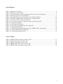
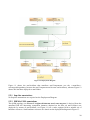
The MOSQUITO evolution across the different releases is shown in Figure 1.
INPUT
Omondo XMI
Export
compatible
Eclipse UML2 V1
Compatible
PLASTIC enabled
Eclipse UML2 V2
compatible
UML2
v 1.0
Standalone version
v 1.1
Distributed RMI version
v 1.2
Distributed SOAP version
v 1.3
v 1.4
v 1.5
v 1.6
SAP•One
Distributed SOAP version
Distributed SOAP version
Distributed SOAP, zipped stream version
Distributed SOAP, zipped stream version
QNM (.PMIF’)
PRIMA-UML
OUTPUT
metaEG (.SPMIF)
EQNM (.PMIF)
EQNM (.PMIF) instanceEG (.SPMIF)
parameterizedEQNM (.PMIF)
Figure 1: Mosquito versioning.
The MOSQUITO 1.6 release provides new features that have been added to the previous version.
Now MOSQUITO 1.6 fully support the SAP·One and PRIMA-UML methodologies: it is now able
to build all the analysis models required by these methodologies:
SAP·ONE: Queuing Network Model (QNM);
PRIMA-UML: Extended Queuing Network Model (EQNM);
PRIMA-UML: meta Execution Graph (metaEG);
PRIMA-UML: instance Execution Graph (instanceEG); (new)
PRIMA-UML: parameterized Extended Queuing Network (pEQNM); (new)
4
2 Getting Started
MOSQUITO (MOdel driven conStruction of QUeuIng neTwOrks ) is a tool developed in JAVA
language as plug-in for the Eclipse Platform. To use it you need to install a Java Virtual Machine
and the Eclipse Platform with a compatible Eclipse UML SDK.
2.1 Installation Requirements
Server Side
Operating System:
Web Application Container:
JDK version:
Independent
Apache Tomcat 6.0 with Axis2 1.4
1.5 or higher
Client Side
Eclipse:
Eclipse EMF SDK:
Eclipse UML2 SDK:
JDK version:
3.2 or higher
2.2.x
2.x
1.5 or higher
2.2 Getting Eclipse with Eclipse UML
The main Web site for Eclipse is www.eclipse.org. On that page, you can see the latest Eclipse
news and links to a variety of online resources, including articles, newsgroups, bug tracking, and
mailing lists.
The latest version of Eclipse can be downloaded from the main download page at
www.eclipse.org/downloads (if this site is unavailable, a number of mirror sites around the world
are available). Go ahead and download the latest release or stable build.
The download page for each release includes various notes concerning that release as well as links
to every platform version. Eclipse supports a large number of platforms, including Windows, Linux,
Solaris, HP, Mac OSX, and others. Choose the Eclipse SDK download link corresponding to your
platform and save the Eclipse zip file to your computer's hard drive. This will generally be a very
large file (>105 MB), so be patient unless you have sufficient bandwidth available to quickly
download the file.
Once the Eclipse zip file has been successfully downloaded, unzip it to your hard drive. Eclipse
does not modify the Windows registry, so it does not matter where it is installed.
MOSQUITO was developed with Eclipse 3.2 and subsequently tested with Eclipse 3.2 and higher
versions.
It is very important to download a version of Eclipse equipped with the EclipseUML SDK plug-in
to manage the UML models that represent the input to MOSQUITO. However, if you already have
an Eclipse installation without EclipseUML, you can update your platform with the update manager
selecting Help --> Software Updates --> Find and Install --> Search for New features to Install.
5
2.3 Installing MOSQUITO
You can download MOSQUITO client from the following web page
http://sealabTools.di.univaq.it/SeaLab/MosquitoDownload.html.
MOSQUITO is a plug-in for the Eclipse platform, and its installation (like every other Eclipse plugin) is very simple. It is sufficient to unzip the zip file di.univaq.MOSQUITO in the main folder of
Eclipse (e.g., c:/eclipse). After this step verify if the plug-in jar file appears in the plug-in directory
(e.g., c:/eclipse/plugins/di.univaq.MOSQUITO_x.x.x.jar). Take care to remove all the previous
versions of MOSQUITO.
Eclipse caches plug-ins information in a configuration directory. For this reason, the first launching
of Eclipse with the installed MOSQUITO plug-in must be performed using the –clean commandline option so that the cached plug-ins information will be rebuilt.
To do this you must use the prompt to launch Eclipse. If you are in the directory of Eclipse
installation them you must type the “Eclipse –clean” command as reported in Figure 2.
Figure 2 Eclipse refresh procedure
After started the Eclipse platform, you can verify the correct MOSQUITO installation by inspecting
the plug-in details under Help -> About Eclipse SDK -> Plug-in Detail. The MOSQUITO plug-in
must appear in the list of the currently installed plug-ins.
This step can be also performed once and for all by modifying the eclipse.ini configuration file by
adding the “-clean” option on the top of this file.
For example
-clean
-showsplash
org.eclipse.platform
…
6
3 MOSQUITO and the supported model-based methodologies
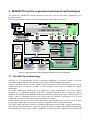
The shows the MOSQUITO model generation processes (Ax and Bx paths) illustrated in the
previous sections
The two methodologies will be briefly explained in the following two sections.
0
.UML
Eclipse UML2 Model
.UML
.EG
.UML
.EQNM
.EG .EQNM
.aEG
.aEG .EQNM
.pEQNM
B1
B2
B3
B4
UCD – CD – SD - DD
.UML
.PMIF’
MOSQUITO CLIENT
SOAP/TCP-IP
A1
MOSQUITO SERVER@AQ
(CD.SD)2QN
(UCD.SD.DD)2EG
A1
B1
QNM
Architectural
Performance
Model
(UCD.SD.DD)2EQNM
metaEG
Sw Perf.Model
.SPMIF
Annotate EG
.PMIF’
B3
instanceEG
Sw Perf.Model
WEASEL
PLATFORM
INDEPENDENT
INDICES
.TXT
…
EQNM
Platform
Performance
Model
.SPMIF
.PMIF
Mapping EGÆEQNM
QN EDITOR
QN Solver 1 QN Solver 2
B2
QN Solver N
PLATFORM
SPECIFIC
INDICES
pEQNM
Parametrized
HW/SW Performance Model
B4
.PMIF
.TXT
Figure 3: The performance analysis model generation carried out by Mosquito.
3.1 The SAP·One methodology
SAP·One [1] is a methodology for the performance modelling of a software system. It consists
essentially in the generation of a queuing network from an UML architectural model.
SAP·One has been conceived to be applied in the first phases of the software process to reveal
architectural flaws as soon as possible, so the developer will be able to modify the system
architecture.
The UML architectural model (step 0) is formed by a static and dynamic view of the system
provided by a Component Diagram (CD) and a Sequence Diagram (SD), respectively. These
diagrams are enriched with additional information about the system performance from the SPT [4]
profile, such as scheduling policies and service times of software components (on CD) and
workloads on interaction between component instances (on SD).
In this approach the service centers of the QNM don't represent hardware resources (such as disks
or processors) rather they represent the software components of the system architecture.
The UML model represents therefore a platform-independent model (PIM), and the performance
indices that can be obtained are “somehow” parametric. This is because the assumption underlying
the methodology is that every software component will be placed on a logical device, and that all
7
the devices will have the same “speed” but they can manage requests through queues of different
capacity and different scheduling policy
In practice, the SAP·One analysis is comparative, in that the obtained performance values are useful
to reveal bad architectural choices, but they are of little value as absolute performance indices.
3.2 The PRIMA-UML methodology
PRIMA-UML [3] is a methodology for the performance modelling of a hw/sw model: starting from
properly annotated UML2 diagrams, generates a sw/hw performance model. PRIMA-UML is based
on the Software Performance Engineering (SPE) methodology.
The UML software/hardware model contains two viewpoints: the static view shows which
components instances are executed on which hardware hosts (DD) while the dynamic view define
the operational profile (i.e. frequencies of use of the system functionalities by the users, depicted on
the UCD) and the interactions (i.e. invocation messages) between software components (SD). From
a source UML sw/hw model in these settings, two different kind of performance models (defined in
SPE) are obtained:
(i)
a software performance model represented as Execution Graph (EG): a graph of
processing steps (i.e operation invocations) that perform a function of the software
system and where arcs represent the order of execution (very similar to UML Activity
Diagram). PRIMA-UML splits the EG generation in two phases:
a) first, a metaEG is generated representing a generic topology (just node and arcs)
b) then an instanceEG is generated on the base of the metaEG that contains a matrix of
values (overhead matrix) representing the software resource (i.e. n# of CPU
instructions or number of messages exchanged or n# of database accesses) required
by each processing steps and how these software resource requirements are
translated in terms of hardware resource requirements.
Different execution paths with different execution probabilities are determined by he
operational profile on the UCD and by the message exchanged by component instances
on the SD.
(ii)
a platform performance model represented as an Extended Queuing Network Model
(EQNM). It shows which are the execution environment of each components in terms of
available hardware resource (CPUs and DISKs) and possible DELAYs due to different
configurations (e.g. interactions between components deployed on different networked
nodes are “delayed”). PRIMA-UML splits the EQNM generation in two phases:
a) first, a EQNM is generated representing a generic topology with featured service
centers (e.g. with scheduling policies) of different type (CPU, DISK or DELAY) and
arcs connecting them;
b) a parameterized EQNM resulting from the merging of an already existing instance
EG (i.b) and EQNM (ii.a). The merging of the instance EG and the EQNM models
ends the model analysis generation phase.
This type of system analysis is better suited when the developers have already some ideas on the
potential target platforms because EQNM service centers, in PRIMA-UML, represent hw resources.
8
4 MOSQUITO implementation technologies
MOSQUITO is a client/server application. The plug-in di.univaq.MOSQUITO implements the
client side that provides the functionality to invoke the operations (i.e. model2model
transformations) exposed by the MOSQUITO Web Service installed on a server running at
University of L’Aquila.
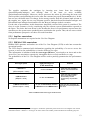
The system architecture is shown in Figure 4.
Web Services
.UML
.PMIF’
UML2QN
.UML
.EG
UML2EG
.UML
.EQNM
.EG .EQNM
.aEG
.aEG .EQNM
.pEQNM
UML2EQNM
AnnotateEG
Merge aEG-EQNM
SOAP/TCP-IP
Mosquito Client
(Eclipse plug-in)
Mosquito Server
@ Univ.AQ
Figure 4: Mosquito client-server architecture.
In particular MOSQUITO is exposed as a Web Service: This will allow any user to implement an
alternative client, using the preferred languages and technologies, to use the services of
MOSQUITO server placed at di.univaq.it domain.
The MOSQUITO client that we provide is an Eclipse plug-in that allows an entirely automated
process. The user must only properly create and annotate UML models according to the selected
methodology (i.e SAP·One or PRIMA-UML).
The extension point used for the MOSQUITO interface is the Eclipse popup menu. After the
creation of a model the user must only select the correct source models (see Figure 3 ) and activate
the desired transformation, as shown in the following Figure 5.
9
Figure 5. Invoking Mosquito transformations from Eclipse Platform.
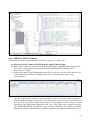
The result of the transformation will be showed in the Eclipse XML editor as follows: eventually, a
WARNING or ERROR tabs will be displayed containing the warnings or errors about input model,
respectively (Figure 6).
Figure 6: Mosquito output models are displayed as xml-based files.
10
5 MOSQUITO at work
In this section we explain how to introduce the SAP·One and PRIMA-UML annotations in the
Eclipse UML models1. The presentation is driven by the eCommerce System example.
5.1 eCommerce System Specification
In the electronic commerce system, there is a supplier that publishes his catalogue on the web. The
catalogue can be visioned by registered and unregistered users. Registered users become customers
for the supplier. The supplier accepts customer orders and delivers the ordered items maintaining all
the relevant data. He needs to maintain information on data, on the catalogue and on the orders
purchased by his customers. Each registered customer has a cart where he/she can insert or delete
items. The customer can order only if the cart is not empty. The system also allows the customer to
monitor the order status and to confirm the delivery in order to permit the payment.
Figure 7: Overview of the eCommerce System
Figure 7 shows the system structure at a high level of details. In a first analysis, some databases
(Customer DB, Cart DB, Order DB,etc.) and four process type (CustomerProcess, SupplierProcess,
etc.) are identified. For each involved database, there is a server that permits to communicate with
it. The interactions with these servers are asynchronous. Each customer has associated a
(individual) CustomerProcess. If the customer is not registered, the process allows the browsing of
the catalogue only, whereas if he is a registered one, the process activates all the functionalities the
system provides him (cart managing, order placement, etc.). All the functionalities provided by the
system to the supplier, instead, are coded in the SupplierProcess. The DeliveryOrderProcess and
InvoiceProcess are processes that manage the activities to be executed to dispatch an order and to
produce the corresponding invoice. In the system one DeliveryOrderProcess instance and one
1
Generating an Eclipse UML2 model (.uml) as input to Mosquito implies a more detailed description using the terms
used by the OMG UML 2.1 Superstructure specification (e.g the names used for metaclasses and their tags) and by an
UML2 SPT profile (e.g. names used for stereotypes and their tags). That kind of detailed and precise should allow a
tighter mapping between the Import/Export API code and its textual description: Eclipse UML uses the official OMG
UML 2.1 Superstructure specification to define its own API.
11
Invoice Process instance are running, any time, for each order and for each invoice in process,
respectively.
For the sake of presentation, a simplified version of this system is considered. The focus is on a
subset of customer functionalities. In particular, only catalogue browsing, cart browsing, item
insertion and deletion to/from the cart, order placement functionalities will be considered.
5.2 Use Case Diagram
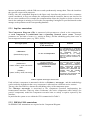
Figure 8 shows the use case diagram (UCD) for the e-commerce system. Three actors are in the
system: Customer, Supplier and Bank. The e-commerce customer can browse both the cart
(BrowseCart) and the catalogue (BrowseCatalog), she/he can insert and delete items to/from the cart
(InsertItem and DeleteItem, respectively). She/He can place an order and check its status
(PlaceOrder and BrowseOrderStatus), and finally she/he can confirm the delivery
(ConfirmDelivery) of the items ordered. The use case diagram also specifies that both InsertItem
and DeleteItem functionalities use the BrowseCart in their execution.
Figure 8: UCD of the eCommerce System with the operational profile.
12
The supplier maintains the catalogue by inserting new items from the catalogue
(InsertNewItemInCatalogue) and deleting from it the items no more available
(DeleteItemFromCatalogue). Moreover, she/he processes the orders by delivering the items sold
(DeliveryOrder) and producing the invoice after the customer has payed (Payment&Invoice). In this
last use case, the bank actor is in charge for the money transfer from the customer bank account to
the supplier one. Again, the use case diagram specifies that both InsertNewItemInCatalogue and
DeleteItemFromCatalogue functionalities use the BrowseCatalogue in their execution.
For the sake of presentation, in this document a simplified version of this system is considered. The
focus is on the customer view by considering only the software system functionalities reported on
the figure. The choice has been driven by the fact that the focus is on performance aspects hence the
customers are the system actors producing more workload to the system. Thus, the use cases critical
from performance perspective are those accessed from them.
5.2.1 Sap·One annotations
No Sap•One annotations are required on the Use Case Diagram.
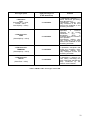
5.2.2 PRIMA-UML annotations
PRIMA-UML annotates and makes use of the Use Case Diagram (UCD) to take into account the
operational profile.
The UCD must be annotated with information regarding the probability of a user to access the
system, as well as the probabilities to invoke different use cases.
This information is introduced with the stereotype «REuser»2 associated to an Actor and on the
Actor-Use Case association, respectively, through the ReAccessProb and ReService tags.
The probabilities of the Use Case Diagram will be used to partially parameterize the performance
model.
Stereotype Syntax
Apply Stereotype on
(UML metaclasses)
Semantic
<<REuser>>
It denotes the probability
that an user accesses the
system
On the uml.Actor
{REaccessprob = value}
It denotes the probability
that a provided system
functionality can be
accessed by all possible
users.
<<REservice>>
On the uml.UseCase
{REprob = value}
<<REserviceUsage>>
{REserviceprob = value}
On the uml.Association between
<<REuser>> and <<REservice>>
It denotes the probability for
the user to invoke a particular
use case.
Table 1: PRIMA-UML Stereotypes used on UCD.
2
UML SPT profile doesn’t provide stereotypes to model the operational profile on the Use Case Diagram. We extend
UML SPT with the <<REuser>> stereotype. Its name comes from another profile introduced for reliability purposes.
13
5.3 Component Diagram
Figure 9: Component Diagram
In Figure 9 we present the UML 2.0 Component Diagram (CD) for the portion of the e-commerce
system we consider. This diagram highlights the software components and their required and
provided interfaces. The provided interfaces are represented by a circle whereas the required ones
are represented by a semicircle.
In general, an interface is composed by a set of operations provided or required by a software
component. Here, to simplify the presentation of the parameterization phase, we assume that an
uml.Interface represents uml.Operation of the uml.Component. Then each uml.Operation is
annotated, according to the UML SPT profile3, in order to introduce performance aspects of software
components. All the values for the execution times of the uml.Operation are assumed (see the assm
keyword in the tag value), as our intent is to carry on a performance analysis at the software
architecture level when such information is not available, whereas it can be guessed by the designers
on the basis of their experience or on the basis of previous releases of the same software system.
The considered (sub)system is composed by six components. Four of them (OrderServer,
CatalogServer, CartServer, CustomerServer) interact with the corresponding databases by easying
the insertion, deletion, reading and updating of data. These components allow asynchronous
communications, hence all the interfaces they provide contain asynchronous operations. The
remaining two components, namely CustomerProcess and DeliveryOrderProcess, provide the GUI
to interact with the system, the back end process that manages all her/his request (as made through
the GUI) and the business process to manage the order delivery, respectively. These components
3
Note that we extend the <<PAstep>> stereotype with the Operation metaclass in order to allow the annotation of the
component Operation.
14
interact asynchronously with the DB servers and synchronously among them. Thus the interfaces
they provide respect such properties.
Finally, since the component diagram in the figure only describes the portion of the e-commerce
system considered, it does not contains the components and the interfaces that are not involved in
the use cases considered. For example the component that allows the Supplier to delete or insert an
item in the catalogue is missing, as well as the corresponding CatalogServer provided interfaces that
manage such operations on the corresponding database.
5.3.1 Sap·One annotations
The Component Diagram (CD) is annotated with parameters related to the components,
as each component is transformed into a Queueing Network server center. Example
paramters are: the kind of center (i.e. waiting or delay), and the scheduling policy that it uses to
extract requests from its queue (e.g. FIFO, IS etc).
Stereotype Syntax
Apply Stereotype on
(UML metaclasses)
<<PAhost>>
On the uml.Component
{PAschdPolicy='type'}
Semantic
If a component is extended
with this stereotype its queue
has a type. If a component is
not
extended,
then
it
corresponds to a delay
resource without queue and
with an infinite number of
instances.
<<PAstep>>
{ PAdemand =
('assm','mean',( value,'unit time'))}
On the component
uml.Operation implementing
the homonymous provided
uml.Interface.
XOR
{ PAdelay =
('assm','mean',( value,'unit time'))}
The execution time to satisfy
each
services
request.
PAdemand must to be used for
active components whereas
PAdelay must be used for
passive ones. PAdemand and
PAdelay tags are mutually
exclusive
because
a
component can’t be active and
passive at the same time.
Table 2: Sap•One Stereotypes used on CD.
Each software component is annotated with the <<PAhost>> stereotype , and the methodology
works under the hypothesis that every component is allocated on a different active resource.
The tag value PAschdPolicy denotes the scheduling policy of the component queue.
The «PAstep» stereotype is associated to the component operation implementing the
homonymous interface: both tag values PAdemand (for active components) and PAdelay (for
passive components) model the component execution time to satisfy a request exposed by the
interface.
In particular the syntax to use within the CD is summarized in Table 2.
5.3.2 PRIMA-UML annotations
No PRIMA-UML annotations are required on the Component Diagram.
15
5.4 Sequence Diagram
Interaction diagrams are a common mechanism for describing systems, at varying levels of detail, in
a way comprehensible by both software designers and potential end users and stakeholders of the
system. Typically the interaction diagrams do not describe the whole system behavior but selected
execution traces. There are normally other legal and possible interactions that are not contained
within the drawn diagrams. Originally, interaction diagrams represent system objects and how
they interact. In the new conception (UML 2.0), such diagrams describe the system by means of
participants (that can be system modules at a different level of abstraction such as subsystem or
component instances, objects and so on) and how they interacts each other to accomplish a task. In
the UML terminology, interactions are units of behavior that focus on the observable exchange of
information between elements (such as objects) in form of messages. UML 2.0 defines four
different interaction diagrams: sequence diagram, communication diagram, interaction overview
diagram and timing diagram. Among these diagrams both Sap•One and PRIMAUML
methodologies use Sequence Diagrams: they specify messages that are exchanged between
component instances (whose types are depicted on Component Diagram) that are in charge to
provide the system functionalities (i.e. the use cases depicted on Use Case Diagram).
As example scenario the PlaceOrder sequence diagram is presented in Figure 10. The Sequence
Diagram is composed by several (nested) combined fragments and their operands. In particular, it
shows an example of two alternative behaviors specified by means of an alt operator with two
InteractionOperand. A Customer asks for an order placing through his own CustomerInterface
and, first of all, the CustomerProcess reads the cart status on the CartServer. If the cart is empty
the order cannot be placed (see the second interaction operand in the alt combined fragment).
Otherwise the CustomerProcess proceeds in collecting the customer information (such as for
example his mail address) and creates a new order in the Order DB. Finally it empties the customer
cart. In this scenario it is assumed that all the information the customer must provide to place an
order is collected before and the PlaceOrder request corresponds to the final submission from the
customer. Moreover, the payment procedure is encompassed in a different use case. For example, if
the customer decided to pay by a credit card, the Payment&Invoice use case (see Figure 8) will be
in charge to manage the bank transfer.
16
Figure 10: the Sequence Diagram
17
5.4.1 Sap·One annotations
The Sequence Diagram (SD) must be enriched with the information in the following table.
Stereotype Syntax
Apply Stereotype on
(UML metaclasses)
<<PAclosedLoad>>
{PApopulation=population
quantity,
PAextDelay=(‘assm', 'mean'
,(30,’ms’))}
On the first uml.Message of the
Sequence Diagram
<<PAstep>>
{PAprob = value}
On the first uml.Message used on
the two uml.InteractionOperand
(i.e. if and then operands)of the
Alt uml.CombinedFragment
Semantic
This stereotype denotes the
closed workload of the
scenario depicted on the
Sequence Diagram, in
particular its population and
the think time.
It denotes the probability to
activate the message in the
uml.CombinedFragment.
With probability 1-value the
control is given to the first
message following the alt
compartment.
Table 3: Sap•One Stereotypes used on SD.
The stereotype «PAclosedLoad» specifies the closed workload intensity and it is used to annotate
the first message of every Sequence Diagram, where the used tag values are: PApopulation (i.e.
number of user) and PAextDelay (i.e. required time to execute a request). Possible alternative
behaviors in the UML interaction fragments are annotated with the <<PAstep>> stereotype. The
PAprob tag value specifies the execution probability of each behavior.
5.4.2 PRIMA-UML annotations
The Sequence Diagram must be enriched with the information in the following table.
Stereotype Syntax
Apply Stereotype on
(UML metaclasses)
<<PAstep>>
{PAprob = value}
<<PAstep>>
{PArepetitionFactor =
value}
On the first uml.Message used on
the two uml.InteractionOperand
(i.e. if and then operands)of the
Alt uml.CombinedFragment
On the first uml.Message
exchanged in the Loop
uml.CombinedFragment
Semantic
It denotes the probability to
activate the message in the
uml.CombinedFragment.
With probability 1-value the
control is given to the first
message following the alt
compartment.
It denotes the number of the
iterations in the loop fragment.
Table 4: PRIMA-UML Stereotypes used on SD.
It is worth to note that the <<PAstep>> stereotype is applied on the first message of the Alt
uml.CombinedFragment in the same manner as the Sap•One methodology.
18
5.5 Deployment Diagram
A Deployment Diagram shows the configuration of run-time processing elements and the software
components that live on them. It is a graph where nodes (i.e., the processing elements, uml.Node)
are connected by communication path (i.e. uml.CommunicationPath). Nodes can contain artifacts
(uml.Artifact) that manifest components (see Figure 11). Therefore a DD shows the mapping of
components on processing elements (see Figure 12).
Figure 11: The artifacts that manifest each component
19
Figure 12: Deployment Diagram
Figure 11 shows the uml.Artifacts that manifests uml.Components (see the <<manifest>>
stereotyped dependency between the uml.Component and its own uml.Artifacts), whereas Figure 12
shows uml.Artifacts deployed on uml.Nodes.
5.5.1 Sap•One annotations
No Sap•One annotations are required on the Deployment Diagram.
5.5.2 PRIMA-UML annotations
The QNM topology (see Errore. L'origine riferimento non è stata trovata.) is derived from the
annotated DD: the interacting component instances depicted on the SDs (as uml.Lifelines) are
deployed (by means of uml.Artifacts, see Figure 11) on a node equipped with a suitable set of
hardware resources. Such hardware resources are shown on the deployment diagram in Figure 13.
20
Figure 13: Annotated Deployment Diagram for the PRIMA-UML methodology.
Hardware resources are distinguished in active and passive ones by means the <<PAhost>> and
<<PAresource>> stereotypes, respectively [3]. The PRIMA-UML methodology makes use of three
different kind of resources over a uml.Node:
• CPU, as the name itself suggests, is a (active <<PAhost>>) resource representing CPUs;
• DISK that represents a storage (passive4 <<PAresource>>) resource;
• TERMINAL5 that represents users/jobs that access the container node.
Table 5 specifies the additional information that has to be specified for such kind of resources.
4
A processing resource (i.e. PAhost) is a device which has processing steps allocated to it. A passive resource (i.e.
PAresource) represents a resource protected by an access mechanism (e.g., a semaphore), which is accessed during the
execution of an operation.
5
CPU, DISK and TERMINAL are reserved words.
21
Stereotype Syntax
<<PAhost>>
CPU
{PAschdPolicy = value,
PArate = value,
PAmultiplicity = value}
<<PAresource>>
DISK
Apply Stereotype on
(UML metaclasses)
On uml.Node.
A processing resource is a
device which has processing
steps allocated to it.
PAmultiplicity defines how
many instances of the CPU
resource are available on the
containing uml.Node.
On uml.Node.
A
passive
resource
represents
a
resource
protected by an access
mechanism
(e.g.,
a
semaphore),
which
is
accessed during the execution
of an operation.
PAmultiplicity defines how
many instances of the DISK
resource are available on the
containing uml.Node.
On uml.Node.
It represents users/jobs that
access the containing node.
PAmultiplicity defines how
many users/jobs access the
containing uml.Node.
On uml.Node.
It represents a network (i.e.
LAN, WAN) connecting two
Node. PAaxTime specifies the
delay introduced by the
network communication.
{PAmultiplicity = value}
<<PAresource>>
TERMINAL
{PAmultiplicity = value}
<<PAresource>>
DELAY
{PAaxTime = value}
Semantic
Table 5: PRIMA-UML Stereotypes used on DD.
22
5.6 Generating Analysis Models
0
.UML
Eclipse UML2 Model
B2
.aEG .EQNM
.pEQNM
B1
.EG .EQNM
.aEG
.UML
.EQNM
.UML
.PMIF’
MOSQUITO CLIENT
.UML
.EG
UCD – CD – SD - DD
B3
B4
SOAP/TCP-IP
A1
MOSQUITO SERVER@AQ
(CD.SD)2QN
(UCD.SD.DD)2EG
A1
B1
QNM
Architectural
Performance
Model
(UCD.SD.DD)2EQNM
metaEG
Sw Perf.Model
.SPMIF
Annotate EG
.PMIF’
B3
instanceEG
Sw Perf.Model
WEASEL
PLATFORM
INDEPENDENT
INDICES
.TXT
…
EQNM
Platform
Performance
Model
.SPMIF
.PMIF
Mapping EGÆEQNM
QN EDITOR
QN Solver 1 QN Solver 2
B2
QN Solver N
PLATFORM
SPECIFIC
INDICES
pEQNM
Parametrized
HW/SW Performance Model
B4
.PMIF
.TXT
Figure 14: Analysis Models generation steps.
This section shows how to generate all the analysis models (step Ax and Bx, see Figure 14):
1. Open your Eclipse Platform;
2. Create a Simple Project. You can also use the Empty EMF Project that is better organized.
3. You can organize your models as (i) EclipseUML2-compliant modeling tool format (e.g.
MagicDraw®) (ii) Eclipse UML model exported from the previous tool, (iii) Analysis
Models
5.6.1 Sap•One QNM
This section shows how to generate the QNM model (step A1, see Figure 14):
23
4. Select all the *.uml file within the EclipseUML folder;
5. Right click to show the contextual menu. Select MOSQUITO>Sap•One. You need a
working internet connection to invoke the MOSQUITO Web Service at University of
L’Aquila.
6. If the source model (*.uml) is correct you obtain the target analysis model, the QNM (a
valid PMIF’ xml model ).
7. You can visually check the QNM on the Eclipse XML Editor;
8. Save the QNM in Analysis Model.
24
5.6.2 PRIMA UML Meta EG
This section shows how to generate the QNM model (step B1, see Figure 14):
9. Select all the *.uml file within the EclipseUML folder;
10. Right click to show the contextual menu. Select MOSQUITO>PRIMAUML>create EG
Topology6. You need a working internet connection to invoke the MOSQUITO Web
Service at University of L’Aquila.
11. If the source model (*.uml) is correct you obtain the target analysis model, the meta EG (a
valid SPMIF xml model ).
12. You can visually check the meta EG on the Eclipse XML Editor;
13. Save the meta EG in Analysis Model.
5.6.3 PRIMA UML EQNM
This section shows how to generate the EQNM model (step B2, see Figure 14):
14. Select all the *.uml file within the EclipseUML folder;
15. Right click to show the contextual menu. Select MOSQUITO>PRIMAUML>create QN
Topology. You need a working internet connection to invoke the MOSQUITO Web Service
at University of L’Aquila.
16. If the source model (*.uml) is correct you obtain the target analysis model, the EQNM (a
valid PMIF xml model ).
17. You can visually check the EQNM on the Eclipse XML Editor;
18. Save the EQNM in Analysis Model.
6
A meta Execution Graph is also called EG Topology because it contains only a graph of node representing operation
invocations and arcs connecting them.
25
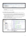
5.6.4 PRIMA UML EG instance
This section shows how to generate the EG instance (step B3, see Figure 14):
19. Select the meta EG and the EQNM from the Analysis Model folder;
20. Right click to show the contextual menu. Select MOSQUITO>PRIMAUML>Annotate EG.
You need a working internet connection to invoke the MOSQUITO Web Service at
University of L’Aquila.
21. If the source models (the EQNM and the meta EG) are correct a wizard will be shown to fill
in information about software and hardware resource consumption by means of an
overheadmatrix.
The rows represent the software resource available. You can or remove them pressing the
Add and Remove buttons, respectively. Once the software resources have been defined you
need to fill in the columns. Each column represent an hardware resource: they have been
specified on the Deployment Diagram (static view of the UML source model) using the
CPU DISK TERMINAL and DELAY “special” inner uml.Nodes. The number of columns
depends also by the “PAmultiplicity” attribute assigned to the aforementioned node. If you
26
specify “PAmultiplicity = 3” for the DISK node within a Server node you obtain
Server_DISK_x where x varies from 0 to 2 (as in the shown overhead matrix).
The cell value represent a “consumption link” between software and hardware resources:
(WorkUnit,Client_CPU_0) = 20 means that one workunit corresponds to 20 units of time at
hardware level.
On the second matrix here below, the user can check if the additional information
introduced on th UML Model have been suitably reported. The “ServiceTime” column
contains the “multiplier” for the cell value of overhead matrix.
Then (WorkUnit,Client_CPU_0) = 20 * (Client_CPU_0, ServiceTime) corresponds to the
amount (in terms of “time” ) of hardware resource required by one “WorkUnit” of software
resource.
22. Click the Next Button;
23. Fill in the Software Resource Demand Vector for each metaEG node that represents a
system operation invocation. Obviously you can “guess” some values and try different
solutions creating different EG instance model. You have to fill in all the fields.
27
24. Press the Next button and the resulting EG instance model will be displayed on the Eclipse
XML editor;
25. Save the EG instance in Analysis Model.
5.6.5 PRIMA UML parameterized EQNM
This section shows how to generate the parameterized EQNM model (step B4, see Figure 14):
26. Select the EQNM model obtained at step B2 and the EG instance obtained at step B3;
27. Right click to show the contextual menu. Select MOSQUITO>PRIMAUML>Merge
Annotated EG and QN. You need a working internet connection to invoke the MOSQUITO
Web Service at University of L’Aquila.
28. If the source models are correct you obtain the target analysis model, the parameterized
EQNM (a valid PMIF xml model ).
29. You can visually check the parameterized EQNM on the Eclipse XML Editor;
30. Save the parameterized EQNM in Analysis Model.
28
5.6.6 Analysis of Performance Model
The target performance models, Sap•One QNM and PRIMA-UML parameterized EQNM, can be
sent to any PMIF’ and PMIF compliant QN solver. In Figure 3 we report the
WEASELMOSQUITO. http://sealabtools.di.univaq.it/SeaLab/MosquitoHome.html.[6] tool we
are developing within the Department of Computer Science at University of L’Aquila.
6 References
[1] A. Di Marco, P. Inverardi “Compositional generation of Software Architecture
Performance QN Models”. Proc. 4th Working IEEE/IFIP Conference on Software
Architecture (WICSA’04), 2004.
[2] A.Di Marco. Model-based Performance Analysis of Software Architectures. PhD
thesis, '05.
[3] V. Cortellessa, R.Mirandola “PRIMA-UML: a Performance Validation Incremental
Methodology on Early UML Diagrams”, Science of Computer Programming , 44
(2002), no.1, pagg.101-129.
[4] OMG, UML Profile, for Schedulability, Performance, and Time, Version 1.1,
formal/05-01-02.
[5] C. Smith, L.G.Williams. Performance Solutions, Addison Wesley, 2002.
[6] MOSQUITO. http://sealabtools.di.univaq.it/SeaLab/MosquitoHome.html.
29
7 Appendix
In this appendix we report details of the methodology mechanisms.
7.1 Queuing Network process creation (SAP·One methodology)
The creation process of the queuing network through the SAP·One methodology can be summarized
in two steps:
•
Identification of the service centers and their carachteristics: A delay or waiting service
center is associated to every component of the Component Diagram. An offered service that
corresponds, in practice, to every interface of the component, indicates what job classes are
managed by each server.
Service center characteristics (e.g. time service, kind of center and scheduling policy) are
defined from the associated tag values.
•
Classes chain and workload definition: The Sequence Diagrams (with the annotated
information) represent the workload intensity, while the net topology is defined analysing
the dynamics of communication between components. The idea is to associate a connection
in the queuing network from each sender component (i.e. a component that sends a
30
messages in some Sequence Diagrams) to each receiving component. The receiving
component will have infinite queue if the interaction is asynchronous, whereas a null queue
if synchronous.
SAP·One defines a set of translation rules combined to various architectural patterns corresponding
to at interaction fragment of UML Sequence Diagrams. In this way it is possible to generate the
complete architectural topology stepwise while parsing the UML diagrams [1].
7.2 Execution Graph creation (PRIMA-UML methodology)
The translation rules used from the PRIMA-UML methodology can be summarized in the following
steps.
Estimation of scenarios execution probability:
In Figure 15 an annotated UCD is shown: users and arcs are annotated with weights that lead to
compute the probability that each use case is expected to occur. Note that, early in the lifecycle,
these weights come out from designer’s guesses on the operational profile, whereas later they can
be obtained from actual measures.
Figure 15: Generically annotated UCD
Let us suppose to have a UCD with m types of users and n use cases. Let pu(i) (i=1,…,m) be the ith
user type probability of usage of the software system (i.e. <<REuser>> REaccessprob) . We have
that:
m
∑ p (i ) = 1
i =1
u
Let qi(j) (j=1,…,n) be the probability that the ith user makes use of the software system by
executing the use case j (i.e. <<REserviceUsage>> REserviceprob). We have that:
n
∑ q ( j) = 1
j =1
i
31
The probability for whatever scenario j (described by means of a Sequence Diagram (SD)
associated to the UseCase j) to be executed is then given by
m
P( j ) = ∑ pu (i )qi ( j ) = 1
i =1
This can be equivalently expressed as:
m
REprobREservice j = ∑ REaccessprobREuseri ⋅ REserviceprobREuseri REservice j = 1
i =1
Sequence Diagram processing and meta-Eg building:
In this step an algorithm is used to transform all the Sequence Diagrams in an Execution Graph that
is called a meta-EG [2]. The meta-EG is a platform independent annotated Execution Graph. The
idea of the algorithm it is to apply the following translating rules for Sequence Diagram patterns.
Translation rule for the sequential steps.
Translation rules for the alternative fragmetn.
32
Translation rule for the loop fragments.
Translation rule for the parallel fragments.
For what concerns Sequence Diagram fragments, the following mapping is adopted.
The Reference operator, corresponding at the key word Ref, denotes that a Sequence Diagram
includes a defined behaviour in another Sequence Diagram. This is translated so that the queuing
network corresponding to the first diagram merges the sub-net corresponding to the second
diagram.
The alternative operator, corresponding at the key word Alt, denotes the presence, in the diagram,
of a choice between two behaviours, or more simply the choice to execute or not a specific
behaviour. The methodology translates the operator as a net branching point with probabilities
associated to the matching patterns.
The Parallel operator, corresponding at the key word Par, denotes two or more different patterns to
be executed in parallel. It is translated with a pair of fork/join nodes in the network.
33
The methodology is able also to translate other operators, as described in [1],that are not yet
implemented in MOSQUITO.
34