Download NEC visualization, optimization and sweeping tool

#$K
NEC visualization, optimization and sweeping tool
The 4nec2 tool is a windows- and Nec-2 or Nec-4 based tool for both the starting and experienced
antenna modeler that can be used to create, view and check your antenna geometry structure and
generate, display and compare near- and far-field radiation patterns. Also SWR, input impedance,
F/B- and/or F/R-ratio for a range of frequency's on a linear or logarithmic graph (or Smith-Chart) can
be displayed.
Furthermore an optimizer and sweeper is included. With this optimizer you are able to optimize
antenna- and/or other environment-variables for Gain, resonance, SWR, efficiency and/or Front to
Back ratio. With the sweeper you are able to graphically display the effect of changing one or more
antenna- and/or environment-variables for a specified range of values/frequencies.
For the starting antenna-modeler a graphically based 3D geometry-editor is included which required
no additional NEC knowledge while still enabling you to create and visualize current-distribution,
far/near-field patterns and Gain/SWR charts.
To be able to use one of both optimizers or the sweeper, some basic knowledge about the NEC syntax
is required. So one is able to (textually) create NEC based geometry structures and know something
about the results when using GN, EX, LD, and FR cards.
Although this help-file might look comprehensive, this is not directly related to the complexity of the
4nec2 package but much more to the large amount of features available. Considerable effort was
taken to get used to 4nec2 without the need to first read the complete help-file.
The 4nec2 tool consists of four general forms/windows: Main, Geometry, Pattern, Line-chart plus an
Edit-, Matching-, Smith-chart and an Optimizer/Sweeper form. Each form contains a menu bar with
menu-options. Most of these menu-options speak for themselves. Try out each of these menu-options
and see what the results are. However there are some options who are more difficult to understand.
These options are discussed in more detail further on in this help file. To get specific (context
sensitive) help for a certain window/form just push the F1 when the form/window is on-top.
When the 4nec2X eXtended version is installed the real-time 3D-viewer is also available for use.
However this version requires a more modern computer-system and graphics-card.
In all the forms you can process the general buttons F1 to F12, Ctrl+O and Ctrl+Z / Esc. These
buttons, for which also a menu-option is included in the 'Main' form, have the following meaning
F1 Display this help file
F2 Select Main form
F3 Select Geometry form
F4 Select Pattern form
F5 Select Line-chart form
F6 View or Edit (4)nec2 input data
F7 Start NEC-engine and Generate new output data
F8 View NEC output-file
F9 Start/select 3D-viewer form
F10 Start Matching form
F11 Display Smith-chart form
F12 Optimize or Sweep variables
Ctrl+O Open (new) input file
Ctrl+S Save output file (as)
Ctrl+Z
Exit program (also ESC may be used)
Some entry points to other Help information:
Nec-2/4 reference
Validate structure
LC-Traps(LD 6)
Ground types
Propagation prediction
Wire table
Capture/Print
Variables and constants
Current-sources (EX 6)
Wire coating (LD 7)
MiniNec ground (GN 3)
gnuplot Plotting program
Genetic Algorithms
Troubleshooting
Modeling guide-lines
Wire loading (LD 5)
Auto-Segmentation
Using NGF files
Program Settings
DBW and dBuV conversion
About 4nec2
The 4nec2 help file contains so-called context–sensitive Help, making it possible that when using the
F1 key in a particular window or form, help-text describing that particular window/form is displayed.
For easy reading the content of the 4nec2 help-file is also available as a (rich)text file. To print this file,
open and print the file “4nec2.rtf”, located in the “..\4nec2\exe” folder, in your Word or Wordpad text
editor.
Other recommended sources for NEC related informations are the Nec-2 and Nec-4 user-manuals and
the excellent collection of antenna-modeling articles by L.B. Cebik (W4RNL), both available on the
internet. You can further read the _GetStarted.txt text-file included in the 4nec2 package.
The use of this 4nec2 software package is for own risk and the author of it cannot be held responsible
for any faulty results or damage resulting from the use of this software.
#$K
Main form
F2
Show general data
In this form the general data, as listed in the 4nec2 input- or NEC output-file, is displayed. When the
output-file is not yet generated, only few fields are filled.
After the 4nec2 program is started, by default, the last loaded Nec2/4 file input-file is re-opened.
This file represents the data you are working with. This data is used to generate near- of far-field
patterns and may also used by the optimizer.
Using File -> open you are able to choose and open another *.nec input-file. You are also allowed
to select and open *.ant (antenna optimizer) or *.ez (Eznec) type input-files which are
automatically converted to 4nec2 type input-files.
To support the starting antenna modeler, in version 5.3, a graphical based 3D ‘Geometry editor’
was included. The benefit of this editor is the fact that it is now much more easy to create/modify
antenna structures. On the other side however, using this kind of editor, it is not possible to
specify symbolic information as used by the optimizer/sweeper. For further information about
using and selecting between the available types of editors, see Edit.
It is furthermore possible to specify an output-file. If this is the case, the program displays the
data present in the output-file, but it is not possible to generate new data or use the optimizer.
This option is useful to compare intermediate output file data if saved with a different name.
Please note that all numbers used in 4nec2 use the dot as the decimal seperator, independent of
windows regional settings on the computer. So, especially for European users it is important to use the
dot (.) instead of the comma (,) when entering decimal numbers.
Voltages and Currents specified and/or listed in the 4nec2 program use effective values. These are
derived from the maximum values as listed in the NEC output-file by multiplication with 0.707.
Furthermore the voltage- and current-values displayed and the field-strength values shown for the
Near- and Far-field-pattern are in accordance with the input-power specified in the ‘Settings’ menu-bar
option. For further info about this, see the ‘Input-Power’ paragraph in Settings.
With the menu-bar on this form you have access to the most important 4nec2 options and features.
With the Calculate -> Generate NEC data command it is possible to start the NEC-engine and
generate new NEC output data. With the Calculate -> Optimize design command you can start the
4nec2 optimizer to optimize data made available through the 4nec2 input file
Use Calculate -> Matching networks to let 4nec2 automatically calculate L, Pi or T matching networks
to create an 1:1 match and determine the losses for the selected network.
With the ‘Show -> voltage sources’ or ‘show-> RLC loading data’ option it is possible to view detailed
voltage source or RLC loading data, including SWR, delivered or dissipated power.
Note however that if only two (connected) voltage sources are specified in the input file, it is assumed
that a split voltage source is used. In the general data on the ‘main (F2)’ form and the impedance/SWR
data on the ‘line-chart (F5)’ form the impedances and voltages are added. This is not the case of only
one or more than two sources are specified.
Using ‘File -> Import’ one is able to import OpenPF or tab/white-space delimited far-field pattern
data. This to let 4nec2 visualize the imported far-field pattern.
For a further description about the OpenPF format see Pattern
For an example of a tab/white space delimited far-field text file, open the file named
‘FarFieldImportExample.txt’ file in your ‘..\4nec2\plot folder’.
Such a text file contains one or more sets of full/3D far field data. Each set is preceded by a line
prefixed with a # and containing the text ‘Frequency’ with a numeric frequency value.
After this a number of Theta sets are listed (from 0 to 180 degrees), each containing the gain
values for a full 2D horizontal/Phi pattern (0 to 360 degrees).
If (during import) an optional frequency, theta or phi angle is specified, the set for this specific
entry is filtered out. Else the first/only set is loaded.
Geometry builder
Using the ‘Run -> Geometry builder’ menu-bar command one can start the ‘Geometry builder’. This is
a powerfull tool to automatically create complex geometry structures using ‘auto-segmentation’ and/or
‘equal-area rules’.
To merge one or more structures to an existing model, open both the created *.nec and your 4nec2 file
using Notepad and cut/paste the required cards/lines into your model. To remove overlapping wires,
use ‘Geometry-edit’, select and remove wires one by one or select more wires by dragging a rectangle
around them and remove them as a whole.
#$K
Geometry form
F3
Show structure geometry
In this form, the structure geometry (including voltage sources, transmission lines, (wire)loading and
patches) as defined in the input file or as generated in the output file is displayed. With the cursor
movement key's or mouse you can rotate and shift the structure. With the page-up/down buttons you
can zoom-in/out on the structure. When currents display or far-field pattern display is on these buttons
zoom in/out on currents or far-field pattern. Other options are available as both keyboard-buttons and
menu-bar options.
When no NEC output file is available the background is displayed in a none-white color, and some
menu-bar options are disabled. When an output file is generated the data in this output-file is
displayed. The background color is changed to white. The menu bar options are enabled according to
the data in the output file.
After editing the input file (by pressing F6), initially the (modified) input file data is displayed
(none-white background). This is done so you directly can see the modifications you made to the input
file. To see the resulting output file data you first have to generate a new output file by pressing the
Generate (F7) key.
You can switch between I(nput) and O(utput) file view by pressing the ‘I’ or ‘O’ button when the
Geometry form is on top.
Wires/segments with a tag-number of 9800 or above are not displayed. This way it is possible to use
far-away dummy wires while the main structure is still visible with normal scaling. Structure validation
(see below) is also not performed on these dummy wires.
You may left-click on any wire or segment to select a wire/segment and view additional information. To
‘reset’ click anywhere else on the form. If a wire/segment is selected and the right mouse button is
pressed, the ‘wire/segment’ pop-up menu is displayed. One useful option in this menu is the ‘center’
option. With this option you can set the rotation center for the structure on the middle of the selected
wire/segment. With ‘reset’ you reset the center to the origin for the Y,Y,Z axis.
A selected wire is displayed in blue color with a filled and an open black circle. The closed circle is
end-1, the open circle is end-2 for the selected wire.
A further special and important option, which requires more explanation, is the “Validate” menu-bar
option. This option can be used to manually or automatic validate the most important NEC segmentand geometry-requirements. When the output-file view is active more segment checks are available
than with input-file view. For a further description of what kind of checks are performed see Validate.
Automatic Geometry-checking is done before each Nec-run. Automatic Segment-checking is always
done after the Nec-run. Because of the time-consuming nature of the Geometry-checks, one can
enable or disable automatic geometry-checks, using the “auto geo-check” menu option on the
“Geometry (F3)” form. Segment checking is always active.
Further geometry validation can be done using “Show -> Open ends”. With this you you can check for
open ends. Using “Show->Junctions” you can check for the number of connected wires at junctions.
And last but not least you can use the “3D-viewer” to validate your structure. This viewer shows all
wires with their real radius. This way it is very easy to see if certain wires intersect or not. At junctions
with short fat segments you should check if a segments ‘volume’ does not lay more than about 1/3 in
another segments ‘volume’.
Under the ‘Show’ menu-bar option the following log-data is available:
- Last NEC input Pure Nec 2/4 input data which was send to the NEC engine for last run.
- Auto-segm log
Logging about geometry modifications made by the auto-segmentation process
- Step-rad log
Logging about geometry changes made by stepped radius correction process
- Symbol conversion
Intermediate values for converted and calculated symbols/variables
The near- and far-field menu-bar options are only available if an output file is loaded which contains
near- or far-field data, generated with the RP- or NE/NH card or by using the Generate (F7) command.
You can toggle the display for the near/far-field on or off with the menu-bar option or with the
“R”(adiation) button.
When far-field display is enabled you can use the ‘far-field’ menu-bar option to let 4nec2 colorize the
far-field pattern using gain/magnitude, tilt/phase, axial ratio or sense data from the output-file.
With the “<” and “>” key's it is possible to switch between the different hor/vert/total or X/Y/Z patterns.
If there are multiple patterns selected on the “Pattern (F4)” form for comparison, these key's are used
to switch directly between the far-field patterns for the different NEC output-files.
Under the 'wire/segment' menu bar option you can 'walk' through al the structure wires/segments,
select a specific wire/segment and display the wire geometry (input file) data or the segment current in
polar or cartesian notation (output file). It is also possible to select a wire/segment by clicking with the
mouse on or near a wire/segment.
When the display of current-distibution is enabled, and also a freq-sweep calculation was performed,
the function of the cursor/arrow key’s is changed from structure movement/rotation to frequency
‘movement’. Using the left- and right arrow key’s one can ‘walk’ through the frequencies included in the
sweep and inspect the change in current-disribution over the structure while changing the frequency.
Tip: for optimal display of current-distrubution with changing frequencies it’s recommended to use
current- instead of the default voltage-sources. See Edit.’ for more info about specifying excitation
sources.
One can perform a frequency sweep by specifying a start-, stop- and step-frequency or by specifying a
list of frequencies included in a text file. See ‘Generate’ for more info about this subject.
Use ‘Currents->Multi color’ and ‘Currents->Incr./Dec. Log-factor’ to visualize current distribution for
small currents over gridded surfaces and/or large external structures.
You can use the ‘Plot’ menu-option to create and/or print linear 2D gnuplot graphs for one, more or all
currents in the geometry structure.
Use the ‘File->Print’ to capture and print/save the geometry structure or other forms or windows.
The 4nec2 tool was initially developed to assist on wire-geometry structures and the display of
(arbritrary shaped) surface patches is not that sophisticated. For instance the current on patches are
not visualized (yet), also structure validation is only performed in a limited way for patches.
Rectangular, triangular and quadrilateral patches are displayed according the specified XYZcoordinates. For arbritrary shaped patches a square shape is assumed. However not always
appropriate, this will give you well enough information about if center-, normal-vector and/or
patch-area data are correctly specified.
Under ‘Show -> Povray’ you may select between the generation of a true 3D geometry or far field
pattern povray file.
#$K
Validate
Validate geometry structure
The Validate menu option on the Geometry (F3) form is used to check a large number of NEC
requirements concerning the geometry structure and segmentation. With this, there are two different
tests to distinguish:
* Geometry checking/validation
* Segment checking/validation
Because the “Geometry check” (especially for models containing a large number of wires) can take
some time, model validation is split into two different tests. Geometry validation is (optionally) performed
before each Nec-run, Segment validation is automatically performed after each Nec-run. With ‘set auto
Geo-check” on the Geometry form you can enable/disable automatic geometry checking.
After a geometry-check with errors and/or warnings a report-log is displayed. After a segment-check
with errors a message is displayed. To get a report-log for the segment-check, manually run a
segment-check. After each test all wires/segments subjected to warnings or errors are displayed in
grey and red colors. Use the left mouse-button, to select a wire and get specific segment error/warning
info for the selected wire/segment.
Geometry-check validates the below:
1)
Crossing or unconnected segments.
This error condition occurs when the distance between two or more segments is below
seg-length/1000 and the connection point is not a wire-end or a segment junction.
2)
Intersecting wires/segments.
This warning is generated when the volumes of two or more wires are intersecting at a point other
than their wire ends
3)
Sharp angles or too short/thick segments.
This warning is generated when the intersecting volume of two or more wires, connected at their
end-points or segment-junction becomes too large.
4)
Overlaid wires
This error condition occurs it two or more wires are overlaid (same end-points)
5)
Unequal segmentation for parallel wires.
This warning is generated if parallel wires within 1/20 wavelength distance and having an ‘overlap’
length of more than 1/10 wavelength have unequal segmentation.
6)
Vertical/horizontal wire height below xxx.
This condition occurs when the height of one or both of the end-points for a certain wire goes below
the limit as specified by its direction and the use of reflection coefficient or sommerfeld/norton
ground.
Note however that above warnings (or even errors) do not say that your model is not usable. They
merely inform you about where extra attention might be needed to improve accuracy.
Segment-check validates the below:
(L = segment length, R = segment radius, wl = wavelength, A=area)
Run segment-checks ‘9’ Generate error/warning report and view log-file
Show all seg-checks ‘0’ Show results of all below checks.
‘1’ Check segment length
‘2’ Check segment radius
‘3’ Check length/radius (def.)
(EK)
Junc. L big / L small ‘4’ Check length at junction
Junc. R big / R small ‘5’ Check radius at junction
Junc. Len / Rad
‘6’ Check len/rad at junction
Warning(gray)
L > wl / 10
R > wl / 100
L < 8*R
L < 2*R
R1 > 5 * R2
L< 6*R
Surf-patch area
Error when : A > (wl*wl)/25
Segment Length
Segment Radius
Segm. Len / Rad
‘7’ Check max patch-area
Error (red)
L > wl / 5 or L < wl / 1000
R > wl / 30
L < 2*R
L < 0.5 * R
L1 < 5 * L2
R1 > 10 * R2
L < 2*R
EX/LD requirem. ‘8’ Check EX/LD requirements
Furthermore the 3D-viewer is also extremely usefull for further analyzing and detecting crossing,
intersecting and/or overlaid (fat and short) wire-segments (at sharp junction angles).
Additional validation for the geometry structure is possible by performing an Average-Gain
test or Convergence test
#$K
Pattern form
F4
Show far- or near field pattern
In this form the far- or near-field pattern data is displayed.
Far-field display
If far-field data is requested, the far-field is displayed in a polar diagram. You can select between
linear- or the ARRL-style (semi-logarithmic) scaling. When scaling is in dB’s, by default the ARRL-style
is set to let the minor lobes be more distinguishable. When scaling is in V/m linear-scaling is set and
recommended for use.
With the arrow-key's you can 'walk' through the different Phi- or Theta-angles. When calculations for a
range of frequencies are asked (frequency sweep), the left- and right-arrow keys are used to 'walk'
through the frequency range.
If the ‘display far-field option’ is enabled on the ‘Geometry (F3)’ form, the selected pattern is
highlighted in the complete 3D drawing. Selections made on the ‘Pattern (F4)’ form are reflected on
the ‘Geometry’ form.
When clicking on or near the far-field pattern line, the far-field data (angle and gain/field) for this point
is displayed. Click anywhere else on the form to clear this data.
With the 'Home' key you can select one of three normalization types (logged in the upper left) when
viewing far-field Gain-data.
Using the 'compare' option (‘Insert’ and ‘Remove’ key’s) you can compare far-field radiation patterns
for two or more previously generated output-files. You may add a total of 5 different far-field patterns.
You can also remove a pattern and add a different one. The only thing you must keep in mind is that
the number of theta- and phi-steps for the patterns to compare must agree.
With the '>' or ’,’ and '<' or ‘.’ keys you may cycle through the different far- or near-field
columns/patterns as included in the output file data. The default pattern for the far-field is the 'Total
gain' pattern. Using ‘Far-field->Show Multi pattern’ you can display all patterns together.
To show the circular polarized components RHCP- and, LHCP gain or E (left) and E (right) for the
far-field pattern, check the ‘show circular polarization’ option on the ‘Settings’ menu and use the ‘<’ or
‘>’ keys to cycle between the circular polarized components, or use the ‘M’ key to show all
components using a Multi-pattern view.
With the 'G'(eometry) key or ‘Show -> structure’ option you can include structure geometry in the nearof far-field pattern display. Try the other menu-bar options to see what action they perform.
For information about beam-width, nr of lobes, max-gain and/or front to back ration you may enter
the ‘I’(nfo) key or select ‘show -< info’. Also the ‘J’ key or ‘show->indicator’ may be usefull to get
additional information. This indicator is also displayed if you click on or near the pattern-line.
When one or more patterns to compare are loaded and ‘information’ or ‘indicator’ is enabled, the
‘<’ and ‘>’ keys are used to select between the different loaded patterns.
Use the ‘OpenPf’ menu bar option to import or export far-field data using the OpenPF file format.
This way one is able to exchange far-field data between 4nec2 and for instance Eznec or AO.
This way could also store (export) generated far-field patterns for later usage, by importing it into
another or similar model.
Using the ‘FFtab’ menu bar option one is able to generate an Eznec style FarField table. One
(requested) usage for this could be to import the far field table into a program like Tant.exe for
calculating Antenna Temperature and G/T ratio data. For further info see
http://www.yu7ef.com/LowTemperatureAnt.htm
You can use the ‘Plot’ menu-option to create and/or print none-polar 2D or 3D far-field graphs using
the gnuplot program.
Near-field display
If near-field data is requested, the near-field data is displayed in the XY, XZ or YZ plane. You can
select a specific Z, Y or X position with the left of right arrow-keys. You can set the active display plane
with the 'spacebar'. When pressing the Page-up and Page-down key's you can switch between this 2D
view and a line-chart view in which the field-strength is displayed as function of the X, Y or Z position.
In the 2D view you can select the vertical X, Y or Z position for the graph with the up- and down-arrow
key's
When displaying near-field data points on or in close proximity of the geometry structure this may
result in a large maximum field strength value for certain field-points. This will also result in a large
difference between the minimum and maximum field-strengths values, resulting in a low
‘color-resolution’ for the near-field display. To avoid this, two options are available. First you can
'remove' field-points with field strength above a specified value. This is done with the 'Del' key in the
pattern window. The second option is to set the linear field strength scale to a more (anti) logarithmic
scale. This is done with the <Alt> and <page-up> or <page-down> keys. For both options also
menu-items are included in the pattern form. These changes will also affect the display of the 3D
pattern on the geometry form.
The default ‘pattern’ for the near field is the 'E/H Total' pattern. This 'E/H Total' pattern is not
included in the output file data, but is computed as the 'sum' of the E/H(x), E/H(y) and E/H(z)
fields. With the '>' or ’,’ and '<' or ‘.’ keys you may cycle through the different near-field patterns for
E/H(x), E/H(y), E/H(z) and E/H(total).
This ‘total pattern’ is calculated as below (as discussed by L.B.Cebik):
Ex, Ey, Ez = magnitude given in peak volts/m or peak amps/m
Px,Py,Pz = phase angle of Ex, Ey, Ez
Cp = Ex*Ex*cos(2*Px)+Ey*Ey*cos(2*Py)+Ez*Ez*cos(2*Pz)
Sp = Ex*Ex*sin(2*Px)+Ey*Ey*sin(2*Py)+Ez*Ez*sin(2*Pz)
Tp = Cp*Cp+Sp*Sp
Etot = Sqrt ( 0.5 * (Ex*Ex+Ey*Ey+Ez*Ez+Sqrt(Tp) ) )
Furthermore keep in mind that the data as shown in 4nec2 is presented in RMS volt/m or RMS
amp/m and based on the power level set in the ‘Settings’ menu.
#$K
Line-chart form
F5
Show impedance, SWR and gain graphs
This form is used to display the input impedance, the SWR and, if specified, the gain, front-to-back
(F/B) and front-to-rear (F/R) ratio as function of frequency- or variable-change on a line-chart. The
form contains valid information if a frequency-sweep is requested with the Generate (F7) command or
when a Sweeping-action (F12) was performed.
When the charts are too rude, try a smaller frequency/sweep step-size. If this is not possible you can
smoothen the curve, by letting 4nec2 do a cubic-spline interpolation on the graph. Note however that
this option can introduce considerable errors when the curve goes steep op or down, so increasing the
number of calculation steps is recommended. Use ‘View->Smooth’ or the “O” key to smooth the curve.
The maximum usable number of steps is set in the ‘Settings’ menu on the ‘Main’ form.
Use ‘Show -> Log X-scale’ (“F” key), to switch between linear and logarithmic frequency/variable axis
scaling. Use ‘Show -> Log Y-scale’ (“L” key) to switch between linear and logarithmic Y-axis scaling.
Initially after a frequency- or variable-sweep the R-in, Z-in and SWR graphs are set to logarithmic
scaling. The others default to linear scaling. If values pass the Y=0 line, like when X-in is changing
from inductive to capacitive, the chart can not be set to logarithmic scaling.
You may click anywhere on a graph to let 4nec2 display additional X,Y value information. Use the
left/right arrow key to move the selection.
The form can be resized by dragging the window-borders.
Try the menu-bar options to see what actions can be performed on the graphs.
With the ‘Tab’ key you can select one or both of the Graph windows for changing the scaling or
switching between Linear or Logarthmic (if possible).
Impedance and SWR information is also available on the Smith-chart (F11) form.
Note: If two (connected) voltage sources are specified in the input file, it is assumed that a split
voltage source is used. In the general data on the ‘main (F2)’ form and the impedance/SWR data on
the ‘line-chart (F5)’ form the impedances and voltages are added. This is not the case of only one or
more than two sources are specified.
If more than two voltage- or current sources are specified use ‘V/I source -> previous/next’ to switch
the SWR- or Impedance-plot from one source to the other.
#$K
Edit
F6
Enter/modify or delete 4nec2 input data
With this function you can view, enter or modify your 4nec2 antenna input-model. With version 5.3.0
and later can select between three different kind of entry systems, so called ‘editors’ to use: The
Notepad-, NEC-based- or the graphically-based geometry editor. You select between one of these
editors with the Settings menu-bar option. When pushing the F6 function key (or using Edit->Input file
on the Main(F2) window) the selected editor is started and available for entering or changing your
antenna-model/geometry-structure
With version 5.6.5 a fourth editor, based on the old NEC-editor was added. You can select between
below four types of editor:




Notepad edit
Nec-edit (old)
Geometry-edit
Nec-edit (new)
The drag-and-draw style ‘Geometry-editor’ (or the new NEC-editor) is especially suited for the starting
Antenna-Modeler, whereas the experienced NEC user may prefer ‘Notepad-’ or the old style
NEC-editor.
#$K
Notepad edit
This is the ‘traditional’ (4)nec2 windows-editor, which lets you directly modify the (4)nec2 input-file.
When using this editor it is presumed the user has good knowledge about the NEC-syntax, because
no syntax checking is done. On the other side this delivers maximum flexibility to use any kind of
Nec-card and/or symbolic- and equational data.
One important difference between this Notepad- and the other editors is the fact that the
Notepad-editor requires closing (or saving) the new data, before the NEC-engine can be run. The
other editors can stay active when performing a NEC calculation (F7 key).
To create new 4nec2 input-files using Notepad, Open an existing NEC-file, edit it and save it using a
different name. If done, use again the ‘open’ command to load the newly created file.
#$K
Geometry edit
This drag-and-draw style geometry editor graphically supports the user in drawing/moving/rotating
wires and placing sources, loads and transmission-lines. The user is guided in selecting between the
available
source-, load- and ground-types. Pre-defined wire-radius, wire-conductivity and
ground-parameter settings are available and one can select between metric, feet, inch or wavelength
based length and/or radius units.
With this editor however it is not possible to specify symbolic (and equational) data to be used within
the optimizer/sweeper. This due to the drag-and-draw based nature of the editor.
See Geometry-edit below for further help-information.
See Menu-bar functions for a listing of available functions.
n.b. If someone has suggestions for a general usable algorithm to convert 3D numerical wire
end-coordinates to a SYmbol based lay-out, to be used by the optimizer/sweeper, please let me know.
Despite numerous thoughts about this I did not yet succeed in finding an acceptable solution.
However; in version 5.4.0, a first try was done to write the output of the Geometry editor to the
corresponding *.nec file using symbols(variables) which then could be used by the optimizer to
improve the model. Select ‘Options -> Write symbols/variables’ in the ‘Geometry-edit’ window to switch
between default NEC syntax and 4nec2 symbolic syntax. Use ‘distinguish XYZ coords’ to avoid using
the same symbol for both X,Y and/or Z coordinates when they are the same value.
#$K
NEC editor (old)
This text-based NEC-syntax aware editor guides the user when entering or changing 4nec2
input-data. In contrast to the above editor, no pre-defined radius, conductivity or ground specifications
are available, but it is throughout possible to include symbolic- and equational-data to be used within
the optimizer or sweeper.
With this editor the selected GW, LD or EX card in the Edit window is highlighted on the Geometry
window. If a wire is selected on the Geometry window, the corresponding GW line is highlighted in the
Edit window. Any (wire)changes made in the Edit-window are reflected on the Geometry window
whenever the current row on the Edit-window is changed
You may select one or more lines to be used for cut, copy and/or paste. Pressing SHIFT and clicking
the mouse or pressing SHIFT and one of the arrow keys (UP ARROW, DOWN ARROW, LEFT
ARROW, and RIGHT ARROW) extends the selection from the previously selected row item to the
current row. Pressing CTRL and clicking the mouse selects or deselects a row in the list. You can also
use copy/paste to copy and/or paste (using the clipboard) between the NEC-editor and other
text-based NEC-(input)files.
To add a new NEC card, use ‘new line’ and select the required card-type from the ‘card’ combo-box.
When selected use the <TAB> key to fill the next fields for the selected card-type. When field-entry is
done, use up/down-arrow to add the new card-data to the list of NEC cards. As long as the card-data
is not added to the list it is possible to change the card-type. Once added to the list it is not directly
possible to change the card-type. To do so, first delete the current card-line/row.
While editing you do not have to save your data first to see the Nec results. Just click the “Calculator”
button or push <F7> to run the NEC-engine using the current data as displayed in the Edit window.
Once you are satisfied (or not) you can save your data (or not) using ‘File->Save(as)’
#$K
NEC editor (new)
Because I didn’t like the old style Nec-editor, I decided to create a new spreadsheet style
Nec-editor. For the moment the new Nec-editor is only Nec2 compatible, however in the near
future Nec4 support will be added. For those using 4nec2 together with a Nec4 engine it’s
suggested to use the Notepad editor or the old style Nec-editor.
You can select the new style Nec-editor on the Main (F2) window by using ‘settings->Nec edit
(new)’.
You can start the editor by using the F6 key (or select ‘Edit -> Nec input-file’). After this a new
window should show up containing multiple Tabs, some with an Excel style grid and some with
ordinary text- and/or drop-down boxes. To navigate around between the individual cells in the
Excel style grid, use the up/down/left/right arrow keys or directly select a cell using your mouse.
When navigating between cells, the help-text box (just below the menu commands) is updated for
each new cell.
This new Nec-edit window will show you below Tab pages:
Symbols
On this page you can specify and/or modify all Symbols (variables) used in your model. At the
bottom of this page you can select between different scaling methods. Scaling does affect the
data on the Geometry page and all symbols used on this page. When ‘custom’ scaling is selected
one can enter a user specific scaling factor. Note that you may also specify symbols to be used
on the ‘Source/load’, ‘Frequency/Ground’ and other Tab-pages.
Note: when using already existing Nec input (example) files it’s possible that one or more SY
variables have been re-used (defined more than once). These (position dependent) SY variables
are mostly defined just before they are used in multiple GW, LD or EX lines. A warning message
is generated when saving such a file.
To avoid unexpected results using the new Nec-editor, these files (which have been created with
the Notepad- or old-style Nec-editor) need some slight modifications so that all used SY variables
are unique throughout the Nec input-file.
Geometry
The Geometry page does contain all data used to specify the model’s geometry structure. On the
first column (named ‘type’) you can select between the different geometry types:



Wire, to specify a straight wire containing the specified number of segments



copy/move, to move and/or copy one or more of the preceding geometry lines






arbitrary shaped surface-patch, to specify an arbitrary surface with known area
Helix, to specify a helical or spiral structure built from straight line segments
Arc, to specify a circular arc built from straight line wire segments
rotate, to rotate preceding geometry lines to create a cylindrical structure
mirror, to mirror the structure in X, Y and/or Z-plane to benefit from symmetry
triangular sp, ditto for a triangular shape
rectangular sp, ditto for a rectangular shape
quadrilateral sp, ditto for a quadrilateral shape
patch continuation, to specify a string of rectangular/quadrilateral patches
multiple (rectangular) sp, to cover a rectangular region with a number of rectangular patches
To specify tapered wires, both in segment-length and/or in wire-radius, check the ‘use wire
tapering’ box. If checked, additional columns for straight wire rows will show up.
Source/Load
Using the check-boxes at the top of this page, one can specify additional antenna structure data
such as:

Excitation sources; at least one source, mostly a voltage- or current-source, is needed to get
useful output-data


Wire/RLC loads; used to specify wire conductivity, trap/RLC loads or wire insulation. You may
use a single or multiple antenna materials.
Transmission lines; to model open-wire or coaxial feed/transmission lines. These are
equational lines and do not contribute to the radiation pattern.
Frequency/Ground
With this page you can specify the environment in which the antenna is placed. A (design)
frequency specification is required. When no ground is specified, free space is used.
If the antenna is placed above none-perfect ground, one can use the drop-down boxes to select
between different ground types. Select ‘user-specified’ to manually enter specific ground
conditions.
Check ‘use ground screen’ to model an additional radial wire ground screen.
Check ‘use second ground’ to model a two-stage ground as on a hill-top or near a cliff or (salty)
beach.
Others
This page is used to enter more specific Nec2 data. You may (un)check ‘Ground connection’ if
you would like to have your wires with an end at Z=0 to be connected or isolated from ground.
The ‘Read/Write geometry’ box is used to read or write predefined geometry structures.
There’s no harm in always using the ‘extended kernel’
Comment
To provide your model with additional comments, use this page.
Menu-bar commands
On top of the Nec-edit window a number of menu-bar commands are available. Most of them will
be familiar to the average computer user, however some require additional explanation. Under
the ‘Cell’ menu-option, cut/copy/paste commands are available for editing a single cell. Under the
‘Rows’ menu-option, cut/copy/paste commands are available for editing multiple rows at once.
Under the ‘Selection’ menu-option commands are available to perform certain actions on a
number of selected cells. To select one or more cells, hold down left mouse-button and drag
around over the cells you would like to include in the selection. Or click on the upmost row or
leftmost column to select a specific column or row. After a selection has been made you can use
‘make same value’, ‘add same value’ or ‘multiply same value’ to treat all selected cells the same
way. Use ‘make same value’ to enter equal values in all selected cells. Use ‘add/multiply same
value’ to add or multiply existing cell values with a second user supplied value.
Use ‘Options->Auto update geometry window’ to let 4nec2 automatically update the Geometry
(F3) window after each change. However if a complex structure is specified using large number of
geometry lines this updating could become irritatingly slow. If this is the fact, uncheck the
menu-bar option.
To let 4nec2 automatically resize column-widths when window size is changed, check the
‘autoresize columns’ option.
You can individually change column widths by clicking and dragging the column separator bars on
the upmost row (containing the header names). These settings will be saved, so next time when
Nec-edit is started, your column widths will be restored.
Command buttons
Two command buttons have been placed on the Edit window. From right to left, a Save button
and a Calculate button. The Save button saves all changes to the current file (as does
File->Save). The Calculate button does start a new Nec calculation using actual data, whether or
not this data is saved before. If you don’t like the outcome resulting from latest changes you can
quit the edit window without saving.
#$K
Geometry Edit
This editor is used to specify the antenna structure like creating a (schematic) drawing. In the edit
window a 2D or 3D-view of the antenna input-file geometry is displayed which can be modified using
select-, draw- and drag/drop methods.
To switch between 2D and 3D view, select one of the four leftmost view-mode buttons labeled “3D”,
“XZ”,”YZ” or “XY” on the upper left of the Edit-window. For 2D view you can switch between XZ, YZ or
XY plane.
Next three buttons
source/load/Tr-line objects.
are used to Add, Select or Delete (new)wires or
The rightmost seven object-buttons are used to select the kind of object on which you want to perform
an edit, create or delete operation. These objects are devided into two groups. A first group with both
drag/drop- and textual-edit capabilities and a second group with only textual-edit capabilities. Wires,
Sources, Loads and Transmission-lines belong to the first group. Comment, Frequency and
Ground-parameters belong to the second group.
Select, Add or Remove (new) wire(s).
Select, Add or Remove voltage/current sources.
Select, Add or Remove RLC/Wire-loading, LC-traps or Wire-coating.
Select, Add or Remove transmission-lines.
Add or modify comment or edit wire-data on spread-sheet form
Enter or modify design frequency or select ‘thin-wire’ kernel.
Add, modify or remove ground specifications.
When viewing a structure or modifying none-wire objects you may use either 3D or 2D view. When
modifying Wire-geometry it is advised to use only the 2D-view to avoid unexpected results. This
because when moving a wire in 3D-view it automatically connects to the nearest available wire. To
undo a faulty movement, use the right mouse-button while the mouse-pointer is over the selected wire
or use the ‘edit’ menu.
To select between metric, feet, inch or wavelength as the
menu-bar option in the “Main” window.
Modify existing objects
length/radius units use the ‘Settings’
To modify an existing object, select the type of object (wire, source, load, etc...) by clicking the
corresponding top-row object-button. If a none drag/drop-type object is selected the corresponding
data is directly available on the right part of the edit-window.
When a ‘drag/drop’ type object is selected you will also have to select the desired object from the
range of similar objects by clicking on the appropriate item in the 2D or 3D picture or by using the
scroll-bar on the mid-right part of the screen.
If an object is selected the wire or segment on which it is located is highlighted and the mouse-pointer
changes from the default arrow to a two- or four-point arrow, indicating that the object is ready for
moving. The corresponding object data is available for textual editing on the right of the screen. If a
two-point arrow is visible, the whole wire is movable. When a four-point arrow is visible only one end is
moved.
Note: When modifying a drop-down-list or a text-box-value, enter the <Tab> key, click another text-box
or anywhere inside the picture-box to let 4nec2 know that the value has changed and the model can
be repainted.
In 2D-view, wires can be moved to any other 2D position. According to the “Snap to grid” or “Snap to
wire” check box setting, the moved wire-end(s) ‘snap’ to the nearest grid-position or to another near
wire-end. When a wire is moved in 3D-view it always automatically connects to the nearest wire. The
‘snap’-range for ‘Snap-to-wire’ corresponds to roughly half the grid-line spacing.
When a wire is selected the wire is displayed with a green and red open or filled box on either side of
the wire. The bleu box represents end-1, the red box end-2. A filled (blue or red) box indicates that this
wire-end is connected to one or more other wires. (positive NEC current flows from end-1 to end-2, so
in the direction of end-2. Think about the ‘red’ end-1 as the back-light of a car).
To release connected wires or to keep them connected while moving, (un)check the “Keep connected”
check box within the wire-data. This option is also in effect when modifying the XYZ end-position,
length or theta/phi wire-data text boxes.
When a two- or four-point mouse-pointer is visible one can use the right mouse-button to perform
additional edit operations. It is possible to connect or disconnect a certain wire-end by using the
right-mouse button while the mouse-pointer is over a selected wire-end. “Disconnect end” or “Connect
to near wire” are only available when the mouse-pointer is over a certain wire-end. Most other actions
are available if a certain wire is selected.
When the mouse-pointer is not located over an object (default pointer visible) the right mouse-button is
used to shift the whole picture up/down or left/right.
Sources, Loads and Tr-line(ends) can only be moved from one wire/segment to another wire/segment.
They automatically snap to a near segment. The ‘snap-range’ for this equals half the grid-line spacing.
Add new objects
To add new objects, select the “Add” button. The mouse-pointer changes to a cross-hair indicating
“Add” mode is active.
When object-type “Wire” is selected (2D view), click inside the picture-box to set end-1, hold down the
button, draw the wire and release to set end-2. By default the third (depth)dimension in the 2D view is
set to zero (highlighted text-box on right side of screen). You may modify this value to create objects
for other ‘depth’-coordinates.
Use “Options->Hide wires not in plane” to draw overlapping or almost overlapping 2D- structures for
different ‘depth’-coordinates (for instance cubical quads). This will avoid selecting the wrong wire and
new or moved wires do not accidentally connect to wires lying in another ‘depth’ plane.
When a wire is created or the length for a wire is changed the number of segments is automatically
updated according the specified “Set segmentation” option. You can select between “low”, “medium”
and “high” segment-count in the “Options” menu-bar option, corresponding to 10, 25 or 100 segments
per half/wave. When a whole wire is moved the number of segments is not changed.
To avoid updating the segmentation when wire length is changed, select/check “Stop segmentation” in
the above menu. This could be (temporary) usefull when a precise segment-count was already
specified due to short wires/sharp bents
If the (design)frequency for the model is changed the segment-counts are not automatically updated.
Use the “Recalculate segm.” option to let 4nec2 recalculate the segmentation for the selected wire(s)
according the specified segmentation density and new frequency. (use Ctrl+A to select all wires).
When creating new wires, it is not strictly needed to position the mouse-pointer on the exact XYZ
coordinates. After having drawn (part of) the required structure you may select a wire and use the
end-1 or -2 edit-boxes on the right part of the window to specify more exact coordinates. Use the
end-1 or -2 option-boxes to specify which wire-end should stay in position. Use the ‘Keep connected’
box to specify whether other connected wires should stay connected or not after modifying the
wire-data.
The default radius used for new wires is made equal to the radius specified for the last added/create
wire (available wire with the highest wire-number). When adding the first wire to a new model, the
wire-radius is explicitely asked for. Use “Snap to grid” to place wire-end coordinates relative to the
specified grid. Use ‘Snap to wire’ to automatically connect a moved wire-end to another nearby
wire-end.
To add a source- or load-object, click the desired object-type button, click anywhere inside the
picture-box to create a new source/load object and drag the source/load onto the desired
wire/segment using the left mouse-button. When done, edit the source/load data on the right part of
the screen to select between different source/load types and to specify additional source/load data.
To add a Transmission-line object, click the Tr-line button and click on the desired wire/segment to set
end-1 of the new Transmission-line. Hold down the left mouse-button and move onto the second
wire/segment to set the other end-2 of the new Transmission-line. Edit the data on the right part of the
screen to set char-impedance, line length and/or crossed line.
To create/modify ground parameters use the right-most button and select between free-space or the
other available ground-types. To specify a linear or radial cliff, select the “second/far ground” box to
specify additional ground data.
Use the “Create” menu to create rectangular-, grid-style-, circular- or helix-type shapes. Using the
‘circle’ option you can also create triangles, squares and other n-sided structures by specifying a
number of sections of 3 or 4 or more. You can create wire-arcs by deleting one or more wires from a
previous created circle.
Selecting multiple wires
To select multiple wires for moving, deleting, copying or pasting click anywhere near a wire, hold down
the left mouse-button and move the ‘selection-box’ over the wires to select. When 3D view is active
hold down the <Shift> key to avoid rotating the 3D structure. To add distinct wires to the current
selection, use the <Ctrl> key while selecting other wire(s). When in 2D view it is sometimes possible
not all selected wires are visualized (red color), because one or more wires may overlap each other.
A selection of multiple wire always contains a ‘main’ wire. This wire is displayed as a more thick line
with a green and red open/filled box on either side. To move a selection of multiple wires, locate the
mousepointer over this ‘main’ wire till the mouse-pointer changes to a 2-point arrow. When no previous
wire was selected the ‘main’ wire is the first of all selected wires. If a single wire was previously
selected the selected wire becomes the ‘main’ wire.
When moving multiple wires the complete selection is snapped to a grid-point or nearest wire indicated
by the end-1 or end-2 of this ‘main’ wire. To ‘snap’ for a certain end, click near the required end when
moving is started.
When having selected one or more wires you can use the right mouse-button to perform additional
actions.
One special operation is the “Rotate and Move” action. With this operation (similar to the original NEC
based GM card) you can rotate and/or move selected wires or you can create one or more similar
structures, for instance to create a stack of yagi’s. When using the rotate and move operation, it is
important to keep in mind the order of transformations. First, all selected wires are rotated around the
X-axis for the specified amount of clockwise degrees followed by rotation around the Y-axis, followed
by rotation around the X-axis. Finally the resulting structure is moved according the specified X,Y,Z
distances.
When the ‘Create N new structures’ option is selected, each new structure is created with the selected
or previous created structure as the reference for the next transformation.
Another operation is “Rescale wire(s)”. This operation is used to scale all selected wires to a new
frequency or by a specified scaling-factor. This scaling involves both wire length/coordinates and
wire-radius.
Two important things to keep in mind using above operations is the fact that the “Keep connected”
check-box is not in use (unselected but connected wires are not moved) and these operations can
only be undone by performing ‘reverse’ operations.
To rotate a certain wire around one of his ends, first move the end to the center of the XYZ-axis, do the
rotation and then move the wire back, or directly edit the the Phi/Azim or Theta/Elev text boxes on the
right part of the screen. If the latter action is performed, bu sure you selected the correct “Fix end-1” or
“end-2” check-box.
You can use the “Resequence trag-nr” operation to renumber the tag-nr’s after creating, cutting,
copying and/or pasting one or more wires.
Tip: Use the 3D-viewer together with the Geometry-edit function and meanwhile switch between both
windows to see the immediate 3D results when changing wire lengths, posistions and/or radius. This
to avoid overlaid or intersecting wires.
Spread-sheet wire-table edit
Another way to modify Wire-data is by selecting the “Wire data/Comment” object-button. All wire data
is displayed in a spreadsheet like grid for textual editing. You can select, remove, delete cut and/or
copy one or more wires to get the wire sequence that suits your needs. You can also cut and/or paste
textual (wire) content to or from another document.
You can use the operations in the “Edit” menu to perform similar actions on one or more selected cells,
rows or columns. For instance to change wire-diameter for the whole or part of the structure or set the
segment-count to user required values.
Other
Select the “Show Nec” menu-bar option to see the corresponding NEC cards and to become used to
the NEC syntax. Use “Options -> Write symbols/variables” to switch between default NEC and
symbolic 4nec2 syntax.
To create a new design, use “New” from the “File” menu. This will clear the drawing and reset all data.
Before starting the drawing it is required to enter the ‘design frequency’. This will also initialize the
grid/axis-size according the specified wavelength.
While editing you do not have to save your data first to see the Nec results. Just click the “Calculator”
button or push <F7> to run the NEC-engine using the current data. Once you are satisfied (or not) you
can save your data (or not) using ‘File->Save(as)’
Some shortcut-key’s:
W
T
E
S
show/hide wire-nr
show/hide tag-nr
show/hide ends
show/hide segments
X
Y
Z
3
<Home>
<Page-up>/Page-down>
Shift + <Page-up>/Page-down>
<up>/<down>/<left>/<right>
set YZ plane
set XZ plane
set XY plane
set 3D view
Reset view
Structure zoom in/out
Grid zoom in/out
Rotate 3D view
#$K
Menu-bar functions:
File
New
Open
Save
Save as
Exit
Clear screen and create new model
Open other existing model/input-file
Save current model
Save current model using another name
Exit editor without saving changes
Options
Set square picture
Show struc/wire loading
Hide wires not in plane
Set segmentation
Stop auto-segmentat.
Redo segmentation
TAB as fieldseparator
Write symbols/variables
Distinguish XYZ coord.
Resize window so circular structures are shown circular.
Toggle the visualization of wire- and structure loading.
Hide overlapping wires when in ‘Add-mode’
Set low, medium or high segmentation (for new/changed wires)
Do not recalculate when wire-length(s) is/are changed
Redo (exact) segmentation for selected wires in structure
Use <Tab> as field separator when saving model to file
Use symbols(variables) when saving model to file
Use different symbols for X,Y or Z coordinates of same (abs)value
Edit (wire-model view)
Connect closest wire
Disconnect end
Split wire
Reverse wire
CeNter at wire
Rescale wire(s)
Rotate/move wire(s)
Select All
Copy wire(s)
Paste wire(s)
Automatically connect selected wire-end to closest wire.
Didsconnect selected wire-end from attched wire(s).
Split selected wire into 2 or more sub-wires.
Reverse end-1 and end-2 of selected wire.
Center window at middle of selected wire.
Perform rescaling for one or more selected wires
Rotate and/or move one or more selected wires
Select all wires for the model
Copy one of more selected wires
Paste previously cut or copied wires
Cut/Delete wire(s)
Resequence Tag-nrs
Undo delete
Undo Move
Cur or delete one or more selected wires
Renumber all tag-numbers starting with 1.
Undo previous delete for one or more wires
Undo previous move for one or more wires
Edit (spread-sheet view)
Rotate / Move Wire(s)
Insert wire
Delete wire
Make &Same value
Add same value
Multiply same value
Cut
Copy
Paste
Rotate and/or move wires for one or more selected rows
Insert new row/wire
Delete current wire
Make selected cells, row(s) or column(s) all same value
Add specified value to selected cell(s), row(s) or column(s)
Multiply selected cell(s), row(s) or column(s) with value.
Cut one or more selected rows/wires
Copy one or more selected rows/wires
Paste previously cut pr copied rows/wires
Create
Rectangle
Rect-grid
Circle
Helix
Radials
Let 4nec2 create a rectangular structure
Let 4nec2 create a rectangular gridded structure
Let 4nec2 create a circular structure
Let 4nec2 create a helical structure
Let 4nec2 create some radials
Show Nec
Segm-info
View how the current model would be saved in textual format.
View wire- and segment info.
Notepad- and Nec-edit
The default/minimal lay-out for a simple 4nec2 input file is the following:
Zero or more CM (comment) cards.
One CE (comment end) card
One or more GW (wire geometry) cards
One GE (geometry end) card
One FR (design frequency) card
One or more EX (excitation point) cards
Zero or one GN (Ground condition) card
Zero or more LD (loading) cards
One EN (end of file) card
You may include comment in the input file used by 4nec2 by using the ' character (single quotation
mark) anywhere in the input file. See also the example files on your 4nec2 home-folder.
You may also hide specific (far away) wires in your geometry structure by using tag-numbers in the
range 9800-9900. This way the model initially might be more correctly scaled. Don’t specify
tag-numbers above 9900, because these tags are internally used by 4nec2 to model Current-sources.
To use the built-in 4nec2 Current-source Excitation-type see Current-sources (EX 6)
To use the built-in 4nec2 LC-trap Loading-or Wire-coat loading type see LC-Traps (LD 6) and Wire
coat (LD 7)
For additional ground- and/or wire-loading data see Ground conditions or (wire) loading
All text after the first EN card is ignored, so you may use this area for temporary cutting and pasting of
NEC cards.
With version 5.7.0 and later it’s also possible to enter the position of Voltage/Current sources (EX),
Spot-loads (LD) and Transmission lines/Networks (TL/NT) on the wire in percents from the beginning
(end-1).
You do this by entering a value from 0 to 100 followed by a percent (%) sign. 4nec2 will automatically
convert this percentile distance to the required segment-number. Note however that the more
segments a wire consists of the more precise the positioning will be related to the specified percentile
value.
For those who are not yet familiar with the NEC syntax and/or antenna modeling, there are a lot of
recommendable articles, written by L.B. Cebik (W4RNL), available on the internet.
#$K
EX 6 Specifying Current Sources
Besides the use of the standard NEC Voltage Sources (EX 1), 4nec2 also supports the use of
Current Sources. To make this work, the standard NEC type for the EX card is extended with an
additional type 6 specifying a current source. When using a text editor as the 4nec2 entry system
the fields for this card are the same as those for the voltage source, however the real and
imaginary parts are specified in Amperes
When using the ‘geometry editor’, current-sources are automatically created when ‘Current’ is
selected as the excitation source type.
Internally in 4nec2 this EX type 6 is converted to a voltage-source on a dummy segment and
connected to the initial segment through a network NT-card. To see the results of the internal
current- to voltage source conversion, use ‘Show -> Nec 2 input’ on the ‘Geometry (F3)’ window
after a (4)Nec2 calculation is done or select the ‘show Nec’ menubar option when using the
‘geometry editor’.
Mostly the default Nec voltage-source (EX 0) is used. When modeling with multiple sources
where the current for each source requires a specific phase relationship, the use of
current-sources (EX 6) is needed.
Split sources
When two sources are specified on two nearby and connected segments, a so called split-source
is assumed. Such a split-source is usefull to specify a source on a segment junction, such as
could be used for an inverted-V antenna. Furthermore split-sources are very usefull to preserve
symmetry when a GX card is involved. This to minimize calculation time.
For a split-source impedances and voltages are added on the ‘Main (F2)’ and ‘Line-chart (F5)’
windows. This to represent a single source.
#$K
LD 6 Specifying LC-Traps
Together with the use of the standard NEC Loading types from LD1 to LD5, 4nec2 also supports
the use of the LC-Trap loading type. To make this work, the standard NEC type for the LD card is
extended with an additional type 6; specifying an LC-trap. The fields for this card are the same as
for the parallel/Series RLC card, except for the R(esistance) field. For the LC-trap this field (F1)
represents the unloaded–Q of the inductor. A zero in this field defaults to a unloaded-Q of 100.
When using the ‘Geometry’ editor you can select ‘LC-trap’ after adding a new or selecting an
existing RLC-load object. The corresponding LD card is automatically created.
When using a text editor as the 4nec2 entry system the LD 6 card has the below syntax:
Cmd
LD 6
Tag-nr
2
Start-seg
1
End-seg
16
coil-Q
16
L (in H)
5.5e-6
C (in F)
45e-12
[fr]
Internally in 4nec2 this LD-type 6 is converted to a parallel-RLC loading type. For calculating the
coil loss-resistance (which depends both on coil-Q and the reactance X of the coil) the design
frequency from the nec input-file (First FR card) is used to get to coil reactance.
Optionally you can specify different frequencies to use for reactance- and thus loss-calculation for
each coil/trap.
Internally in 4nec2 this LD-type 6 is converted to parallel-RLC loading type using the frequency
value as specified on the initial FR-card. To see the results of the internal LD conversion, use
‘Show -> Nec 2 input’ on the ‘Geometry (F3)’ window after a (4)Nec2 calculation is done or select
the ‘Show Nec’ menubar option when using the ‘geometry editor’.
You may also specify the start- en end-segments as a percentile distance (0 to 100) from the
beginning of the wire.
#$K
LD 7 Specifying Insulated wires (Wire-coating)
Besides the default NEC Loading types from LD1 to LD5, 4nec2 also enables you to specify data
for the insulation wrapped around conducting wires. This insulation produces shortening effects in
the specified wires, thus lowering the velocity factor. To make this work, 4nec2 uses an extra LD7
type.
The method used in this was described by L.B. Cebik in ‘www.cebik.com/amod/amod83.htm’l
When specifying insulated wires, there are two radii of interest. First the radius of the conducting
wire (as specified in the GW card) and second the radius of the wire plus insulation. The
difference between both values is the thickness of the insulation layer.
Furthermore the dielectric constant for the insulation material is of interest. In 4nec2 a high
insulating effect (very low conductivity) for the material is presumed.
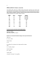
On the internet the below dielectric constants were found:
Aluminium-oxide
Bakelite
Copper-oxide
Glass
Glass (window)
Mica
Neoprene
Oil
Paper
Parrafin
Pertinax
Plexiglas
Polycarbonate
Polyethylene
Polyamide (nylon)
Polystyrene
Porcelain
PVC (hard)
10
3.5 - 4.5
18.1
5.0 - 9.0
7.6
4.0 - 8.0
4.0 - 6.7
1.5 - 4.7
1.6 - 2.6
2.0 - 3.0
4.3 - 5.5
2.6 - 3.5
2.9 - 3.2
2.4
3.4 - 3.5
2.4 - 3.0
5.0 - 6.5
3.0 - 4.0
PVC (soft)
Rubber
Shellac (Nat.)
Styrofoam
Teflon
Water (destil)
Wood (dry)
4.0 - 5.0
2.7 - 3.2
2.9 - 3.9
1.03
2.1
34 - 78
1.4 - 2.9
Most plastics appear to have a dielectric constant (permittivity) between 2.0 and 3.5. The
dielectric constant of air is around 1.0, so if we would specify a value of 1.0, no matter what
radius we would get the performance of bare wire.
When using the ‘Geometry’ editor you can select ‘Coat’ after adding a new or selecting an
existing RLC-load object. The corresponding LD card is automatically created.
When using a text editor as the 4nec2 entry system the LD 7 card has the below syntax:
Cmd
LD 7
Tag-nr
2
Start-seg
1
End-seg
16
Diel-const Coat-radius (mtr)
2.8
.003
The parameters ‘Tag=nr’, ‘Start-seg’ and ‘End-seg’ are the same as the corresponding
parameters used by the LD 0 through LD 5 command’s.
You may also specify these start- en end-segments as a percentile distance (0 to 100) from the
beginning of the wire.
The first floating point parameter ‘Diel-Const’, specifies the dielectric constant for the insulation
material used. The second floating-point parameter specifies the overall radius for the wire plus
insulation.
Internally the LD7 command is converted to an LD2 command using the below equation:
L = 2e-7 * (diel * R/r) ^ (1/12) * (1 - 1/diel) * Ln(R/r)
L
Value for distributed inductance in Henry/meter
diel
Ln
R
r
Dielectric constant (as specified in the LD7 command)
Natural Logarithm
Radius of of wire plus insulation (as specified in the LD7 command)
Radius of wire (as specified in the corresponding GW command)
This equation is especially suited for dielectric-constants between 2 and 3.5, the normal range of
insulation materials used by radio amateurs.
To see the results of the internal LD conversion, use ‘Show -> Nec 2 input’ on the ‘Geometry (F3)’
window after a (4)Nec2 calculation is done or select the ‘Show Nec’ menubar option when using
the ‘Geometry editor’.
#$K
GN 3 Specifying MiniNec type ground
When ‘connecting’ wires to a Real (SomNec)- or Finite (Fast)- ground (using a Z-value of zero)
the reported antenna impedance is usually unpredictable. To avoid this, use Real/SomNec
ground with an elevated radial system or, when using verticals, use the MiniNec ground type.
When computing far-field data the MiniNec ground takes into account the ground conductivity and
dielectric constant at a distance. However, when computing currents and antenna input-
impedance it consideres the ground to be perfect. (as could be the case using a nearly perfect
buried radial system).
This ground system however is only valid when the antenna structure does not contain horizontal
wires below 0.2 wavelength. This mostly restricts the use to vertical antennas. When modeling
other antenna types, use an elevated radial system together with the Real/SomNec ground type.
(see http://www.cebik.com/ for more info about this subject).
The MiniNec ground type is available through the “GN 3” extension on top of the default “GN –1”
to “GN 2” default NEC command set.
When using a text editor as the 4nec2 entry system the LD 6 card has the below syntax:
1
2 Cmd
I2
I3
I4
Diel-const Conductivity
3 GN 3
0
0
0
14
0.006
4
5 Internally in 4nec2 this GN-type 3 is converted to a combination of perfect ground (GN 1)
and a second circular cliff ground-medium (GD 0 0 0 0 diel cond). This second ground
medium starts at a distance zero from the antenne and also has a height of zero.
6
7 To see the results of this internal GN conversion, use ‘Show -> Nec 2 input’ on the
‘Geometry (F3)’ window after a (4)Nec2 calculation is done or select the ‘Show Nec’
menubar option when using the ‘geometry editor’.
8
9
#$K
Using a Numerical Green’s Function file (NGF)
10 Numerical Green Function files (NGF) are used to split a nec-based geometry structure in
one or more a static reusable part(s) and a dynamic part. As the static part for instance
one could specify a number of different refelctor screen’s while the dynamic part
describes the radiator. Both parts are created using standard nec input-files.
11
12 For the first file, the static part, the structure is pre-calculated, thus generating a so called
NGF file. This NGF file is created by adding a ‘WG’ card to the nec input-file.
13
14 In the second file, containing the more dynamic part (e.g. the radiator) a card is added
which specifies to import/include the pre-generated NGF file. This file is ‘imported’ by
using the ‘GF’ card.
15
16 Mostly the (first) input-file creating the NGF file contains far more geometry cards than
the file using the NGF file. Because the NGF file is pre-generated, (re)calculation the
overall structure will much more time efficient.
17
18 The frequency and ground-settings to use must be specified in the first file, producing the
NGF file. The second file which uses the pre-generated NGF file may not contain any FR
or GN/GD cards.
19
20 When using Numerical Green's Function files (NGF) some considerations must be taken
into account.
21
22 Using the Nec2dXS*.exe engines it's possible to explicitely specify the name of the NGF
file to use. The following syntax applies:
23
24 To create a NGF file
: WG file.ext
25 To use a NGF file
: GF file.ext
26
27 'file.ext' can by any file-name like 'ngf.nec' or 'screen.ngf' or 'refl.ngf'. When no NGF
file-name is specified the name defaults to 'NGF2X.NEC'. These files are placed in your
'..\4nec2\exe' folder.
28
29 When a NGF file-name is specified it's also possible to use the 'Print table of coordinates'
flag. The following syntax applies:
30
31 To print a coord-table
32 Don't print coordinates
: GF 1 file.ext
: GF 0 file.ext
33
34 Furthermore note that when using/importing a NGF file, 4nec2 is not able anymore to
automatically detect the specified number of segments from the *.NEC input-file. To let
4nec2 select the appropriate nec2dXS*.exe engine it is needed to manually set the total
number of segments.
35
36 This is done with 'Setting -> Nec-engine -> Min-nr segments'. You can enter a value just
above the total number of segments specified in both *.nec files. (the one generating the
NGF file and the one using the NGF file)
37
38 Also because ground parameters are specified in the binary *.NGF file and thus are not
directly available through the second *.NEC file it is required to use an appropriate GE
(-)1 or GE 0 specification in the second *.NEC file so 4nec2 knows if it has to generate a
half (180 degree) or a full (360 degree) far field pattern.
39
40 #$K
Symbols
Declaration of symbols/variables
41 In version 4.0 and later versions, variables, also known as symbols (especially for those using
Antenna Optimizer by Brian Beezley) were introduced.
42
43 With this feature you can assign a certain numeric value or numeric expression to a
(character) variable. For instance you may set the variable 'len' to 20, and use this variable
anywhere in your 4nec2 input-file where you want to specify a length of 20.
44
45 This is done by including a special card in your 4nec2 input file with the “SY” identifier. For
instance, if you want to specify a length of 20, a height of 10 and a width =0.1, you specify the
following:
46
SY len=20, hgh=10, width=0.1
47 You have to include the SY card before using the variable in one of the succeeding NEC
cards.
48
49 Furthermore you may include expressions/equations when declaring variables. For instance:
50
SY len=10, height = 5+10*len
‘ Height is 5; increased with 10 times length
51 Valid operators in these are + , - , * , / and ^
52
53 You may also include functions like sin", "cos", "tan", "atn", "sqr", "exp", "log", "log10", "abs",
"sgn", "fix", "int" and "mod". For instance:
54
SY ang=60, len=20, lenX = len*cos(ang), lenY = len*sin(ang)
55 Or even
56
57 SY dist=30mm, diam=1.3mm, Z0 = 276 * log10 ( (2*Dist) / Diam)
58
59
60 Standard scientific precedence rules apply. If they must be overruled you can use brackets.
61
62 Below operators are also included, however I did not yet find any real use for it:
63
"and", "or", "not", "xor", "eqv" and "<", ">"’, "<=", "<="
64 You may divide your variable declarations over one or more SY cards. The SY cards can be
included anywhere in your input file as long as the variables are declared before they are
used. You can then use these variables and/or equations in any NEC card you should like.
65
66 Variable declarations have to be separated by comma's (",").
67
68 A couple of fixed pre-defined identifiers are also included. They are:
69
cm
70
71
72
73
74
(centimeter)
mm
(millimeter)
in
(inch)
ft
(feet)
pF, nF, uF, nH
(pico-, nano and micro Farad)
nH and uH
(nano- and micro Henry).
75 Note that the variables and identifiers are not case sensitive.
76
77 When variables are used in two or more 4nec2 input-files it is possible to declare them only
once in a separate definition-file. Use ‘Settings -> predefined symbols’ to view, add ,delete or
modify these predefined symbols. This file could be used to declare, for instance, AWG # wire
gauges, your default ground parameters and/or wire conductivity values.
78
79 Prefdefined variables (constants) can be ‘overwritten’ in ‘SY lines’ in the 4nec2 input file.
80 Remark: Please do not use the above mentioned pre-defined identifiers or functions as SYmbol names
because this will lead to unpredictable results.
#$K
Modeling guide-lines
81
82 Although most of the below described guide-lines are (automatically) checked when loading or
generating new output-data or by using the structure validation option it is suggested to keep the
below modeling guide-lines in mind when creating new or modifying existing models.
Wire modeling
83
84 Len = segment length
85 Rad
86 WL
= segment radius (diameter/2)
= Wave Length
87
88 1)
2)
len < WL/10 for accuracy in most cases
len < WL/20 in critical regions
89 len < WL/5
on long straight segments
90 3)
4)
Positive current flows from end-1 to end-2
Avoid extremely short segments (len < .0001 WL)
‘rad’ must be small relative to ‘len’ and ‘WL’
91 rad < len/2
92 rad < 2*len
93 rad < len/10
with default thin wire kernel
with extended thin wire kernel
default usage
94 5) Avoid - Large changes in radius, especially on short segments
 Sharp bends in thick wires
6)
Wires that are connected must contact at segment ends
(connection separation < len/1000)
7)
Use equal source segment length and lengths for segments next to source
8) No voltage sources (EX 0) or loads at wire open ends
9)
Use same segmentation for close parallel wires.
9) GE (Geometry End) usage
GE 0
:
No ground (free space)
GE 1
:
Ground plane present, ‘touch’ wires (Z=0) are connected to ground
GE -1 :
Ground plane present, ‘touch’ wires (Z=0) are insulated from ground
Wire grid modeling
1)
Grid-size is not too critical (appr. WL/10 at midband)
2)
Len/rad not critical (10 < len/rad < 30 goor for wires attaching surface)
3)
Minimize ‘len’ and ‘rad’ changes (<2:1) at connection pts of wires and surfaces
4)
Use denser gridding (2*) at connection points of wires and surfaces
5)
Also acceptable for thin structures (plates, wings, etc)
6)
Try two segments/side
7)
Not usable for surface charges or currents
Surface patch modeling
1)
Make sure surface is closed and not too thin (no plates, fins or wings)
2)
Maximim patch size may not exceed 0.2 * 0.2 WL
3)
Corners are defined using right hand rule.
4)
Avoid long thin/narrow pathes
5)
Large patches on smooth surfaces, smaller ones on curved areas
6)
Currents are defined at centre only, so not good for edge currents
8)
When wires are connected they must do so at patch centers
9)
Use ‘wire-grids’ where edge connections are needed.
- Wire grid equals surface if mesh is ‘small enough’
- Problem:
- can’t afford real fine meshes (*
- Sparse meshes have too much L, not enough C
- Possible solutions:
- negative L distributed loading
- fat, rod-like wires
#$K
Calculate
F7
Generate NEC output-data
This general option is used for generating new NEC output-data.
If one of the below described options is selected, first of all, 4nec2 pre-processes the active *.nec input
file to remove all comment and to solve the variable- and constant definitions. The resulting intermediate
file, containing pure NEC input-data is placed in the “\out” folder with the *.inp extension. When this is
done, the Nec-2 or Nec-4 engine is started and the *.inp file is red by the engine to generate new NEC
output-data. This output-data is placed as an *.out output-file in the “\out” folder. When all calculations
are done 4nec2 open this output-file and the results are displayed on the F2 to F5 forms.
When a Sommerfeld-Norton ground is specified, 4nec2 automatically generates or copies the
appropriate ground file to be used by the Nec-2 engine. These ground files (with the *.gnd extension) are
stored in the “\out” folder. If the requested file already exists, it is copied; otherwise a new one is created
with the somnec engine. When using the Nec2dXS engine the SomNec data is calculated by the engine
itself and the additional somnec engine and ground files are not required.
When the ‘Generate’ command-button is selected, a pop-up window is displayed with different options to
choose from.
The following generate options are available:
Use original file Run NEC-engine and generate new output from active *.nec input file
Far field pattern Run NEC and generate specified 3D far field pattern for input file
Full
Generate full 3D far-field pattern.
Ver.
Generate vertical far-field pattern for specified phi angle.
Hor.
Generate horizontal far-field pattern for specified theta angle.
Frequency sweep Run NEC and request for calculations for a range of frequencies
Gain.
Run NEC and generate SWR and Gain graphs for specified phi and theta.
Ver.
Generate vertical far-field pattern for each frequency and SWR and Gain graphs.
Hor.
Generate horizontal far-field pattern for each frequency and SWR and Gain graphs.
Full
Generate 3D far-field pattern to get full Gain, F/B- and F/R-ratio data for graphs.
Near field pattern
Run NEC and generate specified near field pattern
E-fld
Generate near-electric-field data and show in 2/3D pattern and graph style.
H-fld
Generate near-magnetic-field data and show in 2/3D pattern and graph style.
360 degree Gain table
Generate ItsHF 360 * 90 degree Gain-table for specified frequency
Gain @ 30 frequencies Generate ItsHF 90 degree Gain-tables for 30 frequencies
Batch (button)
More (button)
To run multiple files as a single batch, see below.
To define more settings.Visible when one of both ItsHF options is seleceted.
Use Original file
When this option is used, the 4nec2 input file is converted to default NEC format and send directly to the
NEC-engine, without further modifications and/or additions. You can use this option for a quick first test
after creating a new nec file or to specify calculation options not supported by 4nec2.
When using one of the other (below) options it is recommended to remove all RP and NE/NH cards from
the *.nec input file.
Far-field pattern
The most used calculation probably will be the default far-field pattern calculation. This pattern
determines in which direction you antenna system will radiate/receive best and in which direction signal
is supressed. It may also be used for signal-coverage studies and interference-level analysis.
When the default far-field (full, horizontal or vertical) pattern is requested one must specify the resolution
to use. This resolution value defines the stepsize increments for the Phi/Azimuth and Theta/Elevation
angles.
When a ground(plane) is involved, only the upper halve of the ‘radiation-sphere’ is calculated. When low
resolution (< 1 deg.) is specified it is possible that the max-nr of field-points is exceeded. If so, use the
‘ver’ or ‘hor’ option, or increase the max-nr of far-field points in the settings menu.
When running a Full/3D far field pattern, by default the radiation-efficiency and the Receiving Directivity
Factor (RDF) are also calculated and displayed on the Main (F2) window. RDF is specified as the
difference between (maximum) forward-gain of an antenna and the calculated average-gain of the
antenna. For more info, see Radiation-efficiency.
Note that when running a horizontal/vertical 2D pattern or when a surface-wave request is made, no
radiation-efficiency is calculated.
On the middle-right of the window one can specify if an average-gain-test (AGT) should be performed.
With this you can check if your antenna model is more or less a valid Nec2/4 model. See Average
Gain-Test for additional info about the subject. Running an average-gain test is only possible if the full/3D
far-field option (without surface wave) is selected.
Experienced NEC users can use the ‘expert’ button to set special far-field calculating options. For
additional info about these ‘XNDA’ options, please consult the Nec-2 or Nec-4 user-guide. Default XNDA
settings are:
1:
0:
0:
2:
Ver/Hor/total field,
No normalization
Power-gain
Compute average-gain
If required, ‘Auto-segmentation’ or ‘Step-radius correction’ can be enabled through the ‘Setttings’ menu.
When the far-field option is selected, besides the Gain values the default E-field is calculated. If required,
one can check the “E-fld” box. If done so, one may enter a certain distance (in Km) for which the E-field
is calculated. (Use “<” and “>” on the Pattern [F4] window to switch between Gain and E-field values).
By default only the space-wave and the ground-refelected wave are used for far-field calculations. To
include the surface-wave in the calculations, check the “Surf-wave” box. If this is used, additional
parameters are required:
-
Max-Z
Dist
Maximum height (meter) for which the far-field is calculated.
Distance for which the far-field is calculated, mostly set to 1 Km
Frequency sweep
When a frequency-sweep is requested (starting with version 5.8.0) on can choose between two further
options:
a) Sweep by specifying a start- and stop frequency together with a fixed step-size (delta frequency)
b) Sweep using a predefined list of frequencies. If this is required, the ‘from file’ box should be checked.
Starting with version 5.8.0 one can let 4nec2 show you the change in current-distribution by ‘walking’
throught the list of calculated frequencies. For futher info see the Geometry window.
When an a) type frequency-sweep is requested, additional Start, Stop and Step-size data have to be
specified. Do not specify a Start (and Stop) frequency very much apart from the design frequency,
otherwise certain NEC requirements, such as segments per wavelength, might be violated.
To evaluate the performance over a wide range of frequencies you could consider using the Sweeper
function with Auto-segmentation enabled.
With the first option, called ‘Gain’ you must supply the Phi/Theta or Azimuth/Elevation Forward-angle for
which a Gain-graph should be plotted. Because only one far-field point is calculated (that for the
specified direction) no F/B-ratio and F/R-ration data is available or displayed.
To get F/B (front-to-back) or F/R (front-to-rear) plots; select one of the other options. Ver(tical)-,
Hor(izontal)- or 3D-pattern. Using the ‘Ver’ and ‘Hor’ options, for each frequency step, a complete
vertical- or horizontal-pattern is calculated for the specified Theta/Elev or Phi/Azim angle.
Furthermore the F/B and F/R ratio is calculated and plotted on the ‘Line-chart (F5)’ form. These ratios
are calculated for the selected plane. To get F/B and F/R-ratio calculated in 3D space (as generally
used), select the 3D option.
Note that none-directional antenna systems don’t produce meaningful F/B- and/or F/R-ratio data.
Note also that when using the ‘Full’ option only the whole 3D pattern for the last frequency-step is
displayed on the ‘Patten (F4)’ form. This to limit the overall memory usage for the 4nec2 package. To
visualize multiple patterns, select the ‘hor’ or ‘ver’ option. Use the arrow-keys to visualize the changing of
the pattern (play-back) for the specified frequency-range.
When specifying the main-beam direction the backward direction is automatically updated, according the
selected option (ver/hor or 3D) and the free-space/ground-plane settings. You may overwrite these
defaults manually with your own settings.
When the b) type frequency-sweep is requested one can specify the list of frequencies to use by
selecting ‘Settings -> pre-defined frequencies’ on the ‘Main (F2)’ window. Be sure to specify the list of
frequencies with increasing frequency values, else you will get a somewhat corrupted ‘line-chart’ display.
Gain calculation
By default forward-gain is calculated as the single gain-value for the specified direction. F/B ratio is
calculated as the difference in gain between the forward- and backward-directions. The F/R-ratio is
calculated as the difference between the forward-gain and the maximum gain-value for the backward
half of the radiation pattern which is centered around the backward-direction.
To get more control over how forward-gain and F/B-ratio are calculated (especially usefull when
optimizing) it is possible to specify delta-theta and -phi values for both the forward- and
backward-direction. If a none zero value is specified the gain over the specified region as defined by the
Theta/Phi value plus or minus the specified delta value is averaged. The number of averaging steps is
determined by the specified resolution.
Sommerfeld ground
When using the Real/SomNec ground in a frequency-sweep in conjunction with de default nec2d engine,
the ‘negative conductivity trick’ is used, in which the Real/SomNec ground data is generated only once
for all frequencies. However this Nec-2 behavour will generate less precise data.
To overcome this ‘problem’ one could use the Sweeper function and specify the frequency as a variable
or you could select the enhanced nec2dXS engine. This modified Nec-2 engine recalculates the
Real/SomNec ground data for each frequency-step, so precision is not degraded.
Troubleshooting
During generation of near/far-fields, frequency-sweep- or ItsHF-data, additional NEC card's are added to
the original *.nec input file. If error's are generated during calculation, you may inspect this temporary
NEC input-file by selecting ‘View -> Last NEC input’ on the ‘Geometry (F3)’ form, just after performing
the (failed) calculation. Use the F8 function-key to inspect NEC output-file data.
Near-field pattern
The field close to the antenna is called the near-field. This field is quite different from the far-field that
characterizes propagated electromagnetic waves. Near-field intensities are very usefull for EMI studies,
RFI and TVI minimization or FR-hazard analysis.
In contrast with the far-field, the near-field is calculated over a 3D grid of points. Start, Stop and
Step-size values for the three dimensions X, Y and/or Z have to be specified. Mostly a step-size of (Stop
– Start) / 20 will be fine. You can select between the electric or magnetic component of the near field to
be computed.
Use the ‘test’ button to let 4nec2 automatically create start-, stop- and stepsize-settings for a 3D volume
which includes the whole geometry structure. This to quickly create initial near-field patterns which can
then be used to further fine-tune the start-, stop- and stepsize settings.
ItsHF option
With version 5.6.0 and later a more user-friendly interface with the ItsHF software has been created. The
new interface enables you to create two different types of ItsHF compatible Antenne input-files:
- Full 360 degree Gain table for sepcified/design frequency for the antenne under test (type 13)
- Set of 2D gain tables for a specified Phi/Azimuth angle for frequencies from 2 to 30 Mhz (type 14)
Both types of antenna files (and other pre-defined ItsHF types) can then be used to create
Area-coverage or Point-to-point plots. After the antenna files are created one can let 4nec2
automatically create 4 kinds of plots:
- Area-coverage map
- Point-to-point time plot
- Point-to-point distance plot
- Point-to-point graph plot
Plot showing propagation performance on a (partial) world-map.
Chart showing propagation performance as function of time
Chart showing propagation performance as function of distance
Chart showing propagation performance as function of time and frequency
Above ‘propagation performance’ can be visualized using user selectable parameters like ‘Signal
strength at receiver’, “Signal to Noise ratio’, ‘Maximum usable frequency’ or ‘Radiation angle’
Besides transmitter- and receiver-antennas and -locations, the ItsHF propagation prediction software
requires additional settings to automatically create the requested plot. These parameters, settings and
options are discussed under ItsHF propagation prediction.
To use the ItsHF software package it must be installed on your computer system. Use 'Settings ->
Folders' to specify your ItsHF home folder.
#$K
Batch mode
With version 5.4.1 running 4nec2 in batch-mode was added. This way one is able to run 4nec2 for a
complete set of 4nec2, Antenna-optimizer or EZnec input-files as a single batch of work.
To use this feature, Open the “Generate (F7)” form/window and select the required calculation option.
After this, click the “Batch” button at the bottom of the window. If done so, a new “Batch processing”
form/window is displayed. To add files to the list, select the required files using Windows-Explorer (with
Ctrl- and Shift key’s), drag them to the Batch-processing window (while holding down the left-mouse
button) and drop them onto the window. All selected files are now automatically added to the list of files
to process. You can add a single file using the “Add” button. To delete one or more files, select these files
using the left mouse-button and click the “Del” button. To select (and delete) all files use Ctrl+A.
When all required files are added, click the “Start” button to let 4nec2 process all listed files. In the
column labeled “Status” the outcome of the calculation and geometry/segment validation is logged.
To (temprorarely) halt batch processing of input-files, click the “Halt” button and wait till the NEC
calculations for the current file are done. If you think this will take too long, you can alternatively abort the
NEC calculations by clicking/selecting the NEC-engine in the windows task-bar and clicking the close
button of it. To resume batch processing use the “Start after last” menu-option.
When all files are calculated, depending on the “File -> Refresh 4Nec2 data” option you can move the
focus or double-click on any of the listed files to let 4nec2 immediately load and display the data for the
selected file.
Click on the ‘File’ column-header to sort all file-names in ascending or descending order.
Batch processing can also be used to convert multiple antenna-optimizer (*.ant) or Eznec (*.ez)
input-files into Nec based files.
#$K
Command-line mode
With version 5.7.3, none-interactive command-line mode was added. This way one can start 4nec2 from
a windows batch file (*.bat) and let 4nec2 read the specified 4nec2 input-file, pre-process the data, run
the Nec2/4 calculation engine and create a Nec output-file.
To create usefull far- or near-field data one must add his/her own RP, NE or NH command in the $nec2
input-file to be used. One can use the ‘use original-file option’ on the “Calculate (F7)” to check the results
of the RP, NE or NH card specified.
To use 4nec2 in command-line mode, create (for instance) a test.bat file (in the same folder where the
input-files are listed) and use below syntax:
“C:\4nec2\exe\4nec2.exe <file1.nec> -I”
“C:\4nec2\exe\4nec2.exe <file2.nec> -I”
“C:\4nec2\exe\4nec2.exe <file3.nec> -I”
etc…
When the “-I” argument is not used, 4nec2 does start in ‘normal’ interactive mode with the specified
input-file.
#$K
Auto-segmentation
When optimizing and/or sweeping antenna performance, it is likely that dimensions and/or frequencies
are changing, so it is possible that certain NEC requirements, such as the minimum number of segments
per half-wave are not met any more. To overcome this problem, Auto-Segmentation is used.
If this feature is enabled (See Settings on Main window), each calculation/optimization/sweeping step,
the wire length for each wire is checked against the actual wave-length and the specified number of
segments per wire, and the position for voltage/current sources, RLC-loading and transmission lines is
updated.
If a certain number of segments is already specified in the input file, at least this number of segments is
set with auto-segmentation. This to avoid auto-segmentation decrease the number of segments
specified for critical regions. If you do not want to specify a minimum, set the number of segments to
one.
If the number of segments is preceded by a “+” sign the number of segments is fixed, meaning, the
segments for this wire are not affected by the auto- segmentation process.
When enabling the Auto-Segmentation feature, you are asked to specify the number of segments per
half-wave. Although, mostly accuracy improves if more segments are specified, also the computation
time is increased. For ‘simple’ structures, without sharp angles, a value from 10 to 20 will be sufficient. If
precise impedance values are required or if wires joining at sharp angles are used more segments could
be required. If you are not sure what amount to specify, please use increasing values and compare the
results. (You could do this using the Sweeper function). Also abrupt current changes on the structure
might indicate an insufficient number of segments. One place more segments aren’t better is if wires of
different diameters are connected.
If computer performance is an issue, you could consider not to the use the auto-segmentation feature. If
this feature is disabled, the processing especially for large input files with many wires is speed-up.
#$K
Step-radius correction
When modeling Yagis or other antennas with stepped diameter wires, 4nec2 can perform an automatic
stepped radius (stepped diameter) correction.
If this feature is enabled (See Settings on Main window) a substitute element is created for each tapered
one found (with certain restrictions, see “Tapering to perfection” by L.B. Cebik at www.cebik.com). The
substitute element has a uniform diameter and a length that yield essentially the same self-impedance
as the tapered diameter element. Thus, the substitute can be expected to behave--either by itself or in
an array of elements--in the same way as the tapered element. All this to minimize inaccuracy when
using large radius differences on a single element.
It does no harm to request the use of a stepped radius correction even in cases where the correction can
not be applied. However, this results in some unnecessary processing that will increase the total time
needed for calculations so I suggest you not use StepRad except in cases where it is necessary.
The conversion program has a limitation in that it will not apply the correction to Yagi elements unless
they are parallel to either the X or Y axis. Yagis that "point" in a direction other than a multiple of 90°
azimuth, or Yagis that have been oriented for vertical polarization, will not be corrected
In case of problems using this option, please don’t hesitate to ask me for support.
#$K
Average-Gain-Test
To check the reliability of your model, you can run an ‘average gain test’ (AGT). To run such a test, use
the ‘Generate (F7)’ command, select ‘Far field pattern’ and check ‘Aver-Gain test’. Then click the
‘Generate’ button.
When the ‘expert’ button is selected and using the lowest option-box, one should select the ‘1 – average
gain’ option to perform this same test. (The other option-boxes could be left to 1:Ver/Hor/Tot field, 0: no
norm, 0: power-gain).
To get usefull test results 4nec2 automatically (temporary) removes all wire- and other resistive loading
and (if specified) changes the gound-conditions to perfect-ground when doing the required calculations.
The test-results are presented on the main (F2) form.
The following gradation can be made for the Average-Gain-Test results:
> 0.95
> 0.90
> 0.80
< 0.80
and < 1.05
and < 1.10
and < 1.20
or > 1.20
Model is likely to be accurate
Model is usable for most purposes.
Model may be useful, but can be improved.
Model is questionable and should be refined.
When the resulting value is below 0.8 or above 1.2 the value is displayed in red color.
The db value between brackets can be used to correct the far-field pattern gain.
#$K
Radiation efficiency
If ground-, wire- or other R(LC)-losses are involved, the value for ‘Radiation efficiency’ might be usefull
data.
Radiation efficiency is defined as the ratio of ‘pure’ radiated power to the antenne input-power.
This data is automatically generated and displayed on the ‘Main’ form when a full/3D far-field request is
made. When using the ‘expert’ one can manually decide between letting Nec2/4 calculate average-gain
and thus radiation-efficiency data. To do so, set the lower option box on the ‘Generate (F7)’ form to “2:
Radiation efficiency” .
#$K
Open file
Ctrl+O
Open NEC input file
This general option is used to open another input (or output) file. You may specify an alternative folder
or file-extension to search for. When opening the selected file, the program first try's to locate the
corresponding output file with the extension *.out. When such a file exists, this file is loaded and the
data is displayed on the Main, Geometry, Pattern and Line-chart forms.
When the default output file is not available, the *.nec input file is loaded, pre-processed and
converted to a *.inp file and the corresponding data is displayed in the Main and Geometry forms. The
Pattern, Line-chart and Smith-chart forms are not available.
It is possible that the 4nec2 program generates an error when or after loading a default or temporary
output file. This is mostly the case if the output file is incomplete, because incorrect input file data is
used. If this is the case, remove the *.out file from the “\out” folder, change the *.nec input file and try
again.
When specifying an input-file with the '.ant' extension it is assumed you selected a AO (antenna
optimizer) or Nec-wires input file and you are asked if this file has to be converted to 4nec2 format. If
confirmed, most of the input data is automatic translated from AO/Nec-wires format to 4nec2 format.
However the following items must be checked for:
- The need to include the optional GX card when X-axis symmetry was specified.
- Additional excitation and spot-loads when the GX card is included.
- Excitation and spot-load placement on wire ends.
When specifying an input-file with the '.ez' extension it is assumed you selected an EZnec type input
file and you are asked if this file has to be converted to 4nec2 format. If confirmed a new file with the
same name but with an “.nec” extension is created and opened.
For as far as I (the author) am aware all Eznec files should automatically be converted without needing
further (manual) corrections.
On the internet, nec files with the slightly different Unix/Linux text-file format are available. If you would
want to load such a file, this format is automatic detected by 4nec2. If so, you are asked if this file has
to be converted to the default windows type text-file.
#$K
Save file as
Ctrl+S
Save output file as
This general option is used to save the active output file data to an output-file with a different name.
This option is useful for comparing different far field radiation patterns or if you want to save
calculation or optimizer results for later investigation. (Open file with *.out or other extension)
When comparing different far field patterns be sure these files are generated with the same Theta en
Phi settings. If not, you won't be able to open these files.
If you want to compare optimizer results with manual generated results note that the optimizer only
calculates far-field points for theta angles between 0 and 90 (ground) or 180 (free-space) degrees and
this is only done when a resolution unequal zero is set.
If you are not sure which RP card settings are used for a specific calculation or optimization cycle,
open the *.out output-file (F8 key) and look for the RP settings.
#$K
Settings
Modify user-, program- or memory-usage settings
The Settings option on the Main form is used to modify default-, user- or program- settings. The
setting under 'memory settings' are program settings. The maximum values for these settings
depend on you computer configuration.
The following settings are available:
Notepad edit
NEC editor (old)
Geometry edit
NEC editor (new)
Use windows default Notepad editor to edit input-file
Use old-style NEC-syntax aware editor to edit input-file
Use drag-and-draw style geometry editor to edit input-file
Use new-style NEC-syntax aware editor to edit input-file
Auto-Segmentation To enable auto-segmentation feature and specify nr of segments
Step-radius corr.
To enable stepped-radius correction.
Show circular-polar. Show circular polarization components E-left/right instead of E-theta/phi
Char-impedance
Input-power
To set the characteristic line impedance for SWR plot and Smith chart
Input power used for voltage, current and field strength calculations
Phi/Azim unit
Length unit
Radius unit
Predefined Freq’s
Predefined symbols
To select between Phi/Theta and Elevation/azimuth usage.
To select between meter, wavelength, feet or inch as length unit.
To select between millimeter or inch/Awg as radius unit.
To edit the list of fixed frequencies for a ‘from file’ frequency-sweep.
To edit your predefined SYmbols list.
Nec-engine:
Nec2d engine
Nec2dXS engine
Nec4D engine
special engine
Manual select
engine name
Min-nr segments
Memory usage:
max-nr fld-points
max freq/sweep
max-nr LD cards
max-nr TL cards
max-nr EX cards
max-nr 3D-points
max-nr of SYmbols
Use Nec2d*.exe as NEC calculation engine (1)
Use Nec2dXS*.exe engine, especially for windows-XP systems (2)
Use Nec4D*.exe as NEC calculation engine (3)
Use special engine
Use ‘min-Nr segments’ to select engine-‘size’ or specify Nec4
To set the nec2d(XS).exe as selected by 4nec2 (see below)
Maximum nr of near/far field calculation points
Maximum nr of steps for frequency/variable-sweep.
Maximum nr of (wire) loading cards
Maximum nr of transmission-lines
Maximum nr of excitation sources
Maximum nr of points used in 3D-viewer (graphics memory)
Maximum nr of SYmbols to use with optimizer/evoluter.
Optimizer settings:
Absolute steps
If selected use absolute steps else use relative steps
Max-initial step size
Initial/maximum step size used for the optimization process in %
Step size if optimizedStep size for which the optimization is considered to be ready in %
ItsHF settings:
--- area coverage----By default only the type-13 area-coverage antenna file is generated
Create ‘Area’ input-file
If selected create *.ICE/REC/VOA area-plot input file
Calculate Area-plot data If selected create *.IG1/RG1/VG1 plot/data-file
Show Area-plot on screen
If selected generate and show Area plot on the screen
--- Point-to-Point -----By default, only the type-14 point-to-point antenna file is
generated
Create ‘Point’ input-file If selected create *.ICE/REC/VOA point-to-point input file
Calculate Point plot-data
Show Point-plots on screen
--- engines-------------use ICEPAC
use REC533
use VOAcap
If selected create time/distance/graph plot-data file
If selected generate and show point-to-point plot on screen
Select predicion model/engine to use
If selected, use ICEAREA/ICEPAC model for calculation
If selected, use RECAREA/REC533 model for calculation
If selected, use VOAREA/VOAPAC model for calculation
Other settings:
Rear segment size
Wait for DOS-box
Fast/(auto)redraw
LIN min. value
LOG min. value
To specify the size of the rearward segment for F/R calculation
If checked wait in calculation engine dos-box for Enter key
To select between maximum speed or automatic screen refresh
Default minimum scale value for linear far field dB-scale
Default minimum scale value for logarithmic far field dB-scale
Folder settings
Notepad editor
Wordpad editor
ItsHF folder
program
gnuplot folder
NecWin+ folder
To set the path to Notepad.exe or other custom editor
To set the path to Wordpad.exe or other custom editor
To set the main/home-folder for the ItsHF propagation prediction
To set the main/home-folder for the ‘gnuplot’ plotting program
To set the main/home-folder for NecWinPlus
Input power
The 'power' setting is used to compute the structure currents and the magnitude for the near
electric and magnetic field. The effect is that the voltage for the voltage source on the EX card is
modified in such a way as if it would be perfectly matched and delivers the specified input-power
to the antenna structure. (Constant power mode, (multiplication with SQRT
(specified_input_power / input_power_from_output_file)) If you would like to keep the original
specified voltage in the EX card, please specify an input-power of 0 (zero) watts. (Constant
voltage mode)
Please note also that the Voltages and Currents specified in the 4nec2 program are effective
values, and not maximum values as used by the NEC-engine.
Number of segments
The maximum number of segments that can be modelled on your system depends on the of
physical memory (RAM) available on your computer. For different number of segments separate
engines (requiring different amounts of memory) are selected by 4nec2.
Select ‘Help -> About 4nec2’, to see the total amount of physical memory available on your
system.
In version 5.0 or later, 4nec2 automatically calculates the engine-‘size’ that is required. Mostly this
will be fine. The engine selected is the one specified by both the number of segments (and
patches) in your model and the ‘Min-nr of segments’ setting (see below). If segment-count goes
up, a ‘larger’ engine is automatically selected.
However in special cases when using the the NGF (numerical Green’s fuction) or related to GX
and GM cards, it is possible the wrong engine is selected. (an error like: “nr of segments and
surface patches exceeds dimension limit” may be generated). If this is the case when using a
Nec-2 based engine, you could switch to ‘manual selection’. To do this, set the ‘Manual select’
option and then specify the ‘Max-nr of segments’ setting. The engine(size) used now is selected
according the number of segments specified.
When using a licensed Nec-4 engine you can use this option to manually specify the executable
file-name to use as the NEC-engine
The following table gives you some indication about the available public-domain Nec2d engines,
the maximum number of segments to calculate and the minimum required amount of RAM. Note
however that these numbers are based on running the old DOS operating system. Because
4nec2 is based on the windows-XX system, less memory is available for the nec engine,
especially when running windows-XP which uses a large amount of available memory by
itself……
Name of
Max number Approximate
executable
of segm.
memory use (MB)
- - - - - - - - - - - - - - - - - - - - - /
NEC2D.EXE
256
1.5 (*)
These are |
NEC2D512.EXE
512
5
found in
|
NEC2D960.EXE
960
16
nec-pc.zip |
NEC2D1K4.EXE
1392
32
\
NEC2D1K9.EXE
1950
60
/
NEC2D2K8.EXE
2800
122
These files |
NEC2D4K.EXE
4000
247
are in
|
NEC2D5K7.EXE
5700
500
nec-pc-x.zip|
NEC2D8K1.EXE
8100
1006
\
NEC2D11K.EXE
11000
1852
(*) NEC2D.EXE should be in the directory from where you run
the other executables, it is the only one that contains the
DOS-extender. The others borrow it from NEC2D.EXE.
Nec2dXS engines are available for the following maximum number of segments:
Nec2dXS500
Nec2dXS1k5
Nec2dXS3k0
Nec2dXS5k0
Nec2dXS8k0
Nec2dXS11k
max 500 segments
(5 Mb)
max 1500 segments
(40 Mb)
max 3000 segments
(150 Mb)
max 5000 segments
(512 Mb)
max 8000 segments
(appr 1Gb)
max 11000 segments(appr 2Gb)
By default 4nec2 uses the smallest executable available for the number of segments specified in the
*.nec inputfile. However when using the original nec2d engine this may cause problems on systems
with 128 Mb of RAM or more.
When using a 'simple' nec input file with few segments in combination with a 'small' exe and with a
‘large’ amount of RAM, a message "Program requires MS-DOS mode,...." might be displayed. If this is
the case, increase the number of segments in the ‘nr of segments’ setting, till the message no longer
appears. On the other hand, don't set a far too big number of segments, because this will decrease
calculating performance.
For troubleshooting and additional information about engine selection, see: troubleshooting
ZIP files for the nec2d and the nec2dXS executables can be found at the “Unofficial NEC archives”:
(See
http://www.si-list.org/swindex2.html)
or
on
the
4nec2
home-page
at
http://www.qsl.net/4nec2/index.html.
These *.exe files should all be placed in your ..\4nec2\exe folder.
Additional notes:
(1) The Nec2d engine used is the one created by Jos Bergervoet.
(2) The Nec2dXS engine is based on the nec2dX engine made available by Raymond Anderson.
(3) The Nec4D engines are available as a licensed product from Lawrence Livermore National Laboratory.
The Nec2dXS engine is an improved engine as it does not require the additional Somnec2d.exe
program. Besides this, when running a Nec-2 frequency sweep the Real/SomNec ground data is
recalculated for every frequency-Step. The original nec2d engine calculates this Real/SomNec ground
data only once (using a negative conductivity setting. For more info, see nec-2 user-manual), so
accuracy is improved.
#$K
ItsHF
Propagation prediction using the ItsHF package
In this paragraph the Area- and Point-to-Point Coverage options available with the Generate command
are described in more detail. These both options are used in conjunction with the HFwin32 high
frequency propagation-modeling program developed by NTIA/ITS, which is freely available on the
Internet. (See http://elberts.its.bldrdoc.gov/hf.html) or do a Google search.
Within the combination of 4nec2 and the ItsHF package/program it is possible to create
Area-Coverage maps or create Point-to-Point plots. By default the ItsHF package contains a number
of pre-defined antenna types to be used for propagation prediction. 4nec2 however enables you to
create your own ItsHF type antenna input files based on your (4)nec2 model.
On the Generate (F7) form you can choose between two 4nec2 specific types of ItsHF antenna
files to create:
- 360 degree Gain-table (Type 13: 360 degree Gain-table (Gain table versus azimuth and &
elevation angle)
- Gain @ 30 frequencies (Type 14: Gain-table at 30 frequencies (Gain versus elevation angle &
frequency)
When running a propagation prediction both Transmitter (Xmtr) and Receiver (Rcvr) antenna must be
specified. If <current> is set as the antenna (type) to use, the above selected antenna-type is
automatically created from your Nec model (if not already available) and used for the prediction.
Running a prediction
Before running a propagation prediction you must choose between four types of plots:




Map
Area-coverage plot showing propagation performance on a (partial) world-map.
Time
Point-to-point chart showing propagation performance as function of time-of-day
Distance Point-to-point chart showing propagation performance as function of distance
Graph plot
frequency
Point-to-point chart showing propagation performance as function of time and
After having selected the required plot-type additional settings can be specified and/or modified as listed
below:
Phi-max
(or Azim-max) When generating an ItsHF antenna-file you will have to specify the NEC based
phi/azimuth angle for the main beam for the antenna under test. Usually this will be 0 or 90 degrees.
This value is used so the NEC main-beam angle corresponds to the ItsHF main-beam azimuth angle
of 0 degrees.
Bearing
For a point-to-point type of plot (time, distance or graph) it is required to specify both the transmitter
and receiver location. Both these locations determine the antenna direction (bearing) from transmitter
to receiver and from receiver to transmitter. When changing one or both locations the antenna
direction for the transmitter is automatically updated. Manual modification however is still possible. For
an area-coverage plot a receiver location is not strictly needed. This location however is used to
determine the default antenna direction.
Map
This box let’s you select between the different map ‘sizes’ for an Area-Coverage plot. Selection is
disabled when a time, distance or graph type plot is selected. When using <default> the setting as
specified in the 4nec2.ice (.rec or .voa) template file is used
Power
Using this text-box you can overrule the default transmitting power as specified under 'Settings on the
Main (F2) window.
Param
This selection box let’s you select between the different parameters to visualize on the plot. Selection is
disabled for a ‘Graph’ type of plot. For the moment you can select the following:
- <use default file>
- Signal at receiver
- Noise at receiver
- Field strength
- Signal/Noise ratio
- % above req. SNR
- Max usable frequency
- Radiation angle
Use parameter(s) as specified in 4nec2 template file (see below).
SDBW – Monthly median signal power at receiver (dBW).
NDBW - Monthly median noise power at receiver (dBW)
DBU – Monthly median field strength at receive location (dBu)
SNR – Monthly median signal-to-noise ratio (dB)
REL - Time availability, % days/month SNR exceeds required SNR
MUF - Maximum Usable Frequency – monthly median (MHz)
ANGLE – Radiation angle at Xmtr (degrees)
Note: Due to some strange inconsistancy between the ItsHF Time/Distance and Graph type of plots, with
the Graph type plot it is required to manually select the required plot once the prediction calculations are
done and the ItsHF plot-window pops-up. This manual intervention is not required for the
Area-Coverage, Time and Distqance plots.
‘Required SNR’ is specified using the ‘Mode of operations’ available through the <More> button.
See DBW and dBuV conversion for conversion from DBW and dBuV to S-meter readings.
Fixed
To set Fixed contour scaling for Area-coverage-maps and Graph-plots and fixed Y-axis scaling for timeand distance-plots. When not set scaling is done automatically by the ItsHF program. Fixed
Contour/Y-axis scaling is usefull when using the picture-viewer to scroll through a set of plot-files. Sets of
plot-files are created when a none-zero time-span is selected for area-coverage map’s or when the
4nec2 Variable-sweeper is used.
You can use the ItsUtil.exe program (‘Run -> ItsHF colors and scaling’ on ‘Main [F2]’ ) to change Color-,
Contour- and/or Y-axis-scaling for Area-coverage, Graph and Time/Distance plots to meet specific
needs.
Month
To select the (starting) month of interest. Furthermore this sets the so-called Smoothed Sunspot Number,
(SSN) which is an important propagation parameter. When selecting <def>, the value from the template
file is used. If a certain month is selected, this value together with the specified year is used to let 4nec2
automatically get the proper SSN from the internal ‘sunspot.txt’ file.
SSN
To select the year for setting the Smoothed Sunspot Number (see above) this selection box is used. To
manually specify the SSN value (in the second text box), select the ‘manual’ setting.
UTC
The UTC selection box is used to specify the (starting) time-of-day for which a (set of) prediction(s)
should be done. Set <def> to use the value from the template file.
Span
You can run multiple Area-Coverage or Point-to-Point Time, Distance or Graph plots for a selected
time-span.
When running an Area-Coverage predictions for a certain time-span, multiple plots are created. All plots
are automatically cut and pasted into the new ‘picture-viewer’ window with which you can manually scroll
through or switch between the different plots.
When running a Point-to-Point Distance prediction for a certain time-span, you must use the ‘New plot’
menu-bar option on the plot-window to manually select between the different plots. This same option is
used to select between the different frequencies as specified using the <More> button (see below). Time,
Distance and Graph plots are not automatically copied to the ‘picture-viewer’ window.
When an Area-Coverage map is selected additional ‘frequency’ and ‘month’ span-selections are
available. These are used to create a set of plots for each frequency as specified using the <More>
button or a set of plots for 6 months with 1 or 2 month interval.
Location
Both of these command buttons are used to specify the transmitter (Xmtr) or Receiver (Rcvr) location. A
new window will pop-up, in which you first will have to select the file-name containing a list of locations to
choose from. After this selection all locations in the file are listed on the second part of the window. You
can click the top-row for a specific column of the list to sort the list. You can select a certain location by
double clicking in the desired location.
Antenna
Using these both command buttons you can specify the antenna used at the transmitter (Xmtr) or
Receiver (Rcvr) location. A new window will pop-up, in which you first will have to select the folder
containing the antenna files to choose from.
The 4nec2 folder contains the type-13 and -14 antenna-files created in previous 4nec2 sessions. Select
<Current> to automatically create (or re-use) the type-13 or type-14 antenna-file for the current antenna
under test.
After selection all antennas contained in the selected folder are listed on the second part of the window.
You can click the top-row for a specific column of the list to sort the list. You can select a certain antenna
by double clicking in the desired antenna.
The ‘Transmit’ and ‘ Receive’ folders contain general HAM related transmit- and receiving antennas. All
receiving antennas are omni-directional and the Dipole- and Yagi-types are artificial derivations of their
directional counterparts.
These omni-directional receiving antennas are especially usefull for Area-coverage prediction, because
for each receiver in the ‘grid of receivers’ and as seen from the receiver another direction/bearing
applies. If you would use a directional receiving-antenna with a direction/bearing of 0 degrees (aimed
North) the receivers North of the transmitter would be pointing with their backs towards the transmitter
whereas the receivers to the South would be properly aimed. If propagation would be the same in all
directions and you would use an omnidirectional transmitting antenna this would result in unequal
coverage.
These artificial receiving antennas are also perfectly usable as a receiving antenna in point-to-point
predictions.
More (button)
This button is used to specify additional circuit related parameters:
Mode of operation which determines the minimum required signal to noise ratio for the selected
mode. (Used to calculate the ‘% above req. SNR’ (REL) parameter)
‘Noise level at receiver’, which specifies the Man-made noise level at the receiver location(s).
Above settings are used when running a ‘Signal/Noise ratio’ (SNR) or ‘% above req. SNR’ (REL)
prediction
‘Extra Frequencies’, for the Point-to-Point Time- and Distance-plots, additional frequencies to
calculate a plot for can be specified. After prediction calculations are done you can use the ‘New
plot’ menu-bar option on the ItsHF time- or distance plot-windows to select a plot for a different
frequency or even for all frequencies at once.
Using the ‘HAM-bands’ or ‘ Broadcast’ buttons, initial/default frequencies for Ham- or Broadcast
bands are set. One can manually change these values.
When using the ItsHF package its important to keep in mind that the ItsHF programs uses azimuth and
elevation angles whereas 4nec2 and NEC by default use Phi and Theta angles. For later 4nec2
versions however it is possible to switch between Phi/Theta and Azimuth/Elevation presentation.
When elevation increases from 0 to 90 degrees, the theta angle changes from 90 or -90 degrees to 0
degrees. Azimuth increases in a clockwise direction from 0 to 360 degrees. Phi increases in an
anti-clockwise direction from 0 to 360 degrees.
All automatically generated area-coverage or point-to-point input-files are derived from default
4nec2.ice, 4nec2.rec or 4nec2.voa template files as located in your ‘..\ItsHF\areadata\default’ or
‘..\ItsHF\saved\default’ folders. This is especially true if, for the selection boxes on the Generate form,
the <default> selection is used. When other selections are used the settings as specified in the
template files are overruled by the setting as selected.
You are free to modify these template files. For instance to set a larger area-coverage grid-density.
You can do so by using ‘Run -> ItsHF Area Coverage’ in the ‘Main (F2)’ window, select the ‘default
folder and open the 4nec2.* file. After modification, save this file under the same name. Next time you
run a predication the new settings are used (if not overruled by the user-settings on the Generate
form).
To use the ItsHF software package it must be installed on your computer system. Use 'Settings ->
Folders' to specify your ItsHF home folder. In this same Settings-menu you can choose between the
ICEPAC, VOACAP or REC533 model to use for the propagation-prediction. At the time of writing this the
VOACAP and ICEPAC models are considered to be the most accurate. Note that folder-names
containing more than eight characters are not allowed. If possible use the default C:\ITSHFBC folder.
Propagation Prediction using the Variable-sweeper
You may use the Variable-sweeper to see the effect of changing certain antenna dimensions on
propagation performance. To do so, first select ‘ Sweep’ as the required function and then select
‘type-13’ or ‘type-14’ as the antenna-type of interest using the ‘Option’ selection-box on the
optimizer/sweeper form. During sweep a number of ItsHF antenna-, input- and output/plot-files are
created. For this, the 4nec2 (antenna) filename is truncated to six characters and a two character
sequence-number is added to this left-over filename to distinguish between the different calculation
steps. This may produce a lot of files in the ..\antenna\4nec2, ..\areadata\4nec2 or ..\saved\4nec2
folders. If disk-space is an issue you may delete these files without further problems.
During the sweep all created plot-files are cut and pasted into the ‘picture-viewer’ window with which
you can manually scroll through the different images if calculations and plottings are finished. You can
use the ‘Save’ or ‘Print’ buttons to save or print specific images. Use the ‘Sel(ect)’ button to select part
of an image for save or print.
Steps to distinguish when running a prediction:
For Area-coverage map generation 4nec2 processes the following steps:
1) Nec is run and depending on the antenna-type selected, output data for a 90 * 360 sample far-field
request or for a 90 sample far-field request at 30 frequencies is generated and translated into a
type-13 or type-14 antenna input-file with name <name>.n13 or <name>.n14.
2) From the ItsHF parameters specified on the Generate form and (depending on the model selected
in the settings menu) a <name>.ice, <name>.rec or <name>.voa Area-Coverage input-file is
created.
3) Using both the Area-coverage and Antenna input-files the ItsHF engine for the specified model is
run and an Area-coverage plot/output-file is created with name <name>.ig1, <name>.rg1 or
<name>.vg1
4) If not specified otherwise in the settings menu the generated output/plot-file is displayed on the
screen. You can move the mouse around the Map and click a location to read distance and
parameter values or use the ‘Parameter’ menu-option to select another parameter to plot.
For Point-to-point plots, 4nec2 processes the following steps:
95 Nec is run and depending on the antenna-type selected, output data for a 90 * 360 sample
far-field request or for a 90 sample far-field request at 30 frequencies is generated and
translated into a type-13 or type-14 antenna input-file with name <name>.n13 or <name>.n14.
96 From the ItsHF parameters specified on the Generate form and depending on the model
selected in the Settings menu a <name>.ice, <name>.rec or <name>.voa Point-to-point
input-file is created
3) Using both the Point-to-Point and Antenna input-files the ItsHF engine for the specified model is
run and an Time-, Distance or Graph- output-file is created with name <model>T.dat,
<model>D.dat or <model>G.dat
4) If not specified otherwise in the Settings menu the generated output-data is displayed as a Time,
Distance or Graph plot on the screen. You can manually select between the different time- and/or
frequency plots using the ‘New plot’ menu-option.
The following files/extensions are used in the process:
ICEPAC
VOACAP
REC533
- Type 13 ant-file:
- Type 14 ant-file:
- Template-file:
- Area Input-file:
- P-to-P Input-file:
- Area output-file:
- P-to-P output-file
<name>.n13
<name>.n14
4nec2.ice
<name>.ice
<name>.ice
<name>.ig1
icepacX.dat
<name>.n13
<name>.n14
4nec2.voa
<name>.voa
<name>.voa
<name>.vg1
voacapX.dat
<name>.n13
<name>.n14
4nec2.rec
<name>.rec
<name>.rec
<name>.rg1
rec533X.dat
For the P-to-P output file the ‘X’ character is replaced by T, D or G for Time, Distance and Graph plot
requests.
Type-13 and –14 antenna input-files are created in folder ‘..\ItsHF\antennas\4nec2’.
Area-coverage input-files are created in folder ‘..\ItsHF\areadata\4nec2’.
Area-coverage plot-files are created in folder ‘..\ItsHF\areadata\4nec2’.
Point-to-point input-files are created in folder ‘..\ItsHF\saved\4nec2’.
Point-to-point output-files are created in folder ‘..\ItsHF\run’.
The filename <name> for your antenna under test is truncated to eight characters for use with the
ItsHF software.
#$K
360 degree Gain-table
(Type 13: 360 degree Gain-table [Gain table versus azimuth and & elevation angle])
When using the ItsHF software to run a propagation prediction, one needs to specify the
antenna-types used at the transmitter (Xmtr) and receiver (Rcvr) locations. ItsHF by itself already
contains a large number of more or less general antenna-types. Performance (radiation pattern) for
these pre-defined antenna types is determined by equations, which are run by the ItsHF engine when
a prediction is done.
You can view the far-field radiation patterrn for these predefined antennas by using the ItsHF built-in
antenna-viewer. This viewer is started using the ‘Run -> ItsHF antenna-view’ menu-command on the
‘Main (F2)’ window.
On the other side ItsHF enables us to use so called gain-tables, in which for each theta/phi value
covering half the hemisfere a gain-value is listed. When propagation in a certain direction has to be
calculated, ItsHF consults these tables and uses the listed gain for the required direction.
When using 4nec2 together with the ItsHF software we distinguish two different antenna-types using
gainTables: a) the type-13 antenna, containing a full 3D 90*360 degree gain-table for a single frequency
and b) the type-14 antenna, containing a set of 1*90 degree gain-tables for specified
phi/azimuth-angle, but for all integer frequencies from 1 to 30 Mhz.
Both of these antenna-types are created using 4nec2. This is automatically done by selecting the
required antenna-type in the ‘Generate (F7)’ window. If an antenna-file for the selected type is already
available it is re-used. You can overrule this behavour by checking the ‘run Nec’ check-box.
The ‘360 degree Gain-table’ option on the Generate window lets you generate 360 * 90 degree
Gain-table file for a single frequency (type-13). This type of file is the default antenna file to use for
calculating and plotting Area-coverage Maps for your antenna structure under test.
When running a Time- or Distance plot for the working/design frequency for the antenna under test (as
is the case running a plot through 4nec2) a type-13 antenna files is the one to use. However when
Time/Distance plots for multiple frequencies are run, type-14 files are preferred.
When using a type-13 file to run a Area-coverage map for multiple frequencies or to create a
Point-to-point Graph type of plot (propagation versus time and frequency) keep in mind that this single
360 degree radiation pattern is used for all frequencies steps ranging from 2 to 30 Mhz, so type-14
antenna-files (Gain @30 frequencies) are the better choice.
#$K
Gain @ 30 frequencies
(Type 14: Gain-table at 30 frequencies [Gain table versus elevation angle & frequency])
In the description about the type-13 antenna-file it is explained how these antenna-files are created
and how these are used by 4nec2/ItsHF.
The ‘Gain @ 30 frequencies’ option on the Generate window lets you create a set of 1 * 90 degree
gain tables for a single Phi/Azimuth angle. For each whole/integer frequency between 1 and 30 Mhz a
set of 90 gain values (one for each theta/elevation angle) is generated.
The Phi/azimuth angle for which each vertical pattern is generated is defined by the difference
between the real ‘bearing’ between the Transmitter- and Receiver location (listed behind the Xmtr/Rcvr
antenna button) and the ‘Bearing’ (antenna direction) value as (manually) specified on the ‘Generate’
form.
This type of file (type-14) is the default antenna input-file for calculating and plotting the point-to-point
Graph type of plots (frequency/time). These graphs for instance can show you the MUF, SNR or field
strength as function of frequency and time of day.
Type-14 files can also be used for multi-frequency Area-coverage and point-to-point Time- and
Distance-plots. When a none integer (design) frequency is specified used/selected the pattern to be
used for the prediction is interpolated from the patterns for the two nearby integer frequencies.
When generating a type-14 antenna file through 4nec2 note however that segmentation can become
an issue. because both at 2 and at 30 Mhz Nec-requirements must be met. Depending on the
frequency range of interest and the accuracy needed, you can run a default 4nec2 far-fiels 3D pattern
at both the upper- and lower frequencies to check if Nec-requirements are not violated or not, and if
so, how much.
On the other hand however one will rarely use a single antenna for all frequencies between 2 and 30
Mhz. For those who would like to specify different antennas for specific frequency-bands or –ranges
one could use the original ItsHF point-to-point user inteface. With this it is possible to specify up to 10
different antennas with corresponding frequency-ranges.
#$K
3D viewer form
F9 Show geometry/pattern in real-time 3D.
The 3D-viewer form is available only for the extended freeware version 4nec2X, and requires a
computer system on which the Microsoft DirectX 8.0 or later hardware–acceleration drivers are
installed. For further information about how to check for DirectX or how to install, see the
_ReadMeFirst.txt file.
The 3D viewer is used to display structure geometry and/or 3D far- and near-field pattern in real-time
3D. Compared with the Geometry-view F3, this viewer shows the structure much more as it is in
real-life. It also shows the real wire-radius.
However when the radius becomes too small to be visible, for instance for wire-antennas, a correction
is applied on the wire-radius, to keep it visible. A check box is available on the right of the form, which
is enabled if it’s possible to re-enable the real-radius display.
This way it is very easy to see if wires are overlaid or intersect (at unexpected places) or not. Also at
junctions with short fat segments the intersected area should not be more than about 1/3 of the
segment length. With some experience it’s also possible, for wire grids, to check the ‘equal area’ rule.
When patches are included in the structure geometry, the ‘shiny’ side of the patch is the one from
where the normal-vector is pointing outwards. This side of the patch should be considered as being
part of the NEC calculation process.
Use the structure drop-down box to select different structure-display options.
Use the ‘Res’ button to reset all zoom-, shift- and/or rotate-actions.
The following key’s and mouse-buttons are available to change the viewing-position.
Key-combination:
- Rotate structure
- Move structure
- Forward/backward
- Zoom-in/out
Mouse-action:
Left/Right or Up/Down arrow Move mouse with left button pressed
Ctrl+Left/Right-arrow
Move mouse with right button pressed
Ctrl+Page-up/down
Move mouse with both button pressed
Page-up/down
When the display of currents is enabled, and also a freq-sweep calculation was performed, the
function of the cursor/arrow key’s is changed from structure movement/rotation to frequency
‘movement’.
The upper drop-down box lets you select different types of structure (geometry) display. If ‘wires’ or
‘segments’ is selected, the red end is end-1 and the green end is end-2.
If ‘currents’ is enabled use the ‘Log factor’ scroll-bar to visualize small currents on gridded/external
objects.
If NEC output-data is available the drop-down boxes on the right of the form are enabled. This lets
you visualize the 3D far- or near field E/H pattern in 3D. You have the choise between single-color or
multi-color mode. In multi-color mode a blue to red scale is applied to the pattern for which the color
corresponds to the color-scale on the left of the form.
When, for the far-field, the 2D-slice display option is selected, a 2D-pattern slice is displayed for a
certain theta/elevation or phi/azimuth value. You can change the Theta/Elevation or Phi/Azimuth
angle for which the slice is displayed, on the ‘Pattern (F4)’ form while simultaneously watching the 3D
form. In the ‘Pattern (F4)’ form, use the space-bar to switch between horizontal/vertical slice.
When on the Pattern-form multiple far-field patterns are selected to be compared against each other,
you can also switch between these patterns on the 3D-viewer form. Use the selection-box in which
the file-name is displayed to select one of the patterns. You may also use the ‘<’ and ‘>’ keys (with or
without <Shift>)
On certain computer monitors it showed up that color display sometimes is not optimal. To overcome
this ‘problem’, use Ctrl+C to bring-up the color settings window. Select the appropriate structure part
and use the sliders to change color or to alter background- or, directional-light intensity.
When no key’s are pressed for a certain amount af time, the structure is rotated automatically. You
may maximize the window and use this functionallity as a kind of screen-saver. You may use the ‘Z’
key to start to spinning directly without waiting for the time-out.
When structures are viewed with a large number of (bent)segments and/or junctions, a certain
simplification is done when creating the 3D picture. For instance, by default, all wire ends are closed
and wire-radius-changes and junctions for more than two segments are smoothened.
For very high-segment structures these actions are not performed. This is represented by the ‘Quality’
slide bar on the lower right corner. Eventually one can use this slide-bar to change the default 3D
structure quality and increase speed, ranging in three steps from left to right.
FPS
Tri’s
Left
Middle
Right
:
:
:
Show ‘simple’ structure as a wire-grid.
Show structure with open ends and none smoothed junctions
Show high-res structure with closed ends and smoothed junctions
= number of frames (screen refreshes) per second.
= number of triangles used to constuct the 3D objects
When a large number of far/near-field points is requested or when structures with a large number of
segments and with ‘high-quality’ are viewed, it could be necessarry to increase the ‘Max-nr of
3D-points’ in the setting-menu. If so, a message will inform you about this possibility. However,
because this setting also affects the amount of video-card memory used, large values can
sometimes result in strange video effects. If so, lower this setting.
#$K
Matching
F10 Impedance matching networks.
For maximum power transfer from the source to your antenna/load and/or to reduce
transmission-line losses it is needed to match your antenna to the characteristic impedance (Z0)
of your feed/transmission-line. In many cases however it is not possible to choose all impedance
such that overall matched conditions result. These situations require that matching networks be
used.
In general, matching networks are constructed with reactive components only so that minimal
loss is added to the overall network. For frequencies up to approximately 500 MHz matching
networks containing lumped elements (L, Pi or T networks) may be used. The circuit elements
(capacitors and inductors) must be small enough relative to wavelength.
Another way of antenna to feedline matching is called Stub-Matching and uses parallel or series
stubs. These stubs are open or closed (at the end) pieces of transmission-line with different
impedance placed somewhere along the feedline.
A third method is called Series-Matching. This method uses a series matching system consisting
of three sections of transmission line. The middle section does have different characteristic
impedance.
L, Pi or T-network matching
Using L, Pi or T-networks it is theoretically possible to match any source/load impedance
combination. However in practice certain reactance/resistance values could result in additional
component losses and the use of lumped elements does reduce your overall system bandwidth.
4nec2 supports the automatic calculation of the required components for low- and high-pass L, Pi
and T(ee) networks using the ‘Matching (F10)’ window/form.
When this form is first displayed 4nec2 checks if already a matching network is present. If not, the
antenna/structure input-impedance value and the design-frequency is copied into the ‘Matching
(F10)’ form and the Z0 as specified under the ‘Settings’ menu is set as the (source) impedance to
match. With these impedance’s then the required component-values to create low- and high-pass
L, Pi and Tee networks are calculated and displayed on the screen.
For both inductors and capacitors their quality ‘Q’ may be specified using the Q-coil and Q-cap.
Text-boxes. By default capacitors are considered lossles (indefinitely high Q, entered as zero),
whereas inductors are given a default Q of 250. If sufficiently high (100-300) then the low series
resistance will not influence the required network components for a 1:1 match much.
To let 4nec2 automatically add the matching network to your (4)nec2 antenna design, first select
the required network and then click the “use network” button and let 4nec2 generate new NEC
data. You can use the default option “use original file” to generate only the new input-impedance.
If done so, 4nec2 will create a (far-away) dummy wire, place the voltage-source on it and connect
this dummy wire with the original excitation wire/segment through a network NT-card. The Y11,
Y12 and Y22 values to be used with the NT card are calculated when the network is selected.
After generation the new input impedance together with the resulting losses for the selected
matching network will be displayed on the ‘Main (F2)’ window.
As long as the ‘Matching (F10)’ window is active you can re-generate using other selected
networks. Once the ‘Matching’ window is closed you will first have to generate the ‘raw’
input-impedance using the default ‘Generate (F7)’ function, before you are able to use the
‘Matching (F10)’ window again.
For Pi and Tee networks by default 4nec2 uses the lowest possible Q. This to minimize losses. If
more manageable components or extra attenuation of undesired frequencies is desired (for Pi
and Tee) a different/higher value may be specified in the min-network-Q textbox. A higher
network-Q however will increase network-losses and reduce bandwidth.
Note:
- You may manually change Z-ant, Z-src and/or Frequency to let 4nec2 directly reflect these
changes in the calculated L, Pi or Tee network-values. This way you can use this form as a
general tool to match for other impedances and/or frequencies
- After a certain L, Pi or Tee network has been selected, you can also manually change
component values (L, C, Ql or Qc) or the network-Q to see how these changes directly affect the
NT network parameters Y11 to Y22.
- Click the ‘use network’ button to see the effect on overall input-impedance and power losses in
the network due to your manual changes (tolerances) of Network component values.
You will see that using inferior components and thus lowering component-Q (and increasing
network-Q for Pi/Tee) will increase losses and deviate the input-impedance more and more from
the specified Z0. On the other hand an infinite high coil- and capacitor-Q (enter a value of zero)
will deliver an exact 1:1 match.
Click the <Reset> button to restore all fields to their initial values.
Stub/series matching
You can reach the stub/series matching form by clicking the ‘stub’ button on the upper-right on the
Network matching form.
When the form is first displayed 4nec2 checks if a matching network is already included. If not,
the antenna/structure input-impedance value is copied onto the Stub-matching form as ‘Z-load
(antenna). The design-frequency and the Z0 (as specified on the Main-form’s settings-menu) are
also copied onto this form.
With the ‘select matching network’ selection box you can choose between the matching network
to use. For now, below types are available:
- Series section; this type of match uses three sections of transmission line in series, in which the
middle transmission line does have different impedance. The impedance transformation is
defined by the Z0 of the series section, the length of (default) feed/transmission-line from antenna
to the middle series-section and the length of this series-section. An arbitrary third (lower) length
of (default) feed-line connects the series section to your rig.
- Parallel stub, open or short; this type of matching-network also uses a second different type of
transmission-line which is connected somewhere between the antenna and your rig on the
feedline. The parallel stub is connected as the name already implies in parallel with your feedline.
The impedance transformation is defined by the distance between antenna and the point on the
feedline where the stub is connected and the characteristic impedance and length of the
stub-line. The required lengths are influenced by the fact weather you choose to use a short or
open end for you stub.
- Series stub, open or short; this matching-network uses the same principles as the parallel stub,
but now the stub is connected in series with one of both feeder-lines. For the series stub one can
also choose between an open or a short stub.
Also included on the form are two selection boxes to select both types of feed/transmission-line.
The first sets your default type of feedline; the second sets the characteristics for the
series-section or stub-line. When ‘user-specified’ is selected you can manually enter
characteristic-impedance (Z0) and/or velocity-factor (Vf) values.
For each selection the resulting line-length results are displayed in the lower ‘edit/select results’
portion of the window. If ‘none’ is displayed, there is no valid solution for the selected network
and/or type of transmission-line(s). You will have to select another network or transmission-line.
For each selection 2 possible solutions are available, labeled A and B. When stub-matching is
used one can furthermore select between using a short or open stub. This selection is done by
using the ‘select solution’ selection-box or by clicking on one of the length text-boxes. Values
highlighted represent the actual selection.
To use the selected matching-network with specified lengths in your model, click the ‘use
selection’ button. 4nec2 will now automatically add the required transmission lines to your model
with the specified lengths and configuration and calculate the results, which are displayed on the
Main(F2) and Geometry(F3) form.
You can also manually overwrite the lengths as initially calculated by 4nec2 on the stub-matching
form. This way you are able to see what results you get if you do not exactly follow the calculated
line-lengths.
#$K
Smith Chart
F11
Show impedance and SWR on Smith-chart
In this form the input impedance is plotted on a Smith-chart. When a Nec based frequency-sweep was
done more than one impedance point is plotted. The active SWR is displayed as a circle. On the left of
the Form additional information such as reflection loss, SWR in dB, refl-coeff (U/I), refl-coeff (P) and
return loss is displayed.
With the Shit+left or Shift+Right buttons you can specify any length of transmission line connected
between the load and the generator and read the resulting impedance. With Ctrl+P you can capture
and save/print the Smith-chart form for further graphical analysis.
When you requested a frequency-sweep you can 'walk' through each frequency with the RIGHT and
LEFT arrow-keys. The corresponding frequency and the real and imaginary values for the impedance
are displayed in the lower right of the form. With the 'X' button you can switch between polar- or
cartesian-notation. With the 'Home' button you can switch between a normalized chart or a chart
based on the characteristic impedance.
With pressing the Right or Left button together with the SHIFT button a second phase line is displayed.
With this line you may specify a length of feed-line. On the lower left of the form a second pair of
values is displayed, showing the real and imaginary values for the impedance on the other side of this
feed-line, corresponding with the given SWR and phase angle.
When selecting a phase difference of 180 degrees (lambda/4) this can also be used for reading the
admittance values for the selected impedance. You can add and remove your own user
impedance/admittance points by pressing the Insert and Delete keys.
The grid for the Smith chart can be changed between fine and course with the corresponding option
under the Show menu-bar option. For those who want to further customize their grid layout; the layout
is described in the Smith.dat files in the “\exe” folder, but before changing it, be sure you made a
backup or this file.
Position your mouse and push <Insert> to add manual points, or use right mouse-button. Push
<Delete> to remove last manual point.
Use the ‘Export’ menu-bar option to export your smith-chart data in Touchstone (Z or S params) or
Microsmith (*.gam) format.
Use the ‘Import’ menu-bar option to (re)import a Touchstone (Z or S prams) or Microsmith (*.gam)
data/export-file. When importing data you are asked if existing data-points should be cleared ot not. If
existing data is cleared, the new import data is also available through the line-chart form.
#$K
The Optimizer and sweeper
F12
The optimizer/sweeper is started by pressing the F12 key or by selecting calculate -> optimize on the
menu-bar in the Main window. The optimizer, as part of the 5.4 and later versions, contains four
different options:
- Optimize
- Evolve
- Sweep
- Conv-test
Use the traditional hill-climbing method to optimize you design
Use Genetic Algorithms to evolve (optimize) your antenna design
Use the Sweeper to visualize the effect of user specified design/variable changes.
To validate your model by running an automatic Convergence-test
You may select between one of these options with the "Function" box on the upper-left of the optimizer
window. With the "Option" box you can select between different sub-options. For most cases 'Default'
will be the appropriate choise.
The traditional hill-climbing optimizer was based on principles as described by Brian Beezley and used
by the AO (antenna-optimizer) program. A scaled down freeware version of this program is available at
the ARRL web-site.
For a description of how to ‘evolve’ your desing using the genetic algorithm based optimizer see
Genetic Optimizer, but before doing so, please read the below section about how to specify the
antenna properties and variables to optimize/evolve.
A description of the traditional hill-climbing optimizer is given below, a description of the Sweeper
function is given in a separate section. How to run a convergence-test is described in Conv-test.
When you want to use the optimizer the 4nec2 input file must include variables (constants). These
variables serve as input for the optimizer. You may specify any combination of variables (and/or
equations) anywhere in your 4nec2 input file (GW, LD, EX, FR card).
You can select only “simple” variables (constants) as the ones to optimize. These are variables not
containing any expressions like +, -, *, functions and/or other equations. These "simple" variables are
the ones that are altered during the optimization process. (See the 3el-inverted-V.nec file for a more
dedicated example).
The optimizer window is devided into four different sections, one input and three output sections.
Antenna properties to optimize
The main input-section is named 'settings', and is used to specify the variable(s) to modify and the
(antenna) properties to optimize. These properties are SWR (standing wave ratio) ,Gain (forward gain
or Electric-fld), F/B (Front to back ration), F/R (Front to Rear ratio), R-a (Input resistance), X-a (input
reactance) and/or Eff. (Efficiency). When the 'include surface wave' box is checked, the Gain property
defaults to E-fld.
For each of these properties you must specify the importance of it by specifying a value between 0 and
100% (weighting factor). This factor determines the effect on the overall performance for the
corresponding property. For instance when optimizing only on SWR, the SWR factor is 100% and the
other factors are set to zero. You can toggle this weighting factor between 0 and 100 by right clicking
on the "SWR", "Gain", "F/B", "F/R", "R-a", "X-a" or "Eff." text label or on the corresponding text box.
Other values have to be entered by keyboard. (Negative values or values > 100% are allowed).
By default the SWR and X-in properties are minimized and the Gain, F/B, F/R, R-in and Eff. properties
are maximized. In order to change these defaults or to specify your own targer value, click with the
right mouse-button on the corresponding text-label (SWR to Eff). A pop-up menu is displayed in which
you can specify if you want to maximize or minimize this property or if you want it to reach a
user-specified target value.
The following targets are set when optimization towards minimum or maximum (the default) is
selected:
Property
Min
Max
SWR
Gain
F/B
F/R
R-a
X-a
Eff.
1
-999
-999
-999
0
0
0
100
100
+999
+999
9999
+9999
100
When no (wire)loading cards (LD) are included, optimizing on efficiency has no effect.
User specified targets are accepted for values anywhere between -9999 and +9999. Note however
that if one specifies a target of +9999 for, for instance, forward Gain, this does not improve optimizer
accuracy. A target in or near the range of theoretical (min/max) property values for the antenna type to
optimize will yield better results.
The absolute difference between the actual value and the target value for each property is rescaled to
a range from 0 to 10000 and summed according the specified weighting factors. The resulting value is
used as input for the optimization process.
The optimizer calculates electric-field values in relation to the specified input power value, so
optimization is done with a constant power setting and not as might be expected with a constant
voltage (or current) setting. If the latter is required, select a power-level of zero watts and specify an
appropriate voltage- or current-source.
When optimizing for (forward) Gain or F/B-ratio you will have to specify the Theta and Phi angle for
which the Gain (and F/B, F/R ratio) should be calculated. If a resolution of 0 degrees is specified the
Gain (and F/B ratio) is calculated for this one and only angle. To optimize on F/R-ratio it is required to
use a none-zero resolution to enable gain calculation and maximization to be performed for the whole
180 degree backward-region.
It is possible to specify a certain forward- and/or backward-region for which the Gain or F/B ratio
should be averaged. This is done by specifying a certain resolution in combination with a delta-Phi
and/or delta-Theta (d-Phi, d-Theta) value. Averaging is performed for angles between Phi – d_Phi and
Phi + d_Phi. The same holds for the Theta and d_Theta angles. The resolution determines how many
iteration-steps are made between + d_Theta/Phi and – d_Theta/Phi angles. Using a none-zero
resolution will show a considerable increase in required optimization time, because far more gain
angles are calculated.
Frequency-sweep
With version 5.1 the possibility to optimize over a certain frequency-band (for instance the 40-meter
band) was added. To enable this option, check the ‘freq-sweep’ box. If done so additional input-boxes
are displayed in which you can specify the start- and stop-frequencies and the step-size thus
specifying the frequency-band of interest.
For each frequency step a complete set of results is calculated. All results for each property are then
summed and devided by the freq-step count at the end of the sweep to get the average values to be
used as input for the optimization process.
Antenna dimensions/characteristics to change
To optimized one or more of the properties, antenna dimensions/characteristics have to be modified.
These dimensions/characteristics are represented by (combinations of) “simple” variables. All available
“simple” variables to optimize are displayed in the upper left box on the settings section. You select
one or more variables by clicking on the variable name. Then this variable is added to the box on the
right. This box lists all the variables, which are used to optimize the selected antenna properties. You
can remove a variable by clicking again on the variable name in the left or right box.
When using the genetic optimizer (evolve) you will also have to specify the minimum and maximum
allowable variable values. This determines the so called 'search-space', in which feasible solutions are
searched. By default the minimim value equals the actual variable value devided by 2, the maximum
value equals the actual value times two.
The traditional optimization process
If the traditional optimizing function is selected, clicking the 'Start' button starts the optimizer. First of all
some initial calculations are done to determine the sensitive and direction for the selected variables on
the requested propertie(s) to optimize. The results of these calculations are shown in the upper right
section. After that, the actual optimization is started and the variables are modified with a certain initial
step-size to achieve better performance. The results of these optimization steps are displayed in the
lower left and right section.
The first initial/max step size determines how quickly an optimization solution will be found. A small
step size could lead to a long optimization run. With a too big step size it is possible that with sensitive
variables it is possible that the first minimum/maximum is skipped. This value is available in the
'Settings -> optimizer' menu. Mostly a max/initial step size of 10% will be fine.
Optimization steps continue as long as there is still improvement. When there is no further
improvement a new sensitive run is performed to determine how the selected variables have to be
modified to achieve, if possible, a new better performance and new optimization steps, with smaller
step sizes, are done. This continues till the step-size has reached a certain minimum step-size and the
optimization process stops. This minimum step size determines how accurate the minimum/maximum
will be. This value can be changed in the ‘Settings -> Optimizer' menu. Mostly a value of 0.01% will be
fine.
By default the delta step size is relative to the active value of the variable to optimize. However it is
possible to use absolute (fixed) step sizes. If this option is selected in the Settings -> Optimizer menu,
after a sensitivity run, an absolute delta step size is initially calculated and this step size value is not
changed until the minimum/maximum is passed and a new sensitivity run is performed.
You can examine the optimization results on the two lower output sections on the window.
(Intermediate) variable results are stored in the file *.opt on the 4nec2 main home-folder.
To save the new optimized variable values to the original *.nec input file, use the 'Update Nec-file'
button on the optimizer window. The existing variable values are overwritten with the new values.
It is possible to halt the optimizer before the process automatically stops by pressing the 'Halt' button.
After the optimizer is stopped or halted you may exit the optimizer or alter, add or remove variable or
property settings and continue by pressing the "Resume" button. The optimization process continues
with the latest calculated variable values. To (re)start with the initial variable values, you have to exit
the optimizer and start it again without saving the results.
When only one variable is selected the optimizer can be initially forced in a certain direction to find the
next maximum/minimum. This is done by selecting "increase" or "decrease" in the Upper left Function
box on the 'Settings" section of the window. After the first maximum/minimum is passed, the normal
optimization process is continued.
After optimization it is wise to validate the new geometry structure, and if you updated/saved your
results, to perform an additional Average-Gain-Test.
Additional Gain and F/B settings
When selecting Forward gain (Gain), front-to-back (F/B) or front-to-rear ratio (F/R) also the angles
which define the forward- or backward-direction and a certain pattern-resolution must be specified.
Optionally delta-Theta and delta-Phi values can be specified. This is used to average the forward
(and/or backward) gain over a certain region between Theta/Phi - delta_theta/phi and Theta/Phi +
delta_theta/phi. The step-size determines the number of averaging steps. (see Generate for additional
information. These delta-theta or –phi values can be used to minimize both maximum or average
side-lobe level in a certain direction.
By default when ground is specified, the backward theta/levation angle used for the F/B ratio
calculations is set to the same value as the theta angle used for the forward-gain (Theta-back =
Theta-forward and Phi back = Phi-forward+180). If free space is selected the backward-angle used is
the angle on the opposite side of the XY plane (Theta-back = 180-Theta-forward and Phi-back =
Phi-forward+180) It is possible to manually overrule the default backward Theta and/or Phi angles to
be used for the F/B ratio calculations.
Furthermore one may include ground wave calculations or select between Horizontal-, Vertical- or
total-gain, E-theta, E-Phi or E-radial when performing the Forward gain of front-to-back/rear
optimizations.
Output log
During the optimization process, the optimizer variable- and property values (calculated results) are
logged in a log file called "Optimizer.log". This log-file is located in the 4nec2 home-folder. This log-file
is available for further examination of the results using the ‘Show’ command button. The next time the
optimizer is started, the old log-file is replaced with the new version.
To visualize the results and/or behavour of the optimization process one can use the ‘Plot results’
command-button. After this you will be asked for a property- and one or two variable-names for which
a 2D or 3D plot is generated using the gnuplot program.
Tip(s):
1) During the optimization process you can resize or move the ‘Optimizer’ window to make more/other
data visible. You can 'click' on one of the other windows or use the F2 to F5 key's to bring one or more
of the windows in front of the other or you can 'drag' one or more of the windows aside.
2) You can only change a certain viewpoint on the 'geometry (F3) or 3D (F9) form or select a specific
2D pattern type on the F4 form, when the optimizer is halted. You can do this before the 'Start' button
is used, or you can temporarely pause the optimization after it is started by pressing the 'Halt' button,
change setting and press 'Restart'.
3) To sequentially switch from Genetic- to Hill-climbing-optimization or back, for the same input-file,
use “Update Nec-file” to temporarely save the results of the previous run, exit the optimizer and
open/load this temporary file as input for the next optimization run. Use ‘seed with curr-data’ to use
existing optimization data in the Genetic optimization process.
#$K
The variable-sweeper
In the optimizer window it is possible to evaluate the effect of changing one or more antenna or
environmental dimensions. This is done by selecting the ‘Sweeper’ option in the Function box on the
upper left of the Optimizer window. The dimensions to sweep must be specified as variables in the
4nec2 input file.
After the Sweeper function is selected, one ore more variables to sweep have to be selected in the
‘Available variables’ box. For each variable selected it is now possible to specify the min(start) and
max(end) values for the sweep. It’s not required for ‘max’ to be greater than ‘min’. For instance to
sweep from 20 to 10 specify 20 as the ‘min’-value and 10 as the ‘max’-value.
Furthermore the number of steps for the sweep must be specified. This is done in the ‘Nr of steps’
Box’.
By default the ‘used fixed stepsize’ box is checked, resulting in equal steps when the variable values
are changed from min to max. If un-checked multiplicative steps are used. In this case it is not
possible to sweep from <0 to >0 or reverse.
The Theta/Elev and Phi/Azim value boxes are used to specify the angles for which the forward gain,
F/B-ratio and for none-zero resolutions, the F/R-ratio is calculated. It is furthermore possible to include
ground wave data at a specified distance or to select between Horizontal, Vertical and total gain,
E-theta, E-Phi or E-radial when sweeping on forward-gain.
If a none zero resolution is specified one can select between the horizontal or vertical (or 3D) pattern
to be displayed for each step during the sweep. The angle for which the hor/ver pattern is calculated is
determined by the specified leftmost Theta/Phi values. All generated patterns can be played-back
(using the arrow-keys) after the sweep when the Pattern form (F4) is selected.
Because full F/R (and F/B) data is not available when only far-field values are calculated for a certain
horizontal or vertical slice, the 3D-pattern option is available. Using this option full gain, F/B and F/R
data is generated to be visualized through the ‘Line-chart (F5)’ window. When this 3D option is
selected no horizontal or vertical far-field pattern play-back data is available, because only the last
generated full 3D pattern is stored.
Sweep output data (to be imported in a spreadsheet or other programs) is also reported through the
optimizer/sweeper logfile. To view this data, select ‘View -> Optimizer log’ on the Geometry window.
When a none zero resolution is specified, sweeping speed will decrease because of the additional
gain calculations, especially when the 3D option is used.
Note:
Sweeper results are stored in memory only and not on disk (as is the default 4nec2 behavour), so if
4nec2 is shut-down or another (4)nec2 input-files is selected the sweeper results are lost. The log-file
is kept till a new optimization or variable-sweep is done.
#$K
Convergence-Test
During a convergence test the design/model is validated by running it over a number of steps, in which
for each next step the number of segments for all wire is increased by a certain amount (20-50%)
while Gain, Input-impedance, Efficiency and other values are observed. These values will have to
converge towards a certain value.
To automatically run such a test select the Conv-Test function on the Optimizer window. If done so, the
number of steps to run from default- to the highest allowable number of segments is calculated and
displayed in the ‘Nr of steps’ text-box. When started, on each step the number of segment for wires
(for which the highest allowable segmentation is not yet reached) is increased with 33%, till all wires
have (almost) reached maximum segmentation.
When done, click the “Exit” button, and on the “Line-chart (F5)” window Gain- and Impedance-data is
visualized for further evaluation. Abrupt changes or an increasing slope for one or more of the graphs
on the chart could point to an unrealiable model.
For a description about how to use the Theta/Elev and Phi/Azim input boxes (to specify the angles for
which Gaind and F/B ratio are calculated) see the Sweeper function.
#$K
The Genetic Optimizer
The genetic algorithm (GA) used in 4nec2 is a real-value based algorithm. This GA includes a
number of selection-, crossover- and mutation-techniques like Roulette-Wheel-, SUS-, or
tournament selection, N-point-, Blend- or Simulated binary crossover and random-, gaussian- or
none-uniform mutation.
Why use GA’s ?
GA’s are fundamentally different from other optimization techniques. Analytical optimizers usually
compute derivatives (hill-climbing/gradient methods) to locate maximum or minimum points for the
function being optimized. GA’s by contrast, create random populations of individuals/chromosomes
which are then ‘evolved’ to converge to an optimum solution. Gradient methods produce one ‘best’
answer, but they are often trapped in local extremes, which prevent the global optimum from being
found. GA’s can produce groups of solutions, no one if which is necessarily the global optimum, but all
of which are ‘good’ solutions.
Furthermore when a large number of variables is involved with mutual influences among each other,
performance of the GA is expected to better than that of the Hill-Climbing optimizer.
One drawback of GA’s is that it mostly takes more time to optimize a design using a GA than it takes
to optimize using traditional methods.
Before starting the algorithm, the variables to optimize must be selected, together with their
minimum and maximum allowable values (limits). These user-selectable upper- and lower- limits
define the boundaries for the ‘search-space’. Mostly these limits are set according physical limits,
like available space, maximum height or width etc.
However, setting a too wide range may slow down the GA and might cause it to miss a good
solution, because it searched not long enough. Setting a too narrow range might exclude useful and
interesting solutions. Experience in this is the most important factor and insight in what may affect
antenna performance is also very usefull.
Each variable to optimize is called a gene. All the genes together form the chromosome. When the
GA is started an initial random population is created by uniform random selection of the gene value
on the interval between the lower and upper variable limits.
A population is a group of N chromosomes or individuals. Each individual representing a different
4nec2 antenna design. The GA ‘evolves’ the initial random population by creating successive
generations of individuals. The population size N is constant from generation to generation, but the
individuals comprising the population are genetically altered from one generation to the other.
One of the most important features of a GA is its ability to optimize a population using any desired
measure of ‘goodness’. Unlike gradient methods GA’s easily handle discontinuous functions. The
only requirement for a useful ‘Figure Of Merit’ (FOM) is that it is calculable. The data used for the
FOM is usually generated by a separate computer program (calculation engine) that models the
system being optimized and not by the GA itself. The GA inputs data from the engine and uses this
to computer the FOM or fitness values. This procedure is also known as the ‘objective’ function.
The FOM calculation used with the GA is the same as the one used with the traditional hill-climbing
4nec2 optimizer.
For one or more antenna properties a weighting factor from 0 to 100 (or more) percent is specified
by the user, together with an optional target value (click on property using right mouse-button). The
absolute difference between the actual value and the target value for each property is then rescaled
to a range from 0 to 10000 and summed according the specified weighting factors. The resulting
value is then used as input for the rank-based fitness calculations as described below.
Generation after generation is created this way with the expectation that each successive
generation will contain better antenna designs. But because of its stochastic nature a GA may not
create improved designs in every successive generation, and the FOM/fitness-value may actually
go down. Experience has demonstrated that a well-designed GA will converge to an optimum
solution if allowed to run for enough generations with a sufficient large population size.
GA parameters
All parameters used by the 4nec2 GA are available on the ‘Optimizer’ form (F12). It may be
required to click the ‘GA’ (option) button to make them visible.
Max-generation.
This parameter sets the maximum number of generation after which the evolution of new
populations will stop. You are now able to save any of the resultant antenna design files or exit
the optimizer and/or consult the summary log-file for all population data (use 'Show Log' button).
You can also resume the generation of new populations by pressing the 'Resume' button. A new
set of ‘max-generation’ populations is now processed.
You may halt Evolution, before the max number of generations is reached. For instance because
the solutions have converged, an adequate solution is available or if you want to change one or
more of the Genetic Operators and resume.
Halt if N % same fitness
During the GA evolution process, the overall fitness of all the individuals will increase and finally
converge around a certain solution. At this point most of the chromosomes (with exception of the
onces just mutated) will have a similar fitness. You can specify to halt the optimization if a certain
percentage of individuals have reached the same maximum fitness value. Mostly this value will
be somewhere around 50-90%. To be sure all generations as specified by the ‘max-generation’
setting are evolved, set this percentage to 100%.
Population size
This parameter specifies the number of chromosomes (individual antenna designs) included in
each population. As a general rule, values in the range 30-200 provide a good starting point,
depending on the number of segments and how fast a CPU is available.
Seed with current data
This option is used to seed the coming GA run, thereby initiating the GA search around a
particular solution in its search space. The ‘seed’ individual (design) is inserted as individual #1 in
generation #1. Its function is similar to the ‘Elitism’ function as described below.
Save best file for last N generations
When a GA run is completed either because it was aborted or because the maximum number of
generations was reached, all individual *.nec antenna designs for the last population are available
in the “\opt” sub-folder below your current *.nec input-file folder. Furthermore for a specified
number of last generations the *.nec file for the best individual is saved. This number of last
generation is specified in the field “save best file for last .N. generations”.
Update Nec-file button
This command button is used to let the user select the best file from last N generations. After this
the original *.nec input file is updated with the new variable-values from the selected file and the
results are saved to a file with the same or a different name. This file could then be used as a
temporary or final result or as a seed for subsequent GA runs.
GA specific parameters
The other GA specific parameters are described in the more general Genetic Algorithms section.
These parameters are supplied for those who want to further explore the (dis)advantages of
Genetic Algorithms for optimization of antenna designs.
It is strongly recommended that every one using the GA optimizer reads this section.
As a good starting point one could use the below settings:
- Linear Ranking
- Roulette Wheel Selection, chromosomes to re-use=1
- Blend Crossover, alpha = 0.5, probability = 70%
- Uniform mutation, probability = 4%
With all possible ranking-, selection-, crossover- or mutation-operators you will be able to get good
results. However specification of very different crossover- or mutation probabilities may result in
unsuccesfull or unwanted evolution of your design.
#$K
Capture and Save or Print form/window (picture viewer)
With version 5.4.1 or later you can capture any form, window or other part of the screen for printing or
saving as a bitmap file. You can also copy the captured part of the screen to the clipboard to paste it
into your favorite text- or graphic processing tool. As an extra feature you can also paste any other
image placed on the clipboard back into the 4nec2 capturing tool for printing or saving.
With version 5.6, additional functionallity (picture viewer) was added to capture a range of
pictures/images. Each additional picture pasted from the clipboard is added to the already existing
range of pictures/images. If two or more pictures are pasted, a scroll-bar is visualized with which you
can scroll through the range of pictures. You can also use the right- and left-arrow key for this. The ‘0’
to ‘9’ number-keys are available for direct switching between two separate pictures. This
picture-viewer function is used in conjunction with the ItsHF propagation prediction software to
‘animate’ the propagation-changes during the day, the year, between different frequencies or as the
result of a antenna-variable sweep.
To capture and print/save the current/active 4nec2 form, use the “Show -> Print” menu-bar option on
each form or use the Ctrl+P key’s. A new pop-up window in displayed in which, by default, as a small
image the captured form is visible. Then, use the “Print” button to print the image on your default
printer or use “Save” to save the image as a bitmap file.
The following function/buttons are available
- Form
- Window
- Screen
To capture the last active 4nec2 form/window. (first select window, then use button)
To capture any other (none 4nec2) window. (click button first, then select window)
To capture the whole screen.
- Clear
- Sel.
To clear the captured image
To switch to full-size image and select partial image to print/save
- Print
- Save
To print the captured image on your default printer
To save the captured image as a bitmap (*.bmp) file
- Copy
- Paste
Copy the image to the clipboard.
Paste an image from the clipboard for printing or saving.
When “Window” is selected you will have to activate/select the window you would like to capture for
printing or saving. After the message-box is closed you will have to seconds to do so.
When you captured a complete form/window or screen and would like to print/save only part of this
image, use the ‘Sel’(ect) button. The image will change to full-size and while pushing the left-mouse
button you can select any part of the image for printing or saving. Use ‘Res’(et) to reset the selection
and/or try again.
When using Hewlett-Packard (HP) LaserJet Series II printers it is possible that a general protection
fault is generated or that only a blank page is printed. To eliminate this problem, reset the color depth
of the video driver on your System to 256 colors or less, or 8 bits per pixel or less. You can do this by
changing the display properties (Click left mouse button on blank part of your desktop)
You can also use the gnuplot program to directly print 2D and/or 3D graphs/plots through the ‘plot’
menu-option/command.
#$K
gnuplot
The gnuplot plotting program
In version 5.4.0 and later the use of a separate freeware plotting program called ‘gnuplot’ was added
to the 4nec2 package. The gnuplot program is used by 4nec2 to plot and print 2D and 3D
charts/graphs for various data available through the “plot” menu-bar option on the “Geometry (F3)”,
“Pattern (F4)”, “Line- chart (F5)” windows and through the “plot” button on the “Optimizer (F12)”
window.
However, before 4nec2 is able to use the gnuplot program, it has the be downloaded from the Internet
at http://www.gnuplot.info/download.html and installed on your system. After this the gnuplot main
directory/folder path has to be specified in 4nec2 by selecting “Setting -> Folders -> gnuplot” on the
“Main (F2)” window. See Settings for additional info.
When a plot request is made for a certain data-item two additional windows are displayed. The
“plotting options” window in which a number of plot-options can be changed and the “gnuplot graph”
window itself in which the resulting graph(s) is/are displayed.
In the “gnuplot graph” window (which belongs to the gnuplot program), when a 2D graph is displayed
you can use the right mouse-button to zoom-in on the graph. Use the “u” key to unzoom and/or reset.
When a 3D graph is displayed you can use the left mouse-button to rotate the graph.
To print the current plot/graph click on the graph icon located on the left at the title-bar for the “gnuplot
graph” window and select ‘Options->Print”
In the “plotting options” window you can set/switch the following plotting options:
General options:
- Color
- Line-width
- Style
- Point-type
- Smooth
- Grid-lines
To switch plotting color(s)
To change the width of the plotted lines and/or points
To switch between different plotting styles
To switch point-types for ‘points’ and ‘linespoints; plotting-style
To ‘smooth’ the graph by selecting a smoothing algorithm.
To enable/disable the grid-lines display.
- Open plot
- Add plot
- Save plot
- Rem plot
To open/load a previously saved plot/graph.
To add a previously saved plot/graph to the current plot.
To save the current plot/graph for future use.
To remove/delete the last added plot/graph from the current plot.
2D options
- Log X-axis
- Log Y-axis
- Double Y-axis
- Y2 or Y1 grid
To switch between a linear or logarithmic X-axis
To switch between a linear or logarithmic Y-axis
single(left) or double(left+right) Y-axis when two or more plots loaded
To switch between left(Y1)- or right(Y2) Y-axis grid-lines.
3D options
- View as map
- Size
- Show surface
- Log Z-axis
- Contour plot
- Nr cont
To switch between a 3D or a 2D map-view.
To change the size of the 3D or map-view.
To switch between grid- or a closed-surface 3D style.
To switch between a linear or logarithmic vertical Z-axis
To display contour lines on the 3D or map-view
To change the number of contour lines to display.
- Surface colors To switch between color mapping styles.
- Color style
To select between different color maps.
- Make surface To create full 3D surface when only limited (scattered) 3D data is available
All plotting commands generated by 4nec2 are send to gnuplot through a third (normally minimized)
command window “gnuplot”. You can open/restore this window in case of problems and/or if you are
curious about the commands used. But before doing so, I would suggest to first consult the gnuplot
help-files available in the ‘..\gnuplot\doc’ folder.
For those interested in the effectiveness of the optimization algorithms used by 4nec2 it is possible to
use the ‘plot’ button after an optimization run (hill-climb or genetic) is done and visualize the search
results or 3D search-space….
#$K
POVRAY Generate true 3D views
With this feature you are able to generate true 3D views for your geometry structure or the far field
radiation pattern.
This feature works in conjunction with the Povray ray-tracing software, freely available on the
internet at http://www.povray.com/
The povray files are generated under the “..\4nec2\pov” folder. These files are based on the default
povray file named default.pov under the “..\4nec2\exe” folder. In this default file the settings for the light
source and the camera position are described. For the more experienced povray users it is possible to
modify this default file to get other light or camera settings.
#$K
DBW and dBuV to S-meter conversion
The following table shows how S DBW (median signal power expected at the receiver input
terminals) values can be mapped to S meter readings. There are a few assumptions: the receiver
input impedance is 50 Ohms and the transmission lineloss is minimal. Also we assume that the S
meter is correctly calibrated. In practice, S meters are mostly imprecise and can only give relative
readings. (dB values are rounded to integer numbers)
S DBW
-64
-73
-83
-93
-103
-109
-115
-121
-127
-133
-139
-145
-150
DBuV
74
65
55
44
34
28
22
16
10
4
-2
-8
-14
microvolts
4050
1350
450
150
50
25
12.5
6.25
3.13
1.56
0.78
0.39
0.20
S Meter
S9+40 dB
S9+30 dB
S9+20 dB
S9+10 dB
S9
S8
S7
S6
S5
S4
S3
S2
S1
For ease-of-use one could use the below approximation:
S9 equals 34 dBuV
S9 equals –103 DBW
each 6 dB less equals one S-point
Equations to Calculate The Median Voltage at the Input of the Receiver
Ohm's Law:
E = I*R or I = E/R
Power formula:
P = EI
P is in Watts, E is in Volts and I is in Amps and R is in Ohms.
Then:
P = E * [E/R] = (E^2)/R
Solve for Voltage:
E^2 = [P*R]
Convert to dB:
10 Log E^2 = 20 Log E = 10 Log [P*R]
Express E in terms of microVolts such that E(V) = E (uV) x 10^6, then:
20 Log E + 20 Log [ 1V / 10^6] = 10 Log [P*R]
E(dBuV) - 120 = 10 Log P + 10 Log R
Assume R = 50 Ohms:
E(dBuV) - 120 = 10 Log P + 10 Log (50 Ohms) = P(dBW) + 17
E(dBuV) = P(dBW) + 17 + 120 = P(dBW) + 137
Finally, E in uV is 10^(dBuV/20) or antilog [(dBuV)/20]. Example: 35 dBuV = 10^(35/20) = 56 uV.
NOTE: VOACAP computes the signal power [S DBW] which is equivalent to the P(dBW) in the
above equations. DO NOT confuse the predicted field strength in the VOACAP output, DBU (dB
relative to 1 microVolt per meter), with the voltage at the receiver as given by dBuV (dB relative to
1 microVolt) in the above equations.
#$K
Ground types
Below some various ground types with their conductivity and dielectric constant are given. These
values can be used when specifying the GN card for the types 0 (finite ground) and 2
(Sommerfeld-Norton)
Note: When using GN type 2, the required ground file is automatically generated
GN card, soil Description:
Conductivity Permittivity Rel-Quality
In S/m
(Diel-const.)
Salt water
Fresh water
Pastoral, low hills, rich soil, typical from
Dallas, TX, to Lincoln, NE
Pastoral, low hills, rich soil, typical of OH
and IL
Flat country, marshy, densely wooded, typical
of LA near the Mississippi River
Pastoral, medium hills, and forestation, typical
of MD, PA, NY (exclusive of mountains and
coastline)
Pastoral, medium hills, and forestation, heavy
clay soils, typical of central VA
Rocky soil, steep hills, typically mountainous
Sandy, dry, flat, coastal
Cities, industrial areas
Cities, heavy industrial areas, high buildings
5.0
0.001
81
80
0.0303
20
Very Good
0.01
14
Good
0.0075
12
0.006
13
0.005
0.002
0.002
0.001
0.001
13
12-14
10
5
3
Average
Poor
Very Poor
Extremely Poor
#$K
Wire conductivity
Below a wire conductivity table to be used for LD card type 5, wire loading
Material
Conductivity
S/m
Perfect
9.9e99
(lossless)
Silver
6.29e7
Copper
5.80e7
Pure Alumin.3.77e7
Al. 6063-T832 3.08e7
Al. 6061-T6
2.49e7
Brass
1.56e7
Phospor bronze 9.09e6
Stnlss Stl 302 1.39e6
#$K
AWG Copper Wire Table
AWG Copper Wire Table, converted to metric units.
Note:
To get wire radius, divide Diameter by 2.
Diameter
AWG
(mm)
0000
000
00
0
1
2
3
4
5
6
7
8
9
10
11
12
13
14
15
16
17
18
19
20
21
22
23
24
25
26
27
28
29
30
31
32
33
34
35
36
37
38
39
40
Area
Ohms per Meters Meters
Max.I
(mm^2)
1000 m
per kg per ohm
(A)
11.6840 136.5159
0.1608
1.05 6217.9 0.0000
10.4038 108.2399
0.2028
1.32 4931.7 0.0000
9.2659 85.8573
0.2556
1.66 3910.6 0.0000
8.2525 68.1031
0.3225
2.10 3102.9 0.0000
7.3482 53.9963
0.4065
2.65 2459.7 0.0000
6.5430 42.8114
0.5128
3.34 1950.7 22.0000
5.8268 33.9511
0.6463
4.22 1546.9 17.5000
5.1892 26.9280
0.8153
5.31 1226.8 13.8000
4.6203 21.3468
1.0279
6.70
972.9 11.0000
4.1148 16.9316
1.2963
8.45
771.4 8.7100
3.6652 13.4338
1.6345
10.65
611.7 6.9100
3.2639 10.6530
2.0610
13.43
485.2 5.4800
2.9058
8.4434
2.5988
16.94
384.7 4.3500
2.5883
6.6991
3.2772
21.36
305.1 3.4400
2.3038
5.3074
4.1339
26.94
242.0 2.7400
2.0523
4.2120
5.2100
33.96
191.9 2.1700
1.8288
3.3445
6.5715
42.83
152.2 1.7200
1.6281
2.6508
8.2841
54.00
120.7 1.3700
1.4503
2.1035
10.4462
68.08
95.7 1.0830
1.2903
1.6649
13.1759
85.87
75.9 0.8530
1.1506
1.3239
16.6142
108.29
60.2 0.6810
1.0236
1.0478
20.9482
136.56
47.7 0.5390
0.9119
0.8315
26.4140
172.21
37.9 0.4270
0.8128
0.6606
33.3005
217.12
30.0 0.3370
0.7239
0.5240
41.9948
273.78
23.8 0.2690
0.6452
0.4162
52.9528
345.22
18.9 0.2120
0.5740
0.3295
66.7979
435.31
15.0 0.1700
0.5105
0.2607
84.2192
548.98
11.9 0.1330
0.4547
0.2067 106.2008
692.18
9.4 0.1056
0.4039
0.1631 133.8911
872.78
7.5 0.0853
0.3607
0.1301 168.8648 1100.37
5.9 0.0672
0.3200
0.1024 212.9265 1387.71
4.7 0.0530
0.2870
0.0824 268.4711 1750.25
3.7 0.0148
0.2540
0.0645 338.5827 2206.78
3.0 0.0333
0.2261
0.0511 426.8373 2782.81
2.3 0.0270
0.2032
0.0413 538.3858 3509.23
1.9 0.0213
0.1803
0.0325 678.8058 4424.97
1.5 0.0163
0.1600
0.0256 855.9711 5579.05
1.2 0.0128
0.1422
0.0202 1079.3963 7035.91
0.9 0.0000
0.1270
0.0161 1360.8924 8868.74
0.7 0.0000
0.1143
0.0131 1716.2073 11184.95
0.6 0.0000
0.1016
0.0103 2164.0420 14105.39
0.5 0.0000
0.0889
0.0079 2729.0026 17791.19
0.4 0.0000
0.0787
0.0062 3441.6010 22430.33
0.3 0.0000
#$K
Genetic Algorithms
Genetic algorithms (GA’s) are stochastic search methods that mimic the metaphor of natural
biological evolution. These algorithms operate on a population of potential solutions applying the
principle of survival of the fittest to produce better and better approximations to a solution. At each
generation, a new set of approximations is created by the process of selecting individuals
according to their level of fitness in the problem domain and breeding them together using
operators borrowed from natural genetics. This process leads to the evolution of populations of
individuals that are better suited to their environment than the individuals that they were created
from, just as in natural adaptation. Genetic or evolutional algorithms model natural processes,
such as selection, recombination and mutation. They work on populations of individuals instead of
single solutions.
An individual, also called chromosome, is a solution to a problem. A chromosome is made up of a
collection of genes which are simply the parameters to be optimized. An objective function is used
to determine the fitness (relative performance) of an individual.
At the beginning of the computation a number of individuals (the population or collection of
chromosomes) are randomly initialized. The objective function is then evaluated for these
individuals. The first/initial generation is produced. If the optimization criteria are not met the
creation of a new generation starts. Individuals are selected according to their fitness-rank for the
production of offspring. Parents are recombined to produce offspring and offspring is then
mutated with a small probability. The fitness of the offspring is then computed. The offspring
(together with an optional number of parents to survive into the next generation (elitism)) are
inserted into the population replacing the original parents thus producing a new generation. This
cycle is performed until the optimization criteria are reached.
Selection and Ranking
Selection determines, which individuals are chosen for mating (recombination) and how many
offspring each selected individual produces. The first step is ranking of individuals according their
fitness. By default linear ranking is used.
Ranking
The population is sorted according to their FOM values. The ranking assigned to each individual
depends only on its position in the individuals rank and not on the actual FOM value. Rank-based
fitness assignment overcomes the scaling problems of the proportional fitness assignment.
(Stagnation in the case where the selective pressure is too small or premature convergence
where selection has caused the search to narrow down too quickly.) Rank-based fitness
assignment behaves in a more robust manner than proportional fitness assignment and is the
default method used.
If required 'exponential' ranking can be used. The use of non-linear ranking permits higher
selective pressures than the default linear ranking method. Exponential ranking requires an
additional 'base'value. With this value the selective pressure is controlled. This value is the base
for the (rank-1) exponent. For base > 1, on average better individuals will be selected, for large
'base' values only the best ones.
Common 'base'values are between 1.1 and 1.5. Base values < 1 would benefit below average
individuals.
The following list shows the recalculated fitness values for exponential ranking for a given base
value:
rank
1
2
3
4
fitness for base:
2
1
2
4
8
3
1
3
9
27
.5
8
4
2
1
Probability as used with the roulette-wheel or SUS selection (see below) equals individual fitness
divided by the sum of all fitness values.
The actual selection is performed in the next step. Parents are selected according to their fitness
by means of one of the following algorithms:
- Roulette-wheel selection (SSR)
- Stochastic Universal Sampling (SUS)
- Select Top best percent (truncation)
- Tournament selection
Roulette-wheel selection (SSR)
The simplest selection scheme is roulette-wheel selection, also called stochastic sampling with
replacement (SSR). This involves the following technique: The individuals are mapped to
contiguous segments of a line, such that each individual's segment is equal in size to its fitness. A
random number is generated and the individual whose segment spans the random number is
selected. The process is repeated until the desired number of individuals is obtained. This
technique is analogous to a roulette wheel with each slice proportional in size to the fitness. The
below list gives an example.
Individual:
1
Fitness
1
Selection probability 1/16
2
8
1/2
3
2
1/8
4
4 (exp-ranking with base 2)
1/4
Stochastic Universal Sampling (SUS)
Stochastic universal sampling provides zero bias and minimum spread. The individuals are again
mapped to contiguous segments of a line, such that each individual's segment is equal in size to
its fitness exactly as in roulette-wheel selection. Here equally spaced pointers are placed over the
line, as many as there are individuals to be selected. Consider N as the number of individuals to
be selected, then the distance between the pointers is 1/N and the position of the first pointer is
given by a randomly generated number in the range 0 to 1/N. For 4 individuals to be selected,
the distance between the pointers is 1/4=0.25 All individuals are selected in a single 'turn of the
wheel'.
It is claimed that stochastic universal sampling ensures a selection of offspring, which is closer to
what is deserved, then roulette wheel selection.
Top N percent selection (truncation)
Compared to the previous methods 'Top N percent' selection is a more artificial selection method.
It is used by breeders for large populations/mass selection. In Top N percent selection individuals
are sorted according to their fitness. Only the best N percent of the individuals are selected for
parents. These selected parents are randomly chosen to produce offspring. The parameter is the
percentage of the population to be selected as parents and takes values ranging from 50%-10%.
Tournament selection
In tournament selection a number Tour of individuals is chosen randomly from the population and
the best individual from this group is selected as parent. This process is repeated as often as
individuals to choose. The selected parents are randomly chosen to produce offspring. An
additional parameter for tournament selection is the tournament size. This takes values ranging
from 1 - N (number of individuals in population)
If tournament size is 1 this defaults to random selection. A tournament size of N defaults to best
selection. 2 (standard and not very selective ) and 7 (relatively highly selective) are popular
values.
Using larger tournaments has the effect of increasing the selective pressure, since below average
individuals are less likely to win a tournament, while above average individuals are more likely to
win.
Elitism
One way to ensure that the best individual(s) will increase from one generation to the next is to
re-use the best chromosomes from each generation in next one, bypassing the selection,
crossover and mutation operators for those chromosomes. This strategy is frequently referred as
‘elitism’. Its benefit is obvious, but there may be a cost, namely loss of diversity in the population.
If elitism is used the number of best chrom’s re-used in the next population is specified in the
‘Chro’s to re-use’ field.
Recombination
Recombination is done through crossover and mutation. After selection has been carried out, the
parents to create the new population are known.
The crossover operator is a method of sharing information between chromosomes; it combines
the features of two parent chromosomes to form two new offspring., with the possibility that good
chromosomes may produce better ones. The crossover operator is not usually applied to all
parents. A random choice is made, where the like hood of crossover being applied depends on
the so-called crossover probability. This probability plays a central role in Genetic Algorithms. Its
value is mostly set somewhere between 60-90 percent.
The mutation operator arbitrarily alters one or more genes (variables) of a selected chromosome
so as to increase structural variability of the population. The role of mutation in GA’s is that of
restoring lost or unexplored solutions into the population to prevent the premature convergence of
GA to sub-optimal solutions. It ensures that the probability of reaching any point in search space
is never zero. Each gene/variable in the chromosome undergoes a random change according the
mutation probability, which mostly has a value between 1 and 4 percent. For large number of
variables the lower values could be specified, for fewer variables a higher value could be
appropriate.
The below real-value based crossover algorithms are available:
- Arithmic crossover
- Heuristic crossover
- Blend crossover (BLX)
- Simulated binary crossover (SBX)
- 1-point crossover
- 2-point crossover
- Uniform crossover
Arithmic crossover
With arithmic crossover offspring variables are created at a certain point linear between both
parent values. The position is determined by the 'alpha' parameter. The below equation is used:
offspring1(j) = alpha * parent1(j) + (1-alpha) * parent2(j)
offspring2(j) = (1-alpha) * parent1(j) + alpha * parent2(j)
Heuristic crossover
This crossover operator uses the fitness values of the two parents to determine the direction for
which to create new offspring. The offspring are created according to the following equations:
offspring1(j) = best-parent(j) + Rnd * (best-parent(j) - worst-parent(j))
offspring2(j) = best-parent(j)
Rnd = a random value between 0 (inclusive) and 1. The offspring variables are clipped between
the variables upper- and lower limits.
Blend crossover (BLX)
With blend crossover a point is chosen randomly on the (extended) interval between both parent
variables. The parameter alpha specifies the amount for which this interval is extended on either
side of the interval. For example:
parent1 variable : 10, parent2 variable : 20 -> delta interval : 20-10=10
if alpha = 0.5 then the range for offspring random variable selection is between
10-(0.5*delta) = 5
and
20+(0.5*delta) = 25
The below equations are used to create offspring:
gamma = (1+2*alpha) * Rnd - alpha
offspring1(j) = gamma * parent1(j) + (1-gamma)* parent2(j)
offspring1(j) = (1-gamma) * parent1(j) + gamma* parent2(j)
Rnd = a random value between 0 (inclusive) and 1. The offspring variables are clipped between
the variables upper- and lower limits.
It is claimed that BLX with an alpha parameter of 0.5 performs better than other alpha values.
BLX with an alpha value of zero is the equivalent to flat crossover that uniformly samples
offspring between the two parents.
Simulated binary crossover (SBX)
Simulated binary crossover (SBX) was developed by incorporating the essence of the
self-adaption mechanism into the crossover operator. This approach is similar to BLX in the
sense that the offspring is created in proportion to the difference between the parents but SBX
has an unique property – that is, solution-points near the parents are more likely to be selected as
their offspring than solution-points distant from the parents
An additional parameter, the distribution index is required. This is a nonnegative real number. A
large value gives a higher probability for creating near parent solutions and a small value of
allows distant solutions to be selected as children solutions
As an example: 2.0 produces distant- and 5.0 near-parent offspring.
It was reported that a GA with SBX outperformed a GA with BLX – 0.5 on some test functions.
1-point crossover
In 1-point crossover one crossover position k between 1 and N (number of variables) is randomly
selected and the variables exchanged between the individuals about this point, then two new
offspring are produced. Consider the following two individuals with 5 variables each, which will
also be used to illustrate the other types of recombination:
parent1
parent2
12.5
10.5
88.4
102.0
22.6
15.8
4.5 33.2
9.2 42.1
The chosen crossover position is:
2
After crossover the new individuals are created:
offspring1
offspring2
12.5
10.5
88.4
102.0
15.8
22.6.
9.2 33.2
4.5 42.1
2-point crossover
In 2-point crossover two random ''switching' points are chosen between 1 and N and the variables
exchanged between the individuals about both points and again two new offspring are produced.
Uniform crossover
Uniform crossover performs an exchange of variable values between two individuals by looping
through all variables from 1 to N and randomly deciding from which of both parents to get the
variable value. The other offspring is created the ‘inverse' way.
parent1
parent2
12.5
10.5
88.4
102.0
22.6
15.8
4.5 33.2
9.2 42.1
For each variable the parent who contributes its variable to the offspring is chosen randomly with
equal probability. After crossover the new individuals are created:
offspring1
offpsring2
12.5
10.5
102.0
88.4
22.6
15.8
9.2 42.1
4.5 33.2
Mutation
After recombination through crossover, offspring undergo mutation. Offspring variables are
mutated by the addition of small random values, with low probability. The below real-value based
mutation operators are available:
- Boundary
- Uniform
- Gaussian
- None-uniform
Boundary mutation
A mutation operator that replaces the value of the chosen variable with either the upper or lower
bound for that gene (chosen randomly).
Uniform mutation
With uniform mutation the value for the selected variable is replaced by a random value chosen
uniformly from the interval between the user-specified lower- and upper variable bounds.
Gaussian mutation
A gaussian distribution represents a bell-shaped curve around a certain mean value and with a
certain width, called the deviation. If a random gaussian number is generated, there is a bigger
possibility that it is generated near the mean value and a smaller possibility that it is generated
further away. For a standard-deviation of one and a mean of zero, 68 % of all random values are
between +1 and –1, between –2 and +2 are 95% of the values and between –3 and +3 are 99.7
percent of all values.
With the gaussian mutation operator, an additional ‘sigma’ value is used. The default for this value
is 2, meaning that a deviation value is chosen equally to the difference between the
user-specified upper- and lower gene-bounds devided by 2. Resulting in a possibility of 95
percent that the generated value is in range. You may manually change this ‘sigma’ parameter to
use other deviations. The ‘mean’ value for the random number equals the current gene-value to
mutate.
The new variable/gene value is clipped if it falls outside of the lower- or upper-bound for the gene.
If a ‘sigma’ of zero is specified, the actual sigma value is related to the number of generations,
ranging from 2 at the start to almost zero at the end; according the below equation:
sigma = 0.5 * 1/ (1+sqrt(generation number))
This will enable a more broad search at the beginning and narrow it at the end of the process.
None-uniform mutation
Another mutation operator that increases the probability that the amount of the mutation will be
close to 0 as the generation number increases. This mutation operator keeps the population from
stagnating in the early stages of the evolution then allows the genetic algorithm to fine tune the
solution in the later stages of evolution. The chosen gene is mutated according to the following
equations:
mutated gene a) gene + delta(gener_nr, MAX-var)
or b) gene - delta(gener_nr, var-MIN)
for Rnd() < 0.5
for Rnd() >= 0.5
delta(t,Y) = Y * (1 - Rnd ^ ((1- t / max_generations ) ^ b
t = gener_nr
b = user parameter specifying degree of dependency on nr of iterations.
#$K
Nec-2/4 Short Reference guide
Fieldnr ->
1
2
3
4
5
6
Wire geom
GW TagNr NrSegs X1
No ground
Gnd plane
Ground
GE
0
1
-1
Y1
8
9
Z1
X2
10
Y2
11
Z2
0
-
0
diel. cond. radius
diel. cond. 0
(changes RP)
Tagnr Segnr --XX U-real U-imag
Tagnr Segnr --XX I-real I-imag
(*)
Nullify
LD -1
Serie RLC
0
Tagnr beg-S 0/end R(ohm) L(H) C(F)
Paral. RLC
1
Tagnr beg-S 0/end R(ohm) L(H) C(F)
Serie RLC
2
Tagnr beg-S 0/end R
Xl
Xc
Paral. RLC
3
Tagnr beg-S 0/end R
Xl
Xc
Impedance
4
Tagnr beg-S 0/end Z(ohm) 0
0
Wire cond.
5
Tagnr beg-S 0/end Y(S/m) 0
0
LC trap
6
Tagnr beg-S 0/end coil-Q L(H) C(F)
Insul-wire
7
Tagnr beg-S 0/end Diel-c Radius
Trans-line
Network
Freq-lin.
Freq-log.
TL Tag-1 Seg-1 Tag-2 Seg-2 Z0
Length G1r
NT Tag-1 Seg-1 Tag-2 Seg-2 Y11r
FR
0
1
All curr.
PT -2
No curr.
–1
Spec curr.
0
Receiv. pat
1
All charg. PQ -1
Spec charg.
0
Far Field
RP
add surf-W
Gnd cond.
Gnd screen
Condit+Scr.
rad
(Mirror struc, current expans, GN required: rad-W blank)
(Mirror struct, no current exp, GN required)
Free space GN -1
Finit. gnd
0
W-rad 0
Perf. gnd
1
Sommerfeld
2
0
0
Voltage src EX 0
Current src
6
7
steps 0
steps 0
0
0
Tagnr beg-S
Tagnr beg-S
Y11i
Y12r
(*)
(*)
G1i
Y12i
G2r
Y22r
G2i
Y22i
Start St-siz Start St-siz 0/end 0/end -
Tagnr beg-S 0/end -
-
-
-
0
nr-Th nr-Ph XNDA sta-Th sta-Ph siz-TH siz-Ph 0/dist 0/gain
1
nr-Th nr-Ph XNDA sta-Th sta-Ph siz-TH siz-Ph distan. 0/gain
2,3
nr-Th nr-Ph XNDA sta-Th sta-Ph siz-TH siz-Ph 0/dist. 0/gain
4
nr-Th nr-Ph XNDA sta-Th sta-Ph siz-TH siz-Ph 0/dist. 0/gain
5,6
nr-Th nr-Ph XNDA sta-Th sta-Ph siz-TH siz-Ph 0/dist. 0/gain
Elec. Field NE 0
Magn. Field NH 0
nr-X nr-Y nr-Z sta-X sta-Y sta-Z
nr-X nr-Y nr-Z sta-X sta-Y sta-Z
Geometry : XX I1
I2
F1
F2
F3
F4
12 3-5
6-10 11-20 21-30 31-40 41-50
Prog ctrl : XX I1
I2
I3
I4
F1
F2
F3
F4
F5
F6
12 3-5
6-10 11-25 16-20 21-30 31-40 41-50 51-60 61-70 71-80
--XX:19: 0=No action, 1=print rel admit. matrix
20: 0=No action, 1 print imp’s for freq sweep
XNDA:
17: 0=major/minor axis, 1=vert/hor gain
18: 0=no norm. gain, 1-5=norm gain
19: 0-power gain, 1=directivity gain
20: 0=no averaging, 1=average gain, 2=radiation-efficiency
TL:
Multiple ports are connected in parallel
If connected to segment with LD, LD is in series with TL
NW:
LC fields: positive -> L in Henry, negative -> C in Farad
Note:
- This summary is far from complete. It only lists the most important cards used by the author for his
initial steps on the antenna-modeling path.
- Use the ‘NEC editor’ (See ‘Settings’ option on the ‘Main’ form) or consult the Nec-2 or
Nec-4user-manual to assist with filling the appropriate positions for the different NEC cards.
(*) 4nec2 extension to default ‘NEC-language’
#$K
Information and Troubleshooting
For problems concerning memory-settings or those related to segment/dimension limits and the
selected NEC-engine, see Settings
For additional information or troubleshooting, see the _ReadMeFirst.txt text file located in your
4nec2 home-folder. Or contact the author (See About)
#$K
About 4nec2
The 4nec2 program initially was made as a home building project because there were no means for
defining a user specified antenna structure with the ItsHF propagation software, but when more and
more features were added it seemed to me that it would be nice if other people could also use the
program. So the program reached the Internet where it is free for download.
The first version was developed in the year 1995 under the DOS operating System with the Q-basic
language. In the following year it was ported to windows-95 and modified to run with the visual basic
3.0 version. Unfortunately this visual basic version was based on the older 16-bit operating system
layout, so real “multi-tasking” was not supported. Version 4.0, was the first 32 bit version. With this
version the NEC-editor, variables/symbols and the optimizer were included.
Later on, new versions with additional features and possibilities were created such as a real-time 3D
viewer and a graphically based geometry-editor and provisions were added to also read/process
Nec-4 based in- and output-files. The name 4nec2 however was not changed, but it should now be
seen as “for NEC too”, meaning another piece of software to use with NEC.
However, because it's a home building project and I don't have very much time testing all the program
features, it is most likely that there are still errors in the program included. If you detect such an error,
please contact me, and if possible describe the problem, include your NEC based input file and I will
try to correct the problem and send you an updated version.
If you have any remarks, complaints, questions or suggestions for additional features or would
like to add or alter functionality, please don't hesitate to contact me at [email protected]
Unfortionally because of the rapidly increasing amount of Spam and
Virusses and thus to avoid deleting your mail as Spam, please include
“4nec2 modeller” as the subject !!
Finally I want to thank Raymond Anderson for giving me the opportunity to publish this program
on the internet, Livio Cicala for his help with my first steps on 3D-Drawing, Hardy Lau for his
extensive support to get 4nec2 work together with Nec-4 based files and all others who contacted
me to report bugs, information and/or suggestions.
Greetings from Holland,
Arie Voors.