Download GAMESSPLUS: - Chemical Theory Center

GAMESSPLUS:
A Module Incorporating
Electrostatic Potential Hessians for Site–Site Electrostatic Embedding,
QM/MM Geometry Optimization,
Internal-Coordinate-Constrained Cartesian Geometry Optimization,
Generalized Hybrid Orbital QM/MM Methods,
the SM5.42, SM5.43, SM6, SM8, SM8AD, and SM8T Solvation Models,
the Löwdin and Redistributed Löwdin Population Analysis Methods,
and the CM2, CM3, CM4, and CM4M Charge Models
into GAMESS
Users Manual
Version 2010-2
Date of finalization of this version of the software: Sep. 30, 2010
Date of most recent change in this document: Sep. 30, 2010
Masahiro Higashi,a Aleksandr V. Marenich,a Ryan M. Olson,a
Adam Chamberlin, a Jingzhi Pu,a Casey P. Kelly,a
Jason D. Thompson,a James D. Xidos,a Jiabo Li,a Tianhai Zhu,a
Gregory D. Hawkins,a Yao-Yuan Chuang,a Patton L. Fast,a Benjamin J. Lynch,a
Daniel A. Liotard,b Daniel Rinaldi,c Jiali Gao,a
Christopher J. Cramer,a and Donald G. Truhlara
a Department of Chemistry and Supercomputer Institute, University of Minnesota, Minneapolis, MN
55455-0431, U. S. A.
b Laboratoire de Physico-Chimie Theorique, Universite de Bordeaux 1, 351 Cours de la Liberation,
33405 Talence Cedex, France
c Laboratoire de Chimie Theorique, Universite de Nancy I, Vandoeuvre-Nancy 54506, France
Distribution site: http://comp.chem.umn.edu/gamessplus
The code and manual are copyrighted, 1998-2010.
2
Contents
Executive Summary ................................................................................................................................. 5
Extended Abstract .................................................................................................................................. 12
Löwdin Population Analysis and Redistributed Löwdin Population Analysis ......................................... 12
Charge Models Based on Class IV Charges: CM2, CM3, CM4, and CM4M ........................................... 12
SM5.42, SM5.43, SM6, SM8, SM8AD, and SM8T Solvation Models ........................................................ 13
Incorporating temperature dependence into the SMx models: SM8T ........................................................................... 15
A comment on using gas-phase geometries to calculate solvation free energies .......................................................... 15
Why use SM5.42, SM5.43, SM6, SM8 or SM8AD? .................................................................................................... 16
Analytical gradients and geometry optimization in liquid-phase solutions .................................................................. 17
Notation for Solvation Models ....................................................................................................................... 18
Solvent Parameters ......................................................................................................................................... 18
NDDO and CM2 Specific Reaction Parameters (SRP) Models .................................................................. 18
Solubility Calculations.................................................................................................................................... 19
Soil Sorption Calculations .............................................................................................................................. 19
QM/MM Calculations at the Ab Initio HF Level with the GHO Boundary Treatment ........................... 20
Electrostatically Embedded QM Calculation with a Site–Site Representation of the QM/MM
Electrostatic Interaction ................................................................................................................................. 20
The TINKER tapering function for long-range electrostatic interactions ................................................. 24
QM/MM Potential Energy Calculation and Geometry Optimization with a Site–Site Representation of
the QM−MM Electrostatic Interaction ......................................................................................................... 24
Constrained Geometry Optimization in Cartesian Coordinates by Projection Operator Method ......... 26
GHO-AIHF QM/MM Calculations ............................................................................................................... 27
GAMESSPLUS Citation ........................................................................................................................ 29
Literature References ............................................................................................................................ 30
Quick index to literature ............................................................................................................................................... 36
Usage ...................................................................................................................................................... 39
Notes on GAMESSPLUS Input ...................................................................................................................... 39
Namelists $GMSOL and $CM2 ..................................................................................................................... 42
Namelist $CM2SRP ........................................................................................................................................ 51
Namelist $NDDOSRP ..................................................................................................................................... 52
GAMESSPLUS Keywords .............................................................................................................................. 53
Namelist $EEQM ............................................................................................................................................ 55
Namelist $MM ................................................................................................................................................. 58
Namelist $AMBTOP ....................................................................................................................................... 59
Namelist $AMBCRD ...................................................................................................................................... 60
Namelist $QMMM .......................................................................................................................................... 60
Namelist $INTFRZ ......................................................................................................................................... 63
3
Special Notes on Basis Sets ............................................................................................................................. 64
MIDI! basis set ............................................................................................................................................................. 64
cc-pVDZ basis set in Gaussian ..................................................................................................................................... 65
6-31G(d) and 6-31+G(d) basis sets in CMx (x = 2 or 3) and SMx (x = 5.42, 5.43, 6, or 8) .......................................... 66
Special Notes on SCF Schemes ...................................................................................................................... 66
Input Examples ...................................................................................................................................... 68
Density Functionals Recommended for Use with CM4/CM4M and SM6/SM8 ................................. 71
Program Distribution............................................................................................................................. 73
A Note on GAMESS Versions ............................................................................................................... 75
Standard Method for Updating and Compiling GAMESSPLUS ........................................................ 76
Makepatch Method for Updating and Compiling GAMESSPLUS ..................................................... 76
Manually Updating and Compiling GAMESSPLUS ........................................................................... 77
Platforms ................................................................................................................................................ 80
Notes on Running GAMESSPLUS ....................................................................................................... 81
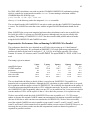
Representative Performance Data on Running GAMESSPLUS in Parallel ...................................... 82
GAMESSPLUS Test Suite ..................................................................................................................... 83
Description of Test Suite for EEQM ............................................................................................................. 83
Description of Test Suite for INTFRZ .......................................................................................................... 83
Description of Test Suite for QM/MM .......................................................................................................... 84
Short Tutorial for Making AMBER Parameter/Topology and Coordinate Files..................................... 84
Description of Test Suite for CM2, CM3, CM4, CM4M, SM5.42, SM5.43, SM6, SM8, and SM8T ....... 89
Subset A and Subset B .................................................................................................................................................. 89
Subset C ........................................................................................................................................................................ 91
Subset D ........................................................................................................................................................................ 92
Subset E ........................................................................................................................................................................ 93
Subset F ........................................................................................................................................................................ 93
Verifying Installation of GAMESSPLUS Using Test Suite Results .................................................... 94
GAMESSPLUS Revision History and Version Summaries ................................................................. 94
APPENDIX I: GAMESSPLUS Solubility Utility ............................................................................... 110
Executive summary..................................................................................................................................................... 110
The SM5.42 and SM5.43 continuum solvation models .............................................................................................. 110
Usage .......................................................................................................................................................................... 111
Input specific to the GAMESSPLUS solubility utility................................................................................................. 113
Input options specific to the $VAPOR namelist ......................................................................................................... 114
Test calculations ......................................................................................................................................................... 115
Input ............................................................................................................................................................................ 115
Output ......................................................................................................................................................................... 116
Installing and running the solubility utility program .................................................................................................. 117
APPENDIX II: GAMESSPLUS Soil Sorption Utility........................................................................ 118
Executive summary..................................................................................................................................................... 118
Solvent descriptors for bulk soil ................................................................................................................................. 119
Usage .......................................................................................................................................................................... 120
Test calculations ......................................................................................................................................................... 120
4
Input ............................................................................................................................................................................ 121
Output ......................................................................................................................................................................... 124
Installing and running the soil sorption utility program .............................................................................................. 126
5
Executive Summary
GAMESSPLUS is a module that currently incorporates the following methods into GAMESS:
• Löwdin population analysis
• redistributed Löwdin population analysis (RLPA)
• CM2, CM3, CM4, and CM4M charge models
• SMx (x = 5.42, 5.43, 6, 8, 8AD) solvation models
• SM8 with temperature dependence (SM8T)
• electrostatically embedded quantum mechanical (EEQM) energy and its first and second
derivatives with respect to coordinates and electrostatic potentials with a site–site
representation of the QM−MM electrostatic interaction
• QM/MM geometry optimization with a site–site representation of the QM−MM
electrostatic interaction
• internal-coordinate-constrained geometry optimization in Cartesian coordinates by
projection operator method
• combined quantum mechanics and molecular mechanics (QM/MM) with the generalized
hybrid orbital (GHO) boundary treatment
The current version of GAMESSPLUS (version 2010-2) has been developed to work with the
latest (R1) revision of GAMESS (version of April 11, 2008).
The SMx solvation models are based on the generalized Born method for electrostatics augmented with
semiempirical surface tensions for non-bulk electrostatics. These models can calculate free energies of
solvation using gas-phase geometries, as well as carry out geometry optimization in the liquid phase
using analytical gradients.
The EEQM energy calculations with a site–site representation of the QM−MM electrostatic interaction
enable one to calculate the electronic energy in the presence of an external electrostatic potential such
as the electrostatic potential from a solvent or a molecular mechanics region. In these calculations, the
external electrostatic potential distribution is described as the collection of the values of the external
electrostatic potential at the locations of the QM nuclei. The first and second derivatives of the EEQM
energy with respect to coordinates and external electrostatic potentials can be calculated.
GAMESSPLUS can carry out QM/MM geometry optimization with a site–site representation of the
QM−MM electrostatic interaction. The QM/MM geometry optimization routine in GAMESSPLUS was
originally developed by Hayashi and Ohmine (ref. HO00) and modified by Higashi and Truhlar (refs.
HT08 and HT09). The AMBER force field is used for the MM subsystem. For the QM−MM
electrostatic interaction around the QM−MM boundary, advanced algorithms such as the balanced
redistributed-charge algorithm are available.
GAMESSPLUS can also perform constrained geometry optimization in Cartesian coordinates by a
projection operator method. The current version of GAMESSPLUS can constrain bond lengths, the
sums or differences of bond lengths, bond angles, and torsional angles.
To use GAMESSPLUS, the user needs to obtain the GAMESS package from Iowa State
University (April 11, 2008 R1 version of GAMESS) and GAMESSPLUS (version 2010-2) from the
University of Minnesota. For QM/MM calculations with a site–site representation of the
6
electrostatic potential, the user also needs to obtain AmberTools (we used version 1.3) from the
Amber Home Page (http://ambermd.org/) in order to make parameter/topology and coordinate
files of the total QM/MM system. (This is done in a separate run, and the output is then used to make
input for GAMESSPLUS.) The GHO QM/MM method is available by means of a
CHARMM/GAMESSPLUS combination package for treating the QM subsystem at the ab initio
Hartree-Fock level. The GHO analytical gradients are also available for QM/MM geometry
optimizations. The compilation of the CHARMM/GAMESSPLUS combination package as an integrated
executable is supported by a utility package called CGPLUS, which is available
at http://comp.chem.umn.edu/cgplus. The usage of the CHARMM/GAMESSPLUS combination
package for carrying out GHO-AIHF calculations is covered in the CGPLUS manual (see the
CGPLUS-v2008 User Manual). CGPLUS also provides a separate test suite for testing the GHO-AIHF
functionality of the CHARMM/GAMESSPLUS combination package. To perform GHO QM/MM
calculations, the user needs to obtain GAMESS from Iowa State University (April 11, 2008 R1
version of GAMESS), GAMESSPLUS from the University of Minnesota, and CHARMM from
Harvard University.
H0
In order to make the following description of some of the capabilities of GAMESSPLUS more clear,
we note that the following basis sets use Cartesian d functions:
MIDI!6D (also known as MIDIX6D)
6-31G(d)
6-31+G(d)
6-31+G(d,p)
6-31G(d,p)
DZVP
and the following basis sets use spherical harmonic d functions:
MIDI! (also known as MIDI!5D and MIDIX5D)
cc-pVDZ
GAMESSPLUS adds the following new capabilities to GAMESS:
•
The B3LYP hybrid density functional theory method, as it is implemented in Gaussian and
HONDOPLUS (i.e., using version III of the VWN correlation functional) has been added. This
method can be used to obtain restricted and unrestricted wave functions and is requested with the
DFTTYP=B3LYP3 keyword in the $DFT data group; see the section entitled Notes on
GAMESSPLUS input below. (The DFTTYP=B3LYP5 keyword uses version V of the VWN
functional, which is the non-standard form of the VWN functional).
•
The MPWX, where X is the percentage of Hartree-Fock exchange, hybrid density functional theory
method. This method can be used to obtain restricted and unrestricted wave functions and is
requested with the DFTTYP=MPWX keyword in the $DFT data group; see the section entitled
Notes on GAMESSPLUS input below.
•
For all restricted and unrestricted HF, DFT, and hybrid DFT methods using basis sets containing
functions up to f in angular momentum, gas-phase and liquid-phase Löwdin partial atomic charges
(Class II charges) can be calculated. For calculations using the 6-31+G(d) and 6-31+G(d,p) basis
7
sets, gas-phase and liquid-phase redistributed Löwdin population analysis (RLPA) partial atomic
charges can be calculated for all restricted and unrestricted HF, DFT, and hybrid DFT methods
available in GAMESS.
•
Gas-phase and liquid-phase CM2 class IV charges can be determined for the following
combinations of electronic structure theory and basis set (using either a restricted or an unrestricted
formalism):
AM1
PM3
HF/MIDI!
B3LYP/MIDI!
HF/MIDI!6D
BPW91/6-31G(d)
HF/6-31G(d)
HF/6-31+G(d)
BPW91/MIDI!
HF/cc-pVDZ
BPW91/MIDI!6D
BPW91/DZVP
•
Gas-phase and liquid-phase CM3 class IV charges can be determined for the following
combinations of electronic structure theory and basis set (using either a restricted or an unrestricted
formalism):
AM1
PM3
HF/MIDI!6D
HF/6-31G(d)
MPWX/MIDI!
MPWX/MIDI!6D
MPWX/6-31G(d)
MPWX/6-31+G(d)
MPWX/6-31+G(d,p)
BLYP/6-31G(d)
B3LYP/MIDI!6D
B3LYP/6-31G(d)
B3LYP/6-31+G(d)
MPWX is a method that uses the mPW exchange functional of Adamo and Barone (Adamo, C.;
Barone, V. J. Chem. Phys. 1998, 108, 664), the PW91 correlation functional (Perdew, J. P. Electronic
Structure of Solids '91; Zieesche, P., Eshrig, H., Eds.; Akademie: Berlin, 1991) and a percentage of HF
exchange, X. Note that MPWX includes the following special cases:
MPW0 ≡ mPWPW91
MPW6 ≡ MPW1S
MPW25 ≡ mPW1PW91
MPW42.8 ≡ MPW1K
MPW60.6 ≡ MPW1KK
For all of the MPWX methods listed above, CM3 has been parameterized for five specific values of X,
namely 0, 25, 42.8, 60.6, and 99.9, and these parameter sets are available in MN-GSM. Every CM3 and
CM4 parameter is a linear or a quadratic function of the percentage of HF exchange used in the mPW
exchange functional. So, in addition to the specific CM3 and CM4 parameter sets (i.e. when X in
MPWX is 0, 25, 42.8, 60.6, and 99) the CM3 and CM4 Charge Models are available for any value of X
in MPWX between 0.0 and 100.0. Note that the CM3 and CM4 parameters were optimized using a
corrected version of the modified Perdew-Wang density functional as implemented in Gaussian. The
details of this correction are described fully in “The Effectiveness of Diffuse Basis Functions for
Calculating Relative Energies by Density Functional Theory” by Lynch, B. J.; Zhao, Y.; Truhlar, D. G.
J. Phys. Chem. A, 2003, 107, 1384.
8
The CM3 model for the BLYP and B3LYP methods uses a slightly modified mapping scheme for
compounds that contain N and O. For more information, see “Parameterization of Charge Model 3 For
AM1, PM3, BLYP, and B3LYP” by Thompson, J. D.; Cramer, C. J.; Truhlar, D. G. J. Comput. Chem.,
2003, 24, 1291. We have also developed a special CM3 model for assigning partial atomic charges to
high-energy materials. This model is called CM3.1, and it uses the same mapping scheme as the CM3
model for BLYP and B3LYP. This model has been parameterized for use with HF/MIDI!, and is
described in “Accurate Partial Atomic Charges for High-Energy Molecules with the MIDI! Basis Set”
by Kelly, C. P.; Cramer, C. J.; Truhlar, D. G. Theor. Chem. Acc., 2005, 113, 133.
• Gas-phase and liquid-phase CM4 class IV charges can be determined for the following
combinations of electronic structure theory and basis set (using either a restricted or an unrestricted
formalism):
BLYP/MIDI!6D
BLYP/6-31+G(d)
BLYP/6-31G(d)
BLYP/6-31+G(d,p)
G96LYP/MIDI!6D
G96LYP/6-31+G(d)
G96LYP/6-31G(d)
G96LYP/6-31+G(d,p)
B3LYP/MIDI!6D
B3LYP/6-31+G(d)
B3LYP/6-31G(d)
B3LYP/6-31+G(d,p)
MPWX/MIDI!
MPWX/MIDI!6D
MPWX/6-31G(d)
MPWX/6-31+G(d)
MPWX/6-31G(d,p)
MPWX/6-31+G(d,p)
MPWX/cc-pVDZ
MPWX/DZVP
MPWX/6-31B(d)
MPWX/6-31B(d,p)
• The CM4M charge model is an extension of the earlier CM4 model. The CM4M model was
individually optimized for the M06 suite of density functionals (namely, M06-L, M06, M06-2X,
and M06-HF) for eleven basis sets which are MIDI!, MIDI!6D, 6-31G(d), 6-31+G(d), 6-31+G(d,p),
6-31G(d,p), cc-pVDZ, DZVP, 6-31B(d), and 6-31B(d,p).
• Calculation of the solvent-accessible surface areas (SASAs) of the atoms of a given solute. The
SASA is that defined by Lee and Richards (see Lee, B.; Richards, F. M. Mol. Biol. 1971, 55, 379.)
and Hermann (see Hermann, R. B. J. Phys. Chem. 1972, 76, 2754.). In this definition, the solvent is
taken to be a sphere of radius rS and the solute is represented by a set of atom-centered spheres of a
given set of radii. By default, the van der Waals radii of Bondi are used when defined; in cases
where the atomic radius is not given in Bondi’s paper (Bondi, A. J. Phys. Chem. 1964, 68, 441) a
radius of 2.0 Å is used. The SASA is the area generated by rolling the spherical solvent molecule on
the van der Waals surface of the molecule. The SASA is calculated with the Analytic Surface Area
(ASA) algorithm (see Liotard, D. A.; Hawkins, G. D.; Lynch, G. C.; Cramer, C. J.; Truhlar, D. G. J.
Comput. Chem. 1995, 16, 422. By default, the solvent radius is set to 0.40 Å (see Thompson, J. D.;
Cramer, C. J.; Truhlar, D. G. J. Phys. Chem. A 2004, 108, 6532 for a justification of this value for
the solvent radius), but the user can specify a different value for the solvent radius (including zero,
which yields the van der Waal’s surface area) with the keyword “SolvRd”. A solvent radius of 0.0 Å
is recommended for predicting solvation free energies with SM5.42, while the default value of 0.40
Å is recommended for predicting solvation free energies with SM5.43, SM6, SM8, and SM8AD.
See the section entitled GAMESSPLUS Keywords for more details.
9
• Liquid-phase calculations based on gas-phase geometries can be performed with SM5.42 for the
following restricted and unrestricted Hartree-Fock, DFT, and adiabatic-connection-method wave
functions (i.e. hybrid DFT wave functions) that employ spherical harmonic or Cartesian d functions:
HF/MIDI!
HF/MIDI!6D
HF/6-31G(d)
BPW91/MIDI!
BPW91/MIDI!6D
B3LYP/MIDI!
BPW91/6-31G(d)
HF/6-31+G(d)
HF/cc-pVDZ
BPW91/DZVP
• Liquid-phase calculations based on gas-phase geometries can be performed with SM5.43 for the
following restricted and unrestricted Hartree-Fock, DFT, and adiabatic-connection-method wave
functions (i.e. hybrid DFT wave functions) that employ spherical harmonic or Cartesian d functions:
HF/6-31G(d)
MPWX/MIDI!
MPWX/6-31G(d)
MPWX/6-31+G(d,p)
•
B3LYP/6-31G(d)
MPWX/MIDI!6D
MPWX/6-31+G(d)
Liquid-phase calculations based on gas-phase geometries can be performed with SM6 for the
following restricted and unrestricted DFT and adiabatic-connection-method wave functions (the
four basis sets for which SM6 is parameterized use Cartesian d functions):
BLYP/MIDI!6D
BLYP/6-31G(d)
G96LYP/MIDI!6D
G96LYP/6-31G(d)
B3LYP/MIDI!6D
B3LYP/6-31G(d)
MPWX/MIDI!6D
MPWX/6-31G(d)
BLYP/6-31+G(d)
BLYP/6-31+G(d,p)
G96LYP/6-31+G(d)
G96LYP/6-31+G(d,p)
B3LYP/6-31+G(d)
B3LYP/6-31+G(d,p)
MPWX/6-31+G(d)
MPWX/6-31+G(d,p)
•
Liquid-phase calculations based on gas-phase geometries can be performed with SM8 or SM8AD
and any choice of electronic structure method and basis set combination for which CM4 or CM4M
charges can be calculated. The CM4M charge model is recommended for use with the M06 suite of
density functionals (M06, M06-HF, M06-L, M06-2X).
•
Liquid-phase analytical gradients for SM6, SM8, and SM8AD are available for basis sets that use
Cartesian d shells.
•
Note that the B3LYP options in the lists above should use the standard version III VWN
functional, which is requested with the ‘DFTTYP=B3LYP3’ keyword in data group $DFT.
•
Löwdin population analysis partial atomic charges can be used in conjunction with the generalized
Born method to calculate the electrostatic contribution to the free energy of solvation using HF,
DFT, and hybrid DFT and basis sets containing s, p, d, and f functions. For basis sets involving
10
Cartesian d and f functions, analytic gradients of the generalized Born free energy are available,
and they can be used for geometry optimizations and numerical Hessian and vibrational frequency
calculations.
•
Redistributed Löwdin population analysis charges can be used in conjunction with the generalized
Born method to calculate the electrostatic contribution to the free energy of solvation using HF,
DFT, and hybrid DFT and the 6-31G(d) and 6-31+G(d,p) basis sets. Analytic gradients of the
generalized Born free energy are available, and they can be used for geometry optimizations and
numerical Hessian and vibrational frequency calculations (by numerical differentiation of
analytically calculated gradients).
•
CM2, CM3, and CM4 (CM4M) charges can be used in conjunction with the generalized Born
method to calculate the electrostatic contribution to the free energy of solvation using any of the
CM2, CM3, and CM4 (CM4M) methods detailed above. Liquid-phase geometry optimizations and
Hessian and vibrational frequency analysis calculations are available for the CM2, CM3, and CM4
(CM4M) methods for which analytical gradients of the generalized Born solvation energy are
available.
•
The necessary modification of NDDO Hamiltonians to carry out AM1-SRP and PM3-SRP
calculations has been implemented.
•
GAMESSPLUS includes the GAMESSPLUS solubility utility for calculating the solubility of a
given solute A in a given solvent B. This utility is described in a self-contained section of this
manual. Therefore users who only want to calculate solubilities do not need to be familiar with the
entire GAMESSPLUS manual.
•
GAMESSPLUS includes the GAMESSPLUS soil sorption utility for calculating the soil sorption
coefficients. This utility is described in a self-contained section of this manual. Therefore users
who only want to calculate soil sorption coefficients do not need to be familiar with the entire
GAMESSPLUS manual.
•
GAMESSPLUS can now be used for GHO QM/MM calculations with the CHARMM package
through the CHARMM/GAMESSPLUS interface for QM/MM calculations. GHO QM/MM
calculations are combined QM/MM calculations with the QM/MM boundary treated by the
generalized hybrid orbital (GHO) method at the ab initio HF level (GHO-AIHF). A parametrized
version of GHO-AIHF is available for the MIDI! basis set.
•
The QM energy can be calculated in the presence of an external electrostatic potential with a site–
site representation of the QM−MM electrostatic interaction energy. The first and second derivatives
with respect to coordinates and electrostatic potentials are available. Note that when the
electrostatic potential of the MM subsystem is treated with a site–site representation, if there is a
QM−MM boundary that passes through a covalent bond, the link atom method is used. (The option
for QM/MM calculations with a site–site interaction should not be confused with the option for
GHO QM/MM calculations.)
•
QM/MM energy calculations and geometry optimization can be performed whereby the QM−MM
electrostatic interaction is treated by a site–site representation and the AMBER force field is used
11
as the MM potential energy function. Whereas the MM potential energy terms and their derivatives
are evaluated by CHARMM when one uses the GHO QM/MM option (and therefore one must link
to CHARMM), these terms are evaluated by routines in the eeqmmm.src file of GAMESSPLUS
when one carries out QM/MM calcuations with a site–site represenatation of the electrostatics.
Therefore one does not need to add a separate program for calculating the MM terms. However,
this part of the code does use AmberTools to read the MM input in Amber format.
•
GAMESSPLUS can carry out the geometry optimization in Cartesian coordinates but with
constraints expressed in internal coordinates. The user can enforce constraints on bond lengths,
sums or differences of bond lengths, bond angles, and torsional angles.
12
Extended Abstract
Löwdin Population Analysis and Redistributed Löwdin Population Analysis
Löwdin population analysis, like Mulliken analysis, provides class II atomic partial charges, but the
Löwdin method has certain advantages. It has been implemented in GAMESSPLUS because Löwdin
population analysis charges are used for obtaining CM2, CM3, CM4, and CM4M charges. However,
there may be some independent interest in Löwdin analysis since it can be used with any basis set
(whereas CM2, CM3, CM4, and CM4M are defined only for selected basis sets), and Löwdin analysis
will usually yield more useful population analyses than Mulliken’s method. Note that Löwdin and
Mulliken charges are identical for AM1 and PM3 because overlap is neglected in these methods.
Partial atomic charges obtained from Löwdin population analysis can, however, be sensitive to basis
set size, particularly for extended basis sets that include diffuse functions. We have developed and
implemented a new method, called redistributed Löwdin population analysis (or RLPA), which
alleviates some of this sensitivity to basis set size. For methods using diffuse basis sets 6-31+G(d) and
6-31+G(d,p), RLPA charges are used for obtaining CM3 and CM4 charges.
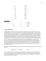
Charge Models Based on Class IV Charges: CM2, CM3, CM4, and CM4M
Class IV charges have the following advantages over class III charge models (e.g., ChElPG and MerzKollman algorithms):
•
Class III charges are unreliable for buried charges (this problem is widely recognized, as discussed
in work by Kollman and Francl and their respective coworkers). Class IV charge models provide a
practical and stable way to obtain reasonable charges for buried atoms.
•
Class III charges are at best as good as the basis set and wave function used, whereas class IV
charges represent extrapolation to full CI with a complete basis.
Class IV charges are useful for any purpose for which ChElPG or Merz-Kollman charges are useful,
but we believe that they are better.
Charge Model 2 (CM2), Charge Model 3 (CM3), and Charge Model 4 (CM4) are our second-, third-,
and fourth-generation models of class IV charges, respectively. The CM4M charge model is an
extension of the CM4 model. Charge Model 3 has been parameterized with a larger training set than
CM2 (398 data vs. 198 data), and it is available for different combinations of electronic structure
theory and basis sets than CM2. Furthermore, it is parameterized for Li and for molecules that contain
Si-O, Si-F, and Si-Cl bonds (CM2 is not). Charge Model 4 has been parametrized against the same
training set that CM3 was, except that CM4 gives improved charges for aliphatic functional groups,
which is important for modeling hydrophobic effects. The CM4M model was individually optimized
for the M06 suite of density functionals (see details in Olson, R. M.; Marenich, A. V.; Cramer, C. J.;
Truhlar, D. G. “Charge Model 4 and intramolecular charge polarization,” J. Chem. Theory Comput.
2007, 3, 2046).
13
SM5.42, SM5.43, SM6, SM8, SM8AD, and SM8T Solvation Models
SM5.42, our earliest ab initio solvation model implemented in GAMESSPLUS, is a universal solvation
model based on SM5 functional forms for atomic surface tensions (hence the first three characters in
the name of the method are SM5), built on class IV point charges (hence .4 comes next) of the CM2
type (hence 2). A more recent model, called SM5.43, uses the same functional forms for atomic
surface tensions as does SM5.42, but SM5.43 uses CM3 charges (hence the 3 in the name). The SM6
model is based on SM6 functional forms for atomic surface tensions and uses class IV CM4 point
charges. The SM6 model has only been parametrized for aqueous solvent.
The SM8 and SM8AD are the most recent universal continuum solvation models where "universal"
denotes applicable to all solvents (see MO07 for more details). With universal models, if desired, one
can calculate solvation free energies for two different solvents (e.g., water and 1-octanol) and use the
results to calculate log P, where P is the partition coefficient. SM8/SM8AD is applicable to any
charged or uncharged solute composed of H, C, N, O, F, Si, P, S, Cl, and/or Br in any solvent or liquid
medium for which a few key descriptors are known, in particular dielectric constant, refractive index,
bulk surface tension, and acidity and basicity parameters. It may be used with any level of electronic
structure theory as long as accurate partial charges can be computed for that level of theory; we
recommend using it with self-consistently polarized Charge Model 4 or other self-consistently
polarized class IV charges, in which case analytic gradients are available. The cavities for the bulk
electrostatics calculation are defined by superpositions of nuclear-centered spheres whose sizes are
determined by intrinsic atomic Coulomb radii. The difference between SM8 and SM8AD is that the
SM8 model uses the formula of Still et al. for the Born radius used in the generalized Born
approximation for bulk electrostatics while the SM8AD model utilizes the asymmetric descreening
(AD) algorithm for the Born radius suggested by Grycuk. See MC09 for more detail.
The SM8T solvation model is an extension of SM8 to include the temperature dependence of the free
energy of solvation relative to 298 K. The SM8T model models the temperature dependence of the
solvation free energy using the same functional forms as those in SM8, but with additional terms added
to account for temperature dependence (thus, a calculation carried out at 298 K with the SM8T model
will yield the same solvation free energy as the same calculation carried out with SM8). The SM8T
model has only been parametrized for aqueous solution.
There was also the SM7 model. The SM7 model is an intermediate model between SM6 and SM8.
Like in the case of SM5.42 and SM5.43, the non-bulk electrostatic part of the SM7 model was
parametrized to predict solvation free energies in both aqueous and nonaqueous solutions. Unlike
SM5.42 and SM5.43, the SM7 model is based on SM6 functional forms for atomic surface tensions
and uses class IV CM4 point charges as well as the SM6 model. However, the electrostatic part of the
SM7 model is based on the SM6 model’s Coulomb radii, which were optimized for aqueous solution
only. In the new model called SM8, the radii depend on the nature of a solvent. This feature of the
SM8 model makes it more accurate than SM7 when there is a need to calculate solvation energies in
nonaqueous solutions. Thus, we skip the SM7 model hereafter.
There was also the SM6T model. The SM6T model is an extension of SM6 to include the temperature
dependence of the free energy of solvation relative to 298 K. When the SM8 model came into
existence, the old temperature-dependent terms from SM6T were augmented with a few new ones and
the SM8T merged the SM6T. Since the SM8T model has some additional functionalities, we opt to
skip the more inferior SM6T model hereafter.
14
The SMx solvation models provide a way to calculate electronic wave functions in liquid-phase
solution and free energies of solvation. For solvation calculations based on gas-phase geometries, the
standard-state free energy of solvation ∆GSo (R ) is given by two components:
∆GSo (R ) = ∆GEP + GCDS
(1)
∆GEP = ∆EE + GP
(2)
where
In equations (1) and (2), ∆GEP is the bulk electrostatic component of the solvation free energy; it is the
sum of the polarization energy GP (representing favorable solute-solvent interactions and the
associated solvent rearrangement cost) and the distortion energy ∆EE (the cost of distorting the solute
electronic charge distribution to be self-consistent with the solvent electric polarization). GCDS
accounts for first-solvation-shell effects.
∆GEP is determined by a self-consistent reaction field (SCRF) calculation, which allows the solventinduced change in the solute electronic wave function to be optimized variationally. GCDS is not a selfconsistent term; it has no effect on the solute electronic wave function. In its simplest form GCDS is
defined as:
GCDS = ∑ Ak σ k
k
(3)
where Ak is the exposed surface area of atom k (this depends on the solute’s 3-D geometry and is
calculated by the Analytical Surface Area (ASA) algorithm as described in reference LH95 and as
included in recent versions of AMSOL, and σk is the atomic surface tension of atom k. The atomic
surface tension σk is itself a function of the solute’s 3-D geometry and a small set of solvent
descriptors. References LH98, ZL98, and LZ99 present a more expanded form of GCDS than what
appears in equation (3).
The surface tension functional forms are the same in all SM5.42 and SM5.43 models. SM6 and SM8
use a different set of functional forms. The SM6 and SM8 functional forms are better for most
purposes than those used in SM1–SM5.
Allowed combinations of solvent model, electronic structure theory, and basis set are described
using keywords ICMD and ICDS (see the section entitled Notes on GAMESSPLUS input below). The
SM5.42 and SM5.43 models have been parametrized for a few combinations of the methods and they
should be applied with these combinations. The SM6 model has been tested against several different
density functionals, and has been shown to retain its accuracy when different density functionals
besides MPWX (the method against which the CM4 and SM6 parameters were originally developed).
Thus, the SM6 model is only basis-set-dependent, and can be used with any good density functional.
There is a single set of the SM8 parameters (radii and CDS terms) that can be used with any basis set
as long as accurate partial charges can be computed for that basis set. The SM8T model is applicable to
15
the same combinations of theory and basis set as SM8, but it has been parametrized only for aqueous
solution. A list of density functionals that are available in GAMESSPLUS and that are recommended
for use with SM6 and SM8 is in the section entitled “Density Functionals Recommended for use with
CM4/CM4M and SM6/SM8 in GAMESSPLUS”.
Incorporating temperature dependence into the SMx models: SM8T
To account for the variation of the free energy of solvation as a function of temperature, the
temperature dependence of both the bulk electrostatic, ΔGEP, and the non-bulk electrostatic, ΔGCDS,
contributions are included. The effect of temperature on the bulk-electrostatic contributions to the free
energy of solvation is accounted for using a temperature dependent dielectric constant, ε (T ) which was
computed using the following equation
(4)
ε(T)=249.21-.79T+.00072T 2
where T is the temperature of the aqueous solvent. This is a empirically derived equation found in the
CRC Handbook of Chemistry and Physics 76th edition, ed. Lide, D. R., 1995, CRC Press, New York.
The variation of the free energy of solvation due bulk electrostatic contributions is quite small. The
majority of the temperature dependence of aqueous free energies of solvation must by accounted for
using ΔGCDS.
In SM8T the ΔGCDS term mimics the thermodynamic equation for the temperature dependence of free
energies of solvation where the thermodynamic properties, the heat capacity and the entropy of
solvation, have been replaced parameterized atomic surface tensions:
T 

C
GCDS (T ) = (T − 298)∑ Ak σ kB +  T − 298 − T ln
∑ Ak σ k
(5)
298  k

k
where σ kB and σ kC are atomic surface tensions with identical functional forms to those of σk, but the
parameters are different. Caution should be used in assigning any physical meaning to the atomic
surface tensions shown above. While the sum
∑ Ak σ kB appears to be the solute’s entropy of solvation
k
and the sum
∑
Ak σ kC
appears to be the solute’s heat capacity, it must be pointed out that some of the
k
temperature dependence of the free energy of solvation has been accounted for in the electrostatic
term. Additionally the covariance between the two terms in the above equation and the relatively small
number of points for each compound (on average 10 points were used) means that the actual numerical
values of these two terms may vary significantly from experimental entropies and heat capacities of
solvation while still reproducing experimental values with high accuracy. Note that the model has only
been developed for solutes in aqueous solutions for the temperature 273.15 to 373.15 K.
A comment on using gas-phase geometries to calculate solvation free energies
For SM1–4 and SM5.4, geometry optimization in solution was an essential part of the
parameterization. SM5.42, SM5.43, SM6, SM8, and SM8AD are parameterized in such a way that one
16
fixes the geometry at a reasonable value (any reasonably accurate gas-phase geometry should be
acceptable) and calculates the solvation energy without changing the geometry. Thus, geometry
optimization in the presence of solvent is not required to obtain accurate solvation free energies. This
method of obtaining solvation parameters based on gas-phase geometries was adopted for several
reasons. First, previous experience has shown that the difference one gets from re-optimizing the
geometry in the presence of solvent in almost all cases is small – less than the average uncertainty in
the method or in any competing method. Second, for many solutes, less expensive (e.g. semiempirical
or molecular mechanics methods) can yield accurate gas-phase geometries. Third, for other solutes,
such as transition states, solutes with low-barrier torsions, multiple low-energy conformations, weakly
bound complexes, and in cases where one or more solvent molecules are treated explicitly, more
expensive levels of theory might be needed to yield accurate geometries. Finally, solvation energies
obtained using gas-phase geometries can be added conveniently to gas-phase energies for separableequilibrium-solvation dynamics calculations.
In some cases, geometry optimization in the presence of solvent is important. In these cases, one can
also apply the SM5.42, SM5.43, SM6, SM8 or SM8AD models at a solute geometry R that is not an
approximation to an equilibrium gas-phase geometry. This type of calculation corresponds to the fixedR solvation energy, which is still given by ∆GSo (R ) of equation (1). Evaluation of this quantity for
geometries that do not correspond to an equilibrium structure is useful for dynamics calculations
because the potential of mean force is given by
W (R ) = V (R ) + ∆GSo (R )
(6)
where VI is the gas-phase potential energy surface (which is itself given by the sum of the gas-phase
electronic energy and the gas-phase nuclear repulsion energy). If one applies the SM5.42, SM5.43,
SM6, or SM8 models to a geometry optimized in solution and subtracts the gas-phase energy at a
geometry optimized for the gas phase, one obtains the true solvation energy for the given method.
Furthermore ∆GSo (R ) depends on standard state choices; the values given directly by the SM5, SM6,
and SM8 models correspond to using the same molar density (e.g., one mole per liter) in the gas phase
and in the liquid-phase solution. Furthermore the liquid-solution standard state corresponds to an ideal
dilute solution at that concentration. However, one may adjust the results to correspond to other
choices of standard state by standard thermodynamic formulae. Note that changing the standard state
corresponds to adding a constant to WI; thus the gradient of WI, which is used for dynamics, is not
affected.
Why use SM5.42, SM5.43, SM6, SM8 or SM8AD?
•
•
The semiempirical CDS terms make the above models more accurate than alternative models for
absolute free energies of solvation of neutral solutes.
SM5.42, SM5.43, SM8, and SM8AD are universal models, i.e., the semiempirical parameters are
adjusted for water and for all solvents for which a small number of required solvent descriptors are
known or can be estimated; this includes essentially any organic solvent.
17
•
•
•
SM5.42, SM5.43, SM6, SM8, and SM8AD use class IV charges to calculate the bulk electrostatic
contribution to the solvation free energy; this is typically more accurate than calculating the charge
distribution directly from the approximate wave function. This has two consequences:
(1) The electrostatic contributions to the solvation free energy are estimated more
realistically.
(2) CM2, CM3, and CM4 yield very accurate charges both in the gas phase and in liquidphase solutions, and this is useful for a qualitative understanding of solvent-induced
changes in the solute. (We should note here that partial atomic charges are not physical
observables, but they can still be considered accurate within a given model context if
they vary physically with molecular geometry and environment and can be used to
accurately reproduce observables such as dipole moments or if they can be derived
consistently and realistically from accurate experimental data, for instance, from the
dipole moment of a diatomic molecule.)
SM5, SM6, SM8, and SM8AD parameterizations included an extremely broad range of solute
functional groups, including molecules containing phosphorus, which are very hard to treat.
SMx do not need to be corrected for outlying charge error, which can be large in some other
methods.
Furthermore, our most recent models, SM8 and SM8AD, have several advantages compared to earlier
solvent models (e.g. SM5.42, SM5.43, or SM6) developed within our group:
•
•
•
•
SM8 can be used with any of the density functional methods supported in GAMESSPLUS.
SM8 significantly outperforms SM5.42, SM5.43, and all other competing continuum solvation
models against which it has been tested (prior to SMVLE) for predicting aqueous solvation free
energies of ions. This is important because aqueous solvation free energies of ions can be used in
various thermodynamic cycles to calculate pKa.
SM8 and SM8AD use an improved set of surface tension functionals; using this new set of surface
tension functionals significantly improves the performance of the model for molecules containing
peroxide functional groups.
SM8 and SM8AD use class IV CM4 or CM4M charges, which give more realistic partial atomic
charges for aliphatic groups than our previous class IV models; this is important for accurately
modeling hydrophobic effects.
Analytical gradients and geometry optimization in liquid-phase solutions
Analytical gradients for liquid-phase calculations have been implemented in GAMESSPLUS beginning
with version 2.0. In particular, GAMESSPLUS contains analytical gradients for restricted and
unrestricted wave functions for basis sets with Cartesian d shells. However, analytical gradients are not
available for basis sets with spherical harmonic d functions (e.g., for HF/MIDI!, HF/cc-pVDZ), and
methods using basis sets containing functions higher in angular momentum than f. Analytical gradients
are also available when the AM1 and PM3 or method is used.
The availability of gradients allows for efficient geometry optimization in liquid-phase solution. This is
necessary in many cases. For example, the transition state geometry for the SN2 reaction of ammonia
and chloromethane (the Menschutkin reaction) depends strongly on solvent. Other applications include
18
the study of phase-dependent reaction mechanisms and solvent-dependent molecular conformational
preferences.
A full derivation of the analytical gradient is presented in the paper by T. Zhu et al. entitled
“Analytical Gradients of a Self-Consistent Reaction-Field Solvation Model Based on CM2 Atomic
Charges” (J. Chem. Phys. 1999, 110, 5503-5513).
Notation for Solvation Models
1.
Geometry optimized at level X/Y in the gas phase, followed by a single-point SMx solvation
calculation at level W/Z, where W/Z is one of the choices supported by ICMD:
SMx/W/Z//X/Y
2.
If X/Y is the same as W/Z, then //X/Y may be substituted by //g,, where g denotes gas-phase:
SMx/W/Z//g
Previously, solvation calculations carried out using gas-phase geometries were denoted by
including an “R” suffix after the name of the SMx model. Here, this older notation has been
replaced with the notation above.
3.
For a liquid-phase geometry optimization the //X/Y is dropped, and this calculation is denoted
as follows:
SMx/W/Z
Previously, solvation calculations carried out using liquid-phase geometries were denoted by
dropping the “R” suffix after the name of the SMx model. Here, we drop this suffix for all
solvation calculations and use the notation described above.
Solvent Parameters
Solvent parameters for common organic solvents are tabulated in the Minnesota Solvent Descriptor
Database. The latest version of this database is available at: http://comp.chem.umn.edu/solvation.
1H
NDDO and CM2 Specific Reaction Parameters (SRP) Models
GAMESSPLUS can use specific reaction parameters (i.e., nonstandard parameters optimized for a
specific system or reaction or limited range of systems or reactions) for the NDDO Hamiltonians of the
AM1 and PM3 models in the gas-phase for the CM2/AM1 and CM2/PM3 methods and in the
liquid-phase for the CM2/AM1, CM2/PM3, SM5.42/AM1, and SM5.42/PM3 methods.
AM1 and PM3 calculations in either the gas-phase or liquid-phase may be performed without using the
arithmetic mean rule for the resonance parameters. In standard AM1 and PM3 calculations, the
19
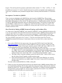
resonance parameter β lxl ′y for interaction of an orbital with angular momentum l on an atom of
element x and an orbital with angular momentum l′ on an atom of element y is given by
(7)
β lxl ′y = ( β lx + β l ′y ) / 2
where βlx and β l ′y are standard parameters. The user can now override eq. (7) by inputting specific
values of the resonance parameter for one or more sets of l, x, l′ and y. A reference for this general
procedure is reference CE95 in the Literature References section.
Solubility Calculations
The solubility of a given solute A, in a liquid solvent, B are calculated using a thermodynamic
relationship between the solubility, free energy of solvation, and pure-substance vapor pressure of
solute A, which is given by:
− ∆GSo

 •

(8)
S =  PA o  exp 
RT 
P




In this equation, S is the solubility of solute A in solvent B, PA• is the equilibrium vapor pressure of
solute A over a pure solution of A, P o is the pressure of an ideal gas for a given standard-state (a 1
molar standard-state at 298 K is used in this calculation for all phases; therefore P o is 24.45 atm),
∆GSo is the standard-state free energy of solvation of solute A in solvent B, R is the universal gas
constant, and T is temperature. Full details are given in the Appendix I of this manual entitled
GAMESSPLUS Solubility Utility.
Soil Sorption Calculations
For a given solute, the soil sorption coefficient ( K OC ) is defined as
C / C
K OC = soil soil

Cw / Cw
(9)
where Csoil is the concentration of solute per gram of carbon in standard soil, C w is the concentration


of solute per volume of aqueous solution, and Csoil
and C w
are the standard state concentrations of
organic carbon for soil and aqueous solution, respectively. Typically, a standard state of 1 µg of


solute/g of organic carbon is used for Csoil
, and 1 mol/L is used for Cw
. K OC may be calculated
according to
(


K OC = ρ soil ∆Gw
− ∆Gsoil
)

where ρs o is the density of soil (in g/mL), ∆Gw
is the standard state free energy associated with

transferring a solute from the gas phase to aqueous solution, and ∆Gsoil
is the standard state free
(10)
20
energy associated with transferring a solute from the gas phase to soil. Full details are given in the
Appendix II of this manual entitled GAMESSPLUS Soil Sorption Utility.
QM/MM Calculations at the Ab Initio HF Level with the GHO Boundary Treatment
GAMESSPLUS can be compiled into a CHARMM/GAMESSPLUS combination package for
calculations that combine ab initio HF wave functions with molecular mechanics. For the QM/MM
partition along a covalent bond, the generalized hybrid orbital (GHO) method is used to provide a
smooth connection between the QM subsystem and the MM subsystem. In the GHO treatment, sp3
carbons are often chosen as GHO boundary atoms, denoted by B. Such a B atom is both a QM atom
and an MM atom. The QM atom bonded to B is called a QM frontier atom, denoted by A. The other
three MM atoms directly bonded to B are denoted by X, Y, and Z. A set of generalized hybrid orbitals
{ηB, ηx, ηy, ηz} is placed on the GHO boundary atom B, where the hybridization scheme is
completely determined by the local geometry of the QM/MM boundary (atoms Q, B, X, Y, and Z).
Among the four hybrid orbitals, one approximately pointing toward A (denoted by ηB) will participate
in the SCF procedure with other QM basis functions and is therefore called an active hybrid orbital.
The remaining three hybrid orbitals {ηx, ηy, ηz} are called auxiliary orbitals, and they are excluded
from the SCF procedure. With this restriction, on one hand, the active molecular orbitals (MOs) in
GHO are only allowed to be expanded over the active basis functions (including ηB). On the other
hand, each auxiliary hybrid orbital forms an auxiliary MO by itself, and it is occupied by a fixed
auxiliary charge density. To distribute the MM point charge on B over the three auxiliary orbitals, the
charge density for each auxiliary orbital is determined as 1 − qB/3.0, where qB denotes the MM point
charge on B.
In GAMESSPLUS, the implementation of GHO at the ab initio HF level (GHO-AIHF) is based on
algorithms described in the paper of J. Pu, J. Gao, and D. G. Truhlar (see Ref. PG04). The major
features of this extension include: (i) The basis set on the GHO boundary B is chosen as an STO-3Gv
set; the 1s core electrons are not explicitly present. (ii) The active basis functions are orthogonalized to
the auxiliary orbitals to maintain the global MO orthonormal constraints. Four orthogonalization
schemes are proposed and implemented. (iii) The GHO gradients are calculated analytically by
incorporating additional forces due to the basis transformations of the GHO scheme. Further details of
the CHARMM/GAMESSPLUS combination package are given in the CGPLUS user manual.
Electrostatically Embedded QM Calculation with a Site–Site Representation of the QM/MM
Electrostatic Interaction
In the electrostatically embedded QM calculations with a site–site representation of the QM/MM
electrostatic interaction, the sum of the QM electronic energy and the QM/MM electrostatic interaction
energy is given by
V EEQM ( RΦ
, )=
Ψ Hˆ 0 +Qˆ TΦ Ψ ,
where R stands for the collection of the coordinates R a
( a = 1, 2,, N ) of atoms in the QM
QM
region, Ψ is the electronic wave function, Ĥ 0 is the electronic Hamiltonian (including nuclear
(11)
21
repulsion) of the QM region, Qˆ a is the population operator that generates the partial charge Qa on QM
atomic site a ,
Qa =
Ψ Qˆ a Ψ ,
(12)
and Φ a is the electrostatic potential at atom a from the MM region. In GAMESSPLUS, one can
choose the operator Qˆ according to Löwdin population analysis (LPA), redistributed Löwdin
a
population analysis (RLPA), Charge Model 2 (CM2), Charge Model 3 (CM3), Charge Model 4 (CM4),
or Charge Model 4M (CM4M). The LPA charge Qa0 (LPA) is given by
(
Qa0 (LPA) = −∑ S 2 P S 2
r∈a
1
1
)
,
(13)
rr
where r is the indices of atomic basis function, S is the overlap matrix, and P is the density matrix.
The RLPA charge Qa0 (RLPA) is given by
(
)
(
)
2
2
,
Qa0 (RLPA)= Qa0 (LPA) + Z aYa ∑ exp −α a Rab
− ∑ Z bYb exp −α b Rab
b≠ a
b≠ a
(14)
where Z a is an empirical parameter, α a is the diffuse orbital exponent on atom a, and Ya is the
Löwdin population that is associated with the diffuse basis functions on atom a,
Ya =
diffuse
∑
r∈a
(S P S )
1
2
1
2
.
(15)
rr
The CMx (x = 2,3,4) charge model is determined from wave-function-dependent charges, the Mayer
bond order, and empirical parameters that are determined to reproduce experimental or converged
theoretical charge-dependent observables:
Qa =
Qa0 + ∑ Bab ( Dab + Cab Bab ) ,
(16)
b≠ a
where Qa0 is the partial atomic charge from either a LPA for nondiffuse basis sets or a RLPA for
diffuse basis sets; Dab and Cab are empirical parameters. Bab is the Mayer bond order between atom
a and b,
Bab = ∑∑ ( PS )rs ( PS ) sr .
(17)
r∈a s∈b
In GAMESSPLUS, one can calculate V EEQM and its first and second derivatives with respect to R and
Φ for given R and Φ . The first derivative of V EEQM with respect to a component of R can be
obtained in a similar way in Ref. ZL99. In addition to terms that appear in the gas-phase calculation,
22
∂Q T
Φ with P fixed at the converged value P (1) , and add it to the first derivative.
∂R
When Q is the LPA charge, the first derivative with respect to R is given by
one has to calculate
1
2
 ∂S 12 (1) 1
 ∂Qa0 (LPA) 
1
(1) ∂S
2
2
P S +S P
−∑ 

 =

∂R c
∂R c
r∈a  ∂R c

P(1)

 .

rr
(18)
1
∂S 2
The method to calculate
is given in Ref. ZL99. When Q is the RLPA charge, the first derivative
∂R c
with respect to R is given by
 ∂Qa0 (RLPA) 
 ∂Qa0 (LPA) 
=




∂R b
∂R c

P(1) 
P(1)
 ∂Y 
2
2
R ac
+ Z a  a  ∑ exp −α a Rab
+ 2 Z aYaα a exp −α a Rac
 ∂R c P(1) b ≠ a
 ∂Y 
2
2
R ac ,
− ∑ Zb  b  exp −α b Rab
− 2 Z cYcα c exp −α c Rac
R
∂
(1)
b≠a
c

P
(
)
(
)
(
)
(
)
(19)
where
 ∂Ya 
=


 ∂R c P(1)
diffuse 
∑
r∈a
1
1
1
∂S 2 (1) 12
∂S 2
P S +S 2 P (1)


∂R c
 ∂R c

 .

rr
(20)
When Q is the CMx charge, the first derivative with respect to R is given by
 ∂Qa0 
 ∂Qa 
 ∂Bab 
=

 + ∑


 ( Dab + 2Cab Bab ) ,
 ∂R c P(1)  ∂R c P(1) b ≠ a  ∂R c P(1)
(21)
where
 ∂Bab 
=


 ∂R c P(1)

∂S 
(1)
 P S
c  rs
∑∑  P(1) ∂R
r∈a s∈b 

(
) + (P S)
(1)
sr
 (1) ∂S  
P
 .
rs
∂R c  sr 

In GAMESSPLUS, the second derivative of V EEQM with respect to R is obtained by numerical
differentiations of the first derivatives.
The first derivative of V EEQM with respect to a component of Φ is given by
(22)
23
∂V EEQM
= Ψ Qˆ a Ψ = Qa .
∂Φ a
(23)
Then the second partial derivatives of V EEQM (first or second order in electrostatic potential) are
∂V EEQM ∂Qa
=
≡ κ ab .
∂Φ a ∂Rb ∂Rb
(24)
∂V EEQM ∂Qa
=
≡ χ ab ,
∂Φ a ∂Φ b ∂Φ b
(25)
and
These variables χ ab and κ ab are known as charge response kernels (CRKs). In GAMESSPLUS, the
CRKs can be obtained by numerical differentiations of the charges.
In GAMESSPLUS, Φ can be given directly (IRDMM=0 in namelist $EEQM) or calculated from the
MM charges Q MM and coordinates R MM , which are read from namelist $MM (IRDMM=1). In the
latter case, Φ is given by
(
Φa Ra , R
MM
)
N MM
QAMM
=
∑ R − R MM ,
A=1
a
A
(26)
where N MM is the number of MM atoms. One can use the TINKER tapering function (see next section)
for the QM−MM electrostatic interactions. Furthermore, Φ can be regarded as a function of R and
R MM (IADDGP=1). In this case, the first derivative of V EEQM with respect to R is given by
dV EEQM ∂V EEQM ∂V EEQM ∂Φ a
=
+
dR a
∂R a
∂Φ a ∂R a
∂Φ a
∂V EEQM
=
+ Qa
,
∂R a
∂R a
(27)
and that with respect to R MM is given by
dV EEQM
∂V EEQM ∂Φ a
=∑
∂Φ a ∂R MM
dR MM
a
A
A
= ∑ Qa
a
∂Φ a
.
∂R MM
A
(28)
24
V EEQM and its first and second derivatives can be used as input for electrostatically embedded
multiconfiguration mechanics calculation.
The TINKER tapering function for long-range electrostatic interactions
In GAMESSPLUS, the TINKER tapering function is available for the QM−MM electrostatic
interactions in the EEQM calculation with IRDMM=1. If the charge-charge electrostatic interaction
energy Vab between atom a and b is sharply truncated at a cutoff distance rcut , namely,
 Qa Qb

Vab ( rab ) =  rab
 0

rab < rcut
,
(29)
rab ≥ rcut
where rab is the distance between atoms a and b, and Qa and Qb are the atomic charges on atom a
and b, Vab is not a continuous function at rab = rcut . In order to make Vab a continuous and
differentiable function, many shifted or switched functions have been developed (see Ref. SB93). In
the TINKER tapering method, the charge-charge electrostatic potential is given by
Qa Qb Qa Qb

−

rab
rc

7
 5
Q Q Q Q 
=
Vab ( rab )  ∑ ck rabk  a b − a b  + Qa Qb ∑ f k rabk
rc 
k 0
=
 rab
 k 0=

0


rab ≤ rtap
rtap < rab < rcut
rcut ≤ rab
(
)
1
rtap + rcut , and
2
and determined to connect Vab at rab = rtap and
where rtap ( < rcut ) is a tapering distance, the beginning of the tapering window,
rc
=
ck and f k are coefficients calculated from rtap and rcut
(30)
rab = rcut smoothly. This potential energy function is continuous and differentiable in the entire range
of rab , and it has continuous second derivatives.
QM/MM Potential Energy Calculation and Geometry Optimization with a Site–Site
Representation of the QM−MM Electrostatic Interaction
In QM/MM methods, the total potential energy V total of a QM/MM system is described as the sum of
three terms:
(
)
(
)
(
)
(
)
V total R, R MM =
V QM R, R MM + V QM/MM R, R MM + V MM R MM ,
(31)
25
where R and R MM stand for the collection of the coordinates R a
( a = 1, 2,, N )
QM
and R MM
A
( A = 1, 2,, N ) of atoms in the QM and MM subsystems, respectively. The first term V
MM
QM
is the
electronic energy of the QM region, and the last term V MM is the MM potential energy. The middle
term V MM is the QM−MM interaction energy and can be separated into three terms:
(
)
(
)
(
)
(
)
QM/MM
QM/MM
QM/MM
V QM/MM R, R MM = Vele
R, R MM + VvdW
R, R MM + Vval
R, R MM ,
(31)
QM/MM
QM/MM
QM/MM
where Vele
, VvdW
and Vval
are the electrostatic, van der Waals, and valence interaction
QM/MM
energies, respectively. In GAMESSPLUS, Vele
is represented by a site–site representation,
(
)
QM/MM
ˆT
Vele
R, R MM
Φ =
ΨQ
Ψ ,
(32)
where Ψ is the electronic wave function of the QM region, Qˆ a is the population operator that
generates the partial charge Qa on QM atomic site a , Φ a is the electrostatic potential at atom a from
the MM region. In GAMESSPLUS, the user can choose the operator Qˆ according to Löwdin
a
population analysis (LPA), redistributed Löwdin population analysis (RLPA), Charge Model 2 (CM2),
Charge Model 3 (CM3), Charge Model 4 (CM4), or Charge Model 4M (CM4M). For the details, see
the section entitled Electrostatically Embedded QM Calculation with a Site–Site Representation of the
QM/MM Electrostatic Interaction.
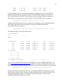
For QM/MM calculations with site–site electrostatics, GAMESSPLUS uses the AMBER force field as
the MM potential energy function. The AMBER force field (ref. CC95) is described as
∑ Kb ( b − beq )
V MM
=
bonds
+
∑
dihedrals
2
+
∑
(
Kθ θ − θ eq
)
2
angles
 A B qq′ 
1 + cos ( nφ − γ )  + ∑  12 − 6 +
2
r 
r
non-bonded  r
Kφ
(33)
pairs
where b, θ , φ , and r are bond length, bond angle, dihedral angle, and distance between non-bonded
atoms, respectively. The other quatities in Eq. (33) are parameters. Note that the user can use any force
field that has the form described in Eq. (33), e.g., TIP3P and OPLS, as the MM potential energy
function. (In this manual, we call the force field described by Eq. (33) the “AMBER force field ” for
simplicity.) There are many versions of the AMBER force field . The AmberTools manual recommends
the ff03 force field (ref. DW03) and ff99SB force field (refs. WC00 and HA06) for proteins. The
default water model in the AmberTools program is TIP3P (ref. JC83). For non-protein molecules, one
can use the general AMBER force field (GAFF, ref. WW04).
GAMESSPLUS reads AMBER parameter/topology and coordinate inputs generated by the AmberTools
program. In the current version of GAMESSPLUS, the link atom method is used when the QM–MM
boundary cuts a covalent bond. The link atoms QL (usually hydrogen or fluorine) are always located
on the Q1-M1 bonds, where Q1 and M1 denote the QM and MM boundary atoms, respectively.
26
The position of the link atoms can be determined in two possible ways. The first way is as proposed by
Morokuma and co-workers (ref. DK99). In this type of link-atom placement, the ratio of the Q1-QL
bond length to the Q1-M1 bond length is fixed:
R QL =+
R Q1 CQL ( R M1 − R Q1 ) ,
(34)
where CQL is constant and is specified in the input file. The second way is the one proposed by Walker
et. al. (ref. WC07) and is the method used in the AMBER program. In this type of link-atom placement,
the Q1-QL bond length is fixed:
R=
R Q1 + d QL
QL
R M1 − R Q1
R M1 − R Q1
,
(35)
where d QL is the length of the Q1-QL bond.
In the current version of GAMESSPLUS, the redistributed charge, redistributed charge and dipole,
balanced redistributed charge, balanced redistributed charge and dipole, and AMBER default methods
are all available to treat the QM−MM electrostatic interaction near the QM−MM boundary.
GAMESSPLUS can perform QM/MM geometry optimization. The QM and MM portions of geometry
optimization are carried out separately. First, the QM geometry is optimized with the MM atoms fixed
by the original GAMESS routine (usually the quasi-Newton-Raphson method). Then the MM geometry
is optimized with the QM atom fixed by the GAMESSPLUS conjugate gradient method. This
procedure is repeated until the gradients of both the QM and MM atoms are below the convergence
criterion. When the QM–MM cuts a covalent bond, and the link atoms are placed on the Q1-M1 bonds,
the M1 atoms are optimized with the QM geometry.
Constrained Geometry Optimization in Cartesian Coordinates by Projection Operator Method
GAMESSPLUS can carry out the geometry optimization with internal coordinate constraints in
Cartesian coordinates. Projection operator is used to project out forces along the constraints (ref. LZ91).
The projection operator P is described as
m
P = ∑ ei eiT ,
(36)
i=1
where m is the number of constraints, and ei has 3n components in the Cartesian coordinate for an
n - atom system and is the orthonormalized vector constructed from the row vector ei of Wilson B
matrix corresponding to the constrained internal coordinate. For example, if one wants to constraint the
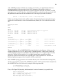
distance between atom A and B, the nonzero elements of the row vector ei are
27
∂ ( R A − RB )
R − RBα
,
ei, Aα N=
N AB Aα
=
AB
∂RAα
R A − RB
(37)
∂ ( R A − RB )
R − RAα
,
ei, Bα N=
N AB Bα
=
AB
∂RBα
R A − RB
(38)
and
RKα , α
{=
where N AB is the normalized constant,
=
RK
x, y, z} is the Cartesian coordinate of atom K
( K = A, B) . When there is only one constraint, ei = ei . If there are more than one constrains, ei is
obtained by Gram-Schmidt orthogonalization,
 i −1

ei = Ni 1 − ∑ 1 − δ ij ei eiT  ei .
 j =1

(
)
(39)
The constrained geometry optimization is performed with the projected gradient, (1 − P ) g ( g is force
vector in Cartesian coordinates). Even if the geometry optimization is carried out with the projected
gradient, the values of the constrained internal coordinates may deviate from the initial ones due to the
nonlinear character of the constraints. In GAMESSPLUS, SHAKE method is used to maintain the
constraints every geometry optimization step.
The current version GAMESSPLUS supports four types of internal coordinate constraints: bond lengths,
sums or differences of bond lengths, bond angles, and torsional angles.
GHO-AIHF QM/MM Calculations
The GHO-AIHF model in combined QM/MM calculations has been tested for a series of closed-shell
and open-shell small molecules and ions with various functional groups close to the QM/MM
boundary. The rotation barrier around the central C-C bond in n-butane has been studied by using
GHO-AIHF. The proton affinities of small alcohols, amines, thiols, and acids computed by GHOAIHF showed that the method is also reliable for energetics. In those tests, various basis sets were used
for the QM part, namely: STO-3G, 6-31G(d), 6-31+G(d), 6-31+G(d,p), 6-31++G(d,p), and MIDI!.
As compared to a projected basis scheme and a scheme based on neglect of diatomic differential
overlap involving auxiliary orbitals, using hybrid orbitals based on global Löwdin orthogonalized
atomic orbitals is more robust. It has been shown that only the non-orthogonality of atoms near the
boundary is important, and needs to be removed by the explicit orthogonalization scheme in GHO;
therefore only a local orthogonalization is necessary. Considering the localization of the boundary
treatment, this method is more theoretically promising. Therefore a local Löwdin orthogonalization
algorithm has also been implemented. Instead of doing a Löwdin orthogonalization over the entire QM
system, only orbitals on: GHO boundary atoms, QM frontier atom A, and QM atoms directly bonded
to A (these atoms are also called geminal atoms) are orthogonalized to each other before the
hybridization. By using this local Löwdin orthogonalization method, the mixing of tails from other QM
atoms far from the boundary is eliminated and the perturbation introduced to the QM subsystem is
minimized.
28
Although the unparametrized GHO-AIHF method gives reasonable optimized geometries and charges,
one can obtain even better results by scaling the integrals involving the boundary orbitals. Such a
parametrized version of GHO-AIHF (based on local Löwdin orthogonalization) is available for the
MIDI! basis set, in which the scaling factors are obtained from a small training set containing propane,
propanol, propanoic acid, n-butane, and 1-butene .
29
GAMESSPLUS Citation
Publications including work performed with GAMESSPLUS should cite the software package in the
following ways:
Journal of Chemical Physics or World Scientific style
M. Higashi, A. V. Marenich, R. M. Olson, A. C. Chamberlin, J. Pu, C. P. Kelly, J. D. Thompson, J.
D. Xidos, J. Li, T. Zhu, G. D. Hawkins, Y.-Y. Chuang, P. L. Fast, B. J. Lynch, D. A. Liotard, D.
Rinaldi, J. Gao, C. J. Cramer, and D. G. Truhlar, GAMESSPLUS – version 2010-2, University of
Minnesota, Minneapolis, 2010, based on the General Atomic and Molecular Electronic Structure
System (GAMESS) as described in M. W. Schmidt, K. K. Baldridge, J. A. Boatz, S. T. Elbert, M. S.
Gordon, J. H. Jensen, S. Koseki, N. Matsunaga, K. A. Nguyen, S. J. Su, T. L. Windus, M. Dupuis,
and J. A. Montgomery, J. Comput. Chem. 14, 1347 (1993).
Elsevier style
M. Higashi, A. V. Marenich, R. M. Olson, A. C. Chamberlin, J. Pu, C. P. Kelly, J. D. Thompson, J.
D. Xidos, J. Li, T. Zhu, G. D. Hawkins, Y.-Y. Chuang, P. L. Fast, B. J. Lynch, D. A. Liotard, D.
Rinaldi, J. Gao, C. J. Cramer, D. G. Truhlar, GAMESSPLUS – version 2010-2, University of
Minnesota, Minneapolis, 2010, based on the General Atomic and Molecular Electronic Structure
System (GAMESS) as described in M. W. Schmidt, K. K. Baldridge, J. A. Boatz, S. T. Elbert, M. S.
Gordon, J. H. Jensen, S. Koseki, N. Matsunaga, K. A. Nguyen, S. J. Su, T. L. Windus, M. Dupuis,
J. A. Montgomery, J. Comput. Chem. 14 (1993) 1347.
ACS style
Higashi, M.; Marenich, A. V.; Olson, R. M.; Chamberlin, A. C.; Pu, J.; Kelly, C. P.; Thompson, J.
D.; Xidos, J. D.; Li, J.; Zhu, T.; Hawkins, G. D.; Chuang, Y.-Y.; Fast, P. L.; Lynch, B. J.; Liotard,
D. A.; Rinaldi, D.; Gao, J.; Cramer, C. J.; Truhlar, D. G. GAMESSPLUS – version 2010-2,
University of Minnesota, Minneapolis, 2010, based on the General Atomic and Molecular
Electronic Structure System (GAMESS) as described in Schmidt, M. W.; Baldridge, K. K.; Boatz, J.
A.; Elbert, S. T.; Gordon, M. S.; Jensen, J. H.; Koseki, S.; Matsunaga, N.; Nguyen, K. A.; Su, S. J.;
Windus, T. L.; Dupuis, M.; Montgomery J. A. J. Comput. Chem. 1993, 14, 1347.
Theoretical Chemistry Accounts style
Higashi M, Marenich AV, Olson RM, Chamberlin AC, Pu J, Kelly CP, Thompson JD, Xidos JD,
Li J, Zhu T, Hawkins GD, Chuang Y-Y, Fast PL, Lynch BJ, Liotard DA, Rinaldi D, Gao J, Cramer
CJ, Truhlar DG (2009) GAMESSPLUS – version 2010-2, University of Minnesota, Minneapolis,
2009, based on the General Atomic and Molecular Electronic Structure System (GAMESS) as
described in Schmidt MW, Baldridge KK, Boatz JA, Elbert ST, Gordon MS, Jensen JH, Koseki S,
Matsunaga N, Nguyen KA, Su SJ, Windus TL, Dupuis M, Montgomery JA (1993) J. Comput.
Chem. 14: 1347
In addition, as usual, the user should give literature references for any methods used. A convenient
collection of literature references in provided in the following section.
30
Literature References
ASA algorithm
LH95 Liotard, D. A; Hawkins, G. D.; Lynch, G. C.; Cramer, C. J.; Truhlar, D. G. “Improved Methods
for Semiempirical Solvation Models” J. Comp. Chem. 1995, 16, 422.
MIDI! Basis set
EG96 Easton, R. E.; Giesen, D. J.; Welch, A.; Cramer, C. J.; Truhlar, D. G. “The MIDI! Basis Set for
Quantum Mechanical Calculations of Molecular Geometries and Partial Charges” Theor. Chim.
Acta 1996, 93, 281.
LC98 Li, J.; Cramer, C. J.; Truhlar, D. G. “MIDI! Basis Set for Silicon, Bromine, and Iodine” Theor.
Chem. Acc. 1998, 99, 192.
TW01 Thompson, J. D.; Winget, P.; Truhlar, D. G. “MIDIX basis set for the lithium atom: Accurate
geometries and partial atomic charges with minimal computational cost”, PhysChemComm,
2001, 4, 72.
Corrected modified Perdew-Wang hybrid DFT method
LZ03 Lynch, B. J.; Zhao, Y.; Truhlar, D. G. “The Effectiveness of Diffuse Basis Functions for
Calculating Relative Energies by Density Functional Theory”, J. Phys. Chem. A 2003, 107,
1384.
MPW1K
LF00 Lynch, B. J.; Fast, P. L.; Harris, M.; Truhlar D. G. “Adiabatic Connection for Kinetics”, J.
Phys. Chem. A 2000, 104, 4811.
MPWPW91, mPW1PW91, and MPWX
AB98 Adamo, C.; Barone, V.; “Exchange functionals with Improved Long-Range Behavior and
Adiabatic Connection Methods without Adjustable Parameters: The mPW and mPW1PW
Models” J. Chem. Phys. 1998, 108, 664.
PT02 Pu, J.; Truhlar, D. G. “Parameterized Direct Dynamics Study of Rate Constants of H with CH4
from 250 to 2400K”, J. Chem. Phys. 2002, 116, 1468.
Löwdin population analysis
LD50 Löwdin, P. –O. J. Chem. Phys. 1950, 18, 365. (b) Del Re, G.; In Quantum Science; Calais, J. –
L., Goscinski, O., Linderberg, J., Öhrn, Y., Eds.; Plenum Press: New York, 1976; p 53.
31
Redistributed Löwdin population analysis
TX02 Thompson, J. D.; Xidos, J. D.; Sonbuchner, T. M.; Cramer, C. J.; Truhlar, D. G. “More
Reliable Partial Atomic Charges when using Diffuse Basis Sets”, PhysChemComm, 2002, 5,
117.
Original parameterizations of the CM2 Charge Model
LZ98 Li, J.; Zhu, T.; Cramer, C. J.; Truhlar, D. G. “A New Class IV Charge Model for Extracting
Accurate Partial Charges from Wave Functions” J. Phys. Chem. A 1998, 102, 1820.
Parameterization of the CM2 model for HF/cc-pVDZ
LX99 Li, J.; Xing, J.; Cramer, C. J.; Truhlar, D. G. “Accurate Dipole Moments from Hartree-Fock
Calculations by Means of Class IV Charges” J. Chem. Phys. 1999, 111, 885.
Original parameterizations of the CM3 Charge Model
WT02 Winget, P.; Thompson J. D.; Xidos, J. D.; Cramer, C. J.; Truhlar, D. G. “Charge Model 3: A
Class IV Charge Model based on Hybrid Density Functional Theory with Variable Exchange”
J. Phys. Chem. A, 2002, 106, 10707.
Extension of CM3 to AM1, PM3, BLYP, and B3LYP
TC03 Thompson, J. D.; Cramer, C. J.; Truhlar, D. G. “Parameterization of Charge Model 3 For AM1,
PM3, BLYP, and B3LYP” J. Comput. Chem., 2003, 24, 1291.
Extension of CM3 and CM3.1 to HF/MIDI!
KC05a Kelly, C. P.; Cramer, C. J.; Truhlar, D. G. “Accurate Partial Atomic Charges for High-Energy
Molecules with the MIDI! Basis Set” Theor. Chem. Acc., 2005, 113, 133.
Parameterizations of the CM4 Charge Model
KC05b Kelly, C. P.; Cramer, C. J.; Truhlar, D. G. “SM6: A Density Functional Theory Continuum
Solvation Model for Calculating Aqueous Solvation Free Energies of Neutrals, Ions, and
Solute-Water Clusters” J. Chem . Theory Comput. 2005, 1, 1133.
SM5.42/DFT method and ISCRF=1 option
ZL98 Zhu, T.; Li, J.; Hawkins, G. D.; Cramer, C. J.; Truhlar, D. G. “Density Functional Solvation
Model Based on CM2 Atomic Charges” J. Chem. Phys. 1998, 109, 9117.
SM5.42/MIDI!6D method and more efficient version of ISCRF=1 option
LH98 Li, J.; Hawkins, G. D.; Cramer, C. J.; Truhlar, D. G. “Universal Reaction Field Model Based on
Ab Initio Hartree-Fock Theory” Chem. Phys. Lett. 1998, 288, 293.
32
Additional SM5.42 parameterizations and ISCRF=2 option
LZ99 Li, J.; Zhu, T.; Hawkins, G. D.; Winget, P.; Liotard, D. A.; Cramer, C. J.; Truhlar, D. G.
“Extension of the Platform of Applicability of the SM5.42R Universal Solvation Model”
Theor. Chem. Acc. 1999, 103, 9.
SM5.42 parameterization for Si
WT02 Winget, P.; Thompson, J. D.; Cramer, C. J.; Truhlar, D. G. “Parameterization of a Universal
Solvation Model for Molecules Containing Silicon” J. Phys. Chem. B, 2002, 106, 5160.
Parameterization of SM5.42 for soil
WC00 Winget, P.; Cramer, C. J.; Truhlar, D. G. “Prediction of Soil Sorption Coefficients Using a
Universal Solvation Model” Env. Sci. Technol. 2000, 34, 4733.
SM5.43 parameterizations for HF/6-31G(d), B3LYP/6-31G(d), mPW1PW91/6-31G(d), and
mPW1PW91/6-31+G(d)
TC04 Thompson, J. D.; Cramer, C. J.; Truhlar, D. G. “New Universal Solvation Model and
Comparison of the Accuracy of the SM5.42R, SM5.43R, C-PCM, D-PCM, and IEF-PCM
Continuum Solvation Models for Aqueous and Organic Solvation Free Energies and Vapor
Pressures” J. Phys. Chem. A 2004, 108, 6532.
SM5.43 parameterizations for MPWX/MIDIX, MPWX/MIDI!6D, MPWX/6-31G(d),
MPWX/6-31+G(d), and MPWX/6-31+G(d,p)
TC05 Thompson, J. D.; Cramer, C. J.; Truhlar, D. G. “Density-Functional Theory and Hybrid DensityFunctional Theory Continuum Solvation Models for Aqueous and Organic Solvents: Universal
SM5.43 and SM5.43R Solvation Models for Any Fraction of Hartree-Fock Exchange” Theor.
Chem. Acc. 2005, 113, 107.
SM6 aqueous model
KC05b Kelly, C. P.; Cramer, C. J.; Truhlar, D. G. “SM6: A Density Functional Theory Continuum
Solvation Model for Calculating Aqueous Solvation Free Energies of Neutrals, Ions, and
Solute-Water Clusters” J. Chem. Theory Comput. 2005, 1, 1133.
SM8 universal model
MO7
Marenich, A. V.; Olson, R. M.; Kelly, C. P.; Cramer, C. J.; Truhlar, D. G. “Self-consistent
reaction field model for aqueous and nonaqueous solutions based on accurate polarized partial
charges” J. Chem. Theory Comput. 2007, 3, 2011.
33
SM8AD universal model
MC09 Marenich, A. V.; Cramer, C. J.; Truhlar, D. G. “Universal solvation model based on the
generalized Born approximation with asymmetric descreening” J. Chem. Theory Comput. 2009,
5, 2447.
Temperature-dependent aqueous models
AC06 Chamberlin, A. C.; Cramer, C. J.; Truhlar, D. G. “Predicting Free Energies of Solvation as
Functions of Temperature” J. Phys. Chem. B 2006, 110, 5665.
AC08 Chamberlin, A. C.; Cramer, C. J.; Truhlar, D. G. “Extension of a temperature-dependent
aqueous solvation model to compounds containing nitrogen, fluorine, chlorine, bromine, and
sulfur” J. Phys. Chem. B 2008, 112, 3024.
Analytical gradients of the SM5.42, SM5.43, SM6, and SM8 models
ZL99 Zhu, T.; Li, J.; Liotard, D. A.; Cramer, C. J.; Truhlar, D. G. “Analytical Gradients of a SelfConsistent Reaction-Field Solvation Model Based on CM2 Atomic Charges” J. Chem. Phys.
1999, 110, 5503.
Overview article including SM5.42
HZ99 Hawkins, G. D.; Zhu, T.; Li, J.; Chambers, C. C.; Giesen, D. J.; Liotard, D. A.; Cramer, C. J.;
Truhlar, D. G. “Universal Solvation Models” in Combined Quantum Mechanical and
Molecular Mechanical Methods, Gao, J., Thompson, M. A., Eds.; American Chemical Society:
Washington DC; 1998; pp. 201-219.
Sample applications of SM5.42
TC98 Truhlar, D. G.; Cramer, C. J. “Solvent Effects on 1,3-Dipolar Addition Reactions” Faraday
Discussions 1998, 110, 477.
LC99 Li, J.; Cramer, C. J.; Truhlar, D. G. “Application of a Universal Solvation Model to Nucleic
Acid Bases. Comparison of Semiempirical Molecular Orbital Theory, Ab Initio Hartree-Fock
Theory, and Density Functional Theory” Biophys. Chem. 1999, 78, 147.
WH00 Winget, P.; Hawkins, G. D.; Cramer, C. J.; Truhlar, D. G. “Prediction of Vapor Pressures from
Self-Solvation Free Energies Calculated by the SM5 Series of Universal Solvation Models” J.
Phys. Chem. B, 2000, 104, 4726.
WW00 Winget, P.; Weber, E. J.; Cramer, C. J.; Truhlar, D. G. “Computational Electrochemistry:
Aqueous Oxidation Potentials for Substituted Anilines,” Phys. Chem. Chem. Phys., 2000, 2,
1231.
CR99 Chuang, Y.-Y.; Radhakrishnan, M. L.; Fast, P. L.; Cramer, C. J.; Truhlar, D. G. “Direct
Dynamics for Free Radical Kinetics in Solution: Solvent Effect on the Rate Constant for the
Reaction of Methanol with Atomic Hydrogen” J. Phys. Chem. A 1999, 103, 4893.
34
ST01 Sicinska, D.; Truhlar, D. G.; Paneth, P. “Solvent-Dependent Transition states for
Decarboxylations”, J. Am. Chem. Soc. 2001, 123, 7863.
SP02 Sicinska, D.; Paneth, P.; Truhlar, D. G. “How Well Does Microsolvation Represent
Macrosolvation? A Test case: Dynamics of Decarboxylation of 4-Pyridylacetic Acid
Zwitterion” J. Phys. Chem. B 2002, 106, 2708.
AM1-SRP and PM3-SRP models
GO91 Gonzàlez-Lafont, A.; Truong, T. N.; Truhlar D. G. “Direct Dynamics Calculations with
Neglect of Diatomic Differential Overlap Molecular Orbital Theory with Specific Reaction
Parameters,” J. Phys. Chem. 1991, 95, 4618.
CE95 Corchado, J. C.; Espinosa-Garcia, J.; Hu, W.-P.; Rossi, I.; Truhlar, D. G. “Dual-Level
Reaction-Path Dynamics (The /// Approach to VTST with Semiclassical Tunneling).
Application to OH + NH3→ H2O + NH2,” J. Phys. Chem. 1995, 99, 687.
CR99 Chuang, Y.-Y.; Radhakrishnan, M. L.; Fast, P. L.; Cramer, C. J.; Truhlar, D. G. “Direct
Dynamics for Free Radical Kinetics in Solution: Solvent Effect on the Rate Constant for the
Reaction of Methanol with Atomic Hydrogen,” J. Phys. Chem. A 1999, 103, 4893.
Solubility
TC03 Thompson, J. D.; Cramer, C. J.; Truhlar, D. G. “Predicting Aqueous Solubilities From Aqueous
Free Energies of Solvation and Experimental or Calculated Vapor Pressures of Pure
Substances,” J. Chem. Phys. 2003, 119, 1661-1670.
QM/MM with GHO-AIHF boundary treatment
PG04 Pu, J.; Gao, J.; Truhlar, D. G. “Generalized Hybrid Orbital (GHO) Method for Combining Ab
Initio Hartree-Fock Wave Functions with Molecular Mechanics,” J. Phys. Chem. A 2004, 108,
632-650.
Charge response kernel
MK97 Morita, A.; Kato, S. “Ab Initio Molecular Orbital Theory on Intramolecular Charge
Polarization: Effect of Hydrogen Abstraction on the Charge Sensitivity of Aromatic and
Nonaromatic Species,” J. Am. Chem. Soc. 1997, 119, 4021-4032.
LY04 Lu, Z.; Yang, W. “Reaction path potential for complex systems derived from combined ab
initio quantum mechanical and molecular mechanical calculations,” J. Chem. Phys. 2004, 121,
89-100.
HT08 Higashi, M.; Truhlar, D. G. “Electrostatically Embedded Multiconfiguration Molecular
Mechanics Based on the Combined Density Functional and Molecular Mechanical Method,” J.
Chem. Theory Comput. 2008, 4, 790-803.
TINKER tapering fucntion
35
PJ97 Ponder, J. W.; TINKER–version 3.5; Washington University: St. Louis, MO, 1997.
SB93 Steinbach, P. J.; Brooks, B. R. “New Spherical-Cutoff Methods for Long-Range Forces in
Macromolecular Simulation,” J. Comput. Chem. 1993, 15, 667-683.
QM/MM method with a site–site representation of the QM−MM electrostatic interaction
HO00 Hayashi, S.; Ohmine, I. “Proton Transfer in Bacteriorhodopsin: Structure, Excitation, IR
Spectra, and Potential Energy Surface Analyses by an ab Initio QM/MM Method,” J. Phys.
Chem. B 2000, 104, 10678-10691.
HT08 Higashi, M.; Truhlar, D. G. “Electrostatically Embedded Multiconfiguration Molecular
Mechanics Based on the Combined Density Functional and Molecular Mechanical Method,” J.
Chem. Theory Comput. 2008, 4, 790-803.
HT09 Higashi, M.; Truhlar, D. G. “Efficient Approach to Reactive Molecular Dynamics with
Accurate Forces,” J. Chem. Theory Comput. 2009, 5, 2925-2929.
AMBER ff94 force field (this provides the functional form that we call the AMBER force field)
CC95 Cornell, W. D.; Cieplak, P.; Bayly, C. I.; Gould, I. R.; Merz, Jr., K. M.; Ferguson, D. M.;
Spellmeyer, D. C.; Fox, T.; Caldwell, J. W.; Kollman, P. A. “A Second Generation Force Field
for the Simulation of Proteins, Nucleic Acids, and Organic Molecules,” J. Am. Chem. Soc.
1995, 117, 5179-5197.
AMBER ff03 force field
DW03 Duan, Y.; Wu, C.; Chowdhury, S.; Lee, M.C.; Xiong, G.; Zhang, W.; Yang, R.; Cieplak, P.;
Luo, R.; Lee, T. “A point-charge force field for molecular mechanics simulations of proteins
based on condensed-phase quantum mechanical calculations,” J. Comput. Chem. 2003, 24,
1999–2012.
AMBER ff99SB force field
WC00 Wang, J.; Cieplak, P.; Kollman, P. A. “How well does a restrained electrostatic potential (RESP)
model perform in calculating conformational energies of organic and biological molecules?” J.
Comput. Chem. 2000, 21, 1049-1074.
HA06 Hornak, V.; Abel, R.; Okur, A.; Strockbine, B.; Roitberg, A.; Simmerling, C. “Comparison of
multiple AMBER force fields and development of improved protein backbone parameters,”
Proteins: Struct., Funct., Genet. 2006, 65, 712-725.
TIP3P water model
JC83 Jorgensen, W. L.; Chandrasekhar, J.; Madura, J.; Klein, M. L. “Comparison of simple potential
functions for simulating liquid water,” J. Chem. Phys. 1983, 79, 926–935.
36
General AMBER force field (GAFF)
WW04 Wang, J; Wolf, R. M.;Caldwell, J. W.; Kollman, P. A.; Case, D. A. “Development and Testing
of a General Amber Force Field” J. Comput. Chem. 2004, 25, 1157-1174.
Link atom method with the Q1-QL bond length held to a fixed fraction of the Q1-M1 bond length
DK99 Dapprich, S.; Komáromi, I.; Byun, K.; Morokuma, K; Frisch, M. “A new ONIOM
implementation in Gaussian98. Part I. The calculation of energies, gradients, vibrational
frequencies and electric field derivatives,” THEOCHEM 1999, 461-462, 1-21.
Link atom method with fixed Q1-QL bond lengths and with the AMBER redistributed charge scheme
WC07 Walker, R. C.; Crowley, M. F.; Case, D. A. “The implementation of a fast and accurate
QM/MM potential method in Amber,” J. Comput. Chem. 2007, 29, 1019-1031.
Redistributed charge (RC) and redistributed charge and dipole (RCD) schemes
LT05 Lin, H.; Truhlar, D. G. “Redistributed Charge and Dipole Schemes for Combined Quantum
Mechanical and Molecular Mechanical Calculations,” J. Phys. Chem. A 2005, 109, 3991-4004
Balanced redistributed charge (BRC) and balanced redistributed charge and dipole (BRCD) schemes
WT10 Wang, B.; Truhlar, D. G. “Combined Quantum Mechanical and Molecular Mechanical
Methods for Calculating Potential Energy Surfaces: Tuned and Balanced Redistributed-Charge
Algorithm,” J. Chem. Theory Comput. 2010, 6, in press.
Projection Operator Method for Geometry Optimization with Constraints
LZ91 D.-h. Lu, M. Zhao, and D. G. Truhlar, "Projection Operator Method for Geometry Optimization
with Constraints," Journal of Computational Chemistry 12, 376-384 (1991).
Quick index to literature
The references for the methods supported by GAMESSPLUS are as follows:
Method
Löwdin charges
RLPA charges
mPW hybrid functional
MPW1K
MPWX
CM2/AM1
CM2/PM3
CM2/HF/MIDI!
Reference
LD50
TX02
AB98, PT02, and LZ03
LF00
PT02
LZ98
LZ98
LZ98
37
CM2/HF/MIDI!6D
CM2/HF/6-31G(d)
CM2/BPW91/MIDI!
CM2/BPW91/MIDI!6D
CM2/B3LYP/MIDI!
CM2/BPW91/6-31G(d)
CM2/HF/6-31+G(d)
CM2/HF/cc-pVDZ
CM2/BPW91/DZVP
CM3/AM1
CM3/PM3
CM3/HF/MIDI!
CM3/HF/MIDI!6D
CM3/HF/6-31G(d)
CM3/MPWX/MIDI!
CM3/MPWX/MIDI!6D
CM3/MPWX/6-31G(d)
CM3/MPWX/6-31+G(d)
CM3/MPWX/6-31+G(d,p)
CM3/BLYP/6-31G(d)
CM3/B3LYP/MIDI!6D
CM3/B3LYP/6-31G(d)
CM3/B3LYP/6-31+G(d)
CM3.1/HF/MIDI!
CM4/DFT/MIDI!6D
CM4/DFT/6-31G(d)
CM4/DFT/6-31+G(d)
CM4/DFT/6-31+G(d,p)
SM5.42/HF/MIDI!
SM5.42/HF/MIDI!6D
SM5.42/HF/6-31G(d)
SM5.42/BPW91/MIDI!
SM5.42/BPW91/MIDI!6D
SM5.42/B3LYP/MIDI!
SM5.42/BPW91/6-31G(d)
SM5.42/HF/6-31+G(d)
SM5.42/HF/cc-pVDZ
SM5.42/BPW91/DZVP
SM5.43/HF/6-31G(d)
SM5.43/B3LYP/6-31G(d)
SM5.43/MPWX/MIDI!
SM5.43/MPWX/MIDI!6D
SM5.43/MPWX/6-31G(d)
SM5.43/MPWX/6-31+G(d)
SM5.43/MPWX/6-31+G(d,p)
SM6/DFT/MIDI!6D
LZ98
LZ98
LZ98
LZ98
LZ98
LZ98
LZ98
LX99
LZ98
TC03
TC03
KC05a
WT02
WT02
WT02
WT02
WT02
WT02
WT02
TC03
TC03
TC03
TC03
KC05a
KC05b
KC05b
KC05b
KC05b
LZ99
LH98
LZ99
LZ99
ZL98
LZ99
ZL98
LZ99
LZ99
ZL98
TC04
TC04
TC05
TC05
TC05
TC05
TC05
KC05b
38
SM6/DFT/6-31G(d)
SM6/DFT/6-31+G(d)
SM6/DFT/6-31+G(d,p)
SM8
SM8AD
SM8T
SMx liquid-phase optimizations
GHO-AIHF
CRK
TINKER tapering function
Site–site QM/MM
AMBER ff94 force field
AMBER ff03 force field
AMBER ff99SB force field
TIP3P
General AMBER force field
Link atom method (fixed fraction)
Link atom method (fixed length)
AMBER redistributed charge
RC and RCD
BRC and BRCD
KC05b
KC05b
KC05b
MO07
MC09
AC06, AC08
ZL99 and CR99
PG04
MK97, LY04, and HT08
PJ97 and SB93
HO00, HT08, HT09, and
references for the force field
CC95
DW03
WC00 and HA06
JC83
WW04
DK99
WC07
WC07
LT05
WT10
39
Usage
This section highlights important GAMESS input options and describes the input options in the
namelists $CM2, $GMSOL, $CM2SRP, $NDDOSRP, $EEQM, $MM, $AMBTOP, $AMBCRD,
$QMMM, and $INTFRZ. Namelists $CM2 and $GMSOL are used to define the specifics of
calculations involving CM2, CM3, CM4, CM4M, SM5.42, SM5.43, SM6, and SM8. (Note that
$GMSOL and $CM2 define the same input, and only one of them should be defined in a given input
file. If they are both defined in the same input file, the input parameters defined in the second instance
will be ignored.) Namelist $CM2SRP is used for reading the external parameters for CM2-SRP
methods, and namelist $NDDOSRP is used for reading the external parameters for NDDO-SRP
methods. Namelist $EEQM is used for reading some parameters for the EEQM method. Namelist
$MM is used for reading MM charges and coordinates when IRDMM=1 in $EEQM. $AMBTOP and
$AMBCRD is used for reading AMBER parameter/topology and coordinate inputs for QM/MM
calculation. Namelist $QMMM is used for reading some parameters for QM/MM method. Namelist
$INTFRZ is used to define internal coordinates to be constrained.
Note: GHO-AIHF calculations are carried by the CHARMM/GAMESSPLUS combination package, and
the CHARMM input file controls the GHO options. A detailed description is available in
documentation for the CGPLUS package (http://comp.chem.umn.edu/cgplus, see "CGPLUSv1.0 User Manual")
2H
Notes on GAMESSPLUS Input
Users of GAMESSPLUS should consult at least the first two sections of the GAMESS Users Manual
that is distributed with the GAMESS package. These sections outline the specifics for all aspects of
GAMESS input. For QM/MM calculations with site-site interactions and link atoms, users should also
consult AmberTools Users’ Manual because such QM/MM calculations require parameter/topology
and coordinate inputs generated by AmberTools.
Most GAMESS input is entered in a pseudo-namelist format; where a namelist is a particular group of
keywords. The title of this group, the namelist name, is prefixed by a ‘$’ that must begin in the second
column of an input file (e.g. $SCF). A namelist accepts as arguments a number of possible keywords
that are entered after the namelist name in a free format style that can span multiple lines. Each
keyword accepts either character or numeric values. A namelist is terminated with a $END. Only input
between a namelist name and its corresponding $END will be read from a GAMESS input file.
GAMESSPLUS introduces several new namelists to GAMESS: $CM2, $GMSOL ($CM2 and $GMSOL
define the same input options), $CM2SRP, $NDDOSRP, $EEQM, $MM, $AMBTOP, $AMBCRD,
$QMMM, and $INTFRZ; these new namelists are discussed at length in separate subsections below.
Below is a brief summary of GAMESS namelists and their keywords that are most important to
GAMESSPLUS users. In this section, the namelist name is followed by a brief description, and below
the namelist name is a set pertinent keywords and their options:
Namelist $CONTRL
SCFTYP =
RHF
=
UHF
RUNTYP =
ENERGY
group of global settings for the calculation
restricted Hartree-Fock calculation (default)
unrestricted Hartree-Fock calculation
SCF evaluation (default)
40
MAXIT
ICHARG
MULT
COORD
ISPHER
=
=
=
=
=
GRADIENT
HESSIAN
OPTIMIZE
SADPOINT
EEQM
=
=
=
=
=
=
=
=
N
N
N
UNIQUE
CART
ZMT
–1
1
gradient evaluation
Hessian and possibly vibrational frequency evaluation
geometry optimization to minima
geometry optimization to saddle points
EEQM calculation with a site–site representation of the QM/MM
electrostatic interaction
N is the maximum number of SCF cycles (default = 30)
N is the molecular charge (default = 0)
N is the multiplicity of the electronic state (default = 1)
input symmetry-unique Cartesian coordinates (default)
input all Cartesian coordinates
input Gaussian-style Z-matrix internal coordinates
use Cartesian basis functions (e.g. 6D, 10F; default)
use spherical harmonic basis functions (e.g. 5D, 7F)
Note: The best way to input Cartesian coordinates is to set COORD = UNIQUE (this prevents
coordinate rotation) and to set the symmetry group of the molecule to C1 in $DATA (see
below).
Namelist $SYSTEM
MEMORY=
N
information for controlling the computer’s operation
N is the maximum memory the job can use in words
(default = 1 000 000)
Namelist $DFT
DFTTYP=
density functional theory (DFT) input
N is the density functional or hybrid density functional.
A full list of the density functionals available in
GAMESSPLUS that are suggested for use with CM4 and
SM6 are given in the section entitled “Density Functionals
Recommended for use with CM4/CM4M and SM6/SM8 in
GAMESSPLUS.
Defines the fraction of Hartree-Fock exchange N to be used
when the MPWX functional is used. This keyword must be
specified when MPWX is used. For CM3 and SM5.43
calculations that use MPWX (ICMD = 315 – 319), the
HFE = N must also be specified in the $GMSOL or $CM2
namelist. For CM4 and SM6 (ICMD = 416 – 419), HFE =
N must always be specified in the $GMSOL or $CM2
Namelist.
M is GRID to request grid-based DFT calculation (default)
N
HFE=
N
METHOD=
M
Note: Using the charge or solvation model parameterized for B3LYP, one should specify
‘DFTTYP=B3LYP3’ (not ‘DFTTYP=B3LYP5’) because the original parametrization has
been done for the B3LYP method that uses version III of the VWN correlation functional.
In addition, the charge and solvation models that are based on DFT were parameterized
using grid-based DFT, so ‘METHOD=GRID’ (the default for METHOD) should always
be used.
41
Namelist $BASIS
GBASIS =
=
=
NGAUSS =
NDFUNC =
DIFFSP
=
N31
AM1
PM3
N
N
.TRUE.
input of available standard basis sets
Pople’s N-31G basis sets
AM1 model Hamiltonian
PM3 model Hamiltonian
the ‘N’ of N31 (e.g. N = 6 for 6-31G)
N is the number of polarizing d subshells on heavy atoms
(N = 1 for 6-31G(d); default = 0)
adds a diffuse sp shell to the basis set (default = .FALSE.)
Note: The d subshells have 5 functions if ISPHER=1 , and they have 6 functions if ISPHER= -1,
where ISPHER is defined in the $CONTRL data group. Thus, when using the MIDI!
basis set, ISPHER=1 should be specified in the $CONTRL namelist. When using the
MIDI!6D basis set, ISPHER=−1 should be specified in the $CONTRL namelist.
Examples:
6-31G(d) :
6-31+G(d) :
$BASIS GBASIS=N31 NGAUSS=6 NDFUNC=1 $END
$BASIS GBASIS=N31 NGAUSS=6 NDFUNC=1 DIFFSP=.TRUE. $END
Namelist $DATA
input molecule information
Input consists of the following information:
line 1: title line
line 2: symmetry group (always enter C1 for GAMESSPLUS calculations)
line 3+: molecular coordinates; for Cartesian input, each line consists of the following: atom label, the
atom’s nuclear charge (which should be a floating-point value, i.e., 1.0 for H), and the atom’s
x, y, and z-coordinate. If a general basis set is required, then the basis set for each atom
follows the atom’s coordinates. See examples in the Input and Output Examples section and
in the test suite.
Namelist $FORCE
METHOD =
=
NVIB
=
=
VIBSIZ =
VIBANL =
SEMINUM
FULLNUM
1
2
N
.TRUE.
controls Hessian and vibrational frequency evaluation
numerical second-order derivatives based on analytical first
derivatives
numerical second-order derivatives based on double
differentiation of the total energy
forward-difference for numeric Hessian evaluation(default)
central-difference for numeric Hessian evaluation
N is the displacement size (in Bohr; default = 0.01)
print vibrational analysis (default = .TRUE. for
RUNTYP = HESSIAN, = .FALSE. otherwise)
Note: GAMESSPLUS does not have analytical second derivatives for solvation energies. Do not
use METHOD=ANALYTIC (that is default for certain electronic structure methods in
GAMESS) in the group $FORCE for RUNTYP=HESSIAN in $CONTRL and for
RUNTYP=OPTIMIZE or RUNTYP=SADPOINT in $CONTRL with HESS=CALC or
HSSEND=.TRUE. in $STATPT.
Namelist $STATPT
NSTEP =
N
HESS
=
GUESS
input information for geometry optimization
N is the maximum number of steps (default = 20)
guess positive-definite Hessian (default for
42
=
=
HSSEND =
READ
CALC
.TRUE.
RUNTYP = OPTIMIZE)
read Hessian from $HESS namelist (default for
RUNTYP=SADPOINT)
calculate the Hessian
calculate the Hessian at the end of a successful optimization
(default = .FALSE.)
Note: We recommend calculating the liquid-phase Hessian separately from the geometry
optimization.
Namelists $GMSOL and $CM2
$GMSOL and $CM2 are alternative names for a namelist that controls most of the options for the
solvation and charge models. (Only one of these two names should be used to specify this namelist. If
they are both defined in the same input file, the parameters defined in the second instance will be
ignored.) Below are descriptions of all input variables defined in $GMSOL or $CM2.
ISCRF
ISCRF=0
ISCRF=1
ISCRF=2
Controls the type of calculation to be performed:
Invokes a gas-phase calculation of Löwdin, RLPA, CM2, CM3, or CM4 charges
(default)
Invokes a gas- and liquid-phase solution calculation of Löwdin, RLPA, CM2, CM3, or
CM4 charges and the calculation of solvation free energy using SCF Scheme I (see SCF
Schemes). This method is only available for methods that use nondiffuse basis
functions.
Invokes a gas- and liquid-phase solution calculation of Löwdin or RLPA charges and
CM2, CM3, or CM4 charges and the calculation of solvation free energy using SCF
Scheme II (see SCF Schemes). This is the default method for methods that use diffuse
basis sets.
Note that when a calculation of RLPA charges is requested, Löwdin charges are also calculated.
However, for liquid-phase calculations that use RLPA charges, the Löwdin charges correspond to the
converged SCRF achieved with RLPA charges, not with Löwdin charges. Also note that RLPA
charges should only be calculated by methods that use the 6-31+G(d) or 6-31+G(d,p) basis sets, while
Löwdin charges should be used for all other methods.
ICDS
Selects the set of coefficients that will be used to evaluate the atomic surface tensions.
The table above matches the value of ICDS with the wave function for which the
corresponding CDS parameter set has been optimized. If ICDS is not given then 800 is
the default.
ICDS
0
1
2
3
4
Method which corresponds to set of coefficients
All coefficients equal zero, calculate bulk electrostatics only
SM5.42/HF/MIDI!
SM5.42/HF/MIDI!6D
SM5.42/HF/6-31G(d)
SM5.42/BPW91/MIDI!
43
5
6
7
8
9
10
11
12
303
313
315
316
317
318
319
416
417
418
419
800
801
ICMD
SM5.42/BPW91/MIDI!6D
SM5.42/B3LYP/MIDI!
SM5.42/BPW91/6-31G(d)
SM5.42/HF/6-31+G(d)
SM5.42/HF/cc-pVDZ
SM5.42/BPW91/DZVP
SM5.42/AM1
SM5.42/PM3
SM5.43/HF/6-31G(d)
SM5.43/B3LYP/6-31G(d)
SM5.43/MPWX/MIDI!
SM5.43/MPWX/MIDI!6D
SM5.43/MPWX/6-31G(d)
SM5.43/MPWX/6-31+G(d)
SM5.43/MPWX/6-31+G(d,p)
SM6/DFT/MIDI!6D
SM6/DFT/6-31G(d)
SM6/DFT/6-31+G(d)
SM6/DFT/6-31+G(d,p)
SM8
SM8AD
Selects the set of CM2, CM3, or CM4/CM4M coefficients used for the evaluation of the
CM2 or CM3 or CM4/CM4M charges. Always required.
ICMD
0
1
2
3
4
5
6
7
8
9
10
11
12
300
301
302
303
311
312
313
Wave function which corresponds to set of coefficients
All coefficients equal zero, calculate Löwdin charges
CM2/HF/MIDI! (default for ICMD)
CM2/HF/MIDI!6D
CM2/HF/6-31G(d)
CM2/BPW91/MIDI!
CM2/BPW91/MIDI!6D
CM2/B3LYP/MIDI!
CM2/BPW91/6-31G(d)
CM2/HF/6-31+G(d)
CM2/HF/cc-pVDZ
CM2/HF/DZVP
CM2/AM1
CM2/PM3
Calculate RLPA charges
CM3/HF/MIDI!
CM3/HF/MIDI!6D
CM3/HF/6-31G(d)
CM3/AM1
CM3/PM3
CM3/B3LYP/6-31G(d)
44
314
315
316
317
318
319
320
321
322
415
416
417
418
419
420
422
423
424
425
500
501
502
503
504
505
506
508
509
510
CM3/B3LYP/6-31+G(d)
CM3/MPWX/MIDI!
CM3/MPWX/MIDI!6D
CM3/MPWX/6-31G(d)
CM3/MPWX/6-31+G(d), uses RLPA charges
CM3/MPWX/6-31+G(d,p), uses RLPA charges
CM3/B3LYP/MIDI!6D
CM3/BLYP/6-31G(d)
CM3.1/HF/MIDI!
CM4/DFT/MIDI!
CM4/DFT/MIDI!6D
CM4/DFT/6-31G(d)
CM4/DFT/6-31+G(d), uses RLPA charges
CM4/DFT/6-31+G(d,p), uses RLPA charges
CM4/DFT/6-31G(d,p)
CM4/DFT/cc-pVDZ
CM4/DFT/DZVP
CM4/DFT/6-31B(d)
CM4/DFT/6-31B(d,p)
CM4M/M06/MIDI!
CM4M/M06/MIDI!6D
CM4M/M06/6-31G(d)
CM4M/M06/6-31+G(d)
CM4M/M06/6-31+G(d,p)
CM4M/M06/6-31G(d,p)
CM4M/M06/cc-pVDZ
CM4M/M06/DZVP
CM4M/M06/6-31B(d)
CM4M/M06/6-31B(d,p)
In the above tables, X corresponds to the percentage of Hartree-Fock exchange (see the HFE keyword
for more details). For SM6, DFT refers to any good density functional. A list of density functionals
that are available in GAMESS and GAMESSPLUS is given in the section entitled “Density Functional
Methods Available in GAMESS and GAMESSPLUS”. In cases where the default value of ICDS = 0, a
solvation model does not exist for that particular set of charges. For ICMD = 300, all restricted and
unrestricted HF, DFT, and hybrid DFT methods are available, but only the 6-31+G(d) or the 631+G(d,p) basis set should be used. Note that CM3 for the BLYP and B3LYP methods and CM3.1 for
the HF/MIDI! method in the above table uses a different mapping function for compounds that contain
N and O than CM3 for MPWX and HF does. For more information, see “Parameterization of Charge
Model 3 For AM1, PM3, BLYP, and B3LYP” by Thompson, J. D.; Cramer, C. J.; Truhlar, D. G. J.
Comput. Chem., 2003, 24, 1291 and “Accurate Partial Atomic Charges for High-Energy Molecules
with the MIDI! Basis Set” by Kelly, C. P.; Cramer, C. J; Truhlar, D. G. Theor. Chem. Acc. 2005, 113,
133.
HFE Defines the fraction of Hartree-Fock (HF) exchange to be used when ICMD = 315 to ICMD =
319 or ICMD = 416 to ICMD = 419. For example, if a calculation of CM3 charges by the
mPW1PW91/MIDI! method were to be carried out, then ICMD would be set to 315, and HFE
45
would be set to 0.25. The HFE keyword only defines the fraction of HF exchange for a given
calculation in the charge and solvation model portion of GAMESSPLUS, not in the entire
electronic structure part of the GAMESSPLUS program (thus, when using the MPWX
functional, the HFE keyword must also be specified in the $DFT namelist). This keyword is
only active when ICMD = 315 – 319 or ICMD = 415 – 419 or ICMD = 500 – 510, and in these
instances HFE must be explicitly specified by the user in both the $DFT and the $CM2 or
$GMSPLUS namelists. If ICMD = 315 – 319 or ICMD = 415 – 419 or ICMD = 500 – 510 and
HFE is not defined by the user, GAMESSPLUS will be terminated.
IRADII
IRADII=1
IRADII=2
Determines the atomic radii that will be used during an SCRF calculation:
Use Bondi’s values for the van der Waals radii to build the molecular cavity (2.0 Å is
used in cases where the atomic radii were not defined by Bondi). For evaluating the
SASA, this is always the default set of radii. For other values of IRADII, these radii are
used in cases where the radius of a given atom is not defined for a particular model (see
the table below).
Use the atomic radii optimized for predicting solvation free energies with the SM5.42
solvation model to build the molecular cavity to be used in the SCRF calculation. This
is the default for ICMD = 1 to ICMD = 10.
IRADII=3
Use the atomic radii optimized for predicting solvation free energies with the SM5.43
solvation model to build the molecular cavity to be used in the SCRF calculation. This
is the default for ICMD = 301 to ICMD = 322.
IRADII=4
Use the atomic radii radii optimized for predicting solvation free energies with the SM6
solvation model to build the molecular cavity to be used in the SCRF calculation. This
is the default for ICMD = 0, ICMD = 300, and ICMD = 416 to ICMD = 419.
IRADII=5
Use the atomic radii optimized for predicting solvation free energies with the SM8
solvation model to build the molecular cavity to be used in the SCRF calculation. This
is the default for ICDS = 800.
IRADII=6
Use the atomic radii optimized for predicting solvation free energies with the SM8AD
solvation model to build the molecular cavity to be used in the SCRF calculation. This
is the default for ICDS = 801.
The four sets of radii described above are listed below. Note that Coulomb radii for solutes in water for
the case of IRADII=5 will be equal to those for the case of IRADII=4. The definition of nonaqueous
radii for the case of IRADII=5 is given in the reference MO07, which describes the SM8 model. In
cases where the atomic radius of a given atom is not defined, the default value is Bondi’s value for the
radius. For elements whose atomic radii are not listed in Bondi’s paper, a value of 2.0 Å is used for the
radius (Bondi, A. J. Phys. Chem. 1964, 68, 441). Thus, Generalized Born calculations may be carried
out for a molecule containing any element on the periodic table.
Elementa
H
Li
C
IRADII = 1b
1.20
1.82
1.70
IRADII = 2c,d
0.91
1.32
1.78
IRADII = 3c,e
0.79
—
1.81
IRADII = 4c,f
1.02
—
1.57
46
N
1.55
1.92
1.66
1.61
O
1.52
1.60
1.63
1.52
F
1.47
1.50
1.58
1.47
Ne
1.54
—
—
—
Na
2.27
—
—
—
Mg
1.73
—
—
—
Al
2.50
—
—
—
Si
2.10
—
—
—
P
1.80
2.27
2.01
1.80
S
1.80
1.98
2.22
2.12
Cl
1.75
2.13
2.28
2.02
Ar
1.88
—
—
—
K
2.75
—
—
—
Ni
1.63
—
—
—
Cu
1.40
—
—
—
Zn
1.39
—
—
—
Ga
2.40
—
—
—
Ge
2.10
—
—
—
As
1.85
—
—
—
Se
1.90
—
—
—
Br
1.85
2.31
2.38
2.60
Kr
2.02
—
—
—
Pd
1.63
—
—
—
Ag
1.72
—
—
—
Cd
1.58
—
—
—
In
2.50
—
—
—
Sn
2.20
—
—
—
Sb
2.10
—
—
—
Te
2.06
—
—
—
I
1.98
2.66
—
—
Xe
2.60
—
—
—
aFor atoms not listed in this table, a radius of 2.0 Å is used. bBondi’s values for the van der
Waals radius (Bondi, A. J. Phys. Chem. 1964, 68, 441). cIn cases where the atomic radius is not
defined, Bondi’s values are used. In cases where the atomic radius has not been defined by Bondi,
2.0 Å is used for the atomic radius. dThese radii have been optimized for use with the SM5.42
model. eThese radii have been optimized for use with the SM5.43 model. fThese radii have been
optimized for use with the SM6 model.
ISTS
ISTS=5
ISTS=6
Determines the type of surface tension functionals:
Use SM5 functional forms to evaluate GCDS. This is the default when the SM5.42 and
SM5.43 models are invoked.
Use SM6 functional forms to evaluate GCDS . This is the default when the SM6 and
SM8 models are invoked.
47
Note: The ISTS option is deprecated in the current version of GAMESSPLUS.
SolvRd
Value of the solvent radius (in angstroms) for the calculation of the solvent-accessible
surface areas of the atoms of the solute (the default is 0 Å for SM5.42 and 0.40 Å for
SM5.43, SM6, and SM8). For predicting solvation free energies with SM5.42, SolvRd
should be set to 0 Å. For predicting solvation free energies with SM5.43 or SM6 or
SM8 or SM8AD, the default value of 0.40 Å should be used.
IAQU
IAQU=0
Determines the solvent type:
Organic solvent (additional solvent data must be input, see below)
IAQU=1
Aqueous solvent (default, no additional solvent data is required)
Solvent Descriptors: If IAQU=0, then the solvent properties are specified by a series of solvent
property (descriptor) values:
Dielec
dielectric constant, ε , of solvent (default is the value for water, 78.3)
SolN
index of refraction at optical frequencies at 293 K, n20D (default is 1.0)
SolA
Abraham’s hydrogen bond acidity, Σα 2H (default is 0.0)
SolB
Abraham’s hydrogen bond basicity, Σβ 2H (default is 0.0)
SolG
γ = γ m / γ o (default is 0.0), where γ m is the macroscopic surface tension at air/solvent
interface at 298 K, and γo is 1 cal·mol–1·Å–2 (note that 1 dyne/cm = 1.43932 cal·mol–
1 –2
·Å )
SolC
aromaticity, φ : the fraction of non-hydrogenic solvent atoms that are aromatic carbon
atoms (default is 0.0)
SolH
electronegative halogenicity, ψ : the fraction of non-hydrogenic solvent atoms that are
F, Cl or Br (default is 0.0)
For a desired solvent, these values can be derived from experiment or from interpolation or
extrapolation of data available for other solvents. Solvent parameters for common organic solvents are
tabulated in the Minnesota Solvent Descriptor Database. The latest version of this database is available
at: http://comp/chem.umn.edu/solvation.
3H
Solvent Temperature: If IAQU=1, then the solvent temperature may be specified using one of the
following keywords:
SOLK
Specifies that the free energy of solvation for the solute be computed at a single
temperature. The current model is only applicable to H, C and O containing compounds
for the range of temperatures in which water is liquid (273 to 373 K). (Note the model
uses a temperature-dependent dielectric constant, the equation for it was obtained from
the CRC Handbook of Chemistry and Physics 76th edition, ed. Lide, D. R., 1995, CRC
Press, New York.) The default value is SOLK = 298.
48
READK
AVGK
Causes GamessPlus to read in a list of temperatures at which to compute free energies
of solvation from a file labeled KELT. The default value is READK=FALSE. KELT
must be located in the scratch directory.
Example KELT file: 3
273
298
373
The first line in the input file must list the number of temperatures at which the free
energy of solvation is to be computed. Then each succeeding line should list only one
temperature.
This option is similar to READK however instead of computing the electronic energy of
the solute in solution at each temperature; it computes the electronic energy of the
solute at the average temperature and scales the electronic energy of the solute using the
following factor
1 − 1 

ε T 



1 − 1ε 
Avg 

where ε Avg is the dielectric constant of water at the average temperature and ε T is the
dielectric constant of water at a given temperature, T. This corresponds to assuming that
the charge on the solute does not change significantly as a function of temperature. This
approach can compute a large number of temperatures with nearly the same
computation time as that of a single temperature. This approach does deviate mildly
from the individual computations performed at each temperature; however, the
deviation is negligible. The default value is AVGK=FALSE.
IGEOM
IGEOM=0
IGEOM=1
Determines whether the inputted structure is already optimized in the gas-phase.
Perform a geometry optimization in the gas-phase and use the optimized gas-phase
structure as the initial guess for the liquid-phase optimization (default)
Use the inputted structure as the initial point for the liquid-phase geometry optimization
(i.e., do not perform a gas-phase optimization on the inputted structure).
IGAS
Determines which gas-phase energy is used in the evaluation of ∆GSo .
IGAS=0
Use the gas-phase energy of either the inputted geometry (IGEOM = 1) or of the
optimized gas-phase structure (IGEOM = 0; IGAS = 0 is the default). Once this gasphase energy is obtained, the gas-phase SCF is skipped, i.e., the liquid-phase SCRF
begins at first SCF cycle.
IGAS=1
IGAS=2
IGAS=3
Gas-phase energy is updated for every new geometry.
Gas-phase energy is read in using the ETGAS keyword.
Gas-phase energy is read in using the ETGAS keyword, and gas-phase SCF is always
skipped; i.e., the liquid phase SCRF begins at first SCF cycle. This option is not
available when ISCRF = 2.
Note: The relative free energy of solvation indicated in the string ‘(9) DeltaG-S(liq) free energy of
solvation’ (see an output file) depends on the reference gas-phase energy indicated in the
string ‘(0) E-EN(g) gas-phase’.
49
Note: Since the SCRF calculation with ISCRF = 2 cannot skip the gas-phase step, IGAS = 3 is
not available for single-point energy calculations and geometry optimizations using
ISCRF = 2. For the same reason, IGAS = 0 is not available for analytical geometry
optimizations using ISCRF = 2 either. To carry out the analytical optimization with
ISCRF = 2, one needs to use IGAS = 2 along with the ETGAS option or IGAS = 1.
However, in case of IGAS = 1 the user needs to add the nuclear (or geometry) relaxation
energy term to the resulting free energy of solvation indicated in the string ‘(9) DeltaGS(liq) free energy of solvation’ (see an output file). The geometry relaxation term in case of
IGAS = 1 should be equal to the difference (in kcal/mol) between the gas-phase total
energy calculated at the gas-phase equilibrium structure and the gas-phase total energy
calculated at the liquid-phase equilibrium structure.
ETGAS
Accepts an inputted value for the gas-phase energy (in hartrees).
The ETGAS keyword must be defined for IGAS = 2 or 3; the calculation will stop otherwise. Note that
if IGAS = 0 or 1, an inputted value of ETGAS will be ignored. Theoretically, the gas-phase SCF
energy used in the evaluation of the free energy of solvation is that of the gas-phase equilibrium
geometry. Inputting an energy for a non-equilibrium structure will lead to theoretically questionable
results.
ICREAD
ICREAD=0
ICREAD=1
Controls the reading of atomic charges from an external file
Do not read in atomic charges (default).
Read in atomic charges from file “CM2CHG” (case-sensitive).
ICSAVE
ICSAVE=0
ICSAVE=1
Controls the saving of the evaluated CM2, CM3, or CM4 charges to an external file.
Do not save the CM2 or CM3 charges (default).
Save the evaluated CM2 or CM3 charges in file “CM2CHG” (case-sensitive).
ISREAD
ISREAD=0
ISREAD=1
Controls the reading of surface tension parameters from an external file
Use the surface tension coefficients provided in the code (default).
Read and use the surface tension coefficients provided in a file called “CDS_Param”
(case-sensitive), and use the surface tension coefficients provided in the code for any
surface tension coefficient that is not provided by the user in the file “CDS_Param”.
Read and use the surface tension coefficients provided in a file called “CDS_Param”,
and set all other surface tension coefficients to zero.
ISREAD=2
Note that the CM2CHG and CDS_Param files must be located in the directory defined to be the
scratch directory for the calculation (i.e., the directory defined by $SCR in the rungms script, see the
section entitled Notes on Running GAMESSPLUS below for a description of the rungms script).
User-provided surface tension coefficients are entered into the input file in the following fashion: the
first line of file contains the total number of surface tension coefficients that the user has provided in
the file, followed by the value of ICoeff, where:
ICoeff = 1:
ICoeff = 2:
use the surface tension coefficients provided in the code for any surface tension
coefficients that are not provided by the user in this input file
set all surface tension coefficients that have not been provided to zero
50
All coefficient types have been assigned a four digit coefficient label (see the table below); the user
provides a coefficient label followed by its corresponding value (in cal/Å2) on each line following the
first line until all data is entered.
Note that only one parameter convention can be entered: either a set of solvent descriptors for water or
a set of solvent descriptor-dependent coefficients can be entered, but not a mix of both (i.e., coefficient
labels must be either all less than 2000 or all greater than 2001).
One-, two-, and three-atom surface tension coefficients:
σ kA , σ kA
1000 + I,
I = 1 – 100
1100 + j,
j = 1 – 100
1201
1202
1203
1204
1205
1206
1207
1210
1211
1212
1213
1214
1215
1216
σˆ i( n)
σˆ i(α )
σˆ i(β)
2000 + I,
I = 1 – 100
2100 + j,
j = 1 – 100
2201
2202
2203
2204
2205
2206
2207
2210
2211
2212
2213
2214
2215
2216
3000 + I,
I = 1 – 100
3100 + j,
j = 1 – 100
3201
3202
3203
3204
3205
3206
3207
3210
3211
3212
3213
3214
3215
3216
4000 + I,
I = 1 – 100
4100 + j,
j = 1 – 100
4201
4202
4203
4204
4205
4206
4207
4210
4211
4212
4213
4214
4215
4216
molecular surface tension coefficients:
5001:
σˆ ( γ )
5002:
2
σˆ (β )
5003:
2
σˆ (φ )
5004:
2
σˆ (ψ )
Example:
coefficient type
atomic coefficient for atoms
with nuclear charge i
H-X, where j is the nuclear
charge on atom X
C-C(1)
C-C(2)
O-C
O-O
N-C(1)
O-N
S-S
C-N
N-C(2)
H-N(2)
H-O(2)
O-P
S-P
N-C(3)
51
The following input defines the values of the following four coefficients: σˆ (Hn) = 40.80, σˆ (Cα ) = 24.51,
σˆ (Hβ,)O = -346.42, and σˆ ( γ ) = 0.3136. All other coefficients are set to zero (Icoeff = 2)
4 2
2001
3006
4108
5001
40.80D0
24.51D0
-346.42D0
0.3136D0
Namelist $CM2SRP
The current version of GAMESSPLUS provides an option for entering external parameters for the CM2
charge model, and this is called CM2-SRP. This option is required when the electronic wave function
used for a calculation does not have a matched CM2, CM3, or CM4 parameter set (for example,
HF/STO-3G), or when it is desired to ‘adjust’ the parameters in the charge model to obtain a better
estimation of the dipole moment. To carry out a CM2-SRP, CM3-SRP, or CM4-SRP calculation, the
namelist $CM2SRP is required. In this namelist, there is only one variable, NAME; this variable is
used to indicate the name of a CM2-SRP file, which has a maximum of 8 characters. Note the
CM2-SRP file must be located in the scratch directory used throughout a given calculation. The scratch
directory used for a particular calculation is defined with the $SCR variable in the rungms script (see
the section entitled Notes on Running GAMESSPLUS below).
In order to describe the syntax for the input file defined in $CM2SRP, it will be useful to describe the
CM2 charge mapping scheme. The CM2, CM3, or CM4 charge, qk, on an atom k is given by
q k = q k0 + ∑ Bkk ′ (Dkk ′ + Bkk ′C kk ′ )
(16)
k
where q k0 is the Löwdin or Redistributed Löwdin charge on atom k, Bkk´ is the Mayer bond order
between atoms k and k´, and Dkk´ and Ckk´ are the CM2 parameters. It is the Dkk´ and Ckk´ that may be
defined in the CM2-SRP file. Thus the syntax of a CM2-SRP file is:
<Variable type>
<Atomic pair no.>
<Value>
<Variable type> indicates if the parameter is a C parameter or a D parameter (acceptable input is C or
D), according to equation (16) above, and <Atomic pair no.> corresponds to a particular pair of atoms
k and k´ in equation (16). Allowed values of <Atomic pair no.> and the corresponding pair of atoms
defined for the value of <Atomic pair no.> are given below:
<Atomic pair no.>
1
2
3
4
5
6
7
8
Description
H−C
H−N
H−O
H−Si
H−P
H−S
C−N
C−O
52
9
10
11
12
13
14
15
16
17
18
19
20
C−F
C−Si
C−P
C−S
C−Cl
C−Br
C−I
O−P
F−P
N−O
O−S
P−S
Example input:
C
C
D
D
1
3
8
8
−0.0200
0.0149
−0.0874
0.0215
Namelist $NDDOSRP
Although the AM1 and PM3 methods are parameterized using broad sets of stable molecules, these
methods sometimes do not perform equally well for molecules outside the AM1 or PM3 training set,
for radical species, or for transition states. Furthermore, sometimes one does not want the parameters
that give the best results on the average (i.e., the standard parameters); rather one wants nonstandard
parameters that perform the best for a specific reaction or for a limited range of systems. In order to
‘fix’ the energetic information for a chemical dynamics calculation on a specific reaction or a set of
calculations on a specific range of systems, the specific reaction parameter (NDDO-SRP) method can
be used. To carry out an NDDO-SRP calculation, the namelist $NDDOSRP is required. In this
namelist, there is only one variable, NAME, which is used to indicate the name (with maximum of 8
characters) of an NDDO-SRP file. Note that the NDDO-SRP file must be located in the scratch
directory defined for the given calculation. The scratch directory used for a particular calculation is
defined with the $SCR variable in the rungms script (see the section entitled Notes on Running
GAMESSPLUS below).
The syntax of the NDDO-SRP file is a series of lines, each of which having one of two possible forms.
Form A is
<Variable type>
<Atomic no.>
<Value>
where <Variable type> indicates the type of the parameter, and <Atomic no.> indicates the atomic
number. Form A may be used for changes in the one-electron, one-center energies (USS or UPP), in
the monatomic parameter for one-electron resonance integrals (BETAS or BETAP), and in orbital
exponents (ZS or ZP). For example:
53
USS
UPP
USS
UPP
BETAS
BETAP
BETAS
BETAP
6
6
8
8
6
6
8
8
−49.850
−40.337
−99.181
−80.762
−16.912
−9.190
−28.998
−29.249
Form B is used for modifying the two-center resonance integrals in the NDDO-SRP method without
using the arithmetic mean prescription (see last section of Executive summary). In form B, each line
has the syntax:
BETxy <atom which x orbital taken from> <atom which y orbital taken from> <value>
where BETxy is BETSS, BETSP, or BETPP (i.e., x and y denote orbital types; only S and P type are
available).
For example:
BETSP 1
8
-17.711
Note that BETSP 6 8 is different than BETSP 8 6.
GAMESSPLUS Keywords
Shown in the below table are the GAMESSPLUS keywords required for running standard SM5.42,
SM5.43, SM6, SM8, and SM8AD calculations. Note that the keywords entered in the $GMSOL or
$CM2 namelist are used by the solvation and charge model portion of GAMESSPLUS. Thus, keywords
used by the rest of the GAMESSPLUS program, such as the level of theory, basis set, SCF and
geometry optimization options, etc., must also be included in the route section of the input file. For
convenience, the ISPHER keyword, which is specified in the $CONTRL namelist, is also included in
the table below.
Method
SM5.42/HF/MIDI! b
SM5.42/HF/MIDI!6D
SM5.42/HF/6-31G(d)
SM5.42/HF/6-31+G(d)
SM5.42/HF/cc-pVDZ b
SM5.42/BPW91/MIDI! b
SM5.42/BPW91/MIDI!6D
SM5.42/BPW91/6-31G(d)
SM5.42/BPW91/DZVP
SM5.42/B3LYP/MIDI! b
SM5.43/HF/6-31G(d)
SM5.43/B3LYP/6-31G(d)
ISPHERa ISTS
1
5
-1
5
5
5
5
1
5
-1
5
5
5
1
5
5
5
ICMD
1
2
3
8
9
4
5
7
10
6
303
313
ICDS
1
2
3
8
9
4
5
7
10
6
303
313
IRADII
2
2
2
2
2
2
2
2
2
2
3
3
SolvRd
0.00
0.00
0.00
0.00
0.00
0.00
0.00
0.00
0.00
0.00
0.40
0.40
HFE
N/A
N/A
N/A
N/A
N/A
N/A
N/A
N/A
N/A
N/A
N/A
N/A
54
SM5.43/MPWX/MIDI! b
SM5.43/MPWX/MIDI!6D
SM5.43/MPWX/6-31G(d)
SM5.43/MPWX/6-31+G(d)
SM5.43/MPWX/6-31+G(d,p)
SM6/DFT/MIDI!6D
SM6/DFT/6-31G(d)
SM6/DFT/6-31+G(d)
SM6/DFT/6-31+G(d,p)
SM8/DFT/MIDI!
SM8/DFT/MIDI!6D
SM8/DFT/6-31G(d)
SM8/DFT/6-31+G(d)
SM8/DFT/6-31+G(d,p)
SM8/DFT/6-31G(d,p)
SM8/DFT/cc-pVDZ
SM8/DFT/DZVP
SM8/DFT/6-31B(d)
SM8/DFT/6-31B(d,p)
SM8/M06/MIDI!
SM8/M06/MIDI!6D
SM8/M06/6-31G(d)
SM8/M06/6-31+G(d)
SM8/M06/6-31+G(d,p)
SM8/M06/6-31G(d,p)
SM8/M06/cc-pVDZ
SM8/M06/DZVP
SM8/M06/6-31B(d)
SM8/M06/6-31B(d,p)
SM8AD/DFT/MIDI!
SM8AD /DFT/MIDI!6D
SM8AD/DFT/6-31G(d)
SM8AD/DFT/6-31+G(d)
SM8AD/DFT/6-31+G(d,p)
SM8AD/DFT/6-31G(d,p)
SM8AD/DFT/cc-pVDZ
SM8AD/DFT/DZVP
SM8AD/DFT/6-31B(d)
SM8AD/DFT/6-31B(d,p)
SM8AD/M06/MIDI!
SM8AD/M06/MIDI!6D
SM8AD/M06/6-31G(d)
SM8AD/M06/6-31+G(d)
SM8AD/M06/6-31+G(d,p)
SM8/M06/6-31G(d,p)
1
-1
-1
1
-1
1
-1
1
-1
1
-1
5
5
5
5
5
6
6
6
6
6
6
6
6
6
6
6
6
6
6
6
6
6
6
6
6
6
6
6
6
6
6
6
6
6
6
6
6
6
6
6
6
6
6
6
6
315
316
317
318
319
416
417
418
419
415
416
417
418
419
420
422
423
424
425
500
501
502
503
504
505
506
508
509
510
415
416
417
418
419
420
422
423
424
425
500
501
502
503
504
505
315
316
317
318
319
416
417
418
419
800
800
800
800
800
800
800
800
800
800
800
800
800
800
800
800
800
800
800
800
801
801
801
801
801
801
801
801
801
801
801
801
801
801
801
801
3
3
3
3
3
4
4
4
4
5
5
5
5
5
5
5
5
5
5
5
5
5
5
5
5
5
5
5
5
6
6
6
6
6
6
6
6
6
6
6
6
6
6
6
6
0.40
0.40
0.40
0.40
0.40
0.40
0.40
0.40
0.40
0.40
0.40
0.40
0.40
0.40
0.40
0.40
0.40
0.40
0.40
0.40
0.40
0.40
0.40
0.40
0.40
0.40
0.40
0.40
0.40
0.40
0.40
0.40
0.40
0.40
0.40
0.40
0.40
0.40
0.40
0.40
0.40
0.40
0.40
0.40
0.40
X
X
X
X
X
c
c
c
c
c
c
c
c
c
c
c
c
c
c
c,d
c,d
c,d
c,d
c,d
c,d
c,d
c,d
c,d
c,d
c
c
c
c
c
c
c
c
c
c
c,d
c,d
c,d
c,d
c,d
c,d
55
SM8/M06/cc-pVDZ
SM8/M06/DZVP
SM8/M06/6-31B(d)
SM8/M06/6-31B(d,p)
6
6
6
6
506
508
509
510
801
801
801
801
6
6
6
6
0.40
0.40
0.40
0.40
c,d
c,d
c,d
c,d
In the above table, X corresponds to the percentage of Hartree-Fock exchange used in the mPW hybrid
density functional (see the HFE keyword for more details). For SM6, DFT refers to any good density
functional. A list of recommended density functionals that are supported in GAMESSPLUS is given in
the section entitled “Density Functionals Recommended for Use with CM4/CM4M and SM6/SM8 in
GAMESSPLUS”. Also given in this section are the HFE values required by all of the recommended
density functionals.
aThis keyword is specified in the $CONTRL namelist.
bAnalytic gradients not available for this method.
c When using any of the CM4 or SM6/SM8/SM8AD methods, the HFE keyword must always be
specified (HFE = 0.00 should be entered when using pure DFT functionals).
dM06 stands for the M06 suite of density functionals (M06-L, M06, M06-2X, or M06-HF)
Namelist $EEQM
Namelist $EEQM controls EEQM calculations with a site–site representation of the QM/MM
electrostatic interaction. It is required that RUNTYP=EEQM in namelist $CONTRL to carry out an
EEQM calculation. Currently GAMESSPLUS doesn’t support restricted open-shell Hartree Fock and
restricted open-shell Kohn-Sham calculations when the EEQM option is selected.
EETYP
Determines the type of EEQM calculation, V EEQM ( RΦ
, )=
Ψ Hˆ 0 +Qˆ TΦ Ψ :
EETYP=ENERGY
Calculate energy V EEQM and partial charges Q in the presence of a given
electrostatic potential distribution. (default)
EETYP=GRADIENT
∂V EEQM
and partial charges Q plus the gradient
in
Calculate energy V
∂R
the presence of a given electrostatic potential distribution.
EETYP=HESSIAN
Calculate energy V EEQM and partial charges Q plus the gradient
EEQM
∂V EEQM
∂R
∂ 2V EEQM
plus the Hessian
in the presence of a given electrostatic potential
∂R 2
distribution.
EETYP=DQDR
Calculate energy V EEQM and partial charges Q plus the derivatives of the
∂Q
charges with respect to coordinates
in the presence of a given
∂R
electrostatic potential distribution. See eq. (22).
56
EETYP=DQDPHI
PHI
Calculate energy V EEQM and partial charges Q plus the derivatives of the
∂Q
charges with respect to electrostatic potentials
in the presence of a given
∂Φ
electrostatic potential distribution. See eq. (23).
Electrostatic potential distribution, that is, array of electrostatic potentials Φ k on the atoms
k . The units used for PHI are controlled by IUPHI. The default is Φ = 0 , which corresponds
to a gas-phase calculation.
IUPHI Determines the units of the electrostatic potentials PHI:
IUPHI=0
PHI is in a.u.
IUPHI=1
PHI is in eV. (default)
ICMD
Select the set of coefficients to use to evaluate the CM2, CM3, CM4, or CM4M charges.
This option is the same as ICMD in namelists $GMSOL and $CM2. Two additional options
are allowed:
ICMD=998
Use the set of coefficients read in CCMSRP and DCMSRP. RLPA is not used.
ICMD=999
HFE
Use the set of coefficients read in CCMSRP, DCMSRP, and ZCMSRP.
RLPA is used.
Defines the fraction of Hartree-Fock (HF) exchange to be used when ICMD = 315 to ICMD
= 319 or ICMD = 416 to ICMD = 419. This option is the same as HFE in namelists
$GMSOL and $CM2.
ZCMSRP
Determines the parameters used in the RLPA charge calculation when ICMD=999. The
RLPA charge is given by
(
)
(
)
Qa0 ( RLPA=
) Qa0 ( LPA ) + Z aYa ∑ exp −α a Rab2 − ∑ ZbYb exp −α a Rab2 ,
b≠a
b≠a
where Z a is a empirical parameter, Ya is the Löwdin population that is associated with
the diffuse basis functions on atom a , α a is the diffuse orbital exponent on atom a ,
and Rab is the distance between atom a and b . ZCMSRP(i) determines Z a for atomic
number i. For example, if one uses Z a = 0.11 for a Cl atom, one sets
ZCMSRP(17)=0.11. The default is that all the ZCMSRP are zero.
DCMSRP, CCMSRP
Determines the parameters used in the CM2/CM3/CM4 charge calculation
when ICMD=998 and ICMD=999. These are the same as C and D in
namelist $CM2SRP. The CM2/CM3/CM4 charge is given by
Qa =
Qa0 + ∑ Bab ( Dab + Cab Bab ) ,
b≠ a
57
where Qa0 is the partial atomic charge from either LPA or RLPA, Bab is the
Mayer bond order between atom a and b , and Dab and Cab are empirical
parameters. DCMSRP(i) and CCMSRP(i) determine Dab and Cab for
atomic pair i. The list of the atomic pairs is the same as that in namelist
$CM2SRP. For example, if one uses Dab = −0.02 for a H and C pair and
Dab = 0.11 for a C and Cl pair, one sets DCMSRP(1)=−0.02 and
DCMSRP(13)=0.11. The default is that all the DCMSRP and CCMSRP are
zero.
DR
Defines the displacement size (in bohr) of the coordinate used in computing
∂Q
∂R
(EETYP=DQDR) by numerical differentiation of the charges. Default=0.01
DPHI
Defines the displacement size (in a.u.) of the electrostatic potential used in computing
∂Q
∂Φ
(EETYP=DQDPHI) by numerical differentiation of the charges. Default=0.01
IRDMM
Determines how the electrostatic potential distribution Φ is obtained (See Section
“Electrostatically Embedded QM Calculation with a Site–Site Representation of the QM/MM
Electrostatic Interaction”):
IRDMM=0
Φ is obtained from the input data PHI which is explained above. (default)
IRDMM=1
Φ is calculated from MM charges and coordinates which are read from $MM
namelist. In this case, PHI is ignored, and namelist $MM is required.
***** Parameters below are effective only if IRDMM=1 *****
IADDGP Specifies whether Φ is regarded as the function of R and R MM or not (See Section
“Electrostatically Embedded QM Calculation with a Site–Site Representation of the
QM/MM Electrostatic Interaction”):
IADDGP=0
Φ is regarded as an independent variable, not dependent on R. (default)
IADDGP=1
Φ is regarded as a function of R and R
MM
dV EEQM
dV EEQM
.
and
are
dR a
dR MM
A
outputted.
IUCMM Determines the units of the MM coordinates which are read from namelist $MM:
IUCMM=0
The MM coordinates are in bohr.
IUCMM=1
RCUT
The MM coordinates are in angstrom. (default)
Defines a cutoff distance rcut (in angstrom) for the QM−MM electrostatic interaction.
Default=100.0
58
ITAPER Specifies whether the TINKER tapering function is used for the QM−MM electrostatic
interactions or not (See Section “The TINKER tapering function for long-range electrostatic
interactions”):
ITAPER=0
The TINKER tapering function is not used. (default)
ITAPER=1
The TINKER tapering function is used.
CTAPER
Defines the fraction of rtap with respect to rcut (See Section “The TINKER tapering
function for long-range electrostatic interactions”). rtap =CTAPER × rcut . The default
value is 0.65, which is the same value as that in TINKER.
Namelist $MM
Namelist $MM defines the charges and coordinates of the MM atoms. Namelist $MM is effective only
if IRDMM=1 in namelist $EEQM. The format of namelist $MM is as follows,
$MM
N MM
atom1 Q1MM
x1MM
y1MM
z1MM
Q2MM
x2MM
y2MM
z2MM
atom3 Q3MM
x3MM
y3MM
z3MM
atom 2

atom N MM
QNMM
MM
xNMM
MM
y NMM
MM
z NMM
MM
$END
N MM is the number of MM atoms. atom A is the name of A-th MM atom ( A = 1, 2, , N MM ). QAMM is
the partial charge (in unit of e) of A-th MM atom. x AMM , y AMM , and z AMM are the Cartesian coordinates
of the A-th MM atom, whose units are determined by IUCMM in namelist $EEQM.
Example of namelist $MM:
$MM
4
N
H1
H2
-0.597176
0.199059
0.199059
-6.529000
-5.883013
-7.456819
-5.543000
-5.639386
-5.447792
5.615000
4.840541
5.216662
59
H3
$END
0.199059
-6.484258
-6.400552
6.158074
Note: Three namelists below ($AMBTOP, $AMBCRD, and $QMMM) are used for QM/MM
calculations with site-site electrostatics (and, if the QM–MM boundary passes through a
covalent bond, with link atoms). In these QM/MM calculations, QM atoms and
coordinates are read by namelist $DATA as usual for GAMESSPLUS calculations, while
MM atoms and coordinates are read by namelists $AMBTOP and $AMBCRD. In
addition to these three namelists, namelist $EEQM is required for QM/MM calculations
with link atoms in order to specify which charge model is used to describe QM−MM
electrostatic interactions.
Note: For how to make AMBER topology/parameter and coordinate files, see the section
entitled “Short Tutorial for Making AMBER Parameter/Topology and Coordinate Files”
and the AmberTools manual.
Namelist $AMBTOP
Namelist $AMBTOP is used for reading AMBER parameter/topology input generated by LEaP, which
is one of programs included in AmberTools. Details of input format are described on the AMBER home
page (http://ambermd.org/formats.html). Note that all QM and atoms need to be included in the
AMBER parameter/topology file because evaluation of QM−MM interactions such as van der Waals
interactions requires an MM force field for both QM and MM regions. Some parameters such as
charges and bond stretching parameters for interactions within the QM region are ignored. Current
version of GAMESSPLUS can read only an “old” format of the parameter/topology input, which has no
comment lines. If one has a “new” format of the parameter/topology input (whose first line starts
“%VERSION” comment), the input file must be converted to the old format by new2oldparm program,
which is one of programs included in AmberTools. Usage of new2oldparm program is as follows:
new2oldparm < (input file name) > (output file name)
The current version of GAMESSPLUS does not support QM/MM calculations with water cap, periodic
boundary conditions (including the Ewald method for long-range electrostatic interactions), the
generalized Born implicit solvent model, or the polarizable model. Therefore, if such options are
specified in $AMBTOP, they are ignored.
Example of namelist $AMBTOP:
$AMBTOP
5817
2555
0
N
H1
H
CA
CA HA
C
O
17 3334
3474 8021
0
0
H2 H3 CA
HA CB HB
CB HB2 HB3
N
H
CA
2555 5439 3474 10449 8021
51
105
51
35
1
0
24
1
0
HA CB HB2 HB3 CG HG2 HG3 SD
CG2 HG21HG22HG23CG1 HG12HG13CD1
CG OD1 ND2 HD21HD22C
O
N
HA CB HB CG2 HG21HG22HG23CG1
:
0
0
0 28185
0
0
628
0
CE HE1 HE2 HE3 C
O
N
HD11HD12HD13C
O
N
H
H
CA HA CB HB1 HB2 HB3
HG12HG13CD1 HD11HD12HD13C
60
:
:
0
0
0
0
0
0
0
0
0
0
0
0
0
0
0
0
0
0
0
0
0
$END
Note: There are many versions of the AMBER force field. The AmberTools Manual
recommends the ff03 force field (ref. DW03) and ff99SB force field (refs. WC00 and
HA06) for proteins. If the user wants to use the AMBER ff03 or ff99SB force field for
proteins and the TIP3P model for water, the user should enter
cd $AMBERHOME/dat/leap/cmd
ln -s leaprc.ff03.r1 leaprc
or
cd $AMBERHOME/dat/leap/cmd
ln -s leaprc.ff99SB leaprc
(where $AMBERHOME is the AmberTools install directory) before one runs the LEaP
program. For the details of the LEaP program, see the AmberTools Manual.
Namelist $AMBCRD
Namelist $AMBTOP is used for reading AMBER coordinate input generated by LEaP, which is one of
programs included in AmberTools. Details of input format are described in AMBER home page
(http://ambermd.org/formats.html). As in the case of namelist $AMBTOP, all coordinates of QM and
MM atoms are required. However, coordinates corresponding to QM atoms (and M1 atoms when there
are bonds in QM−MM boundary) are overwritten by ones specified in namelist $DATA.
Example of namelist $AMBCRD:
$AMBCRD
5817
-16.5290000
-17.4568187
-16.2240000
-14.9410000
-15.5430000
-15.4477921
-14.4120000
-14.6040000
15.6150000
15.2166616
16.4830000
17.3290000
:
-15.8830131
-16.4842584
-17.0449078
-14.1156195
-15.6393860
-16.4005517
-14.2789673
-14.9564566
14.8405406
16.1580741
17.1912484
16.7073872
:
:
-4.0821117
-6.1114530
-6.5097623
$END
4.8053907 -16.5831452
-2.4676554
3.1016075
-3.3345304
2.8837967
-4.8408663
-5.7973495
5.1398508 -17.8397302
-2.2140845
2.1844928
Namelist $QMMM
Namelist $QMMM controls QM/MM calculations with a site–site representation of the QM−MM
electrostatic interaction and possibly with link atoms. The current version of GAMESSPLUS supports
61
QM/MM energy calculation and geometry optimization. QM gradient and numerical Hessian
calculations with MM atoms fixed are also available.
Example of namelist $QMMM:
$QMMM IQMMM=1
IQMATM(1)= 1974,-1972, 1975, 1976, 1977,
1978, 1979, 4859, 4860, 4861,
4862, 4863, 4864, 4865, 4866,
ITAPER=1 RCUT=15.0D+00 IBNDRY=3
IMMFIX(1)=
1, -490, 495, -780, 787, -790, 938, -941,
1008,-1038, 1047,-1231, 1296,-1299, 1342,-1361,
1425,-1434, 1444,-1446, 1626,-1633, 1675,-1903,
2122,-2292, 2303,-2304, 2315,-2321, 2473,-2492,
2894,-2899, 2934,-2942, 2988,-2990, 3046,-3050,
3203,-3208, 3225,-3229, 3277,-3280, 3321,-3340,
3376,-3386, 3641,-3651, 3698,-3703, 3742,-3745,
3777,-3778, 3781,-3784, 3792,-3831, 3842,-3845,
4074,-4077, 4225,-4234, 4277,-4308, 4319,-4330,
4451,-4452, 4468,-4487, 4606,-4609, 4617,-4654,
$END
988,-1000,
1373,-1382,
2116,-2118,
2886,-2887,
3155,-3197,
3361,-3365,
3748,-3764,
3847,-3989,
4338,-4448,
4665,-4858
IQMMM Determines whether a QM/MM calculation will be performed or not:
IQMMM=0 A QM/MM calculation will not be performed. (default)
IQMMM=1
A QM/MM calculation will be performed.
***** Parameters below are effective only if IQMMM=1 *****
IQMATM
RCUT
Integer array used to specify which atoms in $AMBTOP input correspond to QM atom
in $DATA. “IQMATM(i)=m” means that i-th QM atom given in $DATA corresponds
to m-th atom in $AMBTOP. If IQMATM(j) is negative and IQMATM(j)=−n, j-th QM
atom in $DATA is a link atom placed on a Q1-M1 bond, and n-th atom in $AMBTOP is
the M1 atom. Q1 atom corresponding to the M1 atom is automatically detected from
$AMBTOP input. Note that in that case, j-th coordinate in $DATA is regarded not as
that of the link atom but rather as that of the M1 atom. The coordinate of the link atom
is generated according to LNKTYP option.
Defines a cutoff distance rcut (in Å) for the QM−MM electrostatic interaction. The default is
15.0 Å.
ITAPER Specifies whether the TINKER tapering function is used for the QM−MM electrostatic
interactions or not (See Section “The TINKER tapering function for long-range electrostatic
interactions”):
ITAPER=0
The TINKER tapering function is not used. (default)
ITAPER=1
The TINKER tapering function is used.
62
CTAPER
Defines the fraction of rtap with respect to rcut (See Section “The TINKER tapering
function for long-range electrostatic interactions”). rtap =CTAPER × rcut . The default
value is 0.65, which is the same value as that in TINKER.
LNKTYP
Specifies how the position of the link atom is determined (See the section entitled
QM/MM Potential Energy Calculation and Geometry Optimization with a Site–Site
Representation of the QM−MM Electrostatic Interaction):
LNKTYP=0 The length of Q1-QL bond is fixed. (Eq. 35, default)
LNKTYP=1 The fraction of Q1-QL bond length to Q1-M1 one is fixed. (Eq. 34)
RLINK
Defines the Q1-QL bond length (in Å) when LNKTYP=0. The default value is 1.090,
which is the same as the CT-HC bond length in the AMBER force field.
SCLINK
Defines fractions of Q1-QL bond length to Q1-M1 one when LNKTYP=1. The default
value is 0.714, which is the fraction of CT-HC bond length (1.090 Å) to CT-CT one
(1.526 Å) in the AMBER force field.
IBNDRY
IBNDRY=0
Specifies how the QM−MM electrostatic interaction near the QM−MM boundary is
treated:
AMBER default scheme (corresponding to adjust_q=2 in AMBER) is used. (default)
IBNDRY=1
The redistributed charge (RC) scheme is used.
IBNDRY=2
The redistributed charge and dipole (RCD) scheme is used.
IBNDRY=3
The balanced redistributed charge (BRC) scheme is used.
IBNDRY=4
The balanced redistributed charge-dipole (BRCD) scheme is used.
CONVMM
Specifies the gradient convergence criterion (in hartree/bohr) in MM geometry
optimization. MM geometry optimization will be finished when the maximum MM
gradient component becomes below CONVMM. The default value is 1.0×10-4.
MXMSTP
Defines the maximum number of MM geometry optimization steps. The default is
10000.
IPRIMM
The MM energy and gradient will be printed during MM geometry optimization at
every IPRIMM-th step. The default is 10.
63
ICYCQM
Defines the maximum iteration cycle between QM and MM geometry optimizations.
The default is −1, which means that QM/MM geometry optimization will be stopped
only when both QM and MM gradients become less than the convergence criteria.
IMMFIX
Integer array that specifies which MM atoms are to be fixed during MM geometry
optimization. IF IMMFIX(i) is negative, MM atoms from IMMFIX(i−1) to
−IMMFIX(i) will be fixed. For example, when IMMFIX(1)=1, 3, −5, 7, MM atoms 1, 3,
4, 5, 7 in $AMBTOP file will be fixed.
IFIRMM
Logical value that specifies first iteration cycle between QM and MM geometry
optimization. When IFIRMM is false (default), QM geometry optimization will be
performed at first. When IFIRMM is true, at first QM energy calculation will be
performed to determine QM charges, then MM geometry optimization will be carried
out with QM atoms fixed.
Namelist $INTFRZ
Namelist $INTFRZ controls internal-coordinate-constrained geometry optimization in Cartesian
coordinates. This option can be used with any type of geometry optimizations, such as gas-phase,
solvation model, and QM/MM calculations.
IFZBND Integer array that specifies bond lengths and sums or differences of bond lengths to be
constrained. “0” means separation of constraints, and more than four nonzero sequential
numbers means sum or difference (when the number is negative) of bonds will be
constrained.
Example:
IFZBND(1)=1,2, 0, 1,3
IFZBND(1)=1,2,1,3
IFZBND(1)=1,2,−1,3
IFZBND(1)=1,2,3,4,−5,6,7,8
1-2 and 1-3 bonds will be constrained.
The sum of 1-2 and 1-3 bonds will be constrained.
The difference between 1-2 and 1-3 bonds will be
constrained.
The R12 + R34 − R56 + R78 value will be constrained,
where Rab is the distance between a and b.
IFZANG Integer array that specifies bond angles to be constrained. Currently, GAMESSPLUS
cannot constrain sums or differences of bond angles. “0” is required between two
constraints when user wants to constrain two or more bond angles.
Example:
IFZANG(1)=2,1,3
IFZANG(1)=2,1,3, 0, 5,4,6
2-1-3 angle will be constrained.
2-1-3 and 5-4-6 angles will be constrained.
IFZTOR Integer array that specifies torsional angles to be constrained. Currently, GAMESSPLUS
cannot constrain the sums or differences of torsional angles. “0” is required between two
constraints when user wants to constrain two or more torsional angles.
64
Example:
IFZTOR(1)=1,2,3,4
IFZTOR(1)=1,2,3,4, 0, 5,6,7,8
1-2-3-4 torsional angle will be constrained.
1-2-3-4 and 5-6-7-8 torsional angles will be constrained.
INITCN Specifies whether internal coordinates to be constrained will be initialized or not:
INITCN=0 Initialization will be not performed. Internal coordinates calculated by Cartesian
coordinates in namelist $DATA are regarded as constraint values. (default)
INITCN=1
Initialization will be performed. Internal coordinates will be modified according to
FRZBND, FRZANG, and FRZTOR.
***** Parameters below are effective only if INITCN=1 *****
FRZBND
Real number array that specifies the constraint values (in Å) corresponding to IFZBND.
For example, when IFZBND(1)=1,2, 0, 3,4, −5,6 and FRZBND(1)=1.5, 0.0, the 1-2
bond length and the difference between 3-4 and 5-6 bonds will be fixed at 1.5 and 0.0 Å,
respectively.
FRZANG
Real number array that specifies the constraint values (in degree) corresponding to
IFZBND. For example, when IFZANG(1)=1,2,3, 0, 4,5,6 and FRZBND(1)=90.0, 120.0,
the 1-2-3 and 4-5-6 angles will be fixed at 90.0 and 120.0 degrees, respectively.
FRZTOR
Real number array that specifies the constraint values (in degree) corresponding to
IFZTOR. For example, when IFZTOR(1)=1,2,3,4, 0, 5,6,7,8 and FRZBND(1)=90.0,
120.0, the 1-2-3-4 and 5-6-7-8 torsional angles will be fixed at 90.0 and 120.0 degrees,
respectively.
Special Notes on Basis Sets
MIDI! basis set
The MIDI! basis (also called MIDIX) is similar to the 3-21G basis set with the following key
differences:
• With the exception of Si, Br, and I, the MIDI! s and p orbitals have different exponents, whereas
the 3-21G valence s orbitals are constrained to have the same exponents as the p orbitals.
• The bang (!) indicates that there is a d shell on every atom except for carbon and hydrogen atoms
and a p shell on Li. There are no p-polarization functions on hydrogen either. Thus bang is part-way
between star and no-star. In the MIDI! basis set, these d shells (and the p shell for Li) have been
carefully optimized.
Note that the following convention regarding MIDI! basis sets: the original MIDI! basis set used 5
spherical harmonic components for each d subshell; and MIDI! by itself denotes using spherical
harmonic d subshells (i.e., 5-component d subshells). However, we sometimes use 6 Cartesian
65
components for d shells; this is denoted MIDI!6D. For emphasis, sometimes we use MIDI!5D to
denote MIDI!.
The MIDI! basis set is not stored internally in GAMESS, but it can be used as an external basis set. For
convenience, the MIDI! basis set is provided in GAMESS format in the file gmsplus-v4.6/Basis/midibang.bas for all 12 elements for which it is defined: H, Li, C, N, O, F, Si, P, S. Cl, Br, I.
MIDI! and MIDIX are synonymous, as are MIDI!6D and MIDIX6D.
cc-pVDZ basis set in Gaussian
There are two ways to write down the cc-pVDZ basis set. For example, for the hydrogen atom, it can
be written as:
Form 1:
-H 0
S
4 1.00
0.1301000000D+02
0.1962000000D+01
0.4446000000D+00
0.1220000000D+00
S
1 1.00
0.1220000000D+00
P
1 1.00
0.7270000000D+00
0.1968500000D-01
0.1379770000D+00
0.4781480000D+00
0.5012400000D+00
0.1000000000D+01
0.1000000000D+01
or as:
Form 2:
-H 0
S
3 1.00
0.1301000000D+02
0.1962000000D+01
0.4446000000D+00
S
1 1.00
0.1220000000D+00
P
1 1.00
0.7270000000D+00
0.1968500000D-01
0.1379770000D+00
0.4781480000D+00
0.1000000000D+01
0.1000000000D+01
These two ways of expressing the basis set give identical wave functions and energies because the
basis functions span the same space. Furthermore, they lead to identical Mulliken charges. However,
the wave function coefficients and the Löwdin charges are different. Our CM2 charge model was
parameterized using the Form 1 expression. Therefore, when you want to use the cc-pVDZ basis set,
use the form that is provided in the file ccpVDZ.bas in the Basis directory.
Whenever we refer to the cc-pVDZ basis sets in conjunction with CM2 and/or SM5.42, we refer to the
cc-pVDZ basis set as extended in “Accurate Dipole Moments from Hartree-Fock Calculations by
Means of Class IV Charges,” J. Li, J. Xing, C. J. Cramer, and D. G. Truhlar, J. Chem. Phys. 1999, 111,
885-892. This extended basis set is identical to the cc-pVDZ basis set for all elements except Br and I,
where MIDI! is used instead.
66
6-31G(d) and 6-31+G(d) basis sets in CMx (x = 2 or 3) and SMx (x = 5.42, 5.43, 6, or 8)
Whenever we refer to the 6-31G(d) and 6-31+G(d) basis sets in conjunction with CM2, SM5.42R, or
SM5.42 calculations, we refer to these basis sets as extended in “A New Class IV Charge Model for
Extracting Accurate Partial Charges from Wave Functions,” J. Li, T. Zhu, C. J. Cramer, and D. G.
Truhlar J. Phys. Chem. A 1998, 102, 1820-1831. The 6-31G(d) basis set was not available for I, so we
used the MIDI!6D instead. The 6-31+G(d) basis set was also not available for I, so we used the
MIDI!6D basis set augmented by diffuse s and p shells with an exponent of 0.03. For the user’s
convenience, the 6-31G(d) and 6-31+G(d) basis sets are included in the files
6-31GS.bas and 6-31PGS.bas, respectively. These files are located in the gmsplus-v4.6/Basis
directory.
Special Notes on SCF Schemes
If ISCRF = 0, only a gas-phase calculation is performed, and this is the default. If ISCRF equals either
1 or 2, then the code does a liquid-phase SCF calculation. Two different SCF schemes have been
implemented. The standard scheme, called scheme I, uses the current solution-phase bond order matrix
values in the Fock or Kohn-Sham operator at every step of the iteration. Scheme I is chosen by setting
ISCRF = 1.
Scheme II uses the gas-phase bond order matrix values at the current geometry to calculate CM2,
CM3, or CM4 corrections of Löwdin or RLPA charges in solution. Scheme II and its physical meaning
may be “justified” as follows. The modification to the Löwdin or RLPA charges is parameterized to fit
to experimental gas-phase dipole moments. So one can assume that the same modification applies to
the solvated molecule with the same geometry in the liquid phase as in the gas phase. The change of
atomic partial charges due to the solvation effects is reflected by the change of Löwdin or RLPA
charges, and all qkM are constants (see references ZL98, LH98, and LZ99 for more detail). This leads to
a very simple expression for solvated Fock matrix elements:
FiS j= Fi g j−
1
1
∑ Vk n (S 2 ) i (nS 2 ) n
(18)
n
where Vk n is the reaction field acting on atom k, the indices i, j, and n refer to basis functions, and kn is
the atom on which basis function n is centered.
Usually scheme I and scheme II give very similar results (see the SM6 and SM8 test suite for
examples). In principle (and in practice), scheme II converges to slightly different results, and thus it
could be considered to be a different model. However, in our experience the difference is usually
small, and scheme II sometimes has better convergence properties, particularly for larger basis sets and
basis sets containing diffuse functions. See the references ZL98, LH98, and LZ99 for more detail on
the SCF schemes.
SCF scheme III (ISCRF = 3) performs a liquid-phase SCRF based on user-provided atomic charges
(ICREAD = 1). These atomic charges remain constant during the SCRF calculation. Analytical
gradients have not been implemented for ISCRF = 3.
SM5.42, SM5.43, SM6, and SM8 calculations cannot use restricted open-shell wave functions, but
unrestricted wave functions can be used. With the corrected implementation of UHF gradients,
67
beginning with GAMESSPLUS-v4.2, SM5.42, SM5.43, SM6, and SM8 are available for both restricted
and unrestricted wave functions, but they are still unavailable for restricted open-shell wave functions.
The SCF procedures used by GHO-AIHF algorithm for combining HF and molecular mechanics are
different from the SCF scheme described above. The GHO wave function is only optimized over an
active space consisting of fully QM basis functions and active hybrid basis functions. Therefore the
conventional SCF procedure is modified to prevent the auxiliary basis functions on GHO boundary
atom from mixing with all active basis functions. For convenience in terms of the implementation, the
total Fock matrix and density matrix are still constructed in the atomic orbital basis in the usual way.
The active Fock matrix and density matrix for solving Roothaan's equations in the GHO active space
are then obtained by a certain basis transformation followed by dropping the corresponding auxiliary
entries. The specific transformation between atomic basis functions and the orthogonalized hybrid
basis functions are also dependent on the specific orthogonalization scheme used by the GHO-AIHF
method. The detailed recipe of the modified SCF procedure for GHO-AIHF based different
orthogonalization procedures can be found in the reference PG04.
68
Input Examples
GAMESSPLUS is transparent if one performs standard GAMESS calculations, that is, the program may
be used in exactly the same way that one uses GAMESS. However, if one would like to use the extra
capabilities provided by GAMESSPLUS, then, at the very least, either the $GMSOL or the $CM2
namelists are required. To use the CM2-SRP method, the $CM2SRP namelist is required, and to use
the NDDO-SRP capability, the $NDDOSRP namelist is required. Below is a set of input examples for
a variety of typical GAMESSPLUS calculations:
Example 1: Gas phase CM2 dipole moment calculation for water using HF/MIDI!, where
MIDI! is inputted as a general basis
$CONTRL SCFTYP=RHF RUNTYP=ENERGY COORD=UNIQUE ISPHER=1 $END
$GMSOL ISCRF=0 ICMD=1 $END
$DATA
water gas-phase CM2 dipole moment
C1
O
8.0
0.000000
0.000000
0.000000
S
3
1
281.8665800
0.0690600000
2
42.4160000
0.3931590000
3
9.0956200
0.6656690000
S
2
1
11.4660300
-0.0808200000
2
0.8878600
0.5820900000
S
1
1
0.2788000
1.0000000000
P
2
1
8.0472400
0.1242710000
2
1.6684200
0.4765940000
P
1
1
0.3725100
1.0000000000
D
1
1
0.8000000
1.0000000000
H1 1.0
0.967300
0.000000
0.000000
S
2
1
4.5018000
0.0704520000
2
0.6814440
0.4078260000
S
1
1
0.1513980
1.0000000000
H1
S
1.0
2
1
2
S
1
1
$END
-0.210300
0.944200
0.000000
4.5018000
0.6814440
0.0704520000
0.4078260000
0.1513980
1.0000000000
Example 2: SM5.42R/HF/6-31+G(d) calculation of a water molecule in methanol solution
$CONTRL SCFTYP=RHF RUNTYP=ENERGY COORD=UNIQUE $END
$BASIS GBASIS=N31 NGAUSS=6 NDFUNC=1 POLAR=POPLE DIFFSP=.TRUE. $END
69
$CM2 ISCRF=1 IGAS=0 ICMD=8 IAQU=0 SolN=1.3288 SolA=0.43
SolB=0.47 SolG=31.77 Dielec=32.613 $END
$DATA
SM5.42R/HF/6-31+G(d) calculation of water in methanol
C1
O
8.0
0.000000
0.000000
0.000000
H1
1.0
0.967300
0.000000
0.000000
H1
1.0
-0.210300
0.944200
0.000000
$END
Example 3: SM5.42/HF/AM1 geometry optimization of water in aqueous solution
$CONTRL SCFTYP=RHF RUNTYP=OPTIMIZE COORD=UNIQUE $END
$BASIS GBASIS=AM1 $END
$STATPT NSTEP=50 $END
$GMSOL ISCRF=1 ICMD=11 IAQU=1 $END
$DATA
optimization of water in water
C1
O
8.0
0.000000
0.000000
0.000000
H1
1.0
0.967300
0.000000
0.000000
H1
1.0
-0.210300
0.944200
0.000000
$END
Example 4: Numerical frequency evaluation using central differences and a step size of
0.0005 bohr for water in liquid acetone using SM5.42/HF/PM3
$CONTRL SCFTYP=RHF RUNTYP=HESSIAN COORD=UNIQUE $END
$FORCE METHOD=NUMERIC NVIB=2 VIBSIZ=0.0005 VIBANL=.TRUE. $END
$CM2 ISCRF=1 ICMD=12 IAQU=0 Dielec=20.493 SolN=1.3588 SolA=0.04
SolB=0.49 SolG=33.77 SolC=0.000 SolH=0.000 $END
$DATA
frequency calculation of water in acetone
C1
O
8.0
0.000000
0.000000
0.000000
H1
1.0
0.967300
0.000000
0.000000
H1
1.0
-0.210300
0.944200
0.000000
$END
Example 5: Transition state optimization for the reaction of Cl- and CH3Br using Z-matrix
input and SM5.42/HF/AM1, with numerical Hessian evaluation before and after the
optimization using forward differences and a step-size of 0.001 bohr.
$CONTRL SCFTYP=RHF RUNTYP=SADPOINT COORD=ZMT ICHARG=-1 $END
$BASIS GBASIS=AM1 $END
$STATPT NSTEP=50 HESS=CALC HSSEND=.TRUE. $END
$FORCE METHOD=NUMERIC NVIB=1 VIBSIZ=0.001 $END
$GMSOL ISCRF=1 ICMD=11 IAQU=1 $END
$DATA
SN2 rxn TS: Cl- + CH3Br
C1
C1
H2
C1
B1
70
H3
H4
Cl
Br
C1
C1
C1
C1
B1
=
B2
=
B3
=
B4
=
B5
=
A1
=
A2
=
A3
=
A4
=
D1
=
D2
=
D3
=
$END
B2
B3
B4
B5
H2
H2
H2
H2
A1
A2
A3
A4
H3
H3
H3
D1
D2
D3
1.09846481
1.09846481
1.09846481
2.03270616
2.35911154
119.44411379
119.44411379
94.29818687
85.70181313
-165.20732678
97.39633661
-82.60366339
Note: The user cannot enter both a Z-matrix and a general basis set in $DATA, i.e., for Zmatrix input the user is limited to using only GAMESS-supported basis sets that can be
entered using the $BASIS namelist.
Example 6: EEQM calculation of charge response kernel with respect to electrostatic potential
for water in the presence of an electrostatic potential using MPW1K/6-31G(d).
$CONTRL SCFTYP=RHF RUNTYP=EEQM $END
$EEQM EETYP=DQDPHI ICMD=417 HFE=0.428
PHI(1)= 1.2873,-0.0734,-0.0734
$END
$DFT DFTTYP=MPWX HFE=0.428 NRAD=80 NTHE=16 NPHI=32 $END
$BASIS GBASIS=N31 NGAUSS=6 NDFUNC=1 $END
$DATA
water, MPW1K/6-31G(d)
C1 0
O
8.0
.0000000000
.0000000000
-.0931046833
H
1.0
-.7633156080
.0000000000
.5148742072
H
1.0
.7633156080
.0000000000
.5148742072
$END
71
Density Functionals Recommended for Use with CM4/CM4M and SM6/SM8
The CM4 and CM4M charge models and the SM6 and SM8 solvation models can be used with any
density functional, as long as the density functional gives a reasonable electronic distribution for the
molecule of interest. Shown in the table below is a list of density functional methods that are
recommended for use with CM4/CM4M and SM6/SM8 in GAMESSPLUS. For the hybrid density
functional theory methods recommended for use in GAMESSPLUS, the percent Hartree-Fock exchange
for each functional is also given.
Pure DFT functionals recommended for use in GAMESSPLUS. Note that the keyword HFE=0.00 should
be specified in the $CM2 or $MNGSM namelist when these, or any other pure DFT functionals are used
in conjunction with the CM4 or SM6/SM8 models .
Method
GAMESSPLUS Keyword
Reference(s)
BLYP
DFTTYP=BLYP
Becke, A. D. Phys. Rev. A 1988, 38, 3098.
(HFE=0.0 must be
Lee, C.; Yang, W.; Parr, R. G. Phys. Rev. B 1988, 37, 785.
specified in the $CM2 or
Miehlich, B.; Savin, A.; Stoll, H.; Preuss, H. Chem. Phys. Lett.
$GMSOL namelist only)
1989, 157, 200.
G96LYP
DFTTYP=GLYP
Gill, P. M. W. Mol. Phys. 1996, 89, 433.
(HFE=0.0 must be
Adamo, C.; Barone, V. J. Comp. Chem. 1998, 19, 419.
specified in the $CM2 or
Lee, C.; Yang, W.; Parr, R. G. Phys. Rev. B 1988, 37, 785.
$GMSOL namelist only)
Miehlich, B.; Savin, A.; Stoll, H.; Preuss, H. Chem. Phys. Lett.
1989, 157, 200.
mPWPW91 DFTTYP=MPWX
Adamo, C.; Barone, V. J. Chem. Phys. 1998, 108, 664.
(HFE=0.0 must be
Burke, K.; Perdew, J. P.; Wang, Y. in Electronic Density
specified in both the $DFT Functional Theory: Recent Progress and New Directions;
namelist, and in the $CM2 Dobson, J. F., Vignale, G., Das, M. P., Eds.; Plenum: New York,
or $GMSOL namelist)
1998.
Perdew, J. P. in Electronic Structure of Solids‘91; Ziesche, P,
Eschrig, H., Eds.; Akademie Verlag: Berlin, 1991.
Perdew, J. P.; Chevary, J. A.; Vosko, S. H.; Jackson, K. A.;
Pederson, M. R.; Singh, D. J.; Fiolhais, C. Phys. Rev. B 1992, 46,
6671.
Perdew, J. P.; Burke, K.; Wang,Y. Phys. Rev. B 1996, 54, 16533.
Hybrid DFT functionals recommended for use in GAMESSPLUS. Note that the HFE keyword should
be specified in the $CM2 or $GMSOL namelist when these, or any other hybrid DFT functionals are
used in conjunction with the CM4 or SM6/SM8 models.
Method
Fraction HFE GAMESSPLUS Keyword(s)
Reference(s)
B3LYP
0.200
DFTTYP=B3LYP3
Stephens, P. J.; Devlin, F. J.;
(version III
(HFE = 0.200 must be specified Chabalowski, C. F.; Frisch, M. J.
VWN)
in the $CM2 or $GMSOL
J. Phys. Chem. 1994, 98, 11623.
namelist only)
mPW1PW91
0.250
DFTTYP=MPWX
Adamo, C.; Barone, V. J. Chem. Phys.
(HFE = 0.250 must be specified 1998, 108, 664.
72
MPW1S
0.060
MPW1N
0.406
MPW1K
0.428
MPWX
0.000 – 0.999
in both the $DFT namelist and
the $CM2 or $GMSOL
namelist)
DFTTYP=MPWX
(HFE = 0.060 must be specified
in both the $DFT namelist and
the $CM2 or $GMSOL
namelist)
DFTTYP=MPWX
(HFE = 0.406 must be specified
in both the $DFT namelist and
the $CM2 or $GMSOL
namelist)
DFTTYP=MPWX
(HFE = 0.428 must be specified
in both the $DFT namelist and
the $CM2 or $GMSOL
namelist)
DFTTYP=MPWX
(HFE = X must be specified in
both the $DFT namelist and the
$CM2 or $GMSOL namelist)
Lynch, B. J.; Zhao, Y.; Truhlar, D. G.
J. Phys. Chem. A 2003, 107, 1384.
Kormos, B. L.; Cramer, C. J.
J. Phys. Org. Chem. 2002, 15, 712.
Lynch, B. J.; Fast, P. L.; Harris, M.;
Truhlar, D. G. J. Phys. Chem. A 2000,
104, 4811.
Winget, P.; Thompson, J. D.; Xidos, J.
D.; Cramer, C. J.; Truhlar, D. G.
J. Phys. Chem. A 2002, 106, 10707.
Minnesota density functionals recommended for use in GAMESSPLUS. Note that the HFE keyword
should be specified in the $CM2 or $GMSOL namelist when these, or any other hybrid DFT functionals
are used in conjunction with the CM4M or SM6/SM8 models.
Method/Keyword
Fraction HFE Reference
DFTTYP=M05
0.280
Zhao, Y.; Schultz, N. E.; Truhlar, D. G. J. Chem. Theory
Comput. 2006, 2, 364.
DFTTYP=M05-2X
0.560
Zhao, Y.; Schultz, N. E.; Truhlar, D. G. J. Chem. Theory
Comput. 2006, 2, 364.
DFTTYP=M06
0.270
Zhao, Y.; Truhlar, D. G. Th. Chem. Acc. 2008, 120, 215.
DFTTYP=M06-2X
0.540
Zhao, Y.; Truhlar, D. G. Th. Chem. Acc. 2008, 120, 215.
DFTTYP=M06-L
0.000
Zhao, Y.; Truhlar, D. G. Th. Chem. Acc. 2008, 120, 215.
DFTTYP=M06-HF
1.000
Zhao, Y.; Truhlar, D. G. Th. Chem. Acc. 2008, 120, 215.
73
Program Distribution
The GAMESSPLUS program package consists of a compressed tar file called “gmsplus-x.tar.gz”
(where x is the number of the given version of GAMESSPLUS). The top-level directory of this file
system is “gmsplus-x” that contains the file modgms and the following subdirectories: Basis, Code,
EEQMTests, gmsplus_soil, gmsplus_solubility, Patch, SMxTests. The content of these subdirectories
are explained below.
Basis contains files with basis set information:
631GS.bas
631PGS.bas
ccpVDZ.bas
midi-bang.bas
Code contains the modified GAMESS modules, new GAMESSPLUS modules, and a script to make
new patch files:
bassto.src (GAMESS)
grd2a.src (GAMESS)
mpcint.src (GAMESS)
dft.src (GAMESS)
grd2b.src (GAMESS)
mpcmol.src (GAMESS)
dftxca.src (GAMESS)
grd2c.src (GAMESS)
mthlib.src (GAMESS)
eeqmmm.src (GAMESSPLUS) inputa.src (GAMESS)
nddosrp.src (GAMESSPLUS)
eeqm.src (GAMESSPLUS)
inputb.src (GAMESS)
rhfuhf.src (GAMESS)
gamess.src (GAMESS)
int1.src (GAMESS)
smx.src (GAMESSPLUS)
gho.src (GAMESSPLUS)
int2a.src (GAMESS)
statpt.src (GAMESS)
ghodum.src (GAMESSPLUS)
intfrz.src (GAMESSPLUS)
symorb.src (GAMESS)
grd1.src (GAMESS)
mpcgrd.src (GAMESS)
makepatch
EEQMTests contains two subdirectories called Tests and Output. The subdirectory Tests contains
the EEQM test suite input (.inp) files and the subdirectory Output contains the corresponding output
samples (*.log). There are additional files in EEQMTests/Tests: a script used to verify correct
installation of GAMESSPLUS called compare.pl and other scripts used for running the EEQM test suite
(run.bat, rungmsplus, and run.pbs).
INTFRZTests contains two subdirectories called Tests and Output. The subdirectory Tests contains
the INTFRZ test suite input (.inp) files, and the subdirectory Output contains the corresponding output
samples (*.log).
gmsplus_soil contains files required to run calculations with the soil sorption utility program
(midi-bang.bas, rungmsplus, soil.pl, test1.inp, test2.inp, test3.inp) and the subdirectory Output with
output samples (test1.log, test2.log, and test3.log).
gmsplus_solubility contains files required to run calculations with the solubility utility program
(midi-bang.bas, pentane1.inp, pentane2.inp, rungmsplus, solubility.pl) and the subdirectory Output
with output samples (pentane1.log and pentane2.log).
Patch contains patch files for GAMESS version April 11, 2008 R1 and execution script to generate
new patch files for other versions of GAMESS
bassto.src.patch
inputa.src.patch
rhfuhf.src.patch
dft.src.patch
inputb.src.patch
statpt.src.patch
dftxca.src.patch
int1.src.patch
symorb.src.patch
gamess.src.patch
int2a.src.patch
74
grd1.src.patch
grd2a.src.patch
grd2b.src.patch
grd2c.src.patch
mpcgrd.src.patch
mpcint.src.patch
mpcmol.src.patch
mthlib.src.patch
QMMMTests contains three subdirectories called AmberTools, Tests and Output. The subdirectory
AmberTools contains some files used to make AMBER parameter/topology and coordinate files. (See
the section entitled “Short Tutorial for Making AMBER Paramter/Topology and Coordinate Files”)
The subdirectory Tests contains the QM/MM test suite input (.inp) files, and the subdirectory Output
contains the corresponding output samples (*.log).
SMxTests contains two subdirectories called Tests and Output. The subdirectory Tests contains the
SMx solvation test suite input (.inp) files and the subdirectory Output contains the corresponding
output samples (*.log). The directory SMxTests/Tests also contains a script (compare.pl) used to
verify correct installation of GAMESSPLUS, scripts used to run the SMx test suite (run.bat, rungmsplus,
and run.pbs), the T20ASRP and T20ACSRP files used to run testA20a, the T20BSRP file used to run
testA20b, and the CDS_Param file used to run testB13c and testB13d.
Acknowledgment. The authors are grateful to Prof. Shigehiko Hayashi for providing the original
version of the QM/MM program included in eeqmmm.src (in the Code subdirectory) and for
permission to include it in modfified form in GAMESSPLUS.
75
A Note on GAMESS Versions
In updating GAMESS, it is important to understand GAMESS versions. GAMESS versions are primarily
determined by the date printed in the box at the top of the output. However, that is not a unique version
indicator. A complete (unique) specification of a version of GAMESS therefore requires specifying not
only the date in the box at the top of the output but also whether or not any routines have dates later
than this and, if so, which routines and what dates.
The present version of GAMESSPLUS is designed for use with the April 11, 2008 (R1) version of
GAMESS. For users with this version of GAMESS, updating and compiling can be accomplished using
the “Standard Method for Updating and Compiling GAMESSPLUS”. For users with other versions of
GAMESS, updating and compiling can usually be accomplished using the “Makepatch Method for
Updating and Compiling GAMESSPLUS”.
76
Standard Method for Updating and Compiling GAMESSPLUS
Instructions for modifying the April 11, 2008 (R1) version of GAMESS to produce a GAMESSPLUS
code that can carry out CM2, CM3, CM4, SM5.42, SM5.43, SM6, SM8, NDDO-SRP, CM2-SRP and
EEQM calculations are summarized as follows (for all other versions of GAMESS, use the Makepatch
Method for Updating and Compiling GAMESSPLUS):
1. Obtain the April 11, 2008 (R1) version of GAMESS from Iowa State University and obtain
GAMESSPLUS from the University of Minnesota.
2. Place both files in the same directory (e.g.; ~jsmith/gamessplus), and gunzip and untar them. The
files will untar into the directories ~jsmith/gamessplus/gamess and ~jsmith/gamessplus/gmsplus-x
(where x is the number of the given version of GAMESSPLUS; for instance, x = v2010-2). Move
into the gmsplus directory and execute modgms (./modgms). This script might prompt you for a
few bits of system information, and then it will compile GAMESSPLUS. If GAMESSPLUS
compiled successfully, the script should end with something like (if x = v2010-2):
------------------- done with all compilations -------------------GAMESS will be linked into the executable image gamessplus.v2010-2.x.
chdir object
xlf -o ../gamessplus.v2010-2.x -q64 -Wl,-m -Wl,-bloadmap:../lked.map gamess.o unport.o …
.
.
. messages (but no errors) from linker
.
## End of GAMESPLUSS INSTALL ##
The executable gamessplus.v2010-2.x should now be in the ~jsmith/gamessplus/gamess directory.
Makepatch Method for Updating and Compiling GAMESSPLUS
Instructions for modifying versions of GAMESS other than the April 11, 2008 (R1) version to produce
a GAMESSPLUS code that can carry out CM2, CM3, CM4, SM5.42, SM5.43, SM6, SM8,
NDDO-SRP, CM2-SRP, and EEQM calculations are summarized as follows:
1. Obtain GAMESS from Iowa State University and obtain GAMESSPLUS from the University of
Minnesota.
2. Place both files in the same directory (e.g.; ~jsmith/gamessplus), and gunzip and untar them. The
files will untar into the directories ~jsmith/gamessplus/gamess and ~jsmith/gamessplus/gmsplus-x
(where x is the number of the given version of GAMESSPLUS; for instance, x = v2010-2).
3. Move into the gmsplus/Code directory and execute makepatch (./makepatch).
4. Move into the gmsplus directory and execute modgms (./modgms). This script might prompt you
for a few bits of system information, and then it will compile GAMESSPLUS. If GAMESSPLUS
compiled successfully, the script should end with something like (if x = v2010-2):
77
------------------- done with all compilations -------------------GAMESS will be linked into the executable image gamessplus.v2010-2.x.
chdir object
xlf -o ../gamessplus.v2010-2.x -q64 -Wl,-m -Wl,-bloadmap:../lked.map gamess.o unport.o …
.
.
. messages (but no errors) from linker
.
## End of GAMESPLUSS INSTALL ##
The executable gamessplus.v2010-2.x should now be in the ~jsmith/gamessplus/gamess directory.
Manually Updating and Compiling GAMESSPLUS
If there was a problem with either of the installations outlined above, you can make all the
modifications by hand, following the next six steps detailed below.
1.
In the gamess/source directory of the GAMESS distribution, check the first line of each of the
GAMESS files listed below for the latest modification date:
bassto.src
September 19, 2005
dft.src
April 11, 2008
dftxca.src
April 11, 2008
gamess.src
April 11, 2008
grd1.src
August 20, 2007
grd2a.src
April 11, 2008
grd2b.src
December 22, 2006
grd2c.src
December 22, 2006
inputa.src
April 21, 2008
inputb.src
April 11, 2008
int1.src
April 11, 2008
int2a.src
April 11, 2008
mpcgrd.src
November 6, 2006
mpcint.src
March 12, 2008
mpcmol.src
March 12, 2008
mthlib.src
April 11, 2008
rhfuhf.src
April 14, 2008
statpt.src
April 11, 2008
symorb.src
August 20, 2007
For each of these files in the GAMESS distribution whose latest modification date matches the date
above, simply replace the whole file in the GAMESS distribution with the corresponding file in the
gmssplus-x/Code directory (where x is the number of the given version of GAMESSPLUS; for
instance, x = v2009). If the latest modification date for one of the above files in the GAMESS
distribution is later than the corresponding date above, then the modifications should be carried out
line-by-line. Note that all modifications to the GAMESS code start with “CGMSPLUSSTR” and
end with “CGMSPLUSEND”. Thus, the corresponding file in the Code directory can be used as a
template for modifying the file in the GAMESS distribution. If any problems are encountered in this
78
procedure, contact the GAMESSPLUS developers (see http://comp.chem.umn.edu/gamessplus/ for
contact information).
2. Copy gmsplus-x/Code/smx.src, gmsplus-x/Code/nddosrp.src, gmsplus-x/Code/ghodum.src, and
gmsplus-x/Code/eeqm.src to the gamess/source directory (where x is the number of the given
version of GAMESSPLUS; for instance, x = v2010-2).
3. Go to the gamess/tools directory and copy file actvte.code to file actvte.f, then modify file actvte.f
based on the instructions given there. Compile actvte.f to generate an executable file called actvte.x
(f77 actvte.f -o actvte.x).
4. Go to the gamess/ddi directory and edit the compddi script. In this file, modify the “set
TARGET=” line to list the appropriate machine type. Compile the distributed data interface portion
of the GAMESS code by typing ./compddi. When this compilation is completed, move the file
named ddikick.x to the gamess directory.
5. In the gamess directory, edit the three compile script files in the gamess directory: compall, comp,
and lked. In all three files, modify the “set TARGET=” line to list the appropriate machine type
and the “chdir” line to list the directory name where GAMESS resides. Add the lines:
comp smx
comp nddosrp
comp ghodum
comp eeqm
after the “comp zmatrix” line in compall. Finally, add “smx.o nddosrp.o ghodum.o
eeqm.o” to the list of object files in file lked (near the end of the file). On some platforms, the
FORTRAN optimization level may have to be lowered for some of the source files. This can be
determined by running the full test suite and checking for any discrepancies between results
obtained and those provided in the distribution (see the next section). For example, for SGI
computers the optimization level has been set to O3 in the compilation script comp for most of the
source files. For this setting the gradient evaluations in testw.x2y (where w = 1 – 8, x = 1 or 2, and y
= 2, 3, 11, and 12) produces erroneous results, and the geometry optimizations in test cases test13
and test14 both fail. Reducing the optimization level for grd1.src to O1 solves this problem. The
optimization level is set in the compilation script comp. The following is the portion of the script
comp that sets compile options for SGI machines, modified to lower the optimization level for
grd1.src:
if (($TARGET == sgi32) || ($TARGET == sgi64)) then
set OPT='-O3'
if ($MODULE == grd2c) set OPT='-O2'
if ($MODULE == rxncrd) set OPT='-O2'
if ($MODULE == grd1) set OPT='-O1'
set ARCH='-r12000'
set INTS=' '
if ($TARGET == sgi64) set INTS='-i8'
set FLAGS='-64 -mips4 -automatic -G0 -woff 2290 -OPT:Olimit=0'
set echo
f77 -c $OPT $ARCH $FLAGS $INTS $MODULE.f
unset echo
endif
79
6.
Type compall and GAMESS should start compiling. After the GAMESS compilation, type lked.
An executable named gamess.00.x will be created. Optionally, typing lked name version, where
name is a filename, and version is a number string, produces a GAMESS executable named
name.version.x (e.g. typing lked gamessplus 01 gives an executable named gamessplus.01.x).
Note that modifying name will require appropriate modifications to the rungms script;
modifying version requires the user to type sh rungms version to run GAMESS.
Note: The compilation of CHARMM with GAMESSPLUS as a combination package with an integrated
executable is supported by a utility package called CGPLUS. The step-by-step instructions for
modifying GAMESS, GAMESSPLUS, and CHARMM to create the CHARMM/GAMESSPLUS
combination package to perform QM/MM calculations at the HF ab initio level with the GHO
boundary treatment can be found in the chapter "Compiling CHARMM with GAMESSPLUS" of
the CGPLUS-v2008 User Manual (http://comp.chem.umn.edu/cgplus).
5H4
80
Platforms
The current version of GAMESSPLUS has been tested with the April 11, 2008 (R1) version of
GAMESS on the following platforms (the hardware specifications in more detail can be found at
http://www.msi.umn.edu/hardware):
•
•
•
•
•
•
•
•
•
SGI Altix Intel Itanium 2, running SUSE Linux 2.6.5, compiled with the Intel Fortran compiler,
version 8.1 (in the comp, compall, and lked compilation scripts, $TARGET was set to ‘linux-ia64’)
SGI Altix Intel Itanium 2, running SUSE Linux 2.6.5, compiled with the GNU Fortran compiler,
version gcc-4.2.4 gfortran (in the comp, compall, and lked compilation scripts, $TARGET was set to
‘linux64’)
SGI Altix XE 1300 with Intel Xeon processors, running SUSE Linux 2.6.16, compiled with the Intel
Fortran compiler, version 11.0 (in the comp, compall, and lked compilation scripts, $TARGET was set
to ‘linux-ia64’)
SGI Altix XE 1300 with Intel Xeon processors, running SUSE Linux 2.6.16, compiled with the
GNU Fortran compiler, version gcc-4.1.2 gfortran (in the comp, compall, and lked compilation
scripts, $TARGET was set to ‘linux64’)
SGI Altix XE 1300 with Intel Xeon processors, running SUSE Linux 2.6.16, compiled with the
PathScale compiler, version 3.2 (in the comp, compall, and lked compilation scripts, $TARGET
was set to ‘linux64’)
Sun Fire X4600 Linux cluster with AMD Opteron processors, running SUSE Linux 2.6.16,
compiled with the Intel Fortran compiler, version 11.1 (in the comp, compall, and lked
compilation scripts, $TARGET was set to ‘linux-ia64’)
Sun Fire X4600 Linux cluster with AMD Opteron processors, running SUSE Linux 2.6.16,
compiled with the PathScale compiler, version 3.2 (in the comp, compall, and lked compilation
scripts, $TARGET was set to ‘linux’)
Sun Fire X4600 Linux cluster with AMD Opteron processors, running SUSE Linux 2.6.16,
compiled with the Portland Group Fortran compiler, version 8.0 (in the comp, compall, and
lked compilation scripts, $TARGET was set to ‘linux’)
Sun Fire X4600 Linux cluster with AMD Opteron processors, running SUSE Linux 2.6.16,
compiled with the GNU Fortran compiler, version gcc-4.1.2 gfortran (in the comp, compall,
and lked compilation scripts, $TARGET was set to ‘linux’)
Note that the GHO-AIHF module has been tested with CGPLUS-v2008 and CHARMM version c30a1
on the IBM SP and IBM Regatta computers.
Previous versions of GAMESSPLUS (all parts except the GHO-AIHF module) have been tested on the
following additional platforms:
•
•
•
IBM Blade Center AMD Opteron Linux Cluster, running SUSE Linux 2.6.5, compiled with the
version 6.2 Portland Group Fortran (in the comp, compall, and lked compilation scripts, $TARGET
was set to ‘linux64’)
SGI Altix XE 1300, running SUSE Linux 2.6.16, compiled with the Intel Fortran compiler, version
10.1 (in the comp, compall, and lked compilation scripts, $TARGET was set to ‘linux-ia64’)
IBM pSeries 690 and pSeries 655 Nodes (Power 4 processors), running AIX version 5.3,
compiled with the XL Fortran compiler version 10.1 (in the comp, compall, and lked
compilation scripts, $TARGET was set to ‘ibm64’)
81
•
•
•
•
•
•
•
•
•
IBM pSeries 690 and pSeries 655 Nodes (Power 4 processors), running AIX version 5.2,
compiled with the XL Fortran compiler version 9.1 (in the comp, compall, and lked compilation
scripts, $TARGET was set to ‘ibm64’)
Netfinitiy Linux cluster running Red Hat Linux, kernel version 2.4.21, compiled with the g77
compiler, version 3.2.3 (in the comp, compall, and lked compilation scripts, $TARGET was set
to ‘linux-pc’)
SGI-Altix with Itanium 2 processors, running Red Hat Linux, kernel 2.4.21, compiled with the
Intel Fortran compiler, version 8.0 (in the comp, compall, and lked compilation scripts,
$TARGET was set to ‘linux-ia64’)
IBM SP with WinterHawk+ (Power 3 processors) nodes, running AIX version 5.1, compiled
with the XL Fortran compiler version 7.1.12 (in the comp, compall, and lked compilation
scripts, $TARGET was set to ‘ibm64’)
IBM SP with NightHawk (Power3 processors), running AIX version 5.1, compiled with the XL
Fortran compiler version 7.1.12 (in the comp, compall, and lked compilation scripts, $TARGET
was set to ‘ibm64’)
IBM Regatta (Power 4 processors, that is, pSeries 690 and pSeries 655 nodes), running AIX
version 5.1, compiled with the XL Fortran compiler version 7.1.12 (in the comp, compall, and
lked compilation scripts, $TARGET was set to ‘ibm64’)
Netfinity Linux cluster running RedHat Linux, version 7.2 and kernel version 2.4.9, compiled
with the g77 compiler, version 3.2 (in the comp, compall, and lked compilation scripts,
$TARGET was set to ‘linux-pc’)
Sun Blade 2000 with UltraSparc III processors, running Solaris 8, compiled with Forte
Developer 7 Fortran version 7.0 compiler (in the comp, compall, and lked compilation scripts,
$TARGET was set to ‘sun64’)
SGI-Altix 3000 with Madison processors, running RedHat Linux, and compiled with the Intel
Fortran compiler, version 8.0 (in the comp, compall, and lked compilation scripts, $TARGET
was set to ‘linux-ia64’)
Versions previous to version 3.9 have been successfully tested on:
•
SGI Origin 3800 with R14000 CPUs, running IRIX 6.5.12f, compiled with MIPSpro compiler
version 7.3.1.2m (in the compilation scripts, comp, compall, and lked, the variable $TARGET
was set to ‘sgi64’)
Notes on Running GAMESSPLUS
It is recommended that GAMESS be run using a modified version of the script called “rungms” that is
provided in the top-level directory of the GAMESS distribution. An example of such a script (called
“rungmsplus”) modified to run GAMESSPLUS comes with the GAMESSPLUS distribution (see the
directories EEQMTests/Tests and SMxTests/Tests). The user needs to edit rungmsplus to set up a
variable called GMSPATH that indicates the path to the location of gamessplus.v2010-2.x and
ddikick.x. The user may need to make other corrections of rungmsplus to make it run on a certain
platform.
The usage of the rungmsplus script is as follows:
./rungmsplus input_file total_number_of_nodes total_number_of_CPUs >& output_file
82
For GHO-AIHF calculations, one needs to run the CHARMM/GAMESSPLUS combination package,
which is compiled as an integrated executable charmm. To start running a calculation with the
CHARMM input file $JOB.inp, type:
path/charmm <$JOB.inp> $JOB.out
where path is the directory path to the integrated charmm executable.
The user should run the full GAMESSPLUS test suite to make sure that the GAMESSPLUS installation
is correct. The GAMESS test suite that comes with the original GAMESS distribution should also be
run.
Many GAMESS jobs (except semi-empirical and some other calculations) can be run as parallel jobs.
For serial jobs, ddikick.x spawns two GAMESS processes, although only one process actually does
anything. The running of GAMESSPLUS-v2010-2 has been tested in both parallel and serial modes
using the full GAMESSPLUS and GAMESS test suites.
Representative Performance Data on Running GAMESSPLUS in Parallel
The performance data below were obtained on an SGI Altix cluster using up to 16 Intel Itanium2
"Madison"-class processors. We performed an SM8/RHF/3-21G single point energy and analytical
gradient calculation for the heme A molecule (C49H56O6N4Fe) in its singlet spin state. The system
contains 116 atoms, 452 electrons, and 672 atomic orbitals. The option DIRSCF=.TRUE. in $SCF was
used.
The timing is given in minutes.
setup/Hückel guess
57 RHF iterations
properties
1,2-electron gradients
total CPU time
total wall time
1 proc
0.9
299.5
0.3
80.4
381.1
381.9
2 procs
0.7
179.8
0.3
78.9
259.7
261.8
4 procs
0.7
120.7
0.3
77.6
199.3
206.2
8 procs
0.7
90.2
0.3
78.8
170.0
173.4
16 procs
0.6
71.3
0.3
80.0
152.2
241.8
The user should take the liberty to decide if there is a need to run GAMESSPLUS in parallel for a
particular task on a particular platform. Although the SCF calculation is quite scalable, there is no speedup for gradients with the current version of GAMESSPLUS. The scalability also depends on the quality of
a network interconnecting different nodes or CPUs within the same node. In general, we recommend to
run GAMESSPLUS either sequentially (that is on one CPU) or in parallel on one N-core processor (in this
case the number of CPUs will be equal to N that is 2 for a dual-core processor, 4 for a quad-core one).
We have successfully tested the whole GAMESSPLUS test suite in parallel on 4 – 32 CPUs except
subtest A (because the original GAMESS cannot run semiempirical calculations in parallel) and testE14
(because it fails due to some run-time error unrelated to GAMESSPLUS). We have also successfully
tested the original GAMESS test suite in parallel except exam05, exam23, exam25, exam27, exam32,
exam39, and exam42, which cannot be run in parallel with the current version of GAMESS. However, we
encourage the user to always make sure that the computational results are identical regardless of
sequential or parallel execution.
83
GAMESSPLUS Test Suite
The GAMESSPLUS test suite is located in the directories EEQMTests and SMxTests of the
GAMESSPLUS distribution. There are two subdirectories (Tests and Output) in each of these
directories. Input files of test calculations and scripts to run the test suite and analyze the results are
located in the Tests directory. Output files corresponding to a successful installation of GAMESSPLUS
are located in the Output directory. In the following sections, a discussion of the contents of the test
suite, how to run the test suite, and how to verify that GAMESSPLUS is installed correctly by
analyzing the test suite is presented.
Note: Because the use of the GHO-AIHF functionality of GAMESSPLUS requires usage of CHARMM,
a separate test suite is provided by the CGPLUS package for testing GHO-AIHF through the
CHARMM/GAMESSPLUS combination package (http://comp.chem.umn.edu/cgplus, see the
CGPLUS-v1.0 Users Manual).
4H6
Description of Test Suite for EEQM
There are totally 150 test calculations in the EEQM test suite with IRDMM=0 located in /EEQMTests.
Three molecules were selected to test the EEQM calculations with a site–site representation of the
QM/MM electrostatic interactions. In all cases, calculations were performed using the MPWX density
functional (where X is the percentage of Hartree-Fock exchange) and the 6-31G(d) basis set. The three
molecules are water (test1.a.t), methyl chloride (test2.a.t), and the transition state of the SN2 reaction of
methyl chloride with chloride anion (test3.a.t).
Calculation type
EEQM energy calculation
EEQM gradient calculation
EEQM Hessian calculation
EEQM CRK calculation with respect to
coordinates
EEQM CRK calculation with respect to
electrostatic potential
test cases
testx.a.t, where x = 1–3 and a= 0, 25, 428, 606,
or 999 and t=1 (gas phase) or 6 (embedded)
testx.a.t, where x = 1–3 and a= 0, 25, 428, 606,
or 999 and t=2 (gas phase) or 7 (embedded)
testx.a.t, where x = 1–3 and a= 0, 25, 428, 606,
or 999 and t=3 (gas phase) or 8 (embedded)
testx.a.t, where x = 1–3 and a= 0, 25, 428, 606,
or 999 and t=4 (gas phase) or 9 (embedded)
testx.a.t, where x = 1–3 and a= 0, 25, 428, 606,
or 999 and t=5 (gas phase) or 10 (embedded)
There are two test calculations (test4.0.inp and test4.1.inp) in the EEQM test suit with IRDMM=1
located in /EEQMTests. The QM/MM system consists of 1,2-dichloroethane and haloalkane
dehalogenase. The QM subsystem is 1,2-dichloroethane and the side chain of Asp124, and the MM
subsystem is the rest of the protein and water. IADDGP=0 in test4.0.inp, and IADDGP=1 in test4.1.inp.
Description of Test Suite for INTFRZ
There are 4 test calculation in the INTFRZ test suite located in /QMMMTests. The test1.inp calls for
geometry optimization of a water molecule with two O-H bonds fixed at 1.0 Å. The test2.inp calls for
geometry optimization of a water molecule with the H-O-H angle fixed at 120.0 degrees. The test3.inp
calls for geometry optimization of 1,2-dichloroethane with the Cl-C-C-Cl torsional angle fixed at 60.0
84
degrees. The test4.inp calls for geometry optimization of the reaction Cl− + CH 3 F → ClCH 3 + F− with
the difference between C-Cl and C-F bonds fixed at 0.03 Å, which corresponds to the transition state.
In all cases, calculations were performed using the M06-2X density functional and the 6-31G(d) basis
set.
Description of Test Suite for QM/MM
There is one test calculation in the QM/MM test suite located in /QMMMTests. The test input
(test1.inp) calls for QM/MM geometry optimization of a system consisting of 1,2-dichloroethane and
haloalkane dehalogenase in water solvent. The QM subsystem is 1,2-dichloroethane and the side chain
of Asp124, and the MM subsystem is the rest of the protein and water. The electronic structure theory
used is MPW1K, and the basis set is 6-31G(d,p) for C and H atoms and 6-31+G(d,p) for O and Cl. The
MM force field used for this test run is AMBER ff03 for the protein and TIP3P for water. This system is
treated in reference HT09.
Short Tutorial for Making AMBER Parameter/Topology and Coordinate Files
As written in the “Namelist $AMBTOP” and “Namelist $AMBCRD” sections, QM/MM calculations with
a site–site representation of the QM−MM electrostatic interaction require AMBER parameter/topology and
coordinate files. Here, as an example, we treat a system consisting of 1,2-dichloroethane (DCE) and
haloalkane dehalogenase, and we briefly show how to make AMBER parameter/topology and coordinate
files from a PDB file using AmberTools version 1.3. The files used in this tutorial are located in
/QMMMTests/AmberTools directory. For the details of how to use AmberTools, see the AmberTools
manual.
1.
Get or make a PDB file for the target system. One can get the PDB file from Protein Data Bank
(http://www.rcsb.org/). One may have to edit the PDB file to meet one’s purpose. In the case of the
example, the crystal structure of the enzyme−substrate complex (2DHC.pdb, Nature 1993, 363, 693)
was downloaded from the Protein Data Bank. The modification was made as follows,
• His289 was protonated at the delta position according to the previous study (J. Am. Chem.
Soc. 1998, 120, 5611), while other histidines were protonated at the epsilon position. The
name of the 289th residue in the PDB file was changed from “HIS” to “HID”. (The default
setting of AmberTools assumes that “HIS” is an epsilon-protonated histidine, “HIE”.)
• The center of the Cartesian coordinate system was moved to the C1 atom of DCE, where
the side chain of Asp129 attacks, and the reaction occurs.
• Water molecules beyond 20 Å from the C1 atom of DCE in the PDB file were deleted,
whereas water molecules were added within 20 Å of the C1 atom of DCE to solvate the
reaction center.
The name of the modified PDB file is 2DHC_20wat.pdb.
2.
If there are some non-protein molecules that are not included in the AMBER parameter library, the
user should make parameter files for those molecules using antechamber and parmchk, which are
included in AmberTools. The general AMBER force field (GAFF, ref. WW04) is used for determining
such parameters. In the example case, one has to make a parameter file for DCE. First, a PDB file
including only DCE (DCE.pdb) was created as follows,
ATOM
ATOM
ATOM
ATOM
1
2
3
4
C1
H11
H12
CL1
DCE
DCE
DCE
DCE
1
1
1
1
0.000
-0.487
-0.487
1.679
-0.754
-1.147
-1.147
-1.347
0.000
-0.885
0.885
0.000
85
ATOM
ATOM
ATOM
ATOM
5
6
7
8
C1
H11
H12
CL1
DCE
DCE
DCE
DCE
1
1
1
1
0.000
0.487
0.487
-1.679
0.754
1.147
1.147
1.347
0.000
-0.885
0.885
0.000
For partial charges on atoms in molecules treated by the charges in the GAFF force field, ref.
WW04 recommends using restrained electrostatic potential (RESP) charges calculated by the
HF/6-31G(d) method or AM1-BCC (bond charge correction) charges. When one wants to use
RESP charges, one can generate a Gaussian input file from the PDB file by antechamber,
antechamber -i DCE.pdb -fi pdb -o DCE.ginp -fo gcrt
Assuming that DCE.gout is the Gaussian output file calculated by Gaussian using the input file
(DCE.ginp) created by the above command, one can get an AMBER parameter file
(DCE_resp.mol2) by antechamber,
antechamber -i DCE.gout -fi gout -o DCE_resp.mol2 -fo mol2 -c resp
The output file (DCE_resp.mol2) looks like this:
@<TRIPOS>MOLECULE
MOL
8
7
1
SMALL
resp
0
@<TRIPOS>ATOM
1 C1
-0.4730
2 H1
-1.0950
3 H2
-1.0950
4 Cl1
0.4730
5 C2
0.4730
6 H3
1.0950
7 H4
1.0950
8 Cl2
-0.4730
@<TRIPOS>BOND
1
1
2 1
2
1
3 1
3
1
4 1
4
1
5 1
5
5
6 1
6
5
7 1
7
5
8 1
@<TRIPOS>SUBSTRUCTURE
1 MOL
1 TEMP
0
0.5920
0.5990
0.5990
2.1120
-0.5920
-0.5990
-0.5990
-2.1120
0.0000
0.8800
-0.8800
0.0000
0.0000
0.8800
-0.8800
0.0000
c3
h1
h1
cl
c3
h1
h1
cl
0 ****
****
1
1
1
1
1
1
1
1
MOL
MOL
MOL
MOL
MOL
MOL
MOL
MOL
-0.065447
0.131379
0.131379
-0.197311
-0.065447
0.131379
0.131379
-0.197311
0 ROOT
If one wants to calculate RESP charges by GAMESSPLUS, see the AMBER “RESP FAQ” web
page (http://ambermd.org/Questions/resp.html). When one wants to use AM1-BCC charges, one
can directly obtain an AMBER parameter file (DCE_bcc.mol2) from the PDB file by antechamber,
antechamber -i DCE.pdb -fi pdb -o DCE_bcc.mol2 -fo mol2 -c bcc
Note that the charges as determined above are not used in the QM/MM calculation because the
QM charges are replaced by the ones derived from the QM electronic structure calculations. The
charge determination procedure is nevertheless required if the charges are to be used in
equilibrium MM MD simulations (see below).
86
After AMBER parameter mol2 files are created by antechamber, one should check if there are
missing parameters for the molecules in the GAFF parameters file (gaff.dat, which is in
$AMBERHOME/dat/leap/parm directory) by parmchk program. Note that antechamber can find
atom types (e.g., c3 or h1 in the above case) and bonds for the molecules, but does not check if all
the parameters for the molecules are available or not. The usage of parmchk is as follows,
parmchk -i DCE_resp.mol2 -f mol2 -o DCE_resp.frcmod
If there are missing parameters, they will be written with parameters for more general atom types,
which will be used instead, in a force field modification (frcmod) file. The frcmod file looks like
this:
remark goes here
MASS
BOND
ANGLE
ca-c3-c1
c1-c1-cx
c1-cx-hc
c1-cx-cx
64.784
56.400
48.300
64.200
110.735
177.990
109.750
111.590
Calculated with empirical approach
same as c1-c1-c3
same as c1-c3-hc
same as c1-c3-c3
DIHE
IMPROPER
ca-ca-ca-ha
1.1
180.0
torsional angle (2 general atom types)
n -o -c -os
10.5
180.0
torsional angle (2 general atom types)
c -ca-n -hn
1.1
180.0
torsional angle (2 general atom types)
ca-ca-ca-n
1.1
180.0
2.0
General improper\
2.0
General improper\
2.0
General improper\
2.0
Using default value
NONBON
This is frcmod.save file in $AMBERHOME/test/antechamber/sustiva directory. In that case, for
example, parameters for c1-c1-cx angles (where c1 means general sp1 carbon, and cx means sp3
carbon in triangle systems) are unavailable, and parameters for c1-c1-c3 angles (where c3 means
general sp3 carbon) will be used for c1-c1-cx angles instead. In the example case, all the
parameters required to describe DCE are available in the GAFF parameter file. Therefore, no
additional parameter appears in the frcmod file (DCE_resp.frcmod).
3.
Make AMBER topology/parameter and coordinate files by LEaP. Note that before running LEaP,
one has to specify what version of the AMBER force field is used for proteins. In the example case,
the AMBER ff03 force field is chosen by using the following commands,
cd $AMBERHOME/dat/leap/cmd
ln -s leaprc.ff03.r1 leaprc
First, a LEaP input file (leap.inp), which consists of a series of commands, is prepared like this:
source leaprc.gaff
mods= loadAmberParams DCE_resp.frcmod
DCE = loadMol2 DCE_resp.mol2
2DHC = loadPdb 2DHC_wat20.pdb
set 2DHC cap { 0.0 0.0 0.0 20.0 }
87
set default OldPrmtopFormat on
savePdb 2DHC 2DHC_wat20_tleap.pdb
saveAmberParm 2DHC 2DHC_wat20.top 2DHC_wat20.crd
quit
• The first line “source leaprc.gaff” means that the GAFF parameters will be loaded.
• The second line “mods= loadAmberParams DCE_resp.frcmod” means that additional parameters
will be loaded from the DCE_resp.frcmod file. (In the example case, there is no additional
parameter in the DCE_resp.frcmod file. However, this line was added specifically for this
•
•
•
•
•
•
•
tutorial.)
The third line “DCE = loadMol2 DCE_resp.mol2” means that the parameters for DCE
will be loaded from the DCE_resp.mol2 file and assigned to residues named “DCE.”
The fourth line “2DHC = loadPdb 2DHC_wat20.pdb” means that atoms and their
coordinates will be loaded from 2DHC_wat20.pdb file and assigned to variable “2DHC,”
which becomes the name of the target system in the program. If some atoms are missing in
the PDB file (usually, the PDB file does not contain hydrogen atoms.), they are
automatically generated by LEaP.
The fifth line “set 2DHC cap { 0.0 0.0 0.0 20.0 }” is part of the control of the
equilibrium MD simulation (see below) and is ignored in QM/MM calcuations by the
current version of GAMESSPLUS. This line requests that a water cap be added to the
2DHC system. A half-harmonic potential will be added at 20 Å from the center of the
system in order to prevent water molecules from drifting away during the MD simulation.
The sixth line “set default OldPrmtopFormat on” means that the AMBER parameter/
topology files will be printed with “old” format. Note that the current version of
GAMESSPLUS supports only “old” formats.
The seventh line is optional, which mean the atoms and their coordinates, including those
generated by LEaP in the 2DHC system, will be printed into a file called
2DHC_wat20_tleap.pdb with PDB format.
The eighth line “saveAmberParm 2DHC 2DHC_wat20.top 2DHC_wat20.crd” means that
the AMBER topology/parameter and coordinate files for the 2DHC system will be saved as
files called 2DHC_wat20.top and 2DHC_wat20.crd, respectively.
The LEaP program will be stopped by the last command “quit”.
One can also enter these commands step by step on the LEaP terminal. After the LEaP input file is
created, one can run the LEaP program as follows,
tleap -f leap.inp >& leap.out
The output file (leap.out) will be like this:
-I:
-I:
-I:
-I:
-f:
Adding
Adding
Adding
Adding
Source
~/amber10/dat/leap/prep to search path.
~/amber10/dat/leap/lib to search path.
~/amber10/dat/leap/parm to search path.
~/amber10/dat/leap/cmd to search path.
leap.in.
Welcome to LEaP!
Sourcing leaprc: ~/amber10/dat/leap/cmd/leaprc
Log file: ./leap.log
Loading parameters: ~/amber10/dat/leap/parm/parm99.dat
Reading title:
PARM99 for DNA,RNA,AA, organic molecules, TIP3P wat. Polariz.& LP
incl.02/04/99
88
Loading parameters: ~/amber10/dat/leap/parm/frcmod.ff03
Reading force field modification type file (frcmod)
Reading title:
Duan et al ff03 phi psi torsions
Loading library: ~/amber10/dat/leap/lib/ions94.lib
Loading library: ~/amber10/dat/leap/lib/solvents.lib
Loading library: ~/amber10/dat/leap/lib/all_nucleic94.lib
Loading library: ~/amber10/dat/leap/lib/all_aminoct03.lib
Loading library: ~/amber10/dat/leap/lib/all_aminont03.lib
Loading library: ~/amber10/dat/leap/lib/all_amino03.lib
Sourcing: ./leap.in
----- Source: ~/amber10/dat/leap/cmd/leaprc.gaff
----- Source of ~/amber10/dat/leap/cmd/leaprc.gaff done
Log file: ./leap.log
Loading parameters: ~/amber10/dat/leap/parm/gaff.dat
Reading title:
AMBER General Force Field for organic mol., add. info. at the end (June,
2003)
Loading parameters: ./DCE_resp.frcmod
Reading force field modification type file (frcmod)
Reading title:
remark goes here
Loading Mol2 file: ./DCE_resp.mol2
Reading MOLECULE named MOL
Loading PDB file: ./2DHC_wat20.pdb
(starting new molecule for chain X)
total atoms in file: 3334
Leap added 2483 missing atoms according to residue templates:
2483 H / lone pairs
Writing pdb file: 2DHC_wat20_tleap.pdb
Converting N-terminal residue name to PDB format: NMET -> MET
Converting C-terminal residue name to PDB format: CGLU -> GLU
Checking Unit.
WARNING: The unperturbed charge of the unit: -16.999999 is not zero.
-- ignoring the warning.
Building topology.
Building atom parameters.
Building bond parameters.
Building angle parameters.
Building proper torsion parameters.
Building improper torsion parameters.
total 1035 improper torsions applied
Building H-Bond parameters.
Not Marking per-residue atom chain types.
Marking per-residue atom chain types.
(Residues lacking connect0/connect1 these don't have chain types marked:
res
total affected
CGLU
MOL
NMET
WAT
1
1
1
317
)
(no restraints)
iMaxAoms (2) 24
Quit
One can use the AMBER parameter/topology and coordinate files created in this way as the input
for GAMESSPLUS QM/MM calculations by pasting them—with “$AMBTOP” or “$AMBCRD”
before the first line, and “$END” after the last line—into a GAMESSPLUS input file.
89
4.
Before the QM/MM geometry optimization is performed, an equilibrium MD simulation and a
minimization with a pure MM force field should be carried out by the AMBER program because
the structure created from the PDB file (in particular, the automatically generated hydrogen atoms)
may be too compressed. In the case of test1.inp, an equilibrium MM MD simulation and a
minimization with only hydrogen atoms allowed to move were performed first. Then a simulation
was performed in which all the atoms within 20 Å of the center of the system moved were allowed
to move.
Description of Test Suite for CM2, CM3, CM4, CM4M, SM5.42, SM5.43, SM6, SM8, and SM8T
There are 763 test calculations in the SMx test suite located in /SMxTests. This test suite is broken in
five subsets: A, B, C, D, E, and F.
Subset A and Subset B
Subset A contains 57 input files for testing gas-phase CM2 and CM3 charges and SM5.42 solvation
energies and analytical gradients in aqueous and organic solvent calculated in combination with semiempirical models AM1 and PM3. Note that all of these tests fail being run in parallel because the
parallel execution cannot be carried out for semi-empirical methods in GAMESS.
Subset B contains 564 input files for testing gas-phase CM2, CM3, and CM4 charges and SM5.42 and
SM5.43 solvation energies and analytical gradients in aqueous and organic solvent calculated in
combination with the Hartree-Fock method and DFT.
There are twelve molecules used in subset A and in subset B. Nine molecules (out of 12) have been
selected for these tests such that all of the CM2 parameters and all of the SM5.42 atomic surface
tension parameters are tested. The nine molecules (w = 1 – 9) are nitroethyne, methyl disulfide,
fluorochlorobromoiodomethane, water, hydrazine, acetamide, hydrogen cyanide, hydrogen
thionophosphate, and 1-(P-fluorophosphino)-1-silylmethanesulfonic acid. These calculations are
named testS1.x2y – testS9.x2y, where S = A or B, x indicates if a gas-phase calculation of the CM2
charges (x = 0), an evaluation of the SM5.42 free energy of solvation in aqueous solution (x = 1) or in
liquid chloroform (x = 2) is carried out, the number 2 indicates that CM2 charges are used in the
calculation, and the value of y corresponds to the value of ICMD (see the section entitled Namelists
$GMSOL and $CM2 for allowed values of ICMD) used in the calculation. For calculations
corresponding to x > 0, SCF Scheme I is used except for those calculations involving
SM5.42/HF/6-31+G(d) (ICMD = 8, testBw.x28, w = 1 – 8); many SCRF evaluations using ICMD = 8
and ISCRF = 1 diverge (note that ISCRF = 1 is no longer available for methods that use diffuse basis
functions because of this property), so where appropriate, SCF scheme II is used (ISRCF = 2). In
addition, when x > 0, when the basis set employed uses Cartesian d shells, and when ISCRF = 1,
analytical gradient evaluations are performed (i.e., for ICMD = 2, 3, 11, and 12). The table below
summarizes this portion of the test suite.
Calculation type
Löwdin and CM2 charges by AM1 and PM3
SM5.42 energy and analytical gradient evaluation in
test cases
testA9.02y, y = 11 and 12
testAw.q2y, where w = 1 – 8, q = 1 and 2,
90
aqueous and organic solvent by AM1 and PM3
Löwdin and CM2 charges by HF and B3LYP
SM5.42 energy evaluation in aqueous and organic
solvent by HF and B3LYP
SM5.42 energy and analytical gradient evaluation in
aqueous and organic solvent by HF
y = 11 and 12
testB9.02y, y = 1, 2, 3, 6, 8, 9
testBw.q2y, where w = 1 – 8, q = 1 and 2,
y = 1, 6, 8, 9
testBw.q2y, where w = 1 – 8, q = 1 and 2,
y = 2 and 3
Eight of these nine molecules are used to test most of the CM3 and CM4 parameters and all of the
SM5.43 parameters (CM3 and SM5.43 do not contain parameters for I). Because CM3 and CM4 are
also parameterized for Li and for molecules that containing Si-O, Si-F, and Si-Cl bonds, three
additional compounds, orthosilicic acid, HSi(OH)FCl and Li2C2N2OFClSH13 (w = 10, 11, and 12,
respectively), have been added to the test suite. These test calculations are named testS1.qy –
testS12.qy, where S = A or B, q = 0, 1, or 2 and y is the value of ICMD used in the calculation. Note
that in the portion of the test suite that tests the CM2 parameters, a value of 2 for CM2 was included in
the name before the value of ICMD, while an analogous value of 3 for CM3 and 4 for CM4 is already
included in the values of ICMD that request a calculation of CM3 or CM4 charges. The table below
summarizes this portion of the test suite:
Calculation type
Löwdin and CM3 charges by AM1 and PM3
Löwdin and CM3 charges by HF, BLYP, and
B3LYP
Löwdin, RLPA, and CM3 charges by B3LYP
Löwdin and CM3 charges by MPWX
RLPA and CM3 charges by MPWX
Löwdin and CM3.1 charges by HF/MIDI!
SM5.43 energy and analytical gradient
evaluation in aqueous and organic solvent by
HF/6-31G(d) and B3LYP/6-31G(d)
SM5.43 energy evaluation in aqueous and
organic solvent by MPWX
Löwdin and CM4 charges by MPWX
RLPA and CM4 charges by MPWX
test cases
testAw.0y, where w = 1, 2, 4 – 12, y = 312
testAw.0y, where w = 1, 2, 4 – 11, y = 311
testBw.0y, where w = 1, 2, 4 – 8, y = 301
testBw.0y, where w = 1, 2, 4 – 12, y = 302, 320, 321
testBw.0y, where w = 9, 10, 11, 12, y = 303, 313
testBw.0y, where w = 1, 2, 4 –12, y = 314
testBw.x.0y, where w = 9 – 12, x = 0, 517, 999,
y = 315, 316, 317
testBw.x.0y, where w = 9 – 12, x = 0, 517, 999,
y = 318 and 319
testBw.0322, where w = 1, 4, 5, 6, 7
testBw.qy, where w = 1, 2, 4 – 8, q = 1 or 2,
y = 303 and 313
testBw.x.qy, where w = 1, 2, 4 – 8, x = 0, 517, 999,
q = 1 or 2, y = 315, 316, 317, 318, 319
testBw.x.0y, where w = 9 – 12, x = 0, 517, 999,
y = 416 and 417
testBw.x.0y, where w = 9 – 12, x = 0, 517, 999,
y = 418 and 419
The remaining test jobs test the remaining keywords available in GAMESSPLUS.
Two test cases in subset A test the SRP models:
• gas-phase CM2-SRP/AM1-SRP evaluation for methanol using Form A input (testA20a)
• gas-phase AM1-SRP SCF evaluation for methanol using Form B input (testA20b)
91
The T20ASRP and T20ACSRP files used to run testA20a and the T20BSRP file used to run testA20b
should be kept in the scratch directory.
Two test cases are performed using SM5.42/HF/MIDI!6D (ISCRF = 1):
• geometry optimization of 2,4-pentadione in acetonitrile solution (testB13).
• transition state optimization for the SN2 reaction of NH3 and CH3Cl in aqueous solution (the
Menschutkin reaction; testB14). Two numerical Hessian calculations are carried out in testB14:
one before the optimization to generate a good Hessian guess, and one after the optimization to
ensure that the stationary-point is a first-order saddle point.
Test case testB16a performs a generalized Born electrostatic solvation energy and gradient evaluation
using Löwdin partial atomic charges and UHF/6-31G(d,f) for peroxyl radical in aqueous solution. Test
case testB16b performs a generalized Born calculation of the electrostatic contribution to the free
energy of solvation by RHF/MG3. Test case testB16a tests the use of Cartesian f functions in the basis
set and the use of unrestricted wave functions in generalized Born calculations. Test case testB16b
tests the use of spherical harmonic f functions in the basis set.
Test cases testB17a, testB17b, testB17c, and testB17d all perform an SM5.42/MIDI!6D calculation of
water solute in acetone solvent using ISCRF = 2:
• testB17a tests the ICREAD = 1 option
• testB17b tests the ICSAVE = 1 option
• testB17c tests the ISREAD = 1 option
• testB17d tests the ISREAD = 2 option
Test case testB21 tests the calculation of the bond order using an unrestricted wave function. In
particular, testB21 performs an SM5.42/UHF/6-31G(d) energy calculation of C H+4 in water. Test case
testB22 calculates the electrostatic contribution to the aqueous free energy of solvation of water using
RLPA charges. The corresponding free energy gradient is also calculated in testB22. TestB23 tests the
new CM3 mapping scheme for compounds that contain N and O. In particular, testB23 is a calculation
of the electrostatic contribution to the aqueous free energy of solvation of pyramidal formamide using
the generalized Born method and CM3 charges calculated by B3LYP/6-31G(d). The free energy
gradient (which is calculated analytically) is also calculated in testB23.
Test cases testB24 and testB25 test the MPW1K functional. Test cases testB26 and testB27 both test
the B3LYP functional. In testB26, the version III VWN correlation functional is used (B3LYP3, the
version of B3LYP implemented in Gaussian); testB27 uses the version V VWN correlation functional
(B3LYP5, the version of B3LYP implemented in GAMESS). Test case testB28 tests the MPW1PW91
functional (also called MPW25), and test case testB29 tests the MPWX functional and the use of the
HFE keyword in the $DFT namelist.
Subset C
Subset C contains 96 input files for testing the SM6 solvation model. Eight molecules have been
selected such that all of the SM6 atomic surface tension parameters are tested. In all cases, calculations
were performed using MPWX (where X is the percentage of Hartree-Fock exchange). The eight
molecules are nitroethyne (testC1.a.1b), methyl disulfide (testC2.a.1b), hydrogen peroxide
92
(testC3.a.1b), water (testC4.a.1b), hydrazine (testC5.a.1b), acetamide (testC6.a.1b), hydrogen cyanide
(testC7.a.1b), and hydrogen thionophosphate (testC8.a.1b). In the names above, a is the value of X in
MPWX (between 0 and 999), and b is the value of ICMD (between 416 and 419).
Two important issues that arise when optimizing geometries is the level of accuracy that should be
used for both the SCF convergence tolerance (this is also an issue for single-point calculations) and the
gradient convergence tolerance. For both single-point calculations and geometry optimizations in
GAMESSPLUS, by default, the SCF convergence is set to 10-5 a.u., the gradient convergence tolerance
is set to 10-4 a.u./bohr for the maximum value of the gradient, and to 1/3 the value of tolerance for the
maximum value of the gradient for the root mean square of the gradient. Our tests show that in many
cases the default options in GAMESSPLUS are suitable for performing geometry optimizations in
solution. However, the user should be aware that in some cases the default options may lead to
convergence problems. In these cases, depending on the non-default options specified, the calculated
results should be interpreted with some degree of caution.
Another important issue is the difference between using SCF Scheme I and SCF Scheme II for liquidphase calculations involving diffuse basis functions. This is an important issue, because past
experience has shown that in some cases, when SCF Scheme I is used with diffuse basis functions, the
liquid-phase SCF calculation is unable to reach convergence (in particular, drastic fluctuations in the
Mayer bond orders occur between the gas phase and the liquid phase when using SCF Scheme I,
leading to poor SCF convergence). In cases where this occurs, using SCF Scheme II usually resolves
this problem. (In contrast, this issue rarely arises when non-diffuse basis sets are used, as demonstrated
by the results from above). Because of the small difference between the aqueous solvation free
energies computed using SCF Scheme I and those computed using SCF Scheme II, and because for the
majority of the test cases where diffuse basis functions were used, SCF Scheme I led to poor
convergence, SCF Scheme I is no longer available for calculations that use diffuse basis-functions.
Subset D
Subset D contains 22 input files for testing the temperature-dependent solvation model. Five molecules
were selected to test the SM8T atomic surface tension parameters. In all cases, calculations were
performed using MPWX (where X is the percentage of Hartree-Fock exchange). The five molecules are
benzene (testD1.a.b), furfural (testD2.a.b), water (testD3.a.b), dimethyl sulfoxide (testD4.a.b), and
urea (testD5.a.b). In the names below, a is the type of temperature calculation, b is temperature. All of
the computations were carried out using the 6-31+G(d,p) basis set using ISCRF=2, ICMD=419,
ICDS=419 (for testD1, testD2, and testD3) or ICDS=800 (for testD4 and testD5). The KELT file used
to run test files testDx.2 and testDx.3 should be kept in the scratch directory.
Calculation type
Single temperature calculations using SOLK = k
Multiple temperature calculations using
individually computed electronic terms at each
temperature using the READK keyword.
Multiple temperature calculations using scaled
electronic terms at each temperature using the
AVGK keyword.
test cases
testDx.1.k, where x = 1 – 5, k = 273, 298, 348, 373
testDx.2, where x = 1 – 5
testDx.3, where x = 1 – 5
93
Subset E
Subset E contains 20 input files for testing the SM8 solvation model (ICDS = 800) as well as the CM4
and CM4M charge models.
Test file
testE1
testE1.M06
testE1.M06-2X
testE1.M06-HF
testE1.M06-L
testE2
testE3
testE4
testE5
testE6
testE7
testE8
testE9
testE10
testE11
testE12
testE13
testE14
testE15
testE16
description
B3LYP/6-31G(d) energy of 2,2-dichloroethenyl dimethyl phosphate in water
M06/6-31G(d) energy of 2,2-dichloroethenyl dimethyl phosphate in water
M06-2X/6-31G(d) energy of 2,2-dichloroethenyl dimethyl phosphate in water
M06-HF/6-31G(d) energy of 2,2-dichloroethenyl dimethyl phosphate in water
M06-L/6-31G(d) energy of 2,2-dichloroethenyl dimethyl phosphate in water
B3LYP/6-31G(d) analytical gradients of 2,6-dichlorothiobenzamide in aniline
B3LYP/6-31+G(d) analytical gradients of 2,6-dichlorothiobenzamide in methanol
B3LYP/6-31G(d) analytical gradients of protonated methanol CH3OH2+ in water
B3LYP/6-31G(d) numerical gradients of protonated methanol CH3OH2+ in water
HF/6-31+G(d) semi-numerical frequencies for CH3OH2+ in methanol by numerical
differentiation of analytical gradients (METHOD=SEMINUM NVIB=2 in $FORCE)
HF/6-31+G(d) numerical frequencies for CH3OH2+ in methanol by double
differentiation (METHOD=FULLNUM NVIB=2 VIBSIZ=0.001 in $FORCE)
HF/MIDI geometry optimization and frequency calculation for the transition state of an
SN2 reaction in water
HF/MIDI geometry optimization and frequency calculation for the Ru(II) complex with
6 water molecules in water
UHF/MIDI analytical gradients for the Ru(III) complex with 6 water molecules in water
HF/STO-3G analytical gradients for fullerene C60 in toluene
HF/6-31G(d) analytical gradients for 2,2-dichloroethenyl dimethyl phosphate in water
HF/6-31+G(d,p) analytical gradients for 5-fluorouracil in fluorobenzene
HF/STO-3G analytical gradients for an arbitrary molecule containing 47 atoms in water
M06-2X/6-31+G(d) geometry optimization using analytical gradients for water in water
M06-2X/6-31+G(d) geometry optimization using numerical gradients for water in water
Note that testE14 fails to run in parallel.
Subset F
Subset F contains 5 input files for testing the SM8AD solvation model (ICDS = 801) as well as the
CM4 and CM4M charge models.
Test file
testF1
testF2
testF3
testF4
testF5
description
HF/STO-3G analytical gradients of an arbitrary molecule containing 47 atoms in water
HF/6-31G(d) analytical gradients for 1,1,1,3,3,3-hexafluoropropan-2-ol water cluster
HF/MIDIX! 6D analytical gradients for 5-fluorouracil in fluorobenzene
HF/MIDIX! 6D numerical gradients for 5-fluorouracil in fluorobenzene
HF/MIDIX! 6D seminumerical frequencies for 5-fluorouracil in fluorobenzene
94
Note that testF14 fails to run in parallel.
Verifying Installation of GAMESSPLUS Using Test Suite Results
A PERL script, named compare.pl, is provided in the GAMESSPLUS distribution (it is located in the
*Tests directories). This script compares important output from test suite output files to corresponding
output files in a subdirectory called Output. To use this script after running some or all of the test suite
calculations, use the command
./compare.pl output-file(s)
where output-file is a test suite output file. Note that you can select more than one output file to
compare, e.g., you can use the command
./compare.pl *.log > compare.out
to compare all the test calculations that you have completed. A difference in the last digit is acceptable.
TestB13 can produce a difference in the second digit that is acceptable too.
GAMESSPLUS Revision History and Version Summaries
Note: First and second level revisions (e.g., 2.0, 2.1) are enhancements. Third level revisions (e.g.,
1.1.1, 2.0.1) are bug fixes. Versions 1.0 through 3.1 were called GAMESOL. Beginning with version
3.9 the name is changed to GAMESSPLUS. In the revision histories, for each version of
GAMESSPLUS (GAMESOL), we list the authors of that version and we also list the version of
GAMESS on which it was based. For recent versions we also list the names of the persons responsible
for the new version.
GAMESOL Version 1.0 (December 1997)
Authors: J. Li, G. D. Hawkins, D. A. Liotard, C. J. Cramer, and D. G. Truhlar
GAMESS version: October 31, 1996
•
This version added the Löwdin and CM2 charge models, and the SM5.42R solvation model to the
Oct. 31, 1996 version of GAMESS. Parameters for following methods were included (5D wave
functions and DFT models not yet available in GAMESS):
CM2/HF/MIDI!
SM5.42R/HF/MIDI!
CM2/HF/MIDI!6D
CM2/HF/6-31G(d)
CM2/BPW91/MIDI!
CM2/BPW91/MIDI!6D
CM2/B3LYP/MIDI!
SM5.42R/HF/MIDI!6D
SM5.42R/HF/6-31G(d)
SM5.42R/BPW91/MIDI!6D
SM5.42R/B3LYP/MIDI!
CM2/BPW91/631G(d)
CM2/HF/6-31+G(d)
CM2/HF/cc-pVDZ
CM2/BPW91/DZVP
CM2/AM1
CM2/PM3
SM5.42R/HF/6-31+G(d)
SM5.42R/BPW91/DZVP
GAMESOL Version 1.1 (March 1998)
Authors: J. Li, G. D. Hawkins, D. A. Liotard, C. J. Cramer, and D. G. Truhlar
GAMESS version: October 31, 1996 and January 6, 1998
•
This version can be used with either the Oct. 31, 1996 version or the Jan. 6, 1998 version of
GAMESS. The same CM2 and SM5.42R methods are supported as in version 1.0.
GAMESOL Version 1.1.1 (September 1998)
95
Authors: J. Li, G. D. Hawkins, D. A. Liotard, C. J. Cramer, and D. G. Truhlar
GAMESS version: October 31, 1996 and January 6, 1998
•
This version fixed two bugs in subroutine SM5CDS for the surface tension functional and a bug in
subroutine GBSCRF for option ISCRF = 1. A few typos in the text file of solvent properties have
also been corrected.
GAMESOL Version 2.0 (September 1998)
Authors: J. Li, T. Zhu, G. D. Hawkins, D. A. Liotard, D. Rinaldi, C. J. Cramer, and D. G. Truhlar
GAMESS version: January 6, 1998
•
This version added analytical gradients and the capability to optimize solute geometries in liquid
solutions by the SM5.42/HF solvation model.
GAMESOL Version 2.0.1 (January 1999)
Authors: J. Li, T. Zhu, G. D. Hawkins, D. A. Liotard, D. Rinaldi, C. J. Cramer, and D. G. Truhlar
GAMESS version: January 6, 1998
•
•
•
•
•
•
Bugs in the subroutine for the CDS term were fixed. The bugs were for the terms involving CC
triple bonds and amides.
Some errors in parameters for SM5.42R/AM1 and SM5.42R/PM3 models have been corrected.
The code now uses the correct Coulomb radii for SM5.42R/AM1, SM5.42R/PM3, SM5.42/AM1,
and SM5.42/PM3 when these methods are invoked. Note that these Coulomb radii are different
from the SM5.42R/HF and SM5.42/HF Coulomb radii for P and S.
In version 2.0, GAMESOL would crash after the gas-phase Hartree-Fock calculation was done
during the gas-phase geometry optimization phase of an SM5.42 calculation. The Hessian matrix
from the last step of gas-phase geometry optimization was not being stored, and thus there was no
previous Hessian available for the SM5.42 calculation.
Some common blocks have been rearranged so that longer variables come first, i.e., the common
blocks have been made byte aligned (floating-point variables before integer variables before logical
variables). Although this is not required on most machines, on some machines running the Linux
operation system a compilation error will be generated if the variables in a common block are not
properly arranged.
Some debug lines have been removed.
GAMESOL Version 2.1 (January 1999)
Authors: J. Li, T. Zhu, G. D. Hawkins, Y.- Y. Chuang, D. A. Liotard, D. Rinaldi, C. J. Cramer, and D.
G. Truhlar
GAMESS version: January 6, 1998 and May 6, 1998
•
This version added SM5.42R/AM1, SM5.42R/PM3, SM5.42/AM1, and SM5.42/PM3 solvation
models. The following models can be used in GAMESOL:
Rigid solvation model:
Solvation models with analytical gradient:
SM5.42R/MIDI!6D
SM5.42/MIDI!6D
SM5.42R/6-31G(d)
SM5.42/6-31G(d)
96
SM5.42R/6-31+G(d)
SM5.42R/AM1
SM5.42R/PM3
SM5.42/6-31+G(d)
SM5.42/AM1
SM5.42/PM3
•
Three new subroutines, GPDER1, SMXPUN, and DOGEOM were added. Subroutine GPDER1
calculates the analytical gradient for SM5.42/AM1 and SM5.42/PM3, and is called by subroutine
MPCGRD (in mpcgrd.src). Subroutine SMXPUN prints out the energy components from solvation
calculations in required by POLYRATE, and is called by subroutine DOSOLV. Subroutine
DOGEOM initiates liquid-phase geometry optimization, and is called from subroutine DISPLC (in
statpt.src).
•
The capability of inputting specific reaction parameters (SRP) for AM1, PM3, and/or CM2 is
added. The former capability is called NDDO-SRP, and the latter is called CM2-SRP. A new
subroutine RCM2SRP has been added to the smx.src and a new module nddosrp has been
implemented in file nddosrp.src.
•
Namelist input is now implemented by calling the GAMESS subroutine NAMEIO. This enhances
the portability of the code, since namelist input is machine dependent.
•
ICDS is set equal to ICMD by default. Thus, a user does not need to specify ICDS.
•
The GAMESOL version number is printed in the summary of solvation calculations.
•
GAMESOL now works with both the Jan. 6, 1998 and May 6, 1998 versions of GAMESS.
•
The Users Manual has been re-organized and improved.
GAMESOL Version 2.2 (April 1999)
Authors: J. Li, T. Zhu, G. D. Hawkins, Y.- Y. Chuang, D. A. Liotard, D. Rinaldi, C. J. Cramer, and D.
G. Truhlar
GAMESS versions: January 6, 1998, May 6, 1998, and December 1, 1998
•
•
•
GAMESOL now supports the Mar. 15, 1999 version of GAMESS as well as with the Jan. 6, 1998
and May 6, 1998 version of GAMESS.
New NDDO-SRP options BETSS and BETSP are added with a new test run 11.inp as an example.
The DATA statements in smx.src are moved after the declaration statements of the variables
according to the standard FORTRAN syntax.
GAMESOL Version 2.2.1 (April 1999)
Authors: J. Li, T. Zhu, G. D. Hawkins, Y.- Y. Chuang, P. L. Fast, D. A. Liotard, D. Rinaldi, C. J.
Cramer, and D. G. Truhlar
GAMESS versions: January 6, 1998, May 6, 1998, and March 15, 1999
•
The name of directory gamesol.2.2.mod/Dec98 is changed to gamesol2.2.1.mod/Mar99 to reflect
that the version of GAMESS we received from Iowa State had changes later than the date printed in
the box.
97
GAMESOL Version 2.2.2 (May 1999)
Authors: J. Li, T. Zhu, G. D. Hawkins, Y.- Y. Chuang, P. L. Fast, D. A. Liotard, D. Rinaldi, C. J.
Cramer, and D. G. Truhlar
GAMESS versions: January 6, 1998, May 6, 1998, and March 15, 1999
•
The parameter NUMATM has been assigned to be the same as MXATM (which is 500) in the
subroutines BORNRD, CALCDS, CALSTN, DAREAL, GBMOD, GPDER, GPDER1, and
SM5CDS (in smx.src) to allow for solvation calculation on molecules containing more than 100
atoms.
GAMESOL Version 2.2.3 (July 1999)
Authors: J. Li, T. Zhu, G. D. Hawkins, Y.- Y. Chuang, P. L. Fast, D. A. Liotard, D. Rinaldi, C. J.
Cramer, and D. G. Truhlar
GAMESS versions: January 6, 1998, May 6, 1998, and March 15, 1999
•
The parameter NUMATM has been assigned to 100 in the subroutines BORNRD, CALCDS,
CALSTN, DAREAL, GBMOD, GPDER, GPDER1, and SM5CDS (in smx.src) due to the size of
the executable files.
GAMESOL Version 2.2.4 (August 1999)
Authors: J. Li, T. Zhu, G. D. Hawkins, Y.- Y. Chuang, P. L. Fast, D. A. Liotard, D. Rinaldi, C. J.
Cramer, and D. G. Truhlar
GAMESS versions: January 6, 1998, May 6, 1998, and March 15, 1999
•
The subroutines RNDDOSRP and RCM2SRP were modified to allow them to read the
NDDO−SRP and CM2SRP parameter files on both the IBM-SP and SGI Origin2000 workstations.
Before compiling nddosrp.src and smx.src on IBM-SP machines that run the AIX operating
system, the “*AIX” at the beginning of lines contained in these subroutines must be removed. No
source modification is required for the SGI workstations.
98
GAMESOL Version 2.2.5 (October 2000)
Authors: J. D. Xidos, J. Li, T. Zhu, G. D. Hawkins, Y.- Y. Chuang, P. L. Fast, D. A. Liotard, D.
Rinaldi, C. J. Cramer, and D. G. Truhlar
GAMESS versions: January 6, 1998, May 6, 1998, and March 15, 1999
•
•
•
•
•
Corrected an error in the analytical derivative of the N-C=O surface tension term in subroutine
SM5CDS.
Moved the evaluation of DIELEC after the IF(ISOL.LT.0) line in subroutine DOSOLV. The
previous implementation would crash during gas-phase calculations on some machines.
Uncommented the following line in subroutine DISPLC (in statpt.src):
IF(CVGED) GO TO 700
!jx0700
The absence of this line causes incorrect printing of molecular information after geometry
optimization has concluded for both gas-phase and liquid-phase geometry optimizations.
Common block /GBCNTL/ in subroutine SMXPUN was made consistent with all other instances
of this common block.
The absolute free energy of the solute is now passed to the routines that handle geometry
optimization. This should improve convergence in some cases.
GAMESOL Version 3.0 (February 2001)
Authors: J. D. Xidos, J. Li, T. Zhu, G. D. Hawkins, Y.- Y. Chuang, P. L. Fast, D. A. Liotard, D.
Rinaldi, C. J. Cramer, and D. G. Truhlar
GAMESS version: June 11, 2000
•
CM2 and Löwdin atomic charge and SM5.42R solvation energies can now be evaluated using
wave functions that use spherical harmonic d functions. As a consequence, the following new
methods are added to GAMESOL in this version:
CM2/HF/MIDI!
CM2/HF/cc-pVDZ
SM5.42R/HF/MIDI!
SM5.42R/HF/cc-pVDZ
•
SCRF evaluations can now be performed using Löwdin charges. This option is available for
restricted or unrestricted HF wave functions that employ Cartesian or spherical harmonic basis
functions. Analytical gradients of SCRF energies with respect to the nuclear coordinates are
available for restricted or unrestricted HF wave functions that employ Cartesian basis functions up
to f shell (i.e., 6D/10F).
•
The surface tension parameters for SM5.42R/HF/cc-pVDZ have been added.
•
Trapezoidal numerical integration has been replaced by the Gauss-Legendre quadrature method of
reference LH95 in subroutine BORNRD. This change in method improves dramatically the
accuracy of the analytical gradient, leading to more successful optimizations.
•
Subroutine SETSOL was modified to allow for transition state optimizations and for Hessian
evaluations in solution (i.e., RUNTYP = SADPOINT and RUNTYP = HESSIAN are now
recognized).
•
The new $CM2 keyword ISREAD has been added to allow users to input surface tension
coefficients in a file called “CDS_Param”.
99
•
GAMESOL now produces more informative output consistent with other codes that implement the
SM5.42R and/or the SM5.42 solvation models. In addition, the printing of charges and dipole
moments has been changed for option ICREAD = 1.
•
A check for whether the Coulomb radii for all of the atoms in the input are available in the code
has been introduced. If there are any missing radii and a liquid-phase calculation is being
performed, then the program stops. If there are any missing radii and only gas-phase CM2 charges
are being calculated, then the program continues, but the printing of NOPOL information is
suppressed.
•
A new, comprehensive test suite has been added.
GAMESOL Version 3.0.1 (August 2002)
Authors: J. D. Xidos, J. Li, T. Zhu, G. D. Hawkins, J. D. Thompson, Y.- Y. Chuang, P. L. Fast, D. A.
Liotard, D. Rinaldi, C. J. Cramer, and D. G. Truhlar
GAMESS version: June 11, 2000
•
In previous versions of GAMESOL, the program would terminate in subroutine SHALF if the
number of basis functions for the calculation was greater than 300. However, the maximum
number of basis functions allowed in a normal GAMESS calculation is 2047. To make GAMESOL
program limitations the same as GAMESS program limitations, which consequently makes
GAMESOL transparent to normal GAMESS users, the maximum number of basis functions
allowed in subroutine SHALF is now 2047. This modification requires that the parameter MXBAS
be set to 2047 throughout the file smx.src. In addition, the array that stores the square root of the
overlap matrix is dimensioned to 2047*(2047+1)/2.
•
The parameter MXATM, which defines the maximum number of atoms in GAMESOL was
inconsistently defined in various subroutines used in GAMESOL. The maximum number of atoms
allowed in GAMESS is 500, so to make GAMESOL program limitations consistent with GAMESS
program limitations, all occurrences of MXATM in GAMESOL-specific code has been set to 500.
•
Mayer’s bond order formula for unrestricted wave functions was incorrectly implemented in
version previous to 3.0.1. GAMESOL now supports energy calculations using unrestricted wave
functions, but not analytical gradients.
GAMESOL Version 3.1 (August 2002)
Authors: J. D. Xidos, J. Li, T. Zhu, G. D. Hawkins, J. D. Thompson, Y.- Y. Chuang, P. L. Fast, D. A.
Liotard, D. Rinaldi, C. J. Cramer, and D. G. Truhlar
GAMESS version: June 11, 2000
•
CM2, CM3, Löwdin, RLPA, SM5.42R, and SM5.42 calculations can now be carried out for wave
functions that use spherical harmonic f functions.
•
The CM3 parameter sets, which allow for evaluation of CM3 charges, were added to this version of
GAMESOL. This provides the capability to evaluate gas-phase CM3 charges, liquid-phase CM3
charges, and the electrostatic contribution to the free energy of solvation using the generalized
Born model. The corresponding CM3/GB gradient may also be evaluated and used for geometry
optimizations.
100
•
The redistributed Löwdin population analysis (RLPA) method was also added to this version of
GAMESOL. This new method can be used to evaluate gas-phase RLPA charges and liquid-phase
RLPA charges. The RLPA charges can further be used in a calculation of the electrostatic
contribution to the free energy of solvation using the generalized Born model and of the
corresponding free energy gradient, which can also be used for geometry optimizations.
•
The namelist has been broadened to support the new options as well as the previous ones. The
namelist is now called $GMSOL (although the old name, $CM2, may also be used if desired).
To accommodate the new methods, the allowed values of the ICMD keyword have been extended
to include 300, 302, and 303.
•
•
The test suite was extended to test all of the CM3 parameter sets and to test the use of RLPA
charges.
•
For portability issues, common block /DSOLVA/ was removed in this version of GAMESOL. This
common block stored the gradients of the effective Born radii, the gradients of the Coulomb
integrals, the gradients of the solvent accessible surface areas, and the gradients of GCDS. These
quantities are now stored on GAMESS’s direct-access file (i.e., the ‘DICTNRY’ file, records
267 - 270) and GAMESS main work array.
GAMESSPLUS Version 3.9 (April 2003)
Authors: J. D. Xidos, J. Li, T. Zhu, G. D. Hawkins, J. D. Thompson, Y.- Y. Chuang, P. L. Fast, D. A.
Liotard, D. Rinaldi, C. J. Cramer, and D. G. Truhlar
GAMESS version: January 14, 2003 (R3)
•
The name of the program, GAMESOL, has been changed to the more general name,
GAMESSPLUS.
•
The parameters for CM3/AM1, CM3/PM3, CM3/BLYP/6-31G(d), CM3/B3LYP/MIDI!6D,
CM3/B3LYP/6-31G(d), and CM3/B3LYP/6-31+G(d) were added. The new mapping scheme for
compounds that contain N and O for these CM3 methods was also added. For these methods, this
provides the capability to evaluate gas-phase CM3 charges, liquid-phase CM3 charges, and the
electrostatic contribution to the free energy of solvation using the generalized Born (GB) model.
For all six methods, the corresponding CM3/GB gradient may also be evaluated and used for
geometry optimizations. Modifications were made to routine STVDER in the source file grd1.src
and to various subroutines in the source file smx.src. The test suite was extended to test all of the
CM3 parameters and to test the new charge-mapping scheme for compounds that contain N and O.
The extended test suite also tests the B3LYP method implemented in this version of
GAMESSPLUS.
•
The PM3 parameters for Li, which are necessary to carry out CM3/PM3 calculations for
compounds containing Li, were added. Modifications were made to subroutine MPCDAT in the
source file mpcdat.src. The source file mpcdat.src is now part of the GAMESSPLUS distribution.
These parameters are tested in the portion of the test suite that tests the new CM3/PM3 parameters
•
The B3LYP hybrid density functional theory method that uses version III of the VWN correlation
functional (i.e., the version of B3LYP coded in Gaussian and HONDO/S) was added. This method
101
is requested by using the keyword ‘DFTTYP=B3LYP3’ in data group $DFT. Minor modifications
were made to subroutines INPGDFT, CALCEXC in the source file dftexc.src. In addition, a new
subroutine, called VWN3SCF, was created. This routine is located in the source file smx.src. The
source file dftexc.src is now part of the GAMESSPLUS distribution. Using the keyword B3LYP
now causes the program to stop and ask the user to specify B3LYP3 or B3LYP5.
•
In the previous version of GAMESSPLUS (GAMESOL-version 3.1), common block /DSOLVA/,
which stored the gradients of the effective Born radii, the gradients of the Coulomb integrals, the
gradients of the solvent accessible surface areas, and the gradients of GCDS, was removed. The data
in these arrays were instead stored on GAMESS’s direct-access file (i.e., the ‘DICTNRY’ file,
records 267 - 270). Because the gradients of the effective Born radii and the gradients of the
solvent accessible surface areas are each only used locally in one specific subroutine, they do not
need to be written to disk, so they are no longer stored on the ‘DICTNRY’ file.
GAMESSPLUS Version 4.0 (September 2003)
Authors: J. D. Xidos, J. Li. T, Zhu, G. D. Hawkins, J. D. Thompson, Y.- Y. Chuang, P. L. Fast, D. A.
Liotard, D. Rinaldi, C. J. Cramer, and D. G. Truhlar
GAMESS version: January 14, 2003 (R3)
•
A utility program for calculating solubilities with the GAMESSPLUS program has been added. This
utility program computes the solubility for a solute in a given solvent by computing the
standard-state free energy of solvation of the solute in the solvent using the SM5.42R solvation
model and by computing the pure-solute vapor pressure of the solute (which is defined by the free
energy of self-solvation of the solute) with SM5.42R. In addition, the user can specify a value for
the vapor pressure instead of calculating it with SM5.42R. The solubility utility program is a PERL
script, called solubility.pl. It has been added to the GAMESSPLUS distribution package. No
modifications have been made to the GAMESSPLUS source code.
GAMESSPLUS Version 4.1 (January 2004)
Authors: J. Pu, J. D. Thompson, J. D. Xidos, J. Li, T. Zhu, G. D. Hawkins, Y.- Y. Chuang, P. L. Fast,
D. A. Liotard, D. Rinaldi, J. Gao, C. J. Cramer, and D. G. Truhlar
GAMESS version: July 3, 2003 (R2)
•
The generalized hybrid orbital (GHO) module is added into the GAMESSPLUS program to
combine ab initio HF wave functions with molecular mechanics. Four orbital orthogonalization
schemes for this purpose were implemented, with energy and analytical gradients available for all
four. Using these methods requires building the CHARMM/GAMESSPLUS combination program,
which is described in the CGPLUS user manual.
•
Twelve modules (bassto, gamess, grd1, grd2a, grd2b, grd2c, inputa, inputb, int1, int2a, rhfuhf,
symorb) of GAMESS have been modified to incorporate the GHO functionality in GAMESSPLUS.
The GHO-related modifications can be located by the string "QLINK" in the corresponding .src
files for these modules listed above. A new gho module is added to GAMESSPLUS in a file called
gho.src to accommodate routines for defining GHO data structure, constructing the basis
transformations, and performing gradient calculations.
102
•
A file called ghodum.src has been added to compile GAMESSPLUS based on GAMESS in the
absence of CHARMM. The gho module in GAMESSPLUS is written largely following the
CHARMM programming style which utilizes include statements and conditional compilations
through a pre-processor in CHARMM. For compiling the CHARMM/GAMESSPLUS as an
integrated executable, locating the CHARMM pre-processor will be properly handled by the utility
package CGPLUS when the gho module is compiled; therefore it is not a problem. However, for a
user who is not planning to use GHO-AIHF in GAMESSPLUS, the compilation of GAMESSPLUS
with CHARMM is not necessary, and the compilation of GAMESSPLUS with GAMESS itself is still
needed to run GAMESSPLUS enhancements to GAMESS. To meet this need, the file ghodum.src
has been created; it contains all necessary dummy routine required to compile GAMESSPLUS with
GAMESS.
•
A set of integral scaling factors is included for GHO-AIHF; the parameters were optimized for
GHO-AIHF/MIDI! with the local Löwdin orthogonalization treatment.
•
The comment lines to mark the GAMESSPLUS modifications have been changed from
"CGAMESOLSTR" and "CGAMESOLEND" to "CGMSPLUSSTR" and "CGMSPLUSEND" to
be consistent with the name of the program.
•
In mpcgrd.src, the lines for reading the gradients of the CDS term and the gradients of Coulomb
integrals from the direct access file records 269 and 270 are commented. These calls to DAREAD
occurred even for gas-phase MOPAC-type calculations. For gas-phase-only MOPAC-type
calculations, these resulted in an error because these records (269 and 270) were never created. To
avoid this error, a separate subroutine GET_GRAD is called instead to handle both the gas-phase
case and the solvation case properly.
The following three items are related to the SM5.42/UHF analytical gradients:
•
A bug has been fixed to evaluate the density-weighted matrix correctly for SCRF calculations with
UHF wave functions. The density force contribution in analytical gradients for UHF wave
functions is:
∂S µ ν
Density force = ∑ Wµ ν
(1)
∂
R
µ ν
where W is the total energy-weighted density matrix (UHF expression):
NA
β α
Wµ = ∑
ν ε i no
i =1
α α
i cicµ ciν c+
NB
∑,ε iβ noβ
i =1
β β
i cicµ ciν c
(2)
In GAMESSPLUS-v4.0, the UHF energy-weighted matrix is evaluated in an alternative way:
1 α α α
β β β
 (P F P + P F P ) µ µµ = ν
(3)
Wµ =ν 2
 ( Pα Fα Pα + P β F β P β ) µ ν µ ≠ ν

where P and F are the density matrix and the Fock matrix, for the alpha and the beta set,
respectively. The expression in Eq. (3) is identical to Eq. (2) except that the diagonal elements of
Eq. (3) are one-half of those in Eq. (2). However, they give identical results when the density force
in Eq. (1) is evaluated, because all gradients of the diagonal overlap elements vanish (dSµµ/dR =
0).
Note that the above equivalence only holds if one uses the density matrix and the Fock matrix
consistently. For example, in gas-phase calculations, both P and F are obtained without any
103
reaction fields included. In solvation calculations, the solvation effect (for GB model, the mutual
polarization of the solute and solvent through the GP term) is included as a correction term to the
Fock matrix during the SCF procedure:
∂GP
(4)
∂Pµ ν
Unfortunately, the Fock matrix in the conventional storage space is still the gas-phase Fock
Fµ ν= Fµ0 ν+
matrix F (0) . When GAMESSPLUS uses Eq. (3) for gradient in any SCRF calculations, the density
matrix P is the solvated one, but the gas-phase Fock matrix F (0) without the Gp correction will be
used. This inconsistency makes the use of Eq. (3) fail to evaluate the energy-weighted density
matrix correctly.
This bug only exists for UHF (and ROHF) cases. For RHF cases, GAMESSPLUS-v4.0
evaluates the W matrix using Eq. (2) for one set of orbitals only.
In GAMESSPLUS-v4.1, we fix this bug. When SCRF is on, GAMESSPLUS-v4.1 uses Eq. (2)
instead of Eq. (3) to compute W matrix. Modifications have been made in module 'grd1.src'.
•
Modified implementation for gradients of the Mayer bond order based on UHF wave functions:
In GAMESSPLUS-v4.0, the Mayer bond order has been correctly implemented as follows, both
of which are correct for both RHF and UHF wave functions.
BA = ∑
λ∈A
= 2∑
λ∈A
∑[(P S )ω (P S )λλ + (Pω S )ω (P S )λλ ]
ω
S
B
(5)
∈B
[(Pα S ω
∑
ω
∈B
S
( Pα S
λλ
)+ (P βωS )ω (P β S
λλ
])
(6)
where Pα and P β are the alpha and beta spin density matrices, respectively, P = Pα + P β is the
spinless density matrix, and P S = P α − P β is the spin density matrix. Note that for RHF wave
functions, the spin density matrix P S is zero by definition. However, the gradients of the bond
order are not implemented consistently with Eq. (5) in GAMESSPLUS-v4.0. Therefore, the
GB/CM2/UHF (or SM5.42/UHF) gradients based on CM2 charges were incorrect.
In the GAMESSPLUS-v4.1, the form of the ∂B ∂R part of ∂GP ∂R (the energy gradient) changes
due to the implementation of Eq. (5) for the Mayer bond order. Necessary modifications have been
made in module 'smx.src'.
•
With the bug fix mentioned above and the correct implementation of the Mayer bond order
derivatives, the new version of GAMESSPLUS gives the correct analytical gradients for both
GB/Löwdin/UHF and SM5.42/UHF calculations. Therefore, GAMESSPLUS-v4.1 now supports
analytical gradients using unrestricted wave functions. Note that GAMESSPLUS-v4.1 is still unable
to carry out analytical gradients for SM5.42/ROHF wave functions. If ROHF is specified with
SCRF on, the program prints an error message and stops.
104
GAMESSPLUS Version 4.2 (March 2004)
Authors: J. Pu, J. D. Thompson, J. D. Xidos, J. Li, T. Zhu, G. D. Hawkins, Y.- Y. Chuang, P. L. Fast,
D. A. Liotard, D. Rinaldi, J. Gao, C. J. Cramer, and D. G. Truhlar
GAMESS version: July 3, 2003 (R2)
•
The SM5.43 parameter sets for HF/6-31G(d) and B3LYP/6-31G(d) were added. The test suite
was updated to test these new models. Modifications to subroutines SETSOL, DOSOLV,
COULRD, SM5STN, and OSM5 in smx.src were made.
GAMESSPLUS Version 4.3 (July 2004)
Authors: J. Pu, J. D. Thompson, J. D. Xidos, J. Li, T. Zhu, G. D. Hawkins, Y.- Y. Chuang, P. L. Fast,
D. A. Liotard, D. Rinaldi, J. Gao, C. J. Cramer, and D. G. Truhlar
GAMESS version: May 19, 2004 (R3)
•
The GAMESSPLUS module was implemented into the May 19, 2004 (R3) version of GAMESS.
This version of GAMESS provides PM3 parameters for lithium that were previously provided by
the GAMESSPLUS module. Thus the GAMESSPLUS distribution no longer contains the file
mpcdat.src.
GAMESSPLUS Version 4.3.1 (September 2004)
Authors: J. Pu, J. D. Thompson, J. D. Xidos, J. Li, T. Zhu, G. D. Hawkins, Y.- Y. Chuang, P. L. Fast,
D. A. Liotard, D. Rinaldi, J. Gao, C. J. Cramer, and D. G. Truhlar
GAMESS version: May 19, 2004 (R3)
•
A bug was fixed in the program. This bug was due to duplicate lines appearing in the file
inputb.src. This bug was introduced in version 4.3.
GAMESSPLUS Version 4.4 (December 2004)
Authors: J. Pu, J. D. Thompson, J. D. Xidos, J. Li, T. Zhu, G. D. Hawkins, Y.- Y. Chuang, P. L. Fast,
B. J. Lynch, D. A. Liotard, D. Rinaldi, J. Gao, C. J. Cramer, and D. G. Truhlar
GAMESS version: May 19, 2004 (R3)
•
A script to compile GAMESSPLUS was added. The script modgms will automatically make all the
changes described in the installation section.
GAMESSPLUS Version 4.5 (January 2005)
Authors: J. Pu, J. D. Thompson, J. D. Xidos, J. Li, T. Zhu, G. D. Hawkins, Y.- Y. Chuang, P. L. Fast,
B. J. Lynch, D. A. Liotard, D. Rinaldi, J. Gao, C. J. Cramer, and D. G. Truhlar
GAMESS version: May 19, 2004 (R3)
105
•
The mPW exchange functional was added for restricted and unrestricted calculations.
•
The PW91 correlation functional was added for restricted and unrestricted calculations.
•
The keywords MPW1K and mPW1PW91 are now options for DFTTYP in the $DFT input section.
•
A numerical issue was resolved in the VWN3 and VWN5 functionals so that they now both work
for hydrogen atom.
GAMESSPLUS Version 4.6 (February 2005)
Authors: J. Pu, J. D. Thompson, J. D. Xidos, J. Li, T. Zhu, G. D. Hawkins, Y.- Y. Chuang, P. L. Fast,
B. J. Lynch, D. A. Liotard, D. Rinaldi, J. Gao, C. J. Cramer, and D. G. Truhlar
GAMESS versions: November 22, 2004 (R1), May 19, 2004 (R3)
•
This version works with two different versions of GAMESS.
•
More helpful error messages are produced when the installation fails.
GAMESSPLUS Version 4.7 (August 2005)
Authors: J. Pu, J. D. Thompson, J. D. Xidos, J. Li, T. Zhu, G. D. Hawkins, Y.- Y. Chuang, P. L. Fast,
B. J. Lynch, D. A. Liotard, D. Rinaldi, J. Gao, C. J. Cramer, and D. G. Truhlar
GAMESS versions: November 22, 2004 (R1) plus others (see the section on “Makepatch Method for
Updating and Compiling GAMESSPLUS”)
An alternate way to compile GAMESSPLUS is now available. This way, called the “Makepatch
Method for Compiling GAMESSPLUS” is explained in the manual. A script called “makepatch.pl” is
located in the gmsplus4.7/Code directory, and a directory called “Patches” has been added under the
gmsplus4.7 directory. This alternate method of compiling GAMESSPLUS was designed with making
GAMESSPLUS compatible with multiple previous versions of GAMESS and future versions of
GAMESS in mind.
The keyword MPWX is now an option for DFTTYP in the $DFT namelist. Note that using this
keyword requires specifying the percentage of Hartree-Fock exchange (X in MPWX), with the new
“HFE” keyword. Note that X is a percentage and HFE is a fraction. Thus X=100*HFE. This keyword is
entered in the $DFT namelist for gas-phase calculations, and also in the $CM2 or $GMSOL namelist
for CM3, CM4, SM5.43, or SM6 calculations. A test job, test 29, has been added to the test suite that
tests the MPWX and HFE keywords.
The keywords IRADII, ISTS, and SOLVRD were added. The IRADII keyword specifies the set of
atomic-number-dependent radii that are used to build the molecular cavity. The ISTS keyword
determines whether SM5- or SM6-type functionals are used. The SOLVRD keyword specifies the
solvent radius that is used for the SASA. The default value has been set to 0.40 Å. Coulomb radii for
SM6 were added. In previous versions of the code, a default value of 0.0 Å was assigned to elements
for which an intrinsic Coulomb radii had not been optimized. In version 4.7, the default atomic radius
for elements for which an intrinsic Coulomb radius has not been optimized is Bondi’s value for the van
der Waals radius when available, and 2.0 Å for all other atoms.
The atomic radii used in the SCRF calculation (intrinsic Coulomb radii) are now printed out by default.
106
The CM3 parameter sets for MPWX/MIDI! (ICMD = 315), MPWX/MIDI!6D (ICMD = 316),
MPWX/6-31G(d) (ICMD = 317), MPWX/6-31+G(d) (ICMD = 318), and MPWX/6-31+G(d,p) (ICMD
= 319) were added and tested.
The CM3 and CM3.1 parameter sets for HF/MIDI! were added and tested (ICMD = 301 and ICMD =
322, respectively).
The CM4 parameter sets for DFT/MIDI!6D (ICMD = 416), DFT/6-31G(d) (ICMD = 417),
DFT/6-31+G(d) (ICMD = 418), and DFT/6-31+G(d,p) (ICMD = 419) were added and tested.
The SM5.43 parameter sets for aqueous and organic solvents for MPWX/MIDI! (ICDS = 315),
MPWX/MIDI!6D (ICDS = 316), MPWX/6-31G(d) (ICDS = 317), MPWX/6-31+G(d) (ICDS = 318),
and MPWX/6-31+G(d,p) (ICDS = 319) were added and tested.
The SM6 parameter sets for aqueous solution for DFT/MIDI!6D (ICDS = 416), DFT/6-31G(d) (ICDS
= 417), DFT/6-31+G(d) (ICDS = 418), and DFT/6-31+G(d,p) (ICDS = 419) were added and tested.
The SM6 test suite has been added. This test suite tests the ability of GAMESSPLUS to perform
liquid-phase geometry optimizations and liquid-phase, single-point calculations with methods that use
diffuse functions.
SCF Scheme I is no longer available for liquid-phase calculations that involve the use of diffuse basis
functions, due to convergence problems.
If ISCRF=1 (SCF Scheme I) is specified for a method that uses diffuse functions, the code prints out a
message and automatically switches to ISCRF=2 (SCF Scheme II).
A new method for installing the GAMESSPLUS solubility utility is used in this version of
GAMESSPLUS. This new method uses the script called install.pl.
The GAMESSPLUS Soil sorption utility has been added. This program uses the same installation
procedure as the solubility utility.
GAMESSPLUS Version 4.8 (May 2006)
Authors: A. C. Chamberlin, J. Pu, J. D. Thompson, J. D. Xidos, J. Li, T. Zhu, G. D. Hawkins, Y.- Y.
Chuang, P. L. Fast, B. J. Lynch, D. A. Liotard, D. Rinaldi, J. Gao, C. J. Cramer, and D. G.
Truhlar
GAMESS versions: November 22, 2004 (R1) plus others (see the section on “Makepatch Method for
Updating and Compiling GAMESSPLUS”)
Minor corrections to the code were implemented:
The atomic surface tensions used to compute the temperature dependence of the free energy of
solvation have been added.
107
A new keyword (SOLK) to read in the temperature of liquid aqueous solution and to compute free
energies of solvation at the given has been added. The keyword only accepts values within the range of
273 to 373 K
A new keyword (READK) to read in temperatures from a file named KELT and to compute free
energies of solvation for a particular molecule in aqueous solution has been added. Note that this
approach used the solution phase electronic structure as an initial guess for successive temperatures, so
one may obtain identical electronic energies if the temperatures are very near one another. To avoid
this either use very strict convergence criteria, or do not order similar temperatures very near one
another. The differences in electronic energies are negligible anyway.
Another keyword (AVGK), which is similar to READK, computes the electrostatics by computing the
electronic energy of the solute in solution at the average of all the temperatures in the file KELT and
then uses a scaling factor to compute the electronic energy at a given temperature. Note this option is
considerably faster than the READK option.
An additional test suite for SM6T has been added.
GAMESSPLUS Version 2008 (April 2008)
Authors: M. Higashi, A. C. Chamberlin, J. Pu, J. D. Thompson, J. D. Xidos, J. Li, T. Zhu, G. D.
Hawkins, Y.- Y. Chuang, P. L. Fast, B. J. Lynch, D. A. Liotard, D. Rinaldi, J. Gao, C. J.
Cramer, and D. G. Truhlar
GAMESS versions: March 24, 2007 (R6) plus others (see the section on “Makepatch Method for
Updating and Compiling GAMESSPLUS”)
This version works with the March 24, 2007 (R6) version of the GAMESS program. Some modules of
GAMESS have been modified. This version also works with the CGPLUS-v2008 package.
The capability to carry out electrostatically embedded quantum mechanical (EEQM) calculations with
a site–site representation of the QM/MM electrostatic interaction has been added. RUNTYP=EEQM in
the $CONTRL namelist carries out the EEQM calculation. The new namelist $EEQM is available.
Two new parameters, MXSATM and MXSBAS have been added in smx.src to reduce the memory
requirement. MXSATM and MXSBAS control the maximum number of atoms and basis functions in
the smx module. Now these parameters have been set at MXSATM=100 and MXSBAS=512.
The default parameter SolvRd in Namelists $GMSOL and $CM2 has been changed. Now SolvRd=0 Å
for SM5.42 calculation, and SolvRd=0.40 Å for SM5.43 or later models. In GAMESSPLUS-v4.7 and
v4.8, SM5.42 calculations without specifying SolvRd=0 Å had errors because the default parameter
SolvRd was set at 0.40 Å for all the solvation model calculations.
All the test input files have been rechecked. All the test output files have been replaced with those
calculated by GAMESSPLUS-v2008. In addition, in many cases of the SM6 geometry optimization
calculations, better initial guesses were provided for the test run geometries, and the natural coordinate
option was turned on for some of the geometry optimizations.
GAMESSPLUS Version 2008 – 2 (August 2008)
108
Authors: M. Higashi, A. V. Marenich, R. M. Olson, A. C. Chamberlin, J. Pu, J. D. Thompson, J. D.
Xidos, J. Li, T. Zhu, G. D. Hawkins, Y.- Y. Chuang, P. L. Fast, B. J. Lynch, D. A. Liotard,
D. Rinaldi, J. Gao, C. J. Cramer, and D. G. Truhlar
GAMESS versions: April 11, 2008 (R1) plus others (see the section on “Makepatch Method for
Updating and Compiling GAMESSPLUS”)
The major modifications of the code in this version are as follows:
•
•
•
•
•
•
•
•
•
•
•
•
•
•
•
The SM8 model was added.
The temperature-dependent SM8T model was added.
The CM4M model was added.
The CM4 model parameters for additional basis sets were added.
The maximum number of atoms in the solvation module has been extended to 250 instead of
100. The maximum number of basis functions in the solvation module has been extended to
2500 instead of 512. The corresponding limits in the EEQM module have not been changed.
Errors in the output of CDS energy contributions for the temperature-dependent model
(formerly SM6T, now SM8T) were fixed.
A problem with wrong numerical gradients in the SMx solvation module was detected and
fixed. The problem did not affect any other functionality of GAMESSPLUS or GAMESS except
calculations using the SMx solvation models.
A compiler (gfortran gcc-4.1.2) error related to the misplaced initialization of maxqmlink in the
GAMESSPLUS patch of int2a.src was fixed.
The previous versions of GAMESSPLUS failed to run correctly EXAM03 in the GAMESS test
suite (gas-phase ROHF gradients) due to a bug in the GAMESSPLUS patch for a GAMESS
module called grd1.src. This problem was fixed.
All tabs were removed because they caused run-time I/O errors (‘unexpected element in
format’) while running the code compiled by gfortran gcc-4.1.2.
This version of GAMESSPLUS was modified to be run in parallel. Running on up to 32 CPUs
was tested.
A problem with analytical gradients in the SMx solvation module for running in parallel was
detected and fixed. There was no such problem in the EEQM module.
To make this version of GAMESSPLUS to be compatible with the latest version of GAMESS
(April 11, 2008) the following modules located in the directory Code were modified line-byline to reflect the change from the old version of GAMESS to the new one: dftxca.src (the old
name is dftexc.src), dft.src, gamess.src, grd2a.src, inputa.src, inputb.src, int1.src, int2a.src,
mpcint.src, mpcmol.src, mthlib.src, rhfuhf.src, and statpt.src.
The subroutine tdgrad was removed from mhtlib.src because in the latest version of GAMESS
this subroutine is located in the module gamess.src.
The size of pnrm(35) in the shlnrm common block in the GAMESSPLUS patch of the grd2c.src
module was not compatible with the size of this block in other modules. The correct size is 84.
GAMESSPLUS Version 2009 (April 2009)
109
Authors: M. Higashi, A. V. Marenich, R. M. Olson, A. C. Chamberlin, J. Pu, J. D. Thompson, J. D.
Xidos, J. Li, T. Zhu, G. D. Hawkins, Y.- Y. Chuang, P. L. Fast, B. J. Lynch, D. A. Liotard,
D. Rinaldi, J. Gao, C. J. Cramer, and D. G. Truhlar
GAMESS versions: April 11, 2008 (R1) plus others (see the section on “Makepatch Method for
Updating and Compiling GAMESSPLUS”)
New version by: M. Higashi and D. G. Truhlar
The major modifications of the code in this version are as follows:
•
•
The electrostatic potential distribution can be calculated from the MM charges and coordinates
in the EEQM calculation. Some options were added in namelist EEQM. Namelist $MM was
added.
The previous versions of GAMESSPLUS do not support ICMD ≥ 420 (new CM4 and CM4M
charge models added in GAMESSPLUS-v2008–2) in the EEQM calculations. This version
supports ICMD ≥ 420 in the EEQM calculations.
GAMESSPLUS Version 2010 (February 2010)
Authors: M. Higashi, A. V. Marenich, R. M. Olson, A. C. Chamberlin, J. Pu, J. D. Thompson, J. D.
Xidos, J. Li, T. Zhu, G. D. Hawkins, Y.- Y. Chuang, P. L. Fast, B. J. Lynch, D. A. Liotard,
D. Rinaldi, J. Gao, C. J. Cramer, and D. G. Truhlar
GAMESS versions: April 11, 2008 (R1) plus others (see the section on “Makepatch Method for
Updating and Compiling GAMESSPLUS”)
New version by: M. Higashi and D. G. Truhlar
The major modifications of the code in this version are as follows:
•
•
The capability to carry out QM/MM geometry optimization with a site–site representation of
the QM−MM electrostatic interaction (using link atoms if the QM–MM boundary passes
through a covalent bond) has been added. The new namelists $AMBTOP, $AMBCRD, and
$QMMM were added for this purpose.
The capability to carry out constrained geometry optimization in Cartesian coordinates by a
projection operator method has been added. The new namelist $INTFRZ was added for this
purpose.
GAMESSPLUS Version 2010-2 (September 2010)
Authors: M. Higashi, A. V. Marenich, R. M. Olson, A. C. Chamberlin, J. Pu, J. D. Thompson, J. D.
Xidos, J. Li, T. Zhu, G. D. Hawkins, Y.- Y. Chuang, P. L. Fast, B. J. Lynch, D. A. Liotard,
D. Rinaldi, J. Gao, C. J. Cramer, and D. G. Truhlar
GAMESS versions: April 11, 2008 (R1) plus others (see the section on “Makepatch Method for
Updating and Compiling GAMESSPLUS”)
The major modifications of the code in this version are as follows:
•
The SM8AD solvation model was added.
110
APPENDIX I: GAMESSPLUS Solubility Utility
Executive summary
The GAMESSPLUS solubility utility program is a utility program for GAMESSPLUS that predicts the solubility of a solute
in a given solvent. It utilizes the thermodynamic relationship (see Thompson J. D.; Cramer, C. J.; Truhlar, D. G. J. Chem.
Phys. 2003, 119, 1661) that exists between the solubility, free energy of solvation, and the pure-substance vapor pressure of
a solute, which is shown below for a given solute, A, in a liquid solvent B:
− ∆GSo

 •

S =  PA o  exp 

RT
P 



In this equation, S is the solubility of solute A in solvent B, PA• is the equilibrium vapor pressure of solute A of a pure
solution of A, P o is the pressure of an ideal gas for a given standard-state (a 1 molar standard-state at 298 K is used in this
calculation for all phases; therefore P o is 24.45 atm), ∆GSo is the standard-state free energy of solvation of solute A in
solvent B, R is the universal gas constant, and T is temperature. This relationship is valid on the condition that all phases in
question are ideal (i.e., the saturated solution of the solute in a given solvent, the solute in the gas-phase, and the pure
solution of the solute). It has been shown to be valid for a diverse set of liquid and solid solute data in water solvent (see
Thompson J. D.; Cramer, C. J.; Truhlar, D. G. J. Chem. Phys. 2003, 119, 1661).
The solubility utility program uses various features in the GAMESSPLUS program to calculate solubilities. In particular, it
uses GAMESSPLUS to calculate ∆GSo for a given solute-solvent system using the SM5.42 or SM5.43 continuum solvation
model. It also uses GAMESSPLUS to calculate P • , which is defined by the free energy of self-solvation of the solute (the
free energy of solvation of the solute in a pure solution of itself), using SM5.42 or SM5.43. Instead of using SM5.42 or
SM5.43 to predict the free energy of self-solvation, this utility program can also take as input a user-defined value for the
pure-solute vapor pressure.
The solubility of a solute can be calculated with SM5.42 for the following restricted and unrestricted wave functions:
HF/MIDI!
HF/MIDI!6D
HF/6-31G(d)
HF/6-31+G(d)
B3LYP/6-31G(d)
HF/cc-pVDZ
HF/AM1
HF/PM3
B3LYP/MIDI!
and with SM5.43 with HF/6-31G(d) and B3LYP/6-31G(d) (using either a restricted or unrestricted formalism).
This section and several subsections below of this manual provide a stand-alone introduction to the solubility utility
program for users who just want to calculate solubilities. Such users should first install GAMESSPLUS according to the
instructions given in the sections entitled Notes on Running GAMESSPLUS and Updating and Compiling GAMESSPLUS of
this manual. Users of this utility program should give the appropriate references described in the section entitled
GAMESSPLUS Reference. Then, everything else they need to know is in the following few sections.
The SM5.42 and SM5.43 continuum solvation models
SM5.42 and SM5.43 are universal Solvation Models that use SM5 functional forms for atomic surface tensions (hence the
first three characters in the name of the method are SM5), class IV point charges (hence .4 comes next) of the CM2 or CM3
type (hence 2 or 3), and are parameterized for rigid (hence R) gas-phase geometries.
These solvation models provide a way to calculate electronic wave functions in the liquid phase and free energies of
solvation. The SMx (x = 5.0, 5.2, 5.4, 5.42, and 5.43) solvation models are universal, i.e., they are parameterized for water
and any organic solvent. With universal models, one can calculate solvation free energies of a solute in two different
111
solvents (e.g., water and 1-octanol) and use the results to calculate the partition coefficient. In this part of the program, the
standard-state free energy of solvation ∆GSo (R ) is calculated at the gas-phase geometry and is given by two components:
∆GSo (R ) = ∆GEP + GCDS
(1)
∆GEP = ∆EE + GP
(2)
where
In this equation, ∆GEP is the bulk electrostatic component of the solvation free energy; it is the sum of the polarization
energy GP (representing favorable solute-solvent interactions and the associated solvent rearrangement cost) and the
distortion energy ∆EE (the cost of distorting the solute electronic charge distribution to be self-consistent with the solvent
electric polarization). The quantity, GCDS accounts for first-solvation-shell effects. The quantity ∆GEP is determined by a
self-consistent reaction field (SCRF) calculation, which allows the solvent-induced change in the solute electronic wave
function to be optimized variationally.
The GCDS term is not a self-consistent term; it has no effect on the solute electronic wave function. GCDS is given by
GC
=D ∑ ASk σ k
(3)
k
where Ak is the solvent accessible surface area of atom k (this depends on the solute’s 3-D geometry and is calculated by
the Analytical Surface Area (ASA) algorithm as described in D. A. Liotard, G. D. Hawkins, G. C. Lynch, C. J. Cramer, and
D. G. Truhlar J. Comput. Chem. 1995, 16, 422–440, and as included in recent versions of AMSOL, GAMESSPLUS,
HONDOPLUS, OMNISOL, MN-GSM, ZINDO-MN, and DGSOL), and σk is the atomic surface tension of atom k. The
atomic surface tension σk is itself a function of the solute’s 3-D geometry and a small set of solvent descriptors (discussed
in detail below). The linear parameters in the functional forms for the atomic surface tensions are called the surface tension
coefficients. The functional forms themselves are the same in all SMx (x = 5.42 and 5.43) models.
Usage
Input for the GAMESSPLUS solubility utility program is similar to the input for a typical GAMESSPLUS calculation, with
some additional modifications discussed below. In order to use the utility program, some knowledge of how to run a
GAMESS/GAMESSPLUS calculation is required. A brief description of GAMESS/GAMESSPLUS input that is important to
run this utility program is given below. For more detailed information for setting up GAMESS calculations than is given here,
see the documentation that comes with the GAMESS distribution, particularly the first two sections of the GAMESS user's
manual. These sections specify all aspects of a GAMESS input file.
Most GAMESS input is entered in a pseudo-namelist format; a namelist can be thought of as a particular group of keywords.
The title of this group, the namelist name, is prefixed by a ‘$’ that must be entered in column 2 of an input file (e.g. $SCF).
A namelist accepts as arguments a number of possible keywords that are entered after the namelist name in a free format
style that can span over multiple lines. Each keyword accepts either character or numeric values. A namelist is terminated
with a $END. Only input between a namelist name and its corresponding $END will be read from a GAMESS input file.
Below is a brief summary of GAMESS namelists and their keywords that are most important to users who want to compute
solubilities with the GAMESSPLUS solubility utility program. In this section, the namelist name is followed by a brief
description, and below the namelist name is a set pertinent keywords and their options:
Namelist $CONTRL
SCFTYP
=
=
RUNTYP =
MAXIT
=
ICHARG
=
RHF
UHF
ENERGY
N
N
group of global settings for the calculation
restricted Hartree-Fock calculation (default)
unrestricted Hartree-Fock calculation
SCF evaluation (default)
N is the maximum number of SCF cycles (default = 30)
N is the molecular charge (default = 0)
112
MULT
COORD
ISPHER
Note:
=
=
=
=
=
=
N
UNIQUE
CART
ZMT
–1
1
N is the multiplicity of the electronic state (default = 1)
input symmetry-unique Cartesian coordinates (default)
input all Cartesian coordinates
input Gaussian-style Z-matrix internal coordinates
use Cartesian basis functions (e.g. 6D, 10F; default)
use spherical harmonic basis functions (e.g. 5D, 7F)
Symmetry should not be used with GAMESSPLUS calculations. The best way to input Cartesian coordinates is to
set COORD = UNIQUE (which prevents coordinate rotation) and to set the symmetry group of the molecule to C1
in $DATA (see below).
Namelist $SYSTEM
MEMORY= N
information for controlling the computer’s operation
N is the maximum memory the job can use in words
(default = 1 000 000)
Namelist $DFT
DFTTYP=
density functional theory (DFT) input
N is BLYP, which requests a BLYP calculation, or N is
B3LYP3, which requests a B3LYP (as it is implemented in
Gaussian and HONDOPLUS, i.e., using version III of the
VWN correlation functional) calculation, or N is B3LYP5,
which requests a B3LYP calculation, but using version V of
the VWN correlation functional.
HFE=
N
N
Defines the fraction of Hartree-Fock exchange N to be used
when the MPWX functional is used. This keyword must be
specified when MPWX is used. For CM3 and SM5.43
calculations that use MPWX (ICMD = 315 – 319), the
HFE = N must also be specified in the $GMSOL or $CM2
namelist.
METHOD= M
Note:
All SM5.42 and SM5.43 parameterizations that are based on the B3LYP method use version III of the VWN
correlation functional, so these types of calculations must be carried out using ‘DFTTYP=B3LYP3’, not
‘DFTTYP=B3LYP5’. In addition, all SM5.42 and SM5.43 methods that are based on the BLYP method and/or the
B3LYP (B3LYP3) method were parameterized using grid-based DFT, so ‘METHOD=GRID’ (the default for
METHOD) should always be used.
Namelist $BASIS
GBASIS
=
=
=
NGAUSS =
NDFUNC =
DIFFSP
Note:
M is GRID to request grid-based DFT calculation (default)
=
input of available standard basis sets
Pople’s N-31G basis sets
AM1 model Hamiltonian
PM3 model Hamiltonian
the ‘N’ of N31 (e.g. N = 6 for 6-31G)
N is the number of polarizing d subshells on heavy atoms
(N = 1 for 6-31G(d); default = 0)
.TRUE. adds a diffuse sp shell to the basis set (default = .FALSE.)
N31
AM1
PM3
N
N
The d subshells have 5 functions if ISPHER=1, and they have 6 functions if ISPHER=-1, where ISPHER is
defined in the $CONTRL data group.
Examples:
6-31G(d) :
6-31+G(d) :
$BASIS GBASIS=N31 NGAUSS=6 NDFUNC=1 $END
$BASIS GBASIS=N31 NGAUSS=6 NDFUNC=1 DIFFSP=.TRUE. $END
Namelist $DATA
input molecule information
Input consists of the following information:
line 1:
title line
113
line 2:
line 3+:
symmetry group (always enter C1 for GAMESSPLUS calculations)
molecular coordinates; for Cartesian input, each line consists of the following: atom label, the atom’s nuclear
charge (which should be a floating-point value, i.e., 1.0 for H), and the atom’s x, y, and z-coordinate. If a general
basis set is required, then the basis set for each atom follows the atom’s coordinates. See examples in the Input
and Output Examples section and in the test suite.
Input specific to the GAMESSPLUS solubility utility
The GAMESSPLUS solubility utility adds two new namelists to GAMESSPLUS: the $VAPOR namelist and the $DGS
namelist. Both namelists define the specifics for a particular type of SMx calculation. For a given solute A in a given liquid
solvent B, the $DGS namelist provides the specifics for calculating the standard-state free energy of solvation of the solute
A in solvent B, ∆GSo . The $VAPOR namelist provides the specifics for calculating the standard-state free energy of
self-solvation of solute A, which defines the pure-solute vapor pressure of A, P• . The $VAPOR namelist can also supply a
user-given pure-solute vapor pressure of solute A in several different units; in this case, a free energy of self-solvation
calculation of solute A is not carried out. These two namelists are used to specify the SM5.42 or SM5.43 parameter set,
which corresponds to a particular wave function for which the SM5.42 or SM5.43 parameters were optimized, (the
available wave functions are shown in the section entitled Executive Summary above). They also specify the solvent
descriptors for the two solvents used in the calculation (i.e., the solvent descriptors for the pure solution of the solute
required for the calculation of the free energy of self-solvation and the solvent descriptors of the solvent used in the
calculation of ∆GSo ). For example, for the solubility calculation of n-pentane in methanol, the $VAPOR namelist would be
used to specify the solvent descriptors of n-pentane, and the $DGS namelist would be used to specify the solvent
descriptors of methanol. Below are descriptions of the keywords used in both $VAPOR and $DGS.
ISCRF Controls the type of calculation to be performed:
ISCRF=1
Calculates the free energy of solvation of a solute using the SM5.42 or SM5.43 solvation model and SCF
Scheme I (see SCF Schemes). This is the default value for ISCRF. SCF Scheme I is not available for
methods that employ diffuse basis functions. This is the default for all other methods.
ISCRF=2
Calculates the free energy of solvation of a solute using the SM5.42 or SM5.43 solvation model and SCF
Scheme II (see SCF Schemes)
ICDS
Selects the set of coefficients to use for the SM5.42 or SM5.43 solvation model. Coefficients have been
optimized for specific wave functions, as listed below:
Value of ICDS
1
2
3
6
8
9
11
12
303
313
315
316
317
318
319
ICDS = 0
Wave function (available methods)
SM5.42/HF/MIDI!
SM5.42/HF/MIDI!6D
SM5.42/HF/6-31G(d)
SM5.42/B3LYP/MIDI!
SM5.42/HF/6-31+G(d)
SM5.42/HF/cc-pVDZ
SM5.42/AM1
SM5.42/PM3
SM5.43/HF/6-31G(d)
SM5.43/B3LYP/6-31G(d)
SM5.43/MPWX /MIDI!
SM5.43/MPWX /MIDI!6D
SM5.43/MPWX /6-31G(d)
SM5.43/MPWX /6-31+G(d)
SM5.43/MPWX /6-31+G(d,p)
All atomic surface tension coefficients equal zero (GCDS = 0)
By default, ICDS is set equal to 1. Note that the B3LYP method in the table above corresponds to the one requested by the
‘DFTTYP=B3LYP3’ keyword in the $DFT data group; see the section entitled Notes on GAMESSPLUS input above.
114
IAQU
IAQU=0
Determines the solvent type:
Organic solvent (additional solvent data must be input, see below)
IAQU=1
Aqueous solvent (default, no additional solvent data is required)
Solvent Descriptors:
Dielec
If IAQU=0, then the solvent properties are specified by a series of solvent property (descriptor)
values:
dielectric constant, ε , of solvent (default is the value for water, 78.3)
SolN
index of refraction at optical frequencies at 293 K, n 20 (default is 1.0)
SolA
H
Abraham’s hydrogen bond acidity, Σα 2 (default is 0.0)
SolB
H
Abraham’s hydrogen bond basicity, Σβ 2 (default is 0.0)
SolG
γ = γm /γ o
D
K, and
γo
(default is 0.0), where
γ m is the macroscopic surface tension at air/solvent interface at 298
is 1 cal·mol–1·Å–2 (note that 1 dyne/cm = 1.43932 cal·mol–1·Å–2)
SolC
aromaticity, φ : the fraction of non-hydrogenic solvent atoms that are aromatic carbon atoms (default is
0.0)
SolH
electronegative halogenicity, ψ : the fraction of non-hydrogenic solvent atoms that are F, Cl or Br
(default is 0.0)
For a desired solvent, these values can be derived from experiment or from interpolation or extrapolation of data available
for other solvents. Solvent parameters for common organic solvents are tabulated in the Minnesota Solvent Descriptor
Database. The latest version of this database is available at: http://comp/chem.umn.edu/solvation. Note that unless IAQU is
set to 1, these solvent descriptors are required input. The calculation will not run if they are not specified.
6H7
HFE
Defines the fraction of Hartree-Fock (HF) exchange to be used when ICMD = 315 to ICMD = 319. For example, if
a calculation of CM3 charges by the mPW1PW91/MIDI! method were to be carried out, then ICMD would be set
to 315, and HFE would be set to 0.25. The HFE keyword only defines the fraction of HF exchange for a given
calculation in the charge and solvation model portion of GAMESSPLUS, not in the entire electronic structure part
of the GAMESSPLUS program (thus, when using the MPWX functional, the HFE keyword must also be specified
in the $DFT namelist). This keyword is only active when ICMD = 315 – 319, and in these instances HFE must be
explicitly specified by the user in both the $DFT and the $CM2 or $GMSPLUS namelists. If ICMD = 315 – 319
and HFE is not defined by the user, GAMESSPLUS will terminate.
Input options specific to the $VAPOR namelist
There are three other options specific to the $VAPOR namelist. These options are given below.
DENSITY
Specifies the density of the pure solution of the solute (in units of mol/L)
This keyword is REQUIRED for all solubility calculations.
•
PRESSURE
Defines a user-specified pure-solute vapor pressure of the solute, P in units defined by the user
(with the UNITS keyword, described below)
This keyword allows the user to enter a value for the pure-solute vapor pressure of the solute, instead of calculating it.
When this keyword is given, the keywords, DIELEC, IAQU, SolA, SolB, SolC, SolG, SolH, SolN, and ICDS are not
115
required in $VAPOR. The default units for the vapor pressure are pascals, however, the pressure can be given in other units
specified by the UNITS keyword, see below.
UNITS
Specifies the units of the user-supplied vapor pressure,
The allowed values of this keyword are Pa, atm, bar, and torr, for pressure in units of pascals, atmospheres, bars, and torr,
respectively. The default for this keyword is UNITS=Pa.
Test calculations
Two test calculations are given with the GAMESSPLUS solubility utility program. They are named pentane1.inp and
pentane2.inp and are located under the directory /gmsplus-x/gmsplus_solubility (where x is the number of the given version
of GAMESSPLUS). The first test calculation computes the solubility of n-pentane in water using SM5.42/HF/6-31G(d) to
calculate both ∆GSo and P• . The second test calculation computes the solubility of n-pentane in water using
SM5.42/HF/6-31G(d) to calculate ∆GSo and a user-defined pure-solute vapor pressure with the PRESSURE keyword.
Below are the input files and output files for these two calculations.
Input
pentane1.inp:
$CONTRL SCFTYP=RHF RUNTYP=GRADIENT COORD=UNIQUE $END
$BASIS GBASIS=N31 NGAUSS=6 NDFUNC=1 POLAR=POPLE $END
$END
$DATA
Solubility calculation of n-pentane
C1
C 6.0 -2.551305 .329567 .000000
C 6.0 -1.279490 -.531652 .000000
C 6.0 .000000 .318908 .000000
H 1.0 .000000 .976801 .884631
H 1.0 -1.277493 -1.188738 .883613
H 1.0 -1.277493 -1.188738 -.883613
H 1.0 -2.584647 .975537 -.889230
H 1.0 -2.584647 .975537 .889230
H 1.0 -3.455107 -.294693 .000000
C 6.0 1.279495 -.531646 .000000
H 1.0 1.277498 -1.188730 -.883614
H 1.0 1.277498 -1.188730 .883614
C 6.0 2.551302 .329578 .000000
H 1.0 2.584636 .975547 .889231
H 1.0 2.584636 .975547 -.889231
H 1.0 3.455111 -.294675 .000000
H 1.0 .000000 .976801 -.884631
$END
$vapor ICDS=3 ISCRF=1 IAQU=0 SolN=1.357 SolA=0.0
SolB=0.0 SolC=0.0 SolH=0.0 Dielec=1.837
SolG=22.2951 DENSITY=8.607067
$END
$DGS ICDS=3 ISCRF=1 $END
pentane2.inp:
$CONTRL SCFTYP=RHF RUNTYP=GRADIENT COORD=UNIQUE $END
$BASIS GBASIS=N31 NGAUSS=6 NDFUNC=1 POLAR=POPLE $END
116
$END
$DATA
Solubility calculation of n-pentane
C1
C 6.0 -2.551305 .329567 .000000
C 6.0 -1.279490 -.531652 .000000
C 6.0 .000000 .318908 .000000
H 1.0 .000000 .976801 .884631
H 1.0 -1.277493 -1.188738 .883613
H 1.0 -1.277493 -1.188738 -.883613
H 1.0 -2.584647 .975537 -.889230
H 1.0 -2.584647 .975537 .889230
H 1.0 -3.455107 -.294693 .000000
C 6.0 1.279495 -.531646 .000000
H 1.0 1.277498 -1.188730 -.883614
H 1.0 1.277498 -1.188730 .883614
C 6.0 2.551302 .329578 .000000
H 1.0 2.584636 .975547 .889231
H 1.0 2.584636 .975547 -.889231
H 1.0 3.455111 -.294675 .000000
H 1.0 .000000 .976801 -.884631
$END
$vapor Pressure=0.890832272 Units=Bar Density=8.607067
$END
$DGS ICDS=3 ISCRF=1 $END
Output
pentane1.log:
GAMESSPLUS solubility utility calculation
based on GAMESSPLUS 2008
Wed Apr 16 21:03:51 2008
------ Summary of Solubility Calculation -----Standard-state free energy of self-solvation of solute:
DeltaE-EN(liq) elect-nuc reorganization:
G-P(liq) polarization free energy of solvation:
G-CDS(liq) cavity-dispersion-solvent structure:
Free energy of self-solvation:
.002 kcal/mol
-.082 kcal/mol
-3.164 kcal/mol
-3.244 kcal/mol
Standard-state free energy of solvation of solute:
DeltaE-EN(liq) elect-nuc reorganization:
G-P(liq) polarization free energy of solvation:
G-CDS(liq) cavity-dispersion-solvent structure:
Free energy of self-solvation:
.012 kcal/mol
-.192 kcal/mol
1.766 kcal/mol
1.586 kcal/mol
Density of Solute:
Vapor pressure of solute:
8.607067 mol/L
0.88atm
89083.23Pa
668.18torr
117
0.89bar
Solubility of solute:
Logarithm (base10) of solubility of solute:
0.0025 mol/L
-2.61
pentane2.log
GAMESSPLUS solubility utility calculation
based on GAMESSPLUS 2008
Wed Apr 16 21:05:56 2008
------ Summary of Solubility Calculation -----A value of the pure-solute vapor pressure was supplied by the user,
so no information regarding the free energy of self-solvation is available.
Standard-state free energy of solvation of solute:
DeltaE-EN(liq) elect-nuc reorganization:
G-P(liq) polarization free energy of solvation:
G-CDS(liq) cavity-dispersion-solvent structure:
Free energy of self-solvation:
.012 kcal/mol
-.192 kcal/mol
1.866 kcal/mol
1.687 kcal/mol
Density of Solute:
Vapor pressure of solute:
8.607067 mol/L
0.88atm
89083.23Pa
668.18torr
0.89bar
Solubility of solute:
Logarithm (base10) of solubility of solute:
0.0025 mol/L
-2.61
Installing and running the solubility utility program
A working version of GAMESSPLUS must be installed first, see the sections entitled Notes on Running GAMESSPLUS and
Updating and Compiling GAMESSPLUS in this manual.
The GAMESSPLUS solubility utility program comes with the GAMESSPLUS distribution. It is located in the
gmsplus_solubility directory. In this directory, you will find a PERL script named solubility.pl, a csh script named
rungmsplus, two test cases, pentane1.inp and pentane2.inp, and the file midi-bang.bas, which contains the coefficients
necessary to run calculations that use the MIDI! basis set.
You need to edit rungmsplus to set up a variable called GMSPATH that indicates the path to the location of
gamessplus.v2010-2.x and ddikick.xto. You may need to make other corrections of rungmsplus and solubility.pl to make
them run on your platform.
To execute the utility one should run the following command:
./solubility.pl input
where input is the name of the input file, and x is the number of the given version of GAMESSPLUS. The solubility utility
program creates two input files, vapor.input.log and dgs.input.log corresponding to the calculation of P• and ∆GSo ,
respectively. (When the PRESSURE keyword is used, a vapor pressure calculation is not required, so there will be no
118
vapor.input.log file in this case). The program also creates a file named input.log, which contains a summary of the
calculations of P• , ∆GSo , and the solubility of the solute.
APPENDIX II: GAMESSPLUS Soil Sorption Utility
Executive summary
The GAMESSPLUS soil sorption utility program is a utility program for calculating soil sorption coefficients. For a given
solute, the soil sorption coefficient ( K OC ) is defined as
C / C
K OC = soil soil

Cw / Cw
(1)
where Csoil is the concentration of solute per gram of carbon in standard soil, Cw is the concentration of solute per volume
 and  are the standard state concentrations of organic carbon for soil and aqueous
of aqueous solution, and Csoil
Cw
 , and 1 mol/L is
solution, respectively. Typically, a standard state of 1 µg of solute/g of organic carbon is used for Csoil
 .
used for Cw
The GAMESSPLUS soil sorption utility program calculates K OC according to
(


K OC = ρsoil ∆Gw
− ∆Gsoil
)
(2)
 is the standard state free energy associated with transferring a solute
where ρsoil is the density of soil (in g/mL), ∆Gw
 is the standard state free energy associated with transferring a solute
from the gas phase to aqueous solution, and ∆Gsoil
 values are for a standard
from the gas phase to soil. In the GAMESSPLUS Soil sorption utility program, calculated ∆Gw
 values are for a standard state of 1 mol/L in both the gas
state of 1 mol/L in both the gas and aqueous phase, and ∆Gsoil
phase and in soil.
 , the GAMESSPLUS Soil sorption utility program can
Using the above relationship between K OC , ρsoil , ∆Gw , and ∆Gsoil
calculate K OC several ways. First, given a value for ρsoil , the GAMESSPLUS Soil sorption utility program can calculate
 and
 , and then use these calculated values in eq 2 to determine

∆Gsoil
∆Gw
K OC . For calculating ∆Gw , the SM5.42
 the SM5.42 universal continuum solvation model is used, along
aqueous continuum solvation model is used. For ∆Gsoil
with a set of solvent descriptors that have been empirically optimized for modeling bulk soil (for a description of the
SM5.42 model for soil, as well as a discussion of modeling soil as a homogenous medium, see Winget, P.; Cramer, C. J.;
Truhlar, D. G. “Prediction of Soil Sorption Coefficients Using a Universal Solvation Model”, Environ. Sci. Technol. 2000,
34, 4733).
The GAMESSPLUS Soil sorption utility program also allows K OC values to be calculated with user-supplied data for
 . Thus, in cases where an experimental value for
 is known, it can be used in eq 2 to calculate
∆Gw
∆Gw
K OC . In fact, a
 value obtained from any reliable method (e.g. SM5.43 or SM6) can be used in lieu of the
 value calculated
∆Gw
∆Gw
using SM5.42 in eq 2.
This section and several subsections below of this manual provide a stand-alone introduction to the GAMESSPLUS Soil
sorption utility program for users who just want to calculate soil sorption coefficients. Such users should first install
GAMESSPLUS according to the instructions given in the sections entitled Notes on Running GAMESSPLUS and Updating
119
and Compiling GAMESSPLUS of this manual. Users of this utility program should give the appropriate references
described in the section entitled GAMESSPLUS Reference. Then, all of the information required to run a standard
calculation with the GAMESSPLUS Soil sorption utility program is in the following few sections.
The SM5.42 continuum solvation model uses SM5 functional forms for atomic surface tensions (hence the first three
characters in the name of the method are SM5), class IV point charges (hence .4 comes next) of the CM2 type (hence 2).
SM5.42 provides a way to calculate electronic wave functions in different liquid phases and in soil, and free energies of
transfer between the gas phase and various condensed phases. The SM5.42 solvation model is universal, i.e., it is
parameterized for water and any medium that can be characterized by a set of solvent descriptors. In the case of bulk soil, a
set of solvent descriptors have been empirically optimized using a data base of experimental K OC values. (see Winget, P.;
Cramer, C. J.; Truhlar, D. G. Environ. Sci. Technol. 2000, 34, 4733).
In the GAMESSPLUS Soil sorption utility program, standard-state free energies of transfer are calculated using rigid, gasphase geometries (i.e. no geometry optimization in solution is performed). Our experience has shown that in most cases,
there is very little error associated with using gas-phase geometries to calculate free energies of solvation. Thus, one may
use as input gas-phase geometries optimized at any reliable level of theory. However, it is important to point out that in
some cases the geometry of a given solute might undergo significant relaxation between the gas-phase and solution (or
soil). As a result, the transfer free energy calculated using a rigid, gas-phase geometry might differ significantly from the
transfer free energy calculated using a relaxed geometry. In cases where significant geometric relaxation is expected to
occur upon transfer from the gas-phase to water or soil, a geometry optimized in soil should be used as input for a
GAMESSPLUS Soil Sorption calculation (for water, a separate calculation should be carried out with the main
 for the relaxed geometry; this value should then be used as input for a
GAMESSPLUS program to obtain the value of ∆Gw
soil sorption calculation). The instructions for performing geometry optimizations with the main GAMESSPLUS are
outlined in the main part of this manual. In the main GAMESSPLUS program, the solvent descriptors for soil must be
explicitly defined in the input file (in the GAMESSPLUS Soil sorption utility program, the descriptors are automatically
defined, depending on the level of theory). For aqueous solution, solvent descriptors for bulk water do not need to be
provided in either the GAMESSPLUS Soil sorption utility program or the main GAMESSPLUS program. The solvent
descriptors for soil are described in the section below.
Solvent descriptors for bulk soil
For nonaqueous solvents, the SM5.42 universal continuum solvent model uses a set of 7 solvent descriptors to characterize
the properties of the solvent of interest. These seven solvent descriptors are as follows: ε, the dielectric constant of the
solvent, n, refractive index at the wavelength of the Na D line; α, Abraham’s hydrogen bond acidity parameter Σα2 ; β,
Abraham’s hydrogen bond basicity parameter Σβ2 ; γ, macroscopic molecular surface tension in units of cal mol-1 Å-2 ;
φ2, square of the fraction φ of nonhydrogenic solvent atoms that are aromatic carbon atoms (aromaticity); and ψ2, square of
the fraction ψ of nonhydrogenic solvent atoms that are F, Cl, or Br (electronegative halogenicity). For bulk soil, φ and ψ are
both zero. The remaining five solvent descriptors have been empirically optimized against experimental values. Note that
the solvent descriptors for soil, which are listed below, should only be used with the levels of theory for which they are
optimized (AM1 and HF/MIDI!).
SM5.42 Solvent Descriptors for Bulk Soil
Descriptor
GAMESSPLUS Keyworda
ε
DIELEC
SOLN
SOLA
SOLB
SOLG
SOLC
SOLH
n
α
β
γ
φ
ψ
AM1
$SCF = AM1
15.0
1.541
0.36
0.34
63.3
0.0
0.0
aNot required input for the GAMESSPLUS Soil sorption utility program.
HF/MIDI!
$SCF = ABINITIO
15.0
1.379
0.61
0.60
46.0
0.0
0.0
120
Usage
A description of the input that is required to run this utility program is given below. For more detailed information for
setting up GAMESS or other GAMESSPLUS calculations, see the documentation that comes with the GAMESS distribution
and the main part of the GAMESSPLUS manual.
All of the input required to run a calculation with the GAMESSPLUS Soil Sorption program is entered in a pseudo-namelist
format; a namelist can be thought of as a particular group of keywords. The title of this group, the namelist name, is
prefixed by a ‘$’ that must be entered in column 2 of an input file (e.g. $SCF). A namelist accepts as arguments a number
of possible keywords that are entered after the namelist name in a free format style that can span over multiple lines. Each
keyword accepts either character or numeric values. A namelist is terminated with a $END. Only input between a namelist
name and its corresponding $END will be read from a GAMESS input file.
Below is a brief summary the namelists that are used by the GAMESSPLUS Soil sorption utility program.
$SOILDENSITY Soil density (in g/mL)
By default, K OC values are calculated using a soil density of 0.11 g/mL in eq 2, which is a representative value
of soil density measured for a variety of soil types from Eastern North America (Federer, C. A.; Turcotte, D. E.;
Smith, C. T. Can. J. For. Res. 1993, 23, 1026). It is recommended that this value be used when calculating K OC
values.
$SCF
Determines the level of electronic structure theory that will be used to calculate transfer free
energies.
Use AM1. This is the default method.
Use HF/MIDI!.
AM1
ABINITIO

User-supplied value for ∆G
 w.
$DELTAGW
If the $DELTAGW namelist is left blank or is not present, ∆Gw will be calculated using the SM5.42 continuum
solvation model, and this value will be used in eq 2 to calculate K OC . Alternatively, a user-supplied value for
 can be entered, and this value will be used in eq 2 to calculate
∆Gw

∆Gw
K OC . Note that when entering a value for
in the $DELTAGW namelist, it must be in units of kcal/mol. Also note that the GAMESSPLUS Soil
sorption utility program uses a standard state of 1 mol/L in both the gas and aqueous phase to calculate K OC .
Thus, user-supplied values for ∆Gw should also correspond to the above standard-state.
$DATA
Input molecule information
Input consists of the following information:
line 1:
title line
line 2:
symmetry group (always enter C1 for GAMESSPLUS calculations)
line 3+: molecular coordinates; for Cartesian input, each line consists of the following: atom label, the atom’s nuclear
charge (which should be a floating-point value, i.e., 1.0 for H), and the atom’s x, y, and z-coordinate. See
examples in the Input and Output Examples section and in the test suite.
Test calculations
Three test calculations are given with the GAMESSPLUS Soil sorption utility program. They are named test1.inp, test2.inp,

values
and test3.inp, and are located under the directory gmsplus_soil. The first test calculation calculates ∆Gw and ∆Gsoil
at the AM1/SM5.42 level of theory, and then uses these calculated free energies in eq 2 to compute K OC . The second test

at the AM1/SM5.42 level of theory, and then uses this calculated value along with an
calculation calculates ∆Gsoil
experimental value for ∆Gw in eq 2 to compute K OC . The third test calculation repeats test calculation 1 at the HF/MIDI!
level of theory. Note that for test3, the coefficients for the MIDI! basis set are entered in the data section. This basis set is
121
included with the GAMESSPLUS distribution, and can be found in the directory gmsplus_soil. Below are the input files and
output files for these three calculations.
Input
test1.inp:
$DATA
Koc calculation for benzene, using calculated values for deltagw and deltagsoil
C1
C
6.0
.000000
1.208141
.697522
C
6.0
.000000
1.208141
-.697522
C
6.0
.000000
.000000
-1.395043
C
6.0
.000000
-1.208141
-.697522
C
6.0
.000000
-1.208141
.697522
C
6.0
.000000
.000000
1.395043
H
1.0
.000000
2.160477
1.247356
H
1.0
.000000
2.160477
-1.247356
H
1.0
.000000
.000000
-2.494707
H
1.0
.000000
-2.160477
-1.247356
H
1.0
.000000
-2.160477
1.247356
H
1.0
.000000
.000000
2.494707
$END
$SCF AM1 $END
$SOILDENSITY 0.11 $END
test2.inp:
$DATA
Koc calculation for benzene, using an experimental value for deltagw
C1
C
6.0
.000000
1.208141
.697522
C
6.0
.000000
1.208141
-.697522
C
6.0
.000000
.000000
-1.395043
C
6.0
.000000
-1.208141
-.697522
C
6.0
.000000
-1.208141
.697522
C
6.0
.000000
.000000
1.395043
H
1.0
.000000
2.160477
1.247356
H
1.0
.000000
2.160477
-1.247356
H
1.0
.000000
.000000
-2.494707
H
1.0
.000000
-2.160477
-1.247356
H
1.0
.000000
-2.160477
1.247356
H
1.0
.000000
.000000
2.494707
$END
$SCF AM1 $END
$SOILDENSITY 0.11 $END
$DELTAGW -0.87 $END
test3.inp:
$SCF ABINITIO $END
$SOILDENSITY 0.11 $END
$DATA
Koc calculation for benzene, using calculated values for deltagw and deltagsoil
C1
C
6.0
.000000
1.198348
.691865
S
3
122
S
S
P
P
C
S
S
S
P
P
C
S
S
S
P
P
C
S
S
S
P
1
2
3
2
1
2
1
1
2
1
2
1
1
153.1722600
23.0730300
4.9232900
0.0707400000
0.3953800000
0.6633110000
5.7255700
0.4550400
-0.0813800000
0.5748530000
0.1470700
1.0000000000
4.2513100
0.8632700
0.1099310000
0.4627130000
0.2013500
1.0000000000
6.0
.000000
3
1
153.1722600
2
23.0730300
3
4.9232900
2
1
5.7255700
2
0.4550400
1
1
0.1470700
2
1
4.2513100
2
0.8632700
1
1
0.2013500
6.0
.000000
3
1
153.1722600
2
23.0730300
3
4.9232900
2
1
5.7255700
2
0.4550400
1
1
0.1470700
2
1
4.2513100
2
0.8632700
1
1
0.2013500
6.0
3
1
2
3
2
1
2
1
1
2
1
2
.000000
1.198348
-.691865
0.0707400000
0.3953800000
0.6633110000
-0.0813800000
0.5748530000
1.0000000000
0.1099310000
0.4627130000
1.0000000000
.000000
-1.383730
0.0707400000
0.3953800000
0.6633110000
-0.0813800000
0.5748530000
1.0000000000
0.1099310000
0.4627130000
1.0000000000
-1.198348
-.691865
153.1722600
23.0730300
4.9232900
0.0707400000
0.3953800000
0.6633110000
5.7255700
0.4550400
-0.0813800000
0.5748530000
0.1470700
1.0000000000
4.2513100
0.8632700
0.1099310000
0.4627130000
123
P
C
S
S
S
P
P
C
S
S
S
P
P
H
S
S
H
S
S
H
S
S
H
S
1
1
0.2013500
1.0000000000
6.0
.000000
3
1
153.1722600
2
23.0730300
3
4.9232900
2
1
5.7255700
2
0.4550400
1
1
0.1470700
2
1
4.2513100
2
0.8632700
1
1
0.2013500
-1.198348
6.0
.000000
3
1
153.1722600
2
23.0730300
3
4.9232900
2
1
5.7255700
2
0.4550400
1
1
0.1470700
2
1
4.2513100
2
0.8632700
1
1
0.2013500
.000000
1.0
2
1
2
1
1
1.0
2
1
2
1
1
1.0
2
1
2
1
1
1.0
2
1
.000000
.691865
0.0707400000
0.3953800000
0.6633110000
-0.0813800000
0.5748530000
1.0000000000
0.1099310000
0.4627130000
1.0000000000
1.383730
0.0707400000
0.3953800000
0.6633110000
-0.0813800000
0.5748530000
1.0000000000
0.1099310000
0.4627130000
1.0000000000
2.130455
1.230017
4.5018000
0.6814440
0.0704520000
0.4078260000
0.1513980
1.0000000000
.000000
2.130455
-1.230017
4.5018000
0.6814440
0.0704520000
0.4078260000
0.1513980
1.0000000000
.000000
.000000
-2.460034
4.5018000
0.6814440
0.0704520000
0.4078260000
0.1513980
1.0000000000
.000000
4.5018000
-2.130455
-1.230017
0.0704520000
124
S
H
S
S
H
S
S
2
1
1
1.0
2
1
2
1
1
1.0
2
1
2
1
1
0.6814440
0.4078260000
0.1513980
1.0000000000
.000000
-2.130455
1.230017
4.5018000
0.6814440
0.0704520000
0.4078260000
0.1513980
1.0000000000
.000000
.000000
2.460034
4.5018000
0.6814440
0.0704520000
0.4078260000
0.1513980
1.0000000000
$END
Output
test1.log:
GAMESSPLUS Soil sorption utility calculation
based on GAMESSPLUS 2008
Tue Apr
8 19:58:36 2008
KOC CALCULATION FOR BENZENE, USING CALCULATED VALUES FOR DELTAGW AND DELTAGSOIL
C1
C
6.0
.000000
1.208141
.697522
C
6.0
.000000
1.208141
-.697522
C
6.0
.000000
.000000
-1.395043
C
6.0
.000000
-1.208141
-.697522
C
6.0
.000000
-1.208141
.697522
C
6.0
.000000
.000000
1.395043
H
1.0
.000000
2.160477
1.247356
H
1.0
.000000
2.160477
-1.247356
H
1.0
.000000
.000000
-2.494707
H
1.0
.000000
-2.160477
-1.247356
H
1.0
.000000
-2.160477
1.247356
H
1.0
.000000
.000000
2.494707
$SCF
=
$SOILDENSITY
AM1
=
0.11
g/mL
All values are for a temperature of 298 K.
Free energies are calculated using a 1M --> 1M standard state
log = log(base10)
----------------------------------------------------------------Free Energy of Transfer (air --> water) -1.51 kcal/mol
Free Energy of Transfer (air --> soil)
-4.32 kcal/mol
Free Energy of Transfer (water --> soil) -2.81 kcal/mol
log Koc
3.02
-----------------------------------------------------------------
125
End of output.
test2.log
GAMESSPLUS Soil sorption utility calculation
based on GAMESSPLUS 2008
Tue Apr
8 20:00:14 2008
KOC CALCULATION FOR BENZENE, USING AN EXPERIMENTAL VALUE FOR DELTAGW AND A
CALCULATED VALUE FOR DELTAGSOIL
C1
C
6.0
.000000
1.208141
.697522
C
6.0
.000000
1.208141
-.697522
C
6.0
.000000
.000000
-1.395043
C
6.0
.000000
-1.208141
-.697522
C
6.0
.000000
-1.208141
.697522
C
6.0
.000000
.000000
1.395043
H
1.0
.000000
2.160477
1.247356
H
1.0
.000000
2.160477
-1.247356
H
1.0
.000000
.000000
-2.494707
H
1.0
.000000
-2.160477
-1.247356
H
1.0
.000000
-2.160477
1.247356
H
1.0
.000000
.000000
2.494707
$SCF
=
$SOILDENSITY
$DELTAGW
=
AM1
=
0.11 g/mL
-0.87 kcal/mol
All values are for a temperature of 298 K.
Free energies are calculated using a 1M --> 1M standard state
log = log(base10)
----------------------------------------------------------------Free Energy of Transfer (air --> water) -0.87 kcal/mol
Free Energy of Transfer (air --> soil)
-4.32 kcal/mol
Free Energy of Transfer (water --> soil) -3.45 kcal/mol
log Koc
3.50
----------------------------------------------------------------End of output.
test3.log
GAMESSPLUS Soil sorption utility calculation
based on GAMESSPLUS 2008
Tue Apr
8 20:00:43 2008
KOC CALCULATION FOR BENZENE, USING CALCULATED VALUES FOR DELTAGW AND DELTAGSOIL
C1
...
$SCF
=
$SOILDENSITY
ABINITIO
=
0.11
g/mL
All values are for a temperature of 298 K.
Free energies are calculated using a 1M --> 1M standard state
log = log(base10)
-----------------------------------------------------------------
126
Free Energy of Transfer (air --> water) -1.34 kcal/mol
Free Energy of Transfer (air --> soil)
-3.77 kcal/mol
Free Energy of Transfer (water --> soil) -2.43 kcal/mol
log Koc
2.74
----------------------------------------------------------------End of output.
Installing and running the soil sorption utility program
A working version of GAMESSPLUS must be installed first, see the sections entitled Notes on Running GAMESSPLUS and
Updating and Compiling GAMESSPLUS in this manual.
The GAMESSPLUS soil sorption utility program comes with the GAMESSPLUS distribution. It is located in the
gmsplus_soil directory. In this directory, you will find a PERL script named soil.pl and a csh script named rungmsplus,
three test cases, test1.inp, test2.inp, and test3.inp, and the file midi-bang.bas, which contains the coefficients necessary to
run calculations that use the MIDI! basis set.
You need to edit rungmsplus to set up a variable called GMSPATH that indicates the path to the location of
gamessplus.v2010-2.x and ddikick.xto. You may need to make other corrections of rungmsplus and soil.pl to make them
run on your platform.
To execute the utility one should run the following command:
./soil.pl input
where input is the name of the input file. The program creates two input files, water.input.inp and soil.input.inp
o and
o , respectively. (When the $DELTAGW keyword is used, a free
corresponding to the calculation of ∆Gw
∆Gsoil
energy calculation in water is not required, so there will be no water.input.inp file in this case). The program also creates a
o ,
o , and the logarithm (base 10) of
file named input.log, which contains a summary of the calculations of ∆Gw
∆Gsoil
K OC .