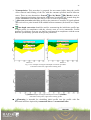
1
Version 2.59
User's Manual
Riga 2014
1
Table of Contents
Section
Page
1. Introduction ....................................................................................................................... 2
2. Brief Description of Georadar ........................................................................................... 3
3. Convention of Terms ......................................................................................................... 5
4. Radiolocation Data Display Examples .............................................................................. 6
5. Routine Installation in Computer ...................................................................................... 7
5.1. Configuring the computer for wire connection with Zond-12e Georadar Control
Unit ............................................................................................................................ 7
5.2. Configuring the computer for wireless connection with Zond-12e or Python
Georadar Control Unit ............................................................................................... 8
6. First Running ................................................................................................................... 14
7. Functions of Menu Options ............................................................................................. 16
8. Adjustment of Georadar .................................................................................................. 22
9. Radiolocation Sounding Run ........................................................................................... 27
10. Radiolocation Sounding Data File Handling ................................................................. 29
12. How to import Zond GPR data files from Prism to Voxler 3D software ...................... 45
13. Our Recommendations .................................................................................................. 48
14. Radiolocation Sounding Data Format ........................................................................... 49
14.1 SEG-Y Sounding Data Format .............................................................................. 49
15. Solving Problem of Layer-by-Layer Determination of Groung Thickness and
Permittivity by CDP Technique in Flat Layer Model ................................................... 52
Appendix A ......................................................................................................................... 55
Attributes ............................................................................................................................. 57
2
1. Introduction
Thank you for your purchase of our radiolocation subsurface sounding equipment
and/or your interest therein. Our Company is using over 30 years of experience in this
field; the studies in this field were launched by Aviation Subsurface Radiolocation
Problem Laboratory (PLAPR) legally succeeded by Radar Systems, Inc.
A modern Ground Penetrating Radar (GPR or “georadar”) is quite a sophisticated
radio engineering device. But with introduction of microprocessor and computer
technologies, it has become simpler in operation as compared with early models. Skill to
operate a georadar actually means knowledge of how to use the routine whose description
you are reading. Apply proper diligence when learning to handle the routine, and you'll see
no difficulty in mastering it.
In many cases, correct interpretation of sounding data results from certain experience
which you have already or which, hopefully, you'll acquire quite soon. The routine will be
your effective aid for the purpose.
Prism2 Software Package is designed to be used in field as a component of Zond12e and/or Python Georadars and also in laboratory for radiolocation sounding data
processing and interpretation. Important: to work with Zond-12e and/or Python
Georadar, computer must be equipped with Ethernet card 10/100 BaseT. For wireless
connection computer must be equipped with WiFi card.
The tasks of Package include:
1. Control of all Georadar modes, and adjustment of its parameters for specific job
conditions.
2. Receiving digital data from Georadar in a radiolocation sounding run, and
recording them in data files on a computer hard disk.
3. Visualization of data being received (or received earlier) on a computer display
in user's specified mode.
4. Digital processing of received data for extracting useful signals and suppressing
noise, interference and non-informative signals.
5. Determination of various signal parameters, spectral computations, and the like.
6. Printout of results.
Package is supplied on CD with the computer installation routine (SETUP.EXE).
Package is compiled as a user's integrated medium, i.e. user starts PRISM.EXE
routine only and deals only with this routine. All and any other auxiliary routines are run
automatically as a function of user's actions.
The routine serves as a multi-window interface which is convenient for comparison
of various profiles, e.g. before and after processing, single section covered using different
antennas, etc.
3
2. Brief Description of Georadar
Georadar is quite a sophisticated engineering device. Below, its simplified structural
schematic is presented, which allows getting a general idea of its principle of operation but
does not reflect its complexity.
Computer with
“Prism2” software
Synchronizer
Stroboscopic
converter
Transmitter
Receiver
Antenna
Surface
Antenna
Target
Fig. 2.1. Simplified structural schematic of Georadar.
The transmitter sends extremely short electric pulses energizing the antenna. The
transmitting antenna radiates ultra-wideband one-and-half-period electromagnetic waves;
their approximate shape is shown in Fig. 2.2.
Fig. 2.2. Shape of electromagnetic wave radiated.
4
These electromagnetic waves are propagating in sounded medium, thus reflecting
from various inhomogeneities (metals, cavities, various objects, layer boundaries with
different parameters, etc.). Reflected sounded waves which carry information on the
medium being sounded are received by the receiver using a receiving antenna. Receiving
signal however, in addition to reflected wave also contain a direct wave that is going by the
shortest distance directly from the transmitting to the receiving antenna. Therefore, the
receiver's output signal is combination of transmitter's pulse (as shown in Fig. 2.2)
followed by reflected pulses. This transmitter's pulse should be used as a starting point for
estimating a delay of reflected signals for the purpose of determining the target's depth of
occurrence in the medium.
Fig. 2.3. Example of receiver's output signal.
Transmitter's pulse is clearly visible to the left.
Passing process shown in Fig. 2.3 is very fast, and takes tens to hundreds of
nanoseconds which in technical terms makes him very difficult to process. Therefore
stroboscopic converter is used to "expand" this process in time. Synchronizer is used for
controlling all Georadar assemblies’ operation, while in its turn synchronizer, is controlled
by the “Prism2” routine from your computer, and its description you are holding in your
hands right now. Computer running “Prism2” is the one that receives radiolocation
sounding data delivered from GPR.
When analyzing received data, it is important to borne in mind that the propagation
speed of electromagnetic waves in sounded medium (other than air) is not equal to the
velocity of light, in fact – its speed is retardation factor times less. The retardation factor is
equal to the square root of the medium's permittivity. Consideration of this factor in the
routine however, is made automatically, and you will see it soon by yourself.
5
3. Convention of Terms
Some terms that are present this text are listed below, since they have different
interpretations in various literature sources.
1. Sample: Unit value comprising reflected signal amplitude at a definite time.
2. Trace: A set of samples comprising one-dimensional information about reflected
signals. Examples of traces are shown in Figs. 2.3 and 4.1.
3. Profile: A set of samples comprising two-dimensional information about reflected
signals generated while passing a survey line. A profile may contain any quantity of
traces. Profile examples in various types of display are shown in Figs. 4.2 and 4.3. The
final result of sounding shall be a profile (or a certain number of profiles) as a file (or
files). Subsequent steps will be data processing (if required), printout (if required) and
interpretation.
4. Zero point: Trace sample corresponding the time of transmitter’s maximum emission.
It is this very sample that has zero number on the scale along the traces, i.e. reflected
signal’s delay time should be counted from this sample. As mentioned above, the
transmitter’s pulse is approximately a one-and-half-period (i.e. three-lobe) signal.
Therefore, zero point should be set to the second lobe of the transmitter’s pulse. The
Zero point setting procedure is described in Section 10 of the present User’s Manual.
It is a rather important parameter which must be considered when measuring the time
delays of signals to determine target’s depth in the sounding medium. Zero point
location examples are shown in Figs. 4.1, 4.2, 4.3.
5. Wiggle plot: Way of profile display where traces are running vertically with some
spacing between them. Drawing of each trace is made by a curve deviating to the right
or to the left from the trace centerline, depending on the sample value in each point of
the trace. Here, positive half-waves are painted in the color corresponding to the
maximum positive level of the color scale selected. Examples of wave profile are
shown in Fig. 4.2.
6. Line scan: Way of profile display where traces are running vertically close to each
other and are drawn by vertical lines. Color in each point of a line shall depend on the
amplitude of a respective trace sample conforming to the color scale selected.
Examples of density profile are shown in Fig. 4.3.
7. Mark: Distinctive feature of any profile’s trace, designating certain uniqueness of a
given trace and therefore of a given point of the survey line. Marks are used to bind a
profile to the terrain. In the course of sounding, you may press a button to enter marks
when passing certain landmarks on terrain or pre-located stations. Further on, when
the profile is visualized on a display, these marks will be shown together with the
profile. Mark display examples are shown in Fig. 4.3.
6
4. Radiolocation Data Display Examples
Fig. 4.1. Trace display example.
Fig. 4.2. Wiggle plot profile display example (black-and-white and color scales).
Fig.4.3 Density profile display example (black-and-white and color scales).
Note: Our experience shows that usually the most informative sounding data display
type is the density profile in the black-and-white scale (see Fig. 4.3, left side).
7
5. Routine Installation in Computer
To install “Prism2” Package on the hard disk of the computer sequentially perform
the following operations:
⇒ Insert “Prism2” CD in the computer CD-ROM.
⇒ If Auto Run is disabled, Press button Start on the main panel and then press Run
(if there is no Run at you Start menu you can always press Windows Key
+
R); type d:\setup in Open line of appeared Run window, where d is the letter of
your disk drive, and then press button OK.
⇒ Follow instructions of the installation routine. When asked, enter the Activating
code that is attached to the CD. You can also get activating code via E-mail,
phone or fax.
5.1. Configuring the computer for wire connection with Zond-12e
Georadar Control Unit
You have to configure your computer, before its using with Zond-12e georadar.
For Windows XP:
1. Click the Start button, point to Settings and then click Control Panel.
2. Double click the Network connections icon.
3. Double click your connection and then click the Properties button.
4. Select Internet protocol [TCP/IP] and click the Properties button.
5. Click the Use the following IP address option.
6. Click the IP Address box and enter 192.168.0.1 (if this address is occupied or
is not accessible, you could use any address from 192.168.0.1 to 192.168.0.254,
except occupied addresses and 192.168.0.10, 192.168.0.100. Please, ask your
network administrator before IP addresses changing and applying).
7. Click the Subnet mask box and enter 255.255.255.0.
8. Press the OK button.
9. Press the OK button.
For Windows Vista:
1. Click the Start button, point to Settings and then click Control Panel.
2. Double click the Network and Sharing Center icon.
3. Click View Status of your connection and then click the Properties button
4. Select Internet Protocol Version 4 (TCP/IPv4) and click the Properties
button.
5. Click the Use the following IP address option.
6. Click the IP Address edit box and enter 192.168.0.1 (if this address is occupied
or is not accessible, you could use any address from 192.168.0.1 to
192.168.0.254, except occupied addresses and 192.168.0.10, 192.168.0.100.
Please, ask your network administrator before IP addresses changing and
applying).
7. Click the Subnet mask box and enter 255.255.255.0.
8
8. Press the OK button.
9. Click the Close button.
10. Click the Close button.
For Windows 7:
1. Click the Start button and click Control Panel.
2. Click the Network and Sharing Center icon or chose the subitem View
network status and tasks, of Network and Internet item.
3. Click the link Change adapter settings in the left part of Network and
Sharing Center.
4. Select your connection icon and click right mouse button on it. Select the item
Properties of the pop-up menu.
5. Select Internet Protocol Version 4 (TCP/IPv4) and click the Properties
button.
6. Click the Use the following IP address option.
7. Click the IP Address edit box and enter 192.168.0.1 (if this address is occupied
or is not accessible, you could use any address from 192.168.0.1 to
192.168.0.254, except occupied addresses and 192.168.0.10, 192.168.0.100.
Please, ask your network administrator before IP addresses changing and
applying).
8. Click the Subnet mask box and enter 255.255.255.0.
9. Press the OK button.
10. Close the Network and Sharing Center window.
If for any reason you don’t like new IP address of your computer you may reset
your old IP address following procedures described above. But before you reset your old
computer IP address you have to change Control Unit IP address. As default it is
192.168.0.10. For information about the default Control Unit IP address changing, refer to
Changing the Control Unit IP address in Appendix A (p.53).
5.2. Configuring the computer for wireless connection with Zond-12e or
Python Georadar Control Unit
For Windows XP:
1. Click the Start button, point to Settings and then click Control Panel.
2. Double click the Network connections icon.
3. Double click your wireless WiFi connection and then click the Properties
button
4. Select Internet protocol [TCP/IP] and click the Properties button.
5. Click the Use the following IP address option.
6. Click the IP Address box and enter 192.168.0.2 (if this address is occupied or
is not accessible, you could use any address from 192.168.0.1 to 192.168.0.254,
except occupied addresses and 192.168.0.10, 192.168.0.100. Please, ask your
network administrator before IP addresses changing and applying).
7. Click the Subnet mask box and enter 255.255.255.0.
8. Press the OK button.
9. Press the OK button.
9
10. Click the right button of mouse on your wireless WiFi connection and then
click Connect button.
11. Select Zond-12e or Python network and click the Connect button.
12. If you are using factory deffault WiFi access point settings then follow to the
next point, otherwise chose the secutity method for WiFi connection end enter
pass code if needed.
13. Press the OK button.
For Windows Vista / Windows 7:
1. Click the Start button and click Control Panel.
2. Chose the subitem View network status and tasks, of Network and Internet
item.
3. Click the link Change adapter settings in the left part of Network and
Sharing Center.
4. Select your wireless WiFi connection icon and click right mouse button on it.
Select the item Properties of the pop-up menu.
5. Select Internet Protocol Version 4 (TCP/IPv4 and then click the Properties
button.
6. Click the Use the following IP Address option.
7. Click the IP Address edit box and enter 192.168.0.2 (if this address is occupied
or is not accessible, you could use any address from 192.168.0.1 to
192.168.0.254, except occupied addresses and 192.168.0.10, 192.168.0.100.
Please, ask your network administrator before IP addresses changing and
applying).
8. Click the Subnet mask box and enter 255.255.255.0.
9. Press the OK button.
10. Press the OK button.
11. Click the right button of mouse on your wireless WiFi connection and then
click the Connect button.
12. Select Zond-12e or Python network and click the Connect button (check the
Connect automatically checkbox to connect to the network automatically in
the feature).
13. If you are using factory deffault WiFi access point settings then follow to the
next point, otherwise chose the secutity method for WiFi connection end enter
pass code if needed.
14. Close the Network and Sharing Center window.
Note: If during connection Set up network dialog appears (or Windows asks the
PIN code for the connection), please click the “Connect to the network without setting it
up” link (like it shown on the figure below).
10
Fig.5.1. Wi-Fi network Set up dialog.
We recommend using Maximum Performance power option for WiFi connections
to avoid problems with weak WiFi signal receiving under Windows Vista / Windows 7.
For Windows Vista / Windows 7:
1. Click the Start button and click Control Panel.
2. Chose the item Power Options.
3. Follow the link Change plan settings (Fig. 5.2.)
4. Follow the link Change advanced power settings
5. Find and collapse item Wireless Adapter Settings and subitem Power Saving
Mode
6. Chose value Maximum Performance for sub itemsoke my On battery and
Plugged in
7. Press the OK button.
Fig.5.2. Power options dialog.
11
Fig.5.3. Edit power options dialog.
Fig.5.4. Power options advanced settings dialog.
Important: In some cases your portable device may have unsatisfactory
connection even with power setting set to maximum performance. In this case you
should use external WiFi USB adapter. We advise to use “NETGEAR N150 Wireless
USB Micro Adapter”.
12
Georadars “Zond-12e Advanced” and „Python-3” has WiFi access points for
wireless connection. Disabled security mode of WiFi communication is presetted by
factory default settings.
Note: It is not recommended to change WiFi access point settings without the
help of your local network administrator.
If you want to change the security mode of WiFi access point, please use following
steps:
1.
2.
3.
4.
5.
6.
Run any internet browser (all examples are based on Internet Explorer 10 here
and below) and use WiFi access point IP address as URL in address line.
Use „Zond12e” as a login name and „zond12e” as a password.
Press Wireless button on the WEB-page.
Chose menu item Security.
Chose Security Mode and enter all necessary information in corresponding
fields.
Press Apply button.
Fig.5.5. WiFi access point login dialog.
13
Fig.5.6. WiFi access point security settings WEB-page.
More detailed information about WiFi access point settings you could find here:
http://www.trendnet.com/asp/download_manager/inc_downloading.asp?iFile=17937
14
6. First Running
You will see four items in the menu after software’s starting up:
Fig. 6.1 “Prism2” Menu at the initial stage.
The default software operating language is English, which is set after installation
(there are English, German, Russian, Greek, Korean and Chinese languages). If you wish
to change it, to Russian for example, select View/Languages menu and press the button
Add language. Select file Russian.lng. Now, you may set Russian as the default language
by pressing Set as default button. You could choose the selected language by OK button
click or by double click on it.
You may choose positioning method with Radar/Positioning menu help. Possible
positioning methods are: Manual, Wheel, GPS and Wheel + GPS. Manual positioning
method allows entering of manually measured length of the passed track when you save
the data to hard drive, or by using Output parameters menu (see Section 10 below). For
the Wheel positioning you have to enter following parameters: the wheel’s diameter, the
number of pulses per revolution and trace spacing (dX), or to calibrate the wheel by
moving on the precisely measured distance. To calibrate the wheel enter
Radar/Positioning/wheel menu item and click on the small window Wheel calibration.
In appeared dialog box press Start button and move antenna with the wheel on the
precisely measured distance, then press Stop button and enter the distance. During by the
wheel positioning current length of the passed distance is calculated, gathered value is
15
recorded to the each trace. Data will not be collected while antenna is not moving. Here in
dialog box you may chose automatic X-interpolation to display traces during data
acquisition equidistantly with preset spacing. You can enter trace spacing every time
before data acquisition or keep entered in dialog box value the same for all acquired data.
When using Zond-12e Advanced, the wheel operates as a two-way device. When the
antenna moves forward the profile on the screen is displayed from left to right, but if after
a stop the antenna moves backward, the profile will also be built backward, i.e., from the
right to the left and is shown as a white vertical marker. If the antenna moves backward
along the same path, then visually on the screen it will look like a back movement of the
white vertical mark over the profile. This function of the wheel is very useful at
determining precise location of underground utilities when upon moving backwards the
white vertical mark precisely coincides with the top of the hyperbola.
Should you like to use the global positioning system (like GPS), you are to choose
the receiver providing digital output of coordinates in format NMEA 0183 (Version 1.5 or
higher). Connection to computer is possible via COM port (including Bluetooth) or USB if
it is defined in computer as COM port after installation. In case of use of GPS there will be
recorded in the heading of each trace current latitude and longitude which are further used
to calculate the length of path passed and of current coordinate of the trace on the profile.
In combined Wheel + GPS positioning there will be recorded in the heading of each trace
current latitude and longitude but length of path passed is calculated by wheel.
If you need to recalibrate the wheel press Recalibrate button and repeat described
above actions.
In Radar/Where to save option, you may specify a directory wherein your sounding
data files will be recorded automatically.
In principle, the routine is now ready for the work with Georadar and sounding data
files; for you to be ready as well, get familiar with functions of Menu options described in
the Section below.
16
7. Functions of Menu Options
The full menu is displayed on the screen upon opening of the data file. Here,
functions are listed for each option of the horizontal menu, followed by descriptions of
respective options of vertical menus.
Fig. 7.1 Full Menu of “Prism2”.
7.1. File – various file handling operations and printout.
Open – using this option, you may select a proper file and have it displayed on the
screen, by typing its file name in File name line, or choosing a proper file in the list
and load it by pressing button Open. In needs of opening more than one file at once
please select them beforehand with the right mouse button click. At the same time,
this option offers some other standard features, such as deletion, renaming, copying
and creation of folders and files.
17
Fig.7.2. File Open dialog box.
Reopen - in this option the last ten opened files’ data are stored for their easier
finding and opening.
Save As – using this option, you may save sounding data as a file on your computer.
Save All – this option gives ability to save all currently opened profiles with
sounding data on your computer
Close All – this option allows closing all currently opened profiles by one click.
Add – joining of profiles.
Export - using this option, you may save the image of displayed data in Bitmap or
JPEG format, as well to record markers position, amplitude values or XYZC (3D
data grid) as text file.
Import – this option allows calling of gain function or zero point position from
another profile, or import GPS coordinates (in NMEA format) from existing text file.
Profiles combining – opens Profiles Combining Wizard that helps to combine all
selected profiles into the one profile.
Profiles splitting – opens Profiles Splitting Wizard that helps to split selected
profile to the several profiles.
Profiles 3D aligning – aligning of parallel profiles acquired for 3D imaging in Easy
Prism 3D or Voxler 3D software.
Print. Profile printout in one of the views supported by the routine. The following
items may be modified in the Print dialog box (Fig. 7.3):
◊ Printer. Printer which you could use for printing.
◊ Printing type – Scaled or Not scaled. In case of scaled print, the vertical and
horizontal scales shall be specified.
◊ Orientation (Landscape or Portrait). When changing orientation of a page, the
outline of the page and the layout of drawing therein are changed, respectively.
◊ Layout. After clicking the drawing and holding left mouse button (the pointer
will be replaced by the crosshair), moving the mouse will change drawing’s
layout on the printing page.
◊ Size. After clicking drawing’s size modification area (small yellow rectangle on
the right down of the drawings area) and holding left mouse button (the pointer
18
will be replaced by the double arrow), moving the mouse will change drawing’s
size.
◊ Printer setup. Standard dialog box for printing settings with profile preview.
Fig. 7.3 Profile Print dialog box.
Properties – printing properties.
Exit – work completion with the routine. Most users may also use the standard
application completion method by clicking the left mouse button on the
button at
the upper right corner of routine’s window or by simultaneous pressing Alt+F4
buttons. If there are any unsaved files you will have to answer relevant questions to
confirm your exit.
7.2. View – routine options determining the appearance features of the routine’s main
window.
◊ Show toolbar – display or not the Toolbar in the upper part of the routine’s main
window.
◊ Show processing toolbar – display or not the processing buttons toolbar located
in upper section of the main screen of the program.
◊ Windows tabs – display or not the profiles tabs in the lower part of the routine’s
main window.
◊ Show status bar – display or not the Status bar in the lower part of the routine’s
main window.
19
Large buttons – increasing toolbar buttons size.
Antialiasing – enables or disables antialiasing when drawing curves (wiggle trace,
power curve etc.).
Languages – choice of the routine’s working language. When supplied, the routine
is provided with English, Russian, German, Chinese, Greek and Korean languages
(language files are located in the root folder of “Prism2” software). If you need
other language to support the routine, don’t hesitate to contact us at communication
addresses listed on the last page of this User’s Manual.
7.3. Tools – tools and options used for profile handling and tuning purposes. See Section
10 for more details.
Color palette – creating, saving and selecting color palette for displaying data as a
profile.
Gain function – gain function window opening (see. p.23). You may choose the
option to display the trace in gain window or not.
Frequency filter – activation of displayed profile’s lower right column for the fast
digital signals’ in frequency domain filtering run. Frequency filter will be active, if
Customized High Pass Filter was used during data acquisition.
Mouse actions – profile handling tools:
◊ Point info – output of the following parameters values: Trace, Position, Sample,
Time delay, Depth, Amplitude - of the specified point in a profile as well as
latitude and longitude applying positioning by GPS. If there is a mark its number
is displayed in bottom line of the dialog box.
◊ Hyperbola – measuring local object distance and environmental permittivity by
the hyperbola technique, with output of values for the following parameters
measured: Position, Depth, Time delay, Permittivity, Velocity.
◊ Zoom in – selected area magnification.
◊ Zoom out – reverse Zoom in operation.
◊ Fit profile – fitting of the whole profile in one window.
◊ Average spectrum – average signals’ spectrum calculation in a selected area
before its amplification or after they have been gained.
◊ Trace inspection – this option is showing separate profile traces (see Fig.4.1.), it
also allows choosing which curves will stay visible in Trace window (wiggle
trace, power curve, attenuation curve).
◊ Sample inspection– output samples of the same number along profile.
◊ Cut traces - this option is deleting undesirable traces from the data file.
◊ Hodograph – solving a problem of layer-by-layer ground thickness and
permittivity determination using the common depth point within a flat layer
model.
◊ Annotations – creating, deleting and editing profile annotations.
◊ Pulse delay adjustment – adjustment of sounding pulse position on time axis.
Lines color – color selection for marks and synthesized hyperbola line.
Marks – adding, deletion and ranking marks on the profile.
Output parameters – profile display parameters output such as Output range,
Length of profile, Output view, Normalizing factor and file heading stored (Text
information). You can also switch on or off displaying of markers and annotations at
the profile or leave annotations only as the final result of probing results
interpretation.
GPS Tracker - survey path applying GPS positioning display.
20
GPS Coordinates Table – display current profile’s editable GPS coordinates table.
Convert to UTM coordinates – latitude / longitude coordinates conversion into
UTM coordinates.
7.4. Radar - control of all Georadar operation modes and sounding data receiving in the
course of sounding.
Connection settings – Control Unit IP address setup. By default it is set to
192.168.0.10. Control Unit IP address changing is described in Appendix A on p.53.
Performance – setting of radar performance: single- or double channel.
Positioning – choosing of method of current coordinates measurement and the total
length of profile (see Section 6 “What to do after installation”).
Sounds – on/off for sound signals during radar operation.
Battery warnings – enables or disables low battery charge warnings.
Tablet controls – enables or disables ability to work with touch panels or computer
mouse.
Show channel labels – enables or disables ability to show semitransparent channel
labels on the foreground of the signals in dual channel or circle data acquisition
mode (Fig. 8.1b.).
Where to save – choosing a directory where sounding data files will be
automatically recorded.
When to save – option that switches when the sounding data will be saved – during
or after the acquisition. Program will ask to enter filename and saving location when
save data During acquisition is chosen (this option is preferable to use for long
profiles, it will protect from losing unsaved data in cases like power loss, insufficient
RAM space, critical system errors, etc.).
Environment options – changes data acquisition menu appearance:
◊ Color setting - Black & White or Colored buttons in data acquisition menu.
◊ OFF computer on exit - if this option is ON, anytime when leaving data
acquisition menu you can simultaneously switch off the computer.
◊ Introduction on start – upon entry, disables or enables colored introduction on
the data acquisition menu screen.
◊ Introduction on setup – upon data acquisition Setup menu entry, disables or
enables additional dialog window.
◊ Password on setup - entering of the password to access the acquisition Setup
menu.
Auto launch – turn on/off the automatic Data Receive dialog box run, during the
routine startup.
Start – equivalent of simultaneously pressing Ctrl+A buttons. This option will start
data acquisition window. See Section 9 for more details.
7.5. Processing – digital files processing that were collected earlier in the course of
radiolocation sounding. Processing goal is to extract the useful signals and of noise,
interference and non-informative signals suppression. See Section 11 for more details
on this menu options and the file handling procedure.
7.6. Window – profile windows layout on the display.
Tile vertical – vertical windows positioning.
Tile horizontal – horizontal windows positioning.
Tile smart – windows positioning in consideration of the profiles’ size.
21
Cascade – cascaded windows positioning.
7.7. Help – help on the routine.
User’s Manual – open this manual.
Radar Systems, Inc. web page – open Radar Systems, Inc. homepage.
Check for updates at startup – turning automatic updates checking on/off at
routine’s startup.
Check for updates – run Prism2 Updater routine.
Version History – history of routine versions.
About – information about the routine (version, developer).
22
8. Adjustment of Georadar
Before you start sounding, be sure to correctly adjust Georadar operation modes. With
some practice, this procedure will take you no more than a minute.
8.1. Connect an appropriate antenna (antennas), battery (if needed) and computer with
installed “Prism2” to the Georadar (see Georadar User’s Manual). Warning! Do not
connect or disconnect cables while Georadar is switched ON! Set the antenna
(antennas) in its working position.
8.2. Switch Georadar and computer ON. If you use wireless connection please make sure
your computer has established wireless connection with corresponding georadar
(Zond-12e or Python) wireless network and only then launch Prism2 software. Enter
option Radar/Start or use Ctrl+A buttons combination. From this instant and up to
returning back to the Main Menu, all control shall be made from the keyboard only
(if Tablet Controls are not enabled see 7.4). This is made specifically for convenient
use of the computer in the field condition. In the Data Acquisition dialog box, use keys
← and → to select Setup and press Enter or Space.
Note: When Georadar is being switched ON, all of its parameters are in random
positions. When the Georadar Adjustment dialog box is entered, the routine sets all
Georadar parameters in some definite stored position. Therefore, to avoid confusion, first
switch Georadar ON, and then after 3 seconds enter the Georadar Adjustment dialog box,
and not vice versa. Otherwise, the routine will be hanging up.
8.3. Once Radar/Start/Setup is activated, the screen shows ZOND SYSTEM 12e
SETUP Georadar Adjustment dialog box. An example of single channel georadar
setup window is shown on fig. 8.1a, but double channel – on fig. 8.1b.
Fig. 8.1a. Single channel georadar adjustment dialog box.
The left-hand window contains the Georadar Control Menu, and the small right-hand
window accommodates permanently alternating traces being received. Below, under
the signal window, auxiliary information and some recommendations are displayed.
Please remember that, during adjustment, the antenna should be set to its working
23
position, e.g. at the initial point of a suggested survey line. It is from this moment that
Georadar adjustment is started. The cursor is controlled using keys ↑ or ↓. Menu
options are selected using keys Enter, Space or →.
Fig. 8.1b. Double channel and Advanced georadars adjustment dialog box.
•
•
•
•
•
Medium – setting the medium that you intend to sound. Choose the closest
medium out of the provided list. Permittivity used for depth calculations is
shown to the right of the name of a respective medium.
Samples – number of samples in a trace. Using Zond-12e Advanced it is
possible to set 1024, 512, 256 or 128 samples. In all other Zond-12 models this
parameter equal 512 and may not be changed. If you reduce samples rate traces
rate is increasing proportionally. But user has to be very attentive to the
information under signal window to avoid situation when number of samples is
not enough for correct signal digitizing.
Stacking – setting a number of traces which will be added together in the course
of sounding. Stacking contributes to suppression of noise and interference and to
increase of the depth rating. However, it should be remembered that stacking
decreases the trace arrival velocity times the number of stacking, and it may
necessitate the antenna moving velocity to be decreased with the objective of
information loss avoidance. If the parameter is set to 1, no staking is performed.
Scan rate – traces per second. The value is adjusting automatically when
samples and stacking are set, In Zond-12e Advanced the maximum value is 320
at 128 samples and stacking =1. In all other Zond-12e models the maximum
value is 80 for Dual Channel version and 56 for Single Channel.
Sounding mode – here, two options are available, namely Continuous or
Stepped. The first mode is the most frequently used one suggesting that, once
you start sounding, Georadar will perform continuous sounding until you
terminate the process by pressing key Esc or button Stop. Stepped profiling is
used in certain cases where it is impossible to draw the antenna continuously
along the route or it is necessary to achieve the deepest sounding possible. But
this will require more time for a sounding run. In this case, generation of each
24
•
•
•
•
•
•
individual trace is made only when key Enter (or key Space for station
marking) is pressed. This mode is recommended to make use of stacking. The
profiling method is as follows. You reposition the antenna in a step-by-step way
(not continuously!) with the same spacing along the survey line, and perform
sounding in each point by pressing the key. Once completed, press Esc or button
Stop.
Mode - it may have two options: Sounding or Test. The first option, as follows
from its name, is the sounding data receiving mode. The second option is used
for testing the control unit for operability with no antennas connected. When
Test is set, a continuous sinusoidal signal is supplied to the control unit’s input.
Tx/Rx cables – only in Single channel georadar - one Combined or two
Separated cables connect Control Unit with antenna. For 38-75-150 MHz
antenna this parameter is always automatically specified as Separated and
cannot be changed. For other antennas this parameter is specified at default as
Combined and may be adjusted for operation in the configuration shown on Fig.
16 of the Georadar User’s Manual.
Channels mode – for Zond-12e Double channel or Advanced georadars only –
there are four (Zond-12e Double channel) or six (Zond-12e Advanced) possible
regimes:
o Channel 1 – single channel mode for operation with one antenna connected
to channel 1.
o Channel 2 – single channel mode for operation with one antenna connected
to channel 2.
o Double channel – double channel mode of operation with alternate
receiving of signals from two antennas connected to channels 1 and 2.
o Tx-1, Rx-2 - single channel mode for operation when the signal is radiated
by the antenna connected to channel 1 and received by the antenna
connected to channel 2. This mode is applied when making measurements
applying the method CDP and also in case of using of the dipole antenna
38-75-150 MHz.
o Tx-2, Rx-1 – (In Zond-12e Advanced only) single channel mode for
operation when the signal is radiated by the antenna connected to channel 2
and received by the antenna connected to channel 1.
o Circle mode – (In Zond-12e Advanced only) alternate signal receiving in
modes: Channel 1; Channel 2; Tx-1, Rx-2; Tx-2, Rx-1.
Channel 1 / Channel 2 – for Zond-12e Double channel or Advanced georadars
only – tabs for different channels settings.
Antenna – this option is used to specify the antenna connected to the georadar’s
channel from the provided list.
Range – one of the most important parameters, to be chosen rather carefully.
You can select the range from a set of proposed values or set it up by yourself at
the item Customized. When specifying the range you should watch at the
information appeared under the signal window. If your specified range is too
wide the legend will appear stating “Warning! Too small sample rate!”. To the
right side of the range value in nanoseconds, its width is indicated in meters for
the selected medium. It determines investigated depths interval for the selected
medium when there is no attenuation. Maximum penetration depth, however, is
defined by the sounding signal attenuation level and varies in different soils.
25
•
•
Therefore, setting this parameter higher than it is required for your task is not
recommended.
Gain - digital gain of the received signals when they are displayed on the screen
as a radar profile. Due to the fact that the signal’s strength is rapidly decreasing
while it is propagating along the soil, the gain of the signal should be increased
with the increasing depth. Therefore at the end of the trace the gain should be
greater than at its beginning. You can set any gain function as a polyline
connecting up to 10 points while each of them can be adjusted within 0-84 dB. It
is important to remember, that the signal itself is digitized and saved on the
disk without any gain. Gain is used only while displaying the data in the form
of radar profile on your computer. When entering the Gain option under the
signal window Digital gain function setup window will appear there will be
movable points, the amount of which is set by pressing keys 2 to 9. To set 10
points press key 0. Point selection is performed with the arrow keys ← and →,
to adjust the gain levels use arrow keys ↑ and ↓. For most cases it is sufficient to
set only two points with values 0 dB at the beginning and 48 dB at the end. If
these settings are not optimal, you can always set other ones when displaying
and processing data in the main menu (see Section 10).
High-pass filter – high-pass filter’s cutoff frequency selection for received
signal to attenuate low-frequency noises, which arises while antenna is crossing
the rough terrain. Pay attention to the recommendations in the information
window. Customized filter is a digital real-time bandpass filter. This option will
disable hardware high-pass filter. Frequency band of customized filter is
modified in appeared filter setup window that is visualizing signal’s spectrum in
accordance to the frequency response. Frequency band is characterized by its
vertexes (each vertex corresponds to filter cutoff frequency). To navigate
through filter’s vertexes use < and >, or tab keys. Changing vertexes’ position
(filter cutoff frequency) could be done by ← and → keys.
Warning: signal itself is recorded in original shape (not filtered). Filtering
(the same as a Gain function) is just a software tool and is used for data
visualization.
We recommend using Customized High-Pass Filter, only if you are familiar
with the spectrum analysis and the digital signal processing. Otherwise we
recommend using Weak, Strong and Super Strong filters, by following
recommendations.
•
Real-time filter – real-time filter selection to remove background noises, which
can arises because of external electronic noises, cables, constant distortions, etc.
Such constant background signals could be seen on the profile as a horizontal
lines that do not change their intensity and time position and may mask the real
reflected signals. To read more detailed information about “background
removal” see 11.
Warning: Real-time filtering rebuilds the original shape of the signal and
records already filtered data! To prevent unexpected data lose a semitransparent red warning message appears in the signal oscillation and profile
receiving windows.
26
•
•
•
Pulse delay – this option is changing sounding signal’s position within the
sounding time range. Default delay values in most cases are not optimal. It is
important to make an appropriate setup at the first start of Georadar with a given
antenna and for the given Range value. Relevant adjustment may be performed
in the automatic or manual mode. When key ‘а’ or ‘A’ is pressed (automatic
mode), a sounding signal shall be automatically positioned to the beginning of
the sounding time range. When in the manual mode, set the sounding signal to
the desirable position in the sounding time range using ← and → (fine tuning)
and keys Page up и Page down (rough adjustment). Optimal sounding pulse
position in the sounding time range is position, where the first lobe is spaced
from the time axis beginning by about 1/20 of its length (see Fig. 8.1). After any
adjustment, the Pulse delay values will be saved for each Antenna – Range
combination, so you won't need to adjust Pulse delay values on subsequent GPR
starts.
Positioning – changing current coordinates measuring method and the total
profile length. Duplicates Radar / Positioning menu item. Operator may change
positioning method without leaving the data acquisition menu.
Close – end of Georadar adjustment, closing Georadar adjustment dialog box
and saving settings for further use.
Note: All Georadar adjustment parameters shall be saved and stored by the
routine in special-purpose file z12c_td.dat. Here, all parameters for every antenna
types shall be stored. If you've made any modifications in the parameters, the
parameters will be saved once adjustment is completed. These very parameters will
be set in subsequent runs of the routine.
Below, you'll see examples of successful and unsuccessful adjustments, with relevant
comments.
Fig. 8.3 Example of good adjustment.
Fig. 8.6. Low-frequency interference present.
High pass filter should be activated.
Fig. 8.7. Incorrect transmitter pulse delay.
Pulse delay should be adjusted.
27
9. Radiolocation Sounding Run
Once you have set all of the required parameters in Radar option menu and made all
needed Georadar adjustments, you may start sounding.
Using option Radar/Where to save, you may choose a directory for recording files
created in the course of sounding. It is advisable to save profiles related to the different
Georadar job in a separate directory to avoid confusion afterwards.
Now, place antenna (antennas) in the working position at the initial point of a
suggested survey line, and exit the Georadar Adjustment dialog box.
When Georadar Adjustment dialog box is closed it will you will see Data Acquisition
dialog box that has control buttons at the bottom. Right now, only the four highlighted
control buttons are accessible, i.e. Setup, Start, Exit, and Palette. Using the key Palette
you can select received data displaying color. Make sure you have chosen correct
positioning that is displayed in informative window at the top of the screen. Button Start is
automatically selected upon entering the Data Acquisition dialog box. Press Enter or
Spacebar to start data acquisition, if Save profile on HDD option is selected, you will be
prompt to enter the file name before process start.
Right after a 0.8 second delay audio signal “Let’s go” will be generated (if option
“Sounds” is selected) notifying that the sounding process has started. Now in real-time on
the screen radiolocation profile will be displayed. Trace signals are simultaneously
displayed in the right side of the screen.
On the top of the screen additional information is displayed about number of
acquired traces, positioning mode, distance (in case of positioning by wheel) and internal
battery voltage (only in Zond-12e Advanced). When the battery level is too low warning
message appears on the screen.
Bear in mind that using positioning by weal data acquisition is performed only
when the wheel is rotating. When the weal stops, data acquisition will be stopped as well.
Once data acquisition is started Stop, Mark and Pause control buttons become
accessible and Mark button will be automatically selected. Without selecting any other
control button, pressing Enter or Spacebar in data acquisition will place Marker on the
current trace (it will immediately become visible as a vertical line with a number of
marker) and audio signal (“Mark”) will be generated. Notice that the first trace will always
be assigned as mark 0, while the last trace will always get the mark with the highest
number.
Pressing Esc or activating Stop control button (by press Enter or Space while it’s
activated) will end data acquisition. Audio signal (“Stopped”) will be generated and Setup,
Start, Exit, Save and Palette control buttons will become accessible while Save button
will automatically be selected.
Now you can save received data by pressing Enter or Space with Save control
button activated. You will be asked to enter profile length (if manual positioning), profile’s
Y-coordinate (if 3D surveys), movement direction (towards or backwards) and a file name
that you may leave as is or modify if you need, you can also chose not to save received
data as an alternative. If the folder where you are saving your file for any reason contain
file with the same name that you are currently saving, routine will suggest to Overwrite,
Add or Cancel.
It is also possible to save the obtained data when exiting Data Acquisition dialog box
by pressing Enter or Space when Exit option is selected. In this case, received profile
shall be automatically displayed in a separate window on the screen named Profile 1. Now,
you may save it by selecting File/Save as option in the Main Menu.
28
To pause data acquisition during the movement select Pause option and press Enter
or Space. The routine will stop the process and generate audio signal (“Paused”). When
you will be ready to continue simply select Continue or Mark options and press Enter or
Space (activating Mark, will not only resume the process but also place the marker at the
last trace before you stopped).
29
10. Radiolocation Sounding Data File Handling
When one ore more profiles have been created in the course of sounding, various
operations may be made thereon, as described below.
Load a sounding data file, and have it displayed on the screen by using option
File/Open. By default, the routine will display data as a line scan profile (Fig. 10.1) in a
separate window with standard Windows attributes in the right-hand upper corner. The file
name will be shown in the left-hand upper corner. The window may be drawn across the
screen, and its size modified, using standard Windows means and ways. The number of
profiles to be displayed in the screen shall be unlimited. By default, they will be arranged
in a cascaded pattern; you may also choose their layout patterns at your discretion in option
Window of the Main menu (see Subsection 7.6).
Fig. 10.1. Profile Output working window.
A radiolocation profile is provided with horizontal and vertical scales, vertical scale
can be moved for zero point adjustment (see Subsection 3.4). To set a zero point, draw the
cursor at the white field to the left of the profile (the cursor will take the form of a double
arrow), now when you press and hold the left mouse button move your mouse up and
down to move the scale so that the zero point coincides with the mid-point in the second
line of the sounding signal, as shown in Figs. 4.2 and 4.3. To the right of the profile, there
are three vertical columns used for quick tuning of the displayed profile. The upper column
is intended to change the color palette of displaying the radiolocation profile; this column
duplicates Tools/Color palette menu option and
button. Color palette modification is
30
described below; professionals however use black-and-white imaging that we also
recommend you to use, especially at the beginning.
The middle column is used to setup the signal’s gain function. At first opening of the
received sounding data, the gain function will be similar to one that was used at data
acquisition. Now however you are able to set any different gain function. To open Gain
function window simply press on the middle vertical line Gain with your left mouse
button.
Right after the first output of a newly created profile, gain function will have the
same form as it was specified at data receiving. To change the gain function you should
point mouse cursor on any vertex, so it will change its shape to arrowed crosshair under
which is the value of gain in dB. Press and hold the vertex and move it left or right, so the
gain will be correspondingly changed. The result of your actions will be immediately
displayed on the profile.
If you need multi vertex gain function, you can add new vertexes (up to 10). For this
purpose press the button
and click on desired point on the Gain Function window and
or
the new vertex will be created. To remove unwanted vertex you could use button
popup menu’s item Delete Vertex. Mouse cursor will be changed to a crosshair. Now you
can simply click on the vertex that you want to remove (gain function needs at least two
extreme vertexes, which are not removable).
By pressing
(trace curve),
(power curve) and
(attenuation curve)
buttons you can change which curves you need to be shown or hidden in the Gain
Function’s window. Track bar located beneath the buttons can be used to regulate curve’s
transparency.
and
To import the desired gain function from a different data file press the button
choose data file by double click. You can also apply this gain function to the all currently
opened profiles by pressing button
.
The lower column is used for digital filter in frequency domain setup. At the first
opening filter’s frequencies will be the same as they were setup at georadar adjustment
dialog box. Lower column will be crossed if in sounding mode digital filter was not used.
Double-clicking on the lower column will activate/deactivate digital filter, one click will
open filter digital filter setup window.
Vertical and horizontal scale dimensions may be modified by pressing the right
mouse button on the white field of a respective scale. If at data receiving mode manual
positioning mode has been used, you should specify profile length in the Set profile new
length drop-down menu option or at Tools/ Output parameters option in Main menu,
which is also duplicated by the toolbar button
. Vertical scale calculations in meters are
calculated using permittivity that is set in the Georadar Adjustment dialog box. You can
also change permittivity levels of a sounded medium after receiving data in the Main menu
Output parameters option
.
Important. Since there a distance between transmitting and receiving antennas (the
antennas offset), the simple time-depth recalculation contains the error. This error depends
on offset and measured depth ratio, because simple recalculation doesn’t consider direct
wave propagation time between transmitter and receiver. This error will be significant on
small depths especially on the depths close to the distance between the antennas. Therefore
there is Processing/Moveout correction program that excludes this error. You need to
31
setup Zero Point correctly before using Moveout correction. To perform Moveout
correction program enter correct distance between antennas. Georadar data already
contains this distance for all "Zond-12e" antennas and will be setup by default, but you can
still change it if it is required. We recommend applying this procedure every time no
matter the depth you are working with.
You can display profile as a Wiggle plot (Fig. 4.2), setting this this mode in the Main
menu Output parameters option (or toolbar button
). Here you could also chose to
display profile as a combined Line scan + Wiggle plot view.
Routine tools used when working with sounding data files are described below, they
are located in Tools option menu and duplicated as a toolbar buttons (Fig. 7.1.).
Point info – parameter values output: Trace number, Position, Sample number,
Time delay, Depth, specified profile’s point Amplitude, Latitude, Longitude and
Altitude as well as UTM Northing, Easting and Zone. If there is a mark its number will
be displayed in the bottom line of the dialog box. After activating Point info option
simply press anywhere on the profile where you need to know those parameters.
Holding left mouse button pressed will display a Point Info window illustrated in Fig.
10.2. Some of the information (trace number or position, sample number or time delay
or depth, latitude, longitude, altitude) is constantly displayed in the status bar located at
the bottom of the main window while you move your cursor along the profile.
Fig. 10.2. Point Info output dialog box.
Hyperbola – Local object’s depth and medium’s permittivity determination.
When a profile intersects diffractive targets, such as pipes, cables, stones, archeological
objects, areas of drastic soil properties variation, their signals on the radiolocation
profiles have hyperbola shape; signal examples are shown in Figs. 4.2, 4.3, 10.3. When
Hyperbola option tool is selected, pressing on the profile will draw hyperbolic line that
goes from a theoretical local target in a theoretically homogeneous medium, and open
an information window with this target and medium parameters. Your task is to match
the theoretical hyperbola with the signal’s hyperbola on the profile. First, align the
vertices of the hyperbolas; for this purpose, bring the cursor to the signal’s hyperbola
vertex, and press the left mouse button. The hyperbola slope may be changed by
pressing right mouse button: position the cursor on the signal’s hyperbola branch, and
press the right mouse button. For more accurate hyperbolas matching we recommend to
use
Zoom in on the Main menu (see below) and make several iterations. Matching
hyperbolas example is shown in Fig. 10.3.
32
Theoretical hyperbola’s line color may be changed in Tools/Lines color dropdown menu.
Fig. 10.3. Hyperbola technique used for measuring local target parameters.
Always remember that parameters determination accuracy fully depends on a
precociously configured profile length and zero point (Tools/Output parameters).
After you finished working with hyperbola, press Point info button and the
theoretical hyperbola will disappear.
Zoom in – selected area magnification. To select magnification area, press and hold
the left mouse button and select required zooming area. After releasing mouse button
selected area will extend to a size of the window. You can also zoom in using your
mouse wheel, simply scroll up the mouse wheel (while in Zoom in mode) and you will
extend the area around the mouse cursor’s position.
Zoom out – Reverse action of Zoom in. You can also zoom out using your mouse
wheel, simply scroll down the mouse wheel (while in Zoom out mode).
Note that you can always (no matter the instrument you are currently using) Zoom
in or Zoom out by scrolling up or down the mouse wheel while holding Ctrl key on
your keyboard!
Scaled output – scaling profile one to one, depending on the selected dimensions
of the vertical scale (samples to traces or depth to distance).
Fit profile – Fits whole profile to the window size.
Average spectrum– selected area signal spectrum average module calculation.
Used for of desired signal spectral characteristics and interference analysis when
choosing bandwidth and suppression frequencies filters: Ormsby bandpass and Notch
filter.
33
Fig.10.4. Spectrum Output dialog box.
To select gained or not gained signal for the spectrum calculation is performed in
Tools/Mouse action/Average spectrum menu option. To select the calculation area,
press and hold left mouse button and select a rectangular area you need. After releasing
mouse button Average Spectrum dialogue box will appear (Fig. 10.4). To get precise
spectrum frequency and density values of a frequency axis point move the cursor to the
required point and press the left mouse button. Two dashed lines intersected at a given
point will appear as well as the spectrum frequency and density values (Fig. 10.4).
Trace inspection – individual profile traces output in a separate window. Click the
left mouse button at the desired place; vertical line with a crosshair on the profile will
appear indicating profile output trace position. You can also move along the profile by
pressing or keys.
Sample inspection – samples output with the same number along the profile.
Movement of displayed samples up and down is possible with or keys.
Hodograph – layer-by-layer ground thickness values and permittivity calculation
using the common depth point within a flat layer model. See Section 14 for more
details.
Cut- data file undesirable traces deletion. Press and hold the left mouse button
then move your mouse to select undesirable trace or samples. When releasing the
mouse button dialog window will appear allowing you to correct initial and final trace
or sample numbers of to be cut.
Pulse delay adjustment – profile time axis position adjustment. Moving the
mouse while press and holding left mouse button will move time axis line to your
desired position on vertical axis. Releasing left mouse button will move profile to the
new position according to the new first lobe of the sounding signal.
GPS tracer – opens GPS tracker window, which displays profiles paths based on
recorded coordinates. Blue and red rectangles indicate starting and ending points. Pin
button
moves GPS tracker window to the left bottom corner and allows you to
34
view the trace’s coordinate, corresponding to the mouse cursor position on the drawn
path (small green rectangle with trace coordinates information).
Annotations – creating, deleting and editing annotations for a profile. When this
button is pressed, the routine switches over to the annotation handling mode, and eight
Annotation Toolbar comprising buttons will appear:
Pointer,
Text,
Area,
Pipe,
Picket,
Edit picket and
Close. Annotations
Lines,
are saved in a separate file with .ann extension having the same file name as the data
file.
o
Pointer – allows working with text and lines objects: moving text, moving line
vertices, deleting objects, and recalling their settings. To move the objects or
vertexes select them by pointing your cursor at them so they will change their color
now press and hold left mouse button and move the cursor at the spot where you
want them to be placed. Selecting items and pressing right mouse button will open
a drop-down menu where you can chose from a variety of options like Delete or
Delete vertex for an example.
o
Text – insert annotation text. Press the left mouse button on the profile where
you would like to add the text. In the appeared dialog box (Fig. 10.5), specify the
text color (FG) with left mouse click and background color (BG) with right mouse
click from 16 provided colors. Specify the font type (Font) and enter the text itself.
Press OK or Enter to confirm.
Fig. 10.5. Text Setting dialog box.
o
Lines – draw a line, specify its thickness, color or arrow type in the appearing
dialog box (Fig. 10.6) After pressing OK start pressing left mouse button setting
the points of the creating line (if you chose to use an arrow, you will need to set
only two points – starting and ending), when you are done press right mouse button
to confirm. If you wish to save created line as ASCII file, select it and press the
right mouse button, in appeared dropdown menu select Save as ASCII file option.
Enter file name and press save button. As default the program will offer the same
filename as initial file name with .txt extension.
35
Fig. 10.6. Lines Settings dialog box.
o
Area. Used to designate profile layers of differing geophysical properties, such
as sand, sandy loam, peat, silt, water, etc., and to set respective sounding signal
propagation velocities for them. Note that a sounding signal propagation velocity in
a medium is computed as the light velocity of 30 cm/ns divided by the square root
of dielectric permeability. To select an area in the profile, you’ll have to specify the
area color (FG) in the appearing dialogue box (Fig. 10.7.a) by clicking left mouse
button on any of 16 colors listed, and enter the mean velocity for the area. In case
you need to fill selected area with a pattern, you may select one out of 52 available
patterns (8x8 pixels each). To do it press the button
and select the pertinent
pattern in the appearing dialogue box (Fig. 10.7.b). Pattern colors shall be a
function of the basic color (FG) and background color (BG) selected. To cancel
. After you confirm by pressing OK
using a pattern, simply press the button
button continue clicking with your left mouse button on the profile to specify areas’
points, when you are done press right mouse button and the last point will connect
with the first one completing the area and filling it with the pattern or the
background color you have chosen. When selecting adjacent areas, there is no need
to redraw all boundaries points. It is enough to set only three points of an existing
outline area that will be connecting old and the new area (fist point of connecting
interface, any point in between and last point of the connecting interfaces) after you
place the third point connecting interface will be automatically constructed
repeating the marked outline portion of an existing area, now you can finish
drawing adjacent area with any additional points.
o
Fig. 10.7.a. Dialogue Box for Area
Tuning.
o
Fig. 10.7.b. Dialogue Box for Area Tuning with
Pattern Selection.
Pipe - is used for symbolic display of the cross-section of a pipe or a cable on
the profile. After selecting this option press and hold left mouse button and then
move the mouse as if you are selecting the area when you are done release mouse
36
button, you will be asked to specify Pipe fill color, to confirm press OK button. To
remove the pipe place the cursor on it, click the right mouse button and select
option Delete.
o
Picket – used to automatically select interfaces between media along the
profile from the maxima of the reflected signals with an option to save the defined
interface as an ASCII file. After selecting this option dialog window will appear
letting you to select color and width of line depicting the interface. Confirm your
choice by pressing the OK button, then place the pointer to the corresponding
signal line of a ground interface and press the left mouse button. In appeared dialog
box specify a profile section, within which interface selection will be made. Press
OK button again and the line of your chosen color and width will be displayed
coinciding with the signal line. If appeared line does not coincide with the signal
correctly please use Edit picket option.
o
Edit picket. Editing should be always performed consequently from left to
right along the profile. After Edit picket option has been selected, place your
cursor at the place of the picket where the failure has occurred. Press and hold left
mouse button and move it to the location where you think the interface should
pass. Release the button to confirm. You can repeat this operation multiple times
until you achieve a satisfactory result. If you wish to save picketing results as
ASCII file, place cursor to the picket line, press right mouse button and select Save
as ASCII file option in the pull down menu. Enter filename and press Save button.
As default the program will offer the same filename as initial file name with .txt
extension.
o
Close – exiting the annotations handling mode.
Color palette – changing data display color scale. This option presents one of the
most distinctive advantages of “Prism2”. In “Prism2”, it is feasible to operate the
entire color palette available in Windows. Color scale will characterize the type of
profile’s line scan (Fig. 10.1), as well as the positive half-wave color when the wiggle
plot profile is used (Fig. 4.2). You may use up to ten basic colors and their relative
levels for the color scale. To change the color palette, you should call up the dialog
window by pressing a respective Toolbar button or by selecting Tools/Color palette
menu option, or by clicking the left mouse button on the color scale icon located at the
upper right corner of the profile window. In appeared Palette color editing dialog box
(Fig. 10.8), you may:
37
Fig. 10.8. Palette color editing dialog box.
o Choose one of eight already created palettes. To do this, press Load button and
select palette from existing ones provided in papered window. Press OK to confirm
your choice.
o Modify existing palettes (add, delete or change colors). Add or delete colors by
pressing square buttons located to the right of the color palette. You may select the
required color by clicking rectangle button located to the right of the square button.
The emerging dialog box will offer you to choose a color from the available basic
colors, as well as an option of making half-tones in the Define Custom Colors
dialog box. To change a color level of color used in palette, point the cursor to the
square button of appropriate color. Here, the small color square will move to the
bend of a line connecting the color palette with the chosen color; the information
window located below the color palette will display given color threshold level
value, ranging from –127 to 127. Move the cursor to the small color square, press
and hold left mouse button and start moving the square changing threshold level of
your choice.
o To save your created palette press Save button and chose which one of eight
existing palettes you wish to overwrite with the new one.
GPS Coordinates Table – current profile’s editable list of coordinates as a table with
the columns: trace number, coordinates, altitude (column quantity and input method of
each column may differ for each coordinate system). Each table’s row represents
coordinates of one trace (Trace column will specify the number of each trace), so the
sum of rows will be equal to number of all traces in the profile. If specific trace has no
coordinates, the row will contain zeros. GPS Coordinates Table window comprises:
Deg
(Degrees Lat Long),
DegMin
(Degrees Minutes),
DegMinSec
(Degrees Minutes Seconds) and UTM (Universal Transverse Mercator) – allows
choosing from varies coordinate systems.
38
Import – allows to import ASCII text file (*.txt) with coordinates data into the GPS
table. To import data with coordinate system differs from Degrees Minutes text file
should have properly identified coordinate system in the beginning (it may have Deg,
DegMin, DegMinSec or UTM). If text file hasn’t coordinate system identification or
it is identified with unsupported coordinate system, its data will be interpreted as
Degrees Minutes.
Export – export coordinate table’s data into ASCII text file (*.txt) in accordance to
selected coordinate system.
Pressing OK button saves coordinates of each row to the coordinates of its
corresponding trace number (it also saves UTM coordinates into each of the trace,
even if it was not in there before opening GPS Coordinates Table).
Output parameters – all of the data file parameters output and its display type.
Here you may input profile length information, change permittivity value, make textual
information corrections, choose data displaying type (line scan profile or wiggle plot
profile) and the data normalization way (entire screen or each trace). Here, you may also
control profile’s auxiliary components output, such as marks and annotations, by
choosing Show marks, Show annotations and Show only annotations options.
Fig. 10.8. Profile Parameters dialog box.
39
11. Radiolocation Sounding Data File Processing
Processing aim is to extract useful signals and suppress noise, interference and noninformative signals. Therefore, before processing, you need to define parameters that are
different for the signals and interference. This may be amplitude, trajectory or spectral
characteristics. The routine contains all and any tools required for analysis of the said
characteristics, such as Trace inspection and Average spectrum.
If your analysis shows that the signal and interference have path differences, use path
processing procedures, i.e. Horizontal LP-filter, Horizontal HP-filter, Migration,
Flattening, Topography, X-interpolation, Reverse or Background removal. In case of
spectral differences, use filters: Ormsby bandpass or Notch filter. In case of amplitude
differences, Amplitude correction, Envelope will be helpful. To draw up in depths scale
profiles you will need Moveout correction and Time-depth conversion.
All available processing procedures are described below. In our program the
processing result is always displayed in the same window where initial file (before
processing) has been displayed. To save processed file use File/Save menu option. Should
you be unsatisfied with processing results or should you like to change procedure
parameters of, you can abolish processing results selecting Processing/undo processing or
by clocking button
. Should you like to redo data processing, select option
.
Processing/redo processing or click on the button
In many cases to achieve the desired result it is required to consequently apply
several processing procedures. For this purpose use Processing flow which can be used
for multiple files processing and can also be saved for its further use. Processing flow
creation is described at the end of this section.
Background removal – the term speaks for itself. Under some sounding
conditions, a signal happens to have “background” which may be seen on the profile as
horizontal lines that do not change their intensity and time position and may mask the
real reflected signals. In these cases, this procedure can ensure efficient background
suppression. The algorithm is as follows: Summation and normalization are carried out
to calculate the profile averaged trace which is then subtracted from each trace of the
original profile. To avoid direct sounding signal removal, you can specify window
height wherein background subtraction will be made.
Fig.11.1. Example of path procedure effect. Left - original profile; right - result.
40
Horizontal LP-filter is a low-pass filter operating along the profile, in the
antenna’s moving direction. It is designed for the fast signal variable suppression and
slow signal variable extraction (e.g. those from layer boundaries). The algorithm used
here ensures that the averaged trace in a definite window shall replace the input profile
trace which is positioned in the mid-window location. The resulting trace thus obtained
shall be recorded in a relevant profile position. The window width shall be an input
parameter for this procedure.
Horizontal HP-filter – high-pass filter acting along the profile in the antenna
movement direction. Intended for profile extensive signals suppression and for rapidly
varying signals extraction (e.g. from small-size objects, pipes, etc.). The algorithm used
here operates so that the trace resulting from accumulation and normalization in a
definite window is subtracted from the output profile trace whose position corresponds
to the middle of the window. The trace thus obtained is recorded in a respective profile
position. The window width is the input parameter for the procedure. If you don’t wish
the procedure to remove the direct sounding signal, specify the height of the window
wherein subtraction will be made.
Ormsby bandpass – a bandpass filter acting along a trace. Designed for lowfrequency interference and signal’s high-frequency components suppression. The
algorithm used here comprises three steps: application of direct FFT (fast Fourier
transform) for transition from the time domain into the frequency domain, of lowfrequency and high-frequency trace spectrum components suppression, and application
of reverse FFT for transition from the frequency domain into the time domain. Input
parameters for this procedure include suppression/pass frequencies in the lowfrequency and high-frequency regions of the frequency axis. The name of the filter is
determined by cosine approximation between specified points of the frequency axis.
Setting of cut off and pass by frequencies is made in the dialog box manually with their
indication directly on averaged spectrum of file displayed by red line. Filter’s
frequency response is displayed by blue line and output signal spectrum – by the green
colored line. Filter’s desired frequency response setup is performed by moving filter’s
cut-off and bandwidth frequencies on the frequency axis with the mouse observing the
shape of spectrum at the output of the filter. Setting the required cut-off and bandwidth
frequencies may be done directly in the small boxes at the bottom of the dialog box.
Desired spectrum part may be expanded for the more accurate cut-off and bandwidth
setup using
and
buttons.
Fig. 11.2. Example of spectral procedure effect. Left - original profile; right - result.
41
Notch filter - used to suppress narrowband interference against the broadband signal
background in case of overlapping signal/interference spectra. The algorithm used here
is inversed to the one used in bandpass filter algorithm.
AGC - Automatic gain control – automatic signal gain within the width of the
window in each separate trace. Used for leveling all signals in a trace. As a result, after
processing, the profile is like one shown in Fig. 11.3.
Fig. 11.3. Example of automatic gain control procedure effect.
Left - original profile; right - result.
Reverse – a procedure used for back-to-front trace rearrangement, i.e. the first trace
becomes the last one, the second trace becomes next to last, and so on. This may be
useful when any area is sounded by tacks, i.e. the first profile is covered, and then the
second is made with an offset and in the opposite direction and so on. For convenience
of subsequent analysis and interpretation of sounding data, the procedure may be used
before each even (or odd) profile.
Topography is a procedure used to restructure a profile as a function of the
sounding locality relief. Input parameters for this procedure shall be marked points
elevations (in meters). To ensure proper procedure operation, marks shall have
ascending numbering. In case of incorrect numbering or excessive marks or missing
marks, they shall have to be properly arranged by using Tools/Marks/Rebuild menu
option.
Fig. 11.5. Example of using the topography procedure.
Left-hand: initial profile; right-hand: resulting profile.
42
o X-interpolation. This procedure is purposed for movement judder along the profile
effect removal and forming of the file with the constant specified interval between
traces. There are two alternatives: General and by Marks . By Marks is used in
cases of manual positioning when marks with known coordinates are located along the
profile. General is used when the wheel or GPS is used for positioning.
o
Moveout correction rebuilding profile to the pattern as it would be if signal radiated
and received in a point located in the middle between antennas (for details see Chapter
10).
Time-depth conversion should be used for restructuring the initial time profile into
a depth profile in compliance with the velocity areas as set in annotations. Profile
portions for which no areas are set shall be restructured in compliance with the mean
dielectric permeability specified in the profile parameters.
Fig. 11.6.a. Example of using the time-depth conversion procedure.
Left-hand: initial areas; right-hand: resulting areas.
Fig. 11.6.b. Example of using the time-depth conversion procedure.
Left-hand: initial profile; right-hand: resulting profile.
Flattening is intended for rebuilding initial profile into the profile with flat
horizontal interface depicted by Annotation/Lines or Annotation/Picket.
43
Fig. 11.7. Example of using the flattening procedure.
Left-hand: initial profile; right-hand: resulting profile.
Migration – reconstruction of original shape of underground interface and local
objects by its radiolocation profile. Very effective when having diffracting objects
underground utilities, fixtures) on the profile. Software provide migration methods
Stolt (F-K) method and Hyperbolic summation .
Fig. 11.8. Example of migration procedure using.
Left-hand: initial profile; right-hand: resulting profile.
Envelope used to obtain signal envelope by Hilbert transform and works along the
trace. The algorithm used here includes four stages: application of FHT (fast Hartley
transform) for transition from the time to the frequency domain, Hilbert transform,
inverse FHT for returning to the time domain, and root sum of squares computation of
the trace initial and Hilbert transformed signals. No input parameters are used for this
procedure.
44
Fig. 11.4. Example of using the envelope selection procedure.
Left-hand: initial trace; right-hand: resulting trace.
o
Processing flow - sequence of procedures creation for several data files processing
under the same algorithm. When using the processing flow on the right in a dialog box
in the Processing List tab entire list of available procedures is displayed, any of those
procedures can be moved to the left side of the dialog box thus building a processing
flow. Movement is performed by the mouse similar to the way it is done in Windows.
Procedures execution sequence goes from top to bottom. Moving any procedure to the
left will make it active, and allow you to change its parameters when selecting (left
mouse click on the active procedure). To change all available parameters for selected
procedure open the Parameters tab located to the left of the Processing List tab.
Processing flow execution will start as soon as Ok button is pressed and the result will
be displayed in the same initial profile window. Do not press OK button until all of
the processing procedures have been set!
The created processing flow with created parameters can be saved in the form of a
separate file with *flw extension and repeatedly applied when processing any other
data sets.
and buttons ↑ and ↓
Procedures removal from the flow is performed with the button
(in the upper left corner of the dialog window) used to move procedures and are similar
to dragging.
45
12. How to import Zond GPR data files from Prism to Voxler 3D
software
Voxler3D by Golden Software, Inc. (USA) (www.goldensoftware.com) is low cost,
easy to use, Internet available software for 3D visualization of geophysical data.
1. First of all user have to be sure that GPR data files are stored as SEG-Y data files in
Prism software (it is usually set up as default). If data files are saved in *rdf format
you have to run Prism software, open necessary GPR data files and Save As it as
SEG-Y file *.sgy (menu “File -> Save As” or toolbar button
). Then all the
files of 3D cube must be equalized in number of samples and traces. To equalize
profiles do please use option File / Profiles 3D aligning.
2. The Voxler window consists of three separate areas (“Network”, “Properties” and
visualization). You can choose the menu “File -> Load Data…” or click right
mouse button in the “Network” area and then choose the menu “Load Data…”
from context menu, to import GPR data files.
Fig. 12.1. Voxler software
3. Please select “SEG-Y Seismic Data Log (*.sgy, *.segy)” in the “Files of type” list
in “Load Data” dialog and find the dirrectory with necessary GPR data files (which
are stored as SEG-Y files). You can import one or several separate GPR data files
46
or import several profiles as an array (for a 3D-cube). You have to mark necessary
files by mouse frame (click the left mouse button on the clear area, hold it and
move mouse to mark files by frame) or by “Ctrl” and “Shift” keys in the Load
Data” dialog.
4. You have to set SEGY Import Options as it shown on the picture bellow (Deviation
from SEG-Y Specification: Litle-endian byte order, Data Type: Detect from
Header, Import format: Import data as 2D Lattice.)
Fig. 12.2. SEGY Import Options
5. Voxler represents separate file or the array of files as a module (like a single small
box with the name of first file, check button for enabling/disabling and small arrow
on the right/left box side
). If you marked some files like an
array, but Voxler represents it in different objects, and then imported profiles don’t
match in samples and/or in traces (check it in the Prism software, and if necessary
cut unmatched profiles – please, see the Prism Software User’s Manual).
6. You have to be sure, that all “Coordinate Limits” of the imported data module are
set properly (to see it just left-mouse click on the module and follow to the
“Properties” area of Voxler window). The X axis corresponds to the
Traces/Distance axis of the GPR data profile. The Y axis corresponds to the
47
Samples/Time/Depth axis of the GPR data profile. And the Z axis corresponds to
the Width of 3D-cube for the files array. The Voxler calculates “Coordinate
Limits” from imported files and gets it like traces quantity for X, Samples
quantities for Y, and 1 for Z. You could apply the calculated values and change
only Z value (for the files array) by yourself, but the correct way is to apply all
XYZ values in meters (Distance, Depth and Width). Distance and Depth you could
get from Prism software (please, see the Prism Software User’s Manual). Please
press the “Update” button after “Coordinate Limits” changing.
7. You could visualize bounding box of your 3D-cube by adding new “Graphic
Output” (click right mouse button on the imported data module in the “Network”
area and then choose the menu “Graphic Output -> BoundingBox” from the context
menu.
8. Each imported data module may have a lot of branches (each “Graphic Output”,
“Computational” or “General Module” represents like child-module of imported
data module). You can brake, connect or disconnect these branches by drag-n-drop
mouse action.
9. Please try to “play” with different graphic outputs to understand how it works and
visualize the imported data. The best graphic output method of 3D-cube is
“Isosurface” – it visualize all objects like a closed 3D-surfaces (for example – pipe
could be visualized like tube). You have to change the “Isovalue” to apply the
threshold value. You could also change the colour output palette and other different
settings.
Fig 12.3. 3D-cube of underground pipes with slice
48
13. Our Recommendations
In this section we want to provide some recommendations concerning the usage of
our hardware and software. We are not claiming that our recommendations are the best for
every situation, but still, if you have no experience with such equipment, we suggest you to
read this section.
In our opinion, black and white color scale is the most informative density profile
displaying type (see Example in Fig. 4.3, left side). It will look as if it was threedimensional and will provide clear visibility of the weak signals.
Always pay attention to the prompts and messages when you work with the routine.
Before you start, it is appropriate to make a separate directory for each particular GPR
job.
Make file headers as informative as possible. You will find it quite helpful when
interpreting and drafting of the report.
49
14. Radiolocation Sounding Data Format
“Prism2” software uses International Geophysical Data Format the by the Society
of Exploration Geophysicists (SEG-Y).
14.1 SEG-Y Sounding Data Format
At the beginning of a file, there is a 3200-byte EBCDIC descriptive reel header
record which contains service information about this file. Following EBCDIC there goes a
400-byte binary reel header record containing service information about the data:
Offset
from file
beginning
3200
Parameter
length,
Bytes
4
Parameter
record
format
int
3204
4
int
Line number
3208
4
int
Reel number
3212
2
short int
Number of data traces per record
3214
2
short int
Number of auxiliary traces per record
3216
2
short int
3220
2
short int
3222
2
–
Sample interval of this reel's data in
PICOseconds
Number of samples per trace for this reel's
data
Unused
3224
2
short int
3226
2
short int
3228
26
–
3254
2
short int
3256
344
–
Comments
Job identification number
Data sample format code:
1 = 32-bit IBM floating point;
2 = 32-bit fixed-point (integer);
3 = 16-bit fixed-point (integer);
4 = 16-bit fixed-point with gain code
(integer).
CDP fold (expected number of data traces
per ensemble)
Unused
Measuring system:
1 = meters;
2 = feet.
Unused
Then there goes trace records, each of it contains a 240-byte binary trace header and
trace data. Offset from the beginning of a file to the Kth trace record is 3600+K*(240+S*2),
where S – number of samples in a trace, and K – trace number (counted from the zero trace
and not from the first one). Trace data recorded sample by sample. No separators or
symbols are used between samples. Each sample is represented as the data sample format
code from binary reel header and takes (2 or 4)*N Bytes. Note that samples and traces are
50
numbered from zero and not from one. Trace header for each trace record is summarized in
the Table below.
Offset
from trace
record
beginning
0
Parameter
length,
Bytes
Parameter
record
format
4
int
Trace sequence number within line
4
4
–
Unused
8
4
int
Original field record number
12
4
int
16
4
–
Trace sequence number within original field
record
Unused
20
4
int
CDP ensemble number
24
4
int
28
2
short int
30
2
short int
32
2
short int
34
2
short int
36
4
–
Trace sequence number within CDP
ensemble
Trace identification code:
1 = seismic data;
2 = dead;
3 = dummy;
4 = time break;
5 = uphole;
6 = sweep;
7 = timing;
8 = water break;
9 = optional use.
Number of vertically summed traces
yielding this trace
Number of horizontally summed traces
yielding this trace
Data use:
1 = production;
2 = test.
Unused
40
4
float
44
26
–
70
2
short int
72
4
float
Scalar for coordinates:
+ = multiplier;
– = divisor.
X source coordinate
76
4
float
Y source coordinate
80
4
float
X receiver group coordinate
Comments
Receiver group elevation
Unused
51
84
4
float
Y receiver group coordinate
88
2
short int
90
18
–
Coordinate units:
1 = length in meters or feets;
2 = arc seconds.
Unused
108
2
short int
110
4
–
114
2
short int
Number of samples in this trace
116
2
short int
118
118
–
Sample interval of this reel's data in
PICOseconds
Unused
236
2
short int
Marks indicator
238
2
short int
Mark number
Lag time between shot and recording start in
PICOseconds
Unused
52
15. Solving Problem of Layer-by-Layer Determination of Groung
Thickness and Permittivity by CDP Technique in Flat Layer Model
Some General Information about the Technique
One of the main problems arising after a profile is taken relates to determination of
electromagnetic wave propagation velocity in layers (or determination of layers
permittivity).
Knowing the permittivity (or wave velocity) in the sounded medium layers is very
important, since it is the permittivity value that defines layer thickness determination
accuracy in data interpretation.
There are some more or less successful methods for estimating the wave propagation
velocities. One of those methods suggests using a synthetic hyperbola superimposed on the
path signal from a small-size target (menu option Tools / Mouse action / Hyperbola), or
Main Menu
button. This method however, has its limitations:
1. You must have a profile with well discernible hyperbolic form signal and it is not
always the case.
2. This method assumes sounded medium to be homogeneous, i.e. having constant
electromagnetic wave velocity in any point thereof; in reality this is not always the
rule, as the most media are layered.
One of the best known methods used for layer-by-layer velocities determination is
Common Depth Point method (CDP) or Common Mean Point method (CMP). The idea
of this method is as follows: over a selected point sounding is performed, with both
antennas being equally spaced apart to opposite sides of the original position (see Fig.
14.1). Two separate antennas are used for transmitting and receiving signals, they are
sounding in a step mode receiving the signal at each discrete distance value between the
antennas. The path of reflected signal at such profile is known as hodograph. You are not
obligated to use two similar antennas for obtaining hodograph. In Zond-12e equipment, for
instance, it is possible to use a 500 MHz antenna with a short cable for receiving, and a 300
MHz antenna with a long cable for transmitting.
T
R
medium 1
medium 2
medium 3
Fig. 14.1. Hodograph taking schematic. T - transmitting antenna; R - receiving antenna.
As a sounding run result, the profile will be looking like one on Fig. 14.2. When antennas
are spaced apart, reflected signal amplitudes drop down considerably; therefore it is
advisable to specify in Output parameters Menu
trace option.
/ Normalizing factor / Entire
53
Fig. 14.2. Type profile shot using Common Depth Point technique.
Three signals are clearly visible on the provided profile, namely:
1 – Air wave path signal. Always appears as an inclined straight line.
2 – Signal path reflected from the first layer interface.
3 – Signal path refracted at the first layer interface and reflected from the
second layer interface.
Important! After you finished sounding and saved the file, be sure to enter the initial
and final antenna spacing in Output parameters.
To calculate medium characteristics (wave velocity or permittivity) by hodographs of
the received signals, activate Hodograph button in the Main menu or use Tools/Mouse
actions/Hodograph menu option. It will open the Hodograph dialog box.
Fig. 14.2. Hodograph Taking dialog box
1. Using Model option in the dialog box, select the quantity of calculation model
layers. This quantity depends on how many layer interfaces are visible in your
profile; it may range from 1 to 5.
54
2. Using Input colors and Output colors options, determine input and output data
line drawing colors. Colors should be chosen so as to be well visible on a profile.
By the default red and blue colors are set, as they are clearly visible on the blackand-white image.
3. In the Initial permittivity, enter initial (estimated) permittivity values for the
layers. By default, the value is set to 5, and for most cases is quite sufficient. You
should adjust that value only when routine is failed to find a solution.
4. In the Initial thickness (meters), enter initial (estimated) layer thickness values in
meters. Attention! Layer thicknesses should be entered, not the depths! By default,
1 m is set for all layers. This is quite sufficient for most cases. Adjustment shall be
made only in cases where the routine fails to find a solution.
5. Now, enter the air wave position which is fully determined by a single point,
because the electromagnetic wave velocity in the air is known and remains constant
(30 cm/ns). For this purpose, press button Air in section Enter layer of the dialog
box. Move the cursor to the profile. It’ll take the shape of crosshair which should
be brought to the wave; click the left-hand key of the mouse. In this location, a
cross will appear. For more accurate calculations, position the cross on the air wave
at the large distances. The routine will immediately ask you to enter Offset
(meters), i.e. the spacing between the antennas is in meters. Here, the entry field
will be already filled by the routine computed value on the basis of the profile
length and the location where the cross is positioned. If it does not contradict with
the truth, press OK. Otherwise, you’ve made a mistake when entering the initial
and final spacing between the antennas.
6. Enter the first layer interface. To do that, you have to activate button 1 in Enter
layer section. Note, that interfaces are numbered from top to bottom. An interface
is entered by the several points in series from left to right by moving the crosshair
to the signal’s path and press the left mouse button. Similarly to the air wave input
case, following each click, the routine will request to enter Offset (meters). Then
Press ОК to confirm. As a result, a broken line will be drawn on the signal path.
That should not confuse you – only nodal points are considered for in the
computation.
7. Use the same procedure to enter the rest of interfaces (if any), activating
sequentially buttons 2, 3, and so on in the Enter layer section and marking signal
paths from respective interfaces. There could be any point number for the each
interface.
8. Everything is ready for the calculation now. Press Calculate button. If the data is
correct, the routine will calculate (this may take a few seconds) and output the
result. Calculated signal paths will be drawn from computer model interfaces that
minimize the discrepancy with real signal paths. Ideally, they should match exactly
those paths that you have entered, whereas in reality they are sure to be somewhat
different. In a separate information window, numerical calculation results will be
displayed for each layer, namely: layer thickness in meters, electromagnetic wave
velocity in cm/ns, permittivity, and mean root square value of approximation error
(Error[MRS]). The smaller the last value the better the result. To exit the
Hodograph menu option press the Close button.
55
Appendix A
Changing the Control Unit IP address
1. Turn ON Zond-12e Control Unit, computer configured according to p.8 of
present User’s Manual, start up the Prism2 software.
2. Enter Radar / Connection settings Menu option. The Ethernet connection
settings dialog box appears.
Fig. A1. Ethernet connection settings dialog box.
3. In IP address section will be Control Unit present IP address of. As default it is
192.168.0.10
4. Click the Unit settings button. The Zond-12e Ethernet settings dialog box
appears.
Note: Please use the Connection troubleshooter if the error message
appears.
Fig. A2. Zond-12e connection settings dialog box.
5. Enter the new desirable Control Unit IP address in the IP address section.
6. Enter the new desirable Control Unit subnet mask in the Subnet mask section.
7. Press the OK button.
Note: Please use the Connection troubleshooter if the error message
appears.
8. Press the OK button of Ethernet connection setting dialog box.
56
Note: Please use the Connection troubleshooter if the error message
appears.
9. Configure new IP address of your computer compatible with the new IP address
of Control Unit you set.
Resetting the default IP address of Control Unit
If you have forgotten or lost the Control Unit IP address, you can reset it to the
default (192.168.0.10). To reset default IP address:
1. Configure your computer according to p.8 of present User’s Manual.
2. Turn ON the Control Unit, wait about 3 seconds and press the RESET button
on the front panel of the Control Unit.
Connection troubleshooter
Error code IP001. “The Control Unit with IP address … is unreachable!”
1.
2.
Possible reasons
Entered IP address is not correct.
Computer is not configured.
3.
Control Unit has unknown IP.
4.
Control Unit is switched off.
5.
6.
The Ethernet cable is unplugged.
The Ethernet cable is broken.
What to do
Reenter IP address and try again your action.
Configure your computer according to p.8 of
present User’s Manual.
Reset default IP address (192.168.0.10) of the
Control Unit according to p.54 of present User’s
Manual
Switch on the Control Unit and try again your
action.
Plug in Ethernet cable.
Use another Ethernet crossover cable.
Error code IP002. “Error in writing into Flash Memory”
1.
2.
Possible reasons
Connection timeout
Control Unit is failed.
What to do
Try again your action.
Contact your dealer or producer for repair.
57
Attributes
We would be grateful if you could point us the shortcomings of the hardware and
software, as well as suggestions for improving their parameters and consumer features.
We are always waiting your feedback with great pleasure.
If you found any difficulty using our equipment, do not hesitate to contact us or our
representatives by phone, e-mail or mail.
We cherish sincere hopes that the equipment manufactured by our company will help
you to achieve success in your business.
Radar Systems, Inc.
Darzauglu 1-105,
Riga LV-1012,
Latvia.
Phone/Fax:
E-mail:
Web:
+371-67141041
[email protected]
www.radsys.lv