1
MASTER THESIS
Design of a low-cost Photon Height
Analyzer for a Mössbauer
spectrometer
Luis Fernando Sarmiento Báscones
SUPERVISED BY
Pere Bruna Escuer
Óscar Casas Piedrafita
Universitat Politècnica de Catalunya
Master in Aerospace Science & Technology
MAY 2012
Design of a low-cost Photon Height Analyzer for a
Mössbauer spectrometer
BY
Luis Fernando Sarmiento Báscones
DIPLOMA THESIS FOR DEGREE
Master in Aerospace Science and Technology
AT
Universitat Politècnica de Catalunya
SUPERVISED BY:
Pere Bruna Escuer
Departament de Física Aplicada
(EETAC – UPC)
Óscar Casas Piedrafita
Departament Enginyeria Electrònica
(EETAC – UPC)
ABSTRACT
Mössbauer spectroscopy is a technique that allows investigating with high accuracy
the changes in the energy levels of an atomic nucleus due to the surrounding
environment. The technique consists in measuring the energy dependence of the
resonant absorption of Mössbauer gamma rays by nuclei. To obtain these gamma
rays a radioactive source is needed. In the laboratory, the isotope 57Co is used,
which spontaneously captures an electron to reach a metastable state of 57Fe, which
in turns decays in a more stable state (ground state) by a gamma ray cascade that
includes the 14.4 keV Mössbauer gamma ray. To work just in this energy range, the
spectrometer has an energy window, which should be centered at 14.4 keV. The
objective of the present work is to design and build a low-cost analyzer of the photon
energy emitted by the radioactive source, in order to be able to check easier and
automatically where the energy window is located and, if necessary, to know how its
position should be modified.
The steps necessary to perform this work are the following. a) Characterization of the
main properties of the emission's peaks (time duration and amplitude) that are going
to be analyzed. These features are needed to know the characteristics of the data
acquisition system (i.e. sampling rate, bit number and price). b) Signal analysis in
order to differentiate properly all the emission peaks from peaks due to noise or
overlap. c) Creation of software to automate all the steps to do and prepare a
graphical user interface easy to understand.
Finally, the performance of the designed system will be evaluated and compared with
analogous commercial equipment.
ACKNOWLEDGEMENTS
I would like to thank my Master Thesis director Pere Bruna Escuer for all the
guidance and support during the master thesis and his great support during the
ending of the project. Furthemore, I would also like to thank my Master Thesis
supervisor Óscar Casas Piedrafita for all the discussion about the electronics of the
data measurement system. I would like to thank Daniel Crespo, for his generous
effort during the ending of the project. The working atmosphere in the office has been
excellent for the execution of the project, as well as the suggestions and discussions
provided by PhD students there.
I would also like to thank my family and friends for their endless support throughout
the development of this thesis. I would finally like to thank Marc and Eric for being
there all this time.
Table of Contents
INTRODUCTION ........................................................................................................ 1
Outline .....................................................................................................................................................1
CHAPTER 1 PRINCIPLES OF MÖSSBAUER SPECTROSCOPY ............................ 3
1.1.
Mössbauer Spectroscopy experimental configuration ............................................................4
1.1.1. Radioactive source ............................................................................................................4
1.1.2. Detector .............................................................................................................................5
1.1.3. Pre-Amplifier and Amplifier ................................................................................................6
CHAPTER 2 MEASURING SYSTEM. ARCHITECTURE AND ERRORS.................. 9
2.1.
Architecture of the instrumentation system ..............................................................................9
2.2.
Data Acquisition System ............................................................................................................10
2.2.1. Analysis of the number of bits .........................................................................................11
2.2.2. Analysis of sampling rate .................................................................................................12
2.2.3. Oscilloscope requirements summary ..............................................................................13
2.3.
Errors introduced by effects of non-ideal system ..................................................................13
2.3.1. Coaxial cable ...................................................................................................................14
2.3.2. External Divisor Probe (EDP) ..........................................................................................18
2.4.
Complete circuit ..........................................................................................................................22
2.5.
Conclusions ................................................................................................................................26
CHAPTER 3 PREVIOUS NUMERICAL DATA TREATMENT WITH MATLAB ....... 28
3.1.
Characterization of oscilloscope’s data acquisition system .................................................28
3.1.1. Sampling rate and time scale ..........................................................................................29
3.1.2. Transfer data velocity ......................................................................................................30
3.1.3. Clipped signal ..................................................................................................................30
3.2.
MatLab code ................................................................................................................................30
3.2.1. Reading data ...................................................................................................................31
3.2.2. Peaks detection over amplifier’s output data ...................................................................32
3.2.3. Peaks detection over the energy window output data .....................................................33
3.2.4. Overlap ............................................................................................................................35
3.2.5. Dead time ........................................................................................................................36
3.2.6. Histogram ........................................................................................................................37
3.2.7. Conclusions .....................................................................................................................39
CHAPTER 4 LABVIEW PROGRAM AND DISPLAY ............................................... 41
4.1.
Data Acquisition .........................................................................................................................41
4.2.
Data Treatment ............................................................................................................................44
4.2.1. Histogram ........................................................................................................................44
4.3.
Display: Elements and user’s manual ......................................................................................47
4.3.1. LabView’s Display elements. ...........................................................................................48
4.3.2. LabView display user’s manual .......................................................................................49
CHAPTER 5 CONCLUSION AND FUTURE WORK ................................................ 51
5.1.
Conclusion ..................................................................................................................................51
5.2.
Future work .................................................................................................................................51
REFERENCES ......................................................................................................... 53
ANNEX I USB OSCILLOSCOPES LIST ................................................................. 54
ANNEX II CIRCUIT ANALYSIS .............................................................................. 55
ANNEX III COMPARING DATA OBTAINED USING COAXIAL CABLE AND
EXTERNAL DIVISOR PROBE ................................................................................. 64
ANNEX IV MATLAB CODE .................................................................................... 67
ANNEX V ALTERNATIVE PEAK DETECTION AND HISTOGRAM ...................... 70
ANNEX VI DYNAMIC DATA EXCHANGE IN LABVIEW (DDE) ............................. 77
List of Figures
Figure 1.1 Basic scheme of Mössbauer effect ............................................................ 3
Figure 1.2 Characteristics of Mossbauer spectra related to nuclear energy levels.
Hyperfine Splitting includes IS, QS and DI [6] ..................................................... 4
Figure 1.3 Basic scheme of MS instrumentation ........................................................ 4
Figure 1.4 57Co Decay Scheme .................................................................................. 5
Figure 1.5 Spectrum obtained with a commercial photon height analyzer ................. 6
Figure 1.6 Scheme of preamplifier and amplifier output ............................................. 7
Figure 1.7 Typical Amplifier Pulses [10] ..................................................................... 7
Figure 1.8 Unipolar output with three different shaping time: 12, 4 and 1
[11] from
wider to thinner .................................................................................................... 8
Figure 2.1 Scheme of the system. ............................................................................ 10
Figure 2.2 Example of the (digital) signal. ................................................................ 11
Figure 2.3 A/D (Analogue/Digital) Converter, the sampling rate could be seen as how
many points it are going to be used to represent the signal .............................. 12
Figure 2.4 Shows one of the peaks detected with the USB oscilloscope. ................ 13
Figure 2.5 Circuit wired with a coaxial cable ............................................................. 14
Figure 2.6 Equivalent circuit. .................................................................................... 15
Figure 2.7 Square signal (f=100 kHz, Amplitude=1 V); ............................................. 16
Figure 2.8 square signal (f=1.5 MHz, Amplitude 1 V) .............................................. 17
Figure 2.9 Circuit’s scheme wired with EDP; Vi is the output signal, Ra is the
amplifier’s output resistance, R is the resistance of the RC net, C is the
adjustable capacitance, Cedp is the capacitance of the coaxial cable which forms
the EDP, Rosc and Cosc are referred to the oscilloscope. ................................... 18
Figure 2.10 Equivalent circuit’s scheme with impedance. ........................................ 19
Figure 2.11 Scheme of equivalent circuit wired with EDP. ....................................... 21
Figure 2.12 Theoretical Bode diagram, and cut frequency (black circle). ................. 22
Figure 2.13 Bode diagram for EDP and coaxial cable. ............................................. 23
Figure 2.14 System response of the whole system for different wiring type (linear
scale x-axis). ..................................................................................................... 24
Figure 2.15 Bode diagram over region of interest..................................................... 25
Figure 2.16 Bode diagram in the region determined by the energy window ............ 25
Figure 2.17 Amplifier-Differentiator. .......................................................................... 26
Figure 3.1 The width of this peak is around 40 points, it means 80 µs. .................... 30
Figure 3.2 Shows that position vector goes between 0 and 1023............................. 31
Figure 3.3 An example (some packs of 1024 points) of the previous position vector
spread out ......................................................................................................... 32
Figure 3.4 Signal without values greater than 50 mV (excepting peaks). ................. 32
Figure 3.5 Amplifier’s output data with all the peaks detected .................................. 33
Figure 3.6 Energy window output data ..................................................................... 34
Figure 3.7 Energy window output data zoomed ....................................................... 34
Figure 3.8 Example of synchronization between amplifier and energy window output
.......................................................................................................................... 35
Figure 3.9 Detected peaks selected by the energy window ..................................... 35
Figure 3.10 Peak overlapped no detected ................................................................ 36
Figure 3.11 Amplifier output histogram including overlapped peaks......................... 37
Figure 3.12 Previous histogram without overlapped peaks ..................................... 38
Figure 3.13 Energy window peaks selected histogram ............................................. 38
Figure 3.14 Comparison between the histograms obtained by the amplifier and the
energy window .................................................................................................. 39
Figure 4.1 signal generated, 2 MHz frequency, 1 vpp................................................ 42
Figure 4.2 Square signal acquired point by point with LV ......................................... 42
Figure 4.3 Sawtooth signal generated, 2 MHz frequency, 1 vpp. ............................... 42
Figure 4.4 Signal acquired in streaming mode with LV. ............................................ 42
Figure 4.5 Data acquisition with LV .......................................................................... 43
Figure 4.6 Creation of the time axis, and obtaining the amplitude axis. ................... 43
Figure 4.7 Histogram pattern code. True case ......................................................... 44
Figure 4.8 Final histogram code. False case ............................................................ 45
Figure 4.9 MatLab script. Case False ...................................................................... 46
Figure 4.10 Histograms: i) in yellow initial peaks detected; ii) red the same peaks
plus the new peaks detected ............................................................................. 47
Figure 4.11 LabView display..................................................................................... 48
Figure 4.12 Initial display set up ............................................................................... 49
Figure 4.13 The figure shows the intermediate step between the first running and the
second ............................................................................................................... 50
Figure 4.14 Final display .......................................................................................... 50
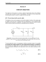
Figure A2.1 Circuit’s scheme wired with coaxial cable; Vi is the output signal, R is the
amplifier’s output resistance, Ccoa is the capacitance of the coaxial cable, Rosc
and Cosc are referred to the oscilloscope’s input .............................................. 55
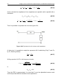
Figure A2.2 Equivalent circuit’s scheme using coaxial cable .................................... 56
Figure A2.3 Circuit’s scheme wired with EDP; Vi is the output signal, Ra is the
amplifier’s output resistance, R is the resistance of the RC net, C is the
adjustable capacitance, Cedp is the capacitance of the coaxial cable, Rosc and
Cosc are referred to the oscilloscope ................................................................ 59
Figure A2.4 Equivalent circuit’s scheme with impedance ......................................... 60
Figure A2.5 Scheme of equivalent circuit wired with EDP ........................................ 62
Figure A2.6 Equivalent circuit’s scheme using coaxial cable .................................... 62
Figure A3.1 Measures done with coaxial cable ........................................................ 64
Figure A3.2 Measures done with EDP ...................................................................... 64
Figure A3.3 Laboratory data histogram (spectrum) .................................................. 65
Figure A5.1 Recreation of the signal observed in the analogue oscilloscope ........... 71
Figure A5.2 Signal without values greater than 65 mV (excepting peaks) ................ 71
Figure A5.3 Non emission level up to -0.065 V........................................................ 72
Figure A5.4 In red, relative minimums smaller than -65 mV ..................................... 73
Figure A5.5 Absolute minimums detected by the code in red ................................... 74
Figure A5.6 Amplitude histogram 0.03 V bar’s width ................................................ 76
Figure A5.7 Amplitude histogram 0.05 V bar’s width ................................................ 76
Figure A6.1 DDE connexion between PropScope and LabView .............................. 77
List of tables
Table 2.1 Resolution offered depending on the number of bits. ............................... 12
Table 2.2 Frequency working range of the signal (using
). ......................... 24
Table 2.3 Frequency range for peaks around 14.4 keV ............................................ 25
Table 3.1 Dependence of the time acquired in a vector against SR, TS. ................. 29
Table A1.1 Oscilloscopes list .................................................................................... 54
Table A3.1 Ratio between points analyzed and minimum detected. ........................ 66
Table A5.1 Time dependence on the execution’s time and minimum time separation
detected between two consecutive peaks due to the size of the segments using
the same data file. ............................................................................................. 73
Table A5.2 Time running comparison between a code with or without the overlap
condition. ........................................................................................................... 76
Introduction
1
INTRODUCTION
The present work consist in designing and building a low-cost analyzer of the photon
energy emitted by a radioactive source, in order to be able to check easy and
automatically where the energy window for selecting the photons needed in a
Mössbauer experiment is located. Moreover, if necessary, it will allow to know how its
position should be modified and also to obtain information about the dead time of the
detector.
It is important to keep in mind that the equivalent commercial equipment and
software cost around 4000 € fifteen years ago. The total price of our system is 200 €
(the price of the USB digital oscilloscope), therefore it is necessary to understand that
it is highly complicated to obtain the same features on accuracy or time duration.
On the one hand, in order to determine where the energy window is located and also
for getting information about the dead time, it is not necessary for the system to be
extremely accurate. Accepting a small error over precision we will save an important
quantity of budget (using a system with less bit’s number, n).
On the other hand, the Photon Height Analyzer is going to be used when the set up
is changed (because the radioactive source is changed, or the distance between
detector to sample, or sample to source is changed) twice or three times a year,
consequently the large time duration of data acquisition can be accepted because
this also will decrease the final price of the project (using a system with a slower
analogue to digital converter).
Outline
The idea of this chapter is to yield an overview of the project, indicating the purpose
of the project and their motivation. It also will provide to the reader the organization of
the project and the methods used.
Chapter 1 contains a basic overview about the Mössbauer Spectroscopy in order to
fix the physics context of the project.
In Chapter 2 is explained how it is the measuring system and it is also included a
study about the architecture of the system and errors. It will permit us to fix the
features needed for our acquisition data system DAS and decide that the best option
to wire our system is using an external divisor probe (EDP).
Before the data treatment it is necessary, first of all, to understand the possible errors
in the measure. In addition, it allows to obtain a deep knowledge about how works
every instrument of the set up.
2
Design of a low-cost Photon Height Analyzer for a Mössbauer Spectroscopy
Chapter 3 is dedicated mainly to proportionate the features of our chosen DAS as
sampling frequency or data transfer velocity; it also contains an explanation in depth
of the MatLab code created for the first data treatment, where it is confirmed that the
data obtained and the DAS proportionate greats results. The idea to use MatLab has
a clear explanation, considering the interest of the author of the project in increase
their knowledge about LabView (LV) programming, was decided to use MatLab
because LV contains a function called MatLab script, which allows to pass directly
the MatLab code to LV. In Chapter 4 it has been also determined some other
parameters necessaries for the right work of the code such us the minimum value
accepted for a maximum peak detected (50 mV) or the threshold values to measure
dead time (
to avoid dead time).
In Chapter 4 it is shown step by step the final LV block diagram, explaining all the
highlights; it is also presented a kind of user’s manual in order to proportionate to the
laboratory worker all the information needed to do a good energy window calibration.
Finally, Chapter 5 includes the main conclusion obtained during the project and also
some ideas about what could be the future work in order to improve the project.
Principles of Mössbauer Spectroscopy
3
Chapter 1
PRINCIPLES OF MÖSSBAUER SPECTROSCOPY
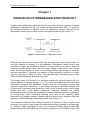
Rudolf Ludwig Mössbauer discovered at the end of the 50’s the recoilless resonant
absorption of gamma rays [1], also known as Mössbauer effect (ME). It consists in
the recoilless emission of gamma rays by a radioactive nucleus followed by the
absorption of these rays by other nucleus of the same species (see Figure 1.1).
Figure 1.1 Basic scheme of Mössbauer effect
Although the theoretical principle of ME was already known many years before, no
one was capable to recreate it in the laboratory. Mössbauer realized that it was
necessary to have the radioactive sample in a solid matrix to be able to have the
emission process without recoil. As the nuclear energy levels have a very narrow
width, the energy loss due to recoil of the emitting nucleus was enough to avoid the
resonant absorption. Therefore, the insertion of the radioactive nucleus in a matrix
was the only way to obtain the effect. The spectroscopic technique based on this
effect is called Mössbauer Spectroscopy (MS).
The energy levels of a nucleus in a solid are modified by its environment. MS it is
hugely sensitive to energy changes (
eV), hence it enables to study three main
interactions between the absorbent nucleus and the surrounding nucleus and
electrons (hyperfine interactions): i) the electric monopole interaction between the
nucleus and its electrons that produces a shift in the nuclear energy levels called
isomer shift (IS), ii) the electric quadrupole interaction between the nuclear
quadrupole moment and an inhomogeneous electric field that produces a splitting of
an energy level called quadrupole splitting (QS), and iii) the magnetic dipole
interaction (DI) between nuclear magnetic dipole moment and a magnetic field that
produces a further splitting of the energy levels (see Figure 1.2).
The information obtained from these interactions is useful not only in physics and
chemistry, but also in a wide range of disciplines as biology, geology or archaeology;
for instance: study mineralogy of rock, soil and dust at Gusev crater in Mars [2],
measurement of the relaxation time of ultrasonic vibrations in Fe foils [3], study of the
4
Design of a low-cost Photon Height Analyzer for a Mössbauer Spectroscopy
basilar membrane motion in the pigeon [4], measure of the astrophysical parameter
red shift in Earth [5].
Figure 1.2 Characteristics of Mossbauer spectra related to nuclear energy levels. Hyperfine
Splitting includes IS, QS and DI [6]
In this chapter we will present the most relevant aspects of the MS experimental
setup used in the laboratory.
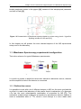
1.1. Mössbauer Spectroscopy experimental configuration
This is the scheme of a typical Mössbauer spectrometer:
Figure 1.3 Basic scheme of MS instrumentation
It is worth to explain in depth the three main elements: radioactive source, detector
and the amplifier at which the detector is connected.
1.1.1. Radioactive source
It is possible to work with a lot of different isotopes in MS, but the most used and the
one that it is used in the laboratory of this master thesis is radioactive 57Co (because
57
Fe has the most advantageous combination of properties for MS [7]). The
radioactive cobalt isotope undergoes a transition by spontaneous electron capture to
reach a metastable state of 57Fe, which in turns decays in a more stable state
Principles of Mössbauer Spectroscopy
5
(ground state) by a gamma ray cascade that includes the 14.4 keV gamma rays that
are used in MS (see Figure 1.4). It is necessary to place the radioactive source in an
electromechanical transducer driven by an appropriate electronic system to obtain by
Doppler’s effect [8], a slightly wider range of energy to analyze the absorber. Without
this energy range one could only study pure Fe. It is important to remember that the
studied system determines the radioactive source needed. For example, with the
57
Co source only systems containing Fe can be studied.
Figure 1.4 57Co Decay Scheme
It is essential to keep in mind that the objective of the project is to design a system
able to measure the energy spectra of the gamma ray cascade in order to be able to
select only the photons with 14.4 keV necessary for the ME.
1.1.2. Detector
There are three different kinds of detectors to work with low energy gamma ray: a)
gas proportional counter (energies lower than 40 keV), b) scintillator (energies
between 50-100 keV, c) Solid state detectors. Due to the energy of Mössbauer
gamma rays (14.4 keV) the most efficient detector is a gas proportional counter.
A gas proportional counter consists in a metallic recipient connected to the ground
and an inner metallic wire, between which a high voltage difference (around 2 kV) is
stablished. The detector has a Beryllium window transparent to the photons that
ionize an inert gas (in the detector of our laboratory is a mixture of Xe and CO 2)
causing an electron avalanche.
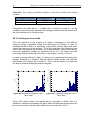
It is possible to observe in figure 1.5 the spectrum of all the received photons and it is
easy to realize that not all the photons with a very well known energy level are
located in a single value; they are spread around it. That happens because not all the
photons travel the same distance as they enter into detector with different input
angles.
The high energy photons produced in the 57Fe decay (122 and 136 keV) are not
enough amplified in the detector because of the gain of the proportional detectors at
these energies is too small (As was argued before, it works successfully in events
involving maximum energies of 40 keV); nevertheless some of these gamma rays
provokes Compton’s effect [9] that produces emission in the zone of tens keV. In
consequence this zone is more pronounced for smaller energies.
6
Design of a low-cost Photon Height Analyzer for a Mössbauer Spectroscopy
Figure 1.5 Spectrum obtained with a commercial photon height analyzer
The output data of the detector offers the possibility to study two different
characteristics depending on the electronics used after it; it is possible to study the
amplitude and shape of the gamma rays emitted in order to get information about the
properties of the source and configuration of the experiment, this is also called
Photon analyzer; it is also possible to study the different hyperfine interaction in the
absorber with a MCA (Multi Channel Analyzer), also called spectrum analyzer.
As was discussed in the introduction, we are going to analyze the energy of the
photon emitted by the radioactive source (photon analyzer).
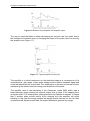
1.1.3. Pre-Amplifier and Amplifier
The pre-amplifier normally consists in a charge integrator. The charge collected in a
capacitor is proportional to the photon energy. A resistance situated in parallel with
the capacitor produce an exponential discharge; the time that takes the capacitor to
discharge is a key parameter because, if during that time other photon arrive, then its
energy amplitude will we modified as shown in figure 1.6.
Principles of Mössbauer Spectroscopy
7
Figure 1.6 Scheme of preamplifier and amplifier output
The way to avoid that effect is either decreasing the arrival’s rate (not useful due to
the increment of measure time) or changing the shape of the pulse, which is done by
the amplifier (see Figure 1.7).
Figure 1.7 Typical Amplifier Pulses [10]
The amplifier is a critical component on the detection stage as a consequence of its
characteristics: gain range, output pulse shape and the relation between signal and
noise that determine the output data. The amplification in the area of interest is lineal,
maintaining the relation between energy and amplitude of the peak.
The amplifier used in the laboratory is the Canberra’s model 2022 which uses a
Near-Gaussian shape working as unipolar output time to peak 2.35x shaping time,
and pulse width 7.3x shaping time (data extracted from Operator’s manual). It means
that if another pulse arrives before 9.65x shaping time the amplifier will suffer
stacking; In this case the energy window will accept events that has not the 14.4 keV
needed and will discard events with the proper Mössbauer gamma ray energy.
8
Design of a low-cost Photon Height Analyzer for a Mössbauer Spectroscopy
Figure 1.8 Unipolar output with three different shaping time: 12, 4 and 1
thinner
[11] from wider to
As a comment, the data of the duration of the event shows that the peak’s shape is
not symmetric (check in Figure 1.8).
Previous numerical data treatment with MatLab
9
Chapter 2
MEASURING SYSTEM. ARCHITECTURE AND
ERRORS
All the elements in a circuit, either active or passive, could modify (introduce errors)
in amplitude or frequency the output data that is going to be measured. This is the
reason why, before analyzing in depth the data to obtain the photon’s energy
spectrum, it is always advisable to study the architecture of the instrumentation
system to receive the signal, in order to be sure that the data have as less error as
possible.
This chapter contains four well differentiate parts.
Section 2.1, will be dedicated to analyze the architecture of the measuring system
necessary to obtain the signal in order to determine which elements make up the
system analyzed.
In section 2.2 the actual system used in the laboratory will be compared with the
different devices that allow acquiring the amplifier’s signal. This section also contains
the study of the amplifier’s signal because it should ensure that the data acquisition
system (DAS) that is going to be bought complies all the requirements of the project.
It is essential to determine device’s features as the sampling frequency fs necessary
to obtain a good digital reconstruction of the signal, the number of bits (n) to obtain
accurate data, and finally the bandwidth, without forgetting that one of the goals of
the project is to design a low-cost equipment.
Section 2.3 will compare the errors caused by the actual type of wiring with the
effects obtained with an external divisor probe.
Finally Section 2.4 will analyze the whole system
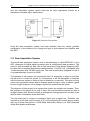
2.1. Architecture of the instrumentation system
The system used in the laboratory consists in three basics elements (Figure 2.1): i)
amplifier; ii) wire type; iii) Data Acquisition System (DAS).
The amplifier send the signal through its output impedance composed of a resistance
(100 Ω) and an output inductance with a non-specified value in the manual.
The actual wire connexion is a 1 meter length coaxial cable that introduces an
impedance in form of capacitance (80 pF each meter length).
10
Design of a low-cost Photon Height Analyzer for a Mössbauer Spectroscopy
And the acquisition system device that has an input impedance formed by a
resistance in parallel with a capacitance.
Figure 2.1 Scheme of the system.
Once the data acquisition system has been decided, then the unique possible
modification in the scheme is to change the type of wire between the amplifier and
the DAS.
2.2. Data Acquisition System
The actual data acquisition system used in the laboratory is called MCDLAP; it is an
ADC (Analogue to digital signal converter) with a multichannel data processor. The
card not only provides the user with a high resolution Pulse Height Analyzing ADC
but also with a complete Multichannel data processor. The ADC is a 16 kchannel with
14 bits resolution and 100 MHz clock rate. The card is particularly designed for use in
x-ray spectroscopy. Its price is 4000€.
The features of this system are so powerful that it is necessary to keep in mind that
we will work in a low-cost project. In consequence it will be impossible to compete
with the previous system in terms of time of execution or precision. The idea is to buy
a low-cost acquisition system with its features good enough in order to obtain a good
Photon Height Analyzer, not to design a system as powerful as the actual.
The objective of this project is to replace this system by another one cheaper. Then,
the purpose of the project is not only to buy a low-cost acquisition system but also to
design software that allows to obtain a good photon energy spectrum and also to be
able to obtain information of the dead time.
The first step was to convert an analogue signal into a digital one. Therefore, the
acquisition of the data could be done (if it is not considering the actual device) mainly
with one of these two options: a DAQ (Data AcQuisition) device or a USB (Universal
Serial Bus) digital oscilloscope.
Previous numerical data treatment with MatLab
11
The relation between cost and performance was clearly favourable for the USB
digital oscilloscope. That is because the DAQ usually has between 8, 16, or 32
channels and they need a huge sampling frequency to obtain the possibility to work
in parallel with all of them, it implies also a huge transfer data velocity that makes the
device more powerful but also increase the price.
To decide which oscilloscope would be the best option it is important to determine its
main specifications: fs, n and Bandwidth. Then the first thing to do is to observe the
signal and characterize it with a commercial analogue oscilloscope.
5
4
Amplitude (V)
3
2
1
0
-1
3800
4000
4200
4400
Time (µs)
4600
4800
5000
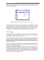
Figure 2.2 Example of the (digital) signal.
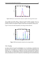
With a signal example (see figure 2.2) it is possible to determine the features that will
decide the optimum device.
2.2.1. Analysis of the number of bits
The first parameter to analyze was the required amplitude’s signal range. This
parameter determines the maximum value of peak to peak voltage ( ) admitted.
The output signal had a maximum value of 5 V and a minimum of -2 V, thus the
minimum ( ) accepted would be 10 V, in order to avoid the clipping effect that could
saturate the oscilloscope.
Once the value of
is known, it is possible to know the needed n (number of bits)
fixing previously the required data resolution using:
(2.1)
It is known that the electronic devices use an even number of bits; therefore, the
discussion was focused between 8, 10 or 12 bits. In Table 1 the resolution obtained
is shown as a function of the bit’s number for
equal to 10 V.
12
Design of a low-cost Photon Height Analyzer for a Mössbauer Spectroscopy
Table 2.1 Resolution offered depending on the number of bits.
n
8
10
12
39,1
9,8
2,4
It is clear that this parameter will affect directly the final photon’s energy spectrum
and the final cost. As an example, a 12 bits oscilloscope is almost five times more
expensive than the equivalent 10 bits oscilloscope (See annex I).
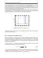
2.2.2. Analysis of sampling rate
The sampling rate is the other key parameter, because it will determine how the
shape of the signal will be rebuilded. A higher sampling rate implies a better
reconstruction of the peak’s shape (Figure 2.3) and in consequence the photon’s
energy spectrum will be more accurate.
Figure 2.3 A/D (Analogue/Digital) Converter, the sampling rate could be seen as how many
points it are going to be used to represent the signal
It is obvious that the best sampling rate would be ideal, but the cost of the device
increases quickly when increasing the sampling rate.
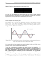
To be able to decide which sampling rate should be good for the project, it is
necessary to know how the shape of the signal to analyze is and also which is the
less intense peak detected. The complete peak could be properly represented as a
kind of delta positive (as maximum will have 3 points) peak and then a nearGaussian peak (explained in Chapter 1) and we should decide how many points are
needed to represent it.
The peak chosen (see Figure 2.4) in the signal to work with had a voltage amplitude
of 2.75 V approximately, and a duration of 70 . With this data, the minimum
Previous numerical data treatment with MatLab
13
sampling rate accepted should be 0.5 Msample/sec in order to have 35 points to
represent the curve.
Example of a peak shape
3
2.5
Amplitude (V)
2
1.5
1
0.5
0
3780
3800
3820
3840
3860
# of point
3880
3900
Figure 2.4 Shows one of the peaks detected with the USB oscilloscope.
It is clear that the fs could be improved, but in consequence the transfer data velocity
would be increased; it implies that the cost would increase considerably.
2.2.3. Oscilloscope requirements summary
With the study done above (section 2.2.1 and 2.2.2) it is possible to conclude that the
future oscilloscope should has at least 0.5 Msample/sec as a sampling frequency,
and ten bit’s number. If it is possible to find an instrument that improves these
requirements and also keeps the cost then it is going to be possible to obtain more
accurate data.
The final decision was to buy a low-cost USB Oscilloscope called PropScope; it has
a sampling rate up to 25 Msample/s, bit’s number of 10, 20 MHz of bandwidth, 35
Kb/s of data velocity transfer; and also includes a function generator and two external
divisor probes.
The complete list of oscilloscopes considered is detailed in annex I.
2.3. Errors introduced by effects of non-ideal system
Ideally the circuit could be seen as an amplifier that is connected to the oscilloscope,
which is the element responsible to acquire the signal. But as was explained in
section 1.1, an ideal system never exists.
14
Design of a low-cost Photon Height Analyzer for a Mössbauer Spectroscopy
Before to start analyzing the acquired data it is necessary to analyze the errors in
amplitude and frequency introduced on the signal due to the impedance of the
passives elements.
The output impedance of the amplifier and the impedance of the coaxial cable were
both commented in section 2.1. Now that has been chosen the data acquisition
system of our system it is necessary to detail which impedance has been added. The
USB PropScope oscilloscope introduces input impedance consisting in a resistance
(1 MΩ) and a capacitance (20 pF).
As was commented in section 2.1 the output impedance of the amplifier and the input
impedance of the DAS are fixed. Along this section the actual circuit and also a
modification of it will be study; that will consist in changing the coaxial cable by an
external divisor probe with the objective to compensate both, the capacitance of the
coaxial and the capacitance of the oscilloscope.
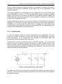
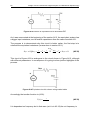
2.3.1. Coaxial cable
In order to establish clearly the effects introduced by the impedances. This subsection will contain two parts: i) the first part will study theoretically the circuit that
forms the system; ii) the second part will compare the theoretical study with
experimental images extracted from the system.
The objective of a circuit’s theoretical study is to find its response in time domain and
also in frequency (complex) domain; this feature is called transfer function. The
transfer function permits understanding the output signal; and also to see how the
input signal changes depending its amplitude and frequency. Then the first circuit
studied is shown in the figure below:
Figure 2.5 Circuit wired with a coaxial cable
To make easy the lecture of the thesis, this section will show a schematic study of
the circuit. Annex II contains a deeper explanation, and it also shows and explains all
the steps performed.
Previous numerical data treatment with MatLab
15
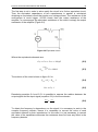
The first step to do in order to solve easily the circuit is to find an equivalent circuit.
Then the equivalent capacitance of two capacitances in parallel is calculated,
obtaining an equivalent circuit that works as a voltage divisor. The resistance of the
oscilloscope is much bigger (10.000 times) than the output resistance of the
amplifier; in consequence the equivalent resistance of the circuit is simply the output
resistance of the amplifier (Figure 2.6).
Figure 2.6 Equivalent circuit.
Where the equivalents elements are:
(2.2)
(2.3)
The solution of the circuit shown in figure 2.6 is:
(2.4)
(2.5)
Reordering equation 2.4 and 2.5 it is possible to express the relation between the
output signal and the input signal (equation 2.6) in the time domain.
(2.6)
To obtain the frequency’s dependence on the signal it is necessary to work in the
complex frequency domain. Hence it is necessary to convert the value of each
equivalent element by their impedances. In this case it is just necessary to convert
the value of the capacitance because the resistance does not have any affect in the
frequency domain.
16
Design of a low-cost Photon Height Analyzer for a Mössbauer Spectroscopy
(2.7)
Where
and is the complex number. Expressing equation 2.6 in the complex
frequency domain,
(2.8)
Equation above shows the dependence in frequency of the circuit’s transfer function
in the complex frequency domain (s). The function has a zero in the denominator that
expresses the cut frequency of the circuit. Then the circuit works as a low-pass filter
and its cut frequency is:
(2.9)
The effect produced by the impedance is to introduce different errors in the acquired
signal depending on the frequency. And it will also cause the lost of peaks that must
contribute to the Photon’s energy spectrum; consequently this effect increases the
time of acquisition.
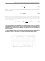
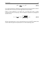
To show graphically these effect two square functions with different frequencies will
be shown in Figure 2.7 and Figure 2.8, in order to analyze the different effects.
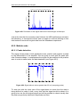
Figure 2.7 Square signal (f=100 kHz, Amplitude=1 V);
Previous numerical data treatment with MatLab
17
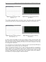
Figure 2.8 square signal (f=1.5 MHz, Amplitude 1 V)
Figure 2.7 and Figure 2.8 shows how the response of the system is. Two features
are clearly seen in the figure above: i) exists a ripple effect in Figure2.7 that is
produced by an output inductance in the amplifier which value is not present in the
manual. This effect will modify the amplitude of the peaks, because adds a ripple on
the semi-Gaussian peak. Its effect will be studied at the end of this chapter; ii) the
value of the slope in Figure 2.8 is not big enough to recreate the shape of the signal;
it will change the shape of the signal.
To do a quantification of the error in amplitude introduced by the impedance, it is
necessary to use the transfer function (equation 2.8) in the complex frequency
domain, calculate its module and use it in the relative error equation:
(2.10)
In figure 2.8 it is obvious that the impedance is not compensated; then the system is
not able to represent properly the square function.
The time that requires charging a capacitor to 63.2 % of full charge is called time
constant, represented by the Greek letter ; figure 2.8 permits to obtain a first
approximation of the time constant:
(2.11)
Once the complex frequency domain has been analyzed, it is worth also to obtain the
transfer function in the time domain. It is necessary to use the equation of the
transfer function in the complex frequency domain (equation 2.8) and apply the
inverse Laplace transform; the result is:
(2.12)
18
Design of a low-cost Photon Height Analyzer for a Mössbauer Spectroscopy
The transfer function in the time domain shows that for an observed peak, the
transfer function applied on the signal is an exponential decay with a discharge time
constant:
(2.13)
Hence if the results of equations 2.11 and 2.13 are compared then the conclusion of
this sub-section is that the theoretical and graphical results do not agree. It means
that probably the system has some other elements that would affect the data.
Analyzing the equation 2.12 it is possible to conclude that as lowest the value of is,
is the better will be rebuilt the shape of the signal. Hence the idea is to find an
equivalent circuit diminishing either the equivalent capacitance or the equivalent
resistance. In this case, it has been explained that the output resistance of the
amplifier is fixed; then the solution will be to use an external divisor probe (EDP).
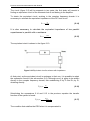
2.3.2. External Divisor Probe (EDP)
To reduce the impedance introduced by the amplifier and the oscilloscope an EDP is
used to wire the system instead of the coaxial cable.
In this case it is just necessary to comment the impedance introduced by the EDP
because the amplifier and the oscilloscopes are the same (see Figure 2.9).
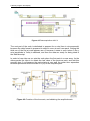
Figure 2.9 Circuit’s scheme wired with EDP; Vi is the output signal, Ra is the
amplifier’s output resistance, R is the resistance of the RC net, C is the adjustable
capacitance, Cedp is the capacitance of the coaxial cable which forms the EDP, Rosc
and Cosc are referred to the oscilloscope.
The EDP includes a coaxial cable with an impedance commented in the previous
sub-section and a RC front circuit with an adjustable capacitance and a resistance of
10 MΩ; it offers a higher input resistance and a lower capacity in parallel than the
oscilloscope alone.
Previous numerical data treatment with MatLab
19
The circuit (figure 2.9) will be separate in two parts; the first study will consist in
finding an equivalent circuit of the elements that do not belong to the amplifier.
To obtain the equivalent circuit, working in the complex frequency domain it is
necessary to calculate the equivalent impedance of the RC front circuit:
(2.14)
It is also necessary to calculate the equivalent impedance of two parallel
capacitances in parallel with a resistance.
(2.15)
The equivalent circuit is shown in the figure 2.10.
Figure 2.10 Equivalent circuit’s scheme with impedance.
At that point, as the equivalent circuit is analogue to that one, it is possible to adapt
the expression found in the sub-section (2.6). Although now it is going to be written
directly in the complex frequency domain; then substituting R by Z1 and Zeq by Z2,
obtaining directly:
(2.16)
Substituting the expressions 2.14 and 2.15 in the previous equation the transfer
function of the system is found:
(2.17)
The condition that satisfies the EDP when it is compensated is:
20
Design of a low-cost Photon Height Analyzer for a Mössbauer Spectroscopy
(2.18)
It justifies that C must be adjustable because each oscilloscope has different
resistance and capacitance.
In the PropScope case, the compensated value for C is:
(2.19)
Returning to (2.17), and assuming (2.18), the transfer function is:
(2.20)
This result, as was expected, means that this part of the circuit does not affect to the
measure data in frequency. In amplitude, data are attenuated by factor 10. Applying
the inverse of the Laplace transform to the expression 2.20 the transfer function in
the time domain is obtained:
(2.21)
This factor is corrected by the oscilloscope’s software because exists an option to
setup the probes.
Using the admittance it is possible to find the values equivalent to the capacitance
and resistance. Then to work with admittance, first it is necessary to calculate the
total impedance:
(2.22)
And the admittance is:
(2.23)
Therefore the system acts as an equivalent resistance and an equivalent capacitance
in parallel with the following values:
(2.24)
Previous numerical data treatment with MatLab
21
(2.25)
Hence the equivalent circuit is shown in Figure 2.11. As was commented at the
beginning of the sub-section, the equivalent system has a bigger input resistance,
and a smaller capacitance than the case of the coaxial cable. Although both are
analogues; taking profit of this fact, only the key expressions in the analysis of the
circuit will be shown. For further explanations, see Annex II.
Figure 2.11 Scheme of equivalent circuit wired with EDP.
Accordingly the transfer function is (2.8):
(2.26)
It is dependent on frequency (as it is in 2.10), but in that case the value of the cut’s
frequency is:
(2.27)
It is a great improvement, because just changing the wire type the system is able to
obtain data with a frequency ten times bigger without being modified. It means that
the peaks with higher frequency will be detected with this wire. A table with this
feature of the system is shown in Annex II.
To find the transfer function in the time domain, the expression found in the previous
sub-section is going to be used (equation 2.12) with the only change of Csys instead
of Ceq. Obtaining:
(2.28)
22
Design of a low-cost Photon Height Analyzer for a Mössbauer Spectroscopy
Finally, as was explained in the section 2.3.2, the peaks with equal or higher
frequencies than the cut frequency, will be modified in amplitude as (analogous to
equation 2.10):
(2.29)
2.4. Complete circuit
Once we have decided which type of wiring we will use, it is the moment to introduce
in the circuit analysis the effect due to the amplifier’s inductance that has been
commented in the previous section.
The output inductance value is not in the user’s manual of the amplifier, then the best
option to find its value is to measure the Bode diagram of the whole system and
compare it with our ideal system (Figure 2.12); it means to introduce a known input
signal to the amplifier (sinusoidal) and measure for each frequency how the signal
changes.
Theoretical Bode diagram
0
Amplificarion (dB)
-5
-10
-15
-20
EDP
Freq. cut
Coaxial
Freq. cut
-25
-30
0
10
1
10
2
10
3
10
4
5
6
10
10
10
Frequency (Hz)
7
10
8
10
9
10
Figure 2.12 Theoretical Bode diagram, and cut frequency (black circle).
The figure above represents in different colours the qualitative shape of a Bode
diagram for a coaxial cable and for an external divisor probe. As was calculated in
section 2.3.1 and also in section 2.3.2, the theoretical results show that the cut
frequency is higher for an EDP than for a coaxial cable.
In order to measure the real Bode diagram of the system, it is necessary to calculate
what the working area of the signal is over the frequency domain.
Previous numerical data treatment with MatLab
23
In previous section 2.2.2, was commented the main feature of a peak. Then in order
to obtain the two slopes which define us the area of work in the frequency domain, it
is necessary to find the maximum and the minimum amplitude of a peak without
overlap and divide its amplitude by the time duration, which could be approximated
for the time passed between two points and a half of this time (looking table 3.1, we
can conclude that for TS of 100 µs, this time will be 3 µs). Consequently the range of
working frequency it is calculated as follow:
(2.30)
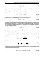
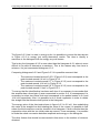
The following graphic (Figure 2.13) shows the real Bode diagram for both wiring
types, EDP and coaxial over all the frequencies.
Bode diagram for the whole system
40
35
Amplification (dB)
30
25
20
15
10
5
0
-5
1
10
EDP
Coaxial
2
10
3
10
4
10
Frequency (Hz)
5
10
6
10
7
10
Figure 2.13 Bode diagram for EDP and coaxial cable.
First of all, it is possible to conclude that the system is not a low pass filter, as we
supposed at the beginning. It means that there are some more passives elements
that we are not considering and also that the amplifier not only works as an amplifier
but it also works as a differentiator.
We can conclude that there exist four reactive elements that provoke two zeros in the
system response: one positioned around 50 Hz and the other one around 2 kHz; and
also two poles: one located around 100 Hz (single pole) and the other one around
200 kHz (triple pole). As a consequence it is not possible to fix what the real
elements of the whole system are (in our case just for the amplifier). Due to the semilogarithmic scale used in the Bode diagram it is not easy to distinguish between the
results obtained for the coaxial cable and the EDP.
In order to get more information about how our system works it will be worth to
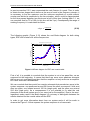
observe the Figure 2.14 that express the system response in a linear scale.
24
Design of a low-cost Photon Height Analyzer for a Mössbauer Spectroscopy
System response
90
EDP
Coaxial
80
70
Amplification
60
50
40
30
20
10
0
0
0.2
0.4
0.6
0.8
1
1.2
Frequency (Hz)
1.4
1.6
1.8
2
6
x 10
Figure 2.14 System response of the whole system for different wiring type (linear scale xaxis).
In Figure 2.14 it is clearer than the cut frequency for coaxial cable (around 200 kHz)
is smaller than the cut frequency for EDP (around 300 kHz). As a consequence, we
can confirm that, although the unknown passive element modifies the cut frequency
in both cases, it does not change that the best option to wire our system is the EDP.
The total range area will be calculated using two peaks: one of the minimum
amplitude and one of the peaks with maximum amplitude (see Table 2.2):
Table 2.2 Frequency working range of the signal (using
Amplitude (V)
0.1
6
).
Frequency
≈ 34 kHz
≈ 1.6 MHz
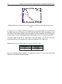
Once the complete Bode diagram is understood, Figure 2.15 will show the Bode
diagram in the signal frequency range.
Previous numerical data treatment with MatLab
25
Bode diagram in the region of interest
40
Amplification (dB)
35
30
25
20
15
10
5
6
10
10
Frequency (Hz)
Figure 2.15 Bode diagram over region of interest
In order to obtain more information, we are going to calculate in table 2.3 where are
located the peaks with its energy inside the energy window filter.
Table 2.3 Frequency range for peaks around 14.4 keV
Amplitude (V)
0.5
1
Frequency (MHz)
≈ 0.16
≈ 0.33
If we compare the results obtained in Table 2.3 with Figure 2.15 it is possible to
observe that the peaks around 14.4 keV are in frequencies around the maximum
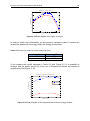
amplification (see Figure 2.16).
Bode diagram around the energy window levels
39
38.5
38
EDP
Coaxial
Amplification (dB)
37.5
37
36.5
36
35.5
35
34.5
34
5.3
10
5.4
10
Frequency (Hz)
5.5
10
Figure 2.16 Bode diagram in the region determined by the energy window
26
Design of a low-cost Photon Height Analyzer for a Mössbauer Spectroscopy
Figure 2.16 is very interesting, there it is possible to appreciate three key features: i)
the EDP amplifies more than the coaxial cable the peaks which important information
for the Mössbauer experiment; ii) the peaks more amplified are the ones who satisfy
the conditions (energy range) imposed by the energy window and finally iii)
comparing it with Figure 2.15, it is possible to conclude that, over the region where
appear the three main peaks of the source (6,4; 14.4, 21) keV the amplifier works
approximately linear.
As was said before, the amplifier is working also as a differentiator, it means that
when the amplifier receives a pulse, first of all it derivates the pulse and amplifies it;
then finally on the negative area is superposed a near-Gaussian form (it allows to
obtain information over the dead time. In order to get an example of what
differentiator does, see Figure 2.17.
Figure 2.17 Amplifier-Differentiator.
2.5. Conclusions
As a conclusion of this chapter, it is worth to make a simple summary.
In section 2.2 we discussed about which acquisition system will be our best option
evaluating features against cost. It was an easy decision because the difference of
cost was huge between a DAQ device and the oscilloscope (around ten times
cheaper). Although it means that our system will be slower.
At the end of the section it was presented the conclusion about the oscilloscope’s
features: (i) 10 bits, (ii) At least 0,5 Msample/sec.
In section 2.3 it was made a theoretical study between wiring our system with a
coaxial cable (as was before the project) or with an external divider probe (EDP).
The theoretical study was clearly favourable to EDP because, although both
connexions make to work the system as a low pass filter, using EDP increases the
cut frequency more than 10 times. It permits to obtain four times more peaks with the
Previous numerical data treatment with MatLab
27
same time sampling (see Annex II). It means that although our system is going to
work slower than the data acquisition system with its commercial software used
before the project, we are able to decrease in four time our acquisition time in
comparison with the time necessary to obtain the same statistics with a coaxial cable.
Considering the information obtained thanks to the analysis of the system’s
response, it is possible to conclude that the amplifier not only works as a linear
amplifier but also as a differentiator which causes that the whole systems response is
a pass band filter.
Finally, it is concluded that the peaks around 14.4 keV, which are those necessary
for the MS are located around the maximum amplification over the frequency domain.
28
Design of a low-cost Photon Height Analyzer for a Mössbauer Spectroscopy
Chapter 3
PREVIOUS NUMERICAL DATA TREATMENT WITH
MATLAB
Since the beginning of the project we thought that could be possible to obtain the
spectrum of the radioactive sample using the peak that has a near-Gaussian shape
instead of the peak that is similar to a Dirac’s delta. We also thought that the
information about dead time could be obtained first, detecting all the peaks, and then
impose an overlapping condition to remove the peaks overlapped.
Finally we realize that the most reliable way of work should be the ones presented in
Chapter 3. Then in Annex V will be shown the first work done in order to obtain a
histogram with the peaks that have a near-Gaussian shape.
In this chapter it is explained how was the process to create the MatLab code with a
wide explanation about its highlights; the idea is to focus into the mathematical idea
of how to treat this kind of signal.
First of all, it is interesting to say that the platform used to make the first code was
MatLab. The reason is that LabView (LV) has as a tool a MatLab script that allows us
to insert the previous code almost directly to LV.
The full code is presented in Annex IV; it contains commentaries about the idea
behind each important step.
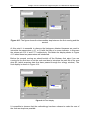
In Chapter 3 is going to be shown how the data were treated, including images to
make it more visual, allowing the reader to understand what was the author’s idea
doing each step.
The first stage of numerical treatment, once the oscilloscope was bought and
available in the laboratory, was to determinate how it works i.e.: sampling frequency
(fs), data transfers, clipped effect, etc.
The final step was to acquire data and starts to create the code in order to start
obtaining the first amplitude’s histogram and information about the dead time.
3.1. Characterization of oscilloscope’s data acquisition system
With the oscilloscope’s software installed on the computer, the first step was to
analyze how it works, for instance: (i) which sampling frequency (f s) is used and how
it changes when the time scale (TS) is changed; (ii) how the oscilloscope transfers
data into the computer; (iii) how the oscilloscope works when the signal is clipped.
Previous numerical data treatment with MatLab
29
3.1.1. Sampling rate and time scale
The USB Propscope oscilloscope has a fs up to 25 Msamples/s; although all digital
low-cost oscilloscopes samples the input data at fixed rates depending on its time
scale. The cost to be working in a low cost project is that the analogue to digital
convertor is not as good as could be. The consequences are that the analogue to
digital convertor is not as fast as we wished, then the internal memory of the
oscilloscope is not as big as would be wished and consequently the transfer data
velocity is also very limited.
Fortunately this project pretend to create an application that will be used once in few
months, when is necessary to check the position of the amplifier energy window; that
is the reason why the project is going to be very useful although it has technical
limitations.
As was commented in the introduction of the chapter, it is necessary to understand
how the digital oscilloscope works. For this reason it is essential to distinguish
between the two modes of work.
On one hand if the TS is slow enough (bigger than 20ms/div) to continuously send all
samples over the USB connexion, then the PropScope goes into streaming mode,
where it is possible to see all samples moving from right to left.
On the other hand, when the TS knob is to set into faster TS, the scope takes a set of
samples and transfers them to be displayed. The sampling rate (SR) is calculated to
return twenty divisions of data over 1024 samples; in consequence it is necessary to
make a balance between the maximum TS possible against the idea to obtain the full
peak inside the 1024 samples vector.
The following table shows the correspondence between SR, TS and the time
acquired in one 1024 sample vector:
Table 3.1 Dependence of the time acquired in a vector against SR, TS.
SR (Msamples/s)
25
10
5
2,5
1
0,5
TS (µs)
2
5
10
20
50
100
Time acquired (µs)
40
100
200
400
1000
2000
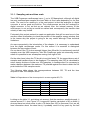
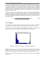
Looking on the table 3.1 and taking into account that the maximum amplitude peak, it
means around 5 V, (see Figure 3.1) is around 40 points, equivalent to 80 µs width, it
does not have too much sense to use a TS faster than 100 µs (because if not, we will
lose information about the dead time); it probably could cut any peak by the half
30
Design of a low-cost Photon Height Analyzer for a Mössbauer Spectroscopy
losing its information. In addition looking the figure below it can be concluded that the
parameter of the amplitude is well measured.
Example of a peak shape
5.5
5
4.5
4
Amplitude (V)
3.5
3
2.5
2
1.5
1
0.5
0
1.062
1.064
1.066
1.068
1.07
# of point
1.072
1.074
1.076
4
x 10
Figure 3.1 The width of this peak is around 40 points, it means 80 µs.
3.1.2. Transfer data velocity
USB PropScope hardware like all digital instruments puts limitations on what can be
done. Main issues are: PropScope analogue to digital convertor velocity, memory
size and USB connexion speed.
These features translated to our system means that exists a limited transfer data
velocity; in that case it is 35Kb/s (low although in consequence of its cost).
For example in order to obtain a file which size is 22,352 KB, PropScope took twenty
minutes approximately.
3.1.3. Clipped signal
When a signal exceed the amplitude allowed (10 Vpp) by the oscilloscope it is said
that the signal is clipped; in this case PropScope just remains with the maximum
value permitted until it starts to descends when the signal value is lower than 10 Vpp.
It does not produce any kind of problem, it just saturate the signal during the time that
the signal exceeds the maximum value allowed.
3.2. MatLab code
In the introduction (chapter 1) was explained which where the goals of the master
thesis; the main one is to create a code that makes the histogram of the emitted
Previous numerical data treatment with MatLab
31
peak’s amplitude (Photon Height Analyzer) and to get information about the dead
time of the detector.
The complete code is shown in Annex (IV); in this section the code will be explained
step by step, focusing on the main ideas that allow analyzing the signal properly.
3.2.1. Reading data
This section is divided in two sub-sections because is going to be worth to
understand the signal obtained through two different outputs.
On one hand, a long data file will be acquired from the amplifier’s unipolar output in
order to obtain the total spectrum of the radioactive sample.
On the other hand, a data file (shorter than the previous) will be acquired from the
energy window output in order to obtain the peaks that accomplish the condition
imposed on the energy by the filter.
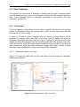
In Figure 3.2 it is shown as a example the signal’s shape using directly the output
data of the amplifier obtained from the oscilloscope with the goal to observe that the
PropScope acquire data packs of 1024 sample length and then the next pack starts
again at zero point.
5
4
amplitude (V)
3
2
1
0
-1
0
200
400
600
sample vector
800
1000
1200
Figure 3.2 Shows that position vector goes between 0 and 1023
As a consequence it is needed to spread out the position vectors in one longer
vector, obtaining the result shown in the Figure 3.3:
32
Design of a low-cost Photon Height Analyzer for a Mössbauer Spectroscopy
5
4
Amplitude (V)
3
2
1
0
-1
0
500
1000
1500
2000
sample number
2500
3000
3500
Figure 3.3 An example (some packs of 1024 points) of the previous position vector
spread out
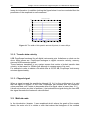
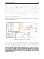
3.2.2. Peaks detection over amplifier’s output data
To understand the signal shape obtained from the amplifier’s unipolar output, it could
be observed Figure 3.3. There, it is shown that the peak consist in a fast increment of
voltage (from 2 µs until 6µs maximum), followed by a negative near-Gaussian peak,
which allow us to obtain information about the dead time.
The MatLab code pretends to find the position and amplitude value of the positives
peaks. In order to know how to detect the positives peaks it is essential to know their
features, therefore the data will be zoomed to obtain some key parameters (see
Figure 3.4).
Amplifier's output data
0.04
Amplitude (V)
0.03
0.02
0.01
0
-0.01
2.61
2.615
2.62
2.625
2.63 2.635
# of point
2.64
2.645
2.65
2.655
4
x 10
Figure 3.4 Signal without values greater than 50 mV (excepting peaks).
Previous numerical data treatment with MatLab
33
Then to characterize basically the signal, there exists to different behaviours: (i) when
there is not emission, the signal remain around zero with a minimum value of 0 V and
a maximum value of 50 mV very well determinate (see Figure 3.4); (ii) when there is
a peak to detect the values are over this 50 mV.
As the objective is to determine the peaks due to emission process, the region (i)
allows determining properly the minimum value accepted to consider a peak as a
maximum; Using a ‘for’ loop and applying the condition expressed in equation 3.1:
(3.1)
The only step to perform later on is to remove over the position and amplitude
vectors and the positions with zero value that do not accomplish the condition. Then
all the peaks will be detected without removing the overlapped ones (see Figure 3.5).
Amplifier's output data; all peaks detected
5
4.5
4
3.5
Amplitude (V)
3
2.5
2
1.5
1
0.5
0
-0.5
1800
1900
2000
2100
2200
# of points
2300
2400
Figure 3.5 Amplifier’s output data with all the peaks detected
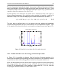
3.2.3. Peaks detection over the energy window output data
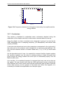
In Figure 3.6 it is possible to observe that the function of energy windows is to
discriminate the peaks, distinguishing the peaks received from the amplifier unipolar
output that are inside of the energy window value from the peaks that are not.
When the discriminator receives a peak with its energy inside the values permitted by
the energy window, then appears a kind of Dirac’s delta synchronized with the
position of the desired peak on the amplifier’s output data file; if it is not, then the
output signal remains constant in a value near to zero.
34
Design of a low-cost Photon Height Analyzer for a Mössbauer Spectroscopy
Energy window output data
6
5
Amplitude (V)
4
3
2
1
0
0
500
1000
1500
2000
2500 3000
# of point
3500
4000
4500
5000
Figure 3.6 Energy window output data
As was done in the previous sub-section 3.2.2, it is interesting to observe zoomed
the signal (see Figure 3.7).
Energy window output data
0.1
0.09
0.08
Amplitude (V)
0.07
0.06
0.05
0.04
0.03
0.02
0.01
0
405
410
415
420
# of points
425
430
Figure 3.7 Energy window output data zoomed
The energy window output data is very well defined; it is possible to observe two
situation: a) if there is no peaks with the energy between the upper and lower limit
the signal remains constant with a value of 19 mV; b) the energy window receives a
peak with its energy between its limits, then the signal has a value around 5 V.
Then in order to know the proper value of the peak, it is necessary to take profit of
the synchronization between the amplifier’s output and the energy window, as could
be observes in Figure 3.8; in this figure it is changed the value of 5 V by 0.5 in order
to obtain a clearer image.
Previous numerical data treatment with MatLab
35
Synchronization between the amplifier’s output and the energy window
1
Amp
EW
0.9
0.8
Amplitude (V)
0.7
0.6
0.5
0.4
0.3
0.2
0.1
0
1972
1974
1976
1978
# of point
1980
1982
1984
Figure 3.8 Example of synchronization between amplifier and energy window output
This condition will make easier to detect the peak’s position, because once it is
detected the peak over the energy window output, it is just necessary to use its
position and find in the amplifier’s unipolar output what the amplitude of this point is.
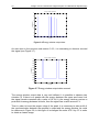
Figure 3.9 shows the selected peaks by the energy window detected.
Detected peaks selected by the energy window
Amp
EW
Peak
0.9
0.8
0.7
Amplitude (V)
0.6
0.5
0.4
0.3
0.2
0.1
0
-0.1
6900
6950
7000
7050
7100 7150
# of point
7200
7250
7300
7350
Figure 3.9 Detected peaks selected by the energy window
3.2.4. Overlap
In order to detect if one peak is overlapped or not, it is necessary to remember how
the behaviour of the peak is. This description can be found at the beginning of the
section 3.2.2. The feature that it is going to be used is that the peak will last as
maximum 6 µs, in consequence will take as much two points before the maximum
value. Therefore, the idea to detect overlap is to analyze the previous two points of a
maximum and then to look out if at least one of them belongs to the area delimited by
36
Design of a low-cost Photon Height Analyzer for a Mössbauer Spectroscopy
the condition of dead time (will be explained in the following section); the condition is
shown in Annex IV, where can be found the whole code.
In other words, the objective is to analyze if when the peak starts, the signal is
modified by a previous peak or remains around their regulars values (given by the
noise level on the signal). It is worthy to remark that this condition works both data
output, either received from amplifier or energy window. As a example, Figure 3.10
will show a peak overlapped avoided by the condition from the amplifier’s output
data.
Amplitude (v)
Peak overlapped no detected
low limit
410
415
420
425
# of point
up limit
430
435
440
Figure 3.10 Peak overlapped no detected
Observing the previous two points of the peak located in the point 434, we can see
that both are located in the area where the detector cannot identified properly the
energy, consequently the code avoid the detection of the peak.
3.2.5. Dead time
One key parameter of the program is to give an idea of how the dead time of the
system is; in other words, to know if the distance between the radioactive source and
the sample to analyze is optimum.
On the one hand if the source is too close to the sample, then the detector will
receive a number of photons too big to be able to have a good response; in
consequence, the information of the photons will be overlapped; it means that the
second photon arrived to the detector will contribute to the histogram with a wrong
energy quantity.
On the other hand, if the distance from the source to the sample is too big, a fraction
of the information could be lost, because the photons emitted by the source will not
impact on the sample.
Previous numerical data treatment with MatLab
37
It is easy to understand that the worst option of both is to have the set up explained
in the first case, where the source is too close to the sample. Then, for avoiding
counting this photons in the histogram with their modified energy, the program
incorporates an option that could be used when the user decide. In order to explain
this idea easily, it is important to know how is the behaviour of the data when
appears an emission peak.
In order to know which the energy limits are, where a photon could be detected with
its correct energy, it is necessary to look the Figure 3.4. As was commented below
that figure, it is possible to observe that the upper limit is 35 mV and the lower limit is
0 V. Then to obtain the percentage of dead time of the detector, it is necessary to use
the equation below:
(3.2)
3.2.6. Histogram
It is known that MatLab contains a function that creates by itself a histogram.
Consequently in this subsection the different histograms of interest will be shown.
Following the order of this chapter, the first histogram to comment is the one which
contains all the peaks received from the amplifier’s data output (Figure 3.11).
Amplifier output histogram including overlapped peaks
900
800
700
counts
600
500
400
300
200
100
0
0
0.5
1
1.5
2
2.5
3
# of points
3.5
4
4.5
5
Figure 3.11 Amplifier output histogram including overlapped peaks
Observing figure above, it is not too clear where are located the three peaks
required. It is supposed that around 0.35 V exists one (6.4 keV), around 0.7 V maybe
exists the second one (14,4 keV), but the third one is really complicated to find it.
In order to obtain a clearer histogram, the Figure 3.12 will remove all the peaks
overlapped.
38
Design of a low-cost Photon Height Analyzer for a Mössbauer Spectroscopy
Amplifier output histogram without overlapped peaks
700
600
counts
500
400
300
200
100
0
0
0.5
1
1.5
2
2.5
3
Amplitude (V)
3.5
4
4.5
5
Figure 3.12 Previous histogram without overlapped peaks
Figure above confirms us that the first two peaks are really the peaks that we chose,
and it is possible to identify the third peak passed 1 V.
In order to confirm our supposition about the position of the peaks, it is going to be
shown in Figure 3.13 the peaks selected by the energy window output.
Energy window histogram
35
30
counts
25
20
15
10
5
0
0
0.5
1
1.5
Amplitude (V)
Figure 3.13 Energy window peaks selected histogram
Definitively it confirms us that the peak that is situated around 0.75 V. This
conclusion is clearer when superposes in the same histogram the peaks of the
Figure 3.12 with the peaks of the Figure 3.13, and comparing this result with the
Figure 3.12 (see Figure 3.14).
Previous numerical data treatment with MatLab
39
Test to detect the position of the energy window over the peak
700
Amp.
EW
600
counts
500
400
300
200
100
0
0
0.5
1
1.5
2
2.5
3
Amplitude (V)
3.5
4
4.5
5
Figure 3.14 Comparison between the histograms obtained by the amplifier and the
energy window
3.2.7. Conclusions
This section is dedicated to emphasise some conclusions obtained during the
elaboration of this chapter and also to makes some comment about the set up.
Along the chapter we have concluded some values that is going to be used by the
USB oscilloscope such us sampling frequency (0.5 Msamples/s) and transfer data
velocity (35 KB/s).
It has been also determined some other parameters necessaries for the right work of
the code such us the minimum value accepted for a maximum peak detected (50
mV) and the threshold values to measure dead time (
to avoid dead
time).
On the theoretical point of view, it is essential to comment that this chapter explains
the condition imposed over the data for avoiding overlap to obtain the peaks that
pass through the energy window and some tips to understand properly how the
MatLab code works.
As a corollary, it is considered important to comment that every new set up done on
the system, the user should check that the USB oscilloscope acquire correctly the
data. Because we found in some cases that the oscilloscope was not able to give the
desire data accuracy for the measure of the dead time. When this happens, it is
necessary to increase the amplification over the input signal.
LabView program and display
41
Chapter 4
LABVIEW PROGRAM AND DISPLAY
In this chapter the creation of the LabView software is explained, commenting all the
difficulties appeared during its evolution from the beginning until the end; it will also
explain all the options that the display offers and how to use it.
The LV software is divided in three parts: 1) data acquisition, 2) data treatment and
3) display; they will be explained in three different sections.
The first section explains how LV acquires the data from the USB oscilloscope and
their previous treatment.
The second section analyze the main data treatment, it means to go a step further to
understand the changes over the MatLab code and how will be displayed the final
histogram.
Finally, the third section will show the final display and will explain some tips to use it
correctly.
4.1. Data Acquisition
The first decision to take at the beginning of the code is to decide how we should
acquire the data from the digital oscilloscope. The decision was pretty simple; the
best option possible was to create a dynamic data exchange (DDE) between the LV
and the digital oscilloscope, which should allow us to acquire data point by point or
also acquire packs of 1024 samples (see Annex IV). The digital oscilloscope accepts
this way of work (the manufacturer ensures us that was possible to establish a DDE
between PropScope and LV).
In order to check the LabView clock (maximum sampling frequency of 1 MHz), we
tried to acquire data point by point. It is possible to observe the results comparing
Figures 4.1 and 4.2 where are shown the generated square signal (Figure 4.1) and
acquired with LV (figure 4.2). It is so clear that working at this sampling rate the
digital oscilloscope is not able to rebuild properly the signal generated; in conclusion
LV does not work fast enough.
Consequently we decide to work in streaming mode, this solutions seems very fair,
because we choose the sampling frequency in order to do not cut the peaks during
the 1024 points pack. Then for our purpose it is a good option to acquire packs of
1024 samples even although the packs are not consecutive.
42
Design of a low-cost Photon Height Analyzer for a Mössbauer Spectroscopy
Figure 4.1 signal generated, 2 MHz
frequency, 1 vpp.
Figure 4.2 Square signal acquired point by
point with LV
The problem appeared when we tried to use it; the data packs were acquired
correctly but they were not scaled and calibrated (see Figure 4.2 and Figure 4.4).
Figure 4.3 Sawtooth signal generated, 2
MHz frequency, 1 vpp.
Figure 4.4 Signal acquired in streaming
mode with LV.
In order to solve this problem we ask to the company contact, and the answer was
that in few days we will receive the PropScope software modified and ready to work
(because it was proprietary software). But they do not contact us anymore; even they
do not reply the e-mails sent.
As a consequence, the final idea was to forget the idea to work with the DDE and to
save the data in a file, and then work over this data file.
Figure 4.5 shows the first part of the LV code. Through the path file it is possible to
call the data file, then the program open the file, measure the size of the file and
finally identify every sample as a number with its format through a while loop and
send as an array with four rows data ready to work (number of point, time, channel 1
and channel 2). Finally the program closes the data file.
LabView program and display
43
Figure 4.5 Data acquisition with LV
The next part of the code is dedicated to prepare the x axis (time in microseconds)
because the data format is prepared to starts in zero at each new pack. Getting the
third row of the file (at code appears as a 2 because it starts to count since 0) the y
axis (amplitude in Volts) is obtained, and then the data are ready for being used in
the MatLab script.
In order to have time as a x axis the code place the first pack in a new array; for the
others packs the idea is to obtain the last value of the previous pack, and add this
quantity plus 2 µs (because the pack starts at zero and the mean time separation
between points with this time scale is 2 µs) to the complete pack.
Figure 4.6 Creation of the time axis, and obtaining the amplitude axis.
44
Design of a low-cost Photon Height Analyzer for a Mössbauer Spectroscopy
4.2. Data Treatment
The objective of this section is basically to explain the few small corrections done
over the MatLab previous code due to the goal to take profit of all possible LabView’s
skills. These changes could be essentially expressed in one section: The final
histogram: is it the first?
4.2.1. Histogram
The final objective of this thesis is to be able to identify and decide if the energy
window is well placed along the energy axis in order to work exclusively with the
photons with 14.4 keV energy.
In order to be able to show a graphic with its x axes in energy units it will be
necessary to acquire twice data files: a) the first time the display will show an
histogram statistically significant with its x axis in voltage; b) the second time the
display will show an histogram with the previous peaks and also with the new ones,
which will be only those that would pass through the energy window. This step will
also calculate the linear equivalence between voltage and energy in order to have
the peaks value expressed in energy units ready for the histogram.
4.2.1.1. Histogram pattern (true case)
Figure 4.7 shows the code done for the case that we are acquiring the histogram
statistically significant.
Figure 4.7 Histogram pattern code. True case
LabView program and display
45
The first step to do is to acquire a data file containing a statistically significant number
of peaks enough to identify the three typical peaks observed in the decay of the
radioactive cobalt isotope (57Co). When the part of the code that we are explaining
receives the information about the peaks detected and the data for creating the graph
then the variable with the value of the peaks is saved in a file (histogramdata.txt)
because we will need these values in the second running. Finally the code creates a
histogram with the x axis in voltage units. In this stage we also should be able to
detect the three peaks commented previously, because the second part of the code
will need their position values in voltage units (x1, x2).
4.2.1.2. Final histogram (false case)
In order to obtain the total histogram compared with the previous one, the code does
some steps (see Figure 4.8).
Figure 4.8 Final histogram code. False case
If we have a look over the bottom left part of the code we can see how it opens the
previous saved file (histogramdata.txt) and gets all the values in order to accomplish
two functions: a) create the histogram pattern with the new x axis in energy units; b)
to be able to add to this array the new peaks obtained in the second data file. These
actions are done by the MatLab script.
First, the code finds the linear equivalent between energy and voltage (Figure 4.9).
Then, using the information of the energy window data output, detect the peaks that
fulfil the energy window condition. Finally both vector, the ones with the previous
maximum and the ones with the previous plus the new peaks, converts their voltage
values in energy ones.
46
Design of a low-cost Photon Height Analyzer for a Mössbauer Spectroscopy
In order to calculate the case (a) it is needed x1, x2 and the energy of those levels
(see Figure 1.5) called in the script as py1, py2, and py3.
Figure 4.9 MatLab script. Case False
The first part of the code is focused on calculate the linear equivalence between
voltage and energy. As it was commented along this section, it is necessary to
introduce as input two values (x1 and x2) chosen during the first running of the
program. Then with x1, py1 and x2, py2 it is simple to calculate it linear equivalence as:
(5.1)
Finally it is simple to find the solution using x1, py1 and x2, py2:
(5.2)
Once we got these values, applying the equation 5.1 with the parameters obtained
via 5.2, it is possible to convert the peak’s amplitude value arrays from voltage units
to energy units.
In order to obtain the case (b),commented at the beginning of the section 4.2.1 (it
means the peaks that contribute to the histogram belonging to the second data file),
a new code was created using the information obtained from the output file which
data have passed through the energy window (it was explained in subsection 4.2.1.2
Energy window output data). The idea of the code (see Annex IV, it contains the
MatLab code) is to find the positions where the discriminator indicates that will
appear a peak that fulfil the energy window conditions. Once we have this position,
the code goes to the amplifier output data vector to find the value of amplitude of this
LabView program and display
47
position. Then as both signals are synchronized, this value is the amplitude of the
peak. The final part of the code, applies the conversion between voltage and energy
in order to obtain a histogram with its x axis in energy units.
The LV code ends plotting the data file in red, and over their peaks is placed a white
circle in order to indicate the peaks taken into account for doing the histogram
(Figure 4.10); the code also does two histograms: (a) in yellow the ones who express
the initial peaks detected; (b) in red the previous peaks plus the peaks that fulfil the
condition of the energy window.
Figure 4.10 Histograms: i) in yellow initial peaks detected; ii) red the same peaks plus the
new peaks detected
To decide if the energy window is well placed (remember that it is the main objective
of the thesis) we should conclude if the histogram plotted in red have the new values
(red over yellow) in the area that corresponds to the peak placed around 14.4 keV. If
it does not happen, then we should look which boundary of the energy windows is
bad placed. For example, if the peaks in red are placed in energies lower that 14.4
keV the inferior limit of the energy window should be shifted to bigger energies, and
then we should obtain another data file and fix the led option is it the first iteration
switched off in order to analyze if the new position is correct. This procedure should
be done until we observe all the peaks in red placed in the area around 14.4 keV.
The corresponding steps should be done if the peaks are located over the 14.4 keV.
4.3. Display: Elements and user’s manual
The objectives of the display is to offer a tool easy to manage, but with all the
information needed.
48
Design of a low-cost Photon Height Analyzer for a Mössbauer Spectroscopy
4.3.1. LabView’s Display elements.
Figure 4.11 shows the display at the moment when it is open where we can observe
the different elements:
Figure 4.11 LabView display
First of all, it is necessary to distinguish between controls and indicators; controls are
in the display in order to introduce any key parameter and indicators are just to show
a result.
Working as a control there are some elements as: path file, first iteration?, x1 (V) and
x2 (V). Instead, as an indicator work: # of peaks 1st, total # of peaks 2nd, dead time
(%), time of execution (s), a [keV/V], b [keV], x1 [keV], x2 [keV] and x3 [keV]. The
function of each element, either control or indicator, will be explained:
Path file: its function is to introduce the data file acquired.
First iteration: this Boolean fix if the data file used is going to be the ones which will
work as a histogram pattern or the ones which will be used to confirm where is
placed the energy window.
x1 (V), x2 (V) : After the first time that the program runs, we should identify the three
peaks with physical meaning. The first two, are x1 and x2. Once we have indentified
the peak, we should use the value of the x axis
# of peaks 1st: shows the length of the array containing the peaks detected in the
first data file.
# of peaks 2nd: shows the length of the array containing the peaks detected thanks
to the energy window discriminator.
dead time (%): shows the percentage of dead time at the detector.
LabView program and display
49
time of execution (s): shows the time that takes MatLab to do the whole data
treatment.
a [keV/V]: shows the slope value of the linear equivalence between voltage and
amplitude.
b [keV]: shows the constant term of the linear equivalence between voltage and
amplitude.
x1 [keV], x2 [keV], x3 [keV]: shows the position of the peaks placed in 6.4 keV, 14.4
and 21 respectively.
4.3.2. LabView display user’s manual
In order to use properly the code presented during this chapter, it is necessary to
carry out three simple steps.
Once we have acquired a statistically significant data file, we set up the display as
shows Figure 4.12.
Figure 4.12 Initial display set up
We should just indicate the data file to work with and indicate if it is the first time that
the program runs (in order to obtain a histogram pattern and the linear equivalence
between voltage and energy).
Once we execute the program, the display obtained is shown in Figure 4.13.
50
Design of a low-cost Photon Height Analyzer for a Mössbauer Spectroscopy
Figure 4.13 The figure shows the intermediate step between the first running and the
second
At this point it is essential to observe the histogram obtained because we need to
introduce the parameters x1 (V), x2 (V) with the help of a cursor indicator, in this case
the values are 0.35 V and 0.7 V respectively. We obtain the display shown in Figure
4.13 when these two parameters are introduced.
Before the second running we should switch off the Boolean that asks if we are
running for the first time or not the code and also to introduce the path file of the new
data file (which acquires data that have passed through the energy window). The
final display is shown in Figure 4.14.
Figure 4.14 Final display
It is possible to observe that the methodology has been chosen to make the use of
the code as simple as possible.
Conclusion and future work
51
Chapter 5
CONCLUSION AND FUTURE WORK
5.1. Conclusion
The main objectives of the projects have been determined since the beginning, and
they are to obtain and design a Photon Height Analyzer displayed as a histogram (or
spectrum) of the radioactive source and also to obtain information about the dead
time of the detector considering that we were involved in a low cost project.
In Chapter 2 we were conscious that, although our set up using an external divisor
probe (instead of a coaxial cable) will improve the data acquired, the digital
oscilloscope analogue to digital converser will increase the time of data acquisition of
our Photon Height Analyzer.
There exists the inconvenient caused by this time increase of the data acquisition
(around fifteen minutes, plus 45 minutes that runs the code); but it is permitted
because, we have replaced a commercial software and acquisition system card that
cost around 4000 € around teen years ago by our system that has cost 200 €. In
addition the system will be only used twice or three times every year.
It was determined that the amplifier is also a differentiator thanks to the image
obtained of the Bode diagram.
5.2. Future work
There are some ideas that could improve this project and could be done as a future
work, but they are out of this project possibilities.
First of all, could be a good idea to build an adapter between the amplifier (and
energy window) and the external divisor probe in order to ensure that during the
twenty minutes that takes the oscilloscope to acquire data, the connexion will be the
best.
Secondly, and example of how to create a dynamic data exchange is shown in
Annex VI just in case the manufacturer decide to send us a software that can allow
us to work in streaming mode (as they promised us.
Third, the possibility to change the hardware of the digital oscilloscope in order to
permit to obtain data faster could also be studied. It would be necessary a faster
analogue to digital converter and also a bigger internal memory for the oscilloscope.
52
Design of a low-cost Photon Height Analyzer for a Mössbauer Spectroscopy
Finally it could be done a complete study of the LabView and MatLab code in order to
check some options for reducing the time that the program is running.
References
53
REFERENCES
[1] Mössbauer, R. L., Z. Physik 151, 124 (1958); Naturwissenschaften 45, 538
(1958); Z. Naturforsch 14a, 211 (1959).
[2] Morris, R.V. et al. “Mössbauer mineralogy of rock, soil, and dust at Gusev Crater,
Mars: Spirit’s journey through weakly altered olivine basalt on the Plains and
pervasively altered basalt in the Columbia Hills”, NASA publication, revised for
Journal of Geophysical Research Planets, October, 2005
[3] Heiman, N., Hester, R. K., and Weeks, S. P., “Mössbauer-Effect”, “Measurement
of the Relaxation Time of Ultrasonic Vibrations in Fe Foils”; Phys. Rev. B 8, 3145–
3150 (1973).
[4] Gummer, A.W., Smolders, J.W.T. and Klinke, R., “Basilar membrane motion in
the pigeon measured with the Mössbauer technique”, Hearing Research, Volume 29,
Issue 1, 1987, Pages 63-92, November,1987.
[5] Pound, R.V. and Rebka Jr., G.V., Phys. Rev. Letters 4, 337 (1960).
[6] Adapted from Dyar, M.D., Agresti, D. G., Schaefer, M. W., Grant, C. A. And
Sklute, E.C., Annu. Rev. Earth Planet. Sci., 2006, 34, 83, (2006).
[7] Dickson, P.E. and Berry, F.J., “Principles of Mössbauer spectroscopy”, Chapter 1
in Mössbauer Spectroscopy, Cambridge University Press, Cambridge (1986).
[8] Doppler, C., “Über das farbige Licht der Doppelsterne und einiger anderer
Gestirne des Himmels”, Abhandlungen der k. böhm. Gessellschaft der
Wissenschaften (V. Folge, Bd. 2, S. 465-482), (1842).
[9] Compton, A. H., “A quantum theory of the Scattering of X-rays by Light
Elements”, Phys. Rev. 21, 483-502, (1923).
[10] Cramberra amplifiers catalogue, http://www.canberra.com/pdf/Products/Model2022-SS-M3833.pdf
[11] Spectroscopy amplifier Model 2022, Operator’s Manual
[12] Planck, M., "On the Law of Distribution of Energy in the Normal Spectrum".
Annalen der Physik, vol. 4, p. 553 ff (1901)
54
Design of a low-cost Photon Height Analyzer for a Mössbauer Spectroscopy
Annex I
USB OSCILLOSCOPES LIST
This is a list with all the different options to choose the USB oscilloscope. As it was
commented in section 3.1.1, the feature that most affect to the prize is the n (number
of bits), followed by the SR (sampling rate).
Table A1.1 Oscilloscopes list
Model
PropScope
PicoScope
2204
Gao 2090
CS320A
TiePie HS3
Channel
2
2
2
2
2
SR (Msamp/sec)
25
1 Channel 100
2 Channel 50
100
100
10
n
10
8
Cost ($US)
250
354
8
12
12
259
1200
1100
The decision was taken considering that the key feature was the bit number, and that
the project needed an oscilloscope of 10 bits. Due to this to affirmations, it was easy
to choose PropScope as a good tool to carry out the project.
Circuit Analysis
55
Annex II
CIRCUIT ANALYSIS
The objective of this annex is to show in detail a theoretically study of the different
wires that can be chosen to work in the laboratory. The idea is to show theoretically
how the system works in order to compare with the real data;
A2.1 Circuit wired with coaxial cable
The objective of a circuit’s analysis is to find the transfer’s function of the system and
to analyze how the errors (introduced by the impedances) in the measured data
depend on the frequency or amplitude. The figure below shows the circuit’s scheme
with the different passives elements as capacitances and resistances.
Figure A2.1 Circuit’s scheme wired with coaxial cable; Vi is the output signal, R is the
amplifier’s output resistance, Ccoa is the capacitance of the coaxial cable, Rosc and Cosc
are referred to the oscilloscope’s input
To solve easily the circuit, it is necessary to build an equivalent circuit. It is possible
to calculate the equivalent impedance of two capacitances in parallel. The equivalent
circuit works as a voltage divisor. If we take into account that the input resistance is
ten thousands time bigger than the output resistance of the amplifier then it is clear
than the equivalent resistance for the equivalent circuit is the output resistance of the
amplifier.
(A2.1)
(A2.2)
56
Design of a low-cost Photon Height Analyzer for a Mössbauer Spectroscopy
Then the equivalent circuit (see Figure A2.2) is formed by a resistance in series with
a capacitance; that is the classical configuration of a low pass filter.
Figure A2.2 Equivalent circuit’s scheme using coaxial cable
This is a basic circuit to solve:
(A2.3)
(A2.4)
Isolating the intensity in equation A2.4, and substituting in equation A2.3, it is
obtained:
(A2.5)
Reordering equation A2.5, it is possible to obtain the transfer’s function of the circuit:
(A2.6)
In order to express the transfer’s function in the complex frequency domain, it is
necessary to express the impedance in terms of frequency (because resistance does
not depend on frequency), then:
(A2.7)
Introducing (A2.7) in (A2.6),
Circuit Analysis
57
(A2.8)
Equation A2.8 shows that the function’s transfer in the complex frequency domain
depends on frequency (represented as s); the circuit works as a low pass filter. To
find the cut frequency of the low-pass filter it is necessary to find the zero of the
transfer function’s divisor.
(A2.9)
Using,
(A2.10)
Finally,
(A2.11)
To determine the transfer’s function at time domain it is necessary to do the reverse
Laplace transform; the expression A2.8 could be rewritten as:
(A2.12)
It is simple to do the reverse Laplace’s transform using the two following properties:
(A2.13)
(A2.14)
Therefore, the transfer’s function expressed at time domain is:
(A2.15)
This equation shows that for a peak observed, the transfer function applied in it is an
exponential decay with a discharge time constant:
58
Design of a low-cost Photon Height Analyzer for a Mössbauer Spectroscopy
(A2.16)
It is possible to see in equation A2.8 that the function’s transfer is a function of
frequency; as it has been commented before, the circuit works as a low pass filter,
and at this point it is possible to calculate the cut’s frequency,
(A2.17)
Using,
(A2.18)
The expression for calculate the cut’s frequency is:
(A2.19)
It means that for frequency equal o higher to the cut’s frequency, the data will be
modified as (using equation A2.8):
(A2.20)
The voltage measured in the oscilloscope can be expressed as the input voltage
multiplied by the transfer function:
(A2.21)
It is necessary to calculate the module of the transfer function because it is a
complex number, with both parts, real and complex.
The transfer function (equation A2.8) has its complex element in the denominator; in
consequence it is going to be multiplied in the numerator and in the divisor also by its
conjugate complex. Then will be possible to separate the real part form the complex
one (as it is shown in the equation below):
(A2.22)
Then, at this point it is possible to separate the real part and the complex ones:
(A2.23)
Circuit Analysis
59
Therefore the module of the function transfer is:
(A2.24)
And finally:
(A2.25)
Going back to equation A2.20, equation below shows how a low pass filter works,
and then depending on the frequency the signal has a different attenuation.
(A2.23)
A2.2 Circuit wired with an external divisor probe
In this section, the external divisor probe (EDP) replaces the coaxial cable. The EDP
includes a coaxial cable and a RC front net with an adjustable capacitance; it offers a
higher input resistance and lower capacity in parallel than the oscilloscope alone
(figure A2.3).
Figure A2.3 Circuit’s scheme wired with EDP; Vi is the output signal, Ra is the amplifier’s
output resistance, R is the resistance of the RC net, C is the adjustable capacitance, Cedp is
the capacitance of the coaxial cable, Rosc and Cosc are referred to the oscilloscope
The circuit will be separated in two parts; the first study will consist in to find an
equivalent circuit of the elements that do not belong to the amplifier.
In consequence, it is necessary to calculate the impedance of a capacitance and a
resistance in parallel:
60
Design of a low-cost Photon Height Analyzer for a Mössbauer Spectroscopy
(A2.24)
And to calculate the impedance of two capacitances in parallel, both in parallel with a
resistance:
(A2.25)
(A2.26)
Then it is possible to represent the circuit as figure A2.4:
Figure A2.4 Equivalent circuit’s scheme with impedance
At that point, it is possible to adapt the expression A2.6 substituting R by Z 1 and Zeq
by Z2, obtaining directly:
(A2.27)
Writing equation A2.27 in the frequency domain:
(A2.28)
If,
(A2.29)
Then the EDP is compensated; it is clear that C must be adjustable because each
oscilloscope has different resistance and capacitance.
Circuit Analysis
61
In the PropScope case, the adjustable C is:
(A2.30)
Returning to equation A2.28, and assuming A2.29, the transfer function resulting is:
(A2.31)
This result, as was expected, means that this part of the circuit does not affect to the
measure data in frequency, but data are attenuated by factor 0,1in amplitude as is
seen in equation A2.32 where the reverse Laplace transform has been applied.
(A2.32)
Using the admittance it is possible to find the values equivalent to the capacitance
and resistance. In order to work with admittance, firs it is necessary to calculate the
total impedance:
(A2.33)
(A2.34)
And the admittance is:
(A2.35)
Therefore the system acts as an equivalent resistance and an equivalent in parallel
with the following values:
(A2.36)
(A2.37)
In consequence, the equivalent circuit is (Figure A2.5):
62
Design of a low-cost Photon Height Analyzer for a Mössbauer Spectroscopy
Figure A2.5 Scheme of equivalent circuit wired with EDP
As it was commented at the beginning of the section A2.2, the equivalent system has
a bigger input resistance, and a smaller capacitance than the case of section A2.1.
The purpose is to demonstrate why this circuit is better option; the first step is to
calculate the equivalent resistance (as was done in section A2.1):
(A2.38)
This circuit of figure A2.6 is analogous to the circuit shown in Figure A2.2, although
with different parameters. In consequence it is going to show just the highlights of the
process.
Figure A2.6 Equivalent circuit’s scheme using coaxial cable
Accordingly the transfer function is (A2.8):
(A2.39)
It is dependent on frequency but in that case (as it is in A2.19) the cut frequency is:
Circuit Analysis
63
(A2.40)
It is a great improvement, because just changing the wire type; the system is able to
obtain data with a frequency ten times bigger without being modified.
Finally, as was explained in the section A2.1, the peaks with equal or higher
frequencies than the cut frequency, will be modified in amplitude as (analogous to
equation A2.23):
(A2.40)
With the study done above, we can conclude that the use of the EDP instead of the
coaxial cable will suppose an improvement of our data measuring system.
64
Design of a low-cost Photon Height Analyzer for a Mössbauer Spectroscopy
Annex III
COMPARING DATA OBTAINED USING COAXIAL
CABLE AND EXTERNAL DIVISOR PROBE
In Chapter 2, section 2.3, were analyzed graphically two options to wire the amplifier
and the USB oscilloscope: coaxial cable (CC) and external divisor probe (EDP).
In section 2.4 was done the same study for the whole system, analyzing both circuits
with their different elements.
In both cases were clear that the introduction of an EDP instead of a CC will improve
the quality of the measures.
In consequence this annex pretends to express these improvements on data,
observing the effects on the final result, the amplitude histogram.
The figure below shows both histograms:
500
2500
450
400
2000
300
# of peaks
# of counts
350
250
200
1500
1000
150
100
500
50
0
-2.5
-2
-1.5
-1
Amplitude (V)
-0.5
Figure A3.1 Measures done with coaxial
cable
0
0
-2.5
-2
-1.5
-1
Amplitude (V)
-0.5
0
Figure A3.2 Measures done with EDP
Just observing both images, it is clear that the histogram of Figure A.3.2 has its
maximums values more concentrated than Figure A.3.1, where they are more
scattered.
Before to analyze both histograms, it is interesting to compare them with a previous
work to be able to give an opinion depending on what we are observing.
Figure A.3.3 shows the data obtained in the laboratory with the previous acquisition
card.
Comparing Data Obtained Using Coaxial Cable and External Divisior Probe
Figure A3.3 Laboratory data histogram (spectrum)
The figure A.3.3 has it x axes in energy units; it is possible to convert the data shown
in Figure A.3.2 to energy just using theoretical results. The idea is identify a
maximum in the histogram with its energy very well known.
That is why the histogram A.3.2 is more clear than the histogram A.3.1 where is more
difficult to be able to determine a maximum. This is the reason why from here in
advance, it is just commented histogram A.3.2.
Comparing histograms A.3.2 and Figure A.3.3 it is possible comment that:
-
The maximum located around 0.35 V (Figure A.3.2) must correspond to the
peak located around 6.4 keV in Figure A.3.3.
The maximum located around 0.7 V (Figure A.3.2) must correspond to the
peak located around 14.4 keV in Figure A.3.3.
The maximum located around 0.9 V (Figure A.3.2) must correspond to the
peak located around 21 keV in Figure A.3.3.
To ensure that the identification has been well done it is necessary to remember that
the amplifier has a lineal gain (it was commented in section 2.4). In consequence it is
necessary to select two points that must correspond to the peaks located in 6.4 and
14.4 keV respectively; then it is possible to do a lineal regression in order to obtain
the straight line that contains both points in the histogram.
The energy value of the third peak shown in figure A.3.3 is 21 keV; then substituting
this value in the straight line and isolating the value of the x axes it is possible to find
where the third maximum must be located in the histogram. If both coincide then the
supposition done with the two initial peaks are correct. If was necessary, it is possible
to make the whole conversion between amplitude and energy on the histogram.
The other feature that should be commented in this annex is the number of minimum
obtained.
65
66
Design of a low-cost Photon Height Analyzer for a Mössbauer Spectroscopy
In section 2.3 was commented that both circuits were working as a low pass filter;
although the circuit wired with EDP had a cut frequency ten times higher. In
consequence the faster peaks cannot be obtained in a circuit with the coaxial cable,
concretely the peaks with frequency higher than 16 MHz (cut frequency of circuit
wired with CC) and lower that 20 MHz (bandwidth of the oscilloscope).
The table A3.1 shows the ratio between points obtained and minimums detected for
both circuits, wired with EDP and CC.
Table A3.1 Ratio between points analyzed and minimum detected.
CC
EDP
# of points
1,329.152
1,348.608
# of peaks
2.751
11.487
Ratio (%)
0,20
0,85
As was predicted by the theory, the ratio between the number of points acquired ant
the peaks detected is more than four time greater for the circuit wired with the
external divisor probe.
The main consequence of this observation is that changing the cable that wires the
circuit, then the acquisition time can be reduced four times maintaining the statistics.
This is a great improvement; more if it is taken into account the limitation that the
oscilloscope imposes over the acquisition time.
MatLab Code
67
Annex IV
MATLAB CODE
Code created to obtain all the peaks from the amplifier unipolar output data
without overlapped peaks
clear all
a=load('finalhisto2amplfine3.txt');
b=length(a(:,1));
a(:,1)=(1:b);
x=a(:,1);
y=a(:,3);
z=a(:,4);
threshold=0.06;
u=0.035;
l=-0.005;
vecmax2(b)=0;
posmax2(b)=0;
vecmax(b)=0;
posmax(b)=0;
for i=2:1:b-2
if y(i)>threshold & y(i)-y(i-1)>0 & y(i)-y(i+1)>0
vecmax(i)=y(i);
posmax(i)=x(i);
vecmax2(i)=y(i);
posmax2(i)=x(i);
else
vecmax(i)=0;
posmax(i)=0;
vecmax2(i)=0;
posmax2(i)=0;
end
if y(i)>u | y(i)<l
xdt(i)=x(i);
else
xdt(i)=0;
end
end
nnzxdt=nnz(xdt);
for i=3:1:b-3
if vecmax(i)>u & y(i-1)<u & y(i-1)>l
vecmax(i)=y(i);
posmax(i)=x(i);
else
vecmax(i)=0;
posmax(i)=0;
end
if vecmax2(i)>u & y(i-2)<u & y(i-2)>l
vecmax2(i)=y(i);
posmax2(i)=x(i);
else
vecmax2(i)=0;
posmax2(i)=0;
68
Design of a low-cost Photon Height Analyzer for a Mössbauer Spectroscopy
end
end
nnzvecmax=nnz(vecmax)
[rvm]=find(vecmax>u);
lrvm=length(rvm);
nnzvecmax2=nnz(vecmax2)
[rvm2]=find(vecmax2>u);
lrvm2=length(rvm2);
index=lrvm+lrvm2
for i=1:1:index
if i<=lrvm
newamp(i)=vecmax(rvm(i));
newpos(i)=posmax(rvm(i));
else
newamp(i)=vecmax2(rvm2(i-lrvm));
newpos(i)=posmax2(rvm2(i-lrvm));
end
end
dtpercentage=(nnzxdt/b)*100
amplitude=[0:0.05:5.5];
hist(newamp,amplitude);
figure;plot(x,y,'b-',newpos,newamp,'ro')
Code created to detect all the peaks that fulfil the energy window condition
without peaks overlapped:
clear all
a=load('dani.txt');
b=length(a(:,1));
a(:,1)=(1:b);
x=a(1:(b/16),1);
y=a(1:(b/16),3);
z=a(1:(b/16),4);
bbb=b/16;
vecmax2(b)=0;
posmax2(b)=0;
vecmax(b)=0;
posmax(b)=0;
u=0.035;
l=-0.005;
for i=2:1:(bbb-1)
if z(i)>0.05 & z(i)-z(i-1)>0 & z(i)-z(i+1)>0
vecmax(i)=y(i);
posmax(i)=x(i);
vecmax2(i)=y(i);
posmax2(i)=x(i);
else
vecmax(i)=0;
posmax(i)=0;
vecmax2(i)=0;
posmax2(i)=0;
end
end
for i=3:1:b-3
if vecmax(i)>u & y(i-1)<u & y(i-1)>l
vecmax(i)=y(i);
posmax(i)=x(i);
MatLab Code
else
vecmax(i)=0;
posmax(i)=0;
end
if vecmax2(i)>u & y(i-2)<u & y(i-2)>l
vecmax2(i)=y(i);
posmax2(i)=x(i);
else
vecmax2(i)=0;
posmax2(i)=0;
end
end
[rvm]=find(vecmax>u);
lrvm=length(rvm);
nnzvecmax2=nnz(vecmax2);
[rvm2]=find(vecmax2>u);
lrvm2=length(rvm2);
index=lrvm+lrvm2;
for i=1:1:index
if i<=lrvm
newamp(i)=vecmax(rvm(i));
newpos(i)=posmax(rvm(i));
else
newamp(i)=vecmax2(rvm2(i-lrvm));
newpos(i)=posmax2(rvm2(i-lrvm));
end
end
amplitude=[0:0.05:5.5];
hist(newamp,amplitude);
figure;plot(x,y,'b-',x,z,'g-',newpos,newamp,'ro')
69
70
Design of a low-cost Photon Height Analyzer for a Mössbauer Spectroscopy
Annex V
ALTERNATIVE PEAK DETECTION AND
HISTOGRAM
Since the beginning of the project we thought that could be possible to obtain
the spectrum of the radioactive sample using the peak that has a nearGaussian shape instead of the peak that is similar to a Dirac’s delta. We also
thought that the information about dead time could be obtained first, detecting
all the peaks, and then impose an overlapping condition to remove the peaks
overlapped.
Finally we realize that the most reliable way of work should be the ones
presented in Chapter 3.
As the final histogram is very similar to the histogram obtained in Chapter 3,
then here will be presented the alternative work.
Some of the previous information necessary to follow this explanation is offered
in Chapter 3, since the beginning until section 3.2.2 Peaks detection.
I would like to explain that at the first stage of numerical treatment the idea was
to simulate the signal observed in the analogue oscilloscope; this MatLab code
was done before the analysis that will be shown later (section A.1) was finished,
at those moments we had not taken the decision of which USB oscilloscope to
buy yet; In consequence the first approach to the data was to create a MatLab
code, which recreates the signal observed in an analogue oscilloscope. The
oscilloscope signal’s recreation could allow starting to check the MatLab code
with a kind of simulated real data. Once the oscilloscope was bought and it was
in the laboratory, the following stage was to determinate how it works i.e.:
sampling frequency (fs), data transfers, clipped effect, etc explained in Chapter
3.
A3.1. Signal simulation
Once the signal was observed, one of the most plausible options was to use the
form of the Planck’s Law [12] because its shape was asymmetrical and similar
to the near-Gaussian curve used in the amplifier. The parameters which
determine the shape where modified randomly because the objective was to
recreate all kind of peaks; figure A5.1 shows the simulation obtained.
It is possible to see that there are peaks with different amplitudes, widths and
some of them are overlapped (as the original signal).
Alternative peak detection and histogram
71
Recreation of the signal observed in the analogue oscilloscope
1
Amplitude (V)
0.8
0.6
0.4
0.2
0
0
500
1000
1500
2000
2500 3000
Time (µs)
3500
4000
4500
5000
Figure A5.1 Recreation of the signal observed in the analogue oscilloscope
Just at the time that the recreation was finished, the USB oscilloscope arrived to
the laboratory; in consequence there was no reason to continue working on this
idea instead to work with original data from the Mössbauer experiment.
A3.2. MatLab code
A3.2.1. Peaks detection
The signal shows peaks in both amplitude zones, positive and negative created
by the differentiator of the amplifier. We are going to work with the peak with
near-Gaussian shape, in consequence the signal can be modified in the positive
area in order to make easier the data treatment (see Figure A5.2).
0.2
0
AMplitude (V)
-0.2
-0.4
-0.6
-0.8
-1
-1.2
0
500
1000
1500
2000
samples number
2500
3000
3500
Figure A5.2 Signal without values greater than 65 mV (excepting peaks)
To work just with the lower part of the signal does not mean that the data is
being altered; to make it clear, every time that the signal would be shown it is
going to be use the full original signal and will be possible to check visually that
the peak are perfectly detected in amplitude and time.
72
Design of a low-cost Photon Height Analyzer for a Mössbauer Spectroscopy
When the signal is amplified around the zero amplitude value, it is possible to
realize that the signal remains swinging around the zero with a minimum value
of 65 mV; this allows to determinate perfectly the minimum value acceptable for
a peak. In other words, it is like creating a filter for amplitudes smaller than 65
mV.
The feature commented in the previous paragraph will make easier the data
treatment. It must be commented that this feature does not happens with the
coaxial cable, where the noise values were much more scattered.
Then to characterize basically the signal, there exists two different behaviours:
(i) when there is not emission, the signal remain around zero with a minimum
value of (-0.065 V) very well determinate (see figure A5.3); (ii) when there is a
peak the values are all of them getting bigger (absolute value). As the objective
is to determine the peaks due to emission process, the region (i) allows to
determine properly the minimum value accepted to consider a minimum; Then
using a ‘for’ loop it is very simple to just hold on the minimum values smaller
(more negatives) than the no emission level.
Consequently, the next step is to distinguish between two areas on the signal:
(i) where the points are getting smaller (more negatives) until arrive to the
minimum value; (ii) where the points start getting bigger (less negatives). If the
idea is understood, then it is easy to decide that a good way to analyze the
signal is making small length vectors (with eight points) and to calculate their
minimum value; it permits to obtain a vector eight times shorter than the
samples vector with all the minimum values of each small segment.
0.2
0.15
Amplitude (V)
0.1
0.05
0
-0.05
-0.1
-0.15
-0.2
2000
2100
2200
2300
2400 2500 2600
sample number
2700
2800
2900
3000
Figure A5.3 Non emission level up to -0.065 V
The size of the segments that divide the signal in smaller parts is a critical
parameter of the code; it is not difficult to realize that the minimum size of the
segments will provoke the maximum time running the code because this part of
the code is the one that takes more time to carry out by the system (see Table
A5.1). Then it is essential to find a medium terminus giving priority to the needs
of the project.
Alternative peak detection and histogram
73
Table A5.1 Time dependence on the execution’s time and minimum time separation
detected between two consecutive peaks due to the size of the segments using the
same data file.
Segment’s size
(# of points)
4
8
16
Time executing
(s)
67,8
30,5
17,3
# of peaks
detected
395
382
363
Min.
Time
separation (µs)
12
28
60
Analyzing table A5.1 it is possible to see that the effect on execution time is
huge; in consequence if not necessary then the best option is to use the
medium size. And only when it will be essential use a smaller segment’s size.
With the bigger segment’s size are lost some peaks that should appear in the
histogram. Working with MatLab code it has been considered that using 8
points a great fraction of the peaks (96%) that must contribute to the code are
identified.
If the whole group of identified peak obtained during the analysis it is not
considered the values greater than -65 mV (samples due to electronics), then
the relative minimums calculated is shown below.
0.2
0
Amplitude (V)
-0.2
-0.4
-0.6
-0.8
-1
1450
1500
1550
1600
1650
1700
sample number
1750
1800
1850
1900
Figure A5.4 In red, relative minimums smaller than -65 mV
Where the red circle indicates the position of the relative minimums along the
curve; a feature to observe is that the most part of them are on the right side of
the peak. This is because the shape used by the amplifier is not symmetrical;
accordingly the time from the signal to peak, is lower than the time from peak to
signal (as was commented in Chapter 1, sub-section 1.1.3.).
Once it is done, the code has to distinguish between which points are absolute
minimum (the minimums that the code uses to do the histogram) and which of
them are just relative minimum of its segment. To do that the code will compare
one value with its previous and following value. In consequence the code will
74
Design of a low-cost Photon Height Analyzer for a Mössbauer Spectroscopy
obtain an absolute minimum when these values are bigger (less negative) than
the value that is analyzed.
0.2
Amplitude (V)
0
-0.2
-0.4
-0.6
-0.8
3200
3300
3400
3500
3600 3700 3800
sample number
3900
4000
4100
Figure A5.5 Absolute minimums detected by the code in red
The figure A5.5 shows how the code works for the minimums that will contribute
to the histogram. It is essential to comment that here is possible to remove
some peak that should be count when comparing two consecutives relative
minimums exist the probability than both peaks are absolutes minimums, but
the statistics of these events is so small that this error can be accepted.
A5.2.2. Overlap
One key parameter of the program is to give an idea of how the dead time of
the system is; in other words, to know if the distance between the radioactive
source and the sample to analyze is optimum.
On the one hand if the source is too close to the sample, then the detector will
receive a number of photons too big to be able to have a good response; in
consequence, the information of the photons will be overlapped; it means that
the second photon arrived to the detector will contribute to the histogram with a
wrong energy quantity.
On the other hand, if the distance from the source to the sample is too big, a
fraction of the information could be lost, because the photons emitted by the
source will not impact on the sample.
It is easy to understand that the worst option of both is to have the set up
explained in the first case, where the source is too close to the sample. Then,
for avoiding counting this photons in the histogram with their modified energy,
the program incorporates an option that could be used when the user decide. In
order to explain this idea easily, it is important to know how is the behaviour of
the data when appears an emission peak.
Alternative peak detection and histogram
In figure A5.5 it is possible to see that before every single minimum peak, the
system has a series of positive values. This is the key for avoiding overlap
effect.
The first step is to find one peak and create a variable with the 40 consecutive
points from the peak minimum value. Then we impose the overlap condition,
which is to search where is located the value of the ten percent of the peak
amplitude value in the variable commented at the beginning of the paragraph.
The idea is to indentify if this value is positive or negative: if the value is
negative, probably does not exist overlap; if the value is positive instead, it is
sure that exists overlap; consequently the program remove the peak overlapped
and does not consider it for the energy histogram. This part of the code is
shown below.
condition(1)=0.2*y(Ifinal(1));
vecmin2(1)=vecmin(1);
[Y(1)]=0;
yoverlap(1)=0;
for j=2:1:(npc-5)
condition(j)=0.2*y(Ifinal(j));
if condition(j)>threshold
condition2(j)=threshold;
else
condition2(j)=condition(j);
end
for i=1:1:40
nooverlap(i,1)=y(Ifinal(1)+i);
nooverlap(i,j)=y(Ifinal(j)+i);
end [Y(j)]=find(nooverlap(:,j)>=condition2(j),1);
matchpos(j)=x(Ifinal(j)+Y(j));
yoverlap(j)=y(Ifinal(j)+Y(j));
if yoverlap(j-1)*vecmin(j)>=0
vecmin2(j)=vecmin(j);
else
vecmin2(j)=0;
end
end
noovernz=nnz(vecmin2);
[z]=find(vecmin2<0);
Ifinaltest=[1,noovernz];
for i=1:noovernz
vecmin3(i)=vecmin2(z(i));
Ireal(i)=Ireal(z(i));
end
It is worth to comment that avoiding overlap in the histogram the program takes
more time running, consequently the user may decide when it is necessary
(normally when the source is changed or the set up moved) or when is not
important. In order to be able to choose easily which mode is going to be used a
parameter is introduced on the code, and also a visual indicator on the LabView
display.
In order to have an idea of this difference of time, a comparison has been done
it and will be shown in Table A5.2.
75
76
Design of a low-cost Photon Height Analyzer for a Mössbauer Spectroscopy
Table A5.2 Time running comparison between a code with or without the overlap
condition.
File length≈0.4 M points Overlapped peaks
Peaks number
1490
Time running (s)
148.997
No overlapped peaks
1253
148.357
Considering the table above, I consider that it should be usual to use the
condition of avoid overlap, because the histogram obtained will be clearer and
the time difference it is not big enough.
A5.2.3. Histogram’s bar width
The main objective of this project is to obtain a histogram of the different
photon’s energy, expressed trough the oscilloscope as voltage. In order to
establish the bar’s width it is necessary to see which are the upper and lower
values that are going to be pictured. To do this long data files containing one
and a half million points were taken, and it was possible to determine that the
maximum amplitude (voltage) to represent will be 2 V; the lower limit was
previously determined by the noise level on the signal; its value is -65 mV.
In order to choose the bar’s width, it is going to be represented the same data
sample, obtained in a measure with an external divisor probe, with different
thicknesses (see Figures A5.6 and A5.7). Then it will be easier to choose the
bar size to observe clearer the peak’s histogram.
2500
2000
1800
2000
1600
# of peaks
# of peaks
1400
1500
1000
1200
1000
800
600
500
400
200
0
-2.5
-2
-1.5
-1
Amplitude (V)
-0.5
Figure A5.6 Amplitude histogram 0.03 V
bar’s width
0
0
-2.5
-2
-1.5
-1
Amplitude (V)
-0.5
0
Figure A5.7 Amplitude histogram 0.05 V
bar’s width
Figure A5.6 shows clearer the results that we expected to obtain. And it is
possible to check that increasing the bar’s width the histogram shows worst the
result. In conclusion, the best bar’s width size for our set up is 0.03 V.
Dynamic Data Exchange in LabView (DDE)
Annex VI
Dynamic Data Exchange in LabView (DDE)
In chapter 4 it is commented that could exist the possibility to obtain the data
from LabView directly via DDE instead of how it is performed at the moment.
The objective of this annex is to show (Figure A6.1) how should be established
a DDE connexion between the USB digital oscilloscope and the LabView.
Figure A6.1 DDE connexion between PropScope and LabView
77