Download View Course PDF

Course Instructions
NOTE: The following pages contain a preview of the final exam. This final exam is
identical to the final exam that you will take online after you purchase the course.
After you purchase the course online, you will be taken to a receipt page online which
will have the following link: Click Here to Take Online Exam. You will then click on
this link to take the final exam.
3 Easy Steps to Complete the Course:
1.) Read the Course PDF Below.
2.) Purchase the Course Online & Take the Final Exam – see note above
3.) Print Out Your Certificate
Structural Deformation Surveying
Quiz Questions
January 21, 2014
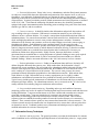
1.
The primary emphasis of this manual is placed on the technical procedures for
performing precise monitoring surveys in support of the Corps periodic inspection and dam
safety programs.
a.
True
b.
False
2.
Considering Deformation Survey Techniques, the general procedures to monitor the
deformation of a structure and its foundation involve measuring the _____________ of
selected object points (i.e., target points) from external reference points that are fixed in
position:
a.
vertical movement.
b.
lateral shifting.
c.
horizontal distance.
d.
spatial displacement.
3.
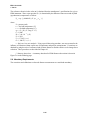
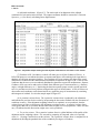
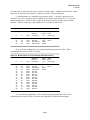
According to Table 2-1, the accuracy requirement for vertical stability/settlement of a
concrete structure is:
a.
± 10 mm.
b.
± 5 - 10 mm.
c.
± 2 mm.
d.
± 20 mm.
4.
Which of the following is NOT an actual Professional Association involved in
deformation studies?
a.
International Association of Geodesy.
b.
National Association of Concrete Flexing.
c.
International Society for Rock Mechanics.
d.
International Society for Mine Surveying.
5.
With regards to Foundation Problems in Dams, differential settlement, sliding, high
piezometric pressures and _____________ are common evidences of foundation distress:
a.
uncontrolled seepage.
b.
frost heaving.
c.
efflorescence.
d.
hairline cracking.
6.
According to Section 2-7, monitoring is not required to assess the safety performance
of lock structures.
a.
True
b.
False
7.
Considering Deformation Measurement and Alignment Instrumentation, the
measuring techniques and instrumentation for deformation monitoring have traditionally
been categorized into _____ groups according to the disciplines of professionals who use the
techniques:
a.
seven.
b.
three.
c.
four.
d.
two.
8.
Differential Leveling provides height difference measurements between a series of
benchmarks.
a.
True
b.
False
9.
All measurements with optical theodolites are subject to Optical Pointing Error due
to such factors as: target design, prevailing atmospheric conditions, ______, and
focusing:
a.
operator bias.
b.
shoddy equipment.
c.
fluctuating magnetic fields.
d.
solar flares.
10.
Figure 5-5 depicts a typical field EDM recording form used at ___________:
a.
Hoover Dam.
b.
Grand Haven Lock and Dam.
c.
Columbia Dam.
d.
Inglis Lock.
11.
Section 6-1 covers standards and specifications for performing precise differential
leveling surveys, as required to monitor settlements in concrete and embankment structures.
a.
True
b.
False
12.
Regarding Total Station Trigonometric Heights, EDM/Total Station trigonometric
heighting can be used to determine __________ in lieu of spirit leveling:
a.
settlement.
b.
lateral movement.
c.
fissure shifts.
d.
height differences.
13.
Chapter 7 describes EDM/Total Station methods for accurately measuring small
relative deflections or absolute deformations in hydraulic structures.
a.
True
b.
False
14.
Figure 7-1 depicts:
a.
alignment micrometer measurements.
b.
EDM/Total Station methods.
c.
a traditional transit.
d.
Port Mayaca Spillway.
15.
Considering Section 7-4, the micrometer observation and calibration procedures
outlined in this chapter are considered _________:
a.
optional.
b.
mandatory.
c.
as recommendations.
d.
obsolete.
16.
With regards to Section 8-5, Surveying Procedures, the objective of deformation
surveys is to determine the position of object points on the monitored structure.
a.
True
b.
False
17.
With respect to GPS Survey Reporting and Results, GPS monitoring surveys produce
_________ data and processing outputs:
a.
very little.
b.
large amounts of.
c.
occasional.
d.
partial.
18.
For Closure and Station Checks, loop misclosures are computed by comparing at least
_______ interconnected baselines:
a.
four.
b.
three.
c.
two.
d.
five.
19.
Concerning Least Squares Adjustment, the Least Squares principle is ______ applied
to the adjustment of surveying measurements because it defines a consistent set of
mathematical and statistical procedures for finding unknown coordinates using redundant
observations.
a.
seldom.
b.
widely.
c.
never.
d.
always.
20.
From Table 9-1, the minimum constraint for Network Type 1D is:
a.
z of 1 point held fixed.
b.
x and y of 2 points held fixed.
c.
x, y, z of 3 points held fixed.
d.
x and y of 4 points held fixed.
21.
Table 9-2 reflects Rejection Criteria for Preprocessing of Deformation Survey Data.
a.
True
b.
False
22.
Figure 9-11 illustrates:
a.
adjustment network plots.
b.
ratio of two lines.
c.
adjustment histograms.
d.
network maps.
23.
Considering Relative Distance Ratio Assessment Methods, certain EDM biases such
as refraction and scale error in EDM distance measurements can be minimized between two
survey epochs, without calculating corrections, by application of "reference line ratio"
methods.
a.
True
b.
False
24.
Figure 10-2 illustrates:
a.
adjustment network plots.
b.
ratio of two lines.
c.
ratios in a triangle.
d.
network maps.
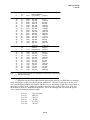
25.
The Elevation for Example Deformation Survey from Table 10-2 for point A1 is:
a.
329.339.
b.
512.799.
c.
281.005.
d.
410.724.
26.
When considering the Analysis and Assessment of Results, even the most precise
monitoring surveys will not fully serve their purpose if they are not properly evaluated and
utilized in a global integrated analysis.
a.
True
b.
False
27.
With regards to Statistical Modeling (11-3), the statistical method establishes an
empirical model of the load-deformation relationship through regression analysis, which
determines the correlations between observed deformations and observed loads (external
and internal causes producing the deformation).
a.
True
b.
False
28.
The Hybrid Analysis Method (11-5) is ___________ at the early stage of dam
operation when only short sets of observation data are available:
a.
not suitable.
b.
preferred.
c.
required.
d.
optional.
29.
For the Report Format (12-1), contained in the final Survey Report are the ________,
supporting analysis, results, and a report of conclusions:
a.
invoice.
b.
field notes.
c.
contract.
d.
description of interferences, if any.
30.
Considering Data Management (12-3), the organization and management of historical
movement data is not critical because the structure is usually replaced every 20 to 25 years.
a.
True
b.
False
EM 1110-2-1009
1 June 2002
US Army Corps
of Engineers
ENGINEERING AND DESIGN
Structural Deformation Surveying
ENGINEER MANUAL
CECW-EE
Manual
No. 1110-2-1009
DEPARTMENT OF THE ARMY
US Army Corps of Engineers
Washington, DC 20314-1000
EM 1110-2-1009
Engineering and Design
STRUCTURAL DEFORMATION SURVEYING
1 June 2002
Table of Contents
Subject
Paragraph
Page
Chapter 1
Introduction
Purpose............................................................................................................1-1
Applicability.....................................................................................................1-2
Distribution ......................................................................................................1-3
References .......................................................................................................1-4
Scope of Manual...............................................................................................1-5
Background......................................................................................................1-6
Deformation Survey Techniques........................................................................1-7
Life Cycle Project Management.........................................................................1-8
Metrics ............................................................................................................1-9
Trade Name Exclusions.....................................................................................1-10
Abbreviations and Terms ..................................................................................1-11
Mandatory Requirements ..................................................................................1-12
Proponency and Waivers...................................................................................1-13
1-1
1-1
1-1
1-1
1-1
1-1
1-2
1-3
1-4
1-4
1-4
1-4
1-4
Chapter 2
Planning, Design, and Accuracy Requirements
Standards for Deformation Surveys....................................................................2-1
Accuracy Requirements for Performing Deformation Surveys .............................2-2
Overview of Deformation Surveying Design .....................................................2-3
Professional Associations ..................................................................................2-4
Causes of Dam Failure ......................................................................................2-5
Foundation Problems in Dams ...........................................................................2-6
Navigation Locks..............................................................................................2-7
Deformation Parameters ...................................................................................2-8
Location of Monitoring Points ...........................................................................2-9
Design of Reference Networks ..........................................................................2-10
Reference Point Monumentation........................................................................2-11
Monitoring Point Monumentation ......................................................................2-12
Design of Measurement Schemes ......................................................................2-13
Measurement Reliability....................................................................................2-14
Frequency of Measurements..............................................................................2-15
Mandatory Requirements ..................................................................................2-16
i
2-1
2-2
2-3
2-7
2-8
2-8
2-10
2-11
2-12
2-13
2-17
2-19
2-21
2-23
2-25
2-27
EM 1110-2-1009
1 Jun 02
Subject
Paragraph
Page
Chapter 3
Deformation Measurement and Alignment Instrumentation
General............................................................................................................3-1
Angle and Distance Measurements ....................................................................3-2
Differential Leveling.........................................................................................3-3
Total Station Trigonometric Elevations ..............................................................3-4
Global Positioning System (GPS) ......................................................................3-5
Photogrammetric Techniques ............................................................................3-6
Alignment Measurements .................................................................................3-7
Extension and Strain Measurements...................................................................3-8
Tilt and Inclination Measurements.....................................................................3-9
Non-Geodetic Measurements ............................................................................3-10
Optical Tooling Technology ..............................................................................3-11
Laser Tooling methods ......................................................................................3-12
Laser Alignment Technology.............................................................................3-13
Laser Alignment Techniques .............................................................................3-14
Laser Alignment Error Sources..........................................................................3-15
Laser Beam Propagation....................................................................................3-16
Laser Alignment Equipment ..............................................................................3-17
Current Laser Alignment Surveys
--Libby and Chief Joseph Dams, Seattle District........................................3-18
Suspended and Inverted Plumblines ...................................................................3-19
Comparison of Alignment and Plumbline Systems ..............................................3-20
Tiltmeter Observations ......................................................................................3-21
Mandatory Requirements ..................................................................................3-22
3-1
3-2
3-6
3-7
3-7
3-11
3-12
3-14
3-16
3-18
3-20
3-21
3-22
3-25
3-27
3-29
3-31
3-34
3-38
3-39
3-41
3-42
Chapter 4
Sources of Measurement Error and Instrument Calibrations
Surveying Measurement Errors .........................................................................4-1
Optical Pointing Error .......................................................................................4-2
Instrument Leveling Error .................................................................................4-3
Instrument Centering Error ................................................................................4-4
Horizontal Angle Measurement Error ................................................................4-5
Electronic Distance Measurement Error .............................................................4-6
Zenith Angle Measurement Error ......................................................................4-7
Refraction of Optical Lines of Sight ...................................................................4-8
Theodolite System Error ...................................................................................4-9
Reflector Alignment Error .................................................................................4-10
EDM Scale Error ..............................................................................................4-11
EDM Prism Zero Error .....................................................................................4-12
EDM Cyclic Error ............................................................................................4-13
Calibration Baselines ........................................................................................4-14
Equipment for Baseline Calibration....................................................................4-15
Procedures for Baseline Calibration ...................................................................4-16
Mandatory Requirements ..................................................................................4-17
ii
4-1
4-2
4-4
4-5
4-7
4-7
4-9
4-10
4-15
4-15
4-15
4-16
4-18
4-18
4-20
4-20
4-22
EM 1110-2-1009
1 Jun 02
Subject
Paragraph
Page
Chapter 5
Angle and Distance Observations--Theodolites, Total Stations and EDM
Scope...............................................................................................................5-1
Instrument and Reflector Centering Procedures ..................................................5-2
Angle and Direction Observations......................................................................5-3
Distance Observations.......................................................................................5-4
Electro-Optical Distance Measurement ..............................................................5-5
EDM Reductions ..............................................................................................5-6
Atmospheric Refraction Correction....................................................................5-7
Mandatory Requirements ..................................................................................5-8
5-1
5-1
5-3
5-5
5-7
5-10
5-10
5-14
Chapter 6
Settlement Surveys--Precise Differential Leveling Observations
Scope...............................................................................................................6-1
Precise Geodetic Leveling.................................................................................6-2
Differential Leveling Reductions .......................................................................6-3
Total Station Trigonometric Heights ..................................................................6-4
Mandatory Requirements ..................................................................................6-5
6-1
6-1
6-5
6-7
6-7
Chapter 7
Alignment, Deflection, and Crack Measurement Surveys--Micrometer Observations
Scope...............................................................................................................7-1
Relative Alignment Deflections from Fixed Baseline ..........................................7-2
Micrometer Crack Measurement Observations....................................................7-3
Mandatory Requirements ..................................................................................7-4
7-1
7-1
7-5
7-11
Chapter 8
Monitoring Structural Deformations Using the Global Positioning System
Purpose............................................................................................................8-1
Background......................................................................................................8-2
Scope of Chapter..............................................................................................8-3
8-1
8-1
8-2
Section I
Monitoring Structural Deformation with GPS
Surveying Requirements ...................................................................................8-4
Surveying Procedures .......................................................................................8-5
Data Processing Procedures ..............................................................................8-6
GPS Monitoring Applications ............................................................................8-7
GPS Survey Reporting and Results ....................................................................8-8
8-3
8-5
8-8
8-10
8-14
iii
EM 1110-2-1009
1 Jun 02
Subject
Paragraph
Page
Section II
GPS Performance on Monitoring Networks
Principles of GPS Carrier Phase Measurement....................................................8-9
GPS Receiving System Performance .................................................................8-10
Sources of Error in GPS Measurements .............................................................8-11
GPS Performance on Monitoring Networks ........................................................8-12
8-15
8-18
8-21
8-23
Section III
Data Quality Assessment for Precise GPS Surveying
Quality Assessment Tools .................................................................................8-13
GPS Session Status ...........................................................................................8-14
Data Post-Processing.........................................................................................8-15
Post-Processing Statistics ..................................................................................8-16
Closure and Station Checks ...............................................................................8-17
8-28
8-29
8-31
8-33
8-36
Section IV
GPS Multipath Error
Description of Multipath Signals........................................................................8-18
Data Cleaning Techniques for GPS Surveys .......................................................8-19
Mandatory Requirements ..................................................................................8-20
8-38
8-40
8-42
Chapter 9
Preanalysis and Network Adjustment
General............................................................................................................9-1
Theory of Measurements...................................................................................9-2
Least Squares Adjustment .................................................................................9-3
Adjustment Input Parameters ............................................................................9-4
Adjustment Output Parameters..........................................................................9-5
Adjustment Procedures .....................................................................................9-6
Sample Adjustment--Yatesville Lake Dam.........................................................9-7
Mandatory Requirements ..................................................................................9-8
9-1
9-1
9-3
9-5
9-10
9-16
9-19
9-31
Chapter 10
Relative Distance Ratio Assessment Methods
Introduction......................................................................................................10-1
Deformation Monitoring Using Ratio Methods ...................................................10-2
Mandatory Requirements ..................................................................................10-3
iv
10-1
10-4
10-16
EM 1110-2-1009
1 Jun 02
Subject
Paragraph
Page
Chapter 11
Analysis and Assessment of Results
General............................................................................................................11-1
Geometrical Analysis ........................................................................................11-2
Statistical Modeling..........................................................................................11-3
Deterministic Modeling.....................................................................................11-4
Hybrid Analysis Method ...................................................................................11-5
Automated Data Management ...........................................................................11-6
Scope of Deformation Analysis .........................................................................11-7
Mandatory Requirements ..................................................................................11-8
11-1
11-2
11-6
11-7
11-8
11-9
11-11
11-11
Chapter 12
Data Presentation and Final Reports
Report Format..................................................................................................12-1
Displacement Data Presentation.........................................................................12-2
Data Management ............................................................................................12-3
Mandatory Requirements ..................................................................................12-4
Appendix A References
Appendix B Applications: Deformation Surveys of Locks and Dams
Central & Southern Florida Flood Control Project
(Jacksonville District)
Surveying for Lock Structure Dewatering
(Lock and Dam No. 4, St. Paul District)
Appendix C Applications: Monitoring Schemes for Concrete Dams
(Libby Dam, Seattle District)
Glossary
v
12-1
12-3
12-3
12-4
EM 1110-2-1009
1 Jun 02
Chapter 1
Introduction
1-1. Purpose
This manual provides technical guidance for performing precise structural deformation surveys of locks,
dams, and other hydraulic flood control or navigation structures. Accuracy, procedural, and quality
control standards are defined for monitoring displacements in hydraulic structures.
1-2. Applicability
This manual applies to all USACE commands having responsibility for conducting periodic inspections
of completed civil works projects, as required under ER 1110-2-100, Periodic Inspection and Continuing
Evaluation of Completed Civil Works Structures.
1-3. Distribution
This publication is approved for public release; distribution is unlimited.
1-4. References
Referenced USACE publications and bibliographic information are listed in Appendix A.
1-5. Scope of Manual
The primary emphasis of this manual is placed on the technical procedures for performing precise
monitoring surveys in support of the Corps periodic inspection and dam safety programs. General
planning criteria, field and office execution procedures, data reduction and adjustment methods, and
required accuracy specifications for performing structural deformation surveys are provided. These
techniques are applicable to periodic monitoring surveys on earth and rock-fill dams, embankments, and
concrete structures. This manual covers both conventional (terrestrial) and satellite (GPS) deformation
survey methods used for measuring external movements. This manual does not cover instrumentation
required to measure internal loads, stresses, strains, or pressures within a structure--refer to the references
at Appendix A for these activities. Example applications on Corps projects are provided at Appendix B
(Deformation Surveys of Locks and Dams) and Appendix C (Monitoring Schemes for Concrete Dams).
The manual is intended to be a reference guide for structural deformation surveying, whether performed
by in-house hired-labor forces, contracted forces, or combinations thereof. This manual should be
directly referenced in the scopes of work for Architect-Engineer (A-E) survey services or other third-party
survey services.
1-6. Background
The Corps of Engineers has constructed hundreds of dams, locks, levees, and other flood control
structures that require periodic surveys to monitor long-term movements and settlements, or to monitor
short-term deflections and deformations. These surveys are usually performed under the directives of ER
1110-2-100, Periodic Inspection and Continuing Evaluation of Completed Civil Works Structures. In
some USACE commands, these types of surveys may be referred to as "PICES Surveys" -- an acronym
which derives from the ER directive.
1-1
EM 1110-2-1009
1 Jun 02
a. Structural deformation. Dams, locks, levees, embankments, and other flood control structures
are subject to external loads that cause deformation and permeation of the structure itself, as well as its
foundations. Any indication of abnormal behavior may threaten the safety of the structure. Careful
monitoring of the loads on a structure and its response to them can aid in determining abnormal behavior
of that structure. In general, monitoring consists of both measurements and visual inspections, as outlined
in ER 1110-2-100. To facilitate the monitoring of hydraulic structures, they should be permanently
equipped with proper instrumentation and/or monitoring points according to the goals of the observation,
structure type and size, and site conditions.
b. Concrete structures. It should be intuitive that deformations and periodic observations will
vary according to the type of structure. Differences in construction materials are one of the larger
influences on how a structure deforms. For example, concrete dams deform differently than earthen or
embankment dams. For concrete dams and other concrete flood control devices, deformation is mainly
elastic and highly dependent on reservoir water pressure and temperature variations. Permanent
deformation of the structure can sometimes occur as the subsoil adapts to new loads, concrete aging, or
foundation rock fatigue. Such deformation is not considered unsafe if it does not go beyond a
predetermined critical value. Therefore, periodic observations are typically configured to observing
relatively long-term movement trends, to include abnormal settlements, heaving, or lateral movements.
Conventional geodetic survey methods from external points and of centimeter-level accuracy are
sufficient to monitor these long-term trends. Highly accurate, short-term deflections or relative
movements between monoliths due to varying temperature or hydraulic loading are more rarely required.
These may include crack measurements or relative movements between monoliths over different
hydraulic loadings. Relative movement deflections to the +0.01-inch accuracy level are common.
c. Earthen embankment structures. Earthen or embankment dams and levees obviously will
deform altogether differently than concrete ones. With earthen dams, the deformation is largely
characterized as more permanent. The self-weight of the embankment and the hydrostatic pressure of the
reservoir water largely force the fill material (and in turn, the foundation, if it too consists of soil) to
settle, resulting in a vertical deflection of the structure. The reservoir water pressure also causes
permanent horizontal deformation perpendicular to the embankment centerline. With earthen dams,
elastic behavior is slight. Deformation survey accuracy requirements are less rigid for earthen
embankments, and traditional construction survey methods will usually provide sufficient accuracy.
Typical surveys include periodic measurement of embankment crest elevations and slopes to monitor
settlements and slope stability. For embankment structures, surveys accuracies at the +0.1 foot level are
usually sufficient for monitoring long-term settlements and movements.
d. Long-term deformation monitoring. Depending on the type and condition of structure,
monitoring systems may need to be capable of measuring both long-term movement trends and short-term
loading deformations. Long-term measurements are far more common and somewhat more complex
given their external nature. Long-term monitoring of a structure's movement typically requires
observations to monitoring points on the structure from external reference points. These external
reference points are established on stable ground well removed from the structure or its construction
influence. These external reference points are inter-connected and termed the "reference network." The
reference network must also be monitored at less-frequent intervals to ensure these reference points have
not themselves moved. Traditional geodetic survey instruments and techniques may be employed to
establish and monitor the reference network points.
1-7. Deformation Survey Techniques
a. Reference and target points. The general procedures to monitor the deformation of a structure
and its foundation involve measuring the spatial displacement of selected object points (i.e., target points)
1-2
EM 1110-2-1009
1 Jun 02
from external reference points that are fixed in position. Both terrestrial and satellite methods are used to
measure these geospatial displacements. When the reference points are located in the structure, only
relative deformation is determined--e.g., micrometer joint measurements are relative observations.
Absolute deformation or displacement is possible if the reference points are located outside the actual
structure, in the foundation or surrounding terrain and beyond the area that may be affected by the dam or
reservoir. Subsequent periodic observations are then made relative to these absolute reference points.
Assessment of permanent deformations requires absolute data.
b. Reference point network. In general, for concrete dams it is ideal to place the reference points
in a rock foundation at a depth unaffected by the reservoir. Once permanently monumented, these
reference points can be easily accessed to perform deformation surveys with simple measurement devices.
Fixed reference points located within the vicinity of the dam but outside the range of its impact are
essential to determination of the deformation behavior of the structure. Thus, monitoring networks in the
dam plane should be supplemented by and connected to triangulation networks and vertical control
whenever possible.
c. Monitoring techniques. The monitoring of dam or foundation deformation must be done in a
manner such that the displacement is measured both horizontally and vertically (i.e., measurement along
horizontal and vertical lines). Such measurements must include the foundation and extend as far as
possible into it. Redundancy is essential in this form of deformation monitoring and is achieved through
measuring at the points intersecting the orthogonal lines of the deformation network. If a dam includes
inspection galleries and shafts, deformation values along vertical lines can be obtained by using hanging
and/or inverted plumb lines and along horizontal lines by traverses--both of these methods are standard
practice for deformation monitoring. Where there are no galleries or shafts (e.g., embankment dams, thin
arch dams, or small gravity dams), the same result can be achieved by an orthogonal network of survey
targets on the downstream face. These targets are sighted by angle measurements (typically combined
with optical distance measurements) from reference points outside the dam.
d. Relative displacement observations. A more routine, less costly, and more frequent
monitoring process can be employed to monitor the short term behavior of dams by simply confining
observation to trends at selected points along the crest and sometimes vertical lines. Such procedures
typically involve simple angle measurement or alignment (supplementing the measuring installation)
along the crest to determine horizontal displacement, and elevation determination by leveling to
determine vertical displacement (i.e., settlement). Even with this monitoring process, it is essential to
extend leveling to some distance beyond the abutments. Alternative methods to that described include
settlement gauges, hose leveling devices, or extensometers.
1-8. Life Cycle Project Management
As outlined in ER 1110-2-100, structural stability assessment surveys may be required through the entire
life cycle of a project, spanning decades in many cases. During the early planning phases of a project, a
comprehensive monitoring plan should be developed which considers survey requirements over a
project's life cycle, with a goal of eliminating duplicate or redundant surveys to the maximum extent
possible. During initial design and preconstruction phases of a project, reference points should be
permanently monumented and situated in areas that are conducive to the performance of periodic
monitoring surveys. During construction, fixed monitoring points should be established on the structure
at points called for in the comprehensive monitoring plan.
1-3
EM 1110-2-1009
1 Jun 02
1-9. Metrics
Both English and metric (SI) units are used in this manual. Metric units are commonly used in precise
surveying applications, including the horizontal and vertical survey work covered in this manual.
Structural movements are usually recorded and reported in SI units. Some measurement instruments
(e.g., micrometers) use English units. In all cases, the use of either metric or non-SI units shall follow
local engineering and construction practices. Accuracy standards and tolerances specified in this manual
are generally stated at the 95% confidence level.
1-10. Trade Name Exclusions
The citation or illustration in this manual of trade names of commercially available survey products,
including other auxiliary surveying equipment, instrumentation, and adjustment software, does not
constitute official endorsement or approval of the use of such products.
1-11. Abbreviations and Terms
Engineering surveying terms and abbreviations used in this manual are explained in the Glossary.
1-12. Mandatory Requirements
ER 1110-2-1150 (Engineering and Design for Civil Works Projects) prescribes that mandatory requirements
be identified in engineer manuals. Mandatory requirements in this manual are summarized at the end of
each chapter. Mandatory accuracy standards, quality control, and quality assurance criteria are normally
summarized in tables within each chapter. The mandatory criteria contained in this manual are based on the
following considerations: (1) dam safety assurance, (2) overall project function, (3) previous Corps
experience and practice has demonstrated the criteria are critical, (4) Corps-wide geospatial data
standardization requirements, (5) adverse economic impacts if criteria are not followed, and (6) HQUSACE
commitments to industry standards.
1-13. Proponency and Waivers
The HQUSACE proponent for this manual is the Engineering and Construction Division, Directorate of
Civil Works. Technical development and compilation of the manual was coordinated by the US Army
Topographic Engineering Center (CEERD-TS-G). Comments, recommended changes, or waivers to this
manual should be forwarded through MSC to HQUSACE (ATTN: CECW-EE).
1-4
EM 1110-2-1009
1 Jun 02
Chapter 2
Planning, Design, and Accuracy Requirements
2-1. Standards for Deformation Surveys
a. General. This chapter provides guidance for planning and implementing structural
deformation surveys on US Army Corps of Engineers civil works projects. It discusses criteria and
objectives used for designing geodetic monitoring networks and for developing reliable and economical
measurement schemes based on precise engineering surveying methods. Monitoring provides
engineering data and analysis for verifying design parameters, for construction safety, for periodic
inspection reports, and for regular maintenance operations. Safety, economical design of man-made
structures, efficient functioning and fitting of structural elements, environmental protection, and
development of mitigative measures in the case of natural disasters (land slides, earthquakes, liquefaction
of earth dams, etc.) requires a good understanding of causes (loads) and the mechanism of deformation,
which can be achieved only through the proper measurement and analysis of deformable bodies.
b. Dam safety. US Army Corps of Engineers owns and operates a wide range of large
engineering structures, including major infrastructure facilities for navigation, flood protection, and large
dams. The responsibility to minimize the risk to the public is critical due to the potential loss of life and
property that a structural failure could cause. USACE dams and reservoirs must be inspected so that their
structural condition and design assumptions can be evaluated and verified. As a result of major disasters
in the United States, the federal government revised laws for supervision of the safety of dams and
reservoirs. The Dam Inspection Act, PL 92-367, 8 August 1972, authorized the Secretary of the Army,
acting through the Chief of Engineers, to undertake a national program of inspection of dams.
c. Engineer regulations. Standards for conducting instrumentation surveys and for periodic
inspections are contained in the following publications.
ER 1110-2-100, Periodic Inspection and Continuing Evaluation of Completed
Civil Works Structures
• ER 1110-2-110, Instrumentation for Safety--Evaluation of Civil Works Projects
• EP 1110-2-13, Dam Safety Preparedness
•
Guidance for Civil Works projects provides for an adequate level of instrumentation to enable designers
to monitor and evaluate the safety of the structures, and to address the need for inspection and evaluation
for stability and operational adequacy, as well as safety. ER 1110-2-100 states that a systematic plan will
be established for the inspection of those features relating to safety and stability of the structure and to the
operational adequacy of the project. Operational adequacy means the inspecting, testing, operating, and
evaluation of those components of the project whose failure to operate properly would impair the
operational capability and/or usability of the structure. Appendix A of ER 1110-2-100 addresses
provisions to collect and permanently retain specific engineering data relating to the project structure and
examine records that detail the principal design assumptions and stability, stress analysis, slope stability,
and settlement analyses.
d. Specialized standards. Federal geospatial data standards, established in OMB Circular No. A16, Coordination of Surveying, Mapping, and Related Spatial Data Activities, provide for activities
conducted to meet special agency program needs. USACE engineering and construction guidance for
geospatial data products prescribes voluntary industry standards and consensus standards, except where
they are non-existent, inappropriate, or do not meet a project’s functional requirement. Specialized
standards for conducting deformation surveys are justified as long as products are consistent with
2-1
EM 1110-2-1009
1 Jun 02
effective government wide coordination and efficient, economical service to the general public.
Deformation monitoring often requires specialized surveying methods that are planned and executed
according to specialized techniques and procedures.
2-2. Accuracy Requirements for Performing Deformation Surveys
a. General. The following table provides guidance on the accuracy requirements for performing
deformation surveys. These represent either absolute or relative movement accuracies on target points
that should be attained from survey observations made from external reference points. The accuracy by
which the external reference network is established and periodically monitored for stability should exceed
these accuracies. Many modern survey systems (e.g., electronic total stations, digital levels, GPS, etc.)
are easily capable of meeting or exceeding the accuracies shown below. However, it is important that
accuracy criteria must be defined relative to the particular structure's requirements, not the capabilities of
a survey instrument or system.
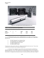
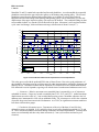
Table 2-1. Accuracy Requirements for Structure Target Points (95% RMS)
Concrete Structures
Dams, Outlet Works, Locks, Intake Structures:
Long-Term Movement
+ 5-10 mm
Relative Short-Term Deflections
Crack/Joint movements
Monolith Alignment
+ 0.2 mm
Vertical Stability/Settlement
+ 2 mm
Embankment Structures Earth-Rockfill Dams, Levees:
Slope/crest Stability
+ 20-30 mm
Crest Alignment
+ 20-30 mm
Settlement measurements
+ 10 mm
Control Structures Spillways, Stilling Basins, Approach/Outlet Channels, Reservoirs
Scour/Erosion/Silting
+ 0.2 to 0.5 foot
b. Accuracy design examples. As an example to distinguish between instrument accuracy and
project accuracy requirements, an electronic total station system can measure movement in an earthen
embankment to the +0.005-foot level. Thus, a long-term creep of say 3.085 feet can be accurately
measured. However, the only significant aspect of the 3.085-foot measurement is the fact that the
embankment has sloughed "3.1 feet" -- the +0.001-foot resolution (precision) is not significant and should
not be observed even if available with the equipment. As another example, relative crack or monolith
joint micrometer measurements can be observed and recorded to +0.001-inch precision. However, this
precision is not necessarily representative of an absolute accuracy, given the overall error budget in the
micrometer measurement system, measurement plugs, etc. Hydraulic load and temperature influences
can radically change these short-term micrometer measurements at the 0.01 to 0.02-inch level, or more.
Attempts to observe and record micrometer measurements to a 0.001-inch precision with a ±0.01-inch
temperature fluctuation are wasted effort on this typical project.
2-2
EM 1110-2-1009
1 Jun 02
2-3. Overview of Deformation Surveying Design
a. General. USACE Engineering Divisions and Districts have the responsibility for formulating
inspection plans, conducting inspections, processing and analyzing instrument observations, evaluating
the condition of the structures, recommending inspection schedules, and preparing inspection and
evaluation reports. This section presents information to aid in fulfilling these objectives.
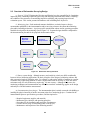
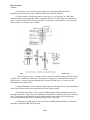
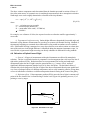
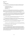
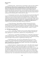
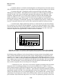
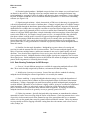
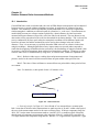
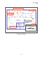
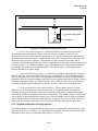
b. Monitoring plan. Each monitored structure should have a technical report or design
memorandum published for the instrumentation and/or surveying scheme to document the monitoring
plan and its intended performance. A project specific measurement scheme and its operating procedures
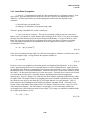
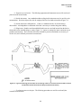
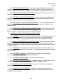
should be developed for the monitoring system (Figure 2-1). Separate designs should be completed for
the instrumentation plan and for the proposed measurement scheme.
Maximum
Expected
Displacement
Accuracy
Requirements
Network
Adjustment
Data
Reductions
Deformation
Modeling
Data
Presentation
Preanalysis &
Survey Design
Data
Collection
Figure 2-1. Deformation Survey Data Flow
(1) Survey system design. Although accuracy and sensitivity criteria may differ considerably
between various monitoring applications, the basic principles of the design of monitoring schemes and
their geometrical analysis remain the same. For example, a study on the stability of magnets in a nuclear
accelerator may require determination of relative displacements with an accuracy of +0.05 mm while a
settlement study of a rock-fill dam may require only +10 mm accuracy. Although in both cases, the
monitoring techniques and instrumentation may differ, the same basic methodology applies to the design
and analysis of the deformation measurements.
(a) Instrumentation plan (design). The instrumentation plan is mainly concerned with building or
installing the physical network of surface movement points for a monitoring project. Contained in the
instrumentation plan are specifications, procedures, and descriptions for:
Required equipment, supplies, and materials,
Monument types, function, and operating principles,
• Procedures for the installation and protection of monuments,
• Location and coverage of monitoring points on the project,
• Maintenance and inspection of the monitoring network.
•
•
2-3
EM 1110-2-1009
1 Jun 02
The plan contains drawings, product specifications, and other documents that completely describe the
proposed instrumentation, and methods for fabrication; testing; installation; and protection and
maintenance of instruments and monuments.
(b) Measurement scheme (design). The design of the survey measurement scheme should include
analysis and specifications for:
Predicted performance of the structure,
Measurement accuracy requirements,
• Positioning accuracy requirements,
• Number and types of measurements,
• Selection of instrument type and precision,
• Data collection and field procedures,
• Data reduction and processing procedures,
• Data analysis and modeling procedures,
• Reporting standards and formats,
• Project management and data archiving.
•
•
The main technique used to design and evaluate measurement schemes for accuracy is known as "network
preanalysis." Software applications specially written for preanalysis and adjustment are used to compute
expected error and positioning confidence for all surveyed points in the monitoring network (see
Chapter 9).
(2) Data collection. The data collection required on a project survey is specifically prescribed by
the results of network preanalysis. The data collection scheme must provide built-in levels of both
accuracy and reliability to ensure acceptance of the raw data.
(a) Accuracy. Achieving the required accuracy for monitoring surveys is based on instrument
performance and observing procedures. Minimum instrument resolution, data collection options, and
proper operating instructions are determined from manufacturer specifications. The actual data collection
is executed according to the results of network preanalysis so that the quality of the results can be verified
during data processing and post-analysis of the network adjustment.
(b) Reliability. Reliability in the raw measurements requires a system of redundant
measurements, sufficient geometric closure, and strength in the network configuration. Geodetic
surveying methods can yield high redundancy in the design of the data collection scheme.
(3) Data processing. Raw survey data must be converted into meaningful engineering values
during the data processing stage. Several major categories of data reductions are:
Applying pre-determined calibration values to the raw measurements,
Finding mean values for repeated measurements of the same observable,
• Data quality assessment and statistical testing during least squares adjustment,
• Measurement outlier detection and data cleaning prior to the final adjustment.
•
•
Procedures for data reductions should be based on the most rigorous formulas and data processing
techniques available. These procedures are applied consistently to each monitoring survey to ensure
comparable results. Network adjustment software based on least squares techniques is strongly
recommended for data processing. Least squares adjustment techniques are used to compute the
coordinates and survey accuracy for each point in the monitoring network. Network adjustment
processing also identifies measurement blunders by statistically testing the observation residuals.
2-4
EM 1110-2-1009
1 Jun 02
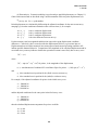
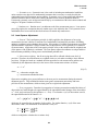
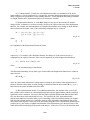
(4) Data analysis. Geometric modeling is used to analyze spatial displacements (see Chapter 11).
General movement trends are described using a sufficient number of discrete point displacements (dn ):
dn (∆x, ∆y, ∆z) for n = point number
Point displacements are calculated by differencing the adjusted coordinates for the most recent survey
campaign (f), from the coordinates obtained at some reference time (i), for example:
∆x = xf - xi
∆y = yf - yi
∆z = zf - zi
∆t = tf - ti
is the x coordinate displacement
is the y coordinate displacement
is the z coordinate displacement
is the time difference between surveys.
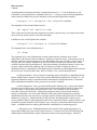
Each movement vector has magnitude and direction expressed as point displacement coordinate
differences. Collectively, these vectors describe the displacement field over a given time interval.
Displacements that exceed the amount of movement expected under normal operating conditions will
indicate possible abnormal behavior. Comparison of the magnitude of the calculated displacement and its
associated survey accuracy indicates whether the reported movement is more likely due to survey error:
dn  < (en )
where
dn  = sqrt (∆x2 + ∆y2 + ∆z2 ) for point n, is the magnitude of the displacement,
(en ) = max dimension of combined 95% confidence ellipse for point n = (1.96) sqrt (σf 2 + σi 2 ),
and
σf is the standard error in position for the (final) or most recent survey,
σi is the standard error in position for the (initial) or reference survey.
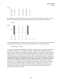
For example, if the adjusted coordinates for point n in the initial survey were:
xi = 1000.000 m
yi = 1000.000 m
zi = 1000.000 m
and the adjusted coordinates for the same point in the final survey were:
xf = 1000.006 m
yf = 1000.002 m
zf = 1000.002 m
then the calculated displacement components for point n would be:
∆x = 6 mm
∆y = 2 mm
∆z = 2 mm
2-5
EM 1110-2-1009
1 Jun 02
Assuming that the horizontal position has a standard deviation of σh = 1.5 mm for both surveys, and
similarly the vertical position has a standard deviation of σv = 2.0 mm, as reported from the adjustment
results, then the combined (95 percent) confidence in the horizontal displacement would be:
(1.96) sqrt (σf 2 + σi 2 ) = (1.96) sqrt (2.25 + 2.25) ~ 4.2 mm at 95% confidence
The magnitude of the horizontal displacement is:
dh  = sqrt (∆x2 + ∆y2 ) = sqrt (36 + 4) = 6.3 mm
These results show that the horizontal component exceeds the expected survey error margin and is likely
due to actual movement of point n in the horizontal plane.
Confidence in the vertical displacement would be:
(1.96) sqrt (σf 2 + σi 2 ) = (1.96) sqrt (4 + 4) ~ 5.5 mm at 95% confidence
The magnitude of the vertical displacement is:
dv = 2.0 mm
The magnitude of the vertical displacement is much smaller than the confidence in the vertical
displacement, and it therefore does not indicate a significant vertical movement. If the structure were to
normally experience cyclic movement of 10 mm (horizontally) and 1 mm (vertically) over the course of
one year, and if our example deformation surveys were made six months apart, then the above results
would be consistent with expected behavior. Specialized methods of geometrical analysis exist to carry
out more complex deformation modeling, and it is sometimes possible to identify the causes of
deformation based on comparing the actual displacements to alternative predicted displacement modes for
the specific type of structure under study. Refer to Chapter 11 for a more detailed discussion.
(5) Data presentation. Survey reports for monitoring projects should have a standardized format.
Reports should contain a summary of the results in both tabulated and graphical form (Chapter 12). All
supporting information, analyses, and data should be documented in an appendix format. Conclusions
and recommendations should be clearly presented in an executive summary.
(6) Data management. Survey personnel should produce hardcopy survey reports and complete
electronic copies of these reports. Survey data and processed results should be archived, indexed, and
cross-referenced to existing structural performance records. These should be easily located and
retrievable whenever the need arises. Information management using computer-based methods is
strongly recommended. One of the main difficulties with creating a data management system that
includes historical data is the time and cost required to transfer existing hardcopy data into an electronic
database for each project. Gradual transition to fully electronic data management on future project
surveys should be adopted. Data management tools such as customized software, database software, and
spreadsheet programs should be used to organize, store, and retrieve measurement data and processed
results. A standard format for archiving data should be established for all monitoring projects.
c. Management plan. Sound administration and execution of the monitoring program is an
integral and valuable part of the periodic inspection process. Personnel involved in the monitoring and
instrumentation should maintain a regular interaction with the senior program manager. Structural
2-6
EM 1110-2-1009
1 Jun 02
monitoring encompasses a wide range of tasks performed by specialists in different functional areas. All
participants should have a general understanding of requirements for the complete evaluation process.
General Engineering for planning and monitoring requests, preparation/presentation of data and
results, and quality assurance measures,
•
Surveying for data collection (in-house or contract requirements), data reduction, processing,
network adjustment, quality assurance, and preparing survey reports,
•
Geotechnical and Structural Engineering for analysis and evaluation of results and preparation
of findings and recommendations,
•
Technical Support for data management, archiving, computer resources, archiving final reports,
and electronic information support.
•
Safety requires consideration of more than just technical factors. Systems should be in place so that any
voice within the organization can be heard. Even experts can make mistakes and good ideas can come
from any level within an organization. Meetings and/or site visits including all participants are held to
ensure that information flows freely across internal boundaries. Integration of separate efforts should be
on going and seamless rather than simply gluing together individual final products.
d. External review. An organization must be willing to accept, in fact it should seek, the
independent review of its engineering practices. Large structures require defensive engineering that
considers a range of circumstances that might occur that threatens their safety. A contingency plan to
efficiently examine and assess unexpected changes in the behavior of the structure should be in place.
Outside experts should be consulted from time-to-time, especially if a project structure exhibits unusual
behavior that warrants specialized measurement and analysis.
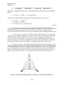
2-4. Professional Associations
a. General. The development of new methods and techniques for monitoring and analysis of
deformations and the development of methods for the optimal modeling and prediction of deformations
have been the subject of intensive studies by many professional groups at national and international
levels.
b. Organizations. Within the most active international organizations that are involved in
deformation studies one should list:
International Federation of Surveyors (FIG) Commission 6 which has significantly contributed
to the recent development of new methods for the design and geometrical analysis of integrated
deformation surveys and new concepts for analyses and modeling of deformations;
•
International Commission on Large Dams (ICOLD) with its Committee on Monitoring of Dams
and their Foundations;
•
International Association of Geodesy (IAG) Commission on Recent Crustal Movements,
concerning geodynamics, tectonic plate movement, and modeling of regional earth crust
deformation.
•
International Society for Mine Surveying (ISM) Commission 4 on Ground Subsidence and
Surface Protection in mining areas;
•
2-7
EM 1110-2-1009
1 Jun 02
International Society for Rock Mechanics (ISRM) with overall interest in rock stability and
ground control; and
•
International Association of Hydrological Sciences (IAHS), with work on ground subsidence
due to the withdrawal of underground liquids (water, oil, etc.).
•
2-5. Causes of Dam Failure
a. Concrete structures. Deformation in concrete structures is mainly elastic and for large dams
highly dependent on reservoir water pressure and temperature variations. Permanent deformation of the
structure can sometimes occur as the subsoil adapts to new loads, concrete aging, or foundation rock
fatigue. Such deformation is not considered unsafe if it does not go beyond a pre-determined critical
value. Monitoring is typically configured to observing relatively long-term movement trends, including,
abnormal settlements, heaving, or lateral movements. Some ways concrete dams can fail are:
Uplift at the base of gravity dams leading to overturning and downstream creep.
Foundation failure or buttress collapse in single or multiple arched dams
• Surrounding embankments that are susceptible to internal erosion.
•
•
b. Embankment structures. Deformation is largely inelastic with earthen dams characterized by
permanent changes in shape. Self-weight of the embankment and the hydrostatic pressure of the reservoir
water force the fill material and the foundation (if it consists of soil) to consolidate resulting in vertical
settlement of the structure. Reservoir water pressure also causes permanent horizontal deformation
mostly perpendicular to the embankment centerline. Some causes of damage to earthen dams are:
•
•
Construction defects that cause the structure to take on anisotropic characteristics over time,
Internal pressures and paths of seepage resulting in inadequately controlled interstitial water.
Usually these changes are slow and not readily discerned by visual examination. Other well-known
causes of failure in earthen dams are overtopping at extreme flood stage and liquefaction due to ground
motion during earthquakes.
c. Structural distress. The following warning signs are evidence for the potential failure of dams.
Significant sloughs, settlement, or slides in embankments such as in earth or rockfill dams,
Movement in levees, bridge abutments or slopes of spillway channels, locks, and abutments,
• Unusual vertical or horizontal movement or cracking of embankments or abutments,
• Sinkholes or localized subsidence in the foundation or adjacent to embankments and structures,
• Excessive deflection, displacement, or vibration of concrete structures
• Tilting or sliding of intake towers, bridge piers, lock wall, floodwalls),
• Erratic movement, binding, excessive deflection, or vibration of outlet and spillway gates,
• Significant damage or changes in structures, foundations, reservoir levels, groundwater
conditions and adjacent terrain as a result of seismic events of local or regional areas,
• Other indications of distress or potential failure that could inhibit the operation of a project or
endanger life and property.
•
•
2-6. Foundation Problems in Dams
a. General. Differential settlement, sliding, high piezometric pressures, and uncontrolled
seepage are common evidences of foundation distress. Cracks in the dam, even minor ones, can indicate
a foundation problem. Clay or silt in weathered joints can preclude grouting and eventually swell the
2-8
EM 1110-2-1009
1 Jun 02
crack enlarging it and causing further stress. Foundation seepage can cause internal erosion or solution.
Potential erosion of the foundation must be considered as erosion can leave collapsible voids. Actual
deterioration may be evidenced by increased seepage, by sediment in seepage water, or an increase in
soluble materials disclosed by chemical analyses. Materials vulnerable to such erosion include dispersive
clays, water reactive shales, gypsum and limestone.
b. Consolidation. Pumping from underground can cause foundation settlement as the supporting
water pressure is removed or the gradient changed. Loading and wetting will also cause the pressure
gradient to change, and may also cause settlement or shifting. The consequent cracking of the dam can
create a dangerous condition, especially in earthfills of low cohesive strength. Foundations with low
shear strength or with extensive seams of weak materials such as clay or bentonite may be vulnerable to
sliding. Shear zones can also cause problems at dam sites where bedding plane zones in sedimentary
rocks and foliation zones in metamorphics are two common problems. An embankment may be most
vulnerable at its interface with rock abutments. Settlement in rockfill dams can be significantly reduced if
the rockfill is mechanically compacted. In some ways, a compacted earth core is superior to a concrete
slab as the impervious element of a rockfill dam. If the core has sufficient plasticity, it can be flexible
enough to sustain pressures without significant damage. Several dam failures have occurred during initial
impoundment.
c. Seepage. Water movement through a dam or through its foundation is one of the important
indicators of the condition of the structure and may be a serious source of trouble. Seeping water can
chemically attack the components of the dam foundation, and constant attention must be focused on any
changes, such as in the rate of seepage, settlement, or in the character of the escaping water. Adequate
measurements must be taken of the piezometric surface within the foundation and the embankment, as
well as any horizontal or vertical distortion in the abutments and the fill. Any leakage at an earth
embankment is potentially dangerous, as rapid erosion may quickly enlarge an initially minor defect.
d. Erosion. Embankments may be susceptible to erosion unless protected from wave action on
the upstream face and surface runoff on the downstream face. Riprap amour stone on the upstream slope
of an earthfill structure can protect against wave erosion, but can become dislodged over time. This
deficiency usually can be detected and corrected before serious damage occurs. In older embankment
dams, the condition of materials may vary considerably. The location of areas of low strength must be a
key objective of the evaluation of such dams. Soluble materials are sometimes used in construction, and
instability in the embankment will develop as these materials are dissolved over time. Adverse conditions
which deserve attention include: poorly sealed foundations, cracking in the core zone, cracking at zonal
interfaces, soluble foundation rock, deteriorating impervious structural membranes, inadequate foundation
cutoffs, desiccation of clay fill, steep slopes vulnerable to sliding, blocky foundation rock susceptible to
differential settlement, ineffective contact at adjoining structures and at abutments, pervious embankment
strata, vulnerability to conditions during an earthquake.
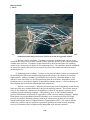
e. Liquefaction. Hydraulic fill dams are particularly susceptible to earthquake damage.
Liquefaction is a potential problem for any embankment that has continuous layers of soil with uniform
gradation and of fine grain size. The Fort Peck Dam experienced a massive slide on the upstream side in
1938, which brought the hydraulic fill dam under suspicion. The investigation at the time focused blame
on an incompetent foundation, but few hydraulic fills were built after the 1930's. Heavy compaction
equipment became available in the 1940's, and the rolled embankment dam became the competitive
alternative.
f. Concrete deterioration. Chemical and physical factors can age concrete. Visible clues to the
deterioration include expansion, cracking, gelatinous discharge, and chalky surfaces.
2-9
EM 1110-2-1009
1 Jun 02
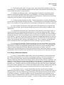
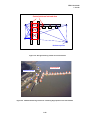
2-7. Navigation Locks
a. Lock wall monoliths. Periodic monitoring is provided to assess the safety performance of lock
structures. Instrumentation should be designed to monitor lateral, vertical, and rotational movement of
the lock monoliths, although not all structural components of a lock complex (e.g., wall/monoliths, wing
walls, gates, dam) may need to be monitored. Navigation locks (including access bridge piers) and their
surroundings are monitored to determine the extent of any differential movements between wall
monoliths, monolith tilt, sheet pile cell movement, cracking, or translation or rotation affecting sections of
the lock structure.
(1) Foundation. Piezometers are used to monitor uplift pressures beneath the lock structure.
Water level monitoring is made through wells fitted with a vibrating wire pressure transducer or designed
for manual measurement with a portable water level indicator. Inclinometer casings are anchored in
stable zones under the structure and are used to monitor lateral movement of selected monoliths. Probe
readings are made at 2-ft increments to measure the slope of the casing. Foundation design concerns
soil/structure interactions, pile or soil bearing strength, settlement, scour protection, stability for uplift,
sliding, and overturning, slide activity below ground level, earthquake forces and liquefaction, horizontal
stresses in underlying strata and residual strength, rock faults that penetrate foundation sedimentary
materials, and evidence of movement in unconsolidated sediment along the rim and foundation of the
surrounding basin.
(2) Expected loads. Lock structures experience dynamic loads due to hydraulic forces, seismic
and ice forces, earth pressures, and thermal stresses. Static loads include weight of the structure and
equipment. Horizontal water pressure and uplift on lock walls vary due to fluctuating water levels, and
horizontal earth pressures and vertical loading vary with drained, saturated, or submerged backfill and
siltation. Seismic forces and impact loads from collisions are accounted for in dynamic analysis for
design of the structure. Loads are generated by filling and emptying system turbulence and barge
mooring, ice and debris, wave pressure, wind loads, and differential water pressure on opposite sides of
sheetpile cutoffs at the bottom of the lock monolith. Loads are generated by gate and bulkhead structures,
machinery and appurtenant items, superstructure and bridge loads imparted to lock walls, temperature,
and internal pore pressure in concrete.
(3) Dewatering maintenance. All locks have temporary closures for dewatering the lock chamber
during maintenance activities or emergencies. Lock wall monitoring is conducted at both gate monoliths
and selected interior chamber monoliths to detect any potential movement due to changing loads as the
water level is lowered during lock chamber dewatering. Monitoring wells placed in the landside
embankment are checked regularly to determine ground water levels that exert pressure on the landside
wall. Monitoring surveys are conducted for measuring the lateral displacement of the lock walls with
respect to each other and to stable ground. These are made continuously, and at regular time intervals
until the chamber is completely dewatered.
b. Lock miter gates. Observations for distress in miter lock gates may include one or more of the
following: top anchorage movement, elevation change, miter offset, bearing gaps, and downstream
movement.
c. Sheet pile structures. Distress in sheet pile structures may include one or more of the
following: misalignment, settlement, cavity formation, or interlock separation.
d. Rubble breakwaters and jetties. Observations for breakwaters and jetties include the seaside
and leeside slopes and crest: seaside/leeside slope - protection side walls should be examined for; armor
loss, armor quality defects, lack of armor contact/interlock, core exposure/loss, other slope defects.
2-10
EM 1110-2-1009
1 Jun 02
Crest/cap - peak or topmost surface areas should be examined for breaching, armor loss, core
exposure/loss. Any number of measurements may be needed to monitor the condition of breakwaters,
jetties, or stone placement. These may involve either lower accuracy conventional surveying,
photogrammetric, or hydrographic methods.
e. Scour monitoring. Hydrographic surveys for scour monitoring employ equipment that will
produce full coverage bathymetric mapping of the area under investigation. The procedures and
specifications should conform to standards referenced in EM 1110-2-1003, Hydrographic Surveying.
Scour monitoring surveys should specify accuracy requirements, boundaries of coverage area, bathymetry
contour interval, delivery file formats, and the required frequency of hydrographic surveying.
2-8. Deformation Parameters
a. General. The main purpose for monitoring and analysis of structural deformations is:
To check whether the behavior of the investigated object and its environment follow the
predicted pattern so that any unpredicted deformations could be detected at an early stage.
•
In the case of abnormal behavior, to describe as accurately as possible the actual deformation
status that could be used for the determination of causative factors which trigger the deformation.
•
Coordinate differencing and observation differencing are the two principal methods used to determine
structural displacements from surveying data. Coordinate differencing methods are recommended for
most applications that require long-term periodic monitoring. Observation differencing is mainly used for
short-term monitoring projects or as a quick field check on the raw data as it is collected.
(1) Coordinate differencing. Monitoring point positions from two independent surveys are
required to determine displacements by coordinate differencing. The final adjusted Cartesian coordinates
(i.e., the coordinate components) from these two surveys are arithmetically differenced to determine point
displacements. A major advantage of the coordinate differencing method is that each survey campaign
can be independently analyzed for blunders and for data adjustment quality. However, great care must be
taken to remove any systematic errors in the measurements, for example by applying all instrument
calibration corrections, and by rigorously following standard data reduction procedures.
(2) Observation differencing. The method of observation differencing involves tracking changes
in measurements between two time epochs. Measurements are compared to previous surveys to reveal
any observed change in the position of monitoring points. Although observation differencing is efficient,
and does not rely on solving for station coordinates, it has the drawback that the surveyor must collect
data in an identical configuration, and with the same instrument types each time a survey is conducted.
b. Absolute displacements. Displacements of monumented points represent the behavior of the
dam, its foundation, and abutments, with respect to a stable framework of points established by an
external reference network.
(1) Horizontal displacements. Two-dimensional (2D) displacements are measured in a critical
direction, usually perpendicular to the longitudinal axis of dam, at the crest, and other important points of
embankments (abutments, toes, etc.) using conventional geodetic methods. Alignment techniques for
alignment-offset measurements are made in relation to a pair of control points having well-known
coordinates. Horizontal movement can also be determined with respect to plumblines having a stable
anchor point (see EM 1110-2-4300, Instrumentation for Concrete Structures).
2-11
EM 1110-2-1009
1 Jun 02
(2) Vertical displacements. Vertical displacements are measured in relation to stable project
benchmarks, such as deeply anchored vertical borehole extensometers, or alternatively, to deep
benchmarks located near the dam using geodetic methods (differential leveling). Hydrostatic leveling is
also sometimes used to determine settlements. Settlement gauges are used to detect settlements of the
foundation, or of interior structural parts which are not readily accessible (core, foundation contact).
Settlements of individual layers of embankments should be monitored through settlement gauges installed
in the different layers (refer to EM 1110-2-2300, Earth and Rock-Fill Dams General Design and
Construction Consideration).
c. Relative displacements. These measurements are intended to determine small differential
movements of points representative of the behavior of the dam, its foundation, and abutments with respect
to other points on the structure, or even on the same structural element.
(1) Deflections. Relative deflections (inclinations) of a concrete dam are measured by direct or
inverted plumblines. Alignment survey techniques are used in the interior galleries of dams to determine
the relative movements between monoliths with respect to a horizontal reference line set along the
longitudinal axis of the dam. Relative horizontal displacements of points inside embankments are
detected by means of inclinometer probes sent through tubes set in drilled shafts. Foundation subsidence
and tilts are measured with geodetic leveling, hydrostatic leveling, and tiltmeters. The last two are
usually permanently installed in galleries.
(2) Extensions. Combinations of geodetic leveling with suspended invar wires equipped with
short reading scales at different levels of the dam and connected to borehole extensometers can supply
information on the relative vertical movements as well as on the absolute vertical displacements and
relative tilts. Extensometers have become important instruments for measuring differential foundation
movements. Strain gauges are embedded in the concrete during construction, installed on the faces of the
dam after completion, or embedded in foundation boreholes. Joint measurements are justified in the case
of joints separating two unsealed structures or to check grouting in dome or arch-gravity dams. Cracks
are measured by the same methods with the instruments being installed on the surface.
2-9. Location of Monitoring Points
a. Normal conditions. Monitoring schemes include survey stations at the points where maximum
deformations have been predicted plus a few observables at the points which, depending on previous
experience, could signal any potential unpredictable behavior, particularly at the interface between the
monitored structure and the surrounding material.
b. Unusual conditions. Once any abnormal deformations are noticed, then additional observables
are added at the locations indicated by the preliminary analysis of the monitoring surveys as being the
most sensitive to identification of causative factors.
c. Long-term monitoring. The spatial distribution of survey monuments should provide complete
coverage of the structure, extending to stable areas of the project if possible. A minimum of four (4)
monitoring points are recommended to model behavior in a plane section (tilts, subsidence, etc.). For
linear structures, monuments are placed at intervals that provide coverage along the structure's total
length, and generally not more than 100 meters apart, when using conventional instruments, to allow for
measurement check ties to nearby monuments. The following are suggested guidelines for the location of
survey monuments for long-term monitoring applications listed according to the type of structure. Refer
also to the generalized monitoring schemes shown in Figures 2-2 through 2-6.
2-12
EM 1110-2-1009
1 Jun 02
(1) Gravity and concrete dams. For gravity dams, each separate block should have at least one
monitoring point. Tilts of the foundation should be measured at the center point for small structures, and
at not less than three points for larger structures.
(2) Multiple-arch and buttress dams. Monitoring points for multiple -arch and buttress dams
should be located at the head and downstream toe of each buttress. For massive buttresses and large
arches, special attention should be paid to the foundations of the buttresses. If buttresses are traversed by
construction joints, the behavior of joints should be observed.
(3) Arch-gravity dams and thick arch dams. Absolute displacements of dam toe and abutments
are critical for arch-gravity dams and thick arch dams. For small structures, the deformation of the central
block is to be monitored. For large structures the measurement of deformations in each block is required.
(4) Thin arch dams. Measurement of horizontal and vertical displacements are required along
the crest for thin arch dams. Special attention should be given to the central cantilever, abutments, and
abutment rock.
(5) Embankment and earthen dams. Measurement of horizontal and vertical displacements are
required at the dam crest, and upstream and downstream toe locations for embankment dams. Surface
displacement monuments should be located to provide coverage across the length of the dam extending to
the adjacent stable areas. Provisions should be made to detect relative and absolute movement of armor
on the dam face. Typically, the spacing of points near abutments and appurtenant structures are closer by
about 50 percent than for the points at the midsection of the crest to provide denser movement data with
respect to the surrounding sides, spillways, and foundation areas. New or temporary monitoring points
may be concentrated in areas where significant movement is detected or repairs are underway.
(6) Navigation lock monoliths. Monitoring points are set on each lock chamber wall, typically
with at least two alignment pins situated close to each monolith joint on each wall. The centerline of the
alignment pins are placed in a longitudinal alignment between at least two major monumented control
points to facilitate making deflection/offset alignment measurements--see Figures 2-4 and 2-5.
Alignment pins are placed after proper curing of the structural concrete, and set back about six (6) inches
perpendicularly from the centerline of the monolith joint, with one bolt located on either side of the joint.
2-10. Design of Reference Networks
a. General. Having multiple control stations in the reference network is critical for improving
the reliability of deformation surveys, and for investigating the stability of reference monuments over
time. Each control station in the reference network should be intervisible to a maximum number of
structural monitoring points (placed on the structure) and to at least two other reference monuments. The
number of reference points for vertical control should be not less than three (3), and preferably four (4)
benchmarks. For horizontal control the minimum number of reference points should be at least four (4),
preferably six (6). Reference stations are usually located at both ends of the dam, along its longitudinal
axis, at the elevation of the dam crest. Geometry and reliability of the reference network can be improved
by adding control stations either upstream or downstream from the crest or on the structure itself.
b. Project datum selection. A project datum defines the relative positions and coordinates
established on the reference network. Coordinates of monitoring points are also calculated with respect to
the project datum. The project datum for large monitoring projects should be based on geodetic NAD83
(or WGS84) coordinates. A geodetic coordinate system is recommended because positioning can be
directly related to a standard reference ellipsoid. Network adjustment processing software often requires
definition of the project datum in geodetic coordinates. Geodetic coordinates are also compatible with
2-13
EM 1110-2-1009
1 Jun 02
standard formulas used to transform 3D positions into two-dimensional plane projections, and can
incorporate data from Global Positioning System (GPS) surveys. See Figures 2-2 and 2-3.
Reference point
near abutment
C
Target points on dam
B
D
A
Downstream reference points
Figure 2-2. Strong monitoring scheme for a concrete or earth/rockfill dam
Figure 2-3. Reference network configuration for a concrete dam depicting reference points near abutments
and at downstream locations
2-14
EM 1110-2-1009
1 Jun 02
Control points on lock and dam
Reference points
Figure 2-4. Strong monitoring scheme for a lock and dam
Control points
Reference points
Figure 2-5. Idealized monitoring scheme for controlling target points on the lock and dam
2-15
EM 1110-2-1009
1 Jun 02
Figure 2-6. Idealized reference network surrounding a hydroelectric dam. External reference points are
established at downstream points and on reservoir to provide strong geodetic network
(1) Reference station coordinates. Coordinates are initially established on at least one or two
stations in the reference network from National Geodetic Reference System (NGRS) control monuments
available in the local area. Coordinates are then transferred by direct measurement to the remaining
stations in the reference network before the first monitoring survey. 3D coordinates should be established
on all structure control points and reference stations for projects that combine horizontal and vertical
positioning surveys.
(2) Monitoring point coordinates. Geodetic or state plane coordinate systems are recommended
for monitoring networks because standard mapping projection will provide consistency in coordinate
transformations. Arbitrary coordinate systems based on a local project construction datum are more
difficult to work with if there is a need for transforming from the local datum. Independent vertical
positioning surveys are needed to augment 2D horizontal positioning networks. Vertical settlements are
then computed apart from the horizontal displacement components.
c. Reference network stability. Reference network stations can be independently measured using
higher precision survey methods than used for the general monitoring network. The reference network
survey is also analyzed in a separate network adjustment to check for any change in reference station
coordinates between monitoring campaigns. GPS technology alone, or GPS combined with high
precision EDM distance measurements is suggested for reference network stability monitoring. Multiple
EDM distance ties provide additional network redundancy as an external check on the GPS results.
Detection and analysis of unstable reference points in the reference network has been successfully
implemented using the Iterative Weighted Similarity Transformation (IWST). This analysis indicates
whether any particular reference station has experienced significant movement between monitoring
surveys by transforming observed displacements independent of the network constraints.
2-16
EM 1110-2-1009
1 Jun 02
2-11. Reference Point Monumentation
a. General. A monument used for deformation monitoring is any structure or device that defines
a point in the survey network. Monuments can be classified as either a reference point or a monitoring
point. A reference point typically is located away from the structure and is to be "occupied" during the
survey, while a monitoring (or object) point is located directly on the structure and is to be "monitored"
during the survey. Each must have long term stability of less than 0.5 mm both horizontally and vertically
with respect to the surrounding area. A permanent one (1) mm diameter reference mark, or forced
centering device, should be used for every monitoring point monument. Further information on specific
monument design and installation is provided in EM 1110-1-1002, Survey Markers and Monumentation.
b. Reference point monuments. Reference points can be either a steel pipe pile or cast-in-place
reinforced concrete pile--Figure 2-7. If a steel pipe pile is used, the nominal diameter will be no less than
20 cm, while the wall thickness will be no less than that for standard weight pipe. If using a cast-in-place
reinforced concrete pile, the nominal diameter will also be no less than 20 cm (Figure 2-8).
Figure 2-7. Reference point monumentation. Concrete pier construction vicinity of a hurricane gate
structure. Forced centering plug set into concrete pier. (Jacksonville District)
c. Reference point installation. Reference points placed in the earth are installed to a depth equal
to at least twice the depth of frost penetration in the project area. The reference point extends above
ground level to a convenient height (e.g., 1.5 m) where the equipment can be force centered. Typically,
at the top of such a reference point pile, a stainless steel plate not less than 2 cm thick is cast into the top
of the pile using a minimum of four steel reinforcing bar anchors welded to the underside of the plate. In
the center of the plate, a 5/8 inch diameter 11NC steel bolt is welded to the plate to allow survey
equipment to be attached.
2-17
EM 1110-2-1009
1 Jun 02
Stainless steel bolt 5/8-in. diam 11NC
Stainless steel plate nominal thickness 2 cm
1.5 m +
Reinforced concrete pile
nominal diam 20 cm
Notes:
1. Pile cast in place
2. Steel reinforcing bar cage shall have
sufficient steel such that the ratio of the area
of longitudinal steel to the cross-sectional
area of the pile is not less than 0.02
3. Concrete shall have 28-day compressive
strength of not less than 15 megaPascals
4. Precast piles installed in predrilled holes
shall not be used
a. Reinforced concrete pile
reference point
Steel pipe
nominal diam 20 cm
wall thickness not less
than for standard
weight pipe
Notes:
1. Pile driven to refusal
2. Pile shall not be
installed in a predrilled
hole
b. Steel pile reference point
Figure 2-8. Reference point monumentation. Detail for reinforced concrete pile or steel pile construction
(1) Steel pipe pile. A steel pipe pile is installed by driving it until refusal. If refusal occurs at a
depth of less than twice the depth of frost penetration in the project area, the pile is removed and its
installation attempted in another location. Steel pipes placed in over sized pre-drilled holes and backfilled
will not be used as reference points. For pipe piles terminating at or slightly below ground level, a
convex stainless steel plate and stub will be installed as described above. The plate will be convex as
required for leveling observations and will have an etched cross at the highest point of the convex surface
for horizontal observation. It is recommended that such piles also have a cylindrical rim and cover
around it for protection. If a cylindrical rim and cover is used, it is further recommended the cover be
buried for easy recovery with a metal detector, as well as to minimize the chance of vandalism.
(2) Cast-in-place reinforced concrete pile. A cast-in-place reinforced concrete pile is installed by
first drilling a hole to at least twice the depth of frost penetration in the project area. The cage of steel
reinforcing bars used will have cross-sectional area of steel to concrete of not less than 0.02. After the
cage is formed, it is placed in the hole. Concrete with a 28-day compressive strength of not less than 15
megaPascals is then poured into the form. Precast reinforced concrete piles driven into pre-drilled holes
or placed in oversized pre-drilled holes and backfilled will not be used for reference points. Reference
points installed in rock or concrete consist of a stainless steel plate as described above, except with a steel
reinforcing bar stub welded to the underside. For installation, a hole at least 50% larger than the stub is
drilled into sound rock or concrete. The plate with the stub attached is secured to the rock or concrete
using adequate epoxy adhesive to completely fill the void between the stub and the rock or concrete.
(3) Insulation. Projects subjected to cold weather conditions will have an insulation sleeve
installed around the reference point pile that extends above the ground. The installation of a sleeve is to
eliminate the possibility of temperature induced pile movements that may be the result of solar radiation
(i.e., temperature variation due to time of day). When this is the case, the sleeve should have an R value
of not less than 10.
2-18
EM 1110-2-1009
1 Jun 02
(4) Stability. If possible, the reference points should be installed at least a year prior to their use
to minimize the effects of pile rebound and shrinkage. If this is not practical, no less than a month prior
to its use will suffice.
2-12. Monitoring Point Monumentation
a. Monitoring point marks. Monitoring points installed in earth consist of a nominal 3 m length
of square steel hollow structural section with a nominal side length of 5 cm and a wall thickness not less
than that for a standard weight square steel hollow structural section. The base of the section is sharpened
by cutting it at a 45 degree angle. Welded approximately 15 cm from the base is one length of 10 mm
thick 20 cm diameter circular helix with a pitch of 7 cm. Welded to the top of the pipe is a steel plate not
less than 5 mm thick. In the center of the plate a 5/8 inch 11NC steel bolt on to which survey equipment
is to be connected is drilled through and welded to the plate. Some method (e.g., through the use of a
cap) should be used to protect the threads of the bolt during the time survey equipment is not attached.
Wild tribrach with forced
centering device
5/8-inch forced centering
plug set into concrete structure
Figure 2-9. Target plug set on concrete structure. Forced centering device on tribrach shown upside down
b. Monitoring point installation. Monitoring points set directly in rock or concrete may be either
a steel bolt or a steel insert into which survey equipment is force centered--see Figure 2-9. Installation of
these types of monuments is as follows:
(1) Steel bolt. The steel bolt is drilled through and welded to a 5 cm diameter, 1 cm thick steel
plate. A steel reinforcing bar stub of suitable length is welded to the head of the bolt. A hole
approximately 50% larger than the stub is drilled in sound rock or concrete. The plate with the stub
attached is secured to the rock or concrete using adequate epoxy adhesive to completely fill the void
between the stub and the rock or concrete. The threads of the bolt should be protected during the time
survey equipment is not attached (e.g., by use of a cap).
2-19
EM 1110-2-1009
1 Jun 02
(2) Steel insert. Steel inserts have been designed as commercial off-the-shelf items.
Manufacturer instructions for proper installation of the insert should be followed.
(3) Other materials. Monitoring points on materials (e.g., steel, masonry, etc.) other than
described in the previous paragraphs will be permanently affixed. For object points to be mounted on
steel, a steel bolt welded to the steel may be suitable. For masonry, or other material, a steel bolt, plate
and rear stub or a steel insert may be suitable.
Figure 2-10. External deep-driven benchmark design--for vertical control only
c. Monitoring point targets. A target is a device with a well-defined aiming point that is placed
vertically over or attached to a monument. The purpose of a target is to connect the measurement to a
physical object. A target is typically installed only for the period of the survey, in some cases, the
monument may be a target itself.
(1) Optical theodolites. Force-centered, standard target sets designed for one second theodolites,
or the actual reference mark on the monument itself can be used as a target.
(2) Electronic total station. Force-centered, standard target set/prism combination used with a
particular total station. Target set/prism combinations not matched to a particular total station will not be
used. Target set/prism combinations for total stations which are non-coaxial, will be tilting target
set/prism combinations that allow for alignment with the line of observation.
(3) EDM prisms. EDM targets will be the reflectors included with the EDM unit. Prisms not
matched to a particular EDM will not be used.
2-20
EM 1110-2-1009
1 Jun 02
(4) Chaining points. Targets for taped distances will be the monuments themselves.
(5) Leveling points. Targets for leveled height difference measurements will be the monuments
themselves. If the monuments are steel inserts, the targets will be stainless steel plugs designed for the
purpose. If more than one plug is to be used on a project, the plugs will be of the same size. Standard
vertical control benchmarks may also be used, as shown in Figure 2-10.
(6) Panel points. Photogrammetric survey targets will consist of a high contrast, white dot on a
black background. The diameter of the white dot is chosen so as to yield an average image diameter of 60
microns. The black background typically is 5 times the diameter of the white target.
(7) GPS reference marks. Targets for GPS surveys shall be the monuments themselves. Antenna
offsets will be measured to relate the antenna phase center to the station marks.
d. Identification. A unique identifier (e.g., numeric or alphanumeric) will be stamped on the
point as appropriate for all installed reference and monitoring points. Permanent records will be kept of
the identifier, description, location and condition of each reference and monitoring point.
2-13. Design of Measurement Schemes
a. Optimal design methods. The optimization of geodetic positioning networks is concerned with
accuracy, reliability, and economy of the survey scheme as the design criteria. Design of deformation
monitoring schemes is more complex and differs in many respects from the design of simple positioning
networks. Monitoring design is aimed at obtaining optimum accuracies for the deformation parameters
(e.g. strain, shear, rotations, etc.), rather than for the coordinates of the monitoring stations. This allows
using various types of (geodetic and non-geodetic) observables with allowable configuration defects.
Multi-objective analytical design methodologies are known but not presently implemented within
USACE because their practical application has not been demonstrated in any real-life examples. These
techniques allow for a fully analytical, multi-objective optimal design of integrated deformation
monitoring schemes with geodetic and geotechnical instrumentation. The method gives a simultaneous
solution for the optimal configuration and accuracy of the monitoring scheme according to the given
criteria and restrictions concerning the locations of some observation stations and required accuracy of the
deformation parameters.
b. Expected movement thresholds. The design of deformation surveys from simple positioning
accuracy criteria requires knowledge of the maximum expected displacement for all monitoring points on
the structure. The amount of expected deformation is predicted using either deterministic modeling (by
finite or boundary element methods), or empirical (statistical) prediction models. For example, predicted
displacements from an engineering analysis may be documented in design memorandums prepared for
construction, or from displacement trends established by geotechnical instruments. Displacements
predicted at specific monument locations are requested from design engineers and then documented in the
Instrumentation Plan.
c. Accuracy requirements. Positioning accuracy required for each monitored point is directly
related to the maximum expected displacement occurring under normal operating conditions. Accuracy
requirements are computed by equating the maximum allowable positioning error to some portion of the
total magnitude of movement that is expected at each point. Specifically, the positioning accuracy (at the
95% probability level) should be equal to one fourth (0.25 times) the predicted value of the maximum
displacement for the given span of time between the repeated measurements. Maximum possible
accuracy is required once any abnormal deformations are noticed. With higher accuracy measurements it
2-21
EM 1110-2-1009
1 Jun 02
is easier to determine the mechanism of any unpredicted deformations. Therefore, monitoring surveys
may require updating of the initial measurement design over the duration of the monitoring project.
d. Survey error budget. The basis for computing the allowable survey error budget is as follows:
(1) Accuracy should be less than one-third of the predicted value for the maximum expected
displacement (D max ) over the given span of time between two surveys. This ensures that the total
uncertainty in coordinates (plus and minus) is less than two-thirds of the total predicted movement as a
minimum safety factor.
P
where
error
< (1/3) D max
(Eq 2-1)
P error = allowed positioning error
D max = maximum expected displacement
(2) Displacements are calculated by differencing coordinates obtained from two monitoring
surveys. Therefore, the total allowable displacement error (d ) must combine uncertainty in both the
initial (1 ) and final (2 ) surveys:
 d = sqrt (1 2 + 2 2 )
where
(Eq 2-2)
1 = positioning uncertainty of initial survey
2 = positioning uncertainty of final survey
Positioning accuracy will be approximately equal (0 ) if the same methods and instruments are used on
each survey:
and
0 2 = 1 2 = 2 2
d = sqrt (2) · (0 )
Therefore, the error budget should be divided by a factor of the square root of 2.
P
error
(Eq 2-3)
= (d ) / sqrt (2)
(3) The developments above assume positioning uncertainty at the 95 percent confidence level.
P 95% < [ (1/3) D max ] / sqrt (2)
(Eq 2-4)
or approximately P 95% = (0.25) (D max ). Expressed as a standard error (one-sigma value), it would need
to be divided by the univariate confidence level expansion factor of 1.96, and changed to:
P one-sigma < [ (1/3) D max ] / [ sqrt (2)·(1.96) ]
or approximately P one-sigma = (0.12) (D max ).
2-22
(Eq 2-5)
EM 1110-2-1009
1 Jun 02
(4) Accuracy Requirement Example. To detect an expected displacement component of x mm
from two independent monitoring surveys (same methods), it should be determined with an accuracy of:
(x / 3) / (1.41) ~ x / 4 mm, at the 95 percent confidence level, or
(x / 4) / (1.96) ~ x / 9 mm, at one standard error.
As a 'rule of thumb,' the measurements of a deformation component should be performed with a standard
deviation (an error at one-sigma level) about nine (9) times smaller than the expected maximum value of
the deformation. At the 95 percent confidence level this equates to approximately four (4) times smaller
than the expected maximum value of the deformation.
e. Network preanalysis. Two closely related techniques for processing survey data are
preanalysis and adjustment of geodetic networks.
• Preanalysis is a measurement design technique used to statistically verify whether a proposed
monitoring survey meets pre-set accuracy requirements. It requires the user to choose approximate
coordinates for each survey point, plan a desired measurement configuration, and assign a standard
deviation to each measurement based on instrument specifications. Preanalysis yields an expected
precision for each monitoring station in the network for a given survey design.
• Adjustment requires the user to process actual survey data. Usually data is collected according
to the same measurement scheme developed from preanalysis. Survey adjustment yields best-fit
coordinates and precision for each monitoring station in the network.
Both preanalysis and adjustment use the same underlying mathematical model to produce results.
Although the required computations are complex, this problem is always transparent to the user because
processing is done by software applications. Preanalysis specifies the expected positioning uncertainty
based on random error only, therefore, a weight is assigned to each survey measurement based on its
predicted standard deviation, which is computed a priori using known variance estimation formulas.
Measurement uncertainties are propagated mathematically into a predicted error value for each station
coordinate. This error is reported graphically by a point confidence ellipse, or by a relative confidence
ellipse between two points. Each point confidence ellipse (error ellipse) encloses a region of maximum
positioning uncertainty at a given statistical confidence level (usually 99-percent for preanalysis and 95percent for adjustment). The corresponding vertical positioning error is reported by a point confidence
interval for each point. Once accuracy requirements are specified for positioning the monitoring points,
different survey designs can be proposed, tested, and modified until the coordinate error becomes small
enough to detect a target level of movement based on accuracy requirements. Instruments used for each
survey design are then selected based on the preanalysis results. Refinements to the survey design are
made by judiciously adding or removing observations to create a finished measurement scheme. Once the
accuracy performance of each survey design has been verified, the selected instruments, the number and
type of measurements, and the survey network layout can be specified for field data collection.
2-14. Measurement Reliability
a. General. Reliability addresses the geometric strength of the observation scheme,
measurement redundancy, and techniques for minimizing measurement biases. Statistical methods can
determine the maximum level of undetected systematic error using outlier detection. Some reliability
factors are:
• Redundant measurements,
• External checks on the validity of the data,
• Instrument calibrations,
2-23
EM 1110-2-1009
1 Jun 02
Reference network stability analysis,
Rigorous data processing techniques,
• Multiple connections between stations.
•
•
b. Redundancy. Multiple sources of monitoring data (instruments and observations) allow for
checking the consistency of deformation surveying measurements. Redundancy on monitoring surveys
provides a means to check results, such as by collecting twice as many measurements as unknown
coordinates, and by keeping parallel but separate sets of instruments that use different measurement
methods. For example, relative displacements can be obtained from tiltmeters and geodetic leveling. A
properly designed monitoring scheme should have a sufficient connection of measurements using
different measuring techniques and such geometry of the scheme that self-checking through closures
would be possible. Redundancy is also a requirement for using least squares adjustment techniques in
data processing.
c. Instrument calibrations. Calibrations of surveying instruments are highly standardized and are
essential for valid results when coordinate differencing is used to compute displacements. Major sources
of systematic error and types of calibrations and procedures are presented in Chapter 4.
d. Stable point analysis. Accuracy in displacement measurements depends greatly on the
stability of the network of reference stations. The reference network survey is analyzed separately to
detect unstable reference stations in monitoring networks (see references listed in Section A-2 of
Appendix A).
e. Rigorous data processing. Most surveying observations will require post processing before
being used in a network adjustment or in the calculation of final displacements, e.g., for the elimination of
nuisance parameters and the management of various data reductions and transformations. Some of the
available reduction formulas are more accurate and complete than others. In general, the more rigorous
version of a given formula is recommended for processing data on deformation networks.
f. Design of complex monitoring schemes. Survey networks can be broken down into several
sub-networks to obtain specialized deformation information where each small piece can be analyzed in
separate network adjustment, or so that measurements made on an isolated structural element can be
connected to the whole. Dividing the network into distinct parts makes it simpler to isolate and identify
gross errors and provides for additional observations between each sub-network to strengthen the overall
measurement scheme. Specialized sub-networks increase the reliability of the survey results.
(1) Cross-sections. Surface monuments can be co-located with geotechnical instrumentation that
are installed on the interior of the structure (e.g., service galleries of a dam). Geodetic monitoring points
and fixed instrumentation placed on the same monolith provides the monitoring scheme with a high
degree of redundancy.
(2) Survey sub-networks. Monitoring networks can be broken down into different types of
smaller surveys (i.e., networks).
• Regional reference network established by a few widely distributed, off-site, reference points to
provide regional information in seismically or geologically active areas;
• Main reference network of project reference points, situated in stable areas surrounding the
structure, are used as a base to survey the monitoring points on the structure. The reference network is
surveyed independently to investigate the stability of the reference stations, and to obtain higher accuracy
of the coordinates of the reference stations.
2-24
EM 1110-2-1009
1 Jun 02
• Secondary network of control monuments, installed directly on the structure, provides for a
system of measurement ties between each other (i.e., between other structure control points). Control
points in the secondary network are inter-connected by measurements and are also directly connected by
measurements to the main reference network. For example, on navigation locks, angles and distances
could be observed between secondary control points on adjacent lock walls, to tie together the separate
alignment sections that are installed on each lock wall.
• Localized networks consist of the major body of survey monitoring points, grouped between
secondary control points, for example, sections of multiple alignment pins that are placed between two
control points on the structure. Such localized surveys provide monitoring coverage over the entire
structure and in any critical areas. Alignment section surveys are examples of localized networks, as well
as the point data gathered from localized instrumentation such as jointmeters or plumbline stations.
(3) Seismic network stations. Pre-surveyed positions can be established on any number of
additional localized monitoring points (i.e., points not intended for routine observation) to determine the
nature and extent of large displacements due to earthquakes. Continuous geodetic measurements also can
be used for monitoring the consequences of seismic activity. One or more points on the structure are
connected to a regional reference network, such as wide-area GPS arrays used for tectonic studies.
2-15. Frequency of Measurements
a. General. Geodetic monitoring surveys (for periodic inspections) are conducted at regular time
intervals rather than by continuous measurements that are more typical of automated structural or
geotechnical instrumentation. The time interval between deformation surveys will vary according to the
purpose for monitoring, but is generally correlated to condition of the structure. Design factors such as
the structure's age, hazard classification, safety regulations, and probability of failure determines an
appropriate frequency for surveys, or the need for establishing more frequent survey campaigns.
b. Continuous monitoring. With automatic data acquisition, such as by DGPS or robotic total
stations, the frequency of measurements does not impose any problem because the data can be decoded at
a pre-programmed time interval without difficulty and at practically no difference in cost of the
monitoring process. Continuous monitoring systems with geodetic measurements are not yet commonly
used and the frequency of measurements of individual observables must be carefully designed to
compromise between the actual need and the cost.
c. Age-based criteria. Guidelines for the frequency for conducting monitoring surveys (e.g.,
International Committee on Large Dams) follow a time table based on the age of the structure.
(1) Pre-construction. It will be useful to carry out some geodetic and piezometric measurements
of the abutments before and during construction.
(2) Initial filling. A complete set of measurements should be made before the first filling is
started. The dates of successive measurements will depend on the level the water has reached in the
reservoir. The closer the water is to the top level, the shorter will be the interval between measurements.
For instance, one survey should be conducted when the water reaches 1/4 of the total height; another
survey when the water reaches mid-height; one survey every tenth of the total height for the third quarter;
one survey every 6 ft of variation for the fourth quarter. The interval between two successive surveys
should never exceed a month until filling is completed.
2-25
EM 1110-2-1009
1 Jun 02
(3) Stabilizing phase. Measurements should be more frequent in the years immediately following
the first filling when active deformation is in progress. Geodetic surveys can be carried out four times a
year and other geotechnical measurements can be made once every 1 to 2 weeks.
(4) Normal operation. After the structure is stable, which can take up to 5 to 10 years or more,
the above frequencies can be reduced by half. The frequencies of measurement can be reduced further
according to what is learned during the first years of operation.
(5) Remedial phase. Once a structure begins showing significant signs of stress or advanced
deterioration, measurement frequencies based on the stabilizing phase can be resumed to track potential
failure conditions. It should be possible to conduct intensive investigations in areas undergoing the most
critical distress to determine the causes of the deformations and plan for repairs.
d. Hazard based criteria. The frequency for conducting monitoring surveys are related to the
hazard classification. Table 2-2 recommends monitoring frequency according to the hazard classification
(HIGH, MEDIUM, or LOW) assigned to the structure.
Table 2-2. Structure Classification
STRUCTURES IN DISTRESS
STRUCTURES NOT IN DISTRESS
Class I: HIGH RISK
Class II: MEDIUM
Class III: LOW
CONTINUOUS MONITORING
MONITOR YEARLY
OR EVERY OTHER
YEAR
MONITOR EVERY
OTHER YEAR
Type A
POTENTIAL FAILURE IMMINENT
Type A
Large
Structures
Type A
Large
Structures
Type B
POTENTIAL FAILURE
SUSPECTED
Type C
DAMS OR RESERVOIRS
UNDERGOING INITIAL
IMPOUNDMENT
Type B
Smaller
Structures
Type B
Smaller
Structures
(1) Class I: HIGH RISK STRUCTURES. The high risk of Class I structures may warrant
continuous monitoring of the structure.
(a) Type A: Potential Failure Imminent. Gather data as prudent. Data is very valuable for later
analysis of why the structure failed. Use any method available to gather data without risk of life or
interference in processes ongoing to save the structure and/or alert the population at risk.
(b) Type B: Potential Failure Suspect. Monitor structure continuously. After potential solution to
save structure is applied, use continuous monitoring until is determined that structure is stabilized.
(c) Type C: Dams or Reservoirs Undergoing Initial Impoundment. Gather initial data before
impoundment procedures start. Monitor continuously until failure is suspected or until impoundment
procedures have halted. Continue monitoring continuously until it is determined that structure has
stabilized and will maintain as planned under load.
2-26
EM 1110-2-1009
1 Jun 02
(2) Class II: MEDIUM RISK STRUCTURES. Such structures are of a category of risk such that
monitoring every year to every other year is prudent. Structures of this category are stable, but whose
failure would affect a population area, result in a high dollar loss of downstream property, cause a
devastating interruption of the services provided by the structure.
(3) Class III: LOWER RISK STRUCTURES. Such structures are of a category of risk such that
monitoring every other year is prudent. Structures of this category are stable, but whose failure would not
affect a population area, not result in a high dollar loss of downstream property, not cause a devastating
interruption of the services provided by the structure.
e. Risk assessment criteria. Conditions that indicate an increased probability of failure, such as,
historical earthquake frequency and magnitude, predicted maximum flood stage and frequency, structure
design lifetime, combined with knowledge of the expected impacts to life and property downstream can
be used to assess the relative risk from different failure modes at a given project. This information can
aid in determining the frequency for monitoring surveys, especially on structures that have innovative or
specialized design features. Examples of certain load cases used in the analysis of stability and
calculation of stresses have been categorized in EM 1110-2-2200 (Gravity Dam Design).
f. Technical instructions and scopes of work. Appendix B contains a sample contract scope of
work for performing periodic deformation monitoring surveys. As is outlined in the example scope, some
of the specialized monitoring instrumentation is furnished by the Government. Not all Architect-Engineer
firms can be expected to have monitoring equipment on hand due to the limited requirement for such
work. Often, a Government representative may be required to accompany the survey team on site.
2-16. Mandatory Requirements
The standards outlined in paragraphs 2-2 and 2-3, including Table 2-1 (Accuracy Requirements for
Structure Target Points), are mandatory.
2-27
EM 1110-2-1009
1 Jun 02
Chapter 3
Deformation Measurement and Alignment Instrumentation
3-1. General
This chapter describes the different techniques and equipment that are used in measuring external
structural deformations.
a. Geodetic and geotechnical measurements. The measuring techniques and instrumentation for
deformation monitoring have traditionally been categorized into two groups according to the disciplines
of professionals who use the techniques:
geodetic surveys, which include conventional (terrestrial), photogrammetric, satellite, and some
special techniques (interferometry, hydrostatic leveling, alignment, etc.)
•
• geotechnical/structural measurements of local deformations using lasers, tiltmeters,
strainmeters, extensometers, joint-meters, plumb lines, micrometers, etc.
b. Comparison of measurement methods. Each measurement type has its own advantages and
drawbacks. Geodetic surveys, through a network of points interconnected by angle and/or distance
measurements, usually supply a sufficient redundancy of observations for the statistical evaluation of their
quality and for a detection of errors. They give global information on the behavior of the deformable
structure while the geotechnical measurements give very localized and, very frequently, locally disturbed
information without any check unless compared with some other independent measurements. On the
other hand, geotechnical instruments are easier to adapt for automatic and continuous monitoring than
conventional geodetic instruments. Conventional terrestrial surveys are labor intensive and require
skillful observers, while geotechnical instruments, once installed, require only infrequent checks on their
performance. Geodetic surveys have traditionally been used mainly for determining the absolute
displacements of selected points on the surface of the object with respect to some reference points that are
assumed to be stable. Geotechnical measurements have mainly been used for relative deformation
measurements within the deformable object and its surroundings. However, with the technological
progress of the last few years, the differences between the two techniques and their main applications are
not as obvious as twenty years ago.
(1) For example, inverted plumb-lines and borehole extensometers, if anchored deeply enough in
bedrock below the deformation zone, may serve the same way as, or even better than, geodetic surveys
for determining the absolute displacements of the object points. Geodetic surveys with optical and
electro-magnetic instruments (including satellite techniques) are always contaminated by atmospheric
(tropospheric and ionospheric) refraction, which limits their positioning accuracy to about ±1 ppm to ±2
ppm (at the standard deviation level) of the distance. So, for instance, given a 500 m average distance
between the object and reference points, the absolute displacements of the object points cannot be
determined to an accuracy better than about ±2 mm at the 95% probability level. In some cases this
accuracy is not adequate. On the other hand, precision electro-optical geodetic instruments for electronic
distance measurements (EDM) with their accuracies of ±0.3 mm over short distances may serve as
extensometers in relative deformation surveys. Similarly, geodetic leveling, with an achievable accuracy
of better than ±0.1 mm over distances of 20 m may provide better accuracy for the tilt determination
(equivalent to ±1 second of arc) than any local measurements with electronic tiltmeters. Measurements of
small concrete cracks can be made to a high degree of accuracy using micrometers--see Chapter 7 for
micrometer observation procedures. New developments in three-dimensional coordinating systems with
electronic theodolites may provide relative positioning in almost real-time to an accuracy of ±0.05 mm
3-1
EM 1110-2-1009
1 Jun 02
over distances of several meters. The same applies to new developments in photogrammetric
measurements with the solid state cameras (CCD sensors). The satellite-based Global Positioning System
(GPS), which, if properly handled, offers a few millimeters accuracy in differential positioning over
several kilometers. GPS is replacing conventional terrestrial surveys in many deformation studies and,
particularly, in establishing the reference networks.
(2) From the point of view of the achievable instrumental accuracy, the distinction between
geodetic and geotechnical techniques no longer applies. With the recent technological developments in
both geodetic and geotechnical instrumentation, at a cost one may achieve almost any practically needed
instrumental resolution and precision, full automation, and virtually real-time data processing. Thus, the
array of different types of instruments available for deformation studies has significantly broadened
within the last few years. This creates a new challenge for the designers of the monitoring surveys: what
instruments to choose, where to locate them, and how to combine them into one integrated monitoring
scheme in which the geodetic and geotechnical/structural measurements would optimally complement
each other.
3-2. Angle and Distance Measurements
Manually operated transits and theodolites have been traditionally used for angle measurement in
structural deformation surveying. Distances were measured using precise surveying chains (tapes) or
manually operated electronic distance measurement (EDM) devices. Electronic total station devices, such
as those shown in Figure 3-1, have largely replaced these older instruments and techniques.
a. Electronic theodolites. Over the last two decades, the technological progress in angle
measurements has been mainly in the automation of the readout systems of the horizontal and vertical
circles of the theodolites. The optical readout systems have been replaced by various, mainly
photo-electronic, scanning systems of coded circles with an automatic digital display and transfer of the
readout to electronic data collectors or computers. Either decimal units (gons) or traditional sexagesimal
units of degrees, minutes, and seconds of arc may be selected for the readout (360 deg = 400 gons). The
sexagesimal system of angular units is commonly accepted in North America. As far as accuracy is
concerned, electronic theodolites have not brought any drastic improvements in comparison with
precision optical theodolites. Some of the precision electronic theodolites, such as the Kern E2
(discontinued production), Leica (Wild) T2002 and T3000, and a few others, are equipped with
microprocessor controlled biaxial sensors (electronic tiltmeters) which can sense the inclination
(misleveling) of the theodolite to an accuracy better than 0.5 inch and automatically correct not only
vertical but also horizontal direction readouts. In optical theodolites in which the inclination is controlled
only by a spirit level, errors of several seconds of arc in horizontal directions could be produced when
observing along steeply inclined lines of sight. Therefore, when selecting an electronic theodolite for
precision surveys, one should always choose one with the biaxial leveling compensator. Atmospheric
refraction is a particular danger to any optical measurements, particularly where the line-of sight lies close
to obstructions. The gradient of air temperature in the direction perpendicular to the line of sight is the
main parameter of refraction.
b. Three-dimensional coordinating systems. Two or more electronic theodolites linked to a
microcomputer create a three-dimensional (3D) coordinating (positioning) system with real-time
calculations of the coordinates. The systems are used for the highest precision positioning and
deformation monitoring surveys over small areas. Leica (Wild) TMS and UPM400 (Geotronics,
Sweden) are examples of such systems. If standard deviations of simultaneously measured horizontal and
vertical angles do not exceed 1 inch, then positions (x, y, z) of targets at distances up to ten meters away
may be determined with the standard deviations smaller than 0.05 millimeters. Usually short invar rods
of known length are included in the measuring scheme to provide scale for the calculation of coordinates.
3-2
EM 1110-2-1009
1 Jun 02
Leica TM 5100
Leica TCA 2003
Figure 3-1. Lieca TCA 2003 and TM 5100 electronic total stations used for high precision machine alignment
and deformation measurements. Accuracy specified at 1.0 mm (distance) and 0.5 sec (angular)
c. Electronic Distance Measurements (EDM). Short range (several kilometers), electro-optical
EDM instruments with visible or near infrared continuous radiation are used widely in engineering
surveys. The accuracy (standard deviation) of EDM instruments may be expressed in a general form as:
 = sqrt ( a 2 + b 2 · S 2 )
(Eq 3-1)
where "a" contains errors of the phase measurement and calibration errors of the so-called zero correction
(additive constant of the instrument and of the reflector), while the value of "b" represents a scale error
due to the aforementioned uncertainties in the determination of the refractive index and errors in the
calibration of the modulation frequency. Typically, the value of "a" ranges from 3 mm to 5 mm. In the
highest precision EDM instruments, such as the Kern ME5000, Geomensor CR234 (Com-Rad, U.K.), and
Tellurometer MA200 (Tellumat, U.K.), the "a" value is 0.2 mm to 0.5 mm based on a high modulation
frequency and high resolution of the phase measurements in those instruments. One recently developed
engineering survey instrument is Leica (Wild) DI2002 that offers a standard deviation of 1 mm over short
distances. Over distances longer than a few hundred meters, however, the prevailing error in all EDM
instruments is due to the difficulty in determining the refractive index.
d. Pulse type measurement. Recently, a few models of EDM instruments with a short pulse
transmission and direct measurement of the propagation time have become available. These instruments,
having a high energy transmitted signal, may be used without reflectors to measure short distances (up to
3-3
EM 1110-2-1009
1 Jun 02
200 m) directly to walls or natural flat surfaces with an accuracy of about 10 millimeters. Examples are
the Pulsar 500 (Fennel, Germany) and the Leica (Wild) DIOR 3002. Cyra Technologies, Inc has
developed automated laser scanning instruments which can be used to scan accurate (+ 5 mm), real-time
detailed models of structures and construction sites--see Figure 3-2.
Modeled grout pipes
Figure 3-2. Real-time laser modeling during 1999 construction of Portugues Dam near Ponce, Puerto Rico-Cyrax Model 2400 (Jacksonville District, Arc Surveying & Mapping, Inc, Cyra Technologies, Inc.)
e. Dual frequency instruments. Only a few units of a dual frequency instrument (Terrameter
LDM2 by Terra Technology) are available around the world. They are bulky and capricious in use but
one may achieve with them a standard deviation of ± 0.1 mm ± 0.1 ppm. Due to a small demand, its
production has been discontinued. Research in the development of new dual frequency instruments is in
progress.
f. Total stations. Any electronic theodolite linked to an EDM instrument and to a computer
creates a total surveying station which allows for a simultaneous measurement of the three basic
positioning parameters, distance, horizontal direction, and vertical angle, from which relative horizontal
and vertical positions of the observed points can be determined directly in the field. Several
manufacturers of survey equipment produce integrated total stations in which the EDM and electronic
angle measurement systems are incorporated into one compact instrument with common pointing optics,
as illustrated in Figure 3-1. Different models of total stations vary in accuracy, range, sophistication of
the automatic data collection, and possibilities for on-line data processing. One total station model
specifically designed for precision engineering surveys is the Leica (Wild) TC2002 which combines the
precision of the aforementioned electronic theodolite, Leica (Wild) T2002, with the precision EDM
instrument, Leica (Wild) DI2002, into one instrument with a coaxial optics for both the angle and distance
measurements.
3-4
EM 1110-2-1009
1 Jun 02
g. Theomat Coaxial Automated Total Station (TCA). Leica Company Inc. produces the
TCA2003 automated total station instrument, which is designed for conducting deformation monitoring
surveys. The TCA2003 system uses a standard tribrach mounting system and internal NiCad batteries or
an external 12-volt battery and/or AC power inverter. The user controls measurement functions with a
keyboard display. Data collection is carried out via PCMCIA type 1 S-RAM data collector cards having a
2-4 MB capacity (approximately 8000 measurements), that can be directly downloaded to a PC equipped
with the proper communications port drivers. It is equipped with a manual-use and/or automatic
correcting biaxial compensator to minimize leveling error. The instrument telescope has a 32× lens
magnification, so pointing errors are limited to not less than approximately 1 arc-second. The 42-mm
objective lens is non-panfocal so that the magnification in this system is fixed. Higher magnification
would be desirable for monitoring applications. The angle measurement system uses an absolute encoder
with four independent circle readings made at each pointing. An eccentricity in the reading scale any
more than 0.5 arc-seconds would be calibrated out at the factory by programming a look-up table of
corrections for all possible circle readings. Internally, the EDM tracks a decade modulated infrared (IR)
carrier wave having a 0.6 mm resolution at 120 meters. The EDM system specifications are for 1 mm and
1 ppm precision to a single prism at a range of 2500 feet
h. Automatic Target Recognition (ATR). Early automated vision systems were installed in
precision theodolites by the 1980's. Its operating components consisted of an external video camera
imaging system and a separate servomotor drive. Modern systems are more sophisticated being packaged
internally and having an active beam sensing capability. An emitted IR signal is transmitted to the prism
that passively reflects the signal back to the instrument. The return spot is imaged on a high-resolution
(500 x 500) pixel CCD array. The center of gravity (centroid) is located in relation to the current position
of the optical cross-hairs (reticule). An initial calibration process is carried out immediately after setting
up the instrument, where a reference object is sighted so that the fixed orientation of the telescope is
registered to the ATR image coordinates. To run the system after calibration, a series of targets are
sighted so the instrument can be trained to their location at least once. With the approximate coordinates
of each target prism stored in memory, the ATR system can then take over the pointing, reading, and
measuring functions completely within the instrument. Target search radius, data rejection thresholds,
and other controls can be programmed into the operating menus by the user. The search pattern is set by
default to one-third of the telescope field of view, but this range can be narrowed to provide better search
and recognition performance once the instrument has been trained to a given point. Factory reliability
tests on the servomotor drive have proven continuous operation of the system over four consecutive years
in a continuous measurement mode.
i. Data communications and software. Recorded data can be downloaded to an external file or
automatically communicated via RS-232, UHF radio link, spread spectrum radio, or radio modem over up
to one kilometer. Although data is transmitted in relatively short streams, its onboard communications
capability is not yet Internet (TCICP) compatible. Software applications for the system range from
writing ASCII file output to pre-packaged analysis software (APS Win) for tracking and monitoring
changes in the measurements. Two versions of the APS Win Software can be purchased. The first is a
full system that has data collection, processing, and analysis capabilities. The second is a light version
with only data logging features. Custom data collector software can also be programmed manually using
a software package known as Geobasic, which provides a high-level programmers development
environment. The APS Win package can be used to remotely configure measurement sequences, such as;
the number of targets, target sighting sequence, and time interval between measurements . However, the
repetition time can be set to no less than once a minute. Downloading the data through a PC computer is
"drag & drop" via a survey office (file manager) software package. A proprietary data format is used to
collect the data, which is translated, into readable ASCII text files by the GSI editor program.
3-5
EM 1110-2-1009
1 Jun 02
j. Survey robots. For continuous or frequent deformation measurements, a fully automatic
system based on computerized and motorized total stations has recently been developed. The first
commercial system was Georobot. Recent advanced systems include for example, the Geodimeter 140
SMS (Slope Monitoring System) and the Leica (Wild) APS and Georobot III systems based on the
motorized TM 3000 series of Leica (Wild) electronic theodolites linked together with any Leica (Wild)
DI series of EDM. These can be programmed for sequential self-pointing to a set of prism targets at
predetermined time intervals, can measure distances and horizontal and vertical angles, and can transmit
the data to the office computer via a telemetry link. Similar systems are being developed by other
manufacturers of surveying equipment. The robotic systems have found many applications, particularly
in monitoring high walls in open pit mining and in slope stability studies. Generally, the accuracy of
direction measurements with the self-pointing computerized theodolites is worse than the measurements
with manual pointing.
3-3. Differential Leveling
a. General. Differential leveling provides height difference measurements between a series of
benchmarks. Vertical positions are determined to very high accuracy (±1 mm) over short distances (10100's of meters) using precision levels. Two major classes of precision levels commonly used for making
deformation measurements are automatic levels and digital levels.
b. Automatic levels. The old method of geometrical leveling with horizontal lines of sight (using
spirit or compensated levels) is still the most reliable and accurate, though slow, surveying method. With
high magnification leveling instruments, equipped with the parallel glass plate micrometer and with invar
graduated rods, a standard deviation smaller than 0.1 mm per set-up may be achieved in height difference
determination as long as the balanced lines of sight do not exceed 20 meters. In leveling over long
distances (with a number of instrument set-ups) with the lines of sight not exceeding 30 m, a standard
deviation of 1 mm per kilometer may be achieved in flat terrain. The influence of atmospheric refraction
and earth curvature is minimized by balancing the lines of sight between the forward and backward
leveling rods. A dangerous accumulation of refraction error, up to 15 mm for each 100 m difference in
elevation, may take place along moderately inclined long routes due to unequal heights of the forward and
backward horizontal lines above the terrain.
c. Digital levels. The recently developed Leica NA2000 and NA3000 digital automatic leveling
systems with height and distance readout from encoded leveling rods (Figure 3-3) has considerably
increased the speed of leveling (by about 30%) and decreased the number of personnel needed on the
survey crew. Some users of the digital level complain that its compensating system demonstrates
systematic deviations in windy weather and, therefore, cannot be classified as a high precision level
unless some improvements are introduced by the manufacturer.
d. Tilt measurements by leveling. Monolith tilt on dams can be determined from leveling
observations using the dimensions and tilting axis of the object. For example, a well-spaced (e.g.,
rectangular) four-point configuration of points provides the attitude of a plane that can be solved by least
squares surface fitting to the measurements. The required survey data inputs are the height differences
between the points and an absolute height tied to at least one point, either transferred or assumed from a
given reference. The unknown two-axis tilt parameters (αX and α Y ) are derived from the solution of the
equation for the plane.
3-6
EM 1110-2-1009
1 Jun 02
Invar bar coded
level rod
Reverse side of
invar level rod
Figure 3-3. Lieca NA 2002 automated digital level and section from bar-coded invar level rod
3-4. Total Station Trigonometric Elevations
a. Zenith angle methods. High precision electronic theodolites and EDM equipment allow for
the replacement of geodetic leveling with more economical trigonometric height measurements. An
accuracy better than 1 mm may be achieved in height difference determination between two targets 200 m
apart using precision electronic theodolites for vertical angle measurements and an EDM instrument. The
measurements must be performed either reciprocally, with two theodolites simultaneously, or from an
auxiliary station with equal distances to the two targets (similar methodology as in spirit leveling) to
minimize atmospheric refraction effects.
b. Measurement accuracy. Zenith angle heighting accuracy is practically independent of the
height differences and is especially more economical than conventional leveling in hilly terrain, and in all
situations where large height differences between survey stations are involved. Trigonometric height
traversing (reciprocal or with balanced lines of sight) with precision theodolites and with the lines of sight
not exceeding 250 m can give a standard deviation smaller than 2 mm per kilometer. For standard height
transfer applications, with automatic data collection and on-line processing, measurements are achieved
independent of the terrain configuration. The refraction error is still the major problem with increasing
the accuracy of trigonometric leveling.
3-5. Global Positioning System (GPS)
a. General. The satellite Global Positioning System (shown in Figures 3-4 and 3-5) offers
advantages over conventional terrestrial methods. Intervisibility between stations is not strictly necessary,
allowing greater flexibility in the selection of station locations than for terrestrial geodetic surveys.
Measurements can be taken during night or day, under varying weather conditions, which makes GPS
measurements economical, especially when multiple receivers can be deployed on the structure during the
survey. With the recent developed rapid static positioning techniques, the time for the measurements at
3-7
EM 1110-2-1009
1 Jun 02
each station is reduced to a few minutes. Reference EM 1110-1-1003, NAVSTAR Global Positioning
System Surveying.
Figure 3-4. GPS equipment setup on a concrete hydropower dam - spillway and intake structure
b. Measurement accuracy. GPS is still a new and not perfectly known technology from the point
of view of its optimal use for deformation surveying and understanding related sources of error. The
accuracy of GPS relative positioning depends on the distribution (positional geometry) of the observed
satellites and on the quality of the observations. Several major sources of error contaminating the GPS
measurements are:
signal propagation errors--tropospheric and ionospheric refraction, and signal multipath,
receiver related errors--antenna phase center variation, and receiver system noise,
• satellite related errors--such as orbit errors and bias in the fixed station coordinates.
•
•
GPS errors relative to deformation survey applications are discussed in detail in Chapter 8.
3-8
EM 1110-2-1009
1 Jun 02
Figure 3-5. Standard GPS equipment for precise surveying. From left to right; graduated rods for antenna
height measurement, GPS antenna with ground plane, tribrach, antenna/tribrach adapter, antenna cable, data
download cable, surveyors tripod, GPS receiver, camcorder batteries, power cord for support module, 12V
battery with attached cable, support module for data downloading.
c. GPS positioning accuracy. Experience with the use of GPS in various deformation studies
indicate that with the available technology the accuracy of GPS relative positioning over areas of up to 50
km in diameter can be expressed in terms of the variance of the horizontal components of the GPS
baselines over a distance (S):
 2 = ( 3mm ) 2 + ( 10-6 · S ) 2
(Eq 3-2)
Systematic biases (rotations and change in scale of the network) are identified and eliminated through
proper modeling at the stage of the deformation interpretation. The accuracy of vertical components of
the baselines is 1.5 to 2.5 times worse than the horizontal components. Systematic measurement errors
over short distances (up to a few hundred meters) are usually negligible and the horizontal components of
the GPS baselines can be determined with a standard deviation of 3 mm or even smaller. Recent
improvements to the software for the GPS data processing allow for an almost real time determination of
changes in the positions of GPS stations.
3-9
EM 1110-2-1009
1 Jun 02
d. Systematic GPS errors. Different types of errors affect GPS relative positioning in different
ways. Some of the errors may have a systematic effect on the measured baselines producing scale errors
and rotations. Due to the changeable geometrical distribution of the satellites and the resulting
changeable systematic effects of the observation errors, repeated GPS surveys for the purpose of
monitoring deformations can affect derived deformation parameters (up to a few ppm). Attention to the
systematic influences should be made when a GPS network is established along the shore of a large body
of water and measurements are performed in a hot and humid climate. The solution for systematic
parameters in a GPS network may be obtained by:
• combining GPS surveys of some baselines (with different orientation) with terrestrial surveys of
a compatible or better accuracy,
• establishing several points outside the deformable area (fiducial stations) which would serve as
reference points.
These aspects must be considered when designing GPS networks for any engineering project.
e. Automated GPS surveys. USACE developed a fully automated system for high-precision
deformation surveys with GPS. With the Continuous Deformation Monitoring System (CDMS) GPS
antennas are located at multiple points on the structure. At least two other GPS antennas must be located
over reference points that are considered stable. The GPS antennas are connected to computers using a
data telemetry link. A prototype CDMS system used 10-channel Trimble 4000SL and Trimvec post
processing software. An operator could access the on-site computer network through a remote hook-up in
the office. In 1989 the system was installed at the Dworshak Dam on the Clearwater River near Orofino,
Idaho (Figure 3-6). The demonstration results show that CDMS can give accuracies of 3 mm both
horizontally and vertically over a 300 m baseline.
GPS reference stations
Target points on dam
Figure 3-6. 1989 Concept sketch depicting GPS deformation monitoring surveys on a dam. GPS monitoring
was first applied at Dworshak Dam, Idaho. (Walla Walla District)
3-10
EM 1110-2-1009
1 Jun 02
Although GPS does not require the intervisibility between the observing stations it requires an
unobstructed view to the satellites which limits the use of GPS only to reasonably open areas. One should
also remember that there might be some additional sources of errors (e.g., multipath, etc.) in GPS
measurements.
f. GPS receiver specifications. When performing GPS based deformation surveys, the receiver
used must be geodetic quality, multi-channel, single frequency, and capable of one second data sampling.
The receiver should also be capable of recording the GPS carrier frequency, receiver clock time, and
signal strength for each data sample. A GPS receiver is required for each reference station in the
reference network. The same model receiver/antenna combination should be used for each setup. Preprocessing of GPS survey data, at a minimum, must include determination of the 3D coordinate
differences and associated variance-covariance matrix in the 3D coordinate system for all baselines
observed, and data screening to eliminate possible outliers. When performing GPS-based deformation
surveys, procedures should be done in accordance with the guidance in Chapter 8 of this manual.
3-6. Photogrammetric Techniques
a. General. If an object is photographed from two or more survey points of known relative
positions (known coordinates) with a known relative orientation of the camera(s), relative positions of any
identifiable object points can be determined from the geometrical relationship between the intersecting
optical rays which connect the image and object points. If the relative positions and orientation of the
camera are unknown, some control points on the object must be first positioned using other surveying
techniques. Aerial photogrammetry has been extensively used in determining ground movements in
ground subsidence studies in mining areas, and terrestrial photogrammetry has been used in monitoring of
engineering structures. The main advantages of using photogrammetry are the reduced time of field
work; simultaneous three dimensional coordinates; and in principle an unlimited number of points can be
monitored. The accuracy of photogrammetric point position determination has been much improved in
the past decade, which makes it attractive for high precision deformation measurements.
b. Terrestrial photogrammetry. Special cameras with minimized optical and film distortions
must be used in precision photogrammetry. Cameras combined with theodolites (phototheodolites), for
instance the Wild P-30 model, or stereocameras (two cameras mounted on a bar of known length) have
found many applications in terrestrial engineering surveys including mapping and volume determination
of underground excavations and profiling of tunnels. The accuracy of photogrammetric positioning with
special cameras depends mainly on the accuracy of the determination of the image coordinates and the
scale of the photographs. The image coordinates may, typically, be determined with an accuracy of about
10 µm, though 3 µm is achievable. The photo scale may be approximately expressed as:
Photo Scale = f / S
(Eq 3-3)
where
f = the focal length of the camera lens
S = the distance of the camera from the object.
Using a camera with f = 100 mm, at a distance S = 100 m, with the accuracy of the image coordinates of
10 µm, the coordinates of the object points can be determined with the accuracy of 10 mm. Special large
format cameras with long focal length are used in close range industrial applications of high precision.
For instance, the model CRC-1 (Geodetic Services, Inc.) camera with f = 240 mm, can give
sub-millimeter accuracy in ‘mapping’ objects up to a few tens of meters away. Recently, solid state
cameras with CCD (charge couple device) sensors have become available for close range
3-11
EM 1110-2-1009
1 Jun 02
photogrammetry in static as well as in dynamic applications. Continuous monitoring with real time
photogrammetry becomes possible with the new developments in CCD cameras and digital image
processing techniques.
c. Photogrammetric standards. When performing photogrammetric based deformation surveys,
only metric cameras will be used. Typically, only one camera is necessary as it is moved from station to
station. The instrument used for image coordinate measurement (e.g., monocomparator,
stereocomparator, or analytical stereocomparator) will be capable of 1 micron or better resolution.
d. Photogrammetry operations. When performing photogrammetric based deformation surveys,
the metric camera used will be mounted in or on a suitable camera platform (e.g., camera tripod). During
exposure, movement of the camera will be minimized. If using an airplane or helicopter for the platform,
a camera with an image motion compensator must be used. Typically, 5 to 20 exposure stations are
necessary to insure sufficient precision for the object point coordinates are determined. To ensure the
whole photo taking portion of the survey is performed correctly, it is highly recommended that only
experienced personnel be used for this phase of the survey. The photogrammetric reduction process also
should be done by experienced personnel trained in image coordinate measurement with the appropriate
equipment. If practicable, it is recommended that this process be automated in order to eliminate
potential gross errors possible with self-calibration. EM 1110-1-1000, Photogrammetric Mapping, and
photogrammetric product manufacturer guidelines should be referred to for more specifics on the
photogrammetric process.
e. Pre-processing photo control survey data. Pre-processing of conventional survey data
consists of applying statistical tests at the time the observations are made in order to reject probable
outliers, and applying atmospheric, instrument calibration, standardization, and geometric corrections so
data can be imported to subsequent network adjustment software. Pre-processing of conventional survey
observations can either be done manually or by appropriate verified and validated PC based programs.
f. Pre-processing photogrammetric survey data. Pre-processing of photogrammetric based
survey data will include the screening of measured image coordinates in order to reject observation which
are outliers and determination of 3D object coordinates and associated variance-covariance matrix in the
local coordinate system. Determination of the 3D object coordinates should be accomplished by a
computer based bundle adjustment program with self-calibration. Also, in the bundle adjustment, the
focal length, position of the principal point, coefficients of radial and asymmetric lens distortion, and
photographic media unflatness will be treated as weighted unknowns. Atmospheric refraction can be
neglected if the exposure distance is kept to what is recommended.
3-7. Alignment Measurements
a. General. Alignment surveys cover an extremely wide spectrum of engineering applications
from the tooling industry, through measurements of amplitude of vibrations of engineering structures, to
deformation monitoring of nuclear accelerometers several kilometers long. Each application may require
different specialized equipment. The methods used in practice may be classified according to the method
of establishing the reference line:
mechanical method in which stretched wire (e.g., steel, nylon) establishes the reference line,
direct optical method (collimation) with optical line of sight or a laser beam to mark the line,
• diffraction method where a reference line is created by projecting a pattern of diffraction slits.
•
•
b. Mechanical methods. Mechanical alignment methods with tensioned wires used as the
reference lines have found many applications, including dam deformation surveys. This is due to their
3-12
EM 1110-2-1009
1 Jun 02
simplicity, high accuracy, and easy adaptation to continuous monitoring of structural deformations using
inductive sensors applicable over distances up to a few hundred meters. Accuracies of 0.1 mm are
achievable using mechanical alignment methods.
c. Direct optical methods. Direct optical methods (Figure 3-7) utilize either an optical telescope
and movable targets with micrometric sliding devices or a collimated laser beam (projected through the
telescope) and movable photo-centering targets. Besides the aforementioned influence of atmospheric
refraction, pointing and focusing are the main sources of error when using optical telescopes. Refer to
Chapter 7 for details on performing micrometer alignment observations.
Reference Target
Alignment Target
Deflection Angle
Instrument
Reference
Alignment
Offset
Control Point
Alignment Pin
Control Point
Figure 3-7. Direct optical alignment technique. Deflection angle method used to measure baseline offsets in
conventional alignment surveys
d. Aligning telescopes. Special aligning telescopes with large magnification (up to 100×) are
available from, among others, Fennel-Cassell (Germany) and Zeiss-Jena (Germany). Aligning telescopes
for the tooling industry and machinery alignment are available in North America from Cubic Precision.
When the optical line of sight is replaced by a collimated laser beam, then the accuracy of pointing may
be considerably improved if special self-centering laser detectors with a time integration of the laser beam
energy are used. The use of laser allows for automation of the alignment procedure and for continuous
data acquisition. Attention must be paid to the stability of the laser cavity when using the laser beam
directly as the reference line. A directional drift of the laser beam as high as 4 inches per deg C may
occur due to thermal effects on the laser cavity. This effect is decreased by a factor of the magnification
when projecting the laser through a telescope.
e. Diffraction methods. In diffraction alignment methods, a pinhole source of monochromatic
(laser) light, the center of a plate with diffraction slits, and the center of an optical or photoelectric sensor
are the three basic points of the alignment line. If two of the three points are fixed in their position, then
the third may be aligned by centering the reticule on the interference pattern created by the diffraction
grating. It should be pointed out that movements of the laser and of its output do not influence the
accuracy of this method of alignment because the laser serves only as a source of monochromatic light
placed behind the pinhole and not as the reference line. Therefore, any kind of laser may be employed in
this method, even the simplest and least expensive ones, as long as the output power requirements are
3-13
EM 1110-2-1009
1 Jun 02
satisfied. Various patterns of diffraction slits are used in practice. The highest accuracy and the longest
range are obtained with the so-called Fresnel zone plates that act as focusing lenses. For instance,
rectangular Fresnel zone plates with an electro-optical centering device were used in alignment and
deformation measurements of a 3 km long nuclear accelerator giving relative accuracy (in a vacuum) of
10-7 of the distance. In the open atmosphere, the thermal turbulence of air seems to have a smaller effect
when using the Fresnel zone plates than in the case of direct optical alignment. The laser diffraction
alignment methods have successfully been applied in monitoring both straight and curved (arch) dams
using self-centering targets with automatic data recording.
f. Micrometer translation stages. Developments in the manufacture of translation stages for
scientific and laboratory use (such as for laser and optical alignment work), as well as other specialized
products used in the field of industrial metrology include a broad array of alignment measurement tools
(such as scales, precise micrometers, and right angle prisms). Modern linear translation stages can
reliably provide extremely high resolution (1/1000 inch at one-sigma) with very stable material and
mechanical properties. Translation stages with large travel ranges are available to adapt these off-theshelf devices to monitoring applications, especially alignment surveys.
3-8. Extension and Strain Measurements
a. Types of extensometers. Various types of instruments, mainly mechanical and electromechanical, are used to measure changes in distance in order to determine compaction or upheaval of soil,
convergence of walls in engineering structures and underground excavations, strain in rocks and in
man-made materials, separation between rock layers around driven tunnels, slope stability, and
movements of structures with respect to the foundation rocks. Depending on its particular application, the
same instrument may be named an extensometer, strainmeter, convergencemeter, or fissuremeter. The
various instruments differ from each other by the method of linking together the points between which the
change in the distance is to be determined and the kind of sensor employed to measure the change. The
links in most instruments are mechanical, such as wires, rods, or tubes. The sensors usually are
mechanical, such as calipers or dial gauges. In order to adapt them to automatic and continuous data
recording, electric transducers can be employed using, for instance, linear potentiometers, differential
transformers, and self-inductance resonant circuits. In general, when choosing the kind of transducer for
automatic data acquisition, one should consult with an electronics specialist on which kind would best
suit the purpose of the measurements in the given environmental conditions. One should point out that
the precision EDM instruments, as described earlier with their accuracy of 0.3 mm over short distances,
may also be used as extensometers particularly when the distances involved are several tens of meters
long. If an extensometer is installed in the material with a homogeneous strain field, then the measured
change ( l ) of the distance ( l ) gives directly the strain component ( ):
= l/l
(Eq 3-4)
in the direction of the measurements. To determine the total strain tensor in a plane (two normal strains
and one shearing), a minimum of three extensometers must be installed in three different directions.
3-14
EM 1110-2-1009
1 Jun 02
Inside & outside micrometers
Various slide and vernier calipers
Figure 3-8. Assortment of Starrett micrometers and calipers that can be used for measuring short distances
in concrete structures to an accuracy of 0.0005 inch or better
b. Wire and tape extensometers. Maintaining a constant tension throughout the use of the wire or
tape extensometer is very important. In some portable extensometers, the constant tensioning weight has
been replaced by precision tensioning springs. One should be careful because there are several models of
spring tensioned extensometers on the market which do not provide any means of tension calibration. As
the spring ages, these instruments may indicate false expansion results unless they are carefully calibrated
on a baseline of constant length before and after each measuring campaign.
(1) Invar wire strain gauge. Among the most precise wire extensometers are the Kern Distometer
(discontinued production) and the CERN Distinvar (Switzerland). Both instruments use invar wires and
special constant tensioning devices which, if properly calibrated and used, can give accuracies of 0.05
mm or better in measurements of changes of distances over lengths from about 1 m to about 20 meters.
Invar is a capricious alloy and must be handled very carefully to avoid sudden changes in the length of the
wire. When only small changes in temperature are expected or a smaller precision (0.1 mm to 1 mm) is
required, then steel wires or steel tapes are more comfortable to use.
(2) Vibrating wire strain gauge. Special high precision strainmeters of a short length (up to a few
decimeters) are available for strain measurements in structural material and in homogeneous rocks. An
example is a vibrating wire strain gauge available from Rocktest (Irad Gage). The instrument employs a
150 mm steel wire in which the changeable resonant frequency is measured. An accuracy of one
microstrain (10-6) is claimed in the strain measurements which corresponds to 0.15 µm relative
displacements of points over a distance of 150 mm.
3-15
EM 1110-2-1009
1 Jun 02
c. Rod, tube, and torpedo extensometers. Steel, invar, aluminum, or fiberglass rods of various
lengths, together with sensors of their movements, may be used depending on the application. Multiple
point measurements in boreholes or in trenches may be made using either a parallel arrangement of rods
anchored at different distances from the sensing head, or a string (in series) arrangement with
intermediate sensors of the relative movements of the rods. A typical accuracy of 0.1 mm to 0.5 mm may
be achieved up to a total length of 200 m (usually in segments of 3 m to 6 m). The actual accuracy
depends on the temperature corrections and on the quality of the installation of the extensometer. When
installing rods in plastic conduit (usually when installing in boreholes), the friction between the rod and
the conduit may significantly distort the extensometer indications if the length of the extensometer
exceeds a few tens of meters. The dial indicator readout may be replaced by potentiometric or other
transducers with digital readout systems. Telescopic tubes may replace rods in some simple applications,
for instance, in measurements of convergence between the roof and floor of openings in underground
mining. Several models of torpedo borehole extensometers and sliding micrometers are available from
different companies producing geotechnical instrumentation. For example, Extensofor (Telemac, France)
consists of a 28 mm diameter torpedo 1.55 m long with an inductance sensor at each end. Reference rings
on the casing are spaced within the length of the torpedo. The sensors and reference rings form the
inductance oscillating circuits. The torpedo is lowered in the borehole and stopped between the
successive rings recording changes in distances between the pairs of rings with a claimed accuracy of 0.1
millimeter. Boreholes up to several hundreds of meters long can be scanned.
d. Interferometric measurements of linear displacements. Various kinds of interferometers using
lasers as a source of monochromatic radiation are becoming common tools in precision displacement
measurements. A linear resolution of 0.01 µm, or even better, is achievable. One has to remember,
however, that interferometric distance measurements are affected by atmospheric refractivity in the same
way as all EDM systems. Therefore, even if temperature and barometric pressure corrections are applied,
the practical accuracy limit is about 10-6 S (equivalent to 1 µm per meter). Thermal turbulence of air
limits the range of interferometric measurements in the open atmosphere to about 60 meters. The laser
interferometer has found many industrial and laboratory applications in the measurement of small
displacements and the calibration of surveying instruments.
e. Use of optical fiber sensors. A new development in the measurements of extensions and
changes in crack-width employs a fully automatic extensometer that utilizes the principle of
electro-optical distance measurements within fiber optic conduits. The change in length of the fiber optic
sensors are sensed electro-optically and are computer controlled.
f. Precise concrete crack measurements. Distances between cracks in concrete structures are
typically measured using precision micrometers or calipers, such as those as shown in Figure 3-8. Details
on micrometer crack observing procedures are covered in Chapter 7.
3-9. Tilt and Inclination Measurements
a. Methods of tilt measurement. The measurement of tilt is usually understood as the
determination of a deviation from the horizontal plane, while inclination is interpreted as a deviation from
the vertical. The same instrument that measures tilt at a point can be called either a tiltmeter or an
inclinometer depending on the interpretation of the results. Geodetic leveling techniques can achieve an
accuracy of 0.1 mm over a distance of 20 m, which would be equivalent to about 1.0 inch of angular tilt.
This accuracy is more than sufficient in most engineering deformation measurements. Various in-situ
instruments are used when higher accuracy or continuous or very frequent collection of data on the tilt
changes is necessary:
3-16
EM 1110-2-1009
1 Jun 02
Engineering Tiltmeters and Inclinometers
Suspended and Inverted Plumb Lines
• Hydrostatic Levels
•
•
Other specialized instruments such as mercury/laser levels have been developed but are not commonly
used in practice.
b. Tiltmeters and inclinometers. There are many reasonably priced models of various liquid,
electrolytic, vibrating wire, and pendulum type tiltmeters that satisfy most of the needs of engineering
surveys. Particularly popular are servo-accelerometer tiltmeters with a small horizontal pendulum. They
offer ruggedness, durability, and low temperature operation. The output signal (volts) is proportional to
the sine of the angle of tilt. The typical output voltage range for tiltmeters is ±5 V, which corresponds to
the maximum range of the tilt. Angular resolution depends on the tilt range of the selected model of
tiltmeter and the resolution of the voltmeter (e.g., 1 mV). There are many factors affecting the accuracy
of tilt sensing. A temperature change produces dimensional changes of the mechanical components,
changes in the viscosity of the liquid in the electrolytic tiltmeters, and of the damping oil in the pendulum
tiltmeters. Drifts of tilt indications and fluctuations of the readout may also occur. Thorough testing and
calibration are required even when accuracy requirements are not very high. Tiltmeters have a wide
range of applications. A series of tiltmeters if arranged along a terrain profile may replace geodetic
leveling in the determination of ground subsidence. Similarly, deformation profiles of tall structures may
be determined by placing a series of tiltmeters at different levels of the structure. A popular application
of tiltmeters in geomechanical engineering is in slope stability studies and in monitoring embankment
dams using the torpedo (scanning) type borehole inclinometers (usually the servo-accelerometer type
tiltmeters). The biaxial inclinometers are used to scan boreholes drilled to the depth of an expected stable
strata in the slope. By lowering the inclinometer on a cable with marked intervals and taking readings of
the inclinometer at those intervals, a full profile of the borehole and its changes may be determined
through repeated surveys. Usually the servo-accelerometer inclinometers are used with various ranges of
inclination measurements, for instance, ±6 deg, ±54 deg, or even ±90 deg. If a 40 m deep borehole is
measured every 50 cm with an inclinometer of only 100 inch accuracy, then the linear lateral
displacement of the collar of the borehole could be determined with an accuracy of 2 millimeters. Fully
automatic (computerized) borehole scanning inclinometer systems with a telemetric data acquisition have
been designed for monitoring slope stability.
c. Suspended and inverted plumb lines. Two kinds of mechanical plumbing are used in
controlling the stability of vertical structures:
(1) Suspended Plumb Lines,
(2) Floating or Inverted Plumb Lines.
Inverted plumb lines have an advantage over suspended plumb lines in the possibility of monitoring
absolute displacements of structures with respect to deeply anchored points in the foundation rocks that
may be considered as stable. In the case of power dams, the depth of the anchors must be 50 m or even
more below the foundation in order to obtain absolute displacements of the surface points. If invar wire is
used for the inverted plumb line, vertical movements of the investigated structure with respect to the
bedrock can also be determined. Caution must be used in installing plumb lines. If the plumb line is
installed outside the dam, a vertical pipe of a proper inner diameter should be used to protect the wire
from the wind. The main concern with floating plumb lines is to ensure verticality of the boreholes so
that the wire of the plumb line has freedom of motion. The tank containing the float is generally filled
with oil or with water to which some anti-freeze can be added. The volume of the float should be such as
to exert sufficient tension on the wire. Thermal convection displacements in a float tank may easily
develop from thermal gradients that may affect measurements--requiring the whole tank to be thermally
3-17
EM 1110-2-1009
1 Jun 02
insulated. Several types of recording devices that measure displacements of structural points with respect
to the vertical plumb lines are produced by different companies. The simplest are mechanical or
electromechanical micrometers. With these, the plumb wire can be positioned with respect to reference
lines of a recording (coordinating) table to an accuracy of ±0.1 mm or better. Traveling microscopes may
give the same accuracy. Automatic sensing and recording is possible, for instance, with a Telecoordinator
(Huggenberger, Switzerland) and with a Telependulum (Telemac, France). Automated vision systems
use CCD video cameras to image the plumb line with a resolution of about 3 micrometer over a range of
75 mm. Two sources of error that may sometimes be underestimated by users are the influence of air
currents and the spiral shape of wires. The plumb line should be protected within a pipe (e.g., PVC tube)
with openings only at the reading tables to reduce the influence of the air pressure.
d. Optical plummets. High precision optical plummets (e.g., Leica ZL (zenith) and NL (nadir)
plummets) offer accuracy of up to 1/200,000 for precise centering, and both can be equipped with laser.
Atmospheric refraction remains as a major source of error for optical instruments.
e. Hydrostatic leveling. If two connected containers are partially filled with a liquid, then the
heights h1 and h2 of the liquid in the containers are related through the hydrostatic equation
h1 + P1 / (g1 r1 ) = h2 + P 2 / (g2 r2 ) = constant
(Eq 3-5)
where P is the barometric pressure, g is gravity, and r is the density of the liquid which is a function of
temperature. The above relationship has been employed in hydrostatic leveling. The ELWAAG 001
(Bayernwerke, Germany) is a fully automatic instrument with a traveling (by means of an electric
stepping motor) sensor pin that closes the electric circuit upon touching the surface of the liquid.
Hydrostatic leveling is frequently used in the form of a network of permanently installed instruments
filled with a liquid and connected by hose-pipes to monitor change in height differences of large
structures. The height differences of the liquid levels are automatically recorded. The accuracy ranges
from 0.1 mm to 0.01 mm over a few tens of meters depending on the types of instruments. The main
factor limiting the survey accuracy is the temperature effect. To reduce this effect the instrument must
either be installed in a place with small temperature variations, or the temperature along the pipes must be
measured and corrections applied, or a double liquid (e.g., water and mercury) is employed to derive the
correction for this effect. Water of a constant temperature is pumped into the system just before taking
the readings for the highest accuracy applications. The instruments with direct measurement of the liquid
levels are limited in the vertical range by the height of the containers. This problem may be overcome if
liquid pressures are measured instead of the changes in elevation of the water levels, where pneumatic
pressure cells or pressure transducer cells may be used.
3-10. Non-Geodetic Measurements
a. General. Deformation of large structures (e.g., dams) is caused mainly by reservoir loads,
temperature, self-weight of the dam, and earth pressure. A monitoring system should therefore include
regular measurements of the reservoir level and temperature and pressure data.
b. Reservoir level measurement. Reservoir levels today should be measured with pressure
balances. Double checking the measurements must be done and can be facilitated by installing a
manometer on either an existing or new pipe connected to the reservoir. The measurement range should
extend at least as far as the dam crest allowing observation and judgment of the flood risk and assessment
of peak inflows.
3-18
EM 1110-2-1009
1 Jun 02
c. Temperature measurement. Temperature measurement is required to determine the impact of
temperature variations on the structure itself, as well as whether precipitation consists of rain or snow and,
if applicable, whether the snow melt period has begun. Temperature measurement should be done at least
daily. The thermometers should be placed at various locations within the dam, either embedded in the
structure itself or within drillholes. Redundancy should be provided for by using a greater number of
thermometers than otherwise would be required.
d. Precipitation measurement. Precipitation measurement should be done by using a
precipitation gauge. Daily readings are recommended. The gauging station does not need to be located at
the dam site, but should not be too far away so as to not be representative of the precipitation level at the
structure itself. Every large structure has some form of seepage through the structure itself or its
foundation, even with a grout curtain. In concrete dams, seepage typically is small and limited to
permeable areas of the concrete, joints, and contact between rock and concrete. Any abnormal seepage is
an immediate warning that something may be wrong with the structure or foundation. In general, seepage
flows cause uplift pressure which must be monitored in view of its critical impact on the overall stability
of the structure. In embankment (i.e., earthen) dams, seepage flow through the structure itself is similar to
that observed in its foundation as the material from which both are made are pervious. Seepage flows not
only cause uplift pressure in these structures, but also pore-water pressure. The pattern of seepage and
water pressures on the structure (especially on the foundation and impervious core) has a significant
impact on the behavior of the dam.
e. Seepage rate. The total seepage rate is the seepage at the face of the structure taken as a
whole. Seepage rate can be measured volumetrically by using a calibrated container and a stopwatch or a
gauging weir or flume. Partial seepage rates are taken in isolated zones of the structure found to be
representative for the area examined. Such rates should be monitored periodically. In the course of
monitoring seepage, if an abnormality (i.e., a change in normal seepage rate) is detected, the critical zone
and cause of the seepage is easier to identify.
f. Chemical property analysis. If the structure is constructed of soluble or easily erodable
material, the seepage should be monitored for turbidity and chemical content also. Doing so will permit
the assessment of the overall stability of the embankment and foundation materials.
g. Pore-water pressure measurement. Structures usually are designed with specific pore-water
pressure values that should not be exceeded. Pressure cells typically are designed or built into the
structure themselves to measure pore-water pressure. The linking together of several cells forms a profile
for the structure. The greater the number of measurement profiles and number of cells per profile, the
more useful the data obtained will be. Even though pressure cells can be installed in structures
themselves, rehabilitation of existing ones is not always practicable. Where pressure cells cannot be used
to monitor pore-water pressure, the phreatic line in selected points will be monitored. Standpipe
piezometers mounted in the embankment at several cross sections should be used to monitor the phreatic
line.
h. Uplift pressure. Seepage underneath a structure causes uplift pressure that can severely alter
the stabilizing effect of the structure's self weight. Uplift pressure can be reasonably controlled by a grout
curtain and drainage holes, but uplift pressure and the physical effectiveness of these control measures
should be carefully monitored. Piezometers connected to a manometer are a reliable means to measure
the uplift pressure in cross-sections and several points on the upstream and downstream face of the
structure.
i. Discharge measurement. If the foundation is being drained, drainage discharge should be
monitored by either volumetric gauging or gauging weir. Any change in flow rate may be indicative of
3-19
EM 1110-2-1009
1 Jun 02
clogging in the drainage system. If possible, the discharge of any spring, river, stream, or flood control
structure downstream of the structure should be monitored.
3-11. Optical Tooling Technology
a. General. This section discusses modern optical metrology. A set of methods known in
industry as optical tooling is used to create precise lines and planes in space from which measurements
are made using light.
b. Definition of optical tooling. Optical tooling is a means for establishing and utilizing a line of
sight (LOS) to obtain precise reference lines and reference planes from which accurate measurements are
made with position sensitive targets [Williams, 1989]. Measurements are made by a person interpreting a
scale or optical micrometer by looking through an alignment telescope, or the lines and planes are created
by a laser with digital measurements. Optical tooling uses the principle that light travels in straight lines
so as to enable precise measurements and level lines with every point is perpendicular to the force of
gravity (e.g., plumb lines can be set to a given level datum). Right angles also can be produced quickly
and precisely with auxiliary equipment components. In the assembly, maintenance, and calibration of
industrial equipment, or alignment of precision systems, up to four basic alignment elements are used.
straightness
flatness
• squareness
• plumb
•
•
A number of techniques have been developed to make these measurements and in some cases it is no
longer necessary to interpret readings or to make constant adjustments and calculations to produce
accurate results. For example, in laser alignment applications, direct precision measurements are made
rapidly and consistently based on existing technology.
c. Straightness. In aligning several points, a tight wire is often used as a reference line. This
technique has some drawbacks and can introduce inaccuracy. Wire has weight, which causes it to sag,
and over long distances this sag can become considerable. Wire vibrates, can bend or kink, and when
stretched in the area to be measured, and equipment cannot be moved around for fear of disturbing the
wire reference line. Even a gentle breeze can cause the wire to move a considerable amount because of
the relatively large aerodynamic drag on a thin wire. In laser alignment, the Line of Sight (LOS) is
established by a laser beam instead of a tight wire. The laser LOS reference has no weight, cannot sag,
kink, or be disturbed, nor is it a safety hazard. It constitutes a precise reference for determining
straightness to within thousandths of an inch. Straightness applications are employed for establishing an
alignment survey reference line.
d. Flatness. A shop level and a straightedge are traditionally employed to determine flatness.
The shop level must be moved from part to part over large horizontal areas to measure the degree of
flatness of each individual surface upon which the level is place. Flatness over a considerable area must
be assured in the erection of large machinery, surface tables and large machine tools. Conventional
bubble levels and "laser levels," offer a way to produce a level datum over a wide area. Laser technology
has overcome the many disadvantages of bubble levels and assures levelness to within a few thousandths
of an inch over hundreds of feet. This high degree of levelness is accomplished by horizontally sweeping
the laser beam manually or via a motor driven rotary stage. This revolving line of laser light becomes a
horizontal "plane of sight," giving a precise horizontal reference datum, sometimes called a waterline.
3-20
EM 1110-2-1009
1 Jun 02
e. Squareness. Perfect squareness implies that one plane forms a 90 degree angle with another
intersecting plane. When a steel square is used to test for this condition, measurements rely upon the
trueness of the steel square, which can vary from square to square with time. Steel squares have a definite
limit in their physical dimensions and consequently the testing of very large surface becomes less
accurate and slower. Laser alignment methods use a transparent penta prism in conjunction with a simple
alignment laser. This optical element will split the beam from the laser into two parts; one beam passes
through the prism undeviated, the other beam is reflected at a 90 deg angle. Other systems use three
independently mounted lasers that are orthogonal to each other.
f. Plumb. A plumbline and pendulum are used to establish a single vertical reference line. As
vertical distances increase, settling time, vibration, air currents, and other disturbances will have increased
effects on the measurements. In the laser alignment method there are several ways to produce a plumb
reference; it can be a plane or a line. To form a plumbline, an alignment laser with auto-collimating
capability is used with a pool of almost any liquid. Autocollimation senses the angle of an external mirror
by reflecting its beam back into the laser head. A position sensor, beamsplitter, and lens measures the
angle of the reflected beam. When the laser is adjusted such that the internal sensor reads zero in both
axes, then the laser is producing a plumb line. If the laser beam is emitted from a manual or motor driver
rotary base whose rotary axis is level, then the swept plane of light is a vertical plane. Position detectors
in this plane will give an indication of how far to one side or other they are with respect to the plane.
3-12. Laser Tooling Methods
a. Straightness alignment. Before lasers and electronic targets came into use, alignment
consisted of sighting through two points, near and far, and deciding if an object placed in-between them
was to the left or right, or up or down with respect to this LOS. The choice of the two reference points is
still the most important selection process of a straightness survey. For example, if a heavy machine tool
is being surveyed, the two reference points that determine the LOS should be located off of the machine.
If for any reason the machine were to move or to deflect, then all measurements would be in error. The
two reference points should be located close enough to be convenient to use and/or out of the way of
other people working in the area. Transits and alignment telescopes were the first instruments used to
make these types of measurements. The use of transits and telescopes require one person to interpret a
reading scale placed on the object of interest; and usually a second person is holding the scale against the
object. It is a two person job that takes time and much training to accomplish. This type of alignment
measurement, commonly called straightness, is the most basic of all alignment applications.
b. Alignment transfer. A another common requirement is to establish a second LOS
perpendicular or parallel to an original LOS. To establish a perpendicular LOS with lasers, a special
prism is used called a penta prism or optical squares as they are often called. Prisms have the property
that rotation around its axis does not deviate the reflected beam at all, and therefore it does not have to be
critically mounted. Tooling bars are also used to establish a parallel LOS with respect to an existing LOS,
especially if the distance is relatively short, for example a meter or less. These bars are made of steel and
hold electronic targets at a precise distance from a center point. Using two bars from the original LOS
establishes a parallel LOS. If the distance between the two LOS is large, then transfer can be done using
the penta prism twice; the first time to turn the beam 90 degrees, followed by a certain distance, and
concluded by turning the beam back 90 degrees. Care must be taken that two LOS are truly parallel
which is usually confirmed from a level reference datum.
c. Oriented alignment. The next alignment application involves measuring the alignment error
between two different LOS datums. A typical application is to determine the lateral offset and angular
error between two shafts (alignment segments). The shafts essentially define the two LOS. The
measurement is made by setting up a laser source parallel to one shaft. Targets are placed on the second
3-21
EM 1110-2-1009
1 Jun 02
shaft and surveyed in. Then the shafts are rotated 180 degrees and surveyed in again. The measured
survey difference is equal to twice the shaft offset. If the target is placed at two axial locations and
measured for offset, then the difference in the offsets divided by twice the axial separation is the angular
error in radians.
d. Alignment plane. A more sophisticated alignment application is to quickly sweep a laser beam
to generate a plane of light. The advantage of this is that many targets can be aligned using one laser
source. In simple straightness applications the target location is restricted to the active area of the
position sensor. In swept plane alignment the targets are sensitive in only one dimension. A typical
application to establish a level plane is to put three or more targets at the same (desired) waterline location
and adjust the structure to the targets until all targets read the same. The targets for a swept plane
alignment can be static, meaning they require the laser beam to be constantly directed in to them. Usually
the laser beam is swept by hand by rotating a knob on the laser source. If the laser plane is moving at
high speed, say once a second or faster, then the targets must capture and hold the position of the laser
beam as the beam sweeps by. The problem becomes harder to accomplish at longer distance because the
beam is on the detector for such short periods of time. Physical high and low spots can be discovered and
measured by moving the targets around the surface.
3-13. Laser Alignment Technology
a. General. The first laser alignment systems appeared in 1961 shortly after the invention of the
helium-neon (HeNe) laser. The HeNe laser was the first practical way to produce continuous wave (CW)
light. The high degree of coherence and Gaussian intensity profile allowed it to be easily collimated, or
formed into a beam that could propagate a long distance without much spreading. Usually the 1 mm
diameter of the HeNe laser was expanded to 6 to 12 mm to provide for good collimation over a useful
range. The physics of propagating laser beams dictate that the larger the initial diameter of the beam, the
less it will spread. Position sensitive targets that can intercept the laser beam at various places along the
path of the beam will provide a straightness measurement and a simple concept for an alignment system.
b. Alignment targeting systems. The first 2D position sensitive targets initially consisted of four
square photodetectors grouped together in a 2 x 2 arrangement called a quadcell [Discol, 1978]. The laser
beam position on the surface of this target was computed with analog signal processing. The most basic
target alignment method simply detects when the beam exactly straddles the boundary between two
photodetectors. This nulling system was very repeatable and it gave the same accuracy independent of
the power of the laser beam. This method does not give meaningful data when the laser beam is displaced
from its nulled position. Developments in targeting technology made since the 1970's are described in the
following paragraphs.
(1) Position sensor photocells. The first position sensitive targets appeared in the early 1970's.
These used the difference in the outputs of two photocells, opposite each other, to measure displacement.
This method was accurate to about 1/8 of a laser beam diameter. Measurement beyond this distance
caused the difference (displacement) signal to decrease in value, finally reaching a terminal value when
the laser beam was completely on only one photocell. In fact, with a quad-cell (or bi-cell target for 1D
applications) it is never possible to measure any farther than 1/2 of a beam diameter from side to side.
Another major drawback in this method is that the measurement is proportional to laser power.
Variations in power received on the detector due to atmospheric attenuation, laser warm-up, power supply
or temperature, would require manual adjustment of signal gain. An interim solution was to frequently
check the displacement value a given target was producing with a field checking fixture. This item was
nothing more than a cylinder that slipped over the front of a target containing a 1/4 inch thick glass
window tipped at a small but precise angle. This fixture produced a known lateral displacement of the
3-22
EM 1110-2-1009
1 Jun 02
laser beam at the surface of the target. If the measurement was too large or small, then a pot was adjusted
to return the measurement to its correct value.
(2) Improved signal processing. The next development in target technology occurred in the mid1970's to improve the signal processing and produce a displacement signal that was independent of laser
beam power. This was done using an integrated circuit called an analog divider. Analog dividers were
formerly large, rack mounted instruments that had been drastically reduced in size and cost to a single
integrated circuit with the advent of microelectronics. The measurement signal was computed by
dividing the difference of the two photocell outputs by their sum. Since both the difference signal and the
sum signal are proportional to laser power, dividing one by the other results in a ratiometric signal that
does not depend on incident laser power, and so it truly measured laser beam position on the target.
Significant disadvantages remained that were a nonlinear measurement, a linear measurement range
restricted to about 1/8 of a beam diameter, and sensitivity to ambient light. Ambient light could be
occluded by the use of tubes placed over the ends of targets or by using interference filters which rejected
any light not of the laser's wavelength. But these filters are expensive and tubes are cumbersome. The
effect of ambient light or shadows cast on the surface of the detector could be rejected if the laser was
amplitude modulated. However, modulating a HeNe laser is particularly difficult because of the 1000
volts required to keep the plasma tube excited. Practically, only a 10% modulation depth is achievable on
a HeNe laser. This essentially cuts down on the useful signal level by a factor of 10 because the static or
DC level of the laser is rejected by the processing circuitry.
(3) Measurement range linearity. The advent of lateral effect photodiode (LEP), or Walmark
photodiode in the late 1970's allowed for larger and more linear measurement ranges. The LEP is a
planar piece of doped silicon that produces a signal that is proportional to the intensity and the position of
the "center of intensity" of the light falling on it. Unlike a quadcell, the LEP does not range saturate when
the light spot has moved more than 1/2 beam diameter. The LEP produces a monotonically increasing
signal as the light spot moves across its surface The LEP does not distinguish structure, that is, it is not
an imaging sensor. It will produce the same signal if a small diameter laser beam of a given power strikes
it, as well as the same power spread out in a large diameter. This is usually not a problem. One
advantage of the LEP is that it is very fast compared to photocells; some have an upper frequency limit of
a megahertz. The typical LEP was termed a tetralateral type as it had 4 electrodes and a ground return
path. These LEP types still exhibited some linearity errors at measuring ranges farther than 25% of its
active diameter. Today there are duo-lateral types with shaped electrodes on the planar surface that give a
very linear signal. Some targets now use CCD (charge coupled array) detectors, as for example, those
typically used in video cameras. CCD targets are much more expensive and slower than LEP types.
They have one big advantage; since they can sense structured light they can determine the centroid of a
beam even in the presence of noise or a non-circular beam. They do this by using digital signal
processing (DSP) techniques. Therefore, these type of targets are more expensive because the signal
processing required is actually image processing, which is computationally time intensive. As the price
of CCDs and DSPs come down and their speed goes up, more and more targets will use CCD array as
their optical position sensors.
(4) Digital signal processing. Microprocessors appeared in the early 1980's and allowed greater
flexibility and processing of signals. Now a system could be almost entirely digital in nature. This
allowed them to be connected to networks and send their data over great distances. An LEP could be
corrected for its errors by calibrating it during manufacture and storing the errors in a software look up
table or by using curve fitting routines. When a measurement is made a curve fitting routine adjusts the
raw data from the LEP into a very accurate displacement signal. One huge advantage with this technique
is that it allows all targets to be metrologically identical independent of the particular LEP used. The
lookup table can be stored in a memory chip right in the target, next to the LEP. Usually this is done with
a non-volatile memory component such as an electrically erasable read-only memory. Finally, the
3-23
EM 1110-2-1009
1 Jun 02
duolateral LEP appeared in the late 1980's that essentially provided better than 0.1% linearity across the
whole detector surface.
c. Laser sources. As mentioned previously, the first sources of laser light were HeNe lasers. At
the beginning they had a very short life, usually less than 1000 hours. Eventually their lifetime was
increased by perfecting the glass-metal seals of the plasma tube. One bad characteristic of He-Ne is their
efficiency which is less than 0.1%. Virtually all of the 5W or so of power required for a 5 milliwatt laser
appears as heat. Recent developments in laser source technology are described in the following
paragraphs.
(1) Pointing error. A critical design characteristic for an alignment system is the pointing error of
the laser. For gas lasers such as the HeNe, the direction that the laser points at startup is not going to be
the same as what it points to after 1 hour due to drift. Typical drift rates are 0.1 to 1 milliradian per hour
and maximum drift can be as large as 10 milliradians. This amount of pointing error would cause a 1 inch
shift at 8 feet. Plasma tube type lasers such as the HeNe are notoriously bad for pointing stability. Even
after they have warmed up, a gentle breeze across its case will cause the laser beam to steer in a different
direction. This type of error always causes errors in measurement unless the operator can make the
measurements in less time than the drift occurs, or re-aims the laser at a known reference point frequently.
(2) Laser diodes. In the early 1990's the first visible laser diodes were introduced for use as a
collimated source. They are small, low cost, require very little power, have efficiencies of 5 to 10% and
vanishingly small drift rates. Optically, however, they are inferior to gas lasers. The light from a typical
laser diode is emitted from a small rectangular aperture about 1 x 3 microns in size. Because of this small
aperture the light diffracts, or spreads strongly with distance; it also has two different spreading angles
because the aperture is rectangular. If a good quality lens is placed such that its back focal length
coincides with the laser diode emitting surface, the beam produced will be elliptical in cross section and
suffer from astigmatism. The astigmatism is a consequence of the aperture and results in a beam that
always has two waists instead of one. Much effort is required to transform the light from a laser diode
into a high quality collimated beam appropriate for use in precision alignment systems. Moreover, the
LEP detector works best with a beam of circular cross section and that has one waist. Therefore, three
approaches are used to improve the quality of a collimated beam from a laser diode; internal and external
cylindrical optics; external prism optics; and fiber coupling.
(3) Cylindrical lens optics. A cylindrical lens is used to make the diffracted light emerging from
the laser diode to have the same diverging angles in both axes. It is now possible to buy a laser diode
with this lens inside the typical 9 mm diameter by 5 mm long laser diode case. Unless this lens is chosen
carefully there still can be significant astigmatism is the optical system.
(4) External prism optics. External prism pairs can be used to circularize the laser beam, but it
does not solve the astigmatism problem.
(5) Fiber coupling optics. The best way found to date that lets a laser diode have most of the
same properties as a HeNe laser is to couple the light from a laser diode into a single mode optical fiber.
This is usually done inside a small package that integrates the laser diode with a pair of aspheric lenses
that efficiently couples the light into the fiber. The light emerging from the other end of the fiber is of
uniform cross section, has no astigmatism, and has a well defined diffraction angle. The fiber end is then
placed at the back focal length of a lens. The collimated beam produced is nearly the same as that
produced by a HeNe laser. By choosing different focal length lenses the laser beam can be of any
diameter desired. The drift rates of these laser sources are caused not by the laser, but by the package in
which it is enclosed. If a steel case is used, maximum drift can be as low at a few arc-seconds. The light
from a laser diode is polarized in one plane. The fiber coupling method does introduce a random
3-24
EM 1110-2-1009
1 Jun 02
polarization to the beam after it has traveled through the fiber. Randomly polarized light is usually not a
problem for an alignment target consisting of a lateral effect photodiode.
d. Mechanical tooling. In all laser measurement applications a question always arises as to how
to mount the targets and laser sources. Usually commercial equipment vendors will supply their own
proprietary mounting hardware. There is only one non-proprietary optical tooling standard for precise
positioning of targets and lasers. It is called the National Aerospace Standard (NAS) and is based on all
components fitting into precision 2.25 inch diameter bores. The NAS mechanical interface is used for
locating and mounting of all optical tooling instruments. This universal mounting system consists of a
tooling sphere and a 3 point cup mount. The tooling sphere is a truncated 3.5 inch diameter steel sphere.
These sphere are 2 inches thick and have a 2.25 inch diameter bore machined precisely though the center
of the sphere. The optical target, or laser source is inserted into the bore of the sphere and then the sphere
is mounted onto a three point mount and clamped. The targets are designed so the optical sensors sit
exactly at the center of the sphere, and if the target is tipped slightly, then the reading doesn't change.
3-14. Laser Alignment Techniques
a. General. Different techniques for conducting laser alignment surveys are presented in this
section. These are related to methods for conducting surveys using single target alignments, two target
alignments, and laser scanning systems.
b. Single target laser alignment. The main disadvantage of early laser alignment systems is that
they only employed a single target. The target placed at a reference station establishes one end of the
LOS and the center of the laser beam is the other end of the LOS. For single target surveys, the laser
source is first carefully aimed at the center of the target, then the operator moves the target from its
reference position to use it at intermediate locations. There are two problems with single target laser
alignment:
(1) the operator is unaware of any movement of the laser beam; and
(2) alignment errors are introduced unless the reference laser position is frequently checked.
The only way to check for beam movement is to stop alignment operations, remove the target from its
working location and move it to the reference station position. The position of the laser beam on the
target at the reference station is then checked, and the laser beam re-aimed if necessary. This method is
only useful for detecting slow variations in laser beam position at the reference station, for example,
caused by thermal disturbances in the structure being aligned, or in long-term (e.g., geologic) instabilities
at the laser source location. High frequency disturbances such as vibration can not be corrected at all.
c. Two target laser alignment. If two targets are used, then the measurement becomes more
accurate because of the addition of a reference target situated at the far end of the LOS that constantly
monitors beam position. The intermediate target used by the operator must allow for passage of light
through to reach the reference target. The intermediate target is called the alignment or transparent target.
In this approach, two different pointing compensation methods are used with transparent targets, namely,
passive and active systems.
(1) Passive pointing compensation. If the two dimensional coordinates of the laser beam on the
reference and alignment target are measured simultaneously, then the position of the alignment target
with respect to a line between the laser and the reference target can be measured independent of any
pointing error of the laser. The laser beam need not even be precisely aimed onto the center of the
reference target. Instead, the coordinates of the laser beam at both targets are used to compensate for any
laser beam movement. When the position of the laser beam is sampled rapidly, the system compensates
3-25
EM 1110-2-1009
1 Jun 02
for thermal pointing errors, initial alignment errors, and vibration errors. In Figure 3-9 the line between
the center of the reference target and the center of the laser beam source defines the LOS, not the laser
beam. The laser beam is shown directed upward representing a laser pointing error. The transparent
alignment target is shown centered with respect to the LOS. The pointing or wedge error as measured at
the reference target is (h), because of similar triangles the pointing error is h' or (d/D) · (h) at the
alignment target. Subtracting this error from the measured beam position at the alignment target results in
a compensated (CXY) alignment measurement, or true position of the target in both the x and y axes:
CXY = h' XY - (d/D)(hXY)
(Eq 3-6)
The LOS is defined by two points: one point being the center of the laser case and the other being the
center of the reference target. The constants d and D are measured in the field or have been previously
entered into the computer. Absolute target distances are not required, only the ratiometric distance, d/D.
In some applications absolute distances are known and entered into the computer interface. In other
applications ratiometric distances are more convenient to use. This technique is particularly useful at long
laser-to-target distances, as angular errors at the laser create large position errors at the targets. Another
advantage of passive pointing compensation is that the operator does not have to precisely aim the laser to
dead center on the target. This allows operators to quickly set up the system. Because of how this
technique uses geometric principles, it is called similar triangle compensation or passive pointing
compensation.
(2) Active pointing compensation. Perhaps the most recent method to compensate for errors in
steering the laser beam, due to thermal, mechanical or atmospheric effects, is to actively steer the laser.
This technique uses all of the same components as passive pointing compensation, except the laser is now
fitted with internal or external pitch and yaw pointing actuators. The reference target sends its error
signals back to the laser where beam steering occurs to null out the error. The system acts as an optical
servo mechanism. One advantage of this method over that of the similar triangle method is that absolute
or ratiometric distances are not needed. Since the laser is always on the reference target center, no
mathematical compensation needs to be applied. Any transparent target placed in the beam at any
distance from the laser simply determines beam position. In this method the laser beam is the LOS.
(3) Scanning systems. Scanning systems can be a simple single-axis laser system that is manually
rotated, or have 3 axes with each axis motor driven. The simplest laser sources for these types of system
are small boxes with leveling feet and bubble vials. The user must set up the source to a level condition
before it can be used. For three axis systems, once a level has been established, the other two axes will
sweep out vertical planes of light that are perpendicular to each other. The most sophisticated scanning
sources sweep out the beam automatically via a motor and they also contain internal level sensors. Some
even control the degree of "levelness" by servo correcting the source if it moves off of level. A simpler
method uses a pendulum on which a lightweight laser diode source is attached. The targets for these type
of sources are always one dimensional. For a manually rotated source the electronics are similar to 2D
targets; the user must aim the beam by hand into the target's window. For dynamic scanning the targets
use very fast detectors as the beam sweeps by in only a few microseconds for a target located at some
distance and a scan rate of 60 RPMs or higher. Sometimes LEPs are used as the sensor. For very high
speed systems a bi-cell sensor is used. The sensor is rectangular and oriented in its long direction. A
typical size would be 30 mm tall by 5 mm wide. But this sensor is split along its diagonal into two
triangular shaped photodetectors. The two triangular shaped parts of the bi-cell are each connected to a
timing circuit. When the time the laser beam spends on each segment is equal, the beam is exactly in the
middle of the bi-cell. Deviations up are down produce a difference in timing that is exactly proportional
to distance. The main advantage of scanning systems is that many targets can be placed in the scan zone.
3-26
EM 1110-2-1009
1 Jun 02
It has a 360 degree scanning window and is designed mainly for leveling applications with accuracy the
same as simple laser alignment.
Figure 3-9. Geometry of a two target laser alignment.
3-15. Laser Alignment Error Sources
a. General. Any laser alignment system has associated measurement errors. Even if active and
passive pointing compensation is not employed, any transparent target must not produce steering or
deviation of the laser beam as it passes through it. The system's accuracy depends on the laser beam
traveling in a straight line from the laser, through (possibly several) transparent target(s) and finally to the
reference target. The transparent target will usually have: some sort of a beam splitter; and have windows
on each end of it. Each window and the beam splitter possess a small amount of wedge error that acts to
mis-steer the beam. Although the wedge error of these components is usually small (tens of arc-seconds),
at long distances the displacement error can become large. There are two types of errors which can be
injected into the error compensation equation; that due to steering of the laser beam by the transparent
target (wedge angle error), and that due to the target being slightly tipped (deviation error).
Figure 3-10. Two target alignment showing wedge error.
b. Wedge angle error. Rotation adjustment of the wedge prisms on the transparent target allows
for the refractive error to be adjusted to less than one arc-second. Figure 3-10 shows a two target system
with the laser beam initially centered on the alignment target. The alignment target is shown with a
wedge error of  and it steers the incident laser beam away from the LOS. The laser beam strikes the
surface of the reference target at a distance of (D-d)  from its center. The compensation equation then
produces an error, , of magnitude:
3-27
EM 1110-2-1009
1 Jun 02
 = (d/D)  (D-d)
(Eq 3-7)
due to the wedge error  of the transparent alignment target. Inspection shows this error is zero when the
alignment target is situated at a distance of 0 or D from the laser source. If the alignment target was
situated next to the reference target (d = D), then it would impart no significant steering error at the
reference target. If it were located next to the laser (d = 0), then the wedge error as seen at the alignment
target is also zero. The error is greatest when the alignment target is located halfway between the laser
source and the reference target. Table 3-1 below shows how transparent target wedge error affects system
alignment accuracy as a function of laser-to-reference target distance (D). The table assumes the
alignment target is situated at D/2, or at one-half of the laser-to-reference target distance.
Table 3-1. Compensation Error Due to Residual Target Wedge Angle
Wedge()
50-ft
100-ft
300-ft
10 arcsec
1 arcsec
.5 arcsec
0.0075 in.
0.00075 in.
0.00037 in.
0.015 in.
0.0015 in.
0.00075 in.
0.045 in.
0.0045 in.
0.0022 in.
c. Target deviation. Another error source is due to tipping of the target, causing a deviation of
the laser beam as it passes through the windows and/or beam splitter. Deviation errors do not grow with
distance as do pointing errors. Table 3-2 below indicates the magnitude of deviation error due to target
tipping in yaw or pitch for a total glass thickness of 8 mm. This thickness represents the thickness of the
windows and beamsplitter in a transparent target.
Table 3-2. Deviation Error Due to Target Tipping
Tipping Angle
Error
1 degree
3 degrees
0.0018 in.
0.0054 in.
d. Target accuracy. Most modern position sensitive targets used in alignment contain dedicated
microprocessors. They can communicate their data over a bus or through the air with optical data links.
The electronics of each target usually consist of a microprocessor; non-volatile, electrically erasable
programmable memory (EEPROM); analog-to-digital converters; filters and serial communication
drivers. Targets come in a variety of different sensing areas and virtually all use lateral photodiode
detectors to sense laser beam position. Quad-cells are almost never used due to their small sensing range.
Since each lateral photodiode detector has slightly different linearity, manufacturers now calibrate each
target on a precision motion platform. Stored within each target are corrections for its detector. The
result is that all targets are metrologically identical. A good rule of thumb for target accuracy is 1 part in
500 of a target's sensor diameter. For example, a target with a LEP sensor diameter of 1 inch would have
a position accuracy of +0.002 inches.
3-28
EM 1110-2-1009
1 Jun 02
3-16. Laser Beam Propagation
a. General. A propagating laser beam does not remain parallel as is frequently assumed. Even
with "perfect" projection optics the laser beam obeys the laws of physics; the dominant law here is
diffraction. All laser beams follow a prescribed propagation characteristic that depends on two
conditions:
(1) how the beam was launched, and
(2) what type of disturbances it encounters along it path.
The first is greatly controllable; the second is usually not.
b. Laser beam launch conditions. The only two parameters which govern how a laser beam
behaves after it is launched are: initial diameter and wavelength [Yoder, 1986]. For a given wavelength,
the larger the initial diameter the less the beam will spread with distance. For a given distance, a laser
beam with a long wavelength will grow in diameter faster than a laser beam of a shorter wavelength.
These propagation characteristics are embedded in the exact equation below which is a result of
electromagnetic theory.
z = 0 · sqrt [1+(z/20 )2 ]
(Eq 3-8)
where 0 is the initial laser beam radius; z is the laser beam radius at a distance z from the source, and 
is the wavelength of light. At long distances the equation simplifies to:
z = (z/0)
(Eq 3-9)
It can be seen how two quantities govern beam spread; wavelength and initial diameter. A laser whose
beam is approximately parallel over a reasonable distance is called a collimated beam. Approximately is
an appropriate term, because any propagating laser beam has associated with it a waist, or the place along
the beam path where it has the smallest diameter. Sometimes this waist is located some distance from the
laser source. At other times the beam waist is at the laser source. The beam waist is chosen to be located
at a certain point, and to possess a particular diameter, depending on desired beam propagation
characteristics. There is a distance over which the laser beam remains essentially parallel which is called
its depth of field. The depth of field of a propagating laser beam is defined as the distance over which the
laser beam does not grow by more than sqrt (2) of its initial diameter or its waist diameter. Table 3-3
below illustrates the relationship between initial beam diameter and depth of field. The beam waist is
located exactly in the middle of the depth of field. The diameter of the beam waist is 1/sqrt (2) or 0.707
of the initial beam diameter. The chart assumes a wavelength () of 635 nanometers, which is the
wavelength of the visible diode lasers used in laser tooling. The z-range over which this conditions holds
for an initial beam diameter of di is:
ZR = ( d 2 i ) / (4)
(Eq 3-10)
3-29
EM 1110-2-1009
1 Jun 02
Table 3-3. Depth of Field for Different Laser Beam Diameters
Initial Diameter
1 mm
4 mm
10 mm
20 mm
25 mm
Depth of Field
(m)
Depth of Field (feet)
1.2
20
123
492
769
4
64
403
1614
2522
c. Atmospheric conditions. A beam of light propagating in a vacuum obeys the laws of
diffraction and is not affected by any other source. The index of refraction for a vacuum is defined as
exactly equal to one (1). However, in an atmosphere the beam will behave differently. The index of
refraction of air being slightly larger (than one) causes changes in the propagation characteristics of a
light beam. Two dominant effects on the beam are to make it move or quiver, and another that is
commonly called "scintillation;" which means the intensity of the light beam varies as a function of time.
(1) Refraction. Much work has been conducted on the effects of atmospheric turbulence on
propagating light. The index of refraction of air being different along the path length causes these two
effects. The index of refraction of air is strongly affected by temperature, and to a lesser extent pressure
and water vapor pressure (humidity). An expression for the index of refraction (n) due to temperature
(T), pressure (P), and humidity (H) is given by:
n = 1+10-6 (79/T) [P+(4800H/T)]
(Eq 3-11)
where T is in degrees Kelvin (Ko = Co +273), and where P and H are in millibars. It can be appreciated
that it is a weak effect by the 10-6 factor in front of the second term. For most applications the expression
is simplified by keeping pressure at a normal 1013 millibars and ignoring humidity.
(2) Scintillation. Perhaps the best known treatise on how the atmosphere affects light and sound
propagation was by Tatarskii (1959). He identified how wind velocity affects scintillation and what the
power spectral density was of the scintillations. He also determined how random side-to-side motions are
scaled with distance and how propagation was affected by different atmospheric conditions.
Measurements were made for all regions of the atmosphere, from the ground, through the troposphere,
and into the stratosphere. Most of the measurements involved the frequency of the scintillations and not
the positional shift of the light beam. Precision optical displacement devices and even lasers were not
available when most measurements were made in the mid-1940's and early 1950's. Perhaps the most
important contribution made was the introduction of atmospheric structure constants. These parameters
provided information on how turbulent the atmosphere was including correlation distance as one of these
important constants.
(3) Correlation distance. This is lateral distance from a propagating beam of light under which
the scintillation and turbulence would be completely different for a neighboring beam. For a quiet
atmosphere where there is gentle and thorough mixing of the air layers, the correlation distance  is equal
to [Smith, 1993]:
 = sqrt (L)
(Eq 3-12)
3-30
EM 1110-2-1009
1 Jun 02
where  is the wavelength of the light and L is the distance from the source. The correlation distance is
important because it affects the choice of beam diameter. For example, if a range of L = 123 meters is
used (from Table 3-3, depth of field for a 10 mm diameter beam), then for a  of 0.635 microns (0.635 x
10-6 m) the correlation distance is 8 mm. What this means is that since the laser beam diameter required
for good collimation is approximately the same size as the correlation distance, the beam will undergo a
slight amount of fading. The fading is due to one side of the beam interfering with the other side, after
traveling a long distance, and so experiencing a different atmosphere. If the beam were less than the
correlation distance this effect would not happen. Indeed, experience has shown in the field that on "long
shots" if one holds a piece of paper up to beam at a long distance from the source, the spot on the paper
will change shape quickly. It will be circular one moment and highly elliptical the next. A non-circular
beam will cause errors in laser beam position measurement, because LEP targets measure the centroid of
the laser beam.
d. Remedies to atmosphere effects. There are a few ways to remedy these atmospheric error
effects. One is to make certain that there is no cross-beam wind component. This can be achieved with
tubes physically enclosing the beam path. Another method is to blow air down the laser beam path with
fans. The idea is to eliminate cross beam wind components with a down beam velocity component. If air
conditioning is used in the building, it should be turned off as the extremely cold air mixing with hot air
gives rise to the worst beam deflections possible. Some other remedies are to change either the range or
the wavelength used. For example, decreasing the alignment range to 50 meters would decrease the
correlation distance to 5.6 mm. Conversely, if a blue wavelength laser were used with a  of 0.42
microns the correlation distance would be about 6.4 mm at 123 meters. The basic consideration in long
distance shots is to have the beam diameter as small as or smaller than the correlation distance. The
highest expected frequency of scintillations is:
f(v) = v/(sqrt (L))
(Eq 3-13)
where v the cross-beam velocity component of the wind. It should be noted that L in this equation and
the above one can not take on any value--i.e., the range L must be located in the far field of the source.
Usually, this distance is on the order of 10 meters. For the same situation as above with L = 123 meters,
 of 0.635 microns, and a 1 meter/sec velocity, the maximum frequency of beam scintillation is 113 Hz.
As in any data acquisition system, if one samples laser beam position at the target at least twice this
frequency, then aliasing errors will not occur.
3-17. Laser Alignment Equipment
a. Commercial systems. This section describes some laser alignment equipment, from ONTRAK Photonics, Inc. (shown in Figure 3-11), and AGL Construction Lasers and Machine Control
Systems. Table 3-4 contains a partial list of manufacturers of laser alignment and scanning systems with
tabulated measurement ranges, target capture areas, accuracies, and product data such as whether the
vendor can design scanning, alignment, and custom systems. This list is not meant to be all inclusive.
3-31
EM 1110-2-1009
1 Jun 02
Figure 3-11. Laser alignment system from ON-TRAK Photonics, Inc.
Table 3-4. Laser system manufacturers and performance
Manufacture
Scan
Align
Custom
Range
Area in.
Accuracy in.
On-Trak
Hamar
Pruf-Tecnik
PinPoint
Y
Y
Y
Y
Y
Y
Y
Y
2700 ft.
100 ft.
30 ft.
30 ft.
0.500
0.075
0.100
0.250
0.001
0.001
0.001
0.010
b. OT-6000 alignment laser system. ON-TRAK Photonics, Inc. produces a commercial laser
alignment system used for measuring 2D spatial deflections from a laser reference line. Components of
the system are:
•
•
•
•
•
OT-6010 Transparent Laser Alignment Target
OT-6020 Reference Laser Alignment Target
OT-6000 DIM Digital Interface Module
OT-6000LL Alignment Laser
OT-6000 DT Data Terminal
Components are sold separately and must be configured and installed on-site by the user. The next four
sections describe each major system component by product type.
(1) Transparent Laser Alignment Target OT-6010. Raw measurement data is gathered by an
alignment target sensor. The OT-6010 transparent laser alignment target consists of a 22.5 mm (0.885
DIA) diameter dual-axis sensor, with an active area set in a vertical 2D plane (X-Z position) orthogonal to
the laser beam. A transparent sensor material, having >85% beam transmission, allows up to 6 targets to
3-32
EM 1110-2-1009
1 Jun 02
be simultaneously aligned to a single laser reference. Each target piece is cased in a 3 inch square by 3.25
inch housing with a precision NAS Standard Tooling Sphere mount at its base. Power supply (standard
110V AC) and digital communications are made over the same cable using an RS-485 to RS-232
converter located in the OT-6000DIM Digital Interface Module. Windows Terminal, hyperterminal, or
other standard communications software is required to operate the system. Target beam-center detection
accuracy is 0.001 inch with programmable resolution set in increments of 0.0001 inch. Beam deviation
through the target is <1 arc-second with a +0.0005 inch centering tolerance when mounted to the NAS
tooling sphere.
(2) Reference Laser Alignment Target OT-6020. One non-transparent reference alignment target
(OT-6020), with similar specifications to the OT-6010 targets, is used to terminate each installed series of
transparent targets.
(3) Central Processing Unit (CPU) OT-4040. An interchangeable OT-4040 CPU system is
required for each laser target. The CPU consists of a self-contained, battery operated laser signal
processing unit that is networked to a host computer. The system uses an RS-232 serial communications
port for data collection, target addressing, and self-calibration. The CPU Unit displays absolute X-Y
position to the operator with a 0.001 inch resolution. Features include adjustable laser pulse averaging
controls, programmable LED brightness, zero offset position adjustment, and target status by remote
query accessed via the network and an RS-232 communications port.
(4) Alignment Laser OT-6000LL. A reference line for the survey alignment is established by a
collimated source of laser light. The OT-6000LL alignment laser is a CDRH II class, 670 nm frequency
solid state Diode laser that outputs a maximum 60 micro-Joules by 20 ms at 5 Hz, providing an operating
range of 100 feet. It is enclosed in a 12-inch, hardened stainless steel casing with a Rockwell C64 hard
chrome surface weighing 6.5 lbs (outside diameter is NAS standard 2.2498 inches, plus 0.000 inch and
minus 0.0003 inch). The system is powered by an AC wall charger through internal NiCad batteries.
Performance of the laser includes an alignment stability (drift) of less than 0.005 inches per hour, beam
centering to within +0.001 inch relative to the mechanical center, parallelism within +2 arc seconds, and
produces a beam diameter of 8 mm at 100 feet.
c. AGL Total Control Laser (TCL). AGL Construction Lasers and Machine Control Systems
produces a commercial laser alignment and digital laser theodolite package used for tunneling, mining,
and alignment control. Components of the system are:
•
•
•
Laser transmitter
Alignment Base Plate
Digital laser theodolite
Components are sold separately and must be configured and installed on-site by the user. The next three
sections describe each system component by product type.
(1) Laser transmitter. The AGL is a 1.9 mw He-Ne laser with a wavelength of 632.8 Nm. The
system runs on 12 volt DC battery, is water resistant, with a length of 19.5 inches and a weight of 6.25
lbs. Sighting through the target set-ups is aided by a sighting telescope mounted to the top of the laser
unit. The chart below (Table 3-5) gives manufacturer supplied beam diameter properties as a function of
distance.
3-33
EM 1110-2-1009
1 Jun 02
Table 3-5. AGL laser system beam diameter and range.
Range (meters)
0
213
427
609
Beam diameter (mm)
9.4
20
45
66
(2) Alignment base plate. The system operates with an assortment of mounting devices that
attach to a tripod. A mounting plate is used to attach the instrument or targets to either a leveling base or
a tilting base tribrach. In operation, the alignment control system is made by positioning three base plates
in a row. The TCL system is mounted to the first plate, with in-line targets positioned on the other two
plates. The targets are positioned at the desired line of control and the laser is adjusted so the beam
passes through the hole on the targets. If the laser alignment is disturbed, the beam will become blocked
indicating loss of control. The beam is used as a guide to mount additional targets down range as work
progresses. The tilting base is used to control alignment attitude and the leveling base is used for
straightness alignments with respect to the gravity vector.
(3) LDT50 digital laser theodolite. The LDT50 system combines a laser diode system and
theodolite for alignment and orientation monitoring applications. The laser beam range in this system is
over 1300 feet with two-stage power output and switching between a focused or a parallel beam mode.
The theodolite has a dual-axis compensator for reducing leveling error.
3-18. Current Laser Alignment Surveys--Libby and Chief Joseph Dams, Seattle District
The following sections are extracted from a USATEC 1999 report "Design and Evaluation of Geodetic
Surveys for Deformation Monitoring at the US Army Engineer District, Seattle." This report contains
technical guidance that may have Corps-wide application.
a. General. Laser alignment is a major tool in deformation monitoring surveys at both Libby and
Chief Joseph dams (Seattle District). The technology currently used dates back to the late 1960's when
laser was still a novelty in engineering applications. At that time, intensive research was conducted on
the propagation of laser in turbulent atmosphere (Chrzanowski and Ahmed, 1971), and on development of
time integrated and self-aligning laser centering targets (Chrzanowski, 1974). The equipment employed
at the Libby and Chief Joseph dams is the simplest available at that time, consisting of a low power HeNe
laser (with expected large thermal directional drift of its output), collimated with a 50 mm diameter
collimator lens and a simple divided (Wheatstone bridge balancing) photodetector for sensing the center
of energy of the laser beam. Since the detector does not perform a time integration of the scintillating
laser spot, the alignment distance is limited by air turbulence to only about 250 m. The translation stage
of the photodetector is also of a very old design equipped with a vernier readout whereas newer
translation stages have micrometer or digital readout systems. Although the system can still give a
resolution of better than 1 mm, it is cumbersome and labor intensive to use. The accuracy of the
deflection measurements is designed to meet a 3 mm tolerance at the 95 percent confidence level. An
upgraded laser system should have a beam-center detection precision in the range of +1-2 mm at the 95%
confidence level at its maximum operating range. At most a total uncertainty in deflection measurement
should be no greater than 5 mm at the 95% confidence level.
3-34
EM 1110-2-1009
1 Jun 02
b. Alignment equipment. The existing laser system has the following potential weaknesses:
•
•
•
•
•
•
•
•
•
•
uses out-of-date technology;
has a limited working range;
requires excessive warm-up time;
exhibits low reliability in beam centering at long range;
lacks internal checks for station centering;
lacks direct referencing to the alignment end-points;
relies on manual reading and manual target alignment;
experiences systematic drift in orientation during the survey;
sensitive to atmospheric disturbances;
affected by refraction errors in the measurements.
The current laser system uses a Spectra-Physics LT-3, Stabilite model 120T HeNe gas laser, (model 257
exciter), with a Model 336 Multiwavelength Collimating Lens, 450-650 nm, 50 mm CA, 200 mm EFL@
587.6 nm. The target system is a custom fabricated light sensor (detector). The target housing consists of
a 6-inch diameter cylinder with a single vertical splitter plate dividing the casing into two chambers (bicell). A cadmium sulfide photo resistive cell is mounted to each chamber and wired into a Wheatstone
bridge circuit. In use the target sensor is known to be centered on the laser beam when the light intensity
on the two photo resistive cells is equal as indicated by a null reading on a microamp meter. A
translucent diffusion screen allows coarse beam centering to be performed by eye before fine
measurement is attempted. The target sensor has both horizontal and vertical motion provided by a
manually operated translation stage. Vertical travel range is 1.7 inches, horizontal travel is 4.0 inches.
Target adjustments are made by threaded-rods (actuators) with the amount of travel referenced to
horizontal and vertical vernier scales that are rigidly mounted to the target assembly.
c. Alignment surveys. Laser targets are forced centered into permanent floor or wall inserts next
to each monolith joint. Offsets are recorded in the U/D stream direction between the target's zero position
over the survey monuments, and the center of the laser beam. The operator translates the target onto the
alignment by mechanical adjustment (actuators). Beam-position centering is made visually from meter
readings and by moving the target until a null readout is obtained. The meter tends to display more erratic
output as the target is moved to its maximum operating distance. Offset measurements are repeated three
times on a vernier scale with 0.001-inch resolution. Reading errors are related mainly to system and
operator bias, and to the operating resolution of the vernier scale. Data is recorded by hand on standard
data cards that are printed on sheets of paper and then the data is transferred a PC text file.
d. Gallery environment. Each gallery has overhead lamps that are turned off during the survey.
Flashlights are needed to navigate between target stations. Movement in the gallery is restricted to avoid
creating air currents across the laser beam or near the targets. Disturbed atmospheric conditions may
delay work for up to 10 minutes after walking near a target station. This slows down the measurements
and moving equipment during the surveys. Localized air turbulence also influences beam collimation and
laser accuracy/detection performance. It takes roughly 3-15 minutes to finish the readings at a single
laser target station. Setup and warm-up times are approximately 30-40 minutes for each time the laser is
moved to a new base segment station. Average survey completion times are on the order of 7-8 hours per
gallery.
e. Laser survey procedures. Due to the length of the laser survey at the two dams (760 m at
Libby Dam and 590 m at Chief Joseph Dam), the survey is broken into a number of segments. The
adjacent segments are oriented relative to one another using common points observed in the overlap
3-35
EM 1110-2-1009
1 Jun 02
region. This observation scenario is depicted in Figure 3-12. The offset measurements from the different
laser segments are referred to the baseline between the two reference endpoints.
SEGMENT 2
SEGMENT 1
OVERLAP REGION
Laser station
Control point at back end of overlap
Reference point
Control point at forward end of overlap
Figure 3-12. Connection of laser survey segments by observation of common points.
Deterioration of the laser beam image with distance from the transmitter has restricted the segment length
to approximately 800 feet (240 m), with about 250-340 feet (75-100 m) of overlap between segments.
This results in a five-segment survey at Libby Dam and a four-segment survey at Chief Joseph Dam.
f. Laser surveys and refraction. It has been observed that there is no way to quantitatively
evaluate the problem of long-period distortions of the reference line due to refraction (which could be
caused by horizontal temperature gradients), while the high-frequency, small-amplitude oscillations
caused by atmospheric turbulence could be reduced by limiting the length of the traverse segments.
High-frequency oscillations caused some difficulties for the observer in photo-electrically centering the
target on the laser beam. Therefore, a survey procedure was developed which minimized the effects of
atmospheric turbulence. At each survey segment, the survey would proceed from the end target (the one
farthest away from the laser) to the closest target, so as to minimize the disturbance of air between the
target and the laser. This procedure minimizes the effect of atmospheric turbulence on the readings, and
allows the observer to collect a set of readings which have good internal precision (i.e., they are close to
the same value). However, the effect of atmospheric turbulence is random, and thus will be averaged out
if enough measurements are taken. The survey procedure does nothing to minimize the much more
serious and difficult to detect problem of systematic refraction caused by horizontal temperature
gradients. In fact, the effect of refraction is most pronounced when the measurements are collected in this
way, because the air between laser and target is allowed to settle into thermal layers. The refraction
problem can be reduced by disturbing or mixing the air between laser and target, which causes the
refraction to be randomized. This would also affect the internal precision of the survey, but the overall
accuracy would be improved. At both Chief Joseph and Libby dams, a horizontal temperature gradient
could exist due to the fact that one wall of the gallery is closer to the pool while the other wall is closer to
the outside air. Even if there is no gradient due to the two walls being different temperatures, it is quite
possible that the walls themselves have a different temperature than the air in the gallery. For this reason,
it is crucial to keep any optical lines of sight as far from the wall as possible. At Chief Joseph dam, the
laser survey is run down the center of the gallery; this is the best possible place for the survey. At Libby
Dam, however, the survey is performed very close to the wall (less than 30 cm).
g. Alignment calculation procedures. To determine the relative orientation of the laser segments,
a procedure is used as illustrated in Figure 3-13. For each overlap region, a number of points are called
'forward' overlap points and others are called 'back' overlap points. Numerous trials are conducted to fit
each possible pair of back and forward overlap points as 'control' points. In each trial, two control points
are fixed to be coincident, and the average error of superposition is calculated for the rest of the overlap
points. The combination of control points that yields the lowest average error of superposition is chosen
to define the relative orientation of the adjacent segments. For the remaining overlap points, readings
3-36
EM 1110-2-1009
1 Jun 02
from the forward segment (i.e., the segment where the overlap points are closer to the laser) are used in
the offset calculation, and data from the back segment is discarded. When all of the segments have been
processed for relative orientation, the whole line is constrained by setting the offsets of the two endpoints
to zero.
Error of
superposition
SEGMENT 1
SEGMENT 2
OVERLAP REGION
back overlap
forward overlap
Figure 3-13. Segment orientation using two overlap points
Reducing the laser survey data by this method has several drawbacks:
•
the overlap error at two points is artificially constrained to be zero, when it is known that these two
points are observed with the same level of accuracy as the other overlap points.
•
the method does not make optimal use of all available data. For example, data from the back
segment of the overlap is discarded. Although the readings from the forward segment should be
higher quality (due to the fact that the targets are closer to the laser in this segment), this is not
enough to justify ignoring the only redundant observations made in the survey. A better procedure
for orienting traverse segments is to use data from all of the overlap points, while incorporating the
knowledge that measurements from the back segment have a higher standard deviation than those in
the forward segment.
•
there is no way to include any external information to yield a better estimate of the offsets. The laser
alignment procedure has the same error propagation characteristics as a straight survey traverse;
where the uncertainty perpendicular to the survey line increases with distance from the control
points. If additional information is used to constrain the measured offsets along the traverse (e.g.,
from plumbline data), it would dramatically improve the precision of the results.
•
statistical assessment of the offset solution is restricted to an analysis of the superposition error
between individual segments. There is no calculation made of the estimated precision of the derived
offset values based on the survey data.
In conclusion, it is recommended to use a more flexible and rigorous data reduction scheme, based on
least squares methods, for processing the relative orientation of laser alignment segments.
h. Laser survey accuracy evaluation. From previous studies evaluating the precision of the laser
system it was concluded that the probable error (i.e., at the 50% confidence level), of the derived offset is
+0.031 inches (0.79 mm). This corresponds to a standard deviation of:
 = + 0.042 inches (1.07 mm),
3-37
EM 1110-2-1009
1 Jun 02
meaning that the derived deflections would have a 95% confidence value of:
(1.07) (sqrt (2)) (1.96) = 2.97 mm.
This accuracy evaluation is a useful for understanding the internal precision of the alignment system.
However, this evaluation does not account for the effect of systematic environmental influences and
therefore does not indicate a real accuracy for the system. The data was reduced using four independent
sets of survey control, but, all of the observations in each epoch were collected as part of the same
observation campaign, and thus could have been affected by the same amount of systematic refraction. In
order to get a valid accuracy assessment, there are two choices:
(1) Either, run the alignment survey several times under different atmospheric conditions and
observe the spread in offset values. In this case, all of the surveys would have to be completed over a
short period of time, so that movement of the structure does not affect the results.
(2) Compare the deflections obtained from the alignment surveys with collocated deflection data
obtained from a different independent source.
The first option would require entirely new field observations. The second option, however, has been
investigated using deflection data from plumbline readings at Libby Dam. A summary of this comparison
indicates a standard deviation of 5.3 mm for the two sets of deflection values (i.e., differencing of pairs of
data at the same epoch). A 95% confidence value of:
(5.3 mm) (1.96) = 10.4 mm
was obtained, and is a more realistic assessment of the accuracy of deflections from the laser alignment
system. This result assumes that the Libby Dam plumblines have been properly installed and carefully
observed. This accuracy level can also be used to approximate accuracies for the Chief Joseph surveys,
bearing in mind that it is slightly shorter than Libby Dam, and that it is run down the center of the gallery
rather than close to one wall.
3-19. Suspended and Inverted Plumblines
Suspended and inverted (floating) plumblines are among the most accurate, easy to maintain, and reliable
instruments used in structural monitoring. The two inverted plumblines at Libby Dam Monoliths 6 and
46 monitor the stability of the end points of the laser alignment system. Plumbline readings since 1991
indicate that both monoliths are stable within +0.25 mm (0.01 inch) in the U/D direction and within +1
mm (0.04 inch) along the axis of the dam. Monoliths 23 and 35 contain both suspended and inverted
plumblines. At each monolith, the suspended plumblines extend from the upper inspection gallery to the
drainage and grouting gallery. The inverted plumblines extend from the drainage and grouting gallery to
an anchor 10 m deep in the bedrock. Therefore, suspended and inverted readings at the drainage and
grouting gallery can be combined to give the total displacement of the upper inspection gallery with
respect to the bedrock. The combined readings at these two monoliths indicate very smooth cyclic
deflections of the dam (particularly at Monolith 23 as shown in Figure 3-14). Movement is well
correlated with the cyclic water load changes, with a maximum total range of deflections of about 18 mm
(0.7 inch).
3-38
EM 1110-2-1009
1 Jun 02
15.00
13.00
11.00
9.00
7.00
5.00
Reading (mm)
3.00
1.00
-1.00
-3.00
-5.00
-7.00
-9.00
-11.00
-13.00
U/S - D/S
RIGHT - LEFT
-15.00
1991
1992
1993
1994
1995
1996
1997
1998
1999
2000
Year
Figure 3-14. Combined readouts from suspended and inverted plumblines at Monolith 23, Libby Dam
3-20. Comparison of Alignment and Plumbline Systems
a. General. The results of the laser alignment have been treated as an independent survey
without any attempt to correlate or integrate the results with indications of other instruments, particularly
with the reliable plumbline measurements. As such, there was no control on the stability of the end points
of the alignment line and no check on possible refraction effects. For example, at Libby Dam, alignment
surveys have been carried out twice yearly, in May and in November. One should note that these two
epochs of observations do not coincide with the maxima and minima of the dam deflections that occur in
March and in September as indicated by the plumbline results. This is working against the principal rule
stated earlier for monitoring the maximum expected deformation. Figures 3-15 and 3-16 show plots of
the May and November laser survey displacements for the years 1991-1999, respectively. There are large
changes in the displacements of individual monoliths from one year to another, reaching a maximum of
20 mm between 1997 and 1999. One cannot explain or correlate the results with water level or
temperature changes. In order to interpret those deflections, the results at station 23R have been
compared with plumbline readings interpolated to the time of the alignment surveys (see Table 3-6).
Discrepancies between the two types of surveys far exceed the errors of plumbline readings that are
estimated at 0.3 mm. The maximum discrepancy (31 October, 1994) reaches 8.1 mm, exceeding by 10
times the actual (plumbline survey) deflection of the dam in comparison with 1991 data. Using the
discrepancies () from Table 3-6 as indicating true errors of the alignment survey, the error in the laser
deflection survey is equal to 10.4 mm at 95% confidence level. This means, that when employing
currently used procedures and calculation methods, the alignment surveys cannot detect displacements
smaller than 10.4 mm.
3-39
EM 1110-2-1009
1 Jun 02
20
121 14 151617 181
18
16
14
12
10
Deflection (mm)
8
6
Grid
21-May-91
26-May-92
10-May-93
16-May-94
30-May-95
4-Jun-96
19-May-97
7-Jun-99
4
2
0
-2
-4
-6
-8
-10
-12
-14
-16
-18
-20
5 6
7
8
9 10 11 12 13 14 15 16 17 18 19 20
21 22 23 24 25 26 27 28 29 30 31 32 33 34 35 36 37 38 39 40 41 42 43 44 45 46
Monolith
Figure 3-15. May results of Libby laser alignment (1991 base)
20
18
16
14
12
10
8
Deflection (mm)
6
4
2
0
-2
-4
-6
Grid
19-Nov-91
7-Dec-92
1-Nov-93
31-Oct-94
14-Nov-95
5-Nov-96
17-Nov-97
-8
-10
-12
-14
-16
-18
-20
5 6
7
8 9 10
11 12 13 14 15 16 17 18 19 20 21 22 23 24 25 26 27 28 29 30 31 32 33 34 35 36 37 38 39 40 41 42 43 44 45 46
Monolith
Figure 3-16. November results of laser alignment (1991 base)
3-40
EM 1110-2-1009
1 Jun 02
Table 3-6. Comparison of laser alignment with plumbline data
Date
Plumb
(mm)
Reduced
(1991)
Laser
(mm)
Diff 
(mm)
Temp
(°C)
T/y
(°C/m)
13
14
11
14
18
14
-0.05
-0.03
-0.11
0.03
-0.04
1991-05-21
1992-05-26
1993-05-10
1994-05-16
1995-05-30
1996-06-04
6.9
5.8
11.8
5.2
3.7
3.5
0.0
-1.1
4.9
-1.7
-3.2
-3.4
0.0
-4.6
2.5
-9.4
-1.0
-6.1
0.0
-3.5
-2.4
-7.7
2.2
-2.7
1991-11-19
1992-12-07
1993-11-01
1994-10-31
1995-11-14
0.4
7.1
-1.3
-0.3
-5.0
0.0
6.7
-1.7
-0.7
-5.4
0.0
14.2
4.6
7.4
-4.3
0.0
7.5
6.3
8.1
1.1
8
3
12
12
8
0.10
0.09
0.12
0.02
b. Refraction effects. The only reasonable explanation for the large error of the laser alignment
surveys is the influence of atmospheric refraction. Using the values of () from Table 3-6, one can
calculate the expected changes of gradients of temperature between the 1991 survey and subsequent
epochs of observations. Those values are listed in the last column of Table 3-6, assuming a survey length
of 760 m and atmospheric pressure of 1000 mb. The results vary between -0.11 deg C/m and +0.12 deg
C/m. Considering the fact that the alignment surveys are performed within a few inches from the wall of
the gallery, those values of gradient changes would be quite realistic.
3-21. Tiltmeter Observations
Tiltmeters require extremely careful and frequent calibration for temporal drift of the output, effect of
temperature changes, and linearity of the conversion factor (Volts vs. angular units). Therefore, tiltmeters
are among the least reliable instruments for permanent installations.
a. Drift calibrations. Accelerometer type tiltmeters should be calibrated for drift on a stable tiltplate station, situated off of the structure, having a known or monitored reference tilt value. Drift error is
modeled by solving for changes in tilt as a function of time at a reference tilt station immediately prior to
and after each survey. Corrections are interpolated for each tilt measurement using observed time and
drift rate from the model.
b. Temperature corrections. Before drift calibrations are computed, a thermal correction needs
to be applied to account for changes in the shape of the accelerometer unit at ambient temperature. This
is especially important when comparing tilt measurements made over different seasons of the year. A
correction is based on a temperature coefficient () supplied by the manufacturer:
/T = +(0.03 % reading + 3 arc sec)/ deg F
Actual temperature readings are made in the gallery during the tiltmeter surveys. Readings in areas
exposed to sunlight should be taken in the early morning before thermal instabilities affect the shape of
the structure. Final tilt angle values are converted to a length-to-distance ratio using a pre-selected
baselength distance. Linear horizontal displacements are found using the elevation difference between
each tilt plate and the bottom of the monolith (as a radius of rotation) assuming the monolith behaves as a
rigid body. Higher resolution electrolytic tiltmeters are available that operate by a liquid bubble level
3-41
EM 1110-2-1009
1 Jun 02
sensor (50 mm vial length). These instruments are permanently fixed to the structure and have a
repeatability of +3 arc-seconds with automated reading systems.
3-22. Mandatory Requirements
There are no mandatory requirements in this chapter.
3-42
EM 1110-2-1009
1 Jun 02
Chapter 4
Sources of Measurement Error and Instrument Calibrations
4-1. Surveying Measurement Errors
a. Random error. Random error is broadly characterized as small, uncontrolled deviations in an
observed measurement value. The expected range of uncertainty in measurements due to random error is
known as precision, and is described by the standard deviation () of the distribution of observations
about their mean value. Measurement precision can be estimated by standard statistical analysis or
predicted a priori from error propagation formulas. Error sources in geodetic measurements with
conventional instruments (e.g., theodolites) are:
pointing error
centering error
• leveling error
• reading error
•
•
An expected variance can be calculated for each type of error component. These are added together to
estimate the measurement standard deviation. Measurement precision is critical information for
analyzing positioning accuracy through survey preanalysis and for assigning appropriate weights to
measurements in a least squares network adjustment.
b. Systematic error. Systematic error is caused by deficiencies in the physical or computation
model used to process the measurements. Systematic error can produce a biased value for the estimated
mean (i.e., it is significantly different than the desired true value). For example, systematic errors in
EDM instruments include:
EDM/prism zero error
EDM scale error
• EDM signal refraction error
• EDM cyclic error
•
•
Corrections to these systematic errors are determined by various instrument calibration techniques. Error
is eliminated from the data during post-processing by applying the resulting correction values to the
measurements. Where systematic errors cannot be adequately determined, sometimes their effects can be
randomized with specialized observation procedures. For example, if the surveying measurements are
repeated under different field conditions--e.g., at different times of the day, under different weather
conditions, and even on different days.
c. Instrument calibrations. Measuring equipment used for deformation monitoring surveys must
be maintained in adjustment and undergo periodic calibration so as to minimize systematic error.
Manufacturer specifications and recommendations will be used as the basis for any internal instrument
adjustments. EDM instruments must be calibrated for the instrument/prism zero correction and for scale
error, as these may change with time. EDMs should be calibrated at least once a year for engineering
projects of high precision, or before and after an important project. The calibration for zero error must
account for all actual combinations of EDM-reflector pairings that are used on the survey since each
reflector may produce a different error value (i.e., there is a different constant for each pairing).
4-1
EM 1110-2-1009
1 Jun 02
4-2. Optical Pointing Error
a. Optical pointing. All measurements with optical theodolites are subject to pointing error due
to such factors as: target design, prevailing atmospheric conditions, operator bias, and focusing. The
approximate magnitude of a single-direction pointing error (i.e., standard deviation) is directly related to
the magnification of the theodolite telescope.
 p = 45" / M
where
(Eq 4-1)
 p = instrument pointing error (arcseconds)
M = objective lens magnification
For example, an objective lens with 30 times magnification would have a pointing error ( p ) of
approximately 1.5 arcseconds (one-sigma) for a single direction. Taking repeated measurements from the
same setup reduces the standard deviation by a factor of 1/sqrt (n), with n being the number of repetitions
(see Figure 4.1). The standard deviation (due to pointing error) of a single direction measured by
repetition in (n) sets can be determined from the following formula:
 δ =  p / sqrt (n)
where
(Eq 4-2)
 δ = single direction pointing error (arcseconds)
 p = instrument pointing error
n = number of repeated sets
This result assumes that each pointing to the backsight and foresight has the same precision.
b. Empirical determination of pointing error. Pointing error can be determined for a given
instrument by making direct observations to a target point (for use with an optical theodolite with
micrometer scales). First, the operator sets and levels the instrument and target according to standard
techniques. Next, the operator points the theodolite crosshairs to the target and records the direction
reading. Repeat the pointing procedure at least twenty times to gather a sufficient number of direction
readings for calculating a mean error value from the data. Then compute the standard deviation of the
resulting test data (in arcseconds). The result is an empirical pointing uncertainty for the instrument. The
reading error component must be subtracted from the combined pointing and reading error.
 p = sqrt [ ( p +  r )2 - ( r )2 ]
where
(Eq 4-3)
 p = instrument pointing error (arcseconds)
( p +  r ) = combined pointing and reading error
 r = instrument reading error (arcseconds)
Reading error (  r ) is determined independently from either the standard deviation of a series of twenty
readings of the theodolite scales with the instrument’s motion locked, or from the instrument
specifications.
c. Minimization of pointing error. Instrument pointing error degrades the precision of horizontal
and vertical angle measurements to a greater degree on long baselines. It can be minimized by observing
4-2
EM 1110-2-1009
1 Jun 02
survey targets under high magnification. Some instruments, such as the Leica T3000 Electronic precision
theodolite, are equipped with interchangeable eyepieces that provide up to 59 times magnification
(compared to 30-43 times when focused to infinity with a standard eyepiece). The technique of averaging
repeated sets of angles is used to reduce instrument pointing error when greater lens magnification is not
available.
d. Atmospheric disturbance. Air turbulence can greatly interfere with instrument pointing
accuracy. This is especially true on structures exposed to direct sunlight (e.g., dams, concrete lock walls).
Very little can be done to eliminate these effects except to observe under more favorable conditions, such
as in the early morning hours, on overcast days, and during cooler seasons. Repeated sets of angles will
again reduce instrument pointing error with poor observing conditions. The spread of repeated
measurements (final standard deviation after repetitions) should be checked to see whether it exceeds the
required measurement accuracy.
Figure 4-1. Standard error decreases as repeated number of directions increases
e. Electronic pointing. Precision EDM instruments use electronic pointing instead of optical
pointing to retrieve the EDM signal. Electronic pointing is a trial-and-error targeting procedure used to
find the peak reading of the EDM signal strength indicator as the instrument fine motion screws are
adjusted. A stronger signal return produces more accurate distance measurements and minimizes the use
of anomalous phase patterns near the return signal beam edges. This is especially critical when making
measurements over short distances (i.e., less than 20 m), where the EDM 'phase inhomogeneity' effect
will be most pronounced.
f. Minimization of electrical pointing error. The modulation wave front issuing from a properly
designed and operating instrument is at all points equidistant from the center of the instrument. However,
the wave front may be distorted in passing through the modulator, and then a portion of the wave may be
ahead or behind the remainder. An instrument senses both reflectors as equidistant because the phase of
the modulated wave is the same for both. If the instrument is moved in azimuth slightly, the distance that
it reads would change. This type of error may be detected simply by multiple pointings at a reflector. If
different pointings yield different results, it may be necessary to take several readings in the field,
swinging off the target and then back until two or three sets of readings agree well. Practice in the field
4-3
EM 1110-2-1009
1 Jun 02
may help eliminate this problem as an experienced operator tends to point and adjust an instrument in the
same way for each measurement.
4-3. Instrument Leveling Error
a. General. Even when exercising great care in setting up the instrument, there is a definite limit
to the ability to level the instrument due to the sensitivity of the plate level bubble. Therefore, at least
some inclination of the instrument's vertical axis with respect to the plumb line is unavoidable.
Theodolite inclination error is computed (for the purpose of measurement design) as:
 I = (0.2) (bubble sensitivity per division)
or at five times less than the level bubble sensitivity of the instrument (e.g., for a thirty-second bubble one
gets approximately 30"/5 = 6" leveling error). The effect of vertical axis inclination error ( I ) on the
measured horizontal angle, is computed as:
 L = ( I ) / [tan (Z)]
where
(Eq 4-4)
 L = leveling error (arcseconds)
 I = inclination error
Z = measured zenith angle
Leveling errors affect the accuracy of horizontal angle measurements mainly when observing over steep
vertical angles. This situation is common in monitoring embankment dams where reference monuments
set on the crest of the dam are used to observe monuments set at the toe of the structure (or vice-versa).
As a result the measurements between the backsight and foresight stations will be subject to 'standing
axis' error causing incorrect horizontal circle readings.
b. Standing axis correction. The inclination of the instrument’s vertical axis can be measured
and corrected for with a special observing technique. First, with the instrument properly leveled and
centered, the inclined target (above or below) is directly sighted through the scope. With the theodolite
vertical circle clamp locked, the vertical angle (VTAR) is read and recorded, then the horizontal clamp is
loosened. Next, the instrument is turned 90 degrees to the right of the line-of-sight and the vertical circle
(still locked) is again read and recorded ( VR ). Next, the instrument is rotated 90 degrees to the left of the
line-of-sight and the vertical circle reading (still locked) in its new position is also recorded ( VL ). The
maximum value of the leveling error correction for a single pointing is half the difference of the right and
left vertical circle readings multiplied by the tangent of the vertical angle initially measured to the
inclined target.
LC = [ (VR - V L ) / 2 ] tan (VTAR)
where
(Eq 4-5)
LC = leveling correction (arcseconds)
VR = recorded vertical angle right,
VL = recorded vertical angle left,
VTAR = vertical angle to target.
The horizontal circle reading is corrected by this amount right or left according to its sign (i.e., with a
positive inclination value, the correction is added as a right deflection).
4-4
EM 1110-2-1009
1 Jun 02
c. Predetermined tolerance. Not every horizontal direction will need to be corrected for leveling
error. The standing axis correction needs to be computed only for steep lines of sight. A vertical angle
threshold value can be pre-determined from the leveling sensitivity of the instrument to decide if the
correction needs to be applied on a given target sighting. This tolerance angle is found by solving the
above correction equation for the VTAR term with a known inclination error for the instrument. For
example, with an instrument plate bubble sensitivity of 30 arcseconds (taken from manufacturer’s
instrument specifications), and a maximum allowable tolerance for the final correction value of one (1)
arcsecond; vertical angles greater than 10 degrees from horizontal would require the correction. On
embankment dams, toe monument stations observed from reference stations on the dam crest at the
opposite end of the structure will typically have vertical angles less than 10 degrees.
d. Internal bi-axial compensator. Modern instruments, such as the Leica TC2002 Total Station
and the T3000 Electronic precision theodolite, can correct horizontal angle readings for slight mislevelment error by employing a bi-axial compensator. The compensator senses the degree of nonverticality of the vertical axis using two liquid sensors mounted along perpendicular horizontal axes
within the instrument. Some instruments equipped with a bi-axial compensator will automatically
compute and apply corrections to the horizontal circle reading.
4-4. Instrument Centering Error
a. General. Either forced centering or an optical plummet built in to the tribrach are standard
means for centering during instrument/target setups. Centering errors are caused when the vertical axis of
the instrument (or target/prism) is not coincident with (i.e., collimated above) the reference mark on the
control point monument.
b. Short baselines. The uncertainty (standard deviation) of an angle measurement due to
centering error can be approximated for the case where centering methods and distances between
backsight and foresight stations are similar:
 b = sqrt [ (  c 2 ) (
where
2
) ( 4 / D2 ) ]
(Eq 4-6)
 b = angle uncertainty due to centering error
 c = centering standard deviation
= 206264.8
D = distance between stations (mm)
The centering standard deviation (c ) is computed as:
 c = ( 0.5mm ) ( HI )
for tribrach optical plummets, and,
 c = ( 0.1mm ) ( HI )
for forced centering.
In each case the height of instrument (HI) is measured in meters. For example, a measurement made over
a distance of 100 m using standard tripods and tribrachs (with optical plummet), can introduce as much as
3.1 arcseconds error in the horizontal angle. Therefore, taking repeated sets of angles (re-centering
4-5
EM 1110-2-1009
1 Jun 02
between sets) is recommended to reduce the effects of centering error. As the distance increases between
the instrument and target stations, the influence of centering error is reduced. Therefore, centering errors
will be especially dangerous for horizontal angle measurements that are made over very short baselines.
c. Optical plummets. Nadir and zenith plummet surveying instruments (Figure 4-2) are specially
designed for precise centering and collimation. These types of instruments are available commercially for
geodetic, deformation monitoring, and mining surveying applications. Their use has been recommended
for deformation surveys because high centering tolerances are required to ensure survey repeatability.
Figure 4-2. Nadir plummet instrument from Leica Co. Nadir plummets operate like an automatic level but
establish a vertical line of sight. The tribrach is centered over the surveyor’s mark using the nadir plummet.
Then a theodolite or a GPS antenna is placed in the tribrach by forced centering
Figure 4-3. Comparison of optical plummet centering devices. The left-hand image shows the field-of-view
and centering circle for a standard optical plummet fixed-mounted in a tribrach. The right hand image shows
the greater magnification and centering ability provided by a nadir plummet instrument. Both images show
the same brass disk at an instrument height of approximately 1.5 meters
4-6
EM 1110-2-1009
1 Jun 02
d. Reference marks. Ground based survey control monuments should be designed with a welldefined reference mark--see Figure 4-3. This visual feature will minimize difficulty in re-establishing an
instrument or target over the reference point, thus, ensuring greater repeatability in centering. Further
information on monuments and targets for deformation surveys can be found in Chapter 2 and in the
references listed in Appendix A.
4-5. Horizontal Angle Measurement Error
a. General. The precision (standard deviation) of horizontal angle measurements made with a
theodolite can be predicted by a summation of variances as follows:
 angl = sqrt [ 2 p + 2 r + 2b +2 L ]
where
(Eq 4-7)
 angl = horizontal angle error (arcseconds)
 p = pointing error
 r = reading error
 b = centering error
 L = leveling error
The above variance components can be determined from the formulas presented in Sections 4-2 thru 4-4.
b. Example horizontal angle error. Using the above formulas, for an objective lens
magnification equal to 30 times, and centering with a tribrach optical plummet with a 1.5 m HI, and a
level bubble sensitivity of 20"/2 mm with a zenith angle of 85 degrees, and a 100 meter slope distance to
the backsight and foresight stations, the precision of the horizontal angle is estimated to be approximately
3.5 arcsec. Using this same example with two independent sets of repeated measurements, the standard
deviation of the angle measurement is approximately 2.4 arcseconds (at the one-sigma level). Using an
electronic theodolite equipped with biaxial compensator, leveling and reading error are negligible.
4-6. Electronic Distance Measurement Error
a. General. The precision (standard deviation) of distance measurements made with EDM
instruments may be expressed in a general form as:
 = sqrt [ a 2 + b2 · S2 ]
where
(Eq 4-8)
a = errors of the phase measurement, centering, and calibration errors
b = scale error due to uncertainties in the determination of the refractive index and the
calibration of the modulation frequency,
S = measured distance.
The standard deviation for near infrared (NIR) and lightwave carrier EDM instruments can be determined
by the following summation of variance components:
S =
sqrt [ 2 res + 2 c + 2 cal + 2 ref ]
(Eq 4-9)
where
4-7
EM 1110-2-1009
1 Jun 02
S =
 res =
c =
 cal =
 ref =
slope distance measurement error
resolution of instrument
centering error
calibration error
refractive index correction error
(1) Resolution ( res). EDM Measurement resolution varies according to each specific type of
instrument, but is generally a function of both the modulated wavelength and its sensitivity to detecting
signal phase difference. The constant value used for EDM resolution (res) is normally given in the
manufacturer’s equipment specifications.
(2) Refraction correction error ( ref). The accuracy of the computed refractive index correction
depends on the accuracy of the temperature and pressure values input into the refraction correction
formula. To compute the effect of inaccurate temperature and pressure on the corrected distance the
following approximation can be used:
 ref = sqrt [ [ ( 2N ) / N2 ]· (S2 ) ]
where
 ref
N
N
S
=
=
=
=
(Eq 4-10)
error in refraction correction determination
error in refractive index determination
estimated refractive index
slope distance
For a simplified estimate of the refraction correction error, an approximate formula for the above
quantities can be used. The following refraction correction error equations neglect the partial water vapor
pressure without creating an extreme distortion to the distance error estimation:
N = 1 + [ ( N G ) ( P ) ] / [ (3.709) ( T ) ] / (1×106 )
2
 N = sqrt [ (A ) (
where
2
Temp
2
) + ( B ) (
2
Press
12
) ] / [1×10 ]
(Eq 4-11)
(Eq 4-12)
NG = (287.604) + [(4.8864) / (λ2 )] + [(0.068) / (λ4 )]
λ = EDM carrier frequency wavelength (micrometers)
T = 273.15 + t
t = temperature in °C (std. = 15°C)
P = pressure in mbar (std. = 1013.25 mb)
A = [ (-N G / 3.709) (P / T2 ) ] 2
B = [ (N G / 3.709) / ( T ) ]2
 Temp = temperature measurement uncertainty
 Press = pressure measurement uncertainty
Relative humidity is the least critical parameter for determination of refractive index for light and NIR
source EDM instruments. Temperature differences between stations can be substituted for temperature
measurement uncertainty to give more conservative estimates of the refraction correction error. The error
also can be determined sufficiently by simply multiplying the distance by 1 ppm for every °C of
temperature measurement error to roughly obtain the standard deviation of the refraction correction term.
4-8
EM 1110-2-1009
1 Jun 02
(3) Centering error ( c ). The estimated centering error for distance measurements ( c ) can be
calculated according to formulas presented earlier in this chapter. For distance measurements the
centering error from both the instrument and target are combined:
 c = sqrt ( 2 inst +  2 tar )
where
(Eq 4-13)
 inst = instrument centering error
 tar = target centering error
(4) Calibration error ( cal). Calibration error refers to the precision (standard deviation) of the
correction constants determined from instrument calibrations. These are standard outputs of statistical
tests performed during the calibration data reduction process (typically less than instrument resolution).
(5) Slope-to-Horizontal distance error. Uncertainty in horizontal distances stem from both the
precision of the height difference determination and the precision of the slope distance measurement.
 horz = ( S / H ) sqrt (  S 2 +  2 hdiff )
where
(Eq 4-14)
 horz = horizontal distance error
 S = slope distance error
 hdiff = height difference error
S = slope distance
H = horizontal distance
b. Example EDM distance error. With an EDM instrument resolution of 3.0 mm, carrier
wavelength of 0.850 micrometer, and centering with a tribrach optical plummet with a 1.5 m HI for both
the instrument and target stations, the resulting distance determination will have an uncertainty of
approximately 3.2 mm (one-sigma level, at 15°C, 1013 mb, over a distance of 200 m), assuming
temperature and pressure were measured to 1°C and 3 mb, respectively. If a temperature difference of
7°C is substituted for temperature error, the distance error estimate increases to 3.5 mm. Using the
example values above and a height difference uncertainty of 3 mm, station height difference reductions
add approximately 1 mm (one-sigma error) to the horizontal distance over a 20 m height difference.
4-7. Zenith Angle Measurement Error
a. General. Zenith angle measurements are determined by the difference of two direction
measurements, with one direction defined by the vertical axis of the theodolite. Theodolite-based zenith
angle measurement precision can be predicted as follows:
 zen = sqrt (2 p + 2 r + 2 I +  ref )
where
(Eq 4-15)
 zen = zenith angle error (arcseconds)
 p = pointing error
 I = inclination error
 r = reading error
 ref = refraction error
4-9
EM 1110-2-1009
1 Jun 02
The above variance components can be determined from the formulas presented in sections 4-2 thru 4-3.
One of the main sources of systematic error in zenith angle measurement is due to atmospheric refraction.
Zenith angle error can be roughly determined as a function of the slope distance:
 ref = sqrt [ ( S2 ) / ( 4 R2 ) (
where
2
) (4 ) ]
(Eq 4-16)
 ref = refraction error (arcseconds)
S = measured slope distance (m)
R = mean radius of the earth (~ 6374000 m)
= 206264.8
For example, over a distance of 100 m, the expected error due to refraction would be approximately 3
arcseconds.
b. Trigonometric height traversing. Station height differences determined from zenith angle and
horizontal or slope distance measurements are not always as accurate as differential leveling. Methods of
trigonometric heighting are warranted where differential leveling would accumulate excessive random
error. If differential leveling is attempted over steep slopes between crest and toe stations on a dam, then
most of the total error in the height difference is introduced during the numerous instrument set-ups. In
cases like this, trigonometric height traversing can directly substitute for differential leveling methods.
4-8. Refraction of Optical Lines of Sight
a. General. All types of measurements with optical instruments are affected by atmospheric
refraction. The line is refracted when the air temperature is not homogeneous but varies across the line of
sight with a gradient of dT/dy. Refraction effects are most pronounced in leveling and zenith angle
measurements when the line of sight is near the ground surface (e.g., 2 meters or less), and has a
significantly different temperature than the layers of air above the surface. The horizontal effects of
refraction may also be dangerous if the line of sight of the observed horizontal direction runs parallel and
very close to prolonged objects of a different temperature, such as walls in tunnels, galleries of long dams,
or rows of transformers or turbines at a different temperature than air flowing in the center of the gallery.
b. Refraction effects. If the temperature gradient (dT/dy) across the line of sight is constant at all
points of the line, then the line is refracted along a circular curve (Figure 4-4) producing an error ('e') of
pointing to a survey target.
Y
S
A
B
e
B'
X
Figure 4-4. Refracted line of sight
4-10
EM 1110-2-1009
1 Jun 02
The value of 'e' can be estimated from:
e = (k)(S2 ) / (2R)
where
(Eq 4-17)
k is a coefficient of refraction,
S is the distance to the target,
R is the earth radius.
The coefficient of refraction (k) is a function of temperature gradient (dT/dy) and it can be approximated
(for the average wavelength of the optical spectrum) by:
k = 508.8 (P/T2 )(dT/dy)
where
(Eq 4-18)
P is barometric pressure [in mb],
T is the average (absolute) air temperature in Kelvin,
t in deg C and T in Kelvin are related by T = 273.15 + t.
By taking the average radius of earth (R = 6371 km), and substituting (Eq 4-17) into (Eq 4-18), the
pointing error may be expressed as a function of the gradient of temperature:
e = 3.9 · (PS2 /T2 )(dT/dy) · 10-5
(Eq 4-19)
For example, given a line of sight S = 200 m; temperature of air t = +30 deg C (i.e., T = 303.15 Kelvin);
barometric pressure 1000 mb, and a constant gradient of temperature across the line of sight, dT/dy = 0.5
deg C/m. From (Eq 4-19) above, we have:
k = 2.8 and e = 8.5 mm.
Usually, the temperature gradient differs from one point to another, producing an irregular shape of the
refracted line of sight (Figure 4-5). In this case, the gradient of temperature and the coefficient of
refraction also change along the line of sight (x direction) and k is a function of position [k(x)]. The
pointing error should be calculated from:
e = (1/R) integral [ k(S-x) dx ]; from 0 to S
(Eq 4-20)
If gradients of temperature are measured at discrete points, say in the middle of each segment si in Figure
4-5, then the integral (Eq 4-20) can be solved using, for example, Simpson's rule, to obtain:
e = 1/2R {si [k1 S+k2 (S-si)]+s2 [k2 (S-s1 )+k3 (S-si -s2 )]+...
...+s n-1 [kn -1(S-s1 -s2...s n-2)+kn (S-s1 -s2 ...s n-2 )]+s n-1 [kn (S-s1 ...sn-1 )]}
4-11
(Eq 4-21)
EM 1110-2-1009
1 Jun 02
Y
B'
A
e
B
k1
k2
k3
0
S
X
Figure 4-5. Effects of changeable gradients of temperature
For example, let us take S = 200 m divided into 4 segments of si = 50 m each, and consider two cases:
(I) For k1 = 2.8 (same as previous example)
where k2 = k3 = k4 = 0.
In this first case, we assume that the refraction takes place only within the first 50 m from the instrument,
while there is no refraction (dT/dy = 0) over the rest of the line.
(II) For k4 = 2.8
where k1 = k2 = k3 = 0.
In this second case, the refraction takes place only in the last segment, near the survey target.
For both cases,
t = 30 deg C
P = 1000 mb
R = 6371 km.
From Equation 4-21 we have:
For Case I:
For Case II:
e = 3.8 mm
e = 1.9 mm
The effects of refraction are more dangerous near the instrument than near the target (see Figure 4-6).
Thus, instruments should be located as far away as possible from any surfaces having different
temperature than the surrounding air.
c. Effects on alignment measurements. In alignment surveys between two fixed stations A and B
(Figure 4-7), the line of sight from A is constrained to point to a target at B. If the gradient of temperature
across the line of sight is constant between A and B, then the alignment reference line will be refracted
along a circular path with the largest error of alignment being in the middle between A and B. Even when
the alignment surveys would be performed in segments (i.e., resetting the alignment telescope or laser in
4-12
EM 1110-2-1009
1 Jun 02
refracted path
refracted path
e
instrument
target
refraction near instrument
e
target
instrument
X
REFRACTION ZONE
Y
REFRACTION ZONE
Y
refraction near target
X
Figure 4-6. Effects of refraction near instrument vs. near target
steps between A and B), the whole survey will follow the same refracted circular curve. For example,
when using a HeNe laser ( = 0.63 m) the maximum error (y) in the center of the refracted path can be
calculated from:
y = [(PS2 )/(101760 T2 )](dT/dy)
where
(Eq 4-22)
P is barometric pressure in [mb],
T is temperature in Kelvin,
S is total length of the alignment line.
With example values of S = 500 m, T = 300 K, P = 1000 mb, and dT/dy = 0.2 deg C. The error of
alignment is y = 5.4 mm.
Y
∆y
A
B
X
Figure 4-7. Refraction effects on alignment survey
d. Methods of reducing refraction effects. The effects of refraction can be reduced by:
(1) avoiding lines of sight running closer than one meter from any prolonged surface that may
have a different temperature than the surrounding air,
(2) Measuring the gradients of temperature with several temperature sensors of high precision
(resolution of at least 0.05 deg C) and calculating the refraction correction, or
4-13
EM 1110-2-1009
1 Jun 02
(3) Using two sources of radiation of a different wavelength (i.e., dispersion method).
The first method is the most practical, but it does not assure a refraction-free line of sight. The second
method, though applicable in practice, requires special instrumentation and tedious measurements. The
third method requires very expensive and difficult to acquire instrumentation and it is applicable only in
scientific measurements of the highest precision (e.g., in industrial metrology). In deformation surveys
only the first method seems to be feasible. If both walls in narrow galleries are exposed to different
temperature, e.g., one wall being exposed to water and another to the sun radiation, even placing the
alignment line in the center of the gallery may not sufficiently reduce the refraction effect. In the latter
case, non-optical methods may be used in the displacement measurements.
e. Effects on direction measurements. Refraction occurs in deflection angle and direction
measurements with optical theodolites. With a uniform temperature gradient over the length (S) of the
line of sight, the refraction error (eref ) in arcseconds of the observed direction may be approximated by:
eref = ( 8" ) [ ( S ) ( P ) / ( T 2 ) ] ( dT/dx )
where
(Eq 4-23)
S = distance between stations (m)
P = barometric pressure (mb)
T = temperature in Kelvin ( T = 273.15 + t° C )
dT/dx = temperature gradient
For example, If a gradient of only 0.1°C/m persists over a distance of 500 m at P = 1000 mb and t = 27°C,
it will cause a directional error of 4.4 arcseconds.
Figure 4-8. Aspirating Psychrometer from Belfort Instrument Co. Psychrometers are equipped with two
thermometers, one with a wet bulb and one with a dry bulb. The wet bulb is covered with a wick that must be
saturated with distilled water. A battery-operated fan in the aspirating psychrometer draws air over the
bulbs. The cooling effect of evaporation produces a lower reading on the wet bulb, which is then used to
determine the relative humidity. The dry bulb is read directly from the dry thermometer. These readings are
used to compute the refractive index correction for the atmosphere in precise distance measurement.
4-14
EM 1110-2-1009
1 Jun 02
4-9. Theodolite System Error
a. General. Theodolite instruments used for angle measurement can have small misalignments
in the system attributed to its manufacturing or normal wear from repeated use and handling. Theodolite
misadjustments produce systematic error in angle measurements. For example:
Trunnion axis not perpendicular to line-of-sight
Horizontal axis not perpendicular to vertical axis
• Vertical circle index error
• Inclined cross-hairs
• Plate eccentric to rotation axis
•
•
b. Elimination of instrument errors. The main technique used to eliminate the above instrument
biases is to observe the target in both the direct and reverse positions of the theodolite at all times. All of
the systematic errors noted above will cancel when measurements are made in two positions of the
theodolite (e.g., double centering).
4-10. Reflector Alignment Error
a. General. Older model reflector prisms can introduce small errors in both distance and
direction measurements due to mis-orientation. The magnitude of the error is based on factors such as the
EDM wavelength, the prism dimensions, the refractive index of the prism glass, and the horizontal and
vertical misalignment angle (non-perpendicular to the line-of-sight). It has been determined for older
prism designs that less than 0.5 mm error in distance will be caused by a misalignment angle under 10
degrees from the line-of-sight, which is well within the normal ability to point the reflector toward the
EDM. With directions (horizontal and vertical) the error can be limited to less than 1 arcsecond (over 500
m) with a misalignment of less than 10 degrees. The angular error is highly dependent on the distance
from the instrument in that shorter distances will produce larger errors.
b. Modern reflector design. Reflector prisms in use today have been specifically re-designed to
minimize the influence of misalignments on distance measurement accuracy. With standard prisms the
resulting distance errors are negligible for small misalignments. However, attention to consistent and
accurate pointing of the prism toward the instrument is still recommended practice.
4-11. EDM Scale Error
a. Temperature frequency drift. Short term drift of the oscillator frequency in EDM instruments
is most likely to occur during the warm-up of its internal electronic components. If a frequency drift
persists throughout the course of a survey, then the measurements will contain a time dependent bias that
can reach a maximum drift value of up to 3 ppm (depending on the instrument and environment).
b. Frequency drift due to aging. Frequency drift can also occur as a result of mechanical aging
of the oscillator crystal over time, so that the EDM develops a bias in its internal measuring scale (in
some instruments less than 1 ppm per year). This can be a critical factor in deformation surveys when the
same EDM instrument is used for repeated surveys and the resulting observations are compared over
time.
c. Scale error calibration. For precise surveying applications, it is recommended that the EDM
be calibrated for scale error at least once a year. The most common method for EDM scale factor
calibration is from measurements made over a certified calibration baseline. Scale error is determined by
comparing a series of distances measured along a linear array of stations where the station coordinates are
4-15
EM 1110-2-1009
1 Jun 02
precisely known. The known distances between stations are differenced from the product of the measured
distance and an unknown scale factor, as shown in the following linear equation:
[( k ) ( S )] - ( D ) = 0
where
(Eq 4-24)
k = unknown scale factor
S = measured distance
D = fixed distance (known)
The horizontal distance measurements (S) are processed together in a linear least squares adjustment to
solve for the unknown scale factor parameter (k). Once the scale error has been determined, all
subsequently measured distances are multiplied by the constant scale factor (k) to yield a corrected
distance.
d. Frequency counter methods. An alternative to using a baseline for EDM scale calibration is to
send the instrument back to the manufacturer for a direct reading of its oscillator frequency. This
laboratory procedure uses a high grade electronic frequency counter to compare the actual and reference
frequencies of the EDM under controlled conditions. The instrument must have a built-in port connector
so that the frequency may be sampled to solve for the instrument scale factor.
4-12. EDM Prism Zero Error
a. Additive constant or zero error. The additive constant is an unknown systematic bias that is
present in all distance measurements made with a particular EDM instrument-prism combination. The
bias is usually small for instruments using light waves. The bias is an absolute constant offset that exists
between the optical and mechanical centers of the reflector prism and the electrical center of the EDM
instrument when centered over the setup station. Distances uncorrected for zero error will produce
discrepancies in the final station coordinates of survey points. These can be detected from check
measurements; such as multiple observations made over a network of points or when more than two
distance intersections are compared as a check on the monument positions.
b. Correction determination. Measured distances can be corrected for zero error by a
determination of the additive constant of the instrument-prism combination on a calibration baseline. The
calibration process relies on comparing distances that are measured over a set of fixed stations. The four
station baseline and observing configuration shown in figure 4-9 allows each of the six measured
distances (m i) to be written as the sum of each true distance (d i ) and one unknown constant bias term (z).
m i = ( d i + z ) for i = 1 thru 6
This basic equation is repeated for each observed station-pair (p i) along the baseline and the method of
parametric linear least squares is used to solve for the constant term (z). For example each measured and
true distance can be expressed using station coordinates as:
m1
m2
m3
m4
m5
m6
=
=
=
=
=
=
(p2 - p1 )
(p3 - p1 )
(p4 - p1 )
(p3 - p2 )
(p4 - p2 )
(p4 - p3 )
+
+
+
+
+
+
z
z
z
z
z
z
i.e.,
i.e.,
i.e.,
i.e.,
i.e.,
i.e.,
d1
d2
d3
d4
d5
d6
=
=
=
=
=
=
p2 - p1
p3 - p1
p4 - p1
p3 - p2
p4 - p2
p4 - p3
4-16
EM 1110-2-1009
1 Jun 02
Since
m1
m2
m3
m4
m5
m6
= - p1
= - p1
= - p1
= 0
= 0
= 0
+ p2
+0
+0
- p2
- p2
+0
+0
+ p3
+0
+ p3
+0
- p3
+0
+0
+ p4
+0
+ p4
+ p4
+z
+z
+z
+z
+z
+z
By setting the coordinate of the initial point (p1 ) to zero, leaving three unknown coordinates (p2 , p3 , and
p4) and one unknown constant (z), this system of equations can be represented in matrix form as:
Ax=b
where
A =
+1
0
0
-1
-1
0
0
+1
0
+1
0
-1
0
0
+1
0
+1
+1
+1
+1
+1
+1
+1
+1
x =
[p2
p3
p4
z ]T
b =
[m1
m2
m3
m4
m5
m6 ]T
The unknown parameter (z) is common to each measurement so an over determined set of measurements
is used to detect the discrepancy it causes between measurements. The least squares solution:
x = (AT P A) -1 AT P b
uses a diagonal weight matrix (P) populated with the inverse of the variances computed for each distance
measurement. In practice, 5 to 7 fixed points are needed, which adds to the observing time but also
provides sufficient redundancy for statistically testing the significance of the additive constant parameter.
National Geodetic Survey (NGS) standards for baseline calibration recommend a four-station baseline to
simultaneously solve for both the scale factor and the additive constant, but this requires measurements
both forward and backward from each station and uses known distances between stations. In either case,
standard data reductions must be applied to the measurements (e.g., refractive index and slope distance
reductions) before solving for the additive constant. Software applications are available from NGS that
cover all aspects of EDM baseline calibration including data collection and associated least squares
computations. The residuals from the data adjustment should be plotted and examined visually for any
obvious trends that would indicate there are systematic errors remaining in the measurements. The
resulting calibration constant is added to each measured distance, with an opposite algebraic sign, to
obtain the corrected distance. The accuracy of the correction itself will depend on the number of
observations made and their precision.
4-17
EM 1110-2-1009
1 Jun 02
m 5
m4
1
2
m 6
3
4
m1
m2
m 3
Figure 4-9. Zero error calibration baseline concept
4-13. EDM Cyclic Error
Stray radiation and signal interference inside the EDM unit can occur at the same phase as the internal
reference signal. A sinusoidal pattern of deviations in the measured phase can systematically change the
distance measurements. The stability of the EDM internal electronics can also vary with age, therefore,
the cyclic error can change significantly over time. Cyclic error is inversely proportional to the strength
of the returned signal, so its effects will increase with increasing distance (i.e., low signal return strength).
Calibration procedures exist to determine the EDM cyclic error that consist of taking bench measurements
through one full EDM modulation wavelength, and then comparing these values to known distances and
modeling any cyclic trends found in the discrepancies. This procedure requires a specialized calibration
baseline designed to detect the presence of cyclic error from the spacing of the measurement intervals.
4-14. Calibration Baselines
a. General. Construction of an EDM calibration baseline requires preparation for the design,
layout, monumentation, and proposed calibration techniques. It should be noted that establishing a
calibration baseline and keeping it in good order can be expensive and time consuming when maintenance
is considered. Use of an established baseline that is available within the local area would be far more
economical than to build a new facility.
b. Standard baselines. A standard baseline design recommended by the National Geodetic
Survey should be used for EDM instrument calibrations. Guidance is provided on EDM calibrations and
baselines in the following publications:
NOAA Technical Memorandum NOS NGS-8, Establishment of Calibration Base Lines,
• NOAA Technical Memorandum NOS NGS-10, Use of Calibration Base Lines.
•
These documents shall be consulted before building a new calibration baseline and for conducting EDM
instrument calibrations following NGS methods.
4-18
EM 1110-2-1009
1 Jun 02
c. Specialized baselines. NGS calibration baselines have at least four monuments set in an
alignment that deviates no more than 5 degrees of arc, which provides 12 measured distances in a
complete calibration session--see Figure 4-9. NGS conventions for baseline design have monuments set
out at 0, 150, 400-430, and 1,000-1,400 m along a straight line. If this spacing is not convenient to the
local terrain, it is recommended to place the intermediate monuments at an even multiple of the unit
wavelength of the EDM instrument to be calibrated (e.g., multiples of 10 m). This 'multiple of 10' rule of
thumb is meant to ensure that the EDM phase detector will sample the return signal at the same point
along the carrier wave for each measurement (i.e., resolve the partial wavelength at the same point along
the carrier wave to avoid the effects of cyclic error in the calibration process). Alternative designs for
calibration baselines can be developed for special purposes (see Rueger, 1990). A determination of
monument spacing for specialized calibration baselines is made using baseline design formulas with the
following input parameters:
Total length of baseline
EDM instrument reference wavelength
• Total number of baseline monuments
•
•
Trial and error combinations of different values for the above design parameters can be tested and the
results examined to evaluate each baseline configuration. Designing a specialized baseline is warranted
where unique EDM resolution, signal frequency, and range limits are encountered. A baseline design
should provide distance combinations that evenly span the working range of the EDM, and the length of
the baseline should be optimized at the minimum range of the EDM when operating under poor
atmospheric conditions with a single reflector prism.
d. Tripod method. The EDM/prism calibration process (i.e., additive constant determination) can
be made using a very short (30-50 m) alignment of at least five tripods instead of on a permanent
baseline. Good results have been obtained by this method; however, forced centering on tripods is less
stable than on pillars. For longer baselines, the stations should be no more than four minutes of arc out of
line, and the tops of the tripods should be set in as straight a vertical alignment as possible relative to each
other (within a few cm or less). Accurate tripod arrangement minimizes deviations in the line-of-sight
from any single instrument setup station and will speed up the field observations. Precise leveling is used
to determine the elevation of each ground point (monument) and fixed height offset measurements are
made to each (tripod mounted) prism. Elevation and offset measurements are made to reduce the slope
distances to horizontal distances.
e. Stability. If pillars are selected as monuments, it should be recognized that their stability can
be influenced by various types of movements, namely, those due to external forces, settlement and tilt,
dry shrinkage of concrete, swelling, and thermal expansion. The horizontal instability of concrete pillars
due to thermal expansion is based on the operating height, width, and temperature change. Pillars should
be set below the frost line and insulated in cold regions. The initial observation of baseline distances is
delayed until the concrete has set through at least one freeze-thaw cycle.
f. Site selection. Permanent baselines should be easily accessible allowing transport and setup of
the instrument and prisms. A roadway alongside the baseline will speed-up the movement of equipment
and personnel between stations. Stations should have about 20 ft clearance on either side, and are set
back 1/4 mile from high voltage lines and transmitters, and 100 feet from metal fences. Reconnaissance
of the proposed baseline location (site visit, aerial photographs, topographic, geologic maps, etc.) is
recommended to investigate soil type, relief, atmospheric conditions (avoid completely unvegetated areas
with no shade). Once a suitable location has been found, a preliminary survey and stake out of temporary
points can be made at the proposed distances.
4-19
EM 1110-2-1009
1 Jun 02
4-15. Equipment for Baseline Calibration
A list of the equipment required for establishing a calibration baseline is provided below. Excluding the
first two items (theodolite and EDM) these are also recommended for conducting calibration sessions.
•
•
•
•
•
•
•
•
•
•
•
•
•
•
•
•
1 Wild T2000 Theodolite
2 Wild DI2000 Electronic Distance Meter
PC type laptop computer
NGS calibration software
1 Nadir Plummet instrument
1 calibrated prism and mounting bracket
tribrachs and tripods for each station
2 communication radios
2 psychrometers
2 barometers
2 (fan driven) thermistors
2 tripods and poles for thermistors
2 thermistor recording and reading units
12 volt battery power supply
1 hand tape measure
2 shade umbrellas
Calibration baselines are established with an instrument that has a higher precision than the instruments
that are intended for calibration (ideally by an order of magnitude), however this is not always feasible for
modern EDM instruments because of their extremely high precision.
4-16. Procedures for Baseline Calibration
a. General. Procedures for conducting measurements on a calibration baseline consist of setting
the instrument at the baseline initial station and recording the distances to all of the others in sequence.
The instrument is then moved up to the next pillar in line and the process is repeated until all of the
baseline stations have been occupied (all distance combinations forward and backward are usually
observed from each instrument setup). With a four-monument baseline, a total of 12 distances are used to
solve four unknown baseline coordinates and each calibration parameter.
b. Preparation. First, set up the tripods and tribrachs over each station on the baseline. The
tripods should be close to the same elevation (i.e., in an alignment or with a slightly up-sloping tilt away
from the zero station to maintain visibility throughout the length of the baseline). The tripod is leveled by
eye so that the tripod head on which the tribrach is mounted is as near level as possible. The tripod head
is further leveled by mounting a calibrated Wild type target (with precise level bubble) into the tribrach,
and then adjusting the legs to the position where the bubble is level in four positions under rotation.
c. Collimation. Accurate centering is critical for the measurement of baseline distances. After
the tripod head is level, the target is replaced by a precision Nadir Plummet having an internal level
compensator. The tribrach and Nadir Plummet assembly is then translated (without rotation) until it is
centered. The collimation is then checked in four positions (90 degree rotations) around the center point.
If the centering is not well-established, then slight adjustments are made to the centering and leveling of
the tribrach until it is collimated. The leveling screws of the tribrach should be moved as little as possible
because the offset from the tripod head to the top of the tribrach mounting plate needs to be measured and
recorded, so if it is kept constant, a pre-calibrated value for the prism height above the tripod head can be
used (reference marks are sometimes painted on the leveling screws and on the upper tribrach housing to
4-20
EM 1110-2-1009
1 Jun 02
verify the offset is correct for the setup). The height of the tripod head is measured in four positions using
the hand tape measure and a mean value is added to the constant height offset value between the
theodolite optical center and the base of the tribrach (known beforehand), giving the height of instrument
above the monument. This value is then added to the known elevation of the baseline monument.
d. Calibration procedures. The procedures for the baseline calibration presented below are to be
repeated for each instrument setup. The observing procedures used to establish coordinates on a new
baseline follow the same basic methodology used for actual instrument calibration.
(1) The instrument is placed at the baseline initial point and powered on while the prism is set up
at the next station along the baseline. Thermistors are mounted on a vertical 3 meter pole, one at the top,
and one at the level of the instrument, perpendicular to the direction of the sun, and oriented so that the
front end faces into the prevailing wind. The two thermistors measure the temperature gradient, and are
capable of reading to a tenth of a degree Celsius. A barometer is placed nearby the instrument and is
capable of reading to one hundredth of an inch Hg. A similar thermistor and barometer arrangement is set
up at the prism station. A psychrometer reading (Figure 4-8) is initially recorded, and thereafter, repeated
only when the instrument is moved to the next setup. The top/bottom thermistor and barometer readings
are recorded on both ends of the measured line at the start and finish of the measurements for each EDM
setup (two different EDM instruments are used at each station when establishing a new baseline).
(2) Mount the first EDM to the theodolite and point it in the direct position at the center of the
forward target (Note: it is important that the EDM ppm value is set to zero). Obtain adequate return
signal strength and then measure five consecutive distances to the forward target. The values are
recorded to the tenth of a millimeter. Reverse the scope and read five more distances. At the conclusion
of the set, read and record the temperatures and pressure at both the instrument and prism stations, (the
exact same procedure is then followed for the second EDM instrument when establishing a new baseline).
(3) Once the measurements for one baseline distance segment are finished (i.e., one station pair),
the instrument stays at the same station and the prism moves to the next point along the baseline.
(4) At each instrument setup distances are measured to every other monument forward and back.
(5) If computed values for the instrument-prism constant exceed instrument tolerances, then the
measurements must be repeated.
e. Calibration results. Field book records should include the following information:
•
•
•
•
•
•
•
•
•
•
•
distance measurements,
from station name,
to station name,
instrument serial number,
prism serial number,
date and time of observation,
height of instrument/prism,
meteorological observations,
units of measurement,
geometrical reductions,
calculation of calibration parameters,
This information is compiled into a calibration report for use in data reductions.
4-21
EM 1110-2-1009
1 Jun 02
4-17. Mandatory Requirements
There are no mandatory requirements in this chapter.
4-22
EM 1110-2-1009
1 Jun 02
Chapter 5
Angle and Distance Observations--Theodolites, Total Stations, and EDM
5-1. Scope
This chapter describes the field procedures for measuring angles with precision theodolites and measuring
distances using electronic distance measurement (EDM) systems. Both these operations are now
combined using electronic total stations.
Figure 5-1. AGA Geodimeter Model 220 electro-optical distance meter mounted in Wild tribrach forcecentered into rigid concrete instrument pedestal.
5-2. Instrument and Reflector Centering Procedures
a. General. Accurate centering of instruments, reflectors, or tribrachs, over the monument
reference marks (as illustrated in Figure 5-1) is a critical procedure for collecting deformation
measurements. Specifications for instrument/prism centering are presented below for tribrach optical
plummets, nadir plummets, and forced centering.
b. Built-in optical plummet. Tribrach centering procedures apply to equipment with an optical
plummet incorporated in the instrument or with a detachable tribrach that will rigidly attach to the
instrument.
(1) Calibration. Tribrach optical plummets shall be calibrated at the beginning of each project
using the procedures outlined in the manufacturer's manual. Failure to perform, certify, and record this
5-1
EM 1110-2-1009
1 Jun 02
calibration process can be grounds for rejecting all subsequent data obtained with an uncalibrated
tribrach.
(2) Tolerances. Tribrachs shall be collimated over the object point mark to an accuracy of ± 1mm
using the built-in optical plummet. Tripod heads shall be aligned as nearly horizontal as is possible prior
to final centering procedures.
(3) Leveling. Final tribrach leveling and centering shall be performed using a level vial from
either a mounted theodolite or a standard Wild target. The built-in circular level bubble is not considered
accurate enough for this process and should only be used for rough tripod head alignment. All centering
leveling vials should be calibrated at the beginning of each project and this fact recorded.
(4) Equipment mounting. Once the tripods and tribrachs have been accurately centered over each
end of the line, then the instrument and reflector may be inserted into the tribrachs without further
adjustment. Extreme care shall be taken to avoid disturbing the tribrach during the insertion and
measurement process.
(5) Check observations. Upon completion of all observations from a particular tripod, a final
level and centering check shall be performed to insure no movement has occurred during this process. If
significant movement is detected during this final check, then the entire observation process shall be
repeated.
c. Nadir plummet. A Nadir plummet (Figure 4-2) can be used for centering instead of the
tribrach optical plummet. A nadir plummet is precision centering device with a built-in automatic level
for use in vertical sighting and collimation. Some models have the capability to define the plumbline to 1
part in 200,000. These plummets have up to five (5) times greater magnification than the optical plummet
supplied with the standard Wild-type tribrach. The station reference mark (no larger than 1 mm in
diameter), may need to be artificially illuminated under low light conditions for optimal viewing under
this increased magnification. Nadir plummet centering should be conducted as follows.
(1) After the tripod is setup over the reference mark, the tripod head is leveled as closely as
possible in two perpendicular directions using a tribrach with a Wild-type target and its sensitive level
bubble.
(2) Once the tribrach is leveled, the nadir plummet is exchanged with the target in the tribrach and
then precisely centered over the mark by a series of fine translation adjustments of the tribrach.
(3) Final collimation is confirmed by observing the mark under rotation in four perpendicular
directions about the plummet axis and by re-observing the tribrach level in two perpendicular directions
with the target level vial.
d. Forced centering. The highest centering accuracies can be achieved using forced centering
techniques. A centering uncertainty of 0.1 mm/m can be expected for trivet/pillar plate combinations,
permanent threaded pins, and machined sleeve-type insert pins. If possible, both the instrument and
reflector should be mounted by forced-centering.
(1) Forced centering pins. Threaded pins on pillars will be used in forced centering mode.
Tribrachs with standard target level vials may be used to level tribrachs directly on threaded pins or over
plugs.
5-2
EM 1110-2-1009
1 Jun 02
(2) Tribrach and tripod combinations. With tripods, standard Wild-type tribrachs should be used
as a forced centering mount. Interchangeable tribrachs shall be used such that the instrument or reflector
may be readily exchanged without affecting centering of the tripod/tribrach mount.
(3) Reflector rods. Threaded aluminum rods for direct insert in monitoring plugs may be used to
support reflectors. When reflector rods are screwed directly into grouted plugs, the same rod shall be
used for each successive project survey. Therefore, the rod number should be recorded so that the same
rod is always used at a particular plug. Reflector HI should be kept as low as possible in order to
minimize the effects of potential non-verticality of the rods.
e. Instrument stability. In precise surveys, towers, stands, and tripods must be substantial. The
use of driven stakes or some type of quick setting cement or dental plaster for tripod leg support may be
required. Catwalks that provide support away from tripod legs may be necessary under some soil or
platform conditions to ensure that the instrument/reflector is unaffected by nearby motion. Use of fixed
pillars is always prefered over less-rigid tripods, if possible.
5-3. Angle and Direction Observations
a. General. When using an optical or electronic theodolite for angle measurement, it will be
accurately plumbed over the occupied point by either forced centering, attaching the theodolite to the
point with a tribrach, or using a tripod and tribrach with an optical plummet, as applicable.
b. Specifications. The following specifications are provided for angle and direction observations:
(1) Repetitions. Both horizontal and zenith angles will be observed in at least four sets. The
instrument will be re-centered and re-leveled between each set. With well designed targets and proper
methodology, an angle measurement accuracy of 1" is possible with precision electronic theodolites if
four sets of observations are taken in two positions of the telescope.
(2) Double centering. Face left and face right (direct and reverse) point and reads will be made
for all targets in all theodolite work. The requirement of two positions must always be followed in order
to eliminate errors caused by mechanical misalignment of the theodolite’s axial system.
second.
(3) Reading precision. All horizontal and vertical circle readings will be recorded to 0.1 arc
(4) Horizon closure. For each station pair (i.e., angle between the backsight and foresight), the
method of observing independent angles will be used. A full set will consist of a direct angle
measurement and a separate horizon closure angle measurement. Their sum will be taken to find the
closure to 360 degrees.
(5) Parallax. Sighting parallax shall be minimized during each pointing operation. The reticule
should be focused first and then the objective lens.
better.
(6) Magnification. The theodolite shall have a minimum telescope magnification of 30 times or
(7) Leveling sensitivity. Theodolites shall have a plate level vial with a sensitivity of 20 seconds
per 2 mm graduation or better. Once measurements are made, the level of the instrument will be checked.
If found to be greater than 10 seconds, the measurements will be repeated with a leveled instrument.
5-3
EM 1110-2-1009
1 Jun 02
When using an electronic theodolite and bi-axial compensator, the instrument will be leveled within 2
minutes of arc.
(8) Observing conditions. Avoid measurements close to any surface that has a different
temperature than the surrounding air (walls of structures or soil exposed to the sun’s radiation, walls of
deep tunnels, etc.). If any suspicion of refraction influence arises, the surveys should be repeated in
different conditions in order to randomize its effect. Ideally, observations should be limited to days when
the weather conditions are fairly neutral (e.g., cloudy day with a light breeze). Days with temperature
extremes should be avoided. If the instrument must be used when the temperature is hot, then it should be
protected from the sun by an umbrella.
c. Data reduction procedures. Angles collected by the method of repeated sets will be reduced
to a mean value using the station adjustment technique (see example below).
(1) Mean value. For each sighted direction in the set, determine the face-left and face-right mean
direction value, starting with the backsight observation.
(2) Reduced value. Subtract the initial or backsight circle reading from the mean direction value
of the foresight in the measurement set (backsight value will then be reduced to zero).
(3) Independent sets. Repeat the above procedures for each of the four independent direct angle
sets and calculate the mean value for each direction,
(4) Horizon closure. Repeat each of the above steps for each corresponding horizon closure
angle set.
(5) Closure correction. Difference the sum of the means of the direct and closure sets from 360
degrees. Distribute the misclosure equally to correct the final mean reduced value from each set. The
general form for the misclosure is expressed as:
W = 360° - ( β d + β c )
where
(Eq 5-1)
W = horizon misclosure
β d = mean direct angle
β c = mean closure angle
and the correction value is determined as:
C=W/2
where
C = correction value
W = horizon misclosure
d. Example data reductions. The station adjustment procedure for reduction of horizontal angles
is demonstrated in the following example.
5-4
EM 1110-2-1009
1 Jun 02
SET 1: Direct
PT FL
FR
Mean
1
0-0-30.0 0-0-38.6 0-0-34.3
2
3-0-36.6 3-0-40.8 3-0-38.7
Reduced Mean Value = 3-0-04.4
Reduced
0-0-00.0
3-0-04.4
SET 1: Closure
PT
FL
FR
Mean
Reduced
2
0-0-30.0
0-0-38.6
0-0-34.3
0-0-00.0
1
357-0-25.4 357-0-27.2 357-0-26.3 356-59-52.0
Reduced Mean Value = 356-59-52.0
SET 2: Direct
PT FL
FR
Mean
1
0-0-30.0 0-0-34.4 0-0-32.2
2
3-0-38.4 3-0-40.8 3-0-39.6
Reduced Mean Value = 3-0-07.4
Reduced
0-0-00.0
3-0-07.4
SET 2: Closure
PT
FL
FR
Mean
Reduced
2
0-0-30.0
0-0-34.4
0-0-32.2
0-0-00.0
1
357-0-26.4 357-0-26.8 357-0-26.6 356-59-54.4
Reduced Mean Value = 356-59-54.4
SET 3: Direct
PT FL
FR
Mean
1
0-0-30.0 0-0-37.4 0-0-33.7
2
3-0-40.6 3-0-43.0 3-0-41.8
Reduced Mean Value = 3-0-08.1
Reduced
0-0-00.0
3-0-08.1
SET 3: Closure
PT
FL
FR
Mean
Reduced
2
0-0-30.0
0-0-34.2
0-0-32.1
0-0-00.0
1
357-0-23.3 357-0-26.5 357-0-24.9 356-59-52.8
Reduced Mean Value = 356-59-52.8
SET 4: Direct
PT FL
FR
Mean
1
0-0-30.0 0-0-32.2 0-0-31.1
2
3-0-36.3 3-0-38.5 3-0-37.4
Reduced Mean Value = 3-0-06.3
Reduced
0-0-00.0
3-0-06.3
SET 4: Closure
PT
FL
FR
Mean
Reduced
2
0-0-30.0
0-0-35.2
0-0-32.6
0-0-00.0
1
357-0-24.2 357-0-25.8 357-0-25.0 356-59-52.4
Reduced Mean Value = 356-59-52.4
Resulting in the following reduced values:
Direct Mean value = 3-0-06.6
Closure Mean value = 356-59-52.9
Misclosure = 360 - ( 359-59-59.5 )
Horizon Closure value = + 0.5"
Correction value = + 0.25"
Final Direct Angle value: 3-0-06.9
Final Close Angle value: 356-59-53.1
5-4. Distance Observations
a. General. Distances of 10 m or less can be measured with a steel or invar tape. Distances of
30 m or less can be measured with a tensioned steel tape, invar tape (or invar wire that can be attached to
the steel bolt or insert directly), a subtense bar, or an EDM. An EDM is the preferred instrument for
distances beyond 30 m. Microwave based EDM systems shall not be used.
b. Distance measurement with a tape. Distances measured between monuments will be made
point-to-point whenever possible. If unable to measure point-to-point, a tripod and theodolite will be
plumbed and leveled over the points and the distance measured between the trunnion axis of the setup. If
tensioned equipment is used, the uncorrected distance should be measured to 0.01 mm. Distance
measurements by tape will be independently made at least two times by repeating the required setup.
When a mean uncorrected distance is determined using a steel tape, invar tape, or invar wire measuring
unit, the following corrections will be applied, when appropriate, to determine true distance.
5-5
EM 1110-2-1009
1 Jun 02
(1) Temperature correction. The correction for thermal expansion of steel tapes between the
observed and standardized tape distance (ignore if using an invar tape) will be:
dL = k a · L · ( T - T o )
where
(Eq 5-2)
k a = 0.0000116
L = measured length (m)
T = measured ambient temperature (°C)
T o = standardized temperature (°C)
(2) Tension correction. The tension correction between the observed and standardized tape
distance will be:
dL = ( P - P o ) ( L ) / ( a ) ( E )
where
(Eq 5-3)
P = applied tension (kg)
P o = standardized tension (kg)
L = measured length (m)
a = cross-sectional area of tape (cm 2 )
E = 2.1 · 10 -6
(3) Sag correction. The correction due to the unsupported length(s) of the tape will be:
dL = ( w 2 ) ( L 2 ) / ( 24 ) ( P 2 )
where
(Eq 5-4)
w = weight of tape per unit length (kg/m)
L = distance between supports (m)
P = applied tension (kg)
(4) Slope correction. The slope distance and height difference correction if applicable will be:
H = sqrt ( S 2 - dH 2 )
where
(Eq 5-5)
H = horizontal distance
S = slope distance
dH = height difference
(5) Standardized tape. The correction due to calibrated standardization error will be:
dL = true length - nominal length
c. Distance measurement with a subtense bar. If measuring the distance with a subtense bar, the
subtense bar and theodolite will be plumbed and leveled over the points defining each end of the line of
observation as described in the previous paragraphs. The optical sight will be used to set the subtense bar
perpendicular to the line of observation. The angle subtended by the subtense bar will be measured with
four independent sets by the theodolite. Record the height of the instrument and height of the target to at
5-6
EM 1110-2-1009
1 Jun 02
least one (1) mm for later reduction of the point-to-point distance. Procedures for angle and direction
setups will be followed for optical theodolites.
5-5. Electro-Optical Distance Measurement
Figure 5-2. EDM observations at control structure in Central & Southern Florida Flood Control Project. EDM
force-centered in concrete pedestal at external reference point.
(Jacksonville District and Arc Surveying & Mapping, Inc.)
a. General. If measuring the distance with an EDM, including those incorporated within total
stations, the instrument will be accurately plumbed and leveled over the point, or force-centered in a
monument as shown in Figure 5-2.
b. Specifications. The following specifications are provided for making EDM distance
observations:
(1) Warm-up period. Prior to its use, an EDM should be allowed to "warm up" according to
manufacturer specifications. An EDM should be operated with fully charged batteries in the
manufacturer recommended range of operating temperatures.
(2) Signal strength. Prior to measurements with the EDM, the target prism will be set
perpendicular to within 10 deg of the line-of-sight. Distances will be measured after electronic pointing
has yielded a maximum signal strength return. If necessary, the prism will be adjusted to maximize the
strength of the signal.
(3) Repetitions. EDM measurements made to target point reflectors will be repeated at least three
(3) times by re-setting and re-pointing the EDM instrument and performing the observation. Five
separate distance readings for each pointing will be recorded to determine their mean value.
5-7
EM 1110-2-1009
1 Jun 02
Tripod base plate
Target
Height from CP up to
top of tripod plate
measured with tape or
graduated rod to 1 mm.
Height from base
of tribrach to
target point.
Tribrach
Control Point
Figure 5-3. Reference points to measure height of target or GPS antenna height. A vertical height is
measured between the ground control point (CP) and the top surface of the tripod base plate. The distance
between the bottom of the tribrach and the center of the target is added to the height of the tripod base plate
to determine the height of target. For GPS antennas, the manufacturers L1 phase center offset value as
specified from the antenna base is added to the height measured from the base of the tribrach to the top of
the tribrach/antenna mounting adapter
(4) Reading precision. Repeated observations will be recorded to the least count on the EDM or
to the nearest 0.001 or 0.0001 meter. The mean result will be recorded to the same degree of precision.
(5) Forward distances. Distances will be observed in one direction when the instrument is set up
on positive centered concrete instrument stands. If required, measurements in both directions will be
made between fixed instrument stands or when using tripod supports if the one-way distance deviated
over 5 mm from previous survey observations.
(6) Meteorological data. Barometric pressure, dry bulb temperature, and wet bulb temperature
will be measured at the instrument stations and at the target station.
(a) Temperature and pressure will be measured in a location shaded from the sun, exposed to any
wind, at least 5 feet above the ground, and away from the observer and instrument.
(b) Barometers shall be capable of 2 mm mercury precision or better (record pressure to 1 mbar).
(c) Thermometers and psychrometers will be capable of 1 degree Celsius precision or better
(record temperature to nearest 1°C).
(d) A zero (0) ppm value for refraction will be entered into the EDM instrument when refractive
index corrections are calculated using the formulas listed in Section 5-7.
(7) Instrument-Reflector combinations. An EDM instrument must be paired with a specific
(numbered) reflector. Only one instrument/reflector combination shall be used for a particular line. The
serial numbers of the instrument and reflector shall be recorded for each observation to verify this fact.
(8) Eccentricity observations. These offset measurements shall be made for each EDM distance.
5-8
EM 1110-2-1009
1 Jun 02
(a) The height of EDM and height of prism will be measured to 1 mm, and similarly for the
theodolite and target if used--see Figure 5-3. Some prism assemblies may be adjusted for lateral
eccentricities, as shown in Figure 5-4.
(b) Engineer scales or pocket tape is used for measuring instrument/reflector heights over base.
(c) Instrument stands with elevations determined relative to domed plugs must be corrected when
HI measurements are relative to the plug base.
(d) The EDM instrument shall have the mechanical center marked such that accurate instrument
heights may be determined for each observation. The center of the reflector shall be similarly marked.
B
A
C
D
E
Figure 5-4. Typical EDM reflector mounted in precision adjustable tribrach. Reflector (A), 5/8-11 Adapter (B),
Adapter ring (C), Translation Stage (D), Tribrach (E) used for alignment-offset measurements
(9) Instrument/prism constant. For each EDM/prism combination used, the calibration constant
shall be recorded in the field book for each observation. Accordingly, the instrument and reflector serial
numbers also must be noted in the field book. Incorrect instrument/reflector serial numbers or constants
will result in rejection of all data.
(10) Instrument scale factor. The constant scale factor for EDM distances shall be recorded in the
field book for each survey. Accordingly, the instrument serial number must be noted in the field book.
5-9
EM 1110-2-1009
1 Jun 02
5-6. EDM Reductions
a. Field corrections. Horizontal distances will be computed and verified/checked in the field
against previously surveyed values with the application of the following corrections and constants.
(1) Instrument/Prism Constant.
(2) Horizontal and Vertical Eccentricities.
(3) Slope-to-Horizontal Correction.
(4) Scale Factor.
(5) Refraction correction
No corrections to sea level need be applied in projects involving short lines (i.e., less than 1000 m) or
projects near sea level. For horizontal distances, slope distances shall be reduced using the elevation
differences determined from differential levels. Field notes and computation/reduction recording forms
shall show the application and/or consideration of all the correction factors described above.
b. Tolerances. The spread from the mean of the observations (3 sets of 5 readings each) shall not
exceed 0.002 meters, or else re-observe the series. Measurements taken in both directions should agree to
0.002 meter after measurements are corrected for slope and atmospheric refraction, as required. If the
distances are not rejected, a single uncorrected distance will be computed as the mean of the three
independent distance measurements.
c. Distance reductions. Three dimensional mark-to-mark spatial straight line distances will be
computed for use in network adjustments based on the following corrections.
(1) Refraction correction. EDM Distances will be corrected for atmospheric refraction using
standard reduction formulas. A determination of the refractive index correction for ambient atmospheric
conditions will be made based on meteorological data collected on-site.
(2) Additive constant. Zero error corrections determined from instrument/reflector calibration
will be applied to distances measured with a particular EDM and prism combination.
(3) Scale error. Correction for EDM frequency scale error will be applied to the EDM distances.
(4) Geometric corrections. Instrument to station eccentricities will be eliminated for both stations
using corrections for EDM, prism, theodolite, and target heights.
5-7. Atmospheric Refraction Correction
a. General. EDM distances must be corrected for the actual refractive index of air along the
measured line. Measurement of atmospheric conditions at several points along the optical path must be
performed with well calibrated thermometers and barometers in order to achieve the 1 ppm accuracy. If
the meteorological conditions are measured only at the instrument station (usual practice), then errors of a
few parts per million may occur, particularly in diversified topographic conditions. In order to achieve
the accuracy better than 1 ppm, one must measure meteorological conditions every few hundred meters
(200m - 300m) along the optical path.
5-10
EM 1110-2-1009
1 Jun 02
Figure 5-5. Typical field EDM recording form--Inglis Lock, Cross Florida Barge Canal (Jacksonville District)
b. Field ppm corrections. Distance reductions that employ a “parts-per-million” (ppm)
correction for atmospheric refraction are useful for preliminary checks on the distance data--see example
at Figure 5-5. The effective ppm value can be dialed into the instrument, but it is not recommended
because final reductions for atmospheric refraction should be made using rigorous formulas, which
requires a zero (0) value for ppm to be entered during measurement. A field check can still be made by
5-11
EM 1110-2-1009
1 Jun 02
finding the appropriate ppm correction value and applying this numerically to the distance recorded in the
field book (instead of within the instrument).
DCORR = [ (ppm / 1·106 ) (D MEAS) ] + D MEAS
where
(Eq 5-6)
D CORR = field corrected distance
ppm = parts per million term
D MEAS = measured distance set with zero ppm
Distance checks in the field are made by comparing the ppm corrected measurements to the corrected
results from previous observation campaigns. Ppm correction values are supplied by look-up tables or
simple nomogram type graphs that are specific to each instrument. Ppm methods only give approximate
refraction correction values based on local temperature and pressure measurements.
c. Measurement of temperature and pressure. When greater accuracy in distance measurement is
required, temperature, pressure, and relative humidity measurements are critical for calculating a rigorous
refractive index correction. One should always use rigorous formulas to calculate the refractive index
correction rather than diagrams or simplified calculation methods supplied by the manufacturers.
(1) Pressure. Pressure should be measured with a barometer at both ends of the line. The mean
of the two values is used in the refractive index correction equation. If it is not possible to place
barometers at both ends of the line, place a barometer at the instrument end, and use the elevations of the
two ends together with the pressure measured at the instrument to calculate the pressure at the other end.
(2) Temperature. Temperature should be measured with a psychrometer at both ends of the line.
The mean of the two values is used in the refractive index correction equation. It is more difficult to
properly measure temperature. Thermometers must be well shielded from the sun's radiation by enclosing
in a reflective insulating shield. However, this permits heat to build up within the shield, and thus a small
fan or some other means must be used to move air over the temperature sensing device so that the true air
temperature is read. Measurements near the ground can be a poor indication of the true temperature.
(3) Relative humidity. The influence of relative humidity is important in the highest precision
measurements. Psychrometers with wet and dry thermometers should be used to determine correction
components for water vapor content.
d. Refractive index correction formulas. Distance reduction calculations for determination of the
refraction (first velocity) correction for precise electro-optical distance measurements are presented
below. The formulas and derivations are developed fully in Rueger, 1990--see Appendix A. The
refraction correction is as follows:
d = (nR / nL ) dMEAS
where
(Eq 5-7)
d = corrected distance
nL = ambient refractive index
nR = reference refractive index
dMEAS = measured distance
5-12
EM 1110-2-1009
1 Jun 02
The reduction is essentially an application of the scale factor (nR / nL ) to the measured distance. The scale
factor relates the instrument reference refractive index to the refractive index based on ambient
atmospheric conditions. The ambient refractive index (nL ) is:
nL = 1 + [ (A + B) / (1 · 10 8 ) ]
where
(Eq 5-8)
A = { [ E1 · (E2 / E3) ] + [ E4 · (E5 / E6) ] } · D S
E1 = 1646386.0
E2 = 238.0185 +  2
E3 = ( 238.0185 -  2 ) 2
E4 = 47729.9
E5 = 57.362 +  2
E6 = ( 57.362 -  2 ) 2
B = [ F1 + F2 - F3 + F4 ] · D W
F1 = 6487.31
F2 = 174.174  2
F3 = 3.55750  4
F4 = 0.61957  6
DS = ( P S / T ) · [ 1 + P S · (G1 - (G2 / T) + (G3 / T 2 ) ) ]
G1 = 57.90 · 10 -8
G2 = 9.325 · 10 -4
G3 = 0.25844
DW = (P w / T) · [ 1 + Pw · ( 1+ ( H1 · Pw ) ) · H2 ]
H1 = 3.7 · 10 -4
H2 = H3 + H4 - H5 + H6
H3 = -2.37321· 10 -3
H4 = 2.23366 / T
H5 = 710.792 / T 2
H6 = (7.75141· 10 -4) / T 3
where
 = 1/λ
λ = instrument carrier wavelength, (in micrometers),
DS = density factor of dry air
DW = density factor of water vapor
P = total atmospheric pressure (mbar)
P w = partial water vapor pressure (mbar)
P S = (P - P w ) = partial pressure of dry air (mbar)
T = Temperature in Kelvin (K) = (273.15 + t)
t = temperature in Celsius (°C)
5-13
EM 1110-2-1009
1 Jun 02
The reference refractive index value (nR) is obtained from the manufacturer’s specifications for a given
EDM instrument. Water vapor pressure (P w ) is determined by the difference between wet and dry bulb
(psychrometer) temperatures as follows:
P w = ep - [ ( 0.000662 ) ( P ) ( t D - t W ) ]
where
P = pressure (mb)
t D = dry bulb temperature (°C)
t W = wet bulb temperature (°C)
ep = ( C + D ) ( E ) exp ( F / G )
C = 1.0007
D = ( 3.46 · 10 -6 ) ( P )
E = 6.1121
F = ( 17.502 ) ( t W )
G = ( 240.97 ) + ( t W )
e. Reference line ratio methods. Using a special observing procedure, one may account for the
influence of refraction without explicit use of temperature and pressure measurements. Corrections are
obtained by using the ratio of a measured and a known distance to find the effective scale change due to
refraction. These procedures are described in Chapter 10.
f. Summary data sheets. A summary data sheet for EDM distance observations is shown in
Figure 5-6 on the following page.
5-8. Mandatory Requirements
The corrections and calibrations to observed distance measurements are considered mandatory.
5-14
EM 1110-2-1009
1 Jun 02
Figure 5-6. Data sheet for periodic distances to fixed points on spillway. 42 observations made during
period 1990 through 1998--only last three tabulated in report. Note some monitor points have moved some 3
to 4 cm since initial construction of the dam. Cerrillos Dam, Puerto Rico (Jacksonville District).
5-15
EM 1110-2-1009
1 Jun 02
Chapter 6
Settlement Surveys--Precise Differential Leveling Observations
6-1. Scope
This section covers standards and specifications for performing precise differential leveling surveys, as
required to monitor settlements in concrete and embankment structures. The standards described are
developed around precision leveling instruments used for long-distance geodetic leveling runs. For many
structures where level runs are relatively short, adequate results may be obtained with traditional leveling
methods (e.g., three-wire or even single-wire observations).
Figure 6-1. Precise leveling runs on levee in Everglades and gate structure. Parallel plate micrometer level
with invar rods. (Jacksonville District)
6-2. Precise Geodetic Leveling
Vertical settlement determined by precision differential leveling is performed using compensatory autocollimation leveling instruments with fixed or attached parallel plate micrometers, and observing invar
double (offset) scale metric rods with supporting struts (Figure 6-1). Automated digital bar-code levels
may also be used. In general, 1 to 3 fixed reference points (bedrock benchmarks) are used to check for
potential movement of various points on the structure. One of the reference points is held fixed with all
subsequent vertical changes tabulated relative to this fixed reference point. Vertical ties between
reference bedrock benchmarks are performed only to monitor potential movement on the reference points,
and to enable selection of the best reference point to hold fixed when two or more benchmarks (BM) are
6-1
EM 1110-2-1009
1 Jun 02
available. Leveling should be referenced to stable benchmarks placed in close proximity to the structure
to minimize systematic errors that can accumulate during the transfer of elevation from vertical control
outside the project area. A stability monitoring program designed specifically for the network of
benchmarks should be established by leveling through each project benchmark. Deep bench, rod
extensometers (preferably at least two), placed directly on the structure and anchored at depth in bedrock
(isolated from surrounding soil), will also provide a stable vertical reference. If benchmarks are located
within the zone of deformation, the vertical network should be made to close on the same benchmark it
started from so that relative height differences and closures will provide a measure of internal precision.
a. Leveling standards. Precision leveling shall be performed in conformance with the methods
and accuracy specifications contained in NOAA Manual NOS NGS 3, Geodetic Leveling, unless
modified in the following guidance. Those performing PICES survey work are expected to be thoroughly
familiar with the contents of this reference manual. Other applicable reference manuals include:
ER 1110-2-1806, Earthquake Design and Analysis for Corps of Engineer Dams
EM 1110-2-1911, Construction Control for Earth and Rock-Fill Dams
• EM 1110-2-2300, Earth and Rockfill Dams, General Design and Construction Considerations
• EM 1110-1-1904, Settlement Analysis
•
•
This last reference provides guidelines for calculations of vertical displacements and settlement of soil
under shallow foundations supporting various types of structures and under embankments.
b. Equipment specifications. Specifications applicable to differential leveling equipment for
deformation monitoring surveys are presented as follows.
(1) Instruments. Instrumentation used should meet requirements for First-Order geodetic
leveling, employing either spirit levels or compensator levels with micrometers, or bar code digital levels.
For spirit leveling, the instrument will be an automatic level with telescope magnification of 40 times or
better, a compensator with a sensitivity of 10 " per 2 mm level vial graduation, and a parallel plate
micrometer capable of 0.1 mm readings.
(2) Leveling staves. The rod to be used should be an invar, double scale rod, or one with a
permanently attached circular level, both having graduations equal to the range of the parallel plate
micrometer (Figure 6-2).
(3) Turning plates (pins). Turning plates should not be used on turf; driven turning pins will be
required in this type of terrain. Turning plates should only be used on pavement or hard packed soil.
c. Instrument calibration requirements. Prior to conducting leveling operations the following
calibrations will be performed.
(1) Maintenance. Precise level rods and instruments will be cleaned and lab calibratedmaintained at least annually.
(2) C-factor collimation calibration. The C-factor shall be determined at the beginning of each
PICES structure observation in accordance with the procedures outlined in Section 3 of NOAA Manual
NOS NGS 3. The C-factor determination is made using Kukkamaki's method, also referred to as a Peg
Test (Figure 6-3). A slightly different calibration format used by the Jacksonville District is shown in
Figure 6-6 at the end of this chapter.
6-2
EM 1110-2-1009
1 Jun 02
Parallel plate
micrometer attachment
Invar plate inside
left & right rod scales
Figure 6-2. Zeiss Ni1 automatic level with parallel plate micrometer attached. Double-scale Invar rod with
constant 3.01550 meter difference in left and right scales
(3) Rejection criteria. The C-factor shall conform to the reject/readjustment criteria of Table 3-1
of NOAA Manual NOS NGS 3, which is 0.005 cm/m. Daily C-factor calibrations are not essential
provided if the instrument is consistently falling within 0.004 cm/m and backsight/foresight distances
(individual setup and accumulated) stay within 1m/2m respectively. C-factor calibrations shall be
performed at least twice weekly when continuously leveling at a single PICES structure, upon
commencing leveling at a new structure, or daily if the C-factors exceed prescribed limits.
d. Leveling procedures. When determining elevation by precise spirit leveling, the following
guidelines will be followed.
(1) Double-run level sections. Sections shall not exceed one kilometer in length. Level lines will
be run in two directions. Either one or two double scale invar rods will be used. For short runs,
traditional three-wire procedures are allowable. Section runs will be conducted via shortest route between
benchmarks.
(2) Sighting convention. Each section shall start and end with the head rod (Rod A) on the BM or
reference point. The head rod (Rod A) is always observed first on each setup, whether it is a backsight or
foresight observation. The instrument shall be leveled with the telescope pointing towards the head rod
(Rod A), thus alternating towards the backsight and foresight at alternate instrument stations.
6-3
EM 1110-2-1009
1 Jun 02
Figure 6-3. C-factor determination using Kukkamaki method
(3) Rod readings. Observing and recording are similar to conventional leveling procedures. The
readings will be recorded manually in the field book or electronically to 0.01 mm. An acceptable version
of the NGS Micrometer Leveling form may be used ( 8.5 x 11 inch loose leaf format--Figure 6-4). Field
books and data recorders are also acceptable. Level sketches and abstracts shall also be prepared.
(4) Stadia distance. The maximum length of the line of sight should not be more than 50 m.
Foresight and backsight distances should be balanced. If the distances cannot be balanced, they will be
recorded so that the height difference can be adjusted during data reduction.
(5) Foresight sideshots. Sideshots shall start from a rigid BM and not from a TBM. Multiple
foresight shots are allowable from a single backsight assuming distances are allowable.
(6) Rod settlement. If using one level rod, it will be moved from backsight to foresight as quickly
as possible to minimize the effects of rod and instrument settlement.
(7) Rod index error. An even number of setups will be made for all differential level section runs
in order to eliminate possible rod index errors.
(8) Ground refraction. The line of sight will not be less than 0.5 m above the ground to minimize
line-of-sight refraction due to higher temperature gradients near ground level.
6-4
EM 1110-2-1009
1 Jun 02
Figure 6-4. Sample precise level notes--parallel plate micrometer leveling with invar rods.
6-3. Differential Leveling Reductions
a. Field checks. Leveling data sheets will be checked in the field with the resulting differential
elevation for each run clearly noted, along with pertinent plug offset characteristics, if any, and
accumulated stadia lengths per circuit/section. See the example at Figure 6-4. A slightly different
recording format developed by Jacksonville District is shown in Figure 6-7 at the end of this chapter.
b. Leveling tolerances. Measurement and closure checks will be made on site with the following
tolerances. For additional information on leveling reductions consult NOAA Manual NOS NGS 3.
(1) Single observation. The setup will be re-observed if the disagreement between the left and
right side scale elevations on either rod exceeds 0.25 millimeters for that setup.
(2) Stadia distance. Backward and forward stadia distances can differ by no more than 2 meters
per setup and 4 meters accumulated along a section.
(3) Re-observation criteria. Re-run level line if external misclosure exceed tolerance value, for
newly established points, or for re-observations when misclosures are rejected on single runs.
(4) Closure requirements. Section level run closure tolerances are calculated as follows.
6-5
EM 1110-2-1009
1 Jun 02
(a) Misclosure tolerance (TOL) for a section run is not to exceed:
TOL = + 3 mm · sqrt (K)
where K is measured in kilometers (km)
(Eq 6-1)
(b) For short lines, the minimum tolerance for a section run is not to exceed:
TOL = + 1 mm (for K less than 0.33 km)
(5) Height difference. If data collected with an automatic level is not rejected, a single height
difference shall be computed as the mean of the height difference computed from the left scale readings
and the height difference computed from the right scale readings. If the foresight and backsight readings
are unbalanced, the single height difference shall be corrected for vertical collimation error.
Figure 6-5. Sample sketch of level loops and level lines around a lock & dam structure on Cross Florida
Barge Canal (Jacksonville District)
(6) Tabulation accuracy. Record elevations to the nearest ten-thousandth (0.0001) meter on the
final reported elevations and settlement. Elevations (and elevation differences) on field sketches and
abstracts should be tabulated to the nearest 0.0001 meters.
c. Final height difference reductions. Redundant elevations (i.e., computed from different level
loops on circuits from the reference BMs) may be simply averaged regardless of lengths run. Since most
6-6
EM 1110-2-1009
1 Jun 02
leveling surveys will involve lines run directly from a reference BM, final adjusted structure elevations
are simply algebraic sums of height differences from the BM using field verified sketch/abstract data.
d. Additional processing. More extensive leveling adjustment procedures, such as least squares
processing, may be necessary in the case of:
•
•
•
•
•
•
Complicated section loop connections,
Three dimensional adjusted networks,
Newly established projects,
Settlement anomalies,
Abnormal movement of BMs,
Redefinition of BM elevation using past data.
e. Report tabulation. Tabulated (carried forward) elevations or averaged elevations will be made
from the field sketch/abstract, holding the BM elevation fixed and computing changes in elevation from
prior observations. Anomalies should be noted on the report tabulation. Recommendations to change the
reference BM (to another BM) should be noted and pursued accordingly.
f. Sketches. Field sketches (see sample at Figure 6-5) of level circuits, section, loops, or spurs
shall be made to clearly show observed elevation differences, leveling direction, and stadia distances--all
taken directly from the (checked) Micrometer Leveling recording forms. From such a sketch, elevations
may be easily carried forward from the reference BM -- an essential computation in verifying external
misclosures and should be stapled to all the data sheets acquired for an individual structure. Elevations
carried forward (from the BM) may be listed on a separate sheet--i.e., an Abstract.
6-4. Total Station Trigonometric Heights
EDM/Total Station trigonometric heighting can be used to determine height differences in lieu of spirit
leveling. In general, these elevation differences will not be as accurate as those obtained from
spirit/differential levels. Exceptions would occur in mountainous terrain where differential leveling is
difficult to conduct. EDM trigonometric height observations conducted over terrain where atmospheric
extremes may be present (e.g., across a large valley or river) must be observed using the technique of
simultaneous reciprocal measurements.
a. Weather conditions. Observations with an EDM should be limited to days when favorable
atmospheric conditions (e.g., slightly cloudy with a light breeze) are prevalent.
b. Setup requirements. Proper targets and instrument height (HI) measuring instruments, as well
as sound HI measurement procedures, should be followed at all times.
c. Measurements. Zenith angles and slope distances should be measured in both the direct and
inverted telescope positions. Recording and reductions follow similar procedures for horizontal angle and
EDM distance measurements.
6-5. Mandatory Requirements
The precise leveling closure and calibration standards in paragraphs 6-3 and 6-4 are considered
mandatory.
6-7
EM 1110-2-1009
1 Jun 02
*
Y R M O DAY CODE
INSTRUMENT SERIAL NO.
M CODE
MICROMETER OBSERVATIONS
ROD SERIAL NO.
CODE
TIME
ROD SERIAL NO.
*
SITE:
TIME
COLLIMATION CHECK - KUKKAMAKI'S METHOD
BACKSIGHT
HIGH SCALE
⊆⊆HB
⊆⊆LB
F TEMPERATURE
END
C
BEGIN
END
OBS
FORESIGHT
LOW SCALE
LOW SCALE
STADIA
BEGIN
SB
⊆⊆
(H - L)
⊆⊆
STADIA
HIGH SCALE
⊆⊆HF
⊆⊆LF
3 0 1 5 5 0
SF
⊆⊆
(H - L)
⊆⊆
3 0 1 5 5 0
MEAN BS1 =
MEAN FS1 =
BS1 - FS1 = h 1 =
3 0 1 5 5 0
3 0 1 5 5 0
MEAN BS =
e20
MEAN FS =
-
e40
.0 0 2 7
BS2
-
.0 1 0 8
FS2 =
BS2 - FS2 = h2 =
C = h1 - h2
SF2 - SB2
=
If C <
required.
+ 0.005 CM/M, no adjustment is
Adjustment : The new correct reading for the high scale foresight rod reading is computed by
New high scale = old high scale - ( C X 40 ) =
Figure 6-6. Recording form for Kukkamaki Method of collimation calibration (Jacksonville District)
6-8
EM 1110-2-1009
1 Jun 02
U.S. ARMY CORPS OF ENGINEERS
STATION
THREAD
NUMBER
READING
BACKSIGHT
JACKSONVILLE DISTRICT
LEVELING
ROD READING
STADIA
RIGHT
LEFT
READING
CHECK
ROD
AND
TEMP
Figure 6-7. Micrometer leveling observations recording form--left side (Jacksonville District)
6-9
EM 1110-2-1009
1 Jun 02
FROM BM
WIND/SUN
THREAD
RE ADING
FORES IGHT
TO BM
TIME
DATE
ROD READING
RIGHT
STADIA
READING
CHECK
REMARKS
LEFT
Figure 6-7 (continued). Micrometer leveling observations recording form--right side (Jacksonville District)
6-10
EM 1110-2-1009
1 Jun 02
Chapter 7
Alignment, Deflection, and Crack Measurement Surveys
--Micrometer Observations
7-1. Scope
This chapter describes micrometer observation methods for accurately measuring small relative
deflections or absolute deformations in hydraulic structures.
Figure 7-1. Alignment micrometer measurements relative to fixed baseline
7-2. Relative Alignment Deflections from Fixed Baseline
Deflections of points along structural sections can be monitored by observing their offset from an
alignment established by two baseline control points. The deflection of a point relative to a fixed baseline
is observed either by micrometer target methods (translation stage--Figure 7-1) or by directly observing
the deflection angle to the alignment pin with a theodolite. The lateral movement is computed relative to
the alignment using trigonometric identities. Alignment requirements for each structure will be listed in
tabular form on project instructions, identifying the baseline reference points used (instrument/target
stands), the deflection points to be observed, and structure loading requirements (e.g., lock fill elevations).
Requirements for establishing new alignment points, and constructing reference baseline
instrument/target stands will be detailed as required. Additional background on relative deflection
techniques is described in EM 1110-2-4300, Instrumentation for Concrete Structures.
a. General. Relative deflections on structures are monitored by measuring the position of a
series of alignment pins set at regular intervals along an alignment section--e.g., the reference baseline
"A" shown in Figure 7-2. Baselines typically range from 100 to 1000 feet in length, depending on the
7-1
EM 1110-2-1009
1 Jun 02
structure. The baseline is established perpendicular to the direction in which deflection observations are
required--e.g., along the axis of a dam. Alignment control points located on the structure form a subnetwork where each pair of structure control points acts as a separate alignment section for making
deflection measurements. The alignment control point (CP) positions are tied directly to the reference
network pillars using the established project coordinate system. Separate or adjacent alignment sections
should be tied together using conventional measurements from at least two other nearby control points
and from at least two reference network stations. Precision distance ties between alignment section
control points should be made to strengthen positioning of the alignment control points.
Reference point
Fixed target
Reference point
Theodolite
Reference line “A”
Target point 50A
Target point 51A
Micrometer set in plug
at target point 51A and
deflection from fixed
reference line “A” is
observed
Figure 7-2. Typical relative alignment deflection measurements of concrete structures relative to fixed
baseline. Micrometer deflections relative to line between theodolite and target set on external points. Port
Mayaca Spillway (S-308C), Central and Southern Florida Flood Control Project, Jacksonville District
b. Instrumentation specifications. Guidance on recommended alignment survey equipment and
procedures are presented as follows.
(1) Instruments. Optical or electronic theodolites such as the Wild T-2 or T-3 theodolite or other
similar instruments such as electronic total stations may be used.
(2) Targets. An inverted "V" or conic plug inserts, prism tribrach combinations with target
housings, or other specialized metrology type targets are acceptable.
(3) Monuments. Permanent alignment pins or other permanent disk type monuments are
acceptable. Structure monitoring target points (or plugs) are normally set (grouted) within ± 0.5 inch
7-2
EM 1110-2-1009
1 Jun 02
from the reference baseline. Established control point monuments on the structure should be used instead
of temporary point-on-line reference marks.
(4) Alignment micrometer. A translation stage type mechanism with forced centering plug insert
with a tribrach or an inverted "V" or conic target mount on the micrometer is acceptable. See EM 11102-4300, Instrumentation for Concrete Structures, for details on forced-centering monument construction
and monolith alignment marker design.
c. Observing procedures. These guidelines are provided for determining offsets using
theodolite-based methods for measurements of deflection angles or with a micrometer-based translation
stage.
(1) Equipment set-up. The theodolite and reference target(s) must be set up on concrete
instrument stands or stable tripods using forced centering devices. After force centering the theodolite,
accurately level theodolite to its reversing point and re-level to the reversing point before each
observation--this leveling/re-leveling procedure is critical. Next, remove parallax from the theodolite's
cross-hairs. The reference target on the opposite end of the reference line is aligned by forced-centering,
ensuring the target is aligned vertically over the plug center. For each alignment pin, the orientation of
the stage axis to the alignment should be perpendicular to within 5 degrees to the alignment. This
alignment tolerance is easily achieved in the field.
(2) Establishing alignment. Both the theodolite and target are force-center mounted at each end
the reference baseline to establish the alignment and measure a reference line distance tie. When using
two instruments, each respectively is centered over a monumented control point that establishes the
alignment section, and each instrument backsights the center circular element within the other theodolite
objective lens.
(3) Deflection angle method. A series of small deflection angles can be measured between the
initial position of the micrometer target when centered over the alignment pin and the reference line. For
the deflection angle method, the instrument is set up at either end of the alignment section, and the prism
or micrometer assembly is centered over the alignment pin closest to one end of the alignment. The
theodolite's vertical cross-hair is centered on the reference target and four (4) alignment deflection sets are
observed with the theodolite in both direct and reverse positions. Redundancy can be increased by
combining both the micrometer offset measurement method with the small deflection angle method by
also sighting the translated position of the target when it is collimated with the alignment section
reference line and recording the micrometer offset measurement and in-line distance. The procedure for
the combined method would be as follows. For each alignment pin, establish the initial alignment as
usual. Turn the instrument onto the prism target centered directly over the alignment pin, read and record
the small deflection angle and measure the distance to the alignment pin, then turn the instrument back
onto the original alignment and observe the conventional micrometer offset and in-line distance.
(4) Micrometer offset measurements. Sight the alignment reference target and move the
alignment micrometer/target into to collimation with theodolite alignment. Radios may be required for
communication between the instrumentman and micrometer operator. Five (5) independent offset
measurements should be observed with the alignment micrometer in the LEFT position. (i.e., micrometer
is to left of baseline as viewed from the theodolite's position). The offset distance from the alignment pin
is measured by moving the target on-line, and recording the offset distance with the micrometer scale.
Read alignment micrometer to nearest + 0.001 (thousandth) inch. Rotate alignment micrometer 180
degrees to its RIGHT position and observe five (5) additional offsets. Always run the micrometer against
the spring such that after each offset measurement, the micrometer should be backed off a few hundredths
7-3
EM 1110-2-1009
1 Jun 02
of an inch. Reversing the micrometer to the LEFT and RIGHT positions eliminates index error in the
device.
(5) Alignment pin in-line distances. Extensional (in-line) movement components for each
alignment pin are determined by measuring the in-line distance to the prism/target when collimated over
the alignment pin and when collimated to the reference baseline. When using two instruments for the
alignment, the offset reading and in-line distance is repeated and confirmed by the instrument at the other
end of the line when the offset bar is rotated 180 degrees.
Figure 7-3. Field alignment micrometer alignment observations and reduction--Inglis Bypass Spillway, Cross
Florida Barge Canal, Jacksonville District
d. Field computations and tolerances. A mean value for the LEFT and RIGHT micrometer
observations (5 each) will be calculated and reported to the nearest 0.001 inch--see sample field notes at
Figure 7-3. The difference between the mean of the LEFT set and the mean of the RIGHT should not
exceed + 0.02 (two-hundredths) inch. If the difference between the two means does exceed this limit
7-4
EM 1110-2-1009
1 Jun 02
then both the LEFT and RIGHT set must be re-observed. Large variations probably indicate poor target
centering, instrument parallax not eliminated, or mis-levelment of the theodolite. The final left/right
deflection angle will be computed in the field after each alignment observation. All field reductions shall
be independently checked in the field.
e. Final micrometer data reductions. From the mean value for the micrometer left/right
readings, compute the adjusted deflection as follows:
(1) Deflection Calculation. The deflection (D) will be calculated as:
D = ( ML - MR ) / 2
Where
(Eq 7-1)
ML = mean value of the five (5) LEFT micrometer readings on baseline
MR = mean value of the five (5) RIGHT micrometer readings on baseline
D = the calculated value for the "+" Right deflection off baseline to structure point as viewed
from theodolite position.
(2) Recording. Round adjusted deflection to the nearest 0.01 inch. Additional accuracy and
recording requirements for micrometer based measurements are found below.
(3) Check sum. The sum of the micrometer LEFT and RIGHT means will not necessarily total to
1.000 inch, given the micrometer index errors.
(4) Tabulation. Tabulate field computed deflection values for the final report using a standard
field survey book or similar recording form for both observations, computations, and adjustments of data.
A sample micrometer alignment field record is shown in Figure 7-3.
(5) Summary sheets. Figure 7-4 depicts a typical summary data sheet for sequential alignment
observations.
7-3. Micrometer Crack Measurement Observations
a. General. This section describes absolute micrometer joint or crack measurement procedures
using micrometers. Crack/joint observations are measured relative to grouted bronze plugs set 12 inches
(±) on center across a concrete crack or structural construction joint where periodic monitoring is
required. Monitoring points are usually set on each adjacent monolith. Monitoring is performed
periodically for long-term trends or during short-term load deformation studies. Often, three plugs are set
across each crack or joint in a triangular pattern. In most cases, two opposite plugs set perpendicular to
the joint/crack plane will be adequate. Expected short-term accuracy is on the order of ± 0.0005 inch,
relative to the fixed calibration reference bar. Errors due to the nonalignment (vertical) of the crack plugs
relative to one another could effect observational accuracy (and long-term repeatability) upwards of ±0.01
inch. Given all of the above errors and uncertainties, estimated long-term crack measurement accuracy is
at the ± 0.005 to 0.010 inch level; totally independent of short-term movements in the structure due to
load or temperature influences. Crack and joint measurement requirements are typically listed in tabular
form, including instructions for varying hydraulic head levels against the monoliths, if applicable.
Requirements and instructions for setting new monitoring points will be provided as required. Structure
loading requirements will also be provided for each new observation point.
7-5
EM 1110-2-1009
1 Jun 02
Figure 7-4. Data summary sheet for alignment observations between 1990 and 1996. Only the first (1990)
and last (seventh) observations are recorded. The change is measured relative to the previous observation
in 1995 (shown in left margin). The cumulative change is relative to the original (1990) measurement.
Hurricane Gate Structure 5, Jacksonville District.
Figure 7-5. Starrett vernier caliper crack measurements between monoliths. Central & Southern Florida
Flood Control Project (Jacksonville District and Arc Surveying & Mapping, Inc)
7-6
EM 1110-2-1009
1 Jun 02
b. Equipment specifications. The following equipment and instruments are used for crack and
joint extension measurements.
(1) Inside micrometer. Any standard machine tooling inside micrometer may be used for crack
measurements. Precision calipers may also be employed in lieu of an inside micrometer (Figure 7-5).
(2) Inside micrometer calibration bar. 12 inch c/c standard reference for all micrometer
observations. An independent re-calibration of this bar is necessary to monitor long term stability.
(3) Plug inserts. Stainless steel threaded half-inch inserts are used and inserted into the dual or
triad points across monolith joints or cracks--Figure 7-6. Inserts are stamped to insure consistent use on
periodic measurements. The 0.500-inch O/D inserts should be precision machined to an accuracy of
±0.001 inch, and verified by micrometer measurement.
Figure 7-6. Typical monitoring point scheme across existing cracks on a concrete structure--HGS-1, Central
and Southern Florida Flood Control Project (Jacksonville District)
c. Crack measurement techniques. The following procedures are used for crack and joint
extension measurements.
7-7
EM 1110-2-1009
1 Jun 02
(1) Micrometer measurement. Insert plug pins and measure crack or joint distance using an
inside micrometer or caliper. Hold micrometer ends as low as possible on each plug pin. Gently rotate
each end for minimum distance observation.
(2) Reading procedures. Read micrometer/caliper values to nearest 0.001 (thousandth) inch.
Read in both directions (i.e., reverse micrometer ends) between crack plugs and mean result to nearest
0.001 (thousandth) inch. Do not attempt to interpolate between 0.001-inch values. Record a single
minimum reading for each direction and mean as required.
(3) Tolerances. Readings in each direction should not vary by more than ±0.001 inch unless it
can be verified that the crack plugs are grossly misaligned vertically. This can be verified by raising the
micrometer at both ends to confirm non-verticality of the grouted plugs.
(4) Dial micrometer. The following applies to a inside micrometer with dial. Lock micrometer to
nearest 0.025 inch division and use dial indicator to obtain minimum distance. (Maximum reading on
scale which is subtracted from the preset micrometer value). Ensure dial range is within 0.025-inch
micrometer setting range to avoid misreadings and insure relatively constant spring tension. The
following example illustrates crack measurement data.
Micrometer set at:
11.475 inches
Maximum dial scale
reading (minimum distance):
-0.021 inch
Observed uncorrected
micrometer length:
11.454 inches
(5) Triad crack/plug configurations. Three marked pins shall be used in the same plug upon each
inspection, per the following convention:
"L"
"H"
"b"
Lowest numbered crack plug
Highest numbered crack plug
"Blank" -- in medium numbered crack plug
For example, at "Inglis Lock" the following naming convention might be used:
PLUG
IL19N4
IL19N5
IL19N6
PLUG
"L"
Blank
"H"
Normally, only one forward/reverse observation will be required for each pair of plugs -- approximately a
1 to 2 minute procedure. Additional observations under different structural loading conditions or
temperature conditions will not be performed unless specifically requested in the project instructions. In
cases where observations are taken over varying points in time or condition, they will not be meaned;
given the external structural variability on the measurements.
7-8
EM 1110-2-1009
1 Jun 02
(6) Tolerance specifications. The measurement rejection criteria are ±0.001 inch between each
direction reversal and ±0.001 inch from nominal calibration bar constant. Failure to obtain agreement in
each direction may be due to non-verticality of the plugs; in which case, no re-observations are necessary.
(7) Recording formats and reductions. Standard field survey books for both observations and
corrected/adjusted lengths are normally used. All observations and reductions shall be computed and
verified in the field--and recorded directly into the field survey book. Micrometer data are corrected for
calibration constants as shown above. Quick comparisons should be made with previous observations to
preclude against blunders. Tabulate field reduced distance into final reports and compute changes from
past readings, as shown in the example at Figure 7-7. Standard forms for periodic crack measurements
are also found in EM 1110-2-4300.
Crack measuring plugs
PML 24, 25, & 26
Figure 7-7. Port Mayaca Lock (St. Lucie Canal) crack measurements--1981 to 1995. Distance changes are
tabulated for successive readings. Cumulative changes are recorded relative to the initial observation in
October 1981.
d. Micrometer calibration bars. The calibration bar is used to insure the micrometer is accurate
by verifying a 12.000-inch center to center distance. The calibration bar should be kept shaded to prevent
dimensional changes. Calibrate caliper/micrometer prior to structure observation using an independent
reference. The single, meaned, forward/backward micrometer positions on the calibration bar should be
observed/recorded to the nearest 0.001 inch.
7-9
EM 1110-2-1009
1 Jun 02
(1) Calibration example. The following example illustrates calibration of a Starrett Micrometer.
The resulting micrometer and caliper calibration correction is then applied to all subsequent crack
readings.
Micrometer
Dial
Reading
FORWARD
11.475
-0.021
11.454
BACKWARD
11.475
-0.020
11.455
Meaned Calibration Reading = 11.454 inches
CALIBRATION CORRECTION
(Nominal Calibration Bar Length)
- (Calibration Reading)
Calibration Correction
12.000
-11.454
00.546 inches
(2) Observation record example. The following is a typicle example of a field book entry for a
crack observation using a Starrett Inside Micrometer:
Cross Florida Barge Canal, Inglis Lock & Spillway
Points: IL19N4 to IL19N5
19 July 1984 0845
Mic-Bergen, Notes-Noles, Bergen
o
T - 86 F, Rain
Lock Full @ 36.0' elev.
FWD
11.475
-0.019
11.456
Mic
Dial
BACK
11.475
-0.020
11.455
Mean =
11.456 in
Calibration Correction =
+ 0.546 inch
Corrected Plug Reading =
(IL19N4 to IL19N5)
12.002 inches
The corrected plug-to-plug reading (12.002 inches) may be directly inserted on tabulation report with no
further adjustments required.
e. Periodic micrometer calibration. Independent annual calibrations should be performed on the
following components:
•
•
•
Inside Micrometer or Calipers
Reference Calibration Bar
Threaded ½ inch Plug Inserts
7-10
EM 1110-2-1009
1 Jun 02
(1) Temperature effects. Calibrations should be checked over the normal temperature range that
these devices are subject to in order to determine if expansion (temperature dependent) corrections
become significant.
(2) Non-verticality of plugs. There is no method for eliminating the error due to non-verticality
of the plugs other than using identical inserts on each visit. Use of inside/outside precision calipers will
eliminate most independent calibration requirements other than the calipers themselves and insure true
roundness and alignment of the threaded plug inserts. The need for a reference calibration bar may also
be eliminated.
7-4. Mandatory Requirements
Micrometer observation and calibration procedures outlined in this chapter are considered mandatory.
7-11
EM 1110-2-1009
1 Jun 02
Chapter 8
Monitoring Structural Deformations Using the Global Positioning System
8-1. Purpose
This chapter provides technical guidance on the use of the Global Positioning System (GPS) for
monitoring and measuring three-dimensional (3D) displacements on large engineering structures.
Applications of GPS for the determination of long-term stability and movement on dams, navigation
locks, and other similar types of construction projects are described. Technical guidance on procedures,
standards, and specifications recommended for data collection and analysis are included.
8-2. Background
The specialized surveying practices described in previous chapters tend to be time and labor intensive.
GPS surveying techniques for structural monitoring have a high potential for reduction in manpower
needed for conducting deformation surveys. Although GPS can yield positions that are comparable to
(and may even exceed) the accuracy levels expected for conventional surveys, its use in the past was
limited because of a requirement for lengthy station occupation times. Reduced occupation times have
now been realized through the use of specialized instrumentation and enhanced software analysis,
resulting in reliable sub-centimeter accuracy from much shorter observing sessions. The technical
guidance presented in this chapter contains the procedures and standards for the use of GPS
measurements on deformation monitoring projects.
a. GPS overview. The GPS is a satellite-based positioning and navigation service used to obtain
geodetic coordinates at a user location in the 1984 World Geodetic System (WGS84). GPS also has the
capability for obtaining precise carrier phase measurements for relative positioning between two survey
stations. Positional accuracy requirements on the order of 5 mm (horizontal and vertical) at the 95%
confidence level can be reliably met using GPS technology, with certain limitations. Station occupation
times can be reduced to approximately 15-30 minutes per station. Specialized receiver-antenna
equipment adequate for use on monitoring surveys is widely available as commercial off-the-shelf
products. GPS observation data can be converted to Receiver Independent Exchange (RINEX) format.
RINEX is a universal means to store GPS raw data and orbit ephemeris files. Multiple GPS receiver units
can be deployed and operated for many hours to conduct monitoring project surveys. Processing outputs
and collected data supply high reliability and statistical assessments routinely applicable to network
adjustment position determination. Simultaneous positioning can be obtained on stations normally
configured for conventional surveying operations. No highly specialized data collection requirements are
needed; however, data processing can become technically complex in more advanced applications of data
filtering and data cleaning.
b. GPS applications and precautions. With further refinement of the data processing strategies
presented in this chapter, lower cost and better performance on monitoring surveys could be expected
from current GPS technology. At the present time, GPS surveying can be used to substitute for
conventional monitoring techniques using the standards presented in this chapter. Attention to actual
GPS data quality and prevention of systematic biases in the measurements must be made to ensure
adequate results. GPS signal disturbances can be unavoidable under certain field conditions. Appropriate
measures must be taken to obtain clean (unbiased) GPS data through mission planning, reconnaissance,
and careful data post-processing and evaluation of the results. GPS is highly recommended for
conducting surveys of the reference network of stable points surrounding the project structure. With high
accuracy coordinates on at least two reference stations, and reasonably clean GPS data collected at
monitoring points, high accuracy relative positioning can be routinely achieved. GPS users must take
8-1
EM 1110-2-1009
1 Jun 02
special care to minimize signal obstructions at sites that are prone to generating multipath signal
reflections. Methods for accomplishing this are presented in this chapter.
8-3. Scope of Chapter
This chapter is divided into four sections, as summarized below.
Section I: Monitoring Structural Deformations with GPS. This section presents practical
guidance for GPS monitoring survey operations. Surveying requirements for accuracy, system
performance, and equipment are discussed. Surveying procedures and specifications for planning,
fieldwork, and data collection are covered. Data processing procedures are covered which describe the
software and processing requirements for baselines and networks, including least squares adjustment
techniques. GPS monitoring applications included in this section cover planning surveys for
reconnaissance, and criteria for the installation of GPS monitoring networks. Also included are
procedures for performing reference network surveys that are conducted for separate high accuracy
positioning tasks, and production surveys configured to follow conventional survey procedures and
layouts. In addition, procedures for performing specialized GPS surveys are described--as may be
required for continuous monitoring, or monitoring under hazardous conditions.
Section II: GPS Performance on Monitoring Networks. This section presents results of field tests
conducted to evaluate GPS surveying capabilities on monitoring networks. Principles of GPS carrier
phase measurements are summarized, including operational components and user survey controls. GPS
receiving system performance, including random and systematic error sources, are discussed. Sources of
error in GPS measurements are described relative to GPS system status and site specific effects that
present major problems over short baseline networks. Examples are included of GPS performance in
actual USACE project monitoring cases, which demonstrate comparable results to conventional surveys.
Section III: Data Quality Assessment for Precise GPS Surveying. This section presents examples
and techniques for describing problems with GPS data quality in monitoring applications. Quality
assessment tools, including statistics and quality control software, are discussed. Data post-processing,
software, and statistics used to solve for baseline position components and evaluate results are described.
This section also demonstrates how external network quality can be determined by closure and station
checks using multiple inter-connected baselines.
Section IV: Mitigation of Multipath Signals. This section presents information for minimizing
and removing multipath errors, which are a major source of systematic error in precise short baseline
surveys. A description of multipath effects on GPS carrier signals is discussed. Possible techniques for
data cleaning and data re-processing are presented, as are data filtering techniques that can be used to
minimize errors and improve solution quality. Also covered are tests on using signal strength values for
carrier phase measurement weighting that indicate improvements in removing bias and more robust
ambiguity resolution.
8-2
EM 1110-2-1009
1 Jun 02
Section I
Monitoring Structural Deformation with GPS
8-4. Surveying Requirements
a. Accuracy requirements. Typical accuracy requirements for PICES surveys range between 10
mm horizontally and 2 mm vertically for concrete structures, and up to 30 mm horizontally and 15 mm
vertically for embankment structures--see Table 2-1. Surveying accuracy specifications are meant to
ensure detection of a given amount of movement under normal operating conditions. Allowable survey
error thresholds are related to the maximum expected displacement that would occur between repeated
measurement campaigns. For each survey, final positioning accuracies at the 95% probability level
should be less than or equal to one-fourth (0.25) of the predicted displacement value. In addition to the
maximum displacement criteria stated above, the expected velocity and/or frequency (cyclic behavior)
should be considered as a further practical basis for the design of accuracy requirements. Specification of
accuracy requirements is a major factor in the evaluation of performance for a given GPS-based
measurement scheme.
(1) Concrete structures. Long-term movement studies on large concrete structures (mass gravity
dams) indicate that normal maximum relative horizontal deflections between any two monolith pairs are
on the order of 20-30 mm, due mainly to cyclic-seasonal temperature and pool elevation changes. This
implies an accuracy of 5-7 mm in relative horizontal positioning from each survey is required at the 95%
confidence level, which is slightly less than the published standard.
(2) Embankment structures. Settlement of earth and rockfill embankments decreases as a
function of time (due to consolidation). Normal vertical subsidence is on the order of 400 mm over a 510 year stabilizing phase, progressing most actively in the first two years. Mean settlement rates of
approximately 50 mm/yr, up to a maximum of 140 mm/yr are typical. Horizontal displacements on
embankment structures follow similar stabilizing trends with maximum displacements on the order 90100 mm, occurring at peak rates of 30 mm/yr. Positioning accuracies of approximately 10 mm/yr
vertically and 5-10 mm/yr horizontally are required at the 95% confidence level.
(3) Navigation locks. Navigation lock structures are subject to foundation uplift pressures
(especially when dewatered for repairs), and progressive deterioration from use, age, and river
environment effects. Lock monitoring includes events such as, ground motion due to nearby seismic
activity, scour and associated wall settlements, and inward rotation of wall monoliths away from retaining
embankments. Relative movement (tilt) on the order of 20 mm or less between the base and top walls
would approach minimum safety and stability thresholds. Survey accuracies on the order of 2-3 mm are
required to observe movement trends and give adequate warning time to evacuate the lock chamber(s)
before failure.
b. System requirements. A successful GPS-based deformation measurement system must meet
the following performance requirements:
(1) The system should provide relative horizontal and vertical positioning accuracies comparable
to those obtained from existing conventional deformation surveys, within stated accuracy requirements of
approximately 5 mm or less at the 95% confidence level.
(2) Station occupation times should be reduced to minutes per station, approximately the amount
of time required for completion of a typical monitoring survey in one working day.
8-3
EM 1110-2-1009
1 Jun 02
(3) The system must operate with commercial off-the-shelf (COTS) equipment having nominal
power requirements, such as the geodetic quality GPS equipment and computers available from
commercial sources. It is desired that the system not require classified access for full performance.
(4) The system must collect data that conforms to Receiver Independent Exchange (RINEX)
standards for subsequent data post-processing. Raw GPS data logging capability must extend over a full
eight hours for multiple reference stations.
(5) The system must provide redundant observations of monitoring point positions so that
reliability, statistical assessments, and detection of outliers are enabled. Applicable GPS positions,
baselines, and measurement weights must be compatible with requirements for geodetic network
adjustment processing.
(6) The system must provide localized coverage over a network of survey points that would be
typically installed on project sites. The system should be capable of simultaneously positioning multiple
receivers/users on the structure.
(7) It is desired that no specialized operational procedures be required to initialize the system and
conduct a mission. Any needed pre-mission operations must be within the capability of the survey crew
to perform.
c. Equipment requirements. Only precise carrier phase relative positioning techniques will yield
accuracies sufficient for GPS structural deformation surveys. Commercial off-the-shelf (COTS) geodetic
type receiver/antenna equipment has the operational capabilities necessary for collecting high-quality
carrier phase data. An inventory of recommended components for such a system are as follows:
(1) Receiver. A geodetic quality GPS receiver must have: L1/L2 phase measurement capability,
with at least a one second data logging rate; up-to-date receiver firmware version, and hardware boards
that include any features available for high fidelity carrier tracking, and RF suppression in static
surveying mode; minimum 3-10 megabyte internal raw data storage with a port connection enabled for
logging to a laptop computer, data collector, or data communications system; and other accessories for
protection and transport, such as carrying cases.
(2) Antenna. At minimum, the antenna must be a dual frequency GPS L1/L2 microstrip antenna
with flat ground plane or choke ring, and type-matched to GPS receiver. Both L1/L2 antenna phase
center offsets must be published within 1 mm as measured along the mechanical axis to the antenna
reference base-plate. Standard antenna base attachment rod/bolt, with 5/8-inch-diameter, 11NC tooling,
or other precision forced centered attachment system is required. Standard antenna-to-tribrach mounting
adapters and Wild-type tribrachs may be used as a forced centering assembly.
(3) Transmission cables. Antenna-receiver, and data communications (RS-232 serial port
interface, or special), connector cables with maximum length of 35 ft. (or suitable number of line
amplifiers to prevent degradation of signal and noise amplifying losses) are required.
(4) Power supply. Power supply (AC/UPS) and/or 12V DC battery power (gel cell, camcorder)
with compatible charger units and cables. System needs to operate for 10 hours or more without
recharge, therefore power requirement design must include peripheral device load. For example, a 12V
DC 80 (+) amp deep-cycle marine battery, protective case, and cigarette lighter adapter cable for PC.
(5) Software. Data downloading, logging, or processing software needed for retrieving raw data
files, and/or for communication with an external computer and/or other permanent data storage media.
8-4
EM 1110-2-1009
1 Jun 02
(6) Computer. Computer equipment should consist of at least a 486 PC type computer and
operating system having: 9-pin RS 232 serial and 25-pin parallel port interface connections; minimum
200 megabyte hard disk; internal battery and external power port; 12V DC power inverter with external
power port connector; external tape/disk drive with PC connector cables and software; and multiple
external disks with large (100 MB) storage capacity.
(7) Field equipment. Miscellaneous equipment may include: steel tape or rods for antenna height
measurements, wide base opening tribrachs, and nadir plummet for precise tribrach centering; stable
surveyors tripod; meteorological instruments; field book; and ground tarp.
(8) Post-processing software. GPS survey data and baseline processing software with RINEX
conversion capability.
For multiple equipment systems deployed on a project, efforts should be made to replicate each unit as
closely as possible. This includes specifications for hardware manufacturer, model, and physical
specifications (e.g., cable lengths), firmware version, and software. Variations in measurement
performance between different receiver-antenna system are reduced because equipment related biases are
common to each system.
8-5. Surveying Procedures
a. Background. The objective of deformation surveys is to determine the position of object
points on the monitored structure. Horizontal and vertical positions are now usually determined by
conventional surveying instruments (e.g., EDM, theodolite or total station). Conventional surveys are
established from a network of reference stations in stable areas nearby the project site. Distance, angle,
and height difference measurements are made to object points on the structure. Work procedures consist
of moving equipment from point-to-point and observing, recording, and checking field data on-site. Field
data collection is designed for high-reliability by making repeated observations, obtaining check loop
closures, conducting instrument calibrations, and collecting auxiliary data (if necessary). Extensive data
processing is required to convert raw survey data into useful engineering values (via data cleaning, data
reductions, final position determination, and displacement calculations). Final coordinates are based on a
least squares adjustment of the survey observations using the fixed coordinates of the reference network.
Position differences are observed over time at each object point. These define a specific displacement
field valid for the time span between two surveys. The total set of point displacements are modeled as a
geometric surface that analytically represents changes in the location, shape, and size of the structure (or
its components). Deformation model parameters (linear strain, differential or block rotation, and
translations) are used to solve for deformations at any desired part of the structure. The sensitivity and
significance of these parameters depend on the number, spacing, and accuracy of the surveyed point
positions.
b. GPS deformation surveys. GPS has several advantages over conventional surveys. It provides
flexibility in the location of monitoring stations, semi-automated data collection and processing, reliable
3D positioning between two points, built-in error analysis and export capability for survey adjustments,
and potentially faster hands-off field survey operation. The fieldwork and procedures for GPS
deformation surveys can be conducted in ways that are very similar to conventional surveying field
operations described in earlier chapters of this manual. Following is a discussion of recommended
procedures for conducting GPS deformation surveys, including preparation, fieldwork, processing, and
monitoring applications.
8-5
EM 1110-2-1009
1 Jun 02
c. Preparation for fieldwork. Data collection efforts with GPS equipment require a moderate
level of planning and coordination.
(1) Mission planning. Typically a GPS monitoring survey will require occupations of multiple
station points. If multiple receiver units are employed, then coordination of different occupation
sequences should be specified prior to the fieldwork. The schedule of station occupation times is based
on GPS mission planning. Satellite constellation status and local observing conditions are determined
from two main sources of information: (1) GPS mission planning software and, (2) Notice Advisory to
NAVSTAR Users (NANU) bulletins. Both should be consulted prior to performing fieldwork.
(a) Mission planning. Software is used to predict the number of visible satellites, DOP values,
the location of each satellite (azimuth and elevation above horizon), and continuous coverage for each SV
over a given time period. The user must supply a recent GPS satellite ephemeris file and specify the time
and geographic location of interest.
(b) Notice Advisory to NAVSTAR Users (NANU). GPS constellation status information is
reported by announcements known as Notice Advisory to NAVSTAR Users (NANU). The US Air Force
Space Command Master Control Station distributes NANU messages as frequently as new information
becomes available. Automated Data Services (ADS) can be checked daily for current outages and
scheduled events through the US Naval Observatory (USNO) Internet link at: http://tycho.usno.navy.mil.
ADS NANU message contents will either describe any warning conditions or indicate nominal operation
of the satellite constellation. NANU message files and archived messages are obtained from U.S. Coast
Guard Navigation Center (NAVCEN) at: http://www.navcen.uscg.mil. The information contained in the
archived NANU files include the NANU message number, relevant start and stop date referred to the Day
of Year (DOY) that begins at 0000 UT, Message Type (Forecast Outages, Unscheduled Outages, Other),
Space Vehicle (SV) and code (PRN), reported Condition, and POC for further information. Standardized
message types are designated by abbreviations that describe the condition being reported. NANU
bulletins should be checked in advance of and after completion for the times scheduled to conduct GPS
monitoring surveys.
(2) GPS equipment. Sufficient time must be budgeted to assemble and organize GPS surveying
equipment for transport and/or shipping to the project site immediately prior to the scheduled work.
Access to project AC power may require coordination with on-site personnel and all portable DC battery
units must be fully pre-charged. A standard property inventory or packing list should be prepared to
ensure all necessary equipment is available. Maintenance and inspection of this inventory should be
completed before and after each monitoring survey. Items to check include: the condition of exposed
parts of the receiver system and accessories, cables and connectors, spare cables, tribrachs and tripods or
forced centering brackets, and any loose or missing mechanical parts. Electronics (GPS receiver) and/or
computer data storage systems need to be cleaned of any obsolete session files, and then tested for cold
start power up/down. All items should be packed and transported in protective cases as appropriate.
d. Fieldwork procedures. Data collection efforts depend on consistent fieldwork practices. The
recommended sequence of events for each monitoring station occupation is as follows.
(1) Preparation. Setup tripod, forced centering device, or other stable antenna-mounting frame
over monitoring point at station mark. Attach tribrach/trivet assembly, level, and precisely center over
reference mark to within 1 mm accuracy. Insert antenna mount adapter into antenna base plate and
secure, then place antenna/adapter into tribrach/trivet receptor assembly and orient the direction of the
antenna. Attach antenna cable to antenna port and feed it to the corresponding receiver data port plug.
Connect 12V DC power supply to the receiver unit power port using battery power cable, or through
8-6
EM 1110-2-1009
1 Jun 02
extension cord, power inverter (e.g., 300W), and receiver power cables when using AC power supply.
Power up receiver unit to begin satellite acquisition search.
(2) Receiver user-defined parameters. Mask angle is set to zero (0) degrees, PDOP cutoff is set to
20 or higher, data logging rate is set to one (1) second, power port control is set to enable primary external
battery, P (Y)-code tracking is disabled, and data type is set to normal (full) data collection.
(3) Station data logging. Antenna heights are measured twice to within less than 1 mm and
recorded on station data sheet. The antenna ground plane is oriented to magnetic/true north, and secured.
Once the receiver unit has acquired at least five satellites (L1/L2 tracking), the survey session can begin.
Initiate data logging using the appropriate user controls. Filename and antenna heights are entered in the
field through the user interface keyboard. Filenames should reflect station names and antenna heights are
designated as vertical or slant range to the ground plane.
(4) At the end of the station observing session, the data logging function is terminated through the
user interface and the receiver unit is powered off. Antenna heights should be re-checked. Equipment is
disassembled and transported to the next station setup.
e. Data collection procedures. The following data collection scheme may be used at each station
to conduct the monitoring survey.
(1) Session length. A session length of 15-30 minutes (L1/L2 GPS carrier phase data) is required
to meet minimum positioning accuracies using two simultaneously observed reference stations. On
stations where unfavorable signal quality is expected, session lengths may need to be increased based on
the outcome of reconnaissance surveys.
(2) Redundancy. Stations are positioned relative to at least two stable reference stations in the
reference network. Simultaneous data collection at all three stations is required. Greater redundancy can
be obtained by observing each station twice at different time periods. This ensures that the satellite
constellation has changed over a significant time period (1-2 hours minimum).
(3) Coverage. A minimum of five (5) visible satellites must be tracked at all times--preferably
five or more satellites will have continuous tracking throughout the session. GPS mission planning
software should be used to maximize the number of continuously tracked satellites in each session.
(4) GPS data types. At a minimum, L1 phase and C/A code data must be recorded by the receiver
at specified logging rates. Dual frequency data should be collected where possible to enable data quality
checks and to provide additional GPS observations that enhance survey reliability.
(5) Station data. Specific information related to the data collection must be noted and recorded
on the appropriate log sheets. These include: station name, L1/L2 phase center offsets (m), receiver and
antenna serial numbers, observer name, date of survey, start and stop times of each session, notes about
problems encountered, entered filename and antenna height, antenna cable lengths (m), and session
number if occupation is repeated.
(6) Recording interval. A one (1) second data logging rate should be used in all data collected for
monitoring surveys. The logging rate is defined as the time interval (in seconds) between each data value
recorded in the receiver's internal memory or written to an external storage device. This can produce very
large data files that can overload even very fast CPUs if processed as recorded. Some file editing to
window the data into manageable pieces is possible once full processing for reference station coordinates
has been completed.
8-7
EM 1110-2-1009
1 Jun 02
8-6. Data Processing Procedures
a. General. Guidance for processing raw data is designed to meet the accuracy requirements set
out on paragraph 8-4 (Surveying Requirements). A variety of software applications are available for GPS
data post-processing and adjustment. Commercial software is adequate for most GPS monitoring
surveys, with some limitations. Scientific versions are more complex and may require auxiliary data to
enable certain user-functions. These higher-end packages are capable of extensive and customized
processing with robust levels of output and statistics. Recommended procedures for GPS data postprocessing on monitoring surveys are summarized below. Background on data processing mechanics is
presented in Section III of this chapter.
b. Software requirements. Most GPS post-processing software has standard features for loading
data and processing baselines. This is because different applications generally have the same
requirements for internal treatments of GPS data and computations. Capabilities for baseline processing
software should include the following considerations. Both static and kinematic mode post-processing
should be available using a standard session input data file (e.g., RINEX). Satellite data deletion and data
editing should be available that is indexed by SV number or by session measurement (indexed by time
epoch). A standard text editor or user-developed software programs should be available for measurement
editing in the RINEX file. GPS L1 and L2 carrier phase measurement and C/A code position solutions
should be available. The option for using only L1 signal or L2 signal data should be selectable for
position solution output. RINEX data and ephemeris file input data should be enabled without any
special problems. Extraction of ASCII format position data in X-Y-Z, Cartesian WGS84 coordinates,
with subsequent conversion of solution data to WGS84 geodetic coordinates, and to projected nothing,
easting, and vertical coordinates, should be available.
c. Raw GPS data. Information required for post-processing raw GPS observations and GPS
ephemeris files are summarized below.
(1) Observation files. Raw data is downloaded from the GPS receiver and imported to the
processing software using a computer. Data files stored in binary form must be translated to native data
structures that are unique to each software. A universal standard for GPS data transfer is known as
RINEX format. This is an ASCII text file format containing a header section followed by time tags with
blocks of GPS observations listed under each time tag--refer to Section III.
(2) Ephemeris files. Orbit data is broadcast in real-time (by the GPS satellite) in the GPS signal
navigation message. An ephemeris file stored by the receiver contains the decoded satellite orbit data.
The broadcast ephemeris can be extracted from the raw GPS data file or is sometimes stored separately
with a conventional file name extension (e.g. *.eph). A more refined orbit, known as the precise
ephemeris, contains smoother, more accurate post-processed orbit data. A daily precise ephemeris is
available over the Internet from the USCG NAVCEN website. Precise ephemeris files usually can be
obtained in either binary (*.E18) or ASCII (*.SP3) format. Both may require the post-processing
software to be able to interpret these formats. GPS ephemeris files are also produced and archived in
RINEX format by university and scientific organizations.
d. Baseline processing. Processing steps for a single GPS baseline are outlined below.
(1) Baseline input data. Computation of baselines requires the following information supplied or
edited by the user: station names specified for each endpoint of the baseline, antenna heights in meters for
both baseline stations, separate filename for GPS data collected at each station, approximate coordinates
8-8
EM 1110-2-1009
1 Jun 02
for each station with position quality, receiver and antenna type with known phase center offset, and
session start and stop times for each station observation set.
(2) Baseline processor controls. Setup functions for baseline processing require the following
control values supplied by the user. Fixed station WGS84 geodetic coordinates must be supplied for at
least one occupied station. Accuracy at the fixed station should be close to the centimeter level for best
results (e.g., ambiguity resolution). Generally, fixed station coordinates from initial GPS installation
surveys or prior monitoring surveys can be used. Satellite elevation mask angle is set between 15-20
degrees. For poor quality data the mask angle may need to be increased (if selectable for each SV). An
alternative is to directly edit the RINEX file to remove satellite data at user-selected low elevations, based
on data quality assessment statistics or other criteria. GPS baselines are processed for L1 solution only,
with the output log file option set to calculate residuals for each double difference combination that was
used in processing. Double difference residuals will not be reported for at least one satellite throughout
the processing session, as it will be fixed internally as a reference. Set the software to use both L1 and L2
phase and code data if available. This additional data is used by the software to improve ambiguity
resolution. Select at least a 95 percent confidence level for reporting all statistical outputs and for
measurement outlier detection. The software may supply a default statistical testing value that is
equivalent to using a formal 95% confidence in the statistics. Both static and kinematic processing modes
can be run using the same baseline processor settings without affecting the mean position solution. Select
options for full information logging for each solution output file. Processor log files are typically created
for both viewing and printing the baseline processing results. If there is a large amount of output data,
printed log files may be easier to view than manually scrolling through it on the monitor.
(3) Evaluation of processing output. The results of each baseline solution are examined for
completeness and then compared to survey design specifications. Acceptable mean and standard
deviation of residuals are generally in the range of 3 mm and 4 mm respectively, with a fixed L1 phase
only solution. Standard deviations of each X-Y-Z baseline component are less than 2.0 mm (one-sigma).
Processing variance factor should be between 0.5 and 2.0, and the ratio of fixed to float RMS should be
greater than seven (7). Distribution of all double difference residuals should pass the Chi-squared
goodness of fit test at the 95 percent confidence level. Scaled point confidence ellipse major semi-axis
should be less than 3-5 mm (95%) for each station. The baseline processor software must remove all
cycle slips and measurement outliers in data.
e. Network processing requirements. The steps used for processing multiple baselines in a
monitoring network are outlined below.
(1) Reference network. The reference network is processed before the monitoring network in
order to establish high accuracy control coordinates for each reference station. All simultaneously
observed baselines are processed separately between each reference station that was occupied during the
survey. One station is selected as a master station having an averaged code position or transferred area
control known in WGS84 Geodetic coordinates. These coordinates are established during network
installation surveys. Control coordinates on the master station are held fixed in a minimally constrained
network adjustment of all reference network baselines. Static session mode solutions are all that is
generally required for processing the reference network baselines. Data and post processed results should
be examined to remove any obviously poor data following session status and data editing criteria
presented in Section III of this chapter. Input controls and output statistics listed above should be
satisfied for all reference network baselines. If there are four or more reference stations, then stable point
analysis can be applied to detect movements in the reference network. Processing outputs and edited data
files are saved separately as part of the project data archive.
8-9
EM 1110-2-1009
1 Jun 02
(2) Monitoring network. All stable reference network stations are fixed with control coordinates
established by the reference network survey processing results. Each monitoring station data file is
processed baseline-by-baseline using each simultaneously observed reference station data file. Input
controls and output statistics listed above should be satisfied for all monitoring network baselines.
Misclosures and data quality checks should be made for baseline post-processing involving each
monitoring point following criteria presented above. Processing outputs and edited data files are saved
separately as part of the project data archive. Solution files are prepared for export to network adjustment
software. An initial adjustment using only minimal constraints can be run between the master reference
station and all of the monitoring points to examine initial survey quality.
f. Network adjustment requirements. Once all of the data has been processed and validated, GPS
baseline ties will connect the entire surveyed network of monitoring points. All post-processed GPS
solution vectors are processed using least squares network adjustment software. Weights are usually
supplied by the baseline processing covariance matrix of parameters. The resulting coordinates for each
point in the monitoring network define the final 3D position of each monitoring station. Stable reference
station coordinates are fixed in the project coordinate system. Standard network adjustment procedures
and outputs are obtained for the GPS monitoring survey. At a minimum, error ellipses (95%) are
compared to accuracy requirements, and residuals examined for systematic bias.
g. Position displacements. Final coordinates are differenced from the previous survey
adjustment to determine the 3D displacement at each survey station. An examination of plotted
movement trends (coordinate differences) and comparison of direction and magnitude to the maximum
expected displacement is made to summarize deformations of the structure. Any unusual or unexpected
movement trends should be traced back so that the supporting GPS data is validated a second time.
8-7. GPS Monitoring Applications
a. General. Various kinds of GPS project surveys are made to obtain specialized information
about the structure and its surroundings. These can be classified into four different application types,
namely: planning surveys, reference surveys, production surveys, and specialized surveys.
b. Planning surveys. Reconnaissance and installation surveys are made before implementing an
extensive program for GPS monitoring. In most cases it will be necessary to collect information about
site-specific GPS performance. This involves fieldwork and measurement tests conducted in the planning
stages of the design to check proposed new or upgraded project monitoring systems.
(1) Reconnaissance surveys. After it has been established that GPS surveys are a strong
candidate system for obtaining deformation measurements (based on job requirements), a site visit is
required for reconnaissance. These surveys are made to determine possible locations for monitoring
stations, to identify any site-specific data collection problems, and to estimate system installation and
future operation/maintenance requirements.
(2) Station placement tests. The objective of the site visit is to collect GPS test data at locations
where monitoring is requested (as specified in the monitoring plan). A second objective is to establish
temporary points within the area of interest where the best quality data can be obtained. The
reconnaissance survey should reflect the proposed permanent survey system as closely as possible using
only enough points to check data quality. Baselines are observed at each major section of the structure,
especially if site conditions change to where data may be suspect. As few as 2 to 3 baselines on the
structure, and, at minimum, one session on each reference station should be observed. Session lengths
should be at least one hour for each test station, and at least one baseline session on the structure should
be greater than 3 hours. Once the data has been collected and processed, an analysis of its suitability at
8-10
EM 1110-2-1009
1 Jun 02
each proposed location is made by data evaluation methods presented in Section III. If problems are
encountered with a particular station, these will be relocated or be reported to the monitoring system
designers for alternative placements.
(3) Example placements. Typical station placement tests might include: stations at the crest and
toe of embankment structures; across the total length of the crest of concrete dams, with separate baseline
ties to rock abutments made from at least one of the crest monoliths; for navigation locks, station ties
from the bank area to the riverside wall, along the length of one wall, and in any areas where stations
must be located near walls or obstructions. One test method is to use multiple GPS units deployed over a
cross-section of 2 to 3 GPS monitoring points, with simultaneous logging on least one reference station.
Most important is that all reference network stations should be occupied and observed for at least one
session during reconnaissance surveys.
(4) Maximum baseline length. GPS baselines should not exceed 1 to 2 km from the furthest
reference station, if possible. Better results are obtained if only hundreds of meter distances separate the
stations. A test should be made over the maximum length baseline on the project to determine the
expected low-end precision for the surveys. The GPS baseline length test is at least 3 hours in duration to
ensure the solution converges to a stable accuracy level. Baseline accuracy can be examined to determine
if the test results meet specifications set out in Section III.
(5) Multipath detection tests. Baseline results and statistics are examined according to methods
presented in Section III and IV--to detect the presence of multipath error.
(6) Receiver signal tests. Two GPS stations located near each other on the structure--say within
10 meters--allow both receivers to collect data that should be nearly identical. Data processing results can
verify signal error levels where there are large nearby obstructions (several meters away) or vertical walls
extending above the antenna.
(7) Mission planning. Reconnaissance surveys can verify mission planning results through
comparison with actual GPS data. Data types such as, number of satellites, continuous coverage, DOP
values, elevation angles, and visibility windows for specific satellites are examined to confirm design
values. Any potential trouble spots in the observing area should be identified before making permanent
station installations.
c. Installation surveys. After permanent monitoring stations are selected (and monumented) an
initial GPS network survey must be made to complete the installation. This procedure involves a site visit
with all field equipment required to conduct the installation survey. The initial survey of project baselines
should be made to higher standards than those designed for production monitoring. Additional GPS data
will yield high accuracy initial positions and supply a relatively large amount of data for a final system
performance checkout. The surveying methods used for the initial survey of the reference network are
identical to those used for production work. Data collected at each of the monitoring points on the
structure may have 25-50 percent longer sessions, or at least one hour of data (whichever is greater).
d. Reference network surveys. The reference network consists of stable monuments set near the
structure as a permanent reference frame for tracking movement of the structure. Surveys of the reference
network require the highest accuracy measurements on monitoring projects. The precise relative position
of each station in the reference network is needed to produce better accuracy during production surveys.
The following design specifications for reference network surveys are recommended.
(1) Number of stations. A minimum of two reference stations must be occupied during the entire
data collection phase of the production surveys. Three or four stations may be required if the project site
8-11
EM 1110-2-1009
1 Jun 02
has difficult station placements (due to terrain, sky visibility, long baselines) or special high position
reliability requirements. At least one (preferably two) continuously occupied control points on the
structure (tied into the reference network surveys) will allow short baselines to be observed to the
monitoring points.
(2) Session length. At least 3-4 hours continuous occupation time at each reference station is
required. More than 4 hours will improve the reliability of the positioning. Reference station surveys are
conducted at the same time as production surveys. Data editing for reference surveys is less critical than
for production surveys because there is usually a larger percentage high accuracy data. A reasonably
clean data set must be obtained for the reference network but this is not usually a problem because
observations are made over much longer sessions.
(3) Visibility. Wide-open areas with sky visibility in the south direction are preferred. Large
objects (buildings, walls, fence lines) in the vicinity of the station should not extend above the antenna
ground plane if possible. Areas free of any obstructions that produce signal reflections (e.g., buildings,
water bodies, and metal structures) are most favorable. Sometimes tourist overlooks and open areas near
parking or picnic facilities can provide the best locations for reference stations on reservoir projects.
(4) Structure reference points. It is recommended that at least one control point station be placed
on the structure itself. With this structure (reference) point scheme there will always be a high-order
station at a short distance to the monitoring points. The structure station is tied into the surrounding
permanent reference network using long observation GPS baseline data. The longer observing session
provides better positioning accuracy and better ambiguity resolution to the monitoring points.
(5) Station occupation. Reference stations should be constructed and maintained according to
guidance presented in previous chapters. Antennas should be force-centered to within 1 mm tolerance.
Antenna heights should be no less than 1.5 meters from the ground. Obstructions in the immediate area
should be no closer than 1 meter to the antenna. Geodetic L1/L2 antennas with ground plane are required,
and choke ring antennas can be used to improve multipath suppression.
(6) Project datum selection. Coordinates in the WGS84 system should be used to define the
project datum if possible. Observing ties to NGS or other local high-order control networks can be used
to establish initial coordinates on monitoring reference networks.
e. Production surveys. GPS production surveys share many practices with conventional
surveying. For example, setting station monuments, occupying these stations, data processing and
reductions, and archiving results. Advantages over conventional surveys include less reliance on station
intervisibility, automatic data collection, semi-automatic data processing, electronic data transfer and
storage, and flexibility in deployment. GPS techniques presented in this section attempt to match the
work flow and field procedures familiar in conventional surveys as closely as possible. Processing
production survey data includes both kinematic and static mode solutions. Kinematic mode allows the
user to examine and edit positioning data within a series of discrete position solutions. Static processing
provides adjustment residuals and robust session statistics. Results of both types of processing should be
compared during the evaluation of the survey.
(1) Kinematic surveys. Kinematic positions are processed sequentially from the raw data to
obtain an output at every measurement epoch, provided the integer ambiguity for each satellite is
resolved. Kinematic processing involves downloading data from each receiver as would be done for a
static session file and then either converting to RINEX or retaining as a binary file. Selecting the
kinematic processing option will force a solution in kinematic mode. All other processing options are set
as if it were a static session. One reference station is held fixed with its high accuracy coordinates. Next,
8-12
EM 1110-2-1009
1 Jun 02
process the L1/L2 data for each two-station baseline and extract the time series of WGS84 X-Y-Z
positions for the monitored point as an ASCII file. Export the data in columns to a spreadsheet or similar
software package. Various statistics can be computed such as a mean value for each coordinate
component (X, Y, and Z), point differences from the mean, and plotting the position deviation time series.
Problem data is identified by inspection and testing according to the quality control procedures in Section
III. Clean data is separated by selecting time epochs associated with the best data quality statistics and
then reported or re-processed. An average of the highest quality kinematic positions is made to obtain the
final position for the monitored point with respect to the reference station.
(2) Static session processing. Data collected in static survey mode is processed as a block to
produce an average position over a given time span. This has the advantage of providing a high degree of
redundancy over the entire GPS observing session. Interpretation of statistical outputs is simplified when
using a static session mode; however, biases can more easily corrupt the processing session as a whole.
Static surveys work best at stations where GPS data has been confirmed to be of high quality, such as
where the observing conditions are historically very favorable.
f. Specialized surveys. GPS can be used for continuous deformation monitoring as a permanent
installation, during temporary repair work, or where human occupations are potentially hazardous.
(1) Continuous monitoring systems. GPS can produce real-time continuous positioning for
monitoring applications. The main practical drawback is the high cost associated with permanently
installing multiple receiver units on the structure and the specialized software to process and display the
desired outputs. Although equipment prices have lowered in recent years, deployment of more than a few
systems on a structure can be cost prohibitive. Generally, continuous GPS monitoring is used for plate
motion and tectonic studies that cover wide regional areas. For example, there is the seismic monitoring
array in the western U.S., and the extensive global GPS tracking networks established by the International
GPS Service for Geodynamics (IGS). Localized GPS networks have also been developed that track
movements on structures in a continuous operating mode. These systems are configured for either static
or real-time survey operations with a GPS receiver, antenna, data communications system, (e.g., radiolink, fiber-optic line), and a power supply. A single off-site GPS base station is used to assemble and
process outputs from multiple GPS units mounted on the structure. Communications to the base station
are through spread spectrum radio and may broadcast either raw data, data corrections, or positions,
depending on the processing configuration. Batteries are used as either a primary or backup power
supply. With adequate power and receiver system protection, these units are designed to operate
continuously for extended periods of time. Problem situations and data corruptions can arise in
continuous operation--for example, occasional abnormal GPS satellite status, extreme weather, equipment
failure, accidents, bird nesting on antennas, and power interruptions. Software required to process
continuous GPS data will usually have to be specially developed to suit the proposed equipment, data
types, and desired outputs. One of the advantages of continuous monitoring systems is their ability to
collect data over very long sessions that can be processed and archived as daily session files. Millimeter
accuracies are typical for daily GPS sessions collected over relatively short baselines. Another advantage
to continuous GPS monitoring is the ability to customize outputs, such as for high accuracy, increased
sensitivity to movement in a particular direction, or to warn the user if movement exceeds a safety
threshold.
(2) Hazardous conditions. Conventional GPS surveys can be used in situations where the
structure is undergoing repairs. In hazardous conditions, GPS can be set up to log continuously in
kinematic solution mode to provide near-instantaneous movement data to site personnel. Usually these
surveys are a temporary source of movement data. A typical configuration is with a GPS rover and a base
station providing continuous real-time position output. Each system is equipped with communications to
enable monitoring at a safe distance while providing the same outputs as conventional GPS monitoring.
8-13
EM 1110-2-1009
1 Jun 02
8-8. GPS Survey Reporting and Results
a. General. This paragraph describes survey reporting, data organization, and permanent storage
of GPS data and results.
b. Survey reporting. GPS monitoring surveys produce large amounts of data and processing
outputs. Some of this information is critical to examine and save--other parts are not valuable or are not
required for the overall objectives of the survey. Important types of information include the final position
outputs from the least squares network adjustment. This includes a numerical summary in the form of
tables for the previous and current surveys. Graphs, charts, and diagrams that document the performance
of the survey at each monitoring station are useful as supporting data. For example, condensed tables of
processing results, statistics, kinematic positioning plots, displacement trends, and reference network
survey reports each as a separate appendix. Statistics should provide survey point positioning error
reports for each station at the 95 percent confidence level. Plots of station error ellipses in their respective
locations (site plan) help visualize the final survey quality. Sessions that undergo any specific data
editing or have specific data quality problems can be placed in a separate appendix. Reporting formats
should follow practices established for conventional monitoring surveys.
c. GPS data storage. Monitoring survey data and results must be archived for future reference
and possible use. Raw data files, processing outputs, and final results should be maintained in electronic
form for data compression. Raw data should be converted to RINEX and stored along with ephemeris
data as a separate data directory. Generally, information will be stored in sub-directories according to the
project name, survey campaign, and by date it was collected or processed. Most GPS processing software
provides an option to archive the entire survey in a single compressed file. Precautions must be taken
against the processing software (version) eventually going out of date where archived project files can not
be retrieved. Enough information should be saved to reconstruct the final results from each survey using
a non-proprietary data archiving system. Custom processing outputs, such as edited output files, plots,
and the final report should also be archived in a separate computer file and directory. An index to the
project survey files is critical and should be placed in a 'readme' file that is easily accessible. For
example, have all survey data in a separate directory, including raw data, ephemeris data, and any edited
data files (annotated in the comment section to describe file edits). A separate directory is reserved for
storing processed outputs such as the software-specific project archive, session log files containing error
reports, and data quality indicators. A separate directory is reserved for the project network adjustment
and its associated results and outputs. A separate directory is reserved for baseline processing solution
files covering static mode sessions and any spreadsheets used to examine kinematic station position
solutions. The recommended media for project archiving is write-once compact disk (CD). Generally,
one CD for each completed monitoring survey will supply enough permanent data storage capacity and
will keep all related survey data and results in one place.
8-14
EM 1110-2-1009
1 Jun 02
Section II
GPS Performance on Monitoring Networks
8-9. Principles of GPS Carrier Phase Measurement
a. General. There are two different methods for positioning with GPS signals, namely: (1) code
range and (2) carrier phase. Only GPS carrier phase is accurate enough to be used for monitoring
surveys. Code ranges are described below only to complete and simplify the carrier phase discussion that
follows.
b. Navigation message. A navigation data message, containing satellite and system information,
is broadcast by each satellite to enable GPS code range positioning at the receiver. The 50 Hz navigation
message is modulated onto each GPS carrier signal in 25 data frames each containing 1500 bits of data.
Each frame is further divided into 300 bit sub-frames containing: satellite clock bias terms (offsets from
GPS master clock); satellite health information; broadcast ephemeris (predicted satellite position in orbit
as a function of time); almanac data (low precision clock and orbit data for all GPS satellites);
constellation health and configuration; text messages; and GPS-UTC time offsets. The navigation
message data stream is compiled into a separate block of data known as the ephemeris file. The GPS
ephemeris file is required for data post-processing.
c. GPS code range. GPS satellites continuously transmit a spread spectrum signal composed of
two binary phase-modulated (PM) pseudo random noise (PRN) codes called C/A code and P(Y) code, and
a navigation data message (ephemeris). Transmitted RF signal power is diffused over a wide bandwidth
to resist signal jamming and interference. Each GPS code output is controlled by a pre-defined chip
sequence unique to each satellite at a given time, and are set to maintain low cross-correlation values (i.e.,
orthogonal). PRN codes follow binary phase shift key (BPSK) formulas with a known structure that
allows the GPS receiver to generate an exact replica code sequence. Cross-correlation and tracking of the
received PRN code recovers precise Space Vehicle (SV) timing data from an on-board atomic standard.
Local receiver generated codes are synchronized to the transmitted code using delay lock loop (DLL)
signal processor. Differences between received and internal code sequences are minimized during
correlation and the active incremental time shifts that occur as a result of correlation matching are
measured and recorded. Time differences are converted to a range value between the antenna and each
GPS satellite. With at least four satellites being tracked, a unique intersection point is defined in relation
to World Geodetic System 1984 (WGS84) coordinates. GPS code ranges provide an absolute point
position that can be output in WGS84 geodetic coordinates. Code ranges do not provide high position
accuracy in relation to the requirements for monitoring structural surveys. Code ranges are used in signal
processing operations involving carrier phase data, such as initial signal acquisition, code stripping, and
timing.
d. GPS carrier phase. GPS code and navigation data are modulated onto two separate L-band
frequency (microwave) EM carrier transmission links (L1 and L2). The L1 frequency carrier has a 19.03
cm wavelength, and the L2 frequency carrier has a 24.42 cm wavelength. GPS carrier signals propagate
as electro-magnetic waves; therefore, signal phase can be tracked in the receiver unit by the use of phase
lock loop (PLL) circuits. Carrier phase measurements are the basis for high precision surveys for relative
positioning. The L1/L2 phase states in two receivers are simultaneously tracked and recorded at regular
epochs by each receiver. Data collected by the GPS receivers is then referenced to a common GPS time
system, which is a requirement for later post-processing. The signal phase processed through each
receiver channel is accumulated by counting the number of cycles and fractions of cycles that have
registered over a given span of time under continuous cycle lock. Both the instantaneous phase difference
and integer number of full wavelengths (integer ambiguity) between each satellite-receiver pair are
8-15
EM 1110-2-1009
1 Jun 02
known at each receiver station. Various linear combinations of the measured phase are processed in a
least squares adjustment to compute coordinates differences between each station. These phase
measurement combinations include single, double, and triple differences. The most important of these
observables is the double difference phase. It has the desirable property of enabling the use of GPS
carrier waves for precise ranging and for eliminating major sources of systematic error.
e. GPS operational components. Components of the receiver/antenna instrument assembly
provide the operational capability to measure GPS carrier phase. GPS surveying equipment consists of
antenna, coupling circuits, transmission line, and receiver unit. Performance of GPS equipment is highly
dependent on the type of electronic, control, and signal processing components in the receiver unit and the
manufacturing quality of the antenna element.
(1) Antenna. GPS microstrip antennas are manufactured to precise dimensions and tolerances to
enable uniform signal reception. GPS antennas operate by generating an electrical response to an
incoming EM signal with high sensitivity to signals arriving in the half-space above the antenna element.
The antenna response is localized at the edges of the microstrip (patch) antenna board. The local EM
field created by the signal waveform is sampled at the phase center of the antenna. An average position
for the distributed field intensity is the best-fit center of phase for the antenna. This location is where the
antenna senses the GPS signal and defines the positioning reference point in GPS surveying. Due to
slight uncontrollable manufacturing defects, phase center position uniformity can vary between different
antennas as a function of satellite elevation angle and azimuth.
(2) Pre-amplifier. The amount of RF power at a specific frequency is low for GPS spread
spectrum signals. Usually it is embedded below thermal noise levels (-160 to -166 dB) before waveform
correlation and de-spreading is used for carrier recovery. Input signals are amplified by low noise preamplifiers located at the base of the GPS antenna (this happens after RF interference bandpass filtering).
(3) Antenna cables. Coaxial transmission cables carry input signal voltages from the antenna preamp to the antenna port plug-in on the receiver casing. Cables are specially designed to have matched
characteristic line impedance and VSWR transmit properties with respect to both the antenna and receiver
terminals. Therefore, substitutions to standard cable equipment supplied by the manufacturer are not
recommended.
(4) Signal converters. Downconverter frequency mixing lowers carrier input to an intermediate
frequency (IF) where analog-to-digital (A/D) conversion and sideband filtering takes place.
(5) Receiver channels. Digital IF signals are input to receiver channels and combined with
replica in-phase (I) and quadrature (Q), orthogonal sine/cosine carrier maps (periodic replica waveforms)
generated by the receiver's internal reference oscillator. Code, data, and carrier stripping for each SV
occurs in the receiver channel.
(6) Phase Lock Loop (PLL). Two signals are input to a PLL circuit, one external and one
internal. The PLL is essentially a clock that adjusts its frequency (or phase) to match an input signal.
PLL electronic control techniques maintain the phase of the internal (local) oscillator signal close to the
phase of the external GPS signal to allow phase tracking. Components of the PLL circuit are the phase
detector (comparator), loop filter, voltage controlled oscillator, and frequency divider.
(a) Phase detector. The phase detector produces an output voltage as a function of phase
difference between the two input signals that are maintained in phase lock.
8-16
EM 1110-2-1009
1 Jun 02
(b) Loop filter. Tuning filters integrate and scale phase/voltage input to produce noise reduction
at its output. Slower narrow bandwidth loop filters supply greater noise reduction at the expense of signal
dynamic range.
(c) Voltage Controlled Oscillator (VCO). Quartz oscillator crystals control VCO frequency
response as a function of input voltage. Loop filter inputs are used to adjust VCO frequency to effect
PLL tracking feedback.
(d) Frequency dividers. A variable phase matching range is maintained in the PLL feedback path
by programmable counter and divider ratio logic that steps output frequency in controlled increments of
the input reference frequency.
f. Phase tracking. Phase tracking is controlled by the operation of PLL circuits. Time-varying
carrier signal inputs create a voltage response in the phase detector due to a phase difference between the
input and reference signals. Carrier loop filters amplify and clean this phase/voltage response to generate
a feedback frequency (phase) shift in VCO output. Range matching is then supplied by frequency
dividers to prepare the updated reference signal for feedback to the phase detector, which closes the PLL
circuit. These tracking system controls are performed by microprocessor chips, and used to monitor
incoming GPS carrier signals. Accumulated phase travel is recorded at user-defined GPS time epochs.
These cycle count values are stored in binary form in receiver memory.
(7) Internal data memory. Data storage is handled by magnetic media that is typically installed in
blocks of 1-10 MB per memory board. The manufacturer upgrades memory at additional cost to the user.
Microprocessors control read-write functions through a LCD screen and user interface, or by preprogrammed survey controls.
g. User survey controls. Most COTS GPS systems are equipped to allow a range of user
programming options that specify its operation on a given survey. Some systems have limited user input
capabilities (eg., power on/off) to simplify installation and use at permanent sites, such as on construction
equipment. These types of systems are designed to give continuous, real-time position outputs to external
radio-link, processor, or software systems. Other GPS units consist of stripped down OEM board
processors used for highly specific positioning and navigation applications controlled by a custom
computer system.
(1) Observing parameters. These options must be set to specific values before data logging
commences.
(a) Mask angle. Mask angle defines the cutoff elevation angle (0-90 degrees) above the
horizontal plane used for search, acquisition, and tracking of GPS satellites.
(b) PDOP cutoff. Position Dilution of Precision (PDOP) describes expected GPS code position
quality. PDOP cutoff defines the value below which the receiver will cease tracking a GPS satellite
signal.
(c) Data logging rate. Specifies the time increment that will initiate recording a new block of
GPS observations to memory for storage and downloading.
(d) File name. Alphanumeric code that identifies individual session files in receiver memory.
Typically COTS GPS receivers will supply a default file name that can be changed during downloading
or post-processing.
8-17
EM 1110-2-1009
1 Jun 02
(e) Antenna height. The user can enter antenna height measurements into the session file, or a
default value of zero is typically provided.
(2) System parameters. Because GPS receivers are designed for many different surveying
applications, alternate operational modes may be available to the user, which must be selected in advance.
(a) Data type. This is a generic setting that designates whether the receiver will automatically
reduce the scope of observations that will be logged to memory.
(b) L1/L2 operation. P-code tracking in crypto-keyed receivers must be disabled before normal
data logging will be allowed. Full wavelength L2 carrier phase measurements are unavailable due to antispoofing (A/S), therefore, cross-correlation with L1 phase or signal squaring is used to reconstruct L2
phase for dual frequency applications.
(c) Communications. Typically any functions related to external communications need to be
disabled for proper static surveying operations.
(3) Operating parameters. Most receivers have customized features that provide convenient
status information to the user.
(a) Power controls. Systems with multiple power source inputs will have some means to check
the level of battery charge or a switch to enable a particular power port.
(b) Tracking status. Various screens are available to determine the number of activated SV
tracking channels, L1/L2 signal acquisition and lock, and code position updates.
8-10. GPS Receiving System Performance
a. General. The RMS error of GPS receiver PLL carrier phase tracking can be characterized by
the phase measurement precision, and by systematic errors that distort the clean GPS signal waveform
during its transmission, propagation, and reception. Thermal noise and oscillator deviations are principle
sources of random noise in GPS receiver units. Systematic error is mainly caused by physical correlation
between the GPS signal and its path environment. The adequacy of GPS surveying can be established in
part by these internal and external receiving system errors. GPS receiving system performance is a major
factor in determining whether surveying systems requirements have been met. Following is a description
of performance and operational limitations that must be accounted for in the design and execution of GPS
monitoring surveys.
b. Receiving system noise. Superior phase tracking performance is obtained if the formal
(random) error in the phase measurement, and in the VCO clock stability, are limited to a sequence of low
noise, zero-mean error states. Under healthy observing conditions, the random error in carrier phase
tracking can be modeled directly from the values for received signal carrier-to-noise power density ratio
(c/no ), and PLL filter noise bandwidth (B). These parameters determine an effective tracking channel
noise figure in each receiver. Major random error sources in GPS signal tracking are: receiver system
thermal (Gaussian) noise (which is dependent on received signal frequency), and short-term phase
tracking jitter induced by random deviations in PLL stability and feedback control inputs associated with
receiver clock performance (Allan variance of local oscillator). For most GPS static surveying
applications, a base resolution of 1/100 part of the wavelength is used as a practical limit for best-case
tracking performance. By combining minimum detectable carrier-to-noise (C/N) deviations with a lowerend PLL noise bandwidth (2 MHz typical), at nominal L1/L2 wavelengths, and accounting for clock
8-18
EM 1110-2-1009
1 Jun 02
stability performance in modern receivers, a maximum of 2-3 mm of phase uncertainty is expected for
GPS phase measurements.
(1) Thermal noise. The equation for approximating the error on the carrier phase (L1 or L2) due
to thermal noise is:
σ PLL = ( λ / 2 π) ( sqrt [ B / (c/n 0) ] ) (m)
where
(Eq 8-1)
B is the carrier tracking loop bandwidth (Hz),
λ is the wavelength of the carrier (m),
c/n 0 is the carrier-to-noise density expressed as a ratio,
and
c/n 0 =
10
(C/No)/10
for C/N 0 expressed in dB-Hz.
This equation gives a nominal value for the L1 noise of 0.2 mm for a 2 Hz noise bandwidth and a C/N0
value of 45 dB-Hz. There is an inherent tradeoff between phase measurement resolution and dynamic
tracking range in the general design of PLL filters. Better performance on monitoring projects will be
obtained from narrow bandwidth correlators. This is because the ground antenna is stationary for the
duration of the observing session and satellite-receiver dynamics are always well below PLL tracking
thresholds. Higher phase resolution at lower PLL bandwidth is practically limited by received noise
power and tolerance to sluggish loop response times.
(2) Clock stability. The equation for approximating RMS phase jitter in the tracking loop has
been given by,
σ 2 = ( λ / 2 π) P (σ A) f L / B · (m)
(Eq 8-2)
where
P is an empirical constant based on the PLL loop-order,
f L is the frequency of the carrier (Hz),
σ A is the Allan deviation expressed as a function of short-term gate time (τ),
Allan deviation is determined for a given PLL filter according to the expected receiver clock frequency
stability ( ∆f/f ) as a function of the loop filter bandwidth.
σ A = ( λ / 2 π) -1 (σ θ) / ( ω L τ )
(Eq 8-3)
where
τ = B-1 (sec),
ωL = 2 π f L (rad/sec).
This equation gives a nominal value for the L1 noise of 0.7 mm for an 18 Hz noise bandwidth and
specified Allan deviation (σA ) of less than 1 ·10 -10 (dimensionless). The performance of the Voltage
Controlled Oscillator (VCO) also contributes to the phase measurement resolution through the random
8-19
EM 1110-2-1009
1 Jun 02
clock drift tolerance term (Allan variance) that impacts the synchronized reference time epoch value
reported by the VCO. Actual phase measurements consist of a time-smoothed PLL output that is
dependent on the clock stability and PLL correlator bandwidth.
(3) Received signal noise. Signals arriving from GPS satellites are received as continuous, quasiperiodic waves, composed of code and data modulated carrier signals plus Doppler frequency shift.
Antenna excitation and response is caused by local electric field variations at the antenna phase center.
Pure carrier signals (e.g., sine waves) have a line spectrum of discrete frequencies (harmonics), described
mathematically by Fourier series analysis of the antenna-input data. The near-field electric field at the
antenna also contains signal distortion effects and noise from: local sources of RF interference; coupled
EM interactions (imaging) between the antenna/ground plane, local electric field, and nearby conductors;
diffraction signal scattering at the edges of the ground plane; signal reception through side lobes (antenna
illumination below ground plane); and signal multipath. The presence of external EM noise and
environmental field effects lowers the spectral purity of transmitted GPS L1/L2 signals. Unwanted noise
power components are characterized as random signals, described statistically by signal power spectral
density, and noise field strength parameters of the antenna. L2 signals are generally noisier than L1
signals, and this noise generally reduces the precision of carrier phase measurements. Measurement noise
is also modeled as random error produced by physical correlation in the generation, propagation, and
reception of GPS signals.
c. Correlation in GPS data . Correlation describes the extent to which measurement errors will
be similar as a result of common external observing conditions and as a result of math modeling applied
to the data. High data correlation reduces the statistical independence between measurement errors and
lowers the significance of random error parameters (mean and variance). This highlights the importance
of using error treatments in post processing that do not neglect data correlation. Both spatial and time
correlation can influence GPS performance and if possible their effects on error estimates should be
accounted.
(1) Physical correlation in GPS data. GPS signal behavior is understood to be highly correlated
when common-mode conditions occur due to geometry, environment, and system specifications used to
mechanize GPS operations. Important sources of physical correlation in GPS data are: geometry of the
satellite constellation; ephemeris (orbit) errors; frequency dependent atmospheric propagation delays;
satellite and receiver clock synchronization; receiver system throughput latency; spectral receiving system
noise; and multipath interference. Spatial correlation in GPS data can be largely related to baseline length
and common mode GPS system status. Biases are minimized by differencing data and by allowing
satellites-in-view to change position (over time) which yields a range of Dilution of Precision (DOP)
states throughout the survey. Changing satellite geometry tends to randomize small residual biases that
occur over short baselines. Correlation times in GPS data are based on both the session length and the
data sample rate needed to span a large percentage of independent (uncorrelated) observations. If the
session is averaged for longer than the total period of the correlated error signal, then short-term
measurement deviations will be evenly distributed about an unbiased mean value. Data sample rates
lower than the data correlation time produce unrealistically low errors.
(2) Mathematical correlation in GPS data. Double difference combinations made during baseline
processing will create mathematical correlation in the processed output--especially as a tendency to
magnify initial measurement errors according to statistical error propagation laws ending up in the
covariance matrix of parameters. As a result, error estimates (baseline component standard deviations)
are generally overly optimistic. Other sources of math correlation are determined by the specific
processing scheme implemented in the GPS software. The most common sources are due to: data
differencing (single, double, triple); least squares filtering; dual frequency L1/L2 atmospheric delay
correction; L1/L2 cross-correlation used to recover L2-carrier data under A/S; dual frequency ambiguity
8-20
EM 1110-2-1009
1 Jun 02
resolution techniques (widelane, narrowlane); choice of reference satellite; specific SV double difference
combinations; and the elimination of nuisance parameters in the normal equations matrix. The manner in
which math correlation is handled is largely dependent on level of rigor used for statistical error treatment
in the software and the proper formulation of error estimates in the covariance matrix of parameters.
d. External data correlation. Studies of the effects of physical correlation on accuracy estimates
in GPS relative positioning have shown that double difference residuals are subjected to empirical
modeling based on various forms of the autocovariance function. The study method was designed to
isolate a distinct error estimate for both mathematical and physical correlation in GPS double difference
residuals. Significant trends in the residuals were modeled to describe baseline error as a consequence of
neglecting physical data correlation. Results over medium length baselines indicate that standard
deviations of coordinate components are typically reported at much lower than actual values (perhaps by
a factor of two). Other relevant findings include a determination of error correlation times for L1 and L2
GPS double differences persisting over 4-5 minutes of data. This could be interpreted as the minimum
observing time period needed to produce independent measurement error values where physical
correlation is not explicitly accounted for in the processor's weighting scheme. A corresponding 20
percent increase in the standard deviation of each coordinate component is indicated. Other empirical
results deal with fixed and float ambiguity variance ratio estimates that are compared against the
convergence times between math and physical correlation trials. Convergence to typical error levels
reported by the software (variance ratio of 7.0) required about 10 minutes to occur. Finally, GPS double
difference observations can be positively correlated for a period of up to 20 minutes on shorter test
baselines. These results are an important indicator of expected performance on monitoring networks for
two reasons. First, baselines are expected to be shorter than used in the above trials (1-2 km), therefore
the reported impacts of correlation could be used as an upper limit for tolerance to physical correlation in
deformation studies. Second, guidance presented in Section I is mainly compatible with these
independently established GPS observing tolerance limits.
8-11. Sources of Error in GPS Measurements
a. General. The observation equation for the GPS carrier phase can be written in length units as:
Φ = ρ + c (dT - dt ) + λ N - d ion + d trop + d mp + noise
(Eq 8-4)
where ρ represents the geometric range between the satellite and receiver, c represents the speed of light
in a vacuum, dT and dt represent the receiver and satellite clock errors respectively, λ represents the
signal wavelength, N the integer cycle ambiguity, d ion represents the phase advance due to the
ionosphere, d trop represents the delay due to the neutral atmosphere (predominantly the troposphere), d mp
represents the delay due to multipath in the antenna environment, and noise in the signal. Additional
small terms such as satellite and receiver hardware delays have been ignored. By differencing
observations recorded simultaneously at two receivers from two satellites, any common mode errors at
either the satellites or the receivers should cancel. The error terms left in the double difference observable
are d ion , d trop, and d mp --as the effect of receiver error, satellite clock error, and satellite position error are
almost completely removed. A differential ambiguity term (DN) is retained in the double difference
equation. The noise component has been amplified in the double difference, by assuming that noise is
equal for the raw observations at two receivers, and the noise of the double difference observation is then
approximately twice as large. This increase is the trade-off accepted for greatly reducing the impact of
the clock errors. Over very short baselines with negligible height difference the trade-off is even more
worthwhile, since atmospheric effects almost completely cancel.
8-21
EM 1110-2-1009
1 Jun 02
b. Cycle slips. Correctly fixing ambiguities requires continuous carrier phase observations with
no cycle discontinuities over the observation time series. Any cycle slips must be removed prior to
estimating the station coordinates. The data sets from each occupied station are pre-processed
individually to scan the carrier phase observation time series for large jumps and excessively noisy data.
An output file of the pseudorange and carrier phases is produced that is free of large cycle slips. Cycle
slips of a small magnitude (at the level of several tens of cycles) are best detected from the time series of
double difference observations, where many of the potential biases have canceled. Cycle-slip detection is
generally implemented as an automated data cleaning process that depends on high quality data and
sufficient redundancy to allow lots of data to be rejected (sometimes unnecessarily).
c. Baseline length. A simple expression for relating common mode GPS range error ( ∆ r) to
baseline error (∆ b) uses the ratio of baseline length (b) to satellite range (R).
( ∆ b / b) = ( ∆ r / R )
(Eq 8-5)
For satellite range of 20,000 km and baseline length of 1 km, a common mode error of 20 meters is
necessary to produce 1 millimeter of baseline error. This relationship emphasizes the advantage to
maintaining short baselines on high precision networks. Short baselines should limit common GPS errors
to less than 20 meters and permit cancellation of highly correlated errors.
d. Atmospheric delay. Ionosphere and troposphere delays are expected to be highly correlated
over short baselines, although small residual effects may persist depending on atmospheric differences
between receiver stations. For this error to increase to harmful levels would require baselines over 1
kilometer, or very substantial station height differences (which may occur on some dam sites).
Uncorrelated delay bias is modeled and removed from the data on medium range baselines (10-100 km).
However, these correction schemes are not accurate enough to determine slight differential biases at short
baseline noise levels.
e. L1/L2 data combinations. GPS software will allow the user to process data in combinations of
L1 and L2 carrier frequencies each having different levels of observation noise. Any combination of
these two observables (e.g., ionosphere-free L1/L2) will increase noise levels due to error propagation.
Over short baselines the ionospheric effect is expected to cancel so there is no advantage to be gained by
using anything other than the L1 observations for positioning purposes. L2 observations however, could
be useful for cycle slip detection and data quality control. The L2 residuals are approximately 1.5 times
noisier (RMS 6.6 mm) than the L1 residuals (RMS 4.4 mm), and the L3 residuals are approximately 3
times noisier (RMS 12.8 mm). Figure 8-1 shows how some of the structure in the L1 residuals is
magnified by the L3 combination. The symmetric pattern of the residuals is due to the particular
formulation of the double difference observations.
f. Satellite geometry. The spatial distribution of satellites in the sky will influence how random
error propagates into the final position. Since GPS satellites are not uniformly distributed, certain areas of
the sky will have less satellite coverage at a given time. If GPS satellites are evenly and widely spread
out, then stronger geometric intersections are possible for code range positioning and carrier phase
measurements. Because there is total lack of sky coverage below the GPS antenna, vertical DOP values
and GPS height errors can be 1-2 times greater, respectively, than HDOP and horizontal position errors.
g. Blunders. Operator mistakes produce large discrepancies in processed GPS data. Only system
redundancy built into the observing scheme can detect blunders--see Section IV. Two common survey
blunders are incorrect antenna height measurements and incorrect filenames entered into the receiver.
8-22
EM 1110-2-1009
1 Jun 02
h. Multipath . See Section IV of this chapter.
Figure 8-1. Typical carrier phase residual noise levels from double difference processing; from top to
bottom, (a) GPS L1 frequency, (b) GPS L2 frequency, (c) GPS L1/L2 widelane combination.
8-12. GPS Performance on Monitoring Networks
a. General. Results of accuracy performance and operational adequacy of GPS surveying for
monitoring applications are presented in this section. Data collected under controlled conditions and at
USACE monitoring projects are described. Simulated deformations are used to test GPS capability to
detect movement over short baselines. Comparisons are made against conventional surveying
performance and requirements outlined in Section I of this chapter.
b. GPS performance trials. Factors used to evaluate GPS performance include: user-set
parameter values for data collection and processing; observing session length; satellite constellation
status--to determine expected repeatability, accuracy, and/or problems with GPS use on monitoring
projects. Results are empirically based on field tests and GPS data analysis.
(1) Coordinate repeatability. Figure 8-2 shows coordinate repeatability obtained from 42 GPS
data sets collected in short-session time blocks (15 minutes, 20 degree mask angle) with fixed values for
integer ambiguities. Discrepancies in the height component vary the most, with the largest variations
being correlated to epochs with low numbers of observations. Two-sigma (95%) repeatability is
approximately 6 mm for the height component and a peak height discrepancy of almost 10 mm.
Horizontal coordinate components have generally better repeatability than vertical components. The level
of repeatability and bias are due to systematic error effects not averaged out over the short time spans and
likely caused by multipath. Baseline component formal errors with the height residuals, determined from
the trace of the inverted normal equation matrix are representative of the Dilution of Precision (DOP) for
the satellite constellation over the solution epochs. Periods of high height residuals correspond to times
where no satellites are below approximately 30 degrees. Therefore, for short observation periods, some
pre-observing planning can minimize the potential DOP values.
(2) Solution convergence. Solution convergence to millimeter level accuracy defines the session
length requirement for establishing project fixed control in surveys conducted on reference networks.
Reference stations normally would be occupied for many hours during production surveys. Figure 8-3
shows convergence times for simulated reference network baselines. Convergence to the millimeter level
8-23
EM 1110-2-1009
1 Jun 02
Figure 8-2. GPS coordinate component repeatability from 15-minute sessions over short baselines.
takes place within several (3-5) hours in low multipath environments. Horizontal coordinate components
converge very quickly (less than one hour) leaving the height component more variable. In higher
multipath environments, convergence takes place almost one order of magnitude later, which is within ten
or twelve hours. Not only does the convergence take longer, but there is a greater variation of the
position components over the whole position time series. These results are particularly important for
selecting the location of reference stations where high accuracy control is required and that the role of
multipath is crucial when attempting to use GPS for positioning tolerances at the millimeter level.
Figure 8-3. Accuracy convergence time plotted as log session length needed to
exceed average baseline position error.
8-24
EM 1110-2-1009
1 Jun 02
(3) Multipath errors. Signal interference from multipath is described in Section IV. The plots
presented below illustrate some of the signs of multipath in GPS carrier phase data. Figure 8-4 shows an
example of high levels of multipath on one satellite pair. The time difference between various peaks on
the plot are approximately 230 and 240 seconds with a peak value of approximately 4 cm, which is almost
80% of the total limit for L1 multipath before cycle slips are expected to occur. Figure 8-5 shows three
traces from two satellite pairs to see the reduction in multipath as the mask angle increases. These plots
show that considerable multipath can still remain when the mask angle is set up to 20 degrees.
Figure 8-4. Typical GPS multipath curves found in L1 (left), and L2 (right) signal strength profiles. Lower
series represents high multipath error, upper series represents normal signal strength profile.
Figure 8-5. Multipath error profile plotted against processing mask angle; satellite elevation top to bottom,
(a) 10 degrees, RMS 6.3 mm (b) 20 degrees, RMS 4.4 mm (c) 30 degrees, RMS 2.9 mm.
(4) Ambiguity resolution. When integer ambiguities were fixed for 42 blocks of 15-minute data,
three blocks had at least one satellite incorrectly fixed, which equates to 7% of incorrect blocks, but only
3% of incorrect ambiguities over all 42 blocks. Re-processing with different mask angles did not improve
the results and in fact produced more incorrect ambiguities in more sessions. These results can be
considered typical for GPS monitoring applications. Constraining the a-priori station coordinates to one
centimeter so that all of the ambiguities in all the blocks are correctly resolved makes an improvement.
8-25
EM 1110-2-1009
1 Jun 02
(5) Satellite ephemeris. Evaluation of monitoring data sets indicates that for static mode sessions
either the broadcast or precise ephemeris can be used without causing significant changes in the solutions.
(6) Antenna mask angle. Changing the satellite elevation mask angle will produce slightly
different processed coordinates. Discrepancies between solutions for 20 and 30 degree mask angle are
generally less than 1 mm except for the height components thus producing a large difference in the
coordinates. High mask angles (>20-30 deg) tend to eliminate too much raw data, depending on the
number of satellites-in-view. Using lower elevation satellite data will improve the overall satellite
geometry but the data is usually of poor quality. As is the convention with lower order GPS surveys, a
15-20 degree mask angle is recommended, especially where additional height control is available on-site.
In practice, data quality indicators can be used to find an optimal mask angle for baseline processing.
(7) Session length. Height coordinates deviations over small networks are at the sub-centimeter
level--sometimes even at stations with high multipath. As long as the integer ambiguities can be reliably
resolved, then short observation sessions of fifteen (15) minutes should be able to achieve results within 6
mm 95 percent of the time. Simulated displacement tests show convergence to less than 1 mm in the
coordinate components after approximately 15 minutes with one-second data.
6
Discrepancy (mm)
5
4
3
2
1
0
1
3
5
7
9
11
13
15
S e ss io n Le ng th (m in ute s)
Figure 8-6. Convergence of coordinate component discrepancies to the true position with a simulated
displacement of 2.5 mm. For each session the components are plotted north, east, height respectively.
Small displacements (millimeters) can be detected using two reference stations, having highly accurate
relative positions determined from long observation sessions, and high quality carrier phase data (low
systematic error). Figure 8-6 shows convergence in northing, easting, and height components every two
minutes over a 15 minute session representing optimal performance for GPS deformation surveys in open
areas. Slightly longer sessions (20-30 minutes) provide additional data redundancy and lower multipath
effects. Very short baselines (10 m) measured directly across the upstream and downstream edges of a
dam crest have compared to about 1 mm with precise leveling data.
c. GPS monitoring trials. GPS surveys can accurately reproduce positioning with conventional
instruments with 2-3 mm point positioning error at 95 percent confidence level. Figure 8-7 shows a
typical comparison between GPS and conventional surveys with average discrepancy of 1-3 mm and up
to 5 mm can occur under slightly adverse conditions. Typical baseline component standard deviations are
optimistically reported at less than 1 mm, data adjustment variance factors range from 1.2 to 4.3 (based on
software) also optimistic due to a one second data logging rate. Error estimates in the covariance matrix
of parameters are scaled up by the variance factor value to produce realistic error reporting. Horizontal
point confidence ellipse dimensions range from 0.1 to 0.5 mm, also optimistic by perhaps a factor of ten
8-26
EM 1110-2-1009
1 Jun 02
based on repeated surveys on monitoring networks. Baseline solutions should have fixed integer
ambiguities, float solution are generally unacceptable. A-posteriori variance ratios (RMS) between fixed
and float solutions are found to range between 10 to 30, with an average of 20, indicating reasonably high
confidence in the fixed integer solution. A minimum value of seven (7) should be produced or problems
with ambiguity resolution might be suspected. Sometimes GPS data is unusable or will not process due
to poor observing conditions
Figure 8-7. Network map of 10 monitoring points compared between GPS and precise conventional
surveying results. Error ellipses are plotted at ten times actual size.
Overall differences are less than 2-3 mm in all cases.
8-27
EM 1110-2-1009
1 Jun 02
Section III
Data Quality Assessment for Precise GPS Surveying
8-13. Quality Assessment Tools
a. General. A major task for meeting accuracy requirements on GPS deformation monitoring
surveys is to obtain high quality raw data and to eliminate or minimize low quality data whenever
possible. Data quality indicators are used to assess the effectiveness of a given GPS session. The
following paragraphs describe techniques to evaluate GPS monitoring data sets for quality control (QC).
b. Mission planning software. See Section I of this chapter.
c. RINEX data processing. Pre-processing begins with converting binary GPS data into a
Receiver Independent Exchange Format (RINEX) file. Most commercial GPS post-processing software
packages include a computer utility for converting to RINEX and for importing translated RINEX data
files to the main baseline processor. Software applications are available over the Internet for GPS data
QC using these RINEX files. QC programs are designed to extract observing status and summary
information about a GPS session and are more specialized than simple RINEX converters.
(1) RINEX format. RINEX files contain raw GPS data in a readable ASCII text format that
allows the user to directly inspect and edit the survey session. RINEX observation files contain station
metadata in a header file followed by a time sequence of GPS observation blocks. RINEX ephemeris
files contain GPS orbit parameters that define the position each satellite as a function of time. Further
details on the structure and content of RINEX formatted data files can be obtained from Internet resources
(e.g., IGS website). A short description of RINEX observation file information is presented below.
(2) RINEX header. The header section appears first in a RINEX file. The header contains the
following information: RINEX Software Version; Conversion Date; Station Marker Name;
Observer/Agency; Receiver/Antenna serial number(s) and GPS antenna type (special code for each type);
Approximate (user) Position (WGS84 X-Y-Z); Antenna Height Offsets (delta H/E/N); Data Types (actual
logged set of observables); Time of First Observation (in GPS Time); Text Comments (user entered); and
an End of Header record. Some header fields may be empty because the file is populated initially with
information that a user enters in the receiver. The header file can be edited to add information about the
project by using the comment line header code.
(3) RINEX time tags. RINEX data blocks start with a GPS time tag which includes: Year,
Month, Day, Hour, Minute, Second in GPS time, along with the actual number of satellites represented in
each data block, followed by each unique satellite identifier number. Every logging epoch that contains
data will have an initial time tag. If data was not logged, then the corresponding time epochs will be
skipped until new data is acquired.
(4) RINEX data. Observation blocks are organized into seven (7) columns containing: L1 phase;
L2 phase; L1 C/A code; L1 P(Y) code; L2 P(Y) code; L1 SNR; and L2 SNR (signal-to-noise ratio) data
types, in that order. Phase is recorded in cycles, code is recorded in meters, and SNR is either recorded as
a manufacturer supplied gain equivalent (similar to dB), or as a conventionally scaled SNR value ranging
between 0-9. Individual observation blocks are recorded sequentially for each logging epoch until the end
of the session (file) is reached. Some data blocks may contain missing data records for one or more data
types. These will be listed as blank or zero entries in their respective column(s).
8-28
EM 1110-2-1009
1 Jun 02
d. TEQC data processing. One widely used QC application is called TEQC (translation, editing,
and quality control) which is distributed on the Internet by UNAVCO (University NAVSTAR
Consortium).
(1) TEQC software. TEQC offers a command line DOS or UNIX system interface and is used for
general data pre-processing. Users must download the compressed TEQC application software and a
companion user manual to operate the software. The program defines a GPS session as a single-site GPS
receiver setup where full GPS data has been logged. TEQC requires a RINEX format GPS data file and a
RINEX format GPS ephemeris file for running full quality control functions. RINEX ephemeris files can
be downloaded from the Central Bureau of IGS (International GPS Service for Geodynamics) public FTP
site. Ephemeris files are compiled from data collected at IGS data centers. Each IGS station contributes
to the global adjusted precise GPS ephemeris file for each day. Once these files have been pre-processed,
basic graphics programs ('qcview.exe' and graphics driver 'egavga.bgi') are available for plotting TEQC
results (also available on-line from UNAVCO).
(2) TEQC descriptive statistics. Data pre-processing packages like TEQC provide the following
output to aid in the evaluation of a GPS session.
(a) Status information. A summary file is created that contains information on continuous L1/L2
tracking status for each SV; input data and ephemeris filenames; session start and stop times; data logging
interval; total number and list of satellites observed; receiver tracking capability; at different elevation
angles the number of observations, possible observations, and missing observations; clock drift and rate;
clock resets and gaps; number and percentage of cycle slips; time of first and last observations; session
length; and other status statistics. The summary file also contains parameters used by the QC program.
(b) Observation summary. For each SV, total number of observations of each type (i.e., L1, L2,
C/A, etc.), above horizon, above mask angle, and for each observable; L1/L2 code multipath levels and
cycle slips for each SV; SV elevation angles and signal strength counts summarized in 5 degree bins.
(c) Auxiliary files. In addition to the summary file contents listed above, for each session, each
satellite, and over each recording epoch, auxiliary files are created that contain SV elevation angles,
azimuths, L1/L2 signal strength data, and L1/L2 code multipath indicators. These can be readily plotted
and examined for each session.
8-14. GPS Session Status
a. General. Data quality is highly related to the observing status during a given GPS session.
Actual GPS survey results are compared with expected performance to detect poor quality data. Data
editing and removal is one means to improve the GPS session. Guidance presented below is meant to
highlight problem areas with GPS data and to list them as a group for convenient reference.
b. Satellite health status and NANU warnings. Satellites designated with an unhealthy status, or
those undergoing prescribed orbit maintenance maneuvers, will alert the receiver to its degraded situation
and automatically store this condition flag in the raw data. Users need to become aware of any scheduled
changes in constellation status by checking NANU bulletins. The following NANU message types are
used.
(1) Forecast outages. Forecasted NANU messages begin with the prefix "FCST": FCSTDV
Forecast Delta-V gives scheduled outage times for Delta-V maneuvers. The satellite is moved for
maintenance and the user may be required to download a new almanac. FCSTMX Forecast Maintenance
gives scheduled outage times for Ion Pump Operations or software tests. FCSTEXTD Forecast Extension
8-29
EM 1110-2-1009
1 Jun 02
extends the scheduled outage time "Until Further Notice"; references the original NANU. FCSTSUMM
Forecast Summary gives the exact outage times for the scheduled outage, including the FCSTEXTD; sent
after the maintenance is complete and the satellite is set healthy to users; references original NANU.
FCSTCANC Forecast Cancellation cancels a scheduled outage; new maintenance time not yet
determined; references the original NANU. FCSTRESCD Forecast Rescheduled reschedules a scheduled
outage; references the original NANU.
(2) Unscheduled outages. Unscheduled outage NANU messages begin with the prefix "UN":
"UNUSUFN Unusable Until Further Notice" notifies the user that a satellite will be unusable to all users
until further notice. UNUSABLE with a reference NANU closes out an UNUSUFN NANU and gives the
exact outage times for the outage; references the UNUSUFN NANU. UNUNOREF UNUSABLE with no
reference NANU gives times for outages that were resolved before a UNUSUFN NANU could be sent.
(3) Other. Other outage NANU messages can cover any remaining conditions. USABINIT
Initially Usable notifies the user that a satellite is set healthy for the first time. LEAPSEC Leap Second is
used to notify users of an impending Leap Second. GENERAL informs the user of general GPS
information.
c. Continuous L1/L2 signal lock. Maintaining continuous phase lock on both L1 and L2 signals
is a critical requirement for obtaining high quality data. Loss-of-lock on any satellite indicates a problem
with its signal reception and tracking. Intermittent data gaps should be suspected of having lower quality
data at or near the affected signal loss times. GPS L2 signals will generally experience tracking problems
before L1 signals (on same SV) due to greater relative noise power on L2. If possible, only data collected
from satellites that maintain continuous signal lock should be used for final baseline processing.
d. SV tracking time. Signal tracking is related to the amount of time a given GPS satellite is in
continuous view of the receiver/antenna. Satellites that are just rising, setting, or are only in view for
short periods of time (less than 15 minutes) are to be suspected as unfit. Problems encountered with data
collected in a short tracking window includes high data correlations based on short averaging time and
low signal strength. Mission planning can be used to rank each satellite by tracking window length for an
overall comparison between SVs throughout the session (Figure 8-8).
e. Satellites-in-view. GPS satellites are more densely placed over the mid-to-lower earth
latitudes. Southern sky exposures in CONUS yield higher satellite-to-receiver coverages. A minimum of
five (5) satellites is recommended for reliable GPS processing results. Generally, eight (8) or more GPS
satellites are available at optimal observing times. Extra satellites in view increases data redundancy and
provides the user the option to select only the highest quality data within a session. A percentage of GPS
data can be judiciously removed prior to re-processing. A comparison is made of before and after
processing statistics to judge its impact on solution quality. Line-of-site coverage can be determined
before fieldwork begins using GPS mission planning software. Sky view plots (Figure 8-8) are modified
to fit a particular site by horizon templates that graphically trace any shadow zones on the sky visibility
diagram (e.g., polar-plot with an above view perspective). Areas with a denied signal are defined by a
series of approximate cutoff elevations and azimuths. These are gathered with compass and inclinometer
instruments during reconnaissance surveys. Obstructions are areas with moderate to high topographic
relief (hillside, slopes, embankments), large solid objects (buildings, walls), or permanent objects that
may block antenna signal reception (trees, poles, overhead wires). Satellite elevation and azimuth data
can be extracted as numerical values from RINEX files using TEQC software, or viewed as skyplots
generated from mission planning software.
8-30
EM 1110-2-1009
1 Jun 02
Figure 8-8. Skyplot of available GPS satellites plotted as a function of elevation angle
and elapsed time (azimuth).
f. Dilution of Precision (DOP). GDOP and PDOP (Geometric and Position DOP respectively)
are measures of geometric and position strength related to satellite constellation geometry and user range
error. PDOP is computed as the ratio range error to the single station position error used in code range
positioning. PDOP has a minimum theoretical value of one (1), which represents the ideal case of no
position error increases occurring due to satellite geometry. Periods of PDOP greater than four (4) are
suspect in practice. Both the geometry and the number of tracked SVs are highly correlated to DOP
values. Effects of low and high DOP windows can be observed in GPS performance results.
g. Satellite elevation angle . Satellites at low elevations generally produce low quality signals
because of signal multipath, refraction, attenuation, and reduced antenna gain. In theory, data from lower
elevation satellites will improve satellite geometry, however, any benefit from geometry is offset by poor
signal quality. Satellites at elevation angles below 20 degrees above the local horizon, and directly at
zenith, experience the greatest problems with signal quality.
h. L1/L2 signal strength. Signal strength on L1/L2 carriers is measured by the receiver as a
carrier-to-noise density (C/N) ratio. C/N is a function of transmitter power; satellite elevation angle;
antenna gain pattern; signal attenuation; and receiver noise power. GPS signal quality is related to the
behavior of its signal strength profile. Low signal strength values indicate relatively higher noise power,
and therefore greater uncertainty in phase measurement. Erratic signal strength values also indicate high
signal disturbances. Raw signal strength data shown in Figure 8-9 has a typical range of 35 SNR units
(dB) with a precision of 0.25 units. Since both GPS frequencies are susceptible to interference there is
often a correlation in the shape of the L1/L2 SNR profiles for each satellite. Generally, the SNR profile
for the L2 signal will be smoother and lower magnitude than the L1 signal.
8-15. Data Post-Processing
Baseline processing is carried out in steps, starting with raw data as input and finishing with baseline
coordinate differences as output. The steps for processing a single GPS baseline are outlined below.
a. Code position. An average absolute position (WGS84) is computed using C/A code
pseudoranges and GPS ephemeris data.
8-31
EM 1110-2-1009
1 Jun 02
Figure 8-9. Plot of satellite elevation angle and corresponding GPS signal strength profile.
b. Phase differencing. Accumulated L1/L2 carrier phase measurements associated with each
GPS satellite are extracted from the two separate raw GPS data files (one file for each GPS receiver).
Simultaneous L1/L2 phase measurements from each receiver are differenced to create single difference
(SD) data. Differencing the SD data between pairs of satellites forms double differences (DD). The
double differencing scheme can be carried out in various combinations of the satellites that were tracked
during the observing session. A typical DD scheme involves taking one satellite as a reference and then
differencing it against all others remaining. The resulting DD data is then differenced once more, over
consecutive time epochs, to form a triple difference (TD). The purpose of differencing is to simplify the
GPS observation equations mainly by canceling specific common errors in each receiver's data. Several
types of GPS biases are highly correlated and are eliminated by double differencing. For example,
satellite orbit errors, and satellite and receiver clock biases are canceled completely. Refraction and
signal propagation delays created during transit through the earth's ionosphere and troposphere are
minimized.
c. Cycle slip detection. Triple difference data eliminates the so-called "integer ambiguity", a
nuisance parameter that exists for each satellite-receiver combination. The ambiguity parameter can be
pictured as the unknown number of whole carrier cycles that were in transit when logging began at the
receiver station. This value is a constant offset (i.e., number of cycles) which needs to be determined by
the software for high accuracy carrier phase processing. One use of TD datasets is to detect cycle slips.
Because ambiguities are constant over time, triple difference data will not carry them because TD is a
time difference. If the signal tracking process experiences cycle jumps during data collection, then they
will be revealed as a large spike in the TD dataset. The cycle slip height on the TD curve roughly
corresponds to the number of cycles (in meters) that were skipped. Any detected cycle slips are corrected
by re-aligning the phase data by whole cycles to create a smooth continuous curve as a function of time.
8-32
EM 1110-2-1009
1 Jun 02
d. Float solution. A first run double difference solution uses pre-processed GPS data that was
corrected for any cycle slips. This float solution resolves the initial cycle ambiguities into real-valued
quantities, and then computes an approximate baseline solution. Ambiguities in the float solution are
processed as un-rounded decimal cycle counts assigned to each satellite-receiver pair.
e. Fixed solution. Since the number of cycle ambiguities is known to be an integer value, the
float ambiguities are rounded or fixed to the nearest whole number. If the real-number float value is very
close to an integer then the rounding is done with high confidence. Fixed solutions will increase the math
model accuracy compared to the float solution. Different possible combinations of integer ambiguity
values are estimated for each satellite-receiver pair and the best-fit combination is determined by
statistical testing. Re-processing GPS data with the correct integer ambiguity values will result in a
double difference fixed ambiguity baseline solution.
f. Statistical evaluation. GPS baseline processing results are analyzed after a fixed DD solution
is obtained. Typical processing outputs include a separate time series of DD residuals for each receiversatellite DD pair (i.e., for each measurement epoch). Global measures of solution quality are reported as
solution statistics, such as, the data adjustment variance factor, the standard deviation and covariance
matrix entries for each baseline component, and fixed to float solution variance ratios.
g. Network adjustment. After the GPS data has been processed a set of baseline solutions will
connect the network of monitoring points. All post-processed solution vectors are then adjusted using
least squares network adjustment software. The first adjustment is made using minimal constraints, i.e.,
only the coordinates for one reference station are held fixed, which permits the user to examine the
internal errors within the network. Once the first adjustment has been edited to remove outlier
measurements, the coordinates of each stable reference station are fixed for the final adjustment. The
resulting geodetic coordinates for each monitoring point in the network defines its 3D position.
8-16. Post-Processing Statistics
a. General. Statistics are used to assess processing output and position solution quality,
especially with respect to random errors, measurement residuals, and the overall solution fit to the data.
Some of the most critical parameters to check after each post-processing session are described below.
b. Double difference residuals. Both L1 and L2 phase measurements will produce DD residuals
from the baseline processing adjustment. The following statistics and descriptors for each series of DD
residuals are checked to reveal possible low quality data.
(1) Shape of residuals. Measurement errors that contain only random error will be distributed
according to the normal probability density function (PDF). Histograms of GPS DD residuals compared
with an assumed normal PDF will indicate skewness or systematic error in the data. DD residual timeseries profiles vary between satellite pairs and each pair should be visually examined for large deviations
from the mean or any kinds of regular patterns in the residual values that might reveal systematic error.
Clean data will have a zero-mean (horizontal line) profile containing high frequency random noise
(Figure 8-10). An obvious systematic error in a DD residual plot does not mean data quality for that
satellite pair is bad. An error trend in one residual series can sometimes show up belonging to the other
satellites in view because the solution itself has been biased to an incorrect value as a result of math
correlations. A possible reason for this is the GPS software assigning a greater weight to biased data, and
because of incorrect assumptions made in its pre-set internal data weighting criteria. Signal quality and
session status criteria, independent of math correlations, are recommended for guiding interpretations
about the shape of DD residuals. See also Figure 8-11.
8-33
EM 1110-2-1009
1 Jun 02
Figure 8-10. An example of GPS (L1) double difference residuals taken from baseline processing
demonstrates a typical profile for relatively clean data.
Figure 8-11. An example of double difference residual taken from GPS baseline processing showing effects
on L1 signal as satellite rises. Residuals become smaller with time and with higher elevation angle.
(2) Mean value of residuals. Double difference residuals will not be exactly equal to zero even
with the highest quality data. Slight shifts in the mean value (less than 5 mm in normal data) are evident
in most processing results. If the mean values of several different DD residuals are shifted in the same
direction (plus or minus), then this may indicate a low frequency bias in the data. This trend is seen when
double differencing involves one reference satellite where its associated biases are mathematically
correlated with other SVs. A mean shift less than 3-5 mm indicates good data (however this must be true
on all satellites), a shift of 5-10 mm or more usually indicates the presence of measurement bias.
(3) Standard deviation of residuals. The standard deviation (unbiased RMS) of the DD residuals
specifies the level of random error in the phase data. Signal noise components, time variable correlations,
session length, and GPS processing techniques determines the standard deviation of the DD residuals.
Each satellite pair can be ranked according to its RMS value. A standard deviation greater than 4 mm is a
cutoff value for identifying poor data. Although standard deviation itself is not sensitive to bias, a large
standard deviation can indicate trouble with GPS signal quality.
(4) L1/L2 residuals. Signal disturbance in the local antenna environment is identified by
inspection or cross-correlation of L1 and L2 DD residuals (Figure 8-12). With anti-spoofing (A/S) full
wavelength L2 data is not directly recovered by P(Y) code-stripping in receiver tracking channels. An
L1/L2 cross-correlation or squaring processes is used to reconstruct L2 carrier from its L1 difference (i.e.,
with respect to L1). Largely similar (L1/L2) DD residual profiles indicates the corresponding recovery
8-34
EM 1110-2-1009
1 Jun 02
correction term must be relatively constant (or linearly related). This indicates L2 is experiencing the
same signal effects as L1. If two (L1/L2) residual profiles are largely different, then the L1 and L2
signals deviate by a significantly variable difference term, and L1/L2 signals are subject to separate
external influences. If the L1/L2 profiles are highly correlated, then the signals are behaving the same.
Figure 8-12. Comparison between L1 (above), and L2 (below), double difference residuals
taken from GPS data corrupted by multipath.
(5) Reference satellite. Double differencing GPS data can be carried out under different
combinations of satellites. A common DD scheme is to select one high elevation satellite to be the
reference and then differencing its data from all others. Biases in the reference satellite data will show up
in the residual profiles of non-reference satellites because of math correlation. Most baseline processors
do not give the user an option to select or change reference satellites. If the processor will allow the user
to select the DD scheme, then each satellite's data can be differenced between "neighboring" satellites to
lower DD math correlations.
c. Fixed and float solution. The RMS ratio between fixed and float solutions (variance ratio) is
an output statistic used to describe the amount of confidence held in the fixed solution. High ratio values
(greater than 7 and up to 40 or above) indicate the fixed solution ambiguity is far better than the next best
solution ambiguity. Values near one (1) indicate the need for closer examination of the GPS data for
quality problems. Only fixed solutions should be accepted for GPS monitoring surveys. Float solution
data should be edited, using data quality indicators as a guide, until a fixed solution is obtained. Correct
estimates of ambiguity parameters are critical for high accuracy positioning over short baselines,
especially for kinematic solutions to prevent excessive data dropouts. The software can accept incorrect
ambiguities at a given statistical confidence level. Normally, a float solution will result if the integer
ambiguity search does not converge below a set confidence threshold. Float solutions can be addressed
first by increasing the number of allowed processing iterations in the software.
8-35
EM 1110-2-1009
1 Jun 02
d. Cycle slip counts. PLL filtering bandwidth limits signal tracking to a set frequency range.
Large transient shifts in input can exceed PLL tracking design. These events create difficulty maintaining
accurate signal phase lock. Signal disturbances falling within the PLL tracking range can still cause cycle
slips because the PLL only discriminates 2π phase shifts. If tracking skips any number of whole cycles
(0.5% of data or less is nominal), then it is possible for the PLL to re-acquire phase lock at the new locus
of phase well before the next measurement cycle arrives. Any detected cycle slips indicate periods of
rapid change in signal dynamics, which implies lower phase tracking and measurement resolution.
e. Adjustment variance factor. Formal errors are directly influenced by the observation residuals
through the a-posteriori variance factor. This is a scalar quantity with an expected value equal to one
(1.0). The variance factor is used to scale random error as reported in the parameter covariance matrix.
Values more than one indicates an overly optimistic weighting scheme was applied to the measurements.
Values less than one indicate an overly pessimistic observation weighting scheme. GPS observing
sessions will typically have a variance factor greater than one because physical and mathematical
correlations have been ignored. Values more than 3-5 indicate the need for closer examination of the
GPS data for quality problems.
f. Adjustment covariance matrix. The covariance matrix of parameters is an upper triangular
(symmetric) matrix containing the precision values for ∆X, ∆Y, and ∆Z baseline components. The
variance of each coordinate component is found along the matrix diagonal. The statistical correlation
(covariance) between coordinate components is defined by the off-diagonal elements. Covariance matrix
entries are used to determine and report absolute and relative positioning error ellipses. GPS covariance
matrix values should be less than 1×10-6 for baselines used on monitoring networks. The covariance
matrix that is output from baseline processing is used to weight the baseline coordinate differences during
network adjustment.
g. Error ellipses. A standard output from the baseline processing adjustment is the confidence
ellipse (or error ellipse). An error ellipse graphically (and geometrically) portrays the region of
positioning uncertainty associated with the adjusted coordinates at a given statistical confidence level.
Absolute or point error ellipses apply only to individual stations. Relative error ellipses apply to the
baselines between two stations. Both types are based on the entries in the covariance matrix of
parameters. The largest dimension of the error ellipse is called the major semi-axis. Its length indicates
the maximum expected position error at a selected confidence level (usually 95 percent). The semi-major
axis of the point ellipse is compared with the positioning accuracy requirements established for the
project. If the value is greater than the allowed position error, then the survey does not meet the design
specification. Generally this will not be the case because error levels reported by baseline processing are
often much too optimistic. GPS error ellipses can be oriented toward a particular direction (azimuth)
indicating greater uncertainty in those position components.
8-17. Closure and Station Checks
a. Baseline misclosures. Loop misclosures are computed by comparing at least four interconnected baselines. Point misclosures are computed from at least two reference stations and one
monitoring point on the structure. Closures that are statistically different from zero indicate potential bias
in the data. Misclosures are automatically smoothed to an average value for the baseline component in
the network adjustment. A test on the sample mean (i.e., position) is used to assess bias in misclosures.
Baselines with misclosures greater than 5 mm are candidates for further quality checks. Any three
baselines connected in a triangle will contain only one misclosure value, but two different point
misclosure schemes can be checked.
8-36
EM 1110-2-1009
1 Jun 02
(1) Reference station ties. For production surveys only short (15-30 minute) observing sessions
are made between any three points (two reference stations and the monitoring point on the structure).
Each reference station is fixed with coordinates from higher accuracy surveys based on collecting many
hours of data just between the two reference stations. The first type of misclosure assessment uses only
the baseline computed between the reference stations. A test on the mean for position change is made
using the long and short GPS sessions between the two reference stations. Coordinate components from
each session are differenced and tested against an expected value of zero. A test on the variance is used
to assess coordinate precision. A design standard deviation of 1.44 mm can be used as the expected
precision for each coordinate component to ensure positioning is below 5 mm at 95 percent.
(2) Monitoring station ties. The second type of misclosure assessment compares the two
baselines from each reference station to the monitored point. A test on the mean is made on the
misclosure between each reference station baseline and the mean position of the monitoring point
computed using both baselines. This second test will indicate the combined position change at the
monitored point derived from both reference stations. Fixing the average adjusted position of the
monitored point allows for inspection of short session data propagated back to each reference station.
The position change at each reference station can then be examined. If there are problems with only one
particular reference station (during the short session), then its raw data should be examined further and
either cleaned or the station de-weighted before processing the final network adjustment.
b. Code positions. Processing code positions at each station can be done separately to investigate
the statistics of the code data. Although code positioning results will not be used to monitor the structure,
data quality for each station and each satellite can be checked. Code measurement time delays are
especially well-related to signal quality. In the TEQC software, an MP (code multipath) parameter is
extracted from code solutions to indicate the relative amount of multipath on each satellite code range.
c. Kinematic position solution. Static GPS data can be forced to process as a kinematic time
series of positions. Kinematic positions are in some ways more easily inspected and reviewed for quality
than the static session. One test used to identify poor quality kinematic data is to compute an expected
phase error based on the RMS of the signal strength data coming from each satellite. The expected phase
error is determined at each measurement epoch and then ranked in increasing order. This process is
repeated for each satellite-receiver combination, so that the signal strength RMS is again ranked in
increasing order between satellites. If there are time periods of more than several minutes at each receiver
where the RMS is consistently below two (2) for at least five (5) satellites, then these will generally
represent higher quality data blocks. RINEX file editing with user-developed software can extract and
process the signal strength data. Re-processed results should be checked against the unedited kinematic
solution time series. Only slight improvements should be observed in position output.
d. Multipath detection. SNR profiles and DD residuals can be inspected for the presence of
multipath by comparing their deviation profiles. To recover these profiles, L1/L2 SNR values can be
extracted from RINEX files, and DD residuals for each satellite pair are output from the processing
adjustment. A multipath signature is verified by comparing the shape (deviations) of the SNR profile to
each double difference residual series at corresponding time epochs for both L1 and L2 frequencies.
They will show similar trends and relative amounts of deviation if systematic error is present. This is true
with multipath because it affects both L1/L2 signal frequencies in a similar manner.
8-37
EM 1110-2-1009
1 Jun 02
Section IV
GPS Multipath Error
8-18. Description of Multipath Signals
a. General. GPS signal interference is a major source of systematic error in GPS monitoring
surveys. Multipath signals are a predominant cause of interference in GPS carrier phase measurements
over short baselines. This section describes the characteristics of multipath signals as a source of error in
precise baseline determination.
b. Properties of multipath signals. Multipath signals are an unavoidable operational trait of the
GPS system in obstructed environments and will occur repeatedly under the right conditions.
(1) Data correlation over sidereal day. The GPS satellite constellation occupies the same position
in orbit with respect to the earth once every sidereal day. A GPS sidereal day differs from a standard
solar day by approximately four minutes less each day (i.e., about 23-hrs 56 min). If the local antenna
environment is unchanged and the antenna remains stationary, then multipath reception will be repeated
over two consecutive sidereal days. In practice, this behavior is not perfectly repeatable due to variable
signal reception, noise power levels, orbit or atmospheric changes, and it assumes similar equipment, data
collection, and processing procedures. Inspection of double difference residuals over consecutive days
can verify the presence of multipath (Figure 8-13). Auto-correlation of the double difference residuals for
satellite pairs observed over consecutive days can estimate the time shift more precisely than inspection.
Figure 8-13. GPS (L1) double difference residuals from sessions separated
by exactly one sidereal day showing correlation of multipath errors.
(2) Reflector distance dependence. Large phase errors can occur with small changes in antennareflector distance. At L1/L2 wavelengths, a change in distance of only 5 cm can produce a maximum
phase error of 90 degrees (i.e., 1/4 of L1 wavelength). As GPS satellites move in orbit with respect to the
receiver, signals may strike different reflectors and travel along different paths to the antenna. A time-
8-38
EM 1110-2-1009
1 Jun 02
varying multipath signal is then expected to occur based on path difference between direct and reflected
signals. A simple geometric model describes this interference at the antenna site.
φ / d sin (θ) = 2 π / λ
(Eq 8-6)
Phase difference (φ) depends on path length difference between direct and reflected signal paths, and a
path length difference of one (L1 or L2) wavelength (λ) corresponds to a phase difference over one
complete wave cycle (2π). Dependence of phase on reflector distance from this ratio is:
φ = (2π/λ) d sin(θ)
(Eq 8-7)
where
φ
λ
d
θ
= phase difference
= wavelength
= antenna-reflector distance
= angle of incidence
characterizes the geometric relationship of phase and reflector distance for multipath signals.
(3) Dependence on signal frequency. The duration of multipath in GPS data will vary with signal
frequency. Figure 8-14 shows a characteristic profile for the time period of L1/L2 multipath signals.
Long-period multipath is a major difficulty in GPS data because its resulting bias is absorbed into the
baseline solution as a position offset. Since multipath is not expected to be correlated between different
satellites, detection of low frequency bias can be attempted by inspection of raw GPS data. Figure 8-14
shows that reflectors close to the antenna will most adversely affect GPS signals.
Figure 8-14. Plot of theoretical multipath period against reflector distance for L1 and L2 GPS signals.
GPS L1 frequency is modeled in the lower curve.
8-39
EM 1110-2-1009
1 Jun 02
(4) Session length dependence. Multipath can persist from a few minutes to several hours based
on distance to the reflector. Sampling at least one complete interference wavelength eliminates long
period multipath by averaging its effects by additive and subtractive phase cancellations. Session lengths
less than 30 minutes would have to have a minimum antenna separation of 1.5 meters from surrounding
reflectors (see Figure 8-14).
(5) Signal strength variations. A basic characteristic of EM waves is that energy is propagated in
a direction perpendicular to the surface of uniform phase. Changes in signal phase are coupled to changes
in signal strength through the interference phenomena produced by multipath. Inspection of observation
double difference residuals show an empirical correlation to associated signal strength values. Both types
of data have a quasi-cyclic patterned profile in receiver-to-satellite data contaminated by multipath. In the
context of code phase DGPS applications a simple relationship exists between phase variance and signalto-noise ratio (SNR) as in, for example, Omega system receivers. An empirical SNR value calculated
from phase variance could be used as a measure of expected signal strength deviation in GPS data.
Recovery and reporting of SNR observables from GPS receivers currently lacks specification in RINEX
format observation files, due in part by the fact that GPS product manufacturers are not obligated to
provide SNR values, or may provide them in a reduced or proprietary format without background details
about their source.
(6) Satellite elevation angle dependence. Multipath has a greater chance of occurring and
surviving to reach the antenna from low elevation satellites. This is because multipath signals are less
likely to experience multiple bounces, and because antennas do not receive signals equally well in all
directions. Low elevation direct signals have lower receive power levels due to antenna gain pattern
(lower gain near horizon). Multipath then has relatively higher signal power compared to low elevation
direct signal power. Partial multipath rejection can be built into the antenna by shaping the antenna gain
pattern (choke ring antenna) or increasing the mask angle.
8-19. Data Cleaning Techniques for GPS Surveys
a. General. Several different strategies are available for suppressing multipath effects in GPS
data. These can be broadly categorized by hardware, environment, and data processing.
b. Modification of antenna environment. Some of the most effective methods for reducing
multipath involve blocking the reflected signal before it is sensed by the antenna.
(1) Source modeling. A proposed multipath reduction strategy is to exploit the dependence of
multipath on site geometry and to calibrate its effects using detailed maps of reflections in the antenna
environment. Creating a topographic site model that accurately predicts multipath signal propagation
would be difficult if the nature of local reflectors is highly variable, giving rise to numerous complicated
signal interactions. If there are only simple sources of reflection at each station, then the modeling
process would need to be repeated for many different station occupations. Processing corrections for
multipath interference based on site geometry are not yet generally practical for GPS.
(2) Choke ring antennas. Specially designed choke ring antennas are manufactured to enhance
attenuation of surface waves traveling along the surface of the antenna. Choke ring antennas have a series
of precisely sized concentric metal collars mounted on top of the ground plane that serve to attenuate
surface waves on the ground plane caused by ground reflections under the antenna. Choke ring antenna
are not generally useful for stopping reflections coming from above the antenna, such as from vertical
walls, rooftops, etc.
8-40
EM 1110-2-1009
1 Jun 02
(3) Antenna placement. A universal technique for reducing multipath is to place the antenna in a
low signal reflection environment. This is probably the most important requirement for reducing effects
of multipath in GPS carrier phase data. Even smaller objects and trees near the station (up to several to
tens of meters) can produce significant multipath interference. Site reconnaissance is essential for
selecting premium locations for GPS stations.
(4) RF absorbent ground planes. Certain high performance materials have applications in
reducing multipath reflections. Sheets or blocks of radio frequency absorbent foam are placed around the
antenna and/or antenna mount. These have been tested to partially intercept and attenuate multipath and
other EM interference in the local antenna environment, but still should be considered as a specialized
approach for dealing with multipath.
c. Robust GPS observing strategies. Optimizing the session observing conditions and enhancing
the likelihood of collecting large amounts of uncorrupted GPS data can reduce multipath effects.
(1) Session length. GPS performance over specified session lengths is described in Section II.
Increased session length tends to randomize the periodic signature of multipath bias. If the GPS session
length is greater than the total period of the error signal, then the phase deviations will have a more
uniform distribution about the mean. A one-second sampling rate should be used mainly for the purpose
of data inspection and quality control. Actual processing of longer station occupations with 5-10 second
data rates usually provides the same mean baseline solution.
(2) Data redundancy. Redundant measurements provide checks on the GPS data and increases
overall reliability of the survey. Several different applications of redundancy can be applied on GPS
monitoring surveys.
(a) Multiple reference stations. Measurements from multiple reference stations can be used to
improve positioning accuracy. More accurate positioning is obtained by collecting data at each
monitoring station with more than one baseline tie. Well connected survey configurations create subnetworks that robustly tie each monitoring point to the reference network.
(b) Multiple station occupations. Multiple sessions and occupations can be used to improve
positioning accuracy. GPS data logged under different observing conditions causes systematic errors to
tend to cancel when repeated baseline solutions are averaged. Surveys with extremely short observation
windows (1-5 minutes) should be re-occupied several times (separated by at least one hour).
(3) Continuous monitoring. Monitoring sessions that span multiple days can use data stacking
techniques. Double difference residuals associated with repeated daily measurements (for example over
one week) are added together to recover a correlated multipath signature. Cross-correlation will magnify
systematic error that can be isolated from random error in the residuals.
d. Kinematic solution processing. Kinematic data processing schemes are well-suited for
selective data editing because position outputs are reported at each logging epoch (e.g., one second). The
objective in kinematic solution post-processing is to select the highest quality data for re-processing.
Averaging only clean GPS data and eliminating poor quality data improves final position accuracy. Data
quality indicators can be used to identify periods of corrupted or less reliable data. The relative data
quality for every epoch in the position output series is ranked and then combined into continuous blocks
that represent the best data. Common GPS data quality indicators are presented in Section III. This
process can be defeated in cases where undetected systematic errors have been absorbed into the baseline
solution. It is important to use data quality indicators that provide independent information about
potential systematic error. Signal strength values and session status parameters are likely to be better
8-41
EM 1110-2-1009
1 Jun 02
sources for position weighting models than residuals. A data quality hierarchy should be used to clean
and reprocess kinematic data. For example, eliminate satellites that have discontinuous phase tracking,
then low elevation satellites, and then data with low signal strength or erratic deviations in signal strength.
In practice, signal strengths below about 20 dB (out of a range of 30-40 dB) start to be unreliable. These
editing schemes are analogous to weighting schemes that can be applied directly to the phase data.
8-20. Mandatory Requirements
There are no mandatory requirements in this chapter.
8-42
EM 1110-2-1009
1 Jun 02
Chapter 9
Preanalysis and Network Adjustment
9-1. General
This chapter discusses preanalysis and network adjustment techniques for processing deformation
surveying observations. A basic problem in surveying is to determine coordinates for a network of points
using various types of measurements that establish a known geometrical relationship between them.
Points with unknown spatial coordinates are connected into the network by the measurements. Surveying
observation equations provide a mathematical model that organizes the measurements into a consistent
form where methods for finding a unique solution for the unknown coordinates are possible.
Instrumentation surveys should always be designed to gather more data than is absolutely necessary to
determine station coordinates because this improves the reliability of the results. With extra
measurements, unavoidable random errors create discrepancies depending on which set of measurements
is used, and there is no unique solution for the coordinates. When this is the case, network adjustment
techniques are used to estimate the most accurate set of possible coordinates by the least squares principle
of minimizing errors in the measurements. Network adjustment permits all of the available survey
measurements to be processed together to determine a weighted mean value for the coordinates.
Coordinate accuracy is determined by the application of error propagation to the observation equations.
A pre-determined uncertainty (standard deviation) is assigned each measurement, which then propagates
to the coordinates during the adjustment. The probable error in the coordinates is reported by the point
confidence ellipse for each point or by the relative confidence ellipse between two points. It is essential
to determine the positioning accuracy, and without adequate knowledge of the probable error in
coordinates the survey should be considered incomplete.
9-2. Theory of Measurements
a. Random variables. Survey measurements are geometrical quantities with numerical values
assigned to them with a certain accuracy. The ‘observable’ is a term used to indicate the type of
surveying measurement, such as direction, distance, azimuth, coordinate difference, and height difference.
An ‘observation’ refers to the specific number assigned to the observable. Surveying observations always
contain random deviations where each observation error is called an instance of a random variable.
Random variables have a well-known expected frequency distribution (Gaussian or normal) that can be
rigorously described by simple parameters.
b. Measures of central tendency. The influence of random error is minimized by computing the
mean value of a series of observations, which is also the most probable estimate of the unknown true
value. The mean value of a sample can be computed as follows:
x = ∑ (xi ) / n
where
(Eq 9-1)
x = sample mean
xi = observations ( where i = 1 through n )
n = number of observations
The accuracy of the sample mean is very sensitive to bias or systematic error in the measurements. An
incorrect value for the sample mean, due to measurement bias, is shifted away from the true population
mean.
9-1
EM 1110-2-1009
1 Jun 02
c. Measures of dispersion. The variance of a sample of measurements is an estimator of
precision or repeatability. The variance describes how closely the measurements are grouped around the
sample mean. The sample variance is computed from the average of the squares of the measurement
deviations about the mean. A large variance implies lower precision and greater dispersion. The standard
deviation or unbiased root mean square (RMS) error is the positive square root of the variance. The
sample variance (s2 ), or population variance (2 ) are calculated as follows:
Sample Variance:
s2 = ( ∑ ( xi - x ) 2 ) / (n - 1)
(Eq 9-2)
Population Variance:
σ 2 = ( ∑ ( xi - µ ) 2 ) / N
where
(Eq 9-3)
xi = observations ( where i = 1 through n )
s 2 = sample variance
x = sample mean = ( ∑ xi ) / n
n = number of observations
σ 2 = population variance
µ = population mean = ( ∑ xi ) / N
N = number of elements within the population
When the population mean (µ) is unknown, the sample variance ( s 2 ) is computed using the sample mean
(x). Another measure of dispersion is the range (R) of a data sample:
R=|x
where
MAX
- x MIN |
(Eq 9-4)
R = range
x MAX = maximum value
x MIN = minimum value
The range R is the absolute value of the difference between the minimum and maximum value.
d. Blunders. Blunders are the result of mistakes by the user or inadvertent equipment failure.
For example, an observer may misread a level rod by a tenth of a foot or a malfunctioning data recorder
may cause erroneous data storage. Blunders are minimized by adopting consistent measurement
procedures that contain self-checks. Blunders must be detected and removed before a final usable set of
data can be compiled. Techniques used to identify blunders in the data include:
calculation of loop and traverse closures to check whether the misclosure is within tolerances
standard deviation of a series of measurements to check if the spread is within tolerance
• comparison of misclosures to a well-determined or to an assumed true position
•
•
9-2
EM 1110-2-1009
1 Jun 02
e. Systematic error. Systematic error is the result of an inadequate mathematical model that
omits some necessary physical or mathematical parameter that is necessary to exactly describe the
relationship between measurements and coordinates. Systematic error is removed through calibrations
and data reductions that are made before entering the data into the network adjustment software.
Unremoved systematic errors are detected statistically by an examination of the observation residuals and
using the Chi-square Goodness-of-Fit test.
f. Random error. Random error is an inherent result of the measurement process. Least squares
processing requires the assumption that only random errors exist within the data. If all systematic errors
and blunders have been removed, then observations will contain only random error.
9-3. Least Squares Adjustment
a. General. The Least Squares principle is widely applied to the adjustment of surveying
measurements because it defines a consistent set of mathematical and statistical procedures for finding
unknown coordinates using redundant observations. If the number of available measurements exceeds the
minimum number required for a unique solution, then an adjustment is used to optimally fit a solution to
all measurements. Application of the least squares principle relies on the condition that the weighted sum
of the squares of the residuals is a minimum. The least squares adjusted coordinates are unique and have
both maximum probability of being correct and minimum probable error.
b. Observation weighting. Not all surveying data will be collected with the same level of
precision. Therefore, the measurements are weighted relative to each other according to their different
precisions. Weights are based on a standard deviation prescribed to each measurement, and these are
calculated (by the adjustment software) as the inverse of the measurement variance as follows:
wi = 1 / i2
where
(Eq 9-5)
wi = observation weight value
i = measurement standard deviation
Observation weighting gives greater influence to the most precise measurements during the network
adjustment process. Large standard deviations mean greater measurement uncertainty and lower
precision for the measurements, which are then given less weight in the adjustment.
c. Error propagation. Formulas for propagation of variances assume that standard deviations of
observations are small enough to be approximated by the squared differential changes of the observables:
x2 = dxdx, and covariances by their products: xy = dxdy. For a function x (a,b) of observations a and b,
the squared differential of the function x is:
(dx)2 = ( x/ a)2 da2 + ( x/ b)2 db2 + 2 ( x/ a)( x/ b) dadb
which may be generalized to any number of observables. For another function y (a,b) of the same
observables a and b, the differentials of the functions x and y are:
dx = ( x/ a) da + ( x/ b) db
dy = ( y/ a) da + ( y/ b) db
which are multiplied to calculate the covariance dxdy.
9-3
EM 1110-2-1009
1 Jun 02
dxdy = ( x/ a)( y/ a) da2 + ( x/ b)( y/ b) db 2 + [( x/ a)( y/ b) + ( x/ b)( y/ a)] dadb
Substitution of standard deviations of a and b for the differentials gives the following error propagation
result in x:
x 2 = (∂x/∂a)2 a 2 + (∂x/∂b)2 b 2 + 2 (∂x/∂a)(∂x/∂b) ab
and in the case of uncorrelated measurements, the variances and covariance in x and y are:
x 2 = (∂x/∂a)2 a 2 + (∂x/∂b)2 b 2
y 2 = (∂y/∂a)2 a 2 + (∂y/∂b)2 b 2
xy = (∂x/∂a)(∂y/∂a) a2 + (∂x/∂b)(∂y/∂b) b2
(Eq 9-6)
d. Covariance matrix of observations. Error propagation formulas are used to calculate a
standard deviation for each measurement in the adjustment (see Chapter 4). Once the measurements have
been individually assigned a standard deviation, they are assembled into the covariance matrix of
observations, and the adjustment software converts to measurement weights by finding the matrix inverse.
e. Covariance matrix of parameters. Before the network adjustment process is completed, the
probable error in positioning is computed for each point. Entries of the covariance matrix of parameters
contain the position accuracy information. The covariance matrix of parameters is derived from
covariance matrix of observations by error propagation using a math model supplied by the adjustment
software. Some degree of correlation of position error will likely exist between different stations in the
network where the points have been tied together by redundant measurements of the same type.
f. Standard error ellipse. The geometric representation of the entries in the covariance matrix of
parameters is through error ellipses describing the boundary of probable error around each point position.
The maximum uncertainty in position is equivalent to the magnitude of the major semi-axis of this ellipse
(i.e., its greatest dimension) for a given probability level used for reporting results. Its orientation and
shape are also determined from the numerical entries of the covariance matrix of parameters. The error
ellipse concept is illustrated by Figure 9-1, which depicts the intersection of two lines-of-position.
Figure 9-1. Error ellipses resulting from two lines of position at varying angles of intersection
9-4
EM 1110-2-1009
1 Jun 02
g. Confidence level. For measurements made with the same level of precision, “one standard
error” represents an uncertainty equivalent to the expectation that 67% of the measurements will fall
within a distance of plus or minus one standard deviation from the mean. The 95% confidence level
represents the probability that a data value lies within approximately two standard deviations from the
mean. The probability of 95 percent (0.05 significance level) is usually accepted for the assessment of
deformation measurements, meaning that the true position of an object point lies within a distance of
1.96- from the computed mean with 95% probability. Other multipliers can be used depending on the
confidence required in the final positioning accuracy. For example:
1.96- corresponds to 95% probability,
2.58- corresponds to 99% probability,
3.00- corresponds to 99.7 % probability.
A probability value of 99% is usually accepted in practice as certainty.
h. Degrees of freedom. The number of redundant measurements in an adjustment is expressed as
the degrees of freedom (df) of the adjustment. It is calculated as the difference between the number of
independent observations and the number of unknown coordinate components in the math model.
df = n - u
where
(Eq 9-7)
n = number of observations
u = number of unknowns
i. Residuals. The residual (v) is the difference between the adjusted value of an observation (i.e.,
as it was fit to the adjusted station position) and the actual input measurement value. Each measurement
will have a residual value after the adjustment process. The residual value represents the amount by
which the measurement failed to match to the adjusted position.
j. Statistical testing. Statistical tests are widely used to determine if a given quantity (e.g.,
residual) is compatible with, or significantly different from, some other quantity (e.g., the mean or
variance of a set of related residuals). For example, one might test whether a particular measurement is
compatible with the mean, or whether it should be removed from the adjustment as a blunder, based on
the statistical testing of residuals. Statistical tests indicate whether one should accept or reject the null
hypothesis. A null hypothesis (Ho ) is a statement that is assumed to be true until proven otherwise,
conversely the alternative hypothesis (Ha) will be true if the null hypothesis is false. For example:
Ho : An observation is compatible with the mean,
Ha : An observation is an outlier.
Statistical tests on the residuals would determine which of the above statements is supported by the data.
For network adjustments, statistical testing is widely used for data quality assessment.
9-4. Adjustment Input Parameters
a. General. Background information is provided below for building network adjustment files.
These computer files typically have a standard list of inputs that are needed to produce results from the
adjustment software. Introductory geodesy textbooks or an adjustment software user's guide can provide
further background for understanding of the principles and practice of network adjustments.
9-5
EM 1110-2-1009
1 Jun 02
b. Adjustment input data. The following sections describe both necessary and optional input data
for a typical network adjustment. Refer to the adjustment data sample for Yatesville Lake Dam at the end
of this chapter for supporting illustrations.
(1) Authorized project name. This record contains basic information for organizing and indexing
the project, such as, project name, type of network, date of survey, user comments, etc.
(2) Ellipsoid parameters. The major and minor semi-axes dimension for the reference ellipsoid
are required to define the geodetic reference system. These parameters describe the size and shape of the
reference ellipsoid to be used for 3D adjustments with geodetic coordinates. Usually a menu-based list of
common reference ellipsoids are presented and indexed (by name) to be selected by the user.
Figure 9-2. User option screens to select the reference ellipsoid and map projection for the adjustment.
GRS80 is the ellipsoid that corresponds to NAD83 coordinates. Major and Minor Semi-Axes define the
dimensions of the ellipsoid. Units are in meters with translations, rotations, and scale change set to zero.
Under the map projection record screen, the projection type and name is selected from a pick list and then
automatically populated with the standard Lambert Map Projection values (e.g., West Virginia South
Projection in this example).
(3) Map projection parameters. Most software will require the user to select a standard map
projection when adjusting plane coordinates. The parameters defining the projection are specified in the
input file by, for example, projection type, name, units of measurement, standard parallel(s), central
meridian, false easting, false northing, as typical categories. Actual parameter values used will depend on
the type of projection chosen and the project’s geographic location. See Figure 9-2.
(4) Computation mode. Many adjustment software applications can process either preanalysis
(survey design) files or the actual data in an adjustment. Therefore, either adjustment or preanalysis mode
is selected by the user. The least squares processing algorithm is identical for both functions but the
computational mode must be specified in the input file. The major difference between these modes is that
preanalysis does not require actual observations for its computations of expected position error.
(5) Measurement units. All data and constants must be entered in the correct linear and angular
units. Never input one variable (e.g., coordinates) in feet and another variable (e.g., measurements) in
meters. Most software packages cannot accommodate mismatched units.
9-6
EM 1110-2-1009
1 Jun 02
(6) Statistical confidence level. For adjustment computations use 95 percent confidence level
(significance level of 0.05) for computing adjustment statistics. It is recommended to use 99 percent
confidence for preanalysis and design of field surveys. The significance level defines how error
magnitudes are statistically tested and reported during the adjustment.
(7) Residual rejection criteria. This criteria defines the probability distribution to be used for data
quality assessment and the critical values needed for outlier detection. The Tau distribution will be used
to calculate statistics for most adjustments. Tau test statistics apply to data sets with prior unknown mean
and variance values (which is the typical case for survey data). This means that normal distribution
probability values are converted to Tau values by the software.
(8) Approximate station coordinates (Figure 9-3). In order to process data in an adjustment, each
station in the network must be given an estimated position. Approximate coordinates accurate to one (1)
meter are sufficient for most networks, although with deformation networks, accuracies less than 0.1
meter should be available. It is imperative that these values are realistic, otherwise the adjustment may
not converge to the correct solution. Adjustments use iterative methods to correct the initial coordinates
until the change between successive computations falls below a certain tolerance (this adjustment
convergence limit is usually set at 0.1 mm). For monitoring networks, the station coordinates coming
from previous instrumentation surveys are usually well known, and should be used as approximate
coordinates on the current adjustment. If for some reason there are no existing station coordinates for a
given control point, such as for new monuments, then traverse sideshot data or plotting from large scale
maps can be used to roughly determine new approximate coordinates.
(9) Network constraints. Network constraints provide information to the adjustment software
about the absolute position and orientation of the network. In practice, all of the stations in the
monitoring network will have some form of position constraint (by their approximate coordinates) that
defines their relationship to the project datum. In most adjustment software packages each coordinate
component can be fixed separately, which permits breaking the network down into separate 2D and 1D
adjustment schemes. There are several different types of network constraints available for adjustment
processing, each having different advantages and uses.
(a) Minimum constraint. Any station in the reference network can be held fixed for a minimally
constrained adjustment, although usually there is a “master” reference station on each project that is
selected to serve as its main control point. For 3D networks, the coordinates of the selected constraint
point are fixed along with the orientation and scale of the three axes of the network coordinate system. A
minimally constrained adjustment is carried out mainly to validate the measurement data, check for
blunders and systematic errors, and to look at the internal consistency of the measurements. The results
from a minimum constraint adjustment will show only errors due to measurements without adding in any
potential errors coming from inaccurate control station coordinates. Table 9-1 lists the ordinary minimum
constraints for adjustment of conventional survey observations.
(b) Fully constrained. In a fully constrained adjustment all stations in the reference network are
assumed to have well-known coordinates (i.e., are stable points), and these are fixed with zero error in the
adjustment input file. With fully constrained adjustments only the monitoring point stations are
9-7
EM 1110-2-1009
1 Jun 02
Figure 9-3. Approximate coordinates for each survey station in an example network. PLH stands for latitude,
longitude, and ellipsoid height. NEO stands for Northing, Easting, and Orthometric height. The code 111 in
the second column means each coordinate is fixed, and the code 000 means each coordinate is unfixed. The
third column contains an abbreviated station name. The next three columns contain the approximate
coordinate values for each station. The last column stands for West Virginia State plane projection 4702.
allowed to float and adjust in position. The drawback to a fully-constrained network adjustment is that
any errors due to inaccurate reference station coordinates will be transferred to the monitoring points.
Therefore, it is important that the reference network stations be surveyed independently with higher
precision, and then checked against previous reference network surveys for stability.
(c) Weighted constraints. With a weighted constraints adjustment every station in the monitoring
network, both the reference stations and the monitoring points, are assigned weights. No station is fixed
absolutely with zero error, but the reference stations are usually given higher weights. The weights are
assigned according to prior knowledge of their positioning uncertainty (i.e., point confidence ellipses)
obtained from the results of a previous network adjustment.
Reference stations are given a weight based on the covariance matrix of parameters resulting
from the most recent project adjustment, or the adjustment of an independent network survey.
•
Monitoring point stations are generally given a lower or essentially zero weight in relation to the
reference network stations.
•
Coordinates for each station are assigned a separate weight matrix for position (e.g., a diagonal matrix
constructed from the standard deviation of each coordinate component). A weighted constraints
adjustment provides the most rigorous form of adjustment error propagation.
(d) Specialized constraints. When GPS survey observations are combined with photogrammetric
surveys, the localized 3D coordinates (e.g., x, y, z coordinates) and associated variance-covariance matrix
from the photogrammetric survey observations and subsequent bundle adjustment will be included.
When only using photogrammetric surveys, free network constraints (i.e., inner constraints) will be used
to define the datum. When photogrammetric surveys are combined only with conventional surveys, the
9-8
EM 1110-2-1009
1 Jun 02
Table 9-1. Minimum Constraints
1
Network Type
Minimum Constraint
1D (i.e., z)
z of 1 point held fixed
2D (i.e., x, y)
with distance
x and y of 1 point held fixed
azimuth of 2nd point held fixed
(standard deviation of azimuth = 0.1")
2D (i.e., x, y)
without distance
x and y of 2 points held fixed
3D (i.e., x, y, z)
with distance
x, y, and z of 1 point held fixed
azimuth and zenith angle to 2nd
point held fixed, zenith angle
to 3rd point held fixed
(standard deviation of azimuth and
zenith angles = 0.1")
3D (i.e., x, y, z)
without distance
x, y, z of 3 points held fixed
1
x = x horizontal value
y = y horizontal value
z = z vertical value (i.e., elevation)
NOTE: minimum constraints applied to opposite sides of network.
datum will be defined by the constraints used in a conventional survey adjustment. If photogrammetric
surveys are combined only with GPS survey observations, the GPS survey observations will be used to
define the datum (e.g., location, orientation, scale). In each of these examples where a covariance matrix
is required, it is an example of using a weighted constraints approach.
(10) Observation type. The type of observation must be declared for each measurement.
Standard observation equations are built into the software for each different type of measurement that
defines the adjustment math model. The level of detail and rigor used in defining the observation
equations determines the quality of the adjustment software. Examples of survey observation types
include; distance, angle, azimuth, direction, absolute coordinates, 2D and 3D coordinate differences,
elevation, height difference, geoid height, and others. See Figure 9-4.
(11) Station connections. Network geometry identifies how the measurements are connected to
each other in relation to distance, height, and orientation. Station names (or other point identifiers) are
referenced to each observation, and are required for every measurement used in the adjustment.
(12) Measurement value. Every observation record will contain the final reduced mark-to-mark
measurement value in its prescribed units. The coordinate system expected for most conventional
observations is the Local Astronomic System. This system is defined to correspond with a level reference
plane, as used by most conventional instruments, and a horizontal reference alignment (i.e., using the
local plumbline and Astronomic North for vertical and horizontal orientation respectively).
9-9
EM 1110-2-1009
1 Jun 02
(13) Measurement standard deviation. Every observation data record will contain an estimated
standard deviation. Its actual value is pre-computed from variance formulas prescribed for each
observation type (Chapter 4).
Figure 9-4. Adjustment input example showing conventional observations used to tie between reference
stations. Each record contains the type of observation, station names, measurement,
and standard deviation value.
9-5. Adjustment Output Parameters
a. Adjustment output. The following sections describe typical output data from an adjustment-refer to the sample adjustment of Yatesville Lake dam.
(1) Degrees of freedom. The degrees of freedom describes the level of redundancy for a given
survey adjustment. Greater degrees of freedom generally means greater statistical reliability of the
solution. If possible, the degrees of freedom should be more than twice the number of unknown
parameters (coordinates) in the adjustment.
(2) Flagged outliers. A measurement is flagged and rejected as an outlier if an observation
residual turns out to be larger than the statistical confidence interval established for the set of observation
residuals as a whole.
(3) Standardized residuals. Higher values for a standardized residual means a low degree of fit,
and indicates the measurement associated with it may be suspect. The value of the standardized residual
for each observation is compared to the standardized residuals of similar measurements to determine
relative data quality.
(4) Confidence ellipse. The point confidence ellipse represents the accuracy of the adjusted
position stated at the probability (significance) level selected for the adjustment. Its dimensions and
orientation (size and shape) are described by:
9-10
EM 1110-2-1009
1 Jun 02
Major semi-axis,
Minor semi-axis,
• Vertical confidence interval,
• Azimuth or orientation of major semi-axis.
•
•
The magnitude of the major semi-axis of the point confidence ellipse represents the maximum expected
error in horizontal position. The orientation of the confidence ellipse represent the principal direction of
the maximum position error. The vertical error bar represents the maximum expected vertical positioning
error. See examples at Figure 9-5.
Figure 9-5. Adjustment output plots showing the reference network and monitoring network. The left-hand
plot shows only the reference network stations with their error ellipses. The right-hand plot shows both the
reference stations and the structure monitoring points with their error ellipses.
(5) Misclosures. (Figure 9-6). Large misclosures can signal problems with initial approximate
coordinates. If an adjustment processing does not converge on a solution, then the approximate
coordinates should be checked for possible data entry blunders. The station coordinates corresponding to
the largest misclosure should be checked first as the most likely source of error.
Figure 9-6. Adjustment output showing an example of misclosures for some observations. All misclosures
shown are only a few centimeters, which indicates the approximate coordinates and the observations are a
close match.
9-11
EM 1110-2-1009
1 Jun 02
(6) Adjusted coordinates. (Figure 9-7). The main result of an adjustment is the adjusted
coordinates for each station in the network. The output coordinates should be converted to a Cartesian
System (x, y, z) for directly calculating linear displacements.
Figure 9-7. Adjustment output showing the final adjusted coordinates for each station in the network.
(7) Goodness-of-fit. Residuals as a whole will either pass or fail the Goodness-of-Fit test. A
Failed Chi-square test can indicate that there are measurement biases still remaining in the input data or
that there are still some unremoved outliers. The Goodness-of-Fit test compares the shape of the actual
distribution of residuals and the standard normal distribution to determine its degree of fit. If the test fails
it indicates that the errors were not randomly distributed as should be expected in an adjustment. Separate
Goodness-of-Fit tests can be made on the residuals from different types of measurements (e.g., distances,
angles, or height differences, etc.). Partitioning the data into separate groups to make separate statistical
tests is a procedure used to locate problems with particular types of measurements. A lack of fit between
observations and coordinates can be determined for any particular group of measurements by examining
the histogram of residuals. See also the sample output in Figure 9-8.
(8) A posteriori variance factor. The a posteriori variance factor is produced by the adjustment
and indicates the precision for the results by incorporating the observation residuals into the assessment of
coordinate accuracy. If the adjustment weighting scheme is too optimistic or too pessimistic, then the
variance factor provides a scale factor to the adjustment covariance matrix. A posteriori variance factor
values greater than one (1.0) indicate that the observation weights were overly-optimistic, values less than
one (1.0) indicate that the observation weights were overly-pessimistic.
b. Test on the variance. The a posteriori variance factor is a global indicator of the quality of the
adjustment and its weighting scheme. It is assessed by comparing its computed value to its expected
value (i.e., 1.0) using a statistical test on the variance. The a posteriori variance factor is computed for an
adjustment by dividing the quadratic form of the residuals by the degrees of freedom.
9-12
EM 1110-2-1009
1 Jun 02
Figure 9-8. Histogram plots for the observation residuals. The left-hand plot shows normally distributed
residuals for the GPS observations. The right-hand plot shows a few observations at the lateral margins
indicating there are some outliers present in the conventional survey data.
 2 = ( VtWV )/df
where
(Eq 9-8)
 2 = A posteriori variance factor
V = Residual vector
W = Covariance matrix of observations
df = Degrees of freedom
The null and alternative hypotheses for the test on the variance are as follows,
Ho : 2 = o2 ∴  2 / o 2 = 1
Ha : 2 ≠ o 2 ∴  2 / o2 ≠ 1
The test fails, and the null hypothesis is rejected, if:
df (2 ) /  χ 2 df, 1-/2 < o2 < df (2 ) /  χ
2
df /2
,
where  χ 2 df, 1-/2 and  χ 2 df, /2 are critical values from the Chi-square (χ) distribution tables based on a
significance level alpha () and the degrees of freedom ( df ).
c. Detection and removal of outliers. An outlier is a measurement that is statistically
incompatible with similar types of measurements from a given survey. Outlier detection is a quality
control procedure essential to pre-processing and data cleaning. An observation is tested against the
confidence level of the mean using a simple statistical test with a known or assumed variance.
µ - (  ) < obsi < µ + ( )
(Eq 9-9)
The probability value  is determined from standard normal probability density tables using degrees of
freedom equal to the number of observations and significance level (0.05).
9-13
EM 1110-2-1009
1 Jun 02
d. Statistical assessment of residuals. Measurement outliers should be removed from the
adjustment processing. Outliers can be identified by sequentially testing each standardized residual to
determine if its value exceeds a defined rejection threshold. The Tau test uses the Tau distribution to
compute rejection critical values.
(1) Tau Test probability. The Tau () distribution can be derived from the Student-t distribution
(t) using the following formula:
 = [ ( df ) 0.5 t df-1] / [(df -1) + (t 2 df-1) ] 0.5
df = degrees of freedom
t = Critical value from the Student-t distribution
(Eq 9-10)
Tau test critical values are computed for a significance value (α) and degrees of freedom (df).
(2) Standardized Residuals. A standardized residual (v') is defined as the observation residual
divided by the standard deviation of the residual.
v' = v /  v
where
(Eq 9-11)
v' = Standardized residual
v = Computed residual
 v = Standard deviation of the residual
Standardized residuals are computed to allow direct comparison between residuals of the same type. A
much higher value for one of the standardized residuals indicates that it does not fit well compared to
other standardized residuals, and its corresponding observation may be flagged as an outlier. When
computing standardized residuals, the standard deviation of the residual (r) can be replaced with the
standard deviation of the corresponding observation (r). However, because the residual standard
deviation is smaller than the observation standard deviation,
|v| / l < |v| / v
an outlier may not be rejected. Therefore, it is recommended that the significance value (α) be increased
for outlier detection in order to decrease the corresponding confidence level when using the observation
standard deviation (l ).
(3) Outlier rejection. The rejection threshold for testing for measurement outliers is computed for
a significance level () using the Tau distribution. The outlier rejection statistic for the standardized
residual,
|v'| < ( df, 1-/2 ) v
determines if the standardized residual exceeds the rejection threshold, if so it is considered an outlier.
The suggested significance value for the technique is α = 0.01. The outlier rejection technique is based
on univariate statistical testing which is most effective when only one significant outlier is present in the
network.
9-14
EM 1110-2-1009
1 Jun 02
e. Rejection criteria. The following table provides guidance on assessing rejection tolerances for
various instruments.
Table 9-2. Rejection Criteria for Preprocessing of Deformation Survey Data
Type of
Instrument
Type of
Measurement
Theodolite1
or
Subtense Bar1
or
Theodolite1
(Trigonometric
Leveling)
Angle
Steel or
Invar Tape
Distance
Angle
Elevation
EDM Distance
or
EDM Elevation
Action to Follow if
Data is Rejected
Test
1. Reduced data must be less than 2 sec onds from
Reobserve the portion of
the mean reduced direction --> Otherwise, reject
the survey rejected
2. Reduced zenith angle not being used to compute a height
difference must be less than 4 seconds from the mean
reduced direction --> Otherwise, reject
3. Reduced and corrected zenith angle not being used to compute
a height difference must be less than 2 seconds from the mean
reduced and corrected zenith angle --> Otherwise, reject
1. Difference between two independently measured
distances must be less than 2 mm --> Otherwise, reject
Remeasure the distance
rejected
1. Maximum difference among the four independent
measured distances must be less than
5 mm --> Otherwise, reject
Remeasure the distance
rejected
Automatic
Level Setup
Elevation
1. Difference between readings on the left and right
Reobserve the portion of
hand scale must be within 0.25 mm of rod
the survey rejected
constant --> Otherwise, reject
2. Difference between height difference determined from
the foresight and backsight readings on the left rod scale
and that determined from foresights and backsight readings
from the rights scale must be less than 0.25 mm --> Otherwise, reject
Network of
Level Setups
Elevation
1. Height difference misclosure in a loop must be less
than 3 mm * _(K in km) --> (Minimum = 1 mm)
Otherwise, reject
Formulate different loops
to determine height
differences
between points common to
loops which have been
rejected; or, reobserve the
portion of the survey rejected
Level and
Meter Rule
HI
1. Difference between two independent readings must
be less than 0.5 mm --> Otherwise, reject
Remeasure the distance
rejected
Mono/stereocomparator
Photo image
coordinates
1. As applied by photogrammetry software for
hardware used --> Otherwise, reject
2. Discrepancy between double measured image coordinates
is less than 2 microns --> Otherwise, reject
Remeasure image coords
GPS Receivers
Horizontal
coordinates
and elevation
1. Tests as detailed in EM 1110-1-1003
Reoccupy baseline
1
When performing these data reductions, no atmospheric, instrumental, standardization, and geometric corrections
are necessary for angular observation made with a theodolite, except in the case of zenith angles which are observed
for the purpose of determining height differences (in which case, earth curvature and refraction need be considered.
Because a deformation survey is on a localized network, skew-normal, arc-to-chord, and normal section to geodetic
correction need not be applied.
9-15
EM 1110-2-1009
1 Jun 02
9-6. Adjustment Procedures
a. General. This section provides an overview of processing procedures and data requirements
for using network adjustment software applications.
b. Coordinate system. Network adjustments that solve for coordinate positions do so in a defined
coordinate system. Some software applications will require the use of geodetic coordinates. Geodetic
coordinates are transferred to the reference network if non-geodetic coordinates are used on the project.
(1) Geodetic coordinates. NAD83 coordinates are recommended for new projects and projects
that incorporate GPS measurements. The project reference network should be tied directly to established
NAD83 control by a separate survey. This avoids potentially inaccurate coordinate transformations that
might be needed when processing the network adjustment based on local coordinates.
(2) Map projection coordinates. Horizontal positions defined with coordinates based on a map
projection are readily handled by most adjustment software applications. State Plane coordinates or
Universal Transverse Mercator (UTM) coordinates still require having an underlying geodetic coordinate
system related to a standard reference ellipsoid.
(3) Local coordinate system. Station and offset coordinates, based on a local construction datum,
are often used for reporting survey results. Some software applications are available that work reasonably
well using only simple plane coordinates. However, an arbitrary coordinate system may restrict user
options for processing an adjustment.
c. Three dimensional networks. Measurement data combined from separate horizontal and
vertical surveys are often used to determine 3D coordinates of network stations. Three dimensional
networks yield the most robust adjustment results because there are a large number of redundant
measurements needed to reliably interconnect the horizontal and vertical network components.
Elevations are required on all reference stations for 3D networks, along with zenith angle measurement
ties to common points in the vertical network.
d. Separate horizontal and vertical networks. Horizontal and vertical networks can be adjusted
independently if they are setup in the proper manner. For example, with horizontal networks, the
elevations for all horizontal network stations should be fixed to a constant, average height, for the entire
network (project) and horizontal distances should be used instead of mark-to-mark slope distances.
Vertical network stations require approximate horizontal coordinates for processing the vertical
adjustment and for error propagation. Vertical networks should include zenith angle ties from the
reference network stations where possible and establishing accurate elevations at the reference stations.
e. Configuration defects. Repeated deformation surveys should involve measurements made
over the same station configuration using the same sub-sets of network stations, otherwise the comparison
between epochs may fail to give adequate results due to configuration defects (i.e., missing observations).
During processing and analysis of the adjustment, the same minimal and fixed constraints should be
applied for both survey epochs and each survey should be adjusted with the same statistical tests and
confidence level.
f. Observation weighting. Observations will be assigned weights according to the a priori
estimation of variance for each measurement (i.e., using the standard deviation computed for each
measurement).
9-16
EM 1110-2-1009
1 Jun 02
(1) For conventional surveys, the standard deviations and error models applicable to each type of
measurement are to be used in the survey data adjustment. The formulas for variance estimation are
provided in Chapter 4.
(2) When GPS survey observations are used in the deformation survey, they will be adjusted with
either the GPS based 3D coordinates or coordinate differences and their associated variance-covariance
matrices according to EM 1110-1-1003, NAVSTAR Global Positioning System Surveying.
g. Survey adjustment. Final processing of the survey data should be made using least squares
adjustment techniques and software. For each adjustment the following quantities will be determined.
adjusted point coordinates,
• variance-covariance matrix of parameters,
• point confidence ellipse major semi-axis,
• standardized residuals for each observation,
• a posteriori variance factor,
• total redundancy of the network,
•
h. Data quality assessment. For each adjustment the following data quality indicators will be
checked.
(1) Examination of misclosures. Computed misclosure values should not exceed one (1) meter,
otherwise examine and correct initial approximate coordinates.
(2) Point confidence ellipse dimensions. The computed major semi-axis of each point confidence
ellipse should not exceed the stated accuracy requirement for the survey. See sample outputs in Figures
9-9 and 9-10.
Figure 9-9. Adjustment output showing confidence regions for each adjusted horizontal and vertical position
of each station in the network. At the 95-percent confidence level, horizontal position uncertainty (MAJOR
SEMI-AXIS) is between 0.9-1.5 mm, and vertical position uncertainty ranges between 1.8-3.7 mm.
(3) Goodness of fit test. The distribution of residuals should pass the Chi-square test for
Goodness of Fit at the 0.05 significance level (95% confidence).
(4) Outlier detection. Standardized residuals should be within the tolerance limits for rejection as
an outlier as established by the residual rejection critical value at the 95 percent confidence level.
Observations flagged as outliers should be removed and the adjustment repeated. Only the single
9-17
EM 1110-2-1009
1 Jun 02
observation associated with the greatest magnitude residual should be removed before reprocessing the
adjustment. Outlier detection should be carried out only on a minimally constrained network.
(5) Chi-Square test on variance factor. The computed a posteriori variance factor should pass the
Chi-square test. If the variance factor does not pass because of a value less than 0.5 or greater than 2.0,
then observation weights should be verified, and if found to be realistic, then the covariance matrix of
parameters should be multiplied by the estimated variance factor to scale its values.
(6) Redundancy number. The computed degrees of freedom should be no less than the number of
unknown coordinate components, preferably two or more times greater.
i. Reference network stability. Examination of a separate adjustment of the reference network
will be done to check whether the reference points were stable between epochs. Any reference points that
are not found to be stable will be left unconstrained in the network adjustment. All reference network
points found to be stable are held fixed.
j. Calculation of displacements. After a network adjustment is completed for two different
instrumentation surveys, the adjusted coordinates for each monitoring point are extracted and differenced
to calculate point displacements, and identify significant movement between the separate time epochs.
k. Required submittal documents. The contracting officer should require the contractor to supply
the final adjustment for each project. The contractor should supply a list containing any observations that
were removed due to blunders. The contractor must provide USACE with an analysis explaining the
methodology used in the adjustment, assumptions, and possible error sources.
Figure 9-10. Adjustment output showing relative confidence regions for horizontal and vertical position
between each station in the network. At the 95-percent confidence level, horizontal position uncertainty
(MAJ-SEMI) is between 0.8-1.5 mm, and vertical position uncertainty is between 1.4-3.8 mm.
9-18
EM 1110-2-1009
1 Jun 02
9-7. Sample Adjustment -- Yatesville Lake Dam
INPUT DATA
TITL
ELIP
COMP
PADJ
PRES
PSOL
RTST
PMIS
CONV
MAXI
VARF
CONF
LUNT
CLEV
LAMB
Yatesville Lake Dam 16th Observation
GRS 80
6378137.0000 6356752.3141
ADJ
YES NO NO NO NO NO
YES NO
YES YES
TAU MAX
YES YES
0.0001
10
YES YES NO
YES YES NO YES NO
ft
0.3048006096
95.0
KYN1601 n 37 30 w 84 15
0.0000 500000.0000 n 38 58 n 37 58
1.0 m
*Reference Station Coordinates
NEO
NEO
NEO
NEO
111
111
111
111
R-1
R-2
R-3
R-4
231672.634
231581.816
231897.263
231717.570
2087616.903
2086624.431
2087483.998
2086570.072
682.105
682.250
682.247
682.732
KYN1601
KYN1601
KYN1601
KYN1601
2087338.110
2087188.450
2087038.150
2086888.340
2086738.540
2087190.540
2087040.500
2086891.070
2087176.720
2087027.520
2086877.240
680.370
680.340
680.320
680.300
680.280
655.740
655.710
655.830
660.230
660.540
660.350
KYN1601
KYN1601
KYN1601
KYN1601
KYN1601
KYN1601
KYN1601
KYN1601
KYN1601
KYN1601
KYN1601
*Monitoring Station Coordinates
NEO
NEO
NEO
NEO
NEO
NEO
NEO
NEO
NEO
NEO
NEO
000
000
000
000
000
000
000
000
000
000
000
C-1
C-2
C-3
C-4
C-5
D-1
D-2
D-3
U-1
U-2
U-3
231697.820
231704.340
231710.460
231717.360
231724.560
231866.180
231872.090
231878.660
231570.700
231576.970
231581.980
*Horizontal Angle Observations
ANGL
ANGL
ANGL
ANGL
ANGL
ANGL
ANGL
ANGL
ANGL
ANGL
ANGL
ANGL
ANGL
R-1
R-1
R-1
R-1
R-1
R-1
R-1
R-1
R-1
R-1
R-1
R-4
R-4
R-4
R-4
R-4
R-4
R-4
R-4
R-4
R-4
R-4
R-4
R-4
R-1
R-1
U-1
U-2
U-3
C-1
C-2
C-3
C-4
C-5
D-1
D-2
D-3
U-1
U-2
9-19
344
348
350
2
1
1
1
0
21
16
13
11
14
30
19
33
42
46
16
3
55
57
37
23
9
37
18.50
23.00
15.30
19.50
28.70
55.10
16.80
31.30
27.50
48.20
18.90
3.70
36.10
1.97
1.75
1.64
2.69
2.01
1.76
1.65
1.59
2.26
1.74
1.64
1.71
1.91
EM 1110-2-1009
1 Jun 02
ANGL
ANGL
ANGL
ANGL
ANGL
ANGL
ANGL
ANGL
ANGL
R-4
R-4
R-4
R-4
R-4
R-4
R-4
R-4
R-4
R-1
R-1
R-1
R-1
R-1
R-1
R-1
R-1
R-1
U-3
C-1
C-2
C-3
C-4
C-5
D-1
D-2
D-3
21
359
358
358
357
355
344
339
330
21
0
46
24
34
9
4
21
53
29.40
53.20
3.70
40.50
45.70
53.30
22.50
32.60
32.00
2.36
1.62
1.71
1.92
2.43
3.18
1.71
1.88
2.53
452.374
597.508
745.544
279.948
429.643
580.016
729.973
879.943
468.998
610.542
755.003
552.872
403.735
253.770
723.094
577.216
433.294
296.703
182.774
247.126
352.963
483.427
622.264
765.236
296.296
445.017
593.831
624.623
479.110
336.535
768.341
618.551
468.170
318.295
168.650
638.628
495.922
360.176
0.0051
0.0054
0.0057
0.0049
0.0050
0.0053
0.0057
0.0060
0.0049
0.0054
0.0059
0.0054
0.0051
0.0049
0.0058
0.0054
0.0051
0.0049
0.0047
0.0048
0.0050
0.0053
0.0057
0.0061
0.0049
0.0054
0.0058
0.0054
0.0051
0.0049
0.0058
0.0054
0.0051
0.0049
0.0047
0.0055
0.0052
0.0054
23.50
2.39
25.10
16.00
2.00
2.33
2.75
2.00
*Distance Observations
DIST
DIST
DIST
DIST
DIST
DIST
DIST
DIST
DIST
DIST
DIST
DIST
DIST
DIST
DIST
DIST
DIST
DIST
DIST
DIST
DIST
DIST
DIST
DIST
DIST
DIST
DIST
DIST
DIST
DIST
DIST
DIST
DIST
DIST
DIST
DIST
DIST
DIST
R-1
R-1
R-1
R-1
R-1
R-1
R-1
R-1
R-1
R-1
R-1
R-2
R-2
R-2
R-2
R-2
R-2
R-2
R-2
R-3
R-3
R-3
R-3
R-3
R-3
R-3
R-3
R-4
R-4
R-4
R-4
R-4
R-4
R-4
R-4
R-4
R-4
R-4
U-1
U-2
U-3
C-1
C-2
C-3
C-4
C-5
D-1
D-2
D-3
U-1
U-2
U-3
C-1
C-2
C-3
C-4
C-5
C-1
C-2
C-3
C-4
C-5
D-1
D-2
D-3
U-1
U-2
U-3
C-1
C-2
C-3
C-4
C-5
D-1
D-2
D-3
*Zenith Angle Observations
ZANG
ZANG
ZANG
ZANG
R-1
R-1
R-1
R-1
U-1
U-2
U-3
C-1
92 46
92 4
91 40
90 21
9-20
EM 1110-2-1009
1 Jan 02
ZANG
ZANG
ZANG
ZANG
ZANG
ZANG
ZANG
ZANG
ZANG
ZANG
ZANG
ZANG
ZANG
ZANG
ZANG
ZANG
ZANG
ZANG
R-1
R-1
R-1
R-1
R-1
R-1
R-1
R-4
R-4
R-4
R-4
R-4
R-4
R-4
R-4
R-4
R-4
R-4
C-2
C-3
C-4
C-5
D-1
D-2
D-3
U-1
U-2
U-3
C-1
C-2
C-3
C-4
C-5
D-1
D-2
D-3
90
90
90
90
93
92
91
92
92
93
90
90
90
90
90
92
93
94
14
10
8
7
13
28
59
3
39
48
10
13
17
26
49
25
7
17
8.70
35.30
35.70
11.20
22.60
38.20
38.90
55.30
15.70
46.20
37.60
19.00
44.50
14.30
54.70
22.00
23.20
0.40
2.03
2.11
2.23
2.32
2.20
2.64
2.85
2.83
2.57
2.24
2.42
2.36
2.24
2.14
2.06
2.77
2.56
2.29
-1.733
-0.027
-0.025
-0.014
-0.022
2.451
-21.882
0.3208
-0.193
21.883
-26.484
-0.027
0.116
26.886
0.006
0.003
0.003
0.003
0.003
0.006
0.012
0.003
0.003
0.012
0.012
0.003
0.003
0.012
*Orthometric Height Difference Observations
OHDF
OHDF
OHDF
OHDF
OHDF
OHDF
OHDF
OHDF
OHDF
OHDF
OHDF
OHDF
OHDF
OHDF
R-1
C-1
C-2
C-3
C-4
C-5
R-1
U-1
U-2
U-3
R-3
D-1
D-2
D-3
C-1
C-2
C-3
C-4
C-5
R-4
U-1
U-2
U-3
R-2
D-1
D-2
D-3
R-4
END
9-21
EM 1110-2-1009
1 Jun 02
ADJUSTMENT OUTPUT
=============================================================================
Yatesville Lake Dam 16th Observation
GeoLab V2.4d
UNITS: ft,DMS
GRS 80
08:15:19, Thu Jun 16, 1998
=============================================================================
INI file:
C:\WINDOWS\GEOLAB.INI
Input file: C:\GEOLAB2\YATES\YLD16.IOB
Output file: C:\GEOLAB2\YATES\YLD16.LST
----------------------------------------------------------------------------PARAMETERS
OBSERVATIONS
----------------------------------------------------------------------------Description
Number
Description
Number
----------------------------------------------------------------------------No. of Stations
15
Directions
0
Coord Parameters
33
Distances
38
Free Latitudes
11
Azimuths
0
Free Longitudes
11
Vertical Angles
0
Free Heights
11
Zenithal Angles
22
Fixed Coordinates
12
Angles
22
Astro. Latitudes
0
Heights
0
Astro. Longitudes
0
Height Differences
14
Geoid Records
0
Auxiliary Params.
0
All Aux. Pars.
0
2-D Coords.
0
Direction Pars.
0
2-D Coord. Diffs.
0
Scale Parameters
0
3-D Coords.
0
Constant Pars.
0
3-D Coord. Diffs.
0
Rotation Pars.
0
Translation Pars.
0
--------------Total Parameters
33
Total Observations
96
----------------------------------------------------------------------------Degrees of Freedom = 63
SUMMARY OF SELECTED OPTIONS
----------------------------------------------------------------------------OPTION
SELECTION
----------------------------------------------------------------------------Computation Mode
Adjustment
Maximum Iterations
10
Convergence Criterion
0.00010
Confidence Level for Statistics
95.000
Covariance Matrix Computation
Full
Residual Rejection Criterion
Tau Max
Confidence Region Types
1D 2D Station
Variance Factor (VF) Known
Yes
CMULT (Multiply Parm Cov With VF)
Yes
RMULT (Multiply Res Cov With VF)
No
Full Inverse Computed
Yes
Normals Reordered
Yes
Coordinates Generated
No
Geoid Interpolation Method
Bi-Linear
9-22
EM 1110-2-1009
1 Jan 02
MISCLOSURES
TYPE AT
FROM
TO
OBSERVATION
STD.DEV.
MISC
----------------------------------------------------------------------------ANGL R-1
R-4
U-1
344 30
18.5
2.0
-4.9
ANGL R-1
R-4
U-2
348 19
23.0
1.8
-1.5
ANGL R-1
R-4
U-3
350 33
15.3
1.6
1.5
ANGL R-1
R-4
C-1
2 42
19.5
2.7
-4.7
ANGL R-1
R-4
C-2
1 46
28.7
2.0
-1.3
ANGL R-1
R-4
C-3
1 16
55.1
1.8
-1.9
ANGL R-1
R-4
C-4
1 3
16.8
1.6
1.2
ANGL R-1
R-4
C-5
0 55
31.3
1.6
-0.4
ANGL R-1
R-4
D-1
21 57
27.5
2.3
-0.3
ANGL R-1
R-4
D-2
16 37
48.2
1.7
-2.0
ANGL R-1
R-4
D-3
13 23
18.9
1.6
-0.2
ANGL R-4
R-1
U-1
11 9
3.7
1.7
1.8
ANGL R-4
R-1
U-2
14 37
36.1
1.9
2.0
ANGL R-4
R-1
U-3
21 21
29.4
2.4
5.3
ANGL R-4
R-1
C-1
359 0
53.2
1.6
1.1
ANGL R-4
R-1
C-2
358 46
3.7
1.7
-0.1
ANGL R-4
R-1
C-3
358 24
40.5
1.9
3.7
ANGL R-4
R-1
C-4
357 34
45.7
2.4
1.7
ANGL R-4
R-1
C-5
355 9
53.3
3.2
4.7
ANGL R-4
R-1
D-1
344 4
22.5
1.7
-0.8
ANGL R-4
R-1
D-2
339 21
32.6
1.9
-2.4
ANGL R-4
R-1
D-3
330 53
32.0
2.5
1.6
DIST
R-1
U-1
452.3740
0.0051
0.0102
DIST
R-1
U-2
597.5080
0.0054
0.0087
DIST
R-1
U-3
745.5440
0.0057
0.0101
DIST
R-1
C-1
279.9480
0.0049
0.0005
DIST
R-1
C-2
429.6430
0.0050
0.0078
DIST
R-1
C-3
580.0160
0.0053
0.0052
DIST
R-1
C-4
729.9730
0.0057
0.0023
DIST
R-1
C-5
879.9430
0.0060
0.0019
DIST
R-1
D-1
468.9980
0.0049
0.0046
DIST
R-1
D-2
610.5420
0.0054 -0.0023
DIST
R-1
D-3
755.0030
0.0059
0.0004
DIST
R-2
U-1
552.8720
0.0054 -0.0036
DIST
R-2
U-2
403.7350
0.0051 -0.0116
DIST
R-2
U-3
253.7700
0.0049 -0.0010
DIST
R-2
C-1
723.0940
0.0058 -0.0080
DIST
R-2
C-2
577.2160
0.0054 -0.0086
DIST
R-2
C-3
433.2940
0.0051 -0.0086
DIST
R-2
C-4
296.7030
0.0049
0.0010
DIST
R-2
C-5
182.7740
0.0047 -0.0060
DIST
R-3
C-1
247.1260
0.0048 -0.0009
DIST
R-3
C-2
352.9630
0.0050
0.0026
DIST
R-3
C-3
483.4270
0.0053
0.0026
DIST
R-3
C-4
622.2640
0.0057
0.0046
DIST
R-3
C-5
765.2360
0.0061
0.0089
DIST
R-3
D-1
296.2960
0.0049
0.0070
DIST
R-3
D-2
445.0170
0.0054
0.0100
DIST
R-3
D-3
593.8310
0.0058
0.0076
9-23
EM 1110-2-1009
1 Jun 02
MISCLOSURES
TYPE AT
FROM
TO
OBSERVATION
STD.DEV.
MISC
----------------------------------------------------------------------------DIST
R-4
U-1
624.6230
0.0054 -0.0114
DIST
R-4
U-2
479.1100
0.0051 -0.0030
DIST
R-4
U-3
336.5350
0.0049 -0.0092
DIST
R-4
C-1
768.3410
0.0058 -0.0049
DIST
R-4
C-2
618.5510
0.0054
0.0058
DIST
R-4
C-3
468.1700
0.0051 -0.0071
DIST
R-4
C-4
318.2950
0.0049 -0.0008
DIST
R-4
C-5
168.6500
0.0047 -0.0103
DIST
R-4
D-1
638.6280
0.0055 -0.0072
DIST
R-4
D-2
495.9220
0.0052 -0.0039
DIST
R-4
D-3
360.1760
0.0054
0.0002
ZANG
R-1
U-1
92 46
23.5
2.0
3.5
ZANG
R-1
U-2
92 4
2.4
2.3
-6.5
ZANG
R-1
U-3
91 40
25.1
2.8
1.8
ZANG
R-1
C-1
90 21
16.0
2.0
-3.7
ZANG
R-1
C-2
90 14
8.7
2.0
-0.8
ZANG
R-1
C-3
90 10
35.3
2.1
-2.3
ZANG
R-1
C-4
90 8
35.7
2.2
2.1
ZANG
R-1
C-5
90 7
11.2
2.3
-0.9
ZANG
R-1
D-1
93 13
22.6
2.2
-1.0
ZANG
R-1
D-2
92 28
38.2
2.6
-4.9
ZANG
R-1
D-3
91 59
38.9
2.9
-4.5
ZANG
R-4
U-1
92 3
55.3
2.8
-0.2
ZANG
R-4
U-2
92 39
15.7
2.6
-4.2
ZANG
R-4
U-3
93 48
46.2
2.2
-4.1
ZANG
R-4
C-1
90 10
37.6
2.4
-0.3
ZANG
R-4
C-2
90 13
19.0
2.4
-1.7
ZANG
R-4
C-3
90 17
44.5
2.2
-0.5
ZANG
R-4
C-4
90 26
14.3
2.1
-3.3
ZANG
R-4
C-5
90 49
54.7
2.1
-5.3
ZANG
R-4
D-1
92 25
22.0
2.8
-1.7
ZANG
R-4
D-2
93 7
23.2
2.6
-3.9
ZANG
R-4
D-3
94 17
0.4
2.3
-1.9
EHDF
R-1
C-1
-1.7330
0.0060 -0.0020
EHDF
C-1
C-2
-0.0270
0.0030 -0.0030
EHDF
C-2
C-3
-0.0250
0.0030
0.0050
EHDF
C-3
C-4
-0.0140
0.0030 -0.0060
EHDF
C-4
C-5
-0.0220
0.0030
0.0020
EHDF
C-5
R-4
2.4510
0.0060
0.0010
EHDF
R-1
U-1
-21.8820
0.0120
0.0070
EHDF
U-1
U-2
0.3208
0.0030 -0.0108
EHDF
U-2
U-3
-0.1930
0.0030
0.0030
EHDF
U-3
R-2
21.8830
0.0120
0.0170
EHDF
R-3
D-1
-26.4840
0.0120 -0.0230
EHDF
D-1
D-2
-0.0270
0.0030 -0.0030
EHDF
D-2
D-3
0.1160
0.0030
0.0040
EHDF
D-3
R-4
26.8860
0.0120
0.0160
9-24
EM 1110-2-1009
1 Jan 02
ADJUSTED NEO COORDINATES (Reference Stations)
NORTHING
EASTING
O-HEIGHT
CODE FFF STATION
STD DEV
STD DEV
STD DEV MAPPROJ
---- --- ------------ ---------------- ---------------- ---------- ------NEO 111 R-1
231672.6340
2087616.9030
682.1050 KYN1601
0.0000
0.0000
0.0000
NEO 111 R-2
231581.8160
2086624.4310
682.2500 KYN1601
0.0000
0.0000
0.0000
NEO 111 R-3
231897.2630
2087483.9980
682.2470 KYN1601
0.0000
0.0000
0.0000
NEO 111 R-4
231717.5700
2086570.0720
682.7320 KYN1601
0.0000
0.0000
0.0000
ADJUSTED NEO COORDINATES (Monitoring Stations)
NORTHING
EASTING
O-HEIGHT
CODE FFF STATION
STD DEV
STD DEV
STD DEV MAPPROJ
---- --- ------------ ---------------- ---------------- ---------- ------NEO 000 C-1
231697.8239
2087338.1127
680.3734 KYN1601
0.0024
0.0025
0.0017
NEO 000 C-2
231704.3414
2087188.4534
680.3451 KYN1601
0.0026
0.0023
0.0018
NEO 000 C-3
231710.4664
2087038.1552
680.3205 KYN1601
0.0026
0.0023
0.0018
NEO 000 C-4
231717.3605
2086888.3414
680.3052 KYN1601
0.0025
0.0023
0.0016
NEO 000 C-5
231724.5637
2086738.5470
680.2838 KYN1601
0.0019
0.0024
0.0012
NEO 000 D-1
231866.1792
2087190.5461
655.7464 KYN1601
0.0030
0.0024
0.0025
NEO 000 D-2
231872.0906
2087040.5051
655.7199 KYN1601
0.0028
0.0025
0.0023
NEO 000 D-3
231878.6622
2086891.0720
655.8359 KYN1601
0.0030
0.0027
0.0023
NEO 000 U-1
231570.7087
2087176.7277
660.2268 KYN1601
0.0028
0.0025
0.0023
NEO 000 U-2
231576.9741
2087027.5281
660.5493 KYN1601
0.0028
0.0025
0.0022
NEO 000 U-3
231581.9820
2086877.2482
660.3560 KYN1601
0.0027
0.0024
0.0022
9-25
EM 1110-2-1009
1 Jun 02
RESIDUALS
(critical value = 3.504):
TYPE AT
FROM
TO
OBSERVATION RESIDUAL STD RES
----------------------------------------------------------------------------ANGL R-1
R-4
U-1
344 30
18.5
-1.8
-1.4
ANGL R-1
R-4
U-2
348 19
23.0
-0.5
-0.4
ANGL R-1
R-4
U-3
350 33
15.3
1.7
1.3
ANGL R-1
R-4
C-1
2 42
19.5
-1.7
-1.0
ANGL R-1
R-4
C-2
1 46
28.7
-0.5
-0.3
ANGL R-1
R-4
C-3
1 16
55.1
0.5
0.4
ANGL R-1
R-4
C-4
1 3
16.8
1.3
0.9
ANGL R-1
R-4
C-5
0 55
31.3
0.6
0.4
ANGL R-1
R-4
D-1
21 57
27.5
0.5
0.3
ANGL R-1
R-4
D-2
16 37
48.2
-1.3
-1.0
ANGL R-1
R-4
D-3
13 23
18.9
0.5
0.4
ANGL R-4
R-1
U-1
11 9
3.7
-1.6
-1.2
ANGL R-4
R-1
U-2
14 37
36.1
-0.8
-0.6
ANGL R-4
R-1
U-3
21 21
29.4
2.2
1.6
ANGL R-4
R-1
C-1
359 0
53.2
-0.0
-0.0
ANGL R-4
R-1
C-2
358 46
3.7
-0.5
-0.4
ANGL R-4
R-1
C-3
358 24
40.5
0.9
0.7
ANGL R-4
R-1
C-4
357 34
45.7
1.4
1.0
ANGL R-4
R-1
C-5
355 9
53.3
0.6
0.4
ANGL R-4
R-1
D-1
344 4
22.5
-0.0
-0.0
ANGL R-4
R-1
D-2
339 21
32.6
-1.9
-1.6
ANGL R-4
R-1
D-3
330 53
32.0
0.9
0.6
DIST
R-1
U-1
452.37400
0.0009
0.2281
DIST
R-1
U-2
597.50800 -0.0003 -0.0556
DIST
R-1
U-3
745.54400
0.0015
0.3063
DIST
R-1
C-1
279.94800 -0.0019 -0.4906
DIST
R-1
C-2
429.64300
0.0045
1.0975
DIST
R-1
C-3
580.01600
0.0004
0.0859
DIST
R-1
C-4
729.97300
0.0009
0.1864
DIST
R-1
C-5
879.94300 -0.0050 -0.9516
DIST
R-1
D-1
468.99800 -0.0016 -0.4173
DIST
R-1
D-2
610.54200 -0.0074 -1.6738
DIST
R-1
D-3
755.00300 -0.0011 -0.2223
DIST
R-2
U-1
552.87200
0.0041
0.9087
DIST
R-2
U-2
403.73500 -0.0041 -0.9908
DIST
R-2
U-3
253.77000
0.0067
1.6943
DIST
R-2
C-1
723.09400 -0.0047 -0.9416
DIST
R-2
C-2
577.21600 -0.0050 -1.0598
DIST
R-2
C-3
433.29400 -0.0018 -0.3996
DIST
R-2
C-4
296.70300
0.0024
0.5768
DIST
R-2
C-5
182.77400
0.0012
0.2831
DIST
R-3
C-1
247.12600 -0.0057 -1.3969
DIST
R-3
C-2
352.96300 -0.0011 -0.2477
DIST
R-3
C-3
483.42700 -0.0046 -0.9979
DIST
R-3
C-4
622.26400
0.0031
0.6163
DIST
R-3
C-5
765.23600
0.0012
0.2193
DIST
R-3
D-1
296.29600
0.0005
0.1289
DIST
R-3
D-2
445.01700
0.0042
0.9480
9-26
EM 1110-2-1009
1 Jan 02
RESIDUALS
(critical value = 3.504):
TYPE AT
FROM
TO
OBSERVATION RESIDUAL STD RES
----------------------------------------------------------------------------DIST
R-3
D-3
593.83100
0.0053
1.1113
DIST
R-4
U-1
624.62300 -0.0058 -1.3055
DIST
R-4
U-2
479.11000
0.0031
0.7507
DIST
R-4
U-3
336.53500 -0.0030 -0.7783
DIST
R-4
C-1
768.34100 -0.0023 -0.4694
DIST
R-4
C-2
618.55100
0.0092
1.9861
DIST
R-4
C-3
468.17000 -0.0020 -0.4592
DIST
R-4
C-4
318.29500
0.0005
0.1364
DIST
R-4
C-5
168.65000 -0.0032 -0.8759
DIST
R-4
D-1
638.62800 -0.0017 -0.3722
DIST
R-4
D-2
495.92200
0.0006
0.1438
DIST
R-4
D-3
360.17600
0.0025
0.6040
ZANG
R-1
U-1
92 46
23.5
1.8
1.2
ZANG
R-1
U-2
92 4
2.4
-3.4
-1.6
ZANG
R-1
U-3
91 40
25.1
3.4
1.3
ZANG
R-1
C-1
90 21
16.0
-1.2
-0.9
ZANG
R-1
C-2
90 14
8.7
1.7
1.0
ZANG
R-1
C-3
90 10
35.3
-2.1
-1.1
ZANG
R-1
C-4
90 8
35.7
3.5
1.6
ZANG
R-1
C-5
90 7
11.2
-0.0
-0.0
ZANG
R-1
D-1
93 13
22.6
1.7
1.0
ZANG
R-1
D-2
92 28
38.2
-1.6
-0.6
ZANG
R-1
D-3
91 59
38.9
-2.9
-1.1
ZANG
R-4
U-1
92 3
55.3
-1.2
-0.4
ZANG
R-4
U-2
92 39
15.7
-0.0
-0.0
ZANG
R-4
U-3
93 48
46.2
-0.1
-0.1
ZANG
R-4
C-1
90 10
37.6
0.7
0.3
ZANG
R-4
C-2
90 13
19.0
0.0
0.0
ZANG
R-4
C-3
90 17
44.5
-0.3
-0.1
ZANG
R-4
C-4
90 26
14.3
0.1
0.1
ZANG
R-4
C-5
90 49
54.7
-0.5
-0.5
ZANG
R-4
D-1
92 25
22.0
0.4
0.2
ZANG
R-4
D-2
93 7
23.2
0.3
0.1
ZANG
R-4
D-3
94 17
0.4
1.6
1.0
OHDF
R-1
C-1
-1.73300
0.0014
0.2570
OHDF
C-1
C-2
-0.02700 -0.0014 -0.7042
OHDF
C-2
C-3
-0.02500
0.0004
0.2296
OHDF
C-3
C-4
-0.01400 -0.0013 -0.6835
OHDF
C-4
C-5
-0.02200
0.0006
0.2837
OHDF
C-5
R-4
2.45100 -0.0028 -0.4848
OHDF
R-1
U-1
-21.88200
0.0038
0.3277
OHDF
U-1
U-2
0.32080
0.0017
1.0556
OHDF
U-2
U-3
-0.19300 -0.0003 -0.1841
OHDF
U-3
R-2
21.88300
0.0110
0.9415
OHDF
R-3
D-1
-26.48400 -0.0166 -1.4262
OHDF
D-1
D-2
-0.02700
0.0005
0.3296
OHDF
D-2
D-3
0.11600 -0.0000 -0.0223
OHDF
D-3
R-4
26.88600
0.0101
0.8668
9-27
EM 1110-2-1009
1 Jun 02
ADJUSTMENT STATISTICS
----------------------------------------------------------------------------S T A T I S T I C S
S U M M A R Y
----------------------------------------------------------------------------Residual Critical Value Type
Tau Max
Residual Critical Value
3.5042
Number of Flagged Residuals
0
Convergence Criterion
0.0001
Final Iteration Counter Value
3
Confidence Level Used
95.0000
Estimated Variance Factor
0.6826
Number of Degrees of Freedom
63
----------------------------------------------------------------------------Chi-Square Test on the Variance Factor:
4.9528e-01
<
1.0000
<
1.0013e+00
THE TEST PASSES
NOTE: All confidence regions were computed using the following factors:
----------------------------------------------------------------------------Variance factor used
=
0.6826
1-D expansion factor
=
1.9600
2-D expansion factor
=
2.4477
For relative confidence regions, precisions are computed from the ratio of
the major semi-axis and the spatial distance between the two stations.
----------------------------------------------------------------------------2-D and 1-D Station Confidence Regions (95.000 percent):
STATION
MAJOR SEMI-AXIS
AZMTH
MINOR SEMI-AXIS
VERTICAL
----------------------------------------------------------------------------C-1
0.0066
128
0.0052
0.0033
C-2
0.0067
149
0.0052
0.0036
C-3
0.0067
155
0.0052
0.0036
C-4
0.0066
148
0.0052
0.0032
C-5
0.0061
106
0.0045
0.0024
D-1
0.0074
178
0.0060
0.0049
D-2
0.0069
3
0.0062
0.0045
D-3
0.0074
17
0.0065
0.0046
U-1
0.0068
11
0.0061
0.0046
U-2
0.0068
175
0.0060
0.0043
U-3
0.0068
162
0.0058
0.0043
9-28
EM 1110-2-1009
1 Jan 02
HISTOGRAMS
1
2
3
4
Figure 9-11. Adjustment histograms of the measurement residuals plotted for different observation types.
(1) Histogram of horizontal angle observations. (2) Histogram of distance observations. (3) Histogram of
zenith angle observations. (4) Histogram of height difference observations. Each example is normally
distributed with no observation outliers present. The horizontal axis indicates the magnitude of the residual.
Residuals are grouped into different classes, each covering a portion of the total range of observed values.
The vertical axis indicates the relative frequency or number of residuals found in each class.
9-29
EM 1110-2-1009
1 Jun 02
NETWORK MAPS
Figure 9-12. Adjustment network map (plan view) showing station names, relative locations, and the point
confidence ellipse (95 percent) for horizontal positioning plotted around each point. Network map and
confidence ellipses are plotted at different scales. Circles indicate monitoring points and diamonds
represent reference stations.
Figure 9-13. Adjustment network map showing station names and connections between points based on
observations made during data collection. R-1 thru R-4 are reference stations, C-1 thru C-5 are centerline
monitoring points, U-1 thru U-3 are upstream monitoring points at the base of the structure, D-1 thru D-3 are
downstream monitoring points at the base of the structure.
9-30
EM 1110-2-1009
1 Jan 02
9-8. Mandatory Requirements
The rejection criteria in Table 9-2 is considered mandatory.
9-31
EM 1110-2-1009
1 Jun 02
Chapter 10
Relative Distance Ratio Assessment Methods
10-1. Introduction
Certain EDM biases such as refraction and scale error in EDM distance measurements can be minimized
between two survey epochs, without calculating corrections, by application of "reference line ratio"
methods. This method uses the fact that distance measurements made over similar line lengths under
similar atmospheric conditions are affected equally by refraction (i.e., scale error). If measurements are
made initially between two reference stations separated by a known distance, the ratio between the
measured and known distance will provide a scale bias value for the network. The true distance to any
other station will be proportional to the scale bias determined for the known baseline. This is also true for
surveys conducted at any later epoch, where the atmospheric conditions will be different, but the ratio
between a reference line and the measured line can be used to detect changes in the ratio of their
distances. Thus, it is not necessary to explicitly determine EDM scale error or refractive index when
using this technique. Although significant accuracy improvements are reported (when compared to
results based on applying calculated refraction corrections), the disadvantage of using this method is that
its accuracy is based on assumptions about uniform local atmospheric conditions. Techniques to reduce
refractive index errors in measurements by using ratios, or reference lines, include two important rules:
Rule 1: Refractive index errors, resulting from end point measurements of temperature and
pressure, tend to be the same for all lines measured from one point within a short period of time.
Rule 2: The ratios of observed distances, measured from one point within a short period of time,
are constant.
Note: For both rules, a short period of time is 30 minutes or less.
B
A
C
Ratio AB/AC = 1.26684250
Figure 10-1. Ratio of two lines
a. General principle. In Figure 10-1, lines AB and AC are measured from a common point.
Rule 1 states that if refractive index measurements are made at points A, B, and C within a short period,
the errors in the measurements tend to be the same at all three points. If the true temperature along line
AB is 20°C, but the mean of measurements made at A and B is 24°C (a condition typical of daytime),
then the mean of temperature measurements at the end points of line AC would also be expected to be
4°C higher than the true temperature along that line. Because 1°C is approximately equivalent to 1 ppm
10-1
EM 1110-2-1009
1 Jun 02
of distance, both lengths will be in error by 4 ppm. However, if the measured length of AB is divided by
the measured length of AC, the resulting ratio will equal the ratio of the true lengths. Thus, the ratio of
two measured lengths will be more accurate than either of the lengths that were used to form the ratio.
For example:
AB was measured to be 2839.611 meters,
AC was measured to be 2241.487 meters.
Their ratio is:
AB/AC = 1.26684250.
Both lines were in error by 4 ppm because of temperature-measuring errors; therefore, the true lengths
were:
AB = 2839.611 + 0.0114 (4 ppm)
AC = 2241.487 + 0.0090 (4 ppm).
The ratio of the true lengths is:
2839.6224/2241.4960 = 1.26684250,
the same as the ratio of measured lengths.
b. Corrected and observed ratios. When ratios are formed from measurements that have had
refractive index corrections applied, they will be called corrected ratios. The property of the corrected
ratio is that it is very accurate. From corrected ratios, angles may be computed that are frequently within
a few tenths of an arc second of their true values. A second set of ratios can be obtained from the same
measurements by using the data before the application of the refractive index corrections. These are
called observed ratios, and they have been formed from lines that have had no temperature of pressure
corrections applied. Rule two states that the observed ratio is constant. This means that the observed
ratio of two lines measured today will agree with the observed ratio of the same two lines measured
months or years later. This will be true even though the observed lengths of the individual lines have
changed greatly because of changes in atmospheric conditions between the two sets of measurements.
The observed ratios will not, however, be the same as the corrected ratios unless certain conditions are
met. To understand this, let us assume for a moment that an instrument has been set upon a hilltop. In
the valley below, two points have been selected that are equidistant from the hilltop stations and are and
the same elevation. The observed distances to the two points would appear the same because the
distances are equal and both lines pass through roughly the same atmosphere. A point is then selected
that is the same distance from the hilltop station as the other points, but with a higher elevation. When the
observed distances are recorded, the two lengths to the valley points are the same, but the observed length
to the higher elevation point is shorter. Because air density decreases with elevation, the light traversing
the higher line travels faster and returns sooner. The instrument then shows the distance to be shorter.
Two lessons can be learned from this. The first lesson is that if the mean elevations of two lines
measured from a point are the same, the ratio of the observed distances is equal to the ratio of the
corrected distances. In the example above, the observed distances to the valley points are the same, and
the ratio of the two observed lengths is 1. The true lengths to the two points are the same so that the ratio
of the corrected lengths is also 1. This is often the case with dams where the alignment markers along the
crest of the dam are all within a few meters of the same elevation. This property of observed ratios will
be used later on. The second lesson is that when the elevations of the end points to which measurements
are being made are different, the ratio of observed lengths is not the same as the ratio of corrected (true)
10-2
EM 1110-2-1009
1 Jun 02
lengths because the refractive indices along the two lines are different. Even though it is not accurate, the
observed ratio does not change with time and it may be used to detect changes in position. Furthermore,
the observed ratio may be corrected by means of an atmospheric model. In many respects, ratios have
properties similar to those of angles. In triangulation, the sum of the three angles of a triangle must equal
180 degrees, and a knowledge of two angles permits calculation of the third. Similarly, the product of
three ratios obtained from a triangle must equal 1, and a knowledge of two ratios permits calculation of
the third. For a triangle with sides A, B, and C as measured from vertices 1, 2, and 3 (Figure 10-2), the
ratio measured from vertex 1 is A1 / B1 , using a counterclockwise convention (A1 /B1 rather than B 1 /A1 )
with the subscript designating the vertex from which the ratio was measured. Two other ratios, B2 /C2 and
C3 /A3 , may also be measured. If the measurements are perfect, then:
A1 = A 3
B1 = B2
C2 = C3
and the ratios are simplified to:
( A1 / B1 ) ( B2 / C2 ) ( C 3 / A3 ) = 1
If the measurements are not perfect (the usual case), the degree to which the product failed to equal 1 is a
measure of the precision of the measurements. If only two ratios were measured, the third may be
calculated. For example:
A1 / B1 = ( C 2 / B2 ) ( A3 / C3 )
Angles may be calculated directly from the ratios by using a modified cosine formula. The use of ratios
yields angles as a result, and the angles determined from the ratios are more accurate than those
determined from the lengths alone because a ratio is more accurate than either of the lengths from which
it is derived. When the angles of a triangle do not sum to 180, the triangle may be adjusted by taking onethird of the difference between 180 and the sum of the angles and by applying it as a correction to each
angle. With ratios, a correction may be made to each ratio. In measuring dams or other large structures,
with the ratio method, refractive index errors are less important because relative displacement values are
needed, and therefore relative, rather than absolute, distances may be used.
2
C
B
1
3
A
Figure 10-2. Ratios in a triangle
10-3
EM 1110-2-1009
1 Jun 02
10-2. Deformation Monitoring Using Ratio Methods
This section provides guidance on performing deformation surveys using EDM ratio difference
techniques. These surveys are done using an EDM or total station. Standard trilateration techniques are
used to compute movements. This process requires measurement of the reference control network and the
structure itself.
a. The reference control network. In monitoring possible movements of the structure with this
technique, points on the structure, object points, must be related to points that that have been selected for
stability, usually at some distance from the structure itself. All movements of the structure are related to
one or more of these reference points. It is important that these reference points not move (i.e., they are
stable), and for this reason, they should be placed in geologically stable positions. They should also
afford a good geometry for trilateration measurements. Good geometry, in turn, consists of measuring
along the line where movement is expected. For example, if measurements of upstream or downstream
movements are required, the reference point should be located correspondingly either upstream or
downstream. Also, the point should be at a sufficient distance from the structure so that the end points, as
well as the center, can be monitored with good geometry. In Figure 10-3, a dam is shown with both an
upstream and downstream control monument. Geometrically, measurements from both the upstream side
of the dam will be poor, while those from the downstream side will be much stronger. If movement in
two dimensions is desired, a point off the end of the dam should also be chosen. For best results, the
angle of intersection should be as close to 90 deg as possible. Figure 10-4 depicts two acceptable
selections of reference network control figures.
Reference point
Dam or embankment
Reference point
Target
Reference point
Figure 10-3. Control Monuments for a Dam
10-4
EM 1110-2-1009
1 Jun 02
P
C
D
C
P
B
A
A
B
b. Simple control figure
a. Strong control figure
Figure 10-4. Strong and simple control figures around a structure
(1) A final criteria for the selection of reference control monuments is intervisibility. Because the
control figure also provides a means of correcting for refractive index when optical electronic
instrumentation is used, the points selected for control at the ends of the dam must be visible from the
upstream and/or downstream points.
(2) In trilateration, lengths to an unknown station from each of two control points will give the
position of the unknown station in two dimensions. Measurements from three control stations will give
three positions of the unknown station and may be used as a check of survey accuracy. Figure 10-4a and
10-4b show good control figures for the measurement of a dam. In the figures, A, B, C, and D are control
monuments, and all are intervisible. In Figure 10-4b, point P is an unknown station on the dam and is
measured from control points A, B, and C. Positions of P are calculated from measurements of lines AP
and BP, from lines BP and CP, and from lines AP and CP. The agreement between the three positions
obtained for point P is a measure of the accuracy of the survey.
(3) When measurements are made of lines exceeding 600 meters, a major source of error is the
inability to determine accurately the refractive index along the line. An error in temperature of 1 degree
or in pressure of 2.5 mm (0.1 inches) of mercury will cause an error in length of one part per million.
These errors may be minimized by considering the ratio of two lines that have been measured within 30
minutes of each other. The errors of each line tend to be the same so that taking a ratio greatly reduces
the magnitude of the error. This may be shown by again referring to Figure 10-4a. Point D has been
selected as a reference point. Its position was chosen so that it would be in stable ground, it would be
visible from the other control points, and the lines to it from the other control points would pass through
similar atmospheric conditions to those from the control points to unknown positions on the dam.
(4) The first time a structure is visited to make trilateration measurements, both ratios and
conventional measurements are made to determine the shape and size of the control figure. The simplest
example would be the triangular figure shown in Figure 10-4b. All control monuments should be
10-5
EM 1110-2-1009
1 Jun 02
occupied by the EDM or total station. At each point, measurements should be made to all of the other
control monuments within a short period of time. In the case of the triangle ABC in Figure 10-4b,
monument A would be occupied and lengths AC and AB measured. Similar measurements should then
be made as the EDM occupies stations B and C. Each line should then be reduced to the level or spheroid
and the have the refractive index corrections applied. A typical set of measurements for triangle ABC is:
Length (in m)
C 2547.447
B 2774.589
Ratio
AC/AB 0.9181349
B to
A 2774.583
C 734.480
BA/BC 3.7776155
C to
B 734.478
A 2547.430
CB/CA 0.2883212
A to
(AC/AB)*(BA/BC)*(CB/CA) = 1.0000018
A
B
C
Adjusted Angles
15° 05' 47.84"
64° 35' 55.08"
100° 18' 17.08"
By way of comparison, angles calculated from the mean lengths would be:
A
B
C
15° 05' 47.59"
64° 35' 53.76"
100° 18' 18.65"
The adjusted angles determined from corrected ratios are more accurate than the angles determined from
the means of the lengths of the sides because ratios are more accurate than the lengths of which they are
composed.
(5) It may be seen from this example that the result of working with ratios is angles, and that in
effect very accurate triangulation is being carried out using an EDM or total station. As in the case of
triangulation, a baseline is necessary to determine the scale when ratios are used. Choose one of the sides
of the triangle to serve as a baseline, and use the mean length as the scale for the triangle. In this
example, AB has been chosen and its length is 2774.586 meters. Next, by using the sine formula and the
angles determined from ratios, the other two sides may be determined:
2774.586 = BC = AC
sin C
sin A sin B
BC = 734.481
AC = 2547.443
(6) The angles obtained by these methods are of the highest accuracy. The scale, however, is
only as accurate as the mean of the two measurements of the baseline. Fortunately, this is not a serious
10-6
EM 1110-2-1009
1 Jun 02
problem with measurements of dams because changes in lengths are desired rather than the absolute
lengths themselves.
(7) The final task in establishing the control network is to assign coordinates to A, B, and C.
These may be fitted into an existing network, or a local control net may be set up for the project.
(8) At a later date, the control figure may once again be occupied. The same procedure may be
used, and the angles determined and compared with those obtained during the first survey. This,
however, requires the use of temperature and pressure measuring devices each time the figure is surveyed.
(9) An easier method is to use the observed ratios, for these do not require knowledge of the
refractive index. Remember that the observed ratios remain constant, and thus comparison of observed
ratios from the first survey with observed ratios from the second survey are sufficient to determine
whether any of the control monuments have moved. In fact, measurements of temperature and pressure
need only be made of the control lines in order to give the proper scale to the figure. And these
measurements need only be made the first time a project is surveyed. From that time on, only observed
distances are required. In addition, all of the measurements from the control monuments to stations on
the dam will be observed distances. Measurements of temperature and pressure are not necessary.
b. Points on the dam. When positions have been established for the monuments in the control
figure, observed ratios will be used to determine the refractive index corrections for measurements of
points on the dam. Referring again to Figure 10-4b, the lines AC, AB, and BC have been corrected for
refractive index and may be used as reference lines. For measurements from control monument A, either
AC or AB may be used as a reference line. A good reference line is one which traverses approximately
the same atmosphere as is found along the lines to points on the dam and is almost the same length or
longer. If we call the corrected length of the reference line RCorr and the observed length of the same line
RObs , the following equation may be written:
RObs · k = RCorr
(Eq 10-1)
where k is a constant owing to the atmospheric conditions along the line at the time it was measured.
Because the reference line has been selected to travel through approximately the same atmosphere as that
to points on the dam, k is also the atmospheric constant for lines measured to the dam. If P Obs is the
observed length to a point on the dam, then PCorr may be found from:
P Obs · k = P Corr
(Eq 10-2)
This technique enables the surveyor to correct for refractive index without using temperature and pressure
measuring equipment. However, k is not really a constant because it changes slowly with time. For this
reason, it must be remeasured at approximately 30 minute intervals, and it must be assumed it changes in
a linear fashion.
(1) The following example will detail the previous phenomena. In Figure 10-5, the EDM has
been set up at A. Measurements are made of AC, AP 1 , AP 2 , AP3 , and again AC.
10-7
EM 1110-2-1009
1 Jun 02
Reference point
C
P3
Reference point
P2
A
P1
Target points (P) on structure
Reference point
B
Figure 10-5. Use of a Reference Line
After the observed lengths have been reduced to the level or the spheroid, the measurements from control
monument A were recorded as listed in Table 10-1.
Table 10-1. Measurement Taken (Example Deformation Survey)
To
Station Time
C
P1
P2
P3
C
1330
1335
1340
1345
1350
Observed
Length
(DObs)
Refractive
Index
Constant
(k)
Corrected
Distance
(DCorr)
2547.326
2477.075
2407.354
2445.152
2547.331
1.0000459
1.0000454
1.0000449
1.0000445
1.0000440
2547.443
2477.187
2407.462
2445.261
2547.443*
Note: AC is the reference line
The first and last measurements are of AC. The length of AC is known and is used as a reference line to
calculate the value of the refractive index constant. At first, the constant was 1.0000459
(2547.443/2547.326), but because of changes in the atmosphere, it changed to 1.0000440
(2547.443/2547.331). The value of k at intermediate times may be found by assuming that the change
was linear. Thus, a value of k may be found for the times when P1 , P2 , and P 3 were measured. Applying
the appropriate value of k to the observed length, DObs , of AP1 gives 2477.075 * 1.0000454 = 2477.187 as
its corrected length, DCorr.
10-8
EM 1110-2-1009
1 Jun 02
(2) Any length in a control figure may serve as a reference line, although some lines will be better
than others. From A, AB would also serve. From B however, BC would be a better choice than BA
because it passes through a similar atmosphere to that found in measuring from B to P1 , P2 , and P3.
c. Reduction to the spheroid. Mention has been made of reducing lines either to the level or the
spheroid. In very accurate work where lines exceed 1 km, the surface upon which a survey is being made
can no longer be considered a plane. If distances are reduced to the level and used to calculate angles, the
angles thus obtained may not agree with angles obtained from a theodolite. Further, the position of a
point calculated from the lengths to two control monuments may not agree with the position of the same
point when measured from two other control monuments. To prevent problems of this type, figures with
line lengths in excess of 1 km should be reduced to the spheroid instead of the level.
Target points (P) on dam
A1
A2 A3
A4
A5 A6
C1
C2
T2
C4
Flow
T1
C3
Reference network
Figure 10-6. Example survey scheme on a concrete dam.
d. Example deformation survey. The example survey developed in the following paragraphs
combines the principles developed for ratio lines. A diagram of the control setup and dam are shown in
Figure 10-6. Control pedestals have been set at points C1, C2, C3, and C4. Markers A1 through A6 have
been set along the crest of the dam, and T1 and T2 have been set near the toe of the dam. Elevations have
been measured to obtain the list in Table 10-2.
(1) Each of the control monuments was occupied with an EDM, and measurements were made to
the other three control monuments. Temperatures and pressures were also taken at both ends of the lines.
After measuring the control lines, the lengths to stations on the dam were measured from three of the
control monuments. Temperatures and pressures were not taken for these lines.
10-9
EM 1110-2-1009
1 Jun 02
Table 10-2. Elevations for Example Deformation Survey
Point
Elevation (m above sea level)
A1
A2
A3
A4
A5
A6
C1
C2
C3
C4
T1
T2
410.724
410.718
410.706
410.721
410.712
411.245
419.911
413.275
463.701
521.537
329.623
329.394
(2) On a separate occasion, the following lengths were measured from C3:
Table 10-3. Measurements from C3 for Example Deformation Survey
#
To
Time
Observed
Distance
DS (meters)
1
2
3
4
5
6
7
8
9
10
11
12
13
14
15
16
17
18
C1
C4
C2
C1
C1
A1
A2
C1
A3
A4
C1
A5
A6
C1
C1
T1
T2
C1
0930
0935
0940
0945
1025
1035
1045
1050
1100
1115
1120
1130
1145
1150
1300
1305
1315
1300
1081.105
945.03216.4
703.78817.0
1081.104
1081.101
968.241
924.456
1081.103
882.721
843.323
1081.104
806.626
772.950
1081.104
1081.100
872.886
836.021
1081.097
Mean
Temp.
(° C)
Mean
Press.
(inches Hg)
16.4
28.09
28.27
16.7
28.26
28.26
Measurements began with the control figure. Either C1 or C2 could have been used for a reference line,
but in this case C1 has been chosen. Because it was the reference line, it was measured before and after
the remaining control lines. This practice helped to check for both drift in the instrument and in the
atmospheric conditions. When the control lines were completed, the operator next measured to points on
the dam. Forty minutes had elapsed after completion of the contour line measurements before the field
party with reflectors was set up on the dam. Because the reference line should be measured
approximately every 30 minutes, the observed distance to C1 was again measured (measurement 5). A
reflector was left unattended at C1 because it was no longer necessary to read the temperature and
pressure. Remember temperature and pressure measurements are made only on the control lines and only
when a study is made for the first time at a particular dam. The next time the dam is visited, perhaps 6 or
10-10
EM 1110-2-1009
1 Jun 02
12 months later, it will not be necessary to measure refractive index. Possible movement in the control
figure may be checked at that time by a comparison of ratios of observed distances.
(3) Measurements were made that same afternoon from C1. Only the control lines were
measured. Three sets of positions will be obtained for the stations on the dam from C2, C3, and C4.
Measurements from C1 would do little to improve the accuracy of these positions in the upstreamdirection. Table 10-4 below gives the lengths from C1 recorded for that session.
Table 10-4. Measurements from C3 for Example Deformation Survey
#
To
Time
Observed
Distance
DS (meters)
19
20
21
22
C2
C3
C4
C2
1400
1405
1410
1415
566.21219.0
1081.095
989.41818.5
566.21518.8
Mean
Temp.
(° C)
28.28
18.8
28.09
28.28
Mean
Press.
(inches Hg)
28.20
(4) A week later, monument C4 was occupied and measurements were taken. These
measurements are shown in Table 10-5 below.
Table 10-5. Measurements from C4 for Example Deformation Survey
#
To
Time
Observed
Distance
DS (meters)
23
24
25
26
27
28
29
30
31
32
33
34
35
36
37
38
C1
C2
C3
C1
C1
A1
A2
A3
C1
A4
A5
A6
C1
T1
T2
C1
0835
0840
0845
0850
0900
0905
0915
0925
0930
0940
0945
0955
1000
1010
1020
1025
989.4466.1
1138.277
945.0505.8
989.4456.2
989.444
1031.587
1042.973
1057.756
989.438
1075.788
1096.925
1120.924
989.432
981.303
987.682
989.431
Mean
Temp.
(° C)
28.85
6.1
28.78
28.85
Mean
Press.
(inches Hg)
28.87
(5) Later that day, monument C2 was occupied and measurements were taken. These
measurements are shown in Table 10-6 below and completed the field measurement phase.
10-11
EM 1110-2-1009
1 Jun 02
Table 10-6. Measurements from C2 for Example Deformation Survey
#
To
Time
Observed
Distance
DS (meters)
39
40
41
42
43
44
45
46
47
48
49
50
C1
C4
C3
C1
A1
A2
A3
C1
A4
A5
A6
C1
1230
1235
1240
1245
1250
1300
1310
1315
1320
1330
1335
1345
566.2258.1
1138.273
703.7997.8
566.2258.3
398.146
337.350
276.652
566.225
216.070
155.828
96.436
566.224
Mean
Temp.
(° C)
29.04
7.6
28.97
29.04
Mean
Press.
(inches Hg)
28.87
(6) The first step in the data reduction is to reduce all the lines (DS) to the spheroid. This has
been done and is shown in Table 10-7 below.
Table 10-7. Corrected Line Lengths
Time
Observed
Distance
DObs (meters)
Corrected
Distance
(meters)
0930
0935
0940
0945
1025
1035
1045
1050
1100
1115
1120
1130
1145
1150
1300
1305
1315
1320
1080.143
943.188
701.931
1080.142
1080.141
966.724
922.873
1080.141
881.068
841.599
1080.142
804.828
771.115
1080.142
1080.138
862.473
825.111
1080.135
1080.156*
943.201*
701.940*
1080.155*
(1080.155)
966.736
922.884
(1080.154)
881.078
841.609
(1080.154)
804.837
771.124
(1080.154)
(1080.154)
862.486
825.125
(1080.154)
#
C1
To
Time
Observed
Distance
DObs (meters)
Corrected
Distance
(meters)
19
20
21
22
C2
C3
C4
C2
1400
1405
1410
1415
566.136
1080.133
984.112
566.139
566.144*
1080.149*
984.128*
566.147*
#
C3
To
1
2
3
4
5
6
7
8
9
10
11
12
13
14
15
16
17
18
C1
C4
C2
C1
C1
A1
A2
C1
A3
A4
C1
A5
A6
C1
C1
T1
T2
C1
10-12
EM 1110-2-1009
1 Jun 02
Note:
#
C4
To
Time
Observed
Corrected
DistanceDistance
(meters)
DObs (meters)
23
24
25
26
27
28
29
30
31
32
33
34
35
36
37
38
C1
C2
C3
C1
C1
A1
A2
A3
C1
A4
A5
A6
C1
T1
T2
C1
0835
0840
0845
0850
0900
0905
0915
0925
0930
0940
0945
0955
1000
1010
1020
1025
984.140
1133.034
943.206
984.139
984.138
1025.543
1036.993
1051.857
984.132
1069.987
1091.232
1115.403
984.126
962.289
968.747
984.125
84.137*
1133.030*
943.203*
984.136*
(984.134)
1025.540
1036.992
1051.858
(984.134)
1069.991
1091.238
1114.411
(984.134)
962.297
968.756
(984.134)
#
C2
To
Time
Observed
Distance
DObs(meters)
Corrected
Distance
(meters)
39
40
41
42
43
44
45
46
47
48
49
50
C1
C4
C3
C1
A1
A2
A3
C1
A4
A5
A6
C1
1230
1235
1240
1245
1250
1300
1310
1315
1320
1330
1335
1345
566.149
1133.149
701.942
566.149
398.112
337.318
276.622
566.149
216.041
155.797
96.408
566.148
566.147*
1133.027*
701.940*
(566.146)
398.110
337.316
276.621
(566.146)
216.040
155.796
96.408
(566.146)
* - Denotes length corrected from temperature and pressure measurements.
( ) - Denotes true length.
(7) When the lines have been reduced to the spheroid, the next step is to define the size and shape
of the control figure, in this case a doubly braced quadrilateral. There are several ways to do this. One
way is that the figure contains four triangles, and these may be individually treated in the same manner as
the triangle in Figure 10-4a. Another way would be to use the means of the six lines in the figure and
adjust these by means of a quadrilateral adjustment. This is the technique that was used in the present
case to obtain the following adjusted lengths:
C1 to C2
C1 to C3
C1 to C4
C2 to C3
C2 to C4
C3 to C4
566.146 meters
1080.154
984.134
701.940
1133.029
943.202
10-13
EM 1110-2-1009
1 Jun 02
(8) The control figure may be fit into an existing coordinate system or a local system may be
devised just for the dam. For the example dam, a local system was used. C4 was selected as a starting
point was assigned coordinates of x = 1000.000 and y = 1000.000. The coordinates of C3 were then
chosen to place C3 at a distance of 943.202 meters from C4; they are x = 1943.202 and y = 1000.000;
The placement of C4 and C3 has determined the scale and orientation of the figure. Using the positions
of C3 and C4 and the appropriate lengths, the positions of C1 and C2 can be determined to be:
C1:
x = 1366.527
y = 1913.333
C2:
x = 1890.936
y = 1699.991
(9) The establishment of the control figure needs be done only once. From that time on, it is only
necessary to check for movements of the control monuments. This may be done by comparing observed
ratios taken at some later time with the original set.
(10) Returning to Table 10-7, one may now calculate the corrected lengths DC to the stations on
the top and toe of the dam from the control monuments. This is done by using reference lines to make
refractive index corrections.
(11) Measurements 15 through 18 from Table 10-7 are given in Table 10-8 below.
Table 10-8. Changes of Correction Factor with Time
#
C3
To
Time
DO
(meters)
Correction
Factor
DC*
(meters)
15
16
17
18
C1
T1
T2
C2
1300
1305
1315
1320
1080.138
862.473
825.111
1080.135
1.0000148
1.0000155
1.0000169
1.0000135
(1080.154)
862.486
825.125
(1080.154)
* () denotes true length.
(12) At 1300, when the distance to C1 was measured, the observed distance, DObs , was found to
be 1080.138 meters. This line, C3 to C1, is a part of the control figure, and its correct length has been
determined to be 1080.154 meters. The atmospheric correction at 1300 may then be found by dividing.
The correction is 1080.154/1080.138 = 1.0000148. Later, at 1320, the atmospheric correction has
become 1.0000176. Assuming the change in correction has been linear as a function of time over the 20
minute interval, we may calculate the correction factor at 1305 and 1315 when observed distances were
measured to T1 and T2. Multiplying the observed distance by the corresponding atmospheric correction
gives the corrected distance, DCorr, to T1 and T2. Thus in Table 10-7, the values in parenthesis in column
5 are the correct or true lengths of reference lines, and the values without an asterisk or parenthesis are the
corrected lengths that have been calculated from reference lines.
(13) Finally, with the corrected lengths and the coordinates of the control monuments from which
they were measured, it is possible to calculate the positions of the points on the dam. Because three
lengths were measured to stations on the crest of the dam, three solutions will be obtained.
Geometrically, some solutions will be superior to others. For stations at the toe of the dam, only one
solution is possible.
10-14
EM 1110-2-1009
1 Jun 02
(14) In Table 10-9, positions of the crest and toe markers are given for various line combinations,
In the case of the crest markers, and adjusted position is also given.
Table 10-9. Crest and Toe Station Positions
Station
X
Y
From
A1
1533.713
1533.710
1533.705
1533.709
1590.161
1590.158
1590.153
1590.157
1646.583
1646.588
1646.594
1646.589
1703.041
1703.038
1703.033
1703.037
1759.465
1759.467
1759.470
1759.468
1815.919
1815.915
1815.912
1815.915
1568.152
1608.187
1875.726
1875.720
1875.723
1875.722
1852.688
1852.682
1852.685
1852.684
1829.648
1829.656
1829.652
1829.653
1806.615
1806.609
1806.613
1806.612
1783.585
1783.588
1783.584
1783.586
1760.547
1760.542
1760.545
1760.544
1776.672
1754.053
C2 to C3
C2 to C4
C3 to C4
Adjusted
C2 to C3
C2 to C4
C3 to C4
Adjusted
C2 to C3
C2 to C4
C3 to C4
Adjusted
C2 to C3
C2 to C4
C3 to C4
Adjusted
C2 to C3
C2 to C4
C3 to C4
Adjusted
C2 to C3
C2 to C4
C3 to C4
Adjusted
C3 to C4
C3 to C4
A2
A3
A4
A5
A6
T1
T2
(15) If desired, alignment may be determined from positions. Using the crest stations A1 and A6
as end points, the alignment of A2 through A5 is given in Table 10-10. T1 and T2 are also included in
the alignment to help monitor any tilt in the dam. Alignment done from positions is not affected by
curved dams, by bends, or by differences in elevations.
Table 10-10. Alignment
Station
A2
A3
A4
A5
T1
T2
Distance
Distance
from A1 (meters) off Line (meters)*
60.968
121.919
182.888
243.836
0.00
- 0.001
+ 0.001
- 0.004
+78.691
+84.505
* + = Downstream
- = Upstream
10-15
EM 1110-2-1009
1 Jun 02
10-3. Mandatory Requirements
There are no mandatory requirements in this chapter.
10-16
EM 1110-2-1009
1 Jun 02
Chapter 11
Analysis and Assessment of Results
11-1. General
This chapter provides guidance on the interpretation of results from periodic monitoring surveys of
hydraulic structures.
a. Concept of the integrated analysis. Even the most precise monitoring surveys will not fully
serve their purpose if they are not properly evaluated and utilized in a global integrated analysis. The
analysis of deformation surveys includes:
• Geometrical Analysis: describes the geometrical status of the deformable body, its change in
shape and dimensions, as well as rigid body movements (translations and rotations) of the
whole deformable body with respect to a stable reference frame, or of a block of the body with
respect to other blocks, and
• Physical Interpretation: which consists of:
Stochastic Interpretation: a statistical (stochastic) method that analyzes (through a
regression analysis) the correlations between observed deformations and observed loads
(external and internal causes producing the deformation),
Deterministic Interpretation: a method utilizing information on the loads, properties of
the materials, and physical laws governing the stress-strain relationship; which describes
the state of internal stresses and the relationship between the causative effects (loads) and
deformations.
Once the load-deformation relationship is established, the results of the physical interpretation may be
used for the development of prediction models. Through a comparison of predicted deformation with the
results of the geometrical analysis of the actual deformations, a better understanding of the mechanism of
the deformations is achieved. On the other hand, the prediction models supply information on the
expected deformation, facilitating the design of the monitoring scheme as well as the selection of the
deformation model in the geometrical analysis. Thus, the expression "integrated analysis" means a
determination of the deformation by combining all types of measurements, geodetic and geotechnical,
even if scattered in time and space, in the simultaneous geometrical analysis of the deformation,
comparing it with the prediction models, enhancing the prediction models; which in turn, may be used in
enhancing the monitoring scheme. The process is iteratively repeated until the mechanism of deformation
is well understood and any discrepancies between the prediction models and actual deformations are
properly explained.
b. Deformation modeling. Recently, the concept of integration has been developed in which all
three--the geometrical analysis of deformation and both methods of the physical interpretation--are
combined into a simultaneous solution for all the parameters to be sought. Implementation of the method
still requires further development. The deterministic and statistical modeling of deformations have been
used in the analysis of dam deformations, at least in some countries, for many years. As aforementioned,
the geometrical analysis has been done so far in a rather primitive way, with geotechnical/structural
engineers analyzing separately the geotechnical observation data and surveyors taking care of the
geodetic survey observations. The geotechnical analyses have usually resulted only in a graphical display
11-1
EM 1110-2-1009
1 Jun 02
of temporal trends for individual observables and the geodetic analysis would result in a plot of
displacements obtained from repeated surveys that may not even be properly adjusted and analyzed for
the stability of the reference points. Over the past ten years, an intensive study by the FIG working group
has resulted in the development of proper methods for the analysis of geodetic surveys and has led to the
development of the so-called "UNB Generalized Method" of the geometrical deformation analysis, which
can combine any type of observations (geotechnical and geodetic) into one simultaneous analysis.
11-2. Geometrical Analysis
a. Identification of unstable reference points. In most deformation studies, the information on
absolute movements of object points with respect to some stable reference points is crucial. One problem
that is frequently encountered in practice in the reference networks is the instability of the reference
points. This may be caused either by wrong monumentation of the survey markers or by the points being
located too close to the deformation zone (wrong assumption in the design about the stability of the
surrounding area). Any unstable reference points must be identified first, and before absolute
displacements of the object points are calculated. Otherwise, the calculated displacements of the object
points and subsequent analysis and interpretation of the deformation of the structure may be significantly
distorted. Given a situation where points A, B, C, and D are reference points used to monitor a number of
object points on a structure; if point B has moved (but this is not recognized) and it is used with point A
to identify the common datum for two survey campaigns, then all the object points and reference points C
and D will show significant changes in their coordinates even when, in reality, all but point B are truly
stable.
b. Iterative Weighted Similarity Transformation (IWST). A method to detect unstable reference
points has been developed which is based on a special similarity transformation that minimizes the first
norm (absolute value) of the observed vector of displacements of the reference points. The IWST
approach to stability monitoring can be performed easily for one-dimensional reference networks and by
an iterative weighting scheme for multi-dimensional reference networks until all the components of the
displacement vectors (d i ) satisfy the condition:
∑ || d i || = minimum
In each iterative solution, the weights (pi ) of each displacement are changed to be:
(Eq 11-1)
pi = 1/d i
After the last iteration (convergence), any transformed displacement vectors that exceed their transformed
point error ellipses (at 95% probability) are identified as unstable reference points. The displacements
obtained from the transformation are, practically, datum independent, i.e., that whatever minimum
constraints have been used in the least squares adjustment of the survey campaigns, the display of the
transformed displacements will always be the same. Thus, the obtained results represents the actual
deformation trend which is used later on in selecting the best fitting deformation model.
c. Stable point analysis. Quality control for reference networks requires analysis of the stability
of each reference station, for example by the Iterative Weighted Similarity Transformation (IWST).
(1) Data processing setup. Software routines must be coded for automated data processing. The
input data for IWST processing consists of the adjusted station coordinates for the reference network (for
both the current and previous monitoring survey), and each associated covariance matrix of parameters.
Both data sets are available from network adjustment post-processing results. Test statistic critical values,
11-2
EM 1110-2-1009
1 Jun 02
degrees of freedom, and the pooled adjustment variance factor are also required for post-processed
statistical assessment.
(2) IWST processing algorithm. The following matrix equation is solved iteratively until the
solution converges on a fixed transformation value (e.g., to less than 0.01 mm).
(d)' = [I-H(HT W H)-1 HTW](d) = [S](d)
where
(Eq 11-2)
d' = transformed displacement vector
d = initial displacement vector
I = Identity matrix
H = datum defect matrix
W = weight matrix
The identity matrix is a matrix with ones along the diagonal and zeroes elsewhere. The datum defect
matrix (H) is designed for the particular type of survey datum used. For example, for GPS surveys it has
a block diagonal structure with a 3 by 3 identity matrix in each block representing the union of datum
defects from each survey (i.e., 3D translations only). The weight matrix (W) is a diagonal matrix with the
entries equal to the inverse of each coordinate component displacement. The displacement vector
contains the displacements between the two surveys for each point. The dimensions of each matrix must
be compatible with n as the number of stations, for example if (d) is 3n × 1, then H, W, and I are 3n × 3n.
The transformation covariance matrix is initially the sum of each adjustment covariance matrix, where the
covariance matrix (Q) is also modified at each iteration by:
Q' = S Q ST
(Eq 11-3)
with S defined above.
d. Geometrical deformation analysis. In order to be able to use any type of geodetic and
geotechnical observations in a simultaneous deformation analysis, the UNB Generalized Method of the
geometrical analysis has been developed. The method is applicable to any type of geometrical analysis,
both in space and in time, including the detection of unstable reference points and the determination of
strain components and relative rigid body motion within a deformable body. It permits using different
types of surveying data (conventional, GPS, and geotechnical/structural measurements. It can be applied
to any configuration of the monitoring scheme as long as approximate coordinates of all the observation
points are known with sufficient accuracy. The approach consists of three basic processes:
identification of deformation models;
• estimation of deformation parameters;
• diagnostic checking of the models and final selection of the "best" model.
•
A brief description of the approach is given below.
(1) Deformation parameters. The change in shape and dimensions of a 3D deformable body is
fully described if 6 strain components (3 normal and 3 shearing strains) and 3 differential rotations at
every point of the body are determined. These deformation parameters can be calculated from the
well-known strain-displacement relations if a displacement function representing the deformation of the
object is known. Since, deformation surveys involve only discrete points, the displacement function must
be approximated through some selected deformation model which fits the observed changes in
11-3
EM 1110-2-1009
1 Jun 02
coordinates (displacements), or any other types of observables, in the statistically best way. The
displacement function may be determined, for example, through a polynomial approximation of the
displacement field.
(2) Displacement function. A displacement function can be expressed in matrix form in terms of
a deformation model B c as:
d (x,y,z,t-to ) = (u,v,w) T = B (x,y,z,t-to ) c
where
(Eq 11-4)
d = displacement of a point (x,y,z) at time t (with respect to a reference time to )
u, v, w = components of the displacement function in the x,y,z directions, respectively,
B = deformation matrix with its elements being some selected base functions,
c = vector of unknown coefficients (deformation parameters).
(3) Deformation models. Examples of typical deformation models (displacement functions) for a
two-dimensional analysis are given below.
(a) Single point displacement or a rigid body displacement of a group of points, say, block B with
respect to block A. The deformation model is expressed by the following displacement functions:
u A = 0,
vA=0
uB = a o ,
vB=b o
where the subscripts represent all the points in the indicated blocks, and a o and b
o
are constants.
(b) Homogeneous strain in the whole body and differential rotation. The deformation model is
linear and it may be expressed directly in terms of the strain components (x,  y ,  xy ) and differential
rotation, ω, as:
u =  x x +  xy y - ωy
v =  xy x + y y + ωx
(Eq 11-5)
(c) A deformable body with one discontinuity, say, between blocks A and B, and with different
linear deformations in each block plus a rigid body displacement of B with respect to A. Then the
deformation model is written as:
uA =  xA x +  xyA y - ωA y
vA = xyA x + yA y + ωA x
and
(Eq 11-6)
uB = a0 +  x B (x - x0 ) + xy B (y - y0 ) - ω B (y - y0 )
vB = b0 +  xy B (x - x0 ) +  y B (y - y0 ) + ω B (x - x0 )
where x0 , y0 are the coordinates of any point in block B.
11-4
(Eq 11-7)
EM 1110-2-1009
1 Jun 02
(4) Combined models. Usually, the actual deformation model is a combination of the above
simple models or, if more complicated, it is expressed by non-linear displacement functions which require
fitting of higher-order polynomials or other suitable functions. If time dependent deformation parameters
are sought, then the above deformation models will contain time variables.
(5) Displacement function. A vector  l of changes in any type of observations, for instance,
changes in tilts, in distances, or in observed strain, can always be expressed in terms of the displacement
function. For example, the relationship between a displacement function and a change ds in the distance
observed between two points i and j in two monitoring campaigns may be written as:
ds i j = [ (xj - xi ) / s ] uj + [ (yj - yi ) / s ) ] vj [ (xj - xi /s ) ] ui - [ (yj - yi) / s ) ] vi
where
uj
ui
(Eq 11-8)
vj
vi
are components of the displacement function at points:
xj
xi
yj
yi
respectively. For example, with a horizontal tiltmeter, the change d of tilt between two survey
campaigns may be expressed in terms of the vertical component (w) of the displacement function as:
d = (∂w/∂x) sin  + (∂w/∂y) cos 
where
(Eq 11-9)
 = the orientation angle of the tiltmeter.
The functional relationships for any other types of observables and displacement functions are written in
matrix form as:
 l = A B  l c
(Eq 11-10)
where A is the transformation matrix (design matrix) relating the observations to the displacements of
points at which the observations are made, and B l is constructed from the above matrix B (x, y, z, t-to )
and related to the points included in the observables.
(6) Best-fit deformation models. For redundant observations, the elements of the vector c and
their variances and covariances are determined through least-squares approximation, and their statistical
significance can be calculated. One tries to find the simplest possible displacement function that would
fit to the observations in the statistically best way. The search for the ‘best’ deformation model
(displacement function) is based on either a priori knowledge of the expected deformations (for instance
from the finite element analysis) or a qualitative analysis of the deformation trend deduced from all the
observations taken together. In the case of the observables being the relative displacements obtained from
geodetic surveys, the iterative weighted transformation of the displacements gives the best picture of the
actual deformation trend helping in the spatial trend analysis. In the case of a series of observations taken
11-5
EM 1110-2-1009
1 Jun 02
over a prolonged period of time, plotting of individual observables versus time helps to establish the
deformation trend and the deformation model in the time domain. In the analysis, one has to separate the
known deformation trend from the superimposed investigated deformation. For example, in order to
distinguish between the cyclic (seasonal) thermal expansion of a structure with a one-year period of
oscillation and a superimposed deformation caused by other effects which are, for instance, linear in time,
all the measurements can be analyzed through a least-squares fitting of the cyclic function
y = a 1 cos (ω t) + a 2 sin (ω t) + a 3 t + a 4 + a 5  (t i) + ...,
(Eq 11-11)
to the observation data, where ω = 2/yr, and (a 3 ) is the rate of change of the observation (extension, tilt,
inclination, etc.). The amplitude and phase of the sinusoid can be derived from (a 1 ) and (a 2 ). The
constant (a 4 ) is the y-intercept and the constants (a 5 , ...) are possible slips (discontinuities) in the data
series where  (t i ) is the Kronecker's symbol which is equal to 1 when t > t i, with t i being the time of the
occurrence of the slip, and is equal to 0 when t < t i .
(7) Deformation modeling procedures. Geometrical deformation analysis using the UNB
Generalized Method is done in four steps:
(a) Trend analysis in space and time domains, and the selection of a few alternative
deformation models, seem to match the trend and make physical sense.
(b) Least-squares fitting of the model or models into the observation data and statistical testing of
the models.
(c) Selection of the ‘best’ model that has as few coefficients as possible with as high a
significance as possible (preferably all the coefficients should be significant at probabilities
greater than 95%) and which gives as small a quadratic form of the residuals as possible.
(d) Graphical presentation of the displacement field and the derived strain field.
The results of the geometrical analysis serve as an input into the physical interpretation and into the
development of prediction models as discussed above.
11-3. Statistical Modeling
a. General. The statistical method establishes an empirical model of the load-deformation
relationship through regression analysis, which determines the correlations between observed
deformations and observed loads (external and internal causes producing the deformation). Using this
model, the forecasted deformation can be obtained from the measured causative quantities. A good
agreement between the forecasts and the measurements then tell us that the deformable body behaves as
in the past. Otherwise, reasons should be found and the model should be refined.
b. Cause-effect model. Interpretation by the statistical method requires a suitable amount of
observations, both of causative quantities and of response effects. Let d (t) be the observed deformation
of an object point at time t. For a concrete dam, for example, it can usually be decomposed into three
components:
d (t) = d H (t) + d T (t) + d r (t)
(Eq 11-12)
11-6
EM 1110-2-1009
1 Jun 02
where d H (t), d T (t), d r (t) are the hydrostatic pressure component, thermal component, and the
irreversible component due to the non-elastic behavior of the dam, respectively. The component d H (t) is
a function of water level in the reservoir, and can be modeled by a simple polynomial:
d H (t) = a 0 + a 1H (t) + a 2 H (t)
2
+ ... + a m H (t) m
(Eq 11-13)
where H (t) is the elevation of the water in the reservoir. The component d T (t) can be modeled in various
ways depending on the information on hand. If some key temperatures T i (t), for i = 1, 2, ..., k, in the
dam are measured, then:
d T (t) = b 1 T 1 (t) + b 2 T 2 (t) + ... + b k T k (t)
(Eq 11-14)
If air temperature is used, the response delay of concrete dams to the change in air temperature should be
considered. If no temperature is measured, the thermal component can be modeled by a trigonometric
function.
c. Elastic deformation. The irreversible component d r (t) may originate from a non-elastic
phenomena like creep of concrete or creep of rock, etc. Its time-dependent behavior changes from object
to object. It may be modeled, for example, with an exponential function. The following function is
appropriate for concrete dams:
d r (t) = c 1 t + c
2
ln (t)
(Eq 11-15)
Coefficients (a i , b i , c i ) in the above equations are determined using the least squares regression analysis.
The final model suggests the response behavior of the different causative factors and is used for
prediction purposes.
d. Plastic deformation. For an earth dam, the thermal effect is immaterial and the irreversible
component becomes dominant. It should be mentioned that the statistical method for physical
interpretation is applicable not only to observed displacements, but also to other monitored quantities,
such as stress, pore water pressure, tilt of the foundation, etc. The only difference is that the response
function for each causative quantity may change.
11-4. Deterministic Modeling
a. General. The deterministic method provides information on the expected deformation from
information on the acting forces (loads), properties of the materials, and physical laws governing the
stress-strain relationship. Deformation of an object will develop if an external force is applied to it. The
external forces may be of two kinds: surface force, i.e., forces distributed over the surface of the body,
and body forces, which are distributed over the volume of the body, such as gravitational forces and
thermal stress. The relation between the acting forces and displacements is discussed in many textbooks
on mechanics. Let d be the displacement vector at a point and f be the acting force. They are related as:
LT D L d + f = 0
(Eq 11-16)
11-7
EM 1110-2-1009
1 Jun 02
where D is the constitutive matrix of the material whose elements are functions of the material properties
(e.g., Young's modulus and Poisson's ratio) and L is a differential operator transforming displacement to
strain. If initial strain  0 and initial stress  0 exist, the above equation becomes:
LT D L d + ( LT  0 - LT D  0 ) + f = 0
(Eq 11-17)
In principle, when the boundary conditions are given, either in the form of displacements or in the form of
acting forces, and the body forces are prescribed, the differential equation can be solved. However, direct
solution may be difficult, and numerical methods such as the finite element or boundary element of finite
differences methods are used. The finite element method (FEM) is the most commonly used method in
structural and geotechnical engineering, particularly in modeling dam deformations.
b. Finite element method. The basic concept of the FEM is that the continuum of the body is
replaced by an assemblage of small elements which are connected together only at the nodal points of the
elements. Within each element a displacement function (shape function) is postulated and the principle of
minimum potential is applied, i.e., the difference between the work done by acting forces and the
deformation energy is minimized. Therefore, the differential operator L is approximated by a linear
algebraic operator. Numerous FEM software packages are available in the market ranging significantly in
prices depending on their sophistication and adaptability to various types of material behavior. Software
packages have been developed for 2D and 3D finite element elastic, visco-elastic, and heat transfer
analyses of deformations. FEM has found many practical applications in dam deformation analyses, in
tectonic plate movements, in ground subsidence studies and in tunneling deformations.
c. Deterministic modeling. In the deterministic modeling of dam deformations, the dam and its
foundation are subdivided into a finite element mesh. The thermal component (dT) and hydrostatic
pressure component (dH) are calculated separately. Assuming some discrete water level in the reservoir,
the corresponding displacements of the points of interest are computed. A displacement function with
respect to water level is obtained by least squares fitting of a polynomial to the FEM-computed discrete
displacements. Then, the displacements at any water level can be computed from the displacement
function. In computation of the thermal components, the temperature distribution inside the structure
should first be solved. Again, FEM could be used, based on some measured temperatures (boundary
conditions). Both the coefficient of thermal diffusivity and the coefficient of expansion of concrete are
required. The thermal components for the points of interest are calculated using FEM with computed
temperature at each nodal point. The total deformation is the sum of these two components plus possible
action of some other forces, e.g., swelling of concrete due to alkali aggregate reaction which can also be
modeled. FEM is certainly a powerful tool in the deterministic modeling of deformations. One has to
remember, however, that the output from the FEM analysis is only as good as the quality of the input and
as good as the experience of the operator who must have a good understanding of not only the computer
operation but, particularly, good knowledge in the mechanics of the deformable bodies.
11-5. Hybrid Analysis Method
a. General. Interpretation by statistical methods requires a large amount of observations, both of
causative quantities and of response effects. The method is not suitable at the early stage of dam
operation when only short sets of observation data are available. Some portions of the thermal and
hydrostatic pressure effects may not be separated by the statistical modeling if the changes in temperature
and in the elevation of water in the reservoir are strongly correlated. The deterministic method proves
very advantageous in these aspects. The deterministic method is of an a priori (design) nature. It uses
the information on geometric shape and material properties of the deformable body and acting loads to
calculate deformations. Due to many uncertainties in deterministic modeling, e.g., imperfect knowledge
11-8
EM 1110-2-1009
1 Jun 02
of the material properties, possibly wrong modeling of the behavior of the material (non-elastic behavior),
and approximation in calculations, the computed displacements may depart significantly from observed
values d(t). With the discrepancy produced by uncertainties in Young's modulus of elasticity, E, and the
thermal coefficient of expansion (α), the deterministic model can be enhanced by combining it with the
statistical method, in the form:
d (t) + v (t) = x d H (t) + y d T (t) + c1 t + c 2 ln (t)
(Eq 11-18)
where v (t) is the residual, d H (t) and d T (t) are the hydrostatic and thermal components, respectively,
calculated from the deterministic modeling, and the last two terms take care of the possible irreversible
component. The functional model for the irreversible component may vary and can be changed by
examining the residuals. The unknowns (x, y, c1 , and c2 ) are estimated from the observations using the
least squares estimation. The coefficient x is a function of Young's modulus and y is a function of the
thermal expansion coefficient of concrete:
x = E0 / E
y =  / 0
(Eq 11-19)
where E 0 and 0 are the values used in the deterministic modeling.
b. Material properties. There must be a calibration of the constants of the material properties
using the discrepancies between the measured displacements of a point at different epochs and that
calculated from FEM. One must be aware, however, that if the real discrepancy comes from other effects
than the incorrect values of the constants (e.g., non-elastic behavior), the model may be significantly
distorted. A concept of a global integration has been developed, where the geometrical analysis of
deformations and both methods of physical interpretation are combined. Using this concept, deformation
modeling and understanding of the deformation mechanism can be greatly enhanced.
11-6. Automated Data Management
a. Advantages and limitations of automation. In the total effort of deformation monitoring, the
quality of the analysis of the behavior of the object being monitored depends on the location, frequency,
type, and reliability of the data gathered. The data concerned is any geotechnical observable as well as
any conventional geodetic observable (angle, distance, height difference, etc.). Apart from the location
and type of instrumentation, the frequency and reliability of the data can be enhanced by employing an
"automatic" system of data gathering or acquisition and processing (including the deformation analysis).
A data management system encompasses everything that happens to the data from the instant at which it
is sensed to the time of analysis. Under ordinary circumstances, the interval of time between sensing and
analysis may extend over several days or more. Under critical conditions, this may have to be nearly
instantaneous in order to provide a warning, if necessary. The volume of data may consist of only several
items (in the simplest routine investigation) to many hundreds or thousands (in very complex, critical
situations, particularly if vibration behavior is of interest). The rate of sampling may be annually,
monthly, weekly, daily, hourly, or even more frequently. The amount of human involvement may range
from total (a "manual" system) to virtually none (an "automatic" system). Neither extreme is practical. A
manual system is labor intensive and liable to errors or blunders and is less flexible in the re-examination
of data. An automatic system is attractive but has some limitations. Although a "data acquisition system"
strictly involves the gathering of data, the phrase has been used by many to mean the whole system of
data management. Advantages and limitations of an automatic data acquisition system are summarized in
the following two lists.
11-9
EM 1110-2-1009
1 Jun 02
Advantages of an automatic data acquisition system:
personnel costs for reading instruments and analyzing data are reduced,
more frequent readings are possible,
• retrieval of data from remote or inaccessible locations is possible,
• instantaneous transmission of data over long distances is possible,
• increased reading accuracy can be achieved,
• increased flexibility in selecting required data can be provided,
• measurement of rapid fluctuations, pulsations, and vibrations is possible,
• recording errors are fewer and immediately recognizable, and
• data can be stored electronically in a format suitable for direct computer analysis.
•
•
Limitations of an automatic system:
a knowledgeable observer is replaced by hardware,
an excess of data could be generated, leading to a failure in timely response,
• the data may be blindly accepted, possibly leading to a wrong conclusion,
• there could be a high initial cost and, possibly, a high maintenance cost,
• often requires site-specific or custom components that may be initially unproven,
• complexity may require an initial stage of debugging,
• specialized personnel may be required for regular field checks and maintenance,
• a manual method is required as backup,
• a reliable and continuous source of power is required, and
• the system may be susceptible to damage by weather or construction activity.
•
•
With an appropriate compromise between manual and automatic functions, a properly designed and
working system can minimize the effects of the limitations mentioned above. Therefore, the advantages
of an automatic ("semi-automatic") system easily outweigh its disadvantages.
b. Automated data system. A data management system with a PC computer or programmed data
collector provides for direct connection to (and sometimes control of) instrumentation and for keyboard
entry for other equipment. The system should accommodate manually recorded data or data directly
acquired from instrumentation. The raw data are contained in observation files, archived for security, and
are processed or "reduced" (using calibration, test values, etc.) into data files which are then used by
various analysis and display software applications.
(1) Field checks. A check file is required for access either during data collecting or available in
hardcopy. The check file contains expected values predicted from stochastic (statistical) analyses of the
data files and provides for a warning in the field. A warning is also given in the processing if the
currently processed value differs beyond a set tolerance from the most recent value in the data file.
(2) Integrated analysis. Any data or derived data, whether geotechnical or geodetic (repeated in a
suitable time series), can be brought together in the integrated deformation analysis of a structure. A time
series is analyzed for trends with the separation of seasonal and long term behavior. The method of least
squares fitting provides a full statistical analysis of the trend with the detection of outlying or erroneous
data. It is possible to derive a new series from two original series or to create a series from repeated
geodetic campaigns (e.g., tilt derived from leveling). The system can also show several series of data
simultaneously, without fitting, to provide a graphical comparison of the series.
11-10
EM 1110-2-1009
1 Jun 02
(3) Interpretation of results. Geodetic data is treated traditionally in campaigns for adjustment
and spatial trend analysis. Once the observations have been repeated a sufficient number of times, they
can be treated as a time series. Geotechnical series are treated in a similar manner (e.g., time series
analysis, spatial series analysis, and plots). The trend analyses are automated by command files that are
setup to control fitting and automated plotting of several series in succession. All of the data can be used
together in simultaneous integrated geometrical analyses following the UNB Generalized Method, or
several series can be plotted simultaneously without fitting. With both the observation files and the data
files as ASCII text files, they are accessible through any text editor for manual entry or editing and can be
input to other software applications.
c. Desirable characteristics of an automated system. Overall, the desirable characteristics of a
data management system for deformation surveys includes:
Data integrity (offering checks in the field and later processing).
Data security (automatic archiving and regular data file backup).
• Automated acquisition, processing, and analysis.
• Compatibility and integration with other observables.
• Flexibility in access to the data for possible manual entry and editing.
• Data openness (useable by other software).
• Flexibility to be modified for additional instrumentation or other forms of analysis.
• On-site immediate access to data or any of the forms of analysis.
• Near-real time results of trend or other analyses.
• Testing and calibration is an integral component of the system.
•
•
11-7. Scope of Deformation Analysis
Over the past 10 years there has been significant progress in the development of new methods for the
geometrical and physical analyses of deformation surveys. FIG has been leading in the developments,
particularly in the areas of integrated geometrical analysis of structural deformations and combined
integrated analysis. However, due to lack of interdisciplinary cooperation and insufficient exchange of
information, FIG developments have not yet been widely adapted in practice. General worldwide use of
the geometrical analysis methods is still poor, including even the basic analysis of geodetic monitoring
networks. The above comments lead to the following:
The analysis of deformation surveys should be in hands of interdisciplinary teams consisting of
geotechnical, structural, and surveying engineers specialized in both geometrical and physical
analyses.
•
More use should be made of the concepts and developed methodologies for the geometrical
integrated analysis and combined deterministic-statistical modeling of deformations.
•
11-8. Mandatory Requirements
There are no mandatory requirements in this chapter.
11-11
EM 1110-2-1009
1 Jun 02
Chapter 12
Data Presentation and Final Reports
12-1. Report Format
All surveying field work and analysis leads to a final presentation of the results. Contained in the final
Survey Report are the field notes, supporting analysis, results, and a report of conclusions. The report
format should include the following standard components.
a. Title page. The title page should list summary project information such as, the authorized
project name, document reference number, date, and reference to the survey.
b. Introduction. This section summarizes the main results in abstract form, and presents an
outline of the project report describing the purpose and execution of the survey.
figures.
c. Project description. Includes a description of the monitoring network using text, tables, and
(1) Site plan that shows the layout of the structure superimposed with the monitoring network.
Figures with plan or cross-sectional views showing the outline of the structure, location of deformation
network points, and their names. All reference points shown in the figures will be denoted by one
symbol, while all object points will be denoted by a different symbol.
(2) List of approximate coordinates for each network station giving,
Station Name
• Point ID
• 3D coordinates
•
(3) Project features described and indexed in a summary paragraph, including,
nature and definition of project datum
number of stations
• designated sub-networks
• date of present survey
• list of previous surveys completed.
•
•
(4) Monument descriptions as to:
type of monument
recovery information
• physical condition
• reference marks.
•
•
d. Equipment. Inventory of equipment used to complete the survey, including:
•
•
identification of each instrument model
serial number.
12-1
EM 1110-2-1009
1 Jun 02
e. Survey design. This section describes the features used in the design of surveys including:
types of measurements
redundancy
• stations measured
• observation weights
•
•
If preanalysis was conducted, a summary of the resulting output files can be substituted.
f. Computations and results. The results section will contain the following components.
(1) A summary list of:
methods for data reductions
calibration values
• initial and final measurement values
•
•
(2) A list of the final coordinates for each station along with associated point confidence ellipses,
(3) A list of the calculated positions for the most recent prior survey. These results also will be
tabulated in digital form independent of the report.
(4) Graphical displays of the network with horizontal and vertical displacements will include
point movements plotted as vectors with their associated error bars and/or error ellipses. Statistically
significant movements will be flagged. Only displacements between two chosen epochs will be plotted
on a given figure. Displacement contours will not be plotted.
(5) Reference network stability analysis showing results of independent monitoring of the
reference network stations.
(6) Cumulative displacements will be reported. Final reports will include figures showing 1D
cumulative displacements of critical points in critical directions versus time. Examples of critical
cumulative displacements include movements in the downstream and vertical directions of a small
number of points on the crest of a dam, or movements in the downhill and vertical directions of a small
number of representative points in a earthen dam or levee. The error bar associated with each
displacement will be plotted. Data from all deformation analyses performed on the project will be
included. Statistically significant cumulative displacements will be flagged.
g. Conclusions. Comparison of the displacements and displacement accuracy to the expected
values for structural movement. Discussion of the overall quality and accuracy of the survey.
h. References. Any additional source material should be referenced. An index to the archived
digital data and field notes should be provided.
i. Network adjustment. Adjustment results will be reported as a separate section. The final
report will include a tabular summary of each network adjustment including the following information:
network constraints applied,
names of points used, or point ID numbers,
• adjusted point coordinates to the nearest 0.1 mm,
• standard deviations of point coordinates to the nearest 0.1 mm,
•
•
12-2
EM 1110-2-1009
1 Jun 02
dimensions of error bars to the nearest 0.1 mm at the one standard deviation level for 1D
network points.
• dimensions of the axes of the error ellipses to the nearest 0.1 mm (one standard deviation),
• orientation angle to the nearest 0.1 degree for 2D network points,
• dimensions of the axes of the error ellipses to the nearest 0.1 mm,
• out-of-plane angles to the nearest 0.1 degree for 3D network point coordinates,
• quadratic form of the residuals,
• total redundancy of the network,
• estimated a posteriori variance factor.
• standardized residuals for each observation,
•
j. Initial and final surveys. Final reports of calculated displacements will include:
•
•
a summary of coordinate data from both adjustments used to compute final displacements.
displacements reported to the nearest 1 mm and associated direction to the nearest 0.1 degree.
12-2. Displacement Data Presentation
a. General. Regular use of engineering illustrations and other visual aids such as, graphs and
plots, give an immediate picture of the structure’s behavior. It is equally important to have tabulated
displacement values, accuracy evaluations, and data quality indicators that support the reliability and
significance of the results. Each single epoch displacement vector should be plotted on a schematic of the
structure along with its associated point error ellipse for the base epoch. To enhance clarity, vertical
movement components are plotted on a separate elevation view.
b. Data plots. Various types of summary data plots can be used for interpreting the structural
displacement time history.
(1) Most recent epoch. For plots of the most recent survey epoch, the displacements are
compared to the initial baseline survey (to indicate total net movement). The actual displacements are
compared against the maximum amount of expected movement.
(2) Critical areas. Detailed plots can be made for areas that require greater attention, such as
structural or foundation interfaces.
(3) Trend plots. Cumulative trends in the coordinate data sets from year to year should be
computed to determine if the movement behavior is consistent over time. Displacement velocity and
acceleration trends can refine the frequency needed for future surveys.
12-3. Data Management
a. General. The organization and management of historical movement data should be given high
priority on deformation monitoring projects because information about the structure has to be kept for a
long period of time. This information may also need to be retrieved on short notice in the event of
problems with the structure. One strategy for data management is to create a dedicated database file
system to archive project survey information.
b Data management. Database systems can quickly extract and summarize dam status
information, and the data can be used to produce graphs, written reports, or specific status summaries on
demand. These systems sort and organize large volumes of data for generally any attributes that can be
listed in table form. It is also an ideal format to archive raw survey data and to store processed results in a
12-3
EM 1110-2-1009
1 Jun 02
permanent file. The database also simplifies project management tasks by tracking annual progress,
setting work priorities, schedules, and recording costs. Standardized dam status record-keeping also
enables comparisons of structural performance from projects throughout USACE.
12-4. Mandatory Requirements
There are no mandatory requirements in this chapter.
12-4
EM 1110-2-1009
1 Jun 02
Appendix A
References
A-1. Referenced Publications
PL 92-367
The Dam Inspection Act
ER 1110-2-100
Periodic Inspection and Continuing Evaluation of Completed Civil Works Structures
ER 1110-2-110
Instrumentation for Safety Evaluations of Civil Works Projects
ER 1110-2-1150
Engineering and Design for Civil Works Projects
ER 1110-2-1806
Earthquake Design and Analysis for Corps of Engineer Dams
EP 1110-2-13
Dam Safety Preparedness
EM 1110-1-1000
Photogrammetric Mapping
EM 1110-1-1002
Survey Markers and Monumentation
EM 1110-1-1003
NAVSTAR Global Positioning System Surveying
EM 1110-1-1005
Topographic Surveying
EM 1110-1-1904
Settlement Analysis
EM 1110-2-1911
Construction Control for Earth and Rock-Fill Dams
EM 1110-2-1003
Hydrographic Surveying
EM 1110-2-1908
Instrumentation of Embankment Dams and Levees
EM 1110-2-2200
Gravity Dam Design
A-1
EM 1110-2-1009
1 Jun 02
EM 1110-2-2300
Earth and Rock-Fill Dams General Design and Construction Considerations
EM 1110-2-4300
Instrumentation for Concrete Structures
USATEC 1996
US Army Topographic Engineering Center 1996. “Handbook for Transformation of Datums,
Projections, Grids and Common Coordinate Systems.” TEC-SR-7.
USATEC 1999
US Army Topographic Engineering Center 1999. "Design and Evaluation of Geodetic Surveys for
Deformation Monitoring at the US Army Engineer District, Seattle."
Federal Geodetic Control Committee 1984
Federal Geodetic Control Committee. 1984. "Standards and Specifications for Geodetic Control
Networks," Rockville, MD.
Federal Geodetic Control Committee 1988
Federal Geodetic Control Committee. 1988 (Reprinted with Corrections: 1 Aug 1989). "Geometric
Geodetic Accuracy Standards and Specifications for Using GPS Relative Positioning Techniques
(Preliminary)," Rockville, MD.
National Geodetic Survey 1977
National Geodetic Survey. 1977. "Use of Calibration Base Lines," NOAA Technical Memorandum NOS
NGS 10, Rockville, MD.
National Geodetic Survey 1982
National Geodetic Survey. 1982. "Establishment of Calibration Base Lines," NOAA Technical
Memorandum NOS NGS 8, Rockville, MD.
National Geodetic Survey 1988
National Geodetic Survey. 1988. "Guidelines for Submitting GPS Relative Positioning Data to the
National Geodetic Survey," Rockville, MD.
National Geodetic Survey (ND)
NOAA Manual NOS NGS 3, "Geodetic Leveling"
Office of Management and Budget 1990
Office of Management and Budget. 1990 (19 Oct). "Coordination of Surveying, Mapping, and Related
Spatial Data Activities," Circular No. A-16, Washington, D.C.
Chrzanowski, A. and F.A. Ahmed 1971
"Alignment Surveys in a Turbulent Atmosphere Using Laser." Proceedings of the American Congress on
Surveying and Mapping, Washington, D.C., 07-12 March, pp. 494-513.
Chrzanowski, A. 1974
"Precision Alignment Surveys Using Laser." Proceedings of the XIVth International Congress of
Surveyors, Washington, D.C., 07-16 September, 6 pp.
A-2
EM 1110-2-1009
1 Jun 02
Discol, W. (Ed.) 1978
Handbook of Optics, McGraw Hill.
Rüeger 1990
Rüeger, J.M. 1990. Electronic Distance Measurement, An Introduction. Springer-Verlag, 266 pp.
Smith, F. 1993
"The Infrared and Electro-Optical Systems Handbook" Vol. 2, Atmospheric Propagation of Radiation,
SPIE Press.
Tatarskii, V. I. 1959
"The Effects of the Turbulent Atmosphere on Wave Propagation", Moscow.
Williams, C.S., Becklund, O.A. and D.C. Williams 1989
Optical Methods of Engineering Metrology. (ISBN 0-412-39640-8), 477 pp.
Yoder, D. 1986
Introduction to the Optical Transfer Function, Wiley-Interscience, (ISBN: 0-471-94770-9), OptoMechanical System Design, New York.
A-2. Related Publications
Although not necessarily referenced in this manual, the following publications contain technical
background information that relates to the performance and analysis of precise structural deformation
surveys.
Baker, L.R. (ND)
Specification and Measurement of Optical Systems. (ISBN 0-8194-0960-X), 250 pp.
Bomford 1980
Bomford, G. 1980. Geodesy. Clarendon, 855 pp.
Chen 1989
Chen, Y.C., Chrzanowski, A., and J.M. Secord 1989. “A Strategy for the Analysis of the Stability of
Reference Points in Deformation Surveys.” CISM Journal ACSGC, Vol 44, No. 2, Summer 1990,
pp.141-149.
Chrzanowski, A., A. Jarzymowski, and M. Kaspar 1976
"A Comparison of Precision Alignment Methods." The Canadian Surveyor, Vol. 30, No. 2, pp. 81-96.
Chrzanowski, A. 1982
"Use of Tiltmeters in Continuous Monitoring of Ground Subsidence." Proceedings of the 7th Conference
of Southern African Surveyors, Johannesburg, 25-29 January, 9 pp.
Chrzanowski 1986
Chrzanowski, A., Chen, Y.C., and J.M. Secord 1986. “Geometrical Analysis of Deformation Surveys.”
Proceedings of the Deformation Measurements Workshop, MIT, Cambridge, pp. 170-206.
Chrzanowski 1987
Chrzanowski, A., 1987. “Geotechnical and other Non-Geodetic Methods in Deformation
Measurements.” Papers of the Deformation Measurements Workshop, MIT, Cambridge, 1986.
A-3
EM 1110-2-1009
1 Jun 02
Chrzanowski 1992
Chrzanowski, A., Avella, S., Chen, Y.C., and J. M. Secord 1992. “Existing Resources, Standards, and
Procedures for Precise Monitoring and Analysis of Structural Deformations - Volumes 1-2.” U.S. Army
Topographic Engineering Center, TEC-0025.
Chrzanowski, A. and A. Szostak-Chrzanowski 1995
"Identification of Dam Deformation Mechanism." Proceedings of the MWA International Conference on
Dam Engineering, Kuala Lumpur, Malaysia, 01-02 August, pp. 179-187.
Department of Defense 1987
"Department of Defense World Geodetic System 1984 - Its Definition and Relationships with Local
Geodetic Systems." 1987. DMA Technical Report 8350.2.
Kavanagh 1989
Kavanagh, B.F. 1989. Surveying With Construction Applications. Prentice Hall, 458 pp.
Kuang Shan-Long 1991
Kuang Shan-Long 1991. “Optimization and Design of Deformation Monitoring Schemes.” University
of New Brunswick, TR No. 157.
Leick and Lambert 1990
Leick, Alfred, and Lambert, Steven. 1990. GPS Satellite Surveying, John Wiley, New York.
Mayoud, M., E. Menant, and J.P. Quesnel 1990
"Technological Evolution of Measurement Tools: Dilemmas, Illusions and Realities", Proceedings,
International Workshops on Accelerator Alignment, Argonne, pp. 229-235.
Mikhail and Ackermann 1976
Mikhail, Edward M., and Ackermann, Friedrich E. 1976. Observations and Least-Squares, IEP Series
Civil Engineering, New York.
Nickerson 1978
Nickerson, B.G. 1978. “A Priori Estimation of Variance for Surveying Observables.” University of
New Brunswick, TR No. 57, 50 pp.
Richardus 1984
Richardus, P. 1984. Project Surveying. A.A. Balkema, Boston, 650 pp.
Secord 1985
Secord, J.M. 1985. “Implementation of a Generalized Method for the Analysis of Deformation Surveys.”
University of New Brunswick, TR. No. 117.
Soler and Hothem 1988
Soler, T., and Hothem, L. 1988. "Coordinate Systems used in Geodesy - Basic Definitions and
Concepts," Journal on Surveying and Engineering, American Society of Civil Engineers.
Trolinger, J.D. (ND)
Optical Inspection and Testing. (ISBN 00-8194-1039-X), 284 pp.
A-4
EM 1110-2-1009
1 Jun 02
A-3. URL Addresses
a. URL addresses for selected USACE commands:
Headquarters, US Army Corps of Engineers
HQ Publications: Engineer Manuals, Regulations
Pamphlets & Circulars
CADD/GIS Technology Center
Coastal and Hydraulics Laboratory
Cold Regions Research and Engineering Laboratory
Hydrologic Engineering Center (HEC)
Joint Airborne LIDAR Bathymetry Technical
Center of Expertise (JALBTCX)
Topographic Engineering Center (TEC)
http://www.usace.army.mil
http://www.usace.army.mil/inet/usace-docs/
http://tsc.wes.army.mil
http://chl.wes.army.mil
http://www.crrel.usace.army.mil
http://www.wrc-hec.usace.army.mil
http://shoals.sam.usace.army.mil
http://www.tec.army.mil
b. URL addresses for selected governmental agencies; standards organizations; and GPS surveying
equipment manufacturers:
Ashtech Precision Products
Cyra Technologies
Federal Geographic Data Committee (FGDC)
FGDC Bathymetric Subcommittee
FGDC Federal Geodetic Control Subcommittee
National Oceanographic and Atmospheric
Administration (NOAA)
NOAA National Ocean Service (NOS)
NOAA Coast Survey
NOAA National Geodetic Survey (NGS)
Trimble Navigation Limited
US Coast Guard Navigation Center (NAVCEN)
University of New Brunswick (UNB)
A-5
http://www.ashtech.com
http://www.cyra.com
http://www.fgdc.gov
http://www.csc.noaa.gov/fgdc_bsc
http://www.ngs.noaa.gov/FGCS/fgcs.html
http://www.noaa.gov
http://www.nos.noaa.gov
http://chartmaker.ncd.noaa.gov
http://www.ngs.noaa.gov
http://www.trimble.com
http://www.navcen.uscg.mil
http://www.unb.ca
EM 1110-2-1009
1 Jun 02
Appendix B
Applications: Deformation Surveys of Locks and Dams
Central & Southern Florida Flood Control Project and Lock Dewatering Project
The following A-E Scope of Work illustrates technical requirements for deformation surveys of typical
concrete lock structures. This sample project requires four types of deformation observations:
•
•
•
•
Concrete crack measurements with inside micrometer
Monolith deflection observations with a target micrometer
Horizontal distance/coordinate trilateration observations with EDM
Vertical settlement observations with precise parallel plate differential leveling
A project sketch is at Figure B-1.
TECHNICAL REQUIREMENTS
STRUCTURAL DEFORMATION MONITORING SURVEYS
CENTRAL AND SOUTHERN FLORIDA FLOOD CONTROL PROJECT
Spillway (Caloosahatchee River) S-77
WP Franklin Lock and Dam (Caloosahatchee River) S-79
St Lucie Lock and Dam (St. Lucie Canal) S-80
Port Mayaca Lock and Spillway (St. Lucie Canal) S-308B & S-308C
Moore Haven Lock (Caloosahatchee River) HGS-1
1. LOCATION OF WORK. The project is located in the vicinity of Clewiston, Florida.
2. SCOPE OF WORK.
2a. Perform Structural Deformation Monitoring Surveys (Periodic Inspection and Continuing
Evaluation of Completed Civil Works Structures--i.e., PICES) for determination of long-term
structural movements. Measurements are made from points external to the structure to
determine horizontal, vertical, alignment, concrete crack, and structural joint movement.
2b. The services to be rendered by the Contractor include all the work described in these
technical requirements. Details not specifically described in these instructions are nevertheless
a firm requirement if they can be identified as an item, or items, commonly a part of professional
grade work of a comparative nature.
2c. The Contractor shall furnish all necessary materials, labor, supervision, equipment (other
than furnished by Government), and transportation necessary to execute and complete all work
required by these specifications.
2d. The Corps of Engineers, Survey Section shall be contacted the same day that the
Contractor plans to commence the work. The POC for this project is Bynum Lunsford at (904)
232-1602.
B-1
EM 1110-2-1009
1 Jun 02
2e. Rights-of-Entry must be obtained verbally and recorded in the field book before entering
private property. Enter the name and address of the property owner contacted.
2f. COMPLIANCE. All Surveying and Mapping products and related work shall be in strict
compliance with the applicable Engineering Manuals and with related technical standards and
publications:
•
•
•
•
•
•
•
EM-1110-1-1000 (Photogrammetric Mapping)
EM 1110-1-1002 (Survey Markers and Monumentation),
EM-1110-1-1003 (NAVSTAR Global Positioning System Surveying)
EM-1110-2-1003 (Hydrographic Surveying)
EM-1110-1-2909 (Geospatial Data And System)
Tri-Services A/E/C CADD Standards, Spatial Data Standards and related Spatial Data
Products
Florida Statues Chapter 177, Chapter 472 and Rule Chapter 61G17, Florida Administrative
Code.
3. FIELD SURVEY EFFORT. The area of work is outlined on Enclosure 1 Quad map,
Enclosure 2 structure drawings, Enclosure 3 PICES historic report tabulation, Enclosure 4
technical requirements, and Enclosure 5 PICES detailed field measurement procedures.
3a. STRUCTURAL MOVEMENT MEASUREMENTS. Obtain horizontal EODM trilateration
observations and vertical settlement measurements for S - 77 Spillway (Caloosahatchee River),
vertical settlement measurements and horizontal alignment measurements for S - 79 WP
Franklin Lock and Dam (Caloosahatchee River), vertical settlement measurements, horizontal
EODM trilateration observations, and horizontal alignment measurements for S - 80 St Lucie
Lock and Dam (St. Lucie Canal), horizontal alignment measurements, vertical settlement
measurements, and crack measurements for S -308B & S - 308C Port Mayaca Lock and
spillway (St. Lucie Canal), vertical settlement measurements for Moore Haven Lock
(Caloosahatchee River) structures on Central And Southern Florida Flood Control Project.
3b. VERTICAL SETTLEMENT MEASUREMENTS
3b1. GENERAL. Vertical settlement is determined by precision differential leveling
methods. Fixed reference points (bedrock benchmarks) are used to check for potential
movement of various settlement points on the structure. Leveling shall be performed in
conformance with the methods and accuracy of 1st -Order Geodetic Leveling.
3b2. PROJECT REQUIREMENTS AND INSTRUCTIONS. Each structure has a drawing
showing the locations of the benchmarks, structure settlement points and instrument stands
along with a tabular report indicating differential changes from previous reading and columns for
this year's data set.
3b3. EQUIPMENT. The Government will furnish a first-order level, self supporting rods
and turning pins.
3b4. RECORDING FORMATS. Micrometer leveling forms will be furnished. Level
sketches and abstracts shall be prepared on 8 1/2" x 11" sheets.
B-2
EM 1110-2-1009
1 Jun 02
3b5. OBSERVING PROCEDURES. Levels between reference BM's and structure points
shall be run using single run/double rod precise leveling methods. Double run/double rod
leveling methods are required when single run lines do not meet external misclosure tolerances.
3b6. INTERNAL MISCLOSURE TOLERANCES. Misclosure Tolerance = 3 mm x sqrt K
(where K is distance in kilometers)
3b7. EXTERNAL MISCLOSURE TOLERANCE. If results do not compare with previously
published report elevations double run line to verify that external misclosure excess is due to
settlement of points and not due to internal problems.
3b8. INSTRUMENT CALIBRATION REQUIREMENTS. C - Factor calibrations shall be
performed twice weekly, or at the beginning of leveling at a new structure, or daily if outside
prescribed limits.
3b9. FIELD/OFFICE COMPUTATIONS AND REDUCTIONS. Leveling data sheets shall
be checked in the field for resultant differential elevations for each run--sketches internal and
external tolerances. Compile values into the current PICES report.
3c. HORIZONTAL EODM TRILATERATION OBSERVATIONS.
3c1. GENERAL. Distances to structural monitoring points are observed from one or more
rigid instrument stands remote from (not influenced by) the structure. Observed structural
movement vectors generally being perpendicular to the structures probable plane of failure.
3c2. PROJECT REQUIREMENTS AND INSTRUCTIONS. Each structure has a drawing
showing the locations of the benchmarks, structure reference points and instrument stands
along with a tabular report indicating differential changes from previous reading and columns for
this year's data set.
3c3. EQUIPMENT. If available a short-range precision Electronic Distance Meter with
numbered reflector and calibrated over a baseline. If unavailable equipment will be furnished by
the Government.
3c4. RECORDING FORMATS. Standard field survey books, showing readings,
atmospheric conditions, height, computations and reductions.
3c5. OBSERVING PROCEDURES. Two sets of five observations.
3c6. INTERNAL REJECTION CRITERIA. A spread for mean of 10 observations (2 sets
of 5) shall not vary by more than +/- 0.002 meter' otherwise, reobserve series.
3c7. EXTERNAL REJECTION CRITERIA. Change of +/- 0.005 meter from previous
PICES length observations.
3c8. CALIBRATION REQUIREMENTS. Calibration must be performed with each
available reflector and the resultant system constants for the instrument/reflector pair clearly
identified by serial numbers.
B-3
EM 1110-2-1009
1 Jun 02
3c9. FIELD/OFFICE COMPUTATIONS AND REDUCTIONS. Final corrected
(atmospheric, system constant, eccentricities, slope & elevation) horizontal distances will be
computed and verified/checked in the field. Compile values into the current PICES report.
3d. HORIZONTAL ALIGNMENT DEFLECTION MEASUREMENTS.
3d1. GENERAL. Horizontal deformation of points on structural sections are monitored by
observing magnitudes (by micrometer) with precision theodolite relative to fixed pints on a
baseline not influenced by the structure.
3d2. PROJECT REQUIREMENTS AND INSTRUCTIONS. Each structure has a drawing
showing the locations of the benchmarks, structure reference points and instrument stands
along with a tabular report indicating differential changes from previous reading and columns for
this year's data set.
3d3. EQUIPMENT. If available Wild T-2 with force centering tribrach targets, plug inserts
and alignment micrometer. If unavailable equipment will be furnished by the Government.
3d4. RECORDING FORMATS. Standard field survey books, showing readings,
atmospheric conditions, height, computations and reductions.
3d5. OBSERVING PROCEDURES. Two sets of five observations with micrometer left
and right.
3d6. INTERNAL REJECTION CRITERIA. Plus or minus 0.02" spread from mean.
3d7. EXTERNAL REJECTION CRITERIA. None.
3d8. CALIBRATION REQUIREMENTS. None.
3d9. FIELD/OFFICE COMPUTATIONS AND REDUCTIONS. Mean left and right
micrometer observations to the nearest 0.001". Variation for left or right mean in the 5 set
series should not exceed +/- 0.02; if so reobserve. Compile values into the current PICES
report.
3e. CRACK MEASUREMENTS.
3e1. GENERAL. Measurements are made relative to grouted plugs set across a concrete
crack or structural construction joint.
3e2. PROJECT REQUIREMENTS AND INSTRUCTIONS. Each structure has a drawing
showing the locations of the benchmarks, structure reference points and instrument stands
along with a tabular report indicating differential changes from previous reading and columns for
this year's data set.
3e3. EQUIPMENT. The Government will furnish Starrett Inside Micrometer
3e4. RECORDING FORMATS. Standard field survey books, showing readings,
computations and reductions.
B-4
EM 1110-2-1009
1 Jun 02
3e5. MEASUREMENT PROCEDURES. Read Micrometer in both directions between
crack plugs and mean results to the nearest 0.001".
3e6. INTERNAL REJECTION CRITERIA. One thousand inch between each direction; +/0.001" from nominal calibration bar.
3e7. EXTERNAL REJECTION CRITERIA. None.
3e8. CALIBRATION REQUIREMENTS. None.
3e9. FIELD/OFFICE COMPUTATIONS AND REDUCTIONS. Compile checked and
verified values into the current PICES report.
3e. CONTROL. The vertical reference datum is assumed 100.00 meters. A horizontal
reference datum is not required.
3f. All original field notes shall be kept in standard pocket size field books and shall become
the property of the Government. The first four pages of the field books shall be reserved for
indexing and the binding outside edge shall be free of all marking.
4. OFFICE REVIEW AND COMPUTATIONS. The Contractor shall make the necessary
computations to verify the correctness of all measurements and apply the proper theory of
location in accordance with the law or precedent and publish the results of the survey. The
contractor shall submit the original field notes and horizontal and vertical abstract (computation
abstract) to Survey Section.
5. CONTRACTOR QUALITY CONTROL/GOVERNMENT QUALITY ASSURANCE.
•
•
•
The Contractor is responsible for quality control.
Government personnel may perform inspections of the Contractor's field operations at any
time during the prosecution of this work. The Contractor shall explain calibration
procedures and operational activities related to their field effort.
If during the Government's review of the Contractor's products it becomes apparent that
little or no review has been done, the Government will return the entire project to the
Contractor for correction.
6. DELIVERIES. On completion, all data required shall be delivered or mailed to Design
Branch, Survey Section at the address shown in the contract, and shall be accompanied by a
properly numbered, dated and signed letter or shipping form, in duplicate, listing the materials
being transmitted. All digital data shall be submitted on CD-ROM's. All costs of deliveries shall
be borne by the Contractor. Items to be delivered include, but are not limited to the following:
6a. Horizontal and Vertical Field Books.
6b. Bound 8-1/2" x 11" abstracts, reductions, computations, adjustments, and tabular
summaries fully annotated with independent checks.
6c. PICES report tabulations.
SUBMITTED BY_____________________B. Lunsford
Engineering Division
Design Branch
B-5
EM 1110-2-1009
1 Jun 02
SUBJECT: Contract No. DACW17-99-D-0046
Mr. John Morgan
Morgan & Ekland, Inc.
8745 U. S. Highway 1
Wabasso, Florida 32970
Mr. Morgan:
Reference contract number DACW17-99-D-0046 for Surveying and Mapping Services. The
Government desires to execute a delivery order under subject contract for the following project:
STRUCTURAL DEFORMATION MONITORING SURVEYS
CENTRAL AND SOUTHERN FLORIDA
FLOOD CONTROL PROJECT
CLEWISTON, FLORIDA (SURVEY NO. 00-211)
Please review the enclosed Scope of Work outlining the Technical Requirements and
submit an itemized fee proposal for this work within 10 working days of receipt of this document.
Please furnish this fee proposal to the attention of the Chief, Design Branch.
This request does not constitute a notice to proceed for the Delivery Order. Please do
not commence work or incur any costs chargeable to the Government. You are cautioned that
preparation of this fee proposal is entirely at your own risk and the Government can assume no
obligation for payment of any related expenses incurred by your firm.
Bynum Lunsford of the Survey Section is the point of contact. Please call him at 904232-1602 if you have questions or need additional information.
Sincerely,
Walter Clay Sanders, P.E
Assistant Chief, Engineering Division
Enclosures
B-6
EM 1110-2-1009
1 Jun 02
Crack Measurement plugs
Alignment points
Figure B-1. Structural monitoring and target points for Port Mayaca Lock and Spillway, Central & Southern
Florida Flood Control Project.
B-7
EM 1110-2-1009
1 Jun 02
Surveying for Lock Structure Dewatering
Lock & Dam No. 4
The following project illustrates plans and procedures for deformation surveys of concrete lock structures.
The most common lock structure uses concrete gravity walls founded on either piling or rock.
Maintenance of navigation locks requires full dewatering of the lock chamber and most flow passages.
Monitoring the relative position of the gate monoliths and wall movement is made to ensure safety and
stability of the structure. This example represents a typical wall monitoring operation for lock
dewatering. Deformation surveys of this type are usually short-term and include the following types of
observations.
Monolith deflection observations with inside micrometer
Horizontal distance/coordinate observations with surveying instruments.
• Vertical settlement observations with differential leveling
• Water level measurements read inside the lock chamber
• Peizometer and well observations on the landside embankment
•
•
1. Project Location and Description.
Lock No. 4 is located in Alma, Wisconsin, at river mile 752.8 on the upper Mississippi River--Figures
B-2 and B-3. The lock is 600 feet long by 110 feet wide, and raises and lowers traffic 7 feet. The dam is
6,867 feet long including movable gate sections and earth fill dike. The movable gate section consists of
six roller gates and 22 tainter gates. Pool 4 formed by this dam is 44.1 river miles encompassing 22 mile
long Lake Pepin, a natural lake in the main channel of the Mississippi. Lock and Dam No. 4 was
completed in 1935, with major rehabilitation completed in 1994 adding 50 years to its serviceability.
Figure B-2. Aerial View of Lock and Dam No. 4, Alma, WI.
B-8
EM 1110-2-1009
1 Jun 02
2. Preparation and General Procedures.
Work will be conducted in 2 – 12 hour shifts, each consisting of Party Chief, Instrumentman, Rodman.
The Wild T2002 will be checked and adjusted 48 hours before surveys start and according to
manufacturers specifications. Tribrachs will be adjusted before starting instrumentation surveys.
Barometric pressure (station pressure) will recorded every hour on the hour. Temperature will be
recorded every hour on the hour. Atmospheric correction (combination of pressure and temperature) will
be recorded and applied to the instrument before each session of measurements. One person will measure
the wells and piezometers, the gauge inside the chamber and number and size of pumps that are running
every two hours.
2. Equipment List.
Wild Leica TC2002, Di2000 With 2 Charged Batteries.
EDM Battery Charger
2 Single Prisms
8 Tripods
8 Tribrachs
30 Sand Bags ½ Filled With Dry Sand
Barometer (Station Type, Not Sea Level)
Thermometer
Wild TC2002 Hand Book With Graphs For Environmental Corrections
Piezometer Gauge Reader (Eng. Div)
Small Plastic Bags To Cover Tribrachs
Umbrella To Keep Instrument Dry If Raining
Water Gauge And Weight For Inside Chamber
Roto Hammer, Anchors, Washers And Pedestals
Lead Wool 15#
4 Flashlights
Hammer And Chisel
10 lb. Maul
Field Books
Warm, Dry Clothes
3. Instrumentation Procedures.
The following instrumentation procedures were followed during the Lock #4 dewatering project 2000.
(Refer to Figures B-4 through B-9).
a. A new baseline will be set along the landside parking lot and Hwy 35. The existing baseline
monuments must be abandoned for a location greater than 25’ from the Railroad tracks. The new base
line monuments will be 1 inch steel rebar 4 feet in length with punch holes. They will be aligned dead
center with each other. These monuments will be checked once per day to ensure there is no movement.
b. Set Leica TC2002 at monument 0+00 on the Intermediate wall, back sight monument L-3
(Station 0+00) on the old baseline. Then turn right angles up and down the Intermediate wall (I-wall) and
set lead plugs with brass tacks at station 2+97.09A, 3+65.86A, 4+01.32A, 1+73.68B and 2+68.18B.
Align tacks dead center with each other.
c. Set the instrument at each of the above stations on the I-wall and turn right angles across the
lock chamber and set stainless steel pedestals. Station 0+00 on the landwall is a brass disc, do not set a
B-9
EM 1110-2-1009
1 Jun 02
pedestal here. At landwall station 4+01.32A and 3+65.86A, set a new pedestal at each station on Control
Building. These pedestals on the building will be heated and bent to the vertical position on the building.
d. With the instrument set at Stations 0+00 on the I-wall, back sight monument L-3 (Station
0+00) on the old base line and plunge line ahead to the parking lot to 0+00 on the new base line. Make
punch hole.
e. Move the instrument to station 0+00 on the new base line, back sight station 0+00 on the Iwall. Turn right angles to the other two base line monuments and make punch marks dead center with
each other.
f. All measurements will be made from the I-wall to the landwall, to the new base line, and to the
building pedestals.
g. Start with measuring the alignment on the new base line each day for three days.
Move the instrument to I-wall station 4+01.32A, measure the distance in meters to station
4+01.32A on the opposite landwall and to station 4+01.32A on the building. Measure the
distance 5 times to each station and record and average the readings.
•
Move the instrument to I-wall station 3+65.86A and measure the distance in meters to station
3+65.86A on the landwall and to the building. Measure the distance 5 times to each station and
record and average the readings.
•
Move the instrument to I-wall station 2+97.09A and measure the distance in meters landwall
station 2+97.09A and to the new base line station 2+97.09A. Measure the distance 5 times to
each station and record and average the readings.
•
Move the instrument to I-wall station 0+00 and measure the distance in meters to landwall
station 0+00 and to the new base line 0+00. Measure the distance 5 times to each station and
record and average the readings.
•
Move the instrument to I-wall station 1+73.68B and measure the distance in meters to landwall
station 1+73.68B. Measure the distance 5 times to each station and record and average the
readings.
•
Move instrument to I-wall station 2+68.18B and measure the distance in meters to landwall
station 2+68.18B on the landwall. Measure the distance 5 times to each station and record and
average the readings.
•
This procedure will be repeated two to three days before de-watering to initialize the system. When the
drawdown starts, this system will be measured every two hours during drawdown. After the lock is dewatered, the system will be measured once per day for five days, then once per week thereafter until the
chamber is refilled, then once per day for two days. The monitoring will then be completed.
4. Special Instructions.
The water inside the lock chamber is not to drop faster than ½ foot per hour. This is a very critical task
and pumps may need to be shut down to maintain this ½ foot per hour. There will be 6 – 8 inch Flyght
pumps and 2 – 6 inch Flyght pumps operating to dewater the lock. If the water is dropping at a faster rate,
B-10
EM 1110-2-1009
1 Jun 02
shut down the 6 inch pumps first. Observe the water gauge in the chamber for the next hour and adjust
the number of operating pumps accordingly.
While observing the monitoring system and 0.006 m of movement is determined, notify the Structural
Branch (POC and phone numbers are posted) that you have detected movement of 6 mm or more and then
keep repeating the measurements at that station every ½ hour, or until instructed otherwise.
The water level inside the wells and in the piezometers are very critical. Try to maintain the target level
on the form provided. If large increases are detected, notify Geotechnical Branch (POC and phone
numbers are posted) that you have detected a large change in water levels. If this happens, you will need
to measure the water levels more frequently, and possibly adjust the valves on the wells.
Figure B-3. Lock and Dam No. 4 showing Intermediate Wall and Land Wall.
B-11
EM 1110-2-1009
1 Jun 02
U.S. ARMY CORPS OF ENGINEERS, ST PAUL DISTRICT
Date
Time
Temp
Pumps
Gauge Reading
Date
Time
Temp
Pumps
In Chamber
12/10/00
12/11/00
2200
2400
-1
-1
4 - 8" Flyght
5 - 8" Flyght
14.74
14.60
30
100
130
200
230
300
330
400
430
500
530
600
630
700
730
800
830
900
1100
-1
-1
-1
-1
-1
-1
-2
-2
-2
-2
-2
-2
-2
-2
-2
-2
-2
-2
0
5
5
5
5
5
5
5
5
5
5
5
5
5
5
5
5
5
5
5
-
8"
8"
8"
8"
8"
8"
8"
8"
8"
8"
8"
8"
8"
8"
8"
8"
8"
8"
8"
Flyght
Flyght
Flyght
Flyght
Flyght
Flyght
Flyght
Flyght
Flyght
Flyght
Flyght
Flyght
Flyght
Flyght
Flyght
Flyght
Flyght
Flyght
Flyght
14.60
14.60
14.30
14.10
14.00
13.80
13.70
13.60
13.60
13.50
13.40
13.40
13.40
13.30
13.30
13.20
13.20
13.00
12.40
1130
1200
1230
1300
1330
1400
1430
1500
1530
1600
1630
1700
1730
1830
1900
1930
2000
2030
2100
2130
2200
1
3
3
2
3
3
3
2
2
2
2
2
2
2
2
555555555555555555555-
8"
8"
8"
8"
8"
8"
8"
8"
8"
8"
8"
8"
8"
8"
8"
8"
8"
8"
8"
8"
8"
Flyght
Flyght
Flyght
Flyght
Flyght
Flyght
Flyght
Flyght
Flyght
Flyght
Flyght
Flyght
Flyght
Flyght
Flyght
Flyght
Flyght
Flyght
Flyght
Flyght
Flyght
12.00
11.70
11.50
11.30
11.15
11.00
10.80
10.50
10.35
10.10
9.90
9.70
9.50
9.30
9.10
9.10
8.70
8.60
8.50
8.40
8.30
Gauge Reading
in Chamber
12/11/00
12/12/00
12/13/00
2230
2300
5 - 8" Flyght
5 - 8" Flyght
8.30
8.20
2330
2400
30
100
230
300
330
400
430
500
530
600
630
700
730
800
830
900
1000
-7
-7
-10
-10
-10
-10
-3
-3
5
5
5
5
5
5
5
5
5
5
5
5
5
5
5
5
5
5
5
8.10
8.10
7.9
7.9
7.5
7.5
7.2
7.0
6.9
6.5
6.4
6.3
6.3
6.3
6.3
6.3
6.3
6.1
5.8
1030
1100
1230
1330
1400
1430
1600
1630
1700
1730
1800
1830
1900
2000
2030
2230
30
100
400
600
-3
-2
0
1
-1
-1
-2
-2
-3
-4
-4
-4
-4
-4
-3
-3
-3
-3
-2
-2
-
8"
8"
8"
8"
8"
8"
8"
8"
8"
8"
8"
8"
8"
8"
8"
8"
8"
8"
8"
Flyght
Flyght
Flyght
Flyght
Flyght
Flyght
Flyght
Flyght
Flyght
Flyght
Flyght
Flyght
Flyght
Flyght
Flyght
Flyght
Flyght
Flyght
Flyght
4 - 8" Flyght
4 - 8" Flyght
4 - 8" Flyght
5 - 8" Flyght
5 - 8" Flyght
5 - 8" Flyght
5 - 8" Flyght
5 - 8" Flyght
5 - 8" Flyght
5 - 8" & 1 - 6"
5 - 8" & 1 - 6"
5 - 8" & 1 - 6"
5 - 8" & 1 - 6"
5 - 8" & 1 - 6"
5 - 8" & 1 - 6"
3 - 8" & 1 - 6"
3 - 8" & 1 - 6"
2 - 8" & 1 - 6"
2 - 8" & 1 - 6"
2 - 8" & 1 - 6"
5.5
5.4
5.0
4.8
4.6
4.5
3.9
3.7
3.5
3.3
3.1
2.8
2.6
2.3
1.8
1.5
1.1
Iced up
Iced up
Dewatered
Figure B-4. Water level (Gauge) readings recorded during dewatering operations.
B-12
EM 1110-2-1009
1 Jun 02
U.S. ARMY CORPS OF ENGINEERS ST. PAUL DISTRICT
Lock #4 Monitoring Measurements
NEW BASELINE SURVEY (NBL)
Date
Time
Temp F
Press.
0+00 NBL
2+97.09A NBL3+65.86A NBL
8-Dec-00
1300 12 Deg F
30.1
0.00
0.00
0.00
9-Dec-00
1400 12 Deg F
30.1
0.00
0.00
0.00
INITIAL SURVEY (Distances in Meters)
0+00 I wall
0+00 I wall
2+97A I wall
2+97A I wall
3+66A I wall
3+66A I wall
4+01A I wall
4+01A I wall
0+00 L wall
0+00 NBL
2+97A L wall
2+97A NBL
3+66A L wall
3+66A Bldg
4+01A L wall
4+01A Bldg 1+74B L wall 2+68B L wall
1+74B I wall
2+68B I wall
8-Dec-00
1400 12 Deg F
30.1
35.2018
86.3114
35.5933
86.3105
34.7282
42.1385
34.7468
42.1747
34.6993
34.6021
9-Dec-00
900 16 Deg F
30.0
35.2027
86.3095
35.5945
86.3125
34.7290
42.1395
34.7477
42.1742
34.6998
34.6065
9-Dec-00
1030 16 Deg F
30.0
35.2042
86.3092
35.5945
86.3122
34.7292
42.1386
34.7463
42.1752
34.7014
34.6065
INITIAL SURVEY (Average Values)
35.2029
86.3100
35.5941
86.3117
34.7288
42.1389
34.7469
34.1750
34.7002
34.6050
MONITORING SURVEY
Date
Time
Temp F
Press.
0+00 I wall
0+00 I wall
2+97A I wall
2+97A I wall
3+66A I wall
3+66A I wall
4+01A I wall
4+01A I wall
0+00 L wall
0+00 NBL
2+97A L wall
2+97A NBL
3+66A L wall
3+66A Bldg
4+01A L wall
4+01A Bldg 1+74B L wall 2+68B L wall
1+74B I wall
2+68B I wall
11-Dec-00
2400
-1
30.05
35.2018
86.3090
35.5990
86.3122
34.7293
42.1395
34.7488
42.1785
34.6976
34.6050
11-Dec-00
200
-1
30.05
35.2032
86.3090
35.5935
86.3127
34.7291
42.1383
34.7557
42.1735
34.6981
34.6030
11-Dec-00
400
-2
30.05
35.2031
86.3086
35.5954
86.3140
34.7355
42.1440
34.7465
42.1736
34.6981
34.6037
11-Dec-00
600
-2
30.05
35.2020
86.3084
35.5959
86.3145
34.7313
42.1397
34.7471
42.1746
34.6996
34.6047
11-Dec-00
800
-2
30.05
35.2021
86.3082
35.5939
86.3136
34.7300
42.1400
34.7491
42.1763
34.6987
34.6031
11-Dec-00
1000
1
30.05
35.2029
86.3084
35.5951
86.3132
34.7320
42.1405
34.7494
42.1773
34.6983
34.6033
11-Dec-00
1200
3
30.00
35.2049
86.3078
35.5941
86.3119
34.7294
42.1392
34.7488
42.1769
34.6980
34.6042
11-Dec-00
1400
3
29.95
35.2038
86.3078
35.5947
86.3126
34.7292
42.1389
34.7479
42.1776
34.6986
34.6038
11-Dec-00
1600
2
29.95
35.2007
86.3077
35.5930
86.3126
34.7304
42.1396
34.7475
42.1752
34.6984
34.6030
11-Dec-00
1800
2
29.97
35.2015
86.3076
35.5945
86.3131
34.7295
42.1419
34.7482
42.1771
34.6978
34.6038
11-Dec-00
2000
2
29.98
35.2006
86.3075
35.5954
86.3111
34.7301
42.1402
34.7475
42.1753
34.6994
34.6028
11-Dec-00
2200
0
29.95
35.2015
86.3075
35.5942
86.3136
34.7288
42.1395
34.7466
42.1765
34.6970
34.6028
12-Dec-00
2400
-1
29.90
35.2025
86.3079
35.5949
86.3130
34.7326
42.1390
34.7470
42.1722
34.6999
34.6044
12-Dec-00
200
-1
29.95
35.2036
86.3079
35.5941
86.3136
34.7298
42.1377
34.7471
42.1746
34.6972
34.6042
12-Dec-00
400
-7
30.00
35.2040
86.3084
35.5937
86.3150
34.7287
42.1388
34.7441
42.1744
34.6989
34.6021
12-Dec-00
600
-7
30.09
35.2011
86.3083
35.5936
86.3122
34.7288
42.1404
34.7425
42.1749
34.6978
34.6030
12-Dec-00
800
-1 0
30.25
35.2024
86.3072
35.5949
86.3135
34.7288
42.1412
34.7430
42.1753
34.6990
34.6038
12-Dec-00
1000
-1
30.30
35.2021
86.3076
35.5941
86.3145
34.7315
42.1415
34.7497
42.1769
34.7000
34.6044
12-Dec-00
1200
9
30.30
35.2024
86.3077
35.5952
86.3136
34.7305
42.1417
34.7493
42.1770
34.6995
34.6053
12-Dec-00
1400
6
30.30
35.2024
86.3075
35.5945
86.3126
34.7314
42.1413
34.7486
42.1763
34.6996
34.6058
12-Dec-00
1600
0
30.30
35.2032
86.3075
35.5960
86.3139
34.7315
42.1411
34.7496
42.1760
34.7012
34.6060
12-Dec-00
1800
-4
30.30
35.2037
86.3077
35.5963
86.3142
34.7308
42.1412
34.7481
42.1755
34.7007
34.6051
12-Dec-00
2000
-4
30.30
35.2057
86.3075
35.5940
86.3124
34.7307
42.1422
34.7475
42.1780
34.6999
34.6027
12-Dec-00
2200
-3
30.30
35.2005
86.3072
35.5951
86.3132
34.7308
42.1389
34.7456
42.1727
34.6984
34.6019
13-Dec-00
2400
-3
30.30
35.2005
86.3073
35.5938
86.3125
34.7302
42.1403
34.7464
42.1726
34.7002
34.6024
13-Dec-00
200
-2
30.00
35.2004
86.3071
35.5966
86.3133
34.7329
42.1402
34.7473
42.1753
34.6996
34.6038
13-Dec-00
600
-2
30.00
35.2004
86.3068
35.5966
86.3121
34.7318
42.1401
34.7481
42.1750
34.6986
34.6046
Figure B-5. Distances measured across lock chamber walls using conventional instrumentation.
B-13
EM 1110-2-1009
1 Jun 02
GPS Wall Monitoring - Baselines (meters)
Hours
I-wall 1
I-wall 2
I-wall 3
L-wall 1
L-wall 2
L-wall 3
0
2
5
9
15
22
28
35
113.9190
113.9219
113.9189
113.9199
113.9189
113.9189
113.9180
113.9160
53.1768
53.1775
53.1768
53.1789
53.1782
53.1739
53.1775
53.1768
112.2112
112.2121
112.2126
112.2127
112.2128
112.2113
112.2163
112.2126
104.0844
104.0818
104.0806
104.0792
104.0815
104.0825
104.0823
104.0798
25.1903
25.1895
25.1915
25.1914
25.1906
25.1894
25.1890
25.1904
101.7617
101.7612
101.7619
101.7589
101.7589
101.7599
101.7619
101.7596
Figure B-6. Processed GPS baselines from the reference station.
GPS Wall Monitoring - Differences (millimeters)
Hours
I-wall 1
I-wall 2
I-wall 3
L-wall 1
L-wall 2
L-wall 3
0
2
5
9
15
22
28
35
0.1
3.0
0.0
1.0
0.0
0.0
-0.9
-2.9
-0.3
0.4
-0.3
1.8
1.1
-3.2
0.4
-0.3
-1.5
-0.8
-0.3
-0.2
-0.1
-1.6
3.4
-0.3
2.9
0.7
-0.5
-1.9
0.4
1.4
1.2
-1.3
0.0
-0.8
1.2
1.1
0.3
-0.9
-1.3
0.1
1.2
0.9
1.6
-1.4
-1.4
-0.4
1.6
-0.7
Figure B-7. Processed GPS baseline differences from the initial survey.
B-14
EM 1110-2-1009
1 Jun 02
0+00 (New Baseline)
2+97.09A
3+65.86A
L-3 0+00 (Old Baseline)
Control Bldg
Pedestals
L- Wall
Pedestals
18
21
28
I- Wall
66
(Monoliths)
71
35
2+68.18B
58
1+73.68B
56
33
0+00
2+97.09A
3+65.86A
4+01.32A
55
19
73
Flow
LD4 Wall Monitoring
Not to Scale
Figure B-8. Instrumentation Plan and Measurement Scheme for conventional deformation surveys.
GPS Reference Station
L-Wall 3
L-Wall 2
55
I- Wall
28
35
0+00
2+68.18B
L- Wall
4+01.32A
18
L-Wall 1
I-Wall 3
66
73
I-Wall 2
I-Wall 1
Lock & Dam No. 4
Flow
GPS Wall Monitoring
Not to Scale
Figure B-9. Instrumentation Plan and Measurement Scheme for GPS-based deformation surveys.
B-15
EM 1110-2-1009
1 Jun 02
Appendix C
Applications: Monitoring Schemes for Concrete Dams
C-1. Background
The following study is taken from a report prepared by the US Army Topographic Engineering Center
"Design and Evaluation of Geodetic Surveys for Deformation Monitoring at the US Army Engineer
District, Seattle." This study of monitoring requirements for Libby Dam illustrates many of the factors
that need to be considered in establishing and maintaining a monitoring program.
C-2. Project Description
The Libby Dam project is located in Lincoln, County, Montana on the Kootenai River 17 miles upstream
of the City of Libby (USGS 1:24,000 quad map - Alexander Mountain ). Libby Dam (Figure C-1) consists
of 46 concrete monoliths including spillway (monoliths 28-30) and intake (monoliths 20-27).
Figure C-1. Libby Dam.
It has a total length of 880 meters, and a maximum height of about 120 meters. It is classified as having a
high downstream hazard potential in the event of failure. The Seattle District, US Army Corps of
Engineers designed Libby Dam and its reservoir is used primarily for flood control and power production.
C-3. Reference Network
The reference network (Table C-1) proposed for Libby Dam consists of four reference stations (R1, R2,
R3, and R4) on the surrounding abutments, and four stations (C06, C23, C35, C46) located on the crest of
the structure on monoliths 6, 23, 35, and 46. Reference station R1 is located on the southwest pillar of the
structure enclosing an existing weather station upstream of the dam on the right abutment. Reference
station R2 is located on an existing survey observation pillar on the right abutment near the picnic area
upstream of the dam. Reference station R3 is located on the left abutment on top of the rock face used for
monitoring potential abutment instability. Reference station R4 is an alternate located next to a
monumented gravity station near the observation deck on the right abutment. Structure reference points
on the upper deck of the dam crest are located at monoliths 6, 23, 35, and 46, each collocated with
existing suspended and inverted plumblines. GPS control stations on monoliths 6 and 46 are not
C-1
EM 1110-2-1009
1 Jun 02
collocated with fixed points for the laser surveys. Alignment fixed points could be either re-situated to
monoliths 6 and 46, or have measured ties to the plumbline station (i.e., at monoliths 6 and 46).
Table C-1. Approximate NAD83 State Plane coordinates (MT West projection 1602 in meters), for Libby Dam
Reference Network.
Station
Northing
Easting
Height
R1
R2
R3
R4
C06
C23
C35
C46
479020.0
478690.0
478010.0
478420.0
478505.0
478315.0
478181.0
478058.0
170214.0
169884.0
170590.0
169494.0
169771.0
170022.0
170198.0
170360.0
765.0
740.0
838.0
777.0
736.0
736.0
736.0
736.0
C-4. Reference Network Reconnaissance
a. General. Photographs of proposed locations for reference stations are shown in Figures C-3
thru C-5. Pillars have been installed for monitoring with conventional instruments, which also appear
suitable for GPS occupations, being less than 2 kilometers from the farthest point on the dam crest and
acceptable for precision baseline measurement. Monitoring to proposed locations at the top of the left
abutment also would be within acceptable range for GPS surveys.
b. Intervisibility study. A study was undertaken of the Libby Dam site to identify zones on the
surrounding abutments, and areas upstream and downstream where reference stations could be situated
with a direct line-of-sight to the structure. Figure C-2 shows reference station placements that will allow
Figure C-2. Intervisibility diagram for reference station placements, blue areas visible, red areas obstructed.
C-2
EM 1110-2-1009
1 Jun 02
dual-use of GPS and conventional surveying equipment. Blue gridlines represent areas that are visible;
red grid-lines represent areas that would be obstructed. The inter-visibility map was developed from a
low resolution USGS Digital Elevation Model (DEM), draped with a B/W Digital Orthophoto Quarter
Quad (DOQQ) raster image. Although the diagram only meets map accuracy standards, geology and
soils maps could be overlain to identify candidate areas for stable reference points.
Figure C-3. Reference Station (R1), Libby Dam.
Figure C-4. Reference Station (R2), Libby Dam.
C-3
EM 1110-2-1009
1 Jun 02
Figure C-5. Existing survey station, Libby Dam.
C-5. Monitoring Requirements
a. General. Displacements of the dam are related mainly to annual cyclic forces from changes in
reservoir elevation and to a lesser extent temperature of the concrete mass. Measured displacements
under normal operating conditions are typically no greater than 2 cm in the horizontal plane, and no
greater than 0.5 cm in the vertical direction. Both the amount and direction of movement across different
structural components (i.e., monolith sections near the powerhouse, spillway, abutment contact zones,
foundation areas, etc.) can show a significant and complex variation. Predicting detailed deformations
would be difficult without further engineering analysis.
b. Expected deformation and monitoring tolerances. Libby dam is exposed to significant
seasonal water level changes of up to 46 m (Figure C-6) and seasonal temperature changes. Data on the
expected deformation of the dam is crucial in evaluating instrumentation. Simplified analysis of the
expected effects of the changeable pool level was conducted to learn what magnitude of accuracy
tolerances should be accepted for designing the deformation measurements.
1991
1992
1993
1994
1995
Figure C-6. Water level variations at Libby Dam
C-4
1996
EM 1110-2-1009
1 Jun 02
c. Deterministic prediction of displacements. The Finite Element Method (FEM) has been used
in analyzing a typical cross-section of Libby dam at monolith 23. Figure C-7 shows the FEM mesh and
the distortion of the dam when the water load reaches its highest level. As this was a simplified analysis,
effects from galleries, penstocks, and other openings were neglected. Since no information on elasticity
parameters were available, two FEM analyses of the effects of the changeable water level were performed
for two values of the Young modulus:
(1) E1 = 15 GPa
(2) E2 = 25 GPa
with the Poisson ratio kept at:
ν = 0.30.
Figures C-8 and C-9 show the expected tilts of the dam for the maximum (114 m) and minimum (68 m)
expected water levels. The results show that the top of the dam (upper gallery) has a maximum total
horizontal U/D displacement between:
∆d = -12.5 mm to +13 mm, or 25.5 mm for E1
∆d = - 7.5 mm to + 8 mm, or 15.5 mm for E2
at the center of the dam when the water level changes by 46 m. On average, one may expect a total
maximum change of displacements between low and high water levels of about 20 mm. This estimate
does not consider the effect of thermal variations of the structure. It may be expected, however, that
temperature induced horizontal displacement in the upper gallery would be of a magnitude of very few
millimeters, while vertical displacements at the top of the dam could reach about 20 mm (assuming a
20°C maximum change of concrete temperature at the upper levels). The monitoring surveys should be
designed to detect:
(20 mm ÷ 3)/(√2) = 5 mm displacements at the 95% probability level.
The standard deviation of each positioning/offset component in an individual observation epoch should
then be smaller than:
(20 mm)/9 = 2.2 mm.
C-6. Existing Measurement Systems
a. General. Instrumentation is placed in Libby Dam to monitor the structural behavior; ensure
safety; determine bending, tilting, and displacement; and check design assumptions and theoretical
computations. Instrumentation includes measurement of interior concrete temperatures, joint movements,
uplift pressures, structural deflections, and internal concrete stresses. Instruments were also placed in the
rock slope adjacent to and above the left abutment for a distance of 2,000 feet upstream to detect
movement in the left bank slope. Some measurements are automatically recorded via remote phone line
connections and the data are reduced and stored in the District office. A report summarizing the
instrumentation evaluations, with data plots, is published twice a year and provided to Operations
Division.
C-5
EM 1110-2-1009
1 Jun 02
120
115
110
105
100
95
90
85
80
Elevation [m]
75
70
65
60
55
50
45
40
35
30
25
20
15
10
5
0
Figure C-7. FEM mesh and displacements (E = 25 GPa, water level = 114 m; displacements 1000 times)
b. Instrumentation. Historical data for all instrumentation readings since 1981 have been
published and are updated on an annual basis. Laser alignment surveys are conducted twice a year in the
upper service gallery section of the dam. Data for plumblines, uplift pressure cells, drains, and the left
abutment are collected monthly with a review for data quality and interpretation made by personnel in
District Geotechnical and Environmental Restoration Branch. A geologist reviews left abutment data on
a monthly basis and a structural engineer performs a quarterly dam information review.
c. Laser alignment surveys. The existing laser alignment system was installed in 1975 for
monitoring the longitudinal alignment of the dam. The lateral offsets of a number of survey points are
measured from a baseline established by a laser beam reference. Surveys are scheduled during expected
maximum upstream and downstream deflections of the dam indicated by plumbline data.
C-6
EM 1110-2-1009
1 Jun 02
X-Deformation vs. Height, Hw=114m, E=15GPa
X-Deformation vs. Height, Hw =114m, E=25GPA
150
150
100
100
Height [m]
Height [m]
50
0
-0.015
50
-0.010
-0.005
0
-0.008
0.000
-0.006
X-Deformation [m]
-0.004
-0.002
0.000
X-Deformation [m]
Figure C-8. Displacement due to water load at high pool
X-Deformation vs. Height, Hw=68m, E=15GPa
X-Deformation vs. Height, Hw=68m, E=25GPa
150
150
100
100
Height [m]
Height [m]
50
0
-0.005
50
0.000
0.005
0.010
0
0.000
0.015
X-Deformation [m]
0.002
0.004
0.006
0.008
0.010
X-Deformation [m]
Figure C-9. Displacement due to water load at low pool
d. Inverted and conventional plumblines. Suspended plumblines are installed in monoliths 23
and 35, both are collocated with inverted plumblines set in observation rooms connected to the upper,
lower, and drainage service galleries. Inverted plumblines are installed in monoliths 6 and 46, and in
monoliths 23 and 35. Until 1975 both sets of plumbline data in monolith 23 showed gradual downstream
deflection believed to reflect structural and foundation stabilization. Subsequent data indicates movement
is primarily related to reservoir pool and concrete temperature variations. Maximum displacement ranges
between 1.5 and 0.5 cm respectively for suspended and inverted plumblines. Isolated lateral movement
toward the right bank of approximately 1 mm per year was observed at the base of monolith 35. Inverted
plumbline stations are read automatically using optical sensing-reading systems connected to the local
data communications network. Plumbline readings since 1991 indicate that both monoliths are stable
within "0.25 mm (0.01") in the U/D direction and within "1 mm (0.04") along the axis of the dam.
C-7
EM 1110-2-1009
1 Jun 02
Monoliths 23 and 35 contain both suspended and inverted plumblines. At each monolith, the suspended
plumblines extend from the upper inspection gallery to the drainage and grouting gallery. The inverted
plumblines extend from the drainage and grouting gallery to an anchor 10 m deep in the bedrock.
Suspended and inverted readings at the drainage and grouting gallery can be combined to give the total
displacement of the upper inspection gallery with respect to the bedrock. The combined readings at these
two monoliths indicate very smooth cyclic deflections of the dam. Movement is well-correlated with the
cyclic water load changes, with a maximum total range of deflections of about 18 mm (0.7").
15.00
13.00
11.00
9.00
7.00
5.00
Reading (mm)
3.00
1.00
-1.00
-3.00
-5.00
-7.00
-9.00
-11.00
-13.00
U/S - D/S
RIGHT - LEFT
-15.00
1991
1992
1993
1994
1995
1996
1997
1998
1999
2000
Year
Figure C-10 Combined readouts from suspended and inverted plumblines.
This value agrees well with the predicted FEM value of about 20 mm. Due to the good performance of
the plumblines, their data create an excellent control for other instrumentation, particularly alignment and
tiltmeter surveys. Plumblines indicate that the maximum U/S deflections occur in March and maximum
D/S deflections occur in September, agreeing well with the time of maximum and minimum water levels.
e. Jointmeters. Relative movement across monolith joints is measured by a set of joint meters
embedded in concrete. Gauges are located at monolith joints 21/22, 22/23, and 32/33. Annual maximum
displacements are on the order of 1-3 mm recorded during spring season. Monoliths adjacent to the left
abutment were instrumented in 1992 with an additional twenty, 3D, joint meters to assist in the evaluation
of possible deep-seated movement in the left abutment. As of 1995, no significant movement trends have
been observed from these gauges.
f. Foundation deformation meters. Downstream of the axis of the dam (10 and 240 feet),
deformation meters are installed 10, 20, and 60 feet deep in each of the foundation monoliths 18, 23, and
29. These measured foundation movement during construction and initial impoundment. Currently these
meters are read monthly and show only minor movement (1-3 mm cyclic motion correlated to pool
elevation).
C-8
EM 1110-2-1009
1 Jun 02
g. Uplift pressure cells. Uplift pressure cells are installed at the foundation in monoliths 14, 18,
23, 29, 34, and 41. Pressure cells are used to monitor both drainage effectiveness and foundation uplift
pressure. Gradients downstream of the grout curtain are reported well below design assumptions.
h. Resistance thermometers. Temperature data to delineate the varying thermal profile through
the monoliths is collected infrequently from resistance thermometers installed in monoliths 29 and 33.
The stabilized mean ultimate interior temperature of the dam is 44-46 degrees F. Changing water and
ambient air temperature mainly causes concrete temperature changes.
i. Strong motion accelerographs. Instruments to record the response of the dam to seismic
motion are installed in the dam (2), powerhouse (1), and downstream above the right abutment. No
earthquakes have occurred of sufficient magnitude to trigger the instruments.
j. Extensometers. Numerous types of wire and rod extensometers are installed to monitor
potential movement in the left abutment nearby a series of rock tendons set after a rockslide that occurred
in 1971. X-type (wire) extensometers are used to monitor movement at specific rock joints.
k. Tiltmeters. Tiltmeter stations are collocated with plumblines in monoliths 23 and 35 in the
upper and lower service gallery, and in the drainage and grouting gallery. Data from portable and
installed tiltmeters are collected on a monthly basis. Automated tiltmeter data from the upper service
gallery is collected on a weekly basis from the same elevation as the plumbline reading station. The
portable tiltmeter system operates by a vertically oriented, uniaxial, force-balanced, servo accelerometer,
with a tilt resolution of 10 arc seconds, assuming measurements are made in two orientations in a
horizontal plane (instrument is rotated by 180 degrees between readings).
C-7. Dam and Powerhouse Structure Alignment Surveys
Laser alignment surveying represents a major part of the data collected about the overall behavior of the
structure. Surveying provides a comprehensive picture of movement trends and/or anomalies unlike most
other types of instrumentation. Alignment offsets are measured at a series of monuments located next to
each monolith joint. The reference line is established using a projected laser beam between two fixed
points located on monoliths 6 and 46. The laser beam does not directly occupy the alignment reference
line during a given measurement campaign. Instead, four separate alignment segments are established
between the endpoints of the primary alignment. No information is collected to tie the endpoints of the
laser survey to reference monuments in stable areas outside of the structure.
C-8. Abutments and Surroundings
a. Left Abutment. Analysis of several years of instrumentation data suggests that movement is
occurring deep within the left abutment rib. Movements define a very large wedge of rock, failing at its
toe by rotation and/or deflection slightly upstream and moving along a complex set of joint surfaces.
Forces from the main portion of the block projecting into the dam foundation where it could create
unacceptable levels of residual stress. Movement of possibly several inches may be necessary before full
resistance of the buttress fill is realized. Jointmeters were installed in 1992 to verify that the observed
rock movement is not affecting left abutment monoliths. Evaluation of deep seated left abutment
movement is not yet complete. Upgraded monitoring of left bank instrumentation is anticipated
depending on the results of the completed evaluation. One to several monitoring points could be
incorporated into surveying scheme to provide data about surface deformations at the left abutment.
b. Reservoir rim slide activity. Minor erosion, sliding, and isolated areas of rock slope instability
along the left bank of the reservoir have been observed. Inspections indicate that the reservoir banks
C-9
EM 1110-2-1009
1 Jun 02
appear to be in good condition and any unstable areas pose no threat to Libby Dam. If the need arises to
collect further information on localized settlements or displacements in upstream areas, some additional
monitoring points could be incorporated into the survey design.
c. Regional effects. Local tectonic activity and cyclic loading of the reservoir were investigated
early on by means of: a regional gravity network; a tiltmeter on the right bank 3 miles upstream; a five
station seismic network for microearthquake monitoring; and a trilateration survey network in the vicinity
of the dam to monitor horizontal displacements. In years of operation no significant seismicity related to
impoundment was exhibited.
C-9. Summary of Instrumentation
The deformation monitoring scheme at Libby consists of two parts: structural monitoring of the dam itself
and geotechnical monitoring of the unstable slope at the left abutment. The main deformation monitoring
scheme at the dam consists of:
•
Suspended plumblines in monoliths 23 and 35 (from the top to the Drainage/Grouting gallery),
Inverted (floating) plumblines anchored about 10 m into bedrock and extended to the upper gallery at
monoliths 6 and 46,
•
Inverted (floating) plumblines anchored about 10 m into bedrock and extended to the drainage and
grouting gallery where they meet with the two suspended plumblines.
•
Laser Alignment System in the upper gallery between monoliths 6 and 46 of a total length of 760 m
with two target stations at each monolith.
•
•
Two in-situ installed and one portable tiltmeters in the upper gallery in monolith 35;
•
Jointmeters between a number of monoliths.
In addition, a number of pressure cells, thermistors, piezometers, strong motion accelerographs, and
deformation meters with automatic data recording installed in the foundation monoliths are observed. No
geodetic observations except the laser alignment system are conducted at Libby Dam. Several borehole
extensometers (wire and rod Multi-Point Borehole Extensometer type) are installed and monitored at the
slope of the left abutment.
•
C-10. Upgrades to Gallery Traversing System
a. General. The recent development of precision total stations (e.g., Leica TCA1800 and
TCA2003) with self-pointing to corner cube reflectors permits efficient, semi-automatic measurements to
a number of targets in a robotic mode. Monitoring deflections of the monoliths using geodetic
measurement techniques consists of running a traverse along the center of the inspection gallery. Targets
mounted on the monolith walls would be observed from the traverse stations. For maximum reliability
and efficiency, the targets should be permanently mounted corner cube reflectors. It would then be
possible to use ATR to perform the measurements. With appropriate data collection software, all the
observer would have to do at each instrument setup is point the instrument approximately at each target in
one round of observations. The total station would then be guided by the data collector to do the rest of
the observations on its own.
C-10
EM 1110-2-1009
1 Jun 02
b. Traversing system configurations. Because the measurements are made from tripod setups,
each different survey configurations uses temporary theodolite stations, with control being defined by
selected wall targets. Observations are made between adjacent theodolite stations, meaning that the
surveys will require up to three tripods and the use of forced centering techniques. Two different
possibilities have been considered for providing survey control.
• Endpoint Station Control. The first and last monoliths in the survey are considered to be stable.
These two monoliths each have three permanently mounted prisms with fixed positions as the only
control points in the survey, (a datum bias is introduced if one of the end monoliths is unstable).
• Plumbline Station Control. The second method uses plumbline data control, which improves
reliability and accuracy. Each monolith with a plumbline will have an additional, permanently
mounted, reflector prism serving as control. Movements indicated by the differences in plumbline
readings will be introduced as movements of these control points in the adjustment of the survey data.
Three different preanalysis trials were made for the traversing system. The first scheme is shown in
Figure C-11, which uses the endpoint monoliths as survey control. Theodolite station spacing is 100
meters, or every 6th monolith, with a theodolite setup in each of the two end monoliths. The second
scenario is shown in Figure C-12. It is similar to the first, but 200 m spacing between theodolites is used.
The third observation scheme is shown in Figure C-13. It uses 200 m station spacing, but plumbline data
is used to control the survey. All scenarios use a standard deviation of 1.0" for direction measurements,
2.0" for zenith angle measurements, and 1.0 mm for distance measurements; these specifications are
based on, for example, a Leica TCA1800 total station.
Figure C-11. 3D traverse survey with 100 m station spacing.
Figure C-11 shows a 3D traverse survey with sighting between adjacent theodolite stations. Maximum
sight length to target is 60 m requiring 8 instrument setups, and 144 direction, distance, and zenith angle
measurements. The largest U/D stream standard deviation is 1.2 mm or 3.3 mm at 95 percent confidence.
This configuration gives good results in all three dimensions. The maximum dimension of any error
ellipse for a single epoch is 3.0 mm at the 95% confidence level.
Figure C-12. 3D geodetic survey with 200 m station spacing.
C-11
EM 1110-2-1009
1 Jun 02
Figure C-12 shows a 3D traverse survey with sighting between adjacent theodolite stations. Maximum
sight length to target is 100 m requiring 5 instrument setups, and 99 direction, distance, and zenith angle
measurements. The largest U/D stream standard deviation is 1.4 mm or 3.8 mm at 95 percent confidence.
This configuration requires considerably less work than the survey with 60 m station spacing, with
slightly lower precision.
Figure C-13. 3D geodetic survey with 200 m station spacing and plumbline control.
Figure C-13 shows a 3D traverse survey with sighting between adjacent theodolite stations. Maximum
sight length to target is 100 m (with plumbline control) requiring 6 instrument setups, and 108 direction,
distance, and zenith angle measurements. The largest U/D stream standard deviation is 0.7 mm or 1.8
mm at 95 percent confidence. This configuration gives much better results than the other schemes
because of the plumbline control distributed at points along the traverse. The survey using 200 m station
spacing and plumbline control is the preferred alternative. It provides excellent precision, with a
manageable number of observations. The observation effort could be further reduced by using only one
target per monolith. It would then be very easy to complete the survey in a few hours by one observer.
C-11. Upgrades to Other Instrumentation
a. Plumblines. Suspended and inverted plumblines are among the most reliable types of
instrumentation that can be used for the measurement structural displacement and tilt. Data from the
suspended and inverted plumblines should be combined to yield displacements of the top of the
suspended plumbline with respect to the anchor of the inverted plumbline. It would also be possible to
monitor the movement of the suspension point by performing GPS measurements on the deck
immediately above the plumbline.
b. Tilt measurements. Tiltmeters should be carefully calibrated for thermal and temporal drift.
Changes in structural tilt indicated by the plumbline readings are of the order of 30 arc-seconds (variation
of approximately 18 mm at monolith 23, with a distance from the anchor point of 120 m assumed).
c. Geodetic leveling. The level of observed changes in tilt given by the plumblines could easily
be detected by using geodetic leveling. A good-quality geodetic level and careful observation procedures
should be capable of determining height differences with a standard deviation of 0.1 mm. If the survey
benchmarks are located a distance of 4 m apart, this gives an angular precision of 5 arc-seconds for a
single survey. Tilt differences would be determined with an accuracy of:
(5)(1.96)(√2) = 14 arc-seconds.
Tilt differences could be evaluated in both the upstream/downstream and left/right directions, as indicated
in Figure C-14. This gives leveling a decided advantage over tiltmeter measurements, which have a
stated standard deviation of 10 arc-seconds and need frequent calibration.
C-12
EM 1110-2-1009
1 Jun 02
plumbline reading station
benchmark
Figure C-14. Tilt measurement with a geodetic level.
d. Vertical movement within galleries. Monitoring schemes are primarily concerned with
upstream/downstream structural movements. However, seasonal variations in water level and
temperature can result in vertical structural movements as well, possibly with a greater magnitude than
the upstream/downstream deflections. Instrumentation can provide verification of the expected vertical
movements and/or structural expansion. Determination of vertical structural movements, and an
evaluation of possible structural expansion, can be accomplished if an observation scheme is implemented
as shown in Figure C-15. Within each gallery, a survey benchmark can be installed on each monolith to
be monitored. Measurements in an individual gallery will yield the relative vertical displacements
between monoliths at the gallery height.
e. Vertical movement between galleries. To determine the relative height changes between the
different galleries (caused by expansion of the structure), a suspended invar wire with attached scales is
used. At each gallery, the scale is observed along with the benchmarks. A change in height difference
between the scale and a nearby benchmark (located in the same monolith) represents the change in height
between the benchmark and the wire suspension point. This is valid only if the wire has a much lower
coefficient of thermal expansion than does the structure, and this is why invar wire should be used.
f. Vertical movement between the dam and bedrock. The inter-gallery changes in height
differences are all made with respect to the structure itself. To determine whether or not there is a
rigid-body movement of the structure with respect to the underlying bedrock, an Multi-point Borehole
Extensometer (MPBX) is installed near the lowest reading station. This MPBX must have anchors deep
in the bedrock. If the height differences from the wire scale to the MPBX reference plate are combined
with the MPBX readings, the change in height difference can then be derived for any of the wire scales
with respect to the bedrock and thus for any of the gallery benchmarks with respect to the bedrock.
C-12. Upgrades to Geodetic Surveying Systems
Conventional geodetic surveying and GPS surveying systems are proposed for positioning points on the
upper deck of the dam crest (Figure C-16). Representative preanalysis trials and measurement schemes
developed for these surveys are illustrated in the Figures C-17 and C-18.
C-13
EM 1110-2-1009
1 Jun 02
benchmark
MPBX
Figure C-15. Measurement of vertical structural expansion with invar wire.
C-13. Schematic Design of Monitoring
a. Reference network. Area monitoring network consists of 4 GPS stations with:
• 2 GPS stations in a stable area within one kilometer from the dam (downstream areas
may generally be more stable);
• Optionally, 1-2 GPS stations at the unstable slope to provide control for the results
coming from the borehole extensometers.
b. Structure control network. Structural monitoring network consists of:
• 2 GPS stations at the upper deck on monoliths 6 and 35, supplemented (if needed) by
two survey stations (pillar type with the self-centering plates) at monoliths 23 and 46 to
connect the network with the plumblines in those monoliths;
c. Localized networks. Local Structural monitoring consists of:
C-14
EM 1110-2-1009
1 Jun 02
• GPS or conventional geodetic surveys across the crest of the structure, or geodetic
traversing in the upper service gallery, between plumblines at monoliths 6, 23, 35, and
46;
• Leveling between monoliths 6 to 46 with one benchmark in each of the intermediate
monoliths.
• Existing (four) inverted and (two) suspended plumblines;
• Existing jointmeters;
• One vertical invar wire extensometer with leveling scales at the upper gallery, lower
gallery and in the drainage gallery;
• One vertical borehole rod extensometer (MPBX type) in the drainage gallery, with
three rods of 5m, 10m, and 15 m in the bedrock (if possible);
• Existing borehole extensometers at the face of the unstable slope;
Reference Point
Control Point
GPS Baseline
Figure C-16. Schematic Plan of monitoring survey
C-15
EM 1110-2-1009
1 Jun 02
Figure C-17. GPS Reference Network Preanalysis
Largest Position Error: 2.0 mm
Number of Stations: Total 5 (1-fixed and 4-unknown)
Number of Setups: 5 Occupations (Stations R1,R2,R3,C06,C46)
Number of Observations: 33 measurements
Repeated Observations: 2 (baselines)
Instrument: Geodetic Quality GPS receiver
2-D and 1-D Station Confidence Regions (99.000 percent):
STATION
C06
C23
C35
C46
R2
R3
MAJOR SEMI-AXIS (m)
0.0020
0.0020
0.0020
0.0020
0.0014
0.0020
VERTICAL (m)
0.0017
0.0017
0.0017
0.0017
0.0012
0.0017
Comments:
Reference network surveys using only GPS systems. Survey scheme meets accuracy
requirements using additional ties to points located on the structure.
C-16
EM 1110-2-1009
1 Jun 02
Figure C-18. Structure Control Network
Description: Structure Network
Largest 2D Position Error: 3.1 mm
Number of Stations: Total 4 (2-fixed and 2-unknown)
Number of Setups: 4 Occupations (C06,C23,C35,C46)
Number of Observations: 20 measurements
Repeated Observations: 2 (repeated sets)
Instrument: Total Station
2-D and 1-D Station Confidence Regions (99.000 percent):
STATION
C23
C35
MAJOR SEMI-AXIS (m)
0.0031
0.0026
VERTICAL (m)
0.0155
0.0113
Comments: 2-point structure control network on dam using only conventional surveys. Survey scheme ties the
plumbline stations with observations from traversing only between endpoints. The survey meets accuracy
requirements. Forced centering is used to reduce centering error in angle measurement.
C-17
EM 1110-2-1009
1 Jun 02
Glossary
1. Abbreviations and Acronyms
1D ...............................One-Dimensional
2D ...............................Two-Dimensional
2DRMS .......................Twice the distance root mean square
3D ...............................Three-Dimensional
A-E .............................Architect-Engineer
ATR ............................Automatic Target Recognition
BM..............................Benchmark
CCD............................Charged Couple Device
CDMS .........................Continuous Deformation Monitoring System
CONUS.......................CONtinental United States
CORPSCON ................CORPS CONvert
COTS ..........................Commercial Off the Shelf
CW..............................Civil Works
DD ..............................Double Differencing
deg ..............................Degree
DoD ............................Department of Defense
DOP ............................Dilution of Precision
DGPS..........................Differential GPS
DSP.............................Digital Signal Processing
EDM ...........................Electronic Distance Measurement
EM ..............................Engineer Manual
EP ...............................Engineer Pamphlet
ER...............................Engineer Regulation
FEM ............................Finite Element Method
FGCS...........................Federal Geodetic Control Subcommittee
FIG..............................International Federation of Surveyors
FOA ............................Field Operating Activity
ft .................................feet
GDOP .........................Geometric Dilution of Precision
GIS..............................Geographic Information System
GPS.............................Global Positioning System
GRS80 .........................Geodetic Reference System of 1980
HARN.........................High Accuracy Regional Networks
HDOP .........................Horizontal Dilution of Precision
Hg...............................Mercury
HI................................Height of Instrument
HQUSACE ..................Headquarters, US Army Corps of Engineers
IR................................Infrared
IWST...........................Iterative Weighted Similarity Transformation
LEP .............................Lateral Effect Photodiode
LOS.............................Line of Sight
mm..............................Millimeter
MSC............................Major Subordinate Command
NAD83........................North American Datum of 1983
NANU ........................Notice Advisory to NAVSTAR Users
NAVD88 .....................North American Vertical Datum 1988
NGRS..........................National Geodetic Reference System
Glossary-1
EM 1110-2-1009
1 Jun 02
NGS ............................National Geodetic Survey
NGVD29 .....................National Geodetic Vertical Datum 1929
NOAA .........................National Oceanic and Atmospheric Administration
NOS............................National Ocean Service
O/D .............................Outside Diameter
OMB ...........................Office of Management and Budget
PICES .........................Periodic Inspection and Continuing Evaluation of (Completed CW) Structures
PLL.............................Phase Lock Loop
PRN ............................Pseudo Random Noise
QC ..............................Quality Control
RINEX ........................Receiver Independent Exchange
RMS............................Root Mean Square
SD...............................Single Differencing
SI ................................International System of Units
SPCS...........................State Plane Coordinate System
SV...............................Space vehicle
TBM............................Temporary Benchmark
TD...............................Triple Differencing
UHF............................Ultra High Frequency
UNB............................University of New Brunswick
USC&GS.....................US Coast & Geodetic Survey
USACE .......................US Army Corps of Engineers
USATEC .....................US Army Topographic Engineering Center
URL ............................Universal Resource Locator
UTC ............................Universal Time Coordinated
UTM ...........................Universal Transverse Mercator
USNO .........................US Naval Observatory
VCO............................Voltage Controlled Oscillator
VDOP .........................Vertical Dilution of Precision
WGS84 ........................World Geodetic System of 1984
2. Terms
Absolute GPS
Operation with a single receiver for a desired position. This receiver may be positioned to be stationary
over a point. This mode of positioning is the most common military and civil application.
Accuracy
The degree to which an estimated (mean) value is compatible with an expected value. Accuracy implies
the estimated value is unbiased.
Adjustment
Adjustment is the process of estimation and minimization of deviations between measurements and a
mathematical model.
Altimeter
An instrument that measures elevation differences usually based on atmospheric pressure measurements.
Altitude
The vertical angle between the horizontal plane of the observer and a directional line to the object.
Glossary-2
EM 1110-2-1009
1 Jun 02
Angle of Depression
A negative altitude.
Angle of Elevation
A positive altitude.
Angular Misclosure
Difference in the actual and theoretical sum of a series of angles.
Archiving
Storing of documents and information.
Azimuth
The horizontal direction of a line clockwise from a reference plane, usually the meridian. Often called
forward azimuth to differentiate from back azimuth.
Backsight
A sight on a previously established traverse or triangulation station and not the closing sight on the
traverse. A reading on a rod held on a point whose elevation has been previously determined.
Baseline
Resultant three-dimensional vector between any two stations with respect to a given coordinate system.
The primary reference line in a construction system.
Base net
The primary baseline used for densification of survey stations to form a network.
Base Points
The beginning points for a traverse that will be used in triangulation or trilateration.
Base Control
The horizontal and vertical control points and coordinates used to establish a base network. Base control
is determined by field surveys and permanently marked or monumented for further surveys.
Benchmark
A permanent material object, natural or artificial, on a marked point of known elevation.
Best Fit
To represent a given set of points by a smooth function, curve, or surface which minimizes the deviations
of the fit.
Blunder
A mistake or gross error.
Calibration
Determining the systematic errors in an instrument by comparing measurements with correct values. The
correct value is established either by definition or by measurement with a device which has itself been
calibrated or of much higher precision.
Chi-square Testing
Non-parametric statistical test used to classify the shape of the distribution of the data.
Glossary-3
EM 1110-2-1009
1 Jun 02
Circle Position
A prescribed setting (reading) of the horizontal circle of a direction theodolite, to be used for the
observation on the initial station of a series of stations that are to be observed.
Circuit Closure
Difference between measured or adjusted value and the true or published value.
Collimation
A physical alignment of a survey target or antenna over a mark or to a reference line.
Collimation Error
The angle between the actual line of sight through an optical instrument and an alignment.
Confidence Level
Statistical probability (in percent) based on the standard deviation or standard error associated with the
normal probability density function. The confidence level is assigned according to an expansion factor
multiplied by the magnitude of one standard error. The expansion factor is based on values found in
probability tables at a chosen level of significance.
Control
Data used in geodesy and cartography to determine the positions and elevations of points on the earth's
surface or on a cartographic representation of that surface. A collective term for a system of marks or
objects on the earth or on a map or a photograph whose positions or elevation are determined.
Control Densification
Addition of control throughout a region or network.
Control Monuments
Existing local control or benchmarks that may consist of any Federal, state, local or private agency points.
Control Point
A point with assigned coordinates is sometimes used as a synonym for control station. However, a
control point need not be realized by a marker on the ground.
Control Survey
A survey which provides coordinates (horizontal or vertical) of points to which supplementary surveys
are adjusted.
Control Traverse
A survey traverse made to establish control.
Coordinate Transformation
A mathematical process for obtaining a modified set of coordinates through some combination of rotation
of coordinate axes at their point of origin, change of scale along coordinate axes, or translation through
space.
Datum
Any numerical or geometrical quantity or set of such quantities which serve as a reference or base for
other quantities.
Glossary-4
EM 1110-2-1009
1 Jun 02
Differential GPS
Process of measuring the differences in coordinates between two receiver points, each of which is
simultaneously observing/measuring satellite code ranges and/or carrier phases from the NAVSTAR GPS
constellation. Relative positioning with GPS can be performed by a static or kinematic modes.
Differential Leveling
The process of measuring the difference of elevation between any two points by spirit leveling.
Direction
The angle between a line or plane and an arbitrarily chosen reference line or plane. At a triangulation
station, observed horizontal angles are referred to a common reference line and termed horizontal
direction. A line, real or imaginary, pointing away from some specified point or locality toward another
point. Direction has two meanings: that of a numerical value and that of a pointing line.
Direct Leveling
The determination of differences of elevation through a continuous series of short horizontal lines.
Vertical distances from these lines to adjacent ground marks are determined by direct observations on
graduated rods with a leveling instrument equipped with a spirit level.
Dumpy Level
The telescope permanently attached to the leveling base, either rigidly to by a hinge that can be
manipulated by a micrometer screw.
Earth-Centered Ellipsoid
Center at the Earth's center of mass and minor semi-axis coincident with the Earth's axis of rotation.
Easting
The distance eastward (positive) or westward (negative) of a point from a particular meridian taken as
reference.
Eccentricity
The ratio of the distance from the center of an ellipse to its focus on the major semi-axis.
Electronic Distance Measurement (EDM)
Timing or phase comparison of electro-magnetic signal to determine an interferometric distance.
Elevation
The height of an object above some reference datum.
Ellipsoid
Formed by revolving an ellipse about its minor semi-axis. The most commonly used reference ellipsoids
in North America are: Clarke 1866, Geodetic Reference System of 1980 (GRS 80), World Geodetic
System of 1972 (WGS 72) and World Geodetic System of 1984 (WGS 84).
Ellipsoid height
The magnitude h of a point above or below the reference ellipsoid measured along the normal to the
ellipsoid surface.
Error
The difference between the measured value of a quantity and the theoretical or defined value of that
quantity.
Glossary-5
EM 1110-2-1009
1 Jun 02
Error Ellipse
An elliptically shaped region with dimensions corresponding to a certain probability at a given confidence
level.
Error of Closure
Difference in the measured and predicted value of the circuit along the perimeter of a geometric figure.
Finite Element Method
Obtaining an approximate solution to a problem for which the governing differential equations and
boundary conditions are known. The method divides the region of interest into numerous, interconnected
subregions (finite elements) over which simple, approximating functions are used to represent the
unknown quantities.
Fixed Elevation
Adopted as a result of tide observations or previous adjustment of spirit leveling, and which is held at its
accepted value in any subsequent adjustment.
Foresight
An observation to the next instrument station. The reading on a rod that is held at a point whose elevation
is to be determined.
Frequency
The number of complete cycles per second existing in any form of wave motion.
Geodesy
Determination of the time-varying size and figure of the earth by such direct measurements as
triangulation, leveling and gravimetric observations.
Geodetic Control
Established and adjusted horizontal and/or vertical control in which the shape and size of the earth have
been considered in position computations.
Geodetic Coordinates
Angular latitudinal and longitudinal coordinates defined with respect to a reference ellipsoid.
Geodetic Height
See Ellipsoid height.
Geodetic Leveling
The observation of the differences in elevation by means of a continuous series of short horizontal lines of
sight.
Geodetic Reference System of 1980
Reference ellipsoid used to establish the NAD83 system of geodetic coordinates.
GPS (Global Positioning System)
DoD satellite constellation providing range, time, and position information through a GPS receiver
system.
Glossary-6
EM 1110-2-1009
1 Jun 02
Histogram
A graphical representation of relative frequency of an outcome partitioned by class interval. The
frequency of occurrence is indicated by the height of a rectangle whose base is proportional to the class
interval.
Horizontal Control
Determines horizontal positions with respect to parallels and meridians or to other lines of reference.
Index Error
A systematic error caused by deviation of an index mark or zero mark on an instrument having a scale or
vernier, so that the instrument gives a non-zero reading when it should give a reading of zero. The
distance error from the foot of a leveling rod to the nominal origin (theoretical zero) of the scale.
Indirect Leveling
The determination of differences of elevation from vertical angles and horizontal distances.
Interior Angle
An angle between adjacent sides of a closed figure and lying on the inside of the figure. The three angles
within a triangle are interior angles.
International Foot
Defined by the ratio 30.48/100 meters.
International System of Units (SI)
A self-consistent system of units adopted by the general Conference on Weights and Measures in 1960 as
a modification of the then-existing metric system.
Intersection
Determining the horizontal position of a point by observations from two or more points of known
position. Thus measuring directions or distances that intersect at the station being located. A station
whose horizontal position is located by intersection is known as an intersection station.
Intervisibility
When two stations are visible to each other in a survey net.
Invar
An alloy of iron containing nickel, and small amounts of chromium to increase hardness, manganese to
facilitate drawing, and carbon to raise the elastic limit, and having a very low coefficient of thermal
expansion (about 1/25 that of steel).
Least Count
The finest reading that can be made directly (without estimation) from a vernier or micrometer.
Least Squares Adjustment
The adjustment of the values of either the measured angles or the measured distances in a traverse using
the condition that the sum of the squares of the residuals is a minimum.
Level
Any device sensitive to the direction of gravity and used to indicate directions perpendicular to that of
gravity at a point.
Glossary-7
EM 1110-2-1009
1 Jun 02
Level Datum
A level surface to which elevations are referred. The generally adopted level datum for leveling in the
U.S. is mean sea level. For local surveys, an arbitrary level datum is often adopted and defined in terms
of an assumed elevation for some physical mark.
Level Net
Lines of spirit leveling connected together to form a system of loops or circuits extending over an area.
Line of Sight
The line extending from an instrument along which distant objects are seen, when viewed with a
telescope or other sighting device.
Local Coordinate System
Where the coordinate system origin is assigned arbitrary values and is within the region being surveyed
and used principally for points within that region.
Local Datum
Defines a coordinate system which is used only over a region of very limited extent.
Mean Angle
Average value of the angles.
Metric Unit
Belonging to or derived from the SI system of units.
Micrometer
In general, any instrument for measuring small distances very accurately. In astronomy and geodesy, a
device, for attachment to a telescope or microscope, consisting of a mark moved across the field of view
by a screw connected to a graduated drum and vernier. If the mark is a hairlike filament, the micrometer
is called a filar micrometer.
Misclosure
The difference between a computed and measured value.
Monument
A physical object used as an indication of the position on the ground of a survey station.
NADCON
The National Geodetic Survey developed the conversion program NADCON (North American Datum
Conversion) to convert to and from North American Datum of 1983. The technique used is based on a biharmonic equation classically used to model plate deflections. NADCON works exclusively in
geographical coordinates (latitude/longitude).
National Geodetic Vertical Datum 1929
Formerly adopted as the standard geodetic datum for heights, based on an adjustment holding 26 primary
tide stations in North America fixed.
Network
Interconnected system of surveyed points.
Glossary-8
EM 1110-2-1009
1 Jun 02
Non-SI units
Units of measurement not associated with International System of Units (SI).
North American Datum of 1927
Formerly adopted as the standard geodetic datum for horizontal positioning. Based on the Clarke
ellipsoid of 1866, the geodetic positions of this system are derived from a readjustment of survey
observations throughout North America.
North American Datum of 1983
Adopted as the standard geodetic datum for horizontal positioning. Based on the Geodetic Reference
System of 1980, the geodetic positions of this system are derived from a readjustment of survey
observations throughout North America.
North American Vertical Datum of 1988
Adopted as the standard geodetic datum for heights.
Northing
A linear distance, in the coordinate system of a map grid, northwards from the east-west line through the
origin (or false origin).
Open Traverse
Begins from a station of known or adopted position, but does not end upon such a station.
Optical Micrometer
Consists of a prism or lens placed in the path of light entering a telescope and rotatable, by means of a
graduated linkage, about a horizontal axis perpendicular to the optical axis of the telescope axis. Also
called an optical-mechanical compensator. The device is usually placed in front of the objective of a
telescope, but may be placed immediately after it. The parallel-plate optical micrometer is the form
usually found in leveling instruments.
Optical Plummet
A small telescope having a 90° bend in its optical axis and attached to an instrument in such a way that
the line of sight proceeds horizontally from the eyepiece to a point on the vertical axis of the instrument
and from that point vertically downwards. In use, the observer, looking into the plummet, brings a point
on the instrument vertically above a specified point (usually a geodetic or other mark) below it.
Order of Accuracy
Defines the general accuracy of the measurements made in a survey. The order of accuracy of surveys
are divided into four classes labeled: first order, second order, third order and fourth or lower order.
Origin
That point in a coordinate system which has defined initial coordinates and not coordinates determined by
measurement. This point is usually given the coordinates (0,0) in a coordinate system in the plane and
(0,0,0) in a coordinate system in space.
Orthometric Height
The elevation H of a point above or below the geoid.
Parallax
The apparent displacement of the position of a body, with respect to a reference point or system, caused
by a shift in the point of observation.
Glossary-9
EM 1110-2-1009
1 Jun 02
Philadelphia Leveling Rod
Having a target but with graduations so styled that the rod may also be used as a self-reading leveling rod.
Also called a Philadelphia rod. If a length greater than 7 feet is needed, the target is clamped at 7 feet and
raised by extending the rod. When the target is used, the rod is read by vernier to 0.001 foot. When the
rod is used as a self-reading leveling rod, the rod is read to 0.005 foot.
Photogrammetry
Deducing the physical dimensions of objects from measurements on photographs of the objects.
Plumb Line
The direction normal to the geopotential field. The continuous curve to which the gradient of gravity is
everywhere tangential.
Positional Error
The amount by which the actual location of a cartographic feature fails to agree with the feature's true
position.
Precision
The amount by which a measurement deviates from its mean.
Project Control
Control used for a specific project.
Project Datum
Datum used for a specific project.
Quadrangle
Consisting of four specified points and the lines or line segments on which they lie. The quadrangle and
the quadrilateral differ in that the quadrangle is defined by four specified angle points, the quadrilateral by
four specified lines or line-segments.
Random Error
Randomly distributed deviations from the mean value.
Readings
The observed value obtained by noting and/or recording scales.
Real-time
An event or measurement reported or recorded at the same time as the event is occurring through the
absence of delay in getting, sending and receiving data.
Reciprocal Leveling
Measuring vertical angles or making rod readings from two instrument positions for the purpose of
compensating for the effects of refraction.
Rectangular Coordinate Systems
Coordinates on any system in which the axes of reference intersect at right angles.
Redundant Measurements
Taking more measurements than are minimally required for a unique solution.
Glossary-10
EM 1110-2-1009
1 Jun 02
Reference Point
Used as an origin from which measurements are taken or to which measurements are referred.
Rejection Criterion
Probabalistic confidence limit used to compare with measurements to determine if the measurements are
behaving according to a hypothesized prediction.
Refraction
The bending of rays by the substance through which the rays pass. The amount and direction of bending
are determined by its refractive index.
Relative Accuracy
Indicated by the dimensions of the relative confidence ellipse between two points. A quantity expressing
the effect of random errors on the location of one point or feature with respect to another.
Repeating Theodolite
Designed so that the sum of successive measurements of an angle can be read directly on the graduated
horizontal circle.
Resection
Determining the location of a point by extending lines of known direction to two other known points.
Sexagesimal System
Notation by increments of 60. As the division of the circle into 360°, each degree into 60 minutes, and
each minute into 60 seconds.
Set-up
In general, the situation in which a surveying instrument is in position at a point from which observations
are made.
Spheroid
Used as a synonym for ellipsoid.
Spirit Level
A closed glass tube (vial) of circular cross-section. Its center line forms a circular arc with precise form
and filled with ether or liquid of low viscosity, with enough free space left for a bubble of air or gas.
Stadia Constant
The sum of the focal length of a telescope and the distance from the vertical axis of the instrument on
which the telescope is mounted to the center of the objective lens-system.
Standard Error
The standard deviation of the errors associated with physical measurements of an unknown quantity, or
statistical estimates of an unknown quantity or of a random variable.
Systematic Error
Errors that affect the position (bias) of the mean. Systematic errors are due to unmodeled affects on the
measurements that have a constant or systematic value.
Glossary-11
EM 1110-2-1009
1 Jun 02
State Plane Coordinate System (SPCS)
A planar reference coordinate system used in the United States.
Strength of Figure
A number relating the precision in positioning with the geometry with which measurements are made.
Subtense Bar
A bar with two marks at a fixed, known distance apart used for determining the horizontal distance from
an observer by means of the measuring the angle subtended at the observer between the marks.
Taping
Measuring a distance on the using a surveyor's tape.
Three-wire Leveling
The scale on the leveling rod is read at each of the three lines and the average is used for the final result.
Transformation
Converting a position from one coordinate system to another.
Traverse
A sequence of points along which surveying measurements are made.
Triangulation
Determination of positions in a network by the measurement of angles between stations.
tribrach
The three-armed base, of a surveying instrument, in which the foot screws used in leveling the instrument
are placed at the ends of the arms. Also called a leveling base or leveling head.
Trigonometric heighting
The trigonometric determination of differences of elevation from observed vertical angles and measured
distances.
Trilateration
Determination of positions in a network by the measurement of distances between stations using the
intersection of two or more distances to a point.
U.S. Survey Foot
The unit of length defined by 1200/3937 m
Variance-Covariance Matrix
A matrix whose elements along the main diagonal are called the variances of the corresponding variables;
the elements off the main diagonal are called the covariances.
Vernier
An auxiliary scale used in reading a primary scale. The total length of a given number of divisions on a
vernier is equal to the total length of one more or one less than the same number of divisions on the
primary scaled.
Vertical Angle
An angle in a vertical plane either in elevation or depression from the horizontal.
Glossary-12
EM 1110-2-1009
1 Jun 02
Vertical Circle
A graduated scale mounted on an instrument used to measure vertical angles.
Vertical Datum
Any level surface used as a reference for elevations. Although a level surface is not a plane, the vertical
datum is frequently referred to as the datum plane.
World Geodetic System of 1984
Adopted as the standard geodetic datum for GPS positioning. Based on the Wold Geodetic System
reference ellipsoid.
Zenith Angle
Measured in a positive direction downwards from the observer's zenith to the observed target.
Zenith Distance
The complement of the altitude, the angular distance from the zenith of the celestial body measured along
a vertical circle.
Glossary-13