1
DARWin
DATA ANALYSIS ROBOT for Windows
The Programming Language
Language Definition and User’s Manual
© 2013 Karel Kupka, TriloByte Statistical Software
2
DARWin
DATA ANALYSIS ROBOT for Windows
The Programming Language
© 2013 Karel Kupka, TriloByte Statistical Software
3
4
1.
Contents
1. CONTENTS .................................................................................................. 5
2. INTRODUCTORY NOTE .......................................................................... 8
2.1.
TERMINOLOGY AND SYNTAX IN THIS MANUAL ............................................................ 8
3. INTERACTIVE ENVIRONMENT IN DARWIN .................................... 8
3.1.
3.2.
3.3.
3.4.
3.5.
3.6.
THE SCRIPT PANEL ................................................................................................... 9
THE LIST OF VARIABLES PANEL ......................................................................... 11
THE VARIABLE CONTENTS PANEL ..................................................................... 12
THE ECHO PANEL .................................................................................................... 13
LOG FILES ................................................................................................................. 13
FILES OF DARWIN ................................................................................................... 14
4. BASIC STRUCTURE AND SYNTAX OF DARWIN LANGUAGE ... 15
4.1.
VARIABLE ................................................................................................................. 15
4.2.
DATA TYPES (VALUES) .............................................................................................. 15
4.2.1.
Numerical value ............................................................................................... 15
4.2.2.
Text string ........................................................................................................ 16
4.2.3.
Logical value.................................................................................................... 16
4.2.4.
Undefined value (INI) ...................................................................................... 16
4.2.5.
Date and time ................................................................................................... 17
4.3.
DATA STRUCTURES ................................................................................................... 18
4.3.1.
Scalar ............................................................................................................... 18
4.3.2.
Vector ............................................................................................................... 19
4.3.3.
Matrix............................................................................................................... 19
4.3.4.
List.................................................................................................................... 20
4.3.5.
Expression ........................................................................................................ 20
4.3.6.
Command ......................................................................................................... 21
4.3.7.
Script ................................................................................................................ 21
5. COMMUNICATION WITH ENVIRONMENT, INPUT AND
OUTPUT ............................................................................................................ 22
5.1.
COMMUNICATION WITHIN QCEXPERT® STATISTICAL SYSTEM ................................ 22
5.1.1.
Panel Contents of variables ............................................................................. 22
5.1.2.
Output To Protocol In QCExpert® (Print) ...................................................... 22
5.1.3.
Output To Data Sheet In QCExpert® .............................................................. 22
5.1.4.
Graphical Output ............................................................................................. 22
5.1.5.
Interactive Dialog Windows ............................................................................ 23
5.1.6.
Message Command .......................................................................................... 23
5.2.
FILE INPUT/OUTPUT .................................................................................................. 23
5.2.1.
Input From Text File ........................................................................................ 23
5
5.2.2.
Output To Text File .......................................................................................... 23
5.2.3.
Output To Graphical File ................................................................................ 23
5.3.
OUTPUT TO PDF FILE ............................................................................................... 23
5.4.
SENDING E-MAILS ..................................................................................................... 23
5.5.
BATCH PROCESSING.................................................................................................. 23
6. LANGUAGE DEFINITION AND SYNTAX .......................................... 24
6.1.
TYPOGRAPHICAL REMARKS ...................................................................................... 24
6.2.
OPERATORS AND SPECIAL CHARACTERS .................................................................. 24
6.2.1.
Comment //, /* .................................................................................................. 24
6.2.2.
Command curly brackets (braces) { } .............................................................. 25
6.2.3.
Variable Assignment = .................................................................................... 25
6.2.4.
Arithmetic Binary Operators + - * / ^ ............................................................. 26
6.2.5.
Scalar Arithmetic Operations With Vectors And Matrices .............................. 26
6.2.6.
Matrix Multiplication # .................................................................................... 27
6.2.7.
List Element Selector $ .................................................................................... 27
6.2.8.
Sequence Operator, Colon : ............................................................................ 28
6.2.9.
BigData suffix % .............................................................................................. 28
6.2.10. Multiline Command @ … ; .............................................................................. 29
6.2.11. Index Square Brackets [ ] ................................................................................ 29
6.2.12. Command separator ; ...................................................................................... 33
6.2.13. Control codes for print formatting \n, \t .......................................................... 33
6.3.
USER-DEFINED FUNCTIONS ....................................................................................... 34
6.3.1.
Function header and formal arguments .......................................................... 35
6.3.2.
Function body .................................................................................................. 35
6.3.3.
Return of a value .............................................................................................. 37
6.3.4.
Language Interpreter Frames .......................................................................... 38
6.3.5.
Recursive Function Call .................................................................................. 38
6.3.6.
Masking And Conflicts Of Functions And Variables ....................................... 39
6.4.
RUNNING SCRIPT FROM QCEXPERT® MENU ........................................................... 39
6.5.
DARWIN FUNCTION LIBRARY ................................................................................. 40
6.5.1.
Creating Function Library............................................................................... 40
6.5.2.
Attaching and Activating Function Library ..................................................... 40
6.5.3.
Function library Help ...................................................................................... 41
6.6.
DARWIN HELP SYSTEM ........................................................................................... 42
7. DARWIN STANDARD COMMANDS AND FUNCTIONS ................. 44
7.1.
7.2.
INTRODUCTORY REMARKS........................................................................................ 44
COMMANDS AND FUNCTIONS ................................................................................... 44
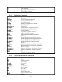
8. APPENDICES AND TABLES................................................................ 207
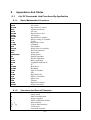
8.1.
LIST OF COMMANDS AND FUNCTIONS BY APPLICATION ........................................ 207
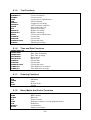
8.1.1.
Basic Mathematical Functions ...................................................................... 207
8.1.2.
Operators And Special Charactrs .................................................................. 207
8.1.3.
Statistical Functions....................................................................................... 208
8.1.4.
Logical And Relation Functions .................................................................... 208
8.1.5.
Text Functions ................................................................................................ 209
8.1.6.
Time and Date Functions ............................................................................... 209
6
8.1.7.
Ordering Functions ........................................................................................ 209
8.1.8.
Basic Matrix And Vector Functions ............................................................... 209
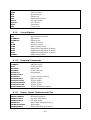
8.1.9.
Linear Algebra ............................................................................................... 210
8.1.10. Graphical Commands .................................................................................... 210
8.1.11. Export, Import, Printing And Files ................................................................ 210
8.1.12. Memory, Variable Definition ......................................................................... 211
8.1.13. Program Flow Control .................................................................................. 211
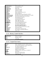
8.1.14. Statistical Methods ......................................................................................... 212
8.2.
FORMAL DEFINITION OF FUNCTIONS AND ARGUMENTS ......................................... 213
9. INDEX OF TERMS, FUNCTIONS AND COMMANDS .................... 220
7
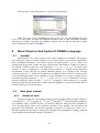
2.
Introductory note
DARWin (Data Analysis Robot for Windows) is a full interpreted algorithmic
vector/matrix-oriented arithmetic language designed for data manipulation and analysis in
QCExpert Statistical System. It uses control structures (like FOR, WHILE, IF), user-defined
functions allowing optional parameters and recursion. The language can interact with user
and computer environment with many input/output functions. DARWin is a part of the
QCExpert® statistical package and runs only within this package. Programs written in
DARWin are not compiled and cannot be used independently. DARWin includes the
development environment (DARWin Workbench), library of standard functions,
mathematical functions, statistical functions, graphical functions, data manipulation, import
and export functions, linear algebra and statistical library. Many external user-written
libraries and functions are also available and the user is not limited in creating and sharing his
own tailored functions and applications.
2.1.
Terminology and syntax in this manual
To help the reader we try to use some simple typographic rules where applicable.
Scripts in DARWin are usually printed in Courier font. Objects of the software
environment like menu items (e.g. File – Settings), dialog box items like Cancel, or keyboard
keys (like Ctrl-F, or F10), etc are printed in italic. In language definition (commands,
functions in chap. 7) we use standard notation and terminology usual in programming.
DARWin doesn’t distinguish small or capital letters: print, PRINT and PrinT are
equivalent commands. More than one spaces between words are ignored unless in text strings
in quotes " ". In language syntax definitions in chapter 7 we use the following notation:
Required text is printed in Courier: for example: DELETEVARS.
Optional text (like optional arguments of functions) is in square brackets, like in
function NORMALR(N [, MEAN=X] [, SDEV=S])where N is required and MEAN=X,
or SDEV=S are optional.
Alternative options – where one of the options is required – are separated by a vertical
line, e.g. in LINEADD(H=Y|V=X|A=I,B=S) we have to use one of the three options:
either H=Y, or V=X, or A=I and B=S.
Possible continuation is marked by three dots e.g.:
BIND(M1 [, M2, M3, ...]) means that the argument M1 is required, but more
(unspecified number of) arguments may be added.
3.
Interactive environment in DARWin
To launch DARWin, first run QCExpert® then in the QCExpert menu select DARWin.
8
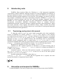
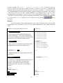
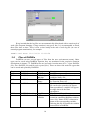
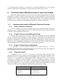
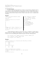
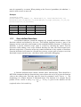
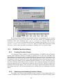
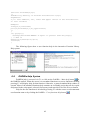
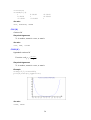
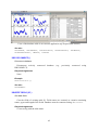
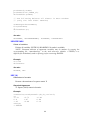
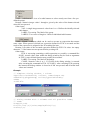
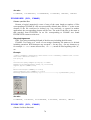
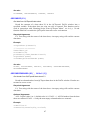
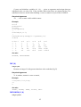
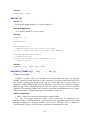
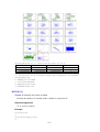
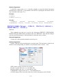
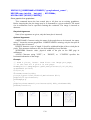
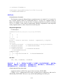
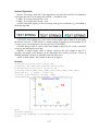
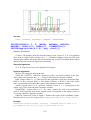
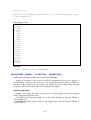
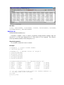
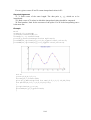
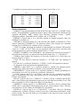
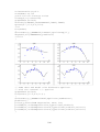
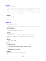
Interactive environment of DARWin consists of four panels. Panel Script, panel
Variable list, panel Variable content and panel Echo, as shown on the figure.
3.1.
The SCRIPT Panel
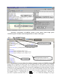
Script panel is a text editor for writing a program (script) in DARWin language.
Scripts can be organized in sheets that can be added, deleted, and renamed. After running
DARWin for the first time or opening a new script file there is one sheet in the Script panel
named Script1. Part of script that is to be executed is highlighted (selected) and then executed
by F10 key or the pushbutton Execute (F10). If no text is selected then all script in the current
sheet is executed. By selecting text the user can execute any part or fragment of script. If you,
for example, select 1+2 from the line A=(X1+247.9)/5 you get the result 3. Of course, if
you select a syntactic nonsense like A=(X1*(X1+247.9)/5 then after hitting F10 you get
9
an error message, like Error : "Invalid variable name". Executed script (or
code) is copied into panel Echo which becomes a record of your work. Command and
expression lines executed in the Script sheet are prefixed by a prompt “>” in the Echo panel
to be distinguishable from the printed results or outputs which have no prompt. The contents
of the Echo panel are lost after closing DARWin or QCExpert®. But it can be saved
automatically by selecting Save log from Echo to file in the DARWin settings (File – Settings
– DARWin). Execution of the script can terminate (a) normally (after finishing all commands),
(b) with an error, or (c) by pressing F10 or clicking the Stop button
execution.
during
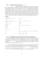
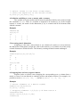
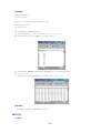
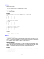
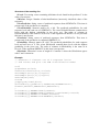
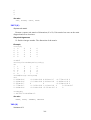
Example
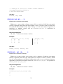
In the left column of the following table is the script with parts of the code selected
(highlighted) to be executed by F10 key. In the right column there is the output into Echo
panel.
Panel Script (Select text and press F10)
Panel Echo
A=normalr(5)/5+15
>normalr(5)/5+15
14.8158476122516
15.1939199213969
15.1542583361369
14.7639928023267
14.9646688732564
/* Executing expression without assigning the
result to variable by = . The result is copied into
panel Echo including the expression. Result of this
expression is a five element column vector */
A=normalr(5)/5+15
/* Only a part of a command or expression can be
highlighted and executed if it makes sense */
A=normalr(5)/5+15
>normalr(5)
-1.12242321838977
2.18020313462297
-0.401253593830604
0.00964743490463493
-1.54085859868898
>5+1
6
/* Highlighting and executing another part of the
same line. */
A=normalr(5)/5+15
>A=normalr(5)/5+15
/* All the line is highlighted and executed by F10,
the value of the expression is assigned into
variable A, therefore the result is no longer
outputted into Echo. Only the executed line is
copied. */
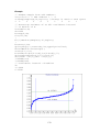
...
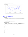
N=1000
print(sqrt(r))
>a=0
>for(i=1,100)
>{
>a=a+i
a=0
for(i=1,100)
{ a=a+i }
10
a
>}
>a
5050
A=vec(2,0,4,0,2,1,0,0,0,2)
...
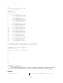
/* Executing highlighted part of script and
displaying content of variable a. */
Recognized standard function and commands of DARWin are shown in blue (or other
user-selected color) to confirm correct syntax and improve readability of code. Variable
names and other parts of expressions and commands are in bold black, text strings are in
black and comments are italic grey. User-defined functions (see later chapter 6.3 and 6.5) are
in green (or other user-selected color). Comments are not copied into Echo panel. Lines in
Script panel are numbered for better reference. Editing in Script panel obey usual rules for
text editing and hotkeys: Ctrl-Z is undo, Ctrl-F is find, etc.
Control buttons in panel Script
Run script or selected script (this button is equivalent to pressing
F10). When script is running this button changes to Stop and can be
used to abort execution.
Find text, equivalent to Ctrl-F.
Script sheets management. Add new sheet, delete active sheet and
rename and/or change properties of a sheet.
Font size selection.
DARWin language help and User functions help, see 6.6.
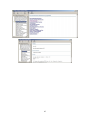
3.2.
The LIST OF VARIABLES Panel
This panel contains a list and information about all defined variables (to be exact, in
the basic instance, or frame) of DARWin. In the column Name are the names of the variables,
11
for variables of type “list” also the structure of the list. In the column Information there is
basic information about the size of the variable (if it is a vector or matrix its size is in the
form [number of rows] x [number of columns]). If the variable is a single number (a scalar)
then the actual value is displayed. Whole content of a selected variable is displayed in the
panel Variable value where it can also be edited. Double-clicking a variable will bring up its
name at the cursor position in the script editor. Variable icons suggest the type of a variable:
Icons for variable types
Scalar (single value) variable, numeric or text string, see 4.3.1, p. 18
Matrix / Vector variable, see4.3.2, 4.3.3
List variable, with the list elements below, see 4.3.4
Big Data variable (scalar, matrix or vector, variable suffix $), see 6.2.9
Undefined variable (when created manually), see 4.2.4
Control buttons of Variable list panel
Manual interactive definition of a new variable and manual deletion
of a variable is useful when passing a matrix from another application
as Excel. A newly defined variable has “undefined” value.
3.3.
The VARIABLE CONTENTS Panel
This panel shows contents of a variable selected in the List of variables panel, see
paragraph 3.2. The format of the table is spreadsheet which allows editing the variable
content, selecting and copying or pasting with immediate effect on the variable. Rows and
columns are numbered. In case of variables of type “List”, only items of the list are displayed.
12
3.4.
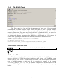
The ECHO Panel
The Echo panel is a log and full documentation of your work. Every executed
command, line, or whole script is copied in this text panel as well as possible results.
Executed commands are prefixed with a prompt “>” to distinguish from results (like variable
contents). The text in Echo panel may be copied (Ctrl-C), searched (Ctrl-F) but cannot be
modified. If set in the DARWin Setup the Echo is automatically saved and archived in a text
file in the work directory when you close DARWin or QCExpert®, see 3.5. A header is
created at the beginning of each Echo file containing time and user information like:
DARWin (c)TriloByte statistical software
QC.Expert version X.X
Current User:User_name Computer Name:Computer_Name
DARWin Start Date: 2011/12/24 19:00:00
Control buttons in the ECHO Panel
Buttons for text search (Search, Find Next, Find Previous)
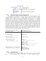
3.5.
Log Files
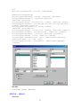
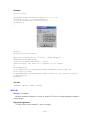
The log mentioned in 3.4 can be archived in log files in the QCExpert® work
directory, default is C:\TEMP\darwinlog\. Archiving option is set in the DARWin Setup
window (MENU: File – Setup – DARWin tab), see below. If the archive option is checked,
then at DARWin startup, a plain text file is created with a name in the format
YYYYMMDD_HHMMSS_TTT.log. The file name is composed of date and time with an
extension .LOG. Log files can be used for documentation and possible partial emergency
backup.
13
Keep in mind that the log files are not automatically deleted and with a certain style of
work (like frequent damping of large matrices) may grow fast. It is recommended to check
these files time to time. There is also a time stamp at the end of each log-file (in case of
normal program termination), for example:
DARWin End Date: 2011/12/31 23:59:59
3.6.
Files of DARWin
DARWin can save several types of files from the user environment (menu). Other
types can be saved using DARWin function, they are mentioned in the respective function
descriptions in chapter 7.2. DARWin files are accessed via main menu (File – Open DARWin
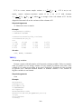
files, Save DARWin files and Recently opened files). There are three four main file types that
can be saved and opened by DARWin:
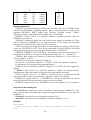
Extension
QCF
QCD
Default directory
C:\TEMP
C:\TEMP
File type
DAR Script
DAR Script
and data
DAR Function
library
DAR variables
QCL
C:\TEMP
VTS
C:\TEMP
LOG
C:\TEMP\darwinlog Log-file
C:\TEMP\darwinvar BigData
variables
14
Description
DARWin scripts and function
DARWin scripts and function and
variables, binary file
DARWin scripts and function intended
for Function library 6.5.
Variables defined in DARWin. This
file can be also opened in QCExpert
Data spreadsheet, variables will appear
as single sheets in the Data
spreadsheet.
Log-file, see 3.5, p. 13
Text files ending with a “%” without
extension containing BigData variables
(see 6.2.9). Name of file is identical to
name of the corresponding variable.
Deleting this file will make the variable
inaccessible in DARWin.
The file type is selected in the Save / Open file dialog window.
Other file types used by DARWin are the log-files (see 3.5) and BigData files (see
6.2.9). You may want to check the BigData directory time to time and delete possible
unnecessary variables. Normally, the BigData variable files are deleted when the variable
itself is deleted or rewritten in DARWin.
4.
Basic Structure And Syntax Of DARWin Language
4.1.
Variable
Data structure as a vector, matrix or list can be assigned to a variable. The structure
may contain two types of values: numbers or text. There is also a special value <undefined>
that is mentioned elsewhere. Text values must be in double quotes: "TEXT". Name of a
variable must begin with a letter and may contain letters and numbers. Length of a name is
not limited. Variable names are case-insensitive, XYZ, Xyz, XyZ, xyz is all the same
variable. A value is assigned to a variable by the operator “=” (equal). In the interactive
environment a value can also be written manually directly to a variable in the Variable
Contents panel, see 3.3. Values in a variable are accessible from the Variable Contents panel,
or by executing the name of the variable in script. Elements of a vector or matrix can be
accessed using index brackets [, ] or [[, ]] (see 4.3.2, 4.3.3, 6.2.11). Elements in a list are
accessed using the dollar selector $, see 6.2.7. Assigning a data structure to a variable
destroys any previous content of the variable, unless assigning to a part of the variable (like to
a matrix element or to a list element).
4.2.
4.2.1.
Data types (values)
Numerical value
Numerical value is a real number, integers are not specially defined. Numeric range of
a real number is –(21024) through –(2–1024), 0, 2–1024 through 21024. In usual decadic notation it
is (in absolute value 5.56268E-309 do 1.797693E308 and zero. Precision of the arithmetic is
15-16 decimal places (this is the technical precision of the number, not necessarily the
precision of all functions). The decadic exponent is entered in a usual way, after E or e.
Decimal separator in the script is always a dot, though in the spreadsheets or dialog windows
it may depend on the national settings in Windows.
15
Examples of valid number formats
>1234.56789
1234.56789
>-5e-10
-5E-10
>.0000000000000000001
1E-19
>100e2
10000
>12345678901234567890
1.23456789012346E19
4.2.2.
Text string
A text string (or character string) is any text closed in double quotes, e.g. "TEXT".
Maximal length of a single string is 16383 characters in a normal variable, but unlimited in
the BigData variable. A special text string is an empty string "". Text strings can be joined
together with a “plus” operator, e.g. "ABC"+"DEF". Joining a text string and a number will
give a text string.
Examples of valid text string formats
>"ABCDEFGH"
"ABCDEFGH"
>"2.718281828"
"2.718281828"
>"Result: "+sqrt(2)
"Result: 1.4142135623731"
>"A"+""+"B" //An empty string does not affect the result
"AB"
4.2.3.
Logical value
Logical values in DARWin are not a special type. Logical „FALSE“ is represented by
numerical value 0, logical value „TRUE“ is represented by numerical value 1. Logical values
are typically used in logical operations (like AND, OR), relational operations (like „greater
then“, „equal“), logical indexing, and in conditional commands IF and WHILE. Results of
logical and relational operations are thus 0 or 1:
>gt(3,5)
0
>gt(5,3)
1
>and(1,0)
0
>or(1,0)
1
>gt(5,vec(3,6,4,-2))
1
0
1
1
Any other non-zero numerical value will be interpreted as 1 in logical operations and
conditional commands.
4.2.4.
Undefined value (INI)
Undefined (initial, null) value can be assigned to one or more variables by the
command INI. This no-value defines only existence of the variable, not its type or structure.
16
Undefined value cannot be used in arithmetical operation. The advantage of an undefined
variable is its use as a starting value in cycles (FOR or WHILE) when constructing a vector or
matrix using the VEC, BIND and BINDV by elements, columns, or rows. In the Variables
panel, the undefined variables are displayed with “Undefined” in the Information column. An
undefined variable may also be created interactively by clicking on the New variable button
in the Variables panel.
Examples and use of INI function and an undefined (empty) value:
INI(A1,A2,A3)
>count(a1)
0
>a1+1
Error : "Invalid
variant
operation"
>vec(a1,100)
100
4.2.5.
>a2=vec(a2,1:3)
>a2
1
2
3
ini(a3)
for(i=1,5)
{
A3=bind(a3,i+sample(1:9,3))
}
>a3
3
6
12
12
13
8
11
9
11
14
7
10
11
5
12
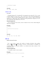
Date and time
Date and time are not special data types. To represent dates and times DARWin uses
numerical value and text strings. Date/time conversion function convert dates and times from
numerical to string and vice versa. Text representation of time is a text string of format
H:M:S.T, where H are hours (0 – 23), M are minutes, S are seconds and T are thousandths of
the second, for example: "5:36:53.430", or "18:58:56.951". Leading zeros are not
required, both the two forms: "05:05:05" and "5:5:5" are valid and equivalent. Date
format contains day, month and year separated by a dot, for example: "23.8.2012", or
"2.12.2012". Date and time can be joined into one “date-time” string separated by a space,
for example:
"23.8.2012 10:48:22.483".
Numerical representation is number of days from the “zeroth” of January 1900. Decimal part
is the part of day starting at midnight, so 0.25 means 6:00 AM, etc. The DARWin’s numerical
precision allows time specification down to a thousandth of a second. The primary functions
to convert between numerical and text representations are DATETIMEN (date-time to numeric)
a DATETIMES (date-time to string), for example:
>datetimes(41123.476663)
"2.8.2012 11:26:23.683"
>datetimen("20.8.2012 23:15:59")
41141.9694328704
The numerical value can be both positive and negative, so it is possible to code any
date between 1.1.0000 and 31.12.65535.
Time differences, or intervals, the distance between two times, dates or date-times are
also expressed as decimal numeric values, namely the number of days, or alternatively, as text
in the time format H:M:S.T, where – in contrast to normal time – the number of hours in
unlimited. For example, the difference between the two date-times 15.3.1848 16:45 and
23.3.1848 9:28 is 8.30347222222 days, or over 199 hours:
17
>datetimedifn("23.3.1848 9:28","15.3.1848 16:45")
8.3034722222219
>timedifs(datetimedifn("23.3.1848 9:28","15.3.1848 16:45"))
"199:17:0.0"
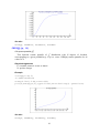
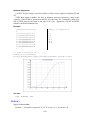
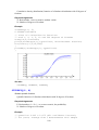
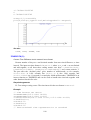
Sunday June 7. 2054 will be 750 000th day since the beginning of AD.
>datetimedifn("7.6.2054 0:0:0","1.1.0001 0:00:00")
750000
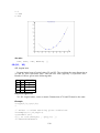
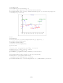
Generating 5 million random numbers and computation of sum of logarithms takes 1.9
seconds (on my computer):
>t1=strdatetime(0)
>x%=normalr(5000000)
>s=sum(ln(x%^2))
>t2=strdatetime(0)
>td=datetimedifn(t2,t1)*86400
>"Comp time = "+round(td,3)+" seconds"
"Comp time = 1.935 seconds"
See time and date functions for more details.
4.3.
4.3.1.
Data Structures
Scalar
A scalar is a single numeric or text value. In this manual we use also a term “number”,
“string”, “value”. Formally, a scalar can be viewed as a one-element vector, or a one-by-one
matrix, most of functions in DARWin do not make difference between a scalar and vector. If
a value 5 is assigned to a variable A, it can be referred to as a scalar, vector or matrix, as
shown below.
Example
>55+66
121
>A=5
>a
5
>a[1]
5
>a[1,1]
5
>b="QWERTY"
>b
"QWERTY"
18
4.3.2.
Vector
A vector is a column matrix. It can be addressed with one or two indices in index
brackets. Although most DARWin functions require a vector or matrix to have the same type
of elements (either numeric or text), DARWin itself allows to mix both those types in one
vector or matrix. A value can be assigned to a vector element using e.g. A[5]=55^2.
Example
>a=vec(1,3,5,7)
>a
1
3
5
7
>a[3]
5
>a[3,1]
5
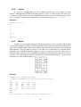
4.3.3.
Matrix
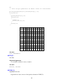
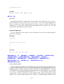
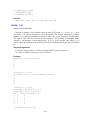
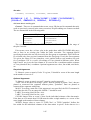
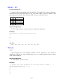
A matrix is a rectangular structure of elements (values) in an n x m table. The number
of rows and columns in a matrix is called dimension of the matrix (in contrast to mathematics,
where this is usually called “type” of the matrix). The elements are accessed by two indices in
index brackets. The first index is always a row index, the second index is a column index.
Although most DARWin functions require a vector or matrix to have the same type of
elements (either numeric or text), DARWin itself allows to mix both those types in one vector
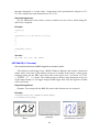
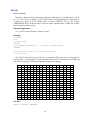
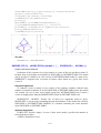
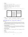
or matrix. The following figure shows elements in a matrix and their indices. A value can be
assigned to a vector element using e.g. A[5,3]=55^2.
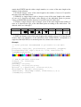
Example
//Matrix of random letters:
> A=matrix(sample("A":"Z",25,repl=1),ncols=5)
>A
"M"
"B"
"P"
"V"
"T"
"J"
"O"
"D"
"D"
"O"
"T"
"P"
"W"
"V"
"P"
"X"
"J"
"M"
"V"
"W"
"R"
"Y"
"G"
"P"
"U"
>A[3,3]
"W"
>A[3,3]="XYZ" // Rewriting the element [3,3]
19
4.3.4.
List
A list is one or more of structures scalar, vector or matrix or list grouped as elements
in a single variable. Each of the elements has its name and order. Names are explicitly
defined in the definition of the list or are given implicitly by the “list” function. Individual
elements of a list are accessed using the selector $ (dollar) placed without spaces between the
name of the list variable and name of the element. The contents of a list variable cannot be
printed or displayed as a whole, only the non-list elements can.
Example
// The following command creates a list with elements X, Y a Z
// and stores (assigns) it to a variable A:
>A=list(X=matrix(1:9,ncols=3),Y=ln(2),Z=list(T="ABC",U=11:13))
// Element X of the list A is accessed using selector $: A$X
>A$X
1
4
7
2
5
8
3
6
9
//Since the element A$X is a matrix, indices can be used:
>A$X[2,2]
5
// Element A$Z is a list with elements T and U, which
// can be reached using another $:
>A$Z$T
"ABC"
>A$Z$U[2]
12
Other examples of different variable types
a1=5.67
b1=seq(1,2,count=20)
c1="Computational Statistics"
d1=list(A=1,B=1:10,C="Sample List")
d1$b[3]
b=sample(0:2,20,repl=1)
B[[ not(zero(B)) ]]
4.3.5.
Expression
An expression is a part of a script that gives a value or any data structure. The result of
an expression can be assigned to a variable.
Examples of expressions and resulting output in the Echo panel
>128
128
>33*44-55
1397
>matrix(11:16,ncols=2)
11
14
20
12
15
13
16
>round(transp(normalr(10)),2)
0.34 0.25 -1.61 -0.23 0.4
0.76 0.45 -0.15 0.11 -0.13
>"A"+(1:3)
"A1"
"A2"
"A3"
>A[2,3]
36
Round arithmetical parenthesis are used in a usual way to alter precedence in
evaluating more complex arithmetic. Default operator precedence (without use of parentheses)
is the following (in decreasing order):
standard and user-defined functions >
„^“ (power) >
„–“ (unary minus) >
„*“, „/“, „#“ (multiplication, division and matrix multiplication) >
„+“, „–“ (add, subtract) >
„:“ (sequence operator, colon) >
„=“ (assigning),
for example:
– 2 ^ 2 gives – 4, but (–2) ^ 2 gives 4. Or, 1 : 3 + 1 gives 1 2 3 4, but (1 : 3) + 1 gives 2 3 4.
Expressions are evaluated according to preference and (in case of the same preference)
from right to left, which may give different result in case of matrix multiplication, see 6.2.6, p.
27.
4.3.6.
Command
A command is a part of script which performs some action, e.g. assigning to a variable,
drawing a plot, export to a file, print, commands FOR and WHILE, any part of script closed in
command “curly” brackets {}, deletion of a variable, etc. A command MUST be written in
one line. If a command is too long for a single line, it can be divided into more lines using a
multi-line operator @ and a semi-colon, see 6.2.10, p. 29.
Examples of commands
>print(ln(10),\t,log(exp(1)))
>export(normalr(100),"random_data.txt")
>A=5
>delete(B)
>plot(normalr(1000))
>x=x+1
>for(i=1,10){print(rnd(1),\n)}
4.3.7.
Script
A script is a sequence of one or more commands (possibly also expressions) that can
be executed. A script is executed from a Script panel. A script can be executed either as a
whole (whole script in the current sheet) or as a part (only a selected part of the script), see
21
3.1. Another possible execution of a script is as a user-defined function (see 6.3) or from the
interactive QCExpert® environment as a QCExpert® main menu item (see 6.4).
5.
Communication With Environment, Input And Output
Input and output operations can be used in wide range of applications for effective
automation of repetitive operation, generating reports, routine diagnostics of data, data flow
integration and control in many processes. Functions mentioned in this chapter are described
in detail in 7.2, p. 44 or in other parts of this manual. Here we just briefly summarize
functions that are available for communicating with the user and the environment.
5.1.
5.1.1.
Communication within QCExpert® Statistical System
Panel Contents of variables
This is a feasible way to insert manually tables from other applications (like Excel)
directly to a given variable using Paste (Ctrl-C). This panel is also used to export contents of
a variable to other applications using Ctrl-V.
5.1.2.
Output To Protocol In QCExpert® (Print)
Results can be printed to a Protocol window of QCExpert® using the DARWin
PRINT command. This command is versatile and allows information to be formatted and
printed in a desired form, exportable to other spreadsheet applications. The maximal size of
the Protocol spreadsheet is limited 65535 lines and 255 columns. Bigger outputs can be done
(again by PRINT command) by printing to a text file, where the size is unlimited. Exported
file has standard TXT/CSV format and can be used by other applications.
5.1.3.
Output To Data Sheet In QCExpert®
A (typically a vector or matrix) variable can be copied using the PUTSHEET
command into the Data sheet of QCExpert® to be processed interactively by the modules of
the QCExpert® statistical system outside DARWin.
5.1.4.
Graphical Output
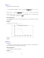
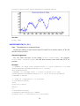
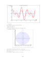
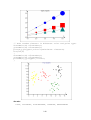
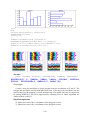
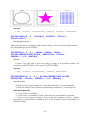
Commands PLOT, LINEADD, GRAPHSHEET and many other functions create
graphical output in the Graph window of the QCExpert® system The plotted graphics can be
exported to a file in graphical formats from DARWin using commands EXPORTGRAPH,
PDFPLOT or interactively from QCExpert® menu. Generally, two types of plotting
commands are available, creative and additive. The creative commands will create a new plot
box and puts the graphics in it. The additive commands add more graphical objects (as dots,
lines, text, polygons, etc.) into the latest created plot. Additive plot commands can only be
used after a creative plot is performed, within the same execution of a script.
Creative commands
Creates a new 2D plot
PLOT
PLOTTEXT
PLOTBAR
PLOTPOLY
Additive commands
Adds to any existing 2D plot
PLOTADD
PLOTTEXTADD
PLOTPOLYADD
LINEADD
22
5.1.5.
Interactive Dialog Windows
The DIALOG function is a versatile tool for interactive input of values and controlling
executed script. Very straightforward and intuitively programmable dialog windows allow to
select options, set parameters, type in values. In combination with the interactive menu this
gives a tool to create new modules in QCExpert®.
5.1.6.
Message Command
The MESSAGE command displays temporarily any message during execution of script
allowing monitoring progress of longer computations or viewing intermediate results. Any
single- or multi-line text can be displayed in a message window.
5.2.
5.2.1.
File Input/Output
Input From Text File
Any text file can be read from file to a variable using IMPORT command. This allows
to read and process files containing text or data structures such as extensive database tables
exported from databases, technological data storage systems or other external applications.
5.2.2.
Output To Text File
Data can be written in any form of a text format using the PRINT or EXPORT
commands. Data tables and variables can be stored in standard CSV format with any column
separator.
5.2.3.
Output To Graphical File
Plots created by DARWin in QCExpert’s Graph window can be exported using
EXPORTGRAPH command in graphical formats BMP, JPG, GIF, WMF. Graphs can be reformatted before export into a different resolution to ensure required quality.
5.3.
Output To PDF File
Publishing PDF documents is a strong tool of DARWin. It allows automatic
programmable generation of reports with extensive formatting features, tables, headers and
footers, automatic page numbering, graphics, plots, etc. The PDF report may be the final
state-of-the-art result of an extensive, yet automatic, pre-programmed analysis. All commands
that handle creation of PDF documents begin with PDF.
5.4.
Sending E-mails
The SENDMAIL command allows sending email with attachments to multiple
recipients via SMTP gate. This can be used to send automatically information, periodic PDF
reports, warnings, etc. based on actual data. We want to warn the user to be cautious using
this command. Due to a mistake or omission in the script it is easy to generate and send
thousands of unwanted mails!
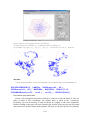
5.5.
Batch Processing
DARWin scripts can be run in BATCH mode from command line, from Windows®
task scheduler, or from other external applications. It is possible to schedule execution of
your scripts periodically without a need to run QCExpert®. A script can be executed by
calling QCEXPERT.EXE from command line with the saved script name (including path) as
a parameter. The script name must be given with its extension .QCF. The script is executed in
23
the background without opening the application window. All scripts (script sheets) found in
the script file are executed sequentially except the functional scripts. If the LOG is active then
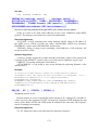
all the executed scripts are written to a log file including possible error messages. Error
messages are also saved into ScriptErr.log in the working directory (default: C:\TEMP), for
example:
28.11.2011 17:44:46 c:\temp\dar_batch01.qcf
zero :: A=5/0
Floating point division by
Scripts run in the batch mode can use interactive tools as dialog windows or message
window (though this is probably not very clever), they will appear during the execution and
will wait for the operator response. For example, if the script file name is
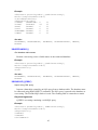
DAR_BATCH01.QCF in the folder (directory) C:\TEMP, the batch call will look like this:
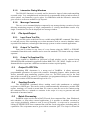
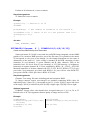
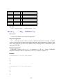
qcexpert c:\temp\dar_batch01.qcf
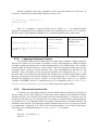
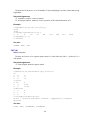
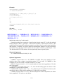
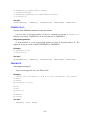
The following picture illustrates batch call from the command line.
6.
Language Definition And Syntax
6.1.
Typographical Remarks
Full description of the language, operators and functions is given in the following
chapters. The DARWin code and echo text is (mostly) printed in Courier New font. If the
text contains combination of commands and immediate outputs it is often taken from the
Echo panel with prompts (“>”) in front of the user commands to distinguish between input
and output. If the code is to be used, the prompt must be deleted before running the code. In
the text we use an English usual in programming languages manuals, e.g. the program “runs”,
a function or an expression “returns” a value, a decimal number (such as 12.99) is a “real”
number, a text value (such as "Hello World!") is called a string, text string, or character
string, a value is “assigned” (stored) to a variable, etc.
6.2.
6.2.1.
Operators And Special Characters
Comment //, /*
Comment is a part of a script that is ignored (skipped) during execution. It is used
mainly for remarks, description, as explanatory text. It is generally recommended for authors
of a script to include comments to describe and explain the program for himself and other
readers of the code. In DARWin, there are two types of comment. Line comment begins with
two slashes “//” and ends at the end of line. Any text on a line after // is ignored. Block
24
comment begins with slash and asterisk /* and ends with asterisk and slash */. Any text
between those two codes is ignored. Block comment may have multiple lines. It is also used
for including Help in user-defined functions (between header and body of a function) and can
be used to temporarily block-out part of program code. “/*” after “//” on the same line is
ignored. “//” within “/* … */” is ignored. It is recommended to use line comments after
the closing brackets of FOR, IF and WHILE commands, like … } // End For I, etc. to
make code more readable.
Example
//---------- Program begin -----------R=0 // Lower limit
S=10 // Upper limit
/*
Inactive "blocked" alternative values of R a S:
R=10
S=30
*/
x=R:S // Fill vector x with integer sequence
for (i=x)
{
print (i,\n)
} // End For i
// ---------- Program end -----------
6.2.2.
Command curly brackets (braces) { }
Command curly brackets (or braces) { } are used to define a sequence of one or more
commands in control structures FOR, IF, WHILE and in function definitions. Command
brackets can be also used in any place to mark significant group of commands anywhere
without any effect to code execution.
Example
for (i=1:10){print(i,\t,log(i),\n)}
x=normalr(1);if (LT(x, 0))
{
x= -x
} // End IF
a=sqrt(x)
6.2.3.
Variable Assignment =
Variable assignment, or “equal” sign = assigns the value of an expression on the right
side of “=” to the variable on the left side. The “equal” sign cannot be used as a logical
relational operator, the function EQ must be used instead.
Example
>A=4+5
>a
9
deletevars
for(i=1,3){ for(j=1,3){ x[i,j]=i*j } }
y=1:10
k=0;k=k+1
25
6.2.4.
Arithmetic Binary Operators + - * / ^
+, -, *, /, ^: addition, subtraction, multiplication, division and raising to
power with usual priority of operations The “plus” operator is moreover used for pasting text
strings together. If at least one of the operands in A + B is a text string, then the result is also
test string. For example 1+2 gives 3, and "1"+2 gives "12". Of course, minus is used also
as a unary minus. If one of the operands is vector or matrix and the other one is scalar (order
doesn’t matter) than the operation is performed for all elements of the matrix or vector. If
both operands are vectors or matrices than they must be either (a) of the same dimensions
(NxM), or (b) one of the operands is a matrix (NxM), the other is either a column vector (Nx1)
or a row vector (1xM). In the case (b) the operation is performed column-wise or row-wise
respectively. This can be used for example when centering or normalizing data columns etc.
Example
>"ABC"+"-4-"+8+123+1
"ABC-4-132"
>1+2*3^4
163
>"ABC"+"-4-"+8+123+"1"
"ABC-4-81231"
>vec("A","B","C")+(1:3)
"A1"
"B2"
"C3"
>"A-"+(1:5)
"A-1"
"A-2"
"A-3"
"A-4"
"A-5"
>(1:4)+10
11
12
13
14
6.2.5.
>(1:4)+vec(10,20,30,40)
11
22
33
44
>matrix(1:9,ncols=3)*vec(10,100,1000)
10
40
70
200
500
800
3000 6000 9000
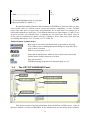
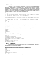
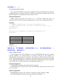
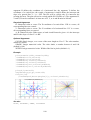
Scalar Arithmetic Operations With Vectors And Matrices
Matrix multiplication using the operator “#” is described in 6.2.6. Further as
mentioned in 6.2.4, matrix (or vector) can be multiplied with a scalar k. Result is a k-multiple
of a matrix. If, for example A is a matrix with elements ai,j then B=3*A will create a matrix
with elements bi,j = 3 ai,j. If A and B are matrices of the same size NxM than the standard
operators +, -, *, /, ^ can be used for operation on A and B, so a matrix C=A/B will
have dimension NxM and elements ci,j = ai,j / bi,j .
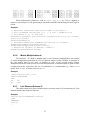
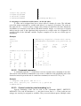
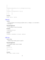
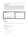
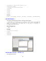
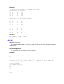
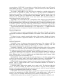
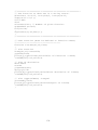
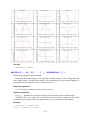
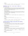
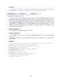
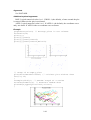
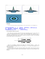
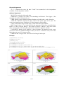
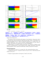
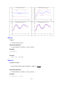
Row-wise and column-wise scalar operations can be performed with a matrix and a
vector. If A is a matrix of dimensions NxM and R is a column vector Nx1 the result of C=A*R
will me a matrix C with dimensions NxM and elements ci,j = ci,j . ri . Similarly, this applies to
other binary arithmetical and logical operation like +, -, *, /, ^ and logical functions
GT, GE, LT, LE, NE, EQ. Three examples are given on the following illustration.
26
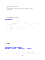
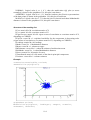
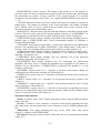
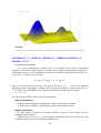
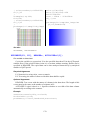
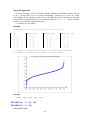
Most mathematical functions, such as sqrt, exp, sin, etc. can be applied to
matrices. An example of code generating a data matrix and then normalizing the data is given
below.
Example
// Generate simulated data from normal distribution
// with standard deviations 0.1, 1, 4 and 7 respectively
// and means 2, 8, 25 and 200:
data=matrix(normalr(40),ncols=4)*transp(vec(0.1,1,4,7))+transp
(vec(2,8,25,200))
data=round(data,2)
// Estimate means and standard deviations of columns:
xmean=apply(data,"average",dir=2)
xstdev=sqrt(apply(data,"var",dir=2))
// Normalize columns to mean=0, stdev=1 :
datanorm=(data-xmean)/xstdev
6.2.6.
Matrix Multiplication #
The character “#” (hash or number sign) is used in matrix multiplication (in contrast
to scalar multiplication described in 6.2.5) of matrices and/or vectors. Number of columns of
the first matrix must be the same as number of rows of the second matrix. Matrix
multiplication has the same priority as scalar multiplication, so attention must be paid to more
complicated matrix expression and use of parentheses is recommended, e.g. when A is a
matrix then A*A#A is not the same as A#A*A.
Example
>X=bind(rep(1,10),1:10)
>XX=transp(X)#X
>XX
10
55
55
385
6.2.7.
List Element Selector $
The dollar character $ placed without spaces between name of a list and name of a list
element returns that element of the list.
Example
>s=list(a=5,b="ABCDEF",c=6:10)
>s$b
"ABCDEF"
>s$c[2]
7
27
6.2.8.
Sequence Operator, Colon :
The sequence operator, colon “:” is a binary operator that crates an integer or onecharacter sequence with step 1 spanning from the first to the second operator. The sequence
operator has lower priority than addition. If the first operator is greater than the second one
the sequence is descending. In examples below, the transposition (transp) is used merely to
save space in the book.
Example
>transp(1:5)
1
2
3
4
>transp(3:-2)
3
2
1
0
>transp((1:10)^2)
1
4
9
16
>transp((1:10)/10)
0.1
0.2
0.3
0.4
5
-1
-2
25
36
49
64
81
100
0.5
0.6
0.7
0.8
0.9
1
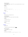
Similarly, the ASCII code sequence may be constructed for characters. Only the first
character of the two string operands is taken.
Example
>transp("ZA":"abc") // (same as "Z":"a")
"Z"
"["
"\"
"]"
"^"
"_"
"`"
"a"
6.2.9.
BigData suffix %
The character “%” (percent) as a suffix in a variable name indicates a BigData
variable. Such variable is stored in a text file in C:\TEMP\darwinvar\ rather in a
spreadsheet table, is displayed in text format in the VARIABLE CONTENT panel in the
workbench and the size of such variables is limited only by the available memory. Use of
BigData variables is the same as normal variables.
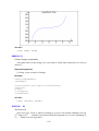
Example
>x=1:100000 // Data do not fit in spreadsheet
Error : "Bad cell reference"
>x%=1:100000 // "BigData" table accommodate millions of rows.
>x%[99990:100000]
99990
99991
99992
99993
99994
99995
28
99996
99997
99998
99999
100000
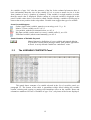
6.2.10. Multiline Command @ … ;
Normally, a command must fit into one line. However, some commands like PLOT,
PRINT, NNLEARN, DIALOG, VEC etc. can get very long and it becomes convenient to
break it into more lines. A multi-line command must begin with an “@” (at) character and
must end with a semicolon. Every single multi-line command must begin and end with its
own “@” and “;”.
Example
//Normal single-line command:
>x=1+2+3
>x
6
// A command splitted (rather meaninglessly) into more lines:
// (Don’t forget SEMICOLON at the end!)
@x=1
+2+
3;
// A long command splitted (meaningfully) into more lines:
@ D2=vec(0,1.128,1.693,2.059,
2.326,2.534,2.704,2.847,2.970,
3.078,3.173,3.258,3.336,3.407,
3.472,3.532,3.588,3.640,3.689,3.735);
6.2.11. Index Square Brackets [ ]
Index square brackets [ ] are used to address cells (elements) in matrices and vectors.
The first index is the row index, the second one is the column index. Vector is a matrix with 1
column and n rows and it is allowed to use only one (row) index for addressing a vector
element. The syntax of DARWin allows several uses of the index brackets which are
described in the following paragraphs.
1. Referring row or column of a matrix or vector
Example
x[3,5] // An element in the matrix x in 3rd row and 5th column
2. Interval indexing, vector indexing, empty index
If an index is a vector than all corresponding rows or columns are returned. If the row
or column index is missing than all existing rows / columns are returned.
Example
Matrix formed by the 10th to 20th rows and 2nd to 6th column of matrix a:
a[10:20,2:6]
Matrix composed by all rows and the 1st, 3rd and 5th column of matrix a:
29
a[,vec(1,3,5)]
Vector of the 1st, 3rd and 5th element of vector b:
b[vec(1,3,5)]
3. Logical indexing [[ ]]
An index in double square brackets of a matrix or vector must be a (logical) vector of
zeros and ones of the same dimension of the respective matrix or length of the vector. It
returns only the elements where the corresponding index is one. The vector of logical indices
can also be shorter than the indexed vector, in that case the index vector is repeated until
exhaustion.
Example
//Get selected elements from
// a vector
>x=1:10
>ii=vec(1,0,0,1,1,1,0,1,0,1)
>x[[ii]]
1
4
5
6
8
10
// All even order elements of x:
x[[0:1]]
// All odd order elements of x:
x[[1:0]]
//Get negative elements
// of a random vector
// and get its indices
>x=normalr(10)
>y=1:10
>x[[lt(x,0)]]
-1.95551799804119
-0.507056775394412
-2.07615542267181
>y[[lt(x,0)]]
1
5
9
Logical indexing also allows to extract whole rows or columns of a matrix using a
logical vector and a comma saying whether the vector addresses rows or columns. This can
be used to select rows fulfilling some condition using one of the three following forms:
X[[<logical row index>,<logical column index>]] or
X[[,<logical column index>]] or
X[[<logical row index>,]]
Example
>a=matrix(vec(1,2,3,10,20,30,100,200,300),ncols=3)
>a[[,vec(1,0,1)]]
1
100
2
200
3
300
>a[[vec(1,0,1),]]
1
10
100
3
30
300
x=matrix(normalr(16),ncols=2)
// Select rows with negatives in the second
column:
x[[lt(x[,2],0),]]
30
// Select values in the first column where
// there are negatives in the second column:
x[[lt(x[,2],0),vec(1,0)]]
4. Definition and filling a vector or matrix with a constant
The variable we want to define and fill must be undefined which can be achieved with
the command delete. Then, if a constant is assigned to an element [n, m] of the variable
(matrix or vector), the matrix of the dimension [n, m] is created with all its elements filled
with the constant.
Example
>delete(a)
>a[3,4]=1
>a
1
1
1
1
1
1
1
1
1
1
1
1
5. Increasing matrix dimension
Assigning a value into a non-existent [n, m] element of a matrix or vector increases
the dimension of that matrix, assigns the value to the element [n, m] and the rest of the newly
created elements are filled with zero. The formerly existing elements remain unchanged.
Example
>a=bind(vec(1,2),vec(4,7))
>a
1
4
2
7
>a[3,5]=99
>a
1
4
2
7
0
0
0
0
0
0
0
0
0
0
99
6. Dropping lines and rows, negative indexes
Negative index or indices cause dropping the corresponding row or column from a
matrix or vector. It is not allowed to combine positive and negative indices. For example, it is
possible to write A[vec(-2, -4), 1] but not A[vec(1, 2, -2, -4), 1].
Example
// Corner elements of a matrix A(4x4)
a=matrix(1:16,ncols=4)
a[-(2:3),-(2:3)]
// Dropping elements 1,3,5,6,11,16 from vector x
>x=normalr(20)
>x1=x[-vec(1,3,5,6,11,16)]
>count(x1)
31
14
// Drop every fifth row
>x=normalr(25)
>xi=1:25
>i=-5*(1:5)
>bind(xi[i],x[i])
1
0.0710872138379552
2
-0.180564729065626
3
1.58436236861215
4
-0.106992352401548
6
0.937575477540491
7
-1.02310933239758
8
0.436291733151174
9
-0.234901786098745
11
2.55209876658992
12
-0.905511308448221
13
-1.04532565890302
14
0.659992912539357
16
0.627633323249614
17
-1.56902175656619
18
1.58550544608754
19
0.770823204730091
21
-0.795454358251783
22
-1.56151447065492
23
0.98218317810612
24
-1.02783119371402
// Extract distinct values from vector x
// (equivalent to SQL select distinct):
>x=sample(1:10,50,repl=1)
>x1=sort(1,x)
>x1[[ne(vec(x1[-1],999),x1)]]
1
2
3
4
5
6
7
8
9
10
7. Indexing an expression
If a result of an expression is a vector or matrix it is possible to index it only if the
expression is closed in parentheses. This syntax is possible also for logical indexing [[ ]].
Example
>(10:19)[2:3]
11
>(1:10)[[lt(random(1:10),0.75)]]
1
32
12
>(ln(1:10))[8:10]
2.07944154167984
2.19722457733622
2.30258509299405
3
4
6
8
9
>(transp(a)#a)[1,1]
8. Assigning to an indexed variable (index „on the left side“)
A value can be assigned into one or more cells of a matrix of vector. The left-hand
part of the assign command is a variable with index [ ] or logical [[ ]] brackets. The value on
the right side of “=” must be either a single value (scalar) or must have the same dimension
and number of elements as the indexed left-hand variable. Single- or vector-type or logical
indices may be used. It the right-hand side expression is a single value it is assigned to all
specified cells of the left-hand variable. Explore examples to see the use of this type of
assignment.
Example
>a=1:3
>a[2]=99
>a
1
99
3
//Replacing negative values with zeros
>a=round(matrix(normalr(12),ncols=4),2)
>a
-0.16
1.37
-0.18
-0.74
0.6
-0.33
0.91
-1.48
1.12
0.54
2.19
0.5
>ii=lt(a,0)
>a=matrix(1:12,ncols=4) >ii
>a
1
0
1
1
1
4
7
10
0
1
0
1
2
5
8
11
0
0
0
0
3
6
9
12
>a[[ii]]=0
>a[1,]=99
>a
>a
0
1.37 0
0
99
99
99
99
0.6 0
0.91 0
2
5
8
11
1.12 0.54 2.19 0.5
3
6
9
12
6.2.12. Command separator ;
A command separator „;“ (semicolon) is used to separate more commands in one line.
This can be used with short commands to save room, or make the code graphically more clear.
Semicolon must be put at the end of a multi-line command, see more in 6.2.10, p. 29.
Example
// Compute and print sum of 2^i:
a=0; b=2; for(i=1,10) {a=a+b^(-i)}; print(a)
0.9990234375
6.2.13. Control codes for print formatting \n, \t
Special formatting codes can be used in the commands PRINT, PDFTEXT,
MESSAGE. The code for tabulator is \t, the code for new line is \n. These codes are not
strings, nor can they be assigned to variables. They are used without quotes. Multiple codes
33
must be separated by a comma. When printing to the Protocol spreadsheet, the tabulator \t
must be used to move to next cell.
Example
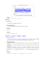
x=normalr(100)
print("Min",\t,"Max",\t, "Average",\t, "Std deviation",\n)
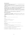
print(min(x),\t,max(x),\t,average(x),\t,sqrt(var(x)),\n,\n,\n)
print("Date:",\t,strdate)
Min
Max
Average
Std deviation
-1.869971 2.171144 -0.041539 0.86654
Date:
6.3.
4.9.2012
User-defined functions
User-defined functions extend the language by virtually unlimited number of new
functions tailored and defined by the user. User-defined functions become a part of the
language and are used in the same manner as the standard DARWin functions. To define user
functions, a special “function script” sheet is created by checking the option Function
definitions when adding a new script. Defined functions are then used from normal (nonfunction) script sheet. A function script may contain definitions of any number of functions.
Function definition itself cannot be executed (but you may execute parts of scripts even in the
functional script as normal script – this allows rather comfortable debugging).
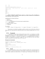
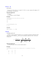
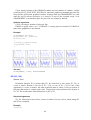
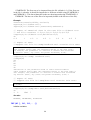
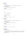
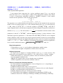
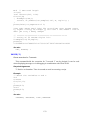
A function definition must contain a headerr and a function body There should be a
RETURN command within the function body (most often at the end of it) to pass the function
value to the calling code. The body must be closed in command “curly” braces { }. The
morphology of a simple function is illustrated below. The function is to compute the dot
product of two vectors x and y, x ⋅ y = ∑ xi yi . If no y is given in the function call the
i
(required) value of x is used for y.
34
6.3.1.
Function header and formal arguments
The function header consists from the word FUNCTION, the function name and a list
of formal arguments in parentheses ( ). Formal argument list may be empty or contain
unassigned formal argument names or assigned formal argument names. An assigned
argument name is a name with a default (pre-defined) value assigned by “=”. Assigned
arguments may then be omitted in function call. Then the assigned value in the function
header is used for that argument. All unassigned parameters must be always submitted when
the function is called. If an assigned parameter is submitted in a function call the actual value
in the call overrides the default value. Assigned formal name(s) must be given together with
their actual value(s) in a function call in the form NAME=VALUE. If a function has both
unassigned and assigned arguments then all the unassigned arguments must precede the
assigned arguments. In a function call, the order of unassigned actual arguments must be the
same as in the definition while the order (and number) of assigned arguments is arbitrary.
Examples of possible function headers and calls are given below.
Function definition (header only)
in the function script
Function call example
(the calling code or script)
function FN1()
// (Function with no argument)
x=FN1()
function FN2(x)
// (One unassigned argument)
r=fn2(1:10)
function FN3(x,y)
// (Two unassigned arguments)
r1=Fn3(10,100)
function fn4(x,y,z=1)
// (Two unassigned
// and one assigned argument)
z=fn4(1,2)
// Actual value of z missing,
// will use z=1.
z=fn4(1,2,z=10)
z=fn4(1,z=10)
//Wrong! Both x and y must be given.
z=fn4(1,z=10,2)
//Wrong! x and y must precede z.
function fn5(x,y,z=1, w=sqrt(x))
//Assigned default value of w is
//a function of other argument.
fn5(1,2)
fn5(1,2,w=10)
fn5(1,2,z=2,w=10)
fn5(1,2,w=10,z=2)
6.3.2.
Function body
The function body is a normal DARWin code (script). It must be closed in command
braces { }. At the beginning of the code there will be – in time of calling the function –
35
actual values available in the variables from the header (argument variables). These argument
variables can be used in the function body as starting input values. Argument variables are
used as normal variables within the function. They can be altered, assigned new values or
deleted. A function can compute values, call other functions and commands (both standard
DARWin and user-defined), can plot graphs, import and export data. Thus a function does not
necessarily have to have a value output (e.g. a function that only draws some plot from input
data). However, typically a function returns a value using the RETURN command, see 6.3.3
for more details.
In the following example we illustrate a very simple definition and use of a user
function.
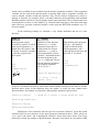
Echo panel:
/*
Main program (script):
A function „myfun“ is called
with actual arguments a,b,
which have the values 5 and
3. Result is stored to variable
c and then copied in the
Echo panel.
*/
a=5
b=3
c=myfun(a,b)
c
/*
Definition of the function:
Function myfun in the
functional script sheet is
defined with two formal
arguments x,y, result is
stored temporarily in local
variable z and transferred to
the main program by the
return command. Do not
execute function definition.
The function computes
(X+Y) (X-Y)+1
*/
After running main program
in Script_1 the function
myfun is called with the
actual arguments 5 and 3
replacing the formal ones and
the result 17 is echoed.
>a=5
>b=3
>c=myfun(a,b)
>c
17
function myfun(x,y)
{
z = (x+y) * (x-y)
return (z+1)
}
User-defined functions can be called from any script sheet in the actually opened QCF
script file. A function can also be called from within another function in the same or another
function sheet. Order of the functions does not matter. A script file may contain more
function sheets. An example of a function calling another function is given below:
function fun2(x)
// Norm of a vector x using function fun1
{
return(sqrt(fun1(x)))
}
function fun1(x)
{
return(transp(x)#x)
}
Definitions of user functions must be typed in a separate “function” script sheet with
checked field Function definition in the sheet properties mentioned above. There will be an
“f(x)” sign in the sheet’s tab to distinguish “function” sheets from other sheets. The Script
panel may contain any number of function sheets, functions in all sheets are accessible within
36
one opened QCF file. Functions are then called from non-function script sheets. DARWin
searches all existing function sheets (and all function libraries, see 6.5) for the function name.
If such function exists it is executed with submitted actual arguments.
Tab of an ordinary script sheet
Tab of a function script sheet
Tab of a menu item script sheet
6.3.3.
Return of a value
A function may return a value as a result. The value is returned using the RETURN
command, typically (but not necessarily) at the end of the function body. Executing this
command will terminate execution of the function. The simple format of the return
command is
return(expression)
The result of the expression is returned to the calling code. Only one expression can
be used as an argument of return. Of course, the result of the expression may be scalar,
vector or matrix. If the function needs to return more than one expression or variable the
list function can be used with advantage to “glue” more variables into one, such as:
return(list(name1=var1, name2=var2, name3=var3, ...))
For example, to return a string ST, a matrix MAT, a vector XX and a single number CC
from a user function MyFunct use something like:
Function myfunct(X,Y,Z)
{
........
//<< some code to compute ST, MAT, XX and CC from X,Y,Z >>
........
return(list(txt=ST, mt=MAT, vectr=XX, correlation=CC))
}
To access the result in the calling script normal “list” syntax is used (see 4.3.4, p. 20):
..........
res=MyFunct(A,B,C)
matr=res$mt
txt=res$txt
co=res$correlation
vect=res$vectr
..........
where A, B, C are the actual arguments passed to MyFunct in place of X, Y, Z. Obviously,
the list is also an expression, so formally this situation is not different from the former
example without a list.
37
Return command with empty parentheses will cause the function to return zero. If
necessary, a function may contain more than one return, as in:
........
if (le(x,0)) { return(-1) }
return(ln(x))
}
Here, if x is negative or zero [le means “less or equal”], a (– 1) is returned and the
function is terminated by the conditional return never reaching the next line. If x is positive
the first return is ignored and a logarithm of x is returned instead by the second return.
Formal syntax of a user function
Example of a definition
of a user function
FUNCTION fname([X1 [, X2,...] ] )
{
...
<<commands in the function body >>
RETURN ( [ A ])
...
}
function Fn1(x)
{
t=x*x
return(t+1)
}
6.3.4.
Example of a use of
the function from the
calling script:
y=fn1(4) + fn1(5)
Language Interpreter Frames
All variables found in the variables panel are main frame variables. Calling a function
will invoke creation of a new frame (or instance, level) of the language in which all objects
(variables) within the function are created independently of the calling frame. All variables
created within by function body are created only in the local temporary frame and are only
accessible while execution of the function code. After terminating the function, all the
variables in the local frame are lost except those passed to the calling code by return. On
the other hand, no variables from the main frame variables are accessible from within a called
function, except those passed to the function as actual arguments. So, a variable A used in a
function has nothing to do with a variable A in the main frame. There are no “global”
variables in DARWin. However, functions may use I/O commands such as PRINT, PLOT,
EXPORT, IMPORT, MESSAGE, DIALOG, etc. which always have global effect.
6.3.5.
Recursive Function Call
A function can call another function (both standard and user-defined) in its body. It
doesn’t matter if the called function is in the same sheet, another sheet within the actually
opened script file, or an external user function from the function library. A function can even
recursively call itself. At every function call a new frame is created with new independent set
of variables (see 6.3.4). Maximal depth of recursion is limited only by available memory and
demands of the function. The following example illustrates the use of a very simple recursion
on computation of factorial of N. This is just a tutorial example; it is of course much faster
and easier to use standard functions FACT(N) or PROD(1:N) instead.
Define
FAC(N) = N * FAC(N – 1)
FAC(1) = 1.
38
Example
// Function for FACTORIAL of N with use of recursion:
function fac(N)
{
if(zero(N)){return(1)}
return(N*fac(N-1))
}
and the function call from normal script will look like:
>fac(5)
120
>fac(70)
1.19785716699699E100
6.3.6.
Masking And Conflicts Of Functions And Variables
If two or more functions with the same name are defined in function script sheet only
the former one (i.e. the first one in a function script sheet or the one in the earlier created
sheet) will be executed. A user function with the same name as a standard DARWin function
will be ignored.
Variables with the same name as a standard or user function can be formally used and
are not in conflict. The only exception are names functions without arguments DELETEVARS,
STOP, TRACEON, TRACEOFF that cannot be used as variable names. When using a function
and variable of the same name, the syntax decides which way it will be interpreted. However,
generally it is not recommended to use variables and functions of the same name. An example
is shown below.
>sin=5
>sin(1)
0.841470984807896
>sin
5
>delete(sin)
>sin
Error : "Variable "SIN" not defined"
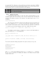
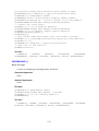
6.4.
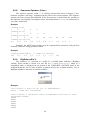
Running Script From QCExpert® Menu
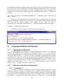
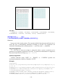
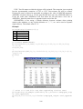
Correctly running code can be easily integrated into main menu of QCExpert® by
checking the box Add to main menu in the dialog box Add script or Rename script. This will
add a new menu item to the DARWin menu in QCExpert®. The name of the item is taken
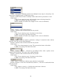
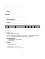
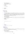
from the name of the list. The DARWin menu always shows all sheets in the currently opened
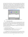
script file that have checked the box Add to main menu, see the illustration below.
39
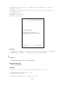
By clicking on the DARWin menu item the complete corresponding script is executed
as by pressing F10 or Execute in the sheet. The script may contain I/O communication and
interactive tools and commands like DIALOG, MESSAGE to interact with the user,
GETSHEET, PUTSHEET to get data from QCExpert® standard Data window, or DBIMPORT,
IMPORT, EXPORT, EXPORTGRAPH, PRINTPDF others to import data and export results
This gives a tool to create a friendly environment to routinely solve very specific tasks.
6.5.
6.5.1.
DARWin Function Library
Creating Function Library
User functions library enables to extend functionality of DARWin and QCExpert®
beyond usual statistical software according to specific need of the user and share new
functionality of the language and the system. Function library is composed of script files with
function sheets saved on a local or network disk with the extension “.QCL” and allows to use
all functions in the QCL library files to be used without the need to open the respective files
exactly in the same manner as the standard DARWin functions. To save a function library,
first write functions in the function sheet (or sheets). The script with all sheets (non-function
sheets are ignored in QCL) is then saved as Function library QCL file. This file is ready to be
attached to the function library. The saved QCL file can be opened and edited at any time.
Any change to the QCL file has an immediate effect, without a need to unload and re-load the
library.
6.5.2.
Attaching and Activating Function Library
Saved QCL files can be loaded (attached) in the Parameter settings dialog (Menu: File
– Setup / DARWin tab). Clicking the Load library button opens an Open File dialog where
40
the desired QCL file with the library is selected and opened (loaded). After loading, the
library appears in the Function library list. To activate the loaded library, the box at its name
must be checked. For each library a short (~2-3 words) description may be typed in after
clicking the Description... button. From this point, all the functions defined in the library are
available together with any help present in the function definitions (see 6.5.3 below). The
libraries remain activated after restarting QCExpert® and need not to be re-loaded, or reactivated every time QCExpert® is started. Thus, functions in once loaded libraries become a
part of DARWin unless the corresponding QCL files are removed or damaged. User defined
function will appear in the script panel in different color than the standard functions. These
colors are defined in the Parameter Settings window as well.
DARWin tab in Parameter setting with two loaded and activated function libraries
6.5.3.
Function library Help
Every function defined in “Function sheet” of the current QCF script file or in the
QCL library files may contain a user help. It is strongly recommended that functions designed
for more than one use are equipped with a help from the author. The help (if any) must be
located between the function header and the opening brace of the function body as plain text
in the form of a multi-line comment /* ......... */. In fact, any multi-line comment
in this place is interpreted as help and displayed in the interactive help for that function. It is
recommended that the format of the help follow the composition of the standard functions
help. Every help should contain:
•
•
•
•
•
A short description of the function;
A comment on the output of the function (if it is not clear from the description);
Required arguments, their type, restrictions;
Optional arguments, their type, restrictions, possibly default assignment;
An executable example (without using external data, if possible).
No formatting codes are used in the help. Below we provide an example of a function
with help. Remember that your function may be used by other people and remember one of
the programmer’s laws: Every uncommented/undocumented program will have to be
rewritten from scratch in the moment you definitely forgot any clue how to write it again!
41
function uniformd(x,a,b)
/*
Probability density of uniform distribution U(a,b)
Arguments:
a, b: real numbers, a<b, lower and upper limits of the distribution.
x: real variable
Example:
x=seq(0,5,count=200)
plot(x,uniformd(x,1,4),type="line")
*/
{
if( ge(a,b)){
message("Uniformd ERROR: A equal or greater than B");stop()
} // End if
d=heav(x-a)*heav(b-x)/(b-a)
return(d)
}
The following figure show a user function help in the interactive Function Library
Help system.
6.6.
DARWin Help System
DARWin help is accessed via F1, or click on the DARWin – Main help button
in
the DARWin toolbar. When the cursor is at a standard function or at a user function with help,
pressing F1 will display help for that function. Otherwise, a general standard help window is
opened. Most of the standard functions help contains an executable script that can be copied
and pasted in the script panel, selected (if necessary) and run with F10 or the Execute button.
Help for the user functions is invoked by pressing F1 with the cursor on a documented
user function name or by clicking the DARWin – User functions help button
42
.
43
7.
DARWin Standard Commands And Functions
7.1.
Introductory Remarks
One (or more) command must be in one line (except multi-line commands with @
and ; - see 6.2.10, p. 29). Formal definitions are given in bold at the beginning of every
function or command. Functions have required and/or optional arguments. Optional
arguments are in brackets [ ]. Named arguments are given in form
ARGUMENT_NAME=VALUE, e.g. MEAN=X. The named argument must be used in full
name when calling a function or command, e.g. MEAN=5. The number and order of named
arguments is arbitrary when calling a function or command. Non-named arguments must be
used in the same order as in definition. For example the function NORMALR for generating
normal random numbers:
NORMALR(N, MEAN=0, SDEV=1) // (The formal function definition)
is possible call in the following manner (let k=10):
normalr(k)
normalr(k,
normalr(k,
normalr(k,
normalr(k,
// mean and sdev is implicitly 0 and 1
mean=4)
sdev=0.1)
sdev=0.1, mean=5)
mean=5, sdev=0.1) //order doesn’t matter
The following calls are incorrect and cause an error:
normalr(k, 4) // named arg must named when calling
normalr(mean=5,k)
// not-named arg k must be in same order as in definition
Other details about syntax are also mentioned in 2.1 on page 8.
7.2.
Commands And Functions
ABS(X)
Absolute value
Absolute value of a number
Required Arguments
X: Number, numeric vector, or a matrix
Example
>abs(-5)
5
>abs(vec(3,-4,-5,2))
3
4
44
5
2
See also
SIGN, ZERO, HEAV, INT, CEIL, FRAC
ACOS(X)
Arc Cosine
Required Arguments
X: a number, numeric vector, or a matrix
See also
ARCSIN, ARCTAN
ACOSH(X)
Hyperbolic arc cosine
Hyperbolic arc cosine, an inverse function to the positive branch of COSH(X).
Required Arguments
X: a number, numeric vector, or a matrix, defined only for X ≥ 1.
Example
>acosh(1:5)
0
1.31695789692482
1.76274717403909
2.06343706889556
2.29243166956118
See also
ASINH, ATANH
AND(X1, X2)
AND, Logical product
Logical product of X1 and X2. Zero (0) represents false and non-zero (typically 1)
represents true. The results of AND are shown in the table.
X1 X2 AND(X1,X2)
0
0
0
0
1
0
1
0
0
1
1
1
Required Arguments
X1, X2: number, numeric vector, or a matrix with logical values.
45
Example
>and(ge(5,3),ge(1,-1))
1
// Select elements in Y with required values
>x=sample(0:1,10,repl=1)
>y=normalr(10)
>y[[and(not(zero(x)),ge(y,0))]]
0.99874719943179
0.810622183581444
See also
OR, NOT, XOR, GT, LT, GE, LE, EQ, NE
APPLY(X, F, DIR=1)
Apply function F on columns or rows of a matrix
Creates row or column vector of values of a given aggregate function F from all rows
or columns of a matrix X. It is used to calculate column or row averages, variances, sums,
etc. of a matrix. F may be any function that takes one vector as input (argument) and gives
one (scalar) value as a result.
Required Arguments
X: a matrix (N x M)
F: a text string with the name of the aggregate function, F may be SUM, AVERAGE,
MEDIAN, VAR, MIN, MAX, PROD, NORM.
DIR: Integer numerical value 1 or 2. Sets the direction of application of F. If DIR=1
(default value), the row values are returned in a column vector of length N, if DIR=2, the
column values are returned in a row vector of length M.
Example
// Maxima in random matrix columns A (10 x 5):
>a=matrix(normalr(50),ncols=5)
>round(apply(a,"max",dir=2),5)
1.7966
1.05819
1.37638
1.86831
2.03436
// Column means are subtracted from columns of B
// giving a matrix B1 with centered columns:
>B=bind(1:4,2:5)
>B1=B-apply(B,"average",dir=2)
>B1
-1.5
-1.5
-0.5
-0.5
0.5
0.5
1.5
1.5
See also
ROWS, COLS, SPLIT, BIND, MATRIX, FUNCTION
46
ARG(X,Y)
Argument function, ARG – function
The Arg function is defined as Arg ( x, y ) = 2 arctan
x+
y
for x < 0 a y
and Arg ( x, y ) = π − 2 arctan
x + x2 + y 2
complex analysis, where x and y is the real and imaginary
z = x + iy. For a complex z it holds that z = z ei arg ( z ) .
for x > 0 a y ≠ 0
x 2 + y 2
y
≠ 0 and is often used in
part of a complex number
Required Arguments
X, Y: Real number or vector. If one of the arguments is a vector, the other one must be
scalar number.
Example
x=seq(-5,5,count=200)
plot(x,arg(x,0.5),type="line")
See also
ATANH
ASCII(S)
ASCII code
ASCII code of the first character of the text string S. ASCII is an abbreviation for
American Standard Code for Information Interchange.
Required Arguments
S: text string or a vector of text strings
Example
>ascii("ABC")
47
65
// This script generates an ASCII table of characters:
print(transp(vec("*",astext(0:9))),\n)
for(i=0:12)
{
print(astext(i),\t)
for(j=0,9)
{
c=10*i+j
print(chr(c),\t)
}
print(\n)
}
*
0
1
2
3
4
5
6
7
8
9
10
11
12
0 1 2 3 4 5 6 7 8 9
(
2
<
F
P
Z
d
n
x
)
3
=
G
Q
[
e
o
y
*
4
>
H
R
\
f
p
z
!
+
5
?
I
S
]
g
q
{
"
,
6
@
J
T
^
h
r
|
#
7
A
K
U
_
i
s
}
$
.
8
B
L
V
`
j
t
~
%
/
9
C
M
W
a
k
u
&
0
:
D
N
X
b
l
v
€
'
1
;
E
O
Y
c
m
w
See also
CHR, ASNUMERIC
ASIN(X)
Arc Sine
Required Arguments
X: A number, numeric vector, or matrix
See also
ARCCOS, ARCTAN
ASINH(X)
Hyperbolic arc sine
Hyperbolic arc sine, inverse of the positive branch of SINH(X).
48
Required Arguments
X: a number, numeric vector, or matrix
Example
>bind((-3:3),asinh(-3:3))
-3
-1.81844645923207
-2
-1.44363547517881
-1
-0.881373587019543
0
0
1
0.881373587019543
2
1.44363547517881
3
1.81844645923207
See also
ACOSH, ATANH
ASNUMERIC(S)
As numeric, convert to number
Converts a string to a number if possible. If the text argument can not be represented as
valid number returns zero.
Required Arguments:
S: text string or a vector of text strings
Example
>asnumeric("453"+"."+"25")+3.53
456.78
See also
ASTEXT
ASTEXT(X)
As text, convert to a string
Converts any value to a string
Required Arguments
X: Any value or vector
Note: Some functions or operators (such as “+”) converts a numeric value to a string if
necessary, see example:
Example
>astext(3^3)+" gallons"
"27 gallons "
>3^3+" gallons"
49
"27 gallons "
>a=1
>b=25
>astext(a)+astext(b)
"125"
>"A"+(1:4)
"A1"
"A2"
"A3"
"A4"
See also
ASNUMERIC, CHR
ATAN(X)
Arc Tangent
Required Arguments
X: a number, numeric vector or matrix
See also
ARCCOS, ARCSIN
ATANH(X)
Hyperbolic Arc Tangent
Required Arguments
X: a number, numeric vector or matrix, -1 < X < +1.
See also
ARCCOSH, ARCSINH
AVERAGE(X)
AVG(X)
Arithmetic average
Arithmetic average of a vector or matrix elements.
Required Arguments
X: a number, numeric vector, or matrix
Example
>average(vec(3,4,4,5,3,4,3,4))
3.75
50
// Average of a million normal random numbers:
>average(normalr(1000000))
0.00173227950478392
See also
MEDIAN, VAR, MEAN
BIND(M1[,M2,M3,...])
Bind vectors or matrices horizontally
Binds two or more scalars, column vectors (Nx1) or matrices (NxM) into one matrix
(NxΣM). Arguments must have the same number of rows or can be a scalar in which case
the column is filled with this scalar value. Calling BIND with more than two arguments is
equivalent to multiple nested call, so BIND(X1,X2,X3) is equivalent to
BIND(BIND(X1,X2),X3).
Required Arguments
M1, M2, …: Matrices or vectors or scalars
Example
>bind(1:3, 11:13, 21:23)
1 11
21
2 12
22
3 13
23
>bind(1,1:4)
1 1
1 2
1 3
1 4
See also
BINDV, SPLIT, SPLITV, VEC
BINDV(M1[, M2, M3, ...])
Bind vectors or matrices vertically
Binds two or more scalars, row vectors (1xM) or matrices (NxM) into one matrix
(ΣNxM). Arguments must have the same number of columns or can be a scalar in which
case the corresponding row is filled with this scalar value. BINDV with more than two
arguments is equivalent to multiple nested call, so BINDV(X1,X2,X3) is equivalent to
BINDV(BINDV(X1,X2),X3).
Required Arguments
M1, M2, …: Matrices or vectors or scalars
Example
>bindv(vec(1,2,3),vec(4,5,6))
1
2
3
51
4
5
6
>bindv(transp(vec(1,2,3)),transp(vec(4,5,6)))
1 2
3
4 5
6
>bindv(1,transp(vec(4,5,6)),9)
1 1
1
4 5
6
9 9
9
See also
BIND, SPLIT, SPLITV
CAPS(S)
Capitals
Converts all letters in a text string to capitals. Letters „a“ through „z“, are converted to
„A“ through „Z“.
Required Arguments
S: Text string or a vector of text strings
Example
>caps("aBcDeFgH")
"ABCDEFGH"
See also
LOWCASE, ASNUMERIC, ASTEXT, LETTERS
CEIL(X)
Integer ceiling
Smallest integer number greater or equal X.
Required Arguments
X: a number, numeric vector, or matrix
Example
>ceil(3.4)
4
>ceil(-3.4)
-3
See also
INT, FRAC, ROUND, FLOOR
52
COL(X, N)
N-th column
Returns the N-th column of a matrix X. If N is a vector, returns all columns of X
corresponding to elements in N.
Required Arguments
X: matrix
N: an integer or vector of integers
Example
>A=bind(vec(1,2,3),vec(11,12,13))
>col(A,2)
11
12
13
>col(transp(A),1:2)
1 2
11 12
See also
ROW, SPLIT, [], VEC
COR(X)
Correlation matrix of X
Returns a square symmetric matrix C(m x m) of sample correlation coefficients of the
matrix X (n x m). Elements ci, j of C are pair correlation coefficients of the i-th and j-th
column of X.
cij =
σˆ 2 ( xi , x j )
σˆ ( xi ) σˆ ( x j )
n
=
∑( x
k =1
ki
− xi ) ( xkj − x j )
∑ ( xki − xi ) ∑ ( xkj − x j )
n
k =1
2
n
2
k =1
Required Arguments
X: numeric matrix. If X is a vector cor(X) returns 1.
Example
>x=bind(vec(3,4,6,7,9),vec(3,3,6,7,7),vec(8,7,5,4,1))
>x
3
3
8
4
3
7
6
6
5
7
7
4
9
7
1
53
>cc=cor(x)
>round(cc,4)
1
0.9299
-0.9941
0.9299
1
-0.8909
-0.9941
-0.8909
1
See also
VAR, AVERAGE, MEAN
COS(X)
Cosine of X
Required Arguments
X: A number, numeric vector, or matrix
See also
SIN, TAN, COTAN
COSH(X)
Hyperbolic cosine of X
Function cosh ( x ) =
e x + e− x
.
2
Required Arguments
X: A number, numeric vector, or matrix
Example
x=seq(-5,5,count=200)
plot(x,cosh(x),type=line)
See also
SINH, TANH
54
COTAN(X)
Cotangent of X
Required Arguments
X: A number, numeric vector, or matrix
See also
SIN, COS, TAN
COUNT(X)
Number of elements
Returns number or elements of a matrix or vector X.
Required Arguments
X: A number, numeric vector, or matrix
Example
>count(unit(12))
144
See also
DIM, NCOLS, NROWS
CUSUM(X)
Cumulative sums
Cumulative sums of a vector X. If X has N elements, returns a length N-vector c of
i
values ci = ∑ xk
k =1
Required Arguments
X: a number or numeric vector
Example
>cusum(vec(1,2,3))
1
3
6
>cusum(normalr(5)) // Gaussian random walk
0.553998671372093
-0.154006915823345
-0.768427579848724
-1.44818904337812
-2.79528101487966
x=cusum(normalr(2000))
55
plot(x,type="line",main="Gaussian Random Walk")
See also
DIFF, SUM
DATETIMEDIFN(D1,D2)
Date – Time difference in numerical format
Returns the number of days between times D1 and D2 as a decadic number. If D1>D2
then the result is positive.
Required Arguments
D1, D2: Date and time in text format "D.M.Z H:M:S.TTT"., for example:
"25.3.1984 14:29:52.009" All valid dates between years 0000 and 65535 are
possible.
Example
// Number of days that passed from 1.1.2010 0:00:00 till now:
>datetimedifn(strdatetime(0),"1.1.2010")
965.518054664353
//Number of seconds form 1.1.2010 0:00:00 till now:
>datetimedifn(strdatetime(0),"1.1.2010 0:0:0")*24*60*60
83420890.9790001
// Time of computation in seconds:
>t1=strdatetime(0)
>a=0
>for(i=1,10000)
>{
>a=a+i
>}
>t2=strdatetime(0)
>td=datetimedifn(t2,t1)*86400
>"Comp time = "+round(td,3)+" seconds"
56
"Comp time = 0.874 seconds"
See also
TIMEDIFS, TIMEDIFN, STRDATETIME, DATETIMEN, DATETIMES
DATETIMEN(D)
Convert DateTime from string to numerical format
Converts date and time from text format "D.M.YYYY H:M:S.ttt" to number of
days since 30.12.1899. DATETIMEN is an inverse to DATETIMES.
Required Arguments
D: Date and time in text format, for example: "25.3.1984 14:29:52.500".
Example
>DATETIMEN("31.12.1999")
36525
>DATETIMEN(strdatetime(0))
41144.5578932523
See also
STRDATETIME, DATETIMEDIFN, DATETIMES, TIMEDIFS, TIMEDIFN
DATETIMES(X)
Convert DateTime from numerical to string format
Converts the date and time in numerical format (i.e. number of days since 30.12.1899)
into text format "D.M.YYYY H:M:S.ttt". Numerical format can be negative, which makes
it possible to handle dates from back to (1.1.0000) till the end of the year 65535.
DATETIMES is inverse to DATETIMEN.
Required Arguments
X: Numerical value or vector representing valid date as (decimal) number of days since
30.12.1899. In X is integer, only date without time is returned, as integer X represents
midnight.
Example
>datetimes(datetimen(strdatetime(0)))
"23.8.2012 13:49:36.996"
>datetimes(int(datetimen(strdatetime(0))))
"23.8.2012"
// 8-minutes intervals since now
57
>dstart=datetimen(strdatetime(0))
>dd=dstart+8*(0:10)/24/60
>datetimes(dd)
"23.8.2012 13:50:13.219"
"23.8.2012 13:58:13.219"
"23.8.2012 14:06:13.219"
"23.8.2012 14:14:13.219"
"23.8.2012 14:22:13.219"
"23.8.2012 14:30:13.219"
"23.8.2012 14:38:13.219"
"23.8.2012 14:46:13.219"
"23.8.2012 14:54:13.219"
"23.8.2012 15:02:13.219"
"23.8.2012 15:10:13.219"
// 8- minutes intervals in whole minutes
>dstart=int(datetimen(strdatetime(0))*24*60)/24/60
>dd=dstart+8*(0:5)/24/60
>datetimes(dd)
"23.8.2012 13:52:00.000"
"23.8.2012 14:00:00.000"
"23.8.2012 14:08:00.000"
"23.8.2012 14:16:00.000"
"23.8.2012 14:24:00.000"
See also
DATETIMEN, STRDATETIME, DATETIMEDIFN, TIMEDIFS, TIMEDIFN
DAYINWEEK(D)
Number of the day in week
Converts the date in text format "D.M.YYYY H:M:S.ttt" to the day in week
(Monday=1, Tuesday=2, Wednesday=3, Thursday=4, Friday=5, Saturday=6, Sunday=7).
Required Arguments
D: Date and time in text format, for example: "25.3.1984 14:29:52.050".
Example
>dayinweek("1.1.2001")
1
>dayname=vec("Monday", "Tuesday", "Wednesday", "Thursday",
"Friday", "Saturday", "Sunday")
>ii=dayinweek("1.1.2001")
>dayname[ii]
"Monday"
See also
DAYINYEAR, STRDATETIME, DATETIMEDIFN, DATETIMES
58
DAYINYEAR(D)
Number of the day in year
Converts the date in text format "D.M.YYYY H:M:S.ttt" to the number of the day
in a year (e.g. January 1 = 1).
Required Arguments
D: Date and time in text format, for example: "25.3.1984 14:29:52.9".
Example
// Leap year
>dayinyear("31.12.2000")
366
See also
DAYINWEEK, STRDATETIME, DATETIMEDIFN, DATETIMES
DBCONNECT(USER=S1, PSWD=S2 [SERVER=S3, DB=S4, ROLE=S5,
LOCALE=S6])
Database connection to a FireBird (or QCE-DataCenter®) database
Connects to an existing FireBird (TriloByte’s QCE-DataCenter® ) database.
Required Arguments
USER: text string, a valid user name
PSWD: text string, a valid user password
Optional Arguments
SERVER: text string, server name
DB: text string, database file name with a full path
ROLE: text string a database role
LOCALE: text string
Example
dbConnect(user="John", pswd="masterkey", SERVER="localhost",
DB="C:\trilobyte\database.fdb")
See also
DBGETFIELDS, DBGETTABLES, DBIMPORT, DBIMPORTTABLE, IMPORT,
EXPORT
DBCREATE (USER=,PSWD=,SERVER=, DB=[,LOCALE=WIN1250])
Create database
59
Creates an empty FireBird database and defines username and password. Table
definitions are made by the command DBCREATETABLE.
Required Arguments
USER: text string, admin name of the new database.
PSWD: text string, admin password for the new database.
SERVER: Name or IP address of the server.
DB: File name with full path of the new database including the extension .FDB.
Optional Arguments
ROLE, LOCALE: text strings
Example
dbcreate(USER="sysdba",PSWD="masterkey",SERVER="localhost",
DB="C:\trilobyte\database.fdb")
See also
DBCREATETABLE, DBCONNECT, DBGETFIELDS, DBGETTABLES, DBIMPORT,
DBIMPORTTABLE, IMPORT, EXPORT
DBCREATETABLE(NAME=[,FORMAT=,MODE="APPEND"|"ERASE"|
"DROP",DATA=,SECURITY=1|0])
Create table in the connected database
Creates an empty table in the connected database, possibly filling it with data.
Required Arguments
NAME: Text string, the name of the table.
Optional Arguments
FORMAT: Matrix with three or four columns containing field names in the form
returned by DBGETFIELDS. Rows in this matrix correspond to individual fields. First
column contains the names of fields as text strings, second column contains types as text
strings: "STRING", "FLOAT", "INTEGER", "NUMERIC", "DATE", "TIME",
"DATETIME". The third column contains lengths of the fields as integer values. The
fourth column is optional and may contain alternative column names used in
QCE-DataCenter®.
Example of the format matrix for six columns:
"TIMED" "DATETIME"
"CODE"
"STRING"
"NOX"
"FLOAT"
"SO2"
"FLOAT"
"BENZENE" "FLOAT"
"TEMP"
"FLOAT"
0
24
0
0
0
0
""
""
""
""
""
""
MODE: text string "APPEND", "ERASE" or "DROP" defining way of adding fields:
MODE="APPEND" adds fields. If the table exists, the fields must exist and have the
60
corresponding type. If the table does not exist, it is created. MODE="ERASE" or "DROP"
deletes existing table of the same name.
DATA: Matrix (table) of data with the type and format corresponding to the FORMAT
argument.
SECURITY: Numeric value 0 or 1. If SECURITY=1 and the existing database was not
created by the DBCREATE command, no action is taken to preserve tables in foreign,
external databases.
Example
// Create empty database:
DBCREATE(USER="sysdba",PSWD="masterkey",SERVER="localhost",
DB="C:\temp\database.fdb")
// Define new table format variable, fmt:
fmt1=vec("Timed","Code","NOX","SO2","Benzene","Temp")
fmt2=vec("DATETIME","STRING","FLOAT","FLOAT","FLOAT","FLOAT")
fmt3=vec(0,24,0,0,0,0)
fmt=bind(fmt1,fmt2,fmt3,"")
//Simulate data for the table:
N=1000
ibase=1:N
// Use big data (%) in case N was bigger than 65000
dates%=datetimes(seq(42000,42366,count=N))
codes%=rep("",N)
for(i=1,N)
{ codes%[i]=letters("A",sample(1:26,4,repl=1)) }
//Data simulation (and making them look real)
air%=3*cusum(normalr(N))+normalr(N)*10+500+200*sin(ibase/100)^4
air%=bind(air%,10*cusum(normalr(N))+normalr(N)*2+140)
air%=bind(air%,3*cusum(normalr(N))+normalr(N)*5+720)
shift=980+200*abs(sin(ibase/100-2))^0.5
air%=bind(air%,4*cusum(normalr(N))+normalr(N)*10+shift)
air%=round(air%,1)
// Plot generated data for convenience:
plot(air%)
//Connect to database and create the new table "AIR":
DBCONNECT(USER="sysdba",PSWD="masterkey",SERVER="localhost",
DB="C:\temp\database.fdb")
xx=bind(dates%,codes%,air%)
DBCREATETABLE(NAME="Air",FORMAT=fmt,MODE="DROP",DATA=xx)
61
View of the database table in an external application (QCExpert DataCenter®)
See also
DBCREATE, DBCONNECT, DBGETFIELDS, DBGETTABLES, DBIMPORT,
DBIMPORTTABLE, IMPORT, EXPORT
DBDISCONNECT()
Disconnect database
Disconnects actively
DBCONNECT).
connected
database
(e.g.
previously
connected
using
Required Arguments
None
Example
DBdisconnect()
See also
DBCONNECT
DBGETFIELDS(S1)
Get table fields
Gets the fields of existing table S1. Field names are returned as a matrix containing
names, types and length of the fields. Database must be connected using dbConnect.
Required Arguments
S1 text string with the table name.
62
Example
>dbConnect(user="sysdba", pswd="masterkey",
DB="C:\temp\database.fdb")
>tab1=dbGetTables()
>dbGetFields(tab1)
"TIMED" "DATETIME" 0
""
"CODE"
"STRING"
24
""
"NOX"
"FLOAT"
0
""
"SO2"
"FLOAT"
0
""
"BENZENE" "FLOAT"
0
""
"TEMP"
"FLOAT"
0
""
See also
DBCONNECT, DBGETTABLES, DBIMPORT, DBIMPORTTABLE, IMPORT,
EXPORT
DBGETTABLES()
Get database table names
Returns a text string vector of table names in the connected database.
Example
>dbconnect(user="sysdba", pswd="masterkey",
DB="C:\temp\database.fdb")
>dbgettables()
"AIR"
See also
DBCONNECT, DBGETFIELDS, DBIMPORT, DBIMPORTTABLE, IMPORT,
EXPORT
DBIMPORT(QUERY)
Import using SQL query
Imports a data table created by an SQL-query from a database table. The database must
be connected using DBCONNECT command. The SQL-query is passed to the database as
a text string. The FireBird SQL-dialect is used. The resulting table is returned as a matrix.
Required Arguments
QUERY: text string containing a valid SQL query
Example
>dbconnect(USER="sysdba", PSWD="masterkey",
DB="C:\temp\database.fdb")
>dbgettables()
"TABLE1"
"TABLE2"
tab="TABLE1"
63
>tab1=dbimport("select * from "+tab)
>dim(tab1)
7212
51
See also
DBCONNECT, DBGETFIELDS, DBGETTABLES, DBIMPORTTABLE, IMPORT,
EXPORT
DBIMPORTTABLE(TABLE [, STARTDATE=, ENDDATE=, FIELDS=,
VALIDONLY=1|0, SYSFIELDS=0|1])
Import table from QCE-DataCenter® or FireBird database
Imports a table from the database connected by DBCONNECT command. The table is
returned as a matrix. The table name is in the argument TABLE. Standard QCEDataCenter fields (columns) Time and Date may be used to select a time interval using
arguments STARTDATE and ENDDATE. If the argument FIELDS is defined only the
selected columns are imported. If SYSFIELDS=1, all columns, including the system ones
are imported. This is an alternative to DBIMPORT without using an SQL query.
Required Arguments
TABLE: Text string, name of the table.
Optional Arguments
STARTDATE: Text string, the starting date in format "DD.MM.YY".
ENDDATE: Text string, the ending date in format "DD.MM.YY".
FIELDS: A vector of text strings (e.g. taken from DBGETFIELDS function which are
to be imported.
VALIDONLY: Numeric value 0 or 1. If VALIDONLY=0, only valid records (rows)
are imported.
SYSFIELDS: Numeric value 0 or 1. If SYSFIELDS=0 (default value) system fields are
not imported.
Example
>dbconnect(USER="sysdba",PSWD="masterkey",
DB="C:\temp\database.fdb")
>dbgettables()
"TABLEA"
"TABLEB"
>tab1=dbimporttable("TABLEB")
>dim(tab1)
7212
40
See also
DBCONNECT, DBGETFIELDS, DBGETTABLES, DBIMPORT, IMPORT,
EXPORT
64
DELETE(V1, [V2,... ])
DEL(V1, [V2,... ])
Delete variables
Deletes one or more variables. No undo is possible.
Note: Deleting an existing variable is useful when defining a new matrix using index.
Required Arguments
V1, V2, ...: Variable names (not in quotes).
Example
>a=5
>b=10
>a
5
>b
10
>delete(B)
>b
Error : "Variable "B" not defined"
>a=5
>delete(a)
>a[3,3]=0
>a
0 0
0
0 0
0
0 0
0
// Create a (3x3) matrix and fill with zeros.
See also
DELETEVARS
DELETESHEET(P1)
Delete data sheet in QCExpert® Data window
Deletes a sheet in QCExpert® data window. Any data in the sheet are lost (if not saved
before). No undo is possible. The sheet name is in the argument P1 as a text string.
Required Arguments
P1: Text string, the name of the sheet to be deleted. Case insensitive. If this sheet does
not exist no action is taken. Attempt to delete the last sheet in the Data window will delete
data from the sheet, but the sheet is retained. Equivalent to deleting a sheet manually from
QCExpert® menu (Menu: Format – Sheet – Delete).
Example
deletevars
sname="DATA_X"
b=1:20
65
putsheet(b,sname)
putsheet(b*20,"DATA_Y")
deletesheet(sname)
// The following deletes all sheets in Data window:
// (only the last sheet remains)
snames=getsheetnames()
for(s=snames)
{
deletesheet(s)
}
See also
GETSHEET, GETSHEETNAMES, PUTSHEET, DELETEVARS
DELETEVARS
Delete all variables
Deletes all variables !WITH NO WARNING! No undo is available.
NOTE: Unwanted deletion of important variables may be undone by copying the
corresponding file “matrixdata.qcf” in the work directory (default: c:\TEMP\) to a
different file immediately and re-opening it after restarting DARWin.
Example
a=1:100
deletevars
See also
DELETE, DEL
DET(X)
Determinant of a matrix
Returns a determinant of a square matrix X
Required Arguments
X: Square (NxN) numerical matrix.
Example
>a=matrix(round(normalr(9),2),ncols=3)
>a
-0.31
-0.73
-0.82
0.8
1.87
0.68
1.43
-0.86
0.14
>det(a)
1.866384
66
See also
INV, PINV, SVD, NORM
DIAG(X)
Diagonal of a matrix or diagonal matrix from a vector
If X is a length (N) vector, returns a square diagonal matrix with elements of X on the
diagonal. If X is an (NxM) matrix, returns its diagonal X[i,i] as a vector of length
min(N,M)
Required Arguments
X: numeric vector or matrix
Example
>a=diag(vec(1,2,3))
>a=inv(a)
>diag(a)
1
0.5
0.333333333333333
See also
TRANSP, UNIT, MATRIX
DIALOG( DLGPARS=dp, Xi=list(TYPE= dlgtype,[VAL=value,
LABEL=itemlabel, [ROWS=rows, FUN=command,
CLOSE=closewin, LABELS=rblabels]])
Create and display user dialog window
This function creates an interactive dialog window according to given arguments and
displays it. Every dialog window always has two buttons OK and CLOSE. Pressing
(clicking) CLOSE closes the window with no action taken. Pressing OK returns contents
of all the control items in the window as a list type value. The items of the resulting list
have the same names as used in the DIALOG function to identify the control items and
types corresponding to the type of the control item (checkbox returns 0 or 1, text field
returns a text string, multiselect list returns a vector of selected items, etc., see below).
Number of control items is not limited (just mind the size of your screen). The order of
the control items in the dialog window is given by the order of the corresponding
arguments of DIALOG. Global properties of the dialog window (as field width, number
of field columns) are defined in a control argument DLGPARS which must be a list type
value (or variable), see required arguments. The result of DIALOG must be always
assigned to a variable, like dlg=dialog( … ). Values of the control items are then
accessible as elements of the resulting list-type variable dlg.
Arguments
DLGPARS: A list with required elements:
67
COLWIDTH: An integer. The width of the dialog window items in points.
Typically 100 or 200.
NCOLS: An integer. Number of field columns, typically 1, 2 or 3.
NAME: Text string. Name of the window, displayed in the window header.
It is advisable to assign this list to a variable before calling DIALOG, see example.
Xi: A list. Definition of a dialog window item. Names of these arguments are defined
by the user. This name is then used as the name of the corresponding item in the resulting
list. This argument is a list structure of which depends on the type of the dialog item.
Required list item of this argument is TYPE. The rest of the list items are optional.
TYPE: A text string defining type of the dialog item. Eleven (11) different
types of the control items are available. Other list items are optional: VAL, LABEL,
LABELS, ROWS, FUN, CLOSE, and differ according to the type of the dialog item.
Possible values of the TYPE item of Xi are:
TYPE= "editnum": Single line edit field for a numerical value.
Returns: Contents of the edit field when OK was pressed (numeric value).
Other items:
VAL: Numeric value. Pre-filled value of the edit field.
LABEL: Text string, label of the dialog item.
TYPE= "editstr": Single line edit field for a text value.
Returns: Contents of the edit field when OK was pressed (text string).
Other items:
VAL: Text string. Pre-filled value of the edit field.
LABEL: Text string, label of the dialog item.
TYPE= "drop": Drop-down list.
Returns: Actual selected value when OK was pressed.
Other items:
VAL: Text or numeric vector. All selectable items of the drop-down list.
LABEL: Text string. The label of the item.
ROWS: Number of visible rows (length of VAL vector is unlimited).
TYPE= "select": Single-selection list.
Returns: Actual selected value when OK was pressed.
Other items:
VAL: Text or numeric vector. All selectable items of the drop-down list.
LABEL: Text string. The label of the item.
ROWS: Number of visible rows (length of VAL vector is unlimited).
68
TYPE= "selectmulti": Multiple-selection list. Multiple items may be selected by Ctrlmouseclick, dragging mouse, or Shift-arrow keys.
Returns: Actual selected value or multiple values when OK was pressed as a vector.
Other items:
VAL: Text or numeric vector. All selectable items of the drop-down list.
LABEL: Text string. The label of the item.
ROWS: Number of visible rows (length of VAL vector is unlimited).
TYPE= "combo": A list with an edit line.
Returns: Contents of the edit line when OK was pressed.
Other items:
VAL: Text or numeric vector. List items to select from.
LABEL: Text string. The label of the item.
ROWS: Number of visible rows (length of VAL vector is unlimited).
TYPE= "slider": Slider for manual „continuous“ setting of a numerical value with an
edit line. The value can be edited manually.
Returns: Contents of the edit line when OK was pressed.
Other items:
VAL: Two-element numeric vector. The start and end value of the slider.
LABEL: Text string. The label of the item.
TYPE= "spinner": Spinner - selection of pre-defined values with a spinner arrow
buttons with an edit line. The value can be edited manually.
Returns: Contents of the edit line when OK was pressed.
Other items:
VAL: Text or numeric vector. List items to select from.
LABEL: Text string. The label of the item.
TYPE= "check": Check box with two states (checked / unchecked).
Returns: Numeric 0 if the box in unchecked, numeric 1, if the box is unchecked when
OK was pressed.
Other items:
VAL: Numeric value 0 or 1. Defines the initial state of the box.
LABEL: Text string. The label of the item.
69
TYPE= "radiobuttons": A set of n radio buttons to select exactly one from a few predefined options.
Returns: Numeric integer value 1 through n given by the order of the button selected
when OK was pressed.
Other items:
VAL: A single integer numeric value from 1 to n. Defines the initially selected
radio button.
LABEL: Text string. The label of the group.
LABELS: Text vector of length n. Labels at individual radio buttons
TYPE= "button": A button which can be used to execute an expression that returns
some value. When pressed (clicked) an expression defined in FUN is executed and the
result of the expression is assigned to the Xi resulting list item.
Returns: Last value of the executed expression defined in FUN if it exists. An empty
character "" if the button was not pressed before pressing OK.
Other items:
FUN: A text string containing a valid expression (or, possibly, a command like
PLOT). Actual values from within the dialog window may be used as arguments
in FUN. A user-defined function may possibly be used here.
LABEL: Text string. The label on the button.
CLOSE: Numeric value 0 or 1. If CLOSE=0 the dialog window is restored
after executing the command in FUN. If CLOSE=1 after executing FUN (pressing
the button) the dialog window is closed as if OK was pressed and all actual item
values are returned.
Example
// Simplest dialog window, 1 column
>dp=list(colwidth=100, ncols=1, name="Input A")
>dd=dialog(dlgpars=dp, A=list(type="editnum"))
>dd$a
12345.678
// Dialog window with 3 columns and all possible items,
// used:
s=rep("",100)
for(i=1,100){s[i]=chr(sample(65:90,5))}
s=sort(1,s)
70
x=0
dp=list(colwidth=140, ncols=3, name="DLG")
@dd=dialog(dlgpars=dp,
A=list(type="editnum", val=50, label="A: editnum"),
B=list(type="editstr", val="John Hopkins",
label="B: editstr"),
C=list(type="drop", val=10*(1:5), rows=3, label="C: drop"),
D=list(type="select", val=vec("A","B","C","D","E","F","G"),
rows=6, label="D: select"),
E=list(type="selectmulti", val=s, rows=6,
label="E: selectmulti"),
F=list(type="combo", val=2*(1:5), rows=5, label="F: combo"),
G=list(type="slider", val=vec(0,100), label="G: slider"),
H=list(type="spinner", val=1:10, label="H: spinner"),
I=list(type="check", val=0, label="I: check"),
J=list(type="radiobuttons", val=1,label="Radio Buttons",
labels=vec("RB - 1", "RB - 2")),
K=list(type="button", fun="x=x+1", label="RUN Command",
close=0)
);
See also
FUNCTION, PARSE, MESSAGE
DIFF(X, ORD=1)
Difference
71
If ORD=1: For a numeric vector X of length N returns a vector of length (N-1)of
differences X[2]-X[1], X[3]-X[2], … , X[N]-X[N-1]. If ORD>1: Computes differences of
an order ORD by repeating DIFF (X) ORD-times, resulting vector will have (N-ORD)
elements.
Required Arguments
X: Numeric vector
Optional Arguments
ORD: Order of the difference (corresponds to the ORD-th derivative of a function).
Example
>a=vec(1,4,9,16,25,36,49)
>diff(a)
3
5
7
9
11
13
See also
CUSUM, SUM
DIM(X)
Dimension of a matrix
Returns a two-element vector with number or rows and number of columns of a matrix
of a vector X.
Required Arguments
X: A number, numeric vector, or matrix
Example
>a=vec(1,4,9,16,25,36,49)
>dim(a)
7
1
>a=diag(vec(1,2,3,4))
>dim(a)
4
4
See also
NCOLS, NROWS, MATRIX, COUNT
72
EIGENVAL(A)
Eigenvalues of a real symmetric matrix
For a real symmetric matrix A (NxN) returns a vector of length N with real eigenvalues
of the matrix A. The function does no check on symmetry of A, so for non-symmetric
matrix this function returns incorrect values. Eigenvalues λi are all N solutions of an
equation Ax=λx for any non-zero vector x.
Required Arguments
X: Symmetric square numeric matrix
Example
>a=matrix(normalr(15),ncols=3) // Random matrix [5x3]
>b=transp(a)#a // Symmetrical matrix (a quadratic form) [3x3]
>eigenval(b) // eigenvalues of A
0,468742773405623
2,60870891107615
3,42363802627921
See also
EIGENVEC, SVDD, SVDU, SVDV
EIGENVEC(X)
Eigenvectors of a real symmetric matrix
For a real symmetric matrix A (NxN) returns a matrix NxN with real eigenvectors of
the matrix A in columns. An eigenvector in i-th column corresponds to the i-th
eigenvector returned by EIGENVAL. The function does no check on symmetry of A, so
for non-symmetric matrix this function returns incorrect values. Eigenvectors are all xi,
i=1,..,N that solve the equation Ax=λx for a real λ.
Required Arguments
X: Symmetric square numeric matrix
Example
>a=matrix(normalr(15),ncols=3)
>b=transp(a)#a
>round(eigenvec(b),3)
-0.704
-0.307
0.64
-0.534
-0.366
-0.763
0.468
-0.879
0.094
See also
EIGENVAL, SVDD, SVDU, SVDV
EQ(X1, X2)
Equal
73
Equality of a pair of numeric or text values. Returns 1 if X1 and X2 are equal (X1=X2)
or 0 if they are different (X1≠X2). If X1 and X2 are vectors or matrices they must have
the same dimension. EQ then returns matrix of zeros and ones of the same dimension as
X1 and X2.
When comparing texts all characters are compared and comparison is case sensitive
("A" ≠ "a").
Logical relation can be used with advantage with logical index brackets, see 6.2.11, p.
29.
Required Arguments
X1, X2: Numeric or text value, vector or matrix.
Example
>eq(3,3)
1
>eq(vec(1,2,3,4),vec(1,1,3,4))
1
0
1
1
See also
NE, LT, GT, LE, GE, ZERO
EXEC( filename [,PARAMS=,DIR=,WAIT=1|0,HIDE=0|1])
Execute (run) external application or execute DOS command
Runs the text string filename as a DOS command with optionals parameters. EXEC
can run external executable programs (.EXE, .COM, .BAT) as well as files with known
(registered) extensions. Necessary caution is recommended since incorrect use (eg. with
WAIT=1, HIDE=1) can freeze QCExpert.
Required Arguments
filename: Text string, the name of application or program or DOS command including
path. Filename can also be a file with known extension which runs the associated
application.
Optional Arguments
PARAMS: Text string that will be passed to the application as parameters.
DIR: Text string, path in which the application will be executed.
WAIT: Logical value (0 or 1). When WAIT=1 DARWin will wait for the called
application to finish.
HIDE: Logical value (0 or 1). When HIDE=1 the application will be run on
background.
Example
// Create a text file and run NOTEPAD to open it
tx=letters("A",sample(1:26,1000,repl=1))
export(tx,"C:\temp\mytext.txt")
74
exec("C:\windows\notepad.exe",params="C:\temp\mytext.txt")
See also
EXPORT, EXPORTGRAPH
EXP(X)
Exponential function
Required Arguments
X: A number, numeric vector, or matrix
Example
>exp(1)
2.71828182845905
See also
LN, LOG, TANH
EXPORT(A,FILENAME,[DELIMITER="\t",DECIMALSEPAR="."])
Export variable to a file
Exports the variable A to a text file specified in FILENAME. The column delimiter
can be specified in DELIMITER.
Required Arguments
A: Variable name (without quotes).
FILENAME: Text string specifying the file name including full path and file extension.
Usually, the extension will be .TXT or .CSV. Path must exist prior to export, non-existent
path will not be crated.
Optional Arguments
DELIMITER: Text string with the column delimiter, typically a comma, semicolon.
Default value is TAB (tabulator).
DECIMALSEPAR: Text string, either comma "," or decimal point ".". Default value is
point.
Example
>R=transp((1:10)/2)
>export(r,"c:\0\data_R.txt",delimiter=";")
// In the folder c:\0 a file "data_R.txt" is saved:
0.5;1;1.5;2;2.5;3;3.5;4;4.5;5
See also
PRINT, COPY, DBIMPORT, DBIMPORTTABLE, IMPORT, FILECOPY
75
EXPORTGRAPH(filename [, RESIZE=vec(width,height),
SHEETNAME=])
Export graphics from GRAPH window to file
Exports all plots in the active Graph window to a file. The file format is determined by
the file name extension (JPG, GIF, BMP, WMF). If no sheetname is given the command
exports only plots drawn within the same script execution. Resolution of the exported plot
may be set by the argument RESIZE.
Required Arguments
FILENAME: A string or string variable, name of the graphics file including full path.
Optional Arguments
RESIZE Numerical two-element vector specifying the width and height of the saved
graphics in pixels. If not submitted, the current size in the Graph window is used.
SHEETNAME A string containing the name of the graph sheet in the Graph window
to be exported.
Example
x=normalr(1000)
plot(x,main="Uncorrelated normal noise")
EXPORTGRAPH("C:\0\FIG_1.jpg",resize=vec(800,480))
EXPORTGRAPH("C:\0\FIG_1.gif",resize=vec(800,480))
EXPORTGRAPH("C:\0\FIG_1.wmf",resize=vec(800,480))
EXPORTGRAPH("C:\0\FIG_1.bmp",resize=vec(800,480))
Note:
If the plots to export use less then 256 colors with no color gradients it is advisable to
use the GIF format which retains the full graphical quality (unlike JPG), however creates
much smaller files due to skipping larger white (monochromatic) areas and preserving
only 8-bit color information. BMP preserves full 32-bit graphical information, but creates
bigger files as it uses no compression. JPG is a compromise between quality and size.
WMF is a vector graphics file, can slightly alter graphical symbols, makes small files for
simple plots with a few objects (lines, points), but can grow fairly big (and slow when
importing to other applications) when plot contains large number of objects. For brief
reference, sizes in bytes of the plot from the example above are given below:
1 536
14
97
314
054
775
772
740
FIG_1.bmp
FIG_1.gif
FIG_1.jpg
FIG_1.wmf
76
See also
EXPORT, PRINT, COPY, PDFPLOT
FACT(N)
Factorial of N
Factorial of a non-negative integer N.
Required Arguments
N: a positive integer number, numeric vector or matrix.
Example
>fact(5)
120
See also
GAMMA, LNGAMMA, PROD
FILECOPY (SRCDIR, DESTDIR, FNAME)
Copy a file or files
Copies files specified in FNAME (file name) from the directory (folder) SRCDIR
(source directory) to the directory (folder) DESTDIR (destination directory).
Required Arguments
SRCDIR: Text string containing full path of the source directory including the disk
name.
DESTDIR: Text string containing full path of the destination directory including the
disk name.
FNAME: Text string or a vector of text strings containing file names to be copied
including extension. Wild characters are accepted: * for any text, ? for any character, so
for example "*.txt" means all text files; "A*.*", means all files beginning with “A”,
etc.
Example
FILECOPY("C:\temp","C:\temp\darwinlog","*.txt")
77
See also
FILEMOVE, FILEEXISTS, FILEDELETE, FILEFIND, EXPORT, IMPORT
FILEDELETE (DIR, FNAME)
Deletes specified files
Returns a logical (numerical) vector of ones of the same length as number of files
corresponding to FNAME If a file was successfully deleted, there will be “1” at the vector
element, If the file could not be deleted (e.g. was read-only, or opened in another
application) the corresponding element will be zero. The order of the files is the same as
that returned from FILEFIND. In no file corresponding to FNAME was found
FILEDELETE returns a scalar zero.
Required Arguments
DIR: Text string containing full path of the directory including the disk name.
FNAME: Text string or a vector of text strings containing file names to be deleted
including extension. Wild characters are accepted: * for any text, ? for any character, so
for example "*.txt" means all text files; "A*.*", means all files beginning with “A”,
etc.
Example
/*This example generates and saves five randomly named text files
and then deletes them.*/
for(i=1,5)
{
fn=letters("A",sample(1:26,5))+".TXT"
X=matrix(round(normalr(100),2),ncols=10)
export(X,"C:\TEMP\"+fn)
}
bb=filefind("C:\TEMP","*.txt")
aa=filedelete("C:\TEMP","*.txt")
message("Deleted files:",\n,"--------------",\n,bb$name[[aa]])
See also
FILEMOVE, FILECOPY, FILEDELETE, FILEFIND, EXPORT, IMPORT
FILEEXISTS (DIR, FNAME)
Checks if a file or files exist
78
Returns a logical vector of the same length as FNAME with ones in i-th element if the
file FNAME[i] exists in the directory DIR and zeros otherwise.
Required Arguments
DIR: Text string containing full path of the directory to search including the disk name.
FNAME: Text string or a vector of text strings containing file names to be copied
including extension. Wild characters are accepted: * for any text, ? for any character, so
for example "*.txt" means all text files; "A*.*", means all files beginning with “A”,
etc.
Example
>fnames=vec("DBSTAT.QCE","LRMODEL.QCE","TEXT.TXT")
>file="QCEXPERT.INI"
>FILEEXISTS("C:\temp",fnames)
1
1
0
>FILEEXISTS("C:\temp","*.qce")
1
1
1
See also
FILEMOVE, FILECOPY, FILEDELETE, FILEFIND, EXPORT, IMPORT
FILEFIND (DIR, FNAME)
Lists files in a directory
Returns a list with names, sizes and dates of all files matching FNAME.
Required Arguments
DIR: Text string containing full path of the directory to search including the disk name.
FNAME: Text string containing file name to find, including extension. Wild characters
are accepted: * for any text, ? for any character, so for example "*.txt" means all text
files; "A*.*", means all files beginning with “A”, etc. The function FILEFIND returns
all files matching FNAME.
Structure of resulting list
$DATE : Vector of strings containing date of all files found.
$FOUND : A logical numeric value (0 if no matching file was found, 1 otherwise).
$NAME : Vector of strings containing names of all files found including extension.
$SIZE : Numeric vector containing sizes of all files found in bytes.
Example
fi=filefind("C:\TEMP","*.q*")
print(bind(fi$name," - ",fi$size))
DBSTAT.QCE
Distribution_Library.qcl
-
379.0
16036.0
79
FLIB_Darwin.qcl
GRAPHS.QCE
LRMODEL.QCE
matrixdata.qcf
newscript.qcf
NLRMODEL.QCE
-
18248.0
581829.0
0
2880.0
2329.0
710.0
See also
FILEMOVE, FILECOPY, FILEDELETE, FILEFIND, EXPORT, IMPORT
FILEMOVE (SRCDIR, DESTDIR, FNAME)
Moves a file or files
Moves files defined in FNAME from source directory SRCDIR to destination directory
DESTDIR.
Required Arguments
SRCDIR: Text string containing full path of the source directory including the disk
name.
DESTDIR: Text string containing full path of the destination directory including the
disk name.
FNAME: Text string or a vector of text strings containing file names to be moved
including extension. Wild characters are accepted: * for any text, ? for any character, so
for example "*.txt" means all text files; "A*.*", means all files beginning with “A”,
etc.
Example
file="QCEXPERT.INI"
FILEMOVE("C:\temp","C:\temp\darwinlog",file)
See also
FILECOPY, FILEEXISTS, FILEDELETE, FILEFIND, EXPORT, IMPORT
FISHERP(X, N1, N2)
Fisher cumulative probability
Fisher cumulative probability (distribution) function with N1 and N2 degrees of
freedom, X is an F-quantile. The function returns probability P(x< FISHERP(X, N1, N2)).
If X is a vector then FISHERP returns a vector of corresponding probabilities.
Required Arguments
X: Non-negative number or numeric vector.
N1, N2: Integer positive numbers, degrees of freedom.
Example
// p-value of a statistic STA:
80
>STA=3
>1-fisherp(STA,5,10)
0.0655575620938438
// Plot of the F-distribution function for N1=25 and N2=10:
x=seq(0,5,count=100)
plot(x,fisherp(x,25,10),type="line")
See also
FISHERQ, NORMALP, CHISQP, STUDENTP
FISHERQ(P,N1,N2)
Fisher quantile
Quantile of the Fisher distribution with N1 and N2 degrees of freedom. P is probability.
Returns F-quantile for a given P. If P is a vector, returns vector of quantiles. FISHERQ is
an inverse function of FISHERP.
Required Arguments
P is a vector of numerical values between 0 and 1; x ≥ 0, x < 1.
N1, N2: Integer positive numbers, degrees of freedom.
Example
>fisherq(0.99,5,10)
5,63632618766905
See also
FISHERP, NORMALQ, CHISQQ, STUDENTQ
81
FLOOR(X)
Floor value
Greatest integer less or equal to X.
Required Arguments
X: a number, numeric vector or matrix
Example
>floor(vec(2.2,2.6,3.9,-1.1))
2
2
3
-2
See also
TRUNC, ROUND, INT, FRAC
FOR(I=N1, N2) {...}
FOR(I=W) {...}
For cycle
The “FOR” control structure with one control variable for iterations and repeated
computations. Repeats commands closed in the command braces {} until all I values are
exhausted. The FOR command has two forms: (a) increase I from N1 to N2 by step 1 and
(b) Cycle for all values taken from a vector W. The body of the cycle must be always
closed in command braces, even if it consists of only one command.
Required Arguments
I is the cycle control variable, N1 is the starting value, N2 is the ending value for I. The
cycle is repeated with I increasing by 1 until I reaches N2. If N1 = N2 the cycle is
executed exactly once. If N1 > N2 the cycle is skipped. If N1 or N2 are non-integer they
are rounded to integer.
Alternatively (b) if W is a numeric or string vector of length Q the cycle is repeated Qtimes with I having values W[1], W[2], … , W[Q].
Note
Many FOR cycles can be replaced by vectorized arithmetic. Vectorized expression are
generally considerably faster than the FOR cycle. So, it is worth to re-consider whether
vector expression can’t be used instead of FOR.
Example
>for(i=1,10){print(i,"-")}
1 - 2 - 3 - 4 - 5 - 6 - 7 - 8 - 9 - 10 –
//Approximation of Pi
82
a=0
for(R=(1:300)^4)
{
a=a+1/R
}
>sqrt(sqrt(a*90))
3.14159264467573
See also
WHILE, IF, :, SEQ
FRAC(X)
Fractional part of X
Returns the fractional part of a positive or negative number, X – INT(X).
Required Arguments
X: Real number, vector or matrix.
Example:
>frac(vec(-1.23,-0.1111,0.999,12.5))
-0.23
-0.1111
0.999
0.5
See also
TRUNC, ROUND, INT, FLOOR
FUNCTION name (ARG)
User function definition
Definition of a user function. The definition is valid only in a functional script sheet
with an icon “f(x)” on its tab. After the word FUNCTION follows the name of the
function and its formal arguments in parentheses (a header of the function). The name of
the function obeys the same rules as names of variable – must start with a letter, may
contain letters and numbers in any order, must not contain any other characters (“.”, “_”,
and other characters are not allowed). Length or the function name is not limited, the
number of arguments is not limited. Case is ignored (MyFunction is the same as
MYFUNCTION or myfunction).
The function header is followed by the body of the function in command braces { }.
Formal arguments take the role of normal variables containing the input values.
Defined user function can be called like the standard DARWin functions with actual
argument values. Function can return a value to the calling code by the RETURN
command. The function is terminated by (a) executing the RETURN command, (b)
reaching the closing brace “}” of the function body, (c) encountering an error, or (d)
83
executing the STOP command. For more details and examples about user functions – see
6.3, page 34 and 6.5, page 40.
Required Arguments
ARG: Required and optional arguments of the function in round parentheses. The
number of arguments can be zero, but the parentheses must be present. If an argument has
no assigned value it is assumed to be required (when calling the function, the value for
that argument must be submitted). Argument with an assigned value can be omitted in the
function call. A value is assigned to a formal argument in the function header using “=”
and the assigned value, for example in fun1(X,Y,Z=0.5) the X and Y are required
arguments, Z is optional. Omitting Z in function call will cause Z to acquire the value 0.5.
For more details see 6.3, page 34.
Example:
//Function definition
//in function script sheet:
// Calling the function
// from normal (non-function) script
function squareplusone(x)
{
a=x*x
return(a+1)
}
//Variable a is defined only in the function frame
//and does not affect any existing variable of the
//same name a in the calling frame.
>T=3
> squareplusone(T)
10
// or:
> squareplusone(3)
10
See also
RETURN
GAMMA(X)
Gamma function
∞
Returns the value of Gamma function Γ ( x ) = ∫ z x −1 e − z dt . For a positive integer, is
0
Γ(n) = (n – 1)!
Required Arguments
X: a positive number, numeric vector or matrix
Example
>x=(4:10)/2
>bind(x,gamma(x))
2
1
2.5
1.32934038817914
3
2
3.5
3.32335097044784
4
6
4.5
11.6317283965674
5
24
84
x=seq(0.1,4,count=200)
plot(x,gamma(x),type="line",width=2)
See also
GAMMALN, FACT
GAMMALN(X)
Log Gamma function
Returns the value of Gamma function logarithm ln Γ ( x ) , for positive integers is
lnΓ(n)= ln((n – 1)!)
Required Arguments
X: a positive number, numeric vector or matrix
Example
>gammaln(25)
54.7847293981123
>ln(fact(24))
54.7847293981123
See also
GAMMA, FACT
GE(X1, X2)
Greater or Equal
Relational function X1 is greater or equal X2, for numerical or text values X1, X2, or
vector or matrix. Returns 1 (in case of X1 ≥ X2), or zero (if X1 < X2). If one of the
arguments is a vector or matrix, the other argument must be either a vector or matrix of
85
the same dimension or a scalar value. Comparison is then performed for all pairs or X1,
X2. The result has the same dimensions as X1 or X2.
Required Arguments
X1, X2: Numerical or text values, vectors or matrices. In case of text, whole strings X1
and X2 are compared.
Example
>ge(2,3)
0
>ge(vec(1,2,3,4),vec(1,4,2,3))
1
0
1
1
>GE("Se","Sa")
1
See also
EQ, NE, LT, GT, LE, ZERO
GETIMAGE(filename)
Get numerical data form a BMP image file as numeric matrix.
This function reads bitmap from a BMP (Windows Bitmap) and returns a numerical
matrix where each pixel of the bitmap converts to a number in the matrix. Values in the
resulting matrix are the RBG color map codes of the pixel color: 0 is black, 16777215
( = FFFFFF = 224 – 1) is white. The resulting matrix will have same dimenions as the size
of the image bitmap, so for bigger images (width bigger than 256) the BigData variable
will be necessary.
Required arguments
filename: Text string with the BMP file name (other formats are not accepted).
Example
img=getimage("C:\TEMP\Bitmap.bmp")
plot3Dsurface(img)
Source image in a graphics
editor
Numerical matrix from
getimage
86
Data representation using
plot3Dsurface function
See also
PUTIMAGE, EXPORTGRAPH, EXPORT, IMPORT
GETSHEET(P1)
Get data form QCExpert® data sheet
Reads the contents of a data sheet P1 in the QCExpert® DATA window into a
specified variable. If the sheet does not exist, an error is reported. This function can be
used in connection with “Running Script From QCExpert Menu”, see 6.4, p. 39 and
function DIALOG to enrich the QCExpert® interactive user environment.
Required Arguments
P1: Text string with the name of the data sheet, An empty string will read the current
data sheet.
Example
>x=getsheet("sheet1")
///*****************
name="data_A"
x=normalr(20)
putsheet(x,name,header="Var1")
a=getsheet(name)
varname=getsheetheader(name)
See also
PRINT, PRINTSHEET, EXPORT, PUTSHEET, GETSHEETHEADER,
GETSHEETNAMES
GETSHEETHEADER(P1[, ALL=0|1])
Get header form QCExpert® data sheet P1
Reads in column headers from QCExpert data sheet in the DATA window. Headers are
returned as a text vector.
Required Arguments
P1: Text string with the name of the data sheet. An empty string will read the current
data sheet.
Optional Arguments
ALL: Logical value 0 or 1, default value is 0. If ALL = 1 all 256 headers from the data
sheet are returned. If ALL = 0 only the non-empty column headers are returned.
Example
>nam="list1"
>x=matrix(normalr(20),ncols=5)
87
>putsheet(x, nam,header="Var"+(1:5))
>a=getsheet(nam)
>varnames=getsheetheader(nam)
>varnames
"Var1"
"Var2"
"Var3"
"Var4"
"Var5"
See also
PRINT, PRINTSHEET, EXPORT, PUTSHEET, GETSHEET, GETSHEETNAMES
GETSHEETNAMES()
Get names of all existing data sheets in QCExpert „Data“ window
Reads names of all existing sheets in QCExpert’s DATA window and returns the
names as a string vector. The names may be then used in GETSHEET or
GETSHEETHEADER functions.
Required Arguments
none
Example
>snam=getsheetnames()
>snam
"Sheet1"
"Sheet2"
"Sheet3"
GRAPHSHEET(COLS=N, ERASE=1|0)
Set graphsheet columns
88
Clears actual contents of the GRAPHS window and sets number of columns. Graphs
created by PLOT, PLOTTEXT, PLOTPOLY, and other graphical commands are placed in
lines into the QCExpert® graphical window. Settings made by GRAPHSHEET are valid
until the end of current execution, so it must be a part of the executed script. If no
GRAPHSHEET is executed the plots are placed in one column by default.
Optional arguments
COLS: An integer. Number of plots per line.
ERASE: Logical value 0 or 1. If ERASE=1 existing plots are deleted. If ERASE=0
plots in the graphsheet is not deleted.
Example
graphsheet(cols=5)
x=(1:200)/10; y=sin(x)
for(i=1,10)
{
plot(x,y,type="line")
y=y+sin(2^i*x)
}
See also
PRINTSHEET, PLOT, EXPORTGRAPH
GT(X1,X2)
Greater Than
Relational function X1 is greater than X2, for numerical or text values X1, X2, or
vector or matrix. Returns 1 (in case of X1 > X2), or zero (if X1 ≤ X2). If one of the
arguments is a vector or matrix, the other argument must be either a vector or matrix of
the same dimension or a single scalar value. Comparison is then performed for all pairs or
X1, X2. The result has the same dimensions as X1 or X2.
Required Arguments
X1, X2: Numerical or text values, vectors or matrices. In case of text, whole strings X1
and X2 are compared.
Example
>gt(2,3)
89
0
>gt(vec(1,2,3,4),vec(1,4,2,3))
0
0
1
1
See also
EQ, NE, LT, LE, GE, ZERO
HEAV(X)
Heaviside step function
Returns 0 if X is negative, otherwise returns 1.
Required Arguments
X: a number, numeric vector or matrix
Example
print(transp(bind(-5:5,heav(-5:5))))
-5
0
-4
0
-3
0
-2
0
-1
0
0
1
1
1
2
1
3
1
4
1
5
1
See also
SIGN, ZERO
CHISQP(X, N)
Chi-square distribution function (χ2)
Returns probability of χ2 distribution with N degrees of freedom for a given quantile
value X. If X is a vector CHISQP returns probabilities for al values of X.
Required Arguments
X: a number, numeric vector or matrix
N: positive integer
Example
>chisqp(5,5)
0.584119813004183
x=seq(0.001,20,count=200)
plot(x,CHISQp(x,5),type="line")
90
See also
CHISQQ, NORMALP, STUDENTP, FISHERP
CHISQQ(p, N)
Chi-square quantile (χ2)
This function returns quantile of χ2 distribution with N degrees of freedom
corresponding to a given probability p. If p is a vector CHISQQ returns quantiles for al
values of X.
Required Arguments
P: a number, numeric vector or matrix
N: positive integer
Example
>chisqq(0.99,5)
15.0862724699129
x=seq(0.0001,0.99,count=200)
plot(x,CHISQq(x,5),type="line",main="Chi-Sq(5) quantiles")
See also
CHISQP, NORMALQ, STUDENTQ, FISHERQ
91
CHR(N)
ASCII Character
Returns a character string containing a character with the given extended ascii code N
(0 ≤ N < 256). If N is an integer vector, CHR returns all corresponding ascii characters in
a single text string. If N<32 CHR returns a space (CHR(32)) for N > 255 returns
CHR(MOD(N,256)). CHR may also be used to insert a double quote (CHR(34)) or other
special character into a string.
Required Arguments
N: A positive integer number, numeric vector.
Example
>chr(97)
"a"
>chr(97:100)
"abcd"
>chr(sample(65:90,4)) // 4-letter random word
"KNUG"
print(15+chr(176)+27+"'"+13.92+chr(34))
15°27'13.92"
The ASCII code table is given below for convenience. The ascii code of a character is
16*row index + column index, see also decadic table at ASCII. Characters over CHR(128)
will differ according to Windows language settings and codepage.
0
0
1
2
3
4
5
6
7
8
9
10
11
12
13
14
15
1
2
3
!
0 1
@ A
P Q
` a
p q
€
‘
ˇ
° ±
Ŕ Á
Đ Ń
ŕ á
đ ń
"
2
B
R
b
r
‚
’
˘
˛
Â
Ň
â
ň
#
3
C
S
c
s
4
$
4
D
T
d
t
„
“ ”
Ł ¤
ł ´
Ă Ä
Ó Ô
ă ä
ó ô
5
6
%
5
E
U
e
u
…
•
Ą
µ
Ĺ
Ő
ĺ
ő
&
6
F
V
f
v
†
–
¦
7
'
7
G
W
g
w
‡
—
§
•
Ć Ç
Ö ×
ć ç
ö ÷
See also
ASCII, ASTEXT, LETTERS
92
8
9
10 11 12 13 14 15
(
8
H
X
h
x
)
9
I
Y
i
y
‰
™
©
ą
É
Ů
é
ů
*
:
J
Z
j
z
Š
š
Ş
ş
Ę
Ú
ę
ú
¨
¸
Č
Ř
č
ř
+
;
K
[
k
{
‹
›
«
»
Ë
Ű
ë
ű
,
<
L
\
l
|
Ś
ś
¬
Ľ
Ě
Ü
ě
ü
=
M
]
m
}
Ť
ť
˝
Í
Ý
í
ý
.
>
N
^
n
~
Ž
ž
®
ľ
Î
Ţ
î
ţ
/
?
O
_
o
Ź
ź
Ż
ż
Ď
ß
ď
˙
IF(EXPR) {...}
IF branching control structure
If the expression EXPR is true (non-zero numerical value) commands in the following
command braces are executed. Otherwise, EXPR is false and the commands in braces are
ignored (skipped). Command braces must always be used.
Required Arguments
EXPR: Logical expression with result 0 or 1. Generally, EXPR may have any
numerical value. Non-zero values are interpreted as 1 (true), zero is interpreted as false.
Example
// Compute square root only for non-negative x’s:
// (this could be done in a more clever way using [[ ]])
x=normalr(5)
for(i=1,5)
{
print(x[i]);if (ge(x[i],0)){print(\t,sqrt(x[i]))}
print(\n)
}
1.548342089
0.3986913991
-0.2721562541
-0.4820386738
0.06227708705
1.244323948
0.6314201447
0.2495537759
See also
WHILE, FOR
IMPORT(A, FILENAME, [DELIMITER="\t", DECIMALSEPAR=".",
STARTROW=, ENDROW=])
Import variable from file
This command reads a file defined in a text file FILENAME and stores its contents
into the variable A. If A had existed, it is rewritten. The type of the variable A is
determined by the data structure in the file. The structure of file must obey syntax rules
for the required structure of A. A delimiter separating columns in the file may be defined
by the argument DELIMITER. If numerical syntax if the imported data is not recognized,
a text string will be returned only in the corresponding element of A.
Required Arguments
A: Name of the variable where the file will be imported.
FILENAME: Name of the text file. If the specified path (directory) does not exist, an
error is reported.
Optional Arguments
DELIMITER: Character used in the file to separate columns (default is TAB)
DECIMALSEPAR: Decimal separator used in the file (default is “.”)
93
STARTROW: The first row to be imported from the file (default is 1). If the first row
in the file is a header, it should be imported to a different variable using STARTROW=1
and ENDROW=1. The data without the header are then imported using STARTROW=2.
ENDROW: The last row of the file to be imported (default is the last row of the file).
Example
a=matrix(normalr(10000),ncols=10)
export(A,"C:\0\data.txt")
import(b,"C:\0\data.txt",startrow=2,endrow=11)
// Import of numerical data in the text file C:\0\data1.txt:
// The file contains: 0.5;1;1.5;2;2.5;3;3.5;4;4.5;5
>import(b,"C:\0\data1.txt",delimiter=";")
>b
0.5
1
1.5
2
2.5
3
3.5
4
4.5
5
// Import of text:
//Suppose the file "C:\temp\handbook.txt" contains this text:
Estimation of the parameters based on finite mixture models
were studied, mainly when the components belong to the same family.
For example, the parameters of a mixture of normals were estimated
by Pearson (1894), Day (1969) and Quandt and Ramsey (1978).
>import(b,"C:\temp\ handbook.txt")
>length(b)
59
67
66
59
>b
"Estimation of the parameters based on finite mixture models"
"were studied, mainly when the components belong to the same family."
"For example, the parameters of a mixture of normals were estimated"
"by Pearson (1894), Day (1969) and Quandt and Ramsey (1978)."
// Import of text:
// Suppose the file "C:\temp\data.csv" contains this text:
3;5;5A;7
>import(b,"C:\temp\data.txt",delimiter=";")
>b
3 5
"5A" 7
See also
EXPORT, DBIMPORT, FILECOPY
INI(A1[, A2, A3,...])
Initialize variables
94
Creates and initializes variables A1, A2, … given as arguments and assigns them an
undefined value, see also 4.2.4. If the variables had existed, they are destroyed first. The
undefined values are useful when building a vector or matrix in cycle FOR or WHILE.
Required Arguments
A1, …: One or more valid variable names.
Example
x=1:5
powers=0:6
ini(x1)
for(i=powers)
{
x1=bind(x1,x^i)
}
table=bindv(transp("i^"+powers),x1)
>table
x^0 x^1
1 1
1 2
1 3
1 4
1 5
x^2
1
4
9
16
25
x^3
1
8
27
64
125
x^4
1
16
81
256
625
x^5
1
32
243
1024
3125
x^6
1
64
729
4096
15625
See also
DELETE, DELETEVARS
INT(X)
Integer part.
Returns an integer N with greatest absolute value such that |N|≤|X|.
Required Arguments
X: A number, numeric vector or matrix,
Example
>int(vec(-2.9,2.9))
-2
2
See also
TRUNC, ROUND, FRAC, FLOOR, CEIL
INTPOWER(X,N)
Integer power.
95
Returns the N-th power of a real number X by multiplying it n times rather than using
logarithms.
Required Arguments
X: a number, numeric vector or matrix
N: an integer number, numeric vector or matrix of the same dimension as X
Example
>intpower(vec(2,10),vec(10,3))
1024
1000
>transp(intpower(2,1:10))
2 4
8
16
32
64
>intpower(2,-7)
0.0078125
128
256
512
1024
See also
POWER, EXP, INT
INV(A)
Matrix inversion.
Returns an inverse of a regular square matrix A such that inv(A)#A = A#inv(A) is a
unit matrix.
Required Arguments
A: Non-singular numeric square matrix
Example
>x=matrix(int(20*normalr(9)),ncols=3)
>x
2 0
0
0 -1
-1
0 0
-4
>inv(x)
0.5 0
0
0 -1
0.25
0 0
-0.25
>x#inv(x)
1 0
0
0 1
0
0 0
1
>inv(rep(transp(1:4),4))
Error : "Cannot evaluate inverse - Apparently singular
matrix"
See also
PINV, DET, EIGENVEC, EIGENVAL
96
ISNUM(X)
Is numeric?
Logical function, returns 1 if X is a numerical value, otherwise returns 0.
Required Arguments
X: any value (text or numeric), vector or matrix
Example
>isnum(vec(1,2,"ABC",4))
1
1
0
1
>a=vec(1,2,"ABC",4)
>ln(a[[isnum(a)]])
0
0.693147180559945
1.38629436111989
See also
ISTEXT, ZERO, ASNUMERIC, ASTEXT
ISTEXT(X)
Is text?
Logical function, returns 1 if X is a string (text), otherwise returns 0.
Required Arguments
X: any value (text or numeric), vector or matrix
Example
>istext("123+5")
1
See also
ISNUM, ASTEXT, ASNUMERIC, LENGTH
ISUNDEF(X)
Is variable undefined?
This function returns 1, if X is undefined (either initialized by the INI command, or
created interactively by the button Add New Variable in the Variable list panel toolbar),
otherwise returns 0.
97
Required Arguments
X: One name of a variable.
Example
>ini(A)
>isundef(A)
1
See also
INI
LE(X1,X2)
Less or equal.
Relational function X1 is less or equal X2, for numerical or text values X1, X2, or
vector or matrix. Returns 1 (in case of X1 ≤ X2), or zero (if X1 > X2). If one of the
arguments is a vector or matrix, the other argument must be either a vector or matrix of
the same dimension or a scalar value. Comparison is then performed for all pairs or X1,
X2. The result has the same dimensions as X1 or X2.
Required Arguments
X1, X2: Numerical or text values, vectors or matrices. In case of text, whole strings X1
and X2 are compared.
Example
>le(5,3)
0
>le(1:4,vec(1,4,2,3))
1
1
0
0
See also
EQ, NE, LT, GT, GE, ZERO
LENGTH(S)
Length of string.
Returns the length (number of characters) of a string S. If S is a string vector, the result
will be a vector of the lengths of the vector elements.
Required Arguments
S: A text string, of a vector of strings.
98
Example
>length("Bill Doyle")
10
>s1=vec("Anna","Carol","Dave","Elisabeth","Jim")
>length(s1)
4
5
4
9
3
See also
POS, ASNUMERIC, ISTEXT
LETTERS(S,N)
Letters or characters starting from S.
Returns a string composed of characters defined by a reference character S and a
vector of ASCII-shifts N. The i-th character of the resulting string is then defined by
CHR(ASCII(S)+N[i]–1).
Required Arguments
S: A single character string (other than the first characters of S are ignored).
N: An integer or a vector of integers.
Example
>letters("A",10) // The tenth letter of the alphabet
"J"
>letters("A",1:26) // The first 26 letters of the alphabet
"ABCDEFGHIJKLMNOPQRSTUVWXYZ"
>letters("0",1:10) // Numbers
"0123456789"
>letters("a",sample(1:26,5)) // 5-character random word
"ltvfc"
See also
LENGTH, ASTEXT, SAMPLE
LINEADD(H=Y|V=X|A=Intercept,
B=Slope[, COLOR=0][, SHADE=100][, WIDTH=1])
Add line to plot.
This command adds a straight line to the latest existing plot. It must be executed
together with the preceding command PLOT, PLOTTEXT, PLOTPOLY, or another
command that creates a 2D plot. The line can be defined in three different ways. The
99
argument H defines the coordinate of a horizontal line, the argument V defines the
coordinate of a vertical line, the couple of arguments A and B define the intercept and
slope of a general line Y = A + BX. The line will be visible only if it intersects the
existing plot area. The plot will not be resized (unlike PLOTADD, etc.) The arguments H,
V and A, B can be combined. At least one of H, V, or A and B must be defined.
Required Arguments
H: Numerical value or vector. The X-coordinate of a vertical line. If H is a vector, all
corresponding lines are created.
V: Numerical value or vector. The Y-coordinate of a horizontal line. If V is a vector,
all corresponding lines are created.
A, B: Numerical value. Either none, or both A and B must be given. A is the intercept
and B is the slope of a line Y=A+BX.
Optional Arguments
COLOR: Single integer, or a vector of the same length as H or V. The color number,
default is 0 (blue).
SHADE: Integer numerical value. The color shade, a number between 0 and 100
(default is 100).
WIDTH: Integer numerical value. Width of the line in pixels (default is 1).
Example
plot(normalr(100),normalr(100))
lineadd(h=-2:2,color=5)
lineadd(v=-2:2,color=5)
lineadd(h=0,color=3,width=3)
lineadd(v=0,color=3,width=3)
lineadd(a=0,b=1,color=6,width=2)
lineadd(a=0,b=-1,color=6,width=2)
plot(0,0,main="")
angles=seq(-pi,pi,count=30)
for(i=1,30)
{lineadd(a=0,b=tan(angles[i]),color=i,width=2)}
See also
PLOT, PLOTADD, TEXT, PLOTPOLY
100
LINREG(X,Y [,W=ONES(NROWS(X)), XNEW=X, ABSOLUTE=1,
ALPHA=0.05])
Least squares linear regression
Least squares linear regression for a given (predictor) matrix X (n x m) and an
observed vector Y (n x 1). The input is a matrix of the independent variable values X and
a vector of observation (dependent variable) y. LINREG computes a least squares
estimate a of the parameter vector α in the linear model
y = xTα + ε,
or
y = α 0 + α 1x1 + α 2x2 + … α mxm + ε
The parameter α0 is called absolute term and may (or may not) be included in the regression
model. Vector of predicted values of y, or the estimated mean value of (y | x) is then given by
ŷ = Xa , where a = ( XT X ) XT y , or with the weights a = ( XT WX ) XT Wy , where W is
−1
−1
square diagonal matrix with the given argument W on the diagonal. Regression residuals are
1 T
defined as e = y − yˆ = y − Ax with variance se2 =
e e Estimated covariance matrix of the
n−m
parameters is then C = se2 ( XT WX ) with the diagonal elements Cii being variances of the
−1
individual regression parameters ai. Hat matrix H = X ( XT WX ) XT W has on its diagonal
−1
relative influence of the i-th point (row) on the regression model. So, data rows corresponding
to high hat-diagonal elements are highly influential and may need to be check for correctness
of the X[i,] or y[i] value. Confidence of predicted y at a given x and given significance
level α can be constructed as xa ∓ se mF1−α ( m, n − n ) x ( XT WX ) xT = xa ∓ CIα .
−1
Required arguments
X: Real matrix (n x m), n > m of predictor (independent variable) values.
Y: Real vector of length n of dependent variable (observed) values.
Optional arguments
W: Real vector of length n of weights (default is rep(1, n), i.e. vector of ones). The
values of W are normalized to give sum(W)= n. So, values of W are “relative” weights.
XNEW: Real matrix (n1 x m) of new predictor values for which new predicted Ys
are to be computed (default is X).
ABSOLUTE: Logical value. If 0, no absolute term is calculated.
ALPHA: Significance level used for confidence interval.
Result is a list with the following elements
$A: Point estimates of model parameters, vector of length m or m +1, depending on
the value of argument ABSOLUTE.
$YPRED: Predicted model values of Y for given X.
$VARA: Covariance matrix of the parameters A, variances of A are on the diagonal.
$CORA: Correlation matrix of the parameters A.
$YNEW: Predicted values of Y for the given matrix XNEW.
$CI: Half-width of the confidence of prediction corresponding to YNEW, so the
confidence interval for YNEW[i] is YNEW[i]-CINEW[i] and YNEW[i]+CINEW[i].
101
$HATDIAG: Diagonal elements of the "Hat" matrix H = X ( XT WX ) XT W
−1
used to assess influence of individual observations.
$SIG2: Estimate of residual variance.
$RESID: Regression residuals (Y - YPRED), vector of length n.
Example:
x=matrix(vec(1,2,3,4,5,6,5,3,2,5,3,7),ncols=2)
y=vec(2,1.2,2,4,5,7)
w=vec(1,1,1,1,1,1)
xnew=x
absolute=1
alpha=0.05
n=nrows(x)
lin=linreg(x,y,w,xnew,absolute,alpha)
plot(lin$ypred,y,main="Regression model – Prediction",
labx="Predicted", laby="Observed")
lineadd(a=0,b=1,color=4)
plot(1:n,lin$hatdiag,type="pointline",main="Hat Matrix
diagonal")
plot((1:n)-0.001,y-lin$ypred,main="Plot of residuals")
lineadd(h=0)
See also
LOCALREG, POLYREG, SPLINE1
LIST([name1=]Z1[...,[nameN=]Zn])
Make list.
Result of this function is a list (see 4.3.4, p. 20) of elements of different structures. This
enables a diverse group of data structures (like scalars, vectors, matrices – numerical or
strings or even other lists) to be stored in a single variable. This is useful in standard and
user-defined functions (see 6.3) when more than one data structure in one variable. The
elements Z1, ...., Zn of a list have their names (name1, ...., nameN) and can be accessed
using the name of the list (a list must be stored in a variable), a “$” (dollar sign) and the
name of the element in the list, for example L$A, where L is the name of the type “list”
variable and A is the name of the list element. If the name is not given, the list elements
get default names 001, 002, etc.
Required Arguments
Z1, Z2, …, Zn: elements of the list (at least one element).
Optional Arguments
name1, name2, …, nameN: names of the elements.
Example
>R=list(P1="John",P2=vec(22,156,20110,15),P3=28)
102
>R$P2
22
156
20110
15
>R$P2[2]
156
// A list containing another list
>r=list(A=1:5,B=list(X=1,Y="EEE",Z=(1:10)/10),C="ABCDEFGH")
>r$B$Z[4:6]
0.4
0.5
0.6
>r$C
"ABCDEFGH"
function qeq(a,b,c) // A list as a result of a function
{ // Quadratic equation a*x^2 + b*x + c = 0
//a=1;b=1;c=-5
D=b*b-4*a*c
if(lt(D,0)){typ="Complex roots"}
if(eq(D,0)){typ="Double real root"}
if(gt(D,0)){typ="Real roots"}
xr=-b/(2*a)
x1i=sqrt(abs(D))/(2*a); x2i=-sqrt(abs(D))/(2*a)
x1r=xr+x1i; x2r=xr+x2i
if(lt(D,0)){id=-1;
x=bindv(transp(vec(xr,x1i)),transp(vec(xr,x2i)))}
if(eq(D,0)){id=0; x=vec(xr,xr)}
if(gt(D,0)){id=1; x=vec(x1r,x2r)}
return(list(type=typ,id=id,roots=x))
}
// Function call:
>Q=qeq(1,3,-5)
>Q$type
"Real roots"
>q$roots
1.19258240356725
-4.19258240356725
>Q=qeq(1,3,5)
>Q$type
"Complex roots "
>q$roots
-1.5
1.6583123951777
-1.5
-1.6583123951777
See also
$, VEC, MATRIX
103
LN(X)
Natural logarithm
Required Arguments
X: a positive number, numeric vector or matrix
Example
>ln(10)
2.30258509299405
>ln(1:10)
0
0.693147180559945
1.09861228866811
1.38629436111989
1.6094379124341
1.79175946922805
1.94591014905531
2.07944154167984
2.19722457733622
2.30258509299405
See also
LOG, LOG2, LOGN, EXP
LOCALREG(X,Y,[POLDEG=1][,KERNEL="quad"][,KWIDTH=0.3]
[,XNEW=SEQ(MIN(x),MAX(x),COUNT=100)][,ALPHA=0.05])
Univariate local regression
For a given vector of independent variable X and dependent variable Y of the same
length performs local regression and returns predicted values of y and their confidence
intervals. An rth-degree polynomial (r=0, 1, 2, 3, ..) is used as local regression model. For
r=0 the model is just local kernel smoother. For r=1 the model is local linear regression,
r=2 gives local quadratic regression, etc. It is not recommended to use higher polynomial
degree than 3. Two kernel types are available – quadratic kernel („QUAD“) and Gaussian
kernel („GAUSS“):
1
2
kQUAD ( x ) =
, resp. kGAUSS ( x ) = exp −3 ( xr R ) ,
2
5 ( xr R ) − 1
( xi − x ) and R is the kernel width parameter (KWIDTH). The kernel
where xr =
max x − min x
function k(x) defines the weight of the individual xi in the computation of the regression
function at point x.
(
)
Required Arguments
X: Real numeric vector of length N of the independent variable values.
Y: Real numeric vector of length N of the dependent variable values.
104
Optional Arguments
POLDEG: Non-negative integer scalar, typically 0, 1, 2, 3, specifying the degree of the
local regression polynomial. Default value is 2
KERNEL: Text string "quad" or "gauss" specifying the kernel type to be used.
Usually, the kernel type does not have dramatic impact on the regression model. Default
value is "quad".
KWIDTH: Positive real value. Relative kernel width. The smaller KWIDTH the more
detailed the regression curve. KWIDTH is the main tuning parameter of local
regressionand its choice is usually result of several trials. Default value is 1.
XNEW: Real numerical vector of length N1 containing new values of the independent
variable. Confidence intervals and prediction is computed for these values. Default value
of XNEW is X.
ALPHA: Positive real value less than 0.5, the chosen significance level for
computation of the confidence interval. Default value is ALPHA=0.05.
Structure of the result list
$CI: Real numeric vector of length N1 containing half-width of the confidence interval
for each predicted y-value from XNEW.
$YPRED: Real numeric vector of length N1 containing the predicted y-values from
XNEW.
Example
// Data simulation: Two sines with noise
n=40
s=0.2
x=seq(0,8,count=n)
y=sin(x)+sin(3*x)+normalr(n)*s
// Arguments for LOCALREG:
deg=2
ker="quad"
wd=0.3
// Data for prediction and plot with 20% extension:
xmin=min(x)
xmax=max(x)
xrange=xmax-xmin
xg=seq(xmin-0.2*xrange,xmax+0.2*xrange,count=100)
// Calculate local regression:
lor=localreg(x,y,poldeg=deg,kernel=ker,kwidth=wd,xnew=xg)
// Plot the regression with confidence interval
plot(x,y,main="Signal reconstruction")
plotadd(xnew,lor$ypred,type="line")
plotadd(xnew,lor$ypred+lor$ci,type="line",color=3)
plotadd(xnew,lor$ypred-lor$ci,type="line",color=3)
105
Illustration of the influence of the KWIDTH argument (ranging from 10 to 0.05) on the
regression, POLDEG = 1. The first model is close to least squares regression line. The last
model is close to a „line through points“, or linear interpolation. Useful models will be
between those two.
See also
LINREG, POLYREG, SPLINE1, SPLINE2
LOG(X)
Decadic logarithm
Required Arguments
X: a positive number, numeric vector or matrix
Example
>log(10)
1
>log(1:10)
0
0.301029995663981
0.477121254719662
0.602059991327962
106
0.698970004336019
0.778151250383644
0.845098040014257
0.903089986991944
0.954242509439325
1
See also
LN, LOG2, LOGN, EXP
LOG2(X)
Binary logarithm
Required Arguments
X: a positive number, numeric vector or matrix
Example
>bind(1:10,log2(1:10))
1 0
2 1
3 1.58496250072116
4 2
5 2.32192809488736
6 2.58496250072116
7 2.8073549220576
8 3
9 3.16992500144231
10 3.32192809488736
See also
LN, LOG, LOGN, EXP
LOGN(Z,X)
General logarithm of the base Z
Required Arguments
X a Z: a positive number, numeric vector or matrix, Z must not be 1
Example
>logn(2:10,10)
3.32192809488736
2.09590327428938
1.66096404744368
1.43067655807339
1.28509720893847
1.18329466245494
1.10730936496245
107
1.04795163714469
1
See also
LN, LOG, LOG2, EXP
LT(X1,X2)
Less than
Relational function X1 is less than X2, for numerical or text values X1, X2, or vector
or matrix. Returns 1 (in case of X1 < X2), or zero (if X1 ≥ X2). If one of the arguments is
a vector or matrix, the other argument must be either a vector or matrix of the same
dimension or a single scalar value. Comparison is then performed for all pairs or X1, X2.
The result has the same dimensions as X1 or X2.
Required Arguments
X1, X2: Numerical or text values, vectors or matrices. In case of text, whole strings X1
and X2 are compared.
Example
>lt(5,3)
0
>lt(1:4,vec(1,4,2,3))
0
1
0
0
See also
EQ, NE, GT, LE, GE, ZERO
MAD(X)
Median Absolute Deviation
For a real vector x returns the median of absolute deviations from median,
MAD = med xi − med ( x ) . This statistic is used as a robust measure of variability. Its
standardized form (see function MADS) is an unbiased and robust estimate of the
standard deviation.
Required Arguments
X: a number, numeric vector or matrix
Example
>mad(vec(2,5,7,3,4,7,3,4,3,6,5))
1
108
See also
MADS, MEDIAN, VAR
MADS(X)
Median Absolute Standard Deviation
For a real vector x returns a robust estimate of the standard deviation σ based on the
MAD
MAD (median absolute deviation), σˆ =
.
−1 3
Φ
4
Required Arguments
X: a number, numeric vector or matrix
Example
>mads(vec(2,5,7,3,4,7,3,4,3,6,5.00))
1.48260222029421
>sqrt(var(vec(2,5,7,3,4,7,3,4,3,6,5.00)))
1.69491217257039
>mads(vec(2,5,7,3,4,7,3,4,3,6,500))
1.48260222029421
>sqrt(var(vec(2,5,7,3,4,7,3,4,3,6,500)))
149.438524909987
See also
MAD, MEDIAN, VAR
MATRIX(X,NCOLS=|NROWS= [,BYROWS=0|1])
Create matrix from vector
This function creates a matrix of a given number of rows or number of columns from
the vector X. Direction of filling the matrix is given by the argument BYROWS. If the
length of the vector X is not an integer multiple or required number of rows or columns,
the incomplete part of row or column is filled with zeros. No check is performed on the
correct length of X.
Required Arguments
X: Numerical or string vector (row- or column- vector), All elements of the vector are
used in the created matrix.
NCOLS, NROWS: Exactly one of these arguments must be defined. Integer numerical
value. Determines the number of rows of the resulting matrix.
Optional Arguments
BYROWS: Logical value 0 or 1 defining the direction of filling the matrix. If
BYROWS=0, the matrix is filled by columns, otherwise it is filled by rows.
109
Example
// Filling a matrix by columns and rows.
>matrix(1:16,ncols=4)
1 5
9
13
2 6
10
14
3 7
11
15
4 8
12
16
>matrix(1:16,ncols=4,byrows=1)
1 2
3
4
5 6
7
8
9 10
11
12
13 14
15
16
>matrix(rep(1:4,4),ncols=4)
1 1
1
1
2 2
2
2
3 3
3
3
4 4
4
4
See also
VEC, UNIT, BIND, BINDV
MAX(X)
Maximum of a vector
Returns maximal element in a vector or matrix X. In case of string argument compares
whole strings.
Required Arguments
X: Any value (text or numeric), vector or matrix.
Example
>max(vec(2,5,7,3,8,4,6,8,1))
8
// Indices (positions) of multiple maximal elements of r
>r=vec(2,5,7,3,8,4,6,8,1,6,0,8,7) //Define r with 3 maxima
>maxr=max(r)
>ii=1:count(r)
>ii[[eq(r,maxr)]]
5
8
12
>max(vec("A","B","C"))
"C"
110
See also
MIN, SORT, ORDER
MEDIAN(X)
Median of X
Returns the sample median of a vector or matrix X.
Required Arguments
X: A number, numeric vector or matrix.
Example
>median(1:4)
2.5
>median(1:5)
3
>x=normalr(100)
// Median absolute deviation (see MAD):
// and a robust estimate of sigma (see MADS):
>median(abs(x-median(x)))
0.728045059231947
>median(abs(x-median(x)))/normalq(0.75)
1.07940122129151
See also
AVERAGE, VAR, MEAN, MAD, MADS
MESSAGE([LABEL=S][, S1[, ..., Sn ]])
Display text message
Displays a window with a text message, the execution does not stop. The message
window cannot be closed while the script is running. Next calling MESSAGE will close
any opened message and displays the new one. More than one message cannot be
displayed. Calling MESSAGE() with no parameter will close any displayed message.
Multiline text can be displayed using the new line code \n. Vectors or matrices can be
displayed. The message window can be used to trace more complicated code or to display
status of iterations, computation progress, intermediate results, etc.
Optional Arguments
LABEL: Single line text string, the message window header.
S1 – Sn: Text strings, numerical values, vectors, matrices to be displayed in the
message window. The maximal size is limited only by the operation system, too big data
structures displayed in message window may lead to invisible “Cancel” button or
overflowing the display. New line can be enforced by inserting the \n code.
111
Example
for(i=1,100)
{
@message(Label="Iteration#"+i,"I= "+i,\n,
"Random value: " +int(rnd(100)),
\n,\n,bind("A":"E",normalr(5)));
pause(0.1)
}
area=1
while(not(zero(area)))
{
dp=list(colwidth=150, ncols=1, name="Input")
@dd=dialog(dlgpars=dp,
area=list(type="editnum", val=0,
label="Input the area of a square (0 to end)")
);
area=dd$area
if(lt(dd$area,0)){message(label="ERROR","Area must be
positive!");stop}
if(ge(dd$area,0)){message(label="Side of the square","Side =
"+sqrt(area))}
pause(1)
}
See also
DIALOG, PAUSE, STOP, PRINT
MIN(X)
Minimum of a vector
Returns minimal element in a vector or matrix X. In case of string argument compares
whole strings.
Required Arguments
X: Any value (text or numeric), vector or matrix.
112
Example
>min(normalr(100000))
-4.39331024998306
>r=vec(2,1,7,5,8,4,6,8,1,6,1,8,7,1)
>minr=min(r)
>ii=1:nrows(r)
>ii[[eq(r,minr)]]
2
9
11
14
>min(vec("AXXX","F","V","R","VF","abc"))
"AXXX"
See also
MAX, SORT, ORDER
MULTIVAR(X [, CORREL=0|1, BIPLOT=0|1, LOADINGS=0|1,
VARIANCES=0|1, COMPO=0|1, NORMAL=0|1, ANDREWS=0|1,
MAHALA=0|1])
Multivariate analysis of a data matrix
Statistical method for an analysis of multivariate data in matrix X. It calls the method
from QCExpert: (Menu – QCExpert – Multivariate methods – Multivariate analysis). The
methods performs principal component analysis and check data for multivariate normality
and presence of outliers. For more details on multivariate analysis see the QCExpert®
user manual. X is the input matrix of data (N rows and M columns), preferably, N >> M.
The function MULTIVAR returns a list and optionally draws requested plots.
Required Arguments
X: A numerical matrix (N x M), N > M.
Optional Arguments
CORREL: Logical value 0 or 1. If CORREL=1 (default value), the variables in X are
scaled to have unit variance (correlation matrix of X is used). If CORREL=0, the
variables in X are not scaled, covariance matrix of X is used.
BIPLOT: Logical value 0 or 1, if 1, then the biplot is drawn in the graphsheet. If 0, this
plot is not drawn.
LOADINGS: 1 Logical value 0 or 1, if 1, then all the loadings plots are drawn in the
graphsheet. If 0, plots are not drawn.
VARIANCES: Logical value 0 or 1, if 1, then the plot of explained variances (also
called scree plot) is drawn in the graphsheet. If 0, this plot is not drawn.
COMPO: Logical value 0 or 1, if 1, then the data plot in all the components are drawn
in the graphsheet. If 0, plots are not drawn.
113
NORMAL: Logical value 0 or 1, if 1, then the multivariate QQ plot (to assess
normality) is drawn in the graphsheet. If 0, this plot is not drawn.
ANDREWS: Logical value 0 or 1, if 1, then the Andrews plot (Fourier representations
of the data points) is drawn in the graphsheet. If 0, this plot is not drawn.
MAHALA: Logical value 0 or 1, if 1, then the plot of classical and robust Mahalanobis
distances is drawn in the graphsheet. If 0, this plot is not drawn.
Structure of the resulting list:
$Corr: matrix M x M: correlation matrix of X
$Cov: matrix M x M: covariance matrix of X
$EigenVectors: matrix M x M: eigen vectors of correlation or covariance matrix of X,
depending on CORREL
$ExpVar: vector M x 1: explained variability for the components in decreasing order
(eigen values of correlation or covariance matrix of X, depending on CORREL)
$Loadings: matrix M x M: loadings
$Maha: vector N x 1: Mahalanobis distances
$Mean: vector M x 1: column averages
$MEstimates: vector M x 1: robust M-estimate of multivariate mean
$RobMaha: vector N x 1: robust Mahalanobis distances
$Scores: matrix N x M: matrix of scores
$Transformed: matrix N x M: matrix of the data in principal components
$Variance: vector M x 1: column variances
Example
>x=matrix(normalr(800),ncols=4)
>MV=multivar(x,biplot=1)
graphsheet(cols=4)
MV=multivar(x,biplot=1, loadings=1, compo=1, normal=1,
andrews=1, mahala=1)
114
>print(mv$corr) // Correlation matrix of X
1
-0.1010051776
-0.06354876422
0.06975904985
-0.1010051776
1
-0.02203884906
0.06543935692
-0.06354876422
-0.02203884906
1
-0.08290587053
0.06975904985
0.06543935692
-0.08290587053
1
// variances of X columns from the diagonal of mv$cov:
>diag(mv$cov)
0.999201522701996
1.11477545448409
0.948125320527254
1.00695676623743
NCOLS(X)
Number of columns of a vector or matrix
Returns the number of columns in the variable or expression X.
Required Arguments
X: A vector or matrix.
Example
>ncols(1:4)
1
>ncols(transp(1:4))
4
115
>ncols(unit(5))
5
See also
NROWS, COUNT, DIM, MATRIX, VEC
NE(X1,X2)
Not equal
Relational function X1 is equal to X2, for numerical or text values X1, X2, or vector or
matrix. Returns 1 (in case of X1 ≠ X2), or zero (if X1 = X2). If one of the arguments is a
vector or matrix, the other argument must be either a vector or matrix of the same
dimension or a scalar value. Comparison is then performed for all pairs or X1, X2. The
result has the same dimensions as X1 or X2.
Required Arguments
X1, X2: Numerical or text values, vectors or matrices. In case of text, whole strings X1
and X2 are compared.
Example
>ne(5,3)
1
>ne(1:4,vec(1,4,2,3))
0
1
1
1
See also
EQ, LT, GT, LE, GE, ZERO
NNLEARN(X, Y[, XNAMES=, YNAMES=, LAYERS=, MODELFILE=,
ITERATIONS=, USEFORTEACH=, EXPONENT=, ALPHA=,
MOMENTUM=, LEARNRATE=, IDENTERROR=, MEANERR=0|1,
RESIDUALS=1|0, GRNET=0|1, GRPREDICT=0|1],
BESTMODEL=0|1])
Learn Neural Network
Trains an artificial neural network (ANN) on the train data X (predictor, dimension n x
p) and Y (response, dimension n x q) for predicting response values from predictor values.
Prediction of new response values may then be performed using NNPREDICT. The goal
of NNLEARN is to find an stochastic relationship between corresponding rows of X and
Y, y = G(x) + ε by minimizing sum of squares || ei ||, ei = yi - G(xi), where yi is the i-th row
in the matrix Y and xi is the i-th row in the matrix X. Here, G(x) is the neural network
model, so for a given p-dimensional vector x G(x) is a q-dimensional prediction of the
116
corresponding y. NNLEARN is equivalent to calling Neural network from QCExpert®
menu (Menu: QCExpert – Predictive Methods – Neural network). For more details on
neural network, see QCExpert® User Manual.
The result of NNLEARN is a list. It needs to be assigned to a variable which can be
then used as an argument to predict new values of y using function NNPREDICT.
Optimization (training, or learning) of the network starts from random starting values and
ANN are generally often over determined, with redundant paths. It follows, that it is
normal for two ANN models trained on the same data to have different parameters,
though the prediction is nearly the same.
According to size of the data X and Y, complexity of the network (given in argument
LAYERS) and required number of iterations (in the argument ITERATIONS), the time
for the optimization on an ANN can get considerably long. It is therefore advisable to start
an unknown problem with simple ANN and a limited number of iterations to get an idea
of the required computational time as the ANN computation cannot be interrupted by F10.
Typical neural network in NNLEARN has 1 or 2 with total or 2 – 20 hidden neurons
depending on number of columns in X and Y and assumed complexity of G(x).
Required Arguments
X: Numeric vector or matrix containing the values of predictor. Number of columns
corresponds to number of independent variables. The number of rows must be the same as
in Y.
Y: Numeric vector or matrix containing the values of the response. Number of columns
corresponds to number of dependent variables. The number of rows must be the same as
in X.
Optional Arguments
XNAMES: Vector of character strings representing names of the columns of X. The
vector must have the same number of elements as the number of columns in X. The
names are used in plots where appropriate. For example, xnames= "A":"D".
YNAMES: XNAMES: Vector of character strings representing names of the columns
of X. The vector must have the same number of elements as the number of columns in X.
The names are used in plots where appropriate. For example, ynames= "Y"+(1:5).
LAYERS: Numerical vector of positive integers specifying the number of neurons in
hidden layers. The number of elements in this vector determines the number of hidden
layers. Default value is vec(2,3), which means two hidden layers with 2 neurons in the
first and 3 neurons in the second hidden layer.
MODELFILE: Character string with the path and filename to which the trained model
is saved. This file can be used by QCExpert® module Prediction or in NNPREDICT. If
this argument is not defined no file is created. Still the model is in the resulting list.
ITERATIONS: Positive integer. Number of iteration in the learning (training) process.
Default value is ITERATIONS=1000. Usual recommended number of iterations is
between 1000 and 20000.
USEFORLEARN: Real positive number less or equal to 100. The fraction of the data
rows to be used for training the ANN. The rest of data is used for model validation.
Default is 100, which means all the data are used to train the ANN. If a model validation
is required, recommended value is between 70 and 90.
EXPONENT: Real number bigger than 1. An Lp-norm exponent for the optimization
criterion. For standard sum of square EXPONENT=2 (the default value). If the value is
between 1 and 2, the resulting model may be more robust to possible outliers in Y.
ALPHA: Real number between 0 and 0.5. Significance level, default is ALPHA=0.05.
117
MOMENTUM: Real number defining dumping in the numerical optimization
algorithm. The default is 0.9.
LEARNRATE: Real number defining step size reduction rate in the numerical
optimization algorithm. The default is 0.1.
IDENTERROR: Real number. Relative error for terminating the optimization
algorithm. Once this value is reached the algorithm stops regardless to the number of
iterations. If not, full number of ITERATIONS is performed. The default is 0, so all
iterations will be done.
MEANERR: Logical value 0 or 1. Specifies if all mean errors history during the
optimizations are stored in the resulting list. The default is 0.
RESIDUALS: Logical value 0 or 1. Specifies if residuals are stored in the resulting list.
The default is 1.
GRNET: Logical value 0 or 1. Specifies if a neural network structure is plotted. The
default is 0.
GRPREDICT: Logical value 0 or 1. Specifies if the predicted values for all Y is stored
in the resulting list. The default is 0.
BESTMODEL: Logical value 0 or 1. Specifies if the model corresponding to the best
mean error is returned (this may not be in the last iteration). Otherwise the resulting model
is the one at the last iteration. The default is 0.
Structure of the result list
$FStat: A numeric value. The F-statistic that can be used to compare different models
on the same data.
$Layers: A numeric vector. Numbers of neurons in the network including the input
and output layers. So, the length of the vector is that given in the LAYERS argument plus
two.
$ModelType: Text string containing the type of the ANN (“NN: static neural
network”), compare to NNTIMELEARN.
$Prediction: Numerical vector or matrix of the same size as Y containing the predicted
values of Y.
$PValue: A numeric value. The p-value of the F-statistic FStat. In PValue is grater
than 0.05, the model can be considered statistically significant.
$RSS: A numeric value. Residual sum of squares.
$UsedForLearn : Logical vector of zeros and ones specifying which rows was
included in training (ones) and which are ignored to enable validating the model. If the
argument USEFORLEARN is not specified, or is 100 then UsedForLearn contains only
ones. This vector can then be used as logical index [[ ]].
$ValueMax: 2 x 1
$ValueMin: 2 x 1
$Weights: Real matrix of the neural network weights (the model parameters). The first
row corresponds to lines connecting the input variables (columns of X) to the first hidden
layer, etc.
$WeightsSV: Real vector containing the values of $Weights arranged into one vector.
Example
//An univariate neural network regression
x=normalr(20)
y=x^2+normalr(20)/5
graphsheet(cols=3)
118
@ann1=NNlearn(x,y,layers=vec(2,3),iterations=5000,
grnet=1,useforlearn=70);
x1=seq(min(x),max(x),count=200)
y1=NNPredict(x1,model=ann1)
plot(x,y)
@plotadd(x[[not(ANN1$UsedForLearn)]],
y[[not(ANN1$UsedForLearn)]], color=3);
plotadd(x1,Y1$Prediction,type="line",color=3)
plot(y,ANN1$Prediction)
lineadd(a=0,b=1,color=4)
See also
NNPREDICT, NNTIMELEARN
NNPREDICT(X, MODELFILE=|Model= [, FORECAST=, ALPHA=])
Predict with Neural Network
Prediction of the response for a given matrix or vector of the new predictor values X.
Predicts from a previously saved model by NNLEARN or NNTIMELEARN. The model
can be saved in a variable or in a file. In case of NNTIMELEARN model of a time series,
NNPREDICT computes also a forecast of future values based on a given time series
vector X.
Required Arguments
X: Numeric vector or matrix of new values of the predictor variable with the same
number of columns as had the X in the NNLEARN or NNTIMELEARN where the model
was created. In case of time series model (created by NNTIMELEARN) the X must a
vector of length greater than the MODELDEPTH used in NNTIMELEARN call.
MODELFILE | MODEL: Exactly one of these two arguments must be given.
MODELFILE is a text string containing the path and filename of the model file saved by
NNLEARN or NNTIMELEARN. MODEL is a variable containing the result structure
from NNLEARN or NNTIMELEARN.
Optional Arguments
FORECAST: Positive integer. In case of time series model, specifies the number of
forecasted future values.
ALPHA: Significance level.
119
Structure of the result list
Forecast : Only present for a time series type model. Numeric vector of the forecasted
values. Length of the vector is given by the FORECAST argument.
Prediction : For a model from NNLEARN, a matrix or vector of the forecasted Yvalues from the given X. The number of rows is the same as number of rows of X, the
number of columns is the same as the number of columns of Y in NNLEARN. For a time
series model from NNTIMELEARN, a vector of length N – R + F, where N is the length
of vector X, R is equal to MODELDEPTH from NNTIMELEARN and F is the value of
the FORECAST argument. This vector thus contains prediction both for the given X
values of a time series and the future forecast.
Example
see NNLEARN, NNTIMELEARN.
See also
NNLEARN, NNTIMELEARN
NNTIMELEARN(X [,IDENT=, MODELTYPE="AR"|"DIFF",
MODELDEPTH=, LAYERS=, MODELFILE=, ITERATIONS=,
EXPONENT=, ALPHA=, MOMENTUM=, LEARNRATE=, IDENTERROR=,
MEANERR=0|1, RESIDUALS=1|0, GRNET=0|1, GRPREDICT=0|1],
BESTMODEL=0|1])
Learn Time Series Neural Network
A new univariate time series neural network is trained. The time series X is a vector of
sequential measured values spaced uniformly in time where it is believed that every value
xi is a function of the d previous values, xi = G(xi–1, xi–2, …, xi–d). Two model types are
available: Autoregression model AR that models directly the x-values and a differentiated
model DIFF that models the first differences ∆xi = (xi – xi–1) using the same neural
network model as in NNLEARN. The trained model can be used to forecast future values
form a series of current values of the time series. Generally, the AR models are suitable
for stationary time series, while the DIFF models are for non-stationary series and series
with linear trend. The result of this function is a list with a structure described below. For
more details, see NNLEARN and the QCExpert® User Manual.
Required Arguments
X: Numeric, real-valued vector, values in a uniformly spaced time series.
Optional Arguments
IDENT: A two-element character string vector. If the model will be used for on-line
prediction in a QCEDataCenter® database, this argument must contain a specification of
the table and a table field (column) in the FDB database in the format
"TABLE=table_name" and "FIELD=column_name" respectively.
MODELTYPE: A text string "AR", or "DIFF". Specifies the type of the model. "AR":
autoregressive model xi = G(xi–1, xi–2, .. xi–R), where R is the depth of the model given by
the argument MODELDEPTH. "DIFF": a first-difference model ∆xi = G(∆xi–1, ∆xi–2, ..
∆xi–R), where R is the depth of the model given by the argument MODELDEPTH and ∆xi
is the difference xi – xi–1.
120
MODELDEPTH: Positive integer. The depth of the model R, or the number of
previous values of X that are taken in the model to predict the current value. Model depth
also determines the number of input variables in the neural network. R is selected
according to expected nature of the series, very roughly MODELDEPTH can be between
3 – 20.
LAYERS: Numerical vector of positive integers specifying the number of neurons in
hidden layers. The number of elements in this vector determines the number of hidden
layers. Default value is vec(2,3), which means two hidden layers with 2 neurons in the
first and 3 neurons in the second hidden layer.
MODELFILE: Character string with the path and filename to which the trained model
is saved. This file can be used by QCExpert® module Prediction or in NNPREDICT. If
this argument is not defined no file is created. Still the model is in the resulting list.
ITERATIONS: Positive integer. Number of iteration in the learning (training) process.
Default value is ITERATIONS=1000. Usual recommended number of iterations is
between 1000 and 20000.
EXPONENT: Real number bigger than 1. An Lp-norm exponent for the optimization
criterion. For standard sum of square EXPONENT=2 (the default value). If the value is
between 1 and 2, the resulting model may be more robust to possible outliers in Y.
ALPHA: Real number between 0 and 0.5. Significance level, default is ALPHA=0.05.
MOMENTUM: Real number defining dumping in the numerical optimization
algorithm. The default is 0.9.
LEARNRATE: Real number defining step size reduction rate in the numerical
optimization algorithm. The default is 0.1.
IDENTERROR: Real number. Relative error for terminating the optimization
algorithm. Once this value is reached the algorithm stops regardless to the number of
iterations. If not, full number of ITERATIONS is performed. The default is 0, so all
iterations will be done.
MEANERR: Logical value 0 or 1. Specifies if all mean errors history during the
optimizations are stored in the resulting list. The default is 0.
RESIDUALS: Logical value 0 or 1. Specifies if residuals are stored in the resulting list.
The default is 1.
GRNET: Logical value 0 or 1. Specifies if a neural network structure is plotted. The
default is 0.
GRPREDICT: Logical value 0 or 1. Specifies if the predicted values for all Y is stored
in the resulting list. The default is 0.
BESTMODEL: Logical value 0 or 1. Specifies if the model corresponding to the best
mean error is returned (this may not be in the last iteration). Otherwise the resulting model
is the one at the last iteration. The default is 0.
Structure of the result list
$FStat: A numeric value. The F-statistic that can be used to compare different models
on the same data.
$Layers: A numeric vector. Numbers of neurons in the network including the input
and output layers. So, the length of the vector is that given in the LAYERS argument plus
two.
$ModelType: Text string containing the type of the ANN (“NN: static neural
network”), compare to NNTIMELEARN.
$Prediction: Numerical vector or matrix of the same size as Y containing the predicted
values of Y.
121
$PValue: A numeric value. The p-value of the F-statistic FStat. In PValue is grater
than 0.05, the model can be considered statistically significant.
$RSS: A numeric value. Residual sum of squares.
$ValueMax: 2 x 1
$ValueMin: 2 x 1
$Weights: Real matrix of the neural network weights (the model parameters). The first
row corresponds to lines connecting the input variables (columns of X) to the first hidden
layer, etc.
$WeightsSV: Real vector containing the values of $Weights arranged into one vector.
Example
// Simulation and prediction of a time series:
N=60
NF=20
dpt=10
x=seq(0,100,count=N)
y=sin(x/8)+sin(x/4)+normalr(N)/10
graphsheet(cols=2)
//Training of the ANN:
ann2=nntimelearn(y,modeldepth=dpt,layers=vec(5,3),iterations
=5000,grnet=1)
//Prediction (blue) and forecast (red)
y1=NNPredict(y,model=ann2,forecast=NF)
plot(1:N,y,main="Time series forecast (red line)")
plotadd((1+dpt):(N+NF),vec(ann2$Prediction,Y1$Forecast),type
="line")
plotadd((N+1):(N+NF),Y1$Forecast,type="line",color=3,width=3)
See also
NNLEARN, NNPREDICT
NORM(X)
Euclidean norm of a vector or matrix
Euclidean norm of a matrix or vector ||X||, defined as a square root of the sum of
squares of all elements of X.
122
n
n
m
Vector norm: x = ∑ xi2 ; Matrix norm: X = ∑∑ xij2 .
i =1 j =1
i =1
Required Arguments
X: Numeric vector or matrix
Example
>norm(vec(1,1))
1.4142135623731
>norm(unit(9))
3
See also
DET, MATRIX, VECTOR
NORMALD(X [, MEAN=0] [, SDEV=1])
Normal density function
This function returns the probability density of a normal distribution with given mean
and standard deviation.
Required Arguments
X: Real number or vector, the random variate.
Optional Arguments
MEAN: A real value. The mean value, µ, default value MEAN=0.
SDEV: A real value. Standard deviation, σ, default value SDEV=1.
Example
x=seq(-4,4,count=200)
plot(x,normald(x),type="line" ,main="Normal curve")
123
See also
NORMALP, NORMALQ, NORMALR
NORMALP(X [, MEAN=0] [, SDEV=1])
Normal distribution function (cumulative probability function)
Returns the value of normal distribution function in X (probability that x < X).
Required Arguments
X Real number or vector, the x-variate.
Optional Arguments:
MEAN: A real value. The mean value, µ, default value MEAN=0.
SDEV: A real value. Standard deviation, σ, default value SDEV=1.
Example
>100*normalp(vec(-3,3))
0.13498980316301
99.865010196837
>x=seq(-4,4,count=200)
>plot(x,normalp(x),type=line)
>lineadd(h=1)
See also
NORMALD, NORMALQ, NORMALR
NORMALQ(P [, MEAN=] [, SDEV=])
Normal quantile function
124
Returns the value of normal quantile function for a given probability P.
Required Arguments
P: real number, 0<p<1, or vector.
Optional Arguments
MEAN: A real value. The mean value, µ, default value MEAN=0.
SDEV: A real value. Standard deviation, σ, default value SDEV=1.
Example
>normalq(vec(0.025,0.975))
-1.95996399862641
1.95996399862641
x=seq(0.0001,0.9999,count=200)
plot(x,normalq(x),type="line")
lineadd(v=1,color=3)
See also
NORMALP, NORMALD, NORMALR
NORMALR(N [, MEAN=X] [, SDEV=S])
Normal random number.
Returns a random number or a vector of independent random numbers from the normal
distribution N(µ, σ2)
Required Arguments
N: Positive integer, the number of the random numbers (sample size, the length of the
resulting vector).
125
Optional Arguments
MEAN: A real value. The mean value, µ, default value MEAN=0.
SDEV: A real value. Standard deviation, σ, default value SDEV=1.
Example
>normalr(5)
-2.07503566751396
-0.323798724462547
-1.0041748046037
0.386989024304513
0.54385775513808
>plot(normalr(1000),normalr(1000))
// Random walk (a non-stationary process) using CUSUM:
>plot(cusum(normalr(1000)))
See also
NORMALP, NORMALQ, NORMALD, RANDOM, RND
126
NROWS(X)
Number of rows
Returns number or rows in a matrix or vector X.
Required Arguments
X: Vector or matrix
Example
>nrows(3:7)
5
>nrows(transp(3:7))
1
>nrows(unit(5))
5
See also
NCOLS, DIM, COUNT
ONES(N)
Vector of ones
Returns a vector of ones of length N.
Required Arguments
N: Positive integer, the length of the vector.
Example
>ones(5)
1
1
1
1
1
// "Scholary" use in quadratic regression,
// where the vector ones(6)
// corresponds to the absolute term a1 in matrix x
// y=a1+a2*x+a3*x^2
x=bind(bind(ones(6),1:6),(1:6)^2)
y=vec(1,1,2,3,5,9)
a=inv(transp(x)#x)#transp(x)#y
// Plot of data and the regression model:
plot(1:6,y)
x1=seq(-1,7,count=100)
plotadd(x1,a[1]+a[2]*x1+a[3]*x1^2,type="line",color=4)
// Point estimates of regression coefficients a1, a2, a3
>round(a,3)
127
2.2
-1.486
0.429
See also
REP, UNIT, VEC, MATRIX, []
OR(X1, X2)
OR, Logical sum
Returns logical sum of logical values X1 and X2. The result has the same dimension as
X1 and X2. Zero represents “false” and non-zero value (typically 1) represents “true”.
Results of OR are given in the following table.
X1 X2 OR(X1,X2)
0
0
0
0
1
1
1
0
1
1
1
1
Required Arguments
X1, X2: Logical value, vector or matrix. Dimensions of X1 and X2 must be the same.
Example
>or(ge(5,3),ge(1,2))
1
// Select Y values matching given conditions
>x=sample(0:1,10,repl=1)
>y=normalr(10)
>y[[ or (not(zero(x)) , ge(y,1)) ]]
-0.0933326548934273
128
-0.168102567972266
1.67348898570269
-0.845369170316211
See also
AND, NOT, XOR, GT, LT, GE, LE, EQ, NE
ORDER(I,X)
Order of vector elements
Returns an integer vector with the order of rows of X so that X[I,ORDER(X)] gives
the values of X sorted according to the I-th column. The integer argument I specifies
number of a column or columns according to which the vector or matrix will be sorted.
The sign of I specifies the direction of sort (positive I will produce an ascending order,
negative I will produce a descending order). If I is a vector (useful only when X is a
matrix), then the resulting order will be by the I[1]-th column, then by the I[2]-th column,
etc.
Required Arguments
I: Positive integer scalar or vector specifying which column to order by.
X: Vector or matrix whose rows are to be sorted.
Example
>order(1,vec(1,0,4,6,2))
2
1
5
3
4
>x=vec(3,2,5,6,1)
>x[order(-1,x)] // Descending ordered
6
5
3
2
1
>x=vec(1,1,3,3,5)
>x=bind(x,vec(5,4,3,2,1))
>x=bind(x,vec(4,2,8,3,0))
>x // Unsorted matrix x
1 5
4
1 4
2
3 3
8
3 2
3
5 1
0
>ii=order(vec(1,2),x)
129
>ii // Indices of rows of X sorted by the 1st and 2nd column
2
1
4
3
5
>x[ii,] // Accordingly sorted rows of X
1 4
2
1 5
4
3 2
3
3 3
8
5 1
0
See also
SORT, MIN, MAX, SEQ
PARSE(S)
Parse and execute string as expression or command
This powerful command translates the string S into a command or expression, checks
it’s syntax and executes it as if it was typed without the string quotes. The string can be
either a command or an expression. Result of PARSE is the executing the command or the
value of the evaluated expression.
Required Arguments
S: Text string containing a syntactically valid command or expression.
Note
Parse can be utilized for example when passing a user expression, or function (e.g.
from an interactive dialog window) to some other user function.
Example
>parse("5/7")
0.714285714285714
// Two equivalent commands:
>a=parse("5/7")
>parse("a=5/7")
>v1="A"
>ex="sqrt(2)"
>parse(v1+"="+ex)
>a
1.4142135623731
// Using PARSE in a user-defined function PlotFun
// which plots the function, it’s derivative and integral
// on a given interval <a1, a2>
130
//******************************************************
// The function to draw are in a string vector.
@func=vec( "x^2-1", "sin(2*x)", "cos(x)*x^2",
"exp(-x^2*1.3)" );
a1=-1.999
a2=2
nf=count(func) // Number of given function
graphsheet(cols=3)
for(i=1:nf)
{
z=plotfun(a1,a2,func[i])
}
//******************************************************
// User function (must be defined in function sheet)
//------------------------------------function PlotFun(x1,x2,funx)
{
// Plot function
x=seq(x1,x2,count=200)
y=parse(funx)
plot(x,y,type="line",main="Plot of function: "+funx)
lineadd(h=0,v=0,color=3)
// Plot of derivative
dx=0.00001
x=x-dx
y1=parse(funx)
dy=(y-y1)/dx
plot(x,dy,type="line",main="First derivative of "+funx)
lineadd(h=0,v=0,color=3)
// Plot (approximate) integral
y2=cusum(y/200)
plot(x,y2,type="line",main="Integral of "+funx)
lineadd(h=0,v=0,color=3)
}
131
See also
FUNCTION, ASTEXT
PASTE(S1 [, S2, S3, ...] [, SEPARATOR=""] )
Paste string arguments into one string
Joins individual text strings in the arguments (strings, string vectors, string matrices)
into a single string. The individual strings can be separated by a user-defined separator. If
the arguments are numerical, they are converted to text.
Required arguments
S1: Text string or numerical value, vector or matrix.
Optional arguments
S2, S3, …: Further text or numerical objects to be included to the resulting string.
SEPARATOR: Text string that is inserted between the source strings in the pasted
resulting string. Default value is an empty string ("") (no characters will be added).
Example
// Generate random text
N=30 // Number or words
132
M=6 // Max word length
ini(st)
lex= letters("a", 1:26)
for(i=1,N)
{ K=sample(1:M,1)
st=vec( st,substr(lex,sample(1:26, K, repl=1)) )
}
paste("The",st,separator=" ")
"The ctdz zmqse naayl bdpi ffu uvocsf bmr qgga zqygpx uoxxn
hj roydcf s hotjy rs zaxupr jy hzx zszn c vnt zmeov i rhkrlf
ddbi jbo ttoq t wanbj ewmgw"
// **********************************************
// String of 50 random digits 0-9:
r=sample(0:9,50,repl=1)
paste(r)
"10109683931479993351010733131367766071022965181430"
See also
VEC, ASTEXT, +
PAUSE(T)
Pause execution for T seconds
This command holds the execution for T seconds. T can be decimal. It can be used
when displaying messages or in debugging in combination with TRACEON.
Required Arguments
T: Positive real number. Time in seconds to wait in executing a script.
Example
// Watch the variables A and I.
a=0
traceon
for(i=1,10)
{
pause(0.5)
a=a+i
pause(0.5)
}
See also
TRACEON, TRACEOFF, STOP, MESSAGE
133
PDFBEGIN(FILE[,Margins=Vec(Left,Top,Right,Bottom),
ORIENTATION=PORTRAIT|LANDSCAPE,TITLE=,AUTHOR=,
SUBJECT=,KEYWORDS=])
Create new PDF document
Initiates a new empty PDF document named by the argument FILE. In PDFBEGIN it
is possible to set margins, document orientation, title, author name, etc. An initiated PDF
document can be written in by other PDF- commands. At the end it must be closed by
PDFEND.
Required Arguments
FILE: Name of the PDF file including extension PDF and full path. The path must
exist in the time of call.
Optional Arguments
MARGINS: Numeric 4-elements vector containing left, upper, right and lower margin
of the page in millimeters (25.4 millimeters is 1 inch).
ORIENTATION: A text string "portrait" or "landscape" specifying the page orientation.
TITLE: Text string. The title of the document in the PDF header “properties” (this is
not the file name).
AUTHOR: A text string defining the author in the PDF Document Summary header
information.
SUBJECT: A text string defining the subject in the PDF Document Summary header
information.
KEYWORDS: A text string defining the keywords in the PDF Document Summary
header information.
Example
// First, create the directory C:\temp:
@PDFBEGIN("c:\temp\Report.pdf",
margins=vec(20,40,20,40), orientation="portrait");
PDFTEXT(\n,\n,chr(sample(vec(65:90,rep(32,8)),4800,repl=1)))
PDFEND(launch=1)
See also
PDFEND, PDFFONT, PDFFOOTER, PDFHEADER, PDFIMAGE,
PDFNEWPAGE, PDFPLOT, PDFTEXT, PDFTABLE, PRINT, EXPORTGRAPH
PDFEND ([LAUNCH=0|1])
Close created document
Closes document that has been previously opened by PDFBEGIN. After closing, it is
not possible to write to the document with DARWin PDF-commands. It is possible to
open the closed document automatically, by specifying the argument LAUNCH=1.
Required Arguments
None.
134
Optional Arguments
LAUNCH: Logical value, 0 or 1. Specifies, whether to open the finished document
automatically (LAUNCH=1). The default is LAUNCH=0. Opening the document will not
stop execution of the script. To o
Example
PDFEND()
PDFEND(launch=1)
See also
PDFBEGIN,
PDFFONT,
PDFFOOTER,
PDFHEADER,
PDFIMAGE,
PDFNEWPAGE, PDFPLOT, PDFTEXT, PDFTABLE, PRINT, EXPORTGRAPH
PDFFONT([NAME="Tahoma", SIZE=12, ITALIC=0|1,BOLD=0|1,
UNDERLINE=0|1, COLOR=])
Sets font.
This command sets font to be used in the subsequent PDFTEXT, PDFHEADER,
PDFFOOTER and PDFTABLE commands until next PDFFONT. This function changes
only the specified parameters. Other parameters remain the same as before.
Required Arguments
At least one of the optional parameters must be given.
Optional Arguments
NAME: Character string containing the exact font name. The font name is found in any
Windows font-setting dialog, for instance, in QCExpert® menu: Format – Font.
SIZE: Positive integer, the font size in points.
ITALIC: Logical value (0 or 1), 1 sets italic font.
BOLD: Logical value (0 or 1), 1 sets bold face font.
UNDERLINE: Logical value (0 or 1), 1 sets underlined text.
COLOR: Integer value, sets color of the text, see the color palette at PLOTADD.
135
Example
@PDFBEGIN("c:\temp\Report.pdf",
margins=vec(20,40,20,40), orientation="portrait");
PDFFONT(NAME="Times New Roman",SIZE=48,COLOR=8)
PDFTEXT(\n,\n,"Report Report")
PDFFONT(NAME="Times New Roman",SIZE=20,COLOR=8)
PDFTEXT(\n,\n,\n,"Report Report Report Report")
PDFFONT(COLOR=4,SIZE=11)
PDFNewPage()
PDFTEXT(\n,\n,chr(sample(vec(65:90,rep(32,8)),4800,repl=1)))
PDFEND(launch=1)
See also
PDFBEGIN,
PDFEND,
PDFFOOTER,
PDFHEADER,
PDFIMAGE,
PDFNEWPAGE, PDFPLOT, PDFTEXT, PDFTABLE, PRINT, EXPORTGRAPH
PDFFOOTER("text left","text right"[,LINE=0|1])
Define footer
Defines the page footer that will repeat from the first use until the end of the document.
Automatic page numbering in the footer appears on all pages regardless on the first use.
Page number is inserted by reserved code "%d". The second use of the code "%d" in the
same footer produces the total number of pages.
Required Arguments
One or two text strings. The first text string is placed to the left (left-indent), the
second string is placed to the right (right-indent). If only right-indented footer is required,
use empty string or a space " " as the first string.
Optional Arguments
LINE: Logical value (0 or 1). Specifies whether to draw a separating line over the
header.
Example
PDFBEGIN("c:\temp\Report.pdf")
PDFFOOTER("Date: "+strDate(0),"Page: %d of %d",LINE=1)
136
See also
PDFBEGIN, PDFEND, PDFFONT, PDFHEADER, PDFIMAGE, PDFNEWPAGE,
PDFPLOT, PDFTEXT, PDFTABLE, PRINT, EXPORTGRAPH
PDFHEADER("text left","text right"[,LINE=0|1])
Define document header
Defines the page header that will repeat from the first use until the end of the document.
Automatic page numbering in the header appears on all pages regardless on the first use.
Page number is inserted by reserved code "%d". The second use of the code "%d" in the
same header produces the total number of pages.
Required Arguments
One or two text strings. The first text string is placed to the left (left-indent), the
second string is placed to the right (right-indent). If only right-indented header is required,
use empty string or a space " " as the first string.
Optional Arguments
LINE: Logical value (0 or 1). Specifies whether to draw a separating line over the
header.
Example
PDFBEGIN("c:\temp\Report.pdf")
PDFHEADER("Date: "+strDate(0),"COMPANY NAME",LINE=1)
See also
PDFBEGIN, PDFEND, PDFFONT, PDFFOOTER, PDFIMAGE, PDFNEWPAGE,
PDFPLOT, PDFTEXT, PDFTABLE, PRINT, EXPORTGRAPH
PDFIMAGE(FNAME,[WIDTHMM=,ALIGN=LEFT|RIGHT|CENTER])
Place bitmap image from file
Inserts an bitmap image from a file (JPG, GIF, BMP, or WMF) to the current position.
The image can be resized. The image is placed as a single character in a separate line.
Required Arguments
FNAME: Character string with the filename including full path.
Optional Arguments
WIDTHMM: Numerical value, the width of the inserted image in millimeters (25.4
millimeters is 1 inch). The height is calculated to retain the original aspect ratio of the
image.
ALIGN: Character string "LEFT", or "RIGHT", or "CENTER" specifies the
horizontal indentation of the image.
Example
// First create a JPG picture using EXPORTGRAPH:
137
plot(normalr(1000),main="Uncorrelated normal noise")
EXPORTGRAPH("C:\temp\FIG_1.jpg",resize=vec(800,480))
PDFBEGIN("c:\temp\Report.pdf")
PDFHEADER("Date: "+strDate(0),"Company name",LINE=1)
PDFFOOTER("Prepared by: "+"J.B.","Page: %d of %d",LINE=1)
PDFFONT(NAME="Times New Roman",SIZE=48,COLOR=8)
// Create the cover page:
PDFTEXT(\n,\n,\n,\n,"Report Report")
PDFFONT(NAME="Times New Roman",SIZE=20,COLOR=8)
PDFTEXT(\n,\n,\n,"Report Report Report Report")
PDFFONT(COLOR=4,SIZE=11)
PDFNewPage()
// Now create some meaningful text and insert picture:
PDFTEXT(\n,\n,chr(sample(vec(65:90,rep(32,8)),800,repl=1)))
PDFTEXT(\n,\n)
PDFIMAGE("C:\temp\FIG_1.jpg",align="Center")
// And look at the result!
PDFEND(launch=1)
See also
PDFBEGIN,
PDFEND,
PDFFONT,
PDFFOOTER,
PDFHEADER,
PDFNEWPAGE, PDFPLOT, PDFTEXT, PDFTABLE, PRINT, EXPORTGRAPH
PDFNEWPAGE()
Begin new page
Creates new blank page including header and footer
Required Arguments
None.
Optional Arguments
None.
Example
PDFBEGIN("c:\temp\Report.pdf")
PDFFONT(name="Times New Roman", size=48)
PDFTEXT(\n,\n,\n,\n, "Weekly Report")
PDFNEWPAGE()
See also
PDFBEGIN, PDFEND, PDFFONT, PDFFOOTER, PDFHEADER, PDFIMAGE,
PDFPLOT, PDFTEXT, PDFTABLE, PRINT, EXPORTGRAPH
138
PDFPLOT([SHEETNAME=CURRENT|"graphsheet_name",
RESIZE=vec(width, height), WIDTHMM=,
ALIGN=LEFT|RIGHT|CENTER])
Place graphics from graphsheet
This command inserts the last created plot or all plots on an existing graphsheet.
Before inserting the plot, the image may be re-formatted to a given resolution. The actual
size in millimeters can be specified retaining the resolution. The image is inserted as
character.
Required Arguments
None (if no arguments are given, only the latest plot is inserted).
Optional Arguments
SHEETNAME: Character string, the name of the graph sheet to be inserted. An empty
string "" inserts the current graph sheet. If SHEETNAME is missing, only the last plot on
the current sheet is inserted.
RESIZE: Numeric vector of length 2. Specifies width and height of the re-sized plot in
pixels. This parameter influences the size and readability of axes and title.
WIDTHMM: Numeric value, physical width of the plot on the PDF page in
millimeters.
ALIGN: Character string "LEFT", or "RIGHT", or "CENTER" specifies the
horizontal indentation of the image.
Example
// Draw 4 plots, insert them first one image per page,
// at the end all 4 plots in one page.
PDFBegin("C:\temp\Report.pdf",margins=vec(15,20,20,20))
graphsheet(cols=2)
for(i=1,4)
{
x=cusum(normalr(100))
plot(x,type="line",width=3,main="PLOT #"+i)
pdfplot(align="center")
pdfnewpage()
}
pdfplot(sheetname="",resize=vec(600,600),widthmm=160)
pdfend(launch=1)
139
See also
PDFBEGIN, PDFEND, PDFFONT, PDFFOOTER, PDFHEADER, PDFIMAGE,
PDFNEWPAGE, PDFTEXT, PDFTABLE, PRINT, EXPORTGRAPH
PDFTABLE(X [, BORDER=1] [, HEADER=""])
Create table from matrix or vector
Prints a vector of matrix at the current position of an opened PDF document in form of
a table. Formatting the table is automatic based on the font used. Size of the table is
affected by page orientation (landscape / portrait) and by the selected font and font size.
The argument BORDER draws lines between rows. Indent in columns is always left. The
table (number of columns) must fit in page, otherwise it is curtailed. Number of rows is
unlimited, table will continue on next pages. The table header (if specified) will be
repeated on every new page.
Required Arguments
X: Matrix or vector to be printed as a table.
Optional Arguments
BORDER: Logical value (0 or 1) specifying whether table rows are separated with
lines.
HEADER: String vector with the same elements as the columns of X. It is used as the
table header.
Example
PDFBegin("C:\trilobyte\Report.pdf",margins=vec(15,20,20,20))
a=matrix(round(normalr(64),4),ncols=8)
b=matrix(round(normalr(1000),8),ncols=10)
bheader="Column "+(1:10)
PDFFONT(NAME="Arial",SIZE=14,COLOR=4)
PDFTEXT("Table - 1")
PDFTABLE(a,border=1)
PDFTEXT(\n,"Table - 2")
PDFFONT(NAME="Arial",SIZE=7,COLOR=5)
PDFTABLE(b,header=bheader)
pdfend(launch=1)
140
See also
PDFBEGIN, PDFEND, PDFFONT, PDFFOOTER, PDFHEADER, PDFIMAGE,
PDFNEWPAGE, PDFPLOT, PDFTEXT, PRINT, EXPORTGRAPH
PDFTEXT(T1[,...,TN]
[,ALIGN=LEFT|RIGHT|CENTER|JUSTIFY])
Insert text
Inserts text in the actual position. The currently defined font, font size and font color is
used. The text is automatically formatted according to ALIGN. The arguments can
contain the formatting codes (without quotes!) \n (new line) and \t (tabulator).
Required Arguments
T1 .. TN: One or more text strings or numerical values, vectors or matrices to be
printed. Every argument I printed on a new line. To print more information in a single line,
they must be put into one string (e.g. "A = "+5*5 )
Optional Arguments
ALIGN: Character string "LEFT", or "RIGHT", or
horizontal indentation of the text. Default is "LEFT".
"CENTER" specifies the
Example
regions=""
for(i=1,30){regions=regions+chr(sample(97:122,sample(5:12,1)
))+", "}
PDFBegin("C:\trilobyte\Report.pdf",margins=vec(15,20,20,20))
PDFHeader("","Environmental Protection Agency Document No.
"+int(random(0)*1e8),line=1)
PDFFONT(name="Times New Roman",SIZE=24,COLOR=8,underline=1)
PDFTEXT(\n,\n,\n,\n,\n,\n,\n,"Regional weekly report")
PDFFONT(NAME="Arial",SIZE=14,COLOR=4,underline=0)
141
PDFFooter("Created on: "+strDate(0),"Prepared by: Arnold
Rimmer",line=1)
PDFTEXT(\n,\n,"Environmental pollution in Western Virginia
for regions:")
PDFFONT(SIZE=10)
PDFTEXT(\n,regions)
pdfend(launch=1)
See also
PDFBEGIN, PDFEND, PDFFONT, PDFFOOTER, PDFHEADER, PDFIMAGE,
PDFNEWPAGE, PDFPLOT, PDFTABLE PRINT, EXPORTGRAPH
PI
Number Pi.
The numerical value of π, 3.14159265358979.
Required Arguments
None, no parentheses.
Example
// Error of three numerical approximations of Pi:
>sqrt(6*sum(1/(1:50000)^2))-pi
-1.9098460222633E-5
>sqrt(sqrt(90*sum(1/(1:1000)^4)))-pi
142
-2.41522801758265E-10
>sqrt(sqrt(sqrt(9450*sum(1/(1:100)^8))))-pi
-4.44089209850063E-16
PINV(X)
Pseudoinverse of a matrix
The function returns the Moore-Penrose pseudo-inverse of a matrix X- of a matrix X.
For a regular (square) matrix X it holds that pinv(X) = inv(X), for a singular matrix X
there is no unique inverse inv(X), but there is unique pseudoinverse pinv(X), such that
X X- X = X. PINV is also useful to numerically stabilize computations with suspected
nearly singular matrices, where classical inversion may fail.
Required Arguments
X: Real matrix.
>x=matrix(vec(1,1,2,2,0,1,3,1,3),ncols=3)
>x
1 2
3
1 0
1
2 1
3
>inv(x)
Error : "Cannot evaluate inverse - Apparently singular
matrix"
>pinv(x)
-0.333333333333333
0.333333333333333 0.333333333333333
0.452380952380952
-0.309523809523809
0.238095238095238
0.119047619047619
0.0238095238095238
0.0952380952380953
>x#pinv(x)#x
1 2
3
1 -2.77555756156289E-16
0.999999999999999
2 1
3
See also
INV, DET, EIGENVAL, EIGENVEC
PLOT(X [, Y][, TYPE="POINT"|"LINE"|"POINTLINE", MAIN=,
LABX=, LABY=, COLOR=1, SHADE=100, WIDTH=1, PTCOLOR=1,
PTSHADE=100, PTTYPE=1, PTSIZE=1])
Create new plot from given data
Arguments and use of PLOT are given in the next entry, PLOTADD.
Calling PLOT() without data will create an empty plot to which new data can be
added using PLOTADD. This use is very useful when plotting in a FOR cycle.
143
Arguments
See PLOTADD.
Additional optional arguments
BOX: Logical numerical value 0 or 1. If BOX=1 (the default), a frame around the plot
is created. Otherwise the plot is not framed.
AXES: Logical numerical value 0 or 1. If AXES=1 (the default), the coordinate axes x
and y are drawn. If AXES=0 the no coordinate axes are drawn.
Example
graphsheet(cols=2) // Arrange plots in two columns
x=normalr(10)
plot(x,y)
plot(x,y,box=0)
plot(x,y,box=0,axes=0)
plot(x,y,box=0,axes=0,main="")
// Usage of an empty plot:
plot(main="Random Paths") // Initiate plot without data
for(i=1,10)
{
n=sample(20:40,1) // Random length of a series
x=cusum(normalr(n)) // Generate random data
plotadd(x,type="pointline",color=i)
}
144
See also
PLOTADD, PLOTPOLY, PLOTTEXT, GRAPHSHEET
PLOTADD(X [,Y] [, TYPE="POINT"|"LINE"|"POINTLINE"],
[COLOR=1, SHADE=100, WIDTH=1, PTTYPE=1])
Add new data to existing plot
General – There are 4 commands that create a new 2D plot and 4 commands that only
work on previously created (in the same execution) 2D plots adding new features on them.
The are summarized in the following table:
Creates a new 2D plot
Adds to any existing 2D plot
PLOT
PLOTADD
PLOTTEXT
PLOTTEXTADD
PLOTBAR
PLOTPOLYADD
PLOTPOLY
LINEADD
The commands PLOTADD, PLOTTEXTADD, PLOTPOLYADD reset the range of
the plot if needed.
Plot creates a new dot- or lines- plot in the graph sheet while PLOTADD adds more
dots or lines in an existing plot within the same execution. The argument MAIN
specifying the main title can only be used in the first group on commands. PLOTADD can
be executed only after previous command from the first group. If only the first argument
X is given, the values of X are plotted on y-axis, and the indices (row numbers) are used
for x-coordinate. If X is a vector, all columns of X are plotted in different colors. When
both X and Y are given, the first column of X is used as the x-coordinate and the columns
of Y are plotted on the y-coordinate. Optional arguments set colors, line width, axis labels,
etc.
Required Arguments
X: Numeric vector or matrix, If also Y is given, X should be vector of the same length
as the number of rows in Y.
Optional Arguments
Y: Numeric vector or matrix, nrows(Y) must be equal to nrows(X).
TYPE: One of the three text strings: "point": data are plotted as points; "line": data are
plotted as connected line segments without points; "pointline": Data are plotted as
connected line segments with points.
MAIN: Text string, main title. If the argument is not specified, the PLOT command is
copied into the title. For an empty title, MAIN="" should be used.
LABX: Text string, label for the x-axis.
LABY: Text string, label for the y-axis.
COLOR: Integer value or vector. Colors for the individual columns of the data matrix.
If the data are in a matrix then COLOR must be either a single number, or a vector of the
same length as the number of data columns.
WIDTH: Integer value or vector. If TYPE="line", or TYPE="pointline" defines the
line width for the individual columns of the data matrix in pixels. If the data are in a
145
matrix then WIDTH must be either a single number, or a vector of the same length as the
number of data columns.
PTCOLOR: Integer vector of the same length as the number of rows in X. Specifies
the color of the individual points.
PTSHADE: A single integer value or integer vector of the same length as the number
of rows in X. Specifies the shade (color density) of the individual points in percent.
Values of PTSHADE should be between 0 (invisible) and 100 (full color).
PTTYPE: A single integer value or integer vector of the same length as the number of
rows in X. Specifies the type of the individual points according to the table below. The
allowed values are 0 through 7.
0
[no symbol]
1
2
3
4
5
6
7
PTSIZE An integer vector of the same length as the number of rows in X. Specifies the
relative linear size (diameter) of the individual points. MIN(PTSIZE) corresponds to a
single dot, MAX(PTSIZE) to a maximal point size, whatever the values are.
Example
// Color palette: Recommended to print&fix on the wall.
//
plot(1:30, rep(1,30), ptcolor=0:29, ptsize=50, pttype=2)
plottextadd(1:30, rep(1,30)+0.15, 0:29, textsize=1.2)
lineadd(h=vec(0,2))
// Sum of periodic functions
x=seq(0, 10, count=200)
y=sin(2*x)
y=bind(y, cos(3*x))
y=bind(y, cos(3*x)+sin(2*x))
@plot(x, y, type="line", color=vec(4,0,3),
main="Sum of Periodic Functions",
labx="Time", laby="Amplitude", width=vec(1,1,3));
lineadd(h=0,color=4)
146
// Spiral
phi=seq(0,30*pi,count=5000)
x=phi*sin(phi)
y=phi*cos(phi)
plot(x,y,type="line",main="Spiral")
lineadd(v=0,h=0)
x=bind(bind(1:5,(1:5)/2),(1:5)/3)
@plot(x,color=vec(0,3,5),pttype=vec(1,2,3),
ptsize=1:5);
plotadd(x,type="line",color=4)
147
// Four random clusters in different color and point type.
x=normalr(20)+15*random(1)
y=normalr(20)+15*random(1)
plot(x,y,pttype=1,color=1,main="Four clusters")
for(i=2,4)
{
x=normalr(20)+15*random(1)
y=normalr(20)+15*random(1)
plotadd(x,y,pttype=i,color=i)
}
See also
PLOT, PLOTTEXT, PLOTTEXTADD, LINEADD, GRAPHSHEET
148
PLOTBAR(X, [MAIN=, LABX=, LABY=,
ORIENTATION="VERTCAL"|"HORIZONTAL", GAP=, STACK=0|1,
LABELS=, KEY=, COLOR=1, WIDTH=1, FILL=1|0,
FILLCOLOR=1])
Plot bars
Draws a bar plot form values in the matrix or vector X. Bars can be stacked
(STACK=1) or separate. Legend can be inserted using the KEY argument. Orientation of
the bars can be vertical or horizontal and bars can be separated by the GAP argument.
Required Arguments
X: Numerical vector or matrix containing the values to plot in columns.
Optional Arguments
MAIN: Text string, main title.
LABX: Text string, label for the x-axis.
LABY: Text string, label for the y-axis.
ORIENTATION: Text string "VERTICAL", or "HORIZONTAL", Sets the columns
orientation.
GAP: Numeric value between 0 and 0.99. Specifies relative width of the gap between
bars. GAP=0 will make no gap.
LABELS: Vector of text strings of the same length as the number of data (rows of X).
Specifies the labels for each column.
KEY: Text vector of the same length as the columns of X. It is used to create the color
key when plotting more than 1 column.
COLOR: Integer value or vector of the same length as the columns of X. It is used to
specify line colors for individual columns.
WIDTH: Integer value, the width of the line. When WIDTH=0, the outline is
suppressed and only the FILLCOLOR is visible.
FILL: Logical value 0 or 1. Specifies whether to fill the bars. If FILL=0 (the default),
the bare are unfilled. If FILL=1 the colors specified in FILLCOLOR are used.
FILLCOLOR Integer value or vector of the same length as the columns of X. It is used
to specify fill colors for individual columns. In unspecified, the system colors (0,1,2,..) are
used.
Example
x=vec(4,2,7,3,4,4.7)
labs= "A"+(1:5)
graphsheet(cols=2)
plotbar(x,main="BarPlot")
plotbar(x,main="BarPlot",orientation="horizontal",labels=labs)
149
n=12
m=8
ori=vec("horizontal","vertical")
graphsheet(cols=4)
for(i=1,8)
{
x=matrix(normalr(n*m),ncols=m)+5
@PLOTBAR(x,MAIN="Stacked bars "+i,width=0,
gap=0.1,fill=1,labels="A"+(1:n),KEY="X"+(1:m),
STACK=1,orientation=ori[i/4+0.9]);
}
See also
PLOT, PLOTADD, PLOTPOLY, PLOTTEXTADD, LINEADD, GRAPHSHEET
PLOTPOLY(X, Y, [MAIN=, LABX=, LABY=, COLOR=1, WIDTH=1,
FILL=0, FILLCOLOR=0, AXES=1|0, BOX=1|0])
Plot polygon
Creates a new plot and draws a closed polygon from the coordinates in X and Y. The
polygon has an outline and fill with individual color. If the last point coordinates are not
equal to the first, the polygon is closed automatically. The outline line may be suppressed
by setting WIDTH=0. The fill is suppressed by choosing FILL=0. Other arguments are
similar to those in PLOT.
Required Arguments
X: Numerical vector, the x-coordinates of the polygon vertices.
Y: Numerical vector, the y-coordinates of the polygon vertices.
150
Optional Arguments
MAIN: Text string, main title.
LABX: Text string, label for the x-axis.
LABY: Text string, label for the y-axis.
COLOR: An integer, color of the outline.
WIDTH: An integer, width of the outline in pixels. If WIDTH=0, the outline is
suppressed.
FILL: Logical value 0 or 1. Specifies whether to fill the polygon. If FILL=0 (the
default), the polygon are unfilled. If FILL=1 the colors specified in FILLCOLOR are used.
FILLCOLOR: An integer, color of the fill.
AXES: Logical value 0 or 1, specifies whether to draw the axes.
BOX: Logical value 0 or 1, specifies whether to draw the box around the plot area.
Example
// ****** Regular polygon
N=7
x=seq(0,(2-2/n)*pi,count=n)
x1=sin(x)
y1=cos(x)
PLOTPOLY(x1,y1,width=4,main="Polygon *"+N )
//****** Star
N=5
x=seq(0,(2-1/n)*pi,count=2*n)
r=rep(vec(1,0.38),n)
x1=r*sin(x)
y1=r*cos(x)
PLOTPOLY(x1,y1,width=0,FILL=1,FILLCOLOR=7)
//****** Stars
N=5;M=10
x=seq(0,(2-1/n)*pi,count=2*n)
r=rep(vec(1,0.38),n)
for(i=1,M)
{
for(j=1,M)
{
x1=r*sin(x)
y1=r*cos(x)
if(eq(i*j,1)){PLOTPOLY(x1+2*(i-1),y1+2*(j-1), width=0, FILL=1,
FILLCOLOR=0, main="One hundred stars", axes=0)}
if(ne(i*j,1)){PLOTPOLYADD(x1+2*(i-1),y1+2*(j-1), width=0,
FILL=1, FILLCOLOR=0)}
}
}
151
See also
PLOT, PLOTADD, PLOTTEXTADD, LINEADD, PLOTBAR, GRAPHSHEET
PLOTPOLYADD(X, Y, [COLOR=0, WIDTH=1, FILL=0,
FILLCOLOR=0)
Add polygon to a plot
Adds a polygon into an existing plot and resets the range of axes if needed. Arguments have
the same meaning as in PLOTPOLY.
PLOTTEXT(X, Y, S [, MAIN=, LABX=, LABY=,
ALIGN=CENTER|LEFT|RIGHT, TEXTSIZE=, COLOR=,
SHADE=1..100, ANGLE=])
Plot text
Creates a new plot with a given text string or strings in a specified positions. For
description of PLOTTEXT see next entry, PLOTTEXTADD.
See also
PLOT, PLOTADD, PLOTTEXTADD, LINEADD, GRAPHSHEET
PLOTTEXTADD(X, Y, S [, ALIGN=CENTER|LEFT|RIGHT,
TEXTSIZE=, COLOR=, SHADE=1..100, ANGLE=])
Add text to plot
Adds given text string or strings S to a specified position X, Y in an existing plot.
At least, the string vector S and the corresponding coordinates X, Y must be given.
Required Arguments
X: Vector of the x-coordinates.
Y: Vector of the y-coordinates, X and Y must have the same number of elements .
S: Vector of text strings (or numeric vector) of the same length as X and Y. Contains
the strings to be plotted at the coordinates X, Y. If S is a numeric vector, the numbers are
plotted as strings.
152
Optional Arguments
MAIN: Text string, main title. If the argument is not specified, the PLOT command is
copied into the title. For an empty title, MAIN="" should be used.
LABX: Text string, label for the x-axis.
LABY: Text string, label for the y-axis.
ALIGN: Specifies aligning of the text string at the given coordinate (x,y) according to
the following table.
ALIGN = "CENTER"
ALIGN = "LEFT"
ALIGN = "RIGHT"
TEXTSIZE: Real number or a real vector of the length equal to that of X specifying
the relative text size. If TEXTSIZE is a single number, it applies to all text strings. If it is
a vector, every text string has its own size given by TEXTSIZE.
COLOR: Integer value or vector of the same length as that of S. If a vector, it specifies
colors for the individual text strings.
SHADE: A single integer value or integer vector of the same length as that of S.
Specifies the shade (color density) of the individual text strings in percent. Values of
SHADE should be between 0 (invisible) and 100 (full color).
ANGLE: Real number, the rotation of the text in degrees.
Example
x=vec(55,36,64,24,29,23,16,53,19)
y=vec(231,410,446,395,249,328,236,424,455)
size=vec(20,25,25,15,21,14,10,12,34)
state=vec("NY","CA","TX","WA","FL","NJ","OK","OR","AL")
@plottext(x, y, state, color=1:9,
color=4, main="Social scores, USA",
labx="Stress", laby="FreeTime", textsize=size/2);
N=10
delete(company)
for(i=1,N){company[i]=chr(sample(65:90,3,repl=1))}
x=1:N
153
y=normalr(N)
ss1=company+"="+round(y,2)
plot(x,y,type="pointline",main="Revenues")
plottextadd(x,y+0.2,ss1,textsize=abs(y)+0.5,color=-sign(y)+2)
lineadd(h=0,color=4)
N=12
delete(ss)
for(i=1,N){ss[i]=chr(sample(65:90,3,repl=1))}
plot(0,0,main="Sales")
sle=abs(normalr(N))
ave75=0.75*average(sle)
for(i=1,N)
{
icol=1; if (lt(sle[i],ave75)) {icol=3}
x=vec(i-0.5,i-0.5,i+0.5,i+0.5)
y=vec(0,sle[i],sle[i],0)
plotadd(x,y,type="line",width=3,color=icol)
}
@plottextadd((1:N),rep(0.2,N),ss,angle=90,
textsize=1.3,align="center");
lineadd(h=ave75,width=2,color=4)
plottextadd(N+2,0.75*average(sle)+0.1,"Awarded",color=3)
154
See also
PLOT, PLOTADD, PLOTTEXT, LINEADD, GRAPHSHEET
PLOT3DPOINTS(X, Y, Z, [MAIN=, ANGLEX=, ANGLEY=,
ANGLEZ=, BOX=0|1|2, AXES=0|1, ISOMETRIC=0|1,
ORIGIN=apply(bind(X,Y,Z),"avg",dir=2)])
Dynamic 3d point plot
Creates a 3D-dynamic point plot from the data given in vectors X, Y, Z in a graphical
sheet with an origin in the averages of (x, y, z). Double-clicking on this plot will open
dynamic plot window where the plot can be rotated and zoomed. For further details about
dynamic 3D plots see the QCExpert® User Manual.
Required Arguments
X, Y, Z: Numerical vectors to be plotted in 3d dot plot.
Optional Arguments
MAIN: Text string, the title on the plot.
ANGLEX, ANGLEY, ANGLEZ: Numerical values, the initial rotation if the plot.
There values correspond to the x, y, z - values in the interactive dynamic window.
BOX: Integer value 0, 1, or 2 that specifies the appearance of the box around the data.
BOX=0: no box is drawn, BOX=1: box outline is drawn, or BOX=2: box with visible
sides. Corresponds to Bounding Box option in the interactive dynamic window.
AXES: Logical value 0 or 1, specifies visibility of axes x, y, z. Corresponds to the
option Axes visible in the interactive dynamic window.
ISOMETRIC: Logical value 0 or 1, The value 1 causes the scale to be normalized,
while 0 will display the data in the original scale. Corresponds to the option Isometric
Axes in the interactive dynamic window.
ORIGIN: Numerical vector of length 3. Defines the origin of the coordinate system.
Default value is vector of averages of x,y,z, apply(bind(X,Y,Z),"avg",dir=2).
Example
R=matrix(normalr(3*900),ncols=3) //Random matrix (900 x 3)
plot3dpoints(R[,1],R[,2],R[,3],main="3d Plot")
155
@R=bind(bind(cusum(normalr(5000)),
cusum(normalr(5000))),cusum(normalr(5000)));
plot3dpoints(R[,1], R[,2], R[,3], main="3d Plot", box=0)
See also
PLOT,GRAPHSHEET,PLOT3DSURFACE,PLOT3DSPLINE,PLOT3DDENSITY
PLOT3DSURFACE(Z, [MAIN=, XLIM=vec(x1, x1),
YLIM=vec(x1, x2), ANGLEX=, ANGLEZ=, BOX=0|1|2,
COLRANGE=vec(col1, col2 [, col3]), GRIDCOLOR=])
Plot surface from matrix data
Draws a 3D rectangular grid surface defined by values in a N by M matrix Z. The row
index is taken as the x-coordinate, the column index is taken as the y-coordinate.
Preferably, but not necessarily, N and M should be roughly of the same magnitude.
Double-clicking on this plot will open dynamic plot window where the plot can be rotated
and zoomed. For further details about dynamic 3D plots see the QCExpert® User Manual.
156
Required Arguments
Z: Real numerical matrix of the dimension [N x M]. The values in the matrix Z are
plotted on the z-coordinate as vertices in the grid. The grid density is determined only by
N and M. The x- and y- coordinates are uniformly spaced and defined by the row and
column index of zi,j or by the XLIM and YLIM arguments, if defined.
Optional Arguments
MAIN: Text string, the title on the plot.
XLIM, YLIM: Numerical vectors of length 2. The ranges for the equidistant x- and ycoordinates in the plot.
ANGLEX, ANGLEZ: Numerical values. Initial view point angle of the plot. The
values correspond to Angle X and Angle Y in the interactive plot window.
BOX: Integer value 0, 1, or 2 that specifies the appearance of the box around the data.
BOX=0: no box is drawn, BOX=1: box outline is drawn, or BOX=2: box with visible
sides. Corresponds to Bounding Box option in the interactive dynamic window.
COLRANGE: Integer vector with two or three elements. The numbers in this vector
are used to color low, middle and high z-values (in case of 3-element vector) or low and
high values (in case of 2-element vector).
GRIDCOLOR : Integer value. The color of the line grid in the plot.
Example
delete(z1,z2)
z1[81,81]=0
z2[81,81]=0
for(i=-40,40)
{for (j=-40,40)
{ x=i/5;y=j/5;t=sqrt(x*x+y*y)
z1[i+41,j+41]=(cos(t))*exp(-0.4*t)
z2[i+41,j+41]=(cos(t*t*0.3))*exp(-0.4*t)
}}
graphsheet(cols=2)
@plot3dsurface(z1,main="3D Surface",
colrange=vec(22,10,23),xlim=vec(-8,8),
ylim=vec(-8,8),anglex=80,anglez=245,box=1);
@plot3dsurface(z2,main="3D Surface",
colrange=vec(22,10,23),xlim=vec(-8,8),
ylim=vec(-8,8),anglex=80,anglez=245,box=1);
@plot3dsurface(z2,main="3D Surface",
colrange=vec(22,4,23),anglex=0,anglez=270,box=1);
157
See also
PLOT,PLOT3DPOINTS,GRAPHSHEET,PLOT3DSPLINE,PLOT3DDENSITY
PLOT3DSPLINE(X, Y, Z, [MAIN=, SMOOTH=1, GRID=vec(a,
b), ANGLEX=, ANGLEZ=, BOX=0|1|2,
COLRANGE=vec(col1, ..), GRIDCOLOR=])
Plot smoothed surface from data
Plots 3D kernel-smoothed surface from the given data. Data are in 3 vectors: X, Y, Z.
and may be irregularly spaced in the x-y plane. The PLOT3DSPLINE command creates a
uniformly spaced grid in the range min(X), max(X) and min(Y), max(Y) and calculates
the smoothed function values given by
1 ( x − x ) 2 ( y − y )2
zi exp i 2
+ i 2
∑
h
s
sy
i =1
x
z ( x, y ) =
,
n
1 ( x − x ) 2 ( y − y ) 2
exp i 2
+ i 2
∑
sy
i =1
h s x
n
where h is smoothing coefficient (the higher the smoother surface), sx and sy are
calculated standard deviations of X a Y. The values xi, yi, zi are the i-th elements of X, Y
and Z respectively.
Double-clicking on this plot will open dynamic plot window where the plot can be
rotated and zoomed. For further details about dynamic 3D plots see the QCExpert® User
Manual.
158
Required Arguments
X, Y, Z: Numerical vectors, the data. X and Y are assumed to be the independent
variables, Z is the dependent variable.
Optional Arguments
MAIN: Text string, the title on the plot.
SMOOTH: A positive real value. The smoothing coefficient h. The bigger h, the
smoother the surface. Default value is 1.
GRID: Integer vector with two elements. Numbers of grids in the x- and y-direction.
ANGLEX, ANGLEZ: Numerical values. Initial view point angle of the plot. The
values correspond to Angle X and Angle Y in the interactive plot window.
values correspond to Angle X and Angle Y in the interactive plot window.
BOX: Integer value 0, 1, or 2 that specifies the appearance of the box around the data.
BOX=0: no box is drawn, BOX=1: box outline is drawn, or BOX=2: box with visible
sides. Corresponds to Bounding Box option in the interactive dynamic window.
COLRANGE: Integer vector with two or three elements. The numbers in this vector
are used to color low, middle and high z-values (in case of 3-element vector) or low and
high values (in case of 2-element vector).
GRIDCOLOR : Integer value. The color of the line grid in the plot.
Example
graphsheet(cols=2)
x=rep(1:10,10)
y=sort(1,x)
z=cusum(normalr(100))
plot3Dspline(x,y,z)
plot3Dspline(x,y,z,smooth=0.1)
plot3Dspline(x,y,z,smooth=0.5,grid=vec(80,80))
plot3Dspline(x,y,z,smooth=0.9,grid=vec(60,60),colrange=1:3)
159
See also
PLOT,PLOT3DPOINTS,GRAPHSHEET,PLOT3DSURFACE,PLOT3DDENSITY
PLOT3DDENSITY(X, Y [, MAIN=, SMOOTH=1, GRID=vec(a, b),
ANGLEX=, ANGLEZ=, BOX=0|1|2, COLRANGE=vec(col1, ..),
GRIDCOLOR=])
Plot kernel-smoothed density of a 2-dimensional distribution
A 3D plot of a kernel estimate of a two-dimensional distribution density f(x,y) for the
given data X,Y. The density is calculated using the Gaussian kernel by
f ( x ) = ( 2π n ) hΣ
−1
−
1
2
1
∑ exp − 2 ( x − x ) ( hΣ ) ( x − x ) ,
n
T
i
i =1
−1
i
where h is the smoothing factor (the bigger the smoother function, default is h = 1), Σ
is the sample covariance matrix of X and Y and xi = (xi, yi) are the i-th elements of the
data vectors X, Y.
Double-clicking on this plot will open dynamic plot window where the plot can be
rotated and zoomed. For further details about dynamic 3D plots see the QCExpert® User
Manual.
Required Arguments
X, Y: Numerical vectors. X and Y are assumed to be a sample from the 2-dimensional
continuous random distribution.
Optional Arguments
MAIN: Text string, the title on the plot.
SMOOTH: A positive real value. The smoothing coefficient h. The bigger h, the
smoother the surface. Default value is 1.
GRID: Integer vector with two elements. Numbers of grids in the x- and y-direction.
ANGLEX, ANGLEZ: Numerical values. Initial view point angle of the plot. The
values correspond to Angle X and Angle Y in the interactive plot window.
values correspond to Angle X and Angle Y in the interactive plot window.
BOX: Integer value 0, 1, or 2 that specifies the appearance of the box around the data.
BOX=0: no box is drawn, BOX=1: box outline is drawn, or BOX=2: box with visible
sides. Corresponds to Bounding Box option in the interactive dynamic window.
COLRANGE: Integer vector with two or three elements. The numbers in this vector
are used to color low, middle and high z-values (in case of 3-element vector) or low and
high values (in case of 2-element vector).
GRIDCOLOR : Integer value. The color of the line grid in the plot.
Example
x=vec(normalr(50),normalr(30)+5)
y=vec(x[1:50]+0.5*normalr(50),x[51:80]+normalr(30)-3)
plot3Ddensity(x,y,grid=vec(50,50),colrange=vec(2,0),box=1)
160
See also
PLOT,PLOT3DPOINTS,GRAPHSHEET,PLOT3DSURFACE,PLOT3DSPLINE
POLYREG(X,Y [,W=REP(1,NROWS(X)),XNEW=X,POLDEG=0:2,
ALPHA=0.05])
Fit polynomial regression
For a given independent variable vector x of length N and vector of dependent
variable y of the same length computes estimates of the regression polynomial coefficients a.
Polynomial terms akxk to be included in the model are defined by the argument POLDEG as a
vector (M x 1) of powers in the model
y = a1 x p1 + a2 x p2 + ... + am x pm ,
where pi are user-selected powers in the model. Powers p1, p2, … can be real numbers
including fractions and negative numbers thus allowing the model to contain terms like 1/x,
x1/2 Default value of POLDEG is 0:2 which corresponds to the full quadratic model
y = a1 + a2x + a3x2.
The function POLYREG returns a list described below
Required arguments
X: Real vector of length N containing the values of independent variable.
Y: Real vector of length N containing the values of dependent variable
Optional arguments
W: Real vector of length N of weights (default is rep(1,N)). The weight vector is
normalized automatically.
XNEW: Real vector (N1 x 1) of new predictor values for which new predicted Ys and
confidence intervals are to be computed (default is X)
161
POLDEG: Vector of length M (M < N) of polynomial powers, e.g. 0:1 for regression
line, 0:3 for cubic polynomial, 1:3 for cubic polynomial without absolute term or
vec(0,2,3,5) for a general user-specified polynomial model. For a general model like
y = a1 + a2
1
+ a3 x + a4 x + a5 x 2
x
the argument would be POLDEG=vec(0, –1, 0.5, 1, 2).
ALPHA: Significance level used for confidence interval. Default value is 0.05.
Resulting list
$A: Numeric vector of length M. Point estimates of model parameters, vector of length
M, depending on the argument POLDEG.
$YPRED: Numeric vector of length N. Predicted model values of Y for given X.
$VARA: Numeric matrix (M x M). Covariance matrix of the parameters A, variances
of A are on the diagonal.
$CORA: Numeric matrix (M x M). Correlation matrix of the parameters A
$YNEW: Predicted values of Y for the given matrix XNEW. Numeric vector of length
N1 .
$CI: Half-width of the confidence of prediction corresponding to YNEW, so the
confidence interval for YNEW[i] is YNEW[i]-CINEW[i] and YNEW[i]+CINEW[i].
Numeric vector of length N1.
$HATDIAG: Diagonal elements of the "Hat" matrix H = X(XTX)–1XT. Numeric vector
of length N. Used to assess influence of individual observations.
$SIG2: Estimate of residual variance.
$RESID: Regression residuals (Y - YPRED), vector of length N.
Example 1
// Input: X, Y and powers for cubic polynomial
err=normalr(9)*5
x=-4:4
y=x^3-2*x^2+x-1 + err
deg=0:3
// No of rows and number of polynomial terms:
n=count(y)
m=count(deg)
// New X for plot and prediction (XNEW):
xg=seq(min(x),max(x),count=200)
// Compute regression:
pr=polyreg(x,y,xnew=xg,poldeg=deg)
// Plots in two columns:
graphsheet(cols=2)
// Data and the regression model with confidence interval
plot(x,y,main="Regression model")
plotadd(xg,PR$YNEW,type="line",main="Regression function")
plotadd(xg,PR$YNEW+PR$CI,type="line",color=3)
plotadd(xg,PR$YNEW-PR$CI,type="line",color=3)
// Influence of individual data points:
plot(x,pr$hatdiag,type="pointline",main="Hat Matrix diagonal")
lineadd(h=2*m/n,color=3)
// Plot of the Studentized and classical residuals:
rstu=PR$RESID/sqrt(PR$SIG2*(1-PR$HATDIAG))
plot(rstu,type="pointline",main="Studentized residuals")
lineadd(h=0,color=3)
plot(PR$RESID/sqrt(PR$SIG2),type="pointline",main="Stdized residuals")
162
lineadd(h=0,color=3)
Example 2
// Model: Y = a1*1/x+a2*sqrt(x)+a3*x+a4*x^2
x=seq(.2,2,count=20)
y=1/x+sqrt(x)+x^2-x+normalr(20)/10
n=count(y)
// Data:
xg=seq(0.2,2,count=200)
//Exponents for regression (without the absolute term):
deg=vec(-1,0.5,1,2)
M=count(deg)
// Compute regression:
pr=polyreg(x,y,xnew=xg,poldeg=deg)
plot(x,y,main="Load (Lbs): ",labx="Deformation",laby="Tension (GPa)")
plotadd(xg,PR$YNEW,type="line")
plotadd(xg,PR$YNEW+PR$CI,type="line",color=3)
plotadd(xg,PR$YNEW-PR$CI,type="line",color=3)
plot(x,PR$HATDIAG,type="pointline",main="Influence of measurements")
lineadd(h=2*M/N,color=3)
// Table of results
table=bind("A"+(1:M),deg,round(PR$A,3),round(sqrt(diag(PR$VARA)),3))
tableh=bind("Coefficient","Power","Estimate","Std.Dev.")
// Print table in Protocol:
print(tableh,\n,table)
163
Coefficient
A1
A2
A3
A4
Power
-1.0
0.5
1.0
2.0
Estimate
0.971
1.349
-1.406
1.063
Std.Dev.
0.046
0.761
0.943
0.223
See also
LINREG, LOCALREG, SPLINE1, SPLINE2
POS(S1,S2)
Position in string
Returns positions of all occurrences of the substring S1 in the string S2 in the form of
an integer numerical vector. If S1 is not found within S2, POS returns zero.
Required Arguments
S1, S2: Text strings.
Example
>pos("a","Sagarmatha")
2 4 7 10
164
>pos("AA","AAAA")
1 2 3
See also
REPLACE, SUBSTR, ASTEXT, LENGTH
POWER(X1,X2)
Power of a real number
A power, X1 raised to a power of X2, equivalent to X1^X2.
Required Arguments
X1, X2: Real numbers, or vectors. If X2 is not integer then X1 must be non-negative.
If X1 or X2 is a vector then the other argument must be either a vector of the same length,
or a scalar.
Example
>power(10,1:6)
10
100
1000
10000
100000
1000000
>power(1:5,2)
1
4
9
16
25
>power(1:4,2:5)
1
8
81
1024
See also
INTPOWER, ^, EXP
PRINT(P1[, P2, ..., Pn][FILE=, APPEND=1|0,
DELIMITER="\t"])
Print to output sheet
Prints text to the current sheet in the QCExpert® Protocol window or to a specified file
as a plain text. The values to print (P1, P2, …) can be strings or numbers, vectors and
matrices. Matrices and vectors are printed automatically as tables into the sheet cells or to
text files separated by tabulators. As the output is plain text, no formatting (as to color,
indentation, font type, size, etc.) is available. Printed objects can be separated by the
tabulator (ascii code: 09) using the control code \t and by new line character (ascii: 10,
13) using the control code \n. The control codes are not in quotes. Printed or saved
output can be imported in any other application (like databases, spreadsheets, etc.). The
default target Protocol sheet name is the same as the name of the script sheet. Printing to a
non-existent file requires the APPEND argument to be set to 0.
Optional arguments
P1, P2, …, Pn: Numerical or string values, vectors or matrices to be printed.
165
FILE: Text file name to which the objects will be printed. The extension is not required,
but the recommended extension is TXT or CSV. Non-existent file will be created.
Existing file may be deleted or appended, according to the value of APPEND argument.
APPEND: A logical value 0 or 1. It the specified file does not exist, APPEND must be 0.
If the file exists, then APPEND=0 will first delete the file and starts a new one, if
APPEND=1 then the printed text is appended on the end of the file.
DELIMITER: A text string, a default delimiter between columns when printing
matrices (the tabulator, or any explicit delimiter as ";", "/", etc. can be used to separate
single objects). The default value is "\t".
Example
print(bind(1:5,sqrt(1:5)))
1
1
2
1.414213562
3
1.732050808
4
2
5
2.236067977
printsheet(NAME="ASDF")
print("Letter",\t,"No",\t,"i^2",\t,"i^3",\t,"i^4",\t,"log
i",\n,\n)
for(i=1,10)
{
print(letters("A",i),\t,"**"+i+"**",\t,i*i,\t,i^3,\t,i^4,\t,
log(i),\n)
print()
}
// Print to a new file and then appending further text:
print(bind(1:10,sample(1950:2010,10)),file="C:\temp\QCE_outp
ut.txt",append=0)
print(\n,"********",\n,file="C:\temp\QCE_output.txt",append=
1)
166
for(i=1,10)
{
print(i+10,\t,sample(1950:2010,1),\n,file="C:\temp\QCE_outpu
t.txt",append=1)
}
QCE_output.txt:
1 1982
2 1999
3 1962
4 1963
5 1997
6 1980
7 1990
8 1989
9 1970
10 1958
********
11 2006
12 1985
13 2001
14 1996
15 1972
16 2002
17 1995
18 1972
19 2003
20 2008
See also
COPY, EXPORT, PLOT, PRINTSHEET
PRINTSHEET([NAME=, COLWIDTH=, ROWHEIGHT])
Create new print sheet in the Protocol window in QCExpert.
Within an execution of the script, the PRINT command will direct the output to a
specified sheet. If the sheet does not exist, it is created. Default sheet name for PRINT is
the same as the current script sheet name. The assignment is only valid within the same
execution. After the execution stops, the assignment is dropped.
Optional Arguments
NAME: Text string, the name of the sheet to which output from the subsequent
PRINT command will be directed.
COLWIDTH: Real positive number, the width of the columns in Protocol. Default is
COLWIDTH=235.
ROWHEIGHT: Real positive number, the height of the rows in Protocol. Default is
COLWIDTH=22.
167
Example
delete(kva)
for(i=1,4)
{
kva[i]=letters("I",rep(1,i))
}
kva="Q-"+kva
for(i=1,4)
{
printsheet(NAME=kva[i])
print("Reports for "+kva[i]," :",\n,\n)
print(bind(1:10,sample(1:20,10)))
}
printsheet(NAME="Random Numbers",colwidth=150)
for(i=1,10)
{ print(transp(sample(10:99,10)),\n) }
See also
PRINT, COPY, EXPORT, PLOT
PROD(X)
Product
168
Product of all elements in a vector or matrix.
Required arguments
X: Numerical vector or matrix.
Example
>prod(1:10) // Factorial of 10
3628800
prod(dim(X)) // Get number of elements in the matrix X
>x=random(1:10) // Check if all x’s are greater than 0.01
>prod(gt(x,0.01))
1
See also
SUM, AVERAGE, FACT
PUTIMAGE(filename, X [, FORMAT=24|1|4|8|16|32])
Create an save BMP bitmap from data matrix.
Numerical matrix X (NxM) is converted into an RGB bitmap imageand saved as BMP
graphics. File extension .BMP must be a part of the file name. Every number in he matrix
X corresponds to one pixel of the bitmap. So, the bitmap dimensions are the same as
dimensions of the matrix X. Color coding is standard 24-bit RGB consisting of three
intensities: R (red channel), G (green channel) and B (blue channel). Each of the
intensities have 256 levels from 0 (zero intensity) to 255 (full intensity, or brightness).
Intensities of separate channels R, G, B are combined by RGB = R + 256*G + 65536*B.
Maximal intensities of all three channels (R=255, G=255, B=255, RGB=16777215) give
pure white. Zero intensities give black with RGB=0. So, pure red has value RGB=255,
pure green is RGB= 65280, pure blue is RGB=16711680.
Required arguments
filename: Text string, file name including path and extension .BMP.
X: Integer numeric matrix (non-integers are rounded) containing RGB values for
individual pixels. Values X[i, j] correspond to pixel [i, j] color. X[0,0] is upper-left corner
of the image, X[N,0] is bottom-left pixel X[0,M] is upper-right, X[N,M] is lower-right.
Optional arguments
FORMAT: Integer value, color depth in bits. Accepted values are 1, 4, 8, 16, 24, or 32.
Default value is 24. This argument controls quality of image and size of file.
Example
n=480;m=640
x%=matrix(rep(16777215,n*m),
ncols=m)
k=sample(1:n,100)
for(i=k)
n=320;m=480
x%=matrix(rep(0,n*m),ncols=m)
for(i=1:m)
{
169
{ r=int(random(1)*16000000)
x%[i,]=r
}
k=sample(1:m,200)
for(i=k)
{ r=int(random(1)*16000000)
x%[,i]=r
}
putimage("c:\temp\linky.bmp"
,x%)
R=int((i/m)*256)
G=int((i/m)*256)*256
B=255*256*256
rr=R + 256*G + 256*256*B
x%[,i]=rr
}
putimage("c:\temp\dar_image.bm
p",x%,format=24)
See also
GETIMAGE, EXPORTGRAPH
PUTSHEET(P1, P2[, HEADER=, AUTOSIZE=0|1])
Put variable to data sheet
Copies the variable (or expression) P1 to the specified data sheet P2 in the QCExpert®
window Data. If the specified sheet exists it is re-written without warning. Header can be
specified in HEADER. The copied data can be then analyzed interactively by analytical
modules of QCExpert®.
Required Arguments
P1: Numerical or string value, vector or matrix.
P2: Text string, the name of sheet to which the data shall be copied.
Optional Arguments
HEADER: Text vector with the names of columns in the data sheet. The length of this
vector must be the same as the number of columns in P1.
AUTOSIZE: Logical value 0 or 1. Specifies whether to set width of the data column
automatically according to the contents.
Example
a=matrix(normalr(100),ncols=10)
hh="Column"+(1:10)
putsheet(a,"list1",header=hh,autosize=1)
170
See also
PRINT, GRAPHSHEET, PRINTSHEET, EXPORT, EXPORTGRAPH, GETSHEET,
GETSHEETHEADER, GETSHEETNAMES
RANDOM(X)
Uniform random number (0,1).
Generates a number, vector or matrix of uniform pseudo-random numbers from the
interval (0, 1) of the same dimension as X. The values of X are ignored. The effective
(securely random) number of decimal places is 9.
Required argument
X: A number, numerical vector or matrix.
Example
>random(0) // Single random number
0.148753047920763
>random(1:5) // Random vector of length 5
0.514378784922883
0.927933687344193
0.121901484439149
0.671193222980946
0.307347321650013
>round(random(unit(5)),5) //Random matrix 5x5
0.40577 0.95026
0.80035
0.34749
0.10891
0.00575 0.99457
0.9912
0.13474
0.39285
0.32817 0.19191
0.51177
0.69527
0.67564
0.8511
0.1427
0.15281
0.6175
0.52945
0.87074 0.93055
0.47401
0.0525
0.69541
// *** 100 log-minima from a million random numbers ***
// (it may take a few seconds)
x=1:100
for(i=1,100)
{
171
x[i]=min(random(1:1000000))
}
plot(log(x))
See also
RND, NORMALR, SAMPLE
REP(X, N [, BYROWS=1|0])
Repeat value
The argument X is repeated N-times. The BYROWS specifies the direction and affects
the shape and dimension of the resulting vector or matrix.
Required Arguments
X: Numerical or string value, vector or matrix to be repeated.
N: Positive integer. Number of repetitions of X.
Optional Arguments
BYROWS: Direction of binding the objects together. When BYROWS=0 the X’s
grow to the right, when BYROWS=1 (the default) the X’s grow downward.
Example
>rep(4,3)
4
4
4
>rep(1:3,2)
1
2
3
1
2
3
172
>rep(1:3,5,byrows=0)
1 1
1
1
1
2 2
2
2
2
3 3
3
3
3
>rep(unit(4),2,byrows=0)
1 0
0
0
1
0 1
0
0
0
0 0
1
0
0
0 0
0
1
0
0
1
0
0
0
0
1
0
0
0
0
1
See also
BIND, BINDV, SEQ, VEC, ONES
REPLACE(S, Z, P)
Replace characters in string.
Replaces a character in the string S on a position P with a string Z. If the string Z is
more than one character long, then the subsequent characters at positions P+1, P+2, … are
rewritten.
Required Arguments
S: Text string in which characters are to be replaced.
Z: Replacing text string (typically a single character).
P: A positive integer or an integer vector of all positions in S at which to replace
characters. Typically, P may be the result returned by the function POS.
Example
>replace("ABC","XXX",3)
"ABXXX"
// Replace all spaces by a dash:
>s1=replace(s,"-",p)
>s="aaa bbb C "
>p=pos(" ",s)
>s1=replace(s,"-",p)
>s
"aaa bbb C "
>s1
"aaa-bbb-C--"
See also
POS, SUBSTR, LENGTH, ASTEXT, CHR
REPLACES(S, OLD, NEW [,ALL=0|1] [,NOCASE=0|1])
Replace substring by another substring in a string
A substring OLD is replaced with the string NEW in the string S. Depending on the
argument ALL, either all or only the first occurrence of OLD is replaced. If S does not
contain the substring OLD, no replacements take place. The resulting string is returned.
173
Required arguments
S: The text string in which the replacements take place.
OLD: The substring of S which is to be replaced.
NEW: New substring which will replace one or all cccurrences of OLD in S.
Optional arguments
ALL: Logical value 0 or 1. If ALL=0, only the first occurrence of OLD in S is replaced
with NEW. If ALL=1, all occurrences of OLD in S are replaced.
NOCASE: Logical value 0 or 1. If NOCASE=0, the case (small/CAPITALS) matters,
only exact match to OLD is found. If NOCASE=1, the case is ignored.
Example
// Deleting spaces:
>replaces("A BB FFFF R TTTT"," ","",all=1)
"ABBFFFFRTTTT"
// Replacing semicolon with TAB:
>replaces("A;BB;FFFF;R;TTTT",";",chr(9),all=1)
"A BB
FFFF R
TTTT"
See also
REPLACE, POS, SUBSTR, ASTEXT, CHR
RETURN (...)
Return result of a function
The last command in an algorithm of a function. Its argument defines the result of the
function. This result will be transferred to the calling code as the function value. In the
function body there may be more than one RETURN if needed. Executing the RETURN
command will terminate the function and return control to the calling code.
Required Arguments
Any expression. Value of this expression will be evaluated in the moment of executing
RETURN and the resulting value will be returned as the result of the called function. Thus,
RETURN will always terminate a function. The expression may have any structure and
type – numerical or string, scalar, vector, matrix or a list. The “list” structure is useful
when the function needs to return more different or inconsistent data structures. The
RETURN command may only be used in the function body in a function script sheet, see
6.3, p. 34. RETURN() with no argument always returns zero as the function result.
Example
function squareplusone(a)
{
return(a^2+1)
}
function PositiveSQRT(x)
{
if(gt(x,0)){ return(sqrt(x)) }
return(0)
}
See also
FUNCTION, STOP
174
REV(X)
Reverse order of rows
Reverse the order of rows in a column vector or matrix.
Required arguments
X: Vector or matrix.
Example
>A=matrix(vec(3,6,2,0,0,7,8,9,2,1,0,5),ncols=4)
>A
3 0
8
1
6 0
9
0
2 7
2
5
// Reverse rows order:
>rev(A)
2 7
2
5
6 0
9
0
3 0
8
1
// Reverse columns order:
>transp(rev(transp(A)))
1 8
0
3
0 9
0
6
5 2
7
2
See also
SORT, ORDER, [], SPLIT
RND(X)
Uniform random number.
Generates a vector or matrix of uniform pseudo-random numbers from interval (0 , b),
where b is defined by the argument. The generated structure is determined by the structure
of the argument. Effective number of random decimal digits is 12.
Required Arguments
X: Vector or matrix of real numbers x[i, j], that define the upper limit b for the random
number. The lower limit is always zero. Negative x[i, j] changes the sign of the random
number. X determines the dimension of the vector or matrix generated by RND.
Example
>rnd(vec(5,-5,100)) // Generates vector with b=5,-5 and 100
4.71171439043246
-2.59433450177312
33.4084410453215
175
>int(rnd(unit(3)*100))
72 0
0
0 34
0
0 0
69
>round(rnd(transp(ones(10))),2)
0.78 0.13 0.73 0.13 0.39 0.84
0.65
0.09
0.79 0.39
See also
RANDOM, NORMALR, SAMPLE
ROUND(X, N)
Round to N decimal places
Rounds X to N decimal places. The last decimal digit is of the order 10 –N.
Required Arguments
X Real number, vector or matrix to be rounded.
N: Integer or vector/matrix of integers. If X is scalar, then N can be scalar, vector or
matrix. If X is vector or matrix, then N can be either a scalar or vector/matrix of the same
dimension as X.
Example
>round(24.555555,2)
24.56
>round(pi,-1:7)
0
3
3.1
3.14
3.142
3.1416
3.14159
3.141593
3.1415927
>round(rnd(10^(1:5)),6:2)
7.393619
29.70178
888.8496
1169.889
10868.99
See also
INT, FLOOR, TRUNC, FRAC
176
ROW(X, N)
N-th row of a matrix or vector.
Returns N-th row of a matrix or vector X. If N is a vector then returns all rows
corresponding to values in N. The function is equivalent to X[, N] for positive N.
Required Arguments
X: Vector or matrix.
N: Positive integer or vector of positive integers.
Example
>A=bind(bind(vec(1,2,3),vec(10,20,30)),vec(100,200,300))
>a
1 10
100
2 20
200
3 30
300
>row(A,3)+row(A,1)
4 40
400
>row(A,3:1)
3 30
300
2 20
200
1 10
100
See also
COL, SPLIT, SPLITV, [], MATRIX
SAMPLE(X, N [, REPL=0|1])
Sample N values from X with or without replacement
This function performs random sampling of N elements from the population vector or
matrix X. The result of SAMPLE is always a vector of length N. Every element of X has
the same probability to be selected in the sample. If the argument REPL=0 (without
replacement, the default value), any element of X can be selected only once. Thus N
cannot be greater than the number of elements in X. If REPL=1 (with replacement), any
element of X can be selected more times and N is not limited.
Required Arguments
X: Vector or matrix, numeric or string. The population that is to be sampled.
N: Positive integer. Sample size, the length of the resulting sample. If REPL=1, N can
be greater than COUNT(X).
Optional Arguments
REPL: Replacement, logical value 0 or 1. Default value is 0. If REPL=0 the elements
chosen to the sample are removed from the sampled population, so no element of X can
be chosen twice. If REPL=1 then nothing is removed from the population and any
element can be chosen more than once.
177
Example
// Random sample from odd numbers:
>x=(1:5)*2-1 // Odd numbers 1 .. 9
>transp(sample(X,10,repl=1)) //Transp is used to save space
3 5
5
5
9
3
3
5
9
1
// Bootstrap estimate of an 80% confidence interval
// of median of X.
x=normalr(30)
nb=1000
bs=rep(0,nb)
for(i=1,nb)
{
bs[i]=median(sample(x,30,repl=1))
}
bs=sort(1,bs)
@plot(seq(0,1,count=nb),bs,type="pointline",
main="Median bootstrap");
a=vec(0.1,0.9)
b=round(vec(bs[0.1*nb],bs[0.9*nb]),5)
@plottextadd(vec(0.5,0.5),b+0.03,
vec("Low: "+b[1],"Hi: "+b[2]));
lineadd(v=a)
lineadd(h=b)
// Confidence interval of median:
>b
-0.0428
0.25361
178
See also
REP, RANDOM, NORMALR, SEQ
SENDMAIL([message_text1[,...,message_textn],]
ACCOUNT=List(HOST=, USER=, PASSWORD=, FROMEMAIL=,
FROMNAME=), TOEMAIL=email|VEC(emails), [SUBJECT=,
ATTACHMENT=attachment|VEC(attachments)])
Send an e-mail with attachment through SMTP given sender account details
Sends an e-mail to all valid email addresses in the vector TOEMAIL using SMTP
protocol. The massage can contain one or more file attachments.
Required Arguments
ACCOUNT: A LIST containing four string elements. HOST: Name or IP address of
the SMTP server; USER: Account user name; PASSWORD: SMTP user password;
FROMMAIL: sender email; FROMNAME: Sender name.
TOEMAIL: String of string vector containing e-mail addresses of all recipients. All
recipients will be visible.
Optional Arguments
A string or strings separated by comma with the email body. Syntax of the email body
is similar to that in PRINT. Control codes \n (new line) and \t (tabulator) may be used.
SUBJECT: Text string defining the email subject.
ATTACHMENT: A text string or text vector defining the path and filename of the
attached file(s).
Example
att=vec("C:\temp\report1.pdf","C:\temp\report2.pdf");
@sendmail("The two reports are attached",\n,"Regards, J.B."
ACCOUNT=List(HOST="0.0.0.111",USER="username",
PASSWORD="my_password",
FROMEMAIL="[email protected]",FROMNAME="My Name"),
TOEMAIL="[email protected]",SUBJECT="DW_Messages",
ATTACHMENT=att);
SEQ(X1, X2 [, COUNT= | STEP=1])
Sequence from X1 to X2
Returns numerical vector of equidistant values starting at X1, ending at X2. Number of
values is given by the argument COUNT, alternatively, argument STEP (defining the step)
can be given. Both COUNT and STEP cannot be defined at the same time. The sequence
can be ascending or descending.
Required Arguments
X1, X2: Numerical values, start and end of the numerical sequence.
179
Optional Arguments
COUNT: Positive integer, specifies number of values in the sequence including X1 and
X2.
STEP: Real positive number, the step, or distance between consecutive values of the
sequence. If abs(STEP) is greater than abs(X2–X1) then only X1 is returned by SEQ. The
sign of STEP must be the same as the sign of (X2–X1). Arguments COUNT and STEP
cannot be defined simultaneously.
Example
>seq(0,1,count=10)
0
0.111111111111111
0.222222222222222
0.333333333333333
0.444444444444444
0.555555555555556
0.666666666666667
0.777777777777778
0.888888888888889
1
>seq(1,-1,step=-0.3)
1
0.7
0.4
0.1
-0.2
-0.5
-0.8
// Plot a function of x
x=seq(-3,3,count=200)
plot(x,normalp(x),type=line,main="Normal probability")
See also
REP, RANDOM, VEC
SIGN(X)
Sign of a real number
Returns –1 for negative argument X, 0 if X is zero, or +1 for positive X.
180
Required arguments
X: Real number. vector or matrix. If X is a vector or matrix the result is a vector or
matrix of the same size.
Example
>sign(-5)
-1
>sign(1e8)
1
>transp(sign(normalr(10)))
-1 -1
1
-1
1
1
-1
1
1
See also
ZERO, INT
SIN(X)
Sine
Sine function of a real argument, sin(x).
Required arguments
X: Real number, vector or matrix, Values of X are in radians.
Example
>sin(pi/(1:4))
1.22460635382238E-16
1
0.866025403784439
0.707106781186547
See also
COS, TAN, ASIN
SINH(X)
Hyperbolic sine
e x − e− x
Hyperbolic sine function defined as sinh ( x ) =
.
2
Required arguments
X: Real number, vector or matrix.
Example
x=seq(-5,5,count=200)
plot(x,sinh(x),type="line",main="Hyperbolic Sine")
181
1
See also
COSH, TANH, ASINH
SMALL(S)
Convert string to small letters
All capital letters in the string S are converted to small. Other characters in S are not
affected.
Required arguments
S: String, vector or matrix of strings.
Example
>small("AbCdEfGh")
"abcdefgh"
>s=vec("SsSs","TriloByte","1234567890")
>small(s)
"ssss"
"trilobyte"
"1234567890"
See also
CAPS, LETTERS, ASTEXT
SORT(N, X)
Sort rows of X
Sorts rows of a vector or matrix according to a given N-th column. Multiple sort (by
N1th, then by N2th, … column) is performed when the argument N is a vector containing N1,
N2, …. Whole rows are kept intact.
182
Required Arguments
N: Positive integer or vector of positive integers. Numbers of columns which to sort by.
If N is positive the rows are sorted increasingly, otherwise the rows are sorted
decreasingly. If, for example, a matrix X is to be sorted by the first and then by the third
column, the first argument of the SORT function should be vec(1,3). If only a column
vector is sorted the first argument must be 1.
X: Column vector or matrix.
Example
>A=bind(vec(1,3,3,4,2,1,1),vec(7,6,5,4,3,2,1))
>A
1
3
3
4
2
1
1
7
6
5
4
3
2
1
>sort(1,A)
1 7
1 2
1 1
2 3
3 6
3 5
4 4
>sort(2,A)
1 1
1 2
2 3
4 4
3 5
3 6
1 7
>sort(1:2,A)
1 1
1 2
1 7
2 3
3 5
3 6
4 4
// Empirical quantile function of normal distribution:
plot(seq(0,1,count=2000),sort(1,normalr(2000)))
See also
ORDER, SEQ, MIN, MAX, REP
SPLINE1(X, Y, X1, W)
SPLINE2(X, Y, X1)
Interpolation spline
183
For two given vectors X and Y returns interpolated values in X1.
Required Arguments
X, Y: Real vector of the same length. The data pairs (xi ,yi), which are to be
interpolated.
X1: Real vector of X-values in which the interpolated values should be computed.
W: Real number, limit for the curvature of the spline. For W=0 the interpolating curve
is the most flat.
Example
N=10
x=seq(0,10,count=N)
y=sin(x)+normalr(N)/10
x1=seq(-1,11,count=10*N)
plot(x,y,main="Interpolation Splines")
plotadd(x1,spline1(x,y,x1,0),type="line",color=5)
plotadd(x1,spline2(x,y,x1),type="line",color=3)
x=1:6
y=vec(3,4,4,3,5,2)
x1=seq(0,7,count=300)
plot(x,y,main="Spline for W=0,0.5,1,2,5,10,20,50")
for(w=vec(0,0.5,1,2,5,10,20,50))
{
y1=spline1(x,y,x1,w)
plotadd(x1,y1,type="line")
}
184
See also
PLOT3DSPLINE
SPLIT(X, N)
Split horizontal
Cuts off columns of X right of Nth column. Returns the first N columns of X. If
number of columns in X is not greater than N, returns the original matrix X.
Required Arguments
X: Matrix or vector.
N: Positive integer. Number of columns to retain.
Example
>split(unit(4),2)
1
0
0
1
0
0
0
0
See also
SPLITV, [], BIND, BINDV, ROW, COL
SPLITV(X, N)
Split vertical
Cuts off rows of X below the Nth row. Returns the first N rows of X. If number of
rows in X is not greater than N, returns the original matrix X.
Required Arguments
X: Matrix or vector.
N: Positive integer. Number of rows to retain.
185
Example
>splitv(unit(4),2)
1
0
0
0
1
0
0
0
See also
SPLIT, [], BIND, BINDV, ROW, COL
SQR(X)
Square of a number
Function x2, equivalent to X^2
Required Arguments
X: Real number, vector or matrix.
Example
>sqr(sqrt(2))-2
4.44089209850063E-16
See also
SQRT, POWER, INTPOWER, ^
SQRT(X)
Square root of a number
Function square root,
X
Required argument
X: Non-negative number, vector or matrix.
Example
sqr(sqrt(2))-2
4.44089209850063E-16
See also
SQR, POWER, INTPOWER, ^
STOP
Stop execution
Stops execution of the script, equivalent to pressing F10 or clicking the button “Stop –
F10”.
Example
r=normalr(1)
186
if (lt(r,0)) {message("Error – Negative X",\n,"X= ",r);stop}
print(sqrt(r))
See also
PAUSE, TRACEON
STRDATE(M)
STRDATETIME(M)
STRTIME(M)
Date and time stamp
These three function return current date, date and time or time as text string.
Required Arguments
M: Real number, number of minutes that will be added to the current time. M can be
negative. For current time, the argument should be zero.
Example:
>STRDATE(0)
"21.11.2011"
>STRDATETIME(0)
"21.11.2011 11:11:09"
>STRTIME(0)
"23:59:59"
print("Current time:",\t,STRDATETIME(0))
Current time:
1.4.2011 12:12:12
// Measure execution time:
a=0
t1=strtime(0)
for(i=1,50000)
{
a=a+i
}
>t1
"11:37:00"
>strtime(0)
"11:37:04"
See also
ASTEXT
STUDENTP(X, N)
Student cumulative distribution function
187
Cumulative density (distribution) function of a Student t-distribution with N degrees of
freedom.
Required Arguments
X: Real number, vector or matrix, random variate.
N: Number of degrees of freedom.
Example
>studentp(-2, 5)
0.0509697394149279
// Plots of t-distribution functions
// with 1, 2, 3, 5, 10 and 500 degrees of freedom
x=seq(-4,4,count=200)
plot(x,studentp(x,1),type="line", main="Student Distrib")
for(i=vec(2,3,5,10,500))
{
plotadd(x,studentp(x,i),type="line")
}
See also
STUDENTQ, NORMALP, NORMALQ
STUDENTQ(P, N)
Student quantile function
Quantile function of a Student t-distribution with N degrees of freedom.
Required Arguments
P: Real number, 0 < P < 1, or vector or matrix, the probability.
N: Number of degrees of freedom.
Example
// Quantiles 0.025 a 0.975 (95% confidence interval)
// for (zero) average from 3 measurements with sample
188
// variance = 1 (N-1=2):
>studentq(vec(0.025,0.975),2)/sqrt(3)
-2.48413771173866
2.48413771173866
See also
STUDENTP, NORMALP, NORMALQ
SUBSTR(S, N)
Substring of a string
Substring of a text string S defined by a vector N.
Required Arguments
S: Text string.
N: Positive integer or vector of integers defining the characters of S that will be in the
resulting substring. If for example, N=vec(1,5,3) then the result will be a string
consisting of the first, fifth and third character of S (in this order).
Example
>substr("ABCDEFGH",2:5)
"BCDE"
// K random letters
K=4
substr(letters("A", 1:26),sample(1:26, K, repl=1))
"OXZU"
See also
REPLACE, POS, LENGTH, LETTERS
SUM(X)
Sum of X
Sum of the numerical elements of X.
Required Arguments
X: Real vector or matrix.
Example
// Sum of the numbers 1 thru 100
>sum(1:100)
5050
// Trace of a matrix ATA:(sum of the diagonal elements)
>A=int(10*random(unit(5)))
>sum(diag(transp(A)#A))
792
189
See also
AVERAGE, CUSUM, PROD
SVDU(X); SVDD(X); SVDV(X)
Singular value decomposition
Singular value decomposition of a matrix X(n x m); X = U D VT, where U(n x m) and
V(m x m) are orthogonal matrices and D(m x m) is diagonal square matrix with the
singular values on the diagonal.
The function SVDU(X) returns the matrix U, SVDD(X) returns the matrix D,
SVDV(X) returns the matrix V.
Required Arguments
X: Real matrix.
Example
// Decomposition of a random matrix A(5 x 5):
>A=int(10*random(unit(5)))
>A
4 4
7
9
0
8 4
6
9
4
8 6
0
0
7
7 4
0
2
0
3 0
6
4
1
>U=SVDU(a)
>D=SVDD(a)
>V=SVDV(a)
>round(U,4)
-0.5139 -0.4571
-0.6442 -0.0959
-0.3824 0.772
-0.2956 0.3073
-0.2956 -0.3024
-0.2295
0.1637
0.3554
-0.8034
0.3857
-0.4843
-0.051
-0.1645
0.4155
0.7505
-0.4897
0.7392
-0.3232
-0.0111
-0.3304
0.593
-0.5805
0.3193
-0.3899
-0.2396
0.1748
-0.5729
-0.567
0.5243
0.2118
>round(D,4)
22.4824 0
0
0
0
0 11.0063
0
0
0
0 0
4.3658
0
0
0 0
0
2.5263
0
0 0
0
0
1.7199
>round(V,4)
-0.5882 0.4384
-0.3607 0.3316
-0.4108 -0.5078
-0.5425 -0.5062
-0.2468 0.4287
-0.2822
-0.308
0.3872
-0.1502
0.8081
190
// Reconstruction of the original matrix
// rounded to 13 decimal places:
>round(U#D#transp(V),13)
4 4
7
9
0
8 4
6
9
4
8 6
0
0
7
7 4
0
2
0
3 0
6
4
1
// Singular values of A:
>diag(D)
22.4824282622287
11.0063489190708
4.3658195391934
2.52631411500781
1.71990105788584
See also
EIGENVAL, EIGENVEC, INV, PINV, DET
SVMC (X, Y[,
KERNEL="LINEAR"|"POLYNOMIAL"|"RBF"|"TANH",
PREDICT=0|1, NEWDATA=X1, TYPE="COST"|"NU", DEGREE=,
GAMMA=, COST=, NU=, R=, SHRINK=1|0, PROBABILITY=0|1,
CPLOT=0|1, BPLOT=0|1, PREDPLOT=0|1, ROCPLOT=0|1] )
Support Vector Classification
The function creates an SVM-C model (Support Vector Machine – Classification) with
a given kernel type and other parameters based on the data X and Y. The predictor X is a
numerical column vector or a matrix, the nominal response Y is a column vector typically
containing text strings representing different values, or levels of response. It is assumed
that the response levels have no defined order. The argument NEWDATA can be used to
calculate predicted response for new values of predictor. The responses are computed by
SVMC together with probabilities of the individual levels.
SVMC returns a list with the structure given below. The function is identical to the
interactive SVM-Classification in the QCExpert® menu. Further information about SVM
and the parameters can be found in SVM literature and the QCExpert® user manual.
Required Arguments
X: Real numerical vector (N x 1) or matrix (N x M), contains the predictor values.
Y: Text or numerical vector (N x 1) containing L<<N distinct values (response levels)
corresponding to each row of X. Y must have the same number of rows as X. If Y is a
numerical vector, the values are taken as text strings with no order or distance, So, it is no
difference between the three levels ("A", "B", "C"); (1, 2, 3); (5, 55, 555) or ("Peter",
"Daniel", "Karin").
191
Example of typical predictor and response (X and Y) (here M=4, L=3):
X
2.6
5.3
7.1
2.7
4.3
3.3
…
2553
3564
4701
3386
3703
2994
…
12.0
17.4
14.3
18.3
18.1
16.3
…
0.0224
0.0644
0.0703
0.0369
0.0296
0.0529
…
Y
"BLUE"
"GREEN"
"GREEN"
"RED"
"GREEN"
"BLUE"
…
Optional Arguments
KERNEL: Text string defining the SVM kernel. Possible values are: "LINEAR" (linear
kernel), "POLYNOMIAL" (polynomial kernel, degree of the polynomial is defined in the
argument DEGREE), "RBF" (Radial Base Function, Gaussian kernel), "TANH"
(Hyperbolic tangent, sigmoidal kernel). Default value is "LINEAR".
PREDICT: Logical value 0 or 1. Specifies whether to compute predicted values for
NEWDATA. Default is 0.
NEWDATA: Numerical matrix (N1 x M) with the same number of columns as X. New
data for prediction. If PREDICT=1, the predicted values of the response are calculated
from the rows of NEWDATA. Number of rows is arbitrary.
TYPE: Text string specifying the method of computing the loss function. The possible
values are: "COST" or "NU". There are two arguments (NU and COST, see below) that
specify parameters for the two methods. Default value is "COST".
DEGREE: If KERNEL="POLYNOMIAL" this argument specifies the used degree of
the polynomial, otherwise it is ignored. Recommended values are 1, 2, 3. Default is 2.
GAMMA: Real number, the steepness of the kernel. Default is 0. Usual values are
between 0 and 10, or more.
COST: The loss function coefficient. Default is 1. If TYPE="NU" this argument is
ignored.
NU: The nu (ν) coefficient. Default is 1. If TYPE="COST" this argument is ignored.
R: Parameter of the polynomial and sigmoidal kernel.
SHRINK: Logical value 0 or 1. Specifies whether to “shrink” the estimated model.
Shrinking may reduce the number of support vectors and stabilize the model.
PROBABILITY: Logical value 0 or 1. Specifies whether to compute probabilities of
each response level for every given row of predictor. Default is 0.
CPLOT: Logical value 0 or 1. If CPLOT=1 and M=2 (X has 2 columns) then SVMC
plots a classification map with color-shaded areas for the predicted levels. Otherwise,
CPLOT is not plotted.
BPLOT: Logical value 0 or 1. If BPLOT =1 and M=2 (X has 2 columns) then SVMC
plots a classification map boundaries between areas with different predicted levels. This
plot corresponds to CPLOT. Otherwise, BPLOT is not plotted.
PREDPLOT: Logical value 0 or 1. If PREDPLOT=1 and M=2 (X has 2 columns) then
SVMC plots a color-shaded classification map for the given predictor values. This plot
corresponds to CPLOT. Otherwise, PREDPLOT is not plotted.
ROCPLOT: Logical value 0 or 1. If ROCPLOT =1 the ROC (Receiver Operating
Characteristic) is plotted. This plot is used to assess the classification performance of the
SVM-C model. The more the points are concentrated to the upper-left corner of the plot
the better model.
192
Structure of the resulting list
$Levels: Text string vector containing all distinct levels found in the predictor Y in the
order of occurrence.
$Misclass: Integer. Number of misclassifications (incorrectly classified values of the
response).
$NewPrediction: String vector of predicted responses from NEWDATA. This item is
present only if the prediction is computed.
$NewProbability: Numeric matrix (N1 x M). The predicted probabilities for each
response level and each row of NEWDATA. The vector $NewPrediction contains those
levels with the highest probability in the given row. The order of columns in
$NewProbability is the same as in $Levels. If the argument NEWDATA is not provided
this item is not present.
$Prediction: String vector of predicted responses from NEWDATA. This item is
present only if the prediction is computed (PREDICT=1).
$Probability: Numeric matrix (N x M). The predicted probabilities for each response
level and each row of Y. The vector $Prediction contains those levels with the highest
probability in the given row. The order of columns in $Probability is the same as in
$Levels. If the argument PREDICT=0 this item is not present.
$Residuals: Numerical vector of length N. Contains 0 where the $Prediction agrees
with Y and 1 otherwise.
Example
// Generate 4 clusters out of 4 response levels
// and create and plot the SVM classification model
n=25
graphsheet(cols=2)
x=matrix(normalr(2*n),ncols=2)
xm1=sample(vec(1,4),n,repl=1)
xm2=sample(vec(1,3),n,repl=1)
xm=bind(xm1,xm2)
x=x+xm
y=apply(xm,"sum",dir=1)
@sv1=svmc(x,y,predict=1,newdata=X,PROBABILITY=1,
CPLOT=1,BPLOT=1,PREDPLOT=1,ROCPLOT=1)
;
sv1=svmc(x,y,KERNEL="RBF",CPLOT=1)
sv1=svmc(x,y,KERNEL="RBF",CPLOT=1,type="COST",cost=10)
sv1=svmc(x,y,KERNEL="LINEAR",CPLOT=1)
sv1=svmc(x,y,KERNEL="POLYNOMIAL",CPLOT=1)
193
See also
SVMR, NNLEARN, LINREG, POLYREG
SVMR(X, Y[, KERNEL="LINEAR"|"POLYNOMIAL"|"RBF"|"TANH",
PREDICT=0|1, NEWDATA=X1, TYPE="EPSILON"|"NU", DEGREE=,
GAMMA=, COST=, NU=, R=, EPSILON=, SHRINK=1|0,
FPLOT=0|1,PREDPLOT=0|1,RESPLOT=0|1] )
Support Vector Regression
The function creates an SVM-R model (Support Vector Machines – Regression) with a
given kernel type and other parameters and based on the data X and Y. The predictor X is
a numerical column vector or a matrix, the numerical response Y is a column vector. The
argument NEWDATA can be used to calculate predicted response for new values of
predictor. The responses are computed for every row of NEWDATA.
SVMR returns a list with the structure listed below. The function is identical to the
interactive SVM-Regression in the QCExpert® menu. Further information about SVM
and the parameters can be found in SVM literature and the QCExpert® user manual.
Required Arguments
X: Real numerical vector (N x 1) or matrix (N x M), contains the predictor values.
Y: Numerical vector (N x 1) response values for every row of X. Y must have the same
number of rows as X.
Example of typical predictor and response (X and Y) (here M=4):
194
X
2.6
5.3
7.1
2.7
4.3
3.3
2553
3564
4701
3386
3703
2994
12.0
17.4
14.3
18.3
18.1
16.3
0.0224
0.0644
0.0703
0.0369
0.0296
0.0529
Y
12.4
8.5
20.7
17.2
15.6
9.7
Optional Arguments
KERNEL: Text string defining the SVM kernel. Possible values are: "LINEAR" (linear
kernel), "POLYNOMIAL" (polynomial kernel, degree of the polynomial is defined in the
argument DEGREE), "RBF" (Radial Base Function, Gaussian kernel), "TANH"
(Hyperbolic tangent, sigmoidal kernel). Default value is "LINEAR".
PREDICT: Logical value 0 or 1. Specifies whether to compute predicted values for
NEWDATA. Default is 0.
NEWDATA: Numerical matrix (N1 x M) with the same number of columns as X. New
data for prediction. If PREDICT=1, the predicted values of the response are calculated
from the rows of NEWDATA. Number of rows is arbitrary.
TYPE: Text string specifying the method of computing the loss function. The possible
values are: "EPSILON" or "NU". There are two arguments (NU and EPSILON, see below)
that specify parameters for the two methods. Default value is "EPSILON".
DEGREE: If KERNEL="POLYNOMIAL" this argument specifies the used degree of
the polynomial, otherwise it is ignored. Recommended values are 1, 2, 3. Default is 2.
GAMMA: Real number, the steepness of the kernel. Default is 0. Usual values are
between 0 and 10, or more.
COST: The loss function coefficient. Default is 1.
NU: The nu (ν) coefficient. Default is 1. If TYPE="COST" this argument is ignored.
R: Parameter of the polynomial and sigmoidal kernel.
EPSILON: The loss function coefficient. Default is 1. If TYPE="NU" this argument is
ignored.
SHRINK: Logical value 0 or 1. Specifies whether to “shrink” the estimated model.
Shrinking may reduce the number of support vectors and stabilize the model.
FPLOT: Logical value 0 or 1. If FPLOT=1 and M=1 (X has 1 column) then SVMR
plots data X and Y with the fitted function. Otherwise, CPLOT is not plotted.
PREDPLOT: Logical value 0 or 1. If PREDPLOT=1 the plot of measured (on vertical
axis) and predicted (on horizontal axis) response values are plotted.
RESPLOT: Logical value 0 or 1. If RESPLOT=1, plot of residuals (Y–Ypred) is plotted.
Structure of the resulting list
$NewPrediction: Numerical vector of predicted responses from NEWDATA. This
item is present only if the prediction is computed (argument NEWDATA is provided and
PREDICT=1).
$Prediction: Numerical vector of predicted responses for X.
$Residuals: Numerical vector of length N containing residuals (Y–Ypred).
Example
deletevars
// Data fitted by SVMR with different kernels and epsilon:
n=25
195
noise=normalr(n)*0.2
x=random(1:n)*10
y=x-0.1*x^2+0.3*sin(x)+noise
x1=seq(0,10,count=100)
graphsheet(cols=2)
ker=vec("LINEAR","POLYNOMIAL","RBF","RBF")
ep=vec(0.7,0.2,0.2,0.01)
ii=1
for(k=ker)
{
@sv1=svmr(x,y,KERNEL=k,FPLOT=1,epsilon=ep[ii],
degree=3,R=1,NEWDATA=x,predict=1)
ii=ii+1
}
// Same data and model with different epsilons
// with the interval +/- epsilon.
graphsheet(cols=2)
for(e=vec(1,0.5,0.2,0.1))
{
@sv2=svmr(x,y,KERNEL="RBF",epsilon=e,newdata=x1,
predict=1);
plot(x,y,main="SVM Regression, EPS= "+e)
plotadd(x1,sv2$newprediction,type="line",width=2)
plotadd(x1,sv2$newprediction+e,type="line",width=1,color=3)
plotadd(x1,sv2$newprediction-e,type="line",width=1,color=3)
}
196
TAN(X)
Tangent
Function tangent, tan(x).
Required arguments
X: Real number (in radians), vector or matrix.
Example
>tan(pi/4)
1
See also
SIN, COS, ARCTAN
TANH(X)
Hyperbolic tangent
Function hyperbolic tangent, hyptan(x), tanh ( x ) =
Required arguments
X: Real number (in radians), vector or matrix.
Example
>tanh(vec(-1,0,1))
197
e x − e− x
e x + e− x
-0.761594155955765
0
0.761594155955765
x=seq(-3,3,count=200)
plot(x,tanh(x),type="line",main="Hyperbolic Tangent")
See also
COSH, SINH, ATANH, TAN
TIMEDIFN(D)
Convert Time Difference text to numeric hours format
Returns number of days as a real decimal number from text time difference, or time
interval. The input text time format is "H:M:S:t", where H, M, S and t are not limited
and add together, so all these three coding means “two days”: timedifn("48");
timedifn("0:2880"); timedifn("0:1440:86400") and return numeric 2.
The part after the “decimal point” gives number of milliseconds, so for example,
"0:0:1.001" is 1.001 seconds, but "0:0:1.1" is also 1.001 seconds, and
"0:0:1.10000" are 11 seconds (1 second plus 10000 milliseconds). TIMEDIFN is an
inverse function to TIMEDIFS and can be used to handle time intervals together with
other functions listed in See also.
Required arguments
D: Text string or string vector. The time interval in the text format "H:M:S:t".
Example
// Time between two dates:
>A=DATETIMEN("15.3.1909 18:33")
>B=DATETIMEN("19.3.1909 11:21")
>c=datetimedifn("19.3.1909 11:21","15.3.1909 18:33")
>timedifs(b-a)
"88:48:0.0"
>timedifs(c)
"88:48:0.0"
// "Non-standard" time representation to standard
198
>timedifn("10:2950:59200.9000")
3.15056712962963
>timedifs(timedifn("10:2950:59200.9000"))
"75:36:49.0"
See also
DATETIMEDIFN, TIMEDIFS, STRDATETIME, DATETIMEN, DATETIMES
TIMEDIFS(X)
Convert Time Difference numeric to text time format
Converts time in decimal number of days to standard text format is "H:M:S:t",
Returns a text string. TIMEDIFS is an inverse function to TIMEDIFN.
Required arguments
X: Real number or vector representing number of days as decimal number X. The
argument X may be result of DATETIMEDIFN or TIMEDIFN.
Example
>timedifs(5.59)
"134:9:36.0"
See also
DATETIMEDIFN, TIMEDIFN, STRDATETIME, DATETIMEN, DATETIMES
TRACEOFF
Set program tracing off
Turns off tracing mode. See also TRACEON.
Example
// Watch the variables A and B in the Variables list panel.
a=0;b=1
traceon
while(gt(b,1e-10))
{
b=b/2
a=a+b
pause(0.1)
}
traceoff
print(a)
See also
TRACEON, STOP, PAUSE
199
TRACEON
Set program tracing on
Turns on tracing mode. Can be used only within running code. In tracing mode all
changes in variable values are visible during execution of the script in Variables list and
Variable contents panels. Tracing mode can be switched on and off as many times as
needed within the executed script. It can be used to visualize changes in variables,
demonstrate computations, for debugging the code, etc. Trace mode will significantly
slow down the execution.
Example
See TRACEOFF.
See also
TRACEOFF, STOP, PAUSE
TRANSP(X)
Transpose matrix or vector
Transposes the matrix X (n x m). Changes rows and columns of X, the result is the
matrix XT (m x n).
Required Arguments
X: Numerical or string matrix or vector.
Example
>transp(1:20)
1 2 3 4 5 6 7 8 9 10 11 12 13 14 15 16 17 18 19 20
>transp(1:20)#(1:20) // Dot product of two vectors
2870
See also
UNIT, INV, NORM
TRUNC(X)
Truncate decimal part
Cuts off the decimal part of a real number. The result is integer.
Required Arguments
X: Real number, vector, or matrix.
Example
>trunc(vec(-3.9,-1.1,-0.1,0.1,3.9))
-3
-1
200
0
0
3
See also
INT, FLOOR, CEIL, FRAC
UNIT(N)
Square unit matrix
Returns a square unit matrix of dimension (N x N). Unit matrix has ones on the main
diagonal and zeros elsewhere.
Required Arguments
N: Positive integer number. The dimension of the matrix.
Example
>unit(5)
1 0
0 1
0 0
0 0
0 0
0
0
1
0
0
0
0
0
1
0
0
0
0
0
1
>rad=5
>R=int(10*random(unit(rad)))
>R
1 1
4
1
9
7 0
5
7
2
6 6
9
3
4
1 1
0
0
8
0 9
7
7
5
>R1=R#inv(R)-unit(rad)
>R1
2.220E-016
-2.220E-016 9.020E-017
2.220E-016
-3.330E-016 2.220E-016
5.551E-017
0
0
2.775E-017
-1.387E-016 1.110E-016
2.220E-016
-2.220E-016 -5.551E-017
>norm(R1)
1.44755372248954E-15
See also
ONES, BIND, TRANSP, MATRIX
VAR(X)
Variance of X
201
-2.775E-016 0
-3.885E-016 0
-3.330E-016 0
0
5.551E-017
0
0
1 n
2
( xi − x ) . If X is an (n x m)
∑
n − 1 i =1
matrix, returns variance-covariance matrix S (m x m) of X with elements
1 n
Sij =
∑ ( xki − xi ) ( xkj − x j ) , where xi is average of the i-th column of X. On the
n − 1 k =1
diagonal of the matrix S are the variances of the columns of X.
If X is a vector, returns sample variance, s 2 =
Required Arguments
X: Numerical vector or matrix.
Example
>var(normalr(1000))
1.08816147429982
>z=matrix(normalr(100),ncols=4)
>cc=round(var(z),3)
>cc
1.139
-0.123
0.242
-0.123
0.854
0.171
0.242
0.171
1.234
0.073
0.093
0.173
0.073
0.093
0.173
0.675
See also
COR, MEAN, AVERAGE
VARS()
Get existing variables
Returns a matrix with information of all currently existing variables. Each row contains
name of variable (as text string), number of rows, number of columns and value of the
variable if it is scalar or text string, or the word “Undefined”. Elements of a list are listed
in separate rows. Maximal allowed number of standard vaiables is 256, number of
BigData variables is not limitted.
Required arguments
none
Example
deletevars
a=diag(1:10)
b=normalr(10)
c="ABCDEFGH"
d=1/sqrt(2)
data=random(1:100)
data2=list(A=123,b="QWERTY",c=1:10)
ini(e)
x%=1:1000000
v=vars()
202
> v
A
B
C
D
DATA
DATA2$A
DATA2$B
DATA2$C
E
X%
10
10
1
1
100
1
1
10
0
1000000
10
1
1
1
1
1
1
1
0
1
ABCDEFGH
0.707106781186547
123
QWERTY
Undefined
See also
DEL, DELETEVARS, ISUNDEFINED, INI
VEC(X1[, ..., XN][, BYROWS=1|0])
Make vector
Creates one column vector from the arguments.
Required Arguments
X1, …, XN: One or more values, vectors, or matrices (numerical or string). A column
vector is created from all values found in the arguments. If the arguments are matrices, the
order of the elements (by rows or by columns) in the resulting vector is determined by the
argument BYROWS.
Optional Arguments
BYROWS: Logical value 0 or 1. If argument of VEC is a matrix, BYROWS
determines whether to take its elements by rows or by columns. Default is 1.
Example
>vec(bind(1:3,11:13),byrows=0)
1
2
3
11
12
13
>vec(bind(1:3,11:13),byrows=1)
1
11
2
12
3
13
203
>vec(1:3,5,7,seq(8,10,count=5))
1
2
3
5
7
8
8.5
9
9.5
10
See also
MATRIX, SEQ, REP, :, BIND, BINDV, FOR, ONES, DIAG
WHILE(EXPR) {}
While cycle
The WHILE control structure repeats the sequence of commands in the command
braces { } (the while-body) while the condition EXPR is non-zero. The expression EXPR
is evaluated at the beginning of the while-body. The command braces must be always
present, even when the while-body is only one command.
Required Arguments
EXPR: Scalar logical numerical expression. Typical expression is GT(x,0.001),
not(zero(N)), etc. If EXPR is zero, the while-body is skipped and the script
execution continues at the first command after the closing brace } of the while-body.
While EXPR is non-zero (typically 1 – the logical value “TRUE”), the while-body is
executed repeatedly.
Example
// Approximate sum of the series R^I
// with terminating condition (A < 1e-10)
R=0.99; a=1; b=0; n=0
while(ge(a,1e-10))
{
n=n+1
a=a*R
b=b+a
}
>b // The sum:
98.9999999901935
>n // Number of iterations:
2292
See also
FOR, IF, {}
204
XOR(X1, X2)
Logical exclusive OR
Exclusive OR for two logical values X1 and X2. If X1 and X2 are vectors or matrices,
the must have the same dimension (n x m). The result is than a vector or matrix of the
same dimension. Results of the function XOR are given in the table below.
X1 X2 XOR(X1,X2)
0
0
0
0
1
1
1
0
1
1
1
0
Required Arguments
X1, X2: Logical values, vectors or matrices of the same dimension.
Example
>xor(vec(1,1,0,0,1),vec(0,1,0,1,0))
1
0
0
1
1
See also
AND, OR, NOT, GT, LT, GE, LE, EQ, NE
ZERO(X)
Zero?
Logical function of a real argument. Returns 1 if the argument is zero, otherwise
returns zero. When X is vector or matrix then ZERO(X) returns logical vector or matrix
of the same dimension.
Required Arguments
X: Real number, vector or matrix.
Example
// Select non zero elements of A using logical index [[ ]]
>A=vec(2,0,4,0,2,1,0,0,0,2)
>A[[ not(zero(A)) ]]
2
4
2
1
2
205
// Find indices of zero elements of A
>n=count(A)
>(1:n)[[ zero(A) ]]
2
4
7
8
9
See also
EQ, NE, LT, GT, LE, GE
206
8.
Appendices And Tables
8.1.
List Of Commands And Functions By Application
8.1.1.
Basic Mathematical Functions
ABS
ACOS
ACOSH
ARG
ASIN
ASINH
ATAN
ATANH
CEIL
COS
COSH
COTAN
EXP
FLOOR
HEAV
INT
INTPOWER
LN
LOG
LOG2
LOGN
PI
POWER
ROUND
SIGN
SIN
SINH
SQR
SQRT
TAN
TANH
TRUNC
8.1.2.
Absolute value
Arc cosine
Hyperbolic arc cosine
Argument function
Arc sine
Hyperbolic arc sine
Arc tangent
Hyperbolic arc tangent
Integer ceiling of a number
Cosine
Hyperbolic cosine
Cotangent
Exponential
Integer floor of a number
Heaviside function
Integer part
Integer power
Natural logarithm
Decadic logarithm
Binary logarithm
Logarithm with base N
Pi
Real power
Rounding
Sign of a number
Sine
Hyperbolic sine
Square of a number
Square root
Tangent
Hyperbolic tangent
Integer truncating
Operators And Special Charactrs
+, -, *, /, ^
#
:
%
[, ]
[[, ]]
$
;
Scalar binary arithmetic operators
Unary minus
Matrix multiplication
Integer sequence
Suffix of BigData variable
Index brackets
Logical index brackets
List selector
Command separator
207
{, }
//
/*
*/
8.1.3.
AVERAGE
DIFF
CHISQP
CHISQQ
COR
COUNT
CUSUM
FACTORIAL
FISHERP
FISHERQ
GAMMA
GAMMALN
MAD
MADS
MEDIAN
NORMALD
NORMALP
NORMALQ
NORMALR
PROD
RANDOM
RND
SAMPLE
STUDENTP
STUDENTQ
SUM
VAR
8.1.4.
AND
EQ
GE
GT
ISNUM
ISTEXT
ISUNDEF
LE
LT
NE
OR
XOR
ZERO
Command curly brackets
Line comment
Beginning of block comment
End of block comment
Statistical Functions
Arithmetic average
Difference
Chi^2, distribution function
Chi^2, quantile function
Correlation matrix
Number of elements in a variable
Cumulative sum
Factorial N!
F-distribution, distribution function
F-distribution, quantile function
Gamma function
Logarithm of gamma function
Median absolute deviation
Median absolute standard deviation
Median
Normal distribution, probability density
Normal distribution, distribution function
Normal distribution, quantile function
Normal distribution, random number
Product
Random number from uniform distribution
Random number from uniform distribution
Random sample
Student t-distribution, distribution function
Student t-distribution, quantile function
Sum
Variance, covariance matrix
Logical And Relation Functions
Logical product (AND)
Equal
Greater or equal
Greater than
Is numeric?
Is text?
Is undefined?
Less or equal
Less than
Not equal
Logical sum (OR)
Logical exclusive OR
Is zero?
208
8.1.5.
Text Functions
ASCII
ASNUMERIC
ASTEXT
CAPS
CHR
LENGTH
LETTERS
PASTE
POS
REPLACE
REPLACES
SMALL
STRDATE
STRTIME
STRDATETIME
SUBSTR
8.1.6.
Time and Date Functions
DATETIMEDIFN
DATETIMEN
DATETIMES
DAYINWEEK
DAYINYEAR
STRDATE
STRTIME
STRDATETIME
TIMEDIFN
TIMEDIFS
8.1.7.
MAX
MIN
ORDER
REV
SORT
8.1.8.
APPLY
BIND
BINDV
COL
DIAG
DIM
MATRIX
NCOLS
ASCII code of a character
Convert to numeric
Convert to text
Convert text to capital letters
ASCII character
Length of a text string
ASCII character sequence
Paste strings into one
Position in a string
Replace in a string
Replace substrings
Convert text to small letters
Current date
Current time
Current date-time
Substring of a string
Date-Time difference to numeric
Date-Time to numeric
Date-Time to string
Day in week
Day in year
Current date
Current time
Current date-time
Time difference to numeric
Time difference to string
Ordering Functions
Maximum
Minimum
Order
Reverse order
Sorting
Basic Matrix And Vector Functions
Apply function on rows or columns of a matrix
Bind columns
Bind rows
Extract column
Diagonal of matrix, or create diagonal matrix
Dimension
Create matrix
Number of columns
209
NROWS
ONES
REP
ROW
SEQ
SPLIT
SPLITV
UNIT
VEC
8.1.9.
Number of rows
Vector of ones
Repeat pattern
Extract row
Equidistant sequence
Cut off columns
Cut off rows
Unit matrix
Create vector
Linear Algebra
#
DET
EIGENVAL
EIGENVEC
INV
NORM
PINV
SVDD
SVDU
SVDV
TRANSP
Matrix multiplication
Determinant of a matrix
Eigenvalues
Eigenvectors
Matrix inversion
Norm of a matrix
Matrix pseudoinverse
Singular decomposition, D-matrix
Singular decomposition, U-matrix
Singular decomposition, V-matrix
Matrix transposition
8.1.10. Graphical Commands
GRAPHSHEET
LINEADD
PLOT
PLOTADD
PLOTBAR
PLOTPOLY
PLOTPOLYADD
PLOTTEXT
PLOTTEXTADD
PLOT3DPOINTS
PLOT3DSURFACE
PLOT3DSPLINE
PLOT3DDENSITY
Graph sheet setup
Add line to plot
Create new plot
Add to plot
Create a bar plot
Plot polygon
Create new plot with text
Add text to plot
3D plot, points
3D plot, surface
3D plot, spline
3D plot, distribution density
8.1.11. Export, Import, Database and Files
DBCONNECT
DBDISCONNECT
DBGETFIELDS
DBGETTABLES
DBIMPORT
DBIMPORTTABLE
DELETESHEET
Connect database
Disconnect database
Get table fields names
Get table names
Import table using SQL-query
Import table
Delete data sheet in QCExpert
210
EXPORT
EXPORTGRAPH
FILECOPY
FILEDELETE
FILEEXISTS
FILEFIND
FILEMOVE
IMPORT
GETIMAGE
GETSHEET
GETSHEETHEADER
GETSHEETNAMES
PDFBEGIN
PDFEND
PDFFONT
PDFFOOTER
PDFHEADER
PDFIMAGE
PDFNEWPAGE
PDFPLOT
PDFTABLE
PDFTEXT
PRINT
PRINTSHEET
PUTIMAGE
PUTSHEET
SENDMAIL
Export variable to text file
Export graphics to file
Copy files on disk
Delete files
Check files on disk
Find files in folder
Move files on disk
Import variable from text file
Import bitmap file
Read data sheet from QCExpert to variable
Read data sheet header from QCExpert to variable
Read names of data sheets in QCExpert
Open new PDF document
Close PDF document
Set font for PDF document
Define PDF page footer
Define PDF page header
Insert bitmap to PDF document
New page in PDF document
Insert plot to PDF document
Insert table into PDF document
Insert text to PDF document
Print to QCExpert protocol sheet or file
Set Protocol sheet
Export matrix to bitmap image
Put variable to QCExpert data sheet
Send e-mail
8.1.12. Memory, Variable Definition
DELETE
DELETEVARS
INI
LIST
VARS
Delete variable
Delete all variables
Initialize variable
Create list
List existing variables
8.1.13. Program Flow Control
{ }
DIALOG
EXEC
FOR
FUNCTION
IF
MESSAGE
PARSE
PAUSE
RETURN
STOP
TRACEOFF
Command curly brackets (braces)
Define and display interactive dialog window
Execute DOS command or external application
For control structure (for cycle)
User function definition
Conditional command structure
Display message window
Evaluate string as expression or command
Time delay
Return user-function value
Terminate script execution
Turn tracing off
211
TRACEON
WHILE
Turn tracing on
While control structure (while cycle)
8.1.14. Statistical Methods
LINREG
LOCALREG
MULTIVAR
NNLEARN
NNPREDICT
NNTIMELEARN
POLYREG
SPLINE1
SPLINE2
SVMC
SVMR
Linear regression
Local non-parametric regression
Multivariate data analysis
Train neural network
Predict using neural network
Train time series neural network
Polynomial regression
Cubic interpolation spline
Cubic interpolation spline
Support vector machines: Classification model
Support vector machines: Regression model
212
Formal Definition Of Functions And Arguments
ABS(arg1)
ACOS(arg1)
ACOSH(arg1)
AND(arg1, arg2)
APPLY(arg1, arg2, DIR=1|2)
ARG(arg1, arg2)
ASCII(arg1)
ASIN(arg1)
ASINH(arg1)
ASNUMERIC(arg1)
ASTEXT(arg1)
ATAN(arg1)
ATANH(arg1)
AVERAGE(arg1)
AVG(arg1)
BIND(arg1, arg2)
BINDV(arg1, arg2)
CAPS(arg1)
CEIL(arg1)
COL(arg1, arg2)
COR(arg1)
COS(arg1)
COSH(arg1)
COTAN(arg1)
COUNT(arg1)
CUSUM(arg1)
DATETIMEDIFN(arg1, arg2)
DATETIMEN(arg1)
DATETIMES(arg1)
DAYINWEEK(arg1)
DAYINYEAR(arg1)
DBCONNECT(USER=, PSWD= [, SERVER=, DB=, ROLE=, LOCALE=])
DBCREATE(USER=,PSWD=,SERVER=,DB=[,LOCALE="WIN1250"])
DBCREATETABLE(NAME=[, FORMAT=, MODE="APPEND"|ERASE"|"DROP",
DATA="name", SECURITY=1|0])
DBDISCONNECT()
DBGETFIELDS(arg1 [, VALIDONLY=1|0, SYSFIELDS=0|1])
DBGETTABLES()
DBIMPORT(query)
DBIMPORTTABLE(table [, STARTDATE=, ENDDATE=, FIELDS=, VALIDONLY=1|0,
SYSFIELDS=0|1])
DEL(arg1 [, arg2, ..., argN])
DELETE(arg1, [arg2, ..., argN])
DELETESHEET(arg1)
DELETEVARS
DET(arg1)
DIAG(arg1)
213
DIALOG(arg1, ……)
DIFF(arg1)
DIM(arg1)
EIGENVAL(arg1)
EIGENVEC(arg1)
EQ(arg1, arg2)
EXEC(filename[,PARAMS=,DIR=,WAIT=1|0,HIDE=0|1])
EXP(arg1)
EXPORT(arg1, filename, [DELIMITER="\t", DECIMALSEPAR="."])
EXPORTGRAPH(file [, RESIZE=vec(width, height), SHEETNAME=])
FACT(arg1)
FILECOPY(srcdir,destdir,filename)
FILEDELETE(dir,filename)
FILEEXISTS(dir,filename)
FILEFIND(dir,filename)
FILEMOVE(srcdir,destdir,filename)
FISHERP(arg1, arg2, arg3)
FISHERQ(arg1, arg2, arg3)
FLOOR(arg1)
FOR(INDEX=start, end| INDEX =vektor) {…}
FRAC(arg1)
GAMMA(arg1)
GAMMALN(arg1)
GE(arg1, arg2)
GETIMAGE(arg1)
GETSHEET(arg1)
GETSHEETHEADER(arg1[, ALL=0|1])
GETSHEETNAMES( )
GRAPHSHEET(COLS=arg1)
GT(arg1, arg2)
HEAV(arg1)
CHISQP(arg1, arg2)
CHISQQ(arg1, arg2)
CHR(arg1)
IF(func=0|<>0) {}
IMPORT(arg1, filename [, DELIMITER="\t", DECIMALSEPAR=".", STARTROW=,
ENDROW=])
INI(var1[, var2,...,varN])
INT(arg1)
INTPOWER(arg1, arg2)
INV(arg1)
ISNUM(arg1)
ISTEXT(arg1)
ISUNDEF(var1)
LE(arg1, arg2)
LENGTH(arg1)
LETTERS(arg1, arg2)
LINEADD([H|V|A, B=] [, COLOR=] [, SHADE=1..100] [, WIDTH=])
LINREG(arg1, arg2 [, W=REP(1,NROWS(par1)), XNEW=par1, ABSOLUTE=1|0,
ALPHA=0.05])
214
LIST([name1=]arg1 [..., [nameN=]argN])
LN(arg1)
LOCALREG(arg1, arg2[, POLDEG=2, KERNEL="QUAD"|"GAUSS", KWIDTH=1,
XNEW=, ALPHA=0.05])
LOG(arg1)
LOG2(arg1)
LOGN(arg1, arg2)
LT(arg1, arg2)
MAD(arg1)
MADS(arg1)
MATRIX(arg1, ncols=|nrows=[, byrows=0|1])
MAX(arg1)
MEDIAN(arg1)
MESSAGE([LABEL=][, par1, ..parN])
MIN(arg1)
MULTIVAR(arg1 [, CORREL=0|1, BIPLOT=0|1, LOADINGS=0|1, VARIANCES=0|1,
COMPO=0|1, NORMAL=0|1, ANDREWS=0|1 , MAHALA=0|1])
NCOLS(arg1)
NE(arg1, arg2)
NNLEARN(arg1, arg2 [, IDENT=, XNAMES=, YNAMES=, LAYERS=, MODELFILE=,
ITERATIONS=, USEFORTEACH=, EXPONENT=, ALPHA=, MOMENTUM=,
TEACHRATE=, IDENTERROR=, MEANERR=0|1, RESIDUALS=1|0, GRNET=0|1,
GRPREDICT=0|1], BESTMODEL=0|1])
NNPREDICT(arg1, MODELFILE=|Model= [, FORECAST=, ALPHA=])
NNTIMELEARN(arg1, [, IDENT=, MODELTYPE=AR|DIFF, MODELDEPTH=,
LAYERS=, MODELFILE=, ITERATIONS=, EXPONENT=, ALPHA=,
MOMENTUM=, TEACHRATE=, IDENTERROR=, MEANERR=0|1,
RESIDUALS=1|0, GRNET=0|1, GRPREDICT=0|1], BESTMODEL=0|1])
NORM(arg1)
NORMALD(arg1, [MEAN=], [SDEV=])
NORMALP(arg1, [MEAN=], [SDEV=])
NORMALQ(arg1, [MEAN=], [SDEV=])
NORMALR(arg1, [MEAN=], [SDEV=])
NROWS(arg1)
ONES(arg1)
OR(arg1)
ORDER(arg1, arg2)
ORDER1(arg1, arg2)
PARSE(arg1)
PASTE(arg1[,..,argN][,SEPARATOR=""])
PAUSE(arg1)
PDFBEGIN(FILE [ ,Margins=Vec(Left,Top,Right,Bottom),
ORIENTATION=PORTRAIT|LANDSCAPE, TITLE=, AUTHOR=, SUBJECT=,
KEYWORDS=])
PDFEND([LAUNCH=0|1])
PDFFONT([NAME="Tahoma", SIZE=12, ITALIC=0|1, BOLD=0|1, UNDERLINE=0|1,
COLOR=])
PDFFOOTER("text left", "text right"[, LINE=0|1])
PDFHEADER("text vlevo", "text vpravo"[ ,LINE=0|1])
PDFIMAGE(filename, [WIDTHMM=, ALIGN=LEFT|RIGHT|CENTER])
215
PDFNEWPAGE()
PDFPLOT([SHEETNAME=CURRENT|"sheet name listu", RESIZE=vec(width,height),
WIDTHMM=, ALIGN=LEFT|RIGHT|CENTER])
PDFTABLE(arg1[, BORDER=1|0, HEADER=])
PDFTEXT(arg1[,...,argN][, ALIGN=LEFT|RIGHT|CENTER|JUSTIFY])
PH(arg1)
PI
PINV(arg1)
PLOT(arg1[, arg2][, TYPE=POINT|LINE|POINTLINE], [MAIN=, LABX=, LABY=,
COLOR=, SHADE=1..100, WIDTH=, PTCOLOR=, PTSHADE=1..100, PTTYPE=,
PTSIZE=])
PLOTADD(arg1, arg2, [TYPE=POINT|LINE|POINTLINE], [COLOR=, SHADE=1..100,
WIDTH=, PTTYPE=])
PLOTBAR(arg1, [MAIN=, LABX=, LABY=,
ORIENTATION="VERTCAL"|"HORIZONTAL", GAP=, STACK=0|1, LABELS=,
KEY=, COLOR=, WIDTH=, FILL=1|0, FILLCOLOR=])
PLOTPOLY(arg1, arg2 [, MAIN=, LABX=, LABY=, COLOR=, WIDTH=, FILL=1|0,
FILLCOLOR=, AXES=1|0, BOX=1|0, TIMEAXIS=1|0])
PLOTPOLYADD(arg1, arg2[, COLOR=, WIDTH=, FILL=1|0, FILLCOLOR=,
TIMEAXIS=1|0])
PLOTTEXT(arg1, arg2, arg3, [MAIN=, LABX=, LABY=, ALIGN=CENTER|LEFT|RIGHT,
TEXTSIZE=, COLOR=, SHADE=1..100])
PLOTTEXTADD(arg1, arg2, arg3, [ALIGN=CENTER|LEFT|RIGHT, TEXTSIZE=,
COLOR=, SHADE=1..100])
PLOT3DPOINTS(arg1, arg2, arg3, [MAIN=, ANGLEX=, ANGLEY=, ANGLEZ=,
BOX=0|1|2, AXES=0|1, ISOMETRIC=0|1, ORIGIN=vec(x, y, z)])
PLOT3DSURFACE(arg1, [MAIN=, XLIM=vec(a, b), YLIM=vec(a, b), ANGLEX=,
ANGLEZ=, BOX=0|1|2, COLRANGE=vec(col1, ..), GRIDCOLOR=])
PLOT3DSPLINE(arg1, arg2, arg3, [MAIN=, SMOOTH=1, GRID=vec(a, b), ANGLEX=,
ANGLEZ=, BOX=0|1|2, COLRANGE=vec(col1, ..), GRIDCOLOR=])
PLOT3DDENSITY(arg1, arg2, [MAIN=, SMOOTH=1, GRID=vec(a, b), ANGLEX=,
ANGLEZ=, BOX=0|1|2, COLRANGE=vec(col1, ..), GRIDCOLOR=])
POLYREG(arg1, arg2 [, W=REP(1,NROWS(par1)), XNEW=par1, POLDEG=2,
ALPHA=0.05])
POS(arg1, arg2)
POWER(arg1, arg2)
PRINT(arg1[, ..., argN][FILE=, APPEND=1|0, DELIMITER="\t"])
PRINTSHEET([NAME=, COLWIDTH=, ROWHEIGHT])
PROD(arg1)
PUTIMAGE(filename,data[,FORMAT=24|1|4|8|16|32])
PUTSHEET(arg1, arg2[, HEADER=, AUTOSIZE=0|1])
RANDOM(arg1)
REP(arg1, arg2[, BYROWS=1|0])
REPLACE(arg1, arg2, arg3)
REPLACES(arg1, arg2, arg3 [, ALL=0|1, NOCASE=0|1])
RETURN(…)
REV(arg1)
RND(arg1)
ROUND(arg1, arg2)
ROW(arg1, arg2)
216
SAMPLE(arg1, arg2[, REPL=0|1])
SENDMAIL([text_zpravy1[,...,text_zpravy],]
ACCOUNT=List(HOST=,USER=,PASSWORD=,FROMEMAIL=,FROMNAME=),
TOEMAIL=email|VEC(emails),
[SUBJECT=,ATTACHMENT=attachment|VEC(attachments)])
SEQ(arg1, arg2, [COUNT|STEP=])
SIGN(arg1)
SIN(arg1)
SINH(arg1)
SMALL(arg1)
SORT(arg1, arg2)
SPLINE1(arg1, arg2, arg3, arg4)
SPLINE2(arg1, arg2, arg3)
SPLIT(arg1, arg2)
SPLITV(arg1, arg2)
SQR(arg1)
SQRT(arg1)
STRDATE()
STRTIME()
STRDATETIME()
STOP
STUDENTP(arg1, arg2)
STUDENTQ(arg1, arg2)
SUBSTR(arg1, arg2)
SUM(arg1)
SVDD(arg1)
SVDU(arg1)
SVDV(arg1)
SVMC(arg1, arg2[, KERNEL="LINEAR"|"POLYNOMIAL"|"RBF"|"TANH",
PREDICT=0|1, NEWDATA=X1, TYPE="COST"|"NU", DEGREE=, GAMMA=,
COST=, NU=, R=, SHRINK=1|0, PROBABILITY=0|1, CPLOT=0|1, BPLOT=0|1,
PREDPLOT=0|1, ROCPLOT=0|1] )
SVMR(arg1, arg2 [, KERNEL="LINEAR"|"POLYNOMIAL"|"RBF"|"TANH", REDICT=0|1,
NEWDATA=, TYPE="EPSILON"|"NU", DEGREE=, GAMMA=, COST=, NU=, R=,
EPSILON=, SHRINK=1|0, FPLOT=0|1, PREDPLOT=0|1, RESPLOT=0|1] )
TAN(arg1)
TANH(arg1)
TIMEDIFS(arg1)
TIMEDIFN(arg1)
TRACEOFF
TRACEON
TRANSP(arg1)
TRUNC(arg1)
UNIT(arg1)
VAR(arg1)
VARS()
VEC(arg1 [, ..., argN][, byrows=1|0])
WHILE(func=0|<>0) {}
XOR(arg1)
ZERO(arg1)
217
User notes:
218
User notes:
219
9.
Index Of Terms, Functions And Commands
A
ABS, 44
ACOS, 45
ACOSH, 45
AND, 45
APPLY, 46
ARG, 47
argument
actual, 36
formal, 35
archive, 13
ASCII, 47
ASIN, 48
ASINH, 48
ASNUMERIC, 49
assignment, 25
ASTEXT, 49
ATAN, 50
ATANH, 50
AVERAGE, 50
axis label, 145, 148, 150,
152
B
batch processing, 23
big data, 14, 28
BIND, 51
BINDV, 51
BMP, 168
C
CAPS, 52
CEIL, 52
COL, 53
color, 145, 152
command, 21
command separator, 33
comment, 24
block, 24
line, 24
COR, 53
COS, 54
COSH, 54
COTAN, 55
COUNT, 55
CUSUM, 55
D
D, 14
Darwin, 8
file types, 14
data structure
list, 20
matrix, 19
scalar, 18
vector, 19
date, 17
DATETIMEDIFN, 56
DATETIMEN, 57
DATETIMES, 57
DAYINWEEK, 58
DAYINYEAR, 59
DBCONNECT, 59
DBCREATE, 59
DBCREATETABLE, 60
DBDISCONNECT, 62
DBGETFIELDS, 62
DBGETTABLES, 63
DBIMPORT, 63
DBIMPORTTABLE, 64
DEL, 65
DELETE, 65
DELETESHEET, 65
DELETEVARS, 66
DET, 66
DIAG, 67
DIALOG, 67
DIFF, 71
DIM, 72
E
EIGENVAL, 73
EIGENVEC, 73
e-mail, 23
EQ, 73
EXEC, 74
EXP, 75
EXPORT, 75
EXPORTGRAPH, 76
expression, 20
extension
LOG, 14
QCD, 14
QCF, 14
QCL, 14
VTS, 14
220
F
FACT, 77
FILECOPY, 77
FILEDELETE, 78
FILEEXISTS, 78
FILEFIND, 79
FILEMOVE, 80
FISHERP, 80
FISHERQ, 81
FLOOR, 82
FOR, 82
FRAC, 83
frames, 38
function
body, 34
header, 34, 35
library, 40
library, attaching, 40
user, help, 41
user-defined, 34
FUNCTION, 83
functions
standard, 44
G
GAMMA, 84
GAMMALN, 85
GE, 85
GETIMAGE, 86
GETSHEET, 87
GETSHEETHEADER, 87
GETSHEETNAMES, 88
GRAPHSHEET, 88
GT, 89
H
HEAV, 90
help, 42
Ch
CHISQP, 90
CHISQQ, 91
CHR, 92
I
IF, 93
IMPORT, 93
index
negative, 31
index brackets, 29
indexing, 29
logical, 30
INI, 94
initialize
variable, 16
INT, 95
interactive environment, 8
interactive item
button, 70
combo, 69
drop, 68
editstr, 68
check, 69
radiobuttons, 70
select, 68
selectmulti, 69
slider, 69
spinner, 69
interactive item
editnum, 68
INTPOWER, 95
INV, 96
ISNUM, 97
ISTEXT, 97
ISUNDEF, 97
L
LE, 98
LENGTH, 98
LETTERS, 99
LINEADD, 99
lineární regrese, 101
list, 20
LIST, 102
list selector, 20
list selector $, 27
LN, 104
LOCALREG, 104
LOG, 106
log files, 13
LOG2, 107
LOGN, 107
LT, 108
M
MAD, 108
MADS, 109
matrix, 19
dimension, 19, 31
MATRIX, 109
matrix multiplication, 27
MAX, 110
MEDIAN, 111
MESSAGE, 111
MIN, 112
multi line command, 29
MULTIVAR, 113
N
NCOLS, 115
NE, 116
NNLEARN, 116
NNPREDICT, 119
NNTIMELEARN, 120
NORM, 122
NORMALD, 123
NORMALP, 124
NORMALQ, 124
NORMALR, 125
NROWS, 127
O
ONES, 127
operator
"#", 27
"$", 20, 27
"/*", 25
"//", 24
"=", 25
colon, 28
precedence, 21
operators, 24
arithmetic, 26
OR, 128
ORDER, 129
output, 22
P
panel
echo, 13
script, 9
variable contents, 12
PARSE, 130
PASTE, 132
PAUSE, 133
PDF, 23
PDFBEGIN, 134
PDFEND, 134
PDFFONT, 135
PDFFOOTER, 136
PDFHEADER, 137
PDFIMAGE, 137
PDFNEWPAGE, 138
221
PDFPLOT, 139
PDFTABLE, 140
PDFTEXT, 141
PI, 142
PINV, 143
PLOT, 143
PLOT3DDENSITY, 159
PLOT3DPOINTS, 154
PLOT3DSPLINE, 157
PLOT3DSURFACE, 155
PLOTADD, 144
PLOTBAR, 148
PLOTPOLY, 149
PLOTPOLYADD, 151
PLOTTEXT, 151
PLOTTEXTADD, 151
polygon, 149
POLYREG, 160
POS, 163
POWER, 164
precedence, 21
PRINT, 164
PRINTSHEET, 166
PROD, 167
PUTIMAGE, 168
PUTSHEET, 169
Q
QCExpert, 8
QCF, 14
QCL, 14, 40
R
RANDOM, 170
recursive call, 38
regrese
lineární, 101
REP, 171
REPLACE, 172
REPLACES, 172
RETURN, 36, 37, 173
REV, 174
RGB, 168
RND, 174
ROUND, 175
ROW, 176
S
SAMPLE, 176
scalar, 18
script, 21
semicolon, 33
SENDMAIL, 178
SEQ, 179
sequence, 21
sequence operator, 28
SIGN, 180
SIN, 180
SINH, 181
skript
execution, 9
SMALL, 181
SORT, 182
SPLINE1, 183
SPLINE2, 183
SPLIT, 184
SPLITV, 185
SQR, 185
SQRT, 186
STOP, 186
STRDATE, 186
STRDATETIME, 186
STRTIME, 186
STUDENTP, 187
STUDENTQ, 188
SUBSTR, 188
SUM, 189
SVDD, 189
SVDU, 189
SVDV, 189
SVMC, 191
SVMR, 194
U
unary minus, 21
UNIT, 201
V
T
TAN, 197
TANH, 197
terminology, 8
text, 16
time, 17
TIMEDIFN, 198
TIMEDIFS, 199
TRACEOFF, 199
TRACEON, 200
TRANSP, 200
TRUNC, 200
type
date, time, 17
logical, 16
numeric, 15
string, 16
undefined, 16
typography, 24
222
VAR, 201
variable, 15, 25
names, 15
VARS, 202
VEC, 203
vector, 19
VTS, 14
W
WHILE, 204
X
XOR, 205
Z
ZERO, 205