Download thesis2 - AUS Masters Theses

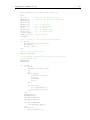
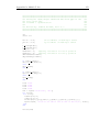
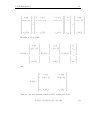
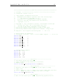
MODELING AND ANALYSIS OF A WAVELET NETWORK
BASED OPTICAL SENSOR FOR VIBRATION
MONITORING
A THESIS IN MECHATRONICS
Presented to the faculty of the American University of Sharjah
School of Engineering
in partial fulfillment of
the requirements for the degree
MASTER OF SCIENCE
by
YASMINE AHMED EL-ASHI
B.S. 2006
Sharjah, UAE
©2010
YASMINE AHMED EL-ASHI
ALL RIGHTS RESERVED
We approve the thesis of Yasmine Ahmed El-Ashi
Date of signature
__________________________
Dr. Rached Dhaouadi
Associate Professor, Electrical Engineering, AUS
Thesis Advisor
__________________
________________________
Dr. Taha Landolsi
Assistant Professor, Computer Engineering, AUS
Thesis Co-Advisor
_________________
________________________
Dr. Khaled Assaleh
Associate Professor, Electrical Engineering, AUS
Graduate Committee
__________________
________________________
Dr. Ameen El-Sinawi
Associate Professor, Mechanical Engineering, AUS
Graduate Committee
__________________
________________________
Dr. Rached Dhaouadi
Associate Professor,
Coordinator, Mechatronics Engineering Graduate Program
__________________
_______________________
Dr. Hany El-Kadi
Associate Dean, College of Engineering
__________________
_______________________
Dr. Yousef Al Assaf
Dean, College of Engineering
__________________
________________________
Mr. Kevin Lewis Mitchell
Director, Graduate & Undergraduate Programs & Research
__________________
MODELING AND ANALYSIS OF A WAVELET NETWORK
BASED OPTICAL SENSOR FOR VIBRATION MONITORING
Yasmine Ahmed El-Ashi, Candidate for Master of Science in Mechatronics
Engineering
American University of Sharjah, 2010
ABSTRACT
The main objective of this research is to present a wavelet network based
optical lateral position sensor for vibration monitoring using a 2×2 photodetector
array. In our approach, the power distribution of the light spot is measured taking
into consideration the radial symmetry of the spot and its Gaussian intensity profile.
The proposed system uses a He-Ne laser source whose Gaussian beam impinges on
the photodetector array. The normalized optical power for each photocell is obtained
theoretically by deriving the optical power equations as the beam scans the plane of
photodetectors. The position detection is based on finding a relationship between the
power distribution of the photodetector array and the position of the beam center.
An experimental setup of the system is developed to validate the theoretical results.
Furthermore, a wavelet network function approximation technique is used to estimate
the x–y position of the beam center corresponding to the measured optical powers.
iii
Contents
Abstract
iii
List of Figures
vi
List of Tables
x
Acknowledgements
xi
1 Introduction
1
2 Beam Optics
2.1 The Wave Equation . . . . . . . . .
2.2 Monochromatic waves . . . . . . .
2.2.1 Complex wavefunction . . .
2.2.2 Complex Amplitude . . . .
2.2.3 The Helmholtz Equation . .
2.2.4 Intensity, Power and Energy
2.3 Wavefronts . . . . . . . . . . . . . .
2.3.1 The Plane Wave . . . . . .
2.3.2 Paraxial Waves . . . . . . .
2.3.3 The Gaussian Beam . . . .
.
.
.
.
.
.
.
.
.
.
.
.
.
.
.
.
.
.
.
.
.
.
.
.
.
.
.
.
.
.
.
.
.
.
.
.
.
.
.
.
.
.
.
.
.
.
.
.
.
.
.
.
.
.
.
.
.
.
.
.
.
.
.
.
.
.
.
.
.
.
.
.
.
.
.
.
.
.
.
.
.
.
.
.
.
.
.
.
.
.
.
.
.
.
.
.
.
.
.
.
3 Functional Approximation with Wavelet Networks
3.1 Function Approximation . . . . . . . . . . . . . . . .
3.2 Neural networks . . . . . . . . . . . . . . . . . . . . .
3.3 Wavelet Transforms . . . . . . . . . . . . . . . . . . .
3.3.1 The Continuous Wavelet Transform (CWT) .
3.3.2 Inverse Wavelet Transform . . . . . . . . . . .
3.3.3 Wavelet bases and frames . . . . . . . . . . .
3.4 Wavelet Networks (WN) . . . . . . . . . . . . . . . .
3.4.1 Adaptive Discretization . . . . . . . . . . . .
3.4.2 Wavelet Network Structure . . . . . . . . . . .
3.4.3 WN Learning . . . . . . . . . . . . . . . . . .
iv
.
.
.
.
.
.
.
.
.
.
.
.
.
.
.
.
.
.
.
.
.
.
.
.
.
.
.
.
.
.
.
.
.
.
.
.
.
.
.
.
.
.
.
.
.
.
.
.
.
.
.
.
.
.
.
.
.
.
.
.
.
.
.
.
.
.
.
.
.
.
.
.
.
.
.
.
.
.
.
.
.
.
.
.
.
.
.
.
.
.
.
.
.
.
.
.
.
.
.
.
.
.
.
.
.
.
.
.
.
.
.
.
.
.
.
.
.
.
.
.
.
.
.
.
.
.
.
.
.
.
.
.
.
.
.
.
.
.
.
.
.
.
.
.
.
.
.
.
.
.
.
.
.
.
.
.
.
.
.
.
.
.
.
.
.
.
.
.
.
.
5
7
75
10
14
10
14
14
10
11
15
16
12
13
17
18
13
15
20
23
17
.
.
.
.
.
.
.
.
.
.
29
23
29
23
25
31
27
34
27
34
30
37
30
37
39
31
39
31
40
32
33
41
.
.
.
.
.
.
.
43
35
35
43
44
35
53
43
64
53
60
69
69
60
63
74
5 Position Detection using Wavelet Network
5.1 Network Initialization . . . . . . . . . . . . . . . . . . . . . . . . . . .
5.2 Training and Testing of Wavelet Network . . . . . . . . . . . . . . . .
5.3 Vibration Monitoring . . . . . . . . . . . . . . . . . . . . . . . . . . .
70
81
71
83
72
84
87
99
4 Optical System Modeling and Design
4.1 System Architecture . . . . . . . . . . . . .
4.2 Theoretical Optical Acquisition Model . . .
4.2.1 Modeling Optical Apodization . . . .
4.2.2 Modeling System Imperfections . . .
4.3 Experimental Study of the Position Detector
4.3.1 Experimental Setup . . . . . . . . . .
4.3.2 Optical Model Validation . . . . . . .
.
.
.
.
.
.
.
.
.
.
.
.
.
.
.
.
.
.
.
.
.
.
.
.
.
.
.
.
.
.
.
.
.
.
.
.
.
.
.
.
.
.
.
.
.
.
.
.
.
.
.
.
.
.
.
.
.
.
.
.
.
.
.
.
.
.
.
.
.
.
.
.
.
.
.
.
.
.
.
.
.
.
.
.
.
.
.
.
.
.
.
6 Conclusions
101
88
Bibliography
102
89
Appendix A: Matlab Codes
105
92
Appendix B: User Manual for Wavelet Network
.1 WN Initialization . . . . . . . . . . . . . . . .
.1.1
Initializing Woh and Woi . . . . . . . .
.1.2
Dyadic Initialization . . . . . . . . . .
.2 Feedforward Algorithm . . . . . . . . . . . . .
.3 Backpropagation Algorithm . . . . . . . . . .
.3.1
Updating the parameters of Woi . . . .
.3.2
Updating the parameters of Woh . . .
.3.3
Updating the parameters of m and d .
Code
. . . .
. . . .
. . . .
. . . .
. . . .
. . . .
. . . .
. . . .
.
.
.
.
.
.
.
.
.
.
.
.
.
.
.
.
.
.
.
.
.
.
.
.
.
.
.
.
.
.
.
.
.
.
.
.
.
.
.
.
.
.
.
.
.
.
.
.
.
.
.
.
.
.
.
.
.
.
.
.
.
.
.
.
.
.
.
.
.
.
.
.
139
152
139
152
140
153
157
143
167
150
154
173
154
174
178
157
180
159
Appendix C: DAQ Code
190
166
Appendix D: Microcontroller Code
194
170
VITA
219
v
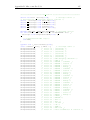
List of Figures
2.1
2.4
2.5
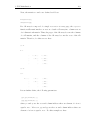
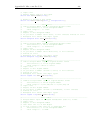
A vibrating string at an instant of time, the quantities shown are used
in the derivation of the classical one-dimensional Wave equation [15].
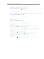
Representation of a monochromatic wave at a fixed position r: (a)
the wavefunction u (t) is a harmonic function of time; (b) the complex
amplitude U = a exp (jϕ) is a fixed phasor; (c) the complex wavefunction U (t) = U exp (j2πf t) is a phasor rotating with angular velocity
ω = 2πf radians/s [13]. . . . . . . . . . . . . . . . . . . . . . . . . . .
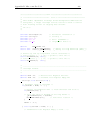
(a) The magnitude of a paraxial wave as a function of the axial distance
z. (b) The wavefronts and wavefront normals of a paraxial wave [13].
Gaussian beam model for the laser source used in the proposed system.
The normalized Gaussian intensity profile. . . . . . . . . . . . . . . .
21
15
26
20
27
20
3.1
3.2
3.3
3.4
3.5
(a) Single neuron model. (b) Simplified schematic of
Feedforward neural network [25]. . . . . . . . . . .
2
Graph of ψ1,0 (x) = ψ (x) = xe−x [26]. . . . . . . .
Graph of ψ1/2,0 [26]. . . . . . . . . . . . . . . . . . .
Function approximation using wavelet networks. . .
25
32
33
26
36
29
36
29
41
33
2.2
2.3
4.1
4.2
4.3
4.4
4.5
single neuron [25].
. . . . . . . . . .
. . . . . . . . . .
. . . . . . . . . .
. . . . . . . . . .
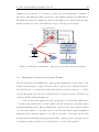
Hardware architecture of the proposed position detection system. . .
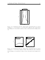
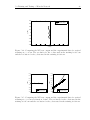
Parameters definition for area Ax . . . . . . . . . . . . . . . . . . . . .
Parameters definition for area Ay . . . . . . . . . . . . . . . . . . . . .
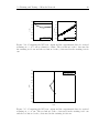
Parameters definition for area Axy . . . . . . . . . . . . . . . . . . . .
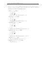
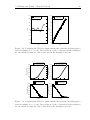
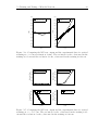
(a) Case 1: x ≥ x0 , (b) Case 2: x ≤ x0 , (c) Case 3: 0 ≤ x ≤ x0 , (d)
Case 4: −x0 ≤ x ≤ 0, (e) Case 5: x = 0, (f ) Case 6: x = x ≥ x0 + ρ0 .
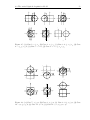
4.6 (a) Case 7: y ≥ y0 , (b) Case 8: y ≤ y0 , (c) Case 9: 0 ≤ y ≤ y0 , (d)
Case 10: −y0 ≤ y ≤ 0, (e) Case 11: y = 0, (f ) Case 12: y = y ≥ y0 + ρ0 .
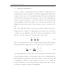
4.7 Example of beam center position as it scans the photocell’s regions. .
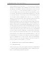
4.8 Quadcell array of photodetectors. . . . . . . . . . . . . . . . . . . . .
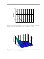
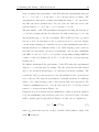
4.9 The normalized power obtained by photocell 1, as the beam center
scans the quadcell plane. . . . . . . . . . . . . . . . . . . . . . . . . .
4.10 The normalized power obtained by photocell 2, as the beam center
scans the quadcell plane. . . . . . . . . . . . . . . . . . . . . . . . . .
4.11 The normalized power obtained by photocell 3, as the beam center
scans the quadcell plane. . . . . . . . . . . . . . . . . . . . . . . . . .
4.12 The normalized power obtained by photocell 4, as the beam center
scans the quadcell plane. . . . . . . . . . . . . . . . . . . . . . . . . .
vi
69
15
11
44
36
37
45
48
39
50
41
58
48
58
48
62
52
65
54
66
56
56
66
67
57
67
57
4.13 Quadcell arrangement for the experimental setup showing different ,
and δ. . . . . . . . . . . . . . . . . . . . . . . . . . . . . . . . . . . .
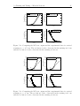
4.14 Variation of the optical power detected by all four photodetectors as
the beam is moved along y = x line for different values of , and δ. . .
4.15 Plot of the normalized power for photocell 1 vs. , when the beam
center is at the origin of the quadcell plane. and δ are assumed to be
equal. . . . . . . . . . . . . . . . . . . . . . . . . . . . . . . . . . . .
4.16 Plot of normalized power for photocell 1 vs. and δ, when the beam
centroid is at the origin of the quadcell plane. . . . . . . . . . . . . .
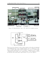
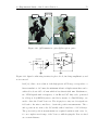
4.17 Experimental prototype of the optical power acquisition system. . . .
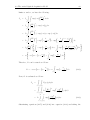
4.18 Block diagram for photo-voltage acquisiton and position measurement
system (HBX: H-bridge for motor X; HBY: H-bridge for motor Y; MX:
motor X; MY: motor Y; PWM1: pulse width modulated signal fed in
to motor X; PWM2: pulse width modulated signal fed in to motor Y;
COM1: communication port 1; COM2: communication port 2; CLK:
clock to synchronize photo-voltage acquisition, position measurement;
DIO: digital input/output channels; PC: personal computer). . . . . .
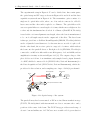
4.19 Optical setup of the system. . . . . . . . . . . . . . . . . . . . . . . .
4.20 (a)Transmission optics.(b)Reception optics. . . . . . . . . . . . . . . .
4.21 Signal conditioning circuitry for photodiode, involving amplification,
and noise removal. . . . . . . . . . . . . . . . . . . . . . . . . . . . .
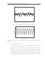
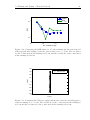
4.22 Plot of photocell output voltage in darkness. . . . . . . . . . . . . . .
4.23 Plot of photocell output voltage in ambient light, when no laser beam
is applied. . . . . . . . . . . . . . . . . . . . . . . . . . . . . . . . . .
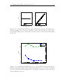
4.24 Plot of photocell output voltage vs. y position of the center of the
beam while setting the x position at 1.05 cm. . . . . . . . . . . . . .
4.25 Plot of photocell output voltage vs. y position of the center of the
beam while setting the x position at − 1.05 cm. . . . . . . . . . . . .
4.26 Plot of photocell output voltage vs. y position of the center of the
beam while setting the x position at 0.55 cm. . . . . . . . . . . . . .
4.27 Plot of photocell output voltage vs. y position of the center of the
beam while setting the x position at −0.55 cm. . . . . . . . . . . . .
4.28 Plot of photocell output voltage vs. y position of the center of the
beam while setting the x position at 0 cm. . . . . . . . . . . . . . . .
4.29 Uncertainity region when initializing the position of the beam center.
5.1
5.2
5.3
5.4
5.5
Position detection system block diagram. . . . . . . . . . . . . . . . .
Wavelet network structure for the position detection problem. . . . .
Dyadic grid for wavelet network Initialization. . . . . . . . . . . . . .
Plot of MSE vs. Iterations for different values of Nw , where the theoretical model without gaps is used for training the WN, µ= 0.0001,
γ= 0.9999, no preprocessing condition is applied on the data. . . . . .
Plot of MSE vs. Iterations for different values of Nw , where the theoretical model without gaps is used for training the WN, µ= 0.1, γ=
0.9, preprocessing condition in equation 5.5 applied on the data. . . .
vii
68
58
68
58
70
59
70
60
71
61
61
71
72
62
73
63
63
73
74
64
64
74
77
66
77
66
78
67
67
78
68
79
69
80
82
70
82
71
72
84
86
74
86
74
5.6
5.7
5.8
5.9
5.10
5.11
5.12
5.13
5.14
5.15
5.16
5.17
Plot of MSE vs. Iterations for different values of Nw , where the theoretical model without gaps is used for training the WN, µ = 0.1, γ =
0.9. . . . . . . . . . . . . . . . . . . . . . . . . . . . . . . . . . . . . .
Plot of MSE vs. Iterations for different values of µ, where the simulated
data without gaps is used for training the wavelet network, Nw = 63 .
Comparing the MSE values vs. Nw after training the theoretical model
with gaps and after testing for the theoretical data set at x = 0 cm.
The resolution for the x data used in the training is 0.1 cm and the
resolution for the y data used in the training is 0.02 cm. . . . . . . .
Comparing the WN test output and the theoretical model with gaps
for vertical scanning at x = 0 cm. The resolution for the x data used
in the training is 0.1 cm and the resolution for the y data used in the
training is 0.02 cm. . . . . . . . . . . . . . . . . . . . . . . . . . . . .
Comparing the WN test output and the theoretical model with gaps
for vertical scanning at x = 0 cm. The resolution for the x data used
in the training is 0.1 cm and the resolution for the y data used in the
training is 0.02 cm. . . . . . . . . . . . . . . . . . . . . . . . . . . . .
Comparing the WN test output and the theoretical model with gaps
for vertical scanning at x = 0 cm. The resolution for the x data used
in the training is 0.1 cm and the resolution for the y data used in the
training is 0.02 cm. . . . . . . . . . . . . . . . . . . . . . . . . . . . .
Comparing the WN test output and the experimental data for vertical
scanning at x = −0.55 cm and x = 0.55 cm. The resolution for the x
data used in the training is 0.1 cm and the resolution for the y data
used in the training is 0.02 cm. . . . . . . . . . . . . . . . . . . . . .
Comparing the WN test output and the experimental data for vertical
scanning at x = −0.55 cm as a function of time. The resolution for
the x data used in the training is 0.1 cm and the resolution for the y
data used in the training is 0.02 cm. . . . . . . . . . . . . . . . . . . .
Comparing the WN test output and the experimental data for vertical
scanning at x = 0.55 cm as a function of time. The resolution for the
x data used in the training is 0.1 cm and the resolution for the y data
used in the training is 0.02 cm. . . . . . . . . . . . . . . . . . . . . .
Comparing the WN test output and the experimental data for vertical
scanning at x = 0 cm. The resolution for the x data used in the training
is 0.1 cm and the resolution for the y data used in the training is 0.02
cm. . . . . . . . . . . . . . . . . . . . . . . . . . . . . . . . . . . . . .
Comparing the WN test output and the experimental data for vertical
scanning at x = 0 cm as a function of time. The resolution for the x
data used in the training is 0.1 cm and the resolution for the y data
used in the training is 0.02 cm. . . . . . . . . . . . . . . . . . . . . .
Comparing the WN test output and the experimental data for vertical
scanning at x = −0.55 cm. The resolution for the x data used in the
training is 0.1 cm and the resolution for the y data used in the training
is 0.02 cm. . . . . . . . . . . . . . . . . . . . . . . . . . . . . . . . . .
viii
87
75
87
75
89
76
89
77
90
78
90
78
79
91
79
91
92
80
80
92
93
81
81
93
5.18 Comparing the WN test output and the experimental data for vertical
scanning at x = 0.55 cm. The resolution for the x data used in the
training is 0.1 cm and the resolution for the y data used in the training
95
is 0.02 cm. . . . . . . . . . . . . . . . . . . . . . . . . . . . . . . . . . 82
5.19 Comparing the WN test output and the experimental data for vertical
scanning at x = 0 cm. The resolution for the x data used in the training
is 0.1 cm and the resolution for the y data used in the training is 0.02
cm. . . . . . . . . . . . . . . . . . . . . . . . . . . . . . . . . . . . . . 83
95
5.20 Comparing the MSE values vs. Nw after training the theoretical model
with gaps and after testing for the theoretical data set at x = 0 cm.
The resolution for the x data used in the training is 0.05 cm and the
resolution for the y data used in the training is 0.02 cm. . . . . . . . 84
96
5.21 Comparing the WN test output and the theoretical model with gaps
for vertical scanning at x = 0 cm. The resolution for the x data used
in the training is 0.05 cm and the resolution for the y data used in the
training is 0.02 cm. . . . . . . . . . . . . . . . . . . . . . . . . . . . . 84
96
5.22 Comparing the WN test output and the theoretical model with gaps
for vertical scanning at x = 0 cm as a function of time. The resolution
for the x data used in the training is 0.05 cm and the resolution for
97
the y data used in the training is 0.02 cm. . . . . . . . . . . . . . . . 85
5.23 Comparing the MSE values vs. Nw after training the theoretical model
with gaps and after testing for the experimental data set at x = 0 cm.
The resolution for the x data used in the training is 0.05 cm and the
97
resolution for the y data used in the training is 0.02 cm. . . . . . . . 85
5.24 Comparing the WN test output and the experimental data for vertical
scanning at x = 0 cm. The resolution for the x data used in the training
is 0.05 cm and the resolution for the y data used in the training is 0.02
98
cm. . . . . . . . . . . . . . . . . . . . . . . . . . . . . . . . . . . . . . 86
5.25 Comparing the WN test output and the experimental data for vertical
scanning at x = 0 cm as a function of time. The resolution for the x
data used in the training is 0.05 cm and the resolution for the y data
used in the training is 0.02 cm. . . . . . . . . . . . . . . . . . . . . . 86
98
5.26 Shaded region indicates the area of detection and × represents the
center of one photocell. . . . . . . . . . . . . . . . . . . . . . . . . . . 100
87
ix
List of Tables
4.1
Table showing the range of each region. . . . . . . . . . . . . . . . . .
x
52
62
Acknowledgements
First and foremost, I thank Allah the Most Gracious, the Most Merciful, for giving me
the will and power to complete my thesis research, and allowing me to pass through
such an experience where not only do you acquire the academic skills of research, but
you also learn other qualities such as patience and perseverance.
Next, I would like to express my sincere gratitude to my research advisors, Dr. Taha
Landolsi and Dr. Rached Dhaouadi, to whom I owe a lot, for their patience, guidance
and encouragement throughout the different stages of the research. I highly appreciate
their vision, novel ideas, and their excitement at every big or small new finding made.
I hope they accept my apologies for any inconveniences or disappointments that I
might have caused.
I am also particularly grateful to my parents for their continuous support. Finally, it
is with pleasure that I express my appreciation to all my friends and colleagues who
supported me and aided me in both the good and hard times.
xi
1
Introduction
There are numerous applications which require accurate, noncontact position measurements, such as vibration monitoring as well as vibration measurement systems
with frequencies ranging from fractions of Hz to kHz and amplitudes varying between
nanometers to meters [1].
Natural vibration is a manifestation of the oscillatory behavior in physical
systems, as a result of a repetitive interchange of two types of energy, such as kinetic
and potential energies among components in mechanical systems [2]. Additional
factors responsible for mechanical vibrations in machines, components and systems,
involve unbalanced inertia, bearing failure in rotating systems, poor kinematic design
resulting in a non-rigid and non-isolating structure, component failure, and operation
outside prescribed load ratings [3]. Such types of vibration are usually categorized as
undesirable or harmful vibration, which also include structural motions generated due
to earthquakes, noise generated by construction equipment, and dynamic interactions
between vehicles and bridges or guide ways. The elimination or suppression of such
Introduction
2
undesirable vibrations will result in a reduction in noise levels and improved work
environment, maintenance of high performance standards and production efficiency,
as well as prolonging the useful life of industrial machinery, thus cutting down the
costs and frequency of maintenance. On the other hand, there are useful forms of
vibration which include those generated by devices used in physical therapy and
medical applications, vibrators used in industrial mixers, part feeders and sorters,
and vibratory material removers such as drills and finishers. For instance, product
alignment for industrial processing or grading can be carried out by means of vibratory
conveyers or shakers [2].
Over the past 50 years, the speeds of operation of machinery have doubled,
and consequently vibration loads generated due to rotational excitation would have
quadrupled if proper actions of design and control were not considered. As vibration isolation and reduction techniques have become an integral part of machine
design the need for accurate measurement and analysis of mechanical vibration has
grown significantly [4]. To accomplish this, we should undergo a phase of monitoring
and diagnostic testing of vibration which would require devices such as sensors and
transducers, signal conditioning and modification hardware (such as filters, amplifiers, analog/digital conversion means), and actuators (such as vibration exciters or
shakers) [2].
Vibrations have been mainly detected by contact and noncontact-type sensors for measuring displacement, velocity or acceleration [4]. Conventional vibration
sensors such as potentiometers or linear variable differential transformers (LVDTs),
piezoelectric accelerometers, and strain gauges are common in practice. Contact-type
sensors such as potentiometers and strain gauges are used to sense displacement either by making physical contact with or attached to the object of interest. However,
in some cases, physical contact may not be practical, in terms of impeding or altering
the natural behavior of the device, or inability to install them in hard-to-reach places,
or when the object is fragile and prone to damage [5]. Moreover, potentiometers have
the following limitations: (1) High frequency or highly transient measurements are
not feasible because of factors such as slider bounce, friction and inertia resistance,
and induced voltages in the wiper arm and primary coil. (2) Resolution is limited by
the number of turns in the coil and by the coil uniformity. (3) Wear out and heating
Introduction
3
up with associated oxidation in the coil and slider contact cause accelerated degradation [2]. Another extensively used vibration sensor is the piezoelectric accelerometer,
an electromechanical device where its output voltage is proportional to an applied
vibratory acceleration. Although it is light in weight, exhibits a high frequency response (up to about 1 MHz), accurate and sensitive, piezoelectric transducers cover a
relatively small area, and are difficult to electrically isolate making them unsuitable
in applications surrounded by electrical and magnetic fields [6].
In situations where physical contact between the sensor and the device is
inaccessible and undesirable, non-contact type sensors provide a better option. These
sensors operate on capacitive, inductive, magnetic or optical principles. For instance,
capacitive sensors have very high resolution (d <0.01 nm), however they are sensitive
to changes in temperature, humidity and surface irregularities. Inductive sensors
measure displacement by current induction when a ferrous or nonferrous metallic
object passes through the electromagnetic field of a coil wound. Such sensors also have
relatively high-resolution (nanometer) and good bandwidth (tens of kilohertz), with
the added advantage of being immune to dirt, water, and lubricating oil. Capacitive
and inductive sensors are generally expensive and require special signal processing
circuitry for operation [5].
In the recent years, optical non-contact position sensors have received great
attention owing to their immunity to electromagnetic interference, resistance to corrosion, chemical inertness, and light weight. Such sensors include Fabry-Perot interferometers, fiber Bragg grating (FBG) arrays, Michelson interferometers, and MachZehnder interferometers (MZI) which are used for measuring mechanical vibrations
at magnetic cores of power transformers [6]. Fabry-Perot interferometers are used
extensively as versatile tools for fast and sensitive vibration analysis in harsh engineering environments. The sensitivity of these sensors is increased by increasing the
length of the sensing area; however, such an approach causes the sensor to be affected
by fluctuations. Not only do these sensors suffer from limitations in signal demodulation caused by phase ambiguity, but the external disturbance aforementioned can
also be observed as a phase drift that is often compensated in order to measure the
dynamic parameters of the system [7],[8]. Furthermore, Bragg gratings have a relatively poor resolution, and are difficult to be located and installed in the structure
Introduction
4
[7]. The conventional Michelson interferometer-based laser vibrometer suffer from
two main drawbacks; limited sensitivity to surface displacement detection and their
intolerance to the presence of optical speckles in the light beams. An abrupt change
in the speckles can lead to a sudden degradation in the optical power reaching the
photodetector, and a misinterpretation of the diminished output [9].
Nevertheless, reflective optical proximity sensors offer comparable performance
to their inductive and capacitive counterparts in terms of resolution and bandwidth.
In an optical sensor, a source impinges light onto a target object, and subsequently
reflects off the object’s surface, which is then projected onto a detector. The sensed
intensity of the light reflected onto the photodiode is related to an object’s distance
from the photodetector. Optical sensors are also relatively inexpensive, unlike the
capacitive and inductive sensors [5].
One feature common to all of the previously mentioned non-contact sensors is
that they are capable of measuring displacement in the direction of the optical axis
of the system. To measure lateral displacement, that is perpendicular to the optical
axis a position-sensitive detector (PSD) is usually used. Makynen, Kostamovaara,
and Myllyla presented in [1] a lateral displacement sensing method based on the
idea of imaging an illuminated cooperative target on a four-quadrant (4Q) PSD. This
arrangement has the advantage of being capable of providing true lateral displacement
instead of angular displacement in large working volume without calibration. This
is possible due to the unique property of a target-focused 4Q detector, in which
the size of the measurement span is determined solely by the size of the cooperative
target, thus providing inherently accurate, constant scaling that is independent of the
target distance. The 4Q detector consists of four photodiodes (quadrants) positioned
symmetrically around the center of the sensor and separated by a narrow gap. The
position information is derived from the signals received by the quadrants as the
image spot moves over the detector surface.
Other analog position-sensitive detectors that have been proposed by Makynen, Kostamovaara, and Myllyla in [10] are the lateral-effect photodiode (LEP) detectors. An LEP is a large-area, single-element photodiode having uniform resistive
layers with two wide edge contacts on both the anode and cathode. The current
carriers generated in the illuminated region are divided between the electrodes in
Introduction
5
proportion to the distance of the current paths between the illuminated region and
the electrodes. The measurement field of the LEP is determined by the size of its
active area and it detects the spot position irrespective of spot size or shape. The
achievable SNR and the resolution of the 4Q detector is better than that of the LEP.
However, LEP provides far better accuracy in a typical outdoor environment because
atmospheric turbulence induced, spatially uncorrelated intensity fluctuations within
the light spot which result from defocusing, derange the measurement resolution of
the 4Q receiver [10].
Furthermore, one of the established non-contact lateral position sensing techniques involve the use of a charge-coupled device (CCD) camera. The CCD sensor
records the light intensity in each pixel by means of charge coupling where the charges
are transferred to a second bank of photosites before analog-to-digital conversion is
made. In this case, position measurment is usually performed by calculating the
center of gravity of the light distribution [11].
The quadcell array for lateral, two dimensional position measurement consists
of square shaped and homogeneous photodetectors (PDs), clustered in a 2×2 configuration [12]. The lateral dimensions of standard discrete commercial PSDs extend up
to several millimeters. Using a quadcell array of photodetectors involves several advantages, such as, large position measurement area, reduced number of direct output
signals, acceptance of a wide range of spot intensity profiles and radii, negligible spatial fluctuation of the signal, immunity to coordinate crosstalk, and possible operation
with modulated or pulsed light [12].
The transfer characteristics of the photodetector depend on the shape and
intensity distribution of the beam spot. In [1], the authors used a perfectly linear
transfer function by assuming a square light spot with uniform intensity distribution
and with its edges parallel to the edges of the quadrants. However, in most practical conditions, the spot intensity profile exhibits radial symmetry and the resulting
response is non-linear [12].
The purpose of this research is to present a wavelet network based, non-contact
optical position sensor using a photodetector array, which measures the power distribution of the light spot, taking into consideration the nonlinearities involved, that is
the radial symmetry of the spot and its Gaussian intensity profile.
Introduction
6
Since only the optical power of each photodetector can be practically acquired,
we aim to find a relationship between the power distribution of the photodetector
array and the position of the spot center, through a theoretical and experimental
model. In our approach, we account for the nonlinear transfer characteristics, by
using a wavelet network as a function approximation technique to estimate the x–y
position of the light spot center, that corresponds to the acquired optical powers.
Therefore, in order to achieve a more accurate system model and to depict a better
comparison between the theoretical results and experimental measurements, we take
into consideration the circular shape and Gaussian intensity profile of the light spot in
formulating the optical power equations. These equations will be further used, along
with a developed algorithm, to simulate the theoretical model of the proposed position
detection system. In addition, system imperfections such as the gap separations
between the photodetectors, have been accounted for in the simulation and their
effect on the optical power distribution is studied. A potential application of our
proposed system will be on vibration monitoring, where the position information will
be employed to obtain characteristics such as the amplitude, frequency and speed of
vibration.
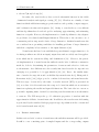
The rest of the thesis report is organized as follows; in Chapters 2 and 3, we
give an overview of beam optics, wavelets and wavelet networks (WN) and their use in
function approximation. Next, in Chapter 4, we describe the design of our proposed
system, which involves the system architecture of the theoretical optical acquisition
model of the position sensor. We also present the experimental setup and results used
to validate the theoretical optical model. Finally, in Chapter 5, we discuss the results
obtained after training and testing the WN.
2
Beam Optics
The optical signal emanating from the He-Ne laser source is commonly modeled as
a Gaussian beam traveling in free-space whose intensity varies with the propagation
distance z and the radius of the beam ρ, measured from its center. As the laser beam
propagates, its power remains constant but its intensity decreases with an inversesquare law. This behavior is important to consider in the theoretical model of the
proposed system as well as the design of the experimental setup because the power
intercepted by the photodetector depends on the area of the detector active surface.
In this Chapter, we will discuss the propagation of light in free-space that would lead
us to the derivation of Gaussian beam optics, intensity and power characteristics.
2.1
The Wave Equation
Light propagates in the form of waves. In free space, light waves travel with speed
co . A homogeneous transparent medium such as glass is characterized by a single
constant, its refractive index ( n ≥ 1). In a medium of refractive index n, light waves
2.1 The Wave Equation
8
travel with a reduced speed.
c=
co
.
n
(2.1)
An optical wave is described mathematically by a real function of position r = (x, y, z)
and time t, denoted by u (r, t) and known as the wavefunction. It satisfies the wave
equation,
∇2 u −
1 ∂ 2u
= 0,
c2 ∂t2
(2.2)
where ∇2 is the Laplacian operator, ∇2 = ∂ 2 /∂x2 + ∂ 2 /∂y 2 + ∂ 2 /∂z 2 . Any function
satisfying (2.2) represents a possible optical wave. Because the wave equation is linear,
the principle of superposition applies, for instance if u1 (r, t) and u2 (r, t) represent
optical waves, then u (r, t) = u1 (r, t) + u2 (r, t) also represents a possible optical wave
[13].
When electric dipoles are forced to oscillate, they induce an electric field that
oscillates at the same frequency. In addition, due to the motion of oscillating charges,
a magnetic field oscillating at the same frequency is also induced. These simultaneous
oscillating fields are the basis for all known modes of electromagnetic radiation. Thus,
X-rays, UV radiation, visible light, and infrared and microwave radiation are all part
of the same physical phenomenon. Although each radiating mode is significantly
different from the others, all modes of electromagnetic radiation can be described by
the same equations, since they all obey the same basic laws.
Oscillation alone is insufficient to account for electromagnetic radiation. The
other important observation is that radiation propagates. It is emitted by a source
and if uninterrupted, can propagate indefinitely in both time and space. Although
there are certain media that can block radiation, we find it more astonishing that
electromagnetic waves can propagate through free space; unlike electrical currents or
sound, conductors are not necessary for the transmission of radiation. Although this
property is unique to radiation, some of its characteristics is analogous to the propagation of acoustical waves or vibrations in solids. These waves, like the electromagnetic
waves combine propagation with the oscillation of a physical parameter. Thus, by
analogy the description of the propagation of electromagnetic radiation should involve equations similar to those describing the propagation of sound waves or the
vibrational modes of solids. Furthermore, since we anticipate that electromagnetic
2.1 The Wave Equation
9
waves are the result of oscillatory motion of electric charges, we should be able to
derive equations describing their propagation from Maxwell’s equations [14].
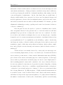
First, to demonstrate the analogy between electromagnetic waves propagation
and that of acoustic waves, we shall derive the wave equation for the case of just one
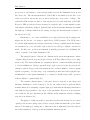
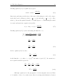
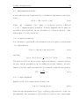
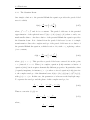
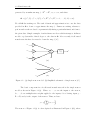
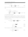
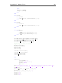
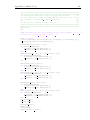
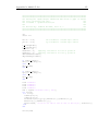
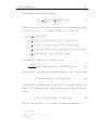
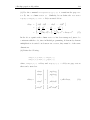
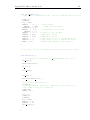
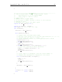
spatial variable, for the physical system represented by a vibrating string. Consider
a perfectly flexible homogeneous string stretched to a uniform tension τ between two
points. Let u (x, t) be the displacement of the string from its horizontal position. The
τ2
θ1
P
Q
θ2
τ1
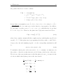
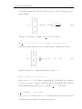
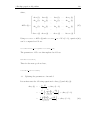
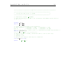
Figure 2.1: A vibrating string at an instant of time, the quantities shown are used in
the derivation of the classical one-dimensional Wave equation [15].
quantities τ1 and τ2 are the tensions at the points P and Q on the string. Both τ1
and τ2 are tangential to the curve of the string. Assuming that there is only vertical
motion of the string, the horizontal components of the tensions at the points along
the string must be equal. Using the notation provided in Figure 2.1, we have the
following relation,
τ1 cos θ1 = τ2 cos θ2 = τ = constant.
(2.3)
There is a net vertical force that causes the vertical motion of the string, which we
find to be,
Fnet = τ2 sin θ2 − τ1 sin θ1 .
(2.4)
By Newton’s second law (F = ma), this net force is equal to the mass ρ∆x along the
segment P Q times the acceleration of the string, ∂ 2 u/∂t2 . Thus, we can state the
following:
τ2 sin θ2 − τ1 sin θ1 = ρ∆x
∂ 2u
.
∂t2
(2.5)
2.1 The Wave Equation
10
Dividing equation (2.5) by equation (2.3) gives:
tan θ2 − tan θ1 =
ρ∆x ∂ 2 u
.
τ ∂t2
(2.6)
Since tan θ1 and tan θ2 are the slopes of the curve of the string at x and x+∆x, respectively, they can be written as, tan θ1 =
∂u
∂x
= ux (x) and tan θ2 =
∂u
∂x
= ux (x + ∆x),
where ux denotes the partial derivative of u with respect to x. Substituting the values
for tan θ1 and tan θ2 into equation (2.6) yields:
ux (x + ∆x) − ux (x) =
ρ∆x ∂ 2 u
.
τ ∂t2
(2.7)
Dividing equation (2.7), by ∆x and setting the limit ∆x → 0,
ρ ∂ 2u
ux (x + ∆x) − ux (x)
=
,
∆x→0
∆x
τ ∂t2
lim
ρ ∂ 2u
∂ux
=
,
∂x
τ ∂t2
∂ 2u
ρ ∂ 2u
=
.
∂x2
τ ∂t2
(2.8)
And so equation (2.7) becomes,
∂ 2u
1 ∂ 2u
=
,
∂x2
v 2 ∂t2
(2.9)
in the limit ∆x → 0, where v = (τ /ρ)1/2 has units of speed [15]. Its extension to
more spatial variables is given by:
1 ∂ 2u
∂ 2u ∂ 2u ∂ 2u
+
+
=
,
∂x2 ∂y 2 ∂z 2
v 2 ∂t2
∇2 u =
1 ∂ 2u
.
v 2 ∂t2
(2.10)
Although, equations for the propagation of electromagnetic waves are likely
to be similar to those for acoustic waves, there is an important distinction between
2.1 The Wave Equation
11
the two. Acoustic wave equations describe the propagation of a scalar quantity;
electromagnetic wave equations describe the propagation of electric and magnetic
fields, which are vectorial.
In order to derive the equations that describe the propagation of electromagnetic waves, we begin with Maxwell’s equations:
∇×E=−
∂B
+ [0] ,
∂t
(2.11)
∂D
∇×H=−
+ j,
∂t
(2.12)
∇ · D = ρ,
(2.13)
∇ · B = 0.
(2.14)
Where, E, D, H, B, j are respectively the electric field, electric displacement, magnetic
field, magnetic induction and current density vectors. To demonstrate the symmetry
between the effects of electricity and magnetism, for each equation describing the
effects of the electric field there is a counterpart describing effects of the magnetic
field. Even the electric charges fit into the symmetric picture, when a term for electric
charge or electric current is present in one equation, a zero term is present in its
magnetic counterpart, representing the absence of magnetic monopoles. Thus, the
zero term in brackets in equation (2.11) is the magnetic analog to the current density
j in equation (2.12). Similarly, the charge density term ρ in equation (2.13) is replaced
by a zero in equation (2.14).
Maxwell’s equations form the basis for the development of the equations that
describe the propagation of electromagnetic waves. Historically, the electromagnetic
wave equations were derived by Maxwell merely to describe the propagation of oscillating electric or magnetic fields in space. Neither Maxwell nor his peers recognized
the relation between the propagation of electromagnetic fields and the propagation
of light. Optics and the propagation of electromagnetic waves were at that time
considered to be separate and unrelated fields of physics. Only after showing that
the propagation velocity of electromagnetic waves was identical to the already measured speed of light, Maxwell suggested that his results might be more general than
expected and hence applicable to the studies of optics.
2.1 The Wave Equation
12
Inspection of Maxwell’s equations reveals that when the magnets or electric
charges are static, the electric field vector in equation (2.13), does not contain any
terms of the magnetic field, and conversely in equation (2.14) is independent of the
electric field. When in motion however the magnets or electric charges induce fields
that are interdependent. This is apparent in both equations (2.11) and (2.12), where
E depends on the time derivative of B, and where H varies with the magnitude or direction of the current flow or with the time derivative of D. Nevertheless, an equation
that describes the propagation of electric waves is expected to be independent of the
terms that include the magnetic field, and vice versa. Since only two equations (2.11)
and (2.12) describe the dynamic effect of these two fields, we will be using them as
our initial point for deriving the equations describing the propagation of electric or
magnetic waves. We first consider equation (2.11). The simplest way of eliminating
the magnetic field term from this equation is by obtaining the curl of both sides:
∇×∇×E=−
∂
∂
(∇ × B) = −µ (∇ × H) .
∂t
∂t
(2.15)
Assuming that the magnetic permeability µ is constant, it was placed outside the
derivative operators, thereby leaving only the magnetic field to be operated on. However, the term ∇ × H in equation (2.15) can be replaced by the right-hand side of
equation (2.12), thereby eliminating the magnetic field term. The following equation,
∂
∂D
∇ × ∇ × E = −µ
−
+j
∂t
∂t
∂ 2D
∂j
= µ 2 −µ ,
∂t
∂t
(2.16)
(2.17)
is now in the desired form; it contains only terms of electric field or electric charge.
Furthermore, it includes both time and space derivations of these quantities and so
describes both the temporal and spatial variation of the electric field due to the
motion of electric charges. Although this equation is complete in itself, it can be
further simplified by using the vector identity, ∇ × ∇ × A = ∇ (∇ · A) − ∇2 A, where
A is an arbitrary vector and ∇2 = ∇ · ∇ is the Laplacian operator. Thus in the
Cartesian coordinate system, operating on any vector A = Ax êx + Ay êy + Az êz with
2.1 The Wave Equation
13
the Laplacian yields,
2
∂ Ay ∂ 2 Ay ∂ 2 Ay
∂ 2 Ax ∂ 2 Ax ∂ 2 Ax
êx +
êy
∇A =
+
+
+
+
∂x2
∂y 2
∂z 2
∂x2
∂y 2
∂z 2
2
∂ Az ∂ 2 Az ∂ 2 Az
+
êz .
+
+
∂x2
∂y 2
∂z 2
2
Thus, the left hand-side of equation (2.17) can be replaced by:
∇ × ∇ × E = ∇ (∇ · E) − ∇2 E.
(2.18)
However, when the medium in which E propagates is homogeneous (i.e., when all the
spatial derivatives of the electric permeability, vanish), and when the medium does
not contain any free charges (i.e., ρ = 0), the first of these terms is ∇ · E = 0. With
the above vector identities, equation (2.17) can be reduced to:
∇2 E = µ
∂ 2 (εE)
∂j
+µ .
2
∂t
∂t
(2.19)
This is the wave equation that describes the propagation of an electric wave. It does
not specify what caused the field or how the field can be annihilated, but it accurately
predicts the magnitude and direction of E at any point in space or time. Since most
optical elements consist of uniform media, the assumption that ε is constant is always
justified. The second assumption, that is, that the density of unbalanced electric
charges is ρ = 0, is met in free space and in all electrically neutral media, whether
dielectric or conducting. Therefore, by replacing E with the optical wave u (r, t) and
setting µ = µo to the magnetic permeability in free space, and ε = εo to the electric
permeability in free space, and
∂j
∂t
= 0, we end up with the following wave equation
for an optical wave:
∇2 u (r, t) = µo εo
Since, the speed of light c =
√1 ,
µo εo
∂ 2 u (r, t)
.
∂t2
(2.20)
we can finally state the wave equation for an
optical signal propagating in free space, as follows [13]:
∇2 u (r, t) =
1 ∂ 2 u (r, t)
.
c2 ∂t2
(2.21)
2.2 Monochromatic waves
2.2
14
Monochromatic waves
A mononchromatic wave is represented by a wavefunction with harmonic time dependence,
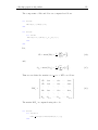
u (r, t) = a (r) cos [2πf t + ϕ (r)] .
(2.22)
Where, a (r) = amplitude, ϕ (r) = phase, f = frequency (cycles/s or Hz) and
ω = 2πf = angular frequency (radians/s). Both the amplitude and the phase are
generally position dependent, but the wavefunction is a harmonic function of time
with frequency f at all positions [13].
2.2.1 Complex wavefunction
It is convenient to represent the real wavefunction u (r, t) in equation (2.22) in terms
of a complex function:
U (r, t) = a (r) exp [jϕ (r)] exp (j2πf t) ,
(2.23)
such that,
u (r, t) = Re {U (r, t)} =
1
[U (r, t) + U ∗ (r, t)] .
2
(2.24)
The function U (r, t) also known as the complex wavefunction, completely describes
the wave, and the wavefunction u (r, t) is simply its real part. Similar to the wavefunction u (r, t) the complex wavefunction U (r, t) must also satisfy the wave equation:
1 ∂ 2U
∇ U − 2 2 = 0.
c ∂t
2
(2.25)
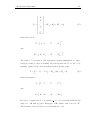
2.2.2 Complex Amplitude
Equation (2.25) can be written in the following form:
U (r, t) = U (r) exp (j2πf t) .
(2.26)
Where the time independent factor U (r) = a (r) exp [jϕ (r)]is referred to as the complex amplitude. The wavefunction u (r, t) is therefore related to the complex ampli-
2.2 Monochromatic waves
15
tude by:
u (r, t) = Re {U (r, t)} = Re {U (r) exp (j2πf t)}
1
=
[U (r) exp (j2πf t) + U ∗ (r) exp (−j2πf t)]
2
(2.27)
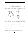
At a given position r, the complex amplitude U (r) is a complex variable as shown
Im {U }
u (t )
a
ϕ ω
ϕ
1
f
R {U }
Re
a
(b )
O
t
Im {U }
ω
(a)
ϕ
a
Re {U }
(c)
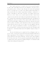
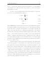
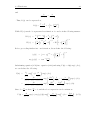
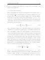
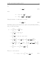
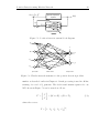
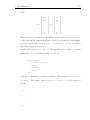
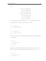
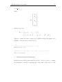
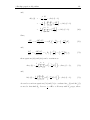
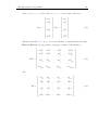
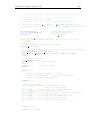
Figure 2.2: Representation of a monochromatic wave at a fixed position r: (a) the
wavefunction u (t) is a harmonic function of time; (b) the complex amplitude U =
a exp (jϕ) is a fixed phasor; (c) the complex wavefunction U (t) = U exp (j2πf t) is a
phasor rotating with angular velocity ω = 2πf radians/s [13].
in Figure 2.2(b), whose magnitude |U (r) | = a (r) is the amplitude of the wave and
whose arg {U (r)} = ϕ (r) is the phase. The complex wavefunction is represented
graphically by a phasor rotating with angular velocity ω = 2πf radians/s (Figure
2.2(c)). Its initial value at t = 0 is the complex amplitude U (r) [13].
2.2.3 The Helmholtz Equation
If we substitute U (r, t) = U (r) exp (j2πf t) into equation (2.25), we get:
∇2 U (r) ej2πf t −
1 ∂2 j2πf t
e
U
(r)
= 0.
c2 ∂t2
(2.28)
2.2 Monochromatic waves
16
Where, the value of the second derivative
∂2
∂t2
U (r) ej2πf t = −(2πf )2 U (r) ej2πf t can
be substituted in the previous equation to arrive at:
(2πf )2
U (r) ej2πf t = 0
c2
∇2 + k 2 U (r) ej2πf t = 0.
∇2 U (r) ej2πf t +
Thus we can now state the Helmholtz equation as follows:
∇2 + k 2 U (r) = 0,
(2.29)
where
k=
ω
2πf
=
c
c
is referred to as the wavenumber [13].
2.2.4 Intensity, Power and Energy
The optical intensity I (r, t), defined as the optical power per unit area (units of
watts/cm2), is proportional to the average of the squared wavefunction,
I (r, t) = 2 u2 (r, t) .
(2.30)
The operation h·i denotes averaging over a time interval of one optical cycle. Using
equation (2.30) along with equation (2.22), we can determine the optical intensity.
Where,
2u2 (r, t) = 2a2 (r) cos2 [2πf t + ϕ (r)]
= |U (r) |2 2cos2 [2πf t + ϕ (r)] .
Using the trigonometric identity, 2cos2 θ = 1 + cos (2θ), we have the following representation for 2u2 (r, t):
2u2 (r, t) = |U (r) |2 {1 + cos (2 [2πf t + ϕ (r)])} ,
(2.31)
2.3 Wavefronts
17
is averaged over an optical period, 1/f ,
I (r, t) = 2 u2 (r, t)
1
=
1/f
Z1/f
|U (r) |2 {1 + cos (2 [2πf t + ϕ (r)])} dt
0
 1/f

Z
Z1/f
|U (r) | 
cos (2 [2πf t + ϕ (r)]) dt
=
1dt +
1/f
0
0
1/f
|U (r) |2
1
|U (r) |2 1
=
t+
sin (2 [2πf t + ϕ (r)])
=
+0
1/f
4πf
1/f
f
0
= |U (r) |2 .
2
Therefore the optical intensity I (r, t) = |U (r) |2 of a monochromatic wave is the
absolute square of its complex amplitude. And interestingly as we have just shown
the intensity of a monochromatic wave does not vary with time [13]. The optical power
P (t) units of watts) flowing into an area A normal to the direction of propagation of
light is the integrated intensity,
Z
P (t) =
I (r, t) dA.
(2.32)
A
The optical energy (units of joules) collected in a given time interval is the time
integral of the optical power over the time interval,
Zt2
E (t) =
P (t) dt.
(2.33)
t1
2.3
Wavefronts
The wavefronts are the surfaces of equal phase, ϕ (r) = constant. The constants
are often taken to be multiples of 2π, ϕ (r) = 2πq, where q is an integer. The
wavefront normal at position r is parallel to the gradient vector ∇ϕ (r) (a vector
with components ∂ϕ/∂x, ∂ϕ/∂y, and ∂ϕ/∂z in a Cartesian coordinate system). It
represents the direction at which the rate of change of the phase is maximum [13].
2.3 Wavefronts
18
2.3.1 The Plane Wave
One of the simplest solutions of the Helmholtz equation in a homogeneous medium
is the plane wave. Using (∇2 + k 2 ) U (r) = 0, we have,
∂ 2U
∂ 2U
∂ 2U
+
+
+ k 2 U = 0.
∂x2
∂y 2
∂z 2
(2.34)
Let U (r) = f (x) g (y) h (z), substitute this expression into equation (2.34) and divide
by U (r):
g (y) h (z) f 00 (x) f (x) h (z) g 00 (y) f (x) g (y) h00 (z) k 2 f (x) g (y) h (z)
+
+
+
= 0,
f (x) g (y) h (z)
f (x) g (y) h (z)
f (x) g (y) h (z)
f (x) g (y) h (z)
f 00 (x) g 00 (y) h00 (z)
+
+
+ k 2 = 0.
f (x)
g (y)
h (z)
(2.35)
Let f 00 /f = −kx2 , g 00 /g = −ky2 , and h00 /h = −kz2 , therefore we can state the following
relations:
kx2 + ky2 + kz2 = k,
(2.36)
d2 f (x)
+ kx2 f (x) = 0,
dx
(2.37)
d2 g (y)
+ ky2 g (y) = 0,
dy
(2.38)
d2 h (z)
+ kz2 h (z) = 0.
dz
(2.39)
When solving for the differential equations (2.37), (2.38), and (2.39), we have:
f (x) = f + e−jkx x + f − ejkx x ,
(2.40)
g (y) = g + e−jky y + g − ejky y ,
(2.41)
h (z) = h+ e−jkz z + h− ejkz z .
(2.42)
The terms with negative exponentials indicate a wave traveling in the positive x, y
or z direction, while the terms with positive exponentials result in waves traveling in
the negative direction. For our present discussion we will select a wave traveling in
2.3 Wavefronts
19
the positive direction, for each coordinate:
U (r) = f (x) g (y) h (z)
= f + e−jkx x g + e−jky y h+ e−jkz z
= f + g + h+ exp [−j (kx x + ky y + kz z)]
= A exp [−j (kx x + ky y + kz z)] .
Let us define a wavenumber vector ~k = kx êx + ky êy + kz êz = ko n̂, where ko = |~k| =
p 2
kx + ky2 + kz2 and n̂ is a unit vector in the direction of propagation. In addition,
we will define a position vector ~r = xêx + yêy + zêz , such that the dot product
~k · ~r = kx x + ky y + kz z. Therefore, the plane wave U (r) can be stated as follows:
~
U (r) = A exp −j k · ~r ,
(2.43)
where A is a complex constant called the complex envelope, and the phase arg {U (r)} =
arg {A} − ~k · ~r. If the plane wave is propagating along the positive z–axis U (r) =
A exp (−jkz) only and assuming arg {A} = 0, the corresponding wavefunction will
be:
u (r, t) = |A| cos (2πf t − kz) .
(2.44)
To maintain a fixed point on the wave (2πf t − kz = constant), one must move in
the positive z direction as time increases, as if following a fixed point on the wave.
The velocity of the wave in this sense is called the phase velocity vp , because it is the
velocity at which a fixed phase point on the wave travels.
d
(arg {U (r)})
dt
d
(2πf t − kz)
dt
dz
2πf − k
dt
2πf − kvp
2πf
vp =
k
=
d
(constant) = 0
dt
= 0
= 0
= 0
ω
=
.
k
2.3 Wavefronts
20
Furthermore, the wavelength λ, is defined as the distance between two successive
maxima (or minima or any other reference points) on the wave, at a fixed instant of
time. Thus we can deduce the following:
[ωt − kz] − [ωt − k (z + λ)] = 2π,
kλ = 2π
2π
,
λ =
k
Since
k=
ω
vp
the wavelength λ can also be stated as:
2πvp
2πvp
vp
2π
=
=
=
k
ω
2πf
f
vp
.
λ =
f
λ =
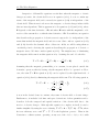
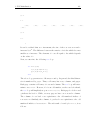
2.3.2 Paraxial Waves
A paraxial wave is a plane wave U (r) = A (r) exp (−jkz), with k =
2π
λ
and wavelength
λ, modulated by a complex envelope A (r) that is a slowly varying function of position.
The envelope is assumed to be approximately constant within a neighborhood of size
λ, so that the wave locally underlies plane wave nature. Since the change of the phase
arg {A (x, y, z)} is small within the distance of a wavelength, the planar wavefronts,
kz = 2πq, of the carrier plane wave bend only slightly, so that their normals are
paraxial rays [13]. For the paraxial wave to satisfy the Helmholtz equation, the
complex envelope A (r) must satisfy another partial differential equation obtained
by substituting U (r) = A (r) exp (−jkz) into equation (2.29). The assumption that
A (r) varies slowly with respect to z signifies that within a distance ∆z = λ, the
change ∆A is much smaller than A itself, i.e., ∆A << A. Since
∆A = (∂A/∂z) ∆z = (∂A/∂z) λ
2.3 Wavefronts
21
| A|
z
λ
(a)
Wavefronts
x
Paraxial rays
y
z
(b )
Figure 2.3: (a) The magnitude of a paraxial wave as a function of the axial distance
z. (b) The wavefronts and wavefront normals of a paraxial wave [13].
it follows that,
∂A
λ
∂z
<< A which implies
∂A
∂z
<<
A
λ
=
Ak
.
2π
And therefore,
∂A
∂z
<< kA.
Similarly, the derivative ∂A/∂z varies slowly within the distance λ, so that
∂ 2 A ∂z 2 << k∂A/∂z
and therefore,
∂ 2A
<< k 2 A
2
∂z
.
Next, we will substitute U (r) = A (r) exp (−jkz) into the Helmholtz equation,
and assume ∂ 2 A/∂z 2 to be negligible in comparison with k∂A/∂z or k 2 A:
∇2 + k 2 U (r) = 0
∇2 + k 2 A (r) exp (−jkz) = 0,
exp (−jkz)
∂ 2A ∂ 2
∂ 2A
+exp
(−jkz)
+
[A exp (−jkz)]+k 2 A exp (−jkz) = 0. (2.45)
∂x2
∂y 2 ∂z 2
2.3 Wavefronts
∂2
∂z 2
The term
22
[A exp (−jkz)] is evaluated accordingly,
∂
∂A
[A exp (−jkz)] =
exp (−jkz) − jkA exp (−jkz) .
∂z
∂z
Therefore,
∂2
∂ 2A
∂A
exp (−jkz)
[A
exp
(−jkz)]
=
exp (−jkz) − jk
2
2
∂z
∂z
∂z
∂A
− jk
exp (−jkz) − jkA exp (−jkz)
∂z
∂ 2A
∂A
exp (−jkz) − k 2 A exp (−jkz) .
=
exp
(−jkz)
−
2jk
∂z 2
∂z
Substituting, the expression for
∂2
∂z 2
[A exp (−jkz)] back into equation (2.45) we get:
∂ 2A ∂ 2A ∂ 2A
∂A
2
2
+
+
− 2jk
− k A + k A exp (−jkz) = 0.
∂x2
∂y 2
∂z 2
∂z
Since we assumed ∂ 2 A/∂z 2 to be relatively very small, we finally obtain the following
Paraxial Helmholtz equation:
∇2T A − 2jk
∂A
= 0,
∂z
(2.46)
where ∇2T = ∂ 2 /∂x2 + ∂ 2 /∂y 2 is the transverse Laplacian operator. An important
solution of the Paraxial Helmholtz equation that exhibits the characteristics of an
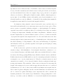
optical beam is a wave known as the Gaussian beam. In principle, the beam power
is concentrated within a small cylinder surrounding the beam axis. The intensity
distribution in any transverse plane is a circularly symmetric Gaussian function centered about the beam axis. The width of this function is minimum at the beam waist
and grows gradually in both directions. In the next discussion, an expression for the
complex amplitude of the Gaussian beam is derived, as well as a description of its
physical properties such as intensity, power and beam radius will be provided [13].
2.3 Wavefronts
23
2.3.3 The Gaussian Beam
One simple solution to the paraxial Helmholtz equation provides the paraboloidal
wave for which,
A1
ρ2
A (r) =
exp −jk
,
z
2z
(2.47)
where, ρ2 = x2 + y 2 and A1 is a constant. The paraboloidal wave is the paraxial
approximation of the spherical wave U (r) = (A1 /r) exp (−jkr) when x and y are
much smaller than z. Another solution of the paraxial Helmholtz equation provides
the Gaussian beam. It is obtained from the paraboloidal wave by use of a simple
transformation. Since the complex envelope of the paraboloidal wave is a solution of
the paraxial Helmholtz equation, a shifted version of it, with z − ξ replacing z where
ξ is a constant,
A1
ρ2
A (r) =
exp −jk
,
q (z)
2q (z)
(2.48)
where q (z) = z − ξ. This provides a paraboloidal wave centered about the point
z = ξ instead of z = 0. When ξ is complex, equation (2.48) remains a solution of
equation (2.46), but it acquires dramatically different properties. In particular, when
ξ is purely imaginary, for instance ξ = −jz0 where z0 is real, equation (2.48) gives rise
to the complex envelope of the Gaussian beam, A (r) = (A1 /q (z)) exp [−jkρ2 /2q (z)],
with q (z) = z + jz0 . In this case, the parameter z0 is known as the Rayleigh range.
To separate the envelope and the phase of this complex envelope, let:
1
1
z − jz0
z − jz0
=
·
= 2
.
q (z)
z + jz0 z − jz0
z + z02
(2.49)
Thus we can write 1/q (z) as:
1
1
λ
=
−j
,
q (z)
R (z)
πW 2 (z)
where,
1
z
= 2
R (z)
z + z02
(2.50)
2.3 Wavefronts
24
and
λ
z0
= 2
2
πW (z)
z + z02
. Thus, R (z) can be expressed as,
z 2 z 2 + z02
0
=z 1+
.
R (z) =
z
z
While W (z) can also be represented as a function of z and z0 in the following manner:
2
λ z 2 + z02
λ
z
W (z) =
= z0
+1
π
z0
π
z02
"
1/2 2
1/2
2 #1/2
z
z
λ
z0
+1
= W0 1 +
.
W (z) =
2
π
z0
z0
2
Before proceeding further into our derivation, let us define the following:
1/2
|q (z) | = z 2 + z02
= z0
arg {q (z)} = tan
−1
z 0
z
"
z
z0
#1/2
2
+1
.
Substituting equation (2.50) into equation (2.48) and using U (r) = A (r) exp (−jkz),
we can deduce the following:
A1
ρ2
U (r) =
exp −jk
exp (−jkz)
q (z)
2q (z)
A1
jkρ2
1
λ
exp −
−j
=
exp (−jkz)
|q (z) | exp (j arg {q (z)})
2
R (z)
πW 2 (z)
A1
jkρ2
kλρ2
=
exp −
−
exp (−jkz) .
|q (z) | exp (j arg {q (z)})
2R (z) 2πW 2 (z)
Since k =
2π
λ
we have,
kλ
2π
= 1, and the above expression can be written as:
A1
ρ2
jkρ2
U (r) =
exp (−j arg {q (z)}) exp − 2
exp −jkz −
. (2.51)
|q (z) |
W (z)
2R (z)
2.3 Wavefronts
25
Substituting the expression for |q (z) |, and − arg {q (z)} = − π2 + ζ (z) into equation
(2.51), then multiplying and dividing by W0 , we have the following:
h π
i
A1 · W0
ρ2
jkρ2
U (r) =
exp −jkz −
exp j − + ζ (z) exp − 2
1/2
2
W
(z)
2R (z)
2
· W0
z0 zz0 + 1
W0
ρ2
jkρ2
A1
·
exp − 2
exp −jkz −
+ jζ (z) .
=
jz0 W (z)
W (z)
2R (z)
Therefore, the expression for the complex amplitude U (r) of the Gaussian beam can
be stated as:
W0
ρ2
ρ2
U (r) = A0
exp − 2
exp −jkz − jk
+ jζ (z) .
W (z)
W (z)
2R (z)
(2.52)
A new constant A0 = A1 /jz0 has been defined for convenience. In addition, the beam
parameters can be stated as follows:
"
W (z) = W0 1 +
z
z0
2 #1/2
,
z 2 0
R (z) = z 1 +
,
z
ζ (z) = tan
W0 =
−1
λz0
π
z
z0
(2.53)
(2.54)
(2.55)
1/2
.
(2.56)
Equations (2.52)–(2.56) will be further used to determine the intensity and power
properties of the Gaussian beam.
2.3 Wavefronts
26
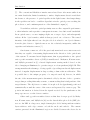
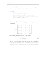
2.3.3.1 Intensity:
The optical intensity I (r) = |U (r) |2 is a function of the axial and radial distances z
1/2
and ρ = (x2 + y 2 )
I (ρ, z) = I0
W0
W (z)
2
2ρ2
exp − 2
,
W (z)
(2.57)
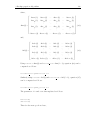
where I0 = |A0 |2 . At each value of z the intensity is a Gaussian function of the radial
distance ρ. Due to this, the wave is called a Gaussian beam. The Gaussian function
has its peak at ρ = 0 (on axis) and decays monotonically as ρ increases.
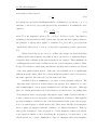
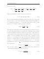
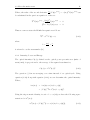
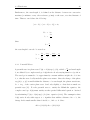
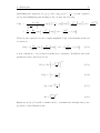
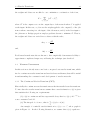
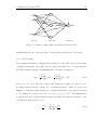
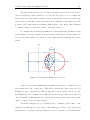
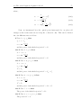
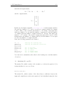
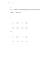
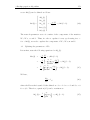
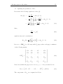
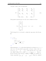
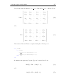
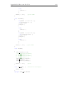
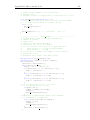
The beam
W (z )
Diffracting Gaussian beam 0
2 2W0
2W0
z
z0
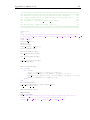
Beam waist at z = z0
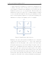
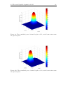
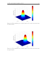
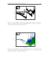
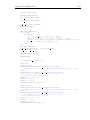
Beam minimum waist Figure 2.4: Gaussian beam model for the laser source used in the proposed system.
width W (z) of the Gaussian distribution increases with the axial distance. On the
beam axis (ρ = 0) the intensity,
I (0, z) = I0
W0
W (z)
2
=
I0
,
1 + (z/z0 )2
(2.58)
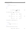
has its maximum value I0 at z = 0 and drops gradually with increasing z, reaching half
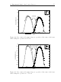
its peak value at z = ±z0 as shown in Figure 2.4. When |z| >> z0 , I (0, z) ≈ I0 z02 /z 2 ,
so that the intensity decreases with the distance in accordance with an inverse-square
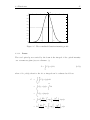
law. The overall peak intensity I (0, 0) = I0 occurs at the beam center (z = 0, ρ = 0).
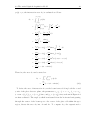
2.3 Wavefronts
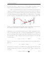
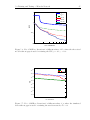
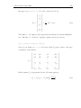
27
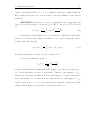
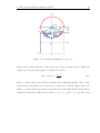
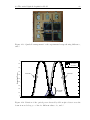
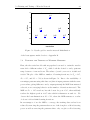
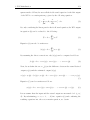
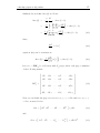
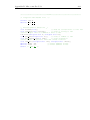
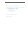
I/I0
1
0.9
0.8
0.7
0.6
0.5
0.4
0.3
0.2
0.1
0
−5
−4
−z0
−3
−2
z0
−1
0
1
z
2
3
4
5
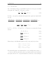
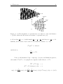
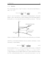
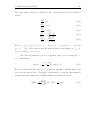
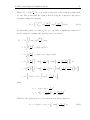
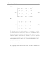
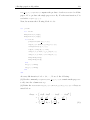
Figure 2.5: The normalized Gaussian intensity profile.
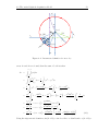
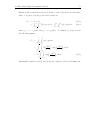
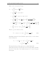
2.3.3.2 Power:
The total optical power carried by the beam is the integral of the optical intensity
over a transverse plane (say at a distance z),
Z
I (ρ, z) dA,
P =
A
where dA = ρdθdρ, therefore the above integral can be evaluated as follows:
Z∞ Z2π
P =
I (ρ, z) ρdρdθ
0
0
Z∞
=
I (ρ, z) ρdρ ·
0
Z2π
dθ
0
Z∞
=
I (ρ, z) 2πρdρ
0
2
Z∞ 2ρ2
W0
=
I0
exp − 2
2πρdρ
W (z)
W (z)
0
= I0
W0
W (z)
Z∞
2
2π
0
2ρ2
exp − 2
ρdρ.
W (z)
(2.59)
2.3 Wavefronts
28
By using a change of variables, u = ρ2 where du/2 = ρdρ, and inserting them into
the above double integral, we attain to the following:
P =
=
=
=
2
Z∞
2u
exp − 2
du
I0
W (z)
0
2
∞
W0
2π −W 2 (z)
2u
I0
·
exp − 2
W (z) 2
2
W (z) 0
2
W0
π 2
−I0
W (z) (0 − 1)
W (z) 2
2
W0
π 2
I0
I0
W (z) =
πW02 .
W (z) 2
2
W0
W (z)
2π
2
Therefore the total optical power can be stated as:
1
PT = I0 πW02 ,
2
(2.60)
where the result is independent of z. Thus the beam power is one-half the peak
intensity times the beam area. Since beams are often described by their power P , it
is useful to express I0 in terms of P using equation (2.60) and to rewrite equation
(2.57) in the form:
2ρ2
2PT
exp − 2
.
I (ρ, z) =
πW 2 (z)
W (z)
(2.61)
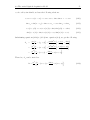
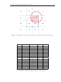
The ratio of the power carried within a circle of radius ρ0 in the transverse plane at
position z to the total power is:
1
PT
Zρ0
2ρ20
I (ρ, z) 2πρdρ = 1 − exp − 2
.
W (z)
(2.62)
0
The power contained within a circle of radius ρ0 = W (z) is approximately 86% of the
total power. About 99% of the power is contained within a circle of radius 1.5W (z).
Since the radius of the circular spot is ρ0 = 0.5 cm, then to achieve 99% of the total
power W0 was set to 1/3 cm in the theoretical model. Therefore, the minimum beam
waist 2W0 is equal to 2/3 cm.
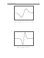
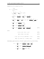
3
Functional Approximation with Wavelet
Networks
In order to estimate the lateral position of the light spot center corresponding to
the power distribution of the photodetector array, a wavelet network will be used as
a function approximation technique. In this chapter, we will introduce the concept
of function approximation, and neural networks. Next, we will discuss the relation
between the wavelet frames and wavelet networks, as well as the wavelet network
structure, and learning procedure that will be adopted in our research.
3.1
Function Approximation
According to T. Poggio in [16], the problem of learning a mapping between an input
and an output space is similar to the problem of synthesizing an associative memory
that retrieves the appropriate output when presented with the input and generalizes
3.1 Function Approximation
30
when presented with new inputs. A classical framework for this problem is approximation theory which deals with the problem of approximating or interpolating a
continuous, multivariate function f (x) by an approximating function F (w, x) having a fixed number of parameters w belonging to some set P. In this case, x and w
are real vectors where x = [x1 , x2 , . . . , xn ] and w = [w1 , w2 , . . . , wm ].
For a choice of a specific F , the problem is to find the set of parameters w
that provides the best possible approximation of f on the given input/output data
set. This can be categorized as the learning stage of our approximation problem.
Therefore, it is important to select an approximating function F that can represent f
as well as possible. It would be pointless to try to learn, if the chosen approximation
function F (w, x) could only give a very poor representation of f (x), even when using
optimal parameter values. Thus, we need to distinguish three main problems invloved
in function approximation; (1) the problem of which approximation to use, that
is which approximating functions F (w, x) would effectively represent the function
f (x); (2) the problem of which algorithm to use for finding the optimal values of the
parameters w for a given choice of F ; (3) the problem of an efficient implementation
of the algorithm either through hardware or software or both [16].
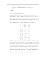
Most approximation schemes can be mapped into a certain network that can
be dubbed as a neural network. In general, networks can be regarded as a graphic
notation for a large class of algorithms. In our discussion, a network is a function
represented by the composition of a number of basic functions.
To measure the quality of the approximation, one introduces a distance function ρ to determine the distance ρ [f (x) , F (w, x)] of an approximation F (w, x) from
f (x). The distance is usually induced by a norm, such as the standard L2 norm. The
approximation problem can then be stated formally as:
DEFINITION 2.1 If f (x) is a continuous function and F (w, x) is an approximation function that depends continuously on w ∈ P and x, the approximation
problem is to determine the parameters w∗ such that,
ρ [F (w∗ , x) , f (x)] ≤ ρ [F (w, x) , f (x)] ,
(3.1)
for all w in the set P.
A solution of this problem, if it exists, is said to be a best approximation.
The existence of a best approximation depends ultimately on the class of functions
3.2 Neural networks
31
to whom F (w, x) belongs [16].
Recently, the wavelet theory has received substantial interest in the fields
of numerical analysis and signal processing [17], [18]. Wavelets are a family of basis
functions which exhibit interesting properties such as orthogonality, compact support,
and localization in time and frequency [19]. Owing to wavelet theory, very efficient
and fast algorithms have been developed for analyzing, approximating, and estimating
functions or signals. However, the implementation of such algorithms is only adequate
for problems of a relatively small input dimension. This is due to the excessive cost of
constructing and storing wavelet basis of large dimension. Artificial neural networks
are considered more promising candidates for handling problems of larger dimension
and their complexity is less sensitive to the input dimension [20].
Neural networks have been established as general function approximation tools
for fitting nonlinear models from input/output data and are widely used in applications which involve system modeling and identification [16]. However, the practical implementation of neural networks suffers from the lack of efficient constructive
methods, both for determining the parameters of neurons and selection of the network structure. At a different rate, the recently introduced wavelet decomposition is
emerging as a powerful tool for approximation [21], [22]. Due to the similar structure of wavelet decomposition and one-hidden-layer neural network, Q. Zhang and A.
Benveniste in [23], [20], [24] proposed to combine both wavelets, and neural networks.
This new type of network by the name of wavelet network (WN), is presented in
[23], as a class of feed-forward networks composed of wavelets which act as activation
functions replacing the traditional sigmoidal functions. The basic idea is to use more
powerful computing units obtained by cascading wavelet transform as an alternative
to neurons. The WN merges the good localization properties of wavelets with the
approximation abilities of neural networks. In addition, the wavelet network learning
is performed by the standard back-propagation type algorithm as in the conventional
feed-forward neural network [19].
3.2
Neural networks
In this section a brief overview of neural networks and their structure will be provided.
Let Θ be a set containing pairs of sampled inputs and the corresponding outputs
3.2 Neural networks
32
generated by an unknown map, f : Rm → Rn , m, n < ∞, such that:
Θ = {(xp , y p ) : y p = f (xp ) ; xp ∈ Rm , y p ∈ Rn , i = 1, . . . , Np , Np < ∞} .
We call Θ the training set. The task of functional approximation is to use the data
provided in Θ to learn or approximate the map f . Numerous existing schemes to
perfom such a task are based on parametrically fitting a particular functional form to
the given data. Simple examples of such schemes are those which attempt to fit linear
models or polynomials of fixed degree to the data in Θ. More recently, feedforward
neural networks have been used to learn the map f [25].
k1
u2
k2
un
k3
∑
g (i)
y
…
u1
b
(a)
u1
u2
y
(b)
un
Figure 3.1: (a) Single neuron model. (b) Simplified schematic of single neuron [25].
The basic component in a feedforward neural network is the single neuron
model as shown in Figure 3.1(a). Where u1 , . . . , un are the inputs to the neuron,
k1 , . . . , kn are multiplicative weights applied to the inputs, b is a biasing input, g :
R → R, and y is the output of the neuron. Thus, we have:
y=g
n
X
!
ki ui + b
i=1
The neuron of Figure 3.1(a) is often depicted as illustrated in Figure 3.1(b), where
3.2 Neural networks
33
the input weights, bias, summation and function g are implicit. Traditinally, the
activation function g has been chosen to be the well known sigmoidal function. This
choice of g was initially based upon the observed firing rate response of biological
neurons. A feedforward neural network is constructed by interconnecting a number
of neurons (such as the one shown in Figure 3.1) so as to form a network in which all
connections are made in the forward direction, that is from input to output without
feedback loops, as shown in Figure 3.2. Neural networks of this form are usually
x
I
Input Layer
tL
Hidden Layer
Output Layer
y
Figure 3.2: Feedforward neural network [25].
composed of an input layer, a number of hidden layers, and an output layer. The
input layer consists of neurons which accept external inputs to the network. Inputs
and outputs of the hidden layers are internal to the network, and hence the term
hidden. Outputs of neurons in the output layer are the external outputs of the
network. Once the structure of the feedforward network has been decided, that is the
number of hidden layers and the number of nodes in each hidden layer has been set,
a mapping is learned by varying the connection weights wij ’s and the biases bj ’s so as
to obtain the desired input-output response for the network. One method often used
to vary the weights and biases is known as the backpropagation algorithm in which
3.3 Wavelet Transforms
34
the weights and biases are modified so as to minimize a cost function of the form,
E=
X
(xp ,y p )∈Θ
k Op − y p k2 ,
where Op is the output vector at the output layer of the network when xp is applied
at the input. In this case, wij denotes the weight applied to the output Oj of the jth
neuron when connecting it to the input of the ith neuron, and bj is the bias input to
the jth neuron. Backpropagation employs gradient descent to minimize E. That is,
the weights and biases are varied in accordance with the rules,
∆wij = −ε
∂E
,
∂wij
∆bj = −ε
∂E
.
∂bj
and,
Feedforward neural networks are known to have empirically demonstrated ability to
approximate complicated maps very well using the technique just described.
3.3
Wavelet Transforms
In this section we shortly state some basic concepts about wavelet transforms, which
involve continuous wavelet transform and wavelet bases and frames, that will be useful
in understanding the construction and development of wavelet networks.
3.3.1 The Continuous Wavelet Transform (CWT)
Historically the continuous wavelet transform was the first studied wavelet transform.
To introduce the wavelet transform we assume that a wavelet function ψ (x) is given
that satisfies the following two requirements:
(1) ψ (x) is continuous and has exponential decay, that is ψ (x) 6 M e−C|x| for
some constants C and M .
(2) The integral of ψ is zero, that is
R∞
ψ (x) dx = 0 [26].
−∞
2
An example of a suitable wavelet function is ψ (x) = xe−x , whose graph is
given in Figure 3.3. In the following discussion, we assume that ψ (x) equals zero
3.3 Wavelet Transforms
35
outside some fixed interval −A 6 x 6 A, which is a stronger condition than the
first condition just given. We are now ready to state the definition of the wavelet
transform.
DEFINITION 2.2 Given a wavelet ψ satisfying the two requirements just
given, the wavelet transform of a function f ∈ L2 (R) is a function w : R2 7→ R given
by
Z∞
1
x−m
dx.
(3.2)
w (d, m) = p
f (x) ψ
d
|d|
−∞
From the preceding definition, it is not clear how to define the wavelet transform at d = 0. However, the change of variables y = (x − m)/d converts the wavelet
transfrom into the following:
∞
p Z
w (d, m) = |d|
f (yd + m) ψ (y) dy.
(3.3)
−∞
From this representation clearly, w (d, m) = 0 when d = 0.
As d becomes small, the graph of
1
ψd,m (x) = p ψ
|d|
x−m
d
,
becomes tall and skinny, as illustrated in the graphs of ψ1,0 and ψ1/2,0 with ψ (x) =
2
xe−x given in Figures 3.3 and 3.4, respectively. Therefore, the frequency of ψd,m
increases as d decreases. In addition, if most of the support of ψ, that is the nonzero
part of the graph of ψ, is located near the origin, then most of the support of ψd,m
will be located near x = m. So w (d, m) measures the frequency component of f that
vibrates with frequency proportional to 1/d near the point x = m.
3.3 Wavelet Transforms
36
0.6
0.4
0.2
0
-0.2
-0.4
-0.6
-3
-2
-1
0
1
2
3
2
Figure 3.3: Graph of ψ1,0 (x) = ψ (x) = xe−x [26].
0.6
0.4
0.2
0
-0.2
-0.4
-0.6
-3
-2
-1
0
1
Figure 3.4: Graph of ψ1/2,0 [26].
2
3
3.3 Wavelet Transforms
37
3.3.2 Inverse Wavelet Transform
The inversion formula of the wavelet transform is given in the following theorem:
Theorem 2.1 Suppose ψ is a continuous wavelet satisfying the following condiR∞
ψ (x) dx = 0. Then for any function
tions; ψ has exponential decay at infinity and
−∞
f ∈ L2 (R), the following inversion formula holds:
1
f (x) =
Cψ
Z∞ Z∞
w (d, m)
|d|−1/2
ψ
d2
x−m
d
dm dd,
(3.4)
−∞ −∞
where, the Fourier transform ψ̂ (ω) of ψ satisfies the following condition in [26], [23]:
Z∞
Cψ = 2π
−∞
|ψ̂ (ω) |2
dω < ∞.
|ω|
(3.5)
Therefore, according to the continuous wavelet decomposition theory, we are
able to decompose any function f (x) ∈ L2 (R) using a family of functions obtained
by dilating and translating a single mother wavelet ψ (x). In addition, the preceding
wavelet inversion theorem states that a function f can be decomposed as a weighted
sum (or integral) of its frequency components, as measured by w (d, m). The wavelet
inversion theorem involves two parameters, namely, the translation m and dialation
d, since the wavelet transform gives a measures of the frequency (using the parameter
d) of f near the point x = m [26].
3.3.3 Wavelet bases and frames
The continuous wavelet transform and its inverse transform are not directly implementable on digital computers. In practice, they have to be discretized [20]. When
the inverse wavelet transform in equation (3.4) is discretized into:
f (x) =
N
X
1
wj p
ϕj (x).
|d
|
j
j=1
(3.6)
some conditions are required so that this discrete version of the reconstruction of f
holds. The wavelet ϕj (x) is derived from its mother wavelet ψ (x) by the following
relation:
ϕj (x) = ψ
x − mj
dj
= ψ (zj ) ,
(3.7)
3.3 Wavelet Transforms
38
where mj and dj are the discretized translation and dilation factors.
Let Ωc be a denumerable family of functions generated by ψ of the following
form:
(
Ωc =
1
p ψ
dj
x − mj
dj
)
: mj ∈ R, dj ∈ R+ , j ∈ Z ,
(3.8)
which constitute an orthonormal basis of some functional space such as L2 (R). Usually a regular lattice {(da0 , tm0 ) : a ∈ Z, t ∈ Z} is used for the discretization where
the scalar parameters d0 and m0 define the step sizes of dilation and translation
discretizations.
Wavelet bases have numerous applications in signal processing and numerical
analysis because they offer very efficient algorithms and provide more useful information than Fourier transform. However, it is not always possible to build orthonormal
wavelet bases with any wavelet function ψ.
Though there are some well developed techniques for constructing the wavelet
function ψ and its associated orthonormal basis, the wavelet function ψ has to satisfy
strong restrictions. These restrictions lead to conflicts between regularity and compactness of the wavelet function, both being desired properties. Furthermore, if one
gives up the idea that the discrete family in equation (3.8) should be a basis of some
considered functional space and requires only that equation (3.8) constitutes a frame,
then one gains more freedom on the choice of ψ [20].
Wavelet frames are redundant basis, constructed by simple operations of translation and dilation of the mother Wavelet, which must satisfy conditions less stringent
than their orthonormal counterparts. The frame condition can be stated as follows;
there exist two constants cmin > 0 and cmax < ∞ such that for all f ∈ L2 (R), the
following inequalities hold:
cmin k f k2 ≤
X
ϕj ∈Ωc
|hϕj , f i|2 ≤ cmax k f k2 .
(3.9)
In this sum, k f k denotes the norm of function and h·, ·i is the inner product in L2 (R)
and the sum ranges over all the elements of the family Ωc [23], [27]. As mentioned
earlier using wavelet frames rather than orthonormal basis provides more freedom
and flexibility in the choice of the wavelet function ψ, however the tradeoff here is
that the reconstruction of the coefficients wj in equation 3.6 becomes nontrivial [20].
3.4 Wavelet Networks (WN)
3.4
39
Wavelet Networks (WN)
In this section we discuss the connection between wavelet networks and the discrete
inverse wavelet transform. In addition, we give an overview of the structure of the
wavelet network and the process of learning for function approximation.
3.4.1 Adaptive Discretization
Although the wavelet bases and frames have been developed with efficient numerical algorithms, their applications have been limited to problems of relatively small
input dimension. The main reason behind this is that wavelet bases and frames are
usually constructed with regularly dilated and translated wavelets, independent of
the available measured information or training data. In practice, the construction
and storage of such wavelet basis or frame of large input dimension is of prohibitive
cost. Therefore, it is expected that the wavelet estimator will be more efficient if the
wavelet basis is constructed according to the training data. This inevitably yields the
idea of adaptive discretization of the continuous wavelet transform [20].
To elaborate more on the preceding point, in order for us to obtain a discrete
reconstruction as shown in equation (3.6), instead of using a fixed lattice of (dj , mj ),
we can adaptively determine the values of (dj , mj ), according to the function f or
the sampled input/output data in the set Θ. By following such a methodology, all
the parameters wj , dj , and mj in equation (3.6) are to be adapted. Thus, equation
(3.6) is very similar to a one hidden layer feedforward neural network. Such adaptive
discrete inverse wavelet transform is called wavelet network.
From this perspective, equation (3.6) can be constructed using techniques
of neural networks. Usually, neural networks used in function approximation are
first randomly initialized and then trained by a backpropagation procedure. The
random initialization makes such learning procedures very inefficient. In contrast,
wavelet networks can be initialized with regular wavelet lattice as will be shown later
in Chapter 5. It is to be remarked that the regular lattices of wavelet frames are
special cases of adaptive discretizations of the continuous inverse wavelet transform.
Consequently, the discrete reconstruction formula in equation (3.6) must hold for
some properly adapted (dj , mj ). Furthermore, if the function f has some particular
3.4 Wavelet Networks (WN)
40
property of regularity, better results can be obtained, due to the flexibility of the
adaptive wavelet family [20].
3.4.2 Wavelet Network Structure
Zhang, and Benveniste introduced the general wavelet network structure, based on
the so-called 1 + 12 -layer neural network [23]. In the next discussion we use the
modified version of this network presented by Zhang in [28]. The main difference
between the two approaches is that in [28] a linear term ak = [ak1 , ak2 , . . . , akN i ]
is introduced to help the learning of the linear relation between the input and the
output signals. The WN architecture used is shown in Figure 3.5, and the equation
that defines the network is given by:
ŷk (x) =
Nw
X
ckj Φj (x) +
j=1
Ni
X
aki xi + bk ,
(3.10)
i=1
where i is the index for input nodes, j is the index for hidden nodes, k is the index for
output nodes, Ni is the number of input nodes, Nw is the number of hidden nodes,
and No is the number of output nodes. As shown in Figure 3.5, the wavelet network is
composed of an input layer with Ni inputs, a hidden layer having Nw wavelet neurons
or wavelons, and an output layer having a linear output neuron. The coefficients of
the linear part of the network which consist of the components of the vector ak and
the bias term bk are called direct connections [27]. In addition, xi refers to the ith
input to the network, ŷk (x) is the kth output of the network, and Φj (x) represents
the multidimensional activation function at the jth hidden wavelon. For modeling
multi-variable processes, multidimensional wavelets Φj : RNi 7→ R must be defined.
These are constructed as the product of Ni scalar wavelets:
Φj (x) =
Ni
Y
i=1
ψ (zji ) =
Ni
Y
ϕji .
(3.11)
i=1
Here, zji = (xi − mji )/dji , and the array x is given by x = [x1 , x2 , . . . , xi , . . . , xN i ]T .
Families of multidimensional wavelets generated according to this scheme have been
shown to be frames of L2 RN i [23], [24]. In this work, we have selected ψ (zji ) =
2
−zji e−zji /2 as our scalar mother wavelet, which satisfies condition (3.5), and in the
3.4 Wavelet Networks (WN)
41
Φ1
x1
ck 1
ak 1
x2
bk
ak 2
...
Φ2
ck 2
∑
yˆk
ak Ni
...
x Ni
ck Nw
Φ Nw
Input nodes
Hidden nodes
Output nodes
Figure 3.5: Function approximation using wavelet networks.
multidimensional case, direct products of such scalar wavelets have been taken.
3.4.3 WN Learning
The learning algorithm for adjusting the parameters of the WN is based on a sample
of input/output pairs, {x, yk (x)}, where yk (x) is the function to be approximated.
The WN training depends on minimizing the following cost function:
Np No
Np No
1 XX p 2 1 XX p
(ek ) =
(yk − ŷkp )2 ,
J (θ) =
2 p=1 k=1
2 p=1 k=1
(3.12)
where epk = ykp − ŷkp is the error between the kth target output, ykp , and the corre-
sponding wavelet network output, ŷkp , for training pattern p, while Np is the total
number of elements in the training set. All the parameters of the wavelet network
to be adjusted are collected in a vector θ = [bk , aki , ckj , mji , dji ]T . The minimization
is performed based on the gradient descent algorithm. The partial derivative of the
cost function with respect to θ is:
Np No
X
X p ∂ ŷ p
∂J
=−
ek k .
∂θ
∂θ
p=1 k=1
(3.13)
3.4 Wavelet Networks (WN)
42
The components of the vector ∂ ŷkp /∂θ for the conventional WN can be derived as
follows:
∂ ŷkp
∂bn
∂ ŷkp
∂ani
∂ ŷkp
∂cnj
∂ ŷkp
∂mji
= δnk
(3.14)
= δnk xpi
(3.15)
= δnk Φpj
(3.16)
p
∂Φpj ∂zji
p
∂zji
∂mji
p
p
p
∂Φj ∂zji
∂ ŷk
= ckj p
.
∂dji
∂zji ∂dji
= ckj
(3.17)
(3.18)
p
Here, zji
= (xpi − mji )/dji , for (i = 1, . . . , Ni ), (j = 1, . . . , Nw ), (k = 1, . . . , No ), and
(p = 1, . . . , Np ). Notice that we used Kronecker’s symbol delta defined as: δnk = 1
for n = k and δnk = 0 for n 6= k.
The network parameter vector θ is updated every epoch by using θnew =
θold + ∆θ (l) where:
1
∆θ (l) = −
Np
∂J
µ
+ γ∆θ (l − 1) .
∂θ
(3.19)
Here, µ is the learning rate and γ = 1 − µ is the momentum coefficient, where both
are set in the interval (0, 1). The figure of merit used to assess the approximation
results is the mean squared error (MSE), which can be stated as follows:
Np No
MSE =
1 XX p
2
J (θ) .
(yk − ŷkp )2 =
N p p=1 k=1
Np
(3.20)
4
Optical System Modeling and Design
4.1
System Architecture
The hardware architecture of our system, as shown in Figure 4.1, consists of a laser
source mounted on two actuators for azimuthal and vertical motion steering. The
laser source is adjusted to point at a mirror placed on a vibrating platform. The
Gaussian beam emitted from the source is reflected by the mirror onto a photodetector
array, which captures the light intensity distribution of the laser spot. Different
photocurrent outputs generated from each photodiode (PD) depend on the relative
beam area intercepted by the different PDs. Thus, the optical power distribution of
the photodetector array depends on the 2 dimensional position of the spot center.
The design problem at hand involves three major parts as demonstrated in
Figure 4.1. The first part, the optical acquisition system, is concerned with acquiring
the optical power distribution P = [P1 · · · Pi · · · Pn ]T of the array of n photodetector
cells. Next, the optical power information is fed into a lateral position detection
system. In this stage a WN is used as a function approximation technique to yield an
4.2 Theoretical Optical Acquisition Model
44
estimate x̂ (P, t) and ŷ (P, t) of both x (P, t) and y (P, t), the Cartesian coordinates of
the center of the light spot that correspond to the acquired optical power distribution.
The final stage uses the estimated position of the light spot for vibration monitoring.
In this research, we focus on the first two stages of the proposed system.
y
Photocell Array
Pn
x
Mirror
Pi
P1
Optical Signal
Acquisition
Laser Beam
Position Detection
System
Laser Source
x̂
Vibration Platform
Gaussian Intensity Profile
" "
ŷ
Vibration Monitoring
Vibration
Monitoring
System
Figure 4.1: Hardware architecture of the proposed position detection system.
4.2
Theoretical Optical Acquisition Model
The theoretical model evaluates the optical power distribution as the center of the
beam is scans the plane of photocell array. Since, optical power is directly related to
R
the incident area of overlap between the photodetector and the beam Pi = IdA ,
closed form equations for the area of intersection for one photodetector cell have been
found for further analytical purposes.
Next, we derive the equations for the optical power covered by the required area
of overlap between the detector active surface and the beam spot, given the beam’s
Gaussian intensity profile. After evaluating the optical power as the beam is scanned
over the active surface of one photodetector cell, the theoretical optical acquisition
system model is extended further to account for an array of four photodiodes with
horizontal and vertical spatial gap separations. The optical power for each photodiode
is calculated as the beam moves about the plane covered by the quadcell.
4.2 Theoretical Optical Acquisition Model
45
The laser beam incident onto a 1 cm×1 cm square photodetector cell is modeled as a circular spot with a radius, ρ0 = 0.5 cm. We developed a code to compute the
interception area between the circular beam spot and the photodetector as the beam
center is moved anywhere outside and inside the boundaries of the square cell. The
position of the beam center is determined with respect to the origin of the Cartesian
coordinate system, located at the center of the photodetector.
To calculate the area through simulation, certain supporting parameters such
as the number of points of intersection between the circular spot and the square cell
Nint , as well as the number of corners Nc of the square that lie within the circle, were
found.
y
dx
ρ1 (α )
O
Ax
α1
( x, y )
x
ρ 2 = ρ0
− x0
x0
Figure 4.2: Parameters definition for area Ax .
Next, we derived the mathematical formulation necessary to obtain the closed
form equations for the overlap area. This will be divided into three categories; (1)
Finding the area of intersection while moving the beam along the x direction only,
(2) Finding the area of intersection while the beam is moved along the y direction
only, and finally (3) Finding the area of intersection as the beam is moved about the
entire x–y plane, along any random path.
As shown in Figure 4.2, (x, y) indicate the coordinates of the center of the
circular spot with respect to the center of the square photodetector cell, and (x0 , y0 )
represent the coordinates of the top right-most corner of the photocell, which in this
4.2 Theoretical Optical Acquisition Model
46
case x0 = 0.5 cm and y0 = 0.5 cm. Let us first define the following parameters:
dx = x − x0 ,
(4.1)
which is the horizontal distance between the spot center and the side at which the
circular spot intersects the square. In addition, we have:
sin α1 = sin α2 =
x − x0
,
ρ0
(4.2)
where, α1 is the angle between the vertical axis crossing through the center of the
beam and the first intersection between the circular spot and the square photocell.
While, α2 is the angle between the vertical axis crossing through the beam center and
the second point of intersection.
Given that α2 = π − α1 , ρ1 (α) = (x − x0 )/ sin α, and ρ2 (α) = ρ0 , we can
calculate the intersection area Ax by evaluating the following double integral:
Ax
Zα2 ρZ2 (α)
=
ρdρdα
α1 ρ1 (α)
Zα2 2 ρ2 (α)
ρ
2
=
α1
ρ0 2
=
2
ρ0 2
=
2
Zα2
α1
Zα2
Zα2
dα =
ρ1 (α)
ρ2 2 ρ1 2
−
dα
2
2
α1
(x − x0 )2
1 − 2 2 dα
ρ0 sin α
sin2 α1
1−
dα
sin2 α
α1
ρ0 2
ρ0 2 2
=
(π − 2α1 ) −
sin α1
2
2
Zα2
1
dα
sin2 α
α1
2
ρ0
(π − 2α1 ) +
2
ρ0 2
=
(π − 2α1 ) +
2
=
2
ρ0
sin2 α1 [cot α]αα21
2
ρ0 2 2
sin α1 [cot α2 − cot α1 ] .
2
(4.3)
4.2 Theoretical Optical Acquisition Model
47
The term cot α2 − cot α1 in the preceding integral can be reduced to the following:
cos α2 cos α1
−
sin α2
sin α1
sin α1 cos α2 − sin α2 cos α1
=
sin α1 sin α2
sin (α1 − α2 )
=
.
sin α1 sin α2
cot α2 − cot α1 =
Since, α2 = π − α1 , hence α1 − α2 = α1 − (π − α1 ) = 2α1 − π, and therefore,
sin (α1 − α2 )
sin α1 sin α2
sin (2α1 − π)
=
sin α1 sin α2
− sin (2α1 )
=
sin α1 sin α2
−2 sin α1 cos α1
−2 cos α1
=
=
.
sin α1 sin α2
sin α2
cot α2 − cot α1 =
Since sin α2 = sin α1 , we can state that:
cot α2 − cot α1 =
−2 cos α1
.
sin α1
(4.4)
Substituting equation (4.4) into equation (4.3), we have:
Ax
ρ0 2
ρ0 2 2
2 cos α1
=
(π − 2α1 ) +
sin α1 −
2
2
sin α1
2
2
ρ0
ρ0
=
(π − 2α1 ) +
sin α1 [−2 cos α1 ]
2
2
ρ0 2
=
[π − 2α1 − sin 2α1 ] .
2
Therefore, Ax can be stated as:
Ax =
ρ20
[π − 2α1 − sin 2α1 ] .
2
(4.5)
Next, to find the intersection area Ay as the beam moves along the y-axis only, as
shown in Figure 4.4, the following parameters were defined:
dy = y − y 0 ,
(4.6)
4.2 Theoretical Optical Acquisition Model
48
y
( x, y )
β1
y0
Ay
ρ1 ( β )
dy
ρ 2 = ρ0
x
O
− y0
Figure 4.3: Parameters definition for area Ay .
which is the vertical distance between the spot center and the side at which the
circular spot intersects the square. In addition, we have:
sin β1 = sin β2 =
y − y0
,
ρ0
(4.7)
where, β1 is the angle between the horizontal axis crossing through the center of the
beam and the first intersection between the circular spot and the square photocell.
While, β2 is the angle between the horizontal axis crossing through the beam center
and the second point of intersection. Using β2 = π − β1 , ρ1 (β) = (y − y0 )/ sin β, and
4.2 Theoretical Optical Acquisition Model
49
ρ2 (β) = ρ0 , the intersection area Ay , is evaluated as follows:
Ay
Zβ2 ρZ2 (β)
=
ρdρdβ
β1 ρ1 (β)
Zβ2 =
ρ2
2
β1
ρ0 2
=
2
Zβ2
Zβ2
ρ2 (β)
dβ =
ρ1 (β)
ρ2 2 ρ1 2
−
dβ
2
2
β1
(y − y0 )2
1 − 2 2 dβ
ρ0 sin β
β1
ρ0 2
=
2
Zβ2
1−
sin2 β1
dβ
sin2 β
β1
ρ0 2
ρ0 2 2
=
(π − 2β1 ) −
sin β1
2
2
Zα2
1
dβ
sin2 β
α1
2
ρ0
2
ρ0 2
=
2
ρ0 2
=
2
ρ0 2
=
2
=
2
ρ0
sin2 β1 [cot β]ββ21
2
ρ0 2 2
(π − 2β1 ) +
sin β1 [cot β2 − cot β1 ]
2
ρ0 2
(π − 2β1 ) +
sin β1 [−2 cos β1 ]
2
(π − 2β1 ) +
[π − 2β1 − sin 2β1 ] .
Therefore, the area Ay can be stated as:
Z
β2
Z
ρ2 (β)
Ay =
=
ρ dρ dβ
β1
ρ20
2
ρ1 (β)
[π − 2β1 − sin 2β1 ] .
(4.8)
To derive the area of intersection Axy as the beam is moved along both the x and
y axis of the photodetector plane, the parameters α1 , β1 , dx = x − x0 , dy = y − y0 ,
φ = tan−1 (dy /dx ), ρx = (x−x0 )/ sin α, and ρy = (y −y0 )/ sin β as shown in Figure 4.4
are first evaluated. The angle φ which is measured from the horizontal axis passing
through the center of the beam spot to the corner of the photocell within the spot
region, bisects the area Axy into A1 and A2 . To compute Axy , the expressions for
4.2 Theoretical Optical Acquisition Model
50
dx
α1
φ
ρy (β )
y0
A2
( x, y )
A1
β1
dy
ρ0
ρ x (α )
x0
Figure 4.4: Parameters definition for area Axy .
areas A1 and A2 are found, then the sum of both is taken.
Zα2 Zρ0
ρdρdα
A1 =
φ+ π2
ρx
Zα2 =
ρ2
2
ρ0
1
dα =
2
ρx
φ+ π2
1
=
2
Zα2
ρ0
φ+ π2
ρ0 2
=
2
Zα2
φ+ π2
ρ0 2
2
ρ0 2
=
2
ρ0 2
=
2
=
2
Zα2
φ+ π2
ρ0 2 − ρx 2 dα
ρ0 2
(x − x0 )2
dα
=
−
2
sin2 α
Zα2
φ+ π2
(x − x0 )2
1 − 2 2 dα
ρ0 sin α
Zα2
sin2 α1
ρ0 2 h
π i ρ0 2 sin2 α1
1
α2 − φ +
−
1−
dα
2 dα =
2
2
2
sin α
sin2 α
φ+ π2
i ρ 2 sin2 α
0
1
2
− α1 − φ +
[cot α]αφ+
π
2
2
2
hπ
i ρ 2 sin2 α h cos α iα2
0
1
− α1 − φ +
2
2
sin α φ+ π2
hπ
i ρ 2 sin2 α cos α
sin (φ + π/2)
0
1
2
− (α1 + φ) +
−
+
.
2
2
sin α2
cos (φ + π/2)
hπ
(4.9)
Using the trignometric identities, sin (A ± B) = sin A cos B±cos A sin B and cos (A ± B) =
4.2 Theoretical Optical Acquisition Model
51
cos A cos B ∓ sin A sin B, we have the following relations:
cos α2 = cos (π − α1 ) = cos π cos α1 + sin π sin α1 = − cos α1
(4.10)
sin α2 = sin (π − α1 ) = sin π cos α1 − cos π sin α1 = sin α1
(4.11)
cos (φ + π/2) = cos φ cos (π/2) − sin φ sin (π/2) = − sin φ
(4.12)
sin (φ + π/2) = sin φ cos (π/2) + cos φ sin (π/2) = cos φ.
(4.13)
Substituting equations (4.10) to (4.13) into equation (4.9), we get the following:
A1
ρ0 2
=
2
ρ0 2
=
2
ρ0 2
=
2
hπ
2
hπ
2
π
2
ρ0 2 sin2 α1
cos α1
sin φ
− (α1 + φ) +
−
+
2
sin α1
cos φ
i ρ 2 sin2 α cos (α + φ) 1
0
1
− (α1 + φ) +
−
2
sin α1 cos φ
sin α1
− (α1 + φ) −
cos (α1 + φ) .
cos φ
i
Therefore, A1 can be stated as:
sin α1
ρ0 2 π
− (α1 + φ) −
cos (α1 + φ) .
A1 =
2 2
cos φ
(4.14)
4.2 Theoretical Optical Acquisition Model
52
Similarly, area A2 is evaluated as follows:
Zβ2 Zρ0
A2 =
ρdρdβ
π−φ ρy
Zβ2 =
ρ2
2
π−φ
1
=
2
Zβ2
ρo
1
dβ =
2
ρy
Zβ2
ρ0 2 − ρy 2 dβ
π−φ
ρ0 2
(y − y0 )2
dβ
=
ρ0 2 −
2
sin2 β
π−φ
ρ0 2
=
2
Zβ2
1−
(y − y0 )2
dβ
ρ0 2 sin2 β
π−φ
Zβ2
Zβ2
sin2 β1
ρ0 2
ρ0 2 sin2 β1
1−
dβ
=
[β
−
(π
−
φ)]
−
2
2
2
sin2 β
π−φ
1
dβ
sin2 β
π−φ
2
2
2
ρ0
ρ0 sin β1
[φ − β1 ] +
2
2
2
2
ρ0 sin2 β1
ρ0
[φ − β1 ] +
=
2
2
2
[cot β]βπ−φ
β
cos β 2
sin β π−φ
ρ0 2
ρ0 2 sin2 β1
cos β2 cos (π − φ)
=
[φ − β1 ] +
−
+
,
2
2
sin β2
sin (π − φ)
=
(4.15)
where,
cos β2 = cos (π − β1 ) = − cos β1
(4.16)
sin β2 = sin (π − β1 ) = sin β1
(4.17)
cos (π − φ) = cos π cos φ + sin π sin φ = − cos φ
(4.18)
sin (π − φ) = sin π cos φ − cos π sin φ = sin φ
(4.19)
Substituting equations (4.16) to (4.19) into equation (4.15) we get the following:
A2
ρ0 2
=
2
ρ0 2
=
2
ρ0 2
=
2
ρ0 2 sin2 β1
cos β1 cos φ
[φ − β1 ] +
−
+
2
sin β1
sin φ
2
2
ρ0 sin β1 sin (φ − β1 )
[φ − β1 ] −
2
sin β1 sin φ
sin β1
φ − β1 −
sin (φ − β1 ) .
sin φ
4.2 Theoretical Optical Acquisition Model
53
Therefore, A2 can be stated as:
sin β1
ρ0 2
φ − β1 −
sin (φ − β1 ) .
A2 =
2
sin φ
(4.20)
Hence, Axy the total area of the shaded region can be written in the following closed
form:
Axy = A1 + A2
Z α2 Z ρ 0
Z
=
ρ dρ dα +
φ+ π2
β2
π−φ
ρx
Z
ρ0
ρ dρ dβ
ρy
ρ20 π
sin α1
sin β1
=
[ − (α1 + β1 ) −
cos(α1 + φ) −
sin(φ − β1 )]. (4.21)
2 2
cos φ
sin φ
4.2.1 Modeling Optical Apodization
The optical power enclosed within a certain area of intersection, is derived for three
different cases, the power as the beam moves along the x direction only, the y direction
only, and both x–y directions. The power for horizontal motion can be evaluated using
the following double integral:
Z
α2
Z
ρ2 (α)
Px =
I0
α1
ρ1 (α)
W0
W (z)
2
exp
−2ρ2
W 2 (z)
ρdρdα
(4.22)
Let,
I1 = I0
W0
W (z)
2
ρ2 (α) = ρ0
x − x0
ρ1 (α) =
.
sin α
(4.23)
(4.24)
(4.25)
Therefore, using the above definitions equation (4.22), can be written as:
Zα2 ρZ2 (α)
−2ρ2
Px = I1
exp
ρdρdα.
W 2 (z)
α1 ρ1 (α)
(4.26)
4.2 Theoretical Optical Acquisition Model
54
Let,
u=
2
W 2 (z)
ρ2 ,
(4.27)
where,
2
u2 = u (ρ2 = ρ0 ) = 2 ρ0 2
W
2
2 x − x0
x − x0
= 2
.
u1 = u ρ1 =
sin α
W
sin α
Taking the derivative of u with respect to ρ we have:
du =
4
ρdρ.
W 2 (z)
(4.28)
Substituting equations (4.27) and (4.28) into equation (4.26) and taking the limits u2
and u1 , we have the following:
Zα2 Zu2
Px = I1
exp (−u)
α1 u1
Zα2 = I1
α1
Zα2 = I1
α1
Zα2 = I1
W
2
2
W
2
2
W
2
2 "
W
2
2
dudα
[− exp (−u)]uu21 dα
[− exp (−u2 ) + exp (−u1 )] dα
2 !#
2 2
2 x − x0
− exp − 2 ρ0 + exp − 2
dα
W
W
sin α
α1

2 Zα2
Zα2
W
2
2 x − x0
− exp − 2 ρ0 2 dα + exp − 2

2
W
W
sin α
α1
α1


Zα2

κ 
x
= κ1 −κ2 (α2 − α1 ) + exp − 2
dα


sin α
= I1
2 !
dα



α1
Therefore, Px can be stated as:
Px = −κ1 κ2 (α2 − α1 ) + κ1
Z
α2
α1
κx exp − 2
dα,
sin α
(4.29)
4.2 Theoretical Optical Acquisition Model
55
where,
2
(x − x0 )2
W2
2
W
= I1
2
2 2
= exp − 2 ρ0 .
W
κx =
(4.30)
κ1
(4.31)
κ2
(4.32)
Next, we investigated how the optical power intercepted by one photocell
changes as the beam center moves along the x direction only. This can be divided
into six different cases as follows:
if Case 1: x ≥ x0 then
dx = x − x0
α1 = sin−1 dρx0
and the power of the shaded region is P = Px
else if Case 2: x ≤ x0 then
dx = −x0 − x
α1 = sin−1 dρx0
and the power of the shaded region is P = Px
else if Case 3: 0 ≤ x ≤ x0 then
dx = −x0 − x
−1 dx
α1 = sin
ρ0
P 0 = Px
and the power of the shaded region is P = PT − Px
else if Case 4: −x0 ≤ x ≤ 0 then
d x = x + x0
−1 dx
α1 = sin
ρ0
P 0 = Px
and the power of the shaded region is P = PT − Px
else if Case 5: x = 0 then
The power of the shaded region is P = PT
else if Case 6: x = x ≥ x0 + ρ0 then
The power is P = 0
4.2 Theoretical Optical Acquisition Model
Where, PT = 2πI1
W 2
2
56
(1 − κ2 ), is the total power of the beam spot with radius
0.5 cm. The power while the beam is moved along the y direction only can be
determined using the following:
Z
β2
Z
ρ2 (β)
I0
Py =
β1
ρ1 (β)
W0
W (z)
2
exp
−2ρ2
W 2 (z)
ρdρdβ.
(4.33)
Provided that, ρ2 (β) = ρ0 , and ρ1 (β) = (y − y0 ) / sin β, a similiar procedure as Px
can be adopted to evaluate the optical power Py as follows:
Zβ2 Zv2
Py = I1
exp (−u)
W
2
2
dudβ
β1 v1
Zβ2 = I1
W
2
2
W
2
2
W
2
2 "
[− exp (−u)]vv21 dβ
β1
Zβ2 = I1
[− exp (−v2 ) + exp (−v1 )] dβ
β1
Zβ2 = I1
2 !#
2 2
2 y − y0
− exp − 2 ρ0 + exp − 2
dβ
W
W
sin β
β1

2 ! 
Zβ2
2
2 y − y0
W
dβ
= I1
− exp − 2 ρ0 2 dβ + exp − 2


2
W
W
sin β
β1
β1



Zβ2

κy
= κ1 −κ2 (β2 − β1 ) + exp − 2
dβ ,


sin β

2 Zβ2
β1
where,
2
v2 = u (ρ2 = ρ0 ) = 2 ρ0 2
W
2
y − y0
2 y − y0
v1 = u ρ 1 =
= 2
.
sin β
W
sin β
Therefore, the optical power Py for vertical motion can be stated as:
Py = −κ1 κ2 (β2 − β1 ) + κ1
Z
β2
β1
κy
exp − 2
dβ,
sin β
(4.34)
4.2 Theoretical Optical Acquisition Model
57
where κy = 2(y − y0 )2 /W 2 . Similarly, we investigated how the optical power intercepted by one photocell changes as the beam center moves along the y direction
only. This can be divided into six different cases.
if Case 7: y ≥ y0 then
dy = y − y0
−1 dy
β1 = sin
ρ0
and the power of the shaded region is P = Py
else if Case 8: y ≤ y0 then
dy = −y0 − y
β1 = sin−1 dρy0
and the power of the shaded region is P = Py
else if Case 9: 0 ≤ y ≤ y0 then
dy = −y0 − y
β1 = sin−1 dρy0
P 0 = Py
and the power of the shaded region is P = PT − Py
else if Case 10: −y0 ≤ y ≤ 0 then
dy = y + y 0
β1 = sin−1 dρy0
P 0 = Py
and the power of the shaded region is P = PT − Py
else if Case 11: y = 0 then
The power of the shaded region is P = PT
else if Case 12: y = y ≥ y0 + ρ0 then
The power is P = 0
4.2 Theoretical Optical Acquisition Model
y
58
y
dx
α1
ρo
x
( x, y )
O
− xo
dx
α1
ρo
P
y
dx
( x, y )
x
O
− xo
xo
(a)
xo
(c )
y
dx
ρo
x
− xo
xo
P′
O ( x, y )
(b)
y
P′
α1
ρo
P
P
y
α1
P
P
x
( x, y ) O
− xo
x
O
− xo
xo
− xo
xo
(d )
x
( x, y )
O
xo
(f)
( e)
Figure 4.5: (a) Case 1: x ≥ x0 , (b) Case 2: x ≤ x0 , (c) Case 3: 0 ≤ x ≤ x0 , (d) Case
4: −x0 ≤ x ≤ 0, (e) Case 5: x = 0, (f ) Case 6: x = x ≥ x0 + ρ0 .
y
y
y
yo
P′
yo
yo
( x, y )
ρo
β1
( x, y )
O
dy
P
O
O
P
− yo
ρo
dy
β1
( x, y )
x
ρo
β1
dy
x
P
x
− yo
− yo
(a)
(b)
y
(c )
y
y
( x, y )
yo
O
− yo
ρo
P′
P
β1
x
O
x
( x, y )
yo
P
P
dy
x
O
− xo
xo
− yo
(d )
( e)
(f)
Figure 4.6: (a) Case 7: y ≥ y0 , (b) Case 8: y ≤ y0 , (c) Case 9: 0 ≤ y ≤ y0 , (d) Case
10: −y0 ≤ y ≤ 0, (e) Case 11: y = 0, (f ) Case 12: y = y ≥ y0 + ρ0 .
4.2 Theoretical Optical Acquisition Model
59
Finally, as the beam is moved along both the x, and y directions over the entire
plane of one photocell, the power can be stated as:
Pxy = P1 + P2
Z
Z α2 Z ρ 0
I(ρ, z) ρ dρ dα +
=
φ+ π2
(4.35)
β2
ρ0
I(ρ, z) ρ dρ dβ,
π−φ
ρx
Z
(4.36)
ρy
where, ρx = x − x0 /sin α and ρy = y − y0 /sin β. To evaluate P1 we proceed in
the following manner:
Zα2 Zρ0
P1 =
I(ρ, z)ρdρdα
φ+ π2 ρx (α)
Zα2 Zρ0
I0
=
φ+ π2
2
exp
−2ρ2
W 2 (z)
−2ρ2
W 2 (z)
ρdρdα.
W0
W (z)
ρdρdα
ρx (α)
Zα2 Zρ0
= I1
exp
(4.37)
φ+ π2 ρx (α)
Substituting equations (4.27) and (4.28) into equation (4.37) and taking the
4.2 Theoretical Optical Acquisition Model
60
limits u2 and u1 , we have the following:
Zα2 Zu2
exp (−u)
P1 = I1
W
2
2
dudα
φ+ π2 u1
Zα2 = I1
W
2
2
W
2
2
W
2
2 "
[− exp (−u)]uu21 dα
φ+ π2
Zα2 = I1
[− exp (−u2 ) + exp (−u1 )] dα
φ+ π2
Zα2 = I1
φ+ π2
= I1
W
2

2 
 Zα2


Zα2
− exp −
φ+ π2
= κ1
2 !#
2
2 x − x0
− exp − 2 ρ0 2 + exp − 2
dα
W
W
sin α
2 2
ρ0 dα +
W2
φ+ π2



π +
−κ2 α2 − φ +

2

Zα2
φ+ π2
2 x − x0
W 2 sin α
exp −
2 !
dα








κ x
exp − 2
dα .

sin α

Therefore, P1 can be stated as follows:
P1 = −κ1 κ2
π α2 − φ +
+ κ1
2
Zα2
φ+ π2
κ x
dα.
exp − 2
sin α
(4.38)
Next, P2 is evaluated as follows:
Zβ2 Zρ0
P2 =
I(ρ, z)ρdρdβ
π−φ ρy (β)
Zβ2 Zρ0
=
I0
2
exp
−2ρ2
W 2 (z)
−2ρ2
W 2 (z)
ρdρdβ.
W0
W (z)
ρdρdβ
π−φ ρy (β)
Zβ2 Zρ0
= I1
exp
(4.39)
π−φ ρy (β)
Substituting equations (4.27) and (4.28) into equation (4.39) and taking the
4.2 Theoretical Optical Acquisition Model
61
limits v2 and v1 , we have the following:
Zβ2 Zv2
exp (−u)
P2 = I1
W
2
2
dudβ
π−φ v1
Zβ2 = I1
W
2
2
W
2
2
[− exp (−u)]vv21 dβ
π−φ
Zβ2 = I1
[− exp (−v2 ) + exp (−v1 )] dβ
π−φ
Zβ2 2 "
2 !#
W
2 2
2 y − y0
= I1
− exp − 2 ρ0 + exp − 2
dβ
2
W
W
sin β
π−φ


2  Zβ2
2 ! 
Zβ2
2 y − y0
2
W
− exp − 2 ρ0 2 dβ +
exp − 2
= I1
dβ


2
W
W
sin β
π−φ
π−φ



Zβ2

κy
= κ1 −κ2 (β2 − (π − φ)) +
exp − 2
dβ .


sin β
π−φ
Therefore, P2 can be stated as follows:
P2 = −κ1 κ2 (β2 − (π − φ)) + κ1
Zβ2
κy
exp − 2
sin β
dβ.
(4.40)
π−φ
Substituting equations (4.38) and (4.40) into equation (4.36), Pxy can be written
in the following form:
Pxy = −κ1 κ2
π
2
Rα2
exp − sinκx2 α dα
− (α1 + β1 ) + κ1
φ+ π2
+κ1
Rβ2
π−φ
exp − sinκy2 β dβ.
(4.41)
The integrals in the preceding equations were evaluated numerically.
Using equations (4.29), (4.34), and (4.41) we developed an algorithm to determine
the power P if the center of the circular beam spot is to be moved along any
random path.
4.2 Theoretical Optical Acquisition Model
62
y
R2
R12
R11
yo
R14
R7
− xo
R8
R1
( x, y )
R13
xo
( 0, 0 )
R15
R5
x
R16
R6
R10
R4
− yo
R3
R9
Figure 4.7: Example of beam center position as it scans the photocell’s regions.
Region
R1
R2
R3
R4
R5
R6
R7
R8
R9
R10
R11
R12
R13
R14
R15
R16
x
x > x0
x < −x0
x < −x0
x > x0
x ≥ x0
x ≥ x0
x ≤ −x0
x ≤ −x0
0 < x ≤ x0
−x0 ≤ x < 0
0 < x ≤ x0
−x0 ≤ x < 0
0 < x < x0
−x0 < x < 0
−x0 < x < 0
0 < x < x0
y
y > y0
y > y0
y < −y0
y < −y0
0 < y ≤ y0
−y0 ≤ y < 0
0 < y ≤ y0
−y0 ≤ y < 0
y ≤ −y0
y ≤ −y0
y ≥ y0
y ≥ y0
0 < y < y0
0 < y < y0
−y0 < y < 0
−y0 < y < 0
dx
x − x0
−x − x0
−x − x0
x − x0
x − x0
x − x0
−x − x0
−x − x0
x0 − x
x0 + x
x0 − x
x0 + x
x0 − x
x0 + x
x0 + x
x0 − x
dy
y − y0
y − y0
−y − y0
−y − y0
y0 − y
y0 + y
y0 − y
y0 + y
−y − y0
−y − y0
y − y0
y − y0
y0 − y
y0 − y
y0 + y
y0 + y
Table 4.1: Table showing the range of each region.
4.2 Theoretical Optical Acquisition Model
63
To do this, the plane for one photocell has been divided into 16 different regions
as shown in Figure 4.7. The power is computed depending on the region where
the center of the beam is located.
if (x, y) ∈ R1 , R2 , R3 , or R4 then
The power of the shaded region is P = Pxy
else if (x, y) ∈ R5 , R6 , R7 , or R8 then
Check the following:
if Nc = 1 and Nint = 2 then
Check the following:
if dx 6= 0 and dy 6= 0 or dx 6= 0 and dy = 0 or dx = 0 and dy 6= 0 then
P = Px − Pxy
else if dx = 0 and dy = 0 then
The power of the shaded region is P = 41 PT .
else if Nc = 0 and Nint = 2 then
The power of the shaded region is P = Px .
end if
else if (x, y) ∈ R9 , R10 , R11 , or R12 then
Check the following:
if Nc = 1 and Nint = 2 then
Check the following:
if dx 6= 0 and dy 6= 0 or dx 6= 0 and dy = 0 or dx = 0 and dy 6= 0 then
The power of the shaded region is P = Py − Pxy .
else if dx = 0 and dy = 0 then
The power of the shaded region is P = 41 PT .
end if
else if Nc = 0 and Nint = 2 then
The power of the shaded region is P = Py .
end if
else if (x, y) ∈ R13 , R14 , R15 , or R16 then
Check the following:
if Nc = 1 and Nint = 2 then
The power of the shaded region is P = PT − (Px + Py − Pxy ).
4.2 Theoretical Optical Acquisition Model
64
else if Nc = 0 and Nint = 4 then
The power of the shaded region is P = PT − (Px + Py ).
end if
end if
4.2.2 Modeling System Imperfections
The quadcell array of photodetectors has been modeled according to the orientation shown in Figure 4.8. Each photocell is represented as a 1 cm×1 cm
square, with centers S1 , S2 , S3 , and S4 . The photocells are separated by a
small horizontal distance and a vertical distance δ. In this case, the origin of
the absolute Cartesian coordinate system is located at the center of the array.
The coordinates of S1 , S2 , S3 and S4 with respect to the origin are:

S1 = 

S2 = 

S3 = 

S4 = 
x1
y1
x2
y2
x3
y3
x4
y4


=


=


=


=
0.5 + ε/2
0.5 + δ/2
−0.5 − ε/2
0.5 + δ/2
−0.5 − ε/2
−0.5 − δ/2
0.5 + ε/2
−0.5 − δ/2








The main objective of the optical acquisition model is to obtain the optical
power distribution generated at each photodetector while the beam is scanned
throughout the entire quadcell plane, thus an algorithm has been developed
to calculate the optical power for each cell. The minimum resolution that can
be generated using our algorithm is 0.01 cm for both the x and y positions.
The mathematical model mentioned in the previous discussion has been obtained while considering the origin of the x–y coordinate system situated at
the center of one photocell. Therefore, to evaluate the optical power for the
quad-cell using equations (4.29), (4.34), and (4.41), the origin of the absolute
4.2 Theoretical Optical Acquisition Model
65
coordinate system will be translated by a certain vector determined by the
coordinates of the center of the cell. The portion of power captured by each
cell is calculated. To find the power distribution for cell 1 in the array, the
translational operation (x, y) − (x1 , y1 ) is first made. Then the earlier power
calculations are carried out on photocell 1. A similar translation is applied
to the second, third and fourth cell, where the power distribution is evaluated for each cell separately. Figures 4.9 to 4.12 show the normalized power
distributions for each photocell, assuming and δ to be negligible.
y
S2
δ
S1
( 0, 0 )
S3
x
S4
ε
Figure 4.8: Quadcell array of photodetectors.
Furthermore, the center of the beam has been simulated to move on the plane
of photodetectors along the trajectory y = x. A plot of the optical power
distribution for the four cells against xc (the x position of the beam center),
following the given trajectory can be shown in Figure 4.14, where and δ are
first set to zero. As illustrated, the beam occupies most of the active surface
areas of photocells 1 and 3, and as it moves away from photocell 3 and into
the vicinity of photocell 1, cells 2 and 4 start detecting a portion of the optical
power. All four cells will ideally detect equal powers when the centroid of the
beam is at the origin of the plane. Since the values for and δ are technically
not equal to zero, their effect on the overall power distribution was investigated.
4.2 Theoretical Optical Acquisition Model
66
Figure 4.9: The normalized power obtained by photocell 1, as the beam center scans
the quadcell plane.
Figure 4.10: The normalized power obtained by photocell 2, as the beam center scans
the quadcell plane.
4.2 Theoretical Optical Acquisition Model
67
Figure 4.11: The normalized power obtained by photocell 3, as the beam center scans
the quadcell plane.
Figure 4.12: The normalized power obtained by photocell 4, as the beam center scans
the quadcell plane.
4.2 Theoretical Optical Acquisition Model
68
ε
δ
Figure 4.13: Quadcell arrangement for the experimental setup showing different ,
and δ.
1
δ=ε=0cm
δ=ε=0.1cm
δ=ε=0.2cm
0.9
0.8
Normalized Power
0.7
Photocell 3
Photocell 1
0.6
0.5
0.4
0.3
}
0.2
0.1
0
−2
−1.5
−1
−0.5
0
xc (cm)
Photocells
2 and 4
0.5
1
1.5
2
Figure 4.14: Variation of the optical power detected by all four photodetectors as the
beam is moved along y = x line for different values of , and δ.
4.3 Experimental Study of the Position Detector
69
Another simulation has been run, when = δ = 0.1 cm and 0.2 cm. As shown
in Figure 4.14, the maximas of the normalized power waveforms for the first
and third photocells shifted to their new center positions, at (0.55,0.55) and
(−0.55,−0.55) for = δ = 0.1 cm, and at (0.6,0.6) and (−0.6,−0.6) for = δ =
0.2 cm. In addition, the power at the origin drops exponentially as and δ
become larger. This effect has been demonstrated in Figure 4.15. The value
for was varied from 0 to 0.9 cm in steps of 0.1 cm. The normalized power at
one of the photocells has a maximum value of 0.25 at = δ = 0 cm. With a
spacing of 0.1 cm, the power at the origin of the plane dropped by 42.0% from
its maximum value. For = δ = 0.2 cm, we have a 70.4% power drop.
In the previous discussion, and δ were equal, however the design of the experimental setup inevitably defies such an assumption. As shown in Figure 4.13,
the photocells are placed on a metallic plate with substrates of size 1.1 cm×1.3
cm. The spacing between them is 1 mm. Thorlabs FDS1010 photodiodes have
been used, where the Si detector is mounted on a 0.45”×0.52”(1.1 cm×1.3 cm)
ceramic wafer with an anode and a cathode. The active area for the FDS1010
is about 9.7 mm×9.7 mm [33]. Taking into account the width of the inactive
region of the photocell, would add an extra 0.2 cm to the vertical spacing
between the photodiodes. Therefore, the experimental values for , and δ can
be approximated to 0.1 cm and 0.3 cm. Using those values in the simulation,
gave us a normalized power of 6.90e−02 at the origin of the quadcell plane.
This is about 72.4% power drop when compared to the ideal case and 52.5%
power drop relative to the case when = δ = 0.1 cm.
4.3
Experimental Study of the Position Detector
4.3.1 Experimental Setup
A laboratory prototype of the optical acquisition system has been implemented
to verify the results obtained through simulation and to idenitify the performance of the WN with experimental testing data.
4.3 Experimental Study of the Position Detector
70
0.25
Normalized Power
0.2
0.15
0.1
0.05
0
0
0.1
0.2
0.3
0.4
0.5
ε (cm)
0.6
0.7
0.8
0.9
Figure 4.15: Plot of the normalized power for photocell 1 vs. , when the beam center
is at the origin of the quadcell plane. and δ are assumed to be equal.
Normalized Power
0.25
0.2
0.15
0.1
0.05
0
0
0.2
0.4
ε (cm)
0.8
0.6
0.6
0.4
0.8
0.2
0
δ (cm)
Figure 4.16: Plot of normalized power for photocell 1 vs. and δ, when the beam
centroid is at the origin of the quadcell plane.
4.3 Experimental Study of the Position Detector
Signal Conditioning
Signal
Conditioning
Circuit
71
Beam Expander
Power Supply
Single mode g
Fiber Cable
Mirror
XY Stage
Quadcell Detector
DAQ
NI PCI‐6143
Collimator
Microcontroller
68HCS12
Figure 4.17: Experimental prototype of the optical power acquisition system.
Quad‐cell Detector Analog inp
put
4
PC
PWM1
CLK
DAQ
DA
card
HBX
MX
M
Encoder X
E
HBY
MY
M
Encoder Y
E
Microcontroller M
68HCS12
PWM2
6 DIO
Setting PWM Duty cycle
COM1
COM2 X, Y positions
Serial 115200baud
Serial 115200baud
Figure 4.18: Block diagram for photo-voltage acquisiton and position measurement
system (HBX: H-bridge for motor X; HBY: H-bridge for motor Y; MX: motor X; MY:
motor Y; PWM1: pulse width modulated signal fed in to motor X; PWM2: pulse
width modulated signal fed in to motor Y; COM1: communication port 1; COM2:
communication port 2; CLK: clock to synchronize photo-voltage acquisition, position
measurement; DIO: digital input/output channels; PC: personal computer).
4.3 Experimental Study of the Position Detector
72
The experimental setup in Figure 4.17 can be divided into three main parts;
the optical setup and XY stage as shown in Figures 4.19 and 4.21 and the data
acquisition system shown in Figure 4.18. The transmitter optics consists of a
single mode optical fiber cable, where one of its ends is connected to a He-Ne
laser source and the other end is coupled to a collimator. The optical fiber cable
acts as a spatial filter at a wavelength of 633 nm, which removes higher modes
so that only the fundamental mode is left. A collimator (F260FC-B, Thorlabs)
is used with a 633 nm alignment wavelength, where the lens is manufactured
to be one focal length away from the output end of the fiber. The laser beam
is then projected into a Galilean Beam Expander (BE03M, Thorlabs) which is
used to adjust the beam diameter to be the same size as one side of a photocell.
On the other hand, the receiver optics is composed of a mirror which reflects
the beam onto the quadcell detector. Each photodiode (FDS1010, Thorlabs) is
connected to an RC noise filter with a cut-off frequency of about 10 kHz, and an
amplification circuitry as shown in Figure 4.21 [33]. The output voltages of the
photodiodes are fed into four simultaneously sampled analog input channels
of a BNC shielded connecter block (NI BNC-2110, National Instruments) for
the Data Acquisition Card (NI PCI-6143, National Instruments), which also
provides a 16-bit resolution, and a sampling rate of up to 250 kS/s per channel.
Beam Expander
Spatial Filter
Mirror
C lli
Collimator
Quad‐cell detector
Laser source
4
From Quad‐cell detector to DAQ
Y Motor
X Motor
Figure 4.19: Optical setup of the system.
The quadcell array has been mounted on XY motorized linear translation stage
(T25XY, Thorlabs) fitted with incremental encoders to measure the x and y
positions of the center of the beam. The T25XY stage provides a travel range of
about 2.5 cm and utilizes two 12 V DC servomotors with a 256:1 gear reduction
4.3 Experimental Study of the Position Detector
73
Single Mode Fiber Cable
Collimator
Mirror
XY Stage
Quad‐cell
Detector
Beam Expander
(a)
(b)
Figure 4.20: (a)Transmission optics.(b)Reception optics.
Amplification
R3
Noise Filter
R1
iph
R4
C
Popt
‐
+++
+5V
R2
PD
Vo
+
R5
Figure 4.21: Signal conditioning circuitry for photodiode, involving amplification, and
noise removal.
head [33]. Since one revolution of the high precision XY stage corresponds to a
linear translation of 0.5 mm, the minimum vibration displacement that can be
achieved is about 4.07e−05 mm which is less than 0.0001 mm. Furthermore,
two PWM signals with a frequency of 330 Hz and 50% duty cycle, generated
by a Dragon 12 (68HCS12) microcontroller by means of a Dual H-bridge, are
used to drive the X and Y motors. The 48 pts/rev rotary encoder signals are
fed back to the microcontroller to obtain the position measurements. The x
and y positions are sent to the PC serially with a baud rate of 115.2 kbits/s.
The power and position measurements are acquired synchronously every 1 s,
for one complete travel range of the Y motor while keeping the X motor fixed
at a certain distance.
4.3 Experimental Study of the Position Detector
74
-3
4
x 10
3
Photo-Voltage (V)
2
1
0
-1
-2
-3
-4
0
0.1
0.2
0.3
0.4
0.5
Time (s)
0.6
0.7
0.8
0.9
1
Figure 4.22: Plot of photocell output voltage in darkness.
0.9
0.8
Photo−Voltage (V)
0.7
0.6
0.5
0.4
0.3
0.2
0.1
0
0
0.01
0.02
0.03
0.04
0.05 0.06
Time (s)
0.07
0.08
0.09
0.1
Figure 4.23: Plot of photocell output voltage in ambient light, when no laser beam is
applied.
4.3.2 Optical Model Validation
Using the data illustrated in Figure 4.22 the calculated RMS (Root Mean
Square) value for the output voltage of a photocell in darkness is about;
4.63e−004 V. To avoid the effect of ambient light on the photocells’ output
voltage as shown in Figure 4.23, the experiment is conducted in a dark room.
Under ambient light conditions, the photodiodes’ readings should be adjusted
to account for additional induced photocurrent. Five different runs were car-
4.3 Experimental Study of the Position Detector
75
ried out, by scanning the beam spot along the y axis of the quadcell plane,
while fixing the x position of the beam center at −1.05 cm, −0.55 cm, 0 cm,
0.55 cm, and 1.05 cm. By referring to Figure 4.8 and given that = 0.1 cm,
the beam spot was first scanned vertically along the left sides of photocells
2 and 3, where the x position of the beam center is −1.05 cm. The second
scan was made along the vertical axis passing through the centers S2 and S3 of
photocells 2 and 3, where x = −0.55 cm. Furthermore, a vertical scan at x =
0 cm along the y axis of the array plane was carried out. The last two runs
were made along the vertical line x = 0.55 cm passing through the centers S1
and S4 , and along x = 1.05 cm passing through the right sides of photocells 1
and 4. The output photo-voltage is directly proportional to the optical power
sensed by a photocell. The output voltage is derived as:
V0 = Av Popt < (R4 + R5 ) ,
(4.42)
where Av is the amplification gain, Popt is the incident optical power, and
R4 + R5 is the load resistance. While <, provides an estimate of the amount
of photocurrent iph expected at a certain wavelength λ.
iph = Popt <.
(4.43)
According to typical responsivity curve for photodiode FDS1010 using Thorlabs calibration services, we have a < ≈ 0.35 A/W for a wavelength of 633 nm
[33]. Therefore, given a linear relation between the photocells’ optical power,
and acquired output voltage, the experimental normalized voltage measurements were compared to the theoretical model obtained through simulation by
setting and δ to 0.1 cm and 0.3 cm.
At x = 1.05 cm, theoretically only photocell 1 will be detecting power as the
y position of the beam center y ≥ 0.35 cm and maximum power which is
half of the total normalized power is detected at y = 0.65 cm. Photocell 4
starts to pick up power for y < 0.35 cm and captures half of the power at
y = −0.65 cm. According to Figure 4.24, the maximum normalized voltage
for photocell 1 was reached at y = 0.71 cm with a voltage percentage error of
4.3 Experimental Study of the Position Detector
76
3.72% from the theoretical maximum value. On the other hand, photocell 4
acquired maximum voltage at y = −0.77 cm with a voltage percentage error
of 3.86%.
In the case where x is fixed to −1.05 cm, only photocell 2 will be detecting
power for y ≥ 0.35 cm, while the power reaches its peak value at y = 0.65 cm. In
addition, according to the theoretical results photocell 3 detects optical power
for y < 0.35 cm and acquires half of the power at y = −0.65 cm. Practically,
by referring to Figure 4.25, the peak normalized voltage for photocell 2 was
detected at y = 0.67 cm with a voltage percentage deviation of 8.85%. The
peak normalized voltage for photocell 3 was reached at y = −0.74 cm and a
percentage error of about 5.9% from the theoretical normalized voltage results.
At x = 0.55 cm as shown in Figure 4.26, the maximum optical power detected
for photocell 1 is at y = 0.65 cm, however when compared to the experimental
results, the peak value is detected at y = 0.66 cm, which gives an approximate
percentage error of 2.03% in the y position of the beam center. For photocell
4 maximum optical power is attained theoretically at y = −0.65 cm, while the
measured y position for the beam center was y = −0.74 cm, hence a percentage
error of about 13.3%.
In Figure 4.27, at x = −0.55 cm, the maximum power obtained through experiment for photocell 2 was at y = 0.68 cm, that is a percentage error of 4.60%
in the y position of the beam center and for photocell 3 the maximum power
obtained was at y = −0.77 cm, thus giving us an error of 18.1%.
At x = 0 cm, the maximum theoretical normalized optical power is 0.3811 for
all photocells, where photocells 1 and 2 attain it at y = 0.65 cm, and photocells
3 and 4 reach it at y = −0.65 cm. As can be seen from Figure 4.28, photocells
1 and 2 gained maximum optical power at y = 0.83 cm, and y = 0.70 cm. The
voltage percentage error for the preceding cases was 20.7% for photocell 1 and
26.2% for photocell 2. Photocells 3 and 4 gained maximum optical power at y
= −0.42 cm and y = −0.74 cm, where their relative voltage percentage errors
were evaluated to be 28.8% and 23.3%.
Figures 4.24, 4.25 and 4.28 demonstrate discrepancies between the theoretical
and experimental results in the values of the photo-voltage or optical power
4.3 Experimental Study of the Position Detector
77
0.7
P1
P2
P3
P4
0.6
Photo-Voltage V0 (V)
0.5
Theoretical
0.4
0.3
0.2
0.1
0
-2
-1.5
-1
-0.5
0
y (cm)
0.5
1
1.5
2
Figure 4.24: Plot of photocell output voltage vs. y position of the center of the beam
while setting the x position at 1.05 cm.
0.5
0.45
P1
P2
P3
P4
Theoretical
0.4
0
Photo-Voltage V (V)
0.35
0.3
0.25
0.2
0.15
0.1
0.05
0
-2
-1.5
-1
-0.5
0
y (cm)
0.5
1
1.5
2
Figure 4.25: Plot of photocell output voltage vs. y position of the center of the beam
while setting the x position at − 1.05 cm.
4.3 Experimental Study of the Position Detector
78
1
0.9
P1
P2
P3
P4
Theoretical
0.8
Photo-Voltage V0 (V)
0.7
0.6
0.5
0.4
0.3
0.2
0.1
0
-2
-1.5
-1
-0.5
0
y (cm)
0.5
1
1.5
2
Figure 4.26: Plot of photocell output voltage vs. y position of the center of the beam
while setting the x position at 0.55 cm.
1
0.9
P1
P2
P3
P4
Theoretical
0.8
Photo-Voltage V0 (V)
0.7
0.6
0.5
0.4
0.3
0.2
0.1
0
-2
-1.5
-1
-0.5
0
y (cm)
0.5
1
1.5
2
Figure 4.27: Plot of photocell output voltage vs. y position of the center of the beam
while setting the x position at −0.55 cm.
4.3 Experimental Study of the Position Detector
79
0.4
P1
P2
P3
P4
Theoretical
0.35
0.25
0
Photo-Voltage V (V)
0.3
0.2
0.15
0.1
0.05
0
-2
-1.5
-1
-0.5
0
y (cm)
0.5
1
1.5
2
Figure 4.28: Plot of photocell output voltage vs. y position of the center of the beam
while setting the x position at 0 cm.
and the y position of the beam center. However, Figures 4.26 and 4.27 have
only shown a slight shift in the y position. To scan the beam spot along the y
axis of the quadcell detector at a fixed x position, an initialization point has
been selected such that the beam center is located at the upper right corner of
photocell 1. This initial position of the beam center is adjusted manually until
the normalized power acquired by photocell 1 is 0.25 ± 0.1. However, with this
q
setting, we have a position uncertainty of ∆s = (∆x)2 + (∆y)2 , where 0.01
cm 6 ∆s 6 0.1 cm. This leads to inaccuracies in both the x and y positions of
the beam center as can be seen in Figure 4.29. A shift in the x and y positions
of the beam center can cause a deviation between the measured voltage and
the corresponding theoretical normalized spatial optical power distribution.
In theory, the beam diameter is assumed to be exactly equal to the side of the
square photodetector, and 99% of the optical power is contained within a beam
spot of radius 1.5W (z), where W (z) is the beam waist at the photodetector
plane. These parameters are not necessarily guaranteed in the experiment.
Practically, the beam radius was adjusted manually by gradually increasing it
using the beam expander, until the beam spot fits into the active area of one
4.3 Experimental Study of the Position Detector
80
Initial position
Initial position
y
Uncertainty region
Δy
Δx
S2
δ
S1
( 0, 0 )
S3
x
S4
ε
Figure 4.29: Uncertainity region when initializing the position of the beam center.
photocell. The radius of the beam spot will be 0.5 cm−∆ρ cm where less than
99% of the optical power is contained, thus causing a reduction in the optical
power obtained in the experiment and that found theoretically.
In addition, the other source of error between the theoretical and practical
results in terms of the shift in the y position and the difference in optical
powers, is due to having ε = 0.1 cm +∆ε cm and δ = 0.3 cm +∆δ cm.
The errors ∆ε cm and ∆δ cm are added distances due to the thickness of the
ceramic wafer surrounding the Si detector, and the fact that the active area for
FDS1010 is about 9.7 mm×9.7 mm which is less than the assumed theoretical
active area of 1 cm×1 cm. Since the quad-cell detector is placed on a metallic
plate, there will be inevitable optical diffraction and reflections which cause
a difference between the theoretical and measured power, especially along the
scan at x = 0 cm where the beam center is passed entirely along the metallic
gap. Moreover, imperfections in the horizontal alignment of the quad-cell
detector plane and slight asymmetry around the center of the sensor at the
receiver optics can be additional sources of error.
5
Position Detection using Wavelet
Network
The proposed position detection system is based on a wavelet network. As
shown in Figure 5.1 the vector P is input to the network and the output is an
estimated position vector Ŷ which is compared to the desired position vector
Y . Accordingly the error between them is used to retune the WN, in order to
achieve a better match.
In this chapter, we report the results obtained from
training the developed WN using theoretical model with and without gaps and
using the experimental data for testing. A Matlab code was built to run the
WN training and testing. In order to detect the position of the center of the
laser beam, the WN acts as a function approximation tool where its outputs x̂p
and ŷ p are estimates of the desired positions xp and y p , while the corresponding
power distribution obtained from the quadcell P p = [P1p , P2p , P3p , P4p ] are input
to the network. The preceding superscript p represents the training pattern
Position Detection using Wavelet Network
Y ( t ) = [ x, y ]
82
Τ
e (t )
+
−
P (t )
Optical Acquisition
System
Yˆ ( t )
Position Detection System
Figure 5.1: Position detection system block diagram.
P1
Φ1
b1
P2
∑
Φ2
x̂
b2
P3
...
∑
P4
ŷ
Φ Nw
Input nodes
Hidden nodes
Output nodes
Figure 5.2: Wavelet network structure for the position detection problem.
number as described earlier in Chapter 2. Batch processing is used in off-line
training of a total of Np patterns. The feed-forward matrix equation for our
WN, shown in Figure 5.2 can be stated as follows:

Ŷ p = 
x̂
ŷ
p
p

 = (Woh ∗ Φp ) + (Woi ∗ Ip ) ,
where the vectors:
Ip =
h
1
P1p
P2p
P3p
P4p
iT
,
(5.1)
5.1 Network Initialization
83
and,
Φp =
h
Φp1 Φp2 · · · Φpj · · · ΦpNw
iT
.
The matrix Woi consists of the direct linear coefficients between the input and
output layers:

Woi = 
b1 a11 a12 a13 a14
b2 a21 a22 a23 a24

.
(5.2)
While the matrix Woh consists of the weights ckj between the hidden and
output layers:

Woh = 
5.1
c11 c12 c13 . . . c1Nw
c21 c22 c23 . . . c2Nw

.
(5.3)
Network Initialization
The initialization procedure adopted in this project is the one proposed by
Zhang and Benveniste in [23]. To initialize the dilation and translation parameters the input domain of the signal is divided into a dyadic grid of the
form shown in Figure 5.3. This grid has its foundation on the use of the first
derivative of the Gaussian wavelet and it is a non-orthogonal grid, since the
support of the wavelet used at a given dilation is higher than the translation
step at this dilation [19]. The total number of wavelons available in the network
depend on the selected number of levels (different dilations), Nw = 2level − 1.
For the multi-dimensional case we handle the dyadic decomposition method
on each input coordinate separately. Furthermore, the weights of the direct
connections bk and aki are estimated using the standard least squares method:
θ̂LS = X T X
−1
X T Y,
(5.4)
where X is the matrix of input vectors and Y is the target output training
sequence over all the patterns. The weights ckj associated with the wavelet
activation functions are initially set to zero. For a more detailed explaination
5.2 Training and Testing of Wavelet Network
84
1.2
j=1
1
dilation
0.8
0.6
j=3
j=2
0.4
j=5
j=4
j=6
j=7
0.2
0
−1
−0.5
0
0.5
1
translation
Figure 5.3: Dyadic grid for wavelet network Initialization.
of the least squares method refer to Appendix B.
5.2
Training and Testing of Wavelet Network
First, the theoretical model without gaps has been used to train the wavelet
network for different values of Nw , while both the desired x and y patterns
range between −2 cm and 2 cm. The values of µ and γ were set to 0.0001 and
0.9999. The plot of the MSE vs. number of learning iterations, for Nw = 127,
Nw = 255, and Nw = 511, is shown in Figure 5.4. Due to the availability of
non-unique patterns using this data set (that is input patterns with the same
power values, giving different x and y output patterns) the MSE demonstrated
a chaotic, non-converging behavior as the number of iterations increased. The
MSE at Nw = 127 wavelons, has the lowest drop at 2.595, then suddenly
reaches the highest peak at 2.637 after which it fluctuates around 2.6. We
observe the least fluctuation at Nw = 511, where the MSE saturates to a value
of about 2.619 at 10000 learning iterations.
In an attempt to force the MSE to converge, the training data set has been
reduced by removing the patterns where none of the four photocells is detecting
power as well as removing the patterns where only one photocell is detecting
5.2 Training and Testing of Wavelet Network
85
power, by applying the following condition:



(P1 = 0 ∩ P2 = 0 ∩ P3 = 0 ∩ P4 = 0)






∪ (P1 6= 0 ∩ P2 = 0 ∩ P3 = 0 ∩ P4 = 0)


∪ (P1 = 0 ∩ P2 6= 0 ∩ P3 = 0 ∩ P4 = 0)




 ∪ (P1 = 0 ∩ P2 = 0 ∩ P3 6= 0 ∩ P4 = 0)




 ∪ (P = 0 ∩ P = 0 ∩ P = 0 ∩ P 6= 0)
1
2
3
4
0










(5.5)










Figure 5.5 shows the plot of the MSE vs. the number of learning iterations
after applying condition 5.5 to the training data, for Nw = 15 and Nw =
127, while setting µ and γ to 0.1 and 0.9. Using these settings the MSE starts
dropping from a value of about 0.530 for both curves, then experiences a highly
fluctuating behavior after reaching a value of 0.446 at iteration number 1151
for Nw = 127, and a value of about 0.473 at iteration number 1729 for Nw =
15.
In order to achieve better results, the number of observations has been restricted to those where all four photocells are detecting power, therefore the
preprocessing uniqueness condition:
P1 6= 0 ∩ P2 6= 0 ∩ P3 6= 0 ∩ P4 6= 0,
(5.6)
has been imposed on the input data. After applying such a condition on the
theoretical data without gaps, the MSE demonstrated a much better converging behavior as the number of learning epochs increased, as shown in Figure
5.6. In addition, the inverse relation between the MSE values and the number
of wavelons Nw is clearly evident, where the MSE is decaying at a faster rate
as Nw is increased. As illustrated in Figure 5.6, after 100,000 iterations the
MSE reached the values 1.86e−03 for Nw = 3, 1.22e−03 for Nw = 7, 7.92e−04
for Nw = 15, and 5.94−04 for both Nw = 63 and Nw = 127.
5.2 Training and Testing of Wavelet Network
0.421
10
86
Nw=127
Nw=255
0.42
10
Nw=511
0.419
10
0.418
MSE
10
0.417
10
0.416
10
0.415
10
0.414
10
4
10
No. of iterations
Figure 5.4: Plot of MSE vs. Iterations for different values of Nw , where the theoretical model without gaps is used for training the WN, µ= 0.0001, γ= 0.9999, no
preprocessing condition is applied on the data.
Nw=15
Nw=127
−0.2
MSE
10
−0.3
10
2
10
3
10
No. of iterations
4
10
Figure 5.5: Plot of MSE vs. Iterations for different values of Nw , where the theoretical
model without gaps is used for training the WN, µ= 0.1, γ= 0.9, preprocessing
condition in equation 5.5 applied on the data.
5.2 Training and Testing of Wavelet Network
87
Nw=3
Nw=7
Nw=15
Nw=63
MSE
Nw=127
−3
10
4
5
10
10
No. of iterations
Figure 5.6: Plot of MSE vs. Iterations for different values of Nw , where the theoretical
model without gaps is used for training the WN, µ = 0.1, γ = 0.9.
µ=0.1
µ=0.01
−3.21
10
µ=0.001
−3.22
10
−3.23
10
MSE
−3.24
10
−3.25
10
−3.26
10
−3.27
10
−3.28
10
5
10
No. of iterations
Figure 5.7: Plot of MSE vs. Iterations for different values of µ, where the simulated
data without gaps is used for training the wavelet network, Nw = 63
5.2 Training and Testing of Wavelet Network
88
To investigate the dependency of the MSE on µ, we first set Nw to 63 instead
of 127 wavelons, since both achieve the lowest MSE as shown in Figure 5.6
and to reduce the complexity of the network structure as well as run time of
the code. The WN is trained with µ = 0.1, µ = 0.01, and µ = 0.001. As
shown in Figure 5.7 the lowest MSE equal to 5.78e−04 was achieved at µ =
0.01 for 100,000 iterations. It can be also observed that the slope of the MSE
at µ = 0.001 is relatively similar to that at µ = 0.1, however it encounters a
sudden change at iteration number 9800, thus becoming steeper and closely
interluding the slope of the MSE at µ = 0.01. After 100,000 iterations the
MSE reaches a value of 5.95e−04 for µ = 0.1 and a value of 5.81e−04 for µ =
0.001.
To assess the performance of the WN, the data set at x = 0 cm has been
removed from the training patterns, and preserved as testing data. In this
case, the theoretical model with vertical gap δ = 0.3 cm and horizontal gap
= 0.1 cm, has been used for training. The resolution for the x position was
set to 0.1 cm, and that for the y position was set to 0.02 cm. Figure 5.8 shows
the training error and the test error, after training the network for 100,000
iterations, for different values of Nw , while keeping µ and γ fixed at 0.01 and
0.99 respectively. Generally, in this regime, the test error is relatively higher
than the training error. At the other extreme of too few hidden wavelons,
the network does not have enough parameters to fit the training data well
and again the test error is high. Thus, we seek an intermediate number of
wavelons where a low test error will be attained. As can be seen in Figure 5.8,
we have a minimum test MSE of 3.45e−03, at Nw = 15 and the corresponding
training MSE has a value of 2.82e−04.
As demonstrated in Figures 5.9 and
5.10, a better match has been achieved between the WN test output ŷ and the
theoretical data, than the WN test output x̂ which is slightly oscillating about
the position x = 0 cm. In addition, Figure 5.11 shows plots of the normalized
optical power measured by the four photocells vs. the theoretical data y, and
the WN test output ŷ, when scanning the beam center vertically along x = 0
cm.
5.2 Training and Testing of Wavelet Network
89
MSEtrain
MSEtest
−2
MSE
10
−3
10
−4
10
0
1
10
2
3
10
10
No. of Wavelons (N )
10
w
Figure 5.8: Comparing the MSE values vs. Nw after training the theoretical model
with gaps and after testing for the theoretical data set at x = 0 cm. The resolution
for the x data used in the training is 0.1 cm and the resolution for the y data used in
the training is 0.02 cm.
0.4
Theoretical model
WN test output
0.3
0.2
y (cm)
0.1
0
−0.1
−0.2
−0.3
−0.4
−0.2
−0.1
0
x (cm)
0.1
0.2
Figure 5.9: Comparing the WN test output and the theoretical model with gaps for
vertical scanning at x = 0 cm. The resolution for the x data used in the training is
0.1 cm and the resolution for the y data used in the training is 0.02 cm.
5.2 Training and Testing of Wavelet Network
0.4
90
0.4
Theoretical model
WN test output
0.3
0.3
0.2
0.2
0.1
0.1
y (cm)
x (cm)
Theoretical model
WN test output
0
0
−0.1
−0.1
−0.2
−0.2
−0.3
−0.3
−0.4
0
10
20
t (s)
30
−0.4
0
40
10
20
t (s)
30
40
Figure 5.10: Comparing the WN test output and the theoretical model with gaps for
vertical scanning at x = 0 cm. The resolution for the x data used in the training is
0.1 cm and the resolution for the y data used in the training is 0.02 cm.
P1 Theoretical model
P1 WN test output
0.35
0.3
Normalized Power
Normalized Power
0.3
0.25
0.2
0.15
0.1
0.05
0
−0.4
−0.2
0
y (cm)
0.2
0.2
0.15
0.1
0
−0.4
0.4
P3 Theoretical model
P3 WN test output
−0.2
0
y (cm)
0.2
0.4
P4 Theoretical model
P4 WN test output
0.35
0.3
Normalized Power
0.3
Normalized Power
0.25
0.05
0.35
0.25
0.2
0.15
0.1
0.05
0
−0.4
P2 Theoretical model
P2 WN test output
0.35
0.25
0.2
0.15
0.1
0.05
−0.2
0
y (cm)
0.2
0.4
0
−0.4
−0.2
0
y (cm)
0.2
0.4
Figure 5.11: Comparing the WN test output and the theoretical model with gaps for
vertical scanning at x = 0 cm. The resolution for the x data used in the training is
0.1 cm and the resolution for the y data used in the training is 0.02 cm.
5.2 Training and Testing of Wavelet Network
91
Experimental data
WN test output
0.5
0.4
0.3
0.2
y (cm)
0.1
0
−0.1
−0.2
−0.3
−0.4
−0.5
−0.5
0
x (cm)
0.5
Figure 5.12: Comparing the WN test output and the experimental data for vertical
scanning at x = −0.55 cm and x = 0.55 cm. The resolution for the x data used in
the training is 0.1 cm and the resolution for the y data used in the training is 0.02
cm.
Experimental data
WN test output
0.5
0.4
0.4
0.3
0.3
0.2
0.2
0.1
0.1
y (cm)
x (cm)
0.5
0
−0.1
0
−0.1
−0.2
−0.2
−0.3
−0.3
−0.4
−0.4
−0.5
−0.5
0
10
20
t (s)
30
Experimental data
WN test output
0
10
20
30
t (s)
Figure 5.13: Comparing the WN test output and the experimental data for vertical
scanning at x = −0.55 cm as a function of time. The resolution for the x data used
in the training is 0.1 cm and the resolution for the y data used in the training is 0.02
cm.
92
0.6
0.6
0.4
0.4
0.2
0.2
y (cm)
x (cm)
5.2 Training and Testing of Wavelet Network
0
−0.2
0
−0.2
−0.4
−0.4
Experimental data
WN test output
−0.6
0
10
t (s)
20
Experimental data
WN test output
−0.6
30
0
10
t (s)
20
30
Figure 5.14: Comparing the WN test output and the experimental data for vertical
scanning at x = 0.55 cm as a function of time. The resolution for the x data used in
the training is 0.1 cm and the resolution for the y data used in the training is 0.02
cm.
0.5
Experimental data
WN test output
0.4
0.3
0.2
y (cm)
0.1
0
−0.1
−0.2
−0.3
−0.4
−0.5
−0.5
−0.4
−0.3
−0.2
−0.1
0
0.1
0.2
0.3
0.4
0.5
x (cm)
Figure 5.15: Comparing the WN test output and the experimental data for vertical
scanning at x = 0 cm. The resolution for the x data used in the training is 0.1 cm
and the resolution for the y data used in the training is 0.02 cm.
5.2 Training and Testing of Wavelet Network
0.5
0.5
Experimental data
WN test output
0.4
0.3
0.3
0.2
0.2
0.1
0.1
y (cm)
x (cm)
0.4
93
0
0
−0.1
−0.1
−0.2
−0.2
−0.3
−0.3
−0.4
−0.4
−0.5
0
10
20
30
Experimental data
WN test output
−0.5
0
t (s)
10
20
30
t (s)
Figure 5.16: Comparing the WN test output and the experimental data for vertical
scanning at x = 0 cm as a function of time. The resolution for the x data used in the
training is 0.1 cm and the resolution for the y data used in the training is 0.02 cm.
0.8
1
P1 Experimental data
P1 WN test output
Normalized Power
Normalized Power
1
0.6
0.4
0.2
0
−0.5
0
y (cm)
Normalized Power
Normalized Power
0.4
0.2
0
y (cm)
0.5
1
P3 Experimental data
P3 WN test output
0.6
0.4
0.2
0
−0.5
P2 Experimental data
P2 WN test output
0.6
0
−0.5
0.5
1
0.8
0.8
0
y (cm)
0.5
0.8
P4 Experimental data
P4 WN test output
0.6
0.4
0.2
0
−0.5
0
y (cm)
0.5
Figure 5.17: Comparing the WN test output and the experimental data for vertical
scanning at x = −0.55 cm. The resolution for the x data used in the training is 0.1
cm and the resolution for the y data used in the training is 0.02 cm.
5.2 Training and Testing of Wavelet Network
94
Next, we studied the performance of the WN when the experimental data sets
at x = − 0.55 cm, x = 0 cm and x = 0.55 cm were used for testing. The
experimental y data used for testing was within the range of −0.5 cm and 0.5
cm. The test errors obtained were 7.91e−02, 7.14e−02, and 2.66e−02 for the
vertical scans at x = −0.55 cm, x = 0.55 cm and x = 0 cm.
The performance of the WN was further investigated by using the data set at
x = 0 cm for testing and the theoretical model with vertical gap δ = 0.3 cm
and horizontal gap = 0.1 cm for training. The resolution for the x position
was set to 0.05 cm and that for the y position was set to 0.02 cm. Figure
5.20 shows the training error and the test error, after training the network for
100,000 iterations, for different values of Nw , while keeping µ and γ fixed at
0.01 and 0.99 respectively. As can be seen in Figure 5.20, we have a minimum
test MSE of 7.90e−05, at Nw = 15 and the corresponding training MSE has
a value of 2.48e−04. In this case, at Nw = 15, the test error is lower than the
training error.
We further investigated the performance of the WN when the experimental
data at x = 0 cm was used for testing. The theoretical model with vertical
gap δ = 0.3 cm and horizontal gap = 0.1 cm, has been used for training. The
resolution for the x position was set to 0.05 cm and that for the y position was
set to 0.02 cm. The network was trained for 100,000 iterations, for different
values of Nw , while keeping µ and γ fixed at 0.01 and 0.99 respectively. We
obtained a minimum test error of about 1.22e−02 at Nw = 63 for the vertical
scan at x = 0 cm as shown in Figure 5.23.
Using the proposed system and the uniqueness condition given in equation
(5.6), the maximum position detection area Ad for an ideal n photocell array
with no spatial gaps is represented in Figure 5.26 and can be computed as:
Ad =
2
√
n − 1 Aph ,
(5.7)
where Aph is the active area for one photocell and n is the number of photocells
√
with n an integer.
5.2 Training and Testing of Wavelet Network
0.8
1
P1 Experimental data
P1 WN test output
Normalized Power
Normalized Power
1
0.6
0.4
0.2
0
−0.5
0
y (cm)
Normalized Power
Normalized Power
P2 Experimental data
P2 WN test output
0.6
0.4
0.2
0
y (cm)
0.5
1
P3 Experimental data
P3 WN test output
0.6
0.4
0.2
0
−0.5
0.8
0
−0.5
0.5
1
0.8
95
0
y (cm)
0.8
0.6
0.4
0.2
0
−0.5
0.5
P4 Experimental data
P4 WN test output
0
y (cm)
0.5
Figure 5.18: Comparing the WN test output and the experimental data for vertical
scanning at x = 0.55 cm. The resolution for the x data used in the training is 0.1 cm
and the resolution for the y data used in the training is 0.02 cm.
0.35
0.35
P1 Experimental data
P1 WN test output
0.3
Normalized Power
Normalized Power
0.3
0.25
0.2
0.15
0.1
0.05
0
−0.5
0.25
0.2
0.15
0.1
0.05
0
0
−0.5
0.5
y (cm)
0.35
0.35
0.5
0.25
0.2
0.15
0.1
0.05
P4 Experimental data
P4 WN test output
0.3
Normalized Power
Normalized Power
0
y (cm)
P3 Experimental data
P3 WN test output
0.3
0
−0.5
P2 Experimental data
P2 WN test output
0.25
0.2
0.15
0.1
0.05
0
y (cm)
0.5
0
−0.5
0
0.5
y (cm)
Figure 5.19: Comparing the WN test output and the experimental data for vertical
scanning at x = 0 cm. The resolution for the x data used in the training is 0.1 cm
and the resolution for the y data used in the training is 0.02 cm.
5.2 Training and Testing of Wavelet Network
96
MSEtrain
MSEtest
−3
MSE
10
−4
10
0
1
10
2
3
10
10
No. of Wavelons (Nw)
10
Figure 5.20: Comparing the MSE values vs. Nw after training the theoretical model
with gaps and after testing for the theoretical data set at x = 0 cm. The resolution
for the x data used in the training is 0.05 cm and the resolution for the y data used
in the training is 0.02 cm.
0.4
Theoretical model
WN test output
0.3
0.2
y (cm)
0.1
0
−0.1
−0.2
−0.3
−0.4
−0.4
−0.3
−0.2
−0.1
0
x (cm)
0.1
0.2
0.3
0.4
Figure 5.21: Comparing the WN test output and the theoretical model with gaps for
vertical scanning at x = 0 cm. The resolution for the x data used in the training is
0.05 cm and the resolution for the y data used in the training is 0.02 cm.
97
0.4
0.4
0.3
0.3
0.2
0.2
0.1
0.1
y (cm)
x (cm)
5.2 Training and Testing of Wavelet Network
0
0
−0.1
−0.1
−0.2
−0.2
−0.3
−0.3
Theoretical model
WN test output
−0.4
0
10
20
t (s)
30
40
−0.4
0
Theoretical model
WN test output
10
20
t (s)
30
40
Figure 5.22: Comparing the WN test output and the theoretical model with gaps for
vertical scanning at x = 0 cm as a function of time. The resolution for the x data
used in the training is 0.05 cm and the resolution for the y data used in the training
is 0.02 cm.
MSEtrain
MSEtest
−2
MSE
10
−3
10
−4
10
0
10
1
2
10
10
No. of Wavelons (Nw)
3
10
Figure 5.23: Comparing the MSE values vs. Nw after training the theoretical model
with gaps and after testing for the experimental data set at x = 0 cm. The resolution
for the x data used in the training is 0.05 cm and the resolution for the y data used
in the training is 0.02 cm.
5.2 Training and Testing of Wavelet Network
98
0.4
Experimental data
WN test output
0.3
0.2
y (cm)
0.1
0
−0.1
−0.2
−0.3
−0.4
−0.4
−0.3
−0.2
−0.1
0
x (cm)
0.1
0.2
0.3
0.4
0.4
0.4
0.3
0.3
0.2
0.2
0.1
0.1
y (cm)
x (cm)
Figure 5.24: Comparing the WN test output and the experimental data for vertical
scanning at x = 0 cm. The resolution for the x data used in the training is 0.05 cm
and the resolution for the y data used in the training is 0.02 cm.
0
0
−0.1
−0.1
−0.2
−0.2
−0.3
−0.4
0
−0.3
Experimental data
WN test output
10
t (s)
20
30
−0.4
0
Experimental data
WN test output
10
t (s)
20
30
Figure 5.25: Comparing the WN test output and the experimental data for vertical
scanning at x = 0 cm as a function of time. The resolution for the x data used in the
training is 0.05 cm and the resolution for the y data used in the training is 0.02 cm.
5.3 Vibration Monitoring
5.3
99
Vibration Monitoring
In order to achieve a better fitting between the WN test output and the experimental data as shown in Figure 5.24, further adjustments should be made
to improve the accuracy of the experimental setup. This involves reducing the
vertical and horizontal gaps between the photocells, as well as eliminating any
sources of power loss along the x = 0 cm axis of the photodetector array in the
optical acquisition system. In addition, more vertical scans should be made
within the detection area, with a lower resolution for the x position (≤ 0.05
cm).
One of the additional features of the proposed system is that it allows us to
measure the rate of change of Ŷ using equation (5.8), where dP /dt is the rate
of change of power distribution and ∂ Ŷ /∂P is the Jacobian matrix of Ŷ with
respect to P as the beam moves along the plane of photocells.
dŶ
∂ Ŷ dP
=
·
.
dt
∂P dt
(5.8)
The Jacobian matrix ∂ Ŷ /∂P can be computed using the trained WN by taking
the partial derivative with respect to P of equation (5.1), as stated below:
p
p


a1i
∂Φ
∂ Ŷ
.
= Woh ∗
+
∂Pi
∂Pi
a2i
(5.9)
A potential application for the position detection system, is in vibration monitoring. Referring to Figure 4.1, if the mirror is placed on a vibrating platform,
this will induce beam vibration where the position of the beam center will
be changing as a function of time. Future work can be done to utilize the
position information to find certain vibration characteristics such as speed,
acceleration, frequency spectrum, and amplitude.
5.3 Vibration Monitoring
100
×
×
×
×
Ad
×
×
×
×
Figure 5.26: Shaded region indicates the area of detection and × represents the center
of one photocell.
6
Conclusions
In this research, an optical position detection scheme using Gaussian beam
analysis, and wavelet networks has been introduced. The closed form equations for the optical power covered by a certain area of overlap between the laser
beam spot and one photodetector were derived, as the beam moves throughout the entire x–y plane. Accordingly, the power distribution acquired by a
quadcell photodetector array was evaluated, taking into consideration the vertical and horizontal spatial gaps, δ and . A laboratory setup of the optical
acquisition model was implemented to validate the results from the theoretical
model and to assess the performance of the WN with experimental data. The
input to the WN is the photodetector array power distribution and the output
is an estimate of the x and y position of the laser beam center. The aspects of
practical implementation and experimental limitations on the power distribution accuracy were discussed and the discrepancies with the theoretical results
were presented.
Bibliography
[1] A. J. Makynen, J. T. Kostamovaara, and R. A. Myllyla, “A highresolution lateral displacement sensing method using active illumination
of a cooperative target and a focused four-quadrant position-sensitive detector,” IEEE Transactions on Instrumentation and Measurement, vol.
44, no. 1, pp. 46-47, Feb. 1995.
[2] C. W. de Silva, Vibration monitoring, testing, and instrumentation. New
York: CRC Press, 2007.
[3] K. Z. Tang, K. K. Tan, C. W. de Silva, T. H. Lee, K. C. Tan, and S.
Y. Soh, “Application of vibration sensing in monitoring and control of
machined health,” IEEE/ASME International Conference on Advanced
Intelligent Mechatronics Proceedings, pp. 377-378, July 2001.
[4] J. P. Sebastia, J. A. Lluch, J. R. L. Vizcaino, and J. S. Bellon, “Vibration
detector based on GMR sensors,” IEEE Transactions on Instrumentation
and Measurement, vol. 58, no. 3, p. 707, March 2009.
[5] Y. Shan, J. E. Speich, and K. K. Leang, “Low-cost IR reflective sensors for
submicrolevel position measurement and control,” IEEE/ASME Trans.
Mechatronics, vol. 13, no. 6, pp. 700-701, Dec. 2008.
[6] Z. Zhang and X. Bao, “Continuous and damped vibration detection based
on fiber diversity detection sensor by rayleigh backscattering,” Journal of
Lightwave Technology, vol. 26, no. 7, p. 832, April 2008.
[7] J. A. Garcia-Souto and H. L. Rivera, “Multichannel fiber-optic interferometric sensor for measurments of temperature and vibrations in composite
materials,” IEEE Journal Selected Topics in Quantum Electronics, vol. 6,
no. 5, p. 780, Sep./Oct. 2000.
[8] T. K. Gangopadhyay, S. Chakravorti, S. Chatterjee, and K. Bhattacharya,
“Time-frequency analysis of multiple fringe and nonsinusoidal signals obtained from a fiber-optic vibration sensor using an extrinsic fabry-perot
interferometer,” Journal of Lightwave Technology, vol. 24, no. 5, pp. 21222123, May 2006.
[9] C. Wang, S. B. Trivedi, F. Jin, S. Stepanov, Z. Chen, J. Khurgin, P.
Rodriguez, and N. S. Prasad, “Human life signs detection using highsensitivity pulsed laser vibrometer,” IEEE Sensors Journal, vol. 7, no. 9,
p. 1370, Sep. 2007.
BIBLIOGRAPHY
103
[10] A. J. Makynen, J. T. Kostamovaara, and R. A. Myllyla, “Displacement
sensing resolution of position-sensitive detectors in atmospheric turbulence using retroreflected beam,” IEEE Transactions on Instrumentation
and Measurement, vol. 46, no. 5, pp. 1133-1134, Oct. 1997.
[11] J. Jason, H. Nilsson, B. Arvidsson, and A. Larsson, “Experimental Study
of an Intensity Modulated Fiber-Optic Position Sensor with a Novel Readout System,” IEEE Sensors Journal, vol. 8, no. 7, July 2008.
[12] L. P. Salles and D. W. de Lima Monteiro, “Designing the Response of an
Optical Quad-Cell as Position-Sensitive Detector,” IEEE Sensors Journal,
vol. 10, no. 2, pp. 286-293, Feb. 2010.
[13] B. E. A. Saleh, Fundamentals of photonics. New York: Wiley, 1991.
[14] G. Laufer, Introduction to optics and lasers in engineering. Cambridge;
New York: Cambridge University Press, 1996.
[15] D. A. McQuarrie, Mathematical methods for scientists and engineers.
Sausalito; California: University Science Books, 2003.
[16] T. Poggio and F. Girosi, “Networks for Approximation and Learning,” in
Proc. IEEE, vol. 78, no. 9, Sept. 1990.
[17] I. Daubechies, Ten Lectures on Wavelets. Philadelphia: CBMS-NSF regional conference series in applied mathematics; 61, 1992.
[18] S. Mallat, A Wavelet Tour of Signal Processing. San Diego: Academic
Press, 1998.
[19] E. S. Garcia-Trevino, V. Alarcon-Aquino, and J. F. Ramirez-Cruz, “Improving Wavelet-Networks Performance with a New Correlation-based Initialisation Method and Training Algorithm,” in Proc. 15th International
Conf. on Computing, IEEE 2006.
[20] Q. Zhang, “Using Wavelet Network in Nonparametric Estimation,” IEEE
Transactions on Neural Networks, vol. 8, no. 2, pp.227-229, July 1996.
[21] I. Daubechies, “The Wavelet Transform, Time-frequency Localization and
Signal Analysis,” IEEE Trans. Information Theory, vol. 36, no. 5, Sept.
1990.
[22] S. G. Mallat, “A Theory for Multiresolution Signal Decomposition: The
Wavelet Representation,” IEEE Transactions of Pattern Analysis and Machine Intelligence, vol. 2, no. 7, July 1989.
[23] Q. Zhang and A. Benveniste, “Wavelet Networks,” IEEE Transactions on
Neural Networks, vol. 3, no. 6, Nov. 1992.
[24] T. Kugarajah and Q. Zhang, “Multidimensional Wavelet Frames,” IEEE
Transactions on Neural Networks, vol. 6, no. 6, Nov. 1995.
BIBLIOGRAPHY
104
[25] Y. C. Pati and P. S. Krishnaprasad, “Analysis and Synthesis of Feedforward Neural Networks Using Discrete Affine Wavelet Transformations,”
Technical Research Report of the University of Maryland, TR 90-44.
[26] A. Boggess and F. J. Narcowich, A First Course in Wavelets with Fourier
Analysis. New Jersey : Prentice-Hall, 2001.
[27] Y. Oussar and G. Dreyfus, “Initialization by Selection for Wavelet Network Training,” Neurocomputing, vol. 34, pp. 134-143, 2000.
[28] Q. Zhang, “Wavelet Network: The Radial Structure and an Efficient Initialization Procedure,” in European Control Conference (ECC), Groningen, Pays-Bas, 1993.
[29] A. E. Siegman, Lasers. University Science Books, 1986.
[30] Y. El-Ashi, R. Dhaouadi, and T. Landolsi, “Design of a novel optical
vibrometer using Gaussian beam analysis,” in Proc. 5th International
Symposium on Mechatronics and its Applications (ISMA08), Amman,
Jordan, May, 27-29 2008.
[31] Y. El-Ashi, R. Dhaouadi, and T. Landolsi, “Accuracy of a Gaussian
Beam Optical Vibrometer with a Quad Photodetector Spatial Separation,” Proc. of 3rd International Conf. on Modeling, Simulation and Applied Optimization, Sharjah, UAE, January, 20-22 2009.
[32] D. Haddad, P. Juncar, G. Geneves, and M. Wakim, “Gaussian Beams,
and Spatial Modulation in Nanopositioning,” IEEE Transactions on Instrumentation and Measurement, Oct. 2008.
[33] http://www.thorlabs.com, retrieved September 2008.
Appenndix A: Matlab Codes
%%%%%%%%%%%%%%%%%%%%%%%%%%%%%%%%%%%%%%%%%%%%%%%%%%%%%%%%%%%%%%%%%
%%%%%%%%%%%%%%%%%%%%%%%%%%%%%%%%%%%%%%%%%%%%%%%%%%%%%%%%%%%%%%%%%
%%% Program to calculate the area of overlap between the
%%%
%%% circular beam spot and the square photocell as the beam
%%%
%%% scans the plane of the photocell.
%%%
%%% filename = 'Research22.m'
%%%
%%%
%%%
%%% Written by: Yasmine El−Ashi, Fall 2007
%%%
%%%%%%%%%%%%%%%%%%%%%%%%%%%%%%%%%%%%%%%%%%%%%%%%%%%%%%%%%%%%%%%%%
%%%%%%%%%%%%%%%%%%%%%%%%%%%%%%%%%%%%%%%%%%%%%%%%%%%%%%%%%%%%%%%%%
clear all
clc
xo=0.5;
yo=0.5;
r=0.5;
xn=−2:0.01:2;
yn=−2:0.01:2;
y1=yo; y2=−yo;
x1=xo; x2=−xo;
%x−dimension of the square photocell
%y−dimension of the square photocell
%Radius of the circle
%x−coordinate of the beam spot center
%y−coordinate of the beam spot center
%*****************************************************%
%% Evaluating the points of intersection between the %%
%% circlular beam spot and the square photocell.
%%
%*****************************************************%
for s=1:length(xn)
for t=1:length(yn)
%Evaluating yup and ydn at x=x1
[yup(1),ydn(1)]=feval('circy',x1,r,xn(s),yn(t));
%Evaluating yup and ydn at x=x2
[yup(2),ydn(2)]=feval('circy',x2,r,xn(s),yn(t));
%Evaluating xup and xdn at y=y1
[xup(1),xdn(1)]=feval('circx',y1,r,xn(s),yn(t));
%Evaluating xup and xdn at y=y2
[xup(2),xdn(2)]=feval('circx',y2,r,xn(s),yn(t));
xaty1=[xup(1) xdn(1)];
xaty2=[xup(2) xdn(2)];
Appendix A: Matlab Codes
106
yatx1=[yup(1) ydn(1)];
yatx2=[yup(2) ydn(2)];
for k=1:2
%If the elements are real, isreal=1, otherwise isreal=0:
nxy1(k)=isreal(xaty1(k));
nxy2(k)=isreal(xaty2(k));
nyx1(k)=isreal(yatx1(k));
nyx2(k)=isreal(yatx2(k));
end
%Replace the imaginary values by twice the dimensions
%of the square:
xaty1(find(nxy1==0))=2*xo;
xaty2(find(nxy2==0))=2*xo;
yatx1(find(nyx1==0))=2*yo;
yatx2(find(nyx2==0))=2*yo;
%Taking the xaty1
jx1=find(xaty1≤xo
%Taking the xaty2
jx2=find(xaty2≤xo
%Taking the yatx1
jy1=find(yatx1≤yo
%Taking the yatx2
jy2=find(yatx2≤yo
with in the range
& xaty1≥−xo);
with in the range
& xaty2≥−xo);
with in the range
& yatx1≥−yo);
with in the range
& yatx2≥−yo);
−xo≤x≤xo
−xo≤x≤xo
−yo≤y≤yo
−yo≤y≤yo
%Setting initial values to xa,xb,xc,xd
xa=i;xb=i;xc=x1;xd=x2;
%Setting initial values to ya,yb,yc,yd
ya=y1;yb=y2;yc=i;yd=i;
%************************************%
%% Evaluating xa and xb, ya and yb. %%
%************************************%
%Case: Circle intersects y1 at two different points
if length(jx1)==2 & xaty1(1)6=xaty1(2)
xa=xaty1(1);
xb=xaty1(2);
ya=y1;
yb=y1;
%Case: Upper and lower part of circle intersect y1
%at the same point
elseif length(jx1)==2 & xaty1(1)==xaty1(2)
jx1=jx1(1);
xa=xaty1(jx1);
%Case: Circle intersects y1 at one and only one point
elseif length(jx1)==1
xa=xaty1(jx1);
%Case: No intersetion between circle and y1
elseif length(jx1)==0 & xa==i
xa=i;
end
%Case: Circle intersects y2 at two different points
if length(jx2)==2 & xaty2(1)6=xaty2(2)
xa=xaty2(1);
Appendix A: Matlab Codes
xb=xaty2(2);
ya=y2;
yb=y2;
%Case: Upper and lower part of circle intersect y2
%at the same point
elseif length(jx2)==2 & xaty2(1)==xaty2(2)
jx2=jx2(1);
xb=xaty2(jx2);
%Case: Circle intersects y2 at one and only one point
elseif length(jx2)==1
xb=xaty2(jx2);
%Case: No intersetion between circle and y2
elseif length(jx2)==0 & xb==i
xb=i;
end
%************************************%
%% Evaluating xc and xd, yc and yd. %%
%************************************%
%Case: Circle intersects x1 at two different points
if length(jy1)==2 & yatx1(1)6=yatx1(2)
yc=yatx1(1);
yd=yatx1(2);
xc=x1;
xd=x1;
%Case: Upper and lower part of circle intersect x1
%at the same point
elseif length(jy1)==2 & yatx1(1)==yatx1(2)
jy1=jy1(1);
yc=yatx1(jy1);
%Case: Circle intersects x1 at one and only one point
elseif length(jy1)==1
yc=yatx1(jy1);
%Case: No intersetion between circle and x1
elseif length(jy1)==0 & yc==i
yc=i;
end
%Case: Circle intersects x2 at two different points
if length(jy2)==2 & yatx2(1)6=yatx2(2)
yc=yatx2(1);
yd=yatx2(2);
xc=x2;
xd=x2;
%Case: Upper and lower part of circle intersect x2
%at the same point
elseif length(jy2)==2 & yatx2(1)==yatx2(2)
jy2=jy2(1);
yd=yatx2(jy2);
%Case: Circle intersects x2 at one and only one point
elseif length(jy2)==1
yd=yatx2(jy2);
%Case: No intersetion between circle and x1
elseif length(jy2)==0 & yd==i
yd=i;
107
Appendix A: Matlab Codes
108
end
%*******************************************%
%% x−y coordinates of intersection points: %%
%*******************************************%
xint=[xa xb xc xd];
yint=[ya yb yc yd];
A=[xint;yint];
p=isreal(A);
if p==0
[m,n]=find(A==i);
if length(n)==4
%No intersection
B=[i,i;i,i];
xint=B(1,:);
yint=B(2,:);
elseif length(n)==1
%3−points of intersection
if n(1)==1
B=[A(:,2),A(:,3),A(:,4)];
elseif n(1)==2
B=[A(:,1),A(:,3),A(:,4)];
elseif n(1)==3
B=[A(:,1),A(:,2),A(:,4)];
elseif n(1)==4
B=[A(:,1),A(:,2),A(:,3)];
end
xint=B(1,:);
yint=B(2,:);
if (abs(B(:,1)−B(:,2))≤1.0e−015) & (abs(B(:,1)−B(:,2))≥0)
C=[B(:,1),B(:,3)];
xint=C(1,:);
yint=C(2,:);
elseif (abs(B(:,2)−B(:,3))≤1.0e−015) & (abs(B(:,2)−B(:,3))≥0)
C=[B(:,1),B(:,2)];
xint=C(1,:);
yint=C(2,:);
elseif (abs(B(:,1)−B(:,3))≤1.0e−015) & (abs(B(:,1)−B(:,3))≥0)
C=[B(:,1),B(:,2)];
xint=C(1,:);
yint=C(2,:);
end
elseif length(n)==2
%2−points of intersection
if n(1)==1 & n(2)==2
B=[A(:,3),A(:,4)];
elseif n(1)==1 & n(2)==3
B=[A(:,2),A(:,4)];
elseif n(1)==1 & n(2)==4
B=[A(:,2),A(:,3)];
elseif n(1)==2 & n(2)==3
B=[A(:,1),A(:,4)];
elseif n(1)==2 & n(2)==4
B=[A(:,1),A(:,3)];
elseif n(1)==3 & n(2)==4
B=[A(:,1),A(:,2)];
Appendix A: Matlab Codes
109
end
if B(:,1)==B(:,2)
C=B(:,1);
xint=C(1,:);
yint=C(2,:);
else
xint=B(1,:);
yint=B(2,:);
end
elseif length(n)==3
%1−point of intersection
f=10−sum(n);
B=[A(:,f)];
xint=B(1,:);
yint=B(2,:);
end
%2−points of intersection, special case
%(half area of circle inside square)
elseif p6=0 & sum(sum(A))==2
B=[A(:,1),A(:,2)];
xint=B(1,:);
yint=B(2,:);
elseif p6=0
%4−points of intersection
xint=A(1,:);
yint=A(2,:);
end
%Distance between corner1 (xo,yo) and centre of circle
D(1)=sqrt((x1−xn(s))ˆ2+(y1−yn(t))ˆ2);
%Distance between corner2 (−xo,yo) and centre of circle
D(2)=sqrt((x2−xn(s))ˆ2+(y1−yn(t))ˆ2);
%Distance between corner3 (−xo,−yo) and centre of circle
D(3)=sqrt((x2−xn(s))ˆ2+(y2−yn(t))ˆ2);
%Distance between corner4 (xo,−yo) and centre of circle
D(4)=sqrt((x1−xn(s))ˆ2+(y2−yn(t))ˆ2);
c=find(D<r);
%Corners of square inside the circle
Xn=xn(s);
Yn=yn(t);
Area=feval('AREAXY2',r,Xn,Yn,xint,yint,xo,yo,c);
area(s,t)=Area;
end
end
%Plot of area vs. position of beam spot center along xy−directions
figure
mesh(xn,yn,area)
xlabel('xn (cm)')
ylabel('yn (cm)')
zlabel('Area of overlap (cmˆ2)')
Appendix A: Matlab Codes
110
%%%%%%%%%%%%%%%%%%%%%%%%%%%%%%%%%%%%%%%%%%%%%%%%%%%%%%%%%%%%%%%%%
%%%%%%%%%%%%%%%%%%%%%%%%%%%%%%%%%%%%%%%%%%%%%%%%%%%%%%%%%%%%%%%%%
%%% Program to calculate the Power at the area of overlap
%%%
%%% overlap between the circular beam spot and the square
%%%
%%% photocell as the beam scans the plane of the photocell.
%%%
%%% filename = 'Research2POWER.m'
%%%
%%%
%%%
%%% Written by: Yasmine El−Ashi, Fall 2007
%%%
%%%%%%%%%%%%%%%%%%%%%%%%%%%%%%%%%%%%%%%%%%%%%%%%%%%%%%%%%%%%%%%%%
%%%%%%%%%%%%%%%%%%%%%%%%%%%%%%%%%%%%%%%%%%%%%%%%%%%%%%%%%%%%%%%%%
clear all
clc
xo=0.5;
yo=0.5;
r=0.5;
xn=−2:0.01:2;
yn=−2:0.01:2;
y1=yo; y2=−yo;
x1=xo; x2=−xo;
%x−dimension of the square photocell
%y−dimension of the square photocell
%Radius of the circle
%x−coordinate of the beam spot center
%y−coordinate of the beam spot center
%*****************************************************%
%% Evaluating the points of intersection between the %%
%% circlular beam spot and the square photocell.
%%
%*****************************************************%
for s=1:length(xn)
for t=1:length(yn)
%Evaluating yup and ydn at x=x1
[yup(1),ydn(1)]=feval('circy',x1,r,xn(s),yn(t));
%Evaluating yup and ydn at x=x2
[yup(2),ydn(2)]=feval('circy',x2,r,xn(s),yn(t));
%Evaluating xup and xdn at y=y1
[xup(1),xdn(1)]=feval('circx',y1,r,xn(s),yn(t));
%Evaluating xup and xdn at y=y2
[xup(2),xdn(2)]=feval('circx',y2,r,xn(s),yn(t));
xaty1=[xup(1) xdn(1)];
xaty2=[xup(2) xdn(2)];
yatx1=[yup(1) ydn(1)];
yatx2=[yup(2) ydn(2)];
for k=1:2
%If the elements are real, isreal=1, otherwise isreal=0:
nxy1(k)=isreal(xaty1(k));
nxy2(k)=isreal(xaty2(k));
nyx1(k)=isreal(yatx1(k));
nyx2(k)=isreal(yatx2(k));
end
%Replace the imaginary values by twice the dimensions
%of the square:
xaty1(find(nxy1==0))=2*xo;
xaty2(find(nxy2==0))=2*xo;
yatx1(find(nyx1==0))=2*yo;
yatx2(find(nyx2==0))=2*yo;
Appendix A: Matlab Codes
%Taking the xaty1
jx1=find(xaty1≤xo
%Taking the xaty2
jx2=find(xaty2≤xo
%Taking the yatx1
jy1=find(yatx1≤yo
%Taking the yatx2
jy2=find(yatx2≤yo
111
with in the range
& xaty1≥−xo);
with in the range
& xaty2≥−xo);
with in the range
& yatx1≥−yo);
with in the range
& yatx2≥−yo);
−xo≤x≤xo
−xo≤x≤xo
−yo≤y≤yo
−yo≤y≤yo
%Setting initial values to xa,xb,xc,xd
xa=i;xb=i;xc=x1;xd=x2;
%Setting initial values to ya,yb,yc,yd
ya=y1;yb=y2;yc=i;yd=i;
%************************************%
%% Evaluating xa and xb, ya and yb. %%
%************************************%
%Case: Circle intersects y1 at two different points
if length(jx1)==2 & xaty1(1)6=xaty1(2)
xa=xaty1(1);
xb=xaty1(2);
ya=y1;
yb=y1;
%Case: Upper and lower part of circle intersect y1
%at the same point
elseif length(jx1)==2 & xaty1(1)==xaty1(2)
jx1=jx1(1);
xa=xaty1(jx1);
%Case: Circle intersects y1 at one and only one point
elseif length(jx1)==1
xa=xaty1(jx1);
%Case: No intersetion between circle and y1
elseif length(jx1)==0 & xa==i
xa=i;
end
%Case: Circle intersects y2 at two different points
if length(jx2)==2 & xaty2(1)6=xaty2(2)
xa=xaty2(1);
xb=xaty2(2);
ya=y2;
yb=y2;
%Case: Upper and lower part of circle intersect y2
%at the same point
elseif length(jx2)==2 & xaty2(1)==xaty2(2)
jx2=jx2(1);
xb=xaty2(jx2);
%Case: Circle intersects y2 at one and only one point
elseif length(jx2)==1
xb=xaty2(jx2);
%Case: No intersetion between circle and y2
elseif length(jx2)==0 & xb==i
xb=i;
end
Appendix A: Matlab Codes
112
%************************************%
%% Evaluating xc and xd, yc and yd. %%
%************************************%
%Case: Circle intersects x1 at two different points
if length(jy1)==2 & yatx1(1)6=yatx1(2)
yc=yatx1(1);
yd=yatx1(2);
xc=x1;
xd=x1;
%Case: Upper and lower part of circle intersect x1
%at the same point
elseif length(jy1)==2 & yatx1(1)==yatx1(2)
jy1=jy1(1);
yc=yatx1(jy1);
%Case: Circle intersects x1 at one and only one point
elseif length(jy1)==1
yc=yatx1(jy1);
%Case: No intersetion between circle and x1
elseif length(jy1)==0 & yc==i
yc=i;
end
%Case: Circle intersects x2 at two different points
if length(jy2)==2 & yatx2(1)6=yatx2(2)
yc=yatx2(1);
yd=yatx2(2);
xc=x2;
xd=x2;
%Case: Upper and lower part of circle intersect x2
%at the same point
elseif length(jy2)==2 & yatx2(1)==yatx2(2)
jy2=jy2(1);
yd=yatx2(jy2);
%Case: Circle intersects x2 at one and only one point
elseif length(jy2)==1
yd=yatx2(jy2);
%Case: No intersetion between circle and x1
elseif length(jy2)==0 & yd==i
yd=i;
end
%*******************************************%
%% x−y coordinates of intersection points: %%
%*******************************************%
xint=[xa xb xc xd];
yint=[ya yb yc yd];
A=[xint;yint];
p=isreal(A);
if p==0
[m,n]=find(A==i);
if length(n)==4
B=[i,i;i,i];
xint=B(1,:);
yint=B(2,:);
%No intersection
Appendix A: Matlab Codes
113
elseif length(n)==1
%3−points of intersection
if n(1)==1
B=[A(:,2),A(:,3),A(:,4)];
elseif n(1)==2
B=[A(:,1),A(:,3),A(:,4)];
elseif n(1)==3
B=[A(:,1),A(:,2),A(:,4)];
elseif n(1)==4
B=[A(:,1),A(:,2),A(:,3)];
end
xint=B(1,:);
yint=B(2,:);
if (abs(B(:,1)−B(:,2))≤1.0e−015) & (abs(B(:,1)−B(:,2))≥0)
C=[B(:,1),B(:,3)];
xint=C(1,:);
yint=C(2,:);
elseif (abs(B(:,2)−B(:,3))≤1.0e−015) & (abs(B(:,2)−B(:,3))≥0)
C=[B(:,1),B(:,2)];
xint=C(1,:);
yint=C(2,:);
elseif (abs(B(:,1)−B(:,3))≤1.0e−015) & (abs(B(:,1)−B(:,3))≥0)
C=[B(:,1),B(:,2)];
xint=C(1,:);
yint=C(2,:);
end
elseif length(n)==2
%2−points of intersection
if n(1)==1 & n(2)==2
B=[A(:,3),A(:,4)];
elseif n(1)==1 & n(2)==3
B=[A(:,2),A(:,4)];
elseif n(1)==1 & n(2)==4
B=[A(:,2),A(:,3)];
elseif n(1)==2 & n(2)==3
B=[A(:,1),A(:,4)];
elseif n(1)==2 & n(2)==4
B=[A(:,1),A(:,3)];
elseif n(1)==3 & n(2)==4
B=[A(:,1),A(:,2)];
end
if B(:,1)==B(:,2)
C=B(:,1);
xint=C(1,:);
yint=C(2,:);
else
xint=B(1,:);
yint=B(2,:);
end
elseif length(n)==3
%1−point of intersection
f=10−sum(n);
B=[A(:,f)];
xint=B(1,:);
yint=B(2,:);
end
%2−points of intersection, special case
Appendix A: Matlab Codes
114
%(half area of circle inside square)
elseif p6=0 & sum(sum(A))==2
B=[A(:,1),A(:,2)];
xint=B(1,:);
yint=B(2,:);
elseif p6=0
%4−points of intersection
xint=A(1,:);
yint=A(2,:);
end
%Distance between corner1 (xo,yo) and centre of circle
D(1)=sqrt((x1−xn(s))ˆ2+(y1−yn(t))ˆ2);
%Distance between corner2 (−xo,yo) and centre of circle
D(2)=sqrt((x2−xn(s))ˆ2+(y1−yn(t))ˆ2);
%Distance between corner3 (−xo,−yo) and centre of circle
D(3)=sqrt((x2−xn(s))ˆ2+(y2−yn(t))ˆ2);
%Distance between corner4 (xo,−yo) and centre of circle
D(4)=sqrt((x1−xn(s))ˆ2+(y2−yn(t))ˆ2);
%Corners of square inside the circle
c=find(D<r);
%Wavelength of a He−Ne laser source in cm
lamda=6.33e−05;
%Spot size of the beam 2Wo=2/3cm, to get 99% of Total power
Wo=1/3;
zo=(pi*Woˆ2)/lamda;
%Rayleigh range in cm
z=0;
%Axial distance z in cm
Io=1;
%Maximum intensity value
W=Wo*sqrt(1+(z/zo)ˆ2); %Beam Width
I1=Io*(Wo/W)ˆ2;
AA=I1*(W/2)ˆ2;
BB=exp((−2*rˆ2)/Wˆ2);
Pc=I1*(2*pi)*((W/2)ˆ2)*(1−BB);
PT=0.5*Io*pi*Woˆ2;
%Power of spot with radius r
%Total Power of the beam
Power=feval('POWERXY2',r,xn(s),yn(t),xint,yint,xo,yo,c);
power(s,t)=Power/Pc;
end
end
%Plot of Normalized Power vs. position of beam
%spot center along xy−directions
figure
mesh(xn,yn,power)
xlabel('xn (cm)')
ylabel('yn (cm)')
zlabel('Normalized Power')
Appendix A: Matlab Codes
115
%%%%%%%%%%%%%%%%%%%%%%%%%%%%%%%%%%%%%%%%%%%%%%%%%%%%%%%%%%%%%%%%%
%%%%%%%%%%%%%%%%%%%%%%%%%%%%%%%%%%%%%%%%%%%%%%%%%%%%%%%%%%%%%%%%%
%%% Function to calculate x−coordinates of the intersection
%%%
%%% points between the circular beam spot and the upper
%%%
%%% or lower side of the square photocell.
%%%
%%% filename = 'circx.m'
%%%
%%%
%%%
%%% Written by: Yasmine El−Ashi, Fall 2007
%%%
%%%%%%%%%%%%%%%%%%%%%%%%%%%%%%%%%%%%%%%%%%%%%%%%%%%%%%%%%%%%%%%%%
%%%%%%%%%%%%%%%%%%%%%%%%%%%%%%%%%%%%%%%%%%%%%%%%%%%%%%%%%%%%%%%%%
%***************************************************************%
%* Input to the function:
*%
%*
r = radius of circular beam spot.
*%
%*
xn = x−coordinate of the center of the beam spot.
*%
%*
yn = y−coordinate of the center of the beam spot.
*%
%*
y = y value of upper or lower side of the
*%
%*
square photocell.
*%
%* Output of the function:
*%
%*
xup = x−coordinate of the first point of intersection. *%
%*
xdn = x−coordinate of the second point of intersection. *%
%***************************************************************%
function [xup,xdn]=circx(y,r,xn,yn)
xup=sqrt(rˆ2−(y−yn)ˆ2)+xn;
xdn=−sqrt(rˆ2−(y−yn)ˆ2)+xn;
%%%%%%%%%%%%%%%%%%%%%%%%%%%%%%%%%%%%%%%%%%%%%%%%%%%%%%%%%%%%%%%%%
%%%%%%%%%%%%%%%%%%%%%%%%%%%%%%%%%%%%%%%%%%%%%%%%%%%%%%%%%%%%%%%%%
%%% Function to calculate y−coordinates of the intersection
%%%
%%% points between the circular beam spot and the right or
%%%
%%% left side of the square photocell.
%%%
%%% filename = 'circy.m'
%%%
%%%
%%%
%%% Written by: Yasmine El−Ashi, Fall 2007
%%%
%%%%%%%%%%%%%%%%%%%%%%%%%%%%%%%%%%%%%%%%%%%%%%%%%%%%%%%%%%%%%%%%%
%%%%%%%%%%%%%%%%%%%%%%%%%%%%%%%%%%%%%%%%%%%%%%%%%%%%%%%%%%%%%%%%%
%***************************************************************%
%* Input to the function:
*%
%*
r = radius of circular beam spot.
*%
%*
xn = x−coordinate of the center of the beam spot.
*%
%*
yn = y−coordinate of the center of the beam spot.
*%
%*
x = x value of upper or lower side of the
*%
%*
square photocell.
*%
%* Output of the function:
*%
%*
yup = x−coordinate of the first point of intersection. *%
%*
ydn = x−coordinate of the second point of intersection. *%
%***************************************************************%
function [yup,ydn]=circy(x,r,xn,yn)
yup=sqrt(rˆ2−(x−xn)ˆ2)+yn;
ydn=−sqrt(rˆ2−(x−xn)ˆ2)+yn;
Appendix A: Matlab Codes
116
%%%%%%%%%%%%%%%%%%%%%%%%%%%%%%%%%%%%%%%%%%%%%%%%%%%%%%%%%%%%%%%%%
%%%%%%%%%%%%%%%%%%%%%%%%%%%%%%%%%%%%%%%%%%%%%%%%%%%%%%%%%%%%%%%%%
%%% Function to calculate the area of overlap between the
%%%
%%% circular beam spot and the square photocell.
%%%
%%% Center of circular beam spot is moving along the x−axis
%%%
%%% while the square photocell is fixed at the origin of the %%%
%%% coordinate system.
%%%
%%% Given, diameter of the circular beam spot is equivalent
%%%
%%% to one side of the square photocell.
%%%
%%% filename = 'AREAX2.m'
%%%
%%%
%%%
%%% Written by: Yasmine El−Ashi, Fall 2007
%%%
%%%%%%%%%%%%%%%%%%%%%%%%%%%%%%%%%%%%%%%%%%%%%%%%%%%%%%%%%%%%%%%%%
%%%%%%%%%%%%%%%%%%%%%%%%%%%%%%%%%%%%%%%%%%%%%%%%%%%%%%%%%%%%%%%%%
%***************************************************************%
%* Input to the function:
*%
%*
r = radius of circular beam spot.
*%
%*
xn = x−coordinate of the center of the beam spot.
*%
%*
yn = y−coordinate of the center of the beam spot.
*%
%*
xint = x−coordinates of the intersection points between *%
%*
the circular beam spot and the square photocell. *%
%*
yint = y−coordinates of the intersection points between *%
%*
the circular beam spot and the square photocell. *%
%*
xo = x−coordinate of the right side of the square
*%
%*
photocell.
*%
%*
yo = y−coordinate of the upper side of the square
*%
%*
photocell.
*%
%*
c = cornenrs of the square inside the circular
*%
%*
beam spot.
*%
%* Output of the function:
*%
%*
Area = Area of intersection between circle and square, *%
%*
as circle moves along x−axis.
*%
%***************************************************************%
function Area=AREAX2(r,xn,yn,xint,yint,xo,yo,c)
px=isreal(xint);
%Check if there is intersection (x−coordinate)
py=isreal(yint);
%Check if there is intersection (y−coordinate)
Ac=pi*(rˆ2);
%Area of circle with radius r
%Case 1: No intersection between circle and square OR just touching
if (px==0 & py==0)|(length(xint)==1)
Area=0;
elseif px6=0 & py6=0
%Case 2: Centre of circle greater than or equal to xo
%(right−most side of square)
if xn≥xo
d=xn−xo;
alpha=asin(d/r);
Area=((rˆ2)/2)*(pi−2*alpha−sin(2*alpha));
%Case 3: Centre of circle less than or equal to −xo
%(left−most side of square)
elseif xn≤−xo
d=−xo−xn;
alpha=asin(d/r);
Area=((rˆ2)/2)*(pi−2*alpha−sin(2*alpha));
%Case 4: Centre of circle between 0 and xo (right half of square)
elseif xn>0 & xn<xo
d=xo−xn;
Appendix A: Matlab Codes
117
alpha=asin(d/r);
A1=((rˆ2)/2)*(pi−2*alpha−sin(2*alpha));
Area=Ac−A1;
%Case 5: Centre of circle between −xo and 0 (left half of square)
elseif xn<0 & xn>−xo
d=xo+xn;
alpha=asin(d/r);
A1=((rˆ2)/2)*(pi−2*alpha−sin(2*alpha));
Area=Ac−A1;
end
end
Appendix A: Matlab Codes
118
%%%%%%%%%%%%%%%%%%%%%%%%%%%%%%%%%%%%%%%%%%%%%%%%%%%%%%%%%%%%%%%%%
%%%%%%%%%%%%%%%%%%%%%%%%%%%%%%%%%%%%%%%%%%%%%%%%%%%%%%%%%%%%%%%%%
%%% Function to calculate the area of overlap between the
%%%
%%% circular beam spot and the square photocell.
%%%
%%% Center of circular beam spot is moving along the y−axis
%%%
%%% while the square photocell is fixed at the origin of the %%%
%%% coordinate system.
%%%
%%% Given, diameter of the circular beam spot is equivalent
%%%
%%% to one side of the square photocell.
%%%
%%% filename = 'AREAY2.m'
%%%
%%%
%%%
%%% Written by: Yasmine El−Ashi, Fall 2007
%%%
%%%%%%%%%%%%%%%%%%%%%%%%%%%%%%%%%%%%%%%%%%%%%%%%%%%%%%%%%%%%%%%%%
%%%%%%%%%%%%%%%%%%%%%%%%%%%%%%%%%%%%%%%%%%%%%%%%%%%%%%%%%%%%%%%%%
%***************************************************************%
%* Input to the function:
*%
%*
r = radius of circular beam spot.
*%
%*
xn = x−coordinate of the center of the beam spot.
*%
%*
yn = y−coordinate of the center of the beam spot.
*%
%*
xint = x−coordinates of the intersection points between *%
%*
the circular beam spot and the square photocell. *%
%*
yint = y−coordinates of the intersection points between *%
%*
the circular beam spot and the square photocell. *%
%*
xo = x−coordinate of the right side of the square
*%
%*
photocell.
*%
%*
yo = y−coordinate of the upper side of the square
*%
%*
photocell.
*%
%*
c = cornenrs of the square inside the circular
*%
%*
beam spot.
*%
%* Output of the function:
*%
%*
Area = Area of intersection between circle and square, *%
%*
as circle moves along y−axis.
*%
%***************************************************************%
function Area=AREAY2(r,xn,yn,xint,yint,xo,yo,c)
px=isreal(xint);
%Check if there is intersection (x−coordinate)
py=isreal(yint);
%Check if there is intersection (y−coordinate)
Ac=pi*(rˆ2);
%Area of circle with radius r
%Case 1: No intersection between circle and square OR just touching
if (px==0 & py==0)|(length(yint)==1)
Area=0;
elseif px6=0 & py6=0
%Case 2: Centre of circle greater than or equal to yo
%(upper side of square)
if yn≥yo
d=yn−yo;
beta=asin(d/r);
Area=((rˆ2)/2)*(pi−2*beta−sin(2*beta));
%Case 3: Centre of circle less than or equal to −yo
%(lower side of square)
elseif yn≤−yo
d=−yo−yn;
beta=asin(d/r);
Area=((rˆ2)/2)*(pi−2*beta−sin(2*beta));
%Case 4: Centre of circle between 0 and yo (upper half of square)
elseif yn>0 & yn<yo
Appendix A: Matlab Codes
119
d=yo−yn;
beta=asin(d/r);
A1=((rˆ2)/2)*(pi−2*beta−sin(2*beta));
Area=Ac−A1;
%Case 5: Centre of circle between −yo and 0 (lower half of square)
elseif yn<0 & yn>−yo
d=yo+yn;
beta=asin(d/r);
A1=((rˆ2)/2)*(pi−2*beta−sin(2*beta));
Area=Ac−A1;
end
end
Appendix A: Matlab Codes
120
%%%%%%%%%%%%%%%%%%%%%%%%%%%%%%%%%%%%%%%%%%%%%%%%%%%%%%%%%%%%%%%%%
%%%%%%%%%%%%%%%%%%%%%%%%%%%%%%%%%%%%%%%%%%%%%%%%%%%%%%%%%%%%%%%%%
%%% Function to calculate the area of overlap between the
%%%
%%% circular beam spot and the square photocell.
%%%
%%% Center of circular beam spot is moving along both the x
%%%
%%% and y axis while the square photocell is fixed at the
%%%
%%% origin of the coordinate system.
%%%
%%% Given, diameter of the circular beam spot is equivalent
%%%
%%% to one side of the square photocell.
%%%
%%% filename = 'AREAXY2.m'
%%%
%%%
%%%
%%% Written by: Yasmine El−Ashi, Fall 2007
%%%
%%%%%%%%%%%%%%%%%%%%%%%%%%%%%%%%%%%%%%%%%%%%%%%%%%%%%%%%%%%%%%%%%
%%%%%%%%%%%%%%%%%%%%%%%%%%%%%%%%%%%%%%%%%%%%%%%%%%%%%%%%%%%%%%%%%
%***************************************************************%
%* Input to the function:
*%
%*
r = radius of circular beam spot.
*%
%*
xn = x−coordinate of the center of the beam spot.
*%
%*
yn = y−coordinate of the center of the beam spot.
*%
%*
xint = x−coordinates of the intersection points between *%
%*
the circular beam spot and the square photocell. *%
%*
yint = y−coordinates of the intersection points between *%
%*
the circular beam spot and the square photocell. *%
%*
xo = x−coordinate of the right side of the square
*%
%*
photocell.
*%
%*
yo = y−coordinate of the upper side of the square
*%
%*
photocell.
*%
%*
c = cornenrs of the square inside the circular
*%
%*
beam spot.
*%
%* Output of the function:
*%
%*
Area = Area of intersection between circle and square, *%
%*
as circle moves along both the x and y axis.
*%
%***************************************************************%
function Area=AREAXY2(r,xn,yn,xint,yint,xo,yo,c)
px=isreal(xint);
%Check if there is intersection (x−coordinate)
py=isreal(yint);
%Check if there is intersection (y−coordinate)
Ac=pi*(rˆ2);
%Area of circle with radius r
%Case 1: No intersection between circle and square OR just touching
if (px==0 & py==0)|(length(xint)==1)
Area=0;
elseif px6=0 & py6=0
%Case 2: Center of circle at the origin of the coordinate system
if xn==0 & yn==0
Area=Ac;
%Case 3: Center of circle moving along the y−axis only
elseif xn==0 & yn6=0
Area=feval('AREAY2',r,xn,yn,xint,yint,xo,yo,c);
%Case 4: Center of circle moving along the x−axis only
elseif xn6=0 & yn==0
Area=feval('AREAX2',r,xn,yn,xint,yint,xo,yo,c);
%Case 5: Center of circle moving along both x and y axis
elseif xn6=0 & yn6=0
if xn>xo & yn>yo
dx=xn−xo;
dy=yn−yo;
%Region 1
Appendix A: Matlab Codes
elseif xn>xo & yn<−yo
dx=xn−xo;
dy=−yn−yo;
elseif xn<−xo & yn>yo
dx=−xn−xo;
dy=yn−yo;
elseif xn<−xo & yn<−yo
dx=−xn−xo;
dy=−yn−yo;
121
%Region 4
%Region 2
%Region 3
elseif xn≥xo & (yn≤yo & yn>0)
dx=xn−xo;
dy=yo−yn;
elseif xn≥xo & (yn≥−yo & yn<0)
dx=xn−xo;
dy=yo+yn;
elseif xn≤−xo & (yn≤yo & yn>0)
dx=−xn−xo;
dy=yo−yn;
elseif xn≤−xo & (yn≥−yo & yn<0)
dx=−xn−xo;
dy=yo+yn;
%Region 5
elseif yn≥yo & (xn≤xo & xn>0)
dx=xo−xn;
dy=yn−yo;
elseif yn≥yo & (xn≥−xo & xn<0)
dx=xo+xn;
dy=yn−yo;
elseif yn≤−yo & (xn≤xo & xn>0)
dx=xo−xn;
dy=−yn−yo;
elseif yn≤−yo & (xn≥−xo & xn<0)
dx=xo+xn;
dy=−yn−yo;
%Region 11
elseif (xn<xo & xn>0) & (yn<yo & yn>0)
dx=xo−xn;
dy=yo−yn;
elseif (xn>−xo & xn<0) & (yn<yo & yn>0)
dx=xo+xn;
dy=yo−yn;
elseif (xn<xo & xn>0) & (yn>−yo & yn<0)
dx=xo−xn;
dy=yo+yn;
elseif (xn>−xo & xn<0) & (yn>−yo & yn<0)
dx=xo+xn;
dy=yo+yn;
end
%Region 13
%Region 6
%Region 7
%Region 8
%Region 12
%Region 9
%Region 10
%Region 14
%Region 16
%Region 15
alpha=asin(dx/r);
beta=asin(dy/r);
phi=atan(dy/dx);
%% Coordinates of the center of the circle (xn,yn) are located
%% in Region 1, 2, 3 or 4:
if(xn>xo & yn>yo)|(xn>xo & yn<−yo ) |
(xn<−xo & yn>yo)|(xn<−xo & yn<−yo)
Appendix A: Matlab Codes
122
Area=((rˆ2)/2)*((pi/2)−(alpha+beta)−
(((sin(alpha))/(cos(phi)))*(cos(phi+alpha)))−
(((sin(beta))/(sin(phi)))*(sin(phi−beta))));
%% Coordinates of the center of the circle (xn,yn) are located
%% in Region 5, 6, 7 or 8:
elseif(xn≥xo & (yn≤yo & yn>0))|(xn≥xo & (yn≥−yo & yn<0))|
(xn≤−xo & (yn≤yo & yn>0))|(xn≤−xo & (yn≥−yo & yn<0))
Ax=((rˆ2)/2)*(pi−2*alpha−sin(2*alpha));
if length(c)==1 & length(xint)==2
if dx6=0 & dy6=0
Axy=((rˆ2)/2)*((pi/2)−(alpha+beta)−
(((sin(alpha))/(cos(phi)))*(cos(phi+alpha)))−
(((sin(beta))/(sin(phi)))*(sin(phi−beta))));
Area=Ax−Axy;
elseif dx6=0 & dy==0
Axy=((rˆ2)/2)*((pi/2)−alpha−(1/2)*sin(2*alpha));
Area=Ax−Axy;
elseif dx==0 & dy6=0
Axy=((rˆ2)/2)*((pi/2)−beta−(1/2)*sin(2*beta));
Area=Ax−Axy;
elseif dx==0 & dy==0
Area=(pi/4)*(rˆ2);
end
elseif length(c)==0 & length(xint)==2
Area=Ax;
end
%% Coordinates of the center of the circle (xn,yn) are located
%% in Region 9, 10, 11 or 12:
elseif (yn≥yo & (xn≤xo & xn>0))|(yn≥yo & (xn≥−xo & xn<0))|
(yn≤−yo & (xn≤xo & xn>0))|(yn≤−yo & (xn≥−xo & xn<0))
Ay=((rˆ2)/2)*(pi−2*beta−sin(2*beta));
if length(c)==1 & length(xint)==2
if dx6=0 & dy6=0
Axy=((rˆ2)/2)*((pi/2)−(alpha+beta)−
(((sin(alpha))/(cos(phi)))*(cos(phi+alpha)))−
(((sin(beta))/(sin(phi)))*(sin(phi−beta))));
Area=Ay−Axy;
elseif dx6=0 & dy==0
Axy=((rˆ2)/2)*((pi/2)−alpha−(1/2)*sin(2*alpha));
Area=Ay−Axy;
elseif dx==0 & dy6=0
Axy=((rˆ2)/2)*((pi/2)−beta−(1/2)*sin(2*beta));
Area=Ay−Axy;
elseif dx==0 & dy==0
Area=(pi/4)*(rˆ2);
end
elseif length(c)==0 & length(xint)==2
Area=Ay;
end
%% Coordinates of the center of the circle (xn,yn) are located
%% in Region 13, 14, 15 or 16:
elseif((xn<xo & xn>0) & (yn<yo & yn>0))|
((xn>−xo & xn<0) & (yn<yo & yn>0))|
((xn<xo & xn>0) & (yn>−yo & yn<0))|
((xn>−xo & xn<0) & (yn>−yo & yn<0))
Appendix A: Matlab Codes
if length(c)==1 & length(xint)==2
Ay=((rˆ2)/2)*(pi−2*beta−sin(2*beta));
Ax=((rˆ2)/2)*(pi−2*alpha−sin(2*alpha));
Axy=((rˆ2)/2)*((pi/2)−(alpha+beta)−
(((sin(alpha))/(cos(phi)))*(cos(phi+alpha)))−
(((sin(beta))/(sin(phi)))*(sin(phi−beta))));
Area=Ac−(Ay+Ax−Axy);
elseif length(c)==0 & length(xint)==4
Ay=((rˆ2)/2)*(pi−2*beta−sin(2*beta));
Ax=((rˆ2)/2)*(pi−2*alpha−sin(2*alpha));
Area=Ac−(Ay+Ax);
end
end
end
end
123
Appendix A: Matlab Codes
124
%%%%%%%%%%%%%%%%%%%%%%%%%%%%%%%%%%%%%%%%%%%%%%%%%%%%%%%%%%%%%%%%%
%%%%%%%%%%%%%%%%%%%%%%%%%%%%%%%%%%%%%%%%%%%%%%%%%%%%%%%%%%%%%%%%%
%%% Function to calculate the Power at the area of overlap
%%%
%%% between circular beam spot and the square photocell.
%%%
%%% Center of circular beam spot is moving along the x−axis
%%%
%%% while the square photocell is fixed at the origin
%%%
%%% of the coordinate system.
%%%
%%% Given, diameter of the circular beam spot is equivalent
%%%
%%% to one side of the square photocell.
%%%
%%% filename = 'POWERX2.m'
%%%
%%%
%%%
%%% Written by: Yasmine El−Ashi, Fall 2007
%%%
%%%%%%%%%%%%%%%%%%%%%%%%%%%%%%%%%%%%%%%%%%%%%%%%%%%%%%%%%%%%%%%%%
%%%%%%%%%%%%%%%%%%%%%%%%%%%%%%%%%%%%%%%%%%%%%%%%%%%%%%%%%%%%%%%%%
%***************************************************************%
%* Input to the function:
*%
%*
r = radius of circular beam spot.
*%
%*
xn = x−coordinate of the center of the beam spot.
*%
%*
yn = y−coordinate of the center of the beam spot.
*%
%*
xint = x−coordinates of the intersection points between *%
%*
the circular beam spot and the square photocell. *%
%*
yint = y−coordinates of the intersection points between *%
%*
the circular beam spot and the square photocell. *%
%*
xo = x−coordinate of the right side of the square
*%
%*
photocell.
*%
%*
yo = y−coordinate of the upper side of the square
*%
%*
photocell.
*%
%*
c = cornenrs of the square inside the circular
*%
%*
beam spot.
*%
%* Output of the function:
*%
%*
Power = Power at the area of intersection between
*%
%*
circlular beam spot and square photocell, as the *%
%*
beam spot moves along x−axis.
*%
%***************************************************************%
function Power=POWERX2(r,xn,yn,xint,yint,xo,yo,c)
lamda=6.33e−05;
%Wavelength of a He−Ne laser source in cm
%Spot size of the beam 2Wo=2/3cm, to get 99% of Total Power
Wo=1/3;
zo=(pi*Woˆ2)/lamda;
%Rayleigh range in cm
z=0;
%Axial distance z in cm
Io=1;
%Maximum intensity value
W=Wo*sqrt(1+(z/zo)ˆ2); %Beam Width
I1=Io*(Wo/W)ˆ2;
AA=I1*(W/2)ˆ2;
BB=exp((−2*rˆ2)/Wˆ2);
px=isreal(xint);
%Check if there is intersection (x−coordinate)
py=isreal(yint);
%Check if there is intersection (y−coordinate)
Pc=I1*(2*pi)*((W/2)ˆ2)*(1−BB);
%Power of spot with radius r
%Case 1: No intersection between circle and square OR just touching
if (px==0 & py==0)|(length(xint)==1)
Power=0;
Appendix A: Matlab Codes
125
elseif px6=0 & py6=0
%Case 2: Centre of circle greater than or equal to xo
%(right−most side of square)
if xn≥xo
d=xn−xo;
kx=(2/Wˆ2)*dˆ2;
Q=@(alpha)exp(−kx./((sin(alpha)).ˆ2));
alpha1=asin(d/r);
alpha2=pi−alpha1;
F= quad(Q,alpha1,alpha2);
Power=AA*(−BB*(alpha2−alpha1)+F);
%Case 3: Centre of circle less than or equal to −xo
%(left−most side of square)
elseif xn≤−xo
d=−xo−xn;
kx=(2/Wˆ2)*dˆ2;
Q=@(alpha)exp(−kx./((sin(alpha)).ˆ2));
alpha1=asin(d/r);
alpha2=pi−alpha1;
F= quad(Q,alpha1,alpha2);
Power=AA*(−BB*(alpha2−alpha1)+F);
%Case 4: Centre of circle between 0 and xo (right half of square)
elseif xn>0 & xn<xo
d=xo−xn;
kx=(2/Wˆ2)*dˆ2;
Q=@(alpha)exp(−kx./((sin(alpha)).ˆ2));
alpha1=asin(d/r);
alpha2=pi−alpha1;
F= quad(Q,alpha1,alpha2);
P1=AA*(−BB*(alpha2−alpha1)+F);
Power=Pc−P1;
%Case 5: Centre of circle between −xo and 0 (left half of square)
elseif xn<0 & xn>−xo
d=xo+xn;
kx=(2/Wˆ2)*dˆ2;
Q=@(alpha)exp(−kx./((sin(alpha)).ˆ2));
alpha1=asin(d/r);
alpha2=pi−alpha1;
F= quad(Q,alpha1,alpha2);
P1=AA*(−BB*(alpha2−alpha1)+F);
Power=Pc−P1;
%Case 6: Centre of circle at the origin of the coordinate system
elseif xn==0
Power=Pc;
end
end
Appendix A: Matlab Codes
126
%%%%%%%%%%%%%%%%%%%%%%%%%%%%%%%%%%%%%%%%%%%%%%%%%%%%%%%%%%%%%%%%%
%%%%%%%%%%%%%%%%%%%%%%%%%%%%%%%%%%%%%%%%%%%%%%%%%%%%%%%%%%%%%%%%%
%%% Function to calculate the Power at the area of overlap
%%%
%%% between circular beam spot and the square photocell.
%%%
%%% Center of circular beam spot is moving along the y−axis
%%%
%%% while the square photocell is fixed at the origin
%%%
%%% of the coordinate system.
%%%
%%% Given, diameter of the circular beam spot is equivalent
%%%
%%% to one side of the square photocell.
%%%
%%% filename = 'POWERY2.m'
%%%
%%%
%%%
%%% Written by: Yasmine El−Ashi, Fall 2007
%%%
%%%%%%%%%%%%%%%%%%%%%%%%%%%%%%%%%%%%%%%%%%%%%%%%%%%%%%%%%%%%%%%%%
%%%%%%%%%%%%%%%%%%%%%%%%%%%%%%%%%%%%%%%%%%%%%%%%%%%%%%%%%%%%%%%%%
%***************************************************************%
%* Input to the function:
*%
%*
r = radius of circular beam spot.
*%
%*
xn = x−coordinate of the center of the beam spot.
*%
%*
yn = y−coordinate of the center of the beam spot.
*%
%*
xint = x−coordinates of the intersection points between *%
%*
the circular beam spot and the square photocell. *%
%*
yint = y−coordinates of the intersection points between *%
%*
the circular beam spot and the square photocell. *%
%*
xo = x−coordinate of the right side of the square
*%
%*
photocell.
*%
%*
yo = y−coordinate of the upper side of the square
*%
%*
photocell.
*%
%*
c = cornenrs of the square inside the circular
*%
%*
beam spot.
*%
%* Output of the function:
*%
%*
Power = Power at the area of intersection between
*%
%*
circlular beam spot and square photocell, as the *%
%*
beam spot moves along y−axis.
*%
%***************************************************************%
function Power=POWERY2(r,xn,yn,xint,yint,xo,yo,c)
lamda=6.33e−05;
%Wavelength of a He−Ne laser source in cm
%Spot size of the beam 2Wo=2/3cm, to get 99% of Total Power
Wo=1/3;
zo=(pi*Woˆ2)/lamda;
%Rayleigh range in cm
z=0;
%Axial distance z in cm
Io=1;
%Maximum intensity value
W=Wo*sqrt(1+(z/zo)ˆ2); %Beam Width
I1=Io*(Wo/W)ˆ2;
AA=I1*(W/2)ˆ2;
BB=exp((−2*rˆ2)/Wˆ2);
px=isreal(xint);
%Check if there is intersection (x−coordinate)
py=isreal(yint);
%Check if there is intersection (y−coordinate)
Pc=I1*(2*pi)*((W/2)ˆ2)*(1−BB);
%Power of spot with radius r
%Case 1: No intersection between circle and square OR just touching
if (px==0 & py==0)|(length(xint)==1)
Power=0;
Appendix A: Matlab Codes
127
elseif px6=0 & py6=0
%Case 2: Centre of circle greater than or equal to yo
%(upper side of square)
if yn≥yo
d=yn−yo;
ky=(2/Wˆ2)*dˆ2;
Q=@(beta)exp(−ky./((sin(beta)).ˆ2));
beta1=asin(d/r);
beta2=pi−beta1;
F= quad(Q,beta1,beta2);
Power=AA*(−BB*(beta2−beta1)+F);
%Case 3: Centre of circle less than or equal to −yo
%(lower side of square)
elseif yn≤−yo
d=−yo−yn;
ky=(2/Wˆ2)*dˆ2;
Q=@(beta)exp(−ky./((sin(beta)).ˆ2));
beta1=asin(d/r);
beta2=pi−beta1;
F= quad(Q,beta1,beta2);
Power=AA*(−BB*(beta2−beta1)+F);
%Case 4: Centre of circle between 0 and yo (upper half of square)
elseif yn>0 & yn<yo
d=yo−yn;
ky=(2/Wˆ2)*dˆ2;
Q=@(beta)exp(−ky./((sin(beta)).ˆ2));
beta1=asin(d/r);
beta2=pi−beta1;
F= quad(Q,beta1,beta2);
P1=AA*(−BB*(beta2−beta1)+F);
Power=Pc−P1;
%Case 5: Centre of circle between −yo and 0 (lower half of square)
elseif yn<0 & yn>−yo
d=yo+yn;
ky=(2/Wˆ2)*dˆ2;
Q=@(beta)exp(−ky./((sin(beta)).ˆ2));
beta1=asin(d/r);
beta2=pi−beta1;
F= quad(Q,beta1,beta2);
P1=AA*(−BB*(beta2−beta1)+F);
Power=Pc−P1;
%Case 6: Centre of circle at the origin of the coordinate system
elseif yn==0
Power=Pc;
end
end
Appendix A: Matlab Codes
128
%%%%%%%%%%%%%%%%%%%%%%%%%%%%%%%%%%%%%%%%%%%%%%%%%%%%%%%%%%%%%%%%%
%%%%%%%%%%%%%%%%%%%%%%%%%%%%%%%%%%%%%%%%%%%%%%%%%%%%%%%%%%%%%%%%%
%%% Function to calculate the Power at the area of overlap
%%%
%%% between circular beam spot and the square photocell.
%%%
%%% Center of circular beam spot is moving along both the
%%%
%%% x and y axis while the square photocell is fixed at the
%%%
%%% origin of the coordinate system.
%%%
%%% Given, diameter of the circular beam spot is equivalent
%%%
%%% to one side of the square photocell.
%%%
%%% filename = 'POWERXY2.m'
%%%
%%%
%%%
%%% Written by: Yasmine El−Ashi, Fall 2007
%%%
%%%%%%%%%%%%%%%%%%%%%%%%%%%%%%%%%%%%%%%%%%%%%%%%%%%%%%%%%%%%%%%%%
%%%%%%%%%%%%%%%%%%%%%%%%%%%%%%%%%%%%%%%%%%%%%%%%%%%%%%%%%%%%%%%%%
%***************************************************************%
%* Input to the function:
*%
%*
r = radius of circular beam spot.
*%
%*
xn = x−coordinate of the center of the beam spot.
*%
%*
yn = y−coordinate of the center of the beam spot.
*%
%*
xint = x−coordinates of the intersection points between *%
%*
the circular beam spot and the square photocell. *%
%*
yint = y−coordinates of the intersection points between *%
%*
the circular beam spot and the square photocell. *%
%*
xo = x−coordinate of the right side of the square
*%
%*
photocell.
*%
%*
yo = y−coordinate of the upper side of the square
*%
%*
photocell.
*%
%*
c = cornenrs of the square inside the circular
*%
%*
beam spot.
*%
%* Output of the function:
*%
%*
Power = Power at the area of intersection between
*%
%*
circlular beam spot and square photocell, as the *%
%*
beam spot moves along both the x and y axis.
*%
%***************************************************************%
function Power=POWERXY2(r,xn,yn,xint,yint,xo,yo,c)
lamda=6.33e−05;
%Wavelength of a He−Ne laser source in cm
%Spot size of the beam 2Wo=2/3cm, to get 99% of Total Power
Wo=1/3;
zo=(pi*Woˆ2)/lamda;
%Rayleigh range in cm
z=0;
%Axial distance z in cm
Io=1;
%Maximum intensity value
W=Wo*sqrt(1+(z/zo)ˆ2); %Beam Width
I1=Io*(Wo/W)ˆ2;
AA=I1*(W/2)ˆ2;
BB=exp((−2*rˆ2)/Wˆ2);
Pc=I1*(2*pi)*((W/2)ˆ2)*(1−BB);
px=isreal(xint);
py=isreal(yint);
%Power of spot with radius r
%Check if there is intersection (x−coordinate)
%Check if there is intersection (y−coordinate)
%Case 1: No intersection between circle and square OR just touching
if (px==0 & py==0)|(length(xint)==1)
Power=0;
Appendix A: Matlab Codes
129
elseif px6=0 & py6=0
%Case 2: Center of circle at the origin of the coordinate system
if xn==0 & yn==0
Power=Pc;
%Case 3: Center of circle moving along the y−axis only
elseif xn==0 & yn6=0
Power=feval('POWERY2',r,xn,yn,xint,yint,xo,yo,c);
%Case 4: Center of circle moving along the x−axis only
elseif xn6=0 & yn==0
Power=feval('POWERX2',r,xn,yn,xint,yint,xo,yo,c);
%Case 5: Center of circle moving along both x and y axis
elseif xn6=0 & yn6=0
if xn>xo & yn>yo
dx=xn−xo;
dy=yn−yo;
elseif xn<−xo & yn>yo
dx=−xn−xo;
dy=yn−yo;
elseif xn<−xo & yn<−yo
dx=−xn−xo;
dy=−yn−yo;
elseif xn>xo & yn<−yo
dx=xn−xo;
dy=−yn−yo;
%Region 1
elseif xn≥xo & (yn≤yo & yn>0)
dx=xn−xo;
dy=yo−yn;
elseif xn≥xo & (yn≥−yo & yn<0)
dx=xn−xo;
dy=yo+yn;
elseif xn≤−xo & (yn≤yo & yn>0)
dx=−xn−xo;
dy=yo−yn;
elseif xn≤−xo & (yn≥−yo & yn<0)
dx=−xn−xo;
dy=yo+yn;
%Region 5
elseif yn≤−yo & (xn≤xo & xn>0)
dx=xo−xn;
dy=−yn−yo;
elseif yn≤−yo & (xn≥−xo & xn<0)
dx=xo+xn;
dy=−yn−yo;
elseif yn≥yo & (xn≤xo & xn>0)
dx=xo−xn;
dy=yn−yo;
elseif yn≥yo & (xn≥−xo & xn<0)
dx=xo+xn;
dy=yn−yo;
elseif (xn<xo & xn>0) & (yn<yo & yn>0)
dx=xo−xn;
dy=yo−yn;
elseif (xn>−xo & xn<0) & (yn<yo & yn>0)
dx=xo+xn;
dy=yo−yn;
%Region 2
%Region 3
%Region 4
%Region 6
%Region 7
%Region 8
%Region 9
%Region 10
%Region 11
%Region 12
%Region 13
%Region 14
Appendix A: Matlab Codes
130
elseif (xn>−xo & xn<0) & (yn>−yo & yn<0) %Region 15
dx=xo+xn;
dy=yo+yn;
elseif (xn<xo & xn>0) & (yn>−yo & yn<0) %Region 16
dx=xo−xn;
dy=yo+yn;
end
alpha1=asin(dx/r);
alpha2=pi−alpha1;
beta1=asin(dy/r);
beta2=pi−beta1;
phi=atan(dy/dx);
kx=(2/Wˆ2)*dxˆ2;
ky=(2/Wˆ2)*dyˆ2;
Qx=@(alpha)exp(−kx./((sin(alpha)).ˆ2));
Qy=@(beta)exp(−ky./((sin(beta)).ˆ2));
Fx=quad(Qx,(phi+(pi/2)),alpha2);
Fy=quad(Qy,(pi−phi),beta2);
Pxy=AA*(−BB*((pi/2)−(alpha1+beta1))+Fx+Fy);
Fxx=quad(Qx,alpha1,alpha2);
Px=AA*(−BB*(alpha2−alpha1)+Fxx);
Fyy=quad(Qy,beta1,beta2);
Py=AA*(−BB*(beta2−beta1)+Fyy);
%% Coordinates of the center of the circle (xn,yn) are located
%% in Region 1, 2, 3 or 4:
if(xn>xo & yn>yo)|(xn>xo & yn<−yo ) |
(xn<−xo & yn>yo)|(xn<−xo & yn<−yo)
Power=Pxy;
%% Coordinates of the center of the circle (xn,yn) are located
%% in Region 5, 6, 7 or 8:
elseif(xn≥xo & (yn≤yo & yn>0))|(xn≥xo & (yn≥−yo & yn<0))|
(xn≤−xo & (yn≤yo & yn>0))|(xn≤−xo & (yn≥−yo & yn<0))
if length(c)==1 & length(xint)==2
if dx==0 & dy==0
Power=Pc/4;
else
Power=Px−Pxy;
end
elseif length(c)==0 & length(xint)==2
Power=Px;
end
%% Coordinates of the center of the circle (xn,yn) are located
%% in Region 9, 10, 11 or 12:
elseif (yn≥yo & (xn≤xo & xn>0))|(yn≥yo & (xn≥−xo & xn<0))|
(yn≤−yo & (xn≤xo & xn>0))|(yn≤−yo & (xn≥−xo & xn<0))
if length(c)==1 & length(xint)==2
if dx==0 & dy==0
Appendix A: Matlab Codes
131
Power=Pc/4;
else
Power=Py−Pxy;
end
elseif length(c)==0 & length(xint)==2
Power=Py;
end
%% Coordinates of the center of the circle (xn,yn) are located
%% in Region 13, 14, 15 or 16:
elseif((xn<xo & xn>0) & (yn<yo & yn>0))|
((xn>−xo & xn<0) & (yn<yo & yn>0))|
((xn<xo & xn>0) & (yn>−yo & yn<0))|
((xn>−xo & xn<0) & (yn>−yo & yn<0))
if length(c)==1 & length(xint)==2
Power=Pc−(Py+Px−Pxy);
elseif length(c)==0 & length(xint)==4
Power=Pc−(Py+Px);
end
end
end
end
Appendix A: Matlab Codes
132
%%%%%%%%%%%%%%%%%%%%%%%%%%%%%%%%%%%%%%%%%%%%%%%%%%%%%%%%%%%%%%%%%
%%%%%%%%%%%%%%%%%%%%%%%%%%%%%%%%%%%%%%%%%%%%%%%%%%%%%%%%%%%%%%%%%
%%% Power calculation program for a quad−cell photodetector
%%%
%%% array at a certain epsilon and ∆, while moving the
%%%
%%% beam spot along both the x and y axis.
%%%
%%%
%%% filename = 'Quadcell POWER.m'
%%%
%%%
%%% Written by: Yasmine El−Ashi, Fall 2007
%%%
%%%%%%%%%%%%%%%%%%%%%%%%%%%%%%%%%%%%%%%%%%%%%%%%%%%%%%%%%%%%%%%%%
%%%%%%%%%%%%%%%%%%%%%%%%%%%%%%%%%%%%%%%%%%%%%%%%%%%%%%%%%%%%%%%%%
clc
clear all
epsn=0.1;
dlta=0.3;
%Epsilon (horizontal gap)
%Delta (vertical gap)
xs1=0.5+(epsn/2);ys1=0.5+(dlta/2);
xs2=−0.5−(epsn/2);ys2=0.5+(dlta/2);
xs3=−0.5−(epsn/2);ys3=−0.5−(dlta/2);
xs4=0.5+(epsn/2);ys4=−0.5−(dlta/2);
xc=−2:0.01:2;
yc=−2:0.01:2;
nxc=length(xc);
nyc=length(yc);
%Centre
%Centre
%Centre
%Centre
of
of
of
of
photocell
photocell
photocell
photocell
1
2
3
4
%x−coordinate of the beam spot center
%y−coordinate of the beam spot center
Xc(1,:)=xc−xs1;Yc(1,:)=yc−ys1;
Xc(2,:)=xc−xs2;Yc(2,:)=yc−ys2;
Xc(3,:)=xc−xs3;Yc(3,:)=yc−ys3;
Xc(4,:)=xc−xs4;Yc(4,:)=yc−ys4;
load 'Pcentre'
V=−3:0.01:3;
nxV=length(V);
nyV=nxV;
%Normalized power for one photocell
%Range for the x and y plane for Pcentre
vx(1,1)=find(abs(V−(Xc(1,1)))≥0 & abs(V−(Xc(1,1)))≤0.001);
vx(1,2)=find(abs(V−(Xc(1,nxc)))≥0 & abs(V−(Xc(1,nxc)))≤0.001);
vx(2,1)=find(abs(V−(Xc(2,1)))≥0 & abs(V−(Xc(2,1)))≤0.001);
vx(2,2)=find(abs(V−(Xc(2,nxc)))≥0 & abs(V−(Xc(2,nxc)))≤0.001);
vx(3,1)=find(abs(V−(Xc(3,1)))≥0 & abs(V−(Xc(3,1)))≤0.001);
vx(3,2)=find(abs(V−(Xc(3,nxc)))≥0 & abs(V−(Xc(3,nxc)))≤0.001);
vx(4,1)=find(abs(V−(Xc(4,1)))≥0 & abs(V−(Xc(4,1)))≤0.001);
vx(4,2)=find(abs(V−(Xc(4,nxc)))≥0 & abs(V−(Xc(4,nxc)))≤0.001);
vy(1,1)=find(abs(V−(Yc(1,1)))≥0 & abs(V−(Yc(1,1)))≤0.001);
vy(1,2)=find(abs(V−(Yc(1,nyc)))≥0 & abs(V−(Yc(1,nyc)))≤0.001);
vy(2,1)=find(abs(V−(Yc(2,1)))≥0 & abs(V−(Yc(2,1)))≤0.001);
vy(2,2)=find(abs(V−(Yc(2,nyc)))≥0 & abs(V−(Yc(2,nyc)))≤0.001);
vy(3,1)=find(abs(V−(Yc(3,1)))≥0 & abs(V−(Yc(3,1)))≤0.001);
vy(3,2)=find(abs(V−(Yc(3,nyc)))≥0 & abs(V−(Yc(3,nyc)))≤0.001);
Appendix A: Matlab Codes
vy(4,1)=find(abs(V−(Yc(4,1)))≥0 & abs(V−(Yc(4,1)))≤0.001);
vy(4,2)=find(abs(V−(Yc(4,nyc)))≥0 & abs(V−(Yc(4,nyc)))≤0.001);
dx(1,1)=vx(1,1)−1;dx(1,2)=nxV−vx(1,2);
dx(2,1)=vx(2,1)−1;dx(2,2)=nxV−vx(2,2);
dx(3,1)=vx(3,1)−1;dx(3,2)=nxV−vx(3,2);
dx(4,1)=vx(4,1)−1;dx(4,2)=nxV−vx(4,2);
Dx(1,1)=dx(1,1)+1;Dx(1,2)=nxV−dx(1,2);
Dx(2,1)=dx(2,1)+1;Dx(2,2)=nxV−dx(2,2);
Dx(3,1)=dx(3,1)+1;Dx(3,2)=nxV−dx(3,2);
Dx(4,1)=dx(4,1)+1;Dx(4,2)=nxV−dx(4,2);
dy(1,1)=vy(1,1)−1;dy(1,2)=nyV−vy(1,2);
dy(2,1)=vy(2,1)−1;dy(2,2)=nyV−vy(2,2);
dy(3,1)=vy(3,1)−1;dy(3,2)=nyV−vy(3,2);
dy(4,1)=vy(4,1)−1;dy(4,2)=nyV−vy(4,2);
Dy(1,1)=dy(1,1)+1;Dy(1,2)=nyV−dy(1,2);
Dy(2,1)=dy(2,1)+1;Dy(2,2)=nyV−dy(2,2);
Dy(3,1)=dy(3,1)+1;Dy(3,2)=nyV−dy(3,2);
Dy(4,1)=dy(4,1)+1;Dy(4,2)=nyV−dy(4,2);
PS1=Pcentre(Dx(1,1):Dx(1,2),Dy(1,1):Dy(1,2));
PS2=Pcentre(Dx(2,1):Dx(2,2),Dy(2,1):Dy(2,2));
PS3=Pcentre(Dx(3,1):Dx(3,2),Dy(3,1):Dy(3,2));
PS4=Pcentre(Dx(4,1):Dx(4,2),Dy(4,1):Dy(4,2));
figure
%Plot of PS1 vs. position of centre of beam spot
mesh(xc,yc,PS1)
xlabel('x (cm)')
ylabel('y (cm)')
zlabel('Normalized Power')
colorbar
figure
%Plot of PS2 vs. position of centre of beam spot
mesh(xc,yc,PS2)
xlabel('x (cm)')
ylabel('y (cm)')
zlabel('Normalized Power')
colorbar
figure
%Plot of PS3 vs. position of centre of beam spot
mesh(xc,yc,PS3)
xlabel('x (cm)')
ylabel('y (cm)')
zlabel('Normalized Power')
colorbar
figure
%Plot of PS4 vs. position of centre of beam spot
mesh(xc,yc,PS4)
xlabel('x (cm)')
ylabel('y (cm)')
zlabel('Normalized Power')
colorbar
133
Appendix A: Matlab Codes
134
%%%%%%%%%%%%%%%%%%%%%%%%%%%%%%%%%%%%%%%%%%%%%%%%%%%%%%%%%%%%%%%%%
%%%%%%%%%%%%%%%%%%%%%%%%%%%%%%%%%%%%%%%%%%%%%%%%%%%%%%%%%%%%%%%%%
%%% Power calculation program for a quad−cell photodetector
%%%
%%% array at different values for epsilon and ∆, while
%%%
%%% moving the beam spot along both the x and y axis.
%%%
%%% Epsilon and ∆ are assumed to be equal.
%%%
%%%
%%% filename = 'Quadcell POWER modifiedfurther.m'
%%%
%%%
%%% Written by: Yasmine El−Ashi, Fall 2007
%%%
%%%%%%%%%%%%%%%%%%%%%%%%%%%%%%%%%%%%%%%%%%%%%%%%%%%%%%%%%%%%%%%%%
%%%%%%%%%%%%%%%%%%%%%%%%%%%%%%%%%%%%%%%%%%%%%%%%%%%%%%%%%%%%%%%%%
clc
clear all
for k=1:10
epsn=0.1*(k−1);
dlta=0.1*(k−1);
%Epsilon (horizontal gap)
%Delta (vertical gap)
xs1=0.5+(epsn/2);ys1=0.5+(dlta/2);
xs2=−0.5−(epsn/2);ys2=0.5+(dlta/2);
xs3=−0.5−(epsn/2);ys3=−0.5−(dlta/2);
xs4=0.5+(epsn/2);ys4=−0.5−(dlta/2);
xc=−2:0.01:2;
yc=−2:0.01:2;
nxc=length(xc);
nyc=length(yc);
%Centre
%Centre
%Centre
%Centre
of
of
of
of
photocell
photocell
photocell
photocell
1
2
3
4
%x−coordinate of the beam spot center
%y−coordinate of the beam spot center
Xc(1,:)=xc−xs1;Yc(1,:)=yc−ys1;
Xc(2,:)=xc−xs2;Yc(2,:)=yc−ys2;
Xc(3,:)=xc−xs3;Yc(3,:)=yc−ys3;
Xc(4,:)=xc−xs4;Yc(4,:)=yc−ys4;
load 'Pcentre'
V=−3:0.01:3;
nxV=length(V);
nyV=nxV;
%Normalized power for one photocell
%Range for the x and y plane for Pcentre
vx(1,1)=find(abs(V−(Xc(1,1)))≥0 & abs(V−(Xc(1,1)))≤0.001);
vx(1,2)=find(abs(V−(Xc(1,nxc)))≥0 & abs(V−(Xc(1,nxc)))≤0.001);
vx(2,1)=find(abs(V−(Xc(2,1)))≥0 & abs(V−(Xc(2,1)))≤0.001);
vx(2,2)=find(abs(V−(Xc(2,nxc)))≥0 & abs(V−(Xc(2,nxc)))≤0.001);
vx(3,1)=find(abs(V−(Xc(3,1)))≥0 & abs(V−(Xc(3,1)))≤0.001);
vx(3,2)=find(abs(V−(Xc(3,nxc)))≥0 & abs(V−(Xc(3,nxc)))≤0.001);
vx(4,1)=find(abs(V−(Xc(4,1)))≥0 & abs(V−(Xc(4,1)))≤0.001);
vx(4,2)=find(abs(V−(Xc(4,nxc)))≥0 & abs(V−(Xc(4,nxc)))≤0.001);
vy(1,1)=find(abs(V−(Yc(1,1)))≥0 & abs(V−(Yc(1,1)))≤0.001);
vy(1,2)=find(abs(V−(Yc(1,nyc)))≥0 & abs(V−(Yc(1,nyc)))≤0.001);
vy(2,1)=find(abs(V−(Yc(2,1)))≥0 & abs(V−(Yc(2,1)))≤0.001);
vy(2,2)=find(abs(V−(Yc(2,nyc)))≥0 & abs(V−(Yc(2,nyc)))≤0.001);
Appendix A: Matlab Codes
135
vy(3,1)=find(abs(V−(Yc(3,1)))≥0 & abs(V−(Yc(3,1)))≤0.001);
vy(3,2)=find(abs(V−(Yc(3,nyc)))≥0 & abs(V−(Yc(3,nyc)))≤0.001);
vy(4,1)=find(abs(V−(Yc(4,1)))≥0 & abs(V−(Yc(4,1)))≤0.001);
vy(4,2)=find(abs(V−(Yc(4,nyc)))≥0 & abs(V−(Yc(4,nyc)))≤0.001);
dx(1,1)=vx(1,1)−1;dx(1,2)=nxV−vx(1,2);
dx(2,1)=vx(2,1)−1;dx(2,2)=nxV−vx(2,2);
dx(3,1)=vx(3,1)−1;dx(3,2)=nxV−vx(3,2);
dx(4,1)=vx(4,1)−1;dx(4,2)=nxV−vx(4,2);
Dx(1,1)=dx(1,1)+1;Dx(1,2)=nxV−dx(1,2);
Dx(2,1)=dx(2,1)+1;Dx(2,2)=nxV−dx(2,2);
Dx(3,1)=dx(3,1)+1;Dx(3,2)=nxV−dx(3,2);
Dx(4,1)=dx(4,1)+1;Dx(4,2)=nxV−dx(4,2);
dy(1,1)=vy(1,1)−1;dy(1,2)=nyV−vy(1,2);
dy(2,1)=vy(2,1)−1;dy(2,2)=nyV−vy(2,2);
dy(3,1)=vy(3,1)−1;dy(3,2)=nyV−vy(3,2);
dy(4,1)=vy(4,1)−1;dy(4,2)=nyV−vy(4,2);
Dy(1,1)=dy(1,1)+1;Dy(1,2)=nyV−dy(1,2);
Dy(2,1)=dy(2,1)+1;Dy(2,2)=nyV−dy(2,2);
Dy(3,1)=dy(3,1)+1;Dy(3,2)=nyV−dy(3,2);
Dy(4,1)=dy(4,1)+1;Dy(4,2)=nyV−dy(4,2);
PS1(:,:,k)=Pcentre(Dx(1,1):Dx(1,2),Dy(1,1):Dy(1,2));
PS2(:,:,k)=Pcentre(Dx(2,1):Dx(2,2),Dy(2,1):Dy(2,2));
PS3(:,:,k)=Pcentre(Dx(3,1):Dx(3,2),Dy(3,1):Dy(3,2));
PS4(:,:,k)=Pcentre(Dx(4,1):Dx(4,2),Dy(4,1):Dy(4,2));
ps1(k)=PS1(201,201,k);
end
epsn=0:0.1:0.9;
%Plot of normalized power of photocell 1 at (0,0) vs. Epsilon
plot(epsn,ps1)
Appendix A: Matlab Codes
136
%%%%%%%%%%%%%%%%%%%%%%%%%%%%%%%%%%%%%%%%%%%%%%%%%%%%%%%%%%%%%%%%%
%%%%%%%%%%%%%%%%%%%%%%%%%%%%%%%%%%%%%%%%%%%%%%%%%%%%%%%%%%%%%%%%%
%%% Power calculation program for a quad−cell photodetector
%%%
%%% array at different values for Epsilon and Delta, while
%%%
%%% moving the beam spot along both the x and y axis.
%%%
%%%
%%% filename = 'Quadcell POWER modifiedfurther2D.m'
%%%
%%%
%%% Written by: Yasmine El−Ashi, Fall 2007
%%%
%%%%%%%%%%%%%%%%%%%%%%%%%%%%%%%%%%%%%%%%%%%%%%%%%%%%%%%%%%%%%%%%%
%%%%%%%%%%%%%%%%%%%%%%%%%%%%%%%%%%%%%%%%%%%%%%%%%%%%%%%%%%%%%%%%%
clc
clear all
for k=1:10
for p=1:10
epsn=0.1*(k−1);
%Epsilon (horizontal gap)
dlta=0.1*(p−1);
%Delta (vertical gap)
xs1=0.5+(epsn/2);ys1=0.5+(dlta/2);
%Centre
xs2=−0.5−(epsn/2);ys2=0.5+(dlta/2);
%Centre
xs3=−0.5−(epsn/2);ys3=−0.5−(dlta/2);
%Centre
xs4=0.5+(epsn/2);ys4=−0.5−(dlta/2);
%Centre
xc=−2:0.01:2;
yc=−2:0.01:2;
of
of
of
of
photocell
photocell
photocell
photocell
1
2
3
4
%x−coordinate of the beam spot center
%y−coordinate of the beam spot center
nxc=length(xc);
nyc=length(yc);
Xc(1,:)=xc−xs1;Yc(1,:)=yc−ys1;
Xc(2,:)=xc−xs2;Yc(2,:)=yc−ys2;
Xc(3,:)=xc−xs3;Yc(3,:)=yc−ys3;
Xc(4,:)=xc−xs4;Yc(4,:)=yc−ys4;
load 'Pcentre'
V=−3:0.01:3;
nxV=length(V);
nyV=nxV;
%Normalized power for one photocell
%Range for the x and y plane for Pcentre
vx(1,1)=find(abs(V−(Xc(1,1)))≥0 & abs(V−(Xc(1,1)))≤0.001);
vx(1,2)=find(abs(V−(Xc(1,nxc)))≥0 & abs(V−(Xc(1,nxc)))≤0.001);
vx(2,1)=find(abs(V−(Xc(2,1)))≥0 & abs(V−(Xc(2,1)))≤0.001);
vx(2,2)=find(abs(V−(Xc(2,nxc)))≥0 & abs(V−(Xc(2,nxc)))≤0.001);
vx(3,1)=find(abs(V−(Xc(3,1)))≥0 & abs(V−(Xc(3,1)))≤0.001);
vx(3,2)=find(abs(V−(Xc(3,nxc)))≥0 & abs(V−(Xc(3,nxc)))≤0.001);
vx(4,1)=find(abs(V−(Xc(4,1)))≥0 & abs(V−(Xc(4,1)))≤0.001);
vx(4,2)=find(abs(V−(Xc(4,nxc)))≥0 & abs(V−(Xc(4,nxc)))≤0.001);
vy(1,1)=find(abs(V−(Yc(1,1)))≥0 & abs(V−(Yc(1,1)))≤0.001);
vy(1,2)=find(abs(V−(Yc(1,nyc)))≥0 & abs(V−(Yc(1,nyc)))≤0.001);
vy(2,1)=find(abs(V−(Yc(2,1)))≥0 & abs(V−(Yc(2,1)))≤0.001);
vy(2,2)=find(abs(V−(Yc(2,nyc)))≥0 & abs(V−(Yc(2,nyc)))≤0.001);
vy(3,1)=find(abs(V−(Yc(3,1)))≥0 & abs(V−(Yc(3,1)))≤0.001);
Appendix A: Matlab Codes
137
vy(3,2)=find(abs(V−(Yc(3,nyc)))≥0 & abs(V−(Yc(3,nyc)))≤0.001);
vy(4,1)=find(abs(V−(Yc(4,1)))≥0 & abs(V−(Yc(4,1)))≤0.001);
vy(4,2)=find(abs(V−(Yc(4,nyc)))≥0 & abs(V−(Yc(4,nyc)))≤0.001);
dx(1,1)=vx(1,1)−1;dx(1,2)=nxV−vx(1,2);
dx(2,1)=vx(2,1)−1;dx(2,2)=nxV−vx(2,2);
dx(3,1)=vx(3,1)−1;dx(3,2)=nxV−vx(3,2);
dx(4,1)=vx(4,1)−1;dx(4,2)=nxV−vx(4,2);
Dx(1,1)=dx(1,1)+1;Dx(1,2)=nxV−dx(1,2);
Dx(2,1)=dx(2,1)+1;Dx(2,2)=nxV−dx(2,2);
Dx(3,1)=dx(3,1)+1;Dx(3,2)=nxV−dx(3,2);
Dx(4,1)=dx(4,1)+1;Dx(4,2)=nxV−dx(4,2);
dy(1,1)=vy(1,1)−1;dy(1,2)=nyV−vy(1,2);
dy(2,1)=vy(2,1)−1;dy(2,2)=nyV−vy(2,2);
dy(3,1)=vy(3,1)−1;dy(3,2)=nyV−vy(3,2);
dy(4,1)=vy(4,1)−1;dy(4,2)=nyV−vy(4,2);
Dy(1,1)=dy(1,1)+1;Dy(1,2)=nyV−dy(1,2);
Dy(2,1)=dy(2,1)+1;Dy(2,2)=nyV−dy(2,2);
Dy(3,1)=dy(3,1)+1;Dy(3,2)=nyV−dy(3,2);
Dy(4,1)=dy(4,1)+1;Dy(4,2)=nyV−dy(4,2);
PS1(:,:)=Pcentre(Dx(1,1):Dx(1,2),Dy(1,1):Dy(1,2));
PS2(:,:)=Pcentre(Dx(2,1):Dx(2,2),Dy(2,1):Dy(2,2));
PS3(:,:)=Pcentre(Dx(3,1):Dx(3,2),Dy(3,1):Dy(3,2));
PS4(:,:)=Pcentre(Dx(4,1):Dx(4,2),Dy(4,1):Dy(4,2));
ps1(k,p)=PS1(201,201);
end
end
epsn=0:0.1:0.9;
dlta=0:0.1:0.9;
%2D Plot of normalized power of photocell 1 at (0,0) vs.
%Epsilon and Delta
surf(epsn,dlta,ps1)
colormap winter
axis([0 0.9 0 0.9 0 0.25])
xlabel('Epsilon (cm)')
ylabel('Delta (cm)')
zlabel('Normalized Power')
Appendix A: Matlab Codes
138
%%%%%%%%%%%%%%%%%%%%%%%%%%%%%%%%%%%%%%%%%%%%%%%%%%%%%%%%%%%%%%%%%
%%%%%%%%%%%%%%%%%%%%%%%%%%%%%%%%%%%%%%%%%%%%%%%%%%%%%%%%%%%%%%%%%
%%% Wavelet network training for multiple input multiple
%%%
%%% output (MIMO) function approximation using dyadic grid
%%%
%%% for WN initialization.
%%%
%%%
%%% filename = 'wavnet52 dyadic initialization.m'
%%%
%%%
%%% Written by: Yasmine El−Ashi, Fall 2009
%%%
%%%%%%%%%%%%%%%%%%%%%%%%%%%%%%%%%%%%%%%%%%%%%%%%%%%%%%%%%%%%%%%%%
%%%%%%%%%%%%%%%%%%%%%%%%%%%%%%%%%%%%%%%%%%%%%%%%%%%%%%%%%%%%%%%%%
close all
clear all
clc
load 'inoutzero.txt' %Loading input/output simulated data (no gaps)
% load 'inout.txt'
%Loading input/output simulated data (with gaps)
% load 'inoutexp'
%Loading input/output experimental data
tic
%−−−−−−−−−−−−−−−−−−−−−−−−−−−−−−−−−−−−−−−−−−−−−−−−−−−−−−−−−−−−−−−%
%
WN Initialization
%
%−−−−−−−−−−−−−−−−−−−−−−−−−−−−−−−−−−−−−−−−−−−−−−−−−−−−−−−−−−−−−−−%
%Input simulated data (no gaps)
x=[inoutzero(:,3),inoutzero(:,4),inoutzero(:,5),inoutzero(:,6)];
%Desired simulated data (no gaps)
Y=[inoutzero(:,1),inoutzero(:,2)];
%Input simulated data (with gaps)
% x=[inout(:,3),inout(:,4),inout(:,5),inout(:,6)];
%Desired simulated data (with gaps)
% Y=[inout(:,1),inout(:,2)];
%Input experimental data
% x=[inoutexp(:,3),inoutexp(:,4),inoutexp(:,5),inoutexp(:,6)];
%Desired experimental data
% Y=[inoutexp(:,1),inoutexp(:,2)];
%Applying preprocessing condition on data:
nzi1=find((x(:,1)6=0 & x(:,2)6=0 & x(:,3)6=0 & x(:,4)6=0));
for ni1=1:length(nzi1)
x new1(ni1,:)=x(nzi1(ni1),:);
Y new1(ni1,:)=Y(nzi1(ni1),:);
end
%Input data after condition
x=x new1;
Y=Y new1;
%Desired output data after condition
tstr=find(Y(:,1)==0);
%Input data used for testing
x test=x(tstr(1):tstr(end),:);
%Desired output data used for testing
Y test=Y(tstr(1):tstr(end),:)';
%Input data used for training
x=[x(1:tstr(1)−1,:);x(tstr(end)+1:end,:)];
%Desired output data used for training
Appendix A: Matlab Codes
139
Y=[Y(1:tstr(1)−1,:);Y(tstr(end)+1:end,:)];
Y=Y';
u=0.01;
gamma=1−u;
Ax=size(x);
Ay=size(Y);
Np=Ax(1,1);
Ni=Ax(1,2);
Nl=3;
Nw=(2ˆNl)−1;
No=Ay(1,1);
I=ones(1,Np);
input=[I; x'];
C=input';
%Setting the learning rate
%Setting the momentum coefficient
%no.
%no.
%no.
%no.
%no.
of
of
of
of
of
patterns
input nodes
levels
hidden nodes
output nodes
%input matrix
%Initializing Woi using Least Squares Method
for k=1:No
Woi1=(inv(C'*C))*C'*Y(k,:)';
Woi1=Woi1';
Woi(k,:)=Woi1;
end
%Initializing Woh to zeros
Woh=zeros(No,Nw);
%Initializing translation and dialation parameters
%using dyadic grid
ak=min(x);
bk=max(x);
for i=1:Ni
for L=1:Nl
div=(bk(i)−ak(i))/(2ˆL);
n=1;
p=0;
while p6=bk(i)
p=ak(1,i)+(n*div);
M(n)=p;
D(n)=div;
n=n+1;
end
for w=1:(n/2)
f(1,w,L)=M(2*w−1);
g(1,w,L)=D(2*w−1);
end
end
F=squeeze(f);
G=squeeze(g);
[pf,qf]=find(F6=0);
[pg,qg]=find(G6=0);
for w=1:length(pf)
s(w)=F(pf(w),qf(w));
end
if F(1,1)==0
m(:,i)=[F(1,1),s];
Appendix A: Matlab Codes
140
elseif F(1,1)6=0
m(:,i)=s;
end
for w=1:length(pg)
t(w)=G(pg(w),qg(w));
end
if G(1,1)==0
d(:,i)=[G(1,1),t];
elseif G(1,1)6=0
d(:,i)=t;
end
end
DWoi=zeros(No,Ni+1,Np);
DWoh=zeros(No,Nw,Np);
Dm=zeros(Nw,Ni,Np);
Dd=zeros(Nw,Ni,Np);
DWoh aver=zeros(No,Nw);
DWoi aver=zeros(No,Ni+1);
Dm aver=zeros(Nw,Ni);
Dd aver=zeros(Nw,Ni);
DeltaWoi old=0*Woi;
DeltaWoh old=0*Woh;
Deltam old=0*m;
Deltad old=0*d;
iterations=10ˆ5;
z=zeros(Nw,Ni,Np);
phi=zeros(Nw,Ni,Np);
phi p=zeros(Nw,Ni,Np);
PHI=zeros(1,Nw,Np);
PHI p=zeros(Nw,Ni,Np);
Y hat=zeros(No,Np);
E=zeros(No,Np);
MSE=zeros(1,iterations);
for loops=1:iterations
loops
%−−−−−−−−−−−−−−−−−−−−−−−−−−−−−−−−−−−−−−−−−−−−−−−−−−−−−−−−−−−−−−−%
%
Feedforward algorithm
%
%−−−−−−−−−−−−−−−−−−−−−−−−−−−−−−−−−−−−−−−−−−−−−−−−−−−−−−−−−−−−−−−%
PHI=ones(1,Nw,Np);
for j=1:Nw
for i=1:Ni
z(j,i,:)=(x(:,i)−m(j,i))./d(j,i);
phi(j,i,:)=(−z(j,i,:)).*exp(−0.5*(z(j,i,:).ˆ2));
phi p(j,i,:)=(((z(j,i,:)).ˆ2)−1).*exp(−0.5*(z(j,i,:).ˆ2));
PHI(1,j,:)=PHI(1,j,:).*phi(j,i,:);
end
end
Appendix A: Matlab Codes
141
%Use squeeze command on PHI to reduce it from a 3D to a 2D matrix
PHI=squeeze(PHI);
%Batch computation of the wavelet network output Y hat
%using the feedforward equation
Y hat=(Woh*PHI) + (Woi*input);
%Computing the error E between the desired output Y
%and the WN output Y hat
E=Y−Y hat;
%Computing the sum of square error (SSE)
SSE=sum(sum(E.*E));
%Computing the mean square error (MSE) for every iteration
MSE(loops)=SSE/Np;
%−−−−−−−−−−−−−−−−−−−−−−−−−−−−−−−−−−−−−−−−−−−−−−−−−−−−−−−−−−−−−−−−−%
%
Backpropagation algorithm
%
%−−−−−−−−−−−−−−−−−−−−−−−−−−−−−−−−−−−−−−−−−−−−−−−−−−−−−−−−−−−−−−−−−%
for k=1:No
DWoi(k,1,:)=E(k,:)*u;
end
for k=1:No
for i=1:Ni
DWoi(k,i+1,:)=E(k,:)*u.*x(:,i)';
end
end
for k=1:No
for j=1:Nw
DWoh(k,j,:)=E(k,:)*u.*PHI(j,:);
end
end
for j=1:Nw
for i=1:Ni
P=phi(j,:,:);
P(1,i,:)=phi p(j,i,:);
PHI p(j,i,:)=prod(P);
end
end
for j=1:Nw
for i=1:Ni
EDmy=zeros(1,1,Np);
EDdy=zeros(1,1,Np);
for k=1:No
p=squeeze(PHI p(j,i,:));
Dmy(k,:)=−(Woh(k,j)/d(j,i)).*p;
zz=squeeze(z(j,i,:));
Ddy(k,:)=Dmy(k,:).*zz';
eDmy(1,1,:)=E(k,:).*Dmy(k,:);
eDdy(1,1,:)=E(k,:).*Ddy(k,:);
EDmy=EDmy+eDmy;
EDdy=EDdy+eDdy;
Appendix A: Matlab Codes
142
end
Dm(j,i,:)=EDmy;
Dd(j,i,:)=EDdy;
end
end
for k=1:No
for j=1:Nw
DWoh aver(k,j)=mean(DWoh(k,j,:));
end
end
for k=1:No
for i=1:Ni+1
DWoi aver(k,i)=mean(DWoi(k,i,:));
end
end
for j=1:Nw
for i=1:Ni
Dm aver(j,i)=mean(Dm(j,i,:));
Dd aver(j,i)=mean(Dd(j,i,:));
end
end
DeltaWoi=DWoi aver+gamma*DeltaWoi old;
DeltaWoh=DWoh aver+gamma*DeltaWoh old;
Deltam=Dm aver+gamma*Deltam old;
Deltad=Dd aver+gamma*Deltad old;
%Updating Woi, Woh, m and d
Woi=Woi+DeltaWoi;
Woh=Woh+DeltaWoh;
m=m+Deltam;
d=d+Deltad;
DeltaWoi old=DeltaWoi;
DeltaWoh old=DeltaWoh;
Deltam old=Deltam;
Deltad old=Deltad;
end
figure(1)
loglog(MSE,'*')
xlabel('Iterations')
ylabel('MSE')
grid on
save 'RP,simulated data no gaps,w=gaussian,Nl=5,Nw=31,gamma=0 99,
u=0 01,loops=10to5,testing 0,divx=0 05,divy=0 05'
figure(2)
plot3(Y hat(1,:),Y hat(2,:),x(:,1))
hold on
plot3(Y(1,:),Y(2,:),x(:,1),'r')
xlabel('x')
ylabel('y')
zlabel('P1')
Appendix A: Matlab Codes
143
figure(3)
plot3(Y hat(1,:),Y hat(2,:),x(:,2))
hold on
plot3(Y(1,:),Y(2,:),x(:,2),'r')
xlabel('x')
ylabel('y')
zlabel('P2')
figure(4)
plot3(Y hat(1,:),Y hat(2,:),x(:,3))
hold on
plot3(Y(1,:),Y(2,:),x(:,3),'r')
xlabel('x')
ylabel('y')
zlabel('P3')
figure(5)
plot3(Y hat(1,:),Y hat(2,:),x(:,4))
hold on
plot3(Y(1,:),Y(2,:),x(:,4),'r')
xlabel('x')
ylabel('y')
zlabel('P4')
figure(6)
plot(Y hat(1,:),'LineStyle',':','LineWidth',2,'Color',[0 0 0])
hold on
plot(Y(1,:),'LineWidth',2,'Color',[0 0 0])
xlabel('N p')
ylabel('x')
legend('Network output','Desired output')
figure(7)
plot(Y hat(2,:),'LineStyle',':','LineWidth',2,'Color',[0 0 0])
hold on
plot(Y(2,:),'LineWidth',2,'Color',[0 0 0])
xlabel('N p')
ylabel('y')
legend('Network output','Desired output')
figure(8)
f=find(Y(1,:)==0);
handlevector(1)=plot(Y(2,f(1):f(end)),x(f(1):f(end),1),
'LineWidth',2,'Color',[0 0 0],'DisplayName','P1 Desired Output');
hold on
handlevector(2)=plot(Y hat(2,f(1):f(end)),x(f(1):f(end),1),
'Marker','ˆ','LineStyle','none','Color',[0 0 0],
'DisplayName','P1 WN output');
xlabel('y (cm)')
ylabel('Normalized Power')
legend(handlevector([1 2]))
figure(9)
handlevector(1)=plot(Y(2,f(1):f(end)),x(f(1):f(end),2),
'LineWidth',2,'Color',[0 0 0],'DisplayName','P2 Desired Output');
hold on
handlevector(2)=plot(Y hat(2,f(1):f(end)),x(f(1):f(end),2),
'Marker','o','LineStyle','none','Color',[0 0 0],
Appendix A: Matlab Codes
144
'DisplayName','P2 WN output');
xlabel('y (cm)')
ylabel('Normalized Power')
legend(handlevector([1 2]))
figure(10)
handlevector(1)=plot(Y(2,f(1):f(end)),x(f(1):f(end),3),
'LineWidth',2,'Color',[0 0 0],'DisplayName','P3 Desired Output');
hold on
handlevector(2)=plot(Y hat(2,f(1):f(end)),x(f(1):f(end),3),
'Marker','square','LineStyle','none','Color',[0 0 0],
'DisplayName','P3 WN output');
xlabel('y (cm)')
ylabel('Normalized Power')
legend(handlevector([1 2]))
figure(11)
hold on
handlevector(1)=plot(Y(2,f(1):f(end)),x(f(1):f(end),4),
'LineWidth',2,'Color',[0 0 0],'DisplayName','P4 Desired Output');
hold on
handlevector(2)=plot(Y hat(2,f(1):f(end)),x(f(1):f(end),4),
'Marker','*','LineStyle','none','Color',[0 0 0],
'DisplayName','P4 WN output');
xlabel('y (cm)')
ylabel('Normalized Power')
legend(handlevector([1 2]))
toc
Appendix A: Matlab Codes
145
%%%%%%%%%%%%%%%%%%%%%%%%%%%%%%%%%%%%%%%%%%%%%%%%%%%%%%%%%%%%%%%%%
%%%%%%%%%%%%%%%%%%%%%%%%%%%%%%%%%%%%%%%%%%%%%%%%%%%%%%%%%%%%%%%%%
%%% Wavelet network testing for multiple input multiple
%%%
%%% output (MIMO) function approximation using dyadic grid
%%%
%%% for WN initialization.
%%%
%%%
%%% filename = 'wavnet52 forward testing.m'
%%%
%%%
%%% Written by: Yasmine El−Ashi, Fall 2009
%%%
%%%%%%%%%%%%%%%%%%%%%%%%%%%%%%%%%%%%%%%%%%%%%%%%%%%%%%%%%%%%%%%%%
%%%%%%%%%%%%%%%%%%%%%%%%%%%%%%%%%%%%%%%%%%%%%%%%%%%%%%%%%%%%%%%%%
clear all
clc
load 'simulated data with gaps,w=gaussian,Nl=6,Nw=63,gamma=0 99,u=0 01,
loops=10to4,LS init,Wavelon init,testing neg0 55,divx=0 1 ,divy=0 02'
load 'x test'
load 'Y test'
N=size(x test);
Np=N(1,1);
I=ones(1,Np);
input tst=[I; x test'];
z=zeros(Nw,Ni,Np);
phi=zeros(Nw,Ni,Np);
phi p=zeros(Nw,Ni,Np);
PHI p=zeros(Nw,Ni,Np);
Y hat tst=zeros(No,Np);
E=zeros(No,Np);
PHI=ones(1,Nw,Np);
for j=1:Nw
for i=1:Ni
z(j,i,:)=(x test(:,i)−m(j,i))./d(j,i);
phi(j,i,:)=(−z(j,i,:)).*exp(−0.5*(z(j,i,:).ˆ2));
phi p(j,i,:)=(((z(j,i,:)).ˆ2)−1).*exp(−0.5*(z(j,i,:).ˆ2));
PHI(1,j,:)=PHI(1,j,:).*phi(j,i,:);
end
end
PHI=squeeze(PHI);
Y hat tst=(Woh*PHI) + (Woi*input tst);
E=Y test−Y hat tst;
SSE=sum(sum(E.*E));
MSE=SSE/Np;
MSE test6=MSE;
save('MSE test,simulated data with gaps,w=gaussian,Nl=6,Nw=63,
gamma=0 99,u=0 01,loops=10to4,LS init,Wavelon init,
testing neg0 55,divx=0 1 ,divy=0 02', 'MSE test6')
Appendix A: Matlab Codes
146
%%%%%%%%%%%%%%%%%%%%%%%%%%%%%%%%%%%%%%%%%%%%%%%%%%%%%%%%%%%%%%%%%
%%%%%%%%%%%%%%%%%%%%%%%%%%%%%%%%%%%%%%%%%%%%%%%%%%%%%%%%%%%%%%%%%
%%% Comparing the MSE values after training simulated data
%%%
%%% with gaps and testing for simulated data set at x=0 cm.
%%%
%%%
%%% filename = 'wavnet52 mse reverse simwithgaps
%%%
divx0 05 divy0 02 testing.m'
%%%
%%%
%%%
%%% Written by: Yasmine El−Ashi, Fall 2009
%%%
%%%%%%%%%%%%%%%%%%%%%%%%%%%%%%%%%%%%%%%%%%%%%%%%%%%%%%%%%%%%%%%%%
%%%%%%%%%%%%%%%%%%%%%%%%%%%%%%%%%%%%%%%%%%%%%%%%%%%%%%%%%%%%%%%%%
clear all
clc
load 'MSE test,RP,simulated data gaps,w=gaussian,Nl=2,Nw=3,gamma=0 99,
u=0 01,loops=10to5,testing 0,divx=0 05,divy=0 02'
load 'RP,simulated data gaps,w=gaussian,Nl=2,Nw=3,gamma=0 99,
u=0 01,loops=10to5,testing 0,divx=0 05,divy=0 02'
MSE train(1)=MSE(end);
MSE test(1)=MSE RPtest2;
load 'MSE test,RP,simulated data gaps,w=gaussian,Nl=3,Nw=7,gamma=0 99,
u=0 01,loops=10to5,testing 0,divx=0 05,divy=0 02'
load 'RP,simulated data gaps,w=gaussian,Nl=3,Nw=7,gamma=0 99,
u=0 01,loops=10to5,testing 0,divx=0 05,divy=0 02'
MSE train(2)=MSE(end);
MSE test(2)=MSE RPtest3;
load 'MSE test,RP,simulated data gaps,w=gaussian,Nl=4,Nw=15,gamma=0 99,
u=0 01,loops=10to5,testing 0,divx=0 05,divy=0 02'
load 'RP,simulated data gaps,w=gaussian,Nl=4,Nw=15,gamma=0 99,
u=0 01,loops=10to5,testing 0,divx=0 05,divy=0 02'
MSE train(3)=MSE(end);
MSE test(3)=MSE RPtest4;
load 'MSE test,RP,simulated data gaps,w=gaussian,Nl=5,Nw=31,gamma=0 99,
u=0 01,loops=10to5,testing 0,divx=0 05,divy=0 02'
load 'RP,simulated data gaps,w=gaussian,Nl=5,Nw=31,gamma=0 99,
u=0 01,loops=10to5,testing 0,divx=0 05,divy=0 02'
MSE train(4)=MSE(end);
MSE test(4)=MSE RPtest5;
load 'MSE test,RP,simulated data gaps,w=gaussian,Nl=6,Nw=63,gamma=0 99,
u=0 01,loops=10to5,testing 0,divx=0 05,divy=0 02'
load 'RP,simulated data gaps,w=gaussian,Nl=6,Nw=63,gamma=0 99,
u=0 01,loops=10to5,testing 0,divx=0 05,divy=0 02'
MSE train(5)=MSE(end);
MSE test(5)=MSE RPtest6;
load 'MSE test,RP,simulated data gaps,w=gaussian,Nl=7,Nw=127,gamma=0 99,
u=0 01,loops=10to5,testing 0,divx=0 05,divy=0 02'
load 'RP,simulated data gaps,w=gaussian,Nl=7,Nw=127,gamma=0 99,
u=0 01,loops=10to5,testing 0,divx=0 05,divy=0 02'
MSE train(6)=MSE(end);
MSE test(6)=MSE RPtest7;
%
load 'MSE test,RP,simulated data gaps,w=gaussian,Nl=8,Nw=255,gamma=0 99,
u=0 01,loops=10to5,testing 0,divx=0 05,divy=0 02'
load 'RP,simulated data gaps,w=gaussian,Nl=8,Nw=255,gamma=0 99,
Appendix A: Matlab Codes
u=0 01,loops=10to5,testing 0,divx=0 05,divy=0 02';
MSE train(7)=MSE(end);
MSE test(7)=MSE RPtest8;
Nw=[3,7,15,31,63,127,255];
figure
loglog(Nw,MSE train,'−*',Nw,MSE test,'−o');
legend('MSE t r a i n','MSE t e s t');
xlabel('No. of Wavelons (Nw)')
ylabel('MSE')
i trn min=find(MSE train==min(MSE train));
Nw min MSE train=Nw(i trn min)
i tst min=find(MSE test==min(MSE test));
Nw min MSE test=Nw(i tst min)
147
Appendix A: Matlab Codes
148
%%%%%%%%%%%%%%%%%%%%%%%%%%%%%%%%%%%%%%%%%%%%%%%%%%%%%%%%%%%%%%%%%
%%%%%%%%%%%%%%%%%%%%%%%%%%%%%%%%%%%%%%%%%%%%%%%%%%%%%%%%%%%%%%%%%
%%% Finding the MSE value after training simulated data
%%%
%%% with gaps and testing for experimental data set at x=0 cm.%%%
%%%
%%% filename = 'wavenet52 reverse testing.m'
%%%
%%%
%%% Written by: Yasmine El−Ashi, Fall 2009
%%%
%%%%%%%%%%%%%%%%%%%%%%%%%%%%%%%%%%%%%%%%%%%%%%%%%%%%%%%%%%%%%%%%%
%%%%%%%%%%%%%%%%%%%%%%%%%%%%%%%%%%%%%%%%%%%%%%%%%%%%%%%%%%%%%%%%%
clear all
clc
load 'RP,simulated data gaps,w=gaussian,Nl=6,Nw=63,gamma=0 99,u=0 01,
loops=10to5,testing 0,divx=0 05,divy=0 02'
load 'inoutexp'
x test=[inoutexp(:,3),inoutexp(:,4),inoutexp(:,5),inoutexp(:,6)];
Y test=[inoutexp(:,1),inoutexp(:,2)];
nz2=find(Y test(:,1)==−0.55);
for ni2=1:length(nz2)
x 2(ni2,:)=x test(nz2(ni2),:);
Y 2(ni2,:)=Y test(nz2(ni2),:);
end
nz22=find((Y 2(:,2)<0.4) & (Y 2(:,2)>−0.4));
for ni22=1:length(nz22)
x 22(ni22,:)=x 2(nz22(ni22),:);
Y 22(ni22,:)=Y 2(nz22(ni22),:);
end
nz3=find(Y test(:,1)==0);
for ni3=1:length(nz3)
x 3(ni3,:)=x test(nz3(ni3),:);
Y 3(ni3,:)=Y test(nz3(ni3),:);
end
nz32=find((Y 3(:,2)<0.4) & (Y 3(:,2)>−0.4));
for ni32=1:length(nz32)
x 32(ni32,:)=x 3(nz32(ni32),:);
Y 32(ni32,:)=Y 3(nz32(ni32),:);
end
nz4=find(Y test(:,1)==0.55);
for ni4=1:length(nz4)
x 4(ni4,:)=x test(nz4(ni4),:);
Y 4(ni4,:)=Y test(nz4(ni4),:);
end
nz42=find((Y 4(:,2)<0.4) & (Y 4(:,2)>−0.4));
for ni42=1:length(nz42)
x 42(ni42,:)=x 4(nz42(ni42),:);
Y 42(ni42,:)=Y 4(nz42(ni42),:);
end
x test=[x 22];
Y test=[Y 22]';
N=size(x test);
Np=N(1,1);
I=ones(1,Np);
input tst=[I; x test'];
Appendix A: Matlab Codes
149
z=zeros(Nw,Ni,Np);
phi=zeros(Nw,Ni,Np);
phi p=zeros(Nw,Ni,Np);
PHI p=zeros(Nw,Ni,Np);
Y hat tst=zeros(No,Np);
E=zeros(No,Np);
PHI=ones(1,Nw,Np);
for j=1:Nw
for i=1:Ni
z(j,i,:)=(x test(:,i)−m(j,i))./d(j,i);
phi(j,i,:)=(−z(j,i,:)).*exp(−0.5*(z(j,i,:).ˆ2));
phi p(j,i,:)=(((z(j,i,:)).ˆ2)−1).*exp(−0.5*(z(j,i,:).ˆ2));
PHI(1,j,:)=PHI(1,j,:).*phi(j,i,:);
end
end
PHI=squeeze(PHI);
Y hat tst=(Woh*PHI) + (Woi*input tst);
E=Y test−Y hat tst;
SSE=sum(sum(E.*E));
MSE=SSE/Np;
t=0:length(Y test(1,:))−1;
figure(3)
subplot(1,2,1)
handlevector(1)=plot(t,Y test(1,f(1):f(end)),
'LineWidth',2,'Color',[0 0 0],'DisplayName','Experimental data')
hold on
handlevector(2)=plot(t,Y hat tst(1,f(1):f(end)),
'Marker','o','LineStyle','none','Color',[0 0 0],
'DisplayName','WN test output')
axis([0 30 −0.6 0.6])
xlabel('t (s)')
ylabel('x (cm)')
legend(handlevector([1 2]))
subplot(1,2,2)
handlevector(1)=plot(t,Y test(2,f(1):f(end)),
'LineWidth',2,'Color',[0 0 0],'DisplayName','Experimental data')
hold on
handlevector(2)=plot(t,Y hat tst(2,f(1):f(end)),
'Marker','square','LineStyle','none','Color',[0 0 0],
'DisplayName','WN test output')
axis([0 30 −0.6 0.6])
xlabel('t (s)')
ylabel('y (cm)')
legend(handlevector([1 2]))
Appendix A: Matlab Codes
150
%%%%%%%%%%%%%%%%%%%%%%%%%%%%%%%%%%%%%%%%%%%%%%%%%%%%%%%%%%%%%%%%%
%%%%%%%%%%%%%%%%%%%%%%%%%%%%%%%%%%%%%%%%%%%%%%%%%%%%%%%%%%%%%%%%%
%%% Saving the input/output simulated data with gaps in the
%%%
%%% file 'inout.txt'.
%%%
%%% filename = 'powerinout.m'
%%%
%%%
%%%
%%% Written by: Yasmine El−Ashi, Fall 2009
%%%
%%%%%%%%%%%%%%%%%%%%%%%%%%%%%%%%%%%%%%%%%%%%%%%%%%%%%%%%%%%%%%%%%
%%%%%%%%%%%%%%%%%%%%%%%%%%%%%%%%%%%%%%%%%%%%%%%%%%%%%%%%%%%%%%%%%
clc
clear all
xc=−2:0.01:2;
yc=−2:0.01:2;
%x−coordinate of beam spot centre
%y−coordiate of beam spot centre
l x=length(xc);
l y=length(yc);
olddiv=0.01;
newdivx=0.05;
%Specify resolution for the x position
newdivy=0.02;
%Specify resolution for the y position
dvx=newdivx/olddiv;
dvy=newdivy/olddiv;
if rem(l x,dvx)6=0
nx=((l x−1)/dvx)+1;
else
nx=l x/dvx;
end
if rem(l y,dvy)6=0
ny=((l y−1)/dvy)+1;
else
ny=l y/dvy;
end
load 'PS1'
load 'PS2'
load 'PS3'
load 'PS4'
fid = fopen('inout.txt', 'wt');
for s=1:nx
for t=1:ny
i=dvx*(s−1)+1;
j=dvy*(t−1)+1;
inout=[xc(i);yc(j);PS1(i,j);PS2(i,j);PS3(i,j);PS4(i,j)];
fprintf(fid, '%6.3f %6.3f %12.6f %12.6f %12.6f %12.6f\n', inout);
end
end
fclose(fid)
Appendix A: Matlab Codes
151
%%%%%%%%%%%%%%%%%%%%%%%%%%%%%%%%%%%%%%%%%%%%%%%%%%%%%%%%%%%%%%%%%
%%%%%%%%%%%%%%%%%%%%%%%%%%%%%%%%%%%%%%%%%%%%%%%%%%%%%%%%%%%%%%%%%
%%% Saving the input/output simulated data with no gaps in the%%%
%%% file 'inoutzero.txt.txt'.
%%%
%%% filename = 'powerinoutzero.m'
%%%
%%%
%%%
%%% Written by: Yasmine El−Ashi, Fall 2009
%%%
%%%%%%%%%%%%%%%%%%%%%%%%%%%%%%%%%%%%%%%%%%%%%%%%%%%%%%%%%%%%%%%%%
%%%%%%%%%%%%%%%%%%%%%%%%%%%%%%%%%%%%%%%%%%%%%%%%%%%%%%%%%%%%%%%%%
clc
clear all
xc=−2:0.01:2;
yc=−2:0.01:2;
%x−coordinate of beam spot centre
%y−coordinate of beam spot centre
l x=length(xc);
l y=length(yc);
olddiv=0.01;
newdivx=0.05;
%Specify resolution for the x position
newdivy=0.05;
%Specify resolution for the y position
dvx=newdivx/olddiv;
dvy=newdivy/olddiv;
if rem(l x,dvx)6=0
nx=((l x−1)/dvy)+1;
else
nx=l x/dvx;
end
if rem(l y,dvy)6=0
ny=((l y−1)/dvy)+1;
else
ny=l y/dvy;
end
load 'PS1zero'
load 'PS2zero'
load 'PS3zero'
load 'PS4zero'
fid = fopen('inoutzero.txt', 'wt');
for s=1:nx
for t=1:ny
i=dvx*(s−1)+1;
j=dvy*(t−1)+1;
inoutzero=[xc(i);yc(j);PS1zero(i,j);PS2zero(i,j);
PS3zero(i,j);PS4zero(i,j)];
fprintf(fid, '%6.3f %6.3f %12.6f %12.6f %12.6f %12.6f\n', inoutzero);
end
end
fclose(fid)
Appenndix B: User Manual for Wavelet
Network Code
This is a user manual to explain the command lines for the wavelet network
training code for multiple input, multiple output (MIMO) function approximation. The code can be divided into three main sections, namely; WN
initialization, feedforward algorithm and backpropagation algorithm. Before
running the code, the input/output data should be saved in the same directory
as a .txt or .MAT file. The data should be stored as a 2 dimensional matrix,
where the number of rows indicate the number of patterns or observations
available, and each column represents either an input or output variable.
.1
WN Initialization
First, load the input/output data file:
load 'inoutzero.txt'
%Input data
x=[inoutzero(:,3),inoutzero(:,4),inoutzero(:,5),inoutzero(:,6)];
%Desired output data
Y=[inoutzero(:,1),inoutzero(:,2)];
Y=Y';
Let us define the column vector:

x1i
x2i
..
.




Xi = 
 xpi

 ..
 .
N
xi p










and the row vector:
Yk =
h
N
yk1 yk2 · · · ykp · · · yk p
i
.1 WN Initialization
153
such that the input matrix,
X = X1 X2 · · · X i · · · XN i
and the output matrix,

Y1
Y2
..
.




Y= 
 Yk
 .
 ..
YNo









In this case, the input/output file 'inoutzero.txt' contains 4 input variables
allocated in columns 3, 4, 5, and 6, as well as 2 output variables in columns
1 and 2. Thus, on the one hand, the matrix x = X consists of the input data
where the number of rows equal the number of patterns Np and the number
of columns equal the number of input variables Ni . On the other hand, the
matrix Y = Y consists of the desired output data that will be used for WN
training where the number of columns equal Np and the number of rows equal
No , the total number of output variables.
Next, the following parameters are defined:
u=0.01;
gamma=1−u;
Ax=size(x);
Ay=size(Y);
Np=Ax(1,1);
Ni=Ax(1,2);
Nl=3;
Nw=(2ˆNl)−1;
No=Ay(1,1);
%Setting the learning rate
%Setting the momentum coefficient
%no.
%no.
%no.
%no.
%no.
of
of
of
of
of
patterns
input nodes
levels
hidden nodes
output nodes
You only need to manually set the value for the learning rate u and the number
of levels Nl.
.1.1 Initializing Woh and Woi
The matrix Woh which consists of the weights ckj as shown in equation (5.3)
is first initialized to zeros as follows:
Woh=zeros(No,Nw);
The matrix Woi which consists of the direct linear coefficients between the
input and output layers as shown in equation (5.2) is initialized using the least
.1 WN Initialization
154
squares method. First, let us recall the feedforward equation for the kth output
of the WN for a certain pattern p, given by the following equation:
ŷkp =
Nw
X
ckj Φj +
j=1
Ni
X
aki xpi + bk .
(1)
i=1
By only considering the linear part for the feedfoward equation, the WN output
in equation (1) can be reduced to the following:
ỹkp
= bk +
Ni
X
aki xpi .
(2)
aki xi (p).
(3)
i=1
Equation (2) can also be written as:
ỹk (p) = bk +
Ni
X
i=1
By assuming the direct connections only ỹk (p) can be computed as follows:
ỹk (p) = bk + ak1 x1 (p) + ak2 x2 (p) + . . . + akNi xNi (p) .
(4)
Next, let us define the error εk (p) as the difference between the actual desired
output yk (p) and the estimated output ỹk (p):
εk (p) = yk (p) − ỹk (p) = yk (p) − bk − ak1 x1 (p) − ak2 x2 (p) − . . . − akNi xNi (p) .
(5)
Equation (5) can be rewritten as follows:
yk (p) = bk + ak1 x1 (p) + ak2 x2 (p) + . . . + akNi xNi (p) + εk (p) .
(6)
Let us assume that the input and the actual output are measured for 1 6 p 6
Np . By substituting p = n, n + 1, . . . , Np into equation (6) and combining the
resulting equations into the vector matrix equation, we obtain:
.1 WN Initialization

yk (n)


 yk (n + 1)



.



.



.

yk (Np )

155

 
 
 
 
 
 
=
 
 
 
 
 
 
1
x1 (n)
. . .
xNi (n)


b
 k

x1 (n + 1) . . . xNi (n + 1)   ak1


 .
.
.
.


 .
.
.
.


 .
.
.
.

x1 (Np ) . . . xNi (Np )
akNi
1
.
.
.
1

εk (n)
 
 
  εk (n + 1)
 
 
 
.
+
 
 
.
 
 
 
.
 
εk (Np )
In addition, let us define:

yk (n)


 yk (n + 1)



.
Yk (Np ) = 


.



.

yk (Np )


εk (n)





 εk (n + 1)






.
 , Ek (Np ) = 




.






.


εk (Np )


b

 k



 ak1





 .
 , Uk (Np ) = 



 .





 .


akNi







,






and,







C (Np ) = 






1
1
.
.
.
1
x1 (n)
. . .
xNi (p)



x1 (n + 1) . . . xNi (p + 1) 



.
.
.
.


.
.
.



.
.
.

x1 (Np ) . . . xNi (Np )
Therefore, the vector matrix equation can be written as follows:
Yk (Np ) = C (Np ) Uk (Np ) + Ek (Np ) .
(7)







.






.1 WN Initialization
156
Let us, define the performance index as:
Np
JNp
1
1X 2
εk (p) = EkT (Np ) Ek (Np ) .
=
2 p=n
2
(8)
Thus, our problem becomes that of determining Uk (Np ) such that the parameter values, bk , ak1 , ak2 , . . . , akNi will best fit the observed data. Let,
JNp =
=
=
=
+
1 T
E (Np ) Ek (Np )
2 k
1
[Yk (Np ) − C (Np ) Uk (Np )]T [Yk (Np ) − C (Np ) Uk (Np )]
2
1 T
Yk (Np ) − UkT (Np ) C T (Np ) [Yk (Np ) − C (Np ) Uk (Np )]
2
1
−UkT (Np ) C T (Np ) Yk (Np ) + UkT (Np ) C T (Np ) C (Np ) Uk (Np )
2
1 T
Yk (Np ) Yk (Np ) − YkT (Np ) C (Np ) Uk (Np )
(9)
2
To minimize JNp with respect to Uk (Np ), we set:
∂JNp
= C T (Np ) C (Np ) Uk (Np ) − C T (Np ) Yk (Np ) = 0.
∂Uk (Np )
(10)
Let us denote Uk (Np ) that satisfies equation (10) as Ũk (Np ). Then, we have:
C T (Np ) C (Np ) Ũk (Np ) = C T (Np ) Yk (Np ) .
(11)
In this analysis, we assume that C T (Np ) C (Np ) is nonsingular, therefore the
inverse of C T (Np ) C (Np ) exists. Hence, solving equation (11) for Ũk (Np ), we
obtain:
−1
Ũk (Np ) = C T (Np ) C (Np ) C T (Np ) Yk (Np ) .
Therefore, the following for loop is used to initialize the matrix Woi :
I=ones(1,Np);
input=[I; x'];
C=input';
%input matrix
(12)
.1 WN Initialization
157
for k=1:No
Woi1=(inv(C'*C))*C'*Y(k,:)';
Woi1=Woi1';
Woi(k,:)=Woi1;
end
where, C = C (Np ), Y(k,:)' = Yk (Np ), and Woi1 = Ũk (Np ).
.1.2 Dyadic Initialization
In this case, the translation and dialation parameters will be initialized using
the dyadic grid method. On the one hand, the translation matrix, m = m,
having mji as its elements, has Nw rows and Ni columns. On the other hand,
the dilation matrix, d = d, having dji as its elements, is also composed of Nw
rows, and Ni columns.
To be able to explain the steps used in the dyadic initialization algorithm, we
will use the dyadic grid shown in Figure 5.3 as an example. As illustrated
in Figure 5.3 we have 3 levels, that is Nl is set to 3, hence Nw the number
of wavelons is 7. In addition, given such an example, each input variable is
assumed to have a range of [−1, +1]. Therefore, the following parameters ak
and bk can be defined in our code as:
ak=min(x);
bk=max(x);
where ak=[−1 −1 −1 −1] and bk=[1 1 1 1], provided that we have four
input variables, that is Ni = 4. The block of code used for the dyadic initialization is given as follows:
for i=1:Ni
for L=1:Nl
div=(bk(i)−ak(i))/(2ˆL);
n=1;
p=0;
while p6=bk(i)
p=ak(1,i)+(n*div);
.1 WN Initialization
158
M(n)=p;
D(n)=div;
n=n+1;
end
for w=1:(n/2)
f(1,w,L)=M(2*w−1);
g(1,w,L)=D(2*w−1);
end
end
F=squeeze(f);
G=squeeze(g);
[pf,qf]=find(F6=0);
[pg,qg]=find(G6=0);
for w=1:length(pf)
s(w)=F(pf(w),qf(w));
end
if F(1,1)==0
m(:,i)=[F(1,1),s];
elseif F(1,1)6=0
m(:,i)=s;
end
for w=1:length(pg)
t(w)=G(pg(w),qg(w));
end
if G(1,1)==0
d(:,i)=[G(1,1),t];
elseif G(1,1)6=0
d(:,i)=t;
end
end
The main for loop is repeated Ni times, such that at every new entry of the
value i, the column vectors m(:,i) = mi and d(:,i) = di are initialized,
.1 WN Initialization
159
where:

m1i


 m2i


 .
mi = 

 .


 .

mNw i


d

 1i



 d2i





 .
 , di = 



 .





 .


dNw i







.






First, let us set i = 1, and L = 1. In addition, let div=(bk(i)−ak(i))/(2ˆL)
= ∆x represent the differential distance between each interval, if the translation scale which ranges between ak(i) = −1 and bk(i) = 1, is to be divided
dyadically, that is in powers of 2.
For the first level at L = 1, ∆x = 1. The parameters n=1 and p=0 are then
initialized to be used in the following while loop:
while p6=bk(i)
p=ak(1,i)+(n*div);
M(n)=p;
D(n)=div;
n=n+1;
end
p should be initialized to a value less than bk. We exit the while loop once
p = bk(i). The output of the above while loop at L = 1, can be stated as
follows:
>> M
M =
0
>> D
1
.1 WN Initialization
160
D =
1
1
>> n
n =
3
The output of the while loop at L = 2, can be stated as follows:
>> M
M =
−0.5000
0
0.5000
1.0000
0.5000
0.5000
0.5000
>> D
D =
0.5000
>> n
n =
5
The output of the while loop at L = 3, can be stated as follows:
>> M
M =
−0.7500
1.0000
−0.5000
−0.2500
0
0.2500
0.5000
0.7500
.1 WN Initialization
161
>> D
D =
0.2500
0.2500
0.2500
0.2500
0.2500
0.2500
0.2500
0.2500
>> n
n =
9
It can be realized that as L increments, the size of the row vectors M and D
increases by 2L . The difference between the enteries of M is ∆x which becomes
smaller as L increases. The elements of D are all equal to ∆x which depends
on the value of L.
Next, we enter into the following for loop:
for w=1:(n/2)
f(1,w,L)=M(2*w−1);
g(1,w,L)=D(2*w−1);
end
The above loop generates two 3D arrays f and g. In general, the third dimension is numbered by pages. Thus, a 3D array has rows, columns, and pages.
Each page contains a 2D array of rows and columns. The for loop will exterminate once w=n/2. However, if n is an odd number, as the case beforehand,
the for loop will implicitly stop at w=floor(n/2). Each page for both f and
g indicate the level L. While, at every page we have one row and w columns.
The columns of f at level L are equivalent to the odd numbered indices of
row vector M. Similarly, the columns of g at level L are equivalent to the odd
numbered indicies of row vector D. The end result of f and g for L=1:3, is as
follows:
.1 WN Initialization
162
>> f
f(:,:,1) =
0
0
0
0
f(:,:,2) =
−0.5000
0.5000
0
0
−0.2500
0.2500
0.7500
0.5000
0
0
0.2500
0.2500
0.2500
f(:,:,3) =
−0.7500
>> g
g(:,:,1) =
1
0
0
0
g(:,:,2) =
0.5000
g(:,:,3) =
0.2500
A point to note, is that just as all of the columns of a 2D array must have the
same number of rows and vice versa, all of the pages of a 3D array must have
the same number of rows and columns. Thus for the first level, or first page, it
is easy to observe that 3 additional zeros have been appended to the original
vector, and for the second level or second page we have two additional zeros,
for both f and g.
.1 WN Initialization
163
Next, the matrices F and G are defined as follows:
F=squeeze(f);
G=squeeze(g);
If a 3D array is composed of a single row vector at every page, the squeeze
function will transform the row vectors of such a 3D array into column vectors
of a 2 dimensional matrix. Thus, the pages of the 3D array become the columns
of a 2D matrix, and the columns of the 3D array become the rows of the 2D
matrix. Therefore, for this case we have:
>> F
F =
0
−0.5000
−0.7500
0
0.5000
−0.2500
0
0
0.2500
0
0
0.7500
1.0000
0.5000
0.2500
0
0.5000
0.2500
0
0
0.2500
0
0
0.2500
>> G
G =
Let us further define, the following parameters:
[pf,qf]=find(F6=0);
[pg,qg]=find(G6=0);
where pf and qf are the row and column indices where an element of F is not
equal to zero. Moreover, pg and qg are the row and column indices where an
element of G is not equal to zero. For this example we have:
.1 WN Initialization
164
>> [pf,qf]
ans =
1
2
2
2
1
3
2
3
3
3
4
3
>> [pg,qg]
ans =
1
1
1
2
2
2
1
3
2
3
3
3
4
3
Next, we need to extract the initial translation and dilation parameters from
the matrices F and G such that:









m1 = 







m11
m21
m31
m41
m51
m61
m71


 
 
 
 
 
 
 
 
=
 
 
 
 
 
 
 
F (1, 1)
F (1, 2)
F (2, 2)
F (1, 3)
F (2, 3)
F (3, 3)
F (4, 3)









,







.1 WN Initialization
165
and,









d1 = 







d11
d21
d31
d41
d51
d61
d71


 
 
 
 
 
 
 
 
=
 
 
 
 
 
 
 
G (1, 1)
G (1, 2)
G (2, 2)
G (1, 3)
G (2, 3)
G (3, 3)
G (4, 3)









.







To do that we first run the following for loops, to generate the row vectors s
and t which consist of the nonzero elements of F and G:
for w=1:length(pf)
s(w)=F(pf(w),qf(w));
end
for w=1:length(pg)
t(w)=G(pg(w),qg(w));
end
Since, m11 = F (1, 1) is zero in this example, the following if statements need
to be applied:
if F(1,1)==0
m(:,i)=[F(1,1),s];
elseif F(1,1)6=0
m(:,i)=s;
end
Using such a dyadic grid the dilation parameters should not be zero, however
just for consistency we apply the same if statements as the code above:
if G(1,1)==0
d(:,i)=[G(1,1),t];
elseif G(1,1)6=0
.1 WN Initialization
166
d(:,i)=t;
end
The i of the main for loop is then incremented and the preceding procedure
is repeated until i=Ni. The end result of the initial values for the matrices m
= m and d = d is as follows:
>> m
m =
0
0
0
0
−0.5000
−0.5000
−0.5000
−0.5000
0.5000
0.5000
0.5000
0.5000
−0.7500
−0.7500
−0.7500
−0.7500
−0.2500
−0.2500
−0.2500
−0.2500
0.2500
0.2500
0.2500
0.2500
0.7500
0.7500
0.7500
0.7500
1.0000
1.0000
1.0000
1.0000
0.5000
0.5000
0.5000
0.5000
0.5000
0.5000
0.5000
0.5000
0.2500
0.2500
0.2500
0.2500
0.2500
0.2500
0.2500
0.2500
0.2500
0.2500
0.2500
0.2500
0.2500
0.2500
0.2500
0.2500
>> d
d =
.2 Feedforward Algorithm
167
where,

m11
m12


 m21
m22

..
 ..
 .
.
m= 

 mj1
mj2

 ..
..
 .
.

mNw 1 mNw 2
···
m1i
···
m1Ni
···
...
m2i
..
.
···
..
.
m2Ni
..
.
···
..
.
mji
..
.
···
..
.
mjNi
..
.

· · · mNw i · · · mNw Ni













(13)
and,

d
d12
 11

 d21
d22

..
 ..
 .
.

d= 
 dj1
dj2

 ..
..
 .
.

dNw 1 dNw 2
···
d1i
···
d1Ni
···
...
d2i
..
.
···
...
d2Ni
..
.
···
..
.
dji
..
.
···
..
.
djNi
..
.
· · · dNw i · · · dNw Ni














(14)
The algorithm described for dyadic initialization of the translation and dialation parameters is not necessarily general. However to ensure that it works for
different ranges, it is recommended to have equal absolute values for ak and bk,
if the range extends to the negative scale. In addition, it is also recommended
to have ak and bk as integers or rational numbers rather than irrational values.
Further adjustments can be made to the above dyadic initialization code, to
account for irrational cases.
.2
Feedforward Algorithm
The feedforward matrix equation for the wavelet network for a pattern p can
be stated as follows:
.2 Feedforward Algorithm
168

ŷ1p







p
Ŷ = 






ŷ2p






 = (Woh ∗ Φp ) + (Woi ∗ I p ) ,






..
.
ŷkp
..
.
p
ŷN
o
(15)
where the vectors:
h
Ip =
1 xp1 · · · xpi · · · xpNi
iT
,
and,
Φp =
h
Φp1 Φp2 · · · Φpj · · · ΦpNw
iT
.
The symbol ‘*’ in equation (15) represents a matrix multiplication. Since,
batch processing is used in training the wavelet network for a total of Np
patterns, equation (15) can be rewritten in the following form:
h
i
Ŷ = Ŷ 1 · · · Ŷ p · · · Ŷ Np = (Woh ∗ Φ) + (Woi ∗ I) ,
(16)
where the matrices:
I=
h
Φ=
h
I
1
I
2
··· I
p
··· I
Np
i
.
and,
Φ1 Φ2 · · · Φp · · · ΦNp
i
,
In order to compute the No × Np matrix Y hat = Ŷ, let us first define the 3D
array PHI = Φ with Np pages. Each page of Φ consists of the row vector Φp .
The elements of the 3D array PHI are initialized to ones:
.2 Feedforward Algorithm
169
PHI=ones(1,Nw,Np);
to be used in the following for loops for computing the parameters Φpj :
for j=1:Nw
for i=1:Ni
z(j,i,:)=(x(:,i)−m(j,i))./d(j,i);
phi(j,i,:)=(−z(j,i,:)).*exp(−0.5*(z(j,i,:).ˆ2));
phi p(j,i,:)=(((z(j,i,:)).ˆ2)−1).*exp(−0.5*(z(j,i,:).ˆ2));
PHI(1,j,:)=PHI(1,j,:).*phi(j,i,:);
end
end
In this case, z = Z is a 3D array with Np pages, where each page constitutes
of the matrix:

p
z11
p
z12

 p
p
 z21
z22

..
 ..
 .
.
p

Z = 
p
p
 zj1
zj2

 ..
..
 .
.

p
p
zN
zN
w1
w2
···
p
z1i
···
..
.
p
z2i
..
.
···
...
p
zji
..
.
···
p
z1N
i
···
..
.
p
z2N
i
..
.
···
...
p
zjN
i
..
.
p
p
· · · zN
· · · zN
wi
w Ni







.






p
Each element zji
is represented by the following equation:
p
zji
(xpi − mji )
.
=
dji
(17)
Therefore, in order to batchly compute the elements of the 3D array Z, we
need to introduce a term known as page vector, which is a vector that extends
across all the pages of a 3D array at a certain row and column. Consequently,
.2 Feedforward Algorithm
170
the page vector z(j,i,:) = Zji can be stated as follows:


1
zji

 2
 zji

 ..
 .
Zji = 
 p
 zji

 ..
 .

N
zji p






 = 1 . (Xi − mji ) .
 dji





(18)
The symbol ‘.’ in equation (18) represents an element by element multiplication. The line of code used to replicate equation (18) is as follows:
z(j,i,:)=(x(:,i)−m(j,i))./d(j,i);
Next, let us define phi = ϕ a 3D array with Np pages, where each page
constitutes of the matrix:

ϕp11
ϕp12

 p
 ϕ21
ϕp22

..
 ..
 .
.
p

ϕ =
 ϕpj1
ϕpj2

 ..
..
 .
.

ϕpNw 1 ϕpNw 2
···
ϕp1i
···
..
.
ϕp2i
..
.
···
..
.
ϕpji
..
.
ϕp1Ni

···
..
.
ϕp2Ni
..
.
···
..
.
ϕpjNi
..
.






.






···
· · · ϕpNw i · · · ϕpNw Ni
Each element ϕpji is represented by the following equation:
ϕpji
=ψ
p
zji
=
p
−zji
p p
zji
zji
exp −
2
.
(19)
.2 Feedforward Algorithm
171
In order, to batchly compute the elements of the 3D array ϕ, we will define
the following page vector:

ϕ1ji

 2
 ϕji

 ..
 .
ϕji = 
 p
 ϕji

 ..
 .

N
ϕjip







 = −Zji . exp − Zji .Zji .

2





(20)
The line of code used to compute phi(j,i,:) = ϕji is as follows:
phi(j,i,:)=(−z(j,i,:)).*exp(−0.5*(z(j,i,:).ˆ2));
Similarly, we will define phi p = ϕ̇ a 3D array with Np pages, where each page
constitutes of the matrix:

ϕ̇p11
ϕ̇p12

 p
 ϕ̇21
ϕ̇p22

..
 ..

.
.
ϕ̇p = 
 p
 ϕ̇j1
ϕ̇pj2

 ..
..
 .
.

ϕ̇pNw 1 ϕ̇pNw 2
···
ϕ̇p1i
···
ϕ̇p1Ni







.






···
...
ϕ̇p2i
..
.
···
...
ϕ̇p2Ni
···
..
.
ϕ̇pji
..
.
···
..
.
ϕ̇pjNi
..
.
..
.
· · · ϕ̇pNw i · · · ϕ̇pNw Ni
Each element ϕ̇pji is represented by the following equation:
ϕ̇pji
p p
zji zji
∂ϕpji
p p
.
=
p = zji zji − 1 exp −
∂zji
2
(21)
.2 Feedforward Algorithm
172
To batchly compute the elements of the 3D array ϕ̇, the following page vector
will be defined:


ϕ̇1ji

 2
 ϕ̇ji

 ..
 .
ϕ̇ji = 
 p
 ϕ̇ji

 ..
 .

N
ϕ̇jip






Z
.Z
ji
ji
 = (Zji .Zji − 1) . exp −
.

2





(22)
The line of code used to compute phi p = ϕ̇ji is as follows:
phi p(j,i,:)=(((z(j,i,:)).ˆ2)−1).*exp(−0.5*(z(j,i,:).ˆ2));
Next, let us define the page vector Φj which can be evaluated as follows:

Φ1j

 2
 Φj

 ..
 .
Φj = 
 p
 Φj

 ..
 .

N
Φj p





 Y
Ni

=
ϕjn =ϕj1 .ϕj2 . . . . .ϕji . . . . .ϕjNi .

 n=1




(23)
Equation (23) can be computed using the following code:
PHI(1,j,:)=PHI(1,j,:).*phi(j,i,:);
where, PHI(1,j,:) = Φj . After constructing the 3D array Φ, the command
PHI=squeeze(PHI); is used to transform the 3D array Φ into the 2 dimen-
sional matrix Φ, that will be used to compute Y hat = Ŷ as follows:
Y hat=(Woh*PHI) + (Woi*input);
where, input = I. The error E = Y − Ŷ between the wavelet network output
Ŷ and the desired output Y is evaluated as follows:
.3 Backpropagation Algorithm
173
E=Y−Y hat;
where,

E1


 E2

 ..
 .
E=

 Ek

 ..
 .

ENo














and the row vector,
Ek =
h
e1k
=
h
yk1 − ŷk1 yk2 − ŷk2 · · · ykp − ŷkp · · · yk p − ŷk p
e2k
···
epk
···
N
ek p
i
N
N
i
Then we compute the sum of square error (SSE) and the mean square error
(MSE) for every iteration as stated below:
%Computing the sum of square error (SSE)
SSE=sum(sum(E.*E));
%Computing the mean square error (MSE) for every iteration
MSE(loops)=SSE/Np;
.3
Backpropagation Algorithm
In this section we will be using equations (3.12) to (3.19) to be able to compute
the parameters of ∆θ (l) for updating the components of the vector θ. The
.3 Backpropagation Algorithm
174
vector ∆θ (l) can be defined as follows:

∆bk (l)





 ∆aki (l) 


µ ∂J


+ γ∆θ (l − 1) .
∆θ (l) =  ∆ckj (l)  = −


Np ∂θ


 ∆mji (l) 


∆dji (l)
(24)
The network parameter vector θ consists of the components of the matrices
Woi , Woh , m and d. Thus, in order to update θ every epoch using θnew =
θold + ∆θ (l), we need to update the components of Woi , Woh , m and d.
.3.1 Updating the parameters of Woi
Let us first, state the following equations for ∆bk (l):
µ ∂J
+ γ∆bk (l − 1)
Np ∂bk
!
Np No
X ∂ ŷ p
X
µ
n
p
en
= −
−
+ γ∆bk (l − 1)
Np
∂bk
p=1 n=1
!
Np No
p
1 XX
∂
ŷ
µepn n + γ∆bk (l − 1) .
=
Np p=1 n=1
∂bk
∆bk (l) = −
(25)
We have,
∂ ŷnp
= δnk ,
∂bk
(26)
where the Kronecker’s symbol delta defined as: δnk = 1 for n = k and δnk = 0
for n 6= k. Therefore, equation (25) can be rewritten as:
1
∆bk (l) =
Np
Np
X
p=1
!
µepk
+ γ∆bk (l − 1) .
(27)
.3 Backpropagation Algorithm
175
Similarly, let us define ∆aki (l) as follows:
µ ∂J
+ γ∆aki (l − 1)
Np ∂aki
!
Np No
p
X
X
µ
∂ ŷ
= −
−
epn n + γ∆aki (l − 1)
Np
∂aki
p=1 n=1
!
Np No
p
∂
ŷ
1 XX
µep n + γ∆aki (l − 1) .
=
Np p=1 n=1 n ∂aki
∆aki (l) = −
(28)
Since,
∂ ŷnp
= δnk xpi ,
∂aki
(29)
equation (28) can be rewritten as:
Np
X
1
∆aki (l) =
Np
!
µepk xpi
p=1
+ γ∆aki (l − 1) .
(30)
Let DWoi = DWoi be a 3D array with Np pages, where each page constitutes
of the following matrix:

dbp1
dap11


 dbp2 dap21

..
 ..
 .
.
p

DWoi = 
 dbpk dapk1

 ..
..
 .
.

dbpNo dapNo 1
···
dap1i
···
···
..
.
dap2i
..
.
···
..
.
···
...
dapki
..
.
···
..
.
dap1Ni

dap2Ni
dapkNi
..
.






.






..
.
· · · dapNo i · · · dapNo Ni
(31)
Next, we can define the page vectors DWoi(k,1,:) = Dbk and DWoi(k,i,:)
= Daki as stated below:
Dbk =
h
db1k
db2k
···
dbpk
···
N
dbk p
i
= µEk ,
(32)
N
dakip
i
= µEk .XiT .
(33)
and,
Daki =
h
da1ki
da2ki
···
dapki
···
.3 Backpropagation Algorithm
176
The components of Dbk and Daki are computed as follows:
for k=1:No
DWoi(k,1,:)=E(k,:)*u;
end
for k=1:No
for i=1:Ni
DWoi(k,i+1,:)=E(k,:)*u.*x(:,i)';
end
end
Let,
1
db̄k = mean [Dbk ] =
Np
Np
X
!
µepk
,
(34)
p=1
and,
1
dāki = mean [Daki ] =
Np
Np
X
!
µepk xpi
.
(35)
p=1
Thus we can define the matrix DWoi aver = DW̄oi as follows:

db̄1 dā11


 db̄2 dā21

..
 ..
 .
.

DW̄oi = 
 db̄k dāk1

 ..
..
 .
.

db̄No dāNo 1
···
dā1i
···
dā1Ni
···
..
.
dā2i
..
.
···
..
.
dā2Ni
..
.
···
...
dāki
..
.
···
...
dākNi
..
.
· · · dāNo i · · · dāNo Ni
The matrix DW̄oi is computed using the code:
for k=1:No
for i=1:Ni+1
DWoi aver(k,i)=mean(DWoi(k,i,:));
end







.






(36)
.3 Backpropagation Algorithm
177
end
In matrix form, equations (27) and (30) can be stated as:
∆Woi (l) = DW̄oi + γ∆Woi (l − 1) .
(37)
where,

∆b1 (l)
∆a11 (l)


 ∆b2 (l) ∆a21 (l)

..
..


.
.
∆Woi (l) = 

 ∆bk (l) ∆ak1 (l)


..
..

.
.

∆bNo (l) ∆aNo 1 (l)
···
∆a1i (l)
···
···
...
∆a2i (l)
..
.
···
...
···
..
.
∆aki (l)
..
.
···
..
.
· · · ∆aNo i (l) · · ·
∆a1Ni (l)



∆a2Ni (l) 

..


.
 . (38)

∆akNi (l) 


..

.

∆aNo Ni (l)
Using DeltaWoi = ∆Woi (l) and DeltaWoi old = ∆Woi (l − 1), equation (37)
can be computed as follows:
DeltaWoi=DWoi aver+gamma*DeltaWoi old;
The parameters of Woi are then updated as follows:
Woi=Woi+DeltaWoi;
Then for the next epoch we have,
DeltaWoi old=DeltaWoi;
.3 Backpropagation Algorithm
178
.3.2 Updating the parameters of Woh
Let us state the following equations for ∆ckj (l):
µ ∂J
+ γ∆ckj (l − 1)
Np ∂ckj
!
Np No
X
X ∂ ŷ p
µ
= −
−
epn n + γ∆ckj (l − 1)
Np
∂ckj
p=1 n=1
!
Np No
p
1 XX
p ∂ ŷn
=
µe
+ γ∆ckj (l − 1)
Np p=1 n=1 n ∂ckj
∆ckj (l) = −
(39)
Since,
∂ ŷnp
= δnk Φpj ,
∂ckj
(40)
equation (39) can be rewritten as:
∆ckj (l) =
1
Np
Np
X
!
µepk Φpj
p=1
+ γ∆ckj (l − 1) .
(41)
Let DWoh = DWoh be a 3D array with Np pages, where each page constitutes
of the following matrix:

DWpoh
dcp11
dcp12


 dcp21 dcp22

..
 ..
 .
.

=
 dcpk1 dcpk2

 ..
..
 .
.

dcpNo 1 dcpNo 2
···
dcp1i
···
..
.
dcp2i
..
.
···
...
dcpki
..
.
dcp1Nw

···
..
.
dcp2Nw
..
.
···
...
dcpkNw
..
.






.






···
· · · dcpNo i · · · dcpNo Nw
(42)
Next, let us define the page vector DWoh(k,j,:) = Dckj as stated below:
Dckj =
h
dc1kj
dc2kj
···
dcpkj
···
N
dckjp
The components of Dckj are computed as follows:
i
= µEk .Φj .
(43)
.3 Backpropagation Algorithm
179
for k=1:No
for j=1:Nw
DWoh(k,j,:)=E(k,:)*u.*PHI(j,:);
end
end
Let,
dc̄kj
1
= mean [Dckj ] =
Np
Np
X
!
µepk Φpj
.
(44)
p=1
Next, define the matrix DWoi aver = DW̄oi as follows:

DW̄oh
dc̄11
dc̄12


 dc̄21 dc̄22

..
 ..
 .
.
=

 dc̄k1 dc̄k2

 ..
..
 .
.

dc̄No 1 dc̄No 2
···
dc̄1i
···
dc̄1Nw
···
..
.
dc̄2i
..
.
···
..
.
dc̄2Nw
..
.
···
...
dc̄ki
..
.
···
..
.
dc̄kNw
..
.
· · · dc̄No i · · · dc̄No Nw







.






(45)
The matrix DW̄oi is computed using the code:
for k=1:No
for j=1:Nw
DWoh aver(k,j)=mean(DWoh(k,j,:));
end
end
In matrix form equation (41) can be stated as:
∆Woh (l) = DW̄oh + γ∆Woh (l − 1) ,
(46)
.3 Backpropagation Algorithm
180
where,

∆c11 (l)
∆c12 (l)


 ∆c21 (l) ∆c22 (l)

..
..


.
.
∆Woh (l) = 

 ∆ck1 (l) ∆ck2 (l)


..
..

.
.

∆cNo 1 (l) ∆cNo 2 (l)
···
∆c1i (l)
···
···
...
∆c2i (l)
..
.
···
...
···
..
.
∆cki (l)
..
.
···
..
.
· · · ∆cNo i (l) · · ·
∆c1Nw (l)



∆c2Nw (l) 

..


.
 . (47)

∆ckNw (l) 


..

.

∆cNo Nw (l)
Using DeltaWoh = ∆Woh (l) and DeltaWoh old = Woh (l − 1), equation (46)
can be computed as follows:
DeltaWoh=DWoh aver+gamma*DeltaWoh old;
The parameters of Woh are then updated as follows:
Woh=Woh+DeltaWoh;
Then for the next epoch we have,
DeltaWoh old=DeltaWoh;
.3.3 Updating the parameters of m and d
Let us first state the following equations for ∆mji (l) and ∆dji (l):
µ ∂J
+ γ∆mji (l − 1)
Np ∂mji
!
Np No
X
X p ∂ ŷ p
µ
= −
−
ek k + γ∆mji (l − 1)
Np
∂mji
p=1 k=1
!
Np No
p
1 XX
p ∂ ŷk
=
µe
+ γ∆mji (l − 1) ,
Np p=1 k=1 k ∂mji
∆mji (l) = −
(48)
.3 Backpropagation Algorithm
181
and,
µ ∂J
+ γ∆dji (l − 1)
Np ∂dji
!
Np No
p
X
X
µ
∂ ŷ
= −
−
epk k + γ∆dji (l − 1)
Np
∂dji
p=1 k=1
!
Np No
p
∂
ŷ
1 XX
=
µep k + γ∆dji (l − 1) .
Np p=1 k=1 k ∂dji
∆dji (l) = −
(49)
Since,
p
∂Φpj ∂zji
1
∂ ŷkp
ckj
p
= ckj p
= ckj Φ̇ji −
= −
Φ̇pji ,
∂mji
∂zji ∂mji
dji
dji
(50)
p p
∂Φpj ∂zji
zji
ckj
∂ ŷkp
p
p
Φ̇pji zji
,
= ckj p
= ckj Φ̇ji −
= −
∂dji
∂zji ∂dji
dji
dji
(51)
and,
then equations (48) and (49) can be rewritten as:
1
∆mji (l) =
Np
Np No
X
X
µepk
p=1 k=1
ckj
− Φ̇pji
dji
!
+ γ∆mji (l − 1) ,
(52)
and,
1
∆dji (l) =
Np
Np No
X
X
p=1 k=1
µepk
ckj
p
− Φ̇pji zji
dji
!
+ γ∆dji (l − 1) .
(53)
As can be seen from equations (52) and (53) to evaluate ∆mji (l) and ∆dji (l)
we need to first find Φ̇pji . Let PHI p = Φ̇ be a 3D array with Np pages, where
.3 Backpropagation Algorithm
182
each page consists of the following matrix:

Φ̇p11
Φ̇p12

 p
 Φ̇21
Φ̇p22

..
 ..
 .
.
p
Φ̇ = 
 p
 Φ̇j1
Φ̇pj2

 ..
..
 .
.

Φ̇pNw 1 Φ̇pNw 2
···
Φ̇p1i
···
Φ̇p1Ni

..
.






.






···
...
Φ̇p2i
..
.
···
...
Φ̇p2Ni
···
..
.
Φ̇pji
..
.
···
..
.
Φ̇pjNi
..
.
· · · Φ̇pNw i · · · Φ̇pNw Ni
(54)
Using equation (23) the page vector Φ̇ji can be evaluated as follows:

Φ̇1ji

 2
 Φ̇ji

 ..
 .
Φ̇ji = 
 p
 Φ̇ji

 ..
 .

N
Φ̇jip







 = ϕj1 .ϕj2 . . . . .ϕ̇ji . . . . .ϕjN .
i






(55)
The following block of code is used to evaluate the components of the 3D array
Φ̇:
for j=1:Nw
for i=1:Ni
P=phi(j,:,:);
P(1,i,:)=phi p(j,i,:);
PHI p(j,i,:)=prod(P);
end
end
When entering the for loop at the ith and jth iteration, we first set P=phi(j,:,:)
where P is a 3D array with Np pages where each page consists of the row
h
i
vector ϕpj1 ϕpj2 · · · ϕpji · · · ϕpjNi . Next, the page vector of P at the
ith column is replaced by ϕ̇ji using P(1,i,:)=phi p(j,i,:). Therefore,
the new 3D array P has each page consisting of the row vector with the folh
i
lowing components; ϕpj1 ϕpj2 · · · ϕ̇pji · · · ϕpjNi . Thus, the command
.3 Backpropagation Algorithm
183
PHI p(j,i,:)=prod(P) computes the product of each row vector for all the
pages of P to produce the single page vector Φ̇ji . For the next iteration, P is
set back to P=phi(j,:,:).
Next, let us state the following block of code:
for j=1:Nw
for i=1:Ni
EDmy=zeros(1,1,Np);
EDdy=zeros(1,1,Np);
for k=1:No
p=squeeze(PHI p(j,i,:));
Dmy(k,:)=−(Woh(k,j)/d(j,i)).*p;
zz=squeeze(z(j,i,:));
Ddy(k,:)=Dmy(k,:).*zz';
eDmy(1,1,:)=E(k,:)*u.*Dmy(k,:);
eDdy(1,1,:)=E(k,:)*u.*Ddy(k,:);
EDmy=EDmy+eDmy;
EDdy=EDdy+eDdy;
end
Dm(j,i,:)=EDmy;
Dd(j,i,:)=EDdy;
end
end
At every kth iteration, for k = 1, 2, . . . , No we do the following:
(1) Use the command p=squeeze(PHI p(j,i,:)) to transform the page vector Φ̇ji into the column vector p.
(2) Define the row vector Dmy(k,:)=−(Woh(k,j)/d(j,i)).*p = Dmyk as
stated below:
Dmyk =
h
=
h
dmyk1
∂ ŷk1
∂mji
dmyk2
∂ ŷk2
∂mji
···
dmykp
∂ ŷkp
∂mji
···
···
ckj
ckj
=
−
.Φ̇ji = −
.p.
dji
dji
···
N
dmyk p
N
∂ ŷk p
∂mji
i
i
(56)
.3 Backpropagation Algorithm
184
(3) Use the command zz=squeeze(z(j,i,:)) to transform the page vector Zji into a column vector zz.
Similarly, let us define the row vector
Ddy(k,:)=Dmy(k,:).*zz' = Ddyk as stated below:
i
N
ddyk1 ddyk2 · · · ddykp · · · ddyk p
h 1
i
N
∂ ŷkp
∂ ŷk p
∂ ŷk
∂ ŷk2
=
· · · ∂dji · · · ∂dji
∂d
∂d
ji ji
ckj
ckj
T
=
−
.Φ̇ji .Zji = −
.p.zz T = Dmyk .zz T .
dji
dji
Ddyk =
h
(57)
In the above equation the column vector zz has been transposed, just to be
consistent with the code, since in Matlab programming, if element by element
multiplication is carried out between two vectors, they must be of the same
dimensions.
(4) Define the following:
eDmy(1,1,:)=E(k,:).*Dmy(k,:);
eDdy(1,1,:)=E(k,:).*Ddy(k,:);
where, eDmy(1,1,:) =eDmy and eDdy(1,1,:) = eDdy are page vectors
that can be stated as:

edmy 1


 edmy 2

..


.
eDmy = 

 edmy p


..

.

edmy Np


µe1k dmyk1
 
 
  µe2k dmyk2
 
..
 
 
.
=
 
  µepk dmykp
 
 
..
 
.
 
N
N
µek p dmyk p







 = µEk .Dmyk ,






(58)
.3 Backpropagation Algorithm
185
and,

eddy 1


 eddy 2

..


.
eDdy = 

 eddy p


..

.

eddy Np



µe1k ddyk1
 
 
  µe2k ddyk2
 
..
 
 
.
=
 
  µepk ddykp
 
 
..
 
.
 
N
N
µek p ddyk p






 = µEk .Ddyk






(59)
In this case, µ has been set to 1 to ensure convergence of the MSE.
(5) Next, define the following page vectors:

No
P
µe1k dmyk1
 k=1
 N
 Po 2
2

 k=1 µek dmyk

..


.
EDmy = 
No
 P

µepk dmykp

 k=1

..

.

 P
No
N
N
µek p dmyk p


No
P
µe1k ddyk1

 k=1

 N

 Po 2
2



 k=1 µek ddyk


..




.
 , EDdy = 
No

 P


µepk ddykp



 k=1


..


.



 P
No
N
N
µek p ddyk p
k=1
k=1
This is done using the following commands:
EDmy=EDmy+eDmy;
EDdy=EDdy+eDdy;
where EDmy and EDdy are fist initialized to zeros, using:
EDmy=zeros(1,1,Np);
EDdy=zeros(1,1,Np);
After exiting the for loop k=1:No, we set the page vectors:
Dm(j,i,:)=EDmy;
Dd(j,i,:)=EDdy;









.








(60)
.3 Backpropagation Algorithm
186
where, Dm(j,i,:) = Dmji and Dd(j,i,:) = Ddji can be stated as:

dm1ji


 dm2ji

 ..
 .
Dmji = 

 dmpji

 ..
 .

N
dmjip


dd1ji





 dd2ji



 ..

 .
 , Ddji = 



 ddpji



 ..

 .


N
ddjip







.






(61)
When we exit the for loop j=1:Nw, we would have constructed the 3D arrays,
Dm and Dd with Np pages where each page consists of the matrices:

dmp11
dmp12


 dmp21
dmp22

..
..


.
.
p

Dm = 
 dmpj1
dmpj2


..
..

.
.

dmpNw 1 dmpNw 2
···
dmp1i
···
dmp1Ni

dmp2Ni
..
.
dmpjNi
..
.






,






···
..
.
dmp2i
..
.
···
..
.
···
...
dmpji
..
.
···
...
· · · dmpNw i · · · dmpNw Ni
(62)
and,

ddp11
ddp12


 ddp21
ddp22

..
..


.
.
p
Dd = 

 ddpj1
ddpj2


..
..

.
.

ddpNw 1 ddpNw 2
···
ddp1i
···
ddp1Ni

..
.






.






···
..
.
ddp2i
..
.
···
..
.
ddp2Ni
···
...
ddpji
..
.
···
..
.
ddpjNi
..
.
· · · ddpNw i · · · ddpNw Ni
(63)
.3 Backpropagation Algorithm
187
Next, let us define the matrices, Dm aver = Dm̄ and Dd aver = Dd̄ as follows:

dm̄11
dm̄12


 dm̄21
dm̄22

..
..


.
.
Dm̄ = 

 dm̄j1
dm̄j2


..
..

.
.

dm̄Nw 1 dm̄Nw 2
···
dm̄1i
···
dm̄1Ni
···
..
.
dm̄2i
..
.
···
..
.
dm̄2Ni
..
.
···
...
dm̄ji
..
.
···
..
.
dm̄jNi
..
.

· · · dm̄Nw i · · · dm̄Nw Ni






,






(64)
and,

dd¯11
dd¯12

 ¯
 dd21
dd¯22

..
..


.
.

Dd̄ = 
 dd¯j1
dd¯j2


..
..

.
.

dd¯Nw 1 dd¯Nw 2
···
dd¯1i
···
...
dd¯2i
..
.
···
..
.
dd¯ji
..
.
dd¯1Ni

···
...
dd¯2Ni
..
.
···
..
.
dd¯jNi
..
.






.






···
· · · dd¯Nw i · · · dd¯Nw Ni
(65)
The matrices Dm̄ and Dd̄ are computed using the following code:
for j=1:Nw
for i=1:Ni
Dm aver(j,i)=mean(Dm(j,i,:));
Dd aver(j,i)=mean(Dd(j,i,:));
end
end
In matrix form equations (52) and (53) can be stated as follows:
∆m (l) = Dm̄ + γ∆m (l − 1) ,
(66)
∆d (l) = Dd̄ + γ∆d (l − 1) ,
(67)
and,
.3 Backpropagation Algorithm
188
where,

∆m11 (l)
∆m12 (l)


 ∆m21 (l)
∆m22 (l)

..
..


.
.
∆m (l) = 

 ∆mj1 (l)
∆mj2 (l)


..
..

.
.

∆mNw 1 (l) ∆mNw 2 (l)
···
∆m1i (l)
···
···
...
∆m2i (l)
..
.
···
...
···
..
.
∆mji (l)
..
.
···
..
.
· · · ∆mNw i (l) · · ·
∆m1Ni (l)



∆m2Ni (l) 

..


.
 , (68)

∆mjNi (l) 


..

.

∆mNw Ni (l)
and,

∆d11 (l)
∆d12 (l)


 ∆d21 (l)
∆d22 (l)

..
..


.
.

∆d (l) = 
 ∆dj1 (l)
∆dj2 (l)


..
..

.
.

∆dNw 1 (l) ∆dNw 2 (l)
···
∆d1i (l)
···
...
∆d2i (l)
..
.
···
∆d1Ni (l)
···
...
∆d2Ni (l)
..
.







 . (69)

· · · ∆dji (l) · · · ∆djNi (l) 


..
..
..
..
.
.

.
.

· · · ∆dNw i (l) · · · ∆dNw Ni (l)
Using Deltam = ∆m (l) and Deltam old = ∆m (l − 1), equation (66) can be
computed as follows:
Deltam=Dm aver+gamma*Deltam old
Similarly, using Deltad = ∆d (l) and Deltad old = ∆d (l − 1), equation (67)
can be computed as follows:
Deltad=Dd aver+gamma*Deltad old
The parameter of m and d are then updated as follows:
m=m+Deltam;
d=d+Deltad;
Then for the next epoch we have,
.3 Backpropagation Algorithm
189
Deltam old=Deltam;
Deltad old=Deltad;
After completing the desired number of epochs or iterations, a plot of the MSE
is generated as follows:
loglog(MSE,'*')
xlabel('Iterations')
ylabel('MSE')
grid on
Appenndix C: DAQ Code
/*********************************************************************
*
* ANSI C Example program:
Acq−IntClk.c
*
*
* Example Category:
AI
*
*
* Description:
This example demonstrates how to acquire a finite amount of data
*
using the DAQ device's internal clock.
*
*
* Instructions for Running:
1. Select the physical channel to correspond to where your
*
signal is input on the DAQ device.
*
2.
Enter
the minimum and maximum voltages.
*
Note:
For
better accuracy try to match the input range to the
*
expected
voltage level of the measured signal.
*
3.
Select
the
number
of samples to acquire.
*
4.
Set
the
rate
of
the
acquisition.
*
Note:
The
rate
should
be
AT LEAST twice as fast as the maximum
*
frequency
component
of the signal being acquired.
*
*
* Steps:
1. Create a task.
*
2. Create an analog input voltage channel.
*
3. Set the rate for the sample clock. Additionally, define the
*
sample mode to be finite and set the number of samples to be
*
acquired per channel.
*
4.
Call
the Start function to start the acquisition.
*
5.
Read
all of the waveform data.
*
6.
Call
the Clear Task function to clear the task.
*
7.
Display
an error if any.
*
*
* I/O Connections Overview:
Make sure your signal input terminal matches the Physical
*
Channel I/O Control. For further connection information, refer
*
to your hardware reference manual.
*
*
*********************************************************************/
Appendix C: DAQ Code
#include
#include
#include
#include
#include
<C:\Program
<C:\Program
<C:\Program
<C:\Program
<NIDAQmx.h>
191
Files\Microsoft
Files\Microsoft
Files\Microsoft
Files\Microsoft
Visual
Visual
Visual
Visual
Studio\VC98\Include\stdio.h>
Studio\VC98\Include\stdlib.h>
Studio\VC98\Include\string.h>
Studio\VC98\Include\cstring>
#define DAQmxErrChk(functionCall)
if( DAQmxFailed(error=(functionCall)) ) goto Error; else
int main(void)
{
int32
error=0;
TaskHandle taskHandle=0;
TaskHandle task=0;
float64
a[4];
float64
photo[1000][4];
int32
value;
uInt8
data[8]={0,0,0,0,0,0,0,0};
char
errBuff[2048]={'\0'};
int
i,k,m,n;
FILE*fin;
/*********************************************/
// DAQmx Configure Code (Voltage Acquisition)
/*********************************************/
DAQmxErrChk (DAQmxCreateTask("",&taskHandle));
DAQmxErrChk (DAQmxCreateAIVoltageChan(taskHandle,
"Dev2/ai0,Dev2/ai1,Dev2/ai2,Dev2/ai3","",
DAQmx Val Diff,−5.0,5.0,DAQmx Val Volts,NULL));
/*********************************************/
// DAQmx Configure Code (Writing Digital)
/*********************************************/
DAQmxErrChk (DAQmxCreateTask("",&task));
DAQmxErrChk (DAQmxCreateDOChan(task,"Dev2/port0/line0:7",
"",DAQmx Val ChanForAllLines));
/*********************************************/
// DAQmx Start Code (Writing Digital)
/*********************************************/
DAQmxErrChk (DAQmxStartTask(task));
/*********************************************/
// DAQmx Start Code (Voltage Acquisition)
/*********************************************/
DAQmxErrChk (DAQmxStartTask(taskHandle));
/*********************************************/
// Create and open file PD.txt
/*********************************************/
fin=fopen("PD.txt","w");
/*********************************************/
// DAQmx Read Code and Write code
/*********************************************/
//Setting Duty cycle to 50% (114 counts) via
//PORTB of the microcontroller
data[7]=0;
Appendix C: DAQ Code
data[6]=1;
data[5]=1;
data[4]=1;
data[3]=0;
data[1]=1;
data[0]=1;
DAQmxErrChk (DAQmxWriteDigitalLines(task,1,1,10.0,
DAQmx Val GroupByChannel,data,NULL,NULL));
for(k=0;k<75;k++){
DAQmxErrChk (DAQmxReadAnalogF64(taskHandle,1,10.0,
DAQmx Val GroupByChannel,a,4,&value,NULL));
DAQmxErrChk (DAQmxWriteDigitalLines(task,1,1,10.0,
DAQmx Val GroupByChannel,data,NULL,NULL));
photo[k][0]=a[0];
photo[k][1]=a[1];
photo[k][2]=a[2];
photo[k][3]=a[3];
data[0]=1−data[0];
for(m=0;m<50000;m++){
for(n=0;n<10000;n++){
m=m+0;
}
}
}
data[7]=0;
data[6]=0;
data[5]=0;
data[4]=0;
data[3]=0;
data[1]=0;
DAQmxErrChk (DAQmxWriteDigitalLines(task,1,1,10.0,
DAQmx Val GroupByChannel,data,NULL,NULL));
/*********************************************/
// Save results in the file PD
/*********************************************/
for(i=0;i<75;i++){
fprintf(fin,"%f
%f
%f
%f\n",
photo[i][0],photo[i][1],photo[i][2],photo[i][3]);
}
/*********************************************/
// Close the file
/*********************************************/
fclose(fin);
Error:
if( DAQmxFailed(error) )
DAQmxGetExtendedErrorInfo(errBuff,2048);
if( taskHandle!=0 ) {
/*********************************************/
// DAQmx Stop Code (Reading function)
/*********************************************/
DAQmxStopTask(taskHandle);
DAQmxClearTask(taskHandle);
192
Appendix C: DAQ Code
}
if( task!=0 ) {
/*********************************************/
// DAQmx Stop Code (Writing function)
/*********************************************/
DAQmxStopTask(task);
DAQmxClearTask(task);
}
if( DAQmxFailed(error) )
printf("DAQmx Error: %s\n",errBuff);
printf("End of program, press Enter key to quit\n");
getchar();
return 0;
}
193
Appenndix D: Microcontroller Code
///////////////////////////main.c///////////////////////////////
#include
#include
#include
#include
#include
<mc9s12dg256.h>
"lcd.h"
"t2i.h"
"pll.h"
"sci1.h"
/*
/*
/*
//
//
Derivative information */
LCD header */
Input Capture header */
Defines BUSCLOCK, sets bus
frequency to BUSCLOCK MHz */
#pragma LINK INFO DERIVATIVE "mc9s12dg256b"
void
show result(void);
/*Show result function prototype*/
////////////////////////Declarations////////////////////////////
char x,y;
//////////////////////PWM Initialization////////////////////////
// PWMCTL : PWM Control Register
//
//
'CONxy=0': Concatenation Disabled (8−bit PWM)
//
//
'PSWAI=0': Continue while in wait mode
//
//
'PFRZ =0': PWM will continue while in freeze mode //
// PWMPOL : PWM Polarity Register
//
//
'PPOL1=1': PWM channel 1 is high at the beginning //
// PWMPRCLK: PWM Prescale Clock Select Register
//
//
'PCKA2=0': Clock A (No Prescaler Division)
//
//
'PCKA1=0': Clock A (No Prescaler Division)
//
//
'PCKA0=0': Clock A (No Prescaler Division)
//
// PWMCLK : PWM Clock Select Register
//
//
'PCLK1=1': Clock SA is the clock source for PWM CH1//
// PWMSCLA: PWM Scale A Register
//
// PWMCAE : PWM Center Align Enable Register
//
//
'CAE1=0':CH1 operates in Left Aligned Output Mode //
// PWMPER1: PWM Channel 1 Period Register
//
// PWMDTY1: PWM Channel 1 Duty Register
//
// PWME
: PWM Enable Register
//
//
'PWME1=1': Pulse Width channel 1 is enabled
//
////////////////////////////////////////////////////////////////
Appendix D: Microcontroller Code
195
void init PWM(void) {
//PWM signal is generated at PP0 (Motor X) and PP1 (Motor Y) pins
DDRB=0x00;
y=PORTB;
x=y & 0xFA;
PWMCTL
= 0x00;
PWMPOL
= 0xFF;
PWMPRCLK = 0x04;
PWMCLK
= 0x03;
PWMSCLA = 10;
PWMCAE
= 0x00;
PWMPER0 = 225;
PWMPER1 = 225;
PWMDTY0 = 0;
PWMDTY1 = 0;
PWME = 0x03;
/*8−bit mode*/
/*High polarity mode*/
//clock source is clock SA
//output is left aligned
//PWM freq. =330Hz,
//PWM freq. =330Hz,
//Duty cycle is 50% of the CW direction
//Duty cycle is 50% of the CW direction
//Enable PWM channel 0 and channel 1
}
///////////////////////////MAIN//////////////////////////////////
void main(void) {
/* set system clock frequency to
PLL Init();
BUSCLOCK MHz (24 or 4) */
EnableInterrupts;
t2 Init();
init PWM();
ADC Init();
SCI1 Init(BAUD 115200);
/* initialize LCD display */
initLCD();
//setting PORTA as output,pin 0 BRK for Y, pin 2 DIR for Y,
//pin 4 BRK for X, pin 6 DIR for X
DDRA=0xFF;
PORTA= 0x10;
for(;;){
DDRB=0x00;
y=PORTB;
x=y & 0xFA;
PWMDTY0 = x;
PWMDTY1 = x;
show result();
}
}
Appendix D: Microcontroller Code
196
//////////////////////////Show Result/////////////////////////////
void
show result() {
lcd
lcd
put
lcd
put
lcd
goto(Line1, 0);
puts("
");
signed num(countx2);
puts("
");
signed num(countx1);
puts("
");
lcd
lcd
put
lcd
put
lcd
goto(Line2, 0);
puts("
");
signed num(county2);
puts("
");
signed num(county1);
puts("
");
}
////////////////////////////THE END////////////////////////////////
Appendix D: Microcontroller Code
197
////////////////////////isr vectors.c/////////////////////////////
extern void near Startup(void);
/* Startup routine */
/* declarations of interrupt service routines */
extern interrupt void OV F ISR(void);
extern interrupt void TIC2ISRX(void);
extern interrupt void TIC2ISRY(void);
extern interrupt void TICISR(void);
extern interrupt void SCI1 isr(void);
#pragma CODE SEG
NEAR SEG NON BANKED /* Interrupt section
for this module. Placement will be in NON BANKED area. */
interrupt void UnimplementedISR(void) {
/* Unimplemented ISRs trap.*/
asm BGND;
}
typedef void (*near tIsrFunc)(void);
const tIsrFunc vect[] @0xFF80 = {
UnimplementedISR,
/* vector 63 :
UnimplementedISR,
/* vector 62 :
UnimplementedISR,
/* vector 61 :
UnimplementedISR,
/* vector 60 :
UnimplementedISR,
/* vector 59 :
UnimplementedISR,
/* vector 58 :
UnimplementedISR,
/* vector 57 :
UnimplementedISR,
/* vector 56 :
UnimplementedISR,
/* vector 55 :
UnimplementedISR,
/* vector 54 :
UnimplementedISR,
/* vector 53 :
UnimplementedISR,
/* vector 52 :
UnimplementedISR,
/* vector 51 :
UnimplementedISR,
/* vector 50 :
UnimplementedISR,
/* vector 49 :
UnimplementedISR,
/* vector 48 :
UnimplementedISR,
/* vector 47 :
UnimplementedISR,
/* vector 46 :
UnimplementedISR,
/* vector 45 :
UnimplementedISR,
/* vector 44 :
UnimplementedISR,
/* vector 43 :
UnimplementedISR,
/* vector 42 :
UnimplementedISR,
/* vector 41 :
UnimplementedISR,
/* vector 40 :
UnimplementedISR,
/* vector 39 :
UnimplementedISR,
/* vector 38 :
UnimplementedISR,
/* vector 37 :
UnimplementedISR,
/* vector 36 :
UnimplementedISR,
/* vector 35 :
UnimplementedISR,
/* vector 34 :
UnimplementedISR,
/* vector 33 :
UnimplementedISR,
/* vector 32 :
UnimplementedISR,
/* vector 31 :
UnimplementedISR,
/* vector 30 :
UnimplementedISR,
/* vector 29 :
UnimplementedISR,
/* vector 28 :
UnimplementedISR,
/* vector 27 :
/* Interrupt table */
(reserved) */
(reserved) */
(reserved) */
(reserved) */
(reserved) */
(reserved) */
PWM emergency shutdown */
PORT P */
MSCAN4 − transmit */
MSCAN4 − receive */
MSCAN4 − errors */
MSCAN4 − wakeup */
MSCAN3 − transmit */
MSCAN3 − receive */
MSCAN3 − errors */
MSCAN3 − wakeup */
MSCAN2 − transmit */
MSCAN2 − receive */
MSCAN2 − errors */
MSCAN2 − wakeup */
MSCAN1 − transmit */
MSCAN1 − receive */
MSCAN1 − errors */
MSCAN1 − wakeup */
MSCAN0 − transmit */
MSCAN0 − receive */
MSCAN0 − errors */
MSCAN0 − wakeup */
FLASH */
EEPROM */
SPI2 */
SPI1 */
IIC bus */
DLC */
SCME */
CRG lock */
Pulse accumulator B overflow */
Appendix D: Microcontroller Code
UnimplementedISR,
UnimplementedISR,
UnimplementedISR,
UnimplementedISR,
UnimplementedISR,
SCI1 isr,
UnimplementedISR,
UnimplementedISR,
UnimplementedISR,
UnimplementedISR,
OV F ISR,
UnimplementedISR,
UnimplementedISR,
UnimplementedISR,
UnimplementedISR,
TIC2ISRY,
TIC2ISRX,
TICISR,
UnimplementedISR,
UnimplementedISR,
UnimplementedISR,
UnimplementedISR,
UnimplementedISR,
UnimplementedISR,
UnimplementedISR,
UnimplementedISR,
Startup
};
/*
/*
/*
/*
/*
/*
/*
/*
/*
/*
/*
/*
/*
/*
/*
/*
/*
/*
/*
/*
/*
/*
/*
/*
/*
/*
/*
198
vector
vector
vector
vector
vector
vector
vector
vector
vector
vector
vector
vector
vector
vector
vector
vector
vector
vector
vector
vector
vector
vector
vector
vector
vector
vector
vector
26
25
24
23
22
21
20
19
18
17
16
15
14
13
12
11
10
09
08
07
06
05
04
03
02
01
00
:
:
:
:
:
:
:
:
:
:
:
:
:
:
:
:
:
:
:
:
:
:
:
:
:
:
:
Modulus down counter underflow */
PORT H */
PORT J */
ATD1 */
ATD0 */
SCI1 (TIE, TCIE, RIE, ILIE) */
SCI0 (TIE, TCIE, RIE, ILIE) */
SPI0 */
Pulse accumulator input edge */
Pulse accumulator A overflow */
Timer Overflow (TOF) */
Timer channel 7 */
Timer channel 6 */
Timer channel 5 */
Timer channel 4 */
Timer channel 3 */
Timer channel 2 */
Timer channel 1 */
Timer channel 0 */
Real−Time Interrupt (RTI) */
IRQ */
XIRQ */
SWI */
Unimplemented Instruction trap */
COP failure reset*/
Clock monitor fail reset */
Reset vector */
Appendix D: Microcontroller Code
199
/////////////////////////////pll.h/////////////////////////////////
/*********************************************************
boosts the CPU clock to 48 MHz
*
*
*********************************************************/
// modified to define BUSCLOCK
// PLL now running at 48 MHz to be consistent with HCS12 Serial Monitor
// fw−07−04
#ifndef
#define
PPL H
PLL H
/* Define the desired bus clock frequency:
no PLL (crystal) −> SYSCLOCK = 4 MHz
−> BUSCLOCK = 2 MHz
PLL on
−> SYSCLOCK = 48 MHz −> BUSCLOCK = 24 MHz
This is used by sci0.c and/or sci1.c to determine the baud rate divider */
#define BUSCLOCK 24
//********* PLL Init ****************
// Set PLL clock to 48 MHz, and switch 9S12 to run at this rate
// Inputs: none
// Outputs: none
// Errors: will hang if PLL does not stabilize
void PLL Init(void);
#endif
/*
PLL H
*/
Appendix D: Microcontroller Code
200
/////////////////////////////pll.c/////////////////////////////////
/*********************************************************
boosts the CPU clock to 48 MHz
*
*
*********************************************************/
// modified to make PLL Init depend on BUSCLOCK (defined in pll.h)
// PLL now running at 48 MHz to be consistent with HCS12 Serial Monitor
// fw−07−04
#include <hidef.h>
#include <mc9s12dp256.h>
#include "pll.h"
/* common defines and macros */
/* derivative information */
/* macro BUSCLOCK */
//********* PLL Init ****************
// Set PLL clock to 48 MHz, and switch 9S12 to run at this rate
// Inputs: none
// Outputs: none
// Errors: will hang if PLL does not stabilize
void PLL Init(void){
/* ensure we're running the controller at an appropriate clock speed */
#if ( BUSCLOCK != 24 && BUSCLOCK != 4)
#error pll.h: BUSCLOCK has to be set to 4 (MHz) or 24 (MHz)
#endif
/* set PLL clock speed */
#if BUSCLOCK == 24
SYNR = 0x05;
// PLLOSC = 48 MHz
#else
SYNR = 0x00;
// PLLOSC = 8 MHz
#endif
REFDV = 0x00;
/* PLLCLK = 2 * OSCCLK * (SYNR + 1) / (REFDV + 1)
Values above give PLLCLK of 48 MHz with 4 MHz crystal.
(OSCCLK is Crystal Clock Frequency)
*/
CLKSEL = 0x00;
/*Meaning for CLKSEL:
Bit 7: PLLSEL = 0 Keep using OSCCLK until we are
ready to switch to PLLCLK
Bit 6: PSTP
= 0 Do not need to go to Pseudo−Stop Mode
Bit 5: SYSWAI = 0 In wait mode system clocks stop.
But 4: ROAWAI = 0 Do not reduce oscillator amplitude in wait mode.
Bit 3: PLLWAI = 0 Do not turn off PLL in wait mode
Bit 2: CWAI
= 0 Do not stop the core during wait mode
Bit 1: RTIWAI = 0 Do not stop the RTI in wait mode
Bit 0: COPWAI = 0 Do not stop the COP in wait mode
*/
PLLCTL = 0xD1;
/*Meaning for PLLCTL:
Appendix D: Microcontroller Code
201
= 1; Clock monitor enable − reset if
bad clock when set
Bit 6: PLLON = 1; PLL On bit
Bit 5: AUTO = 0; No automatic control of bandwidth,
manual through ACQ
But 4: ACQ
= 1; 1 for high bandwidth filter (acquisition);
0 for low (tracking)
Bit 3:
(Not Used by 9s12c32)
Bit 2: PRE
= 0; RTI stops during Pseudo Stop Mode
Bit 1: PCE
= 0; COP diabled during Pseudo STOP mode
Bit 0: SCME = 1; Crystal Clock Failure −> Self Clock mode NOT reset.
Bit 7: CME
*/
while((CRGFLG&0x08) == 0){
// Wait for PLLCLK to stabilize.
}
CLKSEL PLLSEL = 1; // Switch to PLL clock
}
Appendix D: Microcontroller Code
202
/////////////////////////////t2i.h/////////////////////////////////
/**********************************************************
** In this header file we are using the input capture. **
** Bus Clock = 24 MHz , Prescaler = 1
**
**********************************************************/
#include <hidef.h> /* common defines and macros */
#include <mc9s12dg256.h> /* derivative information */
#define MAX 4
extern interrupt void OV F ISR(void);
extern interrupt void TIC2ISRX(void);
extern interrupt void TIC2ISRY(void);
extern interrupt void TICISR(void);
//Global variables
float
CounterX=0,CounterY=0;
int countx1=0,countx2=0,county1=0,county2=0;
//Initialization function
void t2 Init()
{
//connect emcoder to pt2
//TC7
= 0x0000; //Channel 7 compare register is set to 0
TSCR2 = 0x0A;
//TCRE bit is set so that free running counter
// is set to 0000, prescale of 4
TIE
= 0x0E;
//Channel 1,2,3 interrupt enabled
TSCR2 = 0x80;
//TOI inhibited and prescaler factor = 1
TCTL4 = 0x5C;
//Captures on rising edges only for pins 2 and 3,
// both edges for pin 1
TIOS = 0x00;
//Channel 1,2,3 acts as input capture
TSCR1 = 0x80;
//Timer is enabled and normal flag clearing
DDRB = 0x00;
//setting PORTB as input,pin 0 UP/DWN for X,
// pin 2 UP/DWN for Y
}
//Interrupt subroutine
#pragma CODE SEG NON BANKED
#pragma TRAP PROC
void TIC2ISRX()
{
if((PORTB & 0x01)==0x00) {
if (countx1==0x00) {
countx1=0xff;
countx2−−;
}
}
else{
countx1−−;
}
}
if((PORTB & 0x01)==0x01) {
if (countx1==0xff) {
countx1=0x00;
countx2++;
Appendix D: Microcontroller Code
else{
countx1++;
}
}
}
TFLG1 | = 0x04;
//pin2 CLKX
void TIC2ISRY()
{
if((PORTB & 0x04)==0x00) {
if (county1==0x00) {
county1=0xff;
county2−−;
}
else{
county1−−;
}
}
if((PORTB & 0x04)==0x04) {
if (county1==0xff) {
county1=0x00;
county2++;
}
}
else{
county1++;
}
}
TFLG1 | = 0x08;
//pin3 CLKY
void TICISR()
{
}
SCI1 OutChar(0x0d);
//SCI1 OutUDec(countx2);
// SCI1 OutChar(' ');
// SCI1 OutUDec(countx1);
// SCI1 OutChar(' ');
SCI1 OutUDec(county2);
SCI1 OutChar(' ');
SCI1 OutUDec(county1);
TFLG1 | = 0x02;
void OV F ISR() {
//pin1
/*Overflow Interrupt*/
TFLG2 = 0x80;
}
#pragma CODE SEG DEFAULT
203
Appendix D: Microcontroller Code
204
/////////////////////////////lcd.h/////////////////////////////////
/* Dragon−12 LCD Header file
#ifndef
#define
*/
LCD H
LCD H
/* declare public functions */
void initLCD(void);
// must be called first to init LCD
// write a string to LCD
void lcd puts(char *string);
//write single char as command or data to LCD
lcd write(unsigned char x, unsigned char rs);
void put num(unsigned int no);
// write a number to LCD
// write signed nu
void put signed num(int num);
//Move cursor to specific Line and offset location
void lcd goto(unsigned char line, unsigned char offset);
#define Line1 0x80
// Line1 address in LCD
#define Line2 0xc0
// Line2 address in LCD
#endif /* LCD H */
Appendix D: Microcontroller Code
205
/////////////////////////////sci1.h/////////////////////////////////
// filename ******************* sci1.h **************************
// Jonathan W. Valvano 1/29/04
//
//
//
//
//
//
//
//
//
//
//
//
//
This example accompanies the books
"Embedded Microcomputer Systems: Real Time Interfacing",
Brooks−Cole, copyright (c) 2000,
"Introduction to Embedded Microcomputer Systems:
Motorola 6811 and 6812 Simulation", Brooks−Cole,
copyright (c) 2002
Copyright 2004 by Jonathan W. Valvano, [email protected]
You may use, edit, run or distribute this file
as long as the above copyright notice remains
Modified by EE345L students Charlie Gough && Matt Hawk
Modified by EE345M students Agustinus Darmawan + Mingjie Qiu
adapted to the Dragon12 board using SCI1
−−
fw−07−04
// define labels for baudrates
// (necessary 'coz 115200 isn't a 16−bit number anymore
0
#define BAUD 300
#define BAUD 600
1
#define BAUD 1200
2
#define BAUD 2400
3
#define BAUD 4800
4
#define BAUD 9600
5
#define BAUD 19200
6
#define BAUD 38400
7
#define BAUD 57600
8
#define BAUD 115200
9
−−
fw−08−04)
// standard ASCII symbols
#define CR
0x0D
#define LF
0x0A
#define BS
0x08
#define ESC 0x1B
#define SP
0x20
#define DEL 0x7F
//−−−−−−−−−−−−−−−−−−−−−−−−−SCI1 Init−−−−−−−−−−−−−−−−−−−−−−−−
// Initialize Serial port SCI1
// Input: baudRate is tha baud rate in bits/sec
// Output: none
extern void SCI1 Init(unsigned short baudRate);
//−−−−−−−−−−−−−−−−−−−−−−−−−SCI1 InStatus−−−−−−−−−−−−−−−−−−−−−−−−−−
// Checks if new input is ready, TRUE if new input is ready
// Input: none
// Output: TRUE if a call to InChar will return right away with data
//
FALSE if a call to InChar will wait for input
extern char SCI1 InStatus(void);
//−−−−−−−−−−−−−−−−−−−−−−−−−SCI1 InChar−−−−−−−−−−−−−−−−−−−−−−−−
// Wait for new serial port input, busy−waiting synchronization
Appendix D: Microcontroller Code
206
// Input: none
// Output: ASCII code for key typed
extern char SCI1 InChar(void);
// Reads in a String of max length
extern void SCI1 InString(char *, unsigned short);
//−−−−−−−−−−−−−−−−−−−−−−SCI1 InUDec−−−−−−−−−−−−−−−−−−−−−−−−−−−−−−−
// InUDec accepts ASCII input in unsigned decimal format
//
and converts to a 16 bit unsigned number
//
valid range is 0 to 65535
// Input: none
// Output: 16−bit unsigned number
// If you enter a number above 65535, it will truncate without an error
// Backspace will remove last digit typed
extern unsigned short SCI1 InUDec(void);
//−−−−−−−−−−−−−−−−−−−−−−SCI1 InULDec−−−−−−−−−−−−−−−−−−−−−−−−−−−−−−−
// InUDec accepts ASCII input in unsigned decimal format
//
and converts to a 32 bit unsigned number
//
valid range is 0 to 4294967296
// Input: none
// Output: 32−bit unsigned number
// If you enter a number above 4294967296, it will truncate
// without an error
// Backspace will remove last digit typed
extern unsigned long SCI1 InULDec(void);
//−−−−−−−−−−−−−−−−−−−−−−SCI1 InSDec−−−−−−−−−−−−−−−−−−−−−−−−−−−−−−−
// InSDec accepts ASCII input in signed decimal format
//
and converts to a 16 bit signed number
//
valid range is −32768 to +32767
// Input: none
// Output: 16−bit signed number
// If you enter a number outside +/−32767, it will truncate
// without an error
// Backspace will remove last digit typed
extern signed int SCI1 InSDec(void);
//−−−−−−−−−−−−−−−−−−−−−−SCI1 InSLDec−−−−−−−−−−−−−−−−−−−−−−−−−−−−−−−
// InSLDec accepts ASCII input in signed decimal format
//
and converts to a 32 bit signed number
//
valid range is −2,147,483,648 to +2,147,483,647
// Input: none
// Output: 32−bit signed number
// If you enter a number outside +/−2147483648, it will truncate
// without an error
// Backspace will remove last digit typed
extern signed long SCI1 InSLDec(void);
//−−−−−−−−−−−−−−−−−−−−−SCI1 InUHex−−−−−−−−−−−−−−−−−−−−−−−−−−−−−−−−−−−−−−−−
// Accepts ASCII input in unsigned hexadecimal (base 16) format
// Input: none
// Output: 16−bit unsigned number
// Just enter the 1 to 4 hex digits
// It will convert lower case a−f to uppercase A−F
//
and converts to a 16 bit unsigned number
//
value range is 0 to FFFF
Appendix D: Microcontroller Code
207
// If you enter a number above FFFF, it will truncate
// without an error
// Backspace will remove last digit typed
extern unsigned short SCI1 InUHex(void);
//−−−−−−−−−−−−−−−−−−−−−−−SCI1 OutStatus−−−−−−−−−−−−−−−−−−−−−−−−−−−−
// Checks if output data buffer is empty, TRUE if empty
// Input: none
// Output: TRUE if a call to OutChar will output and return right away
//
FALSE if a call to OutChar will wait for output to be ready
extern char SCI1 OutStatus(void);
//−−−−−−−−−−−−−−−−−−−−−−−−−SCI1 OutChar−−−−−−−−−−−−−−−−−−−−−−−−
// Wait for buffer to be empty, output 8−bit to serial port
// busy−waiting synchronization
// Input: 8−bit data to be transferred
// Output: none
extern void SCI1 OutChar(char);
//−−−−−−−−−−−−−−−−−−−−−−−SCI1 OutUDec−−−−−−−−−−−−−−−−−−−−−−−
// Output a 16−bit number in unsigned decimal format
// Input: 16−bit number to be transferred
// Output: none
// Variable format 1−5 digits with no space before or after
extern void SCI1 OutUDec(unsigned short);
//−−−−−−−−−−−−−−−−−−−−−−−−−SCI1 OutString−−−−−−−−−−−−−−−−−−−−−−−−
// Output String (NULL termination), busy−waiting synchronization
// Input: pointer to a NULL−terminated string to be transferred
// Output: none
extern void SCI1 OutString(char *pt);
//−−−−−−−−−−−−−−−−−−−−−−−−−−SCI1 OutUHex−−−−−−−−−−−−−−−−−−−−−−−−−−−−
// Output a 16 bit number in unsigned hexadecimal format
// Input: 16−bit number to be transferred
// Output: none
// Variable format 1 to 4 digits with no space before or after
extern void SCI1 OutUHex(unsigned short);
Appendix D: Microcontroller Code
208
/////////////////////////////sci1.c/////////////////////////////////
/*
**
**
**
**
**
**
*/
sci1.c ******************************
*****************************
This module implements interrupt driven background communications
using SCI1; a single interrupt service routine is used to service
both incoming as well as outgoing data streams.
fw−02−05
#include
#include
#include
#include
#include
<mc9s12dp256.h>
<string.h>
"sci1.h"
"pll.h"
"rb .h"
#define
static char
static char
/* define
/* static
static RB
/* static
static RB
/* derivative information */
/* strlen() */
/* macro SYSCLOCK */
/* ring buffer macros */
MAX BUFLEN 128
outbuf[2*MAX BUFLEN];
inbuf [2*MAX BUFLEN];
/* memory for ring buffer #1 (TXD) */
/* memory for ring buffer #2 (RXD) */
o/p and i/p ring buffer control structures */
struct { ... } out; −> global to this file */
CREATE(out, char);
struct { ... } in; −> global to this file */
CREATE(in, char);
/*
** −−−−−−−−−−−−−−−−−−−−−−−−−−−−−−−−−−−−−−−−−−−−−−−−−−−−−−−−−−−−−−−−−−−−−−
** interrupt handler
** −−−−−−−−−−−−−−−−−−−−−−−−−−−−−−−−−−−−−−−−−−−−−−−−−−−−−−−−−−−−−−−−−−−−−−
*/
#define RDRF 0x20
#define TDRE 0x80
// Receive Data Register Full Bit
// Transmit Data Register Empty Bit
interrupt void SCI1 isr(void) {
/* determine cause of interrupt */
if((SCI1SR1 & RDRF) != 0) {
/* Receive Data Register Full −> fetch character and store */
if(!RB FULL(&in)) {
/* store the value of SCI1DRL in the ring buffer */
*RB PUSHSLOT(&in) = SCI1DRL;
RB PUSHADVANCE(&in);
/* next write location */
}
PORTB ˆ= 0x01;
} else if((SCI1SR1 & TDRE) != 0) {
/* Transmission Data Register Empty −> send... */
Appendix D: Microcontroller Code
209
if(!RB EMPTY(&out)) {
/* start transmission of next character */
SCI1DRL = *RB POPSLOT(&out);
/* remove the sent character from the ring buffer */
RB POPADVANCE(&out);
} else {
/* buffer empty −> disable TX interrupt */
SCI1CR2 &= ¬0x80;
/* ... otherwise the system 'hangs' (continous interrupts) */
}
}
} /* SCI1 isr */
/*
** −−−−−−−−−−−−−−−−−−−−−−−−−−−−−−−−−−−−−−−−−−−−−−−−−−−−−−−−−−−−−−−−−−−−−−
** communication interface
** −−−−−−−−−−−−−−−−−−−−−−−−−−−−−−−−−−−−−−−−−−−−−−−−−−−−−−−−−−−−−−−−−−−−−−
*/
/* O/P : send single character */
//−−−−−−−−−−−−−−−−−−−−−−−−−SCI1 OutChar−−−−−−−−−−−−−−−−−−−−−−−−
// Wait for buffer to be empty, output 8−bit to serial port
// busy−waiting synchronization
// Input: 8−bit data to be transferred
// Output: none
void SCI1 OutChar(char data) {
/* wait until there's space in the ring buffer */
while(RB FULL(&out));
/* place character to be sent in the buffer */
*RB PUSHSLOT(&out) = data;
/* set write position for the next character to be sent */
RB PUSHADVANCE(&out);
SCI1CR2 | = 0x80;
/* (re−)enable interrupt
} /* SCI1 OutChar */
/* O/P : send entire string */
void SCI1 OutString(char *pt) {
while(*pt) {
SCI1 OutChar(*pt);
pt++;
}
} /* SCI1 OutString */
*/
Appendix D: Microcontroller Code
210
/* I/P : get single character */
char SCI1 InChar(void) {
char c;
/* wait until there's data in the ring buffer */
while(RB EMPTY(&in));
/* get character off the buffer */
c = *RB POPSLOT(&in);
/* set write position to the next free slot */
RB POPADVANCE(&in);
return c;
} /* SCI1 InChar */
//−−−−−−−−−−−−−−−−−−−−−−−−−SCI1 Init−−−−−−−−−−−−−−−−−−−−−−−−
// Initialize Serial port SCI1
// Input: baudRate is tha baud rate in bits/sec
// Output: none
void SCI1 Init(unsigned short baudRate) {
/* set−up input and output ring buffers */
/* set up TX ring buffer */
RB INIT(&out, outbuf, 255);
RB INIT(&in, inbuf, 255);
/* set up RX ring buffer */
/* check if bus frequency has been boosted to 24 MHz (fw−07−04) */
#if BUSCLOCK == 24
/* 24 MHz bus frequency (PLL is used, SYNR = 2, REFDV = 0 −> factor 6)
Baud rate generator:
SCI1BDL/H = (24e6/16)/baudrate = 1.5e6/baudrate */
switch(baudRate){
case BAUD 300:
SCI1BDH=19;
SCI1BDL=136;
break;
case BAUD 600:
SCI1BDH=9;
SCI1BDL=196;
break;
case BAUD 1200:
SCI1BDH=4;
SCI1BDL=226;
break;
case BAUD 2400:
SCI1BDH=2;
SCI1BDL=113;
break;
case BAUD 4800:
SCI1BDH=1;
SCI1BDL=56;
break;
case BAUD 9600:
Appendix D: Microcontroller Code
211
SCI1BDH=0;
SCI1BDL=156;
break;
case BAUD 19200:
SCI1BDH=0;
SCI1BDL=78;
break;
case BAUD 38400:
SCI1BDH=0;
SCI1BDL=39;
break;
case BAUD 57600:
SCI1BDH=0;
SCI1BDL=26;
break;
case BAUD 115200:
SCI1BDH=0;
SCI1BDL=13;
break;
}
#else
/* 4 MHz bus frequency (PLL not used, SYNR = REFDV = 0 −> factor 2)
Baud rate generator:
SCI1BDL/H = (4e6/16)/baudrate = 250000/baudrate */
switch(baudRate){
case BAUD 300:
SCI1BDH=3;
SCI1BDL=64;
break;
case BAUD 600:
SCI1BDH=1;
SCI1BDL=160;
break;
case BAUD 1200:
SCI1BDH=0;
SCI1BDL=208;
break;
case BAUD 2400:
SCI1BDH=0;
SCI1BDL=104;
break;
case BAUD 4800:
SCI1BDH=0;
SCI1BDL=52;
break;
case BAUD 9600:
SCI1BDH=0;
SCI1BDL=26;
break;
case BAUD 19200:
SCI1BDH=0;
SCI1BDL=13;
break;
}
#endif /*
BUSCLOCK */
Appendix D: Microcontroller Code
212
SCI1CR1 = 0;
/* bit value meaning
7
0
LOOPS, no looping, normal
6
0
WOMS, normal high/low outputs
5
0
RSRC, not appliable with LOOPS=0
4
0
M, 1 start, 8 data, 1 stop
3
0
WAKE, wake by idle (not applicable)
2
0
ILT, short idle time (not applicable)
1
0
PE, no parity
0
0
PT, parity type (not applicable with PE=0) */
SCI1CR2 = 0xAC;
/* enable both RX and TX interrupts */
/* bit value meaning
7
0
TIE, transmit interrupts on TDRE
6
0
TCIE, no transmit interrupts on TC
5
1
RIE, receive interrupts on RDRF
4
0
ILIE, no interrupts on idle
3
1
TE, enable transmitter
2
1
RE, enable receiver
1
0
RWU, no receiver wakeup
0
0
SBK, no send break */
}
//−−−−−−−−−−−−−−−−−−−−−−−−−SCI1 InStatus−−−−−−−−−−−−−−−−−−−−−−−−−−
// Checks if new input is ready, TRUE if new input is ready
// Input: none
// Output: TRUE if a call to InChar will return right away with data
//
FALSE if a call to InChar will wait for input
char SCI1 InStatus(void) {
return(SCI1SR1 & RDRF);
}
//−−−−−−−−−−−−−−−−−−−−−−−SCI1 OutStatus−−−−−−−−−−−−−−−−−−−−−−−−−−−−
// Checks if output data buffer is empty, TRUE if empty
// Input: none
// Output: TRUE if a call to OutChar will output and return right away
//
FALSE if a call to OutChar will wait for output to be ready
char SCI1 OutStatus(void) {
return(SCI1SR1 & TDRE);
}
//−−−−−−−−−−−−−−−−−−−−−−−−SCI1 InString−−−−−−−−−−−−−−−−−−−−−−−−
// This function accepts ASCII characters from the serial port
//
and adds them to a string until a carriage return is inputted
//
or until max length of the string is reached.
// It echoes each character as it is inputted.
// If a backspace is inputted, the string is modified
//
and the backspace is echoed
// InString terminates the string with a null character
Appendix D: Microcontroller Code
213
// −− Modified by Agustinus Darmawan + Mingjie Qiu −−
void SCI1 InString(char *string, unsigned short max) {
int length=0;
char character;
character = SCI1 InChar();
while(character!=CR){
if(character==BS){
if(length){
string−−;
length−−;
SCI1 OutChar(BS);
}
}
else if(length<max){
*string++=character;
length++;
SCI1 OutChar(character);
}
character = SCI1 InChar();
}
*string = 0;
}
//#ifdef ERASE
//−−−−−−−−−−−−−−−−−−−−−−SCI1 InUDec−−−−−−−−−−−−−−−−−−−−−−−−−−−−−−−
// InUDec accepts ASCII input in unsigned decimal format
//
and converts to a 16 bit unsigned number
//
valid range is 0 to 65535
// Input: none
// Output: 16−bit unsigned number
// If you enter a number above 65535, it will truncate
// without an error
// Backspace will remove last digit typed
unsigned short SCI1 InUDec(void) {
unsigned short number=0, length=0;
char character;
character = SCI1 InChar();
while(character!=CR) {
// accepts until carriage return input
// The next line checks that the input is a digit, 0−9.
// If the character is not 0−9, it is ignored and not echoed
if((character≥'0') && (character≤'9')) {
// this line overflows if above 65535
number = 10*number+(character−'0');
length++;
SCI1 OutChar(character);
}
// If the input is a backspace, then the return number is
// changed and a backspace is outputted to the screen
else if((character==BS) && length) {
Appendix D: Microcontroller Code
214
number /= 10;
length−−;
SCI1 OutChar(character);
}
character = SCI1 InChar();
}
return number;
}
//−−−−−−−−−−−−−−−−−−−−−−SCI1 InULDec−−−−−−−−−−−−−−−−−−−−−−−−−−−−−−−
// InULDec accepts ASCII input in unsigned decimal format
//
and converts to a 32 bit unsigned number
//
valid range is 0 to 4,294,967,296
// Input: none
// Output: 32−bit unsigned number
// If you enter a number above 4294967296, it will truncate
// without an error
// Backspace will remove last digit typed
unsigned long SCI1 InULDec(void) {
unsigned long number=0, length=0;
char character;
character = SCI1 InChar();
while(character!=CR) {
// accepts until carriage return input
// The next line checks that the input is a digit, 0−9.
// If the character is not 0−9, it is ignored and not echoed
if((character≥'0') && (character≤'9')) {
// this line overflows if above 4294967296
number = 10*number+(character−'0');
length++;
SCI1 OutChar(character);
}
// If the input is a backspace, then the return number is
// changed and a backspace is outputted to the screen
else if((character==BS) && length) {
number /= 10;
length−−;
SCI1 OutChar(character);
}
character = SCI1 InChar();
}
return number;
Appendix D: Microcontroller Code
215
}
//−−−−−−−−−−−−−−−−−−−−−−SCI1 InSDec−−−−−−−−−−−−−−−−−−−−−−−−−−−−−−−
// InSDec accepts ASCII input in signed decimal format
//
and converts to a 16 bit signed number
//
valid range is −32768 to +32767
// Input: none
// Output: 16−bit signed number
// If you enter a number outside +/−32767, it will truncate
// without an error
// Backspace will remove last digit typed
signed int SCI1 InSDec(void) {
signed int number=0, length=0;
char sign = 0; // '0': pos, '1': neg
char character;
character = SCI1 InChar();
while(character!=CR) {
// accepts until carriage return input
// The next lines checks for an optional sign character ('+' or '−')
// and then that the input is a digit, 0−9.
// If the character is not 0−9, it is ignored and not echoed
if(character=='+') {
SCI1 OutChar(character);
} else if(character=='−') {
sign = 1;
SCI1 OutChar(character);
} else if((character≥'0') && (character≤'9')) {
// this line overflows if above 4294967296
number = 10*number+(character−'0');
length++;
SCI1 OutChar(character);
}
// If the input is a backspace, then the return number is
// changed and a backspace is outputted to the screen
else if((character==BS) && length) {
number /= 10;
length−−;
SCI1 OutChar(character);
}
character = SCI1 InChar();
}
if(sign == 1) return −number;
else
return number;
}
Appendix D: Microcontroller Code
216
//−−−−−−−−−−−−−−−−−−−−−−SCI1 InSLDec−−−−−−−−−−−−−−−−−−−−−−−−−−−−−−−
// InSLDec accepts ASCII input in signed decimal format
//
and converts to a 32 bit signed number
//
valid range is −2,147,483,648 to +2,147,483,647
// Input: none
// Output: 32−bit signed number
// If you enter a number outside +/−2147483648, it will truncate
// without an error
// Backspace will remove last digit typed
signed long SCI1 InSLDec(void) {
signed long number=0, length=0;
char sign = 0; // '0': pos, '1': neg
char character;
character = SCI1 InChar();
while(character!=CR) {
// accepts until carriage return input
// The next lines checks for an optional sign character
// ('+' or '−')
// and then that the input is a digit, 0−9.
// If the character is not 0−9, it is ignored and not echoed
if(character=='+') {
SCI1 OutChar(character);
} else if(character=='−') {
sign = 1;
SCI1 OutChar(character);
} else if((character≥'0') && (character≤'9')) {
// this line overflows if above 4294967296
number = 10*number+(character−'0');
length++;
SCI1 OutChar(character);
}
// If the input is a backspace, then the return number is
// changed and a backspace is outputted to the screen
else if((character==BS) && length) {
number /= 10;
length−−;
SCI1 OutChar(character);
}
character = SCI1 InChar();
}
if(sign == 1) return −number;
else
return number;
}
//−−−−−−−−−−−−−−−−−−−−−−−SCI1 OutUDec−−−−−−−−−−−−−−−−−−−−−−−
// Output a 16−bit number in unsigned decimal format
Appendix D: Microcontroller Code
// Input: 16−bit number to be transferred
// Output: none
// Variable format 1−5 digits with no space before or after
void SCI1 OutUDec(unsigned short n){
// This function uses recursion to convert decimal number
//
of unspecified length as an ASCII string
if(n ≥ 10){
SCI1 OutUDec(n/10);
n = n%10;
}
SCI1 OutChar(n+'0'); /* n is between 0 and 9 */
}
//−−−−−−−−−−−−−−−−−−−−−SCI1 InUHex−−−−−−−−−−−−−−−−−−−−−−−−−−
// Accepts ASCII input in unsigned hexadecimal
// (base 16) format
// Input: none
// Output: 16−bit unsigned number
// Just enter the 1 to 4 hex digits
// It will convert lower case a−f to uppercase A−F
//
and converts to a 16 bit unsigned number
//
value range is 0 to FFFF
// If you enter a number above FFFF, it will truncate
// without an error
// Backspace will remove last digit typed
unsigned short SCI1 InUHex(void){
unsigned short number=0, digit, length=0;
char character;
character = SCI1 InChar();
while(character!=CR){
digit = 0x10; // assume bad
if((character≥'0') && (character≤'9')){
digit = character−'0';
}
else if((character≥'A') && (character≤'F')){
digit = (character−'A')+0xA;
}
else if((character≥'a') && (character≤'f')){
digit = (character−'a')+0xA;
}
// If the character is not 0−9 or A−F,
// it is ignored and not echoed
if(digit≤0xF ){
number = number*0x10+digit;
length++;
SCI1 OutChar(character);
}
// Backspace outputted and return value changed
// if a backspace is inputted
else if(character==BS && length){
number /=0x10;
length−−;
SCI1 OutChar(character);
}
character = SCI1 InChar();
}
217
Appendix D: Microcontroller Code
return number;
}
//−−−−−−−−−−−−−−−−−−−−−−−−−−SCI1 OutUHex−−−−−−−−−−−−−−−−−−−−
// Output a 16 bit number in unsigned hexadecimal format
// Input: 16−bit number to be transferred
// Output: none
// Variable format 1 to 4 digits with no space before or after
void SCI1 OutUHex(unsigned short number){
// This function uses recursion to convert the number of
//
unspecified length as an ASCII string
if(number≥0x10)
{
SCI1 OutUHex(number/0x10);
SCI1 OutUHex(number%0x10);
}
else if(number<0xA){
SCI1 OutChar(number+'0');
}
else{
SCI1 OutChar((number−0x0A)+'A');
}
}
//#endif /* ERASE */
218
Vita____________________________________________________________ ____219
VITA
Yasmine Ahmed El-Ashi was born on December 31st, 1984, in Khartoum, Sudan. She
completed her IGCSE O-level and A-level examinations in Unity High School, a
missionary private secondary school in Khartoum, in 2001. She earned a Bachelor of
Science degree in Electrical Engineering with a MagnaCumlaude honor (3.8 GPA) from
the American University of Sharjah, in 2006. In addition, she completed a minor in
Applied and Computational Mathematics.
She enrolled in the Mechatronics Masters program in the American University of Sharjah
as a graduate assistant, in 2007. Furthermore, she worked on a project funded by AUS
Research Grant on Modeling and Analysis of a Wavelet Network Based Optical Sensor
for Vibration Monitoring.
Published conference papers:

Y. El-Ashi, R. Dhaouadi, and T. Landolsi, Design of a Novel Optical Vibrometer Using
Gaussian Beam Analysis, Proc. of 5th International Symposium on Mechatronics and its
Applications (ISMA08), Amman, Jordan, May 2008.

Y. El-Ashi, R. Dhaouadi, and T. Landolsi, Accuracy of a Gaussian Beam Optical
Vibrometer with a Quad Photodetector Spatial Separation, Proc. of 3rd International
Conf. on Modeling,Simulation and Applied Optimization, Sharjah, UAE, January 2009.
Published journal paper:

Y. El-Ashi, R. Dhaouadi, and T. Landolsi, Position Detection and Vibration Monitoring
System Using Quad-cell Optical Beam Power Distribution, Journal of the Franklin
Institute, April 2010.
Submitted journal paper:

Y. El-Ashi, R. Dhaouadi, and T. Landolsi, Modeling and Analysis of a Wavelet
Network Based Optical Sensor for Vibration Monitoring, IEEE Transactions on
Sensors, April 2010.