Download Manual - Index of

Modelling of groundwater flow using finite elements
in two-dimensional systems
GGU-SS-FLOW2D
VERSION 10
Last revision:
June 2015
Copyright:
Prof. Dr. Johann Buß
Technical implementation and sales: Civilserve GmbH, Steinfeld
Contents:
1 Preface .................................................................................................................................. 7
2 Licence protection and installation .................................................................................... 7
3 Language selection............................................................................................................... 8
4 Starting the program ........................................................................................................... 8
5 Short description.................................................................................................................. 9
6 Theoretical principles ........................................................................................................ 11
6.1 General ........................................................................................................................... 11
6.2 Horizontal-plane system................................................................................................. 12
6.3 Vertical-plane system and axis-symmetrical system...................................................... 14
7 Description of menu items................................................................................................. 16
7.1 File menu........................................................................................................................ 16
7.1.1 "New" menu item................................................................................................... 16
7.1.2 "Load" menu item.................................................................................................. 16
7.1.3 "Save" menu item .................................................................................................. 16
7.1.4 "Save as" menu item .............................................................................................. 16
7.1.5 "Import ASCII file" menu item.............................................................................. 17
7.1.6 "Save ASCII file" menu item................................................................................. 17
7.1.7 "Export (GGU-3D-SSFLOW)" menu item............................................................ 18
7.1.8 "Print output table" menu item............................................................................... 18
7.1.8.1 Selecting the output format ........................................................................... 18
7.1.8.2 Button "Output as graphics".......................................................................... 19
7.1.8.3 Button "Output as ASCII"............................................................................. 21
7.1.9 "Printer preferences" menu item............................................................................ 22
7.1.10 "Print and export" menu item ................................................................................ 22
7.1.11 "Batch print" menu item ........................................................................................ 24
7.1.12 "Exit" menu item.................................................................................................... 25
7.1.13 "1, 2, 3, 4" menu items........................................................................................... 25
7.2 Mesh menu ..................................................................................................................... 25
7.2.1 "Preferences" menu item........................................................................................ 25
7.2.2 "Mesh" menu item ................................................................................................. 25
7.2.3 "Outline" menu item .............................................................................................. 25
7.2.4 "Define nodes" menu item ..................................................................................... 26
7.2.5 "Change" menu item .............................................................................................. 26
7.2.6 "Move" menu item................................................................................................. 27
7.2.7 "Edit" menu item.................................................................................................... 27
7.2.8 "Array" menu item................................................................................................. 28
7.2.8.1 Select type of array........................................................................................ 28
7.2.8.2 Button "Regular" ........................................................................................... 28
7.2.8.3 Button "Irregular".......................................................................................... 29
7.2.9 "Common systems" menu item.............................................................................. 30
GGU-SS-FLOW2D User Manual
Page 2 of 116
June 2015
7.2.10 "Manual mesh" menu item..................................................................................... 30
7.2.11 "Automatic" menu item ......................................................................................... 30
7.2.12 "Round off" menu item.......................................................................................... 31
7.2.13 "Delete" menu item................................................................................................ 31
7.2.14 Optimise" menu item ............................................................................................. 32
7.2.15 "Align" menu item ................................................................................................. 32
7.2.16 "Refine individually" menu item ........................................................................... 33
7.2.17 "Section" menu item .............................................................................................. 33
7.2.18 "All" menu item ..................................................................................................... 33
7.2.19 Refinement methods .............................................................................................. 34
7.3 z menu (for horizontal-plane systems only) ................................................................... 35
7.3.1 General note........................................................................................................... 35
7.3.2 "Default depths" menu item................................................................................... 35
7.3.3 "Individual depths" menu item .............................................................................. 36
7.3.4 "Modify (depths)" menu item ................................................................................ 36
7.3.5 "In section" menu item........................................................................................... 36
7.3.6 "Layer boundary contours" menu item .................................................................. 37
7.3.7 "Layer thickness contours" menu item .................................................................. 37
7.3.8 "Section" menu item .............................................................................................. 37
7.3.9 "Interpolation mesh" menu item ............................................................................ 38
7.3.10 "Nodes" menu item ................................................................................................ 38
7.3.11 "Mesh" menu item ................................................................................................. 39
7.3.12 "Modify" menu item .............................................................................................. 39
7.3.13 "Contours" menu item............................................................................................ 39
7.3.14 "Import/export" menu item .................................................................................... 40
7.3.15 "Assign" menu item ............................................................................................... 40
7.4 Boundary menu .............................................................................................................. 41
7.4.1 "Preferences" menu item........................................................................................ 41
7.4.2 "Check" menu item ................................................................................................ 41
7.4.3 "Individual potentials" menu item ......................................................................... 41
7.4.4 "(Potentials) In section" menu item ....................................................................... 42
7.4.5 "(Potentials) Linear" menu item ............................................................................ 42
7.4.6 "Point sources" menu item..................................................................................... 43
7.4.7 "Linear sources" menu item................................................................................... 43
7.4.8 "Diffuse sources" menu item ................................................................................. 44
7.4.9 "Diffuse sources for soils" menu item ................................................................... 45
7.4.10 "Individual soils" menu item ................................................................................. 45
7.4.11 "(Soils) In section" menu item............................................................................... 45
7.4.12 "Define pipes" menu item...................................................................................... 45
7.4.13 "Delete pipes" menu item ...................................................................................... 46
7.4.14 "Individual blankets" menu item (only for "leaky aquifer") .................................. 46
7.4.15 "(Blankets) In section" menu item (only for "leaky aquifer") ............................... 47
7.4.16 "(Blankets) Linear" menu item (only for "leaky aquifer")..................................... 47
GGU-SS-FLOW2D User Manual
Page 3 of 116
June 2015
7.5 System menu .................................................................................................................. 48
7.5.1 "Info" menu item ................................................................................................... 48
7.5.2 "Project identification" menu item......................................................................... 48
7.5.3 "Soil properties" menu item................................................................................... 48
7.5.4 "Test" menu item ................................................................................................... 50
7.5.5 "Analyse" menu item ............................................................................................. 51
7.5.5.1 Notes on bandwidth, units and equation solvers ........................................... 51
7.5.5.2 Start analysis ................................................................................................. 52
7.5.6 "Pipe materials" menu item.................................................................................... 53
7.5.7 "Undo" menu item ................................................................................................. 53
7.5.8 "Restore" menu item .............................................................................................. 53
7.5.9 "Preferences" menu item........................................................................................ 53
7.6 Graphics preferences menu ............................................................................................ 54
7.6.1 "Refresh and zoom" menu item ............................................................................. 54
7.6.2 "Zoom info" menu item ......................................................................................... 54
7.6.3 "Pen colour and width" menu item ........................................................................ 54
7.6.4 "Legend font selection" menu item........................................................................ 55
7.6.5 "Draw Mini-CAD elements first" menu item ........................................................ 55
7.6.6 "Mini-CAD toolbar" and "Header toolbar" menu items ........................................ 55
7.6.7 "Toolbar preferences" menu item .......................................................................... 55
7.6.8 "3D toolbar" menu item ......................................................................................... 57
7.6.9 "General legend" menu item.................................................................................. 57
7.6.10 "Soil properties legend" menu item ....................................................................... 58
7.6.11 "Section legend" menu item................................................................................... 59
7.6.12 "kr = f(u) function legend" menu item................................................................... 59
7.6.13 "Pipe legend" menu item ....................................................................................... 60
7.6.14 "Move objects" menu item..................................................................................... 60
7.6.15 "Save graphics preferences" menu item................................................................. 60
7.6.16 "Load graphics preferences" menu item ................................................................ 60
7.7 Page size + margins menu .............................................................................................. 61
7.7.1 "Auto-resize" menu item........................................................................................ 61
7.7.2 "Manual resize (mouse)" menu item...................................................................... 61
7.7.3 "Manual resize (editor)" menu item....................................................................... 61
7.7.4 "Page size and margins" menu item....................................................................... 62
7.7.5 "Font size selection" menu item............................................................................. 62
7.7.6 "Margins and borders" menu item ......................................................................... 63
7.7.7 "Designation of potential" menu item.................................................................... 63
7.8 Evaluation menu............................................................................................................. 63
7.8.1 "Normal contours" menu item ............................................................................... 63
7.8.2 "Coloured" menu item ........................................................................................... 65
7.8.3 "3D" menu item ..................................................................................................... 66
7.8.4 "3D array" menu item ............................................................................................ 68
7.8.5 "Tables" menu item................................................................................................ 69
GGU-SS-FLOW2D User Manual
Page 4 of 116
June 2015
7.8.6 "Circles" menu item............................................................................................... 70
7.8.7 "Discharge" menu item .......................................................................................... 71
7.8.8 "Calculate in section" menu item........................................................................... 72
7.8.9 "Values in node section" menu item ...................................................................... 73
7.8.10 "User-defined section" menu item ......................................................................... 74
7.8.11 "Velocities + gradients" menu item ....................................................................... 76
7.8.12 "Contours + velocities" menu item ........................................................................ 77
7.8.13 "Individual values" menu item............................................................................... 77
7.8.14 "Flow lines preferences" menu item ...................................................................... 77
7.8.14.1 Principles....................................................................................................... 77
7.8.14.2 Preferences .................................................................................................... 78
7.8.15 "Distance increment" menu item ........................................................................... 80
7.8.16 "Time increment" menu item................................................................................. 81
7.8.17 "Difference" menu item ......................................................................................... 81
7.8.18 "Pipe results" menu item........................................................................................ 82
7.9 Special menu (for horizontal-plane systems only) ......................................................... 83
7.9.1 General note........................................................................................................... 83
7.9.2 "Groundwater thickness" menu item ..................................................................... 83
7.9.3 "Coloured" menu item ........................................................................................... 83
7.9.4 "Volume" menu item ............................................................................................. 83
7.9.5 "Groundwater-surface distance" menu item .......................................................... 83
7.9.6 "Coloured" menu item ........................................................................................... 83
7.9.7 "Confined areas" menu item .................................................................................. 83
7.9.8 "Dry areas" menu item........................................................................................... 83
7.9.9 "Blanket layer areas" menu item............................................................................ 83
7.9.10 "Blanket layer circle chart" menu item .................................................................. 84
7.9.11 "Discharge in blanket layer" menu item ................................................................ 84
7.10 ? menu ............................................................................................................................ 85
7.10.1 "Copyright" menu item .......................................................................................... 85
7.10.2 "Maxima" menu item............................................................................................. 85
7.10.3 "Help" menu item .................................................................................................. 85
7.10.4 "GGU on the web" menu item ............................................................................... 85
7.10.5 "GGU support" menu item..................................................................................... 85
7.10.6 "What's new?" menu item...................................................................................... 85
7.10.7 "Language preferences" menu item ....................................................................... 85
8 Tips and tricks.................................................................................................................... 86
8.1 Keyboard and mouse...................................................................................................... 86
8.2 Function keys ................................................................................................................. 87
8.3 "Copy/print area" icon.................................................................................................... 88
9 Worked examples............................................................................................................... 89
9.1 Example 1: Analysis of a horizontal-plane system ........................................................ 89
9.1.1 System description (Example 1) ............................................................................ 89
9.1.2 Step 1: Select the groundwater system (Example 1).............................................. 90
GGU-SS-FLOW2D User Manual
Page 5 of 116
June 2015
9.1.3 Step 2: Define FEM nodes and mesh (Example 1)................................................ 90
9.1.4 Step 3: Assign depth (Example 1) ......................................................................... 91
9.1.5 Step 4: Refine mesh (Example 1) .......................................................................... 93
9.1.6 Step 5: Define boundary conditions (Example 1).................................................. 94
9.1.7 Step 6: Optimise element topology (Example 1) ................................................... 95
9.1.8 Step 7: Assign aquifer base using interpolation mesh (Example 1)....................... 96
9.1.9 Step 8: Assign soil properties (Example 1)............................................................ 97
9.1.10 Step 9: Analyse system (Example 1) ..................................................................... 97
9.1.11 Step 10: Evaluate potentials (Example 1) .............................................................. 98
9.1.12 Step 11: Evaluate well discharge (Example 1) ...................................................... 99
9.1.13 Step 12: Evaluate confined areas (Example 1) .................................................... 100
9.2 Example 2: Analysis of a vertical-plane system........................................................... 101
9.2.1 System description (Example 2) .......................................................................... 101
9.2.2 Step 1: Select the groundwater system (Example 2)............................................ 101
9.2.3 Step 2: Import and process a DXF file for system input (Example 2) ................. 102
9.2.4 Step 3: Define FEM nodes, mesh and soils (Example 2)..................................... 107
9.2.5 Step 4: Define boundary conditions (Example 2)................................................ 108
9.2.6 Step 5: Assign soil properties (Example 2).......................................................... 109
9.2.7 Step 6: Refine and optimise mesh (Example 2) ................................................... 109
9.2.8 Step 7: Analyse system (Example 2) ................................................................... 110
9.2.9 Step 8: Evaluate potentials (Example 2) .............................................................. 111
9.2.10 Step 9: Evaluate discharges (Example 2)............................................................. 111
9.2.11 Step 10: Analyse system without basin liner (Example 2) .................................. 112
10 Index.................................................................................................................................. 113
List of Figures:
Figure 1 Groundwater thickness in aquifer ...................................................................................12
Figure 2 Function kr = f(u)...........................................................................................................14
Figure 3 Unsaturated zone ............................................................................................................15
Figure 4 Optimisation of diagonals ...............................................................................................32
Figure 5 FEM refinement demonstration mesh .............................................................................34
Figure 6 FEM mesh refinement using Method 1............................................................................34
Figure 7 FEM mesh refinement using Method 2............................................................................34
Figure 8 FEM mesh refinement using Method 3............................................................................35
Figure 9 Example of a horizontal-plane system ............................................................................89
Figure 10 Example of a vertical-plane system.............................................................................101
GGU-SS-FLOW2D User Manual
Page 6 of 116
June 2015
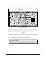
1 Preface
The GGU-SS-FLOW2D program allows modelling of steady-state groundwater flow in
horizontal-plane, vertical-plane and axis-symmetrical groundwater systems using the finiteelement method.
The program system includes a powerful mesh generator and easy-to-use routines for comfortable
evaluation of the modelling results (contours, 3D graphics, etc.).
It is not the aim of this manual to offer an introduction to the finite-element method. For details of
the finite-element method, please see O. C. Zienkiewicz, "Methode der Finiten Elemente" ("FiniteElement Methods"), Carl Hanser Verlag Munich Vienna, 1984. The hydraulic basics used in the
FE program can be taken from, e.g., J. Buß "Unterströmung von Deichen" (Announcement 92,
Leichtweiß-Institut, TU Braunschweig).
Data input is in accordance with WINDOWS conventions and can therefore be learned almost
without a manual. Graphics output supports the true-type fonts supplied with WINDOWS, so that
excellent layout is guaranteed. Colour output and any graphics (e.g. files in formats BMP, JPG,
PSP, TIF, etc.) are supported. DXF files can also be imported by means of the integrated MiniCAD module (see the "Mini-CAD" manual).
The program system has been used in a large number of projects and has been thoroughly tested
(using analytical solutions and in comparison with other FEM applications). No faults have been
found. Nevertheless, liability for completeness and correctness of the program and the manual,
and for any damage resulting from incompleteness or incorrectness, cannot be accepted.
2 Licence protection and installation
In order to guarantee a high degree of quality, a hardware-based copy protection system is used
for the GGU-SS-FLOW2D program.
The GGU software protected by the CodeMeter copy protection system is only available in
conjunction with the CodeMeter stick copy protection component (hardware for connection to the
PC, "CM stick"). Because of the way the system is configured, the protected software can only be
operated with the corresponding CM stick. This creates a fixed link between the software licence
and the CM stick copy protection hardware; the licence as such is thus represented by the CM
stick. The correct Runtime Kit for the CodeMeter stick must be installed on your PC.
Upon start-up and during running, the GGU-SS-FLOW2D program checks that a CM stick is
connected. If it has been removed, the program can no longer be executed.
For installation of GGU software and the CodeMeter software please refer to the information in
the Installation notes for GGU Software International, which are supplied with the program.
GGU-SS-FLOW2D User Manual
Page 7 of 116
June 2015
3 Language selection
GGU-SS-FLOW2D is a multilingual program. The program always starts with the language setting applicable when it was last ended.
The language preferences can be changed at any time in the "?" menu, using the menu item "Language preferences" (in German: "Spracheinstellung", in Spanish: "Configuración de idioma").
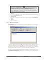
4 Starting the program
After starting the program, you will see two menus at the top of the window:
 File
 ?
After clicking the "File" menu, either an existing file can be loaded by means of the "Load" menu
item, or a new system can be created using "New". The program allows simple system input by
moving directly to the "Mesh/Common systems" menu item after "New" is clicked (see Section
7.2.9). If you do not want to work with the "Common systems" dialog box, click "No" in the
query box or "Cancel" in the subsequent boxes. Select your system and you will then return to the
home screen. Depending on the type of system selected, you will now see either eight or ten
menus along the menu bar:
 File
 Mesh
 z (for horizontal-plane systems only)
 Boundary
 System
 Graphics preferences
 Page size + margins
 Evaluation
 Special (for horizontal-plane systems only)
 ?
After clicking one of these menus, the menu items roll down, allowing you access to all program
functions.
GGU-SS-FLOW2D User Manual
Page 8 of 116
June 2015
The program works on the principle of What you see is what you get. This means that the screen
presentation represents, overall, what you will see on your printer. In the last consequence, this
would mean that the screen presentation would have to be refreshed after every alteration you
make. For reasons of efficiency and as this can take several seconds for complex screen contents,
the GGU-SS-FLOW2D screen is not refreshed after every alteration.
If you would like to refresh the screen contents, press either [F2] or [Esc]. The [Esc] key additionally sets the screen presentation back to your current zoom, which has the default value 1.0,
corresponding to an A3 format sheet.
5 Short description
As reading manuals is, from personal experience, a bit of a chore, there will now follow a short
description of the main program functions. After reading this section you will be in a position to
analyse steady-state groundwater flow. Details can then be taken from further chapters. Worked
examples can be found in Section 9.
 Design the system you wish to analyse.
 Start the GGU-SS-FLOW2D program and go to the menu item "File/New". Answer the
question of the "Common systems" dialog box with "No". Select the type of system which
you would like to work with.
 If necessary, fit the page coordinates to those of your system. For this, use the menu item
"Page size + margins/Manual resize (editor)".
 Then go to the menu item "Mesh/Define nodes".
 Click on the principal nodes (points) of your system with the mouse. The points will be
numbered. Alternatively, you can also enter the system nodes in tabular form, using the
menu item "Mesh/Change". When defining nodes in horizontal-plane systems, new nodes
will be assigned default depths (top and base of aquifer), which may be edited with the
menu item "z/Default depths".
 If the nodes are outside of the page coordinates, go to the menu item "Page size +
margins/Auto-resize" or use the [F9] key.
 Now go to the menu item "Mesh/Manual mesh" and combine the nodes, in groups of
three, to triangular elements. In this way, you create a coarse structure for your system.
Alternatively, you may have the program do this work for you, using the menu item
"Mesh/Automatic".
 If you would like to edit the positions of mesh nodes, go to the menu items
"Mesh/Change", "Mesh/Move" or "Mesh/Edit".
 If, for horizontal-plane systems, you would like to edit the positions of top and base of aquifer, use one of the menu items "z/Individual depths", "z/Modify" or "z/In section".
Using "z/Layer boundary contours", you can get an overview of the positions of the top
and base of the aquifer.
 If you would like to delete a triangular element, go to the menu item "Mesh/Manual
mesh" again and click on the corner nodes of the appropriate element. Using this menu
item, try double-clicking in a triangular element.
 The screen contents can be refreshed at any time using [ESC] or [F2].
GGU-SS-FLOW2D User Manual
Page 9 of 116
June 2015
 Create a fine structure for your system using the menu items "Mesh/Refine individually",
"Mesh/Section" or "Mesh/All".
 Even after a mesh refinement, you can alter the system as you wish using "Mesh/Define
nodes", "Mesh/Manual mesh", etc.
 For demonstration purposes, create one or more acute, and therefore numerically unfavourable, triangular elements using the menu item "Mesh/Move". Then go to the menu item
"Mesh/Optimise" and follow the effects on the screen.
 Define the governing boundary conditions for the system using, e.g., the menu item
"Boundary/Individual potentials".
 Edit, if wished, the soil numbers using the menu item "Boundary/Individual soils".
 Edit, if necessary, the soil properties using the menu item "System/Soil properties".
 When you have completed mesh generation, go to the menu item "System/Analyse" and
begin the analysis. Before analysis starts the program will, if necessary, automatically carry
out a bandwidth optimisation, in order to achieve a numerically favourably configured
equation system.
 After analysis is complete you can, if wished, have the results printed as an output table,
saved to a file or presented in a window (menu item "File/Print output table"). In general,
however, this kind of result presentation will not very be satisfactory for the client.
 For this reason, you should immediately go to the "Evaluation" menu. The menu item
"Evaluation/Coloured" is especially impressive or, for horizontal-plane systems, the menu
item "Evaluation/3D array". The dialog boxes which follow can almost all be exited via
the "OK" button, without further changes having to be made. The program usually makes
sensible suggestions. Only the "Determine extreme values …" button should be clicked
once, otherwise an error message will appear, with a correction note.
 If you have a colour printer installed you can point to the menu item "File/Print and export" and then the "Printer" button in the following dialog box, in order to get colour output to the printer. Grey scale will be used for black and white printers.
 Experiment with the example datasets.
 If you don't like manuals, you can get help using the menu item "?/Help" or the [F1] function key.
This short description demonstrates that only a few menu items must be selected in order to
analyse a groundwater system. All further menu items are mainly for data saving, layout and any
further evaluation of the analysis. A description is given in the following chapters.
GGU-SS-FLOW2D User Manual
Page 10 of 116
June 2015
6 Theoretical principles
6.1
General
An analytical solution is only possible for simple groundwater systems. When analysing complicated systems, numerical solutions are required. In the main
 finite-difference-methods (FDM) and
 finite-element-methods (FEM)
are used. Using finite methods, the whole area is subdivided into a large amount of smaller (finite)
areas (elements). Generally, using FEM, triangles are selected for these areas. Within these triangles simple, generally linear, approximation functions are used. The actual, complicated, whole
solution is pieced together like a mosaic from the many simple partial solutions. Equation systems
result, in which the number of variables corresponds to the number of system nodes. With the
finite-difference-method one generally has only the possibility of defining a discrete whole using
rectangular partial-areas. In contrast to FEM therefore, FDM is a lot less flexible when it comes to
adjusting to complicated boundary structures. Also, in some areas, mesh refinement is not as easy.
Further, the resulting equation systems are numerically more stable for FEM. The main advantage
in FDM is in the theoretically simpler mathematical relationships, which generally will be of little
interest to the program user. The GGU-SS-FLOW2D program uses the finite-element-method.
When using the application please remember that all finite-element or finite-difference-methods
are approximation methods. The quality of the approximation compared to the actual solution
increases with the fineness of the mesh. You should pay attention to the fact that in areas where
the main subsurface hydraulic action takes place (e.g. wells, seepage elements), the mesh
subdivisions should be finer. The type of triangle used also exerts a certain influence. Optimum
conditions are achieved with equilateral triangles. You can get an overview of the solution quality
by calculating the same system with a coarser and a finer mesh subdivision, and comparing the
deviation of the two results.
The following general notes on the GGU-SS-FLOW2D program are important:
 triangular elements are used,
 Darcy's Law is valid,
 the piezometric heads are calculated in a linear manner for each element,
 from the linear approximation of the piezometric heads, a constant approximation of velocities results. In order to achieve a better quality of velocity approximation, the velocities
for calculation of flow lines are averaged to node values in a follow-up calculation.
The procedure is:
For each element node the velocities in the neighbouring elements are added and then divided by the number of neighbouring elements. By doing this, the velocity course can be
better presented. At the boundary nodes, the results are naturally not quite as exact. Further,
the approximation of velocities in the region of element nodes with differing material types
can be worsened in this way. If the velocities at such boundary nodes are of great interest,
help is available by refining the FEM mesh in these areas.
GGU-SS-FLOW2D User Manual
Page 11 of 116
June 2015
6.2
Horizontal-plane system
The program solves the differential equation:
Tx · 2h/x2 + Ty · 2h/y2 + Q = 0
Or, for a leaky aquifer
Tx · 2h/x2 + Ty · 2h/y2 + kv /dv· (H - h)+ Q = 0
Where,
Tx, Ty
= Transmissibility in e.g. m²/s for x and y direction
h
= Piezometric head in e.g. m AD
kv
= Permeability of blanket layer in e.g. m/s
d
= Thickness of blanket layer in e.g. m
Q
= Discharge in e.g. m³/s
x, y
= Coordinates e.g. x and y in m AD
H
= Water level above blanket layer in e.g. m AD
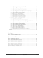
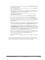
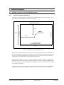
The transmissibilities result from the product of the coefficient of permeability, kx or ky, and the
groundwater thickness in the aquifer d, in e.g. m. In the case of a confined aquifer, the value d is
known in advance. In the case of a non-confined aquifer, the transmissibilities are not immediately
known as, depending upon the position of the groundwater table, different levels will occur at
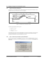
different positions (see Figure 1). In this case an iteration is necessary to analyse each system, in
order to determine the position of the phreatic line. This iteration process is carried out by the
program automatically.
Blanket layer
Phreatic line
d = Groundwater thickness in aquifer
Aquifer
Confining layer
Figure 1 Groundwater thickness in aquifer
GGU-SS-FLOW2D User Manual
Page 12 of 116
June 2015
For the iterative determination of the groundwater thickness in the aquifer, the program first uses
an estimation of the phreatic line. In the current program version this is taken as the top of the
aquifer. With the resulting transmissibilities the program calculates, in the first iteration step, the
piezometric head at all nodes. From these piezometric heads, the transmissibilities for the second
iteration step are calculated. The process is carried on until the transmissibilities between iteration
step (i) and (i - 1) fall below a user-defined deviation.
Note on "leaky aquifer":
The term leaky aquifer can be taken to mean semi-permeable aquifer. This means that water ingress into a lower groundwater system occurs through the blanket layer. The amount of water
entering from above depends upon
 the water level difference between the water level above the blanket layer H and the water
level in the aquifer h,
 the permeability of the blanket layer kv,
 the thickness of the blanket layer dv.
In the differential equation used for analysis (see above), this influence is taken into account in the
term
kv /dv· (H - h).
This expression only creates an additional amount of water, any three-dimensional flow process
cannot be modelled with this simple term. Investigations have shown that for permeability differences of
k / kv > 10.0,
between the aquifer k and the blanket layer kv reliable results can be achieved. The GGU-SSFLOW2D program reliably calculates even small values numerically, without questioning the
physical sense of such input.
Note on boundary conditions:
The case of an impermeable boundary is automatically considered in the finite-element-method.
Valid is, that all system boundaries or partial boundaries which have no water level or source
boundary conditions, are automatically impermeable.
GGU-SS-FLOW2D User Manual
Page 13 of 116
June 2015
6.3
Vertical-plane system and axis-symmetrical system
The program solves the differential equation:
kr · kx · 2h/x2 + kr · ky · 2h/y2 + Q = 0
Where
kx, ky = Permeability in, e.g., m/s for x and y direction
h
= Piezometric head in e.g. m
kr
= Coefficient for determination of permeability in the unsaturated zone
(dimensionless)
Q
= Discharge in e.g. m³/s
x, y
= Coordinates in e.g. m
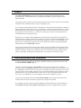
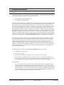
The value kr records the change in permeability in the unsaturated zone r, above groundwater, and
can take on values between 0.0 and 1.0. In the saturated area of the system kr is 1.0. The value kr is
a function of the pore water pressure u. The pore water pressure u is calculated from the piezometric head h, the elevation head y and the unit weight of water w.
u = (h - y) · w
In Figure 2, the curves are presented for three typical soils. Using this value in the differential
equation has the distinct advantage, for the following finite-element calculation, that phreatic lines
can be very easily calculated.
kr
1,0
Area of negative
pore water pressure
Clay
0,5
Silt
u [m]
Sand
-6
-4
-2
0
Figure 2 Function kr = f(u)
GGU-SS-FLOW2D User Manual
Page 14 of 116
June 2015
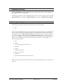
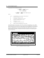
Figure 3 serves as a further explanation. For the case of a horizontal groundwater table, all four
variables h, y, u and kr are given as functions.
Unsaturated zone
h=0
GL
Pore water pressure u negative
y
kr
u
+y
GW
y=0
1,0
+u
Figure 3 Unsaturated zone
If unsaturated zones are present in the system, and a phreatic line analysis is to be carried out, an
iteration process is required, as the position of the phreatic line is not known from the outset. In
the first iteration step, the program assumes that all areas of the system are saturated:
kr = 1.0.
After the initial calculation of the piezometric heads at the system nodes, the pore water pressures
u are calculated and kr determined. With the altered permeabilities, a new calculation of the system follows, with new piezometric heads and correspondingly new pore water pressures and kr
values. The iteration process is carried on until the difference in piezometric head in iteration step
(i) and (i - 1) falls below the user-defined limit value (iteration divergence).
Note on boundary conditions:
The case of an impermeable boundary is automatically taken in to account by the finiteelement-method. Valid is, that all system boundaries or partial system boundaries which
have no water level or source boundary conditions, are automatically impermeable.
GGU-SS-FLOW2D User Manual
Page 15 of 116
June 2015
7 Description of menu items
7.1
7.1.1
File menu
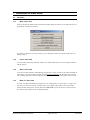
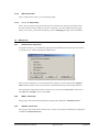
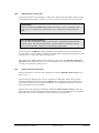
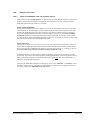
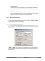
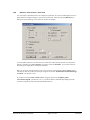
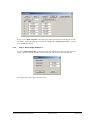
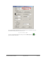
"New" menu item
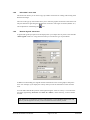
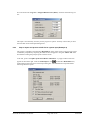
After pointing at the "New" menu item the subsequent dialog box allows you to define the type of
groundwater system to be created.
If you have worked on a previous system you can, if desired, utilise the existing mesh, after confirming a query.
7.1.2
"Load" menu item
You can load a file with system data, which was created and saved at a previous sitting, and then
edit the system.
7.1.3
"Save" menu item
You can save data entered or edited during program use to a file, in order to have them available at
a later date, or to archive them. The data is saved without prompting with the name of the current
file. Loading again later creates exactly the same presentation as was present at the time of saving.
7.1.4
"Save as" menu item
You can save data entered during program use to an existing file or to a new file, i.e. using a new
file name. For reasons of clarity, it makes sense to use ".fen" as file suffix, as this is the suffix
used in the file requester box for the menu item "File/Load". If you choose not to enter an extension when saving, ".fen" will be used automatically.
GGU-SS-FLOW2D User Manual
Page 16 of 116
June 2015
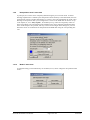
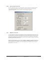
7.1.5
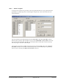
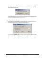
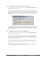
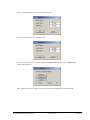
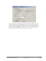
"Import ASCII file" menu item
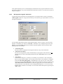
If the coordinates of the FEM mesh nodes are available in ASCII file format, they can be imported
into the program. Each row of the file must contain the x- and y-value of a node. Decimal fractions must use a point, not a comma. When importing the ASCII file you must specify the columns
containing the x- and the y-values.
The current row of the ASCII file is shown at the top. You can navigate through the file using the
arrow buttons on the right. If all the information is correct, the result for the row is shown in the
box below the column. Otherwise, an error message appears. You may need to change the column
delimiter. If the file contains invalid as well as valid rows, these will simply be skipped during the
subsequent import. Finally, select the "Import data" button. The imported coordinates can then
be processed to form an FEM mesh.
7.1.6
"Save ASCII file" menu item
If an FEM mesh has been generated, the node coordinates can be saved to an ASCII file, allowing
them to be imported into other programs where required.
If you are working with a vertical-plane system and the system has already been analysed, an
ASCII record can be exported especially for the GGU's GGU-STABILITY slope stability application. This contains the calculated potentials, beside the node coordinates. These data can be
directly utilised in GGU-STABILITY as a pore water pressure mesh.
GGU-SS-FLOW2D User Manual
Page 17 of 116
June 2015
7.1.7
"Export (GGU-3D-SSFLOW)" menu item
Using this menu item it is possible to export a previously analysed horizontal-plane system to the
GGU's groundwater modelling program GGU-3D-SSFLOW for further processing. The GGU3D-SSFLOW application allows analysis of groundwater flow using finite elements in threedimensional systems.
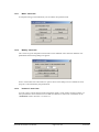
7.1.8
"Print output table" menu item
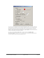
7.1.8.1
Selecting the output format
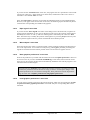
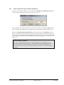
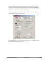
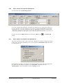
You can have a table printed containing the current analysis results. The results can be sent to the
printer or to a file (e.g. for further editing in a word processor). The output contains all information on the current state of analysis, including the system data.
You have the option of designing and printing the output table as an annex to your report within
the GGU-SS-FLOW2D program. To do this, select "Output as graphics" from the following
options.
If you prefer to easily print or process the data in a different application, you can send them directly to the printer or save them to a file using the "Output as ASCII" button.
GGU-SS-FLOW2D User Manual
Page 18 of 116
June 2015
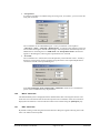
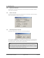
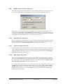
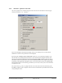
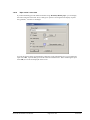
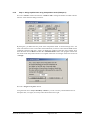
7.1.8.2
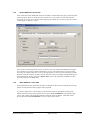
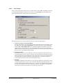
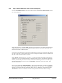
Button "Output as graphics"
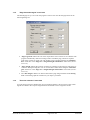
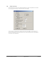
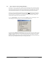
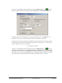
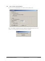
If you selected the "Output as graphics" button in the previous dialog box a further dialog box
opens, in which you can define further preferences for result visualisation.
You can define the desired layout for the output table in various areas of the dialog box. By activating the "Incorporate graphics" button, a sketch of the system is integrated in the output table.
If you need to add a header or footer (e.g. for page numbering), activate the appropriate check
boxes "With headers" and/or "With footers" and click on the "Edit" button. You can then edit as
required in a further dialog box.
GGU-SS-FLOW2D User Manual
Page 19 of 116
June 2015
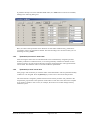
Automatic pagination can also be employed here if you work with the placeholders as described.
After exiting the dialog boxes using "OK" you will see a further dialog box in which you can
select the parameters to be used in the output table. If you click the "Start" button the output table
is presented on the screen page by page. To navigate between the pages, use the arrow tools
in the toolbar. If you need to jump to a given page or back to the graphical representation, click on the
tool. You will then see the following box:
GGU-SS-FLOW2D User Manual
Page 20 of 116
June 2015
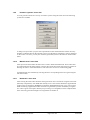
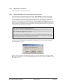
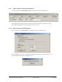
7.1.8.3
Button "Output as ASCII"
You can have your analysis data sent to the printer, without further work on the layout, or save it
to a file for further processing using a different program, e.g. a word processing application. After
selecting the button "Output as ASCII" you will see a further dialog box in which you can select
the parameters to be used. If you click the "Start" button, the following dialog box appears in
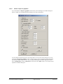
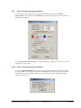
which you can define output preferences.
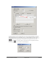
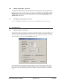
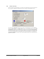
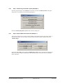
In the dialog box you can define output preferences:
 "Printer preferences" group box
Using the "Edit" button the current printer preferences can be changed or a different printer
selected. Using the "Save" button, all preferences from this dialog box can be saved to a
file in order to have them available for a later session. If you select "GGU-SSFLOW2D.drk" as file name and save the file in the program folder (default), the file will
be automatically loaded the next time you start the program.
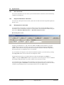
Using the "Page format" button you can define, amongst other things, the size of the left
margin and the number of rows per page. The "Header/footer" button allows you to enter
a header and footer text for each page. If the "#" symbol appears within the text, the current
page number will be entered during printing (e.g. "Page #"). The text size is given in "Pts".
You can also change between "Portrait" and "Landscape" formats.
 "Print pages" group box
If you do not wish pagination to begin with "1" you can add an offset number to the check
box. This offset will be added to the current page number. The output range is defined using "From page no." "to page no.".
 "Output to:" group box
Start output by clicking on "Printer" or "File". The file name can then be selected from or
entered into the box. If you select the "Window" button the results are sent to a separate
window. Further text editing options are available in this window, as well as loading, saving and printing.
GGU-SS-FLOW2D User Manual
Page 21 of 116
June 2015
7.1.9
"Printer preferences" menu item
You can edit printer preferences (e.g. swap between portrait and landscape) or change the printer
in accordance with WINDOWS conventions.
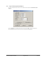
7.1.10
"Print and export" menu item
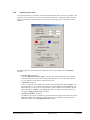
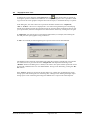
You can select your output format in a dialog box. You have the following possibilities:
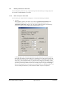
 "Printer"
allows graphic output of the current screen contents (graphical representation) to the
WINDOWS default printer or to any other printer selected using the menu item
"File/Printer preferences". But you may also select a different printer in the following
dialog box by pressing the "Printer prefs./change printer" button.
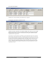
In the upper group box, the maximum dimensions which the printer can accept are given.
Below this, the dimensions of the image to be printed are given. If the image is larger than
the output format of the printer, the image will be printed to several pages (in the above example, 4). In order to facilitate better re-connection of the images, the possibility of entering an overlap for each page, in x and y direction, is given. Alternatively, you also have the
possibility of selecting a smaller zoom factor, ensuring output to one page ("Fit to page"
button). Following this, you can enlarge to the original format on a copying machine, to ensure true scaling. Furthermore, you may enter the number of copies to be printed.
GGU-SS-FLOW2D User Manual
Page 22 of 116
June 2015
If you have activated the tabular representation on the screen, you will see a different dialog box for output by means of the "File/Print and export" menu item button "Printer".
Here, you can select the table pages to be printed. In order to achieve output with a zoom
factor of 1 (button "Fit in automatically" is deactivated), you must adjust the page format
to suit the size format of the output device. To do this, use the dialog box in "File/Print
output table" button "Output as graphics".
 "DXF file"
allows output of the graphics to a DXF file. DXF is a common file format for transferring
graphics between a variety of applications.
 "GGUCAD file"
allows output of the graphics to a file, in order to enable further processing with the
GGUCAD program. Compared to output as a DXF file this has the advantage that no loss
of colour quality occurs during export.
 "Clipboard"
The graphics are copied to the WINDOWS clipboard. From there, they can be imported
into other WINDOWS programs for further processing, e.g. into a word processor. In order
to import into any other WINDOWS program you must generally use the "Edit/Paste"
function of the respective application.
 "Metafile"
allows output of the graphics to a file in order to be further processed with third party software. Output is in the standardised EMF format (Enhanced Metafile format). Use of the
Metafile format guarantees the best possible quality when transferring graphics.
GGU-SS-FLOW2D User Manual
Page 23 of 116
June 2015
If you select the "Copy/print area" tool
from the toolbar, you can copy parts of
the graphics to the clipboard or save them to an EMF file. Alternatively you can send
the marked area directly to your printer (see "Tips and tricks", Section 8.3).
Using the "Mini-CAD" program module you can also import EMF files generated using other GGU applications into your graphics.
 "MiniCAD"
allows export of the graphics to a file in order to enable importing to different GGU applications with the Mini-CAD module.
 "GGUMiniCAD"
allows export of the graphics to a file in order to enable processing in the GGUMiniCAD
program.
 "Cancel"
Printing is cancelled.
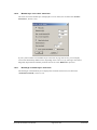
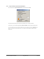
7.1.11
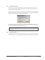
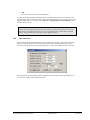
"Batch print" menu item
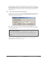
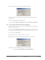
If you would like to print several appendices at once, select this menu item. You will see the following dialog box:
Create a list of files for printing using "Add" and selecting the desired files. The number of files is
displayed in the dialog box header. Using "Delete" you can mark and delete selected individual
files from the list. After selecting the "Delete all" button, you can compile a new list. Selection of
the desired printer and printer preferences is achieved by pressing the "Printer" button.
You then start printing by using the "Print" button. In the dialog box which then appears you can
select further preferences for printer output such as, e.g., the number of copies. These preferences
will be applied to all files in the list.
GGU-SS-FLOW2D User Manual
Page 24 of 116
June 2015
7.1.12
"Exit" menu item
After a confirmation prompt, you can quit the program.
7.1.13
"1, 2, 3, 4" menu items
The "1, 2, 3, 4" menu items show the last four files worked on. By selecting one of these menu
items the listed file will be loaded. If you have saved files in any other folder than the program
folder, you can save yourself the occasionally onerous rummaging through various sub-folders.
7.2
7.2.1
Mesh menu
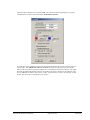
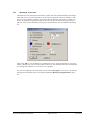
"Preferences" menu item
Using this menu item you can define the appearance of the FEM mesh on the screen. The element
no. and the soil no. cannot be displayed simultaneously.
?
After leaving the dialog box via the "OK button the preferences will be adopted. The "Display
mesh" button produces a direct representation of the FEM mesh using the selected preferences.
If the FEM mesh representation does not fill the screen, point to the "Auto-resize" menu item in
the "Page size + margins" menu or press [F9].
7.2.2
"Mesh" menu item
After going to this menu item the FEM mesh is displayed as defined in "Mesh/Preferences".
7.2.3
"Outline" menu item
After going to this menu item the outlines of the various soils used in the FEM mesh are displayed
as defined in "Mesh/Preferences".
GGU-SS-FLOW2D User Manual
Page 25 of 116
June 2015
7.2.4
"Define nodes" menu item
You can use the left mouse button to define a new node or the right mouse button to delete a previously defined node. This menu item can also be reached using [F3]. If you are editing a horizontal-plane system, each new point created using this menu item will be assigned the default depths
(see "z/Default depths" menu item, Section 7.3.2).
When setting new nodes, the current x- and y-coordinates of the mouse are shown in the status bar
at the bottom of the window. If you have access to a scanner you can scan in the system to be
processed and save it e.g. as a bitmap file (extension: ".bmp"). This bitmap can be displayed on
the screen using the Mini-CAD program module (see the "Mini-CAD" manual). This greatly
simplifies input of the principal system nodes.
Alternatively, you can also import a DXF file using Mini-CAD (see "Mini-CAD" manual). This
can contain the system outline, for example. If Mini-CAD data are already present, the initial
dialog box provides a check box with the option of locking on to Mini-CAD lines.
If you activate this check box the mouse cursor appears as a rectangle with cross-hairs. If the end
point of a Mini-CAD line is located within this rectangle the program will lock on to this point
precisely; if a number of points are located within the rectangle, it will lock on to the one nearest
the centre of the cross-hairs.
7.2.5
"Change" menu item
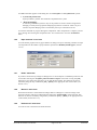
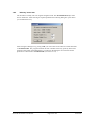
The coordinates of existing nodes can be edited. Three options are available for this:
 "Via a table"
You can edit the coordinates of existing nodes in a dialog box or, alternatively, enter the
coordinates of new nodes.
If you need to edit the current number of nodes click the "x FEM nodes to edit" button and
enter the new number of nodes. You can navigate through the table using "Forw." and
"Back". If you are editing a horizontal-plane system, each new point created using this
menu item will be assigned the default depths (see "z/Default depths" menu item, Section
7.3.2). If you set the number of nodes to 0 the FEM incidence table is deleted.
It is even easier to import node coordinates via the Windows clipboard. For example, if the
x-/y-coordinates of the FEM mesh nodes are available in an Excel table, it is possible to
copy the two columns containing the data into the clipboard ("Edit/Copy") and then to
paste them into the dialog box "Via a table" by pressing "Import clipboard".
GGU-SS-FLOW2D User Manual
Page 26 of 116
June 2015
 "Via equation"
If you have entered the coordinates using the wrong scale, for instance, you can correct this
using this menu item.
The coordinates can be edited differing for x- and y-coordinates via the equation
"value(new) = factor · value(old) + displacement". A rotation of the complete system can
also be achieved using the entered rotation angle. If an interpolation mesh already exists an
additional box containing the two "FEM mesh" and "Interpolation mesh" check boxes
appears in the dialog box, allowing the required mesh to be activated.
 "In section"
The coordinates for a selected area can be displaced by a fixed amount in the x- and the ydirection. Click 4 points counter-clockwise using the mouse. The required displacement
can then be entered in the opened dialog box.
If the "Do not displace nodes with boundary conditions" check box is activated these
points will be excluded from any displacement.
7.2.6
"Move" menu item
The defined FEM system is displayed with the FEM elements after selecting this function. The
nodes can be moved with the left mouse button pressed. The coordinates of the current node are
displayed in the status bar. The last node movement can be undone using the [Backspace] key.
7.2.7
"Edit" menu item
By double-clicking a node using the left mouse button a dialog box appears allowing the coordinates to be edited via the keyboard.
GGU-SS-FLOW2D User Manual
Page 27 of 116
June 2015
7.2.8
"Array" menu item
7.2.8.1
Select type of array
After selecting this menu item you can decide whether new nodes are generated using a regular or
an irregular array.
If you are editing a horizontal-plane system, each new point created with this menu item will be
assigned the default depths (see "z/Default depths" menu item, Section 7.3.2).
7.2.8.2
Button "Regular"
The regular array allows the nodes to be defined in a number of ways:
 "Line"- along one or more lines,
 "Rectangle" - in one or more rectangles,
 "Quadrilateral" - in one or more quadrilaterals.
The procedure is similar for all three cases. Therefore, only the rectangles will be described.
Enter the corner points of the array and the number of subdivisions. If the "Generate new mesh"
check box is activated, all existing nodes are deleted and then the user-defined FEM nodes in the
dialog box are generated with the appropriate FEM mesh.
GGU-SS-FLOW2D User Manual
Page 28 of 116
June 2015
7.2.8.3
Button "Irregular"
In contrast to the regular array procedure, where the generated nodes are evenly spaced within the
generated rows, the spacing can be varied using the irregular array. This can be done in the following dialog box.
The array numbers can be defined using the "No. of dx values" and "No. of dy values" buttons.
Enter the array spacing in "dx" and "dy". If you press the "Recalculate x and y values" button the
first column to the left of "dx" and "dy" are recalculated. These are absolute values for the array.
The array origin is entered in "x0" and "y0".
The program can generate an FEM mesh from the newly generated FEM nodes if the "Generate
new mesh" check box is activated. If a mesh already exists, it can be deleted prior to generating
the new one by activating the "Delete current mesh" check box.
GGU-SS-FLOW2D User Manual
Page 29 of 116
June 2015
7.2.9
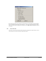
"Common systems" menu item
You can generate a mesh for a variety of common systems using this menu item. The following
systems are available:
A dialog box opens when you press the required button. Enter the dimensions and the necessary
boundary conditions data for the selected system. Once the data is entered the system is displayed
on the screen. Of course, you may also use these generated systems as the basis for further refinements.
7.2.10
"Manual mesh" menu item
After input of the mesh nodes this menu item is used to define the FEM mesh. Three nodes must
be clicked using the left mouse button. Once the three nodes have been selected a box appears for
defining the soil no. of the FEM element. This menu item can also be reached using [F4].
An FEM element can be deleted by selecting the three corresponding nodes once again using the
left mouse button.
7.2.11
"Automatic" menu item
After entering the mesh nodes automatic mesh generation can be carried out using this menu item
(Delauney triangulation). If an FEM mesh already exists it can be either deleted or supplemented.
Under certain circumstances, air holes (incompletely filled FEM mesh) may occur in an existing
FEM mesh being supplemented if this mesh was not generated by means of Delauney triangulation. These regions will require manual post-processing or re-triangulation of the complete FEM
mesh. All newly generated triangles are assigned the soil number 1.
GGU-SS-FLOW2D User Manual
Page 30 of 116
June 2015
7.2.12
"Round off" menu item
During Delauney triangulation a triangular mesh is generated that envelops all nodes. This can
lead to acute-angled triangle elements in the boundary regions. These triangles can be removed
from the FEM mesh using this menu item.
The program first draws the maximum radius ratio of the most unfavourable triangle and displays
the data in a message box. You then see a dialogue box, allowing you to define a maximum radius
ratio above which all triangles with greater values are deleted.
The radius ratio describes the relationship between external radius and internal radius of a triangle.
For an equilateral triangle, this ratio equals 2.0 (optimum). In the example above, all external
triangles with a radius ratio greater than 6 will be removed.
In order to avoid interpolation holes in the triangle system only triangles at the boundaries
are deleted.
7.2.13
"Delete" menu item
This menu item allows you to delete selected system triangles. You must first click four points in
anti-clockwise direction. All triangles with their centroid within this quadrilateral will be deleted.
GGU-SS-FLOW2D User Manual
Page 31 of 116
June 2015
7.2.14
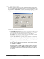
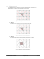
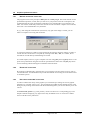
Optimise" menu item
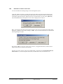
You first select in a dialog box whether the diagonals or the topology should be optimised.
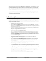
"Diagonals" button
Optimisation of diagonals is implemented in order to create a numerically favourable FEM mesh,
i.e. where possible, equilateral triangles. The effect of the optimisation of diagonals can best be
seen using an example:
Figure 4 Optimisation of diagonals
If an existing unfavourable diagonal cuts two different soil areas, no optimisation takes place,
because this would alter the system.
"Topology" button
This program routine displaces the triangular element nodes so that, where possible, equilateral
triangles are created. Equilateral triangles have especially favourable numerical properties. Because the displacement of system boundaries and element boundaries with neighbouring elements
consisting of different soils does not make much sense, these element boundaries are fixed from
the outset. Nodes with defined water level boundary conditions also remain unaltered. Optimisation of the FEM mesh can be followed on the screen by setting the "With graphics" check box.
The optimisation routine can be aborted at any time by pressing the right mouse button.
In horizontal-plane systems the problem arises that the values for aquifer base and aquifer top, as
well as for top of blanket layer, are not adapted to the new location due to the displacement of
individual nodes. If different values for aquifer base and aquifer top, as well as for top of blanket
layer, exist in the system the program will issue a warning. In this case, activate the "Adapt aq.
base and aq. top" or "Adapt aq. base and aq. top and blanket top"; the values are then adapted
appropriately by the program using interpolation between the neighbouring nodes. It is possible to
assign the precise values via an interpolation mesh following the optimisation (see Step 7 in Example 1, Section 9.1.8).
7.2.15
"Align" menu item
By clicking the left mouse button it is possible to select a node to be aligned depending on certain
criteria (e.g. on a circle).
GGU-SS-FLOW2D User Manual
Page 32 of 116
June 2015
7.2.16
"Refine individually" menu item
Mesh elements can be selected for refinement using the following menu item.
Upon activating the "Consider potential" check box, new nodes located immediately between
two nodes with potential boundary conditions will be assigned the average of the two values. This
procedure is not unequivocal when applied to source boundary conditions and can lead to misunderstandings. Source boundary conditions are therefore not refined in the course of mesh refinement. A description of the 3 refinement methods can be found in Section 7.2.19.
7.2.17
"Section" menu item
A number of elements previously enveloped in a polygon can be refined using this menu item or,
alternatively, pressing [F6]. Potential boundary conditions can be taken into consideration (see
"Mesh/Refine individually" menu item, Section 7.2.16). A description of the 3 refinement methods can be found in Section 7.2.19.
7.2.18
"All" menu item
The following dialog box appears after selecting this menu item or, alternatively, pressing [F7]:
Either all elements or only element with certain material numbers can be refined. Here, too, potential boundary conditions can be taken into consideration (see "Mesh/Refine individually" menu
item, Section 7.2.16). A description of the 3 refinement methods can be found in Section 7.2.19.
GGU-SS-FLOW2D User Manual
Page 33 of 116
June 2015
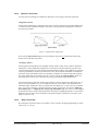
7.2.19
Refinement methods
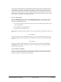
Three different refinement methods can be applied for element refinement. Refinement will be
demonstrated on the following mesh using element 23 as an example.
Figure 5 FEM refinement demonstration mesh
 "Method 1"
An additional node is generated in the centroid of the selected triangle.
Figure 6 FEM mesh refinement using Method 1
 "Method 2"
The selected triangle element and the neighbouring triangle element are halved.
Figure 7 FEM mesh refinement using Method 2
GGU-SS-FLOW2D User Manual
Page 34 of 116
June 2015
 "Method 3"
A new triangle element is inserted at the median of the clicked triangle element. The neighbouring triangle elements are halved.
Figure 8 FEM mesh refinement using Method 3
7.3
7.3.1
z menu (for horizontal-plane systems only)
General note
The "z" menu appears for horizontal plane systems only. It allows simple definition of the z-values
of a system, i.e. the definition of the top of the aquifer, the base of the aquifer and, in addition, the
top of the blanket for a "leaky aquifer".
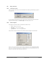
7.3.2
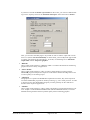
"Default depths" menu item
The default depths defined in this dialog box are assigned to all new FEM nodes defined using
the "Mesh/Define nodes" menu item. The additional entry "Blanket top" appears in the dialog
box for a "leaky aquifer".
If you edit the given value and leave the dialog box using "Done" the newly defined depths will be
adopted as of this moment for newly defined nodes. If nodes are already defined, they can also be
retroactively assigned z values using the "For all" button.
GGU-SS-FLOW2D User Manual
Page 35 of 116
June 2015
7.3.3
"Individual depths" menu item
The z-values of nodes (top/bottom of aquifer, top of blanket layer) can be edited by doubleclicking a node.
7.3.4
"Modify (depths)" menu item
You can modify all z-values as a function of the existing z-values. The following dialog box
shows an example where the base of the aquifer lies at 12 m below the existing aquifer top at all
nodes.
7.3.5
"In section" menu item
After defining a quadrilateral, all nodes within it can be assigned new z-values (top of aquifer,
base of aquifer and, where required, top of blanket). If the "Show depths" check box is activated
in the message box the nodes are labelled with the current depth. This provides a good overview
of the possible depth ranges present.
GGU-SS-FLOW2D User Manual
Page 36 of 116
June 2015
7.3.6
"Layer boundary contours" menu item
In order to clearly present the layer situation it is possible to generate a contour diagram of the top
of the aquifer (aq. top) or the base of the aquifer (aq. base) or the top of the blanket (blanket top)
for a leaky aquifer.
Define the type of contour diagram using the "Normal", "Coloured" and "3D" option buttons.
Details are described in Sections 7.8.1 to 7.8.3. Exit the dialog box by clicking the button for the
layer for which the contour diagram is to be displayed.
7.3.7
"Layer thickness contours" menu item
You can create a contour diagram of the layer thicknesses.
If the "Coloured" check box is activated, colour filled contours are created.
7.3.8
"Section" menu item
The layer boundaries for a given section can be displayed using this menu item. Left-click on
system nodes to define a section. The layer boundaries are displayed after pressing [Return].
If you have evaluated a section for an analysed system using the "Evaluation/Values in node
section" menu item and then saved the section, this section can be reloaded and utilised for layer
boundary representation.
GGU-SS-FLOW2D User Manual
Page 37 of 116
June 2015
7.3.9
"Interpolation mesh" menu item
In principle, the z values can be completely defined using the previous menu items. A further
defining simplification is offered by the interpolation mesh. Similarly to the FEM mesh, this interpolation mesh consists of nodes and triangles. A certain z value can be defined at the nodes. After
defining an interpolation mesh you can assign these z values to the FEM mesh as the base or top
of the aquifer (or, for a "leaky aquifer", as blanket layer top). These are assigned by means of
linear interpolation. The interpolation mesh should (but not must) completely blanket the FEM
mesh. In the simplest case possible, this may consist of one triangle. In the dialog box yoou can
define the colour of visualisation for interpolationa and FEM mesh using the corresponding buttons.
7.3.10
"Nodes" menu item
In complete analogy to the FEM mesh you can define, move, edit or change the interpolation mesh
nodes.
GGU-SS-FLOW2D User Manual
Page 38 of 116
June 2015
7.3.11
"Mesh" menu item
In complete analogy to the FEM mesh you can edit the interpolation mesh.
7.3.12
"Modify" menu item
The z values of given interpolation mesh nodes can be modified. After clockwise definition of a
quadrilateral the following dialog box appears:
Once a constant has been entered the two options shown in the dialog box are available for modifying the z-values defined by the quadrilateral.
7.3.13
"Contours" menu item
You can create a contour diagram of the interpolation mesh z values. Either coloured contours or a
3D representation can be selected. You can find more details on contour line visualisation in the
"Evaluation" menu in Sections 7.8.2 and 7.8.3.
GGU-SS-FLOW2D User Manual
Page 39 of 116
June 2015
7.3.14
"Import/export" menu item
The x- and y-coordinates of the interpolation mesh can be imported from an ASCII file or exported for other applications. A dialog box as described in Section 7.1.5 opens for the "Import
ASCII" option.
If the coordinates are exported using the GGU-SS-FLOW2D format, the information regarding
triangles (incidence table) and z values will also be exported and can be imported again.
7.3.15
"Assign" menu item
After completely processing the interpolation mesh the z-values associated with the interpolation
mesh can be assigned to the FEM mesh as the top of the aquifer, the base of the aquifer or the top
of the blanket.
Because no undo is possible after assigning the z values, it is expedient to save the file beforehand.
GGU-SS-FLOW2D User Manual
Page 40 of 116
June 2015
7.4
7.4.1
Boundary menu
"Preferences" menu item
In the dialog box for this menu item preferences for the presentation of the boundary conditions
on the screen can be specified.
7.4.2
"Check" menu item
This menu item provides a good overview of the locations of all boundary conditions by displaying the required boundary conditions on the screen.
7.4.3
"Individual potentials" menu item
After going to this menu item you will first see the following dialog box:
After clicking the "Graphically" button the FEM mesh is displayed with any existing potentials.
You can define a potential boundary condition at the FEM nodes using the left mouse button, or
edit existing potentials. A right-click deletes existing potentials.
Note:
The piezometric head must be given when handling problems involving groundwater hydraulics. Die piezometric head h results from adding the pore water pressure u (= w·h) and
the elevation head y. The piezometric head is also known simply as the water level. Further
common designations include potential or hydraulic head.
GGU-SS-FLOW2D User Manual
Page 41 of 116
June 2015
If potentials already exist at the individual FEM nodes, the "Table" button will also be available,
leading to the following dialog box:
Here, the values of the potentials can be edited for several nodes simultaneously, potentials be
converted to sources or potentials be deleted. The selected changes are carried out when you exit
the dialog box using "Done".
7.4.4
"(Potentials) In section" menu item
After selecting this menu item several FEM nodes can be simultaneously assigned a potential
boundary condition in a defined section, or an existing boundary condition be deleted. For this
click four points in an anti-clockwise direction using the left mouse button. The right mouse button will undo. The definition refers to all nodes within the quadrilateral.
7.4.5
"(Potentials) Linear" menu item
After going to this menu item you click the nodes of the FEM mesh to which a potential boundary
condition is to be assigned. Press the [Return] key to then enter a start and an end potential.
The selected node is assigned a potential which increases linearly from the start potential to the
end potential, proportional to the separation of the nodes to each other. This menu item is helpful
if you need to consider a water course, for example, the water level of which changes linearly
within the system.
GGU-SS-FLOW2D User Manual
Page 42 of 116
June 2015
7.4.6
"Point sources" menu item
Using this menu items source boundary conditions are defined within the FEM system in analogy
to the displacement boundary conditions. A source is positive if it brings water into the system.
ATTENTION:
When calculating axis-symmetrical groundwater flow these sources are multiplied internally with 2··r, so that no intervention by the user is needed in the running of the program.
Note on impermeable boundaries:
The case of an impermeable boundary is automatically considered by the finite-elementmethod. Valid is, that all system boundaries or partial boundaries which have no water
level or source boundary conditions, are automatically impermeable.
After clicking the "Graphically" button the FEM mesh is displayed with any existing sources.
You can define a source boundary condition at the FEM nodes using the left mouse button, or edit
existing sources. A right-click deletes existing sources.
After clicking the "Table" button the same dialog box opens as for the "Boundary/Individual
potentials" menu item (see Section 7.4.3). You can edit the source values for various nodes, convert sources to potentials or delete sources.
7.4.7
"Linear sources" menu item
General information on sources can be found in the menu item "Boundary/Point sources" (see
Section 7.4.6).
The procedure for defining linear sources is explained in a dialog box. After clicking system
nodes and confirming the selection with the [Return] key, a dialog box opens for defining the
start and the end value. The intermediate boundaries will be assigned the appropriate value in a
linear relationship to the point spacing.
If linear sources have already been defined an additional "Delete all linear sources" button appears in the info box after selecting this menu item again. If you exit the dialog box by using this
button, all linear sources are deleted and a new linear source can be defined.
GGU-SS-FLOW2D User Manual
Page 43 of 116
June 2015
If you need to delete individual linear sources or sections of them, click the system nodes again,
accept with the [Return] key and exit the start and end value dialog box by pressing "OK". The
following dialog box now appears:
Click the "Delete old source" button until all sections of the marked linear source are deleted and
then define the new linear source if required. If you exit the box by pressing "Cancel" before you
are finished, the undeleted boundaries will remain in place.
7.4.8
"Diffuse sources" menu item
Certain elements can be assigned diffuse sourcesby defining the area required as a polygon using
4 counter-clockwise points. You will then see the following dialog box:
If you activate the "Add diffuse source" check box, the value entered will be added to any diffuse
sources already present. If negative entries are made the diffuse source is reduced
correspondingly. If you click the "Delete all" button, all existing diffuse sources are deleted and
you can define a new diffuse source after specifying a new polygon.
GGU-SS-FLOW2D User Manual
Page 44 of 116
June 2015
7.4.9
"Diffuse sources for soils" menu item
Individual soils can be defined as diffuse sources by assigning a discharge to the respective soil
(e.g. m³/s/m²). Select the soil in the dialog box and enter the value for the diffuse source.
Alternatively, you can have the value of the diffuse source determined by the program. If you
click the button "Determine value of diffuse source from sum Q" you must enter the discharge
for the area of the selected soil in the new dialog box. The program then determines the value for
the diffuse source from the data given. You can then accept this value
7.4.10
"Individual soils" menu item
After selecting the type of FEM system screen representation the soil number assignments can be
edited for individual elements of the FEM mesh. This assigns these elements the soil properties
that were defined in the "System/Soil properties" menu item (see Section 7.5.3).
7.4.11
"(Soils) In section" menu item
After selecting the type of FEM system screen representation you define a polygon by clicking 4
points in counter-clockwise direction. All elements with their centroid within this polygon can be
assigned a different soil number. The associated soil properties are defined in the "System/Soil
properties" menu item (see Section 7.5.3).
7.4.12
"Define pipes" menu item
Left-click system nodes to define pipe elements which can then be assigned a material number
after pressing the [Return] key. The defined pipes are shown with the appropriate material number in the graphics. The colour and width of the lines can be edited using the "Graphics preferences/Pen colour and width" menu item (see Section 7.6.3).
If you need to delete individual pipes or sections of them, click the system node again, accept with
the [Return] key and exit the material number dialog box by pressing "OK". Click the "Delete
old pipe" button until all sections of the marked pipe are deleted and then define the new pipe if
required. If you exit the box by pressing "Cancel" before you are finished, the undeleted pipe
sections will remain in place.
GGU-SS-FLOW2D User Manual
Page 45 of 116
June 2015
7.4.13
"Delete pipes" menu item
All defined pipes are deleted after a prompt.
7.4.14
"Individual blankets" menu item (only for "leaky aquifer")
If you are analysing a horizontal-plane system with a "leaky aquifer", proceed as for a simple
horizontal-plane system when generating the system. However, a water level above the blanket
must be additionally assigned for elements below a blanket layer. If you forget to do this the system will be analysed as a horizontal-plane problem without a blanket. Regardless of this, the Aq.
top entry (= top of aquifer) governs the analysis in terms of confined or unconfined. If you do not
assign a water above the blanket layer to individual elements, these elements are also dealt with as
if the problem is a horizontal-plane without a blanket. This may well be the actual case in parts of
the system and may therefore be very useful.
Note on water level above the blanket layer:
Although the designation Water level above the blanket layer has been used for this manual, this does not represent the value between the top of the blanket and the water level; instead, the absolute height is always meant.
For example, if the top of the blanket is at 31.08 m AD and the water level above the blanket is at 33.28 m AD, the water level above the blanket layer to be entered is 33.28 (m AD)
and not the difference of 1.2 m between these two values.
The water level above the blanket is defined for each element. If you click a single element the
following dialog box opens:
Enter the water level above the blanket and assign it to the selected element by clicking the "Define" button. Alternatively, you can also edit an existing water level or remove it completely using
the "Delete" button.
GGU-SS-FLOW2D User Manual
Page 46 of 116
June 2015
7.4.15
"(Blankets) In section" menu item (only for "leaky aquifer")
General principles on the definition of blankets can be found in the "Boundary/Individual blankets" menu item (see Section 7.4.14).
After going to this menu item several FEM elements can be simultaneously assigned a blanket
boundary condition in a defined section, or an existing boundary condition can be deleted. To do
this, left-click four points counter-clockwise; a right mouse click resets the selected points. The
definition refers to all nodes with their centroids within the quadrilateral. The following dialog
box appears:
The "Delete" button deletes any existing water levels. The entered water level is assigned to the
selected elements using the "Define" button. The "Water level = blanket top + c" button assigns
the selected elements either a water level corresponding to the top of the blanket or the top of the
blanket plus a constant c.
7.4.16
"(Blankets) Linear" menu item (only for "leaky aquifer")
General principles on the definition of blankets can be found in the "Boundary/Individual blankets" menu item (see Section 7.4.14).
Using this menu item it is possible to assign a linearly variable water level above the blanket to
several elements. This can be useful for example if you need to model a semi-pervious water
course where the bed has been subject to colmation, that is, it has a blanket layer and displays a
variable water level within the system.
After going to this menu item you click the nodes of the FEM mesh to which a variable water
level is to be assigned. Press the [Return] key to then enter a start and an end water level above
the blanket.
The selected elements are assigned a water level proportional to the separation of the element
centres, increasing from the start water level to the end water level.
GGU-SS-FLOW2D User Manual
Page 47 of 116
June 2015
7.5
7.5.1
System menu
"Info" menu item
You will see information on the current system with the number of elements, nodes and boundary
conditions in a dialog box.
7.5.2
"Project identification" menu item
You can enter a description of the current system; this will then be used in the general legend (see
Section 7.6.9).
7.5.3
"Soil properties" menu item
You can edit the soil properties. A variety of dialog boxes can now appear depending on the selected basic system. The number of input rows corresponds to the soil numbers awarded using the
menu items "Boundary/Individual soils" or "Boundary/(Soils) In section".
Horizontal-plane system
The Darcy permeabilities in x- and y-direction ("khx" and "khy") and the effective pore space
("neff") must be entered. The effective pore space is not incorporated in the basic differential
equation. These values are only required for the subsequent evaluation of the data computed for
flow line generation. A designation entry is not required
If you would like to arrange the soils entered in a different sequence, you can do this by pressing
the "Swap soils" button. You can choose to also adopt the colours.
It often makes more sense in a transient analysis to enter the permeability in "m/hour" or
"m/day". Using the "Edit k-values" button it is possible to convert the given k-value to a different
unit using the appropriate factor (e.g. factor 3600 to convert from m/s to m/h).
To avoid unnecessary explanations when submitting your analyses, the k-value is shown in the
soil properties legend in "m/second". To achieve this, the program internally converts the entered
coefficient of permeability from your selected unit back to m/s (see "Info" button).
GGU-SS-FLOW2D User Manual
Page 48 of 116
June 2015
System with "leaky aquifer"
In addition, the vertical permeability of the blanket ("kv") is required.
Vertical-plane system and axis-symmetrical system
In addition to the Darcy permeability values "khx" and "khy" and the effective pore space "neff",
the function "kr = f(u)" must be given. The effective pore space is not incorporated in the basic
differential equation. These values are only required for the subsequent evaluation of the data
computed for flow line generation.
The variable kr records the change in permeability in the unsaturated zone above the water table
and can assume values between 0.0 and 1.0. In saturated system zones kr equals 1.0. The kr function curve must be entered as a polygon course with increasing pore water pressures u for all soils.
A polygon course need only be specified for negative pore water pressures, since positive pore
water pressures represent saturated conditions. Press the "kr = f(u)" button in order to edit the
values in a dialog box. Alternatively, the default values for the various soil types (gravel, sand,
silt, clay) can be automatically adopted by the program by pressing the "Std" button. The following dialog box opens:
GGU-SS-FLOW2D User Manual
Page 49 of 116
June 2015
By activating the check boxes at the bottom of the dialog box the permeability k and the designation can be additionally adopted for the selected row (= soil layer). The selected values are adopted for all soil layers after an additional confirmation if the "Adopt values for all soils" check box
is activated.
7.5.4
"Test" menu item
The system is tested for the minimum node spacing and overlapping of triangle elements. The test
can be aborted at any time by pressing the right mouse button.
GGU-SS-FLOW2D User Manual
Page 50 of 116
June 2015
7.5.5
"Analyse" menu item
7.5.5.1
Notes on bandwidth, units and equation solvers
After pointing to the "System/Analyse" or, alternatively, pressing [F5], the equation system bandwidth is examined and a message box displayed where necessary. If you do not agree with the
bandwidth optimisation the analysis is cancelled.
NOTE ON BANDWIDTH:
Finite-element methods give rise to equation systems which, depending on the system, only have
values different to "0" in the region of the principle diagonals. The iterative equation solver contained in the FEM applications uses this in order to save memory and thus shorten computation
time. The maximum distance between the principle diagonal and the system's non-zero element
most distant from the principle diagonal is known as the bandwidth. In principle, iterative equation solvers do not require bandwidth optimisation. However, the results are much more stable and
the computation time shorter if the bandwidth is small.
NOTE ON UNITS:
The program works true to your units. If you want to work with common length units (metres), it
follows that all length input must then be made in metres. Beside the permeability and discharge,
time is employed as an additional unit. Here too, only one unit of time T, e.g. seconds [s], may be
used. The results are provided in accordance with the input units used.
In transient analyses it is often useful to define permeability not in m/s, but in m/hour or m/day,
for example. If you have entered appropriately modified permeability values the program converts
these permeability values back to m/s for display in the legend only. This saves unnecessary explanations when submitting analyses.
Following the bandwidth optimisation a dialog box opens where "Cholesky" or "Iterative" can be
selected as equation solver. Information on the differences between the two equation solvers can
be read by pressing the "Equation solver info" button.
GGU-SS-FLOW2D User Manual
Page 51 of 116
June 2015
7.5.5.2
Start analysis
Once you have selected the equation solver start the analysis using "OK". Depending on the type
of system employed slightly variable (shown below for a vertical-plane system) dialog boxes
appear (horizontal-plane, vertical-plane, axis-symmetrical):
The following check boxes and information can be provided in the dialog boxes:
 Generate record for transient modelling
All data and results are saved in a file for possible subsequent transient groundwater analysis (additional module GGU-TRANSIENT), contaminant transport analysis (additional
module GGU-CONTAM-FE/-RW) or for subsequent graphical evaluation of the finiteelement analysis. If this check box is activated the file name of the current file with the
".da1" extension is used by the program for the transient record. The file is always stored at
the same level as the original steady-state file.
 Iteration deviation
If unsaturated zones are present within the system and computation of the phreatic line is
required an iteration process will be necessary. The required iteration deviation for computation of the phreatic line is defined here. The program aborts the iteration if the deviation
of the potentials at all nodes is below this limit value for two consecutive iterations. It
avoids a negative iteration values in horizontal-plane systems.
 Damping
Oscillation around the actual solution can occur during computation of the phreatic line in
complicated groundwater systems. This oscillation is damped by the damping factor. Values between 0.0 and 0.95 make the most sense. A value of 1.0 (complete damping) makes
no sense and will therefore not be accepted by the program. Oscillations occur primarily
when the curve of the kr(u) function is very steep (e.g. as for sand).
GGU-SS-FLOW2D User Manual
Page 52 of 116
June 2015
An additional button appears in the dialog box for vertical-plane or axis-symmetrical systems:
 System with phreatic line
Specify whether a phreatic line should be computed for the system.
 "Dynamic damping"
In extreme groundwater systems it may not be possible to reach a solution using normal
damping. An analysis using dynamic damping may then be carried out. After every five
iteration steps the damping value is increased by 0.05 up to a maximum of 0.99.
You will be informed on progress during the computation. After computation is complete you will
see a message box showing the computation time. You can then move on to the "Evaluation"
menu.
7.5.6
"Pipe materials" menu item
You can edit the properties of any pipes defined. A dialog box opens containing a number of input
rows dependent on the number of pipe materials specified in "Boundary/Define pipes" (Section
7.4.12).
7.5.7
"Undo" menu item
If you have carried out any changes to dialog boxes or moved objects to a different position on the
screen after selecting the "Graphics preferences/Move objects" menu item or using the [F11]
function key, this menu item will allow you to undo the movements. This function can also be
reached by using the key combination [Alt] + [Back] or the appropriate tool in the toolbar (see
Section 7.6.7).
7.5.8
"Restore" menu item
When this menu item is selected the last change made in a dialog box or the last change in the
position of objects, which you undid using the menu item "System/Undo" will be restored. This
function can also be reached by using the key combination [Ctrl] + [Back] or the appropriate tool
in the toolbar (see Section 7.6.7).
7.5.9
"Preferences" menu item
You can activate or deactivate the undo functions.
GGU-SS-FLOW2D User Manual
Page 53 of 116
June 2015
7.6
7.6.1
Graphics preferences menu
"Refresh and zoom" menu item
The program works on the principle of What you see is what you get. This means that the screen
presentation represents, overall, what you will see on your printer. In the last consequence, this
would mean that the screen presentation would have to be refreshed after every alteration you
make. For reasons of efficiency and as this can take several seconds for complex screen contents,
the screen is not refreshed after every alteration.
If, e.g., after using the zoom function (see below), only part of the image is visible, you can
achieve a complete view using this menu item.
A zoom factor between 0.4 and 8.0 can be entered in the input box. By then clicking on "Use" to
exit the box the current factor is accepted. By clicking on the "0.4", "0.6", etc. buttons, the selected factor is used directly and the dialog box closed.
It is much simpler, however, to get a complete overview using [Esc]. Pressing [Esc] allows a complete screen presentation using the zoom factor specified in this menu item. The [F2] key allows
screen refreshing without altering the coordinates and zoom factor.
7.6.2
"Zoom info" menu item
By clicking two diametrically opposed points you can enlarge a section of the screen in order to
view details better. An information box provides information on activating the zoom function and
on available options.
7.6.3
"Pen colour and width" menu item
In order to enhance the clarity of the graphics you can edit the pen settings for various graphic
elements (e.g. potential, sources, etc.). You can edit the pen widths for the elements shown in the
dialog box; by clicking on the button with the element designation you can also edit the pen or fill
colours.
On monochrome printers (e.g. laser printers), colours are shown in a corresponding grey scale.
Graphic elements employing very light colours may be difficult to see. In such cases it makes
sense to edit the colour preferences.
GGU-SS-FLOW2D User Manual
Page 54 of 116
June 2015
7.6.4
"Legend font selection" menu item
With this menu item you can switch to a different true-type font. All available true-type fonts are
displayed in the dialog box.
7.6.5
"Draw Mini-CAD elements first" menu item
Originally, the display sequence could be modified using this menu item. In the program's default
settings Mini-CAD objects are above system graphics; they may therefore cover it.
In Version 7 of the integrated Mini-CAD module you can now work on a total 20 different layers.
To move Mini-CAD objects behind the main program system graphics click the "Layers" icon
in the Mini-CAD popup menu and deactivate the required layers in the "Visualisation"
button dialog box. This draws the Mini-CAD objects in these layers first; they are therefore behind your system section, for example.
7.6.6
"Mini-CAD toolbar" and "Header toolbar" menu items
Using these two menu items you can add free text to the graphics and add lines, circles, polygons
and images (e.g. files in formats BMP, JPG, PSP, TIF, etc.). The same pop-up menu opens for
both menu items, the icons and functions used are described in more detail in the Mini-CAD
manual provided. The differences between the Mini-CAD and Header CAD are as follows:
 Objects created with Mini-CAD are based on the coordinate system (generally in metres),
in which the drawing is produced, and are shown accordingly. You should use the "MiniCAD toolbar" when you wish to add information to the system (for example, labelling of
slope inclinations or the location of any foundations).
 Objects created with the Header CAD are based on the page format (in mm). This makes
you independent of the coordinate system and keeps you in the same position on the page.
You should select the "Header toolbar" if you wish to place general information on the
drawing (company logo, report numbers, plan numbers, stamp etc.). Once you have saved
the header information to disk (see Mini-CAD user manual), you can load it into completely different systems (with different system coordinates). The saved header information
will appear in exactly the same position on the page, which greatly simplifies the creation
of general page information.
7.6.7
"Toolbar preferences" menu item
After starting the program a horizontal toolbar for menu items appears below the program menu
bar. If you would rather work with a popup window with several columns, you can specify your
preferences using this menu item. The smart icons can also be switched off.
At the bottom of the program window you find a status bar with further information. You can also
activate or switch off the status bar here. The preferences will be saved in the "GGU-SSFLOW2D.alg" file (see menu item "Graphics preferences/Save graphics preferences") and will
be active at the next time the program is started.
GGU-SS-FLOW2D User Manual
Page 55 of 116
June 2015
By clicking on the tools (smart icons) for the menu items you can directly reach most of the program functions. The meaning of the smart icons appears as a text box if you hover with the mouse
pointer over the tools. Some of the tool functions cannot be activated from the normal menu items.
"Next page"/"Previous page"
Using this icon, you can navigate between the individual pages in the tabular representation.
"Select page"
If you are in the tabular representation, you can use this icon to jump to a specific page or to
return to the normal representation, that is, to the graphics.
"Zoom out"
If you have previously zoomed in, this tool returns to a full screen display.
"Zoom (-)"/"Zoom (+)"
With the zoom functions you can zoom in or out of parts of the image, by clicking the left mouse
button.
"Colour on/off"
If you need to remove the colour from the system presentation, to create a black and white printout, for example, use this on / off switch.
"Copy/print area"
Use this tool to copy only parts of the graphics in order to paste them, e.g. to a report. You will see
information on this function and can then mark an area, which is copied to the clipboard or can be
saved in a file. Alternatively you can send the marked area directly to your printer (see "Tips and
tricks", Section 8.3).
"Undo move object"
By clicking this icon the last performed movement of graphical elements made using the [F11]
function key or the menu item "Graphics preferences/Move objects" can be undone.
"Restore move object"
By clicking this symbol, the last object movement undo carried out using "Undo move object"
can be restored.
GGU-SS-FLOW2D User Manual
Page 56 of 116
June 2015
7.6.8
"3D toolbar" menu item
This menu item allows you to choose a pop-up window with tools for rotating and zooming three
dimensional images.
The tools in this pop-up 3D window allow you to rotate the graphics around one of the three axes.
The plus and minus signs designate the direction of rotation. The angle of rotation (default: 45°)
can be adjusted as wished using the
7.6.9
tool.
"General legend" menu item
A legend with general properties will be displayed on your output sheet if you have activated the
"Show legend" check box. Using this menu item you can alter the type of presentation.
In addition to the heading, this legend contains information on the current graphics and preferences. For example, if you display the velocity field you will see information on the velocities
scale.
You can define and edit the position of the legend using the values "x" and "y". You control the
size of the legend using "Font size" and "Max. no. of lines"; where necessary, several columns
are used.
The fastest way to modify the position of the legend is to press the [F11] function key and
then to pull the legend to the new position with the left mouse button pressed.
GGU-SS-FLOW2D User Manual
Page 57 of 116
June 2015
In the general legend you can, if wished, display information on the program (name and version)
and on the current file. Any project identification entered (see Section 7.5.2) will also be shown in
the general legend.
7.6.10
"Soil properties legend" menu item
A legend with the soil properties will be displayed on your output sheet if you have clicked the
"Show legend" check box. Using this menu item you can alter the type of presentation or turn off
the legend completely.
You can define and edit the position of the legend using the values "x" and "y". The size of the
legend is controlled by the values for "Font size". The fastest way to modify the position of the
legend is to press the [F11] function key and then to pull the legend to the new position while
holding the left mouse button.
 "Coloured legend "
The soil colours are displayed in the legend. Otherwise, they will be numbered.
 "Automatic soil colours"
The soils are assigned soils colours automatically by the program. If the check box is not
selected, the soil colours individually defined using the "Soil colours" button will be
adopted.
 "Soil colours"
You will see a dialog box, in which you can define your preferences. After clicking the
button with the desired number you can assign each soil layer a new number or reorganise
using the "Soil colours/Reorganise" command button. You can save your colour preferences to a file with "Soil colours/Save" and use them for different systems by means of the
"Soil colours/Load" command button. In the lower group box you can also transfer the
colour preferences to the Windows colour management dialog box, or vice versa, as userdefined colour preferences for example. You can read a further description by pressing the
"Info" button.
GGU-SS-FLOW2D User Manual
Page 58 of 116
June 2015
 "Permeability units"
It often makes more sense in a transient analysis to enter the permeability in "m/hour" or
"m/day". To avoid unnecessary explanations when submitting your analyses, the k-value is
shown in the soil properties legend in "m/second". To achieve this, the program internally
converts the entered coefficient of permeability from your selected unit back to m/s (see
"Info" button).
 "Dimension [m/s] instead of [L/T]"
The program uses [m/s] as the default unit. As explained above, you can also convert to
[m/h] and [m/d]. If different units are required (e.g. yards and minutes), the general format
length [L] and time [T] can be adopted. Just deactivate this check box.
7.6.11
"Section legend" menu item
If you activate the "Show section course" check box in the dialog box for this menu item, a legend containing a sketch showing the location of the section is displayed on the screen. The position of the legend can be defined and edited using the values "x" and "y", "Width" and "Height".
The legend heading and font size can be modified.
7.6.12
"kr = f(u) function legend" menu item
If you activate the "Show kr = f(u) function" check box in this menu item, the function is displayed as a graphic in a legend on the screen. The presentation can be modified to suit your needs
in the dialog box.
The position of the legend can be defined or edited by means of the variables "x" and "y",
"Width" and "Height". If you edit the font sizes you should also always increase the width and
height correspondingly, otherwise the actual function graphic will appear smaller within the defined legend frame.
GGU-SS-FLOW2D User Manual
Page 59 of 116
June 2015
If you activate the "Automatic axes" check box, the program will use a presentation scale including all given values for u. If the check box is deactivated, visualisation of the x-axis can be restricted to a user-defined "Max. u" value.
If the "Use soil colours" check box is activated, the individual graphs are colour-differentiated.
However, if the graph values are the same for all soils, the function graph is automatically drawn
in black and a corresponding note added to the graphics.
7.6.13
"Pipe legend" menu item
If you activate the "Show legend" check box in the dialog box for this menu item, a legend containing general information on any pipes is displayed on the screen. The position of the legend is
defined by the values "x" and "y". The size of the legend is controlled by the values for "Font
size". The fastest way to modify the position of the legend is to press the [F11] function key and
then to pull the legend to the new position with the left mouse button pressed.
7.6.14
"Move objects" menu item
Select this menu item in order to position legends or other graphical elements at the desired position on the output sheet. You can also move objects by pressing [F11] and then positioning the
legend box with the left mouse button pressed. In that case an info-box appears no more.
7.6.15
"Save graphics preferences" menu item
Some of the preferences you made with the menu items of the "Graphics preferences" menu can
be saved to a file. If you select "GGU-SS-FLOW2D.alg" as file name, and save the file on the
same level as the program, the data will be automatically loaded the next time the program is started and need not be entered again.
If you do not go to "File/New" upon starting the program, but open a previously saved file
instead, the preferences used at the time of saving are shown. If subsequent changes in the
general preferences are to be used for existing files, these preferences must be imported using the menu item "Graphics preferences/Load graphics preferences".
7.6.16
"Load graphics preferences" menu item
You can reload a graphics preferences file into the program, which was saved using the "Graphics preferences/Save graphics preferences" menu item. Only the corresponding data will be
refreshed.
GGU-SS-FLOW2D User Manual
Page 60 of 116
June 2015
7.7
7.7.1
Page size + margins menu
"Auto-resize" menu item
This menu item provides a to-scale visualisation, in both x and y coordinates, of the system and
result graphics. If you have previously altered the image coordinates graphically or via editor, you
can quickly achieve a complete view using this menu item. This function can also be accessed
using the [F9] function key.
7.7.2
"Manual resize (mouse)" menu item
You can use the coordinates of a section of the visualisation as the new image coordinates by
marking the desired area with the mouse, pressing the left mouse button and holding the [Ctrl]
and [Shift] keys. The scales of the x- and y-axes are adjusted accordingly. If the previous proportions (scale x-direction/scale y-direction) need to be retained, the "Proportional section" check
box must be activated.
Alternatively, you can simply "Redefine origin" of the visualisation. The previous scale preferences are not affected by this.
7.7.3
"Manual resize (editor)" menu item
You can alter the image coordinates by direct numerical input in a dialog box. This allows precise
scale input. The coordinates refer to the drawing area. This can be defined in the "Page size +
margins/Page size and margins" menu item by means of the plot margins (see Section 7.7.4).
The image coordinates entered here can be saved in a file with the extension ".bxy" and be reloaded later for the same file or for different files.
If you want to recover the previous values during input or use the menu item again after editing
the coordinates, you can do this by pressing the "Old values" button.
GGU-SS-FLOW2D User Manual
Page 61 of 116
June 2015
7.7.4
"Page size and margins" menu item
The default page set-up is A3 when the program is started. You can edit the page format in the
following dialog box.
 "Page in general" defines the size of the output sheet. The A3 format is set as default. The
program automatically draws thin cutting borders around the page, which are required
when using a plotter on paper rolls. The borders can be switched off using the "With borders" check box in the "Page size + margins/Margins and borders" menu item (see Section 7.7.6).
 "Page margin" defines the position of a frame as a distance to the margins. This frame encloses the subsequent diagram. You can switch off the frame deactivating the "With margins" check box in the "Page size + margins/Margins and borders" menu item (see Section 7.7.6).
 The "Plot margin" define a set distance between the page margin and the actual drawing
area in which the graphical evaluation of your input is presented.
7.7.5
"Font size selection" menu item
You can edit font sizes for labelling the various graphical elements. The font sizes of text within
legends are edited in the respective legend editor. Just double-click in a legend to do this.
GGU-SS-FLOW2D User Manual
Page 62 of 116
June 2015
7.7.6
"Margins and borders" menu item
The program automatically draws thin cutting borders around the page, which are required when
using a plotter on paper rolls. Page margins (see menu item "Page size + margins/Page size and
margins") defines the position of a frame as a distance to the cutting border. This frame encloses
the subsequent diagram. You can switch off the lines by deactivating the "With margins" and
"With borders" check boxes.
7.7.7
"Designation of potential" menu item
The term "Potential" in the graphics can be replaced by "Water level" using this menu item.
7.8
7.8.1
Evaluation menu
"Normal contours" menu item
Using this menu item it is possible to visualise the calculated potentials, velocities, gradients or the
function kr for vertical-plane systems as normal contour lines. A dialog box opens for selecting
the required data. A further dialog box then opens, in which the type of visualisation can be modified (an example is shown below with "Potentials" selected).
The program shows you the existing smallest and largest values and the spacing of the contour
lines. If you want the visualisation to begin at a different value, the initial value can be entered
here. You can also vary the spacing, for example, in order to reduce the number of contour lines
drawn.
GGU-SS-FLOW2D User Manual
Page 63 of 116
June 2015
When you select this menu item the settings displayed here are always those automatically selected by the program. Using the "Old values" button, the preferences used for the previous contour line diagram are adopted. This information is saved with the record.
You can also select from three smoothing out procedures:
 "Do not smooth"
As a linear method is implemented within the triangle elements, this will provide analysis
results without smoothing performed by the program.
 "Method 1" and "Method 2"
these smoothing out procedures employ two different Bezier splines. Smoothing out intensities can be given for both in order to acquire smooth contour lines. Method 2 creates very
"round" contours, with the danger that the true results may be falsified.
You can specify the type of visualisation for the contour lines by means of the "Dash preferences" and "Further preferences" buttons. By activating the appropriate check box the soil colour can be used as fill.
Because the program uses unsaturated permeabilities for its analysis of vertical-plane systems, potentials for the unsaturated zone are also acquired; physically, this is absolutely
correct. Experience shows that this confuses some clients. In order to avoid lengthy discussions, simply switch off the potentials in the unsaturated zone using the appropriate check
box.
GGU-SS-FLOW2D User Manual
Page 64 of 116
June 2015
7.8.2
"Coloured" menu item
Using this menu item it is possible to visualise the calculated potentials, velocities, gradients or the
function kr for vertical-plane systems as colour-filled contour lines. A dialog box opens for selecting the required data. A further dialog box then opens, in which the type of visualisation can be
modified.
The following options are available in the dialog box above (the example shows "Potentials"
selected):
 "Contour data" group box
Press the "Determine extreme values…" button. The program then determines the minimum and maximum values for the corresponding layer base. You can then edit these values, for example in order achieve a defined start value.
 "Colour fill" group box
You can control the colour subdivisions of the contour diagram using "No. of colours". In
the example above, 16 colours will be displayed between "Colour 1" and "Colour 2". The
default setting is a colour course from red to blue. These colours can be edited as required
after selecting the "Colour 1" and "Colour 2" buttons, or simply reverse the choice by selecting the "Change colour series" check box.
 "Further preferences" group box
In addition to the colour presentation you can also have the triangle mesh and/or the outline
displayed. Additional contour lines can also be drawn. Line labelling preferences can be
defined by means of the "Labelling preferences" button.
GGU-SS-FLOW2D User Manual
Page 65 of 116
June 2015
 "OK"
The colours will be drawn after confirmation.
A colour bar at the right edge of the sheet allows correlation between the colour and the corresponding value. If this colour bar is drawn in the right page margin, specify a larger value for the
right plotting margin (e.g. 25 mm) in the "Page size + margins/Page size and margins" menu
item (see Section 7.7.4).
As the program calculates with unsaturated permeabilities for vertical-plane systems, potentials in the unsaturated zone are the result, which is physically absolutely correct. From
experience, this confuses some clients. To save long discussions, switch off the potential
lines in the unsaturated zone with the corresponding check box.
7.8.3
"3D" menu item
After selecting the required parameter the lines of equal state variables or the reinforcement parameters can be displayed in 3D for the existing nodes. In the following dialog box you can
choose between perspective and parallel projection, as well as selecting the position of the eye.
The program will generally make sensible suggestions for the input values in the dialog box, so
you will not normally need to make alterations.
GGU-SS-FLOW2D User Manual
Page 66 of 116
June 2015
After leaving the dialog box by pressing "OK" you will see the following dialog box. It greatly
resembles the box shown in the menu item "Evaluation/Coloured".
You can also specify whether an enclosing cube should be displayed; in some cases this improves
the 3D effect. The "Shade from colour 1 to colour 2" check box represents a bit of a special
effect. If this check box is activated a light source is simulated in the region of the eye. The angle
between the light beam and the respective 3D surface represents a measure of the reflection. The
area is shaded in accordance with colours 1 and 2. A good choice of colours, for example, would
be dark grey for colour 1 and pale grey for colour 2.
GGU-SS-FLOW2D User Manual
Page 67 of 116
June 2015
7.8.4
"3D array" menu item
The 3D effect is usually lost in an irregular triangular mesh. The "Evaluation/3D array" menu
item is useful here. After selecting the required parameter the following dialog box opens where
you can define the array.
After leaving the dialog box by pressing "OK" you will at first see the same box as that described
in "Evaluation/3D". The program calculates the state variables at the array points by linear interpolation of the results of the FEM analysis. You then see the dialog box for coloured contours
preferences as described in "Evaluation/3D" (see Section 7.8.3).
GGU-SS-FLOW2D User Manual
Page 68 of 116
June 2015
7.8.5
"Tables" menu item
All important analysis results can be displayed graphically in a table. The parameters for visualisation are selected in the dialog box and their format can be modified.
The result tables are displayed in the graphics directly after using "OK" to exit the dialog box. A
spacing can be defined to ensure that the tables do not overlap. The tables are then only displayed
for the points of the defined grid.
GGU-SS-FLOW2D User Manual
Page 69 of 116
June 2015
7.8.6
"Circles" menu item
After selecting the required parameter, circle charts can be generated. The selected values (potentials, velocities or gradients) are displayed as circles of varying (value-dependent) circles.
If you activate the "Fill circles" check box the values are represented with a colour fill defined
using the "Positive colour" or "Negative colour" buttons, corresponding to their sign. The "Max.
circle diameter" defines the circles diameter for the largest value. The "No. of circle segments"
specifies the resolution of the circle. For example, triangles are represented for a value of 3. Each
circle can be annotated with the corresponding value. The system boundaries or the FEM mesh
can be drawn in addition to the circles. The colour and width of the pens can be specified for the
graphical visualisation.
GGU-SS-FLOW2D User Manual
Page 70 of 116
June 2015
7.8.7
"Discharge" menu item
The FEM mesh will be displayed at the nodes, together with the calculated discharge. Discharges
other than zero are present at the nodes at which you have defined a water level boundary condition or a source boundary condition. At all other nodes the discharge equals zero (continuity condition). By defining an appropriate image section you can have the sum of discharge present in
that part of the system calculated by the program. The presentation can be modified in the dialog
box.
After using "OK" to exit the dialog box you define the area for which the discharge is to be calculated by clicking four point in an anti-clockwise direction. The calculated values are first displayed
in a message box and then as a circle chart in your graphics.
If you are investigating a horizontal-plane system with a leaky aquifer, you may also calculate the
discharge for the blanket only by activating the additional "Discharge through blanket" check
box.
GGU-SS-FLOW2D User Manual
Page 71 of 116
June 2015
7.8.8
"Calculate in section" menu item
You can calculate the discharge along a section through the system.
To do this, define a section by clicking the appropriate nodes using the left mouse button. Intermediate points are inserted automatically by the program. The last point in the list is deleted by
clicking the right mouse button. When the section is located where you want it press [Return].
The calculated discharge through this section will be displayed in an info box.
Here, you also have the option of saving the section to a file. You can repeat the procedure immediately for a different section after clicking on "OK". If you click this menu item a second time the
following dialog box opens:
By pressing "OK" you can now create a new section or, using the other buttons, either return to
the previous section or load one saved earlier.
Sections previously saved to a file can be loaded either via the menu item "Evaluation/Values in
node section" or, if saved using that menu item, be loaded in this one (see Section 7.8.9).
GGU-SS-FLOW2D User Manual
Page 72 of 116
June 2015
7.8.9
"Values in node section" menu item
You can display calculated values, for example for potentials, in a section. Defining the section is
done almost in complete analogy to the previous menu item. After pressing the [Return] key a
dialog box opens allowing you to select the variable for display.
You can define preferences for the section as a function of the selected variable, for example labelling or a display of a fence diagram. If you have selected "Potential", you can also choose to
have the layers displayed, as well as the potentials.
Here you are given the opportunity to save your section to a file using the "Save section" button.
This file can later be opened, for example using the menu item "Evaluation/Calculate(discharge)
in section" (see Section 7.8.8).
If you have activated "Show section course" using the menu item "Graphics preferences/Section legend" (see Section 7.6.11), a location sketch is automatically displayed on the
screen showing the system outline and the defined section.
GGU-SS-FLOW2D User Manual
Page 73 of 116
June 2015
7.8.10
"User-defined section" menu item
After selecting this menu item you will see the following dialog box for defining the section:
For this type of evaluation the section course is no longer bound to the FEM nodes, but consists of
a start and an end point. Using the "By hand" button you can specify the start and end points
using numerical values instead of the mouse. If you have previously saved a section it can be
loaded again using "Load section". The "Prev. section" button is only visible if a section has
already been defined and loads the section defined immediately prior.
Once the section definition is completed by pressing [Return] the number of subdivisions can be
specified in a further dialog box and whether potential, velocity or gradient is to be visualised. The
number of subdivisions defines the number of points required for calculation of the section values.
After confirming with "OK" the following dialog box opens:
GGU-SS-FLOW2D User Manual
Page 74 of 116
June 2015
You can now specify whether the section should be displayed in colour. You can also define the
intercept of the x-axis with the y-axis by entering a value for "y0". In this case the "Use" check
box must be activated. If you do not use this option, the x axis will intercept the y axis at the
smallest y value. The section can also be displayed as a fence diagram. You can save the section
in order to load it again at a later date (see above).
If you have activated "Show section course" using the menu item "Graphics preferences/Section legend" (see Section 7.6.11), a location sketch is automatically displayed on the
screen showing the system outline and the defined section.
GGU-SS-FLOW2D User Manual
Page 75 of 116
June 2015
7.8.11
"Velocities + gradients" menu item
The velocity field can be visualised using this menu item. The size and direction of the seepage
velocity are shown (vs = (k · i)/neff !!).
First, enter the length of the maximum seepage velocity to be displayed. You can then decide
whether the velocities or the gradients are to be displayed.
By selecting the "Velocity arrows on the nodes" check box, you can determine whether or not
the velocities are to be displayed at the nodes or at the centroids of the triangular elements. The
velocity at the centroid is determined by the program from the FEM calculation. The velocities at
the element nodes are determined as a mean of the centroid velocities of the neighbouring triangular elements. The length of the maximum velocity vector must be given in the user-defined length
unit (generally metres). In the following presentation you will see, at the top left, scale information
for length/time units.
For systems with, e.g., wells, very high velocities occur in the area of the well, which may possibly ruin the graphics. Select a length for which velocities should still be presented and activate the
corresponding check box.
GGU-SS-FLOW2D User Manual
Page 76 of 116
June 2015
Additional general visualisation preferences can be specified at the bottom of the dialog box. For
example, all arrows may be drawn the same length or a small animation be displayed. The arrows
can also be visualised in an array, corrected by the program to suit the geometry of the triangular
elements, if necessary. In addition, the soil colours can be used as a background.
As the program analyses using unsaturated permeabilities for vertical-plane systems,
potentials in the unsaturated zone are the result, which is physically absolutely correct.
From experience, this confuses some clients. To save long discussions, switch off the
potential lines in the unsaturated zone with the corresponding check box.
7.8.12
"Contours + velocities" menu item
Using this menu item you can display on the screen a combination of normal contours and velocities. The dialog boxes for contour line and velocities preferences are shown in sequence. The
dialog box descriptions can be found in Sections 7.8.1 und 7.8.11.
7.8.13
"Individual values" menu item
By clicking a FEM node using the left mouse button all analysis results for this node can be
viewed.
7.8.14
"Flow lines preferences" menu item
7.8.14.1
Principles
Flow lines can be drawn from the velocities calculated by the finite-element program. The principle used by the program is also known as the course line method or particle-tracking method. With
this method a water particle, which wanders through the system from any starting point, is observed. The program determines size and direction of seepage from this starting point. With this
velocity vector, the new position of the particle can be determined, whereby either a "distance
increment" or a "time increment" can be selected for calculation of velocity vector length. The
new position of the water particle is then the starting point for the next calculation step. This procedure is carried on as long as a user-defined end-time is not exceeded, or the particle leaves the
system. Small increments mean high precision and long calculation time.
If the increments are too large, nonsensical results can occur. Calculations are performed using the
seepage velocity (vs = (k · i)/neff!). Using this program, you can also follow a particle back
(against flow direction).
GGU-SS-FLOW2D User Manual
Page 77 of 116
June 2015
7.8.14.2
Preferences
After selecting this menu item you can enter various criteria for calculations in the following dialog box:
 "Define starting points"
You can define the starting points of water particles.
 "Starting point (circle)"
You can define several starting points, which can be grouped in a circle around the point
you have determined. This can simplify the input of water particles, e.g., for wells within
the system (key word: "50 day line").
 "Define end points"
If depressions (extraction wells) are present within a system, the result may, in certain circumstances, be an oscillation of the particle track around the well, as all velocities are directed towards the well. In this case, end points can be defined in order to avoid unnecessarily long computation times. A square area must be defined by the user around the end
points. If a water particle enters this square, computation of the corresponding particle
track is ended.
 "Save points"
You can save starting points to a file, in order to have them available for a different system.
 "Load points"
Starting points saved using the previous button can be reloaded into the program using this
button.
GGU-SS-FLOW2D User Manual
Page 78 of 116
June 2015
After selecting one of the buttons for defining points, the following box opens:
The "In FEM mesh" check box displays the FEM mesh when specifying points; otherwise, only
the system outline is displayed. Defined points will be locked on to the system nodes closest to the
mouse pointer when clicked, if the "Lock-on to system nodes" check box is activated. Otherwise
the points can be freely positioned within the system.
If some points are already defined, further points may be added by pressing the "Supplement
existing points" button. Existing points are deleted if you exit the box via the "Define new
points" button.
GGU-SS-FLOW2D User Manual
Page 79 of 116
June 2015
7.8.15
"Distance increment" menu item
You can commence the analysis of a particle track (or tracks). The analysis parameters and the
type of subsequent presentation can be confirmed or edited in the dialog box. Activate the
"Against flow direction" check box in order to retrace the path of a particle.
GGU-SS-FLOW2D User Manual
Page 80 of 116
June 2015
7.8.16
"Time increment" menu item
You can commence the analysis of a particle track (or tracks). The analysis parameters and the
type of subsequent presentation can be confirmed or edited in the dialog box. Activate the
"Against flow direction" check box in order to retrace the path of a particle.
7.8.17
"Difference" menu item
A contour diagram of equal water level differences can be generated using this menu item. To do
this, append to the current dataset an FEM dataset previously computed and saved with the results.
The program then adopts the potential differences between the two computations. More detailed
descriptions (compatibility between datasets, positions of soils, boundary conditions) can be taken
from the dialog box for this menu item.
Before leaving the dialog box, you can use the "Normal", "Coloured" and "3D" option buttons to
specify the type of contour diagram. Once the program has finished the difference calculation you
will see dialog boxes for specifying contour line preferences in accordance with your selection
(see Sections 7.8.1 bis 7.8.3).
GGU-SS-FLOW2D User Manual
Page 81 of 116
June 2015
7.8.18
"Pipe results" menu item
If you have defined pipes with material numbers using "Boundary/Define pipes" you can display
the results using this menu item. First, a dialog box opens for selecting between display of potentials, gradients, velocities or discharges.
You can the specify further general display preferences in the same dialog box. If you confirm the
input with "OK", a special dialog box for the selected variable follows. After confirming the input
with "OK", the results are displayed on the screen.
GGU-SS-FLOW2D User Manual
Page 82 of 116
June 2015
7.9
7.9.1
Special menu (for horizontal-plane systems only)
General note
The menu "Special" is only available for horizontal-plane systems. It allows further evaluation of
such a system.
7.9.2
"Groundwater thickness" menu item
A contour diagram showing the groundwater thicknesses is generated (see menu item "Evaluation/Normal contours", Section 7.8.1).
7.9.3
"Coloured" menu item
A colour-filled contour diagram of the groundwater thicknesses is generated (see menu item
"Evaluation/Coloured", Section 7.8.2).
7.9.4
"Volume" menu item
You see a message box containing information on the groundwater-filled volume of your system.
7.9.5
"Groundwater-surface distance" menu item
A contour diagram showing lines of equal groundwater-surface distance is generated (see menu
item "Evaluation/Normal contours", Section 7.8.1).
7.9.6
"Coloured" menu item
A colour-filled contour diagram showing lines of equal groundwater-surface distance is generated
(see menu item "Evaluation/Coloured", Section 7.8.2).
7.9.7
"Confined areas" menu item
Nodes in areas of the system where confined groundwater conditions are prevalent are marked
with the letter "G". Alternatively, these areas can be colour-coded.
7.9.8
"Dry areas" menu item
If the potential falls below the base of the aquifer in some areas of the system, then these areas are
dry. The nodes in these areas are marked with the letter "T". Alternatively, these areas can be
colour-coded.
7.9.9
"Blanket layer areas" menu item
The water level in the user-defined blanket layer areas is entered in the corresponding FEM elements. The blanket areas can also be colour-coded.
GGU-SS-FLOW2D User Manual
Page 83 of 116
June 2015
7.9.10
"Blanket layer circle chart" menu item
The water level in the blanket layer is displayed as a circle chart (also see menu item "Evaluation/Circles", Section 7.8.6).
If your system contains several blanket layer zones with varying water levels, you can display
circles with substantially different sizes, depending on the water level, by entering a value that is
marginally larger than the smallest prevalent water level in the "Difference" input box.
7.9.11
"Discharge in blanket layer" menu item
The discharges in the blanket layer are displayed as coloured contour lines (see menu item
"Evaluation/Coloured", Section 7.8.2).
GGU-SS-FLOW2D User Manual
Page 84 of 116
June 2015
7.10 ? menu
7.10.1
"Copyright" menu item
You will see a copyright message and information on the program version number.
The "System" button shows information on your computer configuration and the folders used by
GGU-SS-FLOW2D.
7.10.2
"Maxima" menu item
A box opens showing the maximum values allowed by the program for the nodes and elements of
the FEM mesh.
7.10.3
"Help" menu item
The GGU-SS-FLOW2D manual is opened as a PDF document. The help function can also be
accessed using the [F1] function key.
7.10.4
"GGU on the web" menu item
Using this menu item you can access the GGU Software website: www.ggu-software.com.
Keep in touch with new program versions and the regular download offers.
If you would like to be automatically notified about program innovations, please register for the
Newsletter in our Knowledge Base. Go to the following website: http://kbase.civilserve.com.
7.10.5
"GGU support" menu item
This menu item takes to the GGU-Software Support area at www.ggu-software.com.
7.10.6
"What's new?" menu item
You will see information on program improvements in comparison to older versions.
7.10.7
"Language preferences" menu item
This menu item allows you to switch the menus and graphics from German to English or Spanish
and vice versa. The program always starts with the language setting applicable when it was last
ended.
GGU-SS-FLOW2D User Manual
Page 85 of 116
June 2015
8 Tips and tricks
8.1
Keyboard and mouse
You can scroll the screen with the keyboard using the cursor keys and the [Page up] and [Page
down] keys. By clicking and pulling with the mouse, with [Ctrl] pressed, you activate the zoom
function, i.e. the selected section will fill the screen. Use the mouse wheel to zoom in or out of the
screen view or to pan.
In addition, scale and coordinates of the system graphics (drawing area within the plotting margins) can be altered directly using the mouse wheel. The following mouse wheel functions are
available
Change system graphics (new values can be checked in "Page size + margins/Manual resize
(editor)"):
 [Ctrl] + mouse wheel up
= enlarge system graphics (change of scale)
 [Ctrl] + mouse wheel down
= shrink system graphics (change of scale)
 [Shift] + mouse wheel up
= move system graphics up
(change in system coordinates)
 [Shift] + mouse wheel down
= move system graphics down
(change in system coordinates)
 [Shift] + [Ctrl] + mouse wheel up
= move system graphics right
(change in system coordinates)
 [Shift] + [Ctrl] + mouse wheel down = move system graphics left
(change in system coordinates)
Change screen coordinates:
 Mouse wheel up
= move screen image up
 Mouse wheel down
= move screen image down
 [Alt] + [Ctrl] + mouse wheel up
= enlarge screen image (zoom in)
 [Alt] + [Ctrl] + mouse wheel down
= shrink screen image (zoom out)
 [Alt] + [Shift] + mouse wheel up
= move screen image right
 [Alt] + [Shift] + mouse wheel down = move screen image left
GGU-SS-FLOW2D User Manual
Page 86 of 116
June 2015
If you click the right mouse button anywhere on the screen a context menu containing the principal menu items opens.
By double-clicking the left mouse button on legends or Mini-CAD objects, the editor for the selected element immediately opens, allowing it to be edited.
You can simplify system input by integrating graphics or DXF files into the system via the MiniCAD module (see Mini-CAD manual). The size of the graphics or the DXF data can be imported
to the correct scale. However, this is not absolutely necessary for mesh generation. If you do not
model the system to scale using a graphics file, you can perform a scale correction after input is
complete using the menu item "Mesh/Change nodes", "Via equation" button (see Section 7.2.5).
8.2
Function keys
Some of the function keys are assigned program functions. The allocations are noted after the
corresponding menu items. The individual function key allocations are:
 [Esc] refreshes the screen contents and sets the screen back to the given format. This is
useful if, for example, you have used the zoom function to display parts of the screen and
would like to quickly return to a complete overview.
 [F1] opens the manual file.
 [F2] refreshes the screen without altering the current magnification.
 [F3] opens the menu item "Mesh/Define nodes".
 [F4] opens the menu item "Mesh/Manual mesh".
 [F5] opens the menu item "System/Analyse".
 [F6] opens the menu item "Mesh/(Refine) Section".
 [F7] opens the menu item "Mesh/(Refine) All".
 [F9] activates the menu item "Page size + margins/Auto-resize".
 [F11] activates the menu item "Graphics preferences/Move objects".
GGU-SS-FLOW2D User Manual
Page 87 of 116
June 2015
8.3
"Copy/print area" icon
A dialogue box opens when the "Copy/print area" icon
in the menu toolbar is clicked, describing the options available for this function. For example, using this icon it is possible to either
copy areas of the screen graphics and paste them into the report, or send them directly to a printer.
In the dialog box, first select where the copied area should be transferred to: "Clipboard",
"File" or "Printer". The cursor is displayed as a cross after leaving the dialog box and, keeping
the left mouse button pressed, the required area may be enclosed. If the marked area does not suit
your requirements, abort the subsequent boxes and restart the function by clicking the icon again.
If "Clipboard" was selected, move to the MS Word document (for example) after marking the
area and paste the copied graphics using "Edit/Paste".
If "File" was selected, the following dialog box opens once the area has been defined:
The default location of the file is the folder from which the program is started and, if several files
are created, the file is given the file name "Image0.emf" with sequential numbering. If the
"Rename" button in the dialog box is clicked, a file selector box opens and the copied area can be
saved under a different name in a user-defined folder. Saving can be aborted by pressing the "Delete" button.
If the "Printer" button was pressed in the first dialog box, a dialog box for defining the printer
settings opens after marking the area. Following this, a dialog box for defining the image output
settings opens. After confirming the settings the defined area is output to the selected printer.
GGU-SS-FLOW2D User Manual
Page 88 of 116
June 2015
9 Worked examples
9.1
9.1.1
Example 1: Analysis of a horizontal-plane system
System description (Example 1)
Following, a concrete example of calculation of a horizontal-plane system will be shown. A system with the following dimensions is to be investigated:
undurchlässiger
Rand
Impermeable
boundary
Brunnen
Well
150 m
h =h69,0
AD
= 69m
mNN
200 m
h=
70,0
AD
h=
70,0mmNN
100 m
undurchlässiger
Rand
Impermeable
boundary
300 m
Figure 9 Example of a horizontal-plane system
The system is depicted in the figure in plan. A section of the groundwater system of 200 · 300 m
is to be considered. It is known from groundwater level measurements that without the influence
of the well a parallel groundwater flow, from left to right, is present. The water level at the left
system edge is 70 m AD and at the right system edge 69 m AD.
The subsurface consists of sand (k = 2·10-4 m/s), which is covered by a cohesive, slightly permeable valley loam. The top of the sand horizon is at approx. 68 m AD, so slightly confined conditions are met. The base of the sand horizon falls roughly linearly from 59 m AD at the left edge, to
51 m AD at the right edge.
The influence of the well, for a drawdown to 65 m AD, is to be investigated. Apart from the discharge, the areas which are no longer confined during well operations are to be investigated.
GGU-SS-FLOW2D User Manual
Page 89 of 116
June 2015
9.1.2
Step 1: Select the groundwater system (Example 1)
Start the program and go to the "File/New" menu item. Exit the "Common systems" dialog box
using "No". You will then see the following dialog box:
Select the "Horizontal-plane system" button from the dialog box.
9.1.3
Step 2: Define FEM nodes and mesh (Example 1)
The rough system structure consists of four boundary points and one point in the centre (well), so
there are five points in all. The input of system points is therefore easiest using the menu item
"Mesh/Change".
Select the "Via a table" button and the "0 FEM nodes to edit" button in the following dialog box.
Enter 5 as the new number of FEM nodes and confirm the input. Then enter the five coordinate
pairs in the table.
GGU-SS-FLOW2D User Manual
Page 90 of 116
June 2015
Now go to the "Mesh/Automatic" menu item and confirm all message boxes displayed. In order
to achieve a screen-filling display click menu item "Page size + margins/Auto-resize" or simply
press the [F9] function key.
9.1.4
Step 3: Assign depth (Example 1)
Go to the "z/Individual depths" menu item in order to assign the five nodes the values for top of
aquifer and base of aquifer. Double-click the bottom left node and enter the following data:
The node at the top left is given the same values.
GGU-SS-FLOW2D User Manual
Page 91 of 116
June 2015
The two right-hand nodes are given the following values:
The central node is given the following values:
Check your input using the menu item "z/Layer boundary contours". Select the "Aquifer base"
button in the dialog box.
If the aquifer base has been input correctly the contour lines should fall off towards the right.
GGU-SS-FLOW2D User Manual
Page 92 of 116
June 2015
9.1.5
Step 4: Refine mesh (Example 1)
The current system is still very coarse, so a mesh refinement will now follow. Go to the menu item
"Mesh/All" and click on button "3" in the dialog box.
Repeat the procedure. You should now have a system with 64 triangles and 41 nodes (see menu
item "System/Info"). A further refinement in the boundary areas need not be done yet. The area of
the well should, however, be further refined, as this is where the subsurface hydraulics are most
important. Select the menu item "Mesh/Section" and leave the dialogbue box clicking the button
"3".
Go to the menu item "Mesh/Section" and exit the dialog box by pressing the "3" button. Now
trace around the inner rectangle with its four triangles, which touch the (as yet non-existent) well
in the centre of the system. Repeat the process twice for the respective inner rectangle with the 4
new respective triangles around the well.
Now perform an overall refinement of the FEM mesh using the menu item "Mesh/All". The system should now contain 448 triangles and 241 nodes; you can check this by pointing at the "System/Info" menu item (see Section 7.5.1).
During mesh refinement the program automatically computed the values of z for "Aq. top" and
"Aq. base" for new nodes from a linear interpolation of the neighbouring nodes. The "Aq. base"
z-value was defined in the initial coarse structure as decreasing linearly from 59 m AD (at the left
edge) to 51 m AD (at the right edge). This linear course remains intact after mesh refinement. You
can check this by again creating a contour diagram of the base of the aquifer (Aq. base) by pointing at the "z/Layer boundary contours" menu item. The contours are unaltered.
GGU-SS-FLOW2D User Manual
Page 93 of 116
June 2015
9.1.6
Step 5: Define boundary conditions (Example 1)
In order to set boundary conditions go to the menu item "Boundary/(Potentials) In section" and
circumscribe the nine FEM nodes at the left side of the system.
Enter a potential of 70 m AD and accept it for the selected nodes by clicking the "Define" button.
Trace around the nine FEM nodes on the right of the system and enter a potential of 69 m AD.
Point at the "Boundary/Individual potentials" menu item and click the "Graphical" button in
the box. Now click the well, that is node 5 in the centre of the system, and enter a potential of 65
m AD. If you have problems actually hitting the node, enlarge the screen view by tracing the inner
region with the left mouse button and the [Ctrl] key pressed. The [Esc] key resets the screen to an
overall view.
Note on boundary conditions:
The case of an impermeable boundary is automatically taken into consideration by the
finite-element method. Valid is, that all system boundaries or partial boundaries, which do
not posses source or potential boundary conditions, are automatically impermeable. In
finite-element theory, this type of boundary condition is also known as a natural boundary
condition.
GGU-SS-FLOW2D User Manual
Page 94 of 116
June 2015
9.1.7
Step 6: Optimise element topology (Example 1)
In principle, it is always a good idea to optimise the element topology before commencing modelling. However, in horizontal-plane systems this means that the values for aquifer base and aquifer
top cannot be adapted to the new location due to the displacement of individual nodes. If the values for aquifer base and aquifer top vary within the system the program will issue a warning.
Generally, topology optimisation should always be performed after defining the potential boundary conditions, because the program does not displace nodes with potential boundary conditions
during optimisation. If optimisation is carried out before defining the boundary conditions, the
location of the well point in the centre may be altered.
Go to the "Mesh/Optimise" menu item and click the "Topology" button in the dialog box. After
acknowledging the warning message you will see the following dialog box:
If you activate the "Adapt aq. base and aq. top" check box the values for aq. base and aq. top are
adapted to the displaced nodes as well as possible during optimisation. The menu item "z / Layer
boundary contours" allows you to convince yourself that the base of the aquifer no longer displays an exactly linear drop from left to right. In order to restore the exact course the values for aq.
base and aq. top are defined in the next step via an interpolation mesh.
GGU-SS-FLOW2D User Manual
Page 95 of 116
June 2015
9.1.8
Step 7: Assign aquifer base using interpolation mesh (Example 1)
Go to the "z/Nodes" menu item and click "x nodes to edit". Change the number of nodes to 4 and
enter the values from the dialog box below.
By doing this, you define the four points of the interpolation mesh. A small surcharge of 0.1 was
used, with reference to the corner nodes of the FEM mesh, in order to ensure that the FEM mesh is
completely enclosed. With the z values you define the gradient of the base of the aquifer. Now
select the menu item "z/Mesh" and then the "Automatic mesh" button. The program connects the
four nodes of the interpolation mesh to a triangular mesh with two triangles. Select the menu item
"z/Assign".
Press the "Assign z to aq. base" button.
Using the menu item "z/Layer boundary contours" you can convince yourself that the base of
the aquifer has, once again, an exactly linear fall off from left to right.
GGU-SS-FLOW2D User Manual
Page 96 of 116
June 2015
9.1.9
Step 8: Assign soil properties (Example 1)
Go to the menu item "System/Soil properties" and enter the values of the dialog box.
All triangular elements are assigned soil number 1 when the FEM mesh is automatically generated. The dialog box therefore only contains one row for one soil.
9.1.10
Step 9: Analyse system (Example 1)
Go to the menu item "System/Analyse" and confirm the iterative equation solver.
Press the "Start" button. After a certain time, depending upon the power of your computer, you
will see information on analysis completion times.
GGU-SS-FLOW2D User Manual
Page 97 of 116
June 2015
9.1.11
Step 10: Evaluate potentials (Example 1)
A graphic presentation of the contours is to be created. Go to the menu item "Evaluation/Normal
contours".
Choose "Method 2" for smoothing and confirm your input with "OK". The lines of equal potentials are displayed on the screen. If you wish, you can print the resulting graphics.
GGU-SS-FLOW2D User Manual
Page 98 of 116
June 2015
9.1.12
Step 11: Evaluate well discharge (Example 1)
Go to the menu item "Evaluation/Individual values" and click the central FEM node (= well). If
your screen does not have the resolution to allow you to see the point, activate the zoom by pressing the [Ctrl] key and the left mouse button and pulling open a rectangle around the point.
The discharge of the well is 1,1 · 10-2 m³/s = 39,6 m³/h.
GGU-SS-FLOW2D User Manual
Page 99 of 116
June 2015
9.1.13
Step 12: Evaluate confined areas (Example 1)
Go to the menu item "Special/Confined areas" and confirm the with "OK".
It will become clear that an area of about 40 m around the well is no longer confined.
To check this, you can load the supplied file "MANUAL0.FEN", which contains the final system.
You can reanalyse the system with finer subdivisions by selecting the menu item "Mesh/All" once
again, or several times, and selecting button "3". Compare the result quality for different mesh
subdivisions.
GGU-SS-FLOW2D User Manual
Page 100 of 116
June 2015
9.2
9.2.1
Example 2: Analysis of a vertical-plane system
System description (Example 2)
An analysis of a vertical-plane system is demonstrated below using a practical example. An embankment with the given dimensions will be investigated:
15,0
8,5
3,5
9,0
14,0
mNN
20 m
AD
8,0
15 mNN
m AD
2,0
Dränage
Drainage
Ton
Clay
10,0
Sand
Figure 10 Example of a vertical-plane system
The following permeability data are given:
 Sand: k = 10-4 m/s
 Clay: k = 10-7 m/s
 Drainage: k = 10-2 m/s
The pondage on the water side of the embankment is at 20 m AD. A drainage system is installed
on the air side, draining to 15 m AD. The phreatic line and the volume of water percolating
through the embankment will be determined for this system.
9.2.2
Step 1: Select the groundwater system (Example 2)
Start the program and go to the "File/New" menu item. Exit the "Common systems" dialog box
using "No". You will then see the following dialog box; exit by clicking the "Vertical-plane system" button.
GGU-SS-FLOW2D User Manual
Page 101 of 116
June 2015
Go to the menu item "Page size + margins/Manual resize (editor)" and enter the following values:
This input is not absolutely necessary for the program to operate. It merely ensures that you have
the same data for the subsequent dialog boxes.
9.2.3
Step 2: Import and process a DXF file for system input (Example 2)
The system is available as the DXF file "Manual.dxf". Input of the coarse system structure can be
considerably simplified by importing the DXF file into the graphics using the "Mini-CAD" module and then clicking the principal points with the mouse.
To do this, point at "Graphics preferences/Mini-CAD toolbar". A popup window with icons
and load the "Manual.dxf" file,
appears at the bottom right. Click the "DXF import" tool
without altering the preferences in the import dialog box. The DXF data are imported and the
following editor box opens:
GGU-SS-FLOW2D User Manual
Page 102 of 116
June 2015
Normally, a DXF file can be imported without altering the DXF data (all 3 check boxes deactivated) and your system updated by pressing [F9]. However, the coordinates in the "Manual.dxf"
example file are not correct. You therefore see a description of procedure for activated check
boxes (= altering the DXF data). After importing the DXF file, confirm the above dialog box without alterations (= activated check boxes) by pressing "OK".
The system is displayed on the screen. However, it is not drawn to scale. To correct this, proceed
as follows. A dimension line is shown at the top left; it should be 15 m long. Double-click on this
line with the left mouse button to open the editor box.
The actual length of the line is given at the top edge of the dialog box (L = 16.0839). This allows a
reduction factor f (target/actual) to be calculated:
f = 15.0/16.0839 = 0.93261.
GGU-SS-FLOW2D User Manual
Page 103 of 116
June 2015
In order to correspondingly reduce the drawing, select the "Modify objects" tool
from the
Mini-CAD toolbar and enter the calculated value of 0.93261 in the "Zoom factor" dialog box.
In the lower group box of the dialog box you will see "Use for"; select "x coordinates". The
drawing is now to scale in x-direction and only needs to be adapted in y-direction.
A dimension line is shown at the right; it should be 10 m long. Double-click on this line with the
left mouse button and read the actual length from the editor box once again (L = 20.6922). This
allows a reduction factor f to be calculated:
f = 10.0/20.6922 = 0.48327.
from the
In order to correspondingly reduce the drawing, select the "Modify objects" tool
Mini-CAD toolbar and enter the calculated "Zoom factor" of 0.48327. In the lower group box of
the dialog box, this time select "y coordinates" for "Use for" and confirm your input with "OK".
The system is now to scale; only the heights do not fit. So double-click the basin floor (line at the
left of the system) with the left mouse button, because the height of this line is known.
GGU-SS-FLOW2D User Manual
Page 104 of 116
June 2015
The y-value of this line is shown after "y1" (= 13.4518). However, it should be at 15.0 m AD.
This identifies the displacement in the y-direction; it is:
y = 15.0 – 13.4518 = 1.5482.
In order to correspondingly displace the drawing, select the "Modify objects" tool
again from the Mini-CAD toolbar.
GGU-SS-FLOW2D User Manual
Page 105 of 116
once
June 2015
You must now enter a 1 for the zoom factor to avoid further reductions to the drawing. Enter the
calculated 1.5482 as the value for "y displacement". In addition, you should also specify a displacement in x-direction of 4.8671 (= 0.0 - x1 value in the editor box for the left system boundary
line) in order to ensure that the left system boundary lies at x = 0.0 (not absolutely necessary).
This time, select "x and y coordinates" for "Use for". You have now adapted the DXF file data
and can very simply click the principal points of the system with the mouse.
GGU-SS-FLOW2D User Manual
Page 106 of 116
June 2015
9.2.4
Step 3: Define FEM nodes, mesh and soils (Example 2)
Go to the "Mesh/Define nodes" menu item and activate the "Lock-on to Mini-CAD lines" check
box in the dialog box.
After exiting the box by clicking "OK", the mouse cursor appears as a rectangle. If the end points
of Mini-CAD lines are within this rectangle, the program will lock-on to these end points. You
don't need to exactly hit the end points.
Now click all principal points in the system (including the intersection of water table and slope), in
any order. Take care to ensure that the mouse cursor rectangle surrounds the necessary Mini-CAD
line ends. In all, you must click on 15 points.
Finally, donate a further point at x = 25 and y = 5 (centre of bottom system edge). This auxiliary
point only serves to give a nicer mesh for the following mesh creation. As none of the DXF lines
end here, a node at this point will not exactly match the coordinates given above. In order to position this point exactly select the menu item "Mesh/Edit" and double-click on the nodes. Then
enter the coordinates.
Now go to the menu item "Mesh/Automatic". The program connects the 16 nodes to a triangular
mesh. The program creates a mesh which surrounds all nodes. For this reason, 2 to 3 superfluous
elements are created on the water side and on the air side. To delete these, select the menu item
"Mesh/Delete" and trace around the centroids of the superfluous elements with the rectangle.
GGU-SS-FLOW2D User Manual
Page 107 of 116
June 2015
The three different soils still need to be defined. All triangles were automatically assigned soil
number "1" during mesh generation. This soil number will represent sand. Now go to the "Boundary/(soils) In section" menu item and trace with the rectangle around the areas to be defined as
"Clay" (water-side seal) and assign the soil number "2". Do the same for the drainage and assign
the soil number "3".
9.2.5
Step 4: Define boundary conditions (Example 2)
To define boundary conditions go to the menu item "Boundary/(Potentials) In section" and trace
around the three points (two at the bottom of the basin and the intersection of the water surface
with the slope) on the left side of the system.
Enter a potential of 20 m AD and assign it to the points by clicking the "Define" button. Trace
around the two nodes on the air side (base area) of the system and assign the points a potential of
15 m AD as already described.
Note on boundary conditions:
The case of an impermeable boundary is automatically taken into consideration by the finite-element method. Valid is, that all system boundaries or partial boundaries, which do
not posses source or potential boundary conditions, are automatically impermeable. In finite-element theory, this type of boundary condition is also known as a natural boundary
condition.
Save the file (menu item "File/Save as"). For control purposes, you can load the supplied
"MANUAL1.fen" file, which contains this system.
GGU-SS-FLOW2D User Manual
Page 108 of 116
June 2015
9.2.6
Step 5: Assign soil properties (Example 2)
Go to the menu item "System/Soil properties".
As you have assigned three different soil numbers, the dialog box now contains three input rows
for soils. Enter the values in the dialog box. If you have no exaggerated demands on the position
of the phreatic line, you can do without using the "kr = f(u)" buttons, otherwise read the section
"Theoretical principles/Vertical-plane system and axis-symmetrical system" (see Section 6.3).
You can now delete the Mini-CAD data by clicking the "Delete" icon
toolbar.
9.2.7
on the Mini-CAD
Step 6: Refine and optimise mesh (Example 2)
The system entered above has a rather coarse mesh. Although you could now analyse the existing
system, carry out a mesh refinement first. Go to the menu item "Mesh/(Refine) All" and confirm
by clicking button "3".
Go through this procedure a second time. You should now have a system with 272 triangles and
163 nodes. You can check this by going to the "System/Info" menu item. Go to the
"Mesh/Optimise" menu item and then click the "Topology" button.
GGU-SS-FLOW2D User Manual
Page 109 of 116
June 2015
9.2.8
Step 7: Analyse system (Example 2)
Go to the menu item "System/Analyse" and confirm the iterative equation solver.
Enter a value of 0.5 for the damping and click the "Start" button. Depending on the power of your
computer, you will informed after a certain time that analysis is complete.
GGU-SS-FLOW2D User Manual
Page 110 of 116
June 2015
9.2.9
Step 8: Evaluate potentials (Example 2)
A colour-filled contour diagram of the potentials will be generated. Select the "Evaluation/Coloured" men u item and then "Potentials" from the subsequent option box. The following
dialogue box then opens:
Press the "Determine extreme values …" button and then press "OK". If you wish, you can send
the graphics to your printer.
9.2.10
Step 9: Evaluate discharges (Example 2)
Go to the "Evaluation/Discharge" menu item. Accept the display preferences and exit the dialog
box using "OK". The system is now displayed with discharges. Using the rectangle, trace around
the nodes on the water side that are labelled with a discharge. The sum of the discharges is displayed in a message box.
GGU-SS-FLOW2D User Manual
Page 111 of 116
June 2015
Trace around the nodes on the air side that are labelled with a discharge.
The same value is shown in the message box, but with a negative sign, because here the water
exits the system.
The water percolating through the embankment is thus:
Q = 5.7 · 10-6 m³/s/running m of embankment = 0.5 m³/day/running m of embankment
9.2.11
Step 10: Analyse system without basin liner (Example 2)
The system analysed in the previous section is to be investigated again, this time without a seal in
the basin. The slope seal remains.
Go to the menu item "Boundary/(Soils) In section" and trace around the triangles at the base of
the water side, which were defined as "Clay". Give these triangles the soil number "1" (= sand).
Go to the menu item "System/Analyse".
Display the potential contours once again (see Step 8, Section 9.2.9).
Determine the water percolating through the embankment (see Step 9, Section 9.2.10).
The discharge is, as expected, dramatically larger, by a factor of about 40:
Q = 2,2 · 10-4 m³/s/m embankment = 19 m³/d/m embankment
GGU-SS-FLOW2D User Manual
Page 112 of 116
June 2015
10 Index
5
50 day line ........................................................ 78
A
Analysis results, display at FEM nodes
in section ...................................................... 73
Analysis results, display between
any points in section..................................... 74
Analysis results, display for individual
FEM nodes ................................................... 77
Analysis, influence of mesh subdivisions......... 11
Angle of rotation, adjust for system ................. 27
Angle of rotation, define for 3D graphics......... 57
Approximation method..................................... 11
Array, use irregular array for FEM nodes
generation..................................................... 29
Array, use regular array for FEM nodes
generation..................................................... 28
B
Bandwidth, influence on analysis ..................... 51
Blanket layer areas, mark ................................. 83
Blanket layer, define linearly variable
water level.................................................... 47
Blanket layer, define/delete water level
for individual FEM elements........................ 46
Blanket layer, define/delete water level
for several FEM elements ............................ 47
Blanket layer, display discharge as
circle chart.................................................... 71
Blanket layer, display discharge as
colour-filled contours ................................... 84
Blanket layer, display water level as
circle chart.................................................... 84
Blanket layer, water ingress through ................ 13
Boundary conditions, check ............................. 41
Boundary, impermeable........................ 13, 15, 43
C
Cholesky, select as equation solver .................. 51
Circle chart, define for analysis results............. 70
Circle chart, display for blanket water level ..... 84
Clipboard .......................................................... 23
CodeMeter stick.................................................. 7
Colour bar, define for contours......................... 66
Colours, activate display in soil properties
legend........................................................... 58
Colours, define for interpolation/FEM mesh .... 38
Colours, define for soils.................................... 58
Colours, switch on/off ...................................... 56
Colours/pens, define for graphical elements..... 54
Company letterhead, add via Mini-CAD.......... 55
GGU-SS-FLOW2D User Manual
Confined GW areas, mark ................................ 83
Context menu, open.......................................... 87
Continuity condition ......................................... 71
Contours, display for blanket layer discharge .. 84
Contours, display for groundwater thickness.... 83
Contours, display for groundwater-surface
distance ........................................................ 83
Contours, display for layer boundaries ............. 37
Contours, display for layer thickness................ 37
Contours, display for potentials as 3D array
graphics ........................................................ 68
Contours, display for potentials as
3D graphics .................................................. 66
Contours, display for water level differences ... 81
Contours, display for z values of
interpolation mesh........................................ 39
Contours, edit dashing ...................................... 64
Contours, edit preferences for colour-filled
visualisation ................................................. 65
Contours, edit preferences for normal
visualisation ................................................. 63
Coordinates of FEM mesh, import as
ASCII file..................................................... 17
Coordinates of FEM mesh, import via
Windows clipboard ...................................... 26
Coordinates of FEM mesh, save to
ASCII file..................................................... 17
Coordinates of graphics, alter via editor........... 61
Coordinates of graphics, alter with mouse........ 61
Coordinates of graphics, optimise/reset............ 61
Coordinates of graphics, save/load ................... 61
Copy/print area ..................................... 24, 56, 88
Course line method........................................... 77
Cutting borders, switch on/off .......................... 63
D
Damping ........................................................... 52
Darcy permeabilities, enter............................... 48
Darcy's Law...................................................... 11
Dataset description, display .............................. 58
Dataset description, enter ................................. 48
Default depths, define as z values..................... 35
Delauney triangulation ..................................... 30
Delete, all FEM nodes ...................................... 26
Delete, all pipes ................................................ 46
Delete, diffuse sources...................................... 44
Delete, individual blanket layer BCs ................ 46
Delete, individual FEM elements ..................... 30
Delete, individual FEM nodes .......................... 26
Delete, individual potential BCs....................... 41
Delete, linear sources........................................ 43
Delete, point sources......................................... 43
Delete, several blanket layer BCs..................... 47
Delete, several FEM elements .......................... 31
Delete, several potential BCs............................ 42
Delete, several source BCs ............................... 42
Page 113 of 116
June 2015
Differential equation, horizontal-plane system. 12
Differential equation, vertical-plane system..... 14
Diffuse sources, define for certain soils............ 45
Diffuse sources, define/delete for certain
elements ....................................................... 44
Diffuse sources, raise/reduce value .................. 44
Dimension, convert..................................... 48, 59
Discharge in blanket layer, display as
circle chart.................................................... 71
Discharge in blanket layer, display as
colour-filled contours ................................... 84
Discharge, calculate for section........................ 72
Discharge, calculate for system partition.......... 71
Discharge, display at FEM nodes ..................... 71
Discharge, display in a table............................. 69
Drawing area, define ........................................ 62
Dry areas, mark ................................................ 83
DXF file, export................................................ 23
DXF file, import ................................................. 7
E
Editor window, output table ............................. 21
Effective pore space ......................................... 48
EMF format ...................................................... 23
Equation solver, select for analysis .................. 51
Export, FEM mesh coordinates to ASCII file... 17
Export, interpolation mesh data as ASCII file .. 40
Export, pore water pressure mesh for
GGU-STABILITY ....................................... 17
Export, record for 3D analysis.......................... 18
Export, record for transient analysis................. 52
Extraction well, consider in flow line
calculation .................................................... 78
F
FEM elements, assign soil properties ............... 45
FEM elements, refinement methods ................. 34
FEM mesh, define colour for visualisation....... 38
FEM mesh, define/delete FEM elements
using mouse.................................................. 30
FEM mesh, delete FEM elements
automatically................................................ 31
FEM mesh, display mesh.................................. 25
FEM mesh, display outline............................... 25
FEM mesh, edit visualisation preferences ........ 25
FEM mesh, generate automatically .................. 30
FEM mesh, optimise FEM elements................. 32
FEM mesh, refine certain FEM elements ......... 33
FEM mesh, refine individual FEM elements.... 33
FEM mesh, refine several FEM elements......... 33
FEM mesh, show maximum number of
nodes/elements ............................................. 85
FEM nodes, adjust scale ................................... 27
FEM nodes, assign z values subsequently
to all nodes ................................................... 35
FEM nodes, define using array......................... 28
FEM nodes, define z values in advance............ 35
FEM nodes, define/delete using mouse ............ 26
GGU-SS-FLOW2D User Manual
FEM nodes, define/edit all using editor............ 26
FEM nodes, edit all z-values using constant..... 36
FEM nodes, edit individual using editor........... 27
FEM nodes, edit individual z-values ................ 36
FEM nodes, import coordinates via
Windows clipboard ...................................... 26
FEM nodes, move all using editor .................... 27
FEM nodes, move individual using mouse....... 27
FEM nodes, move selected using editor ........... 27
Fence diagram, calculate values at
FEM nodes ................................................... 73
Fence diagram, calculate values between
any points ..................................................... 75
File, display name in legend ............................. 58
File, load/save................................................... 16
Finite-difference-methods................................. 11
Finite-element-methods .................................... 11
Flow lines, calculate with distance increment .. 80
Flow lines, calculate with time increment ........ 81
Flow lines, consider extraction well ................. 78
Flow lines, define/delete points ........................ 79
Flow lines, display............................................ 77
Font selection.................................................... 55
Font size, define for general legend.................. 57
Font size, define for graphical elements ........... 62
Font size, define for kr = f(u) legend ................ 59
Font size, define for pipe legend....................... 60
Font size, define for section legend .................. 59
Font size, define for soil properties legend....... 58
Footer, output table........................................... 19
Function keys ................................................... 87
Function kr = f(u), display in legend ................ 59
Function kr, curves for typical soils ................. 14
Function kr, define............................................ 49
Function kr, display as colour-filled contours .. 65
Function kr, display as normal contours ........... 63
G
General page information, add via
Mini-CAD .................................................... 55
GGU-3D-SSFLOW file, export ........................ 18
GGUCAD file, export....................................... 23
GGUMiniCAD file, export ............................... 24
GGU-STABILITY file, export ......................... 17
Gradients, display as a circle chart ................... 70
Gradients, display as arrows ............................. 76
Gradients, display as colour-filled contours ..... 65
Gradients, display as normal contours.............. 63
Gradients, display in a table ............................. 69
Graphics, add via Mini-CAD............................ 55
Groundwater system, select .............................. 16
Groundwater thickness, display as
colour-filled contours ................................... 83
Groundwater thickness, display as normal
contours........................................................ 83
Groundwater, export for three-dimensional
modelling ..................................................... 18
Groundwater, mark confined areas................... 83
Groundwater, mark dry areas ........................... 83
Page 114 of 116
June 2015
Groundwater-surface distance, display as
colour-filled contours ................................... 83
Groundwater-surface distance, display as
normal contours............................................ 83
H
Header CAD, use.............................................. 55
Header, output table.......................................... 19
Hydraulic head, define...................................... 41
I
Impermeable boundary, note ............................ 43
Import, FEM mesh coordinates ........................ 17
Import, interpolation mesh data........................ 40
Installation .......................................................... 7
Interpolation mesh, define colour for
visualisation ................................................. 38
Interpolation mesh, display z values contours .. 39
Interpolation mesh, edit mesh........................... 39
Interpolation mesh, edit node coordinates ........ 27
Interpolation mesh, edit nodes.......................... 38
Interpolation mesh, modify z values using
constant ........................................................ 39
Interpolation mesh, use for z values
assignation.................................................... 38
Iteration, abort criteria ...................................... 52
Iteration, non-confined aquifer ......................... 12
Iteration, phreatic line calculation .................... 52
Iteration, unsaturated areas ............................... 15
K
Knowledge Base, access................................... 85
k-value, edit units ....................................... 48, 59
L
Language preferences ................................... 8, 85
Layer boundaries, display as contours.............. 37
Layer boundaries, display in section ................ 37
Layer thickness, display as contours ................ 37
Layout, define for output sheet......................... 62
Layout, define for output table ......................... 19
Leaky aquifer, influence on analysis ................ 13
Legend, move with mouse................................ 60
Licence protection .............................................. 7
Linear sources, define/delete ............................ 43
M
Manual, open as PDF file ................................. 85
Metafile, export ................................................ 23
Mini-CAD file, export ...................................... 24
Mini-CAD, display objects behind system
graphics ........................................................ 55
Mini-CAD, use ................................................. 55
Mouse click functions....................................... 87
Mouse wheel functions..................................... 86
GGU-SS-FLOW2D User Manual
N
Navigation, output table ................................... 56
O
Objects, move with mouse................................ 60
Output table, edit output as ASCII.................... 21
Output table, edit output as graphics ................ 19
Output table, navigation ................................... 20
Output table, select the output format............... 18
Output table, switch to system graphics ..... 20, 56
P
Page format, define........................................... 62
Page margins, define......................................... 62
Page margins, switch on/off ............................. 63
Page section, copy/print.............................. 56, 88
Pagination, automatic ................................. 20, 21
Particle, follow back ......................................... 77
Particle-tracking method................................... 77
Pen preferences................................................. 54
Permeabilities, edit units............................. 48, 59
Permeabilities, enter ......................................... 48
Phreatic line, activate analysis.......................... 53
Phreatic line, analysis for unsaturated
areas ....................................................... 15, 52
Piezometric heads, analysis .............................. 11
Piezometric heads, define ................................. 41
Pipes, define ..................................................... 45
Pipes, define material properties....................... 53
Pipes, delete all................................................. 46
Pipes, delete individually/partially ................... 45
Pipes, display in legend .................................... 60
Pipes, display results in graphics ...................... 82
Plot margins, define.......................................... 62
Point sources, define/delete .............................. 43
Pore water pressure mesh, save for
GGU-STABILITY ....................................... 17
Pore water pressure, analysis............................ 14
Potential, replace designation in graphics
by water level ............................................... 63
Potentials, define linearly variable ................... 42
Potentials, define/delete for selected
FEM nodes ................................................... 41
Potentials, define/delete for several
FEM nodes ................................................... 42
Potentials, display as a circle chart ................... 70
Potentials, display as colour-filled contours ..... 65
Potentials, display as normal contours.............. 63
Potentials, display differences as contours ....... 81
Potentials, display in a table ............................. 69
Print, graphics................................................... 22
Print, output table ............................................. 23
Print, section ......................................... 24, 56, 88
Print, several files ............................................. 24
Printer preferences...................................... 21, 22
Program, display name in legend...................... 58
Program, save/load preferences ........................ 60
Page 115 of 116
June 2015
Program, show improvements .......................... 85
Program, show information .............................. 85
Project data, add via Mini-CAD ....................... 55
Project identification, display ........................... 58
Project identification, enter............................... 48
T
Quality of the solution ...................................... 11
Tables, display for analysis results ................... 69
Toolbar, activate for 3D graphics ..................... 57
Toolbar, edit for menu items ............................ 55
Transient GW analysis, generate record ........... 52
Translation, activate ......................................... 85
Transmissibilities.............................................. 12
True-type font................................................... 55
R
U
Radius ratio, FEM elements ............................. 31
Refinement methods, for FEM elements .......... 34
Units, convert ............................................. 48, 59
Units, notes on selection................................... 51
Unsaturated zone, define function kr................ 49
Unsaturated zone, iteration for
phreatic line calculation ......................... 15, 52
Unsaturated zone, switch off analysis
results visualisation .......................... 64, 66, 77
Q
S
Scale, alter with mouse..................................... 61
Scale, define via editor ..................................... 61
Scale, determine automatically......................... 61
Scroll the screen ............................................... 86
Section course, display in legend ..................... 59
Section, calculate values at FEM nodes............ 73
Section, calculate values between any points ... 74
Seepage velocity, display as arrows ................. 76
Smart icons, edit for 3D graphics ..................... 57
Smart icons, for menu items ............................. 56
Smoothing out procedures, select for
contours........................................................ 64
Soil colours/numbers, activate display ............. 58
Soil number, assign for individual
FEM elements .............................................. 45
Soil number, assign for several
FEM elements .............................................. 45
Soil number, swap ............................................ 48
Soil properties, define....................................... 48
Soil properties, display in legend ..................... 58
Soils, define colour........................................... 58
Sources, define/delete for selected
FEM nodes ................................................... 43
Status bar main program, activate .................... 55
System coordinates, alter via editor.................. 61
System coordinates, alter with mouse............... 61
System coordinates, optimise/reset................... 61
System coordinates, save/load .......................... 61
System input, using dxf/bmp files .................... 26
System properties, display in legend ................ 57
System sketch, display in output table.............. 19
System, analyse ................................................ 51
System, generate automatically ........................ 30
System, rotate ................................................... 27
System, show current number of
nodes/elements/BCs ..................................... 48
System, show groundwater-filled volume ........ 83
System, show information ................................ 85
System, test....................................................... 50
GGU-SS-FLOW2D User Manual
V
Velocities, analysis ........................................... 11
Velocities, display as a circle chart................... 70
Velocities, display as arrows ............................ 76
Velocities, display as colour-filled contours..... 65
Velocities, display as normal contours ............. 63
Velocities, display in a table............................. 69
Velocity field, display ...................................... 76
Version number, display in a message box....... 85
Version number, display in legend ................... 58
W
Water level above blanket, define linearly
variable......................................................... 47
Water level above blanket, define/delete
for individual FEM elements........................ 46
Water level above blanket, define/delete
for several FEM elements ............................ 47
Water level differences, display as contours..... 81
Water level, activate designation in graphics ... 63
What you see is what you get ........................... 54
Z
Zienkiewicz ........................................................ 7
Zoom factor, define for full-screen display ...... 54
Zoom function, activate........................ 54, 56, 86
z-values, assign via interpolation mesh ............ 40
z-values, edit for all FEM nodes using
constant ........................................................ 36
z-values, edit for individual FEM nodes........... 36
z-values, edit for several FEM nodes................ 36
Page 116 of 116
June 2015