Download D6.1 Annex: Guidelines and Tool Manuals - Q

Project Deliverable D6.1 Annex
Guidelines and Tool Manuals
Project name:
Contract number:
Project deliverable:
Author(s):
Work package:
Work package leader:
Planned delivery date:
Delivery date:
Last change:
Version number:
Q-ImPrESS
FP7-215013
Annex of D6.1
Vlastimil Babka, Andrea Ciancone, Ondřej David, Mauro Luigi
Drago, Antonio Filieri, Michael Hauck, Lucia Kapova, Jan
Kofroň, Klaus Krogmann, Michal Malohlava, Marco Masetti,
Pavel Parízek, Tomáš Poch, Andrej Podzimek, Cristina
Seceleanu, Petr Tůma
WP6
SFT
M36
25.01.2011
25.01.2011
2.0
Abstract
This document describes the use of the different tools composing the Q-ImPrESS platform.
Keywords:
Modelling, Abstraction, Tools, Manuals, Working Method, Q-ImPrESS IDE, Tool Usage
© Q-ImPrESS Consortium
Dissemination level: public
Page 1 / 207
D6.1 Annex: Guidelines and Tool Manuals
Version: 2.0
Last change: 25.01.2011
Revision history
Version
0.1
0.2
0.3
0.4
0.5
0.6
0.7
0.8
0.9
1
1.1
Change date
09/12/2009
18/12/2009
07/01/2010
12/01/2010
18/01/2010
06/09/2010
29/11/2010
29/11/2010
09/12/2010
10/12/2010
10/12/2010
Author(s)
M. Masetti
M. Masetti
M. Masetti
M. Masetti
M. Masetti
M. Masetti
M. Masetti
M. Masetti
M. Masetti
M. Masetti
M. Masetti
1.2
1.3
13/12/2010
13/12/2010
M. Masetti
M. Masetti
1.4
1.5
1.6
1.7
1.8
1.9
20/12/2010
21/12/2010
22/12/2010
23/12/2010
03/01/2011
06/01/2011
M. Masetti
M. Masetti
M. Masetti
M. Masetti
M. Masetti
M. Masetti
1.95
17/01/2011
M. Masetti
1.96
2.0
24/01/2011
25/01/2011
M. Hauck
M. Hauck
© Q-ImPrESS Consortium
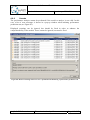
Description
Initial draft.
Several updates
Chapter 1 updated
Chapter 1 updated
Added Maintenance prediction tool manual
Added todo list introductory section
Backbone manual updated
Text editors manual updated
Maintainability manual updated
Added “Getting started” guide
Reverse engineering and Performance Analysis
manual updated
Repository Editor User Manual updated
Reliability
Analysis,
Trade-Off
Analysis,
Consistency Checker User manuals updated
JPMF manual added
Random Program Generator Manual added
Composite Editor Manual added
SEFF Editor Manual updated
Chapter “Design optimisation” deleted
QoS Editor Manual added, updates in section 1.2,
overall tidy up.
After internal review by ENT, CUNI, PMI,
FZI,ITE
Incorporated MDU review
Final version
Dissemination level: public
Page 2 / 207
D6.1 Annex: Guidelines and Tool Manuals
Version: 2.0
Last change: 25.01.2011
Table of contents
Abstract ..................................................................................................................................................... 1 Table of contents....................................................................................................................................... 3 1 Introduction ................................................................................................................................................. 9 1.1 Q-ImPrESS overall workflow ................................................................................................................... 9 1.2 Workflow and tools ................................................................................................................................. 11 1.3 Advantages of using Q-ImPrESS during system design and software development ............................... 12 1.4 Advantages of using Q-ImPrESS during software evolution and maintenance ...................................... 12 2 The Q-ImPrESS method ........................................................................................................................... 13 2.1 Overview of the Q-ImPrESS method....................................................................................................... 13 2.2 Model a change scenario ........................................................................................................................ 14 2.2.1 Components selection ................................................................................................................... 14 2.2.2 Model components as grey/black boxes ........................................................................................ 14 2.2.3 Reverse engineering of selected components ................................................................................ 15 2.2.4 Model system assembly ................................................................................................................ 15 2.2.5 Model system deployment ............................................................................................................ 15 2.2.6 Model system usage ...................................................................................................................... 15 2.2.7 Add quality annotations ................................................................................................................ 16 2.2.8 System Model validation ............................................................................................................... 16 2.2.9 System quality prediction .............................................................................................................. 17 2.2.10 Results trade-off analysis ......................................................................................................... 17 2.2.11 Implement viable alternative and validate model. .................................................................... 17 3 The Q-ImPrESS SAMM: how a system is modelled .............................................................................. 19 4 Tool Manuals ............................................................................................................................................. 21 4.1 Q-ImPrESS IDE installation ................................................................................................................... 22 4.1.1 Downloading Eclipse .................................................................................................................... 22 4.1.2 Installing the Q-ImPrESS tools in Eclipse .................................................................................... 22 4.2 IDE Basics: Working with alternatives................................................................................................... 24 4.2.1 Tool Description............................................................................................................................ 24 4.2.2 Purpose of the tool ........................................................................................................................ 24 4.2.3 Tool relationship with the Q-ImPrESS workflow ......................................................................... 24 4.2.4 Tool Usage .................................................................................................................................... 25 4.2.5 Tool prerequisites .......................................................................................................................... 25 4.2.6 Tool activation .............................................................................................................................. 25 Q-ImPrESS perspective activation ......................................................................................................... 25 Q-ImPrESS project activation ................................................................................................................ 26 Create new Q-ImPrESS project .............................................................................................................. 27 Associating the Q-ImPrESS nature with an existing project .................................................................. 28 Q-ImPrESS project content activation .................................................................................................... 29 Q-ImPrESS project filters activation ...................................................................................................... 30 Q-ImPrESS annotation properties activation .......................................................................................... 30 Q-ImPrESS annotation wizard activation ............................................................................................... 30 4.2.7 Usage instructions and expected outputs ....................................................................................... 31 Q-ImPrESS project view ........................................................................................................................ 31 Creation of a new alternative .................................................................................................................. 32 Selecting default alternative.................................................................................................................... 35 Adding a new model into an alternative ................................................................................................. 36 © Q-ImPrESS Consortium
Dissemination level: public
Page 3 / 207
D6.1 Annex: Guidelines and Tool Manuals
Version: 2.0
Last change: 25.01.2011
Model editing .......................................................................................................................................... 39 Opening model artefact editors ............................................................................................................... 41 Annotation properties ............................................................................................................................. 41 Annotation wizard .................................................................................................................................. 42 4.2.8 Caveats .......................................................................................................................................... 44 Problems with the Q-ImPrESS project ................................................................................................... 44 4.3 Repository Editor Manual ...................................................................................................................... 45 4.3.1 Purpose of the tool ........................................................................................................................ 45 4.3.2 Tool relationship with the Q-ImPrESS workflow ......................................................................... 45 4.3.3 Tool prerequisites .......................................................................................................................... 47 4.3.4 Tool activation .............................................................................................................................. 47 4.3.5 Usage instructions and expected outputs ....................................................................................... 48 Working with editor tools for repository elements ................................................................................. 48 Working with Inner Elements ................................................................................................................. 49 Working with OperationBehaviour......................................................................................................... 50 Deleting elements ................................................................................................................................... 50 Moving elements .................................................................................................................................... 51 Sizing elements ....................................................................................................................................... 51 Working with Composite Components ................................................................................................... 51 4.3.6 Caveats .......................................................................................................................................... 51 4.4 Composite Editor Manual: Modelling service architecture models and composite components ........... 52 4.4.1 Purpose of the tool ........................................................................................................................ 52 4.4.2 Tool relationship with the Q-ImPrESS workflow ......................................................................... 52 4.4.3 Tool activation .............................................................................................................................. 53 4.4.4 Usage instructions and expected outputs ....................................................................................... 54 Opening the editor .................................................................................................................................. 55 Working with components ...................................................................................................................... 55 Deleting elements ................................................................................................................................... 59 Adding elements ..................................................................................................................................... 60 Adding Subcomponent Instances............................................................................................................ 62 4.4.5 Caveats .......................................................................................................................................... 63 4.5 SEFF Editor Manual .............................................................................................................................. 64 4.5.1 Purpose of the tool ........................................................................................................................ 64 4.5.2 Tool relationship with the Q-ImPrESS workflow ......................................................................... 64 4.5.3 Tool prerequisites .......................................................................................................................... 66 4.5.4 Tool activation .............................................................................................................................. 66 4.5.5 Usage instructions and expected outputs ....................................................................................... 66 4.5.6 Caveats .......................................................................................................................................... 69 4.6 QoS Editor Manual ................................................................................................................................. 70 4.6.1 Purpose of the tool ........................................................................................................................ 70 4.6.2 Tool relationship with the Q-ImPrESS workflow ......................................................................... 70 4.6.3 Tool prerequisites .......................................................................................................................... 71 4.6.4 Tool activation .............................................................................................................................. 71 4.6.5 Usage instructions and expected outputs ....................................................................................... 71 4.6.6 Caveats .......................................................................................................................................... 75 4.7 Text Editors Manual ............................................................................................................................... 76 4.7.1 Purpose of the tool ........................................................................................................................ 76 4.7.2 Tool relationship with the Q-ImPrESS workflow ......................................................................... 76 4.7.3 Tool prerequisites .......................................................................................................................... 77 4.7.4 Tool activation .............................................................................................................................. 77 4.7.5 Usage instructions and expected outputs ....................................................................................... 77 4.7.6 Creating new SAMM model ......................................................................................................... 77 4.7.7 Modifying existing SAMM models .............................................................................................. 77 4.8 Reverse Engineering Manual.................................................................................................................. 80 © Q-ImPrESS Consortium
Dissemination level: public
Page 4 / 207
D6.1 Annex: Guidelines and Tool Manuals
Version: 2.0
4.8.1 4.8.2 4.8.3 4.8.4 4.8.5 4.8.6 Last change: 25.01.2011
Purpose of the tool ........................................................................................................................ 80 Tool relationship with the Q-ImPrESS workflow ......................................................................... 80 Tool prerequisites .......................................................................................................................... 81 Tool activation .............................................................................................................................. 81 Usage instructions and expected outputs ....................................................................................... 82 Caveats .......................................................................................................................................... 92 4.9 Performance Prediction Manual ............................................................................................................ 93 4.9.1 Purpose of the tool ........................................................................................................................ 93 4.9.2 Tool relationship with the Q-ImPrESS workflow ......................................................................... 93 4.9.3 Tool prerequisites .......................................................................................................................... 94 4.9.4 Tool activation .............................................................................................................................. 95 4.9.5 Usage instructions and expected outputs ....................................................................................... 99 4.9.6 Caveats ........................................................................................................................................ 102 4.10 Reliability Prediction Manual .......................................................................................................... 103 4.10.1 Purpose of the tool .................................................................................................................. 103 4.10.2 Tool relationship with the Q-ImPrESS workflow .................................................................. 103 4.10.3 Tool prerequisites ................................................................................................................... 104 4.10.4 Tool activation ........................................................................................................................ 104 4.10.5 Usage instructions and expected outputs ................................................................................ 106 4.10.6 Caveats ................................................................................................................................... 107 4.11 Maintainability Prediction Manual.................................................................................................. 108 4.11.1 Purpose of the tool .................................................................................................................. 108 4.11.2 Tool relationship with the Q-ImPrESS workflow .................................................................. 108 4.11.3 Tool usage .............................................................................................................................. 109 Create new KAMP model file .............................................................................................................. 109 Navigation bar ...................................................................................................................................... 111 Specify architecture alternatives ........................................................................................................... 112 Specify change scenarios ...................................................................................................................... 112 Analysis overview ................................................................................................................................ 114 Workplan derivation by wizard dialog ................................................................................................. 116 Effort estimation ................................................................................................................................... 126 Result export ......................................................................................................................................... 127 4.12 Trade-off analysis and results viewer (AHP) ................................................................................... 129 4.12.1 Tool Description ..................................................................................................................... 129 4.12.2 Purpose of the tool .................................................................................................................. 129 4.12.3 Tool relationship with the Q-ImPrESS workflow .................................................................. 129 4.12.4 Tool prerequisites ................................................................................................................... 130 4.12.5 Tool activation ........................................................................................................................ 130 4.12.6 Usage instructions and expected outputs ................................................................................ 131 Persistence ............................................................................................................................................ 131 Stage 1: Quality Comparison ................................................................................................................ 131 Stage 2: Value Comparison .................................................................................................................. 132 Stage 3: Interpretation of Results .......................................................................................................... 132 Caveats.................................................................................................................................................. 133 4.13 Consistency Checker Manual........................................................................................................... 134 4.13.1 Purpose of the tool .................................................................................................................. 134 4.13.2 Tool relationship with the Q-ImPrESS workflow .................................................................. 134 4.13.3 Tool prerequisites ................................................................................................................... 135 4.13.4 Tool activation ........................................................................................................................ 136 4.13.5 Usage instructions and expected outputs ................................................................................ 137 4.13.6 Caveats ................................................................................................................................... 142 4.14 Java Performance Measurement Framework Manual ..................................................................... 143 4.14.1 Purpose of the tool .................................................................................................................. 143 4.14.2 Tool relationship with the Q-ImPrESS workflow .................................................................. 143 © Q-ImPrESS Consortium
Dissemination level: public
Page 5 / 207
D6.1 Annex: Guidelines and Tool Manuals
Version: 2.0
Last change: 25.01.2011
4.14.3 Key concepts .......................................................................................................................... 143 Performance Events .............................................................................................................................. 143 Event Sources ....................................................................................................................................... 144 Event Triggers ...................................................................................................................................... 145 4.14.4 Basic API usage...................................................................................................................... 145 4.14.5 Instrumentation using event triggers ...................................................................................... 146 Instrumentation using event sources ..................................................................................................... 148 4.14.6 Tool prerequisites ................................................................................................................... 150 4.14.7 Tool activation ........................................................................................................................ 150 4.14.8 Usage instructions and expected outputs ................................................................................ 150 Automatic load-time instrumentation ................................................................................................... 151 Configuration ........................................................................................................................................ 151 Simple data analysis ............................................................................................................................. 152 4.14.9 Caveats ................................................................................................................................... 153 4.15 Random Program Generator Manual .............................................................................................. 154 4.15.1 Purpose of the tool .................................................................................................................. 154 4.15.2 Tool relationship with the Q-ImPrESS workflow .................................................................. 154 4.15.3 Tool prerequisites ................................................................................................................... 154 4.15.4 Tool activation ........................................................................................................................ 155 Generating an application ..................................................................................................................... 155 Measuring a generated application ....................................................................................................... 156 Predicting performance of a generated application ............................................................................... 156 4.15.5 Tool configuration .................................................................................................................. 157 4.15.6 Expected outputs .................................................................................................................... 158 Generating an application ..................................................................................................................... 158 Measuring a generated application ....................................................................................................... 160 4.15.7 Caveats ................................................................................................................................... 160 5 Appendix A: Getting started guide ........................................................................................................ 161 5.1 Introduction .......................................................................................................................................... 161 5.2 The Q-ImPrESS IDE ............................................................................................................................. 161 5.3 Quality predictions ............................................................................................................................... 165 5.4 Result viewer and trade-off analysis ..................................................................................................... 168 6 Appendix B: An example on how to edit models using the tree editor ............................................... 171 6.1 Create a Repository Model ................................................................................................................... 171 6.2 DataTypes ............................................................................................................................................. 174 6.3 MessageTypes ....................................................................................................................................... 176 6.4 Interfaces .............................................................................................................................................. 176 6.5 PrimitiveComponents ........................................................................................................................... 177 6.6 CompositeComponents ......................................................................................................................... 178 6.7 Create a Hardware Model .................................................................................................................... 182 6.8 Units ..................................................................................................................................................... 183 6.9 Create a Target Environment Model .................................................................................................... 183 6.10 Create a SEFF Behaviour Model ..................................................................................................... 185 6.11 SEFF Actions ................................................................................................................................... 186 6.11.1 LoopAction, BranchAction, ForkAction ................................................................................ 187 6.12 Create a QoS Annotation Model ...................................................................................................... 187 © Q-ImPrESS Consortium
Dissemination level: public
Page 6 / 207
D6.1 Annex: Guidelines and Tool Manuals
Version: 2.0
7 Last change: 25.01.2011
Appendix C: Concrete syntax for SAMM meta-model ........................................................................ 189 7.1 Predefined terminals ............................................................................................................................. 189 7.2 Core (package samm.core) ................................................................................................................... 190 7.3 Data types (package samm.datatypes) .................................................................................................. 192 7.4 Static structure (package samm.staticstructure) ................................................................................... 193 7.5 Behaviour (package samm.behaviour) ................................................................................................. 197 7.6 Deployment (package samm.deployment)............................................................................................. 198 7.6.1 Target environment (package samm.deployment.targetenvironment) ........................................ 198 7.6.2 Hardware (package samm.deployment.hardware) ...................................................................... 201 7.6.3 Allocation (package samm.deployment.allocation) .................................................................... 203 7.7 Annotation (package samm.annotation) ............................................................................................... 203 7.8 Usage model (package samm.usagemodel) .......................................................................................... 203 7.9 QoS Annotations (package samm.qosannotation) ................................................................................ 205 8 Appendix D: Glossary ............................................................................................................................. 207 © Q-ImPrESS Consortium
Dissemination level: public
Page 7 / 207
D6.1 Annex: Guidelines and Tool Manuals
Version: 2.0
© Q-ImPrESS Consortium
Last change: 25.01.2011
Dissemination level: public
Page 8 / 207
D6.1 Annex: Guidelines and Tool Manuals
Version: 2.0
1
Last change: 25/01/2011
Introduction
This deliverable extends D6.1, providing practical details on the use of the Q-ImPrESS IDE
and related tools and represents a reference manual for software engineers.
This deliverable specifically addresses recommendation R7 of the First Project Review.
The structure of the deliverable is as follows:
Chapter 2 provides a short summary of the Q-ImPrESS method as detailed in D6.1.
Chapter 3 provides in-depth hints on SAM and how a system is modelled.
Chapter 4 contains a reference manual for each of the mentioned tools.
Appendix A contains a “Getting started” guide for beginners.
Appendix B provides a tutorial on how to modify SAM using tree editors.
Appendix C contains the SAMM grammar.
Appendix D provides a glossary.
1.1
Q-ImPrESS overall workflow
Q-ImPrESS provides a platform for software engineers for the quality evaluation of multiple
evolution alternatives of a system. Different quality attributes can be predicted before
implementation takes place. This leads to a shorter time to production while assuring a better
quality of the target system.
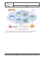
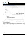
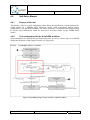
Figure 1 shows an overview of the Q-ImPrESS workflow as applied at ABB/Ericsson:
© Q-ImPrESS Consortium
Dissemination level: public
Page 9 / 207
D6.1 Annex: Guidelines and Tool Manuals
Version: 2.0
Last change: 25/01/2011
Figure 1: Q-ImPrESS workflow overview
Several evolution alternatives of a system can be designed, derived quality attributes are
computed, and a final trade-off analysis is used to choose the best alternative.
© Q-ImPrESS Consortium
Dissemination level: public
Page 10 / 207
D6.1 Annex: Guidelines and Tool Manuals
Version: 2.0
1.2
Last change: 25/01/2011
Workflow and tools
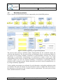
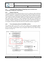
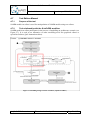
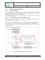
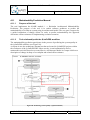
Figure 2 depicts in details all the activities supported by the Q-ImPrESS platform:
Figure 2: Activities supported by the Q-ImPrESS platform
The process starts with an evolution request. Requirements for the evolution request are
collected and formalised. The first activity aims at building the Service Architecture Model of
the system (if not already available). Automatic (or semi-automatic) activities, like reverse
engineering or performance measurements are performed in order to derive the SAM
representation of the system, or manual editors can be used instead. The requirements of the
evolution request are used for manual modelling of alternatives representing different
solutions for the evolution scenario. Model alternatives can also be derived automatically, e.g.
by using evolutionary algorithms.
Various quality assessments are performed for each alternative and quality prediction results
are obtained. The trade-off analysis can be performed in order to estimate the effectiveness of
the alternatives with respect to the evolution scenario requirements. The entire process loops
until a suitable alternative is found.
© Q-ImPrESS Consortium
Dissemination level: public
Page 11 / 207
D6.1 Annex: Guidelines and Tool Manuals
Version: 2.0
Last change: 25/01/2011
1.3
Advantages of using Q-ImPrESS during system design and
software development
Q-ImPrESS is based on the Eclipse and Eclipse EMF frameworks and therefore can be easily
adopted and integrated in the development environment.
With the use of the Q-ImPrESS IDE the model of a large component-based system can be
handled efficiently. Moreover several different evolving alternatives can be modelled and
evaluated thus avoiding the implementation/testing/deployment phases of the traditional
production cycle for several alternatives.
A key feature of the Q-ImPrESS platform is the notion of modelling abstraction level;
Q-ImPrESS allows a software engineer to describe a component either as a grey or black box
in terms of quality attributes (stopping at a high abstraction level), while fully modelling main
components using the analysis tools provided by the platform.
1.4
Advantages of using Q-ImPrESS during software evolution and
maintenance
Especially in domains where software solutions have a long life cycle (Telecom, Industry)
and are characterised by high quality standards, the product evolution and maintenance phase
is crucial. This phase accompanies the product until its commercial end and may last years
(and often decades), therefore very seldom it is performed by the team involved in the initial
product design and implementation. Moreover, shifting maintenance to a different location
than production is becoming a normal procedure for medium/large companies in an effort to
cut down costs.
In this phase, using a development tool that conveys design information and decisions is of
utmost importance. The Q-ImPrESS platform lets perform a reverse engineering of existing
code and can be used to ease maintenance of old software code while allowing testing
alternative solutions without actually coding them.
© Q-ImPrESS Consortium
Dissemination level: public
Page 12 / 207
D6.1 Annex: Guidelines and Tool Manuals
Version: 2.0
2
Last change: 25/01/2011
The Q-ImPrESS method
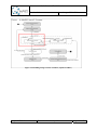
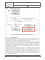
This chapter briefly introduces the Q-ImPrESS method.
2.1
Overview of the Q-ImPrESS method
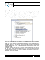
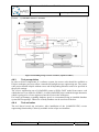
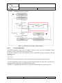
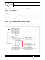
The process of assessing the quality of large, distributed component-based software systems
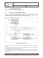
is quite complex. The Q-ImPrESS method, outlined in D6.1 and depicted in Figure 3, splits
the process in a sequence of phases, making the overall procedure easy:
Figure 3: The Q-ImPrESS method
The number reported in each process box is the chapter number in D6.1 describing the
process.
The overall workflow starts with the definition of different change scenarios (alternatives)
each potentially suited to solve new requirements.
Each (assembly) change scenario has to be modelled, prediction analysis is performed for
each model, and results are then confronted pair wise unless a suitable scenario is elected as
the best solution.
© Q-ImPrESS Consortium
Dissemination level: public
Page 13 / 207
D6.1 Annex: Guidelines and Tool Manuals
Version: 2.0
Last change: 25/01/2011
The following sections contain a short description of each method phase, starting from phase
3.3 (Model a change scenario).
2.2
Model a change scenario
Model creation (detailed as process 3.3 in D6.1) is a recursive process, where the main steps
in the cycle are the ones as follows.
2.2.1
Components selection
Depending on the change scenario, only some components of the system are affected.
Moreover, the level of model details (abstraction level) can differ for different components.
The components involved in the change scenario should be thoroughly modelled, as the more
fine grained the model is the more accurate the quality prediction on the alternative can be.
The abstraction level measures the level of details and accuracy of a model with respect to the
system modelled.
At a high abstraction level, a system is described by few composite components or subsystems. As an example, if the system under analysis is a plant PCS (Process Control
System), the legacy ERP system at level 3 could be modelled as a single component,
providing daily production schedules (maybe updated several times a day) and requesting
control data back, without affecting the accuracy of the analysis method on the PCS system.
At a medium abstraction level the number of components increases, but they still lack an
adherent description of their internals (as obtained reverse engineering components code) and
quality annotations are still manually input. Composite components reveal details of their
structure, interfaces and connectors are fully described.
At a low abstraction level the model precisely adheres and describes the components under
analysis.
There is a trade-off to consider while choosing the right abstraction level. As time spent on
modelling decreases shifting toward a higher abstraction level, the deviation between
predicted and measured quality attributes increases. Moreover complexity and size of models
increase at lower abstraction levels. This implies considering another inner loop: a component
model could not be yet at the right abstraction level and another cycle may be needed before
passing to the next component to model. The software engineer should choose this based on
his/her experience.
2.2.2
Model components as grey/black boxes
Components and services not touched by the change scenario do not need to be modelled in
details. The requirement is anyhow that quality annotations for these components meet
requirements. As only component external behaviour has to be defined (we do not need any
detail on the component’s structure), the quickest way to model it is to instrument it at its
connectors, deploy and run it on a reference suite test and monitor it.
© Q-ImPrESS Consortium
Dissemination level: public
Page 14 / 207
D6.1 Annex: Guidelines and Tool Manuals
Version: 2.0
Last change: 25/01/2011
2.2.3
Reverse engineering of selected components
We can obtain a model (a complete component structure) for the selected components from
component code using reverse engineering techniques.
Software may need some adaptations before being ready to be analysed by the reverse
engineering tools provided by the Q-ImPrESS IDE. The time consumption of this phase is
unpredictable, as it is proportional to the LOC size but also depends on the technology used
and the subtle language nuances of that technology (example: VisualC 6 with respect to C++).
The level of details of the component structure can increase recursively applying reverse
engineering. This phase again needs manual input and cannot be fully automated.
As explained in D6.1 (3.3.3.4) the reverse engineering process is basically divided into three
steps: first, code is analysed to obtain an abstract structure, then information regarding
components and interfaces is extracted and finally the user can add behaviour annotations (in
the form of Petri Nets or in other ways as the Q-ImPrESS platform can be extended to include
different plugins to work with).
As explained, the software engineer iterates the previous phases until all of the system
components have been modelled.
2.2.4
Model system assembly
At this point models for all individual components are available. Now they need to be
assembled to represent a Service Architecture Model.
Hence the system architect takes components from repository and plugs them together using
connectors.
The graphical editor can be used for this phase; this makes connection creation and handling
much an easier task with respect to using the text editor.
2.2.5
Model system deployment
The deployment model needs to be updated if the assembly change scenario involves the
creation of new components (that need to be allocated), or in case the HW resources are
changed. For each alternative model the corresponding deployment scheme has to be
modelled.
2.2.6
Model system usage
The workload intensity caused by the users of the service oriented system can be potentially
extracted during the runtime monitoring process, however the need for a manual update of
this model is foreseen and therefore included in the workflow. Moreover, modelling
alternatives for different usage schemes, system quality attributes at different system usage
settings can be investigated.
© Q-ImPrESS Consortium
Dissemination level: public
Page 15 / 207
D6.1 Annex: Guidelines and Tool Manuals
Version: 2.0
Last change: 25/01/2011
2.2.7
Add quality annotations
The software engineer has to provide quality annotations for the modelled components in
order to predict the impact of a change requests on the selected components.
Quality annotations can be derived in different ways depending on their nature.
Regarding performance quality annotation, they can be expressed defining a formula that
relates the performance of a component (or a part of it) with other parameters (the input
throughput, the quantity of RAM or the number of CPU used). To derive it, code has to be
instrumented and executed against a reference scenario. The Q-ImPrESS tool-set provides
basic instrumentation suites, but there are several more sophisticated tools available to
perform fine resolution performance measurements. The software engineer has then to
analyse the performance data (timestamps) and derive (linear) functions of the execution
times with respect to the identified parameters.
Regarding reliability quality annotations, a linear distribution representing the component
reliability can be estimated analysing the data regarding bugs reported for the components
covering a consistent time frame. Other formula can be found in literature regarding this
topic.
The Q-ImPrESS IDE provides editors for editing quality annotations.
2.2.8
System Model validation
For a consistent and valid prediction analysis, the model used to assess quality prediction has
to adhere to the real system under investigation. Model has to be verified and validated before
being used to evaluate change scenarios (design alternatives).
Model validation is not performed as a single step, but usually model gets refined along a
modelling loop, where model comes closer to the system modelled at each loop cycle.
The already mentioned model abstraction is refined as well during these loops. Usually the
software engineer starts modelling the system at a high abstraction level and checks model
consistency before refining the model and scale down to a lower abstraction level.
If the Q-ImPrESS tool is used for prediction analysis, checking model consistency means
instrumenting the code and checking that system performance, for a known use case, closely
match model performance prediction running the same use case.
There is a relationship between the model abstraction level and the 'granularity' of code
instrumentation too: at a high abstraction level, code instrumentation can be rather sparse,
determining performance at component level. As the level of details in the model increases,
instrumentation has to be performed at a finer resolution to check model consistency. Each
time the system has to perform a known execution and the same execution has to be
predicted. If prediction does not match system execution times, the software engineer has to
adjust the model before advancing to a new loop cycle.
To run the model we have first to complete it by providing information regarding the
component deployment scheme and user input. The time spent configuring the model for a
reference scenario depends on the complexity of the system, but usually it should be easier
then running the entire system (at least the model can run on one machine). We collect quality
prediction analysis results from model execution and we check how closely they match with
real quality data we collected for the same reference model. If differences exceed defined
thresholds (say system model performance differs for more than 20% the system performance
© Q-ImPrESS Consortium
Dissemination level: public
Page 16 / 207
D6.1 Annex: Guidelines and Tool Manuals
Version: 2.0
Last change: 25/01/2011
measurements), the software engineer has to go back to phase 2.2.4 checking again the quality
annotations defined for each component.
If the model is coherent, the software engineer, based on the required change scenario, has to
judge if the model abstraction level is enough or some components should be modelled at a
finer resolution. This depends on the system and the change scenario examined. If the
abstraction level is too high the user has to start again at phase 2.2.2 either modelling black
box components as composite components or cycling more on the reverse engineering phase.
2.2.9
System quality prediction
A system model reflecting a change scenario is performed and results are collected back in
the model. Currently prediction analysis is composed by: Performance prediction, Reliability
Prediction, Maintainability prediction. For a prediction analysis to take place, the alternative
model (SAM) has to be converted in the specific prediction tool format (PCM for
performance prediction, KLAPER + PRISM for the reliability analysis). The time
consumption of this phase depends on the complexity of the models.
2.2.10
Results trade-off analysis
Alternatives can then be selected for the trade-off analysis in order to select the most viable
solution. The Q-ImPrESS IDE provides a tool that performs Pareto analysis and derives the
best alternative that meets change quality requirements.
If no alternatives meet quality requirements, the system engineer has to identify new change
scenarios and restart modelling them.
2.2.11
Implement viable alternative and validate model.
The alternative that is judged as the best match is implemented. The JPFChecker tool can be
used in this phase to verify the consistency of a behaviour model with the actual
implementation of a service.
After deployment, the quality of the system is assessed and compared to the predicted. If
analysis results offset exceeds a threshold, the alternative modelled should be checked again
and validated (implementation may be checked as well for compliance with the model.
To effectively apply the Q-ImPrESS method a user has still to comprehend how a system is
modelled and which tools come into play in each of the method processes.
© Q-ImPrESS Consortium
Dissemination level: public
Page 17 / 207
D6.1 Annex: Guidelines and Tool Manuals
Version: 2.0
© Q-ImPrESS Consortium
Last change: 25/01/2011
Dissemination level: public
Page 18 / 207
D6.1 Annex: Guidelines and Tool Manuals
Version: 2.0
3
Last change: 25/01/2011
The Q-ImPrESS SAMM: how a system is modelled
The Q-ImPrESS Service Architecture Meta-Model (SAMM) provides the meta-model for
modelling a Service Architecture Model (SAM).
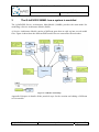
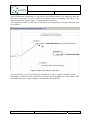
A Service Architecture Model consists of different parts that are split up into several model
files. Figure 4 shows how the different EMF model files are connected with each other.
Figure 4: SAM files relationship
Appendix B depicts in details all the practical steps for the creation and editing of different
service models.
© Q-ImPrESS Consortium
Dissemination level: public
Page 19 / 207
D6.1 Annex: Guidelines and Tool Manuals
Version: 2.0
© Q-ImPrESS Consortium
Last change: 25/01/2011
Dissemination level: public
Page 20 / 207
D6.1 Annex: Guidelines and Tool Manuals
Version: 2.0
4
Last change: 25/01/2011
Tool Manuals
This chapter provides the documentation for all the tools of the Q-ImPrESS platform.
The order tools are presented should reflect a typical usage scenario of the Q-ImPrESS
platform, also described in D6.1, and summarised in chapter 1.2.
Tools can be grouped by the activities they fulfil:
Service Architecture Model Handling: these tools act as a foundation for the rest of the
platform tools. The Backbone tools extend the Eclipse platform and are responsible for
handling new project types, perspectives and other Eclipse elements. From the userperspective, the aim of the Backbone tools is to support the user in the usage of the platform
and the management of SAM models.
Section 4.1 (IDE basics), 4.3 (the Repository Editor), 4.4 (the Composite Editor), 4.5 (the
SEFF Editor), 4.6 (the QoS Editor), 4.7 (the Text Editors) describe the Backbone tools in
detail.
Reverse Engineering: This process phase is covered by section 4.8.
Quality Prediction Analysis: The usage of each analysis tool is provided in section 4.9
(Performance prediction), 4.10 (Reliability prediction), 4.11 (Maintainability prediction).
Trade-Off Analysis: Practical details on how to perform a trade-off analysis based on the
prediction results are given in section 4.12.
Alternative implementation check: Although the implementation phase of the chosen
alternative model is not covered by the Q-ImPrESS platform, a tool to check the adherence of
the Java implementation with the selected alternative behavioural model is provided in
section 4.13.
Off-line tools: External tools are not included in the Q-ImPrESS IDE, but have proved to be
useful during the development of the platform are described in sections 4.14 and 4.15.
© Q-ImPrESS Consortium
Dissemination level: public
Page 21 / 207
D6.1 Annex: Guidelines and Tool Manuals
Version: 2.0
4.1
Last change: 25/01/2011
Q-ImPrESS IDE installation
The Q-ImPrESS IDE can be installed on top of an Eclipse Galileo development environment.
This way, the Q-ImPrESS IDE can be installed on any platform that supports the required
Eclipse platform.
This section describes in detail how to install the Q-ImPrESS IDE.
4.1.1
Downloading Eclipse
In order to install the Q-ImPrESS IDE, please download the “Eclipse Modeling Tools”
distribution from the Eclipse download website: http://www.eclipse.org/downloads/
To install the “Eclipse Modeling Tools” distribution, simply unzip the downloaded ZIP file.
Note: There may be issues when using the built-in ZIP functionality of Windows OS. We
recommend the use of alternative ZIP decompression tools, such as 7-zip (http://www.7zip.org/).
4.1.2
Installing the Q-ImPrESS tools in Eclipse
Once you have installed Java 1.6 and the Eclipse Galileo Modeling Tools distribution, please
execute the following steps to get started with the Q-ImPrESS IDE:








Start Eclipse. Select “Help”  “Install New Software…” from the menu.
Make sure the Galileo update site is available. It should be available with a fresh
Eclipse Galileo Modeling Tools distribution. Otherwise, add the Galileo update site
“http://download.eclipse.org/releases/galileo”.
Add the following update site by clicking on “Add…”
o Name: “Q-ImPrESS Update Site”
o Location: http://q-impress.ow2.org/release
You can now select the newly created update site “Q-ImPrESS Update Site” using the
“Work with” dropdown list.
Select the following items listed in the install window: “Palladio Component Model”,
“Q-ImPrESS Tools (EU FP7 Project)”, and “SISSy”. Then click “Next”.
The following window shows all features that are to be installed. Confirm the
selection with “Finish”.
During the installation process, a security warning might pop up, notifying you that
some of the software contains unsigned content. Continue the installation process by
press “OK”.
After the installation is finished, a window will pop up asking you to restart the
Eclipse workbench. Select “No” and shutdown Eclipse manually.
Locate the eclipse installation folder, and locate the file “config.ini” in the
“configuration” folder
© Q-ImPrESS Consortium
Dissemination level: public
Page 22 / 207
D6.1 Annex: Guidelines and Tool Manuals
Version: 2.0


Last change: 25/01/2011
Open the file and append the following line:
“osgi.framework.extensions=eu.qimpress.ide.editors.text.xtextfix”
If a line starting with “osgi.framework.extensions=” already exists, just append
“,eu.qimpress.ide.editors.text.xtextfix” to the line.
Save and close the file, start Eclipse.
The Q-ImPrESS IDE is now installed.
For more information, refer to the Download section at the Q-ImPrESS website at
http://www.q-impress.eu/wordpress/software/ .
© Q-ImPrESS Consortium
Dissemination level: public
Page 23 / 207
D6.1 Annex: Guidelines and Tool Manuals
Version: 2.0
4.2
Last change: 25/01/2011
IDE Basics: Working with alternatives
4.2.1
Tool Description
The set of Backbone plug-ins constitutes a core part of the Q-ImPrESS IDE. Backbone
plugins integrate all the other tools by providing a uniform infrastructure for the modelling,
visualization and manipulation of models and their alternatives. Leveraging the Q-ImPrESS
toolset over a backbone layer ensures a high IDE consistency and quality standards.
4.2.2
Purpose of the tool
The purpose of the Backbone infrastructure is to provide a layer for simplified access to
various operations over Q-ImPrESS projects, repositories, alternatives, and models and to
support the functionality of the other Q-ImPrESS tools. Backbone is also responsible for
visualization of Q-ImPrESS project artefacts within the Eclipse IDE.
4.2.3
Tool relationship with the Q-ImPrESS workflow
Backbone plugins, being the foundation, participate in all the other parts of Q-ImPrESS
workflow by providing a uniform infrastructure.
© Q-ImPrESS Consortium
Dissemination level: public
Page 24 / 207
D6.1 Annex: Guidelines and Tool Manuals
Version: 2.0
Last change: 25/01/2011
4.2.4
Tool Usage
Q-ImPrESS Backbone is an inherent part of Q-ImPrESS IDE and its functionality is
integrated and shown in various parts of the IDE. Conceptually, it manages five core
Q-ImPrESS IDE artifacts:
 Q-ImPrESS project – encapsulates source code as well as models stored in
alternatives repository, analysis settings and launch configurations
 Alternatives repository – is a repository containing a hierarchical structure of model
alternatives.
 Model alternative – represents one particular version of an application architecture.
The alternative includes various models describing the architecture.
 Default alternative – only one alternative in the tree of alternatives is selected as a
working alternative. The other alternatives are not accessible (their models cannot be
accessed).
 Model – model included in an alternative.
4.2.5
Tool prerequisites
The Backbone has no special prerequisites.
4.2.6
Tool activation
The Backbone is activated during the startup sequence of the Eclipse platform. It publishes
the Q-ImPrESS perspective configuring the Eclipse environment in order to show Q-ImPrESS
related GUI elements (views, buttons, projects’ content).
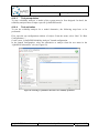
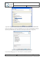
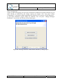
Q-ImPrESS perspective activation
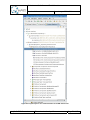
The Q-ImPrESS perspective can be activated by selecting it from the Eclipse perspective
menu (see Figure 5). The perspective activation causes reconfiguration of Eclipse platform
layout to show Q-ImPrESS related tools.
© Q-ImPrESS Consortium
Dissemination level: public
Page 25 / 207
D6.1 Annex: Guidelines and Tool Manuals
Version: 2.0
Last change: 25/01/2011
Figure 5: Perspective selection dialog
Q-ImPrESS project activation
Every Q-ImPrESS project is marked by a dedicated Eclipse nature. When applied to a project,
the Q-ImPrESS nature enables the use of Q-ImPrESS tools. This is indicated by a small icon
of the “Q” letter shown in the bottom-right (moved to upper-right in latest releases) corner of
the project icon ( ).
There are two ways of associating the Q-ImPrESS nature with a project: (i) by creating a new
Q-ImPrESS project, with the nature enabled by default, or (ii) by associating the Q-ImPrESS
nature with an existing project explicitly using the pop-up menu.
© Q-ImPrESS Consortium
Dissemination level: public
Page 26 / 207
D6.1 Annex: Guidelines and Tool Manuals
Version: 2.0
Last change: 25/01/2011
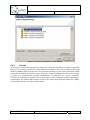
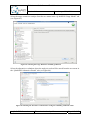
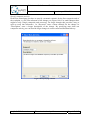
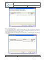
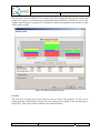
Create new Q-ImPrESS project
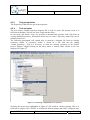
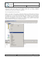
A new Q-ImPrESS project can be created from the main menu “File”  “New” 
“Project…”.
Selecting a Q-ImPrESS project item from the list opens the Q-ImPrESS project creation
wizard (see Figure 6). The wizard allows users to create a new Q-ImPrESS project with a
given name.
Figure 6: Create Q-ImPrESS project
If activated, the Q-ImPrESS perspective contains a dedicated menu action “File” 
“New”  “Q-ImPrESS Project” which also leads to the project creation wizard.
© Q-ImPrESS Consortium
Dissemination level: public
Page 27 / 207
D6.1 Annex: Guidelines and Tool Manuals
Version: 2.0
Last change: 25/01/2011
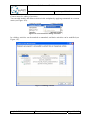
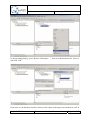
Associating the Q-ImPrESS nature with an existing project
To activate the Backbone infrastructure user has to associate the Q-ImPrESS nature with a
given project. This can be done in the project pop-up menu using menu item “Add/Remove
Q-ImPrESS nature” (see Figure 7). Similarly, the same procedure is used to remove an
existing Q-ImPrESS nature from a project.
An activated Q-ImPrESS nature is indicated by a small icon of “Q“ letter shown in the
bottom-left corner of the project icon ( ) within the Project Explorer view.
Figure 7 Enabling project Q-ImPrESS nature
© Q-ImPrESS Consortium
Dissemination level: public
Page 28 / 207
D6.1 Annex: Guidelines and Tool Manuals
Version: 2.0
Last change: 25/01/2011
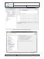
Q-ImPrESS project content activation
By default the Project Explorer view shows the content of a Q-ImPrESS project. It is possible
to customise the list of visible items by using the “Customize View…” item from the view’s
menu. The “Q-ImPrESS navigator extension” content provider is responsible for rendering
the Q-ImPrESS related information (see Figure 8).
Figure 8: List of Project Explorer content extensions
© Q-ImPrESS Consortium
Dissemination level: public
Page 29 / 207
D6.1 Annex: Guidelines and Tool Manuals
Version: 2.0
Last change: 25/01/2011
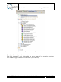
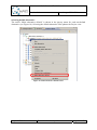
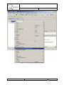
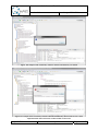
Q-ImPrESS project filters activation
Each Q-ImPrESS project includes a set of files and folders that can easily be managed by
applying view filters within the Project Explorer. To activate or deactivate filters select the
“Customize View…” item in the Project Explorer menu. A window containing the list of
available filters is depicted in the Figure 9. In particular, there are two Q-ImPrESS related
items: (i) “Q-ImPrESS alternatives folder” which manages the rendering of a system folder
containing storage of alternatives; and (ii) “Q-ImPrESS Generic Content Filter” which
provides a group filter for Q-ImPrESS-related tools.
Figure 9: List of content filters
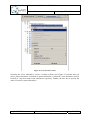
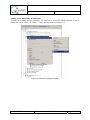
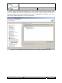
Q-ImPrESS annotation properties activation
Q-ImPrESS annotation properties view is part of the Properties View. This view can be
activated for each model entity through the option “Show properties view“ in the entity popup menu.
Q-ImPrESS annotation wizard activation
The Backbone provides an implementation of an advanced annotation wizard which allows
for associating QoS annotations with selected model entities. The wizard can be activated via
the Eclipse File menu: “File”  “New”  “Annotation Wizard” (see Figure 10), or by
selecting “File”  “New”  “Other…” and choosing the item “Q-ImPrESS Annotation
Wizard” in a list of wizards.
© Q-ImPrESS Consortium
Dissemination level: public
Page 30 / 207
D6.1 Annex: Guidelines and Tool Manuals
Version: 2.0
Last change: 25/01/2011
Figure 10: Activation of the QoS annotations wizard
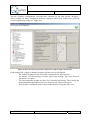
4.2.7
Usage instructions and expected outputs
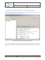
Q-ImPrESS project view
When Q-ImPrESS nature view is associated with a project, two additional nodes are shown.
The first node called “ Alternatives repository” (see Figure 11) contains a repository of
alternatives. Alternatives are organised into a tree. Each alternative is marked with an icon .
The alternative label shows the name and an internal identifier also used as a directory name
where the alternative is persisted.
There is always one alternative from the repository selected as a “default” alternative. This is
indicated by the icon .
The default alternative has a dedicated node in the Project Explorer view that also renders the
associated models depicted by the icon . Each model comprises model artifacts that can be
edited using a generic EMF tree editor, graphical editor or syntax-aware text editor with
highlighting features.
© Q-ImPrESS Consortium
Dissemination level: public
Page 31 / 207
D6.1 Annex: Guidelines and Tool Manuals
Version: 2.0
Last change: 25/01/2011
Figure 11: The project view with enabled Q-ImPrESS nature
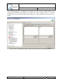
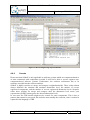
Creation of a new alternative
The “New Alternative” action is located in the pop-up menu of the alternatives repository
node and in the pop-up menu of each alternative (see Figure 12).
© Q-ImPrESS Consortium
Dissemination level: public
Page 32 / 207
D6.1 Annex: Guidelines and Tool Manuals
Version: 2.0
Last change: 25/01/2011
Figure 12: New alternative action
Selecting the “New Alternative” action, a wizard is shown (see Figure 13) and the user can
pick a parent alternative. Provided no parent alternative is selected, a new alternative will be
created as a top-level node in the alternative repository. Further, the user has to specify the
name of a newly created alternative
.
© Q-ImPrESS Consortium
Dissemination level: public
Page 33 / 207
D6.1 Annex: Guidelines and Tool Manuals
Version: 2.0
Last change: 25/01/2011
Figure 13: New alternative wizard
© Q-ImPrESS Consortium
Dissemination level: public
Page 34 / 207
D6.1 Annex: Guidelines and Tool Manuals
Version: 2.0
Last change: 25/01/2011
Selecting default alternative
The action “Make alternative default” is shown in the pop-up menu for each non-default
alternative (see Figure 14). Selecting the default alternative also updates the Project view.
Figure 14: Make alternative default action
© Q-ImPrESS Consortium
Dissemination level: public
Page 35 / 207
D6.1 Annex: Guidelines and Tool Manuals
Version: 2.0
Last change: 25/01/2011
Adding a new model into an alternative
To add a new model into an alternative, the user has to select the default alternative and to
choose the action “New”  “Other…” in the pop-up menu (see Figure 15).
Figure 15: Action for creating new model
© Q-ImPrESS Consortium
Dissemination level: public
Page 36 / 207
D6.1 Annex: Guidelines and Tool Manuals
Version: 2.0
Last change: 25/01/2011
Using a wizard, the user can create a new model by selecting the appropriate option from the
provided types of models (see Figure 16).
Figure 16: Selecting the type of model
© Q-ImPrESS Consortium
Dissemination level: public
Page 37 / 207
D6.1 Annex: Guidelines and Tool Manuals
Version: 2.0
Last change: 25/01/2011
Before a new model is created it is necessary to specify the model name (see Figure 17).
Figure 17: Associating a name with the model
© Q-ImPrESS Consortium
Dissemination level: public
Page 38 / 207
D6.1 Annex: Guidelines and Tool Manuals
Version: 2.0
Last change: 25/01/2011
Finally, a top-level modelling entity has to be selected (see Figure 18). After finishing the
wizard, the new model is created within the selected alternative.
Figure 18: Selecting top-level modelling entity
Model editing
Each model can be edited either using a generated EMF tree editor or directly from the
Project Explorer view using the context pop-up menu. In other words, each model artefact
provides pop-up menu to create child- and sibling-artefacts, to delete an artefact and to show
the property view (see Figure 19). Changes are directly stored into the corresponding model
file.
© Q-ImPrESS Consortium
Dissemination level: public
Page 39 / 207
D6.1 Annex: Guidelines and Tool Manuals
Version: 2.0
Last change: 25/01/2011
Figure 19 Editing model
© Q-ImPrESS Consortium
Dissemination level: public
Page 40 / 207
D6.1 Annex: Guidelines and Tool Manuals
Version: 2.0
Last change: 25/01/2011
Properties of a model can be edited via the Property view (see Figure 20). Also these changes
are automatically saved into the corresponding model file.
Figure 20: Property view for model entity
Opening model artefact editors
Each model artefact can be opened via a predefined set of editors. The possible open actions
are shown in the pop-up menu of each model entity.
Annotation properties
Annotation properties can be shown for each model element. For a selected element, the
annotation properties view shows a list of associated QoS annotations and the properties of
the annotation (see Figure 21). It further allows users to re-associate existing annotations or
create new annotations for a selected element.
Figure 21: QoS annotation properties
© Q-ImPrESS Consortium
Dissemination level: public
Page 41 / 207
D6.1 Annex: Guidelines and Tool Manuals
Version: 2.0
Last change: 25/01/2011
Annotation wizard
The annotation wizard can be used to annotate repository elements with various kinds of
annotations. The wizard can be activated via menu “File”  “New”  ”Annotation Wizard”
(see Figure 22).
Figure 22: Annotation wizard activation
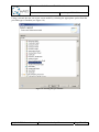
When activated, the wizard displays a dialog with a list of projects. User then selects the
desired subset of projects where the elements will be annotated (see Figure 23).
Figure 23: Annotation wizard – project selector
© Q-ImPrESS Consortium
Dissemination level: public
Page 42 / 207
D6.1 Annex: Guidelines and Tool Manuals
Version: 2.0
Last change: 25/01/2011
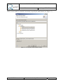
The next wizard dialog shows on the left side the list of provided annotation types. By
selecting an annotation type the right menu shows repository elements which can be
annotated (see Figure 24) by this annotation type. The dialog also shows properties of the
annotation type and the selected repository element at the bottom.
Figure 24: Annotation wizard – annotating repository elements
© Q-ImPrESS Consortium
Dissemination level: public
Page 43 / 207
D6.1 Annex: Guidelines and Tool Manuals
Version: 2.0
Last change: 25/01/2011
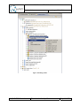
When the “Finish” button is clicked, each selected element is associated with a “default” instance of the
selected annotation type. However, when clicking the “Next” button, the annotation properties can be
fine-tuned for every selected repository entity (see
Figure 25).
Figure 25: Annotation wizard – specification of annotation properties for a selected element
4.2.8
Caveats
Problems with the Q-ImPrESS project
In some cases (e.g., due to an obsolete workspace structure), the Q-ImPrESS project can be
shown in a wrong way. This problem can be fixed by re-opening the affected projects and by
restarting the Eclipse platform.
© Q-ImPrESS Consortium
Dissemination level: public
Page 44 / 207
D6.1 Annex: Guidelines and Tool Manuals
Version: 2.0
4.3
Last change: 25/01/2011
Repository Editor Manual
4.3.1
Purpose of the tool
The Repository Editor tool described here is a graphical editor for components of a Service
Architecture Model (SAM) that ought to be maintained subsequently in a repository. It is
intended as a complementary tool for the textual editor of repository components, primarily
for the users who are more familiar with the graphical editing environments. Last but not
least, such an editor enables users to reorganise the graphical representation of their models
mostly resulting in a cleaner visualization of the model comparing to the automatically
generated visual representations.
The tool is completely integrated into the Eclipse development environment and is available
in an initial version covering a wide range of useful features.
4.3.2
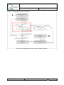
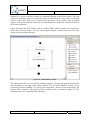
Tool relationship with the Q-ImPrESS workflow
The Repository Editor can be used to create, edit or display repository elements such as
components, interfaces, interface operations, or data types. It can be used anytime during the
Q-ImPrESS workflow. However the most relevant workflow step for using the editor is the
“Model Change Scenario” step (see Figure 26).
© Q-ImPrESS Consortium
Dissemination level: public
Page 45 / 207
D6.1 Annex: Guidelines and Tool Manuals
Version: 2.0
Last change: 25/01/2011
Figure 26: Modelling change scenario workflow (copied from D6.1)
© Q-ImPrESS Consortium
Dissemination level: public
Page 46 / 207
D6.1 Annex: Guidelines and Tool Manuals
Version: 2.0
Last change: 25/01/2011
4.3.3
Tool prerequisites
The Repository Editor has no special prerequisites.
4.3.4
Tool activation
The tool needs a SAMM repository diagram file to work. If such a file already exists, it is
sufficient to Double-Click on it to open it and start the editor.
In case such a file doesn’t exist, it is possible to automatically generate such a file from an
existing SAMM repository. Information about how to create a repository model file can be
found in Section 4.1.
The following paragraphs will explain how to generate a diagram file from an existing
repository model. A repository model is stored in a file with the file ending
“.samm_repository”. First it is necessary to select the existing repository in the Eclipse
Project Explorer. Right-Clicking on the entry shows a context menu similar to the one
displayed in Figure 27.
Figure 27: Generating a diagram file for a repository
Selecting the menu entry highlighted in Figure 27 will result in a dialog opening. Here it is
sufficient to simply select “Finish” to confirm all default settings and create a diagram entry
© Q-ImPrESS Consortium
Dissemination level: public
Page 47 / 207
D6.1 Annex: Guidelines and Tool Manuals
Version: 2.0
Last change: 25/01/2011
with them. The Project Explorer will show a new entry (the diagram has the file ending
“.samm_repository_diagram”) and the editor for the diagram file automatically opens.
The Repository Editor can also be opened by double-clicking on the repository diagram file.
The screenshot in Figure 28 shows the diagram for an example repository.
Figure 28: Editor showing the repository example diagram
4.3.5
Usage instructions and expected outputs
The current section will explain how a user is expected to work with the Repository Editor. It
is assumed that the user already knows how to use a graphical editor, i.e. how to select
elements, drag and drop elements or icons and the like. It is assumed out-of-scope for the
given document to explain such basic knowledge.
When a diagram file is opened, it shows the typical interface for every editor working in an
Eclipse environment. The following explanations make use of the Client/Server Example
project that is shipped with the Q-ImPrESS IDE.
If the diagram has been automatically generated, the automatic placement of graphical
elements may be not suited to allow viewing all elements in their entirety and the connections
between them may be not clearly visible. Section 4.4.4 gives more information about how to
improve the layout of model elements in a diagram file.
Working with editor tools for repository elements
The editor allows using the same elements as the textual editor for the repository. The editor
allows the user to create elements simply by selecting the appropriate tool from the tool
© Q-ImPrESS Consortium
Dissemination level: public
Page 48 / 207
D6.1 Annex: Guidelines and Tool Manuals
Version: 2.0
Last change: 25/01/2011
palette to the right of the editor window. The palette and the available tools are shown in
Figure 29.
Figure 29: Editor tools palette
In order to create such an element a user has to perform the same action independently from
the tool. At first the appropriate entry in the palette must be selected (from the upper section)
and will be shown highlighted. Then the mouse cursor must be moved into the editor canvas.
The mouse cursor shape changes according to the tool selected to show the user that an
element of a given type is going to be created. The action needs to be finished by clicking at
an appropriate location in the editor canvas resulting in the creation of a new element and its
placement at that location.
Working with Inner Elements
The second section in the palette contains tools for the creation of inner elements. Such
elements can only be created within other elements already placed on the editor canvas.
The use of these tools is in no way different from the tools of the upper section. To use such a
tool, its icon must be selected and will be shown highlighted. Moving the mouse cursor into
the canvas of the editor results in different cursor shapes depending whether the chosen tool
can be applied to the given context or element or not.
As an example let’s assume that we want to create a new Operation. We select the tool and
move the mouse cursor over the component “clientComposite”. As it is not possible to create
an Operation for an element of that type, the cursor still shows a crosshair shape. This
changes when we move it over the element “GuiInterface”. It is possible to add an element of
type Operation to this element (an Interface), so the cursor changes into a hollow arrow with a
plus sign to indicate that the operation can be performed.
© Q-ImPrESS Consortium
Dissemination level: public
Page 49 / 207
D6.1 Annex: Guidelines and Tool Manuals
Version: 2.0
Last change: 25/01/2011
The same behaviour is implemented for the other inner elements shown in that section of the
palette. Depending on the type of tool selected and type of element the cursor is pointing to,
the cursor shape indicates the applicability of the chosen tool.
Working with OperationBehaviour
In the Inner Elements section of the palette, Operation Behaviours can be added to Primitive
Components. Adding an element of type OperationBehavior opens a dialog box requiring the
user to choose whether a SEFF behaviour stub or a GAST behaviour stub shall be created.
After specifying the type of behaviour, a dialog box opens that allows the user to select the
operation interface for which the behaviour is to be specified. By double-clicking on a SEFF
behaviour, the graphical SEFF Editor opens which allows displaying and editing the SEFF
behaviour. This editor is explained in detail in chapter 4.5.
Deleting elements
Deleting elements works as can be expected from such graphical editors. After selecting one
or more elements, the mouse context menu (right-click) opens up showing an entry “Delete
from Model” (see Figure 30).
Figure 30: Deletion of elements
The delete operation deletes the selected element. It may also delete some of the elements
associated to the element to be deleted in case those elements cannot exist apart from the
element to delete.
© Q-ImPrESS Consortium
Dissemination level: public
Page 50 / 207
D6.1 Annex: Guidelines and Tool Manuals
Version: 2.0
Last change: 25/01/2011
Moving elements
Elements in the editor can be moved as expected. Simply select them and move them using
the mouse cursor.
Sizing elements
When an element is selected that allows resizing, appropriate handles are shown. Selecting
one of those handles and dragging it with the mouse will change the size of the element
accordingly. In rare cases resizing is not possible and the element will retain its size even after
an attempt to resize it.
Working with Composite Components
Working with composite components is special in that they feature a separate editor of their
own. Double-clicking on a composite component opens the Composite Editor that displays
the contents of the composite component. The editor can be used independently from the
Repository Editor and it is described in a Section 4.4.
However, subcomponent instances for composite components can also be created in the
Repository Editor. To add a subcomponent instance to a composite component, select the tool
SubcomponentInstance from the palette and click inside a composite component on the
canvas. A dialog opens which enables the user to select the subcomponent type for the
subcomponent instance.
4.3.6
Caveats
In its current version, the tool doesn’t extensively check the semantics of models created by
the user. So it may be possible to draw models according to the rules set forth in the meta
model (SAMM) which will not have any practical meaning, as they show situations which
cannot be reasonably expected to occur. It may be necessary to enhance the editor after setting
up rules, e.g. governing the possible combinations of elements in the model. A future version
of the editor may check the model for validity at least when the user saves the model he
created.
© Q-ImPrESS Consortium
Dissemination level: public
Page 51 / 207
D6.1 Annex: Guidelines and Tool Manuals
Version: 2.0
Last change: 25/01/2011
4.4
Composite Editor Manual: Modelling service architecture
models and composite components
4.4.1
Purpose of the tool
The Q-ImPrESS IDE provides a graphical editor for a Service Architecture Model (SAM) and
composite components. As both structures share the same concepts, the editor can be used for
both. It is intended as a complement for the standard Eclipse editor for EMF based models.
Users being more familiar with graphical editing environments will prefer this to the standard
editor. Last but not least such an editor enables users to adapt the graphical representation of
their models mostly resulting in a better visualization than what can be obtained from
automatic visualization tools using the SAM. The editor is opened automatically whenever a
user edits a composite component from the Repository Editor as well. It is also possible to
save diagrams of composite components and Service Architecture Models as diagram files.
4.4.2
Tool relationship with the Q-ImPrESS workflow
The Composite Editor can be used to create, edit or display Service Architecture Models
(SAM) or composite components. It can be used anytime during the Q-ImPrESS workflow,
however the most relevant workflow step for using the editor is the step “Model Change
Scenario” (see Figure 31).
Figure 31: Modelling change scenario workflow (copied from D6.1)
© Q-ImPrESS Consortium
Dissemination level: public
Page 52 / 207
D6.1 Annex: Guidelines and Tool Manuals
Version: 2.0
Last change: 25/01/2011
4.4.3
Tool activation
The Composite Editor can work on Service Architecture Model diagram files. If such a file
already exists, double-clicking on it will automatically open the editor. The editor can also be
opened from within the Repository Editor when a user wants to edit one of the composite
components within the Repository Editor. Please refer to the previous chapter for more
information about it and the integration with the Composite editor.
The screenshot in Figure 32 shows the Project Explorer with an example Q-ImPrESS project
where a suitable Service Architecture Model file and its diagram file are available.
Figure 32: A Service Architecture Model file and the corresponding diagram file in the Project Explorer
In the case shown, a Service Architecture Model diagram file already exists and could be
opened and edited. If no such file exists (in cases where the models have not been edited
using the graphical editor before), it can be automatically generated from an existing Service
Architecture model.
To generate a diagram file, right-click on a Service Architecture Model file (such files have
the file ending “.samm_servicearchitecturemodel”) in the Project Explorer and select
“Initialize graphical model file” (see Figure 33). A dialog opens in which the file location of
the diagram file has to be specified.
© Q-ImPrESS Consortium
Dissemination level: public
Page 53 / 207
D6.1 Annex: Guidelines and Tool Manuals
Version: 2.0
Last change: 25/01/2011
Figure 33: Generate a diagram file for a Service Architecture Model
Using a right-Click on the selected entry shows the menu displayed in Figure 33. Selecting
the highlighted entry will create a new entry in the workspace where the required model
diagram file can be found.
The Composite Editor can be opened for a Service Architecture diagram file by doubleclicking on the file. For a composite component, it can be opened by double-clicking on the
composite component in the graphical Repository Editor.
4.4.4
Usage instructions and expected outputs
The current section will explain how a user is expected to work with the Composite Editor. It
is assumed that this user already knows how to use a graphical editor, i.e. knows how to select
elements drag and drop elements or icons and the like. It is assumed out-of-scope for the
given document to explain such basic knowledge.
When a diagram file is opened, it shows the typical interface for every editor working in an
Eclipse environment. The following explanations are based on the Service Architecture
Model of the Q-ImPrESS Client/Server Example project.
© Q-ImPrESS Consortium
Dissemination level: public
Page 54 / 207
D6.1 Annex: Guidelines and Tool Manuals
Version: 2.0
Last change: 25/01/2011
Opening the editor
The user starts an editing session by double-clicking on the Service Architecture Model
diagram file as shown in Figure 32.
The editor opens in the usual location in the Eclipse environment as shown in Figure 34.
Figure 34: Composite Editor running in the Q-ImPrESS IDE
It should be noted that if the diagram has been automatically generated, not all graphical
elements might be placed in a suitable way.
Working with components
After the automatic generation of the diagram, the main element, the
ServiceArchitectureModel or composite component, might require just enough space in the
editor to show all the contained elements and their labels (see Figure 35). To allow changing
the placement of components, we have to increase the area for this component.
When we click into an otherwise empty area inside the component or its header, the whole
component is selected. The editor indicates this by showing handles around the exterior of the
component (see Figure 36).
When the user moves the mouse cursor over one of these handles, the pointer changes to
another form indicating the action possible when selecting and holding the handle. For the
handles on the sides of the component, this allows moving the selected side thus enlarging the
area taken by the component. For the handles on either edge, it allows moving that edge, thus
enlarging the component by moving two sides simultaneously.
This is compatible with analogous behaviour of other graphical editors and will allow users to
become familiar with the editor in a short period of time.
In our example the component needs to be enlarged in order to allow changing the placement
© Q-ImPrESS Consortium
Dissemination level: public
Page 55 / 207
D6.1 Annex: Guidelines and Tool Manuals
Version: 2.0
Last change: 25/01/2011
of the contained components and connections. This will be achieved by selecting the lower
right corner of our component and drag it to an appropriate location.
Figure 35: Editor with main element selected
After that we need to select one of the inner components to change its placement. Currently
the components are overlapping making it hard to distinguish them from one another. The
best way to select a component is by clicking once on its name. It is possible as well to click
into an otherwise empty area within the component, although this proves difficult in our case
with the overlapping components.
Figure 36: Selecting inner components
© Q-ImPrESS Consortium
Dissemination level: public
Page 56 / 207
D6.1 Annex: Guidelines and Tool Manuals
Version: 2.0
Last change: 25/01/2011
After selecting the component, we can move it to another location. We repeat this with the
two other components as well in order to see them without overlapping each other or any
other element in the editor. Figure 37 shows how this may look.
The next thing to notice is that some of the labels are overlapping as well preventing the user
to read them.
Figure 37: Editor after moving components
To overcome this, we need to enlarge the components or move a label to another location.
Enlarging a component can be achieved by selecting it and dragging one of the handles until
the components area is large enough to accommodate the label text.
© Q-ImPrESS Consortium
Dissemination level: public
Page 57 / 207
D6.1 Annex: Guidelines and Tool Manuals
Version: 2.0
Last change: 25/01/2011
Figure 38: Editor after fixing overlapping labels
We can move labels the same way as we move components, by selecting them and then
dragging them to their new location. The screenshot in Figure 38 shows the editor after both
actions have been performed.
The next thing to do is to improve the layout of the connectors. This can be achieved by
dragging the connector. Note that also the position of the component ports can be changed.
Figure 39 shows the resulting representation of the Service Architecture Model after adapting
the connector layout.
© Q-ImPrESS Consortium
Dissemination level: public
Page 58 / 207
D6.1 Annex: Guidelines and Tool Manuals
Version: 2.0
Last change: 25/01/2011
Figure 39: Editor after improving graphical representation
Deleting elements
In order to demonstrate a special feature of the editor, we will re-create a connector contained
in the model. To be able to do that, we need to delete it first.
Deleting elements works as can be expected from such graphical editors. After selecting one
or more elements, the mouse context menu (right-click) opens up showing an entry “Delete
from Model” (see Figure 40).
© Q-ImPrESS Consortium
Dissemination level: public
Page 59 / 207
D6.1 Annex: Guidelines and Tool Manuals
Version: 2.0
Last change: 25/01/2011
Figure 40: Deletion of connectors
The delete operation deletes the connector together with its associated endpoints.
Other elements are deleted the same way if necessary.
Adding elements
Now we can add a new connector to show the special feature of the editor. Adding elements
is generally possible using the tool palette shown to the right of the editor window (see Figure
34). We need to click on one of the elements shown to select it. The selected element will be
shown highlighted. After that we can move the mouse cursor to the editor pane and it will
change its shape indicating that a new element will be inserted. We need to click in the
location where we want to insert the element and the editor creates a new instance according
to the tool we selected from the palette.
For our example we select the Connector tool and click in the editor somewhere between the
businessLogicInstance component and the databaseInstance component. A new Connector is
being created. We now need to specify its endpoints. Endpoints are used to connect the
Connector elements with component ports (or provided ports of a Service Architecture
Model). We select the SubcomponentEndPoint tool from the palette and move the mouse into
the editor pane. The cursor shape changes to indicate that we are about to create an endpoint,
which for the graphical representation implies connecting the Connector shape with a Port
shape by a line.
We move the mouse cursor over the Connector and click and drag from there to the port with
the label “BusinessLogic_Required_DatabaseInterface”. Here we release the mouse and a
new endpoint will be created. The screenshot in Figure 41 shows the editor after the first
endpoint has been created. To complete the connector, we have to create another endpoint that
© Q-ImPrESS Consortium
Dissemination level: public
Page 60 / 207
D6.1 Annex: Guidelines and Tool Manuals
Version: 2.0
connects
the
connector
with
“Database_Provided_DatabaseInterface”.
Last change: 25/01/2011
the
database
component
port
Figure 41: Editor after creating a SubcomponentEndPoint
SubcomponentEndPoints are used to connect components on the same level, e.g. two
components nested in a composite component, or two components in the Service Architecture
Model. To create a connection between a port of a component with a port of a nested
component, the ComponentEndPoint is used to connect the connector with the port of the
outside component. Such connectors are called delegation connectors and are drawn with a
thick line in the Composite Editor.
Figure 42 shows a delegation connector in the Service Architecture Model of the example
project. It connects the outside port “ServiceArchitectureModel_Provided_GuiInterface” of
the Service Architecture Model with the port “clientComposite_Provided_GuiInterface” of
the “clientCompositeInstance” composite component.
© Q-ImPrESS Consortium
Dissemination level: public
Page 61 / 207
D6.1 Annex: Guidelines and Tool Manuals
Version: 2.0
Last change: 25/01/2011
Figure 42: A delegation connector in the Service Architecture Model
Adding Subcomponent Instances
The editor allows the user to add new subcomponent instances. First the tool must be selected
in the tool palette and the mouse must be clicked in the desired location where the new
subcomponent instance shall be located. The editor so far only knows that a new instance
shall be created, but has no information as to from what component the instance shall be
derived. So the user has to choose this component from the available repositories. A selection
dialog opens and displays the components available in the currently used repositories (see
Figure 43).
In case the component to be instantiated should not be contained in the list shown, the user
can load additional repositories that may contain the required component. After a selection is
made the appropriate element is created in the editor.
© Q-ImPrESS Consortium
Dissemination level: public
Page 62 / 207
D6.1 Annex: Guidelines and Tool Manuals
Version: 2.0
Last change: 25/01/2011
Figure 43: Selection of components to be instantiated
4.4.5
Caveats
In its current version, the tool doesn’t extensively check the semantics of models created by
the user. So it may be possible to draw models according to the rules set forth in the meta
model (SAMM) which will not have any practical meaning, as they show situations which
cannot be reasonably expected to occur. It may be needed to enhance the editor after setting
up rules, e.g. governing the possible combinations of endpoints for a given connector.
Currently it is possible to connect two provided ports with a connector without indicating a
required port. We assume that a future version of the editor may check the model for validity
at least when the user saves the created model.
© Q-ImPrESS Consortium
Dissemination level: public
Page 63 / 207
D6.1 Annex: Guidelines and Tool Manuals
Version: 2.0
4.5
Last change: 25/01/2011
SEFF Editor Manual
4.5.1
Purpose of the tool
The Q-ImPrESS IDE features a graphical editor that allows for modelling service-effect
specification (SEFF) behaviours of primitive component operations (a primitive component is
a component that does not contain other components, as opposed to composite components).
Each provided service of a primitive components comprises such a SEFF behaviour
description.
In the Q-ImPrESS toolchain, components can have different kinds of behaviours. The SEFF
behaviour is an abstract behaviour of a component operation which includes relevant
information for quality analysis offered by the Q-ImPrESS IDE.
4.5.2
Tool relationship with the Q-ImPrESS workflow
The Q-ImPrESS graphical SEFF editor can be used both in reverse-engineering and forwardengineering approaches. In a reverse-engineering approach, initial derived SEFF behaviours
of component operations can be visualised and enhanced using the editor. In a forwardengineering approach, the editor can be used to create and behaviour models from scratch.
The tool described in the chapter belongs to the tool class “Model editing Tools to update
system models” as described in section 2.1 in the document D6.1. This implies that it can be
applied in any place in the tool chain where models of the appropriate type can be edited.
It can be used anytime during the Q-ImPrESS workflow. However the most relevant
workflow step for using the editor is the “Model Change Scenario” (see Figure 44).
© Q-ImPrESS Consortium
Dissemination level: public
Page 64 / 207
D6.1 Annex: Guidelines and Tool Manuals
Version: 2.0
Last change: 25/01/2011
Figure 44: Modelling change scenario workflow (copied from D6.1)
© Q-ImPrESS Consortium
Dissemination level: public
Page 65 / 207
D6.1 Annex: Guidelines and Tool Manuals
Version: 2.0
Last change: 25/01/2011
4.5.3
Tool prerequisites
The SEFF Editor has no special prerequisites except for the existence of at least one provided
service of a primitive component for which a SEFF is going to be created.
4.5.4
Tool activation
The SEFF Editor works on SEFF diagram files which are stored in the corresponding SAM
alternative folder. Diagram files have the file ending “.samm_seff_diagram”, the editor can be
launched by double-clicking the file.All SEFF behaviours for an alternative (i.e. the SEFF
models, not the diagram files) are stored in a common SEFF Repository. This file has the file
ending “.samm_seff” and is located in the alternative folder as well.
If no SEFF behaviour diagram file for a component exists, it can be created from within the
graphical Repository Editor.
In the Repository Editor, all components are displayed, as well as behaviours that have been
specified for a component. Figure 45 shows the Repository Editor with a component
“Database” implementing the interface “DatabaseInterface”. For the interface operation
“getUserForUserId” a SEFF behaviour stub has been specified. The SEFF Editor can be
opened by double-clicking a SEFF behaviour stub. For more information about the
Repository Editor and behaviour stubs, refer to the Repository Editor Manual.
Figure 45: The Repository Editor showing a component with a SEFF behaviour stub
4.5.5
Usage instructions and expected outputs
The SEFF Editor is used in the same way as the other graphical editors. A SEFF behaviour
© Q-ImPrESS Consortium
Dissemination level: public
Page 66 / 207
D6.1 Annex: Guidelines and Tool Manuals
Version: 2.0
Last change: 25/01/2011
contains of a series of actions, which are connected through control flow arrows. The first
action in a behaviour must be a start action, the last action must be a stop action. All actions
and the control flow link can be selected from the palette. Some actions, such as branch
actions, loop actions and fork actions have nested behaviours, which may contain all kinds of
SEFF action elements.
Figure 46 shows the SEFF Editor with an example SEFF, which contains of a start action,
loop action and stop action. The loop action again contains a nested behaviour. The loop
action loops the nested behaviour.
Figure 46: A SEFF Editor example
The editor allows the user to create the elements simply by selecting the appropriate tool from
the tool palette to the right of the editor window. For all action elements, a name can be
specified for better readability. To specify the control flow, actions can be connected by the
Control Flow connector. The palette and the available tools are shown in Figure 47. The
different actions are explained in the following.
© Q-ImPrESS Consortium
Dissemination level: public
Page 67 / 207
D6.1 Annex: Guidelines and Tool Manuals
Version: 2.0
Last change: 25/01/2011
Figure 47: The SEFF Editor tools palette
StartAction
The first action of a behaviour.
InternalAction
Denotes some internal work during an operation for which the control flow is not specified in
more detail. However, different quality annotations can be attached to an internal action, such
as resource demands (for performance analyses) or failure probability (for reliability
analyses). For more details, refer to the guide for QoS Annotations.
ExternalCallAction
Denotes a call to a required interface port of the component, which results in a call to a
control flow outside of the component. When creating an external call action element, a
dialog appears that allows selecting the required interface port of the component. If the dialog
does not display any ports, select “Load Resource…” and then “Browse Workspace”. In the
following dialog, browse to the SAM repository file in which the component is located and
select it. After closing the dialog, all required ports should appear. If still no ports appear, the
component of the operation’s behaviour does not contain any required ports, and a port has to
be added in the component repository file. This can for example be done with the textual
Repository Editor or the graphical Repository Editor.
LoopAction
Contains a nested behaviour that is repeated several times in a loop. To specify the nested
© Q-ImPrESS Consortium
Dissemination level: public
Page 68 / 207
D6.1 Annex: Guidelines and Tool Manuals
Version: 2.0
Last change: 25/01/2011
behaviour, after creating a loop action element, select “ResourceDemandingBehaviour” from
the Composite editor palette and click inside the loop action element. A nested panel is being
created inside the loop action element which allows specifying the nested behaviour. Here, at
least a minimal behaviour has to be provided (i.e. a connected start action and stop action).
The number of loop iterations is again specified as a QoS annotation.
BranchAction
Contains multiple nested behaviours where only one behaviour is executed when the control
flow reaches the branch action. To add a branch behaviour after creating a branch action
element, select “ProbabilisticBranchTransition” from the Composite editor palette and click
inside the branch action element. A nested panel is being created. Then, select
“ResourceDemandingBehaviour” from the Composite editor palette and click inside the
nested panel. Now, nested behaviour elements can be created inside the panel. Again, at least
a minimal behaviour has to be provided (i.e. a connected start action and stop action). For
each branch behaviour, a branch probability has to be provided as a QoS annotation.
ForkAction
Contains multiple nested behaviours where all behaviours are executed in parallel when the
control flow reaches the fork action. To add a forked behaviour, after creating a fork action
element, select “ResourceDemandingBehaviour” from the Composite editor palette and click
inside the fork action element. A nested panel is being created inside the fork action element
which allows specifying the nested behaviour. Again, at least a minimal behaviour has to be
provided (i.e. a connected start action and stop action).
StopAction
The last action of a behaviour.
AcquireAction
Denotes an acquire access to a passive resource. A passive resource denotes some kind of
limited resource, e.g. a thread pool, a semaphore, etc. It is specified for a component in the
repository editor. The mapping between acquire action and passive resource is provided as a
QoS annotation.
ReleaseAction
Denotes a release of a passive resource. The mapping between release action and passive
resource is provided as a QoS annotation (see separate Chapter).
4.5.6
Caveats
In its current version, the tool doesn’t extensively check the semantics of models created by
the user. So it may be possible to draw models according to the rules set in the meta model
(SAMM) which will not have any practical meaning, as they show situations which cannot be
reasonably expected to occur. It may be necessary to enhance the editor after setting up rules,
e.g. governing the possible combinations of elements in the model. We assume that a future
version of the editor may check the model for validity at least when the user saves the model
she created.
© Q-ImPrESS Consortium
Dissemination level: public
Page 69 / 207
D6.1 Annex: Guidelines and Tool Manuals
Version: 2.0
4.6
Last change: 25/01/2011
QoS Editor Manual
4.6.1
Purpose of the tool
The Quality of Service (QoS) Annotations editor allows the specification of QoS attributes for
single actions of a SAMM SEFF behaviour model. Such annotations include failure
probabilities, CPU and HDD demands. The editor represents a convenient and integrated way
to edit the QoS Annotations which are stored in a decorator model for the SAMM SEFF
model.
4.6.2
Tool relationship with the Q-ImPrESS workflow
QoS Annotations are defined along with the behaviour of services. Hence, they are modelled
during the definition of the change scenario (see Figure 48).
Figure 48: Modelling change scenario workflow (copied from D6.1)
© Q-ImPrESS Consortium
Dissemination level: public
Page 70 / 207
D6.1 Annex: Guidelines and Tool Manuals
Version: 2.0
Last change: 25/01/2011
4.6.3
Tool prerequisites
The QoS Annotations Editor requires existing SEFFs to be annotated. These SEFFs must be
part of a Q-ImPrESS design alternative in the Q-ImPrESS IDE, which is the case when
following the tooling documentation.
4.6.4
Tool activation
The QoS Annotations Editor can be activated in from the context menu of graphical editors
and is part of the “properties view”. Right-click on a model element, and select “Show
Properties View” on order to open the view (see Figure 49). In the view, the tab “QoS
Annotations” shows the editor.
Figure 49: Opening the properties view from the context menu
4.6.5
Usage instructions and expected outputs
The QoS Annotations Editor can be accessed from the “properties view” if elements
(typically InternalActions, Loops or Branches of a SAMM SEFF) are selected.
© Q-ImPrESS Consortium
Dissemination level: public
Page 71 / 207
D6.1 Annex: Guidelines and Tool Manuals
Version: 2.0
Last change: 25/01/2011
Figure 50: The QoS annotations editor
When starting with the editor, no annotations are present in the model (see Figure 50). Using
the “New…” button, new QoS Annotations can be added to the SEFF model.
Figure 51: Adding new QoS annotations
A pop-up menu then offers the different Quality of Service (QoS) annotations which are valid
for a certain model element (see Figure 51). For InternalActions, Failure Probabilities, CPU
Resource Demands, and HDD Resource Demands can be added, for Loops the number of
loop iterations, and for Branches the branching probability (other valid annotations are listed
per model element). Multiple QoS Annotations of different types can be added to a single
© Q-ImPrESS Consortium
Dissemination level: public
Page 72 / 207
D6.1 Annex: Guidelines and Tool Manuals
Version: 2.0
Last change: 25/01/2011
element of a model.
All annotations related to a certain model element are afterwards listed in the QoS
Annotations property editor fields.
Figure 52: The QoS annotations editor containing annotations
In order to re-identify QoS Annotations in the next step, use expressive names in the “Name”
field (instead of “aName” as indicated in the screenshot shown in Figure 52). Each QoS
Annotation is stored in the “.samm_qosannotation” file of the selected Q-ImPrESS
alternative. The file contains a decorator model for the other SAMM models (see Figure 53).
© Q-ImPrESS Consortium
Dissemination level: public
Page 73 / 207
D6.1 Annex: Guidelines and Tool Manuals
Version: 2.0
Last change: 25/01/2011
Figure 53: The QoS annotations decorator file
In the “.samm_qosannotation” file, the values for the QoS Annotations can be edited. QoS
Annotations can be identified by their name.
To quantify the QoS Annotations, each QoS Annotation can contain a number of
specifications which can refine each other. Constant numbers are the easiest case with the
lowest expressive power, parametric formula are the most complex and powerful
specification. In typical cases, for rough models, constant numbers are sufficient. To add a
specification, right click on a QoS Annotation in the tree editor of the “.samm_qosannotation”
file, and select the specification from the “New Child” submenu (see Figure 54).
Figure 54: Adding a specification to a QoS annotation
The values are again editable from the properties view. In the following example shown in
Figure 55, a loop is specified as being executed 3 times each time the control flow reaches it.
Figure 55: Specifying specifications for a Qos annotation
© Q-ImPrESS Consortium
Dissemination level: public
Page 74 / 207
D6.1 Annex: Guidelines and Tool Manuals
Version: 2.0
Last change: 25/01/2011
Valid QoS Annotations include the ones listed in Figure 56:
Figure 56: All QoS annotations
All loops, branches, and passive resources must carry QoS Annotations. Otherwise, the
model is invalid and the analyses will fail. For internal actions, QoS Annotations are optional.
4.6.6
Caveats
Currently, no integrated editing of the values of QoS Annotations is possible. The extension
of the editor is subject to future version of the tool. Depending on the analysis, not all QoS
Annotations are supported. For example, currently, black box service response times are not
yet supported by any analysis.
© Q-ImPrESS Consortium
Dissemination level: public
Page 75 / 207
D6.1 Annex: Guidelines and Tool Manuals
Version: 2.0
4.7
Last change: 25/01/2011
Text Editors Manual
4.7.1
Purpose of the tool
SAMM model text editor is used for manipulation of SAMM models using text editors.
4.7.2
Tool relationship with the Q-ImPrESS workflow
SAMM model text editor participates in the process of modelling an architecture scenario (see
Figure 57). It is used as an alternative to other modelling tools like graphical editors or
specialised editors (QoS Annotation editor).
Figure 57: Modelling change scenario workflow (copied from D6.1)
© Q-ImPrESS Consortium
Dissemination level: public
Page 76 / 207
D6.1 Annex: Guidelines and Tool Manuals
Version: 2.0
Last change: 25/01/2011
4.7.3
Tool prerequisites
The tool can be used only in projects having Q-ImPrESS nature.
4.7.4
Tool activation
The tool is available in projects once they acquire the Q-ImPrESS nature. Each entity of
SAMM model has action “Open in text editor” in its pop-up menu. If the user select the
action editor for the selected entity is automatically opened.
4.7.5
Usage instructions and expected outputs
The tool is used for creating and modifying SAMM models using text editors. These two use
cases are described in the next two sections. The last section gives instructions how to edit
particular SAMM model elements.
4.7.6
Creating new SAMM model
Right-click the project folder in the Project Explorer view and select the “New”  “File”
item. Enter the file name where you intend to store new SAMM model. The file name has to
end with the “.edifice” extension. Click the finish button. The wizard creates file having the
entered file name and opens the SAMM model editor (blank window).
4.7.7
Modifying existing SAMM models
In the package explorer right-click the SAMM model you want to modify and select the
“Open with”  “xtext editor” item. The eclipse opens a text editor containing definitions of
SAMM model elements of the selected SAMM model.
The following two figures show the use case. Figure 58 shows the Project Explorer containing
the list of models, Figure 59 shows the editor containing definitions of SAMM model
elements.
© Q-ImPrESS Consortium
Dissemination level: public
Page 77 / 207
D6.1 Annex: Guidelines and Tool Manuals
Version: 2.0
Last change: 25/01/2011
Figure 58: Project Explorer view with an instance of SAMM meta-model
© Q-ImPrESS Consortium
Dissemination level: public
Page 78 / 207
D6.1 Annex: Guidelines and Tool Manuals
Version: 2.0
Last change: 25/01/2011
Figure 59: Text editor for a composite component
Refer to Appendix C for the SAMM model elements grammar.
© Q-ImPrESS Consortium
Dissemination level: public
Page 79 / 207
D6.1 Annex: Guidelines and Tool Manuals
Version: 2.0
4.8
Last change: 25/01/2011
Reverse Engineering Manual
4.8.1
Purpose of the tool
The Q-ImPrESS reverse engineering toolchain consists of two integrated tools: SISSy and
SoMoX.
SISSy is a tool that can be used to reverse-engineer source code. Based on source code, a
GAST representation is being created.
SoMoX is a tool that can be used to detect components of software systems. It takes a GAST
representation as input and creates a SAM model containing the detected components.
Besides components, SoMoX reverse engineers a full instance of the SAM model which
includes interfaces, ports, connectors, component instances, and composite component
structures. The reverse engineered model represents a complete component-based software
architecture.
Components are detected by various heuristics, which can be configured and weighted. Each
heuristic represents a detection strategy which reacts to structures in software artefacts such as
the structure in the code, naming, and communication styles.
4.8.2
Tool relationship with the Q-ImPrESS workflow
Describe how the tool fits into the Q-ImPrESS workflow. Use a diagram to highlight its
position in the overall process.
The reverse engineering toolchain can be used in the process of modelling an architecture
scenario (see Figure 60). In addition to the manual creation of models based on the editors
described in Section 4.3 – Section 4.7, the reverse engineering toolchain can be used to
automatically create models based on existing software systems for which source code is
available.
© Q-ImPrESS Consortium
Dissemination level: public
Page 80 / 207
D6.1 Annex: Guidelines and Tool Manuals
Version: 2.0
Last change: 25/01/2011
Figure 60: Modelling change scenario workflow (copied from D6.1)
4.8.3
Tool prerequisites
In order to detect components of a software system, the source code should be available as
Eclipse workspace project to allow a smooth and straight reverse engineering run. The source
code project should compile without errors and all depending libraries need to be specified in
the project settings.
The reverse engineering run of Q-ImPrESS creates a SISSy GAST model from source code
which then serves as input for SoMoX. A valid Q-ImPrESS project with the design alternative
which is going to be reverse engineered needs to exist in the workspace.
For better performance regarding database speed we recommend using an installed database
system like PostgreSQL. Otherwise a Derby database can be used out of the box.
4.8.4
Tool activation
The tool doesn’t need any activation. After installation of the Q-ImPrESS IDE, reverse
engineering functionality is directly available in the eclipse environment.
© Q-ImPrESS Consortium
Dissemination level: public
Page 81 / 207
D6.1 Annex: Guidelines and Tool Manuals
Version: 2.0
Last change: 25/01/2011
4.8.5
Usage instructions and expected outputs
In order to perform a reverse engineering run to derive a Q-ImPrESS model from source
code, the source code has to be available on the machine, e.g. as an eclipse workspace project.
In the following, we describe how to apply the reverse engineering toolchain on a Java
project. We use the CoCoMe java implementation for this. The CoCoMe implementation can
be downloaded at http://agrausch.informatik.uni-kl.de/CoCoME.
The most convenient way to apply reverse engineering is to provide the source code as a
workspace project first. We switch to the Q-ImPrESS perspective, import the CoCoMe
project into the workspace, and create a Q-ImPrESS project called “Cocome-Q-ImPrESS” in
the workspace (see Figure 61).
Figure 61: Importing the Java project into the workspace
If the Project Explorer view is not displayed, switch to the view (“Window”  “Show View”
 “Project Explorer). Now, right-click on the imported Java project (in the running example,
the CoCoMe project cocome-impl) and select “Create Q-ImPreSS Reverse Engineering
Launch” (see Figure 62).
© Q-ImPrESS Consortium
Dissemination level: public
Page 82 / 207
D6.1 Annex: Guidelines and Tool Manuals
Version: 2.0
Last change: 25/01/2011
Figure 62: Creating a Reverse Engineering launch
© Q-ImPrESS Consortium
Dissemination level: public
Page 83 / 207
D6.1 Annex: Guidelines and Tool Manuals
Version: 2.0
Last change: 25/01/2011
A reverse engineering launch configuration is being created which already contains some
necessary settings, for example the input paths of the source code project and its referenced
libraries. Figure 63 shows the initial tab of the launch configuration, in which the user has to
select the Q-ImPrESS project for reverse engineering.
Figure 63: Reverse Engineering launch configuration: Selecting the Q-ImPrESS alternative
© Q-ImPrESS Consortium
Dissemination level: public
Page 84 / 207
D6.1 Annex: Guidelines and Tool Manuals
Version: 2.0
Last change: 25/01/2011
The second tab of the launch configuration contains SISSy configuration parameters (see
Figure 64). Some parameters have already been derived by the source code project, for
example the path to the source code files that is used for SISSy, or paths to libraries that the
source code requires. If needed, these parameters can be adapted for the reverse engineering
run.
Figure 64: Reverse Engineering launch configuration: SISSy configuration parameters
© Q-ImPrESS Consortium
Dissemination level: public
Page 85 / 207
D6.1 Annex: Guidelines and Tool Manuals
Version: 2.0
Last change: 25/01/2011
In the third tab of the launch configuration, the SISSy database settings have to be adapted
(see Figure 65). SISSy can use a PostgreSQL database or the Java-integrated Derby database.
PostgreSQL can only be used if such a database is available on the machine. A Derby
database can always be used, since it comes with the Java JRE. However, SISSy runs slower
when using Derby.
Figure 65: Reverse Engineering launch configuration: SISSy database settings
When selecting Derby, a database name, user name and password have to be provided. Insert
“sissy” in all three fields.
© Q-ImPrESS Consortium
Dissemination level: public
Page 86 / 207
D6.1 Annex: Guidelines and Tool Manuals
Version: 2.0
Last change: 25/01/2011
The tab “SoMoX Configuration” provides three sub-tabs. In the first sub-tab “Weights”,
select weights for those component detection strategies which best match your preferred
reverse engineering results (see Figure 66).
Figure 66: Reverse Engineering launch configuration: SoMoX weights specification
Each strategy has a single or multiple weights which need to be configured.
- The default weights provide reasonable components for most systems.
- 100 means: Use this strategy; 0 means: ignore this strategy. Any value between
100 and 0 is accepted.
- The most important weights are those for Clustering and Merge: Those define the
minimal and maximal abstraction level of the reverse engineered system.
- Each weight is explained in more detail in the when hovering the slider text.
© Q-ImPrESS Consortium
Dissemination level: public
Page 87 / 207
D6.1 Annex: Guidelines and Tool Manuals
Version: 2.0
Last change: 25/01/2011
The “NameResemblance” sub-tab lets you specify pre and post fixes which should not be
considered as indicators of similarity (see Figure 67). If for example “Event” is a typical
postfix which does not indicate that classes belong to a single component, add “Event” as a
postfix.
Figure 67: Reverse Engineering launch configuration: SoMoX name resemblance specification
© Q-ImPrESS Consortium
Dissemination level: public
Page 88 / 207
D6.1 Annex: Guidelines and Tool Manuals
Version: 2.0
Last change: 25/01/2011
In the “Blacklist” tab (see Figure 68), a blacklist can be specified that holds packages which
should not be part of the metrics calculation. For example, a GAST may contain references to
java API classes organised in the “java.*” packages. Hence, the blacklist contributes in
scoping a reverse engineering project.
Blacklist entries are regular expressions. For example, to remove all API classes just enter
java\..*|javax\..* (“.*” is an infinite number of arbitrary characters; “\.” is the escaped
dot; “|” is the separator for multiple entries).
Figure 68: Reverse Engineering launch configuration: SoMoX blacklist specification
© Q-ImPrESS Consortium
Dissemination level: public
Page 89 / 207
D6.1 Annex: Guidelines and Tool Manuals
Version: 2.0
Last change: 25/01/2011
If you want the tool to create behaviour model in the form of Threaded Behaviour Protocols
(TBP), check the checkbox at the “G-AST2TBP Settings” tab (see Figure 69).
Figure 69: Reverse Engineering launch configuration: G-AST2TBP settings
After a successful run, a TBP file for each primitive component will be created in the
alternative folder. You can modify the text inside the IDE if needed. The TBP models can be
used for checking consistency between component implementation in Java and the TBP
models.
© Q-ImPrESS Consortium
Dissemination level: public
Page 90 / 207
D6.1 Annex: Guidelines and Tool Manuals
Version: 2.0
Last change: 25/01/2011
Afterwards, the basic configuration for the reverse engineering run is complete.
Run the launch configuration to perform the reverse engineering run. Open the console view
to get information about the run (see Figure 70).
Figure 70: Console view during a Reverse Engineering run
Once the run completed successfully, the output model files has been created. The model files
can be found in the folder of the alternative which had been selected for the run (see Figure
71).
© Q-ImPrESS Consortium
Dissemination level: public
Page 91 / 207
D6.1 Annex: Guidelines and Tool Manuals
Version: 2.0
Last change: 25/01/2011
Figure 71: Reverse Engineering output model files
4.8.6
Caveats
Please note that SoMoX is only applicable to software systems which are component-based or
at least constructed with components in mind. It will not be able to reverse engineer noncomponent-based software systems. Furthermore, the software architecture has to be
somehow encoded into the software artifacts.
SoMoX is highly sensitive to merge and compose weights/thresholds. These values almost
always influence the minimal and maximal abstraction level, the number of reverse
engineered components, and the number of reverse engineered abstraction levels. Stepwise
refine these weights for merge and compose until the abstraction level meets your
expectations (SoMoX cannot guess the desired abstraction level).
In rare cases the TBP models might not be created for some components. This is due to
patterns that cannot be processed; this includes most notably the recursion, since it cannot be
captured in the language of TBP.
© Q-ImPrESS Consortium
Dissemination level: public
Page 92 / 207
D6.1 Annex: Guidelines and Tool Manuals
Version: 2.0
4.9
Last change: 25/01/2011
Performance Prediction Manual
4.9.1
Purpose of the tool
The Palladio Component Model (PCM) is a domain-specific language that allows for
modelling the design of component-based software. This design model can be transformed
into a performance analysis model.
The PCM can be included into the Q-ImPrESS platform for performance predictions on
Q-ImPrESS SAM models. Therefore, a SAM model has to be transformed into a PCM model
and the PCM performance analysis has to be performed for the PCM output model.
The Q-ImPrESS platform provides an automated workflow for this.
4.9.2
Tool relationship with the Q-ImPrESS workflow
The performance prediction participates in the process of predicting the system quality in the
Q-ImPrESS workflow (see Figure 72).
After a Q-ImPrESS SAM model has been created either by reverse-engineering or forwardmodelling, different QoS attributes can be analysed by the Q-ImPrESS platform.
For performance analysis the SAM model has to be transformed into a PCM instance. Then
the performance analysis results can be inspected in the Result Viewer and used as input for
the trade-off analysis. Detailed PCM performance analysis results are available in the
integrated PCM Results view in the Q-ImPrESS UI.
© Q-ImPrESS Consortium
Dissemination level: public
Page 93 / 207
D6.1 Annex: Guidelines and Tool Manuals
Version: 2.0
Last change: 25/01/2011
Figure 72: Predicting system quality (copied from D6.1)
4.9.3
Tool prerequisites
The PCM simulation might need a lot RAM. Therefore, make sure the Q-ImPrESS Eclipse
instance is started with useful memory parameters:
In the file eclipse.ini in the root directory of the Q-ImPrESS Eclipse installation, add the
following lines:
-vmargs
-Xms512m
-Xmx768m
(note: the provided instructions could vary depending on the target operating system)
A PCM performance analysis needs a valid PCM input model for input. This model can be
created automatically from a Q-ImPrESS SAM model.
Therefore, a Q-ImPrESS alternative has to be created which holds the SAM model files.
© Q-ImPrESS Consortium
Dissemination level: public
Page 94 / 207
D6.1 Annex: Guidelines and Tool Manuals
Version: 2.0
Last change: 25/01/2011
4.9.4
Tool activation
In the following, we assume that a Q-ImPrESS SAM model is already available. This SAM
model has to be stored in a Q-ImPrESS alternative in the IDE workspace.
Click “Run”  “Run as…” to create a run configuration for the Q-ImPrESS performance
prediction platform. On the left side view, right-click on “Q-ImPrESS Performance Analysis”
and click “New”. A new run configuration is being created and can now be specified.
On the first tab “Q-ImPrESS Alternative” of the configuration, select the Q-ImPrESS
alternative for which a performance analysis should be performed (see Figure 73).
Figure 73: Selecting a Q-ImPrESS alternative for performance prediction
© Q-ImPrESS Consortium
Dissemination level: public
Page 95 / 207
D6.1 Annex: Guidelines and Tool Manuals
Version: 2.0
Last change: 25/01/2011
On the tab “Q-ImPrESS Usage Model”, all defined usage models for the selected alternative
are displayed. Select the usage model for which you want to analyse the SAM performance
(see Figure 74).
Figure 74: Selecting the Usage Model for performance prediction
© Q-ImPrESS Consortium
Dissemination level: public
Page 96 / 207
D6.1 Annex: Guidelines and Tool Manuals
Version: 2.0
Last change: 25/01/2011
On the tab “Q-ImPrESS Alternative Evaluation”, select the alternative evaluation in the
Result Model in which the analysis results should be stored. By clicking on “Create
Alternative Evaluation”, you can specify new alternative evaluations in the subdialog (see
Figure 75).
Figure 75: Selecting the alternative evaluation for storing the performance prediction results
© Q-ImPrESS Consortium
Dissemination level: public
Page 97 / 207
D6.1 Annex: Guidelines and Tool Manuals
Version: 2.0
Last change: 25/01/2011
On the tab “SimuCom”, some necessary configuration for the PCM simulation engine has to
be provided (see Figure 76). In the drop-down field “Persistence Framework”, select
“SensorFramework”. To provide a valid run configuration, a data source has to be provided
that stores the simulation results. This can be a file data source or a memory data source. New
file data sources can be created in the subdialog.
If necessary, the maximum simulation time and number of measurements taken in the
simulation can be adjusted. If the checkbox “Enable verbose logging” is checked, extensive
logging output of the simulation engine is provided.
If you want to include detailed simulation of the networking resources, activate the check box
“Simulate linking resources”.
Figure 76: Configuring the PCM simulation
© Q-ImPrESS Consortium
Dissemination level: public
Page 98 / 207
D6.1 Annex: Guidelines and Tool Manuals
Version: 2.0
Last change: 25/01/2011
4.9.5
Usage instructions and expected outputs
Running a created run configuration starts the performance prediction platform. The SAM
model is being transformed into a PCM model. Once the PCM model has been created, the
simulation starts immediately.
To see the simulation status, make sure the “Simulation Dock Status” is being displayed. This
can be done by clicking “Window”  “Show View”  “Other…” and select the view
“Simulation Dock Status” in the “Other” category. Figure 77 shows the simulation status
view in the Q-ImPrESS IDE.
Figure 77: The simulation status view for a performance prediction run
© Q-ImPrESS Consortium
Dissemination level: public
Page 99 / 207
D6.1 Annex: Guidelines and Tool Manuals
Version: 2.0
Last change: 25/01/2011
After the simulation run has completed, the results can be displayed. Open the results
repository in the Q-ImPrESS project explorer by right-clicking on “RESULTS” and selecting
“Open ResultViewer”. In the result viewer (see Figure 78), different performance analysis
results are displayed, such as usage model response time and throughput, as well as resource
utilizations. For every result, different statistical values are given (mean, median, 10%
quantile and 90% quantile). A detailed description of the Q-ImPrESS results viewer can be
found in Section 4.12.
Figure 78: Performance prediction results in the Q-ImPrESS Results Viewer
© Q-ImPrESS Consortium
Dissemination level: public
Page 100 / 207
D6.1 Annex: Guidelines and Tool Manuals
Version: 2.0
Last change: 25/01/2011
If you want to have a detailed look on the performance simulation results, you can open the
PCM simulation results. Open the simulation results perspectives by clicking “Window” 
“Open Perspective”  “Other…”. Select the “PCM Results” perspective.
In the “Experiments View”, the specified data sources are displayed. Select the specified data
source of the simulation run. The data source contains the results of the simulation runs. For a
performance simulation, these results are stored in sensors. For all operations and usage
scenario, the response time is stored, for all resources, the utilization is stored.
Figure 79: Detailed performance prediction results in the PCM results visualisation
For a response time, different result presentations are possible. A meaningful display of
results is the “Response Time Histogram” or the “Response Time Histogram-based CDF”.
Double-click on the response time sensor in order to select the kind of display. Figure 79
shows the response time of a usage scenario as a histogram.
For a resource, the utilization can be displayed as a pie chart.
© Q-ImPrESS Consortium
Dissemination level: public
Page 101 / 207
D6.1 Annex: Guidelines and Tool Manuals
Version: 2.0
Last change: 25/01/2011
4.9.6
Caveats
The performance analysis cannot be performed if the model to analyse is not valid. In this
case, a list of error messages is shown in a pop-up window when initiating performance
prediction run (see Figure 80).
Displayed warnings can be ignored, but should be fixed in order to enhance the
comprehensibility of the models. Errors cannot be ignored, but must be fixed.
Figure 80: Detected warnings and errors for a Q-ImPrESS model during a performance prediction run
© Q-ImPrESS Consortium
Dissemination level: public
Page 102 / 207
D6.1 Annex: Guidelines and Tool Manuals
Version: 2.0
4.10
Last change: 25/01/2011
Reliability Prediction Manual
4.10.1
Purpose of the tool
The reliability analysis in Q-ImPrESS supports engineers to compute reliability information
about complex systems. It enables engineers to extract the reliability of a service from the
description of the system and a specific usage model.
The Q-ImPrESS platform provides an automated workflow for that purpose starting from a
Service Architectural Model.
4.10.2
Tool relationship with the Q-ImPrESS workflow
The reliability prediction participates in the process of predicting the system quality in the
Q-ImPrESS workflow (see Figure 81).
After a Service Architectural Model has been created either by reverse-engineering or
forward-modelling, the reliability analysis can be performed by the Q-ImPrESS platform.
The analysis results can be inspected in the integrated Q-ImPrESS UI or be used as input for
the trade-off analysis.
Figure 81: Predicting system quality (copied from D6.1)
© Q-ImPrESS Consortium
Dissemination level: public
Page 103 / 207
D6.1 Annex: Guidelines and Tool Manuals
Version: 2.0
Last change: 25/01/2011
4.10.3
Tool prerequisites
To run a reliability analysis, a model of the system must be first designed. In detail, the
reliability analysis takes as input a specific Q-ImPrESS model.
4.10.4
Tool activation
To run the reliability analysis for a model alternative, the following steps have to be
performed:
First, open the run configuration window of eclipse. From the menu, select “Run”  “Run
Configurations...”.
Create a new “Q-ImPrESS Reliability Analysis” launch configuration.
In the launch configuration, select the alternative to analyse from the tree menu in the
“QImPrESS Alternative” tab (see Figure 82).
Figure 82: Selecting a Q-ImPrESS alternative for reliability prediction
© Q-ImPrESS Consortium
Dissemination level: public
Page 104 / 207
D6.1 Annex: Guidelines and Tool Manuals
Version: 2.0
Last change: 25/01/2011
Select the usage scenario to analyse from the tree menu in the “Q-ImPrESS Usage Model” tab
(see Figure 83).
Figure 83: Selecting the Usage Model for reliability prediction
Select the alternative evaluation where the analysis result will be stored from the tree menu in
the “QImPrESS Alternative Result” tab (see Figure 84).
Figure 84: Selecting the alternative evaluation for storing the reliability prediction results
© Q-ImPrESS Consortium
Dissemination level: public
Page 105 / 207
D6.1 Annex: Guidelines and Tool Manuals
Version: 2.0
Last change: 25/01/2011
Set the precision of the reliability result value in the text field of the “Analysis parameters”
tab. Save the configuration and launch it to run the reliability analysis.
4.10.5
Usage instructions and expected outputs
When the analysis is being run, you can see the progress in the Progress Window of Eclipse
(see Figure 85).
Figure 85: The analysis status view for a reliability prediction run
After the analysis has been executed, the result is saved into the result archive of the analysed
Q-ImPrESS project. In particular, the result is available under the chosen alternative
evaluation as shown in Figure 86.
The result value represents the predicted global reliability value for the system alternative
under the specified usage scenario.
Figure 86: The reliability prediction results in the Q-ImPrESS project result model
© Q-ImPrESS Consortium
Dissemination level: public
Page 106 / 207
D6.1 Annex: Guidelines and Tool Manuals
Version: 2.0
Last change: 25/01/2011
4.10.6
Caveats
The reliability analysis cannot be performed if the model to analyse is not valid. In this case, a
list of error messages is shown in a pop-up window when initiating a reliability prediction run
(see Figure 87).
Displayed warnings can be ignored, but should be fixed in order to enhance the
comprehensibility of the models. Errors cannot be ignored, but must be fixed.
Figure 87: Detected warnings and errors for a Q-ImPrESS model during a reliability prediction run
© Q-ImPrESS Consortium
Dissemination level: public
Page 107 / 207
D6.1 Annex: Guidelines and Tool Manuals
Version: 2.0
4.11
Last change: 25/01/2011
Maintainability Prediction Manual
4.11.1
Purpose of the tool
The tool implements the KAMP method, i. e. Karlsruhe Architectural Maintainability
Prediction. The purpose of the tool is to enable software architects to predict the
maintainability of a software system using its architectural model. The core part is support for
a guided estimation of change efforts. In order to predict maintainability the approach
determines efforts estimates for implementing evolution scenarios.
4.11.2
Tool relationship with the Q-ImPrESS workflow
The maintainability prediction participates in the process of predicting the system quality in
the Q-ImPrESS workflow (see Figure 88).
As inputs it uses the architecture alternatives that are located in Q-ImPrESS projects within
the workspace of the Q-ImPrESS IDE. More exactly, it semi-automatically derives
maintenance activities based on a created Service Architecture Model. As output it delivers a
description of change in shape of a workplan and related effort estimates.
Figure 88: Predicting system quality (copied from D6.1)
© Q-ImPrESS Consortium
Dissemination level: public
Page 108 / 207
D6.1 Annex: Guidelines and Tool Manuals
Version: 2.0
Last change: 25/01/2011
4.11.3
Tool usage
In the following, we use the Client-Server example project to illustrate how to use the KAMP
tool for maintainability prediction.
Create new KAMP model file
In the beginning one needs to create a KAMP analysis model file by using a new file wizard.
Select “New”  Other...” in the context menu of a Q-ImPrESS project (see Figure 89).
Figure 89: Creating a new KAMP model file: Open “New” dialog
Select the category “KAMP Models”, and the entry “KAMP Maintainability Analysis Model”
(see Figure 90). The KAMP file contains everything which is necessary to manage
maintainability analysis.
© Q-ImPrESS Consortium
Dissemination level: public
Page 109 / 207
D6.1 Annex: Guidelines and Tool Manuals
Version: 2.0
Last change: 25/01/2011
Figure 90: Creating a new KAMP model file: Select the KAMP Maintainability Analysis Model Wizard
On the next dialog page, select the Q-ImPrESS project for which a maintainability prediction
should be performed, and enter a file name for the analysis model file (see Figure 91).
Figure 91: Creating a new KAMP model file: Specify a file name
Leave the next dialog page as it is. Click “Finish” to create the model file.
© Q-ImPrESS Consortium
Dissemination level: public
Page 110 / 207
D6.1 Annex: Guidelines and Tool Manuals
Version: 2.0
Last change: 25/01/2011
Navigation bar
The file is opened in a separate editor that has a navigation bar on the left side (see Figure
92). The navigation bar can be used to reach preparation and analysis steps of maintainability
prediction.
Figure 92: The navigation bar in the maintainability model editor
© Q-ImPrESS Consortium
Dissemination level: public
Page 111 / 207
D6.1 Annex: Guidelines and Tool Manuals
Version: 2.0
Last change: 25/01/2011
Specify architecture alternatives
The first button of the preparation section “Specify Architecture Alternative(s)” leads to a
specification page for architecture alternatives (see Figure 93). This page is per default filled
with the alternatives present in the current Q-ImPrESS project.
Figure 93: The editor page for specifying architecture alternatives
Architecture alternatives can also be manually added, edited or deleted via the corresponding
button on the right side of the architecture alternative table.
As illustrated in the figure, for our basic example the alternatives are automatically listed.
Note: If architecture alternatives are not automatically listed, try to open the KAMP file from
the “Project Explorer View”.
Specify change scenarios
The second button in the preparation section “Specify Change Scenario(s)” shows a
specification page for change scenarios (see Figure 94). Change scenario specifications are
short descriptions of changes that occur in the system. The objective is to estimate the effort
necessary for implementing change scenarios in architecture alternatives. A change scenario
specification consists of a name and a textual description of the change.
Figure 94: The editor page for specifying change scenarios
© Q-ImPrESS Consortium
Dissemination level: public
Page 112 / 207
D6.1 Annex: Guidelines and Tool Manuals
Version: 2.0
Last change: 25/01/2011
In order to add a change scenario specification press add button (+). Enter a name and a
description of the change scenario (see Figure 95).
Figure 95: Adding a change request
KAMP derives a workplan which contains the activities for implementing the change
scenario. This can be done in two different ways. 1) The first way is to run through a wizard
dialog that asks what changes occur and helps to identify follow-up changes. 2) The second
way is to model the changes in a sub-alternative in the Q-ImPrESS editor. KAMP then
calculates the differences automatically and derives the workplan from the differences.
When adding a change scenario, a checkbox “Automated workplan derivation” is provided
for selecting whether the workplan should be automatically derived from a sub-alternative or
by running a wizard dialog.
© Q-ImPrESS Consortium
Dissemination level: public
Page 113 / 207
D6.1 Annex: Guidelines and Tool Manuals
Version: 2.0
Last change: 25/01/2011
For illustration purposes we added two change scenarios one with and one without automatic
derivation (see Figure 96).
Figure 96: Added change scenarios
Note: A this point there is no explicit mapping from change scenario to architecture
alternative needed. This will be investigated in the first analysis step (i.e. workplan
derivation).
Analysis overview
The first button in the analysis section (“Analysis Overview”) of the navigation bar opens an
overview of analysis instances (see Figure 97). Each analysis instance specifies a pair made of
an architecture alternative and a change scenario for which the change effort should be
determined. Each line in the overview table represents an analysis instance. Analysis
instances can be added and removed by using the buttons (+, -) above the overview table,
respectively.
Figure 97: The analysis overview editor page
© Q-ImPrESS Consortium
Dissemination level: public
Page 114 / 207
D6.1 Annex: Guidelines and Tool Manuals
Version: 2.0
Last change: 25/01/2011
In order to add an analysis instance, press the add button (+) in order to open the dialog
shown in Figure 98.
Figure 98: Adding an analysis instance to the analysis overview
In the first combo box, the target architecture model, for which the changes are described, has
to be selected. In the second combo box, the change request that should be applied has to be
selected.
In case of automatic derivation from sub-alternatives, KAMP calculates differences between
source model and target model. In this case in the third combo-box the parent alternatives can
be selected as source alternative. Differences are calculated between source and target.
In the Client-Server example visible in Figure 99, two analysis instances have been added.
Both instances use the system with database cache as target alternative. The instance in the
first line uses the manual change scenario, whereas the instance in the second line uses the
automatic change scenario.
© Q-ImPrESS Consortium
Dissemination level: public
Page 115 / 207
D6.1 Annex: Guidelines and Tool Manuals
Version: 2.0
Last change: 25/01/2011
Figure 99: Analysis overview with added analysis instances
The analysis steps are enumerated in the columns. Each alternative has buttons for “Deriving
Work Plan” (wheel symbol), “Editing Workplan” and (Bottom-Up-) “Effort Estimation”. In
the last column a “Result Summary” in terms of “Person Days” is shown.
Workplan derivation by wizard dialog
At this point an analysis instance should be specified. Hence in the analysis overview a line
should be present providing buttons for derivation and editing of workplans and effort
estimation. The derivation itself is triggered by pressing the cogwheel button. In this section
we look at the case when workplan derivation is done by running a wizard dialog. Automatic
Workplan derivation is covered in the following section. Pressing the cogwheel button opens
a wizard dialog.
© Q-ImPrESS Consortium
Dissemination level: public
Page 116 / 207
D6.1 Annex: Guidelines and Tool Manuals
Version: 2.0
Last change: 25/01/2011
Specify composite activity
In the first wizard page you have to specify a semantic rationale for the first composite task of
the workplan, e.g. the first milestone of the change (see Figure 100). For small changes there
might be only a single composite task necessary. For larger changes this provides a way to
split up work into milestones. In “Keyword” enter a short rationale for the change. In
“Description” enter a longer description of the change. By specifying more than one
composite activity you can describe larger changes in a more structured and detailed way.
Figure 100: Specifying activities
© Q-ImPrESS Consortium
Dissemination level: public
Page 117 / 207
D6.1 Annex: Guidelines and Tool Manuals
Version: 2.0
Last change: 25/01/2011
Select starting point
On the second wizard page you can select what kind of architecture model elements you can
mark directly as affected by the change request (see Figure 101). You press “Select
Components”, if you know which components are affected. You can press “Select Interfaces”,
if you know interfaces (types) which are affected. You can press “Change Datatype
Definition”, if you know the directly affected data types.
Figure 101: Selecting architecture model elements affected by a change request
© Q-ImPrESS Consortium
Dissemination level: public
Page 118 / 207
D6.1 Annex: Guidelines and Tool Manuals
Version: 2.0
Last change: 25/01/2011
Select “Component Activities”
After pressing “Select Components” you will get to another wizard page, where all
components (from the architecture model) are listed (see Figure 102).
Figure 102: Selecting components affected by a change request
Mark those components which will be changed by implementing the change request.
Additionally select what kind of basic activity (ADD, CHANGE, REMOVE) is done to the
component. In the running example, component “databasePC” is directly affected, so we
mark this component and specify the basic activity “CHANGE”.
Select “Interface Port Activities” (First Refinement of Component Changes)
The next wizard page shows interface ports which are provided or required by selected
components of the previous wizard page. Here the activity description can be refined by
selecting the interface ports which are affected, and selecting the kind of basic activity.
In the running example, the port “Provided_DatabaseInterface” is affected. We mark it and
select the basic activity “CHANGE”.
© Q-ImPrESS Consortium
Dissemination level: public
Page 119 / 207
D6.1 Annex: Guidelines and Tool Manuals
Version: 2.0
Last change: 25/01/2011
Figure 103: Selecting interface ports affected by a change request
Select “Operation Activities”
The next wizard page asks for another refinement step (see Figure 104). Here, the operations
(in the implementation of the previously selected components and interface ports) can be
selected which are affected by the change request.
In the running example, the operation “getUserForUserID...” is marked with the basic activity
“CHANGE”.
Figure 104: Selecting interface operations affected by a change request
© Q-ImPrESS Consortium
Dissemination level: public
Page 120 / 207
D6.1 Annex: Guidelines and Tool Manuals
Version: 2.0
Last change: 25/01/2011
Select “Interface Activities”
Instead of selecting components as described above, “Select Interfaces” can also be chosen as
starting point if it is known that an interface definition has to be changed in order to
accomplish the change request. Selecting interfaces directly gives KAMP tool the chance to
derive proposals for follow-up activities automatically. In the running example, the interface
“DatabaseInterface” is marked, and the basic activity “CHANGE” is selected (see Figure 105)
Figure 105: Selecting interfaces affected by a change request
The next wizard page is comparable to the page shown in Figure 103 regarding the interface
ports. Here the interface ports can be specified which are affected due to the interface
definition change marked before.
Select “Datatype Activities”
As third possible starting point, “Change Datatype Definition” can be selected. This leads to a
wizard page, where the data types can be marked which are affected by the change request.
KAMP can derive proposals for follow-up changes to interface definitions and, as seen in the
previous section, interface port changes.
In the running example the datatype “userData” is marked with the basic activity “CHANGE”
(see Figure 106).
© Q-ImPrESS Consortium
Dissemination level: public
Page 121 / 207
D6.1 Annex: Guidelines and Tool Manuals
Version: 2.0
Last change: 25/01/2011
Figure 106: Selecting datatypes affected by a change request
In the following wizard pages, interface definition changes and interface port changes can be
specified, which are follow-up activities to the marked datatype change.
Automatic workplan derivation from subalternatives
The previous paragraphs covered the derivation of workplan by using a wizard dialog.
Another way is to calculate differences between architecture models and translate them
automatically in change activities in the workplan. For this the architect has to specify
subalternatives where the appropriate changes are done. Target and source alternative are
specified accordingly when adding the analysis instance. Moreover the change scenario
should be set to automatic derivation. The derivation itself is triggered by pressing the
cogwheel button in the analysis instance row. After derivation the work plan can be manually
adapted as described in the next section.
Workplan editing
The workplan is shown in the workplan editor, which is a tree-table widget. Each line
represents an activity. In the first column you see the tree structure and the symbol of the
respective architecture element. In the second column the type of the architecture element is
shown. The third column contains the name of the architecture element. Finally, in the last
column, the basic activity is printed. The tree-structure depends on the selected relation mode
in the top right corner.
Containment relation mode
“Containment Relation” means that the tree-structure represents the activity refinements on
containment abstraction levels. In this mode component activities contain interface port
© Q-ImPrESS Consortium
Dissemination level: public
Page 122 / 207
D6.1 Annex: Guidelines and Tool Manuals
Version: 2.0
Last change: 25/01/2011
activities and these contain operation activities.
In Figure 107, a change to the component “serverComposite” contains a change to the
interface port “...Required_DatabaseInterface” etc.
Figure 107: The workplan editor in containment relation mode
Follow-Up Relation Mode
In follow-up relation mode, the activity hierarchy of the tree reflects the cause-effect
relationship, e.g. interface change causes interface port change. In the example shown in
Figure 108, a change to interface “DatabaseInterface” is followed by a change to interface
ports for “serviceComposite...” and “databasePC...”.
© Q-ImPrESS Consortium
Dissemination level: public
Page 123 / 207
D6.1 Annex: Guidelines and Tool Manuals
Version: 2.0
Last change: 25/01/2011
Figure 108: The workplan editor in follow-up relation mode
The second example shown in Figure 109 also features a change to the datatype definition
“userData” that triggers a change to the interface “DatabaseInterface”, which itself triggers
two interface port changes.
Figure 109: The workplan editor in follow-up relation mode
© Q-ImPrESS Consortium
Dissemination level: public
Page 124 / 207
D6.1 Annex: Guidelines and Tool Manuals
Version: 2.0
Last change: 25/01/2011
Context menu for editing of activities
You can add, modify and delete activities in the workplan by applying commands in a context
menu (see Figure 110).
Figure 110: Context menu for editing of activities
In a dialog, activities can be marked or unmarked, and basic activities can be modified (see
Figure 111).
Figure 111: Editing activities
© Q-ImPrESS Consortium
Dissemination level: public
Page 125 / 207
D6.1 Annex: Guidelines and Tool Manuals
Version: 2.0
Last change: 25/01/2011
Adding milestones (composite activities)
To add an additional milestone, press “Add Changing Domain” below the workplan table
shown in Figure 109. A milestone can then be specified in the dialog shown in Figure 112.
Figure 112: Adding milestones
Effort estimation
The efforts for an analysis instance are determined by using a bottom-up estimation approach.
This means that developers have to provide time effort estimates for sub-activities in the
workplan. To open the effort estimation screen, select “Edit Effort Estimation” in the analysis
instance overview page.
© Q-ImPrESS Consortium
Dissemination level: public
Page 126 / 207
D6.1 Annex: Guidelines and Tool Manuals
Version: 2.0
Last change: 25/01/2011
Figure 113: Effort estimation in the workplan editor
The screenshot in Figure 113 shows a tree-table similar to the workplan editor page. The
difference lies in the fifth and sixth column. In the fifth column the developer can enter effort
estimates for the respective work activity in person days. In the sixth column the effort
estimates are accumulated.
Note: Place the cursor in the first cell and enter a value. Press “Return key” to go directly to
the cell below.
Result export
On the bottom of the Maintainability Analysis Overview page, a summary of the estimation
results can be found. In order to start exporting of the results to the result model of the current
Q-ImPrESS project, select “Export to result model” (see Figure 114).
Figure 114: Result model export
© Q-ImPrESS Consortium
Dissemination level: public
Page 127 / 207
D6.1 Annex: Guidelines and Tool Manuals
Version: 2.0
Last change: 25/01/2011
In the Project Explorer, you can check how results are added to the common result repository.
Before:
After:
If there is no appropriate alternative evaluation already present KAMP will create a new one.
If an appropriate alternative evaluation is found then KAMP will simply add a Maintainability
Prediction Result element.
© Q-ImPrESS Consortium
Dissemination level: public
Page 128 / 207
D6.1 Annex: Guidelines and Tool Manuals
Version: 2.0
Last change: 25/01/2011
4.12
Trade-off analysis and results viewer (AHP)
4.12.1
Tool Description
4.12.2
Purpose of the tool
The AHP Wizard enables the user to perform a trade-off analysis. The results of execution of
different analysis tools in the Q-ImPrESS IDE are saved within the Result Repository of the
project for later refinement. The AHP Wizard is an implementation of the Analytical
Hierarchical Process that helps the user to choose the best alternative by comparing results of
analyses stored in Result Repository.
4.12.3
Tool relationship with the Q-ImPrESS workflow
In the Q-ImPrESS workflow, the trade-off analysis takes quality prediction results of multiple
service architecture alternatives to create an alternative ranking (see Figure 115).
Figure 115: Performing the trade-off analysis (copied from D6.1)
© Q-ImPrESS Consortium
Dissemination level: public
Page 129 / 207
D6.1 Annex: Guidelines and Tool Manuals
Version: 2.0
Last change: 25/01/2011
4.12.4
Tool prerequisites
Results Repository of current working project needs to contain Alternative Evaluations for
every Alternative that user wants to include in trade-off analysis.
4.12.5
Tool activation
Access and configuration of the AHP Wizard is provided by another tool in the Q-ImPrESS
IDE, the Result viewer. To open the Result viewer simply right click on the Results folder in
Project Explorer view of any Q-ImPrESS project and select option "Open Result Viewer".
This is shown in Figure 116.
Figure 116: Result viewer
In the Result viewer we can compare results from different architecture alternatives. Results
are expressed stochastically as random variables. The rationale behind this is that many
aspects of larger software systems, especially in the business information systems area,
cannot be modelled having complete information. Uncertainties can be found in many aspects
of the architecture model. Two main sources stem, for example, from the behaviour of users
and time spans of method executions (because we do not consider real-time environments,
garbage collection, etc.).
The Result viewer is structured as follows: it provides an overview of analysis or simulation
results for performance, reliability and maintainability metrics. For each of the quality
attributes the Result Viewer provides a set of stochastic values for the related metrics. Firstly,
in the case of performance, the response time for each system call scenario and utilisations for
each CPU resource are provided. Secondly, in the case of reliability, the failure probability of
the system alternative is provided. Thirdly, in the case of maintainability, cost and time efforts
for developing a system alternative are provided. Each of the analysed metrics can by
expressed in a form of the mean, or the median, the 10% Quantile or the 90% Quantile. For
example, the 90% Quantile means that in 90% of cases will the response time for analysed
System Call scenario be smaller as the specified value provided by the Result viewer. This
way it is possible to identify the most probable system behaviour without including
exceptional (outlier) cases in the further analysis. Additionally, the Result viewer provides
mean (the expected value of a random variable) and median (the numeric value separating the
higher half of a sample from the lower half, so called middle value) values for each metric.
© Q-ImPrESS Consortium
Dissemination level: public
Page 130 / 207
D6.1 Annex: Guidelines and Tool Manuals
Version: 2.0
4.12.6
Last change: 25/01/2011
Usage instructions and expected outputs
Persistence
The tool automatically saves the last choices that the user has made for certain selection of
alternative evaluations. These choices are automatically loaded at the moment the user
activates the tool with the same set of Alternative Evaluations.
Note: The tool does not store the content of alternative evaluations themselves so it is up to
the user to make adjustments if the data within alternative evaluations got altered.
Stage 1: Quality Comparison
When presented with the AHP Wizard interface as shown in Figure 117, enter your
preferences for ranking of Q-ImPrESS qualities. Each of the qualities needs to be compared to
each other quality.
Example: if the user thinks that “Utilization is very strongly preferred over Cost”, user should
select second option button from the left in the first row. Column name of that button is VS
which indicates very strong preference and it leans towards Utilization quality.
Figure 117: Quality comparison stage
© Q-ImPrESS Consortium
Dissemination level: public
Page 131 / 207
D6.1 Annex: Guidelines and Tool Manuals
Version: 2.0
Last change: 25/01/2011
Stage 2: Value Comparison
After clicking the "Next" button, user will be presented with list of comparisons between
values for Alternative Evaluations for qualities as presented in Figure 118. Within each
quality all pairs of results are compared to select which is preferred. This enables user to
express any kind of preference (for example: user can choose to prefer higher response time).
Comparison method is the same as described in the previous section.
Note that by hovering over the value, you will be presented with a tool tip that displays more
information about currently observed value.
Figure 118: Value comparison stage
Stage 3: Interpretation of Results
Results of a trade-off analysis are displayed as stacked bar graph. In this graph (shown in
Figure 119), colours are used to represent qualities and heights of bars are total preference of
one alternative evaluation over another.
The same data that is presented in stacked bar graph is also presented in a form of table below
the bar graph.
When hovering over any part of bars in bar graph, information about the value that is used to
display that part of bar is presented.
There is a check-box button “Normalize values” that enables the user to apply normalization
to the final results of the trade-off analysis. The normalization will adjust all of the values so
that sum of all qualities for all alternative evaluations is 1.
© Q-ImPrESS Consortium
Dissemination level: public
Page 132 / 207
D6.1 Annex: Guidelines and Tool Manuals
Version: 2.0
Last change: 25/01/2011
The user can choose an HTML file to export all of the settings that led to these results and
results. The export is executed upon pressing Finish button. Besides a HTML file, a PNG file
with the same filename is going to be created that contains the graphical representation of the
AHP analysis results.
Figure 119: Results interpretation stage
Caveats
The tool does currently not provide option to not use some of the qualities. To leave out a
quality from the AHP analysis, simply leave the setting of this quality in the second stage to
Equal (EQ). This quality will not influence the final result then.
© Q-ImPrESS Consortium
Dissemination level: public
Page 133 / 207
D6.1 Annex: Guidelines and Tool Manuals
Version: 2.0
4.13
Last change: 25/01/2011
Consistency Checker Manual
4.13.1
Purpose of the tool
The Consistency checker is a tool for checking consistency between implementation of a
service in the Java language and its behaviour model in the TBP formalism. We say that the
Java implementation is consistent with the behaviour model in TBP, if the actual behaviour of
the implementation reflects the behaviour model and vice versa.
The algorithm for consistency checking is described in Section 3 of the D5.1 document in
detail.
4.13.2
Tool relationship with the Q-ImPrESS workflow
Consistency checking can be used to demonstrate that the implementation (code) and
behaviour model are consistent after either the code or the behaviour model has been
modified during evolution of the software system in any way supported by the Q-ImPrESS
method. The consistency checking participates in the process of validating a model by
measurements in the Q-ImPrESS workflow (see Figure 120). More details are provided in the
D6.1 document.
© Q-ImPrESS Consortium
Dissemination level: public
Page 134 / 207
D6.1 Annex: Guidelines and Tool Manuals
Version: 2.0
Last change: 25/01/2011
Figure 120: Validating model by measurements (copied from D6.1)
4.13.3
Tool prerequisites
The Consistency checker has the following software dependencies: JDK 1.6 (or later), the
Java PathFinder model checker (version 4) and libraries needed by Java PathFinder. It can be
downloaded from its webpage at http://babelfish.arc.nasa.gov/trac/jpf .
While the Consistency checker imposes no strict requirements on the HW, we recommend
using a modern CPU and at least 1 GB of memory for non-trivial services implemented in
Java. In general, the memory requirements of the consistency checking process depend on the
complexity of the Java implementation and the behaviour model in TBP. It is not needed to
use multiple CPUs (or a multi-core CPU), since Java PathFinder and the Consistency checker
are single-threaded programs.
The Consistency checker requires JDK, version 1.6 or later, since it uses the Java-based
compiler that is a part of the JDK. It is not possible to use only JRE, which does not contain
the Java-based compiler – full JDK has to be installed on the system. If you get an error
message similar to “unable to find a javac compiler” (usually on Windows OS), make sure
you have not installed a public JRE along with the JDK, since the public JRE disallows the
virtual machine access to the javac compiler (this is an issue of Java on Windows system, not
one of the consistency checker).
© Q-ImPrESS Consortium
Dissemination level: public
Page 135 / 207
D6.1 Annex: Guidelines and Tool Manuals
Version: 2.0
Last change: 25/01/2011
If you want to run the Consistency checker, the following artefacts are needed as an input:
 A compiled Java implementation of a service (a set of Java class files),
 a behaviour model of the service in the TBP formalism (obtained from G-AST via the
Q-Abstractor plug-in described in a separate document, or created manually for new
systems),
 a definition of all external interfaces (both provided and required) of the service, and
 a specification of method parameter values to be used by the abstract environment of
the service subject to verification.
All the needed input data can be retrieved automatically from an instance of SAMM. The user
is only required to manually create the specification of method parameter values and return
values in the form of a Java class and put it into the SAMM instance.
An example of the specification for the CRMManager service from the eSOA showcase
application is displayed in Figure 121. The Java class with the specification has to be a
subclass of the org.ow2.dsrg.fm.tbpjava.envgen.EnvValueSets class. Actual
parameter values are supplied in calls to the put<Type>Set methods, where Type can be the
name of a primitive Java type (int, long, double, …), String or Object. All these
methods except for putObjectSet have four arguments – name of the service, name of an
interface, name of a method, and a set of values of a particular type (determined by the put
method name). The putObjectSet method has five arguments – the first argument is the
name of the type, and the other four arguments are the same as for the other put methods.
When the interface name supplied to the put method identifies a provided interface, the
given set of values is used for all method parameters of the supplied type. When the supplied
interface name identifies a required interface, then the set of values is used for return values.
While it is recommended to specify parameter and return values for each method separately, it
is possible to define the parameter values of a specific type for all methods of all interfaces in
a single call to a put method by providing empty (“”) interface name and method name.
4.13.4
Tool activation
The following prerequisites have to be satisfied before it is possible to use the Consistency
checker on a service’s implementation in Java:
 The project has to be a Java project and have the Q-ImPrESS nature set (see
Section 4.2.6),
 at least one alternative has to exist,
 the alternative has to be filled with the models obtained either by executing the
SoMoX tool, or manually, and
 source code of the service has to compile in the Eclipse IDE.
Other than that, no special activation procedure is needed.
© Q-ImPrESS Consortium
Dissemination level: public
Page 136 / 207
D6.1 Annex: Guidelines and Tool Manuals
Version: 2.0
Last change: 25/01/2011
package de.itemis.qimpress.showcase.crm_simulator;
public class TestCRMManager extends org.ow2.dsrg.fm.tbpjava.envgen.EnvValueSets
{
public TestCRMManager()
{
super();
putObjectSet(
"de.itemis.qimpress.showcase.crm_simulator.be.filter.CustomerFilter",
"de.itemis.qimpress.showcase.crm_simulator.be.service.CRMManager",
"de.itemis.qimpress.showcase.crm_simulator.be.service.CRMManager",
"queryCustomers",
new Object[]{null}
);
putObjectSet(…
"java.util.List",
"de.itemis.qimpress.showcase.crm_simulator.be.service.CRMManager",
"de.itemis.qimpress.showcase.crm_simulator.be.dao.CountriesDao",
"", // all methods of the interface
new Object[]{new java.util.ArrayList()}
);
// parameters for other methods
}
}
Figure 121: Specification of method parameter values in a Java class
4.13.5
Usage instructions and expected outputs
The Consistency checker can be used on a service implemented in Java by performing the
following four steps:
1. The dialog for definition of the run configuration has to be opened by selecting the
“Run Configuration” item in the “Run” menu (Figure 122).
2. The “Q-ImPrESS Consistency Checker” run configuration has to be selected in the
“Run Configurations” dialog (Figure 123).
3. The run configuration for the Consistency checker has to be completed. In particular,
it is needed to select an alternative and the component to be checked (Figure 124), and
also the behaviour model of the service in TBP and the specification of method
parameter values in the form of a Java class have to be selected (Figure 125).
4. The analysis is started by clicking on the “Run” button in the “Run Configurations”
dialog (Figure 125). The Consistency checker retrieves all inputs from the SAMM
instance, generates the abstract environment for the service subject to checking, and
runs Java PathFinder on the complete Java program composed of the service
implementation and its abstract environment.
© Q-ImPrESS Consortium
Dissemination level: public
Page 137 / 207
D6.1 Annex: Guidelines and Tool Manuals
Version: 2.0
Last change: 25/01/2011
Figure 122: Opening the "Run Configurations" dialog
Figure 123: Selecting the "Q-ImPrESS Consistency Checker" run configuration
© Q-ImPrESS Consortium
Dissemination level: public
Page 138 / 207
D6.1 Annex: Guidelines and Tool Manuals
Version: 2.0
Last change: 25/01/2011
Figure 124: Selecting an alternative and a component to be checked
© Q-ImPrESS Consortium
Dissemination level: public
Page 139 / 207
D6.1 Annex: Guidelines and Tool Manuals
Version: 2.0
Last change: 25/01/2011
Figure 125: Selecting the behaviour model in TBP and the Java class with the specification of method
parameter values; running the Consistency checker
The result of consistency checking is displayed in a way typical to the Eclipse IDE. More
specifically, output of the Consistency checker is printed to the console, including a potential
counterexample and some statistics, and a message box with a short checking summary is
displayed. Figure 126 shows the output in the case that the Consistency checker found no
inconsistency, while Figure 127 shows the output in case the Consistency checker detected an
inconsistency between the implementation and the behaviour model.
A new edit window with the source of the component or the generated abstract environment is
also opened if the Consistency checker found an inconsistency, and the cursor is placed to the
source code line containing the statement that triggered the inconsistency. If a violation of the
protocol specified in the provision part of the behaviour model in TBP is detected, then the
cursor is put to the source code location where the service’s method is invoked in the
generated environment. If a violation of a protocol specified in the reaction part of a TBP
model is detected, then the cursor is put to the Java source code location in the service’s
method implementation.
© Q-ImPrESS Consortium
Dissemination level: public
Page 140 / 207
D6.1 Annex: Guidelines and Tool Manuals
Version: 2.0
Last change: 25/01/2011
Figure 126: Output of the Consistency checker when no inconsistency was found
Figure 127: Output of the Consistency checker when an inconsistency between the service’s Java
implementation and its behaviour model in TBP was detected
© Q-ImPrESS Consortium
Dissemination level: public
Page 141 / 207
D6.1 Annex: Guidelines and Tool Manuals
Version: 2.0
Last change: 25/01/2011
4.13.6
Caveats
The most common reason for the Consistency checker’s failure is when it is applied to a
service, whose implementation in Java uses libraries containing such native calls that are not
yet supported by Java PathFinder. This is, in particular, the case of Java libraries for I/O
(including logging via log4j), networking and database access (e.g. JDBC). There are two
possible workarounds – removal of the library calls from the code for the purpose of
consistency checking, or developing so called native peer classes for Java PathFinder.
Moreover, the user has to carefully create the specification of method parameter values such
that all execution paths in the service’s Java implementation are covered. When the coverage
is incomplete, then the Consistency checker might miss some inconsistencies.
© Q-ImPrESS Consortium
Dissemination level: public
Page 142 / 207
D6.1 Annex: Guidelines and Tool Manuals
Version: 2.0
4.14
Last change: 25/01/2011
Java Performance Measurement Framework Manual
4.14.1
Purpose of the tool
The main purpose of the Java Performance Measurement Framework (JPMF) library is to
simplify the process of obtaining performance data from running applications. Instead of
having to develop a performance measurement harness for each application, the library
provides a generic interface that allows the user to define performance event sources that emit
performance events related to application execution. The user then configures what
performance are to be collected with particular performance events and the JPMF library
takes care of the actual collection and storage of the data in an efficient fashion. The user of
the library thus only needs to concern herself with application instrumentation, which can be
performed either manually at the source code level, or automatically at the Java byte code
level, using tools provided by the library.
4.14.2
Tool relationship with the Q-ImPrESS workflow
Technically, the JPMF library is a standalone tool, independent of other tools found in the
Q-ImPrESS tool chain in the sense that it neither processes input from other tools, nor
provides directly consumable output to other tools. However, it is meant to be used for
measurement purposes. The need to conduct performance measurements can arise either
during the model validation phase, when a model needs to be validated against
implementation, or during performance model design and performance prediction phases,
when some model parameters need to be determined through measurement or when a system
usage profile needs to be determined.
4.14.3
Key concepts
The JPMF library aims to provide a generic framework for collecting performance data from
Java applications, without the need to tediously create a measurement infrastructure from
scratch whenever there is a need to obtain performance data from some application. To this
end, the JPMF library operates with several generic concepts that should be understood prior
to using the library. However, since the purpose of this manual is to provide basic overview
of the operation and usage of the library, many technical details are omitted for clarity and
can be found in the library reference documentation.
Performance Events
The principle of the JPMF library operation is based on receiving named performance events
from an application under test (AUT) and attaching performance data collected upon
performance event reception to records describing the received events. This allows the library
to be used in any context, as long as performance events can be delivered to the library.
The user of the library must ensure that the AUT registers performance events needed to
collect performance data relevant to the performance metrics that need to be determined. Each
performance event must have a unique name, which should be somehow related to the origin
of the event in the application. For component-based applications, the architecture of the
application provides a natural structure for naming performance events.
© Q-ImPrESS Consortium
Dissemination level: public
Page 143 / 207
D6.1 Annex: Guidelines and Tool Manuals
Version: 2.0
Last change: 25/01/2011
To provide support for hierarchical event naming schemes without prescribing a specific
naming structure, the library utilises the ObjectName format defined in the Java JMX
specification. An ObjectName is a string that comprises the following elements, in order:
 The domain.
 A colon (:).
 A list of key/value pairs, separated by a comma.
The boundaries of key/value pair are determined solely by the initial colon and intermediate
commas. Whitespace characters have no special meaning, i.e. they are considered to be part of
a key or its value. The following example represents an ObjectName with two keys, where
each of the keys and the value associated with “ key1 “ begin and end with a space:
domain: key1 = value1 , key2 =value2 This allows grouping related performance events together and simplifies navigation and
runtime event activity management (e.g., a group of events can be enabled or disabled using a
single command).
Each performance event also has a type, which determines the basic data payload provided to
the JPMF runtime and allows the user to use appropriate even type in different contexts. At
the moment, the library supports the following performance event types:
 AtomicEvent, which is intended for generic standalone events,
 IntervalEvent, which is intended for pairs of events delimiting the start and the
end of some generic action,
 LoopEvent, which is intended for pairs of events delimiting the start and the end
of a generic loop in the code, including the number of loop iterations,
 MethodEvent, which is intended for pairs of events delimiting the start and the
end of a method invocation, including (optionally) the cause for method return.
All performance event types carry a high-resolution time stamp, which allows extracting basic
information such as duration of actions, loops, or method invocations from the events alone.
Event Sources
Since multiple related performance events will often originate from the same runtime entity
(object instance, component, or a class), the JPMF library defines an EventSource interface,
which represents a management entity for a group of related events. An event source is an
application-side entity that provides information on supported events and their types, and
control over which performance events should be emitted by the instrumented application
entity. During automatic instrumentation, the instrumentation tool will typically create a
single EventSource instance for each instrumented application entity, such as interface
implementation, and register it with the JPMF library runtime. The JPMF runtime will then
query the event source implementation for the supported performance events and their types
and configure the event source to emit performance events specified by the user in an external
configuration file.
This method of performance event registration is mainly intended for automatic
instrumentation tools, because the cost of creating a custom EventSource implementation
will be amortised by repeated use of the instrumentation tool.
© Q-ImPrESS Consortium
Dissemination level: public
Page 144 / 207
D6.1 Annex: Guidelines and Tool Manuals
Version: 2.0
Last change: 25/01/2011
Event Triggers
To simplify usage in situations where manual instrumentation is needed, the JPMF library
provides an alternative method to register performance events. Instead of having to implement
the EventSource interface, a user can instead request the library to implement the interface
internally and provide the user with a simple trigger interface that can be used to send
performance event notifications to the JPMF library.
Unlike event source, an event trigger only represents a single performance event and its
interface depends on the represented event type. When requesting an event trigger from the
JPMF library, a user must specify the desired event trigger interface in addition to the
structured performance event name. At the moment, the library supports the following event
triggers, directly corresponding to the performance event types mentioned above:
 AtomicEventTrigger
 IntervalEventTrigger
 LoopEventTrigger
 MethodEventTrigger
4.14.4
Basic API usage
The JPMF library itself is application agnostic, therefore it only provides API for registering
performance events that must be used directly by user, or by an automatic instrumentation
tool. Figure 128 shows the API provided by the Jpmf class, which serves as an entry point to
the library. The first three methods provide control over the initialization and shutdown of the
JPMF runtime, while the other two methods allow registration of event sources and
construction of event triggers. Using any of the first three methods is optional.
public class Jpmf { public static void init (Properties properties); public static void flush (); public static void shutdown (); public static void registerEventSource (EventSource eventSource); public static <T extends EventTrigger> T createEventTrigger ( Class <T> triggerType, String triggerName ); } Figure 128: Basic JPMF API
At runtime, the JPMF library provides a singleton implementation, which is initialised in a
lazy manner when the first event source or event trigger is registered. Explicit initialization of
the JPMF library is only required when the user wants to provide different initialization
context represented by the Properties class. The flush() method can be called by the
user to force flushing of buffers containing performance data to disk. And finally the
shutdown() method can be called when the instrumented application is exiting. The JPMF
library registers a shutdown hook with the JVM in order to ensure flushing of data from
buffers to disk, but with manually instrumented applications (where the user is expected to be
in control of application startup and shutdown), it is recommended to call the shutdown()
method explicitly.
© Q-ImPrESS Consortium
Dissemination level: public
Page 145 / 207
D6.1 Annex: Guidelines and Tool Manuals
Version: 2.0
Last change: 25/01/2011
The registerEventSource() and createEventTrigger() methods serve for
performance event registration. Each of those methods is targeted at different user. The
registerEventSource() method is intended for automatic instrumentation tools, which
will automatically create instances of the EventSource interface and register them with the
framework. The createEventTrigger() method is intended for manual instrumentation
and provides an implementation of a simplified event source that only supports a single
performance event. When creating an event trigger, the user has to specify the desired trigger
interface that will be used to trigger performance event notifications.
4.14.5
Instrumentation using event triggers
When using the JPMF library for manual instrumentation using event triggers, the user is
responsible for creating and storing the event trigger instances and invoking their methods
that trigger performance event notifications. The semantics of a particular trigger depends
entirely on the user and her use of the trigger. When defined as an instance variable, its name
should be different for different instances and the events emitted by the trigger are related to a
particular instance. When defined as a static class variable, there will only be a single trigger
instance per class, and the events emitted by the trigger are related to the class (or all
instances of the class).
interface AtomicEventTrigger extends EventTrigger { void fire (); } interface IntervalEventTrigger extends EventTrigger { void start (); void stop (); } interface MethodEventTrigger extends EventTrigger { void enterMethod (); void leaveMethod (); void leaveMethod (MethodExitCause cause); } interface LoopEventTrigger extends EventTrigger { void enterLoop (); void leaveLoop (long loopCount); } Figure 129: Event trigger interfaces
Currently, the JPMF library supports four basic types of event triggers, with their interfaces
shown in Figure 129. The library can be extended to support additional trigger types by
implementing and registering trigger providers with the framework (this is currently beyond
the scope of this manual, description of the interfaces can be found in the JPMF reference
documentation.
The AtomicEventTrigger represents the simplest of performance event triggers. Atomic
events are independent and in subsequent analysis, atomic events can be used to determine
count, rate, or delay between individual events. The trigger interface inly provides a single
© Q-ImPrESS Consortium
Dissemination level: public
Page 146 / 207
D6.1 Annex: Guidelines and Tool Manuals
Version: 2.0
Last change: 25/01/2011
method, fire(), which delivers an event notification (along with a high-resolution time
stamp) to JPMF runtime.
The IntervalEventTrigger represents a pair of events delimiting the start and the end of a
generic action or time interval. The interface provides two methods, start() and stop(),
which should be used to enclose code representing the action. Both methods deliver an event
notification to the JPMF runtime. In addition to time stamp, these two events are also marked
as related, so that the duration of the interval can be easily determined.
The MethodEventTrigger also represents a pair of events, this time delimiting the start and
the end of method invocation. It is basically a variant of the interval event trigger intended
specifically for instrumenting method invocations. In addition to the enterMethod() and
leaveMethod() methods, which should be used to delimit the method invocation, there is
an additional method, leaveMethod(MethodExitCause), which can be used to report
abnormal return from a method, i.e. exception. Like in the case of interval events, the method
invocation events are marked as related, so that the duration of method invocation can be
easily determined.
The LoopEventTrigger also represents a pair of events, this time delimiting the start and the
end of a loop. It is also a specific type of an interval event, intended specifically for
instrumenting loops. To this end, the interface provides the enterLoop() method, which
marks the start of a loop, and leaveLoop(long), which marks the end of a loop and allows
to associate the number of loop iterations with the event data. Like in the case of interval
events, the loop start and end events are marked as related, so that the duration of a loop can
be easily determined.
Figure 130 shows the usage of atomic event triggers to instrument Java code. There are two
triggers, one global for the whole class named __classTrigger, and one local to a
particular instance named __instanceTrigger. The global trigger is fired whenever a new
instance of the class is created, the instance-local trigger is fired whenever the execution
reaches a certain place in the bar() method code. When creating the triggers, the class of the
desired trigger type along with a unique trigger name is passed to JPMF, which creates an
internal event source implementation (so that the event source can be controlled from outside)
for each trigger and returns a façade implementing the trigger interface. The
__getInstanceId() method should be an internal method that is able to assign an
identifier to the instance-specific trigger. The other trigger types are used in a similar way, the
only difference is the interface type passed as an argument to the createEventTrigger()
method and the methods invoked on the trigger instance.
© Q-ImPrESS Consortium
Dissemination level: public
Page 147 / 207
D6.1 Annex: Guidelines and Tool Manuals
Version: 2.0
Last change: 25/01/2011
import org.ow2.dsrg.jpmf.api.AtomicEventTrigger; class Foo { private static final AtomicEventTrigger __classTrigger = Jpmf.createEventTrigger ( AtomicEventTrigger.class, “package=.,class=Foo,id=InstanceCreated” ); private final AtomicEventTrigger __instanceTrigger = Jpmf.createEventTrigger ( AtomicEventTrigger.class, “package=.,class=Foo,method=bar,id=”+ __getInstanceId() ); // . . . public Foo () { __classTrigger.fire (); // . . . constructor code } public bar () { // method code before trigger __instanceTrigger.fire (); // method code after trigger } } Figure 130: Using atomic event triggers to instrument Java code
Instrumentation using event sources
For bulk instrumentation of multiple methods in a class, the JPMF library provides the
EventSource service provider interface, which needs to be implemented by the user and be
registered within the JPMF runtime. The interface allows JPMF to control multiple related
events originating from a single place (e.g. a class).
© Q-ImPrESS Consortium
Dissemination level: public
Page 148 / 207
D6.1 Annex: Guidelines and Tool Manuals
Version: 2.0
Last change: 25/01/2011
public interface EventSource { String id (); List <Event> events (); final class Event { public Event ( final String localId, final Class <? extends EventDelegate> delegateClass ); public String localId (); public Class <? extends EventDelegate> delegateClass (); } void setTimerCounter (TimerCounter timer); void setEventDelegate (int eventIndex, EventDelegate delegate); void enable (); void disable (); boolean isEnabled (); void enableEvent (int eventIndex); void disableEvent (int eventIndex); boolean isEventEnabled (int eventIndex); } Figure 131: Overview of the EventSource interface
Figure 131 lists the methods defined by the EventSource interface. The first set of methods
comprises the id() and events() methods, which provide information about an event
source and the events it supports. Each event has a local identifier which, combined with the
global event source identifier, makes up a fully qualified event name. The fully qualified
name must be unique and should be related to application architecture. Each event also has an
event type, which determines the event delegate interface required by a particular event in
order to provide JPMF with event notifications.
The second set of methods comprises the setTimerCounter(TimerCounter) and
setEventDelegate(int, EventDelegate) methods, which the JPMF uses to provide
the event source with implementations of interfaces required from the framework. The
framework may provide the event source with a common time source in form of a
TimerCounter interface, which allows the event source to obtain timing information that is
compatible with other event sources and the rest of the framework. However, more important
is to provide the event source with an EventDelegate interface reference for each event it
supports. The EventDelegate references will be used to submit event notifications to JPMF.
Finally, the third set of methods comprises the enable(), disable(), isEnabled(),
enableEvent(int), disableEvent(int), and isEventEnabled(int) methods,
which the JPMF uses to control the event notifications emitted by an event source. The
enable() and disable() methods serve as a master switch, which allows JPMF to enable
© Q-ImPrESS Consortium
Dissemination level: public
Page 149 / 207
D6.1 Annex: Guidelines and Tool Manuals
Version: 2.0
Last change: 25/01/2011
na disable event source operation (and, consequently, allow the event source to e.g. remove
instrumentation from the class to reduce passive-state overhead). The enableEvent(int)
and disableEvent(int) methods serve for fine-grained control and allow JPMF to select
events for which the event source should emit event notifications.
The EventSource interface is to be implemented by performance instrumentation code and
allows creating a single event source entity for a set of related events, such as e.g. events
corresponding to interface method invocations. However, because of the support for event
groups and event source configuration, the interface is relatively complex for casual use,
when only a few unrelated performance events need to be defined. In such cases, the manual
instrumentation using event triggers should be used instead. For more information on the
EventSource and related interfaces, please see the reference documentation.
4.14.6
Tool prerequisites
The JPMF library itself requires a Java Runtime Environment version 1.5 or later, and
(optionally) the log4j logging library version 1.2.15 or later. The instrumentation agent also
requires ASM byte code manipulation library version 3.2 or later, which is however included
in the distribution in a JPMF-specific package to avoid interference with other instances of
the library that might be used by the instrumented application.
As for inputs, the JPMF library itself does not require any explicit input and by default, all the
registered event sources are enabled. However, a user might wish to select a subset of
performance events to record and the kind performance data to collect in addition to the data
specific to performance event types. For this purpose, the library can be configured using a
configuration file, the path to which can be specified using the jpmf.conf system property.
The instrumentation agent will also require a complete list of classes to instrument. Such a list
will be derived from the list of classes the user wants to instrument by scanning the class path
and identifying all classes that need to be modified in order to perform the instrumentation.
4.14.7
Tool activation
For information about downloading the tool, see http://www.q-impress.eu/wordpress/tooloverview/#additional_tools .
Being a software library rather than a standalone tool integrated in the Eclipse IDE, no special
activation steps are required, apart from running the instrumented application. For the JPMF
library to collect performance data, the AUT must be instrumented (manually, automatically,
or both) and at least one of the registered performance events must be configured to emit
notifications.
When using the automatic instrumentation agent, the Java Virtual Machine used for executing
the application must be instructed to load the agent using the –javaagent command line
option (see section 0).
4.14.8
Usage instructions and expected outputs
No special steps are required when using the library to collect application performance data.
After executing the AUT, let the application perform the desired workload to generate
© Q-ImPrESS Consortium
Dissemination level: public
Page 150 / 207
D6.1 Annex: Guidelines and Tool Manuals
Version: 2.0
Last change: 25/01/2011
workload-specific performance events and shut down the application. The JPMF library will
produce output files containing the recorded performance events along with sampled
performance data. These can be processed using the JpmfStat tool to obtain either basic
statistical properties from selected events, or a text-based output suitable for further
processing using heavy-duty statistical tools such as R.
Automatic load-time instrumentation
To simplify application instrumentation, the JPMF distribution provides an implementation of
a Java agent that can be used to instrument generic Java applications. The user needs to
provide a list of classes she wants to instrument and use a separate tool called ClassesToInstr
to obtain a complete list of classed that will need to be modified by the instrumentation agent.
The input for the ClassesToInstr tool is a simple text file, with one fully qualified class name
per line (an asterisk “*” can be used as a wildcard to match multiple classes). The
ClassesToInstr tool will process all the classes reachable from the current class path and
output a list of classes that will be instrumented by the agent, which then needs to be supplied
to the agent.
When launching the AUT, the JVM needs to be instructed to load the JPMF instrumentation
agent (packaged in a single jar file) using the –javaagent command line switch and
providing a complete path to the agent jar file. Also, the name of the file containing the
complete list of classes to instrument needs to be passed to the agent. The following example
will instruct the JVM to load the JPMF agent from /opt/jpmf/jpmf‐agent.jar file and
pass /tmp/instrument.cfg as the name of the class list file:
‐javaagent:/opt/jpmf/jpmf‐agent.jar=/tmp/instrument.cfg When the JVM is stared and the agent is activated, it intercepts all attempts to load a class and
redefines (instruments) it if necessary. The instrumentation adds several fields and methods to
the redefined class and also adds code at the beginning and at the end of each public method
that will send performance event notifications to the JPMF runtime.
When an instrumented class is instantiated, the instrumentation code first creates an
EventSource implementation for this particular instance, which will provide performance
events for each instrumented method. The event source is then registered within JPMF.
At the moment, the downside of this approach is a limited ability to select the targets for
instrumentation (only whole classes can be instrumented) and possibly slightly increased
overhead compared to the manual instrumentation approach.
Configuration
The JPMF library can be configured from an XML configuration file, the location of which
can be supplied through a Java system property specified on the command line:
‐Djpmf.conf=/etc/jpmfconf.xml If the jpmf.conf property is not set, the JPMF library by default attempts to load the
configuration from a file named jpmfconf.xml for which it looks in the class path.
© Q-ImPrESS Consortium
Dissemination level: public
Page 151 / 207
D6.1 Annex: Guidelines and Tool Manuals
Version: 2.0
Last change: 25/01/2011
‐d "data files" name of the data files without extension (default: "data/eventdata") ‐e "event name" selects only particular event (default: include all) (supports multiple occurrences) ‐f "field name" selects only particular field (default: include all) (supports multiple occurrences) ‐o "output file" (default: console) ‐s "skip count" skip first x results (default: 100) ‐t "table output mod" (separate/headers) (default: none) prints unprocessed data in a textual form. prints unprocessed data in a textual form separate ‐ prints every event into a separate file headers ‐ events with the same header are printed into the same file Figure 132: JpmfStat command line arguments
Three basic entities configurable via configuration file are events, event sources and
transports. A sample configuration file named jpmfconf.xml.sample can be found in the
JPMF doc/ directory.
Simple data analysis
Output files produced by the JPMF are in binary format. To process these files, JPMF
provides a simple tool called JpmfStat, which can either convert the binary files to human or
machine readable text output, or calculate simple statistics. The statistics are calculated for
each named event (see example below) and contains computed values such as mean, median,
variance, median absolute deviation (MAD) and selected percentiles.
To execute the JpmfStat tool, the JVM must be instructed to execute the
org.ow2.dsrg.jpmf.JpmfStat main class. On Linux, a simple wrapper script called
jpmfstat.sh can be used. The JpmfStat tool accepts various command line arguments
shown in Figure 132.
Figure 133 shows sample output of from the JpmfStat tool. The first part of the table
contains statistical values for various types of sensors such as time in CPU clocks or
application CPU time in seconds. The second part contains the computed percentiles.
© Q-ImPrESS Consortium
Dissemination level: public
Page 152 / 207
D6.1 Annex: Guidelines and Tool Manuals
Version: 2.0
Last change: 25/01/2011
jpmf.event:package=org.cocome...impl,class=StoreImpl,id=0,event=getProductWithStockItem/5 ‐‐‐‐‐‐‐‐‐‐‐‐‐‐‐‐‐‐‐‐‐‐‐‐‐‐‐‐‐‐‐‐‐‐‐‐‐‐‐‐‐‐‐‐‐‐‐‐‐‐‐‐‐‐‐‐‐‐‐‐‐‐‐‐‐‐‐‐‐‐‐‐‐‐‐‐‐‐‐‐‐‐‐‐‐‐‐‐‐‐‐‐‐‐‐‐ | type | mean | median | variance | MAD | ‐‐‐‐‐‐‐‐‐‐‐‐‐‐‐‐‐‐‐‐‐‐‐‐‐‐‐‐‐‐‐‐‐‐‐‐‐‐‐‐‐‐‐‐‐‐‐‐‐‐‐‐‐‐‐‐‐‐‐‐‐‐‐‐‐‐‐‐‐‐‐‐‐‐‐‐‐‐‐‐‐‐‐‐‐‐‐‐‐‐‐‐‐‐‐‐ | time | 40012664.643 | 33473648.500 | 2428576578625785.000 | 3284980.000 | | .../cpu.iowait#_all | 0.071 | 0.000 | 0.164 | 0.000 | | .../cpu.nice#_all | 0.000 | 0.000 | 0.000 | 0.000 | | .../cpu.user#_all | 5.594 | 4.000 | 130.626 | 1.000 | | .../cpu.system#_all | 0.311 | 0.000 | 0.565 | 0.000 | | .../cpu.softirq#_all | 0.034 | 0.000 | 0.033 | 0.000 | ‐‐‐‐‐‐‐‐‐‐‐‐‐‐‐‐‐‐‐‐‐‐‐‐‐‐‐‐‐‐‐‐‐‐‐‐‐‐‐‐‐‐‐‐‐‐‐‐‐‐‐‐‐‐‐‐‐‐‐‐‐‐‐‐‐‐‐‐‐‐‐‐‐‐‐‐‐‐‐‐‐‐‐‐‐‐‐‐‐‐‐‐‐‐‐‐ | type/percentiles | 10 | 20 | 30 | 40 | ... ‐‐‐‐‐‐‐‐‐‐‐‐‐‐‐‐‐‐‐‐‐‐‐‐‐‐‐‐‐‐‐‐‐‐‐‐‐‐‐‐‐‐‐‐‐‐‐‐‐‐‐‐‐‐‐‐‐‐‐‐‐‐‐‐‐‐‐‐‐‐‐‐‐‐‐‐‐‐‐‐‐‐‐‐‐‐‐‐‐‐‐‐‐‐‐‐ | time | 28917998.500 | 29580559.200 | 30577046.600 | 31885300.800 | ... | .../cpu.iowait#_all | 0.000 | 0.000 | 0.000 | 0.000 | ... | .../cpu.nice#_all | 0.000 | 0.000 | 0.000 | 0.000 | ... | .../cpu.user#_all | 3.000 | 3.000 | 3.000 | 3.000 | ... | .../cpu.system#_all | 0.000 | 0.000 | 0.000 | 0.000 | ... | .../cpu.softirq#_all | 0.000 | 0.000 | 0.000 | 0.000 | ... ‐‐‐‐‐‐‐‐‐‐‐‐‐‐‐‐‐‐‐‐‐‐‐‐‐‐‐‐‐‐‐‐‐‐‐‐‐‐‐‐‐‐‐‐‐‐‐‐‐‐‐‐‐‐‐‐‐‐‐‐‐‐‐‐‐‐‐‐‐‐‐‐‐‐‐‐‐‐‐‐‐‐‐‐‐‐‐‐‐‐‐‐‐‐‐‐ Figure 133: Sample output from the JpmfStat tool
4.14.9
Caveats
When used with the automatic instrumentation agent, the JPMF library provides performance
data per instrumented object instance, instead of class, which is common with profiling tools.
This is intentional, because the JPMF library was intended for collecting performance data
from component-based applications, where component instances are usually named and even
though they may be instances of the same class, their performance characteristics may be
different and need to be captured separately. When aggregate performance data are required
for the whole class, they can be obtained either by aggregating the instance-specific data
provided by the library, or by manually instrumenting the class using static triggers, or by
using a custom instrumentation tool.
At the moment, the automatic instrumentation agent does not support fine-grained selection of
entities to instrument. The configuration file can only list classes only lists classes that need to
be instrumented and the agent will always instrument all public methods of given classes.
When other (private or protected) methods need to be instrumented, triggers should be used to
manually instrument the required code parts.
The JPMF library currently supports neither network-based performance data transports, nor
multiple output files.
© Q-ImPrESS Consortium
Dissemination level: public
Page 153 / 207
D6.1 Annex: Guidelines and Tool Manuals
Version: 2.0
4.15
Last change: 25/01/2011
Random Program Generator Manual
4.15.1
Purpose of the tool
The purpose of the Random Program Generator (RPG) tool is to automatically generate
software systems composed from primitive components, together with their models. Then, the
generated systems can be directly executed with a simulated client load, and their
performance (throughput, response times) measured. The corresponding models can be
transformed to a particular performance model and to predict the performance.
By comparing the predicted and measured results, we can validate the quality predictions on a
large number of systems, and, provided that the generated systems are representative enough,
achieve a relatively robust validation of the given prediction method.
In the current version, the tool can generate software systems either from C++ components or
from Java components. A number of components were created by porting workloads from the
SPEC CPU2006 and SPEC jvm2008 benchmark suites. The models of the generated systems
can be imported into the Q-ImPrESS IDE, where the usual workflow can then be applied for
performance prediction. For the purposes of validation, a tool for transformation to SimQPN
performance models has also been implemented.
Focusing more on developers than end users, the tool has a mostly command line interface
and requires a POSIX compliant system (tested on Linux and Solaris) to run. The generated
software systems have the same requirements. For more details on the requirements see
section 4.15.3.
4.15.2
Tool relationship with the Q-ImPrESS workflow
The tool is not intended to be part of the standard Q-ImPrESS workflow. It has been used for
validation of performance prediction of Q-ImPrESS models by comparing the measured and
predicted performance of a large number of generated software systems in the Deliverable
4.2. This approach and the tool can, however, be useful to validate any future changes to the
Q-ImPrESS implementation, or to validate virtually any other performance prediction
methodologies and tools, provided that a transformation to such tool’s input is implemented.
4.15.3
Tool prerequisites
The random system generator tool can be built on a recent Linux system (kernel 2.6) with
standard build tools including GCC, make and binutils, and Java 1.6. The tool has been tested
on x86, x86_64 and sparc architectures. The implementation of the ‘fft’ primitive component
requires the FFTW library 3.0 or higher to be installed. The same prerequisites apply for
executing the generated systems in order to obtain their measurements.
The models of the generated systems can be imported to the Q-ImPrESS IDE by a plugin,
which is a part of the standard Q-ImPrESS IDE installation, and uses the files produced by the
random system generator as its input.
© Q-ImPrESS Consortium
Dissemination level: public
Page 154 / 207
D6.1 Annex: Guidelines and Tool Manuals
Version: 2.0
Last change: 25/01/2011
The tool for transforming the models of the generated system to SimQPN models requires
Java 1.6, and uses the files generated by the RPG tool random system generator as its input.
The scripts for visualization of results require the R project to be installed, with additional
optional R packages detailed in the README file.
The pydot package for Python can be used to generate human-readable graphic
representations of the generated application architectures. This prerequisite is optional.
The tool provides two different sets of component implementations (called modules), one for
the C++ and the other for the Java language. An application can be generated using modules
only from one of the sets, not both at the same time. The input of the generator tool is given
by the means of configuration files, as described below.
4.15.4
Tool activation
Generating an application
The RPG tool is a command-line utility. Started using a shell script, it generates and compiles
an application, according to the configuration options. After checking out, or downloading
and extracting the source directory of the RPG tool, the standard make command will
compile the random application generator and all the components of which the generated
applications will be composed.
The application generators for C++ and Java can be invoked (from the RPG root directory)
using the bin/generate-application-{cpp,java}.sh scripts.. Both scripts take
one mandatory and one optional argument.
The first, mandatory argument specifies the configuration file (called profile) to be loaded
from the configuration directory. For instance, configuration files defining the reliablemulti-threaded profile for C++ and Java modules can be found in the
bin/conf/{java,cpp}/reliable-multi-threaded.conf configuration files.
Both the path and the .conf suffix are automatically added to the command line argument.
The second, optional argument specifies the target directory where the new random
application will reside. This directory will be created and must not exist beforehand. If not
given, a random name starting with rpg. is being generated
The following command (invoked in the RPG root directory) will create a random Java
application in the ~/rpg directory, using the reliable-multi-threaded
configuration profile.
bin/generate-architecture-java.sh reliable-multi-threaded ~/rpg
© Q-ImPrESS Consortium
Dissemination level: public
Page 155 / 207
D6.1 Annex: Guidelines and Tool Manuals
Version: 2.0
Last change: 25/01/2011
Measuring a generated application
The generated applications are invoked from command line as well, which produces
measurements using a built-in benchmarking harness.
The random application can be executed using the main binary for C++ application or
run.sh script for Java applications. This executes the built-in benchmarking harness which
first measures the individual modules in isolation and then the whole application using a
simulated client load. Measurement results will be written to standard output, so it is
recommended to redirect them to a file for later processing.
cd ~/rpg
./main > main.out
or (Java)
./run.sh > main.out
Predicting performance of a generated application
To import the model of generated application to the Q-ImPrESS IDE and predict its
performance, store the output of the generated application (which contains the timings
collected during the execution) into a file called main.out in the directory of the generated
application. Then, import the architecture of the generated application into the Q-ImPrESS
IDE using the “Import RPG Architecture” entry from the Eclipse import menu (see Figure
134).
Figure 134: Importing an RPG architecture into the Q-ImPrESS IDE
The import facility comes in two flavours, one capable of importing a single architecture, one
for importing multiple architectures stored in individual subdirectories. The second flavour is
© Q-ImPrESS Consortium
Dissemination level: public
Page 156 / 207
D6.1 Annex: Guidelines and Tool Manuals
Version: 2.0
Last change: 25/01/2011
more suitable for mass prediction validation such as the prediction that has been carried out
during the Q-ImPrESS project.
The import process can be configured using the radio buttons of the import dialog:
-
The first pair of choices makes it possible to import an architecture whose measurements
are not yet available. Since Q-ImPrESS models require annotations before predictions
can be run, the import plugin will generate random values for all annotations. The
predictions done on models with random annotations will naturally make little sense,
however, the models can still be used to test various IDE features.
-
The next pair of choices determines whether the Q-ImPrESS models will be annotated
with measurements of quality attributes collected from one module at a time (isolated
context) or from all modules executing together (shared context). This option is
meaningful for validation and is explained in the Q-ImPrESS deliverable D4.2:
Prediction Validation. In general, it can be said that measurements from shared context
lead to more precise predictions, but are not always available in practice.
-
The third pair of choices tells whether the Q-ImPrESS model annotations should contain
mean timing values or complete distributions as observed during execution.
-
Finally, it is possible to specify the maximum depth, from the root component, of the
model. During import, all nested components below the maximum depth are coalesced
into a single component in the model. Zero means unlimited depth.
The imported models are immediately usable for prediction.
4.15.5
Tool configuration
Both the application generator and the module instances in a generated random application
use the same mechanism to access their configuration data. This data is loaded from humanreadable text files.
The configuration files for the random generator tool are placed in the bin/conf/cpp or
bin/conf/java directory, depending on which type of components is to be used in the generated
application. Options that are shared by both variants are defined in the bin/conf/shared.conf
file. In each language-specific directory, the configuration is again divided into shared part
(cpp/shared.conf or java/shared.conf) defining available modules, global and default options,
and specific configuration which include and override the shared defaults.
Each configuration file represents a set of parameters in the form of name-value pairs.
Parameter names are divided in two parts separated by ‘::’. The first part can be either a name
of a module, defining a module-specific parameter, a special name ‘default’ defining a
fallback parameter for modules where a module-specific one is not given, or a special name
‘core’ defining global parameters that control behaviour of either the generator or the
generated applications.
Parameter values can specify either a constant (string, integer, float or lists of these) or define
© Q-ImPrESS Consortium
Dissemination level: public
Page 157 / 207
D6.1 Annex: Guidelines and Tool Manuals
Version: 2.0
Last change: 25/01/2011
a random variable of several supported distributions to either randomly generate numbers or
randomly select members of a list. This random generation can be either performed during the
application generation, where the randomly selected value is fixed for all executions of the
application, or performed in the generated application itself, typically on each invocation of a
module.
Each module configuration describes at least a class of the module, which refers to the actual
code implementing it and the relative probability of the module to be selected during the
generation. There might be further parameters, if the module class supports them. Multiple
module configurations can refer to the same class, but with different probability and set of
extra parameters. For example, modules of one of the architectural module classes
sequence and branch have a slots parameter determining the number of submodules
called in the sequence, or selected from in the branch. The remaining architectural module
class loop has an iterations parameter.
As an example. the following configuration file fragment defines two parameters, timemillisec and time-nanosec, both for a module called waiter, and a parameter
loopcount for a loop module. The time-nanosec parameter is a constant. The timemillisec parameter is a random value from a uniform distribution selected during
application generation. The loopcount parameter is a random value from a uniform
distribution selected on each invocation of the loop module.
waiter::time-nanosec = 0
waiter::time-millisec = random-range (min = 50, max = 999)
loop::loopcount
= parameter (classname = "random-range", min
= 3, max = 5)
Two example configuration files are provided (reliable-single-threaded and reliable-multithreaded) for both C++ and Java variants. Check out the provided configuration files for
descriptions of configuration options if overriding the defaults is desired.
4.15.6
Expected outputs
Generating an application
The generated application directory contains:
 An executable binary main (C++), or script run.sh along with jars and class files in
jars, common and modules subdirectories (Java).
 Input files for the modules in the input subdirectory.
 Runtime configuration for the modules and benchmark harness in main.conf.
 Architectural description of the application in main.xml.
© Q-ImPrESS Consortium
Dissemination level: public
Page 158 / 207
D6.1 Annex: Guidelines and Tool Manuals
Version: 2.0
Last change: 25/01/2011
The figures above show an example architecture and control flow diagram of a generated
application. It consists of three instances of architectural modules (sequence, branch and
loop), and four instances of leaf modules. The instance of namd module is called from two
places of the control flow.
Internally, the module instances in a generated application are given an unique ID in the form
of “ModuleX”, where X is a number. These ID’s are used to identify the module instances in
the main.conf and main.xml files.
The main.conf file is read by the generated application. It has the same format as the
generator configuration files. It contains parameter of the individual module instances,
prefixed by their ID, and configuration of the measurement harness, prefixed by app, with
parameters such as number of simulated clients, threads, number of isolated module
measurements and whole app measurements to take. Values of these parameters are taken
directly from the generator configuration. There is no need to modify this file, unless a single
generated application is to be measured with e.g. varying number of clients or threads.
The main.xml file contains a description of the generated application’s architecture. It
describes the module instances, identified by their ID, their parameters and, for architectural
modules, which modules are called from these modules. It contains the following XML
elements:
 Root architecture element with root-module-id attribute identifying the
root module of the architecture.
 For each module instance, a module element with attributes id, classname (class
of the module) and name (the name of the module in the generator configuration).
 For each module parameter, there is a param element corresponding with an option
in the main.conf file. These elements are grouped under a params element, which
is a child of a module element.
© Q-ImPrESS Consortium
Dissemination level: public
Page 159 / 207
D6.1 Annex: Guidelines and Tool Manuals
Version: 2.0

Last change: 25/01/2011
For modules of sequence or branch class, there is a slot element (child of
module ement), with a target-id attribute holding the ID of module that is called
from such module.
A graphic representation of the random application’s architecture can be generated using the
viz-modules.py script. The script parses the main.xml file (created by the application
generator) and writes the resulting image into main.png. Provided that a shell variable
RPG_ROOT contains the path to the RPG root directory and an application has been generated
into the ~/rpg directory, a graphic representation of the application can be obtained as
follows:
cd ~/rpg && "$RPG_ROOT"/bin/utils/viz-modules.py
Measuring a generated application
The random application first measures the invocation time (both wall clock and processor
time) of individual modules. Then, the performance of the whole application is measured
subjected to a simulated client load.
The output of the generated application is logically a table with four columns, where the first
three columns describe a value given in the fourth column. This table is output line-by-line,
with the columns separated by semicolons.
In more detail, the four columns contain:
1. Logical source of the output value. This is either the whole application (denoted app)
or an ID of a module instance (ModuleX).
2. Context of the value. This is either config (a value derived from configuration, such
as number of threads or whether a module is protected by a lock), isolated (for
isolated module timings), or shared (for measurements obtained under simulated
load, both for the whole application and individual modules).
3. Description of the value. This is either a name of a configuration parameter (for
config context), or a time value description. For module sources, this can be
monotonic for wall clock time or threadtime for processor time duration of
invocation. For the app source, monotonic_client gives the duration of the
whole request as perceived by a simulated client, monotonic_end is a timestamp
of when a request finishes, monotonic is again the duration of request, but
excluding the time waiting for a thread to be acquired from the thread pool.
4. The value described by the previous columns. Times are given in nanoseconds.
4.15.7
Caveats
The tool relies on workload modules obtained from the SPEC CPU benchmark suite. The
license for the SPEC CPU benchmark suite does not permit redistribution of code, the tool is
therefore not redistributable in its entirety. Negotiations with the SPEC consortium are
underway to provide a licensing solution, as the tool is deemed useful beyond the scope of the
Q-ImPrESS project.
© Q-ImPrESS Consortium
Dissemination level: public
Page 160 / 207
D6.1 Annex: Guidelines and Tool Manuals
Version: 2.0
5
Appendix A: Getting started guide
5.1
Introduction
Last change: 25/01/2011
The Q-ImPrESS IDE ships with a simple Client/Server example. Here we use this example to
give an introduction of the different parts of the Q-ImPrESS IDE tooling.
Basic knowledge about the Q-ImPrESS approach, as well as a readily installed Q-ImPrESS
IDE, is required.
This appendix covers all parts of the Q-ImPrESS tooling that can be demonstrated with the
Client/Server example. This includes the Q-ImPrESS IDE, the editors, the QoS prediction
tools, the results viewer and the trade-off analysis. It does not cover the reverse-engineering
tooling. For more information about the Q-ImPrESS reverse-engineering approach, see the
Q-ImPrESS Reverse Engineering Manual.
5.2
The Q-ImPrESS IDE
When starting the Q-ImPrESS IDE, the user has to select a workspace which should be used
by the tooling. If the user has installed the Q-ImPrESS IDE by using the Q-ImPrESS drop, a
workspace with the Client/Server example system is already provided. If the IDE has been
installed via the Q-ImPrESS update site, the example system project can be downloaded at
http://www.q-impress.eu/wordpress/client-server-example/.
Q-ImPrESS projects are organised as Eclipse projects. In the workspace, new projects can be
created, and existing projects can be imported.
A Q-ImPrESS project displays the Q-ImPrESS logo in the project explorer. It contains an
alternatives repository, as well as additional model files. All Service Architecture Models
(SAM) for a modelled system alternative are located in one alternative in the IDE. The
alternatives repository displays all alternatives of the project and allows creating additional
alternatives.
The Client/Server example project is called “Client-Server Example”. The alternatives
repository contains a main alternative, as well as two additional alternatives, which feature
some model changes, for which the QoS impacts can be analysed (see Figure 135).
© Q-ImPrESS Consortium
Dissemination level: public
Page 161 / 207
D6.1 Annex: Guidelines and Tool Manuals
Version: 2.0
Last change: 25/01/2011
Figure 135: A Q-ImPrESS alternative repository
The Client/Server example features a model of a small service-oriented client-server
application. The application features a business logic component and a database component.
Only a simple service has been modelled, which can be used to query user data from the
database. The business component provides a service that queries a bulk of user data
information from the database. To enhance the QoS of the system, two different alternatives
have been identified: One alternative consists in adding a database cache component, which
speeds up query response times, as results can be buffered. The second alternative features a
changed database access. Here the bulk information is not retrieved from the database with
multiple simple database calls, but with a single mass query database call.
The Q-ImPrESS IDE displays all model elements for a selected alternative (the default
alternative). To switch the default alternative, right-click on an alternative and select “Make
alternative default”.
An alternative can contain different models, as well as model diagrams. Models have the file
ending “.samm_xy”, model diagrams have the file ending “.samm_xy_diagram”. Every
model file can be inspected in the project explorer. All model elements and attributes can be
displayed and edited. Figure 136 shows model elements of the component repository for the
main alternative of the example system. The model attributes are displayed in the “Properties”
view.
© Q-ImPrESS Consortium
Dissemination level: public
Page 162 / 207
D6.1 Annex: Guidelines and Tool Manuals
Version: 2.0
Last change: 25/01/2011
Figure 136: Contents of a repository model
For some model elements, textual and/or graphical editors are available. These editors can be
opened by right-clicking on the model element in the project explorer and selecting “Open in
textual editor” or “Open in graphical editor”.
For example, a graphical model editor is available for component repositories, composite
component and service architecture models, as well as for SEFF behaviours. Textual editors
are available for most model elements (see Text Editors Manual).
Graphical models can also be saved in a separate diagram file. For example, for a composite
repository, a graphical model file can be created by right-clicking on the “.samm_repository”
file and selecting “Initialize graphical model file”.
For the example system, a diagram file is available for the component repository, the service
architecture file, as well as some SEFF behaviours. Figure 137 shows the graphical model
editor for the service architecture model of the main alternative.
© Q-ImPrESS Consortium
Dissemination level: public
Page 163 / 207
D6.1 Annex: Guidelines and Tool Manuals
Version: 2.0
Last change: 25/01/2011
Figure 137: The Q-ImPrESS Composite Editor for service architecture models
The same diagram is also available for two derived alternatives of the Client/Server example.
For example, the service architecture model of the “WithDatabaseCache” alternative features
an additional component in the system, the database cache, which is placed between the
business logic component and the database component.
The SEFF behaviour diagram of the business logic component in the main alternative is
shown in Figure 138. It features loops that consist of database calls.
© Q-ImPrESS Consortium
Dissemination level: public
Page 164 / 207
D6.1 Annex: Guidelines and Tool Manuals
Version: 2.0
Last change: 25/01/2011
Figure 138: A SEFF behaviour diagram
5.3
Quality predictions
For all three Client/Server example alternatives, performance and reliability analyses have
been performed. The results are stored in the Result Model (see below). For the two
alternatives that have been derived from the main alternative, i.e. the database cache
alternative and the changed database implementation alternative, a maintainability prediction
is also available.
In Q-ImPrESS, service architecture models can be enriched with QoS annotations, which
contain quality properties of the model that are relevant for the analysis. All QoS annotations
are stored in the examplesystem.samm_qosannotation file in the example system alternatives.
Such QoS annotations can be behaviour branch probabilities, loop counts, resource demands,
as well as component failure probabilities. A detailed description of the QoS annotations can
be found in chapter 4.6.
To repeat the performance or reliability prediction, similar steps have to be performed. A
detailed description of the prediction can be found in the SAM Performance Prediction
Manual and the SAM Reliability Prediction Manual.
Both predictions can be launched by creating an Eclipse run configuration. Select
“Run” ”Run Configurations…” and create a new “Q-ImPrESS Performance Analysis” or
© Q-ImPrESS Consortium
Dissemination level: public
Page 165 / 207
D6.1 Annex: Guidelines and Tool Manuals
Version: 2.0
Last change: 25/01/2011
“Q-ImPrESS Reliability Analysis” in the run configurations dialog.
Both types of run configurations have to be configured in a similar way. A Q-ImPrESS model
alternative has to be selected, as well as a usage model and an alternative evaluation (which is
part of the result model that stores the analysis results).
Figure 139 shows the run configuration dialog for the performance prediction analysis.
Figure 139: The Q-ImPrESS launch configuration dialog for performance prediction
© Q-ImPrESS Consortium
Dissemination level: public
Page 166 / 207
D6.1 Annex: Guidelines and Tool Manuals
Version: 2.0
Last change: 25/01/2011
The maintainability prediction works on basis of efforts for an alternative implementation.
The analysis works on a “.kamp” file, which is stored in the workspace project. For the two
derived example system alternatives, maintainability prediction files are available in the
Client/Server
example
project
(“WithDatabaseCache.kamp”,
“ChangedMassQueryImplementation.kamp”).
KAMP supports the user by estimating implementation effort for change scenarios. In our
example a database cache should be added to the basic client-server example. Time efforts for
this change should be estimated using KAMP.
The KAMP file is opened in an editor that has a navigation bar on the left side that provides
buttons for selecting preparation and analysis steps. In the first preparation page (“Specify
Architecture Alternatives”) the architecture alternative that should be estimated has to be
specified. This is done automatically. On the second preparation page the change scenario has
to be specified. We add a change scenario specification with name “Add Cache”. We also
select automatic derivation.
Next we go to the analysis overview, which is shown in Figure 140. Each line in the table
represents a pair of architecture alternative and change scenario. We add a new line by
pressing the + button. A new line appears in the overview table. We derive the workplan by
pressing the button with the cogwheel symbol. It opens the workplan editor shown in Figure
141, where activities in the workplan can be derived from differences between models.
Figure 140: The KAMP editor analysis overview
© Q-ImPrESS Consortium
Dissemination level: public
Page 167 / 207
D6.1 Annex: Guidelines and Tool Manuals
Version: 2.0
Last change: 25/01/2011
Next we look at the workplan and adjust it manually by clicking on the edit button in the
workplan column. When the workplan is adjusted we go back to the analysis overview and go
to the effort estimation by clicking on the button in the effort estimation column. For each
workplan activity we enter the corresponding time effort estimations. For a detailed
description, please refer to the Maintainability Prediction Manuel in Section 4.11.
Figure 141: The KAMP workplan editor
5.4
Result viewer and trade-off analysis
The Results Repository in a Q-ImPrESS project contains all analysis results for the project
alternatives. As for the alternative model files, the results repository can be browsed in the
project explorer (see the project explorer view in Figure 142). A detailed results viewer can
also be opened by right-clicking on RESULTS and selecting “Open ResultViewer”.
Figure 142 shows the Result Viewer for the Client/Server example system. The shipped
example includes performance and reliability prediction results for all three alternatives, as
well as maintainability results (costs and time efforts) for implementing the two derived
alternatives.
© Q-ImPrESS Consortium
Dissemination level: public
Page 168 / 207
D6.1 Annex: Guidelines and Tool Manuals
Version: 2.0
Last change: 25/01/2011
Figure 142: The Q-ImPrESS results repository and result viewer
By looking at the results, we can for example see that alternative 3 (changed database
implementation) provides the best reliability results. However, it also incurs the highest
change efforts. All three alternatives also have different performance results. The Results
Viewer provides usage scenario response times and throughput results, as well as HDD and
CPU utilisations.
In the Results Viewer, alternatives can be selected for which the AHP trade-off analysis
should be performed. After selecting alternatives by enabling the corresponding checkboxes,
the AHP trade-off analysis wizard can be launched by selecting “Run AHP”.
The trade-off analysis allows specifying a rating of the different quality criteria, as well as a
rating of the actual result values. Based on these configurations, it provides a ranking of the
alternatives based on weighted quality attributes. Figure 143 shows the two pages of the AHP
trade-off wizard for the Client/Server example: the ranking of the result values (top) and the
trade-off results (bottom). For the specified rankings, the third alternative (new database
implementation) yields the best results in the trade-off analysis and should be preferred.
A detailed description of the Result viewer and the AHP wizard can be found in Section 4.12.
© Q-ImPrESS Consortium
Dissemination level: public
Page 169 / 207
D6.1 Annex: Guidelines and Tool Manuals
Version: 2.0
Last change: 25/01/2011
Figure 143: The AHP wizard
© Q-ImPrESS Consortium
Dissemination level: public
Page 170 / 207
D6.1 Annex: Guidelines and Tool Manuals
Version: 2.0
Last change: 25/01/2011
6
Appendix B: An example on how to edit models using the
tree editor
In a Q-ImPrESS project, model files can be inserted into the alternative by right-clicking on
the alternative.
In the following, we create a Q-ImPrESS Repository Model, a Q-ImPrESS Hardware Model,
a Q-ImPrESS TargetEnvironment Model, a Q-ImPrESS SEFF Behaviour Model, a
Q-ImPrESS SAM Model, a Q-ImPrESS Usage Model, and a Q-ImPrESS QosAnnotation
Model by using the tree editor. The tree editor is available for all Q-ImPrESS models, as they
are based on the Eclipse Modeling Framework EMF. The framework has been used to autogenerate the EMF tree editors. For general documentation on the EMF tree editor see
http://help.eclipse.org/ganymede/topic/org.eclipse.emf.doc/tutorials/clibmod/clibmod.html#st
ep4.
6.1
Create a Repository Model
Create a new object in the alternative (Right-click on the alternative  New  Other…).
In the following dialog, select the “Q-ImPrESS EMF Models” category, and select
“Repository model”.
© Q-ImPrESS Consortium
Dissemination level: public
Page 171 / 207
D6.1 Annex: Guidelines and Tool Manuals
Version: 2.0
Last change: 25/01/2011
Provide a file name for the repository.
© Q-ImPrESS Consortium
Dissemination level: public
Page 172 / 207
D6.1 Annex: Guidelines and Tool Manuals
Version: 2.0
Last change: 25/01/2011
In the next dialog step, select the root object of the EMF model. In this case, this has to be the
Repository element. Select “Repository” from the list.
After clicking on finish, the EMF file is being created. These steps are similar for the other
Q-ImPrESS models. In the “Q-ImPrESS EMF Models” category, the corresponding element
has to be selected and the appropriate root object has to be selected.
© Q-ImPrESS Consortium
Dissemination level: public
Page 173 / 207
D6.1 Annex: Guidelines and Tool Manuals
Version: 2.0
Last change: 25/01/2011
If the model is not opened automatically, it can be opened from within the Eclipse Package
Explorer view (currently, it is not possible to open the file from within the Project Explorer).
Open the view (WindowShow ViewOther…select Package Explorer from the “Java”
category) and navigate to the folder containing the EMF model element (the folder name is
the alternative id).
Open the file by clicking on it (or right clickOpen WithStaticstructure Model Editor).
In the following, we create the Repository contents.
6.2
DataTypes
First, data types have to be created. The example system contains interfaces with an operation
that takes the user id (integer) as parameter and returns user data (string).
Both parameter and return value data types have to be created.
We create the user id datatype by right-clicking on the repository root element, selecting
“New Child”, and selecting “Primitive Data Type”.
© Q-ImPrESS Consortium
Dissemination level: public
Page 174 / 207
D6.1 Annex: Guidelines and Tool Manuals
Version: 2.0
Last change: 25/01/2011
For this datatype, the type attribute has to be set to string.
Attributes can be set in the properties view. If it is not displayed, right-click on the datatype
element and select “Show Properties View”. In the properties view, set the type to “string”
and the name to “userData”.
The same has to be done for the second primitive data type. Set the name of this data type to
“userID” and the type to “int”.
© Q-ImPrESS Consortium
Dissemination level: public
Page 175 / 207
D6.1 Annex: Guidelines and Tool Manuals
Version: 2.0
6.3
Last change: 25/01/2011
MessageTypes
For the operation parameters, input and output message types have to be created.
Right-click on the repository, select “New Child” and “Message Type”. Set the name of the
message type in the properties view. The example system contains two message types simply
named “messageOutput” and “messageInput”.
For a message type, you can provide references to parameters the message type contains.
For the message type “messageInput”, right-click on the message-type and select “New
Child” and “Parameter”. For this parameter, set a name in the properties view and the
parameter type (the userID parameter).
A messageType “messageOutput” referencing the “userData” parameter type has to be
created in the same way.
6.4
Interfaces
Once the message types are created, we can create the interfaces.
The GUI component of the example system provides one interface containing a operation
“whoisOperation”.
Create this interface by right-clicking on the repository, then select “New Child” and
“Interface”. Set the name of the interface in the properties view (e.g. “GuiInterface”). Add the
operation to the interface by right-clicking on the interface, then select “New Child” and
“Operation”.
In the properties view, set the name of the operation to “whoisOperation”. Set the operation
Input attribute to the messageType “messageInput” and the Output attribute to the
messageType “messageOutput”.
© Q-ImPrESS Consortium
Dissemination level: public
Page 176 / 207
D6.1 Annex: Guidelines and Tool Manuals
Version: 2.0
6.5
Last change: 25/01/2011
PrimitiveComponents
This interface is provided by the client component. This is a composite component containing
two primitive components, the Gui component and the DataRetriever component.
We first create the two primitive components and then the composite component.
Create the primitive component GUI component by right-clicking on the repository, then
select “New Child” and “Primitive Component”. Provide a name for the component by setting
its name attribute in the properties view, e.g. “GuiComponent”.
To provide or require components, a component has to contain ports.
Add a provided interface port to the component by right-clicking on the component, then
select “New Child” and “Provided Interface Port”. Set the name of the port by setting its
name attribute in the properties view, e.g. “GuiComponent Provided GuiInterface”. Besides,
set the interface type to the interface “GuiInterface”.
In the example system, the GuiInterface also requires an interface. Since this interface
contains the same operation, the GuiInterface element is being reused. To require the
interface, we add a “Required Interface Port” to the component. This is done in a similar way
as described above. Right-click on the component, then select “New Child” and “Required
Interface Port”.
Behaviours can be specified for components or component operations. The example system
contains SEFF behaviours for the primitive component operations.
The SEFF behaviour is specified in a SEFF Behaviour model (see below). However, a
behaviour stub has to be created in the component element which is then be referenced by the
actual behaviour.
To add a SEFF behaviour stub to a component, right-click on the component and select “New
© Q-ImPrESS Consortium
Dissemination level: public
Page 177 / 207
D6.1 Annex: Guidelines and Tool Manuals
Version: 2.0
Last change: 25/01/2011
Child” and “Seff Behaviour Stub”. Set the operation in the property view for the stub. This is
the operation for which the behaviour is to be specified, i.e. whoisOperation.
In the same way, we can now create the other primitive components of the example system
(DataRetriever, DataService, DatabaseManager and Database). Confer to D2.1 or the example
system instance for details.
6.6
CompositeComponents
Once all primitive components have been created, composite components which hold
encapsulated primitive components can be created.
We create a composite component that contains the two primitive components GuiComponent
and DataRetriever. This component holds the client logic of the example system.
Right-click on the repository, select “New Child” and then “Composite Component”. The
composite component element is being created in the EMF tree. Set its name in the property
view to ClientComposite.
A composite component can provide or require interfaces in exactly the same way as
primitive components do. Add a provided and required interface to the ClientComposite
component by adding a provided interface port and a required interface port. Both times, the
GuiInterface can be used. In the example system, the ports of the ClientComposite component
are called “ClientComposite Provided GuiInterface” and “ClientComposite Required
GuiInterface”.
In addition, the nested components have to be specified. This means that instances of existing
component types (i.e. instances of the GuiComponent and the DataRetriever component) have
to be specified for the composite component. Right-click on the composite component, select
“Add Child” and “Subcomponent instance”. The newly created subcomponent instance
element has a property name which is to guiComponentInstance. Besides, its “Realized by”
attribute is set to the primitive component GuiComponent.
© Q-ImPrESS Consortium
Dissemination level: public
Page 178 / 207
D6.1 Annex: Guidelines and Tool Manuals
Version: 2.0
Last change: 25/01/2011
Repeat the steps described above to specify a subcomponent instance for the DataRetriever
component.
Finally, the nested subcomponent instances have to be connected with the outer interfaces of
the parent composite component.
The ClientComposite component has a GuiInterface provided port. Calls that occur on this
port have to be delegated to the GuiInterface provided port of the nested GuiComponent.
Calls on the GuiInterface required port of the GuiComponent have to be directed to the other
nested primitive component, i.e. the GuiInterface provided port of the DataRetriever
component. Finally, calls on the GuiInterface required port of the DataRetriever Component
have to be delegated back to the GuiInterface required port of the outer ClientComposite
component.
All three kinds of interface connectors are specified by the Connector element. First, we
create the delegation connector that connects the outer GuiInterface provided port of the
ClientComposite with the inner GuiInterface provided port of the GuiComponent. Right-click
on the ClientComposite component and select “Add Child”, then “Connector”. A new
Conector element is being created. For this connector, two endpoints have to be specified that
reference the both interface port. Right-click on the connector, select “Add Child” and
“Component Endpoint”. This is the endpoint that belongs to the outer GuiInterface provided
port. In the properties view of this endpoint, select the outer interface port (“ClientComposite
Provided GuiInterface”) for the port attribute.
© Q-ImPrESS Consortium
Dissemination level: public
Page 179 / 207
D6.1 Annex: Guidelines and Tool Manuals
Version: 2.0
Last change: 25/01/2011
Then right-click on the connector, select “Add Child” and “Subcomponent Endpoint”. This is
the endpoint that belongs to the inner GuiInterface provided port of the nested
GuiComponent. In the properties view of this endpoint, select the corresponding interface
provided port (“GuiComponent Provided GuiInterface”) for the port attribute.
Besides, the subcomponent instance has to be specified for the subcomponent endpoint (since
a component can be deployed twice in the same composite component, just specifying the
interface port would be ambiguous here). Set the Subcomponent attribute to the
Subcomponent instance guiComponentInstance.
The connector connecting the two nested components has to be created in the same way. It
holds two subcomponent endpoints instead of one component endpoint and one
subcomponent endpoint. The last connector has a subcomponent endpoint referencing the
required interface port of the nested DataRetriever component and a component endpoint
referencing the required interface port of the ClientComposite endpoint. Confer to D2.1 or the
example system instance for details.
The other composite component called ServerComposite has to be created in the same way. It
contains subcomponent instances referencing the DataService and the DatabaseManager
component.
Note that composite components holding other composite components as nested components
© Q-ImPrESS Consortium
Dissemination level: public
Page 180 / 207
D6.1 Annex: Guidelines and Tool Manuals
Version: 2.0
Last change: 25/01/2011
can be created in the same way. The subcomponent instance has to reference a composite
component in this case. However, the example system does not contain composite
components that contain other composite components.
Now, all components have been created.
Finally, set the name of the repository. Select the repository root element and set its name in
the properties view, e.g. “examplesystem Repository”. The example system repository should
be complete now. To make sure no necessary information is missing (e.g. unset attributes),
right-click on the Repository element and select “Validate”. An OCL validation is performed
that checks if all attributes are set correctly. All validation errors should be fixed because
further Q-ImPrESS tools depend on valid model instances.
© Q-ImPrESS Consortium
Dissemination level: public
Page 181 / 207
D6.1 Annex: Guidelines and Tool Manuals
Version: 2.0
Last change: 25/01/2011
The other models are specified in a similar way. Elements are created by selecting “New
Child”, or are being specified as attributes in the property view.
6.7
Create a Hardware Model
Create a new element in the alternative. Select “Hardware Model” and set “Descriptor
Repository” as root object.
A Hardware model is used to specify hardware resources that referenced by resource
definitions in the target environment model later.
All elements reside in a hardware descriptor repository. Open the newly created file (in the
example, it is named examplesystem.samm_hardware) and make sure its root element is set to
“Descriptor Repository”.
For the example system, we create resource types for a processor, a network, a network
interface, a memory, and a hard disk.
For the processor, right-click on the descriptor repository, select “New Child”, and “Processor
Descriptor”. A processor can contain multiple cores. For every core, right-click on the
processor descriptor, select “New Child”, and “Processor Core”. Additionally elements that
can be specified for a processor descriptor are TLB and Caches. The Caches can be
referenced then be processor cores (use the “Caches” attribute).
If the software system that has to be modeled contains multiple servers which all run on the
same processor, only one processor descriptor needs to be specified. The different instances
are specified in the target environment then. However, if you need to model multiple
processors that contain a different number of cores, different processor descriptors have to be
specified.
To specify a network element, right-click on the descriptor repository, select “New Child”,
and “Network Element Descriptor”. A network element contains several attributes that can be
specified if needed. This includes network properties such as latency and bandwidth.
A network interface element can be specified by right-clicking on the descriptor repository
and selecting “New Child”, then “Network Interface Element”. A network interface contains
several attributes that can be specified if needed. This includes network interface properties
such as link latency and link speed.
To specify a memory element, right-click on the descriptor repository, select “New Child”,
and “Memory Descriptor”. A memory resource allows for specifying different attributes, such
as access latency, bandwidth, burst length, and front side bus frequency.
To specify a hard disk element, select “New Child”, and “Storage Device Descriptor”.
Attributes that can be specified include read and write speed, cache size, or request latency.
© Q-ImPrESS Consortium
Dissemination level: public
Page 182 / 207
D6.1 Annex: Guidelines and Tool Manuals
Version: 2.0
6.8
Last change: 25/01/2011
Units
In the whole SAMM model, no concrete unit model exits. Thus, when specifying attributes
that carry a unit, such as disk write speed or network bandwidth, units are not explicitly
specified. Therefore such attributes have to be used in a consistent way. If for example disk
write speed attributes are specified with a value that conforms to kb/s, the time unit is
assumed to be seconds, and QoS predictions should yield results that actually denote time in
seconds. If attributes are specified with values denoting an abstract unit like an abstract time
unit, prediction results also can only be interpreted with abstract time units. Here, no absolute
time results can be obtained, but different prediction results can still be compared against each
other (e.g. the response time of one request takes twice as long as the response time of another
request).
6.9
Create a Target Environment Model
A target environment is used to specify the actual environment of the SAM model that makes
use of resources specified in the hardware descriptor.
Create a new element in the alternative. Select “Targetenvironment Model” and set “Target
Environment” as root object.
A target environment consists of nodes, which correspond to physical servers. On nodes,
execution environments can be modelled, in which the software runs. This is done by the
Container element. For a Container, it can be specified which hardware resources are
available.
For the example system, we create one server node that contains one container. Right-click on
the target environment root element, select “Add Child”, and then “Node”. A node is being
created inside the target environment which represents the server. Set the name attribute of
the node (e.g. to “ExampleSystemServer”). Add a Container to the node by right-clicking on
the Node element, and selecting “Add Child” and “Container”. Specify a name for the
container as well.
To allocate hardware resources to container, the actual hardware resources of the node have to
be specified first. In the following, we specify a CPU resource that references a CPU
Descriptor which has been specified before in the hardware model. Then, a share of the
resource that is available to the container, is specified.
Right-click on the Node element, select “New Child” and then “Processor”. Specify a name
for the processor, e.g. “ServerProcessor”. Besides, the clock frequency attribute can be set. If
the unit of the clock frequency is being regarded as GHz, it has to be set to 2000000000 if the
CPU is a 2GHz CPU.
What is missing is the link to the Processor descriptor in the hardware repository. Therefore,
the hardware repository file has to be referenced by the target environment file. To do so,
right-click in a free part of the editor, and select “Load Resource…” from the context menu.
© Q-ImPrESS Consortium
Dissemination level: public
Page 183 / 207
D6.1 Annex: Guidelines and Tool Manuals
Version: 2.0
Last change: 25/01/2011
In the upcoming dialog, select “Browse Workspace…”, browse to the hardware file, select it,
and click “OK”.
From now on, the hardware model is shown in the editor of the target environment as well. In
© Q-ImPrESS Consortium
Dissemination level: public
Page 184 / 207
D6.1 Annex: Guidelines and Tool Manuals
Version: 2.0
Last change: 25/01/2011
the property view of the attributes for the Processor element (select the corresponding element
to display the attributes), the “Descriptor” attribute can now be set to a Processor Descriptor
element that is available in the hardware descriptor model in the referenced file.
Finally, a fraction of the CPU has to be assigned to the container. Right-click on the
Container element, select “Add Child”, and “Execution Resource”. Set its attribute
“Processor” to the Processor element “ServerProcessor” specified in the Node. If multiple
Container share the same CPUs, a fraction can be specified for each container. This is done
by the fraction attribute of the execution resource.
Similar model elements have to be created to model other hardware resources of the node:
Create a Memory element, Storage Device element, and Network Interface element in the
Node and a Memory Resource element, Storage Resource element and Network Resource
element in the Container. For a detailed description of the different element semantics, refer
to D2.1.
6.10
Create a SEFF Behaviour Model
Create a new element in the alternative. Select “Q-ImPrESS Seff Model” and set “Seff
Repository” as root object.
The Seff Repository in the created file contains all SEFF behaviours of the model. Each
behaviour is specified by a ResourceDemandingSEFF element. This element has a reference
to a SEFF behaviour stub that has been specified in the repository file.
© Q-ImPrESS Consortium
Dissemination level: public
Page 185 / 207
D6.1 Annex: Guidelines and Tool Manuals
Version: 2.0
Last change: 25/01/2011
Create a ResourceDemandingSEFF by right-clicking on the SEFF Repository, selecting “New
Child” and “Resource Demanding SEFF”. In the property tab of the
ResourceDemandingSEFF element, the “Seff Behaviour Stub” property has to be set. Since
the stub is defined in a different file, i.e. in the examplesystem.samm_repository file, the file
has to be loaded as a resource, as described in Section 6.9. Once the file has been loaded, a
stub can be selected in the property tab.
Choose a stub for which a behaviour should be specified, for example the whoisOperation of
the GuiComponent.
6.11
SEFF Actions
A SEFF consist of several actions, which specify the control flow of the called operation.
Therefore, every action has a reference to its predecessor and its successor action. Besides,
StartAction and StopAction elements exist. A StartAction only has to have the successor
action reference to be specified, the ancestor reference can be empty. A StopAction only has
to have the ancestor action reference to be specified, the successor reference can be empty.
In the following, we create a simple SEFF containing a StartAction, which is followed by an
InternalAction. Afterwards, the SEFF contains an ExternalCallAction and finally a
StopAction.
First, create the four Action elements. Right-click on the ResourceDemandingSEFF element,
select “Add Child” and “Start Action”, “Internal Action, “External Call Action”, and “Stop
Action”, respectively. In the property tab for each action, specify the name attribute of the
action.
Next, the predecessor and successor references have to be set. Select the StartAction and
select the InternalAction in the StartAction “Successor Abstract Action” property.
Afterwards, the predecessor reference of the InternalAction has been set automatically. In the
same way, select the InternalAction and set its “Successor Abstract Action” property to the
ExternalCallAction element. Finally, select the ExternalCallAction and set its “Successor
Abstract Action” property to the StopAction element.
The InternalAction can for example be used to specify resource demands that occur at a
certain step in the behaviour. Since resource demands are specified by QoS annotations, they
are not specified in this model file, but in the QosAnnotations model file.
The External Call Action is used to specify calls to other components that occur at a certain
step in the behaviour. Since a component does not know with which other component it is
connected, the action only references a component’s required port and the operation of the
required interface that is being called. Select the ExternalCallAction and specify the required
interface port in the “Called Interface Port” property. The selected port has to be a required
port that belongs to the component for which the behaviour is specified. However, it is not yet
checked automatically if a valid port has been selected. Selecting a provided port or a port
that belongs to a different component must not be selected, although this is not detected when
validating the model.
Besides, select the operation that has to be called. This has to be an operation that is being
provided by the interface the required port references. Select the operation in the “Called
Service” attribute in the property tab of the ExternalCallAction.
© Q-ImPrESS Consortium
Dissemination level: public
Page 186 / 207
D6.1 Annex: Guidelines and Tool Manuals
Version: 2.0
6.11.1
Last change: 25/01/2011
LoopAction, BranchAction, ForkAction
Besides the actions explained above, additional SEFF actions exist that allow for specifying
additional SEFF control flow elements with nested SEFF behaviours.
A LoopAction allows for specifying a nested behaviour that is executed several times in a
row, before the successor action of the LoopAction is being executed.
After creating a LoopAction, right-click on the loop action, select “Add Child” and “Resource
Demanding Behaviour”. This leads to the creation of a nested behaviour element which is
similar to the root ResourceDemandingSEFF element. For this element, nested actions can be
specified again that form the nested behaviour. This set of actions must contain at least a
StartAction and a StopAction. All nested actions have to be connected by specifying the
“Predecessor Abstract Action” and “Successor Abstract Action” references.
The number of iterations of a LoopAction is specified in the QoSAnnotations model file.
A BranchAction allows for specifying several nested behaviours for which just one is taken in
the control flow depending on the branch transition. For every branch, a “Probabilistic Branch
Transition” element can be specified as a nested element in the BranchAction. The branch
probability is specified in the QosAnnotations model file. The nested behaviour is specified
by
adding
a
ResourceDemandingBehaviour
as
nested
element
to
the
ProbabilisticBranchTransition.
This
element
is
comparable
to
the
root
ResourceDemandingSEFF in the way that nested actions can be specified that form the nested
behaviour.
A ForkAction allows for specifying several nested behaviours which are executed
concurrently in the control flow. For every concurrent nested behaviour, a “Forked
Behaviour” element can be specified as a nested element in the ForkAction. This element is
comparable to the root ResourceDemandingSEFF in the way that nested actions can be
specified that form the nested behaviour.
6.12
Create a QoS Annotation Model
Create a new element in the alternative. Select “Qosannotation Model” and set “Qos
Annotations” as root object.
In the following, we describe how to add the following QoS annotations to the model:
SEFF Loop Action number of iterations
SEFF Branch Action branch probability
SEFF Internal Action CPU resource demand
All three kinds of QoS annotations need to reference a corresponding action of a SEFF model,
e.g. the examplesystem.samm_seff file. Add the file as resource to the QoS annotations file as
described in Section 6.9. Besides, specified resource demands need to reference a resource
from a SAM target environment, e.g. the examplesystem.samm_targetenvironment file. Add
© Q-ImPrESS Consortium
Dissemination level: public
Page 187 / 207
D6.1 Annex: Guidelines and Tool Manuals
Version: 2.0
Last change: 25/01/2011
the file as resource to the QoS annotations file as described in Section 6.9.
To add a QoS annotation for specifying the number of iterations of a LoopAction, right-click
on the QoS Annotations root element, select “New Child” and “SEFF LoopCount”.
In the SEFF LoopCount property tab, set the “Loop Action” reference to the LoopAction
element from the SEFF model for which the number of iterations should be specified. The
actual QoS annotation can be a constant number, a distribution, a formula, or a parametric
formula. They are created by selecting the LoopCount element, select “New Child” and then
“Constant Number”, “Distribution”, “Formula”, or “Parametric Formula”, respectively.
A constant number is the simplest way of specifying a QoS annotation. It contains an attribute
“Value” which allows for specifying a double value of the number. This constant number can
be used for example as a fixed value, a mean or median value.
Support for specifying formulas or distribution functions is not yet provided.
Parametric formulas can be specified by using the “Specification” attribute. It contains a
string which can hold a PCM StochasticExpression. For more information about Stochastic
Expressions, have a look at the webinar at http://fast.fzi.de/index.php/pcm-variables, which
shows use of Stochastic Expressions in the PCM.
To add a QoS annotation for specifying the branch probability of a BranchAction branch,
right-click on the QoS Annotations root element, select “New Child” and “SEFF
BranchProbability”.
In the SEFF BranchProbability property tab, set the “Probabilistic Branch Transition”
reference to the ProbabilisticBranchTransition element from a BranchAction specified in the
SEFF model for which the branch probability should be specified. The actual QoS annotation
can specified in the same way as described for a LoopCount QoS annotation. Note that certain
analysis tools might require that all branch probabilities of the same BranchAction always
sum up to 1.0.
To add a QoS annotation for specifying CPU resource demands that occur in a SEFF
InternalAction, right-click on the QoS Annotations root element, select “New Child” and
“CpuResourceDemand”. In its property tab, set the “Execution Resource” attribute to a CPU
execution resource specified in the target environment model. This is the resource on which
the resource demand should occur. Set the “Internal Action” attribute to the InternalAction
element of the SEFF model for which the resource demand should be specified. The actual
QoS annotation can specified in the same way as described for a LoopCount QoS annotation.
© Q-ImPrESS Consortium
Dissemination level: public
Page 188 / 207
D6.1 Annex: Guidelines and Tool Manuals
Version: 2.0
7
Last change: 25/01/2011
Appendix C: Concrete syntax for SAMM meta-model
The appendix contains definition of a concrete syntax for SAMM meta-model elements. The
definition follows a structure of the SAMM meta-model and its packages and declares how its
elements are shown in a textual form. The concrete syntax definition is visualized with help
of so call “railroad diagram” showing terminal and non-terminal symbols of the associated
grammar corresponding to the SAMM meta-model.
The following list contains definition of each element for each SAMM package.
7.1
Predefined terminals
The concrete syntax contains several symbols representing particular sequences of characters.
Letter
Number
Integer
Double
Char
© Q-ImPrESS Consortium
Dissemination level: public
Page 189 / 207
D6.1 Annex: Guidelines and Tool Manuals
Version: 2.0
Last change: 25/01/2011
ID
Qualified name
String
7.2
Core (package samm.core)
Identifier
Entity
© Q-ImPrESS Consortium
Dissemination level: public
Page 190 / 207
D6.1 Annex: Guidelines and Tool Manuals
Version: 2.0
Last change: 25/01/2011
Named entity
© Q-ImPrESS Consortium
Dissemination level: public
Page 191 / 207
D6.1 Annex: Guidelines and Tool Manuals
Version: 2.0
7.3
Last change: 25/01/2011
Data types (package samm.datatypes)
Type
PrimitiveDataType
CollectionDataType
ComplexDataType
© Q-ImPrESS Consortium
Dissemination level: public
Page 192 / 207
D6.1 Annex: Guidelines and Tool Manuals
Version: 2.0
Last change: 25/01/2011
XSDPrimitiveDataTypes
InnerElement
7.4
Static structure (package samm.staticstructure)
Repository
ComponentType
PortEnabledEntity
© Q-ImPrESS Consortium
Dissemination level: public
Page 193 / 207
D6.1 Annex: Guidelines and Tool Manuals
Version: 2.0
Last change: 25/01/2011
InterfacePort
Port
Interface
Operation
MessageType
Parameter
OperationException
© Q-ImPrESS Consortium
Dissemination level: public
Page 194 / 207
D6.1 Annex: Guidelines and Tool Manuals
Version: 2.0
Last change: 25/01/2011
EventPort
Connector
EndPoint
SubComponentEndPoint
ComponentEndPoint
© Q-ImPrESS Consortium
Dissemination level: public
Page 195 / 207
D6.1 Annex: Guidelines and Tool Manuals
Version: 2.0
Last change: 25/01/2011
PrimitiveComponent
CompositeComponent
CompositeStructure
SubcomponentInstance
© Q-ImPrESS Consortium
Dissemination level: public
Page 196 / 207
D6.1 Annex: Guidelines and Tool Manuals
Version: 2.0
Last change: 25/01/2011
ServiceArchitectureModel
7.5
Behaviour (package samm.behaviour)
Behaviour
ComponentTypeBehaviour
OperationBehaviour
SeffBehaviourStub
© Q-ImPrESS Consortium
Dissemination level: public
Page 197 / 207
D6.1 Annex: Guidelines and Tool Manuals
Version: 2.0
Last change: 25/01/2011
GastBehaviourStub
TBPBehaviourStub
7.6
Deployment (package samm.deployment)
The deployment package is divided into three packages: target environment, hardware, and
allocation.
7.6.1
Target environment (package samm.deployment.targetenvironment)
TargetEnvironment
SoftwarePerformanceProfile
FileSystemPerformanceProfile
© Q-ImPrESS Consortium
Dissemination level: public
Page 198 / 207
D6.1 Annex: Guidelines and Tool Manuals
Version: 2.0
Last change: 25/01/2011
NetworkResource
NetworkElement
NetworkInterface
Node
© Q-ImPrESS Consortium
Dissemination level: public
Page 199 / 207
D6.1 Annex: Guidelines and Tool Manuals
Version: 2.0
Last change: 25/01/2011
Container
SchedulingPolicyKind
StorageResource
StorageDevice
MemoryResource
© Q-ImPrESS Consortium
Dissemination level: public
Page 200 / 207
D6.1 Annex: Guidelines and Tool Manuals
Version: 2.0
Last change: 25/01/2011
Memory
ExecutionResource
Processor
PassiveResource
7.6.2
Hardware (package samm.deployment.hardware)
NetworkElementDescriptor
HardwareDescriptor
© Q-ImPrESS Consortium
Dissemination level: public
Page 201 / 207
D6.1 Annex: Guidelines and Tool Manuals
Version: 2.0
Last change: 25/01/2011
CacheKind
TLB
ProcessorCore
Cache
ProcessorDescriptor
StorageDescriptor
© Q-ImPrESS Consortium
Dissemination level: public
Page 202 / 207
D6.1 Annex: Guidelines and Tool Manuals
Version: 2.0
Last change: 25/01/2011
MemoryDescriptor
HardwareDescriptorRepository
NetworkInterfaceDescriptor
7.6.3
Service
Allocation (package samm.deployment.allocation)
7.7
Annotation (package samm.annotation)
Annotation
There is no concrete syntax for annotation.
7.8
Usage model (package samm.usagemodel)
UsageScenario
© Q-ImPrESS Consortium
Dissemination level: public
Page 203 / 207
D6.1 Annex: Guidelines and Tool Manuals
Version: 2.0
Last change: 25/01/2011
UsageModel
UsageScenario
Workload
ClosedWorkload
OpenWorkload
© Q-ImPrESS Consortium
Dissemination level: public
Page 204 / 207
D6.1 Annex: Guidelines and Tool Manuals
Version: 2.0
Last change: 25/01/2011
SystemCall
7.9
QoS Annotations (package samm.qosannotation)
AnnotationType
QosAnnotations
QoS Annotation
ConstantNumber
Distribution
© Q-ImPrESS Consortium
Dissemination level: public
Page 205 / 207
D6.1 Annex: Guidelines and Tool Manuals
Version: 2.0
Last change: 25/01/2011
DistType
Formula
ParametricFormula
© Q-ImPrESS Consortium
Dissemination level: public
Page 206 / 207
D6.1 Annex: Guidelines and Tool Manuals
Version: 2.0
8
Last change: 25/01/2011
Appendix D: Glossary
This section contains definition of special terms contained in the text above.
Service architecture meta-model (SAMM) = Common meta-model which contains
everything to describe the information needed for quality prediction analysis. It serves as
shared data-repository for all quality analysis methods
Service architecture model (SAM) = an instance of the SAMM
Threaded Behaviour Protocols (TBP) = a behaviour model of a component/service
specifying traffic on service provided and required interface ports as visible from outside, i.e.,
by other services communicating with this one
Java PathFinder (JPF) = a code model checker for java programs. It is able to automatically
detect certain errors in the Java code (e.g., uncaught exceptions, assertion violations) via
executing the code under consideration under all relevant threads’ scheduling.
© Q-ImPrESS Consortium
Dissemination level: public
Page 207 / 207