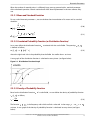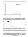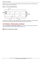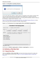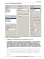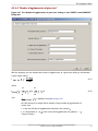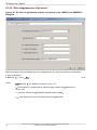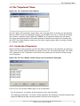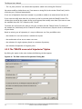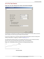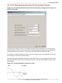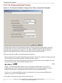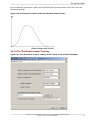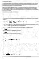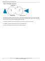
1
ANSYS Polystat User's Guide ANSYS, Inc. Southpointe 275 Technology Drive Canonsburg, PA 15317 [email protected] http://www.ansys.com (T) 724-746-3304 (F) 724-514-9494 Release 15.0 November 2013 ANSYS, Inc. is certified to ISO 9001:2008. Copyright and Trademark Information © 2013 SAS IP, Inc. All rights reserved. Unauthorized use, distribution or duplication is prohibited. ANSYS, ANSYS Workbench, Ansoft, AUTODYN, EKM, Engineering Knowledge Manager, CFX, FLUENT, HFSS and any and all ANSYS, Inc. brand, product, service and feature names, logos and slogans are registered trademarks or trademarks of ANSYS, Inc. or its subsidiaries in the United States or other countries. ICEM CFD is a trademark used by ANSYS, Inc. under license. CFX is a trademark of Sony Corporation in Japan. All other brand, product, service and feature names or trademarks are the property of their respective owners. Disclaimer Notice THIS ANSYS SOFTWARE PRODUCT AND PROGRAM DOCUMENTATION INCLUDE TRADE SECRETS AND ARE CONFIDENTIAL AND PROPRIETARY PRODUCTS OF ANSYS, INC., ITS SUBSIDIARIES, OR LICENSORS. The software products and documentation are furnished by ANSYS, Inc., its subsidiaries, or affiliates under a software license agreement that contains provisions concerning non-disclosure, copying, length and nature of use, compliance with exporting laws, warranties, disclaimers, limitations of liability, and remedies, and other provisions. The software products and documentation may be used, disclosed, transferred, or copied only in accordance with the terms and conditions of that software license agreement. ANSYS, Inc. is certified to ISO 9001:2008. U.S. Government Rights For U.S. Government users, except as specifically granted by the ANSYS, Inc. software license agreement, the use, duplication, or disclosure by the United States Government is subject to restrictions stated in the ANSYS, Inc. software license agreement and FAR 12.212 (for non-DOD licenses). Third-Party Software See the legal information in the product help files for the complete Legal Notice for ANSYS proprietary software and third-party software. If you are unable to access the Legal Notice, please contact ANSYS, Inc. Published in the U.S.A. Table of Contents Using This Manual ....................................................................................................................................... vii 1. The Contents of This Manual .............................................................................................................. vii 2. The Contents of the ANSYS Polyflow Manuals ..................................................................................... vii 3. Contacting Technical Support ............................................................................................................ vii 1. Introduction ............................................................................................................................................ 1 1.1. Objectives ........................................................................................................................................ 1 1.2. How to Characterize Mixing? ............................................................................................................. 1 1.3. Classification of Flows, Capabilities of the Mixing Module .................................................................. 2 1.4. General Explanation on the Way to Solve a Mixing Task ...................................................................... 4 1.5. The Numerical Techniques Involved in the Mixing Module ................................................................. 6 1.6. Examples .......................................................................................................................................... 7 1.6.1. Example 50: The Rectangular Cavity .......................................................................................... 7 1.6.2. Example 51: Coextrusion of Polymers in a Square Channel ........................................................ 7 1.6.3. Example 52: Flat Die ................................................................................................................. 7 1.6.4. Example 46: Periodic Flow Through a Kenics Mixer .................................................................... 8 1.6.5. Example 37: Mixer 2-D .............................................................................................................. 8 1.6.6. Example 65: Adaptive Meshing for Moving Parts; Mixer 2-D ....................................................... 8 1.6.7. Example 91: Dispersion ............................................................................................................ 8 1.6.8. Example 116: Distributive Mixing Analysis in the Mixer GK7N .................................................... 8 1.7. Known Limitations in ANSYS Polystat 15.0 ......................................................................................... 9 2. The Mixing Theory ................................................................................................................................. 11 2.1. Introduction ................................................................................................................................... 11 2.2. Kinematic Parameters ..................................................................................................................... 12 2.2.1. Kinematic Parameters for 2D Flows ......................................................................................... 12 2.2.2. Kinematic Parameters for 3D Flows ......................................................................................... 13 2.2.3. Statistical Analysis .................................................................................................................. 14 2.2.3.1. Mean and Standard Deviation ........................................................................................ 15 2.2.3.2. Cumulated Probability Function (or Distribution Function) ............................................. 15 2.2.3.3. Density of Probability Function ...................................................................................... 15 2.2.3.4. Percentiles ..................................................................................................................... 16 2.2.3.5. Histograms .................................................................................................................... 16 2.2.3.6. Correlations ................................................................................................................... 17 2.3. Homogenization ............................................................................................................................. 17 2.3.1. Definition ............................................................................................................................... 17 2.3.2. Numerical Method ................................................................................................................. 19 2.4. Distributive Mixing ......................................................................................................................... 20 2.4.1. Distribution Index .................................................................................................................. 20 2.4.2. Distribution in Zones .............................................................................................................. 22 2.4.3. Deviation of Points Concentration .......................................................................................... 23 2.5. Disagglomeration ........................................................................................................................... 25 2.6. Comment ....................................................................................................................................... 29 3. Mixing Tasks in Polydata ....................................................................................................................... 31 3.1. Creating a New Mixing Task ............................................................................................................. 31 3.2. Using the General Menu of a Mixing Task ......................................................................................... 33 3.3. Definition of the Flow Domain ........................................................................................................ 35 3.4. Definition of the Boundary Conditions ............................................................................................ 36 3.4.1. Specification of the Boundary Type ......................................................................................... 37 3.4.2. Specification of a Stopping Plane ............................................................................................ 42 3.5. Definition of the Flow Field ............................................................................................................. 44 3.5.1. Steady-State Flow .................................................................................................................. 44 Release 15.0 - © SAS IP, Inc. All rights reserved. - Contains proprietary and confidential information of ANSYS, Inc. and its subsidiaries and affiliates. iii Polystat User's Guide 3.5.2. Time-Dependent Flow ............................................................................................................ 45 3.6. Parameters for the Generation of the Material Points ....................................................................... 49 3.7. Parameters for the Tracking ............................................................................................................. 55 3.8. Selection of Properties .................................................................................................................... 57 3.8.1. Parameters for the Kinematic Mixing Properties ...................................................................... 59 3.9. Parameters for the Storage of the Results ........................................................................................ 61 3.10. Definition of Moving Parts ............................................................................................................. 62 3.11. Definition of the Kinematic Analysis .............................................................................................. 64 3.11.1. Management of Properties ................................................................................................... 67 3.12. Definition of the Distribution Analysis ........................................................................................... 68 4. The Polystat User’s Manual ................................................................................................................... 73 4.1. The “File” Menu ............................................................................................................................... 75 4.1.1. The "Open..." Option ............................................................................................................... 76 4.1.2. The "Options" Option ............................................................................................................. 76 4.1.3. The "Read Data" Option .......................................................................................................... 77 4.1.4. The "Read mesh" Option ......................................................................................................... 78 4.1.5. The "Run" Option ................................................................................................................... 79 4.1.6. The "Draw results" Option ....................................................................................................... 79 4.1.7. The "Draw Stats." Option ........................................................................................................ 84 4.1.8. The "WRITE Trajectories" Option .............................................................................................. 86 4.1.9. The "WRITE Slices" Option ....................................................................................................... 88 4.1.10.The "WRITE Stat." Option ....................................................................................................... 90 4.1.11. The "Save" Option ................................................................................................................ 91 4.2. The “Properties” Menu ..................................................................................................................... 91 4.2.1. Definition ............................................................................................................................... 91 4.2.2. See Properties ........................................................................................................................ 92 4.2.3. Create Properties ................................................................................................................... 93 4.2.3.1.“|| A ||” ............................................................................................................................ 94 4.2.3.2.“A^x” ............................................................................................................................. 95 4.2.3.3.“exp ( A )” ....................................................................................................................... 95 4.2.3.4.“log ( A )” ....................................................................................................................... 96 4.2.3.5.“A + B”,“A - B” .................................................................................................................. 96 4.2.3.6.“A / B” ............................................................................................................................ 96 4.2.3.7.“A * B” ............................................................................................................................ 96 4.2.3.8.“Rotate” ......................................................................................................................... 97 4.2.3.9.“Translate” ..................................................................................................................... 98 4.2.3.10. “Derivate” .................................................................................................................... 99 4.2.3.11. “Integrate” ................................................................................................................. 100 4.2.3.12.“k (constant)” ............................................................................................................. 101 4.2.3.13.“A ( Slice )” .................................................................................................................. 102 4.2.3.14. “Concentration” ......................................................................................................... 104 4.2.3.15.“Min / Max” ................................................................................................................ 105 4.2.3.16. “Extract” .................................................................................................................... 106 4.2.3.17. “Step” ........................................................................................................................ 107 4.2.3.18.“Instant. Eff.” ............................................................................................................... 108 4.2.3.19.“Time Aver. Eff.” .......................................................................................................... 109 4.2.3.20.“Shear Rate” ............................................................................................................... 110 4.2.3.21.“Melting Index” .......................................................................................................... 111 4.2.4. Disagglomeration Properties ................................................................................................ 112 4.2.4.1.“Disagglomeration” ...................................................................................................... 114 4.2.4.2.“Typical size of agglomerates” ...................................................................................... 115 4.2.4.3.“Fraction of agglomerates of given size” ....................................................................... 116 iv Release 15.0 - © SAS IP, Inc. All rights reserved. - Contains proprietary and confidential information of ANSYS, Inc. and its subsidiaries and affiliates. Polystat User's Guide 4.2.4.4.“Number of agglomerates of given size” ....................................................................... 117 4.2.4.5.“Mass of agglomerates of given size” ............................................................................ 118 4.3. The “Trajectories” Menu ................................................................................................................. 119 4.3.1. See the Set of Trajectories ..................................................................................................... 119 4.3.2. The "CREATE a new set of trajectories" Option ....................................................................... 120 4.3.3. The "COMBINE sets of trajectories" Option ............................................................................ 121 4.3.4. The "SELECT one single trajectory" Option ............................................................................ 122 4.3.5. The "SEARCH stagnation points" Option ................................................................................ 122 4.4. The “Slices” Menu .......................................................................................................................... 124 4.4.1. See the Set of Slices .............................................................................................................. 125 4.4.2. The "Automatic Slicing" Option ............................................................................................. 126 4.4.3. The "Manual Slicing" Option ................................................................................................. 126 4.4.4. The "Sub - Slicing" Option ..................................................................................................... 127 4.5. The “Statistics” Menu ..................................................................................................................... 128 4.5.1. See the Statistical Functions ................................................................................................. 128 4.5.2. Create Statistical Functions ................................................................................................... 129 4.5.2.1. The "Property along a trajectory" Function ................................................................... 132 4.5.2.2. The "Sum" Function ..................................................................................................... 133 4.5.2.3. The "Mean + Standard Deviation" Function .................................................................. 134 4.5.2.4. The "Correlation Function" ........................................................................................... 135 4.5.2.5. The “Probability Function” ............................................................................................ 136 4.5.2.6. The "Auto-Correlation Function of the Concentration" Function .................................... 137 4.5.2.7. The "Distance distribution" Function ............................................................................ 138 4.5.2.8.The "Distribution in zones" Function ............................................................................. 139 4.5.2.9. The “Sum A <op> Sum B” Function ............................................................................... 141 4.5.2.10. The “Smoothing” Function .......................................................................................... 142 4.5.2.11. The “Density of Probability Function” .......................................................................... 144 4.5.2.12. The “Percentile” Function ............................................................................................ 145 4.5.2.13. The “Histogram” Function ........................................................................................... 147 4.5.2.14. The “Segregation Scale” Function ................................................................................ 148 4.5.2.15. The “Deviation” Function ............................................................................................ 149 4.5.2.16. The “Points Concentration Deviation” Function ........................................................... 151 4.5.3.“New disagglomeration functions” ........................................................................................ 152 4.5.3.1. The “See disagglomeration along a single trajectory” Function ...................................... 154 4.5.3.2. The “Mean disagglomeration function” ......................................................................... 155 4.5.3.3.The “Probability function” ............................................................................................. 157 4.6. The “Help” Menu ............................................................................................................................ 157 4.7. Additional Definitions ................................................................................................................... 158 4.7.1. The Slices ............................................................................................................................. 158 4.7.2. The Zones ............................................................................................................................ 159 4.7.3. Weighting ............................................................................................................................ 159 A. The Simulation of the Distribution ......................................................................................................... 161 B. The Global Efficiency of Stretching ......................................................................................................... 163 C. Adaptive Meshing and Mixing Task ........................................................................................................ 165 D. Sliding Mesh Technique and Mixing Task ............................................................................................... 167 Bibliography ............................................................................................................................................. 169 Release 15.0 - © SAS IP, Inc. All rights reserved. - Contains proprietary and confidential information of ANSYS, Inc. and its subsidiaries and affiliates. v vi Release 15.0 - © SAS IP, Inc. All rights reserved. - Contains proprietary and confidential information of ANSYS, Inc. and its subsidiaries and affiliates. Using This Manual 1. The Contents of This Manual The ANSYS Polystat User’s Guide tells you how to set up a MIXING task in ANSYS Polydata and how to use the ANSYS Polystat module for statistical postprocessing of results. Important Under U.S. and international copyright law, ANSYS, Inc. is unable to distribute copies of the papers listed in the bibliography, other than those published internally by ANSYS, Inc. Use your library or a document delivery service to obtain copies of copyrighted papers. 2. The Contents of the ANSYS Polyflow Manuals The manuals listed below form the ANSYS Polyflow product documentation set. They include descriptions of the procedures, commands, and theoretical details needed to use ANSYS Polyflow products. • The Polyflow User's Guide explains how to use ANSYS Polydata and ANSYS Polyflow to set up and solve a problem. • The Polyflow Tutorial Guide contains a number of example problems with complete detailed instructions, commentary, and postprocessing of results. • The Polyflow in Workbench User's Guide explains how to use the ANSYS Polyflow application within ANSYS Workbench. • The Polymat User's Guide explains how to use the ANSYS Polymat module for material property evaluation. • The Polystat User's Guide explains how to set up a MIXING task in ANSYS Polydata and how to use the ANSYS Polystat module for statistical postprocessing of results. • The GAMBIT manuals teach you how to use the GAMBIT preprocessor for geometry creation and mesh generation. • The CFD-Post User's Guide explains how to use CFD-Post to examine your results. • The ANSYS Polyflow Examples Manual provides overviews of solutions to a variety of problem types. For details on how to access the ANSYS Polyflow manuals, see ANSYS Polyflow Documentation in the separate Polyflow User's Guide. 3. Contacting Technical Support Technical Support for ANSYS, Inc. products is provided either by ANSYS, Inc. directly or by one of our certified ANSYS Support Providers. Please check with the ANSYS Support Coordinator (ASC) at your company to determine who provides support for your company, or go to www.ansys.com and select Contact ANSYS > Contacts and Locations. Release 15.0 - © SAS IP, Inc. All rights reserved. - Contains proprietary and confidential information of ANSYS, Inc. and its subsidiaries and affiliates. vii Using This Manual If your support is provided by ANSYS, Inc. directly, Technical Support can be accessed quickly and efficiently from the ANSYS Customer Portal, which is available from the ANSYS Website (www.ansys.com) under Support > Customer Portal. The direct URL is: support.ansys.com. One of the many useful features of the Customer Portal is the Knowledge Resources Search, which can be found on the Home page of the Customer Portal. Systems and installation Knowledge Resources are easily accessible via the Customer Portal by using the following keywords in the search box: Systems/Installation. These Knowledge Resources provide solutions and guidance on how to resolve installation and licensing issues quickly. NORTH AMERICA All ANSYS, Inc. Products Web: Go to the ANSYS Customer Portal (http://support.ansys.com) and select the appropriate option. Toll-Free Telephone: 1.800.711.7199 Fax: 1.724.514.5096 Support for University customers is provided only through the ANSYS Customer Portal. GERMANY ANSYS Mechanical Products Telephone: +49 (0) 8092 7005-55 (CADFEM) Email: [email protected] All ANSYS Products Web: Go to the ANSYS Customer Portal (http://support.ansys.com) and select the appropriate option. National Toll-Free Telephone: German language: 0800 181 8499 English language: 0800 181 1565 Austria: 0800 297 835 Switzerland: 0800 546 318 International Telephone: German language: +49 6151 152 9981 English language: +49 6151 152 9982 Email: [email protected] UNITED KINGDOM All ANSYS, Inc. Products Web: Go to the ANSYS Customer Portal (http://support.ansys.com) and select the appropriate option. Telephone: Please have your Customer or Contact ID ready. UK: 0800 048 0462 Republic of Ireland: 1800 065 6642 Outside UK: +44 1235 420130 Email: [email protected] Support for University customers is provided only through the ANSYS Customer Portal. viii Release 15.0 - © SAS IP, Inc. All rights reserved. - Contains proprietary and confidential information of ANSYS, Inc. and its subsidiaries and affiliates. Contacting Technical Support JAPAN CFX , ICEM CFD and Mechanical Products Telephone: +81-3-5324-8333 Fax: +81-3-5324-7308 Email: CFX: [email protected]; Mechanical: [email protected] Fluent Products Telephone: +81-3-5324-7305 Email: Fluent: [email protected]; Polyflow: [email protected]; FfC: [email protected]; FloWizard: [email protected] Icepak Telephone: +81-3-5324-7444 Email: [email protected] Licensing and Installation Email: [email protected] INDIA All ANSYS, Inc. Products Web: Go to the ANSYS Customer Portal (http://support.ansys.com) and select the appropriate option. Telephone: +91 1 800 209 3475 (toll free) or +91 20 6654 3000 (toll) Fax: +91 80 6772 2600 Email: FEA products: [email protected]; CFD products: [email protected]; Ansoft products: [email protected]; Installation: [email protected] FRANCE All ANSYS, Inc. Products Web: Go to the ANSYS Customer Portal (http://support.ansys.com) and select the appropriate option. Toll-Free Telephone: +33 (0) 800 919 225 Toll Number: +33 (0) 170 489 087 Email: [email protected] BELGIUM All ANSYS Products Release 15.0 - © SAS IP, Inc. All rights reserved. - Contains proprietary and confidential information of ANSYS, Inc. and its subsidiaries and affiliates. ix Using This Manual Web: Go to the ANSYS Customer Portal (http://support.ansys.com) and select the appropriate option. Telephone: +32 (0) 10 45 28 61 Email: [email protected] Support for University customers is provided only through the ANSYS Customer Portal. SWEDEN All ANSYS Products Web: Go to the ANSYS Customer Portal (http://support.ansys.com) and select the appropriate option. Telephone: +44 (0) 870 142 0300 Email: [email protected] Support for University customers is provided only through the ANSYS Customer Portal. SPAIN and PORTUGAL All ANSYS Products Web: Go to the ANSYS Customer Portal (http://support.ansys.com) and select the appropriate option. Telephone: +34 900 933 407 (Spain), +351 800 880 513 (Portugal) Email: [email protected], [email protected] Support for University customers is provided only through the ANSYS Customer Portal. ITALY All ANSYS Products Web: Go to the ANSYS Customer Portal (http://support.ansys.com) and select the appropriate option. Telephone: +39 02 89013378 Email: [email protected] Support for University customers is provided only through the ANSYS Customer Portal. x Release 15.0 - © SAS IP, Inc. All rights reserved. - Contains proprietary and confidential information of ANSYS, Inc. and its subsidiaries and affiliates. Chapter 1: Introduction 1.1. Objectives In industry the mixing process is widely present; it occurs in different kind of machines, in a continuous or batch process, like in Banburry mixers, Kenics mixers, extruders, stirred vessels, and so on. The objectives are various too: distribution of pigments or other compatibilizers, generation of interfaces between different fluids in order to enhance chemical reactions, ... The main objective of this module is to offer you the ability to quantify the mixing in the process of your interest. We will define later a set of objective parameters that are relevant for different situations. But we tried to go a step further; there is, at this time, always a certain evolution in the way scientists are quantifying mixing. That's why we developed software that uses existing parameters and allows you to also define new parameters. This module simulates mixing for various flows, but the situation is in general so complex, that numerical simulation cannot take into account all the real phenomena existing in such processes. In a next section of this chapter, we will explain the needed assumptions and hypotheses. 1.2. How to Characterize Mixing? There are various ways to define the process of mixing. Dankwertz in the ‘50s analyzed the mixing as a homogenization process of a concentration field; initially two different fluids are separated in two adjacent zones; as the time goes on, the local concentration of each fluid evolves everywhere in the fluid, and if the mixing is perfect, the concentration must tend to the same value everywhere in the flow; to quantify this homogenization process, Dankwertz defined two parameters; firstly, the segregation scale is the average thickness of the striations existing in the flow domain. Secondly, the intensity of segregation is the standard deviation of the concentration around its mean. These parameters are used when there are only two fluids to mix, and when their proportion in the flow domain is more or less equivalent. Later, in the ‘80s, Ottino defined other parameters based on the Continuum Mechanics Theory. He showed that mixing is a process increasing the interface existing between fluids. But instead of measuring the surface of the interface (that is almost impossible in complex flows), he prefers to measure local increases of infinitesimal surfaces distributed everywhere in the flow. But these parameters are not very useful if we analyze the distribution of a small amount of pigments, tracers, and so on in the flow domain (small percentage in volume of the total flow domain). Based on the work of Manas-Zloczower, we have defined a new parameter in order to measure this process; let us suppose that initially, we place a set of particles in a small zone in the flow domain, as a function of time, these particles move in the flow and distribute. Our parameter measures the deviation of the current distribution with respect to a perfect distribution of particles in the flow domain. Another technique similar to the previous one is now available: we divide the flow domain in a set of adjacent (and non-overlapping) zones. Initially, we place a set of particles in a small box in the flow domain, and they distribute progressively. Then, for a given time, we count the number of points in Release 15.0 - © SAS IP, Inc. All rights reserved. - Contains proprietary and confidential information of ANSYS, Inc. and its subsidiaries and affiliates. 1 Introduction each zone. We get a good distributive mixing, if each zone contains a number of points proportional to its surface/volume. A third option to estimate distributive mixing is to evaluate the local points concentration in various locations in the flow domain, and to compare it with a perfect points concentration, corresponding to the case where we find the same number of points per unit volume everywhere in the mixer. Eventually, a new parameter measures the deviation in points concentration. The dispersive mixing is another important aspect of the mixing: it concerns the break-up of drops into small droplets or the disagglomeration of solid particles in a matrix. The stress applied by the matrix on drops or on solid particles is the "engine" that can lead to dispersion: if the stresses are high enough to compete with surface tension of drops or with internal mechanic resistance of solid particles, dispersion occurs. Dispersion will be better if some elongational effect exists in the flow. This information is available by adding some postprocessors, while defining the set-up for the flow calculation. Next, it will be possible to evaluate them along trajectories of material points. Moreover, a model has been included in Polystat to calculate the disagglomeration process along trajectories. We have found a general and accurate method to calculate all these parameters in a single simulation. The main steps of this method are: firstly, we calculate the flow as usual, secondly, we compute the trajectories of a large set of material points (initially concentrated in the whole flow domain or not), with in complement the calculation along these trajectories of the local deformation of the matter and other relevant properties. Finally, we analyze these results with statistical tools in order to obtain a global, objective, and quantitative overview of the mixing evolution. 1.3. Classification of Flows, Capabilities of the Mixing Module With the mixing module, all the kind of flows cannot be studied. There exist limitations. But first, let us define some concepts: • Open / Closed domain: a closed domain is a domain where there is no entry and no exit of fluid. An open domain is the opposite. Figure 1.1: Open and Closed Domains • Steady state / Time dependent flow: a steady flow is a flow that does not change with time. The general case of a time dependent flow is a flow that evolves continuously with time; our mixing module can study these two kinds of flow. However, for transient flows, the flow domain must not change with time except for flows with moving parts simulated with the 'mesh superposition' technique. If the flow is transient, we have to calculate and store the current flow at successive time steps; let's note them flow( ), flow( ), 2 Release 15.0 - © SAS IP, Inc. All rights reserved. - Contains proprietary and confidential information of ANSYS, Inc. and its subsidiaries and affiliates. Classification of Flows, Capabilities of the Mixing Module ... However, in order to calculate particles path, we have to know the velocity field at intermediate times: two techniques are implemented; – In the first case, the piecewise steady case, we assume the flow is steady between two time steps (with < ), and is equal to flow( ). This assumption is valid if inertia is neglected and if the boundary conditions change abruptly. One example is the oscillating square cavity: , Figure 1.2: Example of a Piecewise Steady Flow In this case, two velocity fields alternate. The first state lasts for DT1 seconds; the upper wall moves to the right while the other walls are at rest. The second state lasts for DT2 seconds; the lower wall moves to the right while the other walls are at rest. With such a flow, we can obtain a far better mixing than with a steady state flow. – In the second case, the more general, the flow changes continuously between time , will be a linear combination of flow( ) and flow( ): where = and = − + − − ≤ ≤ , and ; the flow at (1.1) (1.2) ≠ . • Spatially periodic flows: the flow is spatially periodic if there exists an elementary "module" on which we can calculate the flow field and where the velocity field in the inflow section is equal (exactly) to the velocity field in the outflow section. A spatially periodic flow is necessarily a flow through an open domain. Release 15.0 - © SAS IP, Inc. All rights reserved. - Contains proprietary and confidential information of ANSYS, Inc. and its subsidiaries and affiliates. 3 Introduction Figure 1.3: Example of a Spatially Periodic Flow The flow field is repeated infinitely in space: the flow field in the next module is the same as in the current module, and in the previous module, and so on ... The limitations of our module are the following: • Geometrical limitations: the domain must not change with time: we have to find a frame of reference where the domain occupied by the flow does not vary. For example, if one wants to analyze mixing in a single screw extruder, we assume the screw to be fixed and the barrel to be rotating. If there are moving internal parts, the 'mesh superposition' technique must be used to simulate their motion ! • For a piecewise steady flow, there must be no inertia. • The flow must always be incompressible. • There is no void formation in the flow. The flow domain is completely filled with the same fluid: if we want to mix two or several fluids, they must have the same rheological behavior, no diffusion nor chemical reactions between them, and no interfacial tension. It is thus clear that, despite the fact that we calculate a mixing problem, the flow calculation is identical to that of a single homogeneous fluid. We will examine the time dependence of a set of mixing parameters without making any distinction between the fluids we want to mix. However, there is no limitation on: • the model of fluid: generalized Newtonian or visco-elastic models are available. • the dimensional complexity of the problem: 2D planar, 2D axisymmetric, 2D 1/2 planar (3 components for the velocity field), 2D 1/2 axisymmetric (swirling flows), 3D. • the thermal complexity of the problem: isothermal or non-isothermal simulations are possible. 1.4. General Explanation on the Way to Solve a Mixing Task Three major steps must be performed in order to solve a mixing task: first, we calculate the flow, then we calculate a set of trajectories, and finally we perform statistics on this set. 1. 4 The flow simulation: we have to define a finite element mesh (via GAMBIT, ICEM CFD, Patran, ...); next, we enter in Polydata where a F.E.M. task is defined in order to calculate the flow ONLY. With the data file, we run Polyflow, and finally we obtain a Polyflow result file containing the velocity field, the shear rate, and other fields of interest. If the flow is transient, it is recommended that you save the Polyflow Release 15.0 - © SAS IP, Inc. All rights reserved. - Contains proprietary and confidential information of ANSYS, Inc. and its subsidiaries and affiliates. General Explanation on the Way to Solve a Mixing Task results files at exacts time steps ∆ . However, if the flow is piecewise-steady with successive boundary conditions ( small, in loop or not), it is sometimes easier to perform Polydata sessions, one for each specific set of boundary conditions. We will run Polyflow N times, one for each data file, and we will obtain result files, containing each one a set of fields specific to a particular set of boundary conditions. Figure 1.4: The Flow Simulation 2. The mixing simulation: in a second step, we enter back in Polydata to define a MIXING task. We specify the mesh, the velocity fields to use and the initial position of the material points and other properties to evaluate along trajectories. Next, we run Polyflow with this data file: Polyflow generates randomly the initial position of a set of material points, and calculates their trajectory in the flow domain. Along these trajectories, Polyflow calculates also the evolution of some properties and kinematic parameters (temperature, viscosity, stretching, rate of stretching, rate of dissipation, ...). And finally, Polyflow generates files containing these results. Figure 1.5: The Mixing Simulation 3. The statistical postprocessing: finally, we use the postprocessor Polystat to analyze all these trajectories. We will calculate the time evolution of global mixing parameters such as the segregation scale or the evolution of the mean stretching, and so on. Polystat has been built in such a way that we can define new parameters and test them. New parameters ∂ are created by combining existing parameters in various ways (+, -, *, /, , , , , ...). In such a way, ∂ Polystat can also be used to analyze other processes than mixing; for example, the quality of a molten glass exiting a furnace. Eventually, we calculate statistical functions of these parameters; these functions can be visualized inside Polystat, Excel, ... ∫ Release 15.0 - © SAS IP, Inc. All rights reserved. - Contains proprietary and confidential information of ANSYS, Inc. and its subsidiaries and affiliates. 5 Introduction It is also possible to visualize with Polystat the spatial distribution of a kinematic parameter at a given time, or in a cutting plane, or along a given trajectory. Figure 1.6: The Statistical Postprocessing 1.5. The Numerical Techniques Involved in the Mixing Module Generally, the trajectories are calculated by the time integration of the equation = with an Euler explicit scheme; it's enough if we are only interested in the successive positions of material points. But if we need to know precisely the deformation accumulated along these trajectories, a very accurate numerical technique is required. We chose to combine two techniques: first, we use an explicit Runge-Kutta scheme of the fourth order; second, instead of integrating the motion of a particle in the real space, we perform a coordinate transformation. We calculate the trajectory in the parent element: we integrate with the Runge-Kutta method (1.3) = To know the successive positions of the particle in the real space, we use = ∑ = ∑ (1.4) The algorithm is the following: 1. 2. 6 initialization: a. find an element E, containing the initial position ; b. find the local coordinates of in this element E; while ( no problem & no required stop ) { a. we integrate Equation 1.3 (p. 6), until we cross a boundary of the element E; b. if a boundary of E is crossed, we adapt the time step of integration in such a way that the position is on the boundary; Release 15.0 - © SAS IP, Inc. All rights reserved. - Contains proprietary and confidential information of ANSYS, Inc. and its subsidiaries and affiliates. Examples c. if we are on a boundary of E, in , i. we search the element adjacent to E where to continue the integration; let's note this element E*; ii. find the local coordinates iii. go to step 2.a.; in element E* of the current position ; } We explained this, because some important numerical parameters used by this algorithm must be defined by you in Polydata (see Chapter 3, Parameters for the tracking): for example, we must define the coefficient NBELEM that indicates the mean number of integration steps necessary to cross an element. 1.6. Examples Here below, one can find a short description of the Polyflow examples devoted to mixing. Refer to the documents corresponding to those examples for their full description (in the Polyflow documentation). 1.6.1. Example 50: The Rectangular Cavity This example is the tutorial of the mixing module ! In this first example, we will compare the mixing efficiency of a steady state flow with a piecewise steady flow. It is 2D planar and isothermal flow problem. We explain in detail how to use Polystat: a) how to create new properties, b) how to define a slicing on time, and c) how to define the statistical functions needed for the comparison of the two cases. Moreover, we explain how to extract useful information from those statistical curves. Keywords: piecewise steady flow, distributive mixing, reorientation process, mixing efficiency, Polystat, statistical analysis 1.6.2. Example 51: Coextrusion of Polymers in a Square Channel In this second example, two viscoelastic fluids are injected in a channel. They have identical rheological properties but different colors. We analyze the axial evolution of the interface between those fluids in the square channel: we calculate the axial evolution of the segregation scale in order to quantify the progressive deformations of the interface in the channel. Keywords: 2D 1/2 planar flow, viscoelasticity, coextrusion, secondary motion, Polystat, concentration field, segregation scale 1.6.3. Example 52: Flat Die In this third example, we will analyze a 3D steady state non-isothermal flow through the die section of an extruder. We are specially interested by the residence time distribution and the 'melting' characteristics of the matter leaving the die. Release 15.0 - © SAS IP, Inc. All rights reserved. - Contains proprietary and confidential information of ANSYS, Inc. and its subsidiaries and affiliates. 7 Introduction Keywords: 3D steady state flow, non-isothermal, flat die, Polystat, residence time distribution, melting index, preset statistical analysis 1.6.4. Example 46: Periodic Flow Through a Kenics Mixer In this fourth example, we analyze the distributive mixing generated by a Kenics mixer. As the complete flow domain is too large to be used, we reduce the flow calculation to a single mixing element of the mixer. We assume the flow field to be spatially periodic. We analyze the generation of striations through successive mixing sections and the efficiency of the process. Keywords: 3D steady state flow, periodic boundary conditions, static mixer, Polystat, distributive mixing, preset statistical analysis 1.6.5. Example 37: Mixer 2-D In this fifth example, we simulate the 2D transient flow produced by the rigid rotation of two cams in a batch mixer. Moreover, we evaluate the dispersive mixing capability of the mixer. Forces and torque along the cams are also evaluated. Keywords: mesh superposition technique, batch mixer, transient flow problem, forces and torque, dispersive mixing, mixing index, eigen values of the stress tensor, shear rate, vorticity, Polystat, preset statistical analysis 1.6.6. Example 65: Adaptive Meshing for Moving Parts; Mixer 2-D In this sixth example, we simulate the 2D transient flow produced by the rigid rotation of two cams in a batch mixer. As in example 37, we use the mesh superposition technique to take into account the rotation of the cams. Moreover, we use adaptive meshing to refine the mesh locally in the neighborhood of the cams, in order to get more accurate evaluation of the flow field. As the mesh changes with time, it cannot be used anymore to perform tracking of material points: we have first to save the flow field in a set of csv files, that we map onto a new uniformly refined mesh. The tracking is eventually performed on this new mesh, with the mapped flow field. Keywords: mesh superposition technique, batch mixer, time dependent flow, adaptive meshing, conversion form CSV files, mixing task, statistical analysis 1.6.7. Example 91: Dispersion In this seventh example, we present the models of erosion and rupture in a simple shear flow. By this way, we analyze the effect of various functions and parameters of these models. Keywords: dispersion, disagglomeration, erosion, rupture, Polystat 1.6.8. Example 116: Distributive Mixing Analysis in the Mixer GK7N In this eighth example, we simulate the 3D transient flow produced by the rigid rotation of two rotors in a batch mixer (mixer GK7N). As in Examples 37 and 65, we use the mesh superposition technique to take into account the rotation of the rotors. Moreover, we evaluate the distributive mixing capability of the mixer. 8 Release 15.0 - © SAS IP, Inc. All rights reserved. - Contains proprietary and confidential information of ANSYS, Inc. and its subsidiaries and affiliates. Known Limitations in ANSYS Polystat 15.0 Keywords: mesh superposition technique, batch mixer, time dependent flow, distributive mixing, mixing task, preset statistical analysis, Polystat 1.7. Known Limitations in ANSYS Polystat 15.0 This section lists limitations that are known to exist in ANSYS Polystat. Where possible, suggested workarounds are provided. • Mesh – ANSYS Polystat does not support mixing tasks on CutCell meshes. – ANSYS Polystat does not support mixing tasks on meshes with subdivided elements. See Appendix C (p. 165) for a method to circumvent this limitation. – ANSYS Polystat does not support mixing tasks if the flow field is meshed using the sliding mesh technique. See Appendix D (p. 167) for a method to circumvent this limitation. – When using the Mesh Superposition Technique (MST) with moving parts (with or without slippage along the moving parts), the trajectories and kinematics of the deformation may be affected when material points (massless particles) are close to the surface of the moving parts. – When using MST with moving parts, it may happen that some of the material points get overlapped by a moving part. This is due to the accumulation of small errors along the trajectory of the material points. There are two ways (which can be combined) to limit this problem: decreasing the time step between two successive flows and refining the mesh of the flow domain. – ANSYS Polystat does not support mixing tasks if the mesh of the flow domain changes with time (changes in coordinate position of the mesh vertices and/or number and shape of mesh elements). This does not include the use of the Mesh Superposition Technique with moving parts on a transient flow field, because the underlying mesh remains constant. • Boundary conditions – ANSYS Polystat does not support mixing tasks on flow fields defined by non-conformal boundaries. – In some cases, material points (massless particles) may stop on a non-penetrable boundary (wall, free surface, plane of symmetry) due to stagnation of the flow field in close proximity to these boundaries. This can have a dramatic effect on the flow statistics, particularly if you are analyzing an open flow field (with entry and exit of fluid). When slicing from entry to exit you should confirm that the number of samples in each slice remains constant. If the concentration of samples decreases by more than 10–15%, it may be necessary to refine the mesh. • Material properties – ANSYS Polystat does not support mixing tasks on compressible fluids. Release 15.0 - © SAS IP, Inc. All rights reserved. - Contains proprietary and confidential information of ANSYS, Inc. and its subsidiaries and affiliates. 9 10 Release 15.0 - © SAS IP, Inc. All rights reserved. - Contains proprietary and confidential information of ANSYS, Inc. and its subsidiaries and affiliates. Chapter 2: The Mixing Theory 2.1. Introduction In polymer blending, a minor component is generally present as drops (or filaments) in a continuous phase of a major component. Mixing is a process of deformation and rupture of the drops but also a process of 'distribution' of those drops in the whole flow domain. A good mixing is characterized by small and identical drops distributed uniformly in the all flow domain. Deformation of drops is promoted by the viscous stress exerted on the drops by the flow field and counteracted by the interfacial stress , where is the interfacial tension and , the local radius. is useful to characterize mixing: The capillary number = (2.1) For a given pair of polymers, a critical Capillary number may be found. It corresponds to the situation where the viscous stress competes with the interfacial stress: the drop is extended and finally breaks up into smaller droplets. We name this process "dispersive mixing". Let us note that an extensional flow field is more efficient to break up drops into droplets than a shear flow. If the capillary number is much higher than the critical capillary number, then the viscous stress overrules the interfacial stress, and the drop is extended but does not break up; this process is called "distributive mixing". On the contrary, if the capillary number is much lower than the critical capillary number, then the interfacial stress dominates and the drop is only slightly deformed. In general, mixing begins with a 'distributive' step (drops are deformed passively), followed by a 'dispersive' one (drops break up into droplets), and finally by the distribution of the droplets in the flow. In the paragraphs below, we concentrate mainly on distributive mixing (Kinematic Parameters (p. 12) and Homogenization (p. 17)) and on distribution of material points into the flow domain (Distributive Mixing (p. 20)). However, dispersive mixing can also be analyzed: you can add postprocessors to the flow calculation: a) the mixing index (or 'flow number') indicates if the flow is locally a rigid motion (mixing index = 0), a shear flow (mixing index = 0.5), or in extension (mixing index = 1), b) the eigen values of the extra-stress tensor : with this field we have access to the main component of the stress, which stretches and breaks the drops. Once the flow and those postprocessors are determined, we can calculate the evolution of the mixing index and the main stress along the trajectories of material points. With those data we can evaluate the fraction of the matter experiencing a given stress value, and then evaluate the efficiency of the dispersive mixing. We call also "dispersive mixing" the process where solid particles are broken by erosion or rupture in smaller parts due to stresses applied on them by the matrix (carbon black or silica in a rubber matrix, for example). A new model has been developed by B. Alsteens and V. Legat [2] (p. 169) to simulate this process of disagglomeration: thanks to them, this model is already available in Polystat. The description of the model can be found in Disagglomeration (p. 25). Release 15.0 - © SAS IP, Inc. All rights reserved. - Contains proprietary and confidential information of ANSYS, Inc. and its subsidiaries and affiliates. 11 The Mixing Theory 2.2. Kinematic Parameters A first way to measure mixing is to quantify the capacity of the flow to deform matter and to generate interface. In the theory presented below, we neglect interfacial forces: the interface is passive and no break-up into droplets can occur. For 2D flows, the interface between fluids is a line; in order to avoid to calculate the evolution of this interface (a very complex and impossible task to perform, because of the exponential growth of the interface), we prefer to calculate the stretching of infinitesimal vectors attached to a large number of material points distributed in all the flow domain. As the points move in the flow, the vectors are stretched. The stretching and the rate of stretching of these vectors are interesting properties that vary from place to place in the flow domain, and that evolve with time. Finally, we perform a statistical analysis of the set of results in order to have a global overview of the process. With such a method, we can have an objective and quantitative evaluation of the mixing of any process; we can, for example, find areas in the domain where the mixing is poor (low stretching instead of exponential increase). For 3D flows, we generalize the concept: the interface is now a surface and we will calculate the stretching of infinitesimal surfaces attached to material points. Let and denote the domain occupied by the homogeneous fluid at time 0 and , respectively. The motion of the fluid is described by the relationship (2.2) = where denotes the position of a material point P in and in . The symbols and denote the deformation gradient and the right Cauchy Green strain tensor between both configurations. The velocity gradient and the rate of deformation tensor at time are denoted by and , respectively. For later use, we note that (2.3) = where a dot denotes the material time derivative. 2.2.1. Kinematic Parameters for 2D Flows Consider in a material fiber with a unit orientation that while = with a unit orientation at time . Let which deforms into a material fiber denote the length stretch . It is easy to show [6] (p. 169) = (2.4) is given by (2.5) A good mixing quality requires high values of throughout time and space. A local evaluation of the efficiency of mixing [7] (p. 169) is given by the ratio where = 12 = (2.6) (2.7) Release 15.0 - © SAS IP, Inc. All rights reserved. - Contains proprietary and confidential information of ANSYS, Inc. and its subsidiaries and affiliates. Kinematic Parameters The values of this instantaneous efficiency are always included in the interval [-1; 1]. We can easily show that = (2.8) We note that is a local measure along the path of a material point; the time-averaged efficiency is defined as ∫ = (2.9) ′ ′ However, there exists another way to define a mean efficiency over time: ∫ = ′ ∫ ′ = (2.10) ∫ ′ The physical interpretation of Equation 2.10 (p. 13) is the following: for one material point, at time , is the ratio of what we get (the final stretching obtained at time ) over what we put (the total mechanical dissipation until time ). Eventually, we can define a global efficiency over all the material points distributed initially in the flow: ! = ∫ "% # ∫∫ "% $ (2.11) ′ This global efficiency is the ratio of the output—the mixing obtained—(the total stretching of the matter until time &) over the input—the "energy" we get—(the total mechanical dissipation until time '). 2.2.2. Kinematic Parameters for 3D Flows For 3D flows, we will calculate the local stretching of infinitesimal surfaces by the mean of the area stretch (. In the initial configuration )*, consider an infinitesimal surface +, with a normal direction ɵ . With time, this surface deforms; at time -, this surface is noted ./, with a new normal direction ɵ . The area stretch 0 is the ratio of the deformed surface 12 at time 3 over the initial surface 45: 6=6 ɵ 7 = 89 8: If the fluid is incompressible, we obtain [7] (p. 169): < −= ɵ ;= ɵ (2.12) (2.13) If the fluid is incompressible, the normal direction to the surface >? is: Release 15.0 - © SAS IP, Inc. All rights reserved. - Contains proprietary and confidential information of ANSYS, Inc. and its subsidiaries and affiliates. 13 The Mixing Theory − ɵ= ɵ (2.14) A good mixing quality requires high values of throughout time and space. A local evaluation of the efficiency of mixing [7] (p. 169) is given by the ratio ɵ = (2.15) The values of this instantaneous efficiency are always included in the interval [-1; 1]. After some transformations, it is easy to show that ɵ = − ɵ (2.16) We note that is a local measure along the path of a material point; the time-averaged efficiency is defined as ɵ = ∫ ɵ ′ ′ (2.17) However, there exists another way to define a mean efficiency over time: ɵ ∫ = ′ ∫ ′ = (2.18) ∫ ′ Like for Equation 2.10 (p. 13), the physical interpretation of Equation 2.20 (p. 15) is the following: for one material point, at time , ! " is the ratio of what we get (the final stretching obtained at time #) over what we put (the total mechanical dissipation until time $). Like for 2D kinematic parameters, we can define a global efficiency over all the material points distributed initially in the flow: %+ ɵ & = ∫ ,/ ' () - ∫ ∫ *(& ′() (2.19) ,/ . 2.2.3. Statistical Analysis Let us assign to the 0 material points an initial orientation , which does not need to be identical for all points. While tracking the material points as a function of time, we also calculate successive values of 1 , 23 , and 45 . A global representation of 6 , 78 , and 9: is again obtained by associating a ma- terial point with a small rectangle of size ;< × ;=; the color of the rectangle is associated with the value of the field to be represented. The quality of the representation increases with the number of points >. 14 Release 15.0 - © SAS IP, Inc. All rights reserved. - Contains proprietary and confidential information of ANSYS, Inc. and its subsidiaries and affiliates. Kinematic Parameters When the number of material points is sufficiently large, we may proceed with a statistical treatment of the calculated quantities. Several statistical tools have been implemented in the new software Polystat. 2.2.3.1. Mean and Standard Deviation For any scalar kinematic parameter α, we can calculate the time evolution of its mean and its standard deviation: ∑ = = ∑ (2.20) = = − (2.21) 2.2.3.2. Cumulated Probability Function (or Distribution Function) Let us now define the distribution function associated with the scalar field . The quantity is defined as follows, = ≤ (2.22) where the right-hand side is the probability that the field be smaller than at time . A new graph of the distribution function is calculated at every time (see figure below). Figure 2.1: Distribution Function Graph 2.2.3.3. Density of Probability Function Based on the distribution function #& $ % as follows, ∂ (* '* = ∂) ! of a scalar field ", we can define the density of probability function (2.23) +. , - is the frequency with which we find a value of / in the range 0 − 12 0 + 12 at time 3. A new graph of the density of probability function is calculated at every time 4 (see figure The function below). Release 15.0 - © SAS IP, Inc. All rights reserved. - Contains proprietary and confidential information of ANSYS, Inc. and its subsidiaries and affiliates. 15 The Mixing Theory Figure 2.2: Density of Probability Function Graph 2.2.3.4. Percentiles An easier representation of the mixing progress is based on the time dependence of percentiles. For the field , let us define such that = (2.24) indicates that, at time , % of the material points have a value of lower than , as you see on the figure below: Figure 2.3: Percentiles Graph With the percentiles, we can study the evolution of the mixing for specific fractions of the population of material points; it's interesting, for example, to know the value of the length stretch reached by the 5 or 10% of the points with the lowest stretching; these percentiles can easily show local defects in the stretching. 2.2.3.5. Histograms Another way to represent the frequency of values of a field is to define histograms: you specify a set of intervals of values of , and he obtains the percentage of the points population that have a value of in each interval at time (see figure below): 16 Release 15.0 - © SAS IP, Inc. All rights reserved. - Contains proprietary and confidential information of ANSYS, Inc. and its subsidiaries and affiliates. Homogenization Figure 2.4: Histograms Graph We see that % of the points population has a value of α between 1 and 2 at time . 2.2.3.6. Correlations Finally, once the number of material points is sufficiently large, it is possible to examine the correlation between fields either at the same or at different times. ), and two fields ( and ). For every material point, we plot We have to define two times ( and in ordinate; an analysis of the graph reveals a possible correlation in abscissa and between the fields. Figure 2.5: Correlations Graph 2.3. Homogenization 2.3.1. Definition Suppose we want to mix two fluids A and B: both fluids occupy at time =0 two separated zones of the flow domain (see figure below). Figure 2.6: Mixing Fluids Release 15.0 - © SAS IP, Inc. All rights reserved. - Contains proprietary and confidential information of ANSYS, Inc. and its subsidiaries and affiliates. 17 The Mixing Theory Let denote the concentration of fluid A throughout the mixing process. Since no diffusion occurs between fluids A and B, we conclude that equals either 0 or 1 and remains constant along the trajectory of a material point. Its evolution is governed by the transport equation (2.25) = The concept of concentration allows us to introduce the notion of segregation scale [5] (p. 169), [8] (p. 169). At time , consider a set of pairs of material points separated by a distance . For the th pair and time , let ′ and ″ denote the concentrations at both points of the pair; moreover, let denote the average concentration of all points and the standard deviation. At time , the correlation coefficient for the concentration is defined as follows, ′ − ″ − = = ∑ (2.26) The function ! gives the probability of finding a pair of random points with a relative distance " and with the same concentration. Figure 2.7: The Correlation Coefficient for Concentration over Distance The previous figure shows a typical graph of # as a function of $. Let % be such that & ' ( = ; when ) = * , we cannot predict whether the members of the pair have the same concentration or not. The segregation scale + , is defined as 2 (2.27) - . = / 0 . 10 3 ∫ It is easy to understand that 4 5 is a measure of the size of the regions of homogeneous concentration. 6 7 decreases when mixing improves. 18 Release 15.0 - © SAS IP, Inc. All rights reserved. - Contains proprietary and confidential information of ANSYS, Inc. and its subsidiaries and affiliates. Homogenization While quantities such as , , and are proper to the flow, irrespective of the initial concentration, the segregation scale is a quantity that is affected by the flow but depends strongly upon the initial distribution of concentration. Note Dankwertz defined another parameter, the intensity of segregation: = (2.28) Because of our assumptions (the concentration attached to any material point remains constant with time), this parameter does not change with time and will not be calculated. 2.3.2. Numerical Method We distribute uniformly (but randomly) a set of material points in all the flow domain at time =0. To each point is associated a concentration depending on its situation in a zone of fluid A (=1) or a zone of fluid B (=0). When time progresses, we calculate the new location of each point; it is easy to visualize the current state of the concentration field: for each point, we plot in the domain a small pixel (if 2D flow) with the appropriate color. Once the successive coordinates of material points are stored, a minor effort is needed to calculate at time the concentration corresponding to another set of initial conditions. The limitation of the method lies of course in the size of the material point identified by the pixel, but the number of points can be increased at will together with the computation time. Let us now assume that we have tracked material points. It is easy to calculate the average and the standard deviation of the concentration: (2.29) = = (2.30) = − = ∑ ∑ where is the concentration (0 or 1) of the material point !. Let " #$% be the maximum distance between two material points in the flow domain. We will calculate nbval values of the correlation function for distances uniformly distributed between 0 and & '(). To calculate one value of correlation function (for a distance * ), we select randomly pairs of points , , if their relative distances are in the interval + − 345 + + 345 . The correlation coefficient -./012 -./012 6 7 8 is completed by a linear interpolation through the discrete calculated values. The segregation scale 9 : may then be easily calculated by numerical integration on the basis of Equation 2.27 (p. 18). Release 15.0 - © SAS IP, Inc. All rights reserved. - Contains proprietary and confidential information of ANSYS, Inc. and its subsidiaries and affiliates. 19 The Mixing Theory Figure 2.8: Calculated Values of the Correlation Coefficient There exists a limitation to this method: as the number of points is finite, the mean size of the pixels is finite too; we cannot calculate accurately a segregation scale that is smaller than this characteristic size. If the segregation falls below that size, that means that the mean thickness of the striations in the flow is smaller than the size of the pixels: the concentration field will appear like a random distribution of pixels of the two colors: there are no more continuous lines of one color. Another problem of the segregation scale is that it cannot detect a local defect in the flow; it is a global index of the quality of mixing. Finally, the segregation scale depends on the size of the flow domain. The parameters of this method are: • The initial distribution of the zones of fluid A and B. • • • : the maximum possible distance between two points in the flow domain. : the number of pairs of points necessary to calculate one value of the correlation function : the number of values of the correlation function to calculate 2.4. Distributive Mixing 2.4.1. Distribution Index Suppose we want to distribute a cluster of particles initially concentrated in a small box (see figure below). We suppose that the particles do not affect the flow field and that there is no interaction between them. Their number is supposed to be large. Figure 2.9: Distributing Particles from a Small Box 20 Release 15.0 - © SAS IP, Inc. All rights reserved. - Contains proprietary and confidential information of ANSYS, Inc. and its subsidiaries and affiliates. Distributive Mixing As a function of time, the flow will distribute this set of points. It is important to define a distribution index to quantify this process. Its definition is based on the work performed by Manas-Zloczower and her colleagues [9] (p. 169), [10] (p. 169). At time , we have points distributed (more or less) in the flow domain. Option 1: These points can form − calculate their inter- distance = pairs of points. For each pair of point and , we − . The maximum inter-distance will be of the order of the diameter of the mixer. Option 2: For each point , we search its closest neighbor = and we store their inter-distance − . We have thus only distances. With this method of calculation, we are able to better discriminate distributive capacities of similar mixers. The maximum inter-distance will be of the order of , where is the volume of the mixer. With this set of distances, we can calculate the density of probability function on the distance : the probability to find a pair of points (chosen randomly) such that their inter-distance is included in range [ , +∆ ] at time is: ∆ . Figure 2.10: Density of Probability over Distance Suppose on the other hand, that you have distributed randomly a same number of points in all the flow domain; we can assume that such distribution is ideal. With the same tools, we can calculate the function for this optimal distribution. It is noted !" . The distribution index # is defined as the deviation of the function $ function & ()* ' = ∫ 0 - (real distribution) from the (optimal distribution): +∞ + , % . − - 123 . /. +∈ (2.31) As the distribution improves, the index 4 decreases. This index is dimensionless: it is independent of the size of the flow domain. The evolution of 5 depends—of course—on the initial position of the box. Another important parameter not to forget is the number or material points to distribute: a careful analysis must be done to measure its influence. Release 15.0 - © SAS IP, Inc. All rights reserved. - Contains proprietary and confidential information of ANSYS, Inc. and its subsidiaries and affiliates. 21 The Mixing Theory Two other parameters can also be evaluated: • The difference of the means: = − ∞ ∫ = • The difference of the standard deviations: ∞ = − = ∫ − (2.32) (2.33) Figure 2.11: Real and Optimal Distributions As for the segregation scale, such parameters have limitations: as they are global indices, we cannot detect local defects. 2.4.2. Distribution in Zones As for the distribution index, we want to quantify distributive mixing. But with this new method, we will be able to detect zones of the mixer where material points are missing, and where there is an excess of points. As usual, we distribute a cluster of particles initially concentrated in a small box (see figure below). Figure 2.12: Distributing Particles from a Small Box As a function of time, the flow will distribute this set of points. We define a set of adjacent and non-overlapping zones covering all the flow domain. 22 Release 15.0 - © SAS IP, Inc. All rights reserved. - Contains proprietary and confidential information of ANSYS, Inc. and its subsidiaries and affiliates. Distributive Mixing In the figure below, we have four zones: Figure 2.13: Zones of the Flow Domain Next, we distribute randomly in all the flow domain, the same number of points such a distribution is the optimal one. : we assume that At time , for each zone, for the two distributions, we will determine the number of points included in it. Based on these numbers, we can evaluate a relative error of distribution for each zone : = − where is the number of points of the real distribution included in zone , at time and number of points of the optimal distribution included in the same zone. (2.34) is the is zero for a zone, the right number of points is found in that zone, If is negative for a zone, there is a lack of points in that zone compared to optimum, If is positive for a zone, there are too many points in that zone compared to optimum. If Eventually, we can define a global index based on all the zones: = ∑ (2.35) = The number of points and the zones partitioning can influence dramatically the indices described above. When comparing two different mixers, it is recommended that you keep constant the ratio number of points/zone. In order to have relevant results, this ratio should be higher than 100. 2.4.3. Deviation of Points Concentration As for the distribution index, we want to quantify distributive mixing. However compared to that parameter, we do not need to compute a perfect points distribution; we just need the actual one. As usual, we distribute a cluster of particles initially concentrated in a small box (see figure below). Release 15.0 - © SAS IP, Inc. All rights reserved. - Contains proprietary and confidential information of ANSYS, Inc. and its subsidiaries and affiliates. 23 The Mixing Theory Figure 2.14: Points Within a Cluster As a function of time, the flow will distribute this set of points. At time , we have For each point , points distributed (more or less) in the flow domain. we search its neighbors { } that stay at a distance smaller than a sample radius. Depending on the dimensionality (dim) of the cluster of points at time , we can evaluate the local points concentration : = = = where = = = (2.36) is the number of points of the cluster around at a distance smaller than the radius. On the other side, at perfect distribution, we expect that the points are distributed equally in all the flow domain; we should find everywhere the same number of points per unit volume. Then, we can easily determine the perfect points concentration : it corresponds to the number of points divided by the volume of the flow domain. For other situations, the reader can easily adapt the method of evaluation of the perfect points concentration, as explained in The “Points Concentration Deviation” Function (p. 151). Eventually, the standard deviation of points concentration at time is evaluated as follows: where " = ∑ = − (2.37) is the number of points in the cluster at time , the { !} correspond to the location of points at time # and $% is the perfect points concentration. If one looks carefully at this definition, you must be aware that we evaluate points concentration only at positions where there are points. There is no points concentration evaluation in zones of the mixer empty of material points. If distributive mixing improves, the points concentration deviation should decrease. At perfect distribution, we should have same points concentration in any location in the cluster, and the deviation & should be zero. 24 Release 15.0 - © SAS IP, Inc. All rights reserved. - Contains proprietary and confidential information of ANSYS, Inc. and its subsidiaries and affiliates. Disagglomeration 2.5. Disagglomeration We wish to evaluate the dispersive mixing of solid particles in a fluid matrix in studying the evolution of the size of the agglomerates [2] (p. 169), [1] (p. 169). Let us consider a set of agglomerates of different sizes at the start of the mixing in an internal mixer. In each point of the volume of the mixer, we define a little volume Vx, called representative volume, that contains agglomerates of different sizes as illustrated here below: Figure 2.15: A Representative Volume If the number of agglomerates is large enough in volume Vx, this distribution of agglomerates sizes , where is the time and the size (mean diacan be summarized in a mass density function meter) of the agglomerate. Its unit is [1/µm]. It is discretized by a piecewise-linear curve: Figure 2.16: Discretized Mass Density Function The mass fraction of agglomerates of size in interval is: ∫ . Of course this "mass fraction" distribution will change with time, as the volume Vx attached to the point X moves in the mixer, because of erosion and rupture taking place during mixing. We assume there is no transfer of agglomerates between adjacent volumes, due to the high viscosity of the matrix. Erosion is a slow and continuous process observed for all admissible sizes of agglomerates. This process generates a lot of small particles. Rupture occurs when a critical stress is reached and is observed for large particles. This process generates two or more agglomerates. Erosion and rupture depend on the size of agglomerates, the shear rate and the shear stress. In the following text, we distinguish two types of solid particles: the aggregates and the agglomerates. The Release 15.0 - © SAS IP, Inc. All rights reserved. - Contains proprietary and confidential information of ANSYS, Inc. and its subsidiaries and affiliates. 25 The Mixing Theory first ones are the smallest particles that cannot be eroded or broken anymore. The second ones are larger particles formed of a number of aggregates linked together by cohesive forces. Figure 2.17: Disagglomeration Processes Erosion The erosion model implemented in Polystat is based on the work of Collin and Peuvrel-Disdier [4] (p. 169) on the dispersive mixing of carbon black agglomerates N234 in a SBR matrix. Of course, due to the large variety of models and raw materials, it is possible to adapt or modify the implemented model (accessible in the CLIPS file “disagglomeration.clp” that can be found in $POLYFLOW/bin directory): the corresponding functions are interpreted by Polystat at run time. We consider hereafter the case of low concentration of carbon black pellets, meaning that we neglect erosion due to friction between pellets: we only consider erosion due to hydrodynamic forces. During erosion, small particles are removed continuously from the agglomerates that diminish in size. This removal can occur if the shear stress is above a given threshold . In this case, if we assume that agglomerates are roughly spherical, the variation of size ∆ of the agglomerate after ∆ seconds can be described as follows: − = − (2.38) where is a coefficient of proportionality, the local shear rate and the size of the agglomerate at time and +∆ will be the new size of the agglomerate at time !+∆". Based on the assumption of mass conservation, the mass distribution function becomes: # $+ $ %+ % = $+ $ & # $ % $& (2.39) Moreover, as the total mass of solid particles is constant in the control volume Vx, the mass fraction of aggregates increases has the mass fraction of agglomerates decreases (because of their reduction in size, their number staying constant). This can be seen in the next figure, where we see the effect of erosion on an initial set of agglomerates with sizes ranged between 15 and 25 microns. They are mixed in a matrix with a viscosity of 11000 Pa.s. We applied a constant shear rate of 10 s-1 and we plot the mass distribution function every 25 seconds. We observe the shift to left, the widening and flattening of the Gaussian curve centered initially at 20 microns as erosion develops. But we observe also an increasing peak at extreme left of the graph, in the small sizes, corresponding to the generation of aggregates. 26 Release 15.0 - © SAS IP, Inc. All rights reserved. - Contains proprietary and confidential information of ANSYS, Inc. and its subsidiaries and affiliates. Disagglomeration Figure 2.18: The Effect of Erosion on the Mass Distribution Function over Time Rupture For the model of rupture, also based on [4] (p. 169), we assume that the rupture into a few fragments occurs if an agglomerate is submitted to a shear stress higher than a critical shear stress during a given amount of time (called rupture time). This critical shear stress for rupture function of size can be written: = + (2.40) Indeed, we are more interested by the inverse relation: we have to know which agglomerates can break for a given shear stress . The Equation 2.40 (p. 27) becomes: = − (2.41) All agglomerates with a size greater than can break for a shear stress . In our model, we assume that the rupture time is a constant (the default value is set to 0.1 seconds in the disagglomeration.clp file) and that only a fraction of all particles of a given size will break if rupture criteria are met. Indeed, we can understand easily that all particles of a given size do not have same cohesion or same impregnation level (infiltration of the matrix inside the agglomerate due to diffusion). That is why we can specify the rupture rate, the fraction of particles that break when rupture criteria are met (however, the default value is set to 1 in the disagglomeration.clp file, meaning that all agglomerates break). Eventually, we have to model how a set of agglomerates of size will break in numerous fragments of various sizes. We assume here that the volumes of the fragments follow a Gaussian distribution between 0 and the parent agglomerate volume. In average, the parent agglomerates (of size ) are cut into two fragments of equal volume, leading to a mean size of 0.8. Of course, once again, this behavior can be Release 15.0 - © SAS IP, Inc. All rights reserved. - Contains proprietary and confidential information of ANSYS, Inc. and its subsidiaries and affiliates. 27 The Mixing Theory modified by changing the corresponding function in the disagglomeration.clp file. The transfer function for rupture can be seen in the following figure, with a rupture rate of 1: Figure 2.19: The Transfer Function for Rupture Let us briefly enter in the details of implementation of the rupture model. We associate to each discretized agglomerate size an induction time initialized to zero. As we progress along the trajectory, we evaluate the shear stress ; based on Equation 2.41 (p. 27), we get immediately all the classes where rupture can occur. For classes < , their induction time is reset to zero. For the other classes, their associated induction time is increased by the local time step ∆. For all classes where the induction time is above the rupture time, the rupture occurs and the corresponding induction time is reset to zero (also for agglomerates that do not break, phenomenon occurring when the rupture rate is not 100%). Regarding now classes with ≥ , but with an induction time below the rupture time; they can receive fragments but does not break. Their mass frequency increases, but their induction time must be modified, because we assume that incoming fragments come with their own (zero) induction time. We apply the following rule: + = + + (2.42) where is a function of the ratio of mass frequency of class at previous time and current time +∆. By default, we define as: = (2.43) List of functions used in the erosion and rupture models and available in the disagglomeration.clp file: • DNSPRB: to define the initial mass density distribution function (default = Gaussian distribution between 15 and 25 µm); 28 Release 15.0 - © SAS IP, Inc. All rights reserved. - Contains proprietary and confidential information of ANSYS, Inc. and its subsidiaries and affiliates. Comment • EROSION_MODEL: to define the function of erosion model (see Equation 2.38 (p. 26)); • TRANSFER_RUPTURE: to define the transfer function for rupture model; • CRITICAL_SIZE: to define the minimum size of agglomerates that can break for a given shear stress (see Equation 2.41 (p. 27)); • RUPTURE_TIME: to define the amount of time during which the stress must be above required threshold to get rupture; • RUPTURE_RATE: to define the fraction of agglomerates that will actually break if rupture criteria are met; • MODIFY_INDUCTION_TIME: to define the function (see Equation 2.43 (p. 28)). 2.6. Comment In the presentation of the mixing parameters that we calculate, we always define them as evolving with time. This kind of representation is well suited if the flow occurs in a closed domain; in that case, the mixing evolves with time. But what if the flow occurs in an open domain, such as in a single screw extruder, or in a Kenics mixer? In such a case, the mixing quality evolves from the entry of the machine to the exit. To analyze this process, we generate a set of points in the plane section of the entry; then we calculate their trajectory through the machine, until they reach the exit. For the statistical analysis, we will generate a set of slicing planes uniformly distributed from the entry to the exit. For each slice, we determine the intersections with the trajectories. Then at these intersections, we interpolate the values of the kinematic parameters. For each slice, we can then calculate the mean value of a field , or the distribution function of a field , and so on. As the slices are sorted from the entry to the exit, we can analyze the evolution of the mixing slice by slice. Release 15.0 - © SAS IP, Inc. All rights reserved. - Contains proprietary and confidential information of ANSYS, Inc. and its subsidiaries and affiliates. 29 30 Release 15.0 - © SAS IP, Inc. All rights reserved. - Contains proprietary and confidential information of ANSYS, Inc. and its subsidiaries and affiliates. Chapter 3: Mixing Tasks in Polydata 3.1. Creating a New Mixing Task In order to create a mixing problem, you must have defined and solved the Navier-Stokes equations on the flow domain in a previous session. You will therefore have one or more result files containing the velocity field. In this session, you will use these velocity fields as data for solving a mixing problem. To begin, launch a Polydata session and read a mesh, to display the top level menu shown in Figure 3.1: The Polydata Menu (p. 31). Figure 3.1: The Polydata Menu Next, click Create a new task to open the menu shown in Figure 3.2: The Create a new task Menu (p. 32). Create a new task Release 15.0 - © SAS IP, Inc. All rights reserved. - Contains proprietary and confidential information of ANSYS, Inc. and its subsidiaries and affiliates. 31 Mixing Tasks in Polydata Figure 3.2: The Create a new task Menu Perform the following steps to create the initial mixing task: 1. Specify that it is a mixing task. MIXING task 2. Select one of the following to specify the type of the flow field that was previously calculated. Steady-state problem Time-dependent problem 3. Select one of the following to specify the nature of the geometry of the problem. Note that mixing tasks are not available for 2D or 3D blow molding simulations. 2D planar geometry 2D axisymmetric geometry 2D 1/2 planar geometry 32 Release 15.0 - © SAS IP, Inc. All rights reserved. - Contains proprietary and confidential information of ANSYS, Inc. and its subsidiaries and affiliates. Using the General Menu of a Mixing Task 2D 1/2 axisymmetric geometry 4. Click Accept the current setup to open the mixing task menu, which is described in Using the General Menu of a Mixing Task (p. 33). 3.2. Using the General Menu of a Mixing Task Clicking the Accept the current setup menu item in the Create a new task menu opens a menu like the one shown in Figure 3.3: The MIXING Task 1 Menu (p. 33). Figure 3.3: The MIXING Task 1 Menu Perform the following steps in this general menu: 1. Define the flow domain (not necessarily the complete domain defined by the mesh), as described in Definition of the Flow Domain (p. 35). Definition of the flow domain 2. Define the type of boundaries of this domain, as described in Definition of the Boundary Conditions (p. 36). There are several kinds of possible boundary conditions: for example, a material point can cross an entry, but not a wall. Definition of the boundary conditions Release 15.0 - © SAS IP, Inc. All rights reserved. - Contains proprietary and confidential information of ANSYS, Inc. and its subsidiaries and affiliates. 33 Mixing Tasks in Polydata 3. Define the velocity fields (necessary to calculate the trajectory of the material points), as described in Definition of the Flow Field (p. 44). Definition of the velocity fields 4. Define the zones of the flow domain where the initial positions of the material points are generated, as described in Parameters for the Generation of the Material Points (p. 49). The initial positions can be randomly generated or distributed in an equidistant manner inside each generation zone. Generation of the material points 5. Specify the numerical parameters necessary for the precision of the trajectory calculation in the flow, as described in Parameters for the Tracking (p. 55) Parameters for the tracking 6. You have the option of selecting the properties (such as mixing parameters, or pressure, temperature, etc.) you want to calculate along the trajectories, as described in Selection of Properties (p. 57). Selection of properties 7. Specify how to store the results of the simulation, as described in Parameters for the Storage of the Results (p. 61). You will use the created result files to make a global analysis of the mixing with Polystat. Storage of the results 8. You have the option of defining moving parts that overlap the flow domain, as described in Definition of Moving Parts (p. 62). This step can be necessary if the mesh superposition technique has been used previously to calculate the flow field. Definition of moving parts 9. After you have defined the mandatory information needed for the mixing task (that is, performed steps 1.–5. and 7.), you can enable and customize a preset statistical analysis. These analyses generate typical sets of statistical results and allow you to proceed directly to postprocessing in ANSYS Polystat after the solver has completed the calculation. The two preset statistical analyses that are available are referred to as the following: • the kinematic analysis The kinematic analysis is focused on the kinematic parameters of the material points, and can calculate results for a variety of functions (such as probability functions and density of probability functions) on a set of properties (such as shear rate and stretching) that you select. • the distribution analysis The distribution analysis is focused on the spatial distribution of the material points, and can calculate the global distribution index, the axial distribution index, and the transfer rates between different parts of the mixer. Note that the distribution analysis requires that you have only one generation zone, which must be shaped like a box: if the domain is closed, the box must be located inside the flow domain; if the domain is open, the box must be located on the inflow boundary 34 Release 15.0 - © SAS IP, Inc. All rights reserved. - Contains proprietary and confidential information of ANSYS, Inc. and its subsidiaries and affiliates. Definition of the Flow Domain and have no thickness in the direction of flow. See Parameters for the Generation of the Material Points (p. 49) for details on creating the generation zone. To enable a preset statistical analysis, repeatedly click Modify task type at the top of the menu until the text of the option shows that the task type is set to the kind of analysis you want. Modify task type Depending on your task type selection, the following menu items become available; these additional options allow you to customize the analysis to suit your problem, as described in Definition of the Kinematic Analysis (p. 64) and Definition of the Distribution Analysis (p. 68). Definition of a KINEMATIC analysis Definition of a DISTRIBUTION analysis 3.3. Definition of the Flow Domain Clicking the Definition of the flow domain menu item in the mixing task menu opens the menu shown in Figure 3.4: The Flow domain Menu (p. 35). Definition of the flow domain Figure 3.4: The Flow domain Menu Release 15.0 - © SAS IP, Inc. All rights reserved. - Contains proprietary and confidential information of ANSYS, Inc. and its subsidiaries and affiliates. 35 Mixing Tasks in Polydata With this menu, you can remove (or add) subdomains of the whole mesh in order to define the flow domain, as shown in the example below: Figure 3.5: Fluid and Solid Subdomains The flow domain is the union of the subdomains s2, s3, and s4. The subdomains s1, s5, and s6 (which are solid parts of the problem) should be removed from the upper list of the menu. 3.4. Definition of the Boundary Conditions Clicking the Definition of the boundary conditions menu item in the mixing task menu opens the menu shown in Figure 3.6: The Boundary conditions Menu (p. 37). Definition of the boundary conditions 36 Release 15.0 - © SAS IP, Inc. All rights reserved. - Contains proprietary and confidential information of ANSYS, Inc. and its subsidiaries and affiliates. Definition of the Boundary Conditions Figure 3.6: The Boundary conditions Menu With this menu, you can do two things: you can select each boundary and specify the type as necessary (such as wall, entry, or exit), as described in Specification of the Boundary Type (p. 37); and you can use the button next to the Add, modify or remove stopping planes label to add "stopping planes", as described in Specification of a Stopping Plane (p. 42). 3.4.1. Specification of the Boundary Type Selecting a boundary from the list in the Boundary conditions menu and clicking the Modify button opens a menu like the one in Figure 3.7: The Boundary condition along Boundary 1 Menu (p. 38). Release 15.0 - © SAS IP, Inc. All rights reserved. - Contains proprietary and confidential information of ANSYS, Inc. and its subsidiaries and affiliates. 37 Mixing Tasks in Polydata Figure 3.7: The Boundary condition along Boundary 1 Menu Boundaries are defined as non-penetrable by default. This type covers the following cases: walls, axes of symmetry, and free surfaces. It specifies that a material point cannot cross the boundary. If, for numerical reasons, a material point does cross the boundary, a specific flag attached to it is set and the calculation of the trajectory is interrupted (the stopping is ABNORMAL). Besides non-penetrable boundaries, the following types are available for selection: • inflow An inflow is a part of the boundary where the fluid enters into the flow domain. Normally, a material point cannot cross an inflow boundary (that is, a material point cannot go against the flow). • outflow An outflow is a part of the boundary where the fluid exits the flow domain. When a material point reaches an outflow boundary, the calculation is stopped. In this case, the stopping is NORMAL (as opposed to ABNORMAL). 38 Release 15.0 - © SAS IP, Inc. All rights reserved. - Contains proprietary and confidential information of ANSYS, Inc. and its subsidiaries and affiliates. Definition of the Boundary Conditions Figure 3.8: Inflow and Outflow Boundary Conditions • spatially periodic flow options The remaining options are specific to spatially periodic flows. Remember that a problem is spatially periodic if there exists an elementary "module" on which the flow field can be calculated and where the velocity field in the inflow section is equal (exactly) to the velocity field in the outflow section. The flow field is repeated infinitely in space. With this kind of flow, when a material point reaches the outflow, the calculation can continue by injecting this particle back into the inflow; the particle will travel several times through the same module. There are therefore two systems of coordinates: the first is "relative" to the coordinates in the module; the second is "absolute" and is attached to the real trajectory in the real infinitely repeated domain. See Figure 3.9: Relative and Absolute Trajectories (p. 39) for an illustration. Figure 3.9: Relative and Absolute Trajectories In order to calculate trajectories in spatially periodic flows, the inflow must be connected with the outflow. Note that due to a limitation of the program, the geometrical dimensions and the mesh distribution in the inflow and the outflow must be equal. To define the spatially connected boundaries, you should begin by clicking the boundary that is the entry of the flow domain in the Boundary conditions menu. Next, select Entry boundary (in a spatially periodic flow) in the menu that opens. Entry boundary (in a spatially periodic flow) The dialog box shown in Figure 3.10: Dialog Box for the Entry Boundary (p. 40) will then open. Release 15.0 - © SAS IP, Inc. All rights reserved. - Contains proprietary and confidential information of ANSYS, Inc. and its subsidiaries and affiliates. 39 Mixing Tasks in Polydata Figure 3.10: Dialog Box for the Entry Boundary Here you will enter the number of loops that the material points can do in the flow domain: the calculation of a trajectory is stopped when the material point reaches the exit after this number (or if the lifetime of this particle has expired). After you click OK in the previous dialog box, the menu in Figure 3.11: The Corresponding boundary Menu (p. 40) will open, where you can select the exit boundary that is connected with the entry. Figure 3.11: The Corresponding boundary Menu Finally, you will return to the previous menu, which has changed as shown in Figure 3.12: The Updated Boundary condition along Boundary 1 Menu (p. 41). 40 Release 15.0 - © SAS IP, Inc. All rights reserved. - Contains proprietary and confidential information of ANSYS, Inc. and its subsidiaries and affiliates. Definition of the Boundary Conditions Figure 3.12: The Updated Boundary condition along Boundary 1 Menu You must now specify how the coordinates of the points in the entry section should be transformed in order to relate to the corresponding coordinates in the exit section. The general relation between points in the two sections is: = + Click the Parameters to connect spatially periodic boundaries menu item and then specify the coefficients of the rotation matrix and the translation vector in the dialog boxes that open (see Figure 3.13: The Dialog Box for the Spatially Periodic Boundary Parameters (p. 42) for an example). Parameters to connect spatially periodic boundaries Release 15.0 - © SAS IP, Inc. All rights reserved. - Contains proprietary and confidential information of ANSYS, Inc. and its subsidiaries and affiliates. 41 Mixing Tasks in Polydata Figure 3.13: The Dialog Box for the Spatially Periodic Boundary Parameters Note When you choose the exit boundary connected to the entry boundary (of a spatially periodic flow), the boundary type of the exit boundary is automatically updated. It is not necessary to define it again. 3.4.2. Specification of a Stopping Plane You can define “stopping planes”, so that the calculation is stopped when the material point reaches a defined spacial plane. The purpose of adding stopping planes is to save CPU time when you are only interested in the mixing in a fraction of the domain. Another situation in which you might want to use stopping planes is for 2.5D planar flows, where the mesh is 2D but the velocity field has 3 components (Vz is perpendicular to the mesh). For such flows, there are two systems of coordinates: the "relative" coordinates for the trajectory in the plane of the mesh, and the "absolute" coordinates in the real flow domain (3D). A stopping plane allows you to continue to calculate the trajectory until the material point reaches (in the absolute system) the given plane (see Figure 3.14: 2.5D Flow with a Stopping Plane (p. 42)). Figure 3.14: 2.5D Flow with a Stopping Plane 42 Release 15.0 - © SAS IP, Inc. All rights reserved. - Contains proprietary and confidential information of ANSYS, Inc. and its subsidiaries and affiliates. Definition of the Boundary Conditions Clicking the button next to the Add, modify or remove stopping planes label in the Boundary conditions menu will open the menu shown in Figure 3.15: The Parameters for the stopping planes Menu (p. 43). Add, modify or remove stopping planes Figure 3.15: The Parameters for the stopping planes Menu If you click Add a new stopping plane, you have to respond to the dialog boxes that open, entering the coefficients that define the plane (for example, see Figure 3.16: Dialog Box for Defining Coefficients (p. 43)) and specifying whether it is valid for points to cross the stopping plane (see Figure 3.17: Dialog Box for Specifying Trajectory (p. 44)). Add a new stopping plane Figure 3.16: Dialog Box for Defining Coefficients Release 15.0 - © SAS IP, Inc. All rights reserved. - Contains proprietary and confidential information of ANSYS, Inc. and its subsidiaries and affiliates. 43 Mixing Tasks in Polydata Figure 3.17: Dialog Box for Specifying Trajectory You must be careful when defining a stopping plane: in the algorithm of the trajectory calculation, after every time step of integration, the current position of the material point is entered in each plane equation; if the results are all positive then there is no crossing, and the calculation continues. Otherwise, the calculation is stopped and the trajectory is saved. Figure 3.18: The Parameters for the stopping planes Menu with Multiple Stopping Planes (p. 44) shows how the menu looks after the definition of multiple stopping planes. Figure 3.18: The Parameters for the stopping planes Menu with Multiple Stopping Planes Note that you can Modify a stopping plane or Remove a stopping plane, as necessary. 3.5. Definition of the Flow Field 3.5.1. Steady-State Flow Clicking the Definition of the velocity fields menu item in the mixing task menu for a steady-state flow simulation opens the menu shown in Figure 3.19: The Flow definition Menu for Steady-State Flow (p. 45). 44 Release 15.0 - © SAS IP, Inc. All rights reserved. - Contains proprietary and confidential information of ANSYS, Inc. and its subsidiaries and affiliates. Definition of the Flow Field Definition of the velocity fields Figure 3.19: The Flow definition Menu for Steady-State Flow Click the Enter the result filename and specify the name of the result file containing the velocity field (in the Polyflow result file format). If the file is unformatted, click the Switch to binary (unformatted) file menu item; the note at the top of the menu will reflect your choice and the menu item will change to Switch to ascii (formatted) file. 3.5.2. Time-Dependent Flow Clicking the Definition of the velocity fields menu item in the mixing task menu for a time-dependent flow simulation opens the menu shown in Figure 3.20: The Flow definition Menu for Time-Dependent Flow (p. 46). Definition of the velocity fields Release 15.0 - © SAS IP, Inc. All rights reserved. - Contains proprietary and confidential information of ANSYS, Inc. and its subsidiaries and affiliates. 45 Mixing Tasks in Polydata Figure 3.20: The Flow definition Menu for Time-Dependent Flow Perform the following steps: 1. Select one of the following to specify the kind of flow. Piecewise steady flow Continuous transient flow 2. Specify the list of result files that contain the successive flow fields. There are two ways to specify this: • Automatic selection of result files If Automatic selection of result files is selected (the default), you use the menu items at the bottom of the menu to specify the time step (constant) between two successive flows, the prefix and the format of the Polyflow result files (one particular file for each flow), the number of result files to be read, and the number ID of the first flow. For example, in Figure 3.20: The Flow definition Menu for Time-Dependent Flow (p. 46), the flow is defined in 10 files, named res.1, res.2, etc., until res.10. The prefix is “res”. The first file is res.2. The time step is 1 second between successive flows. Note that all these files must exist: there cannot be missing result files from the specified sequence. If the lifetime of the material points is greater than time_step * number_of_result_files, the succession of velocity fields are used in a loop. 46 Release 15.0 - © SAS IP, Inc. All rights reserved. - Contains proprietary and confidential information of ANSYS, Inc. and its subsidiaries and affiliates. Definition of the Flow Field • Manual selection of result files If Manual selection of result files is selected, the menu items change, as shown in Figure 3.21: The Flow definition Menu with Manual Selection (p. 47). Figure 3.21: The Flow definition Menu with Manual Selection You must specify one by one the list of Polyflow result files that define the flow. To begin, click Modify the list of result files to open the menu shown in Figure 3.22: The Flow definition : list of result files Menu (p. 48). Modify the list of result files Release 15.0 - © SAS IP, Inc. All rights reserved. - Contains proprietary and confidential information of ANSYS, Inc. and its subsidiaries and affiliates. 47 Mixing Tasks in Polydata Figure 3.22: The Flow definition : list of result files Menu In this menu, you can add, remove, and modify the result files, as well as change the order. The parameters for a particular velocity field are summarized in a menu like the one shown in Figure 3.23: The velocity field 1 Menu (p. 48). Figure 3.23: The velocity field 1 Menu You define a new velocity field in this menu, by specifying the name of the result file that stores this field and whether it is formatted. Finally, you enter the time of use of the current velocity 48 Release 15.0 - © SAS IP, Inc. All rights reserved. - Contains proprietary and confidential information of ANSYS, Inc. and its subsidiaries and affiliates. Parameters for the Generation of the Material Points field. If the lifetime of the material points is greater than the sum of all times of use, the succession of velocity fields will be used in a loop. Note The manual selection mode is not practical if many (such as a dozen) result files must be specified. 3.6. Parameters for the Generation of the Material Points Clicking the Generation of the material points menu item in the mixing task menu opens the menu shown in Figure 3.24: The Generation of material points Menu (p. 49). Generation of the material points Figure 3.24: The Generation of material points Menu This menu allows you to define zones where the material points are initially positioned. In order to have a well-defined mixing problem, you must have at least one generation zone. Note that if you plan to use the distribution analysis to generate a statistical analysis of the mixing, you must create only one generation zone, which must be shaped like a box: if the domain is closed, the box must be located inside the flow domain; if the domain is open, the box must be located on the inflow boundary and have no thickness in the direction of flow. As soon as more than one generation zone is defined, a new property is added to the list of properties evaluated along the trajectories and enabled in the Selection of properties menu (see Selection of Properties (p. 57)). This new property, named “label”, is constant along each trajectory and indicates the zone ID of the material point’s origin. Release 15.0 - © SAS IP, Inc. All rights reserved. - Contains proprietary and confidential information of ANSYS, Inc. and its subsidiaries and affiliates. 49 Mixing Tasks in Polydata When you have generated one or more zones (as shown in Figure 3.25: The Generation of material points Menu with Multiple Zones (p. 50)), you can modify the parameters of zones or delete zones. Figure 3.25: The Generation of material points Menu with Multiple Zones The following are definitions for the terms used in the menu shown in Figure 3.25: The Generation of material points Menu with Multiple Zones (p. 50): • The index is the identification number of the zone. For example, in the previous figure the second zone (that is, ID=2) is the flow domain. • The intensity identifies the relative number of points that are generated in the various zones. The previous figure shows two defined zones: every time 4 points are generated in the second zone (flow domain), only 1 point is generated in the first zone (a box in the flow domain). You can add a new generation zone by using the menu shown in Figure 3.26: The Generation Zone 1 Menu (p. 51) opens. Add a new generation zone 50 Release 15.0 - © SAS IP, Inc. All rights reserved. - Contains proprietary and confidential information of ANSYS, Inc. and its subsidiaries and affiliates. Parameters for the Generation of the Material Points Figure 3.26: The Generation Zone 1 Menu You have the following options: • You can modify the name of the generation zone (this is optional and local to Polydata). Modify the name of this generation zone • You can make a selection from the following to specify how the zone is generated: – This zone is all the flow domain The generation zone is the entire flow domain. The initial positions of material points are randomly generated in the flow domain. This option is well suited for flows in a closed domain. – This zone is a box included in the flow domain You define a box by its two corners (xmin, ymin, zmin) and (xmax, ymax, zmax). This box must have a non-empty intersection with the flow domain. Two modes of generation are available. With the first mode, the initial positions of the material points are randomly generated in the box. With the second mode, referred to as the “equidistant distribution”, the material points are initially distributed at equal distance d (which you specify) between neighboring points. If the flow domain is 2D, the points are distributed at vertex positions of a lattice of identical equilateral triangles (see Figure 3.27: Equidistant Distribution of Points in a 2D Box (p. 52)). If the flow domain is 3D, the points are distributed at locations corresponding to the centers of close-packed equal spheres. The generated points that are outside the flow domain will be rejected. Release 15.0 - © SAS IP, Inc. All rights reserved. - Contains proprietary and confidential information of ANSYS, Inc. and its subsidiaries and affiliates. 51 Mixing Tasks in Polydata Figure 3.27: Equidistant Distribution of Points in a 2D Box – This zone is all the inflows of the flow domain In a previous menu, you have defined the boundaries that are the inflows of the flow problem. With this option, the initial positions of material points are randomly generated in these inflows; this option is well suited for flows in an open domain. – This zone is a topo-object With this option, you can define a zone by selecting a topo-object from a list. If the list does not have appropriate topo-objects, it is possible to add new ones, as described in a later step. – This zone is one inflow of the flow domain In a previous menu, you have defined the boundaries that are the inflows of the flow problem. With this option, you select one of these inflow sections. The initial positions of material points are randomly generated in the selected boundary. This option is well suited for flows in an open domain. – This zone is a CSV slice included in the flow domain With this option, you can specify your own initial distribution of points, saved in a comma-separated values (CSV) file. After selecting this option, use the dialog box that opens to specify the name of the CSV file. A question dialog box will then ask if you agree to have all fields reinitialized to default values. Click Yes if you just want the coordinates of the points to be read from the CSV file. The other properties will be reinitialized to their default values: time = 0; logarithm_of_stretching = 0; space_integration = 0; and so on. Click No in the question dialog box if you want Polyflow to read not only the coordinates of the points in the CSV file, but also some other properties. If they are found, they will be used to initialize the property, otherwise the default values will be used for initialization. The properties that are 52 Release 15.0 - © SAS IP, Inc. All rights reserved. - Contains proprietary and confidential information of ANSYS, Inc. and its subsidiaries and affiliates. Parameters for the Generation of the Material Points read in the CSV file are as follows (note that the coordinates must be the first property written in the file): “COORDINATES” (in upper case, always with three components) “time” “logarithm_of_stretching” “space_integration” “direction_of_stretching” “label” All the points defined in the CSV file that are included in the flow domain will be tracked. The other points will be rejected. Another use of this option is the following: assume that you divided your flow simulation into several sections, to simplify and reduce the size of the problem. The flow in each section is evaluated separately. If you then want to track material points across all the sections, you would begin by defining a first tracking through the first flow section. Next, with the generated mixing files, perform a slicing in Polystat at the exit of the first flow domain and save the slice in a CSV file. You can then define a second mixing task in Polydata, on the second flow section; the generation zone will be the CSV file you created in Polystat. In this way, you will continue the tracking in the second flow section. In such a case, it is useful to click No in the question dialog box, in order to keep the history of deformation and stretching throughout the whole flow domain. • You can modify the intensity of the generation of points, in order to generate a higher frequency of points in one zone in comparison with the others. Clicking this menu item opens a dialog box, which you can use to modify the intensity factor of the created zone. A higher intensity value results in a higher frequency of point generation in that zone. Modify the intensity of the generation of points Important If some of the generation zones are based on CSV files, you must set the intensity of each zone equal to the number of material points starting from that zone. Then be sure to set the number of result files and the maximum number of trajectories per file in the Storage of the results menu (as described in Parameters for the Storage of the Results (p. 61)) such that their product is equal to the sum of the intensities. Important If some of the generation zones are defined as boxes with equidistant distribution, it is difficult to estimate the exact number of points that will eventually be generated in those zones. That is why an approximation (an upper bound) of the number of points that will be generated is provided to you when defining the box generation zone. This number can be used to appropriately define the intensity of generation, the number of result files, and the maximum number of trajectories per file, as described in the previous note. Note that the management of topo-objects is done in the Generation of material points menu: Release 15.0 - © SAS IP, Inc. All rights reserved. - Contains proprietary and confidential information of ANSYS, Inc. and its subsidiaries and affiliates. 53 Mixing Tasks in Polydata • Create a new topo-object You can Create a new topo-object by clicking this menu item and using the menu shown in Figure 3.28: The Add topo-objects Menu (p. 54). Figure 3.28: The Add topo-objects Menu To define a topo-object, first specify two objects by making a selection from the list and then clicking the appropriate button (for example, Select object 1). Note that an object like Subdomain 1*Boundary 5 refers to the intersection of Subdomain 1 and Boundary 5. Then select an operator (intersection or union), enter a name for the new topo-object, and click create. Important When using the intersection operator, you must be sure that the resulting object is not empty, as there is no check to avoid such a situation. Running Polyflow with this kind of degenerated generation zone will lead to a fatal error. • Modify the name of a topo-object You can Modify the name of a topo-object by clicking this menu item and then using the Modify name of topo-objects menu that opens. You should select an existing object in the list, click Select object, enter a new name, and then click modify. 54 Release 15.0 - © SAS IP, Inc. All rights reserved. - Contains proprietary and confidential information of ANSYS, Inc. and its subsidiaries and affiliates. Parameters for the Tracking • Delete a topo-object You can Delete a topo-object by clicking this menu item and then using the Delete topo-objects menu that opens. You should select an existing object in the list, click Select object, and then click delete. 3.7. Parameters for the Tracking In order to calculate the trajectory of a material point, you have to specify a set of numerical parameters. These parameters have different purposes, such as deciding when to stop the calculation or when there is a problem. Clicking the Parameters for the tracking menu item in the mixing task menu opens the menu shown in Figure 3.29: The Parameters for the tracking Menu (p. 55). Parameters for the tracking Figure 3.29: The Parameters for the tracking Menu You must modify the following two parameters: • Modification of TIMAX TIMAX is the lifetime (in seconds) of the material points. Their trajectories will be calculated until that time is reached. In order to lower the CPU time of your simulation, do not use unnecessarily large values. • Modification of VNORMX VNORMX is the maximum velocity magnitude in the flow field, and is used to detect stagnation points in the flow. A stagnation point is a point that has a negligible velocity in comparison with the maximum velocity. By default, “negligible” is defined as one millionth of the maximum velocity. You can modify some numerical parameters acting on the accuracy of the integration scheme by clicking Options and using the menu shown in Figure 3.30: The Parameters for the tracking Menu (p. 56). Release 15.0 - © SAS IP, Inc. All rights reserved. - Contains proprietary and confidential information of ANSYS, Inc. and its subsidiaries and affiliates. 55 Mixing Tasks in Polydata Options Figure 3.30: The Parameters for the tracking Menu You can modify the following parameters: • Modification of NBELEM NBELEM affects the number of integration steps used to cross one element of the finite element mesh: the default value of 3 requests that, in the mean, any material point crosses one finite element in 3 steps. This parameter is important for the accuracy of the calculation of kinematic parameters: higher values for NBELEM result in better accuracy. It is not necessary to set NBELEM higher than 3, as the intrinsic accuracy of the method is reached with this value and higher values would be expensive in CPU time. • Modification of EPSPNT EPSPNT is the tolerance on a distance. Two points are identical if the distance between these points is smaller than EPSPNT. • Modification of EPSVIT EPSVIT is the tolerance on a velocity. EPSVIT is used to determine if a point is a stagnation point: if is lower than EPSVIT * VNORMX, then the material point at time is a the local velocity stagnation point. • Modification of EPSTIM EPSTIM is the tolerance on a time step. A time step smaller than EPSTIM is considered to be zero; it will be used to stop the iterative Newton-Raphson procedure that finds the time step needed to reach the border of the current finite element containing the point. 56 Release 15.0 - © SAS IP, Inc. All rights reserved. - Contains proprietary and confidential information of ANSYS, Inc. and its subsidiaries and affiliates. Selection of Properties Figure 3.31: The Trajectory of a Material Point Remember that the trajectory of a material point is calculated piece by piece: the velocity is integrated in a finite element until the border of this element is reached. Then the adjacent element where the calculation is to continue is identified, and so on. It is therefore important to precisely determine the time step needed to reach the border of the current element containing the material point. 3.8. Selection of Properties Clicking the Selection of properties menu item in the mixing task menu opens the menu shown in Figure 3.32: The Selection of properties Menu (p. 58). Selection of properties Release 15.0 - © SAS IP, Inc. All rights reserved. - Contains proprietary and confidential information of ANSYS, Inc. and its subsidiaries and affiliates. 57 Mixing Tasks in Polydata Figure 3.32: The Selection of properties Menu In this menu, you can start with Parameters for the kinematic variables, which allows for the setting of the numerical parameters necessary for the calculation of the mixing parameters evolving along the trajectories (see Parameters for the Kinematic Mixing Properties (p. 59) for details). Note that the default numerical parameter settings are appropriate in many applications, so this step may not be necessary. The next step is to enable the properties you want to store in the mixing result files, by clicking the appropriate menu item. All enabled properties will be listed at the top of the menu. Note that the time and the coordinates are always saved. The first property, the space integration = ∫ , is the length of the trajectory up to the current time : ′ ′ (3.1) The following properties are kinematic parameters that are defined in The Mixing Theory (p. 11): rate of stretching, rate of dissipation, direction of stretching, and logarithm of stretching. • For 2D flows: – The rate of stretching is equal to . – The rate of dissipation is equal to . 58 Release 15.0 - © SAS IP, Inc. All rights reserved. - Contains proprietary and confidential information of ANSYS, Inc. and its subsidiaries and affiliates. Selection of Properties – The direction of stretching is the vector . – The logarithm of stretching is the natural logarithm of . • For 3D flows: – The rate of stretching is equal to . – The rate of dissipation is equal to . – The direction of stretching is the vector . – The logarithm of stretching is the natural logarithm of . The following properties are based on the fields stored in the result files needed for tracking: pressure, velocity, and temperature. These properties come from the flow calculation. If these fields are not in the result files, they are initialized to zero. The following properties are useful to evaluate the accuracy of the calculation: divergence of velocity and determinant of F. The following properties are based on fields stored in the result files needed for tracking: viscosity, mixing index, and first eigenvalue of tensor . These properties are postprocessors defined as additional sub-tasks to the flow calculation. If these fields are not in the result files, they are initialized to zero. These three fields are especially useful for the analysis of the dispersive mixing. The mixing index M indicates whether locally the flow is “rigid” (M = 0), a shear flow (M = 0.5), or an extensional flow (M = 1). Moreover, the first eigenvalue of the extra-stress tensor indicates the local stress, which is an important parameter for the evaluation of the capillary number. You should enable only the properties that are necessary, in order to save time and memory. 3.8.1. Parameters for the Kinematic Mixing Properties Clicking the Parameters for the kinematic variables menu item in the Selection of properties menu opens the menu shown in Figure 3.33: The Parameters for the kinematic variables Menu (p. 60). Parameters for the kinematic variables Release 15.0 - © SAS IP, Inc. All rights reserved. - Contains proprietary and confidential information of ANSYS, Inc. and its subsidiaries and affiliates. 59 Mixing Tasks in Polydata Figure 3.33: The Parameters for the kinematic variables Menu As a material point moves in the flow, a small volume of matter attached to it will deform. To calculate its stretching and rate of stretching, you need to specify the direction in which this stretching is measured (as explained in the theoretical background). You can select from the following two options: • Random initial direction of stretching You do not specify a direction: the computer will randomly generate an initial direction of stretching. This direction will be different from material point to material point. • Imposed initial direction of stretching You specify a direction (dx, dy, dz): every material point has the same initial direction. Over time, the two options are, in fact, equivalent from a statistical point of view. You can also select from the following to define the way in which tensor (the gradient of deformation tensor) is calculated. You can choose to leave tensor unconstrained, or you can constrain it such that the determinant of tensor always remains 1: No constraint over the tensor F Constraint over the tensor F : detF = 1 2D simulations do not present any problems, as the method guarantees that the determinant of will remain 1 (incompressibility); it does not matter whether you choose to constrain the tensor or leave it unconstrained. For 3D flows, on the other hand, you cannot be sure that the tensor will remain 1 along a trajectory of a material point. If you do not constrain the tensor , a future analysis of the results in Polystat will show if the calculations were accurate (that is , if det remains 1 along the trajectories). In the other case, unfortunately, if you constrain such that det remains 1 along trajectories, you cannot be sure 60 Release 15.0 - © SAS IP, Inc. All rights reserved. - Contains proprietary and confidential information of ANSYS, Inc. and its subsidiaries and affiliates. Parameters for the Storage of the Results that this will improve the accuracy of the results; for this reason, it is recommended that you retain the default setting in which is not constrained. 3.9. Parameters for the Storage of the Results Clicking the Storage of the results menu item in the mixing task menu opens the menu shown in Figure 3.34: The Storage of the results Menu (p. 61). Storage of the results Figure 3.34: The Storage of the results Menu With this menu, you will specify how the calculated trajectories and evolution of different properties are stored. These results can be stored in several files, in order to be analyzed by Polystat. The menu items allow you to revise the settings for the following: • result files You can modify the prefix of the result files that are created, which is set to mixing by default. The full name of the result files will be of the following form: [prefix]_x.mix, where x varies from 1 to the total number of files (which you can specify). You can also specify whether the files are formatted (ASCII) or not (binary). Despite the fact that the unformatted files are smaller in size (and so take up less memory space), the default option is formatted. • trajectories and CPU time Release 15.0 - © SAS IP, Inc. All rights reserved. - Contains proprietary and confidential information of ANSYS, Inc. and its subsidiaries and affiliates. 61 Mixing Tasks in Polydata You can specify the maximum number of trajectories that are stored in a single result file, as well as the maximum CPU time (in hours) that is spent before the current file is closed and results begin to be stored in the next file. In this way, files are continuously generated: you can begin the statistical analysis (on a short population of material points), while at the same time Polyflow continues to work. If you are happy with the results, you can interrupt Polyflow. You have the option of running Polyflow again with the same data file; it will begin to generate a new result file without erasing the result files from an old session. • storage You have to select one of the five available ways to store trajectories: – You can store all of the calculated points of the trajectories. Note that this can be very expensive in terms of memory space. – You can store the positions of the material point every dt seconds exactly, where dt is the time step specified in a later step. – You can specify that successive stored positions have a minimal time step of dt seconds, where dt is the time step specified in a later step. – You can store a position every time the length of the trajectory has increased a distance of dl, where dl is the displacement specified in a later step. – You can store a new position if the increase in the trajectory length is greater than dl, where dl is the displacement specified in a later step. The increase in this case is the difference between the trajectory length for the current stored position and the trajectory length for the previous stored position. • time step If you specified that you wanted the material point positions stored based on dt (as described previously), you can modify the exact or minimum time step. • displacement If you specified that you wanted the material point positions stored based on dl (as described previously), you can modify the exact or minimum displacement. 3.10. Definition of Moving Parts Clicking the Definition of moving parts menu item in the mixing task menu opens the menu shown in Figure 3.35: The Define moving parts Menu (p. 63). Definition of moving parts 62 Release 15.0 - © SAS IP, Inc. All rights reserved. - Contains proprietary and confidential information of ANSYS, Inc. and its subsidiaries and affiliates. Definition of Moving Parts Figure 3.35: The Define moving parts Menu With this menu, you specify the moving parts (if any) overlapping the flow domain. This data is used to remove particles that are randomly generated in the flow domain and also included in a given moving part. Important You must specify the moving parts in the same order as in the previous flow task. First, click the Creation of a new moving part menu item to open the menu shown in Figure 3.36: The moving part #1 Menu (p. 63). Creation of a new moving part Figure 3.36: The moving part #1 Menu For this moving part, you specify its domain and its title. Release 15.0 - © SAS IP, Inc. All rights reserved. - Contains proprietary and confidential information of ANSYS, Inc. and its subsidiaries and affiliates. 63 Mixing Tasks in Polydata 3.11. Definition of the Kinematic Analysis If you have set the task type to KINEMATIC analysis in the mixing task menu (by clicking the Modify task type menu item repeatedly, until the task type is defined as shown in Figure 3.37: A Kinematic Analysis Mixing Task (p. 64)), you can click the Definition of a KINEMATIC analysis menu item to open the menu shown in Figure 3.38: The Definition of the KINEMATIC analysis Menu (p. 65). Figure 3.37: A Kinematic Analysis Mixing Task Definition of a KINEMATIC analysis 64 Release 15.0 - © SAS IP, Inc. All rights reserved. - Contains proprietary and confidential information of ANSYS, Inc. and its subsidiaries and affiliates. Definition of the Kinematic Analysis Figure 3.38: The Definition of the KINEMATIC analysis Menu The Definition of the KINEMATIC analysis menu allows you to modify the default settings of the kinematic analysis (as described in Using the General Menu of a Mixing Task (p. 33)), in order to customize the preset statistical analysis of the mixing to fit your problem. Note that at any time you can revert to the default settings by clicking Reset to default values. To begin, you can modify the parameters for the slicing of the trajectories, including the number of slices, the starting position (for an open domain), the starting time (for a closed domain), the increment between slices, and the direction of slicing. For a closed domain, the slices represent moments in time; such slicing allows you to analyze the time evolution of the stretching distributions in a batch mixer, for example. For an open domain, the slices represent parallel spatial planes that are perpendicular to a coordinate axis, which begin at the inflow boundary and proceed to the outflow boundary; such slicing allows you to analyze the spatial evolution of the residence time distributions in a static mixer, for example. The Management of properties menu item allows you to specify which properties are evaluated in the functions, by adding or removing them from the list. See Management of Properties (p. 67) for details. You also have the ability to select the statistical functions that will be evaluated for a specified set of properties. You can choose to evaluate the mean and standard deviation functions, the percentile functions (which are 10%, 50%, and 90%, by default), the probability functions, and the density of probability functions (with or without smoothing). Note that if you added concentration to the list of properties using the Management of properties menu item, the previous functions (mean and standard deviation functions, etc.) will not be calculated for concentration as they are for the other properties; instead, you have the option of enabling the Evaluation of the segregation scale, which will only be calculated for concentration. Release 15.0 - © SAS IP, Inc. All rights reserved. - Contains proprietary and confidential information of ANSYS, Inc. and its subsidiaries and affiliates. 65 Mixing Tasks in Polydata You can click Show advanced options to add menu items to the menu (see Figure 3.39: Advanced Options for the Definition of the KINEMATIC analysis Menu (p. 66)). These additional menu items allow you to modify some of the numerical parameters involved in the evaluation of the statistical functions. Show advanced options Figure 3.39: Advanced Options for the Definition of the KINEMATIC analysis Menu If you want to make major modifications to the slicing method, you can disable the automatic settings. This action will make menu items available that allow you to modify the slicing type and the slicing coordinates. Note that such modifications are not recommended, unless you have extensive expertise in the subtleties of Polyflow. The remaining menu items allow you to modify the number of values used to represent the various curves, as well as the number and values of the percentiles. 66 Release 15.0 - © SAS IP, Inc. All rights reserved. - Contains proprietary and confidential information of ANSYS, Inc. and its subsidiaries and affiliates. Definition of the Kinematic Analysis 3.11.1. Management of Properties Clicking the Management of properties menu item in the Definition of the KINEMATIC analysis menu opens the menu shown in Figure 3.40: The Management of properties for the KINEMATIC analysis Menu (p. 67). Management of properties Figure 3.40: The Management of properties for the KINEMATIC analysis Menu This menu shows the list of properties that will be evaluated as part of the kinematic analysis. The addition of the phrase + stats indicates that for that property, statistical functions will be evaluated for each slice; otherwise, the properties are just evaluated along the trajectories. To add or remove + stats, simply click the menu item associated with that property. You can Remove a property from the list, if there is a property that is not useful for your analysis. You can also Add a property to the list. Besides the properties selected by default (as shown in Figure 3.40: The Management of properties for the KINEMATIC analysis Menu (p. 67)), you can add the following: • space_integration • direction_of_stretching • pressure • temperature • divergence_of_velocity Release 15.0 - © SAS IP, Inc. All rights reserved. - Contains proprietary and confidential information of ANSYS, Inc. and its subsidiaries and affiliates. 67 Mixing Tasks in Polydata • determinant_of_tensor_F • viscosity • mixing_index • first_eigenv_of_tensor_T • melting_index • concentration • min(shear_rate) • min(first_eigenv_of_tensor_T) • max(first_eigenv_of_tensor_T) • min(mixing_index) • max(mixing_index) Note that in order to be evaluated, the following properties must exist in the Polyflow result file(s) used to perform the computation of the material points trajectories: velocities, pressure, temperature, viscosity, mixing_index, and first_eigenv_of_tensor_T. Other properties are derived from these. For example, the melting index is a function of time, viscosity, and temperature; therefore, these last three properties must exist in the Polyflow result file(s) if you want to evaluate the melting index. Still other properties are evaluated during the computation of the trajectories, such as the logarithm of stretching. If you add concentration to the property list, you must define zones where the concentration field is set to 1. If a material point has its starting position in one of these zones, it will be assigned a unit concentration; otherwise, it will be assigned a null concentration. The initially assigned concentration value is transported unchanged along the trajectory for every point, and the diffusion and the chemical reactions are not taken into account. You will be prompted to define the concentration zones when you add concentration to the list. You also have the option of defining zones at a later point by clicking Define zones where concentration=1 in the Management of properties for the KINEMATIC analysis menu. Note that a zone is a box defined by the coordinates of its two extreme corners, (Xmin, Ymin, Zmin) and (Xmax, Ymax, Zmax). 3.12. Definition of the Distribution Analysis If you have set the task type to DISTRIBUTION analysis in the mixing task menu (by clicking the Modify task type menu item repeatedly, until the task type is defined as shown in Figure 3.41: A Distribution Analysis Mixing Task (p. 69)), you can click the Definition of a DISTRIBUTION analysis menu item to open the menu shown in Figure 3.42: The Definition of the DISTRIBUTION analysis Menu (p. 70). 68 Release 15.0 - © SAS IP, Inc. All rights reserved. - Contains proprietary and confidential information of ANSYS, Inc. and its subsidiaries and affiliates. Definition of the Distribution Analysis Figure 3.41: A Distribution Analysis Mixing Task Definition of a DISTRIBUTION analysis Release 15.0 - © SAS IP, Inc. All rights reserved. - Contains proprietary and confidential information of ANSYS, Inc. and its subsidiaries and affiliates. 69 Mixing Tasks in Polydata Figure 3.42: The Definition of the DISTRIBUTION analysis Menu The Definition of the DISTRIBUTION analysis menu allows you to modify the default settings of the distribution analysis (as described in Using the General Menu of a Mixing Task (p. 33)), in order to customize the preset statistical analysis of the mixing to fit your problem. Note that at any time you can revert to the default settings by clicking Reset to default values. To begin, you can modify the parameters for the slicing of the trajectories, including the number of slices, the starting position (for an open domain), the starting time (for a closed domain), the increment between slices, and the direction of slicing. For a closed domain, the slices represent moments in time. For an open domain, the slices represent parallel spatial planes that are perpendicular to a coordinate axis, which begin at the inflow boundary and proceed to the outflow boundary. Next, you can select and define the indices and transfer information you want to evaluate. These values are calculated using the position data of the material points that originate in two separate generation zones. The first generation zone is the single box zone you created for the mixing task; the points that originate in this zone are tracked as they become distributed throughout the flow region as the solution progresses. The second generation zone is created internally by Polyflow, by taking the same number of points as are in the first zone, and randomly distributing them throughout the whole flow region (if the domain is closed) or the whole entry section (if the domain is open); these points are also tracked as their distribution changes as the solution progresses. You have the option of enabling the calculation of the global distribution index. This index compares the distribution of the first generation zone with that of the second generation zone, by using the integral method of the “Deviation” function described in The “Deviation” Function (p. 149). The distribution 70 Release 15.0 - © SAS IP, Inc. All rights reserved. - Contains proprietary and confidential information of ANSYS, Inc. and its subsidiaries and affiliates. Definition of the Distribution Analysis calculation only considers points that are within a certain distance of each other; the Modify max. distance between points menu item allows you to define this distance. For a closed flow domain, you should set this distance to be greater than the maximum distance possible, as defined in Equation 4.20 (p. 138). For closed domains, you can enable the calculation of the axial distribution index. This index compares the point densities of probability associated with the two generation zones along a particular axis, by using the integral method of the “Deviation” function described in The “Deviation” Function (p. 149). When the evaluation of this index is enabled, you can set the axial direction. Note that for a mixer with moving parts, it is recommended that you set the axis to be the axis of rotation of the moving parts. You can evaluate the transfer of the points of the second generation zone as they move from one half of the domain to the other. This information is particularly useful for 3D batch mixers with closed flow domains. You can divide the domain into halves relative to the coordinate axes: the positive direction corresponds to the direction from left to right, the negative direction corresponds to the direction from the upper half to the lower half, and the positive direction corresponds to the direction from back to front. For each direction, two functions are calculated. Each function represents a fraction with respect to time or axial position, depending on whether you have a closed or open domain, respectively. For example, the fractions associated with the Evaluation of the Left-Right Transfer (X dir)? menu item include the left-left fraction (that is, the fraction of the points that originate in the left half of the domain and still remain there) and the left-right fraction (that is, the fraction of the points that originate in the left half of the domain and move to the right half ). Because the fluid is incompressible and the mixer is fully filled, only the left-left and left-right fractions are calculated, because the right-right and right-left fractions are complementary; this statement holds true for all three transfer directions. For more information about these functions and how to interpret the curves that result from a distribution analysis, see Example 116 in the ANSYS Polyflow Examples Manual. Note that if the domain is open, you cannot evaluate the transfer of points in the direction of slicing. If any of the transfer evaluations are enabled, you must define the coordinates for the extreme corners of the smallest box that could surround the mixer by using the Modify surrounding box for transfer functions, XYZ min, and/or XYZ max menu items. You can click Show advanced options to add menu items to the menu (see Figure 3.43: Advanced Options for the Definition of the DISTRIBUTION analysis Menu (p. 72)). These additional menu items allow you to modify some of the numerical parameters involved in the evaluation of the statistical functions. Show advanced options Release 15.0 - © SAS IP, Inc. All rights reserved. - Contains proprietary and confidential information of ANSYS, Inc. and its subsidiaries and affiliates. 71 Mixing Tasks in Polydata Figure 3.43: Advanced Options for the Definition of the DISTRIBUTION analysis Menu If you want to make major modifications to the slicing method, you can Disable automatic settings. This action will make menu items available that allow you to modify the slicing type, the slicing coordinates, and second generation zone. Note that such modifications are not recommended, unless you have extensive expertise in the subtleties of Polyflow. The remaining menu items allow you to modify the number of values used to represent the various functions. 72 Release 15.0 - © SAS IP, Inc. All rights reserved. - Contains proprietary and confidential information of ANSYS, Inc. and its subsidiaries and affiliates. Chapter 4: The Polystat User’s Manual After the calculation of a large set of trajectories (performed with Polyflow), we have to use Polystat in order to treat and / or visualize those results to obtain a global overview of the mixing process in the current flow. To perform such statistical treatment several steps must be performed in a specific order: the main menu of Polystat appears as follows. Note that the Help option summarizes this analysis process and gives information on the way to contact us if necessary (telephone, Email and fax number). Figure 4.1: The Polystat Window The major steps are the following: 1. In the menu "File", we read the results generated by Polyflow (the data necessary to Polystat). 2. In the menu "Properties", we can ask the program to calculate new parameters evolving along the trajectories. For example, we can define any concentration field, or a new mixing index. These new parameters are always a combination of existing parameters (those calculated in Polyflow and stored in the mixing result files). We will see later the different possibilities accessible to you. 3. In the menu "Trajectories", we have the ability to select a subset of trajectories on which we will perform the statistical treatment. For example, we can eliminate all the trajectories that terminated abnormally (on a wall, for example). We will see later the different possibilities accessible to you. 4. In the menu "Slices", we determine the way to "slice" the selected trajectories. For example, let's suppose that we analyze the flow through a cylinder, like shown on the next picture: Release 15.0 - © SAS IP, Inc. All rights reserved. - Contains proprietary and confidential information of ANSYS, Inc. and its subsidiaries and affiliates. 73 The Polystat User’s Manual Figure 4.2: A Cutting Plane Through a Flow Domain To analyze this flow, we place a set of material points in the inflow section, and we calculate their trajectory until they reach the outflow section. We will cut the trajectories with planes disposed regularly from the entry to the exit (this is the slicing step). In each plane, we will calculate statistical functions. Those functions will evolve from entry to exit, and show the way the mixing changes. Remark: if the flow occurs in a closed domain, we want to know the time evolution of statistical functions and the slicing will be done on the time. 5. In the menu "Statistics", we define the set of statistical functions we want to calculate on the defined set of slices. 6. Finally, we go back to the "File" menu, and click the "Run" option. By clicking this option, we order Polystat to calculate actually all our desiderata (new properties, the subset of trajectories, the set of slices, the set of statistical functions). This calculation can last for a while ... When the calculation is over, we can analyze, visualize and store our results. After this brief description of the way to use Polystat, we will now explain in detail every menu, option and window. 74 Release 15.0 - © SAS IP, Inc. All rights reserved. - Contains proprietary and confidential information of ANSYS, Inc. and its subsidiaries and affiliates. The “File” Menu 4.1. The “File” Menu Figure 4.3: The “File” Menu Options The “Open...” option allows you to read an old Polystat session file. The "Options" allow you to specify some parameters for reading trajectories, for slicing and for visualization. The "Read Data" option allows you to read the files containing the trajectories calculated by Polyflow. All the trajectories and the kinematic parameters calculated along those trajectories are stored in Polystat. The "Read mesh" option allows you to read the file containing the finite element mesh (Polyflow format) used to calculate the flow and the trajectories. This mesh is used only by the option "Draw results" to visualize a property in a slice through the flow domain. By clicking the "Run" option, you ask for the calculation of all the objects defined earlier (new properties, new sets of trajectories, new sets of slices, new statistical functions). With the "Draw results" option, you can visualize one selected slice/trajectory in the flow domain: you will see the spatial repartition of any property in this slice/trajectory. The drawings can be saved in Postscript files. With the "Draw Stats." option, you can visualize the calculated statistical functions and save them in Postscript files. With the "WRITE Trajectories" option, you select a set of trajectories to save on files (in the "csv" file format; see the Polyflow User's Manual for more details). With the "WRITE Slices" option, you select a set of slices to save on files (in the "csv" file format; see the Polyflow User's Manual for more details). With the "WRITE Stat." option, you select statistical functions to save on files (in the "crv" file format; see the Polymat User's Manual for more details). Release 15.0 - © SAS IP, Inc. All rights reserved. - Contains proprietary and confidential information of ANSYS, Inc. and its subsidiaries and affiliates. 75 The Polystat User’s Manual The "Save" option allows you to save your current Polystat session. Finally, to quit the program, click the "Quit" option, and confirm your choice. 4.1.1. The "Open..." Option This option allows you to read a file (with a “sav” suffix) containing a previous Polystat session. By this way, it is possible to pursue an interrupted session on the same set of mixing files or to apply same statistical treatment on a new set of mixing files (in this case, the mixing files must have same name, same type (ASCII or binary) and with the same number of mixing files). See The "Save" Option (p. 91) for additional information on the list of objects saved (or not saved) in the Polystat session file. 4.1.2. The "Options" Option Figure 4.4: The "Options" Dialog Box This option allows you to specify some parameters: • The maximum number of instants per trajectory: default value =1000. If a trajectory has more instants than this maximum, we interpolate the properties along the trajectories in order to limit the instants to that number. It may be useful to increase this number, if one knows that some trajectories are very long and have much more instants stored in the mixing file. • The method of intersection between a trajectory and a slice: by default, we compute all the intersections. This may cause some bias in the statistical functions, if one performs a slicing in a space direction and if there are backflows. In that case, it is mandatory to use the “Find first intersection” method. 76 Release 15.0 - © SAS IP, Inc. All rights reserved. - Contains proprietary and confidential information of ANSYS, Inc. and its subsidiaries and affiliates. The “File” Menu 4.1.3. The "Read Data" Option Figure 4.5: The “Read Mixing files” Dialog Box This window shows the list of mixing files already read. If you want to add several mixing files to the list in a single command, click the "Add all" button: the following window will appear: Figure 4.6: The “Read mixing files” Dialog Box In this window, you have to specify the prefix of the mixing files, their first and last indexes and their format. If the mixing files are not in the current directory, click the "Browser" button to search their location with a specific file browser. The names of the mixing files are built like this: [prefix].[000i], where 'i' is the current index. Once those data are entered, click the "OK" button to close the window and actually read the mixing files. Click "Cancel" to close the window without any reading. If you want to add just one file, click the "Add" button: a file browser will appear in which you have to select the file. It is not possible to read the same file twice. When a file has been selected, a new window appears asking if this file is formatted or not; don't make any mistake, because a wrong answer can unfortunately interrupt definitively your session. Release 15.0 - © SAS IP, Inc. All rights reserved. - Contains proprietary and confidential information of ANSYS, Inc. and its subsidiaries and affiliates. 77 The Polystat User’s Manual It is possible to remove from the list one, several or all the files. To remove one file from the list, select it in the list, and then click the "Del" button. To remove all the files, click directly on the "Del All" button. In both cases, Polystat asks for a confirmation of your choice. If there are no file in the list, it is impossible to do anything with Polystat, of course. If the current list seems complete to you, click the "OK" button, and you will go back to the main window. 4.1.4. The "Read mesh" Option When you click this option, the following window appears: Figure 4.7: The “Read a mesh file” Dialog Box In the upper part of the window, just enter the name of the mesh file (Polyflow mesh format) and its format. If the file is not on the current directory, click the "Browser” button: a file browser appears in order to search the location of the file. In the lower part of the window, you can enter specific data in order to visualize later the motion of moving parts (calculated with the mesh superposition technique in a previous Polyflow run). First, answer 'yes' to the question "Moving parts motion ?" Next, enter the prefix of the result files (Polyflow result files) in which are stored the successive flow fields, enter also the number N of those files (in the "last index" input area). Finally specify the format. The result file names will be built like this: [prefix].[id], where 'id' ranges from 1 (first index) to "n" (last index). 78 Release 15.0 - © SAS IP, Inc. All rights reserved. - Contains proprietary and confidential information of ANSYS, Inc. and its subsidiaries and affiliates. The “File” Menu The 'OK' button is used to close the window and read the files. The 'Cancel' button closes the window without any reading. The 'Reset' button reinitializes the internal data structure containing the mesh and the successive positions of the moving parts. Note Be careful not to make any mistake in the format of the files, because a wrong answer can interrupt your session definitively. Note It is absolutely necessary to read a mesh before any visualization of your results. 4.1.5. The "Run" Option By selecting the "Run" option, you want to actually calculate all the objects you defined elsewhere (properties, trajectories, ...). But, it takes time ... That is why, firstly, you will have to confirm your choice: Figure 4.8: The “RUN” Dialog Box If you confirm your order, Polystat will calculate successively the new properties, the new sets of trajectories, the sets of slices and the statistical functions. Upon the time, a message informs you about the current calculations being done. When those calculations are finished, we can visualize our results as described in the section that follows. 4.1.6. The "Draw results" Option With this option, we can see the results of our calculations: we visualize in the flow domain the spatial distribution of a property for a specific slice or for a given trajectory. By clicking the "Draw results" option, the “Graphic Display” window will open: the left side has tabs that allow you to specify what to see in the graphics window on the right side. One can also find a graphics toolbar above the graphics window: this graphics toolbar contains a set of buttons that allows you to manipulate the view (see paragraph 2.8 “Graphics Toolbar” of the Polyflow User’s Guide for more information about the use of these buttons). Release 15.0 - © SAS IP, Inc. All rights reserved. - Contains proprietary and confidential information of ANSYS, Inc. and its subsidiaries and affiliates. 79 The Polystat User’s Manual Figure 4.9: The Graphic Display Window of Polystat In the Graphic Options window, there exist two zones: in the first one, two buttons (“Draw” and “Close”) are placed; in the second one, we can see three tabs (“Slice”, “Prop”, and “Mesh”). First, let's explain the use of every button: • The button "Draw": this button allows you to update the drawing with the current set of options you selected. • The button "Close": with this option, we close the “Graphic Display” window; the current graphic options are saved. Now, let's explain the three tabs of the Graphic Options window. 80 Release 15.0 - © SAS IP, Inc. All rights reserved. - Contains proprietary and confidential information of ANSYS, Inc. and its subsidiaries and affiliates. The “File” Menu Figure 4.10: The Graphic Display Window Tabs Go in the three tabs in the following order: 1. In the “Mesh” tab, you have to specify the parts of the mesh you want to see: In the upper part of the "Mesh" tab, the list of existing domains is shown. A domain is a topological object based on the mesh. The following objects are built automatically: a) the domains, b) an intersection of a domain with another domain (for example, the intersection between the domains 1 and 2 is written Domain1*Domain2), c) an intersection of a domain and a boundary (for example, the intersection between the domain 1 and the boundary 3 is written Domain1*Boundary3), d) the perimeter of the previous objects (the perimeter of Domain1*Boundary3 is written $(Domain1*Boundary3). If you want to visualize a domain of this list, click its name. Then, click the “Add” button; the selected domain will disappear from this list and appear in the list named "Domains to draw". In this list, you can see the set of domains to visualize. If you want to change the color of one domain, click its name in the list of domains to draw (selection); its name now appears in the box "Selected domain" as well as its current color in the box "Color". This color can be changed by clicking the button ↓ . Release 15.0 - © SAS IP, Inc. All rights reserved. - Contains proprietary and confidential information of ANSYS, Inc. and its subsidiaries and affiliates. 81 The Polystat User’s Manual If you don't want to see a domain, click its name in the list of the domains to draw (selection), then click the button "Del". If you click the button "Del All", all the domains will disappear. If you want to see all the domains, then click the button “Add All”. 2. In the “Prop” tab, you have to specify the property you want to see on the slices or along the trajectories: Select a coordinate field (used to position the pixels or the segments in the domain), and a property to draw. Once a property is chosen, you can see the range of values for this property (in boxes named "Min. value" and "Max. value"). If it is a vector field, the range is based on the norm of the field. You have the ability to change this range of values if needed. The “Clip to Range” option is enabled by default, so that areas in which the value is outside of the specified range are left empty. If you disable this option, values below the “Min. value” will be displayed in the color that represents the lowest value on the color scale, and values above the “Max. value” will be displayed in the color that represents the highest value on the color scale. 3. In the “Slice” tab, you have to specify the set of slices or trajectories you want to visualize. You can also specify a possible link between successive slices and successive positions of moving parts: First select a set of slices (or a set of trajectories), second a first slice (or trajectory) index of this set. If you want to see successive slices (or trajectories), enter also a positive increment (step). Then, click the button ‘First’: the first slice (or trajectory) is drawn in the graphics window. Now, each time you click the ‘Next’ button, the current slice (or trajectory) is increased by the step, so that we can analyze easily the complete set. If we want to avoid to click again and again on the ‘Next’ button, click the ‘Animate’ button: all will be automatic. In that case, do not forget to define the pause (in seconds) in the “Options” group box, which corresponds to the waiting time between two successive drawings. Once the animation is started, the button “Animate” changes to “Stop”; if selected, the animation is interrupted. If the mesh superposition technique has been used in Polyflow to calculate a flow with moving parts, it is possible to see the location of those moving parts at different time steps. To do so, select ‘yes’ to the question “Set into motion?” Then select the first position of the moving parts corresponding to the first slice of your set of slices. Enter also an increment (step) for the successive positions of the moving parts you want to look at. Then, click the button ‘First’: the first slice and the first position of the moving parts are drawn in the graphics window. Now, each time you click the ‘next’ button, the current slice is increased by the slice step, and the current moving parts position is increased by the moving parts step. The motion of the moving parts is now linked to the successive slices of the current set. You have the responsibility to define the correct set of slices corresponding to the motion of the moving parts: you have to define an automatic slicing on time, with an increment corresponding to the time step existing between two successive positions of the moving parts. Also, you have to choose correctly the first slice, the first moving parts position, step slice and moving parts step. Note that the default values are rarely correct. You can save the visualized slices or trajectories using the controls in the “Export” group box. To save a series of individual images, select “Image Series” and click “Save”. In Windows, you also have the option of saving an animation: select “Animation”, specify the “Frame Rate”, and then click “Save”. The “Options” group box at the bottom of the “Slice” tab provides the following options for the graphics window: • In the “Color set” group box, you can enable the “Show” option to display the color scale, and change the intervals of the scale from linear to logarithmic using the “Logarithmic Scale” option. 82 Release 15.0 - © SAS IP, Inc. All rights reserved. - Contains proprietary and confidential information of ANSYS, Inc. and its subsidiaries and affiliates. The “File” Menu • The “Enter pixel size” number-entry box allows you to specify the pixel size. • The “Enter pause” number-entry box allows you to specify the waiting time between two successive drawings displayed when you click “Animate”. • In the “Logo” group box, you can specify whether the ANSYS logo is displayed by using the “Show Logo” option, and you can specify whether the color of the logo is black or white by making a selection from the “Color” list. Moreover, there exists a series of shortcuts that can be used for modifying the graphics window. Typically, they can be invoked for modifying the appearance of object, the axes, the background color and the view point. They can be easily invoked when the graphics window is active. The list of keys is the following: • Appearance: – s: displays topological objects in shaded mode. – w: displays topological objects in wireframe. • Axes: – a: removes axes from display. – A: adds axes to display. • Background: – b: sets background color to light blue. – B: sets background color to black. – W: sets background color to white. – G: sets background color to grey. • Views: – x: changes the view to be perpendicular to the plane from a positive coordinate; repeatedly pressing this key will cause the view to alternate with the view from a negative coordinate. – y: changes the view to be perpendicular to the plane from a positive coordinate; repeatedly pressing this key will cause the view to alternate with the view from a negative coordinate. – z: changes the view to be perpendicular to the plane from a positive coordinate; repeatedly pressing this key will cause the view to alternate with the view from a negative coordinate. • Scaling: – X: doubles the scaling of the view in the dimension. – Y: doubles the scaling of the view in the dimension. – Z: doubles the scaling of the view in the dimension. – Ctrl-x: reduces the scaling of the view in the dimension by half. Release 15.0 - © SAS IP, Inc. All rights reserved. - Contains proprietary and confidential information of ANSYS, Inc. and its subsidiaries and affiliates. 83 The Polystat User’s Manual – Ctrl-y: reduces the scaling of the view in the dimension by half. – Ctrl-z: reduces the scaling of the view in the dimension by half. • Resize: – r: removes the scaling factors and fits the display into the window. – R: fits the display into the window while retaining the scaling factors. 4.1.7. The "Draw Stats." Option Figure 4.11: The “Draw Statistical Results” Dialog Box In this window, you will select the functions you want to visualize with Polycurve. Polycurve is a charts editor linked to Polystat: its main goal is to allow you to create and visualize charts (see the chapter 8 of the Polymat User’s Guide, for a complete description of Polycurve). A chart can contain several curves. We can add and remove a curve, change a title, a color, the range of the axes, ... First, you select one function in the upper list. The corresponding set of curves are displayed in the lower list. Then, tick the curves you want to display. Eventually, click the "Ok" button. Then, every ticked curve is "sent" to Polycurve; a chart is automatically created to present them, as can be seen in the next figure. If you want now to visualize curves of another function in another chart, then in the Polycurve window, click the button “New Chart”. Next, click the button “Statistics”; the “Draw Statistical Results” window opens and you can select another statistical function and another set of curves, as explained above. The “Close” button allows you to close the Polycurve window and to go back to the main Polystat window. 84 Release 15.0 - © SAS IP, Inc. All rights reserved. - Contains proprietary and confidential information of ANSYS, Inc. and its subsidiaries and affiliates. The “File” Menu Figure 4.12: The Polycurve Window Release 15.0 - © SAS IP, Inc. All rights reserved. - Contains proprietary and confidential information of ANSYS, Inc. and its subsidiaries and affiliates. 85 The Polystat User’s Manual 4.1.8. The "WRITE Trajectories" Option Figure 4.13: The “Save Set of Trajectories” Dialog Box In this window, you will select the set of trajectories you want to save in formatted files. First, you select one set in the upper list. Then you click the button. The next window appears: Figure 4.14: Setting Up the Writing of Trajectory Data 86 Release 15.0 - © SAS IP, Inc. All rights reserved. - Contains proprietary and confidential information of ANSYS, Inc. and its subsidiaries and affiliates. The “File” Menu You have now the ability to choose the coordinates and time to be used (useful in some case where absolute and relative coordinates exist, or if you defined your own coordinates or time). You can also select the format of writing: • The default format is “CSV format”. One saves the selected set of trajectories in a set of CSV files. The CSV file format (see the Polyflow User's Manual) is a common format for tabulated data that can be read into spreadsheet programs such as Excel. Polystat will generate one file per trajectory; their names are built like this: [prefix]_[trajectory index].csv • The second format is the “FV format”. One saves the selected set of trajectories in a single “FVP” file, that can be loaded in FieldView. This option is useful if your simulation is steady state and if you want a better graphic treatment of your trajectories (for transient simulations, see The "WRITE Slices" Option (p. 88)). Polystat will generate one file with the name: [prefix].fvp • The last format is the “CFD-Post format”. One saves the selected set of trajectories in a single “TRK” file, that can be loaded in CFD-Post. This option is useful if you want a better graphic treatment of your trajectories. Polystat will generate one file with the name: [prefix].trk Enter now the prefix of the files to generate, or select it with the browser (click the “browser” button). After the writing, the set of trajectories already written appear in the list named “Selected set of trajectories” of the window “Save Set of Trajectories”. When you have finished, click the "OK" button in this window to go back to the main window. Release 15.0 - © SAS IP, Inc. All rights reserved. - Contains proprietary and confidential information of ANSYS, Inc. and its subsidiaries and affiliates. 87 The Polystat User’s Manual 4.1.9. The "WRITE Slices" Option Figure 4.15: The “Save Set of Slices” Dialog Box In this window, you will select the set of slices you want to save in formatted files. First, you select one set in the upper list. Then you click the button. The next window appears: Figure 4.16: Setting Up the Writing of Slice Data 88 Release 15.0 - © SAS IP, Inc. All rights reserved. - Contains proprietary and confidential information of ANSYS, Inc. and its subsidiaries and affiliates. The “File” Menu You have now the ability to choose the coordinates and time to be used (useful in some case where absolute and relative coordinates exist, or if you defined your own coordinates or time). The selected property for the COORDINATES will be named “COORDINATES” and will appear as the first property in the file. Useful, if you need to read a CSV file as a generation zone (see Parameters for the Generation of the Material Points (p. 49) for additional information). You have now the ability to save slices in two different formats: • The default format is “CSV format”. One saves the selected set of slices in a set of CSV files. The CSV file format (see the Polyflow User's Manual) is a common format for tabulated data that can be read into spreadsheet programs such as Excel. Polystat will generate one file per slice; their names are built like this: [prefix]_[slice index].csv • The other format is the “FV format”. One saves the selected set of slices in a single “FVP” file, that can be loaded in FieldView. This option is useful if your simulation is transient and if you want a better graphic treatment of your trajectories (for steady state simulations, see The "WRITE Trajectories" Option (p. 86)). Polystat will generate one file with the name: [prefix].fvp After the writing, the set of slices already written appear in the list named “Selected set of slices” of the window “Save Set of Slices”. When you have finished, click the "OK" button in this window to go back to the main window. Release 15.0 - © SAS IP, Inc. All rights reserved. - Contains proprietary and confidential information of ANSYS, Inc. and its subsidiaries and affiliates. 89 The Polystat User’s Manual 4.1.10. The "WRITE Stat." Option Figure 4.17: The “Save Statistical Results” Dialog Box In this window, you will select the functions you want to save in formatted files. First, you select one function in the upper list. Then you click the button. A file browser appears; enter now the filename (or the prefix of the filename) to generate. After the writing, the functions already written appear in the lower list. When you have finished, click the "OK" button in order to go back to the main window. Depending on the type of function to write, Polystat can generate one or several files: for example, if you select a probability function, there exists a function of the type y=f(x) for each slice, and Polystat will generate a file for each one. The name of these files are built like this: you specify the prefix of the files, and Polystat add an index (if necessary) and a suffix depending on the kind of result you want to save: see a property along a trajectory : [prefix]_see[trajectory index].crv correlation between two fields : segregation scale : deviation from an ideal distribution : sum of a property : mean of a property : standard deviation of a property : [prefix]_corr.crv [prefix]_seg.crv [prefix]_dev.crv [prefix]_sum.crv [prefix]_mean.crv [prefix]_stdv.crv deviation of points concentration : operator on functions : [prefix]_pcd.crv [prefix]_opr.crv auto-correlation on concentration field : probability : [prefix]_crc[slice index].crv [prefix]_prb[slice index].crv 90 Release 15.0 - © SAS IP, Inc. All rights reserved. - Contains proprietary and confidential information of ANSYS, Inc. and its subsidiaries and affiliates. The “Properties” Menu density of probability : distance distribution : histograms : [prefix]_dns[slice index].crv [prefix]_dsp[slice index].crv [prefix]_hst[slice index].crv percentiles : [prefix]_pct[percentile index].crv distribution in zones : global deviation deviation for zone i + zones partitioning, points concentration : [prefix]_zonGI.crv [prefix]_zon[zone index].crv [prefix]_[slice index].csv (as a set of csv files!) The .crv files that are generated are ASCII files that can be plotted in ANSYS Polymat and ANSYS Polycurve (see Defining and Plotting Curves in the separate Polymat User's Guide for details), or viewed in other spreadsheet applications. The files have the following format: • The optional header is the first 5 lines: line line line line line 1 2 3 4 5 : : : : : <empty line> title or name of the current curve <empty line> <empty line> <empty line> • The next lines are the set of points defining the curve. On each line there is one pair of (x,y) values: the format is 14 characters per value, with 7 digits after the dot. A white space separates the two numbers. next lines : ±0.0000000E±00 ±0.0000000E±00 ±0.0000000E±00 ±0.0000000E±00 ... 4.1.11. The "Save" Option This option allows you to save in a file (with a “sav” suffix) your current Polystat session. In the session file are saved all information regarding properties (those existing in the mixing files, but also the created ones), set of trajectories, set of slices and of course statistical functions. Let us note that this session file does not contain information regarding mesh and result files (used only for graphical purpose). 4.2. The “Properties” Menu 4.2.1. Definition Figure 4.18: The “Properties” Menu Options Release 15.0 - © SAS IP, Inc. All rights reserved. - Contains proprietary and confidential information of ANSYS, Inc. and its subsidiaries and affiliates. 91 The Polystat User’s Manual With this menu, you have the ability to define new properties, by combination of the existing ones. Along each trajectory, we have stored a list of values for a small set of parameters (also named properties), like explained in the next drawing: Figure 4.19: Positions along a Trajectory For each particle, for each position stored (at time t =0, t1, t2, ... t5, etc.), we can store in the mixing files (from Polyflow) several of the following properties: • the current time, the position (coordinates), the space integration (length of the trajectory from the initial position); • the natural logarithm of stretching (note that the words "stretching" and "elongation" are equivalent) (ln or ln ), the direction of stretching ( ɵ or ɵ ), the rate of stretching ( = or = ), the rate of dissipation ; • the pressure, the velocity, the temperature; • the determinant of the tensor , the divergence of the velocity. Both parameters give information about the accuracy of the calculation (as the flow is supposed to be incompressible, the determinant of must remain equal to one and the divergence of the velocity equal to zero). • the mixing index, the first eigenvalue of tensor , the vorticity. 4.2.2. See Properties After the reading of the mixing files, if you select the option "SEE / MOD / DEL properties" in the "Properties" menu of the main window, you will see the list of the existing properties: Figure 4.20: The “See / Modify / Delete existing properties” Dialog Box 92 Release 15.0 - © SAS IP, Inc. All rights reserved. - Contains proprietary and confidential information of ANSYS, Inc. and its subsidiaries and affiliates. The “Properties” Menu It is possible to modify or to remove from the list one or several properties; note that this is only true for the properties created in Polystat. If you want to modify some data of a property, select it in the list, and then click the "Modify" button. The window that served for the creation of that property will appear; then modify some data. If you want to store the modified data, click "OK". Otherwise, click "Cancel". To remove one property from the list, select it in the list, and then click the "Delete" button. To remove all the created properties, click directly on the "Delete All" button. In both cases, Polystat asks for a confirmation of your choice. 4.2.3. Create Properties Based on existing properties, it is easy to define new properties. First, select the "CREATE a new property" option in the "Properties" menu of the main window. The following window appears: Figure 4.21: The “CREATE a new PROPERTY” Dialog Box Then click the button ↓ at the right of the combo box presenting “<Select Type>”. A drop-down list appears showing the properties that can be created. Eventually, select in this list, the appropriate property. Release 15.0 - © SAS IP, Inc. All rights reserved. - Contains proprietary and confidential information of ANSYS, Inc. and its subsidiaries and affiliates. 93 The Polystat User’s Manual Figure 4.22: Types of Properties that Can Be Created 4.2.3.1.“|| A ||” This method allows you to calculate the amplitude of a property (the velocity, for example), or more precisely, the evolution of the amplitude of a property along all the trajectories. After selecting the item “|| A ||”, the following window appears: 94 Release 15.0 - © SAS IP, Inc. All rights reserved. - Contains proprietary and confidential information of ANSYS, Inc. and its subsidiaries and affiliates. The “Properties” Menu Figure 4.23: The “|| A ||” Settings in the “CREATE a new PROPERTY” Dialog Box The following data is necessary in this case: 1. You select a vectorial or scalar property (the data). 2. You give a name to the new property (the result). There cannot be two properties with the same name. 3. If you agree with the data, click "OK"; the new property will be stored in the list of existing properties. If you click "Cancel", there is no storage of this property. For the other methods, the process is always the same. What changes is the number and the type of the data needed to calculate the new property. Now, let's define each method : 4.2.3.2.“A^x” “A^x”: the new property is the property A exponent x: you have to select the property A (the data), to enter the exponent x, and to give a name to the new property (the result). 4.2.3.3.“exp ( A )” “exp ( A )”: the new property is the exponential of the property A: you have to select the property A (the data), and give a name to the new property (the result). Release 15.0 - © SAS IP, Inc. All rights reserved. - Contains proprietary and confidential information of ANSYS, Inc. and its subsidiaries and affiliates. 95 The Polystat User’s Manual 4.2.3.4.“log ( A )” “log ( A )”: the new property is the natural logarithm of the property A: you have to select the property A (the data), and give a name to the new property (the result). 4.2.3.5.“A + B”,“A - B” “A + B”, “A - B”: the new property is the addition or the subtraction of the properties A and B: you have to select the two properties A and B (the data), and give a name to the new property (the result). The two properties must have the same type (scalar or vectorial). 4.2.3.6.“A / B” “A / B”: the new property is the division of the property A by the property B: you have to select the two properties A and B (the data), and give a name to the new property (the result). The property A can be a scalar or a vector, but the property B must be a scalar. 4.2.3.7.“A * B” “A * B”: the new property is the multiplication of two properties A and B: you have to select the kind of multiplication and the two properties A and B (the data), and give a name to the new property (the result). Figure 4.24: The “A * B” Settings in the “CREATE a new PROPERTY” Dialog Box Three cases are possible: 96 Release 15.0 - © SAS IP, Inc. All rights reserved. - Contains proprietary and confidential information of ANSYS, Inc. and its subsidiaries and affiliates. The “Properties” Menu • "Scalar” product (dot product): both properties A and B are vectors. The result property = + + is a scalar: (4.1) • "Vectorial” product (cross product): both properties A and B are vectors. The result property is a vector: − = − − (4.2) • "Other” product: you can multiply one scalar by another scalar (the result is a scalar), or one vector by a scalar (the result is a vector). 4.2.3.8.“Rotate” “Rotate”: this method allows you to rotate a vectorial property: you have to select the property A to rotate and the time (the data), some data specifying the rotation (rotation axis, angular velocity) and to give a name to the new property (the result). This property allows you to change, if necessary, the frame of reference (one in rotation with respect to the other). The data needed are visualized in the following picture: Figure 4.25: Rotation Data The creation window appears like this: Release 15.0 - © SAS IP, Inc. All rights reserved. - Contains proprietary and confidential information of ANSYS, Inc. and its subsidiaries and affiliates. 97 The Polystat User’s Manual Figure 4.26: The “Rotate” Settings in the “CREATE a new PROPERTY” Dialog Box If the property A is a coordinate field, click the corresponding button. The resulting property C will be: = where + − (4.3) is one point of the rotation axis, and , the matrix of rotation at time . However, if the property A is not a coordinate field, click the "A is another field" button. The resulting property C is: = 4.2.3.9.“Translate” “Translate”: this method allows you to translate a vectorial property: you have to select the property A to translate and the time (the data), some data specifying the translation (direction and amplitude of the translation velocity) and to give a name to the new property (the result). This property allows you to change, if necessary, the frame of reference (one in translation with respect to the other). The creation window appears like this: 98 Release 15.0 - © SAS IP, Inc. All rights reserved. - Contains proprietary and confidential information of ANSYS, Inc. and its subsidiaries and affiliates. (4.4) The “Properties” Menu Figure 4.27: The “Translate” Settings in the “CREATE a new PROPERTY” Dialog Box If the property A is a coordinate field, click the corresponding button. The resulting property C will be: = where + ⋅ (4.5) is the translation velocity and , the time. However, if the property A is not a coordinate field, click the "A is another field' button. The resulting property C is: = + (4.6) 4.2.3.10.“Derivate” “Derivate”: this method allows you to derivate a property along the trajectories: you have to select the property A to derivate and the time (the data) and to give a name to the new property (the result). Release 15.0 - © SAS IP, Inc. All rights reserved. - Contains proprietary and confidential information of ANSYS, Inc. and its subsidiaries and affiliates. 99 The Polystat User’s Manual Figure 4.28: The “Derivate” Settings in the “CREATE a new PROPERTY” Dialog Box 4.2.3.11.“Integrate” “Integrate”: this method allows you to integrate a property along the trajectories (in time): you have to select the property A to integrate and the time (the data) and to give a name to the new property (the result). 100 Release 15.0 - © SAS IP, Inc. All rights reserved. - Contains proprietary and confidential information of ANSYS, Inc. and its subsidiaries and affiliates. The “Properties” Menu Figure 4.29: The “Integrate” Settings in the “CREATE a new PROPERTY” Dialog Box 4.2.3.12.“k (constant)” “k (constant)”: this method allows you to create a property that is constant along all the trajectories. You have to select the type of the constant (scalar, vector with 2 components, vector with 3 components), to specify its value and to give a name to the new property (the result). Release 15.0 - © SAS IP, Inc. All rights reserved. - Contains proprietary and confidential information of ANSYS, Inc. and its subsidiaries and affiliates. 101 The Polystat User’s Manual Figure 4.30: The “k (constant)” Settings in the “CREATE a new PROPERTY” Dialog Box 4.2.3.13.“A ( Slice )” “A ( Slice )”: this method allows you to transport the value of a property along the trajectories : you have to select the property to transport, to define a slice (see The Slices (p. 158)) and to give a name to the new property (the result). 102 Release 15.0 - © SAS IP, Inc. All rights reserved. - Contains proprietary and confidential information of ANSYS, Inc. and its subsidiaries and affiliates. The “Properties” Menu Figure 4.31: The “A ( Slice )” Settings in the “CREATE a new PROPERTY” Dialog Box The next picture explains the concept defined above: Figure 4.32: Transporting a Property from a Slice In general, we want to visualize the current value of a property (for example, the temperature) attached to a material point, at the current position of this point. But for the study of mixing, it may be useful to see results differently. For example, if we study the stretching of a set of particles in a Kenics mixer, it may be useful to see at the initial position of the particles their final stretching. By this way, we can detect zones of the inlet from which the stretching is bad or good. Release 15.0 - © SAS IP, Inc. All rights reserved. - Contains proprietary and confidential information of ANSYS, Inc. and its subsidiaries and affiliates. 103 The Polystat User’s Manual 4.2.3.14.“Concentration” “Concentration”: you can define any concentration field in an initial configuration. As the concentration field is constant for a material point (no diffusion, no chemical reactions), we transport the value of the concentration along the trajectories without making any change: you have to define the initial configuration and give a name to the new property (the result). The initial configuration is composed of two things; first, you have to specify a slice (see The Slices (p. 158)). Second, you specify a list of zones (see The Zones (p. 159)). In this slice, the instants included in a zone have a concentration value of 1. The instants external to all the zones have a concentration of 0. Figure 4.33: Defining Concentration Using a Slice To define such property, the following window appears: 104 Release 15.0 - © SAS IP, Inc. All rights reserved. - Contains proprietary and confidential information of ANSYS, Inc. and its subsidiaries and affiliates. The “Properties” Menu Figure 4.34: The "Concentration” Settings in the “CREATE a new PROPERTY” Dialog Box Every zone must have a different name. To define a new zone, click the "Add" button. If you want to modify an existing zone, select it in the list, and then click the "Mod" button. If you want to delete an existing zone, select it in the list, and then click the "Del" button. 4.2.3.15.“Min / Max” This method allows you to calculate the minimum (or the maximum) of a property A along trajectories. The following parameters must be defined: a) the property A of interest, b) if we want the minimum or the maximum of the property, c) the name of the resulting property, d) if we want the absolute extreme value of property P along the whole trajectory (option "0 -> t_end") or a time evolving extreme value of property P (option "0 -> t"): • option "0 -> t_end": for a given trajectory T min/max ( A ) at any time = min/max { A(ti), for ti = t_o to t_end } • option "0 -> t": for a given trajectory T min/max ( A ) at time t = min/max { A(ti), for ti = t_o to t } Release 15.0 - © SAS IP, Inc. All rights reserved. - Contains proprietary and confidential information of ANSYS, Inc. and its subsidiaries and affiliates. 105 The Polystat User’s Manual Figure 4.35: The “Min / Max” Settings in the “CREATE a new PROPERTY” Dialog Box 4.2.3.16.“Extract” This method allows you to create a new scalar property by extracting a component of a vectorial property A. The following parameters must be defined: a) the vectorial property A, b) the component x, y or z to extract (1=x, 2=y, 3=z), c) the name of the resulting property. 106 Release 15.0 - © SAS IP, Inc. All rights reserved. - Contains proprietary and confidential information of ANSYS, Inc. and its subsidiaries and affiliates. The “Properties” Menu Figure 4.36: The “Extract” Settings in the “CREATE a new PROPERTY” Dialog Box 4.2.3.17.“Step” This method allows you to create a new property C defined as follows: in H mode: • in H mode: C(ti) = Amplitude if property A at time ti ≥ threshold value C(ti) = 0 if property A at time ti < threshold value • in 1-H mode: C(ti) = 0 if property A at time ti ≥ threshold value C(ti) = Amplitude if property A at time ti < threshold value The following parameters must be defined: • the property A • the "H" or "1-H" mode Release 15.0 - © SAS IP, Inc. All rights reserved. - Contains proprietary and confidential information of ANSYS, Inc. and its subsidiaries and affiliates. 107 The Polystat User’s Manual • an amplitude • a threshold value • the name of the resulting property Figure 4.37: The “Step” Settings in the “CREATE a new PROPERTY” Dialog Box 4.2.3.18.“Instant. Eff.” This method allows you to create the instantaneous efficiency of mixing based on the rate of dissipation and the rate of stretching. As seen in Chapter 2, this efficiency is defined as: • in 2D flows: = = (4.7) • in 3D flows: = = (4.8) This property is accessible only if the rate of stretching and the rate of dissipation have been calculated along the trajectories. In the creation window, the default values for the properties are correct. This window appears like this: 108 Release 15.0 - © SAS IP, Inc. All rights reserved. - Contains proprietary and confidential information of ANSYS, Inc. and its subsidiaries and affiliates. The “Properties” Menu Figure 4.38: The “Instant. Eff.” Settings in the “CREATE a new PROPERTY” Dialog Box 4.2.3.19.“Time Aver. Eff.” This method allows you to create the time averaged efficiency of mixing based on the time, the rate of dissipation and the rate of stretching. As seen in Chapter 2, this efficiency is defined as: • in 2D flows: = ∫ (4.9) ∫ (4.10) • in 3D flows: = This property is accessible only if the time, the rate of stretching and the rate of dissipation have been calculated along the trajectories. In the creation window, the default values for the properties are correct. This window appears like this: Release 15.0 - © SAS IP, Inc. All rights reserved. - Contains proprietary and confidential information of ANSYS, Inc. and its subsidiaries and affiliates. 109 The Polystat User’s Manual Figure 4.39: The “Time Aver. Eff.” Settings in the “CREATE a new PROPERTY” Dialog Box 4.2.3.20.“Shear Rate” This method allows you to create the instantaneous (local) shear rate, based on the rate of dissipation defined in The Mixing Theory (p. 11). For 2D and 3D flows, the shear rate is defined as = (4.11) This property is accessible only if the rate of dissipation has been calculated along the trajectories. In the creation window, the default values for the properties are correct. This window appears like this: 110 Release 15.0 - © SAS IP, Inc. All rights reserved. - Contains proprietary and confidential information of ANSYS, Inc. and its subsidiaries and affiliates. The “Properties” Menu Figure 4.40: The “Shear Rate” Settings in the “CREATE a new PROPERTY” Dialog Box 4.2.3.21.“Melting Index” This method allows you to create the melting index, based on the viscosity and the temperature . The concept of a melting index has been introduced by Beerkens et al. [3] (p. 169) to characterize the quality of the glass melting in a furnace. The melting index evolves along a given trajectory (starting at point ) as a function of temperature, viscosity, and time. For 2D and 3D flows, it is defined as = ∫ (4.12) This property is accessible only if temperature and viscosity have been calculated along the trajectories. In the creation window, the default values for the properties are correct. This window appears like this: Release 15.0 - © SAS IP, Inc. All rights reserved. - Contains proprietary and confidential information of ANSYS, Inc. and its subsidiaries and affiliates. 111 The Polystat User’s Manual Figure 4.41: The “Melting Index” Settings in the “CREATE a new PROPERTY” Dialog Box 4.2.4. Disagglomeration Properties Select the “NEW Disagglomeration properties” option in the “Properties” menu. In the specialized window that opens, it is possible to create properties directly related to the model of disagglomeration of solid particles, presented in chapter 2. 112 Release 15.0 - © SAS IP, Inc. All rights reserved. - Contains proprietary and confidential information of ANSYS, Inc. and its subsidiaries and affiliates. The “Properties” Menu Figure 4.42: Types of New Disagglomeration Properties Of course it is not possible to evaluate size, fractions, number of agglomerates without having first define a property of type ‘disagglomeration’. Release 15.0 - © SAS IP, Inc. All rights reserved. - Contains proprietary and confidential information of ANSYS, Inc. and its subsidiaries and affiliates. 113 The Polystat User’s Manual 4.2.4.1.“Disagglomeration” Figure 4.43: The “Disagglomeration” Settings in the “CREATE a new PROPERTY” Dialog Box With this property ‘Disagglomeration’, we will know the time evolution of the mass fraction distribution for a set of agglomerates of various sizes. As explained in chapter 2, the mechanisms of erosion and rupture depends on time, shear rate and viscosity of the matrix. Those properties must be defined first. Let us note that the Polyflow solver evaluates the rate of dissipation instead of the shear rate, which is in fact equal to . Next, you must specify the number of classes of agglomerates he wants to evaluate. He must specify the size of the largest agglomerates and the maximum size of the aggregates (particles that cannot be broken in smallest pieces anymore). Next, you must specify in which ‘CLIPS’ file are defined transfer function for erosion and rupture mechanisms, the kinetics of erosion and rupture (function of shear rate, viscosity, size of agglomerates), and of course the initial distribution function of agglomerates size. As this file is interpreted during the calculation, it is very easy to modify those functions, as the understanding of the disagglomeration improves, or to test new ideas. 114 Release 15.0 - © SAS IP, Inc. All rights reserved. - Contains proprietary and confidential information of ANSYS, Inc. and its subsidiaries and affiliates. The “Properties” Menu 4.2.4.2.“Typical size of agglomerates” Figure 4.44: The “Typical size of agglomerates” Settings in the “CREATE a new PROPERTY” Dialog Box With this function it is possible to evaluate the minimum, mean or maximum size of agglomerates, without taking into account the aggregates. To do that, we evaluate a new distribution function ranged between the maximum size of aggregates ( ) and the maximum size of agglomerates (): ° ∫ = ° (4.13) = The mean size of agglomerates is the following: ° ° = ∫ ∫ (4.14) where ° ∫ (4.15) = The minimum and maximum sizes are evaluated as shown in the picture below. They corresponds -in ° fact- to the 5th percentile and 95th percentile of the function: Release 15.0 - © SAS IP, Inc. All rights reserved. - Contains proprietary and confidential information of ANSYS, Inc. and its subsidiaries and affiliates. 115 The Polystat User’s Manual Figure 4.45: Minimum and Maximum Sizes 4.2.4.3.“Fraction of agglomerates of given size” Figure 4.46: The “Fraction of agglomerates of given size” Settings in the “CREATE a new PROPERTY” Dialog Box With this property, you can evaluate the mass fraction of agglomerates, at a given time, having a size between a given range [ ;]: 116 = ∫ Release 15.0 - © SAS IP, Inc. All rights reserved. - Contains proprietary and confidential information of ANSYS, Inc. and its subsidiaries and affiliates. (4.16) The “Properties” Menu 4.2.4.4.“Number of agglomerates of given size” Figure 4.47: The “Number of agglomerates of given size” Settings in the “CREATE a new PROPERTY” Dialog Box With this property, you can evaluate the number of agglomerates, at a given time, having a size between a given range [ ;]: where ! and = = ∫ (4.17) ∫ & #$ ' #% ( " (4.18) is defined in Equation 4.16 (p. 116) )* is the volume of a sample able to contain a large number of agglomerates of various sizes + is the mass fraction of agglomerates included in the sample ,- . is a shape factor (/ = 0 if we assume that agglomerates are spheres, 1 = , if they are cubes.) Release 15.0 - © SAS IP, Inc. All rights reserved. - Contains proprietary and confidential information of ANSYS, Inc. and its subsidiaries and affiliates. 117 The Polystat User’s Manual 4.2.4.5.“Mass of agglomerates of given size” Figure 4.48: The “Mass of agglomerates of given size” Settings in the “CREATE a new PROPERTY” Dialog Box With this property, you can evaluate the mass of agglomerates, at a given time, having a size between a given range [ ;]: where = (4.19) is defined in Equation 4.16 (p. 116) is the volume of a sample able to contain a large number of agglomerates of various sizes is the mass fraction of agglomerates included in the sample is the density (mass per unit volume) of pure agglomerates 118 Release 15.0 - © SAS IP, Inc. All rights reserved. - Contains proprietary and confidential information of ANSYS, Inc. and its subsidiaries and affiliates. The “Trajectories” Menu 4.3. The “Trajectories” Menu Figure 4.49: The “Trajectories” Menu Options The "SEE / MOD / DEL trajectories" option allows you to manage the list of existing sets of trajectories. With the “CREATE a new set of trajectories” option, you will define a new set as a subset of an existing one, based on a selection criterion. With the “COMBINE sets of trajectories” option, you will define a new set by selecting trajectories with boolean operations between two existing sets. Eventually, with the “SELECT one single trajectory" option, you can select a single trajectory from an existing set based on a selection criterion. 4.3.1. See the Set of Trajectories After the creation of new properties, you have the ability to select the set of trajectories on which you will do some statistical treatment. Before any creation of such sets, if you select the option "SEE / MOD / DEL trajectories" in the "Trajectories" menu of the main window, you will see the list of the existing sets of trajectories: Figure 4.50: The “See / Modify / Delete existing sets of trajectories” Dialog Box In this list, you can see three different types of sets of trajectories: • The "All_trajectories" set contains all the trajectories read in the mixing files. • The "Interrupted_trajectories" set contains all the trajectories the calculations of which have been interrupted (for different possible numerical problems) and read in the mixing files. Release 15.0 - © SAS IP, Inc. All rights reserved. - Contains proprietary and confidential information of ANSYS, Inc. and its subsidiaries and affiliates. 119 The Polystat User’s Manual • The "set_from_filename" sets contain the trajectories stored in the mixing file "filename". We cannot modify or delete those sets. If we remove a mixing file (in the window "Read Data"), the list of existing sets is adjusted automatically. If new sets of trajectories have been created, it is possible to modify or to remove them from the list. If you want to modify some data of a set, select it in the list, and then click the "Modify" button. The window that served for the creation of that set will appear; then modify some data. If you want to store the modified data, click "OK". Otherwise, click "Cancel". To remove one set from the list, select it in the list, and then click the "Delete" button. To remove all the created sets, click directly on the "Delete All" button. In the two cases, Polystat asks for a confirmation of your choice. Based on existing sets of trajectories, it is easy to define new sets. Four possibilities exist: • the creation of a new set based on a condition to respect • the combination of two sets to create a new one • the selection of a single trajectory, based on a criterion of proximity • the selection of trajectories of stagnant points 4.3.2. The "CREATE a new set of trajectories" Option By clicking this option in the main window, the following window appears: Figure 4.51: The “Add a new set of trajectories” Dialog Box 120 Release 15.0 - © SAS IP, Inc. All rights reserved. - Contains proprietary and confidential information of ANSYS, Inc. and its subsidiaries and affiliates. The “Trajectories” Menu With this method, we will select a subset of trajectories that respect a condition. Three kinds of condition are possible: • A trajectory is selected if, along this one, the property has always values in the specified interval. For example, we can select the trajectories that have always the determinant of F between .99 and 1.01 (we reject inaccurate trajectories). • A trajectory is selected if, along this one, the property has never values in the specified interval. • A trajectory is selected if, along this one, the property has one time at least a value in the specified interval. For example, we can select the trajectories that cross a specified box in the flow domain. If the selected property is a scalar, the interval is defined in the rectangles 1 and 4 (the others are set to zero). 4.3.3. The "COMBINE sets of trajectories" Option If we select this option, the following window appears: Figure 4.52: The “set C = set A <operator> set B” Dialog Box With this option, we can combine logically two sets of trajectories A and B in order to create a new set C. For example, in the window above, we selected the sets "All_trajectories" and "Interrupted_trajectories" and the "Intersection" operator. That means that the new set C will contain the trajectories that belong to the two sets A and B. If we select the "Union" operator, the new set C will contain all the trajectories of the two sets A and B (there is no duplication of the trajectories that belong to the two sets). If we select the "Minus" operator, the new set C will contain the trajectories of the set A that do not belong to the set B. If we select the "Difference" operator, the new set C will contain the trajectories of the set A that do not belong to the set B and the trajectories of the set B that do not belong to the set A. We can write this operation as: C = ( A Minus B ) Union ( B Minus A ). Release 15.0 - © SAS IP, Inc. All rights reserved. - Contains proprietary and confidential information of ANSYS, Inc. and its subsidiaries and affiliates. 121 The Polystat User’s Manual 4.3.4. The "SELECT one single trajectory" Option By selecting this option, the following window appears: Figure 4.53: The “Select a single trajectory” Dialog Box With this method, we will select a single trajectory from a set that is the closest to a specified position. We have to specify the following data: • a set of trajectories in which we will search one trajectory • a property • a position • an option for the selection If we choose "Initially", we select the trajectory whom its initial position is the closest to the specified position. If we choose "Independently of the moment.", we don't specify any peculiar moment. The selected property is not necessarily a coordinate property. We can, for example, select the trajectory that has an initial velocity the closest to the value (1,2,3). If the selected property is a scalar, enter the "position" in the rectangle 1 (the rectangles 2 and 3 are set to zero). 4.3.5. The "SEARCH stagnation points" Option By selecting this option, the following window appears: 122 Release 15.0 - © SAS IP, Inc. All rights reserved. - Contains proprietary and confidential information of ANSYS, Inc. and its subsidiaries and affiliates. The “Trajectories” Menu Figure 4.54: The “Search stagnation points” Dialog Box With this method, we will select points having a specific behavior: the points remaining close to their initial position, or those coming back—after a specific period—close to their initial position. We have to specify the following data: • a set of trajectories in which we will search stagnation points • a coordinate field • a time field • a threshold distance: A point is stagnant if the distance between its initial position Xo and some of its successive positions Xt are less than this threshold distance. • a period ‘P’: – If one wants to detect stagnation points close to a fixed wall, we impose the period P to zero: all successive positions Xt will be tested from t=0 until t=stagnation time ts. – If one wants to detect stagnation points close to a rotating wall (of a moving part, for example), we have to specify the period P of rotation of the moving part: all positions Xt = Xo +nP will be tested from t=0 until t=stagnation time ts. • a stagnation time ‘ts’: This stagnation time ‘ts’ must be in the range [0, max. residence time]. • a squeezing factor (sx,sy,sz): Release 15.0 - © SAS IP, Inc. All rights reserved. - Contains proprietary and confidential information of ANSYS, Inc. and its subsidiaries and affiliates. 123 The Polystat User’s Manual It is a way to weight specifically some components of the coordinates when computing distance between Xo and Xt: distance(Xo,Xt) = sqrt ( sx(xo-xt)^2 + sy(yo-yt)^2 + sz(zo-zt)^2 ) By default, the squeezing factor is set to (1, 1, 1). 4.4. The “Slices” Menu Figure 4.55: The “Slices” Menu Options After the creation of new sets of trajectories, you must select one set on which you will perform some statistical treatment. Before this step, you have first to define a list of slices that cut the trajectories. This list is necessary to analyze the evolution of the mixing from one slice to the next, from the beginning of the process to its end. By default, no set of slices exists. Based on an existing set of trajectories, it is easy to define a set of slices. Three possibilities exist: • the automatic creation of a list of slices • the manual definition of each slice, one by one • the subslicing, which is the generation of a new list of slices based on each slice of an other list Remember that a trajectory is a set of instants ordered in time. Each slice will contain a set of instants that are the intersections of the slice and the trajectories. If the intersection of a trajectory and a slice is not a stored instant, we create a new instant by interpolation with the previous and the next instants that surround the intersection, as explained below: Figure 4.56: Interpolating a New Instant 124 Release 15.0 - © SAS IP, Inc. All rights reserved. - Contains proprietary and confidential information of ANSYS, Inc. and its subsidiaries and affiliates. The “Slices” Menu 4.4.1. See the Set of Slices If you select the option "SEE / MOD / DEL sets of slices" in the "Slices" menu of the main window, you will see the list of the existing sets of slices: Figure 4.57: The “See / Modify / Delete existing sets of slices” Dialog Box If you want to modify some data of a set, select it in the list, and then click the "Modify" button. The window that served for the creation of that set will appear; then modify some data. If you want to store the modified data, click "OK". Otherwise, click "Cancel". To remove one set from the list, select it in the list, and then click the "Delete" button. To remove all the created sets, click directly on the "Delete All" button. In the two cases, Polystat asks for a confirmation of your choice. Release 15.0 - © SAS IP, Inc. All rights reserved. - Contains proprietary and confidential information of ANSYS, Inc. and its subsidiaries and affiliates. 125 The Polystat User’s Manual 4.4.2. The "Automatic Slicing" Option Figure 4.58: The “Create ‘Automatically’ a list of slices” Dialog Box With this method, you generate automatically a list of ordered slices. You have first to select a set of trajectories on which the slicing will be done. Second, you specify the first slice of the list; you select a property, a position and a direction for the plane. Third, you enter the number of slices you want and the distance (increment) between two successive planes. Finally, you enter the name of the new set. This slicing is based on a single property and all the slices are parallel to each other. This is not the case for the manual method. 4.4.3. The "Manual Slicing" Option Figure 4.59: The “Create ‘manually’ a list of slices” Dialog Box 126 Release 15.0 - © SAS IP, Inc. All rights reserved. - Contains proprietary and confidential information of ANSYS, Inc. and its subsidiaries and affiliates. The “Slices” Menu With this method, you generate manually, one by one, a list of ordered slices. You have first to select a set of trajectories on which the slicing will be done. Second, you specify each slice one by one. Each slice must have a different name. You can modify or delete existing slices. You can also modify the order of the slices; it is important to notice, because the statistical functions are also ordered in function of the slices on which they are based. Finally, you enter the name of the new set. This slicing is not based on a single property; each slice can be defined on a different property. The slices are not necessarily parallel to each other. This method is more general, but is more time consuming for you. 4.4.4. The "Sub - Slicing" Option Figure 4.60: The “Generate a subslicing on a set of slices” Dialog Box Suppose that you have a 3D unsteady flow, and that you want to visualize the spatial repartition of the stretching in a plane cutting your flow domain. Suppose that you define a slice whom the selected property is the coordinates, the instants in this slice can have various time. What you want to do is to distribute those instants among a list of time intervals, and look at the spatial repartition of the stretching for one time interval. What you have done above is called "subslicing": you defined a list of slices on another list of slices. To define a subslicing, you select first an existing set of slices. Next, you define your slicing data (as for an automatic slicing). What differs is the number of subslices (for each slice) and if the subslicing is periodic or not. Let's define N, the number of subslices by slice. After subslicing, the subslice indices will be: • for the slice 1, the subslices are numbered from 1 to N • for the slice 2, the subslices are numbered from N+1 to 2N Release 15.0 - © SAS IP, Inc. All rights reserved. - Contains proprietary and confidential information of ANSYS, Inc. and its subsidiaries and affiliates. 127 The Polystat User’s Manual • for the slice 3, the subslices are numbered from 2N+1 to 3N • etc. If we select the "Periodic" option, we gather the instants in the following way: for a given slice, the instants included in the series of intervals named "i" are gathered in the subslice "i". Figure 4.61: Periodic Subslicing If we do not select the "Periodic" option, we gather the instants in the following way: for a given slice, the instants included in the interval named "i" are gathered in the subslice "i". Figure 4.62: Nonperiodic Subslicing 4.5. The “Statistics” Menu After the creation of properties, set of trajectories and sets of slices, you have to define the statistical functions you want to calculate on these objects. By default, no function exists. General ones can be created by selecting “CREATE a new function”, while functions specific to the disagglomeration model can be found in “NEW disagglomeration functions”. Figure 4.63: The “Statistics” Menu Options 4.5.1. See the Statistical Functions If you select the option "SEE / MOD / DEL functions" in the "Statistics" menu of the main window, you will see the list of the existing functions: 128 Release 15.0 - © SAS IP, Inc. All rights reserved. - Contains proprietary and confidential information of ANSYS, Inc. and its subsidiaries and affiliates. The “Statistics” Menu Figure 4.64: The “See / Modify / Delete existing functions” Dialog Box If you want to modify some data of a function, select it in the list, and then click the "Modify" button. The window that served for the creation of that function will appear; then modify some data. If you want to store the modified data, click "OK". Otherwise, click "Cancel". To remove one function from the list, select it in the list, and then click the "Delete" button. To remove all the created functions, click directly on the "Delete All" button. In both cases, Polystat asks for a confirmation of your choice. 4.5.2. Create Statistical Functions If you select the option "CREATE a new function" in the "Statistics" menu of the main window, the following window appears: Release 15.0 - © SAS IP, Inc. All rights reserved. - Contains proprietary and confidential information of ANSYS, Inc. and its subsidiaries and affiliates. 129 The Polystat User’s Manual Figure 4.65: The “Create a new function” Dialog Box Then click the button at the right of the combo box presenting “<Select Type>”. A drop-down list appears showing the functions that can be created. Finally, select the appropriate statistical function from this list. 130 Release 15.0 - © SAS IP, Inc. All rights reserved. - Contains proprietary and confidential information of ANSYS, Inc. and its subsidiaries and affiliates. The “Statistics” Menu Figure 4.66: Types of Functions that Can Be Created If you want to go back to the main window, click the "Cancel" button. There exist three kinds of functions; the first one are functions based directly on the instants of slices. The second one are functions based on other functions. Eventually, the last one are functions based on a set of trajectories. To create a new function, click the corresponding item in the list. Let's have a look now to every function in detail. Release 15.0 - © SAS IP, Inc. All rights reserved. - Contains proprietary and confidential information of ANSYS, Inc. and its subsidiaries and affiliates. 131 The Polystat User’s Manual 4.5.2.1. The "Property along a trajectory" Function Figure 4.67: The "Property along a trajectory" Settings for the “Create a new function” Dialog Box With this function, you will see the time evolution of a given property calculated along any trajectory he wants. You have to specify which set of trajectories will be used, to select the property to see, and the time. One has also to give a name to the new function. If you visualize this function, you find on the X axis the time and on the Y axis, the property of interest. In this graph, you have a new function = for each trajectory: Figure 4.68: The Time Evolution of a Property for Two Trajectories 132 Release 15.0 - © SAS IP, Inc. All rights reserved. - Contains proprietary and confidential information of ANSYS, Inc. and its subsidiaries and affiliates. The “Statistics” Menu 4.5.2.2. The "Sum" Function Figure 4.69: The "Sum" Settings for the “Create a new function” Dialog Box To calculate the sum function of a property, you need to specify which set of slices will be used and to select a property. You have also to give a name to the new function. If you want to weight the sum in function of the local velocity, don't forget to select the velocity field. Additional information on weighting is available in Weighting (p. 159). You will obtain the evolution of the sum of a property along the slices. If you visualize this function, you find on the X axis the index of the slice, and on the Y axis, the property : Figure 4.70: The Evolution of the Sum Function of a Property along the Slices Release 15.0 - © SAS IP, Inc. All rights reserved. - Contains proprietary and confidential information of ANSYS, Inc. and its subsidiaries and affiliates. 133 The Polystat User’s Manual 4.5.2.3. The "Mean + Standard Deviation" Function Figure 4.71: The "Mean + Standard Deviation" Settings for the “Create a new function” Dialog Box To calculate the mean and the standard deviation of a property, you need to specify which set of slices will be used and to select a property. You have also to give a name to the new function. If you want to weight the mean and the standard deviation in function of the local velocity, don't forget to select the velocity field. Additional information on weighting is available in Weighting (p. 159). You will obtain two curves: one for the evolution of the mean of a property along the slices, and the second, for the evolution of the standard deviation. If you visualize these functions, you find on the X axis the index of the slice, and on the Y axis, the property : Figure 4.72: The Mean and Deviation of a Property along the Slices 134 Release 15.0 - © SAS IP, Inc. All rights reserved. - Contains proprietary and confidential information of ANSYS, Inc. and its subsidiaries and affiliates. The “Statistics” Menu 4.5.2.4. The "Correlation Function" Figure 4.73: The "Correlation Function" Settings for the “Create a new function” Dialog Box To analyze a possible correlation between two properties in two slices, you have first to select exceptionally a set of trajectories. Second, you define two slices by clicking successively on the "a first slice" and "a second slice" buttons. Third, you specify the properties associated to each slices. Finally, you give a name to this new function. If you want to visualize this function, on the X axis, you have the property associated with the first slice, and on the Y axis, the property associated with the second slice: Figure 4.74: Exploring the Correlation Between Properties in Two Slices Release 15.0 - © SAS IP, Inc. All rights reserved. - Contains proprietary and confidential information of ANSYS, Inc. and its subsidiaries and affiliates. 135 The Polystat User’s Manual 4.5.2.5. The “Probability Function” Figure 4.75: The “Probability Function” Settings for the “Create a new function” Dialog Box To calculate the evolution of the probability function (also named distribution function) of a property, you need to specify which set of slices will be used and to select a property. Don't forget to enter the number of values to represent this function and to give it a name. If you want to weight the function depending on the local velocity, don't forget to select a velocity field (see Weighting (p. 159) for more information). You will obtain a probability function for each slice of the set. If you visualize this function for a given slice, you find on the X axis the property, and on the Y axis, the probability: Figure 4.76: The Probability Function of a Property for a Slice 136 Release 15.0 - © SAS IP, Inc. All rights reserved. - Contains proprietary and confidential information of ANSYS, Inc. and its subsidiaries and affiliates. The “Statistics” Menu 4.5.2.6. The "Auto-Correlation Function of the Concentration" Function Figure 4.77: The “Auto-Correlation Function of the Concentration” Settings for the “Create a new function” Dialog Box To calculate the evolution of the auto-correlation function of the concentration, you need to specify which set of slices will be used. You must select a coordinate property that will serve to calculate the distance between pairs of points in a slice and you must also select a concentration field. Don't forget to specify the number of values necessary to represent the auto-correlation function. You have also to give a name to the new function. You will obtain an auto-correlation function for each slice of the set. If you visualize this function for a given slice, you find on the X axis the distance, and on the Y axis, the auto-correlation function of the concentration: Figure 4.78: The Auto-Correlation Function for a Slice Release 15.0 - © SAS IP, Inc. All rights reserved. - Contains proprietary and confidential information of ANSYS, Inc. and its subsidiaries and affiliates. 137 The Polystat User’s Manual 4.5.2.7. The "Distance distribution" Function Figure 4.79: The “Distance distribution” Settings for the “Create a new function” Dialog Box To calculate the evolution of the distribution function of distances between material points, you need to specify which set of slices will be used. You must select a coordinate property that will serve to calculate the distance between pairs of points in a slice. Don't forget to enter the number of values to represent the distribution function. You have also to give a name to the new function. Finally you have the possibility to choose between two methods: • the first determines the distance distribution between all pairs of points. The maximum distance measured will be about the size of the flow domain, if the flow domain is closed. • the other determines the distance distribution only for pairs of points that are close neighbors. The maximum distance measured, for a closed flow domain, will be: (4.20) ≈ where is the volume of the flow domain and , the number of material points. The search of neighboring points will be done only for distance between 0 and a value you specified. It is recommended that you choose a value greater than the maximum distance evaluated above. In all cases, it is recommended that you have domains or set-ups on a same flow domain. identical, if you want to compare different flow You will obtain a distribution function for each slice of the set. 138 Release 15.0 - © SAS IP, Inc. All rights reserved. - Contains proprietary and confidential information of ANSYS, Inc. and its subsidiaries and affiliates. The “Statistics” Menu If you visualize this function for a given slice, you find on the X axis the distance, and on the Y axis, the distribution function: Figure 4.80: A Distribution Function of Distances Between Material Points 4.5.2.8. The "Distribution in zones" Function Figure 4.81: The “Distribution in zones” Settings for the “Create a new function” Dialog Box Release 15.0 - © SAS IP, Inc. All rights reserved. - Contains proprietary and confidential information of ANSYS, Inc. and its subsidiaries and affiliates. 139 The Polystat User’s Manual To calculate the evolution of the distribution of material points initially concentrated in a box, you need to specify two set of slices: the first one contains points coming from the real distribution, the second one contains points coming from an optimal distribution. Next, you must select a coordinate property used to evaluate in which zones are included the points. Eventually, you must specify in an ASCII file the coordinates of the center of the zones. The format of this file is as follows; on each line, there are the three coordinates (X,Y,Z) of one center. If the flow domain is 2D, the Z is set to zero. +0.0000000e+00 +0.0000000e+00 +0.0000000e+00 +0.0000000e+00 +0.0000000e+00 +0.0000000e+00 +0.0000000e+00 +0.0000000e+00 +0.0000000e+00 With this function, we will obtain for each slice: • for each zone, the evolution of the deviation of the real distribution (compared to optimal distribution) If one wants to save the function, the filename containing this curve is built like this: [prefix]_zon[zone index].crv where , and If = − ⊂ − + (4.21) ( ) is the number of points of the real (optimal) distribution included in zone is the total number of points in the real distribution. is zero, that means that the right number of points is included in zone . is negative, that means that the number of points included in zone is smaller than If the optimum: there is a lack of points in that zone. If is positive, that means that the number of points included in zone is larger than the optimum: there is an excess of points in that zone. • the evolution of the global deviation of the real distribution (compared to optimal distribution) If one wants to save the function, the filename containing this curve is built like this: [prefix]_zonGI.crv ∑ = = ⊂ + (4.22) • additional properties Additional properties are also evaluated, but only available through the 'save functions' option. We will save in csv files (one file per slice_index), the zones partitioning, the deviation from optimal distribution, and the concentration of points in each area of the flow domain. If you want to see those fields, enter Polydata, read the mesh and select 'convert old csv files', enter the name of csv file and ask to save them in files readable by your graphic postprocessor. The concentration of 'real' points will be evaluated like this: for each point of the optimal distribution, we determine the number of points of the real and optimal distributions included in a sphere of radius and center . The concentration at point will be: 140 = + ⊂ + Release 15.0 - © SAS IP, Inc. All rights reserved. - Contains proprietary and confidential information of ANSYS, Inc. and its subsidiaries and affiliates. (4.23) The “Statistics” Menu where = number of points of the real distribution ⊂ sphere( ,), and the optimal distribution ⊂ sphere( ,). = number of points of If the sample size method you chose is the “automatic evaluation”, the radius of the sphere is evaluated as follows. First we determine the smallest box that surrounds all the points of the optimal distribution. Next, we calculate its volume . A typical distance between points is number of instants. Eventually, the radius of the sphere is set to 3 . = , where is the However, if the sample size method you chose is the “User specified” one, you can impose its own value for the radius (that must be a positive real). 4.5.2.9. The “Sum A <op> Sum B” Function Figure 4.82: The “Sum A <op> Sum B” Settings for the “Create a new function” Dialog Box With this method, it is possible to combine two sum functions with an arithmetic operator (addition, multiplication, division and subtraction). Select the two sum functions, the operator and enter the name of the new function. The calculation will be done like this: first, we define a list of x values, distributed linearly along the X axis and enclosed between the X minimum and the X maximum of the two functions. Second, for each x value, we search for the y value of the two functions: y1 = function1(x) & y2 = function2(x). The y value of the result function corresponding to x will be: Release 15.0 - © SAS IP, Inc. All rights reserved. - Contains proprietary and confidential information of ANSYS, Inc. and its subsidiaries and affiliates. 141 The Polystat User’s Manual y = y1 <operator> y2. You will find an example of use of this method in Addendum B. 4.5.2.10. The “Smoothing” Function Figure 4.83: The “Smoothing” Settings for the “Create a new function” Dialog Box First, select the function to smooth. Then select the kind of smoothing you want, and specify some parameters; we will explain that below. You must also enter the number of values to represent the smoothed function (a good practice is to use the same number of values that represent the data function). You have also to give a name to the new function. The type of the result function will be the same as that of the data function. Note that it is impossible to smooth a function that is already a smoothed function. The method of smoothing is the following: to calculate one value of the result function, we calculate the mean of values that surround it in the data function. This process can be iterated several times. The calculation of the mean can be weighted in different ways (type of smoothing). With an equal smoothing, the current Y-value and every neighbor have the same weight : 142 Release 15.0 - © SAS IP, Inc. All rights reserved. - Contains proprietary and confidential information of ANSYS, Inc. and its subsidiaries and affiliates. The “Statistics” Menu Figure 4.84: Equal Smoothing With a centered smoothing, the current Y-value has the highest weight, and the weight decreases linearly as the distance to the current X-value increases: Figure 4.85: Centered Smoothing With the upwind smoothing, we look first at the Y-value of the farthest neighbor. We weight more the size (to the left or the right size of the current X-value) with the highest Y-value: Figure 4.86: Upwind Smoothing With the downwind smoothing, we look first at the Y-value of the farthest neighbor. We weight more the size (to the left or the right size of the current X-value) with the lowest Y-value: Figure 4.87: Downwind Smoothing In general, we obtain a good result with a centered smoothing and with the following parameters: 2 neighbors at left, 2 at right and 2 iterations. Release 15.0 - © SAS IP, Inc. All rights reserved. - Contains proprietary and confidential information of ANSYS, Inc. and its subsidiaries and affiliates. 143 The Polystat User’s Manual 4.5.2.11. The “Density of Probability Function” Figure 4.88: The “Density of Probability Function” Settings for the “Create a new function” Dialog Box To calculate the evolution of a density of probability function, you need to specify which probability function to use. You must enter the number of values to represent such a function (a good practice is to use half the number of values that represent the probability function). You have also to give a name to the new function. As there exists a list of probability functions (one for each slice of a sorted list), you will obtain a density of probability function for each slice : = ∂ ∂ (4.24) If you visualize this function for a given slice, you find on the X axis the property values (the property has been chosen earlier when the probability function has been defined), and on the Y axis, the density of probability: 144 Release 15.0 - © SAS IP, Inc. All rights reserved. - Contains proprietary and confidential information of ANSYS, Inc. and its subsidiaries and affiliates. The “Statistics” Menu Figure 4.89: The Density of Probability Function of a Property for a Slice In order to avoid wiggles, it is a good practice to smooth the probability function before the calculation of the density of probability. And, in general, it is also necessary to smooth the density of probability function before visualization. 4.5.2.12. The “Percentile” Function Figure 4.90: The “Percentile” Settings for the “Create a new function” Dialog Box To calculate the evolution of percentiles, you need to specify which probability function to use. You must define a list of percentiles and also give a name to the new function. Release 15.0 - © SAS IP, Inc. All rights reserved. - Contains proprietary and confidential information of ANSYS, Inc. and its subsidiaries and affiliates. 145 The Polystat User’s Manual To add a percentile to the list (ranged from 0 to 100), enter a value in the box, in the line tagged “<enter new value>” and then click <CR>. To delete one percentile, select it in the list, and then click the "Del" button. As there exists a list of probability functions (one for each slice of a sorted list), you will obtain the evolution of a percentile along the slices (one curve for each percentile). If you visualize all the percentiles, on the X axis, you have the index of the slice, and on the Y axis, the value of the property (chosen earlier when the probability function has been defined): Figure 4.91: Percentiles along the Slices 146 Release 15.0 - © SAS IP, Inc. All rights reserved. - Contains proprietary and confidential information of ANSYS, Inc. and its subsidiaries and affiliates. The “Statistics” Menu 4.5.2.13. The “Histogram” Function Figure 4.92: The “Histogram” Settings for the “Create a new function” Dialog Box To calculate the evolution of histograms, you need to specify which probability function to use. You must define a list of intervals by introducing a set of values; one by one, enter a value in the box, in the line tagged “<enter new value>” and then click <CR>. To delete one value, select it in the list, and then click the "Del" button. You have also to give a name to the new function. As there exists a list of probability functions (one for each slice of a sorted list), you will obtain a histogram function for each slice. If you visualize this function for a given slice, on the X axis, you have the specified intervals of values (the corresponding property has been chosen earlier when the probability function has been defined), and on the Y axis, the percentage of instants of the slice having a property value in each interval: Figure 4.93: The Histograms for a Slice Release 15.0 - © SAS IP, Inc. All rights reserved. - Contains proprietary and confidential information of ANSYS, Inc. and its subsidiaries and affiliates. 147 The Polystat User’s Manual 4.5.2.14. The “Segregation Scale” Function Figure 4.94: The “Segregation Scale” Settings for the “Create a new function” Dialog Box To calculate the evolution of the segregation scale, you need to specify which "auto-correlation on concentration" function to use. You have also to give a name to the new function. As there exists a list of auto-correlation functions (one for each slice of a sorted list), you will obtain the evolution of the segregation scale along the slices. If you visualize this function, on the X axis, you have the index of the slice, and on the Y axis, the value of the segregation scale : Figure 4.95: The Segregation Scale along the Slices 148 Release 15.0 - © SAS IP, Inc. All rights reserved. - Contains proprietary and confidential information of ANSYS, Inc. and its subsidiaries and affiliates. The “Statistics” Menu 4.5.2.15. The “Deviation” Function Figure 4.96: The “Deviation” Settings for the “Create a new function” Dialog Box This function will allow you to calculate the gap existing between two density of probability functions. The second one is supposed to be an "optimal" function. Three different methods exist to evaluate this deviation : • integral ( abs ( f - f_opt ) ) / 2: +∞ = ∫ −∞ − (4.25) • difference of the means: = − (4.26) • difference of the standard deviations: = − where (4.27) +∞ = ∫ −∞ (4.28) and Release 15.0 - © SAS IP, Inc. All rights reserved. - Contains proprietary and confidential information of ANSYS, Inc. and its subsidiaries and affiliates. 149 The Polystat User’s Manual +∞ = ∫ −∞ − (4.29) This distribution index defined in chapter 2 corresponds to the result of the first method. In all cases, you have to specify the density of probability function of the real distribution and the density of probability function of the optimal one. Next, you select a method, and eventually you give a name to the new function. You will obtain the evolution of the deviation along the slices. If you visualize this function, on the X axis, you have the index of the slice, and on the Y axis, the value of the deviation: Figure 4.97: The Deviation along the Slices To simulate and analyze the distribution of matter, a series of steps are necessary to perform. Those are explained in detail in addendum A. 150 Release 15.0 - © SAS IP, Inc. All rights reserved. - Contains proprietary and confidential information of ANSYS, Inc. and its subsidiaries and affiliates. The “Statistics” Menu 4.5.2.16. The “Points Concentration Deviation” Function Figure 4.98: The “Points Concentration Deviation” Settings for the “Create a new function” Dialog Box This function will allow you to calculate the “deviation” of points concentration in a slice compared to a perfect points concentration. This deviation will be evaluated for each slice of the selected set of slices. You must select a set of slices and a coordinate field. Moreover, you must introduce the points concentration for a perfect distribution in each slice. This perfect distribution may be evaluated as follows: • For a 3D open flow domain, we perform a slicing in space, in the direction of the flow; therefore, each slice will be a surface. We assume that each slice as the same perfect points concentration that is equal to the number of points in a slice divided by the area of the part of the slice that cuts the flow domain. • For a 3D closed flow domain, we perform a slicing in time; therefore, each slice will be a volume. We assume that each slice as the same perfect points concentration that is equal to the number of points tracked divided by the volume of the flow domain. • For a 2D open flow domain, we perform a slicing in space, in the direction of the flow; therefore, each slice will be a line. We assume that each slice as the same perfect points concentration that is equal to the number of points in a slice divided by the length of the part of the slice that cuts the flow domain. • For a 2D closed flow domain, we perform a slicing in time; therefore, each slice will be a surface. We assume that each slice as the same perfect points concentration that is equal to the number of points tracked divided by the area of the flow domain. Release 15.0 - © SAS IP, Inc. All rights reserved. - Contains proprietary and confidential information of ANSYS, Inc. and its subsidiaries and affiliates. 151 The Polystat User’s Manual In order to evaluate the points concentration in each slice, around each point, one must specify the radius of the sample; all points in the neighborhood of point at a distance smaller than this radius will be taken to evaluate the local points concentration at position . This radius must be chosen carefully; if it is too small, no points will be found and the local concentration will not be relevant; if it is too large, we will evaluate a global concentration that will be identical for all points in the slice, and that will not change from slice to slice. A first estimation is to take as the radius a tenth of a typical distance in the slice (diameter of a rotor or of a screw, for example). you can also specify the minimum number of points needed to evaluate the points concentration at a position ; the default is set to 3. If the number of neighboring points is smaller than this minimum, we increase progressively the radius (for that position only), until we have that right number of neighbors. Next, you must not forget to specify the dimensionality of the samples. If the samples are straight line segments (dim=1), surfaces (dim=2) or volumes (dim=3). This is needed to evaluate the local points concentration , as explained in Deviation of Points Concentration (p. 23). The deviation in a slice is evaluated as follows: = ∑ = − (4.30) is the number of points in the slice , the { } correspond to the location of points in the slice and is the perfect points concentration. where Eventually, you can give a name to the function. 4.5.3.“New disagglomeration functions” If you select the option "New disagglomeration functions" in the "Statistics" menu of the main window, you will see a window showing the list of functions that can be calculated on properties derived from properties linked to disagglomeration model: 152 Release 15.0 - © SAS IP, Inc. All rights reserved. - Contains proprietary and confidential information of ANSYS, Inc. and its subsidiaries and affiliates. The “Statistics” Menu Figure 4.99: Types of New Disagglomeration Functions The first three functions are specific to disagglomeration model and are explained in the next sections, while the last three functions are identical to general statistics functions (see explanations in The “Smoothing” Function (p. 142), The “Percentile” Function (p. 145), and The “Histogram” Function (p. 147)). Release 15.0 - © SAS IP, Inc. All rights reserved. - Contains proprietary and confidential information of ANSYS, Inc. and its subsidiaries and affiliates. 153 The Polystat User’s Manual 4.5.3.1. The “See disagglomeration along a single trajectory” Function Figure 4.100: The “See disagglomeration along a single trajectory” Settings for the “Create a new function” Dialog Box With this function, you will see the time (or displacement) evolution of the disagglomeration property calculated along any trajectory he wants. you have to specify which single trajectory will be used, to select the disagglomeration property to see, and the time (or displacement). you must also specify the time or space interval where the disagglomeration property will be stored. Eventually, the use gives a name to the new function. If you visualize this function, you find on the X axis the size of agglomerates, and on the Y axis, the density of probability to find agglomerates of a given size. In this graph, you have a new function y=f(x) for each time (or displacement) step: Figure 4.101: Disagglomeration Functions for Two Time Steps 154 Release 15.0 - © SAS IP, Inc. All rights reserved. - Contains proprietary and confidential information of ANSYS, Inc. and its subsidiaries and affiliates. The “Statistics” Menu 4.5.3.2. The “Mean disagglomeration function” Figure 4.102: The “Mean disagglomeration function” Settings for the “Create a new function” Dialog Box you have to select a set of slices and a disagglomeration property. Different types of treatment are available: minimum, maximum, mean, standard deviation, standard deviation for values below the mean and standard deviation for values above the mean. Eventually, the use gives a name to the new function. With this function and the “min” treatment selected, one evaluates for each slice, a min disagglomeration function, based on the disagglomeration property known at each point included in the slice: = ∀ ⊂ (4.31) With this function and the “max” treatment selected, one evaluates for each slice, a max disagglomeration function, based on the disagglomeration property known at each point included in the slice: = ∀ ⊂ (4.32) With this function and the “mean” treatment selected, one evaluates for each slice, a mean disagglomeration function, based on the disagglomeration property known at each point included in the slice: ° = ∑ = ∀ ⊂ (4.33) Release 15.0 - © SAS IP, Inc. All rights reserved. - Contains proprietary and confidential information of ANSYS, Inc. and its subsidiaries and affiliates. 155 The Polystat User’s Manual Figure 4.103: The Mean Disagglomeration Function for a Slice With this function and the “standard deviation” treatment selected, one evaluates for each slice, a standard deviation disagglomeration function, based on the disagglomeration property known at each point included in the slice: = ∑ = ° − ∀ ⊂ (4.34) With this function and the “standard deviation for values below the mean” treatment selected, one evaluates for each slice, another standard deviation disagglomeration function, based on the disagglomeration property known at each point included in the slice: ′ = ′ ∑ ′ = ° − ∀ ⊂ (4.35) ° ≥ With this function and the “standard deviation for values above the mean” treatment selected, one evaluates for each slice, a last standard deviation disagglomeration function, based on the disagglomeration property known at each point included in the slice: 156 ′′ = ″ ∑ ″ = ° − ∀ ⊂ Release 15.0 - © SAS IP, Inc. All rights reserved. - Contains proprietary and confidential information of ANSYS, Inc. and its subsidiaries and affiliates. (4.36) ° ≥ The “Help” Menu 4.5.3.3. The “Probability function” Figure 4.104: The “Probability function” Settings for the “Create a new function” Dialog Box you have to select a density of probability function and to give a name to the new function. With this function, one evaluates for each slice idx, a probability function of probability function on a property : = ∫ −∞ as the integral of a density (4.37) 4.6. The “Help” Menu Three options are available in the Help menu: • The “Polystat User’s Guide ...” option opens the ANSYS help viewer to the table of contents of the Polystat User's Guide. • The “Accessing PDF Help” option can be used to open the ANSYS help viewer to the section of the Polyflow User's Guide that describes how to access PDF files of the documentation (Accessing the PDF Files of the Documentation). • The “About ...” option opens a window that displays installation details, including the version numbers of the ANSYS products you have installed. Release 15.0 - © SAS IP, Inc. All rights reserved. - Contains proprietary and confidential information of ANSYS, Inc. and its subsidiaries and affiliates. 157 The Polystat User’s Manual Figure 4.105: The “Help” Menu Options 4.7. Additional Definitions 4.7.1. The Slices A slice is the set of instants of the trajectories that respect some specified condition. A condition is, for example, "the time t must be equal to 30 seconds", or "the position x must be included in the plane 10x+2y-3z+6=0", etc. The general way to define a condition is the following: for a property P, the value of P must be included in a plane (this plane is defined by a position and a normal direction). To define a slice, the following window appears: Figure 4.106: The “Define a slice” Dialog Box First, you select a property on which the condition will apply. Second, you specify the plane to respect. To define it, enter the position in the rectangles 1 to 3, and the normal direction in the rectangles 4 to 6. Finally, enter the name of the slice. If the selected property is a scalar, the value to respect is specified in the rectangle 1 (the rectangles 2 and 3 are set to zero). The normal direction must be set to (1,0,0). 158 Release 15.0 - © SAS IP, Inc. All rights reserved. - Contains proprietary and confidential information of ANSYS, Inc. and its subsidiaries and affiliates. Additional Definitions 4.7.2. The Zones A zone is an interval of values for a specified property. For example, for a vector property (as the position), we have to define the two extreme corners of a box. Figure 4.107: Defining a Position Zone If the property is a scalar, we define the minimum and the maximum values of the interval. To define a zone, the following window appears: Figure 4.108: The “Define a zone” Dialog Box First, you select a property on which we define the zone. Second, you specify the interval; enter the minimum value in the rectangles 1 to 3, and the maximum value in the rectangles 4 to 6. Finally, enter the name of the zone. If the selected property is a scalar, the minimum value is specified in the rectangle 1 and the maximum value is specified in the rectangle 4 (the rectangles 2, 3, 5 and 6 are set to zero). 4.7.3. Weighting The slicing must been defined on a coordinate field, in order to weight a property by the velocity. The general formula for the sum, the mean and the standard deviation are: ∑ = ∑ Release 15.0 - © SAS IP, Inc. All rights reserved. - Contains proprietary and confidential information of ANSYS, Inc. and its subsidiaries and affiliates. (4.38) 159 The Polystat User’s Manual ∑ = ∑ = ∑ (4.39) − ∑ (4.40) indicates the instant of slice , is the value of at instant , and is the weight at instant . where the index To calculate the probability function ≤+ , we sort the set of pairs: = (4.41) where nbi is the number of instants in slice . Finally the probability to find a value below " # ≤#% = % ()* ! is: ∑ $& ∑ $& & =' & =' (4.42) The value of the weight is: • if no weighting: +, = • if weighting everywhere: -. = /0 ɵ1 4 5 ɵ 6 is positive: 2 3 = 7 8 ɵ 9 if : ; ɵ < > • if weighting when = where 160 , otherwise = > ɵ ? is the dot product of the velocity at instant @ by the normal of the slice A. Release 15.0 - © SAS IP, Inc. All rights reserved. - Contains proprietary and confidential information of ANSYS, Inc. and its subsidiaries and affiliates. Appendix A. The Simulation of the Distribution Let's suppose the flow to be 3D, steady state, in a closed domain. To perform the analysis of the distribution, the following steps are necessary. 1. We calculate the flow (velocity and pressure). 2. We calculate in the mixing task 1 the real distribution: We suppose the material points to be initially concentrated in a small volume. We have to calculate their trajectory for a given time interval. We store these trajectories in files named real_0001 to real_000X (for example). 3. We calculate in the mixing task 2 the optimal distribution: We suppose the material points to be initially distributed in all the flow domain. We have to calculate their trajectory for a very short time interval (infinitesimal amount of time). We store these trajectories in files named opti_0001 to opti_000X. 4. In Polystat, we read the files real_0001 to real_000X, and the files opti_0001 to opti_000X. 5. We define two sets of trajectories: the first one, named "real_set" contains all the trajectories from the real_* files; the second one, named "opti_set" contains all the trajectories from the opti_* files. 6. We define two sets of slices: the first one, named "real_slicing", is a slicing on the time (N slices, every ∆ seconds), for the "real_set" set of trajectories. The second one, named "opti_slicing", is one slice defined for time t=0 and on the "opti_set" set. 7. We define two Distance Distribution functions: the first one, named "real_distribution", is based on the "real_slicing" set of slices. The second one, named "opti_distribution", is based on the "opti_slicing" set of slices. 8. We define one Deviation function, to calculate the deviation of the real distribution ("real_distribution" function) from the perfect distribution ("opti_distribution" function). Release 15.0 - © SAS IP, Inc. All rights reserved. - Contains proprietary and confidential information of ANSYS, Inc. and its subsidiaries and affiliates. 161 162 Release 15.0 - © SAS IP, Inc. All rights reserved. - Contains proprietary and confidential information of ANSYS, Inc. and its subsidiaries and affiliates. Appendix B. The Global Efficiency of Stretching Let's suppose the flow to be 2D, steady state, in a closed domain. We will explain how we can calculate the time evolution of the global efficiency of stretching (see chapter 2 for the definition of this parameter). For example, for the linear stretch, at time , this efficiency is: = ∫ ∫ ∫ ′ (1) To calculate such a parameter, the following steps are necessary: and the dissipation rate along trajectories. 1. In the mixing files are calculated the stretching 2. We have to define, in Polystat, a new property, the cumulated dissipation, which is the time integration of the dissipation rate: = = ∫ ′ ′ (2) This new parameter depends on the material point and on time. 3. We perform a slicing on the time ( slices, every ∆ seconds). 4. We calculate the sum function of the stretching 5. ∫ : (3) ! We calculate the sum function of the cumulated dissipation # 6. = ( $ = ∫ % " : &' (4) )* Finally, we divide the two sum functions to obtain the global efficiency of stretching: +. , = - 01 2 . 3 , - / , Release 15.0 - © SAS IP, Inc. All rights reserved. - Contains proprietary and confidential information of ANSYS, Inc. and its subsidiaries and affiliates. (5) 163 164 Release 15.0 - © SAS IP, Inc. All rights reserved. - Contains proprietary and confidential information of ANSYS, Inc. and its subsidiaries and affiliates. Appendix C. Adaptive Meshing and Mixing Task Example 65 explains the procedure to follow in the case adaptive meshing has been used to evaluate the flow field. Indeed, two limitations of the mixing module forbid to use meshes whom some parts have been sub-divided. Firstly, in case of transient simulations, the mesh of the flow domain can/will change with time: new elements and new nodes are created/deleted. Secondly, as the mesh is refined locally, non-conformity appears: sub-divided elements are adjacent to non sub-divided elements. As the tracking of material points does not allow such cases, we propose the following procedure: • In Polydata, during the definition of the flow task, we ask for the output of CSV results files. • In Polyflow, we evaluate the transient flow, using adaptive meshing; at each time step, a CSV file is generated that contains the current flow field. • In Polydata, we perform a conversion of the CSV files into new Polyflow results files onto a new uniformly refined mesh (the mesh of the flow domain will remain constant in time); at the end of this step, we have a new mesh and a set of res files (1 res file per time step) compatible with this new mesh. • In Polydata, we define a mixing task, based on the new mesh and the new results files. • In Polyflow, we compute the trajectories of a set of material points. • In Polystat, we perform a statistical analysis on these trajectories. Release 15.0 - © SAS IP, Inc. All rights reserved. - Contains proprietary and confidential information of ANSYS, Inc. and its subsidiaries and affiliates. 165 166 Release 15.0 - © SAS IP, Inc. All rights reserved. - Contains proprietary and confidential information of ANSYS, Inc. and its subsidiaries and affiliates. Appendix D. Sliding Mesh Technique and Mixing Task When sliding mesh technique is used, two limitations of the mixing module forbid the use of the computed flow field to perform tracking of material points. Firstly, in the case of transient simulations, the mesh can / will change with time (position of the nodes). Secondly, the mesh is non-conformal. As the tracking of material points does not allow such cases, we propose the following procedure: • In your mesher application, define a mesh constituted of different subdomains for the flow domain: one subdomain is fixed, while the other(s) is (are) rotating. In the figure below, the flow domain is composed of disconnected subdomains 1 to 3. The subdomain #1 is fixed, while subdomain #2 is rotating with the left cam and subdomain #3 is rotating with the right cam. The internal part of the cams are not be meshed. Figure 1: Disconnected Subdomains • In Polydata, during the definition of the flow task, we use the sliding mesh technique; we define motion of the rotating subdomains. Connected boundary conditions are needed between tangential boundaries of fixed and rotating subdomains. Moreover, we ask for the output of CSV results files. • In Polyflow, we evaluate the transient flow, using sliding mesh technique; at each time step, a CSV file is generated that contains the current flow field. • In your mesher application, define a new mesh, where the flow domain is conform, and with new subdomains overlapping the flow domain and corresponding to the moving parts (as if we had to define subdomains for the mesh superposition technique). The position of the moving parts must correspond to the initial position of the moving parts used for the simulation of the flow field! Release 15.0 - © SAS IP, Inc. All rights reserved. - Contains proprietary and confidential information of ANSYS, Inc. and its subsidiaries and affiliates. 167 Sliding Mesh Technique and Mixing Task Figure 2: Overlapping Subdomains • In Polydata, we perform a conversion of the csv files into new Polyflow results files onto this new mesh (the mesh of the flow domain will remain constant in time); at the end of this step, we have a set of res files (1 res file per time step) compatible with the new mesh. • In Polydata, we define a mixing task, based on the new mesh and the new results files. • In Polyflow, we compute the trajectories of a set of material points. • In Polystat, we perform a statistical analysis on these trajectories. 168 Release 15.0 - © SAS IP, Inc. All rights reserved. - Contains proprietary and confidential information of ANSYS, Inc. and its subsidiaries and affiliates. Bibliography [1] B. Alsteens. "Mathematical Modelling and Simulation of Dispersive Mixing". PhD thesis. Université Catholique de Louvain, Louvain-le-Neuve, Belgium. 2005. [2] B. Alsteens and V. Legat. “A Model for the Disagglomeration of Carbon Black in Rubber Matrix”. Proceedings of the 6th Conference Eurheo, Erlangen, Germany. September 2002. [3] R.G.C. Beerkens, T. van der Heijden, and E. Muijsenberg. "Possibilities of Glass Tank Modeling for the Prediction of the Quality of Melting Processes". Ceram. Eng. Sci. Proc.. 14(3–4). 139–160. 1993. [4] V. Collin and E. Peuvrel-Disdier. "Dispersion Mechanisms of Carbon Black in Elastomers". Conference on European Rubber Research – Practical Improvement of the Mixing Process, Paderborn Germany. 2005. [5] P. V. Dankwertz. "The Definition and Measurement of some Characteristics of Mixtures". Applied Science Research. 3. 279–296. 1952. [6] J. M. Ottino. "The Kinematics of Mixing: Stretching, Chaos and Transport". Cambridge University Press. 1989. [7] J. M. Ottino, W.E. Ranz, and C. W. Macosko. "A Framework for Description of Mechanical Mixing of Fluids". AIChE Journal. 27. 4. 565–577. July 1981. [8] Tadmor and Gogos. "Principles of Polymer Processing". John Wiley and Sons. 1979. [9] T. H. Wong and I. Manas-Zloczower. "Two-Dimensional Dynamic Study of the Distributive Mixing in an Internal Mixer". Intern. Polymer Proc.. IX. 1. 3–10. 1994. [10] H-H. Yang and I. Manas-Zloczower. "Analysis of Mixing Performance in a VIC Mixer". Intern. Polymer Proc.. IX. 4. 291–302. 1994. Release 15.0 - © SAS IP, Inc. All rights reserved. - Contains proprietary and confidential information of ANSYS, Inc. and its subsidiaries and affiliates. 169 170 Release 15.0 - © SAS IP, Inc. All rights reserved. - Contains proprietary and confidential information of ANSYS, Inc. and its subsidiaries and affiliates.