Download 5. Feature Tracking & Visualization in VisIt

 1 ABSTRACT
OF
THE
THESIS
Feature
Tracking
&
Visualization
in
VisIt
by
Naveen
Atmakuri
Thesis
Director:
Professor
Deborah
Silver
The study and analysis of huge experimental or simulation datasets in the field of science and engineering pose a great challenge to the scientists. Analysis of these experimental and simulation datasets is crucial for the process of modeling and hypothesis building. Since these complex simulations generate data varying over a period of time, scientist need to glean large quantities of time‐varying data to formulate hypothesis or understand the underlying physical phenomenon. This is where visualization tools can assist scientists in their quest for analysis and understanding of scientific data. Feature Tracking, developed at Visualization & Graphics Lab (Vizlab), Rutgers University, is one such visualization tool. Feature tracking is an automated process to isolate and analyze certain regions or objects of interest, called ‘features’ and to highlight their underlying physical processes in time varying 3D datasets. In this thesis, we present a methodology and documentation on how to port ‘Feature Tracking’ into VisIt. VisIt is a freely available open source visualization software having a rich feature set that can help scientists visualize their data and provide a powerful data analysis tool. VisIt can successfully handle massive data quantities in the range of tera‐scale. The technology covered by this thesis is an improvement over the previous work that focused on Feature Extraction in VisIt. In this thesis, the emphasis is on the visualization of features by assigning a constant color to the objects that move (or change their shape) over a period of time. Our algorithm gives a scientist and users an option to choose only the objects of interest amongst all the extracted objects. Scientists can then focus their attention solely on those objects that could help them in understanding the underlying mechanism better. We tested our algorithm on various datasets and present the results in this thesis. 2 Acknowledgement
I would like to thank my advisor, Prof. Deborah Silver, for her support and encouragement while writing this thesis. Also, I would like to thank my parents and family who provided strong educational foundation and supported me in all my academic pursuits. I also acknowledge the help of VIZLAB at Rutgers. 3 Table
of
Contents ABSTRACT OF THE THESIS ..................................................................................................................................1 Acknowledgement ...................................................................................................................................... 2 1. An Overview of the thesis .................................................................................................................... 5 2. Introduction to Scientific Visualization .......................................................................................... 8 2.1 Underlying principles ....................................................................................................................................8 2.2 The Goal of scientific visualization............................................................................................................8 2.3 Steps involved in scientific visualization ................................................................................................8 2.4 Scientific Visualization tools .......................................................................................................................9 2.5 Scientific Visualization Software Packages ......................................................................................... 10 2.5.1 AVS/Express................................................................................................................................................................10 2.5.2 ParaView .......................................................................................................................................................................12 2.5.3 VisIt .................................................................................................................................................................................14 2.6 Examples of Scientific Visualization ...................................................................................................... 17 3. Feature Tracking ................................................................................................................................. 19 3.1 Feature Tracking Techniques .................................................................................................................. 20 3.2 Feature Tracking Algorithms at Vizlab................................................................................................. 21 3.3 Applications of Vizlab’s Feature Tracking Algorithms .................................................................... 25 3.4 Software Implementations of Feature Tracking Algorithms ........................................................ 26 3.4.1 AVS/Express implementation .............................................................................................................................26 3.4.2 Distributed Feature Tracking Implementation ............................................................................................27 3.4.3 VisIt Implementation...............................................................................................................................................28 4. How VisIt Works .................................................................................................................................. 29 4.1 High level design of VisIt............................................................................................................................ 29 4.2 Connectivity & Communication between components ................................................................... 30 4.3 Workflow of VisIt.......................................................................................................................................... 31 4.4 Plugin types.................................................................................................................................................... 35 4.5 Adding new plugins in VisIt ...................................................................................................................... 36 5. Feature Tracking & Visualization in VisIt ................................................................................... 40 5.1 Motivation....................................................................................................................................................... 40 5.2 Feature Tracking & Visualization Functionalities ............................................................................ 41 5.2.1 TrakTable based Color‐coding ............................................................................................................................41 5.2.2 Selective Feature Tracking....................................................................................................................................42 5.2.3 Picking Objects by Mouse Click ...........................................................................................................................42 5.3 Custom Plugins.............................................................................................................................................. 44 5.3.1 Feature Extraction & Tracking Group ..............................................................................................................44 5.3.2 Visualization Group ..................................................................................................................................................44 5.3.3 Auto‐Generated Files ...............................................................................................................................................45 5.3.4 Newly added files ......................................................................................................................................................47 5.4 Feature Tracking & Visualization Workflow in VisIt ....................................................................... 48 5.5 Modification to Feature Tracking & Visualization Plugins ........................................................... 51 5.5.1 Traktable based coloring .......................................................................................................................................52 5.5.2 Selective Feature Tracking....................................................................................................................................56 5.5.3 Picking Objects by Mouse Click ...........................................................................................................................58 5.6 Technical Challenges with VisIt............................................................................................................... 59 4 6. Results..................................................................................................................................................... 62 7. Conclusion.............................................................................................................................................. 67 References .................................................................................................................................................. 68 Appendix – I ............................................................................................................................................... 70 Installation of Feature Tracking & Visualization plugins in VisIt....................................................... 70 Automatic Installation........................................................................................................................................................70 Manual Installation ..............................................................................................................................................................70 Feature Tracking & Visualization User manual ........................................................................................ 71 Feature Tracking & Extraction .......................................................................................................................................71 Visualization ...........................................................................................................................................................................72 Selective Feature Tracking ...............................................................................................................................................75 Picking Objects by Mouse clicks.....................................................................................................................................76 File Formats .......................................................................................................................................................... 79 .poly ............................................................................................................................................................................................79 .attr..............................................................................................................................................................................................80 .uocd ...........................................................................................................................................................................................82 .trak.............................................................................................................................................................................................83 .trakTable .................................................................................................................................................................................83 colormap.txt............................................................................................................................................................................85 CurrentFile.txt........................................................................................................................................................................85 curpoly.txt................................................................................................................................................................................86 OpacityTable.txt ....................................................................................................................................................................86 Appendix – II.............................................................................................................................................. 88 Data structures in Scientific Visualization.................................................................................................. 88 Uniform Mesh.........................................................................................................................................................................88 Rectilinear Mesh ...................................................................................................................................................................88 Irregular Mesh .......................................................................................................................................................................89 Structured Mesh....................................................................................................................................................................89 Unstructured Mesh ..............................................................................................................................................................90 Pick Modes............................................................................................................................................................. 91 AVS to vtk converter........................................................................................................................................... 92 2D to 3D converter.............................................................................................................................................. 94 5 1.
An
Overview
of
the
thesis
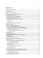
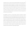
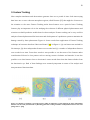
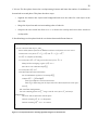
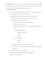
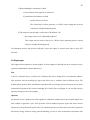
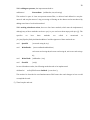
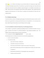
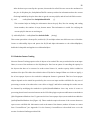
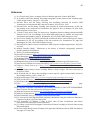
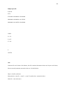
The process of converting raw data into a form that is viewable and understandable to human beings is called Visualization. Visualization allows us to get a better cognitive understanding of the data. Scientific visualization usually deals with scientific data that has a well‐defined representation in 2D or 3D or has a natural geometric structure (e.g. MRI data or wind flows). Analysis of such scientific data usually provides a more intuitive interpretation for the process of hypothesis building and modeling. Examples of scientific visualizations are the visualizations of intense quantities of laboratory or simulation data, or the results from sensors out in the field. The output of these simulations, experimental and sensor data are in the form of 3D scalar datasets. Figure 1 is one such example where 4
CHAPTER 1. INTRODUCTION
we visualize a 2D array of numbers. It very hard to interpret the meaning of these numbers on their own, but when presented as a picture we get a better idea of what the data is representing. 1.2
Basics of Visualization
Figure 1: Visualization of array of number as an image. (Image source – Ch­ 1, Page 12 http://www.cmake.org/Wiki/images/6/65/ParaViewTutorial36.pdf) Put simply, the process of visualization is taking raw data and converting
it to a form that is viewable and understandable to humans. This allows us
In addition, time varying simulations are common in many scientific domains; these are used in the to get a better cognitive understanding of our data. Scientific visualization
is specifically concerned with the type of data that has a well defined represtudy of evolution of phenomena or features. Traditionally, visualization of 3D time‐varying datasets is sentation in 2D or 3D space. Data that comes from simulation meshes and
done using animation, i.e., each frame (or time‐step) is visualized using iso‐surfacing or volume scanner data is well suited for this type of analysis.
rendering, and are
then three
the various run in sequence decipher any visual patterns. There
basic time‐steps steps to are visualizing
your to data:
reading,
filtering,
and rendering. First, your data must be read into ParaView. Next, you may
However, for datasets with continuously evolving features like cloud formations, it is difficult to follow apply any number of filters that process the data to generate, extract, or
derive features from the data. Finally, a viewable image is rendered from the
data.
6 and see patterns in 3D. What is required is a technique to isolate and analyze certain regions of interest also called ’features’ and highlight their underlying physical processes [1, 2]. For example, it is usually important to know what regions are evolving, whether they merge with other regions, and how their volume may change over time. Therefore, region based approaches, such as feature tracking and feature quantification are needed. Moreover, most of the standard visualization methods cannot give a quantitative description of the evolving phenomena, such as the centroid of a merged region or the value of its moments. An automated procedure to track features and to detect particular stages or events in their evolution can help scientists concentrate on regions and phenomena of interest. Color connected iso‐surface based on computed quantification provide visual cues about the events or particular stages of interest. This effectively reduces the amount of data to focus on by curtailing the visual clutter. Another important application of feature tracking is in data mining. By building a database of features, the results over multiple simulations can be used for ’event matching’. In previous work [3,4,5], the Vizlab had pioneered the use of feature tracking to effectively visualize time‐varying datasets. Feature Tracking was implemented as a plugin on AVS, a proprietary visualization software. Thus license costs limit the usability and extendibility over a larger user base. Many open‐source visualization software packages that contain lot more features and functionalities are available to users free of cost. VisIt is one such open source visualization software that is freely available and has a rich feature set. VisIt supports quantitative and qualitative visualization, it has powerful user interface and architecture to support massive datasets in the order of tera scale. VisIt allows development of custom plugins to add new features and functionality. Feature Tracking capability can be introduced in VisIt as plugins, and this would allow VisIt user to study evolving patterns in time varying datasets. Previous work on porting Feature Tracking to VisIt [23] extracted the features from a time varying scalar dataset. However the visualization plugins were found to be incomplete. If an object is moving across a dataset changing its shape and size, the algorithm should be able to identify this phenomenon 7 and assign the same color to object in other frames until they disappear. Even if the object splits into smaller objects, all those smaller objects should continue to have same color until they disappear. Since this kind of behavior is depicted in trakTable, we use trakTable to assign colors and present an algorithm to achieve this task. Our implementation gives the scientist or a user an option to selectively track only few features (or objects) of interest amongst all the extracted features. These features can be selected by mouse clicks. Like most open source softwares, VisIt too lacks proper design documentation. This hampers the development of new features or plugins in VisIt. A lot of time and energy is spent in understanding the design, so this thesis also aims to document the design decisions that could be useful to other developers. The organization of the thesis is as follows: Chapter 2 provides an introduction to Scientific Visualization and describes some software packages like AVS, ParaView and VisIt. Chapter 3 describes Feature Tracking process and various software implementations that exist in Vizlab. Chapter 4 is about Visit. We discuss the design, working and procedure for creating new plugins in Visit. In Chapter 5, we talk about the functionalities that have to be added to VisIt, design of Feature Tracking & Visualization plugins, new methods added, modifications made to the existing code and the challenges faced during this process of designing new plugins. The algorithm was tested on different datasets and results presented in Chapter 6. Finally thesis concludes with reiterating the usefulness of Feature Tracking in VisIt and its benefits as a scientific visualization tool. We provided a detailed user manual about the installation procedure and information on using the plugins in appendix. 8 2.
Introduction
to
Scientific
Visualization
As stated in [8], Scientific visualization is an interdisciplinary branch of science, “primarily concerned with the visualization of three dimensional phenomena (architectural, meteorological, medical, fluid flow, biological etc), where emphasis is on realistic rendering of volumes, surfaces, illumination sources, and so forth, perhaps with a dynamic component of time”. Scientific Visualization is the use of data driven computer graphics to aid in the understanding of scientific data. Is scientific visualization just computer graphics, then? Computer graphics is the medium in which modern visualization is practiced, however visualization (including scientific visualization) is more than simply computer graphics. It uses graphics as a tool to represent data and concepts from computer simulations and collected data. Visualization is actually the process of selecting and combining representations and packaging this information in understandable presentations. 2.1
Underlying
principles
In this section, we will discuss various reasons for using scientific visualization and the effect they have on scientific experiments. Also, we will have a look at some basic steps of visualization. Scientific visualization is form a communication and we need to be very clear of our audience, as they have to grasp what happens to the information as it passes from numbers to pictures. 2.2
The
Goal
of
scientific
visualization
Scientific visualization is employed as a tool to gain insights into natural processes easily. For instance, the goal might be to demonstrate a scientific concept, in which case the presentation to scientist would be different from a presentation that would be shown to the general public. The amount and level of detail required in visualization is based on experience of the intended audience. 2.3
Steps
involved
in
scientific
visualization
At one level, scientific visualization can be thought of analytically as a transfer function between numbers and images. At another level, visualization involves a barrage of procedures, each of which 9 may influence the final outcome and the ability to convey meaningful information. The process of visualization roughly consists of the following steps: •
Data Filtering – includes cleaning and processing of the data to yield meaningful results. Examples would be removing noise, replacing missing values, clamping values in a certain range or producing new numeric forms leading to greater insights. •
Representation – Visual representation of information requires certain literacy on the part of the developer and the viewer [9]. Beyond numerical representation of the output of the simulation, it’s advisable to give information about the simulation itself, for e.g., the grid of the computation domain, coordinate system, scale information and resolution of computation. The goal of visualization limits the medium of delivery, which in turn puts constraints on the possible choices of representations. So, for example, if the motion is an important aspect to show from the data, then a medium that supports time‐varying imagery should be used. •
Feedback – It is a good practice for scientists to question the accuracy and the validity of all the information that is presented to them. It’s always important to get this feedback and make changes to the process in order to get proper and accurate results in visualization for the intended audience. 2.4
Scientific
Visualization
tools
A number of tools are available for creating visualization of information. These tools can be categorized as: •
Plotting
libraries ­ Software libraries were developed that enabled researchers to generate charts, graphs and plots without the need for reinventing the graphics themselves. Since, the form of interaction is through programming, it has limited interactivity.
•
Turn‐key
packages – A turnkey visualization package is a program designed specifically for doing visualization and contains controls (widgets) for most options users would want to exercise when visualizing data. This is accomplished through the use of pull down menus or popup windows with control panels. Examples are Vis‐5D, Gnuplot etc. 10 •
Dataflow
packages – These are designed as tools to be used directly by the scientist. The dataflow concept consists of breaking down the tasks into small programs, each of which does one thing. Each task is represented as a module. Examples of this kind of packages are softwares like AVS. •
Writing
your
own
softwares ­ before dataflow packages and other tools were available, the programs were customized for a particular task in hand. This is sometimes still done with large time varying datasets, but now mostly people use off‐the‐shelf softwares with some modifications to perform a particular task. 2.5
Scientific
Visualization
Software
Packages
Visualization Software package (sometimes referred to as dataflow package) is the mostly prominently used visualization tools. These are modular softwares are based on Object Oriented Programming languages that facilitate addition of new capabilities as modules. In this section, we discuss about 3 different software packages that are widely used. Each of these packages creates a network that is executed to produce visualizations. 2.5.1
AVS/Express
AVS/Express is a comprehensive and versatile data visualization tool for both non‐ programmers and experienced developers. It provides powerful visualization methods for challenging problems in a vast range of fields, including science, business, engineering, medicine, telecommunications and environmental research. AVS/Express enables object‐ oriented development of rich and highly interactive scientific and technical data visualizations for a wide range of computing platforms. [www.avs.com]. AVS/Express has the following attractive features: •
Object Oriented ‐ AVS/Express' development approach is object‐oriented; it supports the encapsulation of data and methods; class inheritance; templates and instances; object hierarchies; and polymorphism. In AVS/Express, all application components, from the lowest to the highest level, are objects. 11 •
Visual development ‐ The Network Editor is AVS/Express' main interface. It is a visual development environment that is used to connect, define, assemble, and manipulate objects through mouse‐driven operations. •
Visualization application ‐ AVS/Express provides hundreds of predefined application components (objects) that process, display, and manipulate data. The objects and application components that you connect and assemble in the Network Editor control how data is processed and how it is displayed. Furthermore, AVS/Express also provides programming interface (APIs) to C, C++ and Fortran, allowing developers to easily integrate their own modules into AVS/Express. From Data to Pictures in AVS. To transform data to Pictures in AVS, one must follow these steps: 1. Import the data in AVS 2. Process the Data, if needed 3. Apply one or more Visualization techniques. 4. View the results. AVS has many built‐in module for performing all of the above mentioned tasks. For e.g. ReadField module importing the data from .fld file into AVS. Downsize modules does the processing of the data and as the name suggests, it does some processing based on some criteria provided by the user. Similarly there are modules to apply visualization techniques and view the results. A user selects the appropriate modules manually and builds a network as shown in Figure 6. AVS facilitates the process of network building by color‐coding the ports. Input and output ports of similar color are connected indicating the flow of the data in the network. Since data is primary to perform any processing, the first module is always be for reading the data and the last module is a viewer module to display the results. Figure 6, shows a simple network in AVS to read field files, downsize the data according to some criteria, and produces the orthoslices for the volume. We have modules for bounds and Axis3D, in the 12 resulting image, we see a bounding box and axis for the volume. Any change in data for any of the module causes entire network to be executed again to represent the change in visualization. Figure 2: AVS Network. (Image source ­ http://help.avs.com/express/doc/help_722/index.htm) 2.5.2
ParaView
ParaView is an open‐source, multi‐platform data analysis and visualization software package. With ParaView, users can quickly build visualizations to analyze their data using qualitative and quantitative techniques. The data exploration can be done interactively in 3D or programmatically using ParaView's batch processing capabilities. It has been successfully tested on Windows, Mac OS X, Linux, IBM Blue Gene, Cray Xt3 and various Unix workstations, clusters and supercomputers. Under the hood, ParaView uses the Visualization Toolkit (VTK) as the data processing and rendering engine and has a user interface written using Qt. Some of the important features of ParaView are given below: •
Visualization Capabilities – ParaView handles structured, unstructured, polygonal, multiblock and AMR data types. All the processing (or filtering) operations produce datasets. ParaView can 13 be used to inspect vector field by applying glyphs, extract contours and iso‐surfaces, cut or clip regions by clipping planes, or generate streamlines using constant step or adaptive iterators. The points in a dataset can be warped with scalar or vector quantities. Python programming interface can be used for advanced data processing. •
Input/Output and file formats‐ ParaView supports a variety of file formats. [ParaView reader] and [writer] provides a complete list of supported file formats. •
User interaction – Qt application framework introduces flexibility and interactivity. Parameters on the filters can be changed by directly interacting with the 3D view using 3D manipulators. Interactive frame rates in maintained by using LOD (level of detail) models. •
Large data and distributed computing – ParaView runs parallelly on distributed and shared memory systems using MPI. These include workstation clusters, visualization systems, large servers, supercomputers, etc. ParaView uses the data parallel model in which the data is broken into pieces to be processed by different processes. Most of the visualization algorithms function without any change when running in parallel. ParaView also supports ghost levels used to produce piece invariant results. Ghost levels are points/cells shared between processes and are used by algorithms which require neighborhood information. ParaView supports both distributed rendering (where the results are rendered on each node and composited later using the depth buffer), local rendering (where the resulting polygons are collected on one node and rendered locally) and a combination of both (for example, the level‐of‐detail models can be rendered locally whereas the full model is rendered in a distributed manner). This provides scalable rendering for large data without sacrificing performance when working with smaller data. •
Scripting and extensibility – ParaView is fully scriptable using simple but powerful Python language. Additional modules can be added by either writing an XML description of the interface or by writing C++ classes. The XML interface allows users/developers to add their own VTK filters to ParaView without writing any special code and/or re‐compiling. 14 From data to Pictures in ParaView The procedure for converting data to picture is ParaView is also similar to that of AVS. First, the data has to be read into ParaView. Since, ParaView is a subset of VTK, ParaView supports most of the file formats supported by VTK. Incase ParaView could not find the reader associated with a particular file format, then additional reader module has to be written to read the data in ParaView. Once the data is read in ParaView, the surface is rendered on the screen as a solid mesh. However, interesting features cannot be determined by simply looking at the surface. There are many variables associated with the mesh (scalars and vectors). Mesh being a solid hides a lot of information inside it. We can discover more information about the data by applying Filters. Filters are functional units that process the data to generate, extract, or derive features from the data. Filters are attached to readers, sources, or other filters to modify its data in some way. These filter connections form a visualization pipeline. These filters can be selected by choosing a corresponding icon on the filter toolbar. ParaView automatically creates this pipeline; users need not worry about connecting the individual modules as in AVS. Once, user has finished selecting the appropriate filters, the results are rendered on the screen on clicking “Apply” Button. ParaView does not give internal details about the visualization pipeline. There is no information on how the pipeline is formed, methods that would be executed or how the modules are connected. ParaView also lacks proper documentation for process of adding new filters or readers. 2.5.3
VisIt
The VisIt [11] project originated at Lawrence Livermore National Laboratory as part of the Advanced Simulation and Computing (ASC) program of the Department of Energy's (DOE) National Nuclear Security Agency, but it has gone on to become a distributed project being developed by several groups. VisIt is an open source, turnkey application for large scale simulated and experimental data sets. Its charter goes beyond pretty pictures; the application is an infrastructure for parallelized, general post‐
processing of extremely massive data sets. Target use cases include data exploration, comparative analysis, visual debugging, quantitative analysis, and presentation graphics. VisIt leverages several third party libraries like: the Qt widget library [12], the Python programming language and the 15 Visualization ToolKit (VTK) library [13] for its data model and many of its visualization algorithms. VisIt has been ported to Windows, Mac, and many UNIX variants, including AIX, IRIX, Solaris, Tru64, and, of course, Linux, including ports for SGI's Altix, Cray's XT4, and many commodity clusters. Some of the key features of VisIt are listed below: •
Rich set of features for scalar, vector and tensor visualization – VisIt’s visualization options can be broadly classified in two main categories (as mentioned in the VisIt Developer Manual [20]): 1. Plots – to visualize data and include boundary, contour, curve, mesh, streamline, subset, surface, tensor, vector. 2. Operators – consists of operations that can be performed on the data prior to visualization, like slice, index, onion peel, iso‐surface etc. •
Qualitative and Quantitative visualization ‐ VisIt is also a powerful analysis tool. It provides support for derived fields that allow new fields to be calculated using existing fields. For example, if a dataset contains a velocity field, it is possible to define a new field that is the velocity magnitude. •
Supports multiple mesh type ‐ VisIt provides support for a wide range of computational meshes, including two‐ and three‐dimensional point, rectilinear, curvilinear, and unstructured meshes. In addition, VisIt supports structured AMR meshes and CSG meshes. •
Powerful full featured Graphical User Interface (GUI) ‐ VisIt’s graphical user interface allows novice users to quickly get started visualizing their data, as well as allowing power users access to advanced features. VisIt automatically creates time‐based animations from data sets that contain multiple time steps. •
Parallel and distributed architecture for visualizing tera­scale data ‐ VisIt employs a distributed and parallel architecture in order to handle extremely large data sets interactively. VisIt’s rendering and data processing capabilities are split into viewer and engine components that may be distributed across multiple machines 16 •
Interfaces with C++, Java and Python ‐ VisIt also supports C++, Python and Java interfaces. The C++ and Java interfaces make it possible to provide alternate user interfaces for VisIt or allow existing C++ or Java applications to add visualization support. The Python scripting interface gives users the ability to batch process data using a powerful scripting language. •
Extensible with dynamically loaded plug­ins ‐ VisIt achieves extensibility through the use of dynamically loaded plugins. All of VisIt’s plots, operators, and database readers are implemented as plugins and are loaded at run‐time from the plugin directory. From Data to pictures in VisIt. The process of conversion of data to pictures in VisIt is very similar to the process in other visualization software packages. The difference comes in the underlying network that is created. VisIt automatically creates an AVT network for the user, depending on the action performed by the user. If the user performs the following actions: 1. Load a data file 2. Apply Operator (or filter) to the data, if any. And user chooses splice operator 3. Choose a plot (contour plot). 4. Execute the network and draw the results on the screen. Figure 3: VisIt Dataflow network. (Image source ­ http://visitusers.org/index.php?title=AVT_Overview) 17 Then a network shown in Figure 3 is generated automatically showing contribution of each step in the entire network. VisIt keeps on adding to this network according to the user action and only when user chooses “Apply”, the network is executed and result rendered on to the viewer (screen). VisIt provides plugins corresponding to each of the action. There are many built‐in plugins for handling database (i.e loading files), operators and plots. More information about the dataflow network is given in Chapter 4. 2.6
Examples
of
Scientific
Visualization
Visualization tools when applied to scientific data produce beautiful pictures. Many scientific fields can benefit from these visualization tools. We discuss application of visualization tools is some scientific fields: Natural
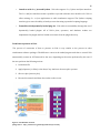
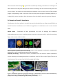
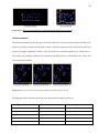
science – Visualization of these phenomenon can useful for studying star formations, understanding gravity waves, visualizing massive supernova explosions and for molecular rendering. Figure 4 shows some of these results. Figure 4:Examples of Visualization in study of natural sciences. a) Star formation. b) Gravity plot. c) Visualization of massive supernova explosion. d) Molecular rendering. (Images Source ­ http://en.wikipedia.org/wiki/Scientific_visualization ) Geography
and
Ecology
–
In
this
field of science, visualization tools are useful for climate visualization, terrain rendering and studying atmospheric anomalies in areas like Times Square. Figure 5 shows the visualizations of the concepts from field of Geography and Ecology. Figure 5: Visualization application in geography and ecology. a) Visualization of terrain. b) Climate Visualization. c) results from simulation framework of atmospheric anamoly around Times Square. (Images source ­ http://en.wikipedia.org/wiki/Scientific_visualization) 18 Formal
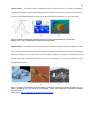
sciences – In formal sciences, visualization tools can benefits users by showing a mapping of topographical surfaces, representing huge quantities of data in curve plot or scatter plots. In Figure 6, we can see that Images annotation can be one of the visualization techniques to convey the results. Figure 6: Examples of Visualization in formal sciences. a) Curve plot b) Image annotations. c) Scatter plot. (Images source ­ http://en.wikipedia.org/wiki/Scientific_visualization) Applied
sciences – Visualization tools are very useful for manufacturing and automobile industry. These tools reveal a lot of information about the design of cars and aircrafts without actually manufacturing them thus saving a lot of money. These tools are used to model cars, study the aerodynamics of an aircraft, and render traffic measurement in the city for city planners to come up with effective traffic management solutions. Figure 7: Examples of Visualization in Applied Sciences. a) Mesh plot of Porsche 911 model. b) Display plots of a dataset representing YF­17 jet aircraft. c) City Rendering ­ results from rendering the description of building footprints in a city. (Image source ­ http://en.wikipedia.org/wiki/Scientific_visualization). 19 3.
Feature
Tracking
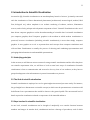
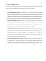
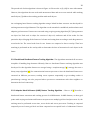
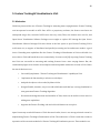
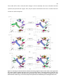
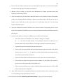
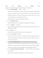
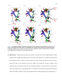
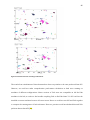
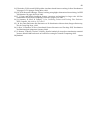
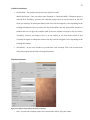
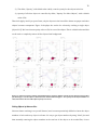
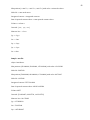
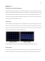
Most complex simulations and observations generate data over a period of time. Such time‐varying data have one or more coherent amorphous regions, called Features [27] that might be of interest to the scientists or the users. Feature Tracking tracks these features over a period of time. Tracking features play an important role in the studying the evolution of different physical phenomenon and scientists can build predictive models based on these analysis. Feature tracking can be very useful in analysis of natural phenomena like hurricanes and development of a prediction system to minimize the damage caused by these phenomena. Figure 11 shows results from application of Feature Tracking technique on hurricane data from ‘Hurricane Bonnie’ [29]. In Figure 11: (a) one feature was tracked for 30 timesteps, (b) three independent features were tracked and (c) a number of independent features were tracked over time. From these results it was possible to see that most of the features under consideration followed a clear pattern such as moving counter clockwise and inwards. It was also possible to see that features closer to hurricane’s center moved faster than the features farther from the hurricane’s eye. Both of these findings were extremely important in terms of the analysis and interpretation of hurricane data. Figure 8: a) Results of tracking a hurricane feature within 30 timesteps. b) Path followed by three independent features over the same period of time. C) Resulting path after tracking a number of independent features over time (Image source – [29]) 20 3.1
Feature
Tracking
Techniques
Over the years, researchers have proposed several different techniques for extracting and tracking features from time varying datasets. These techniques can be broadly classified as: • Overlap based Feature Tracking ‐ Silver & Wang [30, 4] presented a feature tracking technique that extracts features, organizes them into an octree structure and tracks the threshold connected components in subsequent timesteps by assuming that all the features between adjacent timestep overlap. Later they improved the implementation by tracking features in unstructured datasets. • Attribute based Feature Tracking ‐ Reinders et. al [31] described a tracking technique that tracks features based on attributes like mass, position and size. A number of correspondence functions are tested for each attribute resulting in correspondence factor. Correspondence factor makes it possible to match likely feature across subsequent frame in a dataset. • Higher dimensional isosurfacing based Feature Tracking – Ji et al [32] introduced a method to track local features from time varying data by analyzing higher dimensional geometry. Rather than extracting features such as isosurfaces separately from individual frames of a dataset and computing the spatial correspondence between the features, correspondence between the featues can be obtained by higher dimensional isosrufacing. • Machine learning based Feature Tracking ­ Tzen and Ma [33] present a machine learning based visualization system to extract and track features of interest in higher dimensional space without specifying the relations between those dimensions. The visualization system “learns” to extract and track features in complex 4D flow field according to their “visual properties” like the location, shape and size. 21 3.2
Feature
Tracking
Algorithms
at
Vizlab
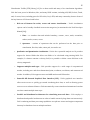
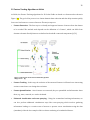
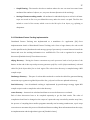
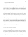
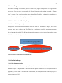
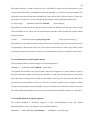
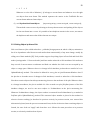
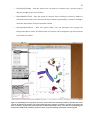
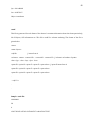
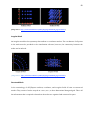
At Vizlab, the Feature Tracking algorithms for 3D Scalar Fields are based on a framework as shown in Figure (12). The goal of the process is to obtain dramatic data reduction and thus help scientist quickly focus on a few features or events of interest. The major steps are: Feature Extraction ‐ The first step is to identify and segment features of interest from the dataset •
to be tracked. The method used depends on the definition of a ’feature’, which can differ from 3
domain to domain. Usually features are defined as threshold‐connected components [6,7,3]. •
Figure 1.1: The Feature Tracking based Visualization pipeline [3]
Figure 9: The Feature Track based visualization pipeline. Image source ­ [6] generate a distributed form of these feature tracking and quantification algorithms in
Feature Tracking ‐ In this step, the evolution of the extracted features is followed over time noting order to accommodate such data. Each processor, over which the dataset is divided,
will
extract and quantify its local features. We then need a procedure to coalesce these
various events that occur during their evolution. •
observations, because a feature may span multiple processors, i.e., perform global fea-
Feature Quantification ‐ Once features are extracted, they are quantified and information about ture identification and resolution, and global calculation of feature attributes once this
them, e.g., mass, centroid, etc. can be calculated. coalescing
is done. Prior work done in this area is documented in [10, 3]. We also need to
•
take
into account
the individual and processor
constraints,
e.g.,
RAM and
mem-tracking information, we Enhanced visualization event querying ‐ Using the hard-drive
accumulated ory specifications. Hence, modifications are necessary to handle large-scale datasets
can also perform additional visualization steps like event querying which involves gathering and perform the feature extraction in parts. This also necessitates special changes to
leading to a certain interest step,
or present new visualization using the data beinformation made to the ensuing
merging
code usedevent for theof coalescing
in order toa accurately
merge
and quantify the large amounts of data involved. These modifications are the
(metadata) collected. One example of this is volume rendering of an individual feature.
primary focus of this thesis.
As research and data collection techniques evolve, there is a need for improved and
enhanced feature tracking and analysis. For example, the ability to do correct color
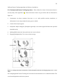
22 Different Feature Tracking algorithms at Vizlab are classified as: 3.2.1
Overlap
based
Feature
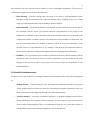
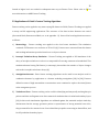
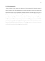
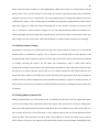
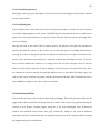
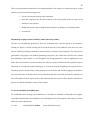
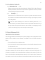
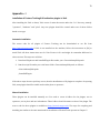
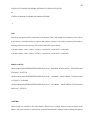
Tracking Algorithms ‐ These define five classes of interactions that are used by many other algorithms [34]. These interaction classes are given below and are illustrated in Figure 13: 1.
Continuation. An object continues from time ti to ti+1 with possible rotation, translation, or deformation. Its size may remain the same, grow or shrink. 2.
Creation. New objects appear. 3.
Dissipation. Objects disappear. (Dissipation generally occurs when regions fall below the specified threshold value.) 4.
Splitting (Bifurcation). An object splits into two or more objects. 5.
Merging (Amalgamation). Two or more objects merge. 7
events are illustrated in Figure 2-2.
continuation
bifurcation
dissipation
amalgamation
creation
Figure 2-2 Tracking interactions: continuation, creation, dissipation, splitting and merging [57]
Figure 10: Tracking Interactions: Continuation, creation, dissipation, bifurcation and merging. Image source – Lian’s Thesis data structure
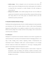
An overlapping based Feature Tracking can be based on Octree datastructure or Linked List based. The rlapping-baseoctree based algorithm works in two phases: volume tracking using an octree data structure is proposed in [48,
the next section, we describe this methodology in detail. Please refer to the papers
23 1. VO‐test: The first phase detects the overlaps among features and limits the number of candidates to be matched in second phase. This phase has three steps: •
Segment the dataset into objects and background and store the nodes for each object in the 8
object list. •
This is maximized when two objects are identical. To normalize the result of
Merge the object lists and sort in ascending order of node ids. matching, R can be computed as below:
•
Compare the two sorted lists from ti to ti+1 to detect the overlap and store these results in overlap table. Volume(O Ai ! OBi !1 )
R"
Volume(O Ai )Volume(OBi !1 )
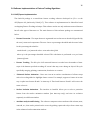
2. Best Matching test: this phase finds the correlation between different features. Feature Tracking
{
For two consecutive time steps t i and t i !1
Extract all the features from the two databases and store each feature in its own octree.
i !1
Construct the octree forests Fi " " p#ti O p and Fi !1 " " q#ti !1 Oq ;
i
i
Use O p as a template for matching
For each feature O p # Fi merge it into the octree forest, Fi !1 to
i
i
Identify all the overlapping regions of O p in t i !1 .
i
Store this in a list called OverLap O p [] .
i
For each feature O p in Fi
Determine bifurcation and continuation:
i
For all combinations of features in OverLap O p [] ,
Compute O p * $ " OverlapO p .
i
i
If the lowest difference is below the tolerance,
i
Mark O p as bifurcating into the object and remove them all from the search space,
i
Next O p .
Else, Determine Amalgamation;
i !1
For each remaining feature in Oq
merge it into the octree forest, Fi and test for
amalgamation
This is the same as bifurcation with the inputs
i
Take the remaining O p in t i as dissipation;
i !1
Take the remaining Oq
in t i !1 as creation.
}
Figure 2-3 Octree based feature tracking algorithm [48]
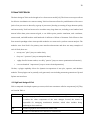
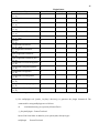
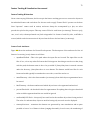
Figure 11: Overlap based Feature Tracking algorithm using Octree datastructure. This tracking algorithm works in two phases:
(1) VO-test: Overlap detection, which is to limit the candidates for best matching test.
(2) Best matching test: to find the correlation between features.
The VO-test has three steps:
24 The pseudocode for this algorithm is shown in Figure 14. Please refer to [3,4,30] for more information. However, this algorithm does not work with unstructured data and errors were noticed while tracking small objects. [3] address the tracking problem with small objects. An overlapping based feature tracking algorithm using a linked list data structure was developed for tracking unstructured grid datasets. This algorithm can be extended to multiblock, multiresolution and adaptive grid structures. Features are extracted using a region‐growing algorithm [35,7] that generates an object list. Each node in object list consists of object id, attributes and all the nodes for that particular object. Merging all the features of a frame and sorting them according to node ids generate a sorted node list. The sorted node lists for two frames are compared to detect overlap. Then best matching is performed on the overlap table to determine the class of interaction for each object in the frame. 3.2.2
Parallel
and
Distributed
Feature
Tracking
Algorithm– The algorithms mentioned till now were incapable of handling large datasets efficiently. Hence a distributed Feature tracking algorithm was developed. In this algorithm features are merged using a complete‐merge [36] strategy that uses a binary swap algorithm [37] for communication between processors. Once the distributed features are extracted on different processors, tracking server operates sequentially to get tracking results. A partial‐merge strategy was also proposed where processors communicate with their neighbors to determine the local connectivity. 3.2.3
Adaptive
Mesh
Refinment
(AMR)
Feature
Tracking
Algorithm – Chen et. al [5] describe a distributed feature extraction and tracking process for AMR datasets. In AMR datasets, we have grid points with varying resolutions and features can span across multiple grid level and processors. So, the tracking must be performed across time, across levels and across processors. Tracking is computed temporally across lowest grid level and then computed across spatial levels of refinement. Features 25 formed in higher level are tracked in subsequent time step as Feature Trees. Please refer to [5] for more information on AMR Feature Tracking. 3.3
Applications
of
Vizlab’s
Feature
Tracking
Algorithms
Feature tracking can be applied to any time‐varying 3D dataset. At Vizlab, Feature Tracking was applied to many real‐life engineering applications. The structure of the data in these datasets was varied. (Structured Mesh, Unstructured Mesh, etc. as in appendix ‐ II). Some of the broad application areas are as follows: 1)
Meteorology – Feature tracking was applied to the cloud water simulation. This simulation consisted of 25 datasets at a resolution of 35*41*23 [4]. Features were extracted from this dataset and tracking information provided visual cues on object evolution. 2)
Isotropic Turbulent Decay Simulation – Feature Tracking was applied to LES simulation of the decay of istrophic turbulence in a box in a compressible flow using unstructured tetrahedral. This simulation dataset having 500 frames (or timesteps) showed that the number of objects changes with as the isotrophic turbulence decays [4]. 3)
Autoignition datasets ‐ Basic feature tracking algorithms can be useful as an analysis tools for combustion datasets by application to a dataset modeling autoignition [28]. In [28], Features defined as areas of high intermediate concentrations were examined to explore the initial phases in the autoigniton process. 4) Turbulence flows – Feature tracking can be useful in identifying and temporally tracking hair pin packets and their wall signatures in direct numerical simulation data of turbulent boundary layers [29]. In this work visualization algorithms are validated against the statistical analysis. And they demonstrate that the average geometric packet is representative of strong statistical ones. Also, they presented for the canonical case of an isolated hair pin packet convecting in channel flow, and for fully turbulent boundary layers. 26 3.4
Software
Implementations
of
Feature
Tracking
Algorithms
3.4.1
AVS/Express
implementation
The Ostrk2.0 package is a stand‐alone feature tracking software developed in C/C++ on the AVS/Express 6.2 platform by Vizlab [17]. This software is implementation for linked‐list based overlapping Feature Tracking technique. This software works not only with unstructured datasets but all other types of datasets too. The main features of this software package are summarized below: •
Feature Extraction ‐ The input dataset is segmented into its features as threshold (specified by the user) connected components. The user choose a percentage threshold and the actual value for this percentage threshold is: actual thresh = p ∗ (max node value − min node value)/100 where p is the percentage threshold selected. This calculation is performed on a per frame (timestep) basis. •
Feature Tracking ‐ The life‐cycle of all extracted features is tracked over the number of time‐
steps of the dataset specified recording all ’events’ that may occur during an objects’ life‐cycle specifically merging, splitting, continuation, dissolution or creation. •
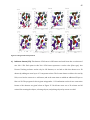
Enhanced Surface Animation ‐ Users can view an iso‐surface visualization of all time‐steps with color‐coding added to highlight feature events. For example, suppose a feature A in time step 1 splits into features B and C in time‐step 2. Then both features B and C will receive the same color as A. •
Surface Isolation Animation ‐ The interface in Ostrk2.0 allows you to select a particular feature from the surface animation window (last time‐step only) and view its evolution separately in a different window. •
Attribute analysis and Printing ‐ The software computes various attributes like volume, mass, centroid, etc., that can be printed on the screen by picking a particular object from a time‐step in the enhanced surface animation window. 27 •
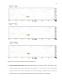
Graph Plotting ‐ The interface also has a window where the user can view how some frame attributes like number of objects, etc., vary over the time (duration of the tracking). •
Storing of Feature tracking results ‐ All attributes for individual objects as well as for all time‐
steps are stored in files in a pre‐defined directory under the users’ run path. The files also include a record of the events, which occur in the life‐cycle of an object, e.g., splitting or dissipation. 3.4.2
Distributed
Feature
Tracking
Implementation
Distributed Feature Tracking was implemented as a standalone C++ application. [38] Gives implementation details of Distributed Feature Tracking code. Given a huge dataset, the code would work in parallel mode (distribute the task among a group of processors) to extract features from all the frames and store the tracking information in a .trakTable file. The code is organized in 4 separate directories [Pinakin’s thesis]. These directories are: objseg directory – During the feature extraction step each processor loads a local portion of the dataset. At the end of this step each processor generates .poly file, .oct file (object attributes), .trak and .table file (local object table) for its local region. The code in this directory is compiled using a MPI compile script. finalmerge directory ­ This part of code includes methods to read in the .table files generated during extraction step to generate a global object table. Also, .poly and .oct files are updated in this step. ftrack directory – here distributed tracking is implemented by partial‐merge strategy. Again MPI compile script is used to compile the code in this directory. score directory – best match is calculated and features across the frames are correlated. Each of these directories have to be compiled separately to get the final results. The order of compilation should not be changed as the output of a particular step is needed by another step. Since, the process of compiling these smaller programs manually was becoming cumbersome, a perl script was written to automate this process of distributed feature tracking. More information about the script, its implementation and the algorithm is given in [Pinakin’s thesis]. 28 3.4.3
VisIt
Implementation
“Feature Tracking of time varying scalar datasets in VisIt environment”,[23] describes porting of Feature Tracking in VisIt. This implementation successfully extracted the features from datasets and tracked those features in VisIt environment. Information about the extracted features were store in .poly, .attr, .uocd and .trak files while the tracking information was written to .trakTable file. This part was implemented as plugin in VisIt that could be easily installed by any other user. Another plugin was designed for visualizing the features extracted from the time‐varying datasets. However, these plugins were found to be incomplete and incompatible with newer versions of VisIt. In this thesis, we use the framework from [23] and make modifications to it. The plugins names are the same as in previous work, but the functionality of these plugins have been modified. 29 4.
How
VisIt
Works
The basic design of VisIt can be thought of as a client‐server model [14]. The client‐server aspect allows for effective visualization in a remote setting. VisIt’s architecture allows for parallelization of the server (task of one processor is shared by a group of processors) thereby processing of large datasets quickly and interactively. VisIt has been used to visualize many large data sets, including a two hundred and sixteen billion data point structured grid, a one billion point particle simulation, and curvilinear, unstructured, and AMR meshes with hundreds of millions to billions of elements. VisIt follows a data flow network paradigm where interoperable modules are connected to perform custom analysis. The modules come from VisIt's five primary user interface abstractions and there are many examples of each. In VisIt, there are: •
twenty‐one ``plots" (ways to render data), •
forty‐two ``operators" (ways to manipulate data) •
eighty‐five file format readers, over fifty ``queries" (ways to extract quantitative information) •
over one hundred ``expressions" (ways to create derived quantities). Further, a plugin capability allows for dynamic incorporation of new plot, operator, and database modules. These plugins can be partially code generated, even including automatic generation of Qt and Python user interfaces. 4.1
High
level
design
of
VisIt
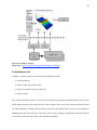
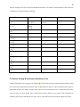
VisIt is composed of multiple separate processes, which are sometimes called as components [19]. They are listed in Table 1: Name Viewer Overview Two primary purposes. First, it centralizes all of VisIt's state. When the state changes, it notifies the other components of the state changes. Second, the viewer is responsible for managing visualization windows, which often includes doing rendering in those windows. Gui Provides a graphical user interface to control VisIt. Cli Provides a command line user interface to control VisIt 30 Vcl Launches jobs on remote machines. The VCL sits idle on remote machines, communicating with the viewer and waiting for requests for jobs to launch. When these jobs come up, it launches them. The purpose of this module is to spare the user from having to issue passwords multiple times. Mdserver The mdserver browses remote file systems, meaning it produces listings of the contents of directories. It also opens files (in a lightweight way) to get meta‐data about a file, allowing the user to set up plots and operators without an engine. Engine The engine performs data processing in response to requests from the viewer. There are both parallel and serial forms of the engine (called engine_ser and engine_par respectively). The engine sometimes performs rendering, although it is also performed on the viewer. [Table 1: VisIt’s multiple separate processes. http://visitusers.org/index.php?title=High_level_design] Source ­ This information is taken from 4.2
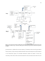
Connectivity
&
Communication
between
components
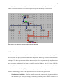
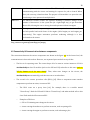
The connections between the various components are shown in the figure 12. At the lowest level, the communication is done with sockets. However, two separate layers are built on top of that. •
The first is for exporting state. The viewer keeps all of its state in various instances of VisIt's AttributeSubject class. UI modules (such as the GUI and CLI) subscribe to this state (refer to [25] by Gamma et al. for more details). Thus, when state changes on the viewer, the AttributeSubjects automatically push this state out to its subscribers •
The second is for remote procedure calls (RPCs) [15]. When a component wants another component to perform an action, it issues an RPC. o
The RPCs come via a proxy class [16]. For example, there is a module named "ViewerProxy". Both the GUI and CLI link in "ViewerProxy" and make method calls to this class. Each method call becomes an RPC. o
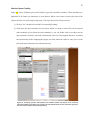
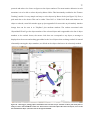
Examples of RPCs are:  GUI or CLI initiating state change in the viewer  viewer causing the mdserver to perform an action, such as opening a file  viewer causing the engine to perform an action, such as drawing a plot. 31 Figure 12: VisIt High level design. (Image source ­ http://visitusers.org/index.php?title=High_level_design) 4.3
Workflow
of
VisIt
Consider a scenario, where a user performs the following actions: 1) Loads a data file 2) Choose a plot (say contour plot) 3) Choose a operator (say slice operator) 4) Click on Draw. As, a result of the above actions, an AVT network (Figure 8) is generated automatically by the VisIt. We briefly mentioned about the network in the earlier chapter. Here, we see the network in detail. We will see what methods are called when the above actions are performed. Each user action corresponds to building some part of the network. VisIt does not do any processing or visualization until the network is executed. Till that time the Viewer sits with the information. 32 1) Load Data File: A user opens a file, which causes the mdserver to open an avtFileFormat and get metadata information from the file. This is the information about the data like the type of mesh, scalar variables etc. The actions are classified into two broad groups: Meta­data server actions 1) First, MDServerConnection::ReadMetaData method that is defined and declared in MDServerConnection.C and MDServerConnection.h is called. • This method must first open a file, so it calls MDServerConnection::GetDatabase. ‐ This method uses an avtDatabaseFactory to instantiate an avtDatabase. The DB factory iterates over viable plugin types 1) For each viable plugin type, the file format is instantiated 2) avtDatabase::GetMetaData is called. This forces the plugin to do some work to see if the file is really of the format's type. 1) GetMetaData ultimately calls: PopulateDatabaseMetaData GetCycles GetTimes 2) No calls will be made to: GetMesh GetVar • The resulting avtDatabase is asked to create meta‐data for the file. This is a no‐op, since the meta‐data was read when opening the file and that meta‐
data was cached. 2) Later, SIL information is requested of the database. This is done in MDServerConnection::ReadSIL using avtDatabase::GetSIL. 1) avtDatabase::PopulateSIL is called. 33 2) avtSILGenerator populates the SIL entirely from the meta‐data. Engine actions The first of the engine actions it to call the method RPCExecutor<OpenDatabaseRPC>::Execute defined in Executors.h. 1)
The appropriate plugin type is known (from the mdserver which is open) and it is loaded. 2)
This calls NetworkManager::GetDBFromCache, which does the following: 1) The file is opened using the database factory. 2) avtDatabase::GetMetaData is called 3) avtDatabase::GetSIL is called 4) The database is registered with the load balancer. 2) Adding a plot or operator ‐ as the user makes the plot and adds operator, the engine responds by constructing an AVT network. There is no communication between different components of VisIt. The viewer just sits with the information and does nothing with it. 3) Clicking on draw ‐ As the user clicks on ‘Draw’, the AVT network is executed and the following steps are executed during this process. •
Preparing for scalable rendering •
In non‐scalable rendering, the resulting surface is transferred to the viewer and rendered locally. The rendering is done using an avtPlot's "mapper" module being called in the context of a VisWindow's visualization window. •
In scalable rendering, the surface is rendered in parallel, and the engine transfers an image back to the viewer. •
Stating which file to use as the source RPCExecutor<ReadRPC>::Execute from Executors.h is called. This method NetworkManager::StartNetwork and the following actions take place: 1) The avtDatabase is identified (it was already created during an OpenDatabaseRPC) 2) An avtTerminatingSource is gotten from the avtDatabase. calls 34 3) An avtExpressionEvaluatorFilter is added to the pipeline (at the top). 4) The avtSILRestriction is registered. •
Setting up the operators 1) RPCExecutor<PrepareOperatorRPC>::Execute is called This must be called first to instantiate the correct type of attributes, so that the subsequent call to “Add Operator” will be able to load the attribute values into this instance. 2) RPCExecutor<AddOperatorRPC>::Execute is called This method calls NetworkManager::AddFilter which does the following actions: 1) The proper plugin type is loaded. 2) An avtFilter is instantiated and registered with a "workingNet". 3) The attributes of the filter are set. •
Setting up the plots This is similar to the setting up of operators. The following actions take place: 1) RPCExecutor<PreparePlotRPC>::Execute is called This must be called first to instantiate the correct type of attributes, so that the subsequent call to "MakePlot" will be able to load the attribute values into this instance. 2) RPCExecutor<MakePlotRPC>::Execute is called 1) NetworkManager::MakePlot is called 1) The proper plugin type is loaded. 2) An avtPlot is instantiated and registered with a "workingNet". 3) The attributes of the plot are set. 2) An Id is obtained from the network manager and returned to the viewer. This Id is used to refer to this plot in the future. (For picks, etc.) •
Executing the network RPCExecute<ReadRPC>::Execute is called. This methods calls the following two methods: 35 1) NetworkManager::GetOutput is called. 1) Each module of the pipeline is connected. 2) DataNetwork::GetWriter is called ‐ avtPlot::Execute is called. The return may be either geometry, or a NULL object saying that we need to kick into Scalable Rendering mode. 2) The output is sent through a socket with a "WriteData" call. ‐ The output comes as an "avtDataObjectWriter". ‐ This output may be either a data set or a NULL object, indicating that we should switch to Scalable Rendering mode. 4) Subsequent actions, like queries and picks, cause the engine to connect new sinks to that AVT network. 4.4
Plugin
types
VisIt supports development of custom plugins. In VisIt, plugins are divided into three categories: plots, operators and database readers and writers. Plot A plot is a viewable object, created from a database that can be displayed in a visualization window. VisIt provides several standard plot types that allow you to visualize data in different ways. The standard plots perform basic visualization operations like contouring, pseudocoloring as well as more sophisticated operations like volume rendering. All of VisIt’s plots are plugins so you can add new plot types by writing your own plot plugins. Operator An operator can be considered as a filter applied to a database variable before the compute engine uses that variable to generate a plot. VisIt provides several standard operator types that allow various operations to be performed on plot data. The standard operators perform data restriction operations like planar slicing, spherical slicing, and thresholding, as well as more sophisticated operations like 36 peeling off mesh layers. All of VisIt’s operators are plugins and you can write your own operator plugins to extend VisIt in new ways. Database VisIt can create visualizations from databases that are stored in many types of underlying file formats. VisIt has a database reader for each supported file format and the database reader is a plugin that reads the data from the input file and imports it into VisIt [22]. If VisIt does not support your data format then you can first translate your data into a format that VisIt can read (e.g. Silo, VTK, etc.) or you can create a new database reader plugin for VisIt. 4.5
Adding
new
plugins
in
VisIt
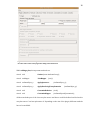
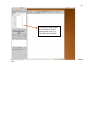
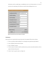
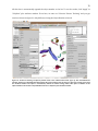
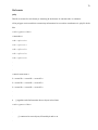
VisIt comes with a graphical plugin creation tool, which greatly simplifies the process of creating new plugins. The user describes the properties of the plugin and then the tool generates most of the code necessary to implement the plugin. The only code you need to write is the C++ code that actually performs the operation. Steps for creating a new plugin VisIt provides with some tools to help developers in adding any new functionality. These tools can be found under the following location: <visithomefolder>/src/bin> and more information about these tools can be found in VisIt’s User Manual [20]. If this folder has been added to the system path, then the tools in this folder can be accessed from any location, by just typing the name of the tool. Otherwise full path has to be mentioned. For example, we want use xml2edit tool in some folder say, /home/admin. Then the commands to run this tool are: cd /home/admin xmledit <visithomefolder/src/bin>xmledit 37 For the rest of commands in this thesis, we assume that VisIt’s bin folder is added to system path. To create new plugins using these tools, one must follow the following steps: 1) Create a directory by the plugin name. The location of this folder depends on the type of the plugin. If the plugin is operator, it should go under <visithomefolder/src/operators>, if it’s a plot it should be in <visithomefolder/src/plots> and if it’s a database plugin then it should be at <visithomefolder/src/database> 2) Change to the location of the directory and run xmledit by following commands: cd < visithomefolder/src/ <plugintype>/ <pluginname> > xmledit A window similar to Figure 11 would appear on the screen. An untitled xml file is opened for the user to fill in the information necessary for creating a plugin. The information includes the name of the plugin, the type of the plugin, attributes and so on (refer to VisIt Developer’s Manual for more details). Attributes are the parameters that allow users to interact with the plugin. For example, opacity for a plot can be changed via a slider. A plugin can have one or more than one attributes. After the attributes are selected, their description entered and all the information provided, the file is saved as an xml file by the same name as that of the plugin. So, if the plugin is TrackPoly, then the xml file should be saved as TrackPoly.xml in TrackPoly folder. 3) Run xml2plugin. This will automatically create a framework to work on. This can be done as follows: cd cd <visithomefolder/src/ <plugintype>/ <pluginname> > xml2plugin <pluginname>.xml 4) The framework depends on the type of plugin. The files generated by VisIt depend on the type of the plugin. Table 1 gives a list of files generated for Feature Tracking plugins. These plugins have to be compiled before using, and some of the methods in these files have to be edited to compile. Again, the methods to be edited/modified depend on type of plugin. 38 Figure 13: Untitled xml file is generated when the user runs xmledit. This file has to be saved with the same name as that of the plugin after filling in the information. While adding a plot, the important methods are: virtual void SetAtts (const AttributeGroup*); virtual avtMapper *GetMapper (void); virtual avtDataObject_p ApplyOperators (avtDataObject_p); virtual avtDataObject_p ApplyRenderingTransformation virtual void CustomizeBehavior (void); virtual void CustomizeMapper (avtDataObject_p); (avtDataObjectInformation &); All these methods part of the class avt<plot­name> and hence would be defined and declared in avt<plot­name>.C and avt<plot­name>.h. Depending on the aim of the plugin, different methods have to be modified. 39 While adding an operator, the important method is: vtkDataset* ExecuteData (vtkDataSet, int, std::string) This method is part of class avt<operator­name>Filter, is declared and defined in avt<plot­
name>.h and avt<plot­name>.C. Any processing or filtering on the dataset can be introduced by adding some lines of code in this method. While writing a database writer, there are four basic methods, which must be implemented, although any of these methods can be no‐ops (i.e. you can leave them empty with just {;}). The specifics on how these methods are called is mentioned in /src/avt/Pipeline/Sinks/avtDatabaseWriter.C and the signature of these methods are: void OpenFile (const std::string &, int); void WriteHeader (const avtDatabaseMetaData *, std::vector<std::string>&,std::vector<std::string>&, std::vector<std::string> &); void WriteChunk (vtkDataSet *, int); void CloseFile (void); In case of database reader, the following method needs to be implemented. vtkDataSet* avtPolyFileFormat::GetMesh (const char*); This method is described in avt<Databasename>FileFormat class and changes in here would accomplish the task. 5) Then Compile and run! 40 5.
Feature
Tracking
&
Visualization
in
VisIt
5.1
Motivation
Vizlab has pioneered the use of Feature Tracking for analyzing time‐varying datasets. Feature Tracking was incorporated as module in AVS. Since AVS is a proprietary software, the license costs limits its widespread usage. Also, renewal of AVS license was very costly. Thus, new avenues were sort for, and Open Source Visualization Software Packages were sought to replace AVS. Among the Open Source Visualization Software Packages VisIt was chosen as the best option to port Feature Tracking. VisIt’s rich feature set, its support of distributed and parallel processing and its architecture made it a good choice. Extending new capabilities like the Feature Tracking & Visualization in VisIt would add a lot more value to VisIt and benefit the users tremendously. Previous work [23] in porting Feature Tracking into VisIt was successful in extracting and tracking features from a time varying dataset. But, the visualization plugins were found to be incomplete and incompatible with newer version of VisIt. Hence the aim of this thesis is to: •
Successfully implement “Feature Tracking and Visualization” capability in VisIt. •
Implement the functionality to selective track objects •
And pick the objects to be tracked, by Mouse clicks. •
Design a flexible, intuitive, easy to use and solid framework that lays a strong foundation for next generation Feature Tracking Algorithm. •
Document the design decisions and workflow of Visit, which can be useful to other users for adding new capabilities. •
Organize the Feature Tracking code and collect all datasets at once place. Apart from many wonderful features of VisIt discussed earlier, there is one strong technical reason for implementing Feature Tracking & Visualization in VisIt. The architecture of VisIt is such that it aides in separation of the two main modules for Feature Tracking & Visualization process. These modules are: 41 •
Feature extraction and Tracking module, •
Visualization module. Incase of AVS, features are extracted for one frame, tracking information updated and the results are rendered on the screen. Then AVS moves to next frame and repeats the process of extracting features, updating tracking information and rendering the result. But VisIt works in a different way. First, features one by one from all frames simultaneously updating the .trakTable. After performing this function, then only the results are rendered on the screen. How is this separation of modules advantageous? Suppose a scientist is analyzing some experimental simulation dataset. After 25 frames, scientist sees some interesting phenomenon on the screen and decides to see feature from Frame 25 onwards. Scientist wants the visualization starting from a different frame. In AVS there is no separation between extraction and visualization stage, then entire process has to be repeated. Even though there isn’t any change in data, just because visualization part cannot be viewed in isolation, the extraction and segmentation part is repeated. For smaller datasets, this might not be a point of concern. But for large datasets, a lot of time and resources are wasted on repeating the process on data that did not change. But VisIt is different; since it separates Feature Extraction & Tracking from Visualization there is no repetition of work. The scientist performs feature extraction and tracking only once. Visualization can now be repeated as many times as the scientist wishes to. As features extraction is not repeated again and again, visualization becomes much more efficient on larger datasets. 5.2
Feature
Tracking
&
Visualization
Functionalities
5.2.1
TrakTable
based
Color‐coding
From figure 14, it is clear that objects in each frame on the left side of the figure have colors assigned to them arbitrarily. There is no correlation between the objects and colors assigned to them. In time varying datasets, an object from one frame can move around in the next few frames of the dataset. It can change its shape and size, splits into smaller objects, form a bigger object by merging or continue as 42 before. Since the object continues to exist (although in a different form) in rest of the frames it should get the same color as in first frame. If a new object is formed in a particular frame, then it should be assigned colors that do not correspond to any of the existing objects. Tracking information is stored in .trakTable file. Hence, a color scheme based on trakTable would produce images similar to those on the right side of figure 14. When the objects following such a color scheme, it becomes very easy for the user to track these objects visually. In Figure 14, we can easily identify that Object A continues in 2 frames and splits in the last frame, while object B moves in the all the frames of the dataset with a very little change in its size and location. Such kind of behavior is useful in analysis and process modeling. 5.2.2
Selective
Feature
Tracking
Sometimes, we just want to visualize and track only those objects that are of interest to us. We should therefore have a mechanism to specify a list of objects to be tracked. This list when passed to the program should render only those objects in the list and remove other objects from the screen. Instead of actually removing the objects, we can adjust the transparency value to make them almost transparent and reduce visual clutter. Users should have the ability to control the opacity value for both the object to be tracked and the objects that are to be made transparent. We assume that the user knows the object numbers of all objects in a frame and selects the appropriate object by writing those numbers in the list. This assumption becomes unviable as the number of objects in a frame increase. To assist the users in such cases, we make our implementation intuitive by selecting the objects at the click of a mouse. 5.2.3
Picking
Objects
by
Mouse
Click
When presented with a lot of data on the screen, it is intuitive for the user to click on a particular region on the screen and get more information about that region. VisIt extends this concept by letting users know more information about the objects rendered on the screen. When a user clicks on any object on the screen in Node Pick or Zone Pick mode, a ‘Pick’ window pops up that has all the additional details about the object. We extend this concept to build a list of objects for selective tracking. A user clicks on all the objects of interest; the plugin would automatically extract the node number and build the list. 43 User would still be able to edit and make changes to the list manually. Once user is finished with this operation, they should click “Apply”. Now, only the objects mentioned in the list are rendered and rest of them are made transparent. Figure 14: The images on the left half show random colors being assigned to objects in the frame, on the right shows the results of feature tracking with proper color codes. The figure shows 3 consecutive frames of vorts data. Lets study the evolution of object A and Object B in (a), (b) and (c). The necessity for assigned coloring based on track tables becomes evident in (c), as its clear the object A has split into two and both the parts retaining the same color. 44 5.3
Custom
Plugins
The Feature Tracking & Visualization project in VisIt has 4 plugins. These plugins are categorized into two groups. The first group is responsible for Feature Extraction and tracking is named as “Feature Track” operator. The second group has three plugin (Poly, TrackPoly, PolyData) for visualizing the results. The descriptions of these plugins are as follows: 5.3.1
Feature
Extraction
&
Tracking
Group
5.3.1.1 FeatureTrack (operator) This operator extracts meaningful features from raw data and tracks them. In [23], this module generated .poly, .attr, .uocd, .trak and .TrakTable files. In addition to those files, we generate one more file per frame in this module. This file has colormap information for objects in the frame and the format of the file can be found in Appendix – I. Figure 15: Feature Tracking Plugin development in VisIt. 5.3.2
Visualization
Group
5.3.2.1 Poly (Database reader) This plugin reads the information in poly files, gathers metadata about the dataset and creates a vtkDataset object to be passed on to the network. This plugin generates a file curpoly.txt (format in Appendix I) to keep track of current frame. In this thesis, we modify the format of the curpoly.txt file from previous work. [23]. 45 5.3.2.2 TrackPoly (operator) This plugin reads curpoly.txt and replaces the last line in the file, indicating the frame number with the current frame number. 5.3.2.3 PolyData (plot) A plot should be able to show the results on screen. PolyData plot aims to visualize the objects listed in a .poly file by displaying them on the screen. TrakTable based coloring scheme allows us to differentiate objects in a frame and track them over a period of time. This plot tracks the objects and assigns them colors accordingly. One may ask, why do we need to have a separate plot for this purpose? Can’t plots like pseudocolor perform this task? The answer is NO, because none of the other plots use tracking information for coloring, so we have to design new plot for this purpose. Pseudocolor plot assign colors based on iso‐
surface values. All distinct iso‐surfaces for a timestep would be allocated different colors. So lets say there are three different iso‐surfaces, so we assign colors like red, blue and green. Now in the next frame, one of the objects splits into 2 objects making a total of 4 objects for the next frame. Now, there are 4 distinct iso‐surfaces and they all should get different colors, so the notion of tracking is gone. The only way this can be achieved is by using .trakTable information and that’s what Polydata plot does. It uses .traktable to assign correct colors to objects in a frame. 5.3.3
Auto‐Generated
Files
VisIt provides with some tools to help developers add new plugins. These tools generate a folder for the plugin with all the essential files needed by VisIt in it. Table 2, lists all auto files generated during the creation of all 4 Feature Tracking plugins using one of the tools xml2plugin. Since, FeatureTrak operator was modified from previous work [23], without any change to the operator attributes (specified in .xml file), FeatureTrack.xml was copied from previous work. The steps involved in creating the plugin framework are listed below: 46 Auto Generated Files avt<PluginName>Filter (.C , .h) avt<PluginName> (.C , .h) avt<PluginName>FileFormat (.C , .h) avt<PluginName>Options (.C , .h) avt<PluginName>Write (.C , .h) Input (.C , .h, .java) pyInput (.C , .h) <PluginName>Attribute (.C , .h, .java) py<PluginName>Attribute (.C , .h) Qvis<PluginName>Window (.C , .h) Qvis<PluginName>Window_moc (.C , .h) <PluginName>CommonPluginInfo (.C , .h) <PluginName>EnginePluginInfo (.C , .h) <PluginName>PluginInfo (.C , .h) <PluginName>GUIPluginInfo (.C , .h) <PluginName>MDServerPluginInfo (.C , .h) <PluginName>ScriptingPluginInfo (.C , .h) <PluginName>ViewerPluginInfo (.C , .h) Plugin Names FeatureTrack TrackPoly PolyData Poly √ √ √ √ √ √ √ √ √ √ √ √ √ √ √ √ √ √ √ √ √ √ √ √ √ √ √ √ √ √ √ √ √ √ √ √ √ √ √ √ √ √ Table 2: List of auto­generated files in VisIt. 1) Use xml2plugin tool (under /src/bin/ directory) to generate the plugin framework. The commands for using xml2plugin are as follows: cd <visithomedirectory/src/operator/FeatureTrack> ../../bin/xml2plugin FeatureTrack.xml Incase VisIt’s bin folder is added to your system path, then just type: xml2plugin FeatureTrack.xml 47 2) Copy the files as mentioned in Table 2, in this folder. To make your operator function properly, you need to modify some of the auto‐generated files. Since, we are using most of the work for this operator from previous section [23], instead of modifying auto‐generated files, we just use files from previous work. 3) Now, compile and FeatureTrack operator plugin is ready to be used. The following commands are used to compile a operator. cd <visithomedirectory/src/operator/FeatureTrack> make Caution: Whenever, a plugin has to be installed which is written by someone else and not included in VisIt. The above steps should be followed. Merely, copying all the files into the new folder by the name of the plugin and compiling that plugin won’t work because, the environment is different on machines. Machines can have different version of Qt, VisIt and other component, and its best if VisIt to figures the right environment and generates the appropriate makefile. 5.3.4
Newly
added
files
In addition to modifying auto‐generated files, some new files were also added. Table 3 gives a list of all the files that have been added in Feature Tracking plugins. Some of the files are marked with an (*), it means that these are auto‐generated files and they have been modified to add new methods or change the functionality of the existing method. The new files are added to the <pluginname> directory. VisIt is so structured that all the plugins (either existing in VisIt or new ones) are grouped in <visithomefolder/src> directory under the categories of plot, operator or databases. So, a file in FeatureTrack operator column is added to <visithomefolder/src/operators/FeatureTrack>. The new files added can be either header file (.h) or implementation files (.C) or both. In the table there are files like “ObjSegment/stRGB.h”, which means the file name is stRGB.h and it’s under a folder called ObjSegment. For FeatureTrack operator plugin, two new methods have been added to avtFeatureTrackFilter class (Figure 14) details of which are given later on in this section. There has 48 been no change to the rest of the files mentioned in table 2 for Feature Track Operator, hence they are retained as it is from previous work [23]. FeatureTrack Operator Polydata Plot avtFeatureTrackFilter (.C, avtPolyDataPlot .h) * (.C , .h) * Ftrack/FeatureTrack QvisPolyDataPlotW
(.C, .h) indow (.C, .h) * Ftrack/FeatureTrackUtil (.h) Interface/InterfaceUtil (.h) ObjSegment/cellinfo (.C , .h) ObjSegment/nodeinfo (.C, .h) ObjSegment/objectinfo (.C, .h) ObjSegment/input (.h) ObjSegment/ObjectSegmen t (.C) ObjSegment/ObjSegmentU til (.h) ObjSegment/stobject1 (.h) ObjSegment/stRGB (.h) ObjSegment/Util (.h) TrackPoly Operator Poly Database Reader avtTrackPolyFilter (.C , .h) * avtPolyFileFormat (.C) * Table 3: List of all files created/modified. * indicates the auto­generated files which were modified. 5.4
Feature
Tracking
&
Visualization
Workflow
in
VisIt
Feature tracking is a two‐step process (Figure 18). The first step extracts and tracks the features, while the second step visualizes the features. Step2 is dependent on Step1 as some of the files (like .poly) are generated in Step1 are input to Step2. Step 1 has to be executed atleast once to generate all the files. Once the files are there Step2 can be performed as many times as user wants. This separation of modules gives VisIt an advantage over AVS. Step 1 creates the files as mentioned in figure 13 (5 files 49 Figure 16: Two step process of Feature Tracking. Step1 does feature extraction and generates files for step 2. Step 2 uses poly file created from step 1 and with TrackPoly operator and Polydata plot does the visualization and produces an output. per frame and one . trakTable file for the entire dataset). The database reader loads a file (provided the format is known to VisIt) caches the metadata information about the file and passes on this information to the FeatureTrack operator. The metadata information includes the number of nodes, their connectivity, scalar values at these nodes and sometime the value of normals at these nodes. Now, the 50 FeatureTrack operator is ready to segment the data, extract the features and write the information about the extracted features to the files. Feature Track operator needs to know some more information about the dataset, like the starting and ending frame numbers, the percentage threshold for segmenting objects, the location of the files and a few other things (for more details, look at FeatureTrack Attributes, chapter 6). These parameters are called Attributes and they are a mechanism for providing user‐input to the plugins. These attributes have to be provided each time to get intended results. These attribute values are highly dependent on the datasets and kind of data they represent. Hence providing a default value does not make sense. FeatureTrack operator generates all the necessary files and passes on the vtkDataSet object to the plot. One may ask, our aim was to generate these file and FeatureTrack operator achieves this, then why do we need to use a plot at all? Isn’t it redundant? VisIt does not allow the application of an operator to the data directly without selecting a plot, hence we had to choose a plot. Since the plot has no useful work to perform and has no bearing on results, we just choose any plot, we decided to use pseudocolor plot as dummy. The output on the screen varies from one to two objects or a blank screen. This is fine as along the intermediate file are generated. Once the files are generated from step 1, it’s the task of visualization plugins to display the results on the screen. The information about the extracted objects is in .poly files and these files are an input to step 2. The format of .poly files is unknown to VisIt, hence Poly database reader was written for this purpose [23]. During the loading of the .poly files, the plugin generates a curpoly.txt text file. This file has information about the file name and number of objects in the file and current frame number (which is extracted from file name). Now the vtkDataSet object created by reading .poly files is passed to TrackPoly Operator. The operator does nothing to vtkDataSet object, but it updates the frame number in curpoly.txt and passes the vtkDataSet object to the plot. The plot opens the curpoly.txt file, reads the current frame number and fetches the corresponding colormap file for the frame (these files are created in step1). From the colormap information a vtkLookUpTable objects is created. This is mechanism by which user can specify their own colors to VisIt and VisIt renders accordingly. vtkLookUpTable is an array of R,G,B and alpha values. Reading the colormap file fills these values and the information is passed to vtkDataSet 51 object. After calling appropriate methods, colormap is applied to the objects and the results are rendered on the screen. The process then repeats for other files (or frames) in the database.
5.5
Modification
to
Feature
Tracking
&
Visualization
Plugins
Plugin Mod. Class Mod./Added Method Functionality Figure 17: A Tree list view of methods added in corresponding classes for achieving the functionality shown on extreme right. 52 Figure 19 is a tree structure describing all new methods added for achieving the target Feature Tracking & Visualization functionalities. The methods are grouped according to the functionality and indicate the classes that need to be modified in respective plugins to accommodate new methods. In the figure, only the names of the methods are given and not their signatures. These methods and their signature are discussed later on in this section, according to the functionality for which they were added/modified. 5.5.1
Traktable
based
coloring
From the workflow of Feature Tracking algorithm (figure 18), FeatureTrack operator seems to be the best place for generation of colormaps and PolyData plot for the application of the colormap to the data. Implementing this functionality involved changes in all the 4 plugins. 5.5.1.1 New methods in FeatureTrack Operator ( for Colormap generation) The colormaps are generated by modifying and adding methods in avtFeatureTrackFilter class (see figure 19) defined and declared in avtFeatureTrackFilter.C and avtFeatureTrackFilter.h files . The signature of these methods and their behavior are given below: 1. int avtFeatureTrackFilter::BeginFeatureTrack (char *, int &); The following steps were added to this method at the end of the existing definition. 1. Get the current frame number 2. If it is the first frame •
Open a new file called, colormap1.txt •
Get number of objects in current frame •
Run a loop from 0 till number of objects in the frame, for each iteration: • generate three random integer values (use rand()) and store them as R, G and B values. Let alpha be 1. • Write down the all the three R, G, B and alpha to the colormap1.txt file •
End the loop and close the file. 53 3. If it’s not the first frame, then open a new colormap file for that frame. If current frame number is 2, then create and open a file called colormap2.txt. 4. Allocate a vector <string> to store the color information for Frame1 (previous frame) and Frame2 (current frame) objects. 5. Open colormap file for previous frame and fill in Frame1 vector from those values. The number of lines in colormap indicates number of objects in previous frame, and that is the size of Frame1 vector. Each entry in the vector have R, G, B and alpha values in it, as one string separated by blank spaces. 6. Open the trakTable file and fill TrakTable vector from the entries corresponding to the current frame. Each element of TrakTable vector is a string. Use ReadCurrentFrameTrackInfo routine for this purpose. 7. Iterate for the number of entries in TrakTable vector and for each iteration: •
Parse each element of TrakTable vector, which is a string. For example, [3 ‐1 2] can be one of the entries, ‐1 is the delimiter, whatever is to the left of ‐1 is previous frame object and the number on the right represent current frame objects. •
Separate out previous frame and current frame objects •
Set the color for current frame objects of Frame2 based on previous frame colors (from Frame1 vector). i.e. for 3 ‐1 2; object2 of current frame (Frame2) should get the color object3 from previous frame (Frame1). •
If there are more than current frame objects, set the same color for all those objects •
If more than one objects from previous frame combine, use find_merge_color routine to get the color of the heaviest object as the final color. •
If the current frame objects are newly created, then generated another set of R,G and B values randomly and set alpha as 1. 8. After step7, Frame2 vector is populated with colors based on Frame1 colors, write these colors to corresponding colormap file and close the file. 2. void avtFeatureTrackFilter::ReadCurrentFrameTrackInfo (string, int, vector<string>&); 54 This helper method or routine would parse the .TrakTrable file and extract the information for the current frame. The format of .trakTable file is given in Appendix – I. So, if the current frame number is 2, this method will extract all the lines starting from “Frame #2” in the file till next frame i.e “Frame #3”. All the lines are written to a vector of string named TrakTable, while skipping blank lines if any. 3. vector<string> avtFeatureTrackFilter::Tokenize (const string &); This method or routine breaks a string into tokens; in this case delimiter is blank space. This is useful on the TrakTable vector, where line has certain number and this routine breaks into separate tokens and process them. 4. string avtFeatureTrackFilter::find_merge_color (Frame &, vector<string> ); This method or routine find the mass of the heaviest object among the given list and returns the color corresponding to the heaviest object. One of the inputs of this method is a Frame type dataset, which contains the information of number of objects in a frame and mass/volume of each object in the frame. 5.5.1.2 Modifications to Poly Database Reader In Poly Database reader, we made changes to the following method: vtkDataSet* avtPolyFileFormat::GetMesh (const char*); This method has the name of the .poly file that is passed as an argument. So, in the method we can get file name and frame number. The task of this method is to read .poly file and generates a mesh from those data values. In this process, it finds out the number of the objects in the frame. We add code to put the file name and number of objects for that file (or frame) in textfile called ‘Curpoly.txt’. Earlier curpoly.txt was having just name and number of objects. In this thesis, we add an extra line to represent the frame number that initially starts from 0 and is modified by the TrackPoly operator for each frame. 5.5.1.3 Modifications to TrackPoly Operator The method modified in TrackPoly operator is from avtTrackPolyFilter class and defined avtTrackPolyFilter.C class. The signature of the modified method is: vtkDataSet* avtTrackPolyFilter::ExecuteData (vtkDataset *, int, std::string); 55 This is auto‐generated method had to be reimplemented for the operator to function properly. In this method, we perform the following actions: •
Get the current path from operator attributes •
Open the curpoly.txt file, this file would be at the current path, that user enters as an attribute to the operator. •
Modify the last line representing the frame number by adding 1 to the existing value. •
Close the file Why modify curpoly.txt from TrackPoly rather than Poly reader? The files are automatically grouped by VisIt into a database that could be played as an animation. Clicking on “Open” or double clicking the file loads the first file in the database. From there on, other files are loaded by clicking on animation control buttons, “forward, reverse and play”. The curpoly.txt is generated by Poly plugin. The method generating curpoly.txt is not called, when the files were loaded from animation control panel. So, even though file was being generated, it was not updated for every frame. We noticed that the operator methods are called every time (whether the file is played as part of animation or its loaded by double clicking it), so we moved the task of updating the curpoly.txt file to TrackPoly operator method. Poly reader plugin just creates the file and TrackPoly plugin just updates it for every time frame. To double check, we introduced another file CurrentFile.txt. This file contains a lot more information and can replace some of the attributes that users need to fill in. Details of this file are given in “Technical challenges” section of this chapter. 5.5.1.4 New methods in PolyData plot For TrakTable based coloring, few methods have to be added or modified in avtPolydata class (figure 13), defined and declared in avtPolydata.C and avtPolydata.h files. The signature and behavior of these methods are described below: 1) void avtPolyDataPlot::SetAtts (const AttributeGroup *a); 56 After the data is processed by the operator, this method is called. Here we can set the attributes for the plot. In Polydata plot, GetInfoAboutThisFile routine provides the information about the current file being handled by the plot. After that we get the current polyfile, and call setColorTable routine. 2) void avtPolyDataPlot::GetInfoAboutThisFile (); This routines helps in finding the information about the poly files, like the starting and ending frame number, the number of steps, dataset name. This information is useful for verifying the current poly file that we are working on. 3) vtkLookUpTable* avtPolyDataPlot::SetColorTable (string); This routine parsed the colormap file, read the R, G, B and alpha values into different vector of doubles. Creates a vtkLoookUp object and passes the R,G,B and alpha information to the vtkLookUpObject, builds the lookuptable and applies it to vtkDataSetObject. 5.5.2
Selective
Feature
Tracking
Selective Feature Tracking requires a list of objects to be tracked. The user provides this list as an input. Hence, it is one of the attributes to the PolyData plot. User has an option of controlling the opacity for the objects that have to be removed to reduce visual clutter. So, another opacity slider is added as attribute of the plot. This slider has a default value of 5% that be changed. When user clicks on ‘Apply’, a list of non‐opaque objects to be tracked in subsequent frames is generated. This list of non‐opaque objects depends on the initial list provided by the user as an input and the trakTable file. Any sort of processing or action to be taken after a user clicks on “Apply” and before rendering the results can can be obtained by modifying the methods in QvisPolyDataPlotWindow class. Any series of events or processing that is based on action buttons on the GUI of the plugin requires modifications to methods in QVis<Pluginname>Window class. To generate the list of non‐opaque objects, new methods are added to QvisPolyDataPlotWindow class (Figure 13). These methods require the name of the current dataset to open correct .trakTable file. Information such as the name of the dataset, number of frames etc comes from “CurrentFile.txt” (see Appendix I for the format). CurrentFile.txt is described later on in the section of technical challenges within VisIt. 57 5.3.2.1 New Methods in PolyData Plot The signature of the new methods added and their behavior is described below: 1) void CreateOpacityTable ( string, string) ; This method is called iteratively for the frames in the dataset. The input for this method is the object(s) to track and the location where the file has to be created. With the help of helper methods described below, it tracks the object(s) provided as input and writes them to a file called “OpacityTable.txt” (see appendix‐I for file format). The helper methods for creation of opacity table are as follows: 2) void ReadInfoForThisFile ( ); This methods help to parse the CurrentFile.txt file [see appendix‐I for file format]. 3) bool startsWith ( string, string); Checks whether a given string (a sentence) starts with the specified pattern and return true if it matches else returns false. 4) string toString ( int ) ; This method converts a given integer type value into a string type value. 5) vector<string> Tokenize (const string &); Given a constant reference to sentence i.e. an address location have a string which cannot be altered, this method breaks into words (separated by comma) and returns the results as a vector of those string tokens. 6) void ReadCurrentFrameTrackInfo (const string &, const int &, map <string, string>& ); This method reads trakTable for a particular frame number and creates a map for the objects in that frame. So every object in the current frame is mapped to an object (or group of objects) in next frame. The map data‐structure allows finding of corresponding objects easily. [24] 7) void SeperateCurrentAndNextFrameObjects (const vector<string> &, vector<string>&, vector<string> &); Suppose an entry in trakTable [refer appendix I for file format] file is like this: 58 1 4 7 ‐1 3 Whatever is to the left of delimiter (‐1) belongs to current frame and whatever is to the right are objects from next frame. This method separates the entries in the TrakTable file into current frame and next frame objects. 8) void PopulateNextFrameObjects (map<string,string>, vector<string>& , vector<string> &) ; This method creates a vector by referring to the map data structure and pushing all the objects for the next frame into a vector. It’s possible to have duplicate entries in the vector; we remove the duplicates and ensure that all the elements are unique. 5.5.3
Picking
Objects
by
Mouse
Click
VisIt uses Observer (also called subscriber – publisher) design pattern in which a Subject, maintains a list of its dependents called observers and notifies them automatically of any state change, usually by calling one of their methods [25]. VisIt provides support for picking object in Zone Pick and Node Pick modes (see Appendix – II for more details) and these modes subscribe to Pick attributes. Pick attributes keep a track of current mouse coordinates and finds out whether the click is on area occupied by an object or empty space. Whenever there is a change in Pick Attribute, pick modes are notified of it via. UpdateWindow() method. This method is defined for every plot in Qvis<Plotname>Window class. If the plot has to be made aware of changes in Pick Attributes, it needs to subscribe to Pick Attributes. Plots have certain subjects that it keeps monitoring, these are the attributes of the plot. Whenever there is a change in attributes, the plot is notified of it. Now to make our plot (PolyData) aware of the Pick Attribute changes, we need to one more subject i.e. PickAttributes in the plot’s monitoring list. Whenever PickAttributes change, the object number is extracted from PickAttributes by a method in PolyData plot’s UpdateWindow() method. This extracted object number is placed in the textbox for selective feature tracking (as described in previous section). In previous section, user entered this information by hand, now the process is automated. Once, the list of selective feature tracking objects is formed, the user clicks on “Apply” and from there on it follows the same procedure as in previous section, to selectively visualize those objects. 59 5.3.3.1 New Methods in PolyData Plot 1) void UpdateObjectPicked ( bool) ; Whenever an object is picked, this method updates the “ObjNumToTrack” widget (Textbox) in PolyData plot attributes, with the current object number. It appends the current object number to already existing list of objects to be tracked. 2) int PickedObject ( ); PickAttributes has lot of information about the object that is picked. This method extracts the object numbers from the whole information and returns an integer representing object number to the calling method. Note: VisIt starts object numbering from 0, whereas our numbering starts from 1, so to maintain consistency in our module, we add 1 to whatever object number VisIt selects. For e.g if the object number of the object double clicked is 4, then we added 1 to it and display it as object 5, because our numbering of objects starts from object1 and not object0. 5.6
Technical
Challenges
with
VisIt
Unpredictable cycle time information One of the biggest hurdles towards development of custom’s plugins for time varying datasets was the inability of VisIt to identify the current timestep. The working of VisIt can be broadly described as follows: •
Data is read from the files via a database reader. •
In case user wants to do some processing, an operator is selected and the data passed on to plot for rendering on the screen. •
Now, the plot can make any additional changes before displaying the data on the screen. Colormaps are generated for each frame and these are applied to the data by PolyData plot. If a colormaps are not applied to their corresponding frames, visualization results go awry. VisIt calls each frame as cycle and employs a guessing mechanism to guess the cycle (or frame) number. If this guessed cycle number was used as the current frame and corresponding colormap chosen, there always was an 60 error. If guessed cycle number was off by one, it could have been fixed easily but predicting cycle number was hard. Even though GUI appeared to show correct cycle number, plot was not getting the correct information. Hence, we devised a workaround that did not rely VisIt guessing mechanism. This is described in next section. Workaround VisIt automatically groups similar files in a folder as a database. This can be seen in Figure 16, where all the vorts poly files in that location are grouped together as vorts*.database. Double clicking any of the files opens the database and VisIt gets a corresponding cycle number by employing a guessing mechanism. All this functionality is provided by VisIt’s GUI module. One of the classes associated with VisIt’s GUI module is QvisFilePanel. QvisFilePanel class has a method called UpdateFileSelection() that monitors the files in the database and reports whenever a new file is selected. A user can load any file in the list by double clicking on the file or using a animation slider to load the required file. This action would call the UpdateFileSelection() method. While making the database of the files, VisIt gather all the metadata information associated with the files in the database. From this metadata information, we extract the location of the file (also called the Path), the number of files (frames) in the database, the starting & the ending frame (or timestep) number, the current file (frame) and the name of the database. We write this information to a text file called “CurrentFile.txt” (see appendix I for the format of this file). Now, VisIt waits for user to add operator or plots and execute the network. The reader loads the data only when the user executes the network. “CurrentFile.txt” is written to the folder, where the .poly files reside. TrackPoly operator and Polydata plot get the location of the folder from their attributes that user enters. Whenever VisIt’s opens a new file, “CurrentFile.txt” gets over written. VisIt loads the new data loaded and issues an RPC to the operator and plot to work on this new data. Hence, we can be sure that operator and plot always have the updated information, as RPC is issued only after CurrentFile.txt is overwritten. 61 All the Files are grouped as a Database. All this information is part of QvisFilePanel methods Figure 18: Grouping of all the files as one database. This is done automatically by VisIt and is part of QvisFilePanel class. 62 6.
Results
Feature tracking helps in studying the evolution of pattern. We were mainly interested in tracking the following patterns: •
Continuation of objects, •
Merging to form new objects, •
Bifurcation, •
Dissipation •
Creation of new objects. We ran Feature Tracking in VisIt on the following datasets and tracked the above patterns in all of those datasets. The functionality of selective feature tracking and picking objects with mouse, proved to be very useful to remove the visual clutter and focus on features of interest. The results from these datasets are given below: 1)
vorts dataset – This simulation of 100 frames (or timesteps) was generated on a Connection Machine (CM5) for studying problems of Computational Fluid Dynamics (CFD) [3]. The dataset contains vorticity and scalar vorticity magnitude is computed for visualization and tracking. This simulation data is courtesy of N.Zabusky and V.Fernandez [27, 28]. Resolution of each frame is 128 * 128 * 128 and at each point a scalar value (float type) is stored. The results for application of feature tracking to visualize frames 5 to 10 of this vorticity dataset are given below in Figure 24. The visual analysis is possible because of a consistent coloring across frames, assisting the user in tracking objects. It’s very clear from the results that, the one of the objects continues (encircled and labeled as continuation in figure 24) in all frames. Also, two objects from frame 7 combine to form a bigger object, a new object is formed in this frame which continues to grow in the rest for the frames. 63 Figure 19: Visualization Results for Feature Tracking on vorticity dataset (vorts) from frames 5 to 10. We can clearly see the object encircled in frame 5 continuing in the rest of the frame. A new object is formed in frame 7 and keep on growing. Also, in Frame7 two objects that were continuing as separate objects till now, combine to form a bigger object in frame 8, one of the objects disappear. 2) DNS Dataset – This dataset consisting of 27 frames is used in the study of hairpin packets of DNS data for Mach 3 turbulent boundary layer. Each frame of the dataset has a resolution of 384*256*69 and each point stores a scalar value (float type). We select a feature of interest in the first frame (object 45) and see its evolution for next few frames. The results for selective tracking of this particular object are given in Figure 25. For getting this dataset to work in VisIt, we had to write a conversion program for converting the data to a format known to VisIt. We converted the files from .fld format (used by AVS) to .vtk (for VisIt) and the details of this program are give in Appendix – II. 64 Figure 20: Selective Feature Tracking for Object 45 on DNS dataset 3) Surfactant molecular Dataset (Modeling and Simulation Department, P&G) – This dataset of 101 frames is named volmap and resolution of each frame is 47 * 47* 47 points. A scalar value (float type) is stored at each of those points. We used Feature Tracking to study the feature evolution in the dataset, we are producing the visualization results for first 8 frames of this dataset. 65 Figure 21: Images from Volmap Dataset 4)
Indicator dataset (2D). This dataset of 50 frames is 2D Dataset and each frame has a resolution of size 384 * 256. Each point in this 384 * 256 frame represents a scalar value (float type). Our Feature Tracking software works only for 3D Datsaset, so we had to fake this dataset as a 3D dataset by adding an extra layer of Z component values. The format dataset could not be read by VisIt, so we had to convert it to .vtk format, and at the same time we added an additional Z layer to fake it is 3D. The program for this is given in Appendix – II. Visualization results of two consecutive frames of this dataset are given below in Figure 27. Each frame now acts a 3D volume and all actions like rotating the objects, selecting objects, and picking objects by mouse are valid. 66 Figure 22: Results of Feature Tracking on 2D Dataset. The results from visualization of these datasets have been very similar to the ones produced from AVS. However, we could not make comprehensive performance calculation as both were running on machines of different configurations. Newer versions of VisIt were not compatible on old Red Hat machines in the lab, as result we had trouble compiling VisIt on Red Hat Linux 7.0. AVS could not be installed on newer machines because of license issues. Hence we could not run AVS and VisIt together to compare the running times of both softwares. However, previous work has tabulated this and VisIt performs better than AVS [23]. 67 7.
Conclusion
Feature Tracking is a really powerful tool for studying the evolution and tracking of features in time varying datasets. VisIt’s rich feature set makes development of Feature Tracking plugins in VisIt much more easier and simpler. Feature tracking adds a lot of value to VisIt and could be useful in studying any kind of 3D datasets. Feature tracking of 2D datasets can also be performed with this plugin, increasing it usability to a wide range of users. With size of datasets growing bigger and bigger, VisIt’s parallel processing feature would be a great tool and Vizlab’s, stand‐alone distributed mode Feature Tracking module would prove to be more than handy. The next generation of Feature Tracking is aiming to be smarter and provide a lot more functionality than before (like detection of super structures and so on), this framework provides a solid foundation to build upon. This framework can be very useful for developing new plugins, and all of Vizlab’s work can be brought on a common platform, which can be shared by many people across different fields. 68 References
1) D. A. Forsyth and J. Ponce. Computer Vision: A Modern Approach. Prentice Hall, 2002. 2) In So Kweon and Takeo Kanade. Extracting topographic terrain features from elevation maps. CVGIP: Image Underst., 59(2):171–182, 1994. 3) Deborah Silver and Xin Wang. Tracking and visualizing turbulent 3d features. IEEE Transactions on Visualization and Computer Graphics, 3(2):129–141, 1997. 4) Deborah Silver and Xin Wang. Tracking scalar features in unstructured datasets. In VIS ’98: Proceedings of the conference on Visualization ’98, pages 79–86, Los Alamitos, CA, USA, 1998. IEEE Computer Society Press. 5) J. Chen, D. Silver, and L. Jiang. The feature tree: Visualizing feature tracking in distributed AMR datasets. In PVG ’03: Proceedings of the 2003 IEEE Symposium on Parallel and Large‐Data Visualization and Graphics, page 14, Washington, DC, USA, 2003. IEEE Computer Society. 6) Frits H. Post, Frank J. Post, Theo Van Walsum, and Deborah Silver. Iconic techniques for feature visualization. In VIS ’95: Proceedings of the 6th conference on Visualization ’95, page 288, Washington, DC, USA, 1995. IEEE Computer Society. 7) Deborah Silver. Object‐oriented visualization. IEEE Computer Graphics Applications, 15(3):54–
62, 1995. 8) Michael Friendly (2008), "Milestones in the history of thematic cartography, statistical graphics, and data visualization". 9) Keates, J.F. Understanding Maps 10) Scientific Visualization, http://en.wikipedia.org/wiki/Scientific_visualization 11) VisIt Homepage, https://wci.llnl.gov/codes/visit/ 12) Qt Widget Library, http://qwt.sourceforge.net/ 13) Visualization Toolkit Homepage, http://www.vtk.org/ 14) Wikipedia description of Client Server model, http://en.wikipedia.org/wiki/Client‐server 15) An overview of Remote Procedure Calls (RPC), http://www.cs.cf.ac.uk/Dave/C/node33.html 16) What is a Proxy Class in C++? http://stackoverflow.com/questions/994488/what‐is‐proxy‐
class‐in‐c 17) L. Jiang. Output‐sensitive feature tracking. Master’s thesis, Rutgers, The State University of New Jersey, 2005. 18) H. Freeman and S. P. Morse, On searching a contour map for a given terrain profile. Journal of the Franklin Institute, 1967: p. 248:1‐25. 19) High level design of VisIt, http://visitusers.org/index.php?title=High_level_design 20) VisIt Use Manual, https://wci.llnl.gov/codes/visit/1.5/VisItUsersManual1.5.pdf 21) AVS Express Homepage, http://www.avs.com/software/soft_t/avsxps.html 22) VisIt supported File Formats wikipedia page, https://visualization.hpc.mil/wiki/VisIt_Data_Formats 23) R. Pangrikar. FEATURE TRACKING OF 3D SCALAR DATASETS IN THE ‘VISIT’ ENVIRONMENT. Master’s thesis, The State University of New Jersey 2008. 24) Map data‐structure description, http://en.wikipedia.org/wiki/Map_(C%2B%2B) 25) Observer Design Pattern, http://userpages.umbc.edu/~tarr/dp/lectures/Observer.pdf 26) VisIt installation, https://wci.llnl.gov/codes/visit/source.html 27) S‐Y. Chen and X. Shan High‐Resolution turbulent simulations using the Connection Machine‐2. Computers in physics, 6(6):643‐646, 1992. 28) V.M. Fernandez, N.J Zabusky, S. Bhat, D. Silver and S.‐Y.Chen. Visualization and feature extraction in isotropic navier‐stokes turbulence. 29) J. J. Caban, A. Joshi and P. Rheingans. Texture based Feature Tracking for effective time‐varying data visualization. 30) D. Silver and X. Wang. Volume Tracking. In R. Yagel and G.M.Nielson, editors, IEEE Visualization ’96, pages 157‐164, 1996 69 31) F. Reinders, F.H.Post and H.J.W Spoelder. Attribute‐based feature tracking. In Data Visualization ’99 pages 63‐72. Springer‐Verlag Wien, 1999. 32) G.Ji, H‐W Shen and R.Wenger. Volume tracking using higher dimensional isosurfacing. In IEEE Visualization ’03 pages 209‐216, 2003. 33) F. Y Tzeng and K.L.Ma Intelligent feature extraction and tracking for large scale 4D flow simulations. In IEEE Supercomputing Conference, pages 8‐15, 2005. 34) R. Samtaney, D. Silver, N. Zabusky, J. Cao, Visualizing Features and Tracking Their Evolution.
IEEE Computer, July 1994: p. 27(7):20-27. 35) M. Gao, Data Extraction and Abstraction in 3D Visualization. Master thesis, Rutgers University, Elec. & Comp. Eng. Dept., 1992. 36) J. Chen, Y. Kusurkar, D. Silver, Distributed Feature Extraction and Tracking. SPIE, Visualization and Data Analysis Symposium, January, 2002. 37) C. Hansen, T. Udeshi, S. Parker, P. Shirley, Parallel methods for isosurface visualization, extended abstract. Ninth SIAM Conference on Parallel Processing for Scientific Computing, 1999. 38) Pinakin’s thesis 70 Appendix
–
I
Installation
of
Feature
Tracking
&
Visualization
plugins
in
VisIt
After installing the VisIt on Linux, VisIt creates 3 main directories under the "src" directory, namely: "operators", "database" and "plots". Any new plugins should be created under one of these folders based on its type. Automatic
Installation
The source code for all plugins of Feature Tracking can be downloaded as .tar file from http://miracle.rutgers.edu. If VisIt is not installed on the machine, follow the instruction in [26] to install VisIt. All these instructions are for Visit Version 1.12.0 and might be somewhat different for other versions. The steps are as follow: 1. Download Plugins.tar and InstallAllPlugins files under your <Yourvisithomefolderpath>. 2. Run the script file under your visit home folder <Yourvisithomefolderpath> as follows: <Yourvisithomefolderpath> ./InstallAllPlugins If the above steps does not yield any errors, then the installations of all plugins is complete. On opening VisIt, new plugins should be visible under either plots or operators. Manual
Installation
These plugins can be installed manually too. You need to create 4 folders for the plugins, two in operators, one in plots and one in databases. These folders should be names as that of the plugin. The source code for these plugins is available at http://miracle.rutgers.edu. The steps for compiling and installing are similar to the ones mentioned for installation of FeatureTrack operator in Chapter 5. 71 Feature
Tracking
&
Visualization
User
manual
Feature
Tracking
&
Extraction
Given a time varying 3D dataset, the first step in the feature tracking process is to extract the objects in the individual frames and track them. For this we need to apply “FeatureTrack” operator on the data. Since “Operator” cannot work in unison, and must always be accompanied by a plot, we select pseudocolor plot for this purpose. This step creates 5 files for each frame (or timestep). These are .poly, .attr, .uocd. .trak, colormap<frame#>.txt (look at Appendix I for format of each file). Also, .trakTable is created, which tracks the interaction of objects from the first to the last frame (or timestep). FeatureTrack Attributes Figure 23 shows the attributes for FeatureTrack operator. The description of the attributes for first 10 frames of a vorticity (vorts) dataset is as follows: •
inputBaseFilePath – This is the path where the input files are located. The input files are the files of .bov, .vtk or any other file format that VisIt supports. One thing to note here is that, along with the path, the dataset name is also to be provided. If /home/data/vorts is entered it means under the directory /home/data there is vorts dataset. The dataset would have files for each frame and would typically be numbered as vorts1.bov, vorts2.bov and so on. •
initialTimestep – this is the frame number (or timestep) from which object segmentation has to be started. •
finalTimestep – the frame number until which objects have to be segmented and tracked. •
percentThreshold – the threshold value for segmentation. Everything above the given threshold value would be segmented and the rest would be ignored. •
smallestObjVolToTrack – this specify how small can be the smallest object that is being tracked. The value of 1 indicates that, objects as small as having only one node are also displayed. •
timestepPrecision – sometimes the datasets are generated by some simulations and its quite possible to have a lot of frames in them (ranging thousands). In such cases, the numbering of 72 the datasets can be vorts0001.poly, vorts0002.poly and so on. In this precision is 4. In case of precision 1, the numbering of the dataset is normal, without adding any zero’s to it. Figure 23:FeatureTrack operator attributes screenshot Visualization
After .poly files are created in the first step, they need to be visualized. This is done as follows: 1. Select a .poly file by double clicking on it or selecting the auto‐generated .poly database. 2. Select “PolyData” plot from the list of plots. 3. Select “TrackPoly” operator. 4. Fill in the Operator attributes and Plot attributes. Once you have entered the attributes, click on apply in both plot and operator. 5. Click on “Draw” to get the results , see Figure 19. 73 TrackPoly Attributes •
PolyFilePath – The path (location) where the .poly files reside. InitialColorScheme – User can either select ‘Random’ or ‘UserSelectedFile’. If Random option is selected then ‘TrackPloy’ operator will randomly assign colors to all the objects in the first frame (or timestep). In subsequent frames each object will be assigned a color depending on the tracking information. If the user selects the ‘UserSelectedFile’ then the ‘SelectedFile’ attribute is enabled and user can give the complete path of the user defined colormap for the first frame. ‘TrackPloy’ operator will assign colors to all the objects in the first frame based on this colormap file. Again in subsequent frames each object will be assigned a color depending on the tracking information. •
SelectedFile – In case user descides to provide their own colormap. This is the location from which the program should read colormap information. PolyData Attributes Figure 24: PolyData and TrackPoly Attributes screenshot •
Path – specifies the complete path to the location folder where .poly files reside. 74 •
SelectiveObjTracking – with this option, user can choose to visualize only a specific group of object(s) and ignore the rest in a frame. •
ObjectNumbertoTrack – Once the option for selective object tracking is selected, a textbox is activated. In this textbox, user can enter the object numbers separated by a comma. If nothing is entered in this textbox, all objects would be tracked. •
OpacityForOtherObjects – With this opacity slider, user can determine, how opaque the background objects can be. The default value is 5% and it can be changed to any value between 0 and 100% via a slider Figure 25: Visualizing the vorts1.poly file created by “Feature Extraction & Tracking” module. (1) Double click on the .poly file as indicated in the figure. (2). Click on plots and select “PolyData” plot from it. (3) Click on Operators and select “TrackPoly”. (4) Fill in the plot and operator attributes individually, one by one. Select the corresponding plot and operator and fill in the attributes. (5) Click on “Draw” to get the following visualization of vorts1.poly file. 75 Selective
Feature
Tracking
Figure 20 shows PolyData (plot) and TrackPoly (operator) attribute windows. These attributes are applicable to all frames (or timesteps) of vorts dataset. When a user wants to track only some of the objects, then the rest of the objects fade away. The steps involved for this process are: 1) Click on “Yes” checkbox for the label “SelectiveObjTracking”. 2) Then enter the object numbers for the objects, which you want, to track. This can be entered either manually (if you know the object number) or you can double click on an object and its object number would be extracted automatically. Note: For this happens because, we added that functionality while designing the plugin, and VisIt should be either in zone pick or node pick mode (next sextion has more details about it). Figure 26: TrackPoly operator and PolyData plot attribute window. The objects to be tracked is entered in textbox (encircled in red), 5 in this case and with the slider we can control the opacity for the other objects in the frame (encircled in blue). 76 3) The slider, “Opacity”, with default value 100%, controls opacity for the objects in the list. 4) Opacity of all other objects is controller by slider, “Opacity For Other Objects”, with a default value of 5%. Then click Apply. And if you press Draw, only the objects in the list will be drawn as opaque and other objects becomes transparent. Figure 21 displays the results for selectively tracking a single object (object No.5). We have chosen opacity value as 5% for rest of the objects. This is a default value and this can be set 0 to completely remove all the objects from background. Figure 27: Selective Feature Tracking and Visualization for an Object Number 5 from vorticity dataset (vorts) frames (or timesteps) 1 to 6. The object is selected via the GUI described in Figure 1. The opacity for the object number 5 is 100% and rest for the rest of the objects opacity is set at 5%. Picking
Objects
by
Mouse
clicks
Selective feature tracking is very useful feature, but it becomes particularly difficult to know the object numbers of each and every object in a frame. It’s easy to get object numbers by using “Label” plot and then manually entering the object numbers in the text box of the objects to be tracked. But, it’s not 77 practical and takes a lot of time to figure out the object numbers. The most intuitive behavior in such situations is is to be able to select objects by Mouse Clicks. This functionality is added to the “Feature Tracking” module. It’s very simple and easy to select objects by Mouse clicks (see Figure 22). First, a pick mode has to be chosen. This can be either “Zone Pick” or “Node Pick” Mode and whenever an object is selected, a new Pick window pops up (see appendix II for more info on pick modes). Another change that can be seen is in “PolyData” plot attribute window. The textbox associated with “ObjectNumToTrack” get the object number of the selected object and is appended to the list of object numbers to be tracked. Incase, the mouse click does not correspond to any object, a message is displayed on the screen and nothing gets added to the list of objects that are being tracked. So instead of manually entering the object numbers, we clicked on the objects that have to be selectively tracked. Figure 28: Selecting (or picking) objects with Mouse Click. The first step is selection of either pick mode (zone or node), we select “Zone Pick Mode” in this case. Then we have to select the objects. We select two objects, one is on the left and labeled as Object A, the other one on the right is Labeled B. 78 All this does is automatically append the object number to the list. To see the results, click “Apply” in “PolyData” plot attribute window. From here, its same as “Selective Feature Tracking” and you get results as shown in figure 21. Only difference being the Object Number selected. Figure 29: Action on selecting an object by Mouse Click. A new window titled “Pick” pops up. This is PickAttribute window, which gives a detailed information about the selected object and lets the user chose any specific action from the attribute window. The object is automatically labeled A. Another change which takes place is addition of the object number to the textbox “ObjectNumberToTrack” in PolyData plot attribute window. 79 File
Formats
.poly
This file is written for each frame (or timestep) in the dataset. It contains node co‐ordinates of the polygon vertices and their connectivity information for iso‐surface visualization. A .poly file looks like: < red > < green > < blue > < numnodes > < x0 > < y0 > < z 0 > < x1 > < y1 > < z 1 > < x2 > < y2 > < z 2 > < x3 > < y3 > < z 3 > < x4 > < y4 > < z 4 > . . . < numof connections > 3 < vertexI D > < vertexI D > < vertexI D > 3 < vertexI D > < vertexI D > < vertexI D > 3 < vertexI D > < vertexI D > < vertexI D > . . 0 // signifies end of information about a object in the frame < red > < green > < blue > . . . . // continues for next objects, followed by 0 and so on. 80 Sample .poly file 0 158 96 6774 67.234009 102.000000 112.000000 68.000000 102.000000 111.367813 68.000000 101.106598 112.000000 . . . 13488 3 1 3 2 3 4 6 5 3 7 9 8 . . 0 10 255 0 . . .attr
Generated for each frame of the dataset, this file contains information about each object in the frame, like its centroid, moments, max node value etc. It looks like this: Object <obj ID> attributes: Max position: (< max X >, < max Y >, < max Z >) with value: < max node value > Node No.: < num node min > Min position: (< min X >, < min Y >, < min Z >) with value: < min node value > Node No.: < num node max > Integrated content: < integrated content > Sum of squared content values: < sum squared content value > Volume: < volume > Centroid: ( <x> , <y>, <z>) Moment: Ixx = < Ixx > Iyy = <Iyy> Izz = <Izz> Ixy = <Ixy> Iyz = <Iyz> Izx = <Izx> Sample .attr file: object 0 attributes: Max position: (63.000000, 56.000000, 127.000000) with value: 12.139389 Node No.: 2087999 Min position: (50.000000, 66.000000, 117.000000) with value: 6.073445 Node No.: 1925426 Integrated content: 52753.316406 Sum of squared content values: 420312.062500 Volume: 6857 Centroid: (54.960667, 66.905724, 118.313576) Moment: Ixx = 81.173683 Iyy = 175.838699 Izz = 76.425446 Ixy = ‐105.836067 81 82 Iyz = ‐90.048668 Izx = 46.851215 Object 1 attributes . . .uocd
This file is generated for each frame of the dataset. It contains information about the frame particularly, No.of Objects, Cell information etc. This file is useful for volume rendering. The format of the file is given below: <time> <num objects> <obj ID> // starts from 0 <volume> <mass> <centroid X > < centroid Y> <centroid Z> // volume is of number of points <Ixx> <Iyy> <Izz> <Ixy> <Iyz> <Izx> <point ID> <point X> <point Y> <point Z> <point value> // point ID starts from 0 <point ID> <point X> <point Y> <point Z> <point value> <point ID> <point X> <point Y> <point Z> <point value> . . < obj I D > . . Sample .uocd file : 10.000000 38 0 12637 83432.195312 68.521065 97.046165 99.475235 83 234.301193 51.264282 245.409286 ‐85.529694 79.158249 ‐222.195129 49 1798593 65.000000 99.000000 109.000000 10.520865 . . 1 . .trak
This file is also generated for each frame of the dataset. This is like a high level summary of the objects in the frame. It contains number of objects and number of nodes to be used for memory allocation for tracking with successive timestep. The format of this file is given below: < file base name> <time> <mass> <volume> <centroid X> <centroid Y> <centroid Z> < file base name> <time> <mass> <volume> <centroid X> <centroid Y> <centroid Z> . . Sample .trak file /home/admin/data/GENERATEDTRACKFILES/vorts10 10.000000 83432.195312 1263768.521065 97.046165 99.475235 /home/admin/data/GENERATEDTRACKFILES/vorts10 10.000000 42605.246094 631662.313812 117.506172 39.228920 /home/admin/data/GENERATEDTRACKFILES/vorts10 10.000000 40073.558594 577162.039474 46.921017 4.576792 .trakTable
There is only one .trakFile for the entire dataset. This file is not created, if there is only one frame in the dataset, otherwise this file is created from second frame and with each new frame, tracking information 84 gets appended at the end of the file. trakTable gives the evolution history of each object frame by frame along with an indication of any events that occur. The format of the file is like this: <Frame # > <Objects of Currents Frame > ‐1 <Corresponding objects in next frame> ‘‐1’ acts as delimiter to help identify between objects of current frame and next frame. If the objects of the current frame are disappearing in next frame, there is nothing to the right of ‐1. If new objects are forming in next frame, then there would nothing to left of ‐1. Sample .trakTable file . . . Frame #3 1 5 7 ‐1 2 5 // 3 object from frame 2 (1, 5, 7) combine as objects 2 & 5 in frame 3 6 ‐1 1 10 // Object 6 from frame 2 splits into Object 1 & 10 in Frame 3 2 ‐1 3 // object 2 continues as object 3 in next frame 4 ‐1 4 ‐1 6 ‐1 7 // this is a new object created in Frame 3 ‐1 8 ‐1 9 3 ‐1 // this object no longer continues in Frame 3, it dissipates. 8 ‐1 . . 85 colormap.txt
This file is generated for each frame of the dataset. VisIt allows to assign different colors to objects in the frame than the ones defined in .poly files. This information has to be provided to the VisIt, and it constructs a color map out of this information. So, this file contains red (R), green (G) , blue (B) intensities and alpha values (opacity) for each object. R, G and B are integer values in the range 0 to 255 and alpha values are floating values between 0.0 and 1.0. Number of entries in this file corresponds to the number of objects in the frame. It looks like this: colormap< Frame number>.txt <R1> <G1> <B1> <alpha1> // object 1 <R2> <G2> <B2> <alpha2> // object 2 // object n . . . <Rn> <Gn> <Bn> <alphan> Sample colormap file for frame 5 with 5 objects. It’s named as colormap5.txt. 10 200 50 1.0 78 110 240 0.8 0 0 255 1.0 255 255 50 1.0 75 75 75 0.5 CurrentFile.txt
This file is updated every time a new file is opened by VisIt with the help of suitable database reader. This is not dependent on any of the Feature Tracking plugins but is applicable to any plot or operator. This file keeps a track of the information about the current file. VisIt automatically creates a database for related files and this file has all the information about this database, like starting and ending frame (or file), cycle number or the current frame (or file opened), number of steps to reach from start cycle 86 to end cycle. If some of the files were missing in between then number of steps would not be difference of start and end cycles. This file also stores the name of the database (from the file name). Sample CurrentFile.txt CURRENT_FILE=/home/admin/data/vorts1.bov PATH=/home/admin/data/ START_CYCLE=1 END_CYCLE=10 CYCLE=1 STEP=10 DATASET_NAME=vorts curpoly.txt
First time this file is generated when “Poly” database reader reads a poly file. Once this file is created, it’s modified by the TrackPoly operator to indicate the current frame number. Other than the frame number, this file also records the name and the number of objects in the frame. This file is just to double check whether the current frame number is conveyed properly or not, as the cycle number in “CurrentFile.txt” also represents this information. This way, we can be sure that PolyData plot gets the correct colormap information. Sample curpoly.txt vorts1.poly // File name 26 // Number of object 1 // Frame number OpacityTable.txt
This file is generated only if the selective tracking option is enabled. There is only one file for the entire dataset. This file has information about the non opaque objects in a frame and for every frame this information gets appended to the already existing file. This is basically the tracking information for the object(s) mentioned in starting frame. Sample OpacityTable.txt file NonOpaqueObject_Frame #1 4 6 NonOpaqueObject_Frame #2 3 5 8 NonOpaqueObject_Frame #1 3 4 5 8 . . . 87 88 Appendix
–
II
Data
structures
in
Scientific
Visualization
A big hurdle in using any visualization system can be getting the data into the package. The form of the geometry in the problem frequently dictates the form of the data: e.g., a spherically symmetric problem results in spherical‐polar coordinates in the data set. Each visualization package has defined a set of data types upon which the algorithms depend to function. Now we will see the basic data structures and the way visualization packages sees them. Uniform
Mesh
A uniform mesh has grid spacings that don't change along the axes. To specify the grid along one axis any three of the four values (min. value, max. value, step size and number of steps) must be specified, and we can find the last value. With three of the above values for each axis the software package can construct the mesh and generate connectivity information. Uniform Mesh (Image source ­ http://sciviz.aict.ualberta.ca/index.php?page=data&sub_page=structure) Rectilinear
Mesh
A rectilinear mesh has orthogonal axes and the grid coordinates are specified along each axis, for 2D datasets we must provide X, Y coordinates and for 3D datasets Z coordinates should also be included. 89 (Image source ­ http://sciviz.aict.ualberta.ca/index.php?page=data&sub_page=structure) Irregular
Mesh
An irregular mesh has less symmetry than uniform or rectilinear meshes. The coordinates of all points in the mesh must be provided to the visualization software, however, the connectivity between the nodes can be inferred. (Image source ­ http://sciviz.aict.ualberta.ca/index.php?page=data&sub_page=structure) Structured
Mesh
In the terminology of AVS/Express uniform, rectilinear, and irregular fields all exist as structured meshes. They consist of nodes arrayed on a one‐, two‐, or three‐dimensional hexagonal grid. This is all the information that is required to know how the nodes are organized and connected in space. 90 (Image source ­ http://sciviz.aict.ualberta.ca/index.php?page=data&sub_page=structure) Unstructured
Mesh
The unstructured mesh is the only type, which must have the connectivity information provided to the module as an input. In unstructured meshes (where cell data is unstructured), nodes exist in space, but as part of a higher organization called a Cell. The nodes are connected together in a certain order to form point, line, triangle, quadrilateral, tetrahedral, pyramid, prism, or hexahedral cells. These cells collectively form the field. (Image source ­ http://sciviz.aict.ualberta.ca/index.php?page=data&sub_page=structure) The language used to describe this mesh varies between the packages as follows: Mesh Type AVS Vtk (or VisIt) Uniform Uniform Mesh Structured Point Rectilinear Rectilinear Mesh Rectilinear Grid Irregular Irregular Mesh Structured Grid Structured Structured Mesh Structured Grid Unstructured Unstructured Mesh Unstructured Grid 91 Pick
Modes
VisIt provides a way to interactively pick values from the visualized data using the visualization window’s Zone Pick and Node Pick modes. When a visualization window is in one of those pick modes, each mouse click in the visualization window causes VisIt to find the location and values of selected variables at the pick point. When VisIt is in Zone pick mode, it finds the variable values for the zones that you click on. When VisIt is in node pick mode, similar information is returned but instead of returning information about the zone that you clicked on, VisIt returns information about the node closest to the point that you clicked. Pick is an essential tool for performing data analysis because it can extract exact information from the database about a point in the visualization. You can put the visualization window into one of VisIt’s pick modes by selecting Zone Pick or Node Pick from the Popup menu’s Mode submenu. After the visualization window is in pick mode, each mouse click causes VisIt to determine the values of selected variables for the zone that contains the picked point or the node closest to the picked point. Each picked point is marked with an alphabetic label, which starts at A, cycles through the alphabets and repeats. The pick marker is added to the visualization window to indicate where pick points have been added in the past. To clear pick points from the visualization window, select the Pick point option from the Clear menu in the Main Window’s Window menu. The dimension of the plots in the visualization does not matter when using pick mode. Both 2D and 3D plots can be picked for values. However, when using pick mode with 3D plots, only the surface of the plots can be picked for values. If you want to obtain interior values then you should use one of the Pick queries or apply operators that expose the interiors of 3D plots before using pick. The Pick Window mainly consists of a group of tabs, each of which displays the values from a pick point. The tab labels A, B, C, etc. corresponds to the pick point label in the visualization window. Since there are a fixed number of tabs in the Pick Window, tabs are recycled as the numbers of pick points increases. When a pick point is added, the next available tab, which is usually the tab to the right of the last unused tab, is populated with the pick information. If the rightmost tab already contains pick information, the leftmost tab is recycled and the process repeats. The information displayed in each tab consists of the database name and timestep, the coordinates of the pick point, the zone/cell that 92 contains the pick point, the nodes that make up the cell containing the pick point, and the picked variables. The rest of the Pick Window is devoted to setting options that format the pick output. The window on the right hand side of figure 20 is pick Window. AVS
to
vtk
converter
VisIt does not understand the .fld file format of AVS. Hence, we wrote a program to convert the .fld files into .vtk format. The source or the binary files for Linux and Windows platform can be downloaded from http://miracle.rutgers.edu/download.html. Sample .fld file # AVS field file ndim=2 # number of computational dimensions in the field dim1=7 # Dimension of axis 1 dim2=4 # Dimension of axis 2 #dim3=1 # Dimension of axis 3 nspace=2 # number of physical coordinates at each point veclen=1 # number of vector components at each point data=float # the data in the file is of type: byte, integer, float or double field=uniform # uniform, rectilinear, irregular min_ext= 0 0 # lower bounds of x, y and z axes max_ext= 6 3 # upper bounds of x, y and z axes label=radius # label the field components unit=arbitrary # units for the field components # For a uniform field read in coords of points with min and max values coord 1 file=unif_2D.dat filetype=ascii skip=11 offset=0 stride=3 coord 2 file=unif_2D.dat filetype=ascii skip=11 offset=1 stride=3 #coord 3 file=unif_2D.dat filetype=ascii skip=11 offset=2 stride=3 93 # Read variables in like this ‐ read data values in 4th column # Don't need the coordinate data in the first three columns variable 1 file=unif_2D.dat filetype=ascii skip=13 offset=3 stride=4 Sample .vtk file vtk DataFile Version 1.0 Structured Points 3D Dataset ASCII DATASET STRUCTURED_POINTS DIMENSIONS 7 4 1 ORIGIN 0 0 0 SPACING 1 1 1 POINT_DATA 28 SCALARS scalars int LOOKUP_TABLE default 1 0 0 0 0 0 0 0 0 0 0 0 0 0 0 0 0 0 0 0 0 0 0 0 0 0 0 1 As we can most of the data in these files is similar, it easy to parse the .fld file and then create appropriate .vtk format for the part parsed. Only, difference comes in coordinates. AVS files can have coordinates in a separate binary file, vtk does not allow this and they have to be presesnt in the same file, under a lookup table. The data here can be in ASCII or Binary mode. Visualization data is such that, there are lot of 0’s in between, hence the size of the fize doesn’t increase much, and are smaller in size compared to binary files. 94 2D
to
3D
converter
As our Feature Tracking does not work on 2D data, we have to fake it as 3D data by adding an additional layer of points, equal to the product X & Y coordinate points. The value given to the points in the new layer is the minimum value in the dataset. We just added one additional layer, but more layer can be added (if needed). The parsing of .fld files and creating .vtk is same as the one discussed in previous section. After this an additional section has to be added, to process the .vtk file. The sample .vtk file given in previous shows is a 2D file, even in 2D file the value of Z coordinates is shown as 1, as all we have to do is update it to a value of 2 and add more points to LOOKUP_TABLE. Once this is done, our 2D Dataset can be used for Feature Tracking in VisIt environment. The source code can be downloaded from http://miracle.rutgers.edu/download.html.