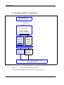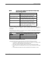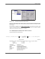
1
Surface Analysis Vacuum Compon Surface Analysis SpecsLab2 Manual Version 2.9 Computer Technology About SpecsLab2 All rights reserved. No part of this manual may be reproduced without the prior permission of SPECS GmbH. User’s Manual for SpecsLab2 Software, Manual Version 2.9 printed 20.10.08. , SPECS GmbH - Surface Analysis and Computer Technology Voltastrasse 5 13355 Berlin, GERMANY PHONE:+49 (0)30 46 78 24 -0 FAX:+49(0)30 4 64 20 83 [email protected] 2 SpecsLab2 Chapter T 1 Installation 1 1.1 R o a d m a p S P E C S i n st a l l a ti o n . . .. .. . .. .. . .. . .. .. . .. . .. .. . .. .. . . 2 1.2 E th e rC a n ( E T H ) w i th E C 1 0 , sh o rt s u m m a r y . . .. .. . .. .. . . 3 1.3 S y s t e m R e q u ir e m e n t s . .. . .. .. . .. . .. .. . .. .. . .. . .. .. . .. . .. .. . .. .. . . 3 1.4 I n t e r f a c e o p t i o n s . . .. .. . .. . .. .. . .. . .. .. . .. .. . .. . .. .. . .. . .. .. . .. .. . . 3 1.5 I n s t a ll i n g Sp e cs L a b 2 . x . . .. .. . .. . .. .. . .. .. . .. . .. .. . .. . .. .. . .. .. . . 4 1 .5 .1 Ins t a ll at io n p rog ra ms : E x am pl e .. .. .. .. .. .. .. .. .. .. .. .. .. .. . 5 1 .5 .2 Wi ndow s ® I ns t al le r . .. .. .. .. ... .. .. .. .. .. .. .. .. .. .. .. .. .. .. .. .. .. . 6 1 .5 .3 S pe cs L ab2 Ins t al la t ion . .. .. ... .. .. .. .. .. .. .. .. .. .. .. .. .. .. .. .. .. . 6 1 .5 .4 Th e Wi ndow s N T /2 00 0 /XP Re gi st r y .. .. .. .. .. .. .. .. .. .. .. .. . 7 1 .5 .5 Runn ing Spe cs L a b2 on Wi ndo ws 20 00 and W in dow s XP w it h non-a dm ini s tr a to r a ccou nt s 8 1.6 I P P r o t o co l R e q u i r e m e n t s .. . .. . .. .. . .. .. . .. . .. .. . .. . .. .. . .. .. . . 9 1.7 E th e rC A N w i th E C 1 0 . . .. . .. .. . .. . .. .. . .. .. . .. . .. .. . .. . .. .. . .. .. 1 1 1 .7 .1 Com me nt s re ga r din g t he E C1 0 .. .. .. .. .. .. .. .. .. .. .. .. .. .. . 1 1 1 .7 .2 S et up f or E C1 0 .. .. .. .. .. .. .. .. ... .. .. .. .. .. .. .. .. .. .. .. .. .. .. .. .. . 1 1 1 .7 .2. 1 1 .7 .2. 2 1 .7 .2. 3 1 .7 .3 1 .7 .3. 1 1 .7 .3. 2 1 .7 .3. 3 S pec s L ab2 Table of Contents Et he r n et c o nn e ct io n . .. .. .. .. ... .. .. .. .. .. .. .. .. .. ... .. .. .. .. .. .. .. .. .. 12 C on fig u rin g t he E C1 0 . .. .. .. ... .. .. .. .. .. .. .. .. .. ... .. .. .. .. .. .. .. .. .. 12 Ru n nin g C on fig ur at io n T oo l . .. .. .. .. .. .. .. .. .. ... .. .. .. .. .. .. .. .. .. 13 S et up w it h se co nd n et w or k ca r d . .. .. .. .. .. .. .. .. .. .. .. .. . 1 5 C abl ing t h e EC 10 w it h a s ec o nd n e tw o rk car d . .. .. .. .. .. .. .. 15 I nst all ing a se c on d ne t w or k c ar d in th e P C . .. .. .. .. .. .. .. .. .. 15 C on fig u rin g t he E C1 0 w ith a se c on d ne t w or k c ar d . .. .. .. .. 16 1.8 I n s t a ll a t i o n o f S p e c s L a b 1 . x . . .. .. . .. .. . .. . .. .. . .. . .. .. . .. .. 1 9 1.9 I n s t a ll a t i o n o f C a s a X P S . .. .. . .. . .. .. . .. .. . .. . .. .. . .. . .. .. . .. .. 1 9 1 2 1.10 S p e c s L a b 2 U p d a t e In st r u c t io n s . . .. .. . .. .. . .. . .. .. . .. . .. .. . 2 0 1.11 G e t I n s ta l l e d Ve r s i o n N u mb e r .. . .. .. . .. .. . .. . .. .. . .. . .. .. . 2 4 1.12 B a c k u p o f R e g i st r y S e tt i n g s .. . .. . .. .. . .. .. . .. . .. .. . .. . .. .. . 2 4 1.13 C l o s e a ll ru n n in g S p e c s A p p l ic a t io n s .. . .. . .. .. . .. . .. .. . 2 4 1.14 U n in s t a l li n g S p e c sL a b 2 . . .. . .. .. . .. . .. .. . .. .. . .. . .. .. . .. . .. .. . 2 4 1 .1 4. 1 U ni ns ta ll in g v e r si ons pr ior to s of tw a r e v er s ion 2 .1 4 . . 24 1 .1 4. 2 U ni ns ta ll in g v e r si on 2 .1 4 an d h igh er . .. .. .. .. .. .. .. .. .. . 2 4 1 .1 4. 3 U ni ns ta ll in g b y ha nd . .. .. .. .. .. ... .. .. .. .. .. .. .. .. .. .. .. .. .. .. . 2 5 Introduction 2.1 O v e rv i e w . .. . .. .. . .. . .. .. . .. .. . .. . .. .. . .. . .. .. . .. .. . .. . .. .. . .. . .. .. . 2 7 2.2 A rc h i t e c tu r e a n d F u n c t io n a l i ty o f Sp e cs L a b . .. . .. .. . 2 7 2.3 S o f t w a r e In st a l la ti o n .. .. . .. . .. .. . .. . .. .. . .. .. . .. . .. .. . .. . .. .. . 2 8 2 .3 .1 I ns t al li ng S pe cs L ab2 .. .. .. .. .. .. ... .. .. .. .. .. .. .. .. .. .. .. .. .. .. . 2 8 2 .3 .2 S t a r ti ng S pe cs L ab2 .. .. .. .. .. .. .. ... .. .. .. .. .. .. .. .. .. .. .. .. .. .. . 2 8 2.4 3 4 C o m m e n t s .. . .. .. . .. . .. .. . .. .. . .. . .. .. . .. . .. .. . .. .. . .. . .. .. . .. . .. .. . 2 9 2 .4 .1 H e lp f or S pe cs L a b2 .. .. .. .. .. .. .. ... .. .. .. .. .. .. .. .. .. .. .. .. .. .. . 2 9 2 .4 .2 S p ec sL a b2 A ppe a ra nce . .. .. .. .. ... .. .. .. .. .. .. .. .. .. .. .. .. .. .. . 3 0 Quick Start 33 3.1 G e tt i n g S ta r t e d .. . .. .. . .. .. . .. . .. .. . .. . .. .. . .. .. . .. . .. .. . .. . .. .. . 3 3 3.2 F i le O p e ra ti o n . . .. . .. .. . .. .. . .. . .. .. . .. . .. .. . .. .. . .. . .. .. . .. . .. .. . 3 4 3.3 D a ta W in d o w .. . .. . .. .. . .. .. . .. . .. .. . .. . .. .. . .. .. . .. . .. .. . .. . .. .. . 3 5 F i l e a nd V i e w M e nu / R e g i o n O pe r a t i on s 37 4.1 F i le s W in d o w .. . .. . .. .. . .. .. . .. . .. .. . .. . .. .. . .. .. . .. . .. .. . .. . .. .. . 3 7 4.2 M e n u F il e / R e g i o n O p e r a t io n .. . .. .. . .. .. . .. . .. .. . .. . .. .. . 3 9 4 .2 .1 N e w F il e / Ne w G ro up .. .. .. .. .. ... .. .. .. .. .. .. .. .. .. .. .. .. .. .. . 3 9 4 .2 .2 N e w Re gio n .. .. .. .. .. .. .. .. .. .. .. .. ... .. .. .. .. .. .. .. .. .. .. .. .. .. .. . 3 9 4 .2 .3 O pen / S a v e / S a ve As / S av e All / C los e . .. .. .. .. .. .. .. .. . 4 0 4 .2 .4 P r in t / Pr i nt P re v i ew .. .. .. .. .. .. ... .. .. .. .. .. .. .. .. .. .. .. .. .. .. . 4 0 4 .2 .5 E x po rt .. .. .. .. .. .. .. .. .. .. .. .. .. .. .. .. ... .. .. .. .. .. .. .. .. .. .. .. .. .. .. . 4 0 4 .2 .6 S e t t ing s .. .. .. .. .. .. .. .. .. .. .. .. .. .. .. ... .. .. .. .. .. .. .. .. .. .. .. .. .. .. . 4 1 4. 2. 6. 1 SpecsLab2 27 S pe c sLab2 X Y D at a F ile S e tt in gs .. .. .. .. .. .. .. .. .. ... .. .. .. .. .. .. 4 1 2 4 .2 .6. 2 4 .2 .6. 3 4 .2 .7 Re st or e A ut os av e .. .. .. .. .. .. ... .. .. .. .. .. .. .. .. .. .. .. .. .. .. .. .. . 4 2 4 .2 .8 Re ce nt F il e s / Ex i t . .. .. .. .. .. ... .. .. .. .. .. .. .. .. .. .. .. .. .. .. .. .. . 4 2 4.3 VAM AS . .. .. .. .. .. .. .. .. .. .. .. .. .. ... .. .. .. .. .. .. .. .. .. .. .. .. .. .. .. .. . 4 3 4 .3 .2 S pe cs L ab2 X Y . .. .. .. .. .. .. .. .. .. ... .. .. .. .. .. .. .. .. .. .. .. .. .. .. .. .. . 4 3 5 .1 .1 5.2 5 .2 .1 5.3 45 Vi si b l e D a t a . .. . .. .. . .. .. . .. . .. .. . .. . .. .. . .. .. . .. . .. .. . .. . .. .. . .. .. 4 5 S ty l e a nd Col or . .. .. .. .. .. .. .. ... .. .. .. .. .. .. .. .. .. .. .. .. .. .. .. .. . 4 5 Vi e w Me n u .. . .. . .. .. . .. .. . .. . .. .. . .. . .. .. . .. .. . .. . .. .. . .. . .. .. . .. .. 4 6 Di ag ra m S et t in gs .. .. .. .. .. .. ... .. .. .. .. .. .. .. .. .. .. .. .. .. .. .. .. . 4 7 To o l b a r s . . .. .. . .. . .. .. . .. .. . .. . .. .. . .. . .. .. . .. .. . .. . .. .. . .. . .. .. . .. .. 4 9 5 .3 .1 M ai n Tool b ar . .. .. .. .. .. .. .. .. ... .. .. .. .. .. .. .. .. .. .. .. .. .. .. .. .. . 4 9 5 .3 .2 Da t a Vi ew .. .. .. .. .. .. .. .. .. .. .. ... .. .. .. .. .. .. .. .. .. .. .. .. .. .. .. .. . 5 0 5 .3 .3 Ana l y ze r Tool ba r .. .. .. .. .. .. ... .. .. .. .. .. .. .. .. .. .. .. .. .. .. .. .. . 5 2 5 .3 .4 Cha nne ls .. .. .. .. .. .. .. .. .. .. .. .. ... .. .. .. .. .. .. .. .. .. .. .. .. .. .. .. .. . 5 4 5 .3 .5 S ty l e .. .. .. .. .. .. .. .. .. .. .. .. .. .. .. ... .. .. .. .. .. .. .. .. .. .. .. .. .. .. .. .. . 5 4 5 .3 .6 S ta t us Ba r .. .. .. .. .. .. .. .. .. .. .. ... .. .. .. .. .. .. .. .. .. .. .. .. .. .. .. .. . 5 4 5.4 C o n t e x t M e n u o f t h e F il e s / R e g io n s W in d o w s . . .. .. 5 4 Ba s i c C o nc e p t s o f O pe r a t i o n 6.1 6 .1 .1 6 .1 .1. 1 6 .1 .2 6 .1 .2. 1 6 .1 .2. 2 6 .1 .2. 3 6 .1 .2. 4 6 .1 .2. 5 6 .1 .3 6 .1 .3. 1 6 .1 .3. 2 6 .1 .3. 3 6.2 S pec s L ab2 E d it M e n u . .. . .. . .. .. . .. .. . .. . .. .. . .. . .. .. . .. .. . .. . .. .. . .. . .. .. . .. .. 4 4 V i e w i n g t he D a t a 5.1 6 D a t a S t r u c t u re .. .. . .. .. . .. . .. .. . .. . .. .. . .. .. . .. . .. .. . .. . .. .. . .. .. 4 2 4 .3 .1 4.4 5 Re se t S e ri aliz er s . .. .. .. .. .. .. ... .. .. .. .. .. .. .. .. .. ... .. .. .. .. .. .. .. .. .. 41 A ut os ave . .. ... .. .. .. .. .. .. .. .. .. ... .. .. .. .. .. .. .. .. .. ... .. .. .. .. .. .. .. .. .. 42 59 A n a l yz e r S e t ti n g s . .. .. . .. . .. .. . .. . .. .. . .. .. . .. . .. .. . .. . .. .. . .. .. 6 0 Ana l y ze r S e r v er .. .. .. .. .. .. .. ... .. .. .. .. .. .. .. .. .. .. .. .. .. .. .. .. . 6 0 D et e ct o r S can . .. .. .. .. .. .. .. .. ... .. .. .. .. .. .. .. .. .. ... .. .. .. .. .. .. .. .. .. 62 S our ce Me t hod / Ser v e r . .. ... .. .. .. .. .. .. .. .. .. .. .. .. .. .. .. .. . 6 3 X RayD um m y se r ve r .. .. .. .. .. ... .. .. .. .. .. .. .. .. .. ... .. .. .. .. .. .. .. .. .. X RayS o ur c e S er ve r . .. .. .. .. .. ... .. .. .. .. .. .. .. .. .. ... .. .. .. .. .. .. .. .. .. m on oX R aySo u rc e S e rv e r . .. ... .. .. .. .. .. .. .. .. .. ... .. .. .. .. .. .. .. .. .. Be am l ine M o no c hr o mat o r Se r ve r . .. .. .. .. .. ... .. .. .. .. .. .. .. .. .. C ha ng e S er ve r O pt io ns an d Er ro r Ha nd lin g .. .. .. .. .. .. .. .. .. .. 64 64 65 65 66 Re mot e Con tr ol .. .. .. .. .. .. .. ... .. .. .. .. .. .. .. .. .. .. .. .. .. .. .. .. . 6 7 D ep th Pr of ile .. .. .. .. .. .. .. .. .. ... .. .. .. .. .. .. .. .. .. ... .. .. .. .. .. .. .. .. .. 67 A MC Mo no c hr o mat o r . .. .. .. ... .. .. .. .. .. .. .. .. .. ... .. .. .. .. .. .. .. .. .. 74 D ela y S e rv er . .. .. .. .. .. .. .. .. .. ... .. .. .. .. .. .. .. .. .. ... .. .. .. .. .. .. .. .. .. 76 R e g io n E d i t W i n d o w . . .. . .. .. . .. . .. .. . .. .. . .. . .. .. . .. . .. .. . .. .. 7 7 3 6 .2 .1 7 R eg ion E dit wi ndow fi e lds . .. ... .. .. .. .. .. .. .. .. .. .. .. .. .. .. . 7 8 6.3 R e g io n s W in d o w . . .. .. . .. .. . .. . .. .. . .. . .. .. . .. .. . .. . .. .. . .. . .. .. . 8 0 6.4 A cq u is i ti o n W in d o w . .. .. . .. . .. .. . .. . .. .. . .. .. . .. . .. .. . .. . .. .. . 8 1 Data Operations 7.1 S y n t a x fo r t h e O p e r a t io n P a r a m e t e rs .. . .. . .. .. . .. . .. .. . 8 4 7.2 B a c k g r o u n d . .. .. . .. . .. .. . .. .. . .. . .. .. . .. . .. .. . .. .. . .. . .. .. . .. . .. .. . 8 6 7 .2 .1 M a t he ma ti ca l De t ai ls of Ba ck gr ound Ca l cul at io n . . 8 7 7. 2. 1. 1 7. 2. 1. 2 7. 2. 1. 3 Lin ear Bac k gr ou n d .. .. .. .. .. .. .. .. ... .. .. .. .. .. .. .. .. .. ... .. .. .. .. .. .. 8 7 S hir le y B ac kg ro u nd . .. .. .. .. .. .. .. ... .. .. .. .. .. .. .. .. .. ... .. .. .. .. .. .. 8 7 Bac k gr o un d co m pu ta tio n af te r T ou g aar d and S ig mu n d. .. 8 8 7.3 F e r m i E d g e . . .. .. . .. . .. .. . .. .. . .. . .. .. . .. . .. .. . .. .. . .. . .. .. . .. . .. .. . 8 8 7.4 L i n e a r O p e r a t io n s .. .. . .. .. . .. . .. .. . .. . .. .. . .. .. . .. . .. .. . .. . .. .. . 9 0 7.5 P e a k F W H M . .. .. . .. . .. .. . .. .. . .. . .. .. . .. . .. .. . .. .. . .. . .. .. . .. . .. .. . 9 0 7.6 P e a k L o c a t i o n . . .. . .. .. . .. .. . .. . .. .. . .. . .. .. . .. .. . .. . .. .. . .. . .. .. . 9 2 7 .6 .1 7.7 M a t he ma ti ca l De t ai ls fo r Pe a k L oca t ion .. .. .. .. .. .. .. . 9 3 S a v i t z k y G o la y S mo o th . . .. . .. .. . .. . .. .. . .. .. . .. . .. .. . .. . .. .. . 9 4 7 .7 .1 8 10 97 M C D C a l ib r a t i o n . . .. .. . .. .. . .. . .. .. . .. . .. .. . .. .. . .. . .. .. . .. . .. .. . 9 7 P r i nt i ng 99 9.1 P r i n t s e t u p . . .. .. . .. . .. .. . .. .. . .. . .. .. . .. . .. .. . .. .. . .. . .. .. . .. . .. .. . 9 9 9.2 P r i n t / P re v i e w . .. . .. .. . .. .. . .. . .. .. . .. . .. .. . .. .. . .. . .. .. . .. . .. .. . 9 9 HSA 3500 Juggler 10.1 101 I n t r o d u c ti o n . .. . .. . .. .. . .. .. . .. . .. .. . .. . .. .. . .. .. . .. . .. .. . .. . .. . 1 0 1 1 0. 1. 1 O v er v ie w .. .. .. .. .. .. .. .. .. .. .. .. .. .. ... .. .. .. .. .. .. .. .. .. .. .. .. .. . 1 0 1 1 0. 1. 2 G e tt i ng S t a r te d . .. .. .. .. .. .. .. .. .. ... .. .. .. .. .. .. .. .. .. .. .. .. .. . 1 0 1 10 .1 .2 .1 10 .1 .2 .2 In st alli ng t he HS A3 50 0 Jug gle r .. .. .. .. .. .. .. .. .. .. ... .. .. .. .. .. . 10 1 S tar t in g th e H SA 35 00 Ju gg le r . ... .. .. .. .. .. .. .. .. .. ... .. .. .. .. .. . 10 2 10.2 1 0. 2. 1 SpecsLab2 D e ri v at i on .. .. .. .. .. .. .. .. .. .. .. .. .. ... .. .. .. .. .. .. .. .. .. .. .. .. .. .. . 9 5 Tools 8.1 9 83 P r o g r a m D e sc r i p t io n . .. .. . .. . .. .. . .. . .. .. . .. .. . .. . .. .. . .. . .. . 1 0 4 G e ner a l .. .. .. .. .. .. .. .. .. .. .. .. .. .. .. ... .. .. .. .. .. .. .. .. .. .. .. .. .. . 1 0 4 4 1 0. 2 .2 S ta r t ing t he P ro gr am .. .. .. ... .. .. .. .. .. .. .. .. .. .. .. .. .. .. .. . 10 5 1 0. 2 .3 Ana l y ze r C ont ro ls . .. .. .. .. .. ... .. .. .. .. .. .. .. .. .. .. .. .. .. .. .. . 10 5 1 0. 2 .4 Volt a ge Di s pla y .. .. .. .. .. .. .. ... .. .. .. .. .. .. .. .. .. .. .. .. .. .. .. . 10 6 1 0. 2 .5 Ra mp Ti me a nd Pu ll Ba ck ... .. .. .. .. .. .. .. .. .. .. .. .. .. .. .. . 10 7 1 0. 2 .6 De t ec tor Cont r ol s . .. .. .. .. .. ... .. .. .. .. .. .. .. .. .. .. .. .. .. .. .. . 10 8 1 0. 2.6 .1 1 0. 2.6 .2 1 0. 2.6 .3 1 0. 2.6 .4 1 08 1 08 1 08 1 09 1 0. 2 .7 Adv a nc ed F unc ti ons .. .. .. .. ... .. .. .. .. .. .. .. .. .. .. .. .. .. .. .. . 10 9 1 0. 2 .8 Q ui tt i ng t he HS A3 5 00 Jug gle r .. .. .. .. .. .. .. .. .. .. .. .. .. . 10 9 10.3 11 I nf o Win do w . .. .. .. .. .. .. .. .. .. ... .. .. .. .. .. .. .. .. .. ... .. .. .. .. .. .. .. .. D ispl ay M o de .. .. .. .. .. .. .. .. .. ... .. .. .. .. .. .. .. .. .. ... .. .. .. .. .. .. .. .. Of fse t an d S cal e .. .. .. .. .. .. .. ... .. .. .. .. .. .. .. .. .. ... .. .. .. .. .. .. .. .. D ispl ay S t yle an d Sp e ed . .. ... .. .. .. .. .. .. .. .. .. ... .. .. .. .. .. .. .. .. A d ju st i n g le n s v o lt a g e s i n c u s t o m i s e d h a r d w a r e S pe cs S py 110 113 11.1 U s e r I n t e rf a c e . .. .. . .. .. . .. . .. .. . .. . .. .. . .. .. . .. . .. .. . .. . .. .. . .. 1 1 4 11.2 E xa m p l e . . .. .. . .. . .. .. . .. .. . .. . .. .. . .. . .. .. . .. .. . .. . .. .. . .. . .. .. . .. 1 1 4 12 Li s t of F i g ur e s 119 13 I nd e x 123 14 Navigation in the SpecsLab2 window 125 S pec s L ab2 5 SpecsLab2 6 Chapter 1 Installation Specs Data Acquisition and Processing Software consists of several components that have to be installed separately on the PC. Which components to install mainly depends on the way one intends to use the software and if one is performing a full installation or an update to the latest software version. The Data Acquisition software SpecsLab was redesigned from scratch and now comes as a new application (SpecsLab 2.x), entirely built on Windows NT/2000/XP. To distinguish the old and new versions (1.x and 2.x) they will be referred to as Specslab1 and SpecsLab2 throughout this document and the installation procedure. Since SpecsLab2 does not yet cover the data processing functionality of SpecsLab1, the latter is provided in this installation to perform analysis tasks such as quantification and fitting. One might as well use any other data processing tool (e.g. CasaXPS, which would make the installation of SpecsLab1 unnecessary) or choose to install these evaluation programs on a different PC. SpecsLab2 acquisition program e.g. CasaXPS evaluation program and/or SpecsLab1 evaluation program P l e a se n ot e ! All installations must be performed with an administrator login. It is necessary to have the operating system CD at hand and ask the network administrator for an IPaddress if the TCP/IP protocol is not already installed on the PC. Different operating systems may cause some differences in windows layout and applications. Please contact your computer specialist. If any problems occur with the installation, please call +49-30-4678240 or send E-mail to [email protected]. SpecsLab2 1 Installation 1 . 1 Ro a d m a p S PE CS i nst a l l a t i o n SpecsLab2 acquisition program ETH typical ETHER CAN connect EC10 box activate the CAN-Bus (Switch on HSA3500) see ’Ethernet connections’ Install TCP/IP network adapter for access to local network (see section ’IP protocol requirements’) Install second network adapter with private TCP/IP network (see ’Second network card’) Install SpecsLab 2 from CD Configure EC10 with IP address from local network Configure EC10 with IP address from private network CasaXPS or SpecsLab1 or ... evaluation program Figure 1.1 Road map for SpecsLab2 installation (See “Non Ethernet-CAN Adapter (PCI, ISA)” on page 137 in 13.2 .) 2 SpecsLab2 EtherCan (ETH) with EC10, short summary 1 . 2 E t h e r C a n ( E T H ) w i t h E C1 0 , s h o r t s um m a r y This chapter is a short summary for a standard EtherCan installation. Following steps should be done for a standard ETH installation (ETHernet, i.e. with an EC10 Ethernet-Can Bus adapter): >STEP 1 : Check ‘System Requirements‘ on page 3. >STEP 2 : Check ‘Interface options‘ on page 3 (standard EC10) >STEP 3 : Follow the procedure ‘Setup for EC10‘ on page 11, i.e. ‘Ethernet connection‘ on page 12 ‘IP Protocol Requirements‘ on page 9 >STEP 4 : Check the section ‘SpecsLab2 Installation‘ on page 6 >STEP 5 : Insert Specs Installation CD. The install shield will start automatically. Select ’Typical ETH’ in the Install Shield Wizard for a standard installation. Please refer to the analyzer manual (PHOIBOS: section 5 ’Operation’ to start acquisition. >STEP 6 : Check the section ‘Configuring the EC10‘ on page 12 ‘Running Configuration Tool‘ on page 13 >STEP 7 : Choose the desired installation for the evaluation program (e.g. the Setup.exe for SpecsLab1 on the installation CD folder for SpecsLab1 or any other data processing tool if not already installed). 1 . 3 S y s t e m R e q u i r e m e nt s • Pentium PC (or better), at least 128 MB RAM (256 MB recommended, 512MB for CCD detector) • Windows NT/2000/XP (NT4.0 Service Pack 6 or higher) • TCP/IP installed SpecsLab requires TCP/IP to be installed on the PC. This is usually the case for all PCs connected to a network or a modem (see “IP Protocol Requirements” on page 9. for installation). • Up to 50 MB of free hard disk space • Ethernet connection or a free PCI slot for a CAN-Bus controller card 1 . 4 I nt e r f a ce op t i o ns Please check at the Test Report (figure 1.2) of the PHOIBOS analyzer which CAN-Bus adapter has been delivered and then either: • Ethernet adapter EC10 (See “EtherCAN with EC10” on page 11 in 1.7 .) or • PCI CAN-Bus card (See “Non Ethernet-CAN Adapter (PCI, ISA)” on page 137 in 13.2 .) or SpecsLab2 3 Installation • ISA CAN-Bus card (See “Non Ethernet-CAN Adapter (PCI, ISA)” on page 137 in 13.2 . must be installed. means EC10 Ethernet adapter is used and delivered Figure 1.2 CAN-Bus adapter type (Test Report page) Please ask the network administrator for an IP-Address for the EC10 (and for an IPAddress for the PC, if TCP/IP not yet had been configured on the PC). Configure your TCP/IP protocol (see section 1.6 on page 9). For a PCI CAN-Bus card you need no additional IP-Address. Either your computer is already linked to a network and has an IP-Address or ask your network administrator for an IP-Address for the PC, if TCP/IP not yet had been configured on the PC and you want to install the data evaluation program SpecsLab1 too. 1 . 5 I n s t a l l i n g S pe c s L a b 2 . x Make sure to be logged in as Administrator. Insert the installation CD. Autorun will start with a section menu. If Autorun is not working please use the file manager and run CD_Explore.exe. Several installations exist on the CD provided. You have to start the desired installation separately. The actual description for the installation programs start in front of the selection menu and is located in software-install-read-me.txt on CD or will be shown if you select the ’Readme first’ item. The SpecsLab2 installation will checks if your Windows platform requires the new Windows® Installer service. If necessary the service will be installed before the Windows® Installer setups will run. 4 SpecsLab2 Installing SpecsLab 2.x 1 . 5 . 1 I ns t al l a t io n p ro gr a m s : E xa m p l e Figure 1.3 Installation CD, menu (CD_Explore.exe) Typical installation Description SpecsLab2 will install SpecsLab2 and EC10 interface software CasaXPS please copy the folder content onto your hard disc, license update code necessary, see specification report Non standard specials if not viewed in the selectable items please use CD content to find the location of the corresponding programs Vci214 CAN-Bus PCI card (only if you use a PCI CAN-Bus card) IXXAT PC-I 03 CAN-Bus card (only if you use a ISA CAN-Bus card) EgControl (only for special electron gun hardware) IgControl (only for special ion gun hardware) The SpecsLab2 installation will checks if your Windows platform requires the new Windows® Installer service. If necessary the service will be installed before the Windows® Installer setups will run. Please complete the installation in the following way: Check the content of the Update folder and copy all files into the corresponding folder (important and necessary!!!). SpecsLab2 5 Installation For example: *.hsa *.raw *.exe *.pdf desired) into into into into \Specs\SpecsLab2\config \Specs\SpecsLab2\tools.bin \SPECS\SpecsLab2\bin \SPECS\SpecsLab2\doc if The pdf files are for your information and can include the newest versions of the manuals. The printed manuals maybe created from an earlier version. Mostly only small improvements are made (which do not influence the normal usage of the printed manuals). Configure the interface to the analyzer supply. (EC10 Ethernet-Can Bus adapter or PCI / ISA - CAN-Bus card) 1 . 5 . 2 W i nd o w s® I ns t a ll e r The Windows® Installer service introduces a faster, more reliable method of application installation. Standardized application installation, enhanced management, and easy customizing of applications are some of the many benefits Windows Installer provides. Another important function of Windows Installer is its ability to diagnose and repair configuration problems when the application is opened. On-demand installation allows the seamless activation of an advertised feature or product without requiring the user to exit from the current program in order to run a separate setup program, a process which often necessitates restarting the computer. 1 . 5 . 3 S p e c s L ab 2 In st a l l at i o n After Windows® Installer is checked or installed the install shield will guide you through the SpecsLab2 installation. All SpecsLab2 executable programs and dynamic link libraries will be installed on the PC. You can choose between a typical (default), compact or customized installation. SPECS recommends the typical installation. For customized installation please contact SPECS service (call +49-30-467824-0 or send email to [email protected]). When the installation has finished and the PC has rebooted, start data acquisition, provided all electronics are properly connected to the PC. SpecsLab2 saves per-user program configuration data. Therefore one would usually not run the program as Administrator, but prefer to use the own user account or one especially created for using SpecsLab2. For Windows 2000 or XP please run SpecsLab2 always as Administrator or with administrator rights for the SPECS program (see ‘Running SpecsLab2 on Windows 2000 and Windows XP with non-administrator accounts‘ on page 8). 8 6 SpecsLab2 Installing SpecsLab 2.x 1 . 5 . 4 T h e W i n d o ws NT / 2 0 0 0 /X P R e g i s t ry The registry is a database that contains information pertaining to the hardware, user and application settings of the computer. The registry is divided up into different sections that are referred to as subtrees. Each subtree contains information that pertains to different aspects of your server. Figure 1.4 Subtrees of the Windows NT/2000/XP registry The SpecsLab2 Software uses two subtrees of the registry: • CURRENT_USER. This subtree contains information about the user who's currently logged onto the computer. This subtree actually points to the user's root key that resides in the Users subtree. • LOCAL_MACHINE. This subtree contains both hardware and software configuration information for the system. Beneath the SOFTWARE root key, one will see subkeys listed for the different software packages loaded on the computer. Microsoft provides the “regedit” tool to allow direct access to the registry. Once one have opened the regedit.exe program, one will notice that it has a very similar look and feel to Windows Explorer, as shown in figure 1.5. One navigate through the folders (trees and keys) in the left panel and one work with items (values) in the right panel. Figure 1.5 Regedit.exe window (has a very similar interface to that of Windows Explorer) SpecsLab2 7 Installation 1 . 5 . 5 R u nn i ng Sp ec sLa b 2 o n W i n d o ws 2 0 0 0 an d W i n d o w s X P w it h no n- ad m i ni s t ra t o r a c c o u nt s To run SpecsLab2 on Windows 2000 and Windows XP with non-administrator accounts It is necessary to set the permission to “Administrator” for the Specs registry branch. Besides REGEDIT, Windows NT/2000/XP has a tool called REGEDT32. This tool is similar to REGEDIT, although perhaps more difficult to use. The most important difference between REGEDIT and REGEDT32 is that REGEDT32 allows setting of permissions on arbitrary registry branches. • • • • • Login as Administrator Start/Run and type regedt32 Choose HKEY_LOCAL_MACHINE chart and go to SOFTWARE\Specs Open the menu Security and select Permission Select the desired user (which will work with SpecsLab2 program) (figure 1.6, page 8) • Do not allow inheritable permissions from parent to propagate to this object! This will pop up a ’Security’ dialog box shown in figure 1.7, page 9. • Select ’Copy’ in this dialog box. • Change the permission to Administrator for this Specs registries, i.e. select the Read and Full Control square (figure 1.6, page 8) • Confirm the changes with OK. • Login as desired user and test SpecsLab2. possible SpecsLab user Read and Full Control should show a mark (but not in grey squares!) Not allow will pop up a window ’Security’ see next figure Figure 1.6 8 Permission for Specs SpecsLab2 IP Protocol Requirements Figure 1.7 Inheritable permission (confirm with ’Copy’) 1.6 IP Protocol Requirements The EC10 as well as SpecsLab2 requires the TCP/IP protocol to be activated on the PC. If the PC is already connected to the network, this will usually be the case. Verify the installation by starting the Network applet in the system's Control Panel (under Start/Settings). Select Protocols and examine the list of installed network protocols. If it does not contain TCP/IP, please add the protocol by clicking on the “Add” button and selecting it from the network protocol list. The figure 1.8 and figure 1.9 shows how to activate and configure TCP/IP. Figure 1.8 SpecsLab2 Select Network Protocol menu 9 Installation Example! Ask your network administrator! Figure 1.9 Network menu Like any other network device, the EC10 must be assigned a unique IP-Address. This IPAddress must be within the same subnet as the PC's IP-Address. Please ask the network administrator for an IP-Address for the EC10 (and for an IP-Address for the PC, if TCP/IP not yet had been configured on the PC). The examples throughout of this document will assume that the following IP-addresses for EC10 (and PC) were obtained: PC's IP-Address: 192.168.236.15 EC10's IP-Address: 192.168.236.16 Subnet mask: 255.255.255.0 (section 1.7.2.2 on page 12) If not sure which IP-Addresses to use, please ask the network administrator. 10 SpecsLab2 EtherCAN with EC10 1.7 EtherCAN with EC10 1.7.1 Co mm en ts regarding the EC10 The EC10 is an external CAN-Bus adapter for the PC. It is connected to the PC via an ethernet network.The PC’s access to CAN-Bus controlled devices like Specs HSA3500 or Specs PCU300 etc. is provided by the EC10. For detailed information about the EC10, including technical data, see the “PHOIBOS Hemispherical Energy Analyzer User Manual”. Communication between the PC and EC10 is handled by the standard TCP/IP network protocol. The section 1.7.2 on page 11 describes the steps to be taken for standard installation of EC10. In most cases it will be sufficient to read this section to make the EC10 ready for operation. Possible reasons for using a second network card • If the number of available IP-Addresses in the network is very limited, the network administrator may refuse to leave an IP-Address for the EC10. So a private network address range can be used. • If the traffic on the network is extremely high, the performance of the EC10 may degrade, or the additional traffic of the EC10 may impede the communication on the network. • If the network is directly connected to the internet without a firewall, a separate network will increase the security against unauthorized access of the EC10. However, the EC10 is password-protected. • If the HUB/switch is a pure 100 MBit device and it can not be configured to 10 MBit. If one or more of the above reasons apply, you will have to use a separate network card. The card as well as the crossover network cable are included in delivery of the Specs system. The section 1.7.3 on page 15 shows how to install EC10 using a second network card in the PC for the communication with EC10. 1 . 7 . 2 S et u p f o r E C 1 0 This section describes the steps to be taken for standard installation of EC10 (no second network card). SpecsLab2 11 Installation 1.7.2.1 Ethernet connection Like other peripherals (e.g. printers, scanners, etc.) the EC10 can be integrated into the network environment of the PC. The figure 1.10 shows how the EC10 is connected to the PC. Terminator PC network cable EC10 CAN-Bus EtherNet card rest of network HUB/switch HSA3500 PCU 300 Terminator Figure 1.10 Standard connection of the EC10 via HUB/switch The EC10 has to be attached to the same HUB or switch that the PC is connected to. The EC10 is a 10 MBit device. Therefore the HUB/switch either must be autosensing between 10 and 100 MBit, or the port where the EC10 is attached has to be manually configured to 10 MBit. If the device is a 10MBit device no action is necessary. Please refer to the manual of the HUB/switch for further details. CAN PC EC10 cross over cable CAN EtherNet card Figure 1.11 Connection of EC10 without network (stand alone) You can use any IP address as long as you are not connected to a network! As in case of the standard installation, make sure that the "LNK" LED of the EC10 and of the network card flash, when the EC10 is powered on. This will indicate that the cabling is correct. 1.7.2.2 Configuring the EC10 • Obtain an IP-Address for the EC10 from the network administrator. If the PC not yet is configured for TCP/IP, obtain an IP-Address for the PC as well. • Activate and configure the TCP/IP protocol on the PC. • Install the Specs software from the SpecsLab CD. 12 SpecsLab2 EtherCAN with EC10 • Connect the EC10 to the HUB/switch using the twisted pair cable (network cable), that came with the EC10. Make sure that the PC is connected to the network as well (figure 1.10 on page 12). • Connect the CAN-Bus devices (HSA3500, PCU300 etc.) to the EC10 using the CAN-Bus cables provided by Specs. See the “PHOIBOS Hemispherical Energy Analyzer User Manual” for correct cabling. • Run the EC10 configuration tool EC10Config on the PC (section 1.7.2.3 on page 13). This tool will configure the EC10 with the IP-Address obtained from the network administrator. The usage of EC10Config is described below. 1.7.2.3 Running Configuration Tool After obtaining an IP-Address for the EC10, the EC10 must be configured to use this address for communication. This configuration has to be done only once. If the IPAddresses in the network requires changing, it may be necessary to also rerun the configuration program. • Power on the HSA3500. The HSA3500 will provide power supply for EC10. Check the correct network connection of the EC10: the LED "LNK" at the front side of the EC10 must flash. • Start the program EC10Config.exe from Start->Programs->Specs. • Enter the IP-Address of the EC10 into the field IP-Address. • Click on the "RUN" button. The EC10Config window should look like figure 1.12 below. Figure 1.12 EC10 configuration tool running • Now press and hold the "CFG" button at the rear side of the EC10 for at least 2 seconds. (use a ball pen or another pointed object to do this) The EC10 will indicate the configuration process by shortly flashing the LEDs "PWR", "SER", "CAN" and "ONL" two times. SpecsLab2 13 Installation If the configuration succeeded, the EC10Config window should look like this: Figure 1.13 EC10 configuration tool successful The EC10 is now configured and ready to use with the Specs software. If the configuration fails, the program will give an error message. The most common error messages and causes for failure are: • "ERROR: No Response from Device" The IP-Address to which the EC10 shall be configured is not reachable by the PC. Please check that the IP-Address has been entered correctly and retry the configuration. It is very important that the IP-Address of the PC and of the EC10 belong to the same subnet of the network. • "ERROR WSAStartup() failed" Please make sure that the TCP/IP protocol on the PC is activated and configured correctly. • “ERROR: bind() failed" There may be another program running on the PC that occupies the port number (UDP, 1962), that the configuration program will use. Please try to terminate all processes on the PC that are not absolute necessary, then retry the configuration process. If the configuration tool gives no message at all, and looks like figure 1.12 after pressing the "CFG" button, the network connection between PC and EC10 may be not working correctly. Please check the network cables between PC and HUB/switch and between HUB/switch and EC10. Final check: >STEP 1 : Start/Run and type ’regedit’ >STEP 2 : /HKEY_LOCAL_MACHINE/SOFTWARE/Specs/DeviceNetServer >STEP 3 : Check the parameters as shown in the figure below. “192.168.236.16” Figure 1.14 14 IP address of the EC10 (IP address : local network address space) Registry entry for (Ethernet) ETH CAN-Bus SpecsLab2 EtherCAN with EC10 1 . 7 . 3 S et u p w i th s ec on d n et w o r k c a rd 1.7.3.1 Cabling the EC10 with a second network card The figure 1.15 shows the cabling of the EC10 with a second network card. CAN PC EC10 cross over cable CAN 1. EtherNet card 2. EtherNet card Figure 1.15 Connecting of the EC10 directly to the PC P l e a se n ot e ! The network card and the EC10 have to be connected using the special network "crossover" cable, which is included in delivery of the Specs components. As in case of the standard installation, make sure that the "LNK" LED of the EC10 and of the network card flash, when the EC10 is powered on. This will indicate that the cabling is correct. 1.7.3.2 Installing a second network card in the PC The following installation instructions apply for the adapter delivered by SPECS. If another kind of network card shall be used, read the respective installation instructions. Shut down the PC and disconnect it from the line voltage. voltage Open the PC, find a free PCIBus slot and insert the card from the box "Advanced Network Adapter". Close the PC, reconnect it to the line voltage and boot. Insert the CD that came along with the card into the CD-ROM drive. It may be possible that the Internet Browser is launched after the CD is inserted. It will show some information about the network card. The information is of no further interest and the window can be closed. If running Windows 2000, the operating system will announce that it has found newly installed hardware and will ask for a driver CD. Install the driver from the CD. Under Windows NT/2000/XP, go to Start -> Settings -> Control Panel -> Network. Click on "Adapters" and then on "Add...". Click on "Have Disk...". One will be asked to enter the path to the driver. If the CD-ROM drive had the drive letter R:, the path to enter would be: R:\drivers\kf-310\winnt40 SpecsLab2 15 Installation 1.7.3.3 Configuring the EC10 with a second network card The rest of the configuration is the same as in the standard case and is described in ‘Running Configuration Tool‘ on page 13. Figure 1.16 Network menu Now click on "OK" to install the driver. Choose duplex mode (see figure 1.17 on page 16) and press “OK”. Figure 1.17 16 Duplex mode menu SpecsLab2 EtherCAN with EC10 Assign an IP-Address for the new card and for the EC10 freely, but some restrictions must be observed: • The second network card must not have the same IP-Address and must not be in the same subnet as the first network card. • The PC and the EC10 must have different addresses, but must be within the same subnet. • Do not use IP-Addresses that will be accessed through the first network card. We recommend to use the following IP-Addresses: PC's IP-Address: 192.168.236.15 EC10's IP-Address: 192.168.236.16 Subnet mask: 255.255.255.0 If not sure which IP-Addresses to use, please ask the network administrator. Click on the “Bindings” file card to make the new driver available for the protocol configuration. Click on the file card “Protocols”, select the TCP/IP protocol and click on “Properties” (see figure 1.18 on page 18). Select the new card and specify an IP address and a subnet mask. The default gateway field can be left empty. Press “OK” and close the menu to finish the installation. After finishing the installation and configuration of the second network adapter, reboot the PC to activate the new card. SpecsLab2 17 Installation Figure 1.18 TCP/IP Properties menu Please reinstall the Service Pack 6 now from your Windows NT install CD or check the SPECS installation CD for service pack updates (e.g. WinNT4.0-sp6a). 18 SpecsLab2 Installation of SpecsLab 1.x 1.8 Installation of SpecsLab 1.x If not updating from a previous SpecsLab installation and are wanting to use SpecsLab1 as a data processing tool, some more components have to be installed. These components are located in the folder SpecsLab_1.x on the installation CD. Read the SpecsLab 1.x manual for further instructions. Additionally either a TCP/IP network adapter for access to local network must be installed or you have to install at least a MS-Loopback protocol to use SpecsLab1 Figure 1.19 MS-Loopback adaptor for SpecsLab1 1.9 Installation of CasaXPS If not updating from a previous installation and use CasaXPS program as a data processing tool, some more components have to be installed. These components are located in the folder CasaXPS on the installation CD. Simply unzip the CasaXPS.zip file. (Copy the unzipped folder from CD to your hard disk and run may cause errors, because of incorrect folder permissions for CasaXPS) .Create a shortcut to your desktop and start menu if desired. Read the CasaXPS manual (doc folder) for further instructions. SpecsLab2 19 Installation 1.10 SpecsLab2 Update Instructions Please read installation. these instructions carefully before updating your SpecsLab2 In case of updating from an earlier version of SpecsLab2 please uninstall this software package first before installing the new version. Please note that personal settings for SpecsLab2 like detector shifts or IP addresses for an ec10 CAN adaptor may be lost, so a registry backup (rename) of that data is highly recommended. Additionally installed software e.g. drivers for CAN bus Adapter or CCD camera should be updated if newer software versions are delivered with the new SpecsLab2 installation disk. For all installation tasks make sure to be logged in as Administrator. If you have any problems with updating your SpecsLab2 installation, please call +49-304678240 or send an email to [email protected]. Update with CDROM (please note the comments in the paragraphs after this summary as well) >STEP 1 : Close all SPECS programs. See “Close all running Specs Applications” on page 24 in 1.13 . >STEP 2 : Open Task-Manager (Ctrl-Alt-Del), find the 'ObjectServer.exe' task and kill this task (End Process) Figure 1.20 >STEP 3 : 20 Task-Manager Copy the /Program Files/SpecsLab2 folder onto your hard disk to a SpecsLab2.original folder. SpecsLab2 SpecsLab2 Update Instructions SpecsLab2 >STEP 4 : Start 'RegEdit' application (e.g. by 'Run...' via Start menu and see see section 1.5.4 , ‘The Windows NT/2000/XP Registry‘ on page 7), >STEP 5 : Locate the 'HKEY_LOCAL_MACHINE\SOFTWARE\Specs' tree. >STEP 6 : Check your existing analyzer type: Select the folder Phoibos-Hsa3500 inside the SPECS folder of the registry and note the strings ’Model’ and ’Workfunction’ (e.g. ’150R5c’ and ’4.5’). This values should be the same after the update (if not replace the new values). >STEP 7 : Export (File/Export) the registry folder of your analyzer model, which is located inside this Phoibos-Hsa3500 registry folder into a file (e.g. 150-R6.regold.yymmdd.backup). See figure 1.21, ‘Export analyzer adjustments ,‘ page 22. This file include all calibration shifts and transmission settings, which may be modified during a MCD calibration or other adjustments. If you did not perform any MCD calibration by yourself before, you can skip this procedure! 21 Installation Example for analyzer model 150R5c and include MCD calibration, Transmission values, which perhaps modified during calibration procedures (after installation). Figure 1.21 Export analyzer adjustments >STEP 8 : Export the complete SPECS registry folder into a file (for example to SPECS.regold.ddmmyy.backup). This file include all old registry entries and maybe helpful for diagnostic purpose (see figure 1.21 on page 22 select SPECS tree instead). >STEP 9 : Insert the installation / update CD and select SpecsLab2 installation. >STEP 10 : See “Uninstalling SpecsLab2” on page 24 in 1.14 .! If the SpecsLab2 was installed with the Windows® Installer you have to choose ’Remove’ to remove the program first (otherwise the SpecsLab2 installation will start. Figure 1.22 22 Install Shield Wizard SpecsLab2 SpecsLab2 Update Instructions >STEP 11 : Select ’Remove’ or uninstall as described in section 1.14 on page 24 >STEP 12 : It may be useful to reboot the computer after uninstalling. >STEP 13 : Run the Upgrade CD again (Autorun or open CD_Explore.exe) and start the SpecsLab2 installation. >STEP 14 : Select the already installed CAN type of your analyzer (EtherCAN with EC10, see 1.7 ,, PCI CAN-Bus card, see 13.2.2 ,ISA CAN-Bus card, see 13.2.3 ) The actual layout may differ! Please select your communication and power supply type! (standard = ETH+HSA3500) Figure 1.23 >STEP 15 : CAN installation type Mostly it is faster, easier and first of all always a good idea to repeat the calibration for the usually slit/lens combination again. If you did not perform any MCD calibration by yourself before, you can skip this procedure! Import the saved registry file for your analyzer model to reinstall the modified MCD or transmission values. Compare the path of the exported registry folder of your analyzer model (>STEP 7 : page 21) to the new path of registry folder of your analyzer model. Older analyzers maybe have not the same path like the new installation. Import (by double click) will not work! Please contact SPECS if you want to use your former MCD shifts. SpecsLab2 >STEP 16 : Check the ’Model’ name of the analyzer in the new registry path (select Phoibos-Hsa3500 and control the Model string, should be the same as before. Replace the ’Workfunction’ string to the old values if necessary. >STEP 17 : Copy/Paste the CasaXPS folder if you need an upgrade for the evaluation program. Re-enter the License in the CasaXSP Help menu (About CasaXPS) >STEP 18 : Check if there are new files in the Update folder of the CD. Copy/Paste all files to the location of the original file (which are the 23 Installation older versions, you note this by an older date or a different file name). Note: If you get trouble with IP addresses, MCD shifts or any other problem, please mail the renamed original registry file and the new one to SPECS and we will modify for you (export both SPECS registry trees into a file). 1.11 Get Installed Version Number To check the installed version of SpecsLab2 please start SpecsLab2 and open the “About SpecsLab” dialog in the Help menu entry. 1 . 1 2 B a c k u p o f R e g i s t r y S e t t i n gs Start the registry editor regedit (select Start / Run / Open regedit). Select the key HKEY_LOCAL_MACHINE\Software\Specs and save the current registry settings via the menu entry Registry / Export Registry File (see figure 1.21 on page 22). 1.13 Close all running Specs Applications All open Specs applications must be closed first. (To make sure that SpecsLab2 and all related applications are definitely stopped you may want to reboot the system.) The Specs ObjectServer running in background must be stopped via the Task-Manager. Open the Task-Manager (Ctrl-Alt-Del), find the 'ObjectServer.exe' task and apply End Process. 1.14 Uninstalling SpecsLab2 Depending on the installed version of SpecsLab2 the deinstallation must be done differently. To check the installed version of SpecsLab2 please start SpecsLab2 and open the “About SpecsLab” dialog in the Help menu entry. 1 . 1 4 . 1 U ni n st a l li n g v e r si o n s p r i o r t o s o f t wa r e ve r s io n 2 . 1 4 Click Start / Settings / Control Panel and start the Add/Remove Programs application. Select SpecsLab2 and start removing this software package. 1 . 1 4 . 2 U ni n st a l li n g v e r si o n 2 . 1 4 an d h i g h er Click Start / Settings / Control Panel and start the Add/Remove Programs application. Select SpecsLab2 and start removing this software package. Use Remove in the InstallShield Wizard to remove the SpecsLab2 program. 24 SpecsLab2 Uninstalling SpecsLab2 1 . 1 4 . 3 U n in s ta l l in g b y ha nd If you need to remove SpecsLab2 completely by hand (may be in case of corrupted registry entries caused by operating system errors) use the following instructions: SpecsLab2 >STEP 1 : Open TaskManager (Ctrl-Alt-Del), find the 'ObjectServer.exe' task and kill it. >STEP 2 : Start 'RegEdit' application (e.g. by 'Run...' via Start menu), locate the 'HKEY_LOCAL_MACHINE\SOFTWARE\Specs' tree, delete it (you can also do an export for backup purposes first) >STEP 3 : Locate the SpecsLab2 installation directory (e.g. C:\Program Files\Specs), delete the directory and all subdirectories (if you can't delete retry after the next reboot, but do the following steps first). >STEP 4 : Open a Windows Explorer (e.g. by right mouse click on Start menu), locate all <windows installation directory> \Profiles\<user>\StartMenu\Programs\Startup (e.g. C:\WINNT\Profiles\All Users\Start Menu\Programs\Startup) and delete the 'ObjectServer' link >STEP 5 : Delete the <windows installation directory> \Profiles\<user>\StartMenu\Programs\Specs (e.g. C:\WINNT\Profiles\All Users\Start Menu\Programs\Specs) directory also. 25 Installation 26 SpecsLab2 Chapter 2 Introduction 2 . 1 Ov e r v i e w SpecsLab2 is an interactive program designed to support data acquisition and data processing for energy dispersive measurements. The interface to the data acquisition equipment known to SpecsLab2 provides access to a number of different acquisition methods. The access to the measurement equipment is separated from the SpecsLab2 tool, thus a wide range of analyzers can be controlled. This way an easy adoption to different measurement equipment is possible without changing the data acquisition tool. SpecsLab2 currently runs on the Microsoft Windows NT/2000/XP (NT with at least Service Pack 5) operating system and needs 200 MB free disk space. For different acquisition methods specialized data processing functions are provided, i.e. satellite subtraction for XPS spectra, specialized background subtraction methods and data base lookups based on the selected method. 2 . 2 A r ch i t e c t ur e a nd F un ct i o na l i t y o f S pe csL a b In 2000 the company undertook a new software project called SpecsLab2, which combines the advantages of a new software architecture with the rich data processing facilities of SpecsLab1. The functionality of SpecsLab2 is extensible under a number of public CORBA (Common Object Request Broker Architecture) interfaces. These interfaces can be implemented for special user purposes, i.g. controlling a special excitation source. This extensibility covers the following aspects: • • • • • SpecsLab2 File I/O (additional file formats) Numerical operations on region data Additional excitation sources Arbitrary synchronous remote actions during data acquisition Data acquisition in general 27 Introduction One of the advantages of using the new architecture is that the process of implementing a given interface and making the implementation available to SpecsLab2 is nearly identical for all aspects described above. The following figure gives an overview of SpecsLab2’s software components and how they relate to each other. Dashed lines denote CORBA service startup. The solid lines indicate SpecsLab2’s access to the services through the CORBA interfaces. All components except SpecsLab2 itself are located and started by a central component, the ObjectServer, which must be active before SpecsLab2 is started by the user. The Objectserver integrates the various services (operation, serializer, ...) and makes them available to SpecsLab2. SpecsLab ObjectServer Source Remote Operation Figure 2.1 Serializer Analyzer DeviceNet Architecture and Functionality of SpecsLab Through this architecture it is possible to reconfigure or retrofit services while SpecsLab is in operation. 2 . 3 S o f t w a r e I ns t a l l a t i o n 2 . 3 . 1 In s t al l i ng S p ec sLa b 2 You must install the application from the SPECS CD onto your hard disk; you cannot run the program from CD. Installation instructions are available in the Install file on the CD. 2 . 3 . 2 S ta r t i ng Sp ec sLa b 2 You start SpecsLab2 just as you would any other application. To start do one of the following: • Choose Start > Programs > Specs > SpecsLab2 28 SpecsLab2 Comments 2 . 4 Co m m e n t s SpecsLab2 is developed to run under Windows operating system and therefore the most common window functions (context menu, Tool bar handling, shortcuts, print windows, ...) which you know from other programs are available. SpecsLab2 provides the following types of command shortcuts: • Keyboard shortcuts • The context (shortcut) menu, whose commands depend on the location of the pointer • The Tool bars, which contains commonly used commands for the different SpecsLab2 windows The context (shortcut) menu contains commonly used commands for the item under the pointer. You can display context menus when the pointer is in the window. To display a context menu: Right-click. With the item Toolbars of the View menu you can select the visible Tool bars for each SpecsLab2 sub window. You can keep the Toolbars open in the work area and click commands as you need them as well as being able to move the Toolbars to the place of your choice on-screen. The Keyboard shortcuts to activate menu items are shown in the menu pop up. For example, CTRL+O to open a file or CTRL+S to save. 2.4.1 He lp for S pe csLab 2 Under the Help menu of SpecsLab2, you can find out particular details of the program under the About Specslab menu option. This is useful for knowing what version of the software you are using, in the event you require support from SPECS ([email protected]). There is also a shortcut to this manual from within the program, under Online Manual. Here all typical search functions are available. SpecsLab CD includes the complete documentation as a pdf file as well as in the online Help, including all of the information in this user guide. SpecsLab2 29 Introduction You start SpecsLab online Help in the following way: • Choose Help > Online Manual 2 . 4 . 2 S p e c s L ab 2 Ap p e a ra n c e Following windows are available in the SpecsLab2 User Interface: • • • • • Files several Data windows Regions Region Edit Acquisition Figure 2.2 SpecsLab window The normal start up of the program is shown figure 2.2. Beside the Data window (‘Data Window‘ on page 35), where the acquisition data will be displayed, the Regions window shows the complete region list (‘Regions Window‘ on page 80). Inside the Region Edit window parameters of a single or multiple regions can be set (‘Region Edit Window‘ on page 77). 30 SpecsLab2 Comments The complete actual structure of the loaded and created data files is shown in the Files window (‘Files Window‘ on page 37). This window is used to select a region / groups or complete files for further manipulation. Within the Acquisition window the status of regions which have been validated can be changed to “waiting for acquisition” or vice versa (‘Acquisition Window‘ on page 81) (). In the Wi nd o w menu you can select the visible SpecsLab2 windows described above. Before the program is terminated the current window layout will be saved. SpecsLab2 31 Introduction 32 SpecsLab2 Chapter 3 Quick Start 3.1 Getting Started • Switch on all required power supplies for your sources and the analyzer supply. • Set the desired excitation conditions. • Start SpecsLab2 and open the item Settings in the menu Analyzer and select the installed analyzer type. • Open the windows in the Windows menu: • Files • Regions • Regions Edit • New Data Window • Do one of the following: - press the New Region icon - or choose the item New Region in the File menu - or press CTRL+R this will add a new file/group/region entry in the Files window and allow you to set your parameter in the Region Edit window. • Select the Region Edit window • set the desired parameter for acquisition. For example: Figure 3.3 SpecsLab2 Quick Start Example: Region Edit 33 Quick Start • Check the recommended detector voltage Udet (see specification of your analyzer) • Validate the parameter set • Start Acquire This starts the data acquisition. The spectrum will now build up in the Data Window. For detailed description of all functions and parameter settings please check the corresponding chapters in this manual. For quick access to your first measurement a short introduction about the File operation and Data window handling follow. 3 . 2 Fi l e O p e r a t i o n Use the above shown menu / icons to Load / Save / Save All data or simply use the File menu item O p e n (CTRL+O) to load files, S a ve (CTRL+S) or S a ve A s (CTRL+A) to save the measured data region in a file or S a v e A l l (CTRL+L) to save the complete file structure shown in the Files window. Select the SpecsLab data format for this operation in the standard window file select box. The default SpecsLab format is set to *.xml (SpecsLab2XMLDataFile). 34 SpecsLab2 Data Window 3 . 3 D a t a W i nd o w Figure 3.4 Data window Inside the data window it is possible to zoom the area of interest. Simply use the drag function of the mouse to zoom into the desired intensity and energy range. Use the Data window Tool bar icons to go forward/backward within the zoom steps or rescale the window as well as select the cursor option and set the autoscale function. Please use the mouse and hold a few seconds on the icon to find out the functions. For the data window layout please use the ‘Diagram Settings‘ (page 47) in the View menu. SpecsLab2 35 Quick Start 36 SpecsLab2 Chapter 4 File and View Menu / Re gion Ope r ations 4.1 Files Window The logical data file structure of SpecsLab is shown in the Files window (select the item Files in the menu Window to display this window) Figure 4.1 File structure in the Files window Complete files, groups or a single region can be manipulated just as in other standard windows applications. For example: move a Region or Group via drag and drop to the desired location within the file tree in the File window. These commands are very helpful when organising your file structure. SELECTION RULES Select several R E G I O N S in the R e g i o n s window: - SHIFT and left mouse click for regions in a row - CTRL and left mouse click to mark several single regions or select one R E G I O N in the F i l e window. You cannot manipulate regions that are currently being used for acquisition! SpecsLab2 37 File and View Menu / Region Operations SpecsLab can handle several files of data (file name with path). Each Fi le (experiment) is structured in G r o u p s and R e g io n s . The regions can be easily sorted into different groups using drag and drop (into groups) or the common Edit operations as well as the context menu operation. Groups are mainly used to structure a large amount of spectra. Using groups may help in cases where more than one set of regions have separated from experimental or logical structure. With different files, complete experiments are easy to compare and easy to handle. The File menu gives access to all necessary file operation as well as the icons in the Main Tool bar Figure 4.2 File menu and Main Tool bar icons Use above shown menu / icons to • O p e n . . . (CTRL+O) files, • S a v e (CTRL+S) or S a ve A s . . . (CTRL+A) to save the measured data regions in a file or • S a v e A ll (CTRL+L) to save the complete file structure shown in the Files window (all files). Please note: If no file is selected, the items S a v e and S a v e A s . . . as well as C l o s e are disabled. 38 SpecsLab2 Menu File / Region Operation 4 . 2 M e n u F i l e / R e g i o n O pe r a t i o n 4 . 2 . 1 N ew F i l e / N ew Gr o up N e w Fi le creates a new file as a root for groups and regions. Single Files can be saved separately with S a v e or S a v e A s . . . in the file menu. New Groups add a new group to the selected File, or create a group in a new file if no file was selected. 4 . 2 . 2 N ew R e g i o n For a new experiment simply add a region (menu File: N e w Re g io n ). The new region appears in the Files window as well as in the Regions and Region Edit window inside the selected file and group. Note: The energy values chosen in the Data window display (zoom function or other regions displayed) will be used as the start and end values for the new region. If a region has already been selected, all region parameters (except start and end, see above) of this selected region will be used to create a new region (Lens Mode, Slit,...). No selection creates a new file and a new group with default parameters. The Files and Regions window shows also the actual status of the region. • ? - means no data inside. • A black arrow shows that the regions are validated. • A black solid arrow indicate that the regions are validated and in progress for measurement. Within the Acquisition window the currently performed and the waiting regions can be checked and changed. • A red solid arrow indicates that the measurement is in progress. • No extra sign at the region label indicates a region with data. Figure 4.3 SpecsLab2 File structure (with empty region and default names) 39 File and View Menu / Region Operations 4 . 2 . 3 O p en / Sa v e / S av e A s/ Sa v e Al l / C l o s e With these operations, files can be loaded, saved, or closed. The keyboard shortcut or the Toolbar icon for this operation allow quicker access. Use the above shown Toolbar icons to Load / Save / Save All data or simply use the File menu item Op en (CTRL+O) to load files, S a ve (CTRL+S) or S a v e A s (CTRL+A) to save the measured data region in a file or S a v e A ll (CTRL+L) to save the complete file structure shown in the Files window. The C lo s e operation will close the selected file after confirmation for save when data are changed. Select the SpecsLab data format for the load and save operation in the standard window file select box. The default SpecsLab format is set to *.xml (SpecsLab2XMLDataFile). 4 . 2 . 4 Pr i n t / P r in t Pr e v i ew This file menu works the same as for all standard windows applications. Pr i nt pops up the default printer box whereas the desired printer and its parameters can be choosen depending on your computer configuration. The P r in t Pr e v ie w item allows to check the print layout in front of your printing. See also ‘Printing‘ on page 99. 4.2.5 Export The E x p o r t function allows you to save the data in non SpecsLab2 format. The possible formats are shown in the export window, using the pull down selection box for the export type. Figure 4.4 40 Export window SpecsLab2 Menu File / Region Operation Please refer to ‘Data Structure‘ on page 42. 4 . 2 . 6 S et t i n g s The menu allows to set the S p e c s L a b 2X Y format convention as well as Au to s a v e options and allows to perform a reset of the S e r i a li ze r operation. Figure 4.5 File / Settings 4.2.6.1 S p e c s L a b 2 X Y D a t a F i le S e t t i n g s Figure 4.6 SpecsLab2XY Data File Settings This options allows to modify the structure (separate scan and channel output yes or no) and syntax (prefix) for the export of the intensity and energy data to a x,y - ASCII file using the export function (‘Export‘ on page 40). Note that the options influence the value for the intensity. 4.2.6.2 Reset Serializers This item resets the Serializer program (Load / Save / Export). If the process of write or read is terminated the Serializer program will be canceled and then restarted. SpecsLab2 41 File and View Menu / Region Operations The S e r i a li ze r is a stand-alone executable which converts the complex SpecsLab2 data for the file operations Load / Save and Export. If any trouble with file handling arises, please use this function to get a fresh Serializer status. 4.2.6.3 Autosave The Au to sa v e option allows to set how often the autosave function will occur. Figure 4.7 Autosave options Autosave will be performed if the Minimum (time) Interval has been reached. 4 . 2 . 7 R e st o r e A u to sa v e This function allows you to restore the last saved data structure, i.e. all files including groups and regions, that were open when SpecsLab2 was previously closed (figure 4.7, ‘Autosave options ,‘ page 42). 4 . 2 . 8 R e c e nt F i l e s / E x it The recent files are sorted below the Print Setup item within the File menu. The most recently used files can be simply loaded into SpecsLab2. E xi t closes the SpecsLab program. If you have changed data or have an acquisition running, you will receive a confirmation window to cancel/abort, or save to this data. 4.3 Data Structure For file operations, select the SpecsLab data format in the standard file dialog box. • The default SpecsLab2 format is set to S p e c s L a b 2 X M L Da t a F i le f o rm a t (* . xm l ). though other supported formats are listed following this one. (Extensible Markup Language (XML) is intended for data exchange and publishing on the World Wide Web. Like HTML, XML uses elements and structure. XML differs from HTML in that it is extensible; users may define a 42 SpecsLab2 Data Structure custom set of element tags. XML provides users with more powerful capabilities than HTML. XML defines an extremely simple dialect of SGML. SGML is the Standard Generalized Markup Language (IS O 88 7 9: 19 8 ), the international standard for defining descriptions of the structure of different types of electronic documents. • The S p e cs L a b 2 B i na r y Da t a F il e f o r ma t ( *. b in ) is used to compress file size. and the following file formats which may result in a loss of information, when read back into SpecsLab2, but may be more convenient and/or portable for some SpecsLab2 users: • V A M A S D a ta F il e (* . v ms ) conforms to the ISO Surface Chemical Analysis Data Transfer Format (IS O 14 9 76 ) (see section 4.3.1 , ‘VAMAS‘ on page 43) • S p e c s L a b 2 X Y D a t a F i le ( *. x y) export the data in x,y ASCII files (see section 4.3.2 , ‘SpecsLab2XY‘ on page 43). • S p e c s L a b 1 D a t a F i le s ( *. e x p ) use the SpecsLab 1 data file format (see SpecsLab1 manual). 4.3.1 VAMAS The VAMAS format allows data from any system to be read by any compatible software to allow Quantitative Surface analysis. The VAMAS format is very general in order to accommodate elemental maps, depth profiles, and data sequences arising from the compatible methods A ES , EDX, FABMS, I S S , SIMS, SNMS, U P S , XP S , XRF. In 1988, the S u r f a c e C h e m ica l A n a ly s is S ta n d a r d D a t a T r a n s f e r F o r ma t was developed by various users and manufacturers in the VAMAS community. For the VA MAS format convention (VAMAS Surface Chemical Analysis Standard Data Transfer Format 1988 May 4) please refer to VAM AS ( ht t p:w w w.v a ma s .o rg ). 4.3.2 SpecsLab2XY Choosing the SpecsLab2XY format, export will convert the data to x,y type for further processing. Please note the possible settings in the File/Settings menu ( ‘Settings‘ on page 41). X,Y format structure: # # # # # # # SpecsLab2 Group: Group1 Region: MA9 Anylsis Method: XPS Analyzer: PHOIBOS HSA3500 150 R5 MCD-9 Analyzer Lens: MediumArea Analyzer Slit: 2:7x20\2:open 43 File and View Menu / Region Operations # Scan Mode: FixedAnalyzerTransmission # Number of Scans: 1 # Curves/Scan: 1 # Values/Curve: 263 # Dwell Time: 0.1 # Excitation Energy: 1253.6 # Kinetic Energy: 881.659 # Pass Energy: 9 # Bias Voltage: 90 # Detector Voltage: 2200 # Eff. Workfunction: 4.4 # Source: XRayDummy # # Cycle: 0, Curve: 0 # 881.65923 33720 881.68719 32870 881.71515 33190 ... 4.4 Edit Menu The Edit menu does not differ from the common edit operations in many windows applications. The parameter of the selected file, group or region will be C o p y to the clipboard. The P a s te operation allow to place the clipboard data to a selected place within the file structure. Copy Diagram copies the active Data window to the clipboard for further processing in standard windows applications. Please use (if desired) the common keyboard shortcuts as well as the standard icons for these operations. 44 SpecsLab2 Chapter 5 V ie w ing the D a ta 5.1 Visible Data In the Files or Regions window, the selection for visible groups / regions (shown in the Data window) will be done by double-clicking on the data icon or selecting the V i s i b l e item in the context menu (section 5.4 on page 54). The visible groups / regions in the Data window are marked with a colored data mark depending on the chosen data style for this region (here a solid red line). Figure 5.1 Visible data In figure 5.1 the region Ep30 is visible in the Data window. Because one region in this group is set to visible, the icon of the visible region as well as the group icon Medium Area is enabled, whereas all other group icons are disabled. 5 . 1 . 1 S t y le a nd C o l o r With the context menu or the shown icons in the Tool bar below, the color and style of each measured region can be set. This allows for easy comparison and handling of region data. SpecsLab2 45 Viewing the Data Note the ‘SELECTION RULES‘ on page 37. Figure 5.2 Color and Style Toolbar and Context menu The possible styles are shown in the Toolbar box above. Sizes of the different marks can be set between 1 and 9 mm. The color table is the common Windows color table with basic and user defined colors. 5.2 View Menu Figure 5.3 View Menu The appearance of the View menu is shown in figure 5.3. Several possibilities to set the Data window style and parameter exist beside the selection of the visible Toolbars. This content of the View menu conforms to the Tool bar D a t a V ie w (see section 5.3.2 on page 50), except the D ia g r a m S e t t in g s item.The Diagram Settings is explained in paragraph section 5.2.1 and the other View menu items are described in the corresponding Toolbar sections in section 5.3 ‘Toolbars‘ on page 49. 46 SpecsLab2 View Menu 5 . 2 . 1 D i ag ra m Se t t in g s The D ia g r a m S e tt i ng s item within the View menu shows a property window with several property sheets for your Data Windows. Choose the desired sheet from the window via the named Tabs to edit the default parameter. Some sheets can be restored to their default settings by pressing the “Restore Defaults” button: Figure 5.4 Title property sheet Use the T i t le sheet to set your desired title in the top of the Data Window as well as for the print. The P ri nt In fo field allows to write a comment for your experiment. The size of the Print Info should adapt to your chosen printer setting (Landscape / Portrait). You can also check the Print Preview in the File menu before printing. See ‘Printing‘ on page 99. Figure 5.5 X Axis property sheet In this sheet the long name of the X axis labels can be edited. Which axis label appears in the Data Window depends on the scanned parameter for the region. SpecsLab2 47 Viewing the Data Figure 5.6 Y Axis property sheet This sheet allows you to edit the name of the Y axis labels. Which axis label appears in the Data Window can be selected via the cps/counts button in ‘Data View‘ on page 50. Figure 5.7 Sizes property sheet The property sheet sets the M in im u m S c re e n S i ze , t h e S i z e a nd P o s it io n o n P a p e r as well as the Z Axi s percentage. Use the Print Preview to check out the correct values for the positioning on paper. Figure 5.8 Font/colors property sheet The common properties for Font, Foreground and Background styles can be edited. 48 SpecsLab2 Toolbars Figure 5.9 Styles property sheet With the check boxes of the Styles property sheet the X axis direction, the visibility of the Z Axis and the Grid as well as the Autoscale function (see also the icons in ‘Data View‘ on page 50) can be changed. 5 . 3 T oo l b a r s You use the toolbars to select several menu items very quickly, to perform file or region operations, to control a measurement, or to apply properties to the data curves. If you leave the mouse pointer over an icon for a few seconds, a tooltip will appear, providing information about that icon’s function. 5.3.1 Main Tool bar The left half of the icons can be used to perform some of the File menu commands. The right side includes some functions to edit a region as well as copy and paste commands. N e w Fi le creates a new file for data acquisition. and N e w G ro up creates a new group within the selected file. ‘New File / New Group‘ on page 39 N e w R e g io n adds a new region with the parameters of the selected (active) region to the current group. ‘New Region‘ on page 39 SpecsLab2 49 Viewing the Data O p e n / S a v e / and S a v e A l l gives access to the file handling operations described in ‘Open / Save / Save As/ Save All / Close‘ on page 40. P ri n t performs the standard Windows print algorithm. ‘Print / Print Preview‘ on page 40 E d it opens or activates the Region Edit window. R e na me allows you to rename the selected region or group. C l e a r removes all measured data of the selected region, group or file after a separate confirmation, but the structure and parameters are still available. The cleared regions behave like new. D e le te remove all data of the selected region, group or file after a separate confirmation. C o p y Pl o t helps to bring the Data window display to common Windows programs using the Windows clipboard. C o p y allows to copy regions as well as groups or files to the clipboard. P a s te inserts the stored data from the clipboard to the insertion point in the Regions or Files window. 5 . 3 . 2 D at a V i ew This tool bar contains commands to set the layout and parameter of the Data window like channel display or zoom steps forward and backward. Check the Tool tips if you place the mouse pointer to the icon. 50 SpecsLab2 Toolbars D a t a displays the energy corrected sum of all channels in one curve in the Data window . C h a n ne l s displays each energy corrected curve of the channels in the Data window . R a w d a t a displays each data point of the selected channels at the measured x,y position in the Data window . S c a li ng will use the Source server parameter in the menu Analyzer / Settings... to calculate a source corrected curve. If no parameter data exists, no change will be performed. T r a n sm i s si o n performs the correction of the data by the given analyzer transmission function. B a c k g r o un d substracts the calculated background. The background is shown in a separate region subordinated to the selected regions, if the background curve has been calculated before (see Background in section 7.2 on page 86). E B toggles the x-axis of the Data window between binding energy and kinetic energy, if source information exists (for example the excitation energy of a X-ray source). The axis is calculated by EB = Excitation - x. The released icon button shows the x-axis in the measured units. c p s toggles the y-axis display of the Data window between counts and counts per second. The released icon button shows counts as y-axis unit. Z - Ax is uses a z-axis to display data curves with additional 3rd parameter in a 3D diagram. The parameter depends on server settings and could be for example a depth information. SpecsLab2 51 Viewing the Data Figure 5.10 3D display in the Data window G r id shows a grid in the Data window at each axis tick. C r o s s C ur s o r shows a cross cursor in the Data window. The position is set with a right mouse click . The x,y position of the cursor is given in the Status tool bar (‘Status Bar‘ on page 54). I f Au t o sc ale is activated, the display in the Data window is automatically rescaled during measurement and region operations to the maximum and minimum of all visible data points. P re s s ing Pr e s e r ve Ze r o will always show the zero base line in the Data window automatically during measurement and region operations. R e s ca le checks the maximum and minimum of all visible data points and rescale the display in the Data window to these values. Preserve zero will set the minimum to zero. Z o o m B a c k / F o rw a r d allows to go step by step through the used zoom levels. 5 . 3 . 3 A na l y ze r T o o l b ar This toolbar as well as the items in the menu Analyzer itself allow you to handle the measurement conditions. 52 SpecsLab2 Toolbars Please note: In the Files window you can only select a single region to apply the analyzer operations. In the Regions window several regions or whole groups can be selected (shift+left mouse button or CTRL+left mouse). Va lid a te is active if no validation of the region was done. The “?” is also seen in the Files window for the empty and not validated regions (see also ‘New Region‘ on page 39). A cq u ir e is active if the selected regions are validated. The use of this button starts the acquisition. The Files window shows also the current status of the region. Status indicator • ? - means • A black arrow no data inside (Validate button is released). • A black solid arrow indicate that the regions are validated and waiting for measurement. Within the Acquisition window the currently performed and the waiting regions could be checked and changed. • A red solid arrow indicate that the measurement is in progress (Abort and Suspend button is released). shows that the regions are validated (Acquire button is released). • No extra sign at the region label indicates a measured region. A cq u is it i o n M o d e allows you to choose the desired acquisition mode. SpecsLab2 • C o n s e c u t iv e means that all selected regions will be measured consecutively, i.e. all scans within the region will be finished before starting the next region in the “Waiting for Acquisition” list (Acquisition window). • Cy cl ic means that after a scan the next region in the “Waiting for Acquisition” list will be active for acquisition. If all waiting regions are measured once, the next scan will start. This procedure will stop for each region if the desired scan value is reached and all regions are measured. • O ve r w ri te means that all selected regions will be measured continuously, i.e. first region one scan, next region one scan up to the end. After this the measurement starts again beginning with the first selected region and the data will be overwritten. This measurement does not 53 Viewing the Data stop automatically, and will continue until the user intervenes (see buttons below). Abo rt is active if the acquisition is underway. The complete acquisition task will be canceled. If only a part of the whole acquisition task should be changed please use the Acquisition window to manipulate the process. S u s p e nd is active if the acquisition was started. The complete acquisition task will be suspended. R e s um e is active if the acquisition was suspended. The complete acquisition task will be restarted. 5 . 3 . 4 C h a nn el s If the measurement was done by multi-channel detection, each single channel can be switched on and off. The result is immediately seen in the Data window. 5 . 3 . 5 S ty l e Please refer to ‘Style and Color‘ on page 45. 5 . 3 . 6 S ta t u s B ar The Status bar shows on the left side the momentarily active status of a measurement (see ‘Analyzer Toolbar‘ on page 52). At the right side the Cross Cursor position is shown depending on axis status (see Cross Cursor handling in ‘Data View‘ on page 50) 5 . 4 Co nt e x t M e n u o f t he F i l e s / R e g i on s W i n do w s The context (shortcut) menu contains commonly used commands for the item under the pointer. You can display context menus when the pointer is in the margin. To display a context menu: Right-click. The context menu for the Files as well as for the Regions window depends on the chosen type (file/group/region) of data where the pointer is set. 54 SpecsLab2 Context Menu of the Files / Regions Windows In particular, the Style and Color parameter are important to distinguish between different regions and groups. For each region, MCD information as well as the excitation source information are available. Select a File allows you to create new groups within this file, beside the commands Copy, Paste, Close, Save and Save As. At the top of the context menu, the visibility of the whole file data can be chosen (double click to the file name does the same, see section 5.1 on page 45). The visibility of groups and regions is stored and is still active if the file is made visible again. Selecting a Group shows the context menu below. Figure 5.11 Context Menu Group The Region data context menu shows same additional entries. Selecting a single region in the Files window pops up the following context menu: Figure 5.12 • Visible SpecsLab2 Context Menu Region make the region visible or invisible. 55 Viewing the Data • View • Data displays the energy corrected sum of all intensities in the selected channels in the Data window. • Channels displays each energy corrected curve of the channels in the Data window. • Raw Data display the raw data points of the channels. • • • • • • • Scaling scales each data point with source intensity. Transmission applies the analyzer transmission function. • • • • • • Background subtract a calculated background. Style defines the style of the data points. Color... defines the color of the data points. Validate allows you to validate the region data. Acquire start the measurement of the selected region (section 5.3.3 on page 52). Edit opens the Region Edit window to edit this region. Rename allows to rename the region. Clear clears the data of this region. Delete removes the region. Copy moves all region data to the clipboard. Paste either overwrites or inserts a new region with the clipboard data. • MCD Info 56 allows you to select the display mode in the Data window (section 5.3.2 on page 50). shows the shift and gain information for each channel in this region SpecsLab2 Context Menu of the Files / Regions Windows • Source Info displays the source information from when the region was measured. • Compact SpecsLab2 57 Viewing the Data 58 SpecsLab2 Chapter 6 Basic Concepts of O pe ra t io n The basic structure of SpecsLab2 is described in ‘Architecture and Functionality of SpecsLab‘ on page 27. In the following section shows the basic concept of the SpecsLab2 operation. Preparations: All supplies set Start program Add a File/Group/Region Validate the regions Modify the sequence Stop/Pause Check the results Save Export Print Preview / Print Exit Figure 6.1 Load Data Files Visibility Layout Edit Operation Background Peak Location Smooth Acquisition process diagram The flow chart shows the common process sequence for the SpecsLab2 program handling. The detailed actions to set the region parameter and for the data handling are described in the corresponding sections. For data acquisition the necessary supplies and source should be set and the SpecsLab2 program should started. Choose the Analyzer, the Source and the Remote type (if installed) in the Analyzer Settings window (‘Analyzer Settings‘ on page 60). SpecsLab2 59 Basic Concepts of Operation Create or modify (if loaded) the regions which do you want to measure (‘Region Edit Window‘ on page 77) and start the acquisition in the menu Analyzer or via the Analyzer Tool bar. The acquisition sequence shown in the Acquisition window give the estimated acquisition time and allow to modify the current started measurement. After acquisition the data can be modified by several operations (Background, Smooth). All measured data points will be saved (each channel, each scan for each x-Axis value) if used the standard SpecsLab2 data format (*.xml, *.bin). Using the Export function or any other possible data format (xy-format, SpecsLab 1 format) can result in a loss of data (scans will be saved as sum or some other experiment informations (source, analyzer,...). 6 . 1 A n a l y z e r S e t t i n gs Figure 6.2 Analyzer Settings Open the Settings window in the Analyzer menu allow to modify the used analyzer, source or other remote device. 6 . 1 . 1 A na l y ze r Se r v er Standard environments usually define one analyzer server (i.e. PHOIBOS HSA3500 MCD9, means: analyzer type / analyzer power supply type / analyzer detector type). 60 SpecsLab2 Analyzer Settings Open the Settings window for the Analyzer (press Settings.. button) allow to set special analyzer parameter for example the detector voltage. The single rows are named and have standard settings. Do not change any value without the knowledge of its meaning. Figure 6.3 Analyzer Settings sub menu Change the V o l ta g e ranges for the desired methods, either if you want to measure at higher maximum voltages or to achieve the optimal step width for the chosen energy range. The D e f a u l t B i a s V o lt a g e of about 90V for electron detection and 2000V for ions are optimized for the analyzer type and should normally not be changed. Please contact [email protected] for more information. The D e f a u lt D e te c to r V o l ta g e is normally given in the specification protocol of the analyzer and s h o u ld b e c h a ng e d c a r e f ul ly. A detector scan gives the actual status of the detector unit (see ‘Detector Scan‘ on page 62). Note: Please choose a moderate end value of the detector voltage scan to prevent a rapid detector aging! The D e fa u lt Wo r k fu nc ti o n is used to calibrate binding energy axis for every new measurement. The work function leads to a constant shift in the spectrum. SpecsLab2 61 Basic Concepts of Operation Measure the peak position for a well known element and set the desired value. The next measurement shows the peak position measured with this default value. Changes in the Region Edit window via the Work Function field will only applied to this special modified region (‘Region Edit window fields‘ on page 78). The single voltage modules are calibrated. Possible G a i n or Of fs et corrections can apply in the Analyzer Settings window for the named voltage modules. Close the window by the ok button will store the changed values within the analyzer supply. 6 . 1 . 1. 1 D e te c to r S c a n Even though the detector is described in each analyzer manual please find an example in this software section. Note that the detector scan is important to set the proper detector voltage and dangerous for the channeltrons. The detector check should be done monthly (choose kinetic energy of 400eV) 62 Figure 6.4 Region Edit window for a detector scan Figure 6.5 Data window with a detector scan SpecsLab2 Analyzer Settings 6 . 1 . 2 S o u r c e M et h o d / S e rv e r The “sources” section of the window serves to choose an excitation source for the different available methods. This could be an x-ray gun with a certain anode material, a synchrotron monochromator or other sources. Figure 6.6 Selection of Source Methods Each of these sources have characteristic parameters that can be defined or even remote controlled in the sources section. For each source there exists a software server that provides the remote control capability. If there is no remote control possible, there are dummy server that permits to type in and protocol key parameters like power or photon energy (e.g. XRayDummy, ElectronGunDummy), see figure 6.6. SpecsLab2 63 Basic Concepts of Operation Server settings representing the designated parameter of the different sources can be stored by “Save Settings”. Stored settings can be reloaded by “Load Settings”. 6 . 1 . 2. 1 X R a y D u m m y s e r v e r Figure 6.7 XRayDummy server dialog box For example the XRayDummy server permits to choose an anode material, a power, an acceleration voltage and an incidence angle. The photon energy according to the anode material (e.g. 1253.6 eV for Mg K-alpha) is used in SpecsLab2 from there on, for example to calculate the binding energy axis in a spectrum (see figure 6.7). 6 . 1 . 2. 2 X R a y S o u r ce S e r v e r The XRaySource server shows a similiar dialog box (see figure 6.8), but now with real parameter setting for anode material, power and acceleration voltage as well as additional inputs for the final condition of the x-ray source after the end of the data acquisition job. The x-ray source power supply is remote-controlled via CAN-Bus (XRC 1000 or XRC 1000 M) or HPIB-Bus by a USB/HPIB-Adapter (XR 20). The PHOIBOS HSA 3500 and PCU 300 spectrometer electronics are linked via CAN-Bus to the EC 10 which manages the connetion the the PC. 64 SpecsLab2 Analyzer Settings Figure 6.8 XRaySource server dialog box The following three states for a x-ray source power supply (e.g. XRC 1000 or XR 20) are available finally at the end of data acquisition: Table 1 Parameter Off Standby Operate x-ray source End of Acquisition Settings Description HV off, Emission Off, Water On HV on, Emission Off, Water On HV on, Emission On, Water On Leaving the XRaySource server window with “ok” or “Apply” will switch the x-ray source power supply to “remote”. 6 . 1 . 2 .3 m on oX R a y S o u r c e S e rv e r The monoXRaySource server is showing a very similiar window after pop-up. As anode materials Al (1486.6 eV for Al K-alpha) and Ag (2984.3 eV for Ag-alpha) are selectable. All the other features are identical. 6 . 1 . 2 .4 B e a m l in e M o n oc h r o m a to r S e rv e r Figure 6.9 Monochromator server One slightly more complex server is applied to operate monochromators at synchrotron radiation sources. The standard SpecsLab2 installation provides a server that communicates via the AMC (asynchronous monochromator control) protocol. The Monochromator control computer is connected via a serial port with the PC which runs SpecsLab2 for Spectrometer control. SpecsLab2 sends the appropriate commands to control the monochromator via this link to the AMC program running on the monochromator control computer. The source server permits to set several monochromator parameters: SpecsLab2 65 Basic Concepts of Operation • Excitation range (min, max, step): minimum and maximum available photon energy and the minimum step size increment for changing the energy • Wavelength set timeout: time in milliseconds that SpecsLab2 will wait for a feedback of the monochromator after having sent a command. After the time out an error message will appear. A typical value is 10 000 ms. • Wavelength set delay: time in milliseconds that SpecsLab2 waits after the monochromator has reached the target wavelength. This is evident for older monochromator models. A typical value is 100 ms. • Default excitation energy: This energy is used as a default value if a new region is created. In addition, this field enables the user to set directly the monochromator to a desired energy. If a value is entered in this field and “Apply” or “OK” is pressed, the monochromator will drive to this energy. This source information will be stored together with the region parameter in the SpecsLab2 data file. Figure 6.10 Monochromator Analyzer Settings 6 . 1 . 2. 5 C h a n g e S e r ve r O p t io n s a n d E r r or H a n d l in g For switching between different remote-controlled servers it is required to select in a first step “none”, followed by the next step to choose the designated new server. For example, the switching between dual (XR 50/XRC 1000) to monochromator x-ray Source (XR50M, FOCUS500) finish the XRaySource server operation by “none” and select the monoXRaySource server as new choice. At the end of the data acquisition and source 66 SpecsLab2 Analyzer Settings operation please select finally “none”. The XRC1000/XR1000M or XR20 will return to “local”. The same procedure as described above, i.e. to switch to “none”, is advised in case of error messages poped-up by the SpecsLab2 program or incorrect reactions by the Source power supplies. 6.1.3 Remo te C ontro l Beside the analyzer and source interface control (discussed in the sections above), the SpecsLab2 program includes other optional possibilities to perform and control the measurement. After installation of the designated software feature the Remote section of the Analyzer Settings window can be activated for this purpose. IRemote is a SpecsLab's interface for controlling remote servers, e.g. sputter devices, manipulators or digital voltmeters. The connected remote server will be triggered at certain states in the measuring process. These states are enumerated as RemoteFrequency: Never, PerRegion, PerScan, PerValue, AfterRegion, AfterScan, AfterValue. 6 . 1 . 3 .1 D e p th P r o f i le SpecsLab2 allows to proceed depth profiles in combination with a remote controlled ion source. For example the SpecsLab2 DepthProfile server can be selected in SpecsLab2 to remote control a SPECS PU-IQE-12/38 (with Firmware V4.10 or higher) via a serial line or a SPECS PS IQE-12/38 via HPIB-Bus. Following the Source server section the Remote server section is arranged (see figure 6.11). SpecsLab2 67 Basic Concepts of Operation Figure 6.11 Depth Profile Remote Server dialog box Remote Settings: The following parameters should be entered by the Remote Settings dialog box (see figure 6.12). Figure 6.12 Remote settings for PU-IQE 12/38 or PS-IQE 12/38 In the table 2 the settings within the first five lines in figure 6.12 are described. 68 SpecsLab2 Analyzer Settings Table 2 Ion Source power supply (e.g. PU IQE 12/38 or PS IQE 12/38) Remote Setting Parameter Parameter IonGun parameter set (1..9) IonGun energy IonGun emission current IonGun etch time Scans per cycle Description Select the parameter set stored in the PU-IQE 12/38. Not implemented for PS IQE 12/38 Set the PU-IQE Energy parameter in addition to the recalled parameter set (0 to 5 kV) Set the PU-IQE emission current in addition to the recalled parameter set (0 to 10 mA) or set the emission current for the PS-IQE 12/38 Set the sputter time (regarding the etch time definition string convention, see table 4) Set the scans per cycle, i.e. scans per every of the regions defined in the Region Editor (see section 6.2 ). Each acquired region needs to festure the same number of scans. To set an arrow in the dialog box “Switch excitation source state” activates an opportunity to define the condition of the x-ray source while ion bombardment is proceeded. The following three states for a x-ray source power supply (e.g. XRC 1000 or XR 20) are available during the ion bombardments: Table 3 x-ray source Remote Settings scheduled while ion sputtering Parameter Off Standby Operate Description HV off, Emission Off, Water On HV on, Emission Off, Water On HV on, Emission On, Water On Restrictions for the Depth Profile Feature: The Depth Profile Feature generally works only with the following restrictions: • To measure a depth profile with more than one region the analyzer mode needs to be “Cyclic”(see figure 6.13 and section 6.4 ). • Each region definied in Region Editor should have the same scan number. • For that reason the measurement time can be only controlled due the dwell time. • The SpecsLab2 tool IgControl must be switched off, de-activated or “local”. SpecsLab2 69 Basic Concepts of Operation Figure 6.13 Acquisition Mode for the Depth Profile feature must be “Cyclic” The depth profile remote server will suspend the acquistion after the number of scans given in “Scans per Cycle” is completed. After the defined sputter time is subsided, the cycle number is increased and SpecsLab2 will resume the acquistion. Depth Profile Cycle Definition / XRaySource Server: Each single depth profile cycle consists per definition of an ion sputtering (e.g. by IQE 12/ 38 with PU-IQE or PS-IQE) followed by the data acquisition of the scheduled regions. In case the XRaySource server was selected the data acquisition occurs together with simultaneous operation of the designated excitation source (e.g. x-ray source XRC 1000 or XR-20). Depth Profling with XRayDummy: For applying the XRayDummy, the exciting x-ray source should be set manually into a stable operation before the Depth Profile starts. Under this circumstance the x-ray source operates permanently during both time periods, the data acquisitions and the ion bombardments conducted by the Depth Profile feature. Typical Example: For example to measure a depth profile with 2 scans per cycle (i.e. 2 scans per every defined region, typed in the Remote Settings dialog box, see figure 6.12) and prospected 5 depth profile cycles of ion sputtering and data acquisition one has to type in 10 scans for each scheduled region in the Region Edit window (see figure 6.14). 70 SpecsLab2 Analyzer Settings Figure 6.14 Type the dot product of depth profile cycles (e.g. 5) and scan numbers per region (e.g. 2) into the “Scans” dialog box of Region Edit Etch Time Definition Strings: The etch time definition string (see figure 6.12) has to be written as a list of single etch time entries, whereas each entry consists of a depth cycle number and an etch time value in seconds, separated by a colon. The list entries have to be separated by a comma. A special definition string can contain only one single etch time value and will be interpreted as etch time to be used starting with the second depth cycle (first line of table 4). Table 4 Etch time definition strings Input 45 Result 1:0, 2: 45 1:10,2:25,10:40 1: 10, 2: 25, 10: 40 SpecsLab2 Description First depth cycle without sputtering. Second depth cycle and all following with 45s etch time. First depth cycle starts with 10s etch time and subsequent data acquisition. Depth cycle 2 to 9 with 45s etch time. Depth cycle 10 and all following with 40s etch time. 71 Basic Concepts of Operation Table 4 Etch time definition strings Input 2:25,15:40, 10:60 Result 1: 0, 2: 25, 10: 60, 15: 40 2:0,3: 45 1:0, 3: 45 Description First depth cycle with 10s etch time. Depth cycle 2 to 9 with 25s etch time. Depth cycle 10 to 14 with 60s etch time. Depth cycle 15 and all following with 40s etch time. First and second depth cycle without sputtering. Third depth cycle and all following with 45s etch time. Preparations before Depth Profiling starts: Before acquiring a depth profile with SpecsLab2 it is advised to prepare the sputter source in front of the measurement. Be sure that the beam position is correctly adjusted by the scan parameter selected and the entire source is working proper. All sample and system preparations and set ups should be completed, namely the sample is advised to be positioned ideally to the analyzer acceptance. The detector should be operative and the excitation source be started (XRayDummy server) or be in standby with cooling water on (XRaySource or XRC20Source server). Ion Source Operation while Depth Profiling: The ion source can start from the “off”, “standby” (or - with reduced sense - “Operate”) modes of PU-IQE 12/38 or PS-IQE 12/38. Because for gas ionization sources by design the stabilization of the emission currents needs a few seconds, the emission current will not be switched off between data acquisition cycles to avoid time losses and unstable sputter onset resulting in non-continuous sputter rates. This point of view is especially evident and essential for very short sputter periods. Between the acquisition cycles therefore the non-sputter state of the PU-IQE12/38 or PSIQE12/38 is defined by the following properties: • High voltage is switched off. • The PU-IQE 12/38 or PS-IQE 12/38 remains in “Operate” mode. • The emission current remains at the pre-setted value. After the depth profile was finished by server the PU-IQE 12/38 or PS-IQE 12/38 will remain within the break state described above. To leave the break state the Depth Profile server should be switched to “none”. The PU-IQE 12/38 or PS-IQE 12/38 turns to “local” and “standby”. Monitoring the Depth Profiling: The Depth Profiling is monitored in the Acquisition window in the line “Current Acquiring”. 72 SpecsLab2 Analyzer Settings Figure 6.15 Monitoring Depth Profiling in Acquisition window Abort Depth Profiling and Error Handling: In case of operator-aborted Depth Profiles the ion sputtering, the data acquisition and the excitation source activities are stopped immediately and the excitation source is adopting the end conditions presetted in the dialog box (see table 1). The ion source will attain the break state defined. The power supplies of the excitation and the ion sources remain in remote or enable-local modes. Therefore a subsequent depth profile could be re-started quickly. In case of error messages, time outs of analyzer and source power supplies as well as other obvious malfunctions, the situation should be diagnosed. Because the main SpecsLab program will not get reverse information about the source´s states, the data acquisition could remain. Stop the data acquisition and save the partly failed results! Switch Source server and Depth Profile server to “none”. Check the modes of the power supplies, whether they are “local”, “enable-local” or “remote”. Analyze the situation and put the power supplies into standby mode or re-initialize all devices to regain the start position for a further depth profile. To start IgControl the Depth Profile server should be set to “none”, otherwise an error message would occur about serial port opening failure. In the event the sources must be switched manually from “remote” to “local” or cutted off from mains (e.g. in emergency situations), set anyhow the servers to “none” before trying a restart. SpecsLab2 73 Basic Concepts of Operation Depth Profile Diagram and Data Evaluation: In figure 6.16 the result of a typical depth profile with two acquired regions is demonstrated. Apply the SpecsLab2 tools to present a quasi-3dimensional picture. For data processing one can transfer the data to CasaXPS. Figure 6.16 SpecsLab2 Data Window 6 . 1 . 3. 2 A M C M on o c h r om a t o r Specs AMC-Monochromator Control is an additional remote server for the Specs data acquisition and processing software. It implements the Asynchronous Monochromator Control (AMC) protocol defined by BESSY. Opional intensity scaling is possible by measuring the probe current in two different ways: 1. with a Keithley voltagemeter and a WASCO ADC adapter ADIODA-PCI12_LCV or 2. with a Specs Picoampmeter and a WASCO ADC adapter ADIODA-PCI12_LCV. Installation of WASCO ADC adapter (optionally) 74 SpecsLab2 Analyzer Settings Install the Wasco ADC adapter ADIODA-PCI12_LCV in a free PCI slot of your PC and restart the PC. Make sure to be logged in as Administrator. Run Setup.exe in the Wasco folder of the Specs CD. Please follow exactly the installation instructions in Install.pdf in the Wasco subdirectory. See the registry entry discription below for configuration. The AMC-Monochromator_Keithley uses input channel 0 (Wasco ADC adapter connector pin 1). Installation of the AMC serial connection After installation of the software and drivers, the AMC monochromator has to be connected to the PC. This is done by connecting a serial port of the PC (see "Registry entries") to the serial port of the PC that controls the AMC monochromator. On the monochromator PC, the "AMC" program has to be started. When the hardware connection is established, the monochromator can be selected as a Source Device in Specslab 2.0. The Specs AMC-Monochromator Control uses one of the system serial ports to communicate with the monochromator. See the registry entry description below for configuration. Registry entries SpecsLab Setup.exe creates default registry entries for AMC-Monochromator Control. By editing these registry entries you can configure Monochromator Control for your needs: Key: SOFTWARE\Specs\Sources\Monochromator\Monochromator0 Entry: InputRange Value: "10Vunipolar" Description: Input range of WASCO ADC adapter (possible values are: 10Vunipolar, 10Vbipolar, 5Vbipolar) Key: SOFTWARE\Specs\Sources\Monochromator\Monochromator0\Serial Entry: COM Value: 0 Description: connected serial port (COM1 = 0, COM2 = 1, ...) Entry: Settings Value: "baud=9600 parity=N data=8 stop=1 to=off xon=off odsr=off octs=off dtr=off rts=off idsr=off" Description: serial port parameter string SpecsLab2 75 Basic Concepts of Operation Figure 6.17 AMC MonochromatorRemote Server 6 . 1 . 3. 3 D e la y S e r ve r The Delay Server is an additional Remote Server which adds the possibility to tag certain measured regions with timestamps. To install the Delay Server simply select in the SpecsLab2 Installer under Remote Control. After starting SpecsLab2 and connecting the analyzer select the Delay Server from the Remote server list and open the settings menu. This settings dialog is shown in figure 6.18. Now one can adjust the scans_per_cycle_value and the delay time. Each time scans_per_cycle is reached the delay time is being waited. This results in customizable breaks between two scans_per_cycle. 76 SpecsLab2 Region Edit Window For each measured region a timestamp (before acquiring the region and _after_ sleeping) in seconds relative to the acquisition start is generated and can be outputted with the XY Serializer or the VAMAS Serializer. It works both for consecutive and cyclic mode. Refer to section 5.3.3 on page 52 for the defintion of cyclic and consecutive. Figure 6.18 Settings menu of the Delay Server Due to hardware timing issues the timestamps are accurate in the region of 1 to 10 seconds. 6 . 2 R e g i on E di t W i nd ow The Region Edit window (activated / open in the menu Window) allows the definition of measurement parameter (region) for data acquisition and allows one to validate / start the acquisition. Before starting a measurement, it is necessary to set the scan boundaries, to set analyzer parameters to obtain the desired resolution and to choose ‘Step‘ width, ‘Scan‘ number and ‘Dwell‘ time as well. All these parameters are shown in one line in the Regions window, named simply ‘Region‘. It is also possible to look at the definition of region boundaries and parameter from experiments loaded from disk and to delete regions or clear its data for a repeated acquisition. Please select the region in the File or Regions window with left mouse button. Within the Regions window ’shift’+’left mouse’ allow to select more than one region as a block and ’CTRL’+’left mouse’ allow to select several regions (standard window marking operation). Inside the Region Edit window (figure 6.19 on page 79) the editable entries can be selected. The possible selections depend on the chosen mode of acquisition (pull down menu in field Analysis Mode). Note: Depending on the analyzer and analyzer power supply capabilities, values outside the possible boundaries will be corrected automatically to prevent any damage. Please check the region parameter after validation carefully to avoid useless measurements. SpecsLab2 77 Basic Concepts of Operation 6 .2.1 R e gion Edit wi nd o w fiel d s N a m e : In the Region Edit window the standard region names (Region1, Region2, etc.) will be used if no new region name is given. Renaming is possible. G r o up simply show the group where the region is placed. A n a l yz e r: This field shows the type of analyzer either the type which will be used for measurement after validation or the used analyzer for regions with data. Ac q ui s it io n D a t e is the date / time stamp when the acquisition in this region was started. M e t h o d : Click the arrow, and choose the desired analysis method from the menu. The choice of the method for the region determines the use of the corresponding source and the scan range of the power supply that will be used. E nt r a nc e a n d E xi t S li t: Click the arrow, and choose the desired slit from the menu. The slit information influences the measurement concerning the energy shift for the single channels (‘MCD Calibration‘ on page 97) and will be stored with region data. When changing the slit, a confirmation dialog pops up. For detailed information about the slit combinations please check the analyzer manual. Le n s M o d e : Click the arrow, and choose the desired lens mode from the menu. The Lens information influences the measurement because of different voltage settings for the analyzer lens stages. Together with the analyzer type information (software installation will set / ask for the used analyzer type) the power supply configuration file Hsa3500Config.dat for the desired lens configuration will be selected (for detailed description of the lens modes please check the analyzer manual). An a l ys is Mo d e: Click the arrow, and choose the desired analysis mode from the menu. For example for a PHOIBOS analyzer the following modes are available: • Constant Initial State: This mode is used on a synchrotron radiation light source with a monochromator (see section 5.1.2). The monochromator is scanned between Eexc start and Eexc end with steps of size Eexc step. At the first point in photon energy, a “snapshot’ with all channeltrons is acquired with the centre channeltron at energy Ekin. For the next points in photon energy, Ekin is shifted by Eexc step, such that in the next snapshot the analyzer measures always at the same binding energy and thus at the same initial state. At each point the single channels are added without any shift to form the sum channel. • Constant Final State: This mode is used on a synchrotron radiation light source with a monochromator (see section 5.1.2). The monochromator is scanned between Eexc start and Eexc end with steps of size Eexc step. At each point in photon energy, a “snapshot’ with all channeltrons is acquired with the centre channeltron at energy Ekin start. The detector stays on that energy while the monochromator is scanned. Thus, the analyzer always measures the same final state. At each point the single channels are added without any shift to form the sum channel. • Fixed Analyzer Transmission (pass energy is fixed, kinetic energy scan) 78 SpecsLab2 Region Edit Window • • • • Fixed Retarding Ratio (ratio kinetic energy / pass energy fixed) Pass Energy Scan Detector Voltage Scan Fixed Energies (all voltages kept constant, editable: number of data points) Depending on your choice (mode of acquisition) different voltages will be scanned. The editable entries corresponding to the analysis mode. Start, step width and end value of the scan parameter are marked in the field heading as Start, Step and End, additionally to the scan parameter name. Figure 6.19 Region Edit window Note: Depending on the selected Analysis Mode, the field headings can be modified! The following fields contain energy values or voltages. The unit for the values is eV or Volts, respectively. Eexc: If the source (‘Analyzer Settings‘ on page 60) gives information about the excitation energy this value will be stored with region data. Ekin Start/End:the desired energy values Epass:Pass energy Ubias:The so called Bias Voltage for ions or electrons between ground plate and detector entrance is set (default figure 6.3 on page 61). Enable the field with the check box above. The entry allows to modify the value for this region only. Udet:Check the recommended detector voltage Ud (see specification report of your analyzer and analyzer manual). SpecsLab2 79 Basic Concepts of Operation Wf:Work Function (see section 6.1.1 on page 60) and the analyzer manual). Enable the field with the checkbox above. The entry allows you to modify the value for this region only. Ekin/Epass:Retarding ratio (enable e.g. for FixedRetardingRatio measurements) Step:the step width (limits depends on selected voltage range of the selected method in the analyzer settings (see figure 6.3 on page 61) Values:the number of data points Scan:the number of scan performed by the desired acquisition mode (see ‘Toolbars‘ on page 49 and ‘Acquisition Window‘ on page 81) Dwell Time:the desired dwell time per data point Comment:Text field to leave a comment (experiment parameter) about the region. Load / Save:You can store and load the complete window data. Previous / Next / New / Validate / Acquisition / Clear: please refer to the description in ‘Analyzer Toolbar‘ on page 52 6 . 3 Re gi o n s W i n d o w All region parameters are shown in one line in the Regions window, named simply ‘Region‘. Please select the region in the Regions window with the left mouse button. Within the Regions window, ’shift’+’left mouse’ allows you to select more than one region as a block and ’CTRL’+’left mouse’ allows you to select several regions (standard window selection). ’CTRL’+’left mouse’ Figure 6.20 Regions window Inside the Regions window, all parameters described in ‘Region Edit Window‘ on page 77 can be seen. 80 SpecsLab2 Acquisition Window 6 . 4 A cq u i si t i o n W i n do w Within the Acquisition window the status of regions which have been validated can be changed to “waiting for acquisition” or vice versa. Figure 6.21 Acquisition If only a part of the whole acquisition task is to be changed, please use the Acquisition window to manipulate the process (arrows). The acquisition sequence shown in the Acquisition window provides the estimated acquisition time and allows you to modify the measurement in progress. A cq u is it i o n M o d e allows you to choose the desired acquisition mode for the: SpecsLab2 • C o n s e c u t iv e means that all selected regions will be measured consecutively, i.e. all scans within the region will be finished before start of the next region in the “Waiting for Acquisition” list (Acquisition window). • Cy cl ic means that after a scan, the next region in the “Waiting for Acquisition” list will be active for acquisition. If all waiting regions are measured once, the next scan will start. This procedure will be stopped for each region if the desired scan value is reached and all regions are measured. • O ve r w ri te means that all selected regions will be measured continuously, i.e. first region one scan, next region one scan, up to the end. After this, the measurement will start again, beginning with the first selected region and the data will be overwritten. This measurement does not stop automatically. 81 Basic Concepts of Operation 82 SpecsLab2 Chapter 7 Data Operations The operations menu contains the following items: • • • • • • ‘Background‘ on page 86 ‘Linear Operations‘ on page 90 ‘Peak FWHM‘ on page 90 ‘Peak Location‘ on page 92 ‘Savitzky Golay Smooth‘ on page 94 A Settings sub-menu for the above listed operations, and in addition, a “Reset Operations” item. In the event that the server process “operation.exe” hangs, it must be killed with the system task manager. The server process can be restarted by selecting the “Reset Operation” item. operations performed to region a2 Figure 7.1 Operations menu / region structure The Operations menu provides access to the data manipulation procedures. The submenu Settings pops up a dialog for each operation. Each settings window is described in the operation sections below. SpecsLab2 83 Data Operations Once an operation is performed, an additional row, named according to its operation, appears in the Files window as a sub-entry under the processed region. Note that the original data remains unchanged. A data processing operation is initiated by selecting its item from the Operations menu. The operation is then applied to the visible, selected regions and within the visible x-axis range in the Data window. Within the F i l e window a single region only can be selected. Multiple regions can be selected in the R e g i o n s window: - SHIFT and left mouse click for selecting contiguous regions - CTRL and left mouse click to select disjointed regions Most of the region processing (‘Files Window‘ on page 37) as well as style and view options (‘Viewing the Data‘ on page 45) can be performed on the resulting data. 7 . 1 S y n t a x f o r t h e O pe r a t i o n P a r a m e t e r s For those operations which include annotations in their output, the user may specify the format of the annotations. The expression form is similar to the printf command of the C language. Macro format < x [ . m ]] [ * f ] [ : { @ [ n ] | [n] . g }> > Terms: x : Parameter name (corresponds to the Parameters entry of the context menu for the resulting operation name, see figure 7.2 on page 85) @ : Default format (see explanation below) m f n g : : : : [ value | error] Scale factor (useful if kcps instead of cps etc.) Field width (number of digits, note: width = digits + sign + separator sign) Fixed-point arithmetic Meta signs: [...] { ... | ... } : : Optional Alternative (exclusive) Literals 84 <,> : Delimit the begin and end of a macro * : Used in combination with the term “f” : : Starts a format term . : Separate the terms “n” and “g” SpecsLab2 Syntax for the Operation Parameters Available parameter names Figure 7.2 Parameter context menu, e.g. for FWHM If the default format “@” is specified, the value is scaled to lie between 1 and 1000 (exclusive) and the prefix used to form decimal multiples and submultiples of the unit is set accordingly. Additionally the standard deviation appears in parenthesis in a standard abbreviated form. This is the rounded two digit integer value of the standard deviation after normalization by the magnitude of the parameter value’s last digit. Examples for the default format: (3435.3518 ± 85.613096) cps is abbreviated to 3.435(86) kcps (881.62159 ± 0.00087205) eV is abbreviated to 881.62159(87) eV (11403390.1 ±5130.74971) cps is abbreviated to 11.4034(51) Mcps (2.668437 ± 0.00006868) eV is abbreviated to 2.668437(69) eV SpecsLab2 85 Data Operations S-B = (<Rate-BG.value:7.5> +- <Rate-BG.error:6.4>) cps \nFWHM = <FWHM:@>eV S-B = ( 3435.4 +- 85.61) cps FWHM = 2.234 eV new line DEFAULT: S-B = <Rate-BG:@>cps \nFWHM = <FWHM:@>eV S-B = 3435(86) kcps FWHM = 2.234 eV Figure 7.3 Operation syntax example 7 . 2 Ba c k g r o u nd The ‘Background Settings’ window can be opened in the ‘Operations / Settings‘ submenu (figure 7.1 on page 83). This window is used to define the background calculation method. The methods are given in a drop-down listbox. The most recently used background calculation method for the active and visible regions can be selected. Figure 7.4 Background settings menu If the result of the background calculation is not satisfactory, the background settings may be redefined and the operation repeated. When the Optimize Range button is selected the range is adjusted within the visibile region to achieve the lowest reasonable background. 86 SpecsLab2 Background The operation is applied to the visible, selected regions and within the visible x-axis range in the Data window. Within the F i l e window only a single region can be selected. Multiple regions can be selected in the R e g i o n s window. Several background types may be selected: • • • • None Linear Tougaard Shirley To start with a defined background, select the ‘Background’ item in the Operations menu. After pressing the ‘Background’ item the background changes in the region visible in the Data window. 7 . 2 . 1 M a t he m a t i c a l De t ai l s o f B a c k g r o un d C al c u l at i o n 1 Peaks appear on a background. The measurement of the peak area for quantification involves decisions about the precise background to use. In literature, a range of methods have been used to define the background. In SpecsLab, either a background method of ‘Linear‘, ‘Shirley‘, ‘Tougaard‘ or ‘None‘ can be chosen. 7 . 2 . 1 .1 L i n e a r Ba ck gr o u n d The most popular method is the straight line drawn between two suitable points, named here ‘Linear‘. The endpoints are calculated selecting several points from the extrems within the visible regions along the energy axis and performing a linear least square fit to those points. Where range optimization is enabled, the extremes are deduced as to achieve the lowest resonable background. This kind of background makes no physical background. 7 . 2 . 1 .2 S h ir l e y Ba ck g ro u n d 2 An alternative to the linear method is that of Shirley, in which the background intensity at a point is determined by an iterative analysis. The background at a given kinetic energy E(i) is proportional to the intensity area above the background between the given energy and the maximum energy boundary N. The shirley background calculation is performed using the formula: 1. D.Briggs and M.P.Seah, Practical Surface Analysis, 2nd edition, Volume 1, 233 (1990) 2. D.A.Shirley, Phys. Rev. B, 5, 5, 4709 (1972) SpecsLab2 87 Data Operations N bi = k ∑ pj j = i+1 Shirley Background (EQ 7.1) iteratively. In the first iteration the background is set zero. In the i-th channel the signal si is the sum of the background bi and the peak intensity pi. The calculation is repeated until the change in results is below the desired error. k is determined to fit the background at the high kinetic energy side. The method assumes that the energy loss function for electron scattering is constant. As in the case of the linear background, the extremes correspond to the visible region or to the value determined through range optimization. The boundary comditions for the calculations are determined in the same manner as the extreme points for the linear background calculation. 7 . 2 . 1. 3 B a c k g r ou n d c o m p u t a t i on a f t e r T ou g a a r d a n d S ig m u n d 1 . A physical model of the background is based upon the elastic and inelastic loss processes in the solid. Tougaard and Sigmund showed that if j(E) is the measured flux of emitted electrons at energy E from a homogenous solid, the primary excitation spectrum F(E) is given by ∞ ∫ E′ – E F ( E ) = j ( E ) – B --------------------------------------- j ( E′ )dE′ [ C + ( E′ – E ) 2 ] 2 E Tougaard and Sigmund Background (EQ 7.2) 7 . 3 Fe r m i E d g e The operation computes a fit of the fermi edge and can be use for energy scale calibration as well as for the estimation of the FWHM of the fermi edge for certain puposes. Please refer to figure 7.5, ‘Fermi Edge operation ,‘ page 89. The figure shown there illustrates the handling of the Fermi Edge operation. 1. S.Tougaard and I.Sigmund, Phys.Rev. B, 25, 4452 (1982) 88 SpecsLab2 Fermi Edge Figure 7.5 Fermi Edge operation The operation is applied to the visible, selected regions and within the visible x-axis range in the Data window. Figure 7.6 Fermi Edge Settings For the parameter context menu please see‘Parameter context menu, e.g. for FWHM‘ on page 85. SpecsLab2 89 Data Operations 7 . 4 Li n e a r O p e r a t i o n s With this, operation data can be manipulated to shift energy and / or intensity as well as to scale with a factor (gain) for either axis. Figure 7.7 Linear Operations Settings Figure 7.8 Result of Linear Operations The operation is applied to the visible, selected regions and within the visible x-axis range in the Data window. 7 . 5 Pe a k F W H M The Full Width at Half Maximum determination is done by using a smoothing spline calculation. The leftward and rightward points for fitting the background line need not be specified by the user. The operation computes a Full Width at Half Maximum for the data in the active, visible regions of the data window. The ‘FWHM Settings’ window can be opened in the ‘Operations / Settings‘ submenu (figure 7.1 on page 83). This window is used to define the background method, the use of the asymmetric factor and the FWHM Annotation for the FWHM operation. The background methods are given in a drop-down listbox. The most recent background method for the active and visible regions can be selected. A defined background 90 SpecsLab2 Peak FWHM (‘Background‘ on page 86) is computed by SpecsLab2 and need not specified by the user. This computation makes sense only if there is a single peak of the current region within the actual display. The results of this operation overwrite previously calculated FWHW data. The operation is applied to the visible, selected regions and within the visible x-axis range in the Data window. Figure 7.9 Peak FWHM Settings Figure 7.10 FWHM Operation For the parameter context menu please see‘Parameter context menu, e.g. for FWHM‘ on page 85. SpecsLab2 91 Data Operations 7 . 6 Pe a k L o c a t i o n 1 SpecsLab2 fits a quadratic function to the topmost region of the peak for calibration purposes (peak location), following the procedure of Anthony and Seah2. Figure 7.11 Peak Location Settings Select the Settings window and choose your desired parameter. Zero in the Left and/or Right Data Points field will perform and data point selection due to SpecsLab2 (top 5% of the peak and at least enough points for fit). To change the Peak Annotation please refer to ‘Syntax for the Operation Parameters‘ on page 84. Select the Peak Location item in the menu Operations apply the operation to the selected region(s). Figure 7.12 Peak Location 1. C.J. Powell, Surf. and Interface Anal. 25, 777-787 (1997) 2. M.T. Anthony and M.P. Seah, Surf. Interface Anal. 6 , 95 (1984), M.P. Seah, J. Vac. Sci. Technol. A 3 , 1330 (1985) 92 SpecsLab2 Peak Location Figure 7.13 Parameter window for Peak Location Using the right mouse at the location region in the File window and select the item Parameter in the context menu. This show the Parameter window for the Peak Location of the region. The operation is applied to the visible, selected regions and within the visible x-axis range in the Data window. To apply the operation to more than one region multiple regions can be selected in the R e g i o n s window. 7 . 6 . 1 M a t he m a t i c a l De t ai l s f o r Pe a k L o c a t i o n The peak location fit is performed by 2 x – center Intensity ( x ) = Intensity ( center ) ⋅ exp – 4 ln 2 ⋅ ------------------------------------- + Slope ⋅ ( x – center ) + Background FWHM ( 1 ± α ) Peak Location (EQ 7.3) Depending on the x values (usually energy) the sign in the (1 ± α) term is either positive x < center or negative for x > center. Intensity(x) Intensity(center) center Slope Background FWHM α SpecsLab2 intensity at x intensity at centers the peak maxima value of x sloping background value constant background intensity Full Width Half Maxima asymmetric factor 93 Data Operations We emphasize that in fitting peaks for energy scale calibration, no sloping background should be used in the fits in order to avoid the systematic error discussed in the article of C.J. Powell1. To locate the position of peaks in spectra that have multiple components (e.g. for the identification of chemical states), fits should be made with the inclusion of an appropriate background and with appropriate functions to obtain satisfactory results. 7 . 7 S a v i t z k y G ol a y S m o ot h 2 The idea behind data smoothing is that SpecsLab2 measures a signal that is both slowly varying and also corrupted by noise. Sometimes it can be useful to replace each data point by a local average of surrounding data points. Since nearby points measure very nearly the same underlying signal, averaging can reduce the level of noise without significant change the signal (and the containing information) obtained. In this section we discuss a particular type of low-pass filter, well-adapted for data smoothing, named Savitzky-Golay. Savitzky-Golay filters were initially (and are still often) used to render visible the relative widths and heights of spectral lines in noisy spectrometric data. A digital filter is applied to a series of equally spaced data values fi = f ( ti ) , where ti = t0 + i ∆ for some constant sample spacing ∆ and i = ... -2 , -1 , 0 , 1 , 2 ,.... The simplest type of digital filter replaces each data value fi by a linear combination gi of itself and some number of nearby neighbors, nR gi = ∑ c n ⋅ fi + n n = – nL Digital Filter (EQ 7.4) Here nL is the number of points used to the left of a data point i , i.e., before it, while nR is the number used to the right, i.e., after. As a starting point for understanding Savitzky-Golay filters, consider the simplest possible averaging procedure: For some fixed nL = nR, compute each gi as the average of the data points from f i - nL to f i + nR . This is sometimes called moving window averaging and corresponds to equation (14.8.1) with constant cn =1 / (nL +nR +1). If the underlying 1. C.J. Powell, Surf. Interface Anal. 23, 121 (1995) 2. A. Savitzky and M. J. E. Golay. Smoothing and differentiation of data by simplified least square procedures., Anal. Chem., 36(8):1627-1639, 1964 94 SpecsLab2 Savitzky Golay Smooth function is constant, or is changing linearly with time (increasing or decreasing), then no bias is introduced into the result. If the underlying function is constant, or is changing linearly with time (increasing or decreasing), then no bias is introduced into the result. Higher points at one end of the averaging interval are on the average balanced by lower points at the other end. A bias is introduced, however, if the underlying function has a nonzero second derivative. At a local maximum, for example, moving window averaging always reduces the function value. In the spectrometric application, a narrow peak has its height reduced and its width increased. Since these parameter are themselves of physical interest, the bias introduced is distinctly undesirable. The idea of Savitzky-Golay filtering is to find filter coefficients cn that preserve higher moments. SpecsLab2 fit a polynomial of degree M in i, to the values fi - nL ... f i + nR. For more detailed description please read the literature1. Select the settings for the Savitzky Golay Smooth in the O p e r a ti o n s menu and choose your desired parameter for the Savitzky Golay Smooth in the settings window. The settings below shows a usual parameter set for a common spectra. Figure 7.14 Savitzky Golay Smooth Settings (example) and result in a smoothed spectra (solid line) as shown in figure 7.15. 7 . 7 . 1 D er i v a t io n For another purpose, namely the computation of numerical derivatives, the useful choice is Derivation Order = 1. The filtered first derivative is the convolution (equation EQ(7.4) page 94) divided by the step size. For derivatives, one usually wants m =4 or larger. 1. A. Savitzky and M. J. E. Golay. Smoothing and differentiation of data by simplified least square procedures., Anal. Chem., 36(8):1627-1639, 1964 SpecsLab2 95 Data Operations Figure 7.15 96 Savitzky Golay Smooth and Derivation SpecsLab2 Chapter 8 Tools 8 . 1 M CD Ca li br a tio n SpecsLab2 software supports a calibration procedure called ’MCD Calibration’ in the ’Tools’ menu. (The procedure should be used for the calibration of a single channel detection analyzer too.) Because of the energy shift between the single channels for a given kinetic energy and the dependence of the transmitted energy range of the entrance angle α 2 ∆E S α ------------ = --------- + -----E pass 2R 0 4 Energy shift (EQ 8.1) (entrance slit S1, exit plane S2, mean radius R0), where S=(S1+ S2)/2, the detector shifts are different for each lens / slit combination. The present values, defined by SPECS in the acquisition software, will be applied automatically and give a good approximation. Nevertheless, for the most combinations the lens slit combinations that are predominantly used, should be calibrated by the customer again to prevent a loss in the analyzer performance. You can easily check if the values are correct if you display the single channels and compare the energy position of each channel. Also compare the peak position for different pass energies. Large differences suggest this lens / slit combination needs a recalibration. The procedure to do this MCD calibration is described below: SpecsLab2 97 Tools Figure 8.1 MCD Calibration 1. Identify a single high intensity peak in your data and set up a region that only measures this peak. 2. Open a separate group and create a number of identical regions within that group. Use the same parameters above , but different pass energies (e.g. for regions with 5, 10, 20, 50 eV pass energies). Apply ’‘Peak Location‘ on page 92’ from the menu ’‘Data Operations‘’ in order to ensure that the software can identify these peaks. 3. Measure the regions. 4. Run the MCD Calibration Tool in the ’Tool’ menu. 5. Calculate the Ek shift / Ep by pressing the ’Calculate’ button. 6. Check to see if the differences and the peak position are reasonable. If the calculation failed; check that the peak position can be calculated for all regions. Mostly, regions with low count rates (low pass energies) fail. Move this region into another group and try again (Drag and drop of the region via mouse in the Files window). If you want to check which region is causing problems, test that each single channel for the region is able to perform the calculation (switch off noisy/ wrong channels of the region and check if the peak location with “Tools”: “Peak Location” work, if work also MCD calibration will work). 7. Pressing the Apply button will apply the calculated shifts to all chosen slit combinations. The default values (registry entries) will be overwritten. For more detailed information please contact SPECS support ( [email protected] ). 98 SpecsLab2 Chapter 9 Printing 9 . 1 Pr i n t s e t u p The SpecsLab2 print setup is controlled by the standard windows printer setting. Select Printers in the Settings menu of the windows Start button and save the desired printer configuration (landscape / portrait, color, ...) for the used printer. Figure 9.1 Printer configuration Note that the Print Preview will also work with this configuration! 9 . 2 Pr i n t / P r e v i e w The file menu and the print icon works in the common way as known for the standard window applications. SpecsLab2 99 Printing P ri n t pops up the default printer dialog, where the desired printer and its parameters can be chosen, depending on your computer configuration (‘Print setup‘ on page 99). The P r in t Pr e v ie w item allows you to check the layout of your print job before it is printed. SpecsLab2 allows to preview the print out via GS view program. (Ghostview should be installed, see SpecsLab2 installation. The program has to be started once separately, before using the preview option, Program/GS Tools/GSview.exe). Figure 9.2 Print Preview window Please read the tips for print layouts given in ‘Diagram Settings‘ on page 47, ‘Data View‘ on page 50 and ‘Style‘ on page 54. With ‘Diagram Settings‘ , all necessary options are available to set the data area as well as the region list below the spectra. (Tip: Please use a narrow font.) Figure 9.3 100 Size settings for print SpecsLab2 Chapter 10 HSA 3500 Juggler 10.1 Introduction 10.1.1 Overview The HSA3500 Juggler serves to control the HSA3500 Universal Power Unit and the detector electronics. It gives direct access to all logical voltages defined in the configuration file of the HSA3500. At the same time it gives access to all logical voltages associated with the detector and displays the output of the detector in an appropriate format, typically in an oscilloscope style window. The main purpose of the HSA3500 Juggler program is to help adjusting voltages in the analyzer or the detector. This is not necessary for standard PHOIBOS packages, but it is very helpful for customised PHOIBOS or HSA3500 versions that control special equipment (e.g. Spin detector or customised high pressure lenses). As opposed to SpecsLab2, the HSA 3500 Juggler is not intended for measuring spectra. It sets the logical voltages to given values and displays the detector response directly. All functionality that is defined in the configuration file of the HSA3500 (e.g. "Hsa3500config11.hsa") is available to the HSA3500 Juggler. This includes all lens modes. The HSA3500 Juggler cannot be used at the same time as SpecsLab2. To start one of the two programs the other one has to be closed. 10.1.2 Getting Started 10.1.2.1 Installing the HSA3500 Juggler Install the application from the SPECS CD onto the hard disk; the program cannot run from CD. Installation instructions are available in the file "Documentation\install.pdf" on the CD. SpecsLab2 101 HSA 3500 Juggler 10.1.2.2 Starting the HSA3500 Juggler To start the HSA3500 Juggler SpecsLab2 must not be running. Start the HSA3500 Juggler just as any other windows application. To start do one of the following: • Choose Start>Programs>Specs>HSA3500 Juggler • Double click on the HSA3500 Juggler icon on the desktop Quick Start 1. Switch on all required power supplies for the excitation sources and the HSA3500 power supply, as well as the detector power supplies if available (e.g. for Spin detector). 2. Set the desired excitation condition on the sources. 3. Start the HSA3500 Juggler. Figure 10.1 HSA3500 Juggler start up 4. Activate the left tab by clicking on the "Analyzer" tab. Click on the "Connect" button and select a HSA3500 power supply from the pull down list (e.g. "Phoibos-Hsa3500"). 5. Activate the right tab by clicking on the "Detector" tab. Click on the "Connect" button and select a detector from the pull down list (e.g. "Pcu300-Spin"). 6. Check one or more boxes of the voltages that should be modified. Type in a target voltage in the "Target" fields of those voltages. Click on the "Start" 102 SpecsLab2 Introduction button. The voltages will be ramped up to the desired value within the time given in the "Ramp Time" field. Figure 10.2 HSA3500 Juggler: ’Detector’ tab 7. Click on the "Info" button. This will display a list of available detector data. Double clicking on a channel deactivates/activates the channel Figure 10.3 Juggler: Detector Data Info window 8. Activate the "Analyzer" tab. Here different modes defined in the configuration file can be chosen. E.g. a lens mode and a Range/Pass energy combination for SpecsLab2 103 HSA 3500 Juggler the Spin detector HSA3500. After changing the lens mode or the Range/Pass energy click on "Start" to switch on the voltages. Figure 10.4 HSA3500 Juggler: ’Analyzer’ tab 9. Click the "Detector" tab. Here parameters associated with the active detector can be set. This would typically be the "Dwell Time" of a multi channel counter. This dwell time will affect the speed of the oscilloscope style display (if applicable). Figure 10.5 HSA3500 Juggler: ’Detector’ tab 10.Below the detector display window are the controls to modify the display parameters. The "Mode" pull down list offers different display modes. The "Offset" field shifts the channels up or down (200 corresponds to full display height). The "Scale" pull down list defines the sensitivity of the detector channel display. 11.To exit the HSA3500 Juggler, switch off both the "Analyzer" and the "Detector" by clicking in the corresponding "Off" radio buttons. Exit the program by closing the application window. 1 0 . 2 Pr o g r a m D e scr i p t i o n 10.2.1 General The HSA3500 Juggler gives full control over the Universal Power Unit HSA3500 as well as detector units connected to the system. The HSA3500 Juggler connects to two software modules that control the hardware: the analyzer module and the detector module. If several HSA3500 power supplies or several detectors are installed in a system, the program allows you to choose to which of them it will be connected. After the connections are established, the HSA3500 Juggler will display a list of all logical voltages that are defined in the configuration file for the HSA3500 that has been chosen. Also, the HSA3500 Juggler will display a detector data window that is appropriate for the type of detector that is connected to the system. Typically this would be a multi channel 104 SpecsLab2 Program Description detector and the display would have an oscilloscope style. But this may vary with the detector type. The following description of the functionality refers to a HSA3500 that is configured as a Spin detector power supply, but the features that are described are very similar with any other HSA3500 power supply. The detector described in the following is a four channel Spin detector, but the description can be applied to other multi channel detectors as well (MCD5 or MCD9). 10.2.2 Starting the Program The HSA3500 Juggler is started as any other windows application. Upon start up the following window will be displayed: Figure 10.6 HSA3500 Juggler start window In the centre there is a switch tab that chooses either the "Analyzer" module or the "Detector" module. Above is the "Connect" button. A connection to the HSA3500 is established when the "Analyzer" tab is active, a connection to the detector is established when the "Detector" tab is active. Before the connection is established, a pull down menu will let you choose to which hardware on the system the connection should be established (there could be several hardware types installed). The "Analyzer"/"Detector" tab toggles between analyzer specific or detector specific settings. These would typically be lens modes for the analyzer and a dwell time for a counter in the detector. 10.2.3 Analyzer Controls Once the connection to the HSA3500 and to the detector has been established, the window will display voltages and detector specific parameters. SpecsLab2 105 HSA 3500 Juggler Figure 10.7 Juggler: PHOIBOS HSA3500 100R5 It is not necessary to establish a connection to both HSA3500 and the detector. You can also control either one of them alone. But since the detector voltages are typically generated in the HSA3500, a connection to both hardware parts is recommended. Even though all voltages are typically generated in the HSA3500, some of those are logically associated with the detector and some are associated with the analyzer. This correspondence is defined in a windows registry entry. 10.2.4 Voltage Display All "logical voltages" associated with the analyzer are displayed in the left part of the window, all logical voltages associated with the detector are displayed in the right part. A "logical voltage" is a voltage that is defined as a logical voltage in the configuration file of the HSA3500 in use (e.g. "Hsa3500config11.hsa"). See the manual for the use of HSA configuration files for further information. Each voltage display consists of three parts: a check box on the left hand side, an "Actual" value and a "Target" value. Voltages will only be changed (when hitting the "Start" button) if the according check box is checked. Voltages with an unchecked box will not be changed, even if "Target" and "Actual" values differ from one another. 106 SpecsLab2 Program Description Figure 10.8 Juggler: Voltage Display To change a voltage, type in the desired value into the "Target" field. The value can also be adjusted using the up/down arrows. The arrows can be configured by a right mouse click into the target field (for voltages with unchecked check box). Once target values for one or more voltages have been defined, the actual voltages are set to the target values when the "Start" button is pressed. 10.2.5 Ramp Time and Pull Back There are two ways the target values can be approached: If the "Ramp Time" check box is unchecked, the voltage will be set immediately to the target value when "Start" is pressed. Figure 10.9 Juggler: Ramp Time and Pull Back If the "Ramp Time" box is checked, the actual voltage is swept towards the target voltage within the time given in the "Ramp Time" field. This allows to set critical voltages slowly and safely. During such a sweep, all voltages in the HSA3500 that depend on the logical voltage that is swept will be changed as well (according to the analytical definitions given in the configuration file). An example would be a ramp time for the kinetic energy: while the kinetic energy in the analyzer is swept, all lens voltages are adjusted according to the definitions in the configuration file. Thus, a slow ramp in kinetic energy mimics a fixed analyzer transmission (FAT) mode spectrum scan with the analyzer. This can be helpful in some cases. While the voltages are being set, the "Start" button changes into a "Stop" button. When the "Stop" button is pressed, the voltages will be fixed to their current values or will be slightly reduced, depending on the setting of the "Pull Back" value. If the "Pull Back" check box is unchecked, the voltages will simply be fixed on their current values. The target value will not be reached and the target and actual value will differ from each other. The voltage setting procedure can be resumed by pressing "Start" again. If the "Pull Back" check box is checked, the voltages will be reduced by the given percentage of the start value minus the actual value. (Example: Say a voltage has been on 100V and a ramp has been started with a target of 1000 volts. The "Stop" button is pressed at an "Actual" value of 600V with a "Pull Back" value of 50%. Then the actual SpecsLab2 107 HSA 3500 Juggler voltage will be reduced to 100+(600-100)*50%=350V) and the ramp will be stopped. This function allows you to prevent damage to your equipment if you discover that something went wrong during a ramp of a voltage. 10.2.6 Detector Controls Voltages that are logically associated with the detector are displayed in the right half of the window. These voltages behave exactly like the voltages described above in the analyzer voltages section, including the "Ramp Time" and "Pull Back" functions. Above the voltages display is an oscilloscope style display with parameter fields (if a single or multi-channel detector is connected). This window displays the current count rate in the channels. In the case of the Spin detector it displays two additional "virtual" channels called "Asymmetric Ratio Channels" that are calculated from the four signals. (Formulas: Asymmetric Ratio Channel #1 = (Ch1-Ch3)/(Ch1+Ch3); Asymmetric Ratio Channel #2 = (Ch2-Ch4)/(Ch2+Ch4) 10.2.6.1 Info Window The "Info" button opens a new window that allows you to activate or deactivate selected channels by double clicking on them. This window also serves as a legend for the channel colours. Hide this window by pressing the "Hide" button (which is the former "Info" button). 10.2.6.2 Display Mode The "Mode" field will present a pull down list from which offers different display modes of the oscilloscope window. scan abs: the channel information will be displayed as absolute values. scan rel.: The channels will be stacked over each other to improve readability on the oscilloscope. level mean: For each channel a rate meter will be displayed which shows a marker on the mean value. level max: For each channel a rate meter will be displayed which shows a marker on the maximum value. scan sum.: The sum of all hardware channels will be displayed. 10.2.6.3 Offset and Scale All channels will be shifted by the value entered in the "Offset" field. A value of 200 shifts the channels by the full display height. Negative values are allowed. The y-range of the oscilloscope display is defined with the pull down menu in the "Scale" field. It is given in Counts. Thus, the displayed value will depend on the dwell time that has been chosen in the "Detector" tab. 108 SpecsLab2 Program Description 10.2.6.4 Display Style and Speed The display speed is defined by the dwell time to which the detector is set. This is a detector specific parameter and it can be set in the "Detector" tab. The slider below the oscilloscope display mimics a brightness knob. It affects the length of the tail of the fluorescent dots. If the "Wrap" check box is checked, channels that leave the top of the display will enter it from the bottom (wrap around mode). "Clear" erases the screen and restarts the acquisition from the left side. The "Hold"/"Free" toggle switch temporarily freezes the image. The data is still acquired in the background and will be displayed upon pressing the "Free" button. 10.2.7 Advanced Functions The "Settings" button in the centre of the screen opens a window that displays preset values for HSA3500 or detector specific parameters. The HSA3500 settings are accessible if the "Analyzer" tab is active; the detector settings are accessible when the "Detector" tab is active. In the HSA3500 setting, offset and gain for the logical voltages can be set. In the detector settings window the following parameters can be set: Channel Gain: each channel is multiplied by the given factor before it is processed further. This function can be used to eliminate asymmetries in the Spin detector setup. Channel Threshold: this parameter sets the threshold level in mV for the discriminators in the detector preamplifier. Channel Deadtime: each counter has a programmable dead time in nanoseconds. After an event, the counter will be unresponsive for the given time. This function is helpful if spurious counts occur due to echoes in the signal lines. Dwell Time: this determines the minimum and maximum available dwell times in the detector Asymmetric Scale: a Spin detector specific parameter. The two "virtual channels" (the asymmetry functions) are multiplied by this value before they are displayed on the oscilloscope. This way it is possible to display the hardware channel on the same oscilloscope range as the asymmetry channels. 10.2.8 Quitting the HSA3500 Juggler The hardware can be disconnected from the HSA3500 Juggler by activating the "Off" radio buttons. The program is terminated by closing the program window. SpecsLab2 109 HSA 3500 Juggler Figure 10.10 Juggler: Mode selector 10.3 Adjusting lens voltages in customised hardware This chapter serves as an example of how to use the HSA3500 Juggler as an adjustment tool. Adjusting voltages is not necessary in the standard PHOIBOS installation. Only special customised analyzer versions are equipped with lens elements that may need to be adjusted (e.g. the PHOIBOS high pressure version). The ability to adjust voltages is implemented in the HSA3500 configuration file (e.g. “Hsa3500config10.hsa’). The idea is to define an additional logical voltage named e.g. “Focus Voltage’ and to add this voltage to the lens element that is to be adjusted. Since all logical voltages appear in the HSA3500 Juggler, the Focus voltage can be adjusted there. The code below shows the sections in the configuration file that include entries for the adjustment voltage (this is not a complete configuration file, only the sections affected by the focus voltage are shown!). In this example Lens5 is made adjustable with a ‘Focus Voltage’ that can range from –20 to 20 V. The focus voltage is simply added to all other voltages making up the lens voltage: Ulens5 = -Ekin + 8*Epass + Work Function + Suction Voltage + Focus Voltage The definition of Lens5 should be made in the first lens mode such that it is inherited to all other modes, if inheritance is used. [LogicalVoltageList] LogicalVoltages # list of all logical voltages { [LogicalVoltage] "Kinetic Energy" [LogicalVoltage] "Pass Energy" [LogicalVoltage] "Detector Voltage" [LogicalVoltage] "Conversion Voltage" [LogicalVoltage] "Screen Voltage" [LogicalVoltage] "Suction Voltage" [LogicalVoltage] "Work Function" [LogicalVoltage] "Focus Voltage" } [LogicalVoltageDef] "Focus Voltage" { ShortName = FV Unit = V AdjustOnly = false AnalyzerOnly = true MinValue = -20.0 MaxValue = 20.0 PolarityFlip = true } [DacVoltage] Lens5 { DacId = 5.0 OperationMode = 0 110 SpecsLab2 Adjusting lens voltages in customised hardware StandbyValue = 0.0 Formula = Sum(x0,...) [Argument] x0 { Factor = -1.0 # electron LogicalVoltage = "Kinetic Energy" } [Argument] x1 { Factor = 8.0 # electron LogicalVoltage = "Pass Energy" } [Argument] x2 { Factor = 1.0 # electron LogicalVoltage = "Work Function" } [Argument] x3 { Factor = 1.0 # electron LogicalVoltage = "Suction Voltage" } [Argument] x4 { Factor = 1.0 # electron LogicalVoltage = "Focus Voltage" } polarity polarity polarity polarity polarity } SpecsLab2 111 HSA 3500 Juggler 112 SpecsLab2 Chapter 11 S pe c s S p y SpecsSpy is a monitoring tool included in the SpecsLab software package. One can connect it to all kind of services from the SpecsLab software and it displays information about the services. It can control the service debug level (an internal variable), and can determine the amount and detail of status and error messages written to the internal Windows system log. To see the internal Windows system log you need a Windows system debugging tool. We advice the freeware program 'DbgView' available from the URL: http://www.sysinternals.com/ntw2k/freeware/debugview.shtml. Figure 11.1 SpecsLab2 SpecsSpy user interface 113 SpecsSpy 1 1 . 1 U s e r I n t e r fa ce The user interface consists of four “blocks”. Each block displays information from one of the SpecsLab2 services. The first block is reserved for the ObjectServer, the other three blocks can be assigned to any running SpecsLab2 service by the user. This is done by two combo boxes at the left side of each block. In the first combo box, the service you want to connect to (e.g. analyzer, detector, ...) is chosen, in the second one you select one of the existing services (if there are more then one, e.g. CCD- or PCU300- detector service). The right side of the block is a text window, displaying the current status and some version and release information of all connected services. The first block connects automatically to an existing Object Server on the local machine after the program starts. If one needs to connect to an ObjectServer running on another computer in the network, one has to enter the object in a special edit file located on the right side above the output field and then press “update”. The communication between SpecsSpy and any services is event driven, so to minimize communication overhead. The status of the services changes when the matching 'Update' button on the left side is pressed, or the 'UpdateAll' button at the top of the dialog. To change the debug level of a service, you have to connect to the service, select the desired debug level in the DebugLevel field at the top of the dialog (Warning, Notice, Info, All) and check the corresponding check box below the selection combo boxes of this block, then press update. 11.2 Example 1. Start SpecsLab2 (or Hsa3500Juggler or CCDAcquire) 2. Start the system log view program (e.g. DbgView) 3. Start SpecsSpy 4. Check if the first block ('URL: ObjectServer') displays some version information about the ObjectServer. If not, there is a problem. It could be that the ObjectServer is not running on this computer, or the object key is wrong. 5. Go to the second block just below the ObjectServer block 6. Select 'Analyzer(SpecsLab2)' (or 'Analyzer(Juggler)') in the first combo box. 7. Select 'Phoibos-HSA3500' (or 'CCD-Phoibos-HSA3500') in the second combo box. Now one must see some version information about the analyzer displayed on the right side. If not, there is a problem; could be that the incorrect analyzer model has been selected or the SpecsLab2 application has not been started. 8. Check the 'Debug' check box below the combo boxes used before. 9. Check the 'Notice' selection box at the top of the SpecsSpy dialog 10.Press the 'Update' button below the combo boxes used before. 11.Perform some action from your SpecsLab2 application. 114 SpecsLab2 Example 12.One should see internal information about voltage calculation in the system log view program. One can copy this information by cut&paste. 13.Don't forget to reset the debug level before exiting SpecsSpy. Figure 11.2 SpecsLab2 Debug View 115 SpecsSpy 116 SpecsLab2 Chapter LT LIST of Table Table 1 x-ray source End of Acquisition Settings Table 2 Ion Source power supply (e.g. PU IQE 12/38 or PS IQE 12/38) Remote Setting Parameter 69 Table 3 x-ray source Remote Settings scheduled while ion sputtering 69 Table 4 Etch time definition strings S pec s L ab2 65 71 117 11 8 SpecsLab2 Chapter LF Figure Figure Figure Figure Figure Figure Figure Figure Figure Figure Figure Figure Figure Figure Figure Figure Figure Figure Figure Figure Figure Figure Figure Figure Figure S pec s L ab2 1.1 1.2 1.3 1.4 1.5 1.6 1.7 1.8 1.9 1.10 1.11 1.12 1.13 1.14 1.15 1.16 1.17 1.18 1.19 1.20 1.21 1.22 1.23 2.1 2.2 List of Figures About SpecsLab2 Road map for SpecsLab2 installation CAN-Bus adapter type (Test Report page) Installation CD, menu (CD_Explore.exe) Subtrees of the Windows NT/2000/XP registry Regedit.exe window Permission for Specs Inheritable permission (confirm with ’Copy’) Select Network Protocol menu Network menu Standard connection of the EC10 via HUB/switch Connection of EC10 without network (stand alone) EC10 configuration tool running EC10 configuration tool successful Registry entry for (Ethernet) ETH CAN-Bus Connecting of the EC10 directly to the PC Network menu Duplex mode menu TCP/IP Properties menu MS-Loopback adaptor for SpecsLab1 Task-Manager Export analyzer adjustments Install Shield Wizard CAN installation type Architecture and Functionality of SpecsLab SpecsLab window 2 2 4 5 7 7 8 9 9 10 12 12 13 14 14 15 16 16 18 19 20 22 22 23 28 30 119 List of Figures Figure Figure Figure Figure Figure Figure Figure Figure Figure Figure Figure Figure Figure Figure Figure Figure Figure Figure Figure Figure Figure Figure Figure Figure Figure Figure Figure Figure Figure Figure Figure Figure Figure Figure Quick Start Example: Region Edit 33 Data window 35 File structure in the Files window 37 File menu and Main Tool bar icons 38 File structure (with empty region and default names) 39 Export window 40 File / Settings 41 SpecsLab2XY Data File Settings 41 Autosave options 42 Visible data 45 Color and Style Toolbar and Context menu 46 View Menu 46 Title property sheet 47 X Axis property sheet 47 Y Axis property sheet 48 Sizes property sheet 48 Font/colors property sheet 48 Styles property sheet 49 3D display in the Data window 52 Context Menu Group 55 Context Menu Region 55 Acquisition process diagram 59 Analyzer Settings 60 Analyzer Settings sub menu 61 Region Edit window for a detector scan 62 Data window with a detector scan 62 Selection of Source Methods 63 XRayDummy server dialog box 64 XRaySource server dialog box 65 Monochromator server 65 Monochromator Analyzer Settings 66 Depth Profile Remote Server dialog box 68 Remote settings for PU-IQE 12/38 or PS-IQE 12/38 68 Acquisition Mode for the Depth Profile feature must be “Cyclic” 70 Figure 6.14 Type the dot product of depth profile cycles (e.g. 5) and scan numbers per region (e.g. 2) into the “Scans” dialog box of Region Edit71 Figure 6.15 Monitoring Depth Profiling in Acquisition window 73 12 0 3.3 3.4 4.1 4.2 4.3 4.4 4.5 4.6 4.7 5.1 5.2 5.3 5.4 5.5 5.6 5.7 5.8 5.9 5.10 5.11 5.12 6.1 6.2 6.3 6.4 6.5 6.6 6.7 6.8 6.9 6.10 6.11 6.12 6.13 SpecsLab2 Figure Figure Figure Figure Figure Figure Figure Figure Figure Figure Figure Figure Figure Figure Figure Figure Figure Figure Figure Figure Figure Figure Figure Figure Figure Figure Figure Figure Figure Figure Figure Figure Figure Figure Figure Figure Figure S pec s L ab2 6.16 SpecsLab2 Data Window 6.17 AMC MonochromatorRemote Server 6.18 Settings menu of the Delay Server 6.19 Region Edit window 6.20 Regions window 6.21 Acquisition 7.1 Operations menu / region structure 7.2 Parameter context menu, e.g. for FWHM 7.3 Operation syntax example 7.4 Background settings menu 7.5 Fermi Edge operation 7.6 Fermi Edge Settings 7.7 Linear Operations Settings 7.8 Result of Linear Operations 7.9 Peak FWHM Settings 7.10 FWHM Operation 7.11 Peak Location Settings 7.12 Peak Location 7.13 Parameter window for Peak Location 7.14 Savitzky Golay Smooth Settings (example) 7.15 Savitzky Golay Smooth and Derivation 8.1 MCD Calibration 9.1 Printer configuration 9.2 Print Preview window 9.3 Size settings for print 10.1 HSA3500 Juggler start up 10.2 HSA3500 Juggler: ’Detector’ tab 10.3 Juggler: Detector Data Info window 10.4 HSA3500 Juggler: ’Analyzer’ tab 10.5 HSA3500 Juggler: ’Detector’ tab 10.6 HSA3500 Juggler start window 10.7 Juggler: PHOIBOS HSA3500 100R5 10.8 Juggler: Voltage Display 10.9 Juggler: Ramp Time and Pull Back 10.10 Juggler: Mode selector 11.1 SpecsSpy user interface 11.2 Debug View 74 76 77 79 80 81 83 85 86 86 89 89 90 90 91 91 92 92 93 95 96 98 99 100 100 102 103 103 104 104 105 106 107 107 110 113 115 121 List of Figures 12 2 SpecsLab2 Chapter I I n de x A Abort Acquire Acquisition Mode Acquisition process Acquisition window Analyzer Controls Analyzer Settings Appearance Architecture Autosave Autoscale B D 54 53 53 59 81 105 60 30 27 42 52 Data Structure Data window Detector Scan Diagram Settings Color Configuring the EC10 Consecutive Context Menu cps Cross Curso Cyclic S pec s L ab2 42 35 62 47 E EB EC10 Edit Menu Eexc Ethernet connection Export 51 11 44 79 12 40 F Background 51, 86 background calculation Fermi Edge method 86 Files Basic Concept 59 Functionality FWHM C I 45 G 12 Groups 53 54 51 H 52 Help 53 88 37 27 90 38 29 Install Shield Wizard 22 Installing 28 Installing SpecsLab 1.x 19 Installing SpecsLab 2.x 4 Interface options 3 Introduction 1, 27 IP protocol requirements 9 IP-Addresses 10, 17 J Juggler 101 M MCD Calibration MCD Info Monitoring Monochromator 97 56 73 65, 66 N New File New Group New Region 39 39 39 O ObjectServer Operations 20 83 123 Index Overwrite 53 Suspend Syntax System Requirements P Peak Location Preserve Zero Preview Print Print Info Print setup Pull Back 92 52 99 99 47 99 107 Q Quick Start R Ramp Time Raw data Recent files RegEdit Region Edit Region Operation Regions Regions Window Registry Remote Reset Serializer Restore Autosave Resume Roadmap SpecsLab2 T Tool Bars Tools Tougaard Transmission 107 51 42 21 78 39 38 80 7 67 41 42 54 2 49 97 88 51 U Update 33 54 84 3 20 V Validate VAMAS View Visible Data Voltage Display 53 43 45 45 106 X XML XRaySource XY Data 42 65 43 Z Z-Axis 51 S Save All Savitzky Golay Scaling second network card Server Settings Shirley Background shortcuts Smooth Source Info Source Method SpecsLab1 Style 12 4 38 94 51 15 63 41 87 29 94 57 63 43 45 SpecsLab2 Chapter N Navigation in the SpecsLab2 window ‘Files Window‘ on page 37 ‘Regions Window‘ on page 80 ‘Viewing the Data‘ on page 45 ‘Acquisition Window‘ on page 81 ‘Region Edit Window‘ on page 77 ‘Main Tool bar‘ on page 49 ‘Data View‘ on page 50 ‘Analyzer Toolbar‘ on page 52 ‘Status Bar‘ on page 54 ‘Channels‘ on page 54 ‘Style‘ on page 54 SpecsLab2 125 Navigation in the SpecsLab2 window 126 SpecsLab2