Download User Manual, version 1.6 dd 24-11-2014, 9.8 Mb (pdf

Xi advies bv
m nijhofflaan 2
2624 es delft
postbus 1000
2600 ba delft
tel 015 2577291
fax 015 2577236
info@xi−advies.nl
www.xi−advies.nl
Authors
ir Pieter J. Dekker
ir Foskea A.T. Kleissen
ing Erwin Maliepaard
dr ir Ivo Wenneker (Deltares)
Version
1.6 November 24th, 2014
3038.13
SWIVT – GUI User Manual v1.6
Contents
Page
1
GENERAL OVERVIEW ................................................................................................................................................. 6
1.1
1.2
1.3
1.4
1.5
1.6
1.7
1.8
1.9
2
MOTIVATION FOR A SWAN INSTRUMENT FOR VALIDATION & TESTING .......................................................................... 6
OBJECTIVES OF SWIVT ........................................................................................................................................... 6
COMPARISON WITH THE EXISTING ONR TESTBED........................................................................................................ 6
VALIDATION VERSUS HINDCAST .................................................................................................................................7
SWIVT CASES ....................................................................................................................................................... 8
IMPORTANT........................................................................................................................................................... 8
DOCUMENTATION ................................................................................................................................................. 8
FREE SOFTWARE, LGPL............................................................................................................................................ 9
ACKNOWLEDGEMENTS............................................................................................................................................ 9
GETTING STARTED .................................................................................................................................................... 10
2.1
INSTALLATION OF SWIVT ....................................................................................................................................... 10
2.1.1
Matlab version ........................................................................................................................................ 10
2.1.2
Standalone version ................................................................................................................................. 10
2.2
START A SWIVT SESSION.........................................................................................................................................11
2.3
GENERAL NAVIGATION RULES .................................................................................................................................. 13
2.3.1
Menu’s and shortcuts............................................................................................................................. 13
2.3.2
Toolbar ..................................................................................................................................................... 14
2.3.3
Light and dark grey fields....................................................................................................................... 15
2.3.4
Mouse usage .......................................................................................................................................... 15
2.3.5
Checking a checkbox ............................................................................................................................. 15
2.3.6
Radio buttons .......................................................................................................................................... 15
2.3.7
Directory and file selector ...................................................................................................................... 15
2.3.8
Trying to do the impossible.................................................................................................................... 16
2.3.9
Close ........................................................................................................................................................ 16
3
SWIVT MAIN WINDOW ............................................................................................................................................. 18
3.1
INTRODUCTION ..................................................................................................................................................... 18
3.2
OPEN AND SAVE AN EXISTING SWIVT SESSION .......................................................................................................... 19
3.3
CLEAR ALL SESSIONS OR LOG FILES ........................................................................................................................... 20
3.4
ADD CASE............................................................................................................................................................ 21
3.4.1
Adding cases from server...................................................................................................................... 21
3.4.2
Adding a case from the local system .................................................................................................. 25
3.5
EDIT CASE ........................................................................................................................................................... 27
3.5.1
Introduction ............................................................................................................................................ 27
3.5.2
Single case ............................................................................................................................................. 28
3.5.2.1
3.5.2.2
3.5.2.3
3.5.2.4
Case properties ............................................................................................................................................... 29
Case parameters ............................................................................................................................................ 30
Range of values............................................................................................................................................... 35
Import and save user defined settings ......................................................................................................... 36
3.5.3
Edit all case: single server case............................................................................................................ 39
3.5.4
Edit all case: multiple, distinct server cases ........................................................................................ 40
3.6
RUN CASE........................................................................................................................................................... 40
3.6.1
Logging progress.................................................................................................................................... 41
3.7
PRESENT CASE ..................................................................................................................................................... 43
3.7.1
Introduction ............................................................................................................................................ 43
3038.13−SWIVT_UserManual_v1.6.docx
1
20−11−2014
SWIVT – GUI User Manual v1.6
3.7.2
Page
Present Case – define combinations, links, sets and templates ...................................................... 43
3.7.2.1
3.7.2.2
3.7.2.3
3.7.3
3.7.4
One case .......................................................................................................................................................... 44
Two cases ........................................................................................................................................................ 44
Two completely different cases or three or more cases ............................................................................. 46
Templates ............................................................................................................................................... 49
Present edit − Template editor .............................................................................................................. 51
3.7.4.1
3.7.4.2
3.7.4.3
3.7.4.4
3.7.4.5
3.7.4.6
3.7.4.6.1
3.7.4.6.2
3.7.4.6.3
3.7.4.6.4
3.7.4.7
3.7.5
3.7.5.1
3.7.5.2
3.7.5.3
3.7.5.4
3.7.5.5
3.7.5.6
3.7.5.7
3.7.5.8
3.7.5.9
3.7.5.10
3.7.5.11
3.7.5.12
3.7.5.13
3.7.5.14
3.7.5.15
3.7.5.16
3.7.5.17
3.7.5.18
3.7.5.19
3.7.5.20
3.7.6
3.7.6.1
3.7.6.2
3.7.6.3
3.7.6.4
3.7.6.5
3.7.6.6
3.7.6.7
3.7.7
3.7.7.1
3.7.7.2
3.7.8
Statistic scores, setting the weighting factor ................................................................................................. 52
Nesting ............................................................................................................................................................. 52
Page selection ................................................................................................................................................. 52
Page style selection ........................................................................................................................................ 53
Presentation selection..................................................................................................................................... 53
Presentation configuration window .............................................................................................................. 55
Locations and colours section ......................................................................................................................... 56
Parameters........................................................................................................................................................ 57
Presentation element layout ............................................................................................................................ 57
Miscellaneous ................................................................................................................................................... 57
Page layout ...................................................................................................................................................... 58
Examples of SWIVT output plots and table; one−case presentation ................................................ 59
Overview of locations, type 1 .......................................................................................................................... 59
Table of calculated values, type 2 ................................................................................................................. 59
Table of calculated versus observed values, type 3 .................................................................................... 60
Calculated variance density spectrum, type 4 ............................................................................................. 60
Calculated versus observed variance density spectrum, type 5 ................................................................. 61
Calculated two dimensional parameter, type 6 .......................................................................................... 62
Calculated two dimensional parameter (wind or current), type 7 .............................................................. 63
Calculated two dimensional parameter (direction), type 8 ......................................................................... 64
Calculated directional variance density plot, type 9 .................................................................................... 64
Table of statistical comparison of calculated versus observed parameters, type 10 ............................... 65
Empty graph, type 11 ....................................................................................................................................... 65
Scatter plot of calculated versus observed values, type 12 ......................................................................... 65
Calculated parameter, computed along a curve, type 13 .......................................................................... 66
Calculated parameter vs Young & Verhagen, Holthuijsen, Bretschneider, Young & Babanin type 14 .. 67
Calculated parameter vs Kahma & Calkoen, Pierson Moskowitz, Wilson, type 15 .................................. 68
Calculated versus observed directional variance density plot, type 16 ..................................................... 68
Calculated versus observed values, type 17 ................................................................................................. 69
Location and depth, type 18 ........................................................................................................................... 69
Overview of locations with weight, type 19 ................................................................................................... 70
All nests, deviation from the plots above ...................................................................................................... 70
Examples of SWIVT output plots and table; Linked cases with same codename ............................ 71
Overview of locations, type 1 ........................................................................................................................... 71
Table of calculated values for case1 and case 2, type 3 .............................................................................. 71
Calculated variance density spectrum for case 1 versus case 2, type 5 ................................................... 72
Difference plot of calculated two dimensional parameter, type 6 ............................................................. 72
Table of statistical comparison of calculated parameters for case 1 versus case 2, type 10 .................. 73
Scatter plot of calculated parameters for case 1 versus case 2, type 12 ................................................... 73
Overview of locations with weight, type 19 ................................................................................................... 74
Examples of SWIVT output plot and table: Linked cases.................................................................... 74
Table of statistical comparison of calculated parameters versus observed values (type 10) .................. 74
Scatter plot of calculated parameters versus observed values (type 12) ................................................... 75
Examples of SWIVT output plot and table: Set comparison ............................................................... 75
3.7.8.1
Table of statistical comparison of calculated parameters for set 1 versus observed values and set 2
versus observed values (type 10) .......................................................................................................................................... 75
3.7.8.2
Scatter plot of calculated parameters for set1 versus observed values and set 2 versus observed
3038.13−SWIVT_UserManual_v1.6.docx
2
20−11−2014
SWIVT – GUI User Manual v1.6
Page
values (type 12) ....................................................................................................................................................................... 76
4
GLOSSARY .................................................................................................................................................................77
5
REFERENCES ............................................................................................................................................................. 78
A.1
A.1.1
A.1.2
EXAMPLES ............................................................................................................................................................ 81
FROM START TO FINISH, A STEP BY STEP EXAMPLE ....................................................................................................... 81
SELECTING A PARAMETER SET .................................................................................................................................. 81
List of Tables
Page
Table 2.1
Description of Menu’s .............................................................................................................................. 14
Table 2.2
Description of Toolbar buttons ................................................................................................................ 14
Table 3.1
Buttons on the main screen .................................................................................................................... 19
Table 3.2
Case property items ................................................................................................................................ 29
Table 3.3
Description of the parameter settings options ...................................................................................... 31
Table 3.4
Predefined key settings with list of associated parameters................................................................ 32
Table 3.5
Predefined parameter settings .............................................................................................................. 33
Table 3.6
Minimum and maximum values for parameters ................................................................................ 35
Table 3.7
Settings versus SWAN versions ............................................................................................................. 40
Table 3.8
Buttons on the Present Case page ........................................................................................................ 44
Table 3.9
Buttons on the Present Case page ........................................................................................................ 45
Table 3.10
Types of presentation for two cases with the same code (options A and B) .................................... 46
Table 3.11
Buttons on the Present Case page ........................................................................................................ 48
Table 3.12
Types of presentation for multiple cases using the Linked Cases option .......................................... 48
Table 3.13
Types of presentation for multiple cases using the Case set comparison option ............................ 48
Table 3.14
Default plot templates ............................................................................................................................ 49
Table 3.15
Types of presentation for aggregated nest data ................................................................................. 52
Table 3.16
Types of presentation and associated parameters for Single case presentation ............................ 54
Table 3.17
Key to Table 3.16 ..................................................................................................................................... 54
Table 3.18
Table of calculated values, type 2 ......................................................................................................... 59
Table 3.19
Table of calculated versus observed values, type 3 ............................................................................ 60
Table 3.20 Table of statistical comparison of calculated versus observed parameters, type 10 ....................... 65
Table 3.21
Table of calculated values for case1 and case 2 vs observed, type 3 ................................................ 71
Table 3.22 Table of statistical comparison of calculated parameters for case 1 versus case 2, type 10 .......... 73
Table 3.23 Table of statistical comparison of calculated parameters for set 1 versus observed values and set
2 versus observed values, type 10 ........................................................................................................................ 75
Table 4.1
Code description cases ...........................................................................................................................77
List of Figures
Figure 1.1
Figure 2.1
Figure 2.2
Figure 2.3
Page
Illustrative figures produced by SWIVT .....................................................................................................7
Example sessions directory......................................................................................................................11
Session directory example ...................................................................................................................... 12
Splash window ......................................................................................................................................... 13
3038.13−SWIVT_UserManual_v1.6.docx
3
20−11−2014
SWIVT – GUI User Manual v1.6
Figure 2.4
Figure 2.5
Figure 2.6
Figure 2.7
Figure 3.1
Figure 3.2
Figure 3.3
Figure 3.4
Figure 3.5
Figure 3.6
Figure 3.7
Figure 3.8
Figure 3.9
Figure 3.10
Figure 3.11
Figure 3.12
Figure 3.13
Figure 3.14
Figure 3.15
Figure 3.16
Figure 3.17
Figure 3.18
Figure 3.19
Figure 3.20
Figure 3.21
Figure 3.22
Figure 3.23
Figure 3.24
Figure 3.25
Figure 3.26
Figure 3.27
Figure 3.28
Figure 3.29
Figure 3.30
Figure 3.31
Figure 3.32
Figure 3.33
Figure 3.34
Figure 3.35
Figure 3.36
Figure 3.37
Figure 3.38
Figure 3.39
Figure 3.40
Figure 3.41
Figure 3.42
Figure 3.43
Figure 3.44
Figure 3.45
Page
Toolbar ...................................................................................................................................................... 14
Directory selector (Windows) ................................................................................................................... 16
Trying to do the impossible ..................................................................................................................... 16
Closing confirmation window ................................................................................................................. 17
SWIVT main window ................................................................................................................................ 18
SWIVT Preferences window for editing the SWIVT server URL .............................................................. 19
Session Selector....................................................................................................................................... 20
Add case window .................................................................................................................................... 21
Add Case window .................................................................................................................................. 22
Confirmation window for retrieving all cases from the server............................................................ 23
Retrieving case window ......................................................................................................................... 23
Case overview ......................................................................................................................................... 24
Html list of cases displaying associated meta information (left most part only) ............................... 24
Show additional info ............................................................................................................................... 25
Example case description ...................................................................................................................... 25
Case identification window .................................................................................................................... 26
Case overview list ................................................................................................................................... 26
Warning issued upon attempt of simultaneously editing subcases .................................................. 27
Edit case window .................................................................................................................................... 28
Case properties ....................................................................................................................................... 29
Case parameters .................................................................................................................................... 30
Extra information on a parameter name ............................................................................................... 31
Range example ....................................................................................................................................... 35
Edit all case window: single server cases ............................................................................................ 39
Edit case window: multiple, distinct server cases ................................................................................ 40
Run Presentation Selection window ....................................................................................................... 41
Please wait windows (left for one case, right for more than one) ....................................................... 41
run_log_20080814T103333.html in a browser window ................................................................ 42
Present Case – I One case ..................................................................................................................... 44
Present Case – II Two cases, same code ............................................................................................. 45
Present Case – III Multiple cases ........................................................................................................... 47
SWIVT presentation – save settings request ......................................................................................... 50
Presentation window ............................................................................................................................... 51
Nest select option .................................................................................................................................... 52
Page selection ......................................................................................................................................... 52
Page name edit box ............................................................................................................................... 53
Page style selection ................................................................................................................................ 53
Presentation selection ............................................................................................................................ 53
Presentation configuration window ...................................................................................................... 55
Locations and colours section ............................................................................................................... 56
Color window .......................................................................................................................................... 56
Parameters .............................................................................................................................................. 57
Presentation element layout .................................................................................................................. 57
Miscellaneous ......................................................................................................................................... 57
Page layout .............................................................................................................................................. 58
Titles on the output page ........................................................................................................................ 58
Overview of locations, type 1 .................................................................................................................. 59
Calculated variance density spectrum, type 4 ..................................................................................... 60
Calculated versus observed variance density spectrum, type 5 ......................................................... 61
3038.13−SWIVT_UserManual_v1.6.docx
4
20−11−2014
SWIVT – GUI User Manual v1.6
Page
Figure 3.46 Calculated two dimensional parameter, type 6, two examples ........................................................ 62
Figure 3.47 Calculated two dimensional parameter (wind or current), type 7 ...................................................... 63
Figure 3.48 Calculated two dimensional parameter (direction), type 8 ................................................................. 64
Figure 3.49 Calculated directional variance density plot, type 9 ............................................................................ 64
Figure 3.50 Scatter plot of calculated versus observed values, type 12 ................................................................. 65
Figure 3.51 Calculated parameter, computed along a curve, type 13 .................................................................. 66
Figure 3.52 Calculated parameter vs Young & Verhagen, Holthuijsen, Bretschneider, Young & Babanin type
14
67
Figure 3.53 Calculated parameter vs Kahma & Calkoen, Pierson Moskowitz, Wilson, type 15 .......................... 68
Figure 3.54 Calculated versus observed values, type 17......................................................................................... 69
Figure 3.55 Location and depth, type 18 ................................................................................................................... 69
Figure 3.56 Overview of locations with weight, type 19 ........................................................................................... 70
Figure 3.57 Scatter plot of calculated versus observed values (all nests), type 12 ................................................ 70
Figure 3.58 Overview of locations, type 1 ................................................................................................................... 71
Figure 3.59 Calculated variance density spectrum for case 1 versus case 2 (one with and one without
observed values), type 5 ........................................................................................................................................ 72
Figure 3.60 Difference plot of calculated two dimensional parameter, type 6 ..................................................... 72
Figure 3.61 Scatter plot of calculated parameters for case 1 versus case 2, type 12 ........................................... 73
Figure 3.62 Overview of locations with weight, type 19 ........................................................................................... 74
Figure 3.63 Scatter plot of calculated parameters for set1 versus observed values and set 2 versus observed
values, type 12 ........................................................................................................................................................ 76
3038.13−SWIVT_UserManual_v1.6.docx
5
20−11−2014
SWIVT – GUI User Manual v1.6
1
General overview
1.1
Motivation for a SWAN Instrument for Validation & Testing
SWAN plays a key role in many coastal climate studies and in the computation of the Hydraulic Boundary
Conditions to assess the required level of protection of the Dutch primary coastal structures. Therefore, quality
assessment of SWAN in the form of validation is important. Validation of a numerical model such as SWAN
requires comparison of a large number of simulation results against objective data sets. These sets consist of
high−quality wave data (integral wave parameters, 1D and 2D spectra) obtained by analytical means or by
means of observations in the laboratory or in the field. Comparing simulation results against objective data is
done quantitatively (tables, statistics, etc.) and qualitatively (figures, etc.). Validation of a complex and broadly
applicable model such as SWAN is a time−consuming task. This is caused by the large amount of model runs
and related post−processing tasks that need to be executed. Fortunately, a lot of steps in a validation process
can be automated to a large extent. This reduces the amount of human workload significantly.
The need for an efficient and flexible validation tool has led to the development of SWIVT (SWAN Instrument for
Validation & Testing).
1.2
Objectives of SWIVT
SWAN is a third−generation wave model that computes random, short−crested wind−generated waves in
coastal regions and inland waters. The purpose of SWIVT is to validate SWAN in stationary mode in a flexible,
efficient and effective way. This is achieved by offering the possibility to compare SWAN simulation results
against observed data as well as against other simulations results (for example obtained with another version
of SWAN or with different SWAN model settings). SWIVT includes validation cases, which are all taken from
well−documented laboratory and field data and from analytical solutions. SWIVT is flexible in the sense that it
offers the user the possibility to include new validation cases, to change physical model settings and to adjust
the presentation of the results. SWIVT is freeware, under LGPL conditions. SWIVT is developed for experienced
SWAN users.
1.3
Comparison with the existing ONR Testbed
The ONR Testbed, see Ris et al 2002, provides an automated run environment for validation yielding graphics
and statistical scores. The validation testcases in the ONR Testbed are fixed in number and form. Its primary
use therefore is that of a regression testbed. Based on a static set of testcases it gives insight into the
development from one SWAN version to another. SWIVT aims at being a dynamic system requiring interaction
with the user:
The user can select either all or a part of the available validation cases. One set of available validation
cases will be the ONR Testbed cases. Therefore, SWIVT is backward compatible with the ONR Testbed.
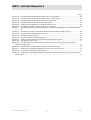
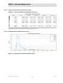
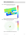
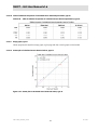
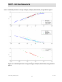
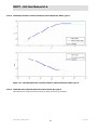
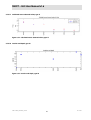
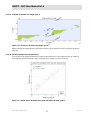
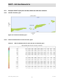
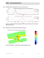
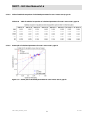
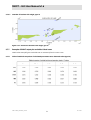
Besides the availability of certain standard graphs (some possible graphs are included here in Figure
1.1 to illustrate the point), it is possible to create tailor−made figures.
To facilitate user−interaction, SWIVT is provided with a GUI.
The user can apply the SWIVT functionalities (ie execution and post−processing) to new SWAN cases
made by him/herself. This assists the user in the execution of new hindcast studies and sensitivity
analysis (ie, studying the influence of variations in the input parameters).
The maintenance party has the possibility to include new validation cases in SWIVT. This may include
recent SWAN hindcast studies and cases in which newly developed physical and numerical options in
3038.13−SWIVT_UserManual_v1.6.docx
6
20−11−2014
SWIVT – GUI User Manual v1.6
SWAN are tested. This keeps the set of available validation cases up−to−date and discloses at the
same time these cases to a broader public (the SWIVT users group).
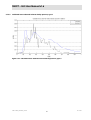
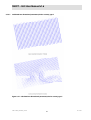
Figure 1.1
1.4
Illustrative figures produced by SWIVT
Validation versus hindcast
SWIVT is a tool to perform a validation study. Validation means comparing computed results with either
observed data, or
computed results obtained with another SWAN version, or
computed results obtained with different SWAN parameter settings.
A validation study then comprises validation of SWAN for a selected set of test cases with suitably chosen
model settings. The validation cases delivered along with SWIVT have been used at some time in the past in
hindcast studies. In such a study, SWAN was applied to determine a historical wave field. Known or closely
estimated inputs for past events were entered into the model to investigate to which extend the SWAN output
matched the observed data. Validation studies and hindcast studies have in common the need to go through
the process of validation: comparing SWAN results with observed data.
Validation studies and hindcast studies differ in the following aspects:
An important part of a hindcast study is the construction of a SWAN model by the user. This
consists of, among others, judging available observed data, creation of required model input
(e.g., grid, bathymetry, wind field and flow field) and selecting suitable parameter settings. A
validation study, on the other hand, uses already available SWAN models (validation cases), in
which typically only the model settings can be adjusted.
Hindcast studies typically aim at studying a limited number of events, for example a number of
instants during a storm in a given geographical region. Validation studies, on the other hand, are
typically performed using a large number of validation cases. This selection of validation cases
should contain a wide variety of different storm events, laboratory cases and analytical cases, to
ensure that the physics in the model is tested thoroughly.
3038.13−SWIVT_UserManual_v1.6.docx
7
20−11−2014
SWIVT – GUI User Manual v1.6
Hindcast studies always involve comparison of SWAN data with observed data, while in
validation studies also SWAN data may be compared with SWAN data obtained with another
SWAN version or different parameter settings.
SWIVT facilitates, briefly speaking, the selection of a number of validation cases, the insertion of parameter
settings in SWAN command files, the running of SWAN and the validation by generating tables and graphs.
1.5
SWIVT cases
A SWIVT case consists of a set of SWIVT files and a set of SWAN files which belong to one SWAN simulation.
There are two types of SWIVT files, both in xml format:
one containing information for the simulation of the physical processes from which a selection can be
made by the user.
one containing information on how to present the results in graphs and/or tables.
The set of SWAN files is described in detail in the SWAN User Manual [SWAN team 2014b]. An example is the
set of SWAN files for simulation of the Friesche Zeegat at 5h00m, on October 9th, 1992. Another example, a
different case, is the set of SWAN files for simulation of the Friesche Zeegat an hour later, at 6h00m, on October
9th, 1992.
Note that two cases are different if the SWAN files (input files and/or SWAN executable) are different, even if
they aim at simulating the same situation. For example, a change in the parameter setting, grid, bathymetry or
wind field, as well as SWAN executable, for the simulation of the Friesche Zeegat at 5h00m, on 9 October 1992,
is a different case. Also two cases are different if they use a different SWAN version.
A SWIVT case is identified by a code, which is described in detail in the Technical Reference [Dekker et al
2014a] and summarised in the Glossary in Chapter 4. Minor changes to a case may result in a subcase, rather
than a new case with a new code.
The first set of SWIVT cases available from the SWIVT server, contains the ONR Testbed cases. It should be noted
that the SWIVT cases incorporate a small number of improvements.
1.6
Important
It is important to realise that SWIVT is an automatic system which is very strict in the setup of a case. The user is
strongly advised not to edit any of the SWIVT (including the Physical Process definitions and the Output section
of the *.swn file) files by hand or otherwise outside SWIVT. Furthermore, in case of the m−code, making
changes via the Matlab window may result in SWIVT not working correctly.
In order to be able to retrieve the cases from the SWIVT server, ensure that your firewall is not blocking the
internet access from Matlab.
1.7
Documentation
SWIVT documentation consists of five documents, which are written in English:
SWIVT Installation Guide
SWIVT User Manual (this document)
SWIVT Technical Reference Documentation
SWIVT Programmers Manual
SWIVT Management and Maintenance Manual
3038.13−SWIVT_UserManual_v1.6.docx
8
20−11−2014
SWIVT – GUI User Manual v1.6
This document is a user manual for the interface of SWIVT. Release Notes are issued in addition to these
documents.
1.8
Free software, LGPL
SWIVT is free software, it can be redistributed and/or modified under the terms of the
GNU Lesser General Public License as published by the Free Software Foundation, either
version 3 of the License, or any later version.
SWIVT is distributed in the hope that it will be useful, but WITHOUT ANY WARRANTY; without even the implied
warranty of MERCHANTABILITY or FITNESS FOR A PARTICULAR PURPOSE. See the GNU Lesser General Public
License for more details.
A copy of the GNU Lesser General Public License is included with SWIVT. If not, see
http://www.gnu.org/licenses/.
1.9
Acknowledgements
The development of SWIVT is part of the SBW (Strength and Loads on Water Defences) study commissioned by
the RijksWaterStaat, department of the Ministry of Public Works in the Netherlands.
3038.13−SWIVT_UserManual_v1.6.docx
9
20−11−2014
SWIVT – GUI User Manual v1.6
2
Getting Started
2.1
Installation of SWIVT
2.1.1
Matlab version
The SWIVT GUI and the accompanying Manuals in Adobe pdf format can be downloaded from
http://swivt.deltares.nl/. The zip−file with the Matlab m−code is protected with a password.
For the installation of the Matlab GUI follow these steps:
1.
2.
3.
4.
5.
6.
Create a directory on your local system, eg C:\projects\swivt and download the zip file there
Extract this zip−file in this swivt directory, retaining its directory structure
Locate the matlab.exe file. This can be found for instance in
C:\Program files\MATLAB\R2006b\bin\win32, and create a shortcut to it on your desktop.
Right click on the Matlab icon, select [Properties] and change the path (Start in) into
C:\projects\swivt
Select as icon the SWIVT icon in C:\projects\swivt
Double click the icon: Matlab will start and the correct paths are set.
Alternative:
1.
2.
3.
4.
Create a directory on your local system, eg C:\projects\swivt and download the zip file there
Extract this zip−file in this swivt directory, retaining its directory structure
Start Matlab
Go to C:\projects\swivt by typing:
>> cd C:\projects\swivt
5.
Type
>> startup
which ensures that the correct paths are set.
Please note that in the alternative method steps 4 and 5 need to be carried out each time SWIVT is
started. The first method, therefore, is more user friendly.
2.1.2
Standalone version
The SWIVT Standalone version can be downloaded from http:// swivt.deltares.nl/ as a zip file. In addition the
required Matlab engine can also be downloaded as a zip file.
For the installation of the Matlab GUI follow these steps:
1.
2.
3.
Create a directory on your local system, eg C:\projects\swivt and download the zip files there.
Extract these zip−files in this swivt directory, retaining their directory structure.
Start the program with the swivt.bat file (in our example the command is
C:\projects\swivt\swivt.bat) . This ensures that the required libraries will be found by the
executable. In our example the contents looks like this:
PATH=v75\bin\win32;v75\runtime\win32;C:\windows;
start swivt.exe
3038.13−SWIVT_UserManual_v1.6.docx
10
20−11−2014
SWIVT – GUI User Manual v1.6
A limited number of graph editing features are available in Matlab Standalone 7.0 and above:
zoom in and out
panning
3D rotation
use data cursor to request x, y and z position in axes
colour bar
legend
however, this is less than is available with the Matlab .m and .p files.
Please note: The standalone version of SWIVT does not include Matlab source files. The Matlab engine does
not need to be downloaded if the SWIVT application is upgraded, unless this is specifically mentioned on the
download site. The Matlab engine version number is used as the name of the directory (eg v75).
2.2
Start a SWIVT session
The program can be started from the Matlab prompt with:
>> swivt
or
>> swivt('new')
In the first instance the last session will be restored, the latter uses the default settings. In this context default
settings mean:
No cases available at start−up. This implies that all locally stored previous sessions will be erased!
Default SWIVT web server URL is used.
When a new session is created, either by using the second option to start SWIVT, by using the new button or
the open button on the main window (see Chapter 3), a new subdirectory is generated in the sessions
directory (which is also generated if it doesn’t already exist) called sessioniii, where iii is the session
identifying counter (3 integers). The only exception to this is when a directory sessioniii , being a subdirectory
of sessions is reopened, in which case the old session identifying counter (iii) is used.
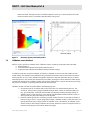
Figure 2.1
Example sessions directory
For example, in Figure 2.1 the options work as follows:
1. swivt(‘new’) removes session001, session002 and session003 from the sessions directory,
and creates a new session001 subdirectory in sessions.
2. assuming swivt was started without the (‘new’) addition:
a. the new button results in the creation of the subdirectory session004 in the sessions
directory
b. the open button:
3038.13−SWIVT_UserManual_v1.6.docx
11
20−11−2014
SWIVT – GUI User Manual v1.6
i.
ii.
opening sessions/session002 will use the existing directory
opening local_sessions/session002 will create and use
sessions/sessions004. In this case the results will also be stored in session004,
and if they need to be preserved with the original data, they will need to be explicitly
saved in the original directory.
Please note that the sessioniii directories may not be created in the sessions directory outside SWIVT, this
will result in an internal error in SWIVT, as it will be unable to locate the cases stored in these directories.
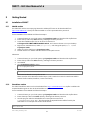
Once a case is downloaded from the server, it will be stored in a subdirectory of sessioniii, in the directory
with the appropriate swanversion number (eg SWAN4041A, SWAN4051A, SWAN4072A, etc), called
code_subcode where subcode 000 indicates that the case has been retrieved from the server. For example:
Figure 2.2
Session directory example
Each code_subcode directory contains two, three or four subdirectories:
model_io, containing the input files for both SWIVT and SWAN. This is also the location where the
(non−presentation) output files will be stored.
observ, containing the files with the observed data.
presentation, created when presentation output is generated by SWIVT.
swivt_ci_pres_set, created when presentation output is generated by SWIVT. This directory is
only relevant in conjunction with the Calibration Instrument developed at Deltares.
For more information on input and output files please refer to the Technical Reference (Dekker et al 2014a).
Once the program is started the splash window will appear:
3038.13−SWIVT_UserManual_v1.6.docx
12
20−11−2014
SWIVT – GUI User Manual v1.6
Figure 2.3
Splash window
After clicking in the SWIVT splash window, or using the [Ctrl] + [O] shortcut, the SWIVT main window
appears. This window is described in Chapter 3.
2.3
General navigation rules
This section describes rules which are applicable for all the SWIVT windows, unless it is stated otherwise in the
appropriate section.
2.3.1
Menu’s and shortcuts
Most navigation commands can be found in the menu’s provided at the top of the window. Menus can be
accessed by using the [Alt] key, for example [Alt]+F for the File menu. The items in the menu list often
provide a shortcut. In addition to this some windows display the Accelerator(s) menu. This is a list with shortcuts
which are used in that particular window, these shortcuts are combined with the [Ctrl] key. The menus are
listed in Table 2.1 together with the associated items and, where appropriate, shortcuts and toolbar buttons.
3038.13−SWIVT_UserManual_v1.6.docx
13
20−11−2014
SWIVT – GUI User Manual v1.6
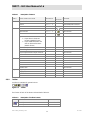
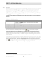
Table 2.1
Description of Menu’s
MENU
MENU ITEM/FUNCTION
Accelerator Open SWIVT
File
SHORTCUT
TOOLBAR
WINDOW
BUTTON
Ctrl + O
Splash window
Cancel
Ctrl + N
Case identification window
OK
Ctrl + O
Case identification window
New session
Ctrl + N
Main window
Open session
Ctrl + O
Main window
Save session
Ctrl + S
Main window
Export
Main window
Export data in observed
locations (Matlab format)
Export SWAN field data and
data in observed locations
(Matlab format)
Clear all sessions
Main window
Clear all log files
Main window
Close all presentation output windows
Edit
Help
Main window
Preferences
Ctrl + F
Main window
Exit
Ctrl + X
Main window
Add case
Ctrl + A
Main window
Remove case
Ctrl + R
Main window
Edit case
Ctrl + E
Main window
Run case
Ctrl + U
Main window
Present case
Ctrl + T
Main window
Ctrl + H
Main window
Help (html)
Help (pdf)
Main window
SWIVT website
Info
2.3.2
Main window
Ctrl + I
Main window
Toolbar
A toolbar is available for general actions:
Figure 2.4
Toolbar
The function of each of the buttons is described in Table 2.2.
Table 2.2
Description of Toolbar buttons
BUTTON FUNCTION
WINDOW/MENU
Close all presentation windows
Main window/File
Close all presentation windows
Presentation
3038.13−SWIVT_UserManual_v1.6.docx
14
20−11−2014
SWIVT – GUI User Manual v1.6
BUTTON FUNCTION
WINDOW/MENU
Close all presentation windows
Present Case
New session
Main window/File
Open the default template default.spt
Presentation
Open an existing session
Main window/File
Open an xml file with user−defined parameters Edit Case
Open a template
Presentation
Save the current session
Main window/File
Save the user−defined parameters to an xml file Edit Case
2.3.3
Save the current settings in a template
Presentation
Show case list as HTML table
Main window
Light and dark grey fields
In selection areas dark grey fields denote that a selection is possible, light grey fields denote that the selection
option is disabled.
2.3.4
Mouse usage
When the user is advised to click using the mouse, the left mouse button needs to be used. If an action requires
the right hand mouse button, this will be stated explicitly. Selecting using the mouse implies pressing the left
mouse button whilst moving the mouse. There are two ways of selecting more than one item from a list:
click on the first item, next keep the [Shift] key down whilst clicking on the second item. This will
result in selecting both items as well as those in between
click on the first item, next keep the [Ctrl] key down whilst clicking on one or more additional items.
This will result in selecting the ‘clicked’ items.
On most windows it is possible to use the mouse to find out more about an item. For example, hover above a
button and a tooltip should appear explaining the purpose of the button.
2.3.5
Checking a checkbox
Click on a checkbox (white square) to add a tick mark. By clicking again the tick mark is removed. A list may
contain more than one tick mark.
2.3.6
Radio buttons
A list of items preceded by radio buttons is a list from which only one item may be chosen. Radio buttons can
be recognised by a white circle whereby in front of the selected item a black dot is placed in the middle. By
clicking a different white circle the black dot will move to that circle.
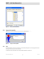
2.3.7
Directory and file selector
On certain windows the
button is available for selecting a file or a directory which opens the standard
directory selection window or file open window of the current platform (Windows or UNIX).
3038.13−SWIVT_UserManual_v1.6.docx
15
20−11−2014
SWIVT – GUI User Manual v1.6
Figure 2.5
2.3.8
Directory selector (Windows)
Trying to do the impossible
When you try to do the impossible you may come across a window like this................
Figure 2.6
2.3.9
Trying to do the impossible
Close
The SWIVT application, and also most windows, can be closed by clicking the cross in the top right hand corner.
All changes made in that part of SWIVT will be lost!
A confirmation window will appear upon closing the SWIVT application, see Figure 2.7:
3038.13−SWIVT_UserManual_v1.6.docx
16
20−11−2014
SWIVT – GUI User Manual v1.6
Figure 2.7
Closing confirmation window
3038.13−SWIVT_UserManual_v1.6.docx
17
20−11−2014
SWIVT – GUI User Manual v1.6
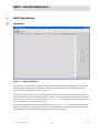
3
SWIVT Main Window
3.1
Introduction
Figure 3.1
SWIVT main window
The key function of this window is to offer access to the main characteristics, called properties , with regard to
the SWAN cases. At the start of a new session no SWAN cases are available in the case overview list. The
overview section will be empty as shown in Figure 3.1.
The open and save a session buttons are described in Section 3.2. A short description of the functionality of
each of the buttons on the right hand side is given in Table 3.1. The windows behind the buttons are described
in turn in the next sections. The only exception is the [Remove case] button, which just removes the selected
case, and whereby no further windows are used.
In the event of absence of an internet connection to the server, the [Add case] button will be disabled. This
button can be enabled by entering the correct server name (if available) in the File/Preferences menu. Entering
a server name to which SWIVT cannot connect will result in an error message.
3038.13−SWIVT_UserManual_v1.6.docx
18
20−11−2014
SWIVT – GUI User Manual v1.6
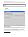
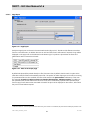
Figure 3.2
SWIVT Preferences window for editing the SWIVT server URL
Table 3.1
Buttons on the main screen
BUTTON
Add case
Remove case
Edit case
Run case
Present case
DESCRIPTION
Add one or more SWAN cases to the overview list. Cases can be retrieved from the SWIVT
server or loaded from the local system. This functionality is described in detail in Section 3.2.
Remove one or more selected SWAN cases from the overview list.
Edit the parameter settings of a SWAN case. This functionality is described in detail in Section
3.5.
Run one or more SWAN cases with their associated SWAN executable. Note that cases are by
definition different (even if the input files are identical) if they are associated with another SWAN
executable (Section 3.5.3).
Plot the results and compute the statistical scores. A predefined or user−defined set of graphs
and tables is plotted (Section 3.7).
A legend indicating that data is available for presentation if the casename is preceded by a
bottom right of the page. An example is given in Section 3.4.1.
is placed on the
Please note that in the remainder of this chapter terms are used like casename, code, subcode, etc. These are
explained in detail in the Technical Reference (Dekker et al 2014a) and summarised in Chapter 4.
3.2
Open and save an existing SWIVT session
As described in Section 2.2 SWIVT will, unless explicitly specified otherwise, reopen the last session during
start−up. Once SWIVT is started the new button on the top left of the main window can be used to start a new
session.
The save button on the toolbar can be used to save a SWIVT session. The user is prompted to select an existing
directory, or to make a new directory to save the session in. The code_subcode subdirectories, their contents
and a *.set file (a Matlab file) with the internal SWIVT parameters will be saved in this directory. The user is free
to choose the name of the directory.
IMPORTANT: Any existing sessions in a directory will be deleted when a new session is saved in this directory.
This implies that a directory can only contain at most one saved session. Furthermore this directory should not
be a subdirectory of sessions, as the sessions directory will be emptied when the swivt(‘new’) command
is used.
To reopen a session, use the open button on the toolbar of the main window. The Session Selector will appear
(see Figure 3.3) after the session number has been selected on the left. The case(s) enclosed in a session can
3038.13−SWIVT_UserManual_v1.6.docx
19
20−11−2014
SWIVT – GUI User Manual v1.6
be seen on the right once an appropriate directory has been selected. When the session is selected the whole
session is copied to a new sessioniii directory and the cases will appear on the overview screen.
Figure 3.3
Session Selector
Selecting a previous session will result in transferring the
More information on the directories can be found in Section 2.2.
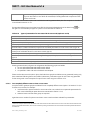
3.3
Clear all sessions or log files
Removing the old sessions from your computer can be done in two ways:
1.
Start SWIVT using the following command (see also Section 2.2):
>> swivt('new')
2.
Use the Clear all sessions option in the File menu on the main screen.
Removing the old log files can be done by using the Clear all log files option in the File menu on the main
screen. (Log files are described in Section 3.6.1)
3038.13−SWIVT_UserManual_v1.6.docx
20
20−11−2014
SWIVT – GUI User Manual v1.6
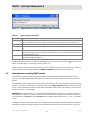
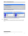
3.4
Add case
Figure 3.4
Add case window
The Add case window offers the user two, mutually exclusive, options:
1. Server (top part of the screen)
Browse through all available SWAN cases on the SWIVT server. When this window is opened the SWIVT
GUI automatically retrieves all browsable properties from the SWIVT server.
2. Local (bottom part of the screen)
The user can browse his or her local system and select a SWAN case directory. Consequently he has
to describe this case with the same properties as are used for the SWAN cases on the SWIVT server.
Only in this way all cases, whether they are locally or remotely selected, can be treated in a uniform
way by the SWIVT GUI.
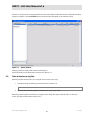
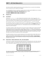
3.4.1
Adding cases from server
For the moment, up to three properties (cf. with the columns in the Add case window) can be chosen to reduce
the number of cases that will be selected from the server.
In the example below, the chosen properties are respectively wind, current and code (see Chapter 4).
3038.13−SWIVT_UserManual_v1.6.docx
21
20−11−2014
SWIVT – GUI User Manual v1.6
Figure 3.5
Add Case window
On pressing the [Ok]−button, all cases complying with the selected properties will automatically be retrieved
from the SWIVT server and stored on the local system in the predefined directory structure. Note that it is
possible to select cases from the complete list of codes, in other words, from the complete list of available
validation cases. Only one item per list can be selected at the time, except for the third (most right) list which is
multiple selectable (see Section 2.3.4).
It is also possible to retrieve all cases available from the server by using the [Retrieve all] button. A
confirmation window (see Figure 3.6) will be displayed before the data is downloaded.
Please note that if the SWAN version is not explicitly chosen, all cases with the same casename and subtype,
but different SWAN versions, will be retrieved.
3038.13−SWIVT_UserManual_v1.6.docx
22
20−11−2014
SWIVT – GUI User Manual v1.6
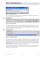
Figure 3.6
Confirmation window for retrieving all cases from the server
Retrieving the data may take a little time, depending on the amount of data requested, the window in Figure
3.7 will be displayed during this process.
Figure 3.7
Retrieving case window
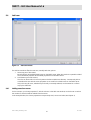
Subsequently an overview of the, now locally available, cases will be presented on the main window. Please
note that in the example below properties other than those in the example above have been used.
3038.13−SWIVT_UserManual_v1.6.docx
23
20−11−2014
SWIVT – GUI User Manual v1.6
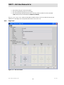
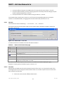
Figure 3.8
Case overview
The
button in the toolbar will generate an HTML−table with meta information on the cases: the properties,
whether processes are switched on or off, where appropriate, the values of the parameters and the session
location of the files associated with the cases. Part of this list is given in , as an example.
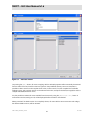
Figure 3.9
Html list of cases displaying associated meta information (left most part only)
Clicking with the right mouse button on a selected line in the Case overview list gives access to menu called
Show additional information see Figure 3.10. This feature is only available for server cases.
3038.13−SWIVT_UserManual_v1.6.docx
24
20−11−2014
SWIVT – GUI User Manual v1.6
Figure 3.10 Show additional info
A document in pdf format with a description of the case will be retrieved from the SWIVT server and opened in
a browser window. An example is given in Figure 3.11. Please note that, for each casename there is only one
pdf, describing the case and the differences between the subtypes. These documents are also available from
the download site. Click on Case meta data in the list on the top right.
Figure 3.11
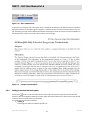
3.4.2
Example case description
Adding a case from the local system
Pressing the
button in the Local select section of the Add case window opens the standard directory
selector of the current platform (Windows or UNIX). Select the required directory for which the structure should
match the structure of the cases from the server.
Two subdirectories should be available:
model_io
containing both SWIVT and SWAN input files, etc.
3038.13−SWIVT_UserManual_v1.6.docx
25
20−11−2014
SWIVT – GUI User Manual v1.6
observ
containing measurements
The content of the input files as well as their names need to satisfy certain conventions which are described in
the Technical Reference document (Dekker et al 2014a).
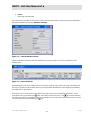
Figure 3.12 Case identification window
After the selection of a directory the Case identification window prompts the user for the definition of the
selected case.
Figure 3.13 Case overview list
Subsequently the local case is added to the Case overview list of the main window. The data associated with
the case is copied to the (local) SWIVT directory, the original data will therefore not be updated nor deleted by
the SWIVT GUI in a later session.
From Figure 3.13 it is clear that the output files for the local cases are not available for presentation, as the
casenames are not preceded by the mark. Once these cases have been run, the
mark will be added to
the overview. Output for presentation purposes is available for those cases that were retrieved from the server
as these casenames are preceded by the mark.
3038.13−SWIVT_UserManual_v1.6.docx
26
20−11−2014
SWIVT – GUI User Manual v1.6
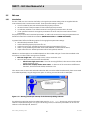
3.5
Edit case
3.5.1
Introduction
The aim of Edit case is to introduce the facility to change the parameter settings that are supplied with the
cases selected in the Case Overview window. These parameter settings comprise:
a list of included (active) and excluded (inactive) physical processes
the actual values of the parameters for the included physical processes
an indication whether or not default numerical convergence parameters are to be used
if user specified numerical convergence parameters are to be used, the actual values of these
parameters
The physical processes and associated parameters, as well as the numerical convergence parameters are
described in detail in the SWAN documentation [SWAN team 2014a and SWAN team 2014b].
In general SWIVT offers the following options for changing these parameter settings:
edit individual parameter values.
switch individual physical processes off or on.
switch the use of user−specified numerical convergence parameters off or on
select a set of predefined parameter values (ONR, HR2006, or SWAN default values).
import a file with user−defined parameter values and (optional) switches.
Whether or not these options are available depends on the number and type of cases that are edited at the
same time. A number of Edit case types are available:
Edit case: single case − edit a single case at a time, see Section 3.5.2.
edit more than one case at the same time (Edit all):
o Edit all case: single server case − the case name (eg f051fries) is the same and the subcode
is 000, see Section 3.5.3.
o Edit all case: multiple, distinct server cases − at least one of the case names is different to
the others, and the subcode is 000, see Section 3.5.4
Non−server cases, ie cases with subcodes other than 000, cannot be edited simultaneously; these cases need
to be edited separately using the Single case option. A warning is issued when this is attempted:
Figure 3.14 Warning issued upon attempt of simultaneously editing subcases
First select the case(s) that need to be edited. Next press the [Edit case] button upon which an Edit case
window is displayed (see Figure 3.15, Figure 3.20 and Figure 3.21) on which the parameters can be set. This
window is automatically built, based on:
3038.13−SWIVT_UserManual_v1.6.docx
27
20−11−2014
SWIVT – GUI User Manual v1.6
the number and type of cases to be edited
the case properties list (upper part of window)
the case parameter settings list (lower part of window), which are taken from the associated
code.xml file (see Technical Reference (Dekker et al 2014a)).
The Edit case: Single case window is described in detail in Section 3.5.2, for the Edit all cases only the
differences to the Single case are stipulated (see Sections 3.5.3 and 3.5.4).
3.5.2
Single case
Figure 3.15 Edit case window
3038.13−SWIVT_UserManual_v1.6.docx
28
20−11−2014
SWIVT – GUI User Manual v1.6
3.5.2.1
Case properties
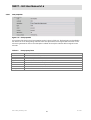
Figure 3.16 Case properties
An overview of the items in the Case properties section is given in Table 3.2. The description can be edited in
this window to aid in distinguishing subcases when case parameters are changed. Please note that a new
subcase is generated as soon as the description is edited. Obviously this subcase will be assigned a new
subcode.
Table 3.2
Case property items
PROPERTY
code
subcode
description
type
wind
current
dimensions
swan_version
DESCRIPTION
this is the code (see Chapter 4)
this is the subcode (see Chapter 4)
a short description of the case
whether the case is an analytical, laboratory or field case
whether the wind is absent or present
whether the current is absent or present
whether the case is one (1D) or two (2D) dimensional
which SWAN version is used in this case
3038.13−SWIVT_UserManual_v1.6.docx
29
20−11−2014
SWIVT – GUI User Manual v1.6
3.5.2.2
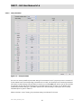
Case parameters
Figure 3.17 Case parameters
The user can choose predefined parameter settings for the selected case. If a physical process is switched off
for the selected case, the corresponding parameters are not used, and similarly for the numerical parameters.
Information on these settings and parameters is stored in an xml file (code.xml), which is part of the case data.
For example, the physical process whitecapping is excluded from the case in Figure 3.13. In addition to the
predefined parameter settings it is possible to provide user−defined settings. A description of the currently
available options is given in Table 3.3.
Please note that in case of nesting, the parameter settings are identical for all nests.
3038.13−SWIVT_UserManual_v1.6.docx
30
20−11−2014
SWIVT – GUI User Manual v1.6
Table 3.3
Description of the parameter settings options
OPTION
user
SWAN**
ONR
HR2006
DESCRIPTION
The user can insert a new set of physical parameters through the SWIVT GUI.
Please note that SWIVT issues a warning if physically unrealistic settings are
chosen. User−defined settings can also be imported from an xml file (see Section
3.5.2.4).
This option ("SWAN defaults settings" columns in Table 3.5) comprises the SWAN
default parameter settings for SWAN version ** for the included physical processes
(which vary from case to case1).
This option refers to the settings as used in the ONR Testbed. The settings in the
ONR Testbed vary from case to case, and are therefore not included in Table 3.5.
This option (last column in Table 3.5) comprises the SWAN parameter settings as
used for the computation of the Dutch Hydraulic Boundary Conditions in 2006 for
the Holland Coast.
Once a predefined option is chosen (like eg ONR) and the OK button is pressed, a new subcase is created and
the new values are stored in the user data block for this subcase. If this subcase is edited, the text user will
again be displayed in the Parameter settings option box (and not ONR as may be expected).
Please note that a subtle, yet important, difference exists between application of the SWIVT parameter options
SWAN4041A, SWAN4051A etc. as given above, and the various SWAN default settings as given in the SWAN
User Manual. The same also holds for the HR2006 settings. This difference is as follows:
The SWAN User Manual and the HR2006 settings define both the in/exclusion of physical processes and the
parameter values to be used. However, SWIVT only uses the specified parameter values from these sources.
The in/exclusion of physical processes is based on the SWIVT case−specific settings, which are initially derived
from the ONR testbed settings, and is defined in the xml file.
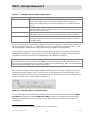
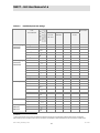
Table 3.5 gives an overview of the currently available predefined parameter settings. The physical process for
which the parameter is defined, is given in the first column. A short description can be obtained by hovering
over the parameter name with the mouse as displayed in Figure 3.18 (this only works if the associated physical
process is selected, or if the numerical block is switched on).
Figure 3.18 Extra information on a parameter name
For more information on an individual parameter please refer to the SWAN Technical Documentation [SWAN
team 2014a] and SWAN User Manual [SWAN team 2014b]. However, as the definition of the whitecapping
parameters, as described here, may not always be clear when referring to the SWAN documentation, it is
clarified below:
1
ie whether the physical process is included, not the default value of the SWAN parameter
3038.13−SWIVT_UserManual_v1.6.docx
31
20−11−2014
SWIVT – GUI User Manual v1.6
The whitecapping source term in SWAN is given by:
k
S ds ,w (σ ,θ ) = −ΓKJ σ~ ~ E (σ ,θ ) ,
k
σ , σ% , θ , k , k%
and E denote the frequency, the mean frequency, the wave direction, the wave
number, the mean wave number and 2D energy spectrum, respectively. The coefficient Γ KJ is given by:
where
2n
n1
2

 k    s% 
Γ KJ = Cds 2 (1 − δ ) + δ    
 .
 k%    s%PM 

In this expression, s% stands for the overall wave steepness, and s%PM is the value of s% for the Pierson−
s = 3.02 * 10 −3 . Parameters C , δ , n en n are tunable coefficients. These
Moskowitz spectrum: ~
PM
ds 2
1
2
are given in the table onder (third column), whereby it should be noted that the input parameter stpm is the
squared value of
s PM . The parameters powst and powk are not listed in the SWAN User Manual, but can be
tuned with SWIVT.
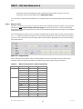
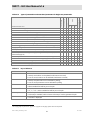
Table 3.4
Predefined key settings with list of associated parameters
PROCESS/KEY
PLACEHOLDER 2
Mode
Whitecapping
GEN3
WCAPON
WCAPOFF
WCAP1ON
GEN3
WCAP KOM
OFF WCAP
WCAP WESTH
WCAP1OFF
QUADON
QUADON
QUADOFF
BREAON
BREAOFF
BREA1ON
BREA1OFF
TRIADON
TRIADOFF
FRICON
FRICOFF
NUMREFRLON
OFF WCAP
QUAD
LIMITER
OFF QUAD
BREA CON
OFF BREA
BREA WESTH
OFF BREA
TRIAD
$
FRIC JONSWAP
$
NUM REFRL
NUMREFRLOFF
NUMON
NUMON
NUMOFF
$
NUM STOPC
NUM STAT
$
Quadruplets
Breaking
Triads
Bottom friction
Numerical
refraction
Numerical
convergence
2
KEY ADDED IN
SWIVT
ASSOCIATED PARAMETERS AVAILABLE IN
SWIVT (MORE INFORMATION IN TABLE 3.5)
cds2, stpm, powst, delta, powk
cds2, br, p0, powst, powk, nldisp, cds3,
powfsh
iquad, lambda, Cnl4
ursell, qb
alpha, gamma
alpha, pown, bref , shfac
trfac, cutfr
cfjon
frlim, power
dabs, drel, curvat, npnts
mxitst
The ‘ON’ placeholder is removed and the ‘OFF’ “placeholder is replaced by a ‘$’ if the process is switched on and vice versa.
3038.13−SWIVT_UserManual_v1.6.docx
32
20−11−2014
SWIVT – GUI User Manual v1.6
Predefined parameter settings
PROCESS
Whitecapping
(WCAPON,
WCAPOFF)
COMMAND
FILE
PARAMETER
40.81
40.91
41.01
2.36E−5
2.36E−5
2.36E−5
2.36E−5
2.36E−5
3.02E−3
3.02E−3
3.02E−3
3.02E−3
3.02E−3
n2
2.0
2.0
2.0
2.0
2.0
δ
0
0.0
0
0.0
0
0.0
0
1.0
1
1.0
−
5.0E−5
5.0E−5
−
−
−
−
−
1.75E−3
4.0
0.0
1.75E−3
4.0
0.0
−
−
−
−
−
−
−
0.0
0.0
−
−
−
−
−
0
1.5
1.0
0
1.5
1.0
−
−
−
−
−
−
λnl 4
2
0.25
2
0.25
2
0.25
2
0.25
8
0.25
Cnl4
Cnl 4
3.0E7
3.0E7
3.0E7
3.0E7
3.0E7
LIMITER
ursell
qb
Ur
qB
10.0
1.0
10.0
1.0
10.0
1.0
10.0
1.0
10.0
10.0
JONSWAP
cfjon
Cds ,bot
0.067
0.067
0.067
0.067
0.0384
1.0
1.0
1.0
1.0
1.0
0.73
0.73
0.73
0.73
0.73
KOM
cds23
C ds 2
~
s2
stpm3
PM
3
WESTH
cds2
br
p0
powst
powk
Bottom friction
Breaking
(BREAON,
BREAOFF)
HR2006
SETTINGS
40.72
ABCDE
delta3
powk3
Quadruplets
SWAN DEFAULT SETTINGS
40.41A
40.51A
40.72A
powst
Whitecapping
(WCAP1ON,
WCAP1OFF)
MATHEMATICAL
SYMBOL IN SWAN
DOCUMENTATION
Table 3.5
nldisp
cds3
powfsh
QUAD
iquad
lambda
CON
alpha
gamma
n1
C ds 2
n2
n1
iquad
α BJ
γ BJ
3
see above
Note that the value for cfjon used in the HR2006 computations depends on the deepwater statistics peak period in location ELD:
cfjon=0.038 if Tp>10s, and cfjon=0.067 if Tp<10s. This data is not available in SWIVT. Therefore, the user must select a suitable value.
4
3038.13−SWIVT_UserManual_v1.6.docx
33
20−11−2014
PROCESS
Breaking
(BREA1ON,
BREA1OFF)
Triads
COMMAND
FILE
PARAMETER
WESTH
alpha
pown
bref
shfac
TRIAD
trfac
cutfr
Numerical
refraction
GEN3 setting
Numerical
convergence
criteria
REFRL
frlim
power
STOPC
dabs
drel
curvat
npnts
STAT
mxitst
MATHEMATICAL
SYMBOL IN SWAN
DOCUMENTATION
SWIVT – GUI User Manual v1.6
SWAN DEFAULT SETTINGS
40.41A
40.51A
40.72A
f max,EB
40.81
40.91
41.01
−
0.98
0.98
−
−
−
−
−
2.5
−1.3963
500
2.5
−1.3963
500
−
−
−
−
−
−
0.1
0.05
0.05
0.05
0.15
2.2
2.5
2.5
2.5
2.25
−
−
KOM
0.2
2
KOM
0.0
0
KOM
0.0
0
KOM
−
−
KOM
0
0.01
0.005
98
0
0.01
0.005
98
0
0.01
0.005
98
0
0.01
0.005
98
0
0.01
0.005
98
15
15
15
15
15
α BJ
α EB
40.72
ABCDE
HR2006
SETTINGS
Please note that :
• the options User and ONR (see Table 3.3) are not included in Table 3.5:
The option ONR implies that the parameter settings as used in the ONR Testbed are taken.
These parameter settings, including the in/exclusion of physical processes, vary from case to
case, and can therefore not be included in Table 3.4. In addition, the ONR option can only be
selected for cases that were originally present in the ONR Testbed. It is not defined for other
cases.
The option User means that the user is free in providing the parameter values and physical
processes. Please note, that as soon as one parameter or physical process setting is
changed, the User option is switched on, even if a different option was selected in the first
place.
• the use of WESTH whitecapping and breaking was introduced in SWAN4072ABCDE, but removed from
SWAN 4091.
• if the third generation mode for wind input, quadruplet interactions and whitecapping (GEN3) is set to
WESTH, the whitecapping is automatically set to WCAP WESTH, if it is set to KOM the whitecapping is
5
in the original HR2006 settings, the process triad interaction was excluded. This means that there were no HR2006 values for the triad
parameters trfac and cutfr. When applying SWIVT however, a user may want to employ the HR2006 parameter values and activate the
process triad interaction at the same time. In that particular case SWIVT needs to propose default values for trfac and cutfr. We have
selected the SWAN 40.41 default values for these parameters, since the HR2006 computations were performed with SWAN version 40.41.
3038.13−SWIVT_UserManual_v1.6.docx
34
20−11−2014
SWIVT – GUI User Manual v1.6
set to KOM. Obviously if whitecapping was switched off in the first place, it stays off. For more
information on these modes please refer to SWAN team 2014a.
For a discussion of the above described theory in conjunction with some examples please refer to Appendix
A.1.1.
3.5.2.3
Range of values
The option to switch from one value to a range of values is also available for each parameter. Using this option
will result in a new subcase for each value in the range. Choosing this option for a number of parameters
might therefore generate a huge amount of cases, and it should be used with care! This option is not available
for the Edit all cases.
In the example given in Figure 3.19, four subcases are generated, using the values 0, 0.022, 0.044 and 0.066
for cfjon. Please note that the end value is not used, it only marks the end of the range. Edit the case again if
you want a case with this value to be included. These subcases will be displayed in the case overview section
of the main window.
Figure 3.19 Range example
A list of minimum and maximum values is used by SWIVT to warn the user that the chosen value may be
unrealistic when this value lies outside the associated range. These values are given in Table 3.6.
Table 3.6
Minimum and maximum values for parameters
PROCESS
WCAP
PARAMETER
cds2
stpm
powst
delta
powk
cds2
br
p0
powst
powk
nldisp
cds3
powfsh
iquad
lambda
Cnl4
WCAP1
QUAD
3038.13−SWIVT_UserManual_v1.6.docx
MINIMUM
MAXIMUM
0
4.00E−5
0.00
6.00E−3
0
4
0
1
0
2
0
4.00E−5
0.00
5.25E−3
0
12
0
4
0
2
0
1
0
4.5
0
3
1 2 3 4 6 8 51 52 53
0
1
0
5.00E7
35
20−11−2014
SWIVT – GUI User Manual v1.6
PROCESS
FRIC
BREA
BREA1
TRIAD
NUMREFRL
NUM
3.5.2.4
PARAMETER
ursell
qb
cfjon
alpha
gamma
alpha
pown
bref
shfac
trfac
cutfr
frlim
power
dabs
drel
curvat
npnts
mxitst
alfa
MINIMUM
1
0
0.0
0
0.0
0
0
−4.19
0
0.0
0.5
0
0
0
0
0
90
0
0
MAXIMUM
20
20
0.2
2
1.5
2
0.75
0
1500
0.30
8.0
0.6
6
0.05
0.1
0.05
101
100
1
Import and save user defined settings
For each case the physical and numerical settings, that can be altered using SWIVT, are stored in the file
code.xml which is part of the case data (see Section 3.5.2.1). However, it is also possible to import user−
defined settings from another (additional) xml file by using the open button at the top left of the Single Case Edit
Case window (see Figure 3.15). This means that the user can define his/her own ‘favourite’ physical or
numerical parameter settings, ie is free to include or exclude physical processes and adjust relevant
parameter values. The imported xml file overrules the code.xml file.
These user−defined settings are included in the standard case−specific xml (code.xml) file once the [Ok]
button is used. A new case is generated each time the [Ok] button is used and one or more parameters have
been changed. This new case is stored with a new subcode which is visible in the Case overview list (see
Figure 3.13).
Similarly the save button can be used to store the chosen settings in a separate xml file, only the user−defined
block will be stored in this file. This file will always include the <selected> tag.
An example of an additional xml file is given below:
<?xml version="1.0" encoding="utf-8"?>
<ROOT xmlns:xsi="http://www.w3.org/2001/XMLSchema-instance"
xsi:noNamespaceSchemaLocation="http://swivt.deltares.nl/swivt.xsd">>
<swivt>
<case>
<code>f051fries001</code>
<settings>
<physics>
<GEN3>
<model>KOM</model>
</GEN3>
<WCAP>
<selected>on</selected>
<cds2>2.36e-005</cds2>
3038.13−SWIVT_UserManual_v1.6.docx
36
20−11−2014
SWIVT – GUI User Manual v1.6
<stpm>0.00302</stpm>
<powst>2</powst>
<delta>0</delta>
<powk>0</powk>
</WCAP>
<WCAP1>
</case>
</swivt>
<selected>off</selected>
<cds2>5e-005</cds2>
<br>0.00175</br>
<p0>4</p0>
<powst>0</powst>
<powk>0</powk>
<nldisp>0</nldisp>
<cds3>1.5</cds3>
<powfsh>1</powfsh>
</WCAP1>
<QUAD>
<selected>on</selected>
<iquad>2</iquad>
<lambda>0.25</lambda>
<Cnl4>30000000</Cnl4>
<ursell>10</ursell>
<qb>1</qb>
</QUAD>
<FRIC>
<selected>on</selected>
<cfjon>0.067</cfjon>
</FRIC>
<BREA>
<selected>off</selected>
<alpha>1</alpha>
<gamma>0.73</gamma>
</BREA>
<BREA1>
<selected>on</selected>
<alpha>0.98</alpha>
<pown>2.5</pown>
<bref>-1.3963</bref>
<shfac>500</shfac>
</BREA1>
<TRIAD>
<selected>on</selected>
<trfac>0.05</trfac>
<cutfr>2.5</cutfr>
</TRIAD>
<NUMREFRL>
<selected>off</selected>
<frlim>0.2</frlim>
<power>2</power>
</NUMREFRL>
</user>
</physics>
<numerics>
<user>
<NUM>
<selected>on</selected>
<dabs>0</dabs>
<drel>0.01</drel>
<curvat>0.005</curvat>
<npnts>98</npnts>
<mxitst>50</mxitst>
</NUM>
</user>
</numerics>
</settings>
</ROOT>
The <selected> tag is optional. This results in two options:
include the <selected> tag, thereby explicitly specifying which physical process to include or
exclude.
omit the <selected> tag, thereby using the already present physical processes (as defined in the
file code.xml). This may result in values specified in the xml file not being used if the associated
physical process was switched off in the first place.
3038.13−SWIVT_UserManual_v1.6.docx
37
20−11−2014
SWIVT – GUI User Manual v1.6
The difference can be explained as follows. Suppose the user has selected the following two testcases:
l021triad001 (1D Beji−Battjes bar) and f021grdpw001 (wave growth in deep water). In the default setting
of l021triad001 triad interaction is included, whereas in f021grdpw001 triad interaction is excluded. The
following three options are possible:
If the <selected> tag is included and ‘on’ for the process triad interaction, then both cases are run
including triad interaction and using the parameter values as specified in the xml file.
If the <selected> tag is included and ‘off’ for the process triad interaction, then both cases are run
excluding triad interaction.
If the <selected> tag is excluded, then the testcase l021triad001 is run including triad
interaction and using the parameter values as specified in the xml file, and the testcase
f021grdpw001 is run excluding triad interaction.
Example files are supplied with SWIVT: UserParamValuesWithProcess.xml, which includes the
<selected> tag, and UserParamValuesWithoutProcess.xml, which excludes the <selected> tag.
These files may be edited by the user to achieve the required settings prior to importing them in SWIVT.
3038.13−SWIVT_UserManual_v1.6.docx
38
20−11−2014
SWIVT – GUI User Manual v1.6
3.5.3
Edit all case: single server case
Figure 3.20 Edit all case window: single server cases
This option is used for cases which bear the same casename (eg f051fries). Furthermore, the cases are
servercases, thus the subcase code is 000. This assumes that the physical processes for these cases are
identical. It is possible to switch the physical processes and the use of user−defined numerical parameters on
or off as required. Furthermore parameter values can be changed. The GEN3 parameter can be changed
provided the SWAN version for all cases is 4051A or above. If one of the cases is run with SWAN4041A the
GEN3 parameter is fixed to the value KOM for all cases. More information on the processes and parameters
can be found in Section 3.5.2. The new settings will then be imposed on all the selected cases, and for each
case a new subcase is generated.
The parameters associated with the newly introduced keywords for SWAN4072ABCDE cannot be used in
earlier versions of SWAN. This means that a SWAN4072ABCDE case cannot be run with earlier SWAN versions
via SWIVT. On the other hand, cases generated for earlier SWAN versions cannot be run by SWAN4072ABCDE,
however, all cases available from the server have also been adapted for SWAN4072ABCDE. In order to
compare a run with eg SWAN4041A to SWAN4072ABCDE for a servercase, both cases need to be retrieved
from the server en run with the associated SWAN version (output may be available for the default settings).
3038.13−SWIVT_UserManual_v1.6.docx
39
20−11−2014
SWIVT – GUI User Manual v1.6
An overview of possible options as illustrated above is given in Table 3.7.
Table 3.7
4041A
4051A
4072A
4072ABCDE
4081
4091
4101
3.5.4
Settings versus SWAN versions
4041A,
4051A
1
1
1
0
0
0
0
4072A
0
0
1
0
0
0
0
4072ABCDE,
4081
0
0
0
1
1
0
0
4091, 4101
ONR
HR2006
0
0
0
0
0
1
1
1
1
1
0
0
0
0
1
1
1
0
0
0
0
Edit all case: multiple, distinct server cases
Figure 3.21 Edit case window: multiple, distinct server cases
As for this option the cases are in general non−related cases, it is only possible to select complete new
parameter value sets, eg HR2006, SWAN4041A, ONR etc. Obviously this includes the option of loading a user−
defined parameter set using the open button on the top left. More information on the processes and
parameters can be found in Section 3.5.2. The new settings will be imposed on all the selected cases, and for
each case a new subcase is generated.
It should be noted that in this situation it is not possible to switch physical processes or numerical convergence
criteria on or off as this setting is part of the case definition, and may differ from case to case. Also the GEN3
parameter cannot be changed.
3.6
Run case
Pressing the [Run case] button will start the execution of SWAN for the selected case(s); selection can be
done by means of the mouse, see Section 2.3.4. Before actually running the case(s), it is possible to decide
whether or not to generate output after the run, see Figure 3.22. If output is to be generated the following can
also be set:
whether to us a generic presentation template
whether to use case specific presentation templates
selecting the required templates
the page layout.
These options are described in detail in Section 3.7.
3038.13−SWIVT_UserManual_v1.6.docx
40
20−11−2014
SWIVT – GUI User Manual v1.6
Figure 3.22 Run Presentation Selection window
The actual run(s) will start after pressing the [Start] button. To avoid carrying out the run use the [Cancel]
button. One of the windows given in Figure 3.23 will be displayed whilst the case is running.
Figure 3.23 Please wait windows (left for one case, right for more than one)
3.6.1
Logging progress
6
The progress is logged in the run_log_yyyymmddThhmmss.html file which is stored in the main swivt
directory. At the start of the run a browser window is opened in which this file is displayed and regularly
updated.
6
yyyymmddThhmmss denotes a time stamp: yyyy=year, mm=month, dd=day, hh=hours, mm=minutes and ss=seconds.
3038.13−SWIVT_UserManual_v1.6.docx
41
20−11−2014
SWIVT – GUI User Manual v1.6
Figure 3.24 run_log_20080814T103333.html in a browser window
The run information is summarised in a txt file. This txt file bears the same name as the html file
(run_log_yyyymmddThhmmss.txt), apart from the extension, and is also located in the main SWIVT directory.
An example is given below (for a different case as the example above):
Begin of SWIVT session
Date
: 14-08-2008
Begin time : 10:33:33
%%%%%%%%%%%%%%%%%%%%%%%%%%%%%%%%%%%%%%%%%%%%%%%%%%%%%%%%%%%%%%
Casename
: f051fries001, subcode 000, SWAN4051A
Session nr : 001
Number of iterations: 8
accuracy OK in
98.45 % of wet grid points ( 98.00 % required)
%%%%%%%%%%%%%%%%%%%%%%%%%%%%%%%%%%%%%%%%%%%%%%%%%%%%%%%%%%%%%%
Casename
: l021triad001, subcode 000, SWAN4051A
Session nr : 001
Number of iterations: 4
accuracy OK in
98.56 % of wet grid points ( 98.00 % required)
%%%%%%%%%%%%%%%%%%%%%%%%%%%%%%%%%%%%%%%%%%%%%%%%%%%%%%%%%%%%%%
End of SWIVT session
Date
End time
: 14-08-2008
: 10:35:57
3038.13−SWIVT_UserManual_v1.6.docx
42
20−11−2014
SWIVT – GUI User Manual v1.6
This file is also useful in determining the directory in which the results of the run are stored as the identifying
session number (here: 001) is listed here (see highlight).
For more detailed information on the SWAN run please refer to the SWAN output file PRINT, which is located in
the sessioniii/swan_version/code_subcode/model_io directory (here:
session001/SWAN4051A/f051fries001_000/model_io and
session001/SWAN4051A/l021triad001_000/model_io).
3.7
Present case
3.7.1
Introduction
Pressing the [Present case] button will generate a presentation window, unless the mark is not in
place in front of the codename of (one of) the case(s), indicating that there is no SWAN data available to present
for that case. Although it seems repetitive in this manual, the buttons are described for each window as this
part of the manual is also used as online help which is available through the [help] button on the page.
The presentation is based on a template, which is stored as an xml file with the extension spt. A template for
each case (and each nest if appropriate) on the server is provided with SWIVT in the templates directory. This
case−specific template is described in Section 3.7.3. The explanation of the use of the presentation window
follows in the sections thereafter.
It is possible to generate a great variety of plots for one case, but also for multiple cases. The options provided
for the legend are basic and may sometimes not be sufficient. However, it is possible to save the plot in the
Matlab fig format which can subsequently be loaded in Matlab using the hgload function for further editing. It
is also possible to use the Plot edit option on the SWIVT Presentation output window. By clicking on the arrow in
the toolbar lots of editing options become available (including adding new items via the Insert menu). Further
information can be found in the Help menu under annotating graphs.
It should be noted that as for each case the individual plots are also generated, the number of plots may rise
rapidly. To avoid memory overload problems when more than two cases are selected, or when all plots are
generated for nested cases, the associated plots are always printed to file (by default in the presentation
directory) instead of to screen. The plots generated for the link and set option (described further on) are stored
with the first case in the list.
3.7.2
Present Case – define combinations, links, sets and templates
In this section an overview is given with the possible combinations of presenting one or more cases at the time.
This overview is based on an example for which the following cases have either been downloaded from the
server or generated by editing one of them (the cases with numbers 4,5 and 6):
1
2
3
4
5
6
7
8
9
=
=
=
=
=
=
=
=
=
a011refra001
a011refra001
a011refra001
a011refra001
a011refra001
a011refra001
f061westr001
f061westr002
f140slote001
|
|
|
|
|
|
|
|
|
000
000
000
001
002
003
000
000
000
|
|
|
|
|
|
|
|
|
SWAN4041A
SWAN4051A
SWAN4072A
SWAN4072A
SWAN4072A
SWAN4072A
SWAN4072A
SWAN4072A
SWAN4072A
The cases are preceded by numbers which are used in the following section to aid identification. It should be
noted that this example is chosen for illustrative purposes only. Several combinations can be made, for
example (not exhaustive):
3038.13−SWIVT_UserManual_v1.6.docx
43
20−11−2014
SWIVT – GUI User Manual v1.6
to study the effect of changes in the SWAN version for one particular case (numbers 1, 2 and 3)
to study the effect of editing a case (eg changing physical or numerical parameter settings) (compare
number 3 (default settings) with 4, 5 and 6)
to study the statistics of a number of SWAN runs (eg numbers 6, 7, 8 and 9)
In the situation that a nested case is chosen in a set of cases to be presented together (in our example
numbers 7 and 8 (f061westr00*), the aggregate of the nests will be used (see Section 3.7.4.2).
3.7.2.1
One case
One of the above cases is selected eg: 1 = a011refra001 | 000 | SWAN4041A.
The Present Case window that appears (after the Case specific SWIVT presentation template is selected) is
illustrated in Figure 3.25.
Figure 3.25 Present Case – I One case
A number of buttons are available, these are described in Table 3.8.
Table 3.8
Buttons on the Present Case page
BUTTON
DESCRIPTION
adapt the template, see Section 3.7.4
locate and select another template
Page layout
defines the page layout and whether or not to generate output files, and if so define them,
see Section 3.7.4.7
close all presentation windows
opens the appropriate part of the manual
return to the main window
generates the graphs defined in the template for the case, depending on the setting in the
page layout on the screen or as a file
It should be noticed that the options link and set are not available and therefore displayed in grey.
Help
Cancel
Start
Examples of output graphs and tables are given in Section 3.7.5.
3.7.2.2
Two cases
SWIVT graphs and tables may be used to present the results of two cases, or to compare the results of two
cases against each other and against measured data. There are a number of options once two cases have
been selected for presentation:
A. Same code, same subcode, different SWAN version
3038.13−SWIVT_UserManual_v1.6.docx
44
20−11−2014
SWIVT – GUI User Manual v1.6
2 = a011refra001 | 000 | SWAN4051A
3 = a011refra001 | 000 | SWAN4072A
eg:
to study, for example, the effect of different SWAN versions for the same case with identical
parameters
B.
Same code, same SWAN version, different subcode
3 = a011refra001 | 000 | SWAN4072A
4 = a011refra001 | 001 | SWAN4072A
eg:
to study, for example, the effect of different model parameter settings
C. Different code, (in−)different subcode, (in−)different SWAN version
7
8
8
9
eg:
or:
=
=
=
=
f061westr001
f061westr002
f061westr002
f140slote001
|
|
|
|
000
000
000
000
|
|
|
|
SWAN4072A
SWAN4072A
SWAN4072A
SWAN4072A
As in options A and B the same observational data is available for both cases, it is possible to generate a
number of plots with the results of both cases and the observation, see Table 3.10. These additional plots can
be generated using the link tick marks described below. In option C the cases usually do not have the
observations in common and less plots are available. These plot options are the same as those for three or
more cases and described there (Section 3.7.2.3).
The Present Case window that appears for options A and B (after the Case specific SWIVT presentation
template is selected and the link tick marks are present in the square boxes) is illustrated in Figure 3.26.
Figure 3.26 Present Case – II Two cases, same code
A number of buttons are available, these are described in Table 3.9.
Table 3.9
Buttons on the Present Case page
BUTTON
DESCRIPTION
adapt the template, see Section 3.7.4
locate and select another template
select all cases to be linked
deselect all cases which were linked
Page layout
defines the page layout and whether or not to generate output files, and if so define them,
see Section 3.7.4.7
Close all presentation windows
Help
Cancel
opens the appropriate part of the manual
return to the main window
3038.13−SWIVT_UserManual_v1.6.docx
45
20−11−2014
SWIVT – GUI User Manual v1.6
generates the graphs defined in the three templates, depending on the setting in the page
layout on the screen or as a file for all cases listed, including linked and compare set cases
if these are chosen.
It should be noticed that the option ‘set’ could also be used to generate these plots. The set option is described
in more detail in Section 3.7.2.3.
Start
The template defined next to the Linked cases field (in this example default.spt) can be edited using
the right to it. The available plot types for options A and B are listed in Table 3.10.
Table 3.10
on
Types of presentation for two cases with the same code (options A and B)
PRESENTATION TYPE
Overview of locations (type 1)
Table of calculated values for case 1 and case 2 and observed values (type 3)
Calculated variance density spectrum for case 1 versus case 2 versus observed values (type 5)
Difference plot of calculated two dimensional parameter (type 6)
Table of statistical comparison of calculated parameters for case 1 versus observed values and case 2 versus
observed values or table of statistical comparison of calculated parameters for case1 versus case 27 (type 10)
Scatter plot of calculated parameters for case1 versus observed values and case 2 versus observed values, or
scatter plot of calculated values for case1 versus case27 (type 12)
Calculated parameters, computed along a curve, case 1 versus case 2 (no observed values) (type 13)
Calculated parameter case 1 vs case 2 vs Young & Verhagen, Holthuijsen, Bretschneider, Young and Babanin
(type 14)
Calculated parameter case 1 vs case 2 vs Kahma & Calkoen, Pierson Moskowitz, Wilson (type 15)
Overview of locations with weights (type 19)
Pressing the Start button in Figure 3.26 will generate the following graphs and tables:
for case a011refra001.000 with SWAN version 4051A
for case a011refra001.000 with SWAN version 4072A
as specified in Table 3.10 and in the linked case template.
If there are less than two tick marks in place, the linked case graphs and tables are not generated, leaving only
those mentioned following the first two bullets. Furthermore, presentation types 14 and 15 are only generated
for the wave growth cases. Examples of output for two cases are given in Section 3.7.6.
3.7.2.3
Two completely different cases or three or more cases
It may be useful to generate graphs and tables for two completely different cases (option C in Section 3.7.2.2) or
for three or more cases, for example:
it will save time to present results for more cases all at once, rather than to repeat the presentation for
each case individually (ie repeat the actions mentioned in Section 3.7.2.1)
statistical scores over the entire group are required
Again there are a number of options once three or more cases have been selected for presentation:
7
Note that to compare SWAN results with SWAN results the tick mark should be absent from the box in front of the Include measured data
option on the Present Edit window, which can be accessed by clicking the Edit button next to the Linked cases field. By default the tickmark
is switched on.
3038.13−SWIVT_UserManual_v1.6.docx
46
20−11−2014
SWIVT – GUI User Manual v1.6
A. Same code, same subcode, different SWAN version
eg:
B.
1 = a011refra001 | 000 | SWAN4041A
2 = a011refra001 | 000 | SWAN4051A
3 = a011refra001 | 000 | SWAN4072A
Same code, same SWAN version, different subcode
eg:
3
4
5
6
=
=
=
=
a011refra001
a011refra001
a011refra001
a011refra001
|
|
|
|
000
001
002
003
|
|
|
|
SWAN4072A
SWAN4072A
SWAN4072A
SWAN4072A
C. Different code, (in−)different subcode, (in−)different SWAN version
eg:
6
7
8
9
=
=
=
=
a011refra001
f061westr001
f061westr002
f140slote001
|
|
|
|
003
000
000
000
|
|
|
|
SWAN4072A
SWAN4072A
SWAN4072A
SWAN4072A
There is no easy rule to distinguish between the possible plot types for the above examples. The set
comparison option has been introduced to facilitate the user in generating plots that provide insight in the
quality of the SWAN results. First two groups of SWAN results, set 1 and set 2, need to be selected. These are
then compared against measurement data. For example:
set 1 may contain a number of cases run with SWAN 4051A, and set 2 may contain the same cases,
but then run with SWAN 4072A
set 1 and set 2 may use different (physical or numerical) parameter settings
Effectively these comparison against measured data also compares them against each other, giving insight in
the quality of each set.
The Present Case window that appears (after the Case specific SWIVT presentation template is selected, and a
(arbitrary) selection has been made) is illustrated in Figure 3.27.
Figure 3.27 Present Case – III Multiple cases
A number of buttons are available, these are described in Table 3.11.
3038.13−SWIVT_UserManual_v1.6.docx
47
20−11−2014
SWIVT – GUI User Manual v1.6
Table 3.11
Buttons on the Present Case page
BUTTON
DESCRIPTION
adapt the template, see Section 3.7.4
locate and select another template
select all cases to be linked
deselect all cases which were linked
Page layout
defines the page layout and whether or not to generate output files, and if so define them,
see Section 3.7.4.7
Close all presentation windows
Help
Cancel
Start
opens the appropriate part of the manual
return to the main window
generates the graphs defined in each template, depending on the setting in the page
layout on the screen or as a file for all cases listed, including linked and compare set cases
if these are chosen.
The template defined next to the Linked cases field (in this example default.spt) can be edited using
on
the right to it. The template defined next to the Case set comparison field can be edited using its associated Edit
button on the right. The available plot types are listed in Table 3.12 and Table 3.13.
Table 3.12
Types of presentation for multiple cases using the Linked Cases option
PRESENTATION TYPE
Table of statistical comparison of calculated parameters versus observed values (type 10)
Scatter plot of calculated parameters versus observed values (type 12)
Table 3.13
Types of presentation for multiple cases using the Case set comparison option
PRESENTATION TYPE
Table of statistical comparison of calculated parameters for set 1 versus observed values and set 2 versus
observed values (type 10)
Scatter plot of calculated parameters for set1 versus observed values and set 2 versus observed values (type
12)
Pressing the [Start] button in will result in the following graphs and tables:
for each of the nine cases
for the linked cases 1, 2 and 3 as specified in Table 3.12 and in the Linked Case template
for set 1 (consisting of cases 3, 4 and 5) and set 2 (consisting of cases 6, 7, 8 and 9) as specified in
Table 3.13 and in the Set Comparison template
If there are less than two tick marks in place, the linked case graphs and tables are not generated (2nd bullet), if
there are less than two sets defined, the set comparison graphs and tables are not generated (3rd bullet) .
Furthermore, presentation types 14 and 15 are only generated for the wave growth cases. Examples of output
for two cases are given in Section 3.7.7.
3038.13−SWIVT_UserManual_v1.6.docx
48
20−11−2014
SWIVT – GUI User Manual v1.6
3.7.3
Templates
The number, types and layout of plots is defined in a template. After pressing the start button or one of the Edit
buttons in the Present Case Window (Figure 3.25, Figure 3.26 or Figure 3.27) a template is loaded8 which
initialises presentation settings. For each case on the server a case−specific template is available in the
templates directory. This template can be identified by the code in the filename (eg f051fries001.spt,
f061westr002_01.spt or f061westr002_all, see Chapter 4). The “_all” template is used to generate the plots
for the aggregated nests and is only required for nested cases.
A number of (generic) default plot templates are available in the main SWIVT directory. These are explained in
Table 3.14.
Table 3.14
Default plot templates
TEMPLATE
default.spt
default_all.spt
default_all_nests.spt
default_link.spt
default_compare_set.spt
DESCRIPTION
used for presentation of one case at the time if there is no code specific template
available in the templates directory. Also used if one of the other default
templates is missing.
default for the Generic SWIVT presentation template option
default for the aggregated plots over all nest steps
default for the linked case option (see Section 3.7.2.2)
default for the compare set option (see Section 3.7.2.3)
The user is free to choose another template. The open button (
) can be used to retrieve a template,
whereas the default template can be reloaded with the new button (
). A request for a plot which is not
supported by SWIVT for the selected case(s) will be ignored. An example of such a request is the Table of
calculated values (type 2) for a presentation of more than one case; it is only possible to generate a table in
which the values for both cases are listed, for a table with case−specific values the Single case presentation
needs to be used.
A user defined page layout can be stored in a template, which can then be used again at a later stage. These
templates can be generated by hand, but it is safer to create the pages with the Presentation section of SWIVT
and to save them as a template. These user−defined templates can be saved anywhere by using the save
button (
). Changes to the default or case−specific templates are not automatically stored for future use, but
the user is asked whether the settings need to be saved upon leaving the presentation GUI.
8
Depending on the size of the template (related to the number of locations) this may take a little while
3038.13−SWIVT_UserManual_v1.6.docx
49
20−11−2014
SWIVT – GUI User Manual v1.6
Figure 3.28 SWIVT presentation – save settings request
An example of default.spt is given below, whereby lines have been skipped to save space. For more details on
the template contents please refer to Dekker et al 2014a.
<?XML VERSION="1.0"?>
<ROOT>
<SWIVT>
<PRESENTATION>
<NAME>SWIVT - DEFAULT PLOT TEMPLATE</NAME>
<PAGE>
<PAGE_STYLE>111</PAGE_STYLE>
<PAGE_NAME>OVERVIEW OF LOCATIONS AND PARAMETERS</PAGE_NAME>
<PRESENTATION_ELEMENT>
<TYPE>1</TYPE>
<LOCATION>
<ID>1</ID>
<NAME>STATION 1</NAME>
<SELECTED>ON</SELECTED>
<STYLE>
<LINESTYLE>NONE</LINESTYLE>
<LINEWIDTH>1</LINEWIDTH>
<COLOR>0.000,0.000,1.0000</COLOR>
<MARKER>NONE</MARKER>
<MARKERSIZE>10</MARKERSIZE>
<MARKEREDGECOLOR>0.000,0.000,1.000</MARKEREDGECOLOR>
<MARKERFACECOLOR>0.000,0.000,1.000</MARKERFACECOLOR>
</STYLE>
</LOCATION>
<LOCATION>
...
</LOCATION>
<PARAMETER>
</PARAMETER>
<LAYOUT>
<TITLE></TITLE>
<X_AXIS>
<SELECTED>OFF</SELECTED>
<LABEL>X-COORDINATE [M] RD</LABEL>
<LIMITS></LIMITS>
<SCALE></SCALE>
</X_AXIS>
<Y_AXIS>
<SELECTED>OFF</SELECTED>
<LABEL>Y-COORDINATE [M] RD</LABEL>
<LIMITS></LIMITS>
<SCALE></SCALE>
</Y_AXIS>
<Z_AXIS>
<SELECTED>OFF</SELECTED>
<LABEL></LABEL>
<LIMITS></LIMITS>
<SCALE></SCALE>
</Z_AXIS>
<COLORMAP>JET</COLORMAP>
<COLORBAR>OFF</COLORBAR>
</LAYOUT>
</PRESENTATION_ELEMENT>
<PRESENTATION_ELEMENT>
...
</PRESENTATION_ELEMENT>
</PAGE>
<PAGE>
3038.13−SWIVT_UserManual_v1.6.docx
50
20−11−2014
SWIVT – GUI User Manual v1.6
...
</PAGE>
</PRESENTATION>
</SWIVT>
</ROOT>
3.7.4
Present edit − Template editor
The presentation window is made up from three main sections:
Page selection
Page style selection
Presentation selection
and a number of buttons.
Figure 3.29 Presentation window
When the option of including or excluding the observed data is available9, the checkbox and the text “include
measured data” will be displayed in black and a tickmark can be placed in or removed from the checkbox as
required. An [Edit] button is available for each plot type on the right hand side in the Presentation selection
section. Using this button will display the Presentation generation window in which the plot layout can be
defined, more details can be found in Section 3.7.4.6. Furthermore information is given on the selected
template and, if appropriate, which nestcode is to be used, at the top right, a button [Page layout] at the
bottom left and the[Start all nests], [Start all], [Start], [Cancel]and [Ok], buttons at the
9
When a single case is to be plotted this option is not available as the resulting plots are defined as another type.
3038.13−SWIVT_UserManual_v1.6.docx
51
20−11−2014
SWIVT – GUI User Manual v1.6
bottom right. These are described in the following sections. In this section first a general background is given
on the presentation section.
3.7.4.1
Statistic scores, setting the weighting factor
It is possible to assign a different weighting factor for each individual location for use in the statistical scores
calculations. This factor should be between 0 and 1 (both inclusive) and can be specified on the Presentation
Configuration screen associated with the statistical table (see Section 3.7.4.6.1).The implementation of this factor
is described in Dekker et al 2014a.
3.7.4.2
Nesting
Certain SWIVT cases involve nested SWAN runs. These cases are identified by means of a nesting code (see
Chapter 4). It is possible to plot the intermediate results by selecting the appropriate nest on the top right of the
page. A default template is available for each nest. By using the button [Start all nests] instead of
[Start], the plots defined in the templates for each nest are generated, as well as three aggregated plots.
Figure 3.30 Nest select option
Table 3.15
Types of presentation for aggregated nest data
PRESENTATION TYPE
Table of aggregated calculated values versus observed values (all nests) (type 3)
Table of statistical comparison for aggregated calculated values versus observed values (all nests) (type 10)
Scatter plot of aggregated calculated values versus observed values (all nests) (type 12)
3.7.4.3
Page selection
Figure 3.31 Page selection
In this section the page to be set up can be selected. By using the
or
buttons on the right a page can
be added or removed respectively. When a page is selected the associated settings are displayed in the Pages
style Selection (Section 3.7.4.4) and the Presentation (Section 3.7.4.5). A new page is always inserted after the
selected (highlighted) page, with the same properties as the selected page.
The title of the page, as displayed after the dash, can be edited by double clicking on it. An edit window will
appear in which the title can be adapted. This title will be displayed on top of the output page.
3038.13−SWIVT_UserManual_v1.6.docx
52
20−11−2014
SWIVT – GUI User Manual v1.6
Figure 3.32 Page name edit box
Note that template pages, which generate plots that are not available due to a certain setting (eg limitations as
result of the link option) will not be available for editing.
3.7.4.4
Page style selection
Figure 3.33 Page style selection
In the section the size and number of plots per page is defined by clicking on the required picture. In Figure
3.33 a layout of three equally sized plots is selected. The styles are grouped by the number of plots on a page.
Up to eight plots per page are available. It is possible to place an empty graph (type 11) if eg 5 or 7 plots are
required, or to position the plots in a different way.
3.7.4.5
Presentation selection
Figure 3.34 Presentation selection
The content of each plot in a page can be defined in the presentation selection. The number of plots on a page
depends on the selection of the page style (see Section 3.7.4.4). Several types of plots are available, they are
listed in Table 3.16. This table is a cross−reference table which is used by SWIVT to generate the contents of the
Presentation configuration window shown in Figure 3.35. Detailed information on the plot types is available in
[Dekker et al 2014a]. In this example it is not possible to change the fact whether or not to include measured
data; this option is available for plots with more than one case at the time.
Note that if there is no data available, surface plots will only display the grid, which may look like a black area
when the grid is fine. Unfortunately it is not possible to display the units with the colour bar as these are not
provided by the current SWAN version.
3038.13−SWIVT_UserManual_v1.6.docx
53
20−11−2014
SWIVT – GUI User Manual v1.6
Table 3.17
Parameters
Title
X−, Y−, and Z−axis
Colorbar
10
Z
COLORMAP
COLORBAR
0
N
N
0
0
1
1
1
0
N
1
1
1
1
1
1
1
1
1
1
1
0
0
1
1
1
0
0
0
0
1
0
0
1
1
1
0
0
0
0
0
0
0
0
0
1
1
1
1
0
0
0
0
0
0
1
0
1
0
0
0
0
0
0
0
1
0
1
1
0
0
N
0
0
1
1
0
1
1
0
1
1
0
1
1
0
0
0
0
0
0
0
0
0
0
0
1
N
N
N
1
1
1
1
0
0
1
1
1
1
1
1
1
1
1
1
1
1
1
1
1
1
1
1
0
0
0
0
0
0
0
0
0
0
0
0
0
0
0
0
0
0
AXIS
N
N
N
N
1
N
0
0
1
N
Key to Table 3.16
ITEM
Locations
Colormap
Y
Scatter plot of calculated versus observed parameters (type 12)
Calculated parameters, computed along a curve (no observed values) (type 13)
Calculated parameter vs Young & Verhagen, Young & Babanin, Holthuijsen,
Bretschneider (type 14)
Calculated parameter vs Kahma & Calkoen, Pierson Moskowitz, Wilson (type 15)
Calculated versus observed directional variance density plot (type 16)
Calculated versus observed values (type 17)
Location and depth (type 18)
Overview of locations with weight (type 19)
X
Overview of locations (type 1)
Table of calculated values (type 2)
Table of calculated versus observed values (type 3)
Calculated variance density spectrum (type 4)
Calculated versus observed variance density spectrum (type 5)
Calculated two dimensional parameter (type 6)
Calculated two dimensional parameter (wind or current) (type 7)
Calculated two dimensional current (magnitude and direction) (type 8)
Calculated directional variance density plot (type 9)
Table of statistical comparison of calculated versus observed parameters (type 10)
Empty graph 10 (type 11)
TITLE
PRESENTATION TYPE
PARAMETERS
Types of presentation and associated parameters for Single case presentation
LOCATIONS
Table 3.16
DESCRIPTION
0 = non−selectable;
1 = exactly one location can be plotted (radio buttons are used);
N = one or more locations can be selected (checkboxes are used)
0 = non−selectable;
1 = exactly one parameter can be selected for plotting;
N = one or more parameters can be selected for plotting
0 = title is disabled;
1 = title is enabled and will be put on the plot
0 = X−, Y−, or Z−axis is disabled;
1 = X−, Y−, or Z− axis is enabled and will be put on the plot
0 = Colormap is disabled, colours cannot be selected;
1 = Colormap is enabled, and the chosen Colormap is used to generate the plot
0 = Colorbar is omitted;
1 = Colorbar is displayed
An empty graph may be used to eg plot 5 or 7 graphs on one page, options which are not preset
3038.13−SWIVT_UserManual_v1.6.docx
54
20−11−2014
SWIVT – GUI User Manual v1.6
3.7.4.6
Presentation configuration window
By pressing the
button the Presentation configuration window will be displayed, see Figure 3.35. The
layout of the associated plot or table can be defined here.
Figure 3.35 Presentation configuration window
The presentation configuration window can be split into four sections which are described in turn in the
sections below.
3038.13−SWIVT_UserManual_v1.6.docx
55
20−11−2014
SWIVT – GUI User Manual v1.6
3.7.4.6.1
Locations and colours section
Figure 3.36 Locations and colours section
This part of the window is the place where the required locations can be selected by placing a tick mark in front
of it. To select all, use the
button on the right hand side, to deselect all use the
button. In addition the
weight, line style, line width, line colour, marker style, marker size, marker edge colour and marker face colour
can be set for each individual location. They can be edited, selected from dropdown boxes or selected by
clicking on a coloured box (make sure a line or marker style has been selected). In the latter case a Color
window appears in which the colour can be selected: The selected colour is marked by a black box around it.
Figure 3.37 Color window
The scroll bar can be used to display more locations if available. If an item cannot be changed for a plot or is
not relevant for the chosen plot, the title appears in grey. The linestyle colour is used in the to indicate locations
(eg type 3, type 19), even if the line style is switched off11. The weight column was added to the locations and
colours section for use in the statistical plots. The weighting factor for each location can be entered here.
11
Please note that the line style color can only be changed when a line style is selected.
3038.13−SWIVT_UserManual_v1.6.docx
56
20−11−2014
SWIVT – GUI User Manual v1.6
3.7.4.6.2
Parameters
Figure 3.38 Parameters
Use the mouse to select the required parameter(s). To select all, use the
button on the right hand side, to
deselect all use the
button. If these are grey (as in Figure 3.35) it means that only one parameter can be
plotted for this plot type.
3.7.4.6.3
Presentation element layout
Figure 3.39 Presentation element layout
Text for the title of the plot and the axes labels can be set in the presentation element layout section,.
Additionally other parameters which define the axes can be set here: the lowest and highest values (limits) and
the scale (linear or log). If the item is enabled but no values are entered, the default values will be generated by
SWIVT. Once a tick mark is in place in the checkbox, the user can enter the information required. In case of the
axes, all information will need to be supplied, including the label, limits and scales.
3.7.4.6.4
Miscellaneous
Figure 3.40 Miscellaneous
The colormap that should be used is defined in the Miscellaneous section, as well as whether to display the
colorbar or not.
3038.13−SWIVT_UserManual_v1.6.docx
57
20−11−2014
SWIVT – GUI User Manual v1.6
3.7.4.7
Page layout
Figure 3.41 Page layout
Finally the Page layout can be set in the associated window (Figure 3.41). The title and the filename are taken
from the case information, in addition the user can add two lines of extra information if required. A logo will be
displayed on the page and can be selected on the bottom right. To produce a plot without the frame and
identification section remove the tick mark.
Figure 3.42 Titles on the output page
By default the plots will be printed directly to a file. This means that, by default, the tick mark is in place in the
white box to the left of the text “Immediate print to file”. The options to select output type and to add a root string
for presentation files are also available. The files will be stored in the presentation subdirectory of the case.
(for example: C:/projects/swivt/sessions/session001/f061westr001_000/presentation). In addition to
the specified format, a table will also be stored as csv file in this subdirectory. By default the specified output
format is png format. Remove the associated tick mark if the plot is to be displayed on the screen12, after which
they can be saved where required.
12
Whenmore than two cases are presented at the same time, plot to screen is not available, the plots will automatically be printed to a file.
3038.13−SWIVT_UserManual_v1.6.docx
58
20−11−2014
SWIVT – GUI User Manual v1.6
3.7.5
Examples of SWIVT output plots and table; one−case presentation
3.7.5.1
Overview of locations, type 1
Figure 3.43 Overview of locations, type 1
3.7.5.2
Table of calculated values, type 2
Table 3.18
Table of calculated values, type 2
The colours on the left of the table correspond to the colours on the location overview plot (unless the user has
changed the colours in such a way that they don’t match anymore).
3038.13−SWIVT_UserManual_v1.6.docx
59
20−11−2014
SWIVT – GUI User Manual v1.6
3.7.5.3
Table of calculated versus observed values, type 3
Table 3.19
Table of calculated versus observed values, type 3
The colours on the left of the table correspond to the colours on the location overview plot (unless the user has
changed the colours in such a way that they don’t match anymore).
3.7.5.4
Calculated variance density spectrum, type 4
Figure 3.44 Calculated variance density spectrum, type 4
3038.13−SWIVT_UserManual_v1.6.docx
60
20−11−2014
SWIVT – GUI User Manual v1.6
3.7.5.5
Calculated versus observed variance density spectrum, type 5
Figure 3.45 Calculated versus observed variance density spectrum, type 5
3038.13−SWIVT_UserManual_v1.6.docx
61
20−11−2014
SWIVT – GUI User Manual v1.6
3.7.5.6
Calculated two dimensional parameter, type 6
Figure 3.46 Calculated two dimensional parameter, type 6, two examples
3038.13−SWIVT_UserManual_v1.6.docx
62
20−11−2014
SWIVT – GUI User Manual v1.6
3.7.5.7
Calculated two dimensional parameter (wind or current), type 7
Figure 3.47 Calculated two dimensional parameter (wind or current), type 7
3038.13−SWIVT_UserManual_v1.6.docx
63
20−11−2014
SWIVT – GUI User Manual v1.6
3.7.5.8
Calculated two dimensional parameter (direction), type 8
Figure 3.48 Calculated two dimensional parameter (direction), type 8
3.7.5.9
Calculated directional variance density plot, type 9
Figure 3.49 Calculated directional variance density plot, type 9
3038.13−SWIVT_UserManual_v1.6.docx
64
20−11−2014
SWIVT – GUI User Manual v1.6
3.7.5.10 Table of statistical comparison of calculated versus observed parameters, type 10
Table 3.20
3.7.5.11
Table of statistical comparison of calculated versus observed parameters, type 10
Empty graph, type 11
Certain page layouts require an empty graph, eg if a page with five or seven graph is to be created.
3.7.5.12 Scatter plot of calculated versus observed values, type 12
Figure 3.50 Scatter plot of calculated versus observed values, type 12
3038.13−SWIVT_UserManual_v1.6.docx
65
20−11−2014
SWIVT – GUI User Manual v1.6
3.7.5.13 Calculated parameter, computed along a curve, type 13
Figure 3.51 Calculated parameter, computed along a curve, type 13
3038.13−SWIVT_UserManual_v1.6.docx
66
20−11−2014
SWIVT – GUI User Manual v1.6
3.7.5.14 Calculated parameter vs Young & Verhagen, Holthuijsen, Bretschneider, Young & Babanin type 14
Figure 3.52 Calculated parameter vs Young & Verhagen, Holthuijsen, Bretschneider, Young & Babanin
type 14
3038.13−SWIVT_UserManual_v1.6.docx
67
20−11−2014
SWIVT – GUI User Manual v1.6
3.7.5.15 Calculated parameter vs Kahma & Calkoen, Pierson Moskowitz, Wilson, type 15
Figure 3.53 Calculated parameter vs Kahma & Calkoen, Pierson Moskowitz, Wilson, type 15
3.7.5.16 Calculated versus observed directional variance density plot, type 16
Calculated versus observed directional variance density plot is not yet available.
3038.13−SWIVT_UserManual_v1.6.docx
68
20−11−2014
SWIVT – GUI User Manual v1.6
3.7.5.17 Calculated versus observed values, type 17
Figure 3.54 Calculated versus observed values, type 17
3.7.5.18 Location and depth, type 18
Figure 3.55 Location and depth, type 18
3038.13−SWIVT_UserManual_v1.6.docx
69
20−11−2014
SWIVT – GUI User Manual v1.6
3.7.5.19 Overview of locations with weight, type 19
Figure 3.56 Overview of locations with weight, type 19
Please note that the weighting factors presented in Figure 3.56 are fictitious and only supplied for illustration
purposes.
3.7.5.20 All nests, deviation from the plots above
The only plot for all−nests that deviates from the plots described above is the scatter plot (type 12), where an
extra legend is placed at the bottom right, explaining which symbols is used for each nest.
Figure 3.57 Scatter plot of calculated versus observed values (all nests), type 12
3038.13−SWIVT_UserManual_v1.6.docx
70
20−11−2014
SWIVT – GUI User Manual v1.6
3.7.6
Examples of SWIVT output plots and table; Linked cases with same codename
3.7.6.1
Overview of locations, type 1
Figure 3.58 Overview of locations, type 1
3.7.6.2
Table of calculated values for case1 and case 2, type 3
Table 3.21
Table of calculated values for case1 and case 2 vs observed, type 3
3038.13−SWIVT_UserManual_v1.6.docx
71
20−11−2014
SWIVT – GUI User Manual v1.6
3.7.6.3
Calculated variance density spectrum for case 1 versus case 2, type 5
Figure 3.59 Calculated variance density spectrum for case 1 versus case 2 (one with and one without
observed values), type 5
3.7.6.4
Difference plot of calculated two dimensional parameter, type 6
Figure 3.60 Difference plot of calculated two dimensional parameter, type 6
3038.13−SWIVT_UserManual_v1.6.docx
72
20−11−2014
SWIVT – GUI User Manual v1.6
3.7.6.5
Table of statistical comparison of calculated parameters for case 1 versus case 2, type 10
Table 3.22
3.7.6.6
Table of statistical comparison of calculated parameters for case 1 versus case 2, type 10
Scatter plot of calculated parameters for case 1 versus case 2, type 12
Figure 3.61 Scatter plot of calculated parameters for case 1 versus case 2, type 12
3038.13−SWIVT_UserManual_v1.6.docx
73
20−11−2014
SWIVT – GUI User Manual v1.6
3.7.6.7
Overview of locations with weight, type 19
Figure 3.62 Overview of locations with weight, type 19
3.7.7
Examples of SWIVT output plot and table: Linked cases
Note that the example figures and tables are not necessarily from the same cases
3.7.7.1
Table of statistical comparison of calculated parameters versus observed values (type 10)
3038.13−SWIVT_UserManual_v1.6.docx
74
20−11−2014
SWIVT – GUI User Manual v1.6
3.7.7.2
Scatter plot of calculated parameters versus observed values (type 12)
3.7.8
Examples of SWIVT output plot and table: Set comparison
3.7.8.1
Table of statistical comparison of calculated parameters for set 1 versus observed values and set 2 versus
observed values (type 10)
Table 3.23 Table of statistical comparison of calculated parameters for set 1 versus observed values
and set 2 versus observed values, type 10
The header of the table indicates the number of locations in each set that are used for the statistical
calculations.
3038.13−SWIVT_UserManual_v1.6.docx
75
20−11−2014
SWIVT – GUI User Manual v1.6
3.7.8.2
Scatter plot of calculated parameters for set1 versus observed values and set 2 versus observed values
(type 12)
Figure 3.63 Scatter plot of calculated parameters for set1 versus observed values and set 2 versus
observed values, type 12
This example shows that two colours are used to differentiate between the sets, as well as the symbol type in
case of the markers.
3038.13−SWIVT_UserManual_v1.6.docx
76
20−11−2014
SWIVT – GUI User Manual v1.6
4
Glossary
TERM
case
casename
code
DESCRIPTION
a SWIVT case consists of a set of SWAN model input files, a SWIVT input file and
optional files with observed data
block 1,2 and 3 of the code (see code)
The code name of a case is built−up as:
a
l iii ccccc iii _ ii
f
where
Table 4.1
ITEM
1st block
2nd block
3rd block
4th block
5th block
loccode
nestcode
pagecode
servercase
session
subtype
subcase
subcode
swanversioncode
tablecode
3038.13−SWIVT_UserManual_v1.6.docx
Code description cases
DESCRIPTION
a = analytical case, l = laboratory case, f = field case
iii = case identifying code (3 integers)
ccccc = case identifying code (5 characters)
iii = subtype identifying code (3 integers)
ii = nestcode identifying nest run (2 integers) (optional)
The first three blocks constitute the casename.
code with the text “loc” followed by two integers. These integers refer to the
position (line number) of the location in the code.loc file. This code is separated
from its predecessors by an underscore.
see code (5th block)
automatically generated code with the text “page” followed by two integers. This
is a number denoting the page number in the page layout list of pages. This
code is separated from its predecessors by an underscore.
a case derived from the SWIVT server, identified by subcode 000 (see also
subcase)
a SWIVT run, ie all activities that take place between starting and closing SWIVT.
see code (4th block)
a case derived from a servercase, identified by subcode other than 000.
automatically generated code of three integers, 000 identifying the base case as
defined on the SWIVT server. This code is placed after the nestcode and
separated from this by an underscore. The subcode is not part of code.
Please note that subcode 000 is reserved for server cases. Local cases always
start with subcode 001.
code starting with SWAN, followed by the version number, eg 4072A. The value
is taken from the property swan_version which comes with the case from the
server.
automatically generated code of one integer, used to identify the table output file
associated with an output page. This code is separated from its predecessors by
an underscore.
77
20−11−2014
SWIVT – GUI User Manual v1.6
5
References
Dekker et al 2007a
Dekker, P.J., F.A.T. Kleissen, E. Maliepaard. SHiVa – Design and Prototype. Xi Advies bv. Version 1.0, 3038.01,
October 24th 2007.
Dekker et al 2007b
Dekker, P.J., F.A.T. Kleissen, E. Maliepaard. SHiVa – Prototype Technical Reference. Xi Advies bv. Version 1.0,
3038.01, October 24th 2007.
Dekker et al 2014a
Dekker, P.J., F.A.T. Kleissen, E. Maliepaard and I. Wenneker. SWIVT – Technical Reference Manual. Xi Advies bv.
Version 1.6, 3038.13, 2014.
Dekker et al 2014b
Dekker, P.J., F.A.T. Kleissen and E. Maliepaard. SWIVT – Programmers Manual. Xi Advies bv. Version 1.6,
3038.13, 2014.
Dekker et al 2014c
Dekker, P.J., F.A.T. Kleissen and E. Maliepaard. SWIVT – Management and Maintenance Manual. Xi Advies bv.
Version 1.6, 3038.13, 2014.
Dekker et al 2014d
Dekker, P.J., F.A.T. Kleissen and E. Maliepaard. SWIVT – Installation Guide. Xi Advies bv. Version 1.6, 3038.13,
2014.
Gerritsen et al 2006
Gerritsen, H., A.J. van der Westhuysen, G. Ph. van Vledder, J. Groeneweg, G. Ruessink en H.F.P. van den
Boogaard. Calibration tool for SWAN. Activity 8.1 and 8.2 of SBW project Waddenzee. Part 1: analysis of
requirements. WL | Delft Hydraulics, Report X0346.
Gerritsen et al 2007
Gerritsen, H., Hummel, S. and Verlaan, M.. Calibration tool for SWAN – Detailed specification Calibration
Instrument. Activity 8.3 of SBW project Waddenzee. WL | Delft Hydraulics, Report H4918.65.
Ris et al 2002
Ris, Holthuijsen, Smith, Booij and Van Dongeren (2002). The ONR Testbed for coastal and oceanic wave
models. ICCE 2002.
SWIVT website
http://swivt.deltares.nl
SWAN team 2014a
SWAN team, SWAN Technical Documentation, Delft University of Technology. Version 41.01, SWAN Cycle III,
2014.
SWAN team 2014b
SWAN team, SWAN User Manual, Delft University of Technology. Version 41.01, SWAN Cycle III, 2014.
3038.13−SWIVT_UserManual_v1.6.docx
78
20−11−2014
SWIVT – GUI User Manual v1.6
SWAN website
http://swan.tudelft.nl or http://swanmodel.sourceforge.net/
3038.13−SWIVT_UserManual_v1.6.docx
79
20−11−2014
SWIVT – GUI User Manual v1.6
A Appendix
3038.13−SWIVT_UserManual_v1.6.docx
80
20−11−2014
SWIVT – GUI User Manual v1.6
A.1
Examples
A.1.1
From start to finish, a step by step example
This example assumes that SWIVT has been installed according to the instructions in Section 2.1. The objective
is to run SWIVT for f051fries001 and to produce the results.
1. Start SWIVT by double clicking the icon on the desktop
2. On the matlab screen enter: swivt(‘new’)
3. Click on the blue SWIVT splash screen
4. Click on Add case to retrieve the case from the server
5. As the name of the case is known, click on Select property and choose code
6. Click on f051fries001
7. Click on OK
8. Click on the top right button in the toolbar to inspect the settings of this case
9. Close the window
10. Click on Edit case if items need to be changed, see Section 3.5 for all the options
11. Click on Run case
12. Select the case specific template, a user defined template can be selected here too
13. Click on Page layout
14. Select Immediate print to file if required.
15. Enter the user defined text to personalise the page
16. Select the required logo
17. Click on OK
18. Click on Start
19. The run log appears in a new window, inspect the results
A.1.2
Selecting a parameter set
Suppose that a user wants to perform a validation, and includes the 1D Beji−Battjes bar (l021triad001) from the
ONR Testbed, in his set of validation testcases. Since this case is 1D, SWAN does not allow for the inclusion of
quadruplets. If the user wanted to perform a validation using the one of the SWAN or HR2006 default settings,
and if the difference introduced in Table 3.3 didn’t exist, there would be no SWAN run, and therefore no result,
for this testcase. The reason is that quadruplets are included in the default settings, but – as just mentioned –
this case does not allow for quadruplets.
Continuing the argument, the Beji−Battjes bar is a good case for testing the triad interaction. Again, using the
one of the SWAN or HR2006 default settings, without the difference in Table 3.3, triad interaction would be
excluded. The reason, again, is that this physical process is excluded by default.
The same argument – optimal results can only be obtained if the in/exclusion of physical processes differs
from the SWAN default settings – also holds for a number of other testcases. We want to prevent the
undesirable situation that a user, after having selected a parameter settings option, needs to manually
(de)activate physical processes in a number of cases in order to get optimal results. This can be cumbersome
and yield undesirable results in particular if a large number of validation cases is selected. This cumbersome
aspect is resolved by taking into account the subtle difference introduced in Table 3.3.
This means that, once the user has selected a parameter settings option, SWIVT will take care of the correct
in/exclusion of physical processes. SWIVT derives the meta information on the in/exclusion of physical
3038.13−SWIVT_UserManual_v1.6.docx
81
20−11−2014
SWIVT – GUI User Manual v1.6
processes from the ONR Testbed settings (for the cases originating from the ONR Testbed) or from the settings
as applied in an earlier study (no cases can enter SWIVT before it has been studied thoroughly).
For the Beji−Battjes bar, for example, this means that quadruplets are automatically excluded, since this is the
case in the ONR Testbed. Furthermore, triads are activated. For example, for parameter cutfr the values 2.2,
5.0, 2.5 and 2.2 are taken after selecting parameter settings options SWAN4041, SWAN4051, SWAN4051A and
HR2006 respectively.
Please note that the user still has the possibility to manually overrule the in/exclusion of physical processes. If
he would activate quadruplet interaction for the Beji−Battjes case (which wouldn’t make sense, but merely for
the sake of argument), then the values mentioned in Table 3.5, depending on the selected parameter option,
will be taken.
The whole reasoning above also holds for the parameter settings options User: the invoked parameter
settings are only used for the physical processes that are included in the selected case.
3038.13−SWIVT_UserManual_v1.6.docx
82
20−11−2014