1
Measurement Guide and Programming Examples
Agilent CSA Spectrum Analyzer
This manual provides documentation for the following instruments:
N1996A-503 (100 kHz to 3 GHz)
N1996A-506 (100 kHz to 6 GHz)
For firmware revision A.02.00 and above
Manufacturing Part Number: N1996-90028
Supersedes N1996-90018
Printed in USA
April 2011
© Copyright 2006 - 2011 Agilent Technologies
Notice
The material contained in this document is provided “as is,” and is subject to being
changed, without notice, in future editions. Further, to the maximum extent
permitted by applicable law, Agilent disclaims all warranties, either express or
implied with regard to this manual and any information contained herein,
including but not limited to the implied warranties of merchantability and fitness
for a particular purpose. Agilent shall not be liable for errors or for incidental or
consequential damages in connection with the furnishing, use, or performance of
this document or any information contained herein. Should Agilent and the user
have a separate written agreement with warranty terms covering the material in
this document that conflict with these terms, the warranty terms in the separate
agreement will control.”
Technology Licenses
The hardware and/or software described in this document are furnished under a
license and may be used or copied only in accordance with the terms of such
license.
Restricted Rights Legend
If software is for use in the performance of a U.S. Government prime contract or
subcontract, Software is delivered and licensed as “Commercial computer
software” as defined in DFAR 252.227-7014 (June 1995), or as a “commercial
item” as defined in FAR 2.101(a) or as “Restricted computer software” as defined
in FAR 52.227-19 (June 1987) or any equivalent agency regulation or contract
clause. Use, duplication or disclosure of Software is subject to Agilent
Technologies’ standard commercial license terms, and non-DOD Departments and
Agencies of the U.S. Government will receive no greater than Restricted Rights as
defined in FAR 52.227-19(c)(1-2) (June 1987). U.S. Government users will
receive no greater than Limited Rights as defined in FAR 52.227-14 (June 1987) or
DFAR 252.227-7015 (b)(2) (November 1995), as applicable in any technical data.
2
Where to Find the Latest Information
Documentation is updated periodically. For the latest information about Agilent
Technologies CSA spectrum analyzers, including firmware upgrades and
application information, please visit the following URL:
http://www.agilent.com/find/csa
Microsoft is a U.S. registered trademark of Microsoft Corporation.
3
4
Contents
2. Options and Accessories . . . . . . . . . . . . . . . . . . . . . . . . . . . . . . . . . . . . . . . . . . . . . . . . . . . 39
Ordering Options and Accessories . . . . . . . . . . . . . . . . . . . . . . . . . . . . . . . . . . . . . . . . . . . . 40
Options . . . . . . . . . . . . . . . . . . . . . . . . . . . . . . . . . . . . . . . . . . . . . . . . . . . . . . . . . . . . . . . . . 41
Option Descriptions . . . . . . . . . . . . . . . . . . . . . . . . . . . . . . . . . . . . . . . . . . . . . . . . . . . . . . . 43
Accessories . . . . . . . . . . . . . . . . . . . . . . . . . . . . . . . . . . . . . . . . . . . . . . . . . . . . . . . . . . . . . . 45
3. Front and Rear Panel Features . . . . . . . . . . . . . . . . . . . . . . . . . . . . . . . . . . . . . . . . . . . . . . 49
Front Panel Overview . . . . . . . . . . . . . . . . . . . . . . . . . . . . . . . . . . . . . . . . . . . . . . . . . . . . . . 50
Rear-Panel Features . . . . . . . . . . . . . . . . . . . . . . . . . . . . . . . . . . . . . . . . . . . . . . . . . . . . . . . 61
Key Overview . . . . . . . . . . . . . . . . . . . . . . . . . . . . . . . . . . . . . . . . . . . . . . . . . . . . . . . . . . . . 63
4. Recommended Test Equipment . . . . . . . . . . . . . . . . . . . . . . . . . . . . . . . . . . . . . . . . . . . . . 65
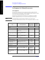
Test Equipment for Making Measurements . . . . . . . . . . . . . . . . . . . . . . . . . . . . . . . . . . . . . 66
5. Spectrum Analyzer . . . . . . . . . . . . . . . . . . . . . . . . . . . . . . . . . . . . . . . . . . . . . . . . . . . . . . . 67
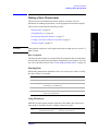
Making a Basic Measurement . . . . . . . . . . . . . . . . . . . . . . . . . . . . . . . . . . . . . . . . . . . . . . . . 69
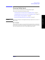
Measuring Multiple Signals . . . . . . . . . . . . . . . . . . . . . . . . . . . . . . . . . . . . . . . . . . . . . . . . . 75
Measuring a Low-Level Signal . . . . . . . . . . . . . . . . . . . . . . . . . . . . . . . . . . . . . . . . . . . . . . . 86
Making Distortion Measurements . . . . . . . . . . . . . . . . . . . . . . . . . . . . . . . . . . . . . . . . . . . . 93
Using the Analyzer as a Fixed Tuned Receiver . . . . . . . . . . . . . . . . . . . . . . . . . . . . . . . . . 101
Channel Power . . . . . . . . . . . . . . . . . . . . . . . . . . . . . . . . . . . . . . . . . . . . . . . . . . . . . . . . . . 104
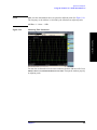
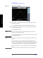
Occupied Bandwidth (OBW) Measurement . . . . . . . . . . . . . . . . . . . . . . . . . . . . . . . . . . . . 107
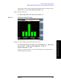
Using the Spectrogram View (Requires Option 271) . . . . . . . . . . . . . . . . . . . . . . . . . . . . . 111
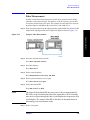
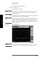
Pulse Measurement . . . . . . . . . . . . . . . . . . . . . . . . . . . . . . . . . . . . . . . . . . . . . . . . . . . . . . . 115
Tune and Listen (Requires Option AFM) . . . . . . . . . . . . . . . . . . . . . . . . . . . . . . . . . . . . . . 117
6. Channel Analyzer Measurements . . . . . . . . . . . . . . . . . . . . . . . . . . . . . . . . . . . . . . . . . . 119
Making Adjacent Channel Power (ACP (I&M)) Measurements . . . . . . . . . . . . . . . . . . . . 121
5
Table of Contents
1. Installation and Setup . . . . . . . . . . . . . . . . . . . . . . . . . . . . . . . . . . . . . . . . . . . . . . . . . . . . . . 9
Introduction . . . . . . . . . . . . . . . . . . . . . . . . . . . . . . . . . . . . . . . . . . . . . . . . . . . . . . . . . . . . . . 12
Initial Inspection . . . . . . . . . . . . . . . . . . . . . . . . . . . . . . . . . . . . . . . . . . . . . . . . . . . . . . . . . . 13
Safety Information . . . . . . . . . . . . . . . . . . . . . . . . . . . . . . . . . . . . . . . . . . . . . . . . . . . . . . . . 15
Power Requirements . . . . . . . . . . . . . . . . . . . . . . . . . . . . . . . . . . . . . . . . . . . . . . . . . . . . . . . 28
Physically Securing Your Analyzer . . . . . . . . . . . . . . . . . . . . . . . . . . . . . . . . . . . . . . . . . . . 32
Turning on the Analyzer for the First Time . . . . . . . . . . . . . . . . . . . . . . . . . . . . . . . . . . . . . 33
Firmware Revision . . . . . . . . . . . . . . . . . . . . . . . . . . . . . . . . . . . . . . . . . . . . . . . . . . . . . . . . 35
Printer Setup and Operation . . . . . . . . . . . . . . . . . . . . . . . . . . . . . . . . . . . . . . . . . . . . . . . . . 36
Protecting Against Electrostatic Discharge . . . . . . . . . . . . . . . . . . . . . . . . . . . . . . . . . . . . . 37
Using the Soft Carrying Case . . . . . . . . . . . . . . . . . . . . . . . . . . . . . . . . . . . . . . . . . . . . . . . . 38
Table of Contents
Contents
7. Stimulus Response Measurements (Requires N8995A) . . . . . . . . . . . . . . . . . . . . . . . . . .125
Two Port Insertion Loss . . . . . . . . . . . . . . . . . . . . . . . . . . . . . . . . . . . . . . . . . . . . . . . . . . . .127
One Port Insertion Loss . . . . . . . . . . . . . . . . . . . . . . . . . . . . . . . . . . . . . . . . . . . . . . . . . . . .130
Return Loss . . . . . . . . . . . . . . . . . . . . . . . . . . . . . . . . . . . . . . . . . . . . . . . . . . . . . . . . . . . . .134
Distance to Fault . . . . . . . . . . . . . . . . . . . . . . . . . . . . . . . . . . . . . . . . . . . . . . . . . . . . . . . . .138
8. Demodulating AM/FM Signals (Requires Option N8996A-1FP) . . . . . . . . . . . . . . . . . .145
Demodulating an AM Signal Using the CSA (Requires Option N8996A-1FP) . . . . . . . . .147
Demodulating an FM Signal Using the CSA (Requires Option N8996A-1FP) . . . . . . . . .153
9. Basic System Operations . . . . . . . . . . . . . . . . . . . . . . . . . . . . . . . . . . . . . . . . . . . . . . . . . .159
System Reference Introduction . . . . . . . . . . . . . . . . . . . . . . . . . . . . . . . . . . . . . . . . . . . . . .162
Setting System References . . . . . . . . . . . . . . . . . . . . . . . . . . . . . . . . . . . . . . . . . . . . . . . . . .163
Setting System Time/Date . . . . . . . . . . . . . . . . . . . . . . . . . . . . . . . . . . . . . . . . . . . . . . . . . .164
Printing a Screen To a File . . . . . . . . . . . . . . . . . . . . . . . . . . . . . . . . . . . . . . . . . . . . . . . . .165
Saving Data . . . . . . . . . . . . . . . . . . . . . . . . . . . . . . . . . . . . . . . . . . . . . . . . . . . . . . . . . . . . .166
File Naming Options . . . . . . . . . . . . . . . . . . . . . . . . . . . . . . . . . . . . . . . . . . . . . . . . . . . . . .167
Configuring for Network Connectivity . . . . . . . . . . . . . . . . . . . . . . . . . . . . . . . . . . . . . . . .169
Setting the Display . . . . . . . . . . . . . . . . . . . . . . . . . . . . . . . . . . . . . . . . . . . . . . . . . . . . . . . .171
Saving, Recalling, and Deleting Instrument States . . . . . . . . . . . . . . . . . . . . . . . . . . . . . . .172
Viewing System Statistics . . . . . . . . . . . . . . . . . . . . . . . . . . . . . . . . . . . . . . . . . . . . . . . . . .175
Using the Option Manager . . . . . . . . . . . . . . . . . . . . . . . . . . . . . . . . . . . . . . . . . . . . . . . . . .176
Testing System Functions . . . . . . . . . . . . . . . . . . . . . . . . . . . . . . . . . . . . . . . . . . . . . . . . . .178
10. Working with Batteries . . . . . . . . . . . . . . . . . . . . . . . . . . . . . . . . . . . . . . . . . . . . . . . . . .179
Installing Batteries . . . . . . . . . . . . . . . . . . . . . . . . . . . . . . . . . . . . . . . . . . . . . . . . . . . . . . . .181
Viewing Battery Status . . . . . . . . . . . . . . . . . . . . . . . . . . . . . . . . . . . . . . . . . . . . . . . . . . . .182
Charging Batteries . . . . . . . . . . . . . . . . . . . . . . . . . . . . . . . . . . . . . . . . . . . . . . . . . . . . . . . .184
Recalibrating Batteries . . . . . . . . . . . . . . . . . . . . . . . . . . . . . . . . . . . . . . . . . . . . . . . . . . . . .186
Battery Care . . . . . . . . . . . . . . . . . . . . . . . . . . . . . . . . . . . . . . . . . . . . . . . . . . . . . . . . . . . . .187
Battery Specifications . . . . . . . . . . . . . . . . . . . . . . . . . . . . . . . . . . . . . . . . . . . . . . . . . . . . .190
11. Concepts . . . . . . . . . . . . . . . . . . . . . . . . . . . . . . . . . . . . . . . . . . . . . . . . . . . . . . . . . . . . . . .193
Resolving Closely Spaced Signals . . . . . . . . . . . . . . . . . . . . . . . . . . . . . . . . . . . . . . . . . . . .194
Trigger Concepts . . . . . . . . . . . . . . . . . . . . . . . . . . . . . . . . . . . . . . . . . . . . . . . . . . . . . . . . .196
AM and FM Demodulation Concepts . . . . . . . . . . . . . . . . . . . . . . . . . . . . . . . . . . . . . . . . .197
Stimulus Response Measurement Concepts . . . . . . . . . . . . . . . . . . . . . . . . . . . . . . . . . . . .198
AM Concepts . . . . . . . . . . . . . . . . . . . . . . . . . . . . . . . . . . . . . . . . . . . . . . . . . . . . . . . . . . . .200
FM Concepts . . . . . . . . . . . . . . . . . . . . . . . . . . . . . . . . . . . . . . . . . . . . . . . . . . . . . . . . . . . .202
Modulation Distortion Measurement Concepts . . . . . . . . . . . . . . . . . . . . . . . . . . . . . . . . . .204
Modulation SINAD Measurement Concepts . . . . . . . . . . . . . . . . . . . . . . . . . . . . . . . . . . . .205
6
Contents
13. Connector Care . . . . . . . . . . . . . . . . . . . . . . . . . . . . . . . . . . . . . . . . . . . . . . . . . . . . . . . . 219
Using, Inspecting, and Cleaning RF Connectors . . . . . . . . . . . . . . . . . . . . . . . . . . . . . . . . 221
14. In Case of Difficulty . . . . . . . . . . . . . . . . . . . . . . . . . . . . . . . . . . . . . . . . . . . . . . . . . . . . . 225
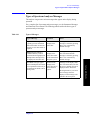
Types of Spectrum Analyzer Messages . . . . . . . . . . . . . . . . . . . . . . . . . . . . . . . . . . . . . . . 227
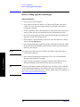
Before Calling Agilent Technologies . . . . . . . . . . . . . . . . . . . . . . . . . . . . . . . . . . . . . . . . . 228
Returning an Analyzer for Service . . . . . . . . . . . . . . . . . . . . . . . . . . . . . . . . . . . . . . . . . . . 231
15. Copyright Information . . . . . . . . . . . . . . . . . . . . . . . . . . . . . . . . . . . . . . . . . . . . . . . . . . 235
7
Table of Contents
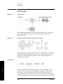
12. Programming Examples . . . . . . . . . . . . . . . . . . . . . . . . . . . . . . . . . . . . . . . . . . . . . . . . . 207
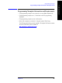
Finding Examples and More Information . . . . . . . . . . . . . . . . . . . . . . . . . . . . . . . . . . . . . . 208
Programming Examples Information and Requirements . . . . . . . . . . . . . . . . . . . . . . . . . . 209
Programming in C Using the VISA . . . . . . . . . . . . . . . . . . . . . . . . . . . . . . . . . . . . . . . . . . 210
Table of Contents
Contents
8
Installation and Setup
1
Installation and Setup
9
Installation and Setup
Installation and Setup
This chapter provides the following information that you may need when you first
receive your spectrum analyzer:
•
“Introduction” on page 11
•
“Initial Inspection” on page 12
•
“Safety Information” on page 14
•
“Power Requirements” on page 27
•
“Physically Securing Your Analyzer” on page 31
•
“Turning on the Analyzer for the First Time” on page 32
•
“Firmware Revision” on page 34
•
“Printer Setup and Operation” on page 35
•
“Protecting Against Electrostatic Discharge” on page 36
•
“Using the Soft Carrying Case” on page 37
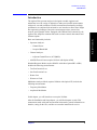
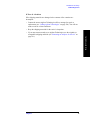
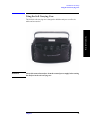
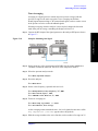
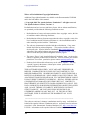
Figure 1-1
CSA 1.0
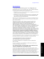
Figure 1-2
CSA 2.0
10
Chapter 1
Installation and Setup
Introduction
Introduction
The Agilent CSA spectrum analyzer is designed to enable engineers and
technicians in a wide variety of industries to make precision RF measurements
with speed, ease and confidence. Flexible measurement functionality and high
performance are combined with an intuitive user interface to allow faster insight
into engineering challenges. Innovative measurement science ensures fast,
accurate, and repeatable results. Equipped with USB and LAN connectivity, the
Agilent CSA simplifies common tasks such as remote control, data transfer and
firmware update.
•
Installation and Setup
Basic test functionality includes:
Spectrum Analyzer:
— Channel Power
— Occupied Bandwidth
•
Channel Analyzer:
— Adjacent Channel Power (ACP (I&M))
•
AM/FM Tune & Listen (requires N1996A with Option AFM)
Stimulus/Response Mode (requires N8995A with either Option SR3 or SR6)
includes the following measurements:
•
Two Port Insertion Loss
•
One Port Insertion Loss
•
Return Loss
•
Distance to Fault
Modulation Analyzer Mode (requires N8996A with Option 1FP) includes the
following measurements:
•
Frequency Modulation
•
Amplitude Modulation
In this chapter, you will learn how to set up the N1996A.
After the Installation and Setup chapter, you will find chapters on each CSA
measurement mode with each measurement in that mode, general information on
batteries, caring for the CSA, and how to return the instrument for service.
Chapter 1
11
Installation and Setup
Initial Inspection
Initial Inspection
Inspect the shipping container and the cushioning material for signs of stress.
Retain the shipping materials for future use, as you may wish to ship the analyzer
to another location or to Agilent Technologies for service. Verify that the contents
of the shipping container are complete. The following table lists the items shipped
with the analyzer.
Item
Description
Installation and Setup
Accessories
AC/DC converter
External power supply 15 VDC 150 W
Power Cable (See Table 1-2 on page 29)
Connection for AC/DC converter power source.
Stimulus /Response Calibration kit Option
SRK (pn N1996A-SRK) includes:
This item is included ONLY when you have
ordered Option SRK.
Coax Accessories Case
Open/Short
Coax Accessories Case, plastic and foam
(5000-0912)
Open/Short, 50 ohm, N-type male (85032-60011)
Termination
Termination, 50 ohm, N-type male (00909-60009)
Standard Documentation Set
Documentation CD-ROM
12
Includes electronic (PDF) versions of the
documents in the standard set (“Manual Set on
CD-ROM” on page 45). In addition, this
Installation and Setup chapter is no the accessible
in a standalone electronic (PDF) version and a text
file of the complete firmware copyright
information. You can view and print the
information as needed. See the front of the
CD-ROM for installation information.
Chapter 1
Installation and Setup
Initial Inspection
If There Is a Problem
If the shipping materials are damaged or the contents of the container are
incomplete:
Contact the nearest Agilent Technologies office to arrange for repair or
replacement (see “Calling Agilent Technologies” on page 229). You will not
need to wait for a claim settlement.
•
Keep the shipping materials for the carrier’s inspection.
•
If you must return an analyzer to Agilent Technologies, use the original (or
comparable) shipping materials (see “Returning an Analyzer for Service” on
page 231).
Chapter 1
Installation and Setup
•
13
Installation and Setup
Safety Information
Safety Information
General
This product and related documentation must be reviewed for familiarization with
safety markings and instructions before operation.
Installation and Setup
This product has been designed and tested in accordance with IEC 61010-1:2001
Second Edition, and has been supplied in a safe condition. The documentation
contains information and warnings that must be followed by the user to ensure safe
operation and to maintain the product in a safe condition.
Safety Earth Ground
An uninterruptible safety earth ground must be provided from the main power
source to the product input wiring terminals, power cord, or supplied power cord
set.
Chassis Ground Terminal
To prevent a potential shock hazard, always connect the rear-panel chassis ground
terminal to earth ground when operating this analyzer from a dc power source.
Safety Information
The following safety conventions are used throughout this manual. Familiarize
yourself with the symbols and their meaning before operating this instrument.
WARNING
A Warning denotes a hazard. It calls attention to a procedure which, if not
correctly performed or adhered to, could result in injury or loss of life. Do not
proceed beyond a warning note until the indicated conditions are fully
understood and met.
CAUTION
A Caution denotes a hazard. It calls attention to a procedure that, if not correctly
performed or adhered to, could result in damage to or destruction of the
instrument. Do not proceed beyond a caution sign until the indicated conditions are
fully understood and met.
NOTE
A Note calls out special information for the user’s attention. It provides operational
information or additional instructions of which the user should be aware.
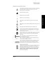
Safety Symbols and Product Markings
The following safety symbols and product markings are located on the analyzer or
the external power supply. Familiarize yourself with the symbols and their
14
Chapter 1
Installation and Setup
Safety Information
meaning before operating this analyzer.
!
The instruction documentation symbol. The product is marked with
this symbol when it is necessary for the user to refer to the
instructions in the documentation.
Indicates hazardous voltages.
Indicates earth (ground) terminal
This symbol is used to mark the on position of the power line
switch.
This symbol is used to mark the standby position of the power line
switch.
This symbol indicates that the input power required is AC.
The CE mark shows that the product complies with all relevant
European legal Directives (if accompanied by a year, it signifies
when the design was proven).
The CSA mark (not to be confused with the Agilent CSA spectrum
analyzer) is a registered trademark of the Canadian Standards
Association.
The C-Tick mark is a registered trademark of the Australian
Spectrum Management Agency.
ISM 1-A
This is a symbol of an Industrial Scientific and Medical Group 1
Class A product (CISPR 11, Clause 4).
This is a marking of an Industrial Scientific and Medical Group 1
Class A product, and to indicate product compliance with the
Canadian Interference-Causing Equipment Standard (ICES-001).
Separate collection symbol.
The Waste Electrical and Electronic Equipment (WEEE) Directive
(2002/96/EC), adopted by EU Commission on 13 Feb. 2003, is
introducing producer responsibility on all Electric and Electronic
appliances from 13 Aug. 2005. Under EU law, all electric and
electronic equipment (EEE) are required to be separated from
normal waste for disposal.
Chapter 1
15
Installation and Setup
Indicates chassis ground terminal
Installation and Setup
Safety Information
Installation and Setup
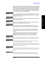
Safety Considerations For This Analyzer
WARNING
This is a Safety Class 1 Product (provided with a protective earth ground
incorporated in the power cord). The mains plug shall be inserted only in a
socket outlet provided with a protected earth contact. Any interruption of the
protective conductor inside or outside of the product is likely to make the
product dangerous. Intentional interruption is prohibited.
WARNING
Failure to ground the analyzer properly when using the external power
supply can result in personal injury. Before turning on the analyzer, you must
connect its protective earth terminals to the protective conductor of the main
power cable. Only insert the main power cable plug into a socket outlet that
has a protective earth contact. DO NOT defeat the earth-grounding
protection by using an extension cable, power cable, or autotransformer
without a protective ground conductor.
WARNING
If this analyzer is to be energized via an autotransformer (for voltage
reduction), make sure the common terminal is connected to the earth terminal
of the power source.
WARNING
If this product is not used as specified, the protection provided by the
equipment could be impaired. This product must be used only in a normal
condition (in which all means for protection are intact).
WARNING
Whenever it is likely that the protection has been impaired, the analyzer must
be made inoperative and be secured against any unintended operation.
WARNING
To prevent electrical shock, disconnect the Agilent Technologies spectrum
analyzer from mains before cleaning. Use a dry cloth or one slightly
dampened with water to clean the external case parts. Do not attempt to clean
internally.
WARNING
When operating from an AC power source, always use the three-prong ac
power cord supplied with this product. Failure to ensure adequate earth
grounding by not using this cord may cause personal injury and/or product
damage.
This product is designed for use in Installation Category II and Pollution
Degree 3 per IEC 61010 and IEC 60664 respectively.
WARNING
The front panel switch is a standby switch only; it is not a LINE switch (power
disconnecting device).
WARNING
Install the product so that the detachable power cord is readily identifiable
16
Chapter 1
Installation and Setup
Safety Information
and easily reached by the operator. The detachable power cord is the product
disconnecting device. It disconnects the mains circuits from the mains supply
before other parts of the product. The front panel switch is only a standby
switch and is not a LINE switch. Alternatively, an externally installed switch
or circuit breaker (which is readily identifiable and is easily reached by the
operator) may be used as a disconnecting device.
Danger of explosion if battery is incorrectly replaced. Replace only with the
same or equivalent type recommended. Discard used batteries according to
manufacturer’s instructions.
WARNING
This instrument has a recharge circuit. Never install non-rechargeable cells or
batteries of a different type.
WARNING
No operator serviceable parts inside. Refer servicing to qualified personnel.
To prevent electrical shock do not remove covers.
WARNING
Servicing instructions are for use by qualified personnel only. To avoid
electrical shock, do not perform any servicing unless you are qualified to do
so.
The opening of covers or removal of parts is likely to expose dangerous
voltages. Disconnect the product from all voltage sources while it is being
opened.
Adjustments described in the service manual are performed with power
supplied to the analyzer while protective covers are removed. Energy
available at many points may, if contacted, result in personal injury.
CAUTION
If you are charging the batteries internally—even while the analyzer is powered
off—the analyzer may become warm. Take care to provide proper ventilation.
CAUTION
To avoid overheating, always disconnect the analyzer from the external power
supply before storing the analyzer in the soft carrying case.
If you prefer to leave the analyzer connected to the external power supply while
inside the soft carrying case, you can disconnect the external power supply from its
power source to prevent overheating.
CAUTION
The external power supply has autoranging line voltage input. Be sure the supply
voltage is within the specified range. (Refer to the specifications guide for your
analyzer.)
CAUTION
When operating this product with the external power supply, always use the
three-prong power cord supplied with this product. Failure to ensure adequate
Chapter 1
17
Installation and Setup
WARNING
Installation and Setup
Safety Information
earth grounding by not using this cord can cause product damage.
CAUTION
VENTILATION REQUIREMENTS: When installing the product in a cabinet, the
convection into and out of the product must not be restricted. The ambient
temperature (outside the cabinet) must be less than the maximum operating
temperature of the product by 4C for every 100 watts dissipated in the cabinet. If
the total power dissipated in the cabinet is greater than 800 watts, then forced
convection must be used.
Installation and Setup
Lifting and Handling
When lifting and handling the Agilent N1996A Spectrum Analyzer use
ergonomically correct procedures. If so equipped, lift and carry the analyzer by the
bail handle.
18
Chapter 1
Installation and Setup
Safety Information
Battery Pack Product Safety Data Sheet
Installation and Setup
Product Safety Data Sheet
PRODUCT NAME: Inspired Energy Rechargeable Battery Pack
Model: NF2040A22
TRADE NAME: NF2040
Volts: 10.8
CHEMICAL SYSTEM: Lithium Ion
Approximate Weight: 340 g
SECTION I – MANUFACTURER INFORMATION
Inspired Energy, Inc.
12705 N US Hwy 441
Alachua, FL 32615
Telephone: (888) 5-INSPIRE (888-546-7747)
Date Prepared: Jan 13th 2003
SECTION II – HAZARDOUS INGREDIENTS
Important Note:
The battery should not be opened or burned. Exposure to the ingredients contained within or
their combustion products could be harmful
Material Safety Data Sheet Attached:
Review cell manufacturer’s MSDS
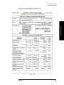
SECTION III – OPERATING PARAMETERS
Maximum Charge Voltage:
12.6 V
Minimum Charge Voltage:
7.5 V
Maximum Charge Current:
3.0 A
Maximum Discharge Current:
3.0 A
Recommended Charging Method:
Use an SMBus charger of level 2 or higher to provide
a 3.0 A current limited constant voltage of 12.6 V. The
charging cycle shall terminate when the average current
falls below 150mA.
The information contained within is provided for your information only. This battery is an article pursuant to 29 CFR
1910.1200 and, as such, is not subject to the OSHA Hazard Communication standard requirement for preparation of a
material safety data sheet. The information and recommendations set forth herein are made in good faith and are
believed to be accurate as of the date of preparation. However, INSPIRED ENERGY, INC. MAKES NO WARRANTY,
EITHER EXPRESSED OR IMPLIED, WITH RESPECT TO THIS INFORMATION AND DISCLAIMS ALL LIABILITY FROM
RELIANCE ON IT.
Chapter 1
19
Installation and Setup
Safety Information
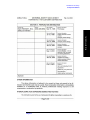
Battery Pack Declaration of Conformity
Installation and Setup
Declaration of Conformance
PRODUCT: Standard Battery for Inspired Energy
Inspired Energy Part Number: NF2040
SECTION I – MANUFACTURER INFORMATION
Inspired Energy, Inc.
25440 NW 8th Place, Newberry FL 32669, USA
Telephone: +1 386 462 3676
Date Prepared: December 21st 2004
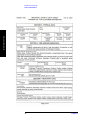
SECTION II – CONFORMANCE INFORMATION
The listed products have been tested in accordance with the UN document
ST/SG/AC.10/11/Rev.3: “Amendments to the Third Revised Edition of the Recommendations
on the Transport of Dangerous Goods, Manual of Tests & Criteria” and found to comply with
the stated criteria
Test #
T1
T2
T3
T4
T5
T6
T7
T8
Description
Altitude Simulation
Thermal Cycling
Shock
Vibration
Short Circuit
Impact (Cell-Level test)
Overcharge
Forced Discharge (Cell-level test)
Date Tested
June 21, 2004
July 23, 2004
September 30 2004
October 01 2004
November 09, 2004
July 2nd 2003
November 15, 2004
July 2nd 2003
Test result
Pass
Pass
Pass
Pass
Pass
Pass
Pass
Pass
Signed:
David W. Hellriegel
Product Test Laboratory manager
The information contained within is provided for your information only. The information and recommendations set forth
herein are made in good faith and are believed to be accurate as of the date of preparation. However, INSPIRED ENERGY,
INC. MAKES NO WARRANTY, EITHER EXPRESSED OR IMPLIED, WITH RESPECT TO THIS INFORMATION AND DISCLAIMS ALL
LIABILITY FROM RELIANCE ON IT.
20
Chapter 1
Installation and Setup
Safety Information
Batteries: Safe Handling and Disposal
Installation and Setup
Chapter 1
21
Installation and Setup
Installation and Setup
Safety Information
22
Chapter 1
Installation and Setup
Safety Information
Installation and Setup
Chapter 1
23
Installation and Setup
Installation and Setup
Safety Information
24
Chapter 1
Installation and Setup
Safety Information
Installation and Setup
Chapter 1
25
Installation and Setup
Installation and Setup
Safety Information
26
Chapter 1
Installation and Setup
Power Requirements
Power Requirements
Typically, the only physical installation of your Agilent spectrum analyzer is a
connection to a power source.
WARNING
Before operating or connecting this analyzer to an external power source,
please read and understand safety information in “Safety Information” on
page 14 and the safety considerations and all safety warnings in “Safety
Considerations For This Analyzer” on page 16.
This analyzer does not contain customer serviceable fuses.
NOTE
If your test system requires a common ground, use the grounding lug provided on
the back of the instrument.
NOTE
For detailed analyzer specifications, see the Specifications guide.
NOTE
In addition to operating the analyzer on AC power using the external AD/DC
converter, you can operate it using internal batteries. For information on the
installation and use of those batteries, refer to Chapter 10, “Working with
Batteries,” on page 179.
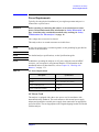
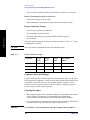
Table 1-1
AC Power Requirements
Description
Specifications
Voltage
90 to 132 Vrms (47 to 440 Hz)
Voltage
195 to 250 Vrms (47 to 66 Hz)
Power Consumption, On
< 115 W
Power Consumption, Standby
<7W
AC Power Cord
The analyzer is equipped with a three-wire power cord, in accordance with
international safety standards. This cord connects to the external power supply
adapter and grounds the external power supply when connected to an appropriate
power line outlet. The cord appropriate to the original shipping location is included
with the analyzer.
Chapter 1
27
Installation and Setup
Line voltage does not need to be selected.
Installation and Setup
Power Requirements
Installation and Setup
Various AC power cables are available that are unique to specific geographic
areas. You can order additional AC power cables for use in different areas. AC
Power Cords, on page 29 lists the available AC power cables, illustrates the plug
configurations, and identifies the geographic area in which each cable is
appropriate.
28
Chapter 1
Installation and Setup
Power Requirements
Table 1-2
AC Power Cords
Installation and Setup
Chapter 1
29
Installation and Setup
Power Requirements
Clock Battery Information
The analyzer uses a Poly-carbonmonofluoride Lithium Coin battery to power the
analyzer clock. The battery is located on the CPU board.
If the analyzer’s clock does not work, the problem is probably the battery. See
“Returning an Analyzer for Service” on page 231.
WARNING
Danger of explosion if battery is incorrectly replaced. Replace only with the
same or equivalent type recommended. Discard used batteries according to
the manufacturer’s instructions.
Installation and Setup
NOTE
30
Chapter 1
Installation and Setup
Physically Securing Your Analyzer
Physically Securing Your Analyzer
To prevent unauthorized removal of your analyzer, you can use a Kensington Slim
MicroSaver security cable to attach the analyzer to an immovable object. Your
analyzer has a Kensington Security Slot located on the back of the analyzer. The
Kensington Security Slot is identified on the analyzer with this logo: . For more
information, visit
http://www.microsaver.com.
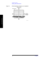
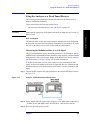
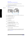
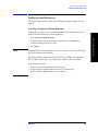
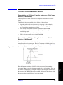
Basic Instructions for Using the Kensington Slim MicroSaver
Installation and Setup
Step 1. Wrap the steel cable around an immovable object.
Step 2. Insert the lock into the Kensington Security Slot.
Step 3. Turn the key.
Chapter 1
31
Installation and Setup
Turning on the Analyzer for the First Time
Turning on the Analyzer for the First Time
Installation and Setup
WARNING
Before operating or connecting this analyzer to an external power source,
please read and understand safety information in “Safety Information” on
page 14 and the safety considerations and all safety warnings in “Safety
Considerations For This Analyzer” on page 16.
o Plug in the power cord. If the analyzer is to be operated on the internal
batteries, ensure that both batteries are installed. They are approximately 50%
charged when you receive them and will provide full performance if you
choose to operate the analyzer without charging them at this time. (View the
charge level for each battery on the battery end display.) If the batteries are
showing 1 bar or less, recharging is recommended at this time.
NOTE
For maximum runtime, it is best to have approximately equal charge levels on both
batteries. The instrument will shut down if either battery becomes fully discharged
during operation.
NOTE
Do not connect anything else to the analyzer yet.
o Press the power switch (located in the lower left-hand corner of the analyzer’s
front panel) to turn the analyzer on. See “Front Panel Overview” on page 50.
NOTE
The instrument requires <2 minutes to power-on.
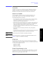
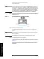
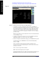
Information
Screen
An information screen appears during the initialization process. The information
screen contains the analyzer product number and a URL for accessing product
support information on the World Wide Web. See “Where to Find the Latest
Information” on page 3.
NOTE
It is important for you to Record the firmware revision and serial number, and keep
it for reference. If you should ever need to call Agilent Technologies for service or
with any questions regarding your analyzer, it will be helpful to have this
information readily available. You can also obtain the firmware revision and serial
number by pressing System, System Stats, Rev Info.
o Allow the spectrum analyzer to warm-up for 30 minutes before making a
calibrated measurement. To meet its specifications, the analyzer must meet
operating temperature conditions.
CAUTION
Ensure protection of the input mixer by limiting the input level to 50 Vdc, +33
dBm.
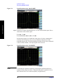
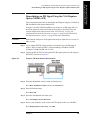
o If using non-DHCP LAN, set the IP address of the analyzer to an appropriate
number for your network (one that the network recognizes, but that is not yet in
32
Chapter 1
Installation and Setup
Turning on the Analyzer for the First Time
use):
— Press System, Controls, IP Admin and note the IP address. This is the IP
address that will be used if IP Config is set to Static. To view the IP Address
selected by DHCP, press Mode.
— If the current address is not appropriate, press IP Config, Static, IP Address
and use the keypad to change it. In addition, you may also need to change
the Net Mask and Gateway settings.
— Press Save.
— Connect the LAN cable to the LAN connector (not the Timing LAN
— Cycle the analyzer power. Refer to “Configuring for Network Connectivity”
on page 169
NOTE
It is necessary to cycle the power to the analyzer after plugging in the LAN for the
analyzer to recognize the network.
NOTE
If you are not using a LAN connection, you may want to set the IP Configuration
to None to reduce the instrument power-on time.
Why Aren’t All the Personality Options Available?
Many measurement personality options are available for your use and are loaded in
the instrument. To make an option available, you must also have a license key
entered.
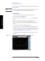
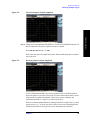
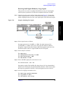
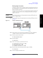
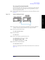
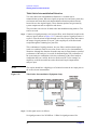
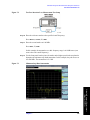
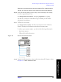
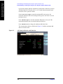
Using an External Reference
If you wish to use an external source as the reference frequency, you must connect
an external reference source and set the reference frequency as follows:
1. Connect an external source to the EXT REF IN connector on the rear panel
(see “Rear-Panel Features” on page 61). The signal level should be greater than
–15 dBm.
2. Select the frequency of the external reference into the analyzer:
a. Press System, Freq/Time/Ref
b. Select the up and down arrow navigation keys to highlight the desired
reference frequency.
c. Press Select to set the reference source and frequency that you have
highlighted.
d. Press Cancel to abort your reference change and retain the previously
selected frequency reference. See “Setting System References” on page
163 for more information.
Chapter 1
33
Installation and Setup
connector) located on the rear panel of your analyzer (see “Rear-Panel
Features” on page 61).
Installation and Setup
Firmware Revision
Firmware Revision
To view the firmware revision of your analyzer, Press System, System Stats, Rev
Info. If you call Agilent Technologies regarding your analyzer, it is helpful to have
this revision and the analyzer serial number available.
Installation and Setup
TIP
You can get automatic electronic notification of new firmware releases and other
product updates/information by subscribing to the Agilent Technologies Test &
Measurement E-Mail Notification Service for the Agilent CSA spectrum analyzer
at:
http://www.agilent.com/find/notifyme
34
Chapter 1
Installation and Setup
Printer Setup and Operation
Printer Setup and Operation
The Agilent CSA spectrum analyzer does not print directly to a printer. You can
print a screen image or measurement data by first saving the information to a USB
memory device and then use a PC with an attached printer to print the file. You can
save a screen image by pressing (Print) (for detail instructions, refer to
“Printing a Screen To a File” on page 165). Also, you can save a screen image or
measurement results by pressing Save and Save Now (for detail instructions, refer
to “Saving Data” on page 166).
Installation and Setup
Chapter 1
35
Installation and Setup
Protecting Against Electrostatic Discharge
Protecting Against Electrostatic Discharge
Electrostatic discharge (ESD) can damage or destroy electronic components (the
possibility of unseen damage caused by ESD is present whenever components are
transported, stored, or used).
Test Equipment and ESD
Installation and Setup
To help reduce ESD damage that can occur while using test equipment:
WARNING
•
Before connecting any coaxial cable to an analyzer connector for the first time
each day, momentarily short the center and outer conductors of the cable
together.
•
Personnel should be grounded with a 1 M resistor-isolated wrist-strap before
touching the center pin of any connector and before removing any assembly
from the analyzer.
•
Be sure that all instruments are properly earth-grounded to prevent build-up of
static charge.
Do not use these first three techniques above when working on circuitry with
a voltage potential greater than 500 volts.
•
Perform work on all components or assemblies at a static-safe workstation.
•
Keep static-generating materials at least one meter away from all components.
•
Store or transport components in static-shielding containers.
•
Always handle printed circuit board assemblies by the edges. This reduces the
possibility of ESD damage to components and prevent contamination of
exposed plating.
For information on ordering static-safe accessories, see “Accessories” on page 45.
Additional Information about ESD
For more information about ESD and how to prevent ESD damage, contact the
Electrostatic Discharge Association (http://www.esda.org). The ESD standards
developed by this agency are sanctioned by the American National Standards
Institute (ANSI).
36
Chapter 1
Installation and Setup
Using the Soft Carrying Case
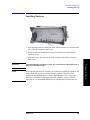
Using the Soft Carrying Case
The N1996A soft carrying case is designed to hold the analyzer as well as its
cables and accessories.
Installation and Setup
WARNING
Always disconnect the analyzer from the external power supply before storing
the analyzer in the soft carrying case.
Chapter 1
37
Installation and Setup
Installation and Setup
Using the Soft Carrying Case
38
Chapter 1
Options and Accessories
2
Options and Accessories
This chapter lists options and accessories available for your analyzer.
39
Options and Accessories
Ordering Options and Accessories
Ordering Options and Accessories
Options and accessories help you configure the analyzer for your specific
applications.
Options (see page 41)
Unless specified otherwise, all options are available when you order a spectrum
analyzer; some options are also available as kits that you can order and install after
you receive the analyzer. Order kits through your local Agilent Sales and Service
Office.
At the time of analyzer purchase, options can be ordered using your product
number and the number of the option you are ordering. For example, if you are
ordering Option SRK for an Agilent N1996A, you would order N1996A-SRK.
If you are ordering an option after the purchase of your analyzer, you will need to
add a K (for kit) to the product number and then specify which option you are
ordering (for example, N1996AK-SRK.)
Options and Accessories
If you know the option you wish to order, refer to “Options” on page 41 which is in
ascending order by option number and type. Complete option descriptions can be
found in the following section, listed in alphabetical order by option name under
“Option Descriptions” on page 43.
For the latest information on Agilent Spectrum Analyzer options and upgrade kits,
visit the following URL:
http://www.agilent.com/find/sa_upgrades
Accessories (see page 45)
Order accessories through your local Agilent Sales and Service Office. For
information on contacting Agilent Sales and Service, refer to “Calling Agilent
Technologies” on page 229.
40
Chapter 2
Options and Accessories
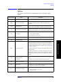
Options
Options
Each option is described below in alpha/numeric order according to option
number.
Option Number
0950-5023
Name
Description
External AC/DC Power Supply
External power supply 16 VDC 150 W
0BW
Service Documentation
The Service guide describes assembly-level troubleshooting
procedures, provides a parts list, and documents post-repair
procedures.
1CM
Rack Mount Kit
Includes rack mount flanges and hardware. Used to rack mount
analyzers without front handles (available as P/N N1996-60028).
1CP
Rack Mount Kit with Handles
Includes the parts necessary to rack mount an analyzer with front
handles attached (available as P/N N1996-60029). (Includes handles.)
Provides a display with a history of the spectrum. You can use it to:
271
Spectrogram
•
•
503
100 kHz to 3 GHz1
Spectrum Analyzer Frequency Range: 100 kHz to 3 GHz
506
100 kHz to 6 GHz1
Spectrum Analyzer Frequency Range: 100 kHz to 6 GHz
Locate intermittent signals.
Track signal levels over time.
ABA
Measurement Guide
Provides details on how to measure various signals, and how to use
catalogs and files.
In addition, this manual covers unpacking and setting up the analyzer,
analyzer features, and how to make a basic measurement. Includes
information on options and accessories, and what to do if you have a
problem.
AB2
Measurement Guide,
Simplified Chinese
Localization
A Simplified Chinese language version of the standard Measurement
Guide.
Provides the same information as Option ABA listed above.
AFM
AM/FM Tune & Listen
Provides the audible detection of AM or FM signals at specific
frequency.
BAT
Battery Pack
Two batteries: 10.8 V 4.56 A-HR LI-ION (pn 1420-0891) (2 batteries
are required for the operation of the instrument).
BCG
External Battery Charger
External charger/DC adapter, includes:
Chapter 2
External power supply AC/DC adapter
Dual battery charger
41
Options and Accessories
An English language printed copy of the standard Measurement
Guide in addition to the standard documentation on the Manual Set on
CD-ROM shipped with the analyzer. For additional information on
the contents of the Documentation CD-ROM, refer to “Manual Set on
CD-ROM” on page 45.
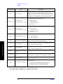
Options and Accessories
Options
Option Number
HTC
Name
Hard Transit Case
Description
The hard transit case will survive commercial transportation. This
rugged case has two wheels and an extendible handle for easy
transport. The case can also accommodate two battery packs and ac
adapters. To order the option HTC which requires the soft carrying
case (option SCC) for filling the space in the hard transit case.
Provides Stimulus/Response measurements:
N8995A - SR3
Stimulus/Response
Measurement Suite to 3 GHz2
•
•
•
•
Distance to Fault
Two Port Insertion Loss
One Port Insertion Loss
Return Loss
Provides Stimulus/Response measurements:
N8995A - SR6
Stimulus/Response
Measurement Suite to 6 GHz3
•
•
•
•
Distance to Fault
Two Port Insertion Loss
One Port Insertion Loss
Return Loss
Provides AM/FM demodulation measurements:
N8996A-1FP
AM/FM Modulation Analysis
0B0
Manual Set on CD-ROM Only
P03
3 GHz Preamplifier
•
•
Amplitude Modulation
Frequency Modulation
The documentation CD-ROM contains the standard documentation
set as well as Adobe Acrobat Reader with Search.
Options and Accessories
An internal preamplifier assembly. For use with Option 503 only.
Frequency Range: 100 kHz to 3 GHz
An internal preamplifier assembly. For use with Option 506 only.
P06
6 GHz Preamplifier
Frequency Range: 100 kHz to 6 GHz
R-50C-011-3
R-51B-001-3C
SCC
3 Year Inclusive Calibration
Contract
Provides your analyzer with a 3 year analyzer calibration contract.
3-Year Warranty Service
Support1
A total of 3 years of return-to-Agilent warranty service support. This
adds a 2-year service contract to the base analyzer 1-year warranty
Soft Carrying Case
An ergonomically designed case to hold the analyzer as well as its
cables and accessories.
The kit includes:
SRK
Stimulus/Response Calibration
Kit
•
•
•
Coax Accessories Case, plastic and foam (5000-0912)
Open/Short, 50 ohm, N-type male (85032-60011)
Termination, 50 ohm, N-type male (00909-60009)
1. Available only at time of purchase
2. The option replaces N1996A/TG3 + N8995A/1FP in CSA1.0.
3. The option replaces N1996A/TG6 + N8995A/1FP in CSA1.0.
42
Chapter 2
Options and Accessories
Option Descriptions
Option Descriptions
Each option is described below in alphabetical order according to option name.
Option
Number
Name
3 Year Inclusive Calibration
Contract
3-Year Warranty Service
Support 1
R-50C-011-3
R-51B-001-3C
100 kHz to 3 GHz Spectrum
Analyzer1
503
100 kHz to 6 GHz Spectrum
Analyzer1
506
Description
Provides your analyzer with a 3 year analyzer calibration contract.
A total of 3 years of return-to-Agilent warranty service support. This
adds a 2-year service contract to the base analyzer 1-year warranty.
Spectrum Analyzer Frequency Range: 100 kHz to 3 GHz
Spectrum Analyzer Frequency Range: 100 kHz to 6 GHz
Provides AM/FM demodulation measurements:
AM/FM Modulation Analysis
N8996A-1FP
•
•
Amplitude Modulation
Frequency Modulation
AM/FM Tune & Listen
AFM
Provides the audible detection of AM or FM signals at specific
frequency.
Battery Pack
BAT
Two batteries: 10.8 V 4.56 A-HR LI-ION (pn 1420-0891) (2 batteries
are required for the operation of the instrument.)
0950-5023
Options and Accessories
External AC/DC Power Supply
External power supply 16 VDC 150 W
External charger/DC adapter, includes:
External Battery Charger
BCG
External power supply AC/DC adapter 24 VDC 2.7 A
Dual battery charger
Hard Transit Case
HTC
The hard transit case will survive commercial transportation. This
rugged case has two wheels and an extendible handle for easy
transport. The case can also accommodate two battery packs and AC
adapters. To order the option HTC which requires the soft carrying
case (option SCC) for filling the space in the hard transit case.
Manual Set on CD-ROM Only
0B0
The documentation CD-ROM contains the standard documentation set
as well as Adobe Acrobat Reader with Search.
An English language printed copy of the standard Measurement Guide
in addition to the standard documentation in the Manual Set on
CD-ROM shipped with the analyzer. For additional information on the
contents of the Documentation CD-ROM, refer to “Manual Set on
CD-ROM” on page 45.
Measurement Guide
ABA
Provides details on how to measure various signals, and how to use
catalogs and files.
In addition, this manual covers unpacking and setting up the analyzer,
analyzer features, and how to make a basic measurement. Includes
information on options and accessories, and what to do if you have a
problem.
Chapter 2
43
Options and Accessories
Option Descriptions
Option
Number
Name
Measurement Guide,
Simplified Chinese
Localization
AB2
Preamplifier, 3 GHz
P03
Description
A Simplified Chinese language version of the standard Measurement
Guide.
Provides the same information as Option ABA listed above.
An internal preamplifier assembly.
Frequency Range: 100 kHz to 3 GHz
An internal preamplifier assembly.
Preamplifier, 6 GHz
P06
Frequency Range: 100 kHz to 6 GHz
Rack Mount Kit
1CM
Includes rack mount flanges and hardware. Used to rack mount
analyzers without front handles (available as P/N 5063-9215 and
N1996-60021).
Rack Mount Kit with Handles
1CP
Includes the parts necessary to rack mount an analyzer with front
handles attached (available as P/N 5063-9222 and N1996-60021).
(Includes handles.)
Service Documentation
0BW
The Service guide describes assembly-level troubleshooting
procedures, provides a parts list, and documents post-repair
procedures.
Soft Carrying Case
SCC
An ergonomically designed case to hold the analyzer as well as its
cables and accessories.
Provides a display with a history of the spectrum. You can use it to:
Options and Accessories
Spectrogram
271
•
•
Locate intermittent signals.
Track signal levels over time.
The kit includes:
Stimulus/Response Calibration
Kit
SRK
•
•
•
Coax Accessories Case, plastic and foam (5000-0912)
Open/Short, 50 ohm, N-type male (85032-60011)
Termination, 50 ohm, N-type male (00909-60009)
Provides Stimulus/Response measurements:
Stimulus/Response
Measurement Suite to 3 GHz2
N8995A - SR3
•
•
•
•
Distance to Fault
Two Port Insertion Loss
One Port Insertion Loss
Return Loss
Provides Stimulus/Response measurements:
Stimulus/Response
Measurement Suite to 6 GHz3
N8995A - SR6
•
•
•
•
Distance to Fault
Two Port Insertion Loss
One Port Insertion Loss
Return Loss
1. Available only at time of purchase
2. The option replaces N1996A/TG3 + N8995A/1FP in CSA1.0.
3. The option replaces N1996A/TG6 + N8995A/1FP in CSA1.0.
44
Chapter 2
Options and Accessories
Accessories
Accessories
A number of accessories are available from Agilent Technologies to help you
configure your analyzer for your specific applications. They can be ordered
through your local Agilent Sales and Service Office and are listed below.
Manual Set on CD-ROM
The documentation CD-ROM contains the standard documentation set in
electronic (PDF) format as well as Adobe Acrobat Reader with Search.
The standard documentation set includes:
User’s/Programmer’s Guide: Describes analyzer features in detail, including
front-panel key descriptions, basic spectrum analyzer programming
information, and SCPI command descriptions.
•
Measurement Guide: Provides details on how to measure various signals, and
how to use catalogs and files. In addition, this manual covers unpacking and
setting up the analyzer, analyzer features, and how to make a basic
measurement. Includes information on options and accessories, and what to do
if you have a problem.
•
Specifications Guide: Documents specifications, safety, and regulatory
information.
•
Instrument Messages and Functional Tests: Includes instrument messages (and
suggestions for troubleshooting them), and manual functional tests.
NOTE
Refer to the front of the CD-ROM, for installation information.
NOTE
Service documentation is not included in the standard documentation set. See
“Options” on page 41 for information on ordering.
50 Ohm Load
The Agilent 909 series loads come in several models and options providing a
variety of frequency ranges and VSWRs. Also, they are available in either 50 ohm
or 75 Ohm. Some examples include the:
909A: DC to 18 GHz
909C: DC to 2 GHz
909D: DC to 26.5 GHz
50 Ohm/75 Ohm Minimum Loss Pad
The Agilent 11852B is a low VSWR minimum loss pad that allows you to make
measurements on 75 Ohm devices using an analyzer with a 50 Ohm input. It is
effective over a frequency range of dc to 2 GHz.
Chapter 2
45
Options and Accessories
•
Options and Accessories
Accessories
75 Ohm Matching Transformer
The Agilent 11694A allows you to make measurements in 75 Ohm systems using
an analyzer with a 50 Ohm input. It is effective over a frequency range of 3 to
500 MHz.
AC Probe
The Agilent 85024A high frequency probe performs in-circuit measurements
without adversely loading the circuit under test. The probe has an input
capacitance of 0.7 pF shunted by 1 M of resistance and operates over a
frequency range of 300 kHz to 3 GHz. High probe sensitivity and low distortion
levels allow measurements to be made while taking advantage of the full dynamic
range of the spectrum analyzer.
AC Probe (Low Frequency)
The Agilent 41800A low frequency probe has a low input capacitance and a
frequency range of 5 Hz to 500 MHz.
Broadband Preamplifiers and Power Amplifiers
Options and Accessories
Preamplifiers and power amplifiers can be used with your spectrum analyzer to
enhance measurements of very low-level signals.
•
The Agilent 8447D preamplifier provides a minimum of 25 dB gain from 100
kHz to 1.3 GHz.
•
The Agilent 87405A preamplifier provides a minimum of 22 dB gain from 10
MHz to 3 GHz. (Power is supplied by the probe power output of the analyzer.)
•
The Agilent 83006A preamplifier provides a minimum of 26 dB gain from 10
MHz to 26.5 GHz.
•
The Agilent 85905A CATV 75 ohm preamplifier provides a minimum of 18 dB
gain from 45 MHz to 1 GHz. (Power is supplied by the probe power output of
the analyzer.)
•
The 11909A low noise preamplifier provides a minimum of 32 dB gain from 9
kHz to 1 GHz and a typical noise figure of 1.8 dB.
RF and Transient Limiters
The Agilent 11867A and N9355/6 RF Limiters protect the analyzer input circuits
from damage due to high power levels. The 11867A operates over a frequency
range of dc to 1800 MHz and begins reflecting signal levels over 1 mW up to 10 W
average power and 100 watts peak power. The N9355/6 microwave limiter (0.1 to
12.4 GHz, usable to 18 GHz) guards against input signals over 1 milliwatt up to 1
watt average power and 10 watts peak power.
The Agilent 11947A Transient Limiter protects the analyzer input circuits from
damage due to signal transients. It specifically is needed for use with a line
46
Chapter 2
Options and Accessories
Accessories
impedance stabilization network (LISN). It operates over a frequency range of 9
kHz to 200 MHz, with 10 dB of insertion loss.
Power Splitters
The Agilent 11667A/B power splitters are two-resister type splitters that provide
excellent output SWR, at 50 impedance. The tracking between the two output
arms, over a broad frequency range, allows wideband measurements to be made
with a minimum of uncertainty.
11667A: DC to 18 GHz
11667B: DC to 26.5 GHz
System II Bottom Feet kit,
System II Feet kit (p/n 5000-0913) is used to make the instrument stackable.
Bottom feet are added to the analyzer. (See Installation Note: 5000-0914). The kit
includes:
•
System II Bottom Feet
•
Tilt Stand
•
Key Lock
Static Safe Accessories
Wrist-strap, color black, stainless steel. Four adjustable links
and a 7 mm post-type connection.
9300-0980
Wrist-strap cord 1.5 m (5 ft.)
Chapter 2
Options and Accessories
9300-1367
47
Options and Accessories
Options and Accessories
Accessories
48
Chapter 2
Front and Rear Panel Features
This chapter gives you an overview of the front and rear panels of your analyzer.
For details on analyzer keys and remote programming, refer to the User’s and
Programmer’s Reference. For connector specifications (including input/output
levels), see the Specifications guide.
49
Front and Rear Panel Features
3
Front and Rear Panel Features
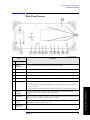
Front Panel Overview
Front Panel Overview
This section provides information on the analyzer’s front panel, including:
•
“Front-Panel Connectors and Keys”, see below.
•
“Display Annotations: Spectrum Display” on page 53.
•
“Display Annotations: Spectrogram (Option 271)” on page 57.
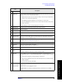
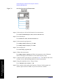
Front-Panel Connectors and Keys
Item
Front and Rear Panel Features
Description
#
Name
1
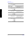
Menu Keys
Menu labels identifying the current function of each menu key appear to the left of each key.
Key menus are dependent on the active menu. Also see “Using Menu Keys” on page 69.
2
Measurement
Keys
Select measurement mode.
Select and set up specific measurements and mode parameters within the current mode.
3
Analyzer Setup
Keys
Set parameters used for making measurements. These settings will affect measurements in
all modes.
4
Marker Keys
Enable markers to obtain specific information about the displayed measurement
50
Chapter 3
Front and Rear Panel Features
Front Panel Overview
Item
Description
#
Name
5
Utility Keys
Access features used with all analyzer modes and affects the state of the entire spectrum
analyzer. See your User’s Guide for more details.
System functions affect the state of the entire analyzer. Various setup and adjustment
routines are accessed with the System key.
The Mode Preset and User Preset keys reset the analyzer to a known state.
The Save and Recall keys enable you to save and to recall measurement results, traces,
states, and screens.
The Print key saves the currently displayed screen to a file.
6
PROBE PWR
Supplies power for external high frequency probes and accessories.
7
Earphone Jack
Jacks for earphone.
8
USB Jacks
Jacks for connecting USB devices. For example, an external memory device.
9
Battery
Indicators
LEDs indicate the status of batteries 1 and 2.
10
RF INPUT 50
Input for an external signal. Make sure that the total power of all signals at the analyzer
input does not exceed +33 dBm (2 watts).
11
Data Controls
Change the numeric value of an active function. Entries appear in the active function area of
the display. Also see “Entering Data” on page 69.
12
Cancel (Esc)
Pressing this key when operating remotely will put the analyzer in local mode.
13
Navigation
Keys
Moves cursor between fields on the display.
Increments and decrements active function values.
14
Return Key
Exits the current menu and returns to the previous menu.
15
Volume Control
Keys/
Enables you to Mute or increase and decrease sound at the internal speaker or the earphones.
Help Key
Press the Help key to access the embedded help information. Use the menu keys or
navigation keys (item 13) to select the desired help topic. Two types of help are available:
16
Used with AM/FM Tune and Listen, N1996A with Option AFM.
1. Task help that will guide you through making a measurement.
2. Key function explanations that provide a short description of a key and the associated
remote command.
You can exit help by pressing Cancel (Esc).
Window Keys
Next Window: On displays with multiple windows, changes the highlighted window that is
(Not currently
implemented.)
currently active.
Front and Rear Panel Features
17
Zoom: Zooms in on the highlighted window.
Multiple Windows: On displays with multiple windows, switches the view to multiple
window.
Chapter 3
51
Front and Rear Panel Features
Front Panel Overview
Item
Description
#
Name
18
Power
On/Standby
NOTE
The front-panel switch is a standby switch, not a LINE switch
(disconnecting device); the analyzer continues to draw power
even when the line switch is in standby. Use the detachable
power cord to disconnect the analyzer from the mains supply.
NOTE
The internal frequency reference is not powered when in standby
mode.
The output for the built-in signal source. This connector is present on all N1996A
analyzers, but the output is enabled only on analyzers with either N8995A, N8995A-SR3 or
N8995A-SR6.
RF OUTPUT
50
Front and Rear Panel Features
19
Turns the analyzer on. A green light indicates power on. A yellow light indicates standby
mode.
52
Chapter 3
Front and Rear Panel Features
Front Panel Overview
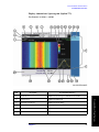
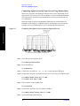
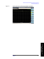
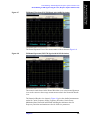
Display Annotations: Spectrum Display
For firmware revisions < A.02.00
Item
Description
Associated Function Keys
Amplitude scale
AMPTD Y Scale, Scale Type or AMPTD Y Scale, Scale/Div
2
Reference level
AMPTD Y Scale, Ref Level
3
Auto Range On indicator
AMPTD Y Scale, Auto Range
4
Active function block
Refer to the description of the activated function.
5
Internal preamp status
AMPTD Y Scale, Internal Preamp
6
Marker
Marker
7
RF attenuation
AMPTD Y Scale, Elec Atten
Chapter 3
Front and Rear Panel Features
1
53
Front and Rear Panel Features
Front Panel Overview
Item
Description
8
Over Range: Indicates that the attenuation
and preamp (if installed) settings are
supplying too much power to the detector.
Distortion may result. Set Auto Range (On)
to clear.
Associated Function Keys
AMPTD Y Scale, Elec Atten
AMPTD Y Scale, Internal Preamp
AMPTD Y Scale, Auto Range
or
<8Smpl/Pt: Indicates that the current
instrument settings have reduced the
number of samples/display point to fewer
than 8. The most accurate averaged
amplitude measurement will be made when
you have at least 8 samples in each display
point.
Trace/Detector, More, Detector, Average
9
Ext Gain
AMPTD Y Scale, Ext Gain
10
Averaging
Trace/Detector, Trace Average or Meas Setup, Avg Mode, Avg
Number: The numbers shown indicates current average number
and the desired number of averages.
11
Time and date display
System, Time/Date/Location, Date/Time
12
Active marker
Marker
13
Trace and detector information
Trace/Detector, Clear Write (W) Trace Average (A) Max Hold (M)
Min Hold (m)
Trace/Detector, More, Detector, Peak (P) Sample(S) Negative Peak (p)
Average (A)
14
Active marker frequency and amplitude
Marker
Front and Rear Panel Features
If in zero span, active marker time and
amplitude is displayed.
15
Key menu title
Dependent on menu selection.
16
Key menu
Menu key labels
17
Stop frequency or if in zero span, stop time
FREQ Channel, Stop Freq
18
Reference frequency source indicator
System, Freq/Time Reference
19
Battery 1 & 2 status indicator
System, System Stats, Battery
20
AC power indicator
Indicates that the analyzer is currently powered by the external
AC/DC power converter
21
Sweep time
Control/Sweep, Sweep Time
22
Span
SPAN X Scale
23
Center frequency
FREQ Channel, Center Freq
24
Display status line
Displays informational and error messages (see “Types of
Spectrum Analyzer Messages” on page 227).
25
Resolution Bandwidth
BW, Res BW
26
Start frequency or if in zero span, 0 sec
FREQ Channel, Start Freq
54
Chapter 3
Front and Rear Panel Features
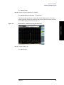
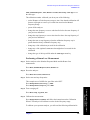
Front Panel Overview
For firmware revision A.02.00 or greater
Item
Description
Associated Function Keys
Amplitude scale
AMPTD Y Scale, Scale Type or AMPTD Y Scale, Scale/Div
2
Reference level
AMPTD Y Scale, Ref Level
3
Auto Range On indicator
AMPTD Y Scale, Auto Range
4
Active function block
Refer to the description of the activated function.
5
Internal preamp status
AMPTD Y Scale, Internal Preamp
6
Marker
Marker
7
RF attenuation
AMPTD Y Scale, Elec Atten
Chapter 3
Front and Rear Panel Features
1
55
Front and Rear Panel Features
Front Panel Overview
Item
Description
8
Over Range: Indicates that the attenuation
and preamp (if installed) settings are
supplying too much power to the detector.
Distortion may result. Set Auto Range (On)
to clear.
Associated Function Keys
AMPTD Y Scale, Elec Atten
AMPTD Y Scale, Internal Preamp
AMPTD Y Scale, Auto Range
or
<8Smpl/Pt: Indicates that the current
instrument settings have reduced the
number of samples/display point to fewer
than 8. The most accurate averaged
amplitude measurement will be made when
you have at least 8 samples in each display
point.
Trace/Detector, More, Detector, Average
9
Ext Gain
AMPTD Y Scale, Ext Gain
10
Averaging
Trace/Detector, Trace Average or Meas Setup, Avg Mode, Avg
Number: The numbers shown indicates current average number
and the desired number of averages.
11
Time and date display
System, Time/Date/Location, Date/Time
12
Active marker
Marker
13
Trace and detector information
Trace/Detector, Clear Write (W) Trace Average (A) Max Hold (M)
Min Hold (m)
Trace/Detector, More, Detector, Peak (P) Sample(S) Negative Peak (p)
Average (A)
14
Active marker frequency and amplitude
Marker
Front and Rear Panel Features
If in zero span, active marker time and
amplitude is displayed.
15
Key menu title
Dependent on menu selection.
16
Key menu
Menu key labels
17
Span
SPAN X Scale
18
Reference frequency source indicator
System, Freq/Time Reference
19
Battery 1 & 2 status indicator
System, System Stats, Battery
20
AC power indicator
Indicates that the analyzer is currently powered by the external
AC/DC power converter
21
Sweep time
Control/Sweep, Sweep Time
22
VBW
BW, Video BW
23
Center frequency
FREQ Channel, Center Freq
24
Display status line
Displays informational and error messages (see “Types of
Spectrum Analyzer Messages” on page 227).
25
Resolution Bandwidth
BW, Res BW
26
Revision indicator
System, System Stats, Show System
56
Chapter 3
Front and Rear Panel Features
Front Panel Overview
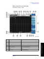
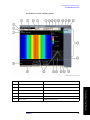
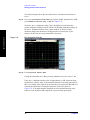
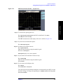
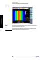
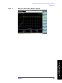
Display Annotations: Spectrogram (Option 271)
For firmware revisions < A.02.00
Item
Description
Associated Function Keys
Amplitude scale
AMPTD Y Scale, Scale Type or AMPTD Y Scale, Scale/Div
2
Reference level
AMPTD Y Scale, Ref Level
3
Auto Range On indicator
AMPTD Y Scale, Auto Range
4
Active function block
Data entry field for the active function.
5
Internal preamp status
AMPTD Y Scale, Internal Preamp
6
RF attenuation
AMPTD Y Scale, Elec Atten
Chapter 3
Front and Rear Panel Features
1
57
Front and Rear Panel Features
Front Panel Overview
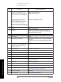
Item
Description
7
Over Range: Indicates that the attenuation
and preamp (if installed) settings are
supplying too much power to the detector.
Distortion may result. Set Auto Range (On)
to clear.
Associated Function Keys
AMPTD Y Scale, Elec Atten
AMPTD Y Scale, Internal Preamp
AMPTD Y Scale, Auto Range
or
<8Smpl/Pt: Indicates that the current
instrument settings have reduced the
number of samples/display point to fewer
than 8. The most accurate averaged
amplitude measurement will be made when
you have at least 8 samples in each display
point.
Trace/Detector, More, Detector, Average
8
Ext Gain
AMPTD Y Scale, Ext Gain
9
Color scale legend
Provides a reference for the color scale.
10
Elapsed time clock
Provides an indicator of the data collection time interval of the
displayed spectrogram.
11
Time and date display
System, Time/Date/Location, Date/Time
12
Active marker
Marker
13
Trace information
Trace/Detector, Clear Write (W) Trace Average (A) Max Hold (M)
Min Hold (m)
Trace/Detector, More, Detector, Peak (P) Sample (S) Negative Peak
(p) Average (A)
14
Active marker frequency and amplitude
Marker
15
Key menu title
Dependent on menu selection.
16
Key menu
Menu key labels
17
Stop frequency or if in zero span, stop time
FREQ Channel, Stop Freq
18
Reference frequency source indicator
System, Freq/Time Reference
19
Battery 1 & 2 status indicator
System, System Stats, Battery
20
AC power indicator
Indicates that the analyzer is currently powered by the external
AC/DC power converter
21
Spectrum display
View/Display, Spectrogram Provides a Spectral display of the
Front and Rear Panel Features
spectrum sampled to create the spectrogram.
22
Start frequency or if in zero span, 0 sec
FREQ Channel, Start Freq
23
Marker
Marker
24
Display status line
Displays informational and error messages (see “Types of
Spectrum Analyzer Messages” on page 227).
25
Metrics Panel
Displays measurement results data metrics.
58
Chapter 3
Front and Rear Panel Features
Front Panel Overview
For firmware revision A.02.00 or greater
Item
Description
Associated Function Keys
Amplitude scale
AMPTD Y Scale, Scale Type or AMPTD Y Scale, Scale/Div
2
Reference level
AMPTD Y Scale, Ref Level
3
Auto Range On indicator
AMPTD Y Scale, Auto Range
4
Active function block
Data entry field for the active function.
5
Internal preamp status
AMPTD Y Scale, Internal Preamp
6
RF attenuation
AMPTD Y Scale, Elec Atten
Chapter 3
Front and Rear Panel Features
1
59
Front and Rear Panel Features
Front Panel Overview
Item
Description
7
Over Range: Indicates that the attenuation
and preamp (if installed) settings are
supplying too much power to the detector.
Distortion may result. Set Auto Range (On)
to clear.
Associated Function Keys
AMPTD Y Scale, Elec Atten
AMPTD Y Scale, Internal Preamp
AMPTD Y Scale, Auto Range
or
<8Smpl/Pt: Indicates that the current
instrument settings have reduced the
number of samples/display point to fewer
than 8. The most accurate averaged
amplitude measurement will be made when
you have at least 8 samples in each display
point.
Trace/Detector, More, Detector, Average (Log/RMS/V)
8
Ext Gain
AMPTD Y Scale, Ext Gain
9
Color scale legend
Provides a reference for the color scale.
10
Elapsed time clock
Provides an indicator of the data collection time interval of the
displayed spectrogram.
11
Time and date display
System, Time/Date/Location, Date/Time
12
Active marker
Marker
13
Trace information
Trace/Detector, Clear Write (W) Average (A) Max Hold (M) Min
Hold (m)
Trace/Detector, More, Detector, Peak (P) Sample (S) Negative Peak
(p) Average (A)
14
Active marker frequency and amplitude
Marker
15
Key menu title
Dependent on menu selection.
16
Key menu
Menu key labels
17
Stop frequency or if in zero span, stop time
FREQ Channel, Stop Freq
18
Reference frequency source indicator
System, Freq/Time Reference
19
Battery 1 & 2 status indicator
System, System Stats, Battery
20
AC power indicator
Indicates that the analyzer is currently powered by the external
AC/DC power converter
21
Spectrum display
View/Display, Spectrogram Provides a Spectral display of the
Front and Rear Panel Features
spectrum sampled to create the spectrogram.
22
Start frequency or if in zero span, 0 sec
FREQ Channel, Start Freq
23
Marker
Marker
24
Display status line
Displays informational and error messages (see “Types of
Spectrum Analyzer Messages” on page 227).
25
Metrics Panel
Displays measurement results data metrics.
26
Revision indicator
System, System Stats, Show System
60
Chapter 3
Front and Rear Panel Features
Rear-Panel Features
Rear-Panel Features
Item
#
Description
Name
1
Battery
Compartment
Location of the two batteries that provide DC power to the analyzer.
2
DC Power
The input for the dc power source. Refer to “Power Requirements” on page 27.
3
USB, Type A
Allows connections of external devices such as an external memory device.
4
USB, Type B
Allows connections of external devices such as a PC controller. (not implemented)
5
Timing LAN
A TCP/IP Interface for connecting internal options to external devices. (not implemented)
6
LAN
A TCP/IP Interface.
•
•
REF OUT
(10 MHz)
An output of the analyzer’s internal 10 MHz frequency reference signal used to lock the
frequency reference of the analyzer to other test equipment.
8
EXT REF IN
Input for an external frequency reference signal. For additional information on using an external
reference, refer to “Using an External Reference” on page 33.
9
EXT TRIGGER
INPUT
A TTL input that accepts the positive or negative edge (selectable) of an external voltage input
that triggers the analyzer internal sweep source.
10
Reserved for
future use.
Chapter 3
61
Front and Rear Panel Features
7
For information on setting the IP address, refer to “Turning on the Analyzer for the First
Time” on page 32.
For information on using the analyzer remotely, refer to the User’s/Programmer’s Guide.
Front and Rear Panel Features
Rear-Panel Features
Item
#
Description
Name
Kensington lock
Slot
Used in conjunction with Kensington Lock to secures analyzer to work space.
12
Mounting tabs
Mounting tabs for mounting the external power supply when analyzer is rack mounted.
13
Grounding lug
Chassis ground connection.
Front and Rear Panel Features
11
62
Chapter 3
Front and Rear Panel Features
Key Overview
Key Overview
The keys labeled FREQ Channel, System, and Marker are all examples of
front-panel keys. The front-panel keys are dark gray, light gray, green, beige, or
white in color. Front-panel keys that are white perform an immediate action rather
than bringing up a menu. The only green keys are the Mode Preset, User Preset, and
Help keys. The Mode Preset and User Preset keys perform an analyzer reset and
the Help key accesses the embedded help system. (A summary of all front panel
keys and their related menu keys can be found in the User’s Guide for your
analyzer). Pressing most of the dark gray, the light gray, or the beige front-panel
keys accesses menus of functions that are displayed along the right side of the
display. These are called menu keys.
Menu keys list functions other than those accessed directly by the front panel keys.
To activate a menu key function, press the key immediately to the right of the
annotation on the screen. The menu keys that are displayed depend on which
front-panel key is pressed and which menu level is enabled.
If a menu key function value can be changed, it is called an active function. The
function label of the active function is highlighted after that key has been selected.
For example, press AMPTD Y Scale. This calls up the menu of related amplitude
functions. Note the function labeled Ref Level (the default selected key in the
Amplitude menu) is highlighted. Ref Level also appears in the active function
block (as well as the reference level value), indicating that it is the active
amplitude function and can now be changed using any of the data entry controls.
A menu key with On and Off in its label can be used to turn the menu key function
on or off. To turn the function on, press the menu key so that On is underlined. To
turn the function off, press the menu key so that Off is underlined. In the manual,
when On should be underlined, it will be indicated as Function (On).
A function with Auto and Man in the label can either be auto-coupled or have its
value manually changed. The value of the function can be changed manually using
the numeric keypad, knob, or step keys. To auto-couple a function, press the menu
key so that Auto is underlined. In the manual, when Auto should be underlined, it
will be indicated as Function (Auto).
Chapter 3
63
Front and Rear Panel Features
In some key menus, one key label will always be highlighted to show which key
has been selected. For example, when you press Marker, you will access a menu of
keys in which some of the keys are grouped together by a yellow highlighted
region of the menu. The Normal key, which is the Marker menu default key, will
be highlighted. When you press another key within the yellow region, such as
Delta, a yellow border around that key becomes visible to show it has been
selected.
Front and Rear Panel Features
Key Overview
In other key menus, one key label will always be highlighted to show which key
has been selected but the menu is immediately exited when a selection is made.
For example, when you press the Avg Type key (on the Meas Setup menu), it will
bring up its own menu of keys. The Log-Pwr Avg key, which is the Avg Type menu
default key, will be highlighted. When you press the Pwr Avg key, the highlight
will move to that key to show it has been selected and the screen will return to the
Meas Setup menu.
Front and Rear Panel Features
The arrow keys located around the Select key to the left of the analyzer display can
be used to navigate within tables or lists, for example the Chan Std table. These
keys are used to move between rows. The cursor (inverse video highlight)
indicates the active item.
64
Chapter 3
Recommended Test Equipment
4
Recommended Test Equipment
65
Recommended Test Equipment
Recommended Test Equipment
Test Equipment for Making Measurements
Test Equipment for Making Measurements
Test Equipment
The table below summarizes the test equipment needed to perform all of the
measurements shown in this guide. Alternate equipment model numbers are given
in case the recommended equipment is not available.
If neither the recommended nor the alternative test equipment are available,
substitute equipment that meets or exceeds the critical specifications listed.
To find descriptions of specific analyzer functions, refer to the Agilent
Technologies N1996A Spectrum Analyzer User’s/Programmer’s Reference Guide.
NOTE
Item
Critical Specifications
Recommended
Agilent Model
Alternate
Agilent
Model
Adapters
Type-N (m) to BNC (f) (3)
1250-0780
Type N (m) to Type N (m)
Frequency: 10 MHz to 6 GHz
VSWR: 1.08:1
1250-1472
Type N (f) to 3.5 mm (f) (for
use with 20 GHz or 26.5 GHz
source)
Frequency: 10 MHz to 6 GHz
VSWR: 1.08:1
1250-1745
Type N (f) to 2.4 mm (f) (for
use with >26.5 GHz source)
Frequency: 10 MHz to 6 GHz
VSWR: 1.08:1
11903B
Cables
BNC, 122-cm (48-in) (3)
10503A
Type N (m) to Type N (m),
<=36 inches long
Frequency: 10 MHz to 6 GHz
VSWR: 1.4:1
11500B
Cable, BNC (m) to BNC (m),
36 inches long
Frequency: 10 MHz nominal
10503
Signal Source (two are required)
Synthesized Signal Generator
(if 8360-Series sweeper is not
used)
Frequency Range: 10 MHz to 6 GHz
Power Level: -10 to +5 dBm
8665B, E8257D,
E8267D, or
E4438C Opt 506
Synthesized Sweeper
(if 8665B, ESG or PSG is not
available)
Frequency Range: 10 MHz to 6 GHz
Power Level: -10 to +5 dBm
83620A/B,
83630A/B,
83640A/B,
83650A/B
66
Chapter 4
Spectrum Analyzer
5
Spectrum Analyzer
67
Spectrum Analyzer
This Chapter provides information making the following measurements.
“Making a Basic Measurement” on page 69
“Measuring Multiple Signals” on page 75
“Measuring a Low-Level Signal” on page 86
“Making Distortion Measurements” on page 93
“Using the Analyzer as a Fixed Tuned Receiver” on page 101
“Channel Power” on page 104
Spectrum Analyzer
“Occupied Bandwidth (OBW) Measurement” on page 107
“Making a Basic Occupied BW Measurement” on page 109
“Using the Spectrogram View (Requires Option 271)” on page 111
“Pulse Measurement” on page 115
“Tune and Listen (Requires Option AFM)” on page 117
68
Chapter 5
Spectrum Analyzer
Making a Basic Measurement
Making a Basic Measurement
This section provides information on basic analyzer operation. For more
information on making measurements, see the appropriate measurement chapter.
This section is divided into the following sections:
“Entering Data” on page 69
“Using Menu Keys” on page 69
“Presetting the Spectrum Analyzer” on page 71
“Viewing a Signal” on page 72
CAUTION
Ensure that the total power of all signals at the analyzer input does not exceed +33
dBm (2 watts).
Basic Assumption
The material in this chapter is presented with the assumption that you understand
the front and rear panel layout, and display annotations of your analyzer. If you do
not, refer to the Measurement Guide “Front and Rear Panel Features” on page 49.
Entering Data
When setting measurement parameters, there are several ways to enter or modify
the value of the active function:
Knob
Increments or decrements the current value.
Arrow Keys
Increments or decrements the current value.
Numeric Keypad
Enters a specific value. Then press the desired terminator (either a
unit menu key, or the Enter key).
Unit Menu Keys
Terminate a value that requires a unit-of-measurement.
Enter Key
Terminates an entry when either no unit of measure is needed, or you
want to use the default unit.
Using Menu Keys
Menu Keys (which appear along the right side of the display) provide access to
many analyzer functions. Here are examples of menu key types:
Toggle
Chapter 5
Allows you to
activate/deactivate states.
Toggles the selection (underlined choice)
each time you press the key.
69
Spectrum Analyzer
“Creating a User Preset and Power-Up State” on page 71
Spectrum Analyzer
Making a Basic Measurement
Example:
Submenu
Displays a new menu of menu
keys.
A submenu key allows you to view a new
menu of menu keys related to the
submenu key category.
Example:
Choice
Spectrum Analyzer
Allows you to make a selection
from a list of values.
A choice key displays the currently
selected submenu choice, in this example,
dBm. When the choice is made, the
submenu automatically returns.
Example:
Adjust
Press this type of key and enter a value.
Highlights the menu key and
sets the active function.
The default for menu keys with an
automatic (Auto) or manual (Man) choice
is automatic. After pressing the key, the
selection changes to manual.
Examples:
70
Chapter 5
Spectrum Analyzer
Making a Basic Measurement
Presetting the Spectrum Analyzer
Preset provides a known starting point for making measurements. The analyzer has
two types of preset:
Mode Preset
This type of preset restores the currently selected
mode to a known factory-defined state.
User Preset
Restores the analyzer to a user-defined state. User
Preset uses the factory-defined state until you create
a custom user preset file.
For details, see the User’s and Programmer’s Reference manual.
User Preset recalls the power-up state, applying the defaults you define using the
Save State button. When you save a state to be used as the User Preset power-up
state, you must name the state “Powerup”. If you want to use the Agilent-defined
defaults at power-up, press Mode Preset to restore the Agilent-defined defaults and
save that state as a new Powerup state file.
If you constantly use settings which are not the factory defaults, use the following
steps to create a user-defined preset:
NOTE
If “Powerup” state already exists in the catalog list, you can set the state to your
preferences and then select “Powerup” in the list. The catalog list can be viewed by
selecting Save, Catalog.
1. Set analyzer parameters as desired.
2. Set filename to “Ask”. Press Save, Name, Filename (Ask).
3. Save to the internal hard drive. Press Save, Location, Internal.
4. Save Powerup state. Press Type, State, Save Now.
5. Using the knob or arrow keys, select the letters from the alphabet window to
create the word, “Powerup” and press OK. The message, “State was saved
successfully: C:Powerup” is displayed. Press OK again to return to the
Save key menu.
The parameters saved in this “Powerup” state file are now enabled as the user
preset option and as the default power-up state.
NOTE
This process is easier for firmware revision A.02.00 or greater. After configuring
the desired parameter settings, press User Preset, Save User Preset.
Disabling User Preset
To restore the factory defined Power On settings, press Mode Preset and follow the
steps listed above to save the resulting state as the new “Powerup” state file. This
Chapter 5
71
Spectrum Analyzer
Creating a User Preset and Power-Up State
Spectrum Analyzer
Making a Basic Measurement
will restore the factory-defined default settings as the power-on settings and as the
user preset settings.
NOTE
For firmware revision A.02.00 or greater, to disable User Preset, the process is
easier, press Mode Preset, then press User Preset, Save User Preset.
Viewing a Signal
1. Select the spectrum analyzer mode. Press Mode, Spectrum Analyzer.
2. Preset the analyzer: Press Mode Preset.
Spectrum Analyzer
3. Connect the analyzer’s rear panel REF OUT (10 MHz) to the front-panel
input.
Setting Center Frequency, Span, Attenuation, and Reference Level.
1. Set the center frequency to 30 MHz: Press FREQ Channel, Center Freq, 30,
MHz.
2. Set the Span to 50 MHz: Press SPAN X Scale, 50, MHz.
3. Adjust the attenuation to 20 dB: Press AMPTD Y Scale, Elec Atten, 20, dB.
4. Adjust the reference level (if the peak of the 10 MHz signal component is not
visible): Press AMPTD Y Scale, Ref Level, 10, dBm. For more information on
this, refer to “Changing Reference Level” on page 73.
The 10 MHz reference signal spectrum appears on the display, as shown in
Figure 5-1.
Figure 5-1
10 MHz Internal Reference Signal and Associated Spectrum
72
Chapter 5
Spectrum Analyzer
Making a Basic Measurement
Reading Frequency & Amplitude
1. Place a marker (labeled 1) on the 10 MHz peak, as shown in Figure 5-2.
Press Peak Search. If necessary, use the menu keys to move the marker to the
proper peak. In addition, you can go to the Marker menu (press Marker) and
use the knob or arrow keys to move the marker.
Note that the frequency and amplitude of the marker appear in the upper-right
corner of the screen.
2. If you have moved the marker, return it to the peak of the 10 MHz signal.
Spectrum Analyzer
Figure 5-2
A Marker on the 10 MHz Peak
Changing Reference Level
1. Press AMPTD Y Scale, and note that reference level (Ref Level) is now the
active function. Press Marker Mkr RL.
Note that changing the reference level changes the amplitude value of the top
graticule line.
Figure 5-3 shows the relationship between center frequency and reference
level. The box represents the analyzer display. Changing the center frequency
changes the horizontal placement of the signal on the display. Changing the
reference level changes the vertical placement of the signal on the display.
Increasing the span increases the frequency range that appears horizontally
across the display.
Chapter 5
73
Spectrum Analyzer
Making a Basic Measurement
Relationship Between Frequency and Amplitude
Spectrum Analyzer
Figure 5-3
74
Chapter 5
Spectrum Analyzer
Measuring Multiple Signals
Measuring Multiple Signals
This section provides information on measuring multiple signals.
This section is divided into the following sections:
“Comparing Signals on the Same Screen Using Marker Delta” on page 76
“Comparing Signals not on the Same Screen Using Marker Delta” on page 78
“Resolving Signals of Equal Amplitude” on page 80
“Resolving Small Signals Hidden by Large Signals” on page 83
Ensure that the total power of all signals at the analyzer input does not exceed +33
dBm (2 watts).
Basic Assumption
The material in this chapter is presented with the assumption that you understand
the front and rear panel layout, and display annotations of your analyzer. If you do
not, refer to the Measurement Guide “Front and Rear Panel Features”.
Chapter 5
75
Spectrum Analyzer
CAUTION
Spectrum Analyzer
Measuring Multiple Signals
Comparing Signals on the Same Screen Using Marker Delta
Using the analyzer, you can easily compare frequency and amplitude differences
between signals, such as radio or television signal spectra. The analyzer delta
marker function lets you compare two signals when both appear on the screen at
one time.
In this procedure, harmonics of the 10 MHz reference signal available at the rear of
the analyzer are used to measure frequency and amplitude differences between two
signals on the same screen. Delta marker is used to demonstrate this comparison.
An Example of Comparing Signals on the Same Screen
Spectrum Analyzer
Figure 5-4
Step 1. Select the spectrum analyzer mode:
Press Mode, Spectrum Analyzer.
Step 2. Preset the analyzer:
Press Mode Preset.
Step 3. Connect the rear panel REF OUT (10 MHz) to the front panel RF input.
Step 4. Set the analyzer center frequency, span and reference level to view the
fundamental and 2nd through fifth harmonics of the 10 MHz reference signal:
Press FREQ Channel, Center Frequency, 30, MHz.
Press SPAN X Scale, Span, 50, MHz.
Press AMPTD Y Scale, Ref Level, 10, dBm
Press AMPTD Y Scale, Elec Atten, 20, dB or Auto Range (On).
Step 5. Place a marker at the highest peak on the display (10 MHz):
Press Peak Search.
76
Chapter 5
Spectrum Analyzer
Measuring Multiple Signals
The Next Peak menu key is available to move the marker from peak to peak. The
marker should be on the 3rd harmonic of the 10 MHz reference signal.
Step 6. Anchor the first marker and activate the Delta marker:
Press Marker, Delta.
The label on the second marker reads 1, indicating that it is the movable marker.
Step 7. Move the second marker to another signal peak or by using the Peak Search key:
Press Peak Search, Next Peak.
Chapter 5
77
Spectrum Analyzer
The amplitude and frequency difference between the markers is shown in the upper
right corner of the display.
Spectrum Analyzer
Measuring Multiple Signals
Comparing Signals not on the Same Screen Using Marker Delta
Measure the frequency and amplitude difference between two signals that do not
appear on the screen at one time. (This technique is useful for harmonic distortion
tests when narrow span and narrow bandwidth are necessary to measure the low
level harmonics.)
In this procedure, frequency and amplitude differences are measured between
harmonics of the analyzer’s 10 MHz reference; one harmonic on screen and one
harmonic off screen. Delta marker is used to demonstrate this comparison.
Comparing One Signal on Screen with One Signal Off Screen
Spectrum Analyzer
Figure 5-5
Step 1. Select the spectrum analyzer mode:
Press Mode, Spectrum Analyzer.
Step 2. Preset the analyzer:
Press Mode Preset.
Step 3. Connect the rear panel REF OUT (10 MHz) to the front panel RF input.
Step 4. Set the center frequency, span and reference level to view only the 30 MHz signal:
Press FREQ Channel, Center Freq, 30, MHz.
Press SPAN X Scale, Span, 5, MHz.
Step 5. Place a marker on the 30 MHz peak:
Press Peak Search.
Step 6. Set the center frequency step size equal to 10 MHz:
Press FREQ Channel, CF Step (Manual), 10, MHz.
Step 7. Activate the marker delta function:
78
Chapter 5
Spectrum Analyzer
Measuring Multiple Signals
Press Marker, Delta.
Step 8. Increase the center frequency by 10 MHz:
Press FREQ Channel, Center Freq, , Peak Search.
The delta marker (1) appears on the peak of the 40 MHz harmonic. The delta
marker annotation displays the amplitude and frequency difference between the 30
and 40 MHz signal peaks. Refer to Figure 5-6.
Figure 5-6
Delta Marker with Reference Signal Off-Screen
Spectrum Analyzer
Step 9. Turn the markers off:
Press Marker, Off.
Chapter 5
79
Spectrum Analyzer
Measuring Multiple Signals
Resolving Signals of Equal Amplitude
In this procedure a decrease in resolution bandwidth is used to resolve two signals
of equal amplitude with a frequency separation of 100 kHz. Notice that the final
RBW selection to resolve the signals is the same width as the signal separation.
Step 1. Connect the output of signal generator #1 to port 2 of the directional coupler and
connect the output of signal generator #2 to port 3 (the coupled port) of the
directional coupler as shown in Figure 5-7.
Setup for Obtaining Two Signals
Spectrum Analyzer
Figure 5-7
Step 2. Set the signal sources as follows:
Set signal generator #1 to 300 MHz at –19 dBm. Set signal generator #2 to
300.1 MHz at –4 dBm (this higher power level overcomes the nominal 16 dB loss
through the coupled arm of the directional coupler).
The amplitude of both signals should be approximately 20 dBm at the output of
the bridge.
Step 3. Setup the analyzer to view the signals:
Press Mode Preset.
Press FREQ Channel, Center Freq, 300, MHz.
Press SPAN X Scale, Span, 2, MHz.
Press Meas Setup, Avg Mode, Exponential.
Press Avg Number, 25, Enter.
Press Trace/Detector, Trace Average.
Press BW, Res BW (Manual), 300, kHz.
A single signal peak is visible. See Figure 5-8 for an example.
80
Chapter 5
Spectrum Analyzer
Measuring Multiple Signals
Figure 5-8
Unresolved Signals of Equal Amplitude
than or equal to the frequency separation of the two signals:
Press BW, Res BW (Manual), 75, kHz.
Notice that the peak of the signal has become flattened indicating that two signals
may be present.
Figure 5-9
Resolving Signals of Equal Amplitude
As the resolution bandwidth is decreased, resolution of the individual signals is
improved and the sweep time is increased. For fastest measurement times, use the
widest possible resolution bandwidth. Under factory preset conditions, the
resolution bandwidth is “coupled” (or linked) to the span.
Since the resolution bandwidth has been changed from the coupled value, a # mark
appears next to Res BW in the lower-left corner of the screen, indicating that the
resolution bandwidth is uncoupled. (For more information on resolution
Chapter 5
81
Spectrum Analyzer
Step 4. Change the resolution bandwidth (RBW) to 75 kHz so that the RBW setting is less
Spectrum Analyzer
Measuring Multiple Signals
bandwidth, refer to the Res BW description in the Agilent CSA Spectrum
Analyzers User’s and Programmer’s Reference guide.)
To resolve two signals of equal amplitude, the resolution bandwidth must be less
than the signal separation. For example, if the signal separation is 200 kHz and the
analyzer only has resolution bandwidth settings in a 1-3-10 sequence, a 100 kHz
RBW is the best choice for the 200 kHz signal separation. But some analyzers,
such as the Agilent CSA and PSA spectrum analyzers, can select a 180 kHz RBW.
Spectrum Analyzer
NOTE
82
Chapter 5
Spectrum Analyzer
Measuring Multiple Signals
Resolving Small Signals Hidden by Large Signals
This procedure uses narrow resolution bandwidths to resolve two input signals
with a frequency separation of 50 kHz and an amplitude difference of 60 dB.
Step 1. Connect two sources to the analyzer input as shown in Figure 5-7. Connect the
output of signal generator #1 to port 2 of the directional coupler and connect the
output of signal generator #2 to port 3 (the coupled port) of the directional coupler.
Figure 5-10
Setup for Obtaining Two Signals
Spectrum Analyzer
Step 2. Set the signal sources as follows:
Set signal generator #1 to 300 MHz at –9 dBm. Set signal generator #2 to
300.450 MHz at –54 dBm. (These power levels plus the nominal 16 dB loss
through the coupled arm and the nominal 1 dB loss through the main arm of the
directional coupler results in a signal 60 dB below the first signal).
Step 3. Set the analyzer as follows:
Press Mode Preset.
Press FREQ Channel, Center Freq, 300, MHz.
Press SPAN X Scale, Span, 5, MHz.
Press BW, Res BW, 100, kHz.
Step 4. Set the 300 MHz signal peak to the reference level:
Press Peak Search, Mkr , Mkr R L.
Note that the Agilent CSA 100 kHz filter shape factor of 8:1 has a bandwidth of
840 kHz at the 60 dB point. The half-bandwidth (420 kHz) is NOT narrower than
the frequency separation of 450 kHz, so the input signals can not be resolved.
Step 5. Activate averaging to smooth the noise:
Press Meas Setup, Avg Mode, Exponential.
Press Avg Number, 25, Enter.
Press Trace/Detector, Trace Average
Chapter 5
83
Spectrum Analyzer
Measuring Multiple Signals
Spectrum Analyzer
Figure 5-11
Signal Resolution with a 100 kHz RBW
Step 6. Reduce the resolution bandwidth filter to view the smaller hidden signal. Place a
delta marker on the smaller signal:
Press BW, 30, kHz.
Press Peak Search, Marker, Delta, 450, kHz.
Note that the Agilent CSA 30 kHz filter shape factor of 8.4 has a bandwidth of
252 kHz at the 60 dB point, however noise sidebands will make the 60 dB
bandwidth appear wider. The half-bandwidth (including effects of noise sidebands)
is narrower than 250 kHz, so the input signals can be resolved.
Figure 5-12
Signal Resolution with a 30 kHz RBW
NOTE
To determine the resolution capability for intermediate amplitude differences,
assume the filter skirts between the 3 dB and 60 dB points are parabolic, like an
ideal Gaussian filter. The resolution capability is approximately:
84
Chapter 5
Spectrum Analyzer
Measuring Multiple Signals
f 2
12.04 dB ---------
RBW
where f is the separation between the signals.
Spectrum Analyzer
Chapter 5
85
Spectrum Analyzer
Measuring a Low-Level Signal
Measuring a Low-Level Signal
This section provides information on measuring low-level signals and
distinguishing them from spectrum noise.
This section is divided into the following sub-sections:
“Reducing Input Attenuation” on page 87
“Decreasing the Resolution Bandwidth” on page 89
Spectrum Analyzer
“Trace Averaging” on page 91
CAUTION
Ensure that the total power of all signals at the analyzer input does not exceed +33
dBm (2 watts).
Basic Assumption
The material in this section is presented with the assumption that you understand
the front and rear panel layout, and display annotations of your analyzer. If you do
not, refer to the Measurement Guide “Front and Rear Panel Features”.
86
Chapter 5
Spectrum Analyzer
Measuring a Low-Level Signal
Reducing Input Attenuation
The ability to measure a low-level signal is limited by internally generated noise in
the spectrum analyzer. The measurement setup can be changed in several ways to
improve the analyzer sensitivity.
The input attenuator affects the level of a signal passing through the instrument. If
a signal is very close to the noise floor, reducing input attenuation can bring the
signal out of the noise.
CAUTION
Ensure that the total power of all input signals at the analyzer RF input does not
exceed +33 dBm (2 watts).
in Figure 5-7.
Figure 5-13
Setup for Obtaining One Signal
Step 2. Set the frequency of the signal source to 295 MHz. Set the source amplitude to
80 dBm. Connect the source RF OUTPUT to the analyzer RF INPUT.
Step 3. Select the spectrum analyzer mode:
Press Mode, Spectrum Analyzer.
Step 4. Preset the analyzer:
Press Mode Preset.
Step 5. Set the center frequency, span and reference level:
Press FREQ Channel, Center Freq, 295, MHz.
Press SPAN X Scale, Span, 1, MHz.
Press AMPTD Y Scale, Ref Level, 40, dBm.
Step 6. Place the marker at the desired peak (in this example, 295 MHz)
Press Peak Search.
Step 7. Activate averaging to smooth the noise:
Chapter 5
87
Spectrum Analyzer
Step 1. Connect the RF Output of the signal generator to the analyzer RF Input as shown
Spectrum Analyzer
Measuring a Low-Level Signal
Press Meas Setup, Avg Number, 10, Enter.
Press Avg Mode, Exponential.
Press Trace/Detector, Trace Average.
Step 8. To see the signal more clearly, set the attenuation to 0 dB:
Press AMPTD Y Scale, Elect Atten, 0, dB.
Figure 5-14 shows 0 dB input attenuation.
Measuring a Low-Level Signal Using 0 dB Attenuation
Spectrum Analyzer
Figure 5-14
Step 9. Set the attenuation to 20 dB: (as shown in Figure 5-15)
Press AMPTD Y Scale, Elec Atten, 20, dB.
Note that increasing the attenuation moves the noise floor closer to the signal level.
Figure 5-15
Measuring a Low-Level Signal
88
Chapter 5
Spectrum Analyzer
Measuring a Low-Level Signal
Decreasing the Resolution Bandwidth
Resolution bandwidth settings affect the level of internal noise without affecting
the level of continuous wave (CW) signals. Decreasing the RBW by a decade
reduces the noise floor by 10 dB.
Step 1. Connect the RF Output of the signal generator to the analyzer RF Input as shown
in Figure 5-7.
Figure 5-16
Setup for Obtaining One Signal
Spectrum Analyzer
Step 2. Set the frequency of the signal source to 295 MHz. Set the source amplitude to
80 dBm. Connect the source RF OUTPUT to the analyzer RF INPUT.
Step 3. Select the spectrum analyzer mode:
Press Mode, Spectrum Analyzer.
Step 4. Preset the analyzer:
Press Mode Preset.
Step 5. Set the center frequency, span and reference level:
Press FREQ Channel, Center Freq, 295, MHz.
Press SPAN X Scale, Span, 1, MHz.
Press AMPTD Y Scale, Ref Level, 40, dBm.
Step 6. Decrease the resolution bandwidth:
Press BW, Res BW (Manual),
The low-level signal appears more clearly because the noise level is reduced (see
Figure 5-17).
Chapter 5
89
Spectrum Analyzer
Measuring a Low-Level Signal
Spectrum Analyzer
Figure 5-17
Decreasing Resolution Bandwidth
RBW Selections
All Agilent CSA RBWs are digital. Refer to the Agilent Technologies
Specifications Guide to determine the selectivity ratio for the particular RBW of
interest. Choosing the next lower RBW for better sensitivity increases the sweep
time. Using the knob or keypad, you can select individual RBW from the full range
of values. This enables you to make the trade off between sweep time and
sensitivity with finer resolution.
90
Chapter 5
Spectrum Analyzer
Measuring a Low-Level Signal
Trace Averaging
Averaging is a digital process in which each trace point is averaged with the
previous average for the same trace point. Trace averaging can facilitate
identifying and characterizing a CW or narrowband signal, such as a carrier or tone
in the presence of noise or other broadband signals.
Selecting averaging, when the analyzer is auto coupled, changes the detection
mode from peak to average, smoothing the displayed noise level.
Step 1. Connect the RF Output of the signal generator to the analyzer RF Input as shown
in Figure 5-7.
Figure 5-18
Setup for Obtaining One Signal
Spectrum Analyzer
Step 2. Set the frequency of the signal source to 295 MHz. Set the source amplitude to
80 dBm. Connect the source RF OUTPUT to the analyzer RF INPUT.
Step 3. Select the spectrum analyzer mode:
Press Mode, Spectrum Analyzer.
Step 4. Preset the analyzer:
Press Mode Preset.
Step 5. Set the center frequency, span and reference level:
Press FREQ Channel, Center Frequency, 295, MHz.
Press SPAN X Scale, Span, 5, MHz.
Press AMPTD Y Scale, Ref Level, 40, dBm.
Step 6. Turn trace averaging on:
Press Meas Setup, Avg Number, 100, Enter.
Press Trace/Detector, Trace Average.
As the averaging routine smooths the trace, low level signals become more visible.
Avg: Exponential (100/100) appears above the graticule.
Step 7. With the average number as the active function, set the number of averages to 25:
Chapter 5
91
Spectrum Analyzer
Measuring a Low-Level Signal
Press Meas Setup, Avg Number, 25, Enter.
Annotation above the graticule shows the type of averaging, the number of traces
averaged, and the number of averages selected.
Changing most active functions restarts the averaging, as does toggling Trace Type
back and forth from Clear Write to Trace Average. Once the set number of sweeps
completes, the analyzer continues to provide a running average based on this set
number, if the Avg Mode is set to Exponential.
Spectrum Analyzer
NOTE
If you want the measurement to stop after the set number of sweeps, use single
sweep and the Repeat Average Mode:
Press the front panel key Meas Setup, then Avg Mode, Repeat, and press the front
panel key Control/Sweep, Restart, and then press the front panel key Single.
92
Chapter 5
Spectrum Analyzer
Making Distortion Measurements
Making Distortion Measurements
This section provides information on measuring and identifying signal distortion.
This section is divided into the following sections:
“Identifying Distortion Products” on page 94
“Third-Order Intermodulation Distortion” on page 98
CAUTION
Ensure that the total power of all signals at the analyzer input does not exceed +33
dBm (2 watts).
The material in this section is presented with the assumption that you understand
the front and rear panel layout, and display annotations of your analyzer. If you do
not, refer to the Measurement Guide “Front and Rear Panel Features”.
Chapter 5
93
Spectrum Analyzer
Basic Assumption
Spectrum Analyzer
Making Distortion Measurements
Identifying Distortion Products
This section provides information on measuring and identifying signal distortion.
This section is divided into the following sections:
“Distortion from the Analyzer” on page 94
“Identifying Analyzer Generated Distortion Example:” on page 94
Spectrum Analyzer
Distortion from the Analyzer
High level input signals may cause analyzer distortion products that could mask
the real distortion measured on the input signal. Using Trace 2 and the RF
attenuator, you can determine which signals, if any, are internally generated
distortion products.
Identifying Analyzer Generated Distortion Example:
Using a signal from a signal generator, determine whether the harmonic distortion
products are generated by the analyzer.
Step 1. Connect a signal generator to the analyzer INPUT.
Step 2. Set the signal generator frequency to 200 MHz and the amplitude to 0 dBm.
Step 3. On the analyzer, perform a mode preset by pressing Mode Preset.
Step 4. Set the center frequency of the analyzer to 400 MHz by pressing FREQ Channel,
Center Freq, 400, MHz.
Step 5. Set the span to 500 MHz by pressing SPAN X Scale, Span, 500, MHz.
Step 6. Set the attenuation to 10 dB by pressing AMPTD Y Scale, Elec Atten, 10 dB.
The signal produces harmonic distortion products in the analyzer input mixer as
shown in Figure 5-19.
94
Chapter 5
Spectrum Analyzer
Making Distortion Measurements
Figure 5-19
Harmonic Distortion
Spectrum Analyzer
Step 7. Change the span to 50 MHz: press SPAN X Scale, Span, 50, MHz.
Step 8. Ensure that the signal is at the center frequency. If necessary press Peak Search,
Marker, MkrCF.
Step 9. Change the attenuation to 0 dB: press AMPTD Y Scale, Elec Atten, 0, dB. Your
display should be similar to Figure 5-20.
Figure 5-20
Harmonic Distortion with 0 dB Attenuation
Step 10. To determine whether the harmonic distortion products are generated by the
analyzer, first save the screen data in trace 2 as follows:
Press Trace/Detector, Select Trace (2), then Clear Write.
Allow the trace to update (two sweeps) and press Trace/Detector, View/Blank
(View), Marker, Delta.
Chapter 5
95
Spectrum Analyzer
Making Distortion Measurements
The analyzer display shows the stored data in trace 2 and the measured data in
trace 1.
Step 11. Next, press Trace/Detector, Select Trace (1), increase the RF attenuation by 10 dB:
press AMPTD Y Scale, Elec Atten, 10, dB. See Figure 5-21.
Spectrum Analyzer
Notice the Mkr1 amplitude reading. This is the difference in the distortion
product amplitude readings between 0 dB and 10 dB input attenuation settings. If
the Mkr1 amplitude absolute value is approximately 1 dB for an input
attenuator change, then distortion is being generated, at least in part, by the
analyzer. In this case more input attenuation is necessary.
Figure 5-21
RF Attenuation of 10 dB
Step 12. Press Peak Search, Marker, Delta
Change the attenuation to 15 dB by pressing AMPTD Y Scale, Elec Atten, 15, dB.
If the Mkr1 amplitude absolute value is approximately 1 dB, then more input
attenuation is required; some of the measured distortion is internally generated. If
there is no change in the signal level, the distortion is not generated internally. For
example, the signal that is causing the distortion, in this case, shown in
Figure 5-22, is not high enough in amplitude to cause internal distortion in the
analyzer so any distortion that is displayed is present on the input signal.
96
Chapter 5
Spectrum Analyzer
Making Distortion Measurements
Figure 5-22
No Harmonic Distortion
Spectrum Analyzer
Chapter 5
97
Spectrum Analyzer
Making Distortion Measurements
Third-Order Intermodulation Distortion
Two-tone, third-order intermodulation distortion is a common test in
communication systems. When two signals are present in a non-linear system, they
can interact and create third-order intermodulation distortion products that are
located close to the original signals. These distortion products are generated by
system components such as amplifiers and mixers.
This procedure tests a device for third-order intermodulation using markers. Two
sources are used.
Step 1. Connect two signal generators, two low pass filters, and a directional coupler to the
Spectrum Analyzer
analyzer input as shown in Figure 5-23. Connect the output of signal generator #1
to port 2 of the directional coupler through one of the low pass filters and connect
the output of signal generator #2 to port 3 (the coupled port) of the directional
coupler through the remaining low pass filter.
This combination of signal generators, low pass filters, and directional coupler
(used as a combiner) results in a two-tone source with very low intermodulation
distortion. Although the distortion from this setup may be better than the specified
performance of the analyzer, it is useful for determining the TOI performance of
the source/analyzer combination. After the performance of the source/analyzer
combination has been verified, the device-under-test (DUT) (for example, an
amplifier) would be inserted between the directional coupler output and the
analyzer input.
NOTE
The coupler should have a high degree of isolation between the two input ports so
the sources do not intermodulate.
Figure 5-23
Third-Order Intermodulation Equipment Setup
Step 2. Set the signal sources as follows:
Set signal generator #1 to 295 MHz at –5 dBm. Set signal generator #2 to
98
Chapter 5
Spectrum Analyzer
Making Distortion Measurements
296 MHz at 11 dBm (this higher power level overcomes the nominal 16 dB loss
through the coupled arm of the directional coupler). This will result in a frequency
separation of 1 MHz.
The amplitude of both signals should be approximately 5 dBm at the output of
the bridge.
Step 3. Set the analyzer center frequency and span:
Press Mode Preset.
Press FREQ Channel, Center Freq, 295.5, MHz.
Press SPAN X Scale, Span, 5, MHz.
Press AMPTD Y Scale, Elec Atten, 10, dB.
Spectrum Analyzer
Step 4. Reduce the RBW until the distortion products are visible:
Press BW, Res BW (Manual),
Step 5. Move the signal to the reference level:
Press Peak Search, Marker , Mkr RL.
Step 6. Calculate the attenuator setting required for a –30 dBm mixer level based upon the
current reference level setting: Atten = Ref Level – (–30 dBm)
Press AMPTD Y Scale, Elec Atten, enter the attenuation value for the calculation
above and press dB.
Step 7. Reduce the RBW until the distortion products are visible:
Press BW, Res BW (Manual),
Step 8. Turn on averaging to increase the visibility of the distortion products:
Press Avg Mode, Exponential, Avg Number, 10, Enter.
Step 9. Activate the second marker and place it on the peak of the distortion product
(beside the test signal) using the Next Peak key.
Press Peak Search, Marker, Delta, Peak Search, Next Peak (active marker should be
on the other input signal), Next Peak (active marker should be on a distortion
product).
Step 10. Measure the other distortion product:
Press Next Peak. (see Figure 5-24)
Chapter 5
99
Spectrum Analyzer
Making Distortion Measurements
Measuring the Distortion Product
Spectrum Analyzer
Figure 5-24
100
Chapter 5
Spectrum Analyzer
Using the Analyzer as a Fixed Tuned Receiver
Using the Analyzer as a Fixed Tuned Receiver
This section provides information on using the analyzer as an AM receiver to
measure modulation parameters.
This section includes the following measurement:
“Measuring the Modulation Rate of an AM Signal” on page 101
CAUTION
Ensure that the total power of all signals at the analyzer input does not exceed +33
dBm (2 watts).
The material in this section is presented with the assumption that you understand
the front and rear panel layout, and display annotations of your analyzer. If you do
not, refer to the Measurement Guide “Front and Rear Panel Features”.
Measuring the Modulation Rate of an AM Signal
This section demonstrates how to determine parameters of an AM signal, such as
modulation rate and modulation index (depth) by using frequency and time domain
measurements (refer to the concepts chapter in the Measurement Guide “AM and
FM Demodulation Concepts” on page 197 for more information).
To obtain an AM signal, you can either connect a source transmitting an AM
signal, or connect an antenna to the analyzer input and tune to a commercial AM
broadcast station. For this demonstration an RF source is used to emulate an AM
signal.
Step 1. Connect the RF Output of the signal generator to the analyzer RF Input as shown
in Figure 5-25.
Figure 5-25
Setup for AM Demodulation Measurement
Step 2. Set the Agilent ESG RF signal source frequency to 300 MHz and the amplitude to
10 dBm. Set the AM depth to 80%, the AM rate to 1 kHz and turn AM on.
Step 3. Select the spectrum analyzer mode:
Chapter 5
101
Spectrum Analyzer
Basic Assumption
Spectrum Analyzer
Using the Analyzer as a Fixed Tuned Receiver
Press Mode, Spectrum Analyzer.
Step 4. Preset the analyzer.
Press Mode Preset.
Step 5. Set the center frequency, span, RBW and the sweep time.
Press FREQ Channel, Center Freq, 300, MHz.
Press SPAN X Scale, Span, 500, kHz.
Press BW, Res BW, 30, kHz.
Spectrum Analyzer
Step 6. Set the y-axis units to volts:
Press AMPTD Y Scale, More, Y-Axis Units, Volts.
Step 7. Position the signal peak near the reference level:
Press AMPTD Y Scale, Ref Level, (rotate front-panel knob).
Step 8. Change the y-scale type to linear:
Press AMPTD Y Scale, Scale Type (Lin).
Step 9. Set the analyzer in zero span to make time-domain measurements:
Press SPAN X Scale, Zero Span.
Press Control/Sweep, Sweep Time, 5, ms.
Step 10. Use the video trigger to stabilize the trace:
Press Meas Setup, Trigger, Video. Adjust the trigger level by using knob for a
stable trace.
Since the modulation is a steady tone, you can use video trigger to trigger the
analyzer sweep on the waveform and stabilize the trace, much like an oscilloscope.
See Figure 5-26.
NOTE
If the trigger level is set too high or too low when video trigger mode is activated,
the sweep stops. You need to adjust the trigger level up or down with the
front-panel knob until the sweep begins again.
Step 11. Measure the AM rate using delta markers:
Press Peak Search, Marker, Delta, Peak Search, Next Pk.
Use markers and delta markers to measure the AM rate. Place the marker on a peak
and then use a delta marker to measure the time difference between adjacent peaks
(this is the AM rate of the signal)
102
Chapter 5
Spectrum Analyzer
Using the Analyzer as a Fixed Tuned Receiver
NOTE
Make sure the delta markers above are placed on adjacent peaks. See Figure 5-26.
The frequency or the AM rate is 1 divided by the time between adjacent peaks:
AM Rate = 1/1.0 ms = 1 kHz
Figure 5-26
Measuring Time Parameters
Spectrum Analyzer
You can also use the marker inverse time readout to calculate AM rate in Hz. Press
Marker, More 1 of 2, Marker Readout, Inverse Time. Then put the markers properly
on adjacent peaks.
Chapter 5
103
Spectrum Analyzer
Channel Power
Channel Power
Spectrum Analyzer
Measuring Signals Using the Channel Power Measurement
You may want to measure the total power of a signal that occupies some
bandwidth. The channel power measurement is used to measure the total (channel)
power in a selected bandwidth. However, if you are not certain of the
characteristics of the signal, or if there are discrete spectral components in the band
of interest, you can use the channel power measurement. This example uses the
analyzer to measure channel power of standard W-CDMA signal at 1 GHz. The
Agilent ESG is used for generating the W-CDMA signal.
Step 1. Connect the RF Output of the signal generator to the analyzer RF Input as shown
in Figure 5-27.
Figure 5-27
Setup for Channel Power Measurement
Step 2. Select the spectrum analyzer mode:
Press Mode, Spectrum Analyzer.
Step 3. Preset the analyzer:
Press Mode Preset.
Step 4. Set the center frequency:
Press FREQ Channel, Center Freq, 1, GHz.
Step 5. Start the channel power measurement:
Press Meas, Channel Power.
Step 6. Set the integration BW:
Press Meas Setup, Integ BW, 5, MHz.
Step 7. Configure the display to show the combined spectrum view with bar graph (span
highlighted in blue):
Press View/Display, Bar Graph (On).
104
Chapter 5
Spectrum Analyzer
Channel Power
Step 8. To adjust the measurement settings, press Meas Setup, then:
1. Averaging: To set the averaging On or Off, switch the Avg Number key
between On and Off. When averaging is On, enter the number of results used in
the averaging calculations. The default average setting is Off and the default
number is 10 when averaging is On. If your input signal changes during the
average period, wait until the averaging has completed or the next averaging
period has started.
2. Averaging Mode: To change the average mode, press the Avg Mode key and
select Exponential or Repeat. The default average mode is Repeat.
3. RRC Filter: Press More 1 of 2, RRC Filter to turn the Root Raised Cosine filter
On or Off.
bandwidth.
5. Filter Alpha: Press More 1 of 2, Filter Alpha to set the alpha value for the Root
Raised Cosine filter.
6. Meas Preset: Press More 1 of 2, Meas Preset to set the default value.
7. Limits: To set limit settings, press Limits:
Press Upper Limit to switch the upper limit between On and Off, the trace
points within the Integ BW are checked to see if they are less than Total Pwr
Ref + Upper Limit. If all the points are less than this value, the upper limit test
is passed. If any point is greater than the limit, the test is failed.
Press Lower Limit to switch the lower limit between On and Off, the trace
points within the Integ BW are checked to see if they are greater than Total Pwr
Ref + Lower Limit. If all the points are greater than this value, the lower limit
test is passed. If any point is less than the limit, the test is failed.
Press Total Pwr Ref to set the absolute power value for computing the limit.
When set to Auto, the total power reference is the measured channel power
value. When set to Man, the result takes on the last measured value or you can
enter the value manually.
Chapter 5
105
Spectrum Analyzer
4. Filter BW: Press More 1 of 2, Filter BW to set the Root Raised Cosine filter
Spectrum Analyzer
Channel Power
Channel Power measurement
NOTE
When Upper Limit or Lower Limit is set to On, a status bar in the top left corner of
the display will show whether the measurement result has passed or failed the limit
test.
Spectrum Analyzer
Figure 5-28
106
Chapter 5
Spectrum Analyzer
Occupied Bandwidth (OBW) Measurement
Occupied Bandwidth (OBW) Measurement
The Occupied BW result corresponds to a span between the markers and is a
multiple of the span between two points. So, for a 10 MHz span, the OBW will
come in multiples of 25 kHz (10 MHz divided by 400 display points). Values will
be 25 kHz, 50 kHz, 75 kHz, etc. For narrow signals (TDMA, PDC, etc.) you will
need to zoom in on the signal to get a reasonably accurate Occupied BW result.
For a 100 kHz span, the OBW resolution will be 250 Hz (100 kHz divided by 400
display points).
The occupied bandwidth measurement can be made in single or continuous sweep
mode. The center frequency and reference level may be set by you.
NOTE
Zero-span is disabled in OBW measurement.
Chapter 5
107
Spectrum Analyzer
Occupied Bandwidth integrates the power of the displayed spectrum and puts
markers at the frequencies between which a selected percentage of the power is
contained. The measurement defaults to 99% of the occupied bandwidth power.
The power-bandwidth routine first computes the combined power of all signal
responses contained in the trace. For 99% occupied power bandwidth, markers are
placed at the frequencies on either side of 99% of the power. This would leave 1%
of the power evenly distributed outside the markers. The frequency difference
between the two markers is the displayed occupied bandwidth. The difference
between the marker frequencies is the 99% power bandwidth and is the value
displayed.
Spectrum Analyzer
Spectrum Analyzer
Occupied Bandwidth (OBW) Measurement
108
Chapter 5
Spectrum Analyzer
Occupied Bandwidth (OBW) Measurement
Making a Basic Occupied BW Measurement
NOTE
For accurate OBW measurements, it is recommended that you use the sample or
average trace detectors. The default detector type is sample. In addition, you
should use Exponential Average or Repeat Average with 100 or more averages.
The following example shows how to make an OBW measurement on a GSM
signal broadcasting at 950 MHz.
Step 1. Connect the RF Output of the signal generator to the analyzer RF Input as shown
in Figure 5-29.
Spectrum Analyzer
Figure 5-29
Setup for OBW Measurement
Step 2. Set a GSM signal on the signal generator with a frequency of 950 MHz a nd the
amplitude set to 10 dBm.
Step 3. Select the spectrum analyzer mode:
Press Mode, Spectrum Analyzer.
Step 4. Preset the analyzer:
Press Mode Preset.
Step 5. Set the center frequency and span:
Press FREQ Channel, Center Frequency, 950, MHz.
Press SPAN X Scale, Span, 1, MHz
Step 6. Select Spectrum Analyzer Occupied BW measurement.
Press Meas, Occupied BW.
A marker pair will appear on the trace and the occupied bandwidth value and the
integrated power in the OBW are displayed in the data window below the trace
graticule. See Figure 5-30
Chapter 5
109
Spectrum Analyzer
Occupied Bandwidth (OBW) Measurement
Spectrum Analyzer
Figure 5-30
OBW Measurement Results
Step 7. You can improve the repeatability of the measurements by setting the Average
number to 100 or greater:
Press Meas Setup, Avg Number, 100, Enter, Trace/Detector, Trace Average.
Step 8. You can change the percentage of power used for calculating the Occupied BW.
The default percentage is 99%.
Press Meas Setup, Power, 80, %.
NOTE
If you are measuring a narrow signal such as TDMA or PDC, zoom in on the
signal for a more accurate OBW results.
Press SPAN X Scale, Span, enter the frequency using the number keypad, and then
press Hz, kHz, MHz, or GHz.
NOTE
For an over the air measurement, connect an antenna and an external filter to the
RF input.
The external filter is necessary to eliminate out-of-band signals that would
otherwise reduce the dynamic range of measurements in the band of interest. The
effect of the out-of-band signals is to raise the noise floor, possibly hiding some or
all of the signal of interest. However, the external filter is optional in this set up:
If you want to limit your search to a specific band of interest, you should use the
filter.
If you want to search beyond a specific band, then you can leave the filter off.
110
Chapter 5
Spectrum Analyzer
Using the Spectrogram View (Requires Option 271)
Using the Spectrogram View (Requires Option 271)
This section provides information on making a measurement using the
Spectrogram View.
This section includes the following measurement:
“Spectrogram View Basics” on page 111
“A Spectrogram Measurement Using the OBW Measurement” on page 111
Spectrogram View Basics
Troubleshooting a transmitter system is often aided by examining the time
evolution of the power distribution.This view provides a history of the spectrum.
You can use it to:
•
locate intermittent signals
•
track signal levels over time.
You may set the following parameters for this view:
•
Update Interval: Allows you to set the update interval to 1 or more seconds.
Or, you may set it to automatically determine the capture interval that provides
the maximum data collection speed.
A data sample is taken every nth trace for display on the spectrogram.
Increasing the capture time allows data capturing over a longer period of time
in the spectrogram. However, it is a sampling technique that allows intermittent
events, which occur between samplings, to be lost. Therefore, if you are
searching for intermittent signals, consider using Repeat Max Hold average
type in conjunction with increasing the capture time.
•
Frame Skip: Allows you to set the number of frames you would like to skip
when capturing data. You may set this value from skip 0 to 2,147,483,647
frames. Increasing the frame skip value causes the display to redraw the
spectrum every nth trace and a block of lines are shown at once instead of a
single line at a time. Higher frame skip values are for use with fast
measurements.
•
Palette: Allows you to set the display to full color or grayscale.
A Spectrogram Measurement Using the OBW Measurement
The following procedure is an example of a Spectrogram measurement using the
Chapter 5
111
Spectrum Analyzer
The Spectrogram view is available in the Spectrum Analyzer mode only. You can
use it with measurements turned off (basic spectrum analyzer) or with the available
spectrum analyzer measurements listed in the measurement menu, such as the
Occupied BW measurement.
Spectrum Analyzer
Using the Spectrogram View (Requires Option 271)
Spectrum Analyzer mode Occupied Bandwidth (OBW) measurement.
Performing a Spectrogram Measurement
Step 1. Connect the RF Output of the signal generator to the analyzer RF Input as shown
in Figure 5-31.
Spectrum Analyzer
Figure 5-31
Setup for OBW Measurement
Step 2. Set a GSM signal on the signal generator with a frequency of 950 MHz a nd the
amplitude set to 10 dBm.
Step 3. Select the spectrum analyzer mode:
Press Mode, Spectrum Analyzer.
Step 4. Preset the analyzer:
Press Mode Preset.
Step 5. Set the center frequency and span:
Press FREQ Channel, Center Frequency, 950, MHz.
Press SPAN X Scale, Span, 1, MHz
Step 6. Set the number of averages to 25 and turn on averaging.:
Press Meas Setup, Avg Number, 25, Enter.
Press Trace/Detector, Trace Average
Step 7. Select Spectrum Analyzer Occupied BW measurement.
Press Meas, Occupied BW.
A marker pair will appear on the trace and the occupied bandwidth value and the
integrated power in the OBW are displayed in the data window below the trace
graticule. See Figure 5-32
112
Chapter 5
Spectrum Analyzer
Using the Spectrogram View (Requires Option 271)
Figure 5-32
OBW Measurement Results – Normal View
Spectrum Analyzer
Step 8. To switch to the Spectrogram view:
Press Spectrogram, Spectrogram (until ON is underlined), 100, Enter,
Trace/Detector, Trace Average.
The OBW measurement results display will now be similar to Figure 5-33
Step 9. If you need to restart the data capture:
Press Reset Spectrogram.
Step 10. If desired set the capture interval:
Press Update Interval,
Enter the interval number using the number keypad.
Select sec or Max Speed.
Max Speed displays every trace captured.
Step 11. If you want to set the number of frames to skip:
Press Frame Skip
Enter the interval number using the number keypad.
Select frames.
Step 12. If you want to set the display color:
Press Palette
Select Full Color or Grayscale.
The color/grayscale top and bottom mappings are determined by the Ref Level and
Scale/Div settings. To change the mapping, go to AMPTD Y Scale and change Ref
Level and Scale/Div.
Chapter 5
113
Spectrum Analyzer
Using the Spectrogram View (Requires Option 271)
OBW Measurement Results – Spectrogram View
NOTE
In the picture, the elapsed time clock shows the amount of time shown on the
graph and stops when the graph is full.
Spectrum Analyzer
Figure 5-33
You can also place the markers (the two vertical lines) as shown to see the
amplitude change of the specific frequency you care.
114
Chapter 5
Spectrum Analyzer
Pulse Measurement
Pulse Measurement
In order to make better measurements of signals whose spectrum varies rapidly
with time, such as pulsed signals, For firmware A.02.00 or greater, you can have
sweep time control in non-zero spans. This example uses the analyzer to measure
the pulsed signal at 100 MHz with period of 20 us and width of 4 us.
Step 1. Setup the pulsed signal using the signal generator Agilent ESG and connect the RF
Output of the signal generator to the analyzer RF Input as shown in Figure 5-34.
Figure 5-34
Setup for Pulse Measurement
Spectrum Analyzer
Step 2. Select the spectrum analyzer mode:
Press Mode, Spectrum Analyzer.
Step 3. Preset the analyzer:
Press Mode Preset.
Step 4. Set the center frequency:
Press FREQ Channel, Center Freq, 100, MHz.
Step 5. Set the spectrum analyzer to zero span:
Press SPAN X Scale, Zero Span.
Step 6. Set the Resolution BW:
Press BW (Manual), 5, MHz.
NOTE
The larger the Resolution BW, the more power will pass through the Res
BW filter, so the less distortion of the pulse signal there will be. Similarly,
more noise will pass through the filter, so the displayed average noise floor
will be higher. The setting of Res BW is therefore an important factor in
determining your measurement results.
Step 7. Set the sweep time:
Chapter 5
115
Spectrum Analyzer
Pulse Measurement
Press Control/Sweep, Sweep Time, 50, us.
Step 8. Set the vertical scale:
Press AMPTD Y Scale, Autoscale.
NOTE
You can set Ref Level, Scale/Div to adjust the AMPTD Y Scale display. For more
information on this front panel key, please see the User’s and Programmer’s
Reference Manual.
Spectrum Analyzer
Step 9. To adjust the trigger settings, press Meas Setup, Trigger and select the trigger mode
Free Run, Video (unfiltered), External and RF Burst.
NOTE
The primary difference between the trigger mode Video and RF Burst is trigger
bandwidth. The RF Burst trigger has a bandwidth that is >50 MHz, while the
Video has <5 MHz. For measuring pulses using Video Trigger, you may also have
to enable Auto Trigger (press Trigger, More 1 of 2, Auto Trig) with a time greater
than the pulse period.
Figure 5-35
Pulse Measurement
NOTE
For more information of each soft key under Meas Setup menu, you can refer to
spectrum analyzer section of User’s and Programmer’s Reference manual.
116
Chapter 5
Spectrum Analyzer
Tune and Listen (Requires Option AFM)
Tune and Listen (Requires Option AFM)
AM/FM Tune and Listen demodulates at the frequency of interest to permit
audible detection of AM or FM modulated signals. This example uses the analyzer
to listen to a FM radio signal at 97.4 MHz.
Step 1. Select the spectrum analyzer mode:
Press Mode, Spectrum Analyzer.
Step 2. Set the center frequency:
Spectrum Analyzer
Press FREQ Channel, Center Freq, 97.4, MHz.
Step 3. Set the span:
Press SPAN X Scale, 10, MHz
Step 4. Set the demodulation type at marker place:
Press Demod, Demod at Marker Type, FM.
Step 5. Set the demodulation at marker:
Press Demod, Demod at Marker, On.
Step 6. Set the demodulation time:
Press Demod, Demod Time, 50, s.
NOTE
Set the demodulation time longer to listen to continuous voice material such as
from a broadcast station. Set the demodulation time shorter (less than 5 seconds) to
listen to two-way radio transmissions.
You can use the three keys below the screen in the front panel to mute, decrease the
volume or increase the volume.
Chapter 5
117
Spectrum Analyzer
Spectrum Analyzer
Tune and Listen (Requires Option AFM)
118
Chapter 5
Channel Analyzer Measurements
6
Channel Analyzer Measurements
119
Channel Analyzer Measurements
This chapter provides information on measuring signal power.
This chapter includes the following measurement:
“Making Adjacent Channel Power (ACP (I&M)) Measurements” on page 121
CAUTION
Ensure that the total power of all signals at the analyzer input does not exceed +33
dBm (2 watts).
Basic Assumption
Channel Analyzer Measurements
The material in this chapter is presented with the assumption that you understand
the front and rear panel layout, and display annotations of your analyzer. If you do
not, refer to the Measurement Guide “Front and Rear Panel Features”.
120
Chapter 6
Channel Analyzer Measurements
Making Adjacent Channel Power (ACP (I&M)) Measurements
Making Adjacent Channel Power (ACP (I&M))
Measurements
Adjacent Channel Power (ACP (I&M)) is a measure of the power that leaks into
adjacent transmit channels. The ACP measurements, as currently implemented, are
suitable for quick checks in installation and maintenance (I&M) applications. They
are not necessarily suitable for ACP measurements in manufacturing or R & D
applications.
The adjacent channel power (ACP (I&M)) measurement is also referred to as the
adjacent channel power ratio (ACPR) and adjacent channel leakage ratio (ACLR).
We use the term ACP to refer to this measurement.
ACP measures the total power (rms voltage) in the specified channel and up to
three pairs of offset frequencies. The measurement result reports the ratios of the
offset powers to the main channel power.
The measurement results can help you determine whether the power is set
correctly and whether the transmitter filter is working properly. Once you have set
the limits, you can easily see whether a test falls within those limits using the mask
feature and the color-coded metrics. You can measure the adjacent channel power
on one to three adjacent channels on each side of your center channel in the
CDMA, TDMA, UMTS (W-CDMA), GSM EDGE and GPRS, AMPS, NMT-450,
Tetra, and iDEN channel bands.
When measuring multiple adjacent channels, the combined channel power must
not exceed +33 dBm at the RF Input.
CAUTION
The maximum power for the RF Input 50 is 33 dBm (2 W). When directly
coupled to a transmitter, the analyzer can be damaged by excessive power applied
to any of these ports.
To prevent damage in most situations when you directly couple the analyzer to a
transmitter, connect a high power attenuator between the analyzer RF Input 50
and the transmitter.
NOTE
For complex modulation such as CDMA, W-CDMA, GSM, the frequency error
measurement is not accurate.
The following example shows how to make an ACP measurement on a simulated
W-CDMA base station signal broadcasting at 1.955 GHz.
Step 1. Connect the RF Output of the signal generator to the analyzer RF Input 50 as
shown in Figure 6-1.
Chapter 6
121
Channel Analyzer Measurements
CAUTION
Channel Analyzer Measurements
Making Adjacent Channel Power (ACP (I&M)) Measurements
Figure 6-1
Setup for ACP Measurement
Step 2. Using the signal generator to setup a W-CDMA signal transmitting at 1.955 GHz
and 10 dBm.
Step 3. Select the channel analyzer mode and the adjacent channel power measurement:
Press Mode, Channel Analyzer.
Step 4. Preset the analyzer.
Press Mode Preset.
Step 5. Set the center frequency to 1.955 GHz:
Channel Analyzer Measurements
Press FREQ Channel, Center Freq, 1.955, GHz.
Step 6. Set the analyzer radio mode to W-CDMA as a base station device:
Press Meas Setup, Format/BW, Format Type (List), Format List, select W-CDMA
sing the up and down arrow buttons, press Select.
Figure 6-2
ACP Measurement Results
122
Chapter 6
Channel Analyzer Measurements
Making Adjacent Channel Power (ACP (I&M)) Measurements
The frequency offsets, channel integration bandwidths, and span settings can all be
modified when you select Meas Setup, Format Type (Cust).
Step 7. Turn the limit test on:
Press Meas Setup, Limits, Power Limits, Power Limits (On).
Figure 6-3
ACP Results with Offset Limits
Press Meas Setup, Limits, Power Limits, Center Chan High Limit, 10, dBm, Center
Chan Low Limit, 30, dBm, Adj Chan 1 High Limit, 45, dB, and
Adj Chan 2 High Limit, 60, dB.
In Figure 6-4 notice that ACP 2 Low and ACP 2 High have both failed, however
all other channels have passed.
Chapter 6
123
Channel Analyzer Measurements
Step 8. You may set different pass/fail limits for each offset:
Channel Analyzer Measurements
Making Adjacent Channel Power (ACP (I&M)) Measurements
Setting Offset Limits
Channel Analyzer Measurements
Figure 6-4
124
Chapter 6
Stimulus Response Measurements
(Requires N8995A)
Stimulus Response Measurements
(Requires N8995A)
7
125
Stimulus Response Measurements (Requires N8995A)
This chapter provides information on measuring signal loss in cables and devices
and making cable fault measurements.
This chapter is divided into the following sections:
“Two Port Insertion Loss” on page 127
“One Port Insertion Loss” on page 130
“Return Loss” on page 134
“Distance to Fault” on page 138
CAUTION
Ensure that the total power of all signals at the analyzer input does not exceed +33
dBm (2 watts).
Basic Assumption
Stimulus Response Measurements
(Requires N8995A)
The material in this chapter is presented with the assumption that you understand
the front and rear panel layout, and display annotations of your analyzer. If you do
not, refer to the Measurement Guide “Front and Rear Panel Features”.
126
Chapter 7
Stimulus Response Measurements (Requires N8995A)
Two Port Insertion Loss
Two Port Insertion Loss
This procedure measures the loss or gain of a filter, amplifier, cable, or other
devices over a specified frequency range.
Insertion loss measurements are important in accurately quantifying the amount of
loss or gain a signal will incur as it passes through a device. In S-parameter terms,
insertion loss is referred to as an S21 measurement. “S” stands for scattering.
NOTE
Before you perform a two port insertion loss measurement, you must first
normalize the measured values for insertion loss by compensating for the loss
associated with the devices (adapters, cables) that connect the analyzer to the
device or assembly being tested. Otherwise, your measurement will be inaccurate.
CAUTION
Note that in step 6 on page 127, excessive signal input may damage the DUT. Do
not exceed the maximum power that the device under test can tolerate.
NOTE
DO NOT make the connection at this time. You will be directed when to make the
connections later in the procedure.
Step 1. To measure the rejection of a low pass filter, connect the RF Output of the analyzer
to the RF Input.
This example uses a 50 MHz low pass filter as the DUT.
Step 2. Set the analyzer to the Two Port Insertion Loss measurement:
Press Mode, Stimulus/Response, Meas, Two Port Insertion Loss
Step 3. Preset the analyzer:
Press Mode Preset.
Step 4. Set the start and stop frequencies:
Press FREQ Channel, Start Freq, 10, MHz.
Press FREQ Channel, Stop Freq, 250, MHz.
Press Meas Setup, Avg Mode, Off.
Step 6. Set the signal source output power of analyzer to –15 dBm:
Press Source, Source Level (Manual), –15, dBm.
CAUTION
Excessive signal input may damage the DUT. Do not exceed the maximum power
that the device under test can tolerate.
Chapter 7
127
Stimulus Response Measurements
(Requires N8995A)
Step 5. Turn averaging off:
Stimulus Response Measurements (Requires N8995A)
Two Port Insertion Loss
NOTE
In this step, the Source Level is set to Manual. In Manual mode, the output level
can be set to any value between –15 dBm and –30 dBm and the output level will
vary typically <+/-1 dB from the value selected. If Source Level is set to Auto, the
output power level will be set to the maximum available at any given frequency.
The output power may vary from 0 dBm to –15 dBm when set to Auto. The user
cannot control the nominal output power when Source Level is set to Auto.
Step 7. Connect the cable (but not the DUT) from the analyzer RF Output to the RF Input
as shown in Figure 7-1.
Figure 7-1
Two Port Insertion Loss Normalization Test Setup
Step 8. Normalize the frequency response:
Press FREQ Channel, Normalize and follow the instructions on the Normalize
Wizard.
NOTE
After normalization, the word “UnNormalized” on the top left of the screen will
turn to “Normalized”.
The normalization is needed each time you change the frequency setting.
Step 9. To measure the rejection of a low pass filter:
Stimulus Response Measurements
(Requires N8995A)
Connect the DUT between the RF Input and RF Output of the analyzer as shown in
Figure 7-2.
Note that the units of the reference level are dB, indicating that this is a relative
measurement.
128
Chapter 7
Stimulus Response Measurements (Requires N8995A)
Two Port Insertion Loss
Figure 7-2
Two Port Insertion Loss Measurement Test Setup
Step 10. Place the reference marker at the specified cutoff frequency:
Press Marker, Normal, 50, MHz.
Step 11. Place the second marker at 100 MHz:
Press Delta, 50, MHz.
In this example, the attenuation over this frequency range is 66.9 dB/octave (one
octave above the cutoff frequency).
Step 12. Use the front-panel knob to place the marker at the highest peak in the stop band to
determine the minimum stop band attenuation. In this example, the peak occurs at
102.589 MHz. The attenuation is 63.2 dB.
Figure 7-3
Minimum Stop Band Attenuation
Stimulus Response Measurements
(Requires N8995A)
Chapter 7
129
Stimulus Response Measurements (Requires N8995A)
One Port Insertion Loss
One Port Insertion Loss
The one port insertion loss measurement allows you to quantify signal loss in a
cable or other device without connecting both ends of the cable or device to the
analyzer. This measurement can be especially useful in measuring the loss of a
feedline connected to the antenna on a tower. This method of measuring insertion
loss is accurate for results up to 10 dB.
This measurement is less accurate than Two Port Insertion Loss. When it is
practical to connect both ends of a device to the analyzer or for insertion loss
measurements greater than 10 dB — for example when measuring a 40 dB
attenuator — it is better to use Two Port Insertion Loss.
NOTE
Test signals can cause interference. When testing cables attached to antennas, test
signals are radiated. Verify that the signal used for the test cannot cause
interference to another antenna.
Calibration - Minimizing your Workload
The One-Port Insertion Loss calibration is the same calibration as performed for
the Return Loss and Distance to Fault (when it is performed with Frequency
Range set to manual) measurements. If you have already calibrated for any of
these three measurements, the calibration will apply to the other two
measurements and “Calibrated”, together with the frequency range over which the
calibration was performed, will be displayed on top left of the screen, indicating
the user calibration data is used.
Stimulus Response Measurements
(Requires N8995A)
If you have not previously performed a calibration, the word “Factory Calibration”
appears at the top left of the measurement screen, indicating the factory calibration
data is used.
It is important that you keep the calibration frequency range as close as possible to
the actual sweep frequencies you intend using for the measurement or
measurements. Calibrating over a large frequency range (for example, 1 GHz)
when you only intend measuring over a much smaller range (a few MHz, for
example) will induce inaccuracies in your results. Furthermore, even if the
measurement frequency range is a subset of the calibration frequency range, the
calibration data can be disregarded if the calibration frequency step (calibration
frequency range / 255) is greater than the factory calibration frequency step (2.926
MHz). In such cases, the factory calibration data will be used.
If you plan to perform a combination of One-Port Insertion Loss measurement,
Return Loss measurement, and Distance to Fault measurements using a frequency
range that you will set manually, you can perform one calibration for all three
measurements as long as you calibrate over a frequency range that incorporates all
three of your measurements, your cables do not change, and the calibration
frequency step is not greater than that of the factory calibration. For this reason, if
you are doing Distance to Fault measurements (using a frequency range that you
130
Chapter 7
Stimulus Response Measurements (Requires N8995A)
One Port Insertion Loss
have set manually) as well as any type of Insertion Loss measurement, Agilent
recommends that you select your cable type before performing calibrations. Press
Mode, Stimulus/Response, Meas, Distance to Fault, Meas Setup, Cable Type to set
the cable type.
The calibration remains valid until you do any one of the following:
•
set the Distance to Fault frequency range to Auto. Note that the calibration will
become valid again as soon as you switch from Auto back to Manual
Frequency Range
•
power off the analyzer
•
change the start frequency to a new value that lies below the start frequency of
your previous calibration
•
change the stop frequency to a new value that lies above the stop frequency of
your previous calibration
•
change the start or stop frequency when the calibration frequency step is
greater than the factory calibration frequency step
•
change any of the cables that you used for the calibration
•
change any of the (optional) attenuators that might have been used for the
calibration
•
change the type of cable specified under the Cable Type menu key
Performing a One Port Insertion Loss Measurement
NOTE
DO NOT make the connection at this time. You will be directed when to make the
connections later in the procedure.
Step 1. Connect the calibrating devices to the analyzer RF Output when prompted in the
procedure, as shown in Figure 7-4, or as shown in the calibration wizard.
To calibrate your spectrum analyzer, you will need the following calibration kit:
•
Open/Short connector.
•
Calibrated 50 ohm Load connector.
This example uses a 10 feet cable as the DUT.
Stimulus Response Measurements
(Requires N8995A)
Chapter 7
131
Stimulus Response Measurements (Requires N8995A)
One Port Insertion Loss
Figure 7-4
One Port Insertion Loss Measurement
Step 2. Set the analyzer to the One Port Insertion Loss measurement:
Press Mode, Stimulus/Response, Meas, One Port Insertion Loss
Step 3. Preset the analyzer:
Press Mode Preset, Meas, One Port Insertion Loss.
Step 4. Set the start and stop frequencies:
Press FREQ Channel, Start Freq, 100, MHz.
Press FREQ Channel, Stop Freq, 500, MHz.
Step 5. Turn averaging off:
Press Meas Setup, Avg Mode, Off.
Step 6. Calibrate the measurement:
Press FREQ Channel, Calibrate and follow the instructions on the Calibration
Wizard. The analyzer will calibrate over the desired frequency range.
Step 7. Connect the DUT to the analyzer, as described in step 1. Note that the units of the
Stimulus Response Measurements
(Requires N8995A)
reference level are dB, indicating that this is relative measurement.
Step 8. Change the amplitude scale to 1 dB per division:
Press AMPTD Y Scale, Scale/Div, 1, dB.
Step 9. Place a marker on the results at the frequency of interest. In this example, the
marker is placed at 299.216 MHz. As you can see the loss is 0.8 dB.
132
Chapter 7
Stimulus Response Measurements (Requires N8995A)
One Port Insertion Loss
Figure 7-5
One Port Insertion Loss Measurement Results, Normalized.
Stimulus Response Measurements
(Requires N8995A)
Chapter 7
133
Stimulus Response Measurements (Requires N8995A)
Return Loss
Return Loss
Return loss is a measure of reflection characteristics. One way you can use the
return loss measurement is to detect problems in an antenna feedline system or the
antenna itself. A portion of the incident power will be reflected back to the source
from each transmission line fault as well as the antenna. The ratio of the reflected
voltages to the incident voltage is called the reflection coefficient. The reflection
coefficient is a complex number, meaning it has both magnitude and phase
information. In S-parameter terms, Return Loss is referred to as an S11
measurement.
NOTE
Test signals can cause interference. When testing cables attached to antennas, test
signals are radiated. Verify that the signal used for the test cannot cause
interference to another antenna.
Calibration - Minimizing your Workload
The Return Loss calibration is the same calibration as performed for the Distance
to Fault and One-Port Insertion Loss (when it is performed with Frequency Range
set to manual) measurements. If you have already calibrated for any of these three
measurements, the calibration will apply to the other two measurements and
“Calibrated”, together with the frequency range over which the calibration was
performed, will be displayed on top left of the screen, indicating the user
calibration data is used.
If you have not previously performed a calibration, the word “Factory Calibration”
appears at the top left of the measurement screen, indicating the factory calibration
data is used.
Stimulus Response Measurements
(Requires N8995A)
It is important that you keep the calibration frequency range as close as possible to
the actual sweep frequencies you intend using for the measurement or
measurements. Calibrating over a large frequency range (for example, 1 GHz)
when you only intend measuring over a much smaller range (a few MHz, for
example) will induce inaccuracies into your results. Furthermore, even if the
measurement frequency range is a subset of the calibration frequency range, the
calibration data can be disregarded if the calibration frequency step (calibration
frequency range / 255) is greater than the factory calibration frequency step (2.926
MHz). In such cases, the factory calibration data will be used.
If you plan to perform a combination of One-Port Insertion Loss measurement,
Return Loss measurement, and Distance to Fault measurements using a frequency
range that you will set manually, you can perform one calibration for all three
measurements as long as you calibrate over a frequency range that incorporates all
three of your measurements, your cables do not change, and the calibration
frequency step is not greater than that of the factory calibration. For this reason, if
you are doing Distance to Fault measurements (using a frequency range that you
have set manually) as well as any type of Insertion Loss measurement, Agilent
recommends that you select your cable type before performing calibrations. Press
134
Chapter 7
Stimulus Response Measurements (Requires N8995A)
Return Loss
Mode, Stimulus/Response, Meas, Distance to Fault, Meas Setup, Cable Type to set
the cable type.
The calibration remains valid until you do any one of the following:
•
set the Distance to Fault frequency range to Auto. Note that the calibration will
become valid again as soon as you switch from Auto back to Manual
Frequency Range
•
power off the analyzer
•
change the start frequency to a new value that lies below the start frequency of
your previous calibration
•
change the stop frequency to a new value that lies above the stop frequency of
your previous calibration
•
change the start or stop frequency when the calibration frequency step is
greater than the factory calibration frequency step
•
change any of the cables that you used for the calibration
•
change any of the (optional) attenuators that might have been used for the
calibration
•
change the type of cable specified under the Cable Type menu key
Performing a Return Loss Measurement
Step 1. Set the analyzer to the Stimulus/ Response Mode and the Return Loss
measurement:
Press Mode, Stimulus/Response, Meas, Return Loss
Step 2. Preset the analyzer:
Press Mode Preset, Meas, Return Loss.
Step 3. Set the start and stop frequencies:
This example uses a 50 MHz low pass filter as the DUT.
Press FREQ Channel, Start Freq, 10, MHz.
Press FREQ Channel, Stop Freq, 250, MHz.
Press Meas Setup, Avg Mode, Off.
Step 5. Calibrate the measurement:
Press FREQ Channel, Calibrate and follow the instructions on the Calibration
Wizard. The analyzer will calibrate over the desired frequency range.
To calibrate your spectrum analyzer, you will need the following calibration kit:
Chapter 7
135
Stimulus Response Measurements
(Requires N8995A)
Step 4. Turn averaging off:
Stimulus Response Measurements (Requires N8995A)
Return Loss
•
Open/short connector.
•
Calibrated 50 ohm Load connector.
Step 6. Connect the test cable (if used) and calibration devices to the analyzer RF Output,
as shown in Figure 7-6, or in the calibration wizard. (If the DUT is a two-port
device, be sure to terminate the unused port in the characteristic impedance of the
device.)
This example uses a 50 MHz low pass filter as the DUT.
Note that the units of the reference level are dB, indicating that this is a relative
measurement.
Figure 7-6
Return Loss Measurement
Step 7. Change the reference level.
Press AMPTD Y Scale, Ref Level, -5, dB.
Step 8. Use the markers to measure the return loss and SWR at any point.
Stimulus Response Measurements
(Requires N8995A)
Press Marker, Normal. Use the knob to place the marker at a frequency of interest.
136
Chapter 7
Stimulus Response Measurements (Requires N8995A)
Return Loss
Figure 7-7
Return Loss Measurement Results, Calibrated.
Stimulus Response Measurements
(Requires N8995A)
Chapter 7
137
Stimulus Response Measurements (Requires N8995A)
Distance to Fault
Distance to Fault
A signal is transmitted from the RF Output connector of the analyzer to the
cable-under-test. The signals reflected from faults in the cable are received by the
analyzer.
In performing this measurement, the analyzer uses frequency domain
reflectometry. The changing interference of the transmitted and reflected signals
contains information about the distance to one or more faults. This information can
be used to find the physical distance to the faults. The distance displayed on the
analyzer is the physical distance to the probable faults, corrected for the cable loss
and velocity factor of the cable.
Measured Distance - the Effects of Frequency and Points
It is not always obvious how frequency range affects measured distance and
resolution, and it often appears to be counter-intuitive. If you are new to making
Distance to Fault measurements, this section will help clarify what is happening.
In the following equations
•
The Speed of Light (‘c’) is a constant value of 3 x 10⁸ meters per second.
•
Your test cable’s transmission speed (relative to light) is VRel
The Measured Distance (in meters) of the DTF (Distance to Fault) measurement is
determined by the following equation:
1-- Number of Points c V Rel
4
Measured Distance (in meters) = ----------------------------------------------------------------------------------Frequency Span
You can see from this equation that:
•
To increase the measured distance:
Stimulus Response Measurements
(Requires N8995A)
— you can increase the number of points, or
— you can reduce the frequency span.
•
To reduce the measured distance:
— you can reduce the number of points, or
— you can increase the frequency span.
138
Chapter 7
Stimulus Response Measurements (Requires N8995A)
Distance to Fault
Resolution - the Effects of Frequency and Points
It is not always obvious how frequency range affects measured distance and
resolution, and it often appears to be counter-intuitive. If you are new to making
Distance to Fault measurements, this section will help clarify what is happening.
Resolution Distance (in meters) of the DTF (Distance to Fault) measurement, that
is, the shortest distance between two faults that can still be resolved by the
analyzer, is determined by the following equation:
Measured Distance (in mete
lution Distance (in meters) = ---------------------------------------------------------------------------1-- Number of Points
2
NOTE
Please be careful how you interpret this equation. Note that to increase the
resolution, you need to reduce the Resolution Distance; to reduce the resolution,
you need to increase the Resolution Distance.
You can see from this equation that:
•
To increase the resolution, that is, to reduce the Resolution Distance:
— you can increase the number of points, or
— you can reduce the measured distance.
•
To reduce the resolution, that is, to increase the Resolution Distance:
— you can reduce the number of points, or
— you can increase the measured distance.
NOTE
Although you can set your number of points to 256, 512, or 1024, you will only
ever be able to save 256 data points when you save trace data. This is because only
256 points are ever used to display the trace, regardless of how many points you
have used to actually make the measurement. You will not, however, be losing any
resolution, or reducing the quality of your data. The results will still reflect the true
number of data points that you specified.
The analyzer provides two ways of measuring distance to fault:
•
Automatic Frequency Range. You select the measurement distance and the
analyzer automatically selects the Start Frequency and the Stop Frequency. The
measurement distance is set using the Start Distance and the Stop Distance menu
keys on the Freq/Dist/Calibrate menu. In this mode, the displayed and
measured distances are the same. There are always 256 measurement points
across the distance you set, so adjusting the distance settings allows you to
Chapter 7
139
Stimulus Response Measurements
(Requires N8995A)
Automatic and Manual Distance to Fault Measurements
Stimulus Response Measurements (Requires N8995A)
Distance to Fault
display the maximum resolution for the portion of the cable you are testing.
The disadvantage is that the start and stop frequencies are automatically set and
may limit the analyzer's ability to sweep through filters or lightning protectors.
This mode is best used for checking a cable that has no frequency limiting
devices.
Example 1: If you set Start Distance to 0 m (0 ft) and the Stop Distance to 60 m
(197 ft), and you specify 256 Data Points (Meas Setup, FFT Size, 256), the
instrument automatically selects a Start Freq of 10 MHz and a Stop Freq of
220.88 MHz.
Example 2: If you again set Start Distance to 0 m (0 ft) and the Stop Distance to
60 m (197 ft), but this time you specify 1024 Data Points (Meas Setup, FFT
Size, 1024) to give you greater resolution, the instrument automatically selects a
Start Freq of 10 MHz and a Stop Freq of 853.52 MHz.
•
Manual Frequency Range. When set to Manual, you must specify the Start
Frequency and the Stop Frequency, and the measured distance is computed
from these frequencies. Generally, the typical start and stop frequencies you
use will result in a measured distance that will be larger than the distance over
which you want to look for faults.
NOTE
The Measured Distance and the Displayed Distance can be different. The distance
over which the instrument has made its measurements, and which has been
derived from the frequencies you specified, is called the Measured Distance.
This is displayed at the top right corner of the measurement screen.
The Displayed Distance refers to that part of the entire Measured Distance that
you choose to display on your measurement screen. You set the Displayed
Distance manually by pressing the Start Distance and the Stop Distance menu
keys on the Freq/Dist/Calibrate menu.
Stimulus Response Measurements
(Requires N8995A)
To help isolate faults over the length of interest, you can set a displayed
distance less than the measured distance. The displayed distance is set using the
Start Distance and the Stop Distance menu keys on the Freq/Dist/Calibrate
menu.
Keep in mind that there are 256, 512, or 1024 measurement points across the
measured distance. The exact number of measurement points is set using the
FFT Size key on the Meas Setup menu. Therefore, the measurement points
across the chosen displayed distance will be a ratio of displayed distance to
measured distance times the number of points you have specified. The higher
the number of data points, the greater the measurement resolution.
In most cases, the default resolution using 256 data points will be adequate to
locate the faults, but if more resolution is needed you can increase the span
between the start and stop frequencies (which will decrease the measured
distance) or use the other approach, automatic frequency range. If the
measurement distance is not long enough for the cable you are testing, reduce
the span between the start and stop frequencies (which will increase the
measurement distance) or use automatic frequency range.
140
Chapter 7
Stimulus Response Measurements (Requires N8995A)
Distance to Fault
NOTE
When testing cables attached to antennas, test signals are radiated from the test
antenna Verify that the signal used for the test, and therefore being radiated from
the test antenna, cannot interfere with other radiated signals from other antennas.
Calibration - Minimizing your Workload
The Distance to Fault calibration is the same calibration as performed for the
Return Loss and One-Port Insertion Loss (when it is performed with Frequency
Range set to manual) measurements. If you have already calibrated for any of
these three measurements, the calibration will apply to the other two
measurements and “Calibrated”, together with the frequency range over which the
calibration was performed, will be displayed on top left of the screen, indicating
the user calibration data is used.
If you have not previously performed a calibration, the word “Factory Calibration”
appears at the top left of the measurement screen, indicating the factory calibration
data is used.
It is important that you keep the calibration frequency range as close as possible to
the actual sweep frequencies you intend using for the measurement or
measurements. Calibrating over a large frequency range (for example, 1 GHz)
when you only intend measuring over a much smaller range (a few MHz, for
example) will induce inaccuracies into your results. Furthermore, even if the
measurement frequency range is a subset of the calibration frequency range, the
calibration data can be disregarded if the calibration frequency step (calibration
frequency range / 255) is greater than the factory calibration frequency step (2.926
MHz). In such cases, the factory calibration data will be used.
If you plan to perform a combination of One-Port Insertion Loss measurement,
Return Loss measurement, and Distance to Fault measurements using a frequency
range that you will set manually, you can perform one calibration for all three
measurements as long as you calibrate over a frequency range that incorporates all
three of your measurements, your cables do not change, and the calibration
frequency step is not greater than that of the factory calibration. For this reason, if
you are doing Distance to Fault measurements (using a frequency range that you
have set manually) as well as any type of Insertion Loss measurement, Agilent
recommends that you select your cable type before performing calibrations. Press
Mode, Stimulus/Response, Meas, Distance To Fault, Meas Setup, Cable Type to set
the cable type.
•
set the Distance to Fault frequency range to Auto. Note that the calibration will
become valid again as soon as you switch from Auto back to Manual
Frequency Range
•
power off the analyzer
•
change the start frequency to a new value that lies below the start frequency of
your previous calibration
Chapter 7
141
Stimulus Response Measurements
(Requires N8995A)
The calibration remains valid until you do any one of the following:
Stimulus Response Measurements (Requires N8995A)
Distance to Fault
NOTE
•
change the stop frequency to a new value that lies above the stop frequency of
your previous calibration
•
change the start or stop frequency when the calibration frequency step is
greater than the factory calibration frequency step
•
change any of the cables that you used for the calibration
•
change any of the (optional) attenuators that might have been used for the
calibration
•
change the type of cable specified under the Cable Type menu key
The distance to fault calibration for the auto frequency range is unique, however. It
is not applicable to return loss or one port insertion loss, or even to the manual
frequency range method for distance to fault.
For distance to fault measurements, separate calibrations need to be performed for
each frequency range mode.
Performing a Distance to Fault Measurement
Step 1. Set the analyzer to the Stimulus/Response mode.
Press Mode, Stimulus/Response.
Step 2. Preset the analyzer and select the Distance to Fault measurement.
Press Mode Preset.
Press Meas, Distance to Fault.
Stimulus Response Measurements
(Requires N8995A)
Step 3. Select the cable type:
Press Meas Setup, Cable Type.
If the cable being measured has an “RG” designation, such as RG-214, select:
Cable Type (RG). or select: Cable Type (BTS). Press, Select Cable. You will then be
given a list of cable types to select. Use the knob or the up/down arrow navigation
keys to highlight the correct cable type and press Select. If the type of cable you are
measuring is not listed, you need to select Cust (Custom Cable) as the cable type
then setup Cable Atten (the attenuation per unit distance of the cable) and
Vel Factor (the relative propagation velocity of the cable).
Step 4. Set the frequency range to auto.
Press FREQ Channel, Freq Range (Auto).
The start and stop frequencies are then automatically set by the start and stop
distances.
Step 5. Set the distance units:
Press FREQ Channel, Units (Feet).
142
Chapter 7
Stimulus Response Measurements (Requires N8995A)
Distance to Fault
Each time you press this menu key, the selected option (Feet or Meters) changes.
The unit you choose here will be used as the unit of the start and stop distances.
Step 6. Set the start and stop distances for the cable you are measuring. In this example,
the cable is approximately 23 feet.
Press FREQ Channel, Start Distance, 0, ft [feet], Stop Distance, 30, ft [feet].
You can also use meters as the unit in this step, the number you enter will be
calculated to feet and shown.
Step 7. Calibrate the measurement:
Press FREQ Channel, Calibrate and follow the instructions on the Calibration
Wizard. The analyzer will calibrate over the desired frequency range.
To calibrate your spectrum analyzer, you will need the following calibration kit:
Figure 7-8
•
Open/short connector.
•
Calibrated 50 ohm Load connector.
Distant to Fault Measurement
Step 8. Connect the calibration devices and test cable to the analyzer RF Output, as shown
in Figure 7-8, or in the calibration wizard.
Stimulus Response Measurements
(Requires N8995A)
Chapter 7
143
Stimulus Response Measurements (Requires N8995A)
Distance to Fault
Figure 7-9
Distance to Fault Measurement, Calibrated
Step 9. Connect the DUT to the analyzer RF Output, as shown in Figure 7-8.
This example uses an RG8A type cable as the DUT.
Step 10. The triangles (up to 4) will indicate the worst faults. Below the graticule, the
Return Loss, Distance, and VSWR of each fault is indicated. (This cable has a fault
indicated at 23 feet.)
Distance to Fault Measurement Results.
Stimulus Response Measurements
(Requires N8995A)
Figure 7-10
144
Chapter 7
Demodulating AM/FM Signals
(Requires Option N8996A-1FP)
8
Demodulating AM/FM Signals
(Requires Option N8996A-1FP)
145
Demodulating AM/FM Signals
(Requires Option N8996A-1FP)
Demodulating AM/FM Signals (Requires Option N8996A-1FP)
This Chapter provides information making the following measurements.
“Demodulating an AM Signal Using the CSA (Requires Option
N8996A-1FP)” on page 147.
“Demodulating an FM Signal Using the CSA (Requires Option N8996A-1FP)”
on page 153.
146
Chapter 8
Demodulating an AM Signal Using the CSA (Requires
Option N8996A-1FP)
This section demonstrates how to demodulate an AM signal using the CSA built-in
AM demodulator with Option N8996A-1FP.
Using the CSA built in AM demodulator you can tune to an AM signal and view
the results displayed in the time domain or the frequency domain (refer to the
concepts chapter in the Measurement Guide “AM Concepts” on page 200,
“Modulation Distortion Measurement Concepts” on page 204 and “Modulation
SINAD Measurement Concepts” on page 205 for more information).
CAUTION
Ensure that the total power of all signals at the analyzer input does not exceed +33
dBm (2 watts).
Step 1. Connect an Agilent ESG RF signal source to the analyzer RF INPUT as shown in
Figure 8-1. Set the ESG frequency to 300 MHz and the amplitude to -10 dBm. Set
the AM depth to 80%, the AM rate to 1 kHz and turn AM on.
Figure 8-1
Setup for AM Demodulation Measurement
Step 2. Select the Modulation Analyzer mode and mode preset:
Press Mode, Modulation Analyzer, then press Mode Preset.
Step 3. Select AM measurement:
Press Meas, AM.
Step 4. Select the demodulation waveform view:
Press View/Display, Demod Waveform.
Demod Waveform is the default setting of View/Display.
Step 5. Set the center frequency to the center of the AM signal (in this case 300 MHz):
Press FREQ Channel, Center Freq, 300, MHz.
Chapter 8
147
Demodulating AM/FM Signals
(Requires Option N8996A-1FP)
Demodulating AM/FM Signals (Requires Option N8996A-1FP)
Demodulating an AM Signal Using the CSA (Requires Option N8996A-1FP)
Demodulating AM/FM Signals
(Requires Option N8996A-1FP)
Demodulating AM/FM Signals (Requires Option N8996A-1FP)
Demodulating an AM Signal Using the CSA (Requires Option N8996A-1FP)
NOTE
There is a function called Global CF in Mode, Mode Setup, Use Global CF (On or
Off). If you turn this On, the CF (center frequency) will use the same center
frequency value as other modes which also have the Global CF switched On. This
means when you want to switch between different modes, you can keep the same
CF.
For example, if you set Use Global CF to On in Modulation Analyzer mode, and
also set Use Global CF to On in Spectrum Analyzer mode, all measurements made
in either mode will use the same center frequency. Any change you make to center
frequency in one measurement or mode will be applied across all measurements in
either mode.
Step 6. Set the IF bandwidth to Auto.
Press Meas Setup, IFBW (Auto).
For most measurements, you can use the Auto setting of IF bandwidth. If the AM
depth is lower than 2%, you need to set the IF bandwidth manually. You should
first calculate the minimum required bandwidth
IFBW = 2 x Modulation Rate
Your IFBW must be greater than this minimum value. Use the IFBW menu key to
select a suitable IFBW.
NOTE
The IFBW can be set to the following values: 5 MHz, 3 MHz, 1.25 MHz, 1 MHz,
500 kHz, 300 kHz, 250 kHz, 100 kHz, 50 kHz, 30 kHz, 10 kHz, 5 kHz, 3 kHz.
Step 7. Set the horizontal scaling:
Press SPAN X Scale, Scale/Div, 500, s.
Step 8. Set the vertical scaling:
Press AMPTD Y Scale, Scale/Div, 40, %.
Step 9. Set your view to show the results in the best way for you. Press View/Display, and
then select Demod Waveform, Demod Spectrum, or Numerical Results. Examples of
these three views are shown below.
The Demod Waveform View of the measurement results is shown in Figure 8-2.
148
Chapter 8
Figure 8-2
AM Demod Waveform (ESG AM Signal with 80% Modulation Index)
The Demod Spectrum View of the measurement results is shown in Figure 8-3.
Figure 8-3
AM Demod Spectrum (ESG AM Signal with 80% Modulation Index)
The numeric results shown in the Demod Waveform view or the Demod Spectrum
view are the current or the average measurement results in the Numerical Results
view.
The Numerical Results view shown in Figure 8-4 gives the detailed measurement
results for AM index, Carrier Power, Modulation Rate, Distortion and SINAD
including the minimum value for AM Index and maximum value for all five
parameters.
Chapter 8
149
Demodulating AM/FM Signals
(Requires Option N8996A-1FP)
Demodulating AM/FM Signals (Requires Option N8996A-1FP)
Demodulating an AM Signal Using the CSA (Requires Option N8996A-1FP)
Demodulating AM/FM Signals
(Requires Option N8996A-1FP)
Demodulating AM/FM Signals (Requires Option N8996A-1FP)
Demodulating an AM Signal Using the CSA (Requires Option N8996A-1FP)
Figure 8-4
AM Numerical Results (ESG AM Signal with 80% Modulation Index)
Step 10. To adjust the measurement settings, press Meas Setup, then:
1. Avg Number: To set the averaging On or Off, switch the Avg Number key
between On and Off. When averaging is On, enter the number of results used in
the averaging calculations. The default average setting is Off and the default
number is 10 when averaging is On. If your input signal changes during the
average period, wait until the averaging has completed or the next averaging
period has started.
When the Avg Number is On, the column title “Current” in Numerical Results
view will change to “Avg”.
2. Avg Mode: To change the average mode, press the Avg Mode key and select
Exponential or Repeat. The default average mode is Repeat.
3. Demod: To change the demodulation settings, press the Demod menu key, then:
To change detector, press AM Detector to select a detector Peak+, Peak-,
Peak+-/2, or RMS.
Peak+ is typically used when analyzing stationary signals like CW or
sinusoids, but is not good for displaying noise, since it will not show the true
randomness of the noise.
Peak+-/2 is the average of Peak+ and Peak-.
RMS is best for measuring the power of signals.
To change the length of time over which your measurement is performed, press
Meas Time and use the numeric keypad to enter the measurement time.
150
Chapter 8
NOTE
If a pulsed signal is being measured, the Meas Time should be set less than or
equal to the Search Length.
When the AM Detector is Peak+ or Peak-, you can access Peak Hold to switch
between On and Off. If Peak Hold is On, the measurement result of the AM
Index is the maximum (when AM Detector is Peak+) or minimum (when AM
Detector is Peak-) value of these peaks over the whole measurement time. If
peak hold is Off, the measurement result of the AM Index (Peak+ or Peakmode) is the average of these peaks over the whole measurement time.
Toggle the Meas Filter key to switch measurement filter between On and Off. If
IFBW is greatly larger than the AM rate, a lot of noise will contaminate the
normal signal. In order to decrease the interference of noise, you can select the
Meas Filter to filter out the noise and improve the accuracy of measurement.
4. Burst Search: To change the settings of the burst search, press Burst Search,
then:
Press Sync to select None or RF Amptd. If RF Amptd is chosen, a burst search
begins.
Press Burst Search Threshold to enter the burst searching power threshold. The
unit is dB because this threshold is defined as the logarithmic ratio of the power
of idle data portion to the power of data portion.
Press Search Length to enter the searching time for the pulsed signal. The
setting of search length should be:
Search Length 2 x length of idle data portion + length of data portion
5. Trigger: To change the settings of trigger, press Trigger, then:
To select the trigger type, press Free Run, External or RF Burst.
If External is chosen, the Trigger Slope and Trigger Delay are available. If RF
Burst is chosen, the Trigger Level and Trigger Delay are available.
To set the trigger level, press Trigger Level, then enter the numeric data to set
the absolute trigger level for the RF burst envelope.
Press Trigger Slope to control the trigger polarity.
Press Trigger Delay to set the wait time of the analyzer before the analyzer
starts a sweep.
6. Limits: To change the limit settings, press More 1 of 2, then press Limits:
Toggle Limits between On and Off to activate or deactivate the limits display.
When the setting is On, the green word “PASS” or the red word “FAIL” at the
Chapter 8
151
Demodulating AM/FM Signals
(Requires Option N8996A-1FP)
Demodulating AM/FM Signals (Requires Option N8996A-1FP)
Demodulating an AM Signal Using the CSA (Requires Option N8996A-1FP)
Demodulating AM/FM Signals
(Requires Option N8996A-1FP)
Demodulating AM/FM Signals (Requires Option N8996A-1FP)
Demodulating an AM Signal Using the CSA (Requires Option N8996A-1FP)
top left of the display indicates whether the measurement results have passed or
failed the limits test. The mark “(P)” or “(F)” beside the measurement result
means this value is passed or failed.
Press Carrier Power Upper to enter the maximum RF carrier power, the
measured maximum value will be changed from green to red when it exceeds
the limit set here.
Press AM Index Upper to enter the maximum AM index to warn you if the
measured maximum value exceeds the limit specified here.
Press AM Index Lower to change the minimum AM index limit.
The measurement results are failed in the Figure 8-5 with the maximum AM
Index exceeds the limit.
Figure 8-5
AM Numerical Results with Limits On
152
Chapter 8
Demodulating an FM Signal Using the CSA (Requires
Option N8996A-1FP)
This section demonstrates how to demodulate an FM signal using the CSA built-in
FM demodulator with Option N8996A-1FP.
Using the CSA built in FM demodulator you can tune to an FM signal and view
the results displayed in the time domain or the frequency domain (refer to the
concepts chapter in the Measurement Guide “FM Concepts” on page 202,
“Modulation Distortion Measurement Concepts” on page 204 and “Modulation
SINAD Measurement Concepts” on page 205for more information).
CAUTION
Ensure that the total power of all signals at the analyzer input does not exceed +33
dBm (2 watts).
Step 1. Use an Agilent ESG RF signal generator or an antenna to get an FM signal to
analyze. In this example an ESG is used transmitting at 300 MHz with FM
deviation of 10 kHz and FM rate of 1 kHz.
Step 2. Connect the RF OUTPUT of the Agilent ESG RF signal generator to the analyzer
RF INPUT as shown in Figure 8-6.
Figure 8-6
Setup for FM Demodulation Measurement
Step 3. Select the Modulation Analyzer mode and mode preset:
Press Mode, Modulation Analyzer, then press Mode Preset.
Step 4. Select FM measurement:
Press Meas, FM.
Step 5. Select the demodulation waveform view:
Press View/Display, Demod Waveform.
Step 6. Set the center frequency to the center of the FM signal (in this case 300 MHz):
Press FREQ Channel, Center Freq, 300, MHz.
Chapter 8
153
Demodulating AM/FM Signals
(Requires Option N8996A-1FP)
Demodulating AM/FM Signals (Requires Option N8996A-1FP)
Demodulating an FM Signal Using the CSA (Requires Option N8996A-1FP)
Demodulating AM/FM Signals
(Requires Option N8996A-1FP)
Demodulating AM/FM Signals (Requires Option N8996A-1FP)
Demodulating an FM Signal Using the CSA (Requires Option N8996A-1FP)
NOTE
There is a function called Global CF in Mode, Mode Setup, Use Global CF (On or
Off). If you turn this On, the CF (center frequency) will use the same center
frequency value as other modes which also have the Global CF switched On. This
means when you want to switch between different modes, you can keep the same
CF.
For example, if you set Use Global CF to On in Modulation Analyzer mode, and
also set Use Global CF to On in Spectrum Analyzer mode, all measurements made
in either mode will use the same center frequency. Any change you make to center
frequency in one measurement or mode will be applied across all measurements in
either mode.
Step 7. Set the IF bandwidth to Auto.
Press Meas Setup, IFBW (Auto).
For measurements with >1(is the ratio of frequency deviation to modulation
rate), you can use the automatic setting of IF Bandwidth. For measurements with
<1, you need to set IF bandwidth manually, you should first calculate the
minimum required bandwidth, Then with CSA IFBW selections, choose a suitable
IFBW = 2 x Frequency Deviation + 2 x Modulation Rate
IFBW:
NOTE
The IFBW can be set as the following values: 5 MHz, 3 MHz, 1.25 MHz, 1 MHz,
500 kHz, 300 kHz, 250 kHz, 100 kHz, 50 kHz, 30 kHz, 10 kHz, 5 kHz, 3 kHz.
Step 8. Set the horizontal scaling:
Press SPAN X Scale, Scale/Div, 500, s.
Step 9. Set the vertical scaling:
Press AMPTD Y Scale, Scale/Div, 5, kHz.
Step 10. Set your view to show the results in the best way for you. Press View/Display, and
then select Demod Waveform, Demod Spectrum, or Numerical Results. Examples of
these three views are shown below.
The Demod Waveform View of the measurement results is shown in Figure 8-7.
154
Chapter 8
Figure 8-7
FM Demod Waveform (ESG FM Signal with 10 kHz Deviation)
The Demod Spectrum View of the measurement results is shown in Figure 8-8.
Figure 8-8
FM Demod Spectrum (ESG FM Signal with 10 kHz Deviation)
The numeric results shown in the Demod Waveform view or the Demod Spectrum
view are the current or the average measurement results in the Numerical Results
view.
The Numerical Results view shown in Figure 8-9 gives the detailed measurement
results for Carrier Frequency Offset, Frequency Deviation, Carrier Power,
Modulation Rate, Distortion and SINAD including the minimum value for
Frequency Deviation and maximum value for all the six parameters.
Chapter 8
155
Demodulating AM/FM Signals
(Requires Option N8996A-1FP)
Demodulating AM/FM Signals (Requires Option N8996A-1FP)
Demodulating an FM Signal Using the CSA (Requires Option N8996A-1FP)
Demodulating AM/FM Signals
(Requires Option N8996A-1FP)
Demodulating AM/FM Signals (Requires Option N8996A-1FP)
Demodulating an FM Signal Using the CSA (Requires Option N8996A-1FP)
Figure 8-9
FM Numerical Results (ESG FM Signal with 10 kHz Deviation)
Step 11. To adjust the measurement settings, press Meas Setup, then:
1. Averaging: To set the averaging On or Off, switch the Avg Number key between
On and Off. When averaging is On, enter the number of results used in the
averaging calculations. The default average setting is Off and the default
number is 10 when averaging is On. If your input signal changes during the
average period, wait until the averaging has completed or the next averaging
period has started.
When the Avg Number is On, the column title “Current” in numerical results
view will change to “Avg”.
2. Averaging Mode: To change the average mode, press the Avg Mode key and
select Exponential or Repeat. The default average mode is Repeat.
3. Demod Settings: To change the demodulation settings, press the Demod menu
key, then:
To change the detector, press FM Detector to select a detector Peak+, Peak-,
Peak+-/2, or RMS.
Peak+ is typically used when analyzing stationary signals like CW or
sinusoids, but is not good for displaying noise, since it will not show the true
randomness of the noise.
Peak+-/2 is the average of Peak+ and Peak-.
RMS is best for measuring the power of signals.
To change the length of time over which your measurement is performed, press
Meas Time and use the numeric keypad to enter the measurement time.
156
Chapter 8
NOTE
If a pulsed signal is being measured, the Meas Time should be less than or equal to
the Search Length.
When the FM Detector is Peak+ or Peak-, you can access Peak Hold to switch
between On and Off. If Peak Hold is On, the measurement result of the
frequency deviation is the maximum (when FM Detector is Peak+) or
minimum (when FM Detector is Peak-) value of these peaks over the whole
measurement time. If peak hold is Off, the measurement result of the frequency
deviation (Peak+ or Peak- mode) is the average of these peaks over the whole
measurement time.
Press AutoCarrFreq to switch between On and Off. When the setting is On, the
analyzer will calculate the carrier frequency offset between the signal source
and signal analyzer then correct this offset for the demodulated baseband
signal. The frequency deviation can be measured more accurate using the
setting On.
Press Meas Filter to switch between On and Off. Measurement Filter here is
used to filter the FM demodulated signal. If IFBW is greatly larger than the
modulation rate, a lot of noise will contaminate the normal signal. In order to
decrease the interference of noise, you can select the Meas Filter On to filter
out noise and improve the accuracy of measurement.
4. Burst Search: To change the settings of the burst search, press Burst Search,
then:
Press Sync to select None or RF Amptd. If RF Amptd is chosen, the burst
searching begin.
Press Burst Search Threshold to enter the burst searching power threshold. The
unit is dB because this threshold is defined as the logarithmic ratio of the power
of idle data portion to the power of data portion.
Press Search Length to enter the searching time for the pulsed signal, the setting
of search length should be:
Search Length 2 x length of idle data portion + length of data portion
5. Trigger: To change the settings of trigger, press Trigger, then:
To select the trigger type, press Free Run, External or RF Burst.
If External is chosen, the Trigger Slope and Trigger Delay are available. If RF
Burst is chosen, the Trigger Level and Trigger Delay are available.
To set the trigger level, press Trigger Level, then enter the numeric data to set
the absolute trigger level for the RF burst envelope.
Press Trigger Slope to control the trigger polarity.
Chapter 8
157
Demodulating AM/FM Signals
(Requires Option N8996A-1FP)
Demodulating AM/FM Signals (Requires Option N8996A-1FP)
Demodulating an FM Signal Using the CSA (Requires Option N8996A-1FP)
Demodulating AM/FM Signals
(Requires Option N8996A-1FP)
Demodulating AM/FM Signals (Requires Option N8996A-1FP)
Demodulating an FM Signal Using the CSA (Requires Option N8996A-1FP)
Press Trigger Delay to set the wait time of the analyzer before the analyzer
starts a sweep.
6. Limits: To change limit settings, press More 1 of 2, then press Limits:
Press Limits key between On and Off to activate or deactivate the limits display.
Press Carrier Power Upper to enter the maximum RF carrier power. The color
of the measured maximum value will be changed from green to red when the
value exceeds the limit set here.
Press Freq Deviation Upper to enter the maximum frequency deviation to warn
you when the measured maximum value exceeds the limit specified here.
Press Freq Deviation Lower to change the minimum frequency deviation limit.
Press Carrier Freq Offset Upper to set the maximum carrier frequency offset
limit.
The Figure 8-10 show the failure result with the maximum carrier power
exceeds the limit.
Figure 8-10
NOTE
FM Numerical Results with Limits On
When Limits is set to On, the word “PASS” or “FAIL” in the left top corner of the
display indicates the measurement results is passed or failed. The mark “(P)” or
“(F)” beside the measurement result means this value has passed or failed the limit
test.
158
Chapter 8
Basic System Operations
9
Basic System Operations
159
Basic System Operations
This chapter contains information on the following Basic System Operations:
“System Reference Introduction” on page 162
“Setting System References” on page 163
“Selecting a Frequency/Timing Reference” on page 163
“Setting System Time/Date” on page 164
“Setting Real Time Clock” on page 164
Basic System Operations
“Printing a Screen To a File” on page 165
“Printing Screens” on page 165
“Saving Data” on page 166
“Saving Data” on page 166
“File Naming Options” on page 167
“Setting Up Automatic File Naming” on page 167
“Setting Up User File Naming” on page 167
“Setting Up Asking For Filename” on page 168
“Configuring for Network Connectivity” on page 169
“IP Administration Using DHCP” on page 169
“IP Administration Without DHCP (Static IP Address)” on page 169
“Setting the Display” on page 171
“Setting the Screen Saver” on page 171
“Setting the Brightness” on page 171
“Saving, Recalling, and Deleting Instrument States” on page 172
“Saving the State” on page 172
“Saving the Power-Up State” on page 172
“Recalling the State” on page 172
“Returning the Power-Up State to Factory Defaults” on page 173
“Deleting States” on page 174
“Viewing System Statistics” on page 175
“Viewing System Release Versions” on page 175
“Viewing System Memory” on page 175
“Viewing Battery Statistics” on page 175
“Using the Option Manager” on page 176
160
Chapter 9
Basic System Operations
“Viewing Installed Options” on page 176
“Viewing Installed Options” on page 176
“Installing an Option” on page 176
“Viewing Installation Information” on page 177
“Testing System Functions” on page 178
“Testing Your Display” on page 178
“Testing Your Keyboard” on page 178
Basic System Operations
Chapter 9
161
Basic System Operations
System Reference Introduction
System Reference Introduction
The N1996A Agilent CSA spectrum analyzers provide a system utility that allows
you to perform non-measurement activities and to configure the analyzer for:
General operations
•
System status updates
•
Data manipulation
•
Basic system functions testing
Basic System Operations
•
162
Chapter 9
Basic System Operations
Setting System References
Setting System References
The Agilent CSA provides a utility to preconfigure the global settings for your
analyzer.
Selecting a Frequency/Timing Reference
Perform this procedure to select a common frequency or timing reference to be
used for all measurement tools (when applicable).
2. Using the knob or the up/down arrow navigation keys to highlight the
frequency/timing reference you want.
3. Press Select.
NOTE
A frequency/time reference indicator in the lower-right of the screen shows both
the selected reference and its status.
Reference indicators include: Int Ref, Even Sec, Ext 1.0 MHz, Ext 2.048 MHz,
Ext 4.95 MHz, Ext 10 MHz, Ext 13 MHz, Ext 15 MHz, or Ext 19.66 MHz.
Status indicators include:
•
•
•
Green dot to indicate that the reference is locked
Yellow triangle to indicate that the reference is acquiring lock
Red X to indicate that the reference is not locked
Chapter 9
163
Basic System Operations
1. Press System, Freq/Time Reference
Basic System Operations
Setting System Time/Date
Setting System Time/Date
The Agilent CSA provide a utility to preconfigure the Time/Date settings for your
analyzer.
Setting Real Time Clock
Perform this procedure to set the system time and date.
Basic System Operations
1. Press System, Time/Date/Location, Time/Date.
2. Press Set Time, using the numeric keys or the up/down arrow navigation keys
to enter the time as format hh:mm:ss.
3. Press Set Date, using the numeric keys or the up/down arrow navigation keys to
enter the date as format mm/dd/yyyy.
4. Press Data Format to choose the data display is MDY (month-day-year) or
DMY (day-month-year).
5. Press Time/Date between On and Off, when the setting is On, the real-time
clock is shown on the right top of the display.
164
Chapter 9
Basic System Operations
Printing a Screen To a File
Printing a Screen To a File
The N1996A lets you save screen images to PNG files. You can save the image
files to a USB mass storage device.
Printing Screens
1. Display data on a measurement screen.
2. Connect a USB mass storage device.
Options” on page 167).
This step must only be performed prior to the first time you save a file, or if you
want to change the method you use.
4. Press
(Print), there will be a status massage “Screen Image capture in
progress” and “*” gives the progress of the saving process at the bottom of the
display.
5. Enter a name for the file (or it is done automatically, depending on the file
naming method you selected) and press OK.
6. When the screen capture is complete, press Ok.
Chapter 9
165
Basic System Operations
3. Select how you want to name the data file you’re saving (see “File Naming
Basic System Operations
Saving Data
Saving Data
Saving Data
You may save and manage data on an external storage device or the internal
analyzer drive. You can save the current screen image, the current analyzer state,
current trace data, and measurement results. To save data:
Basic System Operations
1. Display data on a measurement screen.
2. Press Save, Type and select the type of data you want to save.
3. If you have selected a data type of Trace, press Source, and select the trace for
the data you want to save. Your choices are: Trace 1, Trace 2, Trace 3, Trace 4,
or All.
4. Select how you want to name the data file you are saving (see “File Naming
Options” on page 167).
This step must only be performed prior to the first time you save a file, or if you
want to change the method you use.
5. If you have previously saved a file of the same type or name, select how the
new data will be saved. New data can be saved by action: overwriting an
existing file, appending the new data to the existing file, prompting you to
determine how each save will be handled, automatically increment the file
name number, or timestamping the file to chronologically differentiate between
files. (see “File Naming Options” on page 167).
This step must only be performed prior to the first time you save a file, or if you
want to change the method you use.
6. Enter a name for the file (or it is done automatically, depending on the file
naming method you selected).
7. If you have set data type as State or Trace, select the location where you want
to store the file by pressing Save, Location and press Internal or USB. For
Screen or Measurement type of data, the choice of location can only be USB.
This step must only be performed prior to the first time you save a file, or if you
want to change the file storage location.
8. If you have selected USB as the storage location:
a. Connect a USB mass storage device.
9. Press Save Now.
10. When the data save is complete, press Ok.
166
Chapter 9
Basic System Operations
File Naming Options
File Naming Options
You have three options for naming image files. You can:
•
Name each file automatically using this format:
For a screen image, the format is Screen_YYYYMMDD_HHMMSS.png. For
measurement results, “Screen” is replaced by “Data”. For State, “Screen” is
replaced by “State”. For Trace, “Screen” is replaced by “Trace”. In this
example, the “.png” extension is only for Data Type set to Screen. Other Data
Type have other extensions.
Name each file individually, and enter the name you want. This is called User
file naming.
•
Have the analyzer ask you how you want to name each file for each file you
save.
Setting Up Automatic File Naming
You can choose to have the analyzer automatically assign a file name that includes
the file type and a three-digit number that the analyzer chooses to be the lowest
number in the current sequence that does not conflict with an existing file name.
The format of the file name will be DataType_YYYYMMDD_HHMMSS.xxx. the
extension is different for different type of data.
1. Press Save, Name.
2. On Filename select Auto.
Each time you press this softkey, the selected option changes.
Setting Up User File Naming
You can choose to have the analyzer use the file name you assign.
1. Press Save, Name.
2. On Filename select User.
Each time you press this softkey, the selected option changes.
3. Setup file naming.
a. Press User Filename
b. If the filename does not exist, spell out the name using the knob or up and
down arrow buttons to select a letter and the buttons on the left to change
cursor position.
c. For each character entered, press Enter or Select.
d. Press Ok.
Chapter 9
167
Basic System Operations
•
Basic System Operations
File Naming Options
4. If you have previously saved a file of the same type or name, press
If File Exists.
Basic System Operations
5. Press action: Overwrite, Append, Prompt, Auto Incr, or Timestamp
•
Overwrite—overwrites existing file data with new file data.
•
Append—appends the new data to the end of the existing file data. (Type =
Measurement Results only)
•
Prompt—prompts you to input a new file name.
•
Auto Incr—automatically adds the numeric characters to the filename or
increments the existing numeric character to the next higher number.
•
Timestamp—attaches a timestamp to the filename to distinguish it from the
existing file.
Setting Up Asking For Filename
You can choose to have the analyzer ask you to name the file you wish to save or
print. For every file you save, you enter the filename you want.
1. Press Save, Name.
2. On Filename select Ask.
Each time you press this softkey, the selected option changes.
168
Chapter 9
Basic System Operations
Configuring for Network Connectivity
Configuring for Network Connectivity
The N1996A can operate as a device on any compatible network. Therefore, in
order to be accessible on the network, certain information must be entered so the
analyzer can communicate with other devices. Configuring the analyzer for
network activity is performed by using the IP administrator located in the system
utilities.
IP Administration Using DHCP
1. Press System, Controls, IP Admin, Host Name.
2. Enter the name of the analyzer. This is assigned by the network administrator.
3. Press Ok
4. Press IP Config, DHCP. An IP address and other network information will
automatically be assigned if the Host Name is recognized by the network.
5. Press Save, Yes. Saves the current configuration. DHCP will dynamically
assign an IP address.
6. Cycle the power of the analyzer to access the network and have valid network
information assigned.
IP Administration Without DHCP (Static IP Address)
Perform this procedure to allow your analyzer to be integrated into an existing
network that uses a technique other than DHCP as its IP address assignments. This
procedure requires the following specific data from the network administrator:
•
Host name
•
IP address
•
Net mask
•
Gateway
1. Press System, Controls, IP Admin, Host Name.
2. Enter the name of the analyzer. This is assigned by the network administrator.
3. Press Ok
4. Press IP Config, Static. Now you must specify relevant network information for
the analyzer to be recognized. Contact your network administrator if you do not
have this information.
5. Press IP Address.
Chapter 9
169
Basic System Operations
Perform this procedure to allow your analyzer to be integrated into an existing
network that uses DHCP to dynamically assign IP addresses. This procedure
requires that you have the Host Name (available from your network administrator).
Basic System Operations
Configuring for Network Connectivity
6. Enter the IP address using the knob or the up and down arrows, and menu keys
on the left.
7. Press Ok
8. Press Net Mask
9. Enter the Net Mask using the knob or the up and down arrows, and menu keys
on the left.
10. Press Ok
Basic System Operations
11. Press Gateway
12. Enter the Gateway using the knob or the up and down arrows, and menu keys
on the left.
13. Press Save, Yes. Saves the current configuration.
14. Cycle the power of the analyzer to access the network and have valid network
information assigned.
NOTE
If you are not using a LAN connection, you may want to set the IP Configuration
to None to reduce the instrument power-on time.
170
Chapter 9
Basic System Operations
Setting the Display
Setting the Display
You can activate the screen save function and the time delay before the screen
saver activates. Also you can set the brightness of the screen.
Setting the Screen Saver
Active the screen saver function to save the power, you can set the time delay to
different values before the screen saver activates depending on the power source,
battery or external DC power supply.
2. If the power source is battery, press Screen Save (Battery), using the up/down
arrow navigation keys or the knob to highlight the delay time before the screen
saver activates, press Select.
3. If the power source is eternal DC power supply, press Screen Save (Ext DC),
using the up/down arrow navigation keys or the knob to highlight the delay
time before the screen saver activates, press Select.
The screen will turn to black after the time delay you set. Also a status massage at
the bottom of the display “Back light turning off in 4 seconds...” will be shown
when the residual time is 4 seconds. and after the screen saver activates, you can
press any front panel key to turn on the back light.
Setting the Brightness
There are six brightness level to choose. 6 is the brightest level.
1. Press System, Controls, Adjust Brightness.
2. Select the desired brightness level.
Chapter 9
171
Basic System Operations
1. Press System, Controls, Display Settings.
Basic System Operations
Saving, Recalling, and Deleting Instrument States
Saving, Recalling, and Deleting Instrument States
You can save the current configuration and settings for recall at a later time. You
can also save a customized power-up state, which the analyzer will use each
subsequent time it is powered on. This enables you to configure common usage
and power-on states to make measurements quickly.
Saving the State
1. Configure all measurement settings you want to save. Make sure you are
Basic System Operations
viewing the screen you want to recall later.
2. Press Save, Name, Filename (Ask).
3. Press Return (the front panel key located below the screen window), Location,
Internal or USB.
4. Press Save, Type, State, Save Now
5. Enter your preferred state name, for example, “Remote base station”.
6. Press OK. The message, “State was saved successfully:
C:<filename>” is displayed. Press OK again to return to the Save key menu.
Saving the Power-Up State
1. Configure all measurement settings you want to save. Make sure you are
viewing the screen you want to recall later.
2. Press Save, Name, Filename (Ask).
3. Press Return (the front panel key located below the screen window), Location,
Internal or USB.
4. Press Save, Type, State, Save Now
5. Enter “Powerup” as the state name (the analyzer is case-sensitive, so be sure to
capitalize the “P”). This is the name the analyzer uses to identify the power-up
state. It is also the state loaded by User Preset.
6. Press Ok
NOTE
This process is easier for firmware revision A.02.00 or greater. After configuring
the measurement settings, press User Preset, Save User Preset.
Recalling the State
1. Press Recall, Type, State
2. Select the location from which you want to recall the file by pressing Location
and press Internal or USB.
172
Chapter 9
Basic System Operations
Saving, Recalling, and Deleting Instrument States
This step must only be performed prior to the first time you recall a file, or if
you want to change the file recall location.
3. If you have selected USB as the recall location, connect the USB mass storage
device.
4. If necessary, select how you want the state files sorted by pressing Sort and
then press By Date, By Name, By Extension, By Size, or Order.
5. Press Recall Now.
6. Select from the file list the state file you want to recall using the knob or up and
All states, in addition to two supplied in the analyzer (listed below), are
displayed:
•
Powerup - The default power-up state shipped with the analyzer, or the
power-up state last saved with the analyzer.
•
Factory Defaults - The default power-up state shipped with the analyzer.
You can always revert to it by selecting it in this procedure.
7. Press Select
Returning the Power-Up State to Factory Defaults
1. Press Recall, Type, State
2. Select the location from which you want to recall the file by pressing Location
and press Internal.
This step must only be performed prior to the first time you recall a file, or if
you want to change the file recall location.
3. If necessary, select how you want the state files sorted by pressing Sort and
then press By Date, By Name, By Extension, By Size, or Order.
4. Press Recall Now. (Note that Save, Name, Filename (Auto) (User) (Ask) must be
set to Ask.)
5. Select from the file list the “Factory Defaults” state file using the knob or up
and down arrow buttons.
6. Press Select.
7. When the recall is complete, press Save, Type, State, Save Now. (Note that Save,
Name, Filename (Auto) (User) (Ask) must be set to Ask.)
8. Enter as the state name, “Powerup” (the analyzer is case-sensitive, so be sure to
capitalize the “P”). This is the name the analyzer uses to identify the power-up
state.
9. Press OK, and then OK again to get back to the Save Menu.
Chapter 9
173
Basic System Operations
down arrow buttons.
Basic System Operations
Saving, Recalling, and Deleting Instrument States
Deleting States
If you have saved a state you will no longer use, you can delete it.
1. Press Recall, Type, State, Location (Internal), Catalog.
2. Select from the file list the state file you want to delete using the knob or up and
down arrow buttons or All to delete all saved states.
3. Press Delete. You will then be asked, “Are you sure you wish to
delete the <filename> state?” Press Yes.
Selecting All does not delete the Powerup or Factory Defaults states.
Basic System Operations
NOTE
174
Chapter 9
Basic System Operations
Viewing System Statistics
Viewing System Statistics
Viewing System Release Versions
Perform this procedure to view the current version of software and firmware for
enabled features.
1. Press System, System Stats, Rev Info, and view version information for system
firmware.
Basic System Operations
2. Press Page Up or Page Down to scroll to next screen.
3. Press Return to go back to the System Stats key menu.
Viewing System Memory
Perform this procedure to view current allocation and usage statistics of the
memory available.
1. Press System, System Stats, Memory, and view status of total, used, and
available memory.
2. Press Return to go back to the System Stats key menu.
Viewing Battery Statistics
Perform this procedure to view current status and battery usage.
1. Press System, System Stats, Battery, and view the status of battery conditions.
For details, see “System Statistics—Battery Screen” on page 182.
2. Press Return to go back to the System Stats key menu.
Viewing System Copyrights
Perform this procedure to view current copyrights statistics.
1. Press System, System Stats, Copyrights, and view copyrights of Agilent
Technologies, Inc. and the copyrights for software components from other
manufactures used in the analyzer.
2. Press Return to the System Stats key menu.
Viewing System Identification
Perform this procedure to view current system identification.
1. Press System, System Stats, Show System, and view a list of instrument
identification information.
2. Press Return to go back to the System Stats key menu.
Chapter 9
175
Basic System Operations
Using the Option Manager
Using the Option Manager
Viewing Installed Options
1. Press System, Option Manager, Installed Options. This provides a list of all
installed options as well as their associated license keys.
2. Press Page Up or Page Down as necessary to scroll to next screen.
Basic System Operations
Viewing Installed Options
Perform this procedure to view a list of all options that you can install for the
analyzer. Two lists are displayed: options you can install yourself and options that
must be installed by Agilent.
1. Press System, Option Manager, Installable Options. This provides a list of
options that can be installed.
2. Press Page Up or Page Down as necessary to scroll to next screen.
3. Press Return to go back to the Option Manager key menu.
Installing an Option
1. Press System, Option Manager, Install an Option.
2. If available, press From List. This key will not be available if all options have
already been licensed.
3. Highlight the option to be installed from the list using knob or the up/down
arrow navigation keys then press Select.
4. If you already have the license key for the option selected, press Install Option
and follow the on-screen instructions. Otherwise, you need to order a license
key for this option upgrade by contacting your Agilent sales representative.
5. If the option to be installed is not listed, there are two possible reasons:
•
The option to be installed requires a newer firmware revision than the
revision that is currently installed. For example, Option AFM, AM/FM
Tune and Listen, requires firmware revision A.02.00 or later. You have two
alternatives in such a case. Either upgrade the firmware to the firmware
necessary to support the option and then license the option, or use the Type
Option feature (press Cancel, Type Option) to license the option now and
upgrade the firmware later. Either way, the new option will be available
when it is licensed and the minimum firmware revision is installed.
•
The option to be installed is no longer offered for sale with the current
firmware revision. For example, N1996A Option TG3 and N1996A Option
TG6 have been replaced by N8995A Option SR3 and N8995A Option SR6,
respectively, beginning with firmware revision A.02.00 or later. You can
176
Chapter 9
Basic System Operations
Using the Option Manager
still install the TG3 or TG6 option using the Type Option feature (press
Cancel, Type Option) to license the option.
6. If you want to cancel the installation process, press Return to go back to the
Option Manager key menu.
Viewing Installation Information
Perform this procedure to view current manufacturing information about your
analyzer that must be provided to Agilent to install a user-installable option.
1. Press System, Option Manager, Install Info.
need to provide the information you see on this screen:
•
•
•
Model number
Serial number
Host ID
3. Press Return to go back to the Option Manager key menu.
Chapter 9
177
Basic System Operations
2. When you call your Agilent sales representative to order an option, you will
Basic System Operations
Testing System Functions
Testing System Functions
The N1996A provides two simple tests you can perform to test the basic system
functionality: a display test and a keyboard test.
Testing Your Display
Perform this procedure to verify the correct operation of your display.
Basic System Operations
1. Press System, Service, Verification, Display Test.
2. Follow the on-screen instructions.
Testing Your Keyboard
Perform this procedure to verify the correct operation of your keyboard device.
1. Press System, Service, Verification, Keyboard Test.
2. Press the available buttons and view the results on the screen.
178
Chapter 9
Working with Batteries
10
Working with Batteries
179
Working with Batteries
This chapter contains the following topics on your Agilent CSA batteries:
“Installing Batteries” on page 181
“Viewing Battery Status” on page 182
“Charging Batteries” on page 184
“Recalibrating Batteries” on page 186
“Battery Care” on page 187
Working with Batteries
“Battery Specifications” on page 190
180
Chapter 10
Working with Batteries
Installing Batteries
Installing Batteries
1. Open the battery door by turning the latch counterclockwise several times until
loose. Then pull the battery door open.
2. Insert two batteries. Both batteries must be installed for the instrument to
operate properly.
3. Close the battery door and turn the latch clockwise until tight to secure the
battery door.
This instrument has a recharge circuit. Never install non-rechargeable cells or
batteries of a different type.
NOTE
When operating the analyzer on battery power, batteries of different capacities will
share current in proportion to individual battery capacity. Therefore, when
purchasing and installing batteries, ensure that both batteries have equivalent
capacities. Even batteries that appear physically identical, can have different
capacities. It is recommended that batteries be purchased and installed in pairs.
Chapter 10
181
Working with Batteries
WARNING
Working with Batteries
Viewing Battery Status
Viewing Battery Status
You can view information about battery status in four ways:
•
Two battery LEDs on the analyzer front panel (below the USB connectors,
refer to “Front-Panel Connectors and Keys” on page 50)
•
Icons in the lower right of the front panel screen
•
System Statistics—Battery screen, available from the System menu
•
LCD gauge built into each battery
Battery LEDs
Working with Batteries
NOTE
LED
Charging Status
Green
When battery charging
Blinking green
Battery charging completes
The battery status LEDs will function only when the analyzer is in standby mode
and connected to external power.
Front Panel Icons
Icon
Status
Plug icon
Connected to external power through AC adapter
converter
2 solid batteries
2 batteries installed
1 solid battery
1 battery installed
% displayed beneath
battery
Amount of charge capacity remaining for battery
System Statistics—Battery Screen
To view the battery status, press System, System Stats, Battery. The Battery screen
displays several kinds of information:
•
Temperature—the internal temperature of each battery as measured by a
sensor embedded in each battery
•
Voltage—for each battery cell stack as measured by each battery’s sensor
182
Chapter 10
Working with Batteries
Viewing Battery Status
•
Run Time to Empty—while using external power, External DC Power is
displayed; while using battery power, the predicted remaining battery run time
is displayed in minutes at the present rate of discharge. The instrument mode
you select affects the discharge rate, which determines the run time to empty.
Stimulus/Response uses the most power. The remaining modes use the least
power.
•
Fuel Gauge Error—the present accuracy of each battery’s fuel gauge or
remaining charge capacity. If the error exceeds 10%, you should recalibrate the
battery using the optional stand alone battery charger.
•
Percent Charged—the predicted charge capacity of each battery in percent.
•
Battery Status—For Battery 1 and Battery 2, Present or Missing tells you
whether a battery is installed.
Built-In Battery Gauge
Each Lithium Ion battery has a five-segment LCD gauge that displays its charge
status. Each segment represents 20% of the charge capacity. The gauge is active
unless the battery is in shutdown mode. You can view the gauge with the door
open.
Working with Batteries
Chapter 10
183
Working with Batteries
Charging Batteries
Charging Batteries
You can charge batteries internally or using the external battery charger (Option
BCG). The external charger provides much faster charging time.
CAUTION
Charge batteries internally or with the appropriate charger, an SMBus charger of
level II or higher.
Never use a non-SMBus charger because the battery issues commands over the
SMBus to the charger to control the charge rate and voltage.
Never use a modified or damaged charger.
NOTE
To ensure proper instrument function when operating the analyzer on battery
power, both of the batteries must have equal charge levels.
NOTE
For maximum runtime, it is best to have approximately equal charge levels on both
batteries. The instrument will shut down if either battery becomes fully discharged
during operation.
Working with Batteries
Internal Charging
You can use the N1996A to recharge the batteries while the analyzer is operating
or shut down. For a fully depleted battery, charging time is approximately 4 hours
if the analyzer is in standby, 8 hours if the analyzer is operating.
If two batteries are installed, the analyzer charges both batteries simultaneously.
To charge a battery internally, simply attach the external power supply and turn on
external power.
NOTE
Additional spurious responses may appear when operating the analyzer while
charging a battery. These spurious responses are most noticeable when the battery
is nearly depleted.
External Charging
The external battery charger (available as part of Option BCG) lets you charge two
batteries simultaneously. If the batteries are fully depleted, it takes up to 4 hours to
recharge them.
You have the option of charging batteries before they become fully depleted.
Doing this does not shorten battery life. But repeatedly charging a battery before
it’s fully discharged will impair the accuracy of its internal charge-remaining
indicator.
184
Chapter 10
Working with Batteries
Charging Batteries
External Battery Charger LED
Charging Status
Green on
Charging complete
Green flashing
Charging
Blue flashing
Calibrating—the accuracy of the battery’s
internal LCD charge gauge is being
renewed. Refer to “Recalibrating Batteries”
on page 186.
Blue
Calibration is complete
Red flashing
Battery fuel gauge recalibration
recommended
Red on
Error
Working with Batteries
Chapter 10
185
Working with Batteries
Recalibrating Batteries
Recalibrating Batteries
Each battery contains a microchip that monitors battery usage and tracks how
much capacity is available. This function can become less accurate because of
temperature fluctuations, aging, self-discharge, repeated partial charging, and other
factors. This inaccuracy is displayed on the System Statistics—Battery screen as
Fuel Gauge Error.
To ensure the accuracy of the battery’s internal capacity tracking system,
occasionally you need to recalibrate the battery. Recalibrating is done by fully
charging the battery, fully discharging it, recharging it again, and then verifying
that the error has been corrected.
You can recalibrate a battery with the optional external charger. The charger makes
the process simpler.
Determining if a Battery Needs Recalibration
To view the battery status, press System, System Stats, Battery.
Working with Batteries
NOTE
After recalibrating, if the battery is not fully charged or still shows more than a
10% Fuel Gauge Error reading, repeat the recalibrating procedure. If the second
recalibrating does not restore a full charge and an error reading of 10% or less, the
battery needs replacement. This error will affect all of the displayed battery charge
indicators.
Recalibrating with the External Battery Charger
1. Insert a battery into the external battery charger. Only one of the two battery
bays is capable of recalibrating the battery.
2. If fuel gauge recalibration is recommended by the charger (LED flashing red),
press the button on the front of the external battery charger to initiate a
recalibration cycle.
The charger will charge the battery fully, discharge it completely, then recharge
it fully again. The entire process can take up to 10 hours.
3. Install the battery into the analyzer.
4. On the System Statistics—Battery screen, verify that the battery is fully
charged and recalibrated.
186
Chapter 10
Working with Batteries
Battery Care
Battery Care
WARNING
Lithium Ion and lithium polymer cells and battery packs may get hot,
explode, or ignite and cause serious injury if exposed to abuse conditions. Be
sure to follow these safety warnings:
Do not install the battery backward, so the polarity is reversed.
•
Do not connect the positive terminal and negative terminal of the battery
to each other with any metal object (such as wire).
•
Do not carry or store the battery with necklaces, hairpins, or other metal
objects.
•
Do not pierce the battery with nails, strike the battery with a hammer, step
on the battery, or otherwise subject it to strong impacts or shocks.
•
Do not solder directly onto the battery.
•
Do not expose the battery to water or salt water, or allow the battery to get
wet.
•
Do not disassemble or modify the battery. The battery contains safety and
protection devices, which, if damaged, may cause the battery to generate
heat, explode, or ignite.
•
Do not place the battery in or near fire, on stoves, or in other high
temperature locations. Do not place the battery in direct sunlight, or use or
store the battery inside cars in hot weather. Doing so may cause the battery
to generate heat, explode, or ignite. Using the battery in this manner may
also result in a loss of performance and a shortened life expectancy.
•
Danger of explosion if battery is incorrectly replaced. Replace only with
the same or equivalent type recommended. Discard used batteries
according to manufacturer’s instructions.
•
Do not throw batteries away but collect as small chemical waste
Chapter 10
187
Working with Batteries
•
Working with Batteries
Battery Care
WARNING
Do not discharge the battery using any device except the specified device.
When the battery is used in devices other than the specified device, it may
damage the battery or reduce its life expectancy. If the device causes an
abnormal current to flow, it may cause the battery to become hot, explode, or
ignite and cause serious injury.
Maximizing Battery Life
Working with Batteries
The Lithium Ion battery used in the N1996A has a life span of approximately 300
charge cycles at room temperature, with normal charge and discharge rates. You
can maximize the number of charge cycles with reasonable battery care:
•
Clean the battery contacts occasionally, using a pencil eraser or alcohol and a
cotton swab. Make sure no residue from the eraser or cotton swab is left on the
contact points.
•
Cycle each battery through a full charge and full discharge on a regular basis,
preferably monthly. Even if you use external power most of the time, you will
lengthen battery life by occasionally cycling through a full discharge/recharge
cycle.
•
Do not leave a battery unused and fully charged for an extended period.
Batteries that sit idle eventually lose their ability to hold a charge.
•
Store batteries in a cool, dry location, away from metal objects and corrosive
gases. To extend battery life during long-term battery storage, store the
batteries with a 50% charge level. Storage limits are –20 °C to 60 °C 80% RH.
•
Extended exposure to high humidity or temperatures above 45 degrees Celsius
(113 degrees Fahrenheit) can impair battery performance and shorten battery
life.
•
Allow a battery to warm to room temperature before charging it. Temperature
shock can damage the battery chemistry and in some cases cause a short circuit.
•
Always charge batteries at temperatures between 0 and 45 degrees Celsius (32
to 113 degrees Fahrenheit).
•
Operate the analyzer on battery power between the temperatures of 0 and 50
degrees Celsius (32 to 122 degrees Fahrenheit). Using the batteries at lower or
higher temperatures can damage the batteries and reduce operating life. Cold
temperatures affect battery chemistry, reducing charge capacity, especially
below 0 degrees Celsius (32 degrees Fahrenheit).
•
Batteries are shipped with a minimum of 20% charge capacity to provide at
least a 6-month shelf life at room temperature, before the battery electronics go
into shutdown mode. When a battery has discharged down to 7.1 volts, it goes
into shutdown mode. When this occurs, the battery electronics self-disconnect,
removing their electronic load from the cells. This provides approximately 1
year of room temperature storage before the cells self-discharge to the point
beyond which they should not be recharged. Once a battery has reached
shutdown mode the battery will undergo a self-test immediately upon being put
188
Chapter 10
Working with Batteries
Battery Care
into charge. The charger will then attempt to pre-charge the battery at a very
low initial charge rate. If the voltage does not recover, the battery pack has been
allowed to discharge beyond the point of safe recovery. The charge cycle will
be terminated, and the battery pack needs to be replaced.
If the battery does recover from a shutdown mode, the fuel gauge accuracy will
be reduced. Complete a battery recalibration as soon as possible to calibrate the
fuel gauge.
Initial Charge Cycle
New batteries must be rapid-charged (typically to 80%), then trickle-charged
(slowly charged to 100%) for 24 hours, before their first use and for the first two or
three uses.
Because the batteries you receive for use with the N1996A are new, they have a
minimal charge when you receive them. All batteries require a “break-in” period,
so do not be alarmed if a battery doesn't hold a full charge right away. A new
battery commonly will show a false full charge (voltage) as indicated on the
analyzer or charger, and may not power up the analyzer upon first use. Before
using a new battery, leave it charging for 24 hours.
NOTE
Batteries are not standard on the N1996A, but they can be ordered with a new
analyzer or later as an upgrade kit.
Lithium Ion Battery Disposal
Li-Ion batteries need to be disposed of properly. Contact your local waste
management facility for information regarding environmentally sound collection,
recycling, and disposal of the batteries. Regulations vary for different countries.
Dispose of in accordance with local regulations.
Chapter 10
189
Working with Batteries
When you notice a large decrease in charge capacity after proper recharging, it is
probably time to replace the battery.
Working with Batteries
Battery Specifications
Battery Specifications
The N1996A Agilent CSA Series Spectrum Analyzer uses the Inspired Energy
NF2040HD24 Smart Battery, which produces 10.8 volts DC at approximately 6 A.
The NF2040HD24 is a Lithium Ion battery pack, which uses the System
Management Bus (SMBus) interface to communicate with the analyzer and
charger. To charge the batteries, use only the Agilent approved SMBus charger of
Level II or higher or the N1996A.
•
•
The battery is designed for approximately 300 full charge/discharge cycles at
room temperature and under normal rates of discharge.
The NF2040HD24 uses electronically programmable read-only memory
(EPROM) to store key data regarding the battery cells and charge capacity.
Protection Electronics
The NF2040HD24 SMBus battery uses several protection devices to prevent
damage to the battery and analyzer. The battery is internally protected against
excessive current draws and reduced loads (shorts), excessive voltage and
temperatures.
Working with Batteries
During charging and discharging, the battery will monitor and report its voltage,
current, and temperature. If any of these monitored conditions exceeded their
safety limits, the battery will terminate any further charge or discharge until the
error condition is corrected.
Analyzer Operation: Battery Current Drain in the Off Mode
When the analyzer is operating from battery power, it continues to draw current in
the off mode. When in off mode, the analyzer draws <10 mA per hour, or
approximately 38 days to discharge. Agilent recommends that if the analyzer is not
going to be used for an extended period of time, remove the batteries from your
analyzer. This will ensure you have sufficient battery capacity if you intend to
operate the analyzer from battery power.
Battery and Charger Part Numbers
Option BAT
Description
Part Number
NF2040HD24 Battery (quantity 2)
1420-0891
Option BCG
Description
Part Number
Dual Battery Charger
0950-4776
190
Chapter 10
Working with Batteries
Battery Specifications
NOTE
Replace only with NF2040HD24 or equivalent, Agilent-approved battery.
Additional batteries are also available directly from Inspired Energy, Inc. To
purchase additional or replacement batteries, visit www.inspired-energy.com, or
call toll free USA 1-888-5-INSPIRE (546-7747).
NOTE
When operating the analyzer on battery power, batteries of different capacities will
share current in proportion to individual battery capacity. Therefore, when
purchasing and installing batteries, ensure that both batteries have equivalent
capacities. Even batteries that appear physically identical, can have different
capacities. It is recommended that batteries be purchased and installed in pairs.
Working with Batteries
Chapter 10
191
Working with Batteries
Working with Batteries
Battery Specifications
192
Chapter 10
11
Concepts
Concepts
193
Concepts
Resolving Closely Spaced Signals
Resolving Closely Spaced Signals
Resolving Signals of Equal Amplitude
Two equal-amplitude input signals that are close in frequency can appear as a
single signal trace on the analyzer display. Responding to a single-frequency
signal, a swept-tuned analyzer traces out the shape of the selected internal IF
(intermediate frequency) filter (typically referred to as the resolution bandwidth or
RBW filter). As you change the filter bandwidth, you change the width of the
displayed response. If a wide filter is used and two equal-amplitude input signals
are close enough in frequency, then the two signals will appear as one signal. If a
narrow enough filter is used, the two input signals can be discriminated and appear
as separate peaks. Thus, signal resolution is determined by the IF filters inside the
analyzer.
The bandwidth of the IF filter tells us how close together equal amplitude signals
can be and still be distinguished from each other. The resolution bandwidth
function selects an IF filter setting for a measurement. Typically, resolution
bandwidth is defined as the 3 dB bandwidth of the filter. However, resolution
bandwidth may also be defined as the 6 dB or impulse bandwidth of the filter.
Generally, to resolve two signals of equal amplitude, the resolution bandwidth
must be less than or equal to the frequency separation of the two signals. If the
bandwidth is equal to the separation and the video bandwidth is less than the
resolution bandwidth, a dip of approximately 3 dB is seen between the peaks of the
two equal signals, and it is clear that more than one signal is present.
When the Agilent CSA spectrum analyzer span is > 0 Hz, the sweep time is set
automatically to keep the analyzer measurement calibrated. When the resolution
bandwidth is < 1 kHz, there will be large increases in the sweep time as you
decrease the RBW in a 1, 3, 10 sequence. Fortunately, the Agilent CSA allows you
to also set the RBW to discrete values, thereby allowing you greater flexibility in
trading off sweep time and resolution.
For the shortest measurement times, use the widest resolution bandwidth that still
permits discrimination of all desired signals.
Concepts
For example, in a 10 MHz span, the sweep time with a 300 Hz RBW is 1.23 s, and
the sweep time with a 100 Hz RBW is 9.01 s. If the 300 Hz RBW does not provide
sufficient resolution, and the sweep time with a 100 Hz RBW is too long, you
could try the 200 Hz RBW. The sweep time with a 200 Hz RBW is 2.52 s, over 3
times faster than the sweep time with a 100 Hz RBW.
Resolving Small Signals Hidden by Large Signals
When dealing with the resolution of signals that are close together and not equal in
amplitude, you must consider the shape of the IF filter of the analyzer, as well as
its 3 dB bandwidth. (See “Resolving Signals of Equal Amplitude” on page 194 for
more information.) The shape of a filter is defined by the selectivity, which is the
194
Chapter 11
Concepts
Resolving Closely Spaced Signals
ratio of the 60 dB bandwidth to the 3 dB bandwidth. If a small signal is too close to
a larger signal, the smaller signal can be hidden by the skirt of the larger signal.
To view the smaller signal, select a resolution bandwidth such that k is less than a
(see Figure 11-1). The separation between the two signals (a) must be greater than
half the filter width of the larger signal (k), measured at the amplitude level of the
smaller signal.
The digital filters in the Agilent CSA have filter widths about one-half to one-third
as wide as typical analog RBW filters. This enables you to resolve close signals
with a wider RBW (for a faster sweep time).
Figure 11-1
RBW Requirements for Resolving Small Signals
Concepts
Chapter 11
195
Concepts
Trigger Concepts
Trigger Concepts
With firmware versions prior to A.02.00, the trigger functions are only available
when the Agilent CSA is in zero span. With firmware version A.02.00 and later,
the trigger functions are available in both zero span and non-zero span.
Selecting a Trigger
1. Video Triggering
Video triggering controls the sweep time based on the detected envelope signal
to steady the signal on the display. Video triggering triggers the measurement at
the point at which the rising signal crosses the trigger level horizontal green
line on the display:
Press Meas Setup, Trigger, Video, 30, dBm.
2. External Triggering
In the event that you have an external trigger available that can be used to
synchronize with the signal of interest, connect the trigger signal to the rear of
the Agilent CSA using the EXT TRIGGER IN connector. You can change the
slope of the external trigger signal on which you want the analyzer to trigger
using the Trigger Slope feature.
Press Meas Setup, Trigger, External.
3. RF Burst Triggering
RF burst triggering occurs in the IF circuitry chain, as opposed to after the
video detection circuitry with video triggering. In the event video triggering is
used, the detection filters are limited to the maximum width of the resolution
bandwidth filters. The RF burst signal level can be set using the Trigger Level
feature.
Press Meas Setup, Trigger, RF Burst.
Trigger Delay
Concepts
Trigger delay can be used to move the sweep trigger point arbitrarily to allow
closer examination of waveform patterns (Press Trigger, Trigger Delay, and enter a
delay time).
196
Chapter 11
Concepts
AM and FM Demodulation Concepts
AM and FM Demodulation Concepts
Demodulating an AM Signal Using the Analyzer as a Fixed Tuned
Receiver (Time-Domain)
The zero span mode can be used to recover amplitude modulation on a carrier
signal.
The following functions establish a clear display of the waveform:
•
•
•
•
Triggering stabilizes the waveform trace by triggering on the modulation
envelope. If the modulation of the signal is stable, video trigger synchronizes
the sweep with the demodulated waveform.
Linear display mode should be used in amplitude modulation (AM)
measurements to avoid distortion caused by the logarithmic amplifier when
demodulating signals.
Sweep time to view the rate of the AM signal.
RBW is selected according to the signal bandwidth.
Demodulating an FM Signal Using the Analyzer as a Fixed Tuned
Receiver (Time-Domain)
To recover the frequency modulated signal, a spectrum analyzer can be used as a
manually tuned receiver (zero span). However, in contrast to AM, the signal is not
tuned into the passband center, but to one slope of the filter curve as Figure 11-2.
Figure 11-2
Determining FM Parameters using FM to AM Conversion
Chapter 11
197
Concepts
Here the frequency variations of the FM signal are converted into amplitude
variations (FM to AM conversion). The reason we want to measure the AM
component is that the envelope detector responds only to AM variations. There are
no changes in amplitude if the frequency changes of the FM signal are limited to
the flat part of the RBW (IF filter). The resultant AM signal is then detected with
the envelope detector and displayed in the time domain.
Concepts
Stimulus Response Measurement Concepts
Stimulus Response Measurement Concepts
NOTE
Stimulus response measurements require the N8995A Stimulus Response
Measurement Suite and either option SR3 or SR6.
Stimulus Response Overview
Stimulus response measurements require a source to stimulate a device under test
(DUT), a receiver to analyze the frequency response characteristics of the DUT,
and, for return loss measurements, a directional coupler or bridge. The Agilent
CSA signal source options include a built-in RF bridge. Characterization of a DUT
can be made in terms of its transmission or reflection parameters. Examples of
transmission measurements include flatness and rejection. Return loss is an
example of a reflection measurement.
A spectrum analyzer combined with a signal source forms a stimulus response
measurement system. With the signal source as the swept source and the analyzer
as the receiver, operation is the same as a single channel scalar network analyzer.
The signal source output frequency must be made to precisely track the analyzer
input frequency for good narrow band operation. A narrow band system has a wide
dynamic measurement range. This wide dynamic range will be illustrated in the
following example.
There are three basic steps in performing a stimulus response measurement,
whether it is a transmission or a reflection measurement. The first step is to set up
the analyzer, the second is to normalize, and the last step is to perform the
measurement.
Normalization Concepts
To make a transmission measurement accurately, the frequency response of the test
system must be known. Normalization is used to eliminate this error from the
measurement. To measure the frequency response of the test system, connect the
cable (but not the DUT) from the signal source output to the analyzer input.
Press Mode, Stimulus/Response, Two Port Insertion Loss. Set the desired start and
stop frequencies. Press Normalize, Continue.
Concepts
The frequency response of the test system is automatically stored and a
normalization is performed. This means that the active displayed trace is now the
ratio of the input data to the data stored in memory.
When normalization is on, trace math is performed on the active trace, with the
result placed into the selected trace.
Reconnect the DUT to the analyzer. Note that the units of the reference level are
dB, indicating that this is a relative measurement.
To make a reflection measurement accurately, it is necessary to perform an
198
Chapter 11
Concepts
Stimulus Response Measurement Concepts
open/short/load calibration. An open, short, and load are included in the Stimulus
Response Calibration Kit, Option SRK.
Press Mode, Stimulus/Response, Return Loss. Set the desired start and stop
frequencies. Press Calibrate and follow the instructions.
After the calibration is complete, connect the DUT to the RF OUTPUT connector
to make your return loss measurement. The marker readout returns the amplitude
values in both return loss and VSWR.
Concepts
Chapter 11
199
Concepts
AM Concepts
AM Concepts
Figure 11-3
AM waveform
In AM (Amplitude Modulation), the instantaneous amplitude of the modulated
carrier signal changed in proportion to the instantaneous amplitude of the
information signal.
Figure 11-4
Calculation AM index in time and frequency domain
The modulation index m represents the amount of the modulation or the degree to
which the information signal modulates the carrier signal.The index for an AM
signal can be calculated from the amplitudes of the carrier and either of the
sidebands by the equation:
Equation 11-1
Concepts
E max – E c
E max – E min
E USB + E LSB
2E SB
m = --------------------- = -------------------------- = -------------------------- = ---------Ec
E max + E min
Ec
Ec
For 100% modulation, the modulation index is 1.0, and the amplitude of each
sideband will be one-half of the carrier amplitude expressed in voltage. On a
decibel power scale, each sideband will thus be 6 dB less than the carrier, or
one-fourth the power of the carrier. Since the carrier power does not change with
amplitude modulation, the total power in the 100% modulated wave is 50% higher
200
Chapter 11
Concepts
AM Concepts
than in the unmodulated carrier. The relationship between m and the logarithmic
display can be expressed as:
Equation 11-2
E SB E c dB + 6dB = 20 log m
Concepts
Chapter 11
201
Concepts
FM Concepts
FM Concepts
Figure 11-5
FM waveform
FM (Frequency Modulation) and PM (Phase modulation) belong to angle
modulation. In FM, the instantaneous frequency deviation of the modulated carrier
signal changed in proportion to the instantaneous amplitude of the modulating
signal. And in PM, the instantaneous phase deviation of the modulated carrier with
respect to the phase of the unmodulated carrier is directly proportional to the
instantaneous amplitude of the modulating signal.
The modulation index for angle modulation, , is expressed by this equation:
Equation 11-3
= f p f m = p
Concepts
Where fp is the peak frequency deviation, fm is the frequency of the modulating
signal, and p is the peak phase deviation.
This expression tells us that the angle modulation index is really a function of
phase deviation, even in the FM case. Also, note that the definitions for frequency
and phase modulation do not include the modulating frequency. In each case, the
modulated property of the carrier, frequency or phase, deviates in proportion to the
instantaneous amplitude of the modulating signal, regardless of the rate at which
the amplitude changes. However, the frequency of the modulating signal is
important in FM and is included in the expression for the modulating index
because it is the ratio of peak frequency deviation to modulation frequency that
equates to peak phase.
Unlike the modulation index for AM, there is no specific limit to the value of ,
since there is no theoretical limit to the phase deviation; thus there is no equivalent
of 100% AM. However, in real world systems there are practical limits.
202
Chapter 11
Concepts
FM Concepts
Unlike AM, which is a linear process, angle modulation is nonlinear. This means
that a single sine wave modulating signal, instead of producing only two
sidebands, yields an infinite number of sidebands spaced by the modulating
frequency.
The Bessel function graph shows the amplitudes of the carrier and the sidebands as
a function of modulation index, . The spectral components, including the carrier,
change their amplitudes as the modulation index varies.
Figure 11-6
Carrier and sideband amplitude for angle-modulated signals
In theory, for distortion-free detection of the modulating signal, all the sidebands
must be transmitted. However, in practice, the sideband amplitudes become
negligibly small beyond a certain frequency offset from the carrier, so the
spectrum of a real-world FM signal is not infinite.
Concepts
Chapter 11
203
Concepts
Modulation Distortion Measurement Concepts
Modulation Distortion Measurement Concepts
Purpose
This measurement is used to measure the amount of modulation distortion
contained in the Modulated signal by determining the ratio of harmonic and noise
power to fundamental power. This measurement verifies the modulation quality of
the signal from the UUT.
Measurement Technique
Modulation Distortion is defined as:
Equation 11-4
% ModulationDistortion =
P total – P signal
--------------------------------------- 100%
P total
where: Ptotal = the power of the total signal,
Psignal = the power of the wanted modulating signal, and
Ptotal - Psignal = total unwanted signal which includes harmonic distortion and
noise.
Concepts
First, the received signal is demodulated and filtered to remove DC. Then the
filtered signal is transformed by an FFT into frequency domain. Next, total power
in the total filter band is measured as Ptotal, the peak power of the modulated signal
is computed as Psignal, the square root of the ratio of Ptotal - Psignal to Ptotal is
calculated. The result is signal’s modulation distortion. It can be expressed as dB
or %.
204
Chapter 11
Concepts
Modulation SINAD Measurement Concepts
Modulation SINAD Measurement Concepts
Purpose
Modulation SINAD (SIgnal to Noise And Distortion) measures the amount of
Modulation SINAD contained in the modulated signal by determining the ratio of
fundamental power to harmonic and noise power. Modulation SINAD is reciprocal
of modulation distortion provided by Modulation Distortion measurement. This is
another way to quantify the quality of the modulation process
Measurement Technique
Modulation SINAD is defined as:
Equation 11-5
P total
dB ModulationSINAD = 20 log -------------------------------------P total – P signal
where: Ptotal = the power of the total signal,
Psignal = the power of the wanted modulating signal, and
Ptotal - Psignal = the total unwanted signals which include harmonic distortion
and noise.
First, the received signal is demodulated and filtered to remove DC, then the
filtered signal is transformed by an FFT into frequency domain. Next, total power
in the total filter band is measured as Ptotal, the peak power of the modulated signal
is computed as Psignal, the square root of the ratio of Ptotal to Ptotal - Psignal is
calculated. The result is signal’s Modulation SINAD. It can be expressed as dB or
%.
Concepts
Chapter 11
205
Concepts
Concepts
Modulation SINAD Measurement Concepts
206
Chapter 11
Programming Examples
12
Programming Examples
207
Programming Examples
Programming Examples
Finding Examples and More Information
Finding Examples and More Information
The latest version of programming examples are available from the following
URL:
http://www.agilent.com/find/saprogramming
Interchangeable Virtual Instruments COM (IVI-COM) drivers: Develop system
automation software easily and quickly. IVI-COM drivers take full
advantage of application development environments such as Visual Studio
using Visual Basic, C# or Visual C++ as well as Agilent's Test and
Measurement Toolkit. You can now develop application programs that are
portable across computer platforms and I/O interfaces. With IVI-COM
drivers you do not need to have in depth test instrument knowledge to
develop sophisticated measurement software. IVI-COM drivers provide a
compatible interface to all. COM environments. The IVI-COM software
drivers can be found at the URL
http://www.agilent.com/find/ivi-com
208
Chapter 12
Programming Examples Information and Requirements
•
The programming examples were written for use on an IBM compatible PC.
•
The programming examples use C, Visual Basic and VEE programming
languages.
•
The programming examples use the LAN interface.
•
Most of the examples are written in C using the Agilent VISA library.
The VISA transition library must be installed. The Agilent I/O libraries contain
the latest VISA library and is available at:
www.agilent.com/find/iolib
Chapter 12
209
Programming Examples
Programming Examples
Programming Examples Information and Requirements
Programming Examples
Programming Examples
Programming in C Using the VISA
Programming in C Using the VISA
The C programming examples that are provided are written using the C
programming language and the Agilent (VISA library). This section includes some
basic information about programming in the C language. Note that some of this
information may not be relevant to your particular application. (For example, if
you are not using VXI instruments, the VXI references will not be relevant).
Refer to your C programming language documentation for more details. The
following topics are included:
“Typical Example Program Contents” on page 211
“Linking to VISA Libraries” on page 212
“Compiling and Linking a VISA Program” on page 212
“Example Program” on page 214
“Including the VISA Declarations File” on page 214
“Opening a Session” on page 215
“Device Sessions” on page 215
“Addressing a Session” on page 216
“Closing a Session” on page 218
210
Chapter 12
Typical Example Program Contents
The following is a summary of the VISA function calls used in the example
programs.
visa.h
This file is included at the beginning of the file to provide the
function prototypes and constants defined by VISA.
ViSession
The ViSession is a VISA data type. Each object that will
establish a communication channel must be defined as
ViSession.
viOpenDefaultRM You must first open a session with the default resource
manager with the viOpenDefaultRM function. This function
will initialize the default resource manager and return a pointer
to that resource manager session.
viOpen
viPrintf
viScanf
This function establishes a communication channel with the
device specified. A session identifier that can be used with other
VISA functions is returned. This call must be made for each
device you will be using.
These are the VISA formatted I/O functions that are patterned
after those used in the C programming language. For example,
the viPrintf call sends the IEEE 488.2 *RST command to
the instrument to put it in a known state. The viPrintf call is
used again to query for the device identification (*IDN?). The
viScanf call is then used to read the results.
viClose
This function must be used to close each session. When you
close a device session, all data structures that had been allocated
for the session will be de-allocated. When you close the default
manager session, all sessions opened using the default manager
session will be closed.
Chapter 12
211
Programming Examples
Programming Examples
Programming in C Using the VISA
Programming Examples
Programming Examples
Programming in C Using the VISA
Linking to VISA Libraries
Your application must link to one of the VISA import libraries:
32-bit Version:
C:\VXIPNP\WIN95\LIB\MSC\VISA32.LIB for Microsoft compilers
C:\VXIPNP\WIN95\LIB\BC\VISA32.LIB for Borland compilers
16-bit Version:
C:\VXIPNP\WIN\LIB\MSC\VISA.LIB for Microsoft compilers
C:\VXIPNP\WIN\LIB\BC\VISA.LIB for Borland compilers
See the following section, “Compiling and Linking a VISA Program” for
information on how to use the VISA run-time libraries.
Compiling and Linking a VISA Program
32-bit Applications
The following is a summary of important compiler-specific considerations for
several C/C++ compiler products when developing WIN32 applications.
For Microsoft Visual C++ version 2.0 compilers:
•
Select Project | Update All Dependencies from the menu.
•
Select Project | Settings from the menu. Click on the C/C++ button.
Select Code Generation from the Use Run-Time Libraries list
box. VISA requires these definitions for WIN32. Click on OK to close the
dialog boxes.
•
Select Project | Settings from the menu. Click on the Link button
and add visa32.lib to the Object / Library Modules list box.
Optionally, you may add the library directly to your project file. Click on OK to
close the dialog boxes.
•
You may wish to add the include file and library file search paths. They are set
by doing the following:
1. Select Tools | Options from the menu.
2. Click on the Directories button to set the include file path.
3. Select Include Files from the Show Directories For list box.
4. Click on the Add button and type in the following:
C:\VXIPNP\WIN95\INCLUDE
5. Select Library Files from the Show Directories For list box.
6. Click on the Add button and type in the following:
C:\VXIPNP\WIN95\LIB\MSC
For Borland C++ version 4.0 compilers:
212
Chapter 12
•
You may wish to add the include file and library file search paths. They are set
under the Options | Project menu selection. Double click on
Directories from the Topics list box and add the following:
C:\VXIPNP\WIN95\INCLUDE
C:\VXIPNP\WIN95\LIB\BC
16-bit Applications
The following is a summary of important compiler-specific considerations for the
Windows compiler.
For Microsoft Visual C++ version 1.5:
•
To set the memory model, do the following:
1. Select Options | Project.
2. Click on the Compiler button, then select Memory Model from the
Category list.
3. Click on the Model list arrow to display the model options, and select
Large.
4. Click on OK to close the Compiler dialog box.
•
You may wish to add the include file and library file search paths. They are set
under the Options | Directories menu selection:
C:\VXIPNP\WIN\INCLUDE
C:\VXIPNP\WIN\LIB\MSC
Otherwise, the library and include files should be explicitly specified in the
project file.
Chapter 12
213
Programming Examples
Programming Examples
Programming in C Using the VISA
Programming Examples
Programming Examples
Programming in C Using the VISA
Example Program
This example program queries a LAN device for an identification string and prints
the results. Note that you must change the address.
/*idn.c - program filename */
#include "visa.h"
#include <stdio.h>
void main ()
{
/*Open session to LAN device at IP address 192.168.0.2
*/
ViOpenDefaultRM (&defaultRM);
ViOpen (defaultRM, "TCPIP0::192.168.0.2::inst0::INSTR",
VI_NULL,
VI_NULL, &vi);
/*Initialize device */
viPrintf (vi, "*RST\n");
/*Send an *IDN? string to the device */
printf (vi, "*IDN?\n");
/*Read results */
viScanf (vi, "%t", &buf);
/*Print results */
printf ("Instrument identification string: %s\n", buf);
/* Close sessions */
viClose (vi);
viClose (defaultRM);
}
Including the VISA Declarations File
For C and C++ programs, you must include the visa.h header file at the
beginning of every file that contains VISA function calls:
#include “visa.h”
This header file contains the VISA function prototypes and the definitions for all
VISA constants and error codes. The visa.h header file includes the
visatype.h header file.
The visatype.h header file defines most of the VISA types. The VISA types are
used throughout VISA to specify data types used in the functions. For example, the
viOpenDefaultRM function requires a pointer to a parameter of type
ViSession. If you find ViSession in the visatype.h header file, you will
find that ViSession is eventually typed as an unsigned long.
214
Chapter 12
Opening a Session
A session is a channel of communication. Sessions must first be opened on the
default resource manager, and then for each device you will be using. The
following is a summary of sessions that can be opened:
NOTE
•
A resource manager session is used to initialize the VISA system. It is a
parent session that knows about all the opened sessions. A resource manager
session must be opened before any other session can be opened.
•
A device session is used to communicate with a device on an interface. A
device session must be opened for each device you will be using. When you use
a device session you can communicate without worrying about the type of
interface to which it is connected. This insulation makes applications more
robust and portable across interfaces. Typically a device is an instrument, but
could be a computer, a plotter, or a printer.
All devices that you will be using need to be connected and in working condition
prior to the first VISA function call (viOpenDefaultRM). The system is
configured only on the first viOpenDefaultRM per process. Therefore, if
viOpenDefaultRM is called without devices connected and then called again
when devices are connected, the devices will not be recognized. You must close
ALL resource manager sessions and re-open with all devices connected and in
working condition.
Device Sessions
There are two parts to opening a communications session with a specific device.
First you must open a session to the default resource manager with the
viOpenDefaultRM function. The first call to this function initializes the default
resource manager and returns a session to that resource manager session. You only
need to open the default manager session once. However, subsequent calls to
viOpenDefaultRM returns a session to a unique session to the same default
resource manager resource.
Next, you open a session with a specific device with the viOpen function. This
function uses the session returned from viOpenDefaultRM and returns its own
session to identify the device session. The following shows the function syntax:
viOpenDefaultRM (sesn);
viOpen (sesn, rsrcName, accessMode, timeout, vi);
Chapter 12
215
Programming Examples
Programming Examples
Programming in C Using the VISA
Programming Examples
Programming Examples
Programming in C Using the VISA
The session returned from viOpenDefaultRM must be used in the sesn parameter
of the viOpen function. The viOpen function then uses that session and the
device address specified in the rsrcName parameter to open a device session. The
vi parameter in viOpen returns a session identifier that can be used with other
VISA functions.
Your program may have several sessions open at the same time by creating
multiple session identifiers by calling the viOpen function multiple times.
The following summarizes the parameters in the previous function calls:
sesn
This is a session returned from the viOpenDefaultRM
function that identifies the resource manager session.
rsrcName
This is a unique symbolic name of the device (device address).
accessMode
This parameter is not used for VISA. Use VI_NULL.
timeout
This parameter is not used for VISA. Use VI_NULL.
vi
This is a pointer to the session identifier for this particular
device session. This pointer will be used to identify this device
session when using other VISA functions.
The following is an example of opening sessions with a GPIB multimeter and a
spectrum analyzer on LAN:
ViSession defaultRM, dmm, sa;
.
.
viOpenDefaultRM(&defaultRM);
viOpen (defaultRM, "GPIB0::22::INSTR", VI_NULL,
VI_NULL, &dmm);
viOpen (defaultRM, "TCPIP0::192.168.0.2::inst0::INSTR",
VI_NULL,
VI_NULL, &sa);
.
.
viClose (sa);
viClose (dmm);
viClose(defaultRM);
The above function first opens a session with the default resource manager. The
session returned from the resource manager and a device address is then used to
open a session with the GPIB device at address 22. That session will now be
identified as dmm when using other VISA functions. The session returned from
the resource manager is then used to open a session with the LAN device at IP
Address 192.168.0.2. That session will now be identified as sa when using other
VISA functions. See the following section for information on addressing particular
devices.
Addressing a Session
As seen in the previous section, the rsrcName parameter in the viOpen function is
216
Chapter 12
used to identify a specific device. This parameter is made up of the VISA interface
name and the device address. The interface name is determined when you run the
VISA Configuration Utility. This name is usually the interface type followed by a
number. The following table illustrates the format of the rsrcName for the different
interface types:
Interface
Syntax
VXI
VXI [board]::VXI logical address[::INSTR]
GPIB-VXI
GPIB-VXI [board]::VXI logical address[::INSTR]
GPIB
GPIB [board]::primary address[::secondary address][::INSTR]
TCPIP
TCPIP [board]::host address[::LAN device name]::INSTR
The following describes the parameters used above:
board
VSI logical
address
This is the logical address of the VXI instrument.
primary
address
This is the primary address of the GPIB device.
secondary
address
host
address
LAN device
name
INSTR
NOTE
This optional parameter is used if you have more than one
interface of the same type. The default value for board is 0.
This optional parameter is the secondary address of the GPIB
device. If no secondary address is specified, none is assumed.
The IP address (in dotted decimal notation) or the name of the
host computer/gateway.
The assigned name for a LAN device. The default is inst().
This is an optional parameter that indicates that you are
communicating with a resource that is of type INSTR, meaning
instrument.
If you want to be compatible with future releases of VISA and VISA, you must
include the INSTR parameter in the syntax.
The following are examples of valid symbolic names:
XI0::24::INSTR Device at VXI logical address 24 that is of VISA type INSTR.
VXI2::128
Device at VXI logical address 128, in the third VXI system
(VXI2).
GPIB-VXI0::24 A VXI device at logical address 24. This VXI device is
connected via a GPIB-VXI command module.
Chapter 12
217
Programming Examples
Programming Examples
Programming in C Using the VISA
Programming Examples
Programming Examples
Programming in C Using the VISA
GPIB0::7::0
A GPIB device at primary address 7 and secondary address 0 on
the GPIB interface.
TCPIP::[email protected]::INSTR
A TCPIP device using VXI-11 located at the specified address.
This uses the default LAN Device Name of inst0.
The following is an example of opening a device session with the GPIB device at
primary address23.
ViSession defaultRM, vi;
.
.
viOpenDefaultRM (&defaultRM);
viOpen (defaultRM, "GPIB0::23::INSTR", VI_NULL,VI_NULL,&vi);
.
.
viClose(vi);
viClose (defaultRM);
Closing a Session
The viClose function must be used to close each session. You can close the
specific device session, which will free all data structures that had been allocated
for the session. If you close the default resource manager session, all sessions
opened using that resource manager will be closed.
Since system resources are also used when searching for resources (viFindRsrc)
or waiting for events (viWaitOnEvent), the viClose function needs to be
called to free up find lists and event contexts.
218
Chapter 12
Connector Care
13
Connector Care
219
Connector Care
This chapter contains the following topics on care of your Agilent CSA
connectors:
“Using, Inspecting, and Cleaning RF Connectors” on page 221
“Repeatability” on page 221
“RF Cable and Connector Care” on page 221
“Proper Connector Torque” on page 222
“Connector Wear and Damage” on page 222
Connector Care
“Cleaning Procedure” on page 222
220
Chapter 13
Connector Care
Using, Inspecting, and Cleaning RF Connectors
Using, Inspecting, and Cleaning RF Connectors
Taking proper care of cables and connectors will protect the ability of your
analyzer to make accurate measurements. Inaccurate measurements often result
from improperly made connections or dirty or damaged connectors. Worn,
out-of-tolerance, or dirty connectors degrade the accuracy and repeatability of
measurements.
Repeatability
CAUTION
•
Dirty or damaged connectors
•
Connections that have been made without using proper torque techniques (this
applies primarily when connectors in the analyzer have been disconnected, then
reconnected)
This analyzer contains devices that are static-sensitive. Always take proper
electrostatic precautions before touching the center conductor of any connector, or
the center conductor of any cable that is connected to the analyzer.
RF Cable and Connector Care
Connectors are the most critical link in a precision measurement. These devices
are manufactured to extremely precise tolerances and must be used and maintained
with care to protect the measurement accuracy and repeatability of your analyzer.
To Extend the Life of Your Cables or Connectors:
•
Avoid repeated bending of cables—a single sharp bend can ruin a cable
instantly.
•
Avoid repeated connection and disconnection of cable connectors.
•
Inspect the connectors before connection; look for dirt, nicks, and other signs
of damage or wear. A bad connector can ruin the good connector instantly.
•
Clean dirty connectors. Dirt and foreign matter can cause poor electrical
connections and may damage the connector.
•
Minimize the number of times you bend cables.
•
Never bend a cable at a sharp angle.
•
Do not bend cables near the connectors.
•
If any of the cables will be flexed repeatedly, buy a back-up cable. This will
Chapter 13
221
Connector Care
If you make two identical measurements with your analyzer, the differences should
be so small that they do not affect the value of the measurement. Repeatability (the
amount of similarity from one measurement to another of the same type) can be
affected by:
Connector Care
Using, Inspecting, and Cleaning RF Connectors
allow immediate replacement and will minimize your analyzer’s down time.
Before Connecting the Cables to Any Device:
•
Check all connectors for wear or dirt.
•
When making the connection, torque the connector to the proper value.
Connector Care
Proper Connector Torque
•
Provides more accurate measurements
•
Keeps moisture out the connectors
•
Eliminates radio frequency interference (RFI) from affecting your
measurements
The torque required depends on the type of connector. Refer to Table 13-1. Do not
overtighten the connector.
CAUTION
Never exceed the recommended torque when attaching cables.
Table 13-1
Proper Connector Torque
Connector
Torque
cm-kg
Torque
N-cm
Torque
in-lbs
Wrench part
number
Type-N
52
508
45
8710-1935
3.5 mm
9.2
90
8
8710-1765
SMA
5.7
56
5
8710-1582
Connector Wear and Damage
Look for metal particles from the connector threads and other signs of wear (such
as discoloration or roughness). Visible wear can affect measurement accuracy and
repeatability. Discard or repair any device with a damaged connector. A bad
connector can ruin a good connector on the first mating. A magnifying glass or
jeweler’s loupe is useful during inspection.
Cleaning Procedure
1. Blow particulate matter from connectors using an environmentally-safe aerosol
such as Ultrajet. This product is recommended by the United States
Environmental Protection Agency and contains chlorodifluoromethane.
2. Use an alcohol wipe to wipe connector surfaces. Wet a small swab with alcohol
(from the alcohol wipe) and clean the connector with the swab.
WARNING
Use alcohol in a well ventilated area and allow adequate time for fumes to
222
Chapter 13
Connector Care
Using, Inspecting, and Cleaning RF Connectors
disperse and moist alcohol to evaporate.
3. Allow the alcohol to evaporate off the connector before making connections
CAUTION
Do not allow excessive alcohol to run into the connector. Excessive alcohol
entering the connector collects in pockets in the connector’s internal parts. The
liquid will cause random changes in the connector’s electrical performance. If
excessive alcohol gets into a connector, lay it aside to allow the alcohol to
evaporate. This may take up to three days. If you attach that connector to another
device it can take much longer for trapped alcohol to evaporate.
Connector Care
Chapter 13
223
Connector Care
Connector Care
Using, Inspecting, and Cleaning RF Connectors
224
Chapter 13
In Case of Difficulty
14
In Case of Difficulty
This chapter includes information on how to check for a problem with your
Agilent Technologies spectrum analyzer, and how to return it for service.
If you experience a problem or would like additional information about your
225
In Case of Difficulty
analyzer, Agilent Technologies’ worldwide organization is ready to provide the
support you need. Before calling Agilent Technologies, however (or returning an
analyzer for service), perform the quick checks listed in “Check the Basics” on
page 228. This check may eliminate the problem.
If a problem persists, you may choose to:
•
Repair the analyzer yourself. See “Service Options” on page 229.
•
Return the analyzer to Agilent Technologies for repair. See “Returning an
Analyzer for Service” on page 231, for more information.
WARNING
No operator serviceable parts inside. Refer servicing to qualified personnel.
To prevent electrical shock, do not remove covers.
NOTE
If the analyzer is still under warranty or is covered by a maintenance contract, it
will be repaired under the terms of the warranty or plan (the warranty is located in
the Specifications Guide).
In Case of Difficulty
If the analyzer is no longer under warranty or is not covered by an Agilent
Technologies maintenance plan, Agilent Technologies will notify you of the cost
of the repair after examining the analyzer.
226
Chapter 14
In Case of Difficulty
Types of Spectrum Analyzer Messages
Types of Spectrum Analyzer Messages
The analyzer can generate various messages that appear on the display during
operation.
For a complete list of spectrum analyzer messages, see the Instrument Messages
and Functional Tests manual. The following table describes the three types of
spectrum analyzer messages.
Table 14-1
Types of Messages
Location
Notes
Informational messages
typically provide verification
that an action has occurred. In
general, no user intervention is
required.
Bottom of the
display in the
status line.
Messages will remain until the
message is cleared by pressing
Esc or it is overwritten by
another message.
Status messages indicate a
condition that may result in
erroneous data being displayed.
Multiple status messages may
be displayed at the same time.
Bottom of the
display in the
status line and/or
in the SCPI Status
Register system.
Messages in the display status
line will remain until the
message is cleared by pressing
Esc or it is overwritten by
another message.
User Error messages appear
when an attempt has been made
to set a parameter incorrectly or
an operation has failed (such as
saving a file).
Bottom of the
display in the
status line and in
the SCPI Error
Queue.
Messages in the display status
line will remain until you clear
the error or another message is
displayed in the status line.
Chapter 14
Pressing the Esc key will clear
error messages from the
display, but the messages will
remain in the error queue.
227
In Case of Difficulty
Type of Message
In Case of Difficulty
Before Calling Agilent Technologies
Before Calling Agilent Technologies
Check the Basics
o Is there power at the receptacle?
o Is the analyzer turned on? Check to see if the green LED above the power
switch is on. Also, listen for internal fan noise to determine if the analyzer
cooling fan is running.
o If other equipment, cables, and connectors are being used with your spectrum
analyzer, make sure they are connected properly and operating correctly.
o Review the measurement procedures being performed when the problem first
appeared. Are all of the settings correct?
o If the analyzer is not functioning as expected, return the analyzer to a known
state by pressing Mode Preset.
o Is the measurement being performed, and the results that are expected, within
the specifications and capabilities of the analyzer? Refer to the Specifications
guide for your analyzer.
In Case of Difficulty
NOTE
The analyzer must be powered on with the LAN already connected in order to
recognize the LAN port.
o Is the analyzer displaying an error message? If so, refer to the Instrument
Messages and Functional Tests guide.
o If the necessary equipment is available, perform the functional tests in the
Instrument Messages and Functional Tests guide for your analyzer.
TIP
You can get automatic electronic notification of new firmware releases and other
product updates/information by subscribing to the Agilent Technologies Test &
Measurement E-Mail Notification Service for the Agilent CSA Series analyzers at:
http://www.agilent.com/find/emailupdates
228
Chapter 14
In Case of Difficulty
Before Calling Agilent Technologies
Read the Warranty
The warranty for your analyzer is in the front of your Specifications Guide. Please
read it and become familiar with its terms.
If your analyzer is covered by a separate maintenance agreement, please be
familiar with its terms.
Service Options
Agilent Technologies offers several optional maintenance plans to service your
analyzer after the warranty has expired. Call your Agilent Technologies office for
full details.
If you want to service the analyzer yourself after the warranty expires, you can
purchase the service documentation that provides all necessary test and
maintenance information.
You can order the service documentation, Option 0BW (assembly level
troubleshooting) through your Agilent Technologies office.
You can order calibration software N7813A. This provides performance
verification and calibration software. In addition, you will need to purchase a
license for each Agilent CSA with which you will use the software.
Calling Agilent Technologies
Agilent Technologies has offices around the world to provide you with complete
support for your analyzer.
In any correspondence or telephone conversations, refer to your analyzer by its
product number, full serial number, and firmware revision. To obtain the serial
number, firmware revision, Host identification information, and IP address press
Mode and view the information displayed on the screen. (A serial number label is
also attached to the rear panel of the analyzer.)
Chapter 14
229
In Case of Difficulty
For help with product selection and configuration, technical and application
assistance, consulting and integration services, rental and leasing options,
refurbished equipment, product purchases, education and training, and obtaining
servicing information (including order replacement parts repair, or calibration),
contact the nearest Agilent Technologies office by going to
http://www.agilent.com/find/assist or refer to the numbers listed in Table 14-2 on
page 230.
In Case of Difficulty
Before Calling Agilent Technologies
Table 14-2
Contacting Agilent Technologies
Online assistance:
http://www.agilent.com/find/assist
Americas
(tel) 1 800 829 4444
(fax) 1 800 829 4433
New Zealand
(tel) 64 4 939 0636
(fax) 64 4 972 5364
Japan
(tel) 0120 421 345
(fax) 0120 421 678
Europe
(tel) 31 (0) 20 547 2111
(fax) 31 (0) 20 547 2190
Australia
(tel) 1 800 629 485
(fax) 1 800 142 134
Africa, Middle East
(tel) 32 (0) 2 404 9340
(fax) 32 (0) 2 404 9395
In Case of Difficulty
Canada
(tel) 1 877 894 4414
(fax) 1 800 746 4866
230
Chapter 14
In Case of Difficulty
Returning an Analyzer for Service
Returning an Analyzer for Service
NOTE
Please notify Agilent Technologies before returning your system for service. Any
special arrangements for the system can be discussed at this time. This will help
Agilent Technologies repair and return your system as quickly as possible.
NOTE
For specific analyzer packing instructions, refer to “Preparing the Analyzer for
Shipping” on page 232.
Adjustment, Maintenance, or Repair of the Analyzer
Any adjustment, maintenance, or repair of the N1996A Series Analyzer must be
performed by qualified personnel. Contact your customer engineer through your
local Agilent Technologies Service Center. You may contact Agilent through the
Internet or by telephone. For contact information refer to “Calling Agilent
Technologies” on page 229.
Service Tag
Write a complete description of the failure and attach it to the system. Include any
specific performance details related to the problem. The following information
should be returned with the system:
•
•
•
Type of service required
Date system was returned for repair
Description of the problem:
—
—
—
—
—
—
•
•
•
•
•
Whether problem is constant or intermittent
Whether system is temperature-sensitive
Whether system is vibration sensitive
System settings required to reproduce the problem
Error Code
Performance data
Company Name and return address
Name and phone number of technical contact person
Model number of returned system
Full serial number of returned system
List of any accessories returned with the system
Chapter 14
231
In Case of Difficulty
When you are returning an analyzer to Agilent Technologies for service, fill out
and attach one of the blue service tags provided at the end of this chapter. Please be
as specific as possible about the nature of the problem. If you have recorded any
error messages that appeared on the display, have completed a functional test, or
have any other specific data on the performance of your analyzer, please include a
copy of this information.
In Case of Difficulty
Returning an Analyzer for Service
Packaging
CAUTION
Cover electrical connectors to protect sensitive components from electrostatic
damage.
Spectrum analyzer damage can result from using packaging materials other than
the original materials.
Never use styrene pellets in any shape as packaging materials. They do not
adequately cushion the equipment or prevent it from shifting in the carton. They
cause equipment damage by generating static electricity and by lodging in the
analyzer louvers, blocking airflow.
Original Packaging
When an analyzer is returned to Agilent Technologies for servicing, it must be
adequately packaged (see “Preparing the Analyzer for Shipping” on page 232) and
have a complete description of the failure symptoms attached.
Before shipping, pack the unit in the original factory packaging materials if they
are available. If the original materials were not retained, see “Other Packaging”
(below).
In Case of Difficulty
Other Packaging
You can repackage the analyzer with commercially available materials. If using
alternative packing material, observe the following material requirements and
follow the shipping procedure given in “Preparing the Analyzer for Shipping” on
page 232.
•
Use a strong shipping container. The carton must be both large enough and
strong enough to accommodate the analyzer. A double-walled, corrugated
cardboard carton with 159 kg (350 lb) bursting strength is adequate. Allow at
least 3 to 4 inches on all sides of the analyzer for packing material.
•
Surround the equipment with three to four inches of packing material and
prevent the equipment from moving in the carton. If packing foam is not
available, the best alternative is S.D.-240 Air Cap™ from Sealed Air
Corporation (Hayward, California, 94545). Air Cap looks like a plastic sheet
filled with 1-1/4 inch air bubbles. Use the pink-colored Air Cap to reduce static
electricity. Wrapping the equipment several times in this material should both
protect the equipment and prevent it from moving in the carton.
Preparing the Analyzer for Shipping
1. Attach a completed service tag to the analyzer. Refer to “Service Tag” on page
231.
2. Pack the system in the original shipping containers. Original materials are
available through Agilent Technologies office.
232
Chapter 14
In Case of Difficulty
Returning an Analyzer for Service
3. Wrap the system in anti-static plastic to reduce the possibility of damage
caused by electrostatic discharge.
4. Seal the carton with strong nylon adhesive tape.
5. Mark the shipping container “FRAGILE, HANDLE WITH CARE” to ensure
careful handling
6. Retain copies of all shipping papers.
In Case of Difficulty
Chapter 14
233
In Case of Difficulty
In Case of Difficulty
Returning an Analyzer for Service
234
Chapter 14
15
Copyright Information
Copyright Information
235
Copyright Information
Where to Find Additional Copyright Information
Additional Copyright information is available on the Documentation CD-ROM
and in the front matter of this manual.
Copyright 1999 The Apache Software Foundation. All rights reserved.
The Apache Software License, Version 1.1
Redistribution and use in source and binary forms, with or without modification,
are permitted provided that the following conditions are met:
1. Redistributions of source code must retain the above copyright notice, this list
of conditions and the following disclaimer.
2. Redistributions in binary form must reproduce the above copyright notice, this
list of conditions and the following disclaimer in the documentation and/or
other materials provided with the distribution.
3. The end-user documentation included with the redistribution, if any, must
include the following acknowledgment: “This product includes software
developed by the Apache Software Foundation (http://www.apache.org).”
Alternately, this acknowledgment may appear in the software itself, if and
wherever such third-party acknowledgments normally appear.
4. The names “Xerces” and “Apache Software Foundation” must not be used to
endorse or promote products derived from this software without prior written
permission. For written permission, please contact [email protected].
5. Products derived from this software may not be called “Apache”, nor may
Copyright Information
“Apache” appear in their name, without prior written permission of the
Apache Software Foundation.
THIS SOFTWARE IS PROVIDED ``AS IS'' AND ANY EXPRESSED OR
IMPLIED WARRANTIES, INCLUDING, BUT NOT LIMITED TO, THE
IMPLIED WARRANTIES OF MERCHANTABILITY AND FITNESS FOR A
PARTICULAR PURPOSE ARE DISCLAIMED. IN NO EVENT SHALL THE
APACHE SOFTWARE FOUNDATION OR ITS CONTRIBUTORS BE LIABLE
FOR ANY DIRECT, INDIRECT, INCIDENTAL, SPECIAL, EXEMPLARY, OR
CONSEQUENTIAL DAMAGES (INCLUDING, BUT NOT LIMITED TO,
PROCUREMENT OF SUBSTITUTE GOODS OR SERVICES; LOSS OF USE,
DATA, OR PROFITS; OR BUSINESS INTERRUPTION) HOWEVER CAUSED
AND ON ANY THEORY OF LIABILITY, WHETHER IN CONTRACT,
STRICT LIABILITY, OR TORT (INCLUDING NEGLIGENCE OR
OTHERWISE) ARISING IN ANY WAY OUT OF THE USE OF THIS
SOFTWARE, EVEN IF ADVISED OF THE POSSIBILITY OF SUCH
DAMAGE.
=====================================================
This software consists of voluntary contributions made by many individuals on
behalf of the Apache Software Foundation and was originally based on software
copyright 1999, International Business Machines, Inc., http://www.ibm.com.
For more information on the Apache Software Foundation, please see
236
Chapter 15
Copyright Information
http://www.apache.org.
Copyright 1994-2004 Sun Microsystems, Inc. All Rights Reserved.
Redistribution and use in source and binary forms, with or without modification,
are permitted provided that the following conditions are met:
•
Redistribution of source code must retain the above copyright notice, this list of
conditions and the following disclaimer.
•
Redistribution in binary form must reproduce the above copyright notice, this
list of conditions and the following disclaimer in the documentation and/or
other materials provided with the distribution.
Neither the name of Sun Microsystems, Inc. or the names of contributors may be
used to endorse or promote products derived from this software without specific
prior written permission.
This software is provided “AS IS,” without a warranty of any kind. ALL
EXPRESS OR IMPLIED CONDITIONS, REPRESENTATIONS AND
WARRANTIES, INCLUDING ANY IMPLIED WARRANTY OF
MERCHANTABILITY, FITNESS FOR A PARTICULAR PURPOSE OR
NON-INFRINGEMENT, ARE HEREBY EXCLUDED. SUN MICROSYSTEMS,
INC. (“SUN”) AND ITS LICENSORS SHALL NOT BE LIABLE FOR ANY
DAMAGES SUFFERED BY LICENSEE AS A RESULT OF USING,
MODIFYING OR DISTRIBUTING THIS SOFTWARE OR ITS DERIVATIVES.
IN NO EVENT WILL SUN OR ITS LICENSORS BE LIABLE FOR ANY LOST
REVENUE, PROFIT OR DATA, OR FOR DIRECT, INDIRECT, SPECIAL,
CONSEQUENTIAL, INCIDENTAL OR PUNITIVE DAMAGES, HOWEVER
CAUSED AND REGARDLESS OF THE THEORY OF LIABILITY, ARISING
OUT OF THE USE OF OR INABILITY TO USE THIS SOFTWARE, EVEN IF
SUN HAS BEEN ADVISED OF THE POSSIBILITY OF SUCH DAMAGES.
You acknowledge that this software is not designed, licensed or intended for use in
the design, construction, operation or maintenance of any nuclear facility.
Copyright 1989, 1991 Free Software Foundation, Inc.
GNU General Public License Version 2, June 1991.
Free Software Foundation, Inc. 59 Temple Place, Suite 330, Boston, MA
02111-1307 USA
Everyone is permitted to copy and distribute verbatim copies of this license
document, but changing it is not allowed.
0. This License applies to any program or other work which contains a notice
placed by the copyright holder saying it may be distributed under the terms of this
General Public License. The “Program”, below, refers to any such program or
work, and a “work based on the Program” means either the Program or any
derivative work under copyright law: that is to say, a work containing the Program
or a portion of it, either verbatim or with modifications and/or translated into
Chapter 15
237
Copyright Information
GNU GENERAL PUBLIC LICENSE TERMS AND CONDITIONS FOR
COPYING, DISTRIBUTION AND MODIFICATION
Copyright Information
another language. (Hereinafter, translation is included without limitation in the
term “modification”.) Each licensee is addressed as “you”.
Activities other than copying, distribution and modification are not covered by this
License; they are outside its scope. The act of running the Program is not
restricted, and the output from the Program is covered only if its contents
constitute a work based on the Program (independent of having been made by
running the Program). Whether that is true depends on what the Program does.
1. You may copy and distribute verbatim copies of the Program's source code as
you receive it, in any medium, provided that you conspicuously and appropriately
publish on each copy an appropriate copyright notice and disclaimer of warranty;
keep intact all the notices that refer to this License and to the absence of any
warranty; and give any other recipients of the Program a copy of this License along
with the Program.
You may charge a fee for the physical act of transferring a copy, and you may at
your option offer warranty protection in exchange for a fee.
2. You may modify your copy or copies of the Program or any portion of it, thus
forming a work based on the Program, and copy and distribute such modifications
or work under the terms of Section 1 above, provided that you also meet all of
these conditions:
a) You must cause the modified files to carry prominent notices stating that you
changed the files and the date of any change.
b) You must cause any work that you distribute or publish, that in whole or in part
contains or is derived from the Program or any part thereof, to be licensed as a
whole at no charge to all third parties under the terms of this License.
Copyright Information
c) If the modified program normally reads commands interactively when run, you
must cause it, when started running for such interactive use in the most ordinary
way, to print or display an announcement including an appropriate copyright
notice and a notice that there is no warranty (or else, saying that you provide a
warranty) and that users may redistribute the program under these conditions, and
telling the user how to view a copy of this License. (Exception: if the Program
itself is interactive but does not normally print such an announcement, your work
based on the Program is not required to print an announcement.)
These requirements apply to the modified work as a whole. If identifiable sections
of that work are not derived from the Program, and can be reasonably considered
independent and separate works in themselves, then this License, and its terms, do
not apply to those sections when you distribute them as separate works. But when
you distribute the same sections as part of a whole which is a work based on the
Program, the distribution of the whole must be on the terms of this License, whose
permissions for other licensees extend to the entire whole, and thus to each and
every part regardless of who wrote it.
Thus, it is not the intent of this section to claim rights or contest your rights to
work written entirely by you; rather, the intent is to exercise the right to control the
distribution of derivative or collective works based on the Program.
In addition, mere aggregation of another work not based on the Program with the
238
Chapter 15
Copyright Information
Program (or with a work based on the Program) on a volume of a storage or
distribution medium does not bring the other work under the scope of this License.
3. You may copy and distribute the Program (or a work based on it, under Section
2) in object code or executable form under the terms of Sections 1 and 2 above
provided that you also do one of the following:
a) Accompany it with the complete corresponding machine-readable source code,
which must be distributed under the terms of Sections 1 and 2 above on a medium
customarily used for software interchange; or,
b) Accompany it with a written offer, valid for at least three years, to give any third
party, for a charge no more than your cost of physically performing source
distribution, a complete machine-readable copy of the corresponding source code,
to be distributed under the terms of Sections 1 and 2 above on a medium
customarily used for software interchange; or,
c) Accompany it with the information you received as to the offer to distribute
corresponding source code. (This alternative is allowed only for noncommercial
distribution and only if you received the program in object code or executable form
with such an offer, in accord with Subsection b above.)
The source code for a work means the preferred form of the work for making
modifications to it. For an executable work, complete source code means all the
source code for all modules it contains, plus any associated interface definition
files, plus the scripts used to control compilation and installation of the executable.
However, as a special exception, the source code distributed need not include
anything that is normally distributed (in either source or binary form) with the
major components (compiler, kernel, and so on) of the operating system on which
the executable runs, unless that component itself accompanies the executable.
If distribution of executable or object code is made by offering access to copy from
a designated place, then offering equivalent access to copy the source code from
the same place counts as distribution of the source code, even though third parties
are not compelled to copy the source along with the object code.
4. You may not copy, modify, sublicense, or distribute the Program except as
expressly provided under this License. Any attempt otherwise to copy, modify,
sublicense or distribute the Program is void, and will automatically terminate your
rights under this License. However, parties who have received copies, or rights,
from you under this License will not have their licenses terminated so long as such
parties remain in full compliance.
6. Each time you redistribute the Program (or any work based on the Program), the
recipient automatically receives a license from the original licensor to copy,
Chapter 15
239
Copyright Information
5. You are not required to accept this License, since you have not signed it.
However, nothing else grants you permission to modify or distribute the Program
or its derivative works. These actions are prohibited by law if you do not accept
this License. Therefore, by modifying or distributing the Program (or any work
based on the Program), you indicate your acceptance of this License to do so, and
all its terms and conditions for copying, distributing or modifying the Program or
works based on it.
Copyright Information
distribute or modify the Program subject to these terms and conditions. You may
not impose any further restrictions on the recipients' exercise of the rights granted
herein. You are not responsible for enforcing compliance by third parties to this
License.
7. If, as a consequence of a court judgment or allegation of patent infringement or
for any other reason (not limited to patent issues), conditions are imposed on you
(whether by court order, agreement or otherwise) that contradict the conditions of
this License, they do not excuse you from the conditions of this License. If you
cannot distribute so as to satisfy simultaneously your obligations under this
License and any other pertinent obligations, then as a consequence you may not
distribute the Program at all. For example, if a patent license would not permit
royalty-free redistribution of the Program by all those who receive copies directly
or indirectly through you, then the only way you could satisfy both it and this
License would be to refrain entirely from distribution of the Program.
If any portion of this section is held invalid or unenforceable under any particular
circumstance, the balance of the section is intended to apply and the section as a
whole is intended to apply in other circumstances.
It is not the purpose of this section to induce you to infringe any patents or other
property right claims or to contest validity of any such claims; this section has the
sole purpose of protecting the integrity of the free software distribution system,
which is implemented by public license practices. Many people have made
generous contributions to the wide range of software distributed through that
system in reliance on consistent application of that system; it is up to the
author/donor to decide if he or she is willing to distribute software through any
other system and a licensee cannot impose that choice.
This section is intended to make thoroughly clear what is believed to be a
consequence of the rest of this License.
8. If the distribution and/or use of the Program is restricted in certain countries
either by patents or by copyrighted interfaces, the original copyright holder who
places the Program under this License may add an explicit geographical
distribution limitation excluding those countries, so that distribution is permitted
only in or among countries not thus excluded. In such case, this License
incorporates the limitation as if written in the body of this License.
Copyright Information
9. The Free Software Foundation may publish revised and/or new versions of the
General Public License from time to time. Such new versions will be similar in
spirit to the present version, but may differ in detail to address new problems or
concerns.
Each version is given a distinguishing version number. If the Program specifies a
version number of this License which applies to it and “any later version”, you
have the option of following the terms and conditions either of that version or of
any later version published by the Free Software Foundation. If the Program does
not specify a version number of this License, you may choose any version ever
published by the Free Software Foundation.
10. If you wish to incorporate parts of the Program into other free programs whose
distribution conditions are different, write to the author to ask for permission. For
240
Chapter 15
Copyright Information
software which is copyrighted by the Free Software Foundation, write to the Free
Software Foundation; we sometimes make exceptions for this. Our decision will
be guided by the two goals of preserving the free status of all derivatives of our
free software and of promoting the sharing and reuse of software generally.
NO WARRANTY
11. BECAUSE THE PROGRAM IS LICENSED FREE OF CHARGE, THERE IS
NO WARRANTY FOR THE PROGRAM, TO THE EXTENT PERMITTED BY
APPLICABLE LAW. EXCEPT WHEN OTHERWISE STATED IN WRITING
THE COPYRIGHT HOLDERS AND/OR OTHER PARTIES PROVIDE THE
PROGRAM “AS IS” WITHOUT WARRANTY OF ANY KIND, EITHER
EXPRESSED OR IMPLIED, INCLUDING, BUT NOT LIMITED TO, THE
IMPLIED WARRANTIES OF MERCHANTABILITY AND FITNESS FOR A
PARTICULAR PURPOSE. THE ENTIRE RISK AS TO THE QUALITY AND
PERFORMANCE OF THE PROGRAM IS WITH YOU. SHOULD THE
PROGRAM PROVE DEFECTIVE, YOU ASSUME THE COST OF ALL
NECESSARY SERVICING, REPAIR OR CORRECTION.
12. IN NO EVENT UNLESS REQUIRED BY APPLICABLE LAW OR
AGREED TO IN WRITING WILL ANY COPYRIGHT HOLDER, OR ANY
OTHER PARTY WHO MAY MODIFY AND/OR REDISTRIBUTE THE
PROGRAM AS PERMITTED ABOVE, BE LIABLE TO YOU FOR DAMAGES,
INCLUDING ANY GENERAL, SPECIAL, INCIDENTAL OR
CONSEQUENTIAL DAMAGES ARISING OUT OF THE USE OR INABILITY
TO USE THE PROGRAM (INCLUDING BUT NOT LIMITED TO LOSS OF
DATA OR DATA BEING RENDERED INACCURATE OR LOSSES
SUSTAINED BY YOU OR THIRD PARTIES OR A FAILURE OF THE
PROGRAM TO OPERATE WITH ANY OTHER PROGRAMS), EVEN IF
SUCH HOLDER OR OTHER PARTY HAS BEEN ADVISED OF THE
POSSIBILITY OF SUCH DAMAGES.
Copyright 1991, 1999 Free Software Foundation, Inc.
GNU Lesser General Public License Version 2.1, February 1999.
Free Software Foundation, Inc. 59 Temple Place, Suite 330, Boston, MA
02111-1307 USA
Everyone is permitted to copy and distribute verbatim copies of this license
document, but changing it is not allowed. [This is the first released version of the
Lesser GPL. It also counts as the successor of the GNU Library Public License,
version 2, hence the version number 2.1.]
0. This License Agreement applies to any software library or other program which
contains a notice placed by the copyright holder or other authorized party saying it
may be distributed under the terms of this Lesser General Public License (also
called “this License”). Each licensee is addressed as “you”.
A “library” means a collection of software functions and/or data prepared so as to
be conveniently linked with application programs (which use some of those
Chapter 15
241
Copyright Information
GNU LESSER GENERAL PUBLIC LICENSE TERMS AND CONDITIONS
FOR COPYING, DISTRIBUTION AND MODIFICATION
Copyright Information
functions and data) to form executables.
The “Library”, below, refers to any such software library or work which has been
distributed under these terms. A “work based on the Library” means either the
Library or any derivative work under copyright law: that is to say, a work
containing the Library or a portion of it, either verbatim or with modifications
and/or translated straightforwardly into another language. (Hereinafter, translation
is included without limitation in the term “modification”.)
“Source code” for a work means the preferred form of the work for making
modifications to it. For a library, complete source code means all the source code
for all modules it contains, plus any associated interface definition files, plus the
scripts used to control compilation and installation of the library.
Activities other than copying, distribution and modification are not covered by this
License; they are outside its scope. The act of running a program using the Library
is not restricted, and output from such a program is covered only if its contents
constitute a work based on the Library (independent of the use of the Library in a
tool for writing it). Whether that is true depends on what the Library does and what
the program that uses the Library does.
1. You may copy and distribute verbatim copies of the Library's complete source
code as you receive it, in any medium, provided that you conspicuously and
appropriately publish on each copy an appropriate copyright notice and disclaimer
of warranty; keep intact all the notices that refer to this License and to the absence
of any warranty; and distribute a copy of this License along with the Library.
You may charge a fee for the physical act of transferring a copy, and you may at
your option offer warranty protection in exchange for a fee.
2. You may modify your copy or copies of the Library or any portion of it, thus
forming a work based on the Library, and copy and distribute such modifications
or work under the terms of Section 1 above, provided that you also meet all of
these conditions:
a) The modified work must itself be a software library.
b) You must cause the files modified to carry prominent notices stating that you
changed the files and the date of any change.
Copyright Information
c) You must cause the whole of the work to be licensed at no charge to all third
parties under the terms of this License.
d) If a facility in the modified Library refers to a function or a table of data to be
supplied by an application program that uses the facility, other than as an argument
passed when the facility is invoked, then you must make a good faith effort to
ensure that, in the event an application does not supply such function or table, the
facility still operates, and performs whatever part of its purpose remains
meaningful. (For example, a function in a library to compute square roots has a
purpose that is entirely well-defined independent of the application. Therefore,
Subsection 2d requires that any application-supplied function or table used by this
function must be optional: if the application does not supply it, the square root
function must still compute square roots.)
242
Chapter 15
Copyright Information
These requirements apply to the modified work as a whole. If identifiable sections
of that work are not derived from the Library, and can be reasonably considered
independent and separate works in themselves, then this License, and its terms, do
not apply to those sections when you distribute them as separate works. But when
you distribute the same sections as part of a whole which is a work based on the
Library, the distribution of the whole must be on the terms of this License, whose
permissions for other licensees extend to the entire whole, and thus to each and
every part regardless of who wrote it.
Thus, it is not the intent of this section to claim rights or contest your rights to
work written entirely by you; rather, the intent is to exercise the right to control the
distribution of derivative or collective works based on the Library.
In addition, mere aggregation of another work not based on the Library with the
Library (or with a work based on the Library) on a volume of a storage or
distribution medium does not bring the other work under the scope of this License.
3. You may opt to apply the terms of the ordinary GNU General Public License
instead of this License to a given copy of the Library. To do this, you must alter all
the notices that refer to this License, so that they refer to the ordinary GNU
General Public License, version 2, instead of to this License. (If a newer version
than version 2 of the ordinary GNU General Public License has appeared, then you
can specify that version instead if you wish.) Do not make any other change in
these notices.
Once this change is made in a given copy, it is irreversible for that copy, so the
ordinary GNU General Public License applies to all subsequent copies and
derivative works made from that copy.
This option is useful when you wish to copy part of the code of the Library into a
program that is not a library.
4. You may copy and distribute the Library (or a portion or derivative of it, under
Section 2) in object code or executable form under the terms of Sections 1 and 2
above provided that you accompany it with the complete corresponding
machine-readable source code, which must be distributed under the terms of
Sections 1 and 2 above on a medium customarily used for software interchange.
If distribution of object code is made by offering access to copy from a designated
place, then offering equivalent access to copy the source code from the same place
satisfies the requirement to distribute the source code, even though third parties are
not compelled to copy the source along with the object code.
However, linking a “work that uses the Library” with the Library creates an
executable that is a derivative of the Library (because it contains portions of the
Library), rather than a “work that uses the library”. The executable is therefore
covered by this License. Section 6 states terms for distribution of such executables.
When a “work that uses the Library” uses material from a header file that is part of
Chapter 15
243
Copyright Information
5. A program that contains no derivative of any portion of the Library, but is
designed to work with the Library by being compiled or linked with it, is called a
“work that uses the Library”. Such a work, in isolation, is not a derivative work of
the Library, and therefore falls outside the scope of this License.
Copyright Information
the Library, the object code for the work may be a derivative work of the Library
even though the source code is not. Whether this is true is especially significant if
the work can be linked without the Library, or if the work is itself a library. The
threshold for this to be true is not precisely defined by law.
If such an object file uses only numerical parameters, data structure layouts and
accessories, and small macros and small inline functions (ten lines or less in
length), then the use of the object file is unrestricted, regardless of whether it is
legally a derivative work. (Executables containing this object code plus portions of
the Library will still fall under Section 6.)
Otherwise, if the work is a derivative of the Library, you may distribute the object
code for the work under the terms of Section 6. Any executables containing that
work also fall under Section 6, whether or not they are linked directly with the
Library itself.
6. As an exception to the Sections above, you may also combine or link a “work
that uses the Library” with the Library to produce a work containing portions of
the Library, and distribute that work under terms of your choice, provided that the
terms permit modification of the work for the customer's own use and reverse
engineering for debugging such modifications.
You must give prominent notice with each copy of the work that the Library is
used in it and that the Library and its use are covered by this License. You must
supply a copy of this License. If the work during execution displays copyright
notices, you must include the copyright notice for the Library among them, as well
as a reference directing the user to the copy of this License. Also, you must do one
of these things:
Copyright Information
a) Accompany the work with the complete corresponding machine-readable source
code for the Library including whatever changes were used in the work (which
must be distributed under Sections 1 and 2 above); and, if the work is an
executable linked with the Library, with the complete machine-readable “work that
uses the Library”, as object code and/or source code, so that the user can modify
the Library and then relink to produce a modified executable containing the
modified Library. (It is understood that the user who changes the contents of
definitions files in the Library will not necessarily be able to recompile the
application to use the modified definitions.)
b) Use a suitable shared library mechanism for linking with the Library. A suitable
mechanism is one that (1) uses at run time a copy of the library already present on
the user's computer system, rather than copying library functions into the
executable, and (2) will operate properly with a modified version of the library, if
the user installs one, as long as the modified version is interface-compatible with
the version that the work was made with.
c) Accompany the work with a written offer, valid for at least three years, to give
the same user the materials specified in Subsection 6a, above, for a charge no more
than the cost of performing this distribution.
d) If distribution of the work is made by offering access to copy from a designated
place, offer equivalent access to copy the above specified materials from the same
place.
244
Chapter 15
Copyright Information
e) Verify that the user has already received a copy of these materials or that you
have already sent this user a copy.
For an executable, the required form of the “work that uses the Library” must
include any data and utility programs needed for reproducing the executable from
it. However, as a special exception, the materials to be distributed need not include
anything that is normally distributed (in either source or binary form) with the
major components (compiler, kernel, and so on) of the operating system on which
the executable runs, unless that component itself accompanies the executable.
It may happen that this requirement contradicts the license restrictions of other
proprietary libraries that do not normally accompany the operating system. Such a
contradiction means you cannot use both them and the Library together in an
executable that you distribute.
7. You may place library facilities that are a work based on the Library
side-by-side in a single library together with other library facilities not covered by
this License, and distribute such a combined library, provided that the separate
distribution of the work based on the Library and of the other library facilities is
otherwise permitted, and provided that you do these two things:
a) Accompany the combined library with a copy of the same work based on the
Library, uncombined with any other library facilities. This must be distributed
under the terms of the Sections above.
b) Give prominent notice with the combined library of the fact that part of it is a
work based on the Library, and explaining where to find the accompanying
uncombined form of the same work.
8. You may not copy, modify, sublicense, link with, or distribute the Library except
as expressly provided under this License. Any attempt otherwise to copy, modify,
sublicense, link with, or distribute the Library is void, and will automatically
terminate your rights under this License. However, parties who have received
copies, or rights, from you under this License will not have their licenses
terminated so long as such parties remain in full compliance.
9. You are not required to accept this License, since you have not signed it.
However, nothing else grants you permission to modify or distribute the Library or
its derivative works. These actions are prohibited by law if you do not accept this
License. Therefore, by modifying or distributing the Library (or any work based on
the Library), you indicate your acceptance of this License to do so, and all its terms
and conditions for copying, distributing or modifying the Library or works based
on it.
11. If, as a consequence of a court judgment or allegation of patent infringement or
for any other reason (not limited to patent issues), conditions are imposed on you
Chapter 15
245
Copyright Information
10. Each time you redistribute the Library (or any work based on the Library), the
recipient automatically receives a license from the original licensor to copy,
distribute, link with or modify the Library subject to these terms and conditions.
You may not impose any further restrictions on the recipients' exercise of the rights
granted herein. You are not responsible for enforcing compliance by third parties
with this License. _
Copyright Information
(whether by court order, agreement or otherwise) that contradict the conditions of
this License, they do not excuse you from the conditions of this License. If you
cannot distribute so as to satisfy simultaneously your obligations under this
License and any other pertinent obligations, then as a consequence you may not
distribute the Library at all. For example, if a patent license would not permit
royalty-free redistribution of the Library by all those who receive copies directly or
indirectly through you, then the only way you could satisfy both it and this License
would be to refrain entirely from distribution of the Library.
If any portion of this section is held invalid or unenforceable under any particular
circumstance, the balance of the section is intended to apply, and the section as a
whole is intended to apply in other circumstances.
It is not the purpose of this section to induce you to infringe any patents or other
property right claims or to contest validity of any such claims; this section has the
sole purpose of protecting the integrity of the free software distribution system
which is implemented by public license practices. Many people have made
generous contributions to the wide range of software distributed through that
system in reliance on consistent application of that system; it is up to the
author/donor to decide if he or she is willing to distribute software through any
other system and a licensee cannot impose that choice.
This section is intended to make thoroughly clear what is believed to be a
consequence of the rest of this License.
12. If the distribution and/or use of the Library is restricted in certain countries
either by patents or by copyrighted interfaces, the original copyright holder who
places the Library under this License may add an explicit geographical distribution
limitation excluding those countries, so that distribution is permitted only in or
among countries not thus excluded. In such case, this License incorporates the
limitation as if written in the body of this License.
13. The Free Software Foundation may publish revised and/or new versions of the
Lesser General Public License from time to time. Such new versions will be
similar in spirit to the present version, but may differ in detail to address new
problems or concerns.
Copyright Information
Each version is given a distinguishing version number. If the Library specifies a
version number of this License which applies to it and “any later version”, you
have the option of following the terms and conditions either of that version or of
any later version published by the Free Software Foundation. If the Library does
not specify a license version number, you may choose any version ever published
by the Free Software Foundation.
14. If you wish to incorporate parts of the Library into other free programs whose
distribution conditions are incompatible with these, write to the author to ask for
permission. For software which is copyrighted by the Free Software Foundation,
write to the Free Software Foundation; we sometimes make exceptions for this.
Our decision will be guided by the two goals of preserving the free status of all
derivatives of our free software and of promoting the sharing and reuse of software
generally.
NO WARRANTY
246
Chapter 15
Copyright Information
15. BECAUSE THE LIBRARY IS LICENSED FREE OF CHARGE, THERE IS
NO WARRANTY FOR THE LIBRARY, TO THE EXTENT PERMITTED BY
APPLICABLE LAW. EXCEPT WHEN OTHERWISE STATED IN WRITING
THE COPYRIGHT HOLDERS AND/OR OTHER PARTIES PROVIDE THE
LIBRARY “AS IS” WITHOUT WARRANTY OF ANY KIND, EITHER
EXPRESSED OR IMPLIED, INCLUDING, BUT NOT LIMITED TO, THE
IMPLIED WARRANTIES OF MERCHANTABILITY AND FITNESS FOR A
PARTICULAR PURPOSE. THE ENTIRE RISK AS TO THE QUALITY AND
PERFORMANCE OF THE LIBRARY IS WITH YOU. SHOULD THE
LIBRARY PROVE DEFECTIVE, YOU ASSUME THE COST OF ALL
NECESSARY SERVICING, REPAIR OR CORRECTION.
16. IN NO EVENT UNLESS REQUIRED BY APPLICABLE LAW OR
AGREED TO IN WRITING WILL ANY COPYRIGHT HOLDER, OR ANY
OTHER PARTY WHO MAY MODIFY AND/OR REDISTRIBUTE THE
LIBRARY AS PERMITTED ABOVE, BE LIABLE TO YOU FOR DAMAGES,
INCLUDING ANY GENERAL, SPECIAL, INCIDENTAL OR
CONSEQUENTIAL DAMAGES ARISING OUT OF THE USE OR INABILITY
TO USE THE LIBRARY (INCLUDING BUT NOT LIMITED TO LOSS OF
DATA OR DATA BEING RENDERED INACCURATE OR LOSSES
SUSTAINED BY YOU OR THIRD PARTIES OR A FAILURE OF THE
LIBRARY TO OPERATE WITH ANY OTHER SOFTWARE), EVEN IF SUCH
HOLDER OR OTHER PARTY HAS BEEN ADVISED OF THE POSSIBILITY
OF SUCH DAMAGES.
Copyright Information
Chapter 15
247
Copyright Information
Copyright Information
Copyright 1998-2004, CEE-J, Skelmir, LLC. All rights reserved.
248
Chapter 15
Index
Index
Numerics
10 MHz REF OUTPUT, 61
50 ohm load, 45
50 ohm/75 ohm minimum loss pad, 45
75 ohm matching transformer, 46
A
AC probe, 46
accessories, 45
50 ohm load, 45
50 ohm/75 ohm minimum loss pad,
45
75 ohm matching transformer, 46
AC probe, 46
broadband preamplifiers, 46
power splitters, 47
RF limiters, 46
transient limiters, 46
active function, 63
address, IP, 33
adjacent channel power, 121
adjacent channel power measurement,
121
adjustment, maintenance, or repair of
test set, 231
Agilent Technologies
calling, 229
sales offices, 229, 230
AM demodulation
time-domain demodulation,
manually calculating, 197
AM signal demodulation, 101, 147
amplifiers, 46
analyzer distortion products, 94
annotations, display, 53, 57
arrow keys, using, 69
attenuation
input, reducing, 87
setting manually, 88
averaging
description, 91
types, 91
B
batteries
built-in battery gauge, 183
caring for, 187
charger part numbers, 190
charging, 184
disposal, 189
front panel icons, 182
installing, 181
LEDs, 182
maximizing battery life, 188
part numbers, 190
precautions, 187
reconditioning/recalibrating, 186
specifications, 190
statistics, 175
status, 182
system statistics - battery screen, 182
working with, 179
battery
clock, 31
memory, 31
bench top conversion kit, 47
broadband preamplifiers, 46
C
C language
addressing sessions, 216
closing sessions, 218
compiling and linking, 212
creating, 210
example, 214
opening session, 215
sessions, 215
using VISA library, 210
using VISA transition library, 212,
214
cable and connector care, 221
carrying case
using, 38
channel analyzer measurements, 120
channel power measurement
noise-like signals, 104
charging batteries, 184
cleaning supplies, connector, 222
clock
setting, 164
clock, battery, 31
comparing signals
two signals, 76
two signals not on the same screen,
78
concepts
AM demodulation, 197
FM demodulation, 197
IF filter, defined, 194
modulation distortion measurement,
204
modulation SINAD measurement,
205
resolving signals of equal amplitude,
194
resolving small signals hidden by
large signals, 194
stimulus response, 198
configuring for network connectivity,
169, 171
connectors
10 MHz ref output, 61
care, 221
cleaning, 222
cleaning RF, 221
front panel, 50
inspecting for wear, 222
inspecting RF, 221
ordering cleaning supplies, 222
reference input, 61
RF OUT 50 ohm, 52
torque specifications, 222
USB type A, 61
USB type B, 61
copyrights, 2, 235
D
data
entering from front panel, 69
saving, 166
DC probes
use of, 46
delta marker, 76
demodulating
AM, 101
AM overview, 101, 147
AM signal, 147
FM, 153
FM overview, 153
DHCP, 169, 171
display
testing, 178
display annotations, 53, 57
display, information screen, 33
distance to fault measurement, 138
distortion measurements
identifying TOI distortion, 98
distortion products, 94
documentation
additional set, 41, 43
CD-ROM, 13
CD-ROM only, 42, 43, 45
localized manuals, 41, 44
service, 41, 44
standard set, 13
E
electrostatic discharge (ESD)
protecting against, 37
Enter key, using, 69
equipment, 66
functional tests, 66
ESD safety accessories, 47
examples
ACP, 121
AM demodulation
CSA, 147
manual demodulation, 101
averaging, trace, 91
distortion
249
Index
Index
TOI, 98
FM demodulation
ESA built-in FM demodulation,
153
input attenuation, reducing, 87
noise
channel power, using, 104
power measurements
OBW, 107, 109
resolution bandwidth, reducing, 89
signals
low-level, overview, 87
off-screen, comparing, 78
on-screen, comparing, 76
resolving, equal amplitude, 80
resolving, small signals hidden by
large signals, 83
signals, viewing, 72
trace averaging, 91
EXTERNAL REF INPUT, 61
external reference, 34
F
factory preset, description, 71
feet
system II feet kit, 47
file naming
asking for, 168
automatic, 167
options, 167
user, 167
finding hidden signals, 194
FM demodulation
time-domain demodulation,
manually calculating, 197
FM signal demodulation, 153
frequency/timing reference, 163
front panel
connectors and keys, 50
display annotations, 53, 57
entering data, 69
functional tests
equipment list, 66
See also individual functional tests
functionality in the test set, 12
H
harmonic distortion
measuring low-level signals, 78
I
identifying distortion products, 94
information screen, 33
input attenuation, reducing, 87
insertion loss measurement
one port, 130
250
two port, 127
installation information, 177
installing a battery, 181
instrument preset, 51
intermodulation distortion, third order,
98
introduction to the test set, 12
IP address, 33
IP administration using DHCP, 169,
171
IP administration without DHCP, 169,
171
K
key overview, 63
keyboard
testing, 178
keypad, using, 69
keys, 50
knob, using, 69
L
LAN, setting IP address, 33
licenses, 2
lifting and handling the test set, 19
limiters
RF and transient, 46
load, 50 ohm, 45
low-level signals
harmonics, measuring, 78
input attenuation, reducing, 87
resolution bandwidth, reducing, 89
trace averaging, 91
M
manuals
ordering, 41, 43, 44
standard set, 13
marker
frequency and amplitude, reading, 73
moving
to peak, 73
to reference level, 73
with knob or arrow key, 73
marker annotation
location, 73
markers
delta, 76
measurement technique
modulation distortion measurement
concepts, 204
modulation SINAD measurement
concepts, 205
measurements
ACP or adjacent channel power, 121
distortion
TOI, 98
noise
channel power, 104
TV
fast time-domain sweeps, 196
measuring distance to fault, 138
measuring insertion loss
one port, 130
two port, 127
measuring return loss, 134
memory battery, 31
menu keys, 63
menu keys, auto and man mode, 70
menu keys, basic types, 69
missing options, 34
modulation distortion measurement
concepts, 204
measurement technique, 204
purpose, 204
modulation SINAD measurement
concepts, 205
measurement technique, 205
purpose, 205
N
navigating
tables, 64
network
configuring, 169
connectivity, 169
network connectivity, 169, 171
noise measurements
channel power, using, 104
normalization reference position, 198
Normalize On Off key, 198
numeric keypad, using, 69
O
OBW measurement, 107, 109
occupied bandwidth measurement,
107, 109
occupied BW measurement, 107, 109
option manager, 176
options, 45
installing, 176
option name listing, 43
option number listing, 41
ordering, 40
viewing installable, 176
viewing installed, 176
options not in instrument memory, 34
ordering options, 40
overview, keys and key menus, 63
overviews
low-level signal, 87
resolving signals, 194
Index
Index
P
packaging, 232
personality options not in instrument,
34
power amplifiers, 46
power measurements
OBW, 107, 109
occupied bandwidth, 107, 109
power splitters, 47
power suite
channel power, 104
preamplifiers, 46
preset
factory, 71
types, 71
user, creating, 71
Print key, 51
printer setup, 36
printing screens, 165
probes
AC and DC, 46
product markings, 15
programming
example using C language, 214
using C language, 210
pulse measurement, 115
purpose
modulation distortion measurement
concepts, 204
modulation SINAD measurement
concepts, 205
R
RBW selections, 90
real time clock
setting, 164
rear panel features, 61
reconditioning/recalibrating batteries,
186
reference level, setting, 73
release versions, 175
resolution bandwidth
adjusting, 89
resolving signals, 194
resolving signals
small signals hidden by large signals,
194
resolving two signals
equal amplitude, 80, 194
resolving, equal amplitude, 194
return loss measurement, 134
returning the test set for service, 225,
231
RF cable and connector care, 221
RF connectors, 221
RF limiters, 46
RF OUT 50 ohm, 52
RPG, using, 69
S
safety considerations, 15
safety symbols, 15
saving data, 166
saving displayed screen, 51
saving screens, 165, 166
screen
printing, 165
screen annotation, 53, 57
screen, information, 33
screens
saving, 165
service
returning the test set, 225, 231
shipping the test set, 232
service options, 229
setting
real time clock, 164
shipping
packaging, 232
packaging original, 232
packaging other, 232
shipping the test set, 232
signals
low-level, overview, 87
off-screen, comparing, 78
on-screen, comparing, 76
resolving, overview, 194
separating, overview, 194
signals, viewing, 72
spectrogram measurement, 111
spectrum analyzer
occupied BW measurement, 109
spectrogram measurement, 111
spectrogram view, 111
uses, 107
splitters, 47
state
deleting, 174
power-up, 172
recalling, 172
returning power-up to factory
defaults, 173
saving, 172
static safety accessories, 47
statistics
system, 175
viewing, 175
stimulus response, concepts, 198
sweep time and sensitivity trade off, 90
system
memory, 175
release versions, 175
statistics, 175
system II feet, 47
System key, 51
system operations
configuring for network
connectivity, 169, 171
IP administration using DHCP, 169,
171
IP administration without DHCP,
169, 171
printing screens, 165
saving data, 166
saving screens, 165, 166
selecting a timing reference, 163
setting real time clock, 164
setting system references, 163, 164
using the option manager, 176
viewing battery statistics, 175
viewing system memory, 175
viewing system release versions, 175
viewing system statistics, 175
T
tab key, 64
table
navigation, 64
test equipment, 66
test set functionality, 12
tests. See functional tests
third order intermodulation distortion
example, 98
timing/frequency reference, 163
torque, 222
tracking generator
normalization, 199
stimulus response, 198
transient limiter, 46
tune and listen, 117
turning on the analyzer for the first
time, 33
U
unit menu keys, using, 69
URL, sales and service, 230
USB type A interface connector, 61
USB type B interface connector, 61
user preset, 51
creating, 71
description, 71
disabling, 71
using connectors, 221
using the occupied BW measurement,
107
V
viewing battery statistics, 175
VISA library, 212, 214
251
Index
Index
VTL, compiling and linking C
language, 212
W
warm-up time, 33
warranty, 229
working with batteries, 179
252