Download GNIRS Users Manual - National Optical Astronomy Observatory

GNIRS
Users Manual
Table of Contents
1
Introduction......................................................................................1
2
2.1
2.2
2.3
2.4
Instrument Overview.......................................................................2
Instrument Description.......................................................................2
Science Channel Performance ...........................................................16
Observing Mode Trades.....................................................................26
WFS Performance..............................................................................28
3
3.1
3.2
3.3
3.4
3.5
Observing with GNIRS ...................................................................29
Preparation for Observing..................................................................29
Engineering Interface .........................................................................33
User Interface .....................................................................................38
Calibrations ........................................................................................39
Preliminary Data Reduction...............................................................41
4
4.1
4.2
4.3
4.4
4.5
4.6
4.7
4.8
4.9
4.10
Set-Up and Operation......................................................................43
Software Start-Up ..............................................................................43
Initialize Spectrograph Mechanisms ..................................................43
Initialize Detector...............................................................................44
Initialize OIWFS ................................................................................44
Sensor Checks....................................................................................44
Configuration Checks ........................................................................44
Night-Time Tests ...............................................................................46
Nightly Start-Up.................................................................................47
Shut-Down .........................................................................................47
Nightly Shut-Down ............................................................................48
5
Basic Trouble-Shooting ...................................................................49
APPENDIX A: Supplementary Information for Exposure Time
Calculations....................................................................................................51
APPENDIX B: Representative Calibration and Night Sky Spectra ..............56
GNIRS Users Manual
-i-
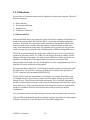
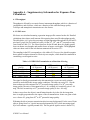
1. Introduction
This is the Users Manual for the Gemini Near-Infrared Spectrograph (GNIRS). GNIRS is
a 0.9-5 µm spectrograph that supports a variety of observing configurations, including
long-slit, cross-dispersed, IFU, and polarization analysis modes, as well as two different
pixels scales and several different spectral resolutions.
The GNIRS Users Manual is organized in several major sections, plus this introduction.
The first major section comprises an overview of the instrument. It is intended to provide
the information a prospective user of the instrument might need, first, to determine
whether the instrument is suitable for his or her scientific needs, and then to write a
proposal to use the instrument on Gemini.
The second major section describes how to observe with the instrument. The information
contained therein allows a user to prepare an observing program, and to carry it out at the
telescope. For observers assigned queue time, not all parts of this section are relevant.
Calibration data and initial data reduction procedures are also discussed in this section.
Portions of this section may be relevant when writing a proposal, if calibrations or
observing strategies are a concern.
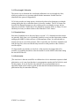
The remaining sections are primarily relevant for people responsible for supporting the
instrument - that is, the instrument scientist and other observatory staff more than the
visiting classical observer. Procedures for setting up and shutting down the instrument are
described, as well as basic trouble-shooting procedures. In general, visiting astronomers
will not find themselves carrying out procedures described here, and should certainly
embark on them with caution.
Additional procedures related to servicing and calibrating the instrument are found in the
Service and Calibration Manual.
GNIRS Users Manual
-1-
2. Instrument Overview
This section provides an overview of GNIRS, including a functional description (2.1),
on-telescope performance of the science channel (2.2), including a discussion of
observing modes (2.3), and performance of the available wavefront sensors (2.4).
2.1 Instrument Description
GNIRS is a cryogenic 1-5 µm spectrograph with an on-instrument wavefront sensor
(guider). The spectrograph can be operated in a variety of different observing mode,
including a choice of 2 pixel scales, 3 spectral resolutions, different cross-dispersion
options, and an integral field mode. The two pixel scales are provided by cameras with
different focal lengths.
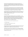
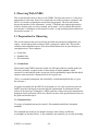
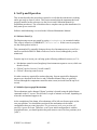
The light flow through the instrument is shown in Figure 2.1
Figure 2.1. “Optical schematic” for GNIRS, showing light flow through the science
channel.
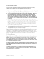
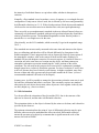
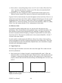
The instrument opto-mechanical layout is shown in Figure 2.2.
GNIRS Users Manual
-2-
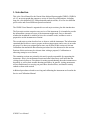
Figure 2.2. Instrument internal structure, showing light paths. The light path in red is the
path through the spectrograph, starting at the entrance window (which is not shown). The
light path in blue is the path through the OIWFS, starting at the pick-off mirror. The
actual internal structure of the instrument differs in some details from this figure.
Both the science channel and the on-instrument wavefront sensor are mounted within a
cold structure contained within a vacuum vessel. The instrument electronics are mounted
externally. The cold structure is operated at a temperature of ~60K in order to minimize
excess background on the detector.
2.1.1 Spectrograph Description
The spectrograph design is a fairly conventional one for infrared spectrographs. There are
two main sections: a fore-optics section, which provides field and pupil stops to limit
excess background, and a spectrograph section, which disperses light from the object of
interest.
GNIRS Users Manual
-3-
2.1.1.1 Fore-Optics
The fore-optics comprise the following elements:
• Entrance window
• Pick-off mirror
• Entrance fold mirror
• Offner relay (primary and secondary mirrors)
• Exit fold mirror
• Filter wheels
The entrance window also acts as a weak lens, in order to ensure that the telescope
secondary is imaged on the Offner secondary mirror, which is where the cold stop is
placed.
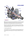
The pick-off mirror acts as a crude field stop, defining the field accessible to the
spectrograph. Light from the rest of the instrument field (roughly 3 arcminutes diameter)
is available in principle to the OIWFS (see 2.1.3). The unvignetted field defined by the
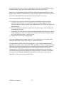
pick-off mirror is basically a 10 x 100 arcsecond strip with a superposed half circular
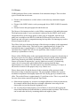
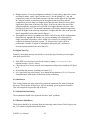
field 15 arcseconds in radius centered on the optical axis, as shown schematically in
Figure 2.3.
15’’ radius
10”
100”
Figure 2.3. GNIRS spectrograph field of view. The long dimension is 100 arcsec; the
width is 10 arcsec except for the additional 15-arcsec semi-circle.
The purpose of the semi-circle is to provide a somewhat larger field for target acquisition
and identification, while at the same time allowing use of guide stars close to targets of
interest. The pick-off mirror is tilted at 45 degrees, and is therefore exactly at the
telescope focus only in the center of the slit. The mirror widens away from its center to
ensure that the spectrograph field is unvignetted. The field available for guiding is
discussed in section 2.1.3.
The Offner relay is serves two functions: it produces an image of the telescope secondary
on the Offner secondary, where a cold stop is located, and it re-images the telescope focal
plane onto the spectrograph slit. The scale at the slit is the same as at the telescope focal
plane.
GNIRS Users Manual
-4-
The spectrograph contains two filter wheels. Each wheel can accommodate 9 filters, in
addition to an "open" position. The first wheel uses several of the positions for focus
masks, a dark position, and a lens used to view the telescope pupil during alignment (see
below). These can be used in series with filters in the second wheel. The remaining
positions in the first wheel can be used for back-up filters.
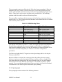
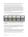
The current filter complement for the instrument is listed below; prospective observers
should verify (e.g., via the Gemini web site) that these are the filters that will be available
at the time they wish to observe.
Table 2.1 GNIRS Blocking Filters
Position Number
0
1
2
3
4
5
6
7
8
9
Filter Wheel 1
open
pupil viewer lens 1
cross disp (0.9-2.5 µm)
order 2 (2.90-4.25 µm)
open
open
open
dark
left mask
right mask
Filter Wheel 2
open
order 1 (4.4-6.0 µm)
order 2 (2.90-4.25 µm)
order 3 (1.92-2.54 µm)
order 4 (1.47-1.80 µm)
order 5 (1.17-1.37 µm)
order 6 (1.03-1.17 µm)
cross disp (0.9-2.5 µm)
open
open
Note that the sorting filters for orders 3, 4, and 5 are roughly equivalent to broadband K,
H, and J filters respectively. The long wavelength cut-off of sorter 3 is significantly
longer than for standard K filters; as a result, the sensitivity for target acquisition will be
worse due to increased background (see section 3.1.4 for more on acquisition
procedures).
The filters are slightly tilted (2.7 degrees) to reduce ghost images; this is also why the
filters precede the slit.
Because the filters are located in a converging beam, they all have the same optical
thickness in order to avoid refocusing the telescope each time a filter is changed. This
also ensures that filter changes keep the object centered on the slit. Any user-supplied
filters must have the same thickness (equivalent to 3 mm of BK7) in order to operate
properly. (Users considering supplying such filters must check with Gemini beforehand,
as installation of such filters requires considerable prior planning.)
2.1.1.2 Spectrograph
The spectrograph section consists of the following elements:
GNIRS Users Manual
-5-
•
•
•
•
•
•
•
Slit/Decker/IFU (2 mechanisms)
Collimator
Acquisition mirror
Prism turret
Grating turret
Camera turret
Focus stage/detector mount
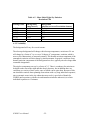
The spectrograph entrance slit is defined by two mechanisms. The width of the slit is
defined by the one of several slits in a photo-etched mask located in the slit slide, while
the length of the slit is defined by one of several openings in the decker slide. The
integral field unit (IFU) is also mounted in the slit slide; there is a location for a second
IFU unit, currently occupied by a dummy module of similar mass.
The slit mask is located at the re-imaged focal plane, while the decker apertures are
slightly ahead of it, and therefore somewhat out of focus (by a few pixels). The decker
sizes are matched to the full width of the array in long slit mode, or to the minimum
spacing between adjacent spectra when the prisms are used. The slit mask in the
instrument can be changed, although it should not be considered a routine operation. The
slit widths currently available are listed below, as are the decker lengths (Tables 2.2 and
2.3).
Table 2.2 GNIRS Slit Widths
Mask
Position
1
2
3
4
5
6
7
8
9
10
arcsec
3.0
1.0
0.20
0.15
0.10
0.30
0.45
0.60
Slit Width
long camera
short camera
pixelsa
pixelsa
dark
20
60
6.7
20
1.3
4
1.0
3
0.7
2
acquisition (Figure 2.2)
2
6
3
9
4
12
a
Widths in pixels are for lowest resolution grating and the acquisition mirror. Projected
widths with the 32 l/mm and 110 l/mm gratings are reduced by 5% and 22% respectively.
In addition, the slit slide can be positioned to use the integral field unit (see 2.1.1.4) or to
use the pupil viewer; for the latter a second lens is placed in the beam (used in series with
the lens in filter wheel 1).
GNIRS Users Manual
-6-
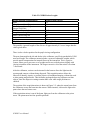
Table 2.3 GNIRS Decker Lengths
Decker Position (Configuration)
Spare
Long Camera Cross-Dispersion
Short Camera Cross-Dispersion
Integral Field Unit
Wollaston Prism (both scales)
Long Camera Long Slit
Short Camera Long Slit
Acquisition
Spare
Pupil Viewer
Usable Length (arcsec)
1.2
3.1
6.1
14.3
49.4
99
99
1.2
Not Applicable
The partially vignetted lengths of the slits are all approximately 0.5 arcsec longer than the
values given above.
There is also a decker position for the pupil viewing configuration.
The next element after the slit and decker is the collimator, an off-axis paraboloid of 1500
mm focal length. The collimator mount includes a system of adjustable weights, which
provide partial compensation for internal flexure in the instrument. This is a passive
system, where gravity acts on a set of weights and levers to tilt the mirror slightly with
varying orientation of the instrument. The largest corrective tilt of the mirror is less than
7 arcseconds.
After the collimator, a mirror can be inserted in the beam to direct the light into the
spectrograph cameras, without being dispersed. This acquisition mirror allows the
observer to identify, acquire, or recenter objects via broadband imaging, without the need
to alter grating and prism tilts. This facilitates prolonged observing sequences on faint
objects, since the dispersive settings remain stable even while target positions are
checked.
The position of the acquisition mirror is shown in Figure 2.2, where the return beam from
the collimator crosses the beam into the camera. When inserted, it diverts the light at the
point where the two beams cross.
If the acquisition mirror is out of the beam, light goes from the collimator to the prism
turret. The prism turret has four possible positions.
GNIRS Users Manual
-7-
Table 2.4 GNIRS Prisms
Position
Mirror
Long camera cross-dispersion
Short camera cross-dispersion
Wollaston prism
Application
Long slit mode for all 4 cameras
Used with long blue camera, 10 l/mm
grating for 0.9-2.5 µm coverage
Used with short blue camera, 32 l/mm
grating for 0.9-2.5 µm coverage
Polarization mode for all 4 cameras
The mirror is used for work beyond 3 µm, or when one wants to work with a long slit at
shorter wavelengths. The two cross-dispersion prisms provide a cross-dispersed low
resolution spectrum over the approximate range 0.9-2.4 µm, where the two prisms are
matched to the two pixel scales produced by the cameras. A complete spectrum is
produced at a resolution of ~1700 (2 pixels); use of higher spectral resolution results in
more or less parallel portions of multiple orders but not a complete spectrum. The
Wollaston prism separates the two linear polarization components of the light, and can be
used through the L band. Because there is substantial internal polarization in the
spectrograph itself, the Wollaston prism configurations must be used with GPOL on the
telescope’s up-looking port.
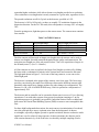
From the prism turret, light goes to the grating turret. The grating turret contains three
gratings.
Table 2.5 GNIRS Grating Resolutions
Grating
10.44 l/mm
31.7 l/mm
110.5 l/mm
Long Camera Resolution
1700
5100
17800
Short Camera Resolution
570
1700
5900
All three gratings are blazed for 6.8 µm (first order Littrow), which provides an effective
first order blaze wavelength of 6.6 µm in the configuration actually used (scattering angle
of 27 degrees).
The different orders of the gratings then correspond fairly well to the atmospheric
windows at 5, 3.5, 2.2, 1.6 and 1.2 µm for orders 1 through 5 respectively; the sorting
filters specified in Table 2.1 cover the free spectral range of the individual orders, with
some allowance for filter roll-off. A filter for order 6 is also supplied; the orders above 5
don't match the atmosphere particularly well.
The resolutions provided by the gratings are tabulated above (Table 2.5). The values
given are with the gratings operated at the blaze peak. Tilts to longer wavelength provide
GNIRS Users Manual
-8-
somewhat higher resolution, while tilts to shorter wavelengths provide lower resolution.
(The resolution in wavelength units is nearly constant for a given order, regardless of tilt.)
The quoted resolutions are all for 2 pixels at the detector, specified as λ/∆λ.
The detector is 1024 x 1024 pixels, so there are roughly 512 resolution elements in the
dispersion direction. For the R=1700 mode, this corresponds to coverage ∆λ/λ of roughly
30%.
From the grating turret, light then passes to the camera turret. The camera turret contains
four cameras.
Table 2.6 GNIRS Cameras
Camera
Long blue camera
Long red camera
Short blue camera
Short red camera
Wavelength Range
0.9-2.5 µm
2.9-5.5 µm
0.9-2.5 µm
2.9-5.5 µm
Focal Length/Pixel Scale
1305 mm/0.05 arcsec
1305 mm/0.05 arcsec
435 mm/0.15 arcsec
435 mm/0.15 arcsec
The blue cameras will not work at longer wavelengths; the red cameras can be used at
shorter wavelengths, but with somewhat degraded image quality and transmission. The
main short wavelength use of the red cameras below 3 µm is for acquisition of targets in
the K band (sorter 3). (See 3.1.4 details.)
All four cameras are close to parfocal; the longer focal lengths are achieved by folding
the beam with a combination of mirrors in the camera barrel and external to the turret.
The light path shown in Figure 2.2 is for one of the long cameras, so one can see the
folded light path.
The detector is mounted at the output of the cameras, on a focus stage. The focus stage
provides correction for the small focus differences between the different cameras (and
potentially other small focus changes produced by other changes in configuration). The
detector is a 1K x 1K ALADDIN III InSb array, which is operated at a temperature of
approximately 31K.
The detector and its controller can be operated at frame rates in excess of 1/sec, allowing
operation at 5 µm with either camera at any spectral resolution (imaging at 5 µm for
acquisition purposes is [probably] not possible). Individual frames can be co-added and
then sent to the Gemini Data Handling System (DHS) to ensure a more manageable data
flow.
For these high background observations, the main concern is minimization of overhead,
since the principal noise source is photon noise from the background. At shorter
wavelengths, especially at higher spectral or spatial resolution, detector read noise can be
significant, even for relatively long exposures. In these situations, the detector can be
read out non-destructively, so the read noise is reduced by multiple sampling (Fowler
GNIRS Users Manual
-9-
sampling). For long exposures and low background, the improved noise performance
more than compensates for the increase in overhead involved.
2.1.1.3 Detector and Controller Properties
The two detector/controller properties that directly affect signal to noise are read noise
and dark current. Read noise can be reduced by multiple sampling ("Fowler sampling"),
at the cost of additional overhead in the form of time spent on the extra reads. In addition,
the effective well size limits how much signal can accumulate.
The relevant properties are tabulated below, for the GNIRS ALADDIN III array (Ser. #
410793):
Table 2.7 - GNIRS Detector Properties
Read Noise (single read)
Read Noise (max useful multiple reads)
Single Read time
Max. Useful Read Time
Mean Dark Current
Well size (<10% non-linearity)
Gain
37 electrons
7 electrons
0.185 sec
~36 sec
0.1 electrons/sec/pixel
110,000 electrons
13 electrons/ADU
Further details on this subject are found in section 2.3.1.
2.1.1.4 Integral Field Unit
The integral field unit (IFU) is an additional optical system, provided for GNIRS by the
University of Durham (UK). The IFU takes a rectangular input field, of approximate
dimensions 3.3 x 4.8 arcsec, and divides it into 22 slices 0.15 arcsec in width. The IFU
optics (see Figure 2.4 eventually) map the slices of the rectangular field onto the input
plane of the spectrograph, aligning the slices more or less along the regular input slit
position (the slices are offset from each other by roughly 2 pixels/slice).
The optics also change the input scale to 0.12 arcsec/pixel along the slit, and 0.075
arcsec/pixel in the dispersion direction. The IFU is intended to feed the short cameras,
and therefore can be operated at a maximum resolution of ~5900.
[Figure 2.4 here]
Figure 2.4. Integral Field Unit Optics Layout.
GNIRS Users Manual
-10-
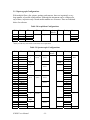
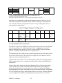
2.1.2 Spectrograph Configurations
With multiple filters, slits, prisms, gratings, and cameras, there are in principle a very
large number of possible configurations. Although the instrument can be configured to
any of these, in practice only a much smaller number are of interest. These are tabulated
below for reference.
Table 2.8 Acquisition Configurations
ID #
Name
Filter
Slit
Decker
Acq
Mirror
1
SBAcq
sorter 3-7 acquisition acquisition
2
SRAcq sorter 1-3a
3
LBAcq
sorter 3-7
4
LRAcq sorter 1-3a
Notes:
a
Ability to read array with sorter #1 uncertain, not a requirement
in
Prism
Grating
Camera
N/A
N/A
short blue
short red
long blue
long red
Table 2.9 Spectroscopic Configurations
ID #
Name
Filter
Slit
Decker
Acq
Mirror
Prism
Grating
Camera
5
6
7
8
SB10
SB31
SB111
SBXD
sorter 37
0.3
arcsecb
100
arcsec
out
mirror
10.44c
31.7
110.5
31.7d
short
blue
9
10
11
12
13
14
15
16
17
18
19
20
21
22
23
24
25
26
27
SB10P
SB31P
SB111P
SB10IFU
SB31IFU
SB111IFU
SR10
SR31
SR111
SR10P
SR31P
SR111P
SR10IFU
SR31IFU
SR111IFU
LB10
LB31
LB111
LB10XD
28
29
30
31
LB10P
LB31P
LB111P
LR10
broadband
sorter 37
sorter 1
&2
sorters 37
6 arcsec
14.4
arcsec
IFU
6 arcsec
0.3
arcsec
100
arcsec
short
prism
Wollaston
mirror
14.4
arcsec
Wollaston
IFU
6 arcsec
mirror
0.1
arcsecb
50 arcsec
broadband
sorters 37
3 arcsec
long prism
14.4
arcsec
Wollaston
sorters 1
50 arcsec
mirror
GNIRS Users Manual
-11-
10.44c
31.7
110.5
10.44c
31.7
110.5
10.44c
31.7
110.5
10.44c
31.7
110.5
10.44c
31.7
110.5
10.44
31.7
110.5
10.44d
10.44
31.7
110.5
10.44
short red
long blue
long red
&2
32
LR31
33
LR111
Wollaston
14.4
34
LR10P
arcsec
35
LR31P
36
LR111P
Notes:
b
Slit listed is width optimally sampled at detector; other widths can be used
c
Spectrum does not fill entire detector width
d
Grating listed provides complete 0.9-2.5 µm spectrum; other gratings can be used
31.7
110.5
10.44
31.7
110.5
In principle, any configuration can be used for diagnostic purposes. However, the two
main optical diagnostics contemplated for the instrument are pupil viewing and focus
tests. Note that, unlike the configurations listed in the two preceding tables, there are
more variables in entries below.
Table 2.10 Regular Diagnostic Configurations
ID #
Name
Filter
Slit
Decker
37
Pupil View
pupil
view
lens #2
pupil view
38
Focus test
FW 1: pupil
view lens #1;
FW 2:
sorters 2-4
FW 1: pupil
masks;
FW 2: any
Acq
Mirror
in
Prism
Grating
Camera
N/A
N/A
long blue
or long
red
Focus tests may be done on any configuration listed in Table 1 and
Table 2 except for filters in FW 1.
2.1.3 On-Instrument Wavefront Sensor
The OIWFS was built for GNIRS by the Institute for Astronomy (Hawaii). The light path
is also shown in Figure 2.2. Light from the guide field - anything in a 3 arcminute
diameter field that misses the pick-off mirror - enters the OIWFS field lens and then
passes to a collimator doublet and then a 2-axis gimbal mirror.
The gimbal mirror can be tilted precisely to direct light from any part of the guide field to
the rest of the OIWFS optics. The usable field is roughly 10 arcsec diameter, which is
sufficient to acquire individual guide stars.
Light from the selected patch of sky is reflected off the gimbal mirror, through a second
doublet, and the guide star is re-imaged on the filter wheel, which contains JHK filters
and apertures.
From the filter wheel, light enters the Shack-Hartmann optics, which are mounted on a
"snout" on the detector mount. The Shack-Hartmann optics form a pupil image at a
shallow four-facet prism, then reimage the star on the detector. Because the light has
passed through the S-H prism, four images of the star are actually formed, corresponding
to 1/4 of the pupil each. Only a small portion of the array is read out, allowing rapid data
rates, which permit the OIWFS to provide high-speed tip-tilt and focus correction in
GNIRS Users Manual
-12-
addition to slower flexure and tracking correction. For fainter guide stars, fast correction
is limited to tip-tilt and does not include focus.
The OIWFS filter wheel contains standard JHK filters. In principle, users should select
the filter that provides the best signal to noise on the guide star (normally H), since the
telescope's acquisition and guide (A&G) system adjusts the OIWFS gimbal mirror
position to compensate for differential refraction between the guide wavelength and the
observing wavelength.
See section 2.4.1 for OIWFS performance, and 3.2.2 for information on OIWFS
operation.
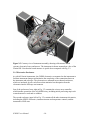
2.1.4 Cryostat
The cold structure shown in Figure 2.2 is contained within a larger cryostat, shown in
cutaway view below (Figure 2.5). The internal structure is maintained at a temperature of
approximately 60K using 4 Leybold RG 5/100 cryocoolers. The initial cool-down of the
instrument can be done either with the cryocoolers alone, which takes over a week, or
with the assistance of a liquid nitrogen pre-cool system, which allows the instrument to
reach operating temperature in 3 days.
The cryostat is a large vacuum vessel, which contains two aluminum passive shields and
a third shield that is connected to the cryocoolers. These act to minimize heat radiated
and conducted into the cold structure, which would otherwise produce unacceptable
temperature gradients and gradient variations under varying ambient conditions. In
addition, a temperature control system adds varying amount of heat to the cooling system
to ensure that the structure is maintained at a constant temperature (±1K or better).
The window at the front of the cryostat has a motor-operated cover that is closed to
protect the window when the instrument is not in use. As it is an external warm device, it
cannot be used as a "dark slide". There is a manual override on the cover so that the
window can be protected even in the event of a power failure.
The window can cool below the dew point in conditions of high humidity, so the window
mount provides a slow flow of dry air across the window to avoid condensation. This also
helps to keep dust off the window.
GNIRS Users Manual
-13-
Figure 2.5. Cutaway view of instrument assembly, showing cold structure inside
cryostat, electronics boxes and trusses. The instrument is shown mounted on a face of the
Gemini ISS. Note that the bench structure is upside down compared with Fig. 2.2.
2.1.5 Electronics Enclosures
As with all Gemini instruments, the GNIRS electronics are mounted on the instrument to
facilitate instrument changes and minimize the complexity of the connections between
the instrument and telescope. The electronics are mounted in two thermal enclosures,
which are insulated, glycol-cooled boxes that minimize heat dissipation from the
electronics into the telescope environment.
One of the enclosures (lower right in Fig. 2.5) contains the science array controller,
which handles operations of the ALADDIN array, including initial processing steps such
as non-destructive reads and co-addition.
The second enclosure (upper left in Fig. 2.5) contains all the other instrument electronics,
including the OIWFS electronics, instrument motor and temperature controls, and the
instrument's VME crate.
GNIRS Users Manual
-14-
The instrument fits (barely) within Gemini's allowed instrument envelope, and is
approximately 2.2m long x 2.5 m wide x 1.3 m high (side-looking orientation). The
instrument weight is just under 2 metric tons; ballast is added to bring its weight up to
2000 kg to balance it against other instruments on the Gemini instrument support
structure.
GNIRS Users Manual
-15-
2.2 Science Channel Performance
The performance of the science channel depends on the instrument configuration and
details of the observations. In general, though, all observations with GNIRS can be
thought of as comprising a measurement of the object and a measurement of the
background, which are then differenced.
The signal is the flux from the object, minus any light losses (slit losses, absorptions and
reflections, etc.), converted to detected electrons.
The noise is the combined effects of photon noise from the object+sky, photon noise
from the subtracted background, photon noise from dark current and internal background,
and detector read noise.
Summary sensitivity tables are given below (2.2.1) for some standard configurations and
conditions; details are provided in subsequent sections (and yet more information in
Appendix A). In general, the Gemini integration time calculator (ITC) should be used,
when it becomes available, for best estimation. However, the following sections and the
appendix can be used until then, and also serve to show the considerations that go into the
ITC.
2.2.1 Sensitivity Summary
2.2.1.1 Baseline Observing Sequence
For observations of objects comparable in size to the slit length or IFU dimensions, the
background observation is actually a separate observation taken by moving away from
the object onto blank sky. For observations with a small object or a long enough slit, it is
possible to position the object successively at different positions on the slit, and thus use
a single observation for both object measurement and background measurement. For
example, if one can measure 5 different slit positions, at any one position there is one
"object" measurement and 4 "background" measurements, which can be combined. In the
limiting case of very many slit positions, the noise contribution from the background
determination become negligible, and has taken no additional time. Compared with the
simple "on-off" case, the multi-position observation will take roughly 1/4 the time to
achieve the same signal to noise.
This discussion assumes that it is possible to provide the same type of spectral extraction
for the different cases. If doing a smaller number of positions provides enough signal to
noise for optimal extraction, but this is not possible for a large number of positions, then
the smaller number may be better. Also, for the shorter slits (cross-dispersed modes in
particular), there may not be enough positions except in very good seeing. Again, use of
the ITC should help in these decisions.
All the tabulations below assume that data were taken at a large number of positions
along the slit. Therefore, for objects comparable in size to the slit, observation times must
GNIRS Users Manual
-16-
be increased by a factor of 4. For objects where only a small number of positions can be
observed (2 or 3), there is a smaller increase in the time required.
2.2.1.2 Overheads
The tabulations do not include any allowance for overhead. This should be allowed for
explicitly. The following rules can be applied provisionally:
• Initial set-up. This includes moving the telescope to the object, acquiring the guide
star in the OIWFS, acquiring the object on the slit, and configuring the instrument.
Allow 15 minutes.
• Instrument reconfiguration. This occurs when the instrument configuration is changed
but the object to be observed is the same. For most changes (filters, grating tilt), the
time required will be <1 minute.
• General overhead. This includes allowance for moving the telescope between
positions on the slit (or on and off), detector readout and write time, periodic checks
of object centering (for long observation sequences). 10% of the calculated total
integration time should be allowed for these purposes. This will increase for longer
wavelength observations, especially M band, where it may approach 50%.
Note that the calculated observing time required for standards will approach half an hour
for typical observations, even though the actual integration time will be a few minutes.
The manual should include an estimate of time requirements for standard star
observations once we have experience at the telescope.
2.2.1.3 Performance Completeness
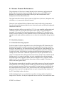
The night sky background is not a smooth function of wavelength, as demonstrated in
Figures 2.6 and 2.7, which show low-resolution night sky spectra.
GNIRS Users Manual
-17-
Figure 2.6. CRSP H-band night sky spectrum at resolution ~1400. [Replace with R=1700
GNIRS spectrum when we have one.] At this resolution, the background varies by well
over an order of magnitude between different wavelengths in the band. As a
consequence, signal to noise will also vary by substantial factors, possibly approaching a
factor of 10 in this case.
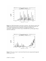
Figure 2.7. The same as Fig. 2.6, but for the K band. Note the rising thermal background
beyond about 2.4 µm.
GNIRS Users Manual
-18-
The situation in other bands and at other resolutions is generally similar, although it is the
case that at longer wavelengths there is more continuum flux (so maximum contrast is
less). Also, at higher resolutions the spectrum increasingly breaks up into resolution
elements with and without lines; at R~18000 roughly 90% of the spectrum does not
contain strong lines. (There will still be enough lines for a reasonable wavelength
calibration.)
It is clear, therefore, that a sensitivity estimate based on the average background within a
spectral window is not necessarily that useful, though it is easy to calculate. Therefore,
for this manual, 90th percentile sensitivity is also calculated, which is the value where
90% of the resolution elements in the spectrum will have greater than the specified signal
to noise, and 10% will have less. It turns out that, due to the nature of the night sky
spectrum, average background is roughly equivalent to 75th percentile background.
The ITC should be used when available, as this provides the most accurate estimates.
This is particularly true when what is of interest is a specific feature or features rather
than a complete spectrum.
2.2.1.4 Standard Observing Conditions
Since many Gemini observations are taken in queue mode, where observing conditions
are specified, it is necessary to indicate which conditions are relevant, and also which
were used for the baseline calculations provided here.
There are five main observing constraints:
•
•
•
•
•
Image quality ("seeing")
Cloud cover
Water vapor
Sky background
Air mass (zenith distance)
Image quality values relevant to GNIRS are tabulated below. Note that these are the
values used in computations in this manual; if Gemini changes the specifications both
this table and the computations must be changed.
Table 2.11 - Gemini Image Quality Constraints
Image FWHM (arcsec)
Wavelength
0.9 µm
1.2 µm
2.2 µm
3.4 µm
20th percentile
0.40
0.35
0.30
0.30
GNIRS Users Manual
50th percentile
0.75
0.55
0.50
0.45
-19-
85th percentile
1.05
0.80
0.75
0.70
"any"
1.70
1.55
1.40
1.25
Image quality at wavelengths beyond 3.4 µm will be similar to that at 3.4 µm.
Results are provided below for both 20th and 50th percentile conditions. Trade-offs
involved in selecting better or worse image quality are discussed in 2.2.2.
Cloud Cover. All calculations assumed conditions were "photometric", which
corresponds to 50th percentile cloud cover. The presence of cloud is undesirable for two
reasons - signal is attenuated, and background will be more variable, complicating sky
subtraction. Note that observations under marginally photometric conditions are
reasonable, since GNIRS spectra will not normally have high absolute photometric
accuracy anyhow (see section 3.4).
Water Vapor affects much of the L and M bands, and the edges of atmospheric windows
(near water bands). You should investigate the exact circumstances of your observations
(look at atmospheric spectra in the ITC) to determine whether drier conditions will make
enough difference to request them. See Figure 2.7 (below) for an example of calculated
transmission for dry conditions. Water vapor at Gemini South has a strong seasonal
dependence, so observations requiring dry conditions will be far more difficult in the
summer (essentially, 20th percentile conditions will occur much less than 20% of the time
then). Because the affected regions typically contain strong, saturated lines, observations
that require dry conditions will be best done with the driest conditions realistically
available.
Figure 2.7. Calculated transmission for 0.9-2.7 µm for 1.6 mm precipitable water on
Mauna Kea. This corresponds to very best conditions on Cerro Pachón. One can see
which regions might be usefully observed in dry conditions, but not otherwise.
Sky Background in the near infrared effectively divides into "night" (80th percentile) and
"twilight". Background is both higher and variable during twilight, so observers will
seldom gain much by trying to observe at these times. All calculations use standard night
sky conditions (2.2.4). Note that there is no reason to request gray time even for the
shortest wavelengths; scattered moonlight is not significant. The only exception will be
for objects located in the ecliptic, where moonlight scattered off the telescope itself will
cause problems.
GNIRS Users Manual
-20-
Air Mass should generally be modest, as background, image quality and differential
refraction all get worse with increasing airmass. All calculations assumed an airmass of
1.0, since the standard sky background and image quality specifications refer to zenith.
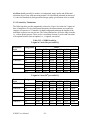
2.2.1.5 Sensitivity Tabulations
The following table provides magnitudes (referred to Vega=0.0) reached at 5 sigma in 1
hour of integration. For low background situations, the measurements are assumed to
comprise 4 exposures of 15 minutes; for high background situations the lengths of the
individual exposures are not relevant. The values tabulated are all for the long slit mode,
i.e., with no prisms present. These are for a resolution element (2 pixels) and extraction
of an optimal window (but not optimal, i.e., weighted, extraction).
Table 2.12 - GNIRS Sensitivity
5-sigma in 1 hour, 20th percentile IQ
Resolution/
Scale
1700/0.05"
5100/0.05"
17800/0.05"
1700/0.15"
5900/0.15"
Background
6 ("x")
21.50
21.23
20.09
19.98
19.16
19.11
21.93
20.54
21.32
20.98
ave
90%
ave
90%
ave
90%
ave
90%
ave
90%
5 ("J")
21.42
21.13
19.97
19.84
19.04
18.98
21.76
21.36
21.16
20.81
Order
4 ("H") 3 ("K")
20.36
19.43
19.96
19.11
19.24
18.47
18.94
18.20
18.54
17.77
18.33
17.57
20.52
19.59
20.08
19.26
20.04
19.07
19.61
18.74
2 ("L")
15.28
14.90
14.35
13.97
13.83
13.45
15.32
14.94
14.90
14.42
1 ("M")
12.03
11.59
11.21
10.78
10.80
10.36
12.18
11.74
11.77
11.33
2 ("L")
14.45
14.07
13.52
13.15
13.00
12.62
14.64
14.26
14.12
13.74
1 ("M")
11.21
10.77
10.39
9.95
9.97
9.54
11.50
11.06
11.09
10.65
5-sigma in 1 hour, 50th percentile IQ
Resolution/
Scale
1700/0.05"
5100/0.05"
17800/0.05"
1700/0.15"
5900/0.15"
Background
ave
90%
ave
90%
ave
90%
ave
90%
ave
90%
GNIRS Users Manual
6 ("x")
20.68
20.41
19.28
19.17
18.35
18.29
21.26
20.86
20.66
20.31
5 ("J")
20.60
20.31
19.15
19.03
18.22
18.17
21.10
20.69
20.50
20.14
-21-
Order
4 ("H") 3 ("K")
19.54
18.61
19.13
18.29
18.42
17.65
18.12
17.38
17.72
16.95
17.51
16.75
19.85
18.91
19.41
18.58
19.37
18.39
18.94
18.07
For observations with the Wollaston prism, there will be two spectra, plus some
reflection losses and vignetting in the prism, so the magnitude required to get 5 sigma in
each spectrum is roughly 0.5 mag brighter than the tabulated values for backgroundlimited observations, and roughly 0.9 mag brighter than the tabulated values for detectorlimited observations.
For observations in cross-dispersed mode, there are some reflection losses in the prism,
as well as absorption losses in the K window (mainly at the red end). The color of the
object determines whether the limiting sensitivity is set at the short or long wavelength
end of the spectral region covered with the prism; the decrease in sensitivity ranges from
~0.1 mag at the shorter wavelengths to ~0.3 mag at the longest wavelengths.
Sensitivity with the IFU is more complicated, because one wants to look at sensitivity for
each spatial sample. IFU observations will generally be done under very good seeing
conditions. A rough approximation is to use the long camera sensitivities, even though
the actual configuration uses the short camera.
2.2.1.6 Long vs. Short
Under the same image quality conditions (except for very best conditions, i.e. ~10th
percentile), the short cameras will provide better performance than the long cameras. The
difference is most significant at R=5100/5900, where the short camera configuration uses
a more efficient grating. At R=1700, the short camera grating is less efficient and
performance is more nearly comparable. The short camera configurations use fewer
pixels along the slit, so there is a reduced contribution from read noise and dark current,
which is significant at short wavelengths (mainly xJH).
The long camera is therefore mainly recommended in two cases:
• R=17800 is needed
• High spatial resolution along the slit is needed
2.2.2 Wavelength Calibration
The night sky will always have enough well-defined emission features to provide a good
wavelength calibration. In addition, the on-telescope calibration unit (GCAL) provides
the ability to observe arc lamps for set-up when the dome is closed.
One should not rely on the instrument control software for more than rough calibration
(good to about 10 pixels for center wavelength). The accuracy is limited by the grating
turret repeatability and the approximations used in modeling the wavelength as a function
of grating tilt and array position.
GNIRS Users Manual
-22-
2.2.3 Slit Tilt and Curvature
The instrument is configured so that the spectrograph slit is aligned with the array
columns when in long slit mode. This alignment is not exact, however:
• There is some residual error in the alignment, which leads to a net rotation of <1 pixel
along a slit running the full width of the array (~1024 pixels).
• As with any long-slit spectrograph, there is also curvature along the slit. The size of
the effect depends on the configuration. The displacement of the center position
relative to the ends varies from less than 0.1 pixel to almost 3 pixels. The effect is
larger for higher resolution and for the short cameras. There can be some change in
the dispersion as well, in that the curvature varies slightly as a function of wavelength
on the array.
• The cross-dispersed modes introduce a tilt of the slit image, which is a function of
position on the array. For the short slits used in these modes, the tilt is modest but still
significant, typically around 0.5 pixel end to end for extreme positions. In addition,
the spectra themselves run at an angle on the array (i.e. constant slit position is not
constant x position on the array). The angle is such that wavelengths seen in more
than one order are at the same x position.
• The separation of the two polarizations in the Wollaston mode is a weak function of
wavelength (decreases with increasing wavelength).
In general, these tilts should not have a substantial effect on the data. However, in some
circumstances, it may be useful to shift spectra slightly before co-adding them. In the
case of spectra using the full slit length, it may also be necessary to interpolate between
multiple wavelength calibrations if precise wavelengths or velocities are required.
2.2.4 Spatial Resolution
In general, the optics in GNIRS provide spatial resolution along the slit as good or better
than that implied by the pixel sampling. For the most part, even the short camera (0.15
arcsec pixels) samples the delivered image quality. Therefore, the instrument's spatial
resolution should be considered to be that defined by the delivered image quality, except
for 20th percentile image quality or better.
For this level of image quality, the resolution along the slit will be limited to ~0.3 arcsec
for the short cameras, and will continue to be limited by the actual image quality for the
long cameras.
The spatial resolution for the IFU is similar to that with the short cameras (0.12 x 0.15
arcsec samples), so the IFU resolution will also be "seeing-limited" until image quality
reaches approximately 20th percentile.
GNIRS Users Manual
-23-
2.2.5 Flexure
GNIRS undergoes flexure as the orientation of the instrument changes. There are three
types of flexure that are relevant:
• Flexure of the instrument as a whole relative to the telescope (instrument support
structure).
• Flexure of the OIWFS relative to the spectrograph slit (or PWFS if OIWFS cannot be
used).
• Flexure between the spectrograph slit and the detector
The flexure of the instrument relative to the ISS has components of tilt and displacement.
The displacement (under 2 arcsec maximum) is taken out by the OIWFS, and is small
enough that effects on the image quality or plate scale are negligible. Note that if no
guide star is available to the OIWFS, so that the PWFS must be used, flexure will be
significant, and will require compensation using look-up tables. Recentering may need to
be more frequent in this case.
The effects of tilt are to decenter the image of the telescope secondary on the instrument's
cold stop (in the Offner relay). This leads to some vignetting and loss of signal. The
maximum decenter is approximately 1% of the pupil diameter, which leads to an
equivalent loss of signal. This effect is not significant, either in terms of overall
sensitivity or photometric accuracy.
Flexure of the OIWFS relative to the spectrograph slit leads to progressive decentering of
the object on the slit. This effect is (predicted to be) relatively small, with the dominant
effect being flexure by the OIWFS mechanisms. The shifts on the slit produced by
flexure are less than 20 microns for 1 gravity; light losses exceed 5% with the long
camera for a 10 micron shift, which implies that recentering should be done
approximately every 2 hours. The short camera can tolerate decentering 2-3x larger, so
one needs to recenter for this purpose only every 4 hours or so.
Flexure between the slit and the detector leads to smearing of the spectrum in both
directions for long accumulated exposures. The spectrograph collimator has a passive
mechanical compensator that slightly adjusts tilt with varying gravity to minimize this
effect. The residual flexure is approximately 0.3 pixel/hour or less. This is very small, but
for some observations cannot be neglected. Specifically:
• Observations requiring very accurate wavelength calibration (velocity measurements,
for example) should ensure that the wavelength calibration is an average for the
observation, not just data from the beginning or end.
• For very long observation sequences (several hours), it may be useful to group the
observations and then shift and add them to retain maximum resolution. This decision
can be made after the fact by examining shifts in the night sky lines.
GNIRS Users Manual
-24-
• Observations requiring cancellation of telluric absorptions, which require observation
of a reference star to provide an absorption template, should be carried out with the
reference star close to object, and with the spectrograph in the same orientation (slit
angle).
• Flexure in acquisition mode is larger, as much as 1 pixel/hour with the long cameras.
See 3.1.4 for a discussion of object acquisition.
2.2.6 Repeatability
The mechanisms in GNIRS are not perfectly repeatable. That is, once a mechanism is
moved, a return to the same nominal position will be close but not exact. The nominal
performance specification is 10 pixels repeatability with the long cameras (<1 pixel with
the slit). From the point of view of exact wavelength calibration, this means that each
configuration of the instrument is a new configuration requiring its own calibration - even
it is nominally the same as a previous calibration.
There are a couple of exceptions to this rule. Filter changes do not change the
configuration after the slit at all, so one can cycle through orders at a fixed grating
orientation and maintain calibration. Also, the acquisition mode inserts a mirror in the
beam, but does not move the prism, grating, or camera, so checking centering will not
alter the spectroscopic configuration. Note that the acquisition mode itself is only
repeatable to a few pixels, [TBD], so one should check centering relative to the image of
the slit and not relative to absolute pixel coordinates.
These considerations would affect observations where one wants to observe both an
object and a reference star in the same, identical configuration (probably so as to divide
out telluric absorptions). In this case, it would be possible to set the grating and measure
orders 3-6 on the object by changing filters, and then go to the reference star and the
repeat the same sequence. If, on the other hand, one wanted to observe at several grating
tilts (perhaps at higher resolution), one would have to observe the object at one tilt, then
the reference star, then change the tilt, then observe the reference and the object at the
new tilt, and so on. Any calibrations that cannot be done later need to be done as well.
GNIRS Users Manual
-25-
2.3 Observing Mode Trades
2.3.1 Instrument Configuration Trades
This section discusses alternative configurations for some types of observations. The
discussion is general, so it is useful to compare situations for specific programs using the
ITC.
•
•
•
Long vs short cameras. The long cameras will give better performance only when
image quality is good enough so slit losses don’t exceed the gains due to reduced
background. Unless maximum spatial or spectral resolution is required, the short
cameras will probably be preferred. Note that for a resolution of 18,000 the long
camera must be used.
Long slit vs cross dispersed. Cross dispersion provides cover of multiple orders, but
at the expense of slit length. If only one atmospheric window is of interest, use long
slit mode. If two or more windows are desired, then the loss of sensitivity due to
limited slit length (limited number of different dither positions) is normally offset by
the ability to observe several orders at once.
IFU vs slit. The IFU is the only efficient way to get 2-dimensional coverage, so it is
clearly the choice when observing objects with structure or in very crowded fields. It
is possible that in poor seeing, the IFU could be used as an image slicer for point
source observations, provided only a single atmospheric window is of interest
(otherwise the multiplex gains from cross-dispersion should offset the gains from
image slicing).
2.3.2 Observation Configuration Trades
This section discusses guidelines for optimizing one's observations in terms of number of
exposures, Fowler sampling, and "dithering" (positional sampling). The emphasis is on
measuring faint objects; for bright objects total time is dominated by overhead, so one
should mainly ensure enough measurements are made at slightly different positions to
provide adequate sky subtraction and flat-fielding.
For faint objects, one would like to measure at different positions along the slit, ideally
enough so that the noise contribution from sky subtraction is negligible (see 2.2.1). At
some point, the number of positions required will become too large to fit along the slit,
and the overheads involved - relative to the decreasingly short exposure times - will also
lead to diminishing returns. For most applications, 5 different positions is a reasonable
compromise.
For the cross-dispersed long camera, where the usable slit length is ~3 arcsec (Table 2.3),
it may not be possible to use this many positions unless image quality is quite good (20th
percentile or better).
GNIRS Users Manual
-26-
Alternatively, for programs requiring very high signal to noise, flat fielding may prove to
be a limitation and additional positions - presumably in long slit mode - would then be
useful.
A second set of choices relates to the read-out mode used - whether one does a single
read or multiple reads. (Note that all exposures actually consist of an array reset, an
initial read-out, integration, and then a final read-out from which the initial read is
subtracted. The read noise given in Table 2.14 is for such sequences.) The use of multiple
reads decreases the effective read noise by up to a factor of 4, but at the price of increased
overhead.
The difference in overhead between the minimum number of reads and the maximum
useful sampling is about 4 seconds, so if one is in fact read noise limited, multiple
sampling is justified for any exposures longer than a few seconds. In practice,
observations below 2.5 µm will benefit from multiple sampling, and observations at
longer wavelengths will not.
The maximum exposure time to be used is set by one of three considerations: the total
integration time required for the object, sky variability, and saturation of the array.
Saturation of the array occurs relatively rapidly in the "M" window (order 1), where
exposure times under a second will be required with the short cameras to avoid
saturation. For these observations, one would co-add multiple short exposures at each slit
position to keep the quantity of data manageable. Because sky subtraction is critical, one
would want to limit the time at each position to tens of seconds, or a few minutes at most.
(Experience with actual conditions at Gemini will be helpful here.) One would then cycle
through the slit positions multiple times to accumulate signal to noise. For high
background situations, the detector bias can be increased to increase the well capacity.
The read noise is also higher at higher bias, so it should be used only in these high
background situations (basically any case where you are limited to exposures of seconds
or less). Always use the same bias for the same configuration.
In the next order, between 3 and 4 µm, backgrounds are substantially less, but still high
enough to limit exposures to under a minute at low spectral resolution. Depending on the
spatial and spectral resolution, one might co-add a small number of images, but still keep
time at any slit position to a few minutes at most, and cycle through the positions as
needed. At the lowest resolutions, use of the high bias may be required (TBD).
At still shorter wavelengths, exposure times could be tens of minutes or even hours
without danger of saturation, so the primary limitation is instead sky variability. A 15minute exposure time would allow one to cycle through 5 slit positions in under 90
minutes (allowing for overheads), which is a reasonable limit if there is still a need to
subtract sky emission lines. For higher resolution (especially R=17800), it may be
possible to ignore the lines, in which case somewhat longer exposures would be
reasonable.
GNIRS Users Manual
-27-
2.4 WFS Performance
For guiding, either the On-Instrument Wavefront Sensor (OIWFS) or the telescope's
Peripheral Wavefront Sensors can be used. The OIWFS is preferred, if a suitable star is
available (see 3.1.1).
2.4.1 OIWFS Performance
The OIWFS performance can be calculated from first principles, or can be assumed to be
very similar to the performance of its equivalent in NIRI. Both assumptions lead to
similar predictions.
For use with the Shack-Hartmann prism, which is permanently installed, the 5-sigma
magnitude per spot for a 10 msec integration is approximately magnitude 13.8 for J or H,
and 13.1 for K. This calculation is for 50th percentile image quality. Performance for 20th
and 85th percentile image quality is estimated to be roughly 0.7 mag better/worse
respectively.
Since image quality is slightly better at H, this is probably the best choice for OIWFS
filter under most circumstances.
In unobscured regions, stars of the required brightness correspond (roughly) to R<16.
The unvignetted GNIRS patrol field is effectively a 3 arcminute diameter circle minus a
strip roughly 20 arcsec across; the area is approximately 6 square arcminutes. Models of
the guide star distribution on the Gemini WFS web page suggest that stars of the required
magnitude will be relatively common at galactic latitude 30 degrees, but less frequent at
higher galactic latitude (roughly half the all fields).
Fainter stars can in principle be used, at the price of losing full tip-tilt and focus
correction. For large, high-latitude samples, guide star availability may be useful way to
select smaller sets of objects for observation.
2.4.2 PWFS Performance
See the Gemini web pages (follow Science Operations link to Telescope, then to WFS
and Guide Stars).
GNIRS Users Manual
-28-
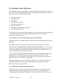
3. Observing With GNIRS
This section describes how to observe with GNIRS. The first sub-section (3.1) discusses
preparation for observing. Some of its content may be needed to prepare a proposal, and
all of it is relevant to preparing the actual observing program. The next sub-sections
discuss the interfaces to the instrument - section 3.2 describes the engineering interface,
which is what the early user must confront, and section 3.3 will eventually describe the
user interface. Calibrations are discussed in section 3.4, and preliminary data reduction is
discussed in section 3.5.
3.1 Preparation for Observing
This section assumes that you have already specified the instrument configuration you
require - spatial and spectral resolution, filters, grating tilts, and the like. This section
considers some additional aspects of the observations that need to be specified prior to
carrying them out. These comprise:
• Guide Stars
• Standard Stars
• Slit Orientation
3.1.1 Guide Stars
Observations with GNIRS cannot be carried out efficiently without a suitable guide star.
The only (probably) exception to this is observations of bright standards, where
exposures are short and the guider set-up time will be substantially longer than the added
exposure time required to compensate for lack of a guide star.
(This is a reasonable assumption, but it should be verified and amplified after we go to
the telescope.)
If a guide star suitable for the OIWFS can be found (see 2.4), this is preferred, since the
OIWFS provides both tip-tilt correction and full compensation for instrument flexure
relative to the telescope. Failing this, a PWFS guide star will provide good compensation,
though the tip-tilt correction will be less effective because of the greater distance between
the guide star and the object.
3.1.2 Standard Stars
Two types of standard stars may be needed - flux standards and telluric absorption
standards.
Flux standards are needed if you intend to measure relative fluxes at different
wavelengths (or absolute fluxes). A flux standard is not needed if you are only measuring
GNIRS Users Manual
-29-
the intensity of individual features as equivalent widths, whether in absorption or
emission.
Normally, a flux standard is used to produce a curve of response vs. wavelength for each
configuration. If only narrow slits are used, this is affected by slit losses and (potentially)
by differential refraction (see 3.1.3). Wide-slit observations of both objects and standards
can be used to convert observation to an absolute flux scale (true spectrophotometry).
There are really no spectrophotometric standards in the near-infrared. Instead, observers
customarily use photometric standards with spectral types that indicate they should have
relatively featureless spectra. The broadband magnitudes are then fitted to produce a
smooth flux vs. wavelength curve for the stars.
(Provisionally, use the LCO standards, which are mostly G-type in the magnitude range
10-12.)
Flux standards are not necessarily measured at the same time and airmass as the objects
they are calibrating, and therefore will be affected differently by absorptions in the
Earth's atmosphere. If one's program looks only at features in relatively clean regions of
the atmospheric windows, such as the centers of the H and K bands, dividing by a
standard will provide adequate correction. For messier regions, it is useful to observe a
correction star at the same time at a location near the object, and then construct an
atmospheric absorption correction normalizing the "clean" portions of the stellar
continuum. The star used for this purpose does not need to be a photometric standard,
though it must have a relatively featureless spectrum. For lower resolution, F and G stars
work well, because they have relatively weak features. At higher resolution, more lines
become evident and early-type stars may be preferable outside the H I lines. (A list of
recommended standards will need to be developed.)
In many cases, it will be possible to arrange the observations so that the same star is used
for both flux calibration and telluric correction. This essentially requires one standard
observation for each object observation, unless objects are close together in the sky and
are fairly bright (e.g., stars in a cluster).
3.1.3 Slit Orientation
Two factors affect the orientation of the slit (and the IFU). One is the structure of the
object to be observed, and the other is differential refraction.
The orientation relative to the object is dictated by the science to be done, and is therefore
specified by the observer.
The optimum orientation from the point of view of differential refraction may be quite
different; observers need to understand the effects involved. Differential refraction
smears the spectrum of an object by an amount that is significant on the scale of the
narrow slits used in GNIRS.
GNIRS Users Manual
-30-
For example, the differential refraction between 0.9 and 2.5 µm (roughly the wavelength
range of the cross-dispersed mode of the spectrograph) is slightly over 0.2 arcsec at a
zenith distance of 45 degrees (airmass ~1.4), and is over 0.4 arcsec at a zenith distance of
60 degrees (airmass ~2.0). If the dispersion is perpendicular to the slit, particularly in
good seeing, the losses at the extreme wavelengths can be considerable.
Ideally, the slit should be oriented in the same direction (parallactic angle) as the
refraction (or an average over the observation), in which case the spectrum may be
slightly skewed but no light will be lost. For point sources, this is not a problem, but for
objects where a particular orientation is desired for scientific reasons there can be a
conflict.
Several approaches are possible to mitigate the problem:
• Plan the observation so the parallactic angle and the desired position angle on the sky
more or less coincide. This may involve observing the object while rising or while
setting. The desired angle may not always be such that this can be done.
• Plan the observation so that observations are done only near zenith.
• Use the short camera instead of the long camera.
• Don't work in cross-dispersed mode, and center the object in each order of the grating
for the observation in that order. The dispersion across any one order is less than 0.1
arcsec for reasonable zenith distances, so slit orientation is far less critical.
3.1.4 Acquisition and Centering
The acquisition mode of GNIRS allows observers to find objects and center them on the
slit efficiently, and to verify centering during the course of long observing sequences.
The sensitivity of the acquisition mode should be comparable to that of NIRI in its f/6
configuration. Note, though, that sorter 3 (K band) extends to longer wavelengths than a
conventional K filter, and will therefore have higher background and lower sensitivity by
a few tenths of a magnitude.
It is not necessary to acquire the object with the filter through which you intend to take a
spectrum (but allow for differential refraction - see 3.1.3). Although the red cameras don't
perform well below 3 µm, it is possible to center objects with these cameras using the H
or K band order sorters. It is also possible to acquire using the equivalent blue camera,
center the object, then change camera and filter.
Because the acquisition mirror is inserted without disturbing any of the dispersing
elements, it is possible to check centering on long observing sequences without losing the
wavelength zero point. Changing the slit or camera during the check will change the zero
point.
GNIRS Users Manual
-31-
For sufficiently faint objects, it may be desirable to center on something brighter nearby,
and then perform a precision offset with the WFS to center the object itself.
In all cases, it is important to realize that flexure and positioning repeatability are such
that the object should be centered relative to the slit itself, and not on an absolute position
on the array (though the slit center should be constant within a few pixels).
The recommended procedure is as follows:
• Configure for acquisition, with the filter/camera combination required, and the
acquisition decker and slit. Set up the WFS and start guiding. Image the field. If
necessary, take two images with the object displaced (use the WFS for the offset) and
difference them.
• Put in the slit/decker combination required for the spectroscopy. Take an image and
determine the slit center.
• Using the WFS, offset the object from its position measured in the first step to the slit
center position. As a check, you can take two images with the object displaced along
the slit and difference them, to verify this step.
• Complete the spectroscopic configuration.
If you are offsetting from a reference object to a very faint target, you can either center
and check the reference object, then offset, or combine the offsets.
Centering checks should be done for long sequences. The recommended time interval
depends on the camera choice somewhat: (TBD - probably 1-2 hours). The procedure that
affects the wavelength zero point least is to insert the acquisition mirror and change the
filter (if desired), then check that the object is still on the slit as above. For a more
accurate check, a wider slit should be inserted and one should more or less repeat the
acquisition process given above (though any offsets should be very small). If necessary,
the camera can be changed, although the repeatability will then be several pixels (as
opposed to 1 pixel or less for slit motions only).
GNIRS Users Manual
-32-
3.2 Engineering Interface
The engineering interface is not intended as the primary user interface to GNIRS while
observing, but can be used for that purpose. (At present, there is no user interface, so
there is no alternative.)
The engineering interface consists of a set of EPICS windows, which can be used to
monitor and control the instrument configuration, data taking and some operations of the
OIWFS. For routine observations, the OIWFS is controlled by the telescope acquisition
and guiding system, and the user needs to interact only with the mechanisms
(components controller) and the array (array controller). In addition, users may wish to
open windows to run IRAF or some other data reduction/analysis package.
The descriptions below cover only those screens required for routine operation of the
instrument. Additional windows used for diagnostics are covered in the Service and
Calibration Manual and in the Software Maintenance Manual. Detailed data reduction
procedures are outside the scope of the manual (but see section 3.5 for an overview).
These descriptions also assumed that the instrument and its associated software are
running - see section 4 for start-up procedures.
The windows for GNIRS are EPICS dm screens, which can be used to monitor and
modify EPICS variables. The diagnostic windows are an interface to the CAD, CAR,
APPLY records, and also show the current status of the system. Several display buttons
will display a menu when right clicking with the mouse. Some of these menus are
dynamically loaded, so if the system is rebooted, or the menu is reloaded after the dm
screen is already displayed, the right click menu won’t be updated. This is easily fixed
by exiting the affected window and re-displaying it from its parent window.
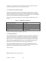
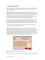
Figure 3.1. GNIRS Top Level Engineering Window
The window shown above (Figure 3.1) is the top level engineering window for GNIRS.
GNIRS Users Manual
-33-
On this window, there are four buttons and status indicators that correspond to the four
major components of the system (see the Service Manual for a complete description).
This window must not be closed, though it can be minimized. The buttons on the left
bring up additional screens, including the screens used for observation. The
State/Health/Busy indicators provide a top-level indication of the instrument status.
Normally, all indicators in the two left columns should be green; the busy indicators may
be busy. (Note: operation of the motors can induce pickup in the temperature sensors, so
it is possible for the components controller health indicator to change color while
mechanisms are operating. If it does, do not be concerned unless it does not change back
to green within 2-3 minutes.)
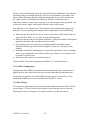
3.2.1 Instrument Configuration
The opto-mechanical configuration of the instrument can be controlled from a single
Mechanism Control screen (Figure 3.2). This is opened by first opening the Instrument
Sequencer screen from the top-level screen (above), and the opening the Mechanism
Control screen from the IS screen. The IS screen can then be closed.
Figure 3.2. Mechanism Control screen. This provides control for all mechanisms.
GNIRS Users Manual
-34-
The user selects mechanism positions for each of the discrete mechanisms. The grating is
positioned using a wavelength and order. The focus is positioned by step number. One
enters all desired changes into the configuration displayed on the screen, and then uses
the "apply" button to reconfigure the instrument. If another configuration or an
observation with the science array is in progress, an error message will be generated. You
will need to use the "apply" button again when the current activity stops.
Note that there is no "common sense" filter applied to the configurations requested. In
particular, if you are making major changes in the configuration, check the following:
• Make sure that only one filter is in use - that is, if you select a filter in Filter Wheel 2,
•
•
•
•
make sure Filter Wheel 1 is on "open" (except for diagnostics).
Make sure that the camera corresponds to the filter - going from xJHK to LM requires
going from the blue to the red cameras (and vice versa).
If you change pixel scale, make sure you change both the slit and the camera.
Remember also that spectral resolution changes by a factor of 3 when pixel scale
changes.
Remember also that the mechanisms are not perfectly repeatable, so once you change
from a given configuration you will not be able to go back to it exactly (but you will
be within 10 pixels or less)
Don’t forget the window cover needs to be open!
Consult section 2 for useful configurations (Tables 2-8 - 2-10 and elsewhere).
3.2.2. OIWFS Configuration
Configuration of the OIWFS is normally done through the telescope's acquisition and
guiding system, and is done by the telescope operator rather than the instrument user.
It is possible, if needed, to access the OIWFS from the top-level screen (Fig. 3.1) by
opening the OIWFS top-level screen and then the OIWFS CC screen.
3.2.3 Data Taking
Two screens are required to set up the array controller and take an observation. The first
screen (Figure 3.3) is the GNAAC main control screen; from that you can access the
Observing Set-Up screen (Figure 3.4), which is used to set up the observation.
GNIRS Users Manual
-35-
Figure 3.3. Array control screen. Used to start an observation and control some
parameters.
Figure 3.4. Observing Set-Up. Used to set up array control parameters.
GNIRS Users Manual
-36-
The observing set-up screen provides more functionality than is normally needed for
observations. Don't alter parameters that are best left alone. The following items (mainly
on the left side of the screen) are relevant:
• Activation. This starts up defaulting to inactive, so you must activate manually when
•
•
•
•
starting up the instrument. Once the detector is activated you can leave this alone.
Integration time. This should be set as needed.
Digital averages and low noise reads. Digital averages should be set to 16 except for
L and M band acquisition (set to 1 in these cases). Low noise reads should be set to 1
for exposures under ~1 minute, and to 64 for exposures >5 minutes. For exposure
times between these values, consult the ITC.
Co-adds. This is the number of frames to be added together. Co-addition is useful if
you have many short exposures, since you save on time writing to the DHS and the
number of images you have to manipulate is less. However, if any one frame is bad,
the co-added image will be bad, so co-addition is not recommended if you are taking
longer exposures.
Number of images. This is the number of separate images to be taken. Note that if
you are also co-adding, the number of exposures is the product of the number of coadds and the number of images.
The only other parameter that may need to be changed is the array bias, which is changes
from the array set up screen (not shown), which is also accessed from the main screen.
Use bias of 0.3V for low background and bias of 0.6V for high background. The low bias
has fewer “hot” pixels but less well depth. Do not change any other voltage on this
screen!
In order to start an exposure, one needs to use the main window, shown above in Figure
3.3. The observe button the top level sequencer screen (not shown) has the same function.
This window has only one function in routine use, which is starting an exposure or
exposure sequence. Note that with the appropriate configuration (see above) it may
produce several images that are sent to the DHS. It is possible to change the exposure
time from this window as well as the observing set-up window.
If one is doing a raster pattern of some sort, for example multiple positions along the slit,
the observing sequence would consist of configuring the instrument and the array
controller, positioning the object to the first location, clicking on the observe button,
waiting for the exposure(s) to finish, offseting the telescope and OIWFS, clicking on the
observe button, and so on. Normally this is done automatically through the sequence
executor, and the screen shown above will not be used.
GNIRS Users Manual
-37-
3.3 User Interface
The user interface, to be provided by Gemini, will provide a more complete interface to
the instrument and relevant telescope systems. It provides the capability to program a
series of rastered ("dithered") observations of a single object, including OIWFS control.
It will also be possible to program a sequence of observing configurations - for example a
sequences of dithered observations with multiple filters.
The interface, despite these added capabilities, will not involve a profusion of windows
or "don't change these" parameters.
This section will contain a complete description of the interface once it is available (or in
test).
GNIRS Users Manual
-38-
3.4 Calibrations
Several types of calibration frames must be obtained for proper data reduction. These fall
into four categories:
•
•
•
•
Darks and flats
Wavelength calibration
Standard stars
Polarization calibration
3.4.1 Darks and Flats
Dark and flat-field frames are required to remove the detector signature. Dark frames are
produced by putting "dark" filter in Filter Wheel 1 in position and taking appropriate
exposures. In general, it is a good idea to take dark frames that match the regular data
frames in terms of bias, exposure time and numbers of digital samples and low noise
reads. Some interpolation on the times is permissible, but in general you will get better
results carrying out your program with a limited number of different integration times.
Flat fields are produced using the on-telescope calibration unit (GCAL). The flat field
produced by this unit is flat to 1% [TBD] over the longest slit used in GNIRS, which is
adequate for nearly all programs. For more accurate calibration of the long slit, the best
alternative is building up a flat using twilight sky exposures (or daytime if the
background is not too high). The sky flat should be viewed as a supplement to the GCAL
flats and will not be needed for most programs.
For exposures done using GCAL, a flat field determination requires measurements with
the light source "on" and "off", which are differenced. For details of the operation of
GCAL, consult the relevant manual [REFERENCE].
The flat field is relatively independent of wavelength, so a separate flat field for each
wavelength setting is not a necessity if there are many similar settings. It is preferable,
though, to have a flat field associated with each setting. This is especially important in
the low resolution and prism modes, where a given configuration will not produce signal
on the entire array. This means that portions of the image will need to be masked off to
produce a reasonable flat field, which will not necessarily be useful for another
configuration.
It is convenient to divide each flat field by an average value to normalize the corrections.
Darks and flat fields should be produced using the average (or median) of a large number
of frames, typically 20-50 for each dark time or flat field configuration.
GNIRS Users Manual
-39-
3.4.2 Wavelength Calibration
The easiest way to determine the wavelength calibration is to use the night sky lines,
which are present in every spectrum taken with the instrument. Suitable lines are
identified in the spectra in Appendix B.
GCAL also provides arc lamp spectra, which can be observed to determine wavelength
settings during the day (or when the dome is closed by weather). The GCAL lamps can
be useful for diagnostic purposes or for verifying exact wavelength coverage, but are
otherwise not needed. Consult the GCAL manual for operation of the arc lamps. It is not
absolutely necessary to subtract darks or flat-field these GCAL frames.
3.4.3 Standard Stars
Selection of standard stars is discussed above (section 3.1.3). Standard star observations
are generally fairly short, so it is [probably] possibly to carry out the observations without
setting up the OIWFS, which can save a certain amount of time. It is still advisable to
measure the star at several slit positions. This is especially true for telluric standards used
with the long slits, where one should really measure at each position on the slit that is
used for objects.
If a large number of positions are involved, or the exposures are longer than a few
seconds, it is probably advisable to take the trouble to use the OIWFS rather than letting
the star drift off the slit.
3.4.4 Polarization
[The issue here is that one would like to calibrate the relative instrument response in both
polarization, yet it is not clear that there is an appropriate unpolarized flat field to be used
for this purpose. It may be that the only solution is to rely on standard stars as
unpolarized light sources and accept the fact that the flat field normalization in the two
polarizations may be somewhat different.]
GNIRS Users Manual
-40-
3.5 Preliminary Data Reduction
The following steps are recommended to carry out preliminary data reduction. They may
in fact suffice for final data reduction as well, but don't delete raw data until you have had
the chance to assess the reduced data calmly.
•
•
•
•
•
•
•
•
Linearity correction
Dark subtraction
Flat fielding
Sky reference generation
Sky reference subtraction
Spectrum extraction
Absorption standard division (optional)
Flux calibration (optional)
The first three steps remove the detector signature; the second two steps remove the night
sky (and telescope) emission, while the final steps produce a spectrum with the
instrumental signature removed.
3.5.1 Linearity Correction, Dark Subtraction and Flat-Fielding
These procedures are essentially automatic if there are always matching dark frames and
flat fields.
The linearity correction is optional if all count levels are low (below 10,000 [TBD]
ADU). If used, the recommended coefficients for the IRAF procedure irlincor are a=
1.0, b=xxx, c=yyy (TBD - actually will need separate values for each bias value). See the
IRAF documentation for an explanation of these coefficients; also confirm that you are
using the most current values for the coefficients.
To remove dark and flat field, subtract the equivalent dark frame and then divide by the
appropriate flat field. Bad pixels or unexposed areas should be masked off in the
operation. If no exact match exists for the dark frame, either interpolate using exposure
times that are close, or use the closest dark frame.
If unmasked bad pixels are noisy in the flat-fielded frames, it is desirable to limit their
maximum and minimum values to reasonable numbers - this ensures that IRAF's
statistical processes are more reliable.
3.5.2 Sky Reference Generation and Subtraction
The details of the sky reference generation depend on the observing procedure. If the
object was measured at many slit positions, the sky reference can be generated by
calculating the scaled median of all images. If a simply "on/off" or "A/B" procedure was
GNIRS Users Manual
-41-
used, then the sky reference is the "off" image (or the mean of the adjacent "off" images).
For a modest number of positions, one can construct a reference for each position by
determining the average of all the other positions. This is the preferred procedure.
The reference should be scaled to the object position flux values and subtracted.
3.5.3 Extraction
If multiple positions on the slit were observed, it is generally preferable to extract
individual spectra, which can then be wavelength calibrated and added. For faint objects,
one can add images taken at the same slit position, then do the extraction.
Note that distortions and tilts require one to determine an extraction profile, even in long
slit mode where the spectrum runs approximately along the rows of the array.
3.5.4 Standard Stars
The summed, extracted spectra in many cases provide enough information to see whether
the observation is successful. Even if this is true, it is still often useful to remove the
atmospheric and instrumental signatures.
The following steps will produce an approximate calibration, but not an optimal one:
• Divide by a standard star extracted spectrum
• Multiply by an artificial curve having the nominal flux distribution of the standard.
(For most purposes this can be a blackbody fit to the standard's broadband
magnitudes.)
This procedure will remove weak atmospheric absorptions, but not strong absorptions. It
will correct for instrumental response. It will also introduce spurious emission features
wherever the standard has absorption features. The result is also uncorrected for
differential light losses at the slit.
GNIRS Users Manual
-42-
4. Set-Up and Operation
This section describes the procedures required to verify that the instrument is working,
and to get ready to observe with it. This section assumes that the instrument has been
properly installed on the telescope (see the Service and Calibration Manual for
installation procedures). The section describes a complete start-up after installation; for
daily start-up see section 4.8.
Software troubleshooting is covered in the Software Maintenance Manual.
4.1 Software Start-Up
The Engineering screens are started by typing nirsSeqStart in a terminal window.
This script is located in {GNIRSROOT}/bin/solaris. If this is not in your path,
use the whole path to invoke it.
This command will (eventually) bring up the top-level instrument screen, as well as a
small screen labeled DM2.4. Both screens must not be closed, although they can be
minimized.
From the top-level screen you can bring up the following additional screens (see 3.2):
• Mechanism control screen (brought up from instrument sequencer screen, which can
then be closed)
• GNAAC top-level screen ("overall control")
• GNAAC observing control screen
No other screens are required for routine observing. Screens required for diagnostic
purposes are described in the Service and Calibration Manual; these are generally
accessed through the components controller main screen (accessed from the top-level
screen).
4.2 Initialize Spectrograph Mechanisms
The mechanisms can be datumed ("home" position is located) using the global datum
command on the CC screen. This will take a couple of minutes to execute, depending on
where the mechanisms happen to be.
At the completion of the datum, all mechanisms will be left near (but not quite at) the
zero-step position. You should then position all the mechanisms to the initial
configuration that you want. Important: The prism turret in the zero position will
partially vignette the beam. Therefore, even if your initial configuration is with the
acquisition mirror, you should position the prism turret to one of its four positions (or to
"park").
GNIRS Users Manual
-43-
4.3 Initialize Detector
The detector is initialized from the GNAAC Engineering Interface. Individual detector
parameters may need to be adjusted from subsidiary screens (see 3.2.3). The most useful
parameters to adjust are the number of digital averages, low noise reads, and number of
co-adds and images. The region of interest (area to be read out) can also be modified, as
well as other array-control parameters. The bias is changed when one switches between
low background (small full well, low noise) and high background (large full well, higher
noise).
In general, it is advisable to leave most parameters unchanged, as this greatly simplifies
subsequent data management and data reduction.
The array is initialized using the three buttons on the lower right of the GNAAC interface
screen.
4.4 Initialize OIWFS
The OIWFS is started as part of the instrument start-up procedure described above. Any
further initialization (e.g., datuming mechanisms) is done by the A&G system. These
procedures are fairly slow (~15 minutes) so make sure they are carried out promptly. You
can initialize the OIWFS, if necessary, from its own engineering screen (accessed from
the top-level screen)
4.5 Sensor Checks
The health of the temperature and pressure sensor values is indicated on the top-level CC
screen. If both health indicators are green, then all values are within range, and there is no
need to check further. If the health indicators are yellow (warning) or red (bad), one or
more readings is out of range. Open the relevant sensor screen and examine the faulty
value or values. Consult the Service and Calibration Manual for details on the individual
sensor values.
If the health is yellow due to a single, slightly out of range sensor, it may be reasonable to
continue observing. However, in this case one should check the relevant screen
periodically to confirm that the situation has not gotten worse.
4.6 Configuration Checks
This section describes simple functionality checks that can be carried out without need to
access the low-level code. Additional checks are described in the service and calibration
manual.
GNIRS Users Manual
-44-
4.6.1 Basic Configurations
The instrument's ability to correctly configure can be checked by setting up a few
configurations, taking an image, and comparing the results with expectations.
For these tests, GNIRS should be looking at GCAL with the arc lamp (Ar) on. Exposure
times of 1 second [TBD] are sufficient. Make sure the window cover is open! Try the
following:
• Configure in acquisition mode (mirror in, acquisition slit and decker) with the H
(sorter 4) filter. Use the short blue camera. The acquisition field should be roughly
centered on the array, and the field should not be vignetted.
• Configure with any grating and any of sorters 3-6, a blue camera, and the short
camera long-slit decker. Use a moderately narrow slit (180 microns). Specify a
wavelength corresponding to one of the figures in Appendix B, and verify that the
wavelengths are about the same (to within 20 pixels) as in the Appendix, and that the
slit is centered on the array to within 20 pixels. Confirm that the FWHM of the lines
is 2.2 pixels or less. Note: at low resolution, some lines are blends; check the labeling
in Appendix B to avoid these.
• Configure to a cross-dispersed mode. Verify that orders 3-7 fall on the array, and that
the lines remain narrow (FWHM ~2 pixels for short camera, closer to 3 pixels for
long camera).
4.6.2 Repeatability
The repeatability test is fairly simple: set up a configuration like one of the ones listed
above, take an exposure, move one or more mechanisms out of position and then back,
and then take another exposure.
The apparent position of spectral lines in both directions should move by less than 10
pixels when the prisms, gratings, and cameras are moved, and by less than 1 pixel when
the filter, slit, decker, and focus are moved. These effects are at least 3 times larger with
the long cameras than with the short cameras, so the tests are best done with a long
camera configuration.
4.6.3 Background and Throughput
The instrument internal background should be measured in two configurations:
• Filter wheel 1 in "dark" position, filter 2 in sorter 1 position, 180 micron slit, short
camera long decker, short red camera, prism turret in mirror position, 110 line
grating set to 5.0 µm (1st order). Use an exposure time of 300 seconds. The observed
count levels (includes dark) should correspond to ~0.1 electrons/sec/pixel. (Gain is
13 e/ADU, don’t forget to divide by number of low noise reads.)
GNIRS Users Manual
-45-
• Same as above, except that grating is now set to 2.2 µm (3rd order), filter wheel 2 in
sorter 3 position, and short blue camera is used. The observed count should still
correspond to ~0.1 electrons/second/pixel.
• Optionally, the same configuration can be repeated with the short camera crossdisperser in place instead of the mirror; the measured counts should be the same.
In general, the best measurements of system throughput are done on the sky. However, an
initial check can be done with GCAL and the continuum flat field source. For the second
configuration above, the count level at the center of the array should be approximately
[TBD] ADU/sec. [Needs more detail]. The measured value should be within 10% [TBD]
of this. Note: this assumes that the GCAL configuration is fairly stable.
4.6.4 Detector Noise
In conjunction with the background tests, one can also look at the detector noise
performance. This is best determined using multiple frames; use IRAF imcombine. The
noise should be measured using minimum Fowler sampling (16 digital average and 1
low-noise read) and maximum sampling (16 digital averages and 64 low-noise reads).
Use a bias of 0.3V. The respective median noise values measured should be ~40 and ~7
electrons in the sigma images.
It is also useful to visually inspect the difference frames for evidence of noise pick-up,
which would appear in the form of patterns superposed on the random noise. Some pickup will probably be present in the minimally-sampled frames, but it should be averaged
out fairly well with multiple samples.
4.7. Night-Time Tests
The following tests should be carried out at the start of the night. The weather does not
need to be photometric.
• Pupil viewing test. Configure for pupil viewing through the K (sorter 3) filter and
acquisition mirror. Use the long blue camera for best results. Verify that the telescope
secondary is centered on the internal cold stop. The images (Fig 4.1) below show a
properly centered and somewhat decentered image. Decentering at the 1% level is not
critical.
Figure 4.1. Pupil viewing images of secondary well-centered on cold stop (left) and
slightly decentered (right).
GNIRS Users Manual
-46-
• Background test. Go to the configuration with the 32 l/mm grating, short blue camera,
and long slit mode, with a 2-pixel slit and sorter 3. Set the grating to 2.2 µm and
compare the results of a 60 second exposure with the relevant figure from Appendix
B. Compare both the overall intensity of the night sky emission lines and the
continuum level at the long wavelength end of the spectrum. Both levels may differ
significantly from what is shown in the figure. If the test is done at the start of the
night, the night sky emission levels will tend to be higher than the reference values,
possibly by a factor of 2. The thermal continuum is affected by ambient temperature,
and will be higher if the telescope temperature is higher than the value at the time the
data in Appendix B were taken (see the figures).
• Throughput test. Observe a standard star with a wide slit in any of the configurations
documented in Appendix B (ideally, one you are intending to use that night). A
simple extraction will produce values within 20% of those you would get with a
complete preliminary reduction (section 3.5); this provides a quick check of
performance. Outside of regions of atmospheric absorption, the variations in
measured counts should be no more than 10%.
4.8 Nightly Start-Up
Normally, the nightly start-up only needs to reverse the steps from the previous night's
shut-down (section 4.9):
• If the EPICS screens have been closed, restart by typing nirsSeqStart in a
terminal window. (See 4.1 above).
• Check the top-level screen to make sure temperature and pressure health are still good
(4.5).
• Re-initialize the detector, including activation (4.3).
• It is a good idea, but not necessary, to re-datum the mechanisms (4.2,4.4). If you are
doing afternoon calibrations, do the datum before calibrating.
4.9. Shut-Down
This section outlines the steps required to prepare the instrument for removal from the
telescope. This includes all steps up to, but not including, powering down electronics.
This is not required except at the end of the run.
4.9.1 Mechanism Positioning
The mechanisms should all be positioned to their "park" positions.
4.9.2 Detector Shut-Down
The detector should be de-activated from the observing control screen. Don't forget to use
the "set" button to implement the deactivation.
GNIRS Users Manual
-47-
4.10 Nightly Shut-Down
It is only necessary to de-activate the detector (see 4.9.2 above), and close the window
cover ("closed" or "park"). The other mechanisms can be left "as is".
GNIRS Users Manual
-48-
5. Basic Trouble-Shooting
This section is not intended to be provide comprehensive diagnostics of all possible
problems with the instrument. Instead, it provides preliminary diagnosis of the most
common problems with the instrument.
This section is expected to be revised as experience using the instrument on Gemini
accumulates.
Problems, diagnosis, and solutions:
• No signal at detector. This may be due to a number of causes:
•
•
•
•
•
− Detector not activated. Activate the detector. If it does not activate, verify that the
detector temperature is correct (low enough).
− Configuration incorrect. Did you forget to configure a mechanism (including the
window cover)? Set the configuration again, and see if mechanisms move;
observe again if they do. If all mechanisms are alleged to be in the correct
position, do a global datum and reconfigure. If this does not solve the problem, try
a configuration with the acquisition positions. Further mechanism diagnosis is
covered in the service manual.
Noise on image. This may be due to grounding problems. Also consider:
− Was the OIWFS being reconfigured during the readout? If so, try again and see if
the noise is absent when the OIWFS mechanisms are not active.
Image does not appear to be the correct configuration. Check:
− Did you make a mistake in selecting the configuration (especially grating
wavelength)?
− If one mechanism appears to be the source of the problem, try (a) repositioning it,
and if that does not work, try (b) datum and re-position. If this is not correct (and
especially if the configuration is still wrong but different) try mechanism
diagnosis procedures in the service manual.
− If the mechanism positions correctly, it may be worth checking repeatability
(move away, then back) to confirm reliability.
Images are fuzzy or otherwise bad. Configuration is otherwise correct.
− Check focus setting
− Check instrument temperature
− Was the telescope slewing or was the instrument rotator changing angle very
rapidly? If so, repeat to see if images return to normal.
Excess background observed.
− Has the instrument cooled sufficiently? The optics will not fully cool for ~12
hours after the bench itself initially reaches 60K.
− Something is in the way (dome, PWFS, etc.). Vignetting should produce excesses
only at KLM. Pupil viewing may help find the culprit if only a long wavelength
excess is seen.
Temperature health abnormal (yellow or red)
GNIRS Users Manual
-49-
− Open the temperature display screen. If only one sensor is reading abnormally, the
diode may be bad. A very low temperature (~23K) is an indication of an open
circuit. A single temperature that is slightly out of range should be monitored.
− If multiple temperature readings are out of range, check that the bench
temperature control is on (temperatures low) or that the cryocoolers are functional
(temperatures high: check operation, also check individual head temperatures for
high values).
− Check that dewar pressure is within range; poor vacuum will conduct excess heat
into the cold structure. In this case, the pressure health should also be bad
(probably red).
• Mechanisms give errors on positioning or datuming.
− If the system has been rebooted or reinitialized, you must redatum all the
mechanisms before you can configure anything.
− If the mechanism gives an error on going to a position (for example, hitting a
limit), redatum and try again.
− Note that the window cover and acquisition mirror position to limits (open/closed
and in/out), so limit messages on these two mechanism are not errors. Hard limit
(OT) messages are errors on all mechanisms, including these two.
− Note also that the rotary mechanisms (turrets and wheels) do not have mechanical
limits, so any limit message is an electrical or software problem, not a mechanism
problem.
− If the mechanism gives an error on doing a datum, try with the back up home
switch and/or do a datum test (see service manual).
GNIRS Users Manual
-50-
Appendix A – Supplementary Information for Exposure Time
Calculations
A.1 Throughput
Throughput is affected by two main factors: instrument throughput, which is a function of
configuration, and slit losses, which are a function of slit width and image quality.
Telescope and atmospheric transmission are also factors.
A.1.1 Slit Losses
Slit losses are calculated assuming a gaussian image profile centered on the slit. Detailed
calculations show that a small amount of decentering does not affect throughput greatly.
The table below (A.1) gives the percentage of light transmitted through the slit for both 2pixel and 3-pixel slits, for both pixel scales, for the 20th, 50th, and 85th percentile seeing
cases listed in Table 2.11. The values listed are for the K band; there are slightly greater
losses at shorter wavelengths, and smaller losses at longer wavelengths. The highlighted
values are those used for the calculations summarized in section 2.2.1.
The sampling in the IFU corresponds to a slit width of 0.15 arcsec. One should recognize
that a spatial resolution element is effectively two samples, which should be combined in
considering overall signal to noise.
Table A.1 GNIRS Slit Transmission as a Function of Seeing
Slit width (arcsec &
pixels)
0.10" - long 2 pixels
0.15" - long 3 pixels
0.30" - short 2 pixels
0.45" - short 3 pixels
20th Percentile
(0.30 arcsec)
31%
44%
76%
92%
50th Percentile
(0.50 arcsec)
19%
28%
52%
71%
85th Percentile
(0.75 arcsec)
13%
19%
36%
52%
The signal is directly proportional to the slit transmission, so one can easily estimate
sensitivity under difference image quality conditions. The tables in section 2.2.1 for the
short cameras provide estimates for 50th percentile image quality. For 20th percentile
image quality, the ratio of slit transmission is 1.46, resulting in a sensitivity gain of ~0.4
mag. The loss in sensitivity at 85th percentile image quality is also ~0.4 mag.
In those cases where the object is much fainter than the sky in the slit, the integration
time is roughly proportional to the square of the slit transmission - hence one gains a little
over a factor of 2 going from 50th to 20th percentile image quality.
Widening the slit to increase transmission also increases background. For the case of faint
objects, going from 2 to 3 pixels increases background by 50%, while increasing signal
by a lesser amount - typically around 40%. The net gain in signal to noise is about 15%,
GNIRS Users Manual
-51-
equivalent to ~0.15 mag or to a factor of 1.3 in integration time for the same object. This
may be worthwhile if the associated loss in spectral resolution is not a concern.
The length of the slit used to actually extract the spectrum is also relevant. It is not
necessarily optimal to use a wide window and get nearly all the signal, since the
increased total background (and total dark current and read noise) may provide a larger
increase in noise. Table A.2 tabulates the percentage of transmitted flux extracted as a
function of slit window length. Thus the total signal extracted is the product of the factors
in this table and the preceding table. For example, a 4 pixel window and a 2 pixel slit
with the short cameras and 50th percentile image quality will extract 44% of the flux
incident on the slit (52% x 84%). Note that still better results can be obtained by means of
optimal extraction using the actual light profile along the slit – but the values in Table
2.11 will be close to those results.
For reference, the relative amount of noise from background (including dark and read
noise) is also indicated (it's simply proportional to the square root of the window size).
Table A.2 - Flux Extracted vs. Slit Window Size
Slit Window
Length
(arcsec)
0.30
0.45
0.60
0.75
0.90
20th Percentile
(0.30 arcsec)
50th Percentile
(0.50 arcsec)
85th Percentile
(0.75 arcsec)
76%
92%
98%
100%
100%
52%
72%
84%
92%
96%
36%
52%
64%
76%
84%
Relative
Background
Noise
0.71
0.87
1.00
1.12
1.22
The optimum window for a given image quality is highlighted in yellow. If performance
is within 2%, multiple values are highlighted. Generally, a window slightly larger than
the image FWHM is optimum. Note that the window to be used can be determined after
data are taken.
Sampling along the slit with the IFU is slightly different than the short camera - about
0.12 arcsec/pixel - so a window of 0.6 arcsec corresponds to 5 pixels rather than 4. Since
the purpose of IFU observations is spatial reconstruction, the observer will probably
extract spectra row by row rather than defining a wider window.
A.1.2 Telescope and Atmosphere
The remaining contributors to throughput are the instrument itself, the telescope, and the
atmosphere. The estimated transmission of the telescope and the atmosphere are tabulated
below, in Table A.3. The atmospheric transmission values are for regions free of strong
absorption lines. GNIRS is assumed to be on a side port, so the ISS fold mirror is
included, as well as the obscuration by the secondary mirror. Telescope reflections are
GNIRS Users Manual
-52-
assumed to be clean aluminum. Values are tabulated for the 6 orders for which the
instrument currently has blocking filters.
Table A.3 - Atmospheric and Telescope Throughput
Grating Order
1 ("M")
2 ("L")
3 ("K")
4 ("H")
5 ("J")
6 ("x")
Atmospheric Transmission
80%
90%
93%
93%
90%
90%
Telescope Transmission
93%
93%
92%
91%
88%
84%
A.1.3 Instrument Throughput
The instrument throughput is calculated, using (for the most part) measured transmissions
or reflections for the optical components, including gratings and filters. The grating
efficiency varies across the band somewhat, so an average value is given for the
wavelength region defined by the order sorting filters. The detector quantum efficiency is
also included.
Table A.4 - GNIRS Throughput
Calculations for Long Cameras
Grating Order
1 ("M")
2 ("L")
3 ("K")
4 ("H")
5 ("J")
6 ("x")
10 l/mm
35%
52%
45%
49%
50%
41%
Grating
32 l/mm
23%
28%
28%
29%
30%
27%
110 l/mm
36%
38%
40%
43%
41%
36%
The tabulated values are all for the long cameras (0.05 arcsec pixel scale). The calculated
values for the short cameras are all within 1% of the long camera values. The lower
values for the 32 l/mm grating are due to the reduced efficiency of this ruling.
The integral field unit is expected to have about 80% throughput. Sensitivity for an object
observed in a single slice will be 0.1-0.2 mag brighter, compared with the same slit width
(0.15 arcsec), depending on whether the primary noise source is background or read noise
and dark current.
The reflection losses in the prisms are 10% or less; in addition the SF57 glass in the
cross-dispersion prisms absorbs significantly in the K window. The absorption averages
about 80% between 2.0 and 2.4 µm.
GNIRS Users Manual
-53-
A.2 External Background
There are two main contributors to the external background: sky background and
emission from the telescope itself (including warm parts of the instrument).
A.2.1 Average Background
The sky background includes airglow, which is dominant at shorter wavelengths; thermal
emission from absorbers at lower altitude, which is important at wavelengths beyond
about 2.4 µm, and some amount of continuum.
The telescope emission is essentially a gray body, proportional to the effective telescope
emissivity, which is typically <10%. (For a well-baffled instrument, such as GNIRS, it is
close to 1 minus the telescope transmission given in Table A.3.)
As noted in 2.2.1.3, the structure in the night sky emission means that one needs to use
caution in applying average flux values to exposure time estimates. In the absence of
detailed night sky spectra taken with GNIRS, the following procedures have been
applied:
• Start with broad band sky brightness estimates
• Compare with model night sky emission spectra (taken in this case from the Gemini
web site)
• Apply corrections for non-standard filter pass band and for flux distribution with
wavelength
This allows one to estimate both an average flux value per resolution element, as well as
flux levels at various percentiles in the distribution. It turns out that the average values
correspond roughly to the 75th percentile for the different windows (i.e. 75% of the
resolution elements in the window have sky fluxes less than or equal to the average). In
addition, the flux values corresponding to 90th percentile are typically 2-3 times the
average. For the calculations presented above (2.2.1), a uniform factor of 2.3 has been
applied.
Table A.5 summarizes the sky background values applied. Note that the fluxes do not
include the corrections applied for atmospheric absorption or telescope and instrument
throughput. The values tabulated are for R=1700; values at other resolutions are inversely
proportional to the resolution.
GNIRS Users Manual
-54-
Table A.5 - Mean Model Night Sky Emission
Resolution 1700
Grating Order
1 ("M")
2 ("L")
3 ("K")
4 ("H")
5 ("J")
6 ("x")
Background
(mag/arcsec2)
-0.2
5.4
13.2
14.1
16.35
16.6
Background
(photons/sec/arcsec2/resolution element)
91,300,000
890,000
1560
1100
206
215
A.2.2 Variability
The background will vary for several reasons.
The telescope background will change with telescope temperature; emission at 2.4 µm
will change by a factor of 3 or so over a 20-degree (C) temperature variation, which is
more or less characteristic of seasonal extremes. The thermal emission component of the
atmospheric emission will also change by similar amounts. In general, variations of any
thermal emission components of the background are slow, typically on scales longer than
reasonable integrations.
The airglow component can vary by a factor of 2-3. There is a tendency for emission to
be higher at the start of the night and then slowly decrease, but in addition there are
variations on a variety of time scales, some of which can be quite short. Because of this,
one should be cautious about planning observations with very long individual exposures,
since systematic errors in the sky subtraction may result. A good rule of thumb for
GNIRS (until experience with the site and instrument indicates otherwise) is to limit
individual exposures to 15 minutes.
GNIRS Users Manual
-55-
Appendix B - Representative Calibration and Night Sky
Spectra
[many lovely spectra appear here....]
GNIRS Users Manual
-56-