Download Agilent 3395 Integrator

Agilent 3395
Integrator
Operating Manual
Agilent Technologies
Manuals 3395_3396 Integrator.qxd
10/6/2003
9:59 AM
Page 1
Agilent 3395/3396
Integrators
Manuals
These manuals may contain references to HP or Hewlett-Packard.
Please note that Hewlett-Packard’s former test and measurement,
semiconductor products and chemicals analysis businesses are
now part of Agilent Technologies. The HP 3395/3396 Integrator
referred to throughout this document is now the Agilent
3395/3396 Integrator.
HP 3395 Integrator
Operating Manual
Manual Part No.
03395-90520
Edition 2, August 1997
Printed in U.S.A.
Printing History
The information contained in this document may be revised without noĆ
tice.
HewlettĆPackard makes no warranty of any kind with regard to this mateĆ
rial, including but not limited to, the implied warranties of merchantability
and fitness for a particular purpose. HewlettĆPackard shall not be liable for
errors contained herein or for incidental or consequential damages in conĆ
nection with the furnishing, performance, or use of this material.
No part of this document may be photocopied or reproduced, or transĆlated
to another program language without the prior written consent of
HewlettĆPackard Company.
Second editionĊAugust 1997
First editionĊJanuary 1995
Printed In USA
E Copyright 1992Ć1997 by HewlettĆPackard Company
All Rights Reserved
Safety Information
The HP 3395 Integrator meets the following IEC (International ElectroĆ
technical Commission) classifications: Safety Class 1, Transient OvervolĆ
tage Category II, and Pollution Degree 2.
This unit has been designed and tested in accordance with recognized safeĆ
ty standards and designed for use indoors. If the instrument is used in a
manner not specified by the manufacturer, the protection provided by the
instrument may be impaired.
Whenever the safety protection of the HP 3395 Integrator has been comĆ
promised, disconnect the unit from all power sources and secure the unit
against unintended operation.
!
The manual reference sign is marked on the product when it is
necessary for the user to refer to the instruction manual. If the
procedure or practice described in the manual is not followed, loss of
data or damage to the instrument could result.
A WARNING CALLS ATTENTION TO A CONDITION OR POSSIBLE
SITUATION THAT COULD CAUSE YOU OR OTHERS INJURY.
A Caution calls attention to a condition or possible situation that
could damage or destroy the product or your work.
Important User Information for
In Vitro Diagnostic Applications
This is a multipurpose product that may be used for qualitative or quantiĆ
tative analyses in many applications. If used in conjunction with proven
procedures (methodology) by a qualified operator, one of these applications
may be In Vitro Diagnostic Procedures.
General instrument performance characteristics and instructions are inĆ
cluded in this manual. Specific In Vitro Diagnostic procedures and methĆ
odology remain the choice and the responsibility of the user and are not
included.
Manual Addendum
This manual addendum addresses changes to sequence operation in reĆ
mote start/stop (RSS) configurations of the HP 3395 Series III integrator.
Sequence Operation in RSS Configuration
If you are an experienced HP 3395 Series II integrator user, you will notice
improvements in the sequence capabilities of the HP 3395 Series III inteĆ
grator when operating with nonĆINET samplers and a new NEXT SEĆ
QUENCE function that allows sequences to be chained within the
sequence preparation dialog. To take advantage of these improvements,
you must operate the sequence differently than with previous HP 3395
integrators.
You can still allow the sequence to be controlled completely by the autoĆ
matic liquid sampler (ALS). In this mode of operation, the HP 3395 SeĆ
ries III integrator sees the sequence as a series of manual runs. This is
how the HP 3395 Series II integrator operated. If you chose to operate in
this mode, follow the instructions in the HP 3395 Series III Integrator OpĆ
erating Manual, pages 9Ć19 to 9Ć25. The disadvantage of using the inteĆ
grator in this manner is that the new integrator features designed to allow
better management of RSS operation cannot be used. For example, the
NEXT SEQUENCE function will not be available (because you are really
doing manual runs).
The HP 3395 Series III integrator must participate in the control of an
RSS sequence to utilize the new sequencing features. To operate in this
mode, prepare the sequence by following the instructions on pages 9Ć4 to
9Ć10 in the HP 3395 Series III Integrator Operating Manual. To start the
sequence, press [SEQ][START].
Contents
Chapter 1:
Meet the HP 3395 Integrator
The keyboard and all instrument functions are introduced
here.
Chapter 2:
Getting Started
This chapter shows you how to start and stop the inteĆ
grator, how to set the date and time, how to do paper
operations, how to select run parameters and how to
time program events to happen on the integrator.
Chapter 3:
Integrating and Reintegrating Data
This chapter shows you how to start integration, select
quantitation parameters: peak width, area reject, and
threshold, and how to use integration functions and do a
reintegration.
Chapter 4:
ÉÉ
É
É
ÉÉ
É
ÉÉ
É
ÉÉ
É
É
ÉÉ
ÉÉÉ
É
ÉÉ
É
É
ÉÉÉ
ÉÉÉ
É
ÉÉÉ
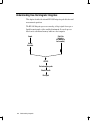
Understanding Integration
This chapter contains background information about how
the HP 3395 Integrator performs integration.
Chapter 5:
ISTD
ĄESTD
ĄĄNORM
ĄĄĄAREA %
ĄĄĄĄHEIGHT %
Chapter 6
Understanding Calibrations
This chapter covers preparing single and multilevel calĆ
ibrations and manipulating calibration files and contains
background information at the end.
Using Calibrations
This chapter explains how to use the HP 3395 to obtain
calibrated analyses.
Chapter 7:
Saving Integrator Data
This chapter tells you how to specify files for storage and
retrieval, how to format a disc, save data from a run and
other types of files, how to manipulate files on the system,
and contains background information about data storage.
Chapter 8:
Using Methods
This chapter tells you what to do before preparing a methĆ
od, how to prepare methods, manipulating method files,
and contains background information.
Chapter 9:
Automating Analyses
This chapter tells you what to do before preparing a seĆ
quence, how to prepare sequences, manipulating sequence
files, and contains background information.
Chapter 10:
Using Reports
This chapter explains how to get a default report, how to
choose report formats, manipulating reports and contains
background information at the end.
Index
1
Meet the HP 3395 Integrator
In this chapter...
H The New HP 3395 Integrator . . . . . . . . . . . . . . . . . . . . . . . . . 1Ć2
H Using the Keyboard . . . . . . . . . . . . . . . . . . . . . . . . . . . . . . . . . . 1Ć3
H Correcting Mistakes . . . . . . . . . . . . . . . . . . . . . . . . . . . . . . . . . . 1Ć5
H Using the Function Keys . . . . . . . . . . . . . . . . . . . . . . . . . . . . . 1Ć6
H Using the Multifunction Keys . . . . . . . . . . . . . . . . . . . . . . . . . 1Ć7
H Using the System Commands . . . . . . . . . . . . . . . . . . . . . . . . . 1Ć9
H Reading the Status Indicators . . . . . . . . . . . . . . . . . . . . . . . . . 1Ć10
H Using Uppercase and Lowercase . . . . . . . . . . . . . . . . . . . . . . . 1Ć11
H Using the Small Font . . . . . . . . . . . . . . . . . . . . . . . . . . . . . . . . . 1Ć12
H Cold, Warm, and Cool Starts . . . . . . . . . . . . . . . . . . . . . . . . . . 1Ć14
Meet the HP 3395 Integrator
1Ć1
The New HP 3395
The HP 3395 Integrator has important improvements in sequence
capabilities. If you are an experienced HP integrator user, be sure to read
Chapter 9, Automating Analyses, before using your new integrator.
Operation with automatic liquid samplers has been improved, and a new
NEXT SEQUENCE function allows sequences to be chained within the
sequence preparation dialog.
1Ć2
Meet the HP 3395 Integrator
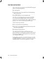
Using the Keyboard
HP 3395 Integrator
KEYBD PREP
LIST
EDIT
DEL
STORE
ZERO
LOAD
ATT 2
SEQ
CHTSP
"
METH
ARREJ
CALIB
THRSH
REPORT AREA% OP( ) COMM
READY RUN
PK WD EXT( ) INTG( )
STOP
START
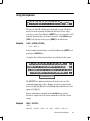
The top row of the HP 3395 Integrator keyboard is a group of dedicated
keys for the most frequently used functions. Each key has two values;
reach the second one by holding the [SHIFT] key as on a typewriter or PC
keyboard. Functional keys are shown in brackets [ ] with boldface type.
[LIST] is the first key in the top row; [PREP] is its shifted form.
Example
[LIST] [METH] [ENTER]
*
LIST: METH @
In this example the method key is reached by holding down [SHIFT] and
pressing the [AR REJ] key.
A complete list of all the functional keys is located later in this chapter.
1 !
ESC
2
@
3
#
Q
CTRL
SHIFT
4 $
W
A
E
S
Z
R
D
X
5 %
6 ^
T
F
C
7 &
Y
G
V A4
8 *
U
H
B
9 (
I
J
N
O
KA
M
_ -
0 )
P
L FF
, <
PLOT
+=
; :
. >
BKSP
TIME
' "
/ ?
ENTER
SHIFT
BREAK
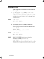
The QWERTYĆlike alphanumeric keyboard is used for the rest of the
commands and parameter values. Number or letter keys appear in this
book as [1], [2], [A], [B] and so forth. Multiple digit numbers such as 123
appear as [1] [2] [3].
System commands are typed and shown in boldface type, without
brackets. A complete list of all system commands is located later in this
chapter.
Example
HELP [ENTER]
*HELP
ANALYZE
ASSIGN
BASIC
BX
COPY
CREATE
DATE etc.
Meet the HP 3395 Integrator
1Ć3
The integrator accepts a command following a prompt. The two possible
prompts are:
*
Ready to accept system level commands.
#
Instrument is being controlled by a host computer. See the
HP PeakĆ96 Information Manager User's Guide.
Conventions
Optional parts of the commands are enclosed in { }. Values appear as
value description (in italics).
Example
Thirty seconds into the run, set the chart speed to 7.
* TIME .5
CHT SP
7
@
is entered by pressing these keys in this order:
[TIME]
runtime
on the right side of the keyboard
a numeric value, in minutes after injection
key
a function key, which is to execute at runtime
a numeric value, if key requires one
{value}
[ENTER] indicates the end of value and terminates the command
Commands execute as soon as all the needed information is entered. In
the example above, the [ENTER] key (a delimiter) is needed because
there is no other way to know when all the digits for value have been
entered.
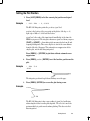
A command without parameters, however, such as [LIST] [CHT SP],
executes as soon as the second key is pressed.
Example
*
LIST: CHT SP = 1.0
A few key combinations require that the [CTRL] key be held while typing
another key. The effect is similar to the [SHIFT] key; it changes the
default value of the key in question.
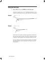
Example
1. Press [CTRL] and hold it while you press [L] to form feed the
printer paper.
Instructional steps (like the one shown in the example above) are listed in
boldface. Supporting information is always indented below the step.
1Ć4
Meet the HP 3395 Integrator
Correcting Mistakes
1.
Press [BKSP] if you notice a typing error before pressing a
delimiter key such as [ENTER].
The printer doesn't back up as a typewriter does. A block character is
printed instead, and the character to the left of the block is erased from
the integrator's memory. It's still on the paper, but gone from memory.
You also have the option to press [ESC] to cancel the entire entry and
start again.
Example
2.
Type the correct character.
3.
Press [CTRL] and hold it while you press [R] to reprint the
corrected line.
[D] [A] [T] [R] [BKSP] [E] [4] [/] [1] [4] [/] [9] [0] [CTRL-R]
shows up on the printer as
*
DATR E 4/14/95 =
DATE 4/14/95
Error Indications and What to Do
Beep
?
INVALID
SYSTEM
COMMAND
A command is ignored when entered during plotting,
integrating, or reintegrating. Either wait or end the
operation and try again. Can also happen if you type faster
than the HP 3395 Integrator can accept input.
A numeric entry is out of limits. Enter a correct value after
the ? or press [ESC] and try again.
This command doesn't exist. Usually a typing error; enter
the command again after the ? or press [ESC] and try
again.
Pressing [BREAK] will cancel the entire command and return to *
Pressing [CTRL] [BREAK] will cancel the current operation. However,
caution should be observed when using these keys because setpoints may
not always be saved.
Meet the HP 3395 Integrator
1Ć5
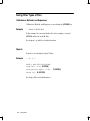
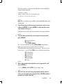
Using the Function Keys
Function
Key
AR REJ
Sets the minimum areas for peaks to be reported.
AREA%
Produces an uncalibrated report using active workspace data.
"
ATT 2
Sets the scale of the signal axis for plotting.
CALIB
Performs operations on calibrations.
CHT SP
Sets the paper advance rate for the plotter.
DEL
Deletes all or part of a calibration, method, or sequence.
EDIT
Modifies part of a calibration, method, or sequence.
INTG( )
Accesses Integration functions. See table on next page.
L FF
With CTRL key formfeeds paper to next top of form.
LIST
With other function keys, prints value of function. Alone, prints run parameters.
LOAD
Copies a calibration, method, or sequence file into the active workspace from memory.
METH
Performs operations on methods.
Accesses options dialogs. See table later in this chapter.
OP( )
See
Chapter...
3
6
2
5
2
2,5,8,9
5,8,9
3,4
2
2,3,5,8,9
5,8,9
8
1
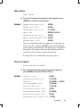
PLOT
Begins a plotting run. (No data integration takes place)
3,4
2
PREP
Starts the preparation dialog for calibrations, methods, or sequences.
5,8,9
Produces a report using data in the active workspace and specified calibration type.
10
9
2,3
2,3
Sets the expected width for peaks to optimize quantitation.
PK WD
REPORT
Performs operations on sequences.
SEQ
START
Begins an integration run.
STOP
Terminates integration or plotting.
STORE
Saves a calibration, method, or sequence.
THRSH
Sets the minimum height for peak detection.
Used with LIST and DEL to perform operations on the time table.
TIME
KA
V A4
ZERO
1Ć6
What the Key Does
With CTRL key sets form size.
Sets the position of the chromatographic baseline on the chart.
Meet the HP 3395 Integrator
5,8,9
3,4
2,9
2
2
Using the Multifunction Keys
Integration Function Key
[INTG()]
The Integration Functions alter the default actions of the integration
software. Chapter 3 discusses the use of these keys; chapter 4 provides a
detailed description of each one.
1.
Press [LIST] [INTG()] [ENTER] for a complete listing of the
integration functions.
Meet the HP 3395 Integrator
1Ć7
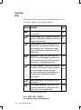
Option Keys
[OP()]
The option keys allow you to specify various method parameters, access
remote host computer, or enter sample information.
See...
Number Function
OP ( )
1
Integration Plot Type:
gram, or No Plot
Select Source, Filtered, UniĆ
OP ( )
2
Run Data Storage: Specify storage or nonstorage of
signal data, storage device, bunched or raw data, and
storage of processed peaks.
Chp 7
OP ( )
3
Calibration Options: Specify response factor for unĆ
calibrated peaks, replacement of calibration fit, retenĆ
tion time updating, internal standard peak number,
internal standard amount, sample amount, and multiĆ
plication factor.
Chp 5
OP ( )
4
Report Options: Specify local report suppression,
HEIGHT% for uncalibrated reports, replacement of reĆ
port title, replacement of amount label, reporting of unĆ
calibrated peaks, and extended report format.
Chp 10
OP ( )
5
Post-Run List Options: Specify report storage and
storage device, external postrun reporting, postrun listĆ
ings of run parameters, timetable, calibration
table, and the remote method, formfeed before and
after report printing, and perforation skipping in
reports and plots.
Chp 2
Chp 10
OP ( )
6
Remote Device Access: Send command strings to a
host computer.
*
OP ( )
7
Default Sample Information: Specify default values
for internal standard amount, sample amount, multiĆ
plication factor, name, and report memo.
Chp 9
* See page 12 in this chapter.
Press [LIST] [OP()] [ENTER]
for a complete listing of the option keys.
1Ć8
Chp 2
Meet the HP 3395 Integrator
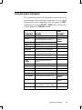
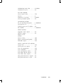
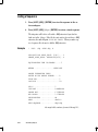
Using the System Commands
These commands are typed in on the alphanumeric keyboard; they do not
have function keys. You need only type as many characters as are required
to distinguish the desired command from others. For example, the COPY
command may be entered as CO, COP, or COPY but not as C, since this is
also the beginning of the CREATE command.
Command
Function
See
Chapter...
ANALYZE
Start reintegration of stored run data.
3
ASSIGN
Assign a BASIC program to a numeric key for
auto execution when the key is pressed.
CREATE
Create a new file.
COPY
Copy a file.
7
DATE
List or set the date.
2
DIRECTORY
List files and space on a storage device.
7
FORMAT
Prepare a disk for data transfer,
with files using the HP 3395 Integrator formats.
7
HELP
List all system commands.
1
IDENTIFIER
Enter a 12Ćcharacter identifier for a report.
10
LOCK
UNLOCK
Prevent communication from/by a host
computer.
NOTEPAD
Enter notations for the printer/plotter chart.
10
PURGE
Delete a file.
7
READY
Report on system readiness.
9
RENAME
Change the name of a file.
7
SET
Set run parameters and the run number.
9
SSET ANALOG
Sets the analog reference signal to 0 or 1.
Reference
Manual
SSET RS232
Override RSĆ232 default settings.
Reference
Manual
SYSTEM
List RSĆ232ĆC configurationsĊdevice
numbers, instruments, or devices, settings.
7
TIME
List and set the time of day.
2
Refer to
Page 12
Meet the HP 3395 Integrator
1Ć9
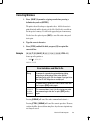
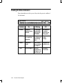
Reading the Status Indicators
Four status indicators in the top row of keys show the present condition of
the instrument.
HP 3395 Integrator
KEYBD
Indicator
1Ć10
COMM
On
KEYBD
Keyboard
command entry
allowed.
COMM
Blinking
STOP
READY RUN
START
Off
No commands
accepted; BX
active or OUT
OF PAPER.
No commands
accepted;
processing or
listing data.
Host computer
is in control of
integrator.
Integrator is
in control and
transmitting
data.
No communiĆ
cation
activity.
READY
Integrator is
ready.
AutoĆTHRSH
measurements
in progress.
Integrator not
ready for start.
RUN
Run in progress.
Postrun
operations in
progress; canĆ
not start run.
Meet the HP 3395 Integrator
Ready for
run to start.
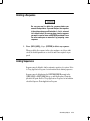
Using Uppercase and Lowercase
By default, or after a long power failure, the HP 3395 Integrator prints all
letters in uppercase (capitals). In this mode, you can press [SHIFT] to
type lowercase (small) letters. You can change the keyboard mode to
conventional typewriter style.
1.
Press [CTRL] and hold it while you press [C] to change the
keyboard mode to conventional typewriter style (lowercase
normally, [SHIFT] for uppercase).
This applies only to the letter keys. Regardless of which style is in use, all
other twoĆvalued keys give the value on the key normally and the value
above the key if [SHIFT] is used.
2.
Press [CTRL] again and hold it while you press [C] to change the
keyboard mode back to the original style.
Meet the HP 3395 Integrator
1Ć11
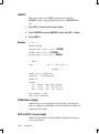
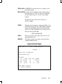
Using the Small Font
It is possible to use a smaller font than the one displayed when the
instrument is turned on. This smaller font can be specified from the
keyboard or through the option 5 dialog.
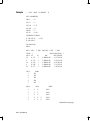
1.
Example
Press [CTRL] and hold while pressing [D] to change to the small
font.
*
REPORT
RUN#
65
OCT
5, 1994
09:01:32
SAMPLE#
7
SIGNAL FILE: M:SIGNAL.BNC
TECH PROPIONIC ACID
the report continues...
*
[CTRL –– D]
*
REPORT
RUN#
65
OCT
5, 1994
09:01:32
SAMPLE#
7
SIGNAL FILE: M:SIGNAL.BNC
TECH PROPIONIC ACID
the report continues...
2.
Example
Press [OP () ] [5] [ENTER] to specify use of the smaller font for
a method.
*
OP # 5
PRINT & POST-RUN LIST OPTIONS
Large font
3.
[Y*/N]:
Press [N] [ENTER] to specify the smaller font.
All printing associated with this method will be in the smaller font.
1Ć12
Meet the HP 3395 Integrator
Remote Device Access Example
The remote device access is used to link the HP 3395 integrator with a
host computer (i.e. using HP Peak96).
Example
1.
To obtain a directory listing from the host computer.
Press [OP( )] [6] [ENTER] to enter into the dialog mode.
The HP 3395 responds with
DEVICE ADDRESS:
2.
Press [-1] [ENTER] to identify that you wish to access a host computer.
This address is the only allowable address for a host computer.
The HP 3395 will prompt for a command string with
COMMAND STRING:
3.
Type DIR.
The command string entered at this point depends on the instrument
receiving the command and your purpose. DIR is a frequently used
command for most systems.
System Commands Examples
Two commonly used commands are Assign and Create.
ASSIGN keynumber,filespec.BAS
ASSIGN
AS
Example
ASSIGN 1,E:USER_INT.BAS
CREATE
CR
Example
CREATE TEMP.DAT,2048
CREATE filespec,size
Meet the HP 3395 Integrator
1Ć13
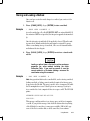
Cold, Warm and Cool Starts
There are three types of powerĆup states for the HP 3396C. The integrator
makes a cold start powerĆup whenever:
H it is first turned on;
H a power failure occurs for longer than the life of the backĆup battery,
which is about 95 hours.
H the [CNTRL] [DEL] keys are pressed simultaneously.
On a cold start, all of the data in the integrator memory (the M: disk)
is lost, any program in the BASIC workspace is deleted, and all run
parameters are set to their default values. After a cold start, the integrator
performs a series of self tests and then brings the INET loop up.
A warm start powerĆup occurs when:
H there is a power failure shorter than 95 hours;
H the electrical cord is unplugged from the wall outlet or the back of the
HP 3396, then plugged back in;
H the integrator is turned off, then on.
On a warm start, the files in memory, and all run parameters are
preserved. Any dialog or chromatographic run in progress will be aborted.
The integrator prints a message indicating that there was a power failure
before bringing the INET loop up.
An intermediate cool start state occurs when the integrator is reset with
the [CNTRL] [BREAK] keys. In this state, any program that is present in
the BASIC workspace is lost, but all other parameters are retained.
1Ć14
Meet the HP 3395 Integrator
2
Getting Started
In this chapter....
H Setting Date and Time . . . . . . . . . . . . . . . . . . . . . . . . . . . . . . . 2Ć2
H Starting the Plot or Integration . . . . . . . . . . . . . . . . . . . . . . . 2Ć3
H Printing Run Time . . . . . . . . . . . . . . . . . . . . . . . . . . . . . . . . . . . 2Ć4
H Selecting Integration Plot Type . . . . . . . . . . . . . . . . . . . . . . . 2Ć5
H Selecting the Plot Quality . . . . . . . . . . . . . . . . . . . . . . . . . . . . . 2Ć6
H Setting the Plot Position . . . . . . . . . . . . . . . . . . . . . . . . . . . . . . 2Ć7
H Setting the Chart Scale . . . . . . . . . . . . . . . . . . . . . . . . . . . . . . . 2Ć8
H Setting the Chart Speed . . . . . . . . . . . . . . . . . . . . . . . . . . . . . . 2Ć9
H Setting Form Size and Top of Form . . . . . . . . . . . . . . . . . . . . 2Ć10
H Advancing the Paper . . . . . . . . . . . . . . . . . . . . . . . . . . . . . . . . . 2Ć11
H Setting Form Feed and Perforation Skipping Options . . . . 2Ć12
H Understanding Time Programming . . . . . . . . . . . . . . . . . . . . 2Ć13
Getting Started
2Ć1
Setting Date and Time
The HP 3395 Integrator has a calendar and a clock to date reports and
time stamp" files.
1.
Type [D] [A] [T] [E] mm/dd/yy [ENTER] to set the calendar.
mm/dd/yy is the month (mm = 01 to 12), the day (dd = 01 to 31), and the
last 2 digits of the year (yy). The slash (/), colon (:), and comma (,) are all
acceptable separators.
Example
* DATE 3/28/95
MAR 28, 1995
2.
00:00:20
Type [T] [I] [M] [E] hh:mm:ss [ENTER] to set the clock.
hh:mm:ss is the hour (hh = 00 to 23), minute (mm = 00 to 59), and secĆ
onds (ss = 00 to 59).
NOTE: The [TIME] key is not used to set the clock.
Example
* TIME 08:35:30
MAR 28, 1995
Example
08:35:30
[D] [A] [T] [E] [ENTER] prints the current date and time.
[T] [I] [M] [E]
[ENTER] prints the time only.
DATE and TIME can be abbreviated as DA and T respectively, since these
are enough letters to distinguish them from all other system commands.
2Ć2
Getting Started
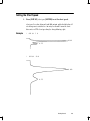
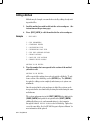
Starting the Plot or Integration
The HP 3395 Integrator operates as a simple signal plotter or as an inteĆ
grator with a builtĆin plotter.
1.
Type [R] [E] [A] [D] [Y] [ENTER] to check system readiness.
2.
Select integration plot type and chart control parameters or use
default settings.
Instructions for setting these parameters are located later in this chapter.
3.
Press [PLOT] to plot the current signal.
In the plotĆonly mode, the integrator plots the signal but does not perform
peak integration, calculation, or reporting. Such plots lack the printed
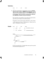
retention times and event markers that appear during an integration run.
Example
* PLOT
STOP
[PLOT] does not send a start signal to a GC or LC.
3.
Example
Press [START] to begin an integration (with plotting) run.
* RUN #
1
MAR
28, 1995
13:46:51
START
0.082
0.173
STOP
4.
Press [STOP] to end the run when peaks of interest have
appeared on the plot.
An integration run can also be ended with a timeĆprogrammed STOP.
See chapter 3 and Understanding Time Programming" at the end of this
chapter for related information.
Getting Started
2Ć3
Printing Run Time
1.
Example
Press the [TIME] key during a run to print the current run time
on the plot.
START
0.092
:1.110
current run time
2Ć4
Getting Started
Selecting Integration Plot Type
The plot type applies only to integrated or reintegrated runs.
1.
Example
Press [OP()] [1] [ENTER] to select the plot type.
INTEGRATION PLOT TYPE
(Source/Filtered/Unigram/No Plot)
ENTER PLOT TYPE [S/F*/U/N]:
An * marks the current selection. F* (filtered) is the default plot forĆ
mat. Descriptions of plot choices are listed below.
2.
Press [ENTER] for a filtered plot. For another plot choice, type
the appropriate letter, then press [ENTER].
Source Plot
Plots the data being received by the instrument, whether analog or from
disk. There is no noise suppression, filtering, or other signal cleanup."
Tick marks (start and stop of peak, for example) are not printed.
Filtered Plot
Default format that displays the data as seen by the integration software
after noise suppression and filtering have occurred. Retention times are
printed. Turning on Integration function 8 provides tick mark annotation.
See chapter 6 for a description of tick marks.
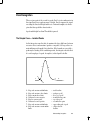
Unigram Plot
Alters both the time and height axes of the plot. The effect spreads peaks
evenly over a nonlinear time axis and makes peak heights on the plot proĆ
portional to peak areas. A unigram plot is useful in selecting values for the
PK WD integration parameter. See Optimizing Peak Recognition" in
chapter 4 for related information on unigrams.
No Plot
No plot appears on the integrator. A report will still be printed at the end
of the run.
Getting Started
2Ć5
Selecting the Plot Quality
You may choose between two plot qualitiesĊdraft and presentation. The
presentation plot is smoother than the draft plot and lags the realĆtime
run. The HP 3395 Integrator uses the draft plot unless the presentation
plot is specified.
1.
Press [OP()] [1] [ENTER].
2.
Select the appropriate plot type or press [ENTER] to keep the
current plot type.
Example
INTEGRATION PLOT TYPE
(Source/Filtered/Unigram/No Plot)
ENTER PLOT TYPE [S/F*/U/N]: [ENTER]
Presentation plot [Y/N*]:
3.
Press [Y] [ENTER] for improved plot quality.
This example selects the presentation plot for the currently active method
and will affect all plotting associated with this method. The presentation
plot can also be selected in the [PREP] or [EDIT] [METH] dialog.
2Ć6
Getting Started
Setting the Plot Position
1. Press [LIST] [ZERO] to list the current plot position and signal
level.
Example
*
LIST: ZERO
=
0, 0.0820
The HP 3395 Integrator prints the position, signal level.
position is the location of the zero point on the plotter (left edge = -6;
right edge = 100) or % of full scale deflection.
signal level is the value of the input signal (in millivolts) at the time the
ZERO key is pressed. The integrator measures signal level when you press
[PLOT] or [START]--then subtracts the measured value from all subĆ
sequent plotted points. This causes all plots to start at the same distance
from the left side of the paper. This automatic zeroĆsuppression affects
only the plot, not the data being integrated.
Press [ZERO] [-] [ENTER] to plot data without automatic zeroĆ
suppression.
2.
Example
Press [ZERO] position [ENTER] to set the baseline position on the
plot.
* ZERO
START
50 @
The integrator positions the plot about halfway across the page.
3.
Press [ZERO] [ENTER] to reĆzero the plot during a run.
Example
ZE@
The HP 3395 Integrator takes a new reading of signal level and begins
subtracting that value from the plotted points. The effect is to move the
pen immediately to position and continue plotting. This does not affect
data integration.
Getting Started
2Ć7
Setting the Chart Scale
1.
Press [ATT 2"] attenuation [ENTER] to set the chart scale.
attenuation is an integer from -8 to 36. Usually the attenuation is chosen
to make the smallest peaks of interest readily visible in the chromatogram.
Example
* ATT 2^
START
5
@
0.082
0.173
Example
*
ATT 2^
6 @
START
0.082
0.173
At attenuation = 0, the plotter sensitivity is approximately 1 mV full scale.
Each step lower doubles the heights. Values may be changed while the plot
is in progress. Each step higher reduces plotted peak heights by one half.
An entry of 36 turns the signal to the plotter off completely and is helpful
when determining the zero point on the plot. This setting does not affect
data integration.
2Ć8
Getting Started
Setting the Chart Speed
1.
Press [CHT SP] chart speed [ENTER] to set the chart speed.
chart speed is a value between 0 and 30.0 cm/min, with a default value of 1
set when power is switched on. An entry less than 0.1 turns the chart
drive motor off. The chart speed may be changed during a plot.
Example
*
CHT SP
5 @
0.082
0.173
*
CHT SP
20 @
0.082
0.173
Getting Started
2Ć9
Setting Form Size and Top of Form
The HP 3395 Integrator can be set for two sizes of paper.
1.
Position the paper with the printhead close to top of form.
See instructions in Advancing the Paper on the next page.
2.
Press [CTRL] and hold it while pressing [K] to set the form size
at 66 lines (USA letter size, 11 inches).
The top of form (TOF) is now set at the present position.
or
Press [CTRL] and hold it while pressing [V] to set form size at 72
lines (ISO A4 size, 297 mm).
The top of form (TOF) is now set at the present position.
2Ć10
Getting Started
Advancing the Paper
1.
Press [CTRL] and hold it while pressing [L] to advance paper to
the next top of form.
The paper advances to the next topĆofĆform location, using the page length
defined in Setting Form Size on the previous page.
2.
Press [CTRL] and hold it while pressing [A] to advance the paĆ
per 1/8 of a line.
This is useful when positioning the paper before setting the form size and
top of form.
3.
Press [ENTER] to advance the paper one line.
Operates like a carriage return with an * printed out at the beginning of
each line.
4.
Press [SHIFT] and hold it while pressing [ENTER] to advance
the paper continuously.
Getting Started
2Ć11
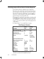
Setting Form Feed and Perforation Skipping Options
1.
Set the form size and top of form.
See instructions earlier in this chapter.
2.
Press [OP()] [5] [ENTER].
Most of the items in this dialog concern the report and information to be
included in it. These items are discussed in chapter 10. The last four items
control paper feed during the plot and report and are discussed here.
Example
*
OP
# 5
PRINT & POST–RUN LIST OPTIONS
See chapter 1
Large font [Y*/N]:
Store post–run report [Y/N*]:
External post–run report [Y/N*]:
List run parameters [Y/N*]:
See
chapter 10
List timetable [Y/N*]:
List calibration [Y/N*]:
List remote method [Y/N*]:
Form–feed before report [Y/N*]: Y [ENTER]
Form–feed after report [Y/N*]: Y [ENTER]
Skip perforations in report [Y/N*]: Y [ENTER]
Skip perforations in plot [Y/N*]: Y [ENTER]
3.
Press Y for each form feed option to ensure that the report and
plot are positioned at the beginning of a page.
The two form feed options cause an advance to the next top of page before
and/or after printing a report.
4.
Press Y for both perforation skipping options to avoid printing
on the perforated area between pages.
Skipping perforations in the plot may only be selected when perforation
skipping in the report is also selected.
2Ć12
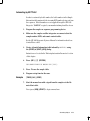
Getting Started
Understanding Time Programming
Time programming creates entries in the timetable. A printed code marks
the execution time on the chromatogram.
Key
Printed
Code
See
Chapter
Chart
Parameters
[ZERO]
[CTRL] [ZERO]
[ATT 2"]
[CHT SP]
ZE
^ZE
AT
CS
4
4
2
2
Integration
Parameters
[PK WD]
[THRSH]
[AR REJ]
PW
TH
AR
3
3
3
Integration
Functions
[INTG( )]
IF
3
End of Run
[STOP]
ST
2
At the end of a run, parameters changed by the timetable revert to initial
values, assuring that each run in a series begins with the same set of operĆ
ating parameters.
Getting Started
2Ć13
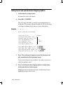
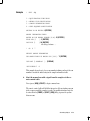
Making Timetable Entries
1.
Press [TIME] run time key {value} [ENTER] to create a timetable
entry.
run time is the number of minutes after the run starts when the function
is to occur; key is one of the timeĆprogrammable keys listed in the table;
and value is the numeric entry associated with key, if there is one.
Example
[TIME] [.] [5] [CHT SP] [7]
[ENTER]
*
@
TIME
.5
CHT SP
7
This example sets the chart speed to 7 at thirty seconds into the run.
Check the timetable entry by pressing
[LIST] [TIME] [ENTER]
* LIST: TIME
@
0.500 CHT SP =
7.0
Timetable entries may also be made from the [PREP] or [EDIT]
[METH] dialog.
Example
[EDIT] [METH] [ENTER]
*
EDIT METH
1 = RUN PARAMETERS
2 = TIMETABLE EVENTS
3 = CALIBRATION FILE
etc.
SECTION TO BE EDITED: [2] [ENTER]
TIMETABLE EVENTS
SELECT EVENTS FROM THE FOLLOWING MENU:
[IF/EX/ZE/^Z/AT/CS/AR/TH/PW/ST]
2Ć14
TIME:
[.] [5] [ENTER]
EVENT:
[C] [S] [ENTER]
VALUE:
[7 ] [ENTER]
Getting Started
Codes for timed events; see previous page
for corresponding keys
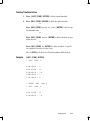
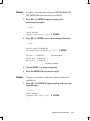
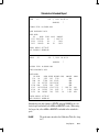
Deleting Timetable Entries
1.
Press [LIST] [TIME] [ENTER] to list the current timetable.
2.
Press [DEL] [TIME] [ENTER] to delete the entire timetable.
or
Press [DEL] [TIME] run time key {value} [ENTER] to delete a speĆ
cific timetable entry.
or
Press [DEL] [TIME] run time [ENTER] to delete all entries at a parĆ
ticular run time.
or
Press [DEL] [TIME] key [ENTER] to delete all entries of a specific
key, regardless of run time or value, if any.
If key is [INTG()], all entries for all function numbers will be deleted.
Example
[LIST] [TIME] [ENTER]
*
LIST:
TIME
@
0.100 INTG # =
8
0.032 AR REJ =
66
0.500 CHT SP =
7.0
5.000 INTG # =
3
7.250 INTG # = –8
*
DELETE
*
LIST:
TIME
INTG
TIME
@
0.032 AR REJ =
66
0.500 CHT SP =
7.0
#
Getting Started
2Ć15
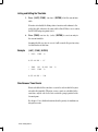
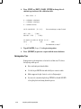
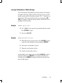
Listing and Editing the Timetable
1.
Press [LIST] [TIME] {run time} [ENTER] to list the current timeĆ
table.
If runtime is included, the listing starts at runtime and continues to the
end of the table; otherwise, the entire table is listed. If there are no entries,
the HP 3395 Integrator prints EMPTY.
2.
Press [TIME] run time key {value} [ENTER] to correct an entry in
the current timetable.
Assuming that the run time is correct, it will overwrite the previous entry
for that function at that time.
Example
[LIST] [TIME] [ENTER]
*
LIST:
TIME
@
0.032 AR REJ =
66
*
TIME
*
LIST:
.032
TIME
0.032 AR REJ =
AR REJ
100
@
@
100
Simultaneous Timed Events
Events scheduled at the same time occur in the order in which they were
entered in the timetable. When two or more events are scheduled at the
same time, only the code for the last event in the group is printed on the
chromatogram.
See chapter 3 for related information about the priority of simultaneous
integration events.
2Ć16
Getting Started
3
Integrating and
Reintegrating Data
In this chapter...
H Starting Integration . . . . . . . . . . . . . . . . . . . . . . . . . . . . . . . . . . 3Ć2
H Checking Parameter Values . . . . . . . . . . . . . . . . . . . . . . . . . . . 3Ć3
H Selecting Peak Width Values . . . . . . . . . . . . . . . . . . . . . . . . . . 3Ć5
H Selecting Threshold Values . . . . . . . . . . . . . . . . . . . . . . . . . . . 3Ć7
H Selecting Area Rejection Values . . . . . . . . . . . . . . . . . . . . . . . 3Ć8
H Using the Integration Functions . . . . . . . . . . . . . . . . . . . . . . 3Ć9
H Reintegration . . . . . . . . . . . . . . . . . . . . . . . . . . . . . . . . . . . . . . . 3Ć13
Integrating and Reintegrating Data
3Ć1
Starting Integration
The HP 3395 Integrator integrates chromatographic information during a
sample run in realĆtime and during reintegration.
To start realĆtime integration:
3Ć2
1.
Be sure the appropriate signal or data source is connected to the
integrator.
See the Installation and Service manual for installation instructions.
2.
Set [ZERO], [ATT2^], and [CHT SP ] or use default values.
See chapter 2 for more information.
3.
Set [AR REJ], [THRSH], and [PK WD ] or use default values.
Instructions for choosing these values are discussed later in this chapter.
4.
Select a plot type for the chromatogram or use the default filĆ
tered plot.
See chapter 2 for more information.
5.
Press [OP()] [2] to store data for later use.
See chapter 7 for more information.
6.
Start the run. [START]
RealĆtime integration produces processed peak data for a report. The data
may be stored for later use. Signal data may also be stored for later reinĆ
tegration.
7.
Stop the run. [STOP]
8.
Inspect the chromatogram and report.
Make appropriate adjustments in run parameters if necessary. See chapter
6 for more information about report reading.
Integrating and Reintegrating Data
Checking Parameter Values
1.
Example
Press [LIST] [LIST] to list the currently selected run parameĆ
ters.
* LIST: LIST
PEAK CAPACITY:
ZERO
ATT 2^
CHT SP
AR REJ
THRSH
PK WD
=
=
=
=
=
=
1244
number of peaks integrator can currently store
0, –0.828
0
1.0
0
0
0.04
Use the default values listed above if you are unsure of the best values to
use for your run. All run parameters may be adjusted during realĆtime
integration or reintegration to optimize presentation, peak detection, or
quantitation.
Individual parameters may also be listed separately.
Example
[LIST] [PK WD] returns only the current peak width value.
*
LIST: PK WD
=
0.01
See chapters 2 and 4 for related information.
Integrating and Reintegrating Data
3Ć3
The presentation of the chromatogram is controlled by
H
[ZERO] the baseline zero position
H
[ATT 2^] attenuation
H
[CHT SP] chart speed.
These parameters are discussed in chapter 2.
The quantitation of the chromatogram is controlled by
H
[AR REJ] area reject
H
[THRSH] threshold
H
[PK WD] peak width
These parameters are discussed in this chapter.
3Ć4
Integrating and Reintegrating Data
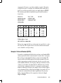
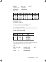
Selecting Peak Width Values
The peak width run parameter specifies the expected widths (in minutes)
of peaks at approximately halfĆheight. If no peak width is selected, the inĆ
tegrator uses a default value of 0.04 minutes, suitable for many analyses.
1.
Example
Press [PK WD]
value
*
@
PK WD
.01
[ENTER] to set peak width.
Use the table below to choose an appropriate peak width value for your
application.
2.
Peak Width Range
Application
0.01 to 0.05 minute
HighĆresolution capillary or packed GC columns
0.04 to 0.2
HighĆperformance LC, moderate length packed
GC columns
0.15 to 0.6
HighĆperformance LC, long packed GC columns
0.5 to 2.5
HighĆperformance LC, low efficiency GC
2.5
LowĆpressure (column) LC, some types of amino acid
analysis, nonchromatographic peak integration
Press [LIST] [PK WD] to list the current value for peak width.
Integrating and Reintegrating Data
3Ć5
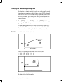
Changing Peak Width Settings During a Run
If peak widths are almost constant through a run, as they usually are with
temperature programming or gradient elution, a single PK WD value will
suffice for the entire run. If the widths change significantly, as in isotherĆ
mal or isocratic runs, a peak width profile can be generated by timeĆproĆ
grammed changes.
1.
Press [TIME] run time [PK WD] new value [ENTER] to timeĆ proĆ
gram a peak width change.
The peak width parameter behaves differently from all other timeĆ proĆ
grammed values. The change to new value is not immediate. Instead, the
value changes in a smooth ramp from the time of the previous value.
Example
*
TIME 1.00
PK WD
.04
@
.04
Peak
Width
Timed
PK WD
Event
Initial
Value
0
Run Time in min. 1
To make a step change, use two timed events close together.
* TIME 1.00 PK WD .04 @
* TIME 1.01 PK WD .16 @
.16
Peak
Width
Initial
Value
0
Timed
PK WD
Events
Run Time in min.
See chapter 4 for related information.
3Ć6
Integrating and Reintegrating Data
1
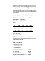
Selecting Threshold Values
The peak detection threshold [THRSH] is a value representing the signal
level below which the HP 3395 Integrator considers all baseline deviations
as noise. A peak with height less than the Threshold value is ignored.
There are two ways to select threshold values.
1.
Press [THRSH]
value
[ENTER] to set threshold.
value is an integer from -6 to 28. The values are a binary series; an inĆ
crease of 1 unit doubles the minimum height that will be accepted. The
minimum value (-6) is equivalent to two height counts. One height count
represents 1/8 microvolt.
Example
*
2.
THRSH
5
@
Press [THRSH] [ENTER] to set autoĆthreshold.
The HP 3395 Integrator then measures the signal noise and assigns an
appropriate value to Threshold. AutoĆTHRSH determinations must be perĆ
formed when the chromatographic signal is stable and peakĆfree, as during
a blank (no sample) run, using the Peak Width value (or profile) selected
for the analysis. The process takes 5 x Peak Width minutes and the Ready
LED blinks during the determination. AutoĆthreshold can be automatically
built into a run by programming INTG() 6. See instructions for the inĆ
tegration functions later in this chapter.
Threshold has two side effects. High values delay the decision whether to
accept or reject a given peak. This delays the printing of the start tick
mark on the chart, so that it may only approximate the position of the real
start of peak. Increasing Threshold also causes solvent peaks to terminate
earlier.
Press [THRSH] [-] [ENTER] to abort autoĆthreshold.
3.
Press [LIST] [THRSH] to list the current value for threshold.
Integrating and Reintegrating Data
3Ć7
Selecting Area Rejection Values
Each peak must have an area count above the area rejection value to be
reported or stored in the processed peak file.
1.
Press [AR REJ]
value
[ENTER] to set the area reject limit.
value is an integer representing area counts in 1/8 mVĆseconds.
Example
*
AR REJ
800
@
As a convenience, area reject may also be entered in scientific notation usĆ
ing EĆformat."
[AR REJ] [1] [E] [6] [ENTER]
is the same as
[AR REJ] [1] [0] [0] [0] [0] [0] [0] [ENTER]
2.
3Ć8
Press [LIST] [AR REJ] to list the current area rejection value.
Integrating and Reintegrating Data
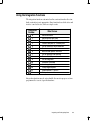
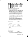
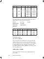
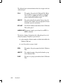
Using the Integration Functions
The integration functions customize baseline construction when the stanĆ
dard construction is not appropriate. Some functions have both active and
inactive (canceled) states; others are single events.
Integration
Number
INTG( )
0
INTG( )
1
2
3
4
5
6
7
8
9
10
11
12
13
14
INTG( )
INTG( )
INTG( )
INTG( )
INTG( )
INTG( )
INTG( )
INTG( )
INTG( )
INTG( )
INTG( )
INTG( )
INTG( )
What it does
Set baseline now
Set baseline at next valley
Set baseline at all valleys
Process next peak as a solvent peak
Turn off automatic solvent detection
Draw horizontal baseline
Measure and update Threshold
Turn off retention time labelling
Turn on Start/Stop marks
Turn off integration
Increment Threshold
Invert negative peaks
Clamp negative peaks
Show functions 11 and 12
Start peak sum window
Integration functions may be entered while the run is in progress or timeĆ
programmed to occur at a specified run time.
Integrating and Reintegrating Data
3Ć9
1.
Press [INTG()] function number [ENTER] to activate an integraĆ
tion function during a run.
Example
0.082
0.173
IF7@
IF–7@
0.574
Integration function 7 is turned on after the second peak so that retention
times for subsequent peaks are not printed until the function is turned off
again.
2.
Press [INTG()] [-] function number [ENTER] to cancel an inĆ
tegration function during a run.
TimeĆProgramming Integration Functions
When the [START] key is pressed to begin a run, all integration functions
are inactive.
1.
Press [TIME] run time [INTG()] function number [ENTER] to actiĆ
vate an integration function.
To have a function active at the start of a run, enter the activating comĆ
mand in the Timetable at time 0.
When a timed event is to apply to a particular peak, the execution time
must be after the retention time (peak apex) of the preceding peak but beĆ
fore the retention time of the target peak.
2.
Press [TIME] run time [INTG()] [-] function number [ENTER] to
cancel an integration function.
The notation IF is printed on the chart when any integration function is
executed.
3Ć10
Integrating and Reintegrating Data
Example
*
TIME
.3
INTG #
7
@
*
TIME
.55
INTG #
–7
@
0.082
0.173
IF
IF
0.574
Integrating and Reintegrating Data
3Ć11
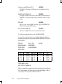
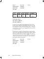
Priority of Baseline Functions
When more than one baseline function is in effect at the same time, a
priority order is applied.
Priority of Baseline Functions
Highest priority
Lowest priority
Example
*
LIST:
INTG() 0
Set Baseline Now
INTG() 5
Extend Baseline Horizontally
INTG() 1
Set Baseline at Next Valley
Point
INTG() 2
Set Baseline at All Valley
Points
INTG() 3
Skim from Next Peak
TIME
@
0.100 INTG # =
0
0.100 INTG # =
1
0.100 INTG # =
5
Thus INTG() 0 will always set the baseline to the current signal value, but
the entry to set baseline at the next valley point (INTG() 1) will be igĆ
nored if the baseline is being constructed horizontally (INTG() 5).
3Ć12
Integrating and Reintegrating Data
Reintegration
Reintegration is the process of reanalyzing signal data from storage. The
data used in reintegration can be either from a realĆtime run or a previous
reintegration.
1.
Press [OP()] [2] [ENTER] to store raw or bunched run data from
a realĆtime run or a reintegration.
Storing bunched signal data, processed peak data, or report data
from the reintegration of a signal data file always overwrites the
previous set of reintegration result files from that same signal data
file, if there were any. Change the input signal data filename before
the reintegration to save the previous copies.
If you specify storage of signal data for a reintegration and then attempt to
reintegrate a .BNA file from the same device as that specified for storage,
the signal data will not be stored, because that would overwrite the input
file. The reintegration will proceed, but the message
Error storing signal; filespec
FILE ALREADY OPEN
will be printed afterward. Either change the name of the input signal file
to something else (COPY or RENAME commands; see HP 3395 IntegraĆ
tor Using Application Programs to automate this process) or use option 2
to disable signal data storage or change its destination. A similar conflict
arises with local run time storage when signal data files are being sent to a
host computer. See chapter 7 for more information.
2.
Make a realĆtime run or reintegration.
3.
Change the method, if desired.
The HP 3395 Integrator uses the integration parameters present in interĆ
nal memory at the time the ANALYZE command is typed, except for samĆ
ple information which is stored with the signal data.
Integrating and Reintegrating Data
3Ć13
To select the integration parameters:
3.
H
Do nothing if the ones in memory are correct.
H
Use key commands to make any desired change.
H
Load a new method with a new set of parameters (see chapter 8).
Type AN{ALYZE filespec , I } to begin reintegration.
Only the first 2 letters are required; everything else is optional.
filespec names the storage device, file name, and file name extension where
the raw or bunched data to be reintegrated is stored. See chapter 7 for more
about filespec. If filespec is omitted, the HP 3395 Integrator selects a default
file:
H
If this is the first reintegration after a realĆtime run, the default is
the signal data file stored during that run. If no data was stored,
the default is undefined.
H
For the second and later reintegrations, the default is the signal
file analyzed in the previous reintegration.
Use the I parameter if you change some of the integration parameters but
want to ensure that the original PK WD profile (which is stored with the
data) is used.
If the device specified, either in filespec or as a default, is H, and the host comĆ
puter link is operating in MUTE Mode, the ANALYZE command will fail. The
message
INVALID MUTE HOST CONVERSATION
will appear. MUTE Mode is the default computer link mode at powerĆon. The
host computer must be programmed to change the HP 3395 Integrator to VOĆ
CAL Mode and to supply the calledĆfor signal data file, for reintegration to
succeed.
During reintegration the HP 3395 Integrator reanalyzes (reintegrates) run
data produced by a prior realĆtime run or reintegration. As in realĆtime
integration, the integrator plots a chromatogram, quantitates the data,
and reports the results. Reintegration stops when the HP 3395 Integrator
reaches the end of the signal in the file, when [STOP] is pressed, when a
TIMETABLE STOP occurs, when a remote control STOP occurs, etc.
3Ć14
Integrating and Reintegrating Data
Example
To produce a report with sample information (ISTD AMT, SAMP AMT,
MUL FACTOR) different from that in the signal data file:
1.
Press OP()] [4] [ENTER] to suppress printing of the
postĆreintegration report.
*
OP # 4
REPORT OPTIONS
Suppress local report [Y/N*]: Y [ENTER]
2.
Press OP()] [7] [ENTER] to enter the new sample information.
*
OP # 7
DEFAULT SAMPLE INFORMATION
USE SAMPLE TABLE IN MANUAL RUN [Y/N*]: Y [ENTER]
Enter new information here
ISTD AMT [0.0000E+00 ]:
SAMPLE AMT [0.0000E+00 ]:
MUL FACTOR [1.0000E+00 ]:
the dialog continues...
3.
Type AN{ALYZE, I } to begin reintegration.
4.
Press the [REPORT] key to generate a report .
Example
To produce a report with a calculation type different from that in the
signal data file:
1.
Press [OP()] [4] [ENTER] to suppress printing of the postĆreinĆ
tegration report.
* OP # 4
REPORT OPTIONS
Suppress local report [Y/N*]: Y [ENTER]
Integrating and Reintegrating Data
3Ć15
2.
Press [PREP] or [EDIT] [CALIB] [ENTER] to change the calĆ
culation type and create the calibration table.
*
PREP CALIB
@
E = EXTERNAL STANDARD
I = INTERNAL STANDARD
N = NORMALIZATION
CALIB PROCEDURE
REF % RTW [
NON-REF % RTW
[E*/I/N]:
Enter new calculation type; see chapter 5 for details
5.000]:
[
5.000]:
RF BASED ON AREA OR HEIGHT [A*/H]:
CAL#
RT
AMT
NAME
1 :
Enter calibration table; see chapter 5
3.
Type AN{ALYZE filespec, I } to begin reintegration.
4.
Press [REPORT] to generate a report with the new calculation.
Reintegration Tips
Reintegration can be many times as fast as the realĆtime run. To achieve
the highest possible speed
3Ć16
H
Store and reintegrate bunched data.
H
Use the largest PK WD value which still gives accurate results.
H
Either suppress the plot (fastest) or select a Unigram plot.
H
If you need a conventional plot, keep CHT SP less than 0.3/PK WD
to keep the plot from slowing down the process.
Integrating and Reintegrating Data
4
Understanding Integration
ÉÉ
ÉÉ
É
ÉÉÉ
ÉÉÉ
ÉÉ
ÉÉ
É
É
É
ÉÉ
ÉÉ
ÉÉ
É
É
É
ÉÉ
ÉÉ
É
É
ÉÉ
É
É
ÉÉ
ÉÉ
É
É
É
ÉÉ
ÉÉ
É
É
ÉÉ
É
É
ÉÉÉ
ÉÉÉÉ
É
É
ÉÉ
É
É
ÉÉ
É
É
ÉÉ
ÉÉ
É
É
É
ÉÉ
ÉÉ
É
É
ÉÉ
É
É
ÉÉÉ
ÉÉÉÉ
ÉÉÉ
ÉÉÉ
É
ÉÉÉ
In this chapter...
H Understanding How the Integrator Integrates . . . . . . . . . . 4Ć2
H Data Acceptance . . . . . . . . . . . . . . . . . . . . . . . . . . . . . . . . . . . . . 4Ć4
H Data Preparation . . . . . . . . . . . . . . . . . . . . . . . . . . . . . . . . . . . . 4Ć5
H Peak Recognition . . . . . . . . . . . . . . . . . . . . . . . . . . . . . . . . . . . . 4Ć7
H Optimizing Peak Recognition . . . . . . . . . . . . . . . . . . . . . . . . . 4Ć11
H Peak Measurement . . . . . . . . . . . . . . . . . . . . . . . . . . . . . . . . . . 4Ć15
H Chromatographic Baseline Construction . . . . . . . . . . . . . . . 4Ć16
H Baseline Corrections . . . . . . . . . . . . . . . . . . . . . . . . . . . . . . . . . 4Ć21
H Peak Data Storage . . . . . . . . . . . . . . . . . . . . . . . . . . . . . . . . . . . 4Ć22
H The Integration Function Descriptions . . . . . . . . . . . . . . . . . 4Ć23
Understanding Integration
4Ć1
Understanding How the Integrator Integrates
This chapter describes the internal HP 3395 Integrator peak detection and
measurement operations.
The HP 3395 Integrator processes an analog (voltage) signal from a gas or
liquid chromatograph or other analytical instrument. It can also process
data from its own internal memory and from a host computer.
Sample
Slice Data
(Internal or
disc memory or
host computer)
Analog
Instrument
HP 3395
Find and measure peaks
Calculate results
Print report
4Ć2
Understanding Integration
The integrator takes the following steps to find and measure peaks:
1. Accepts data
2. Prepares the data for integration
3. Searches the prepared data for peaks
4. Measures the peaks
5. Constructs the chromatographic baseline
6. Corrects the peak measurements for baseline
7. Saves data
8. Calculates amounts for the report (see chapters 5 and 6)
The rest of this chapter discusses these topics in this order. Each discusĆ
sion is divided into:
H
The simplest case
H
One or more complexities
H
Integration Functions, which are deliberate interferences with
normal signal processing, are noted if any apply. The details of the
functions are deferred to the end of the chapter.
Understanding Integration
4Ć3
Data Acceptance
From an Analog Instrument
The instrument produces a voltage that varies with time. The HP 3395
Integrator converts this to a series of digital numbers, each representing
one area slice." An area slice is bounded by the start time of the slice, the
start time plus the slice width, the analog (voltage) signal, and a reference
voltage.
The HP 3395 Integrator uses a slice width of 0.05 seconds (20 slices per
second) and an electrical reference of approximately 0 volts. The reference
is not related in any way to the correct" baseline; it is simply a voltage
lower than any we expect to see from the instrument.
Data collection begins when the [START] key is pressed and ends when
the [STOP] key is pressed or a timeĆprogrammed STOP event occurs.
From a Memory File
The HP 3395 Integrator can accept and process data from files in its own
memory or a host computer. This is usually done to reintegrate, using difĆ
ferent parameters, data that originally came from the HP 3395 Integrator.
4Ć4
Understanding Integration
Data Preparation
Peaks are detected by passing the signal, which is now a stream of area
slices, over an internal pattern or template. When the match is good, we
have a peak; when it isn't, we don't. There is, however, a complication.
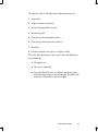
Consider this pair of peaks
A
B
and this simple peak template
The template is a good width match for peak A, but not for peak B. Even
when it is perfectly centered on peak B, there is a great deal of peak charĆ
acter" which is outside the template. This reduces the sensitivity at the
center of peak B and broadens the response as the signal passes the temĆ
plate. The result is to make peak B much harder to detect than peak A.
Understanding Integration
4Ć5
It's clear that the problem is caused by a width mismatch between Peak B
and the template. There are two ways to correct thisĊwiden the template
or narrow the peak. It turns out to be much easier to narrow the peak.
Here's a broad one, represented as a numbered series of area slices:
1
2 3
4
5 6
7
8
If this peak is too wide for a good match with the filters, we can easily narĆ
row it by adding pairs of slices together. The result is:
6
4
2
1
8
3
5
7
This bunched" peak has the same area as the original but is narrower and
higher and easier to detect. Both the retention time and the height have
changed, but since we know what we did, it's easy to correct them.
4Ć6
Understanding Integration
Peak Recognition
There are two parts to the search for peaks. Part 1 rejects random noise in
the signal based on a rough measure of height. Part 2 compares the signal
exceeding the threshold height with a set of internal templates to find reĆ
gions that have peakĆlike characteristics.
A peak with height less than Threshold is ignored.
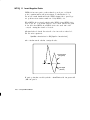
The Simple Case Ċ Isolated Peaks
As the integrator scans the data, it examines the slope (difference between
successive slices) and curvature (positive or negative). So long as these reĆ
main within preset bounds, this is baseline. If the bounds are exceeded, a
peak may be starting. If the condition persists, the integrator decides that
it is on the upslope of a peak. A complete, isolated peak looks like
5
4
6
2
7
1
8
3
1.
2.
3.
4.
5.
6.
7.
8.
Slope and curvature within limits
Slope and curvature above limits
Slope remains above limit
Curvature becomes negative
Slope becomes negative
Curvature becomes positive
Slope and curvature within limits
Slope and curvature remain within
limits
-
track baseline
perhaps a peak?
we've got a peak!
front inflection point
top of the peak
rear inflection point
approaching end of peak
end peak, track
baseline
Understanding Integration
4Ć7
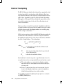
Step 5 identifies the approximate top of the peak. The HP 3395 Integrator
uses the tallest slice and one slice on either side, fits them to a quadratic
equation, and solves the equation to find the retention time and peak
height.
ÉÉ
ÉÉÇÇÇ
ÇÇÇ
ÉÉÇÇÇ
ÇÇÇ
ÇÇÇÉÉ
ÇÇÇ
ÇÇÇÉÉ
ÇÇÇ
ÉÉ
ÇÇÇ
ÇÇÇ
ÇÇÇÉÉÇÇÇ
Used in Quadratic
Fit to Define Apex
Peak end is found using a formula based on the retention time of the peak,
its measured width, the rate at which it approaches baseline, and for solĆ
vent peaks, the present Threshold value. This has been tested against
many peaks and provides a reasonable endĆofĆpeak decision.
4Ć8
Understanding Integration
Complexity 1 Ċ Merged Peaks
A peak may follow all the steps to 7 but then begin to rise again. It is
merged with the following peak so that there is no baseline between them.
The HP 3395 Integrator responds by forcing the first peak to end at the
lowest point and then integrating the second one. This repeats as many
times as necessary when we have a cluster of merged peaks.
5
5
6
4
1
2
3
4
6
7, 2, 3
Peak A
7
8
Peak B
The lowest (valley) point is located in much the same way that the peak
top is found. The HP 3395 Integrator uses the smallest slice and its two
neighbors, fits the data to a quadratic, and solves for the minimum.
Related Integration Functions
1
Set baseline at next valley.
2
Set baseline at all valleys.
See The Integration Function Descriptions" later in the chapter for reĆ
lated information.
Understanding Integration
4Ć9
Complexity 2 Ċ Solvent Peak Detection
#!#! "$!" # ! # "$""%
"" # !# " #" ! '" %#" !
$# # " #!# " "%# #" !"$#" "%# " #!# " "%#" #!#
$# ( $" # !%# #"# $# !" ##
" # # # " !#! " "%#
" # &" "%# ! !!" & #*
!# !#% # ## " & " !& ! # "#!# #
" ## # # "%# &" # #( "
# #
Related Integration Functions
! '# " $### "
) #!# $# "! #" #! # #! !
!# !#
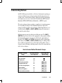
4Ć-0
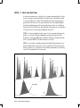
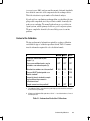
Optimizing Peak Recognition
The best conditions for recognizing isolated, symmetric peaks on a flat,
quiet baseline is to match the Peak Width parameter to the measured
width of the peaks at halfĆheight. The autoĆThreshold value is appropriate
for eliminating noise.
When peaks cluster together or the baseline slopes or is noisy, these ideal
values must be modified. The figure shows how to modify these values apĆ
propriately.
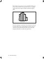
Increasing
Threshold
Threshold HIGH
Peak Width LOW
Threshold HIGH
Peak Width HIGH
This is useful for detecting peaks
on sloping baselines. The reduced
Peak Width improves peak
detection but reduces signal
filtering. Increase Threshold to
avoid detecting noise as peaks.
The higherĆthanĆnormal Peak
Width reduces peak detection
sensitivity so that only major
peaks are found. High Threshold
eliminates residual random noise.
``Ideal''
Values
Threshold LOW
Peak Width LOW
When both broad and narrow
peaks must be detected and it is
not practical to change Peak
Width, the width should be set
for the narrower peaks and
Threshold reduced to ensure
that the broader ones are still
detected.
Threshold LOW
Peak Width HIGH
This combination is effective for
detecting and measuring trace
components (those whose heights
approach the noise level itself).
The penalty is that spurious
peaks, which are actually noise,
will also be detected.
Increasing Peak Width
Understanding Integration
4Ć11
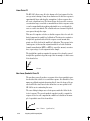
Tips for Selecting Peak Width Values
1. When peaks are large compared to the noise in the signal, a
useful rule of thumb is:
PK WD must be
MORE THAN 1/4 OF
BUT LESS THAN 2 TIMES
the actual width.
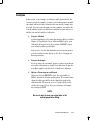
2. When peaks are very small or when noise is high, and particuĆ
larly when both conditions occur simultaneously, it may be
necessary to overfilter" the signal to detect the peak. This is
done by using a largerĆthanĆnormal PK WD value; however, if
PK WD is too much greater than the actual width of the peak,
the peak itself may be filtered out. This situation requires
some experimentation to find the most appropriate value.
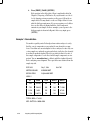
3. The report of analysis contains a column headed WIDTH.
These numbers are good approximations of the widths of peaks
at half the peak height. If the HP 3395 Integrator fails to deĆ
tect peaks that are clearly present, examine the WIDTH values
for the peaks that are found. Use this information and inspecĆ
tion of the chromatogram to select a more appropriate value
for PK WD.
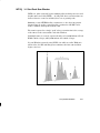
4. The Unigram plot can be used to select an appropriate value or
profile (discussed next) for the PK WD parameter.
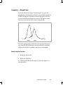
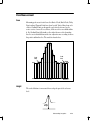
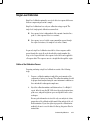
If the PK WD value (or profile) is a good match to the actual peak widths,
all of the peaks in the Unigram will have the same width. The heights are
then proportional to the peak areas.
The Unigram transformation is:
Time axis: Replace linear time with time divided by the peak width.
0.1 x CHT SP
PK WD
Height axis: Replace linear height with height times peak width.
100 x PK WD x (filtered peak height)
4Ć12
Understanding Integration
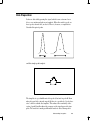
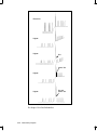
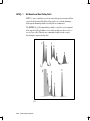
These two figures show the same run data as a filtered plot and as a UniĆ
gram.
Filtered Plot
Unigram
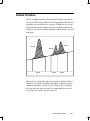
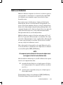
A displacement of the signal may appear in a Unigram as a shift followed
by severe baseline drift. These two effects have different causes, and sepaĆ
rate commands are provided to deal with them.
1.
Press [ZERO] [ENTER] to reset the baseline to the present value
of the signal.
The effect is to move the baseline to the left of the chart.
2.
Press and hold [CTRL] while pressing [ZERO] then release both
and press [ENTER] to remove the drift caused by the signal disĆ
placement.
These commands can be used separately or together, and both may be
timeĆprogrammed.
Understanding Integration
4Ć13
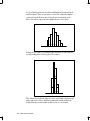
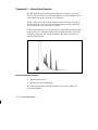
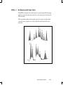
Filtered Plot
Unigram
Unigram
Zero
Control Zero
Unigram
Unigram
See chapter 3 for related information.
4Ć14
Understanding Integration
Zero and
Control Zero
Peak Measurement
Area
Measuring peak areas is trivial once the Start of Peak, End of Peak, Valley
Point, and any Tangent Points have been located. Vertical lines from each
of these Cardinal Points are dropped to an electrical reference level to
create a series of zones. For each zone, all the area slices are added within
it. If a Cardinal Point falls inside a slice rather than on a slice boundary,
the slice area is divided between the two adjacent zones according to where
the point is within the slice. The result is shown below.
ÉÉ
ÉÉÉÉ
ÉÉ
ÉÉÉÉ
ÉÉ
ÉÉ
ÉÉ
ÉÉ
ÉÉ
ÉÉÉÉ
ÉÉ
É
ÉÉ
ÉÉ
ÉÉ
ÉÉ
É
ÉÉ
ÉÉÉÉ
ÉÉ
ÉÉ
ÉÉ
ÉÉÉ
ÉÉÉÉÉÉÉÉÉÉÉÉ
ÉÉ
ÉÉ
É
ÉÉ
ÉÉ
ÉÉ
É
ÉÉ
É
ÉÉÉÉ
ÉÉ
ÉÉ
ÉÉ
ÉÉÉ
ÉÉ
ÉÉ
ÉÉ
ÉÉ
É
ÉÉ
ÉÉ
É
ÉÉ
ÉÉ
ÉÉ
ÉÉ
ÉÉ
ÉÉÉ
ÉÉ
ÉÉ
ÉÉ
ÉÉ
É
ÉÉ
ÉÉ
É
ÉÉÉÉ
ÉÉ
ÉÉ
É
ÉÉ
ÉÉ
ÉÉ
ÉÉ
ÉÉ
ÉÉ
É
ÉÉ
ÉÉ
É
ÉÉ
ÉÉ
ÉÉ
ÉÉ
ÉÉ
ÉÉÉ
ÉÉ
ÉÉ
ÉÉ
ÉÉ
É
ÉÉ
ÉÉ
É
ÉÉ
ÉÉ
ÉÉ
ÉÉ
É
ÉÉ
ÉÉ
ÉÉ
ÉÉ
ÉÉ
ÉÉ
É
ÉÉ
ÉÉ
É
ÉÉÉÉÉÉÉÉÉÉÉÉÉÉÉÉ
ÉÉÉÉÉÉÉ
ÉÉÉÉ
Peak
End
Peak
Start
Zone Area
Signal
Reference
Height
The vertical distance is measured from each peak apex to the reference
level.
Peak
Height
Understanding Integration
4Ć15
Chromatographic Baseline Construction
The Simple Case Ċ No Solvents, No Timed Events
The baseline is a continuous series of straight line segments that connect
these points:
1. The signal level at the START of the run.
2. The start and end of peaks or merged groups. These points are
marked by large tick marks (downscale for start, upscale for
end) on the chart and by the letter B in the start or end posiĆ
tion in the TYPE column of the report.
3. The signal level when STOP occurs, if it happens when no
peak is in progress.
Stop
Complexity 1 Ċ STOP During a Peak
If the STOP occurs before the apex of the peak, the peak is not reported.
If it occurs after the apex, the last segment of the baseline is a horizontal
line drawn from the last declared baseline point to the STOP time, with a
dropline from the signal at this point. The peak type in the report has I
(for incomplete) in the warning column and H (for horizontal extension) in
the end column.
4Ć16
Understanding Integration
ÉÉ
ÉÉ
ÉÉ
ÉÉ
ÉÉ
ÉÉ
Complexity 2 Ċ Solvent Peaks
If a solvent peak starts above baseline, the segment before the solvent is a
horizontal extension from the last declared baseline point to the start of
the solvent peak. The peak TYPE in the report has S in the solvent column
and H in the start column.
Understanding Integration
4Ć17
Solvent peaks normally end using the same test as for ordinary peaks.
They will end sooner if the start, end, or valley point of a rider peak is beĆ
low the Threshold level in effect. Baseline is set to the signal level at the
point, the solvent ends, and tangent skimming ceases. The peak is marked
with an S on the chart to indicate that it ended due to THRSH level.
See Understanding Reports" in chapter 6 for related information.
4Ć18
Understanding Integration
Complexity 3 Ċ Rider Peaks
A local baseline tangent to the tail of the solvent is created for rider peaks.
All such peaks are marked by small tick marks. The TYPE column must be
consulted to determine which points are local baseline points and which
are local valley points. All rider peaks are TYPE T in the solvent column.
The local baseline follows the same rules as the overall baseline.
Understanding Integration
4Ć19
Complexity 4 Ċ Baseline Penetration
If the signal drops below the baseline that has been constructed using
these rules, this is a baseline penetration. The HP 3395 Integrator redraws
the baseline to eliminate the penetration.
Detection of penetration is quite sensitive, often producing P codes for
peaks that appear to be on perfectly normal, flat baselines. If a peneĆ
tration is invisible on the chromatogram relative to the least significant
information being measured, the effect of redrawing the baseline can be
ignored.
Integration Functions Related to the 4 Complexities
0
Set baseline now
1
Set baseline at next valley
2
Set baseline at all valleys
3
Skim from next peak
5
Extend baseline horizontally
See The Integration Function Descriptions" later in the chapter for reĆ
lated information.
4Ć20
Understanding Integration
Baseline Corrections
Zone areas and peak heights have been measured relative to an electrical
reference level that is not related to the chromatographic baseline. We now
know where the real baseline is for every zone. Compute the area (a trapeĆ
zoid) between the baseline and the reference level, subtract, and have the
baselineĆcorrected areas. A similar calculation yields the baselineĆcorrected
peak height.
Area C
Area A
Area B
Zone A
Zone B
Zone C
Rider peaks on a solvent tail require a more elaborate calculation. Zones 1
and 3 are corrected in the way just described. Zone 2 requires some extra
calculation to divide the area above baseline. The part above the tangent
line is reported as the rider peak; the rest is summed with the corrected
areas from Zones 1 and 2 to give the solvent area.
Understanding Integration
4Ć21
Area 2
Area 1
Area 3
Zone 1
Zone 2
Zone 3
Solvent Area = Area 1 + Area 3 + part of
Area 2 below the tangent
Rider Area = Part of Area 2 above the tangent
Peak Data Storage
Data is stored for calculations for each peak with area greater than the
specified Area Reject amount. This peak data includes the retention time
in minutes, the area in 1/8 microvoltĆseconds, and the height in 1/8 microĆ
volts.
4Ć22
Understanding Integration
The Integration Function Descriptions
INTG() 0
Set Baseline Now
INTG() 0 causes an immediate reset of the integrator baseline to the curĆ
rent value of the signal. It is useful where a baseline shift occurs during a
run, such as after a valve switch.
Example
In the figure, INTG() 0 terminates the fourth peak.
If INTG() 0 is activated while tangent skimming peaks from a solvent tail,
both tangent skimming and the solvent peak are terminated.
Understanding Integration
4Ć23
INTG() 1
Set Baseline at Next Valley Point
INTG() 1 causes a baseline reset at the next valley point encountered then
cancels itself automatically. If the valley point is on a solvent downslope,
both tangent skimming and the solvent peak are terminated.
The [INTG()] [-] [1] command is provided to cancel the reset command
if the expected valley should not occur, which would cause the reset to ocĆ
cur at a later valley. Thus the two commands should be used as a pair
bracketing the expected valley time.
[23
4Ć24
Understanding Integration
INTG() 2
Set Baseline at All Valley Points
The INTG() 2 function forces the baseline to pass through all valley points
until it is canceled. It may be used to lift a series of peaks off a broad swell
in the baseline.
This repeated resetting of the baseline can cut off corners of peaks. Such
corners become negative area"; they reduce the total measured area of
the peaks.
Understanding Integration
4Ć25
INTG() 3 Skim from Next Peak
A solvent peak may rise too slowly to be recognized automatically, or there
may be a group of peaks well into the run that you feel should be treated
as a solvent with a set of riders. This usually involves a merged group of
peaks where the first one is far larger than the rest. The simple dropline
treatment would exaggerate the later peaks because they are actually sitĆ
ting on the tail of the first one. By forcing the first peak to be recognized as
a solvent, the rest of the group is skimmed off the tail.
INTG() 3, when executed before the apex of a chosen peak, designates the
peak to be a solvent. Tangent skimming is performed on peaks on the
downslope of this peak. Skimming continues until the solvent peak termiĆ
nates or another INTG() baseline function is executed.
INTG() 3 is useful for isolated peaks that tail badly. The peak may be terĆ
minated and baseline reset before all area under the tail is measured. DeĆ
claring a peak to be a solvent turns off normal termination tests, allowing
area to be accumulated for a longer time.
4Ć26
Understanding Integration
INTG() 4 Disable AutoĆTangent Skimming
INTG() 4, executed before the start of a peak, disables solvent testing. The
function can be used if component peaks of interest have upslopes steep
enough to be detected incorrectly as solvents. INTG() -4 restores normal
operation.
Understanding Integration
4Ć27
INTG() 5 Extend Baseline Horizontally
INTG() 5 extends baseline horizontally from the last declared baseline
point. If the signal penetrates the horizontal baseline, the baseline is reset
to the lowest point, then continued horizontally. The construction continĆ
ues until canceled by INTG() -5.
4Ć28
Understanding Integration
INTG() 8 Turn On Start and Stop Tick Marks
)! &(& '%% #$!&! " # %&$& ! %&"# &
$% "! & $" &"$ !% #$!&! !&$+
&"! #"& &*# "#&"! '%& &$ "$ & $% &" &(&
INTG() 9 Turn Off Integration
% '%' "$ %##! #$&% " & $" &"$ )$ & %+
! "% !&( "$ !&! %! %&'$!% '% * !%
&" & $" &"$# %*%& %' % (( %)&!
&'$!% !&$&"! %! % &$ ! % "'$$ $" &"$ #"& "!&!'% ! & & $ !%
&(
$%' % !&$&"! %! (' & &% & % '% % %! #"!&
INTG() 10 Increment Threshold
!$%% & $%" (' * $%% & *
4Ć29
INTG() 11 Invert Negative Peaks
#+')( #)+ % ( ($ )) ). # %'$(( . )
% '$#)$# # "(*'"#) ($),' ( )) + #
#+') ' "' ,) # # ) $!*"# $ ) '%$') /
)+ % #+'($# $#)#*( *#)! #! . # ( )+) # #)' #$' (
)+ $' ) +#) # #+'($# +! ( () ) ) !() (!# %$#)
!' )' $' ( )+ ) ) )" $ )
+#) ) -()# #+'($# +! ( *(
!! (#! +!*( !$, ) #+'($# +! ' #+') $+' )) !+!
#+'($# &*)$# (
,' "#( ) ($!*) *#(# +!*
Inverted Signal
(Integrated)
Real Signal
(Plotted)
)+ % ( )) -)# .$# ) " !") $ ) #)')$' ,!!
#)')
4Ć30
INTG() 12 Clamp Negative Peaks
# ! " ! ! ! # " ! $ ÉÉÉÉ
ÉÉÉÉ
ÉÉÉÉ
ÉÉÉÉ
ÉÉÉÉ
ÉÉÉÉ
ÉÉÉÉ
ÉÉÉÉ
Clamped Signal
(Integrated)
Real Signal
(Plotted)
4Ć31
INTG() 13 Show Functions 11 and 12
!
ÉÉÉÉ
ÉÉÉÉ
ÉÉÉÉ
ÉÉÉÉÉ
ÉÉÉÉ
ÉÉÉÉÉ
ÉÉÉÉ
ÉÉÉÉÉ
ÉÉÉÉ
ÉÉÉÉÉ
ÉÉÉÉ
ÉÉÉÉÉ
ÉÉÉÉ
Inverted Signal
(Plotted and InteĆ
grated)
Real Signal
ÉÉÉÉ
ÉÉÉÉ
ÉÉÉÉ
ÉÉÉÉ
ÉÉÉÉ
ÉÉÉÉ
ÉÉÉÉ
ÉÉÉÉ
Clamped Signal
(Plotted and
Integrated)
Real Signal
4Ć32
INTG() 14 Start Peak Sum Window
INTG() 14, when activated, begins summing adjacent final peak areas and
heights until canceled by INTG() -14. All peaks whose retention times are
between the two events are included; there are no partial peaks.
Summing occurs AFTER baseline construction, so the other integration
functions may be used to control baseline construction. AR REJ can be
used to eliminate small peaks from the sum.
The sum is reported as a single peak" whose retention time is the average
of the times for the start and the end of the Window.
If multiple sums are created, separate them by at least 0.02 minute if Peak
Width is 0.16 or larger, and by 0.06 minute if it is 0.64 or larger.
If a new Window is started (using INTG() 14) while an earlier Window is
still in effect, the HP 3395 Integrator terminates the first sum and then
begins a new one.
4Ć33
5
Understanding
Calibrations
ISTD
ESTD
NORM
AREA %
HEIGHT %
In this chapter...
H Introduction . . . . . . . . . . . . . . . . . . . . . . . . . . . . . . . . . . . . . . . . 5Ć2
H Calculation Procedures . . . . . . . . . . . . . . . . . . . . . . . . . . . . . . . 5Ć3
H Calibration . . . . . . . . . . . . . . . . . . . . . . . . . . . . . . . . . . . . . . . . . . 5Ć10
H Single Level Calibration . . . . . . . . . . . . . . . . . . . . . . . . . . . . . . 5Ć11
H MultiĆLevel Calibration . . . . . . . . . . . . . . . . . . . . . . . . . . . . . . . 5Ć13
H Curve Fits . . . . . . . . . . . . . . . . . . . . . . . . . . . . . . . . . . . . . . . . . . 5Ć15
H Examples . . . . . . . . . . . . . . . . . . . . . . . . . . . . . . . . . . . . . . . . . . . 5Ć17
Understanding Calibrations
5Ć1
Introduction
This section first explains the calculation procedures used in calibrations,
single and multiĆlevel calibration, and peak identification, then gives
detailed instructions for preparing different kinds of calibrations. It is
designed for those analysts who desire a detailed explanation of the calĆ
ibration process. If you are familiar with the use of calibration, you can
proceed to Chapter 6, Preparing a Calibration. Chapter 6 explains how
to set up a calibration using the HP 3395.
5Ć2
Integrating and Reintegrating Data
Calculation Procedures
The HP 3395 allows you to report the results of an integration from a realĆ
time run or a reanalysis by using one of five calculation formulas. TwoĊ
the Area% and Height% formulasĊdo not require a calibration, hence they
are uncalibrated procedures. The other three formulas require that a valid
calibration table exist in the active workspace, and therefore are calibrated
formulas. They are Normalization, External Standard, and Internal StanĆ
dard.
What is a Calibration?
A calibration involves two steps. First, a standard with known amounts of
the analytes of interest is prepared and analyzed. Then the samples, with
unknown amounts of the same analytes, are analyzed under the same
conditions. The detector response to the standards is used to help compute
the actual amount of sample present. Several terms that are used in this
chapter are defined below.
Measured Response, or Area: The area of a peak relative to the chroĆ
matographic baseline. This is the final value produced by the integration
software. See Understanding Integration for more information on how
this value is determined. The area is a function of the amount of the peak
components in the sample, the sample injection size, the amount of the
material in the peak that elutes from the column, and the response of the
detector to the peak components. The measured response is usually an
area under a peak. The height of the peak can be used instead of the area;
if it is, all calibrations will be based on height.
Corrected Response: The result of applying a calibration to a peak
area. This process corrects for the difference in sensitivity of the detector
to different sample components and for retention of a peak component on
the column. The HP 3395 calculates the corrected response from the area
measured during a run and the sample amount supplied by the chromatogĆ
rapher. Obtaining a corrected response is the essence of calibration.
Multiplication Factor: A parameter that corrects for dilutions, unit conĆ
versions, etc. If the sample contains the same amount of all components,
and the multiplication factor is 1.00, the final amount of each component
that the HP 3395 reports is in the same concentration units as the sample
Understanding Calibrations
5Ć3
components. This can result in very small numbers. To change a reported
result such as 0.000025 mg/ml to 25 ng/ml, enter a multiplication factor of
100,000. The default value is 1.00.
Reference Peak: The HP 3395 identifies peaks by comparing their actuĆ
al retention time to the retention times in the calibration run. Since times
can vary somewhat from run to run, peak identification begins by locating
reference peaks designated by the analyst. If the retention time has shifted
for the reference peaks, the integrator assumes a similar shift has occurred
for all peaks, and detects them accordingly. It is advisable to designate sevĆ
eral reference peaks, near the beginning, middle, and end of the run. The
reference peak can be any peak; it is calibrated and otherwise treated like
a regular sample peak by the integrator. The reference peak must be the
largest peak in the immediate vicinity, since if retention times shift and
two or more peaks appear in the retention time window for the reference
peak, the largest one is assumed by the integrator to be the reference peak.
Response Factor: The response factor is determined by the following
equation:
Response Factor =
(the known amount of material)
(Area from a calibration peak)
It can also be described as the reciprocal of the slope of the curve of the
area versus known amount. The response factor is determined by the HP
3395 from the measured area and the sample amount entered by the chroĆ
matographer. It is used to find the corrected response.
Corrected Response = (Area of sample peak) x (Response Factor)
The primary determinant of the response factor is the detector sensitivity
to the sample component in question.
Sample Amount: The sample amount is the weight or concentration of
the original sample. It must either be in the same units or be corrected
with the multiplication factor each time it is entered.
5Ć4
Integrating and Reintegrating Data
Area Percent (AREA%)
Area% calculates the percentage of the total peak area represented by an
individual peak. The formula used for Area% is:
(Area% of y) =
(Area of y) x 100
(Sum of Areas of all peaks)
Area% is the default calculation formula. It gives a good approximation of
the relative amounts of material in a mixture if the detector is equally senĆ
sitive to all components and if all components elute completely from the
column. Area% is used routinely when qualitative results are desired. It is
also the report generated as the first step in preparing a calibration.
Height Percent (HEIGHT%)
The Height% formula reports the percentage of a detected component's
height with respect to the total height of all components. It is the same
formula as that used for Area%, with peak height used instead of area.
Height% instead of Area% can be selected for reporting results in OP #4,
and in the [PREP] [METH] and [EDIT] [METH] dialogs.
The other calibration procedures (normalization, ESTD, and ISTD) will all
be calculated based on height instead of area if a HEIGHT% report is seĆ
lected.
Normalization (NORM)
The normalization procedure is essentially the same as Area%, except that
corrected responses instead of measured responses (or peak areas) are used
in the calculation. This corrects for differences in detector sensitivity to
different components of the sample.
The formula for normalization is:
(percentage of y) =
(corrected response of y) x 100
(Sum of corrected responses for all peaks)
Normalization can provide better quantitative results than Area% and
Height% because the measured areas are corrected for variations in detecĆ
tor response to the different components. However, two disadvantages of
Understanding Calibrations
5Ć5
this method are that all components must be calibrated, even if only one is
of interest; and the presence of components unseen by the detector, such as
water with an FID, can greatly distort the calculations.
Since normalization is a relative value (%), the amount entered in the diaĆ
log has no effect.
Normalization is selected during [PREP] [CALIB] or in the [EDIT] [CALĆ
IB] dialog.
External Standard (ESTD AND ESTD%)
The External Standard formula reports the amount of each component in
a sample with respect to the absolute response factors for the components.
The multiplication factor must be entered to get an absolute amount. The
equation for determining the ESTD amount is:
(amount of y) = (corrected response of y) x (MF)
MF is the multiplication factor. Remember that the equation for the corĆ
rected response of y is:
(Corrected Response) = (Area of sample peak) x (Response Factor)
A sample amount can be entered by the user in the [PREP] [CALIB],
[OP()] 3, or [OP()] 7 dialogs, and in the sample information table. If a nonĆ
zero amount is entered, the ESTD% is reported instead of an absolute
amount. The absolute ESTD amount, calculated above, and the sample
amount are used to calculate the ESTD%. The equation for determining
the ESTD% is:
(ESTD% of y) =
(amount of y) x 100
(sample amount)
The external standard amount can be reported in all units, and does not
require calibration of peaks that are not of interest. However, ESTD is
very sensitive to sample size; thus it is most suitable for use with an autoĆ
matic sampler.
ESTD is selected during the [PREP] [CALIB] and [EDIT] [CALIB] dialogs.
INTERNAL STANDARD (ISTD AND ISTD%)
An internal standard is a component that is added to the standards that
will be used in the calibration and to the samples to be analyzed. Since the
5Ć6
Integrating and Reintegrating Data
same amount is present in every analysis, it serves as a reference or
normalizing factor. The amount of the components of interest is reported
relative to the internal standard. A properly chosen and precisely meaĆ
sured internal standard can provide the most reliable chromatographic
data for quantitation.
The formula for the calculation of the amount of component y in a mixture
relative to the internal standard is:
(amount of y) =
(corrected response of y) x (amount of ISTD) x (MF)
(corrected response of ISTD)
If desired, a multiplication factor can be entered through [OP()] 7 or a
sample table in [PREP] [CALIB]; if it is, the ISTD amount calculated in
the equation above is multiplied by the multiplication factor.
If a nonĆzero sample amount is entered by the user in the [PREP] [CALĆ
IB], [OP()] 3, or [OP()] 7 dialogs, the ISTD% is calculated by the HP 3395
from the sample amount and the ISTD amount of y, calculated above.
In internal standard calculations, the AMOUNT is the total amount of
sample to which the internal standard was added, but not including the
internal standard.
The formula for internal standard is:
(ISTD% of y) =
(ISTD amount of y) x 100
(sample amount)
Remember that ISTD requires that an extra component, the internal stanĆ
dard, be added in a known amount to every sample. The retention time of
this extra component must be different from the other components in the
sample and the peaks must not overlap. This requirement is generally met
easily with liquid samples but is impractical with gas samples. Fortunately,
the availability of gas sampling valves circumvents the problem of reproĆ
ducible sample size with gases and allows the External Standard method to
be used effectively.
Samples and standards are analyzed and integrated using the same acĆ
quisition and integration parameters. However, in the internal standard
method, the extra component (the internal standard) is treated differently
in the generation of the reports. The advantages of using an ISTD are that
sample size is not critical; instrument setpoint, flow, column drift, etc., are
Understanding Calibrations
5Ć7
compensated for by the internal standard; only the peaks of interest
need be eluted and measured; and each calibrated peak is calculated
independently.
The major disadvantage of the ISTD calculation is that the internal stanĆ
dard must be added to every sample.
Selecting an Internal Standard
Some of the requirements for an internal standard compound are:
H
It must be available in high ( or at least known) purity.
H
It must be stable, both on the shelf and during analysis.
H
It must not react with any of the sample components.
H
It must chromatograph well, yielding a wellĆformed peak.
H
It must have a retention time different from any of the sample
components.
H
It must be soluble in the sample or in the solute used for the
sample.
H
It must elute near the components of interest.
Must the standard be chemically similar to the sample component? That
depends on how it will be used. If it is added to the sample just prior to inĆ
jection, with no intervening sample preparation steps, the answer is usualĆ
ly no. It is only important for it to chromatograph well under the same
conditions as the sample.
You may want the standard peak and the unknown peaks to behave simiĆ
larly in the detector so that they have similar linear ranges and response
factors. For example, it would be inappropriate to use an internal standard
which contains chlorine or phosphorous atoms (which lead to nonĆlinear
behavior in flame ionization detectors) when analyzing hydrocarbons.
If the internal standard is being added to a raw sample such as serum or
plasma which is to be subjected to a series of extractions, concentrations,
derivatizations and other steps before chromatography, the answer is yes.
This is because there will be some component loss during this workup
5Ć8
Integrating and Reintegrating Data
(recovery is never 100%) and you want the amount of internal standard to
have about the same ratio to the component after the workup as before.
This is the situation in a great number of biochemical analyses.
If you do not have a preliminary workup problem, you should use the simĆ
plest possible compounds, since they need not resemble (chemically) the
peaks you are analyzing. The normal hydrocarbons are a good choice in
organic systems, and the primary alcohols are good for aqueous systems.
The more complex the chemical is, the more likely you are to run into
problems.
Content of the Calibration
The type and amount of information required for creating a calibration
varies with the type of calculation procedure desired. Table 5Ć1 summaĆ
rizes the information required for each calculation formula.
ÁÁÁÁÁÁÁÁÁÁÁÁÁÁÁÁÁÁÁÁÁÁÁÁÁÁ
ÁÁÁÁÁÁÁÁÁÁÁÁÁÁÁÁÁÁÁÁÁÁÁÁÁÁ
ÁÁÁÁÁÁÁÁÁÁÁÁÁÁÁ
ÁÁÁ
ÁÁÁÁ
ÁÁÁÁ
ÁÁÁÁÁÁÁÁÁÁÁÁÁÁÁÁÁÁÁÁÁÁÁÁÁÁ
ÁÁÁÁÁÁÁÁÁÁÁÁÁÁÁ
ÁÁÁ
ÁÁÁÁ
ÁÁÁÁ
ÁÁÁÁÁÁÁÁÁÁÁÁÁÁÁÁÁÁÁÁÁÁÁÁÁÁ
ÁÁÁÁÁÁÁÁÁÁÁÁÁÁÁ
ÁÁÁ
ÁÁÁÁ
ÁÁÁÁ
ÁÁÁÁÁÁÁÁÁÁÁÁÁÁÁ
ÁÁÁ
ÁÁÁÁ
ÁÁÁÁ
ÁÁÁÁÁÁÁÁÁÁÁÁÁÁÁÁÁÁÁÁÁÁÁÁÁÁ
ÁÁÁÁÁÁÁÁÁÁÁÁÁÁÁÁÁÁ
ÁÁÁÁÁÁÁ
ÁÁÁÁÁÁÁÁ
ÁÁÁÁ
ÁÁÁÁÁÁÁÁÁÁÁÁÁÁÁ
ÁÁÁÁÁÁÁÁÁÁÁÁÁÁÁÁÁÁÁÁÁÁÁÁÁÁ
ÁÁÁÁÁÁÁÁÁÁÁÁÁÁÁÁÁÁÁÁÁÁÁÁÁÁ
NORM
ESTD
ISTD
Calibration Table based on peak
heights? (a)
OPT
OPT
OPT
One or more additional peaks may be
included as nonĆreference peaks (b)
OPT
OPT
OPT
Retention time windows must be specified?
YES
YES
YES
One peak MUST be designated as an
internal standard?
Ċ
Ċ
YES
Amount of internal standard in sample
may be different from amount in
calibration mixture?
Ċ
Ċ
YES
Sample amount must be specified?
NO
OPT
OPT
a. If the Calibration Table is created based on peak height, postĆrun calculations and reports
are also based on peak height.
b. HP 3395 uses Calibration Table peak whose CAL #" = 1 as a default reference, if none is
entered by the user.
Table 5Ć1. Information Needed for Calibrations.
Understanding Calibrations
5Ć9
Calibration
The HP 3395 allows you to perform singleĆlevel or multiĆlevel calibration.
For multiĆlevel calibrations, three calibration curve fits are possible: pointĆ
toĆpoint, linear, and quadratic.
Choosing Single or MultiĆLevel Calibration
Single level calibrations are used when the sample components exhibit a
linear response to the detector that passes through the origin when
graphed. A single point can be used because the response factor at every
point is the same.
If the response is linear but doesn't pass through the origin, sample is
probably being retained on the column. A multiĆlevel calibration must be
used to obtain the slope of the line. Usually only two levels are needed.
If the detector response to the sample components is nonĆlinear, multiĆlevĆ
el calibration must be chosen, and several levels must be used. However,
nonĆlinearity is not always the fault of the detector. An overheated injector
can decompose the components; reactive or adsorbing column materials
may remove material; and columns, detectors, and electronics may overĆ
load causing nonĆlinearity. You may be able to correct these problems and
avoid multiĆlevel calibration. MultiĆlevel calibration is something you do
only when necessary. It is complicated, more time consuming than a single
point calibration and needs to be checked more frequently, but it can hanĆ
dle situations that a single point calibration cannot.
5Ć10
Integrating and Reintegrating Data
Single Level Calibration
Single level calibration primarily corrects for detector response differences
between components present in a sample.
Single level calibrations have only one calibration entry per peak. The
singleĆlevel (singleĆpoint) calibration assumes that:
H
the response factor is independent of the amount of material in a
peak (i.e., that response factor is a constant);
H
the response (area or height) versus amount line passes through
the origin (for instance, no sample is lost on the column).
In general, single level calibration is useful for a linear response which
passes through the origin. It can be described by a single number (the
slope, or its reciprocal which is the response factor) that can be applied to
all response data. The response curve is a straight line through the origin.
Outline of the Calibration Process
Preparing and using a singleĆlevel calibration consists of the following
steps:
1.
Prepare a calibration mixture in which the exact amounts of the
components of interest are known. This calibration mixture should
be prepared and analyzed using the same instrument conditions as
those intended for subsequent sample runs.
2.
Inject the calibration mixture and obtain an Area % or Height %
report. After the run, the HP 3395 stores the peak retention times,
peak areas, and peak heights in a processed peak file in the active
workspace.
Because peak information is stored for only one analysis at a time,
preparation of the calibration table must follow analysis of the calĆ
ibration mixture. If you do not plan to prepare the calibration imĆ
mediately, be sure to save the data. See Saving Integrator Data for
instructions.
Understanding Calibrations
5Ć11
5Ć12
3.
Go to Chapter 6, Preparing a Calibration, for details of the calibraĆ
tion dialog.
4.
Before you run your samples, edit the method to be used to include
a calibration. Select the calibration filename if the calibration has
been stored, or just leave the calibration in the active workspace.
The HP 3395 will use the calibration in the active workspace to
generate the sample report if no file name is indicated. After you
prepare the calibration, store the method and the calibration will
be saved as part of the method.
Integrating and Reintegrating Data
MultiĆLevel Calibration
MultiĆlevel calibration compensates for a detector's nonĆlinear response to
various amounts or concentrations of a component in the sample. MultiĆ
level calibration can accommodate response curves that do not pass
through the origin.
Some common causes of nonlinearity are column overload (shown by
distorted peaks), detector overload (deformed or flatĆtopped peaks), elecĆ
tronics overload (same symptoms as detector overload), component degraĆ
dation on the column (unexpected peaks from degradation products), and
component adsorption on the column (an otherwise linear curve misses the
origin). Some detection processes, such as sulfur measurement with a
flame photometric detector, are inherently nonlinear.
MultiĆlevel calibration consists of at least two and as many as 63 levels."
Each level" represents a different amount or concentration of the compoĆ
nents in the calibration mixtures. Level 1, in which all the calibrated peaks
in a run are specified, must be created first. The first level is created the
same way a singleĆlevel calibration is created.
Next, a subsequent level is prepared for each sample dilution. At each levĆ
el, the exact amounts or concentration of the components to be calibrated
are entered through the [PREP] [CALIB] dialog.
NOTE
All component peaks calibrated in the second or higher levels
must appear in the first level calibration table.
After the multiĆlevel calibration process, the HP 3395 derives the response
factor for each component from either:
H
an equation that best fits the area or height response of the detecĆ
tor to varying amounts of the component (the linear or nonĆlinear
curve fit), or
H
a pointĆtoĆpoint correspondence among area or height responses
versus sample amounts.
The dataĆfitting technique is chosen during the [PREP] [CALIB] dialog.
The default technique is the pointĆtoĆpoint curve fit.
Understanding Calibrations
5Ć13
Unlike singleĆlevel calibration, multiĆlevel calibration can accommodate
first, second, or higherĆorder detector responses. In addition, multiĆlevel
calibration can also compensate for situations where the response (area or
height) versus amount line may not pass through the origin such as when
sample may have been lost on the column.
The Content of the MultiĆLevel Calibration
MultiĆlevel calibrations must always begin at the first level since this level
must contain the retention times of any peaks calibrated in the first level
and all subsequent levels. The type and amount of information required
for creating a calibration varies with the type of calculation procedure deĆ
sired. Refer to Single Level Calibration for a checklist of information reĆ
quired for a single level calibration.
Preparing a MultiĆLevel Calibration
Follow the steps below to prepare a multiĆlevel calibration.
1.
Prepare a series of dilutions at known concentrations of the calĆ
ibration mixture.
2.
Prepare a single level calibration with the most dilute concentraĆ
tion. See Preparing a Single Level Calibration in Chapter 6.
3.
Prepare additional levels for each dilution by following the detailed
description of the dialog for Preparing a MultiĆlevel Calibration in
Chapter 6.
4.
Store the calibration with a filename and load it before analyzing
the samples, or leave the calibration in the active workspace and
store the method.
After MultiĆLevel Calibration
After the last level is created, the HP 3395 derives an equation that best
fits the detector's response versus component amounts over all levels. This
equation produces the response factor used to convert the measured areas
(or heights) in sample runs into amounts or concentrations. An absolute
response factor is computed for NORM and ESTD procedures. ISTD proceĆ
dures produce relative response factors.
In subsequent sample runs, the integrator uses the computed response facĆ
tor in the chosen calculation formula to report the amount, concentration,
or percentage of each component in the sample.
5Ć14
Integrating and Reintegrating Data
Curve Fits
MultiĆlevel calibration allows one of three curve fits: pointĆtoĆpoint, linear,
and nonĆlinear or quadratic. Each of these curve fitting procedures is deĆ
scribed below. The best way to decide which curve fit to use for your analyĆ
sis is to use the Applications Program Plotting Calibration Curves. In this
Applications Program, the calibration is prepared with at least three levels.
Then each curve fit can be selected and plotted with a few simple steps,
and the graphs are examined for the best fit. The fit of each curve is calcuĆ
lated and expressed mathematically by the HP 3395 to help you select
which one is most appropriate. See Using Application Programs for more
details.
The default curve fit (pointĆtoĆpoint) can be used when you first prepare a
multiĆlevel calibration. Remember to save your data so that you can
change the curve fit in a reanalysis if the fit does not seem appropriate.
You can start by preparing a calibration with three levels. If a good curve
fit is not obtained, you can add levels to the calibration.
PointĆtoĆPoint Curve Fit
For each component in a multiĆlevel calibration, the pointĆtoĆpoint curve
fit computes a response factor for a detector's response that is higher than
second order.
The pointĆtoĆpoint fit is often used to match an arbitrary response curve
within the range of the identified calibration amounts. The segment of the
response below the lowest calibrated amount is assumed by the HP 3395 to
pass through the origin. Therefore, it is good practice to calibrate at a
point below the lowest expected amounts for any samples whose response
curves do not pass through the origin or are unknown.
The segment above the highest calibrated amount is assumed by the inteĆ
grator to be a linear extrapolation of the segment between the second highĆ
est and the highest calibrated amounts. If the actual response above the
highest level is unknown or does not follow this behavior, make sure that
the highest calibrated amount is greater than any expected sample
amounts.
An example of the pointĆtoĆpoint fit is shown below.
Point-to-point
Understanding Calibrations
5Ć15
Linear Curve Fit
The HP 3395's linear curve fit is also known as the least squares fit or linĆ
ear regression technique. It may be used whenever the detector response is
approximately linear and when the assumption of a linear response does
not create a significant error. The linear fit may also be used for a narrow
concentration range over which a somewhat linear detector response exists
or can be assumed without producing substantial error, even though the
curve as a whole is nonlinear. The calculation does not assume the plotted
curve passes through the origin.
This curve fit computes a relative or absolute response factor for each caliĆ
brated component in a multiĆlevel calibration. The integrator constructs a
straightĆline equation that best fits the response versus amount data
points over all the levels in the multiĆlevel calibration. The response factor
(amt/response) is then used in conjunction with the selected calculation
formula (normalization, ESTD, or ISTD) to report the amount, concentraĆ
tion, or percentage of each component in the sample.
The straightĆline equation computes the response factor from the general
straightĆline equation in slopeĆintercept form. An example of a linear curve
fit is shown below.
Linear
NonĆLinear, Quadratic Curve Fit
The nonĆlinear curve fit produces a response factor from a quadratic equaĆ
tion that best fits a detector's secondĆorder response. It is desirable to have
numerous calibration points when using this fit, since the shape of the paĆ
rabola will fit the actual curve better when there are more points for the
HP 3395 to use in constructing the curve.
The curveĆfitting technique uses a least squares method to fit the the deĆ
tector's response. The general quadratic equation is used to compute the
response factor for each component in a multiĆlevel calculation. An examĆ
ple of a quadratic curve fit is shown below.
Non-linear (quadratic)
5Ć16
Integrating and Reintegrating Data
Examples
In this section, several examples of calibration will be demonstrated. You
can just read over the examples, or make a real chromatographic run with
any sample and treat the data obtained in the same way the example data
is treated. If you use your real sample for these examples, you may be able
to decide whether single level calibration is sufficient for your analyses, or
whether you must use multiĆlevel calibration.
1.
Prepare a Method
A detailed explanation of the method preparation dialog is found in
Chapter 8, Using Methods. If you obtain an AREA% report, your
calibration will use peak areas. If you obtain a HEIGHT% report,
your calibration will use peak heights.
Don't forget to save the data obtained from your chromatogram so
you can reanalyze the same data to see the effect of changing calĆ
ibration parameters.
2.
Prepare the Sample
If you are using your own sample, prepare a solution at any known
reasonable concentration for a single level calibration. Prepare the
most dilute sample for the first level of a multiĆlevel calibration.
3.
Obtain a Chromatogram and Report
Unless you selected a HEIGHT% report, the report will be in
AREA%, which is the default reporting option. The retention times
obtained on this report will be used to identify the peaks in the
calibration table. The measure areas (or heights) will be used to
calculate the reponse factors. If you are analyzing a real sample,
inject and press START.
NOTE:
Be sure to elect to save your signal data in the
method preparation dialog.
Understanding Calibrations
5Ć17
4.
Press [PREP] [CALIB] [ENTER]
Each question in the dialog that follows is explained in detail in
Chapter 6, Preparing a Calibration. If you just want to see the efĆ
fect of changing various parameters on the report, follow the exĆ
amples below. You may want to read over Chapter 6 first to learn
what the dialog prompts mean. If you are preparing a real calibraĆ
tion, use the data you obtained with the actual component
amounts in your sample. In these examples, your response to the
dialog prompts is shown in bold print. After every input, press
[ENTER].
Example 1. Normalization
You work in a quality control lab and perform routine analyses to verify
that the correct components are present in the raw chemicals you purĆ
chase. You seldom use an autosampler for these analyses, because only one
or two samples are analyzed on an irregular basis, just before the chemical
is used in the production plant. What you are interested in is the ratio of
the sample components to each other, and all sample components are imĆ
portant. You use normalization to calibrate with the standard chemical
before analyzing a new shipment. The report below was obtained from the
sample injected.
RUN #10
July 5, 1994
08:47:06
METHOD NAME:
M:NORM.MET
SIGNAL FILE:
L:Q8A4A08E.BNC
ÁÁÁÁÁÁÁÁÁÁÁÁÁÁÁÁÁÁÁÁÁÁÁ
ÁÁÁÁÁÁÁÁÁÁÁÁÁÁÁÁÁÁÁÁÁÁÁ
ÁÁÁÁ
ÁÁÁÁÁ
ÁÁÁÁÁ
ÁÁÁÁÁ
ÁÁÁÁ
ÁÁÁÁ
ÁÁÁÁÁ
ÁÁÁÁÁ
ÁÁÁÁÁ
ÁÁÁÁ
ÁÁÁÁÁÁÁÁÁÁÁÁÁÁÁÁÁÁÁÁÁÁÁ
ÁÁÁÁ
ÁÁÁÁÁ
ÁÁÁÁÁ
ÁÁÁÁÁ
ÁÁÁÁ
ÁÁÁÁÁÁÁÁÁÁÁÁÁÁÁÁÁÁÁÁÁÁÁ
AREA %
RT
AREA
TYPE
WIDTH
AREA%
.250
316468
BB
.134
18.3737
.750
126610
BB
.134
7.3508
1.250
12601
BB
.134
0.7316
1.750
1266714
PB
.134
73.5438
TOTAL AREA=1722393
MUL FACTOR=1.0000+E00
5Ć18
Integrating and Reintegrating Data
[PREP] [CALIB] [ENTER]
If there is a calibration already present in the active workspace the
integrator will print CALIB EXITS. If you get this message, press the
function keys [DEL] [CALIB] [ENTER] to delete the calibration, then
press [PREP] [CALIB] [ENTER] again. Only one calibration can exist
in the active workspace.
E = EXTERNAL STANDARD
I = INTERNAL STANDARD
N = NORMALIZATION
CALIB PROCEDURE [E*/I/N]
N [ENTER]
REF % RTW [5.000]
[ENTER]
NONĆREF % RTW [5.000]
[ENTER]
RF BASED ON AREA OR HEIGHT [A*/H]
[ENTER]
ÁÁÁÁÁÁÁÁÁÁÁÁÁÁÁÁÁÁÁÁÁÁÁÁÁÁ
ÁÁÁÁÁÁÁÁÁÁÁÁÁÁÁÁÁÁÁÁÁÁÁÁÁÁ
ÁÁÁÁÁÁÁÁÁÁÁÁÁÁÁÁÁÁÁÁÁÁÁÁÁÁ
ÁÁÁÁÁÁÁÁÁÁÁÁÁÁÁÁÁÁÁÁÁÁÁÁÁÁ
ÁÁÁÁÁÁÁÁÁÁÁÁÁÁÁÁÁÁÁÁÁÁÁÁÁÁ
ÁÁÁÁÁÁÁÁÁÁÁÁÁÁÁÁÁÁÁÁÁÁÁÁÁÁ
ÁÁÁÁ
ÁÁÁÁÁÁÁ
ÁÁÁÁÁÁÁÁ
ÁÁÁÁÁÁÁ
ÁÁÁÁ
ÁÁÁÁÁÁÁÁÁÁÁÁÁÁÁÁÁÁÁÁÁÁ
CAL #
RT
AMT
NAME*
1
0.250 [ENTER]
1 [ENTER]
[ENTER]
2
0.750 [ENTER]
1 [ENTER]
[ENTER]
3
1.250 [ENTER]
1 [ENTER]
[ENTER]
4
1.750 [ENTER]
1 [ENTER]
[ENTER]
5
[ENTER]
*The sample names can be left blank; just press [ENTER].
The calibration table is prepared by filling in a calibration number, retenĆ
tion time, amount, and name, if desired, for each peak. The retention time
must exactly match the time of a peak in the run in current memory to be
valid. If you fill in a retention time that is not an exact match, the integraĆ
tor will print NO MATCH and prompt with the same calibration number
again. In a normalization calibration, all the peaks must be included.
When all the peaks are listed, press [ENTER] to terminate this part of the
dialog.
A reference peak can be designated by putting a minus sign before the
retention time of the reference peak in the table above. If one is not desigĆ
nated, the HP 3395 prompts for a reference peak.
Understanding Calibrations
5Ć19
REF PK CAL #:
1 [ENTER]
REF PK CAL #:
4 [ENTER]
REF PK CAL #:
[ENTER]
The calibration number of the peak to be used as a reference peak is
entered, or peak number 1 is used if no peak is selected. After filling in
as many reference peaks as desired, press [ENTER] to move on to the
next prompt.
GROUP PEAKS [Y/N*]:
[ENTER]
Isomers or other similar peaks can be grouped together. For this exerĆ
cise, choose N.
RF of Uncalibrated Peaks [0.0000E+00]:
[ENTER]
Replace calibration fit [Y/N*]:
[ENTER]
The choice of fit is irrelevant for a single level calibration.
Disable postĆrun RT update [Y/N*]:
[ENTER]
See Chapter 6, Preparing a Calibration, for an explanation of these
prompts.
SAMPLE AMT [0.0000E+00]:
[ENTER]
The sample amount is not used in a normalization calibration; because
the value obtained is expressed as a percentage of the total compoĆ
nents. Just press [ENTER] to go on.
MUL FACTOR [1.0000E+00]:
[ENTER]
The multiplication factor is irrelevant; we are only interested in the
relative amounts of components.
The calibration preparation dialog ends with the multiplication factor. At
this point, you can press [LIST] [CALIB] to review your calibration, or
[REPORT] to see how the report looks with the calibration included. If you
think you may want to use your calibration again, you should store it with
5Ć20
Integrating and Reintegrating Data
an appropriate file name so you don't accidently overwrite it. Now when
you start a new run or a reanalysis, the calibration will be used in the reĆ
port. If you are doing an analysis, inject your sample and press [START].
The chromatogram and the normalization report from this analysis is
shown below.
RUN #139
July 5, 1994
08:12:06
METHOD NAME:
M:SAVEL.MET
SIGNAL FILE:
L:Q8A4A857.BNC
ÁÁÁÁÁÁÁÁÁÁÁÁÁÁÁÁÁÁÁÁÁÁÁÁ
ÁÁÁÁÁÁÁÁÁÁÁÁÁÁÁÁÁÁÁÁÁÁÁÁ
ÁÁÁÁ
ÁÁÁÁÁ
ÁÁÁÁÁ
ÁÁÁÁÁ
ÁÁÁÁÁ
ÁÁÁÁÁÁÁÁÁÁÁÁÁÁÁÁÁÁÁÁÁÁÁÁ
ÁÁÁÁÁÁÁÁÁÁÁÁÁÁÁÁÁÁÁÁÁÁÁÁ
ÁÁÁÁ
ÁÁÁÁÁ
ÁÁÁÁÁ
ÁÁÁÁÁ
ÁÁÁÁÁ
ÁÁÁÁÁÁÁÁÁÁÁÁÁÁÁÁÁÁÁÁÁÁÁÁ
NORMĆAREA
RT
AREA
TYPE
CAL#
AMOUNT
.249
316456
BB
1R
25.005
.749
31630
BB
2
25.008
1.250
3139
BB
3R
24.997
1.749
316668
PB
4
24.899
TOTAL AREA=172293
MUL FACTOR=1.0000+E00
We have four components that are each present at an equal level, so each is
25% of the total. The response factors correct the variations in measured
area to obtain the correct percentage.
Example 2. External Standard (ESTD)
You work for a medium sized lab that has to perform several hundred EPA
analyses per month on their own wastewater to monitor three carcinogens.
Since you have so many identical analyses, you use an autosampler. The
report you fill in for the EPA must give the absolute amounts of the hazĆ
ardous components present in the wastewater; therefore you select an exĆ
ternal standard calibration. You do a purgeĆandĆtrap concentration of 5 ml
of water for each analyses. You know that the calibration curve is not linĆ
ear for the three components of interest, so you prepare a pointĆtoĆpoint
multilevel calibration. You expect your samples to have less than 75 ppb of
each contaminant. If they contain less than 20 ppb of any analyte, the conĆ
centration is considered below the limit of quantitation. For your stanĆ
dards, you prepare dilutions of the components of interest at 20 ppb,
40 ppb, and 80 ppb.
Understanding Calibrations
5Ć21
Follow steps 1 through 4 near the beginning of this section to get ready to
prepare the calibration. The first step in a multiĆlevel calibration is to preĆ
pare a single level calibration. A single level ESTD calibration is demonĆ
strated below. After preparing the single level calibration, you repeat the
process by pressing [PREP] [CALIB] (level number) [ENTER] to prepare
the next level of the calibration. See Chapter 6 for a detailed explanation of
the dialog prompts.
First do a run with the amount of sample that will be used for the first calĆ
ibration level. You will get a report similar to that shown below.
RUN #10
July 5, 1994
08:47:06
METHOD NAME:
M:ESTD.MET
SIGNAL FILE:
L:Q8A4A08E.BNC
AREA %
ÁÁÁÁÁÁÁÁÁÁÁÁÁÁÁÁÁÁÁÁÁÁÁ
ÁÁÁÁÁÁÁÁÁÁÁÁÁÁÁÁÁÁÁÁÁÁÁ
ÁÁÁÁÁÁÁÁÁÁÁÁÁÁÁÁÁÁÁÁÁÁÁ
ÁÁÁÁÁÁÁÁÁÁÁÁÁÁÁÁÁÁÁÁÁÁÁ
ÁÁÁÁÁÁÁÁÁÁÁÁÁÁÁÁÁÁÁÁÁÁÁ
RT
AREA
TYPE
WIDTH
AREA%
.250
316468
BB
.134
47.3817
.750
126610
BB
.134
5.2356
1.750
316472
PB
.134
47.4222
TOTAL AREA=759550
MUL FACTOR=1.0000E+00
The HP 3395 will calculate the response factors for the first level based on
the areas detected here, and the amount entered in the first level calibraĆ
tion dialog demonstrated below.
[PREP] [CALIB] [ENTER]
E = EXTERNAL STANDARD
I = INTERNAL STANDARD
N = NORMALIZATION
5Ć22
CALIB PROCEDURE [E*/I/N]
[ENTER]
REF % RTW [5.000]
[ENTER]
NONĆREF % RTW [5.000]
[ENTER]
RF BASED ON AREA OR HEIGHT [A*/H]
[ENTER]
Integrating and Reintegrating Data
ÁÁÁÁÁÁÁÁÁÁÁÁÁÁÁÁÁÁÁÁÁÁÁÁÁÁ
ÁÁÁÁÁÁÁÁÁÁÁÁÁÁÁÁÁÁÁÁÁÁÁÁÁÁ
ÁÁÁÁÁÁÁÁÁÁÁÁÁÁÁÁÁÁÁÁÁÁÁÁÁÁ
ÁÁÁÁÁÁÁÁÁÁÁÁÁÁÁÁÁÁÁÁÁÁÁÁÁÁ
ÁÁÁÁ
ÁÁÁÁÁÁÁ
ÁÁÁÁÁÁÁÁ
ÁÁÁÁÁÁÁ
ÁÁÁÁ
ÁÁÁÁÁÁÁÁÁÁÁÁÁÁÁ
ÁÁÁÁÁÁÁÁÁÁÁÁÁÁÁ
ÁÁÁÁÁÁÁ
ÁÁÁÁ
ÁÁÁÁÁÁÁ
CAL #
RT
AMT*
NAME**
1
0.250 [ENTER]
100 [ENTER]
xxx [ENTER]
2
0.750 [ENTER]
100 [ENTER]
yyy [ENTER]
3
-1.750 [ENTER]
100 [ENTER]
xyz [ENTER]
4
[ENTER]
*Each standard is present at a level of 100 ng/5 ml of water, or 20 ppb.
**The sample names can be left blank; just press [ENTER].
The calibration table is prepared, filling in a calibration number, retenĆ
tion time, amount, and name for each peak. The retention time must
exactly match the time of a peak in a run in current memory to be valĆ
id. If you fill in a retention time that is not an exact match, the inteĆ
grator will print NO MATCH and prompt with the same calibration
number again. You don't have to include all the peaks for an ESTD
calibration; just skip any that you don't want to calibrate. However,
the first level must be filled in for any peak that you want to calibrate
at any level. When all the peaks to be calibrated are listed, press [ENĆ
TER] to terminate this part of the dialog.
A reference peak is designated by putting a minus sign before the
retention time of the reference peak. If one is not designated, the HP
3395 prompts for a reference peak.
GROUP PEAKS [Y/N*]:
[ENTER]
Since we want to obtain results for individual peaks, we do not want to
group any peaks.
RF of Uncalibrated Peaks [0.0000E+00]
[ENTER]
Replace calibration fit [Y/N*]:
Y [ENTER]
This is where a calibration curve fit is selected for a multiĆlevel
calibration.
P = pointĆtoĆpoint
L = linear
N = nonĆlinear (quadratic)
Calibration fit [N/L/P*]:
[ENTER]
We will leave the curve fit at the default (pointĆtoĆpoint) until we see
the results.
Understanding Calibrations
5Ć23
Disable postĆrun RT update [Y/N*]:
[ENTER]
See Chapter 6, Preparing a Calibration, for an explanation of these
prompts.
SAMPLE AMT [0.0000E+00]:
[ENTER]
If a sample amount is entered, the results from the calibration will be
in ESTD%. For an amount expressed as an absolute result, leave this
empty.
ISTD AMT
[ENTER]
Since we aren't doing an ISTD calibration, just press [ENTER]. The
HP 3395 will ignore the ISTD anyway.
MUL FACTOR [1.000E+00]:
[ENTER]
There is no multiplication factor involved in this analysis.
The calibration preparation dialog ends with MUL FACTOR.
You can obtain a report for the previous run that reflects the calibration
information you just entered by pressing [SHIFT] [REPORT]. The report
is shown below.
RUN #10
July 5, 1994
08:47:06
METHOD NAME:
M:ESTD.MET
SIGNAL FILE:
L:Q8A4A68E.BNC
ESTD Ć AREA
ÁÁÁÁÁÁÁÁÁÁÁÁÁÁÁÁÁÁÁÁÁÁÁÁÁÁÁÁ
ÁÁÁÁÁÁÁÁÁÁÁÁÁÁÁÁÁÁÁÁÁÁÁÁÁÁÁÁ
ÁÁÁÁÁÁÁÁÁÁÁÁÁÁÁÁÁÁÁÁÁÁÁÁÁÁÁÁ
ÁÁÁÁ
ÁÁÁÁÁÁÁ
ÁÁÁÁÁ
ÁÁÁÁÁ
ÁÁÁÁÁÁÁ
ÁÁÁÁÁÁÁÁÁÁÁÁÁÁÁÁÁÁÁÁÁÁÁÁÁÁÁÁ
RT
AREA
TYPE
CAL #
NG*
.250
316468
BB
1
100.063
.750
126610
BB
2
100.009
1.750
316472
PB
3R
99.704
TOTAL AREA=759550
MUL FACTOR=1.0000E+00
Now do a run with the amount of material you want in the next calibration
level. In this example, we will do a purge and trap with 40 ppb, or 200 ng,
of each sample. The report obtained is shown below.
5Ć24
Integrating and Reintegrating Data
RUN #11
July 5, 1994
09:47:06
METHOD NAME:
M:ESTD.MET
SIGNAL FILE:
L:Q8A4A68E.BNC
ESTD Ć AREA
ÁÁÁÁÁÁÁÁÁÁÁÁÁÁÁÁÁÁÁÁÁÁÁÁÁÁÁÁ
ÁÁÁÁÁÁÁÁÁÁÁÁÁÁÁÁÁÁÁÁÁÁÁÁÁÁÁÁ
ÁÁÁÁÁÁÁÁÁÁÁÁÁÁÁÁÁÁÁÁÁÁÁÁÁÁÁÁ
ÁÁÁÁ
ÁÁÁÁÁÁÁ
ÁÁÁÁÁ
ÁÁÁÁÁ
ÁÁÁÁÁÁÁ
ÁÁÁÁ
ÁÁÁÁÁÁÁÁÁÁÁÁÁÁÁÁÁÁÁÁÁÁÁÁ
ÁÁÁÁÁÁÁÁÁÁÁÁÁÁÁÁÁÁÁÁÁÁÁÁÁÁÁÁ
RT
AREA
TYPE
CAL #
NG*
.250
696229
BB
1
200.027
.750
227898
BB
2
199.989
1.750
632944
PB
3R
200.005
TOTAL AREA=1557071
MUL FACTOR=1.0000E+00
*The label for this column is selected in the REPORT section of the
Ămethod preparation dialog. The default label is AMOUNT.
Press [PREP] [CALIB] 2 [ENTER] to enter the amounts for the next calĆ
ibration level. The integrator prompts with the calibration level and retenĆ
tion time, and you fill in the amount.
ÁÁÁÁÁÁÁÁÁÁÁÁÁÁÁÁÁÁÁÁÁ
ÁÁÁÁ
ÁÁÁÁÁÁ
ÁÁÁÁÁÁÁÁÁÁÁ
ÁÁÁÁ
ÁÁÁÁÁÁ
ÁÁÁÁÁÁÁÁÁÁÁ
ÁÁÁÁÁÁÁÁÁÁ
ÁÁÁÁÁÁÁÁÁÁÁ
ÁÁÁÁÁÁÁÁÁÁÁÁÁÁÁÁÁÁÁÁÁ
ÁÁÁÁÁÁÁÁÁÁÁÁÁÁÁÁÁÁÁÁÁ
CAL #
RT
AMT
1
0.250
200 [ENTER]
2
0.750
200 [ENTER]
3
1.750
200 [ENTER]
The second level calibration is now finished. At this point, if you press the
[LIST] [CALIB] function keys you get the report below.
ESTD
REF % RTW:
5.000
NONĆREF % RTW:
5.000
LEVEL:
1
RECALIBRATIONS:
1
LEVEL:
2
RECALIBRATIONS:
1
Understanding Calibrations
5Ć25
ÁÁÁÁÁÁÁÁÁÁÁÁÁÁÁÁÁÁÁÁÁÁÁÁÁÁÁÁ
ÁÁÁÁ
ÁÁÁÁÁÁ
ÁÁÁÁ
ÁÁÁÁÁÁÁ
ÁÁÁÁÁÁÁ
ÁÁÁÁÁÁÁÁÁÁÁÁÁÁ
ÁÁÁÁÁÁÁÁÁÁÁÁÁÁ
ÁÁÁÁÁÁÁÁÁÁÁÁÁÁÁÁÁÁÁÁÁÁÁÁÁÁÁÁ
ÁÁÁÁÁÁÁÁÁÁÁÁÁÁÁÁÁÁÁÁÁÁÁÁÁÁÁÁ
ÁÁÁÁÁÁÁÁÁÁÁÁÁÁÁÁÁÁÁÁÁÁÁÁÁÁÁÁ
ÁÁÁÁÁÁÁÁÁÁÁÁÁÁÁÁÁÁÁÁÁÁÁÁÁÁÁÁ
ÁÁÁÁÁÁÁÁÁÁÁÁÁÁÁÁÁÁÁÁÁÁÁÁÁÁÁÁ
ÁÁÁÁ
ÁÁÁÁÁÁ
ÁÁÁÁ
ÁÁÁÁÁÁÁ
ÁÁÁÁÁÁÁ
ÁÁÁÁÁÁÁÁÁÁÁÁÁÁ
ÁÁÁÁÁÁÁÁÁÁÁÁÁÁ
CAL #
RT
LV
AMT
AMT/AREA
1R
0.250
1
1.0000E+02
3.1599EĆ05
2
2.0000E+02
1.579EĆ05
1
1.0000E+02
3.1827EĆ03
2
2.0000E+02
1.5872EĆ03
1
1.0000E+02
3.1599EĆ05
2
2.0000E+02
1.5872EĆ05
2
3
1.250
1.750
The sample is now run at the next concentration, which in this example is
80 ppb or 400 ng. The report generated is shown below.
RUN #12
July 5, 1994
10:18:00
METHOD NAME:
M:estd.MET
SIGNAL FILE:
L:Q8B3939E.BNC
ESTDĆAREA
ÁÁÁÁÁÁÁÁÁÁÁÁÁÁÁÁÁÁÁÁÁÁÁÁÁÁÁÁ
ÁÁÁÁÁÁÁÁÁÁÁÁÁÁÁÁÁÁÁÁÁÁÁÁÁÁÁÁ
ÁÁÁÁÁÁÁÁÁÁÁÁÁÁÁÁÁÁÁÁÁÁÁÁÁÁÁÁ
ÁÁÁÁÁ
ÁÁÁÁÁÁ
ÁÁÁÁÁ
ÁÁÁÁÁ
ÁÁÁÁÁÁÁ
ÁÁÁÁÁÁÁÁÁÁÁÁÁÁÁÁÁÁÁÁÁÁÁÁÁÁÁÁ
ÁÁÁÁÁÁÁÁÁÁÁÁÁÁÁÁÁÁÁÁÁÁÁÁÁÁÁÁ
RT
AREA
TYPE
CAL#
NG
.249
322835
BB
1R
400.003
0.749
445796
BB
2
400.065
1.750
2034402
BB
3
399.998
TOTAL AREA=2034402
MUL FACTOR=1.0000E+00
These results will be used for calibration level 3. You can proceed to add
additional calibration levels. For each level, prepare a different concentraĆ
tion of the components of interest, inject the sample (or, as in this example,
do a purgeĆandĆtrap of the sample), and obtain a chromatogram. Then
press [PREP] [CALIB] (level number) [ENTER] to start the dialog for that
level of the calibration curve.
[PREP] [CALIB] [3] [ENTER]
The 3 is for the third level. This time we have a 80 ppb sample in 5 ml
water, or 400 ng.
5Ć26
Integrating and Reintegrating Data
ÁÁÁÁÁÁÁÁÁÁÁÁÁÁÁÁÁÁÁÁÁÁ
ÁÁÁÁÁÁÁÁÁÁÁÁÁÁÁÁÁÁÁÁÁÁ
ÁÁÁÁÁÁÁÁÁÁÁÁÁÁÁÁÁÁÁÁÁÁ
ÁÁÁÁÁÁÁÁÁÁÁÁÁÁÁÁÁÁÁÁÁÁ
ÁÁÁÁÁÁÁÁÁÁÁÁÁÁÁÁÁÁÁÁÁÁ
CAL #
RT
AMT
1
0.249
400 [ENTER]
2
0.749
400 [ENTER]
3
1.749
400 [ENTER]
We now have a three level pointĆtoĆpoint calibration curve.
It is best to save the calibration with an appropriate file name at this
point. See Storing Calibrations, Chapter 6. Also at this point, you could
use the Application Program Plotting Calibration Curves," in Using ApĆ
plication Programs, to be sure you are happy with the curve for each anaĆ
lyte, before running the samples.
The final step is to load up the autosampler with your samples and run
them. A series of autosampler runs is usually run as a sequence. Sequence
preparation is explained in Automating Analysis, Chapter 9. The report for
each chromatogram in the sequence will be an ESTD report, based on the
calibration curve prepared here.
Example 3. Internal Standard (ISTD)
You work in a pharmaceutical laboratory that is testing a possible miracle
cure for cancer. Your routine analyses include testing blood samples from
the rats who have received the drug to see how long the drug lasts before it
is metabolized. After the blood samples are sent to your lab, you perform a
series of extractions, centrifugations, etc., to prepare the blood for analysis
by liquid chromatography. You decide to use an internal standard for calĆ
ibration. The internal standard will be added to the blood samples before
extraction.
The first step in the extraction of the blood samples is to mix each one
with an equal amount of chloroform, so you decide to spike the chloroform
with 50 mg/ml of the internal standard before mixing it with the blood samĆ
ples. You prepare enough chloroform with internal standard for both the
standard runs and all the blood samples, to be sure that each sample will
have an identical amount of internal standard. To prepare the standards,
you spike four blood samples from rats that have never been given the mirĆ
acle drug with different drug levels. You decide that using levels of 10, 50,
100, and 200 mg/ml will bracket all expected concentrations of drugs in the
blood samples. You extract the blood samples with standard in the same
way as the samples are treated.
Understanding Calibrations
5Ć27
After following the extraction procedure for the blood samples, you preĆ
pare the ISTD multiĆlevel calibration curve. Follow steps 1 through 4 at
the beginning of this section, using the lowest level of standard to obtain
the chromatogram for the first calibration level, then start the calibration
dialog.
RUN #1
July 25, 1994
08:07:06
METHOD NAME:
M:IST.MET
SIGNAL FILE:
L:Q8A4A19E.BNC
ÁÁÁÁ
ÁÁÁÁÁÁÁ
ÁÁÁÁÁ
ÁÁÁÁÁ
ÁÁÁÁÁÁÁ
ÁÁÁÁ
ÁÁÁÁÁÁÁ
ÁÁÁÁÁ
ÁÁÁÁÁ
ÁÁÁÁÁÁÁ
ÁÁÁÁ
ÁÁÁÁÁÁÁÁÁÁÁÁÁÁÁÁÁÁÁÁÁÁÁÁ
ÁÁÁÁÁÁÁÁÁÁÁÁÁÁÁÁÁÁÁÁÁÁÁÁÁÁÁÁ
ÁÁÁÁÁÁÁÁÁÁÁÁÁÁÁÁÁÁÁÁÁÁÁÁÁÁÁÁ
ÁÁÁÁÁÁÁÁÁÁÁÁÁÁÁÁÁÁÁÁÁÁÁÁÁÁÁÁ
AREA %
RT
AREA
TYPE
WIDTH
AREA%
.250
225422
BB
.134
13.9755
.750
120610
BB
.134
7.4785ĂĂ
1.750
1266714
PB
.134
78.5439
TOTAL AREA:=1612746
MUL FACTOR=1.00E+00
[PREP] [CALIB]
E = EXTERNAL STANDARD
I = INTERNAL STANDARD
N = NORMALIZATION
5Ć28
CALIB PROCEDURE [E*/I/N]
I [ENTER]
REF % RTW [5.000]
5 [ENTER]
NONĆREF % RTW [5.000]
5 [ENTER]
RF BASED ON AREA OR HEIGHT [A*/H]
A [ENTER]
ÁÁÁÁÁÁÁÁÁÁÁÁÁÁÁÁÁÁÁÁÁÁÁÁÁÁÁ
ÁÁÁÁ
ÁÁÁÁÁÁÁÁ
ÁÁÁÁÁÁÁ
ÁÁÁÁÁÁÁÁ
ÁÁÁÁ
ÁÁÁÁÁÁÁÁ
ÁÁÁÁÁÁÁ
ÁÁÁÁÁÁÁÁ
ÁÁÁÁ
ÁÁÁÁÁÁÁÁÁÁÁÁÁÁÁÁÁÁÁÁÁÁÁ
ÁÁÁÁ
ÁÁÁÁÁÁÁÁ
ÁÁÁÁÁÁÁ
ÁÁÁÁÁÁÁÁ
ÁÁÁÁ
ÁÁÁÁÁÁÁÁÁÁÁÁÁÁÁÁÁÁÁÁÁÁÁ
ÁÁÁÁÁÁÁÁÁÁÁÁÁÁÁÁÁÁÁÁÁÁÁÁÁÁÁ
CAL #
RT
AMT
NAME
1
0.249 [ENTER]
50 [ENTER]
INT STD
[ENTER]
4
0.749 [ENTER]
10 [ENTER]
Miracle Drug
[ENTER]
7
[ENTER]
Integrating and Reintegrating Data
The calibration table is prepared, filling in a calibration number, retenĆ
tion time, amount, and name if desired for each peak. The retention
time must exactly match the time of a peak in a run in current
memory to be valid. If you fill in a retention time that is not an exact
match, the integrator will print NO MATCH and prompt with the
same calibration number again. You don't have to include all the peaks
for an ISTD calibration; we know from previous experiments that the
drug elutes at 0.749 minutes. The other peaks are blood components
that do not interest us.
A reference peak is designated by putting a minus sign before the
retention time of the reference peak. If one is not designated, the HP
3395 prompts for a reference peak. It is a good idea to designate the
internal standard as one of the reference peaks, since it was selected to
be a large, well separated peak.
REF PK CAL #:
1 [ENTER]
REF PK CAL #:
[ENTER]
ISTD CAL #:
1[ENTER]
GROUP PEAKS [Y/N*]:
[ENTER]
RF of Uncalibrated Peaks [0.0000E+00]
[ENTER]
Replace calibration fit [Y/N*]:
Y [ENTER]
This is where a calibration curve fit is selected for a multiĆlevel
calibration.
P = pointĆtoĆpoint
L = linear
N = nonĆlinear (quadratic)
Calibration fit [N/L/P*]:
L [ENTER]
We think the response is linear. The fit can be changed during reanalyĆ
sis, so it is not necessary to know what fit to use.
Disable postĆrun RT update [Y/N*]:
N [ENTER]
See Chapter 6, Preparing a Calibration, for an explanation of these
prompts.
Understanding Calibrations
5Ć29
SAMPLE AMT [0.0000E+00]:
[ENTER]
ISTD AMT
50 [ENTER]
We want the internal standard to be at about the same peak size as the
standard peaks. The internal standard responds the same in the UV
detector as the drug, so we use an amount that is about the peak size
of the standards, which will be 10-200 mg.
MUL FACTOR [1.000E+00]:
[ENTER]
The calibration preparation dialog ends with MUL FACTOR.
The first level is prepared. If you press [SHIFT] [REPORT] you will obtain
the report shown below.
Run # 1
Jul 25, 1994
METHOD NAME:
M:IST.MET
SIGNAL FILE:
L:Q8A419E.BNC
08:07:06
ISTDĆAREA
ÁÁÁÁÁÁÁÁÁÁÁÁÁÁÁÁÁÁÁÁÁÁÁÁÁÁÁ
ÁÁÁÁÁ
ÁÁÁÁÁ
ÁÁÁÁÁ
ÁÁÁÁÁ
ÁÁÁÁÁÁÁ
ÁÁÁÁÁ
ÁÁÁÁÁ
ÁÁÁÁÁ
ÁÁÁÁÁ
ÁÁÁÁÁÁÁ
ÁÁÁÁÁÁÁÁÁÁÁÁÁÁÁÁÁÁÁÁÁÁÁÁÁÁÁ
ÁÁÁÁÁÁÁÁÁÁÁÁÁÁÁÁÁÁÁÁÁÁÁÁÁÁÁ
RT
AREA
TYPE
CAL #
.249
225890
BB
1&
.749
482440
BB
2
AMOUNT
10.004
TOTAL AREA=708330
MUL FACTOR=1.0000E+00
ISTD AMT=50.0000E+00
Now proceed to inject the sample for level 2. The report is shown below.
Run # 2
Jul 25, 1994
METHOD NAME:
M:IST.MET
SIGNAL FILE:
L:Q8A710BC
09:51:42
ISTDĆAREA
5Ć30
ÁÁÁÁÁÁÁÁÁÁÁÁÁÁÁÁÁÁÁÁÁÁÁÁÁÁÁ
ÁÁÁÁÁÁÁÁÁÁÁÁÁÁÁÁÁÁÁÁÁÁÁÁÁÁÁ
ÁÁÁÁÁÁÁÁÁÁÁÁÁÁÁÁÁÁÁÁÁÁÁÁÁÁÁ
ÁÁÁÁÁÁÁÁÁÁÁÁÁÁÁÁÁÁÁÁÁÁÁÁÁÁÁ
RT
AREA
TYPE
CAL #
.249
225271
BB
1&*
.749
964880
BB
2
Integrating and Reintegrating Data
AMOUNT
49.940
TOTAL AREA=1190151
MUL FACTOR=1.0000E+00
ISTD AMT=50.0000E+00
*Note: The &" after a peak indicates it is both the internal standard and
ĂĂa reference peak. If the peak was just the internal standard, it would have
ĂĂan S."
Press [PREP] [CALIB] 2 [ENTER] to start the dialog for level 2 of the
calibration curve.
PREP] [CALIB] [2] [ENTER]
The 2 is for the second level. The prompts will ask for the new sample
amount.
ÁÁÁÁÁÁÁÁÁÁÁÁÁÁÁÁÁÁÁÁÁÁ
ÁÁÁÁÁÁ
ÁÁÁÁÁÁ
ÁÁÁÁÁÁÁÁÁÁ
ÁÁÁÁÁÁÁÁÁÁÁÁÁÁÁÁÁÁÁÁÁÁ
CAL #
LEVEL
AMT
1
2
50 [ENTER]
Prepare the rest of the calibration levels in the same way. In our drug analĆ
ysis, we will use 100 mg at level 3 and 200 mg at level 4. This gives us a four
level linear calibration curve, that surrounds the sample concentrations we
expect. The last two reports are shown below.
Run # 4
Jul 25, 1994
METHOD NAME:
M:IST.MET
SIGNAL FILE:
L:Q8A608BC
12:45:42
ISTDĆAREA
ÁÁÁÁÁÁÁÁÁÁÁÁÁÁÁÁÁÁÁÁÁÁÁÁÁÁÁ
ÁÁÁÁÁ
ÁÁÁÁÁ
ÁÁÁÁÁ
ÁÁÁÁÁ
ÁÁÁÁÁÁÁ
ÁÁÁÁÁ
ÁÁÁÁÁ
ÁÁÁÁÁ
ÁÁÁÁÁ
ÁÁÁÁÁÁÁ
ÁÁÁÁÁÁÁÁÁÁÁÁÁÁÁÁÁÁÁÁÁÁÁÁÁÁÁ
ÁÁÁÁÁÁÁÁÁÁÁÁÁÁÁÁÁÁÁÁÁÁÁÁÁÁÁ
RT
AREA
TYPE
CAL #
.249
225613
BB
1&
.749
1929760
BB
2
AMOUNT
100.004
TOTAL AREA=2155373
MUL FACTOR=1.0000E+00
ISTD AMT=50.0000E+00
Understanding Calibrations
5Ć31
Run # 5
Jul 25, 1994
METHOD NAME:
M:IST.MET
SIGNAL FILE:
L:Q8A608BC
13:01:42
ISTDĆAREA
ÁÁÁÁÁÁÁÁÁÁÁÁÁÁÁÁÁÁÁÁÁÁÁÁÁÁÁ
ÁÁÁÁÁ
ÁÁÁÁÁ
ÁÁÁÁÁ
ÁÁÁÁÁ
ÁÁÁÁÁÁÁ
ÁÁÁÁÁ
ÁÁÁÁÁ
ÁÁÁÁÁ
ÁÁÁÁÁ
ÁÁÁÁÁÁÁ
ÁÁÁÁÁÁÁÁÁÁÁÁÁÁÁÁÁÁÁÁÁÁÁÁÁÁÁ
ÁÁÁÁÁÁÁÁÁÁÁÁÁÁÁÁÁÁÁÁÁÁÁÁÁÁÁ
RT
AREA
TYPE
CAL #
.249
225497
BB
1&
.749
3859687
BB
2
AMOUNT
200.124
TOTAL AREA=4085184
MUL FACTOR=1.0000E+00
ISTD AMT=50.0000E+00
It is best to save the calibration with an appropriate file name at this
point. See Storing Calibrations, Chapter 6. Also at this point, you could
use the Application Program Plotting Calibration Curves," in Using ApĆ
plication Programs, to be sure you are happy with the linear curve fit, beĆ
fore running the samples.
The final step is to load up the autosampler with your samples and run
them. A series of autosampler runs is usually run as a sequence. Sequence
preparation is explained in Using Sequences, Chapter 9. The report for
each chromatogram in the sequence will be an ISTD report, based on the
calibration curve prepared here. An example of the report you might obĆ
tain from these analyses is shown below.
Run # 6
Jul 25, 1994
METHOD NAME:
M:IST.MET
SIGNAL FILE:
L:Q8A608BC
ISTDĆAREA
5Ć32
Integrating and Reintegrating Data
15:15:42
ÁÁÁÁÁÁÁÁÁÁÁÁÁÁÁÁÁÁÁÁÁÁÁÁÁÁÁ
ÁÁÁÁÁÁÁÁÁÁÁÁÁÁÁÁÁÁÁÁÁÁÁÁÁÁÁ
ÁÁÁÁÁ
ÁÁÁÁÁ
ÁÁÁÁÁ
ÁÁÁÁÁ
ÁÁÁÁÁÁÁ
ÁÁÁÁÁÁÁÁÁÁÁÁÁÁÁÁÁÁÁÁÁÁÁÁÁÁÁ
ÁÁÁÁÁÁÁÁÁÁÁÁÁÁÁÁÁÁÁÁÁÁÁÁÁÁÁ
RT
AREA
TYPE
CAL #
.249
225012
BB
1&
.749
252201
BB
2
AMOUNT
19.034
TOTAL AREA=2798299
MUL FACTOR=1.0000E+00
ISTD AMT=50.0000E+00
Understanding Calibrations
5Ć33
5Ć34
Integrating and Reintegrating Data
6
Using Calibrations
In this chapter...
H Introduction . . . . . . . . . . . . . . . . . . . . . . . . . . . . . . . . . . . . . . . . 6Ć2
H Preparing a SingleĆLevel Calibration . . . . . . . . . . . . . . . . . . . 6Ć3
H Preparing a MultiĆLevel Calibration . . . . . . . . . . . . . . . . . . . 6Ć8
H Using Arbitrary Calibration Tables . . . . . . . . . . . . . . . . . . . . 6Ć10
H Using Recalibration . . . . . . . . . . . . . . . . . . . . . . . . . . . . . . . . . . 6Ć11
H Editing a Calibration . . . . . . . . . . . . . . . . . . . . . . . . . . . . . . . . . 6Ć12
H Listing a Calibration . . . . . . . . . . . . . . . . . . . . . . . . . . . . . . . . . 6Ć14
H Deleting a Calibration . . . . . . . . . . . . . . . . . . . . . . . . . . . . . . . . 6Ć15
H Storing and Retrieving Calibration Files . . . . . . . . . . . . . . . 6Ć16
Using Calibrations and Calculations
6Ć1
Introduction
This chapter explains the meaning of the prompts in the calibration prepaĆ
ration dialog, and gives detailed instructions for preparing a calibration.
If you have performed calibrated analyses before and understand the calĆ
ibration process, this chapter will give you the information you need to
use the HP 3396 to set up a calibration curve and analyze your samples. If
calibration is new to you, you should read Chapter 5, Understanding CalĆ
ibrations, before you proceed with this chapter. Chapter 5 explains the calĆ
ibration calculations, how to select a calibration, when to use single and
multiĆlevel calibration, and the curve fits available.
6Ć2
Using Calibrations and Calculations
Preparing a SingleĆLevel Calibration
Preparing a singleĆlevel calibration (with some modifications) is also the
first step in creating a multiĆlevel calibration.
1.
Prepare and analyze a standard mixture containing known
amounts of all the components to be calibrated.
For the ISTD calculation, the mixture must contain the internal standard.
Calibration Procedure
2.
Press [PREP] [CALIB] [ENTER] to begin the preparation dialog.
If there is no processed peak data in the active workspace (it should be
from the calibration mixture analysis) the HP 3395 Integrator prints NO
RUN PEAKS STORED.
If a calibration already exists in the active workspace, this message apĆ
pears CALIB EXISTS and the dialog terminates. Instructions for editing
an existing calibration are located later in this chapter. To create a comĆ
pletely new calibration, you must delete the existing one. You may want to
store it away as a file before deleting it from the workspace; see Storing
Calibrations" later in this chapter.
E = EXTERNAL STANDARD
I = INTERNAL STANDARD
N = NORMALIZATION
CALIB PROCEDURE (E*/I/N):
3.
Press [ENTER] to leave the selection unchanged or enter the apĆ
propriate letter for the desired calculation.
The * after E indicates the currently selected procedure (ESTD).
Using Calibrations and Calculations
6Ć3
Retention Time Windows
4.
REF % RTW [
5.000]:
Press [ENTER] to leave the selection unchanged or enter a new
retention time window for reference peaks. Enter the value as
{ [-] } window halfĆwidth [ENTER].
This entry sets a window in which the HP 3395 Integrator will search for
reference peaks. If [-] is used, the halfĆwidth is an absolute number in
minutes. When [-] is omitted, it is a percentage of the retention time of
the reference peak being searched for. See Retention Time Updating" at
the end of this chapter for more information.
Example
REF % RTW [
5.000]: [ENTER]
If the calibration retention time of a reference peak is 10 minutes and winĆ
dow halfĆwidth is 5, the search window extends from 9.5 minutes to 10.5
minutes (10 plus and minus 5%).
Retention Time Window of 5 (+ or -5%)
5
time in
minutes
10
10.120
15
If the halfĆwidth was entered as -5, the window extends from 5 minutes to
15 minutes (10 plus and minus 5 minutes).
ÈÈÈ
ÈÈÈ
ÈÈÈ
ÈÈÈ
ÈÈÈ
ÈÈÈ
Retention Time Window of -5 (+ or -5 minutes)
5
time in
minutes
10
15
5.
6.
6Ć4
10.120
NON-REF % RTW [
5.000]:
Press [ENTER] to leave the selection unchanged or enter a new
retention time window for nonĆreference peaks. Enter the value
as { [-] } window halfĆwidth [ENTER].
RF BASED ON AREA OR HEIGHT [A*/H]:
Press [ENTER] to base the calibration on peak area or enter [H]
to base it on peak height.
Using Calibrations and Calculations
Table Entries
7.
CAL#
RT
AMT
NAME
1 :
Type the retention time to 3 decimal places and press [ENTER].
Type the amount and press [ENTER]. Typing the name (up to 16
characters) for each peak is optional. Press [ENTER] to proceed
to the next line. Repeat this step for each peak to be calibrated.
Press [ENTER] to terminate this part of the dialog.
The retention time entered must be an exact match to the peak retention
time in the report of analysis for the calibration mixture.
To designate a reference peak, enter the retention time, as above, but preĆ
ceded by a minus sign. An entry of 5.20 designates an ordinary" peak; an
entry of -5.20 makes it a reference peak.
Example
CAL#
RT
AMT
NAME
1
:–.082
:10
:S1
2
:.173
:5
:S2
3
:.498
NO MATCH
:S3
minus sign indicates reference peak
retention times must match exactly
0.082
0.173
0.499
0.574
If you do not specify (with a [-] retention time entry) any reference peaks,
the instrument will prompt you for it.
Using Calibrations and Calculations
6Ć5
8.
REF PK CAL#:
Type the CAL# of a reference peak or press [ENTER] to use
CAL #1 as the only reference peak.
This prompt repeats allowing you to enter all reference peaks until you
terminate by replying with [ENTER]. If the calculation procedure selected
earlier is Internal Standard,
ISTD CAL#:
asks you to identify the internal standard peak. Responding with [ENĆ
TER] (no CAL#) selects CAL# 1.
Peak Groups
You may wish to have the sums of groups of peaks reported. This is useful
when isomers of the same compound appear as separate peaks.
9.
GROUP PEAKS [Y/N*]:
Type Y to sum groups of peaks or type N to leave peaks unĆ
grouped.
If you do not choose to group peaks, the dialog continues with CALIBRATION optionS and step 12.
When you choose to group peaks, calculated amounts for peaks will be
summed in the groups that you specify in this dialog.
GRP#
1 :
CAL#
NAME
10. Type the desired CAL# and press [ENTER]. Press [ENTER] again
when the group is complete. Type a name for the peak group.
A group may contain up to 63 entries. A given CAL# may be entered more
than once; it will be added into the group sum as many times as it appears.
Each peak in a group retains its own calibration curve. Up to 127 groups
can be entered. NAME is an optional 16 character group name.
Example
GRP#
1
CAL#
:7
,9
NAME
,10
:BUTENE
11. Press [ENTER] when the GRP# is requested to terminate the
grouping dialog.
Do not use the [BREAK] key to interrupt the group process; the entire group
in progress will be lost. Instead, finish the dialog normally and then reenter or
use [EDIT] [CALIB] to correct the errors.
6Ć6
Using Calibrations and Calculations
Calibration Options
CALIBRATION OPTIONS
RF of uncalibrated peaks [0.0000E+00 ]:
12. Enter the response factor (Amount/Area or Amount/Height/) to be
used for uncalibrated peaks.
For ISTD, enter a relative response factor (Response Factor for the uncaliĆ
brated peaks divided by the Response Factor for the internal standard
peak).
Replace calibration fit [Y/N*]:
13. Type N to leave the calibration fit unchanged.
The choice of fit is irrelevant for a single level calibration. The fit is a
straight line through the origin and the single calibration point.
Disable post-run RT update [Y/N*]:
14. Type Y and press [ENTER] to disable retention time updating or
type N to enable updating.
Retention time updating updates retention times in the calibration table to
reflect shifts observed in sample runs. See Retention Time Updating" at
the end of this chapter for more information.
ISTD AMT [0.0000E+00 ]:
SAMPLE AMT [0.0000E+00 ]:
MUL FACTOR [1.0000E+00 ]:
15. Enter the Internal Standard amount (for ISTD calculations).
Enter the sample amount (for ESTD% or ISTD% calculations).
Enter the multiplication factor.
For an ISTD calibration, you will be prompted for ISTD AMT, SAMPLE
AMT, and MUL FACTOR at this time. For an ESTD calibration, you will be
prompted for SAMPLE AMT and MUL FACTOR. For a NORM calibration,
you will only be prompted for MUL FACTOR. Enter the appropriate values,
or press [ENTER] alone to skip to the next prompt and use the current
value (displayed in brackets). The [PREP] [CALIB] dialog ends with the
MUL FACTOR entry.
Using Calibrations and Calculations
6Ć7
Preparing a MultiĆLevel Calibration
When preparing a multiĆlevel calibration, use the most dilute calibration
mixture and create a single level calibration as described above, with the
exception of steps 12 and 13. Follow the instructions for steps 12 and 13
below. After finishing the first level, add additional levels as described on
the next page.
CALIBRATION OPTIONS
RF of uncalibrated peaks [0.0000E+00 ]:
12. Press [ENTER] to leave the response factor (Amount/Area or
Amount/Height/) at zero.
Replace calibration fit [Y/N*]:
13. Type Y and press [ENTER] to choose a calibration curve fit or
press [ENTER] to keep the current calibration fit.
P = point-to-point
L = linear
N = non-linear (quadratic)
Calibration fit [N/L/P*]:
Use the descriptions below to select the desired fit. Note that a linear curve
fit requires at least two calibration levels and a quadratic curve fit requires
at least three. If you don't provide enough levels for the curve fit selected,
the HP 3395 Integrator uses the default pointĆtoĆpoint fit.
Point-to-point
The pointĆtoĆpoint fit will match any response curve within the range of
the identified calibration amounts. The curve begins at the origin. It is
good practice to calibrate at a point below the lowest expected amount for
any component whose response curve does not pass through the origin or
whose behavior is not known. The last segment (above the highest caliĆ
brated amount) is extended upward indefinitely.
6Ć8
Using Calibrations and Calculations
Linear
This least squares fit requires at least two calibration levels to calculate
the line. It does not necessarily pass through the origin as a single level
calibration does.
Non-linear (quadratic)
This fit requires at least three calibration levels to calculate the curve,
which is a parabola. The origin is not assumed.
See Using Application Programs" for related information about plotting
calibration curves.
Adding Additional Levels
1.
Make a calibration run with a calibration mixture appropriate for
the new level. (The calibration must already exist.)
2.
Press [PREP] [CALIB] level number [ENTER]
level number is a number from 2 to 63 that has not been used already in
the calibration file.
CAL#
3.
RT
AMT
1 : rr.rrr
:
Enter the amount of each component of interest in the particular
level. Press [ENTER] after the AMT prompt to skip a peak.
The CAL# and retention time (rr.rrr) prompts are from level 1. All peaks
need not be present in all levels. New peaks (those not in level 1) must be
edited in with the [EDIT] [CALIB] dialog. The new level is stored with
existing levels in the active workspace.
4.
For ISTD calibrations, enter the ISTD amount for each level as
well.
Using Calibrations and Calculations
6Ć9
Using Arbitrary Calibration Tables
If no Calibration table exists in the active workspace, one can be entered
without first having to run a sample.
1.
Press [EDIT] [CALIB] {level number} [ENTER] to create an arbiĆ
trary calibration.
level number is only required when you wish to edit an upper level of a
multiĆlevel calibration.
The dialog is the same as the [PREP] or [EDIT] [CALIB] dialog. You
will be prompted for AMT/AREA (or AMT/HEIGHT) in addition to the
other table parameters, because, since you are not using the peak data, the
HP 3395 Integrator does not calculate the response factors for you.
For all three calibration types, the HP 3395 Integrator expects an absolute
response factor. For an ISTD calibration, the instrument will calculate the
relative response factor for each component at each level from the absolute
numbers provided for the component and the ISTD peak at that calibraĆ
tion level.
6Ć10
Using Calibrations and Calculations
Using Recalibration
Calibrations have a limited lifetime because instrument sensitivity drifts
and recalibration becomes necessary to maintain the accuracy of the analyĆ
sis. Recalibration updates the Calibration Table either by averaging reĆ
sponse data over a number of calibration runs or by replacing all response
data.
For valid recalibration to occur, these conditions must be met:
1.
H
Peak information from a calibration run must be available in the
active workspace.
H
A calibration based on the same calibration mixture must exist.
H
At least one reference peak must be found.
H
For the Internal Standard procedure, the ISTD peak must be
found.
Press [CALIB] level number [ENTER] to manually initiate an avĆ
eraging of response data.
or
Press [CALIB] [-] level number [ENTER] to replace the old reĆ
sponse data with the new data rather than averaging them.
Recalibrations may be automatically sequenced or can be manually initiĆ
ated. An error message will be printed and the procedure aborted if any
condition fails. Recalibration always uses amounts in the Calibration
Table, regardless of where else they may be specified (e.g., the Sample InĆ
formation Table). Recalibration can be ordered by a Sample Information
Table entry to occur automatically during a series of runs.
Using Calibrations and Calculations
6Ć11
Editing a Calibration
Calibrations may be edited using the [EDIT] [CALIB] or [OP()] [3] diaĆ
logs.
1.
Press [EDIT] [CALIB] {level number} [ENTER] to edit a calibraĆ
tion.
level number is only required when you wish to edit an upper level of a
multiĆlevel calibration.
If you press [EDIT] [CALIB] [ENTER] when no calibration is present,
the HP 3395 Integrator starts the dialog for preparing a new calibration
without calibration run data. With no sample information in the active
workspace (or ignoring what is there), you can create an arbitrary CalibraĆ
tion Table.
You will be prompted for AMT/AREA (or AMT/HEIGHT) in addition to the
other table parameters, because, since you are not using peak data, the HP
3395 Integrator does not calculate the response factors for you. For all
three calibration types, the integrator expects an absolute response factor.
For an ISTD calibration, the instrument will calculate the relative reĆ
sponse factor for each component at each level from the absolute numbers
provided for the component and the ISTD peak at that calibration level.
Example
*
EDIT
CALIB
2
@
1 = CALIB PROCEDURE
2 = RETENTION TIME WINDOWS
3 = TABLE ENTRIES
4 = PEAK GROUPS
5 = CALIB optionS
SECTION TO BE EDITED:
2.
Enter a section number and press [ENTER].
The dialog for each section is the same as in the [PREP] [CALIB] dialog.
When a section is done, the general menu above reappears. Select another
section to edit or press [ENTER] to quit.
Response Factors for ISTD calculations cannot be edited.
6Ć12
Using Calibrations and Calculations
Option 3: Calibration Options
The option 3 dialog lets you change some of the values in the calibration.
This is the set described at the end of the [PREP] [CALIB] dialog. The
changes are permanent, so that option 3 may be regarded as a quick editor
for a specific set of entries. The dialog is shown here, but is explained in
detail in Preparing a Single Level Calibration" earlier in this chapter.
1.
Press [OP()] [3] [ENTER] to begin the option 3 dialog.
2.
Respond to each of the dialog prompts by entering or retaining
the desired values.
3.
Press [BREAK] to abort the dialog.
Example
*
OP()
3
@
CALIBRATION OPTIONS
RF of uncalibrated peaks [0.0000E+00 ]:The numeric values in brackets are
defaults.
Replace calibration fit [Y/N*]:Y [ENTER]
P = point-to-point
L = linear (least square)
N = non-linear (quadratic)
Calibration fit [N/L/P*]:
Disable post-run RT update [Y/N*]:
These lines show up only if ISTD has been
ISTD peak #:
ISTD AMT [1.0000E+00 ]:
chosen in the [PREP] [CALIB ]dialog.
SAMPLE AMT [0.0000E+00 ]:
MUL FACTOR [1.0000E+00 ]:
The Y response to Replace calibration fit causes the printing of
the lines up to Calibration fit. A response of N will skip those lines.
The ISTD peak # value, above, is called ISTD CAL# in the [PREP]
dialog and is requested in a different place in the dialog.
4.
Press [OP()] [-] [3] [ENTER] to reset the calibration to the
default values.
Using Calibrations and Calculations
6Ć13
Listing a Calibration
Entire calibration files can be listed from either the active workspace or a
disk drive.
1.
Press [LIST] [CALIB] {filespec} [ENTER] to list a calibration file.
filespec specifies the device and file name (see chapter 7). If filespec is
omitted, the calibration currently in the active workspace is listed. If there
is no calibration in the active workspace (and filespec is omitted), the HP
3395 Integrator prints NO CALIB TBL.
Example
*
LIST:
CALIB
A:CALIB1
lists a calibration from disk drive A
@
ISTD
REF % RTW:
LEVEL:
CAL#
1&
1
RT
0.082
5.000
NON-REF % RTW: 5.000
RECALIBRATIONS:
LV
AMT
AMT/AREA
1 8.0000E+01
2.1639E–04
& indicates reference and ISTD peak
R indicates reference peak
2
3
CAL#
1
S indicates ISTD peak
NAME
CALIBRATION optionS
RF of uncalibrated peaks ....
Calibration fit .............
Disable post-run RT update ..
ISTD peak # .................
ISTD AMT ....................
SAMPLE AMT ..................
MUL FACTOR ..................
6Ć14
Using Calibrations and Calculations
0.000E+00
P
NO
1
1
1.0000E+00
2.0000E+00
1
Deleting a Calibration
1.
Press [DEL] [CALIB] {filespec} [ENTER] to delete an entire calĆ
ibration.
This deletes the calibration described by filespec from a disk drive. If filesĆ
pec is omitted, the calibration in the active workspace will be deleted. In
both cases, the HP 3395 Integrator prompts
DELETE ALL [Y/N*]:
to ensure that you want to delete the file you have named.
Deleting Selected Levels
1.
Example
Press [DEL] [CALIB] level number [ENTER] to delete the speciĆ
fied level from the calibration in the active workspace.
*
DELETE
CALIB
2
@
Note: Level 1 cannot be selectively deleted.
Deleting Calibration Peaks
Example
1.
Press [EDIT] [CALIB] {level number} [ENTER] to edit a calibraĆ
tion.
2.
Type 3 to edit the calibration table.
3.
Type a minus sign, the number of the peak you wish to remove
from the table and press [ENTER].
*
EDIT
CALIB
2
@
1 = CALIB PROCEDURE
2 = RETENTION TIME WINDOWS
3 = TABLE ENTRIES
4 = PEAK GROUPS
5 = CALIB OPTIONS
SECTION TO BE EDITED: 3 [ENTER]
CAL#:
-1
Using Calibrations and Calculations
6Ć15
Storing and Retrieving Calibration Files
The calibration resides in the active workspace of the HP 3395 Integrator
until it is deleted or overwritten by a new one. A calibration can be stored
individually or as part of a method. See chapter 8 for more information
about methods.
1.
Press [STORE] [CALIB] filespec [ENTER] to store a calibration.
filespec specifies the device and file name for storage.
2.
Press [LOAD] [CALIB] filespec [ENTER] to recall a stored calĆ
ibration to the active workspace.
The HP 3395 Integrator adds a .CAL extension to the filespec if you don't,
for both storing and loading.
6Ć16
Using Calibrations and Calculations
About Sample Information
All the calculations, both calibrated and uncalibrated, include a MultiplicaĆ
tion Factor. ISTD requires the identity and amount of the internal stanĆ
dard, and both ESTD and ISTD use a SAMPLE AMT value. These values
can be set on a sampleĆbyĆsample basis using the sample information table
(see chapter 9) or can be applied to all samples using option 3 or option 7.
The sample table is used when running a sequence or in manual analyses;
the first question in the option 7 dialog sets this up. If data for a specific
sample is found in the table, it will be used. If there is no data for the curĆ
rent sample, but data was found for a previous sample in the sequence,
that data will be used (the assumption is that the current sample is a reĆ
peat of the previous one). If there is no match and no sample was previousĆ
ly matched, then the option 3 or option 7 value is used.
Option 3, option 7, and the calibration all store MUL FACTOR in the same
memory location. When you change one of these entries, you change them
all. Similarly, there is only one storage location for SAMPLE AMT whether
you enter it in the calibration, option 3, or option 7Ċlikewise for ISTD
AMT. At the beginning of each analysis the value in the sample informaĆ
tion table is loaded into this single memory location.
The only way to have different parameter values for different samples is
through the sample information table.
Using Calibrations and Calculations
6Ć17
Option 7: Default Sample Information Dialog
Option 7 is equivalent to a single entry in the Sample Information Table
from the [PREP] [SEQ] dialog. The option 7 values are used when the
Sample Information Table does not provide them. See chapter 9 for more
details about the Sample Information Table.
Respond to each of the dialog prompts by entering or retaining the desired
values. To abort the dialog, press [BREAK]. To retain an existing value,
simply press [ENTER].
Example
1.
Press [OP()] [7] [ENTER] to begin the option 7 dialog.
2.
Respond to each of the dialog prompts by entering or retaining
the desired values.
3.
Press [BREAK] to abort the dialog.
*
OP()
7
@
DEFAULT SAMPLE INFORMATION
USE SAMPLE TABLE IN MANUAL RUN [Y/N*]: Y [ENTER]
Using the sample table allows you to enter data for a set of samples in a
sequence sample table, but use the information while doing manual runs.
Also answer Y if you want to use the Sample Table with an external seĆ
quencing device, i.e., something that supplies START signals through a
Remote Control cable. Manual runs and externally sequenced runs appear
the same to the HP 3395 Integrator.
ISTD AMT [0.0000E+00 ]:
SAMPLE AMT [0.0000E+00 ]:
MUL FACTOR [1.0000E+00 ]:
RECALIBRATION [Y/N*]:
Respond Y to perform automatic recalibration (discussed later in this
chapter) after the next run. If you respond Y, you will get a second prompt.
6Ć18
Using Calibrations and Calculations
LEVEL [0
]:
Enter a positive number: Causes an averaged recalibration of the specified
level. Response data from the next run will be combined with response
data from all runs for this level since the calibration was created or reĆ
placed (see below). The calibration counter, called RECALIBRATIONS in
the calibration listing, is increased by 1.
Enter a negative number: Causes a replacement recalibration of the speciĆ
fied level. The new calibration is based only on the data from the next run.
All previous data for this level are discarded and the calibration counter is
set to 1.
NAME:
A 12Ćcharacter sample name may be entered here. It will appear on the
report.
REPORT MEMO:
A report notation of up to 126 characters may be entered.
4.
Example
Press [OP()] [-] [7] [ENTER] to reset the sample information
to the default values.
*
OP
#
–7
*
LIST:
OP
#
7
DEFAULT SAMPLE INFORMATION
USE SAMPLE TABLE IN MANUAL RUN . NO
ISTD AMT ....................... 0.0000E+00
SAMPLE AMT ..................... 0.0000E+00
MUL FACTOR ..................... 1.0000E+00
RECALIBRATION ................. NO
SAMPLE NAME and REPORT MEMO are not included in the default informaĆ
tion.
Using Calibrations and Calculations
6Ć19
How Calibration Works
When the detection sensitivity varies significantly between components or
when sensitivity varies with the amount of a component, good quantitative
results require the use of a calibrated calculation.
NORM is similar to AREA% or HEIGHT% except that the Measured ReĆ
sponses are corrected before calculating percentages. ESTD and ISTD can
report in any units, not just percent. If a Sample Amount is supplied for
these calculations, the results will be in percents of that amount.
A mixture contains 1 gram per liter of compound A and 1 g/l of compound
B. The chromatogram shows 600 area units for A and 400 area units for B.
Clearly the detector is more sensitive to component A than to component
B. We can express these sensitivities as response factors:
Response Factor =
the known amount (or concentration)
the Measured Response (area or height)
The factors for this example are 1.667E-3 (0.001667) g/l per count for A
and 2.5E-3 (0.0025) g/l per count for B.
A sample containing both A and B yields peak areas of 840 and 730. This
does not mean that there is more A than B. Multiply each Measured ReĆ
sponse by its Response Factor (to correct for the difference in sensitivity of
the detector to the two compounds), and we get 1.4 g/l for A and 1.825 g/l
for B. There is more B than A.
Calibration measures the detector sensitivity for each peak and uses that
information to correct the data obtained from sample runs. Uncalibrated
peaks may be assigned a response factor or omitted from the calculations.
In many cases, a graph of Measured Response versus amount of compoĆ
nent is a straight line passing through the origin. The correction of the
data is simply
Corrected Response = Measured Response x Response Factor
as in the example above. When a component is nonlinear, the Response
Factor changes with component amount. The conversion of Measured ReĆ
sponse to Corrected Response is more complicated. A curve of some sort
must be fit to the calibration data and used to correct the Measured ReĆ
sponses for detector behavior. This is done using a multiĆlevel calibration,
described earlier in this chapter.
6Ć20
Using Calibrations and Calculations
Unknown Peaks
It is common to find unidentified (uncalibrated) peaks in sample runs. A
response factor for these peaks can be supplied as part of the option 3 diaĆ
log.
Option 4 controls the printing of uncalibrated peaks in reports. It is comĆ
pletely independent of option 3.
See Using Application Programs" for related information about plotting
calibration curves.
Using Calibrations and Calculations
6Ć21
Retention Time Updating
The HP 3395 Integrator identifies detected peaks by comparing the actual
retention times with the retention times in the calibration. Since times
vary somewhat from run to run, it begins by locating designated reference
peaks. If these dependable" peaks have shifted, it assumes that similar
shifts apply to all other peaks. It then calculates the expected (after allowĆ
ing for shifts) retention times for the rest of the calibrated peaks and
searches for them there.
Reference peaks are assumed to be prominent, dependable" peaks. If sevĆ
eral peaks are within a reference peak search window, the largest is identiĆ
fied as the reference peak. Overlapping windows are resolved by giving
half the overlap to each window.
If all the reference peaks are detected, the HP 3395 Integrator updates the
retention times in the calibration to reflect the changes in actual times.
The updating is weighted in favor of the older retention times to minimize
the effect of a single bad run. The relationship is:
RT
= [(0.75 x RT )] +[(0.25 x RT )]
(n+1)
a
n
where
RT
RT
RT
(n+1)
a
n
is a new value to be stored in the calibration table
for the next run.
is the current retention time value for a peak stored
in the calibration table.
is the value observed in the last run.
Search windows for nonreference peaks are specified exactly as for referĆ
ence peaks; however, there are important differences in how they are used:
H
H
The search windows are centered on the calibration retention
times after they have been adjusted for the shift revealed by the
reference peaks.
Because a component may be present in any amount, the peak
closest to the adjusted retention time (center of the window) is
identified when multiple peaks are within a window.
You can disable retention time updating through option 3 or an entry in
the [PREP] [CALIB] dialog.
6Ć22
Using Calibrations and Calculations
7
Saving Data
In this chapter ...
H Specifying Files for Storage and Retrieval . . . . . . . . . . . . . . 7Ć2
H Saving Data from a Run . . . . . . . . . . . . . . . . . . . . . . . . . . . . . . 7Ć5
H Saving Other Types of Files . . . . . . . . . . . . . . . . . . . . . . . . . . . 7Ć8
H Listing the File Directory . . . . . . . . . . . . . . . . . . . . . . . . . . . . . 7Ć9
H Copying and Renaming Files . . . . . . . . . . . . . . . . . . . . . . . . . . 7Ć11
H Consolidating Storage Space . . . . . . . . . . . . . . . . . . . . . . . . . . 7Ć12
H Understanding Data Storage . . . . . . . . . . . . . . . . . . . . . . . . . . 7Ć13
Saving Data
7Ć1
Specifying Files for Storage and Retrieval
The integrator stores information in files. A file is a collection of data orgaĆ
nized for easy storage and retrieval.
Files are named by the user or the instrument and stored internally on the
memory disk or on a host computer system. A file specifier, or filespec,
completely designates a particular file.
Example
M:METH625.MET
A filespec has the form d:filename.ext
Identifying the Disk
d: is the disk specifier (abbreviated diskspec) and consists of a disk drive
name followed by a colon (:). If it is not specified, the default diskspec is
used. At powerĆon the default diskspec is M:. H: names the host computer
connected to the RSĆ232" receptacle on the rear panel, and E: is the ApĆ
plications Program Eprom.
The default diskspec may be changed by typing in a disk drive name folĆ
lowed by a colon.
1.
Example
Type H: [ENTER] at a system prompt (*) to make disk drive H:
the default drive.
*H:
Now when you want to store files to the H: disk drive, no diskspec is necesĆ
sary. To specify the internal memory, M: now must be specified.
2.
7Ć2
Type [S] [Y] [ENTER] to see the RSĆ232 settings.
Saving Data
Example
*SY
RS-232-C SWITCH SETTINGS
Baud
9600
Timeout
15 sec
Handshake Delay
Off
Hardware Handshake Disabled
INTERNAL SERIAL NUMBER:
22390
Identifying the File
filename is the name of a file. It may contain up to 8 characters if a file
extension is used (see the following table) or 10 characters without an exĆ
tension. Some commands and keywords add a default extension automatiĆ
cally if none is provided.
Identifying the File Type
.ext is a file extension consisting of a period (.) followed by a threeĆletter
file type code. Note that file extensions do not guarantee the contents of a
file. The COPY and RENAME commands may be used to change or elimĆ
inate the file extension on a file without affecting the contents. For examĆ
ple, changing the file M:SIGNAL.BNC to M:MYFILE does not invalidate
its use as an input file for reintegration. The extension is only guaranteed
valid at the time a file is automatically created by the integrator. It is rareĆ
ly necessary, however, to rename or remove file extensions.
Valid extensions and file descriptions are shown below. Files with .BAA,
.RPT, .RPA, .UA1, .UA2, and .UA3 extensions are LIF ASCII files (Logical
Interchange Format, ASCII encoded character data). All others are LIF
binary files with contents unique to the HP 3395 Integrator.
Saving Data
7Ć3
HP 3395 Integrator Valid File Types
File
Extension
.BAA
.BAS
.BNA
.BNC
.CAL
.DAT
.MET
.PRA
.PRO
.SEQ
.RAW
.RPA
.RPT
.UA1
.UA2
.UA3
.UD1
.UD2
.UD3
7Ć4
Saving Data
File Type
BASIC program file
BASIC program file in memory image format
Bunched data file from an ANALYZE command
Bunched data file from an analytical run
Calibration file
BASIC data file
Method file
Processed peak file from an ANALYZE command
Processed peak file from an analytical run
Sequence file
Unbunched signal data file
Report file from an ANALYZE command
Report file from an analytical run
UserĆdefined ASCII file
UserĆdefined ASCII file
UserĆdefined ASCII file
UserĆdefined file
UserĆdefined file
UserĆdefined file
Saving Data from a Run
Data from a run must be saved if you want to reanalyze the data later. You
may specify storage of signal data through the [PREP] or [EDIT]
[METH] dialogs or through option 2.
Example
*
OP # 2
RUN DATA STORAGE
Store signal data [Y/N*]: [Y] [ENTER]
Device [M*]: [H] [ENTER]
Bunched or raw data [B/R*]: [B][ENTER]
Local run-time storage [Y/N*]:[ENTER]
Keep run-time storage [Y/N*]:[ENTER]
Store processed peaks [Y/N*]:[ENTER]
1.
Press [OP()] [2] [ENTER] to begin the option 2 dialog.
*
2.
3.
OP # 2
RUN DATA STORAGE
Store signal data [Y/N*]:
Type Y to store signal data.
Device [M*]:
Press [ENTER] to retain current storage device or enter appropriĆ
ate letter for a different storage device.
If you specify signal data storage to the Memory (M:) disk, the integrator
uses the filename SIGNAL to store the data. The proper extension (.RAW,
.BNC, or .BNA) is appended. M: is the device specifier. A typical complete
file specifier for signal data storage on the Memory disk is M:SIGNAL.BNC
for bunched data from a run.
Only one file named SIGNAL with a .RAW, .BNC or .BNA
extension may exist on the Memory disk at any time. When
you begin a new run, SIGNAL.RAW, SIGNAL.BNC, and
SIGNAL.BNA files are purged. The integrator warns you of
this condition by printing the message
Saving Data
7Ć5
CAUTION: Previous signal data will be lost
in the option 2 dialog. Before beginning a run, RENAME
the previous run's SIGNAL file to a new filename if you
want to save the data for future use. See Renaming Files
Automatically" in HP 3395 Integrator Using Application
Programs.
Bunched signal data stored during a reintegration will not overwrite data
from a prior run because the integrator uses the extension .BNA instead of
.BNC for signal data generated through reintegration, effectively changing
the file's name. Subsequent reintegrations will overwrite the .BNA files,
however, as the CAUTION above warns.
Raw vs Bunched Data
4.
Bunched or raw data [B/R*]:
Select bunched or raw data storage.
Raw data will be stored by default when you choose to store signal data.
On M: disk there is enough storage space for 37 minutes of raw data.
Bunched data takes less storage space and less time to reintegrate than
raw data. At peak width 0.04, 2 hours and 28 minutes of bunched data can
be stored on M: disk.
During reintegration, only signal data bunched by the PK WD function as
part of the reintegration process (file extension .BNA) can be saved. The
signal being input to the reintegration process cannot be stored because it
is already coming from a previously stored data file.
If you specified a storage device other than a host computer, the dialog
skips to Store processed peaks"; see step 7 on the next page. If you
specified device H: above, you will be asked
5.
Local run-time storage [Y/N*]:
Select storage to a host computer during or after the run.
Pressing [ENTER] keeps no runĆtime storage; signal data is sent to the
host during the run.
Pressing [Y] stores signal data in a file and sends it to the host computer
after the run. The message Copying signal file to host appears
after the run. The file will be on M: before being sent to host.
7Ć6
Saving Data
(See CAUTION above about overwriting of previous reintegration files.)
After the device prompt, you will be asked
6.
Keep run-time storage [Y/N*]:
Choose to keep or delete local signal file after transmission.
Pressing Y keeps the local copy of the data as well as sending it to the host
computer.
Pressing N deletes the local signal file after the run. The message Deleting local signal file appears after the run.
Two files with the same filename may be created when you
reintegrate .BNA files and specify local runĆtime storage
without keeping a local copy. Change the name of the input
signal file using the COPY or RENAME commands to avoid
deleting it when the local signal file of the same name is
deleted. See Renaming Files Automatically" in HP 3395
Integrator Using Application Programs.
Storing Processed Peaks
7.
Store processed peaks [Y/N*]:
Choose processed peak storage.
Processed peaks are the retention time, area, peak type, and baseline inĆ
formation about each peak.
By default, the instrument will not store processed peaks. If you have a
use for this information and choose to store processed peaks, you will be
prompted for a storage device. Processed peak information is used by the
Baseline program and by the HP PeakĆ96 Information Manager.
See the Plotting a Baseline Program" chapter of HP 3395 Integrator UsĆ
ing Applications Programs for related information.
Saving Data
7Ć7
Saving Other Types of Files
Calibrations, Methods, and Sequences
Calibrations, Methods, and Sequences are saved using the [STORE] key.
Example
*
STORE M:METH20.MET
In this example, the current method in the active workspace is named
METH20 and stored on the M: disk.
See chapters 5, 8, and 9 for related information.
Reports
Reports are saved using the option 5 dialog.
Example
*
OP
#
5
PRINT & POST-RUN LIST OPTIONS
Large font
[Y*/N]:[ENTER]
Store post-run report
[Y/N*]:
Device [M*]: H [ENTER]
See chapter 10 for related information.
7Ć8
Saving Data
Y [ENTER]
Listing the File Directory
A directory is the table of contents for the files stored on a disk. Use the
DIRECTORY system command to determine
1.
Example
H
the current names, types, and lengths of files
H
the amount of space taken up by the files present
H
the amount of space left on the HP 3395 Integrator Memory (M:)
disk, or an external disk drive.
Type [D][I ] diskspec or filespec and press [ENTER] to get a direcĆ
tory listing.
*DI
VOLUME NAME: MDISK
DATE: JAN
8, 1995
DRIVE: M
15:20:13
FILE NAME
LENGTH
CREATED/VERSION
SIG_BUFF.RAW
2048
01/05/90 14:48:02
LU1
.MET
256
01/03/90 18:04:45
PROG
.BAS
256
01/05/90 15:07:35
USED
FREE
MAX
FILES
3
27
30
BYTES
2560
96768
100096
When a diskspec is indicated, the integrator lists all the files on the speciĆ
fied drive along with information about the number of files and bytes of
free space available. The integrator responds with information about a
particular file when a filespec is entered.
Terms used in the DIRECTORY listing are described below.
Saving Data
7Ć9
LENGTH
is the file's maximum length in bytes.
FILES USED is the number of files on the disk. FREE is the number of
entries left in the directory. MAX is the maximum number
of files in the directory. After a PACK operation and after
initial formatting, FREE + USED = MAX.
BYTES USED is the total of numbers in the LENGTH column. FREE is the
free space at the end of the disk. MAX is the maximum
number of bytes on the disk, including the directory. After
a PACK operation and after initial formatting,
FREE + USED < MAX.
The example above illustrates how the integrator sets aside a special file
on the Memory disk called M:SIG_BUFF.RAW. It is used as a temporary
staging area (i.e., a buffer) for signal data being sent to external storage
devices. This file is always recreated after a run to make it available for
the next run.
2.
7Ć10
Press [S] [Y] [ENTER] to list the system configuration.
Saving Data
Copying and Renaming Files
The COPY system command duplicates a file. This command allows you
to rename and store a file to another disk.
1.
Example
Type COPY filespec,new filespec and press [ENTER] to copy a file.
*COPY M:CA1.CAL,M:CA1.CAL
Makes a copy of the calibration file CA1 on the M: disk.
The nature of the contents is unchanged in the copy, even if a different exĆ
tension or no extension is specified. The creation time and date of the
original file are preserved in the copy.
2.
Example
Type RENAME filespec, new filespec and press [ENTER] to change
the name of a file on the same disk.
*RENAME M:SIGNAL.BNC,M:RUN5.BNC
Identifies the bunched signal file on the M: disk as data from Run 5.
The contents of the file are unaffected by a change in name or extension.
The filename and extension of the original file must be specified in full.
See Renaming Files Automatically" in HP 3395 Integrator Using ApplicaĆ
tion Programs for related information.
Saving Data
7Ć11
Consolidating Storage Space
To consolidate storage space, delete any unnecessary files from memory.
1.
Type PURGE filespec and press [ENTER] to purge a file from
memory.
The complete name and extension must be entered.
Example
*PURGE M:METH1.MET
METH1.MET is deleted from the M: disk.
Be sure that the file named is the one you really want to
delete.
The M: disk is automatically packed as required.
7Ć12
Saving Data
Understanding Data Storage
The HP 3395 Integrator automatically stores operating parameters, data,
and files created during normal operation in its internal memory. In addiĆ
tion, you can elect to save certain types of files and data. Information you
choose to save may be stored internally in memory or in a host computer
system.
Files are stored with date stamps" that indicate the date and time they
were created.
Where is Data Stored?
Data, files, and programs produced during integrator operation may be
stored in two areas:
H
in the HP 3395 Integrator's internal memory.
H
in a host computer system through RSĆ232ĆC data communiĆ
cations where data can be exchanged between a host computer
system and the integrator for processing, storage, and other
operations.
Internal Memory
The HP 3395 Integrator's internal memory provides:
H
a temporary storage area for currently active operating parameĆ
ters, such as run parameters, integration functions, options, etc. It
also includes calculated results from the last run.
H
a temporary storage area for peak data from the most recent run
or reintegration.
H
a semiĆpermanent storage area for signal data files and other files.
A byte is a unit of measurement for memory storage. A byte often repreĆ
sents one character, such as a single letter or number. A kilobyte, also
called K" or Kbyte" = 1024 bytes.
After a long power failure (greater than about 95 hours), the integrator
performs a coldĆstart powerĆup when power is restored and assigns default
values to all of its operating parameters. Information stored in the
Memory disk may be lost after at least 95 hours without power.
Saving Data
7Ć13
When a power failure is shorter than about 95 hours, the integrator
performs a warmĆstart powerĆup when power is restored. Operating
parameters and the Memory disk are preserved as they were before the
power failure. This memory backup feature not only protects memory
against power failures, it also allows you to move the unit without destroyĆ
ing the contents of memory.
The Active Workspace
The active workspace is the name given to the area of memory where the
currently active parameters and set points in an HP 3395 Integrator sysĆ
tem are stored. The active workspace always represents a complete set of
operating parameters required for making an analysis. The active workĆ
space consists of the following information:
H
Method (including run parameter values, option dialog responses,
and timetables)
H
Processed peak data
H
Calibration data
H
Sequence (for run automation)
H
System configuration information
When you first apply power to the integrator, the operating parameters in
the active workspace are the default, or initial powerĆup values. As you set
the unit up for various operations, you overwrite these default operating
parameters with your own. A given set of operating parameters may be
stored away and saved as a specific method file. Whenever you want to use
that particular set of operating parameters again, the method file can be
loaded (read) back into the active workspace. The operating parameters,
calibration, or automation sequence for an analysis must reside in the acĆ
tive workspace before you begin the analysis.
In addition, the active workspace contains processed peak data from the
most recent run. The key sequence [LIST] [LIST] shows, among other
things, the peak capacity. This number gives an indication of how much
space is left in the active workspace for processed peak data.
7Ć14
Saving Data
The Memory Disk
The Memory (M:) disk portion of the integrator's internal memory (100
Kbytes) is reserved for storing methods, sequences, calibrations, and run
data. Files (other than data files) are not usable for analyses while they
are residing on the M: disk or any external host drive. They must be
loaded (read) into the active workspace in order to be used by the integraĆ
tor.
The Memory disk shares its space in memory with the BASIC program
space. (See the following figure.) M: disk has a minimum size of 80
Kbytes. There is no minimum size for the BASIC space. When no BASIC
Appack programs are executing, M: disk can occupy the entire 100 K of
memory. Because there is limited space, additional files may not fit into M:
disk when a large BASIC program is active. In either of these cases, files
may need to be copied to the host computer or purged in order to load the
new files.
UserĆAccessible Memory
M:disk
80 Kbytes minimum
100 Kbytes maximum
BASIC
Work Area
Partition moves as M: disk or BASIC Work
Area is used.
20 Kbytes maximum
After a long power failure (greater than 95 hours), information stored on
the Memory disk will be lost. Store information on external media if you
wish to avoid vulnerability to very long power failures.
Saving Data
7Ć15
The E: Disk
The EPROM disk is a 128ĆKbyte disk designed for storage of application
programs. A standard set of these programs is included with the HP 3395
Integrator and discussed in Using Application Programs.
External Storage
Data, files, and programs from the integrator may also be stored externally
on a host computer. HewlettĆPackard's PeakĆ96 Information Manager alĆ
lows easy storage of integrator files to a host computer.
The HP 3395 Integrator automatically stores operating parameters, data,
and files created during normal operation in its internal memory. In addiĆ
tion, you can elect to save certain types of files and data. Information you
choose to save may be stored internally in memory or externally to a host
computer system.
7Ć16
Saving Data
8
Using Methods
In this chapter...
H Before You Prepare a Method . . . . . . . . . . . . . . . . . . . . . . . . . 8Ć2
H Preparing a Method . . . . . . . . . . . . . . . . . . . . . . . . . . . . . . . . . . 8Ć4
H Storing and Loading a Method . . . . . . . . . . . . . . . . . . . . . . . . 8Ć11
H Editing a Method . . . . . . . . . . . . . . . . . . . . . . . . . . . . . . . . . . . . 8Ć12
H Listing a Method . . . . . . . . . . . . . . . . . . . . . . . . . . . . . . . . . . . . 8Ć13
H Deleting a Method . . . . . . . . . . . . . . . . . . . . . . . . . . . . . . . . . . . 8Ć16
H Understanding Methods . . . . . . . . . . . . . . . . . . . . . . . . . . . . . . 8Ć17
Using Methods
8Ć1
Before You Prepare a Method...
Before creating a method for a particular analysis, decide on the appropriĆ
ate operations and settings for the run.
1.
Choose the calculation you wish to use.
Some calculations (Normalization, ISTD, ISTD%, ESTD, or ESTD%)
require that calibration be done. If you choose an AREA% or HEIGHT%
report (via the [PREP] or [EDIT] [METH] or option 4 dialog), go to
step 4.
2.
Run the sample to get the calibration information necessary for
the desired report.
3.
After analyzing the calibration sample, create the calibration.
All parameters entered via the [PREP] or [EDIT] [CALIB] dialog autoĆ
matically become part of the currently active method.
4.
Choose run and chart parameters.
H
H
H
H
H
H
zero
attenuation
chart speed
area reject
threshold
peak width
These parameters may be entered for the entire run or programmed to
change during a run by creating a timetable event. See chapter 2 for more
information about time programming.
5.
Choose the necessary integration functions and external events.
Instructions on how to time program integration functions can be found in
chapter 1. Integration functions are listed in chapter 3.
8Ć2
Using Methods
Learning the Mechanics of Method Dialogs
As you work through a method dialog, you will be asked to enter informaĆ
tion and to make choices. When a selection of choices is given, one of the
possible responses will be followed by an asterisk. The *" marks the curĆ
rent selection. If the current selection is the one you want, press [ENĆ
TER]. If you want to change the current selection, enter the letter correĆ
sponding to the desired entry.
Example
HEIGHT% report [Y/N*]:
N (No) or AREA% is the current selection (indicated by the asterisk).
Press [ENTER] to keep it.
Y
Example
(Yes) selects HEIGHT%.
ENTER PLOT TYPE [S/F*/U/N]:
F
(Filtered plot) is the current selection. Press [ENTER] to keep it
or press one of the alternative selections and press [ENTER].
S
(Source plot) is an alternative selection.
U (Unigram) is an alternative selection.
N (No plot) is an alternative selection.
A method dialog can be ended at any time with the [BREAK] key. All set
points entered before the [BREAK] key are retained. All entries not
reached before the [BREAK] key was pressed keep the values they had
before the dialog began.
Using Methods
8Ć3
Preparing a Method
The [PREP] [METH] dialog provides a formal allĆinclusive procedure for
establishing active workspace values. Specific parameters may be set diĆ
rectly using the [EDIT] [METH] or option dialogs.
Once a method is established in the active workspace, it must be stored for
future recall. Subsequent use of [PREP] [METH] or an option dialog will
overwrite the method in the current workspace.
1.
Press [PREP] [METH] to begin the method preparation dialog.
Run Parameters
*
2.
PREP
METH
RUN PARAMETERS
ZERO
[ 0
]:
ATT 2^
[ 0
]:
CHT SP
[ 1.0 ]:
AR REJ
[ 0
]:
THRSH
[ 0
]:
PK WD
[ 0.04 ]:
Enter a new value for each parameter following the colon prompt
or press the [ENTER] key if you wish to keep the current value.
For each run parameter, the current value is shown in brackets. Run
parameters are described in chapters 2 and 3 of this manual.
Timetable Events
3.
8Ć4
TIMETABLE EVENTS
DELETE CURRENT TABLE [Y/N*]:
Type Y to delete the current timetable. Press [ENTER] to retain
the current timetable.
Using Methods
If Y is entered above or a table does not exist in the current method, the
integrator will prompt with
TIMETABLE EVENTS
SELECT EVENTS FROM THE FOLLOWING MENU
[IF/EX/ZE/^Z/AT/CS/AR/TH/PW/ST]
TIME:
Note: EX is for external events available only through HPĆIL, which is disĆ
abled in 3395.
4.
Type the run time at which you want a particular event to occur
and press [ENTER] or press [ENTER] to skip timetable events
and continue with step 8.
If any timed events exist in the current method, the integrator will print
5.
EVENT:
Type the abbreviation for the event you wish to program and
press [ENTER].
IF is integrator function
ZE is plot zero
^Z is [CTRL] [ZERO]
The ^Z event is equivalent to pressing [CTRL][ZERO] during Unigram
Mode. See chapter 4 for more details on its use. For entry as a
Timetable Event through method preparation, however, ^Z is entered as the
character pair ^ (caret) Z. The [CTRL] key is not used in the method dialog.
AT is attenuation
CS is chart speed
AR is area reject
TH is threshold
PW is peak width
ST is stop
6.
VALUE:
Enter a new value for the timetable event (if appropriate) and
press [ENTER].
^Z ([^] [ZERO]) and ST ([STOP]) do not require values.
7.
TIME:
Enter the time, the event to be programmed, and the value for
each event you wish to time program. Press [ENTER] without a
parameter to end the timetable.
Using Methods
8Ć5
Example
TIME:
.30 [ENTER]
EVENT:
PW [ENTER]
VALUE:
.05 [ENTER]
TIME:
.8 [ENTER]
EVENT:
ST [ENTER]
VALUE:
[ENTER]
For each event to be edited, you are asked to specify the time, the event,
and the new value (as shown). Inappropriate entries will result in the ?
prompt. If a value is entered for a nonexistent function or parameter, an
error message will result.
To delete an entry, precede the time of the event to be deleted with a minus
sign [–]. To exit the dialog, press [ENTER] following the time prompt.
Time programming is described in chapter 2.
8Ć6
Using Methods
Calibration File
8.
REPLACE CURRENT CALIBRATION [Y/N*]:
Press [ENTER] or N to retain the current calibration; press Y to
change the calibration.
This prompt is printed only if a calibration is already part of the current
method, otherwise you will be asked
9.
CALIBRATION FILENAME:
Enter the name of the calibration file you wish to use for this
method or press [ENTER] if a calibration is not part of this methĆ
od.
A calibration must already exist in the active workspace or in a stored file
to be included in a method. The integrator will first establish if calibration
is included in the current method.
Example
CALIBRATION FILENAME: M:CALB1
The calibration parameters in M:CALB1.CAL now become part of
the method file. If the filename entered does not exist or no filename
is entered in response to the CALIBRATION FILENAME: prompt, no calĆ
ibration parameters will be included in the current method. An AREA%
report is printed unless an appropriate calibration exists in the active
workspace.
You can prepare a calibration after preparing a method by way of the
[PREP] [CALIB] dialog. The calibration then resides in the active workĆ
space and will automatically be used by the method when no calibration is
specified. This calibration is included if you later choose to store the methĆ
od.
See chapter 5 of this manual for additional information concerning
calibration.
Using Methods
8Ć7
Integration Plot Type
INTEGRATION PLOT TYPE
(Source/Filtered/Unigram/No Plot)
ENTER PLOT TYPE [S/F*/U/N]:
10. Enter the appropriate letter for the desired integration plot type
or press [ENTER] to retain the current selection.
Integration plot type affects plot presentation only and may also be acĆ
cessed through option 1.
S is for Source plot
F is for Filtered plot
U is for Unigram
N is for No plot selection
The No plot selection will suppress plotting and is useful during reintegraĆ
tion. Unigrams and integration are discussed in detail in chapters 3 and 4,
respectively, of this manual. See chapter 2 for a description of plot types.
Presentation plot [Y/N*]:
11. Press Y [ENTER] for improved plot quality.
See chapter 2 for more information about selecting the plot quality.
Run Data Storage
RUN DATA STORAGE
Store signal data [Y/N*]:
12. Press Y to store signal data or press [ENTER] or N for no data
storage.
Storing data allows you to reprocess it without repeating the analysis.
Example
Device [M*]:
[ENTER]
CAUTION: Previous signal data will be lost
Bunched or raw data [B/R*]:
[B] [ENTER]
Store processed peaks [Y/N*]:
[ENTER]
13. Type the appropriate letter to indicate what data will be stored
and where or press [ENTER] to retain the current selection.
The responses shown to the dialog above store bunched run data to the
internal M: disk; processed peaks are not stored. This dialog may be acĆ
cessed directly through option 2. See chapter 7 for a more detailed discusĆ
sion of data storage requirements.
8Ć8
Using Methods
Report Options
REPORT OPTIONS
14. Press Y or N to choose the appropriate report options, or press
[ENTER] to retain the current selection.
Example
Suppress local report [Y/N*]:
[ENTER]
HEIGHT% report [Y/N*]:
[ENTER]
Replace report title [Y/N*]:
[Y] [ENTER]
Report title:
PERFUME ANALYSIS
Replace amount label [Y/N*]:
[ENTER]
Report uncalibrated peaks [Y/N*] [ENTER]
Extended report [Y/N*]:
[ENTER]
This section of the dialog permits you to suppress the report produced on
the integrator after a run, print a HEIGHT% report, report uncalibrated
peaks, or produce an extended report. This dialog may be accessed directly
using option 4. The responses shown to the dialog above keep all the deĆ
fault values for these parameters except for the report title.
See chapter 10 for a more detailed discussion of report options.
Postrun List Options
PRINT & POST-RUN LIST OPTIONS
15. Press Y or N to choose the appropriate postrun list options or
press [ENTER] to retain the current selection.
Example
Large font [Y*/N]:
[ENTER]
Store post-run report [Y/N*]:
[Y] [ENTER]
Device [M*]:
[M] [ENTER] or [ENTER]
List run parameters [Y/N*]:
[Y] [ENTER]
List time table [Y/N*]:
[Y] [ENTER]
List calibration table [Y/N*]:
[ENTER]
Form feed before report [Y/N*]:
[Y] [ENTER]
Form feed after report [Y/N*]:
[ENTER]
Skip perforations in report [Y/N*]: [ENTER]
Using Methods
8Ć9
This section of the dialog permits you to specify if you want to store a reĆ
port and where. You may also elect to list the run parameters, timed
events, the calibration table, and the remote method after the report. In
addition, you can choose to form feed before and after a report and skip
perforations during reports and plots. The same dialog may be accessed
via option 5. The responses shown to the dialog above store the report to
the M: disk, list run parameters and timed events after the report, and do
a form feed before the report.
See chapter 10 for a more detailed discussion of postrun list options.
8Ć10 Using Methods
Storing and Loading a Method
Once you have created or made changes to a method, you can store it for
future recall.
1.
Example
Press [STORE] [METH] filespec [ENTER] to store a method.
*
STORE
METH
M:GCMETH1
@
stores the method as a file called GCMETH1.MET on external disk M. (If
the extension .MET is not specified, the integrator appends it automaticalĆ
ly.)
Once the integrator is switched off, the method is cleared. When the unit
is poweredĆon, default method values will again be assigned. If a power
failure occurs during storage of a method, a file error is returned and the
method must be stored again.
2.
Press [LOAD] [METH] filespec [ENTER] to retrieve a stored methĆ
od file.
Loading a method from a file into the active workspace
overwrites the active method including the entire
Calibration Table. If you want to preserve it, save the
current method in a file before loading a new one. Be
careful when using this command.
Example
*
LOAD
METH
M:GCMETH1
@
Note: Any operation that involves a method file, such as storing a method,
loading a method, or listing a remote method, requires that storage space
be present on the M: disk. The space is used to store a temporary file while
the file manipulation occurs. You will get an error message if you try to
store a method to a host computer if there is no space on M:. The HP 3396
prints:
ATTEMPTED WRITE PAST END OF FILE.
DISK FULL.
This message could mean there is no storage space on the host computer,
or on M:. If you get this message, first check the obtain a directory listing
of the M: disk to be sure there is some space available. If M: is full, copy
some of the files to another disk, or delete some files, then continue.
Using Methods
8Ć11
Editing a Method
Methods may be changed or new methods created by editing already existĆ
ing method files.
1.
Load the method you wish to edit into the active workspace. (See
instructions on the previous page.)
2.
Press [EDIT] [METH] to edit the method in the active workspace.
Example
*
1
2
3
4
5
6
7
8
3.
EDIT METH
=
=
=
=
=
=
=
=
RUN PARAMETERS
TIMETABLE EVENTS
CALIBRATION FILE
INTEGRATION PLOT TYPE
RUN DATA STORAGE OPTIONS
REPORT OPTIONS
POST-RUN LIST OPTIONS
REMOTE DEVICE ACCESS
SECTION TO BE EDITED:
Type the number that corresponds to the section of the method
you wish to edit.
SECTION TO BE EDITED:
will be repeated after exiting from each section in the edit dialog. To exit
from a section of the edit dialog, use the [ENTER] key. The [BREAK]
key quits the editing session completely and returns you to system comĆ
mand mode.
Once the material in the active workspace is edited, the revisions can be
incorporated in the stored method by restoring the method using the same
method name.
The sections and parameters in the [EDIT] [METH] dialog duplicate the
[PREP] [METH] dialog with the exception that the [EDIT] [METH]
additionally allows you to send command strings to a host computer
through the REMOTE DEVICE ACCESS section of this dialog. Option 6 acĆ
cesses the same dialog. See the HP 3395 Integrator Reference Manual for
more information about option 6.
8Ć12 Using Methods
Listing a Method
1.
Press [LIST] [METH] [ENTER] to review the active workspace
method.
The integrator will print out the information entered for the active methĆ
od:
H run parameters
H
timetable events
H
calibration
H
integration plot mode
H
run data storage
H
report options
H
postĆrun list options
or
Press [LIST] [METH] filespec [ENTER] to review a stored methĆ
od.
The integrator will look for a file with the .MET extension, even if you
don't include one in the filespec. If the file does not exist or does not have
a .MET extension, the unit will print “FILE NOT FOUND.” When you
make copies (COPY command) of method files, be sure to add the .MET
extension to the new file name.
The listing of a method from disk cannot be interrupted with the
[BREAK] key.
Using Methods
8Ć13
Example
*
LIST
METH
M:GCMETH1
@
RUN PARAMETERS
ZERO
= 0
ATT 2^
= 2
CHT SP
AR REJ
THRSH
PK WD
=
=
=
=
1.0
0
2
0.01
TIMETABLE EVENTS
0.300 PK WD
= 0.05
0.800 STOP
CALIBRATION
NORM
REF % RTW:
LEVEL: 1
CAL# RT
1R
0.131
2
0.235
3R
0.298
4
0.506
5R
0.673
5.000
LV
1
1
1
1
1
CAL#
1
2
3
4
5
NAME
PK1
PK2
PK3
PK4
PK5
GRP#
CAL#
1
2
3
4
5
2,
3,
4,
2,
1,
4,
5,
5,
4,
3,
NON-REF % RTW:
5.000
RECALIBRATIONS: 1
AMT
AMT/HEIGHT
2.0000E+00
2.6159E–06
3.0000E+00
3.6887E–06
4.0000E+00
4.9270E–06
5.0000E+00
7.1225E–03
6.0000E+00
7.4056E–04
NAME
5,
5,
GRP1
GRP2
GRP3
GRP4
GRP3
continued on next page
8Ć14 Using Methods
INTEGRATION PLOT TYPE ....... FILTERED
Presentation plot ........... NO
RUN DATA STORAGE
Store signal data ...........
Device ......................
Bunched or raw data .........
Store processed peaks .......
YES
M
BUNCHED
NO
CALIBRATION OPTIONS
RF of uncalibrated peaks ....
Calibration fit .............
Disable post-run RT update ..
MUL FACTOR ..................
1.0000E+00
P
NO
1.0000E+00
REPORT OPTIONS
Suppress local report .......
Height% report ..............
Report title:
SLUDGE
Amount label ................
Report uncalibrated peaks ...
Extended report .............
GMS
YES
YES
PRINT & POST-RUN LIST OPTIONS
Large font ..................
Store post-run report .......
List run parameters .........
List timetable ..............
List calibration table ......
Form-feed before report .....
Form-feed after report ......
Skip perforations in report .
Skip perforations in plot ...
YES
NO
YES
YES
NO
NO
NO
NO
NO
NO
NO
Using Methods
8Ć15
Deleting a Method
1.
Press [DEL] [METH] filespec [ENTER] to delete the active methĆ
od, or a method file.
When you use [DEL] [METH] without the filespec, you
delete the entire method in the active workspace, resetting
all operating parameters to their default values, including
the entire Calibration Table. When you delete a method file
with a filespec, you erase the file from the disk. Be careful
when using this command.
Example
*
DELETE
METH METH625.MET
@
deletes the specified method on the default disk. M: is the default disk unĆ
less another default has been specified; see chapter 7 for details.
8Ć16 Using Methods
Understanding Methods
An HP 3395 Integrator method is a collection of instrument operating paĆ
rameters and data storage and report options that the integrator uses to
conduct a run. A method may include a calibration table for determining
how sample areas are to be converted for Normalization, ISTD (Internal
Standard), ISTD%, ESTD (External Standard), or ESTD% reports.
The active workspace always contains a complete set of operating parameĆ
ters for making an analysis. Each individual method is composed of
groups of parameters in the active workspace. Method parameters are acĆ
cessible from the [PREP] or [EDIT] [METH] dialogs, the keyboard, or
through the option dialogs.
Method parameters may be edited several different ways. The [EDIT]
[METH] dialog allows selection of the appropriate entry group for editing.
Certain method parameters may also be edited via the option dialogs 1
through 6. The [EXT()] and [INTG()] keys may be used for editing timeĆ
table entries, the [PREP] or [EDIT] [CALIB] dialogs for editing calibraĆ
tions, and the run parameter keys on the keyboard. Regardless of how a
change is entered, altering a method parameter alters the current method
in the active workspace.
How to Access Method Parameter Groups
Method Parameter
Group
Run parameters
Timed events
Calibration parameters
Integration plot type
Run data storage options
Report options
PostĆrun list options
Paper control parameters
Accessible directly
from Keyboard
yes
yes
no
no
no
no
no
no
Accessible from
Option Dialog
[OP()]
[OP()]
[OP()]
[OP()]
[OP()]
[OP()]
[3]
[1]
[2]
[4]
[5]
[5]
Using Methods
8Ć17
After a coldĆstart, the active method consists of a set of default values.
Default Method Listing
*
LIST: METH
@
RUN PARAMETERS
ZERO
ATT 2^
CHT SP
AR REJ
THRSH
PK WD
=
=
=
=
=
=
0
0
1.0
0
0
0.04
TIMETABLE EVENTS
EMPTY
CALIBRATION
NO CALIB TBL
INTEGRATION PLOT TYPE ....... FILTERED
Presentation plot ........... NO
RUN DATA STORAGE
Store signal data ........... NO
Store processed peaks ....... NO
8Ć18 Using Methods
REPORT OPTIONS
Suppress local report .......
HEIGHT% report ..............
Report uncalibrated peaks ...
Extended report .............
NO
NO
NO
NO
PRINT & POST-RUN LIST OPTIONS
Large font ..................
Store post-run report .......
List run parameters .........
List timetable ..............
List calibration table ......
Form-feed before report .....
Form-feed after report ......
Skip perforations in report .
Skip perforations in plot ...
YES
NO
NO
NO
NO
NO
NO
NO
NO
How Methods are Related to Sequences and Calibrations
Methods, automation sequences, and calibrations operate interdependentĆ
ly, although they are prepared separately using the [PREP] dialogs.
H
Each calibration must be associated with a method.
H
A method may optionally include a calibration.
H
An automation sequence may name a method or use the currently
active method parameters.
See chapter 5 for more information about calibrations and chapter 9 for
more details about automation sequences.
Relationship Among Calibrations, Methods, and Sequences
Calibration
M:CALIB.CAL
Method
M:METHOD.MET
Sequence
M:SEQUENCE.SEQ
D Equilibration Delay
D Run Parameters
D Timetable
D Calibration Table
and Options
D Calibration File
M:CALIB.CAL
D Options
Run Data Storage
Report
PostĆRun List
D Method File
M:METHOD.MET
D Sample Information
Table
Using Methods
8Ć19
Improving a Method with the Analyze Command
The [PREP] or [EDIT] [METH] and option 2 dialogs allow you to store
signal data on the internal M: disk or on host. Once signal data has been
stored, it may be retrieved and reanalyzed in the future using the ANAĆ
LYZE command.
Since new method parameters may be chosen before the reanalyzing takes
place, the ANALYZE command allows method parameters to be improved
based on actual run results. By changing parameters, reanalyzing the data,
replotting with the baseline program, and printing a new report, a method
may be effectively improved. After this fineĆtuning process is completed,
the updated method file must be stored for future use.
See the Plotting a Baseline" and Scheduling Postrun Programs" in HP
3395 Integrator Using Applications Programs for related information.
8Ć20 Using Methods
9
Automating Analyses
In this chapter...
H What Is a Sequence? . . . . . . . . . . . . . . . . . . . . . . . . . . . . . . . . . 9Ć2
H Before You Prepare a Sequence . . . . . . . . . . . . . . . . . . . . . . . . 9Ć3
H Entering Automation Parameters . . . . . . . . . . . . . . . . . . . . . 9Ć4
H Automating Analyses With HP 3395 as the Controller/
Sequencer . . . . . . . . . . . . . . . . . . . . . . . . . . . . . . . . . . . . . . . . . . . 9Ć10
H Automating Analyses With an External Controller/
Sequencer . . . . . . . . . . . . . . . . . . . . . . . . . . . . . . . . . . . . . . . . . . . 9Ć12
H Storing and Loading a Sequence . . . . . . . . . . . . . . . . . . . . . . . 9Ć16
H Editing a Sequence . . . . . . . . . . . . . . . . . . . . . . . . . . . . . . . . . . 9Ć17
H Listing a Sequence . . . . . . . . . . . . . . . . . . . . . . . . . . . . . . . . . . . 9Ć18
H Deleting a Sequence . . . . . . . . . . . . . . . . . . . . . . . . . . . . . . . . . . 9Ć19
H Linking Sequences . . . . . . . . . . . . . . . . . . . . . . . . . . . . . . . . . . . 9Ć19
Automating Analyses
9Ć1
What Is a Sequence?
The HP 3395 Integrator automates an analytical system using sequencesĊ
sets of instructions that define how the integrator performs more than one
automated run.
A sequence includes:
H
instrument equilibration time (up to 9.1 hours)
H
method name (the method must have been stored previously)
H
a sample information table (optional)
The sample information table consists of:
H
ISTD amount (if calibration is ISTD)
H
sample amount (for ISTD% and ESTD%)
H
multiplication factor
H
recalibration (if yes, level number)
H
sample name
H
report memo
A sequence always references a method file or uses the active method paĆ
rameters to define integrator functions. Together, a method and a seĆ
quence determine how a series of analyses are carried out. See chapter 8
for a description of the relationship between methods and sequences.
9Ć2
Automating Analyses
Before You Prepare a Sequence...
1.
Check that your hardware can be automated using sequences.
2.
Prepare the method and calibration table that you plan to use in
your sequence of automated injections.
Instructions for preparing a method are located in chapter 8. Instructions
for creating a Calibration table are located in chapter 6.
3.
Prepare the samples and position them in the automatic sampler.
4.
Follow the instructions for preparing a sequence in this chapter.
Learning the Mechanics of the Sequence Dialog
As you work through the sequence dialog, you will be asked to enter inĆ
formation and to make choices. When a selection of choices is given, one of
the possible responses will be followed by an asterisk. The * marks the
current selection. If the current selection is the one you want, press [ENĆ
TER]. If you want to change the current selection, enter the letter correĆ
sponding to the desired entry.
Example
BOTTLE OR RUN SAMPLE INDEXED [R/B*]:
R Indexes a sequence by run number.
B
Indexes a sequence by bottle number.
The sequence dialog can be ended at any time with the [BREAK] key. All
set points entered before the [BREAK] key are retained. All entries not
reached before the [BREAK] key was pressed keep the values they had
before the dialog began.
Automating Analyses
9Ć3
Entering Automation Parameters
This section steps you through the preparation of a new sequence.
To prepare a sequence, press
[PREP] [SEQ]
You are now in the Prepare Sequence Dialog.
Start Mode
RUNS WAIT FOR START_INPUT: [Y/N*]
REMOTE_START_RELAY: PRERUN/RUN [P/R*]
1.
Select the START mode you desire.
If you select RUNS WAIT FOR START_INPUT: N (NO), the integrator
will generate a pulse that starts the run. If you select Y (YES), the integraĆ
tor will wait for a pulse generated by an external device (in this case, the
sampler) to start the run.
The REMOTE_START_RELAY: PRERUN/RUN prompt occurs only when
the RUNS WAIT FOR START_INPUT: [Y] mode is selected. If you select
REMOTE_START_RELAY: PRERUN, the integrator will start the autoĆ
sampler with a contact closure via SO1/SO2, without starting the run. The
sampler prepares to inject, then starts the run when it injects the sample.
If you select REMOTE_START_RELAY: RUN, the integrator starts the
run without waiting for the sampler to prepare to inject via a contact cloĆ
sure on SO1/SO2.
This section of the dialog allows the user to coordinate the run start time
to the injection cycle of the nonĆINET sampler. The RUNS WAIT FOR
START_INPUT: [Y] mode and REMOTE_START_RELAY: PRERUN mode
are functional only if the RSS cable you use is properly configured to your
GC. The general purpose RSS cable recommended for this purpose is HP
part # 03394Ć60540. This cable is described in the HP 3396 Series III RefĆ
erence Manual.
9Ć4
Automating Analyses
Equilibration Time
2.
EQUILIBRATION TIME IN SECONDS [0
32767)
]: (an integer from 0 to
Enter the number of seconds you wish the system to pause before making
the next injection. Equilibration time starts when the system becomes
ready and continues until the beginning of the next run. The default value
of 0" allows for no equilibration time.
Fill in an equilibration time, if desired.
The equilibration time will allow extra time for the GC oven temperature
to equilibrate at the initial set point before each injection. If the equilibraĆ
tion time is zero, the dialog skips to number 8.
REMOTE READY SENSING [C/S*]
Indicate whether the remote ready sensing wires are connected
or separated.
This prompt only occurs with a nonĆzero equilibration time, in a nonĆINET
sequence.
The HP 3395 needs to know if the remote ready sensing wires in your reĆ
mote start stop (RSS) cable are tied together to correctly manage the equiĆ
libration time. If the remote ready sensing wires are tied together, respond
C, connected; if they are separate, respond S.
To respond appropriately to this prompt, you must know what RSS cable
you are using.
If you are configured to any analytical instrument with a general purpose
(spade lug) cable, (such as HP part # 03394Ć60540), or with a cable you
fabricated, examine the wires to see if the remote ready sensing wires
are connected.
If you are using the RSS cable HP part # 03394Ć60600, the remote ready
sensing wires are connected.
If the HP 3395 Series III is configured to the HP 6890 in a nonĆINET
mode, you could use HP part # 03396Ć61010 instead of a general purpose
cable. This special cable is designed to take advantage of the sequence caĆ
pabilities of the HP 6890; the HP 6890 starts and stops the sequence, and
Automating Analyses
9Ć5
the sequence is controlled on the keyboard of the HP 6890. The integrator
therefore ignores the remote ready sensing parameter.
If you respond S and the HP 3395 fails to become ready for the second and
subsequent injections in a sequence after a reasonable wait for the equiĆ
libration time, the wires in your cable are probably connected. Change the
response to C.
Method File
3.
METHOD [*]:
(a valid filespec)
Enter the name of the method you wish to use during this sequence. To
prepare a method, refer to chapter 8. If you enter the name of a nonexisĆ
tent method, the HP 3395 Integrator prints
CAUTION: Cannot get method file.
However, the method label will be accepted and the sequence will work if a
method is created and stored under that name before the sequence is
started. This works because the method file specified is not loaded until
the sequence is started. If a method cannot be found after a sequence is
started, the integrator prints
FILE NOT FOUND
filespec NOT LOADED and aborts the sequence.
When you don't specify a method, the integrator uses the method parameĆ
ters active at the time of sequence execution. A sequence is stored with a
method name only, not with the active method parameters.
9Ć6
Automating Analyses
Sample Information Table
The last several lines of dialog allow you to customize, by way of a Sample
Information Table, how each sample or run is calculated. The sample
table is listed when you list the sequence. You may choose to organize the
table by bottle or run numbers.
Information from the sample table is used in the report when a bottle or
run number in the table matches the current bottle in the sampler or the
current HP 3395 Integrator run number. The report will then include the
appropriate sample numbers, names, and report memos from the Sample
Information Table. After at least one bottle or run number has matched an
entry in the table, any subsequent bottle or run number that doesn't
match will use the sample values from the previous run or bottle. This
allows consecutive samples to be handled identically without having to
make separate entries in the sample table for each one.
If bottle or run numbers don't match the sample table at the start of a seĆ
quence, option 7 values are used until a match is found. Note that the
bottle numbers entered in this dialog must match the incoming BCD
(binaryĆcoded decimal) numbers to successfully automate nonĆINET samĆ
pling equipment.
The sample table is listed when you list the sequence.
4.
If a Sample Information Table already exists, the integrator asks:
Delete Sample Table [Y/N*]:
Y: Creates a new sample table.
N: Keeps the old sample table.
5. BOTTLE OR RUN SAMPLE INDEXED [R/B*]:
R: The run number is the index into the Sample Information Table.
Choose run number indexing when bottle numbers are not supplied by
the sampler.
B: The bottle number is the default index into the Sample Information
Table. Automatic samplers supply bottle number information to the
integrator.
The Sample Information Table may be used to automate manual (or reĆ
motely start) runs by answering Y to the option 7 question USE SAMPLE
TABLE IN MANUAL RUN [Y/N*]:.
Automating Analyses
9Ć7
When bottle numbers are not supplied and run number indexing is chosen,
use the SET RUNNUM command to reset the run numbers to match the
sample table index. For example, when the Sample Information Table
starts with RUN #1, type:
SET RUNNUM 1 [ENTER]
to set the current HP 3395 run number to match the initial entry in the
Sample Information Table.
6.
When the sampler is to be controlled by the HP3395, the integrator will
use the following entries:
FIRST BOTTLE
or
FIRST RUN [1
[1
]:
(an integer from 0 to 32767)
]:
Enter the first run or bottle number to be indexed. The integrator then
asks:
LAST BOTTLE
or
LAST RUN [1
[1
]:
(an integer from 0 to 32767)
]:
Enter the last indexed run or bottle number.
7.
BOTTLE
# :
or RUN
# :
(an integer from 0 to 32767)
This entry begins the Sample Information Table. Enter the number of the
first bottle or run number to be included in the table.
8.
ISTD
AMT:
(default = 0000.00)
Enter the amount of internal standard added to the sample. If you enter a
SAMPLE AMT (see step 8 below), the calculation will be in percentĆofĆ
sample units.
9.
SAMPLE AMT:
(default = 0000.00)
Enter a sample amount if you want an ISTD% or ESTD% calculation.
10. MUL FACTOR:
(default value = 1.0)
Enter the desired multiplication factor. This parameter corrects for diluĆ
tion, unit conversions, etc.
9Ć8
Automating Analyses
11. RECALIBRATION [Y/N*]:
Y: Recomputes the response factors and retention times based on this
(standard) sample.
N: No calibration is done, and the dialog skips to step 12.
12. LEVEL:
(optional [-] and an integer from 1 to 63)
Enter the level you wish to recalibrate. Preceding the level with a [-] will
replace the old calibration data with new. Without the [-], the old and new
data are averaged. For a description of levels of recalibration and when it is
legal to enter a level higher than 1, see chapter 5.
13. NAME
(1 to 8 characters)
Enter a name for this bottle or run number. Starting with a letter, you
may create a sample name with letters and numbers up to eight characters
in length.
14. REPORT MEMO
(1 to 126 characters)
Type any Sample Information Table notations you wish printed in the reĆ
port.
15. BOTTLE #: or RUN #:
This dialog repeats itself to create a sample table with as many as 32767
entries. Pressing the [ENTER] key without entering a bottle or run numĆ
ber will complete the sample table and end the sequence dialog.
NEXT SEQUENCE:
16. Enter the name of a sequence file if you want another sequence to execute
after the current sequence.
The NEXT SEQUENCE prompt allows you to chain sequences. Each seĆ
quence in the chain will call another sequence when it is finished. Each
sequence can have a unique method and injection parameters, and you can
chain them together indefinitely. If the sequence file does not exist, the HP
3396 prints:
Caution: Cannot get sequence file.
The current sequence will execute, but the NEXT SEQUENCE function
will fail if the sequence file does not exist.
You can also chain sequences using the Sequence Chain Applications ProĆ
gram; see the Using Application Programs Manual for more information.
Automating Analyses
9Ć9
Automating Analyses With HP 3395 as the Controller/Sequencer
When a sequencer is started from the integrator using [SEQ] [START], the
integrator controls the sequence by automatically starting the next run in
the sequence once the system is READY. The integrator waits for the
READY input on the remote cable to indicate the external device, such as a
GC, is ready and then outputs a START signal to start the next run.
Starting a Sequence
To start a sequence, press
[SEQ] [START]
If an instrument is not ready when the sequence is started, the integrator
prints
WAITING FOR SYSTEM READINESS
or
EQUILIBRATION DELAY IN PROGRESS
When the sequence can be started without delay, no message is printed.
Since the method file is not loaded into the active workspace until the seĆ
quence is started, a sequence with an invalid method will be aborted at the
time the sequence is started. The integrator will print
FILE NOT FOUND
filespec NOT LOADED
A sequence will also be aborted before it is started if the disk indicated for
data storage is not operational. An error message DISK DOES NOT EXIST is printed.
The [SEQ] [START] keys start the automated sequence with the FIRST
BOTTLE # or RUN # specified and will continue the sequence through the
LAST BOTTLE # or RUN #. If the current run number is not within the
FIRST RUN # and LAST RUN # range, and a sequence has already been
started, the integrator prints INVALID INDEX; ABORTED.
9Ć10
Automating Analyses
Aborting a Sequence
Pressing [STOP] while a sequence is in progress will abort the sequence
and the current run immediately. Sequence parameters in the active workĆ
space of the HP 3395 Integrator remain unchanged.
If you are operating a sequence with the HP 6890, there are two STOP
functions available. If you are using cable part # 03396Ć61010, pressing
[STOP] on the HP 3396 stops the current run and aborts the sequence.
Pressing STOP on the HP 6890 stops the current run, but the sequence
continues as soon as the GC is ready. If you do not use this cable (either
because you are using INET or a different RSS cable), pressing either stop
key stops the run and aborts the sequence. See the HP 3395 Reference
Manual for more information about RSS cables.
Automating Analyses
9Ć11
Automating Analyses With an External Controller/Sequencer
You can automate analyses by coordinating a series of manual runs.
The sequencer is the controller in this system. The controller must be caĆ
pable of operating the sampler and be electrically and logically compatible
with both the GC and integrator START inputs. An external sampler, an
external valve, or another instrument is synchronized to the START run
signal of the integrator via the Remote Start cable.
The indexing mode is coupled with the run automation. Any binaryĆcoded
decimal (BCD) digits the sequencer supplies to the integrator are printed
as the SAMPLE #" for each bottle or run. In this way, the system can be
set up for a series of injections, with the reports reflecting appropriate run
or bottle numbers.
See Listing a Sequence" for an example listing of a sequence.
Default Sequence Parameters
Parameter
Default
Value
Permitted
Range
Runs Wait for Start_Input
Remote_Start_Relay: Prerun/Run*
Equilibration Time
Remote Ready Sensing**
Method
No
Run
0
S
unspecified
Y or N
P or R
0-32767
S or C
8 characters
(First character
must be a letter.)
SAMPLE INFORMATION TABLE
Bottle or Run Sample Indexed
Bottle # or Run #
ISTD Amt
Sample Amt
Mul Factor
Recalibration
Level
Name
Report Memo
Next Sequence
B
unspecified
0000.00
0000.00
1.0
N
1
unspecified
unspecified
unspecified
R, B
0-32767
Y, N
1-63
8 characters
126 characters
8 characters
Ą*This prompt occurs only when Runs Wait for Start_Input," above, is YES.
**This prompt occurs only when a nonĆzero equilibration time is entered.
9Ć12
Automating Analyses
Automating by BOTTLE #
In order to automate by bottle number, the bottle numbers in the Sample
Information table must match the incoming BCD numbers being sent from
the sequencer. If bottle numbers are not supplied through the HP 3395
Integrator SAMPLE" receptacle, run number indexing should be chosen.
1.
Program the sampler or sequence programming device.
2.
Make sure the sampler and the integrator are connected via the
sample number (BCD) and remote control cables.
See the HP 3395 Integrator Reference Manual for information about how
to install these cables.
3.
Create a Sample Information table indexed by BOTTLE # using
the [PREP] or [EDIT] [SEQ] dialog.
Instructions are located in the Entering Automation Parameters" section
of this chapter.
4.
Press [OP()] [7] [ENTER].
USE SAMPLE TABLE IN MANUAL RUN [Y/N*]:
5.
Press Y to use the sample table.
6.
Program a stop time for the runs.
Example
[TIME] [10.5] [STOP]
7.
Start the manual run with a signal from the sampler via the ReĆ
mote Start cable.
Do not press [SEQ] [START] to begin a manual run.
Automating Analyses
9Ć13
Automating by RUN #
In order to automate by run number, the integrator run number must be
reset before the sequence starts to match the run numbers listed in the
Sample Information table.
1.
Program the sampler or sequence programming device.
2.
Make sure the sampler and the integrator are connected via the
remote control cable.
See the HP 3395 Integrator Reference Manual for information about how
to install this cable.
3.
Create a Sample Information table indexed by RUN # using the
[PREP] or [EDIT] [SEQ] dialogs.
FIRST RUN # and LAST RUN # define the bounds for a sequence of
runs. Instructions are located in the Entering Automation Parameters"
section of this chapter.
4.
Press [OP()] [7] [ENTER].
USE SAMPLE TABLE IN MANUAL RUN [Y/N*]:
5.
Press Y to use the sample table.
6.
Program a stop time for the runs.
Example
[TIME] [10.5] [STOP]
7.
9Ć14
Set the run number to the value of FIRST RUN #, previously enĆ
tered in the [PREP] or [EDIT] [SEQ] dialog.
Automating Analyses
Example
*
1
2
3
4
EDIT
=
=
=
=
SEQ
EQUILIBRATION TIME DELAY
METHOD FILE SPECIFICATION
SAMPLE INFORMATION TABLE
NEXT SEQUENCE SPECIFICATION
SECTION TO BE EDITED:3 [ENTER]
SAMPLE INFORMATION TABLE
BOTTLE OR RUN NUMBER INDEXED [R/B*]:R [ENTER]
FIRST RUN [1
]:5 [ENTER]
LAST RUN [1
]:10 [ENTER]
the dialog continues...
*
OP
#
7
DEFAULT SAMPLE INFORMATION
USE SAMPLE TABLE IN MANUAL RUN [Y/N*]: Y [ENTER]
ISTD AMT [1.0000E+O1
*SET RUNNUM 5
]: [BREAK]
@
This example shows how to choose run number indexing and reset the run
number to match the initial entry in the sample information table.
8.
Start the manual run with a signal from the sampler via the reĆ
mote control cable.
Do not press [SEQ] [START] to begin a manual run.
The remote control cable will hold the integrator off from starting any run
in the sequence until the sampler is ready. An equilibration time may also
be entered in the [PREP] or [EDIT] [SEQ] dialog to pause the system
between runs.
Automating Analyses
9Ć15
Storing and Loading a Sequence
Only one sequence can exist in the active workspace at any one time. To
create a second sequence without losing the first one, you must store the
original sequence as a .SEQ file.
Be sure that the storage device you intend to send a file to
is properly linked to the HP 3395 Integrator before
attempting to use the [STORE] function.
1.
Press [STORE] [SEQ] filespec [ENTER] to store a sequence.
When you store a sequence, you must name it so that you will be able to
retrieve it. Making a note of the names of your sequence files, or using the
directory command (refer to chapter 7 of this manual) will help you reĆ
trieve a particular sequence file at a later date. The HP 3395 Integrator
adds a .SEQ extension to the file name you choose, if you don't include
one.
2.
Press [LOAD] [SEQ] filespec [ENTER] to retrieve a sequence.
The file must have a .SEQ extension to be loaded. The integrator will look
for .SEQ extension even if you do not specify it in the filespec. The mesĆ
sage
FILE NOT FOUND
SEQ NOT CHANGED
is printed if you specify a sequence file that does not end in .SEQ.
In any case where the sequence file cannot be loaded, the unit prints an
appropriate error message and follows it with the SEQ NOT CHANGED mesĆ
sage or the DEFAULT SEQ INVOKED message. Other messages may follow.
As with methods and calibration tables, only one version of a sequence can
exist in the active workspace at any one time. If sequence files are to be
saved and used again, they must be stored (via the [STORE] function) to
an internal or H: disk.
9Ć16
Automating Analyses
Editing a Sequence
You may change one or more sequence parameters via the [EDIT] [SEQ]
dialog. If you plan to use the original version of the sequence again in the
future, be sure to store it before attempting to make any changes. Use the
[STORE] command to save a sequence for future use.
A sequence file already stored must be downloaded from the storage device
to the HP 3395 Integrator active workspace before you enter the [EDIT]
[SEQ] dialog.
1.
Press [EDIT] [SEQ] [ENTER] to edit a sequence in the active
workspace.
1
2
3
4
=
=
=
=
EQUILIBRATION TIME DELAY
METHOD FILE SPECIFICATION
SAMPLE INFORMATION TABLE
NEXT SEQUENCE SPECIFICATION
SECTION TO BE EDITED:
2.
Type the appropriate number to access the part of the sequence
you are interested in changing.
Enter 1 to change the equilibration time and 2 to change the method file.
To remove any reference to a method file , enter a space [ ] and then press
[ENTER] at the method prompt. The previous method name will be
erased.
Enter 3 to alter the Sample Information Table. To change the sample
table, entries must be overwritten or deleted. Any entries not written over
will remain as is. For example, if only the index (BOTTLE # or RUN #) is
changed, the rest of the sample information will remain the same.
To delete sample information without writing over it, enter the bottle or
run number to be deleted with a minus sign in front of it.
Example
RUN
#: -1
The minus sign indicates that the first run in the sample table will be deĆ
leted.
3.
Use the [STORE] function to save an edited sequence for future
use.
Automating Analyses
9Ć17
Listing a Sequence
1.
Press [LIST] [SEQ] [ENTER] to review the sequence in the acĆ
tive workspace.
2.
Press [LIST] [SEQ] filespec [ENTER] to review a stored sequence.
The integrator will look for a file with a .SEQ extension if you don't inĆ
clude one in the filespec. If the file does not exist or does not have a .SEQ
extension, the unit will print “FILE NOT FOUND”. When you make copĆ
ies of sequence files be sure to add the .SEQ extension.
Example
*
LIST:
SEQ
AUTO1.SEQ
@
RUNS WAIT FOR START_INPUT: [Y/N*].....Y
REMOTE_START_RELAY: PRERUN/RUN[P/R*]..P
EQUILIBRATION TIME IN SECONDS ......5
METHOD .................... METH1.MET
SAMPLE INFORMATION TABLE
BOTTLE OR RUN SAMPLE INDEXED .... R
FIRST RUN ....................... 5
LAST RUN ........................ 10
RUN # ......................
ISTD AMT ...................
SAMPLE AMT .................
MUL FACTOR .................
RECALIBRATION ..............
NAME .......................
NEXT SEQUENCE...............
5
0.0000E+00
6.2500E+00
3.1700E+00
NO
GROUP A
SEQ2.SEQ
the sample table continues for runs 6 through 10...
9Ć18
Automating Analyses
Deleting a Sequence
Be sure you want to delete the sequence before you
execute the keystrokes. If you omit filespec, the sequence
in the active workspace will be deleted Ċ that is, returned
to its default values. Be sure you have stored a sequence
you want to save for future use BEFORE you delete it from
the active workspace or overwrite it by preparing a new
sequence.
1.
Press [DEL] [SEQ] filespec [ENTER] to delete any sequence.
When you delete the sequence in the active workspace (no filespec indiĆ
cated), the default parameters are in effect until a new sequence is preĆ
pared.
Linking Sequences
Sequences may be linked to further automate operation of a system. Refer
to Using Application Programs for information about chaining sequences.
Sequences may be linked using the NEXT SEQUENCE prompt in the
[PREP][SEQ] or [EDIT][SEQ] dialogs, or with the Sequence Chain ApĆ
plications Program. Refer to Using Applications Programs for information
about the Sequence Chain Applications Program.
Automating Analyses
9Ć19
9Ć20
Automating Analyses
10
Using Reports
In this chapter...
H Getting Default Reports . . . . . . . . . . . . . . . . . . . . . . . . . . . . . . 10Ć2
H Choosing a Report Format . . . . . . . . . . . . . . . . . . . . . . . . . . . . 10Ć3
H Exercising Your Report Options . . . . . . . . . . . . . . . . . . . . . . . 10Ć6
H Storing and Reprinting Reports . . . . . . . . . . . . . . . . . . . . . . . 10Ć11
H Understanding Reports . . . . . . . . . . . . . . . . . . . . . . . . . . . . . . . 10Ć12
Using Reports
10Ć1
Getting Default Reports
Data analyzed by the integrator from a realĆtime run or reintegration is
consolidated in a printed report. The simplest report is the AREA% report,
produced by default.
1.
Press [AREA%] to produce an AREA% report from the last realĆ
time run or reintegration.
If HEIGHT% was selected in option 4, a HEIGHT% report is printed when
[AREA%] is pressed. (The option 4 dialog is discussed later in this chapĆ
ter.)
Example
*
AREA%
RUN#
65
OCT
5, 1994
09:01:32
SAMPLE#
7
SIGNAL FILE: M:SIGNAL.BNC
TECH PROPIONIC ACID
AREA%
RT
AREA
.138
5076
.200
57910
.295
487595
2.220
32238
2.561 13663360
4.298
126283
6.423
104869
TYPE WIDTH
AREA%
PP .015
.03506
PB .021
.40000
PB .022 3.36799
SBB .068
.22268
BV .614 94.37763
VB .324
.87228
BB .249
.72437
TOTAL AREA=1.4477E+07
MUL FACTOR=1.0000E+00
2.
Press [SHIFT] [REPORT] to produce a calibrated report using
the method parameters in the active workspace.
An AREA% (or HEIGHT%) report is generated if a calibrated report canĆ
not be produced.
10Ć2
Using Reports
Choosing a Report Format
The HP 3395 Integrator produces AREA% and HEIGHT% reports for unĆ
calibrated analyses and Normalization, External Standard, and Internal
Standard reports, based on area or height, for calibrated analyses.
AREA%
This report is the default report produced automatically; no calibration is
necessary. Peaks are not named.
1.
Example
Press [LIST] [OP()] [4] to ensure that the Height % report has not
been selected.
*
LIST:
OP #
4
REPORT OPTIONS
Suppress local report ............ NO
HEIGHT% report ..................... NO
Must be NO to produce AREA% report
Report uncalibrated peaks ....... NO
Extended report .............................. NO
2.
Press [AREA%]
Using Reports
10Ć3
HEIGHT%
Example
This report is similar to the AREA% report but based on height.
HEIGHT% reports can be specified in the option 4 or PREP METH diaĆ
logs.
1.
Press [OP()] [4] to enter the option 4 dialog.
2.
Type Y [ENTER] to specify HEIGHT% report. Exit OP() 4 dialog.
3.
Press [AREA%]
*
OP #
4
REPORT OPTIONS
Suppress local report [Y/N*]: [ENTER]
HEIGHT% report [Y/N*]: Y [ENTER]
Replace report title [Y/N*]: [BREAK]
*
AREA%
RUN#
5
OCT
5, 1994
SAMPLE#
09:01:32
5
SIGNAL FILE: M:SIGNAL.BNC
PEAK FILE : M:Q1EBBE6F.PRO
REPORT #5
HEIGHT%
RT
.255
.200
HEIGHT
32748
57910
TYPE WIDTH HEIGHT%
BB .134.90.91363
I BH .134 9.08636
TOTAL HEIGHT= 36021
MUL FACTOR=1.0000E+00
NORM (Area or Height)
Calibrated report; corrected responses are used in place of measured reĆ
sponses to compensate for difficulties in detection sensitivity for different
components of the sample.
ESTD or ESTD% (Area or Height)
Calibrated report using the external standard calculation based on peak
areas or peak heights.
10Ć4
Using Reports
ISTD or ISTD% (Area or Height)
Calibrated report using the internal standard calculation based on peak
areas or peak heights.
1.
Prepare a calibration using your choice of calculations.
Refer to chapter 5 for detailed information.
2.
Make a run.
A calibrated report is generated automatically when the calibration criteria
are met.
3.
Press [SHIFT] [REPORT] to get additional calibrated reports.
When you change the calibration file and then reintegrate using ANAĆ
LYZE, pressing [SHIFT] [REPORT] will produce a report that reflects
the calibration changes.
Adding Extra Information to Reports
Options 4 and 5 and the method and sequence dialogs offer prompts for
adding additional information to reports.
Information
How to Include in Report
Sample name
Report memo
Instrument identifier
Report title
Change AMOUNT label
Extended report
List run parameters
List timetables
List calibration table
[PREP] or [EDIT] [SEQ] or OP() 7
[PREP] or [EDIT] [SEQ] or OP() 7
IDENTIFIER command
[PREP] or [EDIT] [METH] or OP() 4
[PREP] or [EDIT] [METH] or OP() 4
[PREP] or [EDIT] [METH] or OP() 4
[PREP] or [EDIT] [METH] or OP() 5
[PREP] or [EDIT] [METH] or OP() 5
[PREP] or [EDIT] [METH] or OP() 5
Using Reports
10Ć5
Exercising Your Report Options
Options 4 and 5 and the NOTEPAD and IDENTIFIER commands allow
you to alter the content of a report. Through the option 4 dialog, you can
1.
H
suppress the report produced on the integrator after a realĆtime
run or after reintegration
H
select AREA% or HEIGHT% for an uncalibrated report
H
specify report title and amount column labelling
H
report uncalibrated peaks
H
produce an extended calibrated report
Press [OP ()] [4] [ENTER] to begin the option 4 dialog.
The HP 3395 Integrator prints each dialog prompt and waits for a reply.
Selections are shown in brackets with the current choice marked by an *.
To retain the selection, press [ENTER]. To change it, type in the desired
selection and press [ENTER].
The dialog can be ended any time by pressing [BREAK]. Everything enĆ
tered before the [BREAK] will be retained. Entries that were not reached
will have the values they had before the dialog started.
Example
* OP # 4
REPORT OPTIONS
Suppress local report [Y/N*]:
Y: The integrator does not print a report at the end of a realĆtime run
or after reintegration on its printer/plotter. Printing a report on an
external device is not affected by this response.
N: The unit produces a report after a realĆtime run or after reintegraĆ
tion.
HEIGHT% report [Y/N*]:
Y: Selects HEIGHT% as the uncalibrated report type. Selecting
HEIGHT% bases the calculation for the uncalibrated report on
height. For calibrated reports, the choice of area or height as the basis
for calibration response factors is made in the [PREP] [CALIB] diaĆ
log when the Calibration Table is created. See chapter 5.
N: Selects AREA% as the uncalibrated report type.
10Ć6
Using Reports
Replace report title [Y/N*]:
Y: Allows you to enter a title for your report. The title can be up to
42 upperĆ or lowercase characters in length, including spaces and
punctuation. To erase an existing report title, enter the option 4
dialog, specify Y to this prompt, and then press [ENTER] to the
Report title: prompt.
N: No report title replacement. The current title (if there is one) reĆ
mains.
Replace amount label [Y/N*]:
Y: You will be prompted for an amount label. The amount label can
be up to 10 upperĆ or lowercase characters in length, including
spaces and punctuation. The label you enter will be used instead of
AMOUNT as the column heading for the results column in the reĆ
port for a calibrated procedure. Replace AMOUNT with concentraĆ
tion or measurement units.
To erase your amount label and have the column labelled
AMOUNT again, enter Y to this prompt and press [ENTER]
when asked for the amount label.
N: AMOUNT retained as column heading.
Report uncalibrated peaks [Y/N*]:
Y: Calibrated reports include uncalibrated and calibrated peaks. If
the response factor for uncalibrated peaks is zero, the reported
AMOUNT will be zero (see chapter 5). A response factor for all unĆ
calibrated peaks is set during calibration or by using option 3. This
can be helpful when diagnosing problems with calibration calculaĆ
tions.
N: Calibrated reports contain only calibrated peaks.
Extended report [Y/N*]:
Y: The integrator produces an extended version of a calibrated report
including computed peak types, areas, width, heights, CAL#s,
amounts, names, and group information (if present). The columns
of analysis information shown in an extended report are
RT TYPE AREA WIDTH HEIGHT CAL# AMOUNT
NAME
N: The integrator produces a standard calibrated report consisting of
the following column headings:
Using Reports
10Ć7
RT
AREA TYPE
CAL#
AMOUNT
Peak grouping information (if present) is also included.
Press [OP ()] [-] [4] to reset current option 4 selections back to
the default selections.
2.
Press [LIST][OP ()] [4] to list the current option 4 selections.
Option 5: Listing Additional Information with Your Report
Besides allowing you to store reports, option 5 allows you to
H
choose the font size
H
produce a report on an external printer
H
list the run parameters after the report
H
list the timetable after the report
H
list the Calibration table after the report
These listings occur only after a run or reintegration. They are not printed
with the report when the [AREA%] or [REPORT] keys are used.
1.
Press [OP ()] [5] [ENTER] to begin the option 5 dialog.
As in option 4, press [ENTER] to retain current selections. Abort the diaĆ
log at any point by pressing [BREAK].
After questions about report storage, option 5 continues.
Example
* OP # 5
PRINT & POST-RUN LIST OPTIONS
Large font [Y*/N]: [ENTER]
Store post-run report [Y/N*]: Y [ENTER]
Device [M*]: [ENTER]
List run parameters [Y/N*]:
Y: The integrator prints the run parameters used for the analysis afĆ
ter the report.
N: The run parameters are not printed after the report.
10Ć8
Using Reports
List timetable [Y/N*]:
Y: The HP 3395 Integrator lists Timetable Events after the report. If
no Timetable exists, the integrator prints EMPTY.
N: The Timetable is not printed after the report.
List calibration table [Y/*N]:
Y: The integrator lists the Calibration Table after the report.
N: The Calibration Table is not printed after the report.
Form-feed before report [Y/N*]:
Y: The integrator does a form feed before starting to print the report.
N: The report starts immediately after the chromatogram.
Form-feed after report [Y/N*]:
Y: The integrator does a form feed after the end of each report.
N: No form feed is implemented after reports.
Skip perforations in report [Y/N*]:
Y: The integrator does not print over page breaks in a report when
the Top of Form has been set accurately. At this point, the integraĆ
tor will ask
Skip perforations in plot [Y/N*]:
Y: Plotting is suspended over page breaks when the top of form
has been set accurately.
N: Plotting continues over page breaks.
N: The integrator prints over page breaks when they occur during a
report.
Press [OP ()] [-] [5] to reset current option 5 selections back to the
default selections.
2.
Press [LIST][OP ()] [5] to list the current option 5 selections.
Using Reports
10Ć9
NOTEPAD Command
Use NOTEPAD to make notes, such as chromatographic conditions, analĆ
ysis data, or the like, on the printer/plotter.
1.
Example
Type NOTEPAD [ENTER] then enter the desired text directly on
the report.
* NOTEPAD @
(USE BREAK OR CONTROL-Y TO END)
Testing column conditioning;
First pass –– operator is Kate
2.
*
Terminate the text entry by pressing [BREAK].
The unit will return to system command mode without printing the word
BREAK. This notation cannot be stored.
IDENTIFIER Command
Use IDENTIFIER to identify the data source at the top of the report forĆ
mat.
1.
Type [I] [D] [space] then enter the desired text (up to 12 alphanuĆ
meric characters) and press [ENTER].
Once an IDENTIFIER is set, it will appear on every report until it is
changed or deleted.
Example
* ID Flavors Lab1
*
REPORT
RUN#
19
FEB 18, 1995
09:24:00
IDENTIFIER : Flavors Lab1
the report continues ...
2.
10Ć10
Type [I] [D] [] ["] to delete an identifier.
Using Reports
Storing and Reprinting Reports
Reports may be saved through option 5 and reprinted using the HP
PEAKĆ96 Information Manager.
1.
Press [OP ()] [5] [ENTER] to begin the option 5 dialog.
2.
Store post-run report [Y/N*]:
Type Y [ENTER] to store a report.
The integrator stores the report in LIF ASCII format in a report file on
the device specified below.
If you answer N and a report is not stored in a file, the report can be reproĆ
duced locally by pressing [REPORT] until the current peak data in the
active workspace are overwritten by new data or erased.
3.
Device [M*]:
Enter a disk drive name for the report file.
The default disk is M:, the internal memory disk. Use H: to send reports to
HP PeakĆ96 Information Manager.
4.
Reprint a stored report using the HP PeakĆ96 Information ManagĆ
er.
Using Reports
10Ć11
Understanding Reports
The report has three sections. Identification information leads the report,
followed by columns of data from the analysis and additional calculation
information.
Identification Information
The report heading contains the current date and time and information
identifying the run and the sample. The first line of the report always conĆ
tains the run number and the integrator date and time.
The next lines in the report heading may be optionally inserted before the
calculation procedure.
Report Identification Information
RUN# 7 JAN 15, 1995
21:22:08
set clock for correct DATE and TIME
SAMPLE NAME: SAMPLE NAME
REPORT MEMO
IDENTIFIER: LAB1–GC3
identifier indicates analysis instrument
SIGNAL FILE: M:SIGNAL.RAW
filename assigned by integrator
REPORT FILE: M:Q1FE0F80.RPT
filename assigned by integrator
REPORT TITLE
ISTD PEAK NOT MATCHED
error messages
SAMPLE#
valid sample number provided
the SAMPLE # cable on the
HP 3395 Integrator rear panel
10Ć12
90
Using Reports
Analysis Information
The body of the report starts with the name of the calculation procedure
used to generate the report. Calibrated reports indicate whether the calĆ
culation is based on AREA or HEIGHT; for example, ISTD - HEIGHT is a
calibrated report using the ISTD calculation based on peak heights.
For a complete list of calibrated reports see Choosing Your Report ForĆ
mat" at the beginning of this chapter. A calibrated report is illustrated
below. The columns of information that may be found in either a calibrated
or uncalibrated report are listed below.
RT
The retention times of the peaks in the run, in order of
increasing retention time. Retention time is the unique
identifier for a peak.
AREA
The area in counts for each peak. One count is 1/8 mVĆsec.
The area given is the final area after baseline determinaĆ
tion and/or correction have been done.
HEIGHT
The height in counts for each peak. One count is 1/8 mV.
The height given is the final height after baseline deterĆ
mination and correction have been done.
TYPE
Up to 4 characters which indicate how the peak detection
and quantitation processed the peak. The TYPE provides
information about baseline construction. The table on the
next page lists all the HP 3395 Integrator peakĆtype codes.
Using Reports
10Ć13
HP 3395 Integrator Codes for Peak Types
WARNING Codes (>, I, <, N)
Only one warning code can be printed per peak. If a peak is eligible for more than one,
the highest priority code is printed. The codes are listed in priority order.
The peak exceeds 1000 mV (analog input). Reduce the signal
> (OverĆrange)
level at the chromatograph or reduce the sample size to allow
quantitation.
I (Incomplete)
The peak ends prematurely, after its apex but before the sigĆ
nal returned to baseline, valley, or tangent points. Perhaps
STOP occurred or there was a forced return to baseline
caused by an INTG ( ) function.
< (UnderĆrange)
The (analog) signal was less than -10 mV. Adjust the chroĆmaĆ
tograph's detector output for electrical zero.
N (Negative peak)
A negative peak was inverted by integration function INTG
#11 and then processed as a normal (positive) peak.
SOLVENT Codes (S, T)
Solvent codes indicate a peak is treated in a special manner with respect to baseline
construction.
S (Solvent)
The peak is designated a solvent peak.
T (Tangent Skimmed)
The peak is tangentĆskimmed from the downslope of a peak
declared to be a solvent.
BASELINE Codes (B, V, P, H)
Baseline codes indicate how a peak starts and ends and how the chromatographic baseline
is constructed.
B (Baseline)
Peak begins or ends on baseline.
V (Valley point)
A valley point occurs when a peak begins before the preĆ
vious peak ends by returning to baseline.
P (Baseline penetration)
Baseline is penetrated, then reset to the lowest point at the
beginning or end of the peak.
H (Horizontal baseline)
Baseline is horizontal and extends from the last declared baseĆ
line point.
10Ć14
Using Reports
TOTAL AREA (or HEIGHT) is the sum of the areas (or heights) of all of
the peaks integrated.
MUL FACTOR is a number used to multiply the final calculated value for
unit conversions or to correct for changes in sample diluĆ
tion. More details about MUL FACTOR can be found in
chapter 5.
Uncalibrated reports also list WIDTH and AREA% or
HEIGHT% columns.
WIDTH
During the run, the integrator computes the width of every
peak in the run and reports the results. Width is computed
in units of decimal minutes using the determined height
and area. Use values listed under WIDTH to help you select
the proper value for peak width.
Width = Area/(Height x 60)
AREA%
The area of a peak as a percentage of the total area accuĆ
mulated during the run.
The height of a peak as a percentage of the total height
accumulated during the run.
HEIGHT%
Sample Calibrated Report
RUN#
65
JUL
5, 1994
09:01:32
SAMPLE#
7
SIGNAL FILE: M:SIGNAL.BNC
TECH PROPIONIC ACID
ESTD-AREA
RT
AREA
2.561 13663360
4.298
126283
6.423
104869
TYPE
BV
VB
BB
CAL#
1
2
3R
AMOUNT
100.714
1.042
1.052
TOTAL AREA=1.4477E+07
MUL FACTOR=1.0000E+00
Using Reports
10Ć15
The calibrated report contains information that does not appear in the unĆ
calibrated report.
CAL #
The number of the peak in the Calibration Table. R after
the peak indicates a reference peak. & after a peak indiĆ
cates a reference and ISTD peak. Nonreference ISTD
peaks are indicated by an S in the report.
AMOUNT
The result calculated by the method. You may change the
labelling of this column to reflect the appropriate measureĆ
ment units or percent concentration.
ISTD AMT
The internal standard amount indicated in the Calibration
Table and in option 7.
SAMPLE AMT The amount of sample (greater than 0) for an ISTD% or
ESTD% calculation.
The last three columns of information in the calibrated report have to do
with peak groupings. Group data are present only if
10Ć16
H
peak grouping by calibration number is defined and enabled in the
Calibration Table and
H
any of the peaks in a group are found.
GRP#
The number of the peak grouping listed in the Calibration
Table.
AMOUNT
The combined amounts of the peaks listed under a group
in the Calibration Table.
NAME
The name for a group of peaks indicated in the Calibration
Table.
Using Reports
Standard vs Extended Report
RUN#
65
JUL
5, 1994
09:01:32
SAMPLE#
7
SIGNAL FILE: M:SIGNAL.BNC
TECH PROPIONIC ACID
ESTD-AREA
RT
AREA
2.561 13663360
4.298
126283
6.423
104869
TYPE
BV
VB
BB
CAL#
1
2
3R
AMOUNT
100.714
1.042
1.052
TOTAL AREA=1.4477E+07
MUL FACTOR=1.0000E+00
RUN#
65
JUL
5, 1994
SAMPLE#
09:01:32
7
SIGNAL FILE: M:SIGNAL.BNC
TECH PROPIONIC ACID
ESTD–AREA
RT TYPE
AREA WIDTH HEIGHT CAL# AMOUNT
.138
PP
5076 .015 5749
.000
.200
PB
57910 .021 45993
.000
.295
PB 487595 .022 364146
.000
2.220 SBB
32238 .068 7956
.000
2.561
BV 13663360 .614 371133
1
100.714
4.298
VB 126283 .324 6495
2
1.042
6.423
BB 104869 .249 7032
3R
1.052
NAME
PPA
IBTA
BTA
TOTAL AREA=1.4477E+07
MUL FACTOR=1.0000E+04
Extended reports add columns for WIDTH and peak NAMES to the caliĆ
brated report and include both AREA and HEIGHT counts. (When using
the larger font, either AREA or HEIGHT is included in the extended reĆ
port.)
NAME
The peak name entered in the Calibration Table. See chapĆ
ter 5.
Using Reports
10Ć17
Interpreting Baseline Construction and Area Allocation
The chromatogram and the report contain information indicating baseline
construction and peak area allocation for the run. The chromatogram
shows peak retention times; oneĆ, twoĆ, and fourĆletter mnemonics for
executed functions; the position of the baseline at the start and stop of the
run, and tick marks (optional). The peak type codes in the report and the
allocation of area among the peaks also give clues to construction.
The information in this section is intended as a guide for reading your
chromatogram and its accompanying report.
HP 3395 Integrator Chromatogram
*
RUN #
START
18
JAN 1,
1901
02:53:11
IF Integrator Function On from Timetable
0.173
CS8@ Chart Speed set to 8 manually during run
0.082
Retention Time
0.499
Tick
Marks
0.574
:0.735 Current Run Time
0.832
AT
Attenuation set to 3 from Timetable
1.150
TIMETABLE STOP
10Ć18
Using Reports
Tick Marks
Tick marks are the upstrokes and downstrokes on the chromatogram that
separate peaks. A downstroke marks the recognition of the beginning of a
peak, and an upstroke marks the recognition of the end. If peaks are too
close together, the upstroke may not be printed. The downstroke marking
the beginning of the following peak also marks the end of the preceding
peak.
Large tick marks (3 mm) locate baseline points. The marked peak began
and/or ended on baseline. Small tick marks (1.5 mm) indicate unresolved
baseline. Valley points between merged peaks, the starts and ends of tanĆ
gentĆskimmed peaks, or a penetrated baseline are indicated with short tick
marks. See chapter 3 for instructions about turning on tick marks.
Key Codes and Mnemonics
Various letters and symbols are printed on the plot during a run in integraĆ
tion mode to indicate that some function was executed during the run.
Any Plot Control function executed during a run is echoed on the plot by a
twoĆletter code. These codes are listed in chapter 2. The [START] key is
echoed on the chart at the beginning of the run. The [STOP] key is echoed
if it is entered manually, and TIMETABLE STOP is printed if a STOP is
executed from the Timetable.
If the [TIME] key is pressed during a run, the current run time is printed
preceded by a colon to distinguish it from a retention time. See above.
Retention Time
A peak retention time (printed at the apex of the peak and in the report) is
the time between the start of the run and the apex. Retention times are
not printed for peaks that do not meet threshold or peak width criteria.
Missing Peaks
When a retention time appears on the plot but not in the report, the peak
was recognized and integrated but did not meet the minimum area reĆ
quirement or peak width criteria. When area reject [AR REJ] is set above
the calculated area for a peak, the peak will be rejected and not appear in
the report. Similarly, when the peak width [PK WD] is set for more than
four times the actual width of a peak, the peak may not appear in the reĆ
port. See chapter 3 for more information about area reject and peak width.
Using Reports
10Ć19
10Ć20
Using Reports
Symbols
? prompt, 1Ć5
[AR REJ] key, 3Ć8
[AREA%] key, 10Ć2
[TIME] key, 2Ć14
[ZERO] key, 2Ć7
# prompt, 1Ć4
* prompt, 1Ć4, 9Ć3
^ZE, on chromatogram, 2Ć13
[ATT2^] key, 2Ć8
[BKSP] key, 1Ć5
[BREAK] key, 1Ć5
[CALIB] key, 6Ć3
[CHT SP] key, 2Ć9
[CTRL] [A], 2Ć11
[CTRL] [K], 2Ć10
[CTRL] [L], 2Ć11
[CTRL] [V], 2Ć10
[CTRL] [ZERO], 4Ć13
A
A4 form size, setting, 2Ć10
Aborted sequence, 9Ć10
Accessing method parameter groups, 8Ć17
Active workspace, 7Ć14
AMOUNT label
in a report, 10Ć16
replacing, 10Ć7
Analog data, 4Ć4
[DEL] key, 2Ć15
ANALYZE command
improving a method with, 8Ć20
instructions for, 3Ć14
[EDIT] key, 6Ć12
AR, on chromatogram, 2Ć13
[ESC] key, error correction, 1Ć5
Arbitrary calibration, 6Ć10
[INTG()] key, 1Ć7
AREA, listed in report, 10Ć13
[CTRL] key, 1Ć4
[LIST] key, 1Ć3
[LOAD] key, 6Ć16
[METH] key, 8Ć4
[OP()] keys, 1Ć8
[PK WD] key, 3Ć5
[PLOT] key, 2Ć3
[PREP] key, 6Ć3
[REPORT] key, 3Ć15, 10Ć2
[SHIFT] key, 1Ć4
[START] key, 3Ć2
[STOP] key, 3Ć2
[STORE] key, 6Ć16
[THRSH] key, 3Ć7
Area
allocation of, 10Ć18
corrections, theory of, 4Ć21
measurement, 4Ć15
rejection, selecting values for, 3Ć8
slice, 4Ć4
Area percent, 5Ć5
AREA%
listed in a report, 10Ć15
report, 10Ć2
AT, on chromatogram, 2Ć13
Attenuation, setting, 2Ć8
AutoĆthreshold, using, 3Ć7
Automated run. See Sequence
Automating analyses, 9Ć1
See also Sequence
Automation, specifying methods for, 9Ć6
Averaged recalibration, 6Ć11
B
Baseline
codes for, 10Ć14
codes in report, 10Ć14
construction, 4Ć16, 10Ć18
corrections, 4Ć21
integration functions
extend baseline horizontally, 4Ć28
set baseline at all valleys, 4Ć25
set baseline at next valley, 4Ć24
set baseline now, 4Ć23
interpretation, 10Ć18
penetration, 4Ć20
penetration code, 10Ć14
priority of integration functions for, 3Ć12
Beep, 1Ć5
BOTTLE #, 9Ć8, 9Ć9
BOTTLE OR RUN SAMPLE INDEXED, 9Ć7
Bunched data, 4Ć6, 7Ć6
Byte, definition, 7Ć13
C
CAL#
entering, 6Ć6
in a report, 10Ć16
Calculations
area or height, 6Ć4
for method, 8Ć2
Calendar, setting, 2Ć2
Calibrated, report, 10Ć5, 10Ć15
Calibration
examples, 5Ć17
internal standard, 5Ć27
normalization, 5Ć18
external standard, 5Ć21
arbitrary, 6Ć10
curve fits, 6Ć7
deleting, 6Ć15
editing of, 6Ć12
files, storing and retrieving, 6Ć16
inclusion in method, 8Ć7
listing a, 6Ć14
multilevel, 6Ć8
options, 6Ć13
options dialog, 6Ć7
preparing a method, 8Ć2
relationship to method and sequence, 8Ć19
sample information for, 6Ć18
singleĆlevel, 6Ć3
table entries, 6Ć5
theory of, 6Ć20
Calibration table
arbitrary, 6Ć10
listing with report, 10Ć9
making entries, 6Ć5
overwriting, 8Ć11
Chart
advancing, 2Ć11
scale, setting, 2Ć8
speed, setting, 2Ć9
Chromatogram, reading, 10Ć18
Chromatographic baseline, 4Ć16
Clock, setting, 2Ć2
COMM indicator, 1Ć10
Commands
ANALYZE, 3Ć14
COPY, 7Ć3, 7Ć11
DATE, 2Ć2
DIRECTORY, 7Ć9
entry of, 1Ć4
HELP, 1Ć3
ID, 10Ć10
list of, 1Ć9
NOTEPAD, 10Ć10
PURGE, 7Ć12
RENAME, 7Ć3, 7Ć11
SET RUNNUM, 9Ć15
SYSTEM, 7Ć2
TIME, 2Ć2, 2Ć14
Conventions, keyboard, 1Ć4
Disable autoĆtangent skimming, 4Ć27
DISC DOES NOT EXIST, 9Ć10
Corrected response, 5Ć3
Disk
EPROM (E:), 7Ć16
memory, 7Ć15
memory (M:), 7Ć15
naming a, 7Ć2
Correcting mistakes, 1Ć5
Draft plot, 2Ć6
COPY command, 7Ć3, 7Ć11
Copying files, 7Ć11
Creating a method. See Method
CS, on chromatogram, 2Ć13, 10Ć18
Curve fits, 5Ć15, 6Ć8
D
Data
analog, 4Ć4
choosing raw or bunched, 7Ć6
consolidating storage space, 7Ć12
input, 4Ć4
retrieval, 7Ć2
saving from a run, 7Ć5
storage, 7Ć2, 7Ć13
E
Editing
calibrations, 6Ć12
methods, 8Ć12
sequences, 9Ć17
ENTER PLOT TYPE, 8Ć8
Entering
commands, 1Ć3
sequence parameters, 9Ć3
Entries, timetable, 2Ć14
EPROM disk, 7Ć16
DATE command, 2Ć2
EQUILIBRATION DELAY IN PROGRESS,
9Ć10
Date stamps, 7Ć13
EQUILIBRATION TIME IN SECONDS, 9Ć5
Default
method listing, 8Ć18
reports, 10Ć2
sample information table, 6Ć18
Errors, correcting, 1Ć5
DEFAULT SEQ INVOKED, 9Ć16
Deleting
calibrations, 6Ć15
files, 7Ć12
methods, 8Ć16
sample table, 9Ć7
sequences, 9Ć19
Detection
peak, 4Ć7
solvent peak, 4Ć10
DIRECTORY command, 7Ć9
ESTD, reports, 10Ć4
Extend baseline horizontally, 4Ć28
Extended report, 10Ć7, 10Ć17
External standard, 5Ć6
reports, 10Ć4
External storage, 7Ć16
F
File
calibration, 6Ć14
consolidation of, 7Ć12
copying and renaming, 7Ć11
definition, 7Ć2
deleting a, 7Ć12
directory for, 7Ć9
integrating data from a, 4Ć4
name, 7Ć2, 7Ć3
retrieving, 7Ć2
saving a calibration, 7Ć8
saving a method, 7Ć8
saving a report, 7Ć8
saving a sequence, 7Ć8
SIGNAL, 7Ć5
storing, 7Ć2
type of, 7Ć3
valid extensions for a, 7Ć3
Height percent, 5Ć5
HEIGHT%
definition, 10Ć15
selection of, 10Ć6
HELP command, 1Ć3
Horizontal baseline
code for, 10Ć14
description, 4Ć28
HP 3395, the new, 1Ć2
I
FILE NOT FOUND, 9Ć10, 9Ć16, 9Ć18
ID, 10Ć10
Filtered plot, 2Ć5
IDENTIFIER command, 10Ć10
FIRST BOTTLE, 9Ć8
IF mark, 3Ć10
FIRST RUN, 9Ć8
IF, on chromatogram, 2Ć13, 10Ć18
Font size, changing, 1Ć12
Incomplete code, in reports, 10Ć14
Form feed
before and after reports, 10Ć9
setting, 2Ć12
Increment threshold function, 4Ć29
Form size, setting, 2Ć10
Function keys, description, 1Ć6
Functions, integration, 3Ć9
G
Grouping peaks, 6Ć6
GRP#
entering, 6Ć6
listed in a report, 10Ć16
H
HEIGHT, listed in a report, 10Ć13
Height
calculation, selecting, 6Ć4
measurement, 4Ć16
Instrument identifier, 10Ć10
Integration
disable, 4Ć29
functions
descriptions of, 4Ć23
priority of, 3Ć12
timeĆprogramming, 3Ć10
turn off integration, 4Ć29
using, 3Ć9
plot format, 2Ć5
starting, 3Ć2
theory of, 4Ć2
Integration function key, 1Ć7
Internal memory, description, 7Ć13
Internal standard, 5Ć6
selecting, 5Ć8
reports, 10Ć5
Interpreting
area allocation, 10Ć18
baseline construction, 10Ć18
INVALID INDEX; ABORTED, 9Ć10
INVALID SYSTEM COMMAND, 1Ć5
Invert negative peaks function, 4Ć30
ISTD
amount, entering, 6Ć9, 6Ć18
CAL#, 6Ć6
reports, 10Ć5
ISTD AMT
definition, 10Ć16
entering, 9Ć8
K
Keyboard
conventions, 1Ć4
correcting mistakes on, 1Ć5
how to use the, 1Ć3
illustration of, 1Ć3
indicator (KEYBD), 1Ć10
Keys
function, 1Ć6
multifunction, 1Ć7
calibration table in report, 10Ć9
current date, 2Ć2
disk drives, 7Ć3
file directory, 7Ć9
information with reports, 10Ć8
methods, 8Ć13
parameter values, 3Ć3
in reports, 10Ć8
RSĆ232ĆC switch settings, 7Ć3
sequences, 9Ć18
threshold, 3Ć7
time, 2Ć2
timetable in reports, 10Ć9
Loading
calibrations, 6Ć16
methods, 8Ć11
sequences, 9Ć16
Lowercase printing, 1Ć11
M
Measure and update threshold, 4Ć28
Measured response, 5Ć3
LAST BOTTLE, 9Ć8
Memory
disk, 7Ć15
internal, 7Ć13
userĆaccessible, 7Ć15
LAST RUN, 9Ć8
Merged peaks, 4Ć9
LEDs, status, 1Ć10
METHOD, 9Ć6
LEVEL, entry for average recalibration, 6Ć19,
9Ć9
Method
accessing parameter groups, 8Ć17
before creating a, 8Ć2
calibration file, 8Ć7
creating, 8Ć4
default listing, 8Ć18
deleting a, 8Ć16
dialog mechanics, 8Ć3
editing a, 8Ć12
events, 8Ć5
file specified in sequence, 9Ć6
improving a, 8Ć20
integration plot type, 8Ć8
L
Levels, calibration
adding, 6Ć9
deleting, 6Ć15
Linear curve fit, 5Ć16, 6Ć9
Linking sequences, 9Ć19
LIST METH, 8Ć14
Listing
area rejection, 3Ć8
calibration, 6Ć14
listing a, 8Ć13
loading a, 8Ć11
postrun list options, 8Ć9
relationship to sequence and calibration,
8Ć19
report options, 8Ć9
retrieving a, 8Ć11
run data storage, 8Ć8
run parameters, 8Ć4
storing a, 8Ć11
timetable events, 8Ć4
understanding a, 8Ć17
Mistakes, correcting, 1Ć5
MUL FACTOR
entering, 9Ć8
in a report, 10Ć15
Nonlinear curve fit, 6Ć9
Normalization, 5Ć5
reports, 10Ć4
Notepad command, 10Ć10
O
Option 1, 2Ć5
Option 2, 7Ć5
Option 3, 6Ć13
Option 4, 10Ć6
Option 5, 2Ć12, 10Ć8
Option 6, 1Ć8
Multi-level calibration, 5Ć13
Option 7, 6Ć18
Multifunction keys, 1Ć7
Option dialogs, calibration, 6Ć13
Multil-level calibration, choosing, 5Ć10
Options
for calibration, 6Ć7
for reports, 10Ć6
Multilevel calibration, 6Ć8
Multiplication factor, 5Ć3
N
NAME
entry of for sample, 9Ć9
in a report, 10Ć16
Naming
See also Specifying
peaks, 6Ć6
samples in a sequence, 6Ć19
Negative peaks
clamping, 4Ć31
code for in reports, 10Ć14
inverting, 4Ć30
plotting, 4Ć32
No plot, 2Ć5
Noise rejection, 3Ć7
Non-linear curve fit, 5Ć16
Overlapping windows, 6Ć22
P
Paper
advancing, 2Ć11
form size, 2Ć10
setting speed of, 2Ć9
top of form, 2Ć10
Parameters
area rejection selection, 3Ć8
listing, 3Ć3
presentation, 3Ć4
quantitation, 3Ć4
selecting peak width, 3Ć5
Peak width
and retention times, 10Ć19
changing during a run, 3Ć6
profile, 3Ć6, 3Ć14
selecting values for, 3Ć5, 4Ć12
Peaks
area of, 4Ć15
codes for in reports, 10Ć14
data storage of, 4Ć22
deleting calibration, 6Ć15
detection of, 4Ć7
grouping of, 6Ć6
height of, 4Ć15
identifcation windows, 6Ć4
integration functions for
clamp negative peaks, 4Ć31
invert negative peaks, 4Ć30
skim from next peak, 4Ć26
start peak sum window, 4Ć33
internal standard, 6Ć6
isolated, 4Ć7
measuring, 4Ć15
merged, 4Ć9
missing, 10Ć19
naming, 6Ć6
negative, 4Ć30, 4Ć31
nonreference, 6Ć4
recognition, 4Ć7
recognition of, 4Ć7
optimizing, 4Ć11
reference, 6Ć4
retention time windows for, 6Ć4
rider, 4Ć19, 4Ć21
solvent, 4Ć17, 4Ć21
start and stop marks for, 10Ć19
storing processed, 7Ć7
summation of, 4Ć33
uncalibrated, 6Ć7
unknown, 6Ć21
Penetration, baseline, 4Ć20
Perforation skipping, 2Ć12
Plot
draft, 2Ć6
filtered, 2Ć5
formats, 2Ć5
no, 2Ć5
presentation, 2Ć6
quality, selection of, 2Ć6
selecting type of, 2Ć5
setting position of, 2Ć7
source, 2Ć5
starting a, 2Ć3
unigram, 2Ć5
Point-to-Point curve fit, 5Ć15
PointĆtoĆpoint curve fit, 6Ć8
Positioning plot, 2Ć7
POST-RUN LIST OPTIONS, 8Ć9
Power failure, 7Ć14, 7Ć15
Presentation parameters, 3Ć4
Presentation plot, 2Ć6
Print size, changing, 1Ć12
Printing
run time, 2Ć4
uppercase, lowercase, 1Ć11
Profile, peak width, 3Ć6
Programming
integration functions, 3Ć10
peak width during a run, 3Ć6
timed events, 2Ć13
Prompts, 1Ć4
PURGE command, 7Ć12
PW, on chromatogram, 2Ć13
Q
Quadratic curve fit, 6Ć9
Quantitation parameters, 3Ć4
R
Raw data, 7Ć6
READY command, 2Ć3
READY indicator, 1Ć10
Recalibration, 6Ć11, 6Ć18, 9Ć9
Recognizing peaks, 4Ć7, 4Ć11
Reference peak, 5Ć4
Reference peaks, 6Ć4
Reintegration, 3Ć13
See also ANALYZE command
Rejecting noise, 3Ć7
REMOTE DEVICE ACCESS, 8Ć12
RENAME command, 7Ć3, 7Ć11
Renaming files, 7Ć11
Replacement recalibration, 6Ć11, 6Ć19
REPORT MEMO, 6Ć19, 9Ć9
REPORT OPTIONS, 8Ć9
Reports
analysis information, 10Ć13
AREA%, 10Ć3
calibrated, 10Ć15
codes on, 10Ć19
data in, 10Ć13
default, 10Ć2
extended, 10Ć7, 10Ć17
External standard, 10Ć4
formats for, 10Ć3
formfeeds surrounding, 10Ć9
heading for, 10Ć12
HEIGHT%, 10Ć4
identification information, 10Ć12
Internal standard, 10Ć5
listing uncalibrated peaks in, 10Ć7
making notes in, 10Ć10
Normalization, 10Ć4
options for, 10Ć6
peak type codes in, 10Ć14
reading, 10Ć12
replacing titles in, 10Ć7
reprinting, 10Ć11
skipping perforations in, 10Ć9
standard, 10Ć17
storing, 10Ć11
titles for, 10Ć7
uncalibrated, 10Ć2
understanding, 10Ć12
Response factor, 5Ć4, 6Ć20
Retention time
calculation, 4Ć8
definition, 10Ć19
labeling, 4Ć28
updating, 6Ć22
windows, 6Ć4
Retrieving data, 7Ć2
Rider peaks, 4Ć19
RT, in a report, 10Ć13
Run
saving data from a, 7Ć5
starting a, 3Ć2
RUN #, 9Ć8, 9Ć9
RUN DATA STORAGE, 8Ć8
RUN indicator, 1Ć10
RUN PARAMETERS, 8Ć4
Run parameters
listing, 3Ć3
listing in a report, 10Ć8
Run time, printing, 2Ć4
S
Sample amount, 5Ć4
SAMPLE AMT, 9Ć8
about, 6Ć17
entry of, 6Ć18
in a report, 10Ć16
Sample information
about, 6Ć17
default, 6Ć18
for calculations, 6Ć17
table, 9Ć7
Sample name, how to enter, 10Ć5
Sample table, creating a, 6Ć18
Saving
calibration file, 7Ć8
method file, 7Ć8
report file, 7Ć8
sequence file, 7Ć8
Scaling the chart, 2Ć8
SECTION TO BE EDITED, 8Ć12
SEQ NOT CHANGED, 9Ć16
SingleĆlevel calibration, 6Ć3
Skim
See also Tangent Skim
disabling autoĆtangent, 4Ć27
from next peak, 4Ć26
Sequence
aborted, 9Ć10
automating by bottle number, 9Ć13
automating by run number, 9Ć14
default parameters, 9Ć12
definition of, 9Ć2
deleting a, 9Ć19
dialog mechanics, 9Ć3
editing a, 9Ć17
linking a, 9Ć19
listing a, 9Ć18
loading a, 9Ć16
preparation, 9Ć4
relationship to method and sequence, 8Ć19
stopping a, 9Ć11
storing a, 9Ć16
Skim from next peak, 4Ć26
Series of manual runs, 9Ć12
Speed of paper, 2Ć9
Set baseline at all valleys, 4Ć25
ST, on chromatogram, 2Ć13
Set baseline at next valley point, 4Ć24
Standard report, 10Ć17
Set baseline now, 4Ć23
Start peak sum window, 4Ć33
Setting
chart scale, 2Ć8
chart speed, 2Ć9
date, 2Ć2
form feed, 2Ć12
form size, 2Ć10
peak width during a run, 3Ć6
perforation skipping, 2Ć12
plot position, 2Ć7
time, 2Ć2
top of form, 2Ć10
Starting
a plot, 2Ć3
integration, 2Ć3, 3Ć2
Show functions 11 and 12, 4Ć32
Storing
calibration files, 6Ć16
data, 7Ć2, 7Ć13
methods, 8Ć11
peak data, theory of, 4Ć22
peaks, 7Ć7
SIGNAL file, 7Ć5
signal level, 2Ć7
Single level calibration, 5Ć11
choosing, 5Ć10
Skip perforations, 2Ć12
during a plot, 10Ć9
during a report, 10Ć9
Smaller printing, 1Ć12
Solvent peaks
automatic, 4Ć10
codes for in reports, 10Ć14
detection of, 4Ć10, 4Ć17
forced, 4Ć26
Source plot, 2Ć5
Specifying
disk name, 7Ć2
file name, 7Ć2
Status indicators, 1Ć10
STOP during a peak, 4Ć16
Stopping
a plot, 2Ć3
a sequence, 9Ć11
integration, 2Ć3
Storage space, consolidating, 7Ć12
reports, 10Ć11
sequences, 9Ć16
Summing peaks, 4Ć33
System commands, complete list, 1Ć9
T
Tangent skim
code for in reports, 10Ć14
disabling, 4Ć27
forced, 4Ć26
rider peaks, 4Ć10, 4Ć19
Templates, 4Ć5
TH, on chromatogram, 2Ć13
Threshold
measure and update, integration function,
4Ć28
selecting values for, 3Ć7
Tick marks
description, 10Ć19
integration function description, 4Ć29
Time programming, 2Ć13
Timed events, setting peak width, 3Ć6
Timetable
deleting entries, 2Ć15
events, 8Ć4
integration functions, 3Ć10
listing entries, 2Ć16
listing in reports, 10Ć9
making entries in, 2Ć14
possible entries in, 2Ć13
simultaneous events, 2Ć16
retention time labeling, 4Ć28
Turn on start and stop tick marks, 4Ć29
TYPE, in a report, 10Ć13
U
Uncalibrated
peaks
entering, 6Ć8
listed in report, 10Ć7
reports, 10Ć3
Unigram plot
description, 2Ć5
how to use, 4Ć13
illustration, 4Ć13
transformation, 4Ć12
Updating
retention times, 6Ć22
threshold, 4Ć28
Using methods, 8Ć1
V
Valley point code, in report, 10Ć14
Valley, set baseline at, 4Ć25
W
WAITING FOR SYSTEM READINESS,
9Ć10
Warning codes in a report, 10Ć14
TIMETABLE EVENTS, 8Ć5
WIDTH, in a report, 10Ć15
Titles for reports, 10Ć7
Windows, retention time, 6Ć4
Top of form, setting, 2Ć10
TOTAL AREA, in a report, 10Ć15
Turn off
integration function, 4Ć29
Z
ZE, on chromatogram, 2Ć13
Agilent Technologies
© Agilent Technologies, Inc.
08/97
Part Number
03395-90520