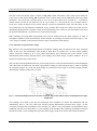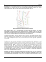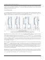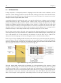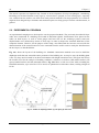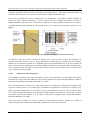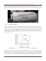
1
Doctoral thesis by:
Luis Segura-Castillo
Directed by:
Antonio Aguado de Cea
Alejandro Josa
Barcelona, September 2013
Universitat Politècnica de Catalunya
Departament d´Enginyeria de la Construcció
DOCTORALTHESIS
Bi-layer diaphragm walls:
Experimental and
numerical analysis.
Curs acadèmic:
Acta de qualificació de tesi doctoral
Nom i cognoms
Programa de doctorat
Unitat estructural responsable del programa
Resolució del Tribunal
Reunit el Tribunal designat a l'efecte, el doctorand / la doctoranda exposa el tema de la seva tesi doctoral titulada
__________________________________________________________________________________________
_________________________________________________________________________________________.
Acabada la lectura i després de donar resposta a les qüestions formulades pels membres titulars del tribunal,
aquest atorga la qualificació:
NO APTE
APROVAT
(Nom, cognoms i signatura)
NOTABLE
EXCEL·LENT
(Nom, cognoms i signatura)
President/a
Secretari/ària
(Nom, cognoms i signatura)
(Nom, cognoms i signatura)
(Nom, cognoms i signatura)
Vocal
Vocal
Vocal
______________________, _______ d'/de __________________ de _______________
El resultat de l’escrutini dels vots emesos pels membres titulars del tribunal, efectuat per l’Escola de Doctorat, a
instància de la Comissió de Doctorat de la UPC, atorga la MENCIÓ CUM LAUDE:
SÍ
NO
(Nom, cognoms i signatura)
(Nom, cognoms i signatura)
Presidenta de la Comissió de Doctorat
Secretària de la Comissió de Doctorat
Barcelona, _______ d'/de ____________________ de _________
Acknowledgments
i
ACKNOWLEDGEMENTS - AGRADECIMIENTOS
Comienzo agradeciendo a las dos personas que hicieron posible esta tesis y, en general, esta experiencia. De
lo general a lo particular, primero, Antonio Aguado, una persona con una visión global excelente, y segundo,
Alejando Josa, detallista y meticuloso. Juntos conforman un equipo magnifico que se complementa casi a la
perfección. Gracias por el tiempo, paciencia y sabiduría que me han dedicado.
Agradezco la financiación brindada por el Ministerio de Educación y Ciencia a través del proyecto BIA201017478: Procesos constructivos mediante hormigones reforzados con fibras. Al Programa de FPU del
Ministerio de Educación por la financiación para la realización del doctorado (AP2010-3789). A Aguado por
la financiación al comienzo de la tesis a través del proyecto: CTT-8062. Y al Instituto de Estructuras y
Transporte de la Universidad de la República (Uruguay), por el constante apoyo recibido.
Al personal del Laboratorio de Tecnología de Estructuras, en especial Jorge Cabrerizo, por su ayuda durante
la campaña experimental. Mi recuerdo a Luis Agulló, que empapaba el ambiente con su alegría. A todos los
compañeros de doctorado: André, Francisco, Francesc, Albert, Nayara, Ju, Izelman, Sandra, Pau, Ana,
Ahmed, Amin, Liao, Nacho, Catalina, Luca, Yohei, Renan, Júlia. Un agradecimiento especial a Sergio, que
estuvo siempre dispuesto y abierto, desde el primer al último día, a dar una mano; y otro a Ricardo, con
quien la lucha se trasladó también fuera de la uni.
Agradezco al IET y la FING de la UdelaR, que me han dado la oportunidad de hacer mis primeras armas en
esta carrera, en especial, a Gemma, Berardi, el Guti, y Atilio, que me han incentivado y apoyado desde el
comienzo y hasta el final de esta aventura que ahora culmina. Al equipo de PERMASTOP, en especial a
Raúl Suarez, con quien compartimos días de lucha a pie de obra.
A todos mis compañeros de piso. Gracias Bea, Andrea (gran compañero de lucha, hoy perdido en la batalla),
David, Jada y Maribel. Pero principalmente a Elena y Mar, que me recibieron, cuidaron, animaron, mimaron
e hicieron posible un comienzo genial de esta aventura. Hicieron que a mi llegada a esta nueva vida me
sintiera como en casa, gracias a ustedes Aragó fue mi hogar. …hasta que llegó Coralinda a poner orden...
aunque, en estos años, hemos podido descubrir, con alegría, que debajo de esa Coraza, hay un Corazón.
Mucha gente grande en Barcelona. Oriol y Mireia (que también intentaron hacerme bailar); Tommy, Lea,
Maco (me hicieron sentir más cerco del barrio); Roberto y Alba (y sus verduras orgánicas!); Susana (siempre
en el aire). A Gerard (el orco de la montaña), Maria Isabel (la presidenta), Alejo, Martha Alejandra (te
visitaré en Celaya, Guanajuato, Méjico!) y Jorge, un gran grupo. Matías, el Borges chileno, nuestros
proyectos recién comienzan. Ita, siempre al firme para ver o hacer rock!
A la flía en Uruguay, mamá, Lauri, Valen, Moni, Marga, el piti, Daisy (que se la re jugó con el título!),
Walter, Shirly, Carla, Bruno, Martina y la poripocha!!! Y la flía en Europa: Martina y Francis, Maia,
Marcelo, Sara y Violeta, María y Jorge, que me bancaron en más de un viaje.
A las barras incondicionales de Uruguay, que en algún u otro momento estuvieron para alentar. Toda la
cadena de Letizia, que siempre tiró pa arriba (Silvina, Isabel, Pedro, Gime, Regi, Vale y Sebas, Mati y Pame,
Henry, Piti, Antonio, Sabri, Fito, Ichu, Damian, Pepe, Geral, Naty, Nadia, Javi rock y Pilar) y la gente más
civilizada, Mari y Sebas, Juampi, Sofi y Andres, Niky, Vero y Fede, Joaquín, Ceci y Crufi, Gago, Martín y
Bi-layer diaphragm walls: Experimental and numerical analysis.
ii
Acknowledgments
Dani, y Maxi y Gabi. Gracias Ani, por tu tiempo por aquí. Gracias a toda la familia Coscia. Omar, tus
correos fueron un cable directo con el paisito, al igual que las novedades y fotos (y hasta algún libro) que me
tiraba Mario de vez en cuando.
Thanks to Simon and Chris, for the opportunity to live the great academic, personal and Olympic experience
in Loughborough! The two big lofbra guys, Dave (A.M.) & James (A.K.), you make a wonderful team, hope
to see you soon. Pratesinha bonina, thanks for the long nights of wine, laugh and crazy talks. And F., please,
remember!
Por último, quiero destacar a personas especiales. A pesar de la distancia, la vida, el tiempo y el espacio,
tienen un lugar importante en mí, en algún lugar de mi corazón, y me ayudaron a avanzar en este proyecto
sabiendo que más cerca o más lejos siempre estaban ahí. Isaac, desde el comienzo hasta el fin! (miro con
ternura la manga de mi camiseta). Flo, una guerrera de la vida, armada con su alegría. Gracias por
compartirla conmigo. Silvana, gracias por todos los almuerzos, y por guiarme en los senderos de esta
existencia espiritual. Vic, gran compañera de la vida. Fabián, creo que hablamos 3 veces en estos 4 años,
pero cada una de esas veces, me sentí en el parque de los niños con un rosado glamour, te extraño. Veronika,
I enjoyed and grew with you, thank for all what we have lived together. Leo, el mejor compañero de viaje.
Giulia, ambarabà ciccì coccò! Abus, gracias por estar siempre esperándome con un café con leche y
galletitas. Poly, te quiero! Angel, Navegar e preciso viver nao e preciso. Nuestros botes no van juntos, pero
se cruzan soplados por los mismos vientos. Caro, siempre ahí, al firme, Beleza! Marga, que me ha sabido
malcriar en cada visita, aguantar todos mis llamadas pre-viajes, y hacerme sentir que siempre estaba cerca.
Lulu, alma hermana, gracias por estar cerca e iluminar mi vida con tus reflexiones y, sobre todo, con tu
sonrisa, alimento de mi alma.
Esta tesis está dedicada a la memoria de tres grandes, que forjaron gran parte de lo que soy. Mi viejo sembró
la semilla de la curiosidad por la vida, me enseñó a dudar, a mirar con ojo crítico la vida. Con Juancito
exploramos y explotamos en discusiones metafísicas existenciales. Ese huracán de ideas, sentimientos y
pasiones que eran el, e hicieron temblar mis cimientos. Pocho es un faro de luz, que sigue iluminando,
marcando el rumbo al que quiero ir, en el que la calidad humana está por encima de todo. A los tres, Gracias.
Luis Segura-Castillo
Summary
iii
SUMMARY
Leakage is a widespread problem associated with the construction of diaphragm walls whenever they are
erected in water-bearing ground. The aim of the present research is to develop a new type of slurry wall: the
bi-layer diaphragm wall (BL), which main objective is to tackle the aforementioned problem. The method to
construct it is based on an existing solution: casting a second waterproof concrete layer against the
diaphragm walls. In the BL technique, the second layer is made of steel fibre reinforced concrete (SFRC)
sprayed over the conventional diaphragm wall (called Mono-Layer diaphragm wall (ML) in this thesis),
including a waterproof admixture. The central idea is to maximize the functional attributes of the second
layer, allowing it to play a structural role in addition to the waterproofing function.
The proposed methodology is based on a combination of experimental works and numerical tools. A design
method for the BL walls, which is based on an uncoupled structural-section model, is proposed. The method
is later used to carry out different comparisons with ML walls and an exhaustive parametric analysis of the
construction processes involved in the walls construction. The experimental campaign comprised test at two
levels. At element level, the structural response of walls built in a real building located in Barcelona was
studied and, at section level, the bond strength between concretes of cores extracted from the
abovementioned walls was measured.
The model at structural level, which is based on a finite element model, was contrasted with the results
obtained in the experimental walls. The sectional analysis is taken from the specialized literature. With the
complete structural-section model, the BL walls are analysed. The study shows that the main flexural
resistance is provided by the first layer (the conventional diaphragm wall), providing the SFRC layer a
secondary flexural resistance.
For the geometrical ranges of the elements considered in the thesis (35 cm to 60 cm width first layer, and 10
cm width second layer) the increase in the cross-section ultimate bending resistance when it is strengthened
by the SFRC layer is between 8% and 15%. This increase allows a reduction in the steel reinforcement of the
first layer (up to 7.0% of the total flexural reinforcement) and, to some extent, it also collaborates with a
displacement reduction (reducing up to 7.3% of the maximum displacements). It was also found that the
spraying sequence is a crucial parameter to be able to take advantage of the SFRC collaboration, and specific
indications are described.
Good concrete to concrete bond strength was obtained for the extracted cores. The average shear strength
value measured for each age (2, 6 and 35 days) was always above 1.0 MPa for the different cases. Beyond
the local test performed, a monolithic behaviour was observed at element level in the experimental walls.
A similar final material consumption was observed between the BL walls and the combined consideration of
a ML wall and an external waterproof system. The consideration of the technology cost entails a higher
construction cost for the BL technique. However, it is still an interesting option under particular
circumstances, like space limitations or if continuous maintenance costs want to be avoided in the future.
In general terms it can be said that the research herein presented lay the foundation for the development of
the bi-layer diaphragm wall technique, which is a promising solution for the leakage problem of diaphragm
walls. Nonetheless, more studies are needed to be able to fully use these types of walls as a standard
Bi-layer diaphragm walls: Experimental and numerical analysis.
iv
Summary
technique, e.g. a detailed cost study and sustainability analysis, debonding risk, waterproofing capability and
above all more full scale experimental cases.
Luis Segura-Castillo
Summary
v
RESUMEN
Un problema habitual en la construcción de pantallas continuas en terrenos con presencia de agua es la
existencia de filtraciones. El objetivo de esta tesis busca resolver este problema mediante el desarrollo de un
nuevo tipo de pantalla: la pantalla bi-capa (BL, por sus siglas en inglés). El método para construir estos
muros se basa en una solución existente: realizar una segunda capa de hormigón impermeable sobre los
muros pantalla. En las pantallas BL, la segunda capa se realiza con hormigón con fibras de acero (SFRC)
proyectado sobre las pantallas convencionales (llamadas ML en esta tesis) e incluyendo a su vez una adición
impermeabilizante. La idea central es maximizar las funciones de la segunda capa, asignándole un rol
estructural, además de la función impermeabilizante.
La metodología propuesta se basa en la combinación de trabajos experimentales y herramientas numéricas.
Se propone un método de diseño para las pantallas BL basado en modelos estructura-sección desacoplados.
Posteriormente se utiliza este método para realizar diferentes comparaciones con pantallas ML y un análisis
paramétrico exhaustivo de distintos procesos constructivos involucrados en la construcción de las pantallas
BL. La campaña experimental realizada comprende dos niveles: a nivel elemento, se estudió la respuesta
estructural de pantallas construidas en un edificio real ubicado en Barcelona; a nivel seccional, se midió el
nivel de adherencia entre ambas capas de hormigón mediante testigos extraídos de las pantallas antes
mencionadas.
El modelo a nivel estructural, basado en elementos finitos, se contrastó con los resultados experimentales
obtenidos. El modelo seccional se tomó de la bibliografía estudiada. Con el modelo estructura-sección
completo se analizaron las pantallas BL. El estudio muestra que la principal resistencia flexional es aportada
por la primera capa (el muro pantalla convencional), siendo secundario el aporte de la capa de SFRC.
Para el rango de elementos considerados en esta tesis (35 cm a 60 cm de espesor de primera capa y 10 cm de
segunda), el incremento de la resistencia última a flexión cuando se considera el aporte de la capa de SFRC,
está entre 8% y 15%. Este incremento permite una reducción en el acero de refuerzo de la primera capa de
hasta un 7.0% del total del acero de flexión y, hasta cierto punto, también colabora con una reducción en los
desplazamientos (alcanzando reducciones de hasta un 7.3% del desplazamiento máximo). Se observó
también que la secuencia de proyección es un factor clave a la hora de aprovechar la colaboración extra
aportada por la capa de SFRC. Indicaciones específicas se describen a este respecto.
Se obtuvo una buena resistencia de adherencia entre hormigones para los testigos extraídos. La resistencia
media medida a cada edad (2, 6, y 35 días) estuvo siempre, para los distintos casos, por encima de 1.0 MPa.
Más allá de los ensayos puntuales, se observó un comportamiento monolítico a nivel elemento para las
pantallas BL experimentales.
Se obtuvo un consumo final de materiales similar entre pantallas BL y la consideración conjunta de una
pantalla ML más un sistema impermeabilizante externo. Considerar los costos tecnológicos conlleva un
costo constructivo mayor para las pantallas BL. Sin embargo, ésta es aún una opción interesante bajo
consideraciones particulares, como limitaciones del espacio subterráneo interior o si se desean evitar costos
continuos de mantenimiento.
Bi-layer diaphragm walls: Experimental and numerical analysis.
vi
Summary
En términos generales, se puede decir que la investigación aquí presentada sienta las bases para el desarrollo
de la técnica de muros pantalla bi-capa, la cual es una solución prometedora para el problema de las
filtraciones en pantallas. No obstante, son necesarios más estudios para poder usar plenamente este tipo de
pantallas de forma habitual, e.g. estudios de sostenibilidad detallados, evaluación del riesgo de
desprendimiento de la segunda capa, capacidad impermeable y, sobre todo, más ensayos experimentales a
escala real.
Luis Segura-Castillo
Table of contents
vii
TABLE OF CONTENTS
ACKNOWLEDGEMENTS - AGRADECIMIENTOS ............................................................................................................ I
SUMMARY.............................................................................................................................................................. III
RESUMEN ................................................................................................................................................................ V
TABLE OF CONTENTS.............................................................................................................................................. VII
LIST OF FIGURES ..................................................................................................................................................... XI
LIST OF TABLES ..................................................................................................................................................... XIII
CHAPTER 1.
1.1.
1.2.
1.3.
INTRODUCTION ............................................................................................................................. 1
MOTIVATION...................................................................................................................................................... 1
THESIS OBJECTIVES ............................................................................................................................................ 4
THESIS BACKGROUND ........................................................................................................................................ 5
1.3.1. Diaphragm walls ..................................................................................................................................... 6
1.3.1.1. Calculation methods .................................................................................................................................6
1.3.1.2. FEM in embedded walls problem .............................................................................................................8
1.4.
1.5.
1.6.
1.3.2. Waterproof concrete .............................................................................................................................. 9
1.3.3. Fibre reinforced concrete ...................................................................................................................... 10
1.3.4. Sprayed concrete .................................................................................................................................. 11
1.3.5. Bond between concretes ...................................................................................................................... 13
GENERAL METHODOLOGY ............................................................................................................................... 13
THESIS STRUCTURE .......................................................................................................................................... 15
1.5.1. Chapters outlook .................................................................................................................................. 17
RESERCH FRAMEWORK .................................................................................................................................... 18
CHAPTER 2.
2.1.
2.2.
2.3.
2.4.
2.5.
2.6.
EXPERIMENTAL AND NUMERICAL STRUCTURAL ANALYSIS ........................................................... 21
INTRODUCTION................................................................................................................................................ 22
EXPERIMENTAL PROGRAM .............................................................................................................................. 23
2.2.1. General Information ............................................................................................................................. 23
2.2.2. Construction of experimental bi-layer walls ......................................................................................... 24
2.2.3. Tests and Instrumentation.................................................................................................................... 26
NUMERICAL MODEL ......................................................................................................................................... 27
EXPERIMENTAL RESULTS.................................................................................................................................. 29
2.4.1. Material characterization ..................................................................................................................... 29
2.4.2. Reliability of inclinometers ................................................................................................................... 30
2.4.3. Selection of representative stages ........................................................................................................ 31
MODEL VS. EXPERIMENTAL COMPARISON ...................................................................................................... 32
2.5.1. Model adjustment ................................................................................................................................ 32
2.5.2. Wall behaviour ..................................................................................................................................... 33
DISCUSSION – DESIGN PROCESS AND COMPARISON ....................................................................................... 34
2.6.1. Description of case studies ................................................................................................................... 35
2.6.2. Results for theoretical cases ................................................................................................................. 35
2.6.2.1. Displacements.........................................................................................................................................35
2.6.2.2. Bending moments ...................................................................................................................................36
Bi-layer diaphragm walls: Experimental and numerical analysis.
viii
Table of contents
2.6.2.3. Optimum design .....................................................................................................................................37
2.7.
2.8.
2.6.3. Comparison ........................................................................................................................................... 38
CONCLUSIONS .................................................................................................................................................. 39
ACKNOWLEDGEMENTS .................................................................................................................................... 40
CHAPTER 3.
3.1.
3.2.
3.3.
3.4.
3.5.
3.6.
3.7.
3.8.
INTRODUCTION................................................................................................................................................ 42
METHODOLOGY ............................................................................................................................................... 42
CHARACTERISTICS OF THE WALLS .................................................................................................................... 44
3.3.1. Geometry and construction sequence .................................................................................................. 44
3.3.2. Material and model characteristics ...................................................................................................... 45
STRUCTURAL RESULTS ..................................................................................................................................... 47
SECTIONAL RESULTS......................................................................................................................................... 50
DISCUSSION ..................................................................................................................................................... 52
CONCLUSIONS .................................................................................................................................................. 54
ACKNOWLEDGEMENTS .................................................................................................................................... 55
CHAPTER 4.
4.1.
4.2.
4.3.
4.4.
4.5.
4.6.
5.3.
PARAMETRIC STUDY OF CONSTRUCTION PROCESSES ................................................................... 57
INTRODUCTION................................................................................................................................................ 58
METHODOLOGY ............................................................................................................................................... 59
4.2.1. Model description ................................................................................................................................. 59
4.2.2. Parameters under study ....................................................................................................................... 60
STRUCTURAL AND SECTIONAL RESULTS ........................................................................................................... 62
4.3.1. Influence of the number of spraying stages ......................................................................................... 65
4.3.2. Influence of the depth of the sprayed concrete layer ........................................................................... 67
4.3.3. Influence of the final structure configuration ....................................................................................... 69
4.3.4. Influence of the construction sequence ................................................................................................ 70
4.3.5. Sectional results .................................................................................................................................... 73
ADDITIONAL CONSIDERATIONS ....................................................................................................................... 74
CONCLUSIONS .................................................................................................................................................. 75
ACKNOWLEDGEMENTS .................................................................................................................................... 75
CHAPTER 5.
5.1.
5.2.
STRUCTURAL AND SECTIONAL ANALYSIS...................................................................................... 41
EVOLUTION OF CONCRETE-TO-CONCRETE BOND STRENGTH AT EARLY AGES ................................ 77
INTRODUCTION................................................................................................................................................ 78
EXPERIMENTAL PROGRAM .............................................................................................................................. 80
5.2.1. Preparation of specimens ..................................................................................................................... 81
5.2.2. Shear test .............................................................................................................................................. 83
RESULTS AND DISCUSSION ............................................................................................................................... 84
5.3.1. Mechanical characterization results ..................................................................................................... 84
5.3.2. Shear test results .................................................................................................................................. 85
5.3.2.1.
5.3.2.2.
5.3.2.3.
5.3.2.4.
5.3.2.5.
5.3.2.6.
5.3.2.7.
5.4.
5.5.
Types of failure .......................................................................................................................................85
Shear stress depending on age ...............................................................................................................87
Shear stress on saturated surfaces .........................................................................................................88
Shear stress on epoxy-bonded surfaces .................................................................................................88
Milling direction ......................................................................................................................................89
Shear angle .............................................................................................................................................90
Relationship between concrete shear strength and compressive strength............................................91
CONCLUSIONS .................................................................................................................................................. 92
ACKNOWLEDGMENTS ...................................................................................................................................... 93
Luis Segura-Castillo
Table of contents
CHAPTER 6.
6.1.
6.2.
6.3.
6.4.
ix
CONCLUSIONS AND FUTURE PERSPECTIVES ................................................................................. 95
INTRODUCTION................................................................................................................................................ 95
GENERAL CONCLUSIONS .................................................................................................................................. 96
SPECIFIC CONCLUSIONS ................................................................................................................................... 97
6.3.1. Viability of the proposed solution. ........................................................................................................ 97
6.3.2. Bond strength reached between the concrete layers. .......................................................................... 97
6.3.3. Structural behaviour of the bi-layer diaphragm walls. ......................................................................... 98
6.3.4. Overall flexural design model (structural and sectional level). ............................................................. 98
6.3.5. Influence of the different constructions processes related to this type of walls. .................................. 98
6.3.6. Efficiency of the bi-layer walls compared with equivalent conventional diaphragm wall alternatives.
99
6.3.7. Dissemination of the results. ................................................................................................................ 99
FUTURE PERSPECTIVES .................................................................................................................................... 99
6.4.1. Crucial research lines .......................................................................................................................... 100
6.4.2. Other research lines ............................................................................................................................ 100
REFERENCES ........................................................................................................................................................ 101
APPENDIX 1.
OFF TESTS
EARLY AGES CONCRETE-TO-CONCRETE BOND STRENGTH ASSESSED THROUGH SHEAR AND PULL111
A1.1. INTRODUCCIÓN ............................................................................................................................................. 112
A1.1.1.
Impermeabilización en pantallas continuas ................................................................................ 112
A1.1.2.
Marco general del proyecto ......................................................................................................... 112
A1.1.3.
Adherencia entre hormigones...................................................................................................... 113
A1.2. OBJETIVOS...................................................................................................................................................... 114
A1.3. METODOLOGÍA .............................................................................................................................................. 114
A1.3.1.
Programa experimental ............................................................................................................... 114
A1.3.2.
Zonas de extracción de testigos ................................................................................................... 116
A1.3.3.
Ensayo a corte.............................................................................................................................. 117
A1.3.4.
Ensayo pull-off ............................................................................................................................. 117
A1.4. RESULTADOS Y ANALISIS ................................................................................................................................ 118
A1.4.1.
Resultados principales del ensayo de corte ................................................................................. 118
A1.4.1.1. Preparación por fresado .......................................................................................................................118
A1.4.1.2. Preparación con puente de adherencia epoxi ......................................................................................120
A1.4.2.
Resultados pull-off ....................................................................................................................... 120
A1.4.3.
Relación corte/pull-off ................................................................................................................. 123
A1.5. CONCLUSIONES .............................................................................................................................................. 124
A1.6. AGRADECIMENTOS ........................................................................................................................................ 125
A1.7. ANEXO – RESULTADOS EXPERIMENTALES DEL ENSAYO PULL-OFF ................................................................................. 126
Bi-layer diaphragm walls: Experimental and numerical analysis.
x
Table of contents
Luis Segura-Castillo
List of figures
xi
LIST OF FIGURES
Fig. 1 - Typical defects of diaphragm walls in joints between panels. .............................................................. 2
Fig. 2 - Bi-layer diaphragm walls. a) general scheme; b) compound section; c) simple section; and d)
spraying of an experimental wall. ....................................................................................................... 4
Fig. 3 - Main knowledge areas needed to materialize the bi-layer diaphragm walls......................................... 5
Fig. 4 - Typical ultimate states modes in embedded walls. [Fuente: Eurocode 7 (EN, 2004a)] ....................... 7
Fig. 5 - Outline of the thesis. ........................................................................................................................... 17
Fig. 6 - Experimental building: (a) site plan; (b) general cross-section; (c) detail of bi-layer cross-section... 23
Fig. 7 - Wall construction sequence ................................................................................................................ 24
Fig. 8 - Bi-layer walls: (a) Spraying of second layer; (b) finished sprayed surface ........................................ 26
Fig. 9 - Finite Element mesh of W35 wall ...................................................................................................... 27
Fig. 10 - Inclinometer results of W35 wall: a- Incremental displacements; b- Check-sum values ................. 30
Fig. 11 - Incremental displacements at the same structural stage and at different times for W35 (Reference
stage: PreElim150) ............................................................................................................................ 31
Fig. 12 - Comparison of incremental displacement values calculated by the PLAXIS model and experimental
values for the representative stages of Wall W35. (Reference stage: Exc180) ................................. 32
Fig. 13 - Comparison of incremental displacements calculated with the PLAXIS model and experimentally
obtained for the representative stages of Wall W45 ......................................................................... 33
Fig. 14 - Horizontal displacements and bending moments obtained by the adjusted PLAXIS model for Wall
W35 ................................................................................................................................................... 34
Fig. 15 - Horizontal displacements and bending moments obtained by the adjusted PLAXIS model for Wall
W45 ................................................................................................................................................... 34
Fig. 16 - Horizontal displacements obtained by the PLAXIS model for the T.BLW45 design ...................... 36
Fig. 17 - Maximum displacements for the three comparative cases................................................................ 36
Fig. 18 - Bending moments obtained by the PLAXIS model for the T.BLW45 design example ................... 37
Fig. 19 - Bending moment envelopes for the three comparative cases ........................................................... 38
Fig. 20 - (a) Sectional discretization; (b) SFRC and (c) steel bar constitutive equations. ............................... 43
Fig. 21 - (a) Model geometry: Anchorages and slabs positions; (b) Simple Section; (c) Compound Section 44
Fig. 22 - Finite element model mesh and main elements ................................................................................ 46
Fig. 23 - Wall displacements: “Anc.Out” stage for the three walls ................................................................. 47
Fig. 24 - Bending moments: (a) Envelopes for the three wall types; (b) Representative stages and envelopes
for the “BL60+10” wall type; (c) envelope areas for all three wall types......................................... 48
Fig. 25 - Diagrams of moments at stages prior to the second anchor installation ........................................... 49
Fig. 26 - Ultimate and design moments for the “BL60+10” wall ................................................................... 52
Fig. 27 - Bi-layer diaphragm walls. a) general scheme; b) compound cross-section; c) simple cross-section;
and d) spraying of an experimental wall. .......................................................................................... 58
Fig. 28 - Final construction design: (a) 2 levels “2u”; (b) 4 levels “4u”. ........................................................ 61
Fig. 29 - Construction sequences: (a) Bottom-Up “BU”; (b) Top-Down “TD”. ............................................. 62
Fig. 30 - Spraying discretization considered. .................................................................................................. 62
Fig. 31 - Example of bi-layer wall bending moment envelopes. ..................................................................... 64
Fig. 32 - Bending moment envelope for different spraying discretizations: (a) 1 spraying stage; (b) 2 spraying
stages; (c) 4 spraying stages. ............................................................................................................. 66
Fig. 33 - Displacements for different spraying discretizations. ....................................................................... 67
Fig. 34 - Bending moment envelope for cases with different depths of sprayed concrete layer: (a) general; (b)
detail. ................................................................................................................................................. 68
Bi-layer diaphragm walls: Experimental and numerical analysis.
xii
List of figures
Fig. 35 - Bending moment envelope for two final structural set-ups: (a) 4 underground levels; (b) 2
underground levels. ........................................................................................................................... 69
Fig. 36 - Displacements for different final structure configurations. .............................................................. 70
Fig. 37 - Bending moment envelope for different construction sequences: (a) Bottom-Up with struts; (b)
Bottom-Up with anchorages; (c) Top-Down. ................................................................................... 71
Fig. 38 - Displacements for different construction sequences. ........................................................................ 72
Fig. 39 - Design and ultimate bending moments envelope examples: (a) efficient design; (b) inefficient
design; (c) large increase in bending moments after spraying; (d) Top-Down case. ........................ 73
Fig. 40 - Sketch of bi-layer wall: general and sectional view. ........................................................................ 78
Fig. 41 - Details of diaphragm walls: (a) site plan; (b) side view.................................................................... 80
Fig. 42 - Main steps in the production of the specimens: (a) milling the wall built in the first phase; (b)
finished surface; (c) water-jet washing; (d) placing the bonding agent; (e) area of water leakage; (f)
spraying the second layer of concrete. .............................................................................................. 82
Fig. 43 - LCB shear test: (a) device sketch, (b) test configuration. ................................................................. 84
Fig. 44 - Core positions for shear test. ............................................................................................................. 84
Fig. 45 - Typical shear test strength-displacement graph. ............................................................................... 86
Fig. 46 - Failure mechanisms in the test. ......................................................................................................... 86
Fig. 47 - Atypical failure: (a) stone chip protruding on one side, (b) on two planes. ...................................... 87
Fig. 48 - Shear stress vs. age of second-phase concrete: surface preparation with milling (MP) and saturated
surface (SP). ...................................................................................................................................... 87
Fig. 49 - Shear stress vs. age of second-phase concrete, surface preparation with epoxy (EP). ..................... 89
Fig. 50 - Direction of stress with regard to milling (MP case). ....................................................................... 89
Fig. 51 - Milling marks on tested cores. .......................................................................................................... 90
Fig. 52 - Failure plane angle. ........................................................................................................................... 91
Fig. 53 - Influence of failure angle on shear strength. ..................................................................................... 91
Fig. 54 - Influence of the strength of base concrete on shear strength (MP case). .......................................... 92
Fig. 55 - Defectos usuales en pantallas continuas: a- Diferencias de posición entre bataches adyacentes, bPérdidas entre juntas durante construcción, c- Pérdidas que aparecen ya en servicio .................... 112
Fig. 56 - Esquema de la solución por muro Bi-Capa. Vista general y vista de una sección.......................... 113
Fig. 57 - Detalle de las pantallas: a) Plano del sitio de obra; b) corte lateral ................................................ 115
Fig. 58 - Esquema de posiciones de extracción de testigos para el ensayo de corte y de realización de ensayos
pull-off in-situ para las distintas preparaciones, e imagen de la pantalla luego de realizadas las
extracciones ..................................................................................................................................... 116
Fig. 59 - Ensayo de Corte LCB: (a) Esquema del dispositivo, (b) Configuración del ensayo ...................... 117
Fig. 60 - Ensayo Pull-off: (a) Esquema del ensayo, (b) Configuración del ensayo....................................... 118
Fig. 61 - Resistencia a corte vs edad del hormigón de 2ª fase ....................................................................... 119
Fig. 62 - Desviación estándar obtenida para las distintas edades .................................................................. 119
Fig. 63 - Resistencia a tracción vs edad del hormigón de 2ª fase para preparación por Fresado .................. 120
Fig. 64 - Resistencia a tracción vs edad del hormigón de 2ª fase para preparación con adhesivo Epoxi ...... 121
Fig. 65 - Esquema de irregularidades en la interfase entre capas y superficie de pantallas .......................... 122
Fig. 66 - Foto del acabado final del proyectado en los muros Bi-Capa ......................................................... 122
Fig. 67 - Ejemplo de desalineaciones sufridas durante la realización del ensayo pull-off ............................ 123
Fig. 68 - Resistencia a tracción vs Resistencia a corte para preparación por Fresado................................... 123
Fig. 69 - Resistencia a tracción vs Resistencia a corte para preparación con adhesivo Epoxi ...................... 124
Luis Segura-Castillo
List of tables
xiii
LIST OF TABLES
Table 1 - Classification and examples of permeability-reducing admixtures ................................................. 10
Table 2 - Summary of objectives and methods ............................................................................................... 15
Table 3 - List of papers and conference papers related to the thesis. .............................................................. 16
Table 4 - Connection between main areas, papers and methodology used. .................................................... 17
Table 5 - Sequential stages of wall construction ............................................................................................. 25
Table 6 - Anchorage properties ....................................................................................................................... 25
Table 7 - Geotechnical parameters used in the PLAXIS model ...................................................................... 28
Table 8 - Thickness and flexural and normal stiffness of the walls used in the PLAXIS model. ................... 28
Table 9 - Compressive strength of concrete in both phases ............................................................................ 29
Table 10 - Sequence of construction stages of theoretical walls ..................................................................... 35
Table 11 - Main results of theoretical comparison performed with PLAXIS model ...................................... 38
Table 12 - Construction stages sequence ......................................................................................................... 45
Table 13 - Flexural and normal stiffness of the different walls ....................................................................... 46
Table 14 - Reinforcements and MU of the different wall types ....................................................................... 51
Table 15 - Comparison of different waterproofing systems ............................................................................ 53
Table 16 - Parameters and alternatives for each case. ..................................................................................... 61
Table 17 - General results for all cases............................................................................................................ 63
Table 18 - General results for the additional cases .......................................................................................... 75
Table 19 - Concrete dosages............................................................................................................................ 81
Table 20 - Types of surface preparation. ......................................................................................................... 83
Table 21 - Compressive strength of concrete in both phases. ......................................................................... 85
Table 22 - Shear test results............................................................................................................................. 85
Table 23 - Resultados ensayo pull-off. .......................................................................................................... 126
Bi-layer diaphragm walls: Experimental and numerical analysis.
xiv
List of tables
Luis Segura-Castillo
CHAPTER 1.
INTRODUCTION
1.1. MOTIVATION
An extended underground infrastructure is nowadays needed in large cities to achieve a sustainable
development (Bobylev, 2006). The compact city strategy, which aims an efficient use of space, specially
below ground level, is one of the possible paths to allow it (Durmisevic, 1999). Moving activities of lesser
social importance (traffic or parking) underground is useful in order to reduce noise pollution and polluting
emissions, protecting the urban environment, ancient buildings, and parks (Rönkä, Ritola, & Rauhala, 1998).
At the same time, placing some functions (e.g. leisure and recreational activities; traffic facilities: tunnels
and car parking; technical maintenance facilities: sewage treatment or power plants) underground, free
aboveground space that can be addressed to recreation and social activities (Durmisevic, 1999).
There are mainly two methods of building underground structures: (a) excavation in an open cut from ground
level; and (b) mining or boring in tunnels. These methods must be implemented without affecting existing
buildings and infrastructures adjacent to the construction site and minimizing the alterations to the daily
activities of the city. In this city scenario, where ground deformations must usually be controlled to avoid
damage to existing buildings, the diaphragm wall technique represents a particularly viable solution when the
first of the abovementioned options is used (Rodriguez Liñan, 1995).
2
Chapter 1
Diaphragm walls (also called slurry walls) (EN 1538, 2010) started being constructed in Italy in the 1950s
(Ou, 2006; Puller, 1994). A synthetized definition of the technique was given by El Hussieny (El Hussieny,
1992), describing the diaphragm walls as “artificial membrane of finite thickness and depth, constructed in
the ground by means of a process of trenching, with the aid of a fluid support”. This is, with a dragging tools
a narrow trench is excavated. While the excavation takes place a stabilizing fluid (bentonite slurry) is
introduced. When the excavation is complete the reinforcement cage is introduced into the trench and the
concrete is cast by tremie pipes, displacing and allowing recovery and recycling of the stabilizing fluid from
the bottom up.
Although their basic principle reminds the same, the technique has been developed, improving the methods
and equipment (e.g.: different types of dragging tools are now available: drilling bit, hydrophraise (or
hydrofrase), trenchcutter, hydraulic grab, mechanical grab, clamshell; improved stability of the cutting face
of the excavation; reduced leakages at panel vertical joints; allowance of force transmission between panels;
improved bracing and anchoring systems), turning it into a competitive solution for deep excavation works.
Moreover, the functionality of diaphragm walls has also widened, being nowadays used as retaining walls,
load bearing walls, cut-off walls, or a combination of the aforementioned.
Despite the technical advances, the technique still presents some drawbacks. One widespread problem
associated with this construction technique is leakage whenever the walls are erected in water-bearing
ground (Puller, 1994), being their waterproof capacity a source of debate since the first walls of this type
were built. Although leakage in the walls can occur for several reasons (detailed in (Puller, 1994)), the main
one is that generally, the joints between panels develop cracks which provide a path for water ingress and,
therefore, have certain degree of permeability (Brown & Bruggemann, 2002; EN 1538, 2010; ICE, 2007;
Puller, 1994). As an example, three diaphragm wall joints can be seen in Fig. 1, where (a) the union of panels
present a tilt, (b) water leakage appeared during construction, and (c) the water leakage appeared after the
structure had been completed.
Fig. 1 - Typical defects of diaphragm walls in joints between panels.
Temporary stop-end is the usual system used in joints to connect the panels (Brown & Bruggemann, 2002).
Even if there is a thin layer of bentonite in the joints, which usually have an acceptable degree of
waterproofness, the deflections in the wall during the excavation process create paths that allow a water flow
(Ou & Lee, 1987). Several methods have been developed to improve the joints against leakages, like water
stop joints (Puller, 1994) or end-plates (overlapping joint) (El-Razek, 1999; Ou & Lee, 1987).
Luis Segura-Castillo
Introduction
3
Notwithstanding the efforts made to achieve waterproofness, there is a general consensus among contractors
and researchers that there is no effective technique to make joints fully watertight (ICE, 2007; Puller, 1994;
Wong, 1997), especially if there is a high water table in the exterior of the walls. Accordingly, ICE guide
states that a complementary waterproof system should be added if a good level of watertightness is needed
(ICE, 2007). With this porpoise, several techniques have been developed to prevent or repair the existence of
leaks (Puller, 1994).
A usual technique is to repair the affected areas as they are detected, injecting a chemical grout into the
problematic cracks and joints, or directly chipping and restoring the element with a more waterproof mortar
(also called grouting (Wong, 1997)). In a similar way, a cement or chemical grout can be injected in the soil
behind the wall, in the areas where leakage is observed (Puller, 1994). (El-Razek, 1999) reported having
successfully used this solution in a diaphragm wall project in Alexandria. However, leakage usually appears
only over lengthy periods and at different times and areas of a wall (see Fig. 1c), even becoming worse with
time (Wong, 1997), which may result in extensive repair works over indefinite periods that require several
sessions, causing problems for both owners and contractors.
Another solution consists of casting an additional layer of mortar or concrete on the interior face of the walls
(also called tanking), which is also a common way to make walls of bored piles watertight (Wong, 1997). As
it can be seen in Fig. 1, it is not strange that deviations from true verticality occur in the panels as they are
constructed. A favourable effect of this technique is that the second layer evens the surface when
irregularities caused by panel deviations are detected.
Few publications were found reporting this solution. For example, (Li, Ju, Han, & Zhou, 2008) used it as a
way to study tensile creep in concrete. Two arranges for the connection between linings that reflect different
possibilities to be used in a real underground structure were studied: (a) continuous design, which connect
both layers with extruding reinforcements; and (b) sliding design, which put an impermeable sheet in
between both concrete layers. Meanwhile, (Sherif & Kudsi, 1975) performed a risk analysis on a double
wall, aiming to quantify the cracking probability, which would lead to leaks.
Since the publication of codes that define three grades of waterproofing protection for underground
structures (e.g. (BS 8102, 2009) or its previous versions) it became common practice in the United Kingdom
(and spread to other countries like USA or Germany) to deal with the waterproof problem by constructing an
inner wall separated by a cavity (Puller, 1994). In this system, the water is directed to an inferior deposit and
pumped out from there. The solution is referred as false wall (Wong, 1997), or drained cavity (BS 8102,
2009).
Nowadays, drained cavities are extensively used. However, this solution loses significant volume because of
the construction tolerances and the cavity. In some cases, the extra space required may have a crucial
influence in the final project value. For example, if an inner leaf 15 cm wide separated by a cavity 10 cm
wide is considered (neglecting construction tolerances), 25 cm in contact with every diaphragm wall would
be lost. In a vehicles parking basement, the additional space would represent the difference to afford a
parking place intended for a luxury car. In addition to the space lost, a drained cavity may, in the worst case,
hide dangerous leakages and even structural problems (Puller, 1994).
Bi-layer diaphragm walls: Experimental and numerical analysis.
4
Chapter 1
In below-grade structures in general, it can be said that leakages are originated mainly by poor design and
workmanship rather than the selection of materials. Therefore the key to avoid leakages resides in the design
and implementation (Shohet & Galil, 2005). Beyond the waterproof method, the early selection of the type of
wall, the construction sequence, and the temporal and permanent use of the retaining structure have a
positive effect on the final cost. Hence, client, designer, and contractor should all be involved in the project
at an early stage (Gaba, Simpson, Powrie, & Beadman, 2003). A holistic vision of the project requirements
should be adopted to achieve optimization, in which the costs of material consumption, the final dimensions
of the wall, maintenance requirements, and construction complexity should all be evaluated throughout its
entire life cycle. Furthermore, to achieve sustainable design the best strategy is to consider environmental
aspects also right from the start of the design process (Kurk & Eagan, 2008).
1.2. THESIS OBJECTIVES
The aim of the research was to develop a new type of slurry wall: The bi-layer diaphragm wall. The method
to construct it is based on the tanking solution described above, where a second waterproof layer is casted
against the diaphragm walls.
The bi-layer diaphragm wall is made of two bonded concrete layers poured and then sprayed, in separate
stages. The first is a conventional Reinforced Concrete (RC) diaphragm wall. Once this wall attains the
necessary strength, soil within the perimeter is excavated and removed, and the second layer, this time of
sprayed Steel Fibre Reinforced Concrete (SFRC) with a waterproof additive, is applied. The solution is
schematically presented in Fig. 2.
Fig. 2 - Bi-layer diaphragm walls. a) general scheme; b) compound section; c) simple section; and d) spraying of
an experimental wall.
The idea is to maximize the functional attributes of the second layer, allowing it to play a structural role, in
addition to its initial intended purpose (waterproofing). Due to the structural role of the second layer, the
thickness and reinforcement of the first layer may be reduced, becoming an attractive structural solution if
the waterproofness is also considered.
Luis Segura-Castillo
Introduction
5
The objectives of the research were:
O1.
Corroborate the viability of the proposed solution.
O2.
Assess the bond strength reached between the concrete layers.
O3.
Assess the structural behaviour of the bi-layer diaphragm walls.
O4.
Develop an overall flexural design model (structural and sectional level).
O5.
Quantify the efficiency of the method when compared with equivalent conventional diaphragm wall
alternatives.
O6.
Study the influence of the different constructions processes related to this type of walls.
O7.
Disseminate the results.
1.3. THESIS BACKGROUND
As it was seen in the previous section, many and diverse disciplines have to be combined in order to
materialize this new structural element. The more important ones are shown in Fig. 3, where some of the
interconnections are schematically represented.
Fig. 3 - Main knowledge areas needed to materialize the bi-layer diaphragm walls
A brief introduction to these topics, which conforms the background of the thesis is presented in this section
with the following aims: a) define the terminology used in the thesis; b) summarize key points in every topic;
and c) guide the reader into specialized bibliography.
Bi-layer diaphragm walls: Experimental and numerical analysis.
6
Chapter 1
1.3.1. Diaphragm walls
A definition of diaphragm wall has already been given in previous sections together with a small description
of the technique. There are several books addressing this structural element (e.g. (Schneebeli, 1981;
Xanthakos, 1979)) and also a European code related to it (EN 1538, 2010).
Diaphragm walls are classified as flexible in the group of the excavation retaining structures, as its
deformation influences in the general behaviour of the element and therefore in the way the element is
designed. In this group it can also be found the following types of walls: sheet pile wall, soldier pile wall
(also called: king post wall), contiguous bored pile wall, and secant bored pile wall.
The walls can be further classified in accordance with different criteria like its structural configuration under
construction (e.g. cantilever, anchored, braced; top-down construction, island excavation, or zoned
excavation) (Ou, 2006). In the first of them (cantilever), the structure stability depends entirely on the
passive earth pressures, while in the others the stability is also given by one or several propping lines.
Furthermore, the propped walls are usually sub-classified in walls with one prop level, or multiple prop
levels.
The prop support system may be temporal (e.g. bracing, temporal anchors, ring wales) or permanent (e.g.
beams or slabs, permanent anchors), and its use depends on the construction sequence adopted. A complete
description of ground anchors for retaining structures can be found in (Fang, 1995).
In this thesis, only propped walls (both in one or multiple levels) are used, conveniently alternating the props
between active anchors, struts, or the structure slabs as required.
1.3.1.1. Calculation methods
Earth retaining structures are designed to withhold both the soil pressures and the external loads that may be
applied to it, being able to retransmit them to the foundation soil, under controlled deformations, and
avoiding the collapse both of the structure and the surrounding soil.
Accordingly, Eurocode 7 (EN, 2004a) specifies two kind of checks to design retaining structures:
serviceability limit state, and ultimate limit state. For the first of them the code is focused in the control of
the displacements of the walls and the ground adjacent to them, mainly in order to avoid damage to existing
adjacent buildings. Regarding the ultimate limit state, the code states:
“The design of retaining structures shall be checked at the ultimate limit state for the design
situations appropriate to that state”.
For embedded walls, there are mainly four groups of ultimate states modes that shall be checked: a) Overall
stability, b) Rotational failure, c) Vertical failure, and d) Structural failure. They can be seen schematically
represented in Fig. 4. Although the first three groups are checked in the cases used in this thesis, they are not
presented, as the thesis is centred in the structural behaviour of the diaphragm walls. Furthermore, when
possible, cases with a large security factor against these modes were used to avoid any possible interaction
with the structural failure.
Luis Segura-Castillo
Introduction
7
There are currently in use a variety of methods to check the previously mentioned ultimate states in order to
design embedded walls. A State of the art about the different available calculation methods was performed
by (Delattre, 2001), were the evolution and development of the different methods is described. According to
(Delattre, 2001), the diversity of methods arises from the complexity of the geotechnical structure, which is
both supported but also loaded by the soil. (Delattre, 2001) classified the methods in the following
categories: (1) classical methods, (2) subgrade reaction method, (3) finite element method and (4) empirical
methods. The different methods are able to tackle, with different precision, the different ultimate states that
should be checked.
The classical design methods are based on the classical Coulomb and Rankine soil behaviour methods and
their extensions. These methods are centred on the pressures exerted on the structures by the soil, not taking
into account the deformations of the structures and the adjacent soil.
The subgrade reaction method (based on the Winkler model) was later developed. It is able to take into
account the soil and structure deformations considering the properties of both the soil and the retaining wall,
and its interaction. However, like the classical methods, it is still not able to take into account the arching
effect.
Fig. 4 - Typical ultimate states modes in embedded walls. [Fuente: Eurocode 7 (EN, 2004a)]
The empirical approach was mainly used in the English-speaking countries. It is based on comparing the
characteristics of the project with monitored case histories results of resembling excavations.
Bi-layer diaphragm walls: Experimental and numerical analysis.
8
Chapter 1
Finally, from the 1970s, with the advance in the numerical methods and the generalization of computer
calculations, the finite element method started to be used in geotechnical problems. The soil is considered as
a continuum, which is discretized in several finite elements. Being both the structure and the soil modelled, it
allows a more comprehensive representation which includes its interaction and the arch effect. Also,
information of all the soil under study is obtained (Sanhueza Plaza & Oteo, 2007).
1.3.1.2. FEM in embedded walls problem
(Potts & Zdravković, 1999) and (Ou, 2006) can be named as example of books focused on geotechnical
analysis through the FEM method.
A positive aspect of the method is that, in theory, as more factors are appropriately considered in the FEM
models the accuracy of the results would be higher than the previous ones. On the other hand, the theories in
which the method is based are wide more complex, as it is also its application, including pre and post
processing. Furthermore, some of the theories and models are still under development (Ou, 2006) and, for
every soil model, specific soil parameters need usually to be evaluated to have the required input data to
acceptably model the soil behaviour.
Nowadays, the more widespread soil models used in FEM studies of diaphragm walls include: the wellknown elastic-perfectly plastic “Mohr-Coulomb” (“MC”), the modified Cam Clay (“MCC” (Roscoe &
Burland, 1968)), the Hyperbolic (“Hyp” (Duncan & Chang, 1970)), and the hardening soil (“HS” (Schanz,
Vermeer, & Bonnier, 1999)) and, to a lesser extent, more advanced models such as the “MIT-E3” (Whittle,
1987).
As the accuracy of FEM-based models depends to a large extent on the selection of appropriate parameters to
represent the constitutive behaviour of soils (Khoiri & Ou, 2013), many researchers focused their attention
on direct or inverse ways to determine those parameters. For example, (Khoiri & Ou, 2013) used the MC and
HS models to predict deformations based on measured data at the first excavation stage, also measuring the
soil Young’s modulus aiming to correlate it with the previous prediction; (Ou & Lai, 1994) analysed layered
sandy and clayey soil using both the Hyp and the MCC models and establishing a procedure to determine the
soil parameters; and (Calvello & Finno, 2004) (Hashash, Levasseur, Osouli, Finno, & Malecot, 2010)
calibrated the soil parameters through back analysis.
There are many recent examples of studies, based on these methods, related to the design of diaphragm
walls. For example, improvements of the empirical methods were performed by (G. T. C. Kung, Juang,
Hsiao, & Hashash, 2007) and (Bryson & Zapata-Medina, 2012), who proposed new semi-empirical methods
based on FEM parametrical analysis; the construction sequences were analysed and compared by (G. T.-C.
Kung, 2009); different soil models (MCC, two variations of HS, MC and “undrained soft clay model”) were
analysed and compared by (Lim, Ou, & Hsieh, 2010) under undrained conditions, who concluded that all
models could predict, with a correct parameter selection, the wall deflections, but only the last one was able
to predict surface settlements correctly; finally, it can be mentioned the (Ou, Chiou, & Wu, 1996) study on
the influence of the spatial effects in the wall behaviour.
It can be concluded that, in the last years, the FEM method (using the abovementioned soil models) has been
frequently and increasingly being used to address wide different aspects of the diaphragm wall technique. In
Luis Segura-Castillo
Introduction
9
the majority of studies, the focus is put both in the displacements of the wall and of the adjacent soil, mainly
due to the importance they have to avoid damage to existing buildings.
Despite the difficulty to calibrate soil parameters, the FEM method seems to give good results regarding wall
deflections with all the above mentioned soil models, therefore, it was chosen for the design of the cases
analysed in this thesis. Among the soil models, the HS soil model was chosen mainly for two practical
reasons: Firstly, it has been previously used in other diaphragm wall studies, were sand had to be modelled.
Therefore, there are good quality documented cases, with soil parameters. Secondly, it was developed
associated with PLAXIS, the FEM program available to carry out the calculations.
1.3.2. Waterproof concrete
Concrete is a porous material. It is possible to water to penetrate both through its porous and for its
microcracks due to capillary absorption or due to hydrostatic pressure. Despite low water/cement ratio
concrete properly produced has generally good durability and low permeability, no concrete can be
considered absolutely waterproof (ACI Committee 212, 2010). However, it may be possible to reduce the
permeability of the concrete of the second layer of the proposed solution to be considered sufficiently
waterproof for the desired application. In this sense, there are a range of products called permeabilityreducing admixtures (PRAs), with variances in performance, capable of reducing the concrete permeability.
(ACI Committee 212, 2010; Chan, Ho, & Chan, 1999; Ramachandran, 1995) can be named as general
references covering this subject, which main aspects are included hereafter.
The PRAs have to be used in well-proportioned concrete mixtures, and a w/c ratio below 0.45 is
recommended for a waterproof concrete. The PRAs are usually divided in two subcategories, depending on
whether the concrete is intended to resist non-hydrostatic conditions (called: PRAN, according to ACI; or
“damproofing”, according to (Ramachandran, 1995)), or if it will be exposed to hydrostatic conditions
(called: PRAH, or “waterproofing”, respectively).
As the range of PRAs is so wide, it is difficult to comprehensively classify these products. Moreover, these
products usually improve other characteristics of the concrete (e.g. drying shrinkage, chloride ion
penetration, freezing-and-thawing resistance, and autogenous sealing) and, at the same time, there are many
admixtures designed for other porpoises that are also able to reduce the permeability of the concrete. ACI
divides the PRAs in the following main families: a) Hydrophobic or water-repellent chemicals, b) Finely
divided solids, and c) Crystalline materials.
(Ramachandran, 1995) presents an extended classification differentiating the finely divided solids into
reactive and inert, and adding the conventional admixtures that are able to reduce permeability. Accordingly,
ACI indicated that some authors included the supplementary cementing materials (CSM) among the finely
divided soils. Within the CSM, the Condensed Silica Fume (CSF, also known as Silica Fume or Microsilica)
shows particularly high performance reducing permeability and improving the durability of the concrete
(Chan et al., 1999). The complete classification and a list of examples can be seen in Table 1. An alternative
classification can be seen in (Chan et al., 1999).
The hydrophobic materials work causing a reversed angle on the water-solid interface, forcing the water out
of the pores. This may be enough protection only if there is no hydrostatic pressure and if the concrete has no
significant cracks. Finely-divided solids significantly reduce permeability increasing the concrete density or
Bi-layer diaphragm walls: Experimental and numerical analysis.
10
Chapter 1
by voids filling. Accordingly, both previous products are usually categorized as PRANs. Crystalline
admixtures have active ingredients that react with the free water and cement particles in the concrete forming
calcium silicate hydrates (needle-like crystals) that block capillaries and microcracks, even generated over
the life of concrete (according to crystalline admixtures manufacturer, crystalline treated concrete is able to
self-seal cracks up to 0.5 mm). As the generated protection is able to resist hydrostatic pressure (up to 120 m
of head are registered) it can be categorized as a PRAH.
Table 1 - Classification and examples of permeability-reducing admixtures
Group
Example
Water repelling
materials
-Soaps
-Fatty acids
-Wax emulsions
-Fullers earth
-Talc
-Bentonite
-Other siliceous powders
-Silicates
-Finely ground blast furnace slag
-Pozzolans
-Proprietary products
Finely divided solids
Inert
(pore filling materials)
Chemically reactive or
SCM
Crystalline materials
Conventional
admixtures and
miscellaneous
-Water reducing
-Air entraining
-Accelerator
-Methyl siliconates
-Polymer
The effects of the admixtures on the permeability of concrete can be evaluated both by direct and indirect
(measuring conductivity of chloride penetration) methods. A review of these methods, even under loaded
and cracked specimens, was performed by (Hoseini, Bindiganavile, & Banthia, 2009). As the measured
permeability is strongly dependant on the test method used, authors seem to agree that there is a need to
standardize the test procedures in order to be able to systematize the comparisons. (Hoseini et al., 2009;
Ramachandran, 1995)
Finally, it can be said that the required waterproofness of the walls, considering the service conditions
expected, can be reached if an appropriate PRA is selected and if cracking of the second layer is controlled.
1.3.3. Fibre reinforced concrete
Fibre reinforced concrete (FRC) is defined by (ACI Committee 116, 2000) as “concrete containing dispersed
randomly oriented fibers”. Its modern development started around the 1960s after the works of Romualdi,
Batson, and Mandel (Zollo, 1997), gradually increasing afterwards its research and use in engineering
applications.
The technique has been addressed in different books, for example: (Bentur & Mindess, 2007; Newman &
Choo, 2003). There are also several manuals in this topic, such as (Aguado, Blanco, de la FUENTE, &
Pujadas, 2012; Gallovich Sarzalejo, Rossi, Perri, Winterberg, & Perri Aristeguieta, 2005). It is also worth
Luis Segura-Castillo
Introduction
11
mentioning as reference the ACI state-of-the-art report (ACI Committee 544, 2002), which also includes an
exhaustive list of standards, books, and other references.
Reinforcement is required in cementitious materials, which are brittle materials with low tensile strengths.
The traditional reinforcement used has been reinforcing bars, appropriately located to withstand tensile
stresses. When fibres are used, as they are discontinuous and usually randomly distributed, they are not as
efficient in withstanding the tensile stresses. On the other hand, as they are more closely spaced, they have a
better performance at controlling cracking. This implies improvements in several properties of the SFRC,
like toughness (ability to absorb energy after cracking), impact resistance, and flexural fatigue endurance.
(ACI Committee 544, 2002)
Following the aforementioned differences, it can be named some nowadays extensively used applications
where the use of fibres has advantages over conventional bars. (Bentur & Mindess, 2007) classify the
applications in three groups:
1. Thin sheet elements. As conventional reinforcement cannot be used, the fibres are used as the
primary reinforcement.
2. Elements subjected to heavy locally applied loads or deformations, e.g. tunnel linings, blast resistant
structures, or precast piles.
3. Elements where cracking due to humidity or temperature variations must be controlled, e.g. slabs
and pavements. In this case, fibres are often referred to as secondary reinforcement.
As an extra advantage, the placing of the mesh or reinforcing bars is eliminated in application where FRC is
used. It is also worth mentioning that in these applications, the fibre reinforcement is not essential for the
structural safety (Zollo, 1997).
A more recently important milestone for the FRC as a structural material in Europe happened with the
publication of design codes and recommendations, which provided a scientifically founded, consistent and
coherent framework for the design of FRC elements (di Prisco, Plizzari, & Vandewalle, 2009). In this sense,
it is worthwhile mentioning, in order of time of publication, the German guidelines (DBV, 2001), the
RILEM TC 162-TDF recommendations (RILEM TC 162-TDF, 2003), the Italian guidelines CNR-DT 204
(CNR, 2006), the Spanish code EHE-08 (CPH, 2008) and the Model Code 2010 (FIB, 2010). An exhaustive
analysis and comparison of the mentioned codes was performed by (Blanco, Pujadas, de la Fuente, Cavalaro,
& Aguado, 2013).
Besides these applications, there are some relatively new ones where the FRC can be partially or totally used
in substitution of the conventional reinforcement. It is also worth mentioning that several studies, now also
included in the codes, demonstrated the possibility of partial or total substitution of the shear reinforcement
in beams, or the transversal reinforcement in thin-web elements (Martinola, Meda, Plizzari, & Rinaldi,
2010).
1.3.4. Sprayed concrete
Sprayed concrete is a special concrete that can be defined as: “Mortar or concrete pneumatically projected at
high velocity onto a surface” (ACI Committee 116, 2000). Although the technique was originally patented as
Bi-layer diaphragm walls: Experimental and numerical analysis.
12
Chapter 1
“Gunite”, it is usually called “Sprayed concrete” in the European influenced countries and “Shotcrete” in the
area of influence of USA. (Simon Austin & Robins, 1995; Newman & Choo, 2003) can be named as book
addressing this technique. It is also worth mentioning as reference the following state-of-the-art reports and
recommendations (AFTES, 1996; Franzén, 1992; ITA, 1993). A brief summary of some of the salient
aspects on the subject are presented hereafter.
The system involves spraying (projecting) the mix, which usually has small-sized aggregates, at a hard
surface. Impelled by compressed air, the material is rapidly placed and compacted, even on vertical surfaces
and, within certain limits, on an overhead position. If it is properly dosed and applied, the sprayed concrete is
a structurally sound and durable material that generally shows a good bond to the usual base materials (e.g.
concrete, rock or steel).
The basic constituent materials of the sprayed concrete are the same as in the conventional one, namely,
cement, aggregates and water. Fibres, admixtures and additions are also usually incorporated into the
concrete mix for spraying. Despite the physical properties of a correctly applied sprayed concrete are similar
to those of a cast concrete with the same composition (Galobardes, 2013), some differences are registered,
which have given place to recent studies focused on analysing and modelling these differences (e.g.
(Galobardes, 2013; Goodier, 2000))
The concrete may be sprayed by two main systems: dry mix and wet mix processes, being the moment when
the water is introduced to the concrete mix the main difference between them. Although the system started
with the dry mix, since the 1990s a change towards the wet mix has been registered, being completely
dominant nowadays in countries like Norway, which has a strong tunnelling activity (Franzén, 1992). The
reason of this change is based principally in two reasons: better performance and environmental advantages.
A comparison of both systems can be seen in (Galobardes, 2013).
One of the central advantages of spraying concrete is that two of the stages of the laying of the concrete
(pouring and compacting) are merged. It is particularly convenient in cases where formwork is difficult to
place, in areas of difficult access, and where thin or with variable thickness layers and extended surfaces are
needed.
There are several applications where sprayed concrete is commonly used. Rock support is one of the main
applications where sprayed concrete is used nowadays, being the technique mainly developed for its use in
tunnelling. The advances in the technique allowed a change of role of the sprayed concrete, going from being
used as a provisional lining in the early days, to a current use as a definitive structural lining. Other relevant
uses of this technique include slope stabilization, structural repairs or reinforcements, and metallic structures
protection.
Regarding the last developments in the sprayed concrete technique, a good insight can be seen in (S Austin,
2002), which presents the “proceedings of the ACI/SCA International Conference on Sprayed
Concrete/Shotcrete”. The conference, that took place in Edinburg in 1996, was the first conference that both
organizations held jointly. According to Austin, the research in that period was focused on specifications,
test methods, admixtures, fibre reinforcement, materials, the spraying process and performance. Moreover,
after the conference it was clearly noticed the need of efforts towards the definition of test methods, and the
research and development of design methods to assist engineers in the design of elements using this
technique.
Luis Segura-Castillo
Introduction
13
The increase in those efforts can be confirmed observing the amount of congresses that took place and
journal papers published in the subsequent years. An idea of the direction of those efforts can be seen in
(Celestino & Ishida, 2009), where the work done by the “ITA working group on sprayed concrete use” was
presented. It includes a report that compile information provided from different “ITA National Groups”,
where it can be highlighted the trends followed in the last years (i.e. towards the wet-mix system, the
progress in the use of alkali free accelerators, the use of sprayed concrete for permanent linings, and the
substitution of wire mesh by fibres.). The report also compares the codes, standards and guidelines adopted
in different countries. It remarks that different concepts were adopted in different countries for the design
with sprayed concrete.
Therefore, despite the efforts and progress made, the sprayed concrete technique is still not mentioned in
some of the more important concrete design codes at European level (e.g. Model Code 2010 (FIB, 2010),
Eurocode 2 (EN, 2004b)), which may be one of the reasons for sprayed concrete not being extendedly used
as a structural material. However, several standards and recommendations address different aspects of this
technique. They can be grouped as they are mainly related to two technical committees: the American
Concrete Institute (ACI) and the European Federation of Producers and Applicators of Specialist Products
for Structures (EFNARC). A summary of standards related to both groups can be found in (Galobardes,
2013). The works related to sprayed concrete performed for this thesis were carried out mainly following the
EFNARC guidelines.
1.3.5. Bond between concretes
Bond strength is a key parameter in the performance of structures composed by concrete placed in different
times. Good bond strength is needed in order to allow the structure to behave monolithically and to
effectively mobilize the strength of the different components.
A brief literature review about bond between concretes, written with a special focus on its application on the
bi--layer diaphragm walls can be found in (Segura-Castillo & Aguado de Cea, 2012a) (Included in section
5.1 of this thesis).
1.4. GENERAL METHODOLOGY
The general work methodology is based on a combination of experimental works (laboratory and field) and
numerical tools, where different data obtained in the experimental campaigns is used as an input for the
models and to validate them. All along the thesis a special emphasis was placed on the SFRC layer
contribution. The general methodology can be broken down into a series of tasks as follows:
M1. An on-site full scale experimental campaign, where the bi-layer walls were constructed, was
performed during the construction of a building located in Barcelona. The campaign was focused on
three aspects: (a) assess viability of the general solution (b) structural behaviour of the walls, and (c)
bond between layers.
For the structural experimentation, displacements were measured by means of inclinometers and invar
tape, strain gauges were placed in the reinforcement bars, and load cells at the anchorage points of two
instrumented panels. Despite the different type of structural measurements, due to different problems
Bi-layer diaphragm walls: Experimental and numerical analysis.
14
Chapter 1
related to the on-site experimentation (load cell broken, need to change the reference point of the invar
tape measurement, strain gages measures missed), the analysis was finally exclusively based on the
inclinometers results, which had complete and reliable data.
For the bond between layers experimentation, cores from the bi-layers walls were extracted at
different ages and taken to the lab to perform shear tests.
M2. A direct shear test feasible to be used on extracted cores was adopted. Some adaptations were
performed to adjust the test, originally designed for bituminous materials, to be used with concrete
cores.
M3. Using the developed test, an experimental campaign evaluating the evolution at early ages of the bond
strength was performed.
M4. A structural model for the walls behaviour was developed.
Two types of soil-structure interaction models where used. In a first instance, a Winkler model was
used with two purposes, firstly to design the experimental campaign, and secondly to perform a
preliminary parametric study in order to identify the main parameters. Afterwards, a FEM based
model was developed to model the walls and the soil. A comparison between models was performed,
after which it was decided to use the FEM model to perform the subsequent analysis.
M5. The structural experimental results were analysed and the FEM model was contrasted and adjusted
with them.
M6. A sectional model, capable of modelling the different materials present in the compound cross-section
(including the SFRC) was adopted. The AES model was chosen because it met the mentioned
requirements.
M7. Both structural and sectional models were integrated to establish an overall design method.
M8. The profitability of the bi-layer walls was assessed using the overall design method.
The evaluation was performed comparing bi-layer diaphragm walls with equivalent alternatives of
mono-layer walls. Both levels of analysis (structural and complete design) were used in the
comparisons.
M9. The overall design method was then used to perform a parametric analysis.
The effectiveness of different construction sequence, walls configuration and spraying sequence
alternatives was studied in the parametric analysis. It focused on the first layer steel reinforcement and
the displacements reduction.
M10. High level refereed journals as well as relevant conferences were selected for publishing papers and to
disseminate the results.
The objectives and methods are summarized in Table 2. It can be seen that the detailed methodology is
related to the objectives established.
Luis Segura-Castillo
Introduction
15
1.5. THESIS STRUCTURE
In order to maximize the dissemination of results a thesis by publication was chosen. Table 3 presents the
list of papers that conforms the main body of thesis. The following information can be seen in the table:
number of paper; Journal, indicating Impact Factor (I.F. 2012, according to ©Thomson Reuters Journal
Citation Reports) and quartile in its category (included in the footnote); complete title of paper; and authors.
Table 2 - Summary of objectives and methods
Objective
Methodology
Corroborate the viability of the proposed solution (O1).
Full scale experimental campaign (M1)
Assess the bond strength reached between the concrete layers
(O2).
Adapt a direct shear test feasible to be used in extracted cores (M2)
and use it to evaluate the evolution at early ages of the bond
strength (M3).
Develop (M4) and validate (M5) a FEM structural model.
Assess the structural behaviour of the bi-layer diaphragm
walls (O3).
Develop an overall flexural design model (structural and
sectional level) (O4).
Adopt a sectional model (M6) and integration with the structural
model (M7) into an overall design method.
Quantify the efficiency of the method when compared with
equivalent mono-layer wall alternatives (O5).
Evaluation of the profitability through therorethical comparisons of
different bi-layer and mono-layer walls (M8).
Study the influence of the different constructions processes
related to this type of walls (O6).
Parametric study based on the using the overall design method
(M9).
Disseminate the results (O7).
Publish in high level refereed journal papers and present papers at
relevant conferences (M10).
It can be seen that the thesis consists of: four journal papers (two of them already published (P. 1 and P. 4)),
one accepted for publication (P. 2), and the last one already submitted and currently under the 2nd review
after the Journal having asked for some changes (P. 3), all of them in renowned international journals; and
one conference papers (already published (C.P. 1)).
The PhD candidate was the first author of all the papers. The papers planning, state of the art, methodology,
analysis, and conclusions were performed entirely by the PhD candidate with the recommendations of his
advisors. The writing of almost the totality of the four papers was also done by the candidate. Furthermore,
all the papers were written during the doctoral studies period.
The thesis is structured around the presented papers. Each of the journal papers conform a self-contained
chapter of the main body of the thesis, as is schematically shown in Fig. 5. In the figure, the common part of
the title of all papers, which describe the element under study (i.e. “Bi-layer diaphragm wall”) was removed
for the sake of clarity. The conference paper (Conference Paper 1) is included as an appendix, which
complements the forth paper.
Besides the abovementioned journal and conference papers, two chapters complete the thesis: an
introductory chapter and a final conclusions chapter. In the first one, the motivations to study the topic, the
objectives, the general methodology, and the general thesis scheme are presented. In the final chapter, firstly,
conclusions are established from the jointly consideration of the results of the different chapters, and then, a
Bi-layer diaphragm walls: Experimental and numerical analysis.
16
Chapter 1
brief summary of the main conclusions arisen in every chapter is presented. Also, further work lines (both
theoretical and experimental) are outlined indicating future steps still needed in order to incorporate the
proposed solution as a regular option.
Table 3 - List of papers and conference papers related to the thesis.
Paper
Paper 1
Journal / Congress
Engineering
Structures, 56, pp.
154-164
Title
Authors
Bi-layer diaphragm walls: Experimental and
numerical structural analysis
Segura-Castillo, Luis
Aguado, Antonio
Josa, Alejandro
Bi-layer diaphragm walls: Structural and
sectional analysis
Segura-Castillo, Luis
Aguado, Antonio
de la Fuente, Albert
Josa, Alejandro
Bi-layer diaphragm walls: Parametric study of
construction processes
Segura-Castillo, Luis
Josa, Alejandro
Aguado, Antonio
Bi-layer diaphragm walls: Evolution of
concrete-to-concrete bond strength at early ages
Segura-Castillo, Luis
Aguado, Antonio
Bi-layer diaphragm walls: Early ages concreteto-concrete bond strength assessed through
shear and pull-off tests
Segura-Castillo, Luis
Aguado, Antonio
I.F.: 1.713 (Q1,CE*)
Paper 2
Journal of Civil
Engineering and
Management
(Accepted)
I.F.: 2.016 (Q1,CE*)
Paper 3
Engineering
Structures
(2nd review)
I.F.: 1.713 (Q1,CE*)
Paper 4
Construction and
Building Materials,
31, pp. 29-37
I.F.: 2.293 (Q1,CB+)
Conference
Paper 1
XXXV Jornadas
Sudamericanas de
Ingeniería
Estructural
(Published)
*CE: ENGINEERING, CIVIL
+
CB: CONSTRUCTION & BUILDING TECHNOLOGY
The research work was originally structured into four main areas: (a) Structural level analysis; (b) Sectional
level analysis; (c) General design and optimization; and (d) Bonding between layers. During the developing
of the thesis, progress was made in parallel in the four areas, achieving different degree of results in each one
of them. As soon as enough rigorous and coherent results were obtained, a paper was written and submitted
for evaluation. Therefore, the papers interconnect the different aspects studied, as it is summarized in Table
4.
It can be seen that, on the one hand, the sectional level is less developed than the rest of the levels, and, on
the other hand, that the bond level is less connected with the other levels (this can also be seen in Fig. 5). To
justify this, it is worth mentioning two important aspects that were in the original thesis plan but could not be
Luis Segura-Castillo
Introduction
17
included in the thesis. Firstly, the experimental analysis at sectional level, and secondly, the connection
between the measured bond and a theoretical evaluation of the bond strength necessary for the correct
behaviour of the walls. The first aspect was not included due to different errors during the experimental
campaign, and the second, is currently under development but could not be included simply because of lack
of time before submitting the thesis. Both aspects are included in the suggestions for future research at the
end of the thesis.
Fig. 5 - Outline of the thesis.
Table 4 - Connection between main areas, papers and methodology used.
Paper
Structural level
analysis
Paper 1
M1 – M4 – M5
Paper 2
M4
Paper 3
Sectional level
analysis
General design
and optimization
Bond Strength
M8
M6
M7 – M8
M9
Paper 4 & C. Paper 1
M1 – M2 – M3
1.5.1. Chapters outlook
A brief outlook of every chapter is outlined below, highlighting the connection between the different papers,
and the methodology (M#) previously described. In each paper, the methodology used is further detailed.
Chapter 2 (Paper 1): Experimental and numerical structural analysis
The structural part of the experimental campaign (M1) is reported in this chapter, together with the structural
model (M4) and its contrast and adjust (M5). A first evaluation of the advantage of the walls is performed
Bi-layer diaphragm walls: Experimental and numerical analysis.
18
Chapter 1
then with the developed model (M8). In this case, the profitability is evaluated just until the structural level,
comparing the bending moments developed both in mono-layer and bi-layer walls.
Chapter 3 (Paper 2): Structural and sectional analysis
In this chapter, the structural model developed in the previous chapter (M4) is extended, changing the soil
model to be able to use it in a larger excavation. A sectional model is adopted (M6) and integrated with the
structural model (M7) to obtain the overall design method. With the overall design method, a study based on
the comparison of various hypothetical cases of bi-layer diaphragm is performed to evaluate again the
profitability of the new wall type (M8). This time, the comparison is based on the final design, comparing the
use of both structural materials, and materials needed to complete different waterproofing systems.
Chapter 4 (Paper 3): Parametric study of construction processes
The overall model described in the previous chapter is used to analyze and quantify the influence of different
construction process in the efficiency of the bi-layer diaphragm wall technique (M9). Thirty numeric
simulations are used to study the parameters, that are grouped in two categories: (a) specific bi-layer
diaphragm walls characteristics (i.e. number of stages of spraying, depth of spraying); and (b) general
diaphragm walls and construction characteristics (i.e. wall thickness, construction sequence, final structure
geometry).
Chapter 5 (Paper 4): Evolution of concrete-to-concrete bond strength at early ages
The part of the experimental campaign corresponding to the bond between layers is reported in this chapter
(M1). To perform it, it was necessary to adapt a shear test to cores extracted from the walls (M2). With the
adapted test, the evolution of bond strength between the two concretes at early ages was studied (M3). Three
preparation techniques were used: milled surfaces, milled and epoxy-bonded surfaces, and saturated milled
surfaces.
Appendix 1 (Conference Paper 1): Early ages concrete-to-concrete bond strength assessed through shear and
pull-off tests.
Besides the shear test, pull-off test were also performed to evaluate the bond strength (M3). The objective
was to establish a simpler test to be used as a routine bond test in this type of walls. The results of the paper 4
are summarized in this conference paper, and correlated with the pull-off results. As it was not possible to
extract conclusive results from this correlation, it was decided to present this paper as an appendix separated
of the thesis main body.
1.6. RESERCH FRAMEWORK
Since the incorporation to the research group headed by professor Antonio Aguado the candidate has
participated in different research projects. The two main ones are directly related to the topic developed in
this thesis. In the first place, the candidate is part of the research team working in the Spanish Ministry of
Science and Innovation (MICINN) project CONSFIB (reference: BIA 1010-17478): Construction processes
Luis Segura-Castillo
Introduction
19
by means of fibre reinforced concretes. Secondly, the candidate participated in the PERMASTOP project
(CTT-8062). This was an enterprise-university project which aim was to develop the bi-layer diaphragm
walls.
Bi-layer diaphragm walls: Experimental and numerical analysis.
20
Chapter 1
Luis Segura-Castillo
“Lo que hagamos debe tener algo que podríamos
llamar economía cósmica, estar de acuerdo con el orden
profundo del mundo, y sólo entonces podrá tener esa autoridad
que tanto nos sorprende frente a las grandes obras del pasado”
― Eladio Dieste
CHAPTER 2.
Experimental and numerical structural analysis 1
ABSTRACT: The bi-layer diaphragm wall, a new type of wall, consists of two concrete layers, the first of
which is poured and the second sprayed, in different construction stages. A major aim of the research
conducted is to maximize the functional attributes of the second layer, enhancing both structural
performance and watertightness. The central objective of this study is to corroborate the structural
behaviour of these walls in experimental and numerical terms. It follows a three-step methodology: a fullscale experimental campaign; development of a Finite Element Model (FEM) capable of predicting the
structural behaviour of the wall; and, assessment of the second layer contribution. The experimental
campaign confirmed the viability of the constructive solution and the FEM model accurately reflected the
experimental data. A comparison between the bi-layer wall and other single-layer walls showed that the
contribution of the second layer permitted reductions in first-layer reinforcement, adding to its various other
functional advantages.
Keywords: Fibre concrete, Sprayed concrete, Numerical analysis, FEM, PLAXIS, Watertightness
1
Segura-Castillo, L., Aguado, A., & Josa, A. (2013). Bi-layer diaphragm walls: Experimental and numerical structural analysis. Engineering
Structures, 56, 154–164. doi:10.1016/j.engstruct.2013.04.018
22
Chapter 2
2.1. INTRODUCTION
Large cities are encouraged to make efficient use of space, especially below ground level (Bobylev, 2006).
Expanding fleets of vehicles require the adaptation of their transport systems for circulation and parking.
Urban metro systems and road tunnels help to reduce traffic congestion and to minimize contamination. The
excavation works that these structures require should not adversely affect existing infrastructure and should
minimize any interruption to the daily life of the city. In this scenario, the conventional diaphragm wall
technique frequently represents a viable solution.
Economies in a diaphragm wall project may be achieved at the beginning of the design process, when
selecting the method, the construction sequence, and the type of wall, and in the optimization of the temporal
and permanent use of the retaining structure (Gaba et al., 2003). Accordingly, material consumption, the
final dimensions of the wall, maintenance requirements, and construction complexity should all be evaluated
before the adoption of any one solution (Gaba et al., 2003).
A widespread problem associated with this construction technique is leakage whenever the walls are erected
in water-bearing ground. As there are no existing techniques to make diaphragm walls fully watertight, a
variety of alternatives have been developed to cope with the leakage problem (Puller, 1994).
A common technique is repairing locally with a waterproof mortar render over areas where leakage is
detected. However, leakage usually only appears over long time periods, at different times, and in different
areas of a wall, causing problems for both owners and contractors. A less widely applied solution consists of
casting a second layer of waterproof mortar (or concrete) over the inner face of the walls. Since the whole
surface is covered, this is an effective albeit expensive solution (Wong, 1997). Finally, another common
practice, already standardized in British construction codes (BS 8102, 1990, 2009), is to construct an inner
wall separated by a cavity (Puller, 1994), at the bottom of which the water is left to accumulate before it is
pumped out. Although dry inner walls are still constructed, this solution presents some drawbacks: the inner
wall loses significant volume in view of the cavity and construction tolerances and it may, at worst, conceal
dangerous leakages and even structural problems.
The major aim of this research project is to maximize the functional attributes of the second layer of
concrete, based on the second lining solution described above, by allowing it to play a structural role, in
addition to its initial intended purpose (waterproofing). In accordance with the structural role of the second
layer, the thickness and reinforcement of the first layer may therefore be reduced. The dimensions of this bilayer diaphragm wall and its improved watertightness suggest that it could be a feasible structural solution.
Thus, the bi-layer diaphragm wall represents a new type of slurry wall made of two bonded concrete layers
poured and then sprayed, in separate stages. The first is a conventional reinforced concrete (RC) diaphragm
wall. Once this wall attains the necessary strength, soil within the perimeter is excavated and removed, and
the second layer, this time of sprayed concrete with steel fibres (SFRC) and a waterproof admixture, is
applied.
This research work has been structured into four main areas: a) Structural level analysis; b) Sectional level
analysis; c) Bonding between layers; and d) General design and optimization. The main objective of this
paper is to corroborate the structural level behaviour of the bi-layer diaphragm walls both experimentally and
Luis Segura-Castillo
Experimental and numerical structural analysis
23
numerically (i.e., the first of the aforementioned areas). To do so, a methodology with three components was
followed: a) demonstrate the viability of the proposed solution, by reporting on the experimental campaign to
assess the structural behaviour of the bi-layer walls; b) develop a Finite Element Model (FEM) capable of
predicting the structural behaviour of the bi-layer diaphragm walls; and, c) assess the structural contribution
of the second layer with the cast RC wall through a theoretical example of use.
2.2. EXPERIMENTAL PROGRAM
2.2.1. General Information
The structural behaviour of various bi-layer walls at a building site in Barcelona (Spain) was analysed in a
full-scale experimental campaign. Before construction began, a geotechnical study analysed the
characteristics of the soil. Inclinometer tubes were placed inside the walls to analyze the structural behaviour
of the composite element, and test specimens with poured concrete were used for material characterization,
as described below. The bond between layers, transversal displacements and anchorage loads were also
measured and have been reported previously elsewhere (Segura-Castillo & Aguado, 2011; Segura-Castillo &
Aguado de Cea, 2012a, 2012b).
Fig. 6a shows the layout of the building site. Standard construction methods were used to build the
diaphragm walls that enclose the building site around its perimeter. The figure also shows the location of the
two experimental walls, both running parallel to the street. Within the walls, the two instrumented panels are
labelled Wall W35 and Wall W45. The number indicates the width of the first layer of cast concrete (e.g.
35cm). Cross-sections views of these panels are shown in Fig. 6b including the finished frameworks up to
street level (level: 0.00 m), the temporary anchors, and the phreatic level. The cross-section detail of a
finished bi-layer wall is schematically represented in Fig. 6c.
Fig. 6 - Experimental building: (a) site plan; (b) general cross-section; (c) detail of bi-layer cross-section.
The design of the experimental campaign was based on an uncoupled structure-section analysis. The
structural analysis was performed using the Cypecad (CYPE Ingenieros, 2011) module for diaphragm walls:
Bi-layer diaphragm walls: Experimental and numerical analysis.
24
Chapter 2
a FEM-based program which considers soil-structure interaction, modelling the walls with FEM beam
elements and the soil with a Winkler model. The numerical simulation of the mechanical behavior of the
composite sections of the Wall was performed with the model “Analysis of Evolutionary Sections” (AES)
(de la Fuente, Aguado de Cea, & Molins, 2008; de la Fuente, Aguado de Cea, Molins, & Armengou, 2012).
This model allows simulation of the non-linear response of sections built with different materials (concrete
and steel) and the structural contribution of the SFRC under tensile stress.
The Auxiliary Anchorage in Wall W35 was deliberately placed to cause flexural moments in the wall once
the bi-layer section had been constructed, facilitating the analysis of the structural collaboration. When the
Auxiliary Anchorage was eliminated, a bending increase in the wall occurred to redistribute the forces to the
remaining anchorages and to the footing of the wall, placing the bi-layer cross-sections under greater
bending moments.
2.2.2. Construction of experimental bi-layer walls
Details of the bottom-up construction sequence of the experimental bi-layer walls are summarized in Table
5. The following information is given for each stage: a brief description; number of days from panel casting
to completion of the stage; a reference name used to identify the inclinometer reading; and the structural
scheme of the model. A schematic diagram of the different construction sequence can be seen in Fig. 7.
Details of the materials used and of the construction sequence are given below.
Fig. 7 - Wall construction sequence
A conventional reinforced-concrete diaphragm wall constituted the first layer of the bi-layer walls, with a
theoretical compressive strength at 28 days of fc= 30 MPa (UNE-EN 12390-3, 2003).
The excavation process began immediately after the cap beam had been placed in position over each
complete line of panels. The main characteristics of the anchorages are given in Table 6. The rods were
positioned when the excavation reached the required depth. Panels with anchorages alternated alongside
panels with no anchorages. Struts instead of anchorages were fixed to the corner panels. A single line of
anchorages was used around the entire perimeter, except in the experimental panel of Wall W35, where two
anchorages were used.
Following completion of the excavation, surface preparation and roughening took place to improve the bond.
Wall W45 was prepared by milling and Wall W35 by milling plus the addition of an epoxy bond product
before spraying.
The second concrete layer was sprayed with a wet-mix process, thereby completing the structural element.
Part of the spraying process can be seen in Fig. 8. There is general agreement in the literature that a bond
Luis Segura-Castillo
Experimental and numerical structural analysis
25
material with a modulus of elasticity that is similar to the modulus of the adjacent concrete is desirable in the
application of concrete repairs, to ensure reliable performance (Saucier, Bastien, Pigeon, & Fafard, 1991;
Wall & Shrive, 1988). The concrete manufacturers were therefore asked to prepare dosages with the same
characteristic strength at 28 days. 30 kg/m3 of DRAMIX RC-65/35-BN steel fibres were mixed into the
concrete to be sprayed in the second layer.
Table 5 - Sequential stages of wall construction
Day
Description of the stage*
Reference name
W35
Scheme
W35
W45
W45
Casting the panel
0
0
Cast
Cast
Fig. 7a
Excavation before anchorage activation
40
33
Exc180
Exc225
Fig. 7b
Anchorage activation
40
33
Anc150
Anc200
Fig. 7c
(W45) Excavation progress-0
---
50
---
ExcInt-0
---
(W35) Excavation (3.80m)
57
---
Exc380
---
Fig. 7d
(W35) Aux. anchorage (3.50m) installation
57
---
Anc350
---
Fig. 7e
Excavation progress-1
68
61
ExcInt-1
ExcInt-1
---
End of excavation (6.30m)
78
71
Exc630
Exc630
Fig. 7f
Spraying of second layer
85
78
Spray
Spray
Fig. 7g
Construction of base slab
91
84
Base
Base
Fig. 7h
(W45) Control measurement-1
---
90
---
Control-0
Fig. 7h
(W35) Before aux. anch. elimination
97
---
PreElim350
---
Fig. 7h
(W35) Aux. anchorage (3.50m) Elimination-1
97
---
Elim350-1
---
Fig. 7i
(W35) Aux. anchorage (3.50m) Elimination-2
97
---
Elim350-2
---
Fig. 7i
Construction of lower slab
100
93
Slab
Slab
Fig. 7j
Before anchorage Elimination
109
102
PreElim150
PreElim150
Fig. 7j
Anch. Elimination-1
109
102
Elim150-1
Elim200-1
Fig. 7k
Anch. Elimination-2
109
102
Elim150-2
Elim200-2
Fig. 7k
Anch. Elimination-3
109
102
Elim150-3
Elim200-3
Fig. 7k
Control Measurement-2
110
103
Control-1
Control-1
Fig. 7k
Control Measurement-3
112
105
Control-2
Control-2
Fig. 7k
Bold letters indicate stages where inclinometer readings were performed
Underlined letters indicate stages selected for the comparison
*W45/W35 specified only where necessary, if stage differs in each wall
Table 6 - Anchorage properties
Initial tensile
load
Depth
Total
length
Bulb
length
Cross-section
area
Elastic
modulus
angle
(kN)
(m)
(m)
(m)
(mm2)
(KN/mm2)
(º)
W35
500
1.5
20.0
14.0
563.92
198.46
30
W35 (Auxiliary)
300
3.5
13.5
8.5
281.96
198.46
30
W45
500
2.0
20.0
14.0
563.92
198.46
30
Anchor
The required thickness of the second layer was 10 cm, however, layer thicknesses ranging from 9 cm to 17
cm were detected in subsequent core extraction tests, due to the intrinsic irregularity of the spraying system
(Segura-Castillo & Aguado de Cea, 2012b). After spraying, the surface was kept wet for a whole day.
Bi-layer diaphragm walls: Experimental and numerical analysis.
26
Chapter 2
Fig. 8 - Bi-layer walls: (a) Spraying of second layer; (b) finished sprayed surface
Details of the mixture compositions and surface preparation used for constructing the walls can be found
elsewhere (Segura-Castillo & Aguado de Cea, 2012a). Once the bi-layer wall had been completed, the base
slab (70 cm thick) and the intermediate slabs (22 cm thick) were constructed.
2.2.3. Tests and Instrumentation
Samples were taken when concreting the walls to characterize the first concrete layer and to determine its
compressive strength (UNE-EN 12390-3 (UNE-EN 12390-3, 2003)). During the spraying of the second
layer, two moulds were filled with the same concrete and the procedure outlined in UNE-EN 14488-1 (UNEEN 14488-1, 2006) was followed; cylindrical cores were extracted from the moulds to determine the
compressive strength of the second layer (UNE-EN 12390-3 (UNE-EN 12390-3, 2003)).
An aluminium inclinometer casing was attached to the steel bar reinforcement cage of each experimental
panel. The cages were then placed in the excavated area for casting the first concrete layer of the panel.
Inclinometer measurements were taken according to standard practice (Dunnicliff, 1993) at different depths
(i), from 9.5m depth to ground level, separated 0.5 m each, at every critical structural stage (t). These stages
are shown in Table 5 in bold. Extra measurements were also performed: at an approximate depth of 5 m in
the excavation (as it was not uniform, it had different depths in the different areas of the construction site);
and in the anchorage release (the auxiliary anchorage in Wall W35 was released in two stages, both of which
were measured, as the two cables that formed the anchorage were cut, one by one). Three measurements
were taken for the main anchorage release, in order to assess the effect of any possible drag on the side
panels. (i.e., one measurement was taken when the anchorage of the instrumented panel was released, and
one for each of the side-anchored panels). Two extra control readings were performed at one and at three
days after the main anchorage releases, to monitor the effects of possible time-dependent behaviour of the
soil.
At each depth (i) and stage (t) two readings were taken: one in the main direction, and then another, repeated
at the same point with 180 degree rotation the probe. The standard measurements of “Check Sum” (ChSit ),
“Incremental Displacement” (Iit ), and “Cumulative Displacement” (Ati ) were then calculated (Dunnicliff,
1993).
Luis Segura-Castillo
Experimental and numerical structural analysis
27
2.3. NUMERICAL MODEL
The numerical model was calculated on the commercial geotechnical finite element software package
PLAXIS (Brinkgreve, 2002). Experimentally determined parameters (or those calculated from them) were
inputted into the model. Then, a final adjustment of the Young’s modulus of the soil and the thicknesses of
each layer were performed through a trial and error procedure.
These two parameters were chosen because of the well-known difficulties in determining the soil elastic
modulus (Hsiung, 2009) and, because of uncertainties over wall thicknesses: the thickness of the grabbing
tool gave a minimum value for the cast layer; and information from the extracted cores gave a range of
values for the second layer (Segura-Castillo & Aguado de Cea, 2012b).
A 2D Finite Element Model (FEM) was used to represent a cross-section of wall and soil. The modelled
panels were placed in the centre of the wall, 9.40 m away from the nearest corner for Wall W35, and 6.63 m,
for Wall W45. Considering that this distance is in the same order as the excavation and, additionally, that the
vertical joints between panels reduce horizontal stiffness, it is reasonable to assume that the constraints
caused by the boundary effects at the corners of the walls were negligible.
The domain used in the analyses for Wall W35 is shown in Fig. 9. Horizontal fixity was assumed for the
vertical boundaries and horizontal and vertical fixities were assumed for the bottom boundary, as shown in
the same figure. A fine global coarseness was taken for the general mesh (automatically defined by the
program), and refined in the vicinity of the bottom of the plate representing the diaphragm wall. A similar
domain was used for Wall W45, differentiated mainly by the anchorage distribution.
The Mohr-Coulomb elastoplastic model assessed all four kinds of soils. It is considered sufficient for the
analysis, as the study focuses more on the structural behaviour of the bi-layer walls than on soil behaviour
and in view of the practical uncertainties involved in the definition of advanced model parameters for soil
behaviour. The selected elements were 15-node triangular finite elements under plane strain.
Fig. 9 - Finite Element mesh of W35 wall
The soil parameters determined by the geotechnical study and used in the model are shown in Table 7: total
unit weight (γ); cohesion (c); friction angle (φ); coefficient of lateral earth pressure at rest (K0), estimated by
the expression of Jaky (Terzaghi, Peck, & Mesri, 1996); initial depth of the level (zini); strength reduction
factor for soil-structure interface (Rinter); Poisson coefficient (ν); the Young’s modulus approximated from
Bi-layer diaphragm walls: Experimental and numerical analysis.
28
Chapter 2
geotechnical parameters (E0), and the one determined in back-analysis (Efinal). As the phreatic level is below
the maximum excavation, no water flows are considered in the analysis. The increase in the E value after
adjustment of the model is in accordance with results published elsewhere (Ou & Hsieh, 2011), which point
to high soil stiffness at small deformations.
Plate structural elements were used to model the diaphragm walls. A specific weight of 24 kN/m3 was
considered for the concrete. Its modulus of elasticity was calculated from the compressive strength (fcm,28)
according to standard EHE-08 (CPH, 2008), where: Ecm,28 = 27756 MPa. The elastic modulus time-evolution
was ignored, as its difference was below 4% (see section 4.1). The same elastic modulus was also considered
for both concrete layers as their values are relatively similar for both concretes (see section 4.1), and the
change in the bi-layer stiffness is largely due to the increase in cross-sectional thickness, rather than any
change in the elastic modulus.
The initial thicknesses considered in the analysis for both layers were their theoretical design values (i.e. 35
and 10 cm for the first and second layers of Wall W35; and 45 and 10 cm for Wall W45 respectively). The
final values obtained after the back analysis are shown in Table 8. These values are reasonable considering,
for the first layer, that an increase in the dig hole may be produced by the digging process and, for the second
layer, the margin of thickness observed in the extracted cores.
Table 7 - Geotechnical parameters used in the PLAXIS model
Level
γ
Type of soil
φ
c
3
2
(kN/m )
(KN/m )
(º)
Ko
zini
Rinter
ν
E0
Efinal
2
(m)
(KN/m )
(KN/m2)
0
Heterogeneous fill
17.75
5.00
25.00
0.577
0.00
0.67
0.4
8000
50000
A
Brown silty clay
18.50
10.00
27.50
0.538
-3.25
0.67
0.4
40000
70000
B
Debris package of
brown sand
18.75
0.01
31.50
0.478
-7.25
0.67
0.3
90000
70000
C
Brown, ochre and
grey marly clay
18.60
13.50
28.00
0.531
-16.25
0.67
0.2
90000
80000
The stiffness values in the model are shown in Table 8. It can be seen that the flexural stiffness of the bilayer wall is almost double that of the simple layer wall. Noting the PLAXIS recommendation: “it is very
important that the ratio of EI / EA is not changed, since this will introduce an out-of-balance force”
(PLAXIS 2D, 2010a), our interest centres on the bending moments that develop and the deflections that they
cause. The calculated EI values for the bi-layer section were used, and the EA values of the bi-layer were
calculated to maintain a constant EI/EA ratio. In the PLAXIS model, the wall stiffnesses were changed from
the simple section to the bi-layer section after the spraying stage.
Table 8 - Thickness and flexural and normal stiffness of the walls used in the PLAXIS model.
EI (MN*m2)
tfinal (m)
EA (MN)
1st layer
2nd layer
Simp.
Bi-layer
Simp.
Bi-layer*
W35
0.450
0.115
210.7
417.1
12.490
24.721
W45
0.550
0.140
384.8
759.8
15.265
30.142
* Value calculated to keep the EI/EA ratio unchanged
Luis Segura-Castillo
Experimental and numerical structural analysis
29
Geogrid structural elements and, node-to-node anchor elements were used to model the body and the free
length, respectively, of the ground anchors. Their properties are shown in Table 6.
Two external loads were considered in the model: 3.0 kN/m2 was placed over the pavement to represent its
extra weight, and 50.0 kN/m2 on the opposite side of the street, to represent the building weight. The street
width is shown in Fig. 6.
2.4. EXPERIMENTAL RESULTS
2.4.1. Material characterization
Table 9 shows the material characterization for both layers of the wall and provides the mean compressive
strength of the concrete and the elastic modulus of each layer. The concrete strengths of the first layer, which
were already reported in (Segura-Castillo & Aguado de Cea, 2012a), corresponds to Wall W35. Other age
strengths and Wall W45 values are also reported in (Segura-Castillo & Aguado de Cea, 2012a).
Table 9 - Compressive strength of concrete in both phases
Age of concrete, days
fcm, N/mm2
Ecm, N/mm2
1st layer
2nd layer
1st layer
2nd layer
28
-
34.82
87
2
91
120
1st layer
2nd layer
2nd layer
(Eq. 1&2)
(Eq. 1&2)
(Eq. 3&4)
-
27756
-
-
38.94*
30.99
28703
27033
22047
6
39.05*
39.22
28728
29012
24826
35
39.97*
45.40
28929
30314
26726
* Values calculated according to the concrete maturity equations (Neville & Brooks, 2010).
The modulus of elasticity was calculated from the characteristic strength by two means. First, according to
the EHE-08 (CPH, 2008) formulas:
Ecm=8500· 3�𝑓𝑐𝑚
Ecm,j = (fcm,j / fcm)0.30·Ecm
(1)
(2)
Where, Em and fcm are the modulus of elasticity and the mean compressive strength at 28 days, respectively,
and Em,j and fcm,j are the modulus of elasticity and the mean compressive strength at time j, respectively.
Considering that for the same characteristic strength, the sprayed concrete seems to have a lower elastic
modulus than the cast concrete (Galobardes, 2013; Malmgren, 2007), an estimation of the elastic modulus
for the second layer concrete was also done by equations 3 and 4 (Galobardes, 2013), which adjust the
coefficients of the EHE-08 formulas for sprayed concrete:
Ecm=7480· 3�𝑓𝑐𝑚
Bi-layer diaphragm walls: Experimental and numerical analysis.
(3)
30
Chapter 2
Ecm,j = (fcm,j / fcm)0.504·Ecm
(4)
It can be seen that the differences in the strength and the elastic modulus of the concretes from both layers
are relatively small, particularly for at least two ages that are shown, when the wall is placed under load. For
example, the second layer elastic modulus, at 35 days, is 5% above (according to Eq. 1 and 2), or 7% below
(according to Eq. 3 and 4) the first layer modulus. This validates the hypothesis of similar modules of
elasticity in both layers.
2.4.2. Reliability of inclinometers
The inclinometer readings presented some systematic and individual measurement errors. Data preprocessing will be described using the results for Wall W35. The same process was followed for Wall W45,
although its description is omitted here.
The values of the incremental displacements (Iit ) are shown in Fig. 10a. Individual errors are abnormal
values recorded at a specific stage and at a specific depth; for example, the four measures that are circled in
Fig. 10a that are clearly beyond the normal range of displacements of the wall. Moreover, these points lie
outside the normal range of recorded values for the offset. These disproportionate displacements may be
produced by local deformations induced by the anchors, as they occurred at stages when the anchors were
activated, and at points near the positions of the anchors.
Systematic error can be of two types: abnormal values repeatedly registered at various depths throughout the
same stage, or at different stages at the same depth.
Two depths (6.5 m & 9.5 m) are circled in Fig. 10a. The readings at a depth of 9.5 m were taken from the
bottom of the inclinometer tube. As it was the first measurement in each series, this reading could have been
taken while the inclinometer sensor was still not properly stabilized. The inconsistencies registered at depth
6.5 m, might be due to an imperfection in the inclinometer tube. At this depth, there is a coupling between
two sections of the inclinometer casing. A slight break could be seen in the connection in a photo taken
during the casting of the wall. Furthermore, the break can be seen if the “absolute position” of the measures
is plotted.
Fig. 10 - Inclinometer results of W35 wall: a- Incremental displacements; b- Check-sum values
Luis Segura-Castillo
Experimental and numerical structural analysis
31
The plot of the Check-sum values is shown in Fig. 10b. Linear trend lines of the values of the offset for
every stage are also shown in Fig. 10b. Systematic errors at these stages can be identified by observing these
trend lines. “The check-sum is usually equal to twice the zero offset (bias) of the transducer (…) and ideally
should remain constant for all depth intervals in a given data set.” “Check-sum may vary randomly about a
mean value. Small variations do not usually indicate a problem” (Dunnicliff, 1993). The area where 13 out
of 16 trend lines are concentrated is shadowed in grey, and the three trend lines clearly out of this area are
individually plotted. Small variations are due to the experimental error. However, the lines further away from
the general trend indicate a systematic error in the measured stage.
Both systematic and individual measurement error will be omitted from any future analysis, in order to
strengthen confidence in the measurements for this analysis. Accordingly, the natural reference stage (i.e. the
“cast” stage) is omitted, so the selected reference stage is specified in each analysis.
2.4.3. Selection of representative stages
Fig. 11 shows the incremental displacements of different readings that correspond to the same structural
stage; in this case, the elimination of the anchor of Wall W35 at a depth of 1.5 m. The instant readings
(stages “Elim150” numbers 2 & 3) were taken immediately after releasing each of the anchors of the
instrumented panel and the adjacent panels. New readings were taken (stages “Control” number 1 & 2), at
one day and at three days after release.
The soil shows time-dependent behaviour. As this study focuses on the structural behaviour of the diaphragm
wall rather than soil behaviour, the most representative reading of each structural stage is taken to perform
the structural analysis. As a rule, the final reading is selected from each stage to record the largest possible
deformations caused by behaviour over time.
Fig. 11 - Incremental displacements at the same structural stage and at different times for W35 (Reference stage:
PreElim150)
Two readings were taken on the day the anchorages were installed: one before the installation and one
immediately after it. The soil could only develop instant deformations between these stages. As the
excavation resumed after installation of the anchors, the effects of any subsequent soil deformation were
combined with the excavation effects. A clear reading of the situation after anchorage installation could not
therefore be taken, so the readings taken just after these stages could not be used in the structural analysis.
Bi-layer diaphragm walls: Experimental and numerical analysis.
32
Chapter 2
Only very slight incremental displacements were observed at some stages, particularly in Wall W45, that
have greater flexural stiffness. Therefore, the results were qualitatively evaluated in the stages with small
displacements (i.e. Wall W45), while the stages with large displacements (i.e. Wall W35) were used for the
quantitative adjustment of the model parameters.
The most representative stages on which to perform the structural analysis, underlined in Table 5, were
selected on the basis of the above-mentioned criteria (i.e.: Elimination of individual and systematic
measurement errors; selecting the last reading when several readings were taken over one structural stage
and; discarding the readings taken just after anchorage installations).
2.5. MODEL VS. EXPERIMENTAL COMPARISON
2.5.1. Model adjustment
The experimental incremental displacements are plotted with error bars in Fig. 12 through the representative
stages of Wall W35. The error bars indicate the standard deviation of the Check Sum of each inclinometer.
The corresponding values obtained by the model are plotted with a continuous line in the same figure.
Worse adjustment was registered for Wall W35 at stage Exc380, at depths of below 3.0 m. The auxiliary
anchorage was positioned at a depth of 3.5 m on this panel after partial excavation in the area surrounding
the panel, and not when the general site excavation had reached the necessary depth. A dragging effect from
the neighbouring panels might have been the cause of these differences between the model and the
experimental data, as soil still surrounding the side panels might have resisted any lateral displacement
towards the excavated area caused by the partial excavation in the experimental panel.
Fig. 12 - Comparison of incremental displacement values calculated by the PLAXIS model and experimental
values for the representative stages of Wall W35. (Reference stage: Exc180)
The series of plots in Fig. 12 show two that correspond to displacements when the bi-layer was still not
activated (stages “Exc380” and “Exc630”), and two that correspond to displacements after the “Spraying”
stage (stages “Elim350-2” and “Control-2”), upon completion of the bi-layer wall. Similar levels of
adjustment were therefore achieved in both the pre and post-spraying stages.
Luis Segura-Castillo
Experimental and numerical structural analysis
33
The corresponding displacements for Wall W45 are plotted in Fig. 13. It can be seen that notably different
levels of adjustments were reached in the different stages.
Fig. 13 - Comparison of incremental displacements calculated with the PLAXIS model and experimentally
obtained for the representative stages of Wall W45
Larger qualitative differences between experimental and model data were recorded in this wall, although the
displacement magnitudes remained within the same range. In this case, the differences might be due to lower
precision of the experimental data at the selected reference stage, evident from the trend of the offset that lay
slightly outside the general trend of the data set at that stage, equivalent to those included in section 4.2. for
Wall W35. In confirmation of this hypothesis, Fig. 13 also shows the relative incremental displacement of
the “Control-2” stage using the “Exc630” stage as a reference stage. The adjustment is evidently better,
although the displacement is smaller.
Notwithstanding the uncertainties in the experimental data and the simplifications in the model, good
adjustment may generally be seen between both in the two walls.
2.5.2. Wall behaviour
Horizontal displacements and bending moments of the adjusted PLAXIS model for Wall W35 are shown in
Fig. 14. The expected qualitative behaviour can be observed in general throughout the different stages. One
result that may attract attention is the small deflection after the first excavation, when the walls behave in
cantilever mode, which could be explained by a number of reasons. A preliminary excavation of 1.0 m in
depth was completed in the area prior to the construction of the walls, which was also included in the model.
Moreover, the high superficial loads (50 kN/m2) on the other side of the street, introduced to account for the
nearby buildings, increase the pressures, and hence the displacements, in the lower parts of the walls. Finally,
the finite element model and the Mohr-Coulomb elasticity model overestimated soil decompression during
the excavation, reducing horizontal pressures in the interior soils, thereby causing large-scale horizontal
displacements at the bottom of the walls towards the interior.
The reason for placing the auxiliary anchorage in Wall W35 is now evident. The change in bending
moments, from stage “exc630” to “elim350”, is indicated by a hatched area in Fig. 14. This increment,
Bi-layer diaphragm walls: Experimental and numerical analysis.
34
Chapter 2
which was activated in a controlled manner through the anchorage release, was resisted by the compound
section.
Fig. 14 - Horizontal displacements and bending moments obtained by the adjusted PLAXIS model for Wall W35
The corresponding Horizontal displacements and Bending moments of Wall W45 are shown in Fig. 15. A
comparison of these plots with those for Wall W35 reveals the difference in stiffness of both walls. While the
displacement of Wall W45 differs by almost 2 mm from the top to the centre, Wall W35 has differences of
more than 3 mm.
Fig. 15 - Horizontal displacements and bending moments obtained by the adjusted PLAXIS model for Wall W45
2.6. DISCUSSION – DESIGN PROCESS AND COMPARISON
A bi-layer wall case study (namely Wall T.BLW35, with a cast layer of 35 cm and a sprayed layer of 10 cm)
is discussed in this section. Its design method takes advantage of the compound section. A comparison with
two conventional single-layer walls quantified differences with regard to the performance of bi-layer walls.
The first wall (T.W35) had the initial thickness of the bi-layer wall (35 cm), and the second (T.W45) had the
final thickness (45 cm). All cases were implemented with the previously described model. The analyses
Luis Segura-Castillo
Experimental and numerical structural analysis
35
presented below cover the structural level, leaving the sectional analysis for a further paper, which will apply
a similar strategy to that presented in (de la Fuente, Aguado de Cea, et al., 2012).
2.6.1. Description of case studies
All the general characteristics of the model of Wall W45 described in section 2.3 are used in these models,
except for the modifications specifically described below.
The construction stages are indicated in Table 10. The characteristics of the anchorage are identical to those
described for the experimental case of Wall W35.
Table 10 - Sequence of construction stages of theoretical walls
Reference name
Description of the stage*
T.W35
T.BLW45
T.W45
Casting of panels
Cast
Cast
Cast
Excavation before anchorage activation
Exc175
Exc175
Exc175
After anchorage activation
Anc150
Anc150
Anc150
(T.BLW45) Intermediate excavation
---
Exc525
---
(T.BLW45) Spraying of second layer
---
Spraying
---
End of excavation
Exc630
Exc630
Exc630
Construction of base & slabs
Base&Slab
Base&Slab
Base&Slab
Anchorage elimination
Elim150
Elim150
Elim150
*T.BLW45 specified when stage differs in other cases
Central to the bi-layer wall design is its capability to withstand the moments that develop during the final
stage of the excavation. The application of a sprayed layer during the construction stages gave the compound
section greater strength to resist these forces as they developed. This situation is no longer the same as in the
previously described experimental cases, in which the compound section was tested through the addition of
an auxiliary anchorage.
2.6.2. Results for theoretical cases
This analysis centres on two usually crucial factors in the design of the walls: on the one hand, the
deformations, and, on the other hand, the bending moments that develop in the walls.
2.6.2.1. Displacements
The displacements that the model generated in the case of Wall T.BLW45 are plotted in Fig. 16. The
maximum deformations at the top and at the centre of the wall are observed in the last constructive stage
(elim150). This stage will be used to perform the comparison, as in the other two theoretical cases.
The maximum displacements in the three theoretical cases are plotted in Fig. 17. Similar displacements were
calculated for the two cases with the same thickness of cast layer (T.W35 and T.BLW45), while a smaller
deep inward displacement, and a larger surface displacement was calculated for the thicker wall (T.W45).
The influence of the second layer on any final displacements was not very large and may in future be
calculated in accordance with the thickness of the first layer.
Bi-layer diaphragm walls: Experimental and numerical analysis.
36
Chapter 2
Fig. 16 - Horizontal displacements obtained by the PLAXIS model for the T.BLW45 design
Fig. 17 - Maximum displacements for the three comparative cases
2.6.2.2. Bending moments
Calculation of the reinforcement is not discussed here for the sake of brevity. Instead, in a simplified
approach, the comparison will be performed directly with the bending moment diagram.
The bending moments in the case of Wall T.BLW45 are plotted in Fig. 18. From the first stage up until stage
exc525, the wall only consists of the cast section. After this stage, the second layer is sprayed, from the top
of the wall to a depth of -5.0 m. Therefore, the contribution of the compound section can be considered in
that area, in the stages after exc525. A slight increment in bending moments at depths of between -3.0 m and
-5.0 m can be seen in Fig. 18 when moving from stage exc525 to stage exc625. Subsequently, when the
anchorage is released, the positive bending moments around the anchorage point, turn negative, when it is
eliminated, creating a new area of bending moments from the top of the wall to a depth of -3.0 m.
Luis Segura-Castillo
Experimental and numerical structural analysis
37
After spraying the second layer, the compound section is able to resist the bending moments that are
generated, which allows us to consider the collaboration of the second layer of sprayed steel fibre concrete in
the aforementioned stages.
Fig. 18 - Bending moments obtained by the PLAXIS model for the T.BLW45 design example
The bending moment envelopes for all three cases are compared in Fig. 19. Clearly, the more flexible the
wall, the smaller its bending moments, which is due to soil behaviour. When the soil structure adapts to the
structure, this leads to changes in soil pressure, tending towards values of smaller magnitude that reflect
active pressure, which explains the larger differences between Wall T.W45 and the other two cases.
There are also differences between the two cast-section walls with a width of 35 cm. These arise after the
spraying stage due to the increased stiffness of Wall T.BLW34. The maximum bending moments in these
two cases are: -48.3 kN·m for Wall T.W.35 and -50.0 kN·m for Wall T.BLW35.
2.6.2.3. Optimum design
Two zones may be differentiated in the case of Wall T.BLW35 in Fig. 19: the bending moment envelope of
the stages where only the simple cross section of the cast layer is operational (continuous line); and the
envelope of stages after spraying of the second layer, where the compound cross section is working (dashed
line, patterned fill). Obviously, the first layer envelope applies to both single-layer walls.
Maximum performance could be reached, if it were possible to design the reinforcements of both layers, in
order to resist those bending moments that they are precisely intended to withstand. In other words, a first
layer section (amount of reinforcement bars) capable of resisting the continuous line envelope of moments,
and a second layer (amount of steel fibres), so that the compound section resists the corresponding dashed
line envelope of moments. Although this ideal situation is difficult to reach, as the steel fibres (with a lower
tensile strength than the traditional reinforcement) strengthen the second layer, it is still possible to give the
second layer considerable load bearing capacity in the ultimate capacity of the compound section.
Bi-layer diaphragm walls: Experimental and numerical analysis.
38
Chapter 2
Fig. 19 - Bending moment envelopes for the three comparative cases
2.6.3. Comparison
The main characteristics and the principal results of the theoretical cases are summarized in Table 11. The
following information is given for each case: area of the bending moments envelope from Fig. 19,
discriminated by type of cross section working, and total of both areas; maximum horizontal displacements,
on the top of wall, and in the central region; theoretical thickness of the wall; and, finally, whether it is a
watertight design.
Table 11 - Main results of theoretical comparison performed with PLAXIS model
T.W35
T.BLW45
T.W45
Bending moments
Simple section
266.3
220.1
393.5
envelope area
Compound section
---
57.9
---
(kN·m·m)
Total
266.3
278.0
393.5
Horizontal displacement
Top
0.63
0.64
0.99
(mm)
Centre
4.99
4.97
4.70
Theoretical thickness (cm)
35
45
45
Waterproof wall
NO
YES
NO
Regarding the displacements of Wall T.W35, the results are even practically comparable to the bi-layer
solution, with differences of below 2%. In return, a reduction in the reinforcement needed for the simple
cross section can be achieved. In the case of Wall T.35, the simple section must withstand 266.3 kN·m·m,
whereas in the T.BLW35, the value to be withstood is reduced to 220.1 kN·m·m (which implies a reduction
of 17%). Although it is impossible to take full advantage of this moment reduction, reductions in the
reinforcement of up to 10% have been obtained in preliminary calculations. It should not be forgotten that
the main advantage of the bi-layer wall is its watertight design.
The single-layer Wall T.W45 was considered to compare two solutions with the same final thickness.
Besides the previously mentioned considerations regarding the addition of the second layer, the slender
solution is advisable for all comparative parameters listed in Table 11, except for deformation in the centre
of the wall. Thus, the thickness of the cast layer may be reduced insofar as is permitted in accordance with
Luis Segura-Castillo
Experimental and numerical structural analysis
39
the maximum displacement. Then, the advisability of using the bi-layer solution may be analysed according
to the guidelines outlined in the previous section.
The main drawback of the bi-layer solution, compared to a single-layer one, may be the increase in cost
implied by the placement of the second layer, which not only includes the material cost, but also other
factors such as placement logistics and design. The additional drawback of an increased final thickness of the
wall in the bi-layer solution (i.e. less available space inside) should also be considered. Nevertheless, the
final thickness of the single-layer wall will ultimately be as thick as, or thicker than, the bi-layer wall,
following the selection and the application of one of the common methods to improve watertightness.
In contrast, the following functional advantages may be outlined for a bi-layer solution: 1- a wall that has
improved watertightness built into its design, avoiding future uncertainty over repair work due to leakage; 2even surface finish provided by the second layer; 3- economical use of space, especially compared with the
construction of inner wall solutions; and 4- improved efficiency in the use of materials, through the multiple
functionalities of the second layer. The solution also appears particularly suitable if used on large
construction sites, where the switch between excavation, temporary support, and spraying tasks is not a
significant problem.
2.7. CONCLUSIONS
A new structural type of slurry wall, referred to as a bi-layer diaphragm wall, and its associated structural
and functional improvements have been described in this paper. Structural sections are usually designed as a
conventional diaphragm wall to which a second waterproofing layer may be added afterwards. However, in
this proposed solution, the second layer is sprayed and bonded to the first one during construction, so that it
fulfils a structural role. Hence, this procedure leads to an optimized section with improved watertightness.
An experimental and theoretical study applied to a full-scale case has been performed which examined two
bi-layer walls of different cross-sections. The experimental results of readings from inclinometers embedded
in the walls were reproduced with a numerical model running on the PLAXIS FEM program. This model
was subsequently used to quantify the structural contribution of the second layer with the cast RC wall.
The following conclusions have been drawn:
1. An experimental campaign involving bi-layer walls was successfully conducted. The results support
the viability of this solution and demonstrate the monolithic behaviour of the combined layers. The
results, however, only apply to this particular case study and care must be taken directly
extrapolating to other examples without further research.
2. A comparison of the results from the calibrated model and from the experimental campaign
demonstrated a very good correlation, which validated the model. It considered cross-sectional
changes in the stages after spraying the second layer and reproduced both the qualitative and the
quantitative displacements of the instrumented walls with a high degree of accuracy.
3. The model compared a theoretical bi-layer wall (35+10 cm thick) with two referenced single-layer
walls (35 cm and 45 cm), in order to identify possible structural improvements. The structural
behaviour of both the bi-layer wall and the single-layer wall with the same first layer thickness was
Bi-layer diaphragm walls: Experimental and numerical analysis.
40
Chapter 2
similar in relation to their bending moments and deformation. The second layer however, allowed a
reduction in the reinforcement required in the first layer. In the theoretical case, a 17% reduction in
bending moments was achieved for the first layer, which would result in a partial reduction in
reinforcement.
2.8. ACKNOWLEDGEMENTS
Funding was made available from the Spanish Ministry of Education and Science through Research Project
BIA2010-17478: Procesos constructivos mediante hormigones reforzados con fibras; and through UPC
project: CTT-8062. Luis Segura is grateful for the Fellowship awarded by the FPU Spanish Research
Program (AP2010-3789). The authors wish to acknowledge the valuable help given by Dr Chris Goodier
from Loughborough University. Thanks are also due to James “A.K.” Hedger for assistance with the review
of earlier versions of the manuscript
Luis Segura-Castillo
“All in all it's just another brick in the wall.
All in all you're just another brick in the wall.”
― Pink Floyd – The Wall
CHAPTER 3.
Structural and sectional analysis 2
ABSTRACT: The bi-layer diaphragm wall, a new slurry wall type designed to cope with the problem of
watertightness is studied in this paper. These walls consist of two bonded concrete layers, the first, a
conventional Reinforced Concrete (RC) diaphragm wall, and the second, a Sprayed Steel Fibre Reinforced
Concrete (SFRC). The main objective of this paper is to analyze the structural and sectional behaviour of
these walls. A study in the form of an uncoupled structural- section analysis based on various hypothetical
cases of bi-layer diaphragm walls was performed to fulfil the objective. It is concluded that there exists a
potential of reduction in the reinforcement of the RC layer through the structural use of the SFRC layer.
However, when the reduction is quantified, even though a reduction of between 3.2% and 1.7% in the RC
reinforcement is confirmed, it appears insufficient to offer a cost-effective solution. Nonetheless, the system
becomes a promising solution when particular conditions are taken into account, such as basement space
limitations.
Keywords: waterproof, diaphragm walls, fibre concrete, sprayed concrete, numerical analysis, FEM,
PLAXIS.
2
Segura-Castillo, L., Aguado, A., de la Fuente, A., & Josa, A. (2013). Bi-layer diaphragm walls: Structural and sectional analysis. Journal of Civil
Engineering and Management (Accepted for publication).
42
Chapter 3
3.1. INTRODUCTION
A widespread problem associated with diaphragm wall construction is the occurrence of leakage whenever
erected in water-bearing ground. There are no techniques to make diaphragm walls fully watertight, so a
variety of alternatives, all of which with different drawbacks, have been developed to cope with the leakage
problem (Puller, 1994). The waterproof system in these solutions is added to the wall after their construction
is complete, so it is not an integral part of the structure of the walls.
Considering the aforementioned points, one conceivable solution would be a waterproof layer that also
assumes a structural function. The bi-layer diaphragm wall, a new slurry wall type, designed to cope with
the problem of watertightness in these types of walls has previously been presented by Segura-Castillo et al.
(2013)(Segura-Castillo, Aguado, & Josa, 2013). These walls consist of two bonded concrete layers poured
and then sprayed, in separate stages. The first is a conventional Reinforced Concrete (RC) diaphragm wall.
Once this wall attains the necessary strength, soil within the perimeter is excavated and removed, and the
second layer, this time of Sprayed Steel Fibre Reinforced Concrete (SFRC) and a waterproof additive, is
applied.
This paper is part of an experimental and theoretical study on bi-layer diaphragm walls, which has been
structured into four main areas: a) Structural level analysis; b) Sectional level analysis; c) Bonding between
layers; and d) General design and optimization. Of these, the structural level behaviour was partially reported
in (Segura-Castillo, Aguado, & Josa, 2013), and the bond analysis in (Segura-Castillo & Aguado de Cea,
2012a).
The main objective of this paper is to analyze the structural and sectional behaviour of the bi-layer
diaphragm walls. The overall design method is presented. With it, the contribution of each layer is
quantified, placing special emphasis on the SFRC layer contribution.
3.2. METHODOLOGY
A study in the form of an uncoupled structural-section analysis based on the hypothetical case of various bilayer diaphragm walls was performed to fulfil our objectives.
A 2D Finite Element Model (FEM) was selected to analyze the structural behaviour. A numerical rather than
a simplified model is necessary, as the constructive sequence is considered (Carrubba & Colonna, 2000),
which includes the cross-section changes that take place when the SFRC is sprayed, together with general
wall and soil properties. The literature contains many studies that utilize these models to analyze ground
movements caused by deep excavations, due to their importance in the prediction of possible damage to
adjacent buildings during excavation process (e.g. (Hsiung, 2009; Khoiri & Ou, 2013; G. T. C. Kung et al.,
2007; G. T.-C. Kung, 2009)). On the other hand, fewer studies (e.g. (Carrubba & Colonna, 2000; Costa,
Borges, & Fernandes, 2007; Ou & Lai, 1994)) have evaluated the forces and stresses produced on the walls.
It should be mentioned that use of the elastic-perfectly plastic “Mohr-Coulomb” model means that the soil
has to be discretized into several horizontal layers and its elastic properties have to be changed as the depth
increases, before the model responds to any increase in the soil modulus of elasticity, due to increased
Luis Segura-Castillo
Structural and sectional analysis
43
vertical pressure (Khoiri & Ou, 2013). The hardening soil model (HS) (Schanz et al., 1999) was therefore
chosen, as it models the entire ground in the study with only one set of parameters.
The numerical simulation of the mechanical behaviour of the composite sections of the wall was performed
with the model “Analysis of Evolutionary Sections” (AES) (de la Fuente, Aguado de Cea, et al., 2012). This
model simulates the non-linear response of sections built with different materials (concrete and steel) and the
structural contribution of the SFRC, when subjected to tension. In the AES model, the concrete sections are
discretized in layers of constant thickness (see Fig. 20a), whereas steel rebars are simulated as concentratedarea elements.
In this study, the procedure to design the reinforcement of the concrete wall followed the basic design
principles for traditional reinforced concrete presented in (EN, 2004b). According to these hypotheses, the
ultimate bending moment (MU) is calculated and compared with the maximum design bending moment (Md),
calculated by the structural analysis, for the most unfavourable construction stage and for each kind of
section.
The compressive behaviour of the concrete (see Fig. 20b) was simulated, on the one hand, by considering
the constitutive law proposed in EC-2 (EN, 2004b). On the other hand, the tensile response of the SFRC was
simulated through constitutive law σc-εc, as suggested in (RILEM TC 162-TDF, 2003). Finally, the
mechanical performance of the steel bars was simulated with the bilinear diagram presented in Fig. 20c.
Fig. 20 - (a) Sectional discretization; (b) SFRC and (c) steel bar constitutive equations.
In addition to the internal equilibrium conditions, the following hypotheses are also considered: (1) the
sections remain plane before the application of the external forces or after imposing fixed strains; (2) failure
of the composite section is achieved when there is either excessive compressive strain in the upper concrete
layer (εRC,t = -3.5‰) and/or excessive elongational strain in the tensioned steel bars (εs,i = 10.0‰); and, (3) a
perfect bond between the concrete and the rebars, as well as between the RC and the SFRC layers. Regarding
Bi-layer diaphragm walls: Experimental and numerical analysis.
44
Chapter 3
the latter, it has to be mentioned that the suitability of this assumption has previously been studied in
(Segura, Aguado 2012).
3.3. CHARACTERISTICS OF THE WALLS
3.3.1. Geometry and construction sequence
This study is based on the hypothetical case of the construction of walls designed for use in a four level
basement. The comparison considers one conventional diaphragm wall, referred as the mono-layer wall
(ML) for the sake of clarity, and two bi-layer walls (BL), differentiated only by their thicknesses (all other
properties remaining constant):
•
ML60: Conventional RC diaphragm wall of 60 cm thickness.
•
BL60+10: Bi-layer RC wall with a thickness of 60 cm onto which a 10 cm thick SFRC layer is sprayed.
•
BL55+10: Bi-layer RC wall with a thickness of 55 cm onto which a 10 cm thick SFRC layer is sprayed.
The general characteristics of the walls used in this study are similar to those used by Carrubba & Colonna
(2000), in order to contrast our results with others from the technical literature. Apart from some minor
differences, a major difference is the increase in the penetration depth of the walls. This change is because
the one in the reference is below the usual range for this depth of excavation (Long, 2001).
The selected diaphragm wall was 20.0 m high and required an excavation depth of 12.5 m (with a 7.5 m
embedded footing), as illustrated in Fig. 21a. During the excavation process, the wall was supported by up to
4 rows of ground anchors vertically spaced at 3.0 m and horizontally spaced at 5.0 m in the two upper rows:
Superior Anchorages (S.A.); and at 2.5 m in the two lower rows: Inferior Anchorages (I.A.).
Fig. 21 - (a) Model geometry: Anchorages and slabs positions; (b) Simple Section; (c) Compound Section
The “bottom-up” construction sequence of the three alternatives is detailed in Table 12. The stages are
divided in 5 groups, the first 4 of which correspond to the Excavation (Exc.) works required for each of the 4
Luis Segura-Castillo
Structural and sectional analysis
45
Anchorage (Anc.) installations. In the fifth group, apart from a small final excavation, the slabs are built and
the 4 anchorages removed (Anc.Out).
Table 12 - Construction stages sequence
Group Depth* (m)
1
2
3
4
5
ML60
BL60+10 and BL55+10
---
Wall constr.
Wall constr.
1.75
Exc.1
Exc.1
1.50
Anc.1
Anc.1
3.75
---
Exc.2a
3.50
---
Spray.2a
4.75
Exc.2
Exc.2b
4.50
---
Spray.2b
4.50
Anc.2
Anc.2
6.75
---
Exc.3a
6.50
---
Spray.3a
7.75
Exc.3
Exc.3b
7.50
---
Spray.3b
7.50
Anc.3
Anc.3
9.75
---
Exc.4a
9.50
---
Spray.4a
10.75
Exc.4
Exc.4b
10.50
---
Spray.4b
10.50
Anc.4
Anc.4
12.50
Exc.5
Exc.5
12.25
---
Spray.5
---
slabs
slabs
---
Anc.Out
Anc.Out
* Excavation base, Anchorage position, or Spraying base, according to the respective stage
The soil extraction process for the BL60+10 and BL55+10 bi-layers walls is sub-divided into shorter stages. In
addition, after each partial excavation stage, the SFRC layer is Sprayed (Spray.), from the last sprayed level
to the lower excavated level, changing the cross-section from the Simple Section (SS, see Fig. 21b) to the
Compound Section (CS, see Fig. 21c) in the sprayed stretch.
3.3.2. Material and model characteristics
The numerical model was calculated on the commercial geotechnical finite-element software package
PLAXIS (Brinkgreve, 2002). The FEM mesh used is shown in Fig. 22. Horizontal fixity was imposed for the
vertical boundaries as well as both horizontal and vertical fixities for the bottom boundary, as shown in the
same figure. A fine global coarseness was taken for the general mesh (automatically defined by the
program), and refined in the vicinity of the wall. A model with a more refined mesh verified that the element
size had no significant effects on the analytical results. Besides, no external loads were considered in the
model.
Plate structural elements (linear elastic) were used to model the diaphragm walls, which were considered
wished in place (Bryson & Zapata-Medina, 2012). A compressive strength fck = 30 MPa, a Poisson ratio υ =
Bi-layer diaphragm walls: Experimental and numerical analysis.
46
Chapter 3
0.2, and a specific weight of 24 kN/m3 were considered for the concrete of both layers. Its modulus of
elasticity, according to EC-2 (EN, 2004b), was Ecm,28 = 33000 MPa.
Fig. 22 - Finite element model mesh and main elements
The flexural (EI) and normal (EA) stiffness values calculated for the SS and the CS cross-sections, are shown
in Table 13. All stiffnesses have been reduced by 20% from the nominal value (uncracked cross-section) to
consider the existence of cracks in the wall (Khoiri & Ou, 2013). In the FEM model, the self-weight and
stiffnesses were updated from the SS to the CS values for the corresponding beam lengths that had been
sprayed after each of the spraying stages. As “it is very important that the ratio of EI / EA is not changed” to
avoid numerical inconsistencies (PLAXIS 2D, 2010a) and our main interest centres on the bending moments,
the EA values of the bi-layer were calculated to maintain a constant EI/EA ratio. It can be seen that the
flexural stiffness of the CS for both bi-layer alternatives increased by about 60% in comparison with that of
the SS.
Table 13 - Flexural and normal stiffness of the different walls
ML60
BL60+10
BL55+10
SS
475.2
475.2
366.0
(MN·m )
SC
---
754.6
604.2
EA
SS
15840
15,840
14,520
---
25,153
23,967
EI
2
(MN)
SC
+
+ Value calculated to keep the EI/EA ratio unchanged.
The soil elements were 15-node triangular finite elements under plane strain. A sandy soil was chosen for
this analysis, as water filtration problems are more likely in a permeable soil.
The soil parameters and the values used for the selected model correspond to the “Lake sand layer”, taken
from an experimental case reported in the literature (Hashash et al., 2010). The coefficient of lateral earth
pressure at rest (K0) was automatically estimated by the program using the expression of Jaky (Terzaghi et
al., 1996). A total unit weight of γ = 20.0 kN/m3 was selected for the soil. Interface elements were set out for
the soil in contact with the plate elements (with a strength reduction factor for soil-structure interface of Rinter
= 0.66 (Khoiri & Ou, 2013)) and continued 1.0 m below the bottom end of the walls, as suggested by
Luis Segura-Castillo
Structural and sectional analysis
47
PLAXIS (PLAXIS 2D, 2010b). A Drained analysis was used, even though the phreatic level was below the
model boundaries and therefore no water flow was considered.
The permanent wall supports were modelled with fixed-end anchors. A normal stiffness of EA = 7.26•106
kN/m (equivalent to a 22 cm thick massive slab) with an equivalent support length of 10 m (the length from
the walls to the axis of symmetry of the model) was used for the upper slabs. A stiffness of EA = 1.65•107
kN/m (equivalent to a 50 cm thick massive slab), also with an equivalent support length of 10 m was used for
the bottom slab.
Geogrid structural elements and node-to-node anchor elements were used to model the body and the free
length, respectively, of the ground anchors. The following properties were used. Initial tensile load: 50 kN/m
for “S.A. 1 and 2” and 100 kN/m for “I.A. 1 and 2”; Horizontal distance: 5.0 m for “S.A. 1 and 2” and 2.5 m for
“I.A. 1 and 2”. The rest of the properties are equal for both types of anchorages. Total length: 20 m; Bulb
length: 14 m; Cross-section area: 450 mm2; Elastic modulus: 200 KN/mm2; and Angle: 30º.
A fibre content of 25 kg/m3 was used in the SFRC. The post-cracking behaviour of the SFRC may be defined
by the expressions given in (de la Fuente, Escariz, de Figueiredo, Molins, & Aguado de Cea, 2012). The
nominal cover used for the RC bars was 70 mm.
3.4. STRUCTURAL RESULTS
The displacement plot of the three wall types corresponding to the final stage (“Anc.Out”) are shown in Fig.
23. The upper part of the plot is enlarged for clarity. In general terms, the displacement of each wall type is
similar, with differences in the maximum displacement value of less than 0.8 mm (4.6%), and within the
order of magnitude of displacements of the reference case (Carrubba & Colonna, 2000).
Fig. 23 - Wall displacements: “Anc.Out” stage for the three walls
Displacements at depths of between -5m to -20m of the walls with a RC width of 60 cm (“ML60” and
“BL60+10”) are practically identical. The reduced influence of the second layer is, on the one hand, due to the
Bi-layer diaphragm walls: Experimental and numerical analysis.
48
Chapter 3
stiffness of the two types of walls, which are the same at depths of between -12.5m and -20.0m. On the other
hand, increased stiffness at depths of between -6.0m and -12.5m following spraying of the SFRC layer is
noted during the final excavation stages, after most of the soil pressure had been already mobilized.
The displacements of the “BL55+10” wall type are slightly higher than the previous ones. This behaviour,
which coincides with data reported in (Segura-Castillo, Aguado, & Josa, 2013), is due to the fact that the
stiffness of the RC layer determines the overall displacement behaviour.
Larger displacements than in “ML60” wall at depths of between 0.0 m and -5.0 m can be seen in the
“BL60+10” wall. Although it might appear contradictory, this is reasonable because the flexural stiffness of the
bi-layer wall increases after spraying of the SFRC layer. Therefore, the curvature increase of the bi-layer
wall is smaller than in the mono-layer alternative as the bending moment increases. In this instant, as the
wall is more restrained in the lower part (at depths of below -5.0 m) owing to the embedded end of the wall
and the stiffer lower anchors, the upper free end of the wall is dragged outwards at greater extent.
The envelope of flexural design moments (Md) obtained for all three wall types, for both the SS and for the
CS sections, are shown in Fig. 24a. A partial factor of γ = 1.5 was applied to the actions of the ground on the
wall. The positive moments of the envelope are the same for both kinds of sections. In turn, while there is a
single envelope for the negative moments of the mono-layer wall, the envelope is broken down into two
envelopes for the bi-layer walls. The envelopes of maximum moment, until the CS was completed (i.e. until
the SFRC was sprayed) are shown by a continuous line ( M dSS ) and the envelopes where the CS was
completed by a dashed line ( M dCS ). The way these envelopes were generated is explained below in greater
detail. In general terms, the envelopes are qualitatively similar and within the order of magnitude of the
reference case (Carrubba & Colonna, 2000).
Fig. 24 - Bending moments: (a) Envelopes for the three wall types; (b) Representative stages and envelopes for
the “BL60+10” wall type; (c) envelope areas for all three wall types.
Luis Segura-Castillo
Structural and sectional analysis
49
Comparing the bi-layer walls, it can be seen that the “BL60+10” shows larger moments than the “BL55+10”
along the whole length of the wall. This is a consequence of the greater stiffness of the RC layer and,
therefore, greater stiffness both in the SS and in the CS cross-section.
The “ML60” and “BL60+10” wall types show practically identical envelopes in the embedded section of the
wall (between depths -12.5m and -20.0m). In this section, both walls have the same cross-section (i.e., the
RC layer) for all the stages. The biggest differences between these wall types was registered in the centre of
the walls, between depths -5.0m and -12.0m, in which the “BL60+10” envelope was larger. As the SFRC layer
is sprayed, the upper stretches become stiffer, diminishing any relative collaboration of the embedded part of
the wall.
The bending moments of the “BL60+10” wall type are detailed in Fig. 24b, in which light-grey lines indicate
the moment of the representative stages of each excavation stage. The interval between the envelopes
previously introduced in Fig. 24a ( M dSS and M dCS ) is highlighted with slanting lines. This area represents the
increase in the moments after spraying the SFRC layer (i.e., where the CS cross-section is working).
As stated in (Segura-Castillo, Aguado, & Josa, 2013), the highlighted area represents the potential use of the
bi-layer wall, since it is possible to cover these moments with the resistance of the CS section. It can be seen
that for the depths where the CS section is present, a significant portion of the bending moments are
developed after the SFRC layer has been sprayed. These increases range from 30% to 269% at depths of
between -2.5m and -11.0m, with an average increase of 123% in the design moment of those depths after the
SFRC layer is sprayed.
The value of the area within the SS cross section envelope is represented with a solid bar graph to compare
the three wall types, in Fig. 24c. The value of the area of the CS cross section (as shown in Fig. 24b) is also
plotted (slanting lines). It may be noted that the potential of use of the SFRC layer covers approximately
25% of the area of moments.
The bending moments plots of the “BL60+10” wall type at depths of between 0.0 m and -5.0 m, for the stages
from “Exc.2a" to “Spray.2b” are shown in Fig. 25. For each plot, dark lines indicate the moments of the
stage and light-grey lines indicate the moments of the previous stages. The envelopes of moments already
shown in Fig. 24 are obtained when the following process explained below is applied to all the stages.
Fig. 25 - Diagrams of moments at stages prior to the second anchor installation
Bi-layer diaphragm walls: Experimental and numerical analysis.
50
Chapter 3
It can be seen that the bending moments of the excavation stage (Fig. 25a) are identical to those of the stage
where the SFRC is sprayed (Fig. 25b). This is because, immediately after spraying, all the SFRC layer adds
is its own-weight, which is considered in the model by updating the weight of the beam element. This
implies a small change in the normal stresses of the element and an insignificant change in the bending
moments. The external loads on the wall remain constant until a new excavation stage takes place.
The differential time-dependent strains between RC and SFRC layers are left out of the model, bearing in
mind that the RC layer, as a slurry wall, has a high confined water content (before excavation) and that the
sprayed SFRC layer, with a waterproofing additive, has a greater capability of withholding moisture.
After the spraying stage, the wall has the CS cross-section at depths of between 0.0m and -3.0m. Therefore,
until this stage is complete, the bending moments are resisted exclusively by the SS cross-section. The
envelope of these moments is represented with an unbroken bold line.
The changes in bending moments of stage “Exc.2b” are shown in Fig. 25c. The increase in bending moments
at depths of between 0.0m to -3.0m can now be withheld by the CS cross-section. The maximum moments
that develop once the CS cross-section is completed are referred to as M dCS , and its envelope is represented
with a bold dashed line, as shown in Fig. 25d. This figure represents the situation after spraying the second
stretch (Spray.2b), in which the two kinds of envelopes may be seen.
3.5. SECTIONAL RESULTS
The design criteria set the ultimate moment resistance as equal or greater than the design moment of each
cross-section (MU ≥ Md). This particular criterion is used for the dimensioning of the main vertical
reinforcement, which accounts for the differences introduced by the various wall types analysed in this study.
Therefore, secondary reinforcements (e.g., for transversal stresses or time-dependant effects) are neglected in
this study as they are considered the same for all three wall types. The shear force, and its reinforcement, is
also neglected as it is not usually a determinant in the design of the walls.
Reinforcement of the RC layer involves: a) a symmetric reinforcement on both sides of the wall with the
minimum mechanical reinforcement “AS,min” (according to the EHE-08 code (CPH, 2008)); and b) one extra
reinforcement per side of the Wall, one for the positive moments “As,+”, and another one for the negative
ones “As,-”, to cover the extra moment that the minimum reinforcement does not cover. The addition of both
areas “AT” was used in the calculations for cross-sections in which both reinforcements were present. Only
tensioned bars were used in the calculation.
Two ultimate moment resistances, whether or not we consider the SFRC layer, were obtained for the bi-layer
wall types, one for the SS (“ M USS ”) and another for the CS cross-section (“ M UCS ”). In this way, the design
condition for the bi-layer walls can be differentiated according to the type of section that is active at each
instant, establishing that every cross-section must at every instant simultaneously satisfy both relationships
given by the following inequalities:
M USS ≥ M dSS
M UCS
≥
M dCS
Luis Segura-Castillo
(5)
(6)
Structural and sectional analysis
51
The values of the reinforcements obtained for the three wall types are shown in Table 14. The following
information is given for each alternative: bar diameter “d” and bar spacing “s” expressed in the form “φd/s”;
the position of the reinforcements “zinf” and “zsup” (see Fig. 26) and the ultimate moment resistance of the SS
and the CS cross-sections.
Table 14 - Reinforcements and MU of the different wall types
Reinforcement
Wall Type
BL60+10
BL55+10
a
MU
z
z
M USS
[m]
[m]
[kN·m] [kN·m]
inf
[mm]/[cm]
ML60
Position a
sup
M UCS
AS,min:
Φ16/24
-20.0
0.0
186
---
AS,+:
Φ12/16
-17.5
-12.0
337
---
AS,-:
Φ10/22
-11.5
-5.0
263
---
AS,min:
Φ16/24
-20.0
0.0
186
223
AS,+:
Φ10/12
-17.5
-12.0
326
---
AS,-:
Φ10/24
-11.5
-5.5
257
294
AS,min:
Φ16/25
-20.0
0.0
161
195
AS,+:
Φ16/28
-17.5
-11.5
300
---
AS,-:
Φ12/28
-11.5
-5.5
240
275
Anchorage length not included.
The ultimate resistance of the CS cross-section where the positive moment reinforcements were placed was
not calculated, since this reinforcement is placed at depths lower than 12.5m, where there is no second layer.
The ultimate moments obtained with the aforementioned reinforcements cover the design moments in the
whole wall (Ec. 1 and 2).
The increase in the ultimate moment resistance, given by the contribution of the SFRC layer, ranges from
14.5% (“AS,-” of the BL55+10 wall type) to 21.0% (“AS,min” of the BL55+10 wall type) in relation to the resistance
of the SS cross-section.
In the wall types with a 60 cm thick RC layer, the above percentages are barely superior to the moment
increase following the application of the second layer, i.e. the increase in the cross-section resistance, when
the SFRC layer is added, is barely higher than the increase in the design moments when the second layer is
considered in the structural calculation. In turn, the reduction of the maximum positive moments in the bilayer wall type also implies a small reduction in the given reinforcements.
As the BL55+10 wall type has a thinner cross-section, it requires, on the one hand, a smaller minimum
reinforcement but, in the other hand, stronger local reinforcements to carry the design moments, even though
these are smaller than in the BL60+10 alternative.
As an example of design, the ultimate moment resistance for the “BL60+10” wall type is shown in Fig. 26. The
previously introduced design moments (“Md”) are also shown in the same plot. It can be seen that
inequalities of Eqs. 5 and 6 are satisfied in every instance.
It can be seen that at depths of between 0.0m and -5.5m the wall contains the SFRC layer although it is not
strictly necessary, as the resistance of the SS cross-section itself is sufficient to cover the design moments. It
Bi-layer diaphragm walls: Experimental and numerical analysis.
52
Chapter 3
would be possible to optimize the use of the fibres, placing them only in the stretches where they are needed
for the ultimate resistance of the cross-section. This is, to place the SFRC layer at depths of between -5.5m
and -12.5m, and to place just sprayed concrete with the waterproofing additive at depths of between 0.0m
and -5.5m (for waterproofing purposes and to even the surface).
Fig. 26 - Ultimate and design moments for the “BL60+10” wall
3.6. DISCUSSION
Besides the structural solutions that have been presented, different systems to deal with leakages on
diaphragm walls are compared in this section.
Two standard systems aiming to ensure a dry inner wall after building a conventional mono-layer wall are: a)
Drained cavity (“DC”): a second inner wall separated from the diaphragm wall. The cavity between them is
drained and the water accumulated at the bottom is later pumped out. b) Waterproof mortar layer (“WML”):
consists of casting a second layer of waterproof mortar over the inner face of the diaphragm wall. This layer
is usually about 5 cm width, and is cast after the diaphragm wall has been finished, without structural
function.
Additionally, an optional modification is added to each of the bi-layer wall types. The Optimized fibres
(“Opt.”) system utilizes the idea introduced at the end of section 5, where the fibres are only placed where
strictly necessary (i.e. at depths of between -5.5m and -12.5m, using a sprayed concrete without fibres for the
rest of the spraying layer). The system where fibres are uniformly placed all along the second layer are called
“Unif.” to differentiate it from the preceding option.
The main differences between these systems are summarised in Table 15. It includes the basic material
required for the construction of the complete systems; the maximum displacement registered; the final
thickness of the system; and its waterproofing if any.
Luis Segura-Castillo
Structural and sectional analysis
53
Table 15 - Comparison of different waterproofing systems
Mono-layer
ML60
Concrete
volume
Steel
weight
Cast layer
Bi-layer
ML60
ML60
BL60+10
BL55+10
BL60+10
BL55+10
+ DC♠
+ WML
“Unif.”
“Unif.”
“Opt.”
“Opt.”
3
12.00
12.00
12.00
12.00
11.00
12.00
11.00
3
(m /m)
Sprayed layer*
(m /m)
---
---
0.63
1.25
1.25
1.25
1.25
Total
(m3/m)
12.00
12.00
12.63
13.25
12.25
13.25
12.25
Cast layer
(kg/m)
391
391
391
382
381
382
381
Sprayed layer
(kg/m)
---
---
---
31
31
18
18
(kg/m)
391
391
391
414
412
400
399
Maximum displacement
Total
(mm)
-17.3
-17.3
-17.3
-17.6
-18.1
-17.6
-18.1
Final thickness+
(cm)
Waterproof system
60
85
65
70
65
70
65
NO
YES
YES
YES
YES
YES
YES
* corresponds to the volume of the mortar layer in the “ML60 + WML” system.
+
the theoretical thickness is considered, without taking accidental deviations into account.
♠
the consumption of extra materials of a different class is not considered in this system.
The different materials are grouped below in accordance with their class. Thus, the volume of the two types
of concrete (RC and SFRC) and the mortar used in the “WML” system are grouped under the heading
“concrete” and the conventional steel bars used in the RC layer and the steel fibres used in the SFRC layer
under “steel”. In both cases (concrete and steel), cast and sprayed materials were differentiated. The
consumption of extra materials of the “DC” system, as it is of a different class, is not considered in the table.
Although the dosages, placing procedures and cost are not the same for the different types of materials, this
simplification allows a simple first approach to compare the different systems.
With regard to material consumption, the ML60 wall type is the one with minor outlay in every material
category. Considering that maximum displacements are similar for all systems and that this one, in
particular, has the smallest ones, and finally, that this system has the smaller thickness, this system is
undoubtedly the most appropriate whenever waterproofness is not required.
The bi-layer wall types achieve a reduction in the RC layer steel reinforcement. The percentage of reduction
in this layer compared with the ML60 alternative is, 2.1% for the BL60+10 wall type and 2.5% for the BL55+10
wall type. However, the steel increment in the SFRC layer exceeds the reduction reached in the RC layer.
The percentage increment compared with the ML60 wall type is 8.0% for the “Unif.” system, and 4.5% for the
“Opt.” bi-layer system. As the material and labour costs per cubic meter of sprayed SFRC are higher than the
cost of RC, the structural system of the bi-layer solutions is not favourable in this case.
Comparing the complete systems, including both the structural and the waterproof system, the “Opt.”
systems are more efficient than the “Unif.” systems and will therefore be used in all subsequent comparisons.
The ML60 + DC system is nowadays one of the more commonly used for waterproofing the wall surface. The
material required for the drained cavity (leaf wall and extraction pump) is assumed to be relatively low. The
main drawbacks of this system are: a- Reduced interior space (crucial in the basements of buildings designed
for underground parking and other economic activities); b-Need to activate a pump as excess water
accumulates; and c- It hides the source and the extent of the leakages, or any other possible structural
problem that the walls may have (Puller, 1994).
Bi-layer diaphragm walls: Experimental and numerical analysis.
54
Chapter 3
If the use of materials of the ML60 + WML system is compared with the BL60+10 (“Opt.”), the latter registers
an increase of 5.0% in concrete use and 2.3% in steel. Considering that the thickness of the BL system is also
larger, the BL alternative is not favourable in this case.
If the ML60 + WML system is compared with the BL55+10 (“Opt.”), it should first of all be noted that both have
the same final thickness and are also the slenderest of all the waterproof systems under study. Regarding the
materials, it can be seen that a reduction of 3.0% in the amount of concrete (the only material-related value
favourable to the bi-layer systems). Finally, an increase in the total amount of steel (2.0%) is still registered.
3.7. CONCLUSIONS
A design method for the bi-layer diaphragm walls, a new type of slurry wall, has been presented. It allows
two levels of comparison, the first of which is based on the structural analysis and the second on the final
design, where the comparison includes final material use. The structural behaviour of a conventional ML
wall (60 cm width RC layer) has been compared with two BL alternatives (60 cm and 55 cm width RC layer
plus 10 cm width SFRC layer). Furthermore, starting with these wall types, several systems to deal with
leakages have been added to the comparison. The main conclusions are summarized in the following points.
There exists a potential of reduction in the reinforcement of the RC layer of the diaphragm walls through the
structural use of the SFRC layer. This potential is measured by the area of moments envelope covered by the
simple section ( M dSS ). This area is reduced 21% and 26% in both BL alternatives, compared with the ML
wall.
However, it is not possible to take advantage of all this potential in the design process for two reasons that
are explained as follows. The increase from the M dSS to the M dCS is, on average, 123% of the M dCS (at
depths of between -2.5m and -11.0m). Besides, the increase from the M USS to the M UCS are, in this case,
between 15% and 20% of the M UCS . This means that, if the SS section is designed to cover only the SS
design moments, the second layer does not provide the additional bending strength to the CS cross-section to
cover the moments developed after the second layer is sprayed. Therefore, the SS sections should be
designed to cover the M dSS and part of the M dCS moments. The second reason, is that the minimum M USS ,
given by the minimum reinforcement, already covers a part of the M dCS design moments.
Even though a reduction in the RC reinforcement is confirmed for both wall types (2.1% and 2.5%), it
appears insufficient to compensate for the extra technologies and consumption of materials to build the bilayer solutions. Nonetheless, the complete waterproof system becomes an interesting solution when
particular conditions are taken into account, such as basement space limitations or if continuous maintenance
wants to be avoided.
Future work should include a parametric study to evaluate, by means of the two level comparison presented
in this study, the influence of the general condition and wall design on the profitability of the bi-layer wall
type.
Luis Segura-Castillo
Structural and sectional analysis
55
3.8. ACKNOWLEDGEMENTS
Funding was made available from the Spanish Ministry of Education and Science through Research Project
BIA2010-17478: Procesos constructivos mediante hormigones reforzados con fibras. Luis Segura-Castillo is
grateful for the Fellowship awarded by the FPU Spanish Research Program (AP2010-3789).
Bi-layer diaphragm walls: Experimental and numerical analysis.
56
Chapter 3
Luis Segura-Castillo
“Seven Deadly Sins:
Wealth without work
Pleasure without conscience
Science without humanity
Knowledge without character
Politics without principle
Commerce without morality
Worship without sacrifice.”
― Mahatma Gandhi
CHAPTER 4.
Parametric study of construction processes 3
ABSTRACT: The bi-layer diaphragm wall is a new type of slurry wall, designed to improve watertightness
and to counter leakage problems. These walls consist of two bonded concrete layers: the first, a conventional
Reinforced Concrete (RC) diaphragm wall and the second, a sprayed Steel Fibre Reinforced Concrete
(SFRC) layer with a waterproof additive. Here, we analyse and quantify the influence of different
construction process parameters on the effectiveness of the bi-layer diaphragm wall technique. Thirty
numeric simulations were conducted with an uncoupled structure-section analysis, placing special emphasis
on the SFRC layer contribution. The results show that, in all cases, the main flexural strength is provided by
the RC layer, with a secondary flexural contribution (between 8% and 15%) by the sprayed SFRC layer.
Using satisfactory spraying sequences (detailed herein), a reduction in the steel reinforcement of the RC
layer can be obtained in every structural configuration and construction sequence, reaching a maximum
percentage reduction of 7.0% of the total bending reinforcement. The displacements are almost completely
governed by the thickness of the first layer, and a minor reduction (less than 7.3%) is obtained, when the
second layer is included.
Keywords: fiber concrete, sprayed concrete, numerical analysis, FEM, PLAXIS, watertightness.
3
Segura-Castillo, L., Josa, A., & Aguado, A. (n.d.). Bi-layer diaphragm walls: Parametric study of construction processes. Engineering Structures
(Submitted).
58
Chapter 4
4.1. INTRODUCTION
Diaphragm walls are hardly ever fully watertight, as there is generally a degree of permeability between their
panel joints (Brown & Bruggemann, 2002). Hence, some techniques have been developed to deal with the
leakage problem in diaphragm walls built in water-bearing ground (Puller, 1994). The bi-layer diaphragm
wall (Segura-Castillo, Aguado, & Josa, 2013) is a new type of slurry wall, mainly designed to counter
leakage. The waterproofing system, added in the course of internal site excavations, assumes a structural
function as an integral part of the wall structure.
A generic solution and part of the construction of the first experimental walls of this type (Segura-Castillo et
al. (Segura-Castillo, Aguado, & Josa, 2013)) can be seen in Fig. 27. These walls consist of two bonded
concrete layers poured and then sprayed, in separate stages. The first is a conventional Reinforced Concrete
(RC) diaphragm wall (which forms the simple cross-section, see Fig. 27c). Once this wall attains the
necessary strength, subsoil in contact with the wall within the perimeter is excavated and removed, and the
second layer, this time of sprayed Steel Fibre Reinforced Concrete (SFRC) and a waterproof additive, is
applied (both layers form the compound cross-section, see Fig. 27b).
Fig. 27 - Bi-layer diaphragm walls. a) general scheme; b) compound cross-section; c) simple cross-section; and
d) spraying of an experimental wall.
The main objective of this paper is to analyze and quantify the influence of different construction process
parameters in the efficiency of the bi-layer diaphragm wall technique, measured in terms of reduction in the
reinforcement and in displacement. This paper is part of an experimental and theoretical study of bi-layer
diaphragm walls, structured into four main areas: a) Structural level analysis (Segura-Castillo, Aguado, de la
Fuente, & Josa, 2013; Segura-Castillo, Aguado, & Josa, 2013); b) Sectional level analysis (Segura-Castillo,
Aguado, de la Fuente, et al., 2013); c) Bonding between layers (Segura-Castillo & Aguado de Cea, 2012a);
and d) General design and optimization. This paper sets out the basis for the fourth of these aforementioned
areas.
The parameters under study are grouped into two categories: (a) specific bi-layer diaphragm walls
characteristics (i.e. number of spraying stages, depth of sprayed concrete layer); and (b) general diaphragm
walls and construction characteristics (i.e. wall thickness, construction sequence, final structural geometry).
Luis Segura-Castillo
Parametric study of construction processes
59
Many studies have reported on the parametric analysis of deep excavations, studying the parameters of the
second of the aforementioned categories. The studies mainly involve two approaches: analysis of a
comprehensive case history database (e.g. (Clough & O’Rourke., 1990; Long, 2001; Moormann, 2004;
Wang, Xu, & Wang, 2010)), and numerical analysis based on models calibrated against well documented
case studies (e.g. (Bose & Som, 1998; Bryson & Zapata-Medina, 2012; G. T. C. Kung et al., 2007; G. T.-C.
Kung, 2009)). The main focus of these studies is on wall and ground movements, due to their importance in
the prediction of damage to adjacent buildings.
Thirty numeric simulations of diaphragm walls, with varied parameters, were run with an uncoupled
structure-section analysis to fulfil the objective. Besides the displacements, the structural response was also
analysed, focusing on the bending moments, with special emphasis on the SFRC layer contribution.
4.2. METHODOLOGY
4.2.1. Model description
A 2D Finite Element Model (FEM) developed in PLAXIS was used in the structural study. The soil was
modelled with the Hardening Soil model (HS) (Schanz et al., 1999) and the wall and supports with linear
elastic elements. In the FEM model, the stiffnesses were updated from the simple cross-section to the
compound cross-section in the corresponding wall sections that had been sprayed after each of the spraying
stages. No movements were considered during struts and slabs installation, and the walls were considered
“wished in place”, i.e. the stress changes or displacement of the wall installation in the soil are not
considered in the model (Bryson & Zapata-Medina, 2012).
In all cases, diaphragm walls of 20 m in height were built for subsequent excavation work to a depth of 12.5
m, and with embedded footings of 7.5 m in depth. No adjacent buildings were considered (i.e. no external
loads were introduced in the models). A sandy soil (“Lake sand layer”) and its parameters were taken from a
case presented elsewhere (Hashash et al., 2010). This is a good quality, only slightly deformable soil. The
type and characteristics of the finite elements, the mesh discretization and its boundary conditions, as well as
properties taken for the wall, anchorages, and slabs, are the same as those in (Segura-Castillo, Aguado, de la
Fuente, et al., 2013). The struts were modelled with fixed-end anchors. A normal stiffness of EA = 2.00•104
kN/m/m for the superior strut and of EA = 4.00•104 kN/m/m for the inferior one was selected, both with an
equivalent support length of 10 m (with stiffnesses in the range of the Kung (G. T.-C. Kung, 2009)
parametric analysis).
The “Analysis of Evolutionary Sections” (AES) model was used to perform the numerical simulation of the
mechanical behaviour of the composite cross-sections of the wall (de la Fuente, Aguado de Cea, et al., 2012;
de la Fuente et al., 2008). It simulates the non-linear response of cross-sections built with different materials
(concrete and steel) and, most especially, the structural contribution of the SFRC under tension. The
characteristics of the aforementioned structural and sectional models are fully described in (Segura-Castillo,
Aguado, de la Fuente, et al., 2013), likewise, the properties of the materials were also taken from the
aforementioned paper.
The design of the reinforcement followed the same criteria in all cases: (a) a symmetric reinforcement at
each face of the wall with the minimum reinforcement area (As,min) (CPH, 2008); and (b) extra
Bi-layer diaphragm walls: Experimental and numerical analysis.
60
Chapter 4
reinforcements (As,ext) in each point where the design bending moment (Md) exceeded the ultimate bending
moments (Mu) given by the reinforcement of (a). Only tensioned bars were taken into account in the
calculation.
For the sake of simplicity, the reinforcement was defined indicating only the necessary steel area, without
defining the type, diameter, and number of bars. On the other hand, although the criteria used in the analysis
are not completely realistic (for example, in some cases, reinforcement is placed just to cover a small
increase in the bending moments), they allow quantification and comparison of the quantity of reinforcement
steel required in the different solutions.
4.2.2. Parameters under study
Table 16 presents the parameters and a brief description of the alternatives that are studied. As the
combination of all alternatives would lead to a total of 120 cases, a selection of combinations (30 cases) is
presented, in order to analyse the influence of: type of wall (mono-layer or bi-layer), construction sequence,
number of underground levels in the final configuration, number of spraying stages and depth of sprayed
concrete layer.
Given the large number of cases, the following labels are proposed for ease of identification:
NL / W1-W2 / CS / NU / NS / DS
where:
NL
is the number of layers of the wall: conventional diaphragm walls, referred to as mono-layer walls
(ML) for the sake of clarity, and bi-layer walls (BL).
W1
is the thickness, in cm, of the 1st layer (the conventional RC wall): 55 and 60.
W2
is the thickness, in cm, of the 2nd layer (the SFRC sprayed layer): 0 (ML wall) and 10.
CS
stands for the construction sequence, where three alternatives are considered: two Bottom-Up (BU)
sequences, one with struts as temporary supports (BUs) and one with temporary anchorages (BUa);
and the Top-Down sequence (TD), where the wall is directly supported by the finished slabs.
NU
is the number of underground levels of the finished structure configuration, where two alternatives are
considered: 2 and 4 underground levels, represented by 2u and 4u (6.0 m and 3.0 m high),
respectively.
NS
is the number of spraying stages performed to cover the whole external wall surface, where four
alternatives are considered (0, 1, 2 and 4 spraying stages), represented by 0S (ML wall), 1S, 2S and
4S, respectively.
DS
stands for the depth of the excavation at the moment where the last spraying stage was carried out.
Four alternatives are considered: (M) where there is no spraying (ML wall); (A) the depth of the final
excavation (i.e. -12.5 m); (B) one meter before the final excavation depth (i.e. -11.5 m); and (C) two
meters before the final excavation depth (i.e. -10.5 m).
As an example, a Wall labelled “BL/55-10/BUs/4u/2S/A” corresponds to a bi-layer wall with a RC layer
thickness of 55 cm and a SFRC layer thickness of 10 cm, built with the Bottom-Up construction sequence
Luis Segura-Castillo
Parametric study of construction processes
61
using struts, with a final structure of 4 underground levels, and a two-stage spraying process, the second of
which is sprayed when an excavation depth of -12.5 m is reached.
Table 16 - Parameters and alternatives for each case.
Parameter
Alternatives
Description
Number of layers
(NL)
1st layer thickness (W1)
ML
BL
55
60
0
10
BUs
BUa
TD
2u
4u
0S
1S
2S
4S
M
A
B
C
Mono-layer
Bi-layer
55 cm 1st layer
60 cm 1st layer
Mono-layer type
10 cm 2nd layer
Bottom-Up with struts
Bottom-Up with anchorages
Top-Down
Infrastructures
Dwelling basements
Mono-layer type
1 stage spraying
2 stage spraying
4 stage spraying
Mono-layer type
Depth: -12.5 m
Depth: -11.5 m
Depth: -10.5 m
2nd layer thickness (W2)
Construction sequence (CS)
Final number of underground levels
(NU)
Number of spraying stages (NS)
Depth of sprayed concrete layer in the
last stage (DS)
The two final configurations, both of which can be relatively common, are shown in Fig. 28. The first
alternative (see Fig. 28a) is a structure with an intermediate slab, apart from the base slab and the ground
level slab. It could, for example, be an underground station, where the upper enclosure would be for the
station service area, and the lower one for the platforms, tracks and other railway equipment. The second
alternative (see Fig. 28b) has three intermediate slabs, besides its top and bottom slabs, which might, for
example, be an underground car park at four levels.
Fig. 28 - Final construction design: (a) 2 levels “2u”; (b) 4 levels “4u”.
Fig. 29 shows examples of the construction sequence. A generic BU sequence for the 4u alternative is
represented in Fig. 29a. The temporary supports are generically represented with a horizontal arrow in the
Bi-layer diaphragm walls: Experimental and numerical analysis.
62
Chapter 4
position where the supports are positioned. The BU construction sequences for the 2u case are equivalent to
those shown here, with the difference that in the “slabs” stage, the slabs that correspond to the 2u final design
are built (see Fig. 28a). The construction sequence TD for the 2u case is represented in Fig. 29b. Four
additional stages must also be considered for the TD sequence of the 4u case: two intermediate excavations
(1.75 m below the slabs: -4.75 m and -10.75 m deep) necessary for the additional intermediate slabs (at
depths of -3.00 m and -9.00 m).
Fig. 29 - Construction sequences: (a) Bottom-Up “BU”; (b) Top-Down “TD”.
Fig. 30 shows examples of the different depths of sprayed concrete layer. The temporal supports and slabs,
which should be considered according to each case, are omitted from the figure. The SFRC is sprayed when
the depth of the excavation is 25 cm below the depth indicated for each spraying section, in case of any
possible excavation irregularities. The three alternatives for the DS parameter (indicated in Fig. 30) were
only studied in cases that involved two spraying stages (2S). When the excavation reaches the final depth,
the last section of the second layer is completed. As it is the last section, and its height is not over 2 m, this
section may be completed with in-situ concrete instead of sprayed concrete. There are actually three spraying
stages in the 2S/(B) and 2S/(C) alternatives, although in view of the short length of the third section they are
left with the 2S cases.
Fig. 30 - Spraying discretization considered.
4.3. STRUCTURAL AND SECTIONAL RESULTS
Table 17 summarizes the general results for all of the cases. The horizontal double line separates the cases
with different final structural configurations (2u and 4u). The dark lines separate the different construction
Luis Segura-Castillo
Parametric study of construction processes
63
sequences for the 2u configurations. In all cases, the light line separates groups of cases with different first
layer thickness (55 cm and 60 cm). The first case in every group corresponds to a mono-layer alternative,
with the remainder referring to different spraying alternatives for the bi-layer walls.
Table 17 - General results for all cases.
SS
CS
EA( M d ) EA( M d )
(kN m m) (kN m m)
Case
M USS
M UCS
(kN m)
(kN m)
W(As,ext) ∆W(As,ext)
(kg)
(kg)
δH(max)
(mm)
∆δH(max)
(mm)
ML/60-0/BUs/4u/0S/M
BL/60-10/BUs/4u/1S/A
BL/60-10/BUs/4u/2S/A
BL/60-10/BUs/4u/4S/A
BL/60-10/BUs/4u/2S/B
BL/60-10/BUs/4u/2S/C
ML/55-0/BUs/4u/0S/M
BL/55-10/BUs/4u/1S/A
BL/55-10/BUs/4u/2S/A
BL/55-10/BUs/4u/4S/A
BL/55-10/BUs/4u/2S/B
BL/55-10/BUs/4u/2S/C
4518
4323
4180
4017
4004
4052
4089
3909
3797
3643
3648
3695
--213
355
568
549
529
--197
294
475
460
413
300.2
298.6
298.6
307.6
265.9
309.8
267.6
264.0
267.8
270.2
234.1
268.7
--336.3
336.3
345.4
303.2
347.6
--299.0
302.8
305.3
268.7
303.8
49.2
48.7
46.4
49.0
35.8
49.2
55.7
55.8
54.0
55.8
42.1
55.3
---0.5
-2.8
-0.3
-13.5
0.0
--0.1
-1.7
0.1
-13.6
-0.4
-9.73
-9.74
-9.74
-9.71
-9.73
-9.70
-10.23
-10.22
-10.24
-10.17
-10.24
-10.21
--0.00
-0.01
0.03
0.01
0.03
--0.01
0.00
0.06
-0.01
0.02
ML/60-0/BUs/2u/0S/M
BL/60-10/BUs/2u/2S/A
BL/60-10/BUs/2u/2S/B
ML/55-0/BUs/2u/0S/M
BL/55-10/BUs/2u/2S/A
BL/55-10/BUs/2u/2S/B
ML/60-0/BUa/2u/0S/M
BL/60-10/BUa/2u/2S/A
BL/60-10/BUa/2u/2S/B
ML/55-0/BUa/2u/0S/M
BL/55-10/BUa/2u/2S/A
BL/55-10/BUa/2u/2S/B
ML/60-0/TD/2u/0S/M
BL/60-10/TD/2u/2S/A
BL/60-10/TD/2u/2S/B
ML/55-0/TD/2u/0S/M
BL/55-10/TD/2u/2S/A
BL/55-10/TD/2u/2S/B
4874
4202
4026
4436
3815
3667
6564
5685
5226
6104
5277
4850
4987
4598
4451
4666
4289
4160
--719
914
--657
824
--1033
1566
--954
1458
--432
623
--423
598
345.1
314.8
319.3
307.7
279.1
283.0
488.0
468.8
479.4
454.9
435.5
447.6
355.8
328.1
298.5
317.3
291.4
273.3
--352.7
357.2
--314.3
318.2
--508.4
519.1
--472.7
484.9
--366.1
336.2
--326.7
308.4
66.5
53.3
54.3
73.6
62.2
63.3
188.1
174.5
176.8
211.6
195.7
204.3
69.7
59.6
48.1
77.8
69.3
61.0
---13.1
-12.1
---11.4
-10.3
---13.5
-11.2
---15.9
-7.3
---10.2
-21.7
---8.5
-16.8
-10.25
-10.12
-10.11
-10.88
-10.69
-10.69
-25.28
-25.29
-25.26
-27.16
-26.95
-26.73
-7.29
-6.84
-6.84
-8.10
-7.55
-7.56
--0.13
0.14
--0.19
0.19
---0.01
0.02
--0.21
0.43
--0.45
0.45
--0.55
0.55
Table 17 includes information on: bending moment envelope areas (as described below), for both the simple
SS
CS
cross-section EA( M d ) and the compound cross-section EA( M d ); internal ultimate moment (MU) for the
negative extra-reinforced cross-section, broken down both for the simple cross-section ( M USS ) and the
compound cross-section ( M UCS ); weight of extra reinforcement steel (W(As,ext)) used in each case (as defined
in section 4.2.1); steel weight variation (∆W(As,ext)), comparing each case with the corresponding mono-layer
alternative (i.e. the first case in each group); maximum displacement (δH(max)); and maximum displacement
variation (∆δH(max)), once again in comparison with the corresponding mono-layer alternative. Although
something different is specifically indicated, all the values in the paper correspond to a 1 m wide strip of
wall.
Bi-layer diaphragm walls: Experimental and numerical analysis.
64
Chapter 4
Only the weight of the extra steel reinforcement is included in Table 17, as the weight of the minimum
reinforcement is constant for each 1st layer thickness (i.e. 261.6 kg for W1 = 60 cm; and 251.8 kg for W1 =
55 cm) and the secondary reinforcement is considered to be similar in all cases. The weights shown
correspond to a 1 m wide wall.
An example of bending moments obtained for a generic bi-layer case is shown in Fig. 31. The design
bending moments (Md) are represented with blue lines. The envelopes, both positive and negative, are broken
SS
down into two in the bi-layer cases. The maximum moments envelope of the simple cross-section ( M d ),
until the stage where the compound cross-section is completed (i.e. when the SFRC is sprayed), are plotted
with a continuous line. The bending envelopes developed when the compound cross-section had already
CS
been completed ( M d ) are plotted by a dashed line. The Md that are shown include a partial security factor
(γ = 1.5). The way these envelopes are generated is explained in (Segura-Castillo, Aguado, de la Fuente, et
SS
al., 2013) in more detail. The figure also shows the ultimate bending moments (MU) ( M U with a continuous
CS
black line; and M U with a dashed black line).
Fig. 31 - Example of bi-layer wall bending moment envelopes.
SS
CS
The design moments increase between M d and M d can be resisted by the ultimate moment of the crossSS
CS
CS
section when the SFRC layer is added ( M U ). Therefore, the area between the M d and the M d envelopes,
indicated in the figure with a pattern fill, which will be called bi-layer area work, is a measure of the
CS
potential contribution of the second layer, which is included in Table 17 as EA( M d ). The area inside the
M dSS envelopes (EA( M dSS )) is also included in Table 17. It can be seen that EA( M dSS ) is smaller in the bi-
layer than in the mono-layer alternatives for all groups, which is consistent with the previous results (SeguraCastillo, Aguado, de la Fuente, et al., 2013; Segura-Castillo, Aguado, & Josa, 2013). The reduction ranges
from 4% to 21% according to each particular case.
Envelope area is not directly related to the variation in steel reinforcement that can be obtained, even though
it is a useful indicator. Different variations in steel reinforcements (∆W(As,ext)) were obtained for the
different cases in each group, ranging from a slight increase (0.1 kg in case “BL/55-10/BUs/4u/4S/A”) to a
Luis Segura-Castillo
Parametric study of construction processes
65
SS
significant drop (-21.7 kg in case “BL/60-10/TD/2u/2S/B”), although the EA( M d ) variation is similar
within each group.
Two considerations should be noted to explain the aforementioned situation. Firstly, the steel reduction is
limited by the contribution of the SFRC layer. As can be seen in Table 17, the MU increase in the crosssection when the SFRC layer is added (from the M USS to the M UCS ) remains relatively constant (between
43.6 kN m and 39.7 kN m in all cases), and represents a percentage increase of between 8% and 15% of the
M USS . The main flexural strength is provided, in all cases, by the strength of the first layer (with
conventional bars reinforcement), while the second layer (with SFRC) provides a secondary flexural
contribution.
Secondly, it can be seen from Table 17 that the spraying sequence is a relevant parameter in the design of bilayer walls. Walls with different spraying sequences, but with the same final structural configuration and
construction sequence lead to widely different steel variations. For example, only a significant steel
reduction (13.5 kg) could be obtained for the case with SD=(B) in the first group. This behaviour is studied
in further detail in the following sections.
It is worth mentioning that for all the final structural configurations and construction sequences under study,
there is at least one bi-layer alternative where a steel reinforcement reduction greater than 10 kg is obtained.
The largest reduction (-21.7 kg) is reached in the case of a TD construction sequence and 60 cm first layer
thickness (“BL/60-10/TD/2u/2S/B”). It represents a percentage reduction of 7.0% of all the longitudinal steel
reinforcement, and of 45.1% in terms of the extra steel reinforcement as defined at the end of section 4.2.1.
Finally, it can be seen that the maximum displacements are closely related to the construction sequence that
is followed with only minor reductions (smaller than 0.6 mm) if the bi-layer type is used. At the same time, it
may be seen that the reduction is generally greater in cases with a 55 cm first layer thickness. However, even
though similar displacements are obtained for each final structure configuration and construction sequence,
in all cases the incorporation of the second layer is not enough to compensate for the extra displacements that
take place, if the cross-section of the first layer is reduced from 60 cm to 55 cm.
4.3.1. Influence of the number of spraying stages
There are construction reasons to analyze the number of spraying stages. On the one hand, spraying the
concrete for the second layer in a single stage may require sophisticated equipment (e.g. a spraying robot)
and might even be impossible in large-scale sections. On the other hand, spraying is easier, if divided into
sections of a few meters, when sprayed from various levels as the excavation progresses, and it is even
possible to do so with manually operated equipment. Likewise, spraying in several stages makes it easier to
coordinate this task with the excavation and the installation of props, thereby reducing construction time.
However, concrete joints between the different spraying stages, where the strength of the concrete may be
weaker and its watertightness less effective, appear in this case in the SFRC layer. This parameter figures in
the structural calculations, as indicated below, and influences the development of bending moments, which
may influence the structural contribution of the SFRC layer.
Fig. 32 shows the bending moment envelopes for the cases with 1, 2 and 4 spraying stages. The negative
local maximums and the moments developed in the intermediate stages where the second layer was sprayed
Bi-layer diaphragm walls: Experimental and numerical analysis.
66
Chapter 4
are also shown in the figure with black lines. A circle indicates the depth of the sprayed concrete layer at the
corresponding stage.
Fig. 32 - Bending moment envelope for different spraying discretizations: (a) 1 spraying stage; (b) 2 spraying
stages; (c) 4 spraying stages.
It can be seen that in the case of a single spraying stage (“BL/60-10/BUs/4u/1S/A”, see Fig. 32a) the area of
bi-layer work is small, representing 5% of the total envelope area. This smaller area is because the SFRC is
sprayed when the excavation is completed (depth -12.5 m), so all the moments provoked by the excavation
have already developed. Therefore, the increase in bending moments after the compound cross-section is
completed is exclusively due to redistribution of the internal forces that took place when the temporal
supports were removed. The redistribution of forces is minor, as the final structural configuration (5 slabs) is
stiffer than the temporal supports (2 struts).
In cases where the spraying was in 2 stages (“BL/60-10/BUs/4u/2S/A”, see Fig. 32b), it can be seen that the
area of bi-layer work was greater than in the previous case (8%). In this case, the increase in bending
moments after the compound cross-section is completed also occurred in the excavation process, in addition
to the aforementioned redistribution of forces. Nonetheless, note that the increase in bending moments in the
sprayed section (at depths of between 0.0 m and -7.0 m) caused by the subsequent excavation is small, even
more so if compared with the change in moments that took place at lower depths (between -7.0 m and 20.0m). For example, the maximum moments variation is 97.8 kN m in the upper section (depth -1.5 m), and
443.9 kN m in the lower section (depth -10.5 m). In other words, most of the moments will have already
developed in the area onto which the second layer will be sprayed.
It can be seen that the case with 4 spraying stages (“BL/60-10/BUs/4u/4S/A”, see Fig. 32c) follows the same
pattern (the greater the spraying discretization, the more work done by the bi-layer area) and rises to 12%.
In contrast, it can be seen that, in general, the maximum negative moments are somehow larger (in absolute
terms), in cases with greater discretization of the spraying stages. This behaviour is logical, considering that
the moment increase, throughout the excavation, is greater in the sections already sprayed, due to the
Luis Segura-Castillo
Parametric study of construction processes
67
increase in cross-sectional stiffness. Nonetheless, the maximum envelopes are quite similar in the three
cases. The greatest difference between them is 9.8 kN m (depth -9.5 m, comparing the “4S” case with the
“1S”), which represents a percentage difference of 3.7%
Fig. 33 shows the horizontal displacements for the corresponding cases shown in Fig. 32. The displacements
of the corresponding mono-layer case (“ML/60-0/BUs/4u/0S/M”) are also included.
Fig. 33 - Displacements for different spraying discretizations.
The displacements are practically identical in all cases, with maximum differences of about 0.1 mm. This is
because the stiffness increase given by the second layer is applied to the sections where the moments (and
therefore the deformations) have already developed (as pointed out for the case in Fig. 32b). In other words,
large deflections will have already taken place in the area that has just been excavated and that is therefore as
yet unsprayed and with no compound cross-sections to assist with the displacement reduction.
4.3.2. Influence of the depth of the sprayed concrete layer
The depth of the excavation level when the spraying takes place and, therefore, the depth of the sprayed
concrete layer, will also influence the contribution of the SFRC layer, as discussed below. Fig. 34 shows the
bending moment envelopes for the cases with a final SFRC layer sprayed at the following depths: (A) -12.5
m (“BL/60-10/BUs/4u/2S/A”); (B) -11.5 m (“BL/60-10/BUs/4u/2S/B”) and (C) -10.5 m (“BL/6010/BUs/4u/2S/C”).
Once again, similarities emerge between the maximum envelopes for the three cases. Moreover, the M dSS
envelopes between depth 0.0 m and -7.5 m are identical, as they are defined at the stages prior to the first
spraying, which are the same in all three cases. The area where the main differences between the three cases
are concentrated is detailed in Fig. 34b, which also includes the position of the maximum local “ M dSS ”
moment before the second section was sprayed.
Bi-layer diaphragm walls: Experimental and numerical analysis.
68
Chapter 4
Firstly, the bending moments increased with the excavation depth, therefore the deeper the excavation when
SS
the second layer is sprayed, the larger the M d envelope. This includes the value of the local maximum
moment (see arrow 1 in Fig. 34b). In the extreme case, when the SFRC is sprayed after the excavation is
completed (depth -12.5 m), the value of the maximum M dSS coincides with the value of M dCS , meaning that
there is no bi-layer area work at all.
Fig. 34 - Bending moment envelope for cases with different depths of sprayed concrete layer: (a) general; (b)
detail.
SS
Secondly, there is a rise in the values of the M d envelope, located at one extreme of the intermediate
sprayed section and produced after a subsequent increase in the bending moments. This rise is not desirable
in the position where the maximum moment develops, as the simple cross-section should be designed to
resist that moment, regardless of the extra strength provided by the second SFRC layer. So, it is convenient
to spray the concrete at a lower excavation depth, so as to move the rise away from the position where the
maximum moment develops (see arrow 2 in Fig. 34b).
Considering both aspects, the design of the bi-layer walls is, in these cases, sensitive to variations in the
parameter under study. The strength increase provided by the SFRC layer can only be used in the
intermediate situation (case (B), red envelope in Fig. 34), while it is of no use in the extreme situations (case
(A), blue envelope, and case (C), green envelope, in Fig. 34). So, the possibility of taking full advantage of
the bi-layer walls depends on a correct selection of the spraying sequence. This is a negative factor of the
technique, complicating both the design and the construction of the wall, as it entails careful control over
excavation depths and spraying sequences on the building site.
Thirdly, it can be seen that the value of the maximum moment differs in the three cases. As seen in the
previous sections, the earlier the SFRC is sprayed, the larger the value of the bending moment, where a
maximum difference of 11.2kN m is observed (3.8%, for case (C) as a percentage of case (A)).
Luis Segura-Castillo
Parametric study of construction processes
69
Finally, it is worth mentioning that although the depth of the sprayed concrete layer was analysed towards
the end of the excavation, the results can be extrapolated to an intermediate excavation situation, at the
maximum local moment between depths of -4.0 m and -6.0 m. Besides, as described in section 4.3.1, in a
similar way, the deformations associated with the three cases are practically identical.
4.3.3. Influence of the final structure configuration
The bi-layer diaphragm walls have a different structural response depending on the final structural
configuration. This aspect is studied further by developing the analysis in the previous sections (all with
NU=4u) for its application to a case with a different final structural configuration (NU=2u).
The bending moment envelopes for a case with 4 underground levels (“BL/60-10/BUs/4u/2S/A”) and a case
with 2 underground levels (“BL/60-10/BUs/2u/2S/A”) are shown in Fig. 35a and Fig. 35b, respectively.
Fig. 35 - Bending moment envelope for two final structural set-ups: (a) 4 underground levels; (b) 2 underground
levels.
As the excavation stages are identical for both cases, the envelopes differ at the stage when the temporal
supports are removed and the walls are supported by the finished slabs. As seen in section 4.3.1, in the “4u”
case (see Fig. 35a) the internal redistribution of forces is small and the values of the maximum bending
moment (around depth -10.0 m) even decrease.
In contrast, the final configuration in the “2u” case (see Fig. 35b) is not as stiff (3 slabs) as in the “4u”
configuration. Therefore, a larger redistribution of forces occurs and, particularly, an increase in the
maximum bending moments after the final excavation (see Fig. 35b, between depths -7.0 m and -11.0 m).
This increase can be resisted with the additional strength given by the SFRC layer, i.e. use the additional
strength given by the second layer, even if it is sprayed after the excavation is finished.
Bi-layer diaphragm walls: Experimental and numerical analysis.
70
Chapter 4
Fig. 36 shows the horizontal displacements for the corresponding cases shown in Fig. 35. It also includes the
displacements in the respective mono-layer cases (“ML/60-0/BUs/4u/0S/M” for the “4u” case; and “ML/600/BUs/2u/0S/M” for the “2u” case).
Fig. 36 - Displacements for different final structure configurations.
As is reasonable to assume, the maximum displacement in the “2u” case is larger (0.4 mm) than in the “4u”
case, in accordance with the different stiffnesses of both final configurations. Once again, there are no
appreciable differences between the mono-layer and bi-layer alternatives for the same structural
configuration, the maximum differences being in an order of magnitude of 0.1 mm. Nonetheless, the
displacements are barely smaller in the bi-layer cases due to the increased stiffness contributed by the second
layer.
4.3.4. Influence of the construction sequence
The selection of the construction sequence in a deep excavation project depends on many factors, for
example: adjacent excavations and constructions (and their foundations); construction timetable, equipment
and budget; and the geometry and dimensions of the building (Ou, 2006). These factors influence the
response of the bi-layer technique and are analysed below.
Fig. 37 shows the bending moment envelopes for the cases with construction sequence BUa (“BL/6010/BUa/2u/2S/A”), BUs (“BL/60-10/BUs/2u/2S/A”), and TD (“BL/60-10/TD/2u/2S/A”). It also includes the
bending moments of six representative intermediate stages (in grey and black lines), which are the stages that
best define these envelopes.
The structural configuration, in both its temporary and its final stages, largely determines the magnitude of
the bending moment values that develop in the walls. The cases that are shown here, although built with
different construction sequences, show comparable results, as all three have 2 supports during the
Luis Segura-Castillo
Parametric study of construction processes
71
construction (2 struts and 2 anchorages in the Bottom-Up cases, and 2 slabs in the Top-Down case. In the
latter case, after the base slab is in place, no further bending moments are evident).
Fig. 37 - Bending moment envelope for different construction sequences: (a) Bottom-Up with struts; (b) BottomUp with anchorages; (c) Top-Down.
It can be seen that the “BUa” case (see Fig. 37b) shows a similar shape in the bending moment diagrams as
the “BUs" case. However, the values are significantly higher, because the upper part of the wall has larger
displacements, as the supports are more flexible (the anchorages have lower stiffness than the struts). The
embedded section of the wall is therefore under greater strain, increasing the bending moments along the
wall.
Behaviour quite unlike the previous two cases (resulting in a different diagram shape), can be seen in the
case with the “TD” construction sequence (see Fig. 37c). As the slabs have a significantly higher stiffness
than the temporal supports and are built during the excavation process, they apply greater reactive forces
than the supports of the other construction sequences. Two consequences can be mentioned. Firstly, as with
the “BUa” case, but in a contrary sense, in this case the supports are stiffer and, therefore, the displacements
and bending moments are smaller. Secondly, that the local maximum moment produced by the intermediate
slab (depth -6.0 m), reaches positive moment values.
There is an area of bi-layer work that can be seen around the positive maximum. The positive moments at
this depth developed after the second layer had been sprayed. Therefore, the additional compound crosssection strength provided by the second layer can be harnessed, this time with the SFRC working in
compression. However, note that there are high shear forces near the support together with the peak of
moments. Therefore, the shear strength of the element and the debonding risk between layers should be
evaluated with particular attention.
Note also that there is no internal redistribution of forces in the TD sequences, as in these cases the walls are
directly supported by the finished slabs.
Bi-layer diaphragm walls: Experimental and numerical analysis.
72
Chapter 4
Fig. 38 shows the horizontal displacements for the corresponding cases shown in Fig. 37. It also includes the
displacements of the respective mono-layer cases (“ML/60-0/BUa/2u/0S/M” for the “BUa” case; “ML/600/BUs/2u/0S/M” for the “BUs” case; and “ML/60-0/TD/2u/0S/M” for the “TD” case).
Fig. 38 - Displacements for different construction sequences.
Large differences can be seen in the displacements of the three construction sequences. The smallest
displacements were registered for the TD case, followed by the BUs, and finally the BUa cases. This order
reflects the support stiffness. Moreover, the anchorages have extra flexibility, provided by the deformability
of the ground surrounding the bulb area, besides the flexibility of the element itself.
The displacements, although small, fall within the range of expected values in the Moormann database
(Moormann, 2004). They reflect reasonable values, if we remember that a relatively stiff soil was used in this
study, and that the supports were placed early in the excavation process, before appreciable displacements
were recorded.
The figure shows that, once again, the influence of the bi-layer (dark lines) in the displacements is small
compared with the differences in the construction sequence. Nonetheless, the differences between bi-layer
and mono-layer in the TD and BUa are greater than in the BUs cases, already described in section Error!
Reference source not found.. In the BUa case (see Fig. 37b), these large differences arise as larger
moments are recorded after the first spraying, which subsequently causes a greater difference in the
curvatures of the bi-layer and mono-layer walls (due to their different stiffnesses). The different deflections
are recorded at the top of the wall, because it is a free end in the structural configuration. The maximum
displacements difference in this case is 0.68 mm. However, the difference in the maximum displacements
(depth -6.0 m) is minimal (0.02 mm in this case).
Meanwhile, large differences in the bending moments can be seen in the TD case, both above and below the
excavation depth, after each excavation stage (see Fig. 37c). Regarding the displacements of this case, they
can be observed mainly between depths -6.0 m and -12.0 m, as depths of between 0.0 m and -6.0 m are
Luis Segura-Castillo
Parametric study of construction processes
73
strongly fixed by the upper slab (depth 0.0 m) and the intermediate slab (depth -6.0 m). Therefore, despite
being a quite stiff structural configuration, a maximum displacement difference of the same order of
magnitude (0.45 mm) may be seen.
4.3.5. Sectional results
As an example, reinforcement design of different walls is shown in Fig. 39. The same representation used for
Fig. 31 is followed here. It can be seen that the design inequalities ( M USS ≥ M dSS and M UCS ≥ M dCS , see
(Segura-Castillo, Aguado, de la Fuente, et al., 2013)) are satisfied in each instance.
Fig. 39 - Design and ultimate bending moments envelope examples: (a) efficient design; (b) inefficient design;
(c) large increase in bending moments after spraying; (d) Top-Down case.
Fig. 39a shows a case (“BL/60-10/BUs/4u/2S/B”) where the maximum design moments are relatively similar
SS
CS
SS
CS
to the ultimate moments for each type of cross-section (i.e. M U ≈ M d ; and M U ≈ M d ). The moments that
are recorded, up until the second layer was sprayed, are resisted by the M USS , and the subsequent moment
CS
increase is resisted by the M U . It can be considered an efficient design, in the sense that, in the ULS, the
entire strength of the materials is needed to resist the design moments, both in the simple cross-section and in
the compound cross-section.
SS
CS
In a case where the maximum M d is equal to the maximum M d (see case “BL/60-10/BUs/4u/2S/C”, Fig.
SS
39b), the M U resisted both design moments. In contrast to the previous one, this design may be considered
inefficient, because even though the second layer increases the strength of the cross-section, this increase is
not needed to cover the design moments. Therefore, it can be said that spraying the SFRC layer is a
necessary but not a sufficient condition: the spraying sequence must also be taken into account to allow a
reduction in the steel reinforcement.
Fig. 39c shows a case (“BL/60-10/BUa/2u/2S/B “) where there is a large increase in the values of bending
moments after the SFRC layer has been sprayed. The values for M dCS are much higher than the values of the
M dSS (for example, in the maximum: M dCS = 519.1 kN m and M dSS = 339.1 kN m).
Bi-layer diaphragm walls: Experimental and numerical analysis.
74
Chapter 4
This situation is not desirable as, on the one hand, the greater the increase in the forces after the spraying the
larger the shear forces in the bond plane. On the other hand, higher bending moments in the compound crosssections mean higher tensile stresses in the SFRC in the service state, which increases the risk of crack
formation and, hence, water filtration. Finally, as was seen in sections Error! Reference source not found.
and Error! Reference source not found., the earlier the SFRC is sprayed, the larger the increase in the
bending moments.
The Top-Down cases (see Fig. 39d) show two areas where reinforcements for the positive moments are
needed, in the embedded area and at the depth where the intermediate slab is connected (-6.0 m). This
moment is larger in the bi-layer alternatives, as the stiffness of the wall is higher after spraying the SFRC
layer. In turn, the negative moments in the intermediate area of the wall (depths between -6.0 m and -15.5 m)
are reduced. This change in the bending moments is also translated into a reduction in the extra
reinforcement, as the negative reinforcement has to be placed across a larger section of the wall than the
positive one.
4.4. ADDITIONAL CONSIDERATIONS
A diaphragm wall civil engineering project involves many parameters. The classification by Kung (G. T.-C.
Kung, 2009) lists some of them: inherent parameters (e.g. stratigraphy, and site environment), design-related
parameters (e.g. properties of retaining system, excavation geometry, and strut prestress), and constructionrelated parameters (e.g. construction methods, over-excavation, and prior construction).
Although the analysis developed here was limited to the study of 6 parameters, it provides the basis for the
understanding of the behaviour of other parameters that are not included; for example, if a stratigraphy with
an elevated ground water table is considered. In this case, a common construction technique consisting of
lowering the water table during the excavation to avoid soil liquefaction may be used. Once the excavation
and the substructure have been completed, the water table may be restored to the original value, increasing
the loads on the wall. This increase can also be covered by the extra strength provided by the SFRC layer, as
was done with the increase caused by the internal redistribution of forces described in section 4.3. In a
similar way, the analysis can be extended to other type of soils.
To quantify this, four additional cases were simulated, comparing mono-layer and bi-layer alternatives. The
first new case (“Water Ground”) is similar to the “BL/60-10/BUs/4u/2S/A” case, but incorporates a water
table at depth -5.0 m. The construction sequence was also modified, adding the lowering of the water level
described above. The second new case (“Loose Sand”) is similar to the “BL/60-10/BUs/2u/2S/A” case, but
the properties of the soil were modified to reflect a looser sand (the elastic parameters E50, Eoed and Eur were
reduced by 50%, and the φ by 5º). The corresponding mono-layer alternatives for each of the previous cases
were also simulated. The main results are summarized in Table 18, where the same information as in the
previous cases is provided.
In the “Water Ground” case, a steel reduction of 8.5 kg is obtained. Although the reduction is not large, it is a
relevant improvement compared with the base case (“BL/60-10/BUs/4u/2S/A”, where the reduction achieved
was of only 2.8 kg), due to the contribution of the SFRC layer that withstands the moment increase caused
by the water table level recuperation. The reduction may even be improved if an adequate spraying sequence
is selected.
Luis Segura-Castillo
Parametric study of construction processes
75
Table 18 - General results for the additional cases
SS
CS
EA( M d ) EA( M d )
(kN m m) (kN m m)
Case
(ML) Water Ground
(BL) Water Ground
(ML) Loose Sand
(BL) Loose Sand
3737
3361
6168
5413
--403
--722
M USS
M UCS
(kN m)
(kN m)
288.0
259.0
514.9
477.9
--296.3
336.3
517.5
W(As,ext) ∆W(As,ext)
(kg)
(kg)
30.0
21.5
139.1
122.7
---8.5
---16.4
δH(max)
(mm)
∆δH(max)
(mm)
-8.85
-8.81
-16.70
-16.47
--0.04
--0.23
In the “Loose Sand” case, it can be seen that both the bending moments and the displacements have
increased considerably compared with the base case (“BL/60-10/BUs/2u/2S/A”), in agreement with the
change made. However, a reduction of 16.4 kg in the amount of steel (within the range of the other cases)
was still possible.
4.5. CONCLUSIONS
By means of a numerical study, a parametric analysis of six relevant bi-layer diaphragm wall parameters has
been performed. Several construction impacts have been detailed through the paper, and the steel
reinforcement and displacements reduction have been quantified. The main conclusions are:
•
In all cases, the main flexural strength is provided by the strength of the first layer (with conventional
bar reinforcements) and a secondary flexural contribution by the second layer (with SFRC). This
contribution increases the ultimate strength of the simple cross-section by between 8% and 15%.
•
Feasibly, all final structural configurations and construction sequences could reduce the steel
reinforcement of the RC layer by taking full advantage of the strength added by the SFRC layer. Using
the appropriate spraying sequence, a reduction in steel reinforcements of over 10 kg can be obtained in
every configuration and sequence, reaching a maximum reduction of up to 21.7 kg. This represents a
percentage reduction of 7.0% of the total bending reinforcement, and of 45.1% over the extra bending
reinforcement.
•
The spraying sequence is a relevant parameter in the design of the bi-layer walls. In general terms, in
cases with no increase in moments following the excavation process, the SFRC should be sprayed
during the excavation, if full advantage is to be taken of the strength increase given by the SFRC layer.
Otherwise, spraying must be done after finishing the excavation process. In each case, the sooner the
SFRC is sprayed, the larger the bending moments that are recorded.
•
The displacements, which are governed by the thickness of the first layer, are practically identical for
each combination of final structural configuration and construction sequence. Although a displacement
reduction is registered when the second layer is included, it is minor compared with the total
displacements. The maximum reduction obtained (0.6 mm) represented a percentage reduction of 7.3%.
4.6. ACKNOWLEDGEMENTS
Funding was made available from the Spanish Ministry of Education and Science through Research Project
BIA2010-17478: Procesos constructivos mediante hormigones reforzados con fibras; and through UPC
Bi-layer diaphragm walls: Experimental and numerical analysis.
76
Chapter 4
project: CTT-8062. Luis Segura-Castillo is grateful for the Fellowship awarded by the FPU Spanish
Research Program (AP2010-3789).
Luis Segura-Castillo
“Crazy, but that's how it goes
Millions of people living as foes
Maybe it's not too late
To learn how to love
And forget how to hate”
― Ozzy Osbourne
CHAPTER 5.
Evolution of concrete-to-concrete bond strength at early
ages 4
ABSTRACT: An innovative structural element typology is proposed, referred to as a bi-layer diaphragm
wall. Its two layers are poured and sprayed, respectively, in two phases; the first layer is a standard
reinforced-concrete diaphragm wall, while the second consists of a layer of sprayed concrete with steel
fibres, which performs a dual waterproofing and structural role. Through an experimental campaign, our
research aims to study the evolution of bond strength between the two concretes at early ages. Three
preparation techniques were studied: milled surfaces, milled and epoxy-bonded surfaces, and saturated
milled surfaces. The results reveal that the shear strength of milled surfaces follows a typical maturity law,
regardless of the milling direction. In contrast, a wide range of results is evident for in-situ epoxy-bonded
surface preparations.
Keywords: shear test, fibre, sprayed concrete.
4
Segura-Castillo, L., & Aguado de Cea, A. (2012). Bi-layer diaphragm walls: Evolution of concrete-to-concrete bond strength at early ages.
Construction and Building Materials, 31(1), 29–37. doi:10.1016/j.conbuildmat.2011.12.090
78
Chapter 5
5.1. INTRODUCTION
Leakage represents a widespread problem in diaphragm walls built under certain conditions, such as
enclosures in water-bearing ground. Ever since the first walls of this type were built, in the 1950s and 1960s,
their potential waterproofness has been widely discussed and several techniques have emerged to prevent the
emergence of leaks or repair them (Puller, 1994).
A standard technique for repairing leaky walls is to repair the affected areas, chipping away the damaged
element and restoring it with a waterproof mortar. Leakage usually only becomes apparent over lengthy
periods and it appears at different times in different areas of the walls, meaning that repair works may often
extend over indefinite periods of time and require several sessions. A solution that is less widely used
consists of casting a second layer of waterproof mortar (or concrete) over the inner face of these walls. Since
the whole surface is covered, this is an effective albeit expensive solution (Wong, 1997). An example of this
solution was used by Li in the study of tensile creep in concrete at early ages (Li et al., 2008).
Part of a larger research project, this study aims to maximize the functional attributes of the second layer of
concrete by allowing it to play a structural role, in addition to its initial intended purpose (waterproofing). In
view of the structural role of the second layer, the thickness of the first layer may be reduced. The
dimensions of this bi-diaphragm wall and its watertightness make it a feasible structural solution.
In this way, the bi-layer diaphragm walls are made of two concrete layers poured and sprayed, respectively,
in separate phases. The first, a diaphragm wall is built in the conventional manner. Once this wall attains the
necessary strength and after excavating the soil within the perimeter, sprayed concrete with steel fibres forms
the second layer. The solution is schematically represented in Fig. 40.
Fig. 40 - Sketch of bi-layer wall: general and sectional view.
The bond between both concretes plays an important role in the performance of the structure. If bond
strength is sufficiently high, the structure behaves monolithically, effectively mobilizing all the strength of
its different elements. This is very necessary for the repair and reinforcement of concrete structures. It is
common practice, first of all, to increase the roughness of the base layer, by applying a bonding agent and/or
steel connectors in some cases, followed by the reinforcement layer (Júlio, Branco, Silva, & Lourenco,
2006). Usual examples of this application include bridges built in several stages, techniques for pavement
Luis Segura-Castillo
Evolution of concrete-to-concrete bond strength at early ages
79
reinforcement (Delatte Jr., Wade, & Fowler, 2000) and more complex techniques such as NSM (Near
Surface Mounted), among others (Bonaldo, Barros, & Lourenco, 2005).
Bond strength depends mainly on interface adhesion, friction, aggregate interlock and time-dependent factors
(Momayez, Ehsani, Ramezanianpour, & Rajaie, 2005). An essential requirement relates to the development
of full bond strength over time between the reinforcement and the base layer. Talbot (Talbot, Pigeon,
Beaupré, & Morgan, 1994), in reinforcement with sprayed concrete, and Delatte (Delatte, Williamson, &
Fowler, 2000), in reinforcement for bridges, both studied bond durability and maturity at increasing ages.
The values obtained for the strength of the bond depend strongly on the chosen test method (Momayez et al.,
2005). Several authors have performed different studies which, on the one hand, describe and classify the
methods and, on the other hand, compare the results they obtain (Abu-Tair, Rigden, & Burley, 1996; Simon
Austin, Robins, & Pan, 1999; Júlio, Branco, & Silva, 2004; Momayez et al., 2005). The slant shear test (Wall
& Shrive, 1988) has become the most widely accepted test and has been adopted by several international
regulations as the test for assessing the bond between resinous repair materials and the base concrete (AbuTair et al., 1996). However, there is no agreement among researchers with regard to the suitability of nonresinous materials (Momayez et al., 2005).
The lack of consensus over any one test or another may be due to their associated problems. In most cases,
the bond surface in a direct shear test is, in fact, subjected to shear stress and to slight bending. In some tests,
shear stress is combined with a normal, either tensile or compressive, stress. Saucier (Saucier et al., 1991)
devised a test for assessing shear bond strength under different compression levels, and Austin (Simon
Austin et al., 1999) considered bond failure as an envelope covering all possible normal/direct stress states.
However, when stress was introduced into the shear plane by means of steel plates, it caused stress
concentrations at the edge of the bond plane. Smaller stress concentrations reduced the scatter in the test
results (Momayez et al., 2005).
The most widespread methods for the shear test are designed to test samples produced in a laboratory. The
LCB test (Miró Recasens, Martínez, & Pérez Jiménez, 2005) and the Guillotine Direct Shear Test (Delatte et
al., 2000) are worth mentioning as suitable tests for cores obtained in the field, .
The aim of this research is to study the evolution of bond strength at early ages (2, 6, and 35 days) that is
obtained between sprayed concrete and a previously-milled base layer of concrete, which together make up
the bi-layer diaphragm wall. The study also analyzes the influence of contact conditions, for which purpose
several other alternatives have been added, such as priming with an epoxy resin coat and water saturation of
the contact surface. Likewise, it examines the influence of the milling direction and the compressive strength
of the constituent concretes on the actual bond strength.
The study was conducted at a real construction site. Some of the techniques that are commonly associated
with the construction of diaphragm walls do not, according to the literature, always offer the best results.
However, it was decided to maintain these techniques to simplify the implementation of the new structural
typology. Thus, for example, milling was used instead of sand blasting (with better results according to
(Júlio, Branco, & Silva, 2005)), and adhesive epoxy, instead of modified-cement (with better results
according to (Momayez et al., 2005)).
Bi-layer diaphragm walls: Experimental and numerical analysis.
80
Chapter 5
This article represents an important step forward in the development of bi-layer diaphragms, contributing
knowledge on the bond formed at early ages by concrete that is sprayed over an existing layer, especially
over a milled concrete surface, one of the most usual practical methods of in situ preparation. It is useful for
engineers that design bi-layer elements and structural repairs involving sprayed concrete reinforcements, in
general.
5.2. EXPERIMENTAL PROGRAM
An experimental campaign was developed to test the proposed methods. The previously described bi-layer
walls were constructed at a building site located in Barcelona (Spain). Inclinometers were placed on the
walls (on both layers), as well as strain gauges and load cells (at the anchorage points); transverse
displacements were measured by means of invar tape, in order to analyze the structural behaviour of the
composite element. Likewise, for the purpose of this study, casts filled with the concrete were used for the
characterization of the material and cores were extracted from the wall in order to study the bond between
the two layers, as described below.
Fig. 41a, shows the layout of the building site. Standard construction methods were used to build the
diaphragm walls that run around the entire perimeter of the building site. As may be seen, the building plant
is not very large and is located in an urban environment with height restrictions laws. The figure also shows
the location used for the analysis of bonding conditions, referred to as follows: MP (milled surface), EP
(epoxy-bonded surface) and SP (saturated surface). Fig. 41b shows a side view of the walls, including the
finished frameworks, up to street level. Five stories are planned to be built above them, reaching a height of
16.5m.
Fig. 41 - Details of diaphragm walls: (a) site plan; (b) side view.
Luis Segura-Castillo
Evolution of concrete-to-concrete bond strength at early ages
81
5.2.1. Preparation of specimens
The first phase of the bi-layer walls was constituted by a conventional reinforced-concrete diaphragm wall
with a compression strength at 28 days of fc=30 MPa (UNE-EN 12390-3(UNE-EN 12390-3, 2003)), the
mixture composition is given in Table 19. For the characterization of the concrete, samples were taken at the
time of concreting the walls, with which the compressive strength of the first-phase concrete was determined
(UNE-EN 12390-3(UNE-EN 12390-3, 2003)). Limestone-type aggregates were used (in both phases).
Table 19 - Concrete dosages.
Component
First-phase
concrete
Cement II/A-M 42.5 R (KG/m3)
365
Cement I 52.5 R (KG/m3)
Second-phase
concrete
450
Corrector sand 0/2 (KG/m3)
355
Sand 0/4 (KG/m3)
970
975
Aggregate 4/12 (KG/m3)
200
300
Gravel 12/20 (KG/m3)
630
Plasticizer (% cement, in kg)
0.8
Nano-silica (% cement, in kg)
1.5
Superplasticizer (% cement, in kg)
1.5
Water/cement ratio
Metallic fibres (kg/m3)
0.47
0.40
30
Once the excavation was finished, cold milling of the exposed wall took place, in order to even out and
prepare the surface and to increase its roughness, so as to improve the bond of the sprayed concrete layer.
Milling was performed with a concrete miller attached to the end of a backhoe (Fig. 42a). A negative aspect
of this type of mechanical treatment is that it can give rise to micro-cracks, which weaken the surface (Júlio
et al., 2004; Talbot et al., 1994). Fig. 42b shows a photo of the surface finish, highlighting a specific area.
Subsequent to milling, one day before the second phase of concrete spraying, the wall was washed with a
water-jet (Fig. 42c), which removes dust and loose particles produced in the milling process. Besides, this
process also saturates the pores of the base concrete but, if performed long enough in advance, the surface
has time to dry out, leaving a dry surface, but with saturated pores. This final preparatory work performed on
the MP walls (milled surface) is considered the best surface moisture condition, though controversy persists
over this point and contradictory results have emerged (Júlio et al., 2004).
The final step in the preparation of the EP walls (epoxy-bonded surface), prior to concrete spraying, was to
place the bonding agent (Fig. 42d) on the wall. “Multitek Adhesive SDH” (a two-component, water-based
epoxy adhesive for bonding concretes) was applied following the manufacturer’s instructions.
Likewise, it is well known that moistening the surface before spraying is a technique that reduces the
resistance of the bond, nevertheless pre-wetting the surface before applying the new concrete layer is
common practice (Talbot et al., 1994). At the time of spraying, a localized water leakage occurred at the
head of the SP walls (Saturated Surface); therefore, the surface of the diaphragm wall in this area was at all
times totally saturated with water (Fig. 42e). As water leakage was present and with the intention of
confirming that this is a harmful situation, an on-the-spot decision was taken to test this zone too.
Bi-layer diaphragm walls: Experimental and numerical analysis.
82
Chapter 5
Fig. 42 - Main steps in the production of the specimens: (a) milling the wall built in the first phase; (b) finished
surface; (c) water-jet washing; (d) placing the bonding agent; (e) area of water leakage; (f) spraying the second
layer of concrete.
Table 20 summarizes the main processes characterizing the three types of surface preparation.
The second-phase concrete was sprayed with a dry-mix process (Fig. 42f), thereby completing the structural
element. There is general agreement in the literature that a bond material with a modulus of elasticity similar
to the adjacent concrete is desirable in the application and for the performance of concrete repairs (Simon
Austin et al., 1999; Wall & Shrive, 1988). As the two phases are placed at different times, different moduli
of elasticity develop in both concretes as they gain strength. Therefore, it is understood that equal moduli
should be achieved throughout the service life of the structure. Various rules (including Eurocode 2 (EN,
2004b)) establish a relation between the modulus of elasticity and concrete strength. Therefore, the firms that
supplied the concrete were asked to prepare dosages with the same characteristic strength at 28 days. The
dosage of the sprayed concrete design (Table 19) was based on proposals made by García et. al. (García
Vicente, Agulló Fité, Aguado de Cea, & Rodríguez Barboza, 2001) and the experience of the concrete
manufacturer.
MEYCO MS 685, OPTIMA 209 nano-silica was used as a superplasticizer. The characteristics of the
metallic fibres that reinforce the structural composition of the composite element were as follows : Length:
35 mm, diameter: 0.55 mm, with hooked ends (brand name: DRAMIX RC-65/35-BN).
The required thickness of the second layer was 10 cm but, due to the intrinsic irregularity of the spraying
system, layer thicknesses ranging from 9 cm to 17 cm were detected in the subsequent extraction of cores.
An Aliva 503 robot was used to for concrete spraying, once the base concrete was 84 (MP) and 86 (EP and
SP) days old. After spraying, the surface was kept wet for a whole day. During the spraying of the second
Luis Segura-Castillo
Evolution of concrete-to-concrete bond strength at early ages
83
layer, two casts were filled with the same concrete and the procedure outlined in UNE-EN 14488-1(UNE-EN
14488-1, 2006) was followed; cores were extracted from the casts and were used to determine their
compressive strength (UNE-EN 12390-3(UNE-EN 12390-3, 2003)).
Table 20 - Types of surface preparation.
Name of preparation
Milled Surface (MP)
Surface with epoxy (EP)
Saturated Surface (SP)
Mechanical treatment
Surface milling
Surface milling
Surface milling
Surface moisture
Saturated and left to dry one day
before second-stage concreting
Saturated and left to dry one day
before second-stage concreting
Saturated during second-stage
concreting
Bonding agent
No bonding agent
Epoxy adhesive
No bonding agent
Bold values indicate the distinctive preparation of each type of surface.
The cores for the study of bonding between the layers were extracted from the wall one day before the
scheduled date for their test. They therefore retained the same curing conditions as the rest of the element for
as long as possible. Since tests were planned at different ages, the extractions were also carried out at
different ages. Core extraction was performed in the MP and EP areas, when the second-phase concrete was
1-day, 5-days and 34-days old.
5 cores from each of the areas were extracted at each age. In the SP area, only 4 cores were extracted at the
age of 34 days. Some cores, mainly those extracted at the earliest ages, broke along the bond plane at the
moment of extraction.
Various agents intervene in studies that take place under real working conditions on-site (e.g. Promoter,
Constructor, Laboratories, Researchers). The circumstances under which this work was carried out made it
very difficult to modify the experimental programme, as initially planned. In addition, especially at the first
age (t=2 days), there was less than one day in which to perform the core extractions and the rest of the
experimental measurements. At that age it was therefore not possible to extract more specimens to replace
the six that debonded at the time of their extraction.
5.2.2. Shear test
The modified LCB test was chosen for the shear test from among those described in the introduction. Fig. 43
shows a sketch of the device and a photograph of the test. This test was chosen for two reasons: on the one
hand, it meant that a shear test could be performed on the extracted cores and, on the other hand, it made it
easier to test irregular bonds between layers (a problem reported in the case of the “guillotine” test (Delatte
Jr. et al., 2000)), as it leaves a small space between the load introduction edges. However, due to this
separation, the bending component acting on the bond to be tested was higher.
The test is based on standard “NLT-328/08” (NLT-382/08, 2008), intended for the assessment of bonding in
pavement layers made of bituminous materials (Miró Recasens et al., 2005), which are much more ductile
materials than concrete, with much greater sensitivity to temperature variations. Because of this, the
temperature control chamber was removed and the displacement speed of the loading piston was reduced
from 2.5 mm/min to a value in the order of those used in shear tests on concrete: 0.25 mm/min (Mirsayah &
Banthia, 2002; Ray, Davalos, & Luo, 2005; Wall & Shrive, 1988). A thin neoprene sheet was placed
Bi-layer diaphragm walls: Experimental and numerical analysis.
84
Chapter 5
between the device and the core, in order to reduce stress concentration in the supports. The test was
performed using a hydraulic press with displacement control.
Fig. 43 - LCB shear test: (a) device sketch, (b) test configuration.
The shear stress which appears in the bonded interface is calculated according to the following formula:
τ = (P/2)/S
(7)
where, τ is the shear stress (MPa), P is the maximum load at failure (N), and S is the area of the cross section
of the specimen (mm2).
Prior to the extraction of the cores, a mark was made on the wall indicating its vertical direction, which
coincided with the milling direction. Using this mark as a reference, the cores were oriented to perform shear
stress in a direction perpendicular to milling (VM), parallel to milling (HM), and in a direction offset by 45º
in relation to the previous ones (OM). Fig. 44 shows a sketch of these positions. The core in Fig. 43b has a
mark in the horizontal position; i.e. the stress runs perpendicular to the direction of milling.
Fig. 44 - Core positions for shear test.
5.3. RESULTS AND DISCUSSION
5.3.1. Mechanical characterization results
Table 21 shows the evolution of strength as regards the age of both concrete phases. As can be seen, the
strength values obtained for all concretes were above the expected design values, presented in section 5.2.1.
The last three lines of the table show the compressive strength of both concretes for the ages at which the
shear tests were carried out. At these ages, the strength of the first-phase concrete was calculated on the basis
of the results from earlier ages, using the concrete maturity formula (Neville & Brooks, 2010), assuming
Luis Segura-Castillo
Evolution of concrete-to-concrete bond strength at early ages
85
constant average temperatures throughout the experimental campaign. This is a reasonable hypothesis, taking
into account that the element is of little thickness and is in contact with the ground.
Table 21 - Compressive strength of concrete in both phases.
Age of 1st phase
concrete, days
fc, 1st phase concrete, N/mm2
MP walls
EP and SP walls
Age of 2nd phase
concrete, days
fc, 2nd phase
concrete, N/mm2
7
26.29
30.26
-
-
28
33.89
34.82
-
-
56
36.83
37.37
-
-
87
39.28*
38.94*
2
30.99
91
39.51*
39.05*
6
39.22
120
40.94*
39.97*
35
45.40
* These values were calculated according to the concrete maturity equations (Neville & Brooks, 2010).
5.3.2. Shear test results
Among the correctly extracted specimens, three were not tested. This was due to a fault (described in 5.3.2.1)
in the first two (MP-35 and SP-38) and due to an error in the load press in the third (MP-35). The results
from the shear test are shown in Table 22. The following information is given for each series: name
specifying surface preparation type and age at testing; number of cores debonded in extraction, rejected tests,
and acceptable tests; test age; surface preparation; mean bond stress, calculated by means of formula (7);
standard deviation; and, finally, the direction with regard to milling used in the tests. These results are
examined in the following sections.
Table 22 - Shear test results.
Series
Number of Cores: extracted/debonded on
extraction/rejected tests/acceptable tests
Age,
days
τm,
Surface
preparation MPa
Standard
deviation, MPa
Milling direction:
FV/FH/FO
MP-2
5/2/0/3
2
MP
1.04
0.160
1/1/1
EP-3
5/4/0/1
3
EP
1.43
-
1/0/0
MP-6
5/1/0/4
6
MP
1.18
0.181
2/2/0
EP-6
5/2/0/3
6
EP
1.18
0.681
1/1/1
MP-35
5/1/2/2
35
MP
1.63
0.046
1/1/0
EP-35
5/0/0/5
35
EP
1.04
0.109
2/2/1
SP-38
4/0/1/3
38
SP
1.01
0.401
-/-/-
5.3.2.1. Types of failure
As shown in Fig. 45, brittle failure was detected in all cases. Once the maximum load (P) was reached, there
was an immediate drop in shear strength. Load P was used in formula (7) to assess the shear stress on the
bond plane. The recorded displacement corresponds to the displacement of the piston by the loading press,
which is therefore also affected by deformation or movements of the whole device, in addition to any
deformation of the concrete under shear stress.
The graph shows a first non-linear stretch, which becomes progressively stiffer as deformation increases. So
that the specimen moves in unison with the clamp, tension should be transferred between them, dispersed
Bi-layer diaphragm walls: Experimental and numerical analysis.
86
Chapter 5
throughout the neoprene sheeting. These sheets are regularly changed, as they are damaged in each test.
Moreover, during the tests, a very slight rotation of the sample in the clamp could be observed. It is thought
that the initial non-linear section is because of this slight rotation and the effect of the damaged neoprene.
Fig. 45 - Typical shear test strength-displacement graph.
The failure plane tended to appear on the bond plane between the two concretes, due to the fact that this is
weaker than any other plane within each of the concretes. There are nevertheless two mechanisms which can
lead to failure on another plane.
Since there is a bending component between the separation of the supports, normal stresses appear on the
bond plane; under compression in the upper area and under tension in the lower area (Fig. 46a). Normal
compression on the bond plane increases the bonding value due to friction. On the other hand, a compressive
strut is created on the plane between the load application points, where perpendicular tensile stresses,
analogous to those in a splitting test, may occur (Fig. 46b). Therefore, failure will occur on this plane if the
aforementioned stresses exceed the tensile strength of the concrete before the tangential strength is overcome
on the bond plane.
Fig. 46 - Failure mechanisms in the test.
Luis Segura-Castillo
Evolution of concrete-to-concrete bond strength at early ages
87
This type of failure took place in some cases, for instance in the example shown in Fig. 47a. In other cases,
failure occurred simultaneously on both planes (Fig. 47b). As this is an abrupt type of failure, the surface on
which it first took place could not be determined. The chip was measured, shown as distance “s” in Fig. 47a,
from its lower edge (perpendicular to the direction of the load) to the uppermost point of the core. When
failure took place largely outside the bond plane of the two concretes (s > 3 cm), the test was declared null
and the result was dismissed.
Fig. 47 - Atypical failure: (a) stone chip protruding on one side, (b) on two planes.
In order to reduce the influence of these secondary mechanisms, failure could be induced on the bond
surface, producing notches on the edges of the bond surface, which leads to failure only along this plane; a
strategy that has been validated in previous studies (Mirsayah & Banthia, 2002).
5.3.2.2. Shear stress depending on age
Fig. 48 shows a graph of the average value and represents the standard deviation for each age of the MP and
SP series.
Fig. 48 - Shear stress vs. age of second-phase concrete: surface preparation with milling (MP) and saturated
surface (SP).
Bi-layer diaphragm walls: Experimental and numerical analysis.
88
Chapter 5
In the case of MP, it can be clearly observed that the shear stress value increases with age. The linear
regression line traced in Fig. 48 shows an excellent fit with Plowman’s modified function:
τ = A + B log(maturity)
(8)
where, A and B are constants to be determined and maturity is defined by the Nurse-Saul function:
maturity = Σ (T-T0)∆t
(9)
where, T0 is the “datum” temperature, usually -10ºC, and ∆t is a time interval.
Therefore, in agreement with Delatte’s study (Delatte et al., 2000), the evolution of shear stress for the
second phase carried out with sprayed concrete fits in with the maturity model, if it is assumed, once again,
that the average temperature of concrete, for the period of time under study, is constant.
Homogeneous low variations of bond strength were obtained at several ages for the MP series (between 0.05
MPa and 0.18 MPa) and a higher variation was obtained (0.40 MPa) at only one age for the SP series.
5.3.2.3. Shear stress on saturated surfaces
The cores with SP preparation were only tested at 38 days. At this age, the bond values observed for the SP
series were lower compared to the MP series. The only difference in the preparation of these series was
surface wetting. The results indicate that total saturation of the surface at the time of concreting reduces the
bonding capacity between the two concretes.
5.3.2.4. Shear stress on epoxy-bonded surfaces
Fig. 49 shows a graph of the average values and represents the standard deviation at each age for the EP
series. Only one core could be tested at the first age (t = 3 days); therefore, the dispersion for this time cannot
be assessed. The variation differed greatly for the two other ages under consideration. The widest dispersion
(0.68 MPa) was recorded at the second age (t = 6 days), and a much smaller standard deviation (0.11 MPa)
was recorded at the third age (t=35 days).
The wider variability of the results for the EP series may be attributed to difficulties in the application of the
bonding agent that is inherent to the work. After application of the product, one hour must elapse before
proceeding to place the second-phase concrete. Likewise, the product must be applied within a period of
approximately two hours; after that period it crystallizes, notably reducing the bonding capacity between
concretes. If we take into account the difficulty of accurately predicting concreting times when spraying, it
may be concluded that areas of varying strength in the bond will probably be found. On the other hand, since
the product must be applied manually, its collocation depends on the experience of the worker applying it,
which implies an additional factor adding more variation to the results.
Notwithstanding the scattered data, a decrease in strength with age is observed. Tu (Tu & Kruger, 1996) also
noted a decrease in strength after 14 days, attributing it to the deterioration of epoxy caused by water that
migrated from the fresh concrete and gradually accumulated at the epoxy-concrete interface.
Luis Segura-Castillo
Evolution of concrete-to-concrete bond strength at early ages
89
Fig. 49 - Shear stress vs. age of second-phase concrete, surface preparation with epoxy (EP).
5.3.2.5. Milling direction
Fig. 50 shows the graph for shear stress according to the age of second-phase concrete at the time of testing,
grouped according to the direction in which the load was applied with regard to the milling direction. This
graph only considers the results of the MP case. Conflicting results were obtained for different ages. At 2
days the strength of the HM case was higher; at 6 days, the results alternated; and at 35 days, the strength of
the VM case was higher.
Fig. 50 - Direction of stress with regard to milling (MP case).
According to these results, there appears to be no connection between the milling direction and the direction
in which the stress is applied, in terms of the strength of the specimen.
Bi-layer diaphragm walls: Experimental and numerical analysis.
90
Chapter 5
Examining the test specimens, it can be observed that the failure plane to a great extent follows the bond
plane and the original milling marks are still visible in many of the specimens (Fig. 51).
Fig. 51 - Milling marks on tested cores.
Among the factors affecting bonding, the milling direction can mainly be associated with aggregate
interlock. It is believed that, in the same way as the friction mechanism, this mechanism only contributes
relevant strength where normal compression on the bond plane is able to mobilize it.
5.3.2.6. Shear angle
The first phase of concrete is cast on the ground, and the second phase, is sprayed. It is therefore extremely
difficult if not impossible for the surfaces of both concrete phases to be plain and parallel to each other. This
makes it impossible to extract a core with an axis that is perpendicular to the bond plane between the two
concretes, which is in all cases the plane of failure.
It was investigated whether the failure angle has any influence on the results obtained. To that end, the
average angle of the failure plane in the load application direction was measured (“αm” in Fig. 52). For its
calculation, the longitudinal difference between the upper and the lower points of the core (marked as “t” in
Fig. 52) was measured. Then αm was calculated by means of the following trigonometric expression:
αm = arctg(t/φm)
( 10 )
where, φm is the average diameter of the contact surface, in mm, and t is the longitudinal difference
previously described, also in mm.
Fig. 53 shows the graph for the shear strength value in relation to the failure angle of the core in the MP
series. In these results, there is a noticeable tendency which fits in with the expected model, based on the
concept of the bonding envelope (Simon Austin et al., 1999). The strength increased slightly for decreasing
values of αm.
Positive angles combine shear with tension, decreasing the value of the strength needed to reach failure
stress. Negative angles combine shear with compression, increasing the value of that strength. In any case,
the influence of the age of the second-phase concrete is greater than that of the angle of the failure plane.
Luis Segura-Castillo
Evolution of concrete-to-concrete bond strength at early ages
91
Fig. 52 - Failure plane angle.
In the future, with more experimental data, if this tendency is confirmed, a function could be determined that
adjusts the values that are obtained with failure angles other than zero. In this way, validated test results
could be used to evaluate extracted cores with irregular bond planes.
Fig. 53 - Influence of failure angle on shear strength.
5.3.2.7. Relationship between concrete shear strength and compressive strength
Fig. 54 shows the compressive strength of both concretes (first and second phase) depending on the shear
strength in the MP series. First-phase concrete maintains almost constant values for compressive strength
but, in accordance with the results obtained by (Júlio et al., 2006), there is an increase in bond strength as the
second-phase concrete gains strength.
According to Eurocode 2 (EN, 2004b), the shear strength of bonds between concretes cast at different ages
with no reinforcement is given by the following formula:
Bi-layer diaphragm walls: Experimental and numerical analysis.
92
Chapter 5
υRdi = cfctd + µσn
( 11 )
where, c and µ are factors which depend on the roughness of the substrate surface; fctd is the tensile strength
of the concrete of lower strength; and σn is the stress caused by the lower normal strength through the surface
that can act simultaneously with shear stress. As can be seen, only the concrete with the lowest strength is
considered for the assessment of the shear strength.
Fig. 54 - Influence of the strength of base concrete on shear strength (MP case).
According to the results obtained, for t = 6 days and t = 35 days the concrete with a lower strength (first
phase) remained almost unchanged; however, the higher strength concrete (second phase) showed a
considerable increase in strength, and at the same time the bond shear strength increased.
Additional research is necessary, but the experimental data and results suggest, as advanced by Júlio, that the
formula to assess shear strength may be improved by incorporating higher concrete strengths.
5.4. CONCLUSIONS
This experimental study has studied bi-layer diaphragm concrete walls and, more particularly, the bond
between the second phase of sprayed concrete placed over a first phase of surface-milled concrete. The
following conclusions have been drawn:
•
The test proposed for determining shear strength between concretes poured in different phases
yielded valid results. With milled surfaces the coefficient of variation (CV) was lower than 15%;
•
Shear strength on the milled surface increased with the age and the strength of the second-phase
concrete, in line with the maturity formulas;
•
Shear strength, when assessed with this test, was not dependent on the direction of the milling on the
bond surface;
Luis Segura-Castillo
Evolution of concrete-to-concrete bond strength at early ages
93
•
Bonding capacity after spraying decreased on the surfaces that had previously been saturated with
water;
•
Finally, the results for in situ preparation of the surface with epoxy showed great variation, with a
CV of up to 57% in the worst case.
In view of these results, it is not advisable to use epoxy products on bi-layer walls or large surfaces in
general, unless the application and execution times of the bonding agent and the concrete spraying are
rigorously controlled.
Improvements to the applied test have been proposed, so that it may potentially become a valid test for
samples produced in the laboratory and for cores extracted on site. Future research work will focus on a)
variations in the angle of the failure plane; and b) the production of notches in the cores and the way these
may influence bond strength.
5.5. ACKNOWLEDGMENTS
The authors would like to thank PERMASTOP TECHNOLOGIES for financial support (CTT-8062),
physical resources and the assistance of their staff (especially Raúl Suarez and Tomás Durán without whom
this work could never have been completed) and the Instituto de Estructuras y Transporte of the Universidad
de la República (Uruguay) for financial support. Funding was also made available from the Spanish Ministry
of Education and Science through the Research Project BIA2010-17478: Procesos constructivos mediante
hormigones reforzados con fibras.
Bi-layer diaphragm walls: Experimental and numerical analysis.
94
Chapter 5
Luis Segura-Castillo
CHAPTER 6.
CONCLUSIONS AND FUTURE PERSPECTIVES
6.1. INTRODUCTION
Underground space use is becoming vital to the developing of modern cities. The diaphragm wall technique
(which causes a limited influence on existing infrastructure and also reduced interruptions to the daily life of
the city during construction) is a viable solution to the construction of underground structures in a city
scenario. A common problem associated with diaphragm walls is that they are frequently not fully
watertight.
The aim of the research was to develop an innovative type of slurry wall: the bi-layer diaphragm wall, which
will offer a new solution to the waterproof problem in diaphragm walls. The bi-layer walls are made of two
bonded concrete layers, the first is a conventional reinforced concrete diaphragm wall, and the second is
made spraying steel fibre reinforced concrete with a waterproof additive over the first layer.
A full scale experiment, where two bi-layer walls of different cross-sections were constructed, was
performed and studied, followed by theoretical analysis to corroborate the advantages provided by the
solution. The study was centred in three key aspects of this type of walls: the structural behaviour of the wall,
the structural advantages provided by the collaboration of the steel fibre reinforced concrete (SFRC) layer,
96
Chapter 6
and the bond between layers. General conclusion of the research is presented in the following section.
Subsequently, specific conclusions in response to the different objectives are presented. Finally, general
lines for future work needed in order to complete de development of the bi-layer diaphragm walls are
introduced.
6.2. GENERAL CONCLUSIONS
In general terms it can be said that the research performed laid the foundation for the development of the bilayer diaphragm wall technique, which is a promising solution for the leakage problem of diaphragm walls.
The advantage of the method resides in the efficient use of the materials of a diaphragm wall that needs to be
waterproof. A double function, structural and waterproofing, is assigned to the second layer, which,
therefore, is able to collaborate with the overall structural response.
In this thesis, a complete flexural design method, based on an uncoupled structural-section analysis, was
established (chapter 3). Furthermore, the structural model, based on a FEM model, was contrasted with the
experimental walls (chapter 2). Various theoretical cases where analysed through this method to quantify the
efficiency of the proposed solution.
For the geometrical ranges of the elements considered in the thesis (first layer between 55 cm and 60 cm, and
second layer of 10 cm) the increase in the cross-section ultimate bending resistance when it is strengthened
by the SFRC layer (i.e. when it changes from the simple cross-section (SS) to the compound cross-section
(CS)) is between 8% and 15%. It follows that the main flexural resistance is provided by the first layer (the
RC diaphragm wall), giving the SFRC layer a secondary flexural resistance.
This allows, in the first place, a reduction in the steel reinforcement of the first layer (up to 7.0% of the total
flexural reinforcement, for the cases of chapter 4). Furthermore, in some extend, it also collaborates with a
displacements reduction (reducing up to 7.3% of the maximum displacements in a 20 m high wall
constructed with the Top-Down construction method. Case BL/55-10/TD/2u/2S/A of chapter 4).. It was also
found that the spraying sequence is a crucial parameter to be able to take advantage of the SFRC
collaboration. Specific indications are described in the following section.
The bonding capacity between layers, which is crucial for the development of the technique, was also
analysed. A good bond level was obtained in a laboratory shear test over the cores extracted from the full
scale experimental walls. The average shear strength value measured for each age, although depending on
the surface preparation, was always above 1.0 MPa. The measures were obtained at 2, 6 and 35 days after the
spraying of the SFRC layer for every preparation. This is a time lapse in the order of the needed for the wall
construction.
Although the bonding strength depends on the test chosen to measure it, the magnitude obtained with the one
used in this thesis is, according to preliminary estimations, an order of magnitude bigger than the shear
stresses between layers that may be produced by the external forces. On the other hand, it is necessary a
deeper study regarding shrinkage and creep in the second layer, which may lead to the need of improving the
bonding to avoid the possibility of debonding of the second layer. Besides the shear test carried out, a
monolithic behaviour was observed at global level in the experimental walls.
Luis Segura-Castillo
Conclusions and future perspectives
97
The material consumption (concrete and reinforcement steel) of two bi-layer diaphragm walls was also
compared with an equivalent mono-layer diaphragm wall combined with an added waterproof system. It was
found that the material used in both solutions was similar, in the best case, or larger in the bi-layer diaphragm
walls (see chapter 3). Considering in addition that the technology to build it is more expensive (i.e. SFRC
instead of RC and sprayed concrete instead of sprayed mortar), it follows that the construction costs should
be higher in the bi-layer diaphragm wall technique.
However, it is an interesting option under particular circumstances, like space limitations or if continuous
maintenance costs (due to drains and pump) should be avoided in future. It is also worth mentioning that the
solution would be more effective if used on large construction sites, where the switch between excavation,
temporary support, and spraying tasks is not a significant problem. A more detailed cost study and
sustainability analysis should be performed to precisely quantify and compare the advantages of the solution.
In the authors’ opinion, one drawback for the implementation of the technique is that it combines different
relatively new structural technologies (sprayed concrete, SFRC, waterproof concrete) and methods of design
(diaphragm wall design through FEM). Each one of them is somehow difficult to introduce as a standard
technique. It is natural to think that, when the different techniques are combined, the difficulties increase
accordingly. However, it can also be a competitive advantage for those companies having the know-how of
this solution (theoretical analysis and construction).
6.3. SPECIFIC CONCLUSIONS
Seven objectives were established in the introductory chapter of this thesis to address the main aim of the
project. Specific conclusions related to those objectives are established in this section. For each objective, the
key contributions are highlighted. The dots are mainly textually extracted from the partial conclusions of the
thesis main body chapters. The specific conclusions summarized in this section provide a general overview
of the contributions in the different subjects.
6.3.1. Viability of the proposed solution.
•
The construction of the experimental walls showed that the bi-layer diaphragm walls are viable with
the present state of the construction technology.
•
Besides the correct structural and bonding behaviour, more experiences are needed to corroborate the
waterproofness and sectional response of the walls.
6.3.2. Bond strength reached between the concrete layers.
•
A test was proposed for determining shear strength between concretes poured in different layers. The
adopted test allows the testing of extracted cores, being therefore suitable to be used on real
structures. It yields valid results, with a coefficient of variation lower than 15%.
•
Shear strength in the milled surface increases with the age of second-layer concrete, fitting to the
maturation formulas.
•
Shear strength, assessed with the proposed test, is independent of the direction in which the milling
of the bond surface is carried out.
Bi-layer diaphragm walls: Experimental and numerical analysis.
98
Chapter 6
•
As expected, the saturation with water of the surface at the time of spraying the second phase
diminishes the bonding capacity of the link.
•
The in situ preparation of the surface with epoxy shows a wider dispersion of results (compared with
the milled surface), with a coefficient of variation of up to 57% in the worst of cases. This behaviour
may be attributed to the inherent difficulties in the application of the epoxy bonding agent.
•
The pull-off test showed a wide range of results which arose from the experimental errors caused due
the difficulties to perform the test on the irregular surfaces of both layers.
6.3.3. Structural behaviour of the bi-layer diaphragm walls.
•
The experimental results of readings from inclinometers embedded in the walls were reproduced
with a FEM numerical model running on the PLAXIS program. A comparison of the results from the
calibrated model and from the experimental campaign demonstrated a very good correlation, which
validated the model.
•
The FEM model considered cross-sectional changes in the stages after spraying the second layer and
reproduced both the qualitative and the quantitative displacements of the instrumented walls with a
high degree of accuracy.
•
The structural behaviour of bi-layer walls and mono-layer walls with the same first layer (SS)
thickness is similar in relation to their total envelope of bending moments and deformations. This is
because the increase in bending moments in the sprayed sections (CS) caused by the subsequent
excavations are small compared with the change in moments that took place in the section not yet
excavated (SS). Therefore, the first layer (SS) governs the general behaviour of the walls.
•
The envelope of moments of the simple cross-section (i.e. the moment that have to be resisted by the
SS cross-section) are smaller in the bi-layer than in the mono-layer alternatives (17% in the cases
shown in chapter 2: 10 m high walls on heterogeneous soil with RC layer thickness of between 35
cm and 45 cm; and more than 20% in chapter 3: 20 m high walls on sandy soil with RC layer
thickness of between 55 cm and 60 cm).
6.3.4. Overall flexural design model (structural and sectional level).
•
A complete flexural design method was presented.
•
The method is based on a FEM structural model developed with PLAXIS (a commercial
geotechnical oriented FEM software) and the AES sectional model (a numerical model for the
analysis, design and checking of composite sections developed in UPC).
•
The complete reinforcement (bars of the first layer and fibres in the SFRC layer) can be designed
and checked using this method.
•
The smallest moments in the simple section and the collaboration of the SFRC layer afford a
reinforcement reduction (2.1% and 2.5% in the chapter 3 cases, and up to 7%, if an adequate
spraying sequence is used, in the chapter 4 cases. In both chapters 20 m high walls on sandy soil
with RC layer thickness of between 55 cm and 60 cm were used).
6.3.5. Influence of the different constructions processes related to this type of walls.
•
It is feasible for all final structural configurations and construction sequences to achieve a
reinforcement steel reduction of the first layer by taking full advantage of the strength added by the
SFRC layer.
Luis Segura-Castillo
Conclusions and future perspectives
99
•
Using the adequate spraying sequence a first layer reinforcement reduction larger than 10 kg/m can
be obtained in every configuration and sequence, reaching a reduction up to 21.7 kg/m in the best
case. This represents a percentage reduction of 7.0% of the total bending reinforcements.
•
The spraying sequence is a relevant parameter in the design of the bi-layer walls. In cases where
moments do not increase after the excavation process is completed the spraying should be performed
during the excavation. Otherwise, spraying must be done after finishing the excavation process. In
every case, the sooner the spraying is performed, the larger the bending moments developed.
•
It is confirmed that the displacements are governed by the thickness of the first layer, being
practically identical for each combination of final structure configuration and construction sequence.
•
A minor reduction in displacement is registered when the second layer is included. The maximum
reduction obtained (0.6 mm) represented a percentage reduction of 7.3%. As it was said in section
6.3.3, the majority of the deflections (caused by the increase in the bending moments) have already
taken place when the excavated sections are sprayed.
6.3.6. Efficiency of the bi-layer walls compared with equivalent conventional diaphragm wall
alternatives.
•
A comparison of different complete systems to deal with leakages (i.e. conventional diaphragm wall
plus an independent waterproofing method) confirmed that the bi-layer walls are efficient only if
waterproofness is needed. This is, a conventional diaphragm wall alone (without waterproofing) is
always more economical than an equivalent bi-layer alternative.
•
The comparison of the material consumption (concrete and reinforcement steel) of chapter 3 showed
that the bi-layer system does not reduce the total use of materials of the complete waterproof
systems, reaching, in the best cases, similar consumption of materials.
•
Therefore, the final cost is probably still higher for the bi-layer system, as the material and labour
costs per cubic meter of sprayed SFRC are higher than the cost of RC of the conventional diaphragm
walls.
6.3.7. Dissemination of the results.
•
Two papers were published, one accepted for publication, and one is under the second review in
international journals (JCR JOURNALS – Q1) (each of them corresponding to each of the chapters
of the thesis main body). With the followed strategy, feedback was obtained from the reviewers in
the publishing process regarding the more advanced parts of the work, at the same time as the rest of
the thesis work was being completed.
•
One paper was published in a South-American international conference. It followed the strategy of
making both the research and the PhD candidate known in the region where he intends to develop his
career as university professor.
6.4. FUTURE PERSPECTIVES
Further research is necessary to complete the advances of the bi-layer diaphragm walls made in this thesis.
This section is organized in two sub-sections. Firstly, crucial research lines are presented. These lines, in the
author’s opinion, are still needed to establish this type of solution as a regular option at the moment of
choosing a waterproof diaphragm wall. Secondly, other possible research lines which would lead to an
improvement of the technique are also highlighted.
Bi-layer diaphragm walls: Experimental and numerical analysis.
100
Chapter 6
6.4.1. Crucial research lines
First of all, more experimental results would be necessary to have more and better data to contrast models.
Both structural and sectional measures would be needed to contrast the FEM and AES models respectively.
Particularly, it would be quite useful to test the bi-layer diaphragm wall up to failure, in order to analyze the
possible failure modes and the limit states that the compound cross-section can reach.
Secondly, the differential time-dependent strains (creep and shrinkage) between both layers was left out of
the model developed in this thesis (chapter 3). Although reasons were established to suppose that these
effects would have a limited influence in the walls behaviour, this is a strong assumption that should be
checked. Excessive shrinkage may lead to early debonding risk or to crack development that would be
harmful for the waterproofness. In this sense, it would be necessary to evaluate the theoretical bond strength
required for the correct behaviour of the walls, and compare it with the measured bond strength.
Additionally, although there are additives to make the concrete waterproof, a real measure of it would be
needed for this application. It should be checked that a sufficient level of waterproofness can be achieved by
the SFRC layer with the cracking levels expected after the differential time-dependent strains developed and
the external forces were applied on the wall.
Finally, as it was seen, the analysis of final materials use revealed a similar material consumption for the
different waterproof systems. It is interesting to perform a complete sustainability analysis (economic, social
and environmental) to obtain a precise evaluation of the complete cost that allows a comparison of the
different waterproofing systems.
6.4.2. Other research lines
It would be interesting to extend the parametric analysis to other relevant variables. For example, all along
the thesis, a thickness of 10 cm was considered for the SFRC layer. It may be interesting to evaluate the
viability of using other thickness or even a variable thickness for different heights of the wall.
Also, some aspects that are currently being investigated in diaphragm walls may also be investigated in the
bi-layer diaphragm walls. For example, the 3D structural behaviour, which may be influenced in the bi-layer
case by the horizontal connection provided by the SFRC layer. Or, the way of linking the walls with other
structural elements (like base slabs) to avoid leakages in the connections.
Luis Segura-Castillo
References
101
REFERENCES
Abu-Tair, A., Rigden, S., & Burley, E. (1996). Testing the bond between repair materials and
concrete substrate. ACI Materials Journal, 93(6), 553–558. Retrieved from
http://www.concrete.org/PUBS/JOURNALS/OLJDetails.asp?Home=MJ&ID=9861
ACI Committee 116. (2000). ACI 116R-00 Cement and Concrete Terminology, 1–73.
ACI Committee 212. (2010). ACI 212.3R-10 Report on Chemical Admixtures for Concrete (Vol. 1).
ACI Committee 544. (2002). ACI 544.1R-96 State-of-the-Art Report on Fiber Reinforced Concrete
(Vol. 96, p. 66). American Concrete Institute.
AFTES, W. G. N. 6. (1996). AFTES recommendations on fibre-reinforced sprayed concrete
technology and practice. Tunnelling and Underground Space Technology, 11(2), 205–214.
doi:10.1016/S0886-7798(96)90088-7
Aguado, A., Blanco, A., de la FUENTE, A., & Pujadas, P. (2012). Manual Sobre el Hormigón con
Fibras (In Spanish) (p. 224). CEMEX-UPC.
ASTM. (2009). D4541 - Standard Test Method for Pull-Off Strength of Coatings Using Portable
Adhesion Testers.
Austin, S. (2002). Sprayed concrete technology (p. 300). Chapman & Hall.
Austin, Simon, & Robins, P. J. (1995). Sprayed Concrete – Properties, Design and Application.
Whittles Publishing Services.
Austin, Simon, Robins, P., & Pan, Y. (1995). Tensile bond testing of concrete repairs. Materials
and
Structures,
28(5),
249–259.
Retrieved
from
http://link.springer.com/article/10.1007/BF02473259
Austin, Simon, Robins, P., & Pan, Y. (1999). Shear bond testing of concrete repairs. Cement and
concrete
research,
29,
1067–1076.
Retrieved
from
http://linkinghub.elsevier.com/retrieve/pii/S0008884699000885
Bentur, A., & Mindess, S. (2007). Fibre Reinforced Cementitious Composites (p. 625). Taylor &
Francis Group.
Blanco, A., Pujadas, P., de la Fuente, A., Cavalaro, S., & Aguado, A. (2013). Application of
constitutive models in European codes to RC–FRC. Construction and Building Materials, 40,
246–259. doi:10.1016/j.conbuildmat.2012.09.096
Bobylev, N. (2006). Strategic environmental assessment of urban underground infrastructure
development policies. Tunnelling and Underground Space Technology, 21(3-4), 469.
doi:10.1016/j.tust.2005.12.106
Bi-layer diaphragm walls: Experimental and numerical analysis.
102
References
Bonaldo, E., Barros, J., & Lourenco, P. (2005). Bond characterization between concrete substrate
and repairing SFRC using pull-off testing. International Journal of Adhesion and Adhesives,
25(6), 463–474. doi:10.1016/j.ijadhadh.2005.01.002
Bose, S. K., & Som, N. N. (1998). Parametric study of a braced cut by finite element method.
Computers and Geotechnics, 22(2), 91–107. doi:10.1016/S0266-352X(97)00033-5
Brinkgreve, R. (2002). PLAXIS 2D, Version 8. A.A. Balkema Publishers, Lisse, The Netherlands (p.
18). A.A. Balkema Publishers, Lisse, The Netherlands.
Brown, A. J., & Bruggemann, D. A. (2002). Arminou Dam, Cyprus, and construction joints in
diaphragm cut-off walls. Géotechnique, 52(1), 3–13. doi:10.1680/geot.2002.52.1.3
Bryson, L. S., & Zapata-Medina, D. G. (2012). Method for Estimating System Stiffness for
Excavation Support Walls. Journal of Geotechnical and Geoenvironmental Engineering,
138(9), 1104–1115. doi:10.1061/(ASCE)GT.1943-5606.0000683.
BS 8102. (1990). Code of practice for protection of below ground structures against water from the
ground (p. 40). British Standard Institution.
BS 8102. (2009). Code of practice for protection of below ground structures against water from the
ground. British Standard Institution.
Calvello, M., & Finno, R. J. (2004). Selecting parameters to optimize in model calibration by
inverse
analysis.
Computers
and
Geotechnics,
31(5),
410–424.
doi:10.1016/j.compgeo.2004.03.004
Carrubba, P., & Colonna, P. (2000). A comparison of numerical methods for multi-tied walls.
Computers
and
Geotechnics,
27,
117–140.
Retrieved
from
http://www.sciencedirect.com/science/article/pii/S0266352X00000070
Celestino, T. B., & Ishida, A. (2009). ACTIVITIES OF THE ITA WORKING GROUP ON
SPRAYED CONCRETE USE. In ECI Symposium Series (Ed.), Shotcrete for Underground
Support XI. Retrieved from http://dc.engconfintl.org/shotcrete/
Chan, R. W. M., Ho, P. N. L., & Chan, E. P. W. (1999). Report on Concrete Admixtures for
Waterproofing
Construction
(p.
41).
Retrieved
from
http://www.archsd.gov.hk/media/11756/c315.pdf
Clough, G. W., & O’Rourke., T. D. (1990). Construction induced movements of insitu walls. In
Design and performance of earth retaining structures (GSP 25) (pp. 439–470). ASCE.
CNR. (2006). CNR-DT 204/2006: Guide for the Design and Construction of Fiber-Reinforced
Concrete Structures.
Costa, P. A., Borges, J. L., & Fernandes, M. M. (2007). Analysis of A Braced Excavation In Soft
Soils Considering The Consolidation Effect. Geotechnical and Geological Engineering, 25(6),
617–629. doi:10.1007/s10706-007-9134-7
Luis Segura-Castillo
References
103
CPH. (2008). EHE-08: Instrucción del Hormigón Estructural (in Spanish).
CYPE Ingenieros. (2011). Software for Architecture, Engineering & Construction. Retrieved from
http://www.cype.es/
DBV. (2001). Guide to Good Practice “Steel Fibre Concrete”, German Society for Concrete and
Construction Technology. Berlin.
De la Fuente, A., Aguado de Cea, A., & Molins, C. (2008). Numerical model for the nonlinear
analysis of precast and sequentially constructed sections (in Spanish). Hormigón & Acero,
57(247), 69–87.
De la Fuente, A., Aguado de Cea, A., Molins, C., & Armengou, J. (2012). Numerical model for the
analysis up to failure of precast concrete sections. Computers & Structures, 106-107, 105–114.
doi:10.1016/j.compstruc.2012.04.007
De la Fuente, A., Escariz, R. C., de Figueiredo, A. D., Molins, C., & Aguado de Cea, A. (2012). A
new design method for steel fibre reinforced concrete pipes. Construction and Building
Materials, 30, 547–555. doi:10.1016/j.conbuildmat.2011.12.015
Delatte Jr., N. J., Wade, D. M., & Fowler, D. W. (2000). Laboratory and field testing of concrete
bond development for expedited bonded concrete overlays. Materials Journal, 97(3), 272–280.
Retrieved from http://www.concrete.org/PUBS/JOURNALS/AbstractDetails.asp?ID=4622
Delatte, N. J., Williamson, M. S., & Fowler, D. W. (2000). Bond strength development with
maturity of high-early-strength bonded concrete overlays. ACI Materials Journal, 97(2), 201–
207.
Retrieved
from
http://www.concrete.org/PUBS/JOURNALS/OLJDetails.asp?Home=MJ&ID=824
Delattre, L. (2001). A century of design methods for retaining walls – The French point of view,
33–52.
Di Prisco, M., Plizzari, G., & Vandewalle, L. (2009). Fibre reinforced concrete: new design
perspectives. Materials and Structures, 42(9), 1261–1281. doi:10.1617/s11527-009-9529-4
Duncan, J., & Chang, C. (1970). Nonlinear analysis of stress and strain in soils. Journal of the Soil
Mechanics
and
Foundations
Division,
96(5),
1629–1653.
Retrieved
from
http://cedb.asce.org/cgi/WWWdisplay.cgi?17188
Dunnicliff, J. (1993). Geotechnical instrumentation for monitoring field performance. New York:
John Wiley & Sons.
Durmisevic, S. (1999). The future of the underground space. Cities, 16(4), 233–245.
doi:10.1016/S0264-2751(99)00022-0
El Hussieny, O. M. (1992). A study of different aspects of diaphragm walls. Tunnelling and
Underground Space Technology, 7(1), 55–58. doi:10.1016/0886-7798(92)90113-V
Bi-layer diaphragm walls: Experimental and numerical analysis.
104
References
El-Razek, M. E. A. (1999). New method for construction of diaphragm walls. Journal of
Construction Engineering and Management, 125(4), 233–241. Retrieved from
http://ascelibrary.org/doi/pdf/10.1061/(ASCE)0733-9364(1999)125%3A4(233)
EN. (2004a). Eurocode 7: Geotechnical design — Part 1: General rules. European Committee for
Standardization.
EN. (2004b). Eurocode 2: Design of Concrete Structures - Part 1-1: General Rules and Rules for
Buildings. European Committee for Standardization.
EN 1538. (2010). Execution of special geotechnical work - Diaphragm walls. European Committee
for Standardization (CEN).
Fang, H.-Y. (1995). Foundation Engineering Handbook (p. 942). Chapman & Hall.
FIB. (2010). Fédération Internationale du Béton. Model Code 2010 – first complete draft, vol. 1.
Bulletin 55. Lausanne (Switzerland).
Foye, K. C., & Jaoude, G. A. (2004). Limit States Design of Deep Foundations. … on Design and
Construction of Deep Foundations, … (p. 245). doi:10.5703/1288284313262.This
Franzén, T. (1992). Shotcrete for underground support: a state-of-the-art report with focus on steelfibre reinforcement. Tunnelling and Underground Space Technology, 7(4), 383–391.
doi:10.1016/0886-7798(92)90068-S
Gaba, A., Simpson, B., Powrie, W., & Beadman, D. (2003). CIRIA C580 - Embedded retaining
walls: guidance for economic design. Proceedings of the Institution of Civil EngineersGeotechnical engineering (Vol. 156, p. 390). London: CIRIA. Retrieved from
http://cat.inist.fr/?aModele=afficheN&cpsidt=17373224
Gallovich Sarzalejo, A., Rossi, B., Perri, G., Winterberg, R., & Perri Aristeguieta, R. E. (2005).
Fibras como elemento estructural para el refuerzo del hormigón - Manual Técnico. (In
Spanish) (p. 251). Maccaferri do Brasil Ltd.
Galobardes, I. (2013). Characterization and control of wet-mix sprayed concrete with accelerators,
Doctoral thesis. Univesidad Politécnica de Catalunya.
García Vicente, T., Agulló Fité, L., Aguado de Cea, A., & Rodríguez Barboza, J. U. (2001).
Propuesta metodológica para dosificación del hormigón proyectado. HORMIGÓN Y ACERO,
220, 43–56. Retrieved from http://dialnet.unirioja.es/servlet/articulo?codigo=292793
Goodier, C. I. (2000). Wet-Process Sprayed Mortar and Concrete for Repair. Doctoral dissertation.
Loughborough University.
Hashash, Y. M. A., Levasseur, S., Osouli, A., Finno, R., & Malecot, Y. (2010). Comparison of two
inverse analysis techniques for learning deep excavation response. Computers and
Geotechnics, 37(3), 323–333. doi:10.1016/j.compgeo.2009.11.005
Luis Segura-Castillo
References
105
Hoseini, M., Bindiganavile, V., & Banthia, N. (2009). The effect of mechanical stress on
permeability of concrete: A review. Cement and Concrete Composites, 31(4), 213–220.
doi:10.1016/j.cemconcomp.2009.02.003
Hsiung, B.-C. B. (2009). A case study on the behaviour of a deep excavation in sand. Computers
and Geotechnics, 36(4), 665–675. doi:10.1016/j.compgeo.2008.10.003
ICE. (2007). Specification for Piling and Embedded Retaining Walls, 2nd edition (p. 242). Thomas
Telford Ltd. doi:10.1680/sfpaerw.33580
ITA, W. G. (1993). Shotcrete for rock support: a summary report on the state of the art in 15
countries. Tunnelling and Underground Space Technology, 8(4), 441–470. doi:10.1016/08867798(93)90006-H
Júlio, E., Branco, F., & Silva, V. D. (2004). Concrete-to-concrete bond strength. Influence of the
roughness of the substrate surface. Construction and Building Materials, 18(9), 675–681.
doi:10.1016/j.conbuildmat.2004.04.023
Júlio, E., Branco, F., & Silva, V. D. (2005). Concrete-to-concrete bond strength: influence of an
epoxy-based bonding agent on a roughened substrate surface. Magazine of Concrete Research,
Retrieved
from
57(8),
463–468.
http://www.icevirtuallibrary.com/content/article/10.1680/macr.2005.57.8.463?crawler=true
Júlio, E., Branco, F., Silva, V. D., & Lourenco, J. (2006). Influence of added concrete compressive
strength on adhesion to an existing concrete substrate. Building and Environment, 41(12),
1934–1939. doi:10.1016/j.buildenv.2005.06.023
Khoiri, M., & Ou, C.-Y. (2013). Evaluation of deformation parameter for deep excavation in sand
through
case
histories.
Computers
and
Geotechnics,
47,
57–67.
doi:10.1016/j.compgeo.2012.06.009
Kung, G. T. C., Juang, C. H., Hsiao, E. C. L., & Hashash, Y. M. A. (2007). Simplified Model for
Wall Deflection and Ground-Surface Settlement Caused by Braced Excavation in Clays.
Journal of Geotechnical and Geoenvironmental Engineering, 133(6), 731–747.
doi:10.1061/(ASCE)1090-0241(2007)133:6(731)
Kung, G. T.-C. (2009). Comparison of excavation-induced wall deflection using top-down and
bottom-up construction methods in Taipei silty clay. Computers and Geotechnics, 36(3), 373–
385. doi:10.1016/j.compgeo.2008.07.001
Kurk, F., & Eagan, P. (2008). The value of adding design-for-the-environment to pollution
prevention assistance options. Journal of Cleaner Production, 16(6), 722–726.
doi:10.1016/j.jclepro.2007.02.022
Li, K., Ju, Y., Han, J., & Zhou, C. (2008). Early-age stress analysis of a concrete diaphragm wall
through tensile creep modeling. Materials and Structures, 42(7), 923–935.
doi:10.1617/s11527-008-9432-4
Bi-layer diaphragm walls: Experimental and numerical analysis.
106
References
Lim, A., Ou, C.-Y., & Hsieh, P.-G. (2010). Evaluation of clay constitutive models for analysis of
deep excavation under undrained conditions. Journal of GeoEngineering, 5(1), 9–20.
Retrieved from http://yo-1.ct.ntust.edu.tw/jge/files/articlefiles/v5i120100525218817485.pdf
Long, M. (2001). Database for retaining wall and ground movements due to deep excavations.
Journal of Geotechnical and Geoenvironmental Engineering, 127(3), 203–224.
Malmgren, L. (2007). Strength, ductility and stiffness of fibre-reinforced shotcrete. Magazine of
Concrete Research, 59(4), 287–296. doi:10.1680/macr.2007.59.4.287
Martinola, G., Meda, A., Plizzari, G. a., & Rinaldi, Z. (2010). Strengthening and repair of RC
beams with fiber reinforced concrete. Cement and Concrete Composites, 32(9), 731–739.
doi:10.1016/j.cemconcomp.2010.07.001
Meyerhof, G. G. (1994). Evolution of safety factors and geotechnical limit state design. Texas USA.
Texas A&M University. Retrieved from https://ceprofs.civil.tamu.edu/briaud/buchanan
web/Lectures/Second Buchanan Lecture.pdf
Miró Recasens, R., Martínez, A., & Pérez Jiménez, F. (2005). Assessing heat-adhesive emulsions
for tack coats. Proceedings of the Institution of Civil Engineers Transport, 158(1), 45–51.
doi:10.1680/tran.158.1.45.57833
Mirsayah, A. A., & Banthia, N. (2002). Shear strength of steel fiber-reinforced concrete. ACI
Materials
Journal,
99(5),
473–479.
Retrieved
from
http://www.concrete.org/PUBS/JOURNALS/OLJDetails.asp?Home=MJ&ID=12326
Momayez, A., Ehsani, M., Ramezanianpour, A. A., & Rajaie, H. (2005). Comparison of methods
for evaluating bond strength between concrete substrate and repair materials. Cement and
Concrete Research, 35(4), 748–757. doi:10.1016/j.cemconres.2004.05.027
Moormann, C. (2004). Analysis of wall and ground movements due to deep excavations in soft soil
based on a new worldwide database. Soils and foundations, 44(1), 87–98.
Neville, A. M., & Brooks, J. J. (2010). CONCRETE TECHNOLOGY (p. 442). Prentice Hall.
Newman, J., & Choo, B. S. (2003). Advanced Concrete Technology - Processes (p. 699). Elsevier
Ltd.
NLT-382/08. (2008). Evaluación de la adherencia entre capas de firme, mediante ensayo de corte.
CEDEX, Madrid.
Ou, C.-Y. (2006). Deep excavation: theory and practice (p. 532). London: Taylor & Francis Group.
Ou, C.-Y., Chiou, D.-C., & Wu, T.-S. (1996). Three-dimensional finite element analysis of deep
excavations. Journal of Geotechnical Engineering, 122(5), 337–345.
Luis Segura-Castillo
References
107
Ou, C.-Y., & Hsieh, P.-G. (2011). A simplified method for predicting ground settlement profiles
induced by excavation in soft clay. Computers and Geotechnics, 38(8), 987–997.
doi:10.1016/j.compgeo.2011.06.008
Ou, C.-Y., & Lai, C. (1994). Finite-element analysis of deep excavation in layered sandy and clayey
soil deposits. Canadian geotechnical journal, 31, 204–214. Retrieved from
http://www.nrcresearchpress.com/doi/abs/10.1139/t94-026
Ou, C.-Y., & Lee, K. H. (1987). Watertightness of the diaphram wall at vertical joints. In
Proceedings of the Eighth Asian Regional Conference on Soil Mechanics and Foundation
Engineering (pp. 309–312). Kyoto, Japan.
PLAXIS 2D. (2010a). Reference Manual. Retrieved from http://www.plaxis.nl/files/files/2D2010-2Reference_02.pdf
PLAXIS 2D. (2010b). Tutorial Manual. Retrieved December
http://www.plaxis.nl/files/files/2D2010-2-Reference_02.pdf
01,
2011,
from
Potts, D. M., & Zdravković, L. (1999). Finite Element Analysis in Geotechnical Engineering:
Theory. London: Telford.
Puller, M. (1994). The waterproofness of structural diaphragm walls. Proceedings of the ICE Geotechnical Engineering, 107(1), 47–57. doi:10.1680/igeng.1994.25720
Ramachandran, V. S. (1995). Concrete Admixtures Handbook - Properties, Science, and
Technology (2nd edition) (p. 1180). Noyes Publications.
Ray, I., Davalos, J., & Luo, S. (2005). Interface evaluations of overlay-concrete bi-layer composites
by a direct shear test method. Cement and Concrete Composites, 27(3), 339–347.
doi:10.1016/j.cemconcomp.2004.02.048
RILEM TC 162-TDF. (2003). σ-ε-Design Method. Materials and Structures, 36(8), 560–567.
doi:http://dx.doi.org/10.1007/BF02480834 PB
Rodriguez Liñan, C. (1995). Pantallas para excavaciones profundas. Construcción y Cálculo (p.
160). Sevilla: Escuela Técnica Superior de Arquitectura de Sevilla.
Rönkä, K., Ritola, J., & Rauhala, K. (1998). Underground space in land-use planning. Tunnelling
and Underground Space Technology, 13(1), 39–49. doi:10.1016/S0886-7798(98)00029-7
Roscoe, K. H., & Burland, J. B. (1968). On the generalized stress-strain behaviour of wet clay. In
Engineering plasticity (pp. 535–609). Cambridge: Heyman and Leckie.
Sanhueza Plaza, C. X., & Oteo, C. (2007). Estudio Comparativo sobre Diferentes Modelos de
Cálculo Aplicados a la Construcción de Muros Pantalla. Revista de la Construcción, 6(1), 13–
27.
Bi-layer diaphragm walls: Experimental and numerical analysis.
108
References
Saucier, F., Bastien, J., Pigeon, M., & Fafard, M. (1991). A combined shear-compression device to
measure concrete-to-concrete bonding. Experimental Techniques, 15(5), 50–55. Retrieved
from http://onlinelibrary.wiley.com/doi/10.1111/j.1747-1567.1991.tb01214.x/abstract
Schanz, T., Vermeer, P. A., & Bonnier, P. G. (1999). The hardening soil model: formulation and
verification. In Beyond 2000 in computational geotechnics —10 years of PLAXIS (pp. 1–16).
Rotterdam: Balkema.
Schneebeli, G. (1981). Muros pantalla : técnicas de realización : métodos de cálculo. Editores
Técnicos Asociados.
Segura-Castillo, L., & Aguado, A. (2011). 2011NT06(V2) - Análisis final de la experiencia edificio
Aprestadora. [in Spanish] (p. 119). Barcelona.
Segura-Castillo, L., Aguado, A., de la Fuente, A., & Josa, A. (2013). Bi-layer diaphragm walls:
Structural and sectional analysis. Journal of Civil Engineering and Management (Accepted for
publication).
Segura-Castillo, L., Aguado, A., & Josa, A. (2013). Bi-layer diaphragm walls: Experimental and
numerical
structural
analysis.
Engineering
Structures,
56,
154–164.
doi:10.1016/j.engstruct.2013.04.018
Segura-Castillo, L., & Aguado de Cea, A. (2012a). Bi-layer diaphragm walls: Evolution of
concrete-to-concrete bond strength at early ages. Construction and Building Materials, 31(1),
29–37. doi:10.1016/j.conbuildmat.2011.12.090
Segura-Castillo, L., & Aguado de Cea, A. (2012b). Bi-layer diaphragm walls: Early ages concreteto-concrete bond strength assessed through shear and pull-off tests. [in spanish]. In XXXV
Jornadas Sudamericanas de Ingeniería Estructural. Río de Janeiro: ASAEE.
Segura-Castillo, L., Josa, A., & Aguado, A. (n.d.). Bi-layer diaphragm walls: Parametric study of
construction processes. Engineering Structures (Submitted).
Sherif, A. S., & Kudsi, T. N. (1975). Reliability of underground concrete structures under water
ingress attack. In Fourth International Symposium on Uncertainty Modeling and Analysis,
2003. ISUMA 2003. (Vol. 52, pp. 40–44). IEEE. doi:10.1109/ISUMA.2003.1236138
Shohet, I. M., & Galil, I. (2005). Decision Support System for Waterproofing of Below-Grade
Structures. Computer-Aided Civil and Infrastructure Engineering, 20(3), 206–220.
doi:10.1111/j.1467-8667.2005.00388.x
Talbot, C., Pigeon, M., Beaupré, D., & Morgan, D. (1994). Influence of surface preparation on
long-term bonding of shotcrete. ACI Materials Journal, 91(6), 560–566. Retrieved from
http://www.concrete.org/PUBS/JOURNALS/AbstractDetails.asp?ID=1376
Terzaghi, K., Peck, R. B., & Mesri, G. (1996). Soil mechanics in engineering practice (p. 592).
New York: John Wiley & Sons.
Luis Segura-Castillo
References
109
Tu, L., & Kruger, D. (1996). Engineering properties of epoxy resins used as concrete adhesives.
ACI
Materials
Journal,
93(1),
26–35.
Retrieved
from
http://www.concrete.org/PUBS/JOURNALS/OLJDetails.asp?Home=MJ&ID=9793
UNE-EN 12390-3. (2003). Ensayos de Hormigón Endurecido - Parte 3: Determinación de la
resistencia a compresión de probetas. Madrid: AENOR, Asociación Española de
Normalización
y
Certificación.
Retrieved
from
http://www.aenor.es/aenor/normas/normas/fichanorma.asp?tipo=N&codigo=N0043808&PDF
=Si#.UkGkxtKno8o
UNE-EN 14488-1. (2006). Ensayos de hormigón proyectado. Parte 1: Toma de muestras de
hormigón fresco y endurecido. Madrid: AENOR; Asociación Española de Normalización y
Certificación.
Retrieved
from
http://www.aenor.es/aenor/normas/normas/fichanorma.asp?tipo=N&codigo=N0035682&PDF
=Si#.UkGkRdKno8o
Wall, J., & Shrive, N. (1988). Factors affecting bond between new and old concrete. ACI Materials
Retrieved
from
Journal,
85(2).
http://www.concrete.org/PUBS/JOURNALS/OLJDetails.asp?Home=MJ&ID=2329
Wang, J. H., Xu, Z. H., & Wang, W. D. (2010). Wall and Ground Movements due to Deep
Excavations in Shanghai Soft Soils. Journal of Geotechnical and Geoenvironmental
Engineering, 136(7), 985–994. doi:10.1061/(ASCE)GT.1943-5606.0000299
Whittle, A. J. (1987). A constitutive model for overconsolidated clays with application to the cyclic
loading of friction piles. Massachusetts Institute of Technology.
Wong, I. (1997). Experience with waterproofness of basements constructed of concrete diaphragm
walls in Singapore. Tunnelling and Underground Space Technology, 12(4), 491–495.
Retrieved from http://linkinghub.elsevier.com/retrieve/pii/S088677989800008X
Xanthakos, P. P. (1979). Slurry walls (p. 622). New York: McGraw-Hill.
Zollo, R. F. (1997). Fiber-reinforced concrete: an overview after 30 years of development. Cement
and
Concrete
Composites,
19(2),
107–122.
Retrieved
from
http://linkinghub.elsevier.com/retrieve/pii/S0958946596000467
Bi-layer diaphragm walls: Experimental and numerical analysis.
110
References
Luis Segura-Castillo
Se abre el telón: Un cubo de hormigón
¿Cómo se llama la obra?
-Atracción fatal-
APPENDIX 1.
Early ages concrete-to-concrete bond
assessed through shear and pull-off tests 5
strength
ABSTRACT: Leakage represents a widespread problem in diaphragm walls built under certain conditions,
such as enclosures in water-bearing ground. An innovative structural element typology is proposed, referred
to as a bi-layer diaphragm wall. Its two layers are poured and sprayed, respectively, in two phases; the first
layer is a standard reinforced-concrete diaphragm wall, while the second consists of a layer of sprayed
concrete with steel fibers, which performs a dual waterproofing and structural role. The bond between both
concretes plays an important role in the performance of the structure. If bond strength is sufficiently high,
the structure behaves monolithically. Through an experimental campaign, our research aims to study the
evolution of bond strength between the two concretes at early ages (2, 6 and 35 days). Two preparation
techniques were studied: milled surfaces and milled and epoxy-bonded surfaces. The bond strength was
assessed through shear and pull-off tests. The results reveal that the shear strength of milled surfaces follows
a typical maturity law. In contrast, a wide range of results is evident for in situ epoxy-bonded surface
preparations. Pull-off tests show, in every case, a wide range of results.
Keywords: diaphragm wall, bi-layer, waterproof, bond, shear, pull-off, concrete, fibers.
5
Segura-Castillo, L., & Aguado de Cea, A. (2012). Bi-layer diaphragm walls: Early ages concrete-to-concrete bond strength assessed through shear
and pull-off tests. [in spanish]. In XXXV Jornadas Sudamericanas de Ingeniería Estructural. Río de Janeiro: ASAEE.
112
Appendix 1
A1.1.
INTRODUCCIÓN
A1.1.1.
Impermeabilización en pantallas continuas
La aparición de filtraciones de agua es un problema habitual en las pantallas continuas realizadas en terrenos
con un nivel freático elevado. Desde la aparición de esta técnica, la impermeabilidad de las pantallas
continuas ha sido motivo de debate, dando lugar a la aparición de diversas técnicas para reparar las
filtraciones cuando estas ocurren, o prevenir su aparición (Puller, 1994). En la Fig. 55 se muestran algunos
ejemplos típicos de defectos ocurridos en pantallas continuas.
Fig. 55 - Defectos usuales en pantallas continuas: a- Diferencias de posición entre bataches adyacentes, bPérdidas entre juntas durante construcción, c- Pérdidas que aparecen ya en servicio
Una técnica habitualmente utilizada en la construcción de pantallas continuas consiste en reparar las zonas
defectuosas luego de que se detectan las pérdidas, repicando estas áreas y restituyéndolas con un mortero
expansivo impermeable. Dado que las pérdidas suelen aparecer en diversas áreas de las pantallas, en tiempos
distintos (incluso luego de finalizadas las obras), esta solución puede extenderse por períodos indefinidos y
requerir varias sesiones de trabajo. Por ello, esta técnica es un gran inconveniente tanto para el propietario
como para la constructora que se tiene que encargar de las reparaciones.
Otra solución consiste en realizar una capa de mortero (u hormigón) impermeable en todo el paramento
interior de estos muros. Al revestirse la totalidad del paramento, esta se vuelve una solución efectiva pero
costosa (Wong, 1997). Un ejemplo de esta solución fue utilizada por (Li et al., 2008) para estudiar el
comportamiento de la fluencia a tracción del hormigón a edades tempranas.
En 1990 se publicó una norma “British Standard Code of Practice, BS 8102”(1990) que definió grados de
estanqueidad. Luego de esta publicación, la práctica común en UK consistió en hacer una cavidad drenada
(cámara bufa) con una bomba permanente en un sumidero en el nivel más bajo. Por lo tanto, el volumen con
que se diseña las bases es reducido por el volumen de la cavidad de drenado, el volumen de los muros de
revestimiento y el volumen de las tolerancias de construcción de los muros pantalla (El Hussieny, 1992).
Todo ello conduce a una pérdida de espacio que puede tener una repercusión negativa con respecto a la
función requerida del espacio.
A1.1.2.
Marco general del proyecto
Este trabajo forma parte de la tesis doctoral del primer autor que se está realizando en la Universidad
Politécnica de Catalunya (UPC). El objetivo central planteado para esta tesis es el desarrollar (evaluando su
Luis Segura-Castillo
Early ages concrete-to-concrete bond strength assessed through shear and pull-off tests
113
viabilidad, modelando numéricamente, contrastando experimentalmente, e indicando el modo de diseño) un
elemento estructural nuevo de características innovadoras: el Muro Pantalla Bi-Capa.
Estos muros, presentan una sección compuesta por dos hormigones: a) hormigón realizado mediante el
sistema de muro pantalla tradicional; y b) una segunda capa de hormigón proyectado con fibras e
impermeabilizante; que suma a las características propias de los muros pantallas (contención del terreno y
capacidad portante) la propiedad de ser impermeable de por sí. Un esquema de la solución se puede ver en la
Fig. 56.
Fig. 56 - Esquema de la solución por muro Bi-Capa. Vista general y vista de una sección
La solución se basa en la idea ya descrita de realizar una 2ª capa en todo el interior del paramento. El
elemento innovador consiste en que se espera maximizar la utilización de la segunda capa de hormigón,
dándole un fin estructural, además de la finalidad original (impermeabilidad) con la que fue pensada. El
aporte estructural de la segunda capa se brindará mediante la utilización de hormigón fibro reforzado (FRC)
en su construcción. De este modo, se espera poder reducir el espesor de la primera capa, lo suficiente para
volver viable la solución conjunta.
A1.1.3.
Adherencia entre hormigones
El desempeño del vínculo entre ambos hormigones cumple un rol importante en el desempeño del conjunto
estructural. Si se logra suficiente adherencia, la estructura reforzada se comporta monolíticamente, siendo los
materiales efectivamente movilizados (Bonaldo et al., 2005).
Este comportamiento es necesario en el campo de la reparación y refuerzo de estructuras de hormigón, donde
la práctica común consiste en, en primer lugar, incrementar la rugosidad de la capa base; en algunos casos,
aplicar un puente de adherencia y/o conectores de acero; y posteriormente colocar la capa de refuerzo (Júlio
et al., 2006). Ejemplos habituales de esta aplicación incluyen puentes construidos en varias etapas o técnicas
de refuerzo de pavimentos (Delatte Jr. et al., 2000) o técnicas más complejas como la NSM (Near Surface
Mounted) (Bonaldo et al., 2005).
Entre otros autores, (Talbot et al., 1994), en refuerzo con hormigón proyectado, y (Delatte et al., 2000) en
refuerzo para puentes, estudiaron la durabilidad y maduración del vínculo con la edad.
Bi-layer diaphragm walls: Experimental and numerical analysis.
114
Appendix 1
Los valores obtenidos de la resistencia del vínculo dependen fuertemente del método de ensayo elegido
(Momayez et al., 2005). Varios autores han realizado diferentes estudios que, por un lado, describen y
clasifican los métodos y, por otro, relacionan los resultados por ellos obtenidos (Abu-Tair et al., 1996; Simon
Austin et al., 1999; Júlio et al., 2004; Momayez et al., 2005)
El slant shear test (Wall & Shrive, 1988) se ha convertido en el ensayo más ampliamente aceptado, y ha sido
adoptado por varias normas internacionales como ensayo para evaluar la adherencia de materiales de
conglomerante orgánico (resinas) al hormigón base (Abu-Tair et al., 1996). Sin embargo, no hay acuerdo
entre investigadores sobre la idoneidad en materiales de conglomerantes hidráulicos (base cemento)
(Momayez et al., 2005).
Los métodos más difundidos para el ensayo a corte están diseñados para ensayar probetas elaboradas en
laboratorio. Como ensayos apropiados para aplicar en testigos obtenidos en campo, podemos mencionar el
ensayo LCB (Miró Recasens et al., 2005), y el ensayo a corte directo “guillotina” (Delatte et al., 2000).
Como ensayo para realizar in-situ, se puede mencionar el ensayo pull-off (Simon Austin, Robins, & Pan,
1995). Mediante el mismo se es capaz de evaluar la adherencia de la unión sometida a esfuerzos de tracción.
En particular, (Júlio et al., 2005) examinaron la correlación entre la adherencia a corte, medida con el ensayo
a corte oblicuo, y la adherencia a tracción obtenida con el ensayo pull-off, registrando una correlación linear.
A1.2.
OBJETIVOS
Los objetivos buscados en la realización de este trabajo son dos:
•
Estudiar la evolución a tempranas edades (2, 6, y 35 días) de la resistencia del vínculo alcanzada
entre el hormigón proyectado sobre el hormigón base, previamente fresado, que conforman el muro
Bi-Capa.
•
Buscar un ensayo práctico para caracterizar la adherencia entre capas, factible de ser utilizado como
control rutinario en la implementación de esta tipología de elementos.
Se analiza además, la influencia de las condiciones de contacto, para lo que se ha analizado también la
alternativa de realizar el vínculo mediante una capa de imprimación con resina epoxi. Todo ello es estudiado
experimentalmente en una actuación real en un edificio.
A1.3.
METODOLOGÍA
A1.3.1.
Programa experimental
La tipología de pantallas descrita fue utilizada en un edificio ubicado en Barcelona. Para el propósito de este
artículo, se extrajeron testigos de las pantallas experimentales para la realización de ensayos de corte, y a su
vez, se realizaron ensayos pull-off in-situ, como se describe a continuación.
En la Fig. 57a se presenta el plano de la planta de la obra. Las pantallas corresponden a todo el perímetro de
la obra, habiéndose construidos por los métodos usuales. Por otro lado, en dicha figura se presentan las
distintas zonas utilizadas para analizar las condiciones adherentes, con la siguiente nomenclatura: PF
Luis Segura-Castillo
Early ages concrete-to-concrete bond strength assessed through shear and pull-off tests
115
(Superficie Fresada), PE (Superficie con epoxi). En la Fig. 57b se muestra un esquema de la vista lateral de
los mismos.
La primera fase de las pantallas Bi-Capa está constituida por una pantalla convencional de hormigón armado
con una resistencia a compresión a 28 días de fc=30 MPa. Al finalizar la excavación se realizó el fresado de
la pared expuesta con el objeto de, por un lado, regularizar y preparar la superficie y, por otro lado, mejorar
la textura cara a favorecer la adherencia de la capa de hormigón proyectado. El fresado se realizó con una
fresadora de hormigón colocada en la punta de una retroexcavadora.
Fig. 57 - Detalle de las pantallas: a) Plano del sitio de obra; b) corte lateral
Con posterioridad al fresado, el día anterior a la colocación del hormigón proyectado de segunda etapa se
realizó una limpieza con chorro de agua. Mediante esta limpieza, se elimina el polvo y partículas sueltas que
se producen en el proceso de fresado. Además, este proceso satura los poros del hormigón base, pero, al ser
realizado con la suficiente antelación, permite el secado superficial, obteniendo una superficie con poros
saturados, pero seca superficialmente. Esta es considerada la mejor situación con respecto a la humedad
superficial, si bien aún hay controversia y resultados contradictorios al respecto (Júlio et al., 2004). En las
pantallas denominadas PF (Superficie Fresada), esta fue la última tarea de preparación de superficie que se
realizó.
En las pantallas denominadas PE (Superficie con Epoxi) se colocó, antes de que se realizara el proyectado, el
puente de adherencia. Se utilizó el adhesivo epoxi bi-componente de base acuosa para unión de hormigones:
“Multitek Adhesivo SDH”, dispuesto de acuerdo a las indicaciones del fabricante.
El hormigón de segunda fase fue proyectado por vía húmeda, completando el elemento estructural. La
dosificación utilizada para este tipo de hormigón se diseñó buscando que hormigones de ambas fases
tuviesen características mecánicas lo más similares posibles.
Los testigos para estudiar la adherencia entre capas se extrajeron del muro un día antes de la fecha prevista
para su ensayo. De esta forma éstos tienen, durante el mayor tiempo posible, las mismas condiciones de
curado que el resto del elemento. Ya que se planeó realizar ensayos a diferentes edades, la extracción
Bi-layer diaphragm walls: Experimental and numerical analysis.
116
Appendix 1
también se realizó en diferentes edades. Cuando el hormigón de segunda fase tenía 1 día, 5 días y 34 días de
edad se realizaron extracciones de testigos en las zonas PF y PE. Para cada edad se extrajeron 5 testigos de
cada una de las zonas.
Se cuenta con series parcialmente incompletas para ambos tipos de ensayos. La razón principal es que
algunos testigos, tanto para el ensayo de corte como para el pull-off, y principalmente los extraídos en las
edades más tempranas, se rompieron por el plano de unión en el momento de realizar la extracción, o la
perforación parcial. Información complementaria sobre el programa experimental se puede obtener en
(Segura-Castillo & Aguado de Cea, 2012a).
PF(B)
PF(A)
GB 45 T1
GC 45 T1
PF(C)
GE 45 T2
GC 45 T3
GB 45 T3
GD 45 T2
descart t3
GD 45 T3
GA 45 T2
GA 45 T3
GC 45 T2
GB 45 T2
GE 45 T3
-6.0 m
GE 45 T1
GA M0 GA M1
-6.0 m
GD 45 T1
GA 45 T1
extras t1 para
calibración
Fondo de excavación
Fondo de excavación
2,5 m
2,5 m
2,5 m
Leyenda:
PULL-OFF
testigo corte
auxiliar testigo corte
P35(B)
P35(A)
GD 35 T3
GC 35 T3
GE 35 T3
GC 35 T2
GD 35 T2
GE 35 T2
-6.0 m
GC 35 T1 GD 35 T1
GB 35 T2
GA 35 T2
GB 35 T3
GA 35 T3
GE 35 T1
GB 35 T1GA 35 T1
Fondo de excavación
2,0 m
2,0 m
Fig. 58 - Esquema de posiciones de extracción de testigos para el ensayo de corte y de realización de ensayos
pull-off in-situ para las distintas preparaciones, e imagen de la pantalla luego de realizadas las extracciones
A1.3.2.
Zonas de extracción de testigos
Para poder relacionar los resultados de ambos ensayos se extrajeron, en cada zona y para cada tiempo, el
testigo necesario para el ensayo de corte junto al lugar donde se realizó el ensayo pull-off. En la Fig. 58 se
pueden observar las posiciones en las que se realizaron las extracciones y los ensayos. Si bien originalmente
se eligió una distribución regular para realizar los ensayos (ver la distribución de los ensayos “T1”,
correspondientes a la primera edad.), debido que el paramento no era completamente plano, sino que
presentaba un relieve con suaves protuberancias generadas por el proyectado, fue necesario extraer los
testigos con una distribución irregular. Se eligieron estas zonas para disponer la máquina de extracción de
testigos, lo más perpendicular al plano medio del paramento del muro.
Luis Segura-Castillo
Early ages concrete-to-concrete bond strength assessed through shear and pull-off tests
A1.3.3.
117
Ensayo a corte
De los ensayos descriptos en la introducción se eligió, para el ensayo a corte, el ensayo LCB-modificado. En
la Fig. 59 se observa un esquema del dispositivo y una fotografía del ensayo. El ensayo se basa en la norma
(NLT-382/08, 2008), pensada para la evaluación de la adherencia en capas de firme compuestas por
materiales bituminosos (Miró Recasens et al., 2005), materiales mucho más dúctiles que el hormigón y cuyas
propiedades son mucho más sensibles a las variaciones de temperatura.
Por tal motivo, se suprimió la cámara de control de temperatura y se redujo la velocidad de desplazamiento
del pistón de carga, de 2,5 mm/mm, a un valor en el orden de los usados para ensayos de corte en hormigón:
0,25 mm/min (Mirsayah & Banthia, 2002; Ray et al., 2005; Wall & Shrive, 1988). Para reducir la
concentración de tensiones en los apoyos, se colocó una lámina fina de neopreno entre el dispositivo y el
testigo. En la realización de los ensayos se ha utilizado una prensa hidráulica con control de
desplazamientos.
Fig. 59 - Ensayo de Corte LCB: (a) Esquema del dispositivo, (b) Configuración del ensayo
La razón de ser de la elección de este ensayo responde a dos motivos: por un lado, permite ensayar a corte
testigos extraídos, por otro lado, permite ensayar más fácilmente uniones irregulares entre capas (problema
reportado para el ensayo “gillotina” (Delatte Jr. et al., 2000)) ya que deja un pequeño espacio entre los
bordes de introducción de carga. Sin embargo, al tener esta separación, la componente de flexión que actúa
en la unión a ensayar es mayor.
La tensión rasante que aparece en la zona de la interfase correspondiente a la junta se calcula según la
fórmula:
τ = (P/2)/S
( 12 )
dónde: τ = tensión de corte (en MPa)
P = fuerza máxima de falla (en N)
S = área de la sección transversal del espécimen (en mm2)
A1.3.4.
Ensayo pull-off
El ensayo pull-off es uno de los métodos de ensayo a tracción más comúnmente utilizados para evaluar la
adherencia entre dos hormigones. De acuerdo a la norma (ASTM, 2009), el procedimiento de ensayo
Bi-layer diaphragm walls: Experimental and numerical analysis.
118
Appendix 1
consiste en pegar, mediante un adhesivo, un disco de carga a la superficie de la segunda capa. Luego de que
el adhesivo se ha endurecido, un dispositivo de carga se fija al disco de carga y se alinea, de forma de que la
fuerza se ejerza en dirección perpendicular a la superficie a ser evaluada. La fuerza aplicada por el
dispositivo se va aumentando gradualmente y de la forma más homogénea y continua posible, de acuerdo a
un ritmo de carga previamente estipulado. La falla ocurre en el plano más débil del sistema compuesto por
el disco de carga, el adhesivo, ambas capas de hormigones, y cada una de las interfaces entre los
componentes anteriores. En la Fig. 60 se puede ver una foto y esquema del mismo.
Una limitación de este tipo de ensayo, es su relativamente poca precisión, evidenciada por las grandes
variaciones de resultados que se obtienen con diferentes dispositivos (Bonaldo et al., 2005). Además, los
resultados dependen de algunos factores como la profundidad del testigo dentro de la capa base, el espesor
de la segunda capa y la excentricidad de la carga (Simon Austin et al., 1995). En este sentido, si no se
garantiza la ortogonalidad de la perforación, la excentricidad de la carga aumentará con la profundidad de
perforación. También se cree que aumentando la profundidad de excavación, aumenta el daño al testigo
generado por las vibraciones de la broca de corte. Además de los aspectos señalados, (Simon Austin et al.,
1995) describen otras cuestiones relativas al ensayo, como propiedades de los materiales ensayados,
condiciones de superficie, geometría, carga, y efectos de disparidad de materiales.
Fig. 60 - Ensayo Pull-off: (a) Esquema del ensayo, (b) Configuración del ensayo
A1.4.
RESULTADOS Y ANALISIS
Los resultados se presentan en los tres apartados siguientes, pudiéndose consultar la totalidad de los
resultados referidos al ensayo de corte (Apartado A1.4.1), así como un análisis de los mismos, en SeguraCastillo & Aguado (2012).
A1.4.1.
Resultados principales del ensayo de corte
En la Fig. 61 se grafica el valor medio obtenido para cada edad, de ambas preparaciones superficiales. En la
Fig. 62 se grafica la dispersión estándar calculada para cada edad de ambas preparaciones superficiales.
A1.4.1.1.
Preparación por fresado
Para las distintas edades se obtuvieron dispersiones homogéneas (entre 0.05 MPa y 0.18 MPa). Se puede
observar claramente el aumento del valor de la resistencia a corte al aumentar la edad. En la Fig. 61 se traza
a su vez la curva de mejor ajuste, se presenta la ecuación de dicha curva y su valor de R2. Dicha ecuación es
de la forma de la función de Plowman modificada:
Luis Segura-Castillo
Early ages concrete-to-concrete bond strength assessed through shear and pull-off tests
τ = A + B * log (madurez)
119
( 13 )
dónde: τ = tensión de corte
A, B = constantes a determinar
madurez = término definido por la función de Nurse-Saul:
madurez = Σ(T-T0) Δt
( 14 )
dónde: T0 = temperatura “datum”, usualmente -10ºC
Δt = intervalo de tiempo
Por lo que, en concordancia con el estudio de (Delatte et al., 2000), la evolución de la resistencia a corte,
para la segunda fase realizada con hormigón proyectado, se ajusta perfectamente al modelo de maduración si
se supone que la temperatura media del hormigón, para el transcurso de tiempo estudiado, es constante. Esta
es una hipótesis razonable si se considera que el elemento es de un espesor pequeño y está en contacto con el
terreno.
Fig. 61 - Resistencia a corte vs edad del hormigón de 2ª fase
Fig. 62 - Desviación estándar obtenida para las distintas edades
Bi-layer diaphragm walls: Experimental and numerical analysis.
120
A1.4.1.2.
Appendix 1
Preparación con puente de adherencia epoxi
En la primer edad (t=3 días) solo se pudo ensayar un testigo, por lo que no se puede evaluar la dispersión
para este tiempo. Para las otras dos edades consideradas, se obtuvieron dispersiones muy diferentes. En la
segunda edad (t=6 días) se registró la mayor dispersión (0.68 MPa), y en la tercer edad, una dispersión
mucho menor (0.11 MPa).
Se adjudica la mayor variabilidad de los resultados del caso PE a las dificultades de aplicación del vínculo de
adherencia inherentes de la obra. Luego de aplicar el producto, se debe esperar una hora antes de poder
colocar el hormigón de segunda etapa. A su vez, se dispone de un lapso de aproximadamente dos horas para
aplicar el producto, luego del cual, el mismo cristaliza, reduciendo notablemente la capacidad adherente
entre hormigones. Si se considera la dificultad de prever con precisión los tiempos de hormigonado cuando
se realiza mediante proyectado, se puede concluir que es probable que se encuentren zonas de muy variada
resistencia en el vínculo. Por otro lado, al ser un producto de aplicación manual, se depende de la experiencia
del operario para su colocación, lo que añade un factor extra que añade más dispersión a los resultados.
Se observa un descenso de la resistencia al aumentar la edad. (Tu & Kruger, 1996) también registraron una
caída de la resistencia luego de 14 días, adjudicando la misma, al deterioro que causa en el epoxi el agua que
migra desde el hormigón fresco, y se acumula gradualmente en la interface unida por el epoxi.
A1.4.2.
Resultados pull-off
En la Table 23, incluida en el Anexo, se presentan los resultados obtenidos para el ensayo pull-off. Los
resultados válidos para nuestro estudio, es decir, aquellos con rotura en la interfase entre capas (R.I. en la
Table 23), se grafican en las Fig. 63 y Fig. 64, para la preparación superficial por fresado y con Epoxi
respectivamente.
Fig. 63 - Resistencia a tracción vs edad del hormigón de 2ª fase para preparación por Fresado
Se puede observar la gran dispersión en los resultados obtenidos para todas las edades y en ambos tipos de
preparaciones. Se adjudica principalmente a dos motivos la existencia de estas grandes dispersiones. Por un
Luis Segura-Castillo
Early ages concrete-to-concrete bond strength assessed through shear and pull-off tests
121
lado, al gran espesor de la 2ª capa de hormigón (teniendo en cuenta el espesor previsto en el diseño), y por
otro, a las desviaciones angulares registradas entre elemento de extracción, eje del testigo, y dirección
perpendicular al paramento. Como se ha comentado en la introducción de este artículo, ambos sucesos son
comunes en este tipo de ensayo pero, por los motivos que se indican a continuación, parecen agravarse
notoriamente en este caso concreto.
Fig. 64 - Resistencia a tracción vs edad del hormigón de 2ª fase para preparación con adhesivo Epoxi
El espesor previsto en diseño para la segunda capa de hormigón era de 10cm. Por las heterogeneidades
propias del sistema de proyección, resulta difícil lograr un espesor homogéneo, dependiendo en gran medida
de la habilidad del operario realizando la tarea. Como se puede observar en la Table 23 (ver Anexo), los
espesores registrados para la segunda capa van desde 8,5 cm a 16,0 cm, que es, en algunos casos, un
aumento considerable si se compara con los usualmente utilizados en los trabajos de referencia (Simon
Austin et al., 1995; Bonaldo et al., 2005; Delatte Jr. et al., 2000; Júlio et al., 2005; Momayez et al., 2005;
Talbot et al., 1994), que van hasta 10 cm como máximo.
Por otro lado, por el sistema de construcción de los muros pantalla bi-capa, es difícil controlar los ángulos
que forman el paramento, la unión entre capas, el eje de perforación del testigo y el eje de esfuerzo del
dispositivo de carga.
En la Fig. 65 se observa un esquema de una sección del muro. La primera capa de hormigón es formada por
el sistema tradicional de construcción de los muros continuos. Por lo tanto, la forma de la superficie exterior
queda determinada por la forma en la que se ha escavado el terreno. La homogeneidad del plano exterior
depende en gran medida de la maquinaria con la que se ha realizado la excavación y del tipo de suelo en el
que esta se inserta. Dependiendo de estas variables es común, en mayor o menor medida, el desprendimiento
de parte del suelo de los paramentos de la excavación, dando lugar luego del hormigonado a la formación de
“barrigas”. En la cara interior del muro, una vez expuesta luego de realizada la excavación interior, es común
la realización de un fresado de homogenización, en donde se eliminan estas “barrigas”. De todos modos, aún
pueden permanecer variaciones más suaves a lo largo del paramento. En la Fig. 65 se denotó como α1 al
ángulo producido entre el plano promedio del muro y el plano en una posición específica.
Bi-layer diaphragm walls: Experimental and numerical analysis.
122
Appendix 1
Fig. 65 - Esquema de irregularidades en la interfase entre capas y superficie de pantallas
La segunda capa es formada mediante hormigón proyectado. Lo dicho anteriormente respecto a la dificultad
en controlar es espesor de la capa de proyectado implica directamente la formación de un nuevo ángulo del
paramento respecto al plano medio de la pantalla. En la Fig. 65 se denotó como α2 a dicho ángulo. En la Fig.
66 se ve una foto de la obra experimental luego de acabo el proyectado. Se puede observar claramente el
acabado con superficie irregular.
Para realizar correctamente el ensayo, sería necesario alinear perpendicularmente al plano determinado por
α1 la máquina para realizar la perforación parcial del testigo. En la experiencia realizada no hemos logrado
encontrar una forma de realizar eficientemente esta alineación. Cabe mencionar que se debieron realizar un
conjunto grande de ensayos en un período limitado de tiempo, disponiendo de poco margen (tanto de tiempo,
como de recursos humanos) para solucionar los problemas que surgían en el transcurso de la
experimentación.
Fig. 66 - Foto del acabado final del proyectado en los muros Bi-Capa
Viendo los resultados obtenidos y considerando los comentarios anteriormente realizados, se puede afirmar
que, claramente, durante el diseño de la campaña experimental se subestimó la influencia de los aspectos
Luis Segura-Castillo
Early ages concrete-to-concrete bond strength assessed through shear and pull-off tests
123
negativos que afectan al ensayo pull-off para la utilización en este caso. Como caso extremo de estas
desalineaciones, en la Fig. 67 se observa la imagen de uno de los testigos extraídos mediante el ensayo pulloff.
Fig. 67 - Ejemplo de desalineaciones sufridas durante la realización del ensayo pull-off
A1.4.3.
Relación corte/pull-off
Se ha indicado anteriormente que varios resultados de cada serie debieron ser descartados. En este apartado
se analizan los resultados para los cuales se obtuvo un ensayo válido para ambos tipos de ensayos. Las
parejas válidas se grafican en las Fig. 68 y Fig. 69, para la preparación superficial por fresado y con Epoxi,
respectivamente. Las gráficas relacionan la resistencia a tracción alcanzada por el ensayo pull-off y la
resistencia obtenida mediante el ensayo de corte, y en cada una se discrimina a su vez la edad en la que se ha
realizado el ensayo.
Fig. 68 - Resistencia a tracción vs Resistencia a corte para preparación por Fresado
En la Fig. 69 se incluye línea de mejor ajuste para la totalidad de los valores (es decir, sin diferenciar por
edad de ensayo). A pesar de la dispersión mencionada en el apartado anterior, se observa una leve
correlación para los ensayos realizados en la superficie con epoxi. Que ambos ensayos brinden resultados
correlacionados, induce a pensar que la dispersión obtenida es producida por las dispersiones en el valor de
Bi-layer diaphragm walls: Experimental and numerical analysis.
124
Appendix 1
la adherencia, y no a que son producto del ensayo utilizado, confirmando lo planteado en el apartado
A1.4.1.2 referido a la variabilidad de la respuesta del epoxi cuando es utilizado en esta aplicación.
Fig. 69 - Resistencia a tracción vs Resistencia a corte para preparación con adhesivo Epoxi
Para las parejas relacionando las resistencias obtenidas para la superficie fresada, la correlación entre ambos
ensayos se pierde, pudiéndose observar simplemente una zona de concentración de valores.
A1.5.
CONCLUSIONES
El presente estudio experimental analiza los muros pantalla bi-capa, particularmente, la adherencia alcanzada
entre el hormigón de la segunda capa, colocado mediante proyectado, y el de la primera capa, perteneciente a
una pantalla continua, previamente fresada; y la búsqueda de un ensayo factible de ser utilizado para el
control rutinario de dichas pantallas. Las siguientes conclusiones pueden ser extraídas:
•
La resistencia al corte con la superficie tratada con fresado aumenta con la edad del hormigón de
segunda fase, ajustándose a las fórmulas de maduración. Para el mismo ensayo, la preparación de la
superficie con Epoxi en obra presenta gran dispersión de resultados, con un CV de hasta 57% en el
peor de los casos.
•
Debido a las características del elemento propuesto, principalmente el espesor de la segunda capa y
las variaciones del plano de interfase y del paramento interior con el plano medio de la pantalla, el
ensayo pull-off registra una gran dispersión de valores.
•
No se puede por lo tanto, en las condiciones en las que se realizó esta experiencia, recomendar la
utilización de este ensayo para el control rutinario de la adherencia.
•
A la vista de los resultados obtenidos, para la utilización en muros bi-capa o grandes superficies en
general, salvo que se realicen controles rigurosos en los tiempos de disposición y ejecución del
puente de adherencia y del proyectado del hormigón, no es aconsejable la utilización de productos
epoxi.
Luis Segura-Castillo
Early ages concrete-to-concrete bond strength assessed through shear and pull-off tests
125
Debido a la gran dispersión obtenida en las distintas series para el ensayo pull-off, consideramos que la
correlación analizada en este apartado debe ser tomada como un resultado meramente orientativo, siendo
necesario repetir la experiencia, tomando precauciones especiales para el control de la perpendicularidad y el
espesor de capa, para poder extraer conclusiones generales sobre la relación entre ambos ensayos.
A1.6.
AGRADECIMENTOS
Los autores agradecen a PERMASTOP TECHNOLOGIES por la financiación brindada (CTT-8062), los
recursos materiales y la asistencia de su equipo (especialmente Raúl Suarez y Tomás Durán) para el
desarrollo de este proyecto. También, a la financiación brindada por el Ministerio de Educación y Ciencia a
través del proyecto BIA2010-17478: Procesos constructivos mediante hormigones reforzados con fibras.
L.S. agradece al Programa de FPU del Ministerio de Educación por la financiación para la realización del
doctorado (AP2010-3789) y al Instituto de Estructuras y Transporte de la Universidad de la República
(Uruguay), por el constante apoyo recibido.
Bi-layer diaphragm walls: Experimental and numerical analysis.
126
A1.7.
Appendix 1
ANEXO – Resultados experimentales del ensayo pull-off
(días)
(cm)
Carga de rotura
Área de sección
de rotura
Fuerza de rotura
Espesor capa
proyectado
Forma de rotura
Validez
Valor Edad
Nombre Edad
Preparación
superficial
Pantalla
Descripción
Table 23 - Resultados ensayo pull-off.
(Kg)
(cm2)
(Kg/cm2)
GA-35-t1
35
PE
T1
2
Rech.
R.S.
191,0
20
9,55
GB-35-t1
35
PE
T1
2
Rech.
R.S.
98,0
20
4,9
GE-35-t1
35
PE
T1
2
Acept.
R.I.
15,0
210,9
41,51
5,08
GD-35-t1
35
PE
T1
2
Rech.*
R.I.
9,2
---
41,51
---
GC-35-t1
35
PE
T1
2
Rech.
R.S.
264,0
20
13,2
GA-45-t1
45
PF
T1
2
Rech.
R.S.
196,0
20
9,8
GC-45-t1
45
PF
T1
2
Acept.
R.I.
16,0
303,9
41,51
7,32
GB-45-T1
45
PF
T1
2
Acept.
R.I.
12,9
168,9
41,51
4,07
GE-45-t1
45
PF
T1
2
Rech.
R.S.
22,2
20
1,11
GD-45-t1
45
PF
T1
2
Acept.
R.I.
8,5
73,1
41,51
1,76
GA-35-t2
35
PE
T2
6
Acept.
R.I.
11,0
313,0
41,51
7,54
GB-35-t2
35
PE
T2
6
Acept.
R.I.
9,5
244,1
41,51
5,88
GC-35-t2
35
PE
T2
6
Acept.
R.I.
8,5
34,0
41,51
0,82
GD-35-t2
35
PE
T2
6
Acept.
R.I.
12,6
70,2
41,51
1,69
GE-35-t2
35
PE
T2
6
Acept.
R.I.
11,2
114,2
41,51
2,75
GA-45-t2
45
PF
T2
6
Acept.
R.I.
16,0
144,0
41,51
3,47
GB-45-t2
45
PF
T2
6
Acept.
R.I.
15,7
302,2
41,51
7,28
GC-45-t2
45
PF
T2
6
Acept.
R.I.
14,3
190,1
41,51
4,58
GD-45-t2
45
PF
T2
6
Rech.
R.S.
180,0
20
9
GE-45-t2
45
PF
T2
6
Rech.
R.S.
186,0
20
9,3
GC-35-t3
35
PE
T3
35
Acept.
R.I.
10,7
94,9
32,17
2,95
GD-35-t3
35
PE
T3
35
Acept.
R.I.
13,0
84,9
32,17
2,64
GE-35-t3
35
PE
T3
35
Rech.
R.A.
233,0
20
11,65
GB-35-t3
35
PE
T3
35
Rech.
R.A.
223,0
20
11,15
GA-35-t3
35
PE
T3
35
Rech.
R.A.
263,0
20
13,15
GC-45-t3
45
PF
T3
35
Acept.
R.I.
99,1
32,17
3,08
GD-45-t3
45
PF
T3
35
Rech.
R.A.
58,0
20
2,9
GA-45-t3
45
PF
T3
35
Rech.
R.A.
167,0
20
8,35
GB-45-t3
45
PF
T3
35
Rech.
R.A.
157,0
20
7,85
GE-45-t3
45
PF
T3
35
Rech.
R.A.
85,0
20
4,25
Códigos de tipos de Rotura:
R.S. = Rotura interna superficial del hormigón proyectado.
R.I. = Rotura por la interfase entre el hormigón proyectado y el hormigón de pantalla
R.A. = Rotura por la interfase entre el adhesivo y el hormigón proyectado.
Comentarios:
* Rechazado debido a rotura defectuosa
Luis Segura-Castillo
14,4