1
Reliability Engineering and System Safety 84 (2004) 33–44
www.elsevier.com/locate/ress
Critical scenarios derivation methodology for mechatronic systems
Hamid Demmoua,*, Sarhane Khalfaouia,b, Edwige Guilhemb, Robert Valettea
a
Laboratoire d’Analyse et d’architecture des Systèmes LAAS CNRS, 7 avenue du Colonel Roche, F-31077 Toulouse cedex, France
PSA Peugeot Citroën, Direction des Systèmes d’Information, 18 rue des Fauvelles, F-92256 La Garenne Colombes cedex, France
b
Abstract
This paper deals with safety in design of mechatronic systems. We propose a method based on a qualitative analysis of a Petri net model of
the system. It allows deriving feared scenarios by determining the sequences of actions and state changes leading to the feared state in which
the passenger’s safety is no longer guaranteed. The Petri net model of the system takes into account normal behaviour, failures and
reconfiguration mechanisms. Our approach uses linear logic as formal framework and is based on a backward and a forward reasoning. It
derives feared scenarios as causal relationships between normal states and the feared one.
q 2003 Elsevier Ltd. All rights reserved.
Keywords: Reliability in design; Feared scenarios; Mechatronic systems; Petri net; Linear logic; Hybrid systems
1. Introduction
New cars include more and more electronic and
computing systems that enhance the engine performance,
active security and reduce petrol consumption and air
pollution. Nevertheless, this enhancement makes more
complex the safety analysis of such embedded systems
composed of mechanic, hydraulic, electronic and computing parts, and called mechatronic systems. Classical
methods of safety, as fault trees, are not sufficient to deal
with this kind of complex and hybrid systems because
they are static [11].
The qualitative analysis of Petri net [1,2] models of
mechatronic systems aims at identifying the actions that
leads to situations, where the safety of passengers is no more
guaranteed. The search of the feared scenarios (by exploring
the reachability graph) contributes to the evaluation of
safety and the choice of the system architecture at the design
stage. Nevertheless, when generating the reachability graph,
we come up against the combinatorial explosion of the
number of states [3].
* Corresponding author. Tel.: þ33-5-61-33-69-16; fax: þ 33-5-61-3369-36.
E-mail addresses: [email protected] (H. Demmou); sarhane.khalfaoui@
mpsa.com (S. Khalfaoui); [email protected] (E. Guilhem);
[email protected] (R. Valette).
0951-8320/$ - see front matter q 2003 Elsevier Ltd. All rights reserved.
doi:10.1016/j.ress.2003.11.007
One way to avoid this combinatorial explosion is to use
directly the Petri net model to extract the feared scenarios
without generating the reachability graph. To do so, it is
helpful to use linear logic [4] to get a new representation
(based on causality point of view) of the Petri net model,
and then extract the scenarios from this new representation.
The advantage is that with linear logic we can express
partial order of transition firings and focus the search on the
parts of the model that are interesting for safety analysis.
This approach is based on the equivalence of reachability in
the Petri net and provability of a sequent1 in linear logic.
The fact that feared scenarios are rare makes the
simulation-based methods ineffective [3]. In order to help
designers to deal with safety constraints, the feared
scenarios must be obtained directly from a model of the
system. A qualitative and quantitative analysis is necessary
to choose the safest architecture. The hybrid aspect of
mechatronic systems (both continuous and discrete features)
leads us to choose a model that associates Petri nets and
differential equations [5]. The Petri net model describes the
operation modes, the failures and the reconfiguration
mechanisms. The differential equations represent the
evolution of continuous variables of the energetic part of
the system.
1
A sequent is a logic expression of the form: G; X r Y; D which means:
G and X permit to deduce Y or D: G; X; Y; and D are logical formulas.
34
H. Demmou et al. / Reliability Engineering and System Safety 84 (2004) 33–44
This paper presents an approach for the analysis of the
safety of mechatronic systems. It aims to characterise the
feared scenarios at the early design stage of the system.
We propose a method based on a qualitative analysis of
the Petri net model, from which we can deduce the feared
scenarios, and identify the sequences of actions leading to
the feared state. The formal framework of our approach is
linear logic.
In Section 2, we present how linear logic is used to
analyse a Petri net model in order to extract feared
scenarios.
In Section 3, we apply the critical scenarios derivation
method on a simple mechatronic system. The results will be
compared to those given by the classical Fault Tree method.
2. Petri nets and linear logic
2.1. Principles of linear logic
Linear logic proposed by Girard [4] is a restriction of the
classical prepositional logic in order to introduce the notion
of resource. The logical propositions are not considered as
eternal truth but are as resources that can be produced and
consumed. A deduction in linear logic consumes the
propositions, which form the premises, and produces the
propositions that form the conclusion. In order to deal with
the concept of resources, Girard introduced new logical
connectors. The set of these connectors is divided in three
groups: multiplicative, additive and exponential connectors.
In our approach we only use a part of the MILL
(Multiplicative Intuitionnistic Linear Logic) fragment. For
sake of simplicity we present only the TIMES (^) and linear
implication (w) connectors, which the most used ones in
our approach.
The TIMES (^) connector is the multiplicative conjunction. It traduces the accumulation of resources. The
proposition A^A means that two resources A are available.
The Linear implication (w) expresses the causality
between production and consumption of resources. The
proposition AwB means that when we consume the
proposition A we produce the proposition B:
2.1.1. Sequent calculus and proof tree
A sequent is a formula of the form G; G0 r D; D0 ; where
the symbol ( r ) means that the conjunctions of G and G0
allows to deduce the disjunction D or D0 .
According to the sequent calculus, proving a sequent is to
construct a proof tree; starting from the sequent and
applying step by step some adapted rule the proof consist
on eliminating the connectors. An example of sequent
proving is given in Fig. 1. In our approach we used only
rules of the MILL fragment. These rules belong to three
groups as shown in Fig. 2.
Fig. 1. Proof tree of sequent A; AwB r A:
2.2. Logical reasoning on Petri nets
One way to deal with reachability in Petri nets is to
resolve the characteristic equation: M 0 ¼ M þ Cs: This
equation gives only the necessary condition (not sufficient)
of the reachability between two markings M and M 0 ; but
doesn’t give the firing order of transitions of sequence s:
Based on the sequent calculus, linear logic helps to get a
necessary and sufficient condition of reachability from one
marking to another, thanks to the equivalence between the
reachability in the Petri net and the provability of
the corresponding sequent [6]. Moreover linear logic gives
the partial firing order of the different transitions to reach a
final marking M 0 from an initial one M:
Translation of a Petri net to linear logic was presented in
Ref. [6]. A logical formula is associated with each marking
and each transition. The left hand of the initial formula
(sequent) must hold the list of all the transitions that must be
fired to obtain a marking M 0 from an initial marking M: The
building of the proof generates a proof tree beginning by a
sequent and finishing by the identity axiom. Moreover, it is
possible to extract information about the firing order of
transitions from the proof tree of the sequent [7], and
temporal evaluation of scenarios in temporal Petri nets. In
this way, linear logic is considered as an analysis tool for
Petri nets.
Some fundamental rules have to be used such as the left
introduction rule of the linear implication.
2.2.1. Left introduction rule of the linear implication
This rule, noted wL; is part of the fragment MILL rules
presented in Fig. 2. It acts on the left member of a sequent
ðG; G0 ; FwG r HÞ and generates two fragments G r F and
Fig. 2. Sequent calculus rules of the MILL fragment.
H. Demmou et al. / Reliability Engineering and System Safety 84 (2004) 33–44
G0 ; G r H as it is shown on the following formula:
G r F G0 ; G r H
wL:
G; G0 ; FwG r HÞ
When analysing a Petri net with linear logic, the use of this
rule corresponds to the firing of a transition.
The other rules of the logical group acts in the same way
as the left implication rule.
2.2.2. Forward reasoning
In this approach, transitions of the Petri net are translated
to linear logic propositions. When building the proof tree,
the consumption of one proposition will represent the
effective firing of the corresponding transition. For a given
Petri net, the translation is done as follows:
1. An atomic proposition P is associated with each place p
of the Petri net.
2. A monome using the multiplicative conjunction ^
(TIMES), is associated with each marking, pre-condition
Pre( ) and post-condition Post( ) of transition.
3. To each transition t of the net an implicative formula is
defined as follows.
t:
^
i[Preðpi ;tÞ
Pi w
^
o[Postðpo ;tÞ
Po
Each sequent of the form M; t1 ; …; tp r M 0 expresses the
reachability between the marking M and M 0 ; by
indicating which are the fired transitions ðt1 ; …; tp Þ: The
proof is derived in a canonical way [4]. Using the rule for
introducing the (^) connector on the left hand side ð^LÞ
allows changing the initial marking with a set of atomic
formulas (tokens, not necessarily used at the same date).
By applying the ðwLÞ rule, it is now possible to extract
the causal relations of the atomic formulas from marking
M to M 0 :
To describe this method we applied it on the following
Petri net with one token in place A and one token in place E :
The forward reasoning is derived on the canonical form
as shown in the following proof tree
2.2.3. Backward reasoning
In this approach, it is possible to do a backward reasoning
from the final marking to the initial one. The reasoning is
done on resources that can be produced, and we are
interested in the date of their production. In the forward
reasoning the resources are consumable and we are
interested in the date of their consumption. In linear logic
35
it leads to exchange the ^ (TIMES) connector by the ‘
(PAR) connector.
For sake of simplicity, we choose to only use the (^)
connector. This is possible if we apply the forward
reasoning on the reversed Petri net (the initial Petri net in
which all arcs are reversed). So, backward reasoning will be
considered as a forward reasoning carried out on the
reversed Petri net.
Another advantage of this choice is to allow the
application of the same algorithm to both forward and
backward reasoning.
2.2.4. Reasoning in an unknown context
We want to find a sequence of actions (transition firings),
and the associated context (necessary tokens) that leads to a
token in the place representing the partial feared state. We
don’t know the initial marking, and about the final marking
we only know a part that contains the partial feared state.
We don’t know which transitions have to be fired.
The problem is to write the right sequent that will initiate
the desired search. It is necessary to write the list of the
transitions that have to be considered, without knowing how
many times exactly they will be fired. To express this kind
of constraints in linear logic we use the exponential
connector ‘!’. When we write !t in a sequent, it means that
transition t can be fired zero, one or k times, depending on
the needs and the progress of the proof.
If Md represents the partial feared state, the sequent that
initiates
the
backward
reasoning
will
be:
Md ; G1; !t1 ; …; !tn r G2; where G is a context that must be
produced simultaneously with Md ; and t1 ; …; tn represent all
the transitions of the Petri net. The formula
Mn ; G; !t1 ; …; !tn r M 0 can be used in the same way for the
forward reasoning.
2.3. Deriving critical scenarios: a general method
The aim of a qualitative analysis is to point out the
sequence of actions that leads to the feared states and to
analyse more precisely what makes the system leave the
normal behaviour and reach the feared state. Our method
starts by a backward reasoning from the feared state in order
to identify the causal chain of actions leading to that feared
state. The backward reasoning is stopped when a nominal
sate is reached. A forward reasoning follows it in order to
obtain all the possible evolutions from this partial nominal
state. The bifurcation between the nominal behaviour and
the feared one is identified and corresponds to a transition
conflict in the Petri net.
2.3.1. Sample example
The proposed approach is now illustrated in the
following example of Fig. 3.
Place D represents the feared state, place N a normal
behaviour state, place A a non-faulty actuator, and place AF
a faulty actuator. Transition t1 corresponds to a normal
36
H. Demmou et al. / Reliability Engineering and System Safety 84 (2004) 33–44
Fig. 3. Sample example.
Fig. 5. Example.
behaviour. We are searching for all the scenarios (set of
transition firings) that lead to the marking of place D: By
applying our method it is possible to find out, in a logical
framework, the causal link between the marking of D and
that of AF.
the process of building the proof and put G2 ; 1 (1 is the
neutral element of the ^). Let’s put M ; N^A: We obtain
the following cycle N; A; !t1 r N^A:
During the proof building, we applied twice the wL
rule. This corresponds to a firing of transition t2 ; followed by
an undefined number of firing of t1 in the reversed Petri net
of Fig. 5. The final sequent resuming all the steps is:
D^A; !t1 ; t2 r N^A:
2.3.1.1. Backward reasoning. At this stage, we use the
reversed Petri net (on Fig. 4) in which all the arcs are reversed.
The transitions of this Petri net are expressed as follows:
t1 : A^NwA^N;
t2 : DwN;
t3 : AFwA:
The initial sequent expressing the reachability of the
marking of D is:
D; G1; !t1 ; !t2 ; !t3 r M
ð1Þ
Only transition t2 consumes a token in place D; so the
sequent can be rewritten
D; G1; t2 ; !t1 ; !t2 ; !t3 r M
ð2Þ
t1 : A^NwA^N;
t2 : NwD;
t3 : AwAF:
Then we apply the wL rule to the sequent (2):
N; G1; !t1 ; !t2 ; !t3 r M D r D
wL
D; G1; t2 ; !t1 ; !t2 ; !t3 r M
We obtain a first sequent that expresses the reachability of
the marking of place N :
N; G1; !t1 ; !t2 ; !t3 r M
2.3.1.2. Forward reasoning. Thanks to the backward
reasoning we have identified a scenario leading to the
marking of place D: It represents the reachability of this
marking from the marking N^A; after an undefined number
of firings of t1 ; followed by one firing of t2 : We are now
going to verify if, starting from the marking N^A; we obtain
a marking different from D^A; with an indeterminate order
of the transition firings.
The transitions of the Petri are now expressed as follows:
ð3Þ
It can be noticed that only transition t1 consumes a token in
place N; but in the same time, it produces a token in place A:
Let’s put G1 ; A^G2 : It corresponds to the enrichment of
the context of the marking, assuming that place A has a
token that will be used at the same time than the one in place
N: We apply again the wL rule to the sequent (3), using the
expression of G1 :
N; A; G2; !t1 ; !t2 ; !t3 r M N^A r N; A
wL
N; A; G2; t1 ; !t1 ; !t2 ; !t3 r M
We can see that the initial sequent, N; A; G2; !t1 ; !t2 ; !t3 r M
of the proof tree, and the sequent obtained after
the application of the wL rule, are the same. We stop
The initial sequent is: N^A^G3 ; !t1 ; !t2 ; !t3 r G4 ; with G3
and G4 representing a priori unknown marking context. We
can see that the transitions t1 and t2 are in conflict, and also
t1 and t3 ; but not t2 and t3 : As a consequence we determine
two different proof trees:
The one corresponding to the firing of t1 (tree 1).
The one representing the firing of the sequence {t2 ; t3 }
(tree 2).
2.3.1.2.1. Proof Tree 1. Firing the transition t1 gives:
N; A r N^A N; A; G3 ; !t1 ; !t2 ; !t3 r G4
wL:
N; A; G3 ; t1 ; !t1 ; !t2 ; !t3 r G4
We obtain the same sequent. So we put G3 ; 1 and G4 ;
N^A (so that N; A r G4 is provable). The obtained scenario
is: N^A; !t1 r N^A: It corresponds to a linear invariant of
transitions.
2.3.1.2.2. Proof Tree 2. The transitions t2 and t3 are
parallel, so their firing order is not significant. Let’s choose
to fire t2 first and write the corresponding proof:
N r N D; A; G5 ; !t1 ; !t2 ; !t3 r G6
wL:
N; A; G5 ; t2 ; !t1 ; !t2 ; !t3 r G6
Now, we can fire t3 and write:
Fig. 4. Reversed Petri net.
A r A D; AF; G5 ; !t1 ; !t2 ; !t3 r G6
wL:
D; A; G5 ; t3 ; !t1 ; !t2 ; !t3 r G6
H. Demmou et al. / Reliability Engineering and System Safety 84 (2004) 33–44
We stop the proof because there is no more fireable
transitions. We put G5 ; 1 and G6 ; D^AF: Finally we
obtain the following sequent: N^A; t2 ; t3 r D^AF: From
this sequent we can see that the scenario leading to the
marking of D; produces simultaneously the marking of the
place AF.
2.3.1.3. Discussion. Our objective is to identify all the
scenarios leading to markings containing place D: We
started from a sequent expressing the reachability of the
marking of D; from an unknown initial marking. By
applying a backward reasoning on this sequent and then a
forward reasoning, we obtain the final sequent
N^A; !t1 ; t2 ; t3 r D^AF that contains all the possible
scenarios leading to the marking of place D: From the
proof tree we deduce two results:
37
to guarantee the coherence of the method. Deriving
scenarios directly from a Petri using linear logic is different
from animating a Petri net with a token player. The main
difference is that with our approach using linear logic we
focus the analysis on partial orders of firings that participate
to the derived scenario. In other words we avoid all the
interleaving of parallel transitions to the ones that are
concerned by the feared scenario. The figure below
illustrates the difference between our algorithm based on
the use of linear logic and a classic token player. With the
token player animating the Petri net on the right it produces
sequences like ðt3 ; t1 ; t4 ; t2 ; t3 ; …Þ: Our algorithm will
produce two sequences ðt3 ; t4 Þ and ðt1 ; t2 Þ highlighting the
causality between t1 and t2 :
If the firing of t1 is the normal behaviour, then the state
with the marking of D is irreversible (if t2 or t3 is fired, it
is no more possible to fire t1 ).
The obtained final sequent associating the marking of D
and AF, gives more information about the conditions of
the occurrence of the feared state, than the one that leads
to the marking of D only.
2.4. Contribution of linear logic
3. Critical scenarios and dynamic reliability
The key point of our method is the reachability of a
partial marking (corresponding to a feared state). Analysing
the reachability is a straightforward method to derive
critical scenarios.
The reachability between two markings in Petri nets can
be analysed n two different ways. The first one is based on
the fundamental equation M 0 ¼ M þ Cs as discussed in
Section 2.2. The resolving of this equation helps to
determine a necessary but not sufficient condition of
reachability. The second one is based on the reachability
graph that we can explore to determine a total ordering of
transitions firing to reach a given marking. Unfortunately it
is not possible to extract the causality links between the
different firings, which is fundamental in scenario deriving.
The other limitation of the reachability graph approach is
combinatorial explosion that is more important with hybrid
systems.
So, what is the contribution of linear logic?
First with linear logic we transpose the problem of
reachability into a problem of sequent proving which is
more simple and efficient, and gives a formal and logical
framework that assure the coherence of the causality links
and the partial orders. Moreover, it is possible to extract
from the proof tree crucial information on the partial order
of firing of the concerned transition and also temporal
evaluations of the scenario.
In second we can derive scenarios directly from the Petri
net without constructing the reachability graph avoiding the
combinatorial explosion. In doing this, linear logic helps us
Dynamic reliability refers to systems that evolve
dynamically and are such that failures, repairs, controls or
operators actions can influence the dynamic and reciprocally. This type of systems can switch from one dynamic to
another.
Our method is based on a Petri net modelling, linear logic
and differential equations (for continuous behaviour). It
aims at characterising the causalities between transition
firings, and then identifying the potential feared scenarios.
This step is based on an analysis of the Petri net model with
linear logic. Finally we determine the real feared scenarios
by eliminating inconsistent potential ones. These inconsistent scenarios don’t satisfy continuous constraints (which
will be represented by thresholds linked to transitions).
3.1. Case study
3.1.1. Presentation
The case study is based on a volume regulation system of
two tanks (Fig. 6).
It is made of a computer, two pumps, three electrovalves,
two volume sensors, the two regulated tanks (tanks 1 and 2)
and a third tank for draining. The two regulated tanks are
used on demand of a user. This demand is described by a
function of time flow rates flow rates ds1ðtÞ and ds2ðtÞ:
The volume of each tank ðiÞ must be kept inside a given
interval ½Vimin ; Vimax : The volume is controlled by the
computer, which decides, according to the values given by
38
H. Demmou et al. / Reliability Engineering and System Safety 84 (2004) 33–44
Fig. 7. Model of nominal behaviour of tank 1.
Fig. 6. Case study.
the volume sensors, to full (or not) the concerned tank by
opening (or not) the concerned electrovalve.
The control law of the computer is such that the
electrovalve is closed when the volume of the controlled
tank over crosses the high limit Vimax : In the other hand, the
computer commands the opening of the electrovalve each
time the value of the volume in the controlled tank is lower
than the limit Vimin : We distinguish two normal phases of the
system, corresponding to the state of the electrovalve:
† A conjunction phase when the electrovalve is open. The
volume in the tank is going up, no matter what is the
value of the outgoing flowrate to the user (the pump
flowrate is much higher than the outgoing flowrate).
† A disjunction phase when the electrovalve is closed. The
volume in the tank is decreasing.
This system supplies the user and must ovoid the overflow
of the tanks. A relief electrovalve is added to the system in
order to drain the tanks in case of overflow. This third
electrovalve is viewed as a shared resource between the two
main tanks, and it can be used to drain an only one tank at a
time. When the volume of one tank over crosses the high
security limit ðViL Þ; the computer commands the opening of
the relief electrovalve until the volume becomes lower than
Vimin : As we focus our study on critical scenarios, and in order
to simplify the problem we consider that only the electrovalves can have failures. A typical failure of the electrovalves
1 and 2 corresponds to a blocked open state (stuck closed) in
which the electrovalve does not react to a closure command
of the computer. These two electrovalves can be repaired
after a failure occurrence. When the electrovalve 3 has a
failure it is considered to be definitely out of service.
have the Sam failures. When the model of tank 1 and its
control law is set up, it is simply duplicated for tank 2,
obtaining a model, where only thresholds for the control
law and parameters of failures and repairing are different.
Fig. 7 shows the model of nominal behaviour of tank 1.
The place V1_dec represents the disjunction phase (the
volume is decreasing), when place V1_cr represents
the conjunction phase in which the volume is increasing.
The place EV1_OK corresponds to a state, where the
electrovalve 1 works well. The transitions t11 represent the
closing command of the electrovalve 1 when the volume
over crosses V1max; while the transition t12 represents the
opening command of the same electrovalve when the
volume becomes lower than V1min:
3.1.2.2. Failure and repairing model of the electrovalve 1.
This mode is described in Fig. 8
It represents the fact that the electrovalve can stay
blocked in an open state after the firing of transition def1,
and that it can be repaired when transition rep1 is fired.
3.1.2.3. Model for the use of the relief electrovalve. This
electrovalve can be used in the same way by the two
tanks 1 and 2. The sum of EV3 flowrate ant outgoing
flowrate is higher than EV1 (or EV2) flowrate (Fig. 9).
When the volume in the tank 1 over crosses the high
security limit ðV1L Þ; and the relief electrovalve is available
(place EV3_OK is marked) then t14 becomes fireable and
the draining process of tank 1 can start via the relief
electrovalve by marking place EV3_oc1. The relief
electrovalve is no longer available for use to drain another
tank (tank 2 in the case study); this corresponds to the place
EV3_OK empty. This phase last the time that it takes for the
volume to reach the low threshold V1min. Then, the
electrovalve 3 is released (place EV3_OK is newly marked),
and a conjunction phase is started again (place V1_cr is
marked) by firing transition t15 :
3.1.2. Modelling
3.1.2.1. Model of nominal behaviour. The nominal
behaviour of the system corresponds to a succession of
conjunction and disjunction phases, consequently to a
series of opening and closing commands from the
computer. The two tanks follow the same process and
have identical successive states, because the same control
law is applied to the tanks, and the two electrovalves
Fig. 8. Failure and repairing of electrovalve 1.
H. Demmou et al. / Reliability Engineering and System Safety 84 (2004) 33–44
Fig. 9. Use of the relief electrovalve.
The electrovalve 3 can have a failure (modelled by
transition def3) stuck closed. In that case, place EV3_HS is
marked and the electrovalve are set out of order.
3.1.2.4. Model of the complete system. The Petri net of
Fig. 10 gives the model of the regulation system. This Petri
net integrates the model of nominal behaviour of the two
tanks (tanks 1 and 2), the failure and repairing model of the
same two tanks, the model for the use of the relief
electrovalve, and finally the models of occurrence of the
feared events (overflow of tank 1 or tank 2).
We say there is overflow on one of the tanks, for instance
tank 1, when the volume in this tank over crosses V1S (V1S is
higher than V1max and V1L ). In that case, transition t13 is
fired and place E_red1 is marked.
3.2. Method for deriving critical scenarios
3.2.1. Basics of the method
As stated in Section 2, the goal of this method is to
point out the sequence of actions and states that leads to
the feared state and to analyse more precisely what makes
the system leave the normal behaviour and goes to the
feared state. The proposed method is based on a
qualitative analysis initiated from the Petri net model.
As seen before, this model describes the nominal
behaviour and also the behaviour in case of failure. This
qualitative analysis is based on causality research between
39
two partial markings (a feared and a nominal one) using
linear logic.
The matter is to derive and to clearly identify the feared
scenarios starting from a model that contains the necessary
knowledge to make the analysis.
The main problem encountered when analysing critical
scenarios by exploring the occurrence graph is the
combinatorial explosion of this graph, added to the fact
that feared events are rare. In order to avoid the exploration
of all the normal states and to focus on the feared states we
introduce the concept of context enrichment. The principle
of this concept is to progressively enrich the context of
occurrence of the event that leads to the feared state. This
enrichment is done by adding tokens to some places that can
have an impact on the critical scenario that is being
explored and by analysing the conflicts that have a causal
link with the occurrence of the feared event.
Starting from a partial knowledge of the conditions of the
feared event occurrence (for instance an alarm signal), we
focus on the behaviour that avoids critical one and that in
fact corresponds to bifurcations represented by conflicts
between transitions.
When analysing the necessary conditions to fire these
bifurcation transitions we get a more complete and precise
information about the occurrence of the feared event. In order
to avoid this occurrence (hence to make a bifurcation from
the critical path), some conditions are necessary, like for
example, the availability of a reconfiguration resource, or the
fact that the system is in a defined working state. If these
conditions are not satisfied there is no way to avoid the
critical scenario and the system will finally reach the feared
state. We have enriched our knowledge about the feared
event by introducing some conditions not directly related to it
(the availability of reconfiguration resource, for example).
The study of the behaviours that are in conflict with those
which are in conflict with the critical ones (and consequently
promote the occurrence of the feared event) give us more
precise information about the context of the feared event.
This is why our method follows the same basics analysing
Fig. 10. Petri net model of the case study.
40
H. Demmou et al. / Reliability Engineering and System Safety 84 (2004) 33–44
step by step each partial state that has an impact on the feared
scenario. We have developed a method based on four steps
the goal of which aims at determining systematically and
formally the conditions for the marking and the unmarking of
some given set of places (called target state).
The four steps of the method are the following:
1. Determining the normal states (qualitatively and quantitatively).
2. Determining the target states (partial feared states or
states to be analysed).
3. Backward reasoning starting from the target state.
4. Forward reasoning starting from the conditioning
states (pointing out the bifurcations between normal
working and feared scenarios).
The first step determines the places that when marked
represent a normal working state. They will be called
‘nominal’ places and will be used as stop criteria for the
backward reasoning. This step can be achieved in two ways:
by using an a priori knowledge of the well working states of
the system, or by a Monte Carlo simulation of the model (in
a short temporal window) in order to determine the marking
probabilities of the places of the Petri net. The places that
will have a non-negligible marking probability will be
considered as nominal places.
The second step determines the target state to be analysed.
This target state can be either a partial feared state or another
partial state with a direct or indirect link to the feared state
(for example a place that represents the availability of a
resource that allows a working with presence of a fault, and
avoid the occurrence of the feared event).
The third step generates the sets of paths that lead to
the partial feared state. It consists on reasoning on the
reversed Petri net model. That is what we call backward
reasoning. Considering this reversed Petri net, the initial
marking is set to the feared state and we search for all the
minimal scenarios [3] (only the necessary transitions are
fired) that lead, from the initial marking to a final marking
containing only places that are associated to the nominal
working and called nominal places. During this step, in
most cases we have to enrich the initial marking (it
consists on adding tokens on some empty places). This
have to be made each time it is necessary to fire a nonfireable transition (from the initial marking) in order to
consume a token in a place not associated to a nominal
working. The added tokens when enriching the marking
corresponds to partial markings that are logical consequences of feared scenarios. This partial marking are
necessarily observed when the system evolves to the
feared state. Reversing the scenarios obtained in this step,
we get the sequences of actions that lead from a normal
state to the feared one. This normal state is called
‘conditioning state’.
The last step of the method consists on carrying out
reasoning on the initial Petri net model and starting from
each conditioning state found in the previous step. This is
called forward reasoning. The objective here is to determine
all the bifurcations between the feared behaviour and the
nominal one, and also the conditions (marking of some
places) of these bifurcations.
This method uses linear logic for both backward and
forward reasoning as described in Section 2. For sake of
simplicity, we don’t give the details of the application
of linear logic rules and just explain the results in terms of
transition firings in the Petri net.
In order to better understand this method of scenario
derivation, we applied it on the tank regulation case study
presented previously.
3.2.2. Application
The algorithm is composed of successive iterations each
one made of the four previously described steps. The
algorithm makes as iterations as necessary to identify all the
components interactions that are involved in the feared
scenarios.
3.2.2.1. First iteration.
1. Nominal states: They are the striped places in the model
of the complete system.
2. Target state: We are interested in the overflow of tank 1.
So the target state will be the partial feared state
corresponding to the marking of place E_red1.
3. Backward reasoning from the target state: This step
gives the list of scenarios leading to the feared state. The
only place following place E_red1 is transition t13 : A
token is then produced on place V1_cr. This place
corresponds to a nominal state, so the backward
reasoning is stopped. The obtained scenario represents
the reachability of the partial feared state E_red1 from
the marking of place V1_cr (the conditioning state), by
firing once transition t13 :
4. Forward reasoning from place V1_cr: The goal of this
step is to point out the bifurcations between the nominal
behaviour and the feared scenarios. The place V1_cr
represents a conditioning state from which the system
can either evolve to the feared state E_red1, or some
other working state. This is indicated by the conflict
between the tree transitions t13 ; t11 and t14 that follow
place V1_cr.
This step gives three possible behaviours, each one
corresponding to the firing of t11 ; t13 or t14 :
† The feared scenario previously found (firing of t13 from
the marking of V1_cr, and obtaining the marking of
E_red1).
† The firing of t11 from the initial marking (a token in place
V1_cr and EV1_OK) leading to the marking of V1_dec
and EV1_OK. This scenario represents the closing of
electrovalve EV1, when it is not blocked open
H. Demmou et al. / Reliability Engineering and System Safety 84 (2004) 33–44
and the volume in tank 1 exceeds the high control
limit ðV . V1max Þ:
† The firing of transition t14 from the marking of V1_cr and
EV3_OK. This firing lead to the marking of place
EV3_oc1. This scenario corresponds to the start of the
draining of tank 1 with the use of the relief electrovalve
EV3 (when EV3 is available).
After the application of the method to the partial feared
state E_red1 (corresponding to the overflow of tank 1), we
obtain the following results:
† The occurrence of the feared event (firing of t13 and/or
marking of E_red1) is due to the fact that transitions t11
and t14 ; in conflict with t13 ; are not fired.
† It becomes necessary to analyse the firing conditions of
transitions t11 and t14 : These conditions are the marking
of V1_cr and EV1_OK for t11 ; and V1_cr and EV3_OK
for t14 : So the analysis is to show how EV1_OK and/or
EV3_OK are marked. When analysing the conflicts of t13
with t11 or t14 ; we consider thresholds values of
continuous variables, associated to the transitions. For
example, t13 is fireable if V1_cr and EV1_OK are
marked, and if the condition ðV1 $ V1max Þ is verified.
In order to analyse these conflicts we will apply a new
iteration of the scenario search method and determine the
exact conditions of the firing of t11 and t14 :
3.2.2.2. Second iteration. Let us begin by the firing
conditions of transition t11 : To this transition is
associated the threshold V1 $ V1max : This condition is
always true when t13 is fireable, since that the threshold
of t13 is V1 $ V1max and that we have V1S . V1max :
Thus, if places EV1_OK and V1_cr are marked, t11 will
always be fired before t13 ; avoiding the overflow. It
becomes necessary to analyse more precisely the
scenarios that lead to that marking. In order to make
our method a recursive one, we have to add to the
original Petri net model of the case study a virtual place
(see Fig. 11) that link, through a transition, the places
that are of interest (namely V1_cr and EV1_OK). This
place (called virtual target state 1) represents a virtual
state (not in the real system) and is only a trick to be
able to apply the method starting from this place. In fact,
searching for the scenarios that produce a token in that
place is exactly the same than searching for the scenarios
Fig. 11. Virtual target state 1.
41
that lead to have simultaneously a token in V1_cr and a
token in EV1_OK.
The scenarios search method gives the following results:
1. Normal states: They are represented by the marking of
the same striped places except EV1_OK and V1_cr.
Since we want to analyse how these places are marked, it
must not be considered as nominal place so that
the backward reasoning can be continued one step
beyond.
2. Target state: We are interested by the marking of the
place ‘virtual target state 1’.
3. Backward reasoning starting from the target state: the
first step of this phase lead to the state corresponding
to the marking of places V1_cr and EV1_OK. The
transitions following V1_cr are t12 and t15 : The
firing of t15 will be analysed during the third
iteration. The firing of t12 produces a token in place
V1_dec that represents a normal state. The transitions
def1 and rep1 can then be fired producing the
same marking. We obtain the scenario corresponding
to the cycle of failure and repair of the electrovalve.
The conditioning state is the marking of place
EV1_OK.
4. Forward reasoning starting from the conditioning
state: The transitions t11 and def1 are in conflict and it
is also possible to fire one (but only one) of them.
3.2.2.3. Third iteration. Let us consider the firing
conditions of transition t14 : As seen for t11 ; the threshold
associated to t14 is so that if the places preceding t14
(V1_cr and EV3_OK) are marked, t14 will be fired
before t13 ; avoiding the feared scenario. We now add the
virtual target state as shown in Fig. 12.
The scenario research method gives the following
results:
(1) Normal states: striped places of the Petri net except
EV3_OK and V1_cr.
(2) New target state: the marking of the place ‘ virtual
target state 2’.
(3) Backward reasoning starting from the target state: The
first step of this phase lead to the state corresponding to
the marking of places V1_cr and EV3_OK. Using the
marking of V1_cr we fire t12 and mark V1_dec. Place
EV3_OK can be marked in two ways after the two
Fig. 12. Virtual target state 2.
42
H. Demmou et al. / Reliability Engineering and System Safety 84 (2004) 33–44
A third one, in conflict with the two preceding ones,
corresponds to the firing of t24 :
Fig. 13. Fault tree of the overflow of tank 1.
following scenarios:
The firing of t15 then t14 (in the reversed Petri net) and
the marking of place V1_cr and EV3_OK.
*
The firing of t25 followed by the firing of t24 ; and the
marking of places of V2_cr and EV1_OK. The first
scenario represents the draining of tank 1 by
successfully using the electrovalve 3. The second
scenario shows the use of electrovalve 3 to drain
the tank 2 and the release of this resource at the end of
the draining (when the volume become less then
V2min ).
(4) Forward reasoning starting from the conditioning
states: We identify the following three conditioning
states: V1_dec, V2_cr and EV3_OK.
*
† Starting from V2_cr we have two alternatives: the
firing of t23 and the marking of place E_red2 (overflow
of tank 2), or the firing of t21 (supposing that EV3_OK
is also marked) and the marking of V2_dec and
EV2_OK. This scenario corresponds to the closing of
the electrovalve 2 when the volume of tank 2
overcrosses V2max :
† Starting from V1_dec, there is only one possible
evolution, which corresponds to the opening of the
electrovalve 1 when the volume crosses the threshold
V1min (firing of t12 ). We find again the conflict situation
between t11 ; t13 and t14 ; and that are in fact analysing.
† Starting from EV3_OK, a scenario corresponds to the
firing of transition def3 (failure of the relief electrovalve 3). Another possible scenario, in conflict with the
preceding one is the firing of transitions t12 and t14 :
The transition t14 is fireable if the two places V1_cr and
EV3_OK are marked. The place EV3_OK is unmarked
when def3 is fired (failure of electrovalve 3) or when t24 is
fired without the firing of t25 (draining of tank 2 using the
elctrovalve 3). The firing of t24 is possible only if EV3_OK
and V2_cr are marked.
3.2.2.4. Results. The feared state will be reached only if
t13 is fired. As stated before, the consequence of the
thresholds associated to the transitions t11 ; t14 and t13 ; is
that the transition t13 will be fired only if t11 and t14 are
not friable. This means that the feared scenarios will be
composed in one part by scenarios containing
transitions in conflict with t11 and t14 ; and in the other
part by the scenario of the firing of t13 : This last
scenario has been determined by the first iteration of the
method. The scenario avoiding the firing of t11 is
determined by the second iteration, and the two scenarios
avoiding the firing of t14 are deduced from the third
iteration.
Let us give some details on the last point. During the
forward reasoning starting from the conditioning states, we
have seen that there are two cases, where the transition t14 is
not fired because of the conflict created by place EV3_OK.
The first case corresponds It corresponds to the firing of def3
(electrovalve 3 is out of order). The second one corresponds
to the firing of t24 (relief draining of tank 2) implying
the presence of a token inV2_cr. Because these two cases
are exclusive, we will have two feared scenarios that will
contain the scenario obtained after the forward reasoning of
the second iteration (firing transition def1). These scenarios
determine a partial order relation between the firings of the
transitions and can consequently be represented by the two
Petri nets of Fig. 13. These Petri nets are in fact graph of
events, which means that there is no conflict. The part, noted
Ite 2 in Fig. 14, of the two scenarios corresponds to the result
Fig. 14. The feared scenario in the form of a Petri net.
H. Demmou et al. / Reliability Engineering and System Safety 84 (2004) 33–44
of the second iteration, when the part noted Ite 3
corresponds to the two cases found during the third iteration.
The place linking transition def1 to t13 expresses the fact
that in order to not fire t11 ; it is necessary to fire def1 before
t13 : In the same way, the place linking def3 to t13 expresses
the fact that t14 must not be fired. But there is no relation of
order between the firing of transitions def1 and def3, for
case (a) and between def1 and t24 for case (b). Thus, a
scenario corresponds to a set of sequences of transition
firings. For example the scenario (a) corresponds to the
sequences (def1; def3; t13 ) and (def3; def1; t13 ).
The symmetry of the functioning of the two tanks (which
is expressed by a symmetry within the Petri net model)
allows extending the results we obtained to the tank 2.
3.2.3. Comparison with fault trees
The description of a scenario as given previously can be
seen as a tree, where the nodes are the events and the arcs
are the partial states.
The most used method in the context of dependability in
order to identify the feared situations is the method of fault
trees. It gives a representation of the causes of failures and
their combination that lead to a feared situation.
We are to proceed, in this section, to a comparison
between the tree that we obtained in Section 3.2.2.4 and the
fault trees applied to the case study that we used.
3.2.3.1. The classical fault tree. The classical fault tree
method [12] takes into account only the states (failure or
normal states) of the components that participate to
the occurrence of a feared situation. The fault tree
corresponding to the overflow of the tank 1 is presented
in Fig. 13
It expresses the fact that if the electrovalves 1 and 3
are in failure states (EV1_HS and EV3_HS), it is
sufficient to have as a consequence the overflow of
tank 1 (it corresponds to the feared state noted E_red1).
In fact this fault tree is not correct because the
electrovalve 3 can be unavailable (it can’t be used)
without being in failure state (out of order). We have to
deal with a dynamic system.
Fig. 15. Fault tree taking into account the states of the electrovalve.
43
3.2.3.2. Fault trees and states of the system. Knowing the
states of the electrovalve 3, it is possible to use the notion of
fault trees and the associated tools (SOFIA from Sofreten
[8]) to generate a fault tree that describes only component
state failures.
For example in the case study of the two tanks, we find a
second scenario that leads to the feared situation corresponding to the failure of the electrovalve 1 while the
electrovalve 3 is used to drain the tank 2 (Fig. 15).
3.2.4. Discussion
The fault tree of Fig. 15 is related only to failure
states of the components and does not explain the state
changes of the system. So we find the two feared
situations (electrovalve 1 and 3 out of order or
electrovalve 1 and 2 out of order and electrovalve 3
used to drain tank 2) without knowing what is the
sequence of state changes that leads from a good
functioning state to one of the two feared situations.
Consequently the scenarios that lead to the feared
situations cannot be deduced from this fault tree. We
just obtain the combination of state failures of the
components likely to lead to the feared situation. Adding
the fact that the system is dynamic, the knowledge of the
probability of components failures is not sufficient to
deduce the probability of the feared situation.
In our approach, each scenario is generated as an oriented
graph. By inverting the arcs of this graph and considering
that the transitions are conjunctions, we obtain descriptions
that are nearly the same than those of the fault trees. Indeed,
each node is a partial state as it is the case in the fault tree of
Fig. 12. The transitions of the graph plays simultaneously
the role of the AND gate of the fault tree, and the indications
of state changes in the timed fault trees.
The use of timed fault trees constitutes an other
approach. We obtain, then, a well-suited representation
of the feared scenarios. Timed fault trees take the
form of logical combinations of conventional static fault
trees relating system parameters at different points in time.
From a specific modelling of the system, the Dynamic
Flowgraph Methodology (DFM) [9] generates systematically timed fault trees, which express how certain
postulated events (desirable or undesirable) may occur in
a system. System model is developed in terms of causal
relationships between physical and software variables. It
expresses the logical and dynamic behaviour of the system.
Then, this model is analysed to determine how the system
can reach a certain state of interest. Developing timed fault
trees do this by backtracking through the model in a
systematic manner. Physic and software variables are
discretised into a finite number of states. This systematic
discretisation may lead to a combinatorial explosion of
states for complex systems.
Like DFM, our approach aims at deriving critical
scenarios from a specific modelling of mechatronic systems,
44
H. Demmou et al. / Reliability Engineering and System Safety 84 (2004) 33–44
which are considered as hybrid dynamic ones. We also
backtrack through the system model. This is called the
backward reasoning. It determines how the system can
reach a feared situation. Moreover, we make a forward
reasoning in order to determine how the system can avoid
the feared situation. The results of this approach are
presented as oriented graphs, similar to timed fault trees.
In our approach, we don’t discretise systematically all
system variables.
simulation on our system model using the a-priori knowledge of the scenarios given by the qualitative analysis (our
method). This aims at reducing time simulation by implying
only concerned components and not all parts of the system.
Instead of starting the simulation from the initial conditions,
we estimate, step-by-step, target states that may lead to the
feared scenario.
References
4. Conclusion
The method that we have presented in this paper is based
on the modelling of a mechatronic system by a Petri net and
a set of differential equations.
This hybrid modelling has the advantage of clearly
separate the continuous aspects from the discreet ones.
This allows a logical analysis (using linear logic [6]) of
the causalities resulting from the state changes. Thanks to
this analysis, and starting from a feared state, it is
possible to go back through the chain of causality and to
point out all the possible scenarios leading to a feared
situation. Each scenario is given by a partial order
between the events necessary to the occurrence of the
feared event, unlike the fault trees that give a set of
static combinations of partial states necessary to obtain
the feared situation.
It is to highlight the fact that our approach is based on
a linear logic framework [3,7] and does not imply a global
enumeration of all the states of the system. It allows
focusing on the proximity of the feared state and
processing only a local enumeration of partial states. In
other words, we consider only the states of the
components directly implicated in the occurrence of the
feared state.
We have developed an algorithm that formalises a
systematic approach for deriving automatically critical
scenarios from the system model [10].
Another interesting point to be addressed is that we can
perform a quantitative analysis to estimate the occurrence
probability of feared scenarios. We make a Monte Carlo
[1] Murata T. Petri nets: properties, analysis and applications. Proc IEEE
1989;77(4):541– 80.
[2] Peterson JL. Petri net theory and the modelling of systems. New Jersy:
Prentice-Hall; 1981. ISBN 0-13-661983-5.
[3] Moncelet G. Application des réseaux de Petri à l’évaluation de la
sûreté de fonctionnement des systèmes mécatroniques du monde
automobile. Thèse de Doctorat, No 3076. Toulouse: Université Paul
Sabatier; 1998.
[4] Girard J. Linear logic. Theor Comput Sci 1987;50:1– 102.
[5] Champagnat R, Esteban P, Pingaud P, Valette R. Modelling and
simulation of a hybrid system through Pr/Tr PN DAE model,
ADPM’98. Third International Conference on Automation of Mixed
Processes, 19–20 March, Reims, France; 1998. p. 131– 7.
[6] Girault F. Formalisation en Logique Linéaire du fonctionnement des
réseaux de Petri. Thèse de Doctorat, No 2870. Toulouse: Université
Paul Sabatier; 1997.
[7] Pradin-Chézalviel B, Valette R, Künzle LA. Scenario duration
characterization of t-timed Petri nets using linear logic, IEEE
PNPM’99. Eighth International Workshop on Petri Nets and
Performance Models, Zaragoza, Spain, September 6–10; 1999. p.
208 –17.
[8] Manuel d’utilisation de l’outil Sofia de la société Sofreten, disponible
à partir de la page web http://www.sofreten.fr/Aide%20Simfia/index.
htm.
[9] Garret CJ, Guarro SB, Apostolakis GE. The dynamic flowgraph
methodology for assessing the dependability of embedded software
systems. IEEE Trans Syst Man Cybernetics 1995;25(5):824–40.
[10] Demmou H, Guilhem E, Valette R, Khalfaoui S. An algorithm for
deriving critical scenarios in mechatronic systems. IEEE-SMC,
Hammamet, Tunisia, 6–9 October; 2002.
[11] Khalfaoui S, Guilhem E, Demmou H, Valette R. Une méthode pour
obtenir des scénarios critiques dans les systèmes mécatroniques.
Colloque Européen de Sûreté de Fonctionnement (lm13), Palais des
Congrès—Lyon—France—18 au 21 Mars; 2002.
[12] Lee WS, Grosh DL, Tillman FA, Lie CH. Fault tree analysis, methods,
and applications—a review. IEEE Trans Reliab 1985;Aug 1:
194 –203. ISSN 0018-9529; R-34.