Download THE USER'S GUIDE FOR THE AUTHORS

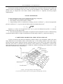
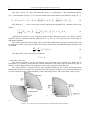
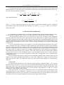
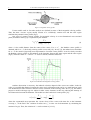
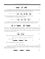
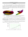
THE PUBLISHING HOUSE
OF THE ROMANIAN ACADEMY
PROCEEDINGS OF THE ROMANIAN ACADEMY, Series A,
Volume 5, Number 3/2004, pp. 000-000
A FREE-WAKE AERODYNAMIC MODEL FOR HELICOPTER ROTORS
Horia DUMITRESCU*, Florin FRUNZULICĂ**
*
**
PhD, Professor, Institute of Statistics and Applied Mathematics, Bucharest, Romania
Lecturer, PhD, Department of Aerospace Engineering, University “POLITEHNICA” of Bucharest, Romania
Corresponding author: Florin FRUNZULICĂ, E-mail: [email protected]
The accurate computation of the induced velocity on helicopter rotor plane is a prerequisite for the
precise evaluation of the angle of attack distribution along the rotor blades, which leads to improved
air loads prediction for aerodynamics and aeroacustics design and performance analysis. The Vortex
Lattice Method (VLM) provides a transparent investigation concerning the role of various physical
parameters which influence the aerodynamic problem of rotor downwash calculation. This paper
presents a method for the calculation of the nonuniform induced downwash of a helicopter rotor using
the vortex ring model for a thin lifting surface coupled with a free-wake model.
Key words: Helicopter rotor; induced velocity; Vortex Lattice Method; free-wake model.
1. INTRODUCTION
During the last few years, considerable research effort has been made with respect to the various
aspects of rotors. In terms of modeling, there is no doubt that significant progress has been achieved during
the last ten years. This progress was mainly based on the existing experience of other engineering fields. As
regards the design of helicopter rotors a number of methods for structural, aerodynamic an aeroacoustic
analysis used in aeronautical engineering have been applied. However, in many cases only simply models
were used. This is true especially as far as Complete Design Tools are concerned. Of course, in order to
devise a flexible and practical design tool, simple models constitute to some extent an obligatory choice.
However, the choice of simple models means that only approximate results can be obtained. Therefore we
need to determine their limitations.
On the other hand during the last few years, within the numerous activities, a number of more elaborate
models has been developed. In most cases the corresponding work was related to the analysis of only one
aspect of the whole design problem of rotor (e.g. advanced aerodynamic models were applied to rigid rotors
and for steady inflow conditions). Though we cannot expect that the advanced models will be applied to
practical design problems at least in the near future, we can use them in order to validate and improve the
simple models.
The collection of the a fore mentioned problems defines the setting of a complete design tool
summarized in the following diagram.
_______________________
Recommended by Virgiliu-Niculae CONSTANTINESCU, member of the Romanian Academy
Horia DUMITRESCU, Florin FRUNZULICĂ
2
Because the unsteady aerodynamic model is the starting step in aeroelastic and aeroacoustic studies our
attention will be concentrated in the next section on the development of the aerodynamic model. In the
present work, we adopted the vortex lattice method (VLM) because of simplicity and easily program
implementation.
2. BASIC ASUMPTIONS
For the aerodynamic model, we have adopted the following assumptions:
1. The rotor blades are regarded as thin lifting surface.
2. The resultant velocity on the blade is subsonic.
3. Compressibility effect is considered by relating a pressure coefficient C p with an incompressible
pressure coefficient C p 0 at a given subsonic Mach number by Prandtl-Glauert rule:
C p = C p 0 / 1 − M ∞2
(1)
Equation (1) relates an incompressible flow over a given two-dimensional profile to a subsonic
compressible flow over the same profile.
4. The elastic displacements of the blades are negletected (the aerodynamic model is calibrated using
assumption that the blades are rigid). Each blade has fixed the angle of attack α b and precone angle βb .
3. VORTEX RING MODEL FOR A THIN LIFTING SURFACE
We have choised for the numerical simulation of lifting surfaces, the aerodynamic model with vortex
rings distributed over the median surface of the blades (fig. 1). The leading segment of the vortex ring is
placed at the panel quarter chord line and the collocation point is at the center of the panel’s three-quarter
chord line. This choice is justified by the fact that the velocity induced by a distribution of vortices is the
same with the one given by a vortex placed at ¼ chord line, with the calculating point considered at ¾ of the
chord line (valid in the case of flat plate)[1].
Figure 1. Vortex ring model for a thin lifting surface
( xb yb zb -blade coordinate system, TE-trailing edge, LE-leading edge, W-wake).
3
A free-wake aerodynamic model for helicopter rotors
!
!
The local velocity ( VP ) for each collocation point is a combination of the self-induced velocity
!
!
( Vind , P ), the kinematic velocity ( Vk , P (t ) ) due the motion of the blade, and the wake-induced velocity ( Vw, P ):
M N
!
!
!
!
!
!
VP = Vk , P (t ) + Vind , P + Vw, P = Vk , P (t ) + ∑∑ Vind , P (t , Γ i , j )
i =1 j =1
(
!
) + ∑∑ (V (t, Γ ))
Mw
i, j
N
i =1 j =1
w, P
i, j
i, j
(2)
The intensity ( Γi , j ) of the vortex rings is found imposing the tangential flow condition on the wing
surface:
M N !
 ∑∑ Vind , P (t , Γi , j )
 i =1 j =1
(
!
!
 !
!
⋅ nP = −Vk , P (t ) ⋅ nP

i, j

) + ∑∑ (V (t, Γ ))
Mw
i, j
N
w, P
i =1 j =1
i, j
(3)
Applying this relation or every collocation point (k=MxN collocation points), one obtains a linear
algebraic system of equations with the unknowns Γ k , k = 1...M × N . This system can be solved using an
appropriate algorithm.
The vortices generated at the trailing edge of each blade maintain their intensity constant in time, and
are transported with a velocity equal to the local velocity of the air flow, such that the theorem of Kelvin will
be satisfied:
!
DΓ ∂Γ
=
+ V ⋅∇ Γ = 0
Dt
∂t
(
)
(4)
The shape of the wake is given by the condition:
! !
V ⋅ γW = 0
(4)
i.e. the wake is force free.
The time-step should be chosen such that the vortex generated at the leading edge should not be
propagated over a distance greater than the smallest dimension of the panel shape at the trailing edge (in
order to avoid the degeneration of the propagated vortex rings, especially at the blade tips).
The wake geometry is complete (fig.2a). But, towards the blade tip, the vortices which spring from
trailing edge roll in space around a curve line generate by the blade tip. In this case is numerically efficient to
use a new model for wake at blade tip which it replace the rollup vortices with a curvilinear vortex (fig.2b).
b.
a.
Figure 2: (a) Complete wake development and (b) simplified wake model at blade tip
Horia DUMITRESCU, Florin FRUNZULICĂ
4
At far distance from panel, using equivalence between the vortex ring model and the dublet with
uniform intensity over the same panel, it is possible to replace the exact formula for the induced velocity by
the vortex ring (the Biot-Savart formula)
!
Γ
VP =
4π
! !
Γ
r × dr
"∫c r 3 = 4π
! ! !
 3 ( r ⋅ n ).r n! 
∫∫S  r 5 − r 3  dσ


(6)
with simplified formula
!
!
! ! !
!
Γ ⋅ A  3 ( r0 ⋅ n ).r0 ! 
VP =
− n  ⋅

4π r03 
r0 2

(7)
where A , n and r0 represent: the panel area, the normal to panel and the distance between collocation
point and the weight center of the panel. The formula (7) is valid for r0 ≥ (3...4 ) ⋅ d , where d is a reference
length of the panel.
4. VORTEX WAKE MODELLING
It is commonly agreed that the key to an accurate calculation of the rotor aerodynamic behaviour is the
correct modeling of the rotor wake. There are two main approaches to the problem of wake modeling:
1. The first method is known as the prescribed wake or rigid wake. According to this method the
geometry of the wake is known a priori, which implies that the velocity field, or rather an approximation to
it, has been assumed. Once the wake geometry has been prescribed, the corresponding induced-velocity and
circulation distributions along the blade can be calculated. The geometry of the wake is determined by using
different kinds of assumptions, while in most of the cases these assumptions are based on experimental
evidence [2-4].
2. The second method is the free-wake analysis [5-6]. In this method an initial geometry of the vortex
wake is assumed. This wake is regarded as being composed of a large number of discrete vortex elements,
and these elements are allowed to convect in the velocity field they create. Provided the numerical method
employed is convergent, the vortex elements will move until they take up positions which are consistent with
the velocity field. As might be expected, the computer requirements for such calculations are prodigious,
which makes this kind of analysis very expensive. This is the reason why some investigators have modeled
the rotor wake with two or three different regions: near, intermediate and far wake. At each region the
computations are done in a way which is appropriate to that region. This approach causes a reduction in the
computational effort.
The present free-wake model is based on the time-marching method where motion begins from an
impulsive start vith the subsequent generation of a vortex wake, modeled by a equence of discrete shed at
equal time intervals. Thus, for steady-state motion, the force and moment responses are asymptotically
achieved.
Vortex model
It is know that the Biot-Savart law for induced velocity produces a singularity when r → 0 . Also, the
induced velocities at points very close to the vortex will lead at unrealistically large induced velocities. These
numerically aspects can create non-physical perturbations to the local angle of attack, unusually large wake
induced velocities at blade tip with effect over tip vortex geometry, large distortion of wake, etc. A direct
consequence is the instability of the solution.
In the present work, a viscous core model has been used to avoid such numerical perturbations. The
experiments that have been conducted to measure the cores of rotary and fixed wing tip vortices have
demonstrated that in real flows, tip vortices have cores with finite radii [7-8]. Because this fact, the selection
of a finite core vortex model in the numerical schemes must be approached cautiously.
5
A free-wake aerodynamic model for helicopter rotors
Figure 3. Tangential velocity profile
Vortex models used in free-wake analysis are defined in terms of their tangential velocity profiles.
Thus, the inner “viscous” region usually consists of a “solid-body” rotation core and the outer region
simulates the potential vortex profile (fig.3).
One series of general velocity profiles for tangential velocity in a two-dimensional cross-sectional
plane (rectilinear vortex)[7,9] is expressed by the formula:
vθ ( r ) =
Γ⋅r
2 π ( rc2 n + r 2 n )
1/ n
(8)
where r is the radial distance from the center of the vortex. For n → ∞ , the Rankine vortex profile is
obtained and for n = 1 , the Scully velocity profile is recoverd [10]. In ref.[7,9], the authors have found that
for n = 2 the model is physically most representative for actual vortex profiles. It can be clearly seen that
the Rankine velocity profile is discontinous at the boundary between the inner region and the outer region
(fig.4), while the values n = 1 and n = 2 assure a smooth, continous transition.
Figure 4. Non-dimensional tangential velocity profiles
Another observation is necessary: the induced velocities depend of the vortex core radius. In the far
wake, it is possible that distance between the vortex and a collocation point can be very small and can result
over-distorted local wake structure, and also lead to oscilations in the evolving wake. In ref. [11], the authors
propose a model with larger tip core radius for older vortex elements, in this way reducing the intensity of
local interaction between the filaments. The model uses the Lamb-Osen vortex profile [12]:
vθ ( r , t ) =
 r2  
Γ 
1
exp
−

−

2π r 
 4ν t  
(9)
where the exponential term represents the viscous decay of the vortex with time due to the kinematic
viscosity,ν , of the fluid. The variation of radius core, rc , in time can be determinate by calculating the
maxima of eq.(9). Thus, the variation of rc can be written as [13-14]:
Horia DUMITRESCU, Florin FRUNZULICĂ
rc ≅ 1.12 4ν δ t
6
(10)
where δ is an experimentally determined decay coefficient. The purpose of this coefficient is to increase the
rate at which the vortex core grows in time.
In this stage of the program development, the equations (9) and (10) are not yet implemented.
Induced velocity at far distance
At far distance from panel, using equivalence between the vortex ring model and the doublet with
uniform intensity over the same panel, it is possible to replace the exact formula for the induced velocity by
the vortex ring (the Biot-Savart formula)
!
Γ
VP =
4π
! !
r × dr
Γ
"∫c r 3 = 4π
! ! !
 3 ( r ⋅ n ).r n! 
∫∫S  r 5 − r 3  dσ


(11)
with simplified formula
!
!
! ! !
!
Γ ⋅ A  3 ( r0 ⋅ n ).r0 ! 
VP =
− n  ⋅

4π r03 
r0 2

(12)
where A , n and r0 represent: the panel area, the normal to panel and the distance between collocation
point and the weight center of the panel. The formula (12) is valid for r0 ≥ (3...4 ) ⋅ d , where d is a
reference length of the panel.
5.COMPUTATIONAL PROCEDURE
The numerical analysis closely follows the concepts presented in the previous section. In all cases,
variables are non-dimensionalized to provide economy in utilization of the computer codes. Velocities are
normalized with R Ω , distances with R , areas with R 2 , time with 1/ Ω , and circulation with R 2 Ω . Force,
torque, and power are non-dimensionalized as indicates in eq.(20).
The general procedure requires that calculations be made at small time increments until a periodic
solution is obtained. Initially there is no wake structure and it is only as the wake develops sufficiently that a
periodic solution is obtained. Based on experience it appears that the wake must be propagating three or four
revolutions for a periodic solution to be achieved.
The computation is initialized by setting the bound vorticity in each blade panel to zero. The
perturbation velocities at each blade panel are then calculated based on all of the vortex filaments in the flow
using eq.(2). These velocities will initially be equal to zero since no wake structure exists and since the
bound vorticity has been set equal to zero. The bound vorticity is then calculated for each panel using eq. (3)
and the last calculated value of the induced velocity. This process is repeated in order to correct the predicted
values of the induced velocities and bound velocities. This simple predictor-corector method appear to be
adequate since the bound vortex rings do not cause large perturbation velocities at nearby blade panels due to
their relative geometric orientation. The next step is the calculation of blade element performance (torque
and power output). These values are output at this point along with induced velocities at each blade element.
The next major step is to recalculate the position of all wake vortex elements using a simple convection
!
!
equation ( dr / dt = V ). Time is incremented and a new set of shed vortices are created. If a revolution has
been completed the rotor performance for the revolution is output. The process is repeated for the desired
number of revolution of the rotor.
The pressure coefficient in a point of interest on the blade surface can be expressed as:
7
A free-wake aerodynamic model for helicopter rotors
2
V 
p − p∞
2 ∂Φ
Cp =
= 1−   − 2
2
ρ V∞ 2
 V∞  V∞ ∂t
(13)
For thin bodies the vorticity inside the bound surface is proportional to the velocity jump across that
surface. In such situation it is useful to express the quantities in terms of relative values, as the difference
between upper and lower surface values. The net-pressure coefficient assumes the form:
∆C p = C p ,l − C p ,u
 V 2  V 2  2  ∂Φ   ∂Φ  
=   −    + 2 
 −

 V∞ u  V∞ l  V∞  ∂t u  ∂t l 
(14)
where u corresponds the upper surface and l corresponds the lower surface of the wing.
The pressure difference across the wing surface is given by:
 V 2   V 2   ∂Φ   ∂Φ  
∆p = pl − pu = ρ 
(15)
 −
 +
 −

 2 u  2 l  ∂t u  ∂t l 
!
!
The velocity V could be broken up on the wing’s surface according to two directions τ i (a direction
!
tangent chordwise to the wing’s surface) and τ j (a direction tangent spanwise to the wing’s surface):
±
Γi , j − Γi −1, j
γ
∂Φ
=± ≈±
,
2
2 ∆ci , j
∂τ i
±
Γi , j − Γi , j −1
∂Φ
≈±
2 ∆bi , j
∂τ j
(16)
where the “+” sign corresponds to the upper surface and the “-” sign corresponds to the lower surface, and
!
!
∆ci , j and ∆bi , j are the panel lengths in the ith and jth directions. The τ i and τ j are defined to be on the
(i , j )
panel. For a vortex ring, the bond between the variation of the potential function by time and the
variation of the circulation by time is:
±
∂Φ i , j
∂t
=±
∂  Γi, j 


∂t  2 
(17)
Hence, the pressure difference between the upper and the lower surface is given by:
∆pi , j
!
!
!
 (uk (t ) + uw ) i + ( vk (t ) + vw ) j + ( wk (t ) + ww (t )) k 
i, j
 
= ρ  Γ − Γ
Γi , j − Γi , j −1 !  ∂Γi , j
i, j
i −1, j !
τi +
τj+
⋅ 
∆bi , j
∂t
  ∆ci , j

⋅




(18)
The force acting upon the (i, j ) element is obtained:
!
!
∆Fi , j = − ( ∆pi , j ⋅ ∆Si , j ) ⋅ ni , j
(19)
The projection of these forces in the reference system attached to the rotor axis allows calculation of
thrust and torque of the rotor. The thrust, torque and power coefficients are defined as nondimensional
parameters of the rotor as follows:
CT =
T
Q
P
, CQ =
, CP =
4
2
5
2
ρπ R Ω
ρπ R Ω
ρ π R 4 Ω3
(20)
Horia DUMITRESCU, Florin FRUNZULICĂ
8
6. RESULTS
Figure 5 shows the wake development in two situation: (a) ascending flight with velocity
V∞Z = −1.75 m / s and (b) forward flight with V∞ = 42 m / s ( 80 tilt axis of rotor). In case (a), the neglect of
development a large core radius for older vortex elements conducts at distorted local wake structure. The
beginning of rotor motion was set impulsively. Because the time for a complete wake development is too
large, the process was stopped after five revolutions. In the future, we intend to “split” the wake in two
regions: the near region where the wake is treated numerically complete, and a far region where the wake is
treated numerically simplified .
a.
b.
Figure 5. The wake development: (a) ascending flight and (b) forward flight. The rotor has two blades with following
characteristics: 3.5 m blade tip radius, 0.3 m hub radius, 30 conical angle. The each blade is modeled with a rigid flat plate with 40
geometric angle of attack, and its are fixed at 35% of blade chord (elastic axis of blade).
For the case test number two, we consider a two blades rotor ( B = 2 ) in hover with characteristics:
solidity B c /(π R) = 0.0637 , tip Mach number R Ω / a0 = 0.19 , pitch angle β = 80 , and constant chord
distribution. The each blade is modeled with a thin lifting surface (rigid flat plate) discretized in 7 points in
chord direction and 13 points in radial direction. Figure 6 shows computed and experimental nondimensional
lift distribution along blade.
The numerical results obtained by VLM ( CT = 0.00391 ) lie closer to the experimental data [15]
( CT ,exp = 0.00380 ) because of more realistic modeling of the free-wake development. These results are
obtained for an axial wake development equal with 1.6 ⋅ R related at rotor plane.
Figure 6. Nondimensional lift distribution along the blade (
y / R =nondimensional radius)
9
A free-wake aerodynamic model for helicopter rotors
7. CONCLUSIONS
The primary objective of this paper has been to describe the implementation of a computational
procedure for helicopter rotor downwash calculations, which utilizes the Vortex Lattice Method for freewake modelling.
The formulation of rotor wake discretization and the resulting induced downwash prediction were
analyzed. The major features of the rotor blade lifting surface aerodynamic model have been outlined.
Several aspects of rotor wake simulation, such as tip vortex roll up process and vortex core modeling
included in the presented methodology were discussed in some detail.
An integrated computer code has been developed applying the presented procedure. Since is based on a
flexible coupling between different modules, it becomes a useful tool for the aerodynamic study and
optimization of helicopter rotors.
The presented computational methodology is under further development regarding more sophisticated
models for blade aerodynamic and dynamic characteristics as well as optimization techniques for wake
geometry calculations.
REFERENCES
1. KATZ, J, PLOTKIN, A: Low-Speed AerodynamicsCambridge University Press 2001
2. Miller,R.H.: On the Computation of Airloads Acting on Rotor Blades in Forward Flight, Journal of the American Helicopter
Society, Vol. 7, No. 2,April1962,pp.56-66
3. Landgrebe,A.J.: An Analytical and Experimental Investigation of Helicopter Rotor Performance and Wake Geometry
Characteristics, USAAM-RDL TR 71-24, June 1971
4. Egolf, T. A., Landgrebe, A. J.: Helicopter Rotor Wake Geometry and its Influence in Forward Flight, Vol. I - Generalized Wake
Geometry and Wake Efect on Rotor Airloads and Performance, NASA CR3726, Oct. 1983
5. Quackenbush, T. R., Bliss, D. B., Wachspress, D. A: Computational Analysis of Hover Performance Using a New Free Wake
Method, Presented at the Second International Conference on Rotorcraft Basic Research, College Park, MD, Feb. 16-18, 1988
6. Miller, W. O., Bliss, D. B.: Direct Periodic Solutions of Rotor Free Wake Calculations, Journal of the American Helicopter
Society, Vol. 38, No. 2, April 1993, pp. 53-60
7. Bagai, A., Leishman, J. G.: Flow Visualization of Compressible VortexStructures using Density Gradient Techniques,
Experiments in Fluids, 15,1993, pp. 431-442
8. Norman, T. R., Light, J. S.: Rotor Tip Vortex Geometry Measurements Using the Wide-Field Shadowgraph Technique, Journal of
the American Helicopter Society, Vol. 32, No. 2, April 1987, pp. 40-50
9. Vatistas, G. H., Kozel, V., Mih, W. C.: A Simpler Model for Concentrated Vortices, Experiments in Fluids, 11, 1991, pp. 73-76
10. Scully, M. P.: Computation of Helicopter Rotor Wake Geometry and Its Influence on Rotor Harmonic Airloads, Massachusetts
Institute of Technology, ASRL TR 178-1, March 1975
11. Bliss, D. B., Quackenbush, T. R., Bilanin, A. J.: A New Methodology for Helicopter Free Wake Analysis, Presented at the 39th
Annual National Forum of the American Helicopter Society, St. Louis, MO, May 9-11, 1983
12. Lamb, Sir Horace, Hydrodynamics, 6th Edition, Cambridge University Press, 1932, pp. 592-593, 668-669
13. Johnson, G. M.: Researches on the Propagation and Decay of Vortex Rings, ARL 70-0093, June, 1970
14. Ogawa, A., Vortex Flow, CRC Series on Fine Particle Science and Technology, CRC Press Inc., 1993
15. Meyer,J.R.,Falabella, G.: An investigation of the experimental aerodynamic loading on a model helicopter rotor blade, NACA
TN 2953, May 1953
Received December 18, 2003