No category

Download A USER GUIDE FOR OPTEX VERSION4 R. Chambon

Transcript

TECHNICAL REPORT
IGE–314
A USER GUIDE FOR OPTEX VERSION4
R. Chambon
Institut de g´enie nucl´eaire
D´epartement de g´enie m´ecanique
´
Ecole
Polytechnique de Montr´eal
July 4, 2015
ii
IGE–314
Contents
Contents . . . . . . . . . . . . . . . . . . . . . . . . . . . . . . . . . . . . . . . . . . . . . . . .
List of Tables . . . . . . . . . . . . . . . . . . . . . . . . . . . . . . . . . . . . . . . . . . . . .
1 OPTEX MODULES
1
Fuel Management Optimization . . . . . . . . . . . . . . .
1.1
The FOBJCT: module . . . . . . . . . . . . . . . . . .
1.1.1
Data input for module FOBJCT: . . . . . .
1.1.2
Data input for module functions deﬁnition
1.1.3
Examples of function deﬁnition . . . . . . .
1.2
The QLPUTL: module . . . . . . . . . . . . . . . . . .
1.2.1
Data input for module QLPUTL: . . . . . .
1.3
The PERTUR: module . . . . . . . . . . . . . . . . . .
1.3.1
Data input for module PERTUR: . . . . . .
1.4
The GPTSRC: module . . . . . . . . . . . . . . . . . .
1.4.1
Data input for module GPTSRC: . . . . . .
1.5
The GPTGRD: module . . . . . . . . . . . . . . . . . .
1.5.1
Data input for module GTPGRD: . . . . . .
1.6
The TABU: module . . . . . . . . . . . . . . . . . . .
1.6.1
Data input for module TABU: . . . . . . . .
2
Output Data Treatment . . . . . . . . . . . . . . . . . . . .
2.1
The ADDOBJ: module . . . . . . . . . . . . . . . . . .
2.1.1
Data input for module ADDOBJ: . . . . . .
2.2
The MATLAB: module . . . . . . . . . . . . . . . . . .
2.2.1
Data input for module MATLAB: . . . . . .
2.3
The GPTVRF: module . . . . . . . . . . . . . . . . . .
2.3.1
Data input for module GPTVRF: . . . . . .
ii
iii
.
.
.
.
.
.
.
.
.
.
.
.
.
.
.
.
.
.
.
.
.
.
.
.
.
.
.
.
.
.
.
.
.
.
.
.
.
.
.
.
.
.
.
.
.
.
.
.
.
.
.
.
.
.
.
.
.
.
.
.
.
.
.
.
.
.
.
.
.
.
.
.
.
.
.
.
.
.
.
.
.
.
.
.
.
.
.
.
.
.
.
.
.
.
.
.
.
.
.
.
.
.
.
.
.
.
.
.
.
.
.
.
.
.
.
.
.
.
.
.
.
.
.
.
.
.
.
.
.
.
.
.
.
.
.
.
.
.
.
.
.
.
.
.
.
.
.
.
.
.
.
.
.
.
.
.
.
.
.
.
.
.
.
.
.
.
.
.
.
.
.
.
.
.
.
.
.
.
.
.
.
.
.
.
.
.
.
.
.
.
.
.
.
.
.
.
.
.
.
.
.
.
.
.
.
.
.
.
.
.
.
.
.
.
.
.
.
.
.
.
.
.
.
.
.
.
.
.
.
.
.
.
.
.
.
.
.
.
.
.
.
.
.
.
.
.
.
.
.
.
.
.
.
.
.
.
.
.
.
.
.
.
.
.
.
.
.
.
.
.
.
.
.
.
.
.
.
.
.
.
.
.
.
.
.
.
1
2
2
3
6
11
13
14
19
20
21
21
23
24
26
26
31
31
31
34
34
37
37
2 OPTEX STRUCTURES
1
Contents of a /tabu/ data structure . . . . . . . . . . . . . . . . . .
1.1
The sub-directories in /tabu/ . . . . . . . . . . . . . . . . . .
2
Contents of a /optimize/ data structure . . . . . . . . . . . . . . . .
2.1
The sub-directory /OLD-VALUE/ in /optimize/ . . . . . . .
2.2
The sub-directory /stepdir/ in /optimize/ . . . . . . . . . . .
2.3
Contents of a /optimize/ data structure for module GPTVRF:
Index . . . . . . . . . . . . . . . . . . . . . . . . . . . . . . . . . . . . . .
.
.
.
.
.
.
.
.
.
.
.
.
.
.
.
.
.
.
.
.
.
.
.
.
.
.
.
.
.
.
.
.
.
.
.
.
.
.
.
.
.
.
.
.
.
.
.
.
.
.
.
.
.
.
.
.
.
.
.
.
.
.
.
.
.
.
.
.
.
.
.
.
.
.
.
.
.
.
.
.
.
.
.
.
39
40
41
43
48
48
49
51
.
.
.
.
.
.
.
.
.
.
.
.
.
.
.
.
.
.
.
.
.
.
.
.
.
.
.
.
.
.
.
.
.
.
.
.
.
.
.
.
.
.
.
.
.
.
.
.
.
.
.
.
.
.
.
.
.
.
.
.
.
.
.
.
.
.
.
.
.
.
.
.
.
.
.
.
.
.
.
.
.
.
.
.
.
.
.
.
iii
IGE–314
List of Tables
1.1
1.2
1.3
1.4
1.5
1.6
1.7
1.8
1.9
1.10
1.11
1.12
1.13
1.14
1.15
1.16
1.17
1.18
1.19
1.20
1.21
1.22
1.23
1.24
1.25
1.26
1.27
1.28
1.29
1.30
1.31
Structure
Structure
Structure
Structure
Structure
Structure
Structure
Structure
Structure
Structure
Structure
Structure
Structure
Structure
Structure
Structure
Structure
Structure
Structure
Structure
Structure
Structure
Structure
Structure
Structure
Structure
Structure
Structure
Structure
Structure
Structure
FOBJCT: . . . . .
(descfobjct) . .
(czdf data) . . .
(fcdf data) . . .
(cstzdf data) . .
(eval data) . . .
(vardef data) .
(seq data) . . .
(data) . . . . . .
QLPUTL: . . . . .
(descqlputl) . .
(def data) . . .
(PERTUR:) . .
(pertur data) .
GPTSRC: . . . . .
gptsrc data . . .
GPTGRD: . . . . .
direct data . . .
gptgrd data . . .
TABU: . . . . . . .
(desctabu) . . .
(def data) . . .
(nelder data) .
ADDOBJ: . . . . .
(addmac data)
(addflu data) .
MATLAB: . . . . .
(descmatlgrd) .
(descmatlflu) .
GPTVRF: . . . . .
gptvrf data . . .
.
.
.
.
.
.
.
.
.
.
.
.
.
.
.
.
.
.
.
.
.
.
.
.
.
.
.
.
.
.
.
.
.
.
.
.
.
.
.
.
.
.
.
.
.
.
.
.
.
.
.
.
.
.
.
.
.
.
.
.
.
.
.
.
.
.
.
.
.
.
.
.
.
.
.
.
.
.
.
.
.
.
.
.
.
.
.
.
.
.
.
.
.
.
.
.
.
.
.
.
.
.
.
.
.
.
.
.
.
.
.
.
.
.
.
.
.
.
.
.
.
.
.
.
.
.
.
.
.
.
.
.
.
.
.
.
.
.
.
.
.
.
.
.
.
.
.
.
.
.
.
.
.
.
.
.
.
.
.
.
.
.
.
.
.
.
.
.
.
.
.
.
.
.
.
.
.
.
.
.
.
.
.
.
.
.
.
.
.
.
.
.
.
.
.
.
.
.
.
.
.
.
.
.
.
.
.
.
.
.
.
.
.
.
.
.
.
.
.
.
.
.
.
.
.
.
.
.
.
.
.
.
.
.
.
.
.
.
.
.
.
.
.
.
.
.
.
.
.
.
.
.
.
.
.
.
.
.
.
.
.
.
.
.
.
.
.
.
.
.
.
.
.
.
.
.
.
.
.
.
.
.
.
.
.
.
.
.
.
.
.
.
.
.
.
.
.
.
.
.
.
.
.
.
.
.
.
.
.
.
.
.
.
.
.
.
.
.
.
.
.
.
.
.
.
.
.
.
.
.
.
.
.
.
.
.
.
.
.
.
.
.
.
.
.
.
.
.
.
.
.
.
.
.
.
.
.
.
.
.
.
.
.
.
.
.
.
.
.
.
.
.
.
.
.
.
.
.
.
.
.
.
.
.
.
.
.
.
.
.
.
.
.
.
.
.
.
.
.
.
.
.
.
.
.
.
.
.
.
.
.
.
.
.
.
.
.
.
.
.
.
.
.
.
.
.
.
.
.
.
.
.
.
.
.
.
.
.
.
.
.
.
.
.
.
.
.
.
.
.
.
.
.
.
.
.
.
.
.
.
.
.
.
.
.
.
.
.
.
.
.
.
.
.
.
.
.
.
.
.
.
.
.
.
.
.
.
.
.
.
.
.
.
.
.
.
.
.
.
.
.
.
.
.
.
.
.
.
.
.
.
.
.
.
.
.
.
.
.
.
.
.
.
.
.
.
.
.
.
.
.
.
.
.
.
.
.
.
.
.
.
.
.
.
.
.
.
.
.
.
.
.
.
.
.
.
.
.
.
.
.
.
.
.
.
.
.
.
.
.
.
.
.
.
.
.
.
.
.
.
.
.
.
.
.
.
.
.
.
.
.
.
.
.
.
.
.
.
.
.
.
.
.
.
.
.
.
.
.
.
.
.
.
.
.
.
.
.
.
.
.
.
.
.
.
.
.
.
.
.
.
.
.
.
.
.
.
.
.
.
.
.
.
.
.
.
.
.
.
.
.
.
.
.
.
.
.
.
.
.
.
.
.
.
.
.
.
.
.
.
.
.
.
.
.
.
.
.
.
.
.
.
.
.
.
.
.
.
.
.
.
.
.
.
.
.
.
.
.
.
.
.
.
.
.
.
.
.
.
.
.
.
.
.
.
.
.
.
.
.
.
.
.
.
.
.
.
.
.
.
.
.
.
.
.
.
.
.
.
.
.
.
.
.
.
.
.
.
.
.
.
.
.
.
.
.
.
.
.
.
.
.
.
.
.
.
.
.
.
.
.
.
.
.
.
.
.
.
.
.
.
.
.
.
.
.
.
.
.
.
.
.
.
.
.
.
.
.
.
.
.
.
.
.
.
.
.
.
.
.
.
.
.
.
.
.
.
.
.
.
.
.
.
.
.
.
.
.
.
.
.
.
.
.
.
.
.
.
.
.
.
.
.
.
.
.
.
.
.
.
.
.
.
.
.
.
.
.
.
.
.
.
.
.
.
.
.
.
.
.
.
.
.
.
.
.
.
.
.
.
.
.
.
.
.
.
.
.
.
.
.
.
.
.
.
.
.
.
.
.
.
.
.
.
.
.
.
.
.
.
.
.
.
.
.
.
.
.
.
.
.
.
.
.
.
.
.
.
.
.
.
.
.
.
.
.
.
.
.
.
.
.
.
.
.
.
.
.
.
.
.
.
.
.
.
.
.
.
.
.
.
.
.
.
.
.
.
.
.
.
.
.
.
.
.
.
.
.
.
.
.
.
.
.
.
.
.
.
.
.
.
.
.
.
.
.
.
.
.
.
.
.
.
.
.
.
.
.
.
.
.
.
.
.
.
.
.
.
.
.
.
.
.
.
.
.
.
.
.
.
.
.
.
.
.
.
.
.
.
.
.
.
.
.
.
.
.
.
.
.
.
.
.
.
.
.
.
.
.
.
.
.
.
.
.
.
.
.
.
.
.
.
.
.
.
.
.
.
.
.
.
.
.
.
.
2
3
3
4
5
6
8
10
11
13
14
16
19
20
21
21
23
24
24
26
26
27
30
31
31
33
34
34
35
37
37
2.1
2.2
2.3
2.4
2.5
2.6
2.7
2.8
Main records and sub-directories in /tabu/ . . . . . .
Main records in sub-directories . . . . . . . . . . . . .
Additional records in NELDER-MEAD directory . . .
Main records and sub-directories in /optimize/ . . . .
Main records and sub-directories in //OLD-VALUE//
Main records and sub-directories in //stepdir// . . . .
/optimize/ in the particular case of module GPTVRF: .
The sub-directory /varpertdir/ in /optimize/ . . . . .
.
.
.
.
.
.
.
.
.
.
.
.
.
.
.
.
.
.
.
.
.
.
.
.
.
.
.
.
.
.
.
.
.
.
.
.
.
.
.
.
.
.
.
.
.
.
.
.
.
.
.
.
.
.
.
.
.
.
.
.
.
.
.
.
.
.
.
.
.
.
.
.
.
.
.
.
.
.
.
.
.
.
.
.
.
.
.
.
.
.
.
.
.
.
.
.
.
.
.
.
.
.
.
.
.
.
.
.
.
.
.
.
.
.
.
.
.
.
.
.
.
.
.
.
.
.
.
.
.
.
.
.
.
.
.
.
.
.
.
.
.
.
.
.
.
.
.
.
.
.
.
.
.
.
.
.
.
.
.
.
40
42
42
44
48
48
49
50
Chapter 1
OPTEX MODULES
1
2
IGE–314
1 Fuel Management Optimization
In this section, modules used for fuel management optimization will be described.
1.1
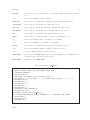
The FOBJCT: module
The FOBJCT: module is used to deﬁne the diﬀerent parameters for an optimization calculation. These
parameters can be decision variables, contraint zone deﬁnitions, constraint limits, ... This module can
also evaluate the objective function and the constraints values.
The calling speciﬁcations are:
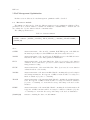
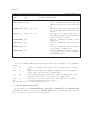
Table 1.1: Structure FOBJCT:
OPTIM := FOBJCT: [ OPTIM ] [ MAPFL ] [ FLUX [ FLUXP ] ] [ MACRO ] [ TRACK INDEX ] ::
(descfobjct)
where
OPTIM
character*12 name of the extended optimize. If OPTIM appears on the RHS, the
information previously stored in OPTIM is modiﬁed if necessary and stored.
MAPFL
character*12 name of the extended map. If MAPFL appears on the RHS, the information in it will be read for many parameters initialisation.
FLUX
character*12 name of the flux linked list. This object is used for the function
evaluation. It is recommended to provide it even if no function evaluation is done for
many parameter reading.
FLUXP
character*12 name of the flux linked list. This object is used for some function
evaluation such as void reactivity.
MACRO
character*12 name of the macrolib linked list ﬁle containing fuel regions description
and burnup informations. If it appears on RHS, it means it will be necessary for a
function evaluation (objective or constraint).
TRACK
character*12 name of the tracking linked list ﬁle containing the tracking informations. If it appears on RHS, it means it will be necessary for a function evaluation
(objective or constraint) or to memorize the average exit burnup or the fuel cost distribution.
INDEX
character*12 name of the index linked list ﬁle containing the index informations. If
it appears on RHS, it means it will be necessary for a function evaluation (objective
or constraint) or to memorize the average exit burnup or the fuel cost distribution.
(descfobjct)
structure containing the data to module FOBJCT:.
3
IGE–314
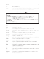
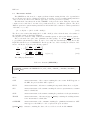
1.1.1 Data input for module FOBJCT:
Table 1.2: Structure (descfobjct)
[
[
[
[
[
[
;
EDIT iprint ]
CTRL-ZONE-DF (czdf data) ]
FUEL-COST-DF (fcdf data) ]
EXIT-B-DIST MEMORY]
CST-ZONE-DF (cstzdf data) ]
EVAL-OBJ-CST (eval data) ]
where
EDIT
key word used to set iprint.
iprint
index used to control the printing in module.
CTRL-ZONE-DF
key word used to deﬁne the decision variables and their zones of inﬂuence.
(czdf data)
structure containing the data to the option CTRL-ZONE-DF.
FUEL-COST-DF
key word used to deﬁne the cost of the uranium is the core.
(fcdf data)
structure containing the data to the option FUEL-COST-DF.
EXIT-B-DIST
key word used to specify that the distribution of the average exit burnup for each
volume will be pre-calculated.
MEMORY
key word used to specify that the distribution of the average exit burnup will be stored
in the OPTIM object.
CST-ZONE-DF
key word used to deﬁne the constraint (type, value, zone of inﬂuence).
(cstzdf data)
structure containing the data to the option CST-ZONE-DF.
EVAL-OBJ-CST
key word used to deﬁne and evaluate the objective and / or constraints functions.
(eval data)
structure containing the data to the option EVAL-OBJ-CST. This will be treated as a
section in itself because other module will refer to it.
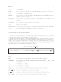
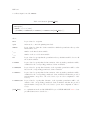
Table 1.3: Structure (czdf data)
[ BURNUP-ZONE burnmin burnmax { ALL | { { Y | N }i ,i=1,nbz } } ]
[ ENRICH-ZONE enrimin enrimax { { Y | N }i ,i=1,nez } ]
where
4
IGE–314
BURNUP-ZONE
key word used to specify that exit-burnup decision variables will be set. This exitburnup zone were deﬁned previously and are stored in the map.
burnmin
minimum value of the exit-burnup.
burnmax
maximum value of the exit-burnup.
ALL
key word used to specify that all burnup-exit zone will be a decision variable.
Y
key word used to specify that a speciﬁc burnup-exit zone will be a decision variable.
N
key word used to specify that a speciﬁc burnup-exit zone will not be a decision variable.
nbz
number of average exit burnup zone.
ENRICH-ZONE
key word used to specify that exit-burnup decision variables will be set. This exitburnup zone were deﬁned previously and are stored in the map.
enrimin
minimum value of the exit-burnup.
enrimax
maximum value of the exit-burnup.
Y
key word used to specify that a speciﬁc enrichment zone will be a decision variable.
N
key word used to specify that a speciﬁc enrichment zone will not be a decision variable.
nez
number of enrichment zone.
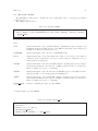
Table 1.4: Structure (fcdf data)
[ FIXED costi ,i=1,nez )
| DEPENDANT εw CN U CS CF AB interest tobt tenr ]
[ MEMORY ]
where
FIXED
key word used to specify that the price of the fuel is ﬁxed for each enrichment zone.
cost
cost of the fuel.
nez
number of enrichment zone.
DEPENDANT
key word used to specify that the price of the fuel is dependant of the enrichment for
each enrichment zone.
εw
U 235 concentration of waste uranium after the separation work.
CN U
natural uranium cost ($/kg).
CS
cost of a separation work unit ($/SWU).
CF AB
cost of fabrication of the bundles ($/kg).
interest
interest rate (y−1 ).
tobt
time to obtain uranium (y).
5
IGE–314
tenr
time for enrichment (y).
MEMORY
key word used to specify that the distribution of the purchase cost of uranium actually
in the reactor will be pre-calculated and stored in the OPTIM object.
Table 1.5: Structure (cstzdf data)
[ KEFF kef f ]
[ MAXPOWER
. . . [[ ZONE-DEF [[ SURV-ZONE nsurv zone [[ PLAN iplan { izonej ,j=1,ncha | SAME jplan } ]]
. . . . . . . . . . . . . . . . . . | BUNDLE { ALL | [[ PLAN iplan { { 0 | 1 }j ,j=1,ncha | SAME jplan } ]]
. . . . . . . . . . . . . . . . . . | CHANNEL { ALL | { 0 | 1 }j ,j=1,ncha } ]]
. . . | VALUE-DEF {{ izone1 cstlim | RANGE izone1 izone2 { cstlimj ,j=izone1 ,izone2 | ALLSAME cstlim } } ]]
. . . END-MAX-POW ]
[ VOID-REACT-FC ρV,F C ]
[ ANALYTIC-FCT csttype cstlim ]
where
KEFF
key word used to deﬁned kef f .
kef f
neutron multiplication factor aimed (this is a constraint of type equal).
MAXPOWER
key word used to deﬁned a maximum power in a zone (this is a constraint of type
inferior).
ZONE-DEF
key word used to specify that the deﬁnition of the zone will be provided.
SURV-ZONE
key word used to speciﬁed that the zone will be deﬁned manually.
nsurv
total number of surveillance zone.
zone
izone
number of the zone that the bundle is part of (0 if no surveillance zone for this bundle).
BUNDLE
key word to speciﬁed that surveillance zone are bundles.
CHANNEL
key word to speciﬁed that surveillance zone are channels.
PLAN
key word to specify that the deﬁnition of surveillance zone for iplan will follow.
iplan
numbers of the plan to be deﬁned.
SAME
key word used to specify that the deﬁnition of surveillance zone in the plan iplan will
be the same one as in the plan jplan .
jplan
number of the plan already deﬁned.
ALL
key word used to specify that the power in all bundles or channels will be a constraint.
ncha
number of channels.
VALUE-DEF
key word used to specify that the limit of maximum zone power will be provided.
izone1
ﬁrst number of surveillance zone.
6
IGE–314
cstlim
constraint limit.
RANGE
key word used to specify that the constraint limit will be speciﬁed for several zones.
izone2
second number of surveillance zone.
ALLSAME
key word used to specify that all the constraint will have the same limit for the zone
number between izone1 and izone2 .
END-MAX-POW
key word used to specify that the deﬁnition of the maximum power surveillance zones
is ﬁnished.
VOID-REAC-FC
key word used to deﬁne the full core void reactivity.
ρV,F C
full core void reactivity.
ANALYTIC-FCT
key word used to specify that the corresponding constraint will be deﬁned analytically.
csttype
type of the analytic constraint (-1 for ≤, 0 for = and 1 for ≥).
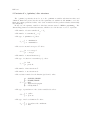
1.1.2 Data input for module functions definition
Because the functions deﬁnition is common with other modules, its description will be grouped in this
section, as a independent part of the FOBJCT: module description.
The functions deﬁnition is based on inverted polish notation logic. Some functions are predeﬁned,
but if it is not the case, new functions can be deﬁned manually. In this particular case, variables may be
required. Some of them are predeﬁned also, otherwise the user can get them with the same logic as the
module GREP. For the functions representing the constraints the user need to specify its number. So it is
important to know the order in which constraints where deﬁned.
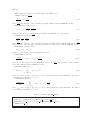
Table 1.6: Structure (eval data)
[[ { FOBJ | CONSTRAINT icst1 icst2 } { [ VARDEF (vardef data) ] (seq data) | FUNCT-PREDEF predef func
} ]]
where
FOBJ
key word used to specify that the objective function will be evaluated.
CONSTRAINT
key word used to specify that constraint functions between number icst1 and icst2 will
be evaluated.
icst1
ﬁrst number of constraint.
icst2
second number of constraint.
VARDEF
key word used to deﬁne the variables needed for the function evaluation.
(vardef data)
structure containing the data to the option VARDEF.
(seq data)
structure containing the data used to deﬁned a function directly by the user.
FUNCT-PREDEF
key word used to specify that a predeﬁned function will be evaluated.
7
IGE–314
name of the predeﬁned function. The predeﬁned function name are :
UCOST
DX-UCOST
DPHI-UCOST
POWERLIMIT
DX-POWER
DPHI-POWER
KEFF
D-KEFF
VOID-REAC-FC
D-VOID-R-FC
KEFF=KREF
kref
D-KEFF=KREF
kref
MINPCMAX
qmoy icst1 icst2
D-MINPCMAX
qmoy icst1 icst2
predef func
Where :
UCOST is deﬁned by FC :
FC =
h
CF (εj )
eacteur
Bj .H, φir´
DX-UCOST is deﬁned by
∂FC
∂Xi
(1.1)
hH, φir´eacteur
=
∂FC
∂Xi :
H
h ∂Cu
∂Xi , B φiVi
hH, φiV
−FC .
+
∂H
, φiVi
h ∂X
i
hH, φiV
DPHI-UCOST is deﬁned by
∂FC
= SF∗ C =
∂φ
hCu
1 ∂H
B ∂Xi
−
H ∂B
B 2 ∂Xi
hH, φiV
, φiVi
i ∈ (1, nvar )
(1.2)
∂FC
∂φ :
Cu
r)
B .H(~
− FC .H(~r)
hH, φiV
(1.3)
POWERLIMIT is deﬁned by qj :
qj = ZP P Fj .
Plim
V hH, φiVj
≤ ¯ = flim
Vj hH, φiV
P
DX-POWER is deﬁned by
∂qj
∂Xi
=
(1.4)
∂qj
∂Xi :
qj
∂ZP P Fj
qj
∂H
.
.δij +
, φiVj .δij
h
ZP P Fj
∂Xi
hH, φiVj ∂Xi
∂H
qj
h
, φiV i ∈ (1, I) et j ∈ (1, ncontrol−zone )
−
hH, φiV ∂Xi
DPHI-POWER is deﬁned by
(1.5)
∂qj
∂φ :
ZP P Fj VVj .H(~rj ) − qj .H(~r)
∂qj
= Sq∗j =
∂φ
hH, φiV
Hj ~r ∈ Vj
where H(~rj ) =
0
otherwise
j ∈ (1, ncontrol−zone )
(1.6)
8
IGE–314
KEFF is deﬁned by kef f : kef f is directly taken in the FLUX object.
dkef f
D-KEFF is deﬁned by dX
:
i
dλ
dkef f
2
= −kef
f
dXi
dXi
(1.7)
dλ
where dX
is the derivative of the eigenvalue previously calculated with the PERTUR: module.
i
VOID-REAC-FC is deﬁned by ρV :
ρV = λ − λV =
1
1
−
kef f
kef f,V
(1.8)
where kef f and kef f,V are directly taken in the FLUX and FLUXP object respectively.
V
D-VOID-R-FC is deﬁned by dρ
dXi :
dλ
dλV
dρV
=
−
dXi
dXi
dXi
(1.9)
dλ
V
is the derivative of the eigenvalue previously calculated with the PERTUR: module and dλ
where dX
dXi
i
is the derivative of the eigenvalue previously calculated for a voided reactor with the PERTUR: module.
KEFF=KREF is deﬁned by ∆kef f :
∆kef f = (kef f − kref )2
(1.10)
where kref is the required reference multiplication factor.
D-KEFF=KREF is deﬁned by
d∆kef f
dλ
2
= −2 ∗ (kef f − kref ) .kef
f
dXi
dXi
(1.11)
where kref is the required reference multiplication factor and
previously calculated with the PERTUR: module.
MINPCMAX is deﬁned by
EP moy =
iX
cst2
dλ
dXi
is the derivative of the eigenvalue
(qj − qmoy )2m
(1.12)
j=icst1 |qj >qmoy
where qmoy is the average power zone. m can be changed with the module QLPUTL:. The sum is
performed from constraint icst1 to icst2 .
D-MINPCMAX is deﬁned by
d∆EP moy
=
dXi
iX
cst2
j=icst1 |qj >qmoy
2m(qj − qmoy )2m−1
dqj
dXi
(1.13)
where qmoy is the average power zone. m can be changed with the module QLPUTL:. The sum is
performed from constraint icst1 to icst2 .
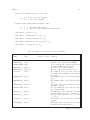
Table 1.7: Structure (vardef data)
[[ LOAD object [[ DOWN repertory ]] GREP data name IN var name ]]
[[ MSYS*FLUX object sys { A | B } object flux [ ADJOINT ] IN var name ]]
[[ PREDEF predef var ]]
9
IGE–314
where
LOAD
key word used to deﬁne the object where the data are stored.
object
name of the object.
DOWN
key word used to go in a sub-directory.
repertory
name of the repertory.
GREP
key word used to deﬁne the name of the data to load.
data name
name of the data to load.
IN
key word used to deﬁne the name of the local variable.
var name
name of the local variable name.
MSYS*FLUX
key word used to specify that a local variable will be calculated by the product of a
system matrix and a ﬂux (or adjoint).
object sys
name of the object L SYSTEM.
A
key word used to specify that the system matrix corresponding to the lost of the
neutrons will be used. (A − λB)φ = 0
B
key word used to specify that the system matrix corresponding to the production of
the neutrons will be used. (A − λB)φ = 0
object flux
name of the object L FLUX.
ADJOINT
key word used to specify that the adjoint ﬂux will be used instead of the ﬂux (default
value). In this case the adjoint system matrix are used automatically.
PREDEF
key word used to specify that a predeﬁned variable will be load.
predef var
name of the predeﬁned variable. The predeﬁned variable name are deﬁne below.
key word
FLUX
AFLUX
FLUX2
AFLUX2
FLUX-AV
FLUX-AX
DIFFX
DIFFY
DIFFZ
TOTAL
NFTOT
NUSIGF
H-FACTORS
CHI
SIGW-0
contents
neutron ﬂux distribution
adjoint ﬂux distribution of the second provided L FLUX
neutron ﬂux distribution of the second provided L FLUX
adjoint ﬂux distribution
average ﬂux distribution by channel
axial average ﬂux distribution
diﬀusion coeﬃcient along X abcisse
diﬀusion coeﬃcient along Y abcisse
diﬀusion coeﬃcient along Z abcisse
total cross-sections
ﬁssion cross-sections
number of neutrons per ﬁssion time ﬁssion cross-sections
ﬁssion cross section times the energy recovered by ﬁssion
ﬁssion spectrum
isotropic component of the within group of the scattering of the
scattering cross-sections
size
nun × ngrp
nun × ngrp
nun × ngrp
nun × ngrp
nch × ngrp × nzone
nz × ngrp
nun × ngrp
nun × ngrp
nun × ngrp
nun × ngrp
nun × ngrp
nun × ngrp
nun × ngrp
nun × ngrp
nun × ngrp
10
IGE–314
SIGW-1
D-TOTAL
D-CHI
D-DIFFX
D-DIFFY
D-DIFFZ
D-NUSIGF
D-NFTOT
D-HFACT
D-SIGW0
D-SIGW1
A*PHI
B*PHI
AP*PHI
BP*PHI
FUNCVALUE
FUNCZVOL
KEFF
KEFF-VOID
D-LAMBDA
D-LAMBDA-V
linearly anisotropic component of the within group of the scattering of the scattering cross-sections
derivative of total cross-sections
derivative of ﬁssion spectrum
derivative of diﬀusion coeﬃcients along X abcisse
derivative of diﬀusion coeﬃcients along Y abcisse
derivative of diﬀusion coeﬃcients along Z abcisse
derivative of ﬁssion cross-sections
derivative of number of neutrons per ﬁssion time ﬁssion crosssections
derivative of ﬁssion cross section times the energy recovered by
ﬁssion
derivative of isotropic component of the within group of the
scattering of the scattering cross-sections
derivative of linearly anisotropic component of the within group
of the scattering of the scattering cross-sections
A system matrix times neutron ﬂux vector
B system matrix times neutron ﬂux vector
perturbated A system matrix times neutron ﬂux vector
perturbated B system matrix times neutron ﬂux vector
value of the function, usually used when the derivative function is calculated (see the deﬁnition of the DX-UCOST prediﬁned
function for example).
value of the volume on which the function is deﬁned / integrated.
kef f
kef f corresponding to a pertubated ﬂux
derivative of the eigenvalue
derivative of the eigenvalue corresponding to a pertubated ﬂux
nun × ngrp
nun
nun
nun
nun
nun
nun
nun
×
×
×
×
×
×
×
ngrp
ngrp
ngrp
ngrp
ngrp
ngrp
ngrp
nun × ngrp
nun × ngrp
nun × ngrp
nun × ngrp
nun × ngrp
nun × ngrp
nun × ngrp
ncst+1
ncst+1
nun
nun
nun
nun
×
×
×
×
ngrp
ngrp
ngrp
ngrp
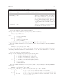
Table 1.8: Structure (seq data)
INIT
[[ (data)
| INTEGRAL { REACTOR | CORE | CST-ZONE | VAR-ZONE | DBL-ZONE | DISCRETE-ALL | DISCRETE-COR |
DISCRETE-CST }
. . . [[ (data) | ENERGY { ALL | gprf rom gprto } [[ (data) ]] END-ENERGY ]]
. . . END-INTEGRAL ]] ]]
END
where
INIT
key word used to specify that the function deﬁnition will follow.
(data)
structure containing the data used to deﬁned parts of the function.
INTEGRAL
key word used to deﬁne an integral over one volume and energy.
REACTOR
key word used to specify that the integration volume is the reactor
CORE
key word used to specify that the integration volume is the core (all the bundles).
11
IGE–314
CST-ZONE
key word used to specify that the integration volume is a control zone of one constraint.
VAR-ZONE
key word used to specify that the integration volume is a zone where a decision variable
applies.
DBL-ZONE
key word used to specify that the integration volume is on the intersection of a control
zone of one constraint and a zone where a decision variable applies.
DISCRETE-ALL
key word used to specify that the integration will be performed only on the energy for
every point of the reactor.
DISCRETE-COR
key word used to specify that the integration will be performed only on the energy for
every point of the core.
DISCRETE-CST
key word used to specify that the integration will be performed only on the energy for
every point of a control zone of one constraint.
ENERGY
key word used to deﬁne the energy part of the integration.
ALL
key word used to specify that the integration will be performed on all energy groups.
grpf rom
number of the ﬁrst energy group for the integration.
grpto
number of the last energy group for the integration.
END-ENERGY
key word used to specify that the deﬁnition of the integral over energy is ﬁnished.
END-INTEGRAL
key word used to specify that the deﬁnition of the integral is ﬁnished.
END
key word used to specify that the deﬁnition of the function is ﬁnished.
Table 1.9: Structure (data)
[[ { real | VAR loc var name | operator | VARF loc var name } ]]
where
real
real number.
VAR
key word used to specify that a local variable will be used.
VARF
key word used to specify that a local variable which depend with the functional will
be used (ex: zone volume).
loc var name
name of a local variable name. Note : it has to be loaded before.
operator
name of a numerical operator. The name must be one of these : PLUS, +, MINUS, -,
TIMES, *, DIVISION, /, POWER, **, MAX, MIN, LOG, LN, EXP, SIN, COS, TAN, ABS, SQRT.
1.1.3 Examples of function definition
We will now give a few examples which will permit users a better understanding of the procedure to
deﬁne the function for optimization in DONJON.
12
IGE–314
1. Predeﬁned function:
OPTIMIZE := FOBJCT: OPTIMIZE FLUX MACRO ::
EVAL-OBJ-CST CONSTRAINT 2 10 PREDEF POWERLIMIT
;
2. Function deﬁend by user:
For example, we suppose that a functional u deﬁned by the user is :
Z
Z
CU
φdE.dV
fcost = 2 ∗ kef f ∗
CORE
allenergygroups
Where :
CU is the fuel cost.
φ the ﬂux distribution.
OPTIMIZE := FOBJCT: OPTIMIZE FLUX MACRO ::
FUEL-COST-DF MEMORY
EVAL-OBJ-CST FOBJ
VARDEF LOAD FLUX GREP K-EFFECTIVE IN KEFF
PREDEF FLUX
2.0
VAR KEFF
*
INTEGRAL CORE
VAR FUELCOST
ENERGY ALL
VAR FLUX
END-ENERGY
*
END-INTEGRAL
*
END
;
(1.14)
13
IGE–314
1.2
The QLPUTL: module
The QLPUTL: module is used to deﬁne the optimization options and tools. It is also used to do some
pre-calcultaion.
The calling speciﬁcations are:
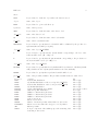
Table 1.10: Structure QLPUTL:
OPTIM := QLPUTL: OPTIM [ FLUX ] [ MAPFL ] [ MACRO [ MACROP ]] [ SYS [SYSP] TRACK
] :: (descqlputl)
where
OPTIMIZE
character*12 name of the extended optimize.
FLUX
character*12 name of the flux linked list. This object is used for the function
evaluation. It is recommended to provide it even if no function evaluation is done for
many parameters reading. ﬁle.
MAPFL
character*12 name of the extended map linked list ﬁle containing fuel regions description and burnup informations. If MAPFL appears on the RHS, the information
in it will be red for many parameters initialisation.
MACRO
character*12 name of the macrolib linked list ﬁle containing the mixtures cross
sections. If it appears on RHS, it means it will be necessary for a function evaluation
(objective or constraint).
MACROP
character*12 name of the macrolib linked list ﬁle containing the mixtures perturbated cross sections. If it appears on RHS, it means it will be necessary for a function
evaluation (objective or constraint).
SYS
character*12 name of the system containing the reference system matrices. system
must be a linked list. If it appears on RHS, it will be necessary for ’system matrice
times ﬂux’ calculations.
SYSP
character*12 name of the system containing the perturbated system matrices. system must be a linked list. If it appears on RHS, it will be necessary for ’perturbated
system matrice times ﬂux’ calculations.
TRACK
character*12 name of the track (type L TRIVAC) containing the tracking informations. track must be a linked list. If it appears on RHS, it will be necessary for
’system matrice times ﬂux’ calculations.
(descqlputl)
structure containing the data to module PQLUTL:.
14
IGE–314
1.2.1 Data input for module QLPUTL:
Table 1.11: Structure (descqlputl)
[ EDIT iprint ]
[ DEFINITION (def data) ]
[ STEP-VALID [ TEST-CST-VLD ] >> test1 << ]
[ STEP-INTERP { PUT | RECOVER >> test2 << } ]
[ DX-METHOD { EPS epsilon | PREVIOUS } ]
[ NEW-VAL-UPDT ]
[ PERTURB-VAR { ivar1 | RESTORE } ]
[ BKP-MACRO-P ivar2 ]
[ MAT*FLUX { A*PHI | B*PHI | AP*PHI ivar3 | BP*PHI ivar3 } ]
[ LA-PNLT [ INITIAL ] [ F-EVAL ] [ COEF-UPDATE ] [ CONV-TEST >> conv << ]
. . . [ ALMOST-FSBLE >> feas << ] ]
[ HISTORY iiter1 [ POWER-CHA ] [ K-EFFECTIVE ] [ QUAD-CST ] ]
. . . [ CONSTRAINT { ALL | RANGE << icst1 >> << icst2 >> | << icst1 >> } ] . . . [ DIRECT << num
>> { vali , i = 1, num} ] ] [ POWER-CHA#2 ] [ POWER-CHA#3 ]
;
where
EDIT
key word used to set iprint.
iprint
index used to control the printing in module.
DEFINITION
key word used to deﬁne the optimization options.
(def data)
structure containing the data to the option DEFINITION.
STEP-VALID
key word used to verify if the new {Xi } ends with a better objective function.
TEST-CST-VLD
key word used to verify if the new {Xi } respects the constraints.
test
logical value
for the validition of the new decision variables. test equals .true. if
FC Xik+1 is better than FC Xik .
STEP-INTERP
key word used to specify that an interpolation of the objective function for the midle
point between {Xik } and {Xik+1 } will be done.
PUT
key word used to calculate and store the middle value.
RECOVER
key word used to verify the middle value.
test2
k+ 1
logical value for the validation of interpolation. If FC Xi 2 is less than FC Xik+1
then the middle value is kept, otherwise the new value is restored.
DX-METHOD
key word used to deﬁne which method will be used to evaluate the perturbated crosssection.
k
Σ(Xi,p
) − Σ(Xik )
dΣ
=
k − Xk
dXik
Xi,p
i
(1.15)
15
IGE–314
k
where Xi,p
is the perturbated decision variable.
EPS
k
key word used to deﬁne Xi,p
by Xik ∗ (1 + ǫ).
epsilon
value of ǫ.
PREVIOUS
k
key word used to deﬁne Xi,p
by Xik−1 .
NEW-VAL-UPDT
key word used to update the new decision variables.
PERTURB-VAR
key word used to perturbate a decision variable.
ivar1
number of the decision variable to perturbate.
RESTORE
key word used to restore the unperturbated decision variables.
BKP-MACRO-P
key word used to store the perturbated macroscopic cross-section. By default all crosssection are stored. To store only some of them, see PQLUTL/DEFINITION/BKPMCR-P-XS.
ivar2
number of the decision variable for which the cross-section are perturbated and will
be stored.
MAT*FLUX
key word used to precalulate the system matrice times the ﬂux.
A*PHI
key word used to precalulate the A.φ (ivar3 =0 is implicit).
B*PHI
key word used to precalulate the B.φ (ivar3 =0 is implicit).
AP*PHI
key word used to precalulate the Ap .φ.
BP*PHI
key word used to precalulate the Bp .φ.
ivar3
number of the step directory where the A.φ and B.φ will be stored. ivar3 represents the
decision variable for which the system matrice were perturbated and will be multiplied
by the ﬂux for optimization. The result will be stored in L OPTIMIZE/’STEP//HSIGN
’ with WRITE(HSIGN,I8) ivar3 .
LA-PNLT
key word used to specify that a task related to the augmented lagrangian or penalty
method is performed.
INITIAL
key word used to initialize the constraint weight (if not already done) and the lagrangian coeﬃcient (when augmented lagrangian method is used).
F-EVAL
key word used to calculate the augmented lagrangian or penalty function. It can be
also used with tabu search to evaluate the corresponding objective function.
COEF-UPDATE
key word used to update the constraint weights and lagrangian coeﬃcients (if necessary) in an external iteration.
CONV-TEST
key word used to specify that a convergence test for external iteration will be performed.
conv
logical value representing the result of the external convergence test.
ALMOST-FSBLE
key word used to specify that a test will be permorfed to check if the current point is
’almost feasible’.
feas
logical value representing the result of the ’almost feasible’ test. The maximum error
allowed to set feas to .true. is a relative diﬀerence between prescribed and current
constraint values lower than the convergence crriterium.
IGE–314
16
HISTORY
key word used to store the decision vector and the functionnal values for iteration
iiter1 .
iiter1
integer representing the iteration number.
POWER-CHA
key word used to specify that the channel power distribution is also stored.
K-EFFECTIVE
key word used to specify that kef f value is also stored.
QUAD-CST
key word used to specify that quadratic constraint limit is also stored.
CONSTRAINT
key word used to specify that some constraint values are also stored.
ALL
key word used to specify that all constraint values are stored.
RANGE
key word used to specify that values of a range of constraint are stored.
icst1
integer representing the ﬁrst or only number of constraint.
icst2
integer representing the second number of constraint.
DIRECT
key word used to specify that values provided by the user are stored.
num
integer representing the number of values provided by the user.
vali
real representing the values provided by the user.
POWER-CHA#2
same key word as POWER-CHA. It can be used when channel power distribution for a
perturbated state of the reactor is also stored.
POWER-CHA#3
same key word as POWER-CHA#2.
Table 1.12: Structure (def data)
[ METHOD { SIMPLEX | LEMKE | MAP | AUG-LAGRANG | PENAL-METH } ]
[ { MAXIMIZE | MINIMIZE } ]
[ INN-STEP-LIM step ]
[ VAR-WEIGHT { TYP-BURNUP weight | TYP-ENRICH weight } ]]
[[ CST-WEIGHT { icst1 weight | RANGE icst1 icst2 { ALLSAME weight | weightj ,j=icst1 ,icst2 } } ]]
[ OUT-STEP-LIM step ]
[ INN-STEP-NMX nmax ]
[ OUT-STEP-NMX nmax ]
[ INN-STEP-EPS ǫext ]
[ OUT-STEP-EPS ǫinn ]
[ STEP-REDUCT { HALF | PARABOLIC } ]
[ CST-QUAD-LIM epsilon4 ]
[ BKP-MCR-P-XS { ADD | NEW } [[ XS name ]] ]
[ F-C-VOLUME [FOBJ {REACTOR | CORE}] [CONSTRAINT icst1 icst2 {REACTOR | CORE | ZONE}]
[ CST-WGT-MFAC α ]
[ CST-VIOL-EPS ǫcst ]
[ MIN(PCMX)^2N m ]
where
17
IGE–314
METHOD
key word used to deﬁne the quasi-linear programming method.
SIMPLEX
key word used to specify that the SIMPLEX method will be used.
LEMKE
key word used to specify that the LEMKE method will be used.
MAP
key word used to specify that the MAP method will be used.
AUG-LAGRANG
key word used to specify that the augmented lagrangian method will be used.
PENAL-METH
key word used to specify that the penalty method will be used.
MAXIMIZE
key word used to specify that the optimization problem will be a maximization.
MINIMIZE
key word used to specify that the optimization problem will be a minimization (default).
INN-STEP-LIM
key word used to limit the inner step of the optimization problem.
step
limit for a step.
VAR-WEIGHT
key word used to set the weight of the diﬀerent types of the decision variables for the
quadratic limit of the outer step of the optimization problem.
X
wi .Xi2 ≤ Sk
(1.16)
CST-WEIGHT
key word used to set the weight of the constraints.
icst1
number of the (ﬁrst) constraint to set the weight.
weight
weight of the constraint(s).
RANGE
key word used to specify that several constraint weights will be set.
icst2
number of the last constraint to set the weight.
ALLSAME
key word used to specify that the several constraint weights will be identical.
TYP-BURNUP
key word used to set a limit for a burnup type decision varaible.
TYP-ENRICH
key word used to set a limit for a enrichment type decision varaible.
weight
weight for the decision variable.
OUT-STEP-LIM
key word used to limit the outer step of the optimization problem.
INN-STEP-NMX
key word used to set the maximum of inner iteration of the optimization problem.
OUT-STEP-NMX
key word used to set the maximum of outer iteration of the optimization problem.
nmax
maximum number of iterations.
INN-STEP-EPS
key word used to set the tolerence of inner iteration convergence criterium of the
optimization problem.
ǫext
tolerence for convergence of inner iterations (real).
OUT-STEP-EPS
key word used to set the tolerence of outer iteration convergence criterium of the
optimization problem.
ǫinn
tolerence for convergence of external iterations (real).
STEP-REDUCT
key word used to deﬁne the method of the reduction of the outer step.
18
IGE–314
HALF
key word used to specify that the step will be reduced by a factor 2.
PARABOLIC
key word used to specify that the step will be reduced with the parabolic method.
CST-QUAD-LIM
key word to set the parameter epsilon4 for the quadratic limit of the step.
epsilon4
parameter ǫ4 .
BKP-MCR-P-XS
key word used to specify which of the perturbated macroscopic cross-section will be
stored on a backup repertory of the L OPTIMIZE object. (for complementary information see PQLUTL/BKP-MACRO-P)
ADD
key word used to add name of cross-section to be stored.
NEW
key word used to deﬁne a new list of name of cross-section to be stored.
XS name
name of the cross-section to be stored. The list of available name is: DIFFX, DIFFY,
DIFFZ, TOTAL, NFTOT, NUSIGF, H-FACTORS, CHI, SIGW-0, SIGW-1, SCAT-0, SCAT-1, CHI,
FIXE.
F-C-VOLUME
key word used to specify that the volume where the functionals apply will be calculated.
FOBJ
key word used to specify that the volume corresponding to the objective function will
be computed.
CONSTRAINT
key word used to specify that the volume corresponding to the constraints between
number icst1 and icst2 will be computed.
icst1
number of the ﬁrst constraint for which the volume will be calculated.
icst2
number of the last constraint for which the volume will be calculated.
REACTOR
key word used to specify that the volume of the functional is the whole reactor.
CORE
key word used to specify that the volume of the functional is the core represented by
all the fuel channels.
ZONE
key word used to specify that the volume of the functional is its corresponding zone.
CST-WGT-MFAC
key word used to set the multiplication factor α for the constraint weight update.
α
multiplication factor for the constraint weight update.
CST-VIOL-EPS
key word used to set the precision ǫcst when the validation of a new point is done with
the constraint validity.
ǫcst
precision for the constraint validity.
MIN(PCMX)^2N
key word used to set the coeﬃcient m of the power distribution optimization problem.
m
coeﬃcient for channel having power greater than the average.
19
IGE–314
1.3
The PERTUR: module
The PERTUR: module is used to compute gradients of function using the ﬁrst order of perturbation
theory. Then it can be used to calculate the variation of reactivity of one reactor with a small perturbation
of the cross-sections. There is two diﬀerent approches to solve the problem of reactivity.
The ﬁrst method uses in fact the module ’SORKEF:’ of the previous version. This part of the module
computes source terms based on a ﬁrst order perturbation theory over diﬀusion equation. The direct
diﬀusion equation for system matrix perturbations ∆A and ∆B can be written for a linear perturbation
of the ﬂux φ = φo + ∆φ :
(Ao − λo Bo )∆φ = −(∆A − λo ∆B − ∆λBo )φo
(1.17)
The direct source term is then simply (∆A − λo ∆B − ∆λBo )φo where ∆λ is the ﬁrst order estimate of
the eiganvalue variation, Rayleigh formulation.
The adjoint source terms are easily obtained from a similar expression of the ajoint diﬀusion equation.
∆λ
The second method is a part of the optimization modules package. To calculate ∆X
, the user has
i
to precalculate system matrices * ﬂux. It can be done easily and automaticaly by using the module
PQLUTL: with the key word ’MAT*FLUX’. For the speciﬁc case of the reactivity, the variation of the
inverse of k-eﬀective is given by the following equation:
!
∂B
∂A
hφ∗ , ∂X
φi hφ∗ , ∂X
φi
∂λ
i
i
(1.18)
= λ
−
∂Xi
hφ∗ , Aφi
hφ∗ , Bφi
!
B
A
hφ∗ , ∆Xp i φi hφ∗ , ∆Xp i φi
∆λ
i ∈ (1, nvar )
(1.19)
= λ
−
∆Xi
hφ∗ , Aφi
hφ∗ , Bφi
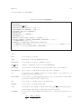
The calling speciﬁcations are:
Table 1.13: Structure (PERTUR:)
OPTIMIZE := PERTUR: OPTIMIZE FLUX [ SYS [ SYSP ] TRACK ] [ MACRO [ MACROP ] ] ::
(pertur data)
where
GPT
character*12 name of the source containing the source terms. If GPT appears on
the RHS, the previous values will be updated.
FLUX
character*12 name of the flux containing the unperturbed ﬂux, direct or adjoint.
SYS
character*12 name of the system containing the reference system matrices. system
must be a linked list.
SYSP
character*12 name of the system containing the perturbation of the system matrices.
TRACK
character*12 name of the track (type L TRIVAC) containing the tracking informations. track must be a linked list.
OPTIMIZE
character*12 name of the optimize containing the optimization informations. GPT
must appear on the RHS to be able to updated the previous values.
(pertur data)
structure containing the data to the second choice for the module PERTUR:.
20
IGE–314
1.3.1 Data input for module PERTUR:
Table 1.14: Structure (pertur data)
[ EDIT iprint ]
[ VARMUN { ivar1 ivar2 | ALL }
. . . {D-LAMBDA | D-LAMBDA/DX | D-LAMBDA-V | D-LAMBDA-V/DX |(eval data) } ] ;
where
EDIT
key word used to set iprint.
iprint
index used to control the printing in module.
VARNUM
key word used to deﬁne the decision variable for which the perturbation theory calculations will be done.
ivar1
number of the ﬁrst decision variable.
ivar2
number of the second decision variable.
ALL
key word used to specify that the perturbation theory calculations will be done for all
the decision variables.
D-LAMBDA
key word used to specify that absolute variation of the eigenvalue perturbation will be
calculated for the corresponding perturbated decision variables.
D-LAMBDA/DX
key word used to specify that derivative of the eigenvalue perturbation will be calculated for the corresponding perturbated decision variables.
D-LAMBDA-V
key word used to specify that absolute variation of the eigenvalue perturbation will be
calculated for the corresponding perturbated decision variables and that the provided
system matrix correspond to the voided reactor (or an other conﬁguration of the
reactor).
D-LAMBDA-V/DX
key word used to specify that derivative of the eigenvalue perturbation will be calculated for the corresponding perturbated decision variables and that the provided
system matrix correspond to the voided reactor (or an other conﬁguration of the reactor).
(eval data)
see explanations in the module FOBJCT: key word ’EVAL-OBJ-CST’ 1.1.2. Some
predeﬁned function are described too.
21
IGE–314
1.4
The GPTSRC: module
The GPTSRC: module is used to calculate the sources terms (direct and / or adjoint) for generalized
perturbation theory.
The calling speciﬁcations are:
Table 1.15: Structure GPTSRC:
{ GPT := GPTSRC: [ GPT ] OPTIMIZE FLUX [ SYS [ SYSP ] TRACK ] [ MACRO ] [ MAPFL ]
:: (gptsrc data)
where
GPT
character*12 name of the gpt linked list ﬁle containing fuel regions description and
burnup informations. If GPT appears on the RHS, the information previously stored
in GPT is modiﬁed if necessary and stored.
OPTIMIZE
character*12 name of the extended optimize linked list.
FLUX
character*12 name of the flux linked list. This object is used for the function
evaluation. It is recommended to provide it even if no function evaluation is done for
many parameters reading. ﬁle.
MACRO
character*12 name of the macrolib linked list ﬁle containing fuel regions description
and burnup informations. If it appears on RHS, is means it will be necessary for a
function evaluation (objective or constraint).
MAPFL
character*12 name of the extended map. If MAPFL appears on the RHS, the information in it will be red for many parameters initialisation.
TABFL
character*12 name of the table linked list ﬁle containing fuel regions description
and burnup informations. If it appears on RHS, is means it will be necessary for a
function evaluation (objective or constraint).
(gptsrc data)
structure containing the data to module GPTSRC:.
1.4.1 Data input for module GPTSRC:
Table 1.16: Structure gptsrc data
[ EDIT iprint ]
[[ DIRECT { ivar1 ivar2 | ALL } ]]
[[ ADJOINT (eval data) ]]
[[ OTHER { DIRECT | ADJOINT } ivar1 (eval data) ]] ;
22
IGE–314
where
EDIT
key word used to set iprint.
iprint
index used to control the printing in module.
DIRECT
key word used to calculate a direct source term for decision variables Si .
Si =
Ap φ − Aφ
∆λ
Bp φ − Bφ
∂ (A − λB)
.φ =
−
.Bφ − λ.
∂Xi
∆Xi
∆Xi
∆Xi
(1.20)
ivar1
number of the ﬁrst decision variable.
ivar2
number of the second decision variable.
ALL
key wod used to specify that the direct source terms calculations will be done for all
the decision variables.
ADJOINT
key word used to calculate a adjoint source term for decision variables Sj∗ .
Sj∗ =
(eval data)
∂Gj
∂φ
(1.21)
see explainations in the module FOBJCT: key word ’EVAL-OBJ-CST’. Some predeﬁned function are described too.
23
IGE–314
1.5
The GPTGRD: module
The GPTGRD: module is used to compute the gradient of functions using the generalized perturbation
theory. To do that the user must precalculate the sources terms (module GPTSRC) and the generalized
adjoints (module GPTFLU).
The GPTGRD: module also allows to deﬁne directly values of gradient of functions.
The calling speciﬁcations are:
Table 1.17: Structure GPTGRD:
OPTIMIZE := GPTGRD: OPTIMIZE FLUXP [ SYS [ SYSP [ SYS2 [ SYS2P ] ] ] TRACK
MACRO [ FLUX ] [ MATEX ] [ MAPFL ] :: [ (direct data) ] (gptgrd data)
OPTIMIZE := GPTGRD: OPTIMIZE :: (direct data)
where
OPTIMIZE
character*12 name of the optimize containing the optimization informations. GPT
must appear on the RHS to be able to updated the previous values.
FLUXP
character*12 name of the flux containing the generalized adjoint ﬂux, explicit or
implicit.
TRACK
character*12 name of the track linked list ﬁle containing tracking information corresponding to FLUXP.
MACRO
character*12 name of the macrolib linked list ﬁle containing fuel regions description
and burnup informations.
FLUX
character*12 name of the flux containing the unperturbed ﬂux, direct or adjoint.
If it appears on RHS, is means it will be necessary for a function evaluation (objective
or constraint).
GPT
character*12 name of the gpt linked list ﬁle containing fuel regions description and
burnup informations. If it appears on RHS, is means it will be necessary for a function
evaluation (objective or constraint).
MATEX
character*12 name of the matex object created by the USPLIT: module and containing the complete reactor material index including devices.
MAPFL
character*12 name of the map linked list ﬁle containing the fuel map informations.
(direct data)
structure containing the data to the direct deﬁnition of gradient for the module
GPTGRD:.
(gptgrd data)
structure containing the data to the generalized theory based gradients choice for the
module GPTGRD:.
24
IGE–314
1.5.1 Data input for module GTPGRD:
Table 1.18: Structure direct data
[ NEW-VALUE ] [ REL ]
DIRECT-VALUE ivar1 [ ivar2 ] { FOBJ | CONSTRAINT if cn1 if cn1 }
. . . . . . grad ( j=1, (ivar2 − ivar1 + 1).(if cn2 − if cn1 + 1) )
[;]
where
NEW-VALUE
key word used to specify that the value of gradient is set to zero.
REL
key word used to recover the epsilon in record OPT-PARAM-R of object OPTIMIZE.
DIRECT-VALUE
key word used to specify that the value of gradient will be directly given by the user.
ivar1
ﬁrst decision variable for which the gradient will be deﬁned.
ivar2
last decision variable for which the gradient will be deﬁned. If it is not deﬁned, the
default value is ivar1 .
FOBJ
key word used to specify that the gradient of the objective function will be deﬁned.
CONSTRAINT
key word used to specify that the gradient of conctraints will be deﬁned.
if cn1
ﬁrst constraint for which the gradient will be deﬁned.
if cn2
last constraint for which the gradient will be deﬁned.
grad
value of the gradient.
;
this key word has to be provided if (gptgrd data) is not used.
Table 1.19: Structure gptgrd data
GPT [[ DIRECT { ivar1 ivar2 | ALL } (eval data) ]]
. . . [[ INDIRECT [ { EXPLICIT | IMPLICIT } ] { ivar1 ivar2 | ALL } ] { FOBJ | CONSTRAINT if cn1 if cn2 } ]]
;
where
DIRECT
key word used to specify that the direct part of the gradient will be calculated.
ivar1
ﬁrst decision variable for which the gradient will be deﬁned.
ivar2
last decision variable for which the gradient will be deﬁned.
ALL
key word used to specify that the gradient will be calculated for all decision variables.
25
IGE–314
(eval data)
see explainations in the module FOBJCT: key word ’EVAL-OBJ-CST’. Some predeﬁned function are described too.
INDIRECT
key word used to specify that the indirect part of the gradient will be calculated.
EXPLICIT
key word used to obtain the solution of an direct ﬁxed source eigenvalue problem.
IMPLICIT
key word used to obtain the solution of an adjoint ﬁxed source eigenvalue problem. If
neither ’EXPLICIT’ nor ’IMPLICIT’ are provided the default value will be chosen as a
function of nvar and ncst + 1.
FOBJ
key word used to specify that the gradient of the objective function will be deﬁned.
CONSTRAINT
key word used to specify that the gradient of conctraints will be deﬁned.
if cn1
ﬁrst constraint for which the gradient will be deﬁned.
if cn2
last constraint for which the gradient will be deﬁned.
26
IGE–314
1.6
The TABU: module
The TABU: module is used to deﬁne options and data storage for the tabu search optimization
algorithm.
The calling speciﬁcations are:
Table 1.20: Structure TABU:
TABUSH [ OPTIM ] := TABU: [ TABUSH ] OPTIM :: (desctabu)
where
TABUSH
character*12 name of the extended tabu linked list ﬁle.
OPTIM
character*12 name of the extended optimize linked list ﬁle. If OPTIM appears on
the LHS, decision variables or their limits (for exemple) may be changed for further
evaluation of the objective function and constraint.
(desctabu)
structure containing the data to module TABU:.
1.6.1 Data input for module TABU:
Table 1.21: Structure (desctabu)
[
[
[
[
[
[
[
[
;
EDIT iprint ]
DEFINITION (def data) ]
NEIGHB-CREAT ]
NEIGHB-CHOIC [ INIT-PRO-LIST ] [ NELDER-MEAD ] ineig ]
NEIGHB-EVAL [ INIT-PRO-LIST ] [ NELDER-MEAD ] ineig ]
NEIGHB-BEST [ CONV-TEST >> Lconv << ] [ PROMISE-TEST [ NO-THRESHOLD ] >> Lpro << ] ]
PROMISE-AREA [ NELDER-MEAD ] { CREATION | UPDATE } ]
NELDER-MEAD (nelder data) ]
where
EDIT
key word used to set iprint.
iprint
index used to control the printing in module.
DEFINITION
key word used to deﬁne the tabu search optimization options.
(def data)
structure containing the data to the option DEFINITION.
NEIGHB-CREAT
key word used to create the neighborhood for the decision variable set stored as the
current one in the TABUSH object.
27
IGE–314
NEIGHB-CHOIC
key word used to specify the number ineig within the neighbors which will be evaluated.
The corresponding decision variable values are copied in the OPTIM object as the
current decision variables.
NEIGHB-EVAL
key word used to specify the number ineig within the neighbors which have been
evaluated. The corresponding functional values and the tabu function result are stored
in the TABU object.
INIT-PRO-LIST
key word used to specify the initial elements of the promising list are selected and
evaluated (and not the neighbors).
NELDER-MEAD
key word used to specify the initial elements of the polytope for the Nelder-Mead
simplex algorithm are selected and evaluated (and not the neighbors).
ineig
integer value for a neighbor point to be / which has been evaluated.
NEIGHB-BEST
key word used to check the neighbors results. The best neighbor result is compared to
the ﬁttest solution ever found. An update is performed if necessary. Tests for global
convergence and promising area detection can be done. The tabu list is updated.
CONV-TEST
key word used to verify if global convergence is achieved.
Lconv
logical value for the global convergence. Lconv equals .true. if N it is greater than
N itmax .
PROMISE-TEST
key word used to verify if a promising area has been detected.
NO-THRESHOLD
key word used to specify that no threshold limits the acceptance of promising areas.
Lconv
logical value for the promising area detection.
PROMISE-AREA
key word used to specify that calculation based on gradient methods will be performed
on a promising area previously detected.
NELDER-MEAD
key word used to specify the Nelder-Mead simplex algorithm is used instead of the
gradient method.
CREATION
key word used to deﬁne the area for the local gradient method optimization algorithm.
A backup of original decision variable limits is done in TABUSH object and new
smaller ones are stored in OPTIM object.
UPDATE
key word used to set the gradient method result for the promising area as the new
current decision variable. An update of the best point ever found is done is necessary.
The promising list is also updated.
NELDER-MEAD
key word used to specify the Nelder-Mead simplex algorithm is selected.
(def data)
structure containing the data to the option NELDER-MEAD corresponding to the diﬀerent
geometric transformations.
Table 1.22: Structure (def data)
[ ISEED seed ]
[ NEIGHBOR-NB ngh ]
[ NEIGHBOR-TYP { RECTANGLE | BALL } ]
continued on next page
28
IGE–314
Structure (def data)
[
[
[
[
[
[
[
[
[
[
[
[
[
[
continued from last page
NEIGHBOR-DIS { GEOMETRIC fact | LINEAR | ISOVOLUME } ]
NEIGHBOR-RAD Rn ]
TABU-RAD Rt ]
PROMIS-RAD Rp ]
NIT-MAX-CONV N itmax ]
TABU-LIST-LG { ALL |Lgt } ]
PROM-LIST-LG { ALL |Lgp } ]
GET-CURRENT [ COMPLETE] ]
PUT-CURRENT ]
INITIALIZE ]
INIT-PRO-LIST ]
RESET-BEST ]
BEST-AS-CURR ]
NELDER-EPS ǫned ]
where
ISEED
key word used to deﬁne the seed for random number generation seed.
seed
integer value for the seed (default given by CLETIM).
NEIGHBOR-NB
key word used to deﬁne the number of neighbors ngh.
ngh
integer value for the number of neighbors (default 5).
NEIGHBOR-TYP
key word used to specify the type of the neighborhood.
RECTANGLE
key word used to specify that the neighborhood will be hyperrectangle crowns (default).
BALL
key word used to specify that the neighborhood will be hypersphere crowns.
NEIGHBOR-DIS
key word used to specify that the type of discretisation within the neighborhood.
GEOMETRIC
key word used to specify that the radius of the crowns are given by a geometric serie.
The radius are given by:
ri = Rn
1
with i ∈ {1, ngh}
f actngh−i
fact
real number (> 1) for the geometric serie for the radius determination.
LINEAR
key word used to specify that the radius of the crowns are given by a linear serie
(default). The radius are given by:
ri = Rn
ISOVOLUME
i
with i ∈ {1, ngh}
ngh
key word used to specify that the radius of the crowns are chosen to have a constant
volume for all crowns. The radius are given by:
ri = Rn
s
nvar
i
with i ∈ {1, ngh}
ngh
29
IGE–314
NEIGHBOR-RAD
key word used to set the radius Rn of the neighborhood.
Rn
real number for neighborhood radius. This radius is a fraction of the total limits and
then must be between 0.0 and 1.0.
TABU-RAD
key word used to set the radius Rt of the hyperrectangle / ball around tabu values.
All the points within this small domain are tabu as well.
Rt
real number for tabu list radius. This radius is a fraction of the total limits and then
must be between 0.0 and 1.0.
PROMIS-RAD
key word used to set the radius Rp of the hyperrectangle / ball around tabu values.
All the points within this small domain are tabu as well.
Rp
real number for promising list radius. This radius is a fraction of the total limits and
then must be between 0.0 and 1.0.
NIT-MAX-CONV
key word used to specify the number N itmax of required external iteration without
improvement of the best solution ever found for global convergence achievement.
N itmax
integer value of required iterations for global convergence.
TABU-LIST-LG
key word used to specify the maximum length of the tabu list.
PROM-LIST-LG
key word used to specify the maximum length of the promising area list.
ALL
key word used to specify the values entering in a list are kept until the end of the
optimization procedure.
Lgt
integer value of maximum tabu list length.
Lgp
integer value of maximum promising area list length.
GET-CURRENT
key word used to specify the decision variable set in OPTIM object will be stored as
the current one in TABUSH object.
COMPLETE
key word used to specify the objective function, the constraints and the penalty functions will also be stored with the current values.
PUT-CURRENT
key word used to specify the current decision variable set in TABU object will be
stored as the variable values in OPTIM object.
INITIALIZE
key word used to initialize (chose a random value) the starting decision variables in
the decision space.
INIT-PRO-LIST
key word used to specify that the initial promising list is created.
RESET-BEST
key word used to reset the best value of the tabu search objective function.
BEST-AS-CURR
key word used to set the best value as the current value.
NELDER-EPS
key word used to set the convergence limit for the Nelder-Mead simplex algorithm.
ǫned
real value for the Nelder-Mead convergence criterium (default 0.01).
30
IGE–314
Table 1.23: Structure (nelder data)
[
[
[
[
FIND-NEW >>iworst << ]
COMPARE-NEW >>Lexp << >>Lctt << >>Lconv << ]
EXPAN-VLD >>Lconv << ]
CONTRACTION >>Lmctt << >>ibest << >>Lconv << ]
where
FIND-NEW
key word used to ﬁnd the worst point of the polytope for the Nelder-Mead simplex
algorithm, and compute its reﬂected point.
iworst
integer value for the index of the worst point of the polytope.
COMPARE-NEW
key word used to compare the reﬂected point of the worst point of the polytope with
the other points. Next geometrical transformation is decided according to the results
of the comparison.
Lexp
logical value for the expansion move.
Lctt
logical value for the contraction move.
Lconv
logical value for convergence.
EXPAN-VLD
key word used to validate the expansion point (comparison of its results with the
reﬂection point).
CONTRACTION
key word used to compare the contraction point (comparison of its results with the
reﬂection point). Next geometrical transformation is decided according to the results
of the comparison.
Lctt
logical value for the multi-contraction move.
ibest
integer value for the index of the best point of the polytope.
31
IGE–314
2 Output Data Treatment
In this section, input of output data treatment modules will be given.
2.1
The ADDOBJ: module
The ADDOBJ: module is used to perform the diﬀerences between two objects or to add two objects.
For the macrolib and flux, this is possible only if they contain the same energy group and material
mixture numbers.
The calling speciﬁcations are:
Table 1.24: Structure ADDOBJ:
MACNEW := ADDOBJ: [ MACNEW ] MACRO1 MACRO2 :: (addmac data)
FLUNEW := ADDOBJ: [ FLUNEW ] FLU1 FLU2 :: (addflu data)
where
MACNEW
character*12 name of the macrolib containing either the nuclear increments, from
the calculation of MACRO1 - MACRO2 or the sum of properties from MACRO1 +
MACRO2. Be aware the order of macrolib is important, even for addition option.
MACRO1
character*12 name of a macrolib.
MACRO2
character*12 name of a macrolib. When addition is performed, it must contain
incremental nuclear properties.
(addmac)
structure containing the data to module ADDOBJ: with the options for macrolib operations.
FLUNEW
character*12 name of the flux which will be the result of the addition or the subtraction of the two old one. This object has to be in create mode only.
FLU1
character*12 name of the ﬁrst flux.
FLU2
character*12 name of the second flux.
(addflu)
structure containing the data to module ADDOBJ: with the options for flux addition.
2.1.1 Data input for module ADDOBJ:
Table 1.25: Structure (addmac data)
[ EDIT iprt ]
[ STEP ilev ]
[ { ADD [ frac1 [ frac2 ] ] | SUB } ]
continued on next page
32
IGE–314
Structure (addmac data)
continued from last page
[ FROM-MP ]
[ { DDIFF | NODIF } ]
;
where
EDIT
key word used to set iprt.
iprt
index used to control the printing. <= 2 minimum printing; > 3 macroscopic diﬀerences are printed.
ADD
keyword to specify that the two objects will be added. If only frac1 is specifeid,
MACRO1 + frac1.MACRO2 will be performed using the options for the diﬀusions
coeﬃcients. If frac1 and frac1 are speciﬁed, frac1.MACRO1 + frac2.MACRO2 will
be performed even for the diﬀusion coeﬃcients.
frac1
ﬁrst real that will multiply the value of the ﬁrst object. (default 1.0)
frac2
second real that will multiply the value of the second object. (default 1.0)
SUB
keyword to specify that the two objects will be substracted. This is the default option.
FROM-MP
keyword to specify that the two objects have been partially calculated by diﬀerent
CPU. An addition will be performed to calculate the ’complete’ object (frac1 and
frac2 equal 1.0).
STEP
key word used to set ilev.
ilev
number of the perturbed level in macrolib. In case of substraction of two macrolib:
If a single set of increments is stored, it must be equal to 1. This step is used to
later compute perturbation system matrices. If this information is absent, incremental
cross sections are stored on root directory. In case of addition of two macrolib: ilev
speciﬁes the perturbed level where informations is stored in the two initial macrolib.
If both macrolib have a perturbed level, it must the same. The resulting properties
will be stored on root directory.
DDIFF
keyword to specify a correct treatment of diﬀusion coeﬃcients. If SUB is speciﬁed, the
resulting incremental diﬀusion coeﬃcient will be:
∆D =
1
D1
1
−
1
D2
where D1 is taken from the ﬁrst macrolib and D2 from the second. If ADD is speciﬁed,
the resulting diﬀusion coeﬃcient will be:
D=
1
D1
1
1
+ ∆D
2
where D1 is taken from the ﬁrst macrolib and ∆D2 from the second.
NODIF
keyword to specify that no addition or substraction of diﬀusion coeﬃcients will be
done. This is the default option.
33
IGE–314
Table 1.26: Structure (addflu data)
[ EDIT iprt ]
{
[ { ADD [ frac1 frac2 ] | SUB } ] [ F-ADJOINT [ ADJ-ONLY ] ]
|
FROM-2-PARTS { FLUX | AFLUX |DFLUX iga1 |ADFLUX iga1 } frac1
. . . . . . { FLUX | AFLUX |DFLUX iga2 |ADFLUX iga2 } frac2
. . . . . . IN { FLUX | AFLUX |DFLUX iga2 |ADFLUX iga2 }
};
where
EDIT
key word used to set iprt.
iprt
index used to control the printing. => 1 structure of the resulting object is printed;
ADD
keyword to specify that the two objects will be added. This is the default option.
frac1
ﬁrst real that will multiply the value of the ﬁrst object. (default 1.0)
frac2
second real that will multiply the value of the second object. (default 1.0)
SUB
keyword to specify that the two objects will be substracted.
F-ADJOINT
keyword to specify that the same numerical operation will performed on ﬂux and
adjoint ﬂux.
ADJ-ONLY
keyword to specify that the numerical operation will be performed on the adjoint ﬂux
only.
FROM-2-PARTS
keyword to specify that the two objects contain one part of the result ﬂux. An addition
will be performed to calculate the ’complete’ object. This option can not be done with
other options (except EDIT) in the same call of the module.
FLUX
keyword to specify that the ﬂux will be used or the result of the addition.
AFLUX
keyword to specify that the adjoint ﬂux will be used or the result of the addition.
DFLUX
keyword to specify that the explicit generalized adjoint will be used or the result of
the addition.
ADFLUX
keyword to specify that the implicit generalized adjoint will be used or the result of
the addition.
iga1
number of the ﬁrst generalized adjoint if applicable.
iga2
number of the second generalized adjoint if applicable.
IN
keyword to specify that the type of ﬂux for the result of the addition.
iga3
number of the third generalized adjoint if applicable.
34
IGE–314
2.2
The MATLAB: module
The MATLAB: module is used to create an ASCII ﬁle executable by MATLAB. Two options are
available. First one is used to create a ﬁle to draw the gradiants of functions calulated in a optimisation
problem. Second option allows to draw maps of the ﬂux distribution.
The calling speciﬁcations are:
Table 1.27: Structure MATLAB:
{ ASCII-MAT := MATLAB: OPTIM :: (descmatlgrd) |
ASCII-MAT := MATLAB: FLUX TRACK INDEX GEOM :: (descmatlflu) }
where
ASCII-MAT
character*12 name of the ASCII ﬁle executable by MATLAB.
OPTIM
character*12 name of the optimisation linked list or xsm ﬁle containing the gradiants and the stored perturbated values of the functions. Such ﬁle is obtained using
the module GPTVRF:.
(descmatlgrd)
structure containing the data input to module MATLAB: for gradiants ploting.
FLUX
character*12 name of the flux linked list or xsm ﬁle containing the ﬂux or adjoint
or generalized adjoints or harmonics to be mapped.
TRACK
character*12 name of the track linked list or xsm ﬁle containing the tracking datas
(TRIVAA is the only type of tracking compatible).
INDEX
character*12 name of the index linked list or xsm ﬁle containing the index datas.
GEOM
character*12 name of the geom linked list or xsm ﬁle containing the geometry description.
(descmatlflu)
structure containing the data input to module MATLAB: for ﬂux distribution’s mapping.
2.2.1 Data input for module MATLAB:
Table 1.28: Structure (descmatlgrd)
[ EDIT iprint ]
OPT-GRAD-VRF
;
where
EDIT
key word used to set iprint.
35
IGE–314
iprint
index used to control the printing in module XSFUEL:. =0 for no print (default value);
=1 for minimum printing; larger values produce increasing amounts of output.
OPT-GRAD-VRF
key word used to select the gradiants veriﬁcation and ploting option and produce the
ASCII-MAT ﬁle. An exemple of the results is presented on the following ﬁgure.
Fobj, Zone #2
0.144
0.143
0.142
0.141
0.14
0.139
0.138
−4
−3
−2
−1
0
1
2
3
Pertubation (%), (0% <=> Burnup de sortie moyen = 6478MWj/t)
4
Table 1.29: Structure (descmatlflu)
[ EDIT iprint ]
MAP-FLUX {FLUX | ADJOINT | GPT-FLU isrc | GPT-ADJOINT isrc | HARMONIC ihrm }
{ NO-GRID | CENTER-GRID | CHANEL-GRID }
;
where
EDIT
key word used to set iprint.
iprint
index used to control the printing in module XSFUEL:. =0 for no print (default value);
=1 for minimum printing; larger values produce increasing amounts of output.
MAP-FLUX
key word used to select the ﬂux distribution mapping option and produce the ASCIIMAT ﬁle.
FLUX
key word used to specify that the distribution of the ﬂux will be drawn.
ADJOINT
key word used to specify that the distribution of the adjoint will be drawn.
GPT-FLU
key word used to specify that the distribution of the explicit generalized adjoint corresponding to the source number iscr will be drawn.
GPT-ADJOINT
key word used to specify that the distribution of the implicit generalized adjoint corresponding to the source number iscr will be drawn.
iscr
identiﬁer for the source number corresponding to generalized adjoint to be drawn.
HARMONIC
key word used to specify that the distribution of the ﬂux corresponding to the harmonic
number ihrm will be drawn.
ihrm
identiﬁer for the harmonic number corresponding to the ﬂux to be drawn.
IGE–314
36
NO-GRID
key word used to specify that no grid will be add on the map of the ﬂux distribution.
An exemple of the results is presented on the ﬁgure a.
CENTER-GRID
key word used to specify that a grid will be add on the map of the ﬂux distribution.
The nodes of the grid correspond to the center of the volumes where the ﬂux are
calculated. An exemple of the results is presented on the ﬁgure b.
CHANEL-GRID
key word used to specify that a grid will be add on the map of the ﬂux distribution.
The squares of the grid correspond to the limits of the channels. An exemple of the
results is presented on the ﬁgure c.
(a)
(b)
FLUX GR#2, Plan #9
FLUX GR#2, Plan #9
3.5
(c)
3.5
3
3
2.5
2.5
2
2
1.5
1.5
1
1
0.5
0.5
0
800
0
800
800
600
600
400
800
600
600
400
400
200
200
0
0
400
200
200
0
0
37
IGE–314
2.3
The GPTVRF: module
The GPTVRF: module is used to verify the computation of the gradients with classical and generalized
perturbation theories. The analytical gradients calculated with the modules PERTUR: and GPTGRD:
are compared with numerical gradients calculated with the Ceshino method using several values of the
functionals for pertubated values of the decision variables.
The calling speciﬁcations are:
Table 1.30: Structure GPTVRF:
OPTIMV := GPTVRF: [ OPTIMV ] OPTIM :: (gptvrf data)
where
OPTIMV
character*12 name of the optimize containing the pertubated and unpertubated
values of the decision variables and of the functionals. If OPTIMV is the same as
OPTIM , then the perturbated datas will be stored in the same optimize object.
OPTIM
character*12 name of the optimize containing the curent values of the decision
variables and of the functionals.
(gptvrf data)
structure containing the data to module GPTVRF:.
2.3.1 Data input for module GPTVRF:
Table 1.31: Structure gptvrf data
[
[
[
[
;
EDIT iprint ]
SAVE-PERT ivar ǫ ]
SAVE-GPT {ABS | REL ǫGP T } ]
COMPARE { ivar1 ivar2 | ALL } { if ct1 if ct2 | ALL } ]
where
EDIT
key word used to set iprint.
iprint
index used to control the printing in module.
SAVE-PERT
key word used to store the current values of the functionals for the corresponding
perturbation ǫ of the decision variable ivar .
ivar
number of the perturbated decision variable.
ǫ
amount of the pertubation (ex: ǫ=0.01 corresponds to 1% of perturbation).
38
IGE–314
SAVE-GPT
key word used to specify that the analytical gradient will be stored.
ABS
key word used to specify that the stored analytical gradient correspond to a absolute
perturbation or that the derivative are already calculated.
REL
key word used to specify that the stored analytical gradient will be devided by the
corresponding amount of perturbation to obtain the relative gradient (the derivative).
ǫGP T
amount of the pertubation (ex: ǫGP T =0.01 corresponds to 1% of perturbation).
COMPARE
key word used to specify that the numerical gradient will be computed and compared
to the analytical gradients.
ivar1
number of the ﬁrst decision variable for which the comparason will be done.
ivar2
number of the last decision variable for which the comparason will be done.
if ct1
number of the ﬁrst functional for which the comparason will be done.
if ct2
number of the last functional for which the comparason will be done.
ALL
key word used to specify that the comparason will be done for all decision variables
and/or all functionals.
Chapter 2
OPTEX STRUCTURES
39
40
IGE–314
1 Contents of a /tabu/ data structure
The /tabu/ speciﬁcation is used to store the decision variable set used for a tabu search optimization
method. The diﬀerent options of this method are also stored in the /tabu/ data structure.
The signature variable for this data structure must be SIGNA=L_TABU
. The dimensioning
parameters for this data structure, which are stored in the state vector Sit , represents:
• The number of neighbors Neig = S1t .
• The type of neighborhood S2t where
S3t
=
1
2
hyperrectangle
ball
• The type of discretisation of the neigborhood. S3t where

 1 geometric
2 linear
S3t =

3 isovolume
• The test for external convergence N itmax = S4t .
• The current number of iterations without improvement of the best value N it = S5t .
• The tabu list maximum size Lt = S6t .
• The promising area list maximum size Lp = S7t .
• The tabu list current size Lct = S8t .
• The promising list current size Lcp = S9t .
t
.
• The number of decision variables Nvar = S10
t
• The number of constraints Ncst = S11
.
t
• The ﬁrst number for the random point generation algorithm S39
(=TIME()).
t
• The number of generated random numbers S40
.
Table 2.1: Main records and sub-directories in /tabu/
Name
Type
SIGNATURE
STATE-VECTOR
C∗12
I(40)
Condition
UnitsComment
Signature of the data structure (SIGNA)
Vector describing the various parameters associated with this data structure Sit and the
tabu search optimization integer options
continued on next page
41
IGE–314
Main records and sub-directories in /tabu/
Name
Type
TABU-PARAM-R
R( 40)
CURRENT-VAL
R(Nvar + Ncst + 2)
BEST-VAL
R(Nvar + Ncst + 2)
NEIGHBORHOOD
Dir
TABU-LIST
Dir
PROMISE-LIST
Dir
NELDER-MEAD
Dir
Condition
continued from last page
UnitsComment
Vector containing various tabu search optimization real options and several current values.
The values of the current decision variables,
the corresponding functionals and the tabu
function
The values of the decision variables, the corresponding functionals and the tabu function
for the best point ever found
Directory containing the neighbor decision
variable set.
Directory containing the tabu decision variable set.
Directory containing the decision variable set
corresponding to promising areas.
Directory containing the decision variable set
corresponding to the polytope for NelderMead Simplex method.
Notes related with the diﬀerent limits and values for the iterative calculations of the optimization
problem:
1st
Rn
neighborhood radius (fraction ∈ [0, 1] of the total decision space). (default:
0.01)
2nd
Rt
radius around tabu list decision variable set within points are also tabu (fraction
∈ [0, 1] of the total decision space). (default: 0.001)
3rd
Rp
radius around promising area list decision variable set within points are also
tabu (fraction ∈ [0, 1] of the total decision space). (default: 0.002)
4th
f act
factor in case of a geometric discretisation of the neighborhood. (default: 2)
5th
best tabu search function value ever achieved.
The other value of the record are not used and set to 0.0.
1.1
The sub-directories in /tabu/
The sub-directories are NEIGHBORHOOD, TABU-LIST, PROMISE-LIST and NELDER-MEAD.
They all have two main records in common. NELDER-MEAD has several additional records. Those two
types of records are presented in the two following tables.
42
IGE–314
Table 2.2: Main records in sub-directories
Name
Type
ITEM
R()
TABU-F-VAL
R(Neig )
Condition
Units
Comment
List of decision variable set, its corresponding
functional and tabu search function values.
The tabu search function values of the neighbors.
The length of the ITEM list is given by:
• Neig for NEIGHBORHOOD directory
• min{Lct , Lt } for TABU-LIST directory
• min{Lcp , Lp } for PROMISE-LIST directory
• Nvar + 1 for NELDER-MEAD directory
Table 2.3: Additional records in NELDER-MEAD directory
Name
Type
IWORST
I(1)
IWORST2
I(1)
IBEST
I(1)
XAVERG
R(Nvar )
REFLECT-VAL
R(Nvar + Ncst + 2)
EXPAN-VLD
R(Nvar + Ncst + 2)
Condition
UnitsComment
Index corresponding to the summit of the
polytope with the worst value of tabu search
fonction.
Index corresponding to the summit of the
polytope with the second worst value of tabu
search fonction.
Index corresponding to the summit of the
polytope with the worst value of tabu search
fonction.
The average values of the decision variables
for all the points of the polytope.
The reﬂection of the worst point of the polytope with the centroid given by XAVERG. It
also includes the corresponding objective function, constraints and tabu search values after
their evaluation.
The reﬂection of the centroid of the polytope
given by XAVERG with the worst point. It
also includes the corresponding objective function, constraints and tabu search values after
their evaluation.
43
IGE–314
2 Contents of a /optimize/ data structure
The /optimize/ speciﬁcation is used to store the optimization variables and functions values and
deﬁnitions, limits and options. It is also used in a particular case with the module GPTVRF: to store the
functions for many perturbated values of the decision variables and the gradients calculated numerically
and analytically.
In any case, the signature variable for this data structure must be SIGNA=L_OPTIMIZE . The
dimensioning parameters for this data structure, which are stored in the state vector Sio , represents:
• The number of decision variables Nvar = S1o .
• The number of constraints Ncst = S2o .
• The type of optimization. S3o where
S3o
=
1 minimization
−1 maximization
• The test for external convergence S4o . where
S4o
=
0
1
not converged
converged
• The number of external iterations S5o .
• The type of reduction for external step S6o . where
S6o =
1
2
half
parabolic
• The number of inner iterations S7o .
• The number of outer iterations S8o .
• The resolution’s method for the linearized problem S9o . where

1 SIMPLEX/LEMKE




 2 LEMKE/LEMKE
3 MAP
S9o =


4 Augmented Lagragian



5 Penalty Method
o
• The type of perturbation for the decision variables S10
. where
o
S10
=
1
2
epsilon
previous
o
• The type of fuel cost deﬁnition S11
. where
o
S11
=
1
2
dependent of the enrichment
ﬁxed
44
IGE–314
o
• The test for a realistic decision vector S12
. where
o
S12
=
0
1
do not respect all constraints
do respect all constraints
o
• A ﬂag for unsuccessful resolution in QLP S13
. where
o
S13
=
0 successful at last iteration
≥ 1 number of iteration with unsuccessful resolution
o
• The number of regions Nr = S16
.
o
• The number of channels in the core Nch = S17
.
o
• The number of bundles per channel Nk = S18
.
o
• The number of unknowns per energy group Nu = S19
.
o
• The number of energy groups G = S20
.
Table 2.4: Main records and sub-directories in /optimize/
Name
Type
SIGNATURE
STATE-VECTOR
C∗12
I(40)
VAR-VALUE
VAR-TYPE
{var-zone}
R(Nvar )
R( Nvar )
I(Nz,v )
VAR-MAX-VAL
R(Nvar )
VAR-MIN-VAL
R(Nvar )
VAR-WEIGHT
R( Nvar )
CST-VOL-TYPE
I(Ncst )
CST-OBJ
R(Ncst )
CST-TYPE
I(Ncst )
{cst-zone}
I(Nz,c )
CST-WEIGHT
R(Ncst )
Condition
Units
Comment
Signature of the data structure (SIGNA)
Vector describing the various parameters associated with this data structure Sio
The values of the decision variables
The type of the decision variables V artype .
The deﬁnition of the zone where i-th decision variable have an inﬂuence on the material
properties.
The maximum values of the decision variables
can be.
The minimum values of the decision variables
can be.
The weight of the decision variables wi in the
quadratic constraint.
Record containing the type for the zone where
the constraints apply.
The limit value of the contraints. The units
depends with the type of the constraint type.
The type of the contraints: =-1 for ≥; =0 for
=; =1 for ≤.
The deﬁnition of the zone where the constraint
j apply.
The weight of the constraint ηj and γj for the
duals and meta-heuristic methods.
continued on next page
45
IGE–314
Main records and sub-directories in /optimize/
Name
Type
FOBJ-CST-VAL
R(Ncst + 1)
OPT-PARAM-R
R(40)
FUNC-ZON-VOL
R(Ncst + 1)
BKP-PERT-XS
I(13)
FUEL-COST
R(dependant)
FUEL-C-DIST
R(Nu )
BURN-C-DIST
R(Nu )
D-LAMBDA
R(Nvar )
D-LAMBDA-V
R(Nvar )
GRADIENT
R(Nvar , Ncst + 1)
OLD-VALUE
Dir
Condition
continued from last page
Units
Comment
The actual values of the objective function
(ﬁrst value) and the contraints (the following
values). The number of the constraints are
assigned in the order they have been deﬁned.
The diﬀerent limits and values for the iterative
calculations of the optimization problem.
The ﬁrst value is the volume where the objective function applies and the followingones
correspond to the volumes where the constraints apllie.
The indexes of the perturbated material properties to backup.
The ﬁxed fuel cost of each enrichment zone if
o
S11
=-1.0, or the parameters to calculate the
o
enrichment dependant cost if S11
=-2.0.
$/kg The fuel cost distribution corresponding to
each point of the neutrons ﬂux unknowns.
M W d/tThe average exit burnup distribution corresponding to each point of the neutrons ﬂux
unknowns.
The gradients or the absolute variation depending of the keyword used in the PERTUR:
module of the eigenvalue with the decision
variables.
The gradients or the absolute variation depending of the keyword used in the PERTUR:
module of the eigenvalue for the coolant
voided reactor with the decision variables.
The gradients of the objective function and
the constraints. The gradients of the objective for all the decision variables are in ﬁrst
position, then follow the gradients of the constraints.
Directory containing diﬀerents informations of
the previous iterations. the values of the decision variables, the objective function, the constraints and the gradients of these functions
for the previous external iteration. This repertory will be created by the module PLQ: unless
it is speciﬁed to not do.
continued on next page
46
IGE–314
Main records and sub-directories in /optimize/
Name
Type
BKP-VALUE
Dir
{/stepdir/}
Dir
Condition
continued from last page
Units
Comment
Directory containing a backup of the values of
the decision variables, the objective function,
the constraints and the gradients of these functions for this external iteration. This repertory will be created if the interpolation of the
objective function in the middle point is calculated.
Directory containing the perturbated properties and the Ap φ and Bp φ vectors.
Notes related with the decision variables deﬁnition:
The type of the decision variable are given by V artype which is deﬁned by:
V artype = itype ∗ 1000 + izone
where
itype

1



2
=
3



4
average exit burnup
enrichment
number of bundles shift
device thickness
izone for the number of the corresponding zone in the L MAP for the decision variable.
The zones deﬁnition information records {var-zone} will be composed using the following FORTRAN
instructions
WRITE(var − zone,′ (A8, I4)′ ) ′ VAR − ZONE′ , i
for 1 ≤ i ≤ Nvar . The size Nz,v of the records depends of the type of the decision variable. For average
exit burnup, enrichment and number of bundles shift, Nz,v = Nch . For device thickness, Nz,v = Nch ∗ Nk .
Notes related with the constraints deﬁnition:
The type of each constraint zones is deﬁned by the following index :

1 one value for the whole reactor (ex: kef f )




2 one value for all channels (ex: total power)




 3 one value for one channel (ex: channel power)
4 one value for one bundle (ex: bundle power)
jtype =


5 one value for one zone deﬁned by many bundles




6 void reactivity



7 analytic function
The zones deﬁnition information records {cst-zone} will be composed using the following FORTRAN
instructions
WRITE(cst − zone,′ (A8, I4)′ ) ′ CST − ZONE′ , j
for 1 ≤ j ≤ Ncst . The size Nz,c of the records depends of the type of the constraint.

1
if jtype = 3, the record contains the number of the channel



2
if jtype = 4, the record contains the number of the channel and the plan
Nz,c =
N
×
N
if jtype = 5, the record contains one value for each bundle : =0 out of the

ch
k


zone j, =1 in the zone j.
IGE–314
47
If jtype = 1 or 2, no record is necessary to deﬁne the volume because it is implicit with the type of the
constraint (reactor or core respectively).
Notes related with the diﬀerent limits and values for the iterative calculations of the optimization
problem:
1st
S
external step limit. It is used for the quadratic constraint if applicable. (default:
1.0)
2nd
δ
internal step limit for MAP method. (default: 0.1)
3rd
εext
limit for external convergence. (default: 10−3 )
4th
εint
limit for internal convergence. (default: 10−3 )
5th
ε4
limit for convergence for the quadratic constraint.
6th
expected value for the objective function calculated with the linearized problem.
7th
ε∆X
relative variation of the decision variables for the ’epsilon’ method of perturbation. (default: 10−2 )
P
2m
8th
m
Exponent for a objective function : min j (Pj − P . (default: 8.0)
9th
α
multiplication factor for constraint weight if S9o = 4 or 5. (default: 2.0)
10th
εα
limit of the error of the constraints for which function penalty weight have to
be adjust.
11th
Vcore
Volume of the core.
12th
Vreactor
Volume of the reactor.
The other value of the record are not used and set to 0.0.
Notes related with the perturbated material properties:
In the record BKP-PERT-XS , 1 and 0 means that the corresponding perturbated material properties
will be backuped or not respectively. The available perturbated material properties are :
1st
DIFFX
diﬀusion coeﬃcient along x axes (Dx )
2nd
DIFFY
diﬀusion coeﬃcient along y axes (Dy )
3rd
DIFFZ
diﬀusion coeﬃcient along z axes (Dz )
4th
TOTAL
total cross-section (Σt )
5th
SCAT0
compressed isotropic component of the scattering matrix
6th
SIGW0
isotropic component of the within group of the scattering of the
scattering cross-section
7th
SCAT1
compressed linearly anisotropic component of the scattering matrix
8th
SIGW1
linearly anisotropic component of the within group of the scattering
of the scattering cross-section
9th
NFTOT
ﬁssion cross-section (Σf )
10th
NUSIGF
product of the ﬁssion cross-section (Σf ) and the steady-state number
of neutron produced per ﬁssion (ν ss )
11th
H-FACTORS
energy production coeﬃcient (H)
12th
CHI
the steady-state energy spectrum of the neutron emitted by ﬁssion
13th
FIXE
ﬁxed sources
Notes related with the fuel cost:
If the cost of the fuel is ﬁxed, the dimension of the record is given by the number of enrichment zones.
Otherwise the record contains the 7 parameters necessary to calculate the fuel cost, which are :
1st concentration in 235 U of the waste uranium (εw ).
2nd cost of natural uranium (CN U $/kg).
3rd cost of a separation work unit (CS $/SW U ).
4th cost of the bundle fabrication (CF AB $/kg).
5th interest rate (int%/day).
6th time to obtain uranium (days).
7th time for enrichment (days).
48
IGE–314
The fuel cost is given by the equation:
Notes related with the perturbated materials properties directory:
The directories {stepdir} will be composed using the following FORTRAN instructions
WRITE(stepdir,′ (A4, I8)′ ) ′ STEP′, i
for 1 ≤ i ≤ Nvar . Each directory contains also the result of the multiplication of the perturbated system
matrix and the ﬂux. i = 0 is used to stored the result of the unperturbated system matrix and the ﬂux.
2.1
The sub-directory /OLD-VALUE/ in /optimize/
Table 2.5: Main records and sub-directories in //OLD-VALUE//
Name
Type
VAR-VALUE
R(Nvar )
FOBJ-CST-VAL
R(Ncst + 1)
GRADIENT
R(Nvar , Ncst + 1)
VAR-VALUE2
R(Nvar )
BEST-VAR
R(Nvar )
BEST-FCT
R(1)
2.2
Condition
UnitsComment
The values of the decision variables of the last
valid iteration.
The values of the objective function and the
contraints of the last valid iteration.
The gradients of the objective function and
the constraints of the last valid iteration.
The values of the decision variables of the
second-last valid iteration.
The values of the decision variables corresponding to the best valid solution ever found.
The value of the objective function corresponding to the best valid solution ever found.
The sub-directory /stepdir/ in /optimize/
Table 2.6: Main records and sub-directories in //stepdir//
Name
Type
{Aphi}
R(Nu )
{Bphi}
R(Nu )
Condition
Units
Comment
The group-dependent vectors representing the
multiplication of a system matrix A and the
unperturbated ﬂux.
The group-dependent vectors representing the
multiplication of a system matrix B and the
unperturbated ﬂux.
continued on next page
49
IGE–314
Main records and sub-directories in //stepdir//
Name
Type
{/grpdir/}
Dir
Condition
Units
continued from last page
Comment
The group-dependent directory containing the
perturbated properties. The content is the
same as for the /macrolib/ but limited to the
properties to be saved only (see. BKP-PERTXS ).
The records {Aphi} and {Bphi} will be composed using the following FORTRAN instructions:
WRITE(Aphi,′ (A5, I7)′ ) ′ A ∗ PHI′ , g
and
WRITE(Bphi,′ (A5, I7)′ ) ′ B ∗ PHI′ , g
respectively where g represent the energy group.
2.3
Contents of a /optimize/ data structure for module GPTVRF:
When the module GPTVRF: is used a new /optimize/ data structure can be created. This new structure
contains a copy of the STATE-VECTOR record of the /optimize/ data structure used on the RHS of
the module. Then only the bare minimum necessary datas for gradients veriﬁcation will be stored. This
structure can also be deleted when a new point of the optimization procedure is calculated. If the same
/optimize/ data structure is used in the module GPTVRF: unnecessary data will be stored for the rest of
the optimization calculations. This is why we recommend to use a new /optimize/ data structure on the
LHS. In both cases, the /optimize/ data structure will contain the data described in the following table.
Table 2.7: /optimize/ in the particular case of module GPTVRF:
Name
Type
SIGNATURE
STATE-VECTOR
C∗12
I(40)
VAR-VALUE-RF
R(Nvar )
GRADIENT-GPT
R(Nvar , Ncst + 1)
Condition
UnitsComment
Signature of the data structure (SIGNA)
Vector describing the various parameters associated with this data structure Sio , same one
or a copy of the previous description.
The references values of the decision variables
for which the gradients are numerically and
analytically calculated.
The gradients calculated analytically. This
record is simply a copy of the record GRADIENT of the /optimize/ data structure on
the RHS.
continued on next page
50
IGE–314
/optimize/ in the particular case of module GPTVRF:
Name
Type
Condition
GRADIENT-EXP
R(Nvar , Ncst + 1)
/varpertdir/
Dir
continued from last page
UnitsComment
The gradients calculated numerically of the
objective function and the constraints. The
gradients are stored the same way as for the
record GRADIENT of the ﬁrst description.
Directory containing the perturbation values
and the corresponding values of the functions
for a decision variable i.
Notes related with the perturbated decision variables directory:
The directories {varpertdir} will be composed using the following FORTRAN instructions
WRITE(varpertdir,′ (A8, I4)′ ) ′ VAR − PERT′, i
for 1 ≤ i ≤ Nvar . Each directory contains also the records described in the following table.
Table 2.8: The sub-directory /varpertdir/ in /optimize/
Name
Type
EPSILON
R(Nε,i )
{fvalpert}
R(Ncst + 1)
Condition
Units
Comment
The value of the perturbation of the decision
variable i.
The values of the objective function and constraints for the perturbation p of the decision
variable i.
The number of perturbation Nε,i can include the unperturbated case (ε = 0.0) and can be diﬀerent
for each decision variable i. Moreover, the values of the perturbation do not have to be in increasing or
decreasing order.
The records {fvalpert} will be composed using the following FORTRAN instructions
WRITE(fvalpert,′ (A9, I3)′ ) ′ F − C − VAL − P′ , p
for 1 ≤ p ≤ Nε,i .
51
IGE–314
Index
CF AB , 4
CN U , 4
CS , 4
Lconv , 30
Lctt , 30
Lexp , 30
Lmctt , 30
Lconv, 26
Lgp , 28, 29
Lgt , 28, 29
Lpro, 26
N itmax , 28, 29
Rn , 29
Rp , 29
Rt , 29
Rn , 28
Rp , 28
Rt , 28
α, 16, 18
ǫ, 37
ǫGP T , 37
ǫcst , 16, 18
ǫext , 16, 17
ǫinn , 16, 17
ǫned , 28, 29
ρV,F C , 5, 6
εw , 4
burnmax , 3, 4
burnmin , 3, 4
cstlim , 5, 6
csttype , 5, 6
enrimax , 3, 4
enrimin , 3, 4
gprf rom , 10
gprto , 10
grpf rom , 11
grpto , 11
ibest , 30
icst1 , 6, 7, 14, 16–18
icst2 , 6, 7, 14, 16–18
if cn1 , 24, 25
if cn2 , 24, 25
if ct1 , 37, 38
if ct2 , 37, 38
iiter1 , 14, 16
ineig , 26, 27
iplan , 5
ivar1 , 14, 15, 20–22, 24, 37, 38
ivar2 , 14, 15, 20–22, 24, 37, 38
ivar3 , 14, 15
ivar , 37
iworst , 30
izone1 , 5, 6
izone2 , 5, 6
izone , 5
jplan , 5
kef f , 5
kref , 7
m, 16, 18
ncha , 5
nmax , 16, 17
nsurv zone , 5
num, 14, 16
qmoy , 7
tenr , 4, 5
tobt , 4
vali , 14, 16
*, 11
**, 11
+, 11
-, 11
.true., 14, 27
/, 11
//OLD-VALUE//, 48
//stepdir//, 48, 49
::, 2, 13, 19, 21, 23, 26, 31, 34, 37
:=, 2, 13, 19, 21, 23, 26, 31, 34, 37
;, 24
A, 8, 9
A*PHI, 10, 14, 15
ABS, 11, 37
ADD, 16, 18, 31–33
(addflu), 31
(addflu data), 31, 33
(addmac), 31
(addmac data), 31, 32
ADDOBJ:, 31
ADFLUX, 33
ADJ-ONLY, 33
ADJOINT, 8, 9, 21, 22, 35
AFLUX, 9, 33
AFLUX2, 9
ALL, 3–5, 10, 11, 14, 16, 20–22, 24, 28, 29, 37
ALLSAME, 5, 6, 16, 17
ALMOST-FSBLE, 14, 15
ANALYTIC-FCT, 5, 6
AP*PHI, 10, 14, 15
ASCII-MAT, 34, 35
AUG-LAGRANG, 16, 17
B, 8, 9
52
IGE–314
B*PHI, 10, 14, 15
BALL, 27, 28
BEST-AS-CURR, 28, 29
BKP-MACRO-P, 14, 15
BKP-MCR-P-XS, 16, 18
BP*PHI, 10, 14, 15
BUNDLE, 5
BURNUP-ZONE, 3, 4
CENTER-GRID, 35, 36
CHANEL-GRID, 35, 36
CHANNEL, 5
CHI, 9, 18
COEF-UPDATE, 14, 15
COMPARE, 37
COMPARE-NEW, 30
COMPLETE, 28, 29
CONSTRAINT, 6, 14, 16, 18, 24, 25
CONTRACTION, 30
conv, 14, 15
CONV-TEST, 14, 15, 26, 27
CORE, 10, 16, 18
COS, 11
cost, 4
CREATION, 26, 27
CST-QUAD-LIM, 16, 18
CST-VIOL-EPS, 16, 18
CST-WEIGHT, 16, 17
CST-WGT-MFAC, 16, 18
CST-ZONE, 10, 11
CST-ZONE-DF, 3
(cstzdf data), 3, 5
CTRL-ZONE-DF, 3
(czdf data), 3
D-CHI, 10
D-DIFFX, 10
D-DIFFY, 10
D-DIFFZ, 10
D-HFACT, 10
D-KEFF, 7, 8
D-KEFF=KREF, 7, 8
D-LAMBDA, 10, 20
D-LAMBDA-V, 10, 20
D-LAMBDA-V/DX, 20
D-LAMBDA/DX, 20
D-MINPCMAX, 7, 8
D-NFTOT, 10
D-NUSIGF, 10
D-SIGW0, 10
D-SIGW1, 10
D-TOTAL, 10
D-VOID-R-FC, 7, 8
(data), 10, 11
data name, 8, 9
DBL-ZONE, 11
DDIFF, 32
(def data), 14, 16, 26–28
DEFINITION, 14, 26
DEPENDANT, 4
(descfobjct), 2, 3
(descmatlflu), 34, 35
(descmatlgrd), 34
(descqlputl), 13, 14
(desctabu), 26
DFLUX, 33
DIFFX, 9, 18
DIFFY, 9, 18
DIFFZ, 9, 18
DIRECT, 14, 16, 21, 22, 24
DIRECT-VALUE, 24
(direct data), 23
direct data, 24
DISCRETE-ALL, 10, 11
DISCRETE-COR, 10, 11
DISCRETE-CST, 10, 11
DIVISION, 11
DOWN, 8, 9
DPHI-POWER, 7
DPHI-UCOST, 7
DX-METHOD, 14
DX-POWER, 7
DX-UCOST, 7, 10
EDIT, 3, 14, 20–22, 26, 31–35, 37
END, 10, 11
END-ENERGY, 10, 11
END-INTEGRAL, 10, 11
END-MAX-POW, 5, 6
ENERGY, 10, 11
ENRICH-ZONE, 3, 4
EPS, 14, 15
epsilon, 14, 15
epsilon4, 16, 18
EVAL-OBJ-CST, 3
(eval data), 3, 6, 20–22, 24, 25
EXIT-B-DIST, 3
EXP, 11
EXPAN-VLD, 30
EXPLICIT, 24, 25
F-ADJOINT, 33
F-C-VOLUME, 16, 18
F-EVAL, 14, 15
fact, 28
(fcdf data), 3, 4
feas, 14, 15
FIND-NEW, 30
53
IGE–314
FIXE, 18
FIXED, 4
FLU1, 31
FLU2, 31
FLUNEW, 31
FLUX, 2, 8, 13, 19, 21, 23, 34
FLUX, 9, 33, 35
flux, 2, 13, 19, 21, 23, 31, 34
FLUX-AV, 9
FLUX-AX, 9
FLUX2, 9
FLUXP, 2, 8, 23
FOBJ, 6, 16, 18, 24, 25
FOBJCT:, 2, 3, 6
frac1, 31–33
frac2, 31–33
FROM-2-PARTS, 33
FROM-MP, 32
FUEL-COST-DF, 3
FUNCT-PREDEF, 6
FUNCVALUE, 10
FUNCZVOL, 10
GEOM, 34
geom, 34
GEOMETRIC, 28
GET-CURRENT, 28, 29
GPT, 19, 21, 23
GPT, 24
gpt, 21, 23
GPT-ADJOINT, 35
GPT-FLU, 35
GPTGRD:, 23
(gptgrd data), 23, 24
gptgrd data, 24
GPTSRC:, 21
(gptsrc data), 21
gptsrc data, 21
GPTVRF:, 34, 37, 43, 49, 50
(gptvrf data), 37
gptvrf data, 37
grad, 24
GREP, 6, 8, 9
H-FACTORS, 9, 18
HALF, 16, 18
HARMONIC, 35
HISTORY, 14, 16
iga1, 33
iga2, 33
iga3, 33
ihrm, 35
ilev, 31, 32
IMPLICIT, 24, 25
IN, 8, 9, 33
INDEX, 2, 34
index, 2, 34
INDIRECT, 24, 25
INIT, 10
INIT-PRO-LIST, 26–29
INITIAL, 14, 15
INITIALIZE, 28, 29
INN-STEP-EPS, 16, 17
INN-STEP-LIM, 16, 17
INN-STEP-NMX, 16, 17
INTEGRAL, 10
interest, 4
iprint, 3, 14, 20–22, 26, 34, 35, 37
iprt, 31–33
iscr, 35
ISEED, 27, 28
ISOVOLUME, 28
isrc, 35
K-EFFECTIVE, 14, 16
KEFF, 5, 7, 8, 10
KEFF-VOID, 10
KEFF=KREF, 7, 8
LA-PNLT, 14, 15
Lconv, 27
LEMKE, 16, 17
LINEAR, 28
LN, 11
LOAD, 8, 9
loc var name, 11
LOG, 11
MACNEW, 31
MACRO, 2, 13, 19, 21, 23
MACRO1, 31, 32
MACRO2, 31, 32
/macrolib/, 49
macrolib, 2, 13, 21, 23, 31, 32
MACROP, 13, 19
MAP, 16, 17
map, 2, 4, 13, 21, 23
MAP-FLUX, 35
MAPFL, 2, 13, 21, 23
MAT*FLUX, 14, 15
MATEX, 23
matex, 23
MATLAB:, 34
MAX, 11
MAXIMIZE, 16, 17
MAXPOWER, 5
MEMORY, 3–5
54
IGE–314
METHOD, 16, 17
MIN, 11
MIN(PCMX)^2N, 16, 18
MINIMIZE, 16, 17
MINPCMAX, 7, 8
MINUS, 11
MSYS*FLUX, 8, 9
N, 4
nbz, 3, 4
nch, 9
ncst, 10
NEIGHB-BEST, 26, 27
NEIGHB-CHOIC, 26, 27
NEIGHB-CREAT, 26
NEIGHB-EVAL, 26, 27
NEIGHBOR-DIS, 28
NEIGHBOR-NB, 27, 28
NEIGHBOR-RAD, 28, 29
NEIGHBOR-TYP, 27, 28
NELDER-EPS, 28, 29
NELDER-MEAD, 26, 27
(nelder data), 26, 30
NEW, 16, 18
NEW-VAL-UPDT, 14, 15
NEW-VALUE, 24
nez, 3, 4
NFTOT, 9, 18
ngh, 27, 28
ngrp, 9, 10
NIT-MAX-CONV, 28, 29
NO-GRID, 35, 36
NO-THRESHOLD, 26, 27
NODIF, 32
nun, 9, 10
NUSIGF, 9, 18
nz, 9
nzone, 9
object, 8, 9
object flux, 8, 9
object sys, 8, 9
operator, 11
OPT-GRAD-VRF, 34, 35
OPT-PARAM-R, 24
OPTIM, 2, 3, 5, 13, 26, 27, 29, 34, 37
optimisation, 34
OPTIMIZE, 13, 19, 21, 23, 24
/optimize/, 43–46, 49, 50
optimize, 2, 13, 19, 21, 23, 26, 37
OPTIMV, 37
OTHER, 21
OUT-STEP-EPS, 16, 17
OUT-STEP-LIM, 16, 17
OUT-STEP-NMX, 16, 17
PARABOLIC, 16, 18
PENAL-METH, 16, 17
(PERTUR:), 19
PERTUR:, 19, 45
(pertur data), 19, 20
PERTURB-VAR, 14, 15
PLAN, 5
PLQ:, 45
PLUS, 11
POWER, 11
POWER-CHA, 14, 16
POWER-CHA#2, 14, 16
POWER-CHA#3, 14, 16
POWERLIMIT, 7
PREDEF, 8, 9
predef func, 6, 7
predef var, 8, 9
PREVIOUS, 14, 15
PROM-LIST-LG, 28, 29
PROMIS-RAD, 28, 29
PROMISE-AREA, 26, 27
PROMISE-TEST, 26, 27
PUT, 14
PUT-CURRENT, 28, 29
QLPUTL:, 13
QUAD-CST, 14, 16
RANGE, 5, 6, 14, 16, 17
REACTOR, 10, 16, 18
real, 11
RECOVER, 14
RECTANGLE, 27, 28
REL, 24, 37
repertory, 8, 9
RESET-BEST, 28, 29
RESTORE, 14, 15
SAME, 5
SAVE-GPT, 37
SAVE-PERT, 37
SCAT-0, 18
SCAT-1, 18
seed, 27, 28
(seq data), 6, 10
SIGW-0, 9, 18
SIGW-1, 10, 18
SIMPLEX, 16, 17
SIN, 11
source, 19
SQRT, 11
STEP, 31, 32
55
IGE–314
step, 16, 17
STEP-INTERP, 14
STEP-REDUCT, 16, 17
STEP-VALID, 14
SUB, 31–33
SURV-ZONE, 5
SYS, 13, 19, 21, 23
SYS2, 23
SYS2P, 23
SYSP, 13, 19, 21, 23
system, 13, 19
TABFL, 21
table, 21
TABU, 27, 29
/tabu/, 40, 41
tabu, 26
TABU-LIST-LG, 28, 29
TABU-RAD, 28, 29
TABU:, 26
TABUSH, 26, 27, 29
TAN, 11
test, 14
TEST-CST-VLD, 14
test1, 14
test2, 14
TIMES, 11
TOTAL, 9, 18
TRACK, 2, 13, 19, 21, 23, 34
track, 13, 19, 23, 34
tracking, 2
TYP-BURNUP, 16, 17
TYP-ENRICH, 16, 17
UCOST, 7
UPDATE, 26, 27
USPLIT:, 23
VALUE-DEF, 5
VAR, 11
VAR-WEIGHT, 16, 17
VAR-ZONE, 10, 11
var name, 8, 9
VARDEF, 6
(vardef data), 6, 8
VARF, 11
VARMUN, 20
VARNUM, 20
/varpertdir/, 50
VOID-REAC-FC, 6–8
VOID-REACT-FC, 5
weight, 16, 17
XS name, 16, 18
xsm, 34
Y, 4
ZONE, 16, 18
ZONE-DEF, 5

Top types

Top brands

Top types

Top brands

Top types

Top brands

Top types

Top brands

Top types

Top brands

Top types

Top brands

Top types

Top brands

Top types

Top brands

Top types

Top brands

Top types

Top brands

Top types

Top brands

Top types

Top brands

Top types

Top brands

Download A USER GUIDE FOR OPTEX VERSION4 R. Chambon