Download User Guide for LDL, a concise sparse Cholesky package

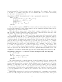
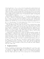
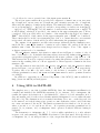
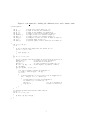
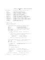
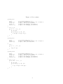
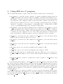
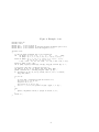
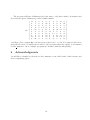
User Guide for LDL, a concise sparse Cholesky package
Timothy A. Davis∗
VERSION 2.0.3, Jan 25, 2011
Abstract
The LDL software package is a set of short, concise routines for factorizing symmetric positive-definite sparse matrices, with some applicability to symmetric indefinite matrices. Its primary purpose is to illustrate much of the basic theory of sparse
matrix algorithms in as concise a code as possible, including an elegant method of
sparse symmetric factorization that computes the factorization row-by-row but stores
it column-by-column. The entire symbolic and numeric factorization consists of less
than 50 lines of code. The package is written in C, and includes a MATLAB interface.
1
Overview
LDL is a set of short, concise routines that compute the LDLT factorization of a sparse
symmetric matrix A. Its primary purpose is to illustrate much of the basic theory of sparse
matrix algorithms in as compact a code as possible, including an elegant method of sparse
symmetric factorization (related to [9, 11]). The lower triangular factor L is computed rowby-row, in contrast to the conventional column-by-column method. Although it does not
achieve the same level of performance as methods based on dense matrix kernels (such as
[12, 13]), its performance is competitive with column-by-column methods that do not use
dense kernels [4, 5, 6].
Section 2 gives a brief description of the algorithm used in the symbolic and numeric
factorization. A more detailed tutorial-level discussion may be found in [14]. Details of the
concise implementation of this method are given in Section 3. Sections 4 and 5 give an
overview of how to use the package in MATLAB and in a stand-alone C program.
2
Algorithm
The underlying numerical algorithm is described below. The kth step solves a lower triangular system of dimension k − 1 to compute the kth row of L and the dkk entry of the
∗
Dept. of Computer and Information Science and Engineering, Univ. of Florida, Gainesville, FL, USA.
email: [email protected]. http://www.cise.ufl.edu/∼davis. This work was supported by the National Science
Foundation, under grant CCR-0203270. Portions of the work were done while on sabbatical at Stanford
University and Lawrence Berkeley National Laboratory (with funding from Stanford University and the
SciDAC program).
1
diagonal matrix D. Colon notation is used for submatrices. For example, Lk,1:k−1 refers
to the first k − 1 columns of the kth row of L. Similarly, L1:k−1,1:k−1 refers to the leading
(k − 1)-by-(k − 1) submatrix of L.
Algorithm 1 (LDLT factorization of a n-by-n symmetric matrix A)
for k = 1 to n
(step 1) Solve L1:k−1,1:k−1 y = A1:k−1,k for y
T
(step 2) Lk,1:k−1 = (D−1
1:k−1,1:k−1 y)
(step 3) lkk = 1
(step 4) dkk = akk − Lk,1:k−1 y
end for
The algorithm computes an LDLT factorization without numerical pivoting. It can thus
factorize any symmetric positive definite matrix, and any symmetric indefinite matrix whose
leading minors are all well-conditioned.
When A and L are sparse, step 1 of Algorithm 1 requires a triangular solve of the form
Lx = b, where all three terms in the equation are sparse. This is the most costly step of the
Algorithm. Steps 2 through 4 are fairly straightforward.
Let X and B refer to the set of indices of nonzero entries in x and b, respectively, in the
lower triangular system Lx = b. To compute x efficiently the nonzero pattern X must be
found first. In the general case when L is arbitrary [8], the nonzero pattern X is the set
of nodes reachable via paths in the graph GL from all nodes in the set B, and where the
graph GL has n nodes and a directed edge (j, i) if and only if lij is nonzero. To compute
the numerical solution to Lx = b by accessing the columns of L one at a time, X can be
traversed in any topological order of the subgraph of GL consisting of nodes in X . That
is, xj must be computed before xi if there is a path from j to i in GL . The natural order
(1, 2, . . . , n) is one such ordering, but that requires a costly sort of X . With a graph traversal
and topological sort, the solution of Lx = b can be computed using Algorithm 2 below. The
computation of X and x both take time proportional to the floating-point operation count.
Algorithm 2 (Solve Lx = b, where L is lower triangular with unit diagonal)
X = ReachGL (B)
x=b
for i ∈ X in any topological order
xi+1:n = xi+1:n − Li+1:n,i xi
end for
The general result also governs the pattern of y in Algorithm 1. However, in this case L
arises from a sparse Cholesky factorization, and is governed by the elimination tree [10]. A
general graph traversal is not required. In the elimination tree, the parent of node i is the
smallest j > i such that lji is nonzero. Node i has no parent if column i of L is completely
zero below the diagonal; i is a root of the elimination tree in this case. The nonzero pattern
of x is the union of all the nodes on the paths from any node i (where bi is nonzero) to the
root of the elimination tree [9, Thm 2.4]. It is referred to here as a tree, but in general it
can be a forest.
Rather than a general topological sort of the subgraph of GL consisting nodes reachable
from nodes in B, a simpler tree traversal can be used. First, select any nonzero entry bi and
2
follow the path from i to the root of tree. Nodes along this path are marked and placed in
a stack, with i at the top of the stack and the root at the bottom. Repeat for every other
nonzero entry in bi , in arbitrary order, but stop just before reaching a marked node (the
result can be empty if i is already in the stack). The stack now contains X , a topological
ordering of the nonzero pattern of x, which can be used in Algorithm 2 to solve Lx = b. The
time to compute X using an elimination tree traversal is much faster than the general graph
traversal, taking time proportional to the size of X rather than the number of floating-point
operations required to compute x.
In the kth step of the factorization, the set X becomes the nonzero pattern of row k of
L. This step requires the elimination tree of L1:k−1,1:k−1 , and must construct the elimination
tree of L1:k,1:k for step k + 1. Recall that the parent of i in the tree is the smallest j such
that i < j and lji 6= 0. Thus, if any node i already has a parent j, then j will remain the
parent of i in the elimination trees of all other larger leading submatrices of L, and in the
elimination tree of L itself. If lki 6= 0 and i does not have a parent in the elimination tree of
L1:k−1,1:k−1 , then the parent of i is k in the elimination tree of L1:k,1:k . Node k becomes the
parent of any node i ∈ X that does not yet have a parent.
Since Algorithm 2 traverses L in column order, L is stored in a conventional sparse column
representation. Each column j is stored as a list of nonzero values and their corresponding
row indices. When row k is computed, the new entries can be placed at the end of each list.
As a by-product of computing L one row at a time, the columns of L are computed in a sorted
manner. This is a convenient form of the output. MATLAB requires the columns of its sparse
matrices to be sorted, for example. Sorted columns improve the speed of Algorithm 2, since
the memory access pattern is more regular. The conventional column-by-column algorithm
[4, 5] does not produce columns of L with sorted row indices.
A simple symbolic pre-analysis can be obtained by repeating the subtree traversals. All
that is required to compute the nonzero pattern of the kth row of L is the partially constructed elimination tree and the nonzero pattern of the kth column of A. This is computed
in time proportional to the size of this set, using the elimination tree traversal. Once constructed, the number of nonzeros in each column of L is incremented, for each entry in X ,
and then X is discarded. The set X need not be constructed in topological order, so no
stack is required. The run time of the symbolic analysis algorithm is thus proportional to
the number of nonzeros in L. This is more costly than the optimal algorithm [7], which takes
time essentially proportional to the number of nonzeros in A. The memory requirements
are just the matrix A and a few size-n integer arrays. The result of the algorithm is the
elimination tree, a count of the number of nonzeros in each column of L, and the cumulative
sum of the column counts.
3
Implementation
Because of its simplicity, the implementation of this algorithm leads to a very short, concise
code. The symbolic analysis routine ldl symbolic shown in Figure 1 consists of only 18 lines
of executable C code. This includes 5 lines of code to allow for a sparsity-preserving ordering
P so that either A or PAPT can be analyzed, 3 lines of code to compute the cumulative
sum of the column counts, and one line of code to speed up a for loop. An additional line
3
of code allows for a more general form of the input sparse matrix A.
The n-by-n sparse matrix A is provided in compressed column form as an int array
Ap of length n+1, an int array Ai of length nz, and a double array Ax also of length nz,
where nz is the number of entries in the matrix. The numerical values of entries in column j
are stored in Ax[Ap[j] . . . Ap[j+1]-1] and the corresponding row indices are in Ai[Ap[j]
. . . Ap[j+1]-1]. With Ap[0] = 0, the number of entries in the matrix is nz = Ap[n]. If
no fill-reducing ordering P is provided, only entries in the upper triangular part of A are
considered. If P is provided and row/column i of the matrix A is the k-th row/column of
PAPT , then P[k]=i. Only entries in the upper triangular part of PAPT are considered.
These entries may be in the lower triangular part of A, so to ensure that the correct matrix
is factorized, all entries of A should be provided when using the permutation input P.
The outputs of ldl symbolic are three size-n arrays: Parent holds the elimination tree,
Lnz holds the counts of the number of entries in each column of L, and Lp holds the cumulative sum of Lnz. The size-n array Flag is used as workspace. None of the output or
workspace arrays need to be initialized.
The ldl numeric numeric factorization routine shown in Figure 2 consists of only 31
lines of executable code. It includes this same subtree traversal algorithm as ldl symbolic,
except that each path is placed on a stack that holds nonzero pattern of the kth row of L.
This traversal is followed by a sparse forward solve using this pattern, and all of the nonzero
entries in the resulting kth row of L are appended to their respective columns in the data
structure of L.
After the matrix is factorized, the ldl lsolve, ldl dsolve, and ldl ltsolve routines
shown in Figure 3 are provided to solve Lx = b, Dx = b, and LT x = b, respectively.
Together, they solve Ax = b, and consist of only 10 lines of executable code. If a fillreducing permutation is used, ldl perm and ldl permt must be used to permute b and x
accordingly.
In addition to appearing as a Collected Algorithm of the ACM [3], LDL is available at
http://www.cise.ufl.edu/research/sparse.
4
Using LDL in MATLAB
The simplest way to use LDL is within MATLAB. Once the ldlsparse mexFunction is
compiled and installed, the MATLAB statement [L, D, Parent, fl] = ldlsparse (A)
returns the sparse factorization A = (L+I)*D*(L+I)’, where L is lower triangular, D is a
diagonal matrix, and I is the n-by-n identity matrix (ldlsparse does not return the unit
diagonal of L). The elimination tree is returned in Parent. If no zero on the diagonal of D
is encountered, fl is the floating-point operation count. Otherwise, D(-fl,-fl) is the first
zero entry encountered. Let d=-fl. The function returns the factorization of A (1:d,1:d),
where rows d+1 to n of L and D are all zero. If a sparsity preserving permutation P is
passed, [L, D, Parent, fl] = ldlsparse (A,P) operates on A(P,P) without forming it
explicitly.
The statement x = ldlsparse (A, [ ], b) is roughly equivalent to x = A\b, when A
is sparse, real, and symmetric. The LDLT factorization of A is performed. If P is provided, x
= ldlsparse (A, P, b) still performs x = A\b, except that A(P,P) is factorized instead.
4
Figure 1: ldl symbolic: finding the elimination tree and column counts
void ldl_symbolic
(
int n,
/* A and L are n-by-n, where n >= 0 */
int Ap [ ],
/* input of size n+1, not modified */
int Ai [ ],
/* input of size nz=Ap[n], not modified */
int Lp [ ],
/* output of size n+1, not defined on input */
int Parent [ ],
/* output of size n, not defined on input */
int Lnz [ ],
/* output of size n, not defined on input */
int Flag [ ],
/* workspace of size n, not defn. on input or output */
int P [ ],
/* optional input of size n */
int Pinv [ ]
/* optional output of size n (used if P is not NULL) */
)
{
int i, k, p, kk, p2 ;
if (P)
{
/* If P is present then compute Pinv, the inverse of P */
for (k = 0 ; k < n ; k++)
{
Pinv [P [k]] = k ;
}
}
for (k = 0 ; k < n ; k++)
{
/* L(k,:) pattern: all nodes reachable in etree from nz in A(0:k-1,k) */
Parent [k] = -1 ;
/* parent of k is not yet known */
Flag [k] = k ;
/* mark node k as visited */
Lnz [k] = 0 ;
/* count of nonzeros in column k of L */
kk = (P) ? (P [k]) : (k) ; /* kth original, or permuted, column */
p2 = Ap [kk+1] ;
for (p = Ap [kk] ; p < p2 ; p++)
{
/* A (i,k) is nonzero (original or permuted A) */
i = (Pinv) ? (Pinv [Ai [p]]) : (Ai [p]) ;
if (i < k)
{
/* follow path from i to root of etree, stop at flagged node */
for ( ; Flag [i] != k ; i = Parent [i])
{
/* find parent of i if not yet determined */
if (Parent [i] == -1) Parent [i] = k ;
Lnz [i]++ ;
/* L (k,i) is nonzero */
Flag [i] = k ;
/* mark i as visited */
}
}
}
}
/* construct Lp index array from Lnz column counts */
Lp [0] = 0 ;
for (k = 0 ; k < n ; k++)
{
Lp [k+1] = Lp [k] + Lnz [k] ;
}
}
5
Figure 2: ldl numeric: numeric factorization
int ldl_numeric
/* returns n if successful, k if D (k,k) is zero */
(
int n,
/* A and L are n-by-n, where n >= 0 */
int Ap [ ],
/* input of size n+1, not modified */
int Ai [ ],
/* input of size nz=Ap[n], not modified */
double Ax [ ],
/* input of size nz=Ap[n], not modified */
int Lp [ ],
/* input of size n+1, not modified */
int Parent [ ],
/* input of size n, not modified */
int Lnz [ ],
/* output of size n, not defn. on input */
int Li [ ],
/* output of size lnz=Lp[n], not defined on input */
double Lx [ ],
/* output of size lnz=Lp[n], not defined on input */
double D [ ],
/* output of size n, not defined on input */
double Y [ ],
/* workspace of size n, not defn. on input or output */
int Pattern [ ],
/* workspace of size n, not defn. on input or output */
int Flag [ ],
/* workspace of size n, not defn. on input or output */
int P [ ],
/* optional input of size n */
int Pinv [ ]
/* optional input of size n */
)
{
double yi, l_ki ;
int i, k, p, kk, p2, len, top ;
for (k = 0 ; k < n ; k++)
{
/* compute nonzero Pattern of kth row of L, in topological order */
Y [k] = 0.0 ;
/* Y(0:k) is now all zero */
top = n ;
/* stack for pattern is empty */
Flag [k] = k ;
/* mark node k as visited */
Lnz [k] = 0 ;
/* count of nonzeros in column k of L */
kk = (P) ? (P [k]) : (k) ; /* kth original, or permuted, column */
p2 = Ap [kk+1] ;
for (p = Ap [kk] ; p < p2 ; p++)
{
i = (Pinv) ? (Pinv [Ai [p]]) : (Ai [p]) ;
/* get A(i,k) */
if (i <= k)
{
Y [i] += Ax [p] ; /* scatter A(i,k) into Y (sum duplicates) */
for (len = 0 ; Flag [i] != k ; i = Parent [i])
{
Pattern [len++] = i ;
/* L(k,i) is nonzero */
Flag [i] = k ;
/* mark i as visited */
}
while (len > 0) Pattern [--top] = Pattern [--len] ;
}
}
/* compute numerical values kth row of L (a sparse triangular solve) */
D [k] = Y [k] ;
/* get D(k,k) and clear Y(k) */
Y [k] = 0.0 ;
for ( ; top < n ; top++)
{
i = Pattern [top] ;
/* Pattern [top:n-1] is pattern of L(:,k) */
yi = Y [i] ;
/* get and clear Y(i) */
Y [i] = 0.0 ;
p2 = Lp [i] + Lnz [i] ;
for (p = Lp [i] ; p < p2 ; p++)
{
Y [Li [p]] -= Lx [p] * yi ;
}
l_ki = yi / D [i] ;
/* the nonzero entry L(k,i) */
D [k] -= l_ki * yi ;
Li [p] = k ;
/* store L(k,i) in column form of L */
Lx [p] = l_ki ;
Lnz [i]++ ;
/* increment count of nonzeros in col i */
}
if (D [k] == 0.0) return (k) ;
/* failure, D(k,k) is zero */
}
return (n) ;
/* success, diagonal of D is all nonzero */
}
6
Figure 3: Solve routines
void ldl_lsolve
(
int n,
/* L is n-by-n, where n >= 0 */
double X [ ],
/* size n. right-hand-side on input, soln. on output */
int Lp [ ],
/* input of size n+1, not modified */
int Li [ ],
/* input of size lnz=Lp[n], not modified */
double Lx [ ]
/* input of size lnz=Lp[n], not modified */
)
{
int j, p, p2 ;
for (j = 0 ; j < n ; j++)
{
p2 = Lp [j+1] ;
for (p = Lp [j] ; p < p2 ; p++)
{
X [Li [p]] -= Lx [p] * X [j] ;
}
}
}
void ldl_dsolve
(
int n,
/* D is n-by-n, where n >= 0 */
double X [ ],
/* size n. right-hand-side on input, soln. on output */
double D [ ]
/* input of size n, not modified */
)
{
int j ;
for (j = 0 ; j < n ; j++)
{
X [j] /= D [j] ;
}
}
void ldl_ltsolve
(
int n,
double X [ ],
int Lp [ ],
int Li [ ],
double Lx [ ]
)
{
int j, p, p2 ;
for (j = n-1 ; j >=
{
p2 = Lp [j+1] ;
for (p = Lp [j]
{
X [j] -= Lx
}
}
}
/*
/*
/*
/*
/*
L is n-by-n, where n >= 0 */
size n. right-hand-side on input, soln. on output */
input of size n+1, not modified */
input of size lnz=Lp[n], not modified */
input of size lnz=Lp[n], not modified */
0 ; j--)
; p < p2 ; p++)
[p] * X [Li [p]] ;
7
5
Using LDL in a C program
The C-callable LDL library consists of nine user-callable routines and one include file.
• ldl symbolic: given the nonzero pattern of a sparse symmetric matrix A and an
optional permutation P, analyzes either A or PAPT , and returns the elimination tree,
the number of nonzeros in each column of L, and the Lp array for the sparse matrix
data structure for L. Duplicate entries are allowed in the columns of A, and the row
indices in each column need not be sorted. Providing a sparsity-preserving ordering is
critical for obtaining good performance. A minimum degree ordering (such as AMD
[1, 2]) or a graph-partitioning based ordering are appropriate.
• ldl numeric: given Lp and the elimination tree computed by ldl symbolic, and an
optional permutation P, returns the numerical factorization of A or PAPT . Duplicate
entries are allowed in the columns of A (any duplicate entries are summed), and the
row indices in each column need not be sorted. The data structure for L is the same
as A, except that no duplicates appear, and each column has sorted row indices.
• ldl lsolve: given the factor L computed by ldl numeric, solves the linear system
Lx = b, where x and b are full n-by-1 vectors.
• ldl dsolve: given the factor D computed by ldl numeric, solves the linear system
Dx = b.
• ldl ltsolve: given the factor L computed by ldl numeric, solves the linear system
LT x = b.
• ldl perm: given a vector b and a permutation P, returns x = Pb.
• ldl permt: given a vector b and a permutation P, returns x = PT b.
• ldl valid perm: Except for checking if the diagonal of D is zero, none of the above
routines check their inputs for errors. This routine checks the validity of a permutation
P.
• ldl valid matrix: checks if a matrix A is valid as input to ldl symbolic and
ldl numeric.
Note that the primary input to the ldl symbolic and ldl numeric is the sparse matrix
A. It is provided in column-oriented form, and only the upper triangular part is accessed.
This is slightly different than the primary output: the matrix L, which is lower triangular in
column-oriented form. If you wish to factorize a symmetric matrix A for which only the lower
triangular part is supplied, you would need to transpose A before passing it ldl symbolic
and ldl numeric.
An additional set of routines is available for use in a 64-bit environment. Each routine
name changes uniformly; ldl symbolic becomes ldl l symbolic, and each int parameter
becomes type UF long. The UF long type is long, except for Microsoft Windows 64, where
it becomes int64.
8
Figure 4: Example of use
#include <stdio.h>
#include "ldl.h"
#define N 10
/* A is 10-by-10 */
#define ANZ 19 /* # of nonzeros on diagonal and upper triangular part of A */
#define LNZ 13 /* # of nonzeros below the diagonal of L */
int main (void)
{
/* only the upper
int
Ap [N+1] =
Ai [ANZ] =
double Ax [ANZ] =
triangular part of A is required */
{0, 1, 2, 3, 4,
6, 7,
9,
11,
15,
ANZ},
{0, 1, 2, 3, 1,4, 5, 4,6, 4,7, 0,4,7,8, 1,4,6,9 } ;
{1.7, 1., 1.5, 1.1, .02,2.6, 1.2, .16,1.3, .09,1.6,
.13,.52,.11,1.4, .01,.53,.56,3.1},
b [N] = {.287, .22, .45, .44, 2.486, .72, 1.55, 1.424, 1.621, 3.759};
double Lx [LNZ], D [N], Y [N] ;
int Li [LNZ], Lp [N+1], Parent [N], Lnz [N], Flag [N], Pattern [N], d, i ;
/* factorize A into LDL’ (P and Pinv not used) */
ldl_symbolic (N, Ap, Ai, Lp, Parent, Lnz, Flag, NULL, NULL) ;
printf ("Nonzeros in L, excluding diagonal: %d\n", Lp [N]) ;
d = ldl_numeric (N, Ap, Ai, Ax, Lp, Parent, Lnz, Li, Lx, D, Y, Pattern,
Flag, NULL, NULL) ;
if (d == N)
{
/* solve Ax=b, overwriting b with the solution x */
ldl_lsolve (N, b, Lp, Li, Lx) ;
ldl_dsolve (N, b, D) ;
ldl_ltsolve (N, b, Lp, Li, Lx) ;
for (i = 0 ; i < N ; i++) printf ("x [%d] = %g\n", i, b [i]) ;
}
else
{
printf ("ldl_numeric failed, D (%d,%d) is zero\n", d, d) ;
}
return (0) ;
}
9
The program in Figure 4 illustrates the basic usage of the LDL routines. It analyzes and
factorizes the sparse symmetric positive-definite matrix









A=








1.7 0
0
0
0
0
0
0 .13 0
0
1.
0
0 .02 0
0
0
0 .01
0
0 1.5 0
0
0
0
0
0
0
0
0
0 1.1 0
0
0
0
0
0
0 .02 0
0 2.6 0 .16 .09 .52 .53
0
0
0
0
0 1.2 0
0
0
0
0
0
0
0 .16 0 1.3 0
0 .56
0
0
0
0 .09 0
0 1.6 .11 0
.13 0
0
0 .52 0
0 .11 1.4 0
0 .01 0
0 .53 0 .56 0
0 3.1


















and then solves a system Ax = b whose true solution is xi = i/10. Note that Li and Lx are
statically allocated. Normally they would be allocated after their size, Lp[n], is determined
by ldl symbolic. More example programs are included with the LDL package.
6
Acknowledgments
I would like to thank Pete Stewart for his comments on an earlier draft of this software and
its accompanying paper.
10
References
[1] P. R. Amestoy, T. A. Davis, and I. S. Duff. An approximate minimum degree ordering
algorithm. SIAM J. Matrix Anal. Applic., 17(4):886–905, 1996.
[2] P. R. Amestoy, T. A. Davis, and I. S. Duff. Algorithm 837: AMD, an approximate
minimum degree ordering algorithm. ACM Trans. Math. Softw., 30(3):381–388, 2004.
[3] T. A Davis. Algorithm 849: a concise sparse cholesky factorization package. ACM
Trans. Math. Softw., 31(4):587–591, 2005.
[4] A. George and J. W. H. Liu. The design of a user interface for a sparse matrix package.
ACM Trans. Math. Softw., 5(2):139–162, Jun. 1979.
[5] A. George and J. W. H. Liu. Computer Solution of Large Sparse Positive Definite
Systems. Prentice-Hall, Englewood Cliffs, New Jersey, 1981.
[6] J. R. Gilbert, C. Moler, and R. Schreiber. Sparse matrices in MATLAB: design and
implementation. SIAM J. Matrix Anal. Applic., 13(1):333–356, 1992.
[7] J. R. Gilbert, E. G. Ng, and B. W. Peyton. An efficient algorithm to compute row
and column counts for sparse Cholesky factorization. SIAM J. Matrix Anal. Applic.,
15(4):1075–1091, 1994.
[8] J. R. Gilbert and T. Peierls. Sparse partial pivoting in time proportional to arithmetic
operations. SIAM J. Sci. Statist. Comput., 9:862–874, 1988.
[9] J. W. H. Liu. A compact row storage scheme for Cholesky factors using elimination
trees. ACM Trans. Math. Softw., 12(2):127–148, Jun. 1986.
[10] J. W. H. Liu. The role of elimination trees in sparse factorization. SIAM J. Matrix
Anal. Applic., 11(1):134–172, 1990.
[11] J. W. H. Liu. A generalized envelope method for sparse factorization by rows. ACM
Trans. Math. Softw., 17(1):112–129, 1991.
[12] E. G. Ng and B. W. Peyton. A supernodal Cholesky factorization algorithm for sharedmemory multiprocessors. SIAM J. Sci. Comput., 14:761–769, 1993.
[13] E. Rothberg and A. Gupta. Efficient sparse matrix factorization on high-performance
workstations - Exploiting the memory hierarchy. ACM Trans. Math. Softw., 17(3):313–
334, 1991.
[14] G. W. Stewart. Building an old-fashioned sparse solver. Technical report, Univ. Maryland (www.umd.cs.edu/∼stewart), 2003.
11